Embed Size (px)
Citation preview
SoftwareProtectionEvaluation
BjornDeSutter
ISSISP2017– Paris
1
SoftwareProtectionEvaluation
2
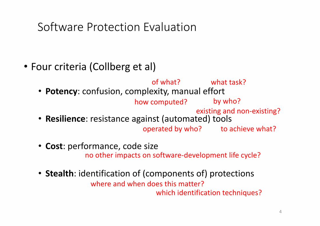
• Fourcriteria(Collbergetal)
• Potency:confusion,complexity,manualeffort
• Resilience:resistanceagainst(automated)tools
• Cost:performance,codesize
• Stealth:identificationof(componentsof)protections
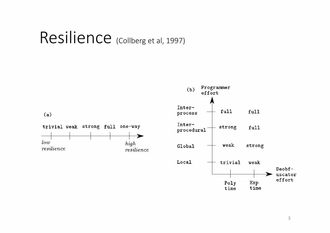
Resilience(Collbergetal,1997)
3
SoftwareProtectionEvaluation
4
• Fourcriteria(Collbergetal)
• Potency:confusion,complexity,manualeffort
• Resilience:resistanceagainst(automated)tools
• Cost:performance,codesize
• Stealth:identificationof(componentsof)protections
ofwhat?
howcomputed?
whattask?
bywho?existingandnon-existing?
operatedbywho? toachievewhat?
nootherimpactsonsoftware-developmentlifecycle?
whereandwhendoesthismatter?whichidentificationtechniques?
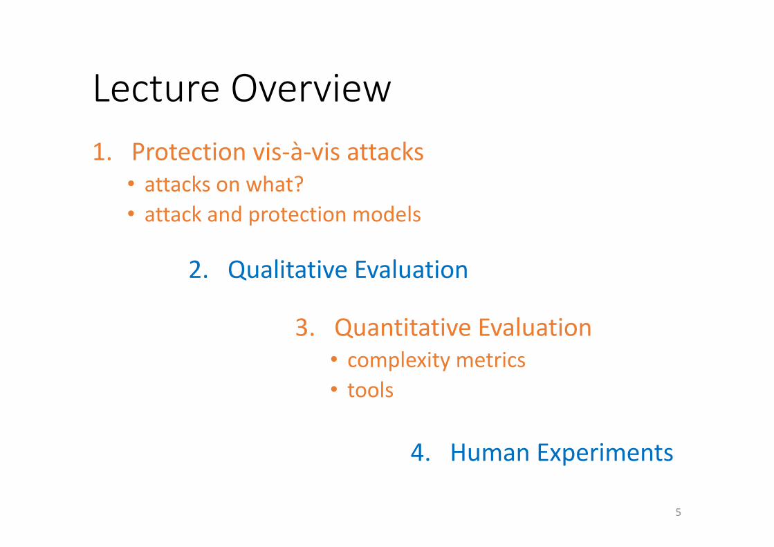
LectureOverview1. Protectionvis-à-visattacks
• attacksonwhat?• attackandprotectionmodels
5
2. QualitativeEvaluation
3. QuantitativeEvaluation• complexitymetrics• tools
4. HumanExperiments
Whatisbeingattacked?
6
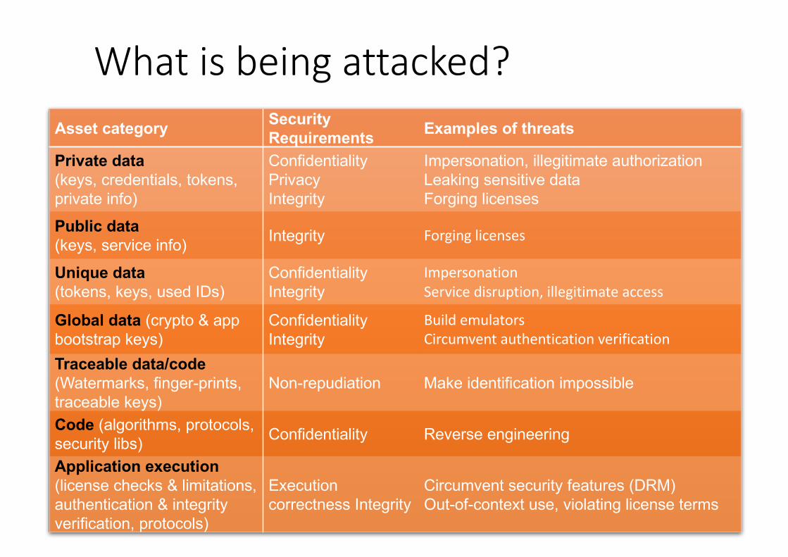
Asset category Security Requirements Examples of threats
Private data(keys, credentials, tokens, private info)
ConfidentialityPrivacyIntegrity
Impersonation, illegitimate authorizationLeaking sensitive dataForging licenses
Public data(keys, service info) Integrity Forginglicenses
Unique data(tokens, keys, used IDs)
ConfidentialityIntegrity
ImpersonationService disruption,illegitimateaccess
Global data (crypto & app bootstrap keys)
ConfidentialityIntegrity
BuildemulatorsCircumventauthenticationverification
Traceable data/code(Watermarks, finger-prints,traceable keys)
Non-repudiation Make identification impossible
Code (algorithms, protocols,security libs) Confidentiality Reverse engineering
Application execution(license checks & limitations, authentication & integrity verification, protocols)
Execution correctness Integrity
Circumvent security features (DRM)Out-of-context use, violating license terms
7
Whatisbeingattacked?
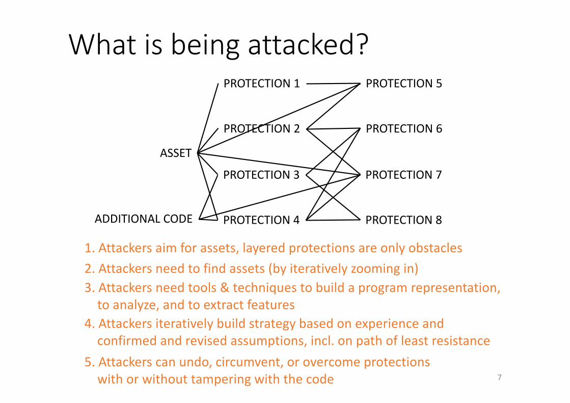
ASSET
PROTECTION1
PROTECTION2
PROTECTION3
PROTECTION4
PROTECTION5
PROTECTION6
PROTECTION7
PROTECTION8ADDITIONALCODE
1.Attackersaimforassets,layeredprotectionsareonlyobstacles2.Attackersneedtofindassets(byiterativelyzoomingin)3.Attackersneedtools&techniquestobuildaprogramrepresentation,toanalyze,andtoextractfeatures
4.Attackersiterativelybuildstrategybasedonexperienceandconfirmedandrevisedassumptions,incl.onpathofleastresistance
5.Attackerscanundo,circumvent,orovercomeprotectionswithorwithouttamperingwiththecode
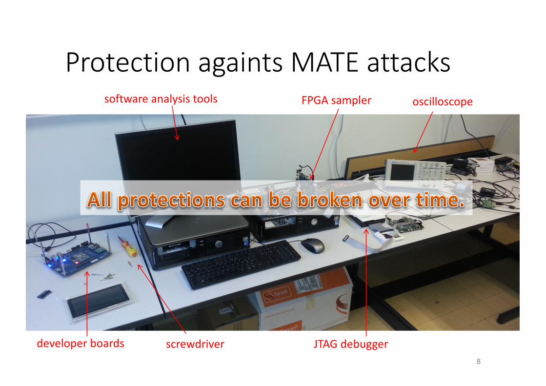
ProtectionagaintsMATEattacksFPGAsampler oscilloscope
developerboards JTAGdebugger
softwareanalysistools
8
screwdriver
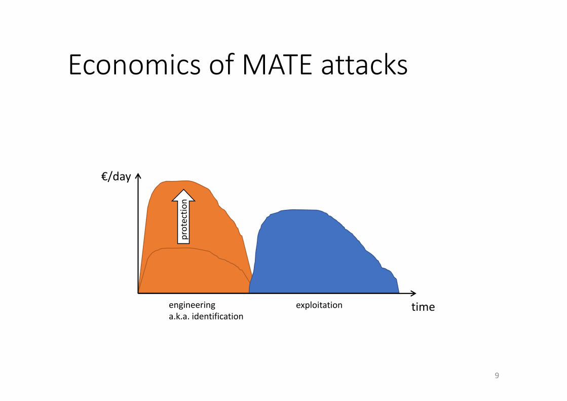
EconomicsofMATEattacks
engineeringa.k.a.identification
exploitation
protectio
n€/day
time
9
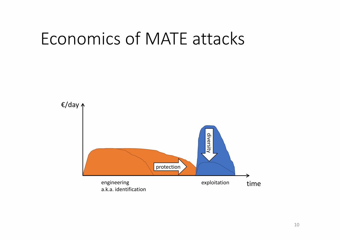
EconomicsofMATEattacks
€/day
timeengineeringa.k.a.identification
exploitation
protection
diversity
10
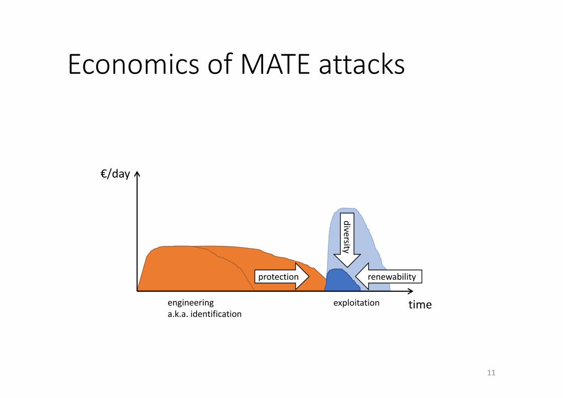
EconomicsofMATEattacks
€/day
timeengineeringa.k.a.identification
exploitation
protection
diversity
11
renewability
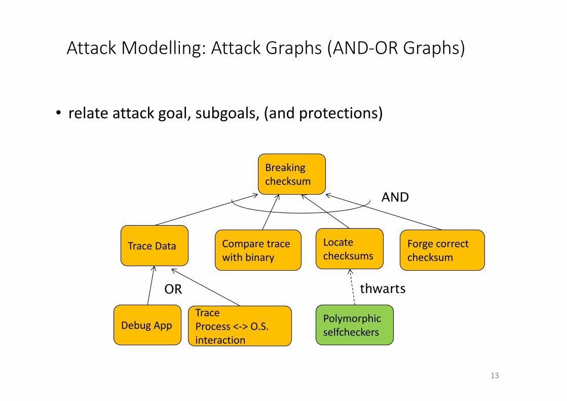
AttackModelling:AttackGraphs(AND-ORGraphs)
TraceData
Polymorphicselfcheckers
Comparetracewithbinary
Locatechecksums
Forgecorrectchecksum
Breakingchecksum
DebugAppTraceProcess<->O.S.interaction
AND
thwartsOR
• relateattackgoal,subgoals,(andprotections)
13
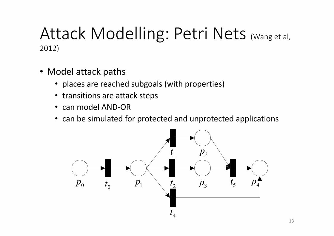
AttackModelling:PetriNets(Wangetal,2012)
13
• Modelattackpaths• placesarereachedsubgoals(withproperties)• transitionsareattacksteps• canmodelAND-OR• canbesimulatedforprotectedandunprotectedapplications
programs which were protected by software tamper resistant transformations they proposed is a NP-complete problem. S. Chow et al. [18] did a similar work.
B. Evaluation based on Attack Researches in this group measure or proof the effectiveness
of protection techniques from the view of attack.
M. Ceccato et al. [9] proposed two manual experiments to empirically measure the effectiveness of identifier renaming, which is an instance of layout obfuscation. I. Sutherland et al. [10] did a similar work, but focused on the reverse engineering process for binary code. Both M. Ceccato and I. Sutherland analyzed factors affecting attack process, for example, attacker’s ability, but none specific metric was proposed.
As well as manually assessment, several anti-protection technologies were used too. C. Linn and S. Debray[19] used three different disassemblers to evaluate the code obfuscation techniques they proposed, and S. Udupa[11] proposed deobfuscation approaches to evaluate control flow flattening obfuscation. J. Hamilton and S. Danicic [22] evaluated Java static watermarking algorithms by obfuscating, which can be treated as a technique for distortive attacks. Except theoretical analysis, C. Wang et al. [17] also proved the effectiveness of the transformation they proposed with a control-flow analysis tool.
Technically, the evaluation approach in this paper belongs to the second group, but acts differently: firstly, we believe all software (a program which is made up of a sequence of code) are the same to attackers, therefore, the approach we proposed does not aim at a specific protection technology; secondly, we propose a metric and a method for counting the metric; thirdly, rather than doing manual attacks or developing specific attack tools, we use an attack model to describe software attacks. Note that H. Goto et al. [21] applied parse tree to evaluate the difficulty of reading tamper-resistant software, however, instead of attacks, they used the model to describe software.
III. ATTACK MODELING BASED ON PETRI NET Attack model has been widely used in information security.
Most time it focuses on how to document attacks in a structured and reusable form [12]. J. Steffan and M. Schumacher [13] compared attack models with programming guidelines, pattern languages, evaluation criteria, and vulnerability databases, and proved that attack model to be the most suitable way to support discovery and avoidance of security vulnerabilities.
In this section, we make a list of the key information included in one software attack process, define the attack model based on Marked Petri Net, and instantiate Token in it.
A. Key Information in Software Attack [13] listed six types of information contained in an informal
attack description. Based on this list, we made a new list for software attack description. (Fig. 1, Table I).
Software Attack
Goal
Method 1
Method 2……
State 1State 2
……
Technique
Sub-goal
ActionPrecondition
Influence
Figure 1. Key information and their relationship
TABLE I. KEY INFORMATION IN ONE SOFTWARE ATTACK PROCESS
Name Meaning
Goal Goal is the purpose of one software attack process, and normally stands for getting or modifying assets contained in software.
Method A Method stands for one possible way to achieve Goal. Usually, more than one Method will be included in one software attack process.
State The sequence of States stands for the detailed process of software attack. Sometimes, State can be treated as step in software attack process.
Technique Technique stands for the attack technique which may be used in the software attack process.
Sub-goal A Sub-goal stands for the goal of a attack technique.
Action Action is the dynamic information in software attack, and stands for performing an attack technique.
Precondition Precondition is the condition of performing an attack technique.
Influence Influence is the consequence of performing an attack technique.
“What’s the condition of attack?”, “If attack can be executed or not?”, and “What will happen after the execution?” are some of the essential questions in the effectiveness evaluation of software protection. Thus, precondition, action, and influence are important elements needing to be described.
One of the most popular attack models is Attack Tree [14]. It is a tree structure to describe the security of systems, with the Goal as the root node and different Methods as leaf nodes. State and Sub-goal are the other nodes in the tree, and there are two kinds of interdependencies of States: AND node and OR node [14]. But Attack Tree cannot describe Precondition, Action, and Influence precisely.
In this paper, we prefer Petri Net (C. A. Petri, 1962), which is a net-like graph and carries more information than Attack Tree.
B. Software Attack Model based on Marked Petri Net Petri Net describes four aspects of a system: states, events,
conditions, and the relationships among them. When condition was satisfied, related event would occur; the occurrence of event would change the states in the system and cause some other conditions to be satisfied [15]. A basic Petri Net is a tuple PN= (P, T, F) where:
x P is a finite set of states, represented by circles.
x T is a finite set of events, represented by rectangles.
x F⊆ {T×P}∪{P×T} , is a multiset of directed arcs.
x P∪T≠Ø, P∩T=Ø.
Fig. 2 is an example of Petri Net. P={p0, p1, p2, p3, p4}is a set of states, T={t0, t1, t2, t3, t4, t5} is a set of events, p0 is input of t0, and p1 is output of t0; at the same time, t0 is the output of p0, and the input of p1. Besides, p0’s next Place is p1.
0p 1p
2p
3p 4p0t
1t
2t 5t
4t
Figure 2. Example of Petri Net
P, T, F are static properties of Petri Net, and fit well with Goal, State, Technique, Sub-goal, and Method in Table I. If we treat Fig. 2 as a process of software attack, then the key
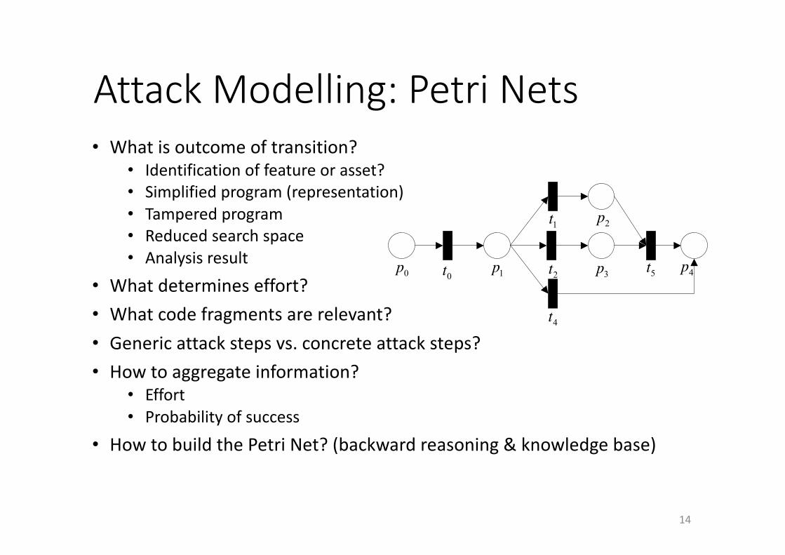
AttackModelling:PetriNets
14
• Whatisoutcomeoftransition?• Identificationoffeatureorasset?• Simplifiedprogram(representation)• Tamperedprogram• Reducedsearchspace• Analysisresult
• Whatdetermineseffort?• Whatcodefragmentsarerelevant?• Genericattackstepsvs.concreteattacksteps?• Howtoaggregateinformation?
• Effort• Probabilityofsuccess
• HowtobuildthePetriNet?(backwardreasoning&knowledgebase)
programs which were protected by software tamper resistant transformations they proposed is a NP-complete problem. S. Chow et al. [18] did a similar work.
B. Evaluation based on Attack Researches in this group measure or proof the effectiveness
of protection techniques from the view of attack.
M. Ceccato et al. [9] proposed two manual experiments to empirically measure the effectiveness of identifier renaming, which is an instance of layout obfuscation. I. Sutherland et al. [10] did a similar work, but focused on the reverse engineering process for binary code. Both M. Ceccato and I. Sutherland analyzed factors affecting attack process, for example, attacker’s ability, but none specific metric was proposed.
As well as manually assessment, several anti-protection technologies were used too. C. Linn and S. Debray[19] used three different disassemblers to evaluate the code obfuscation techniques they proposed, and S. Udupa[11] proposed deobfuscation approaches to evaluate control flow flattening obfuscation. J. Hamilton and S. Danicic [22] evaluated Java static watermarking algorithms by obfuscating, which can be treated as a technique for distortive attacks. Except theoretical analysis, C. Wang et al. [17] also proved the effectiveness of the transformation they proposed with a control-flow analysis tool.
Technically, the evaluation approach in this paper belongs to the second group, but acts differently: firstly, we believe all software (a program which is made up of a sequence of code) are the same to attackers, therefore, the approach we proposed does not aim at a specific protection technology; secondly, we propose a metric and a method for counting the metric; thirdly, rather than doing manual attacks or developing specific attack tools, we use an attack model to describe software attacks. Note that H. Goto et al. [21] applied parse tree to evaluate the difficulty of reading tamper-resistant software, however, instead of attacks, they used the model to describe software.
III. ATTACK MODELING BASED ON PETRI NET Attack model has been widely used in information security.
Most time it focuses on how to document attacks in a structured and reusable form [12]. J. Steffan and M. Schumacher [13] compared attack models with programming guidelines, pattern languages, evaluation criteria, and vulnerability databases, and proved that attack model to be the most suitable way to support discovery and avoidance of security vulnerabilities.
In this section, we make a list of the key information included in one software attack process, define the attack model based on Marked Petri Net, and instantiate Token in it.
A. Key Information in Software Attack [13] listed six types of information contained in an informal
attack description. Based on this list, we made a new list for software attack description. (Fig. 1, Table I).
Software Attack
Goal
Method 1
Method 2……
State 1State 2
……
Technique
Sub-goal
ActionPrecondition
Influence
Figure 1. Key information and their relationship
TABLE I. KEY INFORMATION IN ONE SOFTWARE ATTACK PROCESS
Name Meaning
Goal Goal is the purpose of one software attack process, and normally stands for getting or modifying assets contained in software.
Method A Method stands for one possible way to achieve Goal. Usually, more than one Method will be included in one software attack process.
State The sequence of States stands for the detailed process of software attack. Sometimes, State can be treated as step in software attack process.
Technique Technique stands for the attack technique which may be used in the software attack process.
Sub-goal A Sub-goal stands for the goal of a attack technique.
Action Action is the dynamic information in software attack, and stands for performing an attack technique.
Precondition Precondition is the condition of performing an attack technique.
Influence Influence is the consequence of performing an attack technique.
“What’s the condition of attack?”, “If attack can be executed or not?”, and “What will happen after the execution?” are some of the essential questions in the effectiveness evaluation of software protection. Thus, precondition, action, and influence are important elements needing to be described.
One of the most popular attack models is Attack Tree [14]. It is a tree structure to describe the security of systems, with the Goal as the root node and different Methods as leaf nodes. State and Sub-goal are the other nodes in the tree, and there are two kinds of interdependencies of States: AND node and OR node [14]. But Attack Tree cannot describe Precondition, Action, and Influence precisely.
In this paper, we prefer Petri Net (C. A. Petri, 1962), which is a net-like graph and carries more information than Attack Tree.
B. Software Attack Model based on Marked Petri Net Petri Net describes four aspects of a system: states, events,
conditions, and the relationships among them. When condition was satisfied, related event would occur; the occurrence of event would change the states in the system and cause some other conditions to be satisfied [15]. A basic Petri Net is a tuple PN= (P, T, F) where:
x P is a finite set of states, represented by circles.
x T is a finite set of events, represented by rectangles.
x F⊆ {T×P}∪{P×T} , is a multiset of directed arcs.
x P∪T≠Ø, P∩T=Ø.
Fig. 2 is an example of Petri Net. P={p0, p1, p2, p3, p4}is a set of states, T={t0, t1, t2, t3, t4, t5} is a set of events, p0 is input of t0, and p1 is output of t0; at the same time, t0 is the output of p0, and the input of p1. Besides, p0’s next Place is p1.
0p 1p
2p
3p 4p0t
1t
2t 5t
4t
Figure 2. Example of Petri Net
P, T, F are static properties of Petri Net, and fit well with Goal, State, Technique, Sub-goal, and Method in Table I. If we treat Fig. 2 as a process of software attack, then the key
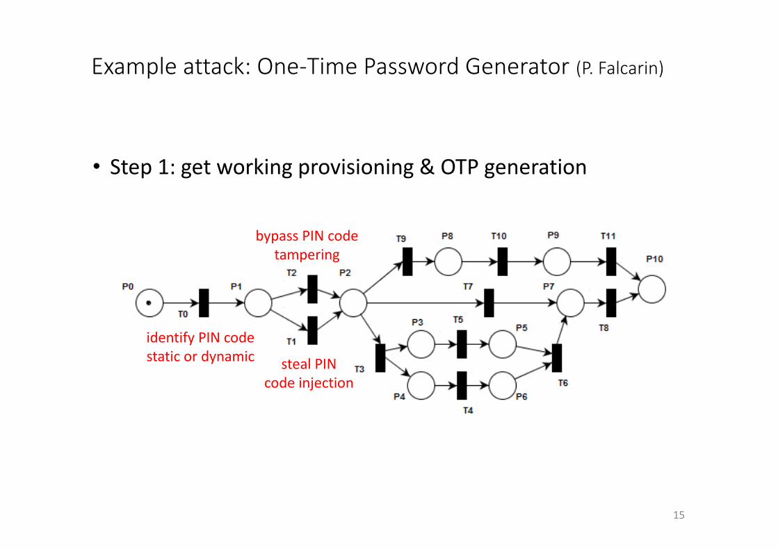
Exampleattack:One-TimePasswordGenerator (P.Falcarin)
15
• Step1:getworkingprovisioning&OTPgeneration
identifyPINcodestaticordynamic
bypassPINcodetampering
stealPINcodeinjection
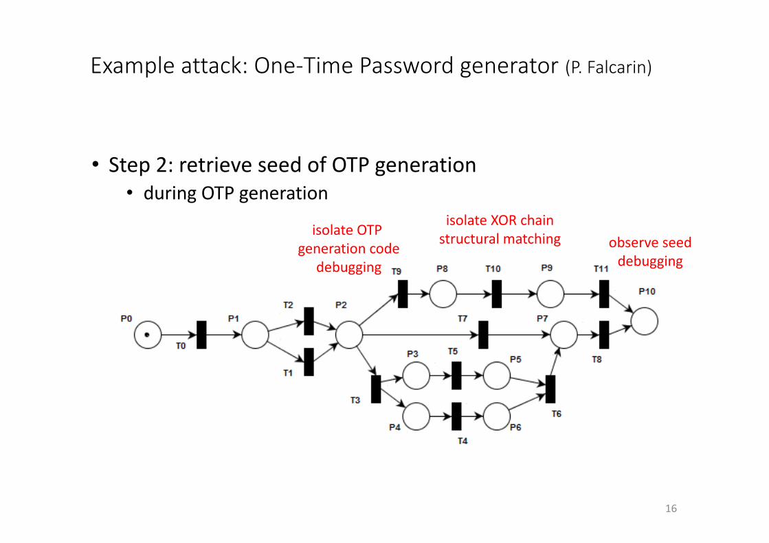
Exampleattack:One-TimePasswordgenerator (P.Falcarin)
16
• Step2:retrieveseedofOTPgeneration• duringOTPgeneration
isolateOTPgenerationcode
debugging
isolateXORchainstructuralmatching observeseed
debugging
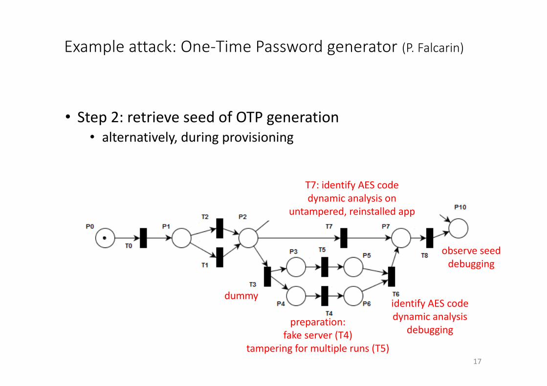
Exampleattack:One-TimePasswordgenerator (P.Falcarin)
17
• Step2:retrieveseedofOTPgeneration• alternatively,duringprovisioning
dummy
preparation:fakeserver(T4)
tamperingformultipleruns(T5)
T7:identifyAEScodedynamicanalysison
untampered,reinstalledapp
identifyAEScodedynamicanalysis
debugging
observeseeddebugging
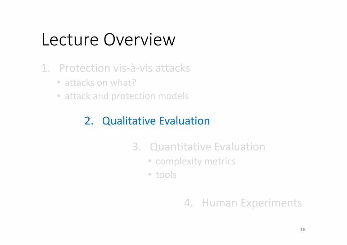
LectureOverview1. Protectionvis-à-visattacks
• attacksonwhat?• attackandprotectionmodels
18
2. QualitativeEvaluation
3. QuantitativeEvaluation• complexitymetrics• tools
4. HumanExperiments
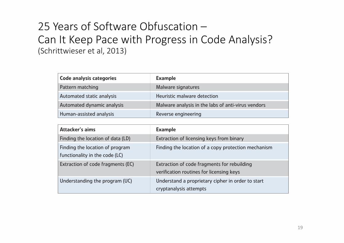
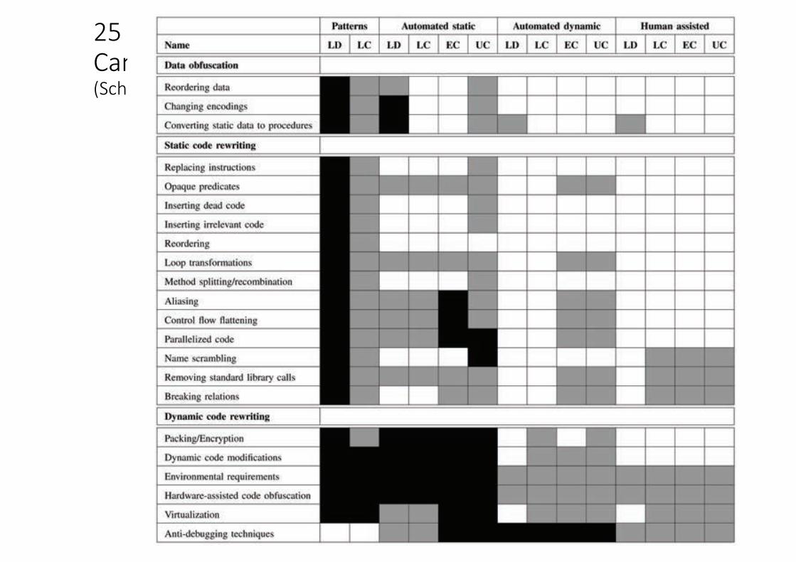
25YearsofSoftwareObfuscation–CanItKeepPacewithProgressinCodeAnalysis?(Schrittwieser etal,2013)
19
Scenarios
Das Kompetenzzentrum SBA Research wird im Rahmen von COMET – Competence Centers for Excellent Technologies durch BMVIT, BMWFJ, das Land Wien gefördert. Das Programm COMET wird durch die FFG abgewickelt.
www.ffg.at/comet
25 Years of Software Obfuscation – Can It Keep Pace with Progress in Code Analysis?
Sebastian Schrittwieser, Stefan Katzenbeisser, Johannes Kinder, Edgar Weippl
f�9G�RTGUGPV�C�PQXGN�ENCUUKƂECVKQP�QH�TGCN�NKHG�CVVCEM�UEGPCTKQU�KP�VJG� context of code obfuscation, derived from a careful analysis of past security incidents involving obfuscated programs
f�9G�ƂTUV�FKUVKPIWKUJ�DGVYGGP�XCTKQWU�CPCN[UKU�VGEJPKSWGU�VJCV�CP� attacker is willing to employ during his attack; then we deal with different aims of an attacker.
Results
Conclusions
f�While, at least in theory, completeness of code analysis seems possible (and most of the analysis approaches introduced in academia indeed � YQTM�HQT�UOCNN�CPF�URGEKƂE�GZCORNGU���NCTIG�TGCN�YQTNF�RTQITCOU�ECP�DG� EQPUKFGTGF�UKIPKƂECPVN[�JCTFGT�VQ�CPCN[\G�
f�A major limiting factor for code analysis is that the high complexity of analysis problems often exceeds resource constrains available for the analyst, thus making it fail for complex programs.
f�6JGTGHQTG��XGT[�UKORNG�QDHWUECVKQP�VGEJPKSWGU�ECP�UVKNN�DG�SWKVG�� GHHGEVKXG�CICKPUV�CPCN[UKU�VGEJPKSWGU�GORNQ[KPI�RCVVGTP�OCVEJKPI�QT� static analysis, which explains the unbroken popularity of obfuscation among malware writers.
f�Dynamic analysis methods, in particular if assisted by a human analyst, are much harder to cope with; this makes code obfuscation for the purpose of intellectual property protection highly challenging.
Figure 1: Analysis of the strength of code obfuscation classes in different attack scenarios
.&���.QECVKPI�&CVC��.%���.QECVKPI�%QFG��'%���'ZVTCEVKPI�%QFG��7%���7PFGTUVCPFKPI�%QFG��
Survey Motivation
f�Code obfuscation has always been a highly controversially discussed research area
f�While theoretical results indicate that provably secure obfuscation in general cannot be achieved, many application areas (e.g., malware, � EQOOGTEKCN�UQHVYCTG��GVE���UJQY�VJCV�EQFG�QDHWUECVKQP�KU�KPFGGF� employed in practice
f�Still, it remains unclear to what extent today's code obfuscation state of the art can keep up with the progress in code analysis and where we stand in the arms race between attackers and defenders
f�Combining these two concepts, we arrive at attack scenarios, which are analyzed in the context of various types of code obfuscation.
f�As not all combinations are reasonable (e.g., pattern matching provides � KPHQTOCVKQP�QP�VJG�EQFG�DWV�ECPPQV�DG�WUGF�HQT�GZVTCEVKPI�EQFG���C�VQVCN� of 14 scenarios must be considered.
Table 1: Code analysis categories and attacker’s aims
��
25YearsofSoftwareObfuscation–CanItKeepPacewithProgressinCodeAnalysis?(Schrittwieseretal,2013)
20
Scenarios
Das Kompetenzzentrum SBA Research wird im Rahmen von COMET – Competence Centers for Excellent Technologies durch BMVIT, BMWFJ, das Land Wien gefördert. Das Programm COMET wird durch die FFG abgewickelt.
www.ffg.at/comet
25 Years of Software Obfuscation – Can It Keep Pace with Progress in Code Analysis?
Sebastian Schrittwieser, Stefan Katzenbeisser, Johannes Kinder, Edgar Weippl
f�9G�RTGUGPV�C�PQXGN�ENCUUKƂECVKQP�QH�TGCN�NKHG�CVVCEM�UEGPCTKQU�KP�VJG� context of code obfuscation, derived from a careful analysis of past security incidents involving obfuscated programs
f�9G�ƂTUV�FKUVKPIWKUJ�DGVYGGP�XCTKQWU�CPCN[UKU�VGEJPKSWGU�VJCV�CP� attacker is willing to employ during his attack; then we deal with different aims of an attacker.
Results
Conclusions
f�While, at least in theory, completeness of code analysis seems possible (and most of the analysis approaches introduced in academia indeed � YQTM�HQT�UOCNN�CPF�URGEKƂE�GZCORNGU���NCTIG�TGCN�YQTNF�RTQITCOU�ECP�DG� EQPUKFGTGF�UKIPKƂECPVN[�JCTFGT�VQ�CPCN[\G�
f�A major limiting factor for code analysis is that the high complexity of analysis problems often exceeds resource constrains available for the analyst, thus making it fail for complex programs.
f�6JGTGHQTG��XGT[�UKORNG�QDHWUECVKQP�VGEJPKSWGU�ECP�UVKNN�DG�SWKVG�� GHHGEVKXG�CICKPUV�CPCN[UKU�VGEJPKSWGU�GORNQ[KPI�RCVVGTP�OCVEJKPI�QT� static analysis, which explains the unbroken popularity of obfuscation among malware writers.
f�Dynamic analysis methods, in particular if assisted by a human analyst, are much harder to cope with; this makes code obfuscation for the purpose of intellectual property protection highly challenging.
Figure 1: Analysis of the strength of code obfuscation classes in different attack scenarios
.&���.QECVKPI�&CVC��.%���.QECVKPI�%QFG��'%���'ZVTCEVKPI�%QFG��7%���7PFGTUVCPFKPI�%QFG��
Survey Motivation
f�Code obfuscation has always been a highly controversially discussed research area
f�While theoretical results indicate that provably secure obfuscation in general cannot be achieved, many application areas (e.g., malware, � EQOOGTEKCN�UQHVYCTG��GVE���UJQY�VJCV�EQFG�QDHWUECVKQP�KU�KPFGGF� employed in practice
f�Still, it remains unclear to what extent today's code obfuscation state of the art can keep up with the progress in code analysis and where we stand in the arms race between attackers and defenders
f�Combining these two concepts, we arrive at attack scenarios, which are analyzed in the context of various types of code obfuscation.
f�As not all combinations are reasonable (e.g., pattern matching provides � KPHQTOCVKQP�QP�VJG�EQFG�DWV�ECPPQV�DG�WUGF�HQT�GZVTCEVKPI�EQFG���C�VQVCN� of 14 scenarios must be considered.
Table 1: Code analysis categories and attacker’s aims
��
LectureOverview1. Protectionvis-à-visattacks
• attacksonwhat?• attackandprotectionmodels
21
2. QualitativeEvaluation
3. QuantitativeEvaluation• complexitymetrics• tools
4. HumanExperiments
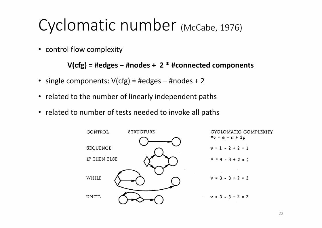
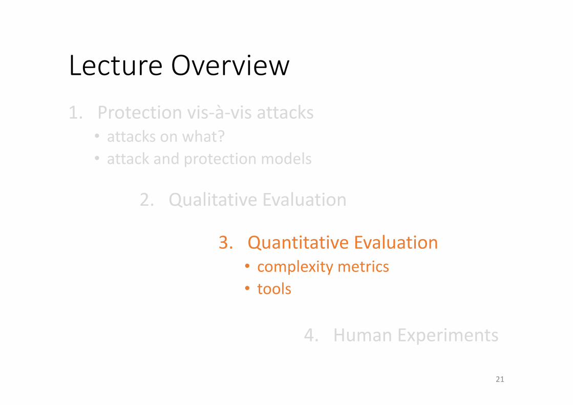
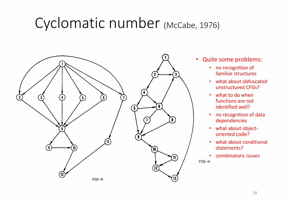
Cyclomatic number(McCabe,1976)
22
• controlflowcomplexity
V(cfg)=#edges−#nodes+2*#connectedcomponents
• singlecomponents:V(cfg)=#edges−#nodes+2
• relatedtothenumberoflinearlyindependentpaths
• relatedtonumberoftestsneededtoinvokeallpathsMC CABE: A COMPLEXITY MEASURE
Theorem 1 is applied to G in the following way. Imagine thatthe exit node (f) branches back to the entry node (a). Thecontrol graph G is now strongly connected (there is a pathjoining any pair of arbitrary distinct vertices) so Theorem 1applies. Therefore, the maximum number of linearly indepen-dent circuits in G is 9-6+2. For example, one could choosethe following 5 independent circuits in G:
Bi: (abefa), (beb), (abea), (acfa), (adcfa).
It follows that Bi forms a basis for the set of all circuits in Gand any path through G can be expressed as a linear combina-tion of circuits from Bi. For instance, the path (abeabebebef)is expressable as (abea) +2(beb) + (abefa). To see how thisworks its necessary to number the edges on G as in
10,
Now for
follows:
(abefa)(beb)(abea)(acfa)(adcfa)
each member of the basis Bi associate a vector as
1 234561 0 0 1 0 0000 1 1 01 00 1 000 1 0 0 0 100 1 00 1
7 8 9 100 1 0 1000 00 00 0
000 11 00 1
The path (abea(be)3 fa) corresponds to the vector 200420011 1and the vector addition of (abefa), 2(beb), and (abea) yieldsthe desired result.In using Theorem 1 one can choose a basis set of circuits
that correspond to paths through the program. The set B2 is a
basis of program paths.
B2: (abef), (abeabef), (abebef), (acf), (adcf),
Linear combination of paths in B2 will also generate any path.For example,
(abea(be)3f) = 2(abebef) - (abef)
and
(a(be)2abef) = (a(be)2f) + (abeabef) - (abef).
The overall strategy will be to measure the complexity of a
program by computing the number of linearly independentpaths v(G), control the "size" of programs by setting an upperlimit to v(G) (instead of using just physical size), and use thecyclomatic complexity as the basis for a testing methodology.A few simple examples may help to illustrate. Below are the
control graphs of the usual constructs used in structured pro-grammning and their respective complexities.
CONTROL STRUCTURE
SEQUENCE
IF THEN ELSE
WHILE
UNTIL
CYCLOMATIC COMPLEXITY*v = e - n + 2p
v = 1 - 2 + 2 = 1
v = 4 - 4 + 2 = 2
v = 3 - 3 + 2 = 2
v = 3 - 3 + 2 = 2
Notice that the sequence of an arbitrary number of nodes al-ways has unit complexity and that cyclomatic complexityconforms to our intuitive notion of "minimum number ofpaths." Several properties of cyclomatic complexity are statedbelow:
1) v(G)>1.2) v(G) is the maximum number of linearly independent
paths in G; it is the size of a basis set.3) Inserting or deleting functional statements to G does not
affect v(G).4) G has only one path if and only if v(G) = 1.5) Inserting a new edge in G increases v(G) by unity.6) v(G) depends only on the decision structure of G.
III. WORKING EXPERIENCE WITH THECOMPLEXITY MEASURE
In this section a system which automates the complexitymeasure will be described. The control structures of severalPDP-10 Fortran programs and their corresponding complexitymeasures will be illustrated.To aid the author's research into control structure complex-
ity a tool was built to run on a PDP-10 that analyzes thestructure of Fortran programs. The tool, FLOW, was writtenin APL to input the source code from Fortran files on disk.FLOW would then break a Fortran job into distinct subrou-tines and analyze the control structure of each subroutine. Itdoes this by breaking the Fortran subroutines into blocks thatare delimited by statements that affect control flow: IF, GOTO,referenced LABELS, DO, etc. The flow between the blocks isthen represented in an n by n matrix (where n is the numberof blocks), having a 1 in the i-jth position if block i can branchto block j in 1 step. FLOW also produces the "blocked"' listingof the original program, computes the cyclomatic complexity,and produces a reachability matrix (there is a 1 in the i-jthposition if block i can branch to block i in any number ofsteps). An example of FLOW'S output is shown below.
IMPLICIT INTEGER(A-Z)COMMON / ALLOC / MEM(2048),LM,LU,LV,LW,LX,LY,LQ,LWEX,
NCHARS,NWORDSDIMENSION MEMORY(2048),INHEAD((4),ITRANS(128)TYPE 1
1 FORMATCDOMOLKI STRUCTURE FILE NAME?" $)NAMDML= SACCEPT 2,NAMDML
2 FORMAT(A5)CALL ALCHAN ( ICHAN)CALL IFILE(ICHAN,'DSK',NAIDML,'AT',Oo0)CALL READB'ICHAN,INHEAD,1?2,NREAD,$990,$990)NCHARS=INHEA1)( 1)NWORDS =INHEAD( 2)
*The role of the variable p will be explained in Section IV. For theseexamples assume p = 1.
309
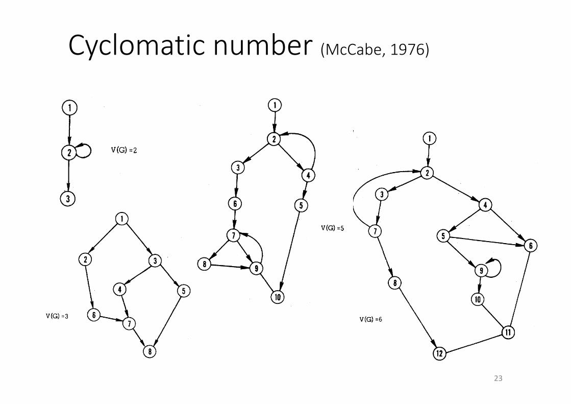
Cyclomatic number(McCabe,1976)
23
310 IEEE TRANSACTIONS ON SOFTWARE EN(
NTCT= (NCHARS+ 7 ) "NWORDSLTOT= (NCHARS+ 5) *NWORDS
******:* BLOCK NO. 1 ********************IF(LTOT,GT,2048) GO TO 900
****** BLOCK NO. 2 ***************************CALL READB(ICHANT,EMORY,LTOT,NREAD,$99 0,$9S0).LIN=OLU= NCHARS *NWORDS+ LMLV=NWORDS+ LULW=NWORDS+ LVLX=NWORDS+ LWLY-NWORDS+ LXLQ=NWORDS+ LYLWEX=NWORDS+LQ
BLOCK NO. 3700 I=,NWORD0************************** 2 V(G) =2
MEMORY(LWEX+I)=(MEMORY(LW+I),OR,(MEMORY(LW+I)*2))700 CONTINUE
******** BLOCK NO. 4 *************************CALL EXTEXT(ITRANS)STOP
********BLOCK NO. 5 ***************************900 TYPE 3,LTOT3 FORNAT(STRUCTURE TOO LARGE FOR CORE; ',18,' WORDS'
t SEE COOPER /)STOP
********BLOCK NO. 6 ************************** 2990 TYPE $4 FORMAT(' READ ERROR, OR STRUCTURE FILE- ERROR; J
' SEE COOPER I)STOPEND
V(G)=3
CONNECTIVITY MATRIX
1 2 3 4 5 6 7
1 011 0 0 0 0
2 O O O O O 1 O032 O 1 0 0 0
4 0 0 0 1 1 0 0
5 0 0 0 0 016 0 0 0 0 0 0 1
7 0 000000 1 6 5
.DL.DL.DL.DL.DL.DL.DL.DL.DL.DL.DL.DL.DL CYCLOMATIC COMPLEXITY = V(G) =
CLOSURE OF CONNECTIVITY MATRIX
1 2 3 4 5 6 7
1 0 1 1 1 1 1 1
2 0 0 0 0 0 1 1
3 0 0 0 1 1 1 1
4 0 0 0 1 1 1 1 7
5 0 0 0 0 0 1 1
6 0 0 0 0 0 0 1
7 0000000 8
,END
V(G)=6
At this point a few of the control graphs that were found inlive programs will be presented. The actual control graphsfrom FLOW appear on a DATA DISK CRT but they are handdrawn here for purposes of illustration. The graphs are pre-sented in increasing order of complexity in order to suggestthe correlation between the complexity numbers and our in-tuitive notion of control flow complexity.
GINEERING, DECEMBER 1976
MC CABE: A COMPLEXITY MEASURE 311
Cyclomatic number(McCabe,1976)
24
• Quitesomeproblems:• norecognitionof
familiarstructures• whataboutobfuscated
unstructuredCFGs?• whattodowhen
functionsarenotidentifiedwell?
• norecognitionofdatadependencies
• whataboutobject-orientedcode?
• whataboutconditionalstatements?
• combinatoric issues
MC CABE: A COMPLEXITY MEASURE 311
HumanComprehensionModels(Nakamuraetal,2003)
25
• Comprehension~mentalsimulationofaprogram
• Modelthebrain,pen&paperasasimpleCPU
• CPUperformanceisdrivenbymisses• cachemisses• TLBmisses• prediction
• Soisthebrain
• Measuremisseswithsmallsizesofmemory
Combineallofthem(Anckaertetal,2007)
26
1. code&codesize• e.g.,#instructions,weightedby"complexity"
2. controlflowcomplexity3. dataflowcomplexity
• sizesslices• sizeslivesets,workingsets• sizespoints-tosets• fan-in,fan-out• datastructurecomplexities
4. data• application-specific
static->graphs
dynamic->traces
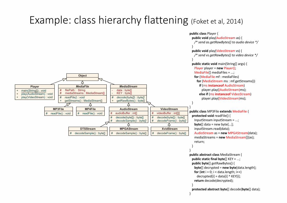
Example:classhierarchyflattening(Foketetal,2014)
27
publicclassPlayer{publicvoidplay(AudioStream as){/*sendas.getRawBytes()toaudiodevice*/
}publicvoidplay(VideoStream vs){/*sendvs.getRawBytes()tovideodevice*/
}publicstaticvoidmain(String[]args){Playerplayer =new Player();MediaFile[]mediaFiles =...;for(MediaFile mf:mediaFiles)for(MediaStream ms:mf.getStreams())if(msinstanceof AudioStream)player.play((AudioStream)ms);
elseif(ms instanceof VideoStream)player.play((VideoStream)ms);
}}publicclassMP3FileextendsMediaFile {protectedvoidreadFile(){InputStream inputStream =...;byte[]data =newbyte[...];inputStream.read(data);AudioStream as=newMPGAStream(data);mediaStreams =newMediaStream[]{as};return;
}}publicabstractclassMediaStream {publicstaticfinalbyte[]KEY=...;publicbyte[]getRawBytes(){byte[]decrypted=newbyte[data.length];for(int i =0;i <data.length;i++)decrypted[i]=data[i]^KEY[i];
return decode(decrypted);}protectedabstractbyte[]decode(byte[]data);
}
Object
MediaStream
- data : byte[]- KEY : byte[]# decode(byte[]) : byte[]+ getRawBytes() : byte[]
Player
main(String[]) : void++ play(AudioStream) : void+ play(VideoStream) : void
AudioStream
# audioBuffer : int[]# decode(byte[]) : byte[]# decodeSample() : byte[]
VideoStream
# videoBuffer : int[][]# decode(byte[]) : byte[]# decodeFrame() : byte[]
MP3File
# readFile() : void
XvidStream
# decodeFrame() : byte[]DTSStream
# decodeSample() : byte[]
MP4File
# readFile() : void
# decodeSample() : byte[]MPGAStream
MediaFile
# filePath : String# mediaStreams : MediaStream[]# readFile() : void+ getStreams() : MediaStream[]
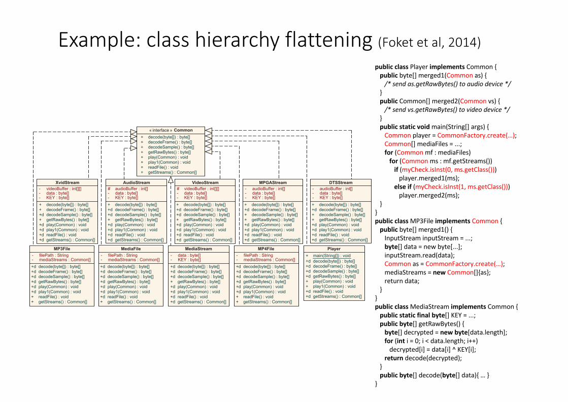
Example:classhierarchyflattening(Foketetal,2014)
28
publicclassPlayerimplements Common{publicbyte[] merged1(Common as){/*sendas.getRawBytes()toaudiodevice*/
}publicCommon[] merged2(Common vs){/*sendvs.getRawBytes()tovideodevice*/
}publicstaticvoidmain(String[]args){Common player=CommonFactory.create(…);Common[]mediaFiles =...;for(Common mf:mediaFiles)for(Common ms:mf.getStreams())if(myCheck.isInst(0,ms.getClass()))player.merged1(ms);
elseif(myCheck.isInst(1,ms.getClass()))player.merged2(ms);
}}publicclassMP3Fileimplements Common {publicbyte[] merged1(){InputStream inputStream =...;byte[]data =newbyte[...];inputStream.read(data);Common as=CommonFactory.create(…);mediaStreams =new Common[]{as};returndata;
}}publicclassMediaStream implements Common{publicstaticfinalbyte[]KEY=...;publicbyte[]getRawBytes(){byte[]decrypted=newbyte[data.length];for(int i =0;i <data.length;i++)decrypted[i]=data[i]^KEY[i];
return decode(decrypted);}publicbyte[]decode(byte[]data){…}
}
« interface » Common+ decode(byte[]) : byte[]+ decodeFrame() : byte[]+ decodeSample() : byte[]+ getRawBytes() : byte[]+ play(Common) : void+ play1(Common) : void+ readFile() : void+ getStreams() : Common[]
XvidStream- videoBuffer : int[][]- data : byte[]- KEY : byte[]+ decode(byte[]) : byte[]+ decodeFrame() : byte[]+d decodeSample() : byte[]+ getRawBytes() : byte[]+d play(Common) : void+d play1(Common) : void+d readFile() : void+d getStreams() : Common[]
MP3File- filePath : String- mediaStreams : Common[]+d decode(byte[]) : byte[]+d decodeFrame() : byte[]+d decodeSample() : byte[]+d getRawBytes() : byte[]+d play(Common) : void+d play1(Common) : void+ readFile() : void+ getStreams() : Common[]
- filePath : String- mediaStreams : Common[]
MediaFile
+d decode(byte[]) : byte[]+d decodeFrame() : byte[]+d decodeSample() : byte[]+d getRawBytes() : byte[]+d play(Common) : void+d play1(Common) : void+d readFile() : void+ getStreams() : Common[]
- data : byte[]- KEY : byte[]
MediaStream
+d decode(byte[]) : byte[]+d decodeFrame() : byte[]+d decodeSample() : byte[]+ getRawBytes() : byte[]+d play(Common) : void+d play1(Common) : void+d readFile() : void+d getStreams() : Common[]
Player+ main(String[]) : void+d decode(byte[]) : byte[]+d decodeFrame() : byte[]+d decodeSample() : byte[]+d getRawBytes() : byte[]+ play(Common) : void+ play1(Common) : void+d readFile() : void+d getStreams() : Common[]
MP4File- filePath : String- mediaStreams : Common[]+d decode(byte[]) : byte[]+d decodeFrame() : byte[]+d decodeSample() : byte[]+d getRawBytes() : byte[]+d play(Common) : void+d play1(Common) : void+ readFile() : void+ getStreams() : Common[]
AudioStream# audioBuffer : int[]- data : byte[]- KEY : byte[]+ decode(byte[]) : byte[]+d decodeFrame() : byte[]+d decodeSample() : byte[]+ getRawBytes() : byte[]+d play(Common) : void+d play1(Common) : void+d readFile() : void+d getStreams() : Common[]
VideoStream# videoBuffer : int[][]- data : byte[]- KEY : byte[]+ decode(byte[]) : byte[]+d decodeFrame() : byte[]+d decodeSample() : byte[]+ getRawBytes() : byte[]+d play(Common) : void+d play1(Common) : void+d readFile() : void+d getStreams() : Common[]
MPGAStream- audioBuffer : int[]- data : byte[]- KEY : byte[]+ decode(byte[]) : byte[]+d decodeFrame() : byte[]+ decodeSample() : byte[]+ getRawBytes() : byte[]+d play(Common) : void+d play1(Common) : void+d readFile() : void+d getStreams() : Common[]
DTSStream- audioBuffer : int[]- data : byte[]- KEY : byte[]+ decode(byte[]) : byte[]+d decodeFrame() : byte[]+ decodeSample() : byte[]+ getRawBytes() : byte[]+d play(Common) : void+d play1(Common) : void+d readFile() : void+d getStreams() : Common[]
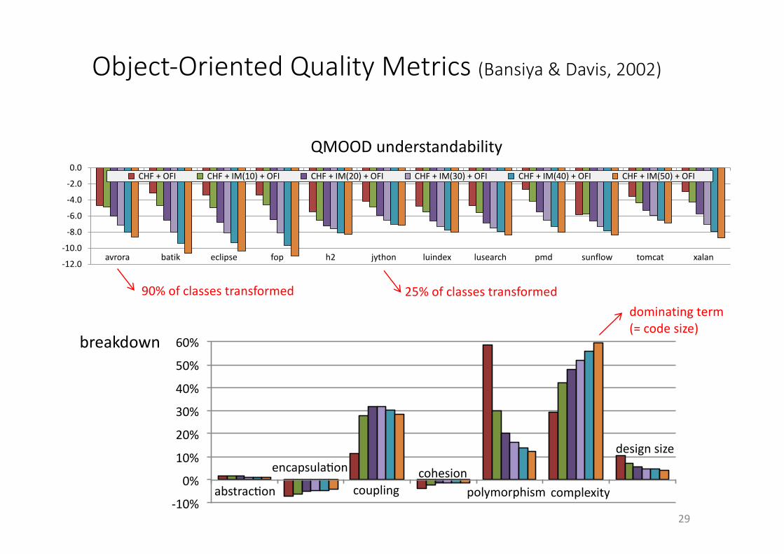
Object-OrientedQualityMetrics(Bansiya&Davis,2002)
-12.0
-10.0
-8.0
-6.0
-4.0
-2.0
0.0
avrora batik eclipse fop h2 jython luindex lusearch pmd sunflow tomcat xalan
Rela
tive
incr
ease
CHF + OFI CHF + IM(10) + OFI CHF + IM(20) + OFI CHF + IM(30) + OFI CHF + IM(40) + OFI CHF + IM(50) + OFI
QMOODunderstandability
90%ofclassestransformed 25%ofclassestransformeddominatingterm(=codesize)
!10%%
0%%
10%%
20%%
30%%
40%%
50%%
60%%
abstrac1on%encapsula1on% coupling% cohesion% polymorphism%complexity% design%size%
(legend:%see%Fig.%10)%Series1%
Series2%
Series3%
Series4%
Series5%
Series6%
abstrac3on
encapsula3on
couplingcohesion
polymorphism complexity
design'size
breakdown
29
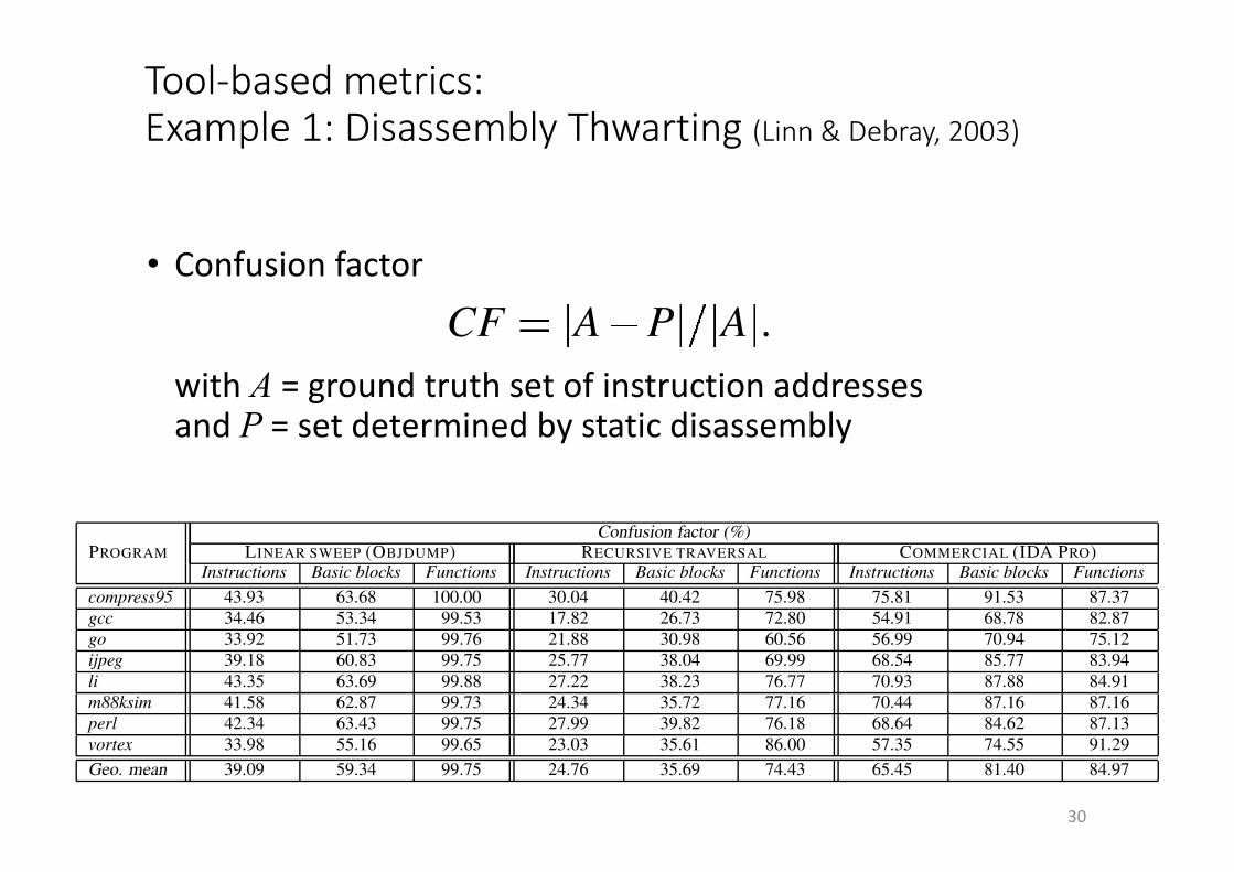
Tool-basedmetrics:Example1:DisassemblyThwarting(Linn&Debray,2003)
30
• Confusionfactor
with A =groundtruthsetofinstructionaddressesandP =setdeterminedbystaticdisassembly
compress gcc go ijpeg li m88ksim perl vortex MeanProgram
0.75
0.80
0.85
0.90
0.95
1.00
frac
tion
of c
andi
date
s con
vert
ed
0.700.800.900.951.00
Thresholds
(a) Fraction of jumps converted to branch function calls
compress gcc go ijpeg li m88ksim perl vortex MeanProgram
1.0
2.0
3.0
4.0
5.0
6.0
slow
dow
n fa
ctor
0.700.800.900.951.00
Thresholds
(b) Slowdown in execution speed
Figure 6: Effect of “hot code threshold” on branch function conversion and execution speed
(Sections 3.4.1 and 3.4.2). We expect to have additional transfor-mations, such as jump table spoofing (Section3.4.4), implementedin the near future.
4. EXPERIMENTAL EVALUATIONWe evaluated the efficacy of our techniques using the SPECint-
95 benchmark suite. Our experiments were run on an otherwiseunloaded 2.4 GHz Pentium IV system with 1 GB of main memoryrunning RedHat Linux 8.0. The programs were compiled with gccversion egcs-2.91.66 at optimization level -O3. The programs wereprofiled using the SPEC training inputs and these profiles were usedto identify any hot spots during our transformations. The final per-formance of the transformed programs were then evaluated usingthe SPEC reference inputs. Each execution time reported was de-rived by running seven trials, removing the highest and lowest timesfrom the sampling, and averaging the remaining five.We experimented with three different “attack disassemblers” to
evaluate our techniques. The first of these is the GNU objdump util-ity which employs a straight-forward linear sweep algorithm. Thesecond, which we wrote ourselves, is a recursive disassembler thatincorporates a variation of speculative disassembly (see Section 2).In addition we also provide the recursive disassembler with extrainformation about the address and size of each jump table in theprogram as well as the start and end address of each function. Theresults obtained from this disassembler therefore serve as a lowerbound estimate of the extent of obfuscation achieved. Our third dis-assembler is IDA Pro [13], a commercially available disassemblytool that is generally regarded to be among the best disassemblersavailable.For each of these, the efficacy of obfuscation was measured by
computing “confusion factors” for the instructions, basic blocks,
and functions. Intuitively, the confusion factor measures the frac-tion of program units (instructions, basic blocks, or functions) inthe obfuscated code that were incorrectly identified by a disassem-bler. More formally, let A be the set of all actual instruction ad-dresses, i.e., those that would be encountered when the programis executed, and P the set of all perceived instruction addresses,i.e., those addresses produced by a static disassembly. A P is theset of addresses that are not correctly identified as instruction ad-dresses by the disassembler. We define the confusion factor CF tobe the fraction of instruction addresses that the disassembler failsto identify correctly:6
CF A P A .
Confusion factors for functions and basic blocks are calculatedanologously: a basic block or function is counted as being “in-correctly disassembled” if any of the instructions in it is incorrectlydisassembled. The reason for computing confusion factors for ba-sic blocks and functions as well as for instructions is to determinewhether the errors in disassembling instructions are clustered in asmall region of the code, or whether they are distributed over sig-nificant portions of the program.As mentioned in Section 3.4.1, we transform jumps to branch
function calls only if the jump does not occur in a “hot” basic block.The first questions we have to address, therefore, are: how are hotbasic blocks identified, and what is the effect of different choices ofwhat constitutes a “hot” block on the extent of obfuscation achievedand the performance of the resulting code? To identify the “hot,” or6We also considered taking into account the set P A of addressesthat are erroneously identified as instruction addresses by the disas-sembler, but rejected this approach because it “double counts” theeffects of disassembly errors.
Confusion factor (%)PROGRAM LINEAR SWEEP (OBJDUMP) RECURSIVE TRAVERSAL COMMERCIAL (IDA PRO)
Instructions Basic blocks Functions Instructions Basic blocks Functions Instructions Basic blocks Functionscompress95 43.93 63.68 100.00 30.04 40.42 75.98 75.81 91.53 87.37gcc 34.46 53.34 99.53 17.82 26.73 72.80 54.91 68.78 82.87go 33.92 51.73 99.76 21.88 30.98 60.56 56.99 70.94 75.12ijpeg 39.18 60.83 99.75 25.77 38.04 69.99 68.54 85.77 83.94li 43.35 63.69 99.88 27.22 38.23 76.77 70.93 87.88 84.91m88ksim 41.58 62.87 99.73 24.34 35.72 77.16 70.44 87.16 87.16perl 42.34 63.43 99.75 27.99 39.82 76.18 68.64 84.62 87.13vortex 33.98 55.16 99.65 23.03 35.61 86.00 57.35 74.55 91.29Geo. mean 39.09 59.34 99.75 24.76 35.69 74.43 65.45 81.40 84.97
Figure 7: Efficacy of obfuscation: confusion factors (θ 1 0)
“frequently executed,” basic blocks, we start with a (user-defined)fraction θ (0 0 θ 1 0) that specifies what fraction of the totalnumber of instructions executed at runtime should be accounted forby “hot” basic blocks. For example, θ 0 8 means that hot blocksshould account for at least 80% of all the instructions executed bythe program. More formally, let the weight of a basic block bethe number of instructions in the block multiplied by its executionfrequency, i.e., the block’s contribution to the total number of in-structions executed at runtime. Let tot instr ct be the total numberof instructions executed by the program, as given by its executionprofile. Given a value of θ, we consider the basic blocks b in theprogram in decreasing order of execution frequency, and determinethe largest execution frequency N such that
∑b:freq b N
weight b θ tot instr ct
Any basic block whose execution frequency is at least N is consid-ered to be hot.The effect of varying the hot code threshold θ on performance
(both obfuscation and speed) is shown in Figure 6. Figure 6(a)shows the fraction of candidates that are converted to branch func-tion calls at different thresholds; this closely tracks the overall con-fusion factors achieved. Figure 6(b) shows the concomitant degra-dation in performance. It can be seen, from Figure 6(a), that mostprograms have a small and well-defined hot spot, and as a resultvarying the threshold from a modest 0.70 to a value as high as 1.0does not dramatically affect the number of candidates converted.The benchmark that is affected the most is gcc, and even here over79% of the candidates are converted at θ 1 0. On average, about91% of the candidates are converted at θ 1 0. However, as il-lustrated in Figure 6(b), varying the hot code threshold has a sig-nificant effect on execution speed. For example, at θ 0 70 theprograms slow down by a factor of 3.67 on average, with the libenchmark experiencing the largest slowdown, by a factor of 5.14.However, as θ is increased the slowdown drops off quickly, to a fac-tor of 3.14 at θ 0 9 and 1.62 at θ 1 0. In summary, choosing athreshold θ of 1.0 still results in most of the candidate blocks in theprogram being converted to branch function calls without excessiveperformance penalty. For the purposes of this paper, therefore, wegive measurements for θ 1 0.Figure 7 shows the efficacy of our obfuscation transformations
for both of the disassembly methods discussed in Section 2. Theconfusion factors achieved for linear sweep disassembly are quitemodest: on average, 39% of the instructions, 59% of the basicblocks, and nearly 100% of the functions are incorrectly disassem-bled. For recursive traversal, the confusion factors are somewhatlower because in this case the disassembler can understand and dealwith control flow somewhat better than with linear sweep and as a
EXECUTION TIME (SECS)PROGRAM Original Obfuscated Slowdown
T0 T1 T1 T0compress95 34.49 34.44 1.00gcc 23.27 23.23 1.00go 53.17 53.08 1.00ijpeg 40.13 40.15 1.00li 26.50 42.91 1.62m88ksim 28.18 30.02 1.07perl 28.62 37.71 1.32vortex 48.84 49.05 1.00Geo. mean 1.13
Figure 8: Effect of obfuscation on execution speed (θ 1 0)
last resort actually reverts to linear sweep for the speculative dis-assembly of undisassembled code. Nevertheless, we find that, onaverage, over 25% of the instructions in the program incur disas-sembly errors. As a result, over 35% of the basic blocks and closeto 74% of the functions, on average, are incorrectly disassembledusing this disassembly method. This is achieved at the cost of a13% penalty in execution speed (see Figure 8).The recursive traversal data reported in Figure 7 are actually
quite conservative since these were gathered using our own recur-sive disassembler which, as mentioned before, is supplied with ex-tra information to avoid unduly optimistic results. To evaluate theefficacy of our techniques in a more realistic situation, we used acommercial disassembly tool, IDA Pro version 4.3x [13], which iswidely considered to be the most advanced disassembler available.The results of this experiment are reported in Figure 7. It can beseen that this tool fails on most of the program: close to 65% of theinstructions, and about 85% of the functions in the program, aredisassembled incorrectly. Part of the reason for this high degree offailure is that IDA Pro only disassembles addresses that (it believes)can be guaranteed to be instruction addresses. This has two effects:first, large portions of the code that are reached by branch functionaddresses are simply not disassembled, being presented instead tothe user as a jumble of hex data; and second, the location imme-diately following a branch function call is treated as an address towhich control returns, and this causes some junk bytes to be erro-neously disassembled. Overall, this shows that our techniques areeffective even against state-of-the-art disassembly tools.Finally, Figure 9 shows the impact of obfuscation on code size,
both in terms of the number of instructions (which increases, forexample, due to branch flipping), as well as the number of bytesoccupied by the text section. The latter includes the effects of thenew instructions inserted as well as all junk bytes added to the pro-gram. Overall, it can be seen that there is a 20% increase in the
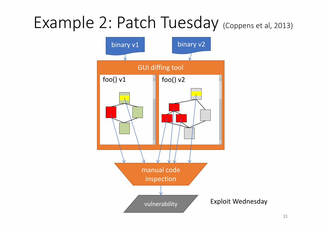
Example2:PatchTuesday(Coppensetal,2013)binaryv1 binaryv2
vulnerability
foo()v1
GUIdiffingtool
foo()v2
manualcodeinspection
31
ExploitWednesday
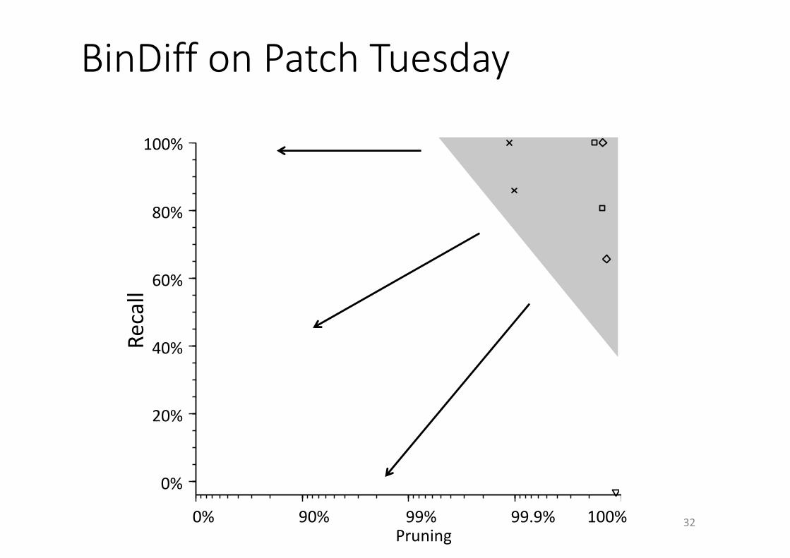
0% 90% 99% 99.9% 100%
0%
20%
40%
60%
80%
100%Re
call
Pruning
BinDiff onPatchTuesday
32
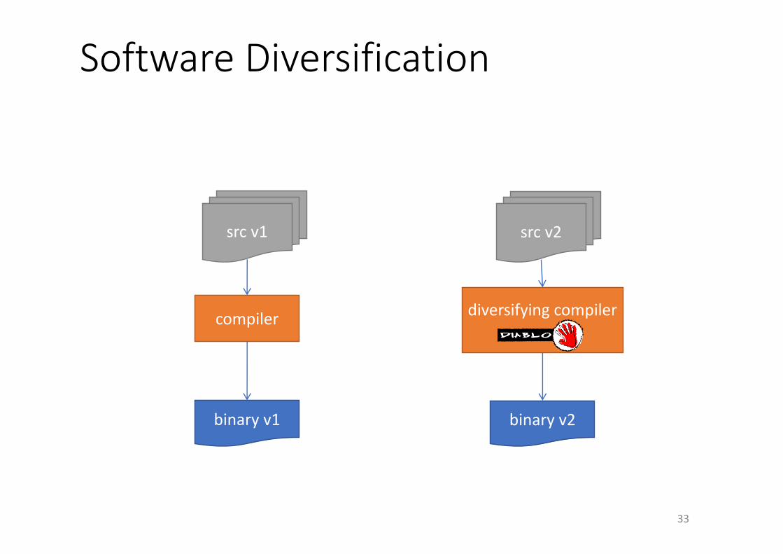
SoftwareDiversification
binaryv1
src v1
compiler
binaryv2
diversifyingcompiler
src v2
33
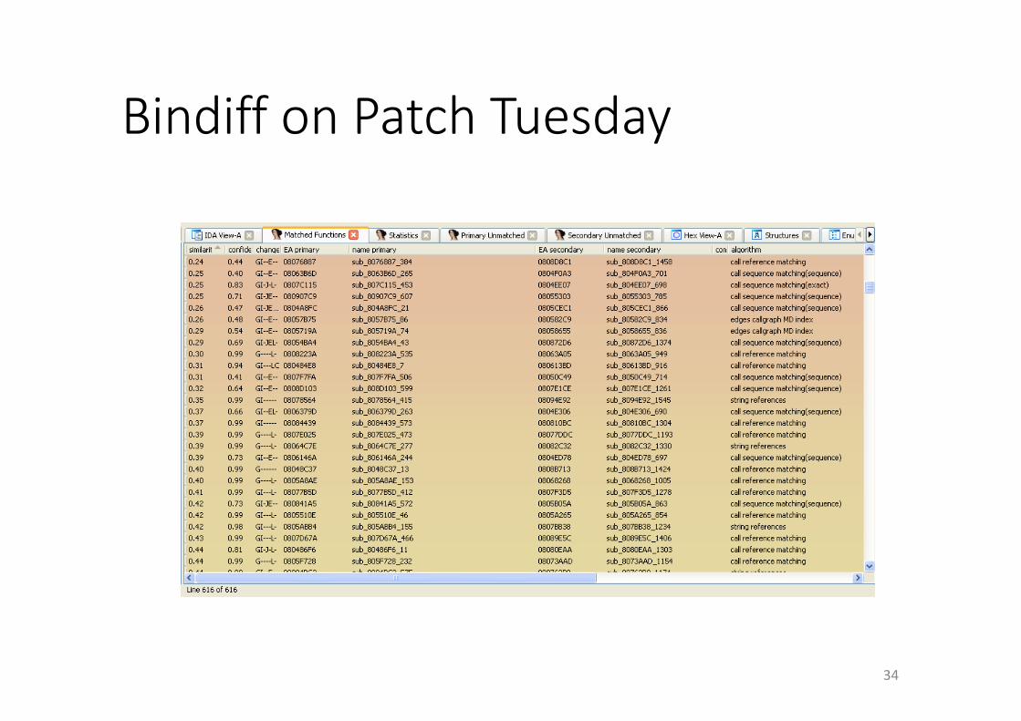
Bindiff onPatchTuesday
34
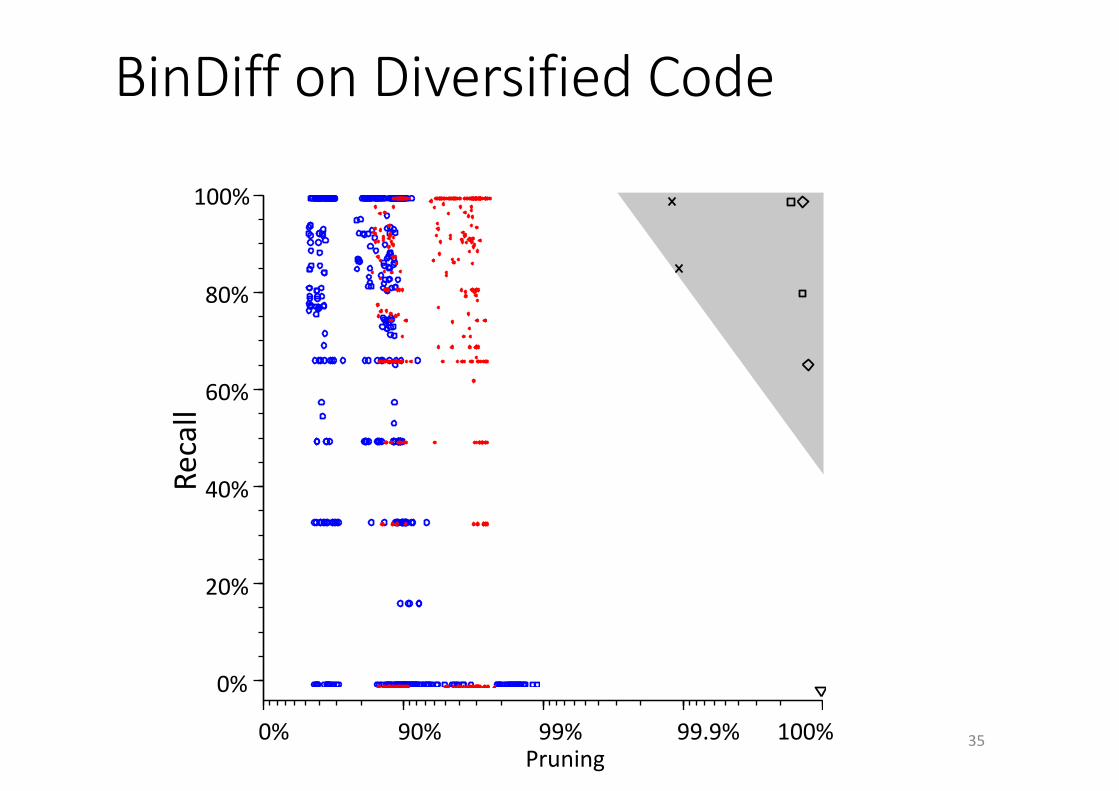
BinDiff onDiversifiedCode
0% 90% 99% 99.9% 100%
0%
20%
40%
60%
80%
100%Re
call
Pruning35
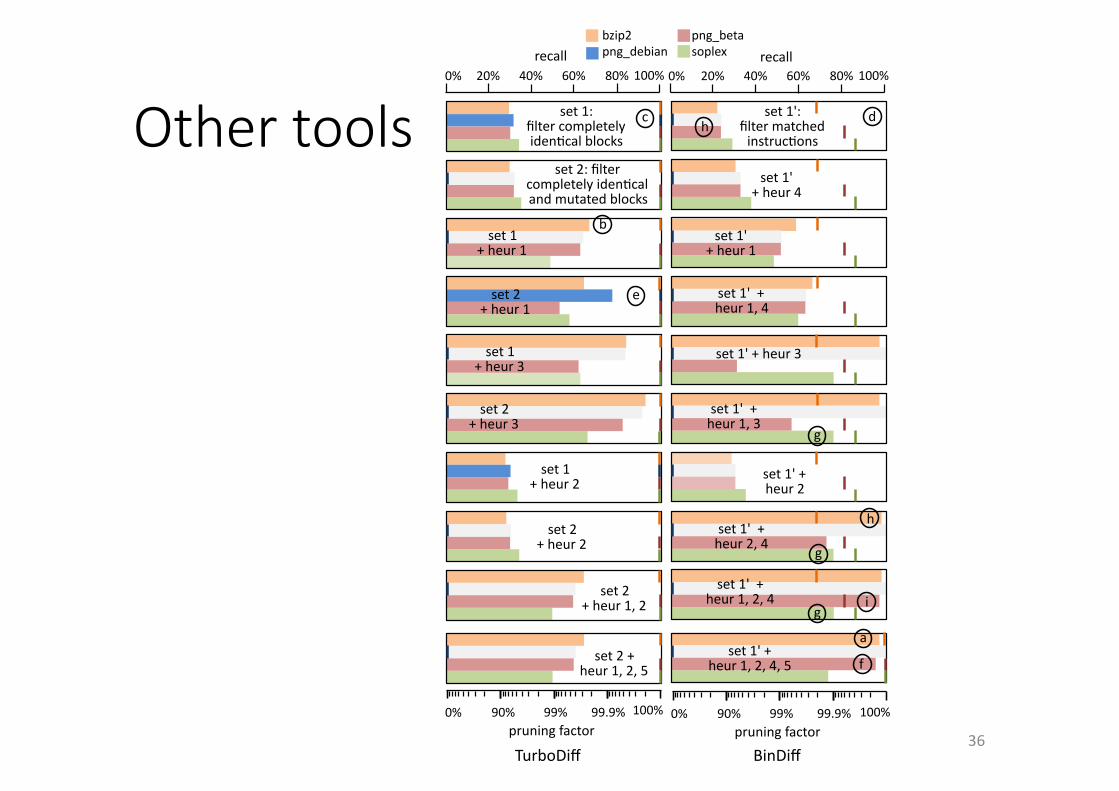
Othertools
36
bzip2 & &png_beta&png_debian &soplex&recall& recall&
TurboDiff& BinDiff&
0%& 20%& 40%& 60%& 80%& 100%&0%& 20%& 40%& 60%& 80%& 100%&
a&
b&
e&
f&
g&
g&
g&
pruning&factor&0%& 90%& 99%& 99.9%& 100%&
pruning&factor&0%& 90%& 99%& 99.9%& 100%&
h&
i&
set&1:&&filter&completely&idenGcal&blocks&
d&set&1':&filter&matched&&instrucGons&
set&2:&filter&&completely&idenGcal&and&mutated&blocks&
set&1&&+&heur&1&
set&2&+&heur&1&
set&1&&+&heur&3&
set&2&&+&heur&3&
set&1&&+&heur&2&
set&2&+&heur&2&
set&2&&+&heur&1,&2&&
set&2&+&&heur&1,&2,&5&
set&1'&&+&heur&4&
set&1'&&+&heur&1&
set&1'&&+&&heur&1,&4&
set&1'&+&heur&3&
set&1'&&+&heur&1,&3&
set&1'&+&&heur&2&
set&1'&&+&heur&2,&4&
set&1'&&+&&heur&1,&2,&4&
set&1'&+&&heur&1,&2,&4,&5&
c&h&
Fig. 4: Pruning factors (bars) and recalls (lines) obtained on undiversified binaries
however, because all syntactic changes in this use case are semantic changes. When such a minimalsecurity fix involving only changed constants is combined with other (non-related) fixes as in png debian,the patch includes many more syntactic mutations, which prevents it from being used as a shortcut.
Considering only the combinations of tools and heuristics with recalls over 60%, the highest pruningfactors obtained with BinDi↵ are 99.988% ( i ), 99.986% ( j ) and 99.909% ( e ). As the fractions ofirrelevant instructions in those cases are 99.997%, 99.986%, and 99.923% resp., BinDi↵ proves to be ableto prune more than 99.98% of all irrelevant instructions for those three use cases.
This demonstrates, for the first time, that for some types of patches and undiversified code, di�ngtools and heuristics are indeed highly valuable cracker tools. For other types of patches, however, theyare much less e↵ective. Moreover, as a cracker does typically not know beforehand which types of patcheshave been applied, he will be hindered by not being able to fine-tune his heuristics.
Diversification
To study the impact of diversification, we used the diversifier Proteus [1] that comes with the free andopen Diablo link-time rewriting framework (http://diablo.elis.ugent.be). This tool supports a number
7
LectureOverview1. Protectionvis-à-visattacks
• attacksonwhat?• attackandprotectionmodels
37
2. QualitativeEvaluation
3. QuantitativeEvaluation• complexitymetrics• tools
4. HumanExperiments
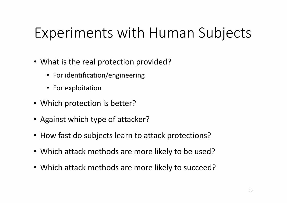
ExperimentswithHumanSubjects
38
• Whatistherealprotectionprovided?• Foridentification/engineering
• Forexploitation
• Whichprotectionisbetter?
• Againstwhichtypeofattacker?
• Howfastdosubjectslearntoattackprotections?
• Whichattackmethodsaremorelikelytobeused?
• Whichattackmethodsaremorelikelytosucceed?
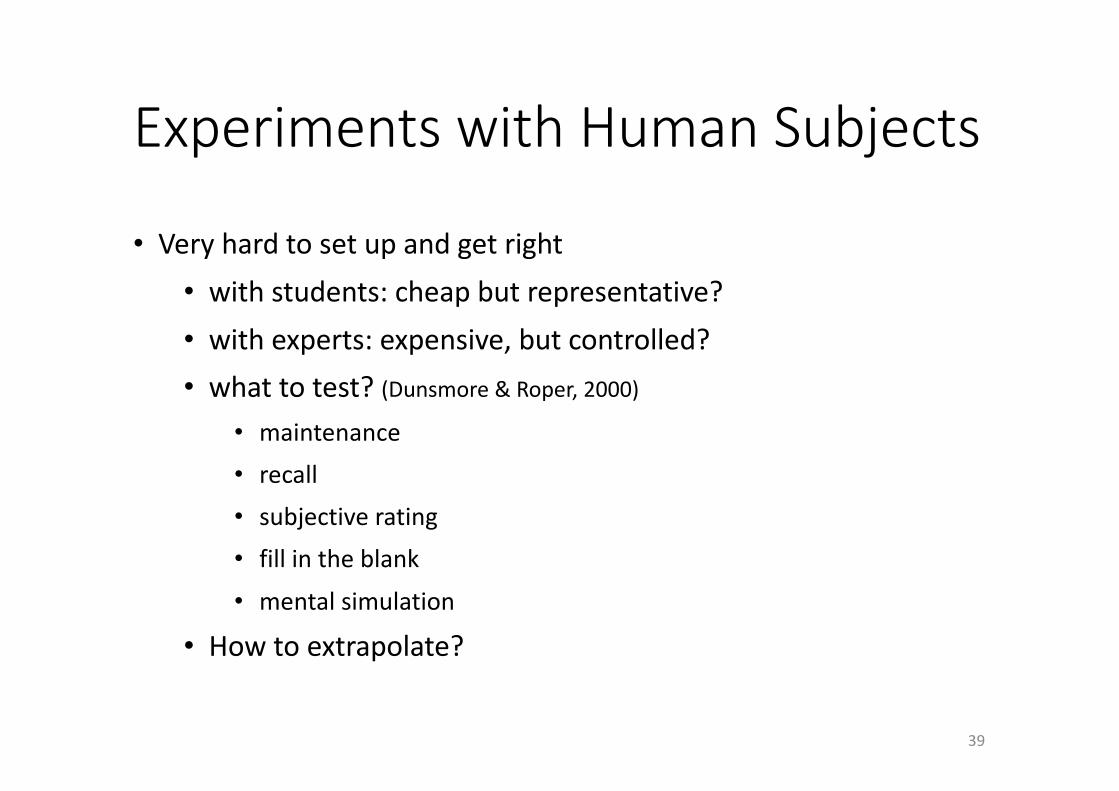
ExperimentswithHumanSubjects
39
• Veryhardtosetupandgetright• withstudents:cheapbutrepresentative?• withexperts:expensive,butcontrolled?• whattotest?(Dunsmore &Roper,2000)
• maintenance• recall• subjectiverating• fillintheblank• mentalsimulation
• Howtoextrapolate?
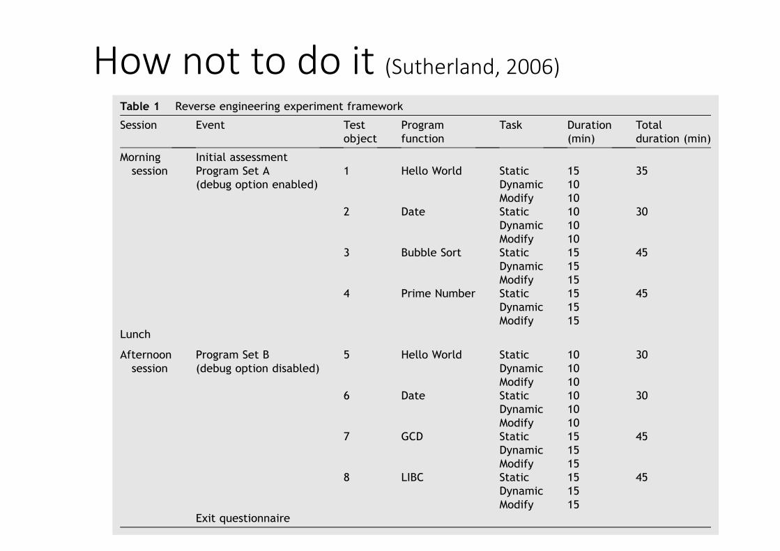
Hownottodoit(Sutherland,2006)
40
that some limited collaboration on experimentalresults would emulate real world conditions pres-ent during actual software exploitation activities.Test subjects were provided with Program Set Bduring the afternoon session of the reverse engi-neering experiment. The experiment developerswere again present to observe any interactionsbetween test subjects.
To further observe the test subject activitiesduring the execution of the reverse engineeringexperiment, the test developers employed anautomated screen capture tool (Camtasia) to pro-vide a permanent record of activities. The reverseengineering experiment platform involved anIntel-based computer executing Linux Redhat 7.2within a VMWare virtual environment hosted onWindows NT4. This enabled the complete experi-mental environment to be retained for futureanalysis and included Bash histories of commandline instructions, and all temporary and historyfiles arising from Internet accesses. The screencaptures, Bash histories, temporary and historyfiles coupled with the initial questionnaire andtutorial worksheets, provide a detailed accountingof the test subject activities.
At the completion of Program Set B the testsubjects were provided an exit questionnaire toenable post-experiment assessment. The exitquestionnaire assessed the amount of materialssupplied on the reading list that were actually usedby test subjects during the experiment along withgeneral comments pertaining to the various stagesof the reverse engineering experiment.
Results
The measurements collected during the reverseengineering experiment are analyzed to validatethe two assertions defined in the beginning of thispaper (section Assertions).
Education/technical ability
The first assertion to be validated by the experi-mental results concerned whether the use ofa statistical model could illustrate the relationshipbetween education and technical ability of thesoftware exploiter and their ability to successfullyreverse engineer a software product. This assertion
Table 1 Reverse engineering experiment framework
Session Event Testobject
Programfunction
Task Duration(min)
Totalduration (min)
Morningsession
Initial assessmentProgram Set A(debug option enabled)
1 Hello World Static 15 35Dynamic 10Modify 10
2 Date Static 10 30Dynamic 10Modify 10
3 Bubble Sort Static 15 45Dynamic 15Modify 15
4 Prime Number Static 15 45Dynamic 15Modify 15
Lunch
Afternoonsession
Program Set B(debug option disabled)
5 Hello World Static 10 30Dynamic 10Modify 10
6 Date Static 10 30Dynamic 10Modify 10
7 GCD Static 15 45Dynamic 15Modify 15
8 LIBC Static 15 45Dynamic 15Modify 15
Exit questionnaire
An empirical examination of the reverse engineering process for binary files 225
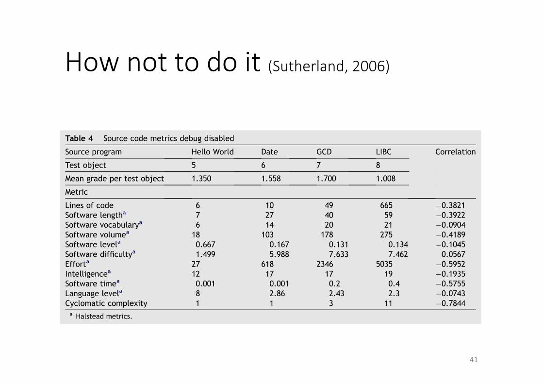
Hownottodoit(Sutherland,2006)
41
a consistent and repeatable fashion. The 10 testsubjects participating in the actual reverseengineering experiment, although representinga relatively small data set, provide the basis ofa preliminary assessment as to the primary factorsthat affect the software reverse engineering pro-cess. The reverse engineering experiment providesquantitative evidence that there is a relationshipbetween the education/technical ability of thesoftware exploiter and their ability to successfullyreverse engineer a software product. This evi-dence provides the foundation for modellingof this relationship using existing predictive mod-els. Development and maturation of a reverseengineering model that characterizes the software
exploitation process will enable commercial soft-ware product developers to quantitatively predictthe time following product deployment when it isanticipated that a software exploiter would haveachieved a given exploitation end goal.
The reverse engineering experiment also pro-vides quantitative evidence that industry acceptedsource code size and complexity metrics are notsuitable for characterizing the size and complexityof binary code files pursuant to estimating thetime required to perform software exploitationactivities. Literary research conducted at thecommencement of this project did not identifybinary size and complexity metrics that could havebeen used instead of the source code size and
Table 3 Source code metrics debug enabled
Source program Hello World Date Bubble Sort Prime Number Correlation
Test object 1 2 3 4
Mean gradeper test object
1.483 1.300 0.786 0.867
Metric
Lines of code 6 10 9 21 !0.5802Software lengtha 7 27 14 33 !0.3958Software vocabularya 6 14 11 15 !0.5560Software volumea 18 103 48 130 !0.4006Software levela 0.667 0.167 2.5 0.094 !0.4833Software difficultya 1.499 5.988 5.988 10.638 !0.7454Efforta 27 618 120 1435 !0.3972Intelligencea 12 17 19 15 !0.6744Software timea 0.001 0.001 0.001 0.001 0Language levela 8 2.86 7.68 1.83 0.1909Cyclomatic complexity 1 1 1 3 !0.4802
a Halstead metrics.
Table 4 Source code metrics debug disabled
Source program Hello World Date GCD LIBC Correlation
Test object 5 6 7 8
Mean grade per test object 1.350 1.558 1.700 1.008
Metric
Lines of code 6 10 49 665 !0.3821Software lengtha 7 27 40 59 !0.3922Software vocabularya 6 14 20 21 !0.0904Software volumea 18 103 178 275 !0.4189Software levela 0.667 0.167 0.131 0.134 !0.1045Software difficultya 1.499 5.988 7.633 7.462 0.0567Efforta 27 618 2346 5035 !0.5952Intelligencea 12 17 17 19 !0.1935Software timea 0.001 0.001 0.2 0.4 !0.5755Language levela 8 2.86 2.43 2.3 !0.0743Cyclomatic complexity 1 1 3 11 !0.7844
a Halstead metrics.
An empirical examination of the reverse engineering process for binary files 227
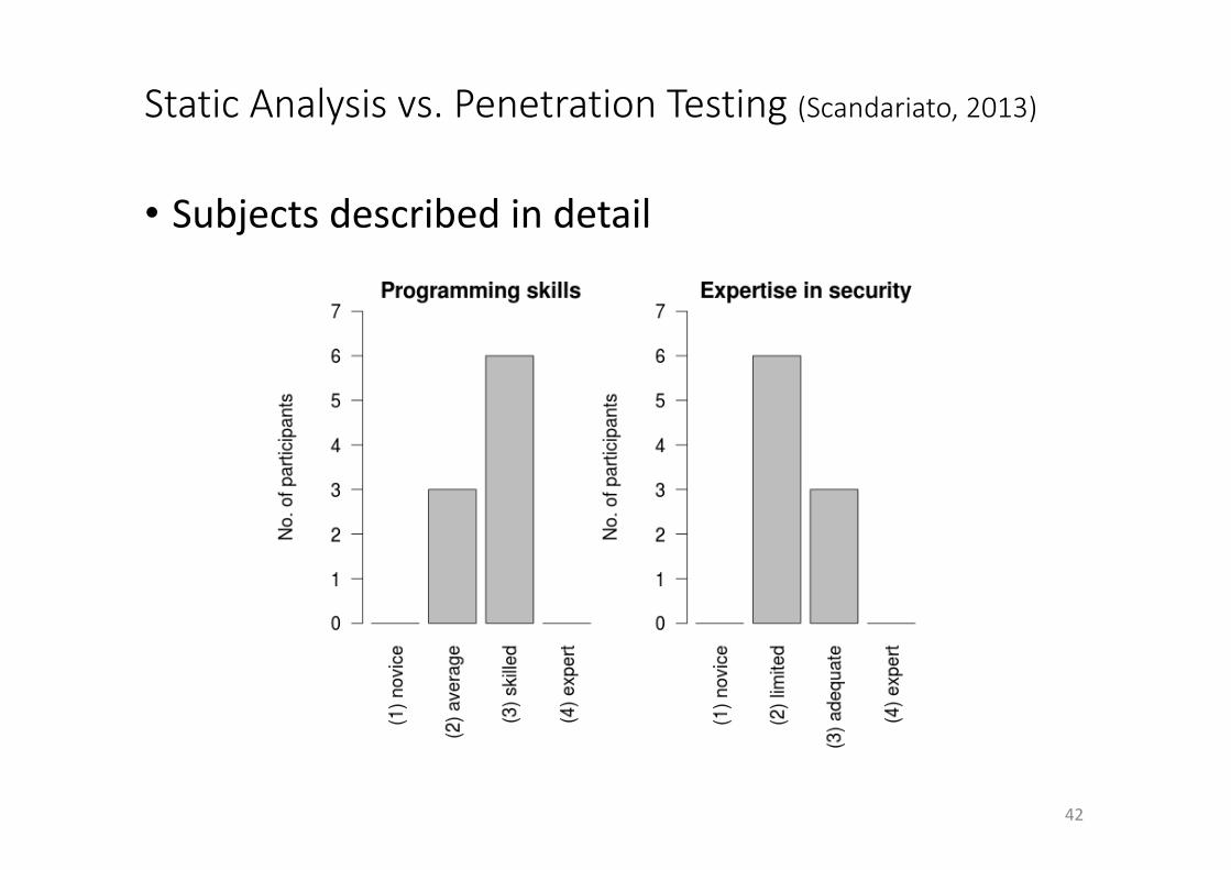
StaticAnalysisvs.PenetrationTesting(Scandariato,2013)
42
• Subjectsdescribedindetail
Fig. 1. Seniority of the participants
Fig. 2. Roles covered in the industry
one in software engineering and the other in computer security.The program is often selected by professionals who, after afew years in the software industry, are seeking a higher degreeto advance in their career. Most of these students are takingevening classes while working full time as software developers.
We surveyed the background of the participants by meansof a questionnaire administered at the beginning of the exper-iment. As shown in Figure 1, seven participants have at leastone year of experience as employees in the software industryand four have a seniority that is greater than three years.Figure 2 describes the roles covered by the participants in theiroccupation. All of them have worked as developers, and asmany as seven also have experience as software designers. Fourof the participants also reported some experience as testers,which is a useful asset for the tasks they carried out in theexperiment, especially for penetration testing. There are moreroles than participants, since participants may work in multipledifferent roles over the course of their career.
We also investigated the programming skills and securityexpertise of the participants, and the results are reported inFigure 3. Good Java programming skills are important for thestatic analysis task as the code needs to be inspected in order tovalidate the warnings produced by the analysis tool. Two thirds
Fig. 3. Skill levels of the participants
of our participants claimed to be skilled Java programmers,although we did not test their skills directly. Concerning theirsecurity knowledge, the participants are not complete novices,although two thirds admit to having limited expertise and onlyone third claimed adequate security skills.
In summary, despite their enrollment in a degree program,the participants have a profile which is closer to that ofprofessionals than of students. Indeed, they have substantialindustrial experience and advanced development skills. Clearly,the participants are not entirely representative of the populationof security analysts, due to their sub-optimal security skills.However, they have the necessary maturity to substantiatethe validity of the results of this work, which focuses onprofessionals beginning their activity in a security team.
C. Experimental Objects
For this experiment, we needed to select two approximatelyequivalent applications that were written in a language withwhich the students were familiar. We also needed vulnerabili-ties found in the applications to be of types that the studentshad studied. In order for the applications to be approximatelyequivalent, we selected them from the same application do-main: weblogs written in Java. In order for the experimentto be authentic, we decided to use open source applicationsthat were currently in use instead of using applications createdsolely for the purposes of this experiment.
We selected two weblog applications for the experi-ment: Apache Roller (roller.apache.org) and Pebble (pebble.sourceforge.net). Both Roller and Pebble are comprehensiveblogging platforms, with support for templates, feeds, multipleusers, threaded comments, and plugins. Both applications arecurrently in development and have a history of vulnerabilitiesrecorded in public databases. The applications are approxi-mately of the same size and complexity.
1) Pebble: Pebble 2.6.3, the version used in the experiment,consists of 56,168 executable lines of code as measured byFortify SCA. Version 2.6.4 is the current version (not availableat the time of the experiment) and 37 versions of Pebble havebeen released since version 1.0 was released in 2003. Pebblestores its data in XML files rather than in a SQL database.
453
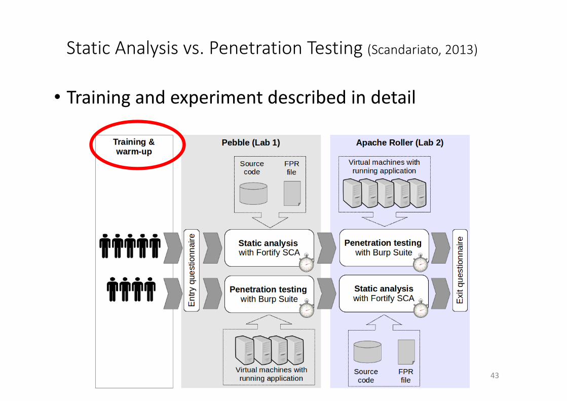
StaticAnalysisvs.PenetrationTesting(Scandariato,2013)
43
• Trainingandexperimentdescribedindetail
Fig. 4. Design of the experiment
• URL: the URL through which the vulnerability isexploitable.
• Input Field: the input field(s) used to exploit thevulnerability.
• Input Data: the input data that is necessary to exploitthe vulnerability.
• Description: the nature of the vulnerability and whatimpact it would have on the application. The partici-pants should also state any assumptions that are madein determining that this is a vulnerability.
The above documentation contains all the information that isnecessary to replicate the attack described by the participant.
E. Design of the Experiment
As shown in Figure 4, the experiment is organized in twolaboratories. In the first lab, five randomly chosen participantsanalyzed the Pebble application by means of static analysis,while the other four analyzed the same application via penetra-tion testing. In the second lab, the Apache Roller applicationwas analyzed, and participants were assigned to the treatmentthey did not apply in the previous lab.
In summary, we chose a paired comparison design (eachparticipant is administered both treatments) but we deemedthat randomizing the order of the treatments would havenot been enough to counter the learning effect and, hence,used two objects, i.e., applications. The two objects can beconsidered equivalent for the sake of the experiment, as thetwo applications provide the same functionality (blogging) andhave similar feature sets. The two applications also have acomparable size of about 60,000 executable lines of code.Furthermore, they have the same maturity as both have about10 years of development history. We also assume that the twoapplications have the same complexity. This assumption hasbeen validated by means of a specific question in the ques-tionnaire that we administered at the end of the experiment.To the question “Did you find that the two applications wereof comparable complexity?”, the participants replied that theyagreed: the median answer is 3 (‘agree’) on a 4-value scaleranging from 1 (strongly disagree) to 4 (strongly agree).
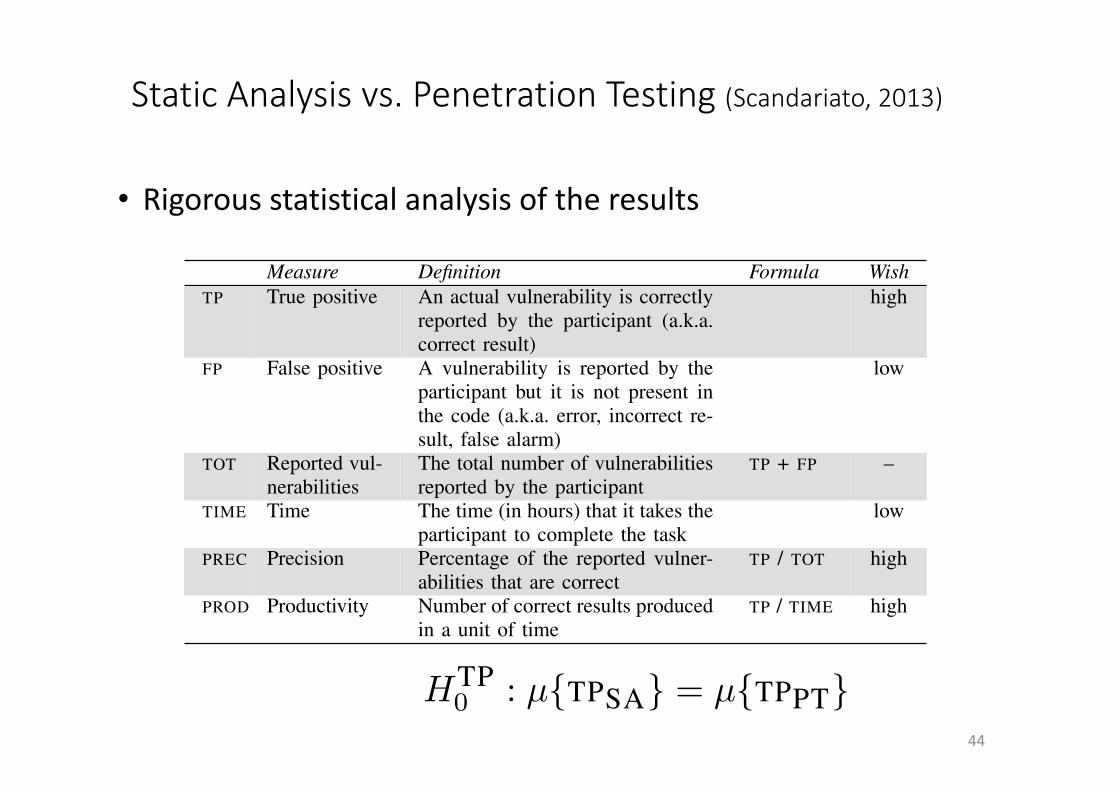
TABLE I. TERMINOLOGY.
Measure Definition Formula WishTP True positive An actual vulnerability is correctly
reported by the participant (a.k.a.correct result)
high
FP False positive A vulnerability is reported by theparticipant but it is not present inthe code (a.k.a. error, incorrect re-sult, false alarm)
low
TOT Reported vul-nerabilities
The total number of vulnerabilitiesreported by the participant
TP + FP –
TIME Time The time (in hours) that it takes theparticipant to complete the task
low
PREC Precision Percentage of the reported vulner-abilities that are correct
TP / TOT high
PROD Productivity Number of correct results producedin a unit of time
TP / TIME high
F. Hypotheses
According to the goals mentioned at the beginning of thissection, we are interested in both the quality of the analysisresults and the productivity of the analyst. The quality isprimarily characterized by the number of correct results (theactual vulnerabilities that are found) as more results meana more complete analysis and, consequently, a more secureapplication. Another important aspect is the number of errors(false alarms) as they result in a waste of resources forboth the analysis team and the quality assurance team thatis tasked with the bug fixing. As summarized in Table I, thecorrect results are called true positives (TP) and the errors arecalled false positives (FP). Next to the total number of truepositives, we quantify the quality by means of the precision(PREC), i.e., the ratio of correct results over the total amountof vulnerabilities reported. The measure of precision takesinto account the number of errors but it scales them withrespect to the total amount of results. This corresponds to thereasonable assumptions that it is more likely to make mistakesif more work is done. The productivity (PROD) is quantifiedwith respect to only correct results. Therefore, it is calculatedas the number of true positives produced per hour.
According to the above definitions, we refine the overallresearch goals into the following three null hypotheses. First,we wonder whether, on average, the two techniques producethe same amount of true positives.
HTP0 : µ{TPSA} = µ{TPPT}
Assuming that the discovered vulnerabilities have a compara-ble importance, a technique that unearths more vulnerabilitiesis clearly to be preferred. Note that in our experiment, thetask of the participants is to focus on the vulnerabilities ofhighest importance (as defined by OWASP) and therefore, theabove-mentioned assumption holds in this study.
Moreover, we are interested in knowing whether, onaverage, the two techniques have the same precision.
HPREC0 : µ{PRECSA} = µ{PRECPT}
A more precise technique implies that less “garbage” is presentin the analysis results, and therefore less effort is wasted whenthe recommendations of the analysis report are followed inorder to fix the security flaws.
Finally, we question whether, on average, the twotechniques yield the same productivity.
455
StaticAnalysisvs.PenetrationTesting(Scandariato,2013)
44
• Rigorousstatisticalanalysisoftheresults
Fig. 4. Design of the experiment
• URL: the URL through which the vulnerability isexploitable.
• Input Field: the input field(s) used to exploit thevulnerability.
• Input Data: the input data that is necessary to exploitthe vulnerability.
• Description: the nature of the vulnerability and whatimpact it would have on the application. The partici-pants should also state any assumptions that are madein determining that this is a vulnerability.
The above documentation contains all the information that isnecessary to replicate the attack described by the participant.
E. Design of the Experiment
As shown in Figure 4, the experiment is organized in twolaboratories. In the first lab, five randomly chosen participantsanalyzed the Pebble application by means of static analysis,while the other four analyzed the same application via penetra-tion testing. In the second lab, the Apache Roller applicationwas analyzed, and participants were assigned to the treatmentthey did not apply in the previous lab.
In summary, we chose a paired comparison design (eachparticipant is administered both treatments) but we deemedthat randomizing the order of the treatments would havenot been enough to counter the learning effect and, hence,used two objects, i.e., applications. The two objects can beconsidered equivalent for the sake of the experiment, as thetwo applications provide the same functionality (blogging) andhave similar feature sets. The two applications also have acomparable size of about 60,000 executable lines of code.Furthermore, they have the same maturity as both have about10 years of development history. We also assume that the twoapplications have the same complexity. This assumption hasbeen validated by means of a specific question in the ques-tionnaire that we administered at the end of the experiment.To the question “Did you find that the two applications wereof comparable complexity?”, the participants replied that theyagreed: the median answer is 3 (‘agree’) on a 4-value scaleranging from 1 (strongly disagree) to 4 (strongly agree).
TABLE I. TERMINOLOGY.
Measure Definition Formula WishTP True positive An actual vulnerability is correctly
reported by the participant (a.k.a.correct result)
high
FP False positive A vulnerability is reported by theparticipant but it is not present inthe code (a.k.a. error, incorrect re-sult, false alarm)
low
TOT Reported vul-nerabilities
The total number of vulnerabilitiesreported by the participant
TP + FP –
TIME Time The time (in hours) that it takes theparticipant to complete the task
low
PREC Precision Percentage of the reported vulner-abilities that are correct
TP / TOT high
PROD Productivity Number of correct results producedin a unit of time
TP / TIME high
F. Hypotheses
According to the goals mentioned at the beginning of thissection, we are interested in both the quality of the analysisresults and the productivity of the analyst. The quality isprimarily characterized by the number of correct results (theactual vulnerabilities that are found) as more results meana more complete analysis and, consequently, a more secureapplication. Another important aspect is the number of errors(false alarms) as they result in a waste of resources forboth the analysis team and the quality assurance team thatis tasked with the bug fixing. As summarized in Table I, thecorrect results are called true positives (TP) and the errors arecalled false positives (FP). Next to the total number of truepositives, we quantify the quality by means of the precision(PREC), i.e., the ratio of correct results over the total amountof vulnerabilities reported. The measure of precision takesinto account the number of errors but it scales them withrespect to the total amount of results. This corresponds to thereasonable assumptions that it is more likely to make mistakesif more work is done. The productivity (PROD) is quantifiedwith respect to only correct results. Therefore, it is calculatedas the number of true positives produced per hour.
According to the above definitions, we refine the overallresearch goals into the following three null hypotheses. First,we wonder whether, on average, the two techniques producethe same amount of true positives.
HTP0 : µ{TPSA} = µ{TPPT}
Assuming that the discovered vulnerabilities have a compara-ble importance, a technique that unearths more vulnerabilitiesis clearly to be preferred. Note that in our experiment, thetask of the participants is to focus on the vulnerabilities ofhighest importance (as defined by OWASP) and therefore, theabove-mentioned assumption holds in this study.
Moreover, we are interested in knowing whether, onaverage, the two techniques have the same precision.
HPREC0 : µ{PRECSA} = µ{PRECPT}
A more precise technique implies that less “garbage” is presentin the analysis results, and therefore less effort is wasted whenthe recommendations of the analysis report are followed inorder to fix the security flaws.
Finally, we question whether, on average, the twotechniques yield the same productivity.
455
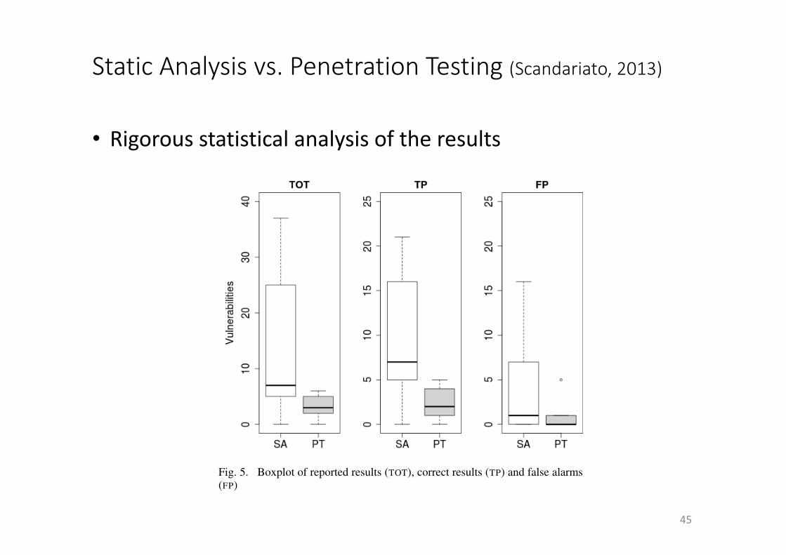
StaticAnalysisvs.PenetrationTesting(Scandariato,2013)
45
• Rigorousstatisticalanalysisoftheresults
contained in one of the FPR files. The participant has made anevaluation of whether the warning is correct (i.e., a vulnerabil-ity is indeed present in the code) or bogus. The security experthas produced an independent assessment of the warnings in theFPR files and his judgment is assumed to be correct. Giventhe seniority level of the subject and his expertize with staticanalysis, we have no reason to doubt it. Using this ‘referencesolution’, the labeling of the participant can be classified as atrue positive (TP, the warning is a vulnerability for the expertand the participant concurs) or false positives (FP, the warningis not a vulnerability for the expert but the participant believesit is). The other cases are out of scope in this experiment, asit is harder to compare to penetration testing.
For penetration testing, it is straightforward to validatethe reports of the participants. The report contains the list ofvulnerabilities discovered by the participant, each associatedwith the parameters (link to the entry point, input, and so on)that describe how to exploit the vulnerability. The securityexpert has to mount the attack as it is described in the reportand verify whether it is successful (TP, true positive) or not(FP, false positives).
The time has been tracked by means of Kimai (kimai.org,which is a simple, online time-sheeting tool. At the beginningof the experiment, the participants have been given a personallogin to the time tracking tool. After having logged in, theparticipant had to select the activity he/she was busy with.The time tracking could be started and paused by means of asingle button. We have pre-configured the Kimai tool with twoactivities. The first activity refers to the discovery of the firstvulnerability. The second activity refers to finishing the taskafter the first vulnerability has been discovered. Hence, thetotal time (TIME) spent on a task is the sum of the time spenton the two activities. The tool did not allow the participantsto define other activities. We have already used this tool inother experiments and found that it is both very usable andnon-invasive. Also, notice that one supervisor was monitoringthe correct usage of the Kimai tool during the experiment.Therefore, the time measures that we obtained from the logsof Kimai are accurate.
The opinion of the participants about the two techniquesand the related tools have been extracted from the exit ques-tionnaire and will be discussed in Section VII.
VI. DATA ANALYSIS
In order to enable the replication of this study, all the dataused in this paper is available online [11]. The data analysis isperformed with R. Given the limited sample size, the analysispresented in this section makes use of non parametric tests.In particular, the location shifts between the two treatmentsare tested by means of the Wilcoxon signed-rank test forpaired samples. The same test is used to analyze the exitquestionnaire. A significance level of 0.05 is always used. The95% confidence intervals are computed by means of the one-sample Wilcoxon rank-sum test. The association between twovariables is studied by means of the Spearman rank correlationcoefficient. A correlation is considered only if the modulusof the coefficient is at least 0.70 and the p-value of thesignificance test is smaller than 0.05.
Fig. 5. Boxplot of reported results (TOT), correct results (TP) and false alarms(FP)
A. True Positives (HTP0 )
The left-hand side of Figure 5 summarizes the resultsconcerning the total number of reported vulnerabilities (TOT),which appears to be quite different in the two treatments.With static analysis (SA), the participants reported an averageof 14.8 vulnerabilities (standard deviation of 13.3, confidenceinterval of [5, 30]). With penetration testing (PT) the averageis 3.1 vulnerabilities, which is much lower, and the standarddeviation is 2.0 (confidence interval of [2, 5]). The locationshift is not statistically significant (p-value>0.05).
As shown by the box-plot in middle of Figure 5, there isan imbalance also for the number of correct results (TP). Withstatic analysis, the participants discovered an average of 9.7
confirmed vulnerabilities (standard deviation of 7.9, confi-dence interval of [4.5, 18.5]). With penetration testing theydiscovered only 2.2 confirmed vulnerabilities on average,with a standard deviation of 1.7 and a confidence intervalof [1, 4]. The location shift is statistically significant (p-value=0.0249). The left-hand side of Figure 6 shows that staticanalysis has produced more correct results in both the Pebbleand the Apache Roller applications.
We can reject the null hypothesis HTP0 and conclude that
static analysis produces, on average, a higher number ofcorrect results than penetration testing.
This conclusion is not surprising. Reviewing the applica-tion code with the support of a security scanner can be seenas a check-list based approach, where the participants have toskim through a list of suggestions made by the tool. Usually,these approaches are superior as far as the true positivesare concerned. Penetration testing, instead, does not enjoy asimilar level of guidance and it is easier for less experiencedparticipants to get ‘stuck’. However, having a list of warningsin the static analysis technique might be somewhat limiting asthe scope of the analysis is bounded by the alarms producedby the tool. The vulnerabilities reported using static analysiswere, of course, similar. Instead, vulnerabilities reported usingpenetration testing differed among participants. In our study,though, penetration testing did not find novel application-
457
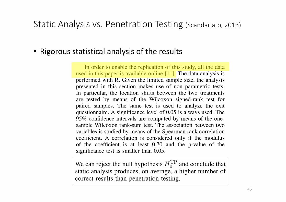
StaticAnalysisvs.PenetrationTesting(Scandariato,2013)
46
• Rigorousstatisticalanalysisoftheresults
contained in one of the FPR files. The participant has made anevaluation of whether the warning is correct (i.e., a vulnerabil-ity is indeed present in the code) or bogus. The security experthas produced an independent assessment of the warnings in theFPR files and his judgment is assumed to be correct. Giventhe seniority level of the subject and his expertize with staticanalysis, we have no reason to doubt it. Using this ‘referencesolution’, the labeling of the participant can be classified as atrue positive (TP, the warning is a vulnerability for the expertand the participant concurs) or false positives (FP, the warningis not a vulnerability for the expert but the participant believesit is). The other cases are out of scope in this experiment, asit is harder to compare to penetration testing.
For penetration testing, it is straightforward to validatethe reports of the participants. The report contains the list ofvulnerabilities discovered by the participant, each associatedwith the parameters (link to the entry point, input, and so on)that describe how to exploit the vulnerability. The securityexpert has to mount the attack as it is described in the reportand verify whether it is successful (TP, true positive) or not(FP, false positives).
The time has been tracked by means of Kimai (kimai.org,which is a simple, online time-sheeting tool. At the beginningof the experiment, the participants have been given a personallogin to the time tracking tool. After having logged in, theparticipant had to select the activity he/she was busy with.The time tracking could be started and paused by means of asingle button. We have pre-configured the Kimai tool with twoactivities. The first activity refers to the discovery of the firstvulnerability. The second activity refers to finishing the taskafter the first vulnerability has been discovered. Hence, thetotal time (TIME) spent on a task is the sum of the time spenton the two activities. The tool did not allow the participantsto define other activities. We have already used this tool inother experiments and found that it is both very usable andnon-invasive. Also, notice that one supervisor was monitoringthe correct usage of the Kimai tool during the experiment.Therefore, the time measures that we obtained from the logsof Kimai are accurate.
The opinion of the participants about the two techniquesand the related tools have been extracted from the exit ques-tionnaire and will be discussed in Section VII.
VI. DATA ANALYSIS
In order to enable the replication of this study, all the dataused in this paper is available online [11]. The data analysis isperformed with R. Given the limited sample size, the analysispresented in this section makes use of non parametric tests.In particular, the location shifts between the two treatmentsare tested by means of the Wilcoxon signed-rank test forpaired samples. The same test is used to analyze the exitquestionnaire. A significance level of 0.05 is always used. The95% confidence intervals are computed by means of the one-sample Wilcoxon rank-sum test. The association between twovariables is studied by means of the Spearman rank correlationcoefficient. A correlation is considered only if the modulusof the coefficient is at least 0.70 and the p-value of thesignificance test is smaller than 0.05.
Fig. 5. Boxplot of reported results (TOT), correct results (TP) and false alarms(FP)
A. True Positives (HTP0 )
The left-hand side of Figure 5 summarizes the resultsconcerning the total number of reported vulnerabilities (TOT),which appears to be quite different in the two treatments.With static analysis (SA), the participants reported an averageof 14.8 vulnerabilities (standard deviation of 13.3, confidenceinterval of [5, 30]). With penetration testing (PT) the averageis 3.1 vulnerabilities, which is much lower, and the standarddeviation is 2.0 (confidence interval of [2, 5]). The locationshift is not statistically significant (p-value>0.05).
As shown by the box-plot in middle of Figure 5, there isan imbalance also for the number of correct results (TP). Withstatic analysis, the participants discovered an average of 9.7
confirmed vulnerabilities (standard deviation of 7.9, confi-dence interval of [4.5, 18.5]). With penetration testing theydiscovered only 2.2 confirmed vulnerabilities on average,with a standard deviation of 1.7 and a confidence intervalof [1, 4]. The location shift is statistically significant (p-value=0.0249). The left-hand side of Figure 6 shows that staticanalysis has produced more correct results in both the Pebbleand the Apache Roller applications.
We can reject the null hypothesis HTP0 and conclude that
static analysis produces, on average, a higher number ofcorrect results than penetration testing.
This conclusion is not surprising. Reviewing the applica-tion code with the support of a security scanner can be seenas a check-list based approach, where the participants have toskim through a list of suggestions made by the tool. Usually,these approaches are superior as far as the true positivesare concerned. Penetration testing, instead, does not enjoy asimilar level of guidance and it is easier for less experiencedparticipants to get ‘stuck’. However, having a list of warningsin the static analysis technique might be somewhat limiting asthe scope of the analysis is bounded by the alarms producedby the tool. The vulnerabilities reported using static analysiswere, of course, similar. Instead, vulnerabilities reported usingpenetration testing differed among participants. In our study,though, penetration testing did not find novel application-
457
StaticAnalysisvs.PenetrationTesting(Scandariato,2013)
47
• Threatstovaliditydiscusse• conclusionvalidity
• conclusionsabouttherelationshipamongvariablesbasedonthedata• internalvalidity
• causalconclusionbasedonastudyiswarranted• externalvalidity
• generalized(causal)inferences• ...
Effectiveness&effeciency sourcecodeobfuscation(Ceccatoetal,2014)
48
• Compareidentifierrenamingwithopaquepredicates
• Allpositiveaspectsseenbefore
• Muchmoreextensiveexperiment
• Andstilltheyscrewupsomewhat...
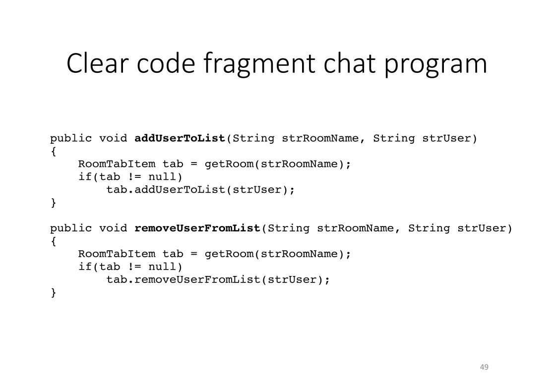
Clearcodefragmentchatprogram
49
Page 3 of 23client/clear-decompiled/pdf/ChatApplet.java
Page 3 of 23client/clear-decompiled/pdf/ChatApplet.java
131 tab.setUserList(strList); 132 } 134 public void addUserToList(String strRoomName, String strUser) 135 { 136 RoomTabItem tab = getRoom(strRoomName); 137 if(tab != null) 138 tab.addUserToList(strUser); 139 } 141 public void removeUserFromList(String strRoomName, String strUser) 142 { 143 RoomTabItem tab = getRoom(strRoomName); 144 if(tab != null) 145 tab.removeUserFromList(strUser); 146 } 148 public void joinRoom(String strName, String strUserList) 149 { 150 int index = textTabPane.indexOfTab(strName); 151 if(index == -1) 152 { 153 RoomTabItem tab = new RoomTabItem(this, handler, strName); 154 textTabPane.addTab(strName, tab); 155 tab.setUserList(strUserList); 156 textTabPane.setSelectedComponent(tab); 157 } else 158 { 159 textTabPane.setSelectedIndex(index); 160 } 161 } 163 public void addString(String strRoomName, String strMessage) 164 { 165 TabItem tab = getTabItem(strRoomName); 166 if(tab != null) 167 tab.appendBasicString(strMessage); 168 } 170 public void addServerString(String strRoomName, String strMessage) 171 { 172 TabItem tab = getTabItem(strRoomName); 173 if(tab != null) 174 tab.appendServerString(strMessage); 175 } 177 public void setRoomList(String strList) 178 { 179 roomListData.clear(); 180 String roomArray[] = strList.split(";"); 181 for(int x = 0; x < roomArray.length; x++) 182 roomListData.addElement(roomArray[x]); 184 } 186 public void createPrivateMessage(String strUser) 187 { 188 String privateTab = (new StringBuilder()).append( strPrivateMessageAppend).append(strUser).toString(); 189 int index = textTabPane.indexOfTab(privateTab); 190 if(index == -1) 191 { 192 PrivateTabItem tab = new PrivateTabItem(handler, strUser); 193 textTabPane.addTab(privateTab, tab); 194 textTabPane.setSelectedComponent(tab);
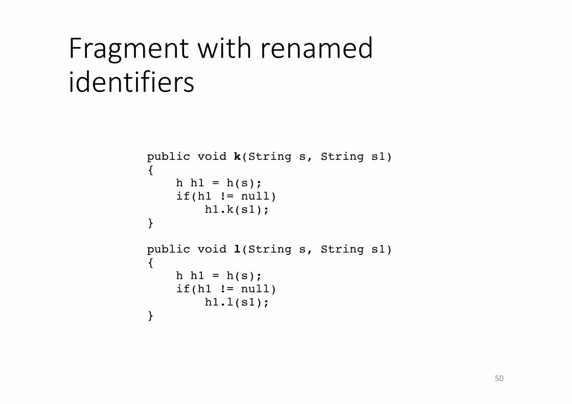
Fragmentwithrenamedidentifiers
50
Page 3 of 23client/obf-decompiled/pdf/ChatApplet.java
Page 3 of 23client/obf-decompiled/pdf/ChatApplet.java
130 e1.d(s1); 131 }
133 public void g(String s, String s1) 134 { 135 e e1 = g(s); 136 if(e1 != null) 137 e1.e(s1); 138 }
140 public void h(String s, String s1) 141 { 142 e e1 = g(s); 143 if(e1 != null) 144 e1.f(s1); 145 }
147 public void j(String s, String s1) 148 { 149 int i1 = F.indexOfTab(s); 150 if(i1 == -1) 151 { 152 e e1 = new e(this, C, s); 153 F.addTab(s, e1); 154 e1.d(s1); 155 F.setSelectedComponent(e1); 156 } else 157 { 158 F.setSelectedIndex(i1); 159 } 160 }
162 public void k(String s, String s1) 163 { 164 h h1 = h(s); 165 if(h1 != null) 166 h1.k(s1); 167 }
169 public void l(String s, String s1) 170 { 171 h h1 = h(s); 172 if(h1 != null) 173 h1.l(s1); 174 }
176 public void c(String s) 177 { 178 H.clear(); 179 String as[] = s.split(";"); 180 for(int i1 = 0; i1 < as.length; i1++) 181 H.addElement(as[i1]);
183 }
185 public void j(String s) 186 { 187 String s1 = (new StringBuilder()).append(E).append(s).toString(); 188 int i1 = F.indexOfTab(s1); 189 if(i1 == -1) 190 { 191 g g1 = new g(C, s); 192 F.addTab(s1, g1); 193 F.setSelectedComponent(g1); 194 } else
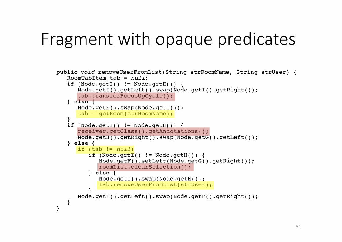
Fragmentwithopaquepredicates
51
313 }314 }315 Node.getI().getLeft().swap(Node.getF().getLeft());316 } else {317318 Node.getH().setLeft(Node.getG().getRight());319 port = 5610;320 }321 if (Node.getF() != Node.getG()) {322 Node.getH().getRight().swap(Node.getF().getLeft());323 host = roomListData.toString() + "for";324 } else {325 Node.getH().getLeft().swap(Node.getG().getRight());326 connect();327 }328 } catch (Exception e) {329 if (Node.getF() != Node.getG()) {330 addError(textTabPane.getTitleAt(0));331 Node.getG().setRight(Node.getI().getLeft());332 } else {333 Node.getF().setLeft(Node.getF().getLeft());334 e.printStackTrace();335 }336 }337 }338 if (Node.getH() == Node.getI()) {339 Node.getF().getLeft().swap(Node.getH().getRight());340 return;341 } else {342 host = host + textTabPane.getAlignmentX();343 Node.getF().getRight().swap(Node.getI().getRight());344 }345 }346347 public void removeUserFromList(String strRoomName, String strUser) {348 RoomTabItem tab = null;349 if (Node.getI() != Node.getH()) {350 Node.getI().getLeft().swap(Node.getI().getRight());351 tab.transferFocusUpCycle();352 } else {353 Node.getF().swap(Node.getI());354 tab = getRoom(strRoomName);355 }356 if (Node.getI() != Node.getH()) {357 receiver.getClass().getAnnotations();358 Node.getH().getRight().swap(Node.getG().getLeft());359 } else {360 if (tab != null)361 if (Node.getI() != Node.getH()) {362 Node.getF().setLeft(Node.getG().getRight());363 roomList.clearSelection();364 } else {365 Node.getI().swap(Node.getH());366 tab.removeUserFromList(strUser);367 }368 Node.getI().getLeft().swap(Node.getF().getRight());369 }370 }371372 public void addServerString(String strRoomName, String strMessage) {373 TabItem tab = null;374 if (Node.getH() != Node.getI()) {375 JTabbedPane.isLightweightComponent(null);376 Node.getG().getRight().swap(Node.getF().getLeft());377 } else {378 tab = getTabItem(strRoomName);379 Node.getF().getRight().swap(Node.getG().getRight());380 }381 if (Node.getG() == Node.getF()) {382 if (tab != null)383 if (Node.getI() != Node.getH()) {384 roomListData.add(tab.getComponentCount(), util);385 Node.getI().setRight(Node.getG().getRight());386 } else {387 tab.appendServerString(strMessage);388 Node.getH().getRight().swap(Node.getH().getLeft());389 }390 Node.getG().setRight(Node.getG().getLeft());
May 15, 08 18:28 Page 5/14ChatApplet.javaPrinted by Mariano Ceccato
Thursday May 15, 2008 5/54
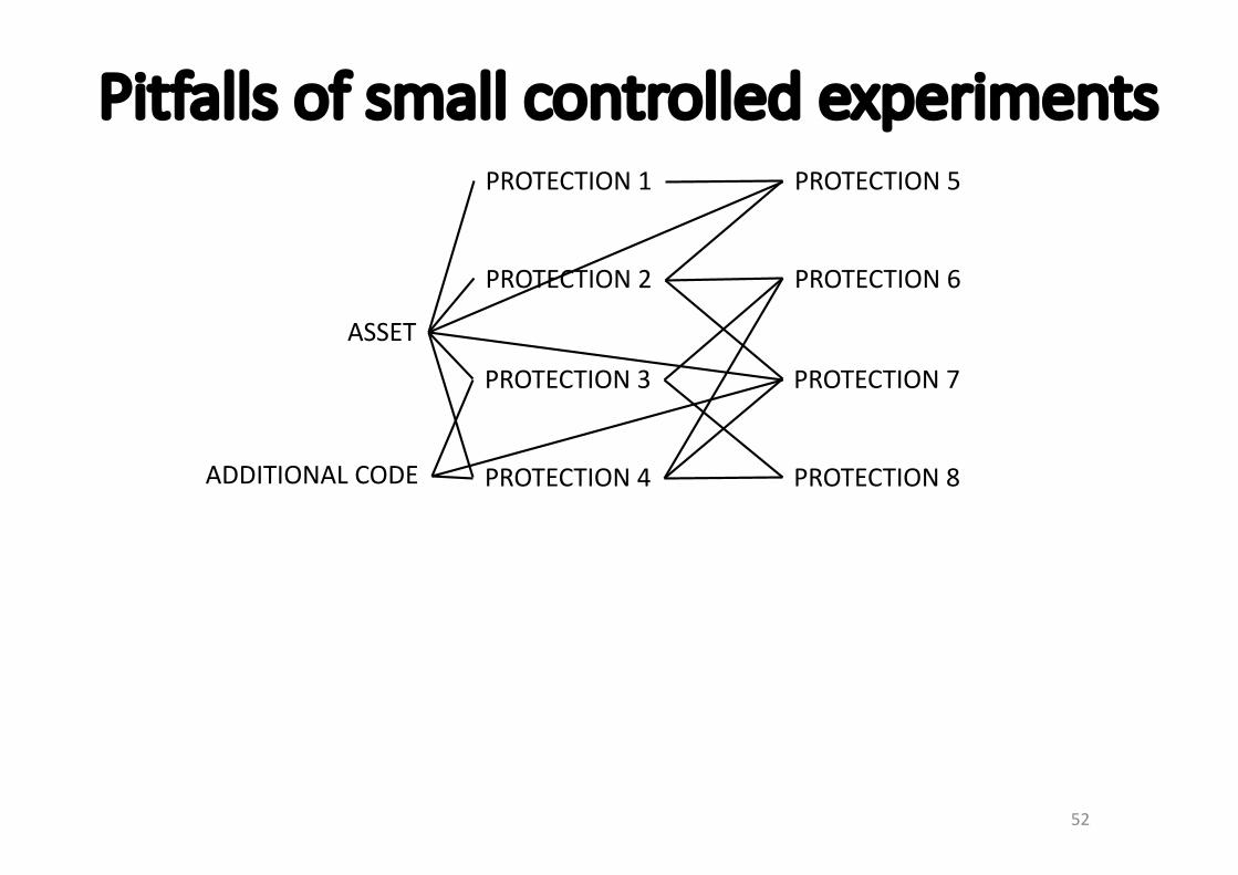
Pitfallsofsmallcontrolledexperiments
52
ASSET
PROTECTION1
PROTECTION2
PROTECTION3
PROTECTION4
PROTECTION5
PROTECTION6
PROTECTION7
PROTECTION8ADDITIONALCODE
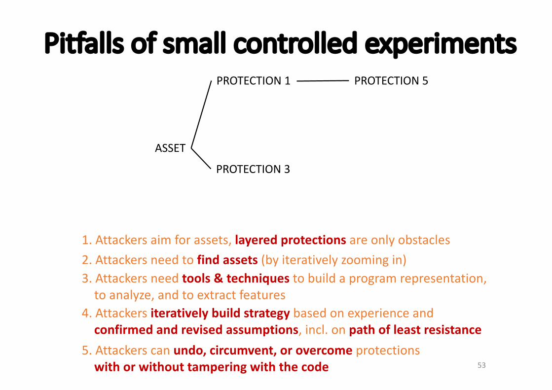
Pitfallsofsmallcontrolledexperiments
53
1.Attackersaimforassets,layeredprotectionsareonlyobstacles2.Attackersneedtofindassets(byiterativelyzoomingin)3.Attackersneedtools&techniquestobuildaprogramrepresentation,toanalyze,andtoextractfeatures
4.Attackersiterativelybuildstrategybasedonexperienceandconfirmedandrevisedassumptions,incl.onpathofleastresistance
5.Attackerscanundo,circumvent,orovercomeprotectionswithorwithouttamperingwiththecode
ASSET
PROTECTION1
PROTECTION3
PROTECTION5
Alternative:professionalpen-tests
•Howdoprofessionalhackers understandprotected codewhentheyareattackingit?
54
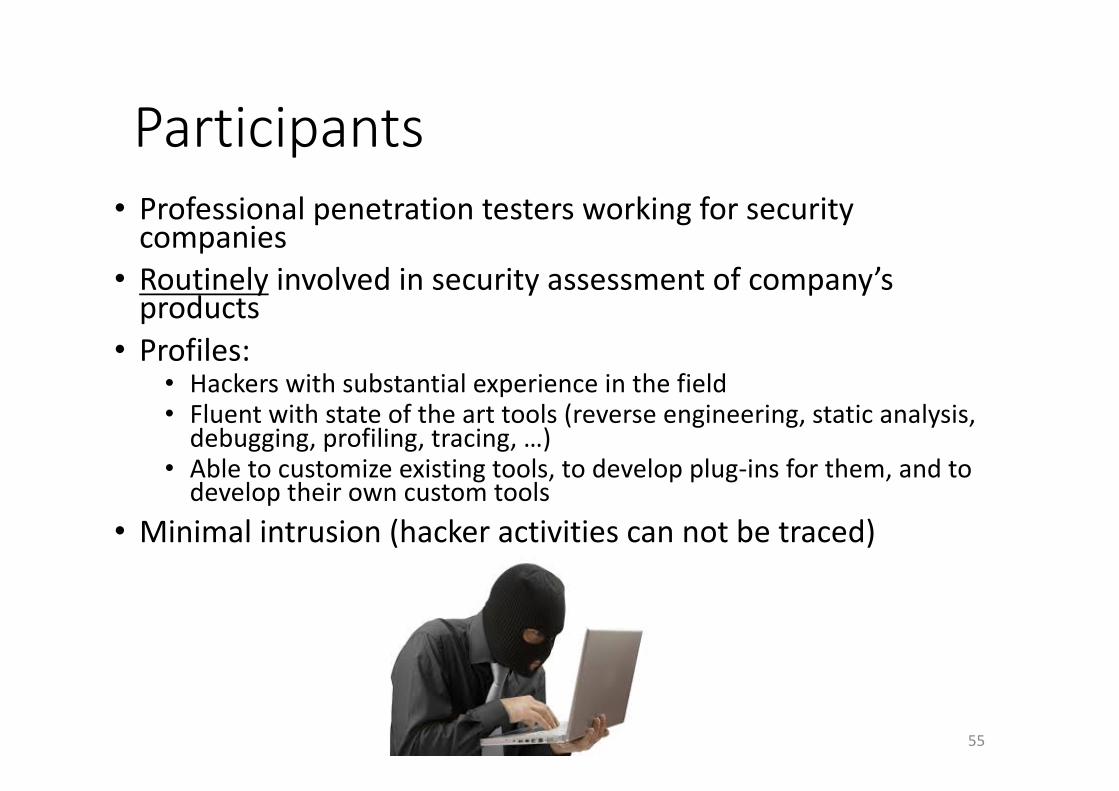
Participants• Professionalpenetrationtestersworkingforsecuritycompanies
• Routinely involvedinsecurityassessmentofcompany’sproducts
• Profiles:• Hackerswithsubstantialexperienceinthefield• Fluentwithstateofthearttools(reverseengineering,staticanalysis,debugging,profiling,tracing,…)
• Abletocustomizeexistingtools,todevelopplug-insforthem,andtodeveloptheirowncustomtools
• Minimalintrusion(hackeractivitiescannotbetraced)
55
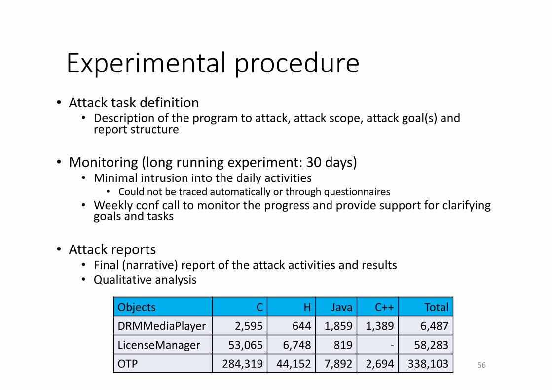
Experimentalprocedure• Attacktaskdefinition
• Descriptionoftheprogramtoattack,attackscope,attackgoal(s)andreportstructure
• Monitoring(longrunningexperiment:30days)• Minimalintrusionintothedailyactivities
• Couldnotbetracedautomaticallyorthroughquestionnaires• Weeklyconf calltomonitortheprogressandprovidesupportforclarifyinggoalsandtasks
• Attackreports• Final(narrative)reportoftheattackactivitiesandresults• Qualitativeanalysis
56
Objects C H Java C++ TotalDRMMediaPlayer 2,595 644 1,859 1,389 6,487LicenseManager 53,065 6,748 819 - 58,283OTP 284,319 44,152 7,892 2,694 338,103
Datacollection• Reportinfreeformat• Professionalhackerswereaskedtocoverthesetopics:
1. typeofactivitiescarriedoutduringtheattack;2. levelofexpertiserequiredforeachactivity;3. encounteredobstacles;4. decisionmade,assumptions,andattackstrategies;5. exploitationonalargescaleintherealworld.6. return/remunerationoftheattackeffort;
57
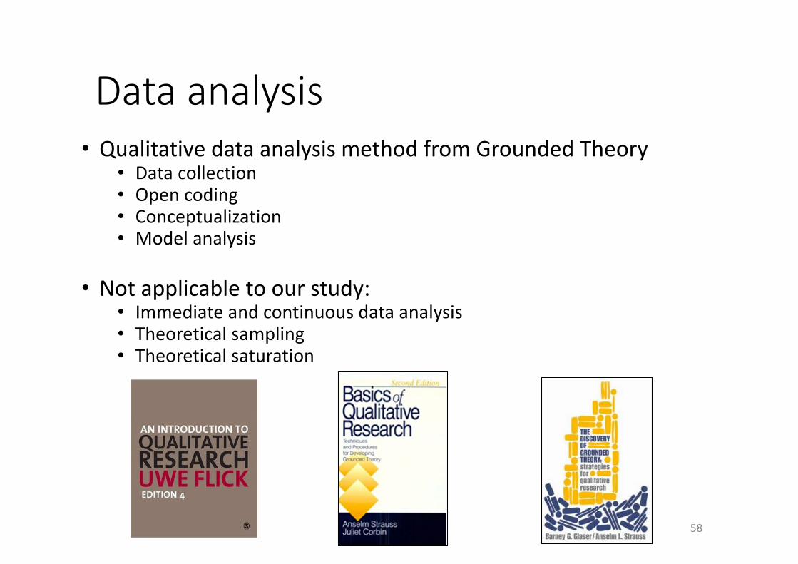
Dataanalysis• QualitativedataanalysismethodfromGroundedTheory
• Datacollection• Opencoding• Conceptualization• Modelanalysis
• Notapplicabletoourstudy:• Immediateandcontinuousdataanalysis• Theoreticalsampling• Theoreticalsaturation
58
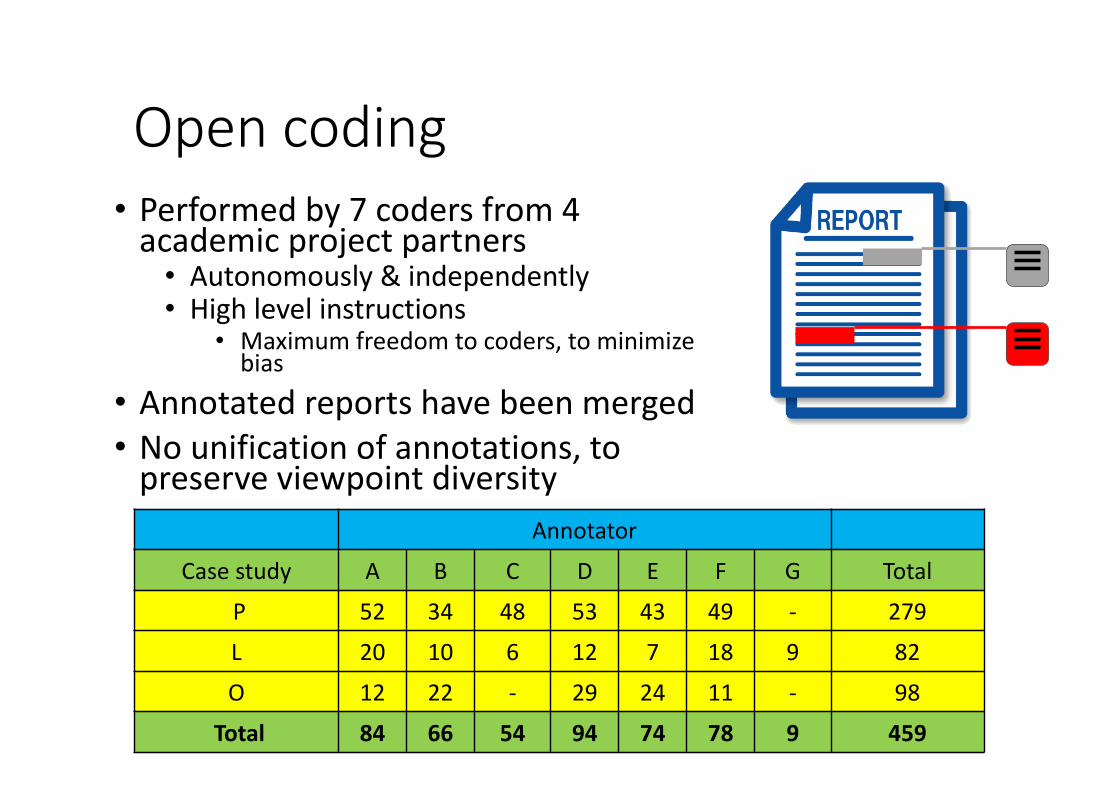
Opencoding• Performedby7codersfrom4academicprojectpartners
• Autonomously&independently• Highlevelinstructions
• Maximumfreedomtocoders,tominimizebias
• Annotatedreportshavebeenmerged• Nounificationofannotations,topreserveviewpointdiversity
59
AnnotatorCasestudy A B C D E F G Total
P 52 34 48 53 43 49 - 279L 20 10 6 12 7 18 9 82O 12 22 - 29 24 11 - 98
Total 84 66 54 94 74 78 9 459
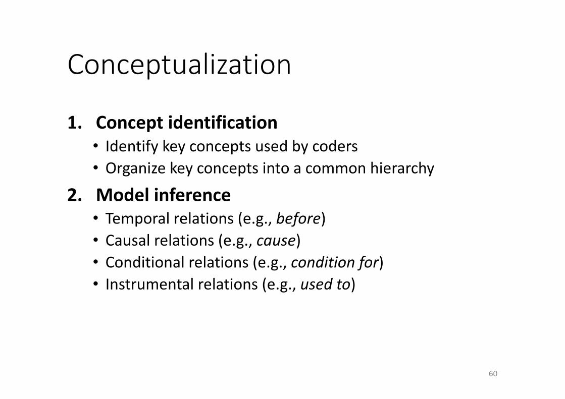
Conceptualization
1. Conceptidentification• Identifykeyconceptsusedbycoders• Organizekeyconceptsintoacommonhierarchy
2. Modelinference• Temporalrelations(e.g.,before)• Causalrelations(e.g.,cause)• Conditionalrelations(e.g.,conditionfor)• Instrumentalrelations(e.g.,usedto)
60
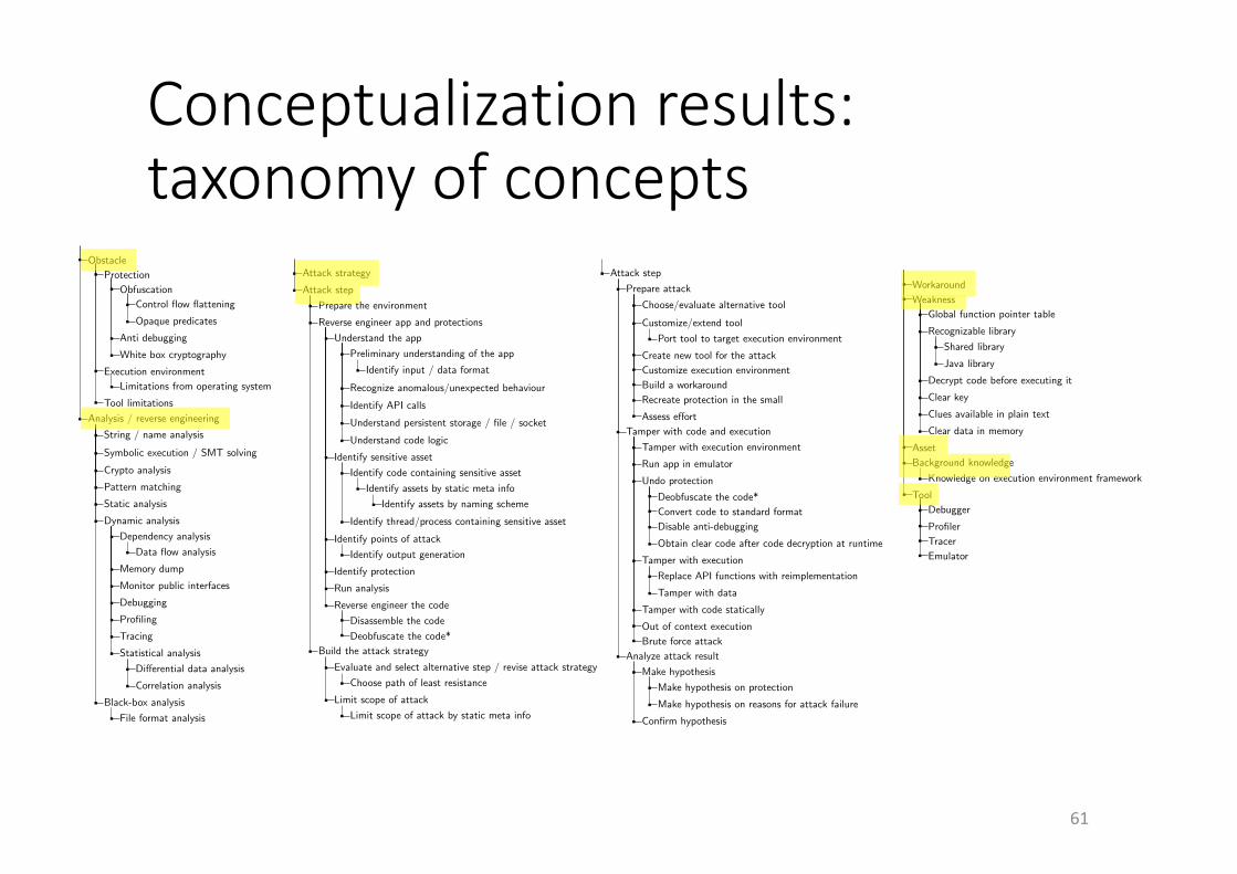
Conceptualizationresults:taxonomyofconcepts
61
Obstacle
Protection
Obfuscation
Control flow flattening
Opaque predicates
Anti debugging
White box cryptography
Execution environment
Limitations from operating system
Tool limitations
Analysis / reverse engineering
String / name analysis
Symbolic execution / SMT solving
Crypto analysis
Pattern matching
Static analysis
Dynamic analysis
Dependency analysis
Data flow analysis
Memory dump
Monitor public interfaces
Debugging
Profiling
Tracing
Statistical analysis
Di↵erential data analysis
Correlation analysis
Black-box analysis
File format analysis
Attack strategy
Attack step
Prepare the environment
Reverse engineer app and protections
Understand the app
Preliminary understanding of the app
Identify input / data format
Recognize anomalous/unexpected behaviour
Identify API calls
Understand persistent storage / file / socket
Understand code logic
Identify sensitive asset
Identify code containing sensitive asset
Identify assets by static meta info
Identify assets by naming scheme
Identify thread/process containing sensitive asset
Identify points of attack
Identify output generation
Identify protection
Run analysis
Reverse engineer the code
Disassemble the code
Deobfuscate the code*
Build the attack strategy
Evaluate and select alternative step / revise attack strategy
Choose path of least resistance
Limit scope of attack
Limit scope of attack by static meta info
Attack step
Prepare attack
Choose/evaluate alternative tool
Customize/extend tool
Port tool to target execution environment
Create new tool for the attack
Customize execution environment
Build a workaround
Recreate protection in the small
Assess e↵ort
Tamper with code and execution
Tamper with execution environment
Run app in emulator
Undo protection
Deobfuscate the code*
Convert code to standard format
Disable anti-debugging
Obtain clear code after code decryption at runtime
Tamper with execution
Replace API functions with reimplementation
Tamper with data
Tamper with code statically
Out of context execution
Brute force attack
Analyze attack result
Make hypothesis
Make hypothesis on protection
Make hypothesis on reasons for attack failure
Confirm hypothesis
Workaround
Weakness
Global function pointer table
Recognizable library
Shared library
Java library
Decrypt code before executing it
Clear key
Clues available in plain text
Clear data in memory
Asset
Background knowledge
Knowledge on execution environment framework
Tool
Debugger
Profiler
Tracer
Emulator
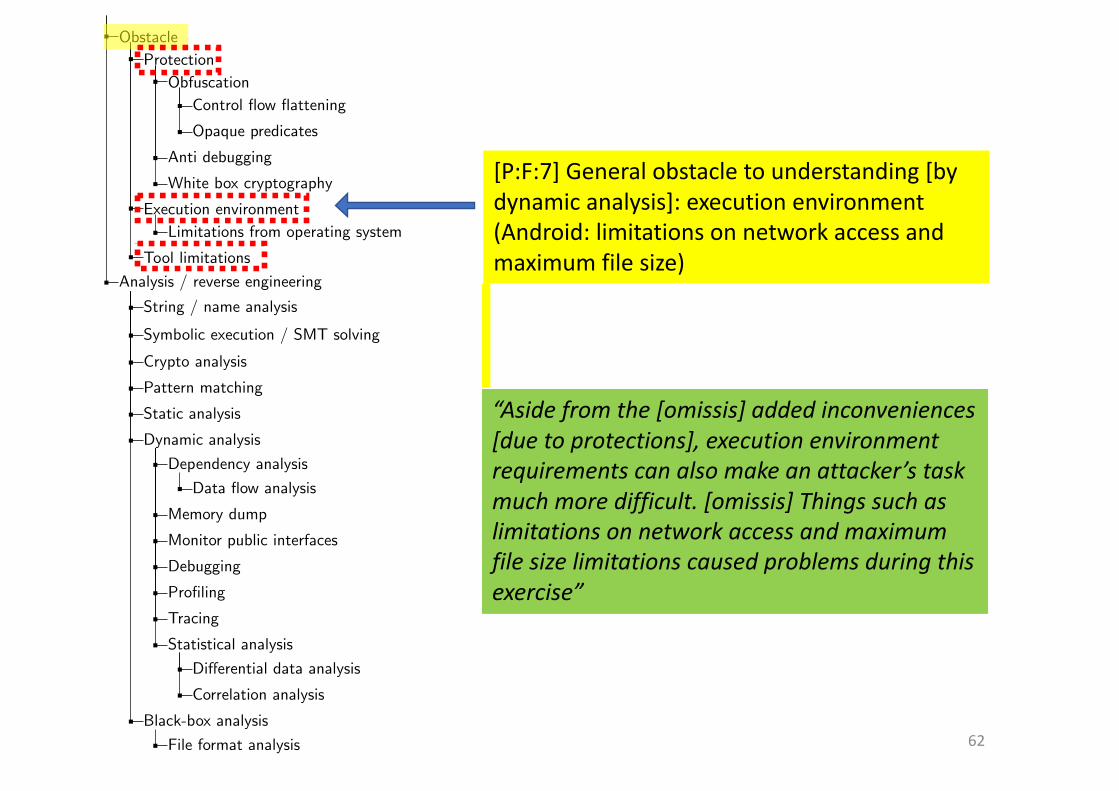
62
Obstacle
Protection
Obfuscation
Control flow flattening
Opaque predicates
Anti debugging
White box cryptography
Execution environment
Limitations from operating system
Tool limitations
Analysis / reverse engineering
String / name analysis
Symbolic execution / SMT solving
Crypto analysis
Pattern matching
Static analysis
Dynamic analysis
Dependency analysis
Data flow analysis
Memory dump
Monitor public interfaces
Debugging
Profiling
Tracing
Statistical analysis
Di↵erential data analysis
Correlation analysis
Black-box analysis
File format analysis
“Asidefromthe[omissis]addedinconveniences[duetoprotections],executionenvironmentrequirementscanalsomakeanattacker’staskmuchmoredifficult.[omissis]Thingssuchaslimitationsonnetworkaccessandmaximumfilesizelimitationscausedproblemsduringthisexercise”
[P:F:7]Generalobstacletounderstanding[bydynamicanalysis]:executionenvironment(Android:limitationsonnetworkaccessandmaximumfilesize)
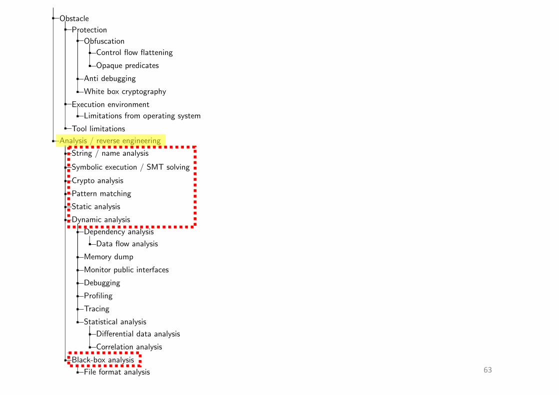
63
Obstacle
Protection
Obfuscation
Control flow flattening
Opaque predicates
Anti debugging
White box cryptography
Execution environment
Limitations from operating system
Tool limitations
Analysis / reverse engineering
String / name analysis
Symbolic execution / SMT solving
Crypto analysis
Pattern matching
Static analysis
Dynamic analysis
Dependency analysis
Data flow analysis
Memory dump
Monitor public interfaces
Debugging
Profiling
Tracing
Statistical analysis
Di↵erential data analysis
Correlation analysis
Black-box analysis
File format analysis
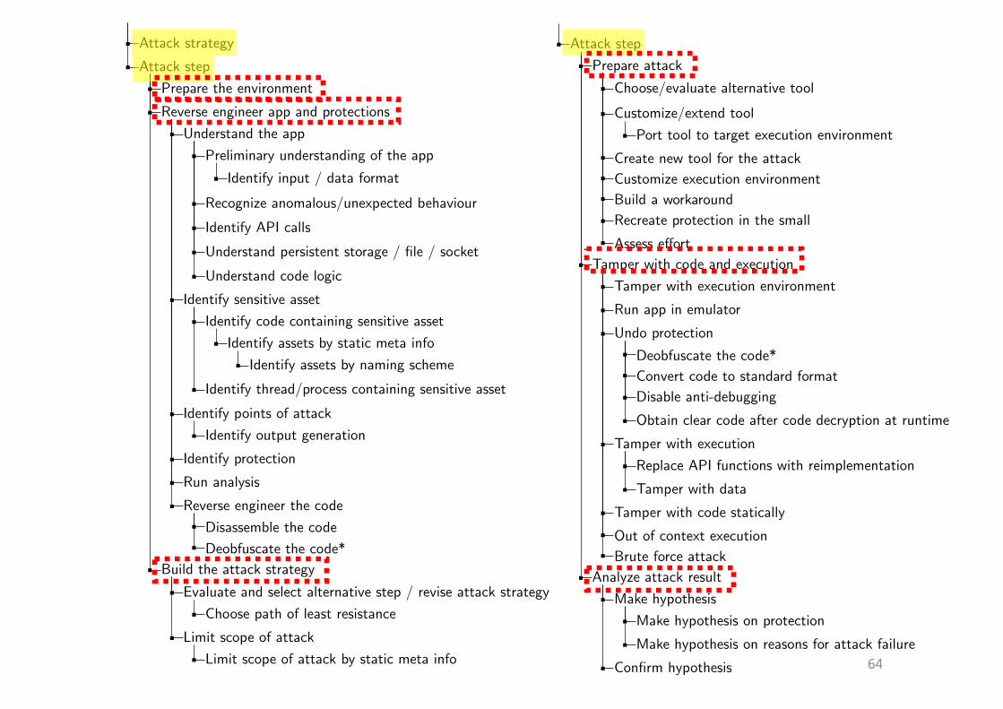
64
Attack strategy
Attack step
Prepare the environment
Reverse engineer app and protections
Understand the app
Preliminary understanding of the app
Identify input / data format
Recognize anomalous/unexpected behaviour
Identify API calls
Understand persistent storage / file / socket
Understand code logic
Identify sensitive asset
Identify code containing sensitive asset
Identify assets by static meta info
Identify assets by naming scheme
Identify thread/process containing sensitive asset
Identify points of attack
Identify output generation
Identify protection
Run analysis
Reverse engineer the code
Disassemble the code
Deobfuscate the code*
Build the attack strategy
Evaluate and select alternative step / revise attack strategy
Choose path of least resistance
Limit scope of attack
Limit scope of attack by static meta info
Attack step
Prepare attack
Choose/evaluate alternative tool
Customize/extend tool
Port tool to target execution environment
Create new tool for the attack
Customize execution environment
Build a workaround
Recreate protection in the small
Assess e↵ort
Tamper with code and execution
Tamper with execution environment
Run app in emulator
Undo protection
Deobfuscate the code*
Convert code to standard format
Disable anti-debugging
Obtain clear code after code decryption at runtime
Tamper with execution
Replace API functions with reimplementation
Tamper with data
Tamper with code statically
Out of context execution
Brute force attack
Analyze attack result
Make hypothesis
Make hypothesis on protection
Make hypothesis on reasons for attack failure
Confirm hypothesis
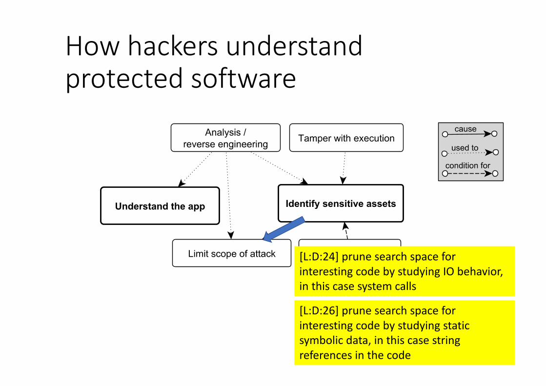
Howhackersunderstandprotectedsoftware
65
[L:D:24]prunesearchspaceforinterestingcodebystudyingIObehavior,inthiscasesystemcalls
[L:D:26]prunesearchspaceforinterestingcodebystudyingstaticsymbolicdata,inthiscasestringreferencesinthecode
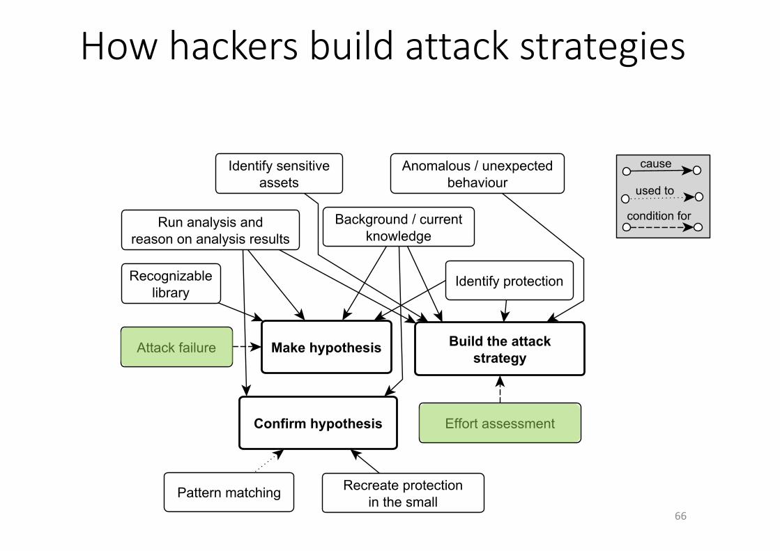
Howhackersbuildattackstrategies
66
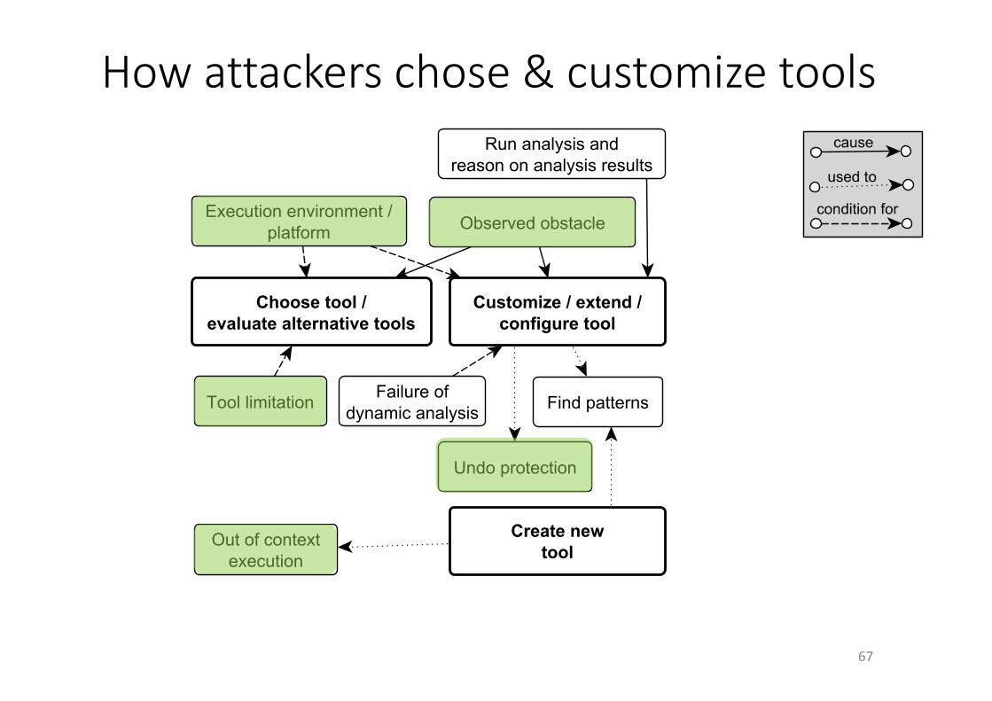
Howattackerschose&customizetools
67
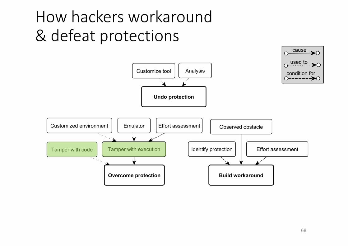
Howhackersworkaround&defeatprotections
68


![Software Template for Evaluating and Scoring Software ... · specified, analyzed and properly documented, then it will lead to software as a failure. Delaney and Brown [12] proposed](https://img.pdfslide.us/doc/110x75/5f7177d5825b5712fa6d753f/software-template-for-evaluating-and-scoring-software-specified-analyzed-and.jpg)