SOFTWARE PROJECT PLANNING

Project Planning The overall goal of project planning is to establish a

pragmatic strategy for controlling, tracking, and monitoring a project

Estimation is a foundation for all other project planning activities and project planning provides the road map for successful software engineering

For estimation of resources, cost, and schedule for a software engineering effort requires experience, access to good historical information, and the courage to commit to quantitative predictions when qualitative information is all that exists.

Project complexity, project size, and the degree of structural uncertainty all affect the reliability of estimates.

Project Planning Process

Establish project scope Determine feasibility Analyze risks Define required resources

Determine require human resources Define reusable software resources Identify environmental resources

Estimate cost and effort Develop a project schedule

Software ScopeSoftware scope describes

The functions and features that are to be delivered to end-users

The data that are input and output The “content” that is presented to users as a consequence

of using the software The performance, constraints, interfaces, and reliability that

bound the system.

Scope is defined using one of two techniques: A narrative description of software scope is developed after

communication with all stakeholders. A set of use-cases is developed by end-users.

Feasibility

Once scope has been identified (with the concurrence of the customer), it is reasonable to ask: Can we build software to meet this scope? Is the project feasible?”

Once scope is understood, the software team and others must work to determine if it can be done within the dimensions just noted.

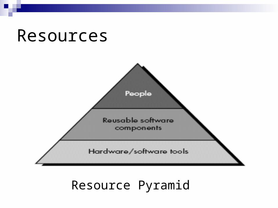
Resources

Resource Pyramid

Contd. The development environment—hardware and software

tools—sits at the foundation of the resources pyramid and provides the infrastructure to support the development effort.

Reusable software components— software building blocks that can dramatically reduce development costs and accelerate delivery.

At the top of the pyramid is the primary resource—people.

Each resources is specified by with four characteristics: Description of the resource, A statement of availability, Time when the resource will be required; Duration of time that resource will be applied.

The last two characteristics can be viewed as a time window.

Human Resources - People

Planner begins by evaluating scope and selecting the skills required to complete development.

The number of people required for a software project can be determined only after an estimate of development effort is made.

Can be measure on skills, specialty (i.e. communication, database admin etc) or position.

Reusable software components Reusable components, must be cataloged for easy reference,

standardized for easy application, and validated for easy integration.

Four software resource categories:1. Off-the-shelf components: Existing software that can be acquired from a third party or

that has been developed internally for a past project. COTS (commercial off-the-shelf) components are purchased

from a third party, are ready for use on the current project, and have been fully validated.

2. Full-experience components: Existing specifications, designs, code, or test data developed

for past projects that are similar to the software to be built for the current project.

Members of the current software team have had full experience in the application area represented by these components.

Therefore, modifications required for full-experience components will be relatively low-risk.

3. Partial-experience components. Existing specifications, designs, code, or test data

developed for past projects that are related to the software to be built for the current project but will require substantial modification.

Members of the current software team have only limited experience in the application area represented by these components.

Therefore, modifications required for partial-experience components have a fair degree of risk.

4. New components. Software components that must be built by the software team specifically for the needs of the current project.

What issues should we consider when we plan to reuse existing software components?

In off-the-shelf components, cost for acquisition and integration of off-the-shelf components will almost always be less and risk relatively is low.

In full-experience components, risks associated with modification and integration are generally acceptable.

In partial-experience components, current project must be analyzed. Integration is difficult and risk is high. In some cases cost for components is also high compare to development of new component.

Environmental Resources

The environment that supports the software project incorporates hardware and software often called the software engineering environment (SEE).

Hardware provides a platform that supports the tools (software) required to produce the work products.

A project planner must prescribe the time window required for hardware and software and verify that these resources will be available.

For example, a computer-based system (incorporating specialized hardware and software) is to be engineered, the software team may require access to hardware elements being developed by other engineering teams (e.g. electronics, mechanical etc.).

SOFTWARE PROJECT ESTIMATION

Software is the most expensive element of virtually all computer-based systems.

For complex, custom systems, a large cost estimation error can make the difference between profit and loss.

There are too many variables— human, technical, environmental, political—can affect the ultimate cost of software and effort applied to develop it.

To achieve reliable cost and effort estimates, a number of options arise:Delay estimation until late in the project

(obviously, can achieve 100% accurate estimates after the project is complete!)

Base estimates on similar projects that have already been completed.

Use relatively simple decomposition techniques to generate project cost and effort estimates.

Use one or more empirical models for software cost and effort estimation

First option – is not practically possible. Cost estimates must be provided "up front.“

Second option - can work reasonably well, if the current project is quite similar to past efforts and other project influences (e.g., the customer, business conditions, deadlines) are equivalent.

Third option - Decomposition techniques take a "divide and conquer“ approach to software project estimation. By decomposing a project into major functions and related software engineering activities, cost and effort estimation can be performed in a stepwise.

Fourth option - Empirical estimation models can be used to complement decomposition techniques and offer a potentially valuable estimation approach in their own right.

Decomposition Techniques Decompose the problem or software, re-characterizing it

as a set of smaller problem or software. Estimation uses problem or process or both forms of

partitioning. Before an estimate can be made, the project planner

must understand the scope of the software to be built and generate an estimate of its “size.”

It comprises of Software size Problem based estimation Process based estimation

Software Size Sizing represents the project planner’s first major

challenge. In the context of project planning, size refers to a

quantifiable outcome of the software project. If a direct approach is taken, size can be measured in

LOC. If an indirect approach is chosen, size is represented as FP.

Four different approaches to the sizing problem: Fuzzy Logic Function point sizing Standard component sizing Change sizing

Fuzzy logic – the planner must identify the type of application, establish its magnitude on a qualitative scale, and then refine the magnitude within the original range.

Function point sizing - The planner develops estimates of the information domain characteristics

Standard component sizing -The project planner estimates the number of occurrences of each standard component and then uses historical project data to determine the delivered size per standard component.

Change sizing - This approach is used when a project encompasses the use of existing software. The planner estimates the number and type (e.g., reuse, adding code, changing code, deleting code) of modifications that must be accomplished.

Each of these sizing approaches be combined statistically to create a “three-point” or “expected value” estimate. This is accomplished by developing optimistic (low), most likely (medium), and pessimistic (high) values

Problem Based estimation

Project planner begins from software scope statement to decompose software into problem functions that can each be estimated individually.

LOC and FP data are used in two ways during software project estimation:

1. As an estimation variable (i.e. LOC or FP) to "size“ each element of the software.

2. As baseline metrics collected from past projects and used in combination with estimation variables to develop cost and effort projections.

LOC or FP (the estimation variable) is then estimated for each function (i.e. cost, effort etc.)

Baseline productivity metrics (e.g., LOC/pm or FP/pm) are then applied to the appropriate estimation variable, and cost or effort for the function is derived.

LOC/pm or FP/pm averages should be computed by project domain. That is, projects should be grouped by team size, application area, complexity, and other relevant parameters.

When a new project is estimated, it should first be allocated to a domain, and then the appropriate domain average for productivity should be used in generating the estimate.

The LOC and FP estimation techniques differ in the level of detail required for decomposition and the target of the partitioning.

If LOC is used as the estimation variable, decomposition is absolutely essential and is often taken to considerable levels of detail.

The greater the degree of partitioning, the more likely reasonably accurate estimates of LOC can be developed.

For FP estimates, decomposition works differently. Rather than focusing on function, each of the information domain characteristics as well as the 14 complexity adjustment values are estimated.

FP value that can be tied to past data and used to generate an estimate.

Project planner begins by estimating a range of values for each function or information domain value.(i.e. regardless of the estimation variable)

Planner estimates an optimistic (low), most likely, and pessimistic (high) size value for each function or count for each information domain value.

The expected value for the estimation variable (size), S, can be computed as a weighted average of the optimistic (Sopt), most likely (Sm), and pessimistic (Spess) estimates.S = (Sopt + 4Sm + Spess)/6

Once the expected value for the estimation variable has been determined, historical LOC or FP productivity data are applied.

Example LOC base estimation

A software package to be developed for a CAD application for mechanical components.

A review of the System Specification indicates that the software is to execute on an engineering workstation and must interface with various computer graphics peripherals including a mouse, digitizer, high resolution color display and laser printer.

Based on system specification, statement of software scope can be developed.

Every sentence of software scope would have to be expanded to provide concrete detail and quantitative bounding ( i.e. major functions of CAD system).

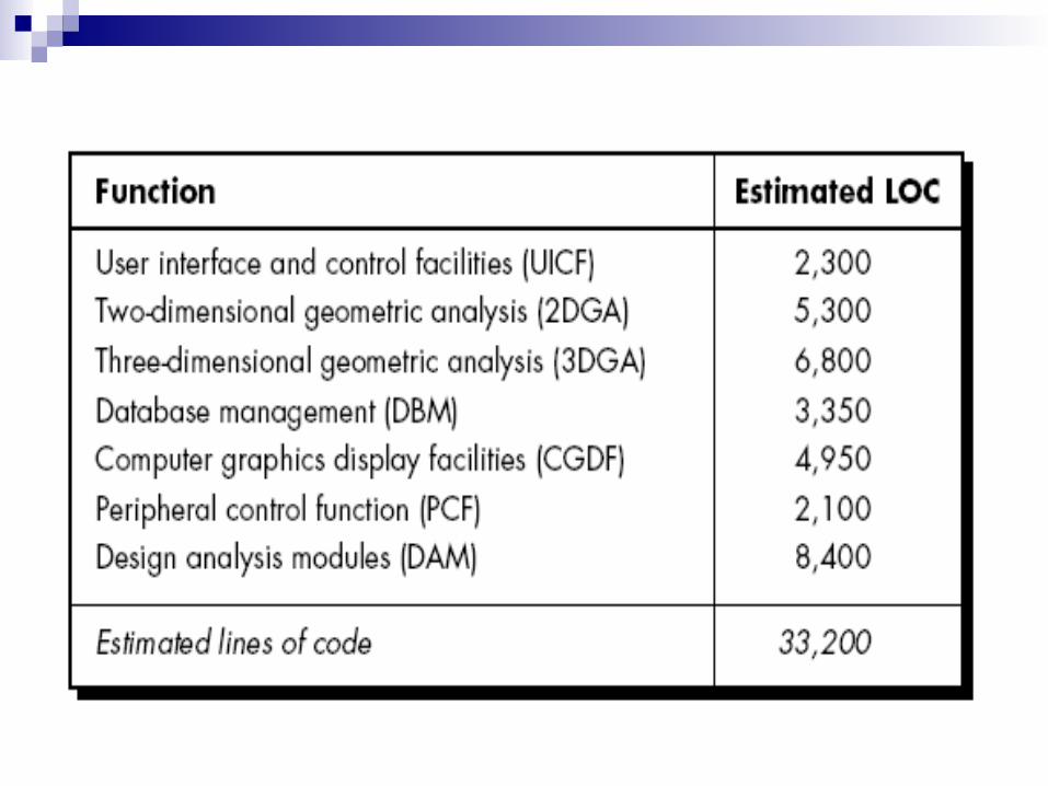
Now, Decomposition technique for LOC, an estimation table, shown in Figure, is developed.

Develop range of LOC estimate for each function. For example, range of LOC estimates for the 3D

geometric analysis function is optimistic 4600 LOC, most likely 6900 LOC, and pessimistic 8600 LOC.

Compute expected value for the 3D geometric analysis function is 6800 LOC.

By summing estimate LOC, 33200 LOC is established for CAD system

Now we can review of historical data indicates average productivity for systems of this type is 620 LOC/pm.

Labor rate is $8000 per month, the cost per line of code is approximately $13 (i.e. 8000/620).

Based on the LOC estimate and the historical productivity data, the total estimated project cost is $431,000 (i.e. 33200 x 13) and the estimated effort is 54 person-months (i.e. 431000 / 8000)

Example FP base estimation

Decomposition for FP-based estimation focuses on information domain values rather than software functions.

project planner estimates inputs, outputs, inquiries, files, and external interfaces for the CAD software.

For the purposes of this estimate, the complexity weighting factor is assumed to be average.

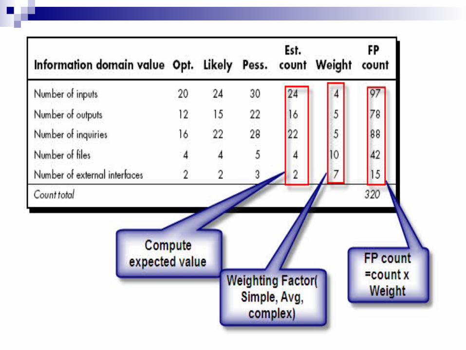
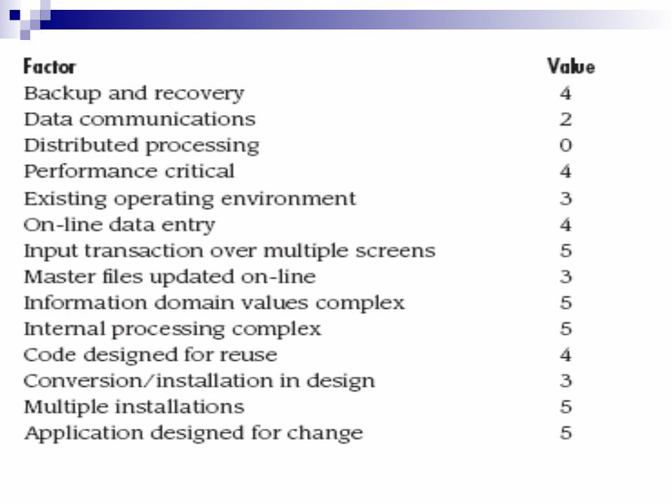
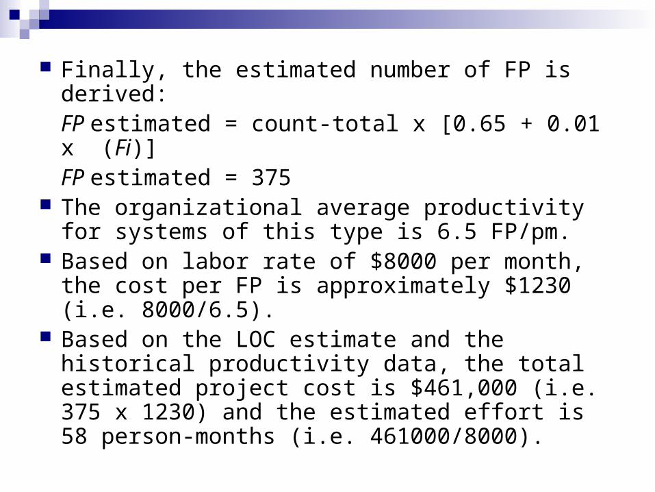
Finally, the estimated number of FP is derived:FP estimated = count-total x [0.65 + 0.01 x (Fi)]FP estimated = 375

The organizational average productivity for systems of this type is 6.5 FP/pm.

Based on labor rate of $8000 per month, the cost per FP is approximately $1230 (i.e. 8000/6.5).

Based on the LOC estimate and the historical productivity data, the total estimated project cost is $461,000 (i.e. 375 x 1230) and the estimated effort is 58 person-months (i.e. 461000/8000).

Process-Based Estimation The process is decomposed into a relatively small set of tasks

and the effort required to accomplish each task is estimated. Like the problem-based techniques, process-based

estimation begins with project scope. Functions and related software process activities may be

represented as part of a table similar to the one presented in Fig.

Once problem functions and process activities are melded, the planner estimates the effort (e.g., person-months) that will be required to accomplish each software process activity for each software function.

Average labor rates (i.e., cost/unit effort) are then applied to the effort estimated for each process activity

If process and problem based estimation performed independently, it means we have two or three estimates for cost and effort that may be compared and reconciled.

If both sets of estimates show reasonable agreement, there is good reason to believe that the estimates are reliable.

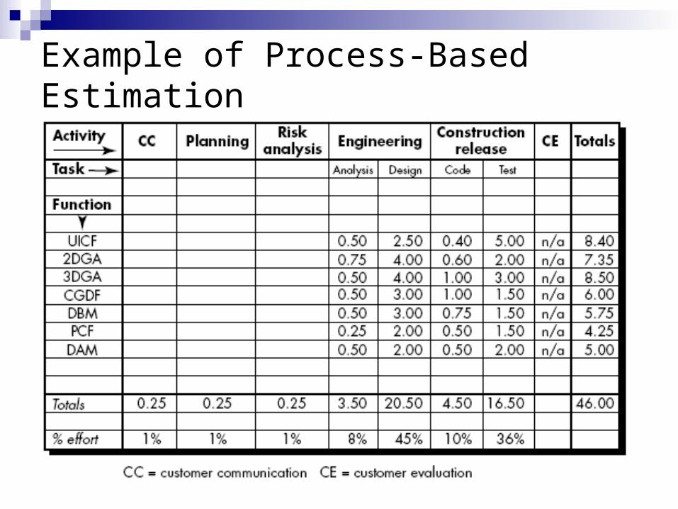
Example of Process-Based Estimation

The engineering and construction release activities are subdivided into the major software engineering tasks shown.

Horizontal and vertical totals provide an indication of estimated effort required for analysis, design, code, and test.

Here, 53 percent of all effort is expended on front-end engineering tasks (requirements analysis and design).

Based on labor rate of $8,000 per month, total estimated project cost is $368,000( i.e. 8000 x 46) and the estimated effort is 46 person-months.

Total estimated effort for the CAD software range from a low of 46 person-months to a high of 58 person-months. The average estimate is 53 person-months.

Empirical estimation models, The COnstructive COst Model (COCOMO) II address the

following areas: Application composition model.

Used during the early stages of software engineering, when prototyping of user interfaces, consideration of software and system interaction, assessment of performance, and evaluation of technology maturity are paramount.

Early design stage model. Used once requirements have been stabilized and basic

software architecture has been established. Post-architecture-stage model.

Used during the construction of the software.

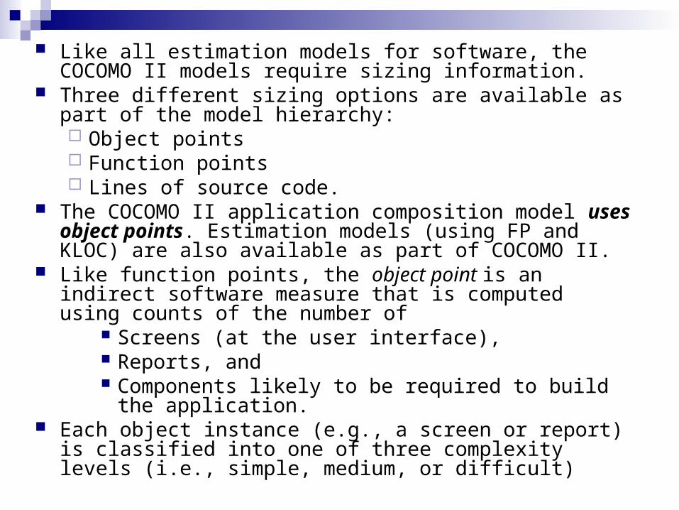
Like all estimation models for software, the COCOMO II models require sizing information.

Three different sizing options are available as part of the model hierarchy: Object points Function points Lines of source code.

The COCOMO II application composition model uses object points. Estimation models (using FP and KLOC) are also available as part of COCOMO II.

Like function points, the object point is an indirect software measure that is computed using counts of the number of

Screens (at the user interface), Reports, and Components likely to be required to build the

application. Each object instance (e.g., a screen or report) is classified

into one of three complexity levels (i.e., simple, medium, or difficult)

Complexity weight can be measure on source of the client and server data tables that are required to generate the screen or report and the number of views or sections presented as part of the screen or report.

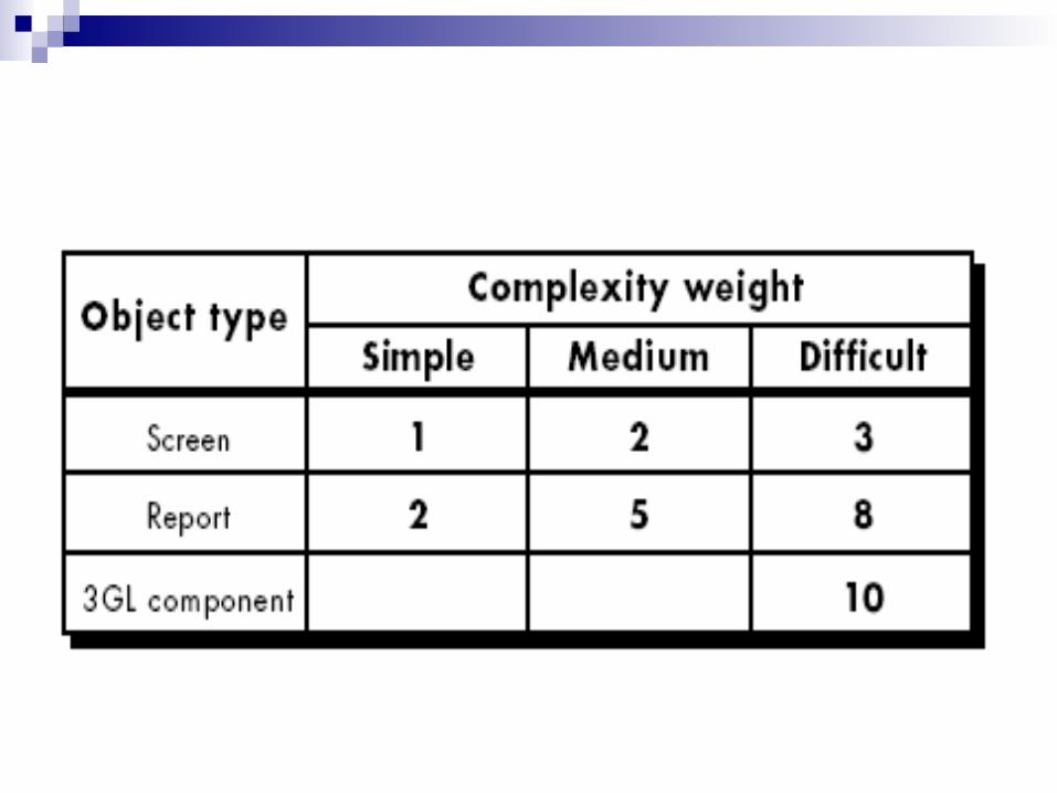
Once complexity is determined, the number of screens, reports, and components are weighted according to Table.

Object point count is then determined by multiplying the original number of object instances by the weighting factor in Table and summing to obtain a total object point count.

When component-based development or general software reuse is to be applied, the percent of reuse (%reuse) is estimated and the object point count is adjusted:

NOP = (object points) x [(100 - %reuse)/100]NOP is defined as new object points.

To derive an estimate of effort based on the computed NOP value, a “productivity rate” must be derived.

PROD = NOP/person-month

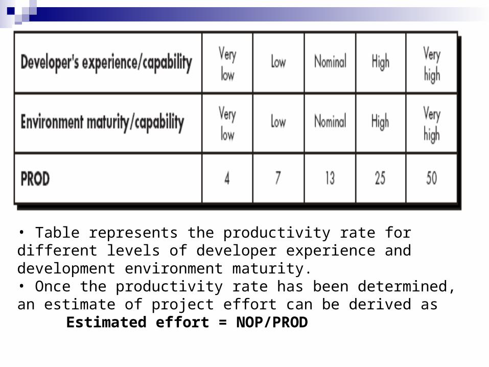
• Table represents the productivity rate for different levels of developer experience and development environment maturity.• Once the productivity rate has been determined, an estimate of project effort can be derived as

Estimated effort = NOP/PROD

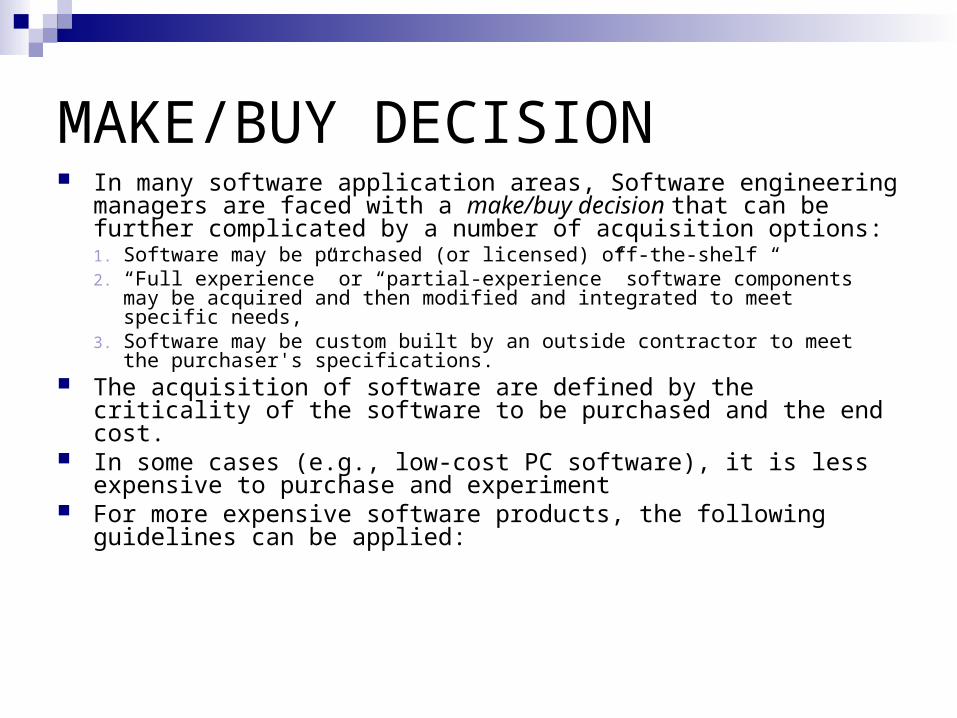
MAKE/BUY DECISION In many software application areas, Software engineering

managers are faced with a make/buy decision that can be further complicated by a number of acquisition options: 1. Software may be purchased (or licensed) off-the-shelf “2. “Full experience” or “partial-experience” software components may be

acquired and then modified and integrated to meet specific needs, 3. Software may be custom built by an outside contractor to meet the

purchaser's specifications. The acquisition of software are defined by the criticality of the

software to be purchased and the end cost. In some cases (e.g., low-cost PC software), it is less expensive

to purchase and experiment For more expensive software products, the following guidelines

can be applied:

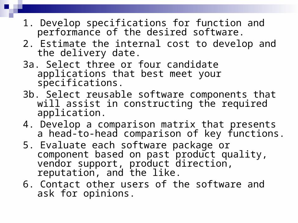
1. Develop specifications for function and performance of the desired software.

2. Estimate the internal cost to develop and the delivery date.

3a. Select three or four candidate applications that best meet your specifications.

3b. Select reusable software components that will assist in constructing the required application.

4. Develop a comparison matrix that presents a head-to-head comparison of key functions.

5. Evaluate each software package or component based on past product quality, vendor support, product direction, reputation, and the like.

6. Contact other users of the software and ask for opinions.

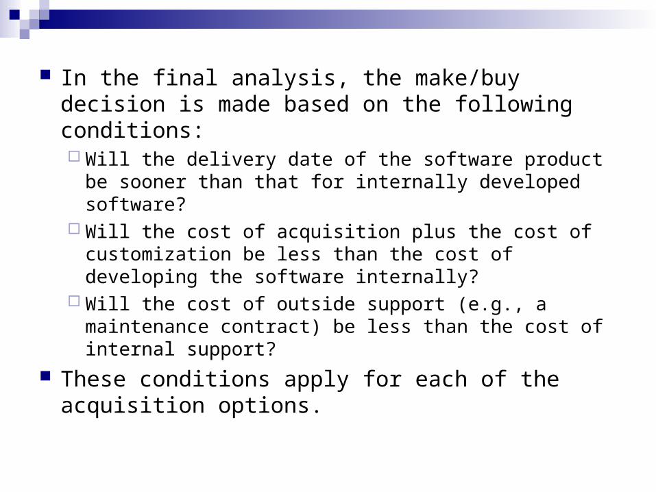
In the final analysis, the make/buy decision is made based on the following conditions: Will the delivery date of the software product be

sooner than that for internally developed software? Will the cost of acquisition plus the cost of

customization be less than the cost of developing the software internally?

Will the cost of outside support (e.g., a maintenance contract) be less than the cost of internal support?

These conditions apply for each of the acquisition options.

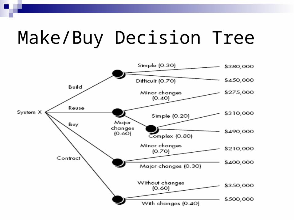
Make/Buy Decision Tree

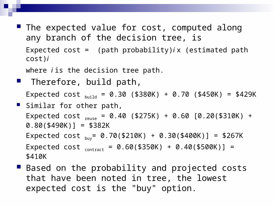
The expected value for cost, computed along any branch of the decision tree, is

Expected cost = (path probability)i x (estimated path cost)i

where i is the decision tree path.

Therefore, build path,

Expected cost build = 0.30 ($380K) + 0.70 ($450K) = $429K

Similar for other path,

Expected cost reuse = 0.40 ($275K) + 0.60 [0.20($310K) + 0.80($490K)] = $382K

Expected cost buy= 0.70($210K) + 0.30($400K)] = $267K

Expected cost contract = 0.60($350K) + 0.40($500K)] = $410K

Based on the probability and projected costs that have been noted in tree, the lowest expected cost is the "buy" option.