SOFT SENSOR FOR ON-LINE MONITORING OF PARTICLE SIZES IN

SOFT SENSOR FOR ON-LINE MONITORING OF PARTICLE SIZES IN

MINIEMULSION POLYMERIZATION

Luis A. Clementia,b

, Jorge R. Vegaa,b

, Luis M. Gugliottab

aFac. Reg. Santa Fe, Universidad Tecnológica Nacional, Lavaise 610, 3000 Santa Fe, Argentina,

http://www.frsf.utn.edu.ar/

bINTEC, Univ. Nac. del Litoral y CONICET, Guemes 3450, 3000 Santa Fe, Argentina,

[email protected], http://www.intec.unl.edu.ar/

Keywords: Polymeric Colloid, Inverse Problems, Tikhonov Regularization, General

Regression Neural Networks

Abstract. This paper proposes a soft-sensor (SS) for on-line monitoring the droplet/particle size

distribution (PSD) in miniemulsion polimerizations. The SS utilizes turbidity measurements and a

global particle refractive index (PRI) estimated on the basis of the instantaneous polymer conversion

and the PRIs of the monomer and the polymer. The proposed method requires solving an ill-

conditioned inverse problem (ICIP). Two different approaches are proposed for solving the ICIP: i) a

Tikhonov regularization (TR), and ii) a General Regression Neural Network (GRNN). Both

approaches are evaluated on the basis of simulated examples corresponding to a styrene miniemulsion

polymerization. For unimodal PSDs, both TR and GRNN produce acceptable estimates of the average

diameters of the PSD along the polymerization. The TR method produces PSDs with spurious peaks,

while the GRNN allows better estimates. For bimodal PSDs both methods produce acceptable average

diameters but erroneous PSDs. Simulation results suggest that the proposed method is a robust tool

for on-line monitoring of the average diameters in miniemulsion polymerizations.

Mecánica Computacional Vol XXXII, págs. 2405-2418 (artículo completo)Carlos G. García Garino, Aníbal E. Mirasso, Mario A. Storti, Miguel E. Tornello (Eds.)

Mendoza, Argentina, 19-22 Noviembre 2013

Copyright © 2013 Asociación Argentina de Mecánica Computacional http://www.amcaonline.org.ar

1 INTRODUCTION

A polymer colloid (or latex) is normally constituted by submicrometric polymer particles

dispersed in an aqueous medium. Latexes are typically used in the production of paints, inks,

coatings, adhesives, immunoassay kits, drugs delivery systems, etc. Synthetic latexes are

mostly obtained through aqueous phase microemulsion, miniemulsión, emulsion, and

dispersion polymerization processes (Gugliotta et al., 2010). Particularly, miniemulsion

polymerization involves the utilization of a surfactant/stabilizer system to produce stable

monomer droplets (the miniemulsion itself) of small sizes (normally, 10 nm – 500 nm)

(Schork et al., 2005). After the initiation (either outside or inside the droplets) the

polymerization is mainly carried out within the monomer droplets. Along a miniemulsion

polymerization the dispersed droplets and particles can exhibit a wide variety of

monomer/polymer ratios since the initiation of the polymerization is not instantaneous in all

monomer droplets. Miniemulsion polymerization represents an alternative for the synthesis of

hybrid latexes; and enables the incorporation of a hydrophobic component into the polymer

particles in a single step process, without requiring its diffusion through the aqueous phase

since the miniemulsion droplets can be generated containing all the components to be

incorporated in the synthesized material (Minari et al., 2009; Ronco et al., 2013).

The particle size distribution (PSD) is a morphological characteristic of primary

importance in several particulate systems including miniemulsions, emulsions, suspensions

and dispersions. In the particular case of a latex, the PSD affects the end-use properties (e.g.,

rheological, mechanical, physical) of the material when used as an adhesive, a paint, an ink, or

a coating. Also, the PSD affects the growth, and the interaction of the particles along

heterogeneous polymerizations (Gugliotta et al., 2010). For such reason, the accurate

knowledge of the PSD is necessary not only for the characterization of the final products, but

also for the understanding of the physicochemical mechanisms that take place in the course of

miniemulsion polymerizations. Additionally, on-line monitoring of the PSD along

miniemulsion polymerizations is important for the developing of control strategies.

On-line monitoring of the PSD is difficult due to the lack of a sensor for measuring the

PSD in the polymerization reactor medium. Alternatively, the PSD can be estimated through

an indirect method that involve: i) the measurement of a given physical property of the

particles, and ii) the resolution of an inverse problem (IP) (Tikhonov and Arsenin, 1977) on

the basis of a mathematical model that relate the measurements with the PSD. At present, a

light scattering (LS) based-method, such as turbidimetry (T), is a powerful technique for

estimating the PSD of a latex. In fact, T is fast, simple, and absolute (in the sense that it does

not require a previous calibration); and besides it does not produce sample damages (Gugliotta

et al., 2010).

Main definitions concerning PSDs of homogeneous spherical particles were reviewed by

Gugliotta et al. (2010). We shall call f(Di) the discrete number PSD. The ordinates of f(Di)

represent the number (or number concentration) of particles contained in the diameter interval

[Di , Di + ΔD] (i = 1, …, I), being ΔD a regular partition of the D axis. For a given discrete

PSD, several average diameters, that we shall call baD ,

, can be defined as follows:

L.A. CLEMENTI, J.R. VEGA, L.M. GUGLIOTTA2406


ba

i

b

ii

i

a

ii

ba

DDf

DDf

D

−

=

=

=

∑

∑

1

I

1

I

1,

)(

)(

(1)

For example, 0,1D = nD is the number-average diameter, and 3,4D = wD is the weight-

average diameter.

In a T experiment, the attenuation of a light beam while traveling through a dilute sample

is measured as a function of the light wavelength, λj (j = 1, …, J), and the turbidity spectrum,

τ(λj), is calculated as follows:

)](/)(ln[)/1()( 0 jtjj II λλλτ ℓ= (2)

where ℓ is the optical path length, and I0(λj) and It(λj) are the intensity of the incident and the

emerging light beams. In absence of multiple scattering (i.e., when the light scattered by a

particle does not interact with any other particle), and assuming spherical and homogenous

particles, the PSD f(Di) is related with the T measurement τ(λj) as follows (Gugliotta et al.,

2010):

∑=

=

I

1

2)()](),(,,[)(

i

iijpjmjiextj DfDnnDQk λλλλττ

; j = 1, …, J (3)

where kτ is a known experimental constant, and )](),(,,[ jpjmjiext nnDQ λλλ is the light

extinction by a particle of diameter Di and refractive index )( jpn λ immersed in a non-

absorbing medium of refractive index )( jmn λ at the wavelength jλ , and is calculated

through the Mie scattering theory (Bohren and Huffman, 1983).

For homogeneous particles composed of two different species, the particle refractive index

(PRI) )( jpn λ can be calculated as follows (Iulian et al., 2010):

)()()( 2,21,1 jpjpjp nnn λϕλϕλ += (4)

where 1ϕ and 2ϕ are the volume fraction of species with PRI )(1, jpn λ and )(2, jpn λ ,

respectively.

Equation (3) represent a system of J linear equation with I unknowns (the ordinates of the

PSD), that can be rewritten in a matrix form, as follows:

fQττk= (5)

where τ (J×1) and f (I×1) are vectors with components τ(λj) and f(Di), respectively, and Q

(J×I) is the matrix with the (j,i)-th component given by 2)](),(,,[ ijpjmjiext DnnDQ λλλ . The

PSD f can be estimated from τ by inverting Eq. (5). To this effect, matrix Q is calculated

through the Mie scattering theory (Bohren and Huffman, 1983) and the PRI )( jpn λ must be

accurately known. Inversion of Eq. (5) is known to be an “ill-conditioned” inverse problem

(ICIP); i.e., small perturbation caused by experimental noise or uncertainties in the PRI can

lead to important deviations in the estimated PSD.

When the colloid exhibits particles of different composition (and thus different PRIs), as in

Mecánica Computacional Vol XXXII, págs. 2405-2418 (2013) 2407


the case of a miniemulsion polymerization, Eq. (5) can be generalized as follows:

][ LL2211 fQfQfQτ +++= ⋯τk (6)

where Ql (J×I) (l = 1, ..., L) is the l-th matrix with components 2

, )](),(,,[ ijlpjmjiext DnnDQ λλλ corresponding to the particle population with a fixed

composition and PRI )(, jlpn λ , and fl (I×1) is the corresponding PSD for a given particle

composition. Note that the global PSD is given by:

N21 ffff +++= ⋯ (7)

On line monitoring of PSDs by T has been scarcely studied in the literature. Moreover,

most papers restrict their study to analyze the sensitivity of T measurements to changes in the

characteristics of the colloid rather than proposing methods for estimating the PSD. For

example, Chicoma et al. (2011) and Higgins et al. (2003) observed meaningful sensitivity of T

measurements along the synthesis of polymeric particles and the production of pharmaceutical

drug nanoparticles, respectively. Brandolin et al. (1991) utilized simulated examples to

investigate the sensitivity of operative parameters (for example, sample time, latex

concentration, light wavelength, etc.) on estimated PSDs obtained by inverting Eq. (5) along

emulsion polymerization of styrene. Kiparissides (1980) investigated the on-line monitoring

of continuous emulsion polymerization of vinyl-acetate through T measurements. In its work,

T at a single wavelength (350 nm) was able to detect the beginning of the polymerization and

whether the system reached a steady state or exhibited oscillations. Other authors have utilized

alternative light scattering measurements such dynamic light scattering (DLS) and multiangle

static light scattering (MALS) for on-line monitoring of average diameters and PSDs along

heterogeneous polymerizations (Çatalgis-Giz et al., 2003; Alb et al., 2006; Alb and Reed,

2008). As far as the authors are aware, monitoring of miniemulsion polymerization on the

basis of light scattering techniques has not been investigated yet.

In this paper a novel method is proposed for on-line monitoring of the PSD along a

miniemulsion polymerization on the basis of T measurements. The method is evaluated

through a simulated example corresponding to an aqueous phase miniemulsion

polymerization of styrene with PSDs of different average diameters. A Tikhonov

regularization method and a general regression neural network are compared as tools for

solving the involved ICIP. All the computer work was carried out in Matlab.

2 THE PROPOSED METHOD

On-line estimation of the global PSD along a miniemulsion polymerization through the

mathematical model of Eq. (6) and (7) is difficult because the droplets and particles exhibit a

wide variety of unknown compositions (and thus, unknown PRIs). In consequence, matrixes

Ql in Eq. (6) cannot be calculated. An approximated estimation method is proposed in what

follows.

Consider the instantaneous polymer conversion, x(t), at each time t, defined as:

0

0 )()(

M

tMMtx

−

= (8)

where M0 and M(t) are the initial and instantaneous mass concentration of the monomer,

respectively. From x(t), the global instantaneous volume fractions of monomer and polymer,



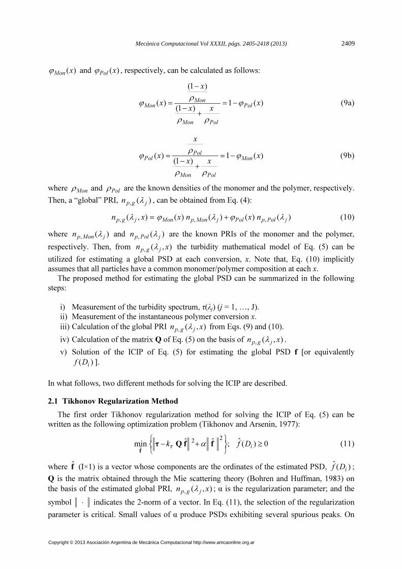
)(xMonϕ and )(xPolϕ , respectively, can be calculated as follows:

)(1)1(

)1(

)( x

xx

x

x Pol

PolMon

MonMon ϕ

ρρ

ρϕ −=

+−

−

= (9a)

)(1)1(

)( x

xx

x

x Mon

PolMon

PolPol ϕ

ρρ

ρϕ −=

+−

= (9b)

where Monρ and Polρ are the known densities of the monomer and the polymer, respectively.

Then, a “global” PRI, )(, jgpn λ , can be obtained from Eq. (4):

)()()()(),(,,, jPolpPoljMonpMonjgp nxnxxn λϕλϕλ += (10)

where )(, jMonpn λ and )(

, jPolpn λ are the known PRIs of the monomer and the polymer,

respectively. Then, from ),(, xn jgp λ the turbidity mathematical model of Eq. (5) can be

utilized for estimating a global PSD at each conversion, x. Note that, Eq. (10) implicitly

assumes that all particles have a common monomer/polymer composition at each x.

The proposed method for estimating the global PSD can be summarized in the following

steps:

i) Measurement of the turbidity spectrum, τ(λj) (j = 1, …, J).

ii) Measurement of the instantaneous polymer conversion x.

iii) Calculation of the global PRI ),(, xn jgp λ from Eqs. (9) and (10).

iv) Calculation of the matrix Q of Eq. (5) on the basis of ),(, xn jgp λ .

v) Solution of the ICIP of Eq. (5) for estimating the global PSD f [or equivalently

)(i

Df ].

In what follows, two different methods for solving the ICIP are described.

2.1 Tikhonov Regularization Method

The first order Tikhonov regularization method for solving the ICIP of Eq. (5) can be

written as the following optimization problem (Tikhonov and Arsenin, 1977):

0)(ˆ;ˆˆmin2

2

ˆ≥

+−i

Dfk ffQτf

ατ

(11)

where f̂ (I×1) is a vector whose components are the ordinates of the estimated PSD, )(ˆi

Df ;

Q is the matrix obtained through the Mie scattering theory (Bohren and Huffman, 1983) on

the basis of the estimated global PRI, ),(, xn jgp λ ; α is the regularization parameter; and the

symbol ⋅ indicates the 2-norm of a vector. In Eq. (11), the selection of the regularization

parameter is critical. Small values of α produce PSDs exhibiting several spurious peaks. On



the other hand, high values of α produce excessively broad PSDs. In general, α depends on: i)

the degree of ill-conditioning of the inverse problem (i.e. the condition number of the matrix

Q); and ii) the measurement noise level. There are a variety of criteria to determine the

optimum value of the regularization parameter (Aster et al., 2005). In this work, the L-curve

technique is utilized (Hansen and O’Leary, 1993). Computer programs for solving the

optimization problem of Eq. (11) were developed based on the regularization tools reported

by Hansen (1994).

2.2 General Regression Neural Network

Figure 1) presents a scheme of the utilized general regression neural network (GRNN).

Figure 1: Schematic representation of the utilized GRNN

The GRNN involves: 2J inputs, the components of the global PRI vector

)],(,),,([ J,1, xnxn gpgp λλ ⋯=pn and the measurement vector τ ; I outputs, the components

of the estimated PSD vector f; an input layer with 2J neurons; an output layer with I neurons;

and a hidden layer with K neurons (Haykin, 1999). The k-th neuron in the hidden layer

receives the vector ][ τnp as input and produces an scalar output of amplitude hk given by:

2

2

2

][

2

1k

k

eh

k

k

σ

πσ

cτnp −

−

= ; k = 1, …, K. (12)

where kcτnp −][ represent the distance between the vector ][ τnp (2J×1) and the center

kc (2J×1) of the k-th neuron in the hidden layer; and kσ is the so-called smoothness

parameter associated with the k-th neuron. From hk, the components )(ˆi

Df (i = 1, …I) of the

output f̂ of the GRNN are calculated as follows:

∑=

=

K

1

,)(ˆ

k

kkii hwDf ; i = 1, …, I. (13)

where kiw ,

is the weight coefficient of the connection between the k-th hidden neuron and the

i-th output neuron.



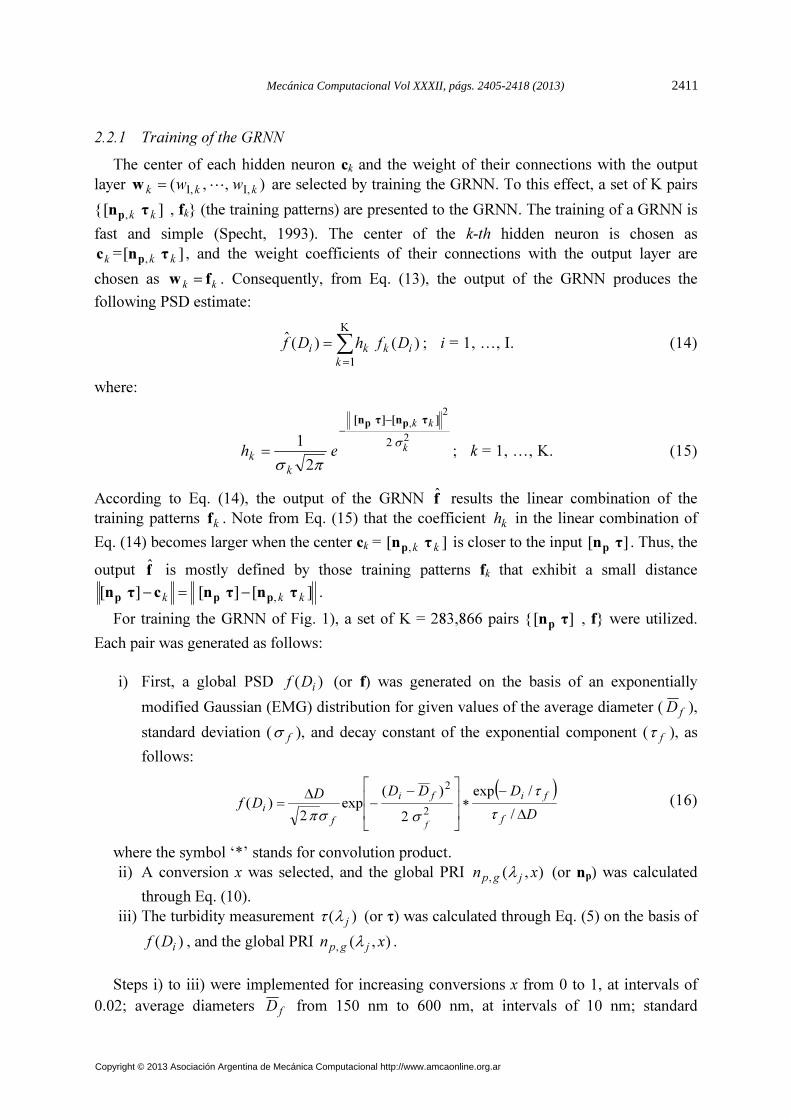
2.2.1 Training of the GRNN

The center of each hidden neuron ck and the weight of their connections with the output

layer ),,( ,I,1 kkk ww ⋯=w are selected by training the GRNN. To this effect, a set of K pairs

{ ][ , kk τnp , fk} (the training patterns) are presented to the GRNN. The training of a GRNN is

fast and simple (Specht, 1993). The center of the k-th hidden neuron is chosen as

kc = ][ , kk τnp , and the weight coefficients of their connections with the output layer are

chosen as kkfw = . Consequently, from Eq. (13), the output of the GRNN produces the

following PSD estimate:

∑=

=

K

1

)()(ˆ

k

ikki DfhDf ; i = 1, …, I. (14)

where:

2

2

,

2

][][

2

1k

kk

eh

k

k

σ

πσ

τnτn pp −

−

= ; k = 1, …, K. (15)

According to Eq. (14), the output of the GRNN f̂ results the linear combination of the

training patterns kf . Note from Eq. (15) that the coefficient kh in the linear combination of

Eq. (14) becomes larger when the center ck = ][ , kk τnp is closer to the input ][ τnp . Thus, the

output f̂ is mostly defined by those training patterns fk that exhibit a small distance

][][][, kkk τnτncτn ppp −=− .

For training the GRNN of Fig. 1), a set of K = 283,866 pairs { ][ τnp , f} were utilized.

Each pair was generated as follows:

i) First, a global PSD )(i

Df (or f) was generated on the basis of an exponentially

modified Gaussian (EMG) distribution for given values of the average diameter ( fD ),

standard deviation ( fσ ), and decay constant of the exponential component ( fτ ), as

follows:

( )

D

DDDDDf

f

fifi

f

i

f∆

−∗

−−

∆=

/

/exp

2

)(exp

2)(

2

2

τ

τ

σσπ

(16)

where the symbol ‘*’ stands for convolution product.

ii) A conversion x was selected, and the global PRI ),(, xn jgp λ (or np) was calculated

through Eq. (10).

iii) The turbidity measurement )( jλτ (or τ) was calculated through Eq. (5) on the basis of

)(i

Df , and the global PRI ),(, xn jgp λ .

Steps i) to iii) were implemented for increasing conversions x from 0 to 1, at intervals of

0.02; average diameters fD from 150 nm to 600 nm, at intervals of 10 nm; standard



deviations fσ from 15 nm to 65 nm, at intervals of 5 nm; and exponential decays fτ from 15

nm to 65 nm, at intervals of 5 nm. Finally, the GRNN was trained on the basis of the

generated pairs. The choice of EMG as basis of the training pattern enables the approximation

of a wide variety of different distributions (e.g. Gaussian, normal-logarithmic, etc).

2.2.2 Selection of the smoothness parameter kσ

The smoothness parameter kσ affects the selectivity of each hidden neuron. A small kσ

typically produces a highly selective GRNN; i.e., only those neurons with a small norm

][][, kk τnτn pp − meaningfully contribute to the output f̂ . On the contrary, a high kσ

produces a less selective GRNN, and therefore neurons with larger distances

][][, kk τnτn pp − will also contribute to the output.

Several methods have been proposed for selecting kσ (Specht, 1991; Zhong et al., 2005).

In this work, a common value of kσ was used for all the hidden neurons, and was selected

according to the “Holdout” method proposed by Specht (1991). To this effect, 10,000 patterns

were randomly selected and removed from the original set of 283,866 training patterns.

Therefore, the GRNN training (see section 2.2.1) was carried out on the basis of the remaining

273,866 patterns and kσ was selected by solving the following optimization problem:

−∑

=

000,10

1

ˆmin

k

kk

k

ffσ

(17)

where kf̂ is the estimated PSD for the k-th removed pattern. According to the “Holdout”

method, kσ is chosen as the value that best reproduces the PSD of the 10,000 removed

patterns. The advantage of this method is the simplicity for its implementation and

automation.

3 ANALISYS OF SIMULATED EXAMPLES

Consider a simplified model of a miniemulsion polymerization of Styrene. The simulated

sample consists of a blend of 10 different species: i) the initial miniemulsion (i.e. droplets of

pure Styrene in which conversion is x0=0); ii) hybrid particles (i.e. particles with monomer

and polymer) exhibiting partial conversion of x1=1/9, x2=2/9, …, x8=8/9; and iii) pure

polystyrene particles (in which conversion is x9=1).

Species with x0=0 exhibits a Normal-Logarithmic PSD, )(0 iDg [Fig. 2)] defined in the

range [50 nm – 700 nm] at regular interval of D∆ = 1 nm and given by:

=

2

2

0

0

2

)]/ln([exp

2)(

σπσ

∆ DD-

D

DDg i

i

i (18)

where 0D = 300 nm is the average diameter and σ = 0.20 is the standard deviation. For the

species with x > 0, a particle contraction is expected since the density of polystyrene (pSt =

1.05 g/cm3) is larger than the density of Styrene (St = 0.909 g/cm

3). Thus, the PSD for the

species with xl > 0, )( il Dg (l = 1, …, 9), were simulated from Eq. (18) assuming the

corresponding contracted average diameter:



0

3/1

St )](/[ DxD lll ρρ= ; (l = 1, …, 9) (19)

with:

pStpStStSt )()()( ρϕρϕρ llll xxx += ; (l = 1, …, 9) (20)

where )( ll xρ is the density of particles corresponding to species with conversion xl; and

)(St lxϕ and )(pSt lxϕ are the volume fractions of styrene and polystyrene for the specie with

conversion lx , respectively, and were obtained from Eqs. (9a) and (9b). Note that for pure

polystyrene particles (i.e. with x9 = 1) it results 03/1

pStSt9 ]/[ DD ρρ= . Figure 2 compare the

normalized (to equal area) PSDs )( il Dg (l = 0, …, 9).

Figure 2: Normalized size distributions )( il Dg (l = 0, …, 9) for the species with conversions

xl = 0, 1/9, 2/9, …, 1

Four examples (EX. 1, EX. 2, EX. 3 and EX. 4) were considered by assuming the number

concentrations of each species, cl, that are presented in Table 1. The aim of EX. 1, EX. 2 and

EX. 3 is to simulate several stages of a miniemulsion polymerization. EX. 1 corresponds to

the initial stage of the polymerization in which only the species with small conversion xl are

present. EX. 2 corresponds to the middle stage in which all species are present. EX. 3

corresponds to the final stage of the polymerization in which only species with high

conversion xl are present. An additional case (EX. 4) was simulated by adding a Normal-

Logarithmic mode [Eq. (18)] of pure polystyrene particles, with average diameter 150 nm,

standard deviation 0.1 and number concentration 0.75, to the case of EX. 2. This kind of PSD

is normally obtained in miniemulsion polymerizations that exhibit simultaneous

polymerization by homogeneous nucleation, thus producing a population of polymer particles

of small diameters.

For each simulated example, the global PSD was obtained according to Eq. (7), as follows:

∑=

=

9

0

)()(l

illi DgcDf (21)

Figure 3a) compare the global PSDs )(1 iDf , )(2 iDf , )(3 iDf and )(4 i

Df for examples EX.

1, EX.2, EX. 3 and EX. 4, respectively.



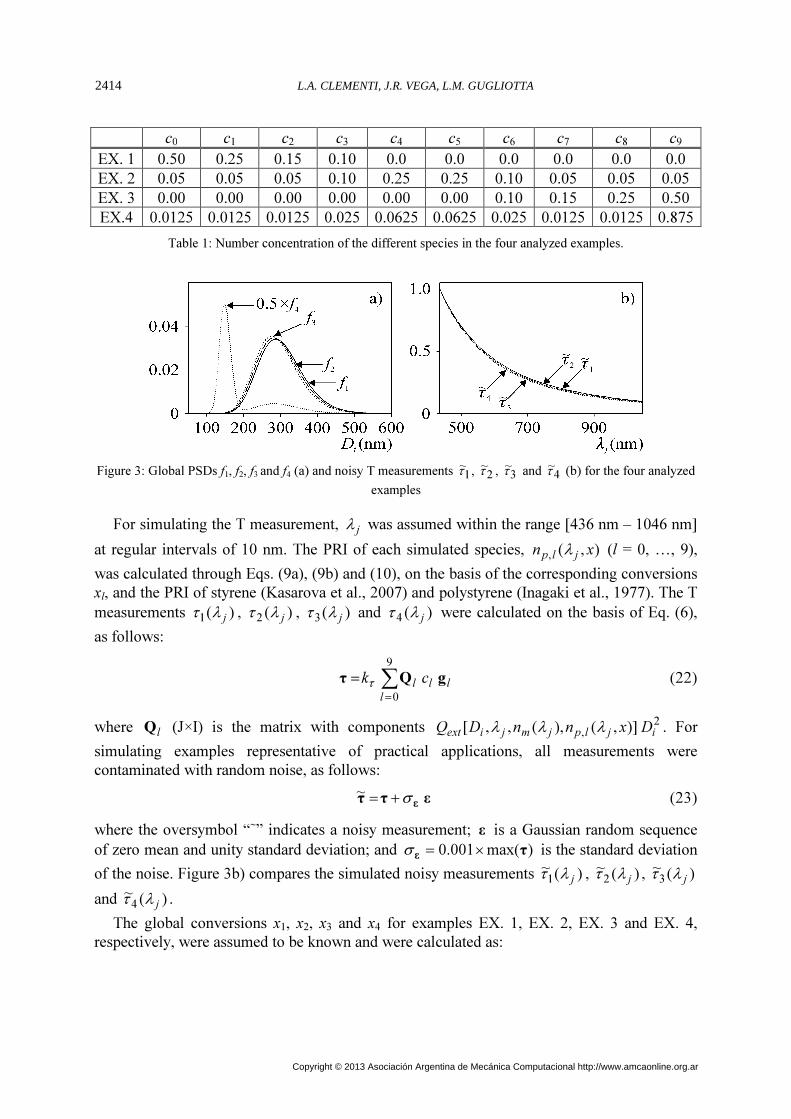
c0 c1 c2 c3 c4 c5 c6 c7 c8 c9

EX. 1 0.50 0.25 0.15 0.10 0.0 0.0 0.0 0.0 0.0 0.0

EX. 2 0.05 0.05 0.05 0.10 0.25 0.25 0.10 0.05 0.05 0.05

EX. 3 0.00 0.00 0.00 0.00 0.00 0.00 0.10 0.15 0.25 0.50

EX.4 0.0125 0.0125 0.0125 0.025 0.0625 0.0625 0.025 0.0125 0.0125 0.875

Table 1: Number concentration of the different species in the four analyzed examples.

Figure 3: Global PSDs f1, f2, f3 and f4 (a) and noisy T measurements 1~

τ , 2~

τ , 3~

τ and 4~

τ (b) for the four analyzed

examples

For simulating the T measurement, jλ was assumed within the range [436 nm – 1046 nm]

at regular intervals of 10 nm. The PRI of each simulated species, ),(, xn jlp λ (l = 0, …, 9),

was calculated through Eqs. (9a), (9b) and (10), on the basis of the corresponding conversions

xl, and the PRI of styrene (Kasarova et al., 2007) and polystyrene (Inagaki et al., 1977). The T

measurements )(1 jλτ , )(2 jλτ , )(3 jλτ and )(4 jλτ were calculated on the basis of Eq. (6),

as follows:

∑=

=

9

0l

lll ck gQττ

(22)

where lQ (J×I) is the matrix with components 2, )],(),(,,[ ijlpjmjiext DxnnDQ λλλ . For

simulating examples representative of practical applications, all measurements were

contaminated with random noise, as follows:

εττεσ+=

~ (23)

where the oversymbol “∼

” indicates a noisy measurement; ε is a Gaussian random sequence

of zero mean and unity standard deviation; and )max(001.0 τε

×=σ is the standard deviation

of the noise. Figure 3b) compares the simulated noisy measurements )(~1 jλτ , )(~

2 jλτ , )(~3 jλτ

and )(~4 jλτ .

The global conversions x1, x2, x3 and x4 for examples EX. 1, EX. 2, EX. 3 and EX. 4,

respectively, were assumed to be known and were calculated as:



=

∑

∑ ∑

=

= =

I

1

3

9

0

I

1

3

)(

)(

i

ilil

l i

ilill

DgDc

DgDcx

x (24)

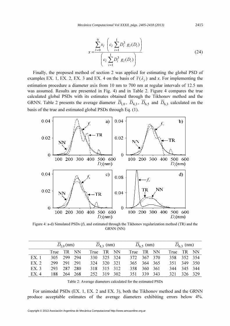
Finally, the proposed method of section 2 was applied for estimating the global PSD of

examples EX. 1, EX. 2, EX. 3 and EX. 4 on the basis of )(~ jλτ and x. For implementing the

estimation procedure a diameter axis from 10 nm to 700 nm at regular intervals of 12.5 nm

was assumed. Results are presented in Fig. 4) and in Table 2. Figure 4 compares the true

calculated global PSDs with its estimates obtained through the Tikhonov method and the

GRNN. Table 2 presents the average diameter 0,1D , 3,4D , 5,6D and 3,6D calculated on the

basis of the true and estimated global PSDs through Eq. (1).

Figure 4: a-d) Simulated PSDs (f), and estimated through the Tikhonov regularization method (TR) and the

GRNN (NN)

0,1D (nm)

3,4D (nm) 5,6D (nm)

3,6D (nm)

True TR NN True TR NN True TR NN True TR NN

EX. 1 305 299 294 330 325 324 372 367 370 358 352 354

EX. 2 299 291 291 324 320 321 365 364 365 351 349 350

EX. 3 293 287 280 318 315 312 358 360 361 344 345 344

EX. 4 188 264 268 252 319 302 351 339 343 321 326 329

Table 2: Average diameters calculated for the estimated PSDs

For unimodal PSDs (EX. 1, EX. 2 and EX. 3), both the Tikhonov method and the GRNN

produce acceptable estimates of the average diameters exhibiting errors below 4%.



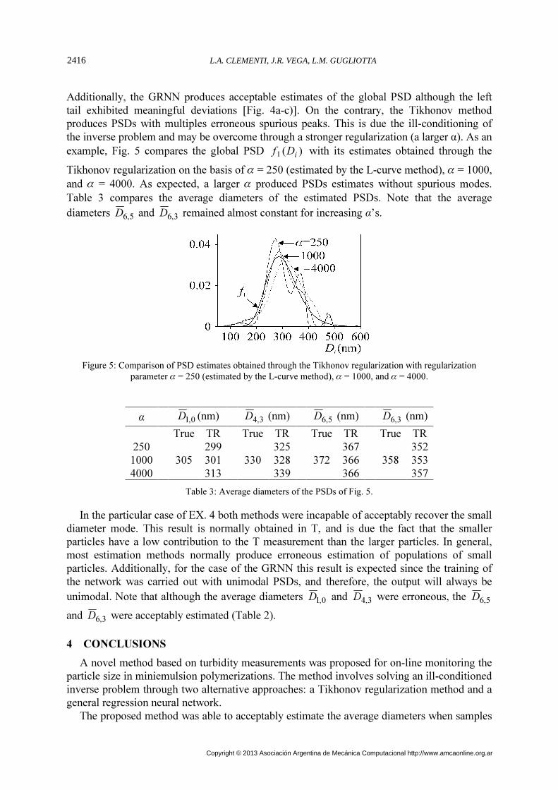
Additionally, the GRNN produces acceptable estimates of the global PSD although the left

tail exhibited meaningful deviations [Fig. 4a-c)]. On the contrary, the Tikhonov method

produces PSDs with multiples erroneous spurious peaks. This is due the ill-conditioning of

the inverse problem and may be overcome through a stronger regularization (a larger α). As an

example, Fig. 5 compares the global PSD )(1 iDf with its estimates obtained through the

Tikhonov regularization on the basis of = 250 (estimated by the L-curve method), = 1000,

and = 4000. As expected, a larger produced PSDs estimates without spurious modes.

Table 3 compares the average diameters of the estimated PSDs. Note that the average

diameters 5,6D and 3,6D remained almost constant for increasing α’s.

Figure 5: Comparison of PSD estimates obtained through the Tikhonov regularization with regularization

parameter = 250 (estimated by the L-curve method), = 1000, and = 4000.

α 0,1D (nm) 3,4D (nm) 5,6D (nm) 3,6D (nm)

True TR True TR True TR True TR

250

305

299

330

325

372

367

358

352

1000 301 328 366 353

4000 313 339 366 357

Table 3: Average diameters of the PSDs of Fig. 5.

In the particular case of EX. 4 both methods were incapable of acceptably recover the small

diameter mode. This result is normally obtained in T, and is due the fact that the smaller

particles have a low contribution to the T measurement than the larger particles. In general,

most estimation methods normally produce erroneous estimation of populations of small

particles. Additionally, for the case of the GRNN this result is expected since the training of

the network was carried out with unimodal PSDs, and therefore, the output will always be

unimodal. Note that although the average diameters 0,1D and 3,4D were erroneous, the 5,6D

and 3,6D were acceptably estimated (Table 2).

4 CONCLUSIONS

A novel method based on turbidity measurements was proposed for on-line monitoring the

particle size in miniemulsion polymerizations. The method involves solving an ill-conditioned

inverse problem through two alternative approaches: a Tikhonov regularization method and a

general regression neural network.

The proposed method was able to acceptably estimate the average diameters when samples



exhibit unimodal PSDs. Additionally, the neural network produced good estimates of the

PSD. The Tikhonov method produced PSDs with erroneous spurious modes. For bimodal

PSDs (typically obtained in reactions that also exhibit homogeneous nucleation) both methods

produced erroneous PSD estimates. However, the proposed method was adequate to estimate

the average diameters 5,6D and 3,6D . Consequently, although the global PSD is erroneously

recuperated in some applications, the proposed method could in principle be used for on-line

monitoring the average diameter (either the 5,6D or the 3,6D ) along miniemulsion

polymerizations. For example, along a miniemulsion polymerization only slight variations of

the average diameter of the global PSD are observed; as can be seen in Table 2 where the

3,6D is 358 nm at the begining of the polymerization (EX. 1) and 344 nm at the end (EX. 3)

(i.e. a variation of aproximately 4%). However, when the polymerization exhibits

homogeneous nucleation (EX. 4) a meaningful decrease in the average diameters of the global

PSD are produced. This can be seen in Table 2 where 3,6D is 321 nm for EX. 4 (i.e. a

variation of almost 11% with respect to EX. 1). Thus, homogeneous nucleation along

miniemulsion polymerization can be detected by monitoring the 5,6D and/or the 3,6D .

With respect to the inversion techniques, although the neural network is less general

because the estimated PSD is highly dependent of the selected training pattern utilized, the

GRNN is a simple and fast technique that does not require previous expertise. On the

contrary, the Tikhonov method requires some level of expertise of the user and frequently the

obtained PSD exhibits spurious modes due the highly ill-conditioning of the inverse problem.

ACKNOWLEDGMENTS

We are grateful for the financial and technical supports received from CONICET,

Universidad Nacional del Litoral, and Universidad Tecnológica Nacional.

REFERENCES

Alb, A.M., Farinato, R., Calbick, J., Reed, W.F., Online Monitoring of Polymerization

Reactions in Inverse Emulsions. Langmuir, 22: 831-840, 2006.

Alb. A.M., Reed, W.F., Simultaneous Monitoring of Polymer and Particle Characteristics

during Emulsion Polymerization. Macromolecules, 41: 2406-2414, 2008.

Aster, R., Borchers B. and Thurber, C., Parameter Estimation and Inverse Problems. Elsevier

Academic Press, USA, 2005.

Bohren, C. and Huffman, D., Absorption and Scattering of Light by Small Particles. Wiley,

New York, 1983.

Brandolin, A., García-Rubio, L., Provder, T., Koeheler, M. y Kuo, C., in Particle Size

Distribution II. Assessment and Characterization (Ed. T. Provder), ACS Symposium

Series No. 472, American Chemical Society, Washington D.C., 20, 1991.

Çatalgi-Giz, H., Giz, A., Alb., A.M., Reed. W.F., Absolute Online Monitoring of Acrylic

Acid Polymerization and the Effect of Salt and PH on Reaction Kinetics. J. Appl. Pol. Sci.,

91(2): 1352-1359, 2003.

Chicoma, D.L., Sayer, C., Giudici, R., In-line Monitoring of Particle Size During Emulsion

Polymerization Under Different Operational Conditions Using NIR Spectroscopy. Macr.

Reac. Eng., 5: 150-162, 2011.

Gugliotta, L., Clementi L., Vega, J., in Measurement of Particle Size Distribution of Polymer

Latexes. Research Signpost, Kerala, India, 2010.



Hansen, P.C. y O’Leary, D.P., The Use of the L-curve in the Regularization of Discrete Ill-

posed Problems. SIAM J. Sci. Comput., 14: 1487-1503, 1993.

Hansen, P.C., Regularization Tools: A Matlab Package for Analysis and Solution of Discrete

Ill-posed Problems. Numerical Algorithms, 6: 1-35, 1994.

Haykin, S., Neural Networks: A Comprehensive Foundation, 2nd Ed. Prentice Hall, New

Jersey, 1999.

Higgins, J.P., Arrivo, S.M., Thurau, G., Green, R.L., Bowen, W., Lange, A., Templeon, A.C.,

Thomas, D.L., Reed, R.A., Spectroscopic Approach for On-line Monitoring of Particle Size

during the Processing of Pharmaceutical Nanoparticles. Anal. Chem., 75: 1777-1785, 2003.

Inagaki T., Arakawa E.T., Hamm R.N., y Williams M.W., Optical Properties of Polystyren

from the Near Infrared to the X-Ray Region and Convergence of Optical Sum Rules.

Physical Review, 6 (15): 3243, 1977.

Iulian, O., Stefaniu, A., Ciocirlan, O., Fedeles, A., Refractive Index in Binary and Ternary

Mixtures With Diathylene Glycol, 1,4-Dioxane and Water Between 293.15-313.15 K.

U.P.B. Sci. Bull., Series B, 72 (4): 37-44, 2010.

Kasarova, S.N., Sultanova, N.G., Ivanov, C.D., Nikolov, I.D., Analysis of the Dispersion of

Optical Plastic Materials. Optical Materials, 29: 1481-1490, 2007.

Kiparissides, C., MacGregor, J.F., Singh, S., Hamielec, A.E., Continuous Emulsion

Polymerization of Vinyl Acetate. Part. III: Detection of Reactor Performance by Turbidity-

Spectra and Liquid Exclusion Chromatography. Canadian Journal of Chemical

Engineering, 58: 65-71, 1980.

Minari R., Goikoetxea M., Beristain I., Paulis M., Barandiaran M., Asua J., Post-

polymerization of Waterborne Alkyd/Acrylics. Effect on Polymer Architecture and Particle

Morphology. Polymer, 50: 5892-5900, 2009.

Ronco L.I., Minari, R.J., Vega, J.R., Meira, G.R., Gugliotta, L.M, Incorporation of

Polybutadiene into Waterborne Polystyrene Nanoparticles via Miniemulsion

Polymerization. European Polymer Journal, 2013 (In Press).

Schork, J.F., Luo, Y., Smulders W., Russum J.P, Butte A., Fontenot K., Miniemulsion

Polymerization. Adv. Polym. Aci., 175: 129-155, 2005.

Specht, D.F., A General Regression Neural Network. IEEE Transactions on Neural Networks,

2(6): 568-576, 1991.

Specht, D.F., The General Regression Neural Network-Rediscovered. Neural Networks, 6(7):

1033-1034, 1993.

Tikhonov A., and Arsenin, V. Solution of Ill-posed Problems. Wiley, New York, 1977.

Zhong, M., Goggeshall, D., Ghaneie, E., Pope, T., Rivera, M., Georgiopoulos, M.,

Anagnostopoulos, G., Mollaghasemi, M. y Richie, S., Gap-Based Estimation: Choosing

the Smoothing Parameters for Probabilistic and General Regression Neural Networks,

National Sciene Foundation, Florida, Orlando, USA, 2005.



Documents

SOFT SENSOR FOR ON-LINE MONITORING OF PARTICLE SIZES IN