SOEPpaperson Multidisciplinary Panel Data Research

Explaining Age and Gender Differenc-es in Employment Rates: A Labor Supply Side Perspective

Stephan Humpert and Christian Pfeifer

449 201

2SOEP — The German Socio-Economic Panel Study at DIW Berlin 449-2012

SOEPpapers on Multidisciplinary Panel Data Research at DIW Berlin This series presents research findings based either directly on data from the German Socio-Economic Panel Study (SOEP) or using SOEP data as part of an internationally comparable data set (e.g. CNEF, ECHP, LIS, LWS, CHER/PACO). SOEP is a truly multidisciplinary household panel study covering a wide range of social and behavioral sciences: economics, sociology, psychology, survey methodology, econometrics and applied statistics, educational science, political science, public health, behavioral genetics, demography, geography, and sport science. The decision to publish a submission in SOEPpapers is made by a board of editors chosen by the DIW Berlin to represent the wide range of disciplines covered by SOEP. There is no external referee process and papers are either accepted or rejected without revision. Papers appear in this series as works in progress and may also appear elsewhere. They often represent preliminary studies and are circulated to encourage discussion. Citation of such a paper should account for its provisional character. A revised version may be requested from the author directly. Any opinions expressed in this series are those of the author(s) and not those of DIW Berlin. Research disseminated by DIW Berlin may include views on public policy issues, but the institute itself takes no institutional policy positions. The SOEPpapers are available at http://www.diw.de/soeppapers Editors: Jürgen Schupp (Sociology, Vice Dean DIW Graduate Center) Gert G. Wagner (Social Sciences) Conchita D’Ambrosio (Public Economics) Denis Gerstorf (Psychology, DIW Research Professor) Elke Holst (Gender Studies) Frauke Kreuter (Survey Methodology, DIW Research Professor) Martin Kroh (Political Science and Survey Methodology) Frieder R. Lang (Psychology, DIW Research Professor) Henning Lohmann (Sociology, DIW Research Professor) Jörg-Peter Schräpler (Survey Methodology, DIW Research Professor) Thomas Siedler (Empirical Economics) C. Katharina Spieß (Empirical Economics and Educational Science)

ISSN: 1864-6689 (online)

German Socio-Economic Panel Study (SOEP) DIW Berlin Mohrenstrasse 58 10117 Berlin, Germany Contact: Uta Rahmann | soeppapers@diw.de

Explaining Age and Gender Differences in Employment

Rates: A Labor Supply Side Perspective

Stephan Humpert a)

a) Corresponding author: Stephan Humpert, Institute of Economics, Leuphana University Lüneburg, Scharnhorststr. 1, 21335 Lüneburg, Germany; phone: +49-4131-

6772322; e-mail: humpert@leuphana.de.

Christian Pfeifer a)b) a) Institute of Economics, Leuphana University Lüneburg, Scharnhorststr. 1, 21335

Lüneburg, Germany; phone: +49-4131-6772301; e-mail: pfeifer@leuphana.de. b) IZA Bonn, Germany.

* Acknowledgements: This work was financially supported by the VolkswagenStiftung.

We thank participants of the Colloquium in Personnel Economics 2011 in Zurich and of

research seminars at Leuphana University Lüneburg for their comments.

Explaining Age and Gender Differences in Employment

Rates: A Labor Supply Side Perspective

Abstract

This paper takes a labor supply perspective (neoclassical labor supply, job search) to

explain the lower employment rates of older workers and women. The basic rationale is

that workers choose non-employed if their reservation wages are larger than the offered

wages. Whereas the offered wages depend on workers' productivity and firms'

decisions, reservation wages are largely determined by workers' endowments and

preferences for leisure. To shed some empirical light on this issue, we use German

survey data to analyze age and gender differences in reservation and entry wages,

preferred and actual working hours, and satisfaction with leisure and work.

Keywords: Age; Family gap; Gender; Job search; Labor supply; Reservation wages

JEL classification: J14, J22, J64

1

1. Introduction

An empirical observation in most labor markets is the lower (re-)employment

probability of female and older workers. In Germany, employment rates decline with

age after the maximum is reached at prime ages between 30 and 50 years for men and

40 to 50 years for women (see Table 1). It can also be seen that women in all age

categories have lower employment rates than men and that this employment gap

increases with age; this disadvantage may emerge during motherhood but still increases

afterwards. Non-employment often leads to individual hardship (e.g., lower

consumption standards) and is also associated with burdens for society, because

taxpayers have to finance unemployment benefits or early retirement schemes. In times

of demographic change, it is a challenge for policy and Human Resource Management

to activate the resources of female and older persons in the labor market to maintain a

sufficiently large labor supply. Furthermore, demographic change has brought financial

problems for public retirement schemes, so that many countries have recently increased

the mandatory retirement age (e.g., in Germany from 65 to 67 years). However, it seems

questionable if older workers still have the necessary employment prospects. Most of

the political discussion focuses on labor demand side factors, i.e., if the productivity of

older workers is still large enough for the wages paid, and assumes that old workers still

want to work. This assumption might not always be correct. For example, we can

observe the active participation of workers in early retirement schemes. In this paper,

we are going to explore age and gender differences in labor supply. More specifically,

we analyze reservation and entry wages, preferred and actual working hours, and

satisfaction with leisure and jobs.

- insert Table 1 about here

2

One stream of the literature in economics and industrial relations analyzes the labor

demand side to explain age and gender specific employment gaps (e.g., discrimination,

productivity and wages). Another stream of the literature looks at the labor supply side.

The neoclassical standard textbook model of labor supply and the job search theory both

assume that individuals only choose employment over non-employment if the offered

wage is larger than the reservation wage. If women and older workers have on average a

larger difference between reservation wages and offered wages compared with men and

younger workers, the employment probability of women and older workers will be

lower. For example, age might have a stronger positive effect on reservation wages

(e.g., due to higher preference for leisure) than on offered wages (e.g., due to

depreciation of human capital), which decreases the average employment probability of

older workers. For women, one might expect that leisure preferences and reservation

wages to increase during motherhood, whereas productivity and, consequently, offered

wages are not positively affected. Because of human capital depreciation, employment

interruptions may even lead to lower wage offers and therefore hamper the integration

of women and especially mothers into the labor market.

We use large scale household panel data from Germany (SOEP: German Socio-

Economic Panel) to analyze average age and gender differences in reservation wages,

entry wages as proxy for offered wages, preferred and actual working hours, and leisure

and job satisfaction. Our analyses focus primarily on the years 2007 and 2008, because

these are the only years for which we can compute hourly reservation wages. For

working hours and satisfaction we can further apply panel estimation techniques for

data from 1997 to 2008 as robustness checks. Previous research has mostly used weekly

or monthly reservation wages, which are not suitable to correctly analyze age and

3

gender differences. If, for example, female and older workers prefer to work fewer

hours than men and younger workers, their weekly or monthly reservation income is,

ceteris paribus, lower. This might even be the case if their hourly reservation wages are

larger but not large enough to compensate for fewer working hours. In our empirical

analysis, we find that older workers indeed have larger hourly reservation wages but

lower monthly reservation wages due to their preference to work fewer hours. The

estimated age effects are larger for women than men. We further find that the presence

of children in the household increases reservation wages and reduces the supplied

working hours of women, whereas no significant effects are detected for men. Although

our econometric analysis is largely descriptive, we find consistent evidence that older

workers and mothers have higher preferences for leisure and higher reservation wages,

which might explain the observed gaps in employment rates.

This paper is structured as follows. The next section summarizes theoretical background

from labor supply and job search models as well as previous empirical studies. Section

3 describes the data, variables and methods. The empirical results are presented in

Section 4. The paper concludes with a summary and discussion of the findings in

Section 5.

2. Theory and Previous Research on Reservation Wages

2.1. Neoclassical Labor Supply Model

In this section we describe the standard neoclassical labor supply model (e.g., Borjas

2009, Chapter 2). Each individual faces the problem of deciding whether to work or not.

4

The decision to work is based on basic utility considerations. The individual optimizes

the utility over consumption and leisure time. While more leisure raises the opportunity

costs of losing income, more work raises the opportunity costs of leisure time. The

utility ( , )U f C L= is a function of consumption C and leisure time L . The utility level

U can be shown in an indifference curve. A curve far apart from the origin represents a

higher utility. Here the slope of the curve is equal to the marginal rate of substitution

/ /U UC L

L C

∂ ∂∆ ∆ = −∂ ∂

. Budget constraint deals with the use of consumption. The

opportunities of consuming goods are equal to income. Consumption ( *C w h z= + )

depends on income with constant hourly market wages w , working hours h and the

non-working income z . Because of a time restriction, the time budget T is a sum of

working time and leisure time (T h L= + ). Bringing together the parts, the budget

constraint is defined in equation (1). The slope of the budget line is the negative of the

wage rate ( w− ).

( * ) *C w T z w L= + − (1)

Solving the optimization problem, an interior solution and two corner solutions are

possible. The corner solutions cover both extremes, to work all the time or not at all.

Preferring leisure time with no hours of work, equation (2) defines the reservation

wages Rw of the individual as the marginal rate of substitution at initial non-working

income or wealth.

Rw MRS= (2)

In Figure 1 we show the point of intersection y of the budget line and the indifference

curve for an individual who decides not to work. This is the endowment point, where

5

the indifference curve has the slope of the lowest wage an individual would accept to

work. The absolute value of the slope is the hourly reservation wage Rw . Because of the

non-working income z , there is still a base level of consumption. If the individual

decides to give up one hour of leisure time, one can move up the budget line and get an

income w for consumption. Working all hours without any leisure time is equal to a

maximum value for consumption ( *w T z+ ). We can see that a general increase in non-

working income z would raise the level of reservation wages.

- insert Figure 1 about here

Although we focus here on non-employed individuals, there are different effects of

increasing wages for employed and non-employed individuals. For a non-working

individual an increase in wages has no income effect. While higher wages make leisure

more expensive, only a substitution effect is given. For a working individual an increase

in market wages w has two different effects. While an income effect lowers the hours

to work, the substitution effect increases them. It is not clear from the theory which of

the contrary effects will dominate.

In this paper, we assume that individuals are heterogeneous with respect to age and

gender, which affects reservation wages and individual labor supply decisions.

Following several authors such as Lazear (1979; 1986), Heckman (1974) and Chang

(1991), we interpret reservation wages as the shadow price of leisure. Lazear (1979)

assumes already in his deferred compensation model that reservation wages increase

with age. Heckman (1974), Lazear (1986), and Chang (1991) discuss different shapes of

reservation wage profiles in the context of life cycle models and retirement decisions.

6

Based on a traditional family model, men should offer more hours of working time than

women. This may be explained by the necessity to earn additional household income for

the family. For women we suppose differences between mothers and childless women.

Non-mothers decide between leisure and working time, while mothers take additional

time exposures into consideration to care for their children (Browning 1992). Therefore,

mothers have a lower time budget they can allocate to market work. Moreover, mothers

might have higher preferences for non-market work and leisure because they want to

spend time with their children. Both considerations lead to a larger marginal rate of

substitution between leisure time and consumption goods and, consequently, to higher

reservation wages of mothers.

Concerning age, we can propose the following considerations. Younger individuals are

likely to have lower reservation wages than the older, because of a lower level of

endowment with consumption goods. Older individuals, on the other hand, can lower

their labor supply or even retire, because of a higher endowment with consumption

goods. After a long duration of working time over the lifespan, they should have a

higher level of non-market income or wealth and should have accumulated a stock of

goods (e.g., savings, real estate, financial assets, greater unemployment benefit

entitlement). These larger endowments should lead to a larger marginal rate of

substitution between leisure time and consumption goods for older individuals. It also

seems likely that older individuals have higher preference for leisure, because they

might want to utilize their stock of accumulated goods and might be already exhausted

from long working careers. Using the words of Gordon and Blinder (1980, p. 278), "(...)

as people age, their preferences may shift in favor of leisure and against work".

7

Following these considerations, older individuals are likely to have higher reservation

wages and, consequently, lower employment rates.

2.2. Job Search Models

Referring to the 2010 winners of the Sveriges Riksbank Prize in Economic Sciences in

Memory of Alfred Nobel, we present a basic of-the-job search model (e.g., Cahuc and

Zylberberg 2004, chapter 3). Here we will follow the influential works of Mortensen

(1970) and McCall (1970). Surveys like those by Mortensen and Pissarides (1999) or

Rogerson et al. (2005) describe countless different model specific options like on-the-

job-search models, matching theories or labor market policy implications. For the case

of elderly and gender specific aspects, we include additional considerations concerning

the tendency. Search theories are modeled in an environment of economic uncertainty.

We assume stationarity and continuity of time. The typical neoclassical matching of a

job searcher and a job opening in an infinitesimally short period of time is not a realistic

assumption. Here we allow for imperfect information on the labor market, regarding

search and information costs. The act of searching is sequential and unemployment

benefits are paid over the whole duration of unemployment. A job searcher accepts the

first offer when the offered wage is equal to or higher than his desired reservation wage

Rw . However, there is only one job offer in one period of time and, once rejected, an

offer is irreversibly lost. An non-employed job searcher is unsure of the exact wages

that various firms offer. He only knows the wage distribution ( )F w of wages w . For

the sake of simplicity, we assume a risk-neutral agent, so we are able to interpret the

flows of income over time ( dt ) as an expected utility. Furthermore, we include the

8

possibility 0q > of losing a job after recruitment and a rate of interest r . Both of them

are exogenous and constant over time. To maximize utility over time we include a

discount factor 1/ (1 )rdt+ . By bringing together these assumptions, we start with a

Bellman equation, the discounted expected utility of an employed individual ( eU ),

considering the utility of remaining not employed ( uU ).

11 (1 )e e urdtU wdt qdt U qdtU+ = + − + (3)

By rearranging expression (3) and multiplying the denominator of the discount factor,

we obtain equation (4). The discounted flow of income is added by a mean utility.

( )e u erU w q U U= + − (4)

We express the discounted expected utility of an employed individual as ( )eU w . We

rewrite the term (5). The gap between both types of utilities rises with higher wages and

falls with the discounted utility of a non-employed individual.

( ) uw rUe u r qU w U −

+− = (5)

Following the restriction that only a single wage job offer can be inspected in one

period of time, equation (6) shows that the reservation wages are equal to the discounted

utility of a job searcher.

Ruw rU= (6)

We turn towards the utility of a job offer (Uλ ). It is the addition of two integrals over

different values of utilities for both, the employed and the non-employed. In a basic

model λ reflects the exogenous and constant job offer rate.

9

0

( ) ( ) ( )R

R

w

u ewU U dF w U w dF wλ

∞= +∫ ∫ (7)

After the intermediate step, we present the utility of a non-employed job searcher uU .

The net non-working income z is the difference between unemployment compensation

0b > and search costs 0c > . The utility depends on z and the possibility of receiving a

new job offer as described in (8).

11 [ (1 ) ]u urdtU zdt dtU dt Uλλ λ+= + + − (8)

By rearranging the utility function, like equations (3) and (4), we get the discounted

utility of a job searcher over time.

[ ( ) ] ( )Ru e uw

rU z U w U dF wλ∞

= + −∫ (9)

As we focus on reservation wages, equation (10) allows us to assume the theoretical

directions of the relevant variables for age and gender aspects.

( ) ( )R

R Rr q w

w z w w dF wλ∞

+= + −∫ (10)

At first, public transfers b have positive effects on reservation wages Rw . Higher

transfers raise the non-working income z and lead ceteris paribus to higher reservation

wages. Unemployment benefits b depend on payoffs from the last job. While wages

increase over the lifespan, older individuals receive higher unemployment benefits and

non-working income z rises as well. The reservation wages of older individuals are

higher and the duration of search is longer. Women face on average lower transfers than

men, because of a higher share in part-time employment with lower income. Here non-

working income z is smaller and female reservation wages are lower. Because mothers

10

get additional child-related public compensation transfers b , non-working income z

and, consequently, reservation wages are higher. This leads to a longer duration of

search for mothers.

Second, we assume that abilities to use modern information technologies and career

networks can be different for older individuals and partly for women. Less access to

formal and informal information concerning job offers reduces reservation wages. Men

and women should have equal abilities for using information technologies. According to

Schleife (2006), however, older people have poorer computer skills than younger

people. They may face higher job search costs c . Higher costs reduce non-working

income z and lead to declining reservation wages Rw .

Third, discrimination by firms may reduce the rate of job offers λ for older workers

and women. This leads to fewer job offers and to lower reservation wages Rw . A fast

sequence allows the job to search for longer, because of a high possibility of attracting

higher wage offers, and vice versa. According to Hutchens (1988), older employees

have a smaller range of career possibilities than younger people. Steiner (2001) shows

that women may face discrimination because of maternity protections.

The quantity and the quality of career networks can be influential on the job offer rate

λ . A larger network may lead to more contacts with firms and more job offers. A

higher quality network should lead to better information concerning specific firms and

their job openings and certain characteristics. Search costs should decline, because of a

better matching quality and fewer contacts with firms. Cappellari and Tatsiramos (2010)

show that both network effects exist. The number of employed friends increases the

probability of re-employment. These jobs are better paid and have lower lay-off risks.

11

We assume that the career network increases in the early years of working life and

shrinks near the retirement age. So, older job searchers should have smaller networks

than younger people. Women may have smaller network groups among the working

population, as well. This may be the case especially for mothers.

2.3. Previous Empirical Findings

A large part of the theoretical and empirical literature on reservation wages is concerned

with macroeconomic aspects such as unemployment rates and public unemployment

insurances (Feldstein and Poterba 1984; Shimer and Werning 2007; Ljungqvist and

Sargent 2008), which are beyond the scope of this paper. Therefore, we summarize only

selected empirical studies that are of special relevance for our paper (see Table 2).

- insert Table 2 about here

Using U.S. data, Kiefer and Neumann (1979) show that reservation wages decline with

duration of unemployment. Gordon and Blinder (1980) analyze the U.S Longitudinal

Retirement History Survey for older men concerning their retirement decisions. Here

age and health play a central role for reservation wages. While reservation wages

increase by about four percent each year from the age of 58 to 65, ill health increases

reservation wages by about seven percent.

For data on Western German unemployment statistics, Franz (1982) presents a positive

effect of public unemployment compensation concerning the duration of

unemployment. Maani and Studenmund (1986) confirm a decline in reservation wages

over unemployment duration for the case of unemployed Chilean men. Jones (1989)

12

presents for Great Britain a positive effect of the last paid wages on the levels of

reservation wages. Women have lower reservation wages than men. Schmidt and

Winkelmann (1993) use official unemployment data for Western Germany to show a

positive effect on reservation wages for men, but no statistical significance for age and

family aspects. Using the Dutch Socio-Economic Panel, Gorter and Gorter (1993)

discuss for the Netherlands a positive relation between education levels and age on

reservation wages. With the same dataset, Bloemen and Stancanelli (2001) show a

positive effect of wealth on reservation wages. They assume a squared age function.

Based on SOEP data for Western Germany, Prasad (2001) finds that higher education

raises reservation wages. Being married or having children lowers reservation wages.

Because of a squared function for age, reservation wages rise in early years and decline

around the age of forty. With the same data set Prasad (2004) shows that married men

have higher reservation wages than married women. Children have a positive effect on

reservation wages only for men, and not for women. Furthermore, there is no statistical

influence of regional or nationwide unemployment rates on reservation wages.

Christensen (2005) uses SOEP data for Western Germany to show that average

reservation wages are higher than the last market wages before non-employment. The

results concerning age and gender are similar to Prasad (2004). Reservation wages do

not decline with duration of unemployment. This finding is interpreted as a stationary

level of reservation wages over time. Similar results are reported by Addison et al.

(2009) by using the European Community Household Panel. Here cross-country

information is used to investigate a positive relation between unemployment insurance

and reservation wages in thirteen countries. Most of them have reservation wages that

are constant over the duration of non-employment. Pannenberg (2010) finds that on

13

average unemployed individuals have higher risk aversion than the employed. By using

SOEP data for Germany, he shows that risk aversion and reservation wages are

negatively correlated.

Using the British Household Panel Survey, Brown et al. (2010a) compare for men

weekly information about reservation wages and market wages. Both types of wages

increase with age, but decline after the age of 55. With the same data, Brown et al.

(2010b) find lower reservation wages among women, which is interpreted as a positive

gender reservation wage gap. Effects of gender and family aspects such as motherhood

explain parts of the gap. Constant et al. (2010) present an increase of hourly reservation

wages between two generations of migrants in Germany. They use information from the

IZA Evaluation Dataset to calculate a gap of 3.5 percent. Krueger and Mueller (2011)

use a sample of unemployed individuals from the U.S. state of New Jersey to analyze

job search. Here reservation wages are stable in younger and middle ages, but decline

after the age of 50.

Chan and Stevens (2001) show for U.S. data that older individuals have low

probabilities of being re-employed after job loss. They compute a gap in employment

rates of about 20 percent between displaced and non-displaced workers. While younger

employees have a wide range of job opportunities, Hutchens (1988) reports that older

employees are clustered into only a few sectors or professional fields. Gielen (2009)

analyzes British micro data and shows that older workers prefer to reduce their working

time. While men reduce their working hours and remain employed, women leave the

labor market completely. This is interpreted as a need for more working time flexibility

especially for women.

14

Hunt (1995) and Steiner (2001) calculate hazard rates for Western Germany based on

SOEP data. Hunt shows that an increase in entitlement to unemployment

compensation increases the duration of unemployment. Steiner argues that the older

non-employed and women with young children have lower probabilities of being

employed than young men or childless women. Fitzenberger and Wilke (2010) confirm

the findings of Hunt and Steiner by using German employment data. They show an

overall increase in duration of non-employment, but not for job searcher between two

jobs.

A review of the literature reveals that most authors use monthly information concerning

reservation wages. We prefer the use of hourly information, because of a possible bias

in the monthly variable. Unfortunately, only a few sources offer this information from

the data. Gordon and Blinder (1980) calculate hourly reservation wages using wage

information out of the Longitudinal Retirement History Survey (LRHS) for their

analyses. As far as we know, only newer papers use hourly information. Bloemen and

Stancanelli (2001) use data from the Dutch Socio-Economic Panel (SEP) for the years

1987 to 1990. Addison et al. (2009) use data of the European Community Household

Panel (ECHP) for the years 1994 to 1999. Information concerning reservation wages is

not always included for every country and every year. The German data, for example,

are taken from special administrative data only for the years 1994 to 1996. Brown at al.

(2010b) use hourly data from the British Household Panel Survey (BHPS) for the years

1991 to 2007. A new source, the IZA Evaluation Dataset, is used by Constant et al.

(2010). Here information is included concerning migration aspects. Krueger and

Mueller (2011) use hourly reservation wages from weekly interviews based on detailed

administrative unemployment information from New Jersey. The survey covers the

15

period of 24 weeks from fall 2009 to spring 2010. The sources using the SOEP data

discussed above have used monthly information, whereas we focus on hourly

information.

3. Data and Variables

We use representative German household data from the German Socio-Economic Panel

(SOEP) (Wagner et al. 2007). Because of missing variables in some waves, the data

set is limited to the waves from 1997 to 2008 with a special focus on the years 2007 and

2008. The distinction between these samples is required because our main interest is in

hourly reservation wages, which can only be computed for the years 2007 and 2008. As

we are interested in non-employed and employed individuals, all pensioners, individuals

in military or community service, individuals in apprenticeships or trainings, self-

employed or freelancers, and individuals working in family businesses have been

excluded from the data. Two estimation samples are used: a cross-section for the two

years of 2007 and 2008 and a longer unbalanced panel from 1997 to 2008, for which

panel estimates are performed as robustness checks to reduce time invariant unobserved

heterogeneity. The short sample includes 3812 observations of 3022 individuals, with

1905 observations of 1522 non-employed individuals concerning reservation wages

(617 men and 905 women) and 1907 observations of 1757 employed individuals

concerning entry wages (819 men and 938 women). The long sample includes a total of

101500 observations of 20712 individuals (10733 men and 9979 women).

In our empirical analysis we are going to compare the results from regressions for log

hourly reservation wages and log hourly entry wages to obtain insights into age and

16

gender differences as potential explanations for differences in observed employment

rates. We further compare these results with estimates for log monthly reservation and

entry wages in order to evaluate a potential specification bias that might lead to wrong

conclusions. Additional regressions for preferred and actual working hours, leisure and

job satisfaction are estimated to analyze if differences in preferences for leisure relative

to work might be the reason for age and gender differences in reservation wages.

Equation (11) presents the basic estimation framework, in which itY represents the

different dependent variables, mentioned above, for individual i in year t . The main

explanatory variables of interest are age groups (18-25 as reference, 26-35, 36-45, 46-

55, 56-65) with coefficients α . itX denotes a vector of additional explanatory variables

with the coefficients β . itε is the usual remaining error term. A list of the variables and

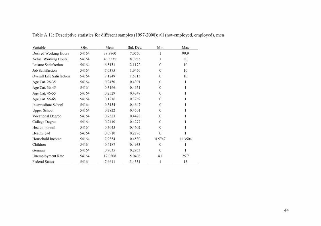
short descriptions are displayed in Table 3. Descriptive statistics for all sub-samples can

be found in Appendix A (Tables A.1 to A.12).

1 2 2, 3 3, 4 4, 5 5,it it it it it it itY Age Age Age Age Xα α α α α β ε= + + + + + + (11)

- insert Table 3 about here

Reservation wages are asked about in the SOEP questionnaire in this way: "How high

would your net income or salary have to be for you to take a position offered to you?".

This question is asked to individuals without paid employment, but who intend to be

engaged in paid employment in the near future. To get hourly information we use a

question concerning the desired working hours of the unemployed, which is included in

the survey since 2007: "In your opinion how many hours a week would you have to

work to earn this net income?". Entry wages are calculated only for employed

individuals with less than one year of tenure. For all wage variables we take the

17

logarithm. Because of implausible interpretation, we drop all observations with wages

below one Euro.

Concerning the working time aspects, we compare desired and actual working hours.

For job searchers we have information about their desired hours only in 2007 and 2008,

while we know these for employed individuals over the long sample as well. For

employed individuals we are able to compare the desired with the actual working time.

To analyze possible effects of shifting preferences, we perform regressions for

satisfaction with leisure and job. While job satisfaction is only given for employed

individuals, satisfaction with leisure is available for everyone. All types of satisfaction

variables use a likert scale of ascending order from 0 to 10.

As explanatory variables we use a set of socioeconomic determinants. We focus on age

and gender aspects and the influence of children on labor supply. Additionally we

control for household income, education, state of health, German citizenship, regional

unemployment rate, years, and federal states. The sample is limited to observations

between 18 and 65 years. The age of 18 is the German age of legal majority and 65 is

the legal retirement age. We use five age groups (18-25, 26-35, 36-45, 46-55, 56-65) to

allow for non-linear age effects. The variable “female” is a dummy for women. Another

dummy variable controls for the presence of children under the age of sixteen in a

household. The household income is used as the logarithm of the adjusted monthly net

household income. This is a proxy for non-working income and wealth. To control for

education we include secondary schooling degrees, vocational and college degrees.

“Schooling” is encoded into three characteristics of lowest, intermediate, and upper

school degree. “Vocational” and “university” are dummy variables for the respective

degrees. The subjective state of health is measured in the variable “health” with three

18

categories: good, normal, and bad. The variable “German” controls for German

citizenship. In the regressions concerning satisfaction with leisure and work, we control

additionally for the overall life satisfaction.

The regional unemployment rate1 in the month of the interview is included to control

for state and month specific differences in labor market conditions. Because of regional

aggregations in the SOEP data, Rhineland-Palatinate and Saarland is treated as one

state. Here we use information in the regional directorate of the Federal Employment

Agency. To control for further regional differences, we include dummy variables for all

German federal states.

4. Empirical Results

4.1. Reservation and Entry Wages

In the first part of our empirical analysis, we estimate log-linear earnings functions in

order to evaluate age and gender differences in reservation and entry wages. Since

information about working hours for stated monthly reservation income is not available

before the year 2007, we can only make use of the waves 2007 and 2008. Due to the

fact that reservation wages are only reported in the case of non-employment and that

entry wages (wages if tenure is less than one year) only occur at the start of an

employment relationship, we estimate cross section OLS regressions. At first, we will

turn to our main results for hourly reservation and entry wages. Afterwards, we will

1 This information is taken from a long time-series of German federal unemployment statistics, which is

published on the homepages of the German Federal Statistical Office.

19

estimate further regressions for monthly reservation and entry wages to show that the

monthly information is unsuitable for many topics, as the results can lead to wrong

conclusions.

The regression results for log hourly reservation and entry wages are displayed in Table

4. The first two columns comprise the results for the complete sample. It can be seen

that hourly reservation and entry wages increase with age, but that the age effect on

reservation wages is greater than on entry wages. This finding is consistent with our

consideration that older workers may remain voluntarily non-employed because their

reservation wages are larger than the potential offered wages for which our entry wages

serve as proxies. Women have on average about 6 percent lower reservation wages than

men. As the entry wages of women are even lower (by approximately 13 percent), the

gap between reservation and entry wages is larger for women, which might partly

explain the gender gap in employment rates. The results further indicate a positive

correlation between reservation and entry wages, on the one side, and the presence of

children in the household, education, good health, and household income, on the other

side.

- insert Table 4 about here

Due to significant gender differences in the determinants of reservation and entry

wages, our further discussion focuses on separate estimates for men and women.

Columns three and four include the results for men and columns five and six for

women. The reservation wages of men do not significantly differ between age groups

from 26 to 55 years but are significantly larger for men older than 55 years. Entry wages

for older male workers increase by about the same amount. The results for women are

20

quite different. Whereas their reservation wages strongly increase with age, their entry

wages do not. An explanation for this finding may be that the age effects on preferences

towards leisure and consumption do not significantly differ between men and women,

which will lead to small differences in the age effects on reservation wages. Entry

wages, on the other hand, depend strongly on productivity, which is positively affected

by on-the-job training and negatively by employment interruptions (depreciation of

human capital). Since women have more frequently interrupted employment

biographies than men (due to, e.g., family responsibilities), their entry wages on average

do not increase with age as is the case for men. From our findings, it follows that the

increasing with age gender gap in employment rates might be a result of the increasing

with age gender gap in the difference between reservation and entry wages.

Another interesting gender difference in the determinants of reservation and entry

wages is the effect of the presence of children in the household. Whereas children have

no effect on the reservation wages of men, they have significant positive effects on the

reservation wages of women. This finding is consistent with our theoretical

consideration that mothers have a lower time budget, from which time can be allocated

to market work, and higher preferences for leisure in order to care for their children.

From both arguments, there follows a larger marginal rate of substitution between

leisure and consumption and, hence, larger reservation wages for mothers. Fathers are

also likely to have preferences for spending time with their children, which will increase

their reservation wages. But to compensate the potential losses of mothers' income and

to generate additional income for the children, fathers may have to search for jobs with

higher intensity and reduce their reservation wages (Browning 1992, p. 1452). We

further find that children have a positive effect on male entry wages but not on female

21

entry wages. Although this finding might seem interesting at first glance, we attribute it

largely to institutional arrangements of tax reductions and family subsidies, which are

usually accounted for on the primary household earner's payroll. The overall results

point to the dominance of the conservative family model, where the mother is concerned

with family work and the father with market work.

To sum up our first piece of empirical evidence, the overall results indicate that women

and especially mothers and older women have higher reservation wages but not higher

entry wages. From this it follows that these groups have lower probabilities of choosing

employment over non-employment, which might explain their lower employment rates.

In the next step, we re-estimate the previous regressions using log monthly reservation

and entry wages instead of hourly wages. Although most previous studies have used

monthly reservation wages instead of hourly reservation wages, a conceptual problem

arises. Because monthly reservation wages include also the preferred number of

working hours which are likely to be influenced by the same variables but not

necessarily in the same direction, estimates are likely to be systematically biased

leading to wrong conclusions and policy recommendations. If compared to the results

for hourly wages in Table 4, the results for monthly reservation and entry wages in

Table 5 illustrate such wrong conclusions. For example, age has negative effects on

monthly reservation and entry wages and the presence of children reduces women's

monthly reservation wages. The reason for these findings are, however, not negative

effects on hourly reservation and entry wages but negative effects on working hours.

Moreover, the gender gaps in reservation and entry wages are substantially larger for

monthly than hourly data because women prefer to work on average fewer hours. That

22

such biased results are the outcome of systematic effects on working hours will be

illustrated in the next section.

- insert Table 5 about here

4.2. Preferred and Actual Working Hours

In order to validate our statements from the previous section about the effects of age,

gender, and presence of children on working hours, we estimate linear regressions for

three outcome variables in the years 2007 and 2008: (1) preferred weekly working hours

by non-employed job searchers, (2) preferred weekly working hours by those who have

started a new job within the last year, and (3) actual weekly working hours by those

who have started a new job within the last year. The results in Table 6 show that

preferred and actual working hours decrease with age and that the age effect is stronger

for women than men. We further find that women prefer on average to work fewer

hours and actually work fewer hours than men. Women with children in the household

prefer to work fewer hours and actually do so, whereas the presence of children does not

significantly affect the labor supply of men (Browning 1992).

- insert Table 6 about here

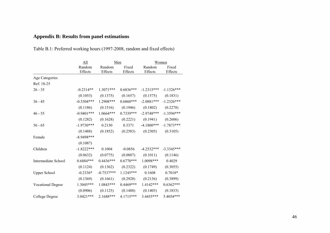
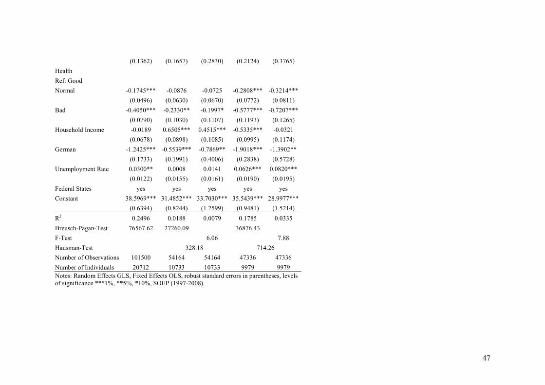
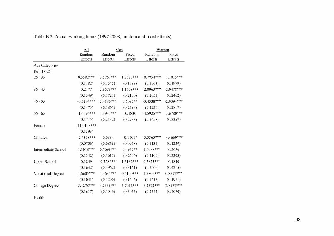
For preferred weekly working hours and actual weekly working hours by those who are

employed, we have longitudinal information and can apply panel estimates for the

observation period 1997 to 2008 to reduce problems stemming from unobserved

heterogeneity. We have estimated random effects and fixed effects linear models, in

which the individual effects are jointly significant. Although the results between the

23

models do not differ qualitatively, Hausman specification tests reject the null hypothesis

of no systematic differences between random and fixed models. As the results from the

panel estimates support in general our previous results from the cross-sections for 2007

and 2008, the estimation output is only displayed in Appendix B (Tables B.1 and B.2).

The overall findings in this section indicate that women, and especially mothers as well

as older workers, voluntarily reduce their labor supply, which might be interpreted as

the outcome of greater preferences for leisure.

4.3. Satisfaction with Leisure and Job

According to the labor supply model discussed in the theory section, differences in

reservation wages as well as in preferred and actual working hours might be an outcome

of leisure preferences. Therefore, we analyze the effect of age on satisfaction with

leisure and job satisfaction. Happiness research in economics has received increasing

attention in recent years. Frey and Stutzer (2002) found that satisfaction is at least

somehow related to the utility concept. Our purpose is to use the information about

satisfaction in the for us relevant domains of leisure and work in order to analyze if

systematic age differences exists. From a ceteris paribus perspective, such systematic

differences are likely to indicate preference changes with age, because we control for

household income as proxy for the endowment with wealth. In order to reduce further

individual heterogeneity in the estimates, we include a control variable for general life

satisfaction. We again use linear regressions for the cross-sections for 2007 and 2008

(see Table 7) and random and fixed effects linear models for the years 1997 to 2008 (see

Table B.3 and Table B.4 in Appendix B).

24

The main consistently estimated result is that older individuals are on average happier

with their leisure but not with their jobs; and that this age effect is stronger for women

than men. Our finding can be interpreted as an increasing with age preference for leisure

relative to work (e.g., Gordon and Blinder 1980), which may explain the higher

reservation wages and lower labor supply that result in the lower employment rates of

older workers - especially older women.

- insert Table 7 about here

5. Conclusion

In times of demographic change, it is a challenge for policy and Human Resource

Management to activate the resources of female and older persons in the labor market to

maintain a sufficiently large labor supply and to reduce financial problems in retirement

schemes. Such an activation strategy is motivated by the empirical observation that

employment rates decrease with age among the elderly and are lower for women than

for men. Much political concern focuses on the employer side and leads to appeals to

recruit more women and older workers. Without neglecting the fact that discrimination

is an important issue, our paper has taken the opposite view and has found empirical

support for labor supply side explanations of differences in employment rates. From a

theoretical perspective (neoclassical labor supply model, job search models) individuals

voluntarily choose non-employment over employment if their reservation wages are

larger than the wages offered by firms. We have indeed found empirical evidence that

hourly reservation wages increase with age for men and women. However, hourly entry

25

wages as proxy for offered wages increase with age only for men and not for women,

which may partly explain the with age increasing gender gap in employment rates.

As a methodological contribution, we can show that the specification of the reservation

wage as an hourly variable instead of a monthly variable yields more plausible results,

because age and gender have simultaneous effects on hourly reservation wages and

preferred working hours. Older workers and women prefer to work fewer hours and

actually do so. In combination with the result that satisfaction with leisure increases

relatively to job satisfaction, our findings support the statement of Gordon and Blinder

(1980, p. 278) that "(...) as people age, their preferences may shift in favor of leisure and

against work". Consequently, the lower employment rates of women and older persons

can be partly attributed to the labor supply side and not necessarily to the labor demand

side. From this it follows, first, that the productivity of women and older workers needs

to be increased so that they can get higher wage offers by firms. Special training

programs inside and outside firms, which are targeted at older persons and especially

women, might help to maintain or even increase productivity and employability.

Second, policy could subsidize employment and especially reintegration into the labor

market (e.g., direct transfers, tax reductions), which would also increase offered wages

and the employment probability.

Furthermore, we have found gender-specific differences in the family context. The

presence of children in the household has positive effects on the reservation wages of

women and negative effects on their labor supply, whereas neither reservation wages

nor working hours of men are significantly affected. These findings point to the

dominance of the traditional family model in Germany that mothers bear the main

responsibility for raising children - voluntarily or involuntarily. In order to activate

26

more mothers for the labor market, firms as well as policy should continue the

expansion of more flexible working time schedules and day care for children at the

workplace and in the close neighborhood. Especially for Germany, additional full-time

school programs might help parents to reduce time restrictions.

27

References

Addison, John T., Centeno, Mario, Portugal, Pedro (2009). Do reservation wages really decline? Some

international evidence on the determinants of reservation wages. Journal of Labor Research 30(1),

1-8.

Bloemen, Hans G., Stancanelli, Elena G. F. (2001). Individual wealth, reservation wages and the

transition into employment. Journal of Labor Economics 19(2), 400-439.

Borjas, George J. (2009). Labor economics. McGraw-Hill/Irwin, Boston.

Brown, Sarah, Roberts, Jenny, Taylor, Karl (2010a). Reservation wages, labour market participation and

health. Journal of the Royal Statistical Society Series A 173(3), 501-529.

Brown, Sarah, Roberts, Jenny, Taylor, Karl (2010b). The gender reservation wage gap: evidence from

British panel data. Sheffield Economic Research Paper Series, Number 2010010.

Browning, Martin (1992). Children and household economic behavior. Journal of Economic Literature

30(3), 1434-1475.

Cahuc, Pierre, Zylberberg, Andre (2004). Labor economics. MIT Press, Cambridge.

Cappellari, Lorenzo, Tatsiramos, Konstantinos (2010). Friends` network and job finding rates. IZA

Discussion Paper, Number 5240.

Chan, Sewin, Stevens, Ann Huff (2001). Job loss and employment patterns of older workers. Journal of

Labor Economics 19(2), 484-521.

Chang, Fwu-Ranq (1991). Uncertain lifetimes, retirement and economic welfare. Economica 58(230),

215-232.

Christensen, Björn (2005). Die Lohnansprüche deutscher Arbeitsloser: Determinanten und Auswirkungen

von Reservationslöhnen. Kieler Studien 333. Springer, Berlin, Heidelberg.

Constant, Amelie F., Krause, Annabelle, Rinne Ulf, Zimmermann, Klaus F. (2010). Reservation wages of

first and second generation migrants. IZA Discussion Paper, Number 5396.

28

Feldstein, Martin, Poterba, James (1984). Unemployment insurance and reservation wages. Journal of

Public Economics 23(1-2), 141-167.

Fitzenberger, Bernd, Wilke, Ralf A. (2010). Unemployment durations in West Germany before and after

the reform of the unemployment compensation system during the 1980s. German Economic Review

11(3), 336-366.

Franz, Wolfgang (1982). The reservation wage of unemployed persons in the Federal Republic of

Germany: theory and empirical tests. Zeitschrift für Wirtschafts- und Sozialwissenschaften 102(1),

29-51.

Frey, Bruno S., Stutzer Alois (2002). What can economists learn from happiness research? Journal of

Economic Literature 40(2), 402-435.

Gielen, Anne C. (2009). Working hours flexibility and older workers` labor supply. Oxford Economic

Papers 61(2), 240-274.

Gordon, Roger H., Blinder, Alan S. (1980). Market wages, reservation wages, and retirement decisions.

Journal of Public Economics 14(2), 277-308.

Gorter, Dirk, Gorter, Cees (1993). The relation between unemployment benefits, the reservation wage

and search duration. Oxford Bulletin of Economics and Statistics 55(2), 199-214.

Heckman, James (1974). Life cycle consumption and labor supply: an explanation of the relationship

between income and consumption over the life cycle. American Economic Review 64(1), 188-194.

Hunt, Jennifer (1995). The effect of unemployment compensation on unemployment duration in

Germany. Journal of Labor Economics 13(1), 88-120.

Hutchens, Robert M. (1988). Do job opportunities decline with age? Industrial and Labor Relations

Review 42(1), 89-99.

Jones, Stephen R. G. (1989). Reservation wages and the cost of unemployment. Economica 56(222), 225-

246.

Kiefer, Nicholas M., Neumann, George R. (1979). An empirical job-search model with a test of the

constant reservation-wage hypothesis. Journal of Political Economy 87(1), 89-107.

29

Krueger, Alan B., Mueller, Andreas (2011). Job search and job finding in a period of mass

unemployment: evidence from high-frequency longitudinal data. IZA Discussion Paper, Number

5450.

Lazear, Edward P. (1979). Why is there mandatory retirement? Journal of Political Economy 87(6),

1261-1284.

Lazear, Edward P. (1986). Retirement from the labor force. Ashenfelter, Orley C., Card, David (Editors):

Handbook of Labor Economics 1. Elsevier, Amsterdam, 305-355.

Ljungqvist, Lars, Sargent, Thomas J. (2008). Two questions about European unemployment.

Econometrica 76(1), 1-29.

Maani, Sholeh A., Studenmund, A. H. (1986). The critical wage, unemployment duration and wage

expectations: the case of Chile. Industrial and Labor Relations Review 39(2), 264-276.

McCall, John J. (1970). Economics of information and job search. Quarterly Journal of Economics 84(1),

113-126.

Mortensen, Dale T. (1970). Job search, the duration of unemployment and the Phillips Curve. American

Economic Review 60(5), 847-862.

Mortensen, Dale T. (1977). Unemployment insurance and job search decisions. Industrial and Labor

Relation Review 30(4), 505-517.

Mortensen, Dale T., Pissarides, Christopher A. (1999). New developments in models of search in the

labor market. Ashenfelter, Orley C., Card, David (Editors): Handbook of Labor Economics 3b.

Elsevier, Amsterdam, 2567-2627.

Pannenberg, Markus (2010). Risk attitudes and reservation wages of unemployed workers: evidence from

panel data. Economics Letters 106(3), 223-226.

Prasad, Eswar S. (2001). The dynamics of reservation wages: preliminary evidence from the SOEP.

Vierteljahrshefte zur Wirtschaftsforschung 70(1), 44-50.

Prasad, Eswar S. (2004). What determines the reservation wage of unemployed workers? New evidence

from German micro data. Fagan, Gabriel, Mongelli, Francesco P., Morgan, Julian (Editors):

30

Institutions and Wage Formation in the New Europe. Edward Elgar, Cheltenham, Northampton, 32-

52.

Rogerson, Richard, Shimer, Robert, Wright, Randall (2005). Search-theoretic models of the labor market:

a survey. Journal of Economic Literature 43(4), 959-988.

Schleife, Katrin (2006). Computer use and employment status of older workers: an analysis based on

individual data. Labour: Review of Labour Economics and Industrial Relations 20(2), 325-348.

Schmidt, Christoph M., Winkelmann, Rainer (1993). Reservation wages, wage offer distribution and

accepted wages. Bunzel, Henning, Jensen, Peter, Westergard-Nielsen, Niels (Editors): Panel Data

and Labour Market Dynamics. North-Holland, Amsterdam, 149-170.

Shimer, Robert, Werning, Ivan (2007). Reservation wages and unemployment insurance. Quarterly

Journal of Economics 122(3), 1145-1185.

Steiner, Viktor (2001). Unemployment persistence in the West German labour market: negative duration

dependence or sorting ? Oxford Bulletin of Economics and Statistics 63(1), 91-113.

Wagner, Gert G., Frick, Joachim R., Schupp, Jürgen (2007). The German Socio Economic Panel Study

(SOEP): scope, evolution and enhancements. Schmollers Jahrbuch 127(1), 139-169.

31

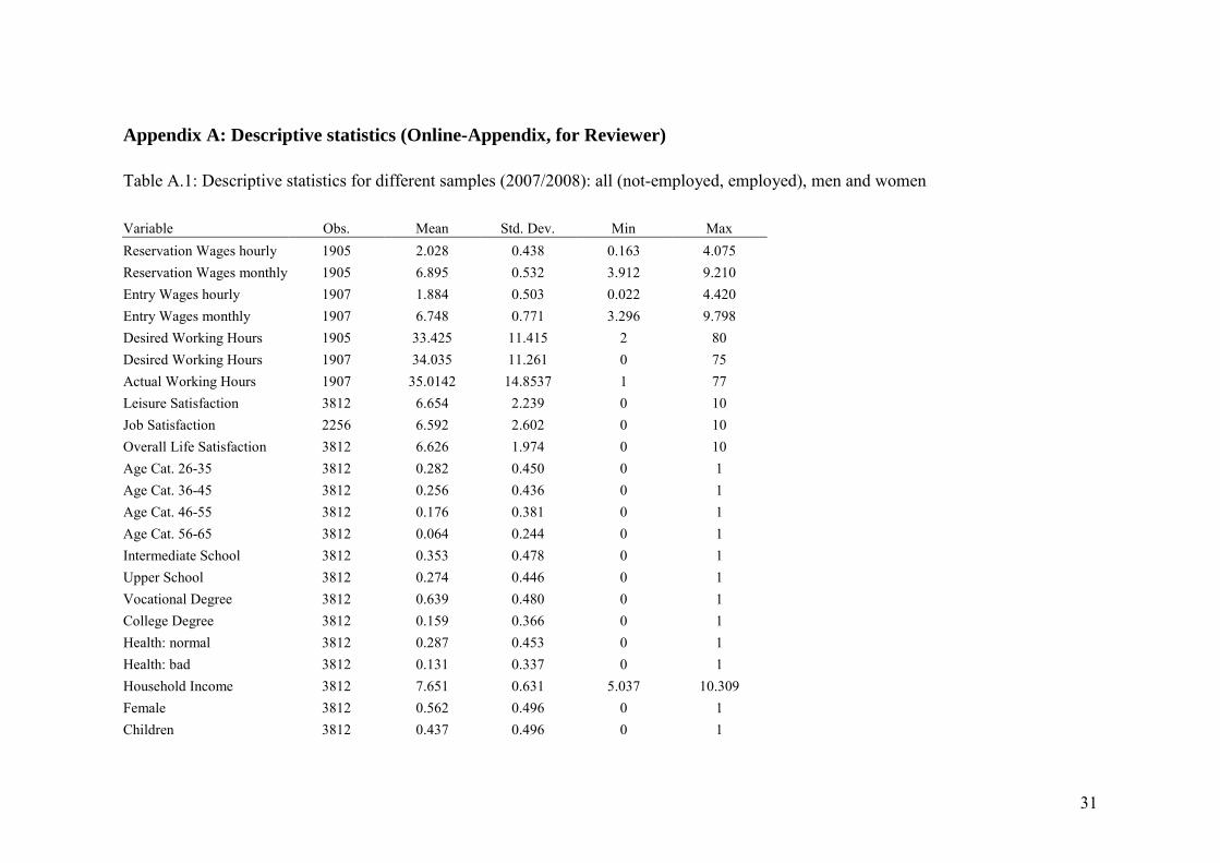
Appendix A: Descriptive statistics (Online-Appendix, for Reviewer)

Table A.1: Descriptive statistics for different samples (2007/2008): all (not-employed, employed), men and women

Variable Obs. Mean Std. Dev. Min Max Reservation Wages hourly 1905 2.028 0.438 0.163 4.075 Reservation Wages monthly 1905 6.895 0.532 3.912 9.210 Entry Wages hourly 1907 1.884 0.503 0.022 4.420 Entry Wages monthly 1907 6.748 0.771 3.296 9.798 Desired Working Hours 1905 33.425 11.415 2 80 Desired Working Hours 1907 34.035 11.261 0 75 Actual Working Hours 1907 35.0142 14.8537 1 77 Leisure Satisfaction 3812 6.654 2.239 0 10 Job Satisfaction 2256 6.592 2.602 0 10 Overall Life Satisfaction 3812 6.626 1.974 0 10 Age Cat. 26-35 3812 0.282 0.450 0 1 Age Cat. 36-45 3812 0.256 0.436 0 1 Age Cat. 46-55 3812 0.176 0.381 0 1 Age Cat. 56-65 3812 0.064 0.244 0 1 Intermediate School 3812 0.353 0.478 0 1 Upper School 3812 0.274 0.446 0 1 Vocational Degree 3812 0.639 0.480 0 1 College Degree 3812 0.159 0.366 0 1 Health: normal 3812 0.287 0.453 0 1 Health: bad 3812 0.131 0.337 0 1 Household Income 3812 7.651 0.631 5.037 10.309 Female 3812 0.562 0.496 0 1 Children 3812 0.437 0.496 0 1

32

German 3812 0.927 0.260 0 1 Year 2008 3812 0.472 0.499 0 1 Federal States 3812 8.082 3.774 1 15 Unemployment Rate 3812 11.399 4.606 4.4 21.2

33

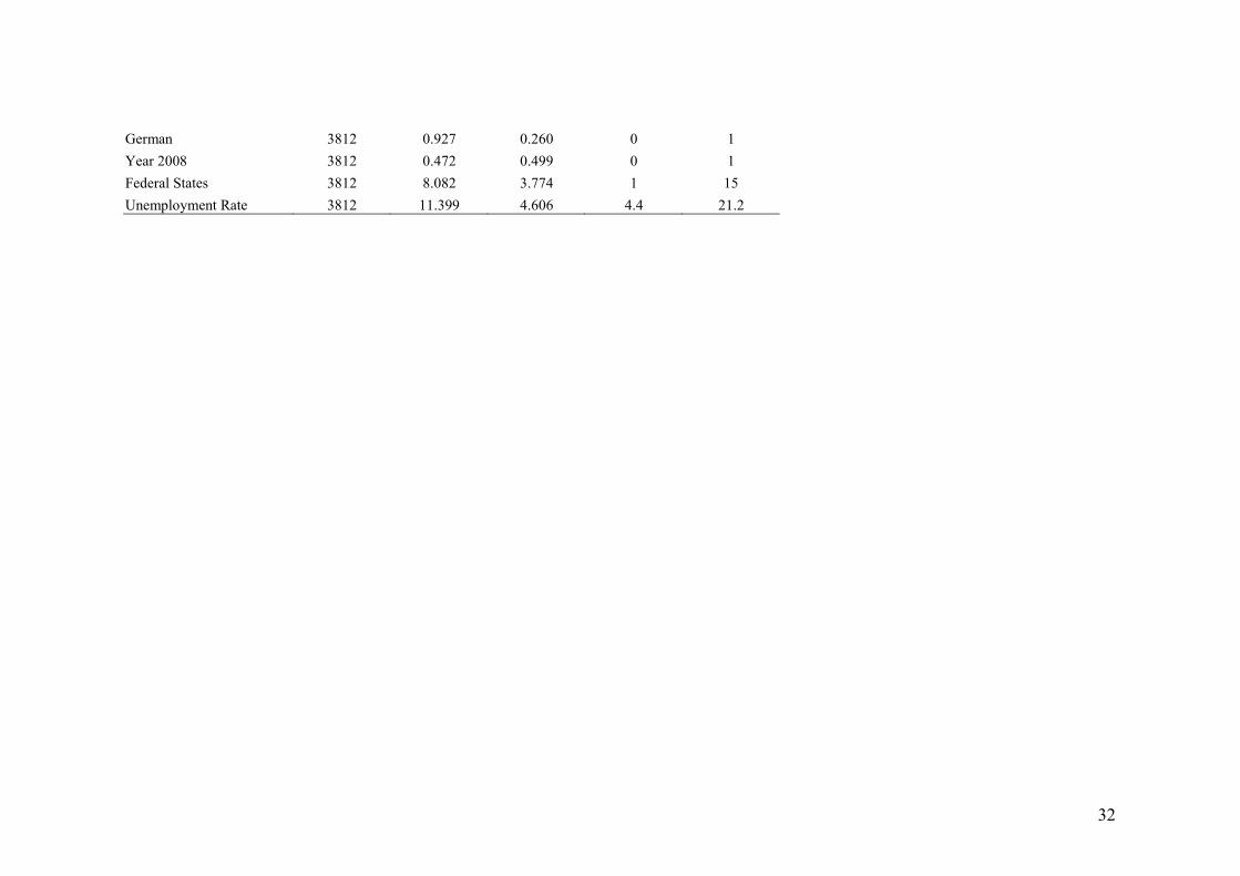
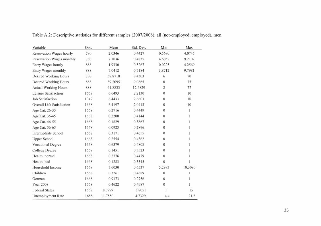
Table A.2: Descriptive statistics for different samples (2007/2008): all (not-employed, employed), men

Variable Obs. Mean Std. Dev. Min Max Reservation Wages hourly 780 2.0346 0.4427 0.5680 4.0745 Reservation Wages monthly 780 7.1036 0.4835 4.6052 9.2102 Entry Wages hourly 888 1.9330 0.5267 0.0225 4.2569 Entry Wages monthly 888 7.0412 0.7184 3.8712 9.7981 Desired Working Hours 780 38.8718 8.4303 6 70 Desired Working Hours 888 39.2095 9.0865 0 75 Actual Working Hours 888 41.8833 12.6829 2 77 Leisure Satisfaction 1668 6.6493 2.2130 0 10 Job Satisfaction 1049 6.4433 2.6603 0 10 Overall Life Satisfaction 1668 6.4197 2.0413 0 10 Age Cat. 26-35 1668 0.2716 0.4449 0 1 Age Cat. 36-45 1668 0.2200 0.4144 0 1 Age Cat. 46-55 1668 0.1829 0.3867 0 1 Age Cat. 56-65 1668 0.0923 0.2896 0 1 Intermediate School 1668 0.3171 0.4655 0 1 Upper School 1668 0.2554 0.4362 0 1 Vocational Degree 1668 0.6379 0.4808 0 1 College Degree 1668 0.1451 0.3523 0 1 Health: normal 1668 0.2776 0.4479 0 1 Health: bad 1668 0.1283 0.3345 0 1 Household Income 1668 7.6030 0.6537 5.2983 10.3090 Children 1668 0.3261 0.4689 0 1 German 1668 0.9173 0.2756 0 1 Year 2008 1668 0.4622 0.4987 0 1 Federal States 1668 8.3999 3.8051 1 15Unemployment Rate 1688 11.7550 4.7329 4.4 21.2

35

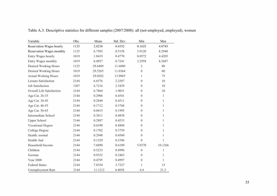
Table A.3: Descriptive statistics for different samples (2007/2008): all (not-employed, employed), women

Variable Obs. Mean Std. Dev. Min Max Reservation Wages hourly 1125 2.0238 0.4352 0.1625 4.0745 Reservation Wages monthly 1125 6.7503 0.5158 3.9120 8.2940 Entry Wages hourly 1019 1.8419 0.4770 0.0572 4.4205 Entry Wages monthly 1019 6.4927 0.7241 3.2958 8.2687 Desired Working Hours 1125 29.6489 11.6880 2 80 Desired Working Hours 1019 29.5265 11.0364 0 60 Actual Working Hours 1019 29.0282 13.9965 1 75 Leisure Satisfaction 2144 6.6576 2.2587 0 10 Job Satisfaction 1207 6.7216 2.5439 0 10 Overall Life Satisfaction 2144 6.7864 1.9051 0 10 Age Cat. 26-35 2144 0.2906 0.4541 0 1 Age Cat. 36-45 2144 0.2840 0.4511 0 1 Age Cat. 46-55 2144 0.1712 0.3768 0 1 Age Cat. 56-65 2144 0.0415 0.1995 0 1 Intermediate School 2144 0.3811 0.4858 0 1 Upper School 2144 0.2887 0.4533 0 1 Vocational Degree 2144 0.6390 0.4804 0 1 College Degree 2144 0.1702 0.3759 0 1 Health: normal 2144 0.2948 0.4560 0 1 Health: bad 2144 0.1329 0.3396 0 1 Household Income 2144 7.6890 0.6109 5.0370 10.1266 Children 2144 0.5233 0.4996 0 1 German 2144 0.9352 0.2463 0 1 Year 2008 2144 0.4795 0.4997 0 1 Federal States 2144 7.8354 3.7327 1 15 Unemployment Rate 2144 11.1212 4.4858 4.4 21.2

37

Table A.4: Descriptive statistics for different samples (2007/2008): not employed, men and women

Variable Obs. Mean Std. Dev. Min Max Reservation Wages hourly 1905 2.0282 .4382 .1625 4.0745 Reservation Wages monthly 1905 6.8949 0.5319 3.9120 9.2102 Desired Working Hours 1905 33.4252 11.4150 2 80 Leisure Satisfaction 1905 6.9239 2.1996 0 10 Overall Life Satisfaction 1905 6.2766 2.1244 0 10 Age Cat. 26-35 1905 0.2446 0.4300 0 1 Age Cat. 36-45 1905 0.2467 0.4312 0 1 Age Cat. 46-55 1905 0.1890 0.3916 0 1 Age Cat. 56-65 1905 0.0740 0.2619 0 1 Intermediate School 1905 0.3491 0.4768 0 1 Upper School 1905 0.2373 0.4255 0 1 Vocational Degree 1905 0.5827 0.4932 0 1 College Degree 1905 0.1087 0.3113 0 1 Health: normal 1905 0.2892 0.4535 0 1 Health: bad 1905 0.1717 0.3772 0 1 Household Income 1905 7.4927 0.6730 5.0370 10.1266 Female 1905 0.5906 0.4919 0 1 Children 1905 0.4724 0.4994 0 1 German 1905 0.9318 0.2522 0 1 Year 2008 1905 0.4509 0.4977 0 1 Federal States 1905 8.4136 3.9929 1 15 Unemployment Rate 1905 12.1472 4.5869 4.4 21.2

38

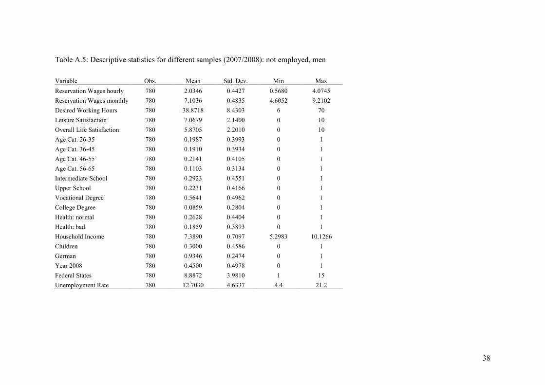
Table A.5: Descriptive statistics for different samples (2007/2008): not employed, men

Variable Obs. Mean Std. Dev. Min Max Reservation Wages hourly 780 2.0346 0.4427 0.5680 4.0745 Reservation Wages monthly 780 7.1036 0.4835 4.6052 9.2102 Desired Working Hours 780 38.8718 8.4303 6 70 Leisure Satisfaction 780 7.0679 2.1400 0 10 Overall Life Satisfaction 780 5.8705 2.2010 0 10 Age Cat. 26-35 780 0.1987 0.3993 0 1 Age Cat. 36-45 780 0.1910 0.3934 0 1 Age Cat. 46-55 780 0.2141 0.4105 0 1 Age Cat. 56-65 780 0.1103 0.3134 0 1 Intermediate School 780 0.2923 0.4551 0 1 Upper School 780 0.2231 0.4166 0 1 Vocational Degree 780 0.5641 0.4962 0 1 College Degree 780 0.0859 0.2804 0 1 Health: normal 780 0.2628 0.4404 0 1 Health: bad 780 0.1859 0.3893 0 1 Household Income 780 7.3890 0.7097 5.2983 10.1266 Children 780 0.3000 0.4586 0 1 German 780 0.9346 0.2474 0 1 Year 2008 780 0.4500 0.4978 0 1 Federal States 780 8.8872 3.9810 1 15 Unemployment Rate 780 12.7030 4.6337 4.4 21.2

39

Table A.6: Descriptive statistics for different samples (2007/2008) not employed, women

Variable Obs. Mean Std. Dev. Min Max Reservation Wages hourly 1125 2.0238 0.4352 0.1625 4.0745 Reservation Wages monthly 1125 6.7503 0.5158 3.9120 8.2940 Desired Working Hours 1125 29.6489 11.6880 2 80 Leisure Satisfaction 1125 6.8240 2.2355 0 10 Overall Life Satisfaction 1125 6.5582 2.0233 0 10 Age Cat. 26-35 1125 0.2764 0.4474 0 1 Age Cat. 36-45 1125 0.2853 0.4518 0 1 Age Cat. 46-55 1125 0.1716 0.3772 0 1 Age Cat. 56-65 1125 0.0489 0.2157 0 1 Intermediate School 1125 0.3884 0.4876 0 1 Upper School 1125 0.2471 0.4315 0 1 Vocational Degree 1125 0.5956 0.4910 0 1 College Degree 1125 0.1244 0.3302 0 1 Health: normal 1125 0.3076 0.4617 0 1 Health: bad 1125 0.1618 0.3684 0 1 Household Income 1125 7.5645 0.6368 5.0370 9.4335 Children 1125 0.5920 0.4917 0 1 German 1125 0.9298 0.2556 0 1 Year 2008 1125 0.4516 0.4979 0 1 Federal States 1125 8.0853 3.9698 1 15 Unemployment Rate 1125 11.7620 4.5162 4.4 21.2

40

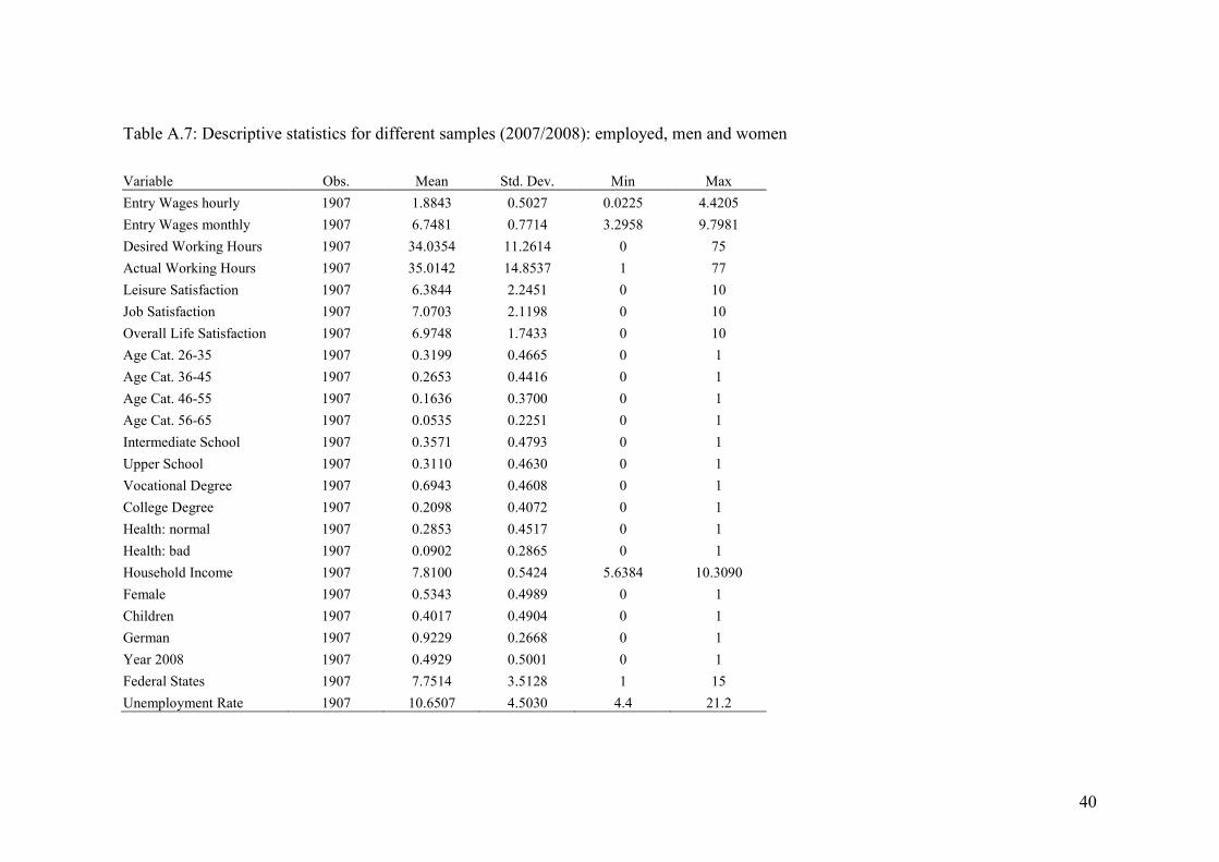
Table A.7: Descriptive statistics for different samples (2007/2008): employed, men and women

Variable Obs. Mean Std. Dev. Min Max Entry Wages hourly 1907 1.8843 0.5027 0.0225 4.4205 Entry Wages monthly 1907 6.7481 0.7714 3.2958 9.7981 Desired Working Hours 1907 34.0354 11.2614 0 75 Actual Working Hours 1907 35.0142 14.8537 1 77 Leisure Satisfaction 1907 6.3844 2.2451 0 10 Job Satisfaction 1907 7.0703 2.1198 0 10 Overall Life Satisfaction 1907 6.9748 1.7433 0 10 Age Cat. 26-35 1907 0.3199 0.4665 0 1 Age Cat. 36-45 1907 0.2653 0.4416 0 1 Age Cat. 46-55 1907 0.1636 0.3700 0 1 Age Cat. 56-65 1907 0.0535 0.2251 0 1 Intermediate School 1907 0.3571 0.4793 0 1 Upper School 1907 0.3110 0.4630 0 1 Vocational Degree 1907 0.6943 0.4608 0 1 College Degree 1907 0.2098 0.4072 0 1 Health: normal 1907 0.2853 0.4517 0 1 Health: bad 1907 0.0902 0.2865 0 1 Household Income 1907 7.8100 0.5424 5.6384 10.3090 Female 1907 0.5343 0.4989 0 1 Children 1907 0.4017 0.4904 0 1 German 1907 0.9229 0.2668 0 1 Year 2008 1907 0.4929 0.5001 0 1 Federal States 1907 7.7514 3.5128 1 15 Unemployment Rate 1907 10.6507 4.5030 4.4 21.2

41

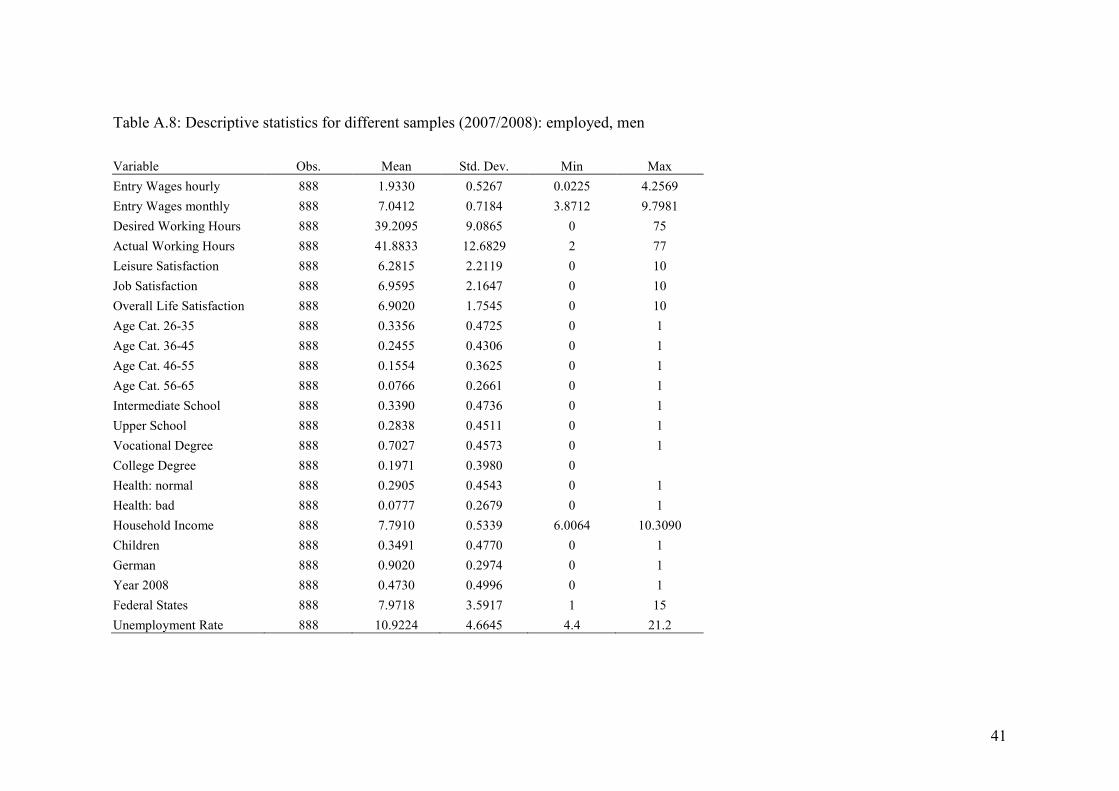
Table A.8: Descriptive statistics for different samples (2007/2008): employed, men

Variable Obs. Mean Std. Dev. Min Max Entry Wages hourly 888 1.9330 0.5267 0.0225 4.2569 Entry Wages monthly 888 7.0412 0.7184 3.8712 9.7981 Desired Working Hours 888 39.2095 9.0865 0 75 Actual Working Hours 888 41.8833 12.6829 2 77 Leisure Satisfaction 888 6.2815 2.2119 0 10 Job Satisfaction 888 6.9595 2.1647 0 10 Overall Life Satisfaction 888 6.9020 1.7545 0 10 Age Cat. 26-35 888 0.3356 0.4725 0 1 Age Cat. 36-45 888 0.2455 0.4306 0 1 Age Cat. 46-55 888 0.1554 0.3625 0 1 Age Cat. 56-65 888 0.0766 0.2661 0 1 Intermediate School 888 0.3390 0.4736 0 1 Upper School 888 0.2838 0.4511 0 1 Vocational Degree 888 0.7027 0.4573 0 1 College Degree 888 0.1971 0.3980 0 Health: normal 888 0.2905 0.4543 0 1 Health: bad 888 0.0777 0.2679 0 1 Household Income 888 7.7910 0.5339 6.0064 10.3090 Children 888 0.3491 0.4770 0 1 German 888 0.9020 0.2974 0 1 Year 2008 888 0.4730 0.4996 0 1 Federal States 888 7.9718 3.5917 1 15 Unemployment Rate 888 10.9224 4.6645 4.4 21.2

42

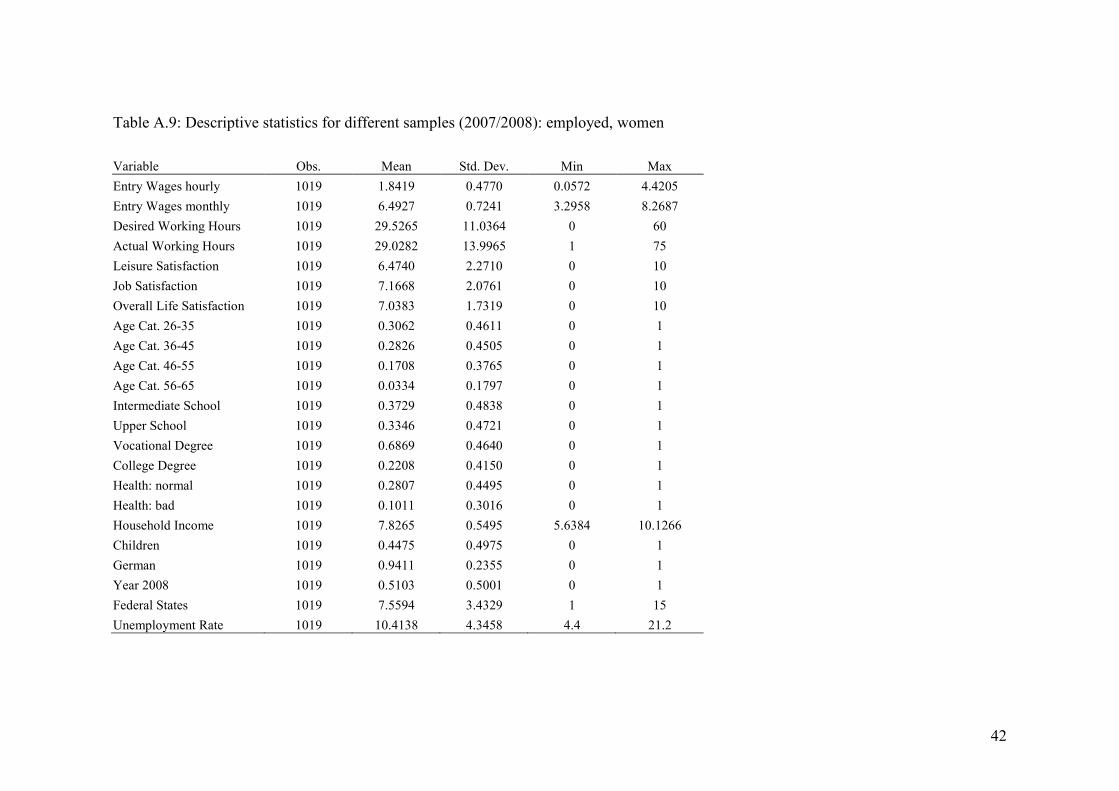
Table A.9: Descriptive statistics for different samples (2007/2008): employed, women

Variable Obs. Mean Std. Dev. Min Max Entry Wages hourly 1019 1.8419 0.4770 0.0572 4.4205 Entry Wages monthly 1019 6.4927 0.7241 3.2958 8.2687 Desired Working Hours 1019 29.5265 11.0364 0 60 Actual Working Hours 1019 29.0282 13.9965 1 75 Leisure Satisfaction 1019 6.4740 2.2710 0 10 Job Satisfaction 1019 7.1668 2.0761 0 10 Overall Life Satisfaction 1019 7.0383 1.7319 0 10 Age Cat. 26-35 1019 0.3062 0.4611 0 1 Age Cat. 36-45 1019 0.2826 0.4505 0 1 Age Cat. 46-55 1019 0.1708 0.3765 0 1 Age Cat. 56-65 1019 0.0334 0.1797 0 1 Intermediate School 1019 0.3729 0.4838 0 1 Upper School 1019 0.3346 0.4721 0 1 Vocational Degree 1019 0.6869 0.4640 0 1 College Degree 1019 0.2208 0.4150 0 1 Health: normal 1019 0.2807 0.4495 0 1 Health: bad 1019 0.1011 0.3016 0 1 Household Income 1019 7.8265 0.5495 5.6384 10.1266 Children 1019 0.4475 0.4975 0 1 German 1019 0.9411 0.2355 0 1 Year 2008 1019 0.5103 0.5001 0 1 Federal States 1019 7.5594 3.4329 1 15 Unemployment Rate 1019 10.4138 4.3458 4.4 21.2

43

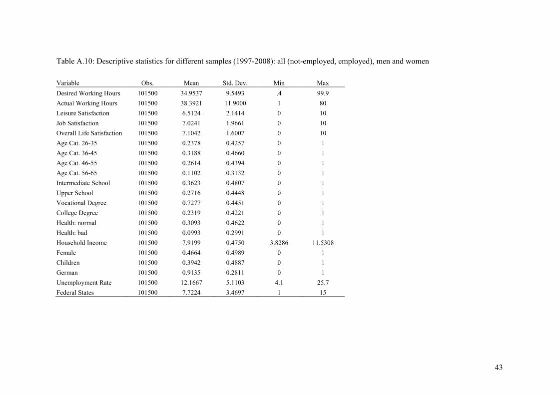
Table A.10: Descriptive statistics for different samples (1997-2008): all (not-employed, employed), men and women

Variable Obs. Mean Std. Dev. Min Max Desired Working Hours 101500 34.9537 9.5493 .4 99.9 Actual Working Hours 101500 38.3921 11.9000 1 80 Leisure Satisfaction 101500 6.5124 2.1414 0 10 Job Satisfaction 101500 7.0241 1.9661 0 10 Overall Life Satisfaction 101500 7.1042 1.6007 0 10 Age Cat. 26-35 101500 0.2378 0.4257 0 1 Age Cat. 36-45 101500 0.3188 0.4660 0 1 Age Cat. 46-55 101500 0.2614 0.4394 0 1 Age Cat. 56-65 101500 0.1102 0.3132 0 1 Intermediate School 101500 0.3623 0.4807 0 1 Upper School 101500 0.2716 0.4448 0 1 Vocational Degree 101500 0.7277 0.4451 0 1 College Degree 101500 0.2319 0.4221 0 1 Health: normal 101500 0.3093 0.4622 0 1 Health: bad 101500 0.0993 0.2991 0 1 Household Income 101500 7.9199 0.4750 3.8286 11.5308 Female 101500 0.4664 0.4989 0 1 Children 101500 0.3942 0.4887 0 1 German 101500 0.9135 0.2811 0 1 Unemployment Rate 101500 12.1667 5.1103 4.1 25.7 Federal States 101500 7.7224 3.4697 1 15

44

Table A.11: Descriptive statistics for different samples (1997-2008): all (not-employed, employed), men

Variable Obs. Mean Std. Dev. Min Max Desired Working Hours 54164 38.9960 7.0750 1 99.9 Actual Working Hours 54164 43.3535 8.7983 1 80 Leisure Satisfaction 54164 6.5151 2.1172 0 10 Job Satisfaction 54164 7.0375 1.9450 0 10 Overall Life Satisfaction 54164 7.1249 1.5713 0 10 Age Cat. 26-35 54164 0.2450 0.4301 0 1 Age Cat. 36-45 54164 0.3166 0.4651 0 1 Age Cat. 46-55 54164 0.2529 0.4347 0 1 Age Cat. 56-65 54164 0.1216 0.3269 0 1 Intermediate School 54164 0.3154 0.4647 0 1 Upper School 54164 0.2822 0.4501 0 1 Vocational Degree 54164 0.7323 0.4428 0 1 College Degree 54164 0.2410 0.4277 0 1 Health: normal 54164 0.3045 0.4602 0 1 Health: bad 54164 0.0910 0.2876 0 1 Household Income 54164 7.9354 0.4530 4.5747 11.3504 Children 54164 0.4187 0.4933 0 1 German 54164 0.9035 0.2953 0 1 Unemployment Rate 54164 12.0308 5.0408 4.1 25.7 Federal States 54164 7.6611 3.4331 1 15

45

Table A.12: Descriptive statistics for different samples (1997-2008): all (not-employed, employed), women

Variable Obs. Mean Std. Dev. Min Max Desired Working Hours 47336 30.3283 9.9079 0.4 90 Actual Working Hours 47336 32.7152 12.4371 1 80 Leisure Satisfaction 47336 6.5093 2.1688 0 10 Job Satisfaction 47336 7.0088 1.9899 0 10 Overall Life Satisfaction 47336 7.0805 1.6334 0 10 Age Cat. 26-35 47336 0.2296 0.4205 0 1 Age Cat. 36-45 47336 0.3213 0.4670 0 1 Age Cat. 46-55 47336 0.2711 0.4445 0 1 Age Cat. 56-65 47336 0.0972 0.2962 0 1 Intermediate School 47336 0.4159 0.4929 0 1 Upper School 47336 0.2596 0.4384 0 1 Vocational Degree 47336 0.7225 0.4478 0 1 College Degree 47336 0.2216 0.4153 0 1 Health: normal 47336 0.3148 0.4644 0 1 Health: bad 47336 0.1088 0.3114 0 1 Household Income 47336 7.9022 0.4984 3.8286 11.5308 Children 47336 0.3662 0.4818 0 1 German 47336 0.9250 0.2634 0 1 Unemployment Rate 47336 12.3222 5.1843 4.4 25.7 Federal States 47336 7.7925 3.5097 1 15

46

Appendix B: Results from panel estimations

Table B.1: Preferred working hours (1997-2008, random and fixed effects)

All Men Women

Random Effects

Random Effects

Fixed Effects

Random Effects

Fixed Effects

Age Categories Ref: 18-25 26 - 35 -0.2314** 1.3071*** 0.6836*** -1.2315*** -1.1326*** (0.1053) (0.1375) (0.1657) (0.1575) (0.1831) 36 - 45 -0.5304*** 1.2908*** 0.6860*** -2.0881*** -1.2326*** (0.1186) (0.1516) (0.1946) (0.1802) (0.2278) 46 - 55 -0.9401*** 1.0664*** 0.7339*** -2.9748*** -1.3594*** (0.1282) (0.1628) (0.2221) (0.1941) (0.2606) 56 - 65 -1.9730*** 0.2150 0.3371 -4.1800*** -1.7873*** (0.1488) (0.1852) (0.2583) (0.2305) (0.3105) Female -8.9498*** (0.1087) Children -1.8222*** 0.1004 -0.0856 -4.2532*** -3.3345*** (0.0632) (0.0775) (0.0887) (0.1011) (0.1146) Intermediate School 0.6884*** 0.4436*** 0.6770*** 1.0098*** 0.4029 (0.1124) (0.1362) (0.2322) (0.1749) (0.3055) Upper School -0.2336* -0.7537*** 1.1245*** 0.1608 0.7018* (0.1369) (0.1661) (0.2928) (0.2136) (0.3899) Vocational Degree 1.3045*** 1.0843*** 0.4469*** 1.4142*** 0.6362*** (0.0906) (0.1125) (0.1488) (0.1403) (0.1833) College Degree 3.0421*** 2.1688*** 4.1715*** 3.4455*** 5.4054***

47

(0.1362) (0.1657) (0.2830) (0.2124) (0.3765) Health Ref: Good Normal -0.1745*** -0.0876 -0.0725 -0.2808*** -0.3214*** (0.0496) (0.0630) (0.0670) (0.0772) (0.0811) Bad -0.4050*** -0.2330** -0.1997* -0.5777*** -0.7207*** (0.0790) (0.1030) (0.1107) (0.1193) (0.1265) Household Income -0.0189 0.6505*** 0.4515*** -0.5335*** -0.0321 (0.0678) (0.0898) (0.1085) (0.0995) (0.1174) German -1.2425*** -0.5539*** -0.7869** -1.9018*** -1.3902** (0.1733) (0.1991) (0.4006) (0.2838) (0.5728) Unemployment Rate 0.0300** 0.0008 0.0141 0.0626*** 0.0820*** (0.0122) (0.0155) (0.0161) (0.0190) (0.0195) Federal States yes yes yes yes yes Constant 38.5969*** 31.4852*** 33.7030*** 35.5439*** 28.9977*** (0.6394) (0.8244) (1.2599) (0.9481) (1.5214) R2 0.2496 0.0188 0.0079 0.1785 0.0335 Breusch-Pagan-Test 76567.62 27260.09 36876.43 F-Test 6.06 7.88 Hausman-Test 328.18 714.26 Number of Observations 101500 54164 54164 47336 47336 Number of Individuals 20712 10733 10733 9979 9979 Notes: Random Effects GLS, Fixed Effects OLS, robust standard errors in parentheses, levels of significance ***1%, **5%, *10%, SOEP (1997-2008).

48

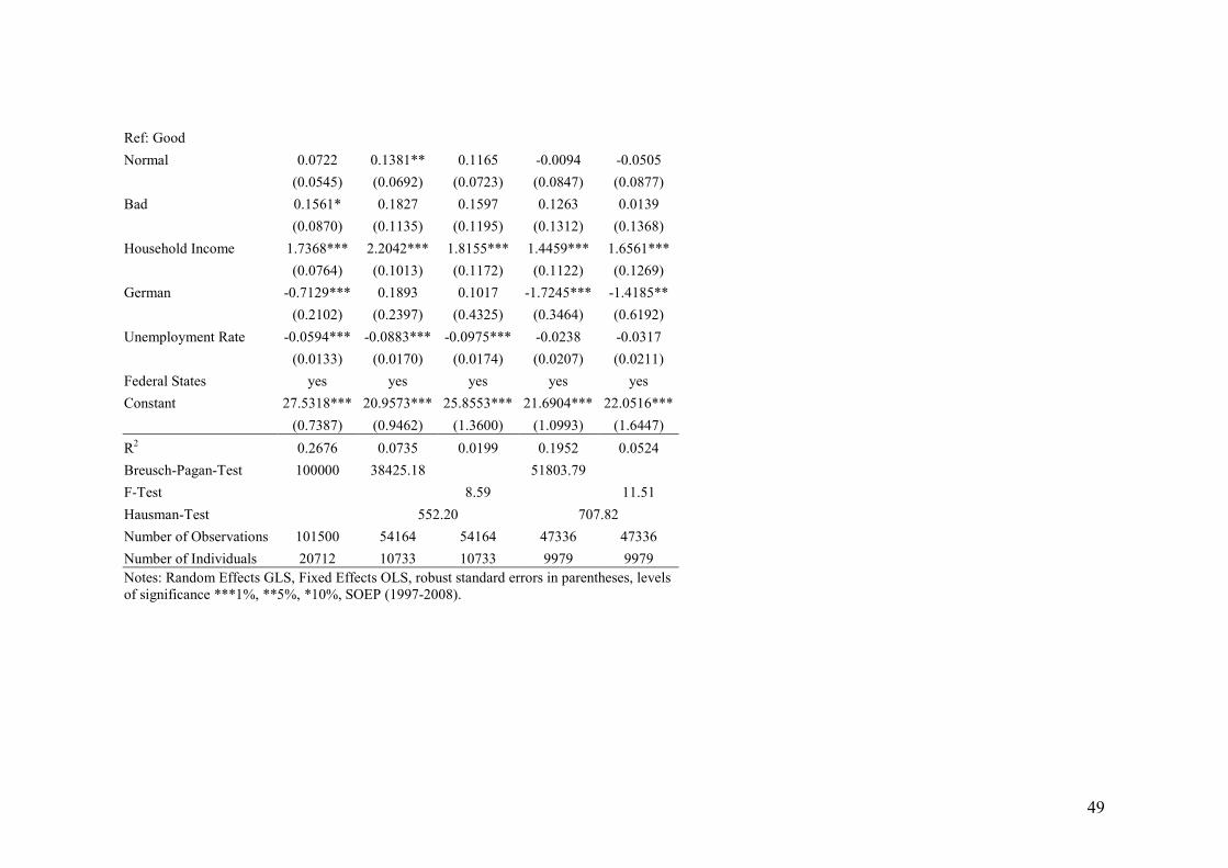
Table B.2: Actual working hours (1997-2008, random and fixed effects)

All Men Women

Random Effects

Random Effects

Fixed Effects

Random Effects

Fixed Effects

Age Categories Ref: 18-25 26 - 35 0.5582*** 2.5767*** 1.2637*** -0.7854*** -1.1015*** (0.1182) (0.1545) (0.1788) (0.1763) (0.1979) 36 - 45 0.2177 2.8578*** 1.1678*** -2.0963*** -2.0478*** (0.1349) (0.1721) (0.2100) (0.2051) (0.2462) 46 - 55 -0.5284*** 2.4180*** 0.6097** -3.4338*** -2.9394*** (0.1473) (0.1867) (0.2398) (0.2236) (0.2817) 56 - 65 -1.6696*** 1.3937*** -0.1830 -4.5925*** -3.6780*** (0.1715) (0.2132) (0.2788) (0.2658) (0.3357) Female -11.0108*** (0.1393) Children -2.4358*** 0.0334 -0.1801* -5.5365*** -4.4660*** (0.0706) (0.0866) (0.0958) (0.1131) (0.1239) Intermediate School 1.1018*** 0.7698*** 0.4932** 1.6088*** 0.3676 (0.1342) (0.1615) (0.2506) (0.2100) (0.3303) Upper School 0.1849 -0.5586*** 1.3182*** 0.7823*** 0.1840 (0.1632) (0.1962) (0.3161) (0.2566) (0.4215) Vocational Degree 1.6605*** 1.4637*** 0.5100*** 1.7806*** 0.8592*** (0.1041) (0.1290) (0.1606) (0.1615) (0.1981) College Degree 5.4278*** 4.2338*** 5.7065*** 6.2372*** 7.8177*** (0.1617) (0.1949) (0.3055) (0.2544) (0.4070) Health

49

Ref: Good Normal 0.0722 0.1381** 0.1165 -0.0094 -0.0505 (0.0545) (0.0692) (0.0723) (0.0847) (0.0877) Bad 0.1561* 0.1827 0.1597 0.1263 0.0139 (0.0870) (0.1135) (0.1195) (0.1312) (0.1368) Household Income 1.7368*** 2.2042*** 1.8155*** 1.4459*** 1.6561*** (0.0764) (0.1013) (0.1172) (0.1122) (0.1269) German -0.7129*** 0.1893 0.1017 -1.7245*** -1.4185** (0.2102) (0.2397) (0.4325) (0.3464) (0.6192) Unemployment Rate -0.0594*** -0.0883*** -0.0975*** -0.0238 -0.0317 (0.0133) (0.0170) (0.0174) (0.0207) (0.0211) Federal States yes yes yes yes yes Constant 27.5318*** 20.9573*** 25.8553*** 21.6904*** 22.0516*** (0.7387) (0.9462) (1.3600) (1.0993) (1.6447) R2 0.2676 0.0735 0.0199 0.1952 0.0524 Breusch-Pagan-Test 100000 38425.18 51803.79 F-Test 8.59 11.51 Hausman-Test 552.20 707.82 Number of Observations 101500 54164 54164 47336 47336 Number of Individuals 20712 10733 10733 9979 9979 Notes: Random Effects GLS, Fixed Effects OLS, robust standard errors in parentheses, levels of significance ***1%, **5%, *10%, SOEP (1997-2008).

50

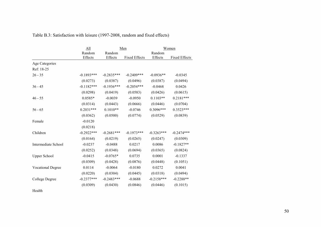
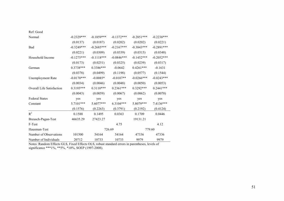
Table B.3: Satisfaction with leisure (1997-2008, random and fixed effects)

All Men Women

Random Effects

Random Effects Fixed Effects

Random Effects Fixed Effects

Age Categories Ref: 18-25 26 - 35 -0.1893*** -0.2835*** -0.2409*** -0.0936** -0.0345 (0.0273) (0.0387) (0.0496) (0.0387) (0.0494) 36 - 45 -0.1182*** -0.1936*** -0.2054*** -0.0468 0.0426 (0.0298) (0.0419) (0.0583) (0.0426) (0.0615) 46 - 55 0.0585* -0.0039 -0.0950 0.1103** 0.2181*** (0.0314) (0.0443) (0.0666) (0.0446) (0.0704) 56 - 65 0.2031*** 0.1010** -0.0746 0.3096*** 0.3523*** (0.0362) (0.0500) (0.0774) (0.0529) (0.0839) Female -0.0120 (0.0218) Children -0.2922*** -0.2681*** -0.1973*** -0.3263*** -0.2474*** (0.0164) (0.0219) (0.0265) (0.0247) (0.0309) Intermediate School -0.0237 -0.0488 0.0217 0.0086 -0.1827** (0.0252) (0.0348) (0.0694) (0.0365) (0.0824) Upper School -0.0415 -0.0765* 0.0735 0.0001 -0.1337 (0.0309) (0.0428) (0.0876) (0.0448) (0.1051) Vocational Degree 0.0114 -0.0064 -0.0180 0.0272 0.0041 (0.0220) (0.0304) (0.0445) (0.0318) (0.0494) College Degree -0.2377*** -0.2483*** -0.0688 -0.2158*** -0.2288** (0.0309) (0.0430) (0.0846) (0.0446) (0.1015) Health

51

Ref: Good Normal -0.2329*** -0.1859*** -0.1372*** -0.2851*** -0.2238*** (0.0137) (0.0187) (0.0202) (0.0202) (0.0221) Bad -0.3249*** -0.2685*** -0.2167*** -0.3843*** -0.2891*** (0.0221) (0.0309) (0.0339) (0.0315) (0.0348) Household Income -0.1275*** -0.1118*** -0.0846*** -0.1452*** -0.2052*** (0.0173) (0.0251) (0.0325) (0.0239) (0.0317) German 0.3738*** 0.3386*** -0.0642 0.4261*** -0.1631 (0.0378) (0.0499) (0.1198) (0.0577) (0.1544) Unemployment Rate -0.0170*** -0.0085* -0.0107** -0.0266*** -0.0243*** (0.0034) (0.0046) (0.0048) (0.0050) (0.0053) Overall Life Satisfaction 0.3195*** 0.3110*** 0.2361*** 0.3292*** 0.2441*** (0.0043) (0.0059) (0.0067) (0.0062) (0.0070) Federal States yes yes yes yes yes Constant 5.7101*** 5.6077*** 6.3104*** 5.8079*** 7.4136*** (0.1576) (0.2263) (0.3791) (0.2192) (0.4124) R2 0.1588 0.1495 0.0363 0.1709 0.0446 Breusch-Pagan-Test 46635.29 27423.27 19131.21 F-Test 4.75 4.12 Hausman-Test 726.69 779.60 Number of Observations 101500 54164 54164 47336 47336 Number of Individuals 20712 10733 10733 9979 9979 Notes: Random Effects GLS, Fixed Effects OLS, robust standard errors in parentheses, levels of significance ***1%, **5%, *10%, SOEP (1997-2008).

52

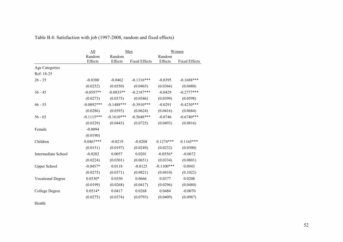
Table B.4: Satisfaction with job (1997-2008, random and fixed effects)

All Men Women

Random Effects

Random Effects Fixed Effects

Random Effects Fixed Effects

Age Categories Ref: 18-25 26 - 35 -0.0380 -0.0462 -0.1316*** -0.0395 -0.1688*** (0.0252) (0.0350) (0.0465) (0.0366) (0.0480) 36 - 45 -0.0597** -0.0835** -0.2187*** -0.0429 -0.2777*** (0.0273) (0.0375) (0.0546) (0.0399) (0.0598) 46 - 55 -0.0892*** -0.1488*** -0.3910*** -0.0291 -0.4230*** (0.0286) (0.0393) (0.0624) (0.0416) (0.0684) 56 - 65 -0.1115*** -0.1610*** -0.5648*** -0.0746 -0.6740*** (0.0329) (0.0443) (0.0725) (0.0493) (0.0816) Female -0.0094 (0.0190) Children 0.0467*** -0.0219 -0.0208 0.1274*** 0.1165*** (0.0151) (0.0197) (0.0249) (0.0232) (0.0300) Intermediate School -0.0202 0.0057 0.0201 -0.0556* -0.0672 (0.0224) (0.0301) (0.0651) (0.0334) (0.0801) Upper School -0.0457* 0.0118 -0.0125 -0.1100*** 0.0943 (0.0275) (0.0371) (0.0821) (0.0410) (0.1022) Vocational Degree 0.0330* 0.0350 0.0666 0.0377 0.0208 (0.0199) (0.0268) (0.0417) (0.0296) (0.0480) College Degree 0.0514* 0.0417 0.0268 0.0484 -0.0070 (0.0275) (0.0374) (0.0793) (0.0409) (0.0987) Health

53

Ref: Good Normal -0.3700*** -0.3748*** -0.3036*** -0.3628*** -0.3065*** (0.0129) (0.0172) (0.0190) (0.0193) (0.0215) Bad -0.6758*** -0.6847*** -0.6002*** -0.6666*** -0.5736*** (0.0206) (0.0284) (0.0317) (0.0300) (0.0339) Household Income 0.0770*** 0.1097*** 0.0804*** 0.0522** -0.0219 (0.0158) (0.0224) (0.0305) (0.0224) (0.0308) German 0.1174*** 0.0828* -0.2048* 0.1485*** 0.1462 (0.0334) (0.0428) (0.1123) (0.0526) (0.1502) Unemployment Rate -0.0039 -0.0053 -0.0093** -0.0019 -0.0058 (0.0032) (0.0043) (0.0045) (0.0048) (0.0051) Overall Life Satisfaction 0.3916*** 0.4242*** 0.3516*** 0.3585*** 0.2885*** (0.0040) (0.0054) (0.0062) (0.0059) (0.0068) Federal States yes yes yes yes yes Constant 3.8316*** 3.3534*** 4.3869*** 4.2492*** 5.7314*** (0.1434) (0.2013) (0.3553) (0.2046) (0.4010) R2 0.2184 0.2524 0.0958 0.1861 0.0707 Breusch-Pagan-Test 22177.39 12471.88 9434.75 F-Test-Test 3.39 3.14 Hausman-Test 678.73 573.66 Number of Observations 101500 54164 54164 47336 47336 Number of Individuals 20712 10733 10733 9979 9979 Notes: Random Effects GLS, Fixed Effects OLS, robust standard errors in parentheses, levels of significance ***1%, **5%, *10%, SOEP (1997-2008).

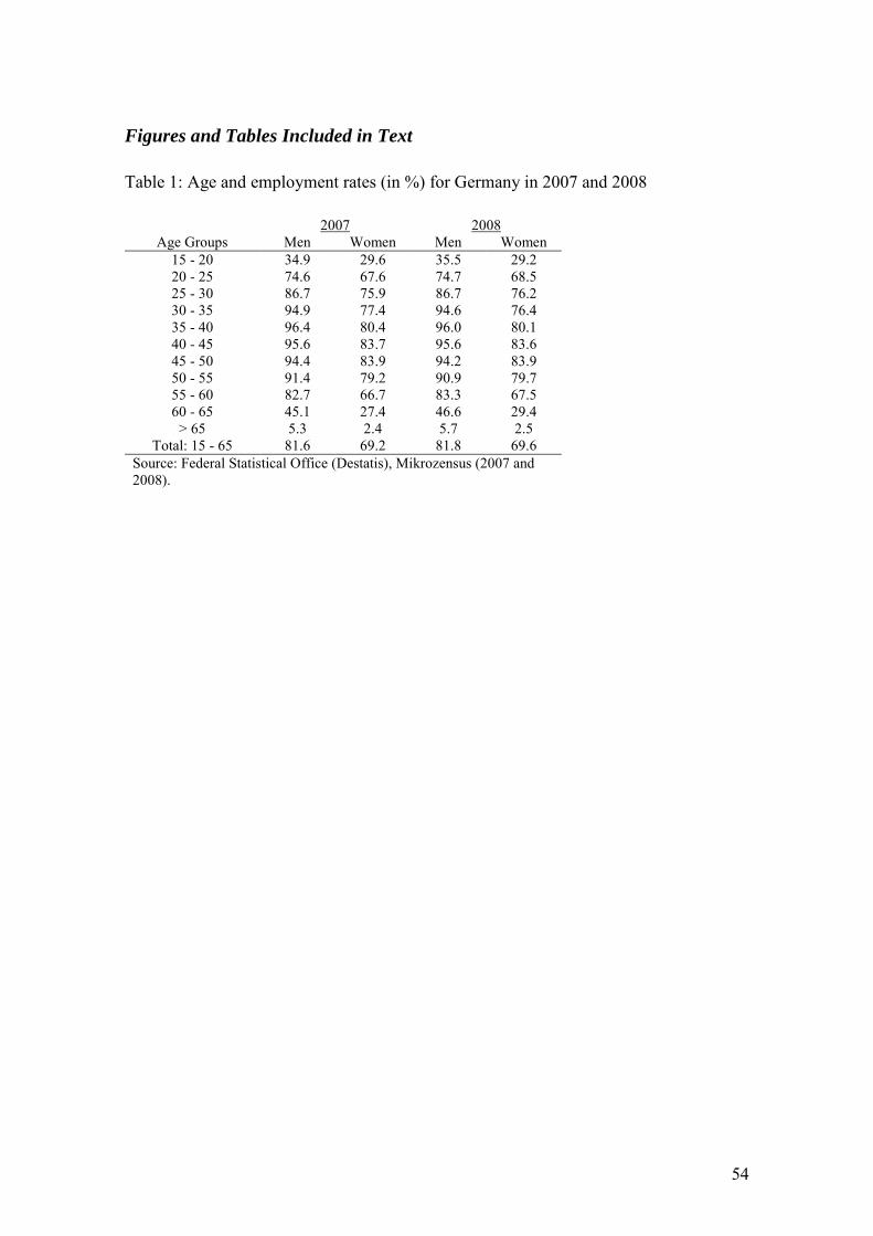
54

Figures and Tables Included in Text

Table 1: Age and employment rates (in %) for Germany in 2007 and 2008

2007 2008 Age Groups Men Women Men Women

15 - 20 34.9 29.6 35.5 29.2 20 - 25 74.6 67.6 74.7 68.5 25 - 30 86.7 75.9 86.7 76.2 30 - 35 94.9 77.4 94.6 76.4 35 - 40 96.4 80.4 96.0 80.1 40 - 45 95.6 83.7 95.6 83.6 45 - 50 94.4 83.9 94.2 83.9 50 - 55 91.4 79.2 90.9 79.7 55 - 60 82.7 66.7 83.3 67.5 60 - 65 45.1 27.4 46.6 29.4

> 65 5.3 2.4 5.7 2.5 Total: 15 - 65 81.6 69.2 81.8 69.6

Source: Federal Statistical Office (Destatis), Mikrozensus (2007 and 2008).

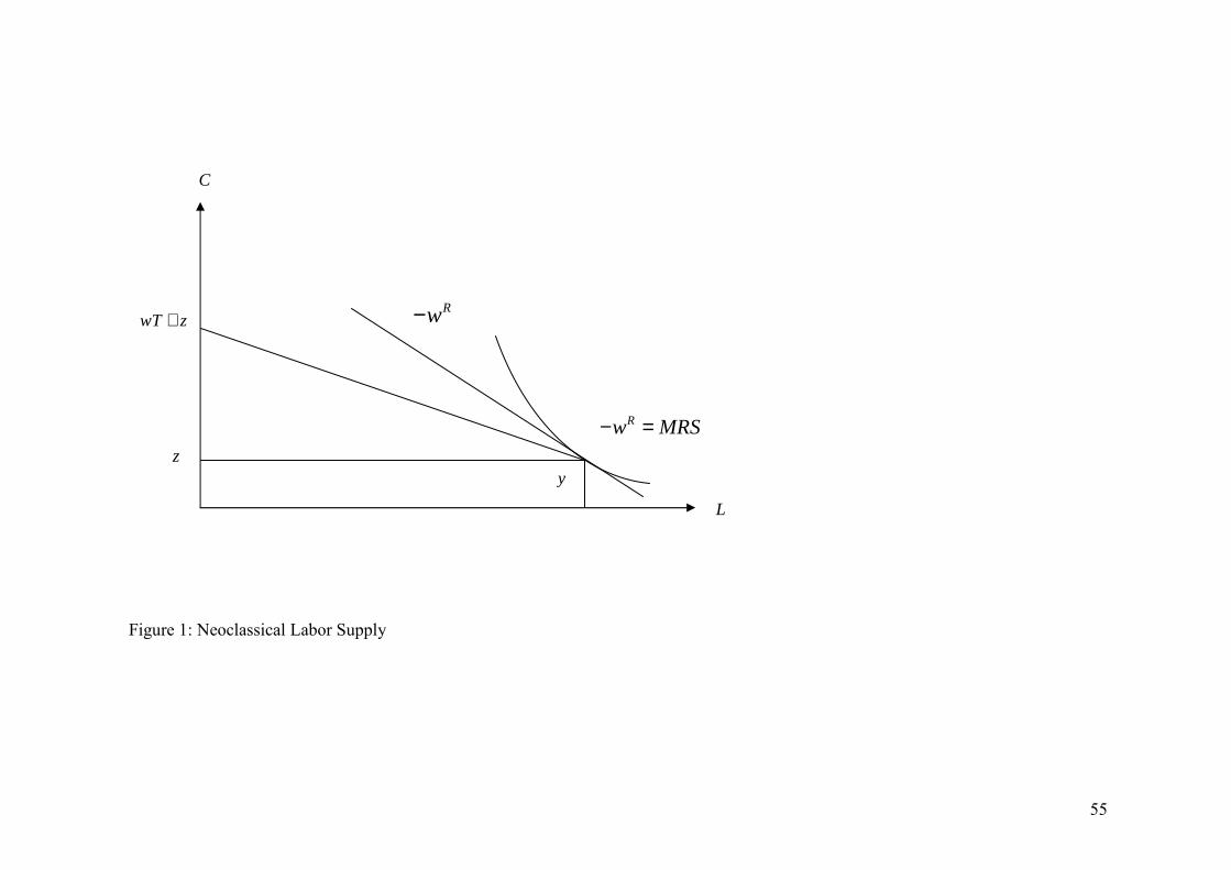
55

Figure 1: Neoclassical Labor Supply

CC

L

wT z+

zz

Rw MRS− =

y

Rw−

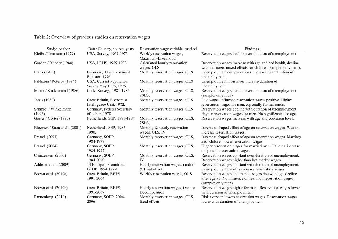
56

Table 2: Overview of previous studies on reservation wages

Study: Author Data: Country, source, years Reservation wage variable, method Findings Kiefer / Neumann (1979) USA, Survey, 1969-1973 Weekly reservation wages,

Maximum-Likelihood, Reservation wages decline over duration of unemployment

Gordon / Blinder (1980) USA, LRHS, 1969-1973 Calculated hourly reservation wages, OLS

Reservation wages increase with age and bad health, decline with marriage, mixed effects for children (sample: only men).

Franz (1982) Germany, Unemployment Register, 1976

Monthly reservation wages, OLS Unemployment compensations increase over duration of unemployment.

Feldstein / Poterba (1984) USA, Current Population Survey May 1976, 1976

Monthly reservation wages, OLS Unemployment insurances increase duration of unemployment.

Maani / Studenmund (1986) Chile, Survey, 1981-1982 Monthly reservation wages, OLS, 2SLS,

Reservation wages decline over duration of unemployment (sample: only men).

Jones (1989) Great Britain, Economist Intelligence Unit, 1982,

Monthly reservation wages, OLS Last wages influence reservation wages positive. Higher reservation wages for men, especially for husbands.

Schmidt / Winkelmann (1993)

Germany, Federal Secretary of Labor ,1978

Monthly reservation wages, OLS Reservation wages decline with duration of unemployment. Higher reservation wages for men. No significance for age.

Gorter / Gorter (1993) Netherlands, SEP, 1985-1987 Monthly reservation wages, OLS, 2SLS,

Reservation wages increase with age and education level.

Bloemen / Stancanelli (2001) Netherlands, SEP, 1987-1990,

Monthly & hourly reservation wages, OLS, IV,

Inverse u-shaped effect of age on reservation wages. Wealth increase reservation wages.

Prasad (2001) Germany, SOEP, 1984-1997

Monthly reservation wages, OLS, Inverse u-shaped effect of age on reservation wages. Marriage and children lower reservation wages.

Prasad (2004) Germany, SOEP, 1984-1997

Monthly reservation wages, OLS, Higher reservation wages for married men. Children increase only men´s reservation wages.

Christensen (2005) Germany, SOEP, 1984-2000

Monthly reservation wages, OLS, IV

Reservation wages constant over duration of unemployment. Reservation wages higher than last market wages.

Addison et al. (2009) 13 European Countries, ECHP, 1994-1999

Hourly reservation wages, random & fixed effects

Reservation wages constant with duration of unemployment. Unemployment benefits increase reservation wages.

Brown et al. (2010a) Great Britain, BHPS, 1991-2004

Weekly reservation wages, OLS, Reservation wages and market wages rise with age, decline after age 55. No influence of health on reservation wages (sample: only men).

Brown et al. (2010b) Great Britain, BHPS, 1991-2007

Hourly reservation wages, Oaxaca Decomposition

Reservation wages higher for men. Reservation wages lower with duration of unemployment.

Pannenberg (2010) Germany, SOEP, 2004-2006

Monthly reservation wages, OLS, fixed effects

Risk aversion lowers reservation wages. Reservation wages lower with duration of unemployment.

57

Constant et al. (2010) Germany, IZA Evaluation Dataset , 2007-2008

Hourly reservation wages, OLS, Oaxaca Decomposition

Reservation wages increases between generations of migrants.

Krueger / Mueller (2011) USA (New Jersey), Survey, 24 weeks in 2009-2010

Hourly reservation wages, OLS, probit

Reservation wages rise with age, decline after age 50. Reservation wages close to last market wage. Amount of job search time decline over unemployment duration.

58

Table 3: Variable list and definitions

Variable Definition Reservation Wages hourly (non-employed) log reservation wages per hour in Euro. (Reservation

Wages monthly / (4.25* Desired Working Hours)) Reservation Wages monthly (non-employed) log reservation wages per month in Euro Entry Wages hourly (employed) log entry wages per hour (only tenure less one year).

(Wages monthly / (4.25*Actual Working Hours) Entry Wages monthly (employed) log entry wages per month (only tenure less one year) Desired Working Hours (non-employed) desired number of working hours (non-employed) Desired Working Hours (employed) desired number of working hours (employed) Actual Working Hours (employed) real number of working hours (employed) Job Satisfaction (employed) satisfaction with job: scale 0 to 10 (0:low, 10:high) Leisure Satisfaction satisfaction with leisure: scale 0 to 10 (0:low, 10:high) Overall Life Satisfaction overall life satisfaction: scale 0 to 10 (0:low, 10:high) Age Categories dummies for five age categories: 18-25 (reference), 26-

35, 36-45, 46-55, 56-65 Household Income log adjusted household income in Euro Female dummy for being female Children dummy for having children under age of 16 in household German dummy for having German citizenship Year 2008 dummy for year 2008 Federal States 15 German federal states (East and West Berlin as

Berlin, Rhineland-Palatinate and Saarland as Rhineland-Palatinate / Saarland)

Unemployment Rate German federal states' unemployment rate (information per state and month, for Rhineland-Palatinate / Saarland information per regional directorate and month)

Health dummies for state of health: good (reference), normal, bad

Intermediate School dummy for having an intermediate school degree (German Realschule)

Upper School dummy for having an upper school degree (German Abitur)

Vocational Degree dummy for having a vocational degree College Degree dummy for having a college degree

59

Table 4: Hourly reservation and entry wages (2007/2008)

All Men Women

Reservation

Wages Entry

Wages Reservation

Wages Entry

Wages Reservation

Wages Entry

Wages Age Categories Ref: 18-25 26 - 35 0.1472*** 0.1315*** 0.1983*** 0.1362*** 0.0901** 0.1572*** (0.0288) (0.0298) (0.0440) (0.0448) (0.0371) (0.0412) 36 - 45 0.1725*** 0.1659*** 0.1835*** 0.2487*** 0.1362*** 0.1378*** (0.0302) (0.0325) (0.0489) (0.0492) (0.0394) (0.0446) 46 - 55 0.1752*** 0.1354*** 0.1849*** 0.1898*** 0.1473*** 0.1055** (0.0345) (0.0373) (0.0526) (0.0543) (0.0461) (0.0496) 56 - 65 0.2268*** 0.1948*** 0.2341*** 0.2360*** 0.2142*** 0.1458* (0.0425) (0.0529) (0.0570) (0.0691) (0.0695) (0.0789) Female -0.0660*** -0.1302*** (0.0202) (0.0206) Children 0.0365 0.0671*** 0.0036 0.1220*** 0.0680** 0.0165 (0.0227) (0.0231) (0.0358) (0.0328) (0.0295) (0.0322) Intermediate School -0.0170 0.0733*** -0.0546 0.0577 -0.0073 0.0755** (0.0230) (0.0269) (0.0345) (0.0382) (0.0315) (0.0376) Upper School 0.1865*** 0.1935*** 0.1998*** 0.1573*** 0.1786*** 0.1976*** (0.0288) (0.0318) (0.0471) (0.0480) (0.0367) (0.0422) Vocational Degree -0.0254 0.0135 0.0420 0.0344 -0.0572** -0.0160 (0.0223) (0.0260) (0.0353) (0.0376) (0.0289) (0.0344) College Degree 0.0654* 0.1865*** -0.0214 0.1962*** 0.1099*** 0.1657*** (0.0338) (0.0337) (0.0656) (0.0500) (0.0388) (0.0439) Health

60

Ref: Good Normal -0.0299 -0.0030 -0.0399 -0.0376 -0.0209 0.0145 (0.0229) (0.0235) (0.0391) (0.0326) (0.0285) (0.0327) Bad -0.0729*** -0.0324 -0.0779* -0.0511 -0.0735** -0.0281 (0.0282) (0.0375) (0.0434) (0.0684) (0.0370) (0.0440) Household Income 0.0701*** 0.2054*** 0.0927*** 0.3390*** 0.0549** 0.0981*** (0.0169) (0.0225) (0.0269) (0.0349) (0.0229) (0.0283) German -0.0404 0.1327*** -0.0914 0.1581*** -0.0040 0.1340* (0.0438) (0.0474) (0.0664) (0.0599) (0.0579) (0.0755) Unemployment Rate -0.0161 -0.0085 0.0121 -0.0207 -0.0356* 0.0095 (0.0166) (0.0167) (0.0300) (0.0223) (0.0188) (0.0249) Year 2008 0.0003 -0.0218 0.1059 -0.0391 -0.0683* -0.0111 (0.0359) (0.0327) (0.0655) (0.0446) (0.0406) (0.0474) Federal States yes yes yes yes yes yes Constant 1.6160*** 0.0938 1.0572*** -0.8232** 1.9041*** 0.6313* (0.2128) (0.2637) (0.3470) (0.3700) (0.2694) (0.3831) R2 0.1592 0.2635 0.1761 0.3746 0.1766 0.2023 adjusted R2 0.1458 0.2517 0.1442 0.3534 0.1548 0.1789 F-Test 14.1749 20.8078 6.0783 16.5399 11.6065 8.6610 Number of Observations 1905 1907 780 888 1125 1019 Number of Individuals 1522 1757 617 819 905 938 Notes: OLS, robust standard errors in parentheses, levels of significance *** 1%, **5%, *10%, SOEP (2007-2008).

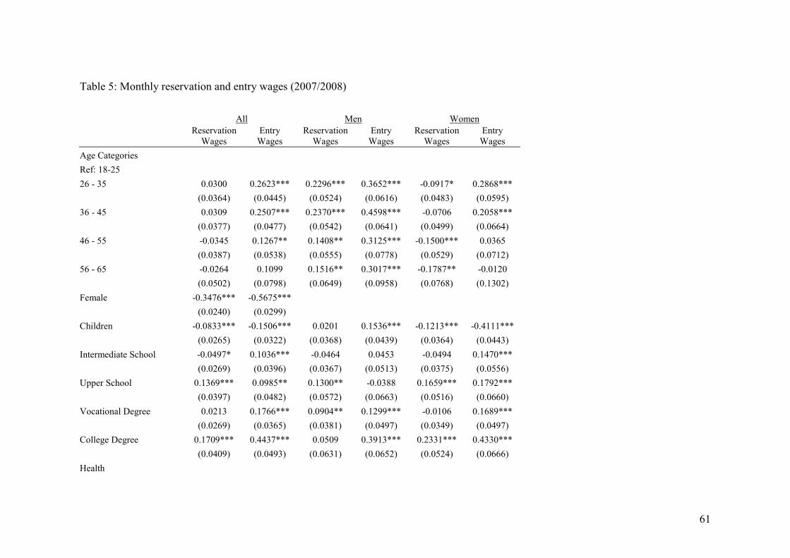
61

Table 5: Monthly reservation and entry wages (2007/2008)

All Men Women

Reservation

Wages Entry

Wages Reservation

Wages Entry

Wages Reservation

Wages Entry

Wages Age Categories Ref: 18-25 26 - 35 0.0300 0.2623*** 0.2296*** 0.3652*** -0.0917* 0.2868*** (0.0364) (0.0445) (0.0524) (0.0616) (0.0483) (0.0595) 36 - 45 0.0309 0.2507*** 0.2370*** 0.4598*** -0.0706 0.2058*** (0.0377) (0.0477) (0.0542) (0.0641) (0.0499) (0.0664) 46 - 55 -0.0345 0.1267** 0.1408** 0.3125*** -0.1500*** 0.0365 (0.0387) (0.0538) (0.0555) (0.0778) (0.0529) (0.0712) 56 - 65 -0.0264 0.1099 0.1516** 0.3017*** -0.1787** -0.0120 (0.0502) (0.0798) (0.0649) (0.0958) (0.0768) (0.1302) Female -0.3476*** -0.5675*** (0.0240) (0.0299) Children -0.0833*** -0.1506*** 0.0201 0.1536*** -0.1213*** -0.4111*** (0.0265) (0.0322) (0.0368) (0.0439) (0.0364) (0.0443) Intermediate School -0.0497* 0.1036*** -0.0464 0.0453 -0.0494 0.1470*** (0.0269) (0.0396) (0.0367) (0.0513) (0.0375) (0.0556) Upper School 0.1369*** 0.0985** 0.1300** -0.0388 0.1659*** 0.1792*** (0.0397) (0.0482) (0.0572) (0.0663) (0.0516) (0.0660) Vocational Degree 0.0213 0.1766*** 0.0904** 0.1299*** -0.0106 0.1689*** (0.0269) (0.0365) (0.0381) (0.0497) (0.0349) (0.0497) College Degree 0.1709*** 0.4437*** 0.0509 0.3913*** 0.2331*** 0.4330*** (0.0409) (0.0493) (0.0631) (0.0652) (0.0524) (0.0666) Health

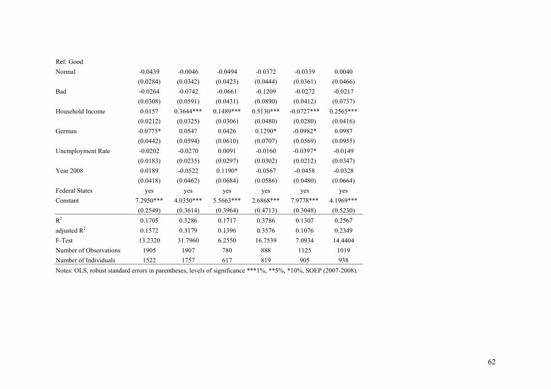
62

Ref: Good Normal -0.0439 -0.0046 -0.0494 -0.0372 -0.0339 0.0040 (0.0284) (0.0342) (0.0423) (0.0444) (0.0361) (0.0466) Bad -0.0264 -0.0742 -0.0661 -0.1209 -0.0272 -0.0217 (0.0308) (0.0591) (0.0431) (0.0890) (0.0412) (0.0737) Household Income 0.0157 0.3644*** 0.1489*** 0.5130*** -0.0727*** 0.2565*** (0.0212) (0.0325) (0.0306) (0.0480) (0.0280) (0.0416) German -0.0775* 0.0547 0.0426 0.1290* -0.0982* 0.0987 (0.0442) (0.0594) (0.0610) (0.0707) (0.0569) (0.0955) Unemployment Rate -0.0202 -0.0270 0.0091 -0.0160 -0.0397* -0.0149 (0.0183) (0.0235) (0.0297) (0.0302) (0.0212) (0.0347) Year 2008 0.0189 -0.0522 0.1190* -0.0567 -0.0458 -0.0328 (0.0418) (0.0462) (0.0684) (0.0586) (0.0480) (0.0664) Federal States yes yes yes yes yes yes Constant 7.2950*** 4.0350*** 5.5663*** 2.6868*** 7.9778*** 4.1969*** (0.2549) (0.3614) (0.3964) (0.4713) (0.3048) (0.5230) R2 0.1705 0.3286 0.1717 0.3786 0.1307 0.2567 adjusted R2 0.1572 0.3179 0.1396 0.3576 0.1076 0.2349 F-Test 13.2320 31.7960 6.2550 16.7539 7.0934 14.4404 Number of Observations 1905 1907 780 888 1125 1019 Number of Individuals 1522 1757 617 819 905 938 Notes: OLS, robust standard errors in parentheses, levels of significance ***1%, **5%, *10%, SOEP (2007-2008).

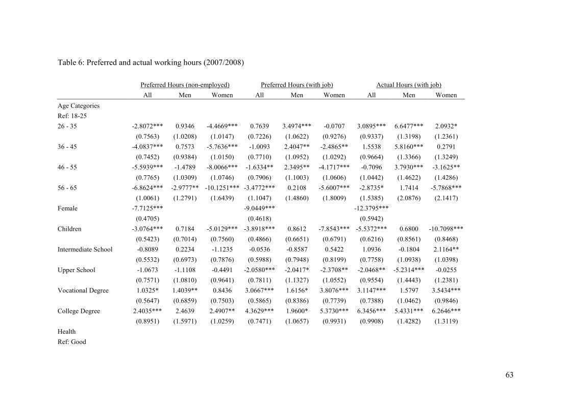
63

Table 6: Preferred and actual working hours (2007/2008)

Preferred Hours (non-employed) Preferred Hours (with job) Actual Hours (with job) All Men Women All Men Women All Men Women Age Categories Ref: 18-25 26 - 35 -2.8072*** 0.9346 -4.4669*** 0.7639 3.4974*** -0.0707 3.0895*** 6.6477*** 2.0932* (0.7563) (1.0208) (1.0147) (0.7226) (1.0622) (0.9276) (0.9337) (1.3198) (1.2361) 36 - 45 -4.0837*** 0.7573 -5.7636*** -1.0093 2.4047** -2.4865** 1.5538 5.8160*** 0.2791 (0.7452) (0.9384) (1.0150) (0.7710) (1.0952) (1.0292) (0.9664) (1.3366) (1.3249) 46 - 55 -5.5939*** -1.4789 -8.0066*** -1.6334** 2.3495** -4.1717*** -0.7096 3.7930*** -3.1625** (0.7765) (1.0309) (1.0746) (0.7906) (1.1003) (1.0606) (1.0442) (1.4622) (1.4286) 56 - 65 -6.8624*** -2.9777** -10.1251*** -3.4772*** 0.2108 -5.6007*** -2.8735* 1.7414 -5.7868*** (1.0061) (1.2791) (1.6439) (1.1047) (1.4860) (1.8009) (1.5385) (2.0876) (2.1417) Female -7.7125*** -9.0449*** -12.3795*** (0.4705) (0.4618) (0.5942) Children -3.0764*** 0.7184 -5.0129*** -3.8918*** 0.8612 -7.8543*** -5.5372*** 0.6800 -10.7098*** (0.5423) (0.7014) (0.7560) (0.4866) (0.6651) (0.6791) (0.6216) (0.8561) (0.8468) Intermediate School -0.8089 0.2234 -1.1235 -0.0536 -0.8587 0.5422 1.0936 -0.1804 2.1164** (0.5532) (0.6973) (0.7876) (0.5988) (0.7948) (0.8199) (0.7758) (1.0938) (1.0398) Upper School -1.0673 -1.1108 -0.4491 -2.0580*** -2.0417* -2.3708** -2.0468** -5.2314*** -0.0255 (0.7571) (1.0810) (0.9641) (0.7811) (1.1327) (1.0552) (0.9554) (1.4443) (1.2381) Vocational Degree 1.0325* 1.4039** 0.8436 3.0667*** 1.6156* 3.8076*** 3.1147*** 1.5797 3.5434*** (0.5647) (0.6859) (0.7503) (0.5865) (0.8386) (0.7739) (0.7388) (1.0462) (0.9846) College Degree 2.4035*** 2.4639 2.4907** 4.3629*** 1.9600* 5.3730*** 6.3456*** 5.4331*** 6.2646*** (0.8951) (1.5971) (1.0259) (0.7471) (1.0657) (0.9931) (0.9908) (1.4282) (1.3119) Health Ref: Good

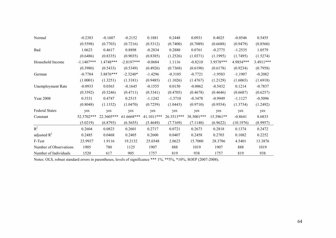
64

Normal -0.2383 -0.1607 -0.2152 0.1881 0.2448 0.0931 0.4025 -0.0546 0.5455 (0.5598) (0.7703) (0.7216) (0.5312) (0.7400) (0.7089) (0.6688) (0.9479) (0.8560) Bad 1.0623 0.4617 0.8898 -0.2834 0.2880 0.0761 -0.2775 -1.2535 1.0579 (0.6486) (0.8335) (0.9035) (0.8385) (1.2526) (1.0371) (1.1995) (1.7495) (1.5274) Household Income -1.1407*** 1.4748*** -2.8197*** -0.0684 1.1116 -0.8210 3.9578*** 4.9854*** 3.4911*** (0.3980) (0.5433) (0.5349) (0.4926) (0.7368) (0.6190) (0.6178) (0.9234) (0.7958) German -0.7784 3.8876*** -2.3240* -1.4296 -0.3105 -0.7721 -1.9503 -1.1907 -0.2082 (1.0001) (1.3251) (1.3181) (0.9485) (1.1026) (1.4767) (1.2129) (1.6065) (1.6918) Unemployment Rate -0.0933 0.0363 -0.1645 -0.1555 0.0150 -0.0062 -0.5432 0.1214 -0.7837 (0.3592) (0.5246) (0.4711) (0.3341) (0.4705) (0.4678) (0.4646) (0.6687) (0.6257) Year 2008 0.3331 0.4747 0.2515 -1.1242 -1.3710 -0.3478 -0.9949 -1.1127 -0.5096 (0.8048) (1.1332) (1.0470) (0.7259) (1.0443) (0.9710) (0.9554) (1.3734) (1.2492) Federal States yes yes yes yes yes yes yes yes yes Constant 52.3702*** 22.3605*** 61.6668*** 41.1011*** 26.3513*** 38.3001*** 15.3961** -0.8641 8.6833 (5.0219) (6.8793) (6.5655) (5.4649) (7.7169) (7.1140) (6.9622) (10.1976) (8.9957) R2 0.2604 0.0823 0.2601 0.2717 0.0721 0.2673 0.2818 0.1374 0.2472 adjusted R2 0.2485 0.0468 0.2405 0.2600 0.0407 0.2458 0.2703 0.1082 0.2252 F-Test 23.9937 1.9116 19.2132 25.0348 2.0623 15.7000 28.3786 4.5401 13.3876 Number of Observations 1905 780 1125 1907 888 1019 1907 888 1019 Number of Individuals 1520 617 905 1757 819 938 1757 819 938 Notes: OLS, robust standard errors in parentheses, levels of significance *** 1%, **5%, *10%, SOEP (2007-2008).

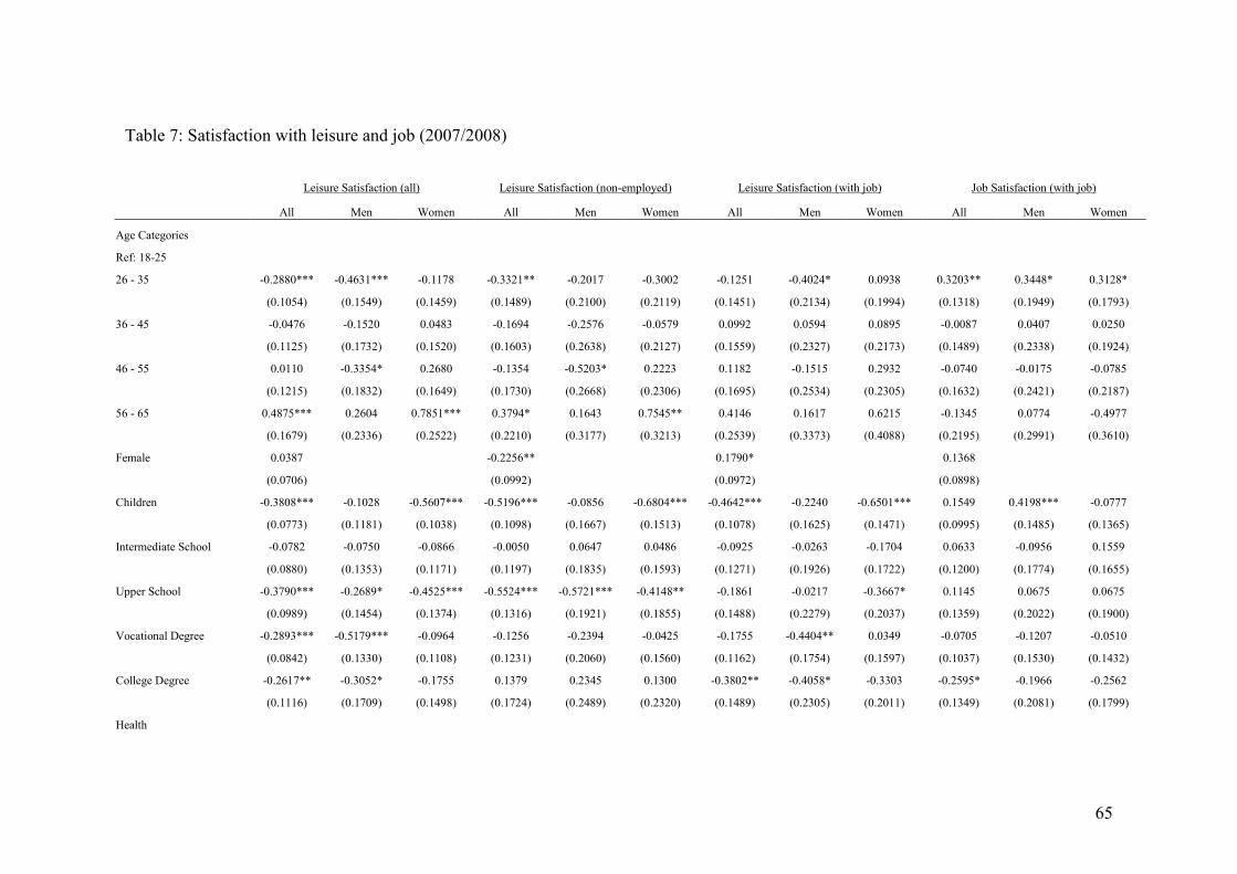
65

Table 7: Satisfaction with leisure and job (2007/2008)

Leisure Satisfaction (all) Leisure Satisfaction (non-employed) Leisure Satisfaction (with job) Job Satisfaction (with job)

All Men Women All Men Women All Men Women All Men Women

Age Categories

Ref: 18-25

26 - 35 -0.2880*** -0.4631*** -0.1178 -0.3321** -0.2017 -0.3002 -0.1251 -0.4024* 0.0938 0.3203** 0.3448* 0.3128*

(0.1054) (0.1549) (0.1459) (0.1489) (0.2100) (0.2119) (0.1451) (0.2134) (0.1994) (0.1318) (0.1949) (0.1793)

36 - 45 -0.0476 -0.1520 0.0483 -0.1694 -0.2576 -0.0579 0.0992 0.0594 0.0895 -0.0087 0.0407 0.0250

(0.1125) (0.1732) (0.1520) (0.1603) (0.2638) (0.2127) (0.1559) (0.2327) (0.2173) (0.1489) (0.2338) (0.1924)

46 - 55 0.0110 -0.3354* 0.2680 -0.1354 -0.5203* 0.2223 0.1182 -0.1515 0.2932 -0.0740 -0.0175 -0.0785

(0.1215) (0.1832) (0.1649) (0.1730) (0.2668) (0.2306) (0.1695) (0.2534) (0.2305) (0.1632) (0.2421) (0.2187)

56 - 65 0.4875*** 0.2604 0.7851*** 0.3794* 0.1643 0.7545** 0.4146 0.1617 0.6215 -0.1345 0.0774 -0.4977

(0.1679) (0.2336) (0.2522) (0.2210) (0.3177) (0.3213) (0.2539) (0.3373) (0.4088) (0.2195) (0.2991) (0.3610)

Female 0.0387 -0.2256** 0.1790* 0.1368

(0.0706) (0.0992) (0.0972) (0.0898)

Children -0.3808*** -0.1028 -0.5607*** -0.5196*** -0.0856 -0.6804*** -0.4642*** -0.2240 -0.6501*** 0.1549 0.4198*** -0.0777

(0.0773) (0.1181) (0.1038) (0.1098) (0.1667) (0.1513) (0.1078) (0.1625) (0.1471) (0.0995) (0.1485) (0.1365)

Intermediate School -0.0782 -0.0750 -0.0866 -0.0050 0.0647 0.0486 -0.0925 -0.0263 -0.1704 0.0633 -0.0956 0.1559

(0.0880) (0.1353) (0.1171) (0.1197) (0.1835) (0.1593) (0.1271) (0.1926) (0.1722) (0.1200) (0.1774) (0.1655)

Upper School -0.3790*** -0.2689* -0.4525*** -0.5524*** -0.5721*** -0.4148** -0.1861 -0.0217 -0.3667* 0.1145 0.0675 0.0675

(0.0989) (0.1454) (0.1374) (0.1316) (0.1921) (0.1855) (0.1488) (0.2279) (0.2037) (0.1359) (0.2022) (0.1900)

Vocational Degree -0.2893*** -0.5179*** -0.0964 -0.1256 -0.2394 -0.0425 -0.1755 -0.4404** 0.0349 -0.0705 -0.1207 -0.0510

(0.0842) (0.1330) (0.1108) (0.1231) (0.2060) (0.1560) (0.1162) (0.1754) (0.1597) (0.1037) (0.1530) (0.1432)

College Degree -0.2617** -0.3052* -0.1755 0.1379 0.2345 0.1300 -0.3802** -0.4058* -0.3303 -0.2595* -0.1966 -0.2562

(0.1116) (0.1709) (0.1498) (0.1724) (0.2489) (0.2320) (0.1489) (0.2305) (0.2011) (0.1349) (0.2081) (0.1799)

Health

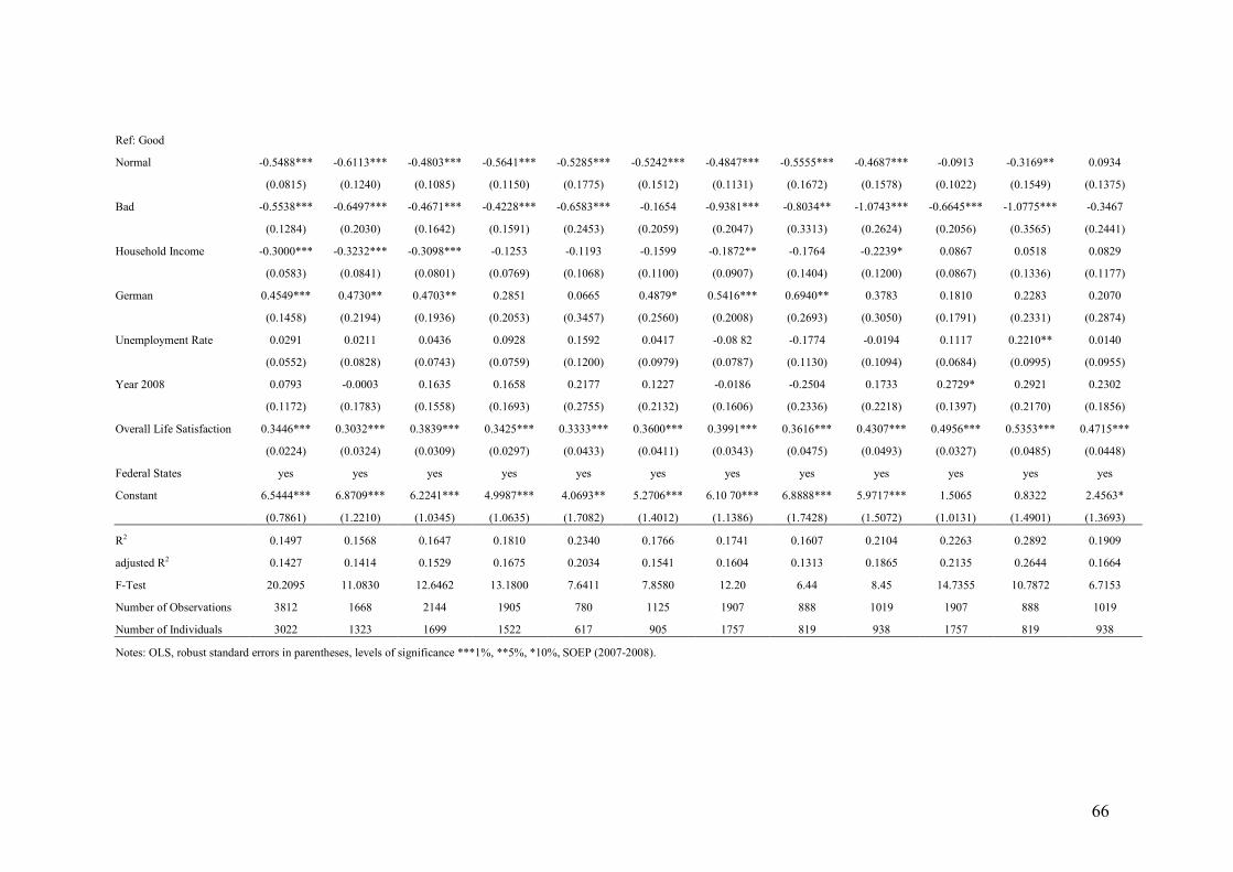
66

Ref: Good

Normal -0.5488*** -0.6113*** -0.4803*** -0.5641*** -0.5285*** -0.5242*** -0.4847*** -0.5555*** -0.4687*** -0.0913 -0.3169** 0.0934

(0.0815) (0.1240) (0.1085) (0.1150) (0.1775) (0.1512) (0.1131) (0.1672) (0.1578) (0.1022) (0.1549) (0.1375)

Bad -0.5538*** -0.6497*** -0.4671*** -0.4228*** -0.6583*** -0.1654 -0.9381*** -0.8034** -1.0743*** -0.6645*** -1.0775*** -0.3467

(0.1284) (0.2030) (0.1642) (0.1591) (0.2453) (0.2059) (0.2047) (0.3313) (0.2624) (0.2056) (0.3565) (0.2441)

Household Income -0.3000*** -0.3232*** -0.3098*** -0.1253 -0.1193 -0.1599 -0.1872** -0.1764 -0.2239* 0.0867 0.0518 0.0829

(0.0583) (0.0841) (0.0801) (0.0769) (0.1068) (0.1100) (0.0907) (0.1404) (0.1200) (0.0867) (0.1336) (0.1177)

German 0.4549*** 0.4730** 0.4703** 0.2851 0.0665 0.4879* 0.5416*** 0.6940** 0.3783 0.1810 0.2283 0.2070

(0.1458) (0.2194) (0.1936) (0.2053) (0.3457) (0.2560) (0.2008) (0.2693) (0.3050) (0.1791) (0.2331) (0.2874)

Unemployment Rate 0.0291 0.0211 0.0436 0.0928 0.1592 0.0417 -0.08 82 -0.1774 -0.0194 0.1117 0.2210** 0.0140

(0.0552) (0.0828) (0.0743) (0.0759) (0.1200) (0.0979) (0.0787) (0.1130) (0.1094) (0.0684) (0.0995) (0.0955)

Year 2008 0.0793 -0.0003 0.1635 0.1658 0.2177 0.1227 -0.0186 -0.2504 0.1733 0.2729* 0.2921 0.2302

(0.1172) (0.1783) (0.1558) (0.1693) (0.2755) (0.2132) (0.1606) (0.2336) (0.2218) (0.1397) (0.2170) (0.1856)

Overall Life Satisfaction 0.3446*** 0.3032*** 0.3839*** 0.3425*** 0.3333*** 0.3600*** 0.3991*** 0.3616*** 0.4307*** 0.4956*** 0.5353*** 0.4715***

(0.0224) (0.0324) (0.0309) (0.0297) (0.0433) (0.0411) (0.0343) (0.0475) (0.0493) (0.0327) (0.0485) (0.0448)

Federal States yes yes yes yes yes yes yes yes yes yes yes yes

Constant 6.5444*** 6.8709*** 6.2241*** 4.9987*** 4.0693** 5.2706*** 6.10 70*** 6.8888*** 5.9717*** 1.5065 0.8322 2.4563*

(0.7861) (1.2210) (1.0345) (1.0635) (1.7082) (1.4012) (1.1386) (1.7428) (1.5072) (1.0131) (1.4901) (1.3693)

R2 0.1497 0.1568 0.1647 0.1810 0.2340 0.1766 0.1741 0.1607 0.2104 0.2263 0.2892 0.1909

adjusted R2 0.1427 0.1414 0.1529 0.1675 0.2034 0.1541 0.1604 0.1313 0.1865 0.2135 0.2644 0.1664

F-Test 20.2095 11.0830 12.6462 13.1800 7.6411 7.8580 12.20 6.44 8.45 14.7355 10.7872 6.7153

Number of Observations 3812 1668 2144 1905 780 1125 1907 888 1019 1907 888 1019

Number of Individuals 3022 1323 1699 1522 617 905 1757 819 938 1757 819 938

Notes: OLS, robust standard errors in parentheses, levels of significance ***1%, **5%, *10%, SOEP (2007-2008).