Embed Size (px)
Citation preview
Deutsches Institut für Wirtschaftsforschung
www.diw.de
Sven Voigtländer • Jan Goebel • Thomas Claßen •Michael Wurm • Ursula Berger • Achim Strunk • Hendrik Elbern
Using geographically referenced data on environmental exposures for public health research: a feasibility study based on the German Socio-Economic Panel Study (SOEP)e
386
Berlin, June 2011
SOEPpaperson Multidisciplinary Panel Data Research

SOEPpapers on Multidisciplinary Panel Data Research at DIW Berlin This series presents research findings based either directly on data from the German Socio-Economic Panel Study (SOEP) or using SOEP data as part of an internationally comparable data set (e.g. CNEF, ECHP, LIS, LWS, CHER/PACO). SOEP is a truly multidisciplinary household panel study covering a wide range of social and behavioral sciences: economics, sociology, psychology, survey methodology, econometrics and applied statistics, educational science, political science, public health, behavioral genetics, demography, geography, and sport science. The decision to publish a submission in SOEPpapers is made by a board of editors chosen by the DIW Berlin to represent the wide range of disciplines covered by SOEP. There is no external referee process and papers are either accepted or rejected without revision. Papers appear in this series as works in progress and may also appear elsewhere. They often represent preliminary studies and are circulated to encourage discussion. Citation of such a paper should account for its provisional character. A revised version may be requested from the author directly. Any opinions expressed in this series are those of the author(s) and not those of DIW Berlin. Research disseminated by DIW Berlin may include views on public policy issues, but the institute itself takes no institutional policy positions. The SOEPpapers are available at http://www.diw.de/soeppapers Editors: Georg Meran (Dean DIW Graduate Center) Gert G. Wagner (Social Sciences) Joachim R. Frick (Empirical Economics) Jürgen Schupp (Sociology)
Conchita D’Ambrosio (Public Economics) Christoph Breuer (Sport Science, DIW Research Professor) Elke Holst (Gender Studies) Martin Kroh (Political Science and Survey Methodology) Frieder R. Lang (Psychology, DIW Research Professor) Jörg-Peter Schräpler (Survey Methodology, DIW Research Professor) C. Katharina Spieß (Educational Science) Martin Spieß (Survey Methodology, DIW Research Professor) ISSN: 1864-6689 (online) German Socio-Economic Panel Study (SOEP) DIW Berlin Mohrenstrasse 58 10117 Berlin, Germany Contact: Uta Rahmann | [email protected]
1
Using geographically referenced data on environmental exposures for public health research: a feasibility study based on the German Socio‐Economic Panel Study (SOEP)
Sven Voigtländer1§, Jan Goebel2, Thomas Claßen3, Michael Wurm4,5, Ursula Berger1, Achim Strunk6,7,
Hendrik Elbern7,8
1 Dept. of Epidemiology & International Public Health, School of Public Health, Bielefeld University,
Bielefeld, Germany 2 Socio‐economic Panel Study (SOEP), German Institute for Economic Research (DIW), Berlin,
Germany 3 Dept. of Environment & Health, School of Public Health, Bielefeld University, Bielefeld, Germany 4 German Remote Sensing Data Center (DFD), German Aerospace Center (DLR), Oberpfaffenhofen‐
Wessling, Germany 5 Dept. of Remote Sensing, University of Würzburg, Würzburg, Germany 6 Royal Dutch Meteorological Institute (KNMI), De Bilt, Netherlands 7 Rhenish Institute for Environmental Research (RIU), University of Cologne, Cologne, Germany 8 Section Troposphere, Institute of Energy and Climate Research (IEK), Jülich Research Centre, Jülich,
Germany
§ Corresponding author
Email addresses:
SV: sven.voigtlaender@uni‐bielefeld.de
TC: thomas.classen@uni‐bielefeld.de
UB: ursula.berger@uni‐bielefeld.de
HE: [email protected]‐koeln.de
2
Abstract
Background In panel datasets information on environmental exposures is scarce. Thus, our goal was to probe the
use of area‐wide geographically referenced data for air pollution from an external data source in the
analysis of physical health.
Methods The study population comprised SOEP respondents in 2004 merged with exposures for NO2, PM10
and O3 based on a multi‐year reanalysis of the EURopean Air pollution Dispersion‐Inverse Model
(EURAD‐IM). Apart from bivariate analyses with subjective air pollution we estimated cross‐sectional
multilevel regression models for physical health as assessed by the SF‐12.
Results The variation of average exposure to NO2, PM10 and O3 was small with the interquartile range being
less than 10µg/m3 for all pollutants. There was no correlation between subjective air pollution and
average exposure to PM10 and O3, while there was a small positive correlation between the first and
NO2. Inclusion of objective air pollution in regression models did not improve the model fit.
Conclusions It is feasible to merge environmental exposures to a nationally representative panel study like the
SOEP. However, in our study the spatial resolution of the specific air pollutants has been too little,
yet.
Keywords SOEP, geographically referenced data, feasibility study, air pollution, EURAD‐IM, physical health
3
Introduction Panel studies like the German Socio‐Economic Panel (SOEP) allow for a longitudinal analysis of
individual characteristics including health [1,2]. In the use of this data, however, researchers usually
face a scarcity of information if they want to study the impact of environmental exposures on
individual health and its changes. Taking the case of the SOEP there are several reasons for that.
First, information on environmental exposures such as air pollution and crime is collected on the
basis of a household questionnaire. This questionnaire is completed by the head of household who
rates, for instance, the degree of his or her subjective disturbance by air pollution. In a recent study
on the impact of neighbourhood deprivation on physical health by two of the authors we did use this
information and found that increases in the subjective disturbance by air pollution are associated
with worsening physical health [3]. However, our estimates are likely to be biased because an
exposure that is self‐rated is liable to individual characteristics such as knowledge, perception as well
as socially patterned expectations [4].
Second, the subjective degree of disturbance by air pollution in general is not very informative in
regard to which specific air pollutant is possibly causing the difference in individual health. To know
this would require information on specific air pollutants like oxides of nitrogen, particulate matter
and ozone that constitute overall air pollution. Such information would also support health
promotion agencies as well as policy makers identifying specific air pollutant exposures that cause
health disparities and that should consequently be modified [5,6].
Third, information regarding self‐rated air pollution as well as other environmental exposures is
collected in a five year interval. This means exposure data is lacking for the years in between the
interval. Of course, one can perform cross‐sectional analyses for the years with available exposure
data but has to put up with the limitations of such analyses, e.g. reverse causality and unobserved
heterogeneity [cf. 7]. For longitudinal analyses, however, one would need at least annual data that
allows estimating associations between annual changes in environmental exposures and annual
changes in health. Some researchers may try to overcome this limitation by making assumptions for
4
the exposure based on the subjective exposure that is available every five years but the validity of an
assumed exposure is highly questionable.
To overcome the problem of self‐rated and rather unspecific data on environmental exposures
within panel studies researchers have to integrate data from external sources. This issue of
integrating data from external sources in cohort, panel and other studies will be one of the major
challenges for epidemiology in the coming years. For instance, on its biennial conference in 2011 the
German Data Forum (German: Rat für Sozial‐ und WirtschaftsDaten, RatSWD) invited speakers that
explored the issue of multiple data sources (e.g. environmental exposure data, cancer registry data,
health insurance data, occupational data) and related problems of data protection and data access
(Link: http://ratswd.de/5kswd/konferenz.html).
In the study presented here we probe the use of geographically referenced data on specific ambient
air pollutants in the panel study SOEP to analyse physical health. The effects of specific air pollutants
on morbidity and mortality have been documented in numerous publications including meta‐
analyses [8‐17]. Further reductions in the levels of pollutants like particulate matter and ozone in
Northern America as well as in Europe are expected to result in substantial health benefits [9,18,19].
Using the EURopean Air pollution Dispersion‐Inverse Model (EURAD‐IM) [20,21] we merge objective
exposures for nitrogen dioxide (NO2), particulate matter less than 10µm in aerodynamical diameter
(PM10), and ozone (O3) to the geographically referenced SOEP households. Based on this dataset we
calculate individual mean values for the time between the current wave and the previous wave while
accounting for individual moves of place of residence. We then explore the association between the
specific exposure to air pollutants and the subjective disturbance by air pollution in the year 2004
before we estimate a cross‐sectional regression model for physical health in 2004.
5
Methods
Data We used data from the SOEP, version 25 [22], which is a longitudinal nationally representative annual
survey of private households in Germany that was started in 1984. Wagner et al. provide further
information on the methodology of the survey [1]. In the analysis we included all respondents aged
18 and above who took part in the survey in 2004 and who were living in a geographically referenced
private household, i.e. a survey household for which the address could be geocoded with block‐level
geographic precision (while preventing identification of individuals by name and guaranteeing their
complete anonymity). The geocoding of the addresses has been done via the field work agency (TNS
Infratest) and the original coordinates cannot be used together with any survey information [cf. 23].
Data on specific air pollutants we obtained from the reanalysis study Air Quality Records which has
been accomplished for the Global Monitoring for Environment and Security (GMES) Service Element
PROMOTE (Link: http://www.gse‐promote.org). For the reanalysis period from January 2002 to
December 2008, observations of various trace gases have been assimilated into EURAD‐IM on a
European grid domain with a horizontal resolution of 45x45 km2 [20,21]. The measurements
comprised hourly observations from routinely operated European networks (AirBase, European
Environment Agency), air‐borne data from the MOZAIC project and NO2, carbon monoxide (CO) and
O3 retrievals from satellite based sensors (GOME, SCIAMACHY, OMI, GOME‐2 and MOPITT). Based on
three hourly analyses inferred with the three dimensional variational data assimilation technique
(3d‐var) and short‐term forecasts, hourly values of a set of chemical constituents are provided from
which NO2, O3 and PM10 have been selected for this study.
The socio‐economic data and datasets of air pollutants have been merged using the statistical
software R [24] as described in the following. The spatial extension of the individual grid‐cells of the
EURAD‐IM data sets was interpolated from 45x45km2 to a grid‐size of 5x5km2. For the interpolation
we used the utility gdalwarp, which is an image reprojection and warping utility [25], with a bilinear
6
interpolation. Via the geographic location of the households, we matched air pollutant data to each
single household. Finally, we calculated the average exposure for the time between the previous
interview in 2003 and the current interview in 2004 (on average one year). In case a respondent had
moved his or her place of residence we calculated the weighted average based on the number of
months the respondent spent at different places.
To control for regional as well as neighbourhood confounders we merged additional data to the
SOEP. Regional information at the level of the 413 German counties (German: “Kreise & kreisfreie
Städte”) was used from the regional INKAR data base of the Federal Institute for Research on
Building, Urban Affairs and Spatial Development (German: Bundesinstitut für Bau‐, Stadt‐ und
Raumforschung, BBSR). Neighbourhood information was matched to the households on the basis of
data from the commercial data provider microm GmbH which is available within the SOEP research
data center [26].
Variables Air pollution
We assessed air pollution by both objective and subjective measures. Our objective measures
comprised simulated ambient air concentrations of NO2 as proxy for total nitrogen oxide (NOx), PM10
as well as O3. Due to their health damaging effects the European Commission has set air quality
standards (amended in 2008 with Directive 2008/50/EC) that are effective in German legislation, too
[27]. For each pollutant we calculated the average exposure of a respondent in µg/m3. Information
on subjective air pollution is based on the household questionnaire that is completed by the head of
household and gathers perceived disturbance by air pollution (graded on a five‐point Likert scale
from “none” to “very strong”).

7
Physical Health
We used the physical component score (PCS) as our health outcome because among all health
outcomes provided by the SOEP this is most sensitive regarding potential health effects of air
pollution. The PCS is based on the short form 12 health questionnaire (SF‐12) that measures health‐
related quality of life and comprises 12 items. Using principal component analysis these items are
aggregated to two summary measures: a physical component score (PCS) and a mental component
score (MCS). Both of them are standardized to a mean of 50 and a standard deviation of 10 whereas
higher values indicate better health. Further details on the computation of the PCS are provided
elsewhere [28].
Covariates
Similar to a recent paper by two of the authors [3] we controlled for a number of individual,
household as well as contextual risk factors that may be correlated with air pollution. The individual
and household risk factors include age, gender, education, unemployment and income. We
measured education by the classification “Comparative Analyses of Social Mobility in Industrial
Nations” (CASMIN) with the categories “still in school”, “low” (German: “bis Hauptschule”),
“intermediate” (German: “Abitur/ Realschulabschluss”), “high” (German: “Hochschulabschluss”) and
“not specified” [29]; unemployment based on the employment status at the day of interview; and
income using the annual net household income from the previous year weighted by the modified
equivalence scale of the Organisation for Economic Co‐operation and Development (OECD) that we
additionally log‐transformed to achieve a symmetric distribution [30,31]. To perform stratified
analyses (outlined below) we classified age into “18 to 39 years”, “40 to 59 years” and “60 years and
above”. In addition we controlled for individual health‐related factors such as smoking with the
categories “never smoker”, “ex‐smoker” “current smoker”; sports participation with the categories
“every week”, “every month”, “less than every month” and “never”; as well as Body Mass Index
(BMI) with the categories “less than 25 kg/m2”, “25 to 30 kg/m2” and “above 30 kg/m2”.
8
The selected contextual risk factors comprise the unemployment quota of the respondent’s county
as well as the average purchasing power of the respondent’s street section. The unemployment
quota describes the number of unemployed inhabitants as a proportion of the labour force. The
average purchasing power of a respondent’s street section is provided by the microm GmbH. The
latter divided Germany in approximately 1.5 million street sections with an average of 27 households
for which they calculate average (household) purchasing powers based on official revenue statistics
[26]. microm GmbH does not publish further information on this variable [32].
Statistical analyses Data analysis was done in several steps. First, we explored the distribution of the three objective air
pollutions measures in boxplots. Second, we calculated bivariate Spearman rank correlation
coefficients stratified by age groups and sex to examine the relationship of the subjective and the
objective measures of air pollution.
Third, we re‐estimated a multilevel linear regression model from a previous publication [3] to analyse
the effect of air pollution measured by objective measures on physical health (PCS) while controlling
for other individual and contextual factors. In this earlier model we used a three‐level‐hierarchy
(individuals nested in households nested in counties) and estimated the association between
subjective air pollution and PCS while controlling for covariates (Model 1). For this article we
estimated the same model but substituted subjective air pollution by the three selected ambient air
pollutants (Model 2). In a third model we included both, subjective as well as objective air pollution
measures, while controlling for the above‐mentioned covariates (Model 2). The models for PCS can
be written as follows:
ihc
cchhiii
vuwzx
εββββ
+++++++++= .........PCS 1111110

9
where xi1 ,… denote characteristics at the individual level (level 1), e.g. age, sex and average exposure
to NO2, PM10 and O3, with the corresponding model coefficients βi1, …. zh1 ,… denote factors
measured at the household level (level 2), i.e. income (log‐transformed), purchasing power as well as
subjective disturbance by air pollution, with the corresponding model coefficients βh1, …. And w1s
denotes the factor at the county level (level 3), i.e. county unemployment quota, with its
corresponding model coefficient βc1. In the multilevel model there is random variation on each level,
mirrored by the random effects, which are assumed to be independently normally distributed with
mean 0. Here, uc is the random effect of the county level (level 3) with variance σ2c, i.e. uc,~N(0,σ 2
c) ,
vh is the random effect of the household level (level 2) with variance σ2h, i.e. vh,~N(0,σ 2
h) , and εi on
the individual level (level 1) are the model residuals with the residual variance σ2i, i.e. εi,~N(0,σ 2
i).
Modelling was done with MLwiN 2.22 [33]. All model parameters were estimated using the iterative
generalised least squares (IGLS) procedure [34]. Goodness of fit was assessed by the likelihood ratio
test.
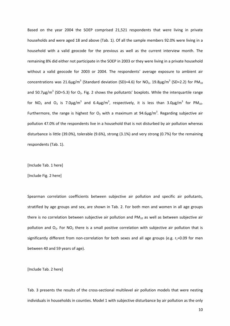
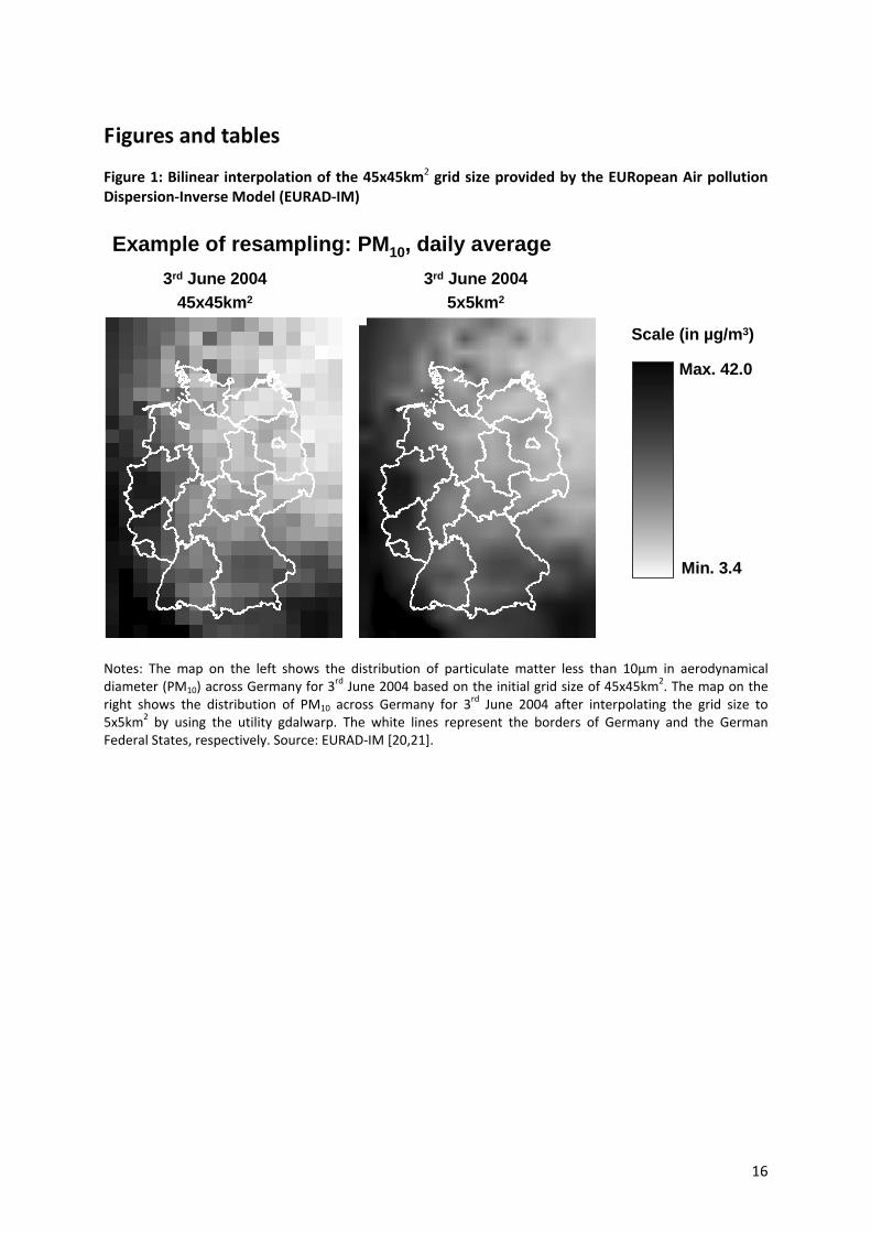
Results Fig. 1 provides an example of the bilinear interpolation that we used to reduce the spatial extension
of the individual grid‐cells of the EURAD‐IM data sets. The map on the left shows the distribution of
PM10 (daily average) across Germany for 3rd June 2004 based on the initial grid size of 45x45km2. The
map on the right shows the distribution of PM10 (daily average) across Germany for 3rd June 2004
after interpolating the grid size to 5x5km2. For this specific day maximum and minimum were
42.0µg/m3 and 3.4µg/m3, respectively.
[Include Fig. 1 here]
10
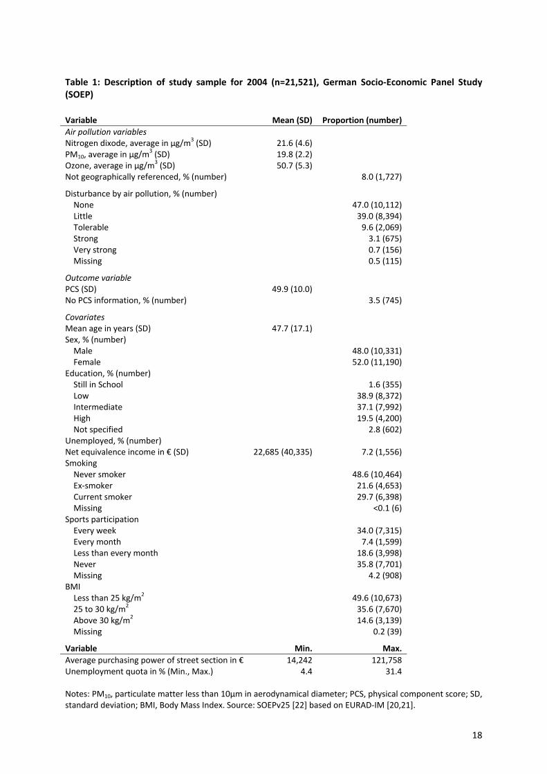
Based on the year 2004 the SOEP comprised 21,521 respondents that were living in private
households and were aged 18 and above (Tab. 1). Of all the sample members 92.0% were living in a
household with a valid geocode for the previous as well as the current interview month. The
remaining 8% did either not participate in the SOEP in 2003 or they were living in a private household
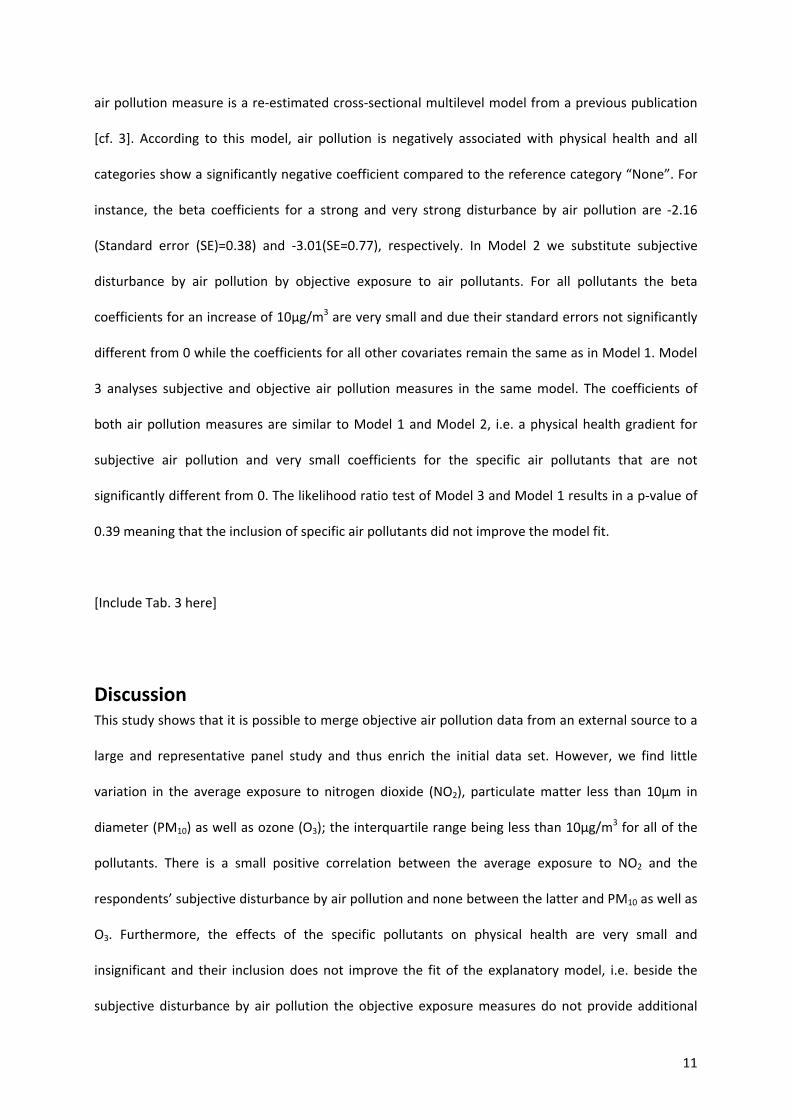
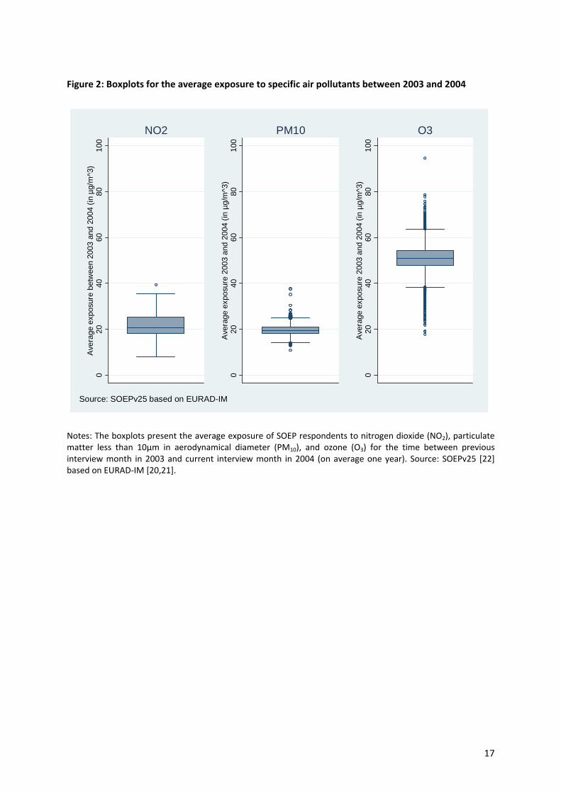
without a valid geocode for 2003 or 2004. The respondents’ average exposure to ambient air
concentrations was 21.6µg/m3 (Standard deviation (SD)=4.6) for NO2, 19.8µg/m3 (SD=2.2) for PM10
and 50.7µg/m3 (SD=5.3) for O3. Fig. 2 shows the pollutants’ boxplots. While the interquartile range
for NO2 and O3 is 7.0µg/m3 and 6.4µg/m3, respectively, it is less than 3.0µg/m3 for PM10.
Furthermore, the range is highest for O3 with a maximum at 94.6µg/m3. Regarding subjective air
pollution 47.0% of the respondents live in a household that is not disturbed by air pollution whereas
disturbance is little (39.0%), tolerable (9.6%), strong (3.1%) and very strong (0.7%) for the remaining
respondents (Tab. 1).
[Include Tab. 1 here]
[Include Fig. 2 here]
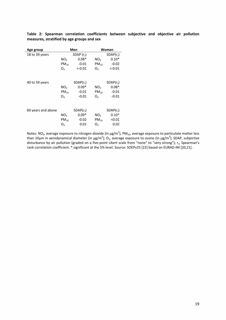
Spearman correlation coefficients between subjective air pollution and specific air pollutants,
stratified by age groups and sex, are shown in Tab. 2. For both men and women in all age groups
there is no correlation between subjective air pollution and PM10 as well as between subjective air
pollution and O3. For NO2 there is a small positive correlation with subjective air pollution that is
significantly different from non‐correlation for both sexes and all age groups (e.g. rs=0.09 for men
between 40 and 59 years of age).
[Include Tab. 2 here]
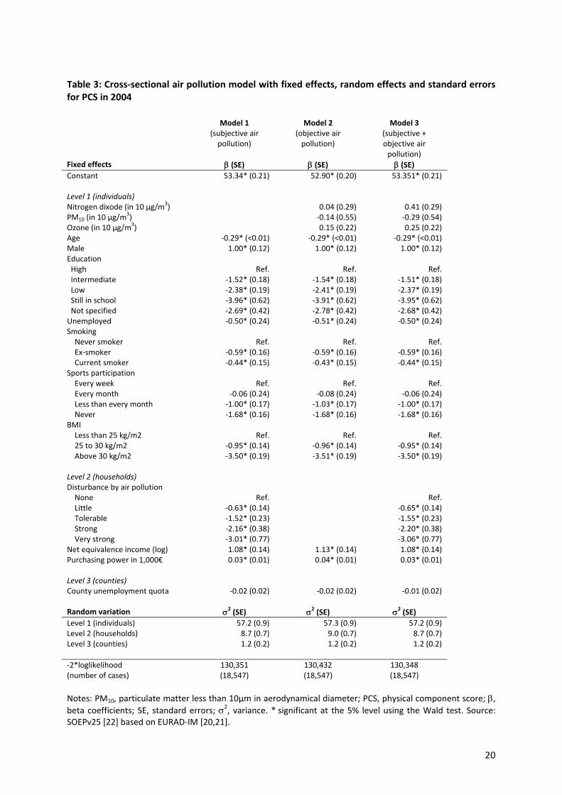
Tab. 3 presents the results of the cross‐sectional multilevel air pollution models that were nesting
individuals in households in counties. Model 1 with subjective disturbance by air pollution as the only
11
air pollution measure is a re‐estimated cross‐sectional multilevel model from a previous publication
[cf. 3]. According to this model, air pollution is negatively associated with physical health and all
categories show a significantly negative coefficient compared to the reference category “None”. For
instance, the beta coefficients for a strong and very strong disturbance by air pollution are ‐2.16
(Standard error (SE)=0.38) and ‐3.01(SE=0.77), respectively. In Model 2 we substitute subjective
disturbance by air pollution by objective exposure to air pollutants. For all pollutants the beta
coefficients for an increase of 10µg/m3 are very small and due their standard errors not significantly
different from 0 while the coefficients for all other covariates remain the same as in Model 1. Model
3 analyses subjective and objective air pollution measures in the same model. The coefficients of
both air pollution measures are similar to Model 1 and Model 2, i.e. a physical health gradient for
subjective air pollution and very small coefficients for the specific air pollutants that are not
significantly different from 0. The likelihood ratio test of Model 3 and Model 1 results in a p‐value of
0.39 meaning that the inclusion of specific air pollutants did not improve the model fit.
[Include Tab. 3 here]
Discussion This study shows that it is possible to merge objective air pollution data from an external source to a
large and representative panel study and thus enrich the initial data set. However, we find little
variation in the average exposure to nitrogen dioxide (NO2), particulate matter less than 10µm in
diameter (PM10) as well as ozone (O3); the interquartile range being less than 10µg/m3 for all of the
pollutants. There is a small positive correlation between the average exposure to NO2 and the
respondents’ subjective disturbance by air pollution and none between the latter and PM10 as well as
O3. Furthermore, the effects of the specific pollutants on physical health are very small and
insignificant and their inclusion does not improve the fit of the explanatory model, i.e. beside the
subjective disturbance by air pollution the objective exposure measures do not provide additional
12
information when explaining health inequalities. All other things being equal (‘ceteris paribus’) the
beta coefficients of the specific air pollutants are implausible.
There are several reasons for the implausible estimates of which we want to discuss the most
important ones. First, the original grid size of 45x45km2 was rather large and implies little spatial
variation in the exposure to specific air pollutants. The aim of the EURAD‐IM reanalysis study was to
provide air pollution analyses for a large entity such as Europe as well as for a long period and
therefore it uses a rather coarse grid size. Although exposure to air pollution is usually confined to a
much smaller area, so‐called hotspots [35‐38], a certain air quality situation or such a hotspot (e.g.,
an ambient air monitoring site dominated by urban traffic emissions) has a limited representative‐
ness for the model based analyses on the large grid size. We tried to compensate for that by
interpolating the data to a grid size of 5x5km2 but this grid size would still not be sufficient to
measure an extreme exposure to air pollutants and the bilinear spatial interpolation method does
not necessarily improve the informational content of the source data. Second, our physical health
measure might not have been sensitive enough to reflect health effects from air pollution that are
linked to respiratory and cardiovascular disease. Third, we did not use information regarding the
composition of PM10 or the exposure to particulate matter less than 2.5µm in diameter (PM2.5). The
latter is supposed to have stronger health effects [9,17]. Fourth, our research design is not able to
measure short‐term health effects of air pollution. For this, we would need to use detailed exposure
data for the few weeks or days before the interview took place.
For future studies it is, based on our results, necessary to use specific air pollutants data with a
higher spatial resolution. Integrating data concerning the exposure to PM2.5 would very likely provide
more valid beta coefficients for health outcomes. Regarding the latter, future waves of the SOEP may
provide information on more sensitive health outcomes like respiratory or cardiovascular symptoms
so that the association between air pollution and health can be measured more accurately. Thus it
13
will also be possible to estimate the degree of subjectivity in the respondents’ assessment of their
disturbance by air pollution.
Conclusions It is possible to enrich a large and representative datasets like the SOEP with external and area‐wide
geographically referenced data for air pollution. This can potentially be done with other environ‐
mental exposures, too. Although the presented data on the exposure to specific air pollutants is so
far of limited use (e.g. large grid size) this should not be discouraging because there may be solutions
to these problems [e.g. 36]. Integrating data from external sources in cohort, panel and other studies
will probably be one of the major challenges for epidemiology in the coming years as it helps to make
better use of existing datasets that by nature comprise a limited number of health‐related exposures.
Acknowledgements The work for this paper was partly supported by the German Research Foundation (DFG), grant
number: RA 889/2‐1, and the Bielefeld School of Public Health.

14
References 1. Wagner GG, Frick JR, Schupp J: The German Socio‐Economic Panel Study (SOEP) ‐ Scope, Evolution and
Enhancements. Schmollers Jahrbuch 2007, 127:139‐169. 2. Frick JR, Goebel J, Engelmann M, Rahmann U: The Research Data Center (RDC) of the German Socio‐
Economic Panel (SOEP). Schmollers Jahrbuch 2010, 130:393‐401. 3. Voigtländer S, Berger U, Razum O: The impact of regional and neighbourhood deprivation on physical
health in Germany: a multilevel study. BMC Public Health 2010, 10:403. 4. Ross CE, Van Willigen M: Education and the subjective quality of life. J Health Soc Behav 1997, 38:275‐
297. 5. Künzli N, Perez L: Evidence based public health ‐ the example of air pollution. Swiss Med Wkly 2009,
139:242‐250. 6. Claßen T, Hornberg C: Evidence‐based Public Health ‐ Handlungsleitend im Umgang mit Feinstaub? In
Evidence‐based Public Health. Bessere Gesundheitsversorgung durch geprüfte Informationen. Edited by Gerhardus A, Breckenkamp J, Razum O, Schmacke N, Wenzel H. Bern: Hans Huber Verlag; 2010:241‐256.
7. Baltagi BH: Econometric analysis of panel data. Chichester: Wiley; 2005. 8. Anderson HR: Air pollution and mortality: A history. Atmospheric Environment 2009, 43:142‐152. 9. Kappos AD, Bruckmann P, Eikmann T, Englert N, Heinrich U, Hoppe P, Koch E, Krause GH, Kreyling WG,
Rauchfuss K et al.: Health effects of particles in ambient air. Int J Hyg Environ Health 2004, 207:399‐407. 10. Janke K, Propper C, Henderson J: Do current levels of air pollution kill? The impact of air pollution on
population mortality in England. Health Economics 2009, 18:1031‐1055. 11. Pope CA, III, Ezzati M, Dockery DW: Fine‐particulate air pollution and life expectancy in the United
States. N Engl J Med 2009, 360:376‐386. 12. Schulz H, Harder V, Ibald‐Mulli A, Khandoga A, Koenig W, Krombach F, Radykewicz R, Stampfl A, Thorand
B, Peters A: Cardiovascular effects of fine and ultrafine particles. J Aerosol Med 2005, 18:1‐22. 13. Pope CA, III, Dockery DW: Health effects of fine particulate air pollution: lines that connect. J Air Waste
Manag Assoc 2006, 56:709‐742. 14. von Klot S, Peters A, Aalto P, Bellander T, Berglind N, D'Ippoliti D, Elosua R, Hormann A, Kulmala M, Lanki
T et al.: Ambient air pollution is associated with increased risk of hospital cardiac readmissions of myocardial infarction survivors in five European cities. Circulation 2005, 112:3073‐3079.
15. Gehring U, Heinrich J, Kramer U, Grote V, Hochadel M, Sugiri D, Kraft M, Rauchfuss K, Eberwein HG, Wichmann HE: Long‐term exposure to ambient air pollution and cardiopulmonary mortality in women. Epidemiology 2006, 17:545‐551.
16. Schikowski T, Sugiri D, Ranft U, Gehring U, Heinrich J, Wichmann HE, Kramer U: Long‐term air pollution exposure and living close to busy roads are associated with COPD in women. Respir Res 2005, 6:152.
17. Anderson HR, Atkinson RW, Peacock JL, Konstantinou K: Meta‐analysis of time‐series studies and panel studies of Particulate Matter (PM) and Ozone (O3). Copenhagen: World Health Organization; 2004.
[http://www.euro.who.int/__data/assets/pdf_file/0004/74731/e82792.pdf]; (accessed 12 April 2011). 18. Barr CD, Dominici F: Cap and trade legislation for greenhouse gas emissions: public health benefits from
air pollution mitigation. JAMA 2010, 303:69‐70. 19. Hurley F, Hunt A, Cowie H, Holland M, Miller B, Pye S, Watkiss P: Methodology for the Cost‐Benefit
analysis for CAFE. Volume 2: Health Impact Assessment. Oxon: AEA Technology Environment; 2005. [http://ec.europa.eu/environment/archives/cafe/pdf/cba_methodology_vol2.pdf]; (accessed 12 April
2011). 20. Elbern H, Strunk A, Schmidt H, Talagrand O: Emission Rate and Chemical State Estimation by 4‐
Dimensional Variational Inversion. Atmos Chem Phys 2007, 7:3749‐3769. 21. Strunk A, Ebel A, Elbern H, Friese E, Goris N, Nieradzik LP: Four‐Dimensional Variational Assimilation of
Atmospheric Chemical Data ‐ Application to Regional Modelling of Air Quality. In Large‐scale scientific computing. Volume 5910. Edited by Lirkov I, Margenov S, Wasniewski J. Berlin: Springer; 2010:214‐222.
22. SOEP. Data for years 1984‐2008, version 25 (SOEPv25). Berlin: German Institute for Economic Research; 2009.
15
23. Hintze P, Lakes T: Geographically Referenced Data in Social Science: A Service Paper for SOEP Data Users. Berlin: German Institute for Economic Research; 2009.
[http://www.diw.de/documents/publikationen/73/diw_01.c.338625.de/diw_datadoc_2009‐046.pdf]; (accessed 12 April 2011).
24. R Development Core Team. R: A language and environment for statistical computing. Vienna: R Foundation for Statistical Computing; 2007.
25. GDAL. GDAL ‐ Geospatial Data Abstraction Library: Version 1.7.3. Open Source Geospatial Foundation; 2010.
26. Goebel J, Spieß CK, Witte NRJ, Gerstenberg S: Die Verknüpfung des SOEP mit Microm‐Indikatoren: Der MICROM‐SOEP Datensatz. Berlin: German Institute for Economic Research; 2007.
[http://www.diw.de/documents/publikationen/73/diw_01.c.78103.de/diw_datadoc_2007‐026.pdf]; (accessed 12 April 2011).
27. Federal Environment Agency: Trends in Air Quality in Germany. Dessau‐Roßlau 2009. [http://www.cisherzog.de/cis_en/download/air‐bmu.pdf]; (accessed 12 April 2011). 28. Andersen HH, Mühlbacher A, Nübling M, Schupp J, Wagner GG: Computation of Standard Values for
Physical and Mental Health Scale Scores Using the SOEP Version of the SF‐12v2. Schmollers Jahrbuch 2007, 127:171‐182.
29. Brauns H, Scherer S, Steinmann S: The CASMIN educational classification in international comparative research. In Advances in cross‐national comparison. Edited by Edited by Hoffmeyer‐Zlotnik J, Wolf C. New York: Kluwer; 2003:221‐244.
30. Grabka MM: Codebook for the $PEQUIV File 1984‐2008. CNEF Variables with Extended Income Information for the SOEP. Berlin: German Institute for Economic Research; 2009.
[http://www.diw.de/documents/publikationen/73/diw_01.c.338519.de/diw_datadoc_2009‐045.pdf]; (accessed 12 April 2011).
31. OECD: The OECD List of Social Indicators. Paris 1982. 32. microm GmbH: Handbuch Daten DE. Neuss 2009. 33. Rasbash J, Charlton C, Browne WJ, Healy M, Cameron B. MLwiN Version 2.22. Bristol: Centre for
Multilevel Modelling, University of Bristol; 2009. 34. Rasbash J, Steele F, Browne WJ, Goldstein H: A user's guide to MLwiN. Version 2.10. 2009. 35. Hak C, Larssen S, Randall S, Guerreiro C, Denby B, Horálek J: Traffic and Air Quality: Contribution of
Traffic to Urban Air Quality in European Cities. Bilthoven: European Topic Centre on Air and Climate Change; 2010.
[http://acm.eionet.europa.eu/docs/ETCACC_TP_2009_12_transport_and_air_quality_in_cities.pdf]; (accessed 12 April 2011).
36. Horálek J, de Smet P, de Leeuw F, Coòková M, Denby B, Kurfürst P: Methodological improvements on interpolating European air quality maps. Bilthoven: European Topic Centre in Air and Climate Change; 2010.
[http://acm.eionet.europa.eu/docs/ETCACC_TP_2009_16_Improving_SpatAQmapping.pdf]; (accessed 12 April 2011).
37. Dragano N, Hoffmann B, Moebus S, Mohlenkamp S, Stang A, Verde PE, Jockel KH, Erbel R, Siegrist J: Traffic exposure and subclinical cardiovascular disease: is the association modified by socioeconomic characteristics of individuals and neighbourhoods? Results from a multilevel study in an urban region. Occup Environ Med 2009, 66:628‐635.
38. Salam MT, Islam T, Gilliland FD: Recent evidence for adverse effects of residential proximity to traffic sources on asthma. Curr Opin Pulm Med 2008, 14:3‐8.
16
Figures and tables
Figure 1: Bilinear interpolation of the 45x45km2 grid size provided by the EURopean Air pollution Dispersion‐Inverse Model (EURAD‐IM)
Example of resampling: PM10, daily average3rd June 2004
45x45km2
3rd June 20045x5km2
Scale (in µg/m3)
Max. 42.0
Min. 3.4
Notes: The map on the left shows the distribution of particulate matter less than 10µm in aerodynamical diameter (PM10) across Germany for 3rd June 2004 based on the initial grid size of 45x45km2. The map on the right shows the distribution of PM10 across Germany for 3rd June 2004 after interpolating the grid size to 5x5km2 by using the utility gdalwarp. The white lines represent the borders of Germany and the German Federal States, respectively. Source: EURAD‐IM [20,21].
17
Figure 2: Boxplots for the average exposure to specific air pollutants between 2003 and 2004
020
4060
8010
0A
vera
ge e
xpos
ure
betw
een
2003
and
200
4 (in
µg/
m^3
)
NO2
020
4060
8010
0A
vera
ge e
xpos
ure
2003
and
200
4 (in
µg/
m^3
)
PM10
020
4060
8010
0A
vera
ge e
xpos
ure
2003
and
200
4 (in
µg/
m^3
)
O3
Source: SOEPv25 based on EURAD-IM
Notes: The boxplots present the average exposure of SOEP respondents to nitrogen dioxide (NO2), particulate matter less than 10µm in aerodynamical diameter (PM10), and ozone (O3) for the time between previous interview month in 2003 and current interview month in 2004 (on average one year). Source: SOEPv25 [22] based on EURAD‐IM [20,21].
18
Table 1: Description of study sample for 2004 (n=21,521), German Socio‐Economic Panel Study (SOEP) Variable Mean (SD) Proportion (number) Air pollution variables Nitrogen dixode, average in µg/m3 (SD) 21.6 (4.6) PM10, average in µg/m
3 (SD) 19.8 (2.2) Ozone, average in µg/m3 (SD) 50.7 (5.3) Not geographically referenced, % (number) 8.0 (1,727)
Disturbance by air pollution, % (number) None 47.0 (10,112) Little 39.0 (8,394) Tolerable 9.6 (2,069) Strong 3.1 (675) Very strong 0.7 (156) Missing 0.5 (115)
Outcome variable PCS (SD) 49.9 (10.0) No PCS information, % (number) 3.5 (745)
Covariates Mean age in years (SD) 47.7 (17.1) Sex, % (number) Male 48.0 (10,331) Female 52.0 (11,190) Education, % (number) Still in School 1.6 (355) Low 38.9 (8,372) Intermediate 37.1 (7,992) High 19.5 (4,200) Not specified 2.8 (602) Unemployed, % (number) Net equivalence income in € (SD) 22,685 (40,335) 7.2 (1,556) Smoking Never smoker 48.6 (10,464) Ex‐smoker 21.6 (4,653) Current smoker 29.7 (6,398) Missing <0.1 (6) Sports participation Every week 34.0 (7,315) Every month 7.4 (1,599) Less than every month 18.6 (3,998) Never 35.8 (7,701) Missing 4.2 (908) BMI Less than 25 kg/m2 49.6 (10,673) 25 to 30 kg/m2 35.6 (7,670) Above 30 kg/m2 14.6 (3,139) Missing 0.2 (39)
Variable Min. Max. Average purchasing power of street section in € 14,242 121,758 Unemployment quota in % (Min., Max.) 4.4 31.4 Notes: PM10, particulate matter less than 10µm in aerodynamical diameter; PCS, physical component score; SD, standard deviation; BMI, Body Mass Index. Source: SOEPv25 [22] based on EURAD‐IM [20,21].
19
Table 2: Spearman correlation coefficients between subjective and objective air pollution measures, stratified by age groups and sex Age group Men Women18 to 39 years SDAP (rs) SDAP(rs) NO2 0.08* NO2 0.10* PM10 ‐0.01 PM10 ‐0.02 O3 <‐0.01 O3 <‐0.01 40 to 59 years SDAP(rs) SDAP(rs) NO2 0.09* NO2 0.08* PM10 ‐0.01 PM10 ‐0.01 O3 ‐0.01 O3 ‐0.01 60 years and above SDAP(rs) SDAP(rs) NO2 0.09* NO2 0.10* PM10 ‐0.02 PM10 <0.01 O3 0.01 O3 0.02 Notes: NO2, average exposure to nitrogen dioxide (in µg/m
3), PM10, average exposure to particulate matter less than 10µm in aerodynamical diameter (in µg/m3); O3, average exposure to ozone (in µg/m
3); SDAP, subjective disturbance by air pollution (graded on a five‐point Likert scale from “none” to “very strong”); rs, Spearman’s rank correlation coefficient. * significant at the 5% level. Source: SOEPv25 [22] based on EURAD‐IM [20,21].
20
Table 3: Cross‐sectional air pollution model with fixed effects, random effects and standard errors for PCS in 2004
Model 1 (subjective air pollution)
Model 2 (objective air pollution)
Model 3 (subjective + objective air pollution)
Fixed effects β (SE) β (SE) β (SE) Constant 53.34* (0.21) 52.90* (0.20) 53.351* (0.21) Level 1 (individuals) Nitrogen dixode (in 10 µg/m3) 0.04 (0.29) 0.41 (0.29) PM10 (in 10 µg/m
3) ‐0.14 (0.55) ‐0.29 (0.54) Ozone (in 10 µg/m3) 0.15 (0.22) 0.25 (0.22) Age ‐0.29* (<0.01) ‐0.29* (<0.01) ‐0.29* (<0.01) Male 1.00* (0.12) 1.00* (0.12) 1.00* (0.12) Education High Ref. Ref. Ref. Intermediate ‐1.52* (0.18) ‐1.54* (0.18) ‐1.51* (0.18) Low ‐2.38* (0.19) ‐2.41* (0.19) ‐2.37* (0.19) Still in school ‐3.96* (0.62) ‐3.91* (0.62) ‐3.95* (0.62) Not specified ‐2.69* (0.42) ‐2.78* (0.42) ‐2.68* (0.42) Unemployed ‐0.50* (0.24) ‐0.51* (0.24) ‐0.50* (0.24) Smoking Never smoker Ref. Ref. Ref. Ex‐smoker ‐0.59* (0.16) ‐0.59* (0.16) ‐0.59* (0.16) Current smoker ‐0.44* (0.15) ‐0.43* (0.15) ‐0.44* (0.15) Sports participation Every week Ref. Ref. Ref. Every month ‐0.06 (0.24) ‐0.08 (0.24) ‐0.06 (0.24) Less than every month ‐1.00* (0.17) ‐1.03* (0.17) ‐1.00* (0.17) Never ‐1.68* (0.16) ‐1.68* (0.16) ‐1.68* (0.16) BMI Less than 25 kg/m2 Ref. Ref. Ref. 25 to 30 kg/m2 ‐0.95* (0.14) ‐0.96* (0.14) ‐0.95* (0.14) Above 30 kg/m2 ‐3.50* (0.19) ‐3.51* (0.19) ‐3.50* (0.19) Level 2 (households) Disturbance by air pollution None Ref. Ref. Little ‐0.63* (0.14) ‐0.65* (0.14) Tolerable ‐1.52* (0.23) ‐1.55* (0.23) Strong ‐2.16* (0.38) ‐2.20* (0.38) Very strong ‐3.01* (0.77) ‐3.06* (0.77) Net equivalence income (log) 1.08* (0.14) 1.13* (0.14) 1.08* (0.14) Purchasing power in 1,000€ 0.03* (0.01) 0.04* (0.01) 0.03* (0.01) Level 3 (counties) County unemployment quota ‐0.02 (0.02) ‐0.02 (0.02) ‐0.01 (0.02) Random variation σ2 (SE) σ2 (SE) σ2 (SE) Level 1 (individuals) 57.2 (0.9) 57.3 (0.9) 57.2 (0.9) Level 2 (households) 8.7 (0.7) 9.0 (0.7) 8.7 (0.7) Level 3 (counties) 1.2 (0.2) 1.2 (0.2) 1.2 (0.2) ‐2*loglikelihood (number of cases)
130,351 (18,547)
130,432 (18,547)
130,348 (18,547)
Notes: PM10, particulate matter less than 10µm in aerodynamical diameter; PCS, physical component score; β, beta coefficients; SE, standard errors; σ2, variance. * significant at the 5% level using the Wald test. Source: SOEPv25 [22] based on EURAD‐IM [20,21].