SOCY7709: Quantitative Data Management Instructor: …Loops Loops help automate repetitive operations, from the simplest to very complex. “Old” syntax examples To define simple

1

SOCY7709: Quantitative Data Management

Instructor: Natasha Sarkisian

Automating Your Work: Macros and Loops

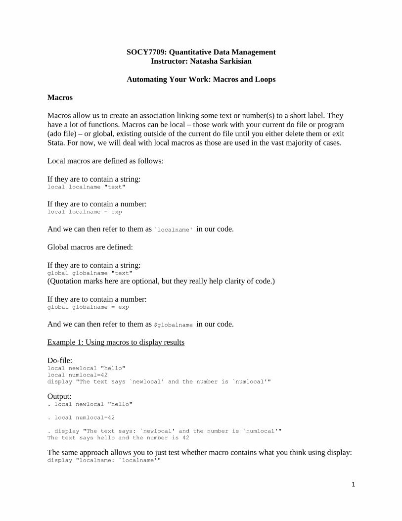
Macros

Macros allow us to create an association linking some text or number(s) to a short label. They

have a lot of functions. Macros can be local – those work with your current do file or program

(ado file) – or global, existing outside of the current do file until you either delete them or exit

Stata. For now, we will deal with local macros as those are used in the vast majority of cases.

Local macros are defined as follows:

If they are to contain a string: local localname "text"

If they are to contain a number: local localname = exp

And we can then refer to them as `localname' in our code.

Global macros are defined:

If they are to contain a string: global globalname "text"

(Quotation marks here are optional, but they really help clarity of code.)

If they are to contain a number: global globalname = exp

And we can then refer to them as $globalname in our code.

Example 1: Using macros to display results

Do-file: local newlocal "hello"

local numlocal=42

display "The text says `newlocal' and the number is `numlocal'"

Output: . local newlocal "hello"

. local numlocal=42

. display "The text says: `newlocal' and the number is `numlocal'"

The text says hello and the number is 42

The same approach allows you to just test whether macro contains what you think using display: display "localname: `localname'"

2

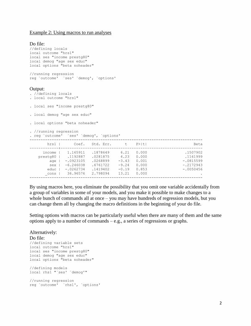
Example 2: Using macros to run analyses

Do file: //defining locals

local outcome "hrs1"

local ses "income prestg80"

local demog "age sex educ"

local options "beta noheader"

//running regression

reg òutcome' `ses' `demog', òptions'

Output: . //defining locals

. local outcome "hrs1"

. local ses "income prestg80"

. local demog "age sex educ"

. local options "beta noheader"

. //running regression

. reg òutcome' `ses' `demog', òptions'

------------------------------------------------------------------------------

hrs1 | Coef. Std. Err. t P>|t| Beta

-------------+----------------------------------------------------------------

income | 1.165911 .1878649 6.21 0.000 .1507902

prestg80 | .1192887 .0281875 4.23 0.000 .1161999

age | -.0923105 .0268899 -3.43 0.001 -.0815599

sex | -6.246038 .6761722 -9.24 0.000 -.2172943

educ | -.0262734 .1419402 -0.19 0.853 -.0050456

_cons | 36.96576 2.798094 13.21 0.000 .

------------------------------------------------------------------------------

By using macros here, you eliminate the possibility that you omit one variable accidentally from

a group of variables in some of your models, and you make it possible to make changes to a

whole bunch of commands all at once – you may have hundreds of regression models, but you

can change them all by changing the macro definitions in the beginning of your do file.

Setting options with macros can be particularly useful when there are many of them and the same

options apply to a number of commands – e.g., a series of regressions or graphs.

Alternatively:

Do file: //defining variable sets





//defining models

local rhs1 "`ses' `demog'"


reg òutcome' `rhs1', òptions'

3

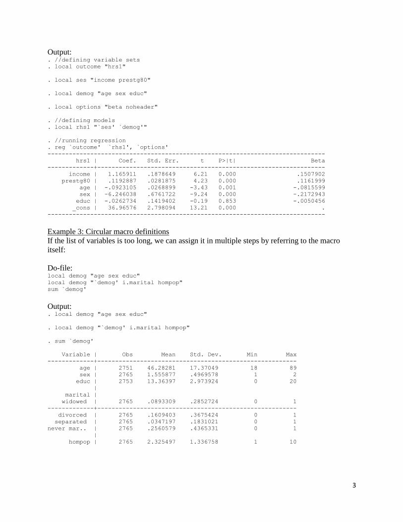
Output: . //defining variable sets

. local outcome "hrs1"

. local ses "income prestg80"

. local demog "age sex educ"

. local options "beta noheader"

. //defining models

. local rhs1 "`ses' `demog'"

. //running regression

. reg òutcome' `rhs1', òptions'

------------------------------------------------------------------------------

hrs1 | Coef. Std. Err. t P>|t| Beta

-------------+----------------------------------------------------------------

income | 1.165911 .1878649 6.21 0.000 .1507902

prestg80 | .1192887 .0281875 4.23 0.000 .1161999

age | -.0923105 .0268899 -3.43 0.001 -.0815599

sex | -6.246038 .6761722 -9.24 0.000 -.2172943

educ | -.0262734 .1419402 -0.19 0.853 -.0050456

_cons | 36.96576 2.798094 13.21 0.000 .

------------------------------------------------------------------------------

Example 3: Circular macro definitions

If the list of variables is too long, we can assign it in multiple steps by referring to the macro

itself:

Do-file: local demog "age sex educ"

local demog "`demog' i.marital hompop"

sum `demog'

Output: . local demog "age sex educ"

. local demog "`demog' i.marital hompop"

. sum `demog'

Variable | Obs Mean Std. Dev. Min Max

-------------+--------------------------------------------------------

age | 2751 46.28281 17.37049 18 89

sex | 2765 1.555877 .4969578 1 2

educ | 2753 13.36397 2.973924 0 20

|

marital |

widowed | 2765 .0893309 .2852724 0 1

-------------+--------------------------------------------------------

divorced | 2765 .1609403 .3675424 0 1

separated | 2765 .0347197 .1831021 0 1

never mar.. | 2765 .2560579 .4365331 0 1

|

hompop | 2765 2.325497 1.336758 1 10

4

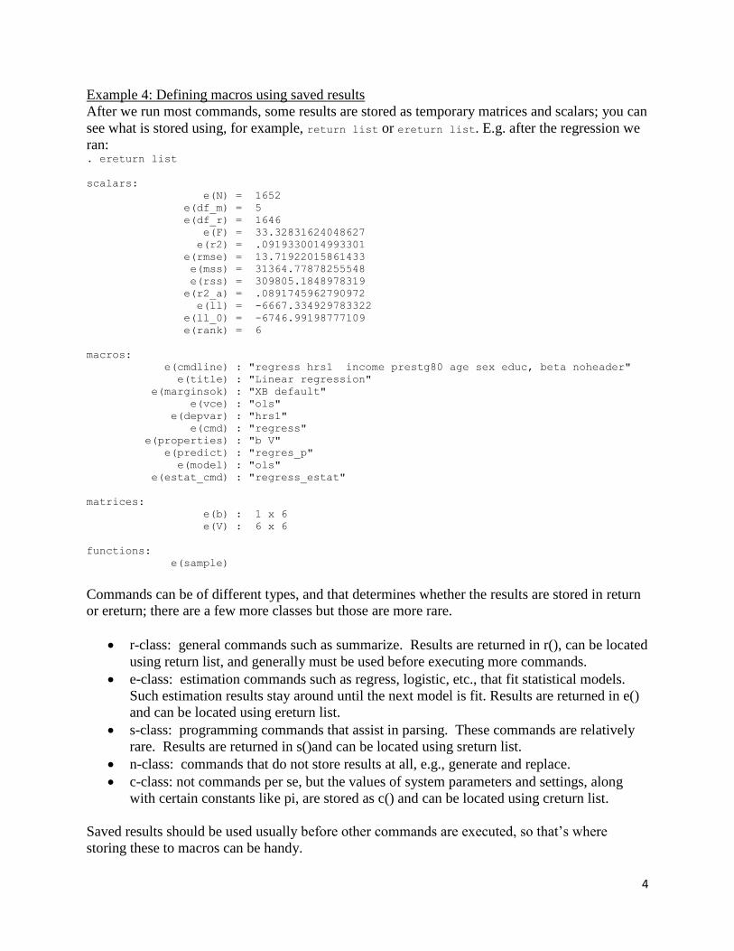
Example 4: Defining macros using saved results

After we run most commands, some results are stored as temporary matrices and scalars; you can

see what is stored using, for example, return list or ereturn list. E.g. after the regression we

ran: . ereturn list

scalars:

e(N) = 1652

e(df_m) = 5

e(df_r) = 1646

e(F) = 33.32831624048627

e(r2) = .0919330014993301

e(rmse) = 13.71922015861433

e(mss) = 31364.77878255548

e(rss) = 309805.1848978319

e(r2_a) = .0891745962790972

e(ll) = -6667.334929783322

e(ll_0) = -6746.99198777109

e(rank) = 6

macros:

e(cmdline) : "regress hrs1 income prestg80 age sex educ, beta noheader"

e(title) : "Linear regression"

e(marginsok) : "XB default"

e(vce) : "ols"

e(depvar) : "hrs1"

e(cmd) : "regress"

e(properties) : "b V"

e(predict) : "regres_p"

e(model) : "ols"

e(estat_cmd) : "regress_estat"

matrices:

e(b) : 1 x 6

e(V) : 6 x 6

functions:

e(sample)

Commands can be of different types, and that determines whether the results are stored in return

or ereturn; there are a few more classes but those are more rare.

r-class: general commands such as summarize. Results are returned in r(), can be located

using return list, and generally must be used before executing more commands.

e-class: estimation commands such as regress, logistic, etc., that fit statistical models.

Such estimation results stay around until the next model is fit. Results are returned in e()

and can be located using ereturn list.

s-class: programming commands that assist in parsing. These commands are relatively

rare. Results are returned in s()and can be located using sreturn list.

n-class: commands that do not store results at all, e.g., generate and replace.

c-class: not commands per se, but the values of system parameters and settings, along

with certain constants like pi, are stored as c() and can be located using creturn list.

Saved results should be used usually before other commands are executed, so that’s where

storing these to macros can be handy.

5

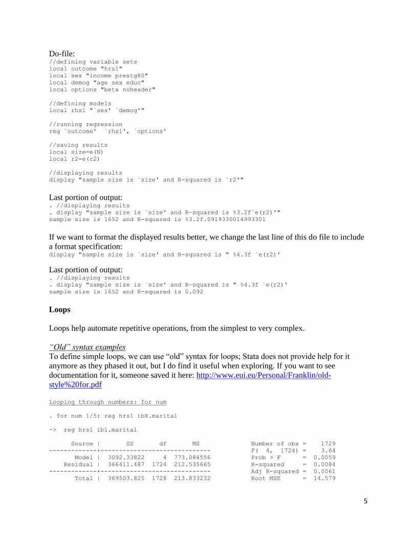
Do-file: //defining variable sets





//defining models

local rhs1 "`ses' `demog'"


reg òutcome' `rhs1', òptions'

//saving results

local size=e(N)

local r2=e(r2)

//displaying results

display "sample size is `size' and R-squared is `r2'"

Last portion of output: . //displaying results

. display "sample size is `size' and R-squared is %3.2fè(r2)'"

sample size is 1652 and R-squared is %3.2f.0919330014993301

If we want to format the displayed results better, we change the last line of this do file to include

a format specification: display "sample size is `size' and R-squared is " %4.3f è(r2)'

Last portion of output: . //displaying results

. display "sample size is `size' and R-squared is " %4.3f è(r2)'

sample size is 1652 and R-squared is 0.092

Loops

Loops help automate repetitive operations, from the simplest to very complex.

“Old” syntax examples

To define simple loops, we can use “old” syntax for loops; Stata does not provide help for it

anymore as they phased it out, but I do find it useful when exploring. If you want to see

documentation for it, someone saved it here: http://www.eui.eu/Personal/Franklin/old-

style%20for.pdf

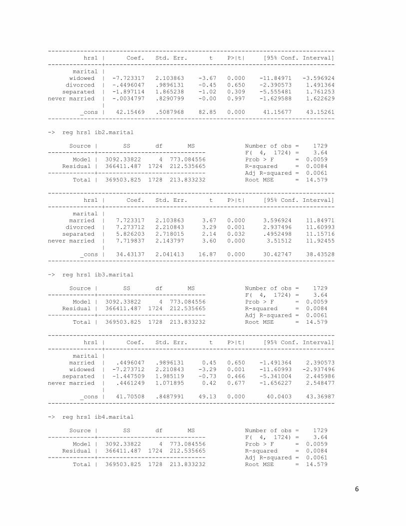
Looping through numbers: for num

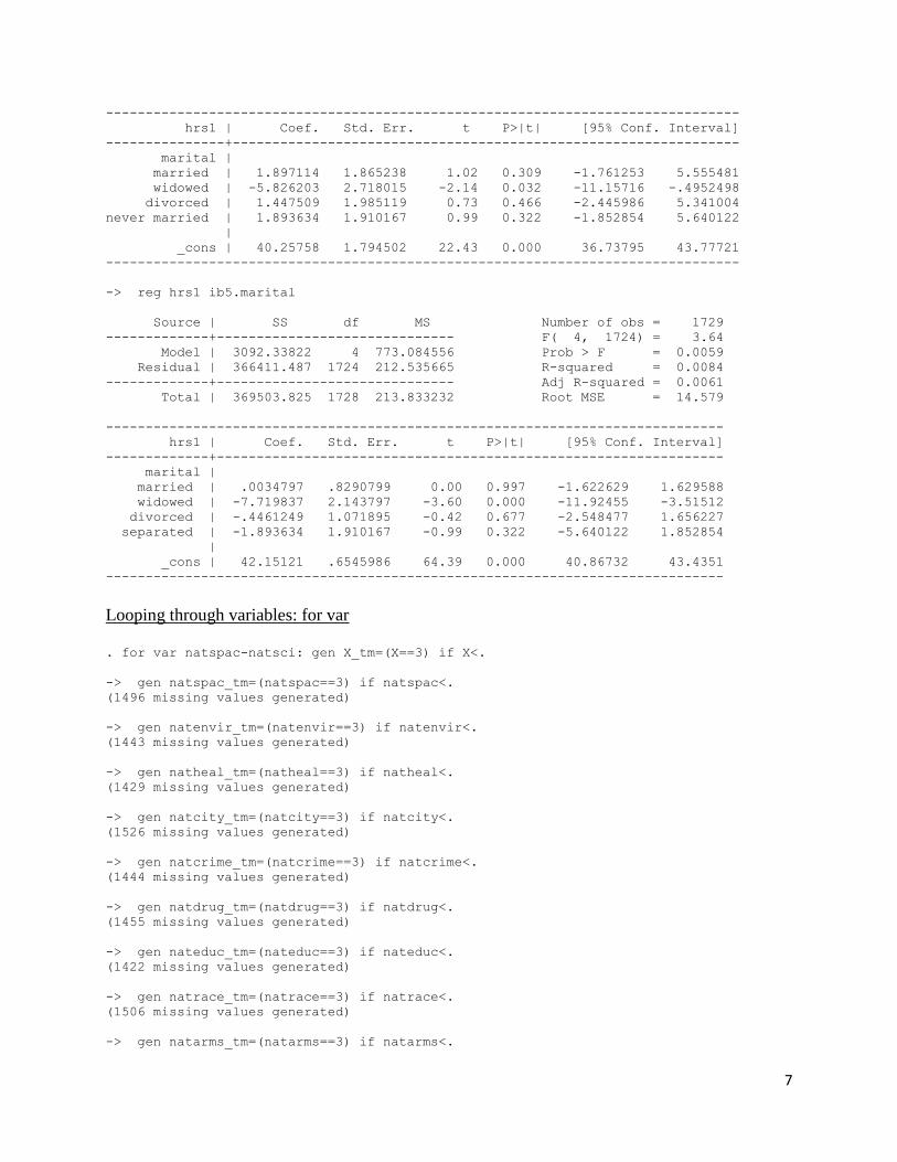
. for num 1/5: reg hrs1 ibX.marital

-> reg hrs1 ib1.marital

Source | SS df MS Number of obs = 1729

-------------+------------------------------ F( 4, 1724) = 3.64

Model | 3092.33822 4 773.084556 Prob > F = 0.0059

Residual | 366411.487 1724 212.535665 R-squared = 0.0084

-------------+------------------------------ Adj R-squared = 0.0061

Total | 369503.825 1728 213.833232 Root MSE = 14.579

http://www.eui.eu/Personal/Franklin/old-style%20for.pdf

http://www.eui.eu/Personal/Franklin/old-style%20for.pdf

6

--------------------------------------------------------------------------------

hrs1 | Coef. Std. Err. t P>|t| [95% Conf. Interval]

---------------+----------------------------------------------------------------

marital |

widowed | -7.723317 2.103863 -3.67 0.000 -11.84971 -3.596924

divorced | -.4496047 .9896131 -0.45 0.650 -2.390573 1.491364

separated | -1.897114 1.865238 -1.02 0.309 -5.555481 1.761253

never married | -.0034797 .8290799 -0.00 0.997 -1.629588 1.622629

|

_cons | 42.15469 .5087968 82.85 0.000 41.15677 43.15261

--------------------------------------------------------------------------------



-------------+------------------------------ F( 4, 1724) = 3.64

Model | 3092.33822 4 773.084556 Prob > F = 0.0059


-------------+------------------------------ Adj R-squared = 0.0061

Total | 369503.825 1728 213.833232 Root MSE = 14.579

--------------------------------------------------------------------------------


---------------+----------------------------------------------------------------

marital |

married | 7.723317 2.103863 3.67 0.000 3.596924 11.84971

divorced | 7.273712 2.210843 3.29 0.001 2.937496 11.60993

separated | 5.826203 2.718015 2.14 0.032 .4952498 11.15716

never married | 7.719837 2.143797 3.60 0.000 3.51512 11.92455

|

_cons | 34.43137 2.041413 16.87 0.000 30.42747 38.43528

--------------------------------------------------------------------------------



-------------+------------------------------ F( 4, 1724) = 3.64

Model | 3092.33822 4 773.084556 Prob > F = 0.0059


-------------+------------------------------ Adj R-squared = 0.0061

Total | 369503.825 1728 213.833232 Root MSE = 14.579

--------------------------------------------------------------------------------


---------------+----------------------------------------------------------------

marital |

married | .4496047 .9896131 0.45 0.650 -1.491364 2.390573

widowed | -7.273712 2.210843 -3.29 0.001 -11.60993 -2.937496

separated | -1.447509 1.985119 -0.73 0.466 -5.341004 2.445986

never married | .4461249 1.071895 0.42 0.677 -1.656227 2.548477

|

_cons | 41.70508 .8487991 49.13 0.000 40.0403 43.36987

--------------------------------------------------------------------------------



-------------+------------------------------ F( 4, 1724) = 3.64

Model | 3092.33822 4 773.084556 Prob > F = 0.0059


-------------+------------------------------ Adj R-squared = 0.0061

Total | 369503.825 1728 213.833232 Root MSE = 14.579

7

--------------------------------------------------------------------------------


---------------+----------------------------------------------------------------

marital |

married | 1.897114 1.865238 1.02 0.309 -1.761253 5.555481

widowed | -5.826203 2.718015 -2.14 0.032 -11.15716 -.4952498

divorced | 1.447509 1.985119 0.73 0.466 -2.445986 5.341004

never married | 1.893634 1.910167 0.99 0.322 -1.852854 5.640122

|

_cons | 40.25758 1.794502 22.43 0.000 36.73795 43.77721

--------------------------------------------------------------------------------



-------------+------------------------------ F( 4, 1724) = 3.64

Model | 3092.33822 4 773.084556 Prob > F = 0.0059


-------------+------------------------------ Adj R-squared = 0.0061

Total | 369503.825 1728 213.833232 Root MSE = 14.579

------------------------------------------------------------------------------


-------------+----------------------------------------------------------------

marital |

married | .0034797 .8290799 0.00 0.997 -1.622629 1.629588

widowed | -7.719837 2.143797 -3.60 0.000 -11.92455 -3.51512

divorced | -.4461249 1.071895 -0.42 0.677 -2.548477 1.656227

separated | -1.893634 1.910167 -0.99 0.322 -5.640122 1.852854

|

_cons | 42.15121 .6545986 64.39 0.000 40.86732 43.4351

------------------------------------------------------------------------------

Looping through variables: for var

. for var natspac-natsci: gen X_tm=(X==3) if X<.

-> gen natspac_tm=(natspac==3) if natspac<.

(1496 missing values generated)

-> gen natenvir_tm=(natenvir==3) if natenvir<.


-> gen natheal_tm=(natheal==3) if natheal<.


-> gen natcity_tm=(natcity==3) if natcity<.


-> gen natcrime_tm=(natcrime==3) if natcrime<.


-> gen natdrug_tm=(natdrug==3) if natdrug<.


-> gen nateduc_tm=(nateduc==3) if nateduc<.


-> gen natrace_tm=(natrace==3) if natrace<.


-> gen natarms_tm=(natarms==3) if natarms<.

8


-> gen nataid_tm=(nataid==3) if nataid<.


-> gen natfare_tm=(natfare==3) if natfare<.


-> gen natroad_tm=(natroad==3) if natroad<.


-> gen natsoc_tm=(natsoc==3) if natsoc<.


-> gen natmass_tm=(natmass==3) if natmass<.


-> gen natpark_tm=(natpark==3) if natpark<.


-> gen natchld_tm=(natchld==3) if natchld<.


-> gen natsci_tm=(natsci==3) if natsci<.


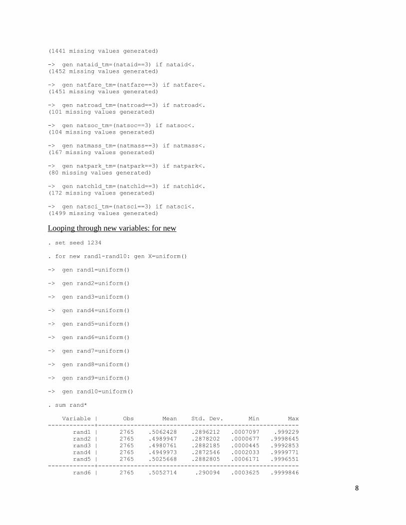
Looping through new variables: for new

. set seed 1234

. for new rand1-rand10: gen X=uniform()

-> gen rand1=uniform()










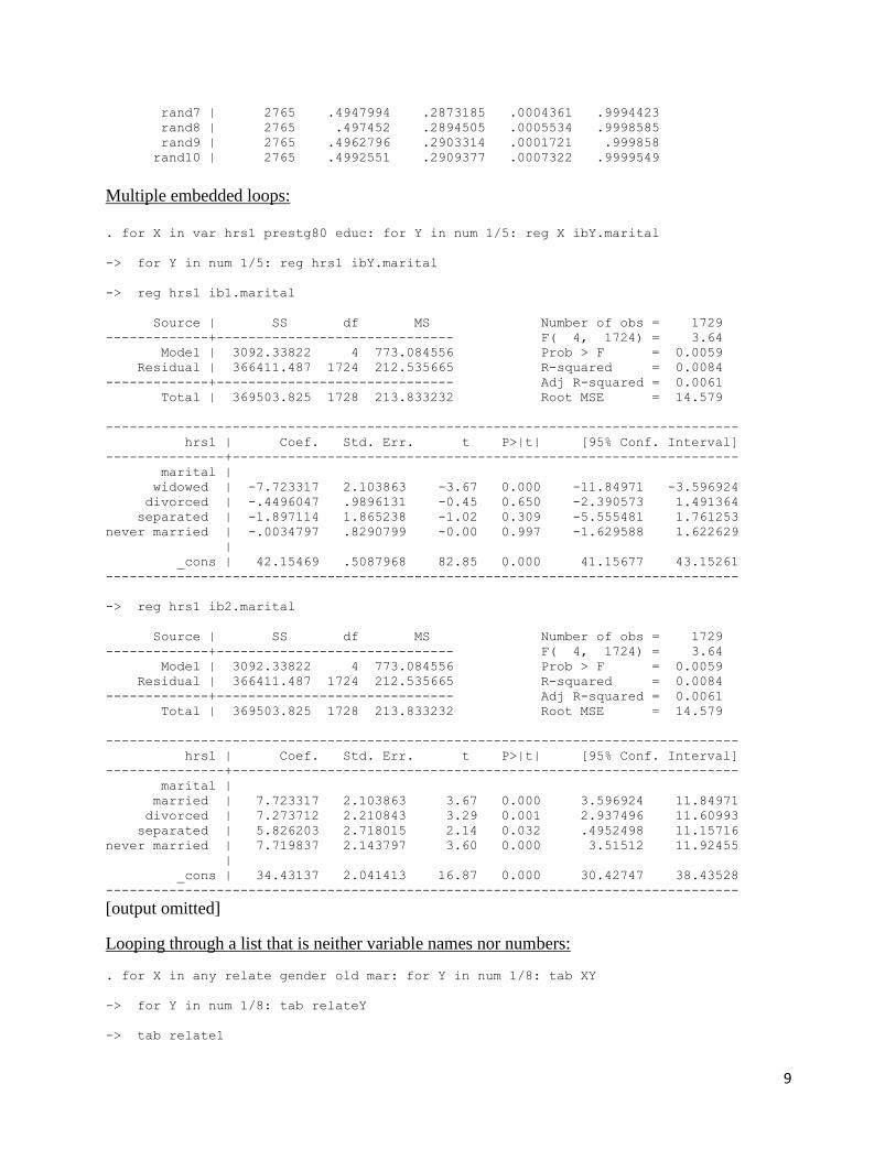
. sum rand*

Variable | Obs Mean Std. Dev. Min Max

-------------+--------------------------------------------------------

rand1 | 2765 .5062428 .2896212 .0007097 .999229

rand2 | 2765 .4989947 .2878202 .0000677 .9998645

rand3 | 2765 .4980761 .2882185 .0000445 .9992853

rand4 | 2765 .4949973 .2872546 .0002033 .9999771

rand5 | 2765 .5025668 .2882805 .0006171 .9996551

-------------+--------------------------------------------------------

rand6 | 2765 .5052714 .290094 .0003625 .9999846

9

rand7 | 2765 .4947994 .2873185 .0004361 .9994423

rand8 | 2765 .497452 .2894505 .0005534 .9998585

rand9 | 2765 .4962796 .2903314 .0001721 .999858

rand10 | 2765 .4992551 .2909377 .0007322 .9999549

Multiple embedded loops:

. for X in var hrs1 prestg80 educ: for Y in num 1/5: reg X ibY.marital

-> for Y in num 1/5: reg hrs1 ibY.marital



-------------+------------------------------ F( 4, 1724) = 3.64

Model | 3092.33822 4 773.084556 Prob > F = 0.0059


-------------+------------------------------ Adj R-squared = 0.0061

Total | 369503.825 1728 213.833232 Root MSE = 14.579

--------------------------------------------------------------------------------


---------------+----------------------------------------------------------------

marital |

widowed | -7.723317 2.103863 -3.67 0.000 -11.84971 -3.596924

divorced | -.4496047 .9896131 -0.45 0.650 -2.390573 1.491364

separated | -1.897114 1.865238 -1.02 0.309 -5.555481 1.761253

never married | -.0034797 .8290799 -0.00 0.997 -1.629588 1.622629

|

_cons | 42.15469 .5087968 82.85 0.000 41.15677 43.15261

--------------------------------------------------------------------------------



-------------+------------------------------ F( 4, 1724) = 3.64

Model | 3092.33822 4 773.084556 Prob > F = 0.0059


-------------+------------------------------ Adj R-squared = 0.0061

Total | 369503.825 1728 213.833232 Root MSE = 14.579

--------------------------------------------------------------------------------


---------------+----------------------------------------------------------------

marital |

married | 7.723317 2.103863 3.67 0.000 3.596924 11.84971

divorced | 7.273712 2.210843 3.29 0.001 2.937496 11.60993

separated | 5.826203 2.718015 2.14 0.032 .4952498 11.15716

never married | 7.719837 2.143797 3.60 0.000 3.51512 11.92455

|

_cons | 34.43137 2.041413 16.87 0.000 30.42747 38.43528

--------------------------------------------------------------------------------

[output omitted]

Looping through a list that is neither variable names nor numbers:

. for X in any relate gender old mar: for Y in num 1/8: tab XY

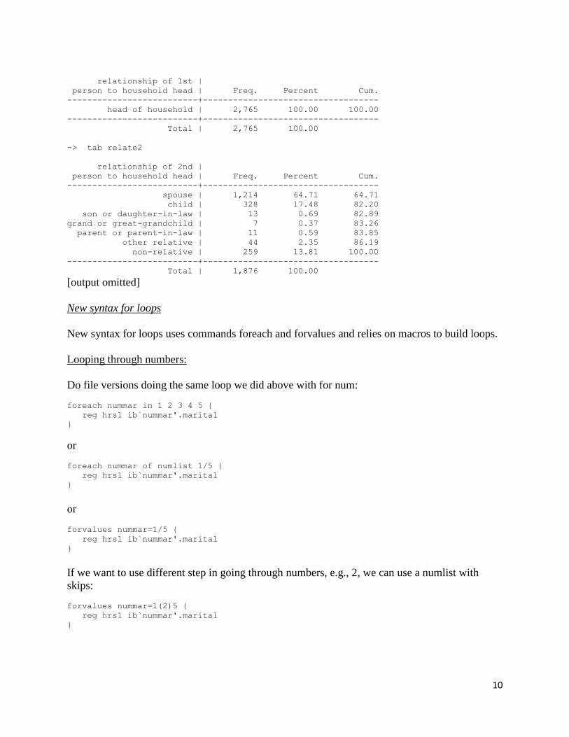
-> for Y in num 1/8: tab relateY

-> tab relate1

10

relationship of 1st |

person to household head | Freq. Percent Cum.

--------------------------+-----------------------------------

head of household | 2,765 100.00 100.00

--------------------------+-----------------------------------

Total | 2,765 100.00

-> tab relate2

relationship of 2nd |

person to household head | Freq. Percent Cum.

--------------------------+-----------------------------------

spouse | 1,214 64.71 64.71

child | 328 17.48 82.20

son or daughter-in-law | 13 0.69 82.89

grand or great-grandchild | 7 0.37 83.26

parent or parent-in-law | 11 0.59 83.85

other relative | 44 2.35 86.19

non-relative | 259 13.81 100.00

--------------------------+-----------------------------------

Total | 1,876 100.00

[output omitted]

New syntax for loops

New syntax for loops uses commands foreach and forvalues and relies on macros to build loops.

Looping through numbers:

Do file versions doing the same loop we did above with for num:

foreach nummar in 1 2 3 4 5 {

reg hrs1 ib`nummar'.marital

}

or

foreach nummar of numlist 1/5 {


}

or

forvalues nummar=1/5 {


}

If we want to use different step in going through numbers, e.g., 2, we can use a numlist with

skips:

forvalues nummar=1(2)5 {


}

11

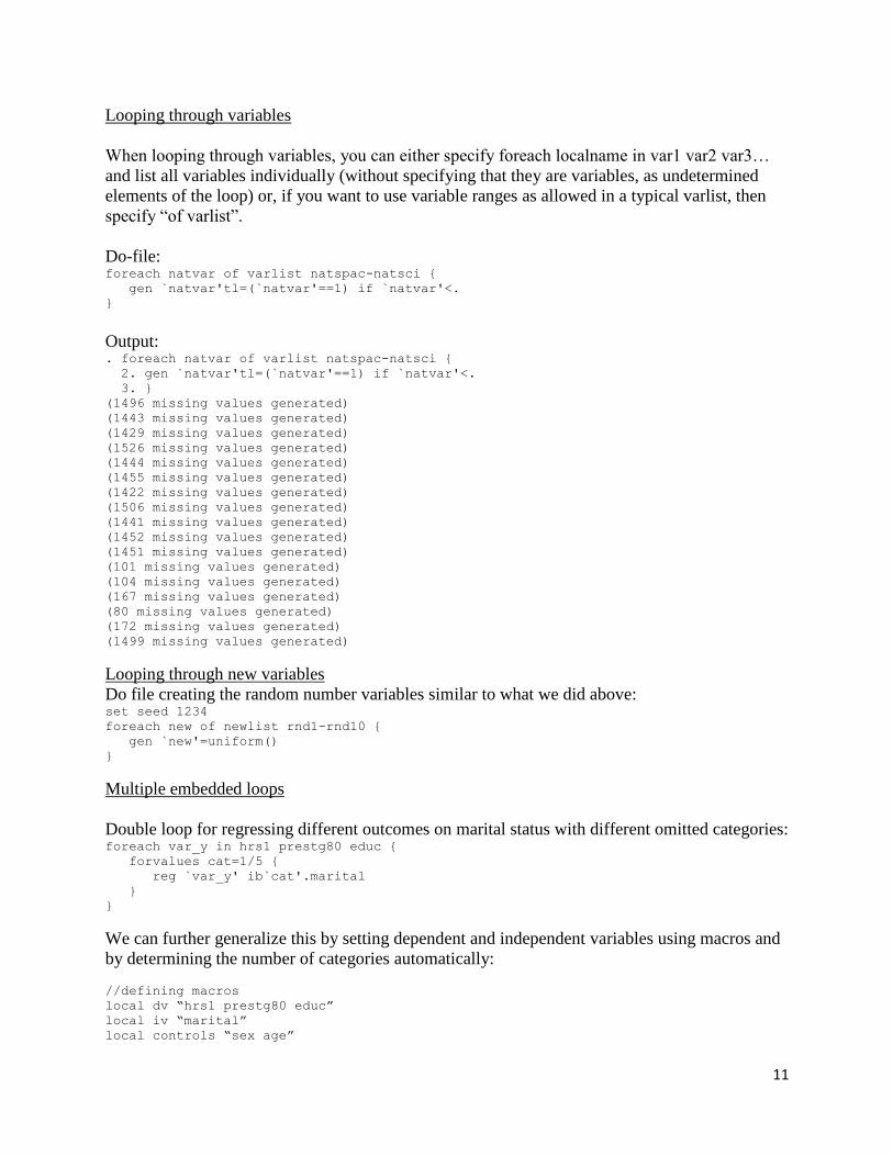
Looping through variables

When looping through variables, you can either specify foreach localname in var1 var2 var3…

and list all variables individually (without specifying that they are variables, as undetermined

elements of the loop) or, if you want to use variable ranges as allowed in a typical varlist, then

specify “of varlist”.

Do-file: foreach natvar of varlist natspac-natsci {

gen `natvar'tl=(`natvar'==1) if `natvar'<.

}

Output: . foreach natvar of varlist natspac-natsci {

2. gen `natvar'tl=(`natvar'==1) if `natvar'<.

3. }


















Looping through new variables

Do file creating the random number variables similar to what we did above: set seed 1234

foreach new of newlist rnd1-rnd10 {

gen `new'=uniform()

}

Multiple embedded loops

Double loop for regressing different outcomes on marital status with different omitted categories: foreach var_y in hrs1 prestg80 educ {

forvalues cat=1/5 {

reg `var_y' ib`cat'.marital

}

}

We can further generalize this by setting dependent and independent variables using macros and

by determining the number of categories automatically:

//defining macros

local dv “hrs1 prestg80 educ”

local iv “marital”

local controls “sex age”

12

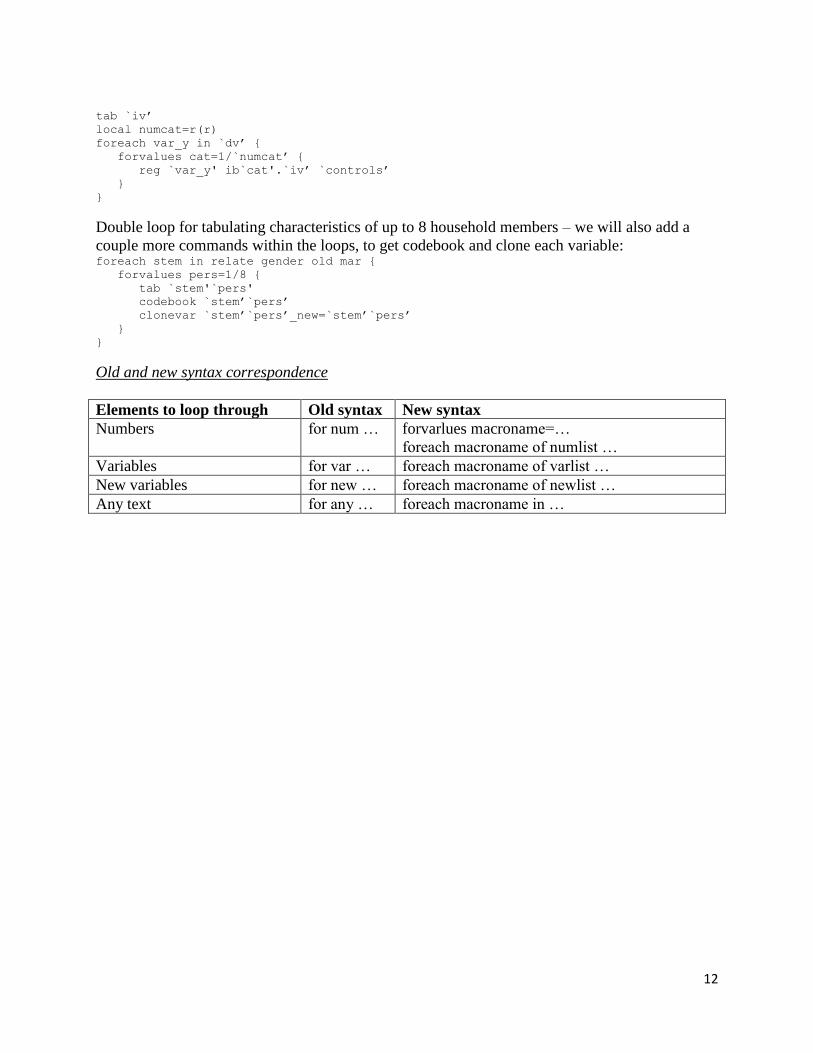
tab ìv’

local numcat=r(r)

foreach var_y in `dv’ {

forvalues cat=1/`numcat’ {

reg `var_y' ib`cat'.ìv’ `controls’

}

}

Double loop for tabulating characteristics of up to 8 household members – we will also add a

couple more commands within the loops, to get codebook and clone each variable: foreach stem in relate gender old mar {

forvalues pers=1/8 {

tab `stem'`pers'

codebook `stem’`pers’

clonevar `stem’`pers’_new=`stem’`pers’

}

}

Old and new syntax correspondence

Elements to loop through Old syntax New syntax

Numbers for num … forvarlues macroname=…

foreach macroname of numlist …

Variables for var … foreach macroname of varlist …

New variables for new … foreach macroname of newlist …

Any text for any … foreach macroname in …

Documents

SOCY7709: Quantitative Data Management Instructor: …Loops Loops help automate repetitive operations, from the simplest to very complex. “Old” syntax examples To define simple