Embed Size (px)
Citation preview
SOCS
User’s GuideRelease 7.1

ii THE BOEING COMPANY M&CT-TECH-01-014
CONTENTS
Contents
1 Introduction 1
2 Nonlinear Optimization 5
2.1 Optimization Background . . . . . . . . . . . . . . . . . . . . . . . . . . . . . . . . . 5
2.1.1 Sequential Quadratic Programming . . . . . . . . . . . . . . . . . . . . . . . . 5
2.1.2 Interior Point Algorithm . . . . . . . . . . . . . . . . . . . . . . . . . . . . . . 9
2.2 Subprograms for Optimization . . . . . . . . . . . . . . . . . . . . . . . . . . . . . . 13
2.3 Optimization Iteration Output . . . . . . . . . . . . . . . . . . . . . . . . . . . . . . 215
2.3.1 SQP Algorithms . . . . . . . . . . . . . . . . . . . . . . . . . . . . . . . . . . 215
2.3.2 Barrier Algorithms . . . . . . . . . . . . . . . . . . . . . . . . . . . . . . . . . 220
2.4 Reverse Communication Program Structure . . . . . . . . . . . . . . . . . . . . . . . 223
3 Finite Difference Derivatives 225
3.1 Mathematical Background . . . . . . . . . . . . . . . . . . . . . . . . . . . . . . . . . 225
3.2 Subprograms for Finite Differences . . . . . . . . . . . . . . . . . . . . . . . . . . . . 235
4 Advanced Usage Examples 297
4.1 Introduction—Advanced Application Examples . . . . . . . . . . . . . . . . . . . . . 297
4.2 Reverse Communication Dense NLP with Finite Difference Derivatives . . . . . . . . 298
4.3 Sparse Finite Differences with Sparse NLP . . . . . . . . . . . . . . . . . . . . . . . . 306
4.4 Sparse Finite Differences with Sparse Least Squares . . . . . . . . . . . . . . . . . . 316
4.5 Diagnostic Line Search Output . . . . . . . . . . . . . . . . . . . . . . . . . . . . . . 326
4.6 Problem Diagnostics using Postoptimality Analysis . . . . . . . . . . . . . . . . . . . 330
5 Optimal Control Background 337
M&CT-TECH-01-014 THE BOEING COMPANY iii
CONTENTS
6 Optimal Control Software 345
6.1 Overview of Sparse Optimal Control Software . . . . . . . . . . . . . . . . . . . . . . 345
6.2 Subprograms for Optimal Control . . . . . . . . . . . . . . . . . . . . . . . . . . . . . 349
6.3 User-Supplied Subprograms for Optimal Control . . . . . . . . . . . . . . . . . . . . 378
6.4 Utility Subprograms for Optimal Control . . . . . . . . . . . . . . . . . . . . . . . . 414
6.5 Optimal Control Error Messages . . . . . . . . . . . . . . . . . . . . . . . . . . . . . 468
6.6 Optimal Control Iteration Output . . . . . . . . . . . . . . . . . . . . . . . . . . . . 476
6.6.1 Sparse NLP Iteration Output . . . . . . . . . . . . . . . . . . . . . . . . . . . 476
6.6.2 Optimal Control Output . . . . . . . . . . . . . . . . . . . . . . . . . . . . . . 477
6.6.3 Differential Equation Output . . . . . . . . . . . . . . . . . . . . . . . . . . . 493
6.6.4 Sparse Finite Difference Output . . . . . . . . . . . . . . . . . . . . . . . . . 494
7 Usage Examples 495
7.1 Linear Tangent Steering Example . . . . . . . . . . . . . . . . . . . . . . . . . . . . . 495
7.1.1 Problem Definition . . . . . . . . . . . . . . . . . . . . . . . . . . . . . . . . . 495
7.1.2 HDSOCS Implementation . . . . . . . . . . . . . . . . . . . . . . . . . . . . . 496
7.2 Generalized Linear Tangent Steering Example . . . . . . . . . . . . . . . . . . . . . . 510
7.2.1 Problem Definition . . . . . . . . . . . . . . . . . . . . . . . . . . . . . . . . . 510
7.2.2 HDSOCS Implementation . . . . . . . . . . . . . . . . . . . . . . . . . . . . . 510
7.3 Workshop Self-Instructional Examples . . . . . . . . . . . . . . . . . . . . . . . . . . 529
7.3.1 Problem 1: Simplified Usage Dense NLP–HDNLPD . . . . . . . . . . . . . . 529
7.3.2 Problem 2: Reverse Communication Dense NLP–HDNLPR . . . . . . . . . . 531
7.3.3 Problem 3: Sparse NLP–HDSNLP . . . . . . . . . . . . . . . . . . . . . . . . 531
7.3.4 Problem 4: Sparse Least Squares–HDSLSQ . . . . . . . . . . . . . . . . . . . 533
7.3.5 Problem 5: Reverse Communication NLP, Finite Difference Gradients . . . . 533
7.3.6 Problem 6: Sparse NLP with Sparse Finite Differences . . . . . . . . . . . . . 534
7.3.7 Problem 7: One Phase Example . . . . . . . . . . . . . . . . . . . . . . . . . 534
7.3.8 Problem 8: User Routines Example . . . . . . . . . . . . . . . . . . . . . . . 535
7.3.9 Problem 9: Path Constraint Example . . . . . . . . . . . . . . . . . . . . . . 535
7.3.10 Problem 10: Quadrature Example . . . . . . . . . . . . . . . . . . . . . . . . 536
7.3.11 Problem 11: Point Function Example . . . . . . . . . . . . . . . . . . . . . . 536
iv THE BOEING COMPANY M&CT-TECH-01-014
CONTENTS
7.3.12 Problem 12: Initial Guess Example . . . . . . . . . . . . . . . . . . . . . . . . 537
7.3.13 Problem 13: Auxilliary Output Example . . . . . . . . . . . . . . . . . . . . . 537
7.3.14 Problem 14: Two Phase Example . . . . . . . . . . . . . . . . . . . . . . . . . 537
7.4 SOCS Demonstration/Test Examples . . . . . . . . . . . . . . . . . . . . . . . . . 538
7.4.1 Zermelo’s Problem . . . . . . . . . . . . . . . . . . . . . . . . . . . . . . . . . 538
7.4.2 Goddard Rocket Problem . . . . . . . . . . . . . . . . . . . . . . . . . . . . . 538
7.4.3 Van der Pol Oscillator Problem . . . . . . . . . . . . . . . . . . . . . . . . . . 538
7.4.4 Maximum Crossrange Space Shuttle Reentry Problem . . . . . . . . . . . . . 541
7.4.5 Minimum Time to Climb Problem . . . . . . . . . . . . . . . . . . . . . . . . 541
7.4.6 Low-Thrust Orbit Transfer . . . . . . . . . . . . . . . . . . . . . . . . . . . . 541
7.4.7 Two-Burn Orbit Transfer . . . . . . . . . . . . . . . . . . . . . . . . . . . . . 542
7.4.8 Industrial Robot . . . . . . . . . . . . . . . . . . . . . . . . . . . . . . . . . . 542
7.4.9 Multibody Mechanism . . . . . . . . . . . . . . . . . . . . . . . . . . . . . . . 542
7.4.10 Heat Flow–Parabolic PDE . . . . . . . . . . . . . . . . . . . . . . . . . . . . . 542
7.4.11 Embedding (Homotopy) Example Problem . . . . . . . . . . . . . . . . . . . 542
7.4.12 Orbit Determination (Parameter Estimation) Example Problem . . . . . . . 543
7.4.13 First-Order Irreversible Chain Reaction Parameter Estimation Problem . . . 543
7.4.14 Initial Value and Shooting Method Example Problems . . . . . . . . . . . . . 543
8 Spline Data Approximations 545
8.1 Overview of Data Fitting and Approximation . . . . . . . . . . . . . . . . . . . . . . 545
8.2 Subprograms for Tensor Product Spline Approximations of Multvariate Data . . . . 546
9 Getting Started 615
A Interface with the NPSOL Optimization Algorithm 617
B The Index Set Array 619
C The MATLAB Toolbox 623
C.1 Introduction . . . . . . . . . . . . . . . . . . . . . . . . . . . . . . . . . . . . . . . . . 623
C.2 Nonlinear optimization . . . . . . . . . . . . . . . . . . . . . . . . . . . . . . . . . . . 623
C.3 Spline Data Approximations . . . . . . . . . . . . . . . . . . . . . . . . . . . . . . . . 639
M&CT-TECH-01-014 THE BOEING COMPANY v

CONTENTS
C.4 Overview of Data Fitting and Approximation . . . . . . . . . . . . . . . . . . . . . . 639
C.5 Subprograms for Tensor Product Spline Approximations of Multivariate Data . . . . 640
C.6 Usage of the Spline Data Approximation . . . . . . . . . . . . . . . . . . . . . . . . . 683
vi THE BOEING COMPANY M&CT-TECH-01-014
LIST OF TABLES
List of Tables
6.1 Software Characteristics . . . . . . . . . . . . . . . . . . . . . . . . . . . . . . . . . . 346
6.2 Setting ITERM(4,j) when ITERM(3,j) = −1 . . . . . . . . . . . . . . . . . . . . . . 395
6.3 Setting ITERM(4,j) when ITERM(3,j) = 0 . . . . . . . . . . . . . . . . . . . . . . . 396
C.1 Aerodynamic data . . . . . . . . . . . . . . . . . . . . . . . . . . . . . . . . . . . . . 683
C.2 Matlab code to calculate linear, quadratic, and cubic approximations. . . . . . . . . 684
C.3 Matlab code for approximation with constant error tolerance. . . . . . . . . . . . . . 685
C.4 Matlab code for approximation with constant error tolerance. . . . . . . . . . . . . . 686
C.5 Matlab code for approximation with adjusted error tolerance. . . . . . . . . . . . . . 687
C.6 Matlab code for approximation without local monotonicity enforced. . . . . . . . . . 689
C.7 Matlab code for approximation with reduced continuity. . . . . . . . . . . . . . . . . 690
M&CT-TECH-01-014 THE BOEING COMPANY vii

LIST OF TABLES
viii THE BOEING COMPANY M&CT-TECH-01-014
List of Subprograms
List of Subprograms
HDNLPD: Dense Nonlinear Programming . . . . . . . . . . . . . . . . . . . . . . . . . . . . . 14
HDNLPR: Dense Nonlinear Programming–Reverse Communication Format . . . . . . . . . . 33
HDSNLP: Sparse Nonlinear Programming . . . . . . . . . . . . . . . . . . . . . . . . . . . . . 51
HDSLSQ: Sparse Constrained Nonlinear Least Squares . . . . . . . . . . . . . . . . . . . . . . 70
HDSQSH: Sparse Quadratic Programming . . . . . . . . . . . . . . . . . . . . . . . . . . . . . 91
HDSNPV: Sparse Nonlinear Programming Parameter Retrieval . . . . . . . . . . . . . . . . . 105
HDBNPD: Dense Barrier Nonlinear Programming . . . . . . . . . . . . . . . . . . . . . . . . 107
HDBNPR: Dense Barrier Nonlinear Programming–Reverse Communication Format . . . . . . 123
HDBNLP: Sparse Barrier Nonlinear Programming . . . . . . . . . . . . . . . . . . . . . . . . 141
HDBLSQ: Sparse Barrier Constrained Nonlinear Least Squares . . . . . . . . . . . . . . . . . 161
HDBLPQ: Sparse Barrier Quadratic Programming . . . . . . . . . . . . . . . . . . . . . . . . 181
HHSNLP: Sparse Nonlinear Programming Input Procedure . . . . . . . . . . . . . . . . . . . 196
HDDFDJ: Dense Finite Difference Jacobian—Reverse Communication Format . . . . . . . . 236
HDDFDH: Finite Difference Jacobian and Hessian—Reverse Communication Format . . . . . 245
HJSFDI: Generate Sparse Finite Difference Index Sets . . . . . . . . . . . . . . . . . . . . . . 256
HDSFDJ: Sparse Finite Difference Jacobian—Reverse Communication Format . . . . . . . . 263
HDSFDH: Sparse Finite Difference Jacobian/Hessian—Reverse Communication Format . . . 276
HDSFDC: Check Sparsity Pattern for Missing Elements—Reverse Communication Format . 288
HDSFDP: Print Out Sparse Matrix . . . . . . . . . . . . . . . . . . . . . . . . . . . . . . . . 293
HDSOCS: Sparse Optimal Control . . . . . . . . . . . . . . . . . . . . . . . . . . . . . . . . . 351
HDSOPE: Sparse Optimal Parameter Estimation . . . . . . . . . . . . . . . . . . . . . . . . . 358
HHSOCS: Sparse Optimal Control Input Procedure . . . . . . . . . . . . . . . . . . . . . . . 365
DDLOAD: Discrete Data Load . . . . . . . . . . . . . . . . . . . . . . . . . . . . . . . . . . . 378
ODEIGS: Optimal Control Initial Guess . . . . . . . . . . . . . . . . . . . . . . . . . . . . . . 381
M&CT-TECH-01-014 THE BOEING COMPANY ix

List of Subprograms
ODEINP: Optimal Control Problem Definition . . . . . . . . . . . . . . . . . . . . . . . . . . 384
ODEPRT: Optimal Control Print . . . . . . . . . . . . . . . . . . . . . . . . . . . . . . . . . . 401
ODEPTF: Optimal Control Point Function Evaluation . . . . . . . . . . . . . . . . . . . . . . 405
ODERHS: Optimal Control Right Hand Side Evaluation . . . . . . . . . . . . . . . . . . . . . 409
AUTOLK: Auto Link Variable Utility . . . . . . . . . . . . . . . . . . . . . . . . . . . . . . . 414
AUTOPL: Auto Phase Length Constraint Utility . . . . . . . . . . . . . . . . . . . . . . . . . 416
AUXOUT: Auxiliary Output Utility . . . . . . . . . . . . . . . . . . . . . . . . . . . . . . . . 418
BSPDEF: B-Spline Algebraic Variable Utility . . . . . . . . . . . . . . . . . . . . . . . . . . . 422
CTLFIL: Optimal Control Input From a File . . . . . . . . . . . . . . . . . . . . . . . . . . . 427
CTLSTA: Optimal Control Software Status Utility . . . . . . . . . . . . . . . . . . . . . . . . 429
FETCH: Variable Retrieval Utility . . . . . . . . . . . . . . . . . . . . . . . . . . . . . . . . . 430
FYLFMT: Restart File Format Conversion Utility . . . . . . . . . . . . . . . . . . . . . . . . 432
LINKST: Optimal Control Linkage Utility . . . . . . . . . . . . . . . . . . . . . . . . . . . . . 435
NUMGRD: Gridpoint Evaluation Utility . . . . . . . . . . . . . . . . . . . . . . . . . . . . . . 437
OCSEVL: Optimal Control Solution Evaluation Utility . . . . . . . . . . . . . . . . . . . . . 439
OCSGRD: Optimal Control Solution Grid Evaluation Utility . . . . . . . . . . . . . . . . . . 443
OCSRNG: Optimal Control Solution Range Utility . . . . . . . . . . . . . . . . . . . . . . . . 445
OCSTAU: Optimal Control Solution Spline Evaluation Utility . . . . . . . . . . . . . . . . . . 447
PHSLNG: Optimal Control Phase Duration Utility . . . . . . . . . . . . . . . . . . . . . . . . 450
PNTCON: Optimal Control Point Constraint Utility . . . . . . . . . . . . . . . . . . . . . . . 452
PTHAUX: Path Constraint with Auxiliary Functions . . . . . . . . . . . . . . . . . . . . . . 455
PTHCON: Path Constraint Utility . . . . . . . . . . . . . . . . . . . . . . . . . . . . . . . . . 458
RST2SP: Restart File to Spline Array Utility . . . . . . . . . . . . . . . . . . . . . . . . . . . 461
SCTFIL: Save an Optimal Control Input File . . . . . . . . . . . . . . . . . . . . . . . . . . . 463
TRMAUX: Terminate Auxiliary Function Construction . . . . . . . . . . . . . . . . . . . . . 465
WATCH: Variable Monitor Utility . . . . . . . . . . . . . . . . . . . . . . . . . . . . . . . . . 467
HDMGDI: Tensor Product Spline Interpolation of Gridded Data . . . . . . . . . . . . . . . . 547
HDGDWH: Tensor Product Spline Approximation of Gridded Data with Holes . . . . . . . . 556
HDCMVS: Constrained Tensor Product Approximation of Multivariate Data . . . . . . . . . 567
HDNPVL: Evaluation of a Tensor Product Spline . . . . . . . . . . . . . . . . . . . . . . . . . 586
HDENVL: Spline Evaluation with Extrapolation . . . . . . . . . . . . . . . . . . . . . . . . . 593
x THE BOEING COMPANY M&CT-TECH-01-014
List of Subprograms
HDFNVL: Fast Spline Evaluation without Error Checking . . . . . . . . . . . . . . . . . . . . 601
HDFEVL: Fast Spline Evaluation with Extrapolation, but without Error Checking . . . . . . 607
SOCS NLP: Local Optimization Method . . . . . . . . . . . . . . . . . . . . . . . . . . . . . . 624
FUNBOX: Function evaluator for SOCS NLP. . . . . . . . . . . . . . . . . . . . . . . . . . . 628
SOCS NLP INIT: Set parameter values for SOCS NLP. . . . . . . . . . . . . . . . . . . . . . 629
callHDNLPR: Shell for calling HDNLPR or HDBNPR. . . . . . . . . . . . . . . . . . . . . . . 632
callHDDFDJ: Shell for calling HDDFDJ. . . . . . . . . . . . . . . . . . . . . . . . . . . . . . 635
callHDDFDH: Shell for calling HDDFDH. . . . . . . . . . . . . . . . . . . . . . . . . . . . . . 637
BCSLIB GDWH: Tensor Product Spline Approximation of Gridded Data with Holes . . . . . 640
BCSLIB GDWH INIT: Set standard values for optional parameters. . . . . . . . . . . . . . . 649
BCSLIB GRIDDATA: Bivariate Spline Approximation and Evaluation. . . . . . . . . . . . . 650
BCSLIB GRIDDATAN: Multivariate Spline Approximation and Evaluation. . . . . . . . . . . 659
BCSLIB NPVL: Evaluation of a Tensor Product Spline . . . . . . . . . . . . . . . . . . . . . 662
BCSLIB FNVL: Fast Evaluation of a Tensor Product Spline without error checking . . . . . 666
BCSLIB ENVL: Evaluation of a Tensor Product Spline with extrapolation . . . . . . . . . . 670
BCSLIB FEVL: Evaluation of a Tensor Product Spline with extrapolation . . . . . . . . . . . 674
BCSLIB CONVERTSPLINE: Convert Matlab structure spline information into an array . . . 678
BCSLIB WRITESPLINE: Write Matlab spline information to a FORTRAN accessible file. . 679
M&CT-TECH-01-014 THE BOEING COMPANY xi

List of Subprograms
xii THE BOEING COMPANY M&CT-TECH-01-014
Chapter 1
Introduction
This document describes software that is available to solve nonlinear optimization, optimal control,and parameter estimation problems with equality and inequality constraints, as well as providenumerical estimates for the requisite function derivatives. The suite of capability in the optimizationlibrary OPTLIB is available on most major hardware.
Chapter 2 describes a suite of algorithms capable of solving problems with nonlinear objectiveand constraint functions. Two fundamentally distinct methods are implemented in the nonlinearprogramming software suite. The first group of routines are based on a sequential quadratic pro-gramming method which is described in Section 2.1. Two distinct methods for solving the quadraticprogramming subproblem are available, one suitable for large sparse applications, the other for smalldense problems. Section 2.2 describes software which implements the method for different levelsof sophistication. The first subroutine HDNLPD (p. 14) is a forward communication algorithmwhich is appropriate for small dense applications with simplified usage requirements. The secondroutine HDNLPR (p. 33) is a reverse communication implementation which permits user suppliedgradient information to be incorporated for dense applications. The third routine HDSNLP (p. 51)is a reverse communication subroutine which accommodates large sparse nonlinear programmingapplications. This general purpose algorithm is more sophisticated to use, as one might expect forvery large sparse applications. The fourth routine HDSLSQ (p. 70) is a reverse communicationsubroutine which accommodates large sparse constrained problems with least squares objectivefunctions. Subroutine HDSQSH (p. 91) is the underlying sparse quadratic programming algorithmused by the higher level nonlinear programming routines.
The second group of routines are based on an interior point method which is described in Section2.1. Section 2.2 describes software that implements the method for different levels of sophistica-tion. Section 2.2 also describes the procedure for setting optional parameters for any algorithm inthe suite. The routine HHSNLP (p. 196) used for optional input of algorithm parameters is dis-cribed. Section 2.3 describes the options available for obtaining iteration output from the suite ofsubroutines. This material describes the optimization software collectively referred to as SPRNLP.
Chapter 3 describes a collection of support algorithms for computing finite difference derivatives.Section 3.1 provides an overview of the methods and introduces the relevant terminology. Softwarefor constructing finite difference derivative approximations when matrix sparsity is not exploitedare documented in Section 3.2. First derivatives of a set of nonlinear functions can be computedusing subroutine HDDFDJ (p. 236). Subroutine HDDFDH (p. 245) can be used to construct finite
M&CT-TECH-01-014 THE BOEING COMPANY 1
Introduction
difference approximations to the second derivative (Hessian) matrix. Subprograms which implementsparse finite differencing techniques are also described in Section 3.2. The first is HJSFDI (p. 256),which determines the partitioning of the variables into index sets that may be used by the othersubroutines in the package. HDSFDJ (p. 263) is the subroutine for computing the Jacobian matrixof the set of functions, i.e., the matrix of first partial derivatives of the functions with respectto the variables. When in addition the second partial derivatives of the functions are needed,HDSFDH (p. 276) will form the Hessian matrix for an arbitrary linear combination of the inputfunctions. For diagnostics, the subroutine HDSFDP (p. 293) is provided to print out either thefull matrices or subsets of them, while HDSFDC (p. 288) can be used to check the input sparsitypattern for missing elements. Finally, Appendix B describes the data structure used to communicateinformation between the subroutines in the finite difference package.
Chapter 4 presents a collection of advanced usage examples which are designed to illustrate featuresof the optimization software suite commonly encountered in scientific applications.
Chapter 5 describes the mathematical background for optimal control problems, and presents abrief overview of the direct transcription method. The Sparse Optimal Control Software (SOCS )package is a collection of FORTRAN 90 subroutines capable of solving optimal control problems.The software suite is described in Chapter 6. The package implements the direct transcription orcollocation method to convert the continuous control problem into a discrete approximation. Thediscretization yields a finite dimensional sparse nonlinear programming problem which can be solvedusing one of the sparse optimization algorithms discussed in Chapter 2. Numerical procedures toimprove the accuracy of the discretization by mesh refinement are implemented in the package.
This document describes Version 7.1 of the SOCS software suite, which supercedes earlier versionsof the software. Release 7.1 of SOCS introduces the following new features:
• The SOCS library incorporates FORTRAN 90 language constructs. Consequently the usermust also use a FORTRAN 90 compiler. Legacy code written in FORTRAN 77 which con-forms to ANSI standards should be compatible with FORTRAN 90, however, nonstandardcompiler extensions may not be applicable. In short, existing FORTRAN 77 implementationsshould be upward compatible.
• The ability to represent an algebraic (control) variable using a finite dimensional B-splineparameterization has been incorporated. See BSPDEF (p. 422) for complete documentation.
• The ability to retrieve user specified quantities using a dynamic “fetch” utility procedure hasbeen incorporated. This process permits the user to retrieve any labeled quantity includingstate, control, adjoint, and residual information. See FETCH (p. 430) and WATCH (p. 467)for complete documentation.
• A new format for all dynamic output has been introduced.
• A new fixed step Runge-Kutta integration option (METHOD = 5, |NSTG(1)| = 6) has beenintroduced. See ODEINP (p. 384) for complete documentation.
• The scattered data tensor product spline procedure HDCMVS (p. 567) incorporates newoptions to utilize either the sparse SQP algorithm HDSNLP (p. 51) or the sparse barrieralgorithm HDBNLP (p. 141).
Chapter 7 presents examples which are designed to illustrate features of the optimal control softwaresuite commonly encountered in scientific applications, and includes a collection of typical application
2 THE BOEING COMPANY M&CT-TECH-01-014
examples. Chapter 8 describes software for constructing spline approximations to tabular data.Chapter 9 presents guidelines for using the tool.
REFERENCES AND FURTHER READING
Each subprogram abstract in this manual assumes that the reader is familiar with the mathematicsand computer science aspects of the functional area that the subprogram supports. Listed beloware a few representative references that a user of BCSLIB may consult for appropriate backgroundmaterial.
Additional information on nonlinear programming can be found in References [7], [6], [16], [17],and [18]. For more information on finite difference techniques consult References [12], and [13].Background on optimal control methods can be found in References [5], [8], [9], [4], [3], [14], [20],[21], and [15]. Information on the mathematical support libraries can be found in [2] and [1].
M&CT-TECH-01-014 THE BOEING COMPANY 3

Introduction
4 THE BOEING COMPANY M&CT-TECH-01-014
Chapter 2
Nonlinear Optimization
2.1 Optimization Background
The Nonlinear Programming Problem (NLP) requires computing the vector x = (x1, x2, . . . , xn)which minimizes the objective function
f(x)
subject to the nonlinear constraints
cL ≤ c(x) ≤ cU
and the simple bounds
xL ≤ x ≤ xU
where c is an m-vector. Equality constraints are imposed by setting cL = cU and variables canbe fixed by setting xL = xU . A point is said to be feasible if the bounds and constraints areboth satisfied. It is assumed that the objective and constraint functions are twice continuouslydifferentiable. Two different algorithms for solving this problem have been implemented and aredescribed in the following subsections.
2.1.1 Sequential Quadratic Programming
A sequential quadratic programming (SQP) method is one approach used to solve the nonlinearprogramming (NLP) problem. The SQP algorithm requires an initial guess x. A new iterate isformed according to the formula
x = x+ αp,
where the vector p is the search direction, and α > 0 is a scalar step length. The search directionp is found by solving a quadratic programming (QP) subproblem defined at the current point x;minimize the quadratic
gT p+1
2pTHp
subject to the linear constraints
ℓ ≤[Gp
p
]≤ u,
M&CT-TECH-01-014 THE BOEING COMPANY 5
Nonlinear Optimization
where ∇xf(x) = g(x) = g is the n-dimensional gradient vector, G is the m × n Jacobian matrixof constraint gradients and H is a symmetric n × n approximation to the Hessian matrix of theLagrangian L = f − λT c− νTx. The upper bound vector is defined by
u =
[cU − c
xU − x
],
with a similar definition for the lower bound vector ℓ, where c(x) = c. Two techniques are availablefor solving the quadratic programming subproblem. When many elements in the Jacobian andHessian matrices are zero the quadratic programming subproblem is efficiently solved using thesparse Schur-Complement Method. For small to moderate size problems with dense Jacobian andHessian matrices, a null-space quadratic programming algorithm is employed.
The Hessian matrix used in the QP subproblem is
H = HL + τ(|σ| + 1)I,
where the Hessian of the Lagrangian is
HL = ∇2xf −
m∑
i=1
λi∇2xci.
Since HL is not necessarily positive definite in the nullspace of the active constraints for a givenQP subproblem, simply using H = HL may cause the QP subproblem to be ill-posed. The strategyis to use H = HL when possible, but to modify HL if necessary. The Levenberg parameter τ ischosen such that 0 ≤ τ ≤ 1 and is normalized using the bound σ for the most negative eigenvalueof HL. Since quadratic convergence of the algorithm can only occur when τ = 0, the parameter isadjusted at every iteration and the rate of decrease is accelerated by monitoring the change in thenorm of the projected gradient.
The software provides four options for constructing an approximation B to the Hessian HL. Thefirst is a symmetric rank-one (SR1) approximation given by
B = B +(w −Bv)(w −Bv)T
(w −Bv)T v
where the differences w = ∇xL(x)−∇xL(x−) and v = x−x− involve the gradients at the previouspoint x−. A second option, the BFGS or Broyden-Fletcher-Goldfarb-Shanno update given by
B = B +wwT
wT v− BvvTB
vTBv
is a symmetric rank-two positive definite approximation. To insure that the approximation remainspositive definite it is necessary to adjust the steplength α such that wT v > 0 and in some casesintroduce a modified update. A third option, the SSQN or Self-scaling Quasi-Newton update isgiven by
B = τB +wwT
wT v− τ
BvvTB
vTBv
where τ = min[1, wT v
vT Bv
]. As a final option the Hessian of the Lagrangian may be approximated
using finite differences, which is achieved using the finite difference methods described in Chapter3. The simplified usage subprogram HDNLPD constructs all first derivative information using the
6 THE BOEING COMPANY M&CT-TECH-01-014
Optimization Background
finite difference procedures HDDFDJ and/or HDDFDH. Finite difference perturbation sizes areselected automatically to balance truncation and roundoff error. Forward difference estimates areutilized when possible for efficiency, and central difference estimates are invoked when necessary toimprove accuracy. The user must supply first and second derivatives for the reverse communicationroutines HDNLPR, HDSNLP and HDSLSQ, and thus it is possible to incorporate analytic and/orsparse difference estimates as desired.
The scalar step length α is adjusted using a line search algorithm to produce a sufficient reductionin an augmented Lagrangian merit function,
M = f − λT (c− s) − νT (x− t) +1
2(c− s)TQ(c− s) +
1
2(x− t)TR(x− t),
where s and t are implicit slack variables for the constraints and bounds, with correspondingLagrange multipliers λ and ν. The diagonal matrices Q and R consist of a set of penalty weightsfor each constraint and bound that are adjusted at each iteration. The decrease in the meritfunction is determined to be “sufficient” if
M(α) −M(0) < µαM ′(0),
where M ′(0) is the slope of the merit function in the search direction evaluated at α = 0 andµ = 10−4. Furthermore a reduction in the slope according to the expression
|M ′(α)| < −δsM ′(0)
is required, where δs ∈ [0, 1) is a user specified slope tolerance.
Algorithm Strategy
The iterative process begins at the initial point x0, and terminates at the solution (or final point)x∗. The path followed by the iterates is determined by the algorithm strategy. Four differentstrategies for locating the solution are implemented.
M Minimize. Beginning at x0 solve a sequence of quadratic programs until the so-lution x∗ is found. For well formulated problems this option may be the mostefficient. Unfortunately since intermediate iterations are neither feasible nor op-timal, premature termination of the algorithm because of formulation difficultiesmay not be helpful in debugging.
FM Feasible Minimize. Find a feasible point then minimize. Beginning at x0 solve a se-quence of quadratic programs to locate a feasible point xf , and then beginning fromxf solve a sequence of quadratic programs until the solution x∗ is found. Locatinga feasible point is often useful since formulation difficulties are quickly identified.Although feasibility is not maintained, subsequent iterates usually remain “nearly”feasible and often this enhances performance. This is the default option.
FME Feasible Minimize Equality. Find a feasible point then minimize subject to equal-ities. Beginning at x0 solve a sequence of quadratic programs to locate a feasiblepoint xf , and then beginning from xf solve a sequence of quadratic programs whilemaintaining feasible equalities until the solution x∗ is found.
F Feasible. Find a feasible point. Beginning at x0 solve a sequence of quadraticprograms to locate a (possibly non-unique) feasible point xf = x∗.
M&CT-TECH-01-014 THE BOEING COMPANY 7
Nonlinear Optimization
The first strategy is probably the most aggressive, and is normally used when the initial guess is“good” and/or the quadratic/linear model for the objective and constraints is “good”. The secondstrategy is the default option, while the FME strategy is probably the most conservative. The finalstrategy F, is useful when formulating a new problem or when optimization is not required.
Convergence Criteria
The solution point x∗ must satisfy the Kuhn-Tucker necessary conditions for a local minimum:
(1) x∗ is feasible, i.e. the constraints and bounds are satisfied;
(2) there exist Lagrange multipliers λ and ν such that
g = GTλ+ ν;
(3) the Lagrange multiplier for a constraint or variable active at its lower bound must be non-negative;
(4) the Lagrange multiplier for a constraint or variable active at its upper bound must be non-positive;
(5) the Lagrange multiplier for a strictly feasible constraint or free variable must be zero.
In general it may not be possible or desirable to satisfy the Kuhn-Tucker conditions exactly becauseof limited precision in the computed quantities. Instead, the algorithm is terminated at a pointx ≈ x∗. For a given set of tolerances (δc, δo, δp) the point x is considered an estimate of the truesolution x∗ when it satisfies the following conditions:
(a) it must be feasible, that is,cL − δc ≤ c(x) ≤ cU + δc,
xL − δc ≤ x ≤ xU + δc;
(b) it must satisfy the optimality conditions,
‖g −GTλ− ν‖∞ < δp max[1, ‖g‖∞];
(c) the current objective f and predicted minimum must be within tolerance,
|f − f∗| = |gT p+1
2pTHp| < δo;
(d) the steplength must be within tolerance,
maxi
[α|pi|
1 + |xi|
]<
[δo
1 + |f |
] 12
;
(e) the Lagrange multipliers for the inequalities must have the correct sign,
νi ≥ 0 for xi = xLi;
νi ≤ 0 for xi = xUi;
λi ≥ 0 for ci = cLi;
λi ≤ 0 for ci = cUi.
8 THE BOEING COMPANY M&CT-TECH-01-014
Optimization Background
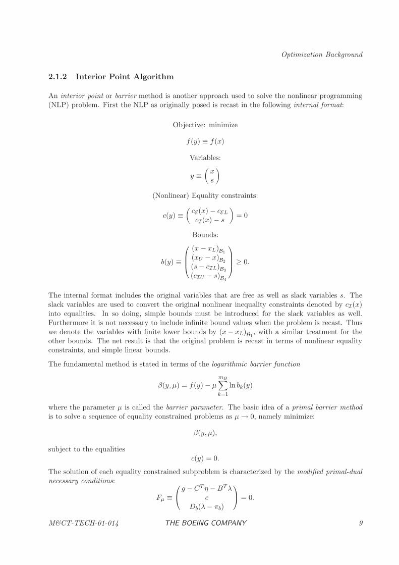
2.1.2 Interior Point Algorithm
An interior point or barrier method is another approach used to solve the nonlinear programming(NLP) problem. First the NLP as originally posed is recast in the following internal format:
Objective: minimize
f(y) ≡ f(x)
Variables:
y ≡(xs
)
(Nonlinear) Equality constraints:
c(y) ≡(cE(x) − cEL
cI(x) − s
)= 0
Bounds:
b(y) ≡
(x− xL)B1
(xU − x)B2
(s− cIL)B3
(cIU − s)B4
≥ 0.
The internal format includes the original variables that are free as well as slack variables s. Theslack variables are used to convert the original nonlinear inequality constraints denoted by cI(x)into equalities. In so doing, simple bounds must be introduced for the slack variables as well.Furthermore it is not necessary to include infinite bound values when the problem is recast. Thuswe denote the variables with finite lower bounds by (x− xL)B1
, with a similar treatment for theother bounds. The net result is that the original problem is recast in terms of nonlinear equalityconstraints, and simple linear bounds.
The fundamental method is stated in terms of the logarithmic barrier function
β(y, µ) = f(y) − µmB∑
k=1
ln bk(y)
where the parameter µ is called the barrier parameter. The basic idea of a primal barrier methodis to solve a sequence of equality constrained problems as µ→ 0, namely minimize:
β(y, µ),
subject to the equalitiesc(y) = 0.
The solution of each equality constrained subproblem is characterized by the modified primal-dualnecessary conditions:
Fµ ≡
g − CT η −BTλ
cDb(λ− πb)
= 0.
M&CT-TECH-01-014 THE BOEING COMPANY 9
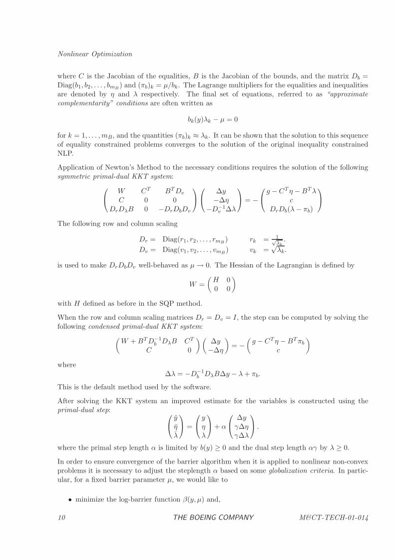
Nonlinear Optimization
where C is the Jacobian of the equalities, B is the Jacobian of the bounds, and the matrix Db =Diag(b1, b2, . . . , bmB
) and (πb)k = µ/bk. The Lagrange multipliers for the equalities and inequalitiesare denoted by η and λ respectively. The final set of equations, referred to as “approximatecomplementarity” conditions are often written as
bk(y)λk − µ = 0
for k = 1, . . . ,mB, and the quantities (πb)k ≈ λk. It can be shown that the solution to this sequenceof equality constrained problems converges to the solution of the original inequality constrainedNLP.
Application of Newton’s Method to the necessary conditions requires the solution of the followingsymmetric primal-dual KKT system:
W CT BTDv
C 0 0DrDλB 0 −DrDbDv
∆y−∆η
−D−1v ∆λ
= −
g − CT η −BTλ
cDrDb(λ− πb)
The following row and column scaling
Dr = Diag(r1, r2, . . . , rmB) rk = 1√
λk.
Dv = Diag(v1, v2, . . . , vmB) vk =
√λk.
is used to make DrDbDv well-behaved as µ→ 0. The Hessian of the Lagrangian is defined by
W =
(H 00 0
)
with H defined as before in the SQP method.
When the row and column scaling matrices Dr = Dv = I, the step can be computed by solving thefollowing condensed primal-dual KKT system:
(W +BTD−1
b DλB CT
C 0
)(∆y−∆η
)= −
(g −CT η −BTπb
c
)
where∆λ = −D−1
b DλB∆y − λ+ πb.
This is the default method used by the software.
After solving the KKT system an improved estimate for the variables is constructed using theprimal-dual step:
yηλ
=
yηλ
+ α
∆yγ∆ηγ∆λ
.
where the primal step length α is limited by b(y) ≥ 0 and the dual step length αγ by λ ≥ 0.
In order to ensure convergence of the barrier algorithm when it is applied to nonlinear non-convexproblems it is necessary to adjust the steplength α based on some globalization criteria. In partic-ular, for a fixed barrier parameter µ, we would like to
• minimize the log-barrier function β(y, µ) and,
10 THE BOEING COMPANY M&CT-TECH-01-014
Optimization Background
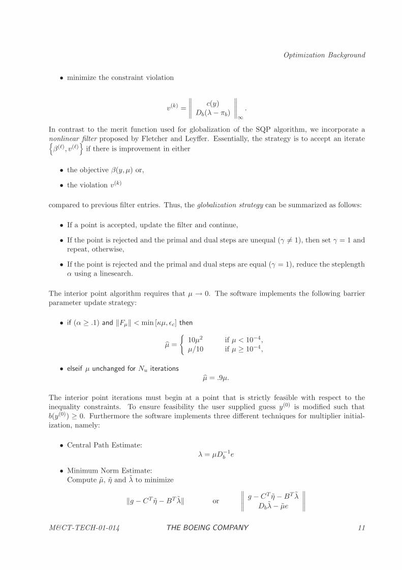
• minimize the constraint violation
v(k) =
∥∥∥∥∥c(y)
Db(λ− πb)
∥∥∥∥∥∞.
In contrast to the merit function used for globalization of the SQP algorithm, we incorporate anonlinear filter proposed by Fletcher and Leyffer. Essentially, the strategy is to accept an iterate{β(ℓ), v(ℓ)
}if there is improvement in either
• the objective β(y, µ) or,
• the violation v(k)
compared to previous filter entries. Thus, the globalization strategy can be summarized as follows:
• If a point is accepted, update the filter and continue,
• If the point is rejected and the primal and dual steps are unequal (γ 6= 1), then set γ = 1 andrepeat, otherwise,
• If the point is rejected and the primal and dual steps are equal (γ = 1), reduce the steplengthα using a linesearch.
The interior point algorithm requires that µ → 0. The software implements the following barrierparameter update strategy:
• if (α ≥ .1) and ‖Fµ‖ < min [κµ, ǫc] then
µ =
{10µ2 if µ < 10−4,µ/10 if µ ≥ 10−4,
• elseif µ unchanged for Nu iterations
µ = .9µ.
The interior point iterations must begin at a point that is strictly feasible with respect to theinequality constraints. To ensure feasibility the user supplied guess y(0) is modified such thatb(y(0)) ≥ 0. Furthermore the software implements three different techniques for multiplier initial-ization, namely:
• Central Path Estimate:λ = µD−1
b e
• Minimum Norm Estimate:Compute µ, η and λ to minimize
‖g − CT η −BT λ‖ or
∥∥∥∥∥g − CT η −BT λ
Dbλ− µe
∥∥∥∥∥
M&CT-TECH-01-014 THE BOEING COMPANY 11
Nonlinear Optimization
To ensure the multipliers are feasible the initial values λ are modified such that λ ≥ 0.
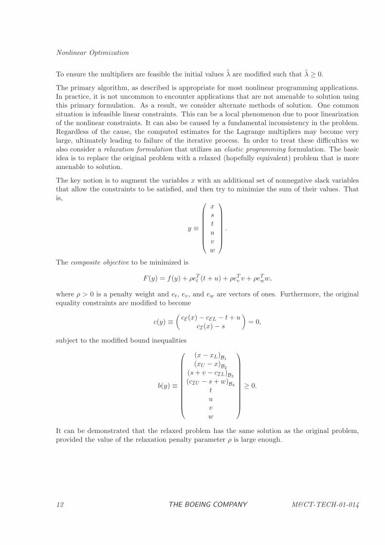
The primary algorithm, as described is appropriate for most nonlinear programming applications.In practice, it is not uncommon to encounter applications that are not amenable to solution usingthis primary formulation. As a result, we consider alternate methods of solution. One commonsituation is infeasible linear constraints. This can be a local phenomenon due to poor linearizationof the nonlinear constraints. It can also be caused by a fundamental inconsistency in the problem.Regardless of the cause, the computed estimates for the Lagrange multipliers may become verylarge, ultimately leading to failure of the iterative process. In order to treat these difficulties wealso consider a relaxation formulation that utilizes an elastic programming formulation. The basicidea is to replace the original problem with a relaxed (hopefully equivalent) problem that is moreamenable to solution.
The key notion is to augment the variables x with an additional set of nonnegative slack variablesthat allow the constraints to be satisfied, and then try to minimize the sum of their values. Thatis,
y ≡
xstuvw
.
The composite objective to be minimized is
F (y) = f(y) + ρeTt (t+ u) + ρeTv v + ρeTww,
where ρ > 0 is a penalty weight and et, ev, and ew are vectors of ones. Furthermore, the originalequality constraints are modified to become
c(y) ≡(cE(x) − cEL − t+ u
cI(x) − s
)= 0,
subject to the modified bound inequalities
b(y) ≡
(x− xL)B1
(xU − x)B2
(s+ v − cIL)B3
(cIU − s+w)B4
tuvw
≥ 0.
It can be demonstrated that the relaxed problem has the same solution as the original problem,provided the value of the relaxation penalty parameter ρ is large enough.
12 THE BOEING COMPANY M&CT-TECH-01-014
Subprograms for Optimization
2.2 Subprograms for Optimization
SQP Subprograms
HDNLPD: Dense Nonlinear Programming . . . . . . . . . . . . . . . . . . . . . . . . . . . . . 14
HDNLPR: Dense Nonlinear Programming–Reverse Communication Format . . . . . . . . . . 33
HDSNLP: Sparse Nonlinear Programming . . . . . . . . . . . . . . . . . . . . . . . . . . . . . 51
HDSLSQ: Sparse Constrained Nonlinear Least Squares . . . . . . . . . . . . . . . . . . . . . . 70
HDSQSH: Sparse Quadratic Programming . . . . . . . . . . . . . . . . . . . . . . . . . . . . . 91
HDSNPV: Sparse Nonlinear Programming Parameter Retrieval . . . . . . . . . . . . . . . . . 105
Barrier Subprograms
HDBNPD: Dense Barrier Nonlinear Programming . . . . . . . . . . . . . . . . . . . . . . . . 107
HDBNPR: Dense Barrier Nonlinear Programming–Reverse Communication Format . . . . . . 123
HDBNLP: Sparse Barrier Nonlinear Programming . . . . . . . . . . . . . . . . . . . . . . . . 141
HDBLSQ: Sparse Barrier Constrained Nonlinear Least Squares . . . . . . . . . . . . . . . . . 161
HDBLPQ: Sparse Barrier Quadratic Programming . . . . . . . . . . . . . . . . . . . . . . . . 181
Optional Algorithm Parameters
HHSNLP: Sparse Nonlinear Programming Input Procedure . . . . . . . . . . . . . . . . . . . 196
M&CT-TECH-01-014 THE BOEING COMPANY 13
Nonlinear Optimization
HDNLPD: Dense Nonlinear Programming
PURPOSE
HDNLPD computes the vector x = (x1, x2, . . . , xn) which minimizes the objective function
f(x)
subject to the m nonlinear constraints
cL ≤ c(x) ≤ cU
and the simple bounds
xL ≤ x ≤ xU
Equality constraints are imposed by setting cLi = cUi and variables can be fixed by setting xLi =xUi. HDNLPD works under the assumption that the objective and constraint functions are twicecontinuously differentiable, and if this is not true algorithm performance is unpredictable. HDNLPDuses a forward communication format and the user must supply a subroutine to compute thevalues of the objective and constraint functions. First and second derivatives of the user suppliedfunctions are computed numerically. The matrix of second derivatives (Hessian of the Lagrangian)can be constructed using a quasi-Newton recursive estimate or by central differencing. SubroutineHDNLPD calls the sparse nonlinear programming algorithm HDSNLP, and is intended for simplifiedusage as appropriate for small dense problems.
RELATED SUBPROGRAMS
HDDFDJ Finite Difference Jacobian
HDDFDH Finite Difference Hessian
HDBNPD Dense Barrier Nonlinear Programming
HDSNLP Sparse Nonlinear Programming
HHSNLP Sparse Nonlinear Programming Input Procedure
METHOD
A sequential quadratic programming (SQP) approach is used to solve the nonlinear programming(NLP) problem. Although the dense null-space method is the default, the Schur-complementmethod can be selected to solve the quadratic programming subproblem. HDNLPD provides fouralternatives for constructing an approximation to the Hessian matrix which are described in thebackground section of this document. The default is a symmetric rank-one (SR1) approximation,with options for using a BFGS, SSQN, or finite difference estimate instead. HDNLPD constructsall first derivative information using the finite difference procedures HDDFDJ and/or HDDFDH.Finite difference perturbation sizes are selected automatically to balance truncation and roundofferror. Forward difference estimates are utilized when possible for efficiency, and central differenceestimates are invoked when necessary to improve accuracy. Although default values are set for allalgorithm parameters, HHSNLP can be utilized to override the defaults.
14 THE BOEING COMPANY M&CT-TECH-01-014
Subprograms for Optimization
WARNING
The objective function and constraints supplied by the user are assumed to be continuous andhave continuous first and second derivatives. Nondifferentiable functions can cause unpredictableperformance in the optimization algorithm. It should be emphasized that discontinuities in theHessian matrices can significantly degrade the speed of convergence without producing any otherobvious difficulties. The following common sources of error should be avoided when evaluating theobjective and constraint functions:
(1) nonsmooth interpolation of data;
(2) iterative procedures inside the function evaluation process, such as adaptive quadrature or rootsolving;
(3) discontinuous behavior caused by branching for IF tests;
(4) nondifferentiable functions such as ABS, MAX, and MIN.
The user must provide a procedure to evaluate the objective and constraint functions. If it is notpossible to evaluate the functions (for example, c(x) = 1/x at x = 0) then set IFERR = 1 andexit the function evaluation process. Otherwise, set IFERR = 0 when the functions are evaluated.The function error flag should be used to avoid computational difficulties, but never in lieu of anexplicit constraint.
The HDNLPD software uses internal common blocks to communicate information. To avoid con-flict with these internal commons the user should not have commons with the following names:NPSPRR, NPSPRI, NPSPRC, STATIS, KONSTN, NPSALG, NPSDFL, NLPERR, PERCOM,ITEREF, and CLKCOM.
USAGE
INTEGER IER, NDIM, MCON, NHOLD, NIHOLD, NEEDED
INTEGER ISTATV(NDIM), ISTATC(MCON), IHOLD(NIHOLD)
DOUBLE PRECISION FBAR, XBAR(NDIM), XLWR(NDIM), XUPR(NDIM), VECNU(NDIM)
DOUBLE PRECISION CBAR(MCON), CLWR(MCON), CUPR(MCON)
DOUBLE PRECISION VECLAM(MCON), HOLD(NHOLD)
EXTERNAL FUNBOX
CALL HDNLPD(FUNBOX, XBAR, XLWR, XUPR, ISTATV, VECNU, NDIM,
$ FBAR, CBAR, CLWR, CUPR, ISTATC, VECLAM, MCON,
$ HOLD, NHOLD, IHOLD, NIHOLD, NEEDED, IER)
ARGUMENTS
FUNCTION EVALUATION PROCEDURE
FUNBOX [INPUT, SUBROUTINE]
M&CT-TECH-01-014 THE BOEING COMPANY 15
Nonlinear Optimization
Name of user-supplied subroutine to evaluate objective and constraint functions;see USER-SUPPLIED SUBPROGRAM
INDEPENDENT VARIABLE DATA
XBAR [INPUT/OUTPUT, DOUBLE PRECISION, ARRAY]A real array of length NDIM of current variable values x. An initial guess mustbe input. When IER = 0, +101, the final point corresponds to a local optimum.When IER = +104, . . . , +111, +114, +116, +117, +119, the final point is eitherthe best feasible point if one has been found, or the last iterate.
XLWR [INPUT, DOUBLE PRECISION, ARRAY]A real array of length NDIM containing the variable lower bounds xL. For variablesthat have no lower bound set xLi ≤ −.01/HDMCON(5). See Section 2.2 of theBCSLIB Manual [2] for HDMCON.
XUPR [INPUT, DOUBLE PRECISION, ARRAY]A real array of length NDIM containing the variable upper bounds xUi. For vari-ables that have no upper bound set xUi ≥ .01/HDMCON(5).
ISTATV [INPUT/OUTPUT, INTEGER, ARRAY]An integer array of length NDIM indicating variable status. On input ISTATVdefines an estimate of the active variable bounds, and on output ISTATV definesthe bounds active at the solution.
ISTATV(i)= 0 Variable is strictly feasible, i.e. xLi < xi < xUi.
ISTATV(i)= 1 Variable lower bound is active, i.e. xLi = xi.
ISTATV(i)= 2 Variable upper bound is active, i.e. xi = xUi.
ISTATV(i)= 3 Fixed permanently.
ISTATV(i)= 10 Output only: Violated variable lower bound, i.e. xLi−δc > xi.
ISTATV(i)= 20 Output only: Violated variable upper bound, i.e. xi > xUi+δc.
ISTATV(i)= 30 Output only: Violated fixed variable. Either xi < xLi − δc orxi > xUi + δc.
When ISTATV(i) = 3 it is necessary that xLi = xUi where xLi = XLWR(i) andxUi = XUPR(i). When ISTATV(i) 6= 3, it is necessary that xLi < xUi with|xLi − xUi| > δc.
VECNU [INPUT/OUTPUT, DOUBLE PRECISION, ARRAY]An array of length NDIM of bound multipliers ν.
NDIM [INPUT, INTEGER]Number of variables, where NDIM ≥ 1.
OBJECTIVE FUNCTION DATA
16 THE BOEING COMPANY M&CT-TECH-01-014
Subprograms for Optimization
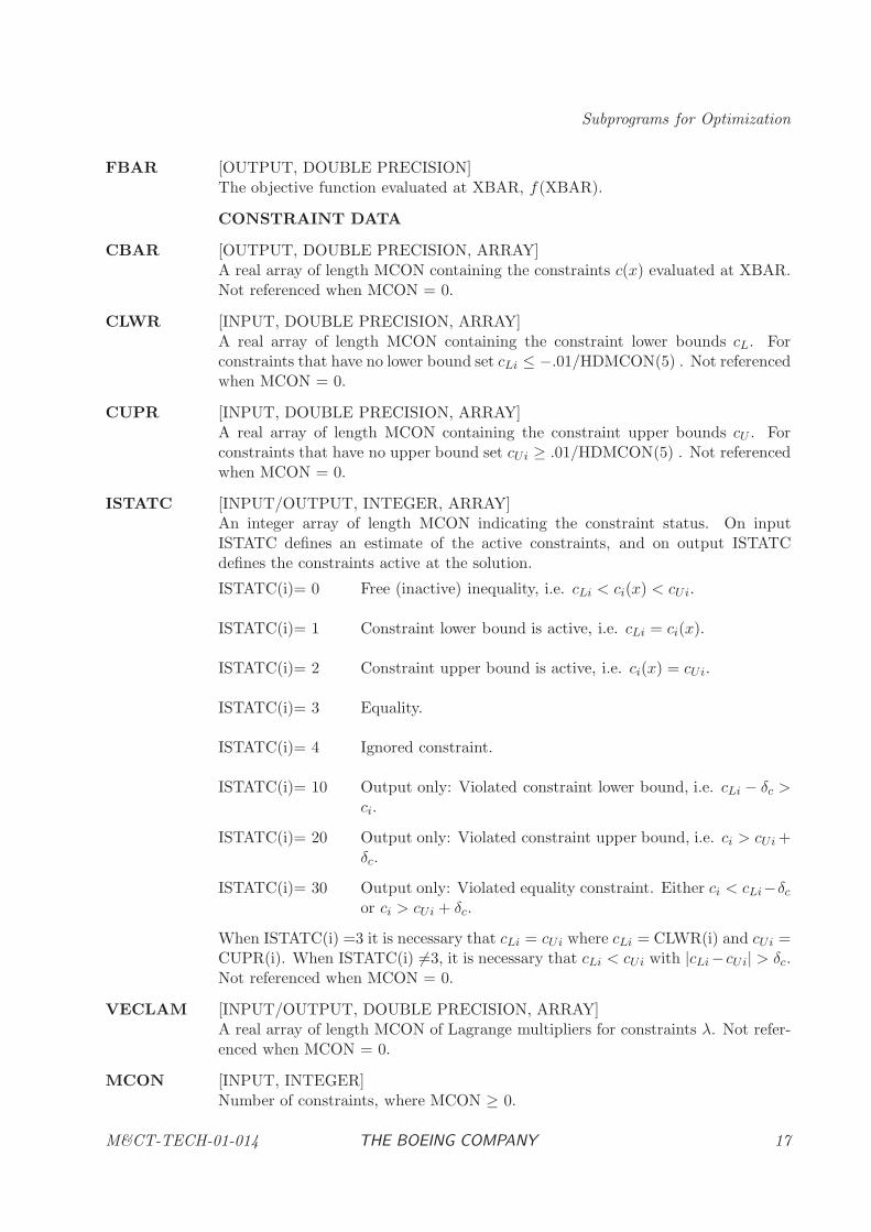
FBAR [OUTPUT, DOUBLE PRECISION]The objective function evaluated at XBAR, f(XBAR).
CONSTRAINT DATA
CBAR [OUTPUT, DOUBLE PRECISION, ARRAY]A real array of length MCON containing the constraints c(x) evaluated at XBAR.Not referenced when MCON = 0.
CLWR [INPUT, DOUBLE PRECISION, ARRAY]A real array of length MCON containing the constraint lower bounds cL. Forconstraints that have no lower bound set cLi ≤ −.01/HDMCON(5) . Not referencedwhen MCON = 0.
CUPR [INPUT, DOUBLE PRECISION, ARRAY]A real array of length MCON containing the constraint upper bounds cU . Forconstraints that have no upper bound set cUi ≥ .01/HDMCON(5) . Not referencedwhen MCON = 0.
ISTATC [INPUT/OUTPUT, INTEGER, ARRAY]An integer array of length MCON indicating the constraint status. On inputISTATC defines an estimate of the active constraints, and on output ISTATCdefines the constraints active at the solution.
ISTATC(i)= 0 Free (inactive) inequality, i.e. cLi < ci(x) < cUi.
ISTATC(i)= 1 Constraint lower bound is active, i.e. cLi = ci(x).
ISTATC(i)= 2 Constraint upper bound is active, i.e. ci(x) = cUi.
ISTATC(i)= 3 Equality.
ISTATC(i)= 4 Ignored constraint.
ISTATC(i)= 10 Output only: Violated constraint lower bound, i.e. cLi − δc >ci.
ISTATC(i)= 20 Output only: Violated constraint upper bound, i.e. ci > cUi +δc.
ISTATC(i)= 30 Output only: Violated equality constraint. Either ci < cLi−δcor ci > cUi + δc.
When ISTATC(i) =3 it is necessary that cLi = cUi where cLi = CLWR(i) and cUi =CUPR(i). When ISTATC(i) 6=3, it is necessary that cLi < cUi with |cLi−cUi| > δc.Not referenced when MCON = 0.
VECLAM [INPUT/OUTPUT, DOUBLE PRECISION, ARRAY]A real array of length MCON of Lagrange multipliers for constraints λ. Not refer-enced when MCON = 0.
MCON [INPUT, INTEGER]Number of constraints, where MCON ≥ 0.
M&CT-TECH-01-014 THE BOEING COMPANY 17
Nonlinear Optimization
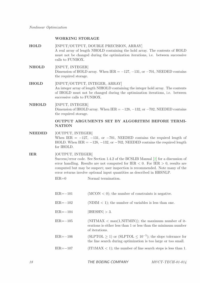
WORKING STORAGE
HOLD [INPUT/OUTPUT, DOUBLE PRECISION, ARRAY]A real array of length NHOLD containing the hold array. The contents of HOLDmust not be changed during the optimization iterations, i.e. between successivecalls to FUNBOX.
NHOLD [INPUT, INTEGER]Dimension of HOLD array. When IER = −127, −131, or −701, NEEDED containsthe required storage.
IHOLD [INPUT/OUTPUT, INTEGER, ARRAY]An integer array of length NIHOLD containing the integer hold array. The contentsof IHOLD must not be changed during the optimization iterations, i.e. betweensuccessive calls to FUNBOX.
NIHOLD [INPUT, INTEGER]Dimension of IHOLD array. When IER = −128, −132, or −702, NEEDED containsthe required storage.
OUTPUT ARGUMENTS SET BY ALGORITHM BEFORE TERMI-NATION
NEEDED [OUTPUT, INTEGER]When IER = −127, −131, or −701, NEEDED contains the required length ofHOLD. When IER = −128, −132, or −702, NEEDED contains the required lengthfor IHOLD.
IER [OUTPUT, INTEGER]Success/error code. See Section 1.4.2 of the BCSLIB Manual [2] for a discussion oferror handling. Results are not computed for IER < 0. For IER > 0, results arecomputed but may be suspect; user inspection is recommended. Note many of theerror returns involve optional input quantities as described in HHSNLP.
IER=0 Normal termination.
IER=−101 (MCON < 0); the number of constraints is negative.
IER=−102 (NDIM < 1); the number of variables is less than one.
IER=−104 |IHESHN| > 3.
IER=−105 (NITMAX < max(1,NITMIN)); the maximum number of it-erations is either less than 1 or less than the minimum numberof iterations.
IER=−106 (SLPTOL ≥ 1) or (SLPTOL ≤ 10−5); the slope tolerance forthe line search during optimization is too large or too small.
IER=−107 (IT1MAX < 1); the number of line search steps is less than 1.
18 THE BOEING COMPANY M&CT-TECH-01-014
Subprograms for Optimization
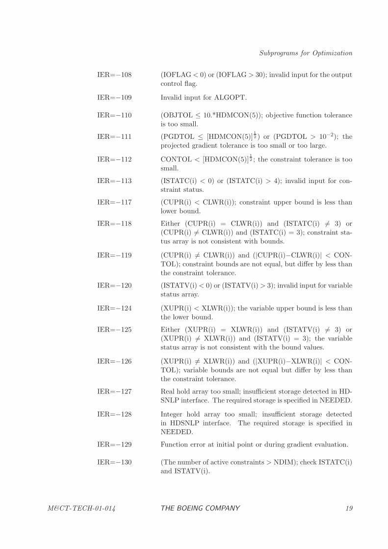
IER=−108 (IOFLAG< 0) or (IOFLAG > 30); invalid input for the outputcontrol flag.
IER=−109 Invalid input for ALGOPT.
IER=−110 (OBJTOL ≤ 10.*HDMCON(5)); objective function toleranceis too small.
IER=−111 (PGDTOL ≤ [HDMCON(5)]12 ) or (PGDTOL > 10−2); the
projected gradient tolerance is too small or too large.
IER=−112 CONTOL < [HDMCON(5)]12 ; the constraint tolerance is too
small.
IER=−113 (ISTATC(i) < 0) or (ISTATC(i) > 4); invalid input for con-straint status.
IER=−117 (CUPR(i) < CLWR(i)); constraint upper bound is less thanlower bound.
IER=−118 Either (CUPR(i) = CLWR(i)) and (ISTATC(i) 6= 3) or(CUPR(i) 6= CLWR(i)) and (ISTATC(i) = 3); constraint sta-tus array is not consistent with bounds.
IER=−119 (CUPR(i) 6= CLWR(i)) and (|CUPR(i)−CLWR(i)| < CON-TOL); constraint bounds are not equal, but differ by less thanthe constraint tolerance.
IER=−120 (ISTATV(i)< 0) or (ISTATV(i) > 3); invalid input for variablestatus array.
IER=−124 (XUPR(i) < XLWR(i)); the variable upper bound is less thanthe lower bound.
IER=−125 Either (XUPR(i) = XLWR(i)) and (ISTATV(i) 6= 3) or(XUPR(i) 6= XLWR(i)) and (ISTATV(i) = 3); the variablestatus array is not consistent with the bound values.
IER=−126 (XUPR(i) 6= XLWR(i)) and (|XUPR(i)−XLWR(i)| < CON-TOL); variable bounds are not equal but differ by less thanthe constraint tolerance.
IER=−127 Real hold array too small; insufficient storage detected in HD-SNLP interface. The required storage is specified in NEEDED.
IER=−128 Integer hold array too small; insufficient storage detectedin HDSNLP interface. The required storage is specified inNEEDED.
IER=−129 Function error at initial point or during gradient evaluation.
IER=−130 (The number of active constraints > NDIM); check ISTATC(i)and ISTATV(i).
M&CT-TECH-01-014 THE BOEING COMPANY 19
Nonlinear Optimization
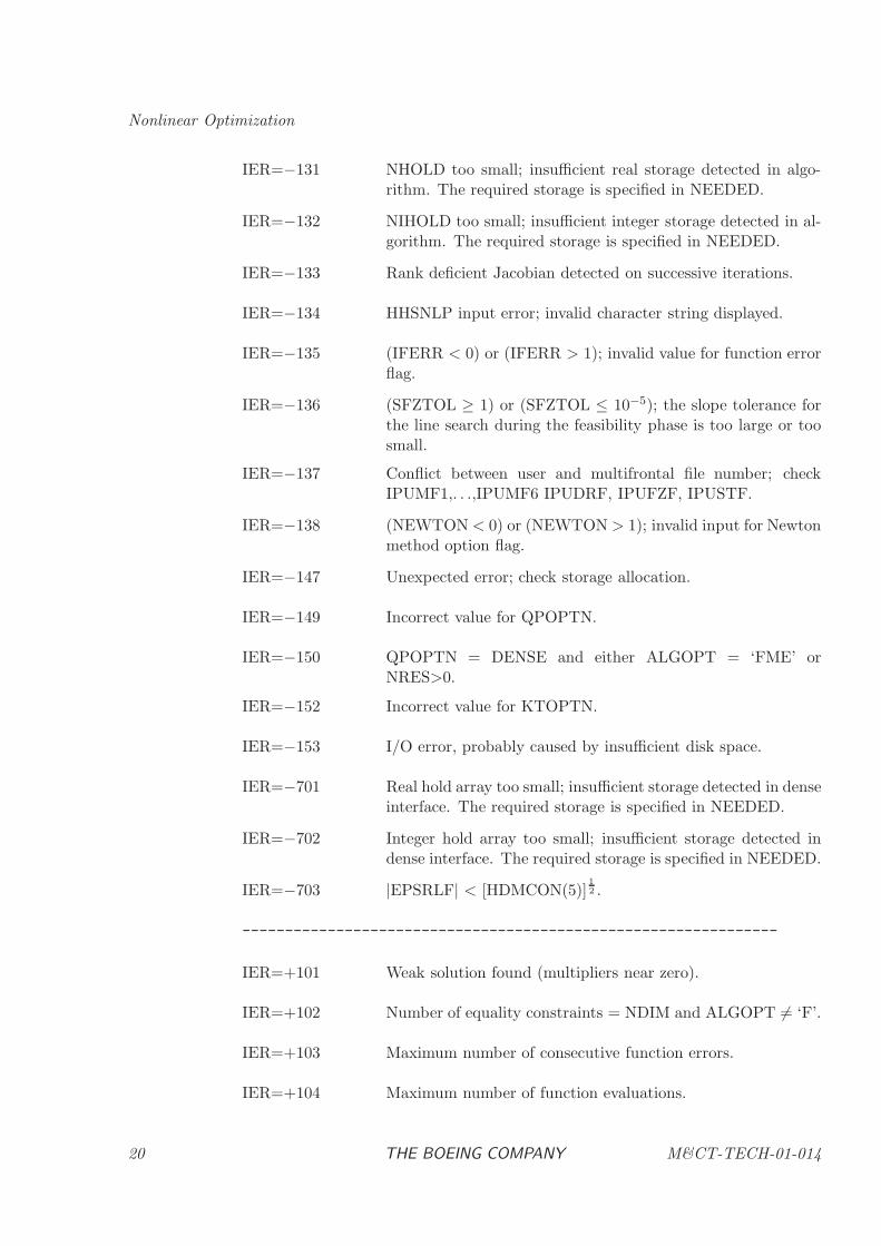
IER=−131 NHOLD too small; insufficient real storage detected in algo-rithm. The required storage is specified in NEEDED.
IER=−132 NIHOLD too small; insufficient integer storage detected in al-gorithm. The required storage is specified in NEEDED.
IER=−133 Rank deficient Jacobian detected on successive iterations.
IER=−134 HHSNLP input error; invalid character string displayed.
IER=−135 (IFERR < 0) or (IFERR > 1); invalid value for function errorflag.
IER=−136 (SFZTOL ≥ 1) or (SFZTOL ≤ 10−5); the slope tolerance forthe line search during the feasibility phase is too large or toosmall.
IER=−137 Conflict between user and multifrontal file number; checkIPUMF1,. . .,IPUMF6 IPUDRF, IPUFZF, IPUSTF.
IER=−138 (NEWTON < 0) or (NEWTON > 1); invalid input for Newtonmethod option flag.
IER=−147 Unexpected error; check storage allocation.
IER=−149 Incorrect value for QPOPTN.
IER=−150 QPOPTN = DENSE and either ALGOPT = ‘FME’ orNRES>0.
IER=−152 Incorrect value for KTOPTN.
IER=−153 I/O error, probably caused by insufficient disk space.
IER=−701 Real hold array too small; insufficient storage detected in denseinterface. The required storage is specified in NEEDED.
IER=−702 Integer hold array too small; insufficient storage detected indense interface. The required storage is specified in NEEDED.
IER=−703 |EPSRLF| < [HDMCON(5)]12 .
---------------------------------------------------------------
IER=+101 Weak solution found (multipliers near zero).
IER=+102 Number of equality constraints = NDIM and ALGOPT 6= ‘F’.
IER=+103 Maximum number of consecutive function errors.
IER=+104 Maximum number of function evaluations.
20 THE BOEING COMPANY M&CT-TECH-01-014
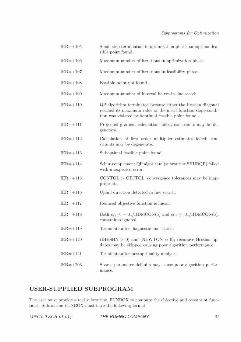
Subprograms for Optimization
IER=+105 Small step termination in optimization phase; suboptimal fea-sible point found.
IER=+106 Maximum number of iterations in optimization phase.
IER=+107 Maximum number of iterations in feasibility phase.
IER=+108 Feasible point not found.
IER=+109 Maximum number of interval halves in line search.
IER=+110 QP algorithm terminated because either the Hessian diagonalreached its maximum value or the merit function slope condi-tion was violated; suboptimal feasible point found.
IER=+111 Projected gradient calculation failed; constraints may be de-generate.
IER=+112 Calculation of first order multiplier estimates failed; con-straints may be degenerate.
IER=+113 Suboptimal feasible point found.
IER=+114 Schur-complement QP algorithm (subroutine SHURQP) failedwith unexpected error.
IER=+115 CONTOL > OBJTOL; convergence tolerances may be inap-propriate.
IER=+116 Uphill direction detected in line search.
IER=+117 Reduced objective function is linear.
IER=+118 Both cLi ≤ −.01/HDMCON(5) and cUi ≥ .01/HDMCON(5);constraints ignored.
IER=+119 Terminate after diagnostic line search.
IER=+120 (IHESHN > 0) and (NEWTON = 0); recursive Hessian up-dates may be skipped causing poor algorithm performance.
IER=+121 Terminate after postoptimality analysis.
IER=+703 Sparse parameter defaults may cause poor algorithm perfor-mance.
USER-SUPPLIED SUBPROGRAM
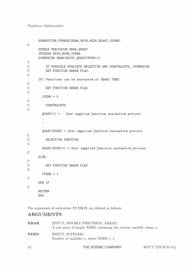
The user must provide a real subroutine, FUNBOX to compute the objective and constraint func-tions. Subroutine FUNBOX must have the following format:
M&CT-TECH-01-014 THE BOEING COMPANY 21
Nonlinear Optimization
SUBROUTINE FUNBOX(XBAR,NDIM,MCON,QUANT,IFERR)
C
DOUBLE PRECISION XBAR,QUANT
INTEGER NDIM,MCON,IFERR
DIMENSION XBAR(NDIM),QUANT(MCON+1)
C
C IF POSSIBLE EVALUATE OBJECTIVE AND CONSTRAINTS, OTHERWISE
C SET FUNCTION ERROR FLAG.
C
IF( Functions can be evaluated at XBAR) THEN
C
C SET FUNCTION ERROR FLAG
C
IFERR = 0
C
C CONSTRAINTS
C
QUANT(1) = User supplied function evaluation process
.
.
.
QUANT(MCON) = User supplied function evaluation process
C
C OBJECTIVE FUNCTION
C
QUANT(MCON+1) = User supplied function evaluation process
C
ELSE
C
C SET FUNCTION ERROR FLAG
C
IFERR = 1
C
END IF
C
RETURN
END
The arguments of subroutine FUNBOX are defined as follows:
ARGUMENTS
XBAR [INPUT, DOUBLE PRECISION, ARRAY]A real array of length NDIM containing the current variable values x.
NDIM [INPUT, INTEGER]Number of variables n, where NDIM ≥ 1.
22 THE BOEING COMPANY M&CT-TECH-01-014
Subprograms for Optimization
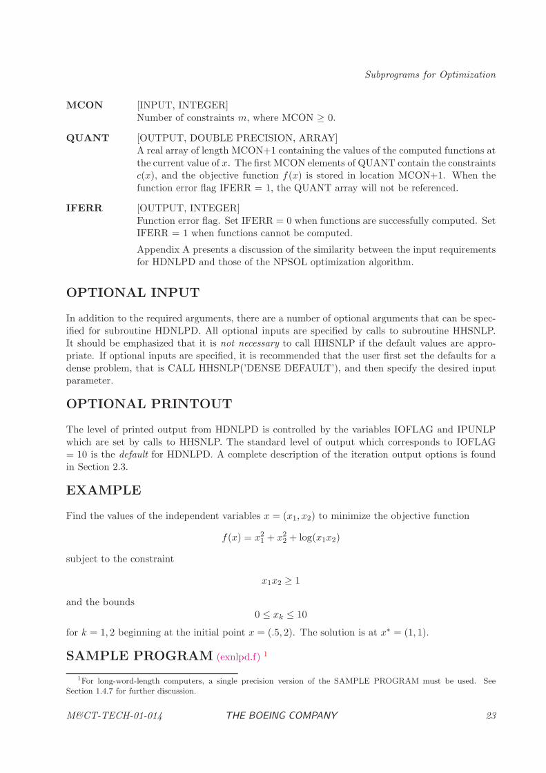
MCON [INPUT, INTEGER]Number of constraints m, where MCON ≥ 0.
QUANT [OUTPUT, DOUBLE PRECISION, ARRAY]A real array of length MCON+1 containing the values of the computed functions atthe current value of x. The first MCON elements of QUANT contain the constraintsc(x), and the objective function f(x) is stored in location MCON+1. When thefunction error flag IFERR = 1, the QUANT array will not be referenced.
IFERR [OUTPUT, INTEGER]Function error flag. Set IFERR = 0 when functions are successfully computed. SetIFERR = 1 when functions cannot be computed.
Appendix A presents a discussion of the similarity between the input requirementsfor HDNLPD and those of the NPSOL optimization algorithm.
OPTIONAL INPUT
In addition to the required arguments, there are a number of optional arguments that can be spec-ified for subroutine HDNLPD. All optional inputs are specified by calls to subroutine HHSNLP.It should be emphasized that it is not necessary to call HHSNLP if the default values are appro-priate. If optional inputs are specified, it is recommended that the user first set the defaults for adense problem, that is CALL HHSNLP(’DENSE DEFAULT’), and then specify the desired inputparameter.
OPTIONAL PRINTOUT
The level of printed output from HDNLPD is controlled by the variables IOFLAG and IPUNLPwhich are set by calls to HHSNLP. The standard level of output which corresponds to IOFLAG= 10 is the default for HDNLPD. A complete description of the iteration output options is foundin Section 2.3.
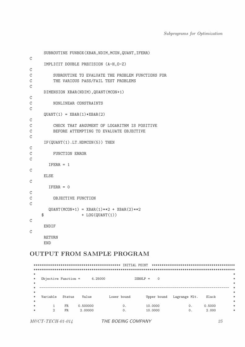
EXAMPLE
Find the values of the independent variables x = (x1, x2) to minimize the objective function
f(x) = x21 + x2
2 + log(x1x2)
subject to the constraint
x1x2 ≥ 1
and the bounds0 ≤ xk ≤ 10
for k = 1, 2 beginning at the initial point x = (.5, 2). The solution is at x∗ = (1, 1).
SAMPLE PROGRAM (exnlpd.f) 1
1For long-word-length computers, a single precision version of the SAMPLE PROGRAM must be used. See
Section 1.4.7 for further discussion.
M&CT-TECH-01-014 THE BOEING COMPANY 23
Nonlinear Optimization
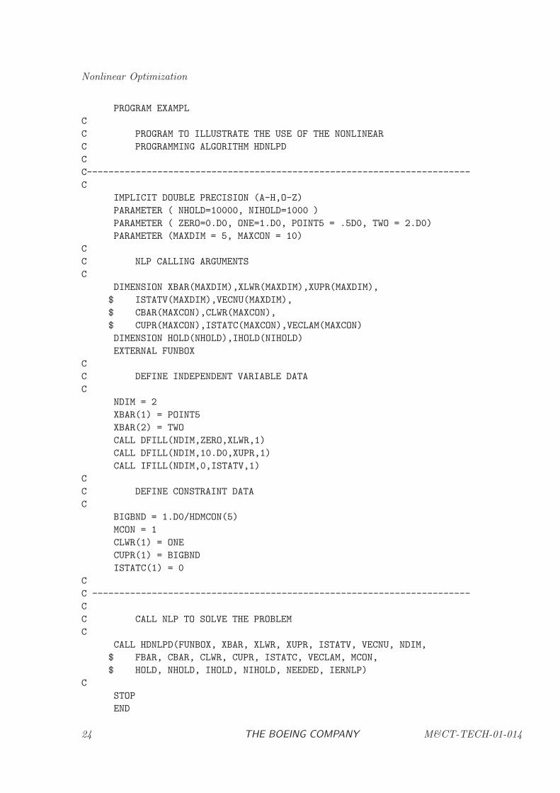
PROGRAM EXAMPL
C
C PROGRAM TO ILLUSTRATE THE USE OF THE NONLINEAR
C PROGRAMMING ALGORITHM HDNLPD
C
C-----------------------------------------------------------------------
C
IMPLICIT DOUBLE PRECISION (A-H,O-Z)
PARAMETER ( NHOLD=10000, NIHOLD=1000 )
PARAMETER ( ZERO=0.D0, ONE=1.D0, POINT5 = .5D0, TWO = 2.D0)
PARAMETER (MAXDIM = 5, MAXCON = 10)
C
C NLP CALLING ARGUMENTS
C
DIMENSION XBAR(MAXDIM),XLWR(MAXDIM),XUPR(MAXDIM),
$ ISTATV(MAXDIM),VECNU(MAXDIM),
$ CBAR(MAXCON),CLWR(MAXCON),
$ CUPR(MAXCON),ISTATC(MAXCON),VECLAM(MAXCON)
DIMENSION HOLD(NHOLD),IHOLD(NIHOLD)
EXTERNAL FUNBOX
C
C DEFINE INDEPENDENT VARIABLE DATA
C
NDIM = 2
XBAR(1) = POINT5
XBAR(2) = TWO
CALL DFILL(NDIM,ZERO,XLWR,1)
CALL DFILL(NDIM,10.D0,XUPR,1)
CALL IFILL(NDIM,0,ISTATV,1)
C
C DEFINE CONSTRAINT DATA
C
BIGBND = 1.D0/HDMCON(5)
MCON = 1
CLWR(1) = ONE
CUPR(1) = BIGBND
ISTATC(1) = 0
C
C ----------------------------------------------------------------------
C
C CALL NLP TO SOLVE THE PROBLEM
C
CALL HDNLPD(FUNBOX, XBAR, XLWR, XUPR, ISTATV, VECNU, NDIM,
$ FBAR, CBAR, CLWR, CUPR, ISTATC, VECLAM, MCON,
$ HOLD, NHOLD, IHOLD, NIHOLD, NEEDED, IERNLP)
C
STOP
END
24 THE BOEING COMPANY M&CT-TECH-01-014
Subprograms for Optimization
SUBROUTINE FUNBOX(XBAR,NDIM,MCON,QUANT,IFERR)
C
IMPLICIT DOUBLE PRECISION (A-H,O-Z)
C
C SUBROUTINE TO EVALUATE THE PROBLEM FUNCTIONS FOR
C THE VARIOUS PASS/FAIL TEST PROBLEMS
C
DIMENSION XBAR(NDIM),QUANT(MCON+1)
C
C NONLINEAR CONSTRAINTS
C
QUANT(1) = XBAR(1)*XBAR(2)
C
C CHECK THAT ARGUMENT OF LOGARITHM IS POSITIVE
C BEFORE ATTEMPTING TO EVALUATE OBJECTIVE
C
IF(QUANT(1).LT.HDMCON(5)) THEN
C
C FUNCTION ERROR
C
IFERR = 1
C
ELSE
C
IFERR = 0
C
C OBJECTIVE FUNCTION
C
QUANT(MCON+1) = XBAR(1)**2 + XBAR(2)**2
$ + LOG(QUANT(1))
C
ENDIF
C
RETURN
END
OUTPUT FROM SAMPLE PROGRAM
********************************************* INITIAL POINT *******************************************
********************************************************************************************************
* *
* Objective Function = 4.25000 IERNLP = 0 *
* *
* -------------------------------------------------------------------------------------------------- *
* *
* Variable Status Value Lower bound Upper bound Lagrange Mlt. Slack *
* *
* 1 FR 0.500000 0. 10.0000 0. 0.5000 *
* 2 FR 2.00000 0. 10.0000 0. 2.000 *
M&CT-TECH-01-014 THE BOEING COMPANY 25
Nonlinear Optimization
* *
* -------------------------------------------------------------------------------------------------- *
* *
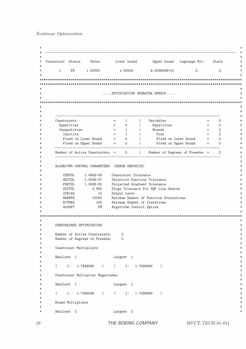
* Constraint Status Value Lower bound Upper bound Lagrange Mlt. Slack *
* *
* 1 FR 1.00000 1.00000 4.503600E+15 0. 0. *
* *
********************************************************************************************************
********************************************************************************************************
* *
* .....OPTIMIZATION OPERATOR SPRNLP..... *
* *
********************************************************************************************************
* *
* *
* ------------------------------------------------------------------------------------- *
* Constraints = 1 | Variables = 2 *
* Equalities = 0 | Equalities = 0 *
* Inequalities = 1 | Bounds = 2 *
* Inactive = 1 | Free = 2 *
* Fixed on Lower Bound = 0 | Fixed on Lower Bound = 0 *
* Fixed on Upper Bound = 0 | Fixed on Upper Bound = 0 *
* ------------------------------------------------------------------------------------- *
* Number of Active Constraints = 0 | Number of Degrees of Freedom = 2 *
* ------------------------------------------------------------------------------------- *
* *
* ALGORITHM CONTROL PARAMETERS (DENSE DEFAULTS) *
* *
* CONTOL 1.490E-08 Constraint Tolerance *
* OBJTOL 1.000E-07 Objective Function Tolerance *
* PGDTOL 1.000E-05 Projected Gradient Tolerance *
* SLPTOL 0.900 Slope Tolerance For SQP Line Search *
* IOFLAG 10 Output Level *
* MAXNFE 10000 Maximum Number of Function Evaluations *
* NITMAX 100 Maximum Number of Iterations *
* ALGOPT FM Algorithm Control Option *
* *
********************************************************************************************************
* *
* CONSTRAINED OPTIMIZATION *
* *
* Number of Active Constraints: 2 *
* Number of Degrees of Freedom: 0 *
* *
* Constraint Multipliers *
* *
* Smallest 1 Largest 1 *
* *
* ( 1: 1.7499999 ) ( 1: 1.7499999 ) *
* *
* Constraint Multiplier Magnitudes *
* *
* Smallest 1 Largest 1 *
* *
* ( 1: 1.7499999 ) ( 1: 1.7499999 ) *
* *
* Bound Multipliers *
* *
* Smallest 2 Largest 2 *
26 THE BOEING COMPANY M&CT-TECH-01-014
Subprograms for Optimization
* *
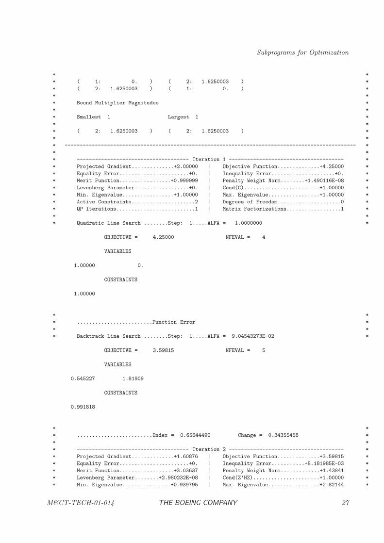
* ( 1: 0. ) ( 2: 1.6250003 ) *
* ( 2: 1.6250003 ) ( 1: 0. ) *
* *
* Bound Multiplier Magnitudes *
* *
* Smallest 1 Largest 1 *
* *
* ( 2: 1.6250003 ) ( 2: 1.6250003 ) *
* *
* ------------------------------------------------------------------------------------------------ *
* *
* ------------------------------------- Iteration 1 -------------------------------------- *
* Projected Gradient..............+2.00000 | Objective Function..............+4.25000 *
* Equality Error.......................+0. | Inequality Error.....................+0. *
* Merit Function.................+0.999999 | Penalty Weight Norm........+1.490116E-08 *
* Levenberg Parameter..................+0. | Cond(G).........................+1.00000 *
* Min. Eigenvalue.................+1.00000 | Max. Eigenvalue.................+1.00000 *
* Active Constraints.....................2 | Degrees of Freedom.....................0 *
* QP Iterations..........................1 | Matrix Factorizations..................1 *
* *
* Quadratic Line Search ........Step: 1.....ALFA = 1.0000000 *
OBJECTIVE = 4.25000 NFEVAL = 4
VARIABLES
1.00000 0.
CONSTRAINTS
1.00000
* *
* .........................Function Error *
* *
* Backtrack Line Search ........Step: 1.....ALFA = 9.04543273E-02 *
OBJECTIVE = 3.59815 NFEVAL = 5
VARIABLES
0.545227 1.81909
CONSTRAINTS
0.991818
* *
* .........................Index = 0.65644490 Change = -0.34355458 *
* *
* ------------------------------------- Iteration 2 -------------------------------------- *
* Projected Gradient..............+1.60876 | Objective Function..............+3.59815 *
* Equality Error.......................+0. | Inequality Error...........+8.181985E-03 *
* Merit Function..................+3.03637 | Penalty Weight Norm.............+1.43841 *
* Levenberg Parameter........+2.980232E-08 | Cond(Z’HZ)......................+1.00000 *
* Min. Eigenvalue................+0.939795 | Max. Eigenvalue.................+2.82144 *
M&CT-TECH-01-014 THE BOEING COMPANY 27
Nonlinear Optimization
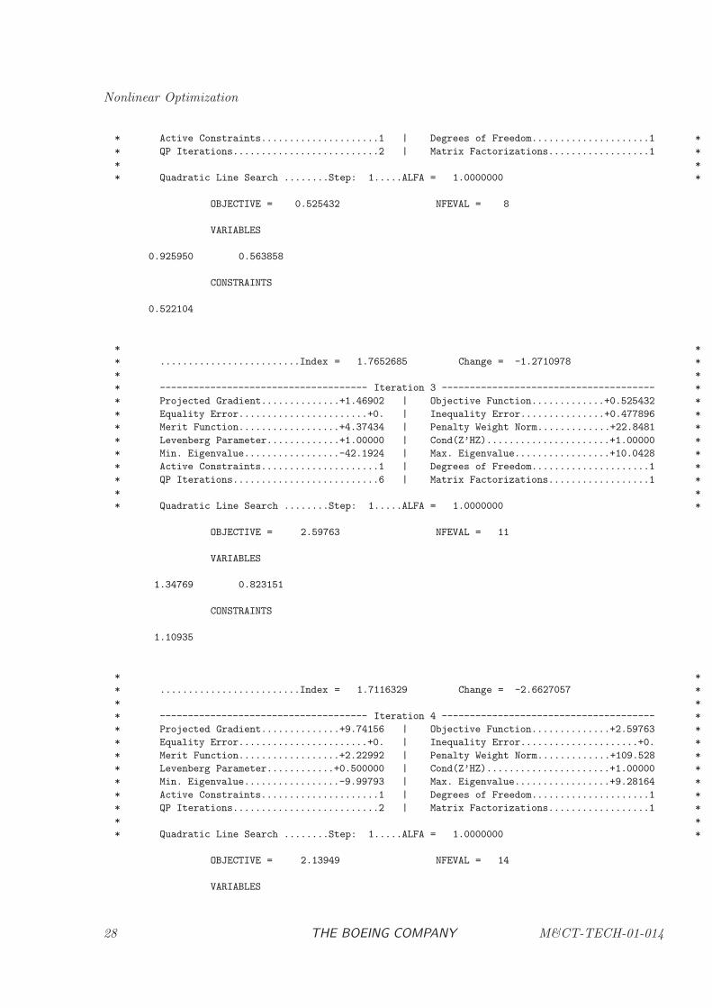
* Active Constraints.....................1 | Degrees of Freedom.....................1 *
* QP Iterations..........................2 | Matrix Factorizations..................1 *
* *
* Quadratic Line Search ........Step: 1.....ALFA = 1.0000000 *
OBJECTIVE = 0.525432 NFEVAL = 8
VARIABLES
0.925950 0.563858
CONSTRAINTS
0.522104
* *
* .........................Index = 1.7652685 Change = -1.2710978 *
* *
* ------------------------------------- Iteration 3 -------------------------------------- *
* Projected Gradient..............+1.46902 | Objective Function.............+0.525432 *
* Equality Error.......................+0. | Inequality Error...............+0.477896 *
* Merit Function..................+4.37434 | Penalty Weight Norm.............+22.8481 *
* Levenberg Parameter.............+1.00000 | Cond(Z’HZ)......................+1.00000 *
* Min. Eigenvalue.................-42.1924 | Max. Eigenvalue.................+10.0428 *
* Active Constraints.....................1 | Degrees of Freedom.....................1 *
* QP Iterations..........................6 | Matrix Factorizations..................1 *
* *
* Quadratic Line Search ........Step: 1.....ALFA = 1.0000000 *
OBJECTIVE = 2.59763 NFEVAL = 11
VARIABLES
1.34769 0.823151
CONSTRAINTS
1.10935
* *
* .........................Index = 1.7116329 Change = -2.6627057 *
* *
* ------------------------------------- Iteration 4 -------------------------------------- *
* Projected Gradient..............+9.74156 | Objective Function..............+2.59763 *
* Equality Error.......................+0. | Inequality Error.....................+0. *
* Merit Function..................+2.22992 | Penalty Weight Norm.............+109.528 *
* Levenberg Parameter............+0.500000 | Cond(Z’HZ)......................+1.00000 *
* Min. Eigenvalue.................-9.99793 | Max. Eigenvalue.................+9.28164 *
* Active Constraints.....................1 | Degrees of Freedom.....................1 *
* QP Iterations..........................2 | Matrix Factorizations..................1 *
* *
* Quadratic Line Search ........Step: 1.....ALFA = 1.0000000 *
OBJECTIVE = 2.13949 NFEVAL = 14
VARIABLES
28 THE BOEING COMPANY M&CT-TECH-01-014
Subprograms for Optimization
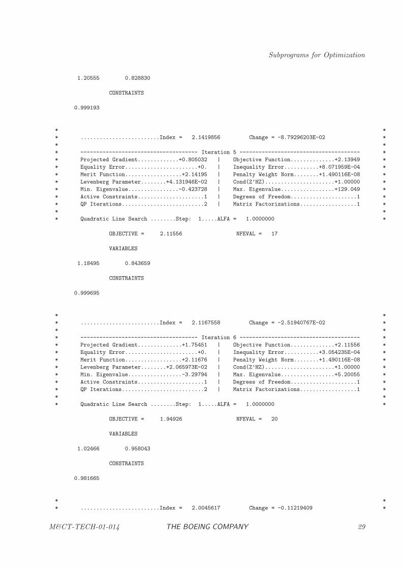
1.20555 0.828830
CONSTRAINTS
0.999193
* *
* .........................Index = 2.1419856 Change = -8.79296203E-02 *
* *
* ------------------------------------- Iteration 5 -------------------------------------- *
* Projected Gradient.............+0.805032 | Objective Function..............+2.13949 *
* Equality Error.......................+0. | Inequality Error...........+8.071959E-04 *
* Merit Function..................+2.14195 | Penalty Weight Norm........+1.490116E-08 *
* Levenberg Parameter........+4.131946E-02 | Cond(Z’HZ)......................+1.00000 *
* Min. Eigenvalue................-0.423728 | Max. Eigenvalue.................+129.049 *
* Active Constraints.....................1 | Degrees of Freedom.....................1 *
* QP Iterations..........................2 | Matrix Factorizations..................1 *
* *
* Quadratic Line Search ........Step: 1.....ALFA = 1.0000000 *
OBJECTIVE = 2.11556 NFEVAL = 17
VARIABLES
1.18495 0.843659
CONSTRAINTS
0.999695
* *
* .........................Index = 2.1167558 Change = -2.51940767E-02 *
* *
* ------------------------------------- Iteration 6 -------------------------------------- *
* Projected Gradient..............+1.75451 | Objective Function..............+2.11556 *
* Equality Error.......................+0. | Inequality Error...........+3.054235E-04 *
* Merit Function..................+2.11676 | Penalty Weight Norm........+1.490116E-08 *
* Levenberg Parameter........+2.065973E-02 | Cond(Z’HZ)......................+1.00000 *
* Min. Eigenvalue.................-3.29794 | Max. Eigenvalue.................+5.20055 *
* Active Constraints.....................1 | Degrees of Freedom.....................1 *
* QP Iterations..........................2 | Matrix Factorizations..................1 *
* *
* Quadratic Line Search ........Step: 1.....ALFA = 1.0000000 *
OBJECTIVE = 1.94926 NFEVAL = 20
VARIABLES
1.02466 0.958043
CONSTRAINTS
0.981665
* *
* .........................Index = 2.0045617 Change = -0.11219409 *
M&CT-TECH-01-014 THE BOEING COMPANY 29
Nonlinear Optimization
* *
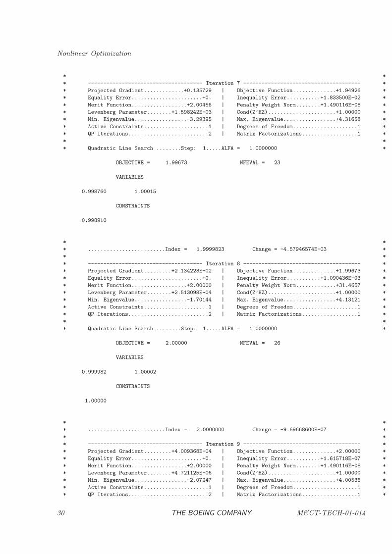
* ------------------------------------- Iteration 7 -------------------------------------- *
* Projected Gradient.............+0.135729 | Objective Function..............+1.94926 *
* Equality Error.......................+0. | Inequality Error...........+1.833500E-02 *
* Merit Function..................+2.00456 | Penalty Weight Norm........+1.490116E-08 *
* Levenberg Parameter........+1.598242E-03 | Cond(Z’HZ)......................+1.00000 *
* Min. Eigenvalue.................-3.29395 | Max. Eigenvalue.................+4.31658 *
* Active Constraints.....................1 | Degrees of Freedom.....................1 *
* QP Iterations..........................2 | Matrix Factorizations..................1 *
* *
* Quadratic Line Search ........Step: 1.....ALFA = 1.0000000 *
OBJECTIVE = 1.99673 NFEVAL = 23
VARIABLES
0.998760 1.00015
CONSTRAINTS
0.998910
* *
* .........................Index = 1.9999823 Change = -4.57946574E-03 *
* *
* ------------------------------------- Iteration 8 -------------------------------------- *
* Projected Gradient.........+2.134223E-02 | Objective Function..............+1.99673 *
* Equality Error.......................+0. | Inequality Error...........+1.090436E-03 *
* Merit Function..................+2.00000 | Penalty Weight Norm.............+31.4657 *
* Levenberg Parameter........+2.513098E-04 | Cond(Z’HZ)......................+1.00000 *
* Min. Eigenvalue.................-1.70144 | Max. Eigenvalue.................+4.13121 *
* Active Constraints.....................1 | Degrees of Freedom.....................1 *
* QP Iterations..........................2 | Matrix Factorizations..................1 *
* *
* Quadratic Line Search ........Step: 1.....ALFA = 1.0000000 *
OBJECTIVE = 2.00000 NFEVAL = 26
VARIABLES
0.999982 1.00002
CONSTRAINTS
1.00000
* *
* .........................Index = 2.0000000 Change = -9.69668600E-07 *
* *
* ------------------------------------- Iteration 9 -------------------------------------- *
* Projected Gradient.........+4.009368E-04 | Objective Function..............+2.00000 *
* Equality Error.......................+0. | Inequality Error...........+1.615718E-07 *
* Merit Function..................+2.00000 | Penalty Weight Norm........+1.490116E-08 *
* Levenberg Parameter........+4.721125E-06 | Cond(Z’HZ)......................+1.00000 *
* Min. Eigenvalue.................-2.07247 | Max. Eigenvalue.................+4.00536 *
* Active Constraints.....................1 | Degrees of Freedom.....................1 *
* QP Iterations..........................2 | Matrix Factorizations..................1 *
30 THE BOEING COMPANY M&CT-TECH-01-014
Subprograms for Optimization
* *
* Quadratic Line Search ........Step: 1.....ALFA = 1.0000000 *
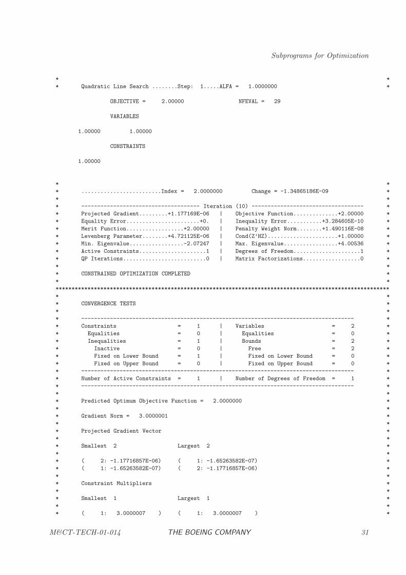
OBJECTIVE = 2.00000 NFEVAL = 29
VARIABLES
1.00000 1.00000
CONSTRAINTS
1.00000
* *
* .........................Index = 2.0000000 Change = -1.34865186E-09 *
* *
* ------------------------------------- Iteration (10) ----------------------------------- *
* Projected Gradient.........+1.177169E-06 | Objective Function..............+2.00000 *
* Equality Error.......................+0. | Inequality Error...........+3.284605E-10 *
* Merit Function..................+2.00000 | Penalty Weight Norm........+1.490116E-08 *
* Levenberg Parameter........+4.721125E-06 | Cond(Z’HZ)......................+1.00000 *
* Min. Eigenvalue.................-2.07247 | Max. Eigenvalue.................+4.00536 *
* Active Constraints.....................1 | Degrees of Freedom.....................1 *
* QP Iterations..........................0 | Matrix Factorizations..................0 *
* *
* CONSTRAINED OPTIMIZATION COMPLETED *
* *
********************************************************************************************************
* *
* CONVERGENCE TESTS *
* *
* ------------------------------------------------------------------------------------- *
* Constraints = 1 | Variables = 2 *
* Equalities = 0 | Equalities = 0 *
* Inequalities = 1 | Bounds = 2 *
* Inactive = 0 | Free = 2 *
* Fixed on Lower Bound = 1 | Fixed on Lower Bound = 0 *
* Fixed on Upper Bound = 0 | Fixed on Upper Bound = 0 *
* ------------------------------------------------------------------------------------- *
* Number of Active Constraints = 1 | Number of Degrees of Freedom = 1 *
* ------------------------------------------------------------------------------------- *
* *
* Predicted Optimum Objective Function = 2.0000000 *
* *
* Gradient Norm = 3.0000001 *
* *
* Projected Gradient Vector *
* *
* Smallest 2 Largest 2 *
* *
* ( 2: -1.17716857E-06) ( 1: -1.65263582E-07) *
* ( 1: -1.65263582E-07) ( 2: -1.17716857E-06) *
* *
* Constraint Multipliers *
* *
* Smallest 1 Largest 1 *
* *
* ( 1: 3.0000007 ) ( 1: 3.0000007 ) *
M&CT-TECH-01-014 THE BOEING COMPANY 31
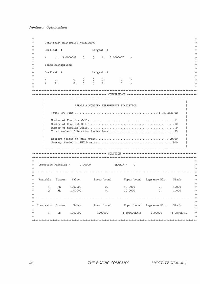
Nonlinear Optimization
* *
* Constraint Multiplier Magnitudes *
* *
* Smallest 1 Largest 1 *
* *
* ( 1: 3.0000007 ) ( 1: 3.0000007 ) *
* *
* Bound Multipliers *
* *
* Smallest 2 Largest 2 *
* *
* ( 1: 0. ) ( 2: 0. ) *
* ( 2: 0. ) ( 1: 0. ) *
* *
********************************************************************************************************
*********************************************** CONVERGENCE ********************************************
-------------------------------------------------------------------------------------------
| |
| SPRNLP ALGORITHM PERFORMANCE STATISTICS |
| |
| Total CPU Time.....................................................+1.929229E-02 |
| |
| Number of Function Calls......................................................11 |
| Number of Gradient Calls......................................................10 |
| Number of Hessian Calls........................................................9 |
| Total Number of Function Evaluations..........................................33 |
| |
| Storage Needed in HOLD Array................................................9960 |
| Storage Needed in IHOLD Array................................................800 |
| |
-------------------------------------------------------------------------------------------
*********************************************** SOLUTION ***********************************************
********************************************************************************************************
* *
* Objective Function = 2.00000 IERNLP = 0 *
* *
* -------------------------------------------------------------------------------------------------- *
* *
* Variable Status Value Lower bound Upper bound Lagrange Mlt. Slack *
* *
* 1 FR 1.00000 0. 10.0000 0. 1.000 *
* 2 FR 1.00000 0. 10.0000 0. 1.000 *
* *
* -------------------------------------------------------------------------------------------------- *
* *
* Constraint Status Value Lower bound Upper bound Lagrange Mlt. Slack *
* *
* 1 LB 1.00000 1.00000 4.503600E+15 3.00000 -3.2846E-10 *
* *
********************************************************************************************************
32 THE BOEING COMPANY M&CT-TECH-01-014
Subprograms for Optimization
HDNLPR: Dense Nonlinear Programming–Reverse Communication Format
PURPOSE
HDNLPR computes the vector x = (x1, x2, . . . , xn) which minimizes the objective function
f(x)
subject to the m nonlinear constraints
cL ≤ c(x) ≤ cU
and the simple boundsxL ≤ x ≤ xU
Equality constraints are imposed by setting cLi = cUi and variables can be fixed by setting xLi =xUi. HDNLPR works under the assumption that the objective and constraint functions are twicecontinuously differentiable, and if this is not true algorithm performance is unpredictable. HDNLPRuses a reverse communication format and upon request the user must supply the values of thefunctions, and their first derivatives. The matrix of second derivatives (Hessian of the Lagrangian)can be constructed using a quasi-Newton recursive estimate or supplied by the user. SubroutineHDNLPR calls the sparse nonlinear programming algorithm HDSNLP, and is intended for simplifiedusage as appropriate for small dense problems.
RELATED SUBPROGRAMS
HDBNPR Dense Barrier Nonlinear Programming–Reverse Communication Format
HDSNLP Sparse Nonlinear Programming
HHSNLP Sparse Nonlinear Programming Input Procedure
METHOD
A sequential quadratic programming (SQP) approach is used to solve the nonlinear programming(NLP) problem. Although the dense null-space method is the default, the Schur-complementmethod can be selected to solve the quadratic programming subproblem. HDNLPR provides fouralternatives for constructing an approximation to the Hessian matrix. The default is a symmetricrank-one (SR1) approximation, with options for using a BFGS, or PSB. As a final option theHessian of the Lagrangian may be supplied by the user. If the user cannot provide this informationanalytically, the finite difference techniques described in Chapter 3 should be utilized.
WARNING
The objective function and constraints supplied by the user are assumed to be continuous andhave continuous first and second derivatives. Nondifferentiable functions can cause unpredictableperformance in the optimization algorithm. It should be emphasized that discontinuities in theHessian matrices can significantly degrade the speed of convergence without producing any otherobvious difficulties. The following common sources of error should be avoided when evaluating theobjective and constraint functions:
M&CT-TECH-01-014 THE BOEING COMPANY 33
Nonlinear Optimization
(1) nonsmooth interpolation of data;
(2) iterative procedures inside the function evaluation process, such as adaptive quadrature or rootsolving;
(3) discontinuous behavior caused by branching for IF tests;
(4) nondifferentiable functions such as ABS, MAX, and MIN.
The user must provide a procedure to evaluate the objective and constraint functions in additionto first and (optionally) second derivatives of these quantities. If it is not possible to evaluate thefunctions (for example, c(x) = 1/x at x = 0) then set IFERR = 1 and exit the function evaluationprocess. Otherwise, set IFERR = 0 when the functions are evaluated. The function error flagshould be used to avoid computational difficulties, but never in lieu of an explicit constraint.
The HDNLPR software uses internal common blocks to communicate information. To avoid con-flict with these internal commons the user should not have commons with the following names:NPSPRR, NPSPRI, NPSPRC, STATIS, KONSTN, NPSALG, NPSDFL, NLPERR, PERCOM,ITEREF, and CLKCOM.
USAGE
INTEGER IRVCOM, IFERR, NFEVAL, IER, NEEDED
INTEGER NDIM, MCON, NONZH, NONZG, NHOLD, NIHOLD
INTEGER IREVRS(5), ISTATV(NDIM), ISTATC(MCON), IHOLD(NIHOLD)
PARAMETER (NONZG=NDIM*MCON, NONZH=NDIM*(NDIM+1)/2 )
DOUBLE PRECISION FBAR, XBAR(NDIM), XLWR(NDIM), XUPR(NDIM), VECNU(NDIM)
DOUBLE PRECISION DELF(NDIM), HMAT(NONZH), CBAR(MCON), CLWR(MCON)
DOUBLE PRECISION CUPR(MCON), VECLAM(MCON), GMAT(NONZG), HOLD(NHOLD)
CALL HDNLPR( IRVCOM, IREVRS, XBAR, XLWR, XUPR, ISTATV,
$ VECNU, NDIM, FBAR, DELF, HMAT, CBAR,
$ CLWR, CUPR, ISTATC, MCON, VECLAM, GMAT,
$ IFERR, NFEVAL, HOLD, NHOLD, IHOLD, NIHOLD,
$ NEEDED, IER )
ARGUMENTS
ARGUMENTS TO CONTROL REVERSE COMMUNICATION
IRVCOM [INPUT/OUTPUT, INTEGER]Continuation control flag. This argument must be initialized. Thereafter it is setby the algorithm and must not be changed by the calling program.
IRVCOM = −1 Initialization pass.
IRVCOM = 0 Termination (normal or abnormal).
34 THE BOEING COMPANY M&CT-TECH-01-014

Subprograms for Optimization
IRVCOM = +1 Perform an evaluation and then reenter HDNLPR. Opera-tions to be performed are defined by the output variablesIREVRS(1), IREVRS(2), IREVRS(3), and IREVRS(4) below.IREVRS(5) contains information which may be valuable tothe interface but does not require any action on the part ofthe user.
IREVRS [OUTPUT, INTEGER, ARRAY]An integer array of length 5, containing reverse communication control information.IREVRS(1) Function evaluation request
= 0 Function evaluation not requested; Warning:do not change the current function and con-straint values.
= 1 Function evaluation requested; evaluate ob-jective function and all constraints at currentpoint XBAR.
IREVRS(2) Gradient evaluation request= 0 Gradient evaluation not requested; Warning:
do not change the current gradient and Jaco-bian.
= 1 Approximate (e.g. forward difference) gradi-ent requested; evaluate gradient vector g andJacobian matrix G at current point XBAR. (Ifavailable, accurate or analytic gradients maybe supplied)
= 2 Accurate (e.g. central difference or analytic)gradient requested; evaluate gradient vectorg and Jacobian matrix G at current pointXBAR.
M&CT-TECH-01-014 THE BOEING COMPANY 35

Nonlinear Optimization
IREVRS(3) Hessian evaluation request= 0 Hessian evaluation not requested; Warning:
do not change the current Hessian.
= 1 Hessian diagonal requested; get ready for fullHessian evaluation with (IREVRS(3)=2) atcurrent point (XBAR,VECLAM) and option-ally evaluate diagonal elements of Hessian ma-trix H.
= 2 Full Hessian evaluation requested; eval-uate Hessian matrix H of the functionL(x, λ) = f − ∑m
k=1 λkck at current point(XBAR,VECLAM). A full evaluation re-quest is always preceded by a call withIREVRS(3)=1 at the same point XBAR, andconsequently it may not be necessary to re-compute the diagonal elements.
IREVRS(4) System print (output) request= 0 System print not requested.
= 1 System print requested; perform any outputoperations (print, write files, etc.) desiredto display problem specific information at thecurrent point XBAR. The frequency of printis defined by the output control flag IOFLAG(see Optional Printout).
IREVRS(5) Algorithm information flag= 0 Call was made from the interface portion of
the algorithm.
= 1 Call was made from the optimization portionof the algorithm.
= 2 Call was made from the optimization portionof the algorithm requesting Hessian reset.
= 3 Call was made from the optimization portionof the algorithm requesting optimal perturba-tion size adjustment.
= 4 Call was made from the feasiblity portion ofthe algorithm.
INDEPENDENT VARIABLE DATA
XBAR† [INPUT/OUTPUT, DOUBLE PRECISION, ARRAY]A real array of length NDIM of current variable values x.
IRVCOM=−1 Initial guess must be input.
36 THE BOEING COMPANY M&CT-TECH-01-014
Subprograms for Optimization
IRVCOM=0 Final point is output. When IER = 0, +101, the final pointcorresponds to a local optimum. When IER = +104, . . . ,+111, +114, +116, +117, +119, the final point is either thebest feasible point if one has been found, or the last iterate.
IRVCOM=1 Intermediate iteration points are output.
XLWR† [INPUT, DOUBLE PRECISION, ARRAY]A real array of length NDIM containing the variable lower bounds xL. For variablesthat have no lower bound set xLi ≤ −.01/HDMCON(5). See Section 2.2 of theBCSLIB Manual [2] for HDMCON.
XUPR† [INPUT, DOUBLE PRECISION, ARRAY]A real array of length NDIM containing the variable upper bounds xU . For variablesthat have no upper bound set xUi ≥ .01/HDMCON(5).
ISTATV [INPUT/OUTPUT, INTEGER, ARRAY]An integer array of length NDIM indicating variable status. On input ISTATVdefines an estimate of the active variable bounds, and on output ISTATV definesthe bounds active at the solution.
ISTATV(i)= 0 Variable is strictly feasible, i.e. xLi < xi < xUi.
ISTATV(i)= 1 Variable lower bound is active, i.e. xLi = xi.
ISTATV(i)= 2 Variable upper bound is active, i.e. xi = xUi.
ISTATV(i)= 3 Fixed permanently.
ISTATV(i)= 10 Output only: Violated variable lower bound, i.e. xLi−δc > xi.
ISTATV(i)= 20 Output only: Violated variable upper bound, i.e. xi > xUi+δc.
ISTATV(i)= 30 Output only: Violated fixed variable. Either xi < xLi − δc orxi > xUi + δc.
When ISTATV(i) = 3 it is necessary that xLi = xUi, where xLi = XLWR(i)and xUi = XUPR(i). When ISTATV(i) 6= 3, it is necessary that xLi < xUi with|xLi − xUi| > δc.
VECNU# [INPUT/OUTPUT, DOUBLE PRECISION, ARRAY]An array of length NDIM of bound multipliers ν.
NDIM† [INPUT, INTEGER]Number of variables n, where 1 ≤ NDIM.
OBJECTIVE FUNCTION DATA
FBAR‡ [INPUT, DOUBLE PRECISION]The objective function evaluated at XBAR, f(XBAR).
M&CT-TECH-01-014 THE BOEING COMPANY 37
Nonlinear Optimization
DELF‡ [INPUT, DOUBLE PRECISION, ARRAY]A real array of length NDIM containing the gradient g of FBAR at XBAR.
HMAT‡ [INPUT, DOUBLE PRECISION, ARRAY]A real array of length n(n+ 1)/2 containing the elements of Hessian matrix HL =∇2
xf −∑mi=1 λi∇2
x ci. of the Lagrangian function. Since the Hessian is symmetric,only the lower triangular part is input (see USAGE REMARKS).
CONSTRAINT DATA
CBAR‡ [INPUT, DOUBLE PRECISION, ARRAY]A real array of length MCON containing the constraints c(x) evaluated at XBAR.Not referenced when MCON = 0.
CLWR† [INPUT, DOUBLE PRECISION, ARRAY]A real array of length MCON containing the constraint lower bounds cL. Forconstraints that have no lower bound set cLi ≤ −.01/HDMCON(5) . Not referencedwhen MCON = 0.
CUPR† [INPUT, DOUBLE PRECISION, ARRAY]A real array of length MCON containing the constraint upper bounds cU . Forconstraints that have no upper bound set cUi ≥ .01/HDMCON(5) . Not referencedwhen MCON = 0.
ISTATC [INPUT/OUTPUT, INTEGER, ARRAY]An integer array of length MCON indicating the constraint status. On inputISTATC defines an estimate of the active constraints, and on output ISTATCdefines the constraints active at the solution.
ISTATC(i)= 0 Free (inactive) inequality, i.e. cLi < ci(x) < cUi.
ISTATC(i)= 1 Constraint lower bound is active, i.e. cLi = ci(x).
ISTATC(i)= 2 Constraint upper bound is active, i.e. ci(x) = cUi.
ISTATC(i)= 3 Equality.
ISTATC(i)= 4 Ignored constraint.
ISTATC(i)= 10 Output only: Violated constraint lower bound, i.e. cLi − δc >ci.
ISTATC(i)= 20 Output only: Violated constraint upper bound , i.e. ci >cUi + δc.
ISTATC(i)= 30 Output only: Violated equality constraint. Either ci < cLi−δcor ci > cUi + δc.
When ISTATC(i) =3 it is necessary that cLi = cUi, where cLi = CLWR(i) and cUi =CUPR(i). When ISTATC(i) 6=3, it is necessary that cLi < cUi with |cLi−cUi| > δc.Not referenced when MCON = 0.
38 THE BOEING COMPANY M&CT-TECH-01-014
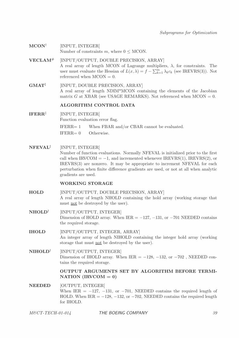
Subprograms for Optimization
MCON† [INPUT, INTEGER]Number of constraints m, where 0 ≤ MCON.
VECLAM# [INPUT/OUTPUT, DOUBLE PRECISION, ARRAY]A real array of length MCON of Lagrange multipliers, λ, for constraints. Theuser must evaluate the Hessian of L(x, λ) = f −∑m
k=1 λkck (see IREVRS(3)). Notreferenced when MCON = 0.
GMAT‡ [INPUT, DOUBLE PRECISION, ARRAY]A real array of length NDIM*MCON containing the elements of the Jacobianmatrix G at XBAR (see USAGE REMARKS). Not referenced when MCON = 0.
ALGORITHM CONTROL DATA
IFERR‡ [INPUT, INTEGER]Function evaluation error flag.
IFERR= 1 When FBAR and/or CBAR cannot be evaluated.
IFERR= 0 Otherwise.
NFEVAL‡ [INPUT, INTEGER]Number of function evaluations. Normally NFEVAL is initialized prior to the firstcall when IRVCOM = −1, and incremented whenever IREVRS(1), IREVRS(2), orIREVRS(3) are nonzero. It may be appropriate to increment NFEVAL for eachperturbation when finite difference gradients are used, or not at all when analyticgradients are used.
WORKING STORAGE
HOLD [INPUT/OUTPUT, DOUBLE PRECISION, ARRAY]A real array of length NHOLD containing the hold array (working storage thatmust not be destroyed by the user).
NHOLD† [INPUT/OUTPUT, INTEGER]Dimension of HOLD array. When IER = −127, −131, or −701 NEEDED containsthe required storage.
IHOLD [INPUT/OUTPUT, INTEGER, ARRAY]An integer array of length NIHOLD containing the integer hold array (workingstorage that must not be destroyed by the user).
NIHOLD† [INPUT/OUTPUT, INTEGER]Dimension of IHOLD array. When IER = −128, −132, or −702 , NEEDED con-tains the required storage.
OUTPUT ARGUMENTS SET BY ALGORITHM BEFORE TERMI-NATION (IRVCOM = 0)
NEEDED [OUTPUT, INTEGER]When IER = −127, −131, or −701, NEEDED contains the required length ofHOLD. When IER = −128, −132, or −702, NEEDED contains the required lengthfor IHOLD.
M&CT-TECH-01-014 THE BOEING COMPANY 39
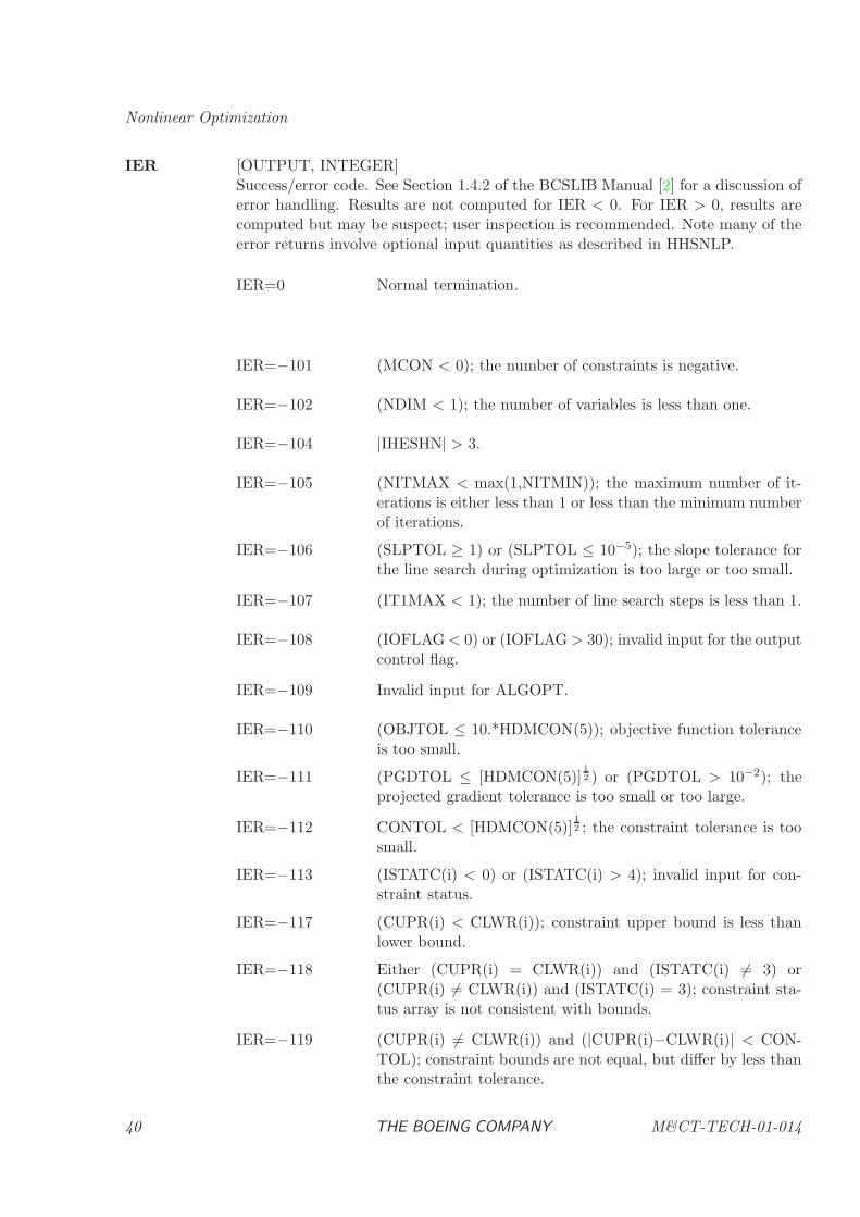
Nonlinear Optimization
IER [OUTPUT, INTEGER]Success/error code. See Section 1.4.2 of the BCSLIB Manual [2] for a discussion oferror handling. Results are not computed for IER < 0. For IER > 0, results arecomputed but may be suspect; user inspection is recommended. Note many of theerror returns involve optional input quantities as described in HHSNLP.
IER=0 Normal termination.
IER=−101 (MCON < 0); the number of constraints is negative.
IER=−102 (NDIM < 1); the number of variables is less than one.
IER=−104 |IHESHN| > 3.
IER=−105 (NITMAX < max(1,NITMIN)); the maximum number of it-erations is either less than 1 or less than the minimum numberof iterations.
IER=−106 (SLPTOL ≥ 1) or (SLPTOL ≤ 10−5); the slope tolerance forthe line search during optimization is too large or too small.
IER=−107 (IT1MAX < 1); the number of line search steps is less than 1.
IER=−108 (IOFLAG< 0) or (IOFLAG > 30); invalid input for the outputcontrol flag.
IER=−109 Invalid input for ALGOPT.
IER=−110 (OBJTOL ≤ 10.*HDMCON(5)); objective function toleranceis too small.
IER=−111 (PGDTOL ≤ [HDMCON(5)]12 ) or (PGDTOL > 10−2); the
projected gradient tolerance is too small or too large.
IER=−112 CONTOL < [HDMCON(5)]12 ; the constraint tolerance is too
small.
IER=−113 (ISTATC(i) < 0) or (ISTATC(i) > 4); invalid input for con-straint status.
IER=−117 (CUPR(i) < CLWR(i)); constraint upper bound is less thanlower bound.
IER=−118 Either (CUPR(i) = CLWR(i)) and (ISTATC(i) 6= 3) or(CUPR(i) 6= CLWR(i)) and (ISTATC(i) = 3); constraint sta-tus array is not consistent with bounds.
IER=−119 (CUPR(i) 6= CLWR(i)) and (|CUPR(i)−CLWR(i)| < CON-TOL); constraint bounds are not equal, but differ by less thanthe constraint tolerance.
40 THE BOEING COMPANY M&CT-TECH-01-014
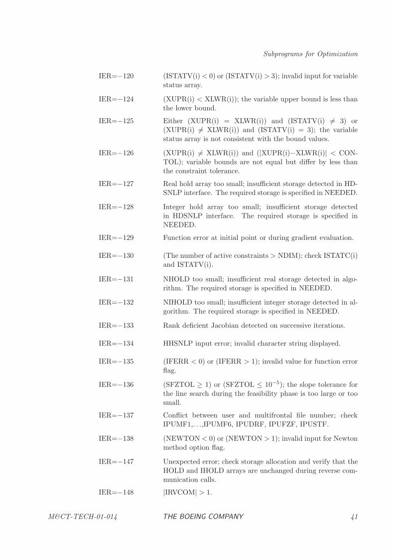
Subprograms for Optimization
IER=−120 (ISTATV(i)< 0) or (ISTATV(i) > 3); invalid input for variablestatus array.
IER=−124 (XUPR(i) < XLWR(i)); the variable upper bound is less thanthe lower bound.
IER=−125 Either (XUPR(i) = XLWR(i)) and (ISTATV(i) 6= 3) or(XUPR(i) 6= XLWR(i)) and (ISTATV(i) = 3); the variablestatus array is not consistent with the bound values.
IER=−126 (XUPR(i) 6= XLWR(i)) and (|XUPR(i)−XLWR(i)| < CON-TOL); variable bounds are not equal but differ by less thanthe constraint tolerance.
IER=−127 Real hold array too small; insufficient storage detected in HD-SNLP interface. The required storage is specified in NEEDED.
IER=−128 Integer hold array too small; insufficient storage detectedin HDSNLP interface. The required storage is specified inNEEDED.
IER=−129 Function error at initial point or during gradient evaluation.
IER=−130 (The number of active constraints > NDIM); check ISTATC(i)and ISTATV(i).
IER=−131 NHOLD too small; insufficient real storage detected in algo-rithm. The required storage is specified in NEEDED.
IER=−132 NIHOLD too small; insufficient integer storage detected in al-gorithm. The required storage is specified in NEEDED.
IER=−133 Rank deficient Jacobian detected on successive iterations.
IER=−134 HHSNLP input error; invalid character string displayed.
IER=−135 (IFERR < 0) or (IFERR > 1); invalid value for function errorflag.
IER=−136 (SFZTOL ≥ 1) or (SFZTOL ≤ 10−5); the slope tolerance forthe line search during the feasibility phase is too large or toosmall.
IER=−137 Conflict between user and multifrontal file number; checkIPUMF1,. . .,IPUMF6, IPUDRF, IPUFZF, IPUSTF.
IER=−138 (NEWTON < 0) or (NEWTON > 1); invalid input for Newtonmethod option flag.
IER=−147 Unexpected error; check storage allocation and verify that theHOLD and IHOLD arrays are unchanged during reverse com-munication calls.
IER=−148 |IRVCOM| > 1.
M&CT-TECH-01-014 THE BOEING COMPANY 41
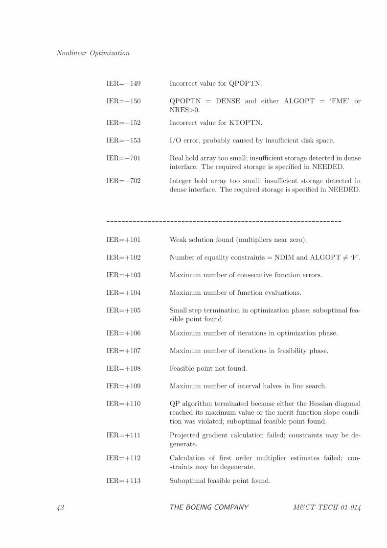
Nonlinear Optimization
IER=−149 Incorrect value for QPOPTN.
IER=−150 QPOPTN = DENSE and either ALGOPT = ‘FME’ orNRES>0.
IER=−152 Incorrect value for KTOPTN.
IER=−153 I/O error, probably caused by insufficient disk space.
IER=−701 Real hold array too small; insufficient storage detected in denseinterface. The required storage is specified in NEEDED.
IER=−702 Integer hold array too small; insufficient storage detected indense interface. The required storage is specified in NEEDED.
---------------------------------------------------------------
IER=+101 Weak solution found (multipliers near zero).
IER=+102 Number of equality constraints = NDIM and ALGOPT 6= ‘F’.
IER=+103 Maximum number of consecutive function errors.
IER=+104 Maximum number of function evaluations.
IER=+105 Small step termination in optimization phase; suboptimal fea-sible point found.
IER=+106 Maximum number of iterations in optimization phase.
IER=+107 Maximum number of iterations in feasibility phase.
IER=+108 Feasible point not found.
IER=+109 Maximum number of interval halves in line search.
IER=+110 QP algorithm terminated because either the Hessian diagonalreached its maximum value or the merit function slope condi-tion was violated; suboptimal feasible point found.
IER=+111 Projected gradient calculation failed; constraints may be de-generate.
IER=+112 Calculation of first order multiplier estimates failed; con-straints may be degenerate.
IER=+113 Suboptimal feasible point found.
42 THE BOEING COMPANY M&CT-TECH-01-014
Subprograms for Optimization
IER=+114 Schur-complement QP algorithm (subroutine SHURQP) failedwith unexpected error.
IER=+115 CONTOL > OBJTOL; convergence tolerances may be inap-propriate.
IER=+116 Uphill direction detected in line search.
IER=+117 Reduced objective function is linear.
IER=+118 Both cLi ≤ −.01/HDMCON(5) and cUi ≥ .01/HDMCON(5);constraints ignored.
IER=+119 Terminate after diagnostic line search.
IER=+120 (IHESHN > 0) and (NEWTON = 0); recursive Hessian up-dates may be skipped causing poor algorithm performance.
IER=+121 Terminate after postoptimality analysis.
IER=+703 Sparse parameter defaults may cause poor algorithm perfor-mance.
† Variable set when IRVCOM=−1, and not changed by user thereafter‡ Variable set when IRVCOM=+1, as required by IREVRS(*)# Variable optionally set when IRVCOM=−1, and not changed by user thereafter
USAGE REMARKS
When IHESHN = 0 and IREVRS(3) > 0, the user must supply the Hessian matrix of the followingLagrangian function:
L(x, λ) = f −m∑
k=1
λkck
that is,
L(XBAR,VECLAM) = FBAR - VECLAM(1)*CBAR(1) - . . . - VECLAM(MCON)*CBAR(MCON) .
Consider the following example in which n = 3:
H =
1.1 2 .1 3 .12.1 2.2 3 .23.1 3.2 3.3
Since the Hessian is a symmetric matrix only the lower triangular portion must be specified. Forthis example NDIM = 3 and the values are specified as HMAT(*) = (1.1, 2.1, 3.1, 2.2, 3.2, 3.3).Notice that the columns of the lower triangular portion are stored sequentially and the elementsin the upper triangular portion are not specified. Additional information on packed format forsymmetric matrices is found in BCSLIB [2].
M&CT-TECH-01-014 THE BOEING COMPANY 43
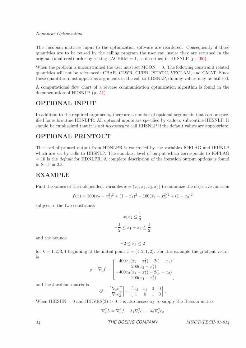
Nonlinear Optimization
The Jacobian matrices input to the optimization software are reordered. Consequently if thesequantities are to be reused by the calling program the user can insure they are returned in theoriginal (unaltered) order by setting JACPRM = 1, as described in HHSNLP (p. 196).
When the problem is unconstrained the user must set MCON = 0. The following constraint relatedquantities will not be referenced: CBAR, CLWR, CUPR, ISTATC, VECLAM, and GMAT. Sincethese quantities must appear as arguments in the call to HDSNLP, dummy values may be utilized.
A computational flow chart of a reverse communication optimization algorithm is found in thedocumentation of HDSNLP (p. 51).
OPTIONAL INPUT
In addition to the required arguments, there are a number of optional arguments that can be spec-ified for subroutine HDNLPR. All optional inputs are specified by calls to subroutine HHSNLP. Itshould be emphasized that it is not necessary to call HHSNLP if the default values are appropriate.
OPTIONAL PRINTOUT
The level of printed output from HDNLPR is controlled by the variables IOFLAG and IPUNLPwhich are set by calls to HHSNLP. The standard level of output which corresponds to IOFLAG= 10 is the default for HDNLPR. A complete description of the iteration output options is foundin Section 2.3.
EXAMPLE
Find the values of the independent variables x = (x1, x2, x3, x4) to minimize the objective function
f(x) = 100(x2 − x21)
2 + (1 − x1)2 + 100(x4 − x2
3)2 + (1 − x3)
2
subject to the two constraints
x1x2 ≤ 1
2
−1
2≤ x1 + x3 ≤ 1
2
and the bounds−2 ≤ xk ≤ 2
for k = 1, 2, 3, 4 beginning at the initial point x = (1, 2, 1, 2). For this example the gradient vectoris
g = ∇xf =
−400x1(x2 − x21) − 2(1 − x1)
200(x2 − x21)
−400x3(x4 − x23) − 2(1 − x3)
200(x4 − x23)
and the Jacobian matrix is
G =
[∇xcT1
∇xcT2
]=
[x2 x1 0 01 0 1 0
].
When IHESHN = 0 and IREVRS(3) > 0 it is also necessary to supply the Hessian matrix
∇2xL = ∇2
xf − λ1∇2xc1 − λ2∇2
x c2
44 THE BOEING COMPANY M&CT-TECH-01-014
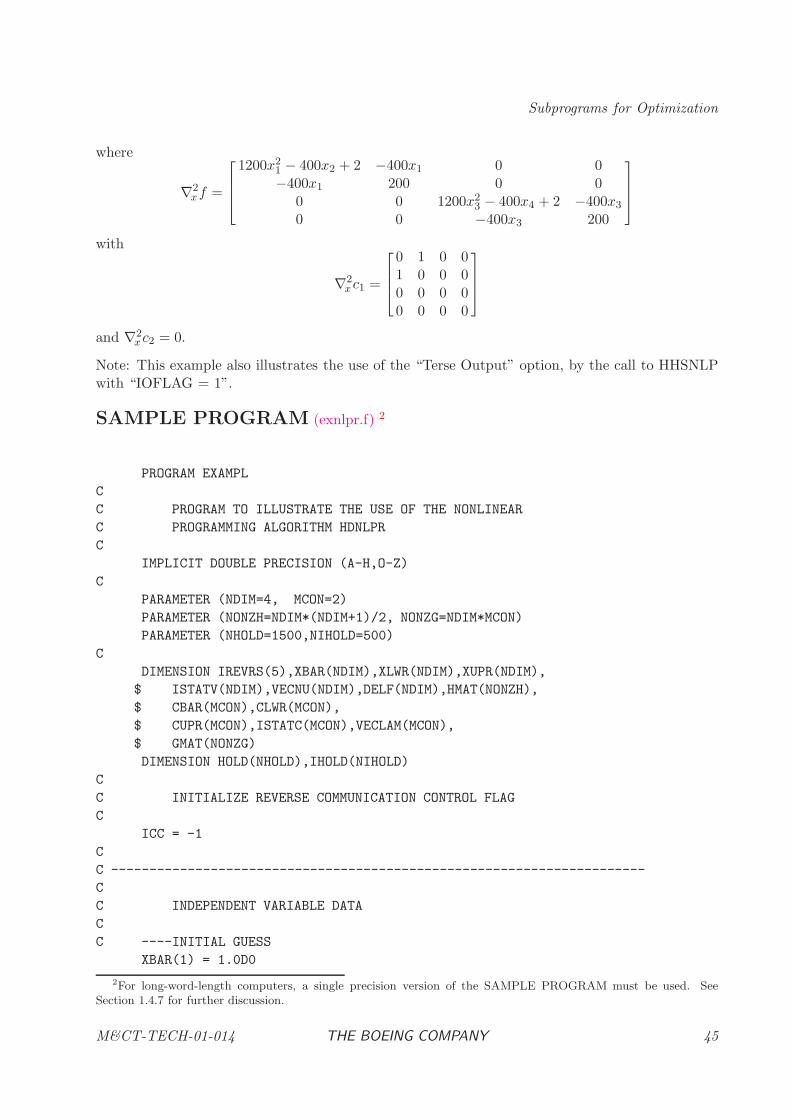
Subprograms for Optimization
where
∇2xf =
1200x21 − 400x2 + 2 −400x1 0 0−400x1 200 0 0
0 0 1200x23 − 400x4 + 2 −400x3
0 0 −400x3 200
with
∇2xc1 =
0 1 0 01 0 0 00 0 0 00 0 0 0
and ∇2xc2 = 0.
Note: This example also illustrates the use of the “Terse Output” option, by the call to HHSNLPwith “IOFLAG = 1”.
SAMPLE PROGRAM (exnlpr.f) 2
PROGRAM EXAMPL
C
C PROGRAM TO ILLUSTRATE THE USE OF THE NONLINEAR
C PROGRAMMING ALGORITHM HDNLPR
C
IMPLICIT DOUBLE PRECISION (A-H,O-Z)
C
PARAMETER (NDIM=4, MCON=2)
PARAMETER (NONZH=NDIM*(NDIM+1)/2, NONZG=NDIM*MCON)
PARAMETER (NHOLD=1500,NIHOLD=500)
C
DIMENSION IREVRS(5),XBAR(NDIM),XLWR(NDIM),XUPR(NDIM),
$ ISTATV(NDIM),VECNU(NDIM),DELF(NDIM),HMAT(NONZH),
$ CBAR(MCON),CLWR(MCON),
$ CUPR(MCON),ISTATC(MCON),VECLAM(MCON),
$ GMAT(NONZG)
DIMENSION HOLD(NHOLD),IHOLD(NIHOLD)
C
C INITIALIZE REVERSE COMMUNICATION CONTROL FLAG
C
ICC = -1
C
C ----------------------------------------------------------------------
C
C INDEPENDENT VARIABLE DATA
C
C ----INITIAL GUESS
XBAR(1) = 1.0D0
2For long-word-length computers, a single precision version of the SAMPLE PROGRAM must be used. See
Section 1.4.7 for further discussion.
M&CT-TECH-01-014 THE BOEING COMPANY 45
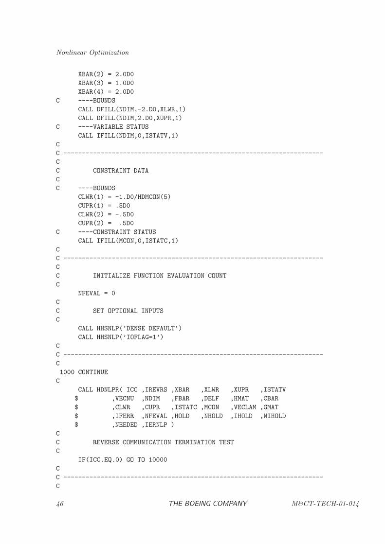
Nonlinear Optimization
XBAR(2) = 2.0D0
XBAR(3) = 1.0D0
XBAR(4) = 2.0D0
C ----BOUNDS
CALL DFILL(NDIM,-2.D0,XLWR,1)
CALL DFILL(NDIM,2.D0,XUPR,1)
C ----VARIABLE STATUS
CALL IFILL(NDIM,0,ISTATV,1)
C
C ----------------------------------------------------------------------
C
C CONSTRAINT DATA
C
C ----BOUNDS
CLWR(1) = -1.D0/HDMCON(5)
CUPR(1) = .5D0
CLWR(2) = -.5D0
CUPR(2) = .5D0
C ----CONSTRAINT STATUS
CALL IFILL(MCON,0,ISTATC,1)
C
C ----------------------------------------------------------------------
C
C INITIALIZE FUNCTION EVALUATION COUNT
C
NFEVAL = 0
C
C SET OPTIONAL INPUTS
C
CALL HHSNLP(’DENSE DEFAULT’)
CALL HHSNLP(’IOFLAG=1’)
C
C ----------------------------------------------------------------------
C
1000 CONTINUE
C
CALL HDNLPR( ICC ,IREVRS ,XBAR ,XLWR ,XUPR ,ISTATV
$ ,VECNU ,NDIM ,FBAR ,DELF ,HMAT ,CBAR
$ ,CLWR ,CUPR ,ISTATC ,MCON ,VECLAM ,GMAT
$ ,IFERR ,NFEVAL ,HOLD ,NHOLD ,IHOLD ,NIHOLD
$ ,NEEDED ,IERNLP )
C
C REVERSE COMMUNICATION TERMINATION TEST
C
IF(ICC.EQ.0) GO TO 10000
C
C ----------------------------------------------------------------------
C
46 THE BOEING COMPANY M&CT-TECH-01-014
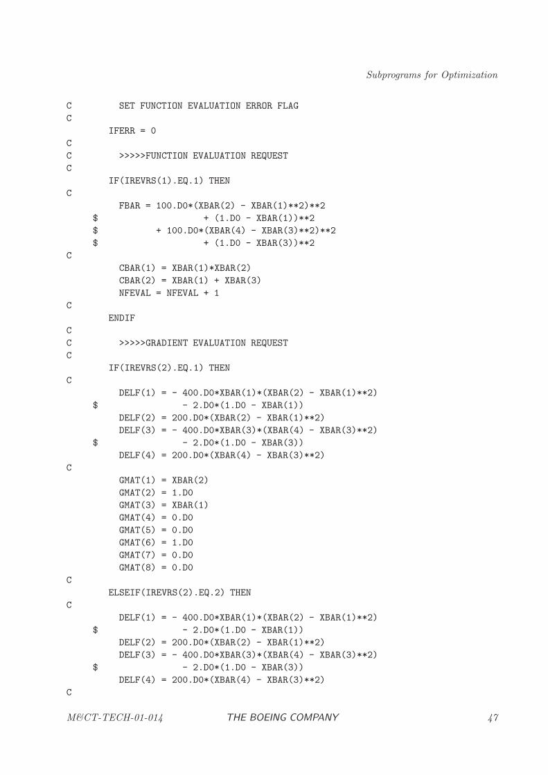
Subprograms for Optimization
C SET FUNCTION EVALUATION ERROR FLAG
C
IFERR = 0
C
C >>>>>FUNCTION EVALUATION REQUEST
C
IF(IREVRS(1).EQ.1) THEN
C
FBAR = 100.D0*(XBAR(2) - XBAR(1)**2)**2
$ + (1.D0 - XBAR(1))**2
$ + 100.D0*(XBAR(4) - XBAR(3)**2)**2
$ + (1.D0 - XBAR(3))**2
C
CBAR(1) = XBAR(1)*XBAR(2)
CBAR(2) = XBAR(1) + XBAR(3)
NFEVAL = NFEVAL + 1
C
ENDIF
C
C >>>>>GRADIENT EVALUATION REQUEST
C
IF(IREVRS(2).EQ.1) THEN
C
DELF(1) = - 400.D0*XBAR(1)*(XBAR(2) - XBAR(1)**2)
$ - 2.D0*(1.D0 - XBAR(1))
DELF(2) = 200.D0*(XBAR(2) - XBAR(1)**2)
DELF(3) = - 400.D0*XBAR(3)*(XBAR(4) - XBAR(3)**2)
$ - 2.D0*(1.D0 - XBAR(3))
DELF(4) = 200.D0*(XBAR(4) - XBAR(3)**2)
C
GMAT(1) = XBAR(2)
GMAT(2) = 1.D0
GMAT(3) = XBAR(1)
GMAT(4) = 0.D0
GMAT(5) = 0.D0
GMAT(6) = 1.D0
GMAT(7) = 0.D0
GMAT(8) = 0.D0
C
ELSEIF(IREVRS(2).EQ.2) THEN
C
DELF(1) = - 400.D0*XBAR(1)*(XBAR(2) - XBAR(1)**2)
$ - 2.D0*(1.D0 - XBAR(1))
DELF(2) = 200.D0*(XBAR(2) - XBAR(1)**2)
DELF(3) = - 400.D0*XBAR(3)*(XBAR(4) - XBAR(3)**2)
$ - 2.D0*(1.D0 - XBAR(3))
DELF(4) = 200.D0*(XBAR(4) - XBAR(3)**2)
C
M&CT-TECH-01-014 THE BOEING COMPANY 47
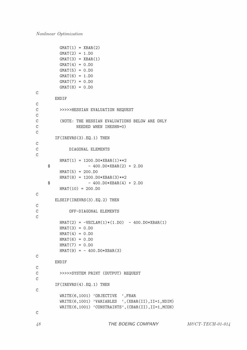
Nonlinear Optimization
GMAT(1) = XBAR(2)
GMAT(2) = 1.D0
GMAT(3) = XBAR(1)
GMAT(4) = 0.D0
GMAT(5) = 0.D0
GMAT(6) = 1.D0
GMAT(7) = 0.D0
GMAT(8) = 0.D0
C
ENDIF
C
C >>>>>HESSIAN EVALUATION REQUEST
C
C (NOTE: THE HESSIAN EVALUATIONS BELOW ARE ONLY
C NEEDED WHEN IHESHN=0)
C
IF(IREVRS(3).EQ.1) THEN
C
C DIAGONAL ELEMENTS
C
HMAT(1) = 1200.D0*XBAR(1)**2
$ - 400.D0*XBAR(2) + 2.D0
HMAT(5) = 200.D0
HMAT(8) = 1200.D0*XBAR(3)**2
$ - 400.D0*XBAR(4) + 2.D0
HMAT(10) = 200.D0
C
ELSEIF(IREVRS(3).EQ.2) THEN
C
C OFF-DIAGONAL ELEMENTS
C
HMAT(2) = -VECLAM(1)*(1.D0) - 400.D0*XBAR(1)
HMAT(3) = 0.D0
HMAT(4) = 0.D0
HMAT(6) = 0.D0
HMAT(7) = 0.D0
HMAT(9) = - 400.D0*XBAR(3)
C
ENDIF
C
C >>>>>SYSTEM PRINT (OUTPUT) REQUEST
C
IF(IREVRS(4).EQ.1) THEN
C
WRITE(6,1001) ’OBJECTIVE ’,FBAR
WRITE(6,1001) ’VARIABLES ’,(XBAR(II),II=1,NDIM)
WRITE(6,1001) ’CONSTRAINTS’,(CBAR(II),II=1,MCON)
C
48 THE BOEING COMPANY M&CT-TECH-01-014
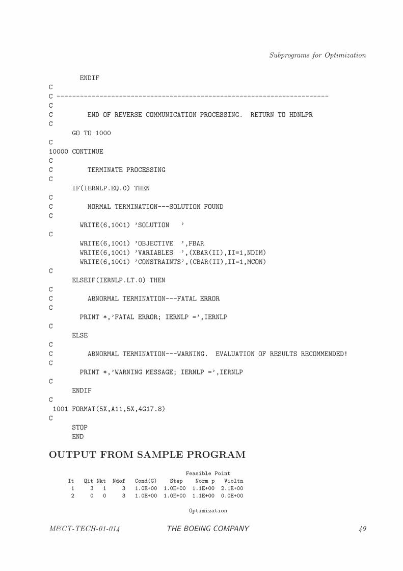
Subprograms for Optimization
ENDIF
C
C ----------------------------------------------------------------------
C
C END OF REVERSE COMMUNICATION PROCESSING. RETURN TO HDNLPR
C
GO TO 1000
C
10000 CONTINUE
C
C TERMINATE PROCESSING
C
IF(IERNLP.EQ.0) THEN
C
C NORMAL TERMINATION---SOLUTION FOUND
C
WRITE(6,1001) ’SOLUTION ’
C
WRITE(6,1001) ’OBJECTIVE ’,FBAR
WRITE(6,1001) ’VARIABLES ’,(XBAR(II),II=1,NDIM)
WRITE(6,1001) ’CONSTRAINTS’,(CBAR(II),II=1,MCON)
C
ELSEIF(IERNLP.LT.0) THEN
C
C ABNORMAL TERMINATION---FATAL ERROR
C
PRINT *,’FATAL ERROR; IERNLP =’,IERNLP
C
ELSE
C
C ABNORMAL TERMINATION---WARNING. EVALUATION OF RESULTS RECOMMENDED!
C
PRINT *,’WARNING MESSAGE; IERNLP =’,IERNLP
C
ENDIF
C
1001 FORMAT(5X,A11,5X,4G17.8)
C
STOP
END
OUTPUT FROM SAMPLE PROGRAM
Feasible Point
It Qit Nkt Ndof Cond(G) Step Norm p Violtn
1 3 1 3 1.0E+00 1.0E+00 1.1E+00 2.1E+00
2 0 0 3 1.0E+00 1.0E+00 1.1E+00 0.0E+00
Optimization
M&CT-TECH-01-014 THE BOEING COMPANY 49
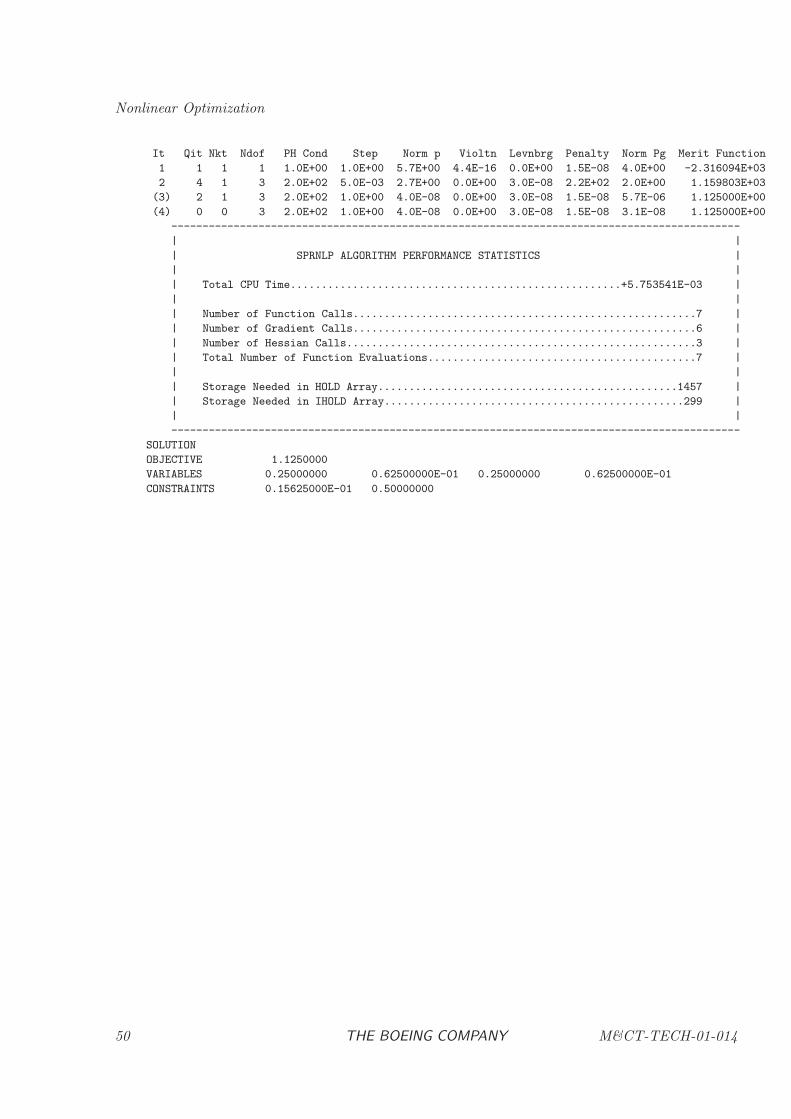
Nonlinear Optimization
It Qit Nkt Ndof PH Cond Step Norm p Violtn Levnbrg Penalty Norm Pg Merit Function
1 1 1 1 1.0E+00 1.0E+00 5.7E+00 4.4E-16 0.0E+00 1.5E-08 4.0E+00 -2.316094E+03
2 4 1 3 2.0E+02 5.0E-03 2.7E+00 0.0E+00 3.0E-08 2.2E+02 2.0E+00 1.159803E+03
(3) 2 1 3 2.0E+02 1.0E+00 4.0E-08 0.0E+00 3.0E-08 1.5E-08 5.7E-06 1.125000E+00
(4) 0 0 3 2.0E+02 1.0E+00 4.0E-08 0.0E+00 3.0E-08 1.5E-08 3.1E-08 1.125000E+00
-------------------------------------------------------------------------------------------
| |
| SPRNLP ALGORITHM PERFORMANCE STATISTICS |
| |
| Total CPU Time.....................................................+5.753541E-03 |
| |
| Number of Function Calls.......................................................7 |
| Number of Gradient Calls.......................................................6 |
| Number of Hessian Calls........................................................3 |
| Total Number of Function Evaluations...........................................7 |
| |
| Storage Needed in HOLD Array................................................1457 |
| Storage Needed in IHOLD Array................................................299 |
| |
-------------------------------------------------------------------------------------------
SOLUTION
OBJECTIVE 1.1250000
VARIABLES 0.25000000 0.62500000E-01 0.25000000 0.62500000E-01
CONSTRAINTS 0.15625000E-01 0.50000000
50 THE BOEING COMPANY M&CT-TECH-01-014
Subprograms for Optimization
HDSNLP: Sparse Nonlinear Programming
PURPOSE
HDSNLP computes the vector x = (x1, x2, . . . , xn) which minimizes the objective function
f(x)
subject to the m nonlinear constraints
cL ≤ c(x) ≤ cU
and the simple boundsxL ≤ x ≤ xU .
Equality constraints are imposed by setting cLi = cUi and variables can be fixed by setting xLi =xUi. HDSNLP works under the assumption that the objective and constraint functions are twicecontinuously differentiable, and if this is not true algorithm performance is unpredictable. HDSNLPuses a reverse communication format and upon request the user must supply the values of thefunctions, and their first and second derivatives. The matrix of first derivatives (the Jacobian) andthe matrix of second derivatives (Hessian of the Lagrangian) are represented in a sparse formatconsistent with that used in BCSLIB-EXT [1].
RELATED SUBPROGRAMS
HDBNLP Sparse Barrier Nonlinear Programming
HHSNLP Sparse Nonlinear Programming Input Procedure
METHOD
A sequential quadratic programming (SQP) approach is used to solve the nonlinear programming(NLP) problem. The quadratic programming algorithm requires an estimate for the Hessian matrixHL. If the user cannot provide this information analytically, the sparse finite difference techniquesdescribed in Chapter 3 should be utilized. For sparse applications the quadratic programmingsubproblem is efficiently solved using the sparse Schur-Complement Method. If problem sparsityis not exploited the QP subproblem can be solved efficiently using a dense null-space algorithm.
WARNING
The objective function and constraints supplied by the user are assumed to be continuous andhave continuous first and second derivatives. Non-differentiable functions can cause unpredictableperformance in the optimization algorithm. It should be emphasized that discontinuities in theHessian matrices can significantly degrade the speed of convergence without producing any otherobvious difficulties. The following common sources of error should be avoided when evaluating theobjective and constraint functions:
(1) non-smooth interpolation of data;
(2) iterative procedures inside the function evaluation process, such as adaptive quadrature or rootsolving;
M&CT-TECH-01-014 THE BOEING COMPANY 51
Nonlinear Optimization
(3) discontinuous behavior caused by branching for IF tests;
(4) non-differentiable functions such as ABS, MAX, and MIN.
The user must provide a procedure to evaluate the objective and constraint functions in additionto first and second derivatives of these quantities. If it is not possible to evaluate the functions(for example, c(x) = 1/x at x = 0) then set IFERR = 1 and exit the function evaluation process.Otherwise, set IFERR = 0 when the functions are evaluated. The function error flag should beused to avoid computational difficulties, but never in lieu of an explicit constraint.
The HDSNLP software uses internal common blocks to communicate information. To avoid con-flict with these internal commons the user should not have commons with the following names:NPSPRR, NPSPRI, NPSPRC, STATIS, KONSTN, NPSALG, NPSDFL, NLPERR, PERCOM,ITEREF, and CLKCOM.
USAGE
INTEGER IRVCOM, IFERR, NFEVAL, IER, NEEDED
INTEGER NDIM, MCON, NONZH, NONZG, NHOLD, NIHOLD
INTEGER IREVRS(5), ISTATV(NDIM), IROWH(NONZH), JSTRH(NDIM+1)
INTEGER ISTATC(MCON), IROWG(NONZG), JCOLG(NONZG), IHOLD(NIHOLD)
DOUBLE PRECISION FBAR, XBAR(NDIM), XLWR(NDIM), XUPR(NDIM), VECNU(NDIM)
DOUBLE PRECISION DELF(NDIM), HMAT(NONZH), CBAR(MCON), CLWR(MCON)
DOUBLE PRECISION CUPR(MCON), VECLAM(MCON), GMAT(NONZG), HOLD(NHOLD)
CALL HDSNLP( IRVCOM ,IREVRS ,XBAR ,XLWR ,XUPR ,ISTATV
$ ,VECNU ,NDIM ,FBAR ,DELF ,HMAT ,IROWH
$ ,JSTRH ,NONZH ,CBAR ,CLWR ,CUPR ,ISTATC
$ ,MCON ,VECLAM ,GMAT ,IROWG ,JCOLG ,NONZG
$ ,IFERR ,NFEVAL ,HOLD ,NHOLD ,IHOLD ,NIHOLD
$ ,NEEDED ,IER )
ARGUMENTS
ARGUMENTS TO CONTROL REVERSE COMMUNICATION
IRVCOM [INPUT/OUTPUT, INTEGER]Continuation control flag. This argument must be initialized. Thereafter it is setby the algorithm and must not be changed by the calling program.
IRVCOM = −1 Initialization pass.
IRVCOM = 0 Termination (normal or abnormal).
52 THE BOEING COMPANY M&CT-TECH-01-014

Subprograms for Optimization
IRVCOM = +1 Perform an evaluation and then reenter HDSNLP. Opera-tions to be performed are defined by the output variablesIREVRS(1), IREVRS(2), IREVRS(3), and IREVRS(4) below.IREVRS(5) contains information which may be valuable tothe interface but does not require any action on the part ofthe user.
IREVRS [OUTPUT, INTEGER, ARRAY]An integer array of length 5, containing reverse communication control information.IREVRS(1) Function evaluation request
= 0 Function evaluation not requested; Warning:do not change the current function and con-straint values.
= 1 Function evaluation requested; evaluate ob-jective function and all constraints at currentpoint XBAR.
IREVRS(2) Gradient evaluation request= 0 Gradient evaluation not requested; Warning:
do not change the current gradient and Jaco-bian.
= 1 Approximate (e.g. forward difference) gradi-ent requested; evaluate gradient vector g andJacobian matrix G at current point XBAR. (Ifavailable, accurate or analytic gradients maybe supplied)
= 2 Accurate (e.g. central difference or analytic)gradient requested; evaluate gradient vectorg and Jacobian matrix G at current pointXBAR.
M&CT-TECH-01-014 THE BOEING COMPANY 53

Nonlinear Optimization
IREVRS(3) Hessian evaluation request= 0 Hessian evaluation not requested; Warning:
do not change the current Hessian.
= 1 Hessian diagonal requested; get ready for fullHessian evaluation with (IREVRS(3)=2) atcurrent point (XBAR,VECLAM) and option-ally evaluate diagonal elements of Hessian ma-trix H.
= 2 Full Hessian evaluation requested; eval-uate Hessian matrix H of the functionL(x, λ) = f − ∑m
k=1 λkck at current point(XBAR,VECLAM). A full evaluation re-quest is always preceded by a call withIREVRS(3)=1 at the same point XBAR, andconsequently it may not be necessary to re-compute the diagonal elements.
IREVRS(4) System print (output) request= 0 System print not requested.
= 1 System print requested; perform any outputoperations (print, write files, etc.) desiredto display problem specific information at thecurrent point XBAR. The frequency of printis defined by the output control flag IOFLAG(see Optional Printout).
IREVRS(5) Algorithm information flag= 0 Call was made from the interface portion of
the algorithm.
= 1 Call was made from the optimization portionof the algorithm.
= 2 Call was made from the optimization portionof the algorithm requesting Hessian reset.
= 3 Call was made from the optimization portionof the algorithm requesting optimal perturba-tion size adjustment.
= 4 Call was made from the feasiblity portion ofthe algorithm.
INDEPENDENT VARIABLE DATA
XBAR† [INPUT/OUTPUT, DOUBLE PRECISION, ARRAY]A real array of length NDIM of current variable values x.
IRVCOM=−1 Initial guess must be input.
54 THE BOEING COMPANY M&CT-TECH-01-014
Subprograms for Optimization
IRVCOM=0 Final point is output. When IER = 0, +101, the final pointcorresponds to a local optimum. When IER = +104, . . . ,+111, +114, +116, +117, +119, the final point is either thebest feasible point if one has been found, or the last iterate.
IRVCOM=1 Intermediate iteration points are output.
XLWR† [INPUT, DOUBLE PRECISION, ARRAY]A real array of length NDIM containing the variable lower bounds xL. For variablesthat have no lower bound set xLi ≤ −.01/HDMCON(5). See Section 2.2 of theBCSLIB Manual [2] for HDMCON.
XUPR† [INPUT, DOUBLE PRECISION, ARRAY]A real array of length NDIM containing the variable upper bounds xU . For variablesthat have no upper bound set xUi ≥ .01/HDMCON(5).
ISTATV† [INPUT/OUTPUT, INTEGER, ARRAY]An integer array of length NDIM indicating variable status. On input ISTATVdefines an estimate of the active variable bounds, and on output ISTATV definesthe bounds active at the solution.
ISTATV(i)= 0 Variable is strictly feasible, i.e. xLi < xi < xUi.
ISTATV(i)= 1 Variable lower bound is active, i.e. xLi = xi.
ISTATV(i)= 2 Variable upper bound is active, i.e. xi = xUi.
ISTATV(i)= 3 Fixed permanently.
ISTATV(i)= 10 Output only: Violated variable lower bound, i.e. xLi−δc > xi.
ISTATV(i)= 20 Output only: Violated variable upper bound, i.e. xi > xUi+δc.
ISTATV(i)= 30 Output only: Violated fixed variable. Either xi < xLi − δc orxi > xUi + δc.
When ISTATV(i) = 3 it is necessary that xLi = xUi, where xLi = XLWR(i)and xUi = XUPR(i). When ISTATV(i) 6= 3, it is necessary that xLi < xUi with|xLi − xUi| > δc.
VECNU# [INPUT/OUTPUT, DOUBLE PRECISION, ARRAY]An array of length NDIM of bound multipliers ν.
NDIM† [INPUT, INTEGER]Number of variables n, where 1 ≤ NDIM.
OBJECTIVE FUNCTION DATA
M&CT-TECH-01-014 THE BOEING COMPANY 55
Nonlinear Optimization
FBAR‡ [INPUT, DOUBLE PRECISION]The objective function evaluated at XBAR, f(XBAR).
DELF‡ [INPUT, DOUBLE PRECISION, ARRAY]A real array of length NDIM containing the gradient g of FBAR at XBAR.
HMAT‡ [INPUT, DOUBLE PRECISION, ARRAY]A real array of length NONZH containing the nonzero elements of Hessian matrixHL = ∇2
xf −∑mi=1 λi∇2
x ci. of the Lagrangian function. Since the Hessian is sym-metric, only the lower triangular part is input (see USAGE REMARKS). Storagefor the diagonal elements must be provided even if they are zero.
IROWH† [INPUT, INTEGER, ARRAY]An integer array of length NONZH containing the row indices of the Hessian nonze-ros, where 0 < IROWH(k) ≤ NDIM for k = 1, . . . ,NONZH. The diagonal elementsmust be specified, i.e. IROWH(JSTRH(k))= k for k = 1, . . . ,NDIM.
JSTRH† [INPUT, INTEGER, ARRAY]An integer array of length NDIM+1 containing the column start indices of nonze-ros, where JSTRH(1) = 1, JSTRH(NDIM+1)=NONZH +1, and JSTRH(k) <JSTRH(k + 1) for k = 1, . . . ,NDIM.
NONZH† [INPUT, INTEGER]Number of nonzero Hessian elements, where n ≤ NONZH ≤ n(n+ 1)/2.
CONSTRAINT DATA
CBAR‡ [INPUT, DOUBLE PRECISION, ARRAY]A real array of length MCON containing the constraints c(x) evaluated at XBAR.Not referenced when MCON = 0.
CLWR† [INPUT, DOUBLE PRECISION, ARRAY]A real array of length MCON containing the constraint lower bounds cL. Forconstraints that have no lower bound set cLi ≤ −.01/HDMCON(5) . Not referencedwhen MCON = 0.
CUPR† [INPUT, DOUBLE PRECISION, ARRAY]A real array of length MCON containing the constraint upper bounds cU . Forconstraints that have no upper bound set cUi ≥ .01/HDMCON(5) . Not referencedwhen MCON = 0.
ISTATC† [INPUT/OUTPUT, INTEGER, ARRAY]An integer array of length MCON indicating the constraint status. On inputISTATC defines an estimate of the active constraints, and on output ISTATCdefines the constraints active at the solution.
ISTATC(i)= 0 Free (inactive) inequality, i.e. cLi < ci(x) < cUi.
ISTATC(i)= 1 Constraint lower bound is active, i.e. cLi = ci(x).
ISTATC(i)= 2 Constraint upper bound is active, i.e. ci(x) = cUi.
56 THE BOEING COMPANY M&CT-TECH-01-014
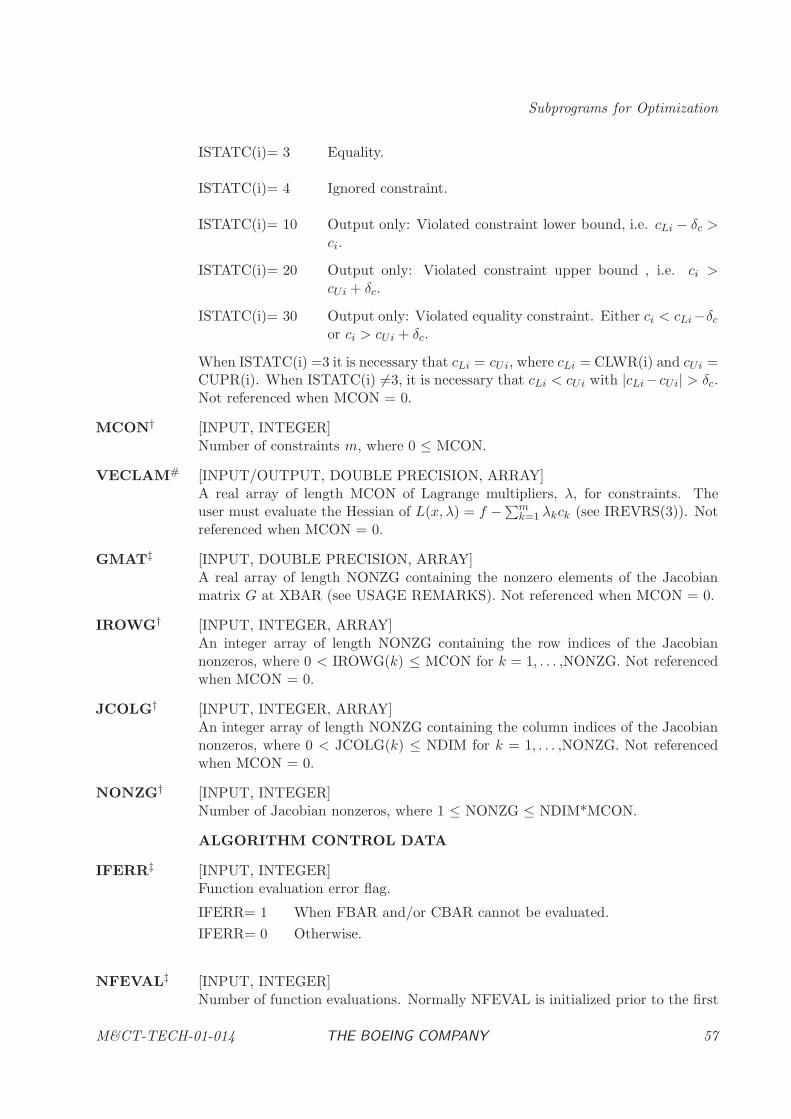
Subprograms for Optimization
ISTATC(i)= 3 Equality.
ISTATC(i)= 4 Ignored constraint.
ISTATC(i)= 10 Output only: Violated constraint lower bound, i.e. cLi − δc >ci.
ISTATC(i)= 20 Output only: Violated constraint upper bound , i.e. ci >cUi + δc.
ISTATC(i)= 30 Output only: Violated equality constraint. Either ci < cLi−δcor ci > cUi + δc.
When ISTATC(i) =3 it is necessary that cLi = cUi, where cLi = CLWR(i) and cUi =CUPR(i). When ISTATC(i) 6=3, it is necessary that cLi < cUi with |cLi−cUi| > δc.Not referenced when MCON = 0.
MCON† [INPUT, INTEGER]Number of constraints m, where 0 ≤ MCON.
VECLAM# [INPUT/OUTPUT, DOUBLE PRECISION, ARRAY]A real array of length MCON of Lagrange multipliers, λ, for constraints. Theuser must evaluate the Hessian of L(x, λ) = f −∑m
k=1 λkck (see IREVRS(3)). Notreferenced when MCON = 0.
GMAT‡ [INPUT, DOUBLE PRECISION, ARRAY]A real array of length NONZG containing the nonzero elements of the Jacobianmatrix G at XBAR (see USAGE REMARKS). Not referenced when MCON = 0.
IROWG† [INPUT, INTEGER, ARRAY]An integer array of length NONZG containing the row indices of the Jacobiannonzeros, where 0 < IROWG(k) ≤ MCON for k = 1, . . . ,NONZG. Not referencedwhen MCON = 0.
JCOLG† [INPUT, INTEGER, ARRAY]An integer array of length NONZG containing the column indices of the Jacobiannonzeros, where 0 < JCOLG(k) ≤ NDIM for k = 1, . . . ,NONZG. Not referencedwhen MCON = 0.
NONZG† [INPUT, INTEGER]Number of Jacobian nonzeros, where 1 ≤ NONZG ≤ NDIM*MCON.
ALGORITHM CONTROL DATA
IFERR‡ [INPUT, INTEGER]Function evaluation error flag.
IFERR= 1 When FBAR and/or CBAR cannot be evaluated.
IFERR= 0 Otherwise.
NFEVAL‡ [INPUT, INTEGER]Number of function evaluations. Normally NFEVAL is initialized prior to the first
M&CT-TECH-01-014 THE BOEING COMPANY 57
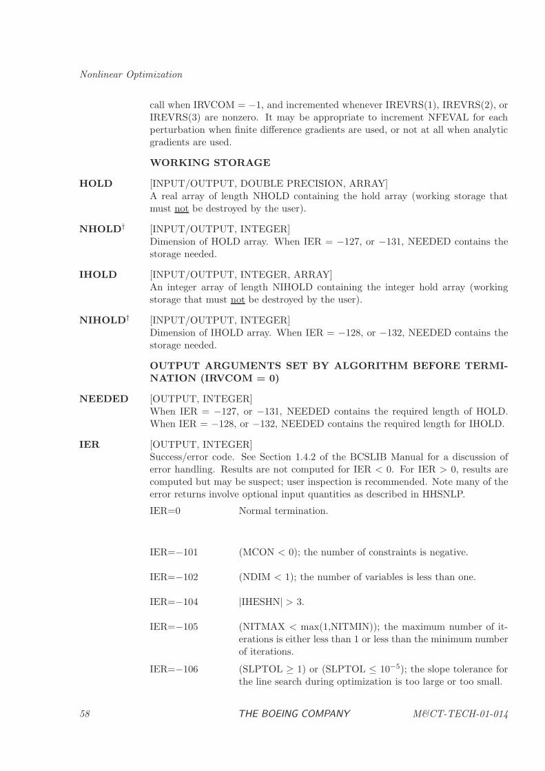
Nonlinear Optimization
call when IRVCOM = −1, and incremented whenever IREVRS(1), IREVRS(2), orIREVRS(3) are nonzero. It may be appropriate to increment NFEVAL for eachperturbation when finite difference gradients are used, or not at all when analyticgradients are used.
WORKING STORAGE
HOLD [INPUT/OUTPUT, DOUBLE PRECISION, ARRAY]A real array of length NHOLD containing the hold array (working storage thatmust not be destroyed by the user).
NHOLD† [INPUT/OUTPUT, INTEGER]Dimension of HOLD array. When IER = −127, or −131, NEEDED contains thestorage needed.
IHOLD [INPUT/OUTPUT, INTEGER, ARRAY]An integer array of length NIHOLD containing the integer hold array (workingstorage that must not be destroyed by the user).
NIHOLD† [INPUT/OUTPUT, INTEGER]Dimension of IHOLD array. When IER = −128, or −132, NEEDED contains thestorage needed.
OUTPUT ARGUMENTS SET BY ALGORITHM BEFORE TERMI-NATION (IRVCOM = 0)
NEEDED [OUTPUT, INTEGER]When IER = −127, or −131, NEEDED contains the required length of HOLD.When IER = −128, or −132, NEEDED contains the required length for IHOLD.
IER [OUTPUT, INTEGER]Success/error code. See Section 1.4.2 of the BCSLIB Manual for a discussion oferror handling. Results are not computed for IER < 0. For IER > 0, results arecomputed but may be suspect; user inspection is recommended. Note many of theerror returns involve optional input quantities as described in HHSNLP.
IER=0 Normal termination.
IER=−101 (MCON < 0); the number of constraints is negative.
IER=−102 (NDIM < 1); the number of variables is less than one.
IER=−104 |IHESHN| > 3.
IER=−105 (NITMAX < max(1,NITMIN)); the maximum number of it-erations is either less than 1 or less than the minimum numberof iterations.
IER=−106 (SLPTOL ≥ 1) or (SLPTOL ≤ 10−5); the slope tolerance forthe line search during optimization is too large or too small.
58 THE BOEING COMPANY M&CT-TECH-01-014
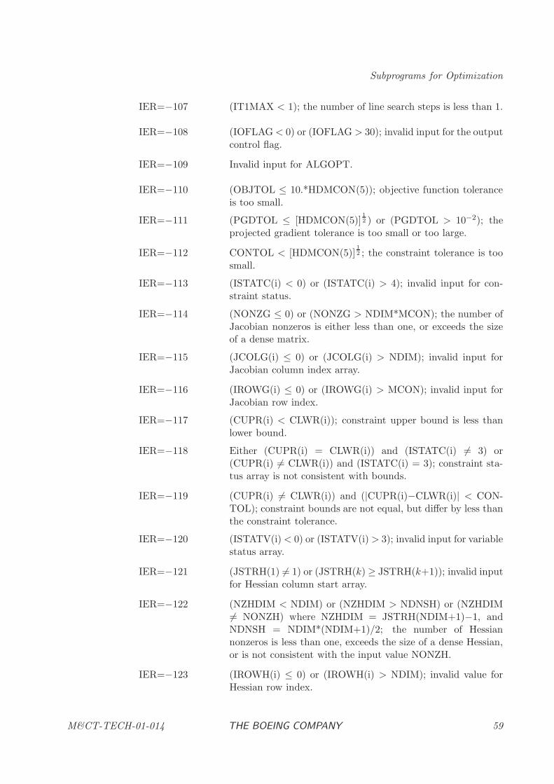
Subprograms for Optimization
IER=−107 (IT1MAX < 1); the number of line search steps is less than 1.
IER=−108 (IOFLAG< 0) or (IOFLAG > 30); invalid input for the outputcontrol flag.
IER=−109 Invalid input for ALGOPT.
IER=−110 (OBJTOL ≤ 10.*HDMCON(5)); objective function toleranceis too small.
IER=−111 (PGDTOL ≤ [HDMCON(5)]12 ) or (PGDTOL > 10−2); the
projected gradient tolerance is too small or too large.
IER=−112 CONTOL < [HDMCON(5)]12 ; the constraint tolerance is too
small.
IER=−113 (ISTATC(i) < 0) or (ISTATC(i) > 4); invalid input for con-straint status.
IER=−114 (NONZG ≤ 0) or (NONZG > NDIM*MCON); the number ofJacobian nonzeros is either less than one, or exceeds the sizeof a dense matrix.
IER=−115 (JCOLG(i) ≤ 0) or (JCOLG(i) > NDIM); invalid input forJacobian column index array.
IER=−116 (IROWG(i) ≤ 0) or (IROWG(i) > MCON); invalid input forJacobian row index.
IER=−117 (CUPR(i) < CLWR(i)); constraint upper bound is less thanlower bound.
IER=−118 Either (CUPR(i) = CLWR(i)) and (ISTATC(i) 6= 3) or(CUPR(i) 6= CLWR(i)) and (ISTATC(i) = 3); constraint sta-tus array is not consistent with bounds.
IER=−119 (CUPR(i) 6= CLWR(i)) and (|CUPR(i)−CLWR(i)| < CON-TOL); constraint bounds are not equal, but differ by less thanthe constraint tolerance.
IER=−120 (ISTATV(i)< 0) or (ISTATV(i) > 3); invalid input for variablestatus array.
IER=−121 (JSTRH(1) 6= 1) or (JSTRH(k) ≥ JSTRH(k+1)); invalid inputfor Hessian column start array.
IER=−122 (NZHDIM < NDIM) or (NZHDIM > NDNSH) or (NZHDIM6= NONZH) where NZHDIM = JSTRH(NDIM+1)−1, andNDNSH = NDIM*(NDIM+1)/2; the number of Hessiannonzeros is less than one, exceeds the size of a dense Hessian,or is not consistent with the input value NONZH.
IER=−123 (IROWH(i) ≤ 0) or (IROWH(i) > NDIM); invalid value forHessian row index.
M&CT-TECH-01-014 THE BOEING COMPANY 59
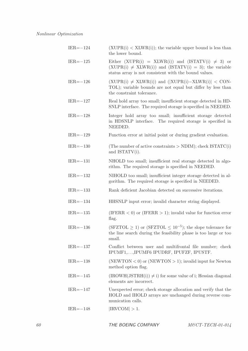
Nonlinear Optimization
IER=−124 (XUPR(i) < XLWR(i)); the variable upper bound is less thanthe lower bound.
IER=−125 Either (XUPR(i) = XLWR(i)) and (ISTATV(i) 6= 3) or(XUPR(i) 6= XLWR(i)) and (ISTATV(i) = 3); the variablestatus array is not consistent with the bound values.
IER=−126 (XUPR(i) 6= XLWR(i)) and (|XUPR(i)−XLWR(i)| < CON-TOL); variable bounds are not equal but differ by less thanthe constraint tolerance.
IER=−127 Real hold array too small; insufficient storage detected in HD-SNLP interface. The required storage is specified in NEEDED.
IER=−128 Integer hold array too small; insufficient storage detectedin HDSNLP interface. The required storage is specified inNEEDED.
IER=−129 Function error at initial point or during gradient evaluation.
IER=−130 (The number of active constraints > NDIM); check ISTATC(i)and ISTATV(i).
IER=−131 NHOLD too small; insufficient real storage detected in algo-rithm. The required storage is specified in NEEDED.
IER=−132 NIHOLD too small; insufficient integer storage detected in al-gorithm. The required storage is specified in NEEDED.
IER=−133 Rank deficient Jacobian detected on successive iterations.
IER=−134 HHSNLP input error; invalid character string displayed.
IER=−135 (IFERR < 0) or (IFERR > 1); invalid value for function errorflag.
IER=−136 (SFZTOL ≥ 1) or (SFZTOL ≤ 10−5); the slope tolerance forthe line search during the feasibility phase is too large or toosmall.
IER=−137 Conflict between user and multifrontal file number; checkIPUMF1,. . .,IPUMF6 IPUDRF, IPUFZF, IPUSTF.
IER=−138 (NEWTON < 0) or (NEWTON > 1); invalid input for Newtonmethod option flag.
IER=−145 (IROWH(JSTRH(i)) 6= i) for some value of i; Hessian diagonalelements are incorrect.
IER=−147 Unexpected error; check storage allocation and verify that theHOLD and IHOLD arrays are unchanged during reverse com-munication calls.
IER=−148 |IRVCOM| > 1.
60 THE BOEING COMPANY M&CT-TECH-01-014
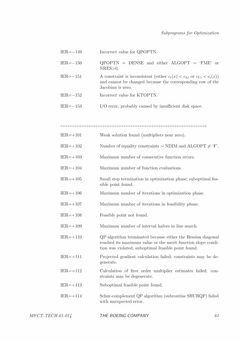
Subprograms for Optimization
IER=−149 Incorrect value for QPOPTN.
IER=−150 QPOPTN = DENSE and either ALGOPT = ‘FME’ orNRES>0.
IER=−151 A constraint is inconsistent (either ci(x) < cLi or cUi < ci(x))and cannot be changed because the corresponding row of theJacobian is zero.
IER=−152 Incorrect value for KTOPTN.
IER=−153 I/O error, probably caused by insufficient disk space.
---------------------------------------------------------------
IER=+101 Weak solution found (multipliers near zero).
IER=+102 Number of equality constraints = NDIM and ALGOPT 6= ‘F’.
IER=+103 Maximum number of consecutive function errors.
IER=+104 Maximum number of function evaluations.
IER=+105 Small step termination in optimization phase; suboptimal fea-sible point found.
IER=+106 Maximum number of iterations in optimization phase.
IER=+107 Maximum number of iterations in feasibility phase.
IER=+108 Feasible point not found.
IER=+109 Maximum number of interval halves in line search.
IER=+110 QP algorithm terminated because either the Hessian diagonalreached its maximum value or the merit function slope condi-tion was violated; suboptimal feasible point found.
IER=+111 Projected gradient calculation failed; constraints may be de-generate.
IER=+112 Calculation of first order multiplier estimates failed; con-straints may be degenerate.
IER=+113 Suboptimal feasible point found.
IER=+114 Schur-complement QP algorithm (subroutine SHURQP) failedwith unexpected error.
M&CT-TECH-01-014 THE BOEING COMPANY 61
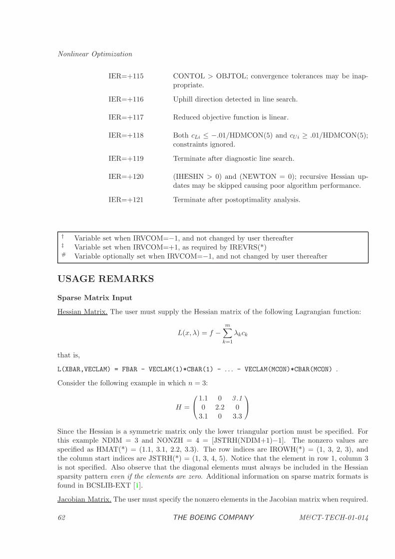
Nonlinear Optimization
IER=+115 CONTOL > OBJTOL; convergence tolerances may be inap-propriate.
IER=+116 Uphill direction detected in line search.
IER=+117 Reduced objective function is linear.
IER=+118 Both cLi ≤ −.01/HDMCON(5) and cUi ≥ .01/HDMCON(5);constraints ignored.
IER=+119 Terminate after diagnostic line search.
IER=+120 (IHESHN > 0) and (NEWTON = 0); recursive Hessian up-dates may be skipped causing poor algorithm performance.
IER=+121 Terminate after postoptimality analysis.
† Variable set when IRVCOM=−1, and not changed by user thereafter‡ Variable set when IRVCOM=+1, as required by IREVRS(*)# Variable optionally set when IRVCOM=−1, and not changed by user thereafter
USAGE REMARKS
Sparse Matrix Input
Hessian Matrix. The user must supply the Hessian matrix of the following Lagrangian function:
L(x, λ) = f −m∑
k=1
λkck
that is,
L(XBAR,VECLAM) = FBAR - VECLAM(1)*CBAR(1) - . . . - VECLAM(MCON)*CBAR(MCON) .
Consider the following example in which n = 3:
H =
1.1 0 3 .10 2.2 0
3.1 0 3.3
Since the Hessian is a symmetric matrix only the lower triangular portion must be specified. Forthis example NDIM = 3 and NONZH = 4 = [JSTRH(NDIM+1)−1]. The nonzero values arespecified as HMAT(*) = (1.1, 3.1, 2.2, 3.3). The row indices are IROWH(*) = (1, 3, 2, 3), andthe column start indices are JSTRH(*) = (1, 3, 4, 5). Notice that the element in row 1, column 3is not specified. Also observe that the diagonal elements must always be included in the Hessiansparsity pattern even if the elements are zero. Additional information on sparse matrix formats isfound in BCSLIB-EXT [1].
Jacobian Matrix. The user must specify the nonzero elements in the Jacobian matrix when required.
62 THE BOEING COMPANY M&CT-TECH-01-014
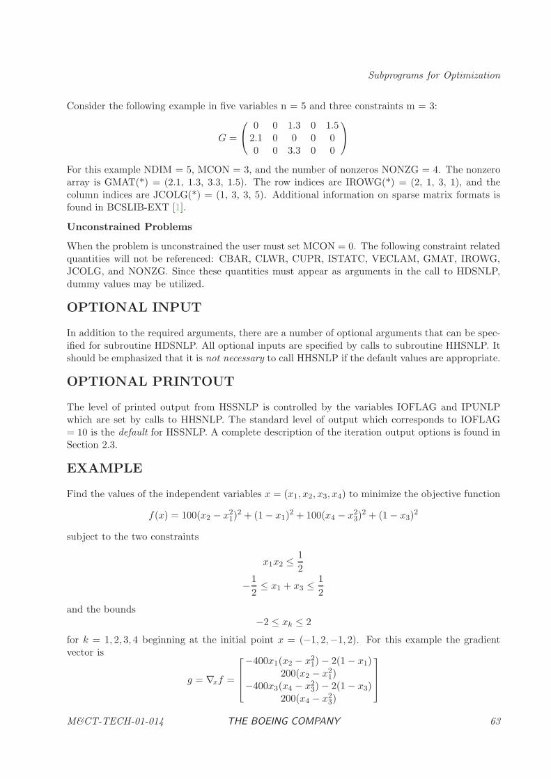
Subprograms for Optimization
Consider the following example in five variables n = 5 and three constraints m = 3:
G =
0 0 1.3 0 1.5
2.1 0 0 0 00 0 3.3 0 0
For this example NDIM = 5, MCON = 3, and the number of nonzeros NONZG = 4. The nonzeroarray is GMAT(*) = (2.1, 1.3, 3.3, 1.5). The row indices are IROWG(*) = (2, 1, 3, 1), and thecolumn indices are JCOLG(*) = (1, 3, 3, 5). Additional information on sparse matrix formats isfound in BCSLIB-EXT [1].
Unconstrained Problems
When the problem is unconstrained the user must set MCON = 0. The following constraint relatedquantities will not be referenced: CBAR, CLWR, CUPR, ISTATC, VECLAM, GMAT, IROWG,JCOLG, and NONZG. Since these quantities must appear as arguments in the call to HDSNLP,dummy values may be utilized.
OPTIONAL INPUT
In addition to the required arguments, there are a number of optional arguments that can be spec-ified for subroutine HDSNLP. All optional inputs are specified by calls to subroutine HHSNLP. Itshould be emphasized that it is not necessary to call HHSNLP if the default values are appropriate.
OPTIONAL PRINTOUT
The level of printed output from HSSNLP is controlled by the variables IOFLAG and IPUNLPwhich are set by calls to HHSNLP. The standard level of output which corresponds to IOFLAG= 10 is the default for HSSNLP. A complete description of the iteration output options is found inSection 2.3.
EXAMPLE
Find the values of the independent variables x = (x1, x2, x3, x4) to minimize the objective function
f(x) = 100(x2 − x21)
2 + (1 − x1)2 + 100(x4 − x2
3)2 + (1 − x3)
2
subject to the two constraints
x1x2 ≤ 1
2
−1
2≤ x1 + x3 ≤ 1
2
and the bounds−2 ≤ xk ≤ 2
for k = 1, 2, 3, 4 beginning at the initial point x = (−1, 2,−1, 2). For this example the gradientvector is
g = ∇xf =
−400x1(x2 − x21) − 2(1 − x1)
200(x2 − x21)
−400x3(x4 − x23) − 2(1 − x3)
200(x4 − x23)
M&CT-TECH-01-014 THE BOEING COMPANY 63

Nonlinear Optimization
and the Jacobian matrix is
G =
[∇xcT1
∇xcT2
]=
[x2 x1 0 01 0 1 0
].
It is also necessary to supply the Hessian matrix
∇2xL = ∇2
xf − λ1∇2xc1 − λ2∇2
x c2
where
∇2xf =
1200x21 − 400x2 + 2 −400x1 0 0−400x1 200 0 0
0 0 1200x23 − 400x4 + 2 −400x3
0 0 −400x3 200
with
∇2xc1 =
0 1 0 01 0 0 00 0 0 00 0 0 0
and ∇2xc2 = 0. Note: this example also illustrates the use of the “Terse Output” option by the call
to HHSNLP with “IOFLAG = 1”.
SAMPLE PROGRAM (exsnlp.f) 3
PROGRAM EXAMPL
C
C PROGRAM TO ILLUSTRATE THE USE OF THE SPARSE NONLINEAR
C PROGRAMMING ALGORITHM HDSNLP
C
IMPLICIT DOUBLE PRECISION (A-H,O-Z)
C
PARAMETER (NDIM=4, MCON=2)
PARAMETER (NONZH=6, NONZG=4)
PARAMETER (NHOLD=2000,NIHOLD=2000)
C
DIMENSION IREVRS(5),XBAR(NDIM),XLWR(NDIM),XUPR(NDIM),
$ ISTATV(NDIM),VECNU(NDIM),DELF(NDIM),HMAT(NONZH),
$ IROWH(NONZH),JSTRH(NDIM+1),CBAR(MCON),CLWR(MCON),
$ CUPR(MCON),ISTATC(MCON),VECLAM(MCON),
$ GMAT(NONZG),IROWG(NONZG),JCOLG(NONZG)
DIMENSION HOLD(NHOLD),IHOLD(NIHOLD)
C
C INITIALIZE REVERSE COMMUNICATION CONTROL FLAG
C
ICC = -1
C
C ----------------------------------------------------------------------
3For long-word-length computers, a single precision version of the SAMPLE PROGRAM must be used. See
Section 1.4.7 for further discussion.
64 THE BOEING COMPANY M&CT-TECH-01-014

Subprograms for Optimization
C
C INDEPENDENT VARIABLE DATA
C
C ----INITIAL GUESS
XBAR(1) = -1.0D0
XBAR(2) = 2.0D0
XBAR(3) = -1.0D0
XBAR(4) = 2.0D0
C ----BOUNDS
CALL DFILL(NDIM,-2.D0,XLWR,1)
CALL DFILL(NDIM,2.D0,XUPR,1)
C ----VARIABLE STATUS
CALL IFILL(NDIM,0,ISTATV,1)
C
C ----------------------------------------------------------------------
C
C OBJECTIVE FUNCTION DATA
C
C ----HESSIAN SPARSITY PATTERN (ROW INDICES)
IROWH(1) = 1
IROWH(2) = 2
IROWH(3) = 2
IROWH(4) = 3
IROWH(5) = 4
IROWH(6) = 4
C ----HESSIAN SPARSITY PATTERN (COLUMN START INDICES)
JSTRH(1) = 1
JSTRH(2) = 3
JSTRH(3) = 4
JSTRH(4) = 6
JSTRH(5) = 7
C
C ----------------------------------------------------------------------
C
C CONSTRAINT DATA
C
C ----BOUNDS
CLWR(1) = -1.D0/HDMCON(5)
CUPR(1) = .5D0
CLWR(2) = -.5D0
CUPR(2) = .5D0
C ----CONSTRAINT STATUS
CALL IFILL(MCON,0,ISTATC,1)
C ----JACOBIAN SPARSITY PATTERN (ROW INDICES)
IROWG(1) = 1
IROWG(2) = 2
IROWG(3) = 1
IROWG(4) = 2
M&CT-TECH-01-014 THE BOEING COMPANY 65
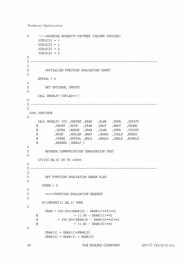
Nonlinear Optimization
C ----JACOBIAN SPARSITY PATTERN (COLUMN INDICES)
JCOLG(1) = 1
JCOLG(2) = 1
JCOLG(3) = 2
JCOLG(4) = 3
C
C ----------------------------------------------------------------------
C
C INITIALIZE FUNCTION EVALUATION COUNT
C
NFEVAL = 0
C
C SET OPTIONAL INPUTS
C
CALL HHSNLP(’IOFLAG=1’)
C
C ----------------------------------------------------------------------
C
1000 CONTINUE
C
CALL HDSNLP( ICC ,IREVRS ,XBAR ,XLWR ,XUPR ,ISTATV
$ ,VECNU ,NDIM ,FBAR ,DELF ,HMAT ,IROWH
$ ,JSTRH ,NONZH ,CBAR ,CLWR ,CUPR ,ISTATC
$ ,MCON ,VECLAM ,GMAT ,IROWG ,JCOLG ,NONZG
$ ,IFERR ,NFEVAL ,HOLD ,NHOLD ,IHOLD ,NIHOLD
$ ,NEEDED ,IERNLP )
C
C REVERSE COMMUNICATION TERMINATION TEST
C
IF(ICC.EQ.0) GO TO 10000
C
C ----------------------------------------------------------------------
C
C SET FUNCTION EVALUATION ERROR FLAG
C
IFERR = 0
C
C >>>>>FUNCTION EVALUATION REQUEST
C
IF(IREVRS(1).EQ.1) THEN
C
FBAR = 100.D0*(XBAR(2) - XBAR(1)**2)**2
$ + (1.D0 - XBAR(1))**2
$ + 100.D0*(XBAR(4) - XBAR(3)**2)**2
$ + (1.D0 - XBAR(3))**2
C
CBAR(1) = XBAR(1)*XBAR(2)
CBAR(2) = XBAR(1) + XBAR(3)
66 THE BOEING COMPANY M&CT-TECH-01-014
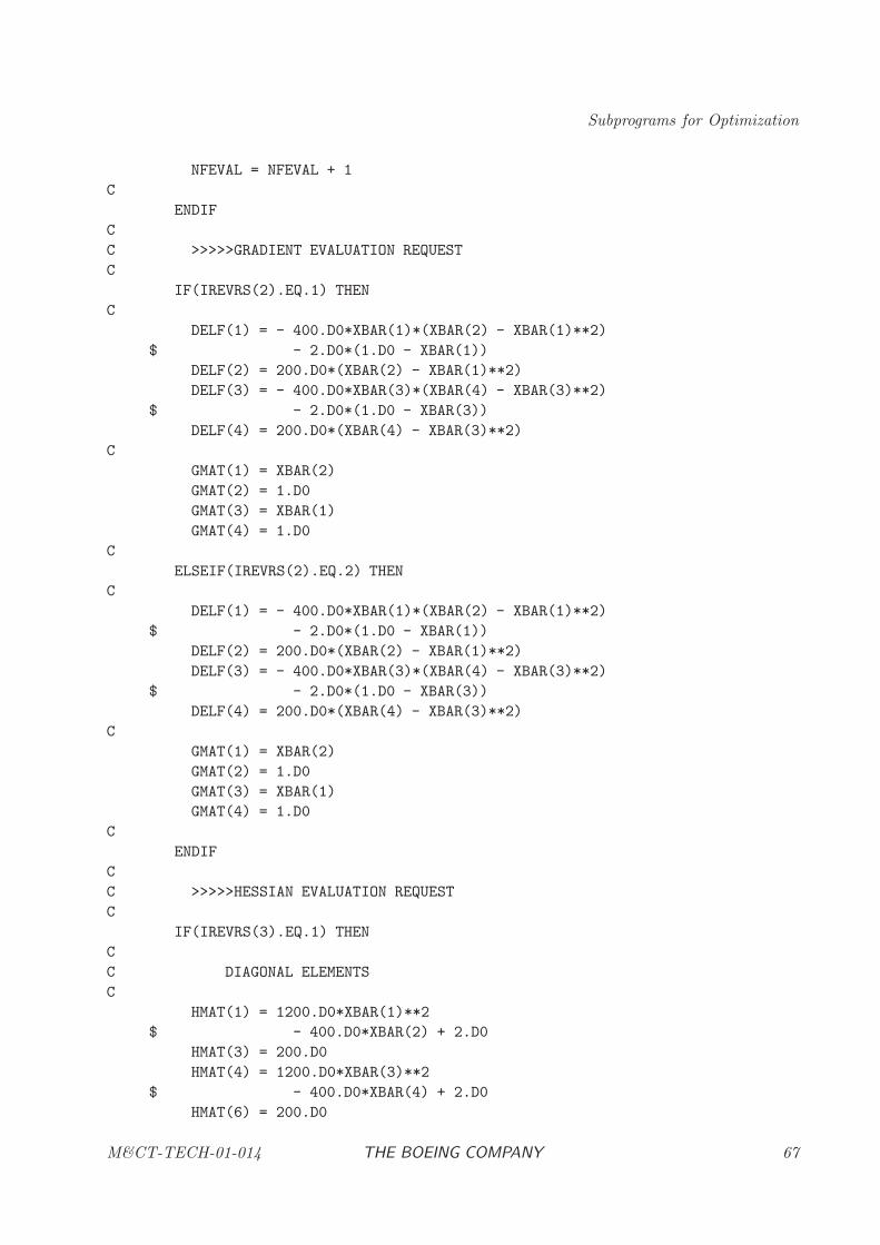
Subprograms for Optimization
NFEVAL = NFEVAL + 1
C
ENDIF
C
C >>>>>GRADIENT EVALUATION REQUEST
C
IF(IREVRS(2).EQ.1) THEN
C
DELF(1) = - 400.D0*XBAR(1)*(XBAR(2) - XBAR(1)**2)
$ - 2.D0*(1.D0 - XBAR(1))
DELF(2) = 200.D0*(XBAR(2) - XBAR(1)**2)
DELF(3) = - 400.D0*XBAR(3)*(XBAR(4) - XBAR(3)**2)
$ - 2.D0*(1.D0 - XBAR(3))
DELF(4) = 200.D0*(XBAR(4) - XBAR(3)**2)
C
GMAT(1) = XBAR(2)
GMAT(2) = 1.D0
GMAT(3) = XBAR(1)
GMAT(4) = 1.D0
C
ELSEIF(IREVRS(2).EQ.2) THEN
C
DELF(1) = - 400.D0*XBAR(1)*(XBAR(2) - XBAR(1)**2)
$ - 2.D0*(1.D0 - XBAR(1))
DELF(2) = 200.D0*(XBAR(2) - XBAR(1)**2)
DELF(3) = - 400.D0*XBAR(3)*(XBAR(4) - XBAR(3)**2)
$ - 2.D0*(1.D0 - XBAR(3))
DELF(4) = 200.D0*(XBAR(4) - XBAR(3)**2)
C
GMAT(1) = XBAR(2)
GMAT(2) = 1.D0
GMAT(3) = XBAR(1)
GMAT(4) = 1.D0
C
ENDIF
C
C >>>>>HESSIAN EVALUATION REQUEST
C
IF(IREVRS(3).EQ.1) THEN
C
C DIAGONAL ELEMENTS
C
HMAT(1) = 1200.D0*XBAR(1)**2
$ - 400.D0*XBAR(2) + 2.D0
HMAT(3) = 200.D0
HMAT(4) = 1200.D0*XBAR(3)**2
$ - 400.D0*XBAR(4) + 2.D0
HMAT(6) = 200.D0
M&CT-TECH-01-014 THE BOEING COMPANY 67
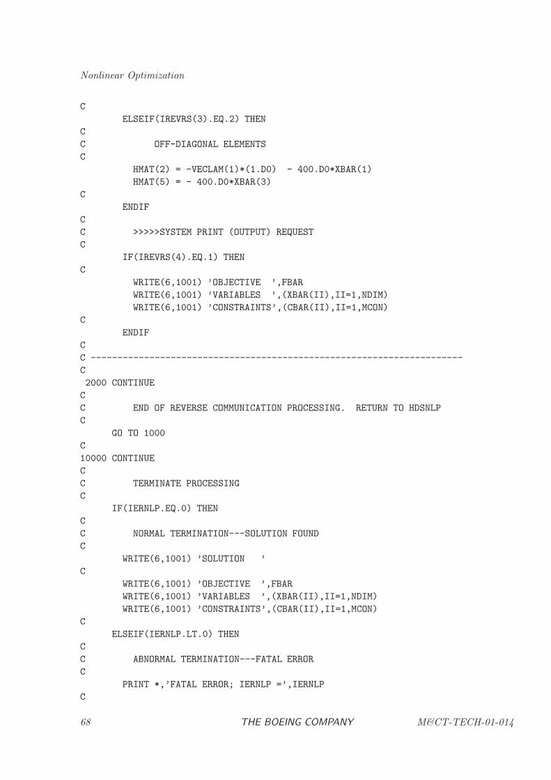
Nonlinear Optimization
C
ELSEIF(IREVRS(3).EQ.2) THEN
C
C OFF-DIAGONAL ELEMENTS
C
HMAT(2) = -VECLAM(1)*(1.D0) - 400.D0*XBAR(1)
HMAT(5) = - 400.D0*XBAR(3)
C
ENDIF
C
C >>>>>SYSTEM PRINT (OUTPUT) REQUEST
C
IF(IREVRS(4).EQ.1) THEN
C
WRITE(6,1001) ’OBJECTIVE ’,FBAR
WRITE(6,1001) ’VARIABLES ’,(XBAR(II),II=1,NDIM)
WRITE(6,1001) ’CONSTRAINTS’,(CBAR(II),II=1,MCON)
C
ENDIF
C
C ----------------------------------------------------------------------
C
2000 CONTINUE
C
C END OF REVERSE COMMUNICATION PROCESSING. RETURN TO HDSNLP
C
GO TO 1000
C
10000 CONTINUE
C
C TERMINATE PROCESSING
C
IF(IERNLP.EQ.0) THEN
C
C NORMAL TERMINATION---SOLUTION FOUND
C
WRITE(6,1001) ’SOLUTION ’
C
WRITE(6,1001) ’OBJECTIVE ’,FBAR
WRITE(6,1001) ’VARIABLES ’,(XBAR(II),II=1,NDIM)
WRITE(6,1001) ’CONSTRAINTS’,(CBAR(II),II=1,MCON)
C
ELSEIF(IERNLP.LT.0) THEN
C
C ABNORMAL TERMINATION---FATAL ERROR
C
PRINT *,’FATAL ERROR; IERNLP =’,IERNLP
C
68 THE BOEING COMPANY M&CT-TECH-01-014
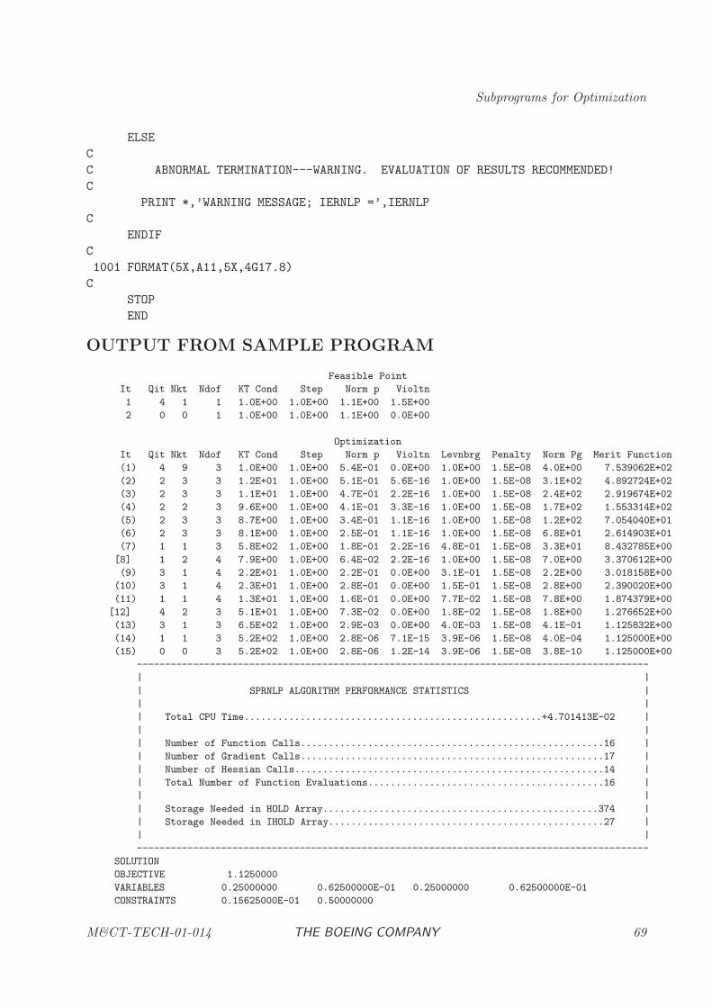
Subprograms for Optimization
ELSE
C
C ABNORMAL TERMINATION---WARNING. EVALUATION OF RESULTS RECOMMENDED!
C
PRINT *,’WARNING MESSAGE; IERNLP =’,IERNLP
C
ENDIF
C
1001 FORMAT(5X,A11,5X,4G17.8)
C
STOP
END
OUTPUT FROM SAMPLE PROGRAM
Feasible Point
It Qit Nkt Ndof KT Cond Step Norm p Violtn
1 4 1 1 1.0E+00 1.0E+00 1.1E+00 1.5E+00
2 0 0 1 1.0E+00 1.0E+00 1.1E+00 0.0E+00
Optimization
It Qit Nkt Ndof KT Cond Step Norm p Violtn Levnbrg Penalty Norm Pg Merit Function
(1) 4 9 3 1.0E+00 1.0E+00 5.4E-01 0.0E+00 1.0E+00 1.5E-08 4.0E+00 7.539062E+02
(2) 2 3 3 1.2E+01 1.0E+00 5.1E-01 5.6E-16 1.0E+00 1.5E-08 3.1E+02 4.892724E+02
(3) 2 3 3 1.1E+01 1.0E+00 4.7E-01 2.2E-16 1.0E+00 1.5E-08 2.4E+02 2.919674E+02
(4) 2 2 3 9.6E+00 1.0E+00 4.1E-01 3.3E-16 1.0E+00 1.5E-08 1.7E+02 1.553314E+02
(5) 2 3 3 8.7E+00 1.0E+00 3.4E-01 1.1E-16 1.0E+00 1.5E-08 1.2E+02 7.054040E+01
(6) 2 3 3 8.1E+00 1.0E+00 2.5E-01 1.1E-16 1.0E+00 1.5E-08 6.8E+01 2.614903E+01
(7) 1 1 3 5.8E+02 1.0E+00 1.8E-01 2.2E-16 4.8E-01 1.5E-08 3.3E+01 8.432785E+00
[8] 1 2 4 7.9E+00 1.0E+00 6.4E-02 2.2E-16 1.0E+00 1.5E-08 7.0E+00 3.370612E+00
(9) 3 1 4 2.2E+01 1.0E+00 2.2E-01 0.0E+00 3.1E-01 1.5E-08 2.2E+00 3.018158E+00
(10) 3 1 4 2.3E+01 1.0E+00 2.8E-01 0.0E+00 1.5E-01 1.5E-08 2.8E+00 2.390020E+00
(11) 1 1 4 1.3E+01 1.0E+00 1.6E-01 0.0E+00 7.7E-02 1.5E-08 7.8E+00 1.874379E+00
[12] 4 2 3 5.1E+01 1.0E+00 7.3E-02 0.0E+00 1.8E-02 1.5E-08 1.8E+00 1.276652E+00
(13) 3 1 3 6.5E+02 1.0E+00 2.9E-03 0.0E+00 4.0E-03 1.5E-08 4.1E-01 1.125832E+00
(14) 1 1 3 5.2E+02 1.0E+00 2.8E-06 7.1E-15 3.9E-06 1.5E-08 4.0E-04 1.125000E+00
(15) 0 0 3 5.2E+02 1.0E+00 2.8E-06 1.2E-14 3.9E-06 1.5E-08 3.8E-10 1.125000E+00
-------------------------------------------------------------------------------------------
| |
| SPRNLP ALGORITHM PERFORMANCE STATISTICS |
| |
| Total CPU Time.....................................................+4.701413E-02 |
| |
| Number of Function Calls......................................................16 |
| Number of Gradient Calls......................................................17 |
| Number of Hessian Calls.......................................................14 |
| Total Number of Function Evaluations..........................................16 |
| |
| Storage Needed in HOLD Array.................................................374 |
| Storage Needed in IHOLD Array.................................................27 |
| |
-------------------------------------------------------------------------------------------
SOLUTION
OBJECTIVE 1.1250000
VARIABLES 0.25000000 0.62500000E-01 0.25000000 0.62500000E-01
CONSTRAINTS 0.15625000E-01 0.50000000
M&CT-TECH-01-014 THE BOEING COMPANY 69
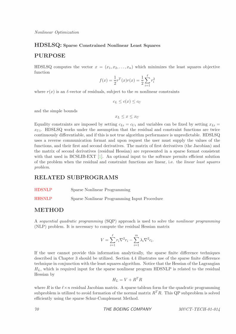
Nonlinear Optimization
HDSLSQ: Sparse Constrained Nonlinear Least Squares
PURPOSE
HDSLSQ computes the vector x = (x1, x2, . . . , xn) which minimizes the least squares objectivefunction
f(x) =1
2rT (x)r(x) =
1
2
ℓ∑
i=1
r2i
where r(x) is an ℓ-vector of residuals, subject to the m nonlinear constraints
cL ≤ c(x) ≤ cU
and the simple boundsxL ≤ x ≤ xU
Equality constraints are imposed by setting cLi = cUi and variables can be fixed by setting xLi =xUi. HDSLSQ works under the assumption that the residual and constraint functions are twicecontinuously differentiable, and if this is not true algorithm performance is unpredictable. HDSLSQuses a reverse communication format and upon request the user must supply the values of thefunctions, and their first and second derivatives. The matrix of first derivatives (the Jacobian) andthe matrix of second derivatives (residual Hessian) are represented in a sparse format consistentwith that used in BCSLIB-EXT [1]. An optional input to the software permits efficient solutionof the problem when the residual and constraint functions are linear, i.e. the linear least squaresproblem.
RELATED SUBPROGRAMS
HDSNLP Sparse Nonlinear Programming
HHSNLP Sparse Nonlinear Programming Input Procedure
METHOD
A sequential quadratic programming (SQP) approach is used to solve the nonlinear programming(NLP) problem. It is necessary to compute the residual Hessian matrix
V =ℓ∑
i=1
ri∇2ri −m∑
i=1
λi∇2ci.
If the user cannot provide this information analytically, the sparse finite difference techniquesdescribed in Chapter 3 should be utilized. Section 4.4 illustrates use of the sparse finite differencetechnique in conjunction with the least squares algorithm. Notice that the Hessian of the LagrangianHL, which is required input for the sparse nonlinear program HDSNLP is related to the residualHessian by
HL = V +RTR
where R is the ℓ×n residual Jacobian matrix. A sparse tableau form for the quadratic programmingsubproblem is utilized to avoid formation of the normal matrix RTR. This QP subproblem is solvedefficiently using the sparse Schur-Complement Method.
70 THE BOEING COMPANY M&CT-TECH-01-014
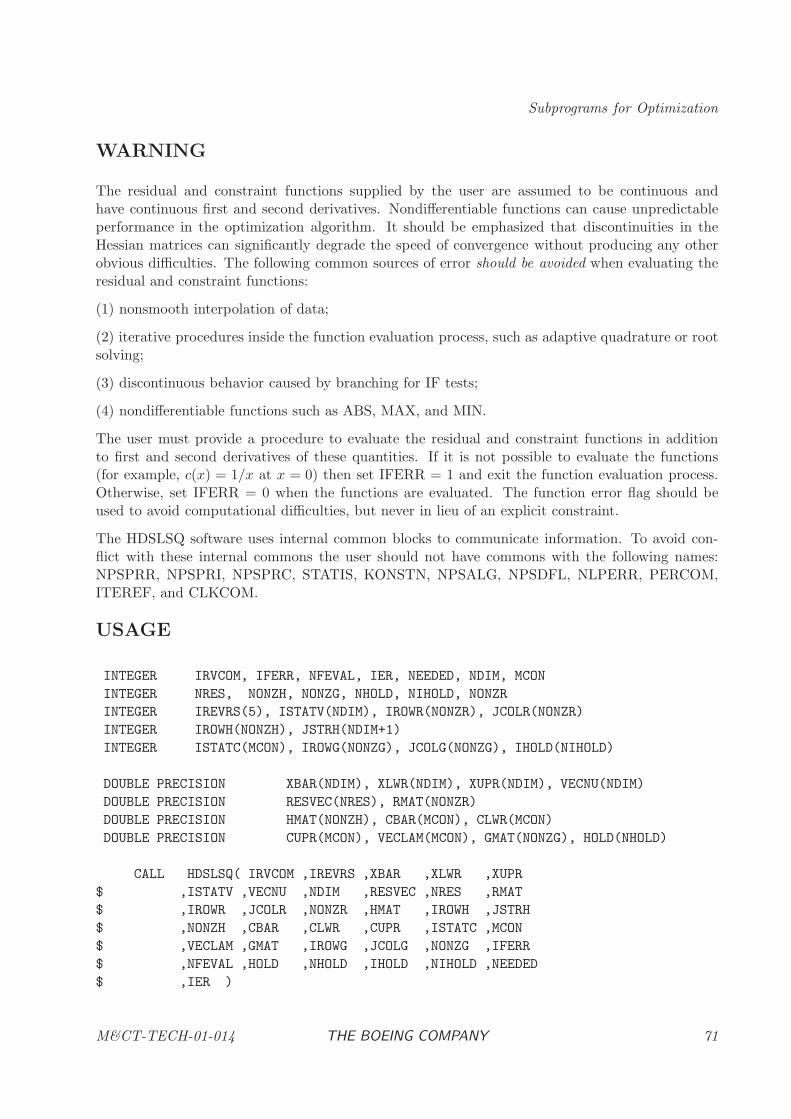
Subprograms for Optimization
WARNING
The residual and constraint functions supplied by the user are assumed to be continuous andhave continuous first and second derivatives. Nondifferentiable functions can cause unpredictableperformance in the optimization algorithm. It should be emphasized that discontinuities in theHessian matrices can significantly degrade the speed of convergence without producing any otherobvious difficulties. The following common sources of error should be avoided when evaluating theresidual and constraint functions:
(1) nonsmooth interpolation of data;
(2) iterative procedures inside the function evaluation process, such as adaptive quadrature or rootsolving;
(3) discontinuous behavior caused by branching for IF tests;
(4) nondifferentiable functions such as ABS, MAX, and MIN.
The user must provide a procedure to evaluate the residual and constraint functions in additionto first and second derivatives of these quantities. If it is not possible to evaluate the functions(for example, c(x) = 1/x at x = 0) then set IFERR = 1 and exit the function evaluation process.Otherwise, set IFERR = 0 when the functions are evaluated. The function error flag should beused to avoid computational difficulties, but never in lieu of an explicit constraint.
The HDSLSQ software uses internal common blocks to communicate information. To avoid con-flict with these internal commons the user should not have commons with the following names:NPSPRR, NPSPRI, NPSPRC, STATIS, KONSTN, NPSALG, NPSDFL, NLPERR, PERCOM,ITEREF, and CLKCOM.
USAGE
INTEGER IRVCOM, IFERR, NFEVAL, IER, NEEDED, NDIM, MCON
INTEGER NRES, NONZH, NONZG, NHOLD, NIHOLD, NONZR
INTEGER IREVRS(5), ISTATV(NDIM), IROWR(NONZR), JCOLR(NONZR)
INTEGER IROWH(NONZH), JSTRH(NDIM+1)
INTEGER ISTATC(MCON), IROWG(NONZG), JCOLG(NONZG), IHOLD(NIHOLD)
DOUBLE PRECISION XBAR(NDIM), XLWR(NDIM), XUPR(NDIM), VECNU(NDIM)
DOUBLE PRECISION RESVEC(NRES), RMAT(NONZR)
DOUBLE PRECISION HMAT(NONZH), CBAR(MCON), CLWR(MCON)
DOUBLE PRECISION CUPR(MCON), VECLAM(MCON), GMAT(NONZG), HOLD(NHOLD)
CALL HDSLSQ( IRVCOM ,IREVRS ,XBAR ,XLWR ,XUPR
$ ,ISTATV ,VECNU ,NDIM ,RESVEC ,NRES ,RMAT
$ ,IROWR ,JCOLR ,NONZR ,HMAT ,IROWH ,JSTRH
$ ,NONZH ,CBAR ,CLWR ,CUPR ,ISTATC ,MCON
$ ,VECLAM ,GMAT ,IROWG ,JCOLG ,NONZG ,IFERR
$ ,NFEVAL ,HOLD ,NHOLD ,IHOLD ,NIHOLD ,NEEDED
$ ,IER )
M&CT-TECH-01-014 THE BOEING COMPANY 71
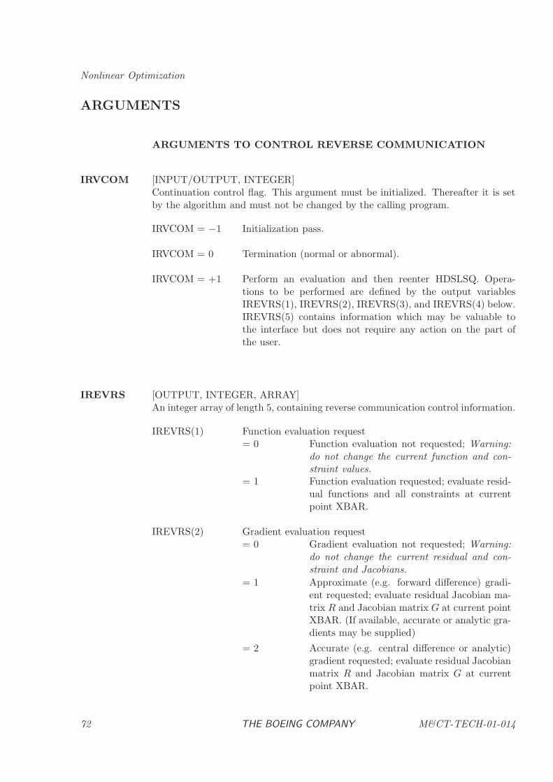
Nonlinear Optimization
ARGUMENTS
ARGUMENTS TO CONTROL REVERSE COMMUNICATION
IRVCOM [INPUT/OUTPUT, INTEGER]Continuation control flag. This argument must be initialized. Thereafter it is setby the algorithm and must not be changed by the calling program.
IRVCOM = −1 Initialization pass.
IRVCOM = 0 Termination (normal or abnormal).
IRVCOM = +1 Perform an evaluation and then reenter HDSLSQ. Opera-tions to be performed are defined by the output variablesIREVRS(1), IREVRS(2), IREVRS(3), and IREVRS(4) below.IREVRS(5) contains information which may be valuable tothe interface but does not require any action on the part ofthe user.
IREVRS [OUTPUT, INTEGER, ARRAY]An integer array of length 5, containing reverse communication control information.
IREVRS(1) Function evaluation request= 0 Function evaluation not requested; Warning:
do not change the current function and con-straint values.
= 1 Function evaluation requested; evaluate resid-ual functions and all constraints at currentpoint XBAR.
IREVRS(2) Gradient evaluation request= 0 Gradient evaluation not requested; Warning:
do not change the current residual and con-straint and Jacobians.
= 1 Approximate (e.g. forward difference) gradi-ent requested; evaluate residual Jacobian ma-trix R and Jacobian matrix G at current pointXBAR. (If available, accurate or analytic gra-dients may be supplied)
= 2 Accurate (e.g. central difference or analytic)gradient requested; evaluate residual Jacobianmatrix R and Jacobian matrix G at currentpoint XBAR.
72 THE BOEING COMPANY M&CT-TECH-01-014
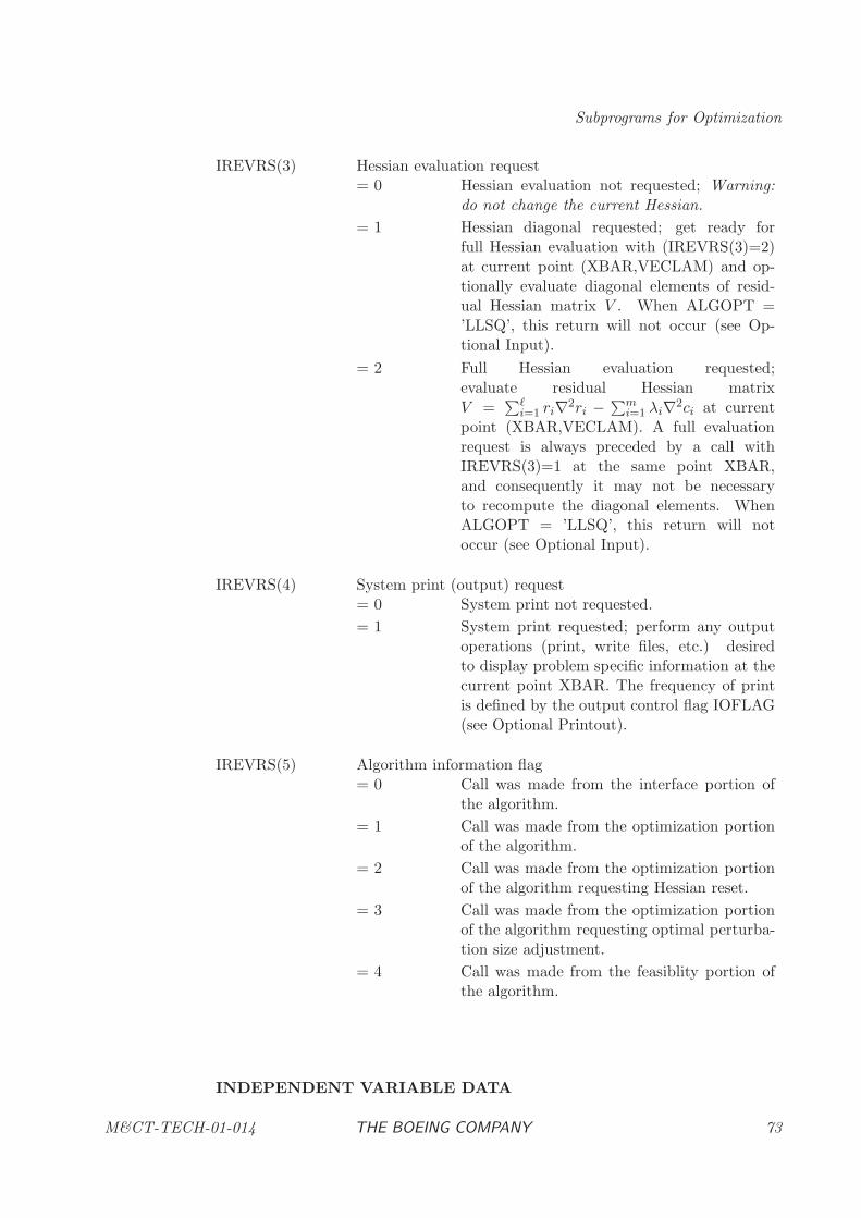
Subprograms for Optimization
IREVRS(3) Hessian evaluation request= 0 Hessian evaluation not requested; Warning:
do not change the current Hessian.
= 1 Hessian diagonal requested; get ready forfull Hessian evaluation with (IREVRS(3)=2)at current point (XBAR,VECLAM) and op-tionally evaluate diagonal elements of resid-ual Hessian matrix V . When ALGOPT =’LLSQ’, this return will not occur (see Op-tional Input).
= 2 Full Hessian evaluation requested;evaluate residual Hessian matrixV =
∑ℓi=1 ri∇2ri −
∑mi=1 λi∇2ci at current
point (XBAR,VECLAM). A full evaluationrequest is always preceded by a call withIREVRS(3)=1 at the same point XBAR,and consequently it may not be necessaryto recompute the diagonal elements. WhenALGOPT = ’LLSQ’, this return will notoccur (see Optional Input).
IREVRS(4) System print (output) request= 0 System print not requested.
= 1 System print requested; perform any outputoperations (print, write files, etc.) desiredto display problem specific information at thecurrent point XBAR. The frequency of printis defined by the output control flag IOFLAG(see Optional Printout).
IREVRS(5) Algorithm information flag= 0 Call was made from the interface portion of
the algorithm.
= 1 Call was made from the optimization portionof the algorithm.
= 2 Call was made from the optimization portionof the algorithm requesting Hessian reset.
= 3 Call was made from the optimization portionof the algorithm requesting optimal perturba-tion size adjustment.
= 4 Call was made from the feasiblity portion ofthe algorithm.
INDEPENDENT VARIABLE DATA
M&CT-TECH-01-014 THE BOEING COMPANY 73
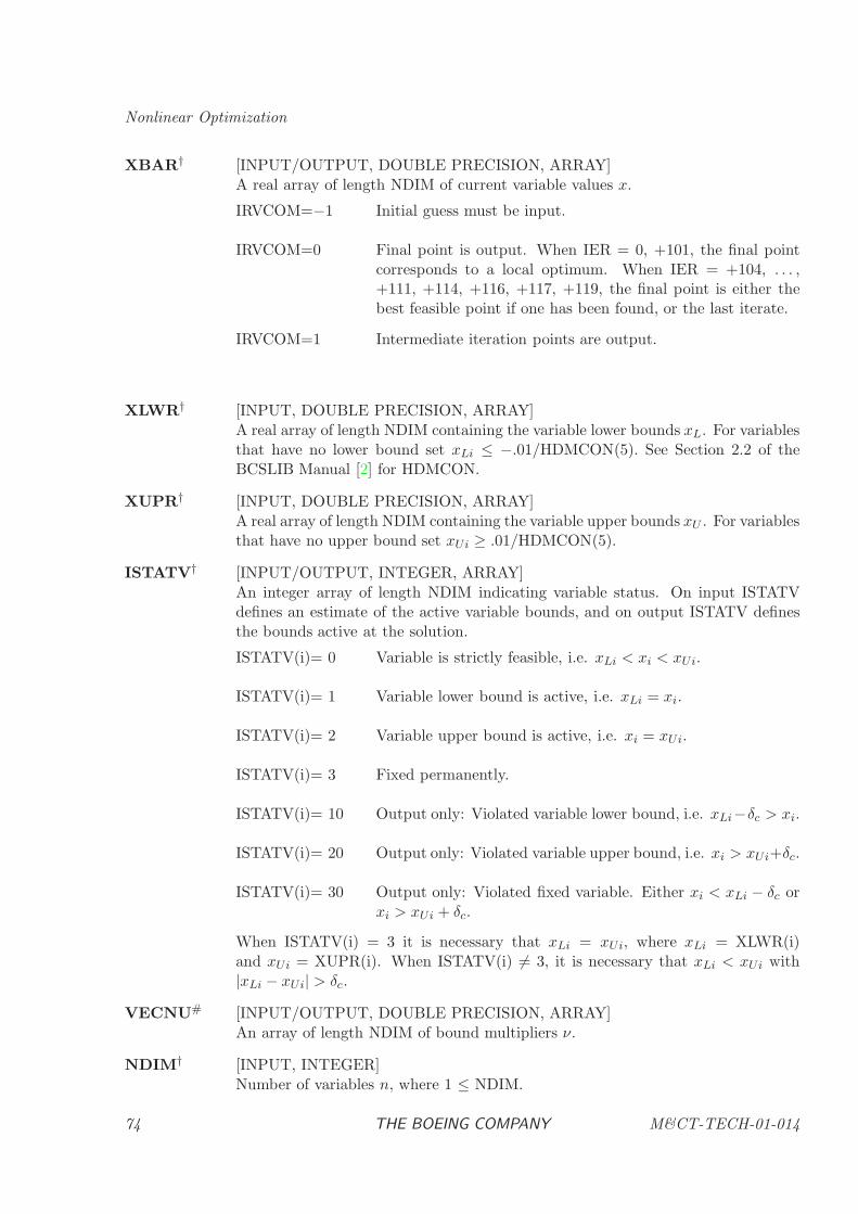
Nonlinear Optimization
XBAR† [INPUT/OUTPUT, DOUBLE PRECISION, ARRAY]A real array of length NDIM of current variable values x.
IRVCOM=−1 Initial guess must be input.
IRVCOM=0 Final point is output. When IER = 0, +101, the final pointcorresponds to a local optimum. When IER = +104, . . . ,+111, +114, +116, +117, +119, the final point is either thebest feasible point if one has been found, or the last iterate.
IRVCOM=1 Intermediate iteration points are output.
XLWR† [INPUT, DOUBLE PRECISION, ARRAY]A real array of length NDIM containing the variable lower bounds xL. For variablesthat have no lower bound set xLi ≤ −.01/HDMCON(5). See Section 2.2 of theBCSLIB Manual [2] for HDMCON.
XUPR† [INPUT, DOUBLE PRECISION, ARRAY]A real array of length NDIM containing the variable upper bounds xU . For variablesthat have no upper bound set xUi ≥ .01/HDMCON(5).
ISTATV† [INPUT/OUTPUT, INTEGER, ARRAY]An integer array of length NDIM indicating variable status. On input ISTATVdefines an estimate of the active variable bounds, and on output ISTATV definesthe bounds active at the solution.
ISTATV(i)= 0 Variable is strictly feasible, i.e. xLi < xi < xUi.
ISTATV(i)= 1 Variable lower bound is active, i.e. xLi = xi.
ISTATV(i)= 2 Variable upper bound is active, i.e. xi = xUi.
ISTATV(i)= 3 Fixed permanently.
ISTATV(i)= 10 Output only: Violated variable lower bound, i.e. xLi−δc > xi.
ISTATV(i)= 20 Output only: Violated variable upper bound, i.e. xi > xUi+δc.
ISTATV(i)= 30 Output only: Violated fixed variable. Either xi < xLi − δc orxi > xUi + δc.
When ISTATV(i) = 3 it is necessary that xLi = xUi, where xLi = XLWR(i)and xUi = XUPR(i). When ISTATV(i) 6= 3, it is necessary that xLi < xUi with|xLi − xUi| > δc.
VECNU# [INPUT/OUTPUT, DOUBLE PRECISION, ARRAY]An array of length NDIM of bound multipliers ν.
NDIM† [INPUT, INTEGER]Number of variables n, where 1 ≤ NDIM.
74 THE BOEING COMPANY M&CT-TECH-01-014
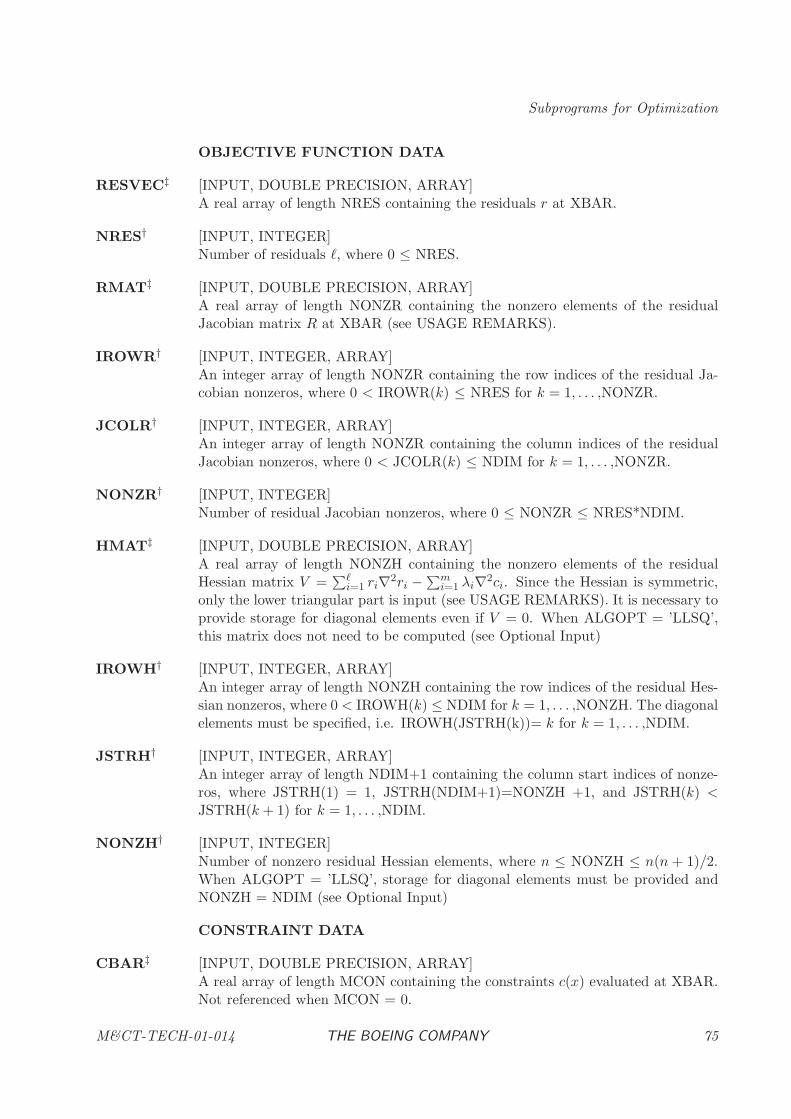
Subprograms for Optimization
OBJECTIVE FUNCTION DATA
RESVEC‡ [INPUT, DOUBLE PRECISION, ARRAY]A real array of length NRES containing the residuals r at XBAR.
NRES† [INPUT, INTEGER]Number of residuals ℓ, where 0 ≤ NRES.
RMAT‡ [INPUT, DOUBLE PRECISION, ARRAY]A real array of length NONZR containing the nonzero elements of the residualJacobian matrix R at XBAR (see USAGE REMARKS).
IROWR† [INPUT, INTEGER, ARRAY]An integer array of length NONZR containing the row indices of the residual Ja-cobian nonzeros, where 0 < IROWR(k) ≤ NRES for k = 1, . . . ,NONZR.
JCOLR† [INPUT, INTEGER, ARRAY]An integer array of length NONZR containing the column indices of the residualJacobian nonzeros, where 0 < JCOLR(k) ≤ NDIM for k = 1, . . . ,NONZR.
NONZR† [INPUT, INTEGER]Number of residual Jacobian nonzeros, where 0 ≤ NONZR ≤ NRES*NDIM.
HMAT‡ [INPUT, DOUBLE PRECISION, ARRAY]A real array of length NONZH containing the nonzero elements of the residualHessian matrix V =
∑ℓi=1 ri∇2ri −
∑mi=1 λi∇2ci. Since the Hessian is symmetric,
only the lower triangular part is input (see USAGE REMARKS). It is necessary toprovide storage for diagonal elements even if V = 0. When ALGOPT = ’LLSQ’,this matrix does not need to be computed (see Optional Input)
IROWH† [INPUT, INTEGER, ARRAY]An integer array of length NONZH containing the row indices of the residual Hes-sian nonzeros, where 0 < IROWH(k) ≤ NDIM for k = 1, . . . ,NONZH. The diagonalelements must be specified, i.e. IROWH(JSTRH(k))= k for k = 1, . . . ,NDIM.
JSTRH† [INPUT, INTEGER, ARRAY]An integer array of length NDIM+1 containing the column start indices of nonze-ros, where JSTRH(1) = 1, JSTRH(NDIM+1)=NONZH +1, and JSTRH(k) <JSTRH(k + 1) for k = 1, . . . ,NDIM.
NONZH† [INPUT, INTEGER]Number of nonzero residual Hessian elements, where n ≤ NONZH ≤ n(n + 1)/2.When ALGOPT = ’LLSQ’, storage for diagonal elements must be provided andNONZH = NDIM (see Optional Input)
CONSTRAINT DATA
CBAR‡ [INPUT, DOUBLE PRECISION, ARRAY]A real array of length MCON containing the constraints c(x) evaluated at XBAR.Not referenced when MCON = 0.
M&CT-TECH-01-014 THE BOEING COMPANY 75
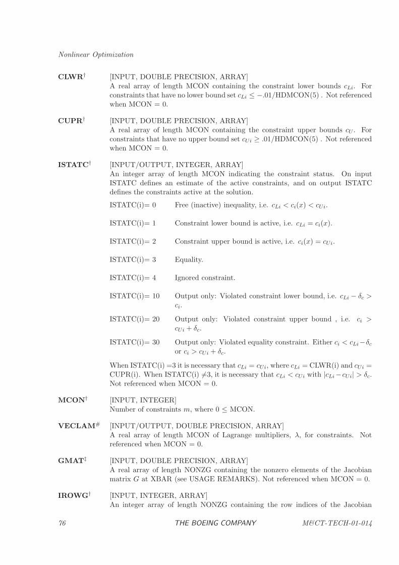
Nonlinear Optimization
CLWR† [INPUT, DOUBLE PRECISION, ARRAY]A real array of length MCON containing the constraint lower bounds cLi. Forconstraints that have no lower bound set cLi ≤ −.01/HDMCON(5) . Not referencedwhen MCON = 0.
CUPR† [INPUT, DOUBLE PRECISION, ARRAY]A real array of length MCON containing the constraint upper bounds cU . Forconstraints that have no upper bound set cUi ≥ .01/HDMCON(5) . Not referencedwhen MCON = 0.
ISTATC† [INPUT/OUTPUT, INTEGER, ARRAY]An integer array of length MCON indicating the constraint status. On inputISTATC defines an estimate of the active constraints, and on output ISTATCdefines the constraints active at the solution.
ISTATC(i)= 0 Free (inactive) inequality, i.e. cLi < ci(x) < cUi.
ISTATC(i)= 1 Constraint lower bound is active, i.e. cLi = ci(x).
ISTATC(i)= 2 Constraint upper bound is active, i.e. ci(x) = cUi.
ISTATC(i)= 3 Equality.
ISTATC(i)= 4 Ignored constraint.
ISTATC(i)= 10 Output only: Violated constraint lower bound, i.e. cLi − δc >ci.
ISTATC(i)= 20 Output only: Violated constraint upper bound , i.e. ci >cUi + δc.
ISTATC(i)= 30 Output only: Violated equality constraint. Either ci < cLi−δcor ci > cUi + δc.
When ISTATC(i) =3 it is necessary that cLi = cUi, where cLi = CLWR(i) and cUi =CUPR(i). When ISTATC(i) 6=3, it is necessary that cLi < cUi with |cLi−cUi| > δc.Not referenced when MCON = 0.
MCON† [INPUT, INTEGER]Number of constraints m, where 0 ≤ MCON.
VECLAM# [INPUT/OUTPUT, DOUBLE PRECISION, ARRAY]A real array of length MCON of Lagrange multipliers, λ, for constraints. Notreferenced when MCON = 0.
GMAT‡ [INPUT, DOUBLE PRECISION, ARRAY]A real array of length NONZG containing the nonzero elements of the Jacobianmatrix G at XBAR (see USAGE REMARKS). Not referenced when MCON = 0.
IROWG† [INPUT, INTEGER, ARRAY]An integer array of length NONZG containing the row indices of the Jacobian
76 THE BOEING COMPANY M&CT-TECH-01-014
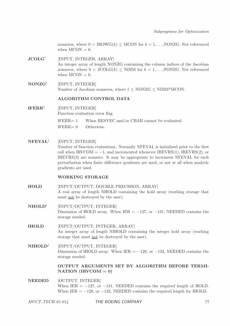
Subprograms for Optimization
nonzeros, where 0 < IROWG(k) ≤ MCON for k = 1, . . . ,NONZG. Not referencedwhen MCON = 0.
JCOLG† [INPUT, INTEGER, ARRAY]An integer array of length NONZG containing the column indices of the Jacobiannonzeros, where 0 < JCOLG(k) ≤ NDIM for k = 1, . . . ,NONZG. Not referencedwhen MCON = 0.
NONZG† [INPUT, INTEGER]Number of Jacobian nonzeros, where 1 ≤ NONZG ≤ NDIM*MCON.
ALGORITHM CONTROL DATA
IFERR‡ [INPUT, INTEGER]Function evaluation error flag.
IFERR= 1 When RESVEC and/or CBAR cannot be evaluated.
IFERR= 0 Otherwise.
NFEVAL‡ [INPUT, INTEGER]Number of function evaluations. Normally NFEVAL is initialized prior to the firstcall when IRVCOM = −1, and incremented whenever IREVRS(1), IREVRS(2), orIREVRS(3) are nonzero. It may be appropriate to increment NFEVAL for eachperturbation when finite difference gradients are used, or not at all when analyticgradients are used.
WORKING STORAGE
HOLD [INPUT/OUTPUT, DOUBLE PRECISION, ARRAY]A real array of length NHOLD containing the hold array (working storage thatmust not be destroyed by the user).
NHOLD† [INPUT/OUTPUT, INTEGER]Dimension of HOLD array. When IER = −127, or −131, NEEDED contains thestorage needed.
IHOLD [INPUT/OUTPUT, INTEGER, ARRAY]An integer array of length NIHOLD containing the integer hold array (workingstorage that must not be destroyed by the user).
NIHOLD† [INPUT/OUTPUT, INTEGER]Dimension of IHOLD array. When IER = −128, or −132, NEEDED contains thestorage needed.
OUTPUT ARGUMENTS SET BY ALGORITHM BEFORE TERMI-NATION (IRVCOM = 0)
NEEDED [OUTPUT, INTEGER]When IER = −127, or −131, NEEDED contains the required length of HOLD.When IER = −128, or −132, NEEDED contains the required length for IHOLD.
M&CT-TECH-01-014 THE BOEING COMPANY 77
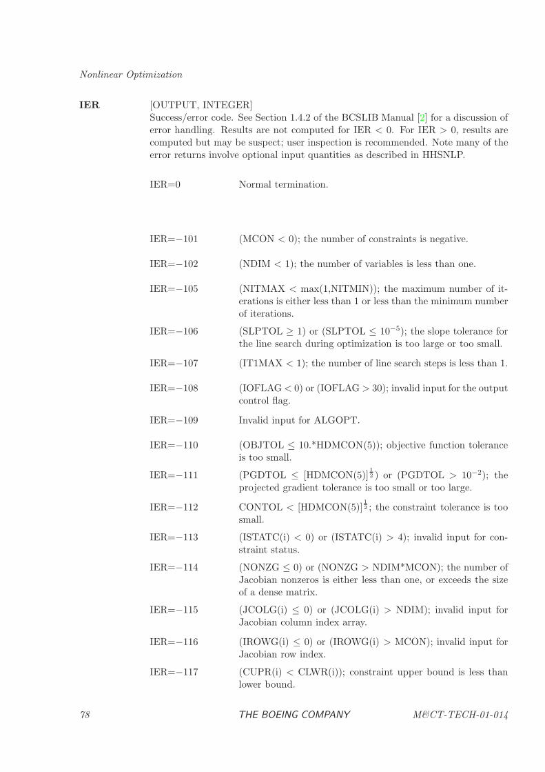
Nonlinear Optimization
IER [OUTPUT, INTEGER]Success/error code. See Section 1.4.2 of the BCSLIB Manual [2] for a discussion oferror handling. Results are not computed for IER < 0. For IER > 0, results arecomputed but may be suspect; user inspection is recommended. Note many of theerror returns involve optional input quantities as described in HHSNLP.
IER=0 Normal termination.
IER=−101 (MCON < 0); the number of constraints is negative.
IER=−102 (NDIM < 1); the number of variables is less than one.
IER=−105 (NITMAX < max(1,NITMIN)); the maximum number of it-erations is either less than 1 or less than the minimum numberof iterations.
IER=−106 (SLPTOL ≥ 1) or (SLPTOL ≤ 10−5); the slope tolerance forthe line search during optimization is too large or too small.
IER=−107 (IT1MAX < 1); the number of line search steps is less than 1.
IER=−108 (IOFLAG< 0) or (IOFLAG > 30); invalid input for the outputcontrol flag.
IER=−109 Invalid input for ALGOPT.
IER=−110 (OBJTOL ≤ 10.*HDMCON(5)); objective function toleranceis too small.
IER=−111 (PGDTOL ≤ [HDMCON(5)]12 ) or (PGDTOL > 10−2); the
projected gradient tolerance is too small or too large.
IER=−112 CONTOL < [HDMCON(5)]12 ; the constraint tolerance is too
small.
IER=−113 (ISTATC(i) < 0) or (ISTATC(i) > 4); invalid input for con-straint status.
IER=−114 (NONZG ≤ 0) or (NONZG > NDIM*MCON); the number ofJacobian nonzeros is either less than one, or exceeds the sizeof a dense matrix.
IER=−115 (JCOLG(i) ≤ 0) or (JCOLG(i) > NDIM); invalid input forJacobian column index array.
IER=−116 (IROWG(i) ≤ 0) or (IROWG(i) > MCON); invalid input forJacobian row index.
IER=−117 (CUPR(i) < CLWR(i)); constraint upper bound is less thanlower bound.
78 THE BOEING COMPANY M&CT-TECH-01-014
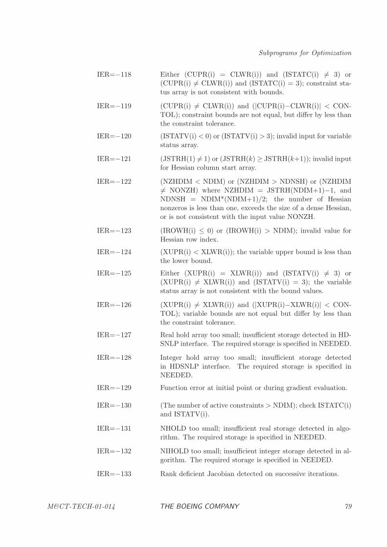
Subprograms for Optimization
IER=−118 Either (CUPR(i) = CLWR(i)) and (ISTATC(i) 6= 3) or(CUPR(i) 6= CLWR(i)) and (ISTATC(i) = 3); constraint sta-tus array is not consistent with bounds.
IER=−119 (CUPR(i) 6= CLWR(i)) and (|CUPR(i)−CLWR(i)| < CON-TOL); constraint bounds are not equal, but differ by less thanthe constraint tolerance.
IER=−120 (ISTATV(i)< 0) or (ISTATV(i) > 3); invalid input for variablestatus array.
IER=−121 (JSTRH(1) 6= 1) or (JSTRH(k) ≥ JSTRH(k+1)); invalid inputfor Hessian column start array.
IER=−122 (NZHDIM < NDIM) or (NZHDIM > NDNSH) or (NZHDIM6= NONZH) where NZHDIM = JSTRH(NDIM+1)−1, andNDNSH = NDIM*(NDIM+1)/2; the number of Hessiannonzeros is less than one, exceeds the size of a dense Hessian,or is not consistent with the input value NONZH.
IER=−123 (IROWH(i) ≤ 0) or (IROWH(i) > NDIM); invalid value forHessian row index.
IER=−124 (XUPR(i) < XLWR(i)); the variable upper bound is less thanthe lower bound.
IER=−125 Either (XUPR(i) = XLWR(i)) and (ISTATV(i) 6= 3) or(XUPR(i) 6= XLWR(i)) and (ISTATV(i) = 3); the variablestatus array is not consistent with the bound values.
IER=−126 (XUPR(i) 6= XLWR(i)) and (|XUPR(i)−XLWR(i)| < CON-TOL); variable bounds are not equal but differ by less thanthe constraint tolerance.
IER=−127 Real hold array too small; insufficient storage detected in HD-SNLP interface. The required storage is specified in NEEDED.
IER=−128 Integer hold array too small; insufficient storage detectedin HDSNLP interface. The required storage is specified inNEEDED.
IER=−129 Function error at initial point or during gradient evaluation.
IER=−130 (The number of active constraints > NDIM); check ISTATC(i)and ISTATV(i).
IER=−131 NHOLD too small; insufficient real storage detected in algo-rithm. The required storage is specified in NEEDED.
IER=−132 NIHOLD too small; insufficient integer storage detected in al-gorithm. The required storage is specified in NEEDED.
IER=−133 Rank deficient Jacobian detected on successive iterations.
M&CT-TECH-01-014 THE BOEING COMPANY 79
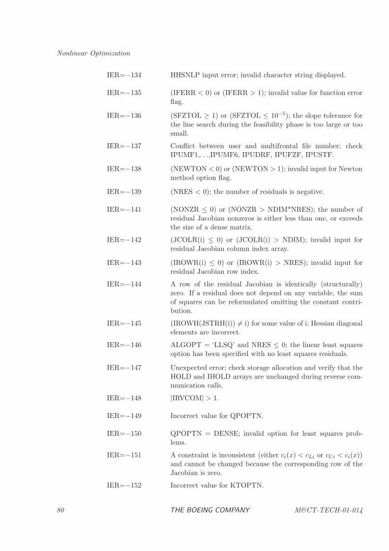
Nonlinear Optimization
IER=−134 HHSNLP input error; invalid character string displayed.
IER=−135 (IFERR < 0) or (IFERR > 1); invalid value for function errorflag.
IER=−136 (SFZTOL ≥ 1) or (SFZTOL ≤ 10−5); the slope tolerance forthe line search during the feasibility phase is too large or toosmall.
IER=−137 Conflict between user and multifrontal file number; checkIPUMF1,. . .,IPUMF6, IPUDRF, IPUFZF, IPUSTF.
IER=−138 (NEWTON < 0) or (NEWTON > 1); invalid input for Newtonmethod option flag.
IER=−139 (NRES < 0); the number of residuals is negative.
IER=−141 (NONZR ≤ 0) or (NONZR > NDIM*NRES); the number ofresidual Jacobian nonzeros is either less than one, or exceedsthe size of a dense matrix.
IER=−142 (JCOLR(i) ≤ 0) or (JCOLR(i) > NDIM); invalid input forresidual Jacobian column index array.
IER=−143 (IROWR(i) ≤ 0) or (IROWR(i) > NRES); invalid input forresidual Jacobian row index.
IER=−144 A row of the residual Jacobian is identically (structurally)zero. If a residual does not depend on any variable, the sumof squares can be reformulated omitting the constant contri-bution.
IER=−145 (IROWH(JSTRH(i)) 6= i) for some value of i; Hessian diagonalelements are incorrect.
IER=−146 ALGOPT = ‘LLSQ’ and NRES ≤ 0; the linear least squaresoption has been specified with no least squares residuals.
IER=−147 Unexpected error; check storage allocation and verify that theHOLD and IHOLD arrays are unchanged during reverse com-munication calls.
IER=−148 |IRVCOM| > 1.
IER=−149 Incorrect value for QPOPTN.
IER=−150 QPOPTN = DENSE; invalid option for least squares prob-lems.
IER=−151 A constraint is inconsistent (either ci(x) < cLi or cUi < ci(x))and cannot be changed because the corresponding row of theJacobian is zero.
IER=−152 Incorrect value for KTOPTN.
80 THE BOEING COMPANY M&CT-TECH-01-014
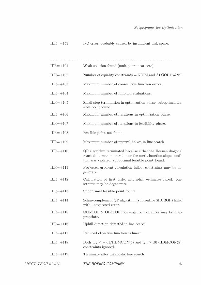
Subprograms for Optimization
IER=−153 I/O error, probably caused by insufficient disk space.
---------------------------------------------------------------
IER=+101 Weak solution found (multipliers near zero).
IER=+102 Number of equality constraints = NDIM and ALGOPT 6= ‘F’.
IER=+103 Maximum number of consecutive function errors.
IER=+104 Maximum number of function evaluations.
IER=+105 Small step termination in optimization phase; suboptimal fea-sible point found.
IER=+106 Maximum number of iterations in optimization phase.
IER=+107 Maximum number of iterations in feasibility phase.
IER=+108 Feasible point not found.
IER=+109 Maximum number of interval halves in line search.
IER=+110 QP algorithm terminated because either the Hessian diagonalreached its maximum value or the merit function slope condi-tion was violated; suboptimal feasible point found.
IER=+111 Projected gradient calculation failed; constraints may be de-generate.
IER=+112 Calculation of first order multiplier estimates failed; con-straints may be degenerate.
IER=+113 Suboptimal feasible point found.
IER=+114 Schur-complement QP algorithm (subroutine SHURQP) failedwith unexpected error.
IER=+115 CONTOL > OBJTOL; convergence tolerances may be inap-propriate.
IER=+116 Uphill direction detected in line search.
IER=+117 Reduced objective function is linear.
IER=+118 Both cLi ≤ −.01/HDMCON(5) and cUi ≥ .01/HDMCON(5);constraints ignored.
IER=+119 Terminate after diagnostic line search.
M&CT-TECH-01-014 THE BOEING COMPANY 81
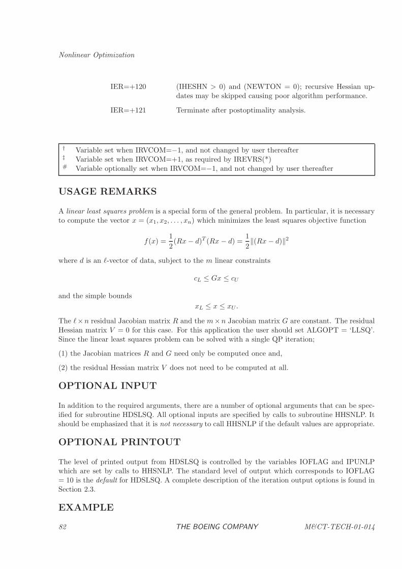
Nonlinear Optimization
IER=+120 (IHESHN > 0) and (NEWTON = 0); recursive Hessian up-dates may be skipped causing poor algorithm performance.
IER=+121 Terminate after postoptimality analysis.
† Variable set when IRVCOM=−1, and not changed by user thereafter‡ Variable set when IRVCOM=+1, as required by IREVRS(*)# Variable optionally set when IRVCOM=−1, and not changed by user thereafter
USAGE REMARKS
A linear least squares problem is a special form of the general problem. In particular, it is necessaryto compute the vector x = (x1, x2, . . . , xn) which minimizes the least squares objective function
f(x) =1
2(Rx− d)T (Rx− d) =
1
2‖(Rx− d)‖2
where d is an ℓ-vector of data, subject to the m linear constraints
cL ≤ Gx ≤ cU
and the simple bounds
xL ≤ x ≤ xU .
The ℓ×n residual Jacobian matrix R and the m×n Jacobian matrix G are constant. The residualHessian matrix V = 0 for this case. For this application the user should set ALGOPT = ‘LLSQ’.Since the linear least squares problem can be solved with a single QP iteration;
(1) the Jacobian matrices R and G need only be computed once and,
(2) the residual Hessian matrix V does not need to be computed at all.
OPTIONAL INPUT
In addition to the required arguments, there are a number of optional arguments that can be spec-ified for subroutine HDSLSQ. All optional inputs are specified by calls to subroutine HHSNLP. Itshould be emphasized that it is not necessary to call HHSNLP if the default values are appropriate.
OPTIONAL PRINTOUT
The level of printed output from HDSLSQ is controlled by the variables IOFLAG and IPUNLPwhich are set by calls to HHSNLP. The standard level of output which corresponds to IOFLAG= 10 is the default for HDSLSQ. A complete description of the iteration output options is found inSection 2.3.
EXAMPLE
82 THE BOEING COMPANY M&CT-TECH-01-014
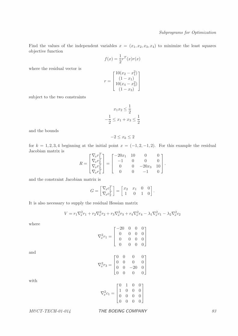
Subprograms for Optimization
Find the values of the independent variables x = (x1, x2, x3, x4) to minimize the least squaresobjective function
f(x) =1
2rT (x)r(x)
where the residual vector is
r =
10(x2 − x21)
(1 − x1)10(x4 − x2
3)(1 − x3)
subject to the two constraints
x1x2 ≤ 1
2
−1
2≤ x1 + x3 ≤ 1
2
and the bounds
−2 ≤ xk ≤ 2
for k = 1, 2, 3, 4 beginning at the initial point x = (−1, 2,−1, 2). For this example the residualJacobian matrix is
R =
∇xrT1
∇xrT2
∇xrT3
∇xrT4
=
−20x1 10 0 0−1 0 0 00 0 −20x3 100 0 −1 0
.
and the constraint Jacobian matrix is
G =
[∇xcT1
∇xcT2
]=
[x2 x1 0 01 0 1 0
].
It is also necessary to supply the residual Hessian matrix
V = r1∇2xr1 + r2∇2
xr2 + r3∇2xr3 + r4∇2
xr4 − λ1∇2xc1 − λ2∇2
xc2
where
∇2xr1 =
−20 0 0 00 0 0 00 0 0 00 0 0 0
and
∇2xr3 =
0 0 0 00 0 0 00 0 −20 00 0 0 0
with
∇2xc1 =
0 1 0 01 0 0 00 0 0 00 0 0 0
M&CT-TECH-01-014 THE BOEING COMPANY 83
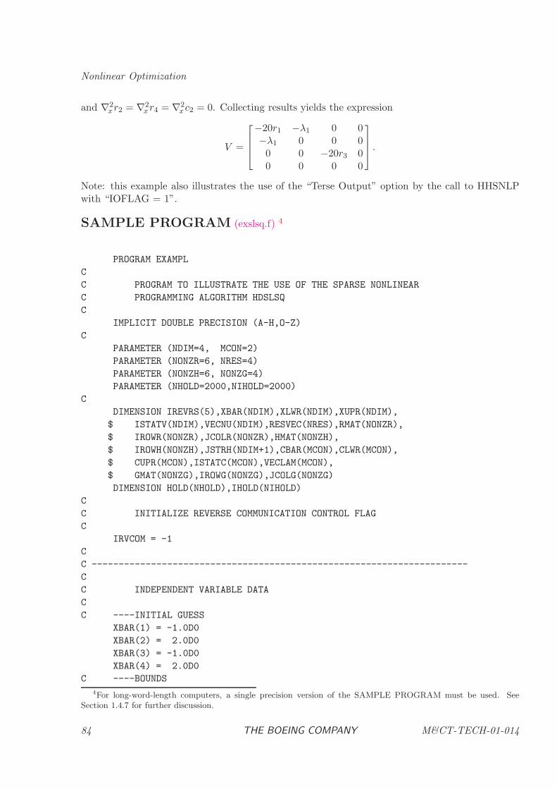
Nonlinear Optimization
and ∇2xr2 = ∇2
xr4 = ∇2x c2 = 0. Collecting results yields the expression
V =
−20r1 −λ1 0 0−λ1 0 0 00 0 −20r3 00 0 0 0
.
Note: this example also illustrates the use of the “Terse Output” option by the call to HHSNLPwith “IOFLAG = 1”.
SAMPLE PROGRAM (exslsq.f) 4
PROGRAM EXAMPL
C
C PROGRAM TO ILLUSTRATE THE USE OF THE SPARSE NONLINEAR
C PROGRAMMING ALGORITHM HDSLSQ
C
IMPLICIT DOUBLE PRECISION (A-H,O-Z)
C
PARAMETER (NDIM=4, MCON=2)
PARAMETER (NONZR=6, NRES=4)
PARAMETER (NONZH=6, NONZG=4)
PARAMETER (NHOLD=2000,NIHOLD=2000)
C
DIMENSION IREVRS(5),XBAR(NDIM),XLWR(NDIM),XUPR(NDIM),
$ ISTATV(NDIM),VECNU(NDIM),RESVEC(NRES),RMAT(NONZR),
$ IROWR(NONZR),JCOLR(NONZR),HMAT(NONZH),
$ IROWH(NONZH),JSTRH(NDIM+1),CBAR(MCON),CLWR(MCON),
$ CUPR(MCON),ISTATC(MCON),VECLAM(MCON),
$ GMAT(NONZG),IROWG(NONZG),JCOLG(NONZG)
DIMENSION HOLD(NHOLD),IHOLD(NIHOLD)
C
C INITIALIZE REVERSE COMMUNICATION CONTROL FLAG
C
IRVCOM = -1
C
C ----------------------------------------------------------------------
C
C INDEPENDENT VARIABLE DATA
C
C ----INITIAL GUESS
XBAR(1) = -1.0D0
XBAR(2) = 2.0D0
XBAR(3) = -1.0D0
XBAR(4) = 2.0D0
C ----BOUNDS
4For long-word-length computers, a single precision version of the SAMPLE PROGRAM must be used. See
Section 1.4.7 for further discussion.
84 THE BOEING COMPANY M&CT-TECH-01-014
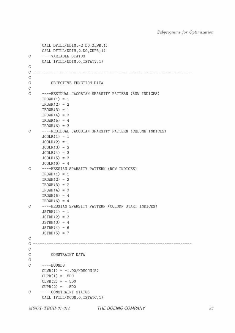
Subprograms for Optimization
CALL DFILL(NDIM,-2.D0,XLWR,1)
CALL DFILL(NDIM,2.D0,XUPR,1)
C ----VARIABLE STATUS
CALL IFILL(NDIM,0,ISTATV,1)
C
C ----------------------------------------------------------------------
C
C OBJECTIVE FUNCTION DATA
C
C ----RESIDUAL JACOBIAN SPARSITY PATTERN (ROW INDICES)
IROWR(1) = 1
IROWR(2) = 2
IROWR(3) = 1
IROWR(4) = 3
IROWR(5) = 4
IROWR(6) = 3
C ----RESIDUAL JACOBIAN SPARSITY PATTERN (COLUMN INDICES)
JCOLR(1) = 1
JCOLR(2) = 1
JCOLR(3) = 2
JCOLR(4) = 3
JCOLR(5) = 3
JCOLR(6) = 4
C ----HESSIAN SPARSITY PATTERN (ROW INDICES)
IROWH(1) = 1
IROWH(2) = 2
IROWH(3) = 2
IROWH(4) = 3
IROWH(5) = 4
IROWH(6) = 4
C ----HESSIAN SPARSITY PATTERN (COLUMN START INDICES)
JSTRH(1) = 1
JSTRH(2) = 3
JSTRH(3) = 4
JSTRH(4) = 6
JSTRH(5) = 7
C
C ----------------------------------------------------------------------
C
C CONSTRAINT DATA
C
C ----BOUNDS
CLWR(1) = -1.D0/HDMCON(5)
CUPR(1) = .5D0
CLWR(2) = -.5D0
CUPR(2) = .5D0
C ----CONSTRAINT STATUS
CALL IFILL(MCON,0,ISTATC,1)
M&CT-TECH-01-014 THE BOEING COMPANY 85
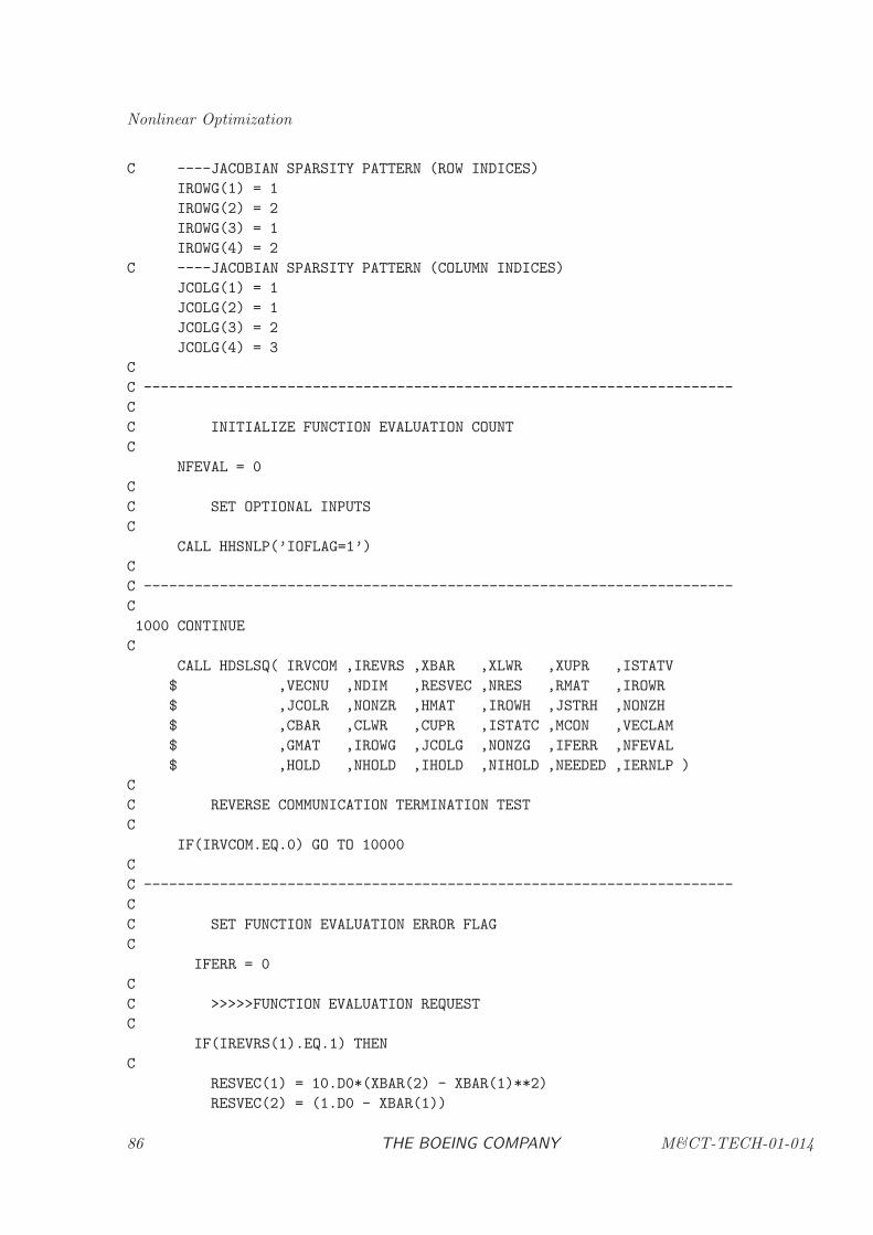
Nonlinear Optimization
C ----JACOBIAN SPARSITY PATTERN (ROW INDICES)
IROWG(1) = 1
IROWG(2) = 2
IROWG(3) = 1
IROWG(4) = 2
C ----JACOBIAN SPARSITY PATTERN (COLUMN INDICES)
JCOLG(1) = 1
JCOLG(2) = 1
JCOLG(3) = 2
JCOLG(4) = 3
C
C ----------------------------------------------------------------------
C
C INITIALIZE FUNCTION EVALUATION COUNT
C
NFEVAL = 0
C
C SET OPTIONAL INPUTS
C
CALL HHSNLP(’IOFLAG=1’)
C
C ----------------------------------------------------------------------
C
1000 CONTINUE
C
CALL HDSLSQ( IRVCOM ,IREVRS ,XBAR ,XLWR ,XUPR ,ISTATV
$ ,VECNU ,NDIM ,RESVEC ,NRES ,RMAT ,IROWR
$ ,JCOLR ,NONZR ,HMAT ,IROWH ,JSTRH ,NONZH
$ ,CBAR ,CLWR ,CUPR ,ISTATC ,MCON ,VECLAM
$ ,GMAT ,IROWG ,JCOLG ,NONZG ,IFERR ,NFEVAL
$ ,HOLD ,NHOLD ,IHOLD ,NIHOLD ,NEEDED ,IERNLP )
C
C REVERSE COMMUNICATION TERMINATION TEST
C
IF(IRVCOM.EQ.0) GO TO 10000
C
C ----------------------------------------------------------------------
C
C SET FUNCTION EVALUATION ERROR FLAG
C
IFERR = 0
C
C >>>>>FUNCTION EVALUATION REQUEST
C
IF(IREVRS(1).EQ.1) THEN
C
RESVEC(1) = 10.D0*(XBAR(2) - XBAR(1)**2)
RESVEC(2) = (1.D0 - XBAR(1))
86 THE BOEING COMPANY M&CT-TECH-01-014
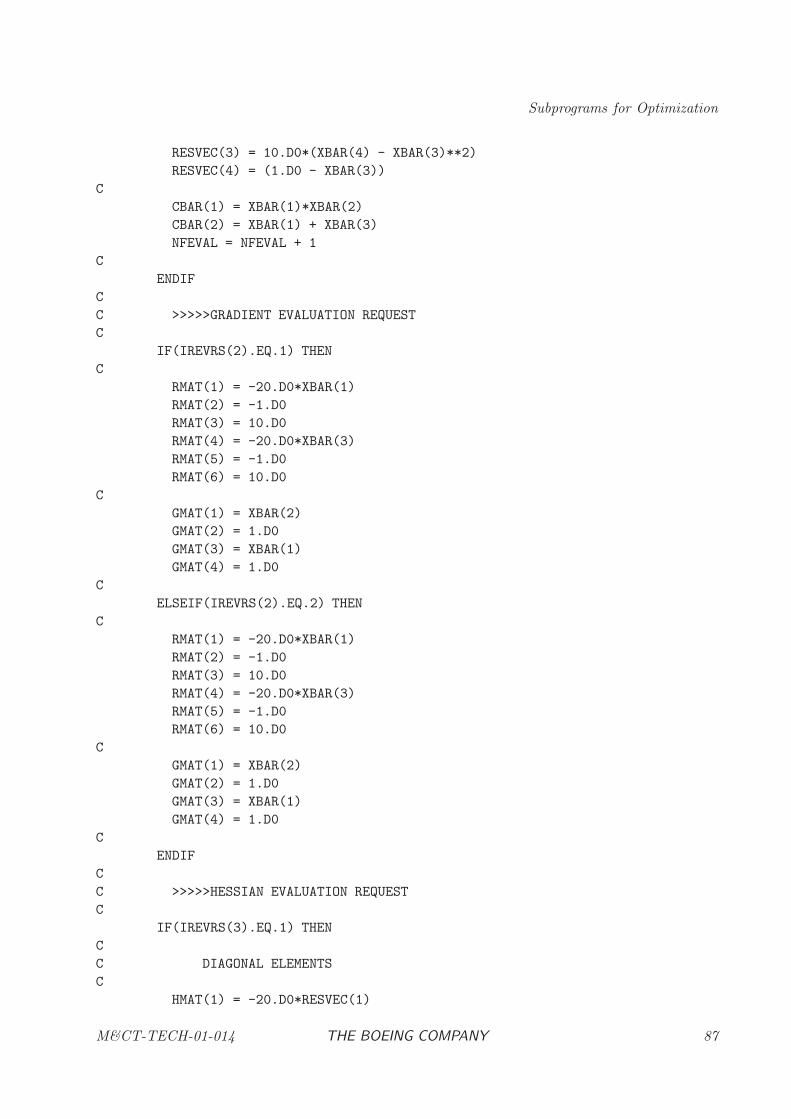
Subprograms for Optimization
RESVEC(3) = 10.D0*(XBAR(4) - XBAR(3)**2)
RESVEC(4) = (1.D0 - XBAR(3))
C
CBAR(1) = XBAR(1)*XBAR(2)
CBAR(2) = XBAR(1) + XBAR(3)
NFEVAL = NFEVAL + 1
C
ENDIF
C
C >>>>>GRADIENT EVALUATION REQUEST
C
IF(IREVRS(2).EQ.1) THEN
C
RMAT(1) = -20.D0*XBAR(1)
RMAT(2) = -1.D0
RMAT(3) = 10.D0
RMAT(4) = -20.D0*XBAR(3)
RMAT(5) = -1.D0
RMAT(6) = 10.D0
C
GMAT(1) = XBAR(2)
GMAT(2) = 1.D0
GMAT(3) = XBAR(1)
GMAT(4) = 1.D0
C
ELSEIF(IREVRS(2).EQ.2) THEN
C
RMAT(1) = -20.D0*XBAR(1)
RMAT(2) = -1.D0
RMAT(3) = 10.D0
RMAT(4) = -20.D0*XBAR(3)
RMAT(5) = -1.D0
RMAT(6) = 10.D0
C
GMAT(1) = XBAR(2)
GMAT(2) = 1.D0
GMAT(3) = XBAR(1)
GMAT(4) = 1.D0
C
ENDIF
C
C >>>>>HESSIAN EVALUATION REQUEST
C
IF(IREVRS(3).EQ.1) THEN
C
C DIAGONAL ELEMENTS
C
HMAT(1) = -20.D0*RESVEC(1)
M&CT-TECH-01-014 THE BOEING COMPANY 87
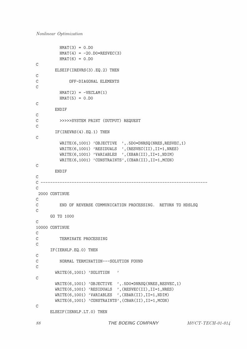
Nonlinear Optimization
HMAT(3) = 0.D0
HMAT(4) = -20.D0*RESVEC(3)
HMAT(6) = 0.D0
C
ELSEIF(IREVRS(3).EQ.2) THEN
C
C OFF-DIAGONAL ELEMENTS
C
HMAT(2) = -VECLAM(1)
HMAT(5) = 0.D0
C
ENDIF
C
C >>>>>SYSTEM PRINT (OUTPUT) REQUEST
C
IF(IREVRS(4).EQ.1) THEN
C
WRITE(6,1001) ’OBJECTIVE ’,.5D0*DNRSQ(NRES,RESVEC,1)
WRITE(6,1001) ’RESIDUALS ’,(RESVEC(II),II=1,NRES)
WRITE(6,1001) ’VARIABLES ’,(XBAR(II),II=1,NDIM)
WRITE(6,1001) ’CONSTRAINTS’,(CBAR(II),II=1,MCON)
C
ENDIF
C
C ----------------------------------------------------------------------
C
2000 CONTINUE
C
C END OF REVERSE COMMUNICATION PROCESSING. RETURN TO HDSLSQ
C
GO TO 1000
C
10000 CONTINUE
C
C TERMINATE PROCESSING
C
IF(IERNLP.EQ.0) THEN
C
C NORMAL TERMINATION---SOLUTION FOUND
C
WRITE(6,1001) ’SOLUTION ’
C
WRITE(6,1001) ’OBJECTIVE ’,.5D0*DNRSQ(NRES,RESVEC,1)
WRITE(6,1001) ’RESIDUALS ’,(RESVEC(II),II=1,NRES)
WRITE(6,1001) ’VARIABLES ’,(XBAR(II),II=1,NDIM)
WRITE(6,1001) ’CONSTRAINTS’,(CBAR(II),II=1,MCON)
C
ELSEIF(IERNLP.LT.0) THEN
88 THE BOEING COMPANY M&CT-TECH-01-014
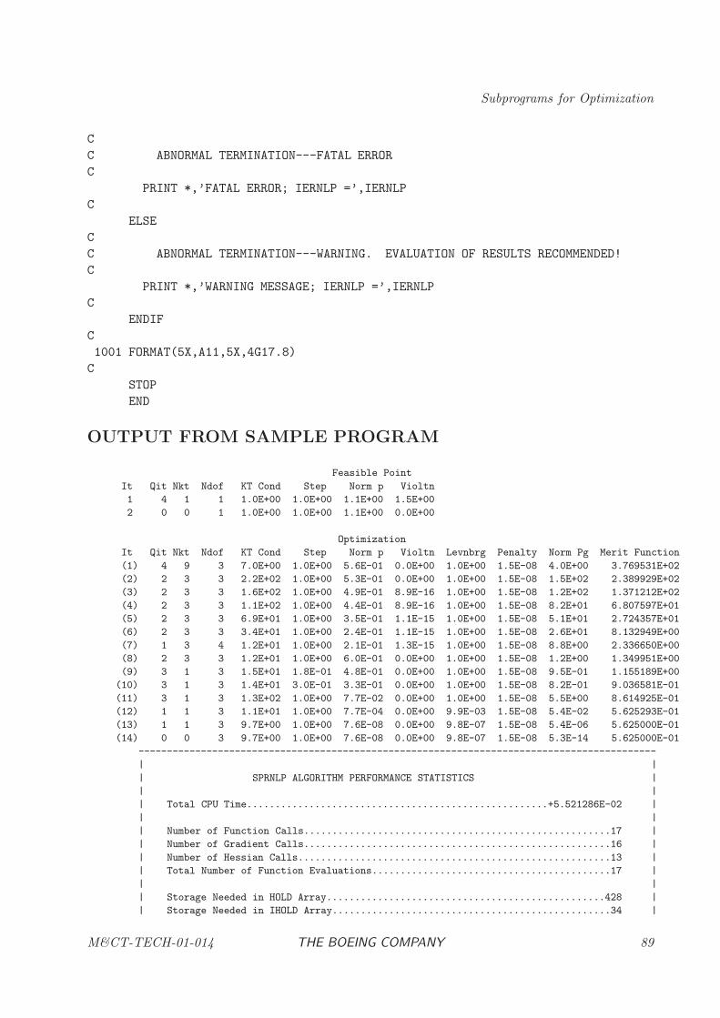
Subprograms for Optimization
C
C ABNORMAL TERMINATION---FATAL ERROR
C
PRINT *,’FATAL ERROR; IERNLP =’,IERNLP
C
ELSE
C
C ABNORMAL TERMINATION---WARNING. EVALUATION OF RESULTS RECOMMENDED!
C
PRINT *,’WARNING MESSAGE; IERNLP =’,IERNLP
C
ENDIF
C
1001 FORMAT(5X,A11,5X,4G17.8)
C
STOP
END
OUTPUT FROM SAMPLE PROGRAM
Feasible Point
It Qit Nkt Ndof KT Cond Step Norm p Violtn
1 4 1 1 1.0E+00 1.0E+00 1.1E+00 1.5E+00
2 0 0 1 1.0E+00 1.0E+00 1.1E+00 0.0E+00
Optimization
It Qit Nkt Ndof KT Cond Step Norm p Violtn Levnbrg Penalty Norm Pg Merit Function
(1) 4 9 3 7.0E+00 1.0E+00 5.6E-01 0.0E+00 1.0E+00 1.5E-08 4.0E+00 3.769531E+02
(2) 2 3 3 2.2E+02 1.0E+00 5.3E-01 0.0E+00 1.0E+00 1.5E-08 1.5E+02 2.389929E+02
(3) 2 3 3 1.6E+02 1.0E+00 4.9E-01 8.9E-16 1.0E+00 1.5E-08 1.2E+02 1.371212E+02
(4) 2 3 3 1.1E+02 1.0E+00 4.4E-01 8.9E-16 1.0E+00 1.5E-08 8.2E+01 6.807597E+01
(5) 2 3 3 6.9E+01 1.0E+00 3.5E-01 1.1E-15 1.0E+00 1.5E-08 5.1E+01 2.724357E+01
(6) 2 3 3 3.4E+01 1.0E+00 2.4E-01 1.1E-15 1.0E+00 1.5E-08 2.6E+01 8.132949E+00
(7) 1 3 4 1.2E+01 1.0E+00 2.1E-01 1.3E-15 1.0E+00 1.5E-08 8.8E+00 2.336650E+00
(8) 2 3 3 1.2E+01 1.0E+00 6.0E-01 0.0E+00 1.0E+00 1.5E-08 1.2E+00 1.349951E+00
(9) 3 1 3 1.5E+01 1.8E-01 4.8E-01 0.0E+00 1.0E+00 1.5E-08 9.5E-01 1.155189E+00
(10) 3 1 3 1.4E+01 3.0E-01 3.3E-01 0.0E+00 1.0E+00 1.5E-08 8.2E-01 9.036581E-01
(11) 3 1 3 1.3E+02 1.0E+00 7.7E-02 0.0E+00 1.0E+00 1.5E-08 5.5E+00 8.614925E-01
(12) 1 1 3 1.1E+01 1.0E+00 7.7E-04 0.0E+00 9.9E-03 1.5E-08 5.4E-02 5.625293E-01
(13) 1 1 3 9.7E+00 1.0E+00 7.6E-08 0.0E+00 9.8E-07 1.5E-08 5.4E-06 5.625000E-01
(14) 0 0 3 9.7E+00 1.0E+00 7.6E-08 0.0E+00 9.8E-07 1.5E-08 5.3E-14 5.625000E-01
-------------------------------------------------------------------------------------------
| |
| SPRNLP ALGORITHM PERFORMANCE STATISTICS |
| |
| Total CPU Time.....................................................+5.521286E-02 |
| |
| Number of Function Calls......................................................17 |
| Number of Gradient Calls......................................................16 |
| Number of Hessian Calls.......................................................13 |
| Total Number of Function Evaluations..........................................17 |
| |
| Storage Needed in HOLD Array.................................................428 |
| Storage Needed in IHOLD Array.................................................34 |
M&CT-TECH-01-014 THE BOEING COMPANY 89

Nonlinear Optimization
| |
-------------------------------------------------------------------------------------------
SOLUTION
OBJECTIVE 0.56250000
RESIDUALS -0.52735594E-14 0.75000000 -0.52735594E-14 0.75000000
VARIABLES 0.25000000 0.62500000E-01 0.25000000 0.62500000E-01
CONSTRAINTS 0.15625000E-01 0.50000000
90 THE BOEING COMPANY M&CT-TECH-01-014
Subprograms for Optimization
HDSQSH: Sparse Quadratic Programming
PURPOSE
HDSQSH computes the vector x = (x1, x2, . . . , xn) which minimizes the quadratic function
cTx+1
2xTHx
subject to the m linear constraints
bL ≤ Ax ≤ bU ,
and the simple bounds
xL ≤ x ≤ xU
Equality constraints are imposed by setting bLi = bUi and variables can be fixed by settingxLi = xUi. HDSQSH works under the assumption that the quadratic programming problem has aunique, finite solution. Thus, it is assumed that the projected Hessian matrix is positive definiteat the solution. The matrix of first derivatives (the Jacobian) and the matrix of second derivatives(Hessian) are represented in a sparse format consistent with that used in BCSLIB-EXT [1].
RELATED SUBPROGRAMS
HHSNLP Sparse Nonlinear Programming Input Procedure
HDBLPQ Sparse Barrier Quadratic Programming
METHOD
A sparse Schur-Complement Method is used to solve the quadratic programming (QP) problem.The quadratic programming algorithm requires the Hessian matrix H and the Jacobian matrix A,both which must be specified in a sparse format. The Schur-complement method is efficient becauseit is necessary to factor the large sparse symmetric indefinite KT matrix only once. Subsequentchanges to the active set of constraints can be computed using a “solve” with the original largesparse system and a solve with the small dense Schur-complement. The multifrontal algorithmdescribed in BCSLIB-EXT [1] is used to factor and solve this large sparse linear system. Theoriginal Schur-complement algorithm proposed by Gill, Murray, Saunders, and Wright requiresfactorization of a linear system including active and inactive inequality constraints and can beexercised by setting the algorithm input KTOPTN to “large.” The default method (correspondingto KTOPTN “small”) factors a linear system which includes only the active constraints.
WARNING
The projected Hessian matrix is assumed to be positive definite at the solution, i.e. with thecorrect active constraints. If this is not true, the software will detect an incorrect value for thematrix inertia. When this occurs the algorithm will terminate and no attempt is made to alter theproblem definition. The software will not solve indefinite quadratic programming problems.
The HDSQSH software uses internal common blocks to communicate information. To avoid con-flict with these internal commons the user should not have commons with the following names:
M&CT-TECH-01-014 THE BOEING COMPANY 91
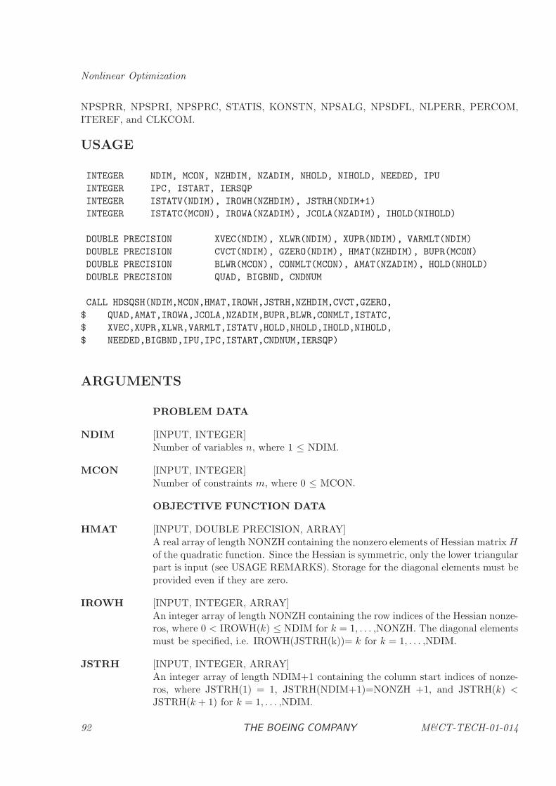
Nonlinear Optimization
NPSPRR, NPSPRI, NPSPRC, STATIS, KONSTN, NPSALG, NPSDFL, NLPERR, PERCOM,ITEREF, and CLKCOM.
USAGE
INTEGER NDIM, MCON, NZHDIM, NZADIM, NHOLD, NIHOLD, NEEDED, IPU
INTEGER IPC, ISTART, IERSQP
INTEGER ISTATV(NDIM), IROWH(NZHDIM), JSTRH(NDIM+1)
INTEGER ISTATC(MCON), IROWA(NZADIM), JCOLA(NZADIM), IHOLD(NIHOLD)
DOUBLE PRECISION XVEC(NDIM), XLWR(NDIM), XUPR(NDIM), VARMLT(NDIM)
DOUBLE PRECISION CVCT(NDIM), GZERO(NDIM), HMAT(NZHDIM), BUPR(MCON)
DOUBLE PRECISION BLWR(MCON), CONMLT(MCON), AMAT(NZADIM), HOLD(NHOLD)
DOUBLE PRECISION QUAD, BIGBND, CNDNUM
CALL HDSQSH(NDIM,MCON,HMAT,IROWH,JSTRH,NZHDIM,CVCT,GZERO,
$ QUAD,AMAT,IROWA,JCOLA,NZADIM,BUPR,BLWR,CONMLT,ISTATC,
$ XVEC,XUPR,XLWR,VARMLT,ISTATV,HOLD,NHOLD,IHOLD,NIHOLD,
$ NEEDED,BIGBND,IPU,IPC,ISTART,CNDNUM,IERSQP)
ARGUMENTS
PROBLEM DATA
NDIM [INPUT, INTEGER]Number of variables n, where 1 ≤ NDIM.
MCON [INPUT, INTEGER]Number of constraints m, where 0 ≤ MCON.
OBJECTIVE FUNCTION DATA
HMAT [INPUT, DOUBLE PRECISION, ARRAY]A real array of length NONZH containing the nonzero elements of Hessian matrixHof the quadratic function. Since the Hessian is symmetric, only the lower triangularpart is input (see USAGE REMARKS). Storage for the diagonal elements must beprovided even if they are zero.
IROWH [INPUT, INTEGER, ARRAY]An integer array of length NONZH containing the row indices of the Hessian nonze-ros, where 0 < IROWH(k) ≤ NDIM for k = 1, . . . ,NONZH. The diagonal elementsmust be specified, i.e. IROWH(JSTRH(k))= k for k = 1, . . . ,NDIM.
JSTRH [INPUT, INTEGER, ARRAY]An integer array of length NDIM+1 containing the column start indices of nonze-ros, where JSTRH(1) = 1, JSTRH(NDIM+1)=NONZH +1, and JSTRH(k) <JSTRH(k + 1) for k = 1, . . . ,NDIM.
92 THE BOEING COMPANY M&CT-TECH-01-014
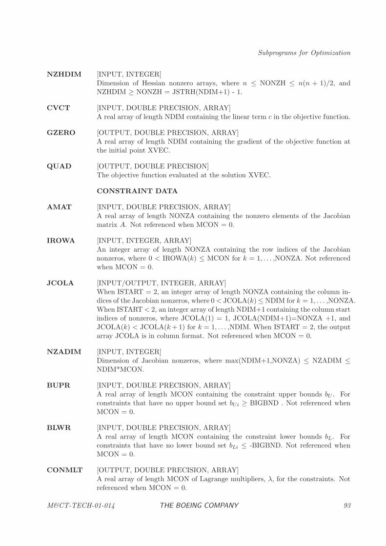
Subprograms for Optimization
NZHDIM [INPUT, INTEGER]Dimension of Hessian nonzero arrays, where n ≤ NONZH ≤ n(n + 1)/2, andNZHDIM ≥ NONZH = JSTRH(NDIM+1) - 1.
CVCT [INPUT, DOUBLE PRECISION, ARRAY]A real array of length NDIM containing the linear term c in the objective function.
GZERO [OUTPUT, DOUBLE PRECISION, ARRAY]A real array of length NDIM containing the gradient of the objective function atthe initial point XVEC.
QUAD [OUTPUT, DOUBLE PRECISION]The objective function evaluated at the solution XVEC.
CONSTRAINT DATA
AMAT [INPUT, DOUBLE PRECISION, ARRAY]A real array of length NONZA containing the nonzero elements of the Jacobianmatrix A. Not referenced when MCON = 0.
IROWA [INPUT, INTEGER, ARRAY]An integer array of length NONZA containing the row indices of the Jacobiannonzeros, where 0 < IROWA(k) ≤ MCON for k = 1, . . . ,NONZA. Not referencedwhen MCON = 0.
JCOLA [INPUT/OUTPUT, INTEGER, ARRAY]When ISTART = 2, an integer array of length NONZA containing the column in-dices of the Jacobian nonzeros, where 0< JCOLA(k) ≤ NDIM for k = 1, . . . ,NONZA.When ISTART< 2, an integer array of length NDIM+1 containing the column startindices of nonzeros, where JCOLA(1) = 1, JCOLA(NDIM+1)=NONZA +1, andJCOLA(k) < JCOLA(k+ 1) for k = 1, . . . ,NDIM. When ISTART = 2, the outputarray JCOLA is in column format. Not referenced when MCON = 0.
NZADIM [INPUT, INTEGER]Dimension of Jacobian nonzeros, where max(NDIM+1,NONZA) ≤ NZADIM ≤NDIM*MCON.
BUPR [INPUT, DOUBLE PRECISION, ARRAY]A real array of length MCON containing the constraint upper bounds bU . Forconstraints that have no upper bound set bUi ≥ BIGBND . Not referenced whenMCON = 0.
BLWR [INPUT, DOUBLE PRECISION, ARRAY]A real array of length MCON containing the constraint lower bounds bL. Forconstraints that have no lower bound set bLi ≤ -BIGBND. Not referenced whenMCON = 0.
CONMLT [OUTPUT, DOUBLE PRECISION, ARRAY]A real array of length MCON of Lagrange multipliers, λ, for the constraints. Notreferenced when MCON = 0.
M&CT-TECH-01-014 THE BOEING COMPANY 93
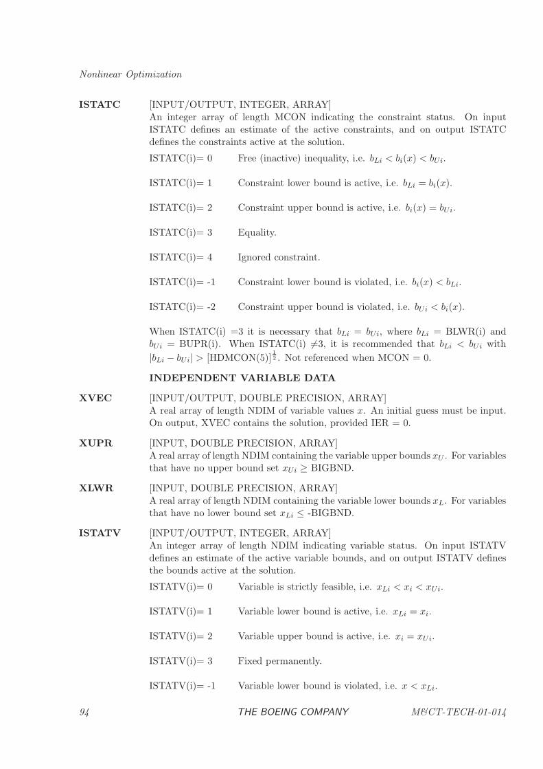
Nonlinear Optimization
ISTATC [INPUT/OUTPUT, INTEGER, ARRAY]An integer array of length MCON indicating the constraint status. On inputISTATC defines an estimate of the active constraints, and on output ISTATCdefines the constraints active at the solution.
ISTATC(i)= 0 Free (inactive) inequality, i.e. bLi < bi(x) < bUi.
ISTATC(i)= 1 Constraint lower bound is active, i.e. bLi = bi(x).
ISTATC(i)= 2 Constraint upper bound is active, i.e. bi(x) = bUi.
ISTATC(i)= 3 Equality.
ISTATC(i)= 4 Ignored constraint.
ISTATC(i)= -1 Constraint lower bound is violated, i.e. bi(x) < bLi.
ISTATC(i)= -2 Constraint upper bound is violated, i.e. bUi < bi(x).
When ISTATC(i) =3 it is necessary that bLi = bUi, where bLi = BLWR(i) andbUi = BUPR(i). When ISTATC(i) 6=3, it is recommended that bLi < bUi with
|bLi − bUi| > [HDMCON(5)]12 . Not referenced when MCON = 0.
INDEPENDENT VARIABLE DATA
XVEC [INPUT/OUTPUT, DOUBLE PRECISION, ARRAY]A real array of length NDIM of variable values x. An initial guess must be input.On output, XVEC contains the solution, provided IER = 0.
XUPR [INPUT, DOUBLE PRECISION, ARRAY]A real array of length NDIM containing the variable upper bounds xU . For variablesthat have no upper bound set xUi ≥ BIGBND.
XLWR [INPUT, DOUBLE PRECISION, ARRAY]A real array of length NDIM containing the variable lower bounds xL. For variablesthat have no lower bound set xLi ≤ -BIGBND.
ISTATV [INPUT/OUTPUT, INTEGER, ARRAY]An integer array of length NDIM indicating variable status. On input ISTATVdefines an estimate of the active variable bounds, and on output ISTATV definesthe bounds active at the solution.
ISTATV(i)= 0 Variable is strictly feasible, i.e. xLi < xi < xUi.
ISTATV(i)= 1 Variable lower bound is active, i.e. xLi = xi.
ISTATV(i)= 2 Variable upper bound is active, i.e. xi = xUi.
ISTATV(i)= 3 Fixed permanently.
ISTATV(i)= -1 Variable lower bound is violated, i.e. x < xLi.
94 THE BOEING COMPANY M&CT-TECH-01-014
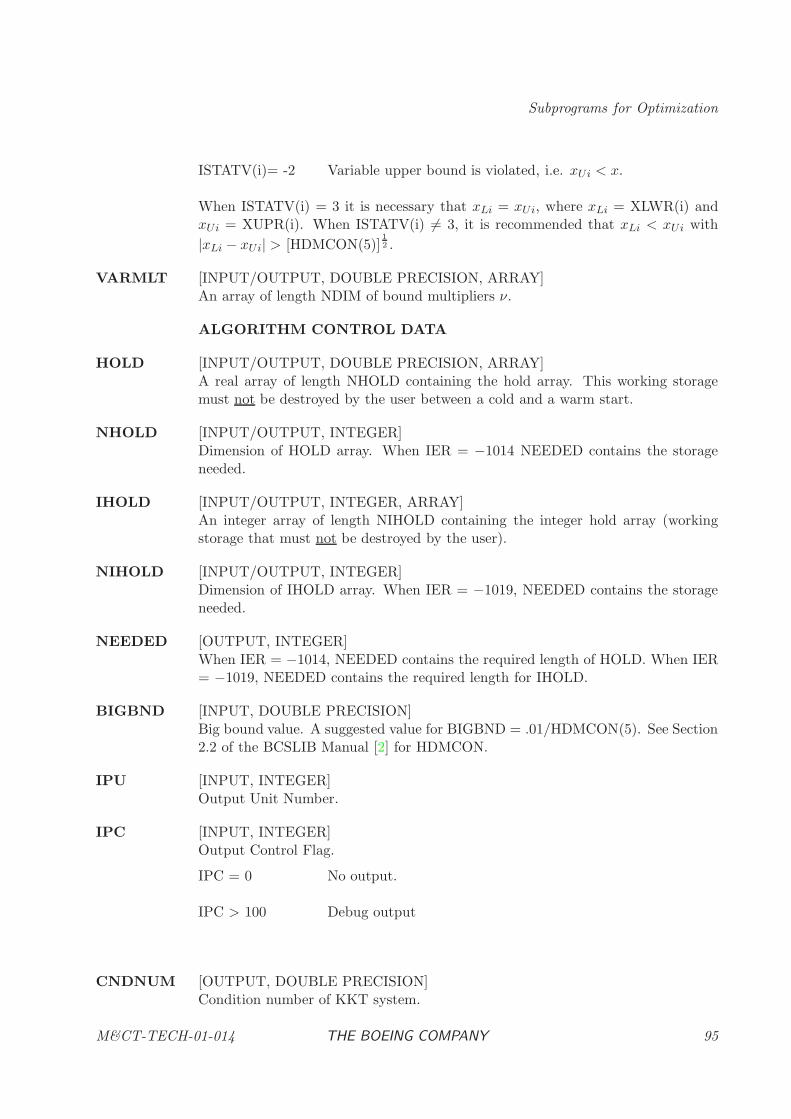
Subprograms for Optimization
ISTATV(i)= -2 Variable upper bound is violated, i.e. xUi < x.
When ISTATV(i) = 3 it is necessary that xLi = xUi, where xLi = XLWR(i) andxUi = XUPR(i). When ISTATV(i) 6= 3, it is recommended that xLi < xUi with
|xLi − xUi| > [HDMCON(5)]12 .
VARMLT [INPUT/OUTPUT, DOUBLE PRECISION, ARRAY]An array of length NDIM of bound multipliers ν.
ALGORITHM CONTROL DATA
HOLD [INPUT/OUTPUT, DOUBLE PRECISION, ARRAY]A real array of length NHOLD containing the hold array. This working storagemust not be destroyed by the user between a cold and a warm start.
NHOLD [INPUT/OUTPUT, INTEGER]Dimension of HOLD array. When IER = −1014 NEEDED contains the storageneeded.
IHOLD [INPUT/OUTPUT, INTEGER, ARRAY]An integer array of length NIHOLD containing the integer hold array (workingstorage that must not be destroyed by the user).
NIHOLD [INPUT/OUTPUT, INTEGER]Dimension of IHOLD array. When IER = −1019, NEEDED contains the storageneeded.
NEEDED [OUTPUT, INTEGER]When IER = −1014, NEEDED contains the required length of HOLD. When IER= −1019, NEEDED contains the required length for IHOLD.
BIGBND [INPUT, DOUBLE PRECISION]Big bound value. A suggested value for BIGBND = .01/HDMCON(5). See Section2.2 of the BCSLIB Manual [2] for HDMCON.
IPU [INPUT, INTEGER]Output Unit Number.
IPC [INPUT, INTEGER]Output Control Flag.
IPC = 0 No output.
IPC > 100 Debug output
CNDNUM [OUTPUT, DOUBLE PRECISION]Condition number of KKT system.
M&CT-TECH-01-014 THE BOEING COMPANY 95
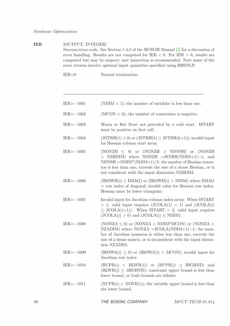
Nonlinear Optimization
IER [OUTPUT, INTEGER]Success/error code. See Section 1.4.2 of the BCSLIB Manual [2] for a discussion oferror handling. Results are not computed for IER < 0. For IER > 0, results arecomputed but may be suspect; user inspection is recommended. Note some of theerror returns involve optional input quantities specified using HHSNLP.
IER=0 Normal termination.
---------------------------------------------------------------
IER=−1001 (NDIM < 1); the number of variables is less than one.
IER=−1002 (MCON < 0); the number of constraints is negative.
IER=−1003 Warm or Hot Start not preceded by a cold start. ISTARTmust be positive on first call.
IER=−1004 (JSTRH(1) ≤ 0) or (JSTRH(k) ≥ JSTRH(k+1)); invalid inputfor Hessian column start array.
IER=−1005 (NONZH ≤ 0) or (NONZH > NDNSH) or (NONZH> NZHDIM) where NONZH =JSTRH(NDIM+1)−1, andNDNSH =NDIM*(NDIM+1)/2; the number of Hessian nonze-ros is less than one, exceeds the size of a dense Hessian, or isnot consistent with the input dimension NZHDIM.
IER=−1006 (IROWH(i) ≤ IDIAG) or (IROWH(i) > NDIM) where IDIAG= row index of diagonal; invalid value for Hessian row index.Hessian must be lower triangular.
IER=−1007 Invalid input for Jacobian column index array. When ISTART= 1, valid input requires (JCOLA(1) = 1) and (JCOLA(i)≤ JCOLA(i+1)). When ISTART = 2, valid input requires(JCOLA(i) > 0) and (JCOLA(i) ≤ NDIM).
IER=−1008 (NONZA ≤ 0) or (NONZA > NDIM*MCON) or (NONZA >NZADIM) where NONZA =JCOLA(NDIM+1)−1; the num-ber of Jacobian nonzeros is either less than one, exceeds thesize of a dense matrix, or is inconsistent with the input dimen-sion NZADIM.
IER=−1009 (IROWA(i) ≤ 0) or (IROWA(i) > MCON); invalid input forJacobian row index.
IER=−1010 (BUPR(i) < BLWR(i)) or (BUPR(i) ≥ BIGBND) and(BLWR(i) ≤ -BIGBND); constraint upper bound is less thanlower bound, or both bounds are infinite.
IER=−1011 (XUPR(i) < XLWR(i)); the variable upper bound is less thanthe lower bound.
96 THE BOEING COMPANY M&CT-TECH-01-014
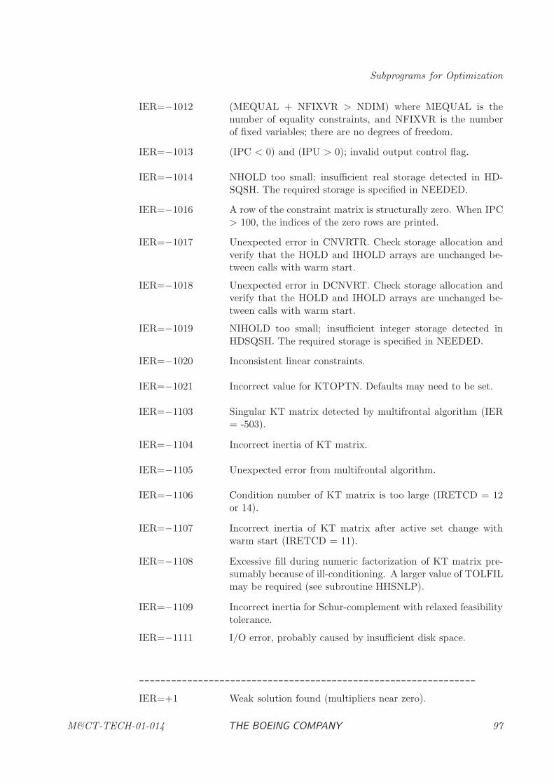
Subprograms for Optimization
IER=−1012 (MEQUAL + NFIXVR > NDIM) where MEQUAL is thenumber of equality constraints, and NFIXVR is the numberof fixed variables; there are no degrees of freedom.
IER=−1013 (IPC < 0) and (IPU > 0); invalid output control flag.
IER=−1014 NHOLD too small; insufficient real storage detected in HD-SQSH. The required storage is specified in NEEDED.
IER=−1016 A row of the constraint matrix is structurally zero. When IPC> 100, the indices of the zero rows are printed.
IER=−1017 Unexpected error in CNVRTR. Check storage allocation andverify that the HOLD and IHOLD arrays are unchanged be-tween calls with warm start.
IER=−1018 Unexpected error in DCNVRT. Check storage allocation andverify that the HOLD and IHOLD arrays are unchanged be-tween calls with warm start.
IER=−1019 NIHOLD too small; insufficient integer storage detected inHDSQSH. The required storage is specified in NEEDED.
IER=−1020 Inconsistent linear constraints.
IER=−1021 Incorrect value for KTOPTN. Defaults may need to be set.
IER=−1103 Singular KT matrix detected by multifrontal algorithm (IER= -503).
IER=−1104 Incorrect inertia of KT matrix.
IER=−1105 Unexpected error from multifrontal algorithm.
IER=−1106 Condition number of KT matrix is too large (IRETCD = 12or 14).
IER=−1107 Incorrect inertia of KT matrix after active set change withwarm start (IRETCD = 11).
IER=−1108 Excessive fill during numeric factorization of KT matrix pre-sumably because of ill-conditioning. A larger value of TOLFILmay be required (see subroutine HHSNLP).
IER=−1109 Incorrect inertia for Schur-complement with relaxed feasibilitytolerance.
IER=−1111 I/O error, probably caused by insufficient disk space.
---------------------------------------------------------------
IER=+1 Weak solution found (multipliers near zero).
M&CT-TECH-01-014 THE BOEING COMPANY 97
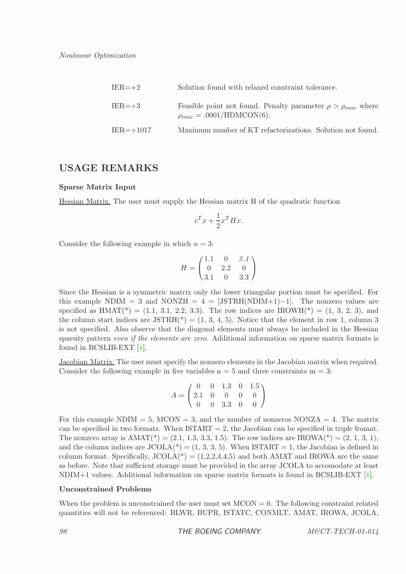
Nonlinear Optimization
IER=+2 Solution found with relaxed constraint tolerance.
IER=+3 Feasible point not found. Penalty parameter ρ > ρmax whereρmax = .0001/HDMCON(6).
IER=+1017 Maximum number of KT refactorizations. Solution not found.
USAGE REMARKS
Sparse Matrix Input
Hessian Matrix. The user must supply the Hessian matrix H of the quadratic function
cTx+1
2xTHx.
Consider the following example in which n = 3:
H =
1.1 0 3 .10 2.2 0
3.1 0 3.3
Since the Hessian is a symmetric matrix only the lower triangular portion must be specified. Forthis example NDIM = 3 and NONZH = 4 = [JSTRH(NDIM+1)−1]. The nonzero values arespecified as HMAT(*) = (1.1, 3.1, 2.2, 3.3). The row indices are IROWH(*) = (1, 3, 2, 3), andthe column start indices are JSTRH(*) = (1, 3, 4, 5). Notice that the element in row 1, column 3is not specified. Also observe that the diagonal elements must always be included in the Hessiansparsity pattern even if the elements are zero. Additional information on sparse matrix formats isfound in BCSLIB-EXT [1].
Jacobian Matrix. The user must specify the nonzero elements in the Jacobian matrix when required.Consider the following example in five variables n = 5 and three constraints m = 3:
A =
0 0 1.3 0 1.5
2.1 0 0 0 00 0 3.3 0 0
For this example NDIM = 5, MCON = 3, and the number of nonzeros NONZA = 4. The matrixcan be specified in two formats. When ISTART = 2, the Jacobian can be specified in triple fromat.The nonzero array is AMAT(*) = (2.1, 1.3, 3.3, 1.5). The row indices are IROWA(*) = (2, 1, 3, 1),and the column indices are JCOLA(*) = (1, 3, 3, 5). When ISTART = 1, the Jacobian is defined incolumn format. Specifically, JCOLA(*) = (1,2,2,4,4,5) and both AMAT and IROWA are the sameas before. Note that sufficient storage must be provided in the array JCOLA to accomodate at leastNDIM+1 values. Additional information on sparse matrix formats is found in BCSLIB-EXT [1].
Unconstrained Problems
When the problem is unconstrained the user must set MCON = 0. The following constraint relatedquantities will not be referenced: BLWR, BUPR, ISTATC, CONMLT, AMAT, IROWA, JCOLA,
98 THE BOEING COMPANY M&CT-TECH-01-014
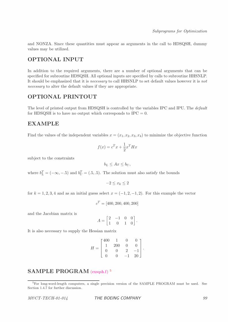
Subprograms for Optimization
and NONZA. Since these quantities must appear as arguments in the call to HDSQSH, dummyvalues may be utilized.
OPTIONAL INPUT
In addition to the required arguments, there are a number of optional arguments that can bespecified for subroutine HDSQSH. All optional inputs are specified by calls to subroutine HHSNLP.It should be emphasized that it is necessary to call HHSNLP to set default values however it is notnecessary to alter the default values if they are appropriate.
OPTIONAL PRINTOUT
The level of printed output from HDSQSH is controlled by the variables IPC and IPU. The defaultfor HDSQSH is to have no output which corresponds to IPC = 0.
EXAMPLE
Find the values of the independent variables x = (x1, x2, x3, x4) to minimize the objective function
f(x) = cTx+1
2xTHx
subject to the constraints
bL ≤ Ax ≤ bU ,
where bTL = (−∞,−.5) and bTU = (.5, .5). The solution must also satisfy the bounds
−2 ≤ xk ≤ 2
for k = 1, 2, 3, 4 and as an initial guess select x = (−1, 2,−1, 2). For this example the vector
cT = [400, 200, 400, 200]
and the Jacobian matrix is
A =
[2 −1 0 01 0 1 0
].
It is also necessary to supply the Hessian matrix
H =
400 1 0 01 200 0 00 0 2 −10 0 −1 20
.
SAMPLE PROGRAM (exsqsh.f) 5
5For long-word-length computers, a single precision version of the SAMPLE PROGRAM must be used. See
Section 1.4.7 for further discussion.
M&CT-TECH-01-014 THE BOEING COMPANY 99
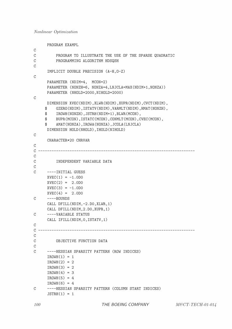
Nonlinear Optimization
PROGRAM EXAMPL
C
C PROGRAM TO ILLUSTRATE THE USE OF THE SPARSE QUADRATIC
C PROGRAMMING ALGORITHM HDSQSH
C
IMPLICIT DOUBLE PRECISION (A-H,O-Z)
C
PARAMETER (NDIM=4, MCON=2)
PARAMETER (NONZH=6, NONZA=4,LNJCLA=MAX(NDIM+1,NONZA))
PARAMETER (NHOLD=2000,NIHOLD=2000)
C
DIMENSION XVEC(NDIM),XLWR(NDIM),XUPR(NDIM),CVCT(NDIM),
$ GZERO(NDIM),ISTATV(NDIM),VARMLT(NDIM),HMAT(NONZH),
$ IROWH(NONZH),JSTRH(NDIM+1),BLWR(MCON),
$ BUPR(MCON),ISTATC(MCON),CONMLT(MCON),CVEC(MCON),
$ AMAT(NONZA),IROWA(NONZA),JCOLA(LNJCLA)
DIMENSION HOLD(NHOLD),IHOLD(NIHOLD)
C
CHARACTER*20 CHRVAR
C
C ----------------------------------------------------------------------
C
C INDEPENDENT VARIABLE DATA
C
C ----INITIAL GUESS
XVEC(1) = -1.0D0
XVEC(2) = 2.0D0
XVEC(3) = -1.0D0
XVEC(4) = 2.0D0
C ----BOUNDS
CALL DFILL(NDIM,-2.D0,XLWR,1)
CALL DFILL(NDIM,2.D0,XUPR,1)
C ----VARIABLE STATUS
CALL IFILL(NDIM,0,ISTATV,1)
C
C ----------------------------------------------------------------------
C
C OBJECTIVE FUNCTION DATA
C
C ----HESSIAN SPARSITY PATTERN (ROW INDICES)
IROWH(1) = 1
IROWH(2) = 2
IROWH(3) = 2
IROWH(4) = 3
IROWH(5) = 4
IROWH(6) = 4
C ----HESSIAN SPARSITY PATTERN (COLUMN START INDICES)
JSTRH(1) = 1
100 THE BOEING COMPANY M&CT-TECH-01-014
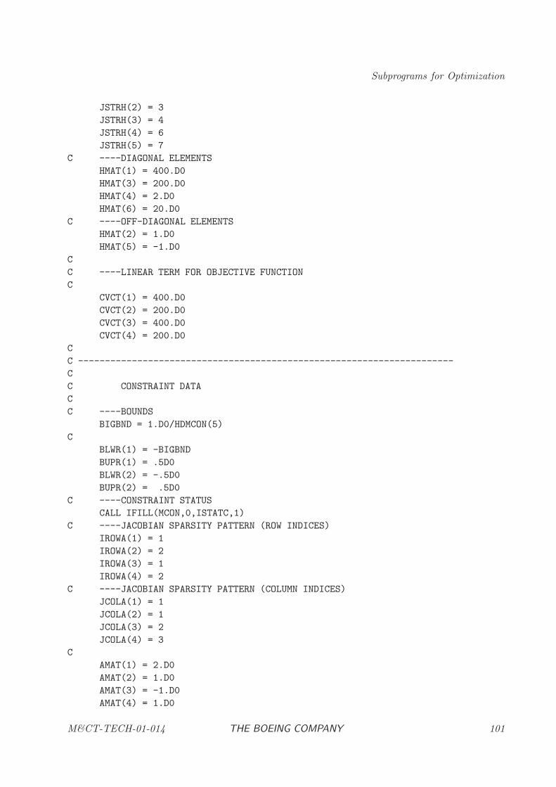
Subprograms for Optimization
JSTRH(2) = 3
JSTRH(3) = 4
JSTRH(4) = 6
JSTRH(5) = 7
C ----DIAGONAL ELEMENTS
HMAT(1) = 400.D0
HMAT(3) = 200.D0
HMAT(4) = 2.D0
HMAT(6) = 20.D0
C ----OFF-DIAGONAL ELEMENTS
HMAT(2) = 1.D0
HMAT(5) = -1.D0
C
C ----LINEAR TERM FOR OBJECTIVE FUNCTION
C
CVCT(1) = 400.D0
CVCT(2) = 200.D0
CVCT(3) = 400.D0
CVCT(4) = 200.D0
C
C ----------------------------------------------------------------------
C
C CONSTRAINT DATA
C
C ----BOUNDS
BIGBND = 1.D0/HDMCON(5)
C
BLWR(1) = -BIGBND
BUPR(1) = .5D0
BLWR(2) = -.5D0
BUPR(2) = .5D0
C ----CONSTRAINT STATUS
CALL IFILL(MCON,0,ISTATC,1)
C ----JACOBIAN SPARSITY PATTERN (ROW INDICES)
IROWA(1) = 1
IROWA(2) = 2
IROWA(3) = 1
IROWA(4) = 2
C ----JACOBIAN SPARSITY PATTERN (COLUMN INDICES)
JCOLA(1) = 1
JCOLA(2) = 1
JCOLA(3) = 2
JCOLA(4) = 3
C
AMAT(1) = 2.D0
AMAT(2) = 1.D0
AMAT(3) = -1.D0
AMAT(4) = 1.D0
M&CT-TECH-01-014 THE BOEING COMPANY 101
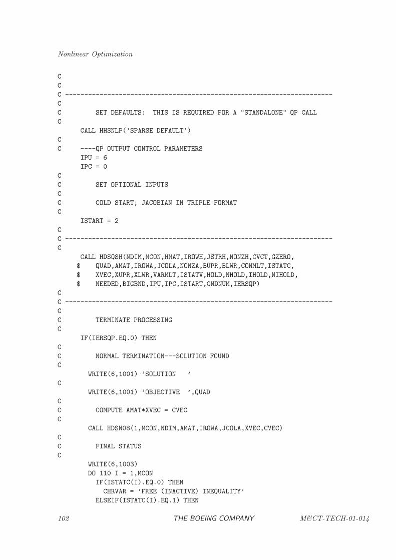
Nonlinear Optimization
C
C
C ----------------------------------------------------------------------
C
C SET DEFAULTS: THIS IS REQUIRED FOR A "STANDALONE" QP CALL
C
CALL HHSNLP(’SPARSE DEFAULT’)
C
C ----QP OUTPUT CONTROL PARAMETERS
IPU = 6
IPC = 0
C
C SET OPTIONAL INPUTS
C
C COLD START; JACOBIAN IN TRIPLE FORMAT
C
ISTART = 2
C
C ----------------------------------------------------------------------
C
CALL HDSQSH(NDIM,MCON,HMAT,IROWH,JSTRH,NONZH,CVCT,GZERO,
$ QUAD,AMAT,IROWA,JCOLA,NONZA,BUPR,BLWR,CONMLT,ISTATC,
$ XVEC,XUPR,XLWR,VARMLT,ISTATV,HOLD,NHOLD,IHOLD,NIHOLD,
$ NEEDED,BIGBND,IPU,IPC,ISTART,CNDNUM,IERSQP)
C
C ----------------------------------------------------------------------
C
C TERMINATE PROCESSING
C
IF(IERSQP.EQ.0) THEN
C
C NORMAL TERMINATION---SOLUTION FOUND
C
WRITE(6,1001) ’SOLUTION ’
C
WRITE(6,1001) ’OBJECTIVE ’,QUAD
C
C COMPUTE AMAT*XVEC = CVEC
C
CALL HDSN08(1,MCON,NDIM,AMAT,IROWA,JCOLA,XVEC,CVEC)
C
C FINAL STATUS
C
WRITE(6,1003)
DO 110 I = 1,MCON
IF(ISTATC(I).EQ.0) THEN
CHRVAR = ’FREE (INACTIVE) INEQUALITY’
ELSEIF(ISTATC(I).EQ.1) THEN
102 THE BOEING COMPANY M&CT-TECH-01-014
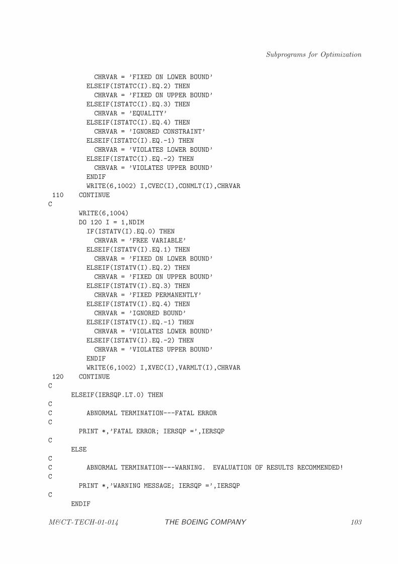
Subprograms for Optimization
CHRVAR = ’FIXED ON LOWER BOUND’
ELSEIF(ISTATC(I).EQ.2) THEN
CHRVAR = ’FIXED ON UPPER BOUND’
ELSEIF(ISTATC(I).EQ.3) THEN
CHRVAR = ’EQUALITY’
ELSEIF(ISTATC(I).EQ.4) THEN
CHRVAR = ’IGNORED CONSTRAINT’
ELSEIF(ISTATC(I).EQ.-1) THEN
CHRVAR = ’VIOLATES LOWER BOUND’
ELSEIF(ISTATC(I).EQ.-2) THEN
CHRVAR = ’VIOLATES UPPER BOUND’
ENDIF
WRITE(6,1002) I,CVEC(I),CONMLT(I),CHRVAR
110 CONTINUE
C
WRITE(6,1004)
DO 120 I = 1,NDIM
IF(ISTATV(I).EQ.0) THEN
CHRVAR = ’FREE VARIABLE’
ELSEIF(ISTATV(I).EQ.1) THEN
CHRVAR = ’FIXED ON LOWER BOUND’
ELSEIF(ISTATV(I).EQ.2) THEN
CHRVAR = ’FIXED ON UPPER BOUND’
ELSEIF(ISTATV(I).EQ.3) THEN
CHRVAR = ’FIXED PERMANENTLY’
ELSEIF(ISTATV(I).EQ.4) THEN
CHRVAR = ’IGNORED BOUND’
ELSEIF(ISTATV(I).EQ.-1) THEN
CHRVAR = ’VIOLATES LOWER BOUND’
ELSEIF(ISTATV(I).EQ.-2) THEN
CHRVAR = ’VIOLATES UPPER BOUND’
ENDIF
WRITE(6,1002) I,XVEC(I),VARMLT(I),CHRVAR
120 CONTINUE
C
ELSEIF(IERSQP.LT.0) THEN
C
C ABNORMAL TERMINATION---FATAL ERROR
C
PRINT *,’FATAL ERROR; IERSQP =’,IERSQP
C
ELSE
C
C ABNORMAL TERMINATION---WARNING. EVALUATION OF RESULTS RECOMMENDED!
C
PRINT *,’WARNING MESSAGE; IERSQP =’,IERSQP
C
ENDIF
M&CT-TECH-01-014 THE BOEING COMPANY 103
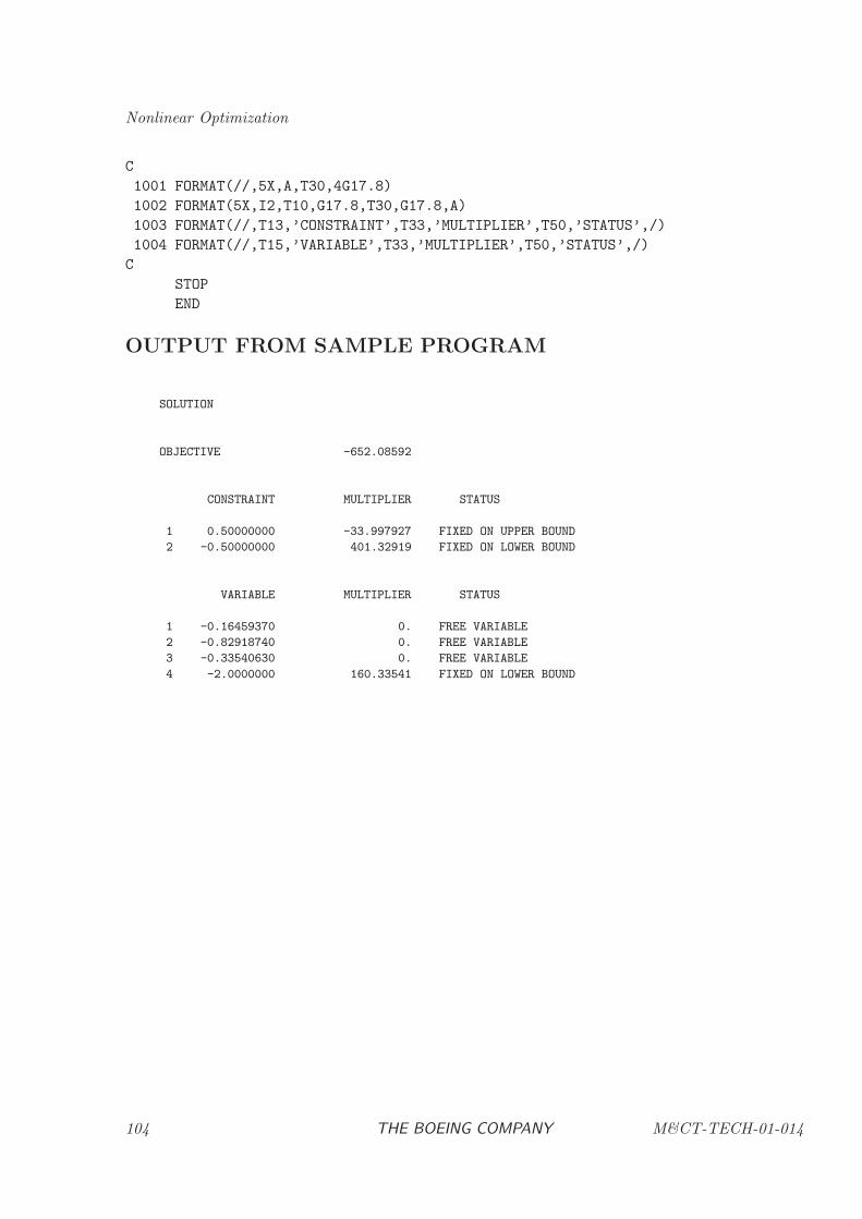
Nonlinear Optimization
C
1001 FORMAT(//,5X,A,T30,4G17.8)
1002 FORMAT(5X,I2,T10,G17.8,T30,G17.8,A)
1003 FORMAT(//,T13,’CONSTRAINT’,T33,’MULTIPLIER’,T50,’STATUS’,/)
1004 FORMAT(//,T15,’VARIABLE’,T33,’MULTIPLIER’,T50,’STATUS’,/)
C
STOP
END
OUTPUT FROM SAMPLE PROGRAM
SOLUTION
OBJECTIVE -652.08592
CONSTRAINT MULTIPLIER STATUS
1 0.50000000 -33.997927 FIXED ON UPPER BOUND
2 -0.50000000 401.32919 FIXED ON LOWER BOUND
VARIABLE MULTIPLIER STATUS
1 -0.16459370 0. FREE VARIABLE
2 -0.82918740 0. FREE VARIABLE
3 -0.33540630 0. FREE VARIABLE
4 -2.0000000 160.33541 FIXED ON LOWER BOUND
104 THE BOEING COMPANY M&CT-TECH-01-014
Subprograms for Optimization
HDSNPV: Sparse Nonlinear Programming Parameter Retrieval
PURPOSE
HDSNPV is a utility subroutine used to retrieve algorithm control parameter values from the sparsenonlinear programming algorithms HDSNLP and HDSLSQ or the dense algorithms HDNLPR andHDNLPD.
RELATED SUBPROGRAMS
HHSNLP Sparse Nonlinear Programming Input Procedure
HDNLPD Dense Nonlinear Programming
HDNLPR Dense Nonlinear Programming–Reverse Communication Format
HDSNLP Sparse Nonlinear Programming
HDSLSQ Sparse Constrained Nonlinear Least Squares
METHOD
Subroutine HDSNPV can be used to retrieve the value for any optional parameter that can be setby the routine HHSNLP. Subroutine HHSNLP permits input in the following format:
’ symbol = value ’
Given the character string ’symbol ’, HDSNPV retrieves the quantity ’value ’. A single parametervalue is retrieved with a single call to HDSNPV.
USAGE
CHARACTER STRING*6
INTEGER IVAL
DOUBLE PRECISION RVAL
CHARACTER*6 CVAL
CALL HDSNPV(STRING,IVAL,RVAL,CVAL)
ARGUMENTS
STRING [INPUT, CHARACTER]Character variable where STRING(1:6) corresponds to the input ’symbol ’ in theHHSNLP routine.
IVAL [OUTPUT, INTEGER]Integer value for the parameter with mnemonic STRING(1:6). If STRING(1:6)does not correspond to any integer parameter then IVAL = JHMCON(1).
RVAL [OUTPUT, DOUBLE PRECISION]Real value for the parameter with mnemonic STRING(1:6). If STRING(1:6) doesnot correspond to any real parameter then RVAL = HDMCON(1).
M&CT-TECH-01-014 THE BOEING COMPANY 105

Nonlinear Optimization
CVAL [OUTPUT, CHARACTER]Character*6 value for the parameter with mnemonic STRING(1:6). If STRING(1:6)does not correspond to any character parameter then CVAL = ’ ’.
106 THE BOEING COMPANY M&CT-TECH-01-014
Subprograms for Optimization
HDBNPD: Dense Barrier Nonlinear Programming
PURPOSE
HDBNPD computes the vector x = (x1, x2, . . . , xn) which minimizes the objective function
f(x)
subject to the m nonlinear constraints
cL ≤ c(x) ≤ cU
and the simple boundsxL ≤ x ≤ xU
Equality constraints are imposed by setting cLi = cUi and variables can be fixed by settingxLi = xUi. HDBNPD works under the assumption that the objective and constraint functionsare twice continuously differentiable, and if this is not true algorithm performance is unpredictable.HDBNPD uses a forward communication format and the user must supply a subroutine to com-pute the values of the objective and constraint functions. First and second derivatives of the usersupplied functions are computed numerically. The matrix of second derivatives (Hessian of theLagrangian) can be constructed using a quasi-Newton recursive estimate or by central differencing.Subroutine HDBNPD calls the sparse barrier nonlinear programming algorithm HDBNLP, and isintended for simplified usage as appropriate for small dense problems.
RELATED SUBPROGRAMS
HDDFDJ Finite Difference Jacobian
HDDFDH Finite Difference Hessian
HDNLPD Dense Nonlinear Programming
HDBNLP Sparse Barrier Nonlinear Programming
HHSNLP Sparse Nonlinear Programming Input Procedure
METHOD
An interior point or barrier method is used to solve the nonlinear programming (NLP) problem.HDBNPD provides four alternatives for constructing an approximation to the Hessian matrix whichare described in the background section of this document. The default is a symmetric rank-one(SR1) approximation, with options for using a BFGS, SSQN, or finite difference estimate instead.HDBNPD constructs all first derivative information using the finite difference procedures HDDFDJand/or HDDFDH. Finite difference perturbation sizes are selected automatically to balance trun-cation and roundoff error. Forward difference estimates are utilized when possible for efficiency,and central difference estimates are invoked when necessary to improve accuracy. Although defaultvalues are set for all algorithm parameters, HHSNLP can be utilized to override the defaults.
WARNING
M&CT-TECH-01-014 THE BOEING COMPANY 107
Nonlinear Optimization
The objective function and constraints supplied by the user are assumed to be continuous andhave continuous first and second derivatives. Nondifferentiable functions can cause unpredictableperformance in the optimization algorithm. It should be emphasized that discontinuities in theHessian matrices can significantly degrade the speed of convergence without producing any otherobvious difficulties. The following common sources of error should be avoided when evaluating theobjective and constraint functions:
(1) nonsmooth interpolation of data;
(2) iterative procedures inside the function evaluation process, such as adaptive quadrature or rootsolving;
(3) discontinuous behavior caused by branching for IF tests;
(4) nondifferentiable functions such as ABS, MAX, and MIN.
The user must provide a procedure to evaluate the objective and constraint functions. If it is notpossible to evaluate the functions (for example, c(x) = 1/x at x = 0) then set IFERR = 1 andexit the function evaluation process. Otherwise, set IFERR = 0 when the functions are evaluated.The function error flag should be used to avoid computational difficulties, but never in lieu of anexplicit constraint.
The HDBNPD software uses internal common blocks to communicate information. To avoid con-flict with these internal commons the user should not have commons with the following names:NPSPRR, NPSPRI, NPSPRC, STATIS, KONSTN, NPSALG, NPSDFL, NLPERR, PERCOM,ITEREF, and CLKCOM.
USAGE
INTEGER IER, NDIM, MCON, NHOLD, NIHOLD, NEEDED
INTEGER ISTATV(NDIM), ISTATC(MCON), IHOLD(NIHOLD)
DOUBLE PRECISION FBAR, XBAR(NDIM), XLWR(NDIM), XUPR(NDIM), VECNU(NDIM)
DOUBLE PRECISION CBAR(MCON), CLWR(MCON), CUPR(MCON)
DOUBLE PRECISION VECLAM(MCON), HOLD(NHOLD)
EXTERNAL FUNBOX
CALL HHSNLP(’BARRIER DEFAULT’)
CALL HDBNPD(FUNBOX, XBAR, XLWR, XUPR, ISTATV, VECNU, NDIM,
$ FBAR, CBAR, CLWR, CUPR, ISTATC, VECLAM, MCON,
$ HOLD, NHOLD, IHOLD, NIHOLD, NEEDED, IER)
ARGUMENTS
FUNCTION EVALUATION PROCEDURE
FUNBOX [INPUT, SUBROUTINE]Name of user-supplied subroutine to evaluate objective and constraint functions;see USER-SUPPLIED SUBPROGRAM
108 THE BOEING COMPANY M&CT-TECH-01-014
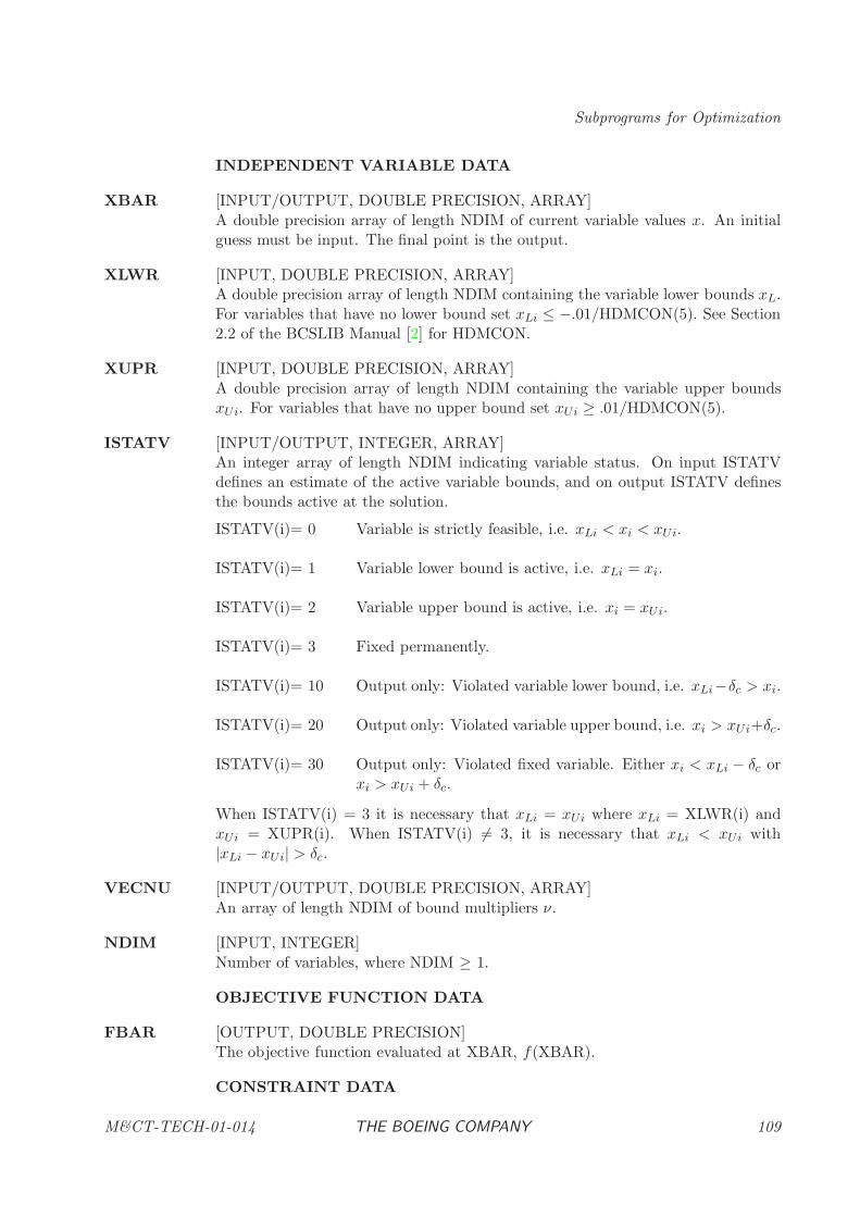
Subprograms for Optimization
INDEPENDENT VARIABLE DATA
XBAR [INPUT/OUTPUT, DOUBLE PRECISION, ARRAY]A double precision array of length NDIM of current variable values x. An initialguess must be input. The final point is the output.
XLWR [INPUT, DOUBLE PRECISION, ARRAY]A double precision array of length NDIM containing the variable lower bounds xL.For variables that have no lower bound set xLi ≤ −.01/HDMCON(5). See Section2.2 of the BCSLIB Manual [2] for HDMCON.
XUPR [INPUT, DOUBLE PRECISION, ARRAY]A double precision array of length NDIM containing the variable upper boundsxUi. For variables that have no upper bound set xUi ≥ .01/HDMCON(5).
ISTATV [INPUT/OUTPUT, INTEGER, ARRAY]An integer array of length NDIM indicating variable status. On input ISTATVdefines an estimate of the active variable bounds, and on output ISTATV definesthe bounds active at the solution.
ISTATV(i)= 0 Variable is strictly feasible, i.e. xLi < xi < xUi.
ISTATV(i)= 1 Variable lower bound is active, i.e. xLi = xi.
ISTATV(i)= 2 Variable upper bound is active, i.e. xi = xUi.
ISTATV(i)= 3 Fixed permanently.
ISTATV(i)= 10 Output only: Violated variable lower bound, i.e. xLi−δc > xi.
ISTATV(i)= 20 Output only: Violated variable upper bound, i.e. xi > xUi+δc.
ISTATV(i)= 30 Output only: Violated fixed variable. Either xi < xLi − δc orxi > xUi + δc.
When ISTATV(i) = 3 it is necessary that xLi = xUi where xLi = XLWR(i) andxUi = XUPR(i). When ISTATV(i) 6= 3, it is necessary that xLi < xUi with|xLi − xUi| > δc.
VECNU [INPUT/OUTPUT, DOUBLE PRECISION, ARRAY]An array of length NDIM of bound multipliers ν.
NDIM [INPUT, INTEGER]Number of variables, where NDIM ≥ 1.
OBJECTIVE FUNCTION DATA
FBAR [OUTPUT, DOUBLE PRECISION]The objective function evaluated at XBAR, f(XBAR).
CONSTRAINT DATA
M&CT-TECH-01-014 THE BOEING COMPANY 109
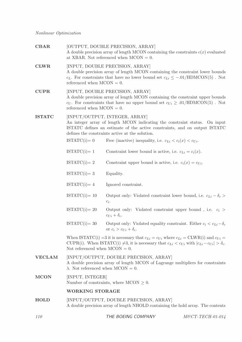
Nonlinear Optimization
CBAR [OUTPUT, DOUBLE PRECISION, ARRAY]A double precision array of length MCON containing the constraints c(x) evaluatedat XBAR. Not referenced when MCON = 0.
CLWR [INPUT, DOUBLE PRECISION, ARRAY]A double precision array of length MCON containing the constraint lower boundscL. For constraints that have no lower bound set cLi ≤ −.01/HDMCON(5) . Notreferenced when MCON = 0.
CUPR [INPUT, DOUBLE PRECISION, ARRAY]A double precision array of length MCON containing the constraint upper boundscU . For constraints that have no upper bound set cUi ≥ .01/HDMCON(5) . Notreferenced when MCON = 0.
ISTATC [INPUT/OUTPUT, INTEGER, ARRAY]An integer array of length MCON indicating the constraint status. On inputISTATC defines an estimate of the active constraints, and on output ISTATCdefines the constraints active at the solution.
ISTATC(i)= 0 Free (inactive) inequality, i.e. cLi < ci(x) < cUi.
ISTATC(i)= 1 Constraint lower bound is active, i.e. cLi = ci(x).
ISTATC(i)= 2 Constraint upper bound is active, i.e. ci(x) = cUi.
ISTATC(i)= 3 Equality.
ISTATC(i)= 4 Ignored constraint.
ISTATC(i)= 10 Output only: Violated constraint lower bound, i.e. cLi − δc >ci.
ISTATC(i)= 20 Output only: Violated constraint upper bound , i.e. ci >cUi + δc.
ISTATC(i)= 30 Output only: Violated equality constraint. Either ci < cLi−δcor ci > cUi + δc.
When ISTATC(i) =3 it is necessary that cLi = cUi where cLi = CLWR(i) and cUi =CUPR(i). When ISTATC(i) 6=3, it is necessary that cLi < cUi with |cLi−cUi| > δc.Not referenced when MCON = 0.
VECLAM [INPUT/OUTPUT, DOUBLE PRECISION, ARRAY]A double precision array of length MCON of Lagrange multipliers for constraintsλ. Not referenced when MCON = 0.
MCON [INPUT, INTEGER]Number of constraints, where MCON ≥ 0.
WORKING STORAGE
HOLD [INPUT/OUTPUT, DOUBLE PRECISION, ARRAY]A double precision array of length NHOLD containing the hold array. The contents
110 THE BOEING COMPANY M&CT-TECH-01-014
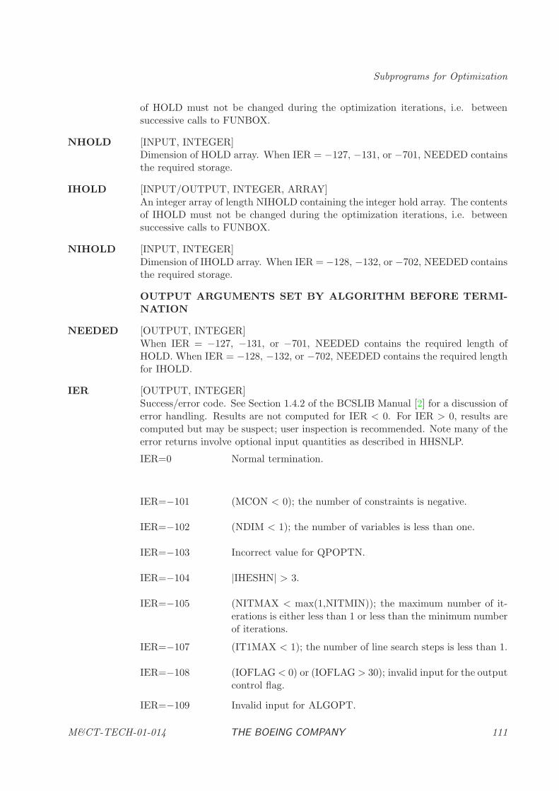
Subprograms for Optimization
of HOLD must not be changed during the optimization iterations, i.e. betweensuccessive calls to FUNBOX.
NHOLD [INPUT, INTEGER]Dimension of HOLD array. When IER = −127, −131, or −701, NEEDED containsthe required storage.
IHOLD [INPUT/OUTPUT, INTEGER, ARRAY]An integer array of length NIHOLD containing the integer hold array. The contentsof IHOLD must not be changed during the optimization iterations, i.e. betweensuccessive calls to FUNBOX.
NIHOLD [INPUT, INTEGER]Dimension of IHOLD array. When IER = −128, −132, or −702, NEEDED containsthe required storage.
OUTPUT ARGUMENTS SET BY ALGORITHM BEFORE TERMI-NATION
NEEDED [OUTPUT, INTEGER]When IER = −127, −131, or −701, NEEDED contains the required length ofHOLD. When IER = −128, −132, or −702, NEEDED contains the required lengthfor IHOLD.
IER [OUTPUT, INTEGER]Success/error code. See Section 1.4.2 of the BCSLIB Manual [2] for a discussion oferror handling. Results are not computed for IER < 0. For IER > 0, results arecomputed but may be suspect; user inspection is recommended. Note many of theerror returns involve optional input quantities as described in HHSNLP.
IER=0 Normal termination.
IER=−101 (MCON < 0); the number of constraints is negative.
IER=−102 (NDIM < 1); the number of variables is less than one.
IER=−103 Incorrect value for QPOPTN.
IER=−104 |IHESHN| > 3.
IER=−105 (NITMAX < max(1,NITMIN)); the maximum number of it-erations is either less than 1 or less than the minimum numberof iterations.
IER=−107 (IT1MAX < 1); the number of line search steps is less than 1.
IER=−108 (IOFLAG< 0) or (IOFLAG > 30); invalid input for the outputcontrol flag.
IER=−109 Invalid input for ALGOPT.
M&CT-TECH-01-014 THE BOEING COMPANY 111
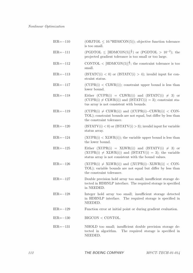
Nonlinear Optimization
IER=−110 (OBJTOL ≤ 10.*HDMCON(5)); objective function toleranceis too small.
IER=−111 (PGDTOL ≤ [HDMCON(5)]12 ) or (PGDTOL > 10−2); the
projected gradient tolerance is too small or too large.
IER=−112 CONTOL < [HDMCON(5)]12 ; the constraint tolerance is too
small.
IER=−113 (ISTATC(i) < 0) or (ISTATC(i) > 4); invalid input for con-straint status.
IER=−117 (CUPR(i) < CLWR(i)); constraint upper bound is less thanlower bound.
IER=−118 Either (CUPR(i) = CLWR(i)) and (ISTATC(i) 6= 3) or(CUPR(i) 6= CLWR(i)) and (ISTATC(i) = 3); constraint sta-tus array is not consistent with bounds.
IER=−119 (CUPR(i) 6= CLWR(i)) and (|CUPR(i)−CLWR(i)| < CON-TOL); constraint bounds are not equal, but differ by less thanthe constraint tolerance.
IER=−120 (ISTATV(i)< 0) or (ISTATV(i) > 3); invalid input for variablestatus array.
IER=−124 (XUPR(i) < XLWR(i)); the variable upper bound is less thanthe lower bound.
IER=−125 Either (XUPR(i) = XLWR(i)) and (ISTATV(i) 6= 3) or(XUPR(i) 6= XLWR(i)) and (ISTATV(i) = 3); the variablestatus array is not consistent with the bound values.
IER=−126 (XUPR(i) 6= XLWR(i)) and (|XUPR(i)−XLWR(i)| < CON-TOL); variable bounds are not equal but differ by less thanthe constraint tolerance.
IER=−127 Double precision hold array too small; insufficient storage de-tected in HDBNLP interface. The required storage is specifiedin NEEDED.
IER=−128 Integer hold array too small; insufficient storage detectedin HDBNLP interface. The required storage is specified inNEEDED.
IER=−129 Function error at initial point or during gradient evaluation.
IER=−130 BIGCON < CONTOL.
IER=−131 NHOLD too small; insufficient double precision storage de-tected in algorithm. The required storage is specified inNEEDED.
112 THE BOEING COMPANY M&CT-TECH-01-014
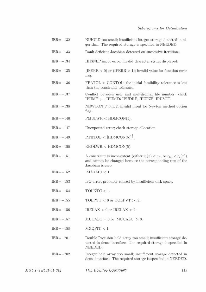
Subprograms for Optimization
IER=−132 NIHOLD too small; insufficient integer storage detected in al-gorithm. The required storage is specified in NEEDED.
IER=−133 Rank deficient Jacobian detected on successive iterations.
IER=−134 HHSNLP input error; invalid character string displayed.
IER=−135 (IFERR < 0) or (IFERR > 1); invalid value for function errorflag.
IER=−136 FEATOL < CONTOL; the initial feasibility tolerance is lessthan the constraint tolerance.
IER=−137 Conflict between user and multifrontal file number; checkIPUMF1,. . .,IPUMF6 IPUDRF, IPUFZF, IPUSTF.
IER=−138 NEWTON 6= 0, 1, 2; invalid input for Newton method optionflag.
IER=−146 PMULWR < HDMCON(5).
IER=−147 Unexpected error; check storage allocation.
IER=−149 PTHTOL < [HDMCON(5)]12 .
IER=−150 RHOLWR < HDMCON(5).
IER=−151 A constraint is inconsistent (either ci(x) < cLi or cUi < ci(x))and cannot be changed because the corresponding row of theJacobian is zero.
IER=−152 IMAXMU < 1.
IER=−153 I/O error, probably caused by insufficient disk space.
IER=−154 TOLKTC < 1.
IER=−155 TOLPVT < 0 or TOLPVT > .5.
IER=−156 IRELAX < 0 or IRELAX > 2.
IER=−157 MUCALC = 0 or |MUCALC| > 3.
IER=−158 MXQPIT < 1.
IER=−701 Double Precision hold array too small; insufficient storage de-tected in dense interface. The required storage is specified inNEEDED.
IER=−702 Integer hold array too small; insufficient storage detected indense interface. The required storage is specified in NEEDED.
M&CT-TECH-01-014 THE BOEING COMPANY 113
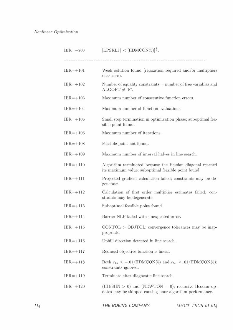
Nonlinear Optimization
IER=−703 |EPSRLF| < [HDMCON(5)]12 .
---------------------------------------------------------------
IER=+101 Weak solution found (relaxation required and/or multipliersnear zero).
IER=+102 Number of equality constraints = number of free variables andALGOPT 6= ‘F’.
IER=+103 Maximum number of consecutive function errors.
IER=+104 Maximum number of function evaluations.
IER=+105 Small step termination in optimization phase; suboptimal fea-sible point found.
IER=+106 Maximum number of iterations.
IER=+108 Feasible point not found.
IER=+109 Maximum number of interval halves in line search.
IER=+110 Algorithm terminated because the Hessian diagonal reachedits maximum value; suboptimal feasible point found.
IER=+111 Projected gradient calculation failed; constraints may be de-generate.
IER=+112 Calculation of first order multiplier estimates failed; con-straints may be degenerate.
IER=+113 Suboptimal feasible point found.
IER=+114 Barrier NLP failed with unexpected error.
IER=+115 CONTOL > OBJTOL; convergence tolerances may be inap-propriate.
IER=+116 Uphill direction detected in line search.
IER=+117 Reduced objective function is linear.
IER=+118 Both cLi ≤ −.01/HDMCON(5) and cUi ≥ .01/HDMCON(5);constraints ignored.
IER=+119 Terminate after diagnostic line search.
IER=+120 (IHESHN > 0) and (NEWTON = 0); recursive Hessian up-dates may be skipped causing poor algorithm performance.
114 THE BOEING COMPANY M&CT-TECH-01-014
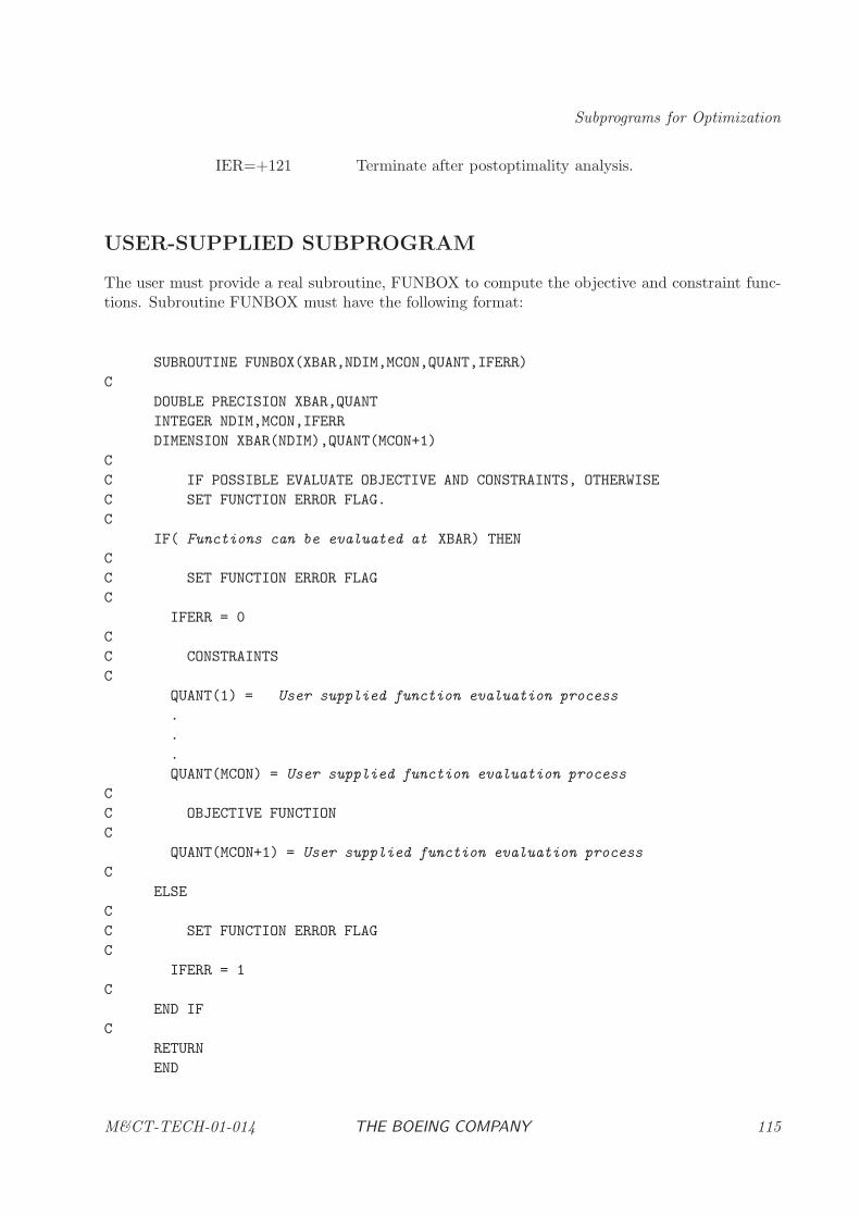
Subprograms for Optimization
IER=+121 Terminate after postoptimality analysis.
USER-SUPPLIED SUBPROGRAM
The user must provide a real subroutine, FUNBOX to compute the objective and constraint func-tions. Subroutine FUNBOX must have the following format:
SUBROUTINE FUNBOX(XBAR,NDIM,MCON,QUANT,IFERR)
C
DOUBLE PRECISION XBAR,QUANT
INTEGER NDIM,MCON,IFERR
DIMENSION XBAR(NDIM),QUANT(MCON+1)
C
C IF POSSIBLE EVALUATE OBJECTIVE AND CONSTRAINTS, OTHERWISE
C SET FUNCTION ERROR FLAG.
C
IF( Functions can be evaluated at XBAR) THEN
C
C SET FUNCTION ERROR FLAG
C
IFERR = 0
C
C CONSTRAINTS
C
QUANT(1) = User supplied function evaluation process
.
.
.
QUANT(MCON) = User supplied function evaluation process
C
C OBJECTIVE FUNCTION
C
QUANT(MCON+1) = User supplied function evaluation process
C
ELSE
C
C SET FUNCTION ERROR FLAG
C
IFERR = 1
C
END IF
C
RETURN
END
M&CT-TECH-01-014 THE BOEING COMPANY 115
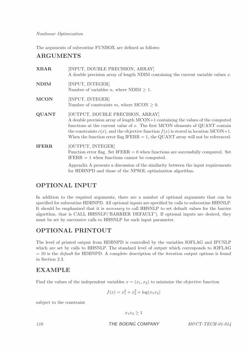
Nonlinear Optimization
The arguments of subroutine FUNBOX are defined as follows:
ARGUMENTS
XBAR [INPUT, DOUBLE PRECISION, ARRAY]A double precision array of length NDIM containing the current variable values x.
NDIM [INPUT, INTEGER]Number of variables n, where NDIM ≥ 1.
MCON [INPUT, INTEGER]Number of constraints m, where MCON ≥ 0.
QUANT [OUTPUT, DOUBLE PRECISION, ARRAY]A double precision array of length MCON+1 containing the values of the computedfunctions at the current value of x. The first MCON elements of QUANT containthe constraints c(x), and the objective function f(x) is stored in location MCON+1.When the function error flag IFERR = 1, the QUANT array will not be referenced.
IFERR [OUTPUT, INTEGER]Function error flag. Set IFERR = 0 when functions are successfully computed. SetIFERR = 1 when functions cannot be computed.
Appendix A presents a discussion of the similarity between the input requirementsfor HDBNPD and those of the NPSOL optimization algorithm.
OPTIONAL INPUT
In addition to the required arguments, there are a number of optional arguments that can bespecified for subroutine HDBNPD. All optional inputs are specified by calls to subroutine HHSNLP.It should be emphasized that it is necessary to call HHSNLP to set default values for the barrieralgorithm, that is CALL HHSNLP(’BARRIER DEFAULT’). If optional inputs are desired, theymust be set by successive calls to HHSNLP for each input parameter.
OPTIONAL PRINTOUT
The level of printed output from HDBNPD is controlled by the variables IOFLAG and IPUNLPwhich are set by calls to HHSNLP. The standard level of output which corresponds to IOFLAG= 10 is the default for HDBNPD. A complete description of the iteration output options is foundin Section 2.3.
EXAMPLE
Find the values of the independent variables x = (x1, x2) to minimize the objective function
f(x) = x21 + x2
2 + log(x1x2)
subject to the constraint
x1x2 ≥ 1
116 THE BOEING COMPANY M&CT-TECH-01-014
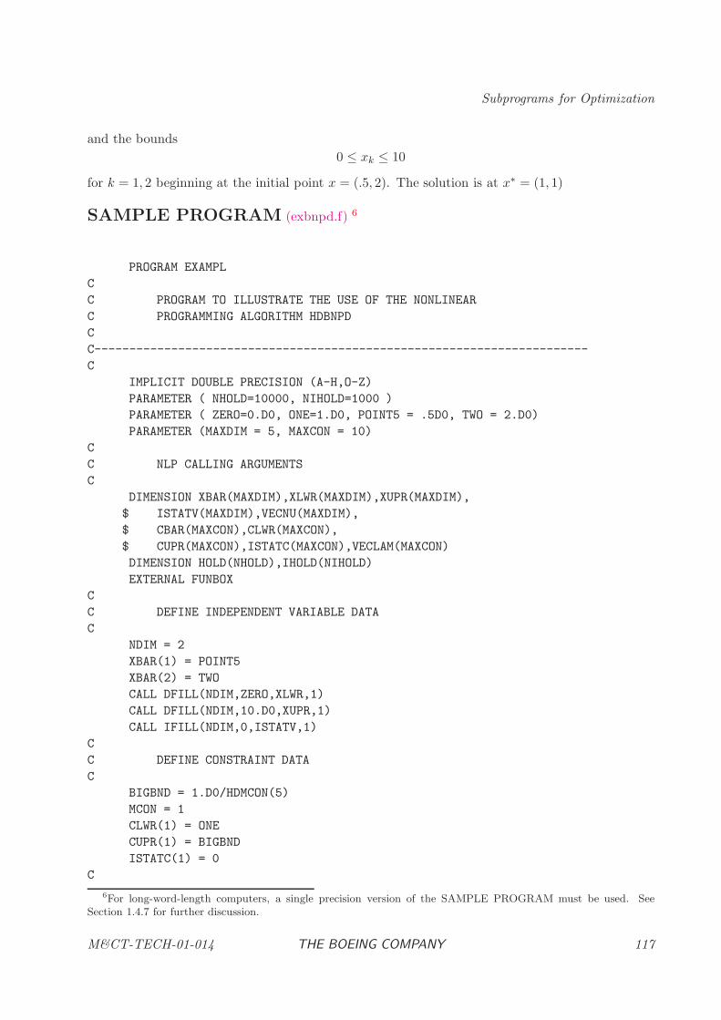
Subprograms for Optimization
and the bounds
0 ≤ xk ≤ 10
for k = 1, 2 beginning at the initial point x = (.5, 2). The solution is at x∗ = (1, 1)
SAMPLE PROGRAM (exbnpd.f) 6
PROGRAM EXAMPL
C
C PROGRAM TO ILLUSTRATE THE USE OF THE NONLINEAR
C PROGRAMMING ALGORITHM HDBNPD
C
C-----------------------------------------------------------------------
C
IMPLICIT DOUBLE PRECISION (A-H,O-Z)
PARAMETER ( NHOLD=10000, NIHOLD=1000 )
PARAMETER ( ZERO=0.D0, ONE=1.D0, POINT5 = .5D0, TWO = 2.D0)
PARAMETER (MAXDIM = 5, MAXCON = 10)
C
C NLP CALLING ARGUMENTS
C
DIMENSION XBAR(MAXDIM),XLWR(MAXDIM),XUPR(MAXDIM),
$ ISTATV(MAXDIM),VECNU(MAXDIM),
$ CBAR(MAXCON),CLWR(MAXCON),
$ CUPR(MAXCON),ISTATC(MAXCON),VECLAM(MAXCON)
DIMENSION HOLD(NHOLD),IHOLD(NIHOLD)
EXTERNAL FUNBOX
C
C DEFINE INDEPENDENT VARIABLE DATA
C
NDIM = 2
XBAR(1) = POINT5
XBAR(2) = TWO
CALL DFILL(NDIM,ZERO,XLWR,1)
CALL DFILL(NDIM,10.D0,XUPR,1)
CALL IFILL(NDIM,0,ISTATV,1)
C
C DEFINE CONSTRAINT DATA
C
BIGBND = 1.D0/HDMCON(5)
MCON = 1
CLWR(1) = ONE
CUPR(1) = BIGBND
ISTATC(1) = 0
C
6For long-word-length computers, a single precision version of the SAMPLE PROGRAM must be used. See
Section 1.4.7 for further discussion.
M&CT-TECH-01-014 THE BOEING COMPANY 117
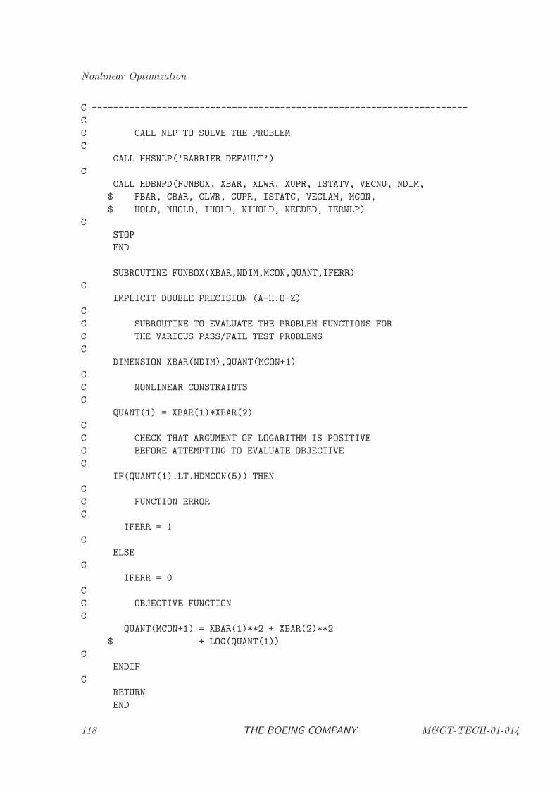
Nonlinear Optimization
C ----------------------------------------------------------------------
C
C CALL NLP TO SOLVE THE PROBLEM
C
CALL HHSNLP(’BARRIER DEFAULT’)
C
CALL HDBNPD(FUNBOX, XBAR, XLWR, XUPR, ISTATV, VECNU, NDIM,
$ FBAR, CBAR, CLWR, CUPR, ISTATC, VECLAM, MCON,
$ HOLD, NHOLD, IHOLD, NIHOLD, NEEDED, IERNLP)
C
STOP
END
SUBROUTINE FUNBOX(XBAR,NDIM,MCON,QUANT,IFERR)
C
IMPLICIT DOUBLE PRECISION (A-H,O-Z)
C
C SUBROUTINE TO EVALUATE THE PROBLEM FUNCTIONS FOR
C THE VARIOUS PASS/FAIL TEST PROBLEMS
C
DIMENSION XBAR(NDIM),QUANT(MCON+1)
C
C NONLINEAR CONSTRAINTS
C
QUANT(1) = XBAR(1)*XBAR(2)
C
C CHECK THAT ARGUMENT OF LOGARITHM IS POSITIVE
C BEFORE ATTEMPTING TO EVALUATE OBJECTIVE
C
IF(QUANT(1).LT.HDMCON(5)) THEN
C
C FUNCTION ERROR
C
IFERR = 1
C
ELSE
C
IFERR = 0
C
C OBJECTIVE FUNCTION
C
QUANT(MCON+1) = XBAR(1)**2 + XBAR(2)**2
$ + LOG(QUANT(1))
C
ENDIF
C
RETURN
END
118 THE BOEING COMPANY M&CT-TECH-01-014
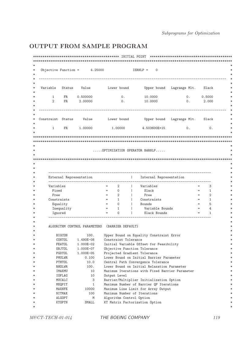
Subprograms for Optimization
OUTPUT FROM SAMPLE PROGRAM
********************************************* INITIAL POINT *******************************************
********************************************************************************************************
* *
* Objective Function = 4.25000 IERNLP = 0 *
* *
* -------------------------------------------------------------------------------------------------- *
* *
* Variable Status Value Lower bound Upper bound Lagrange Mlt. Slack *
* *
* 1 FR 0.500000 0. 10.0000 0. 0.5000 *
* 2 FR 2.00000 0. 10.0000 0. 2.000 *
* *
* -------------------------------------------------------------------------------------------------- *
* *
* Constraint Status Value Lower bound Upper bound Lagrange Mlt. Slack *
* *
* 1 FR 1.00000 1.00000 4.503600E+15 0. 0. *
* *
********************************************************************************************************
********************************************************************************************************
* *
* .....OPTIMIZATION OPERATOR BARNLP..... *
* *
********************************************************************************************************
* *
* *
* ------------------------------------------------------------------------------------- *
* External Representation | Internal Representation *
* ------------------------------------------------------------------------------------- *
* Variables = 2 | Variables = 3 *
* Fixed = 0 | Slack = 1 *
* Free = 2 | Free = 2 *
* Constraints = 1 | Constraints = 1 *
* Equality = 0 | Bounds = 5 *
* Inequality = 1 | Variable Bounds = 4 *
* Ignored = 0 | Slack Bounds = 1 *
* ------------------------------------------------------------------------------------- *
* *
* ALGORITHM CONTROL PARAMETERS (BARRIER DEFAULT) *
* *
* BIGCON 100. Upper Bound on Equality Constraint Error *
* CONTOL 1.490E-08 Constraint Tolerance *
* FEATOL 1.000E-02 Initial Variable Offset for Feasibility *
* OBJTOL 1.000E-07 Objective Function Tolerance *
* PGDTOL 1.000E-05 Projected Gradient Tolerance *
* PMULWR 0.100 Lower Bound on Initial Barrier Parameter *
* PTHTOL 10.0 Central Path Convergence Tolerance *
* RHOLWR 100. Lower Bound on Initial Relaxation Parameter *
* IMAXMU 10 Maximum Iterations with Fixed Barrier Parameter *
* IOFLAG 10 Output Level *
* MUCALC 3 Barrier/Multiplier Initialization Option *
* MXQPIT 1 Maximum Number of Barrier QP Iterations *
* MAXNFE 10000 Maximum Line Limit for Array Output *
* NITMAX 100 Maximum Number of Iterations *
* ALGOPT M Algorithm Control Option *
* KTOPTN SMALL KT Matrix Factorization Option *
* *
M&CT-TECH-01-014 THE BOEING COMPANY 119
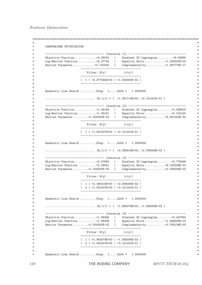
Nonlinear Optimization
********************************************************************************************************
* *
* CONSTRAINED OPTIMIZATION *
* *
* ------------------------------------- Iteration (1) ------------------------------------ *
* Objective Function..............+4.25000 | Gradient Of Lagrangian..........+6.59956 *
* Log-Barrier Function............+4.27744 | Equality Error.............+1.000000E-02 *
* Barrier Parameter..............+0.100000 | Complementarity............+1.387779E-17 *
* -------------------------------------- *
* Filter: B(y) |c(y)| *
* -------------------------------------- *
* | 1 | +4.277444E+00 | +1.000000E-02 | *
* -------------------------------------- *
* *
* Quadratic Line Search ..........Step: 1.....ALFA = 1.0000000 *
* *
* ............................... (B,|c|) = ( +1.061710E+00, +3.151201E-01 ) *
* *
* ------------------------------------- Iteration (2) ------------------------------------ *
* Objective Function..............+1.06148 | Gradient Of Lagrangian.........+0.439618 *
* Log-Barrier Function............+1.06151 | Equality Error.................+0.315120 *
* Barrier Parameter..........+1.000000E-02 | Complementarity............+8.991003E-02 *
* -------------------------------------- *
* Filter: B(y) |c(y)| *
* -------------------------------------- *
* | 1 | +1.061507E+00 | +3.151201E-01 | *
* -------------------------------------- *
* *
* Quadratic Line Search ..........Step: 1.....ALFA = 1.0000000 *
* *
* ............................... (B,|c|) = ( +2.085415E+00, +2.056006E-02 ) *
* *
* ------------------------------------- Iteration (3) ------------------------------------ *
* Objective Function..............+2.07983 | Gradient Of Lagrangian.........+0.776446 *
* Log-Barrier Function............+2.08541 | Equality Error.............+9.165028E-03 *
* Barrier Parameter..........+1.000000E-02 | Complementarity............+2.056006E-02 *
* -------------------------------------- *
* Filter: B(y) |c(y)| *
* -------------------------------------- *
* | 1 | +2.085415E+00 | +2.056006E-02 | *
* | 2 | +1.061507E+00 | +3.151201E-01 | *
* -------------------------------------- *
* *
* Quadratic Line Search ..........Step: 1.....ALFA = 1.0000000 *
* *
* ............................... (B,|c|) = ( +1.983079E+00, +1.568306E-02 ) *
* *
* ------------------------------------- Iteration (4) ------------------------------------ *
* Objective Function..............+1.96426 | Gradient Of Lagrangian.........+0.427564 *
* Log-Barrier Function............+1.98308 | Equality Error.............+1.568306E-02 *
* Barrier Parameter..........+1.000000E-02 | Complementarity............+3.768136E-03 *
* -------------------------------------- *
* Filter: B(y) |c(y)| *
* -------------------------------------- *
* | 1 | +1.983079E+00 | +1.568306E-02 | *
* | 2 | +1.061507E+00 | +3.151201E-01 | *
* -------------------------------------- *
* *
* Quadratic Line Search ..........Step: 1.....ALFA = 1.0000000 *
120 THE BOEING COMPANY M&CT-TECH-01-014
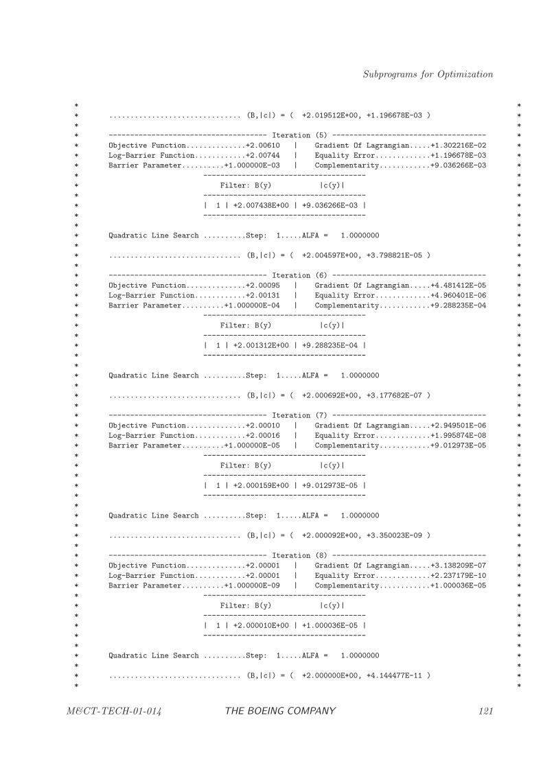
Subprograms for Optimization
* *
* ............................... (B,|c|) = ( +2.019512E+00, +1.196678E-03 ) *
* *
* ------------------------------------- Iteration (5) ------------------------------------ *
* Objective Function..............+2.00610 | Gradient Of Lagrangian.....+1.302216E-02 *
* Log-Barrier Function............+2.00744 | Equality Error.............+1.196678E-03 *
* Barrier Parameter..........+1.000000E-03 | Complementarity............+9.036266E-03 *
* -------------------------------------- *
* Filter: B(y) |c(y)| *
* -------------------------------------- *
* | 1 | +2.007438E+00 | +9.036266E-03 | *
* -------------------------------------- *
* *
* Quadratic Line Search ..........Step: 1.....ALFA = 1.0000000 *
* *
* ............................... (B,|c|) = ( +2.004597E+00, +3.798821E-05 ) *
* *
* ------------------------------------- Iteration (6) ------------------------------------ *
* Objective Function..............+2.00095 | Gradient Of Lagrangian.....+4.481412E-05 *
* Log-Barrier Function............+2.00131 | Equality Error.............+4.960401E-06 *
* Barrier Parameter..........+1.000000E-04 | Complementarity............+9.288235E-04 *
* -------------------------------------- *
* Filter: B(y) |c(y)| *
* -------------------------------------- *
* | 1 | +2.001312E+00 | +9.288235E-04 | *
* -------------------------------------- *
* *
* Quadratic Line Search ..........Step: 1.....ALFA = 1.0000000 *
* *
* ............................... (B,|c|) = ( +2.000692E+00, +3.177682E-07 ) *
* *
* ------------------------------------- Iteration (7) ------------------------------------ *
* Objective Function..............+2.00010 | Gradient Of Lagrangian.....+2.949501E-06 *
* Log-Barrier Function............+2.00016 | Equality Error.............+1.995874E-08 *
* Barrier Parameter..........+1.000000E-05 | Complementarity............+9.012973E-05 *
* -------------------------------------- *
* Filter: B(y) |c(y)| *
* -------------------------------------- *
* | 1 | +2.000159E+00 | +9.012973E-05 | *
* -------------------------------------- *
* *
* Quadratic Line Search ..........Step: 1.....ALFA = 1.0000000 *
* *
* ............................... (B,|c|) = ( +2.000092E+00, +3.350023E-09 ) *
* *
* ------------------------------------- Iteration (8) ------------------------------------ *
* Objective Function..............+2.00001 | Gradient Of Lagrangian.....+3.138209E-07 *
* Log-Barrier Function............+2.00001 | Equality Error.............+2.237179E-10 *
* Barrier Parameter..........+1.000000E-09 | Complementarity............+1.000036E-05 *
* -------------------------------------- *
* Filter: B(y) |c(y)| *
* -------------------------------------- *
* | 1 | +2.000010E+00 | +1.000036E-05 | *
* -------------------------------------- *
* *
* Quadratic Line Search ..........Step: 1.....ALFA = 1.0000000 *
* *
* ............................... (B,|c|) = ( +2.000000E+00, +4.144477E-11 ) *
* *
M&CT-TECH-01-014 THE BOEING COMPANY 121
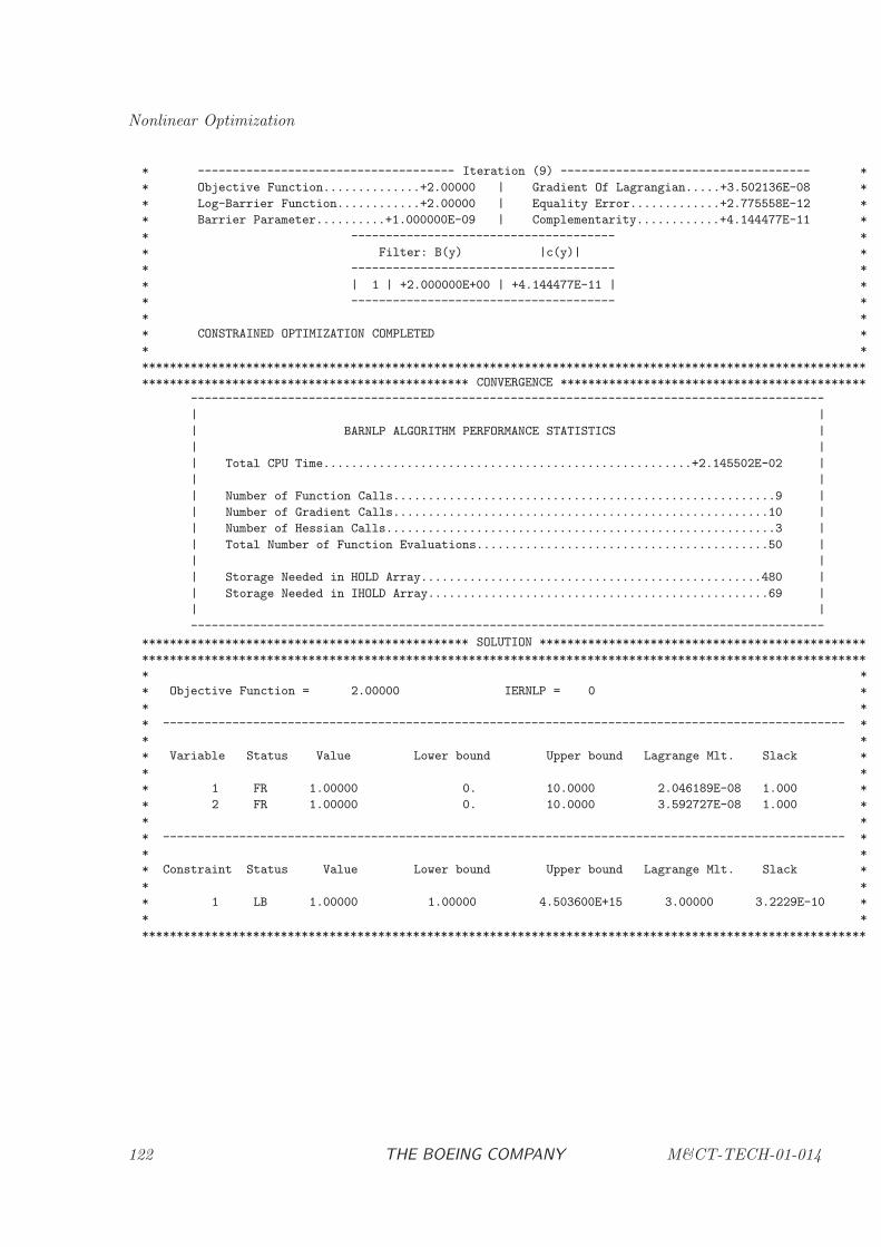
Nonlinear Optimization
* ------------------------------------- Iteration (9) ------------------------------------ *
* Objective Function..............+2.00000 | Gradient Of Lagrangian.....+3.502136E-08 *
* Log-Barrier Function............+2.00000 | Equality Error.............+2.775558E-12 *
* Barrier Parameter..........+1.000000E-09 | Complementarity............+4.144477E-11 *
* -------------------------------------- *
* Filter: B(y) |c(y)| *
* -------------------------------------- *
* | 1 | +2.000000E+00 | +4.144477E-11 | *
* -------------------------------------- *
* *
* CONSTRAINED OPTIMIZATION COMPLETED *
* *
********************************************************************************************************
*********************************************** CONVERGENCE ********************************************
-------------------------------------------------------------------------------------------
| |
| BARNLP ALGORITHM PERFORMANCE STATISTICS |
| |
| Total CPU Time.....................................................+2.145502E-02 |
| |
| Number of Function Calls.......................................................9 |
| Number of Gradient Calls......................................................10 |
| Number of Hessian Calls........................................................3 |
| Total Number of Function Evaluations..........................................50 |
| |
| Storage Needed in HOLD Array.................................................480 |
| Storage Needed in IHOLD Array.................................................69 |
| |
-------------------------------------------------------------------------------------------
*********************************************** SOLUTION ***********************************************
********************************************************************************************************
* *
* Objective Function = 2.00000 IERNLP = 0 *
* *
* -------------------------------------------------------------------------------------------------- *
* *
* Variable Status Value Lower bound Upper bound Lagrange Mlt. Slack *
* *
* 1 FR 1.00000 0. 10.0000 2.046189E-08 1.000 *
* 2 FR 1.00000 0. 10.0000 3.592727E-08 1.000 *
* *
* -------------------------------------------------------------------------------------------------- *
* *
* Constraint Status Value Lower bound Upper bound Lagrange Mlt. Slack *
* *
* 1 LB 1.00000 1.00000 4.503600E+15 3.00000 3.2229E-10 *
* *
********************************************************************************************************
122 THE BOEING COMPANY M&CT-TECH-01-014
Subprograms for Optimization
HDBNPR: Dense Barrier Nonlinear Programming–Reverse Communication For-mat
PURPOSE
HDBNPR computes the vector x = (x1, x2, . . . , xn) which minimizes the objective function
f(x)
subject to the m nonlinear constraints
cL ≤ c(x) ≤ cU
and the simple boundsxL ≤ x ≤ xU
Equality constraints are imposed by setting cLi = cUi and variables can be fixed by settingxLi = xUi. HDBNPR works under the assumption that the objective and constraint functionsare twice continuously differentiable, and if this is not true algorithm performance is unpredictable.HDBNPR uses a reverse communication format and upon request the user must supply the val-ues of the functions, and their first derivatives. The matrix of second derivatives (Hessian of theLagrangian) can be constructed using a quasi-Newton recursive estimate or supplied by the user.Subroutine HDBNPR calls the sparse nonlinear programming algorithm HDBNLP, and is intendedfor simplified usage as appropriate for small dense problems.
RELATED SUBPROGRAMS
HDNLPR Dense Nonlinear Programming–Reverse Communication Format
HDBNLP Sparse Barrier Nonlinear Programming
HHSNLP Sparse Nonlinear Programming Input Procedure
METHOD
An interior point or barrier method is used to solve the nonlinear programming (NLP) problem.HDBNPD provides four alternatives for constructing an approximation to the Hessian matrix whichare described in the background section of this document. The default is a symmetric rank-one(SR1) approximation, with options for using a BFGS, SSQN, or finite difference estimate instead.If the user cannot provide this information analytically, the finite difference techniques describedin Chapter 3 should be utilized.
WARNING
The objective function and constraints supplied by the user are assumed to be continuous andhave continuous first and second derivatives. Nondifferentiable functions can cause unpredictableperformance in the optimization algorithm. It should be emphasized that discontinuities in theHessian matrices can significantly degrade the speed of convergence without producing any otherobvious difficulties. The following common sources of error should be avoided when evaluating theobjective and constraint functions:
M&CT-TECH-01-014 THE BOEING COMPANY 123
Nonlinear Optimization
(1) nonsmooth interpolation of data;
(2) iterative procedures inside the function evaluation process, such as adaptive quadrature or rootsolving;
(3) discontinuous behavior caused by branching for IF tests;
(4) nondifferentiable functions such as ABS, MAX, and MIN.
The user must provide a procedure to evaluate the objective and constraint functions in additionto first and (optionally) second derivatives of these quantities. If it is not possible to evaluate thefunctions (for example, c(x) = 1/x at x = 0) then set IFERR = 1 and exit the function evaluationprocess. Otherwise, set IFERR = 0 when the functions are evaluated. The function error flagshould be used to avoid computational difficulties, but never in lieu of an explicit constraint.
The HDBNPR software uses internal common blocks to communicate information. To avoid con-flict with these internal commons the user should not have commons with the following names:NPSPRR, NPSPRI, NPSPRC, STATIS, KONSTN, NPSALG, NPSDFL, NLPERR, PERCOM,ITEREF, and CLKCOM.
USAGE
INTEGER IRVCOM, IFERR, NFEVAL, IER, NEEDED
INTEGER NDIM, MCON, NONZH, NONZG, NHOLD, NIHOLD
INTEGER IREVRS(5), ISTATV(NDIM), ISTATC(MCON), IHOLD(NIHOLD)
PARAMETER (NONZG=NDIM*MCON, NONZH=NDIM*(NDIM+1)/2 )
DOUBLE PRECISION FBAR, XBAR(NDIM), XLWR(NDIM), XUPR(NDIM), VECNU(NDIM)
DOUBLE PRECISION DELF(NDIM), HMAT(NONZH), CBAR(MCON), CLWR(MCON)
DOUBLE PRECISION CUPR(MCON), VECLAM(MCON), GMAT(NONZG), HOLD(NHOLD)
CALL HHSNLP(’BARRIER DEFAULT’)
CALL HDBNPR( IRVCOM, IREVRS, XBAR, XLWR, XUPR, ISTATV,
$ VECNU, NDIM, FBAR, DELF, HMAT, CBAR,
$ CLWR, CUPR, ISTATC, MCON, VECLAM, GMAT,
$ IFERR, NFEVAL, HOLD, NHOLD, IHOLD, NIHOLD,
$ NEEDED, IER )
ARGUMENTS
ARGUMENTS TO CONTROL REVERSE COMMUNICATION
IRVCOM [INPUT/OUTPUT, INTEGER]Continuation control flag. This argument must be initialized. Thereafter it is setby the algorithm and must not be changed by the calling program.
IRVCOM = −1 Initialization pass.
IRVCOM = 0 Termination (normal or abnormal).
124 THE BOEING COMPANY M&CT-TECH-01-014

Subprograms for Optimization
IRVCOM = +1 Perform an evaluation and then reenter HDBNPR. Opera-tions to be performed are defined by the output variablesIREVRS(1), IREVRS(2), IREVRS(3), and IREVRS(4) below.IREVRS(5) contains information which may be valuable tothe interface but does not require any action on the part ofthe user.
IREVRS [OUTPUT, INTEGER, ARRAY]An integer array of length 5, containing reverse communication control information.IREVRS(1) Function evaluation request
= 0 Function evaluation not requested; Warning:do not change the current function and con-straint values.
= 1 Function evaluation requested; evaluate ob-jective function and all constraints at currentpoint XBAR.
IREVRS(2) Gradient evaluation request= 0 Gradient evaluation not requested; Warning:
do not change the current gradient and Jaco-bian.
= 1 Approximate (e.g. forward difference) gradi-ent requested; evaluate gradient vector g andJacobian matrix G at current point XBAR. (Ifavailable, accurate or analytic gradients maybe supplied)
= 2 Accurate (e.g. central difference or analytic)gradient requested; evaluate gradient vectorg and Jacobian matrix G at current pointXBAR.
M&CT-TECH-01-014 THE BOEING COMPANY 125

Nonlinear Optimization
IREVRS(3) Hessian evaluation request= 0 Hessian evaluation not requested; Warning:
do not change the current Hessian.
= 1 Hessian diagonal requested; get ready for fullHessian evaluation with (IREVRS(3)=2) atcurrent point (XBAR,VECLAM) and option-ally evaluate diagonal elements of Hessian ma-trix H.
= 2 Full Hessian evaluation requested; eval-uate Hessian matrix H of the functionL(x, λ) = f − ∑m
k=1 λkck at current point(XBAR,VECLAM). A full evaluation re-quest is always preceded by a call withIREVRS(3)=1 at the same point XBAR, andconsequently it may not be necessary to re-compute the diagonal elements.
IREVRS(4) System print (output) request= 0 System print not requested.
= 1 System print requested; perform any outputoperations (print, write files, etc.) desiredto display problem specific information at thecurrent point XBAR. The frequency of printis defined by the output control flag IOFLAG(see Optional Printout).
IREVRS(5) Algorithm information flag= 0 Call was made from the interface portion of
the algorithm.
= 1 Call was made from the optimization portionof the algorithm.
= 2 Call was made from the optimization portionof the algorithm requesting Hessian reset.
= 3 Call was made from the optimization portionof the algorithm requesting optimal perturba-tion size adjustment.
= 4 Call was made from the feasiblity portion ofthe algorithm.
INDEPENDENT VARIABLE DATA
XBAR† [INPUT/OUTPUT, DOUBLE PRECISION, ARRAY]A real array of length NDIM of current variable values x.
IRVCOM=−1 Initial guess must be input.
126 THE BOEING COMPANY M&CT-TECH-01-014
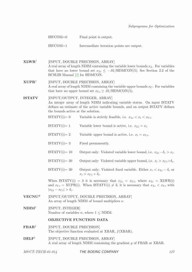
Subprograms for Optimization
IRVCOM=0 Final point is output.
IRVCOM=1 Intermediate iteration points are output.
XLWR† [INPUT, DOUBLE PRECISION, ARRAY]A real array of length NDIM containing the variable lower bounds xL. For variablesthat have no lower bound set xLi ≤ −.01/HDMCON(5). See Section 2.2 of theBCSLIB Manual [2] for HDMCON.
XUPR† [INPUT, DOUBLE PRECISION, ARRAY]A real array of length NDIM containing the variable upper bounds xU . For variablesthat have no upper bound set xUi ≥ .01/HDMCON(5).
ISTATV [INPUT/OUTPUT, INTEGER, ARRAY]An integer array of length NDIM indicating variable status. On input ISTATVdefines an estimate of the active variable bounds, and on output ISTATV definesthe bounds active at the solution.
ISTATV(i)= 0 Variable is strictly feasible, i.e. xLi < xi < xUi.
ISTATV(i)= 1 Variable lower bound is active, i.e. xLi = xi.
ISTATV(i)= 2 Variable upper bound is active, i.e. xi = xUi.
ISTATV(i)= 3 Fixed permanently.
ISTATV(i)= 10 Output only: Violated variable lower bound, i.e. xLi−δc > xi.
ISTATV(i)= 20 Output only: Violated variable upper bound, i.e. xi > xUi+δc.
ISTATV(i)= 30 Output only: Violated fixed variable. Either xi < xLi − δc orxi > xUi + δc.
When ISTATV(i) = 3 it is necessary that xLi = xUi, where xLi = XLWR(i)and xUi = XUPR(i). When ISTATV(i) 6= 3, it is necessary that xLi < xUi with|xLi − xUi| > δc.
VECNU# [INPUT/OUTPUT, DOUBLE PRECISION, ARRAY]An array of length NDIM of bound multipliers ν.
NDIM† [INPUT, INTEGER]Number of variables n, where 1 ≤ NDIM.
OBJECTIVE FUNCTION DATA
FBAR‡ [INPUT, DOUBLE PRECISION]The objective function evaluated at XBAR, f(XBAR).
DELF‡ [INPUT, DOUBLE PRECISION, ARRAY]A real array of length NDIM containing the gradient g of FBAR at XBAR.
M&CT-TECH-01-014 THE BOEING COMPANY 127
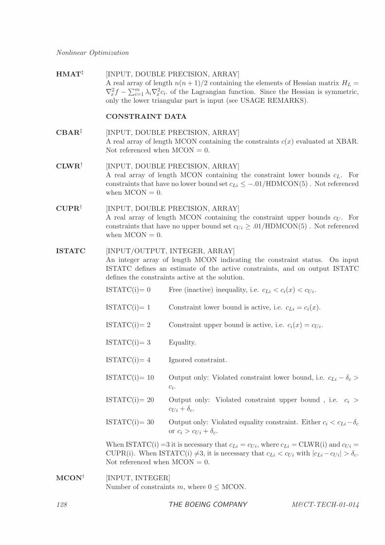
Nonlinear Optimization
HMAT‡ [INPUT, DOUBLE PRECISION, ARRAY]A real array of length n(n+ 1)/2 containing the elements of Hessian matrix HL =∇2
xf −∑mi=1 λi∇2
x ci. of the Lagrangian function. Since the Hessian is symmetric,only the lower triangular part is input (see USAGE REMARKS).
CONSTRAINT DATA
CBAR‡ [INPUT, DOUBLE PRECISION, ARRAY]A real array of length MCON containing the constraints c(x) evaluated at XBAR.Not referenced when MCON = 0.
CLWR† [INPUT, DOUBLE PRECISION, ARRAY]A real array of length MCON containing the constraint lower bounds cL. Forconstraints that have no lower bound set cLi ≤ −.01/HDMCON(5) . Not referencedwhen MCON = 0.
CUPR† [INPUT, DOUBLE PRECISION, ARRAY]A real array of length MCON containing the constraint upper bounds cU . Forconstraints that have no upper bound set cUi ≥ .01/HDMCON(5) . Not referencedwhen MCON = 0.
ISTATC [INPUT/OUTPUT, INTEGER, ARRAY]An integer array of length MCON indicating the constraint status. On inputISTATC defines an estimate of the active constraints, and on output ISTATCdefines the constraints active at the solution.
ISTATC(i)= 0 Free (inactive) inequality, i.e. cLi < ci(x) < cUi.
ISTATC(i)= 1 Constraint lower bound is active, i.e. cLi = ci(x).
ISTATC(i)= 2 Constraint upper bound is active, i.e. ci(x) = cUi.
ISTATC(i)= 3 Equality.
ISTATC(i)= 4 Ignored constraint.
ISTATC(i)= 10 Output only: Violated constraint lower bound, i.e. cLi − δc >ci.
ISTATC(i)= 20 Output only: Violated constraint upper bound , i.e. ci >cUi + δc.
ISTATC(i)= 30 Output only: Violated equality constraint. Either ci < cLi−δcor ci > cUi + δc.
When ISTATC(i) =3 it is necessary that cLi = cUi, where cLi = CLWR(i) and cUi =CUPR(i). When ISTATC(i) 6=3, it is necessary that cLi < cUi with |cLi−cUi| > δc.Not referenced when MCON = 0.
MCON† [INPUT, INTEGER]Number of constraints m, where 0 ≤ MCON.
128 THE BOEING COMPANY M&CT-TECH-01-014
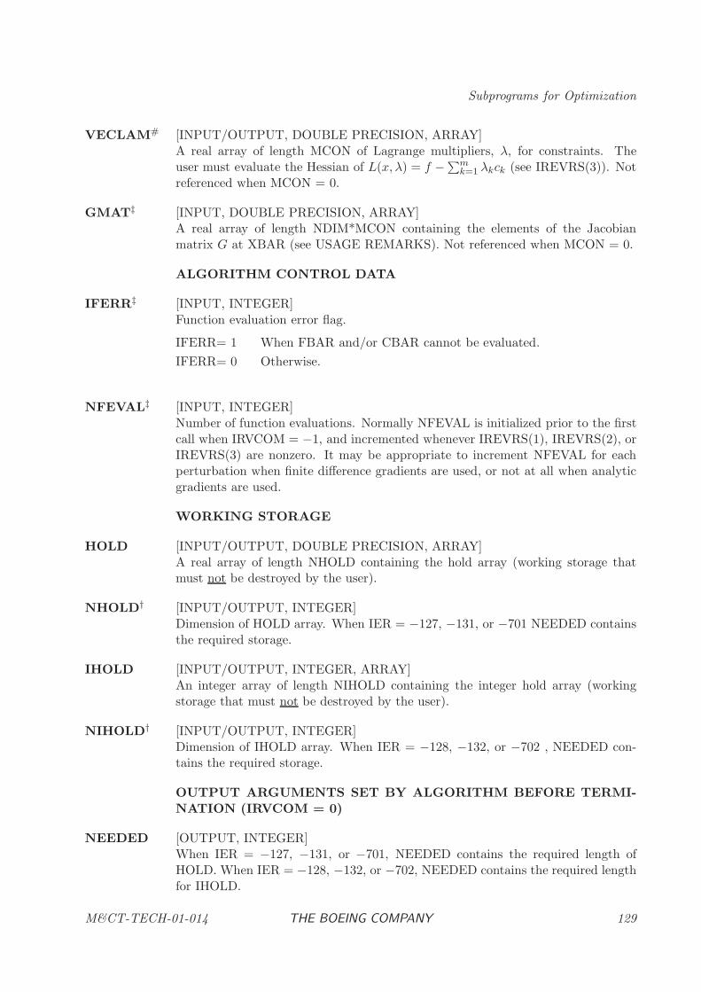
Subprograms for Optimization
VECLAM# [INPUT/OUTPUT, DOUBLE PRECISION, ARRAY]A real array of length MCON of Lagrange multipliers, λ, for constraints. Theuser must evaluate the Hessian of L(x, λ) = f −∑m
k=1 λkck (see IREVRS(3)). Notreferenced when MCON = 0.
GMAT‡ [INPUT, DOUBLE PRECISION, ARRAY]A real array of length NDIM*MCON containing the elements of the Jacobianmatrix G at XBAR (see USAGE REMARKS). Not referenced when MCON = 0.
ALGORITHM CONTROL DATA
IFERR‡ [INPUT, INTEGER]Function evaluation error flag.
IFERR= 1 When FBAR and/or CBAR cannot be evaluated.
IFERR= 0 Otherwise.
NFEVAL‡ [INPUT, INTEGER]Number of function evaluations. Normally NFEVAL is initialized prior to the firstcall when IRVCOM = −1, and incremented whenever IREVRS(1), IREVRS(2), orIREVRS(3) are nonzero. It may be appropriate to increment NFEVAL for eachperturbation when finite difference gradients are used, or not at all when analyticgradients are used.
WORKING STORAGE
HOLD [INPUT/OUTPUT, DOUBLE PRECISION, ARRAY]A real array of length NHOLD containing the hold array (working storage thatmust not be destroyed by the user).
NHOLD† [INPUT/OUTPUT, INTEGER]Dimension of HOLD array. When IER = −127, −131, or −701 NEEDED containsthe required storage.
IHOLD [INPUT/OUTPUT, INTEGER, ARRAY]An integer array of length NIHOLD containing the integer hold array (workingstorage that must not be destroyed by the user).
NIHOLD† [INPUT/OUTPUT, INTEGER]Dimension of IHOLD array. When IER = −128, −132, or −702 , NEEDED con-tains the required storage.
OUTPUT ARGUMENTS SET BY ALGORITHM BEFORE TERMI-NATION (IRVCOM = 0)
NEEDED [OUTPUT, INTEGER]When IER = −127, −131, or −701, NEEDED contains the required length ofHOLD. When IER = −128, −132, or −702, NEEDED contains the required lengthfor IHOLD.
M&CT-TECH-01-014 THE BOEING COMPANY 129
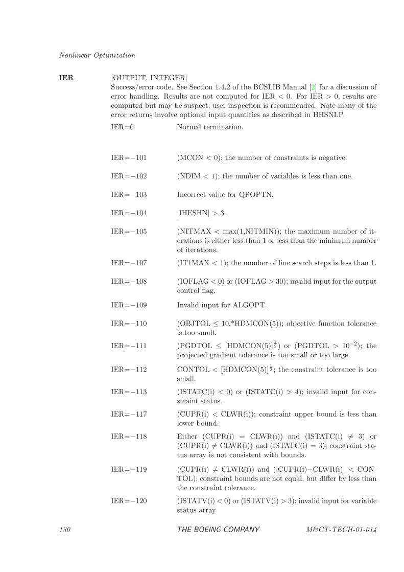
Nonlinear Optimization
IER [OUTPUT, INTEGER]Success/error code. See Section 1.4.2 of the BCSLIB Manual [2] for a discussion oferror handling. Results are not computed for IER < 0. For IER > 0, results arecomputed but may be suspect; user inspection is recommended. Note many of theerror returns involve optional input quantities as described in HHSNLP.
IER=0 Normal termination.
IER=−101 (MCON < 0); the number of constraints is negative.
IER=−102 (NDIM < 1); the number of variables is less than one.
IER=−103 Incorrect value for QPOPTN.
IER=−104 |IHESHN| > 3.
IER=−105 (NITMAX < max(1,NITMIN)); the maximum number of it-erations is either less than 1 or less than the minimum numberof iterations.
IER=−107 (IT1MAX < 1); the number of line search steps is less than 1.
IER=−108 (IOFLAG< 0) or (IOFLAG > 30); invalid input for the outputcontrol flag.
IER=−109 Invalid input for ALGOPT.
IER=−110 (OBJTOL ≤ 10.*HDMCON(5)); objective function toleranceis too small.
IER=−111 (PGDTOL ≤ [HDMCON(5)]12 ) or (PGDTOL > 10−2); the
projected gradient tolerance is too small or too large.
IER=−112 CONTOL < [HDMCON(5)]12 ; the constraint tolerance is too
small.
IER=−113 (ISTATC(i) < 0) or (ISTATC(i) > 4); invalid input for con-straint status.
IER=−117 (CUPR(i) < CLWR(i)); constraint upper bound is less thanlower bound.
IER=−118 Either (CUPR(i) = CLWR(i)) and (ISTATC(i) 6= 3) or(CUPR(i) 6= CLWR(i)) and (ISTATC(i) = 3); constraint sta-tus array is not consistent with bounds.
IER=−119 (CUPR(i) 6= CLWR(i)) and (|CUPR(i)−CLWR(i)| < CON-TOL); constraint bounds are not equal, but differ by less thanthe constraint tolerance.
IER=−120 (ISTATV(i)< 0) or (ISTATV(i) > 3); invalid input for variablestatus array.
130 THE BOEING COMPANY M&CT-TECH-01-014
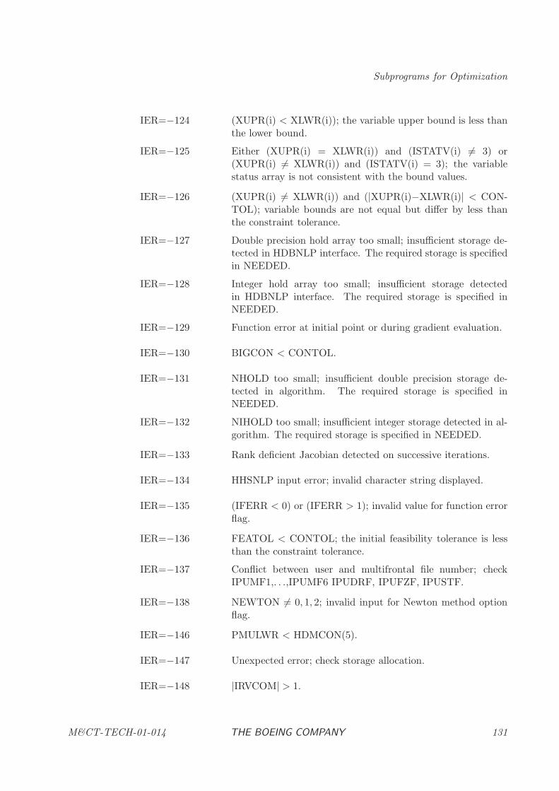
Subprograms for Optimization
IER=−124 (XUPR(i) < XLWR(i)); the variable upper bound is less thanthe lower bound.
IER=−125 Either (XUPR(i) = XLWR(i)) and (ISTATV(i) 6= 3) or(XUPR(i) 6= XLWR(i)) and (ISTATV(i) = 3); the variablestatus array is not consistent with the bound values.
IER=−126 (XUPR(i) 6= XLWR(i)) and (|XUPR(i)−XLWR(i)| < CON-TOL); variable bounds are not equal but differ by less thanthe constraint tolerance.
IER=−127 Double precision hold array too small; insufficient storage de-tected in HDBNLP interface. The required storage is specifiedin NEEDED.
IER=−128 Integer hold array too small; insufficient storage detectedin HDBNLP interface. The required storage is specified inNEEDED.
IER=−129 Function error at initial point or during gradient evaluation.
IER=−130 BIGCON < CONTOL.
IER=−131 NHOLD too small; insufficient double precision storage de-tected in algorithm. The required storage is specified inNEEDED.
IER=−132 NIHOLD too small; insufficient integer storage detected in al-gorithm. The required storage is specified in NEEDED.
IER=−133 Rank deficient Jacobian detected on successive iterations.
IER=−134 HHSNLP input error; invalid character string displayed.
IER=−135 (IFERR < 0) or (IFERR > 1); invalid value for function errorflag.
IER=−136 FEATOL < CONTOL; the initial feasibility tolerance is lessthan the constraint tolerance.
IER=−137 Conflict between user and multifrontal file number; checkIPUMF1,. . .,IPUMF6 IPUDRF, IPUFZF, IPUSTF.
IER=−138 NEWTON 6= 0, 1, 2; invalid input for Newton method optionflag.
IER=−146 PMULWR < HDMCON(5).
IER=−147 Unexpected error; check storage allocation.
IER=−148 |IRVCOM| > 1.
M&CT-TECH-01-014 THE BOEING COMPANY 131
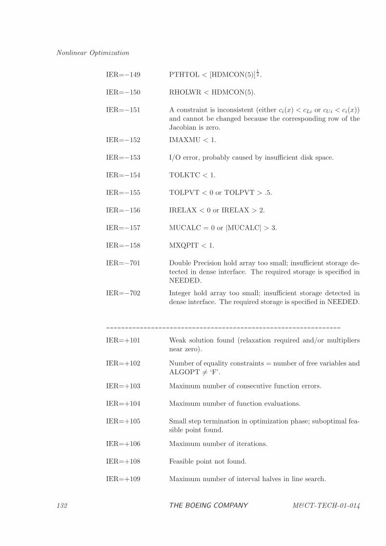
Nonlinear Optimization
IER=−149 PTHTOL < [HDMCON(5)]12 .
IER=−150 RHOLWR < HDMCON(5).
IER=−151 A constraint is inconsistent (either ci(x) < cLi or cUi < ci(x))and cannot be changed because the corresponding row of theJacobian is zero.
IER=−152 IMAXMU < 1.
IER=−153 I/O error, probably caused by insufficient disk space.
IER=−154 TOLKTC < 1.
IER=−155 TOLPVT < 0 or TOLPVT > .5.
IER=−156 IRELAX < 0 or IRELAX > 2.
IER=−157 MUCALC = 0 or |MUCALC| > 3.
IER=−158 MXQPIT < 1.
IER=−701 Double Precision hold array too small; insufficient storage de-tected in dense interface. The required storage is specified inNEEDED.
IER=−702 Integer hold array too small; insufficient storage detected indense interface. The required storage is specified in NEEDED.
---------------------------------------------------------------
IER=+101 Weak solution found (relaxation required and/or multipliersnear zero).
IER=+102 Number of equality constraints = number of free variables andALGOPT 6= ‘F’.
IER=+103 Maximum number of consecutive function errors.
IER=+104 Maximum number of function evaluations.
IER=+105 Small step termination in optimization phase; suboptimal fea-sible point found.
IER=+106 Maximum number of iterations.
IER=+108 Feasible point not found.
IER=+109 Maximum number of interval halves in line search.
132 THE BOEING COMPANY M&CT-TECH-01-014
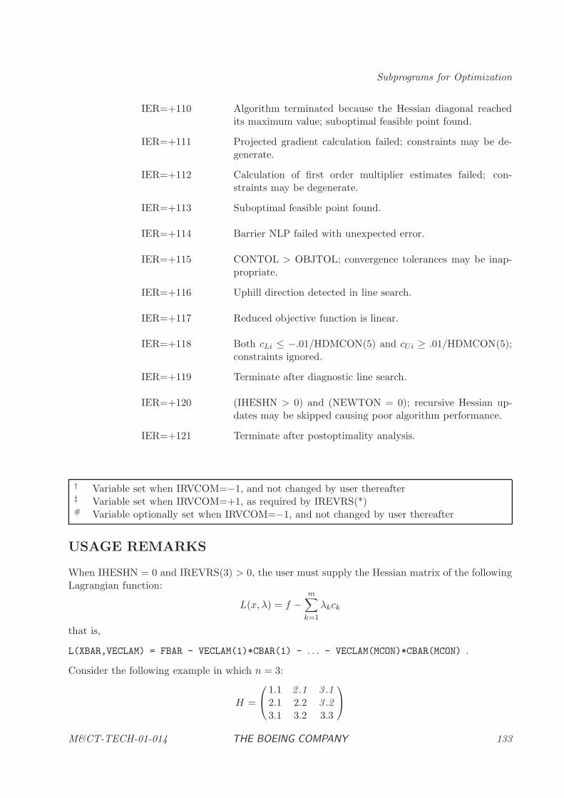
Subprograms for Optimization
IER=+110 Algorithm terminated because the Hessian diagonal reachedits maximum value; suboptimal feasible point found.
IER=+111 Projected gradient calculation failed; constraints may be de-generate.
IER=+112 Calculation of first order multiplier estimates failed; con-straints may be degenerate.
IER=+113 Suboptimal feasible point found.
IER=+114 Barrier NLP failed with unexpected error.
IER=+115 CONTOL > OBJTOL; convergence tolerances may be inap-propriate.
IER=+116 Uphill direction detected in line search.
IER=+117 Reduced objective function is linear.
IER=+118 Both cLi ≤ −.01/HDMCON(5) and cUi ≥ .01/HDMCON(5);constraints ignored.
IER=+119 Terminate after diagnostic line search.
IER=+120 (IHESHN > 0) and (NEWTON = 0); recursive Hessian up-dates may be skipped causing poor algorithm performance.
IER=+121 Terminate after postoptimality analysis.
† Variable set when IRVCOM=−1, and not changed by user thereafter‡ Variable set when IRVCOM=+1, as required by IREVRS(*)# Variable optionally set when IRVCOM=−1, and not changed by user thereafter
USAGE REMARKS
When IHESHN = 0 and IREVRS(3) > 0, the user must supply the Hessian matrix of the followingLagrangian function:
L(x, λ) = f −m∑
k=1
λkck
that is,
L(XBAR,VECLAM) = FBAR - VECLAM(1)*CBAR(1) - . . . - VECLAM(MCON)*CBAR(MCON) .
Consider the following example in which n = 3:
H =
1.1 2 .1 3 .12.1 2.2 3 .23.1 3.2 3.3
M&CT-TECH-01-014 THE BOEING COMPANY 133
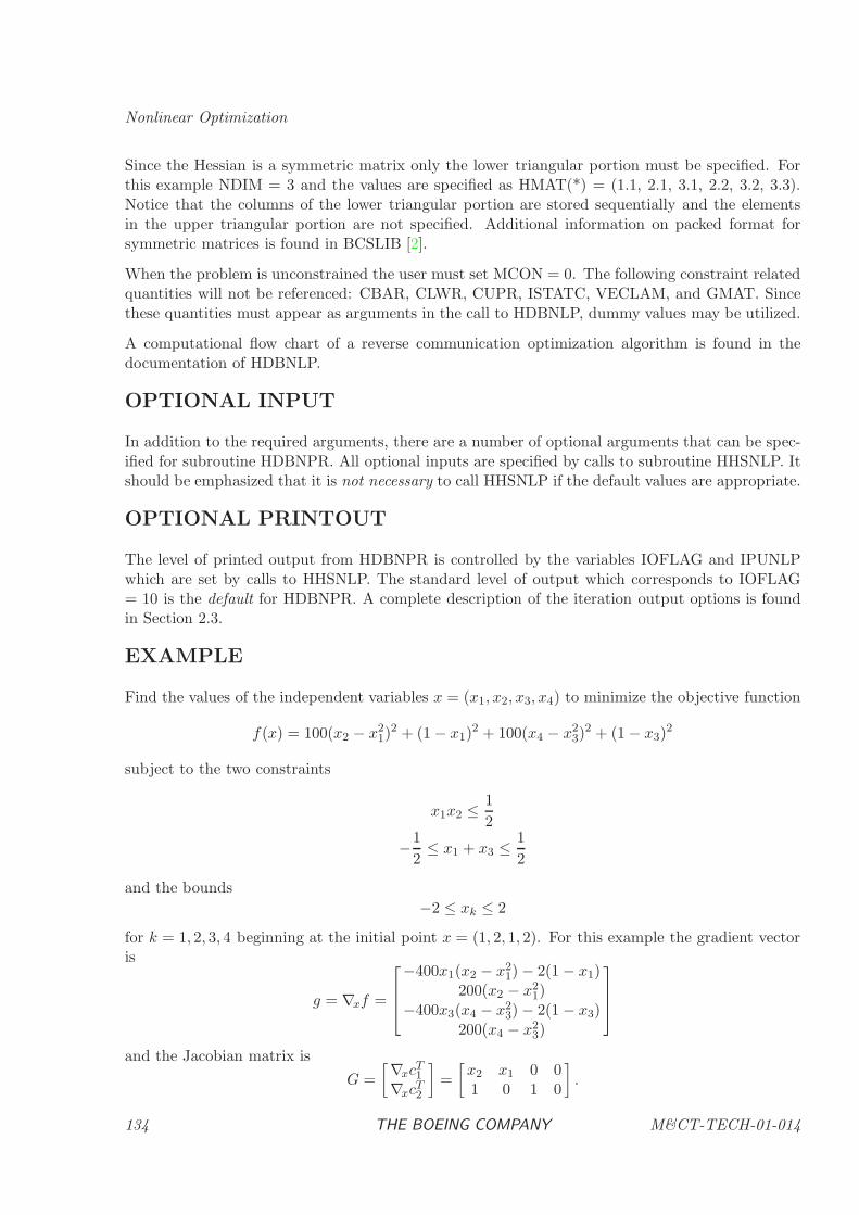
Nonlinear Optimization
Since the Hessian is a symmetric matrix only the lower triangular portion must be specified. Forthis example NDIM = 3 and the values are specified as HMAT(*) = (1.1, 2.1, 3.1, 2.2, 3.2, 3.3).Notice that the columns of the lower triangular portion are stored sequentially and the elementsin the upper triangular portion are not specified. Additional information on packed format forsymmetric matrices is found in BCSLIB [2].
When the problem is unconstrained the user must set MCON = 0. The following constraint relatedquantities will not be referenced: CBAR, CLWR, CUPR, ISTATC, VECLAM, and GMAT. Sincethese quantities must appear as arguments in the call to HDBNLP, dummy values may be utilized.
A computational flow chart of a reverse communication optimization algorithm is found in thedocumentation of HDBNLP.
OPTIONAL INPUT
In addition to the required arguments, there are a number of optional arguments that can be spec-ified for subroutine HDBNPR. All optional inputs are specified by calls to subroutine HHSNLP. Itshould be emphasized that it is not necessary to call HHSNLP if the default values are appropriate.
OPTIONAL PRINTOUT
The level of printed output from HDBNPR is controlled by the variables IOFLAG and IPUNLPwhich are set by calls to HHSNLP. The standard level of output which corresponds to IOFLAG= 10 is the default for HDBNPR. A complete description of the iteration output options is foundin Section 2.3.
EXAMPLE
Find the values of the independent variables x = (x1, x2, x3, x4) to minimize the objective function
f(x) = 100(x2 − x21)
2 + (1 − x1)2 + 100(x4 − x2
3)2 + (1 − x3)
2
subject to the two constraints
x1x2 ≤ 1
2
−1
2≤ x1 + x3 ≤ 1
2
and the bounds
−2 ≤ xk ≤ 2
for k = 1, 2, 3, 4 beginning at the initial point x = (1, 2, 1, 2). For this example the gradient vectoris
g = ∇xf =
−400x1(x2 − x21) − 2(1 − x1)
200(x2 − x21)
−400x3(x4 − x23) − 2(1 − x3)
200(x4 − x23)
and the Jacobian matrix is
G =
[∇xcT1
∇xcT2
]=
[x2 x1 0 01 0 1 0
].
134 THE BOEING COMPANY M&CT-TECH-01-014
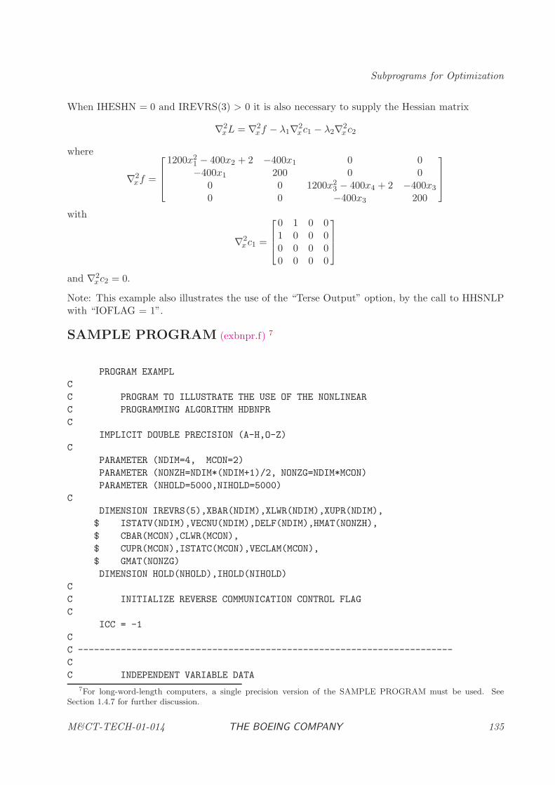
Subprograms for Optimization
When IHESHN = 0 and IREVRS(3) > 0 it is also necessary to supply the Hessian matrix
∇2xL = ∇2
xf − λ1∇2xc1 − λ2∇2
x c2
where
∇2xf =
1200x21 − 400x2 + 2 −400x1 0 0−400x1 200 0 0
0 0 1200x23 − 400x4 + 2 −400x3
0 0 −400x3 200
with
∇2xc1 =
0 1 0 01 0 0 00 0 0 00 0 0 0
and ∇2xc2 = 0.
Note: This example also illustrates the use of the “Terse Output” option, by the call to HHSNLPwith “IOFLAG = 1”.
SAMPLE PROGRAM (exbnpr.f) 7
PROGRAM EXAMPL
C
C PROGRAM TO ILLUSTRATE THE USE OF THE NONLINEAR
C PROGRAMMING ALGORITHM HDBNPR
C
IMPLICIT DOUBLE PRECISION (A-H,O-Z)
C
PARAMETER (NDIM=4, MCON=2)
PARAMETER (NONZH=NDIM*(NDIM+1)/2, NONZG=NDIM*MCON)
PARAMETER (NHOLD=5000,NIHOLD=5000)
C
DIMENSION IREVRS(5),XBAR(NDIM),XLWR(NDIM),XUPR(NDIM),
$ ISTATV(NDIM),VECNU(NDIM),DELF(NDIM),HMAT(NONZH),
$ CBAR(MCON),CLWR(MCON),
$ CUPR(MCON),ISTATC(MCON),VECLAM(MCON),
$ GMAT(NONZG)
DIMENSION HOLD(NHOLD),IHOLD(NIHOLD)
C
C INITIALIZE REVERSE COMMUNICATION CONTROL FLAG
C
ICC = -1
C
C ----------------------------------------------------------------------
C
C INDEPENDENT VARIABLE DATA
7For long-word-length computers, a single precision version of the SAMPLE PROGRAM must be used. See
Section 1.4.7 for further discussion.
M&CT-TECH-01-014 THE BOEING COMPANY 135
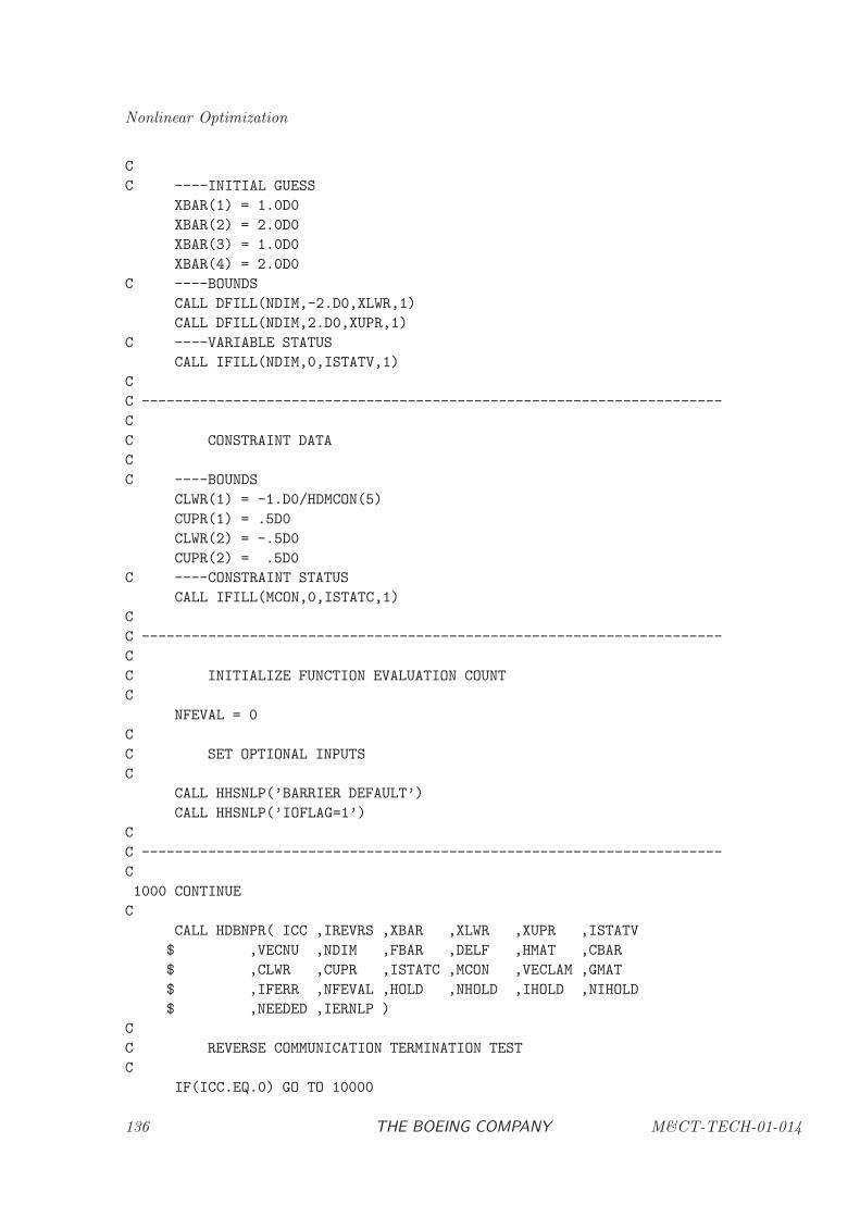
Nonlinear Optimization
C
C ----INITIAL GUESS
XBAR(1) = 1.0D0
XBAR(2) = 2.0D0
XBAR(3) = 1.0D0
XBAR(4) = 2.0D0
C ----BOUNDS
CALL DFILL(NDIM,-2.D0,XLWR,1)
CALL DFILL(NDIM,2.D0,XUPR,1)
C ----VARIABLE STATUS
CALL IFILL(NDIM,0,ISTATV,1)
C
C ----------------------------------------------------------------------
C
C CONSTRAINT DATA
C
C ----BOUNDS
CLWR(1) = -1.D0/HDMCON(5)
CUPR(1) = .5D0
CLWR(2) = -.5D0
CUPR(2) = .5D0
C ----CONSTRAINT STATUS
CALL IFILL(MCON,0,ISTATC,1)
C
C ----------------------------------------------------------------------
C
C INITIALIZE FUNCTION EVALUATION COUNT
C
NFEVAL = 0
C
C SET OPTIONAL INPUTS
C
CALL HHSNLP(’BARRIER DEFAULT’)
CALL HHSNLP(’IOFLAG=1’)
C
C ----------------------------------------------------------------------
C
1000 CONTINUE
C
CALL HDBNPR( ICC ,IREVRS ,XBAR ,XLWR ,XUPR ,ISTATV
$ ,VECNU ,NDIM ,FBAR ,DELF ,HMAT ,CBAR
$ ,CLWR ,CUPR ,ISTATC ,MCON ,VECLAM ,GMAT
$ ,IFERR ,NFEVAL ,HOLD ,NHOLD ,IHOLD ,NIHOLD
$ ,NEEDED ,IERNLP )
C
C REVERSE COMMUNICATION TERMINATION TEST
C
IF(ICC.EQ.0) GO TO 10000
136 THE BOEING COMPANY M&CT-TECH-01-014
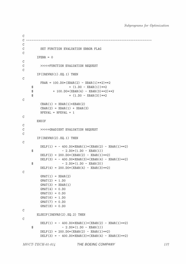
Subprograms for Optimization
C
C ----------------------------------------------------------------------
C
C SET FUNCTION EVALUATION ERROR FLAG
C
IFERR = 0
C
C >>>>>FUNCTION EVALUATION REQUEST
C
IF(IREVRS(1).EQ.1) THEN
C
FBAR = 100.D0*(XBAR(2) - XBAR(1)**2)**2
$ + (1.D0 - XBAR(1))**2
$ + 100.D0*(XBAR(4) - XBAR(3)**2)**2
$ + (1.D0 - XBAR(3))**2
C
CBAR(1) = XBAR(1)*XBAR(2)
CBAR(2) = XBAR(1) + XBAR(3)
NFEVAL = NFEVAL + 1
C
ENDIF
C
C >>>>>GRADIENT EVALUATION REQUEST
C
IF(IREVRS(2).EQ.1) THEN
C
DELF(1) = - 400.D0*XBAR(1)*(XBAR(2) - XBAR(1)**2)
$ - 2.D0*(1.D0 - XBAR(1))
DELF(2) = 200.D0*(XBAR(2) - XBAR(1)**2)
DELF(3) = - 400.D0*XBAR(3)*(XBAR(4) - XBAR(3)**2)
$ - 2.D0*(1.D0 - XBAR(3))
DELF(4) = 200.D0*(XBAR(4) - XBAR(3)**2)
C
GMAT(1) = XBAR(2)
GMAT(2) = 1.D0
GMAT(3) = XBAR(1)
GMAT(4) = 0.D0
GMAT(5) = 0.D0
GMAT(6) = 1.D0
GMAT(7) = 0.D0
GMAT(8) = 0.D0
C
ELSEIF(IREVRS(2).EQ.2) THEN
C
DELF(1) = - 400.D0*XBAR(1)*(XBAR(2) - XBAR(1)**2)
$ - 2.D0*(1.D0 - XBAR(1))
DELF(2) = 200.D0*(XBAR(2) - XBAR(1)**2)
DELF(3) = - 400.D0*XBAR(3)*(XBAR(4) - XBAR(3)**2)
M&CT-TECH-01-014 THE BOEING COMPANY 137
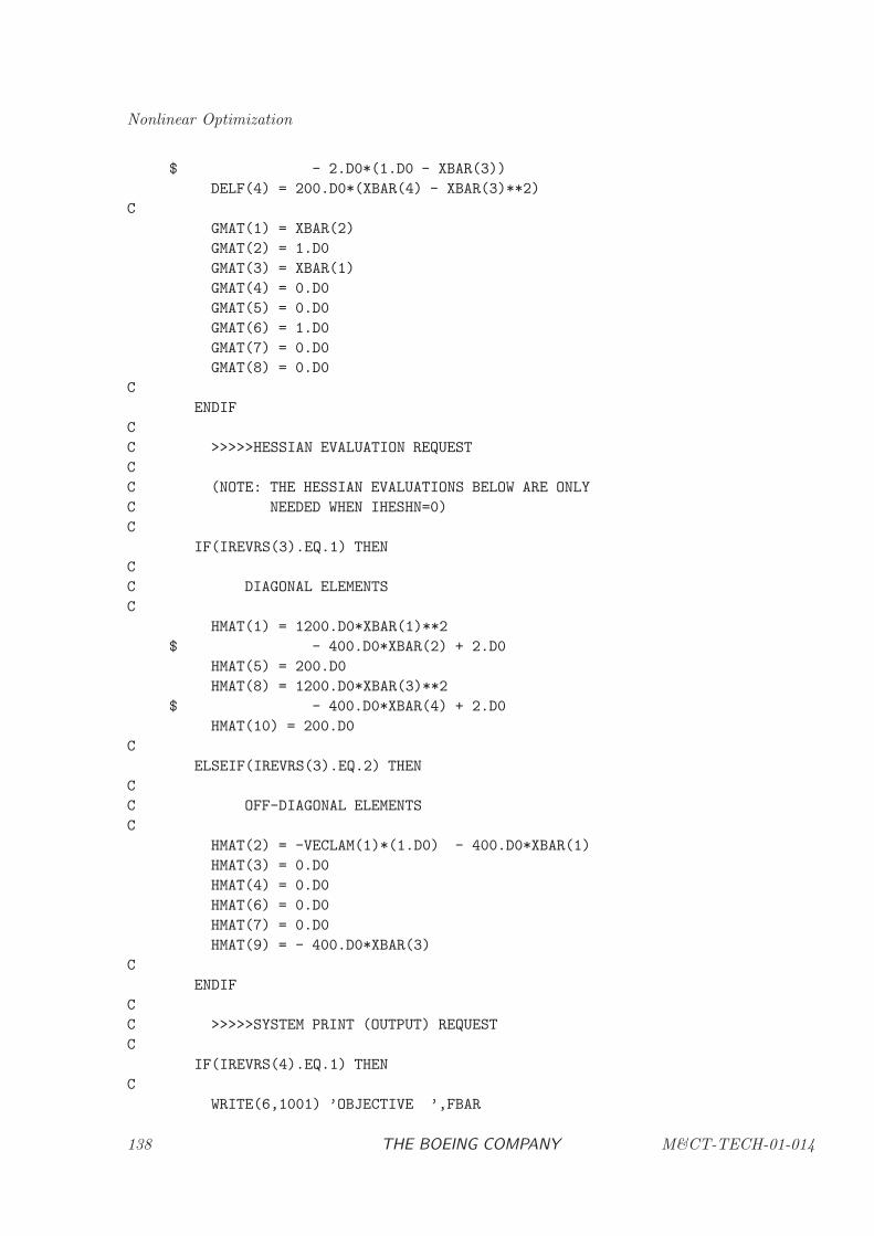
Nonlinear Optimization
$ - 2.D0*(1.D0 - XBAR(3))
DELF(4) = 200.D0*(XBAR(4) - XBAR(3)**2)
C
GMAT(1) = XBAR(2)
GMAT(2) = 1.D0
GMAT(3) = XBAR(1)
GMAT(4) = 0.D0
GMAT(5) = 0.D0
GMAT(6) = 1.D0
GMAT(7) = 0.D0
GMAT(8) = 0.D0
C
ENDIF
C
C >>>>>HESSIAN EVALUATION REQUEST
C
C (NOTE: THE HESSIAN EVALUATIONS BELOW ARE ONLY
C NEEDED WHEN IHESHN=0)
C
IF(IREVRS(3).EQ.1) THEN
C
C DIAGONAL ELEMENTS
C
HMAT(1) = 1200.D0*XBAR(1)**2
$ - 400.D0*XBAR(2) + 2.D0
HMAT(5) = 200.D0
HMAT(8) = 1200.D0*XBAR(3)**2
$ - 400.D0*XBAR(4) + 2.D0
HMAT(10) = 200.D0
C
ELSEIF(IREVRS(3).EQ.2) THEN
C
C OFF-DIAGONAL ELEMENTS
C
HMAT(2) = -VECLAM(1)*(1.D0) - 400.D0*XBAR(1)
HMAT(3) = 0.D0
HMAT(4) = 0.D0
HMAT(6) = 0.D0
HMAT(7) = 0.D0
HMAT(9) = - 400.D0*XBAR(3)
C
ENDIF
C
C >>>>>SYSTEM PRINT (OUTPUT) REQUEST
C
IF(IREVRS(4).EQ.1) THEN
C
WRITE(6,1001) ’OBJECTIVE ’,FBAR
138 THE BOEING COMPANY M&CT-TECH-01-014
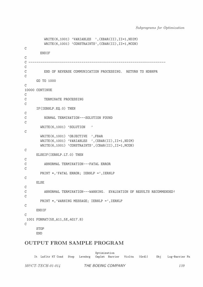
Subprograms for Optimization
WRITE(6,1001) ’VARIABLES ’,(XBAR(II),II=1,NDIM)
WRITE(6,1001) ’CONSTRAINTS’,(CBAR(II),II=1,MCON)
C
ENDIF
C
C ----------------------------------------------------------------------
C
C END OF REVERSE COMMUNICATION PROCESSING. RETURN TO HDBNPR
C
GO TO 1000
C
10000 CONTINUE
C
C TERMINATE PROCESSING
C
IF(IERNLP.EQ.0) THEN
C
C NORMAL TERMINATION---SOLUTION FOUND
C
WRITE(6,1001) ’SOLUTION ’
C
WRITE(6,1001) ’OBJECTIVE ’,FBAR
WRITE(6,1001) ’VARIABLES ’,(XBAR(II),II=1,NDIM)
WRITE(6,1001) ’CONSTRAINTS’,(CBAR(II),II=1,MCON)
C
ELSEIF(IERNLP.LT.0) THEN
C
C ABNORMAL TERMINATION---FATAL ERROR
C
PRINT *,’FATAL ERROR; IERNLP =’,IERNLP
C
ELSE
C
C ABNORMAL TERMINATION---WARNING. EVALUATION OF RESULTS RECOMMENDED!
C
PRINT *,’WARNING MESSAGE; IERNLP =’,IERNLP
C
ENDIF
C
1001 FORMAT(5X,A11,5X,4G17.8)
C
STOP
END
OUTPUT FROM SAMPLE PROGRAM
Optimization
It Lnfltr KT Cond Step Levnbrg Cmplmt Barrier Violtn |Grdl| Obj Log-Barrier Fn
M&CT-TECH-01-014 THE BOEING COMPANY 139
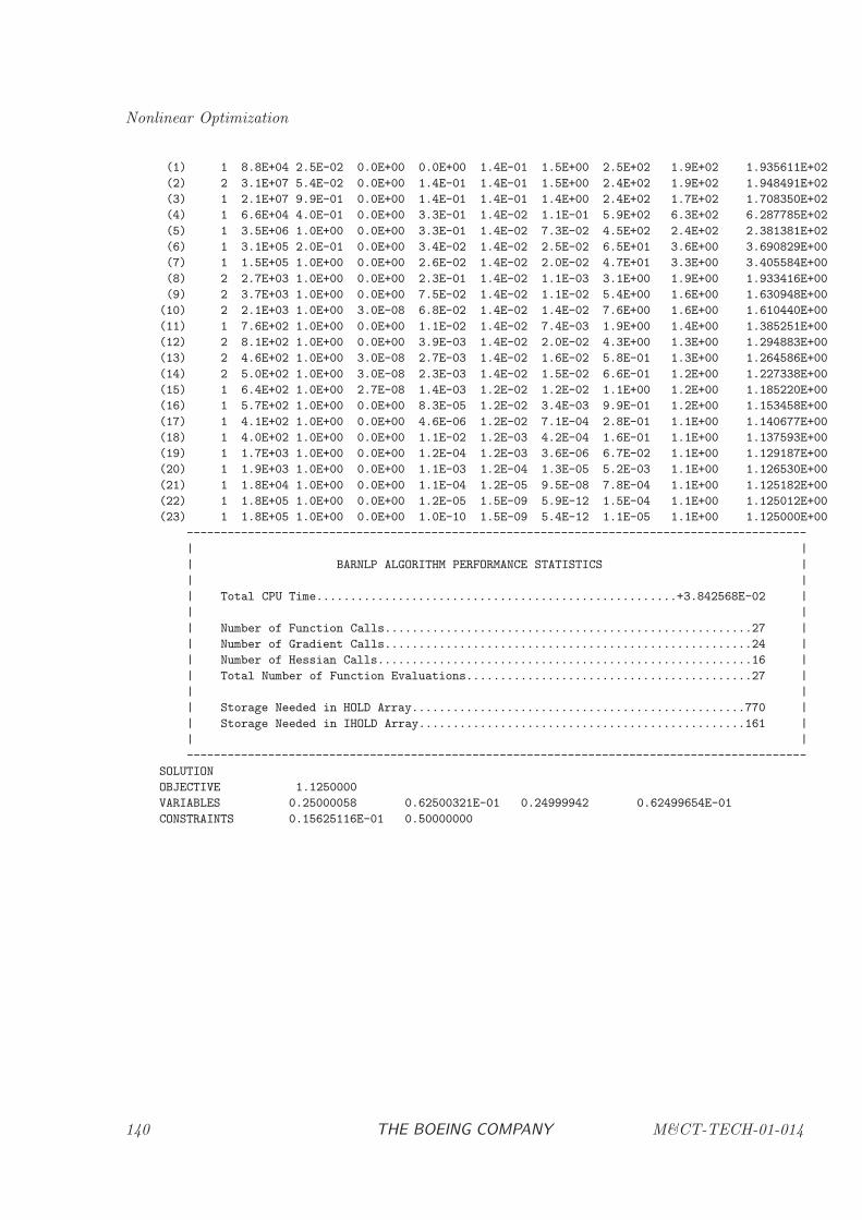
Nonlinear Optimization
(1) 1 8.8E+04 2.5E-02 0.0E+00 0.0E+00 1.4E-01 1.5E+00 2.5E+02 1.9E+02 1.935611E+02
(2) 2 3.1E+07 5.4E-02 0.0E+00 1.4E-01 1.4E-01 1.5E+00 2.4E+02 1.9E+02 1.948491E+02
(3) 1 2.1E+07 9.9E-01 0.0E+00 1.4E-01 1.4E-01 1.4E+00 2.4E+02 1.7E+02 1.708350E+02
(4) 1 6.6E+04 4.0E-01 0.0E+00 3.3E-01 1.4E-02 1.1E-01 5.9E+02 6.3E+02 6.287785E+02
(5) 1 3.5E+06 1.0E+00 0.0E+00 3.3E-01 1.4E-02 7.3E-02 4.5E+02 2.4E+02 2.381381E+02
(6) 1 3.1E+05 2.0E-01 0.0E+00 3.4E-02 1.4E-02 2.5E-02 6.5E+01 3.6E+00 3.690829E+00
(7) 1 1.5E+05 1.0E+00 0.0E+00 2.6E-02 1.4E-02 2.0E-02 4.7E+01 3.3E+00 3.405584E+00
(8) 2 2.7E+03 1.0E+00 0.0E+00 2.3E-01 1.4E-02 1.1E-03 3.1E+00 1.9E+00 1.933416E+00
(9) 2 3.7E+03 1.0E+00 0.0E+00 7.5E-02 1.4E-02 1.1E-02 5.4E+00 1.6E+00 1.630948E+00
(10) 2 2.1E+03 1.0E+00 3.0E-08 6.8E-02 1.4E-02 1.4E-02 7.6E+00 1.6E+00 1.610440E+00
(11) 1 7.6E+02 1.0E+00 0.0E+00 1.1E-02 1.4E-02 7.4E-03 1.9E+00 1.4E+00 1.385251E+00
(12) 2 8.1E+02 1.0E+00 0.0E+00 3.9E-03 1.4E-02 2.0E-02 4.3E+00 1.3E+00 1.294883E+00
(13) 2 4.6E+02 1.0E+00 3.0E-08 2.7E-03 1.4E-02 1.6E-02 5.8E-01 1.3E+00 1.264586E+00
(14) 2 5.0E+02 1.0E+00 3.0E-08 2.3E-03 1.4E-02 1.5E-02 6.6E-01 1.2E+00 1.227338E+00
(15) 1 6.4E+02 1.0E+00 2.7E-08 1.4E-03 1.2E-02 1.2E-02 1.1E+00 1.2E+00 1.185220E+00
(16) 1 5.7E+02 1.0E+00 0.0E+00 8.3E-05 1.2E-02 3.4E-03 9.9E-01 1.2E+00 1.153458E+00
(17) 1 4.1E+02 1.0E+00 0.0E+00 4.6E-06 1.2E-02 7.1E-04 2.8E-01 1.1E+00 1.140677E+00
(18) 1 4.0E+02 1.0E+00 0.0E+00 1.1E-02 1.2E-03 4.2E-04 1.6E-01 1.1E+00 1.137593E+00
(19) 1 1.7E+03 1.0E+00 0.0E+00 1.2E-04 1.2E-03 3.6E-06 6.7E-02 1.1E+00 1.129187E+00
(20) 1 1.9E+03 1.0E+00 0.0E+00 1.1E-03 1.2E-04 1.3E-05 5.2E-03 1.1E+00 1.126530E+00
(21) 1 1.8E+04 1.0E+00 0.0E+00 1.1E-04 1.2E-05 9.5E-08 7.8E-04 1.1E+00 1.125182E+00
(22) 1 1.8E+05 1.0E+00 0.0E+00 1.2E-05 1.5E-09 5.9E-12 1.5E-04 1.1E+00 1.125012E+00
(23) 1 1.8E+05 1.0E+00 0.0E+00 1.0E-10 1.5E-09 5.4E-12 1.1E-05 1.1E+00 1.125000E+00
-------------------------------------------------------------------------------------------
| |
| BARNLP ALGORITHM PERFORMANCE STATISTICS |
| |
| Total CPU Time.....................................................+3.842568E-02 |
| |
| Number of Function Calls......................................................27 |
| Number of Gradient Calls......................................................24 |
| Number of Hessian Calls.......................................................16 |
| Total Number of Function Evaluations..........................................27 |
| |
| Storage Needed in HOLD Array.................................................770 |
| Storage Needed in IHOLD Array................................................161 |
| |
-------------------------------------------------------------------------------------------
SOLUTION
OBJECTIVE 1.1250000
VARIABLES 0.25000058 0.62500321E-01 0.24999942 0.62499654E-01
CONSTRAINTS 0.15625116E-01 0.50000000
140 THE BOEING COMPANY M&CT-TECH-01-014
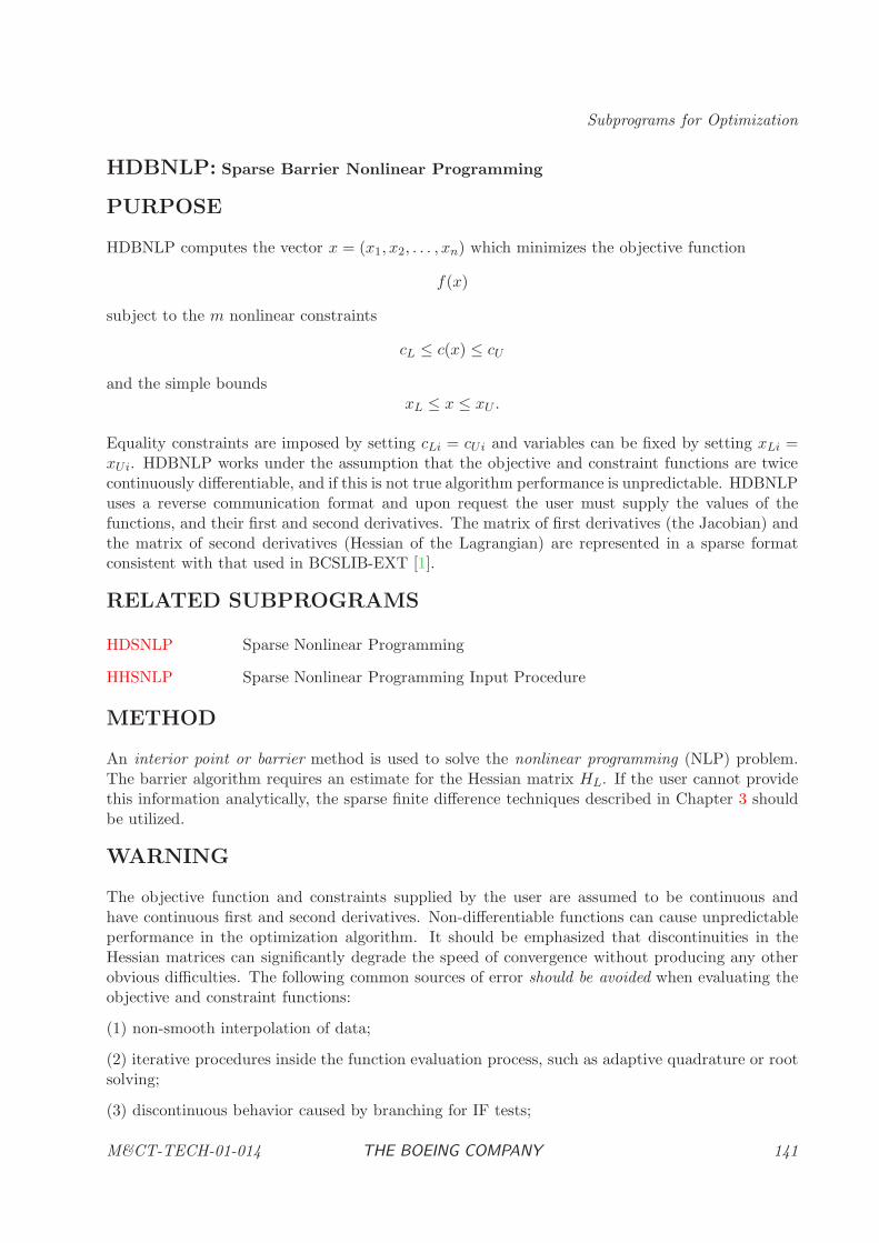
Subprograms for Optimization
HDBNLP: Sparse Barrier Nonlinear Programming
PURPOSE
HDBNLP computes the vector x = (x1, x2, . . . , xn) which minimizes the objective function
f(x)
subject to the m nonlinear constraints
cL ≤ c(x) ≤ cU
and the simple boundsxL ≤ x ≤ xU .
Equality constraints are imposed by setting cLi = cUi and variables can be fixed by setting xLi =xUi. HDBNLP works under the assumption that the objective and constraint functions are twicecontinuously differentiable, and if this is not true algorithm performance is unpredictable. HDBNLPuses a reverse communication format and upon request the user must supply the values of thefunctions, and their first and second derivatives. The matrix of first derivatives (the Jacobian) andthe matrix of second derivatives (Hessian of the Lagrangian) are represented in a sparse formatconsistent with that used in BCSLIB-EXT [1].
RELATED SUBPROGRAMS
HDSNLP Sparse Nonlinear Programming
HHSNLP Sparse Nonlinear Programming Input Procedure
METHOD
An interior point or barrier method is used to solve the nonlinear programming (NLP) problem.The barrier algorithm requires an estimate for the Hessian matrix HL. If the user cannot providethis information analytically, the sparse finite difference techniques described in Chapter 3 shouldbe utilized.
WARNING
The objective function and constraints supplied by the user are assumed to be continuous andhave continuous first and second derivatives. Non-differentiable functions can cause unpredictableperformance in the optimization algorithm. It should be emphasized that discontinuities in theHessian matrices can significantly degrade the speed of convergence without producing any otherobvious difficulties. The following common sources of error should be avoided when evaluating theobjective and constraint functions:
(1) non-smooth interpolation of data;
(2) iterative procedures inside the function evaluation process, such as adaptive quadrature or rootsolving;
(3) discontinuous behavior caused by branching for IF tests;
M&CT-TECH-01-014 THE BOEING COMPANY 141
Nonlinear Optimization
(4) non-differentiable functions such as ABS, MAX, and MIN.
The user must provide a procedure to evaluate the objective and constraint functions in additionto first and second derivatives of these quantities. If it is not possible to evaluate the functions(for example, c(x) = 1/x at x = 0) then set IFERR = 1 and exit the function evaluation process.Otherwise, set IFERR = 0 when the functions are evaluated. The function error flag should beused to avoid computational difficulties, but never in lieu of an explicit constraint.
The HDBNLP software uses internal common blocks to communicate information. To avoid con-flict with these internal commons the user should not have commons with the following names:NPSPRR, NPSPRI, NPSPRC, STATIS, KONSTN, NPSALG, NPSDFL, NLPERR, PERCOM,ITEREF, and CLKCOM.
USAGE
INTEGER IRVCOM, IFERR, NFEVAL, IER, NEEDED
INTEGER NDIM, MCON, NONZH, NONZG, NHOLD, NIHOLD
INTEGER IREVRS(5), ISTATV(NDIM), IROWH(NONZH), JSTRH(NDIM+1)
INTEGER ISTATC(MCON), IROWG(NONZG), JCOLG(NONZG), IHOLD(NIHOLD)
DOUBLE PRECISION FBAR, XBAR(NDIM), XLWR(NDIM), XUPR(NDIM), VECNU(NDIM)
DOUBLE PRECISION DELF(NDIM), HMAT(NONZH), CBAR(MCON), CLWR(MCON)
DOUBLE PRECISION CUPR(MCON), VECLAM(MCON), GMAT(NONZG), HOLD(NHOLD)
CALL HHSNLP(’BARRIER DEFAULT’)
CALL HDBNLP( IRVCOM ,IREVRS ,XBAR ,XLWR ,XUPR ,ISTATV
$ ,VECNU ,NDIM ,FBAR ,DELF ,HMAT ,IROWH
$ ,JSTRH ,NONZH ,CBAR ,CLWR ,CUPR ,ISTATC
$ ,MCON ,VECLAM ,GMAT ,IROWG ,JCOLG ,NONZG
$ ,IFERR ,NFEVAL ,HOLD ,NHOLD ,IHOLD ,NIHOLD
$ ,NEEDED ,IER )
ARGUMENTS
ARGUMENTS TO CONTROL REVERSE COMMUNICATION
IRVCOM [INPUT/OUTPUT, INTEGER]Continuation control flag. This argument must be initialized. Thereafter it is setby the algorithm and must not be changed by the calling program.
IRVCOM = −1 Initialization pass.
IRVCOM = 0 Termination (normal or abnormal).
142 THE BOEING COMPANY M&CT-TECH-01-014
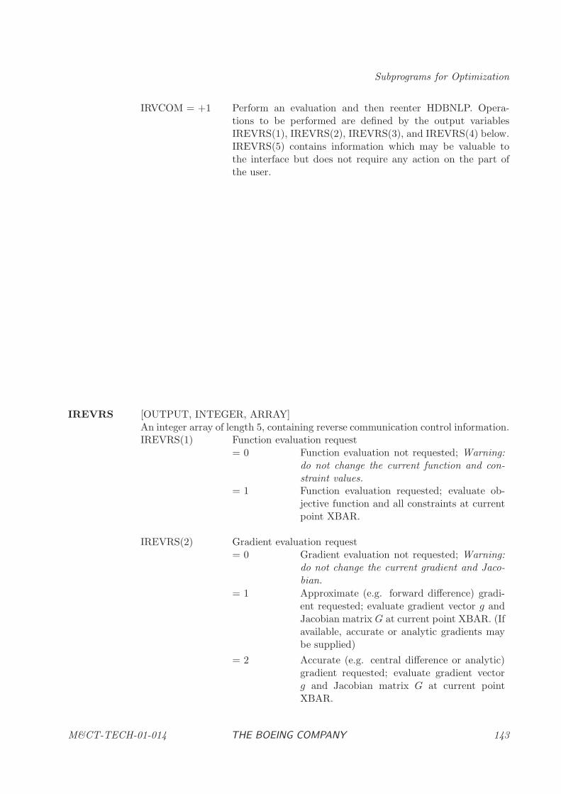
Subprograms for Optimization
IRVCOM = +1 Perform an evaluation and then reenter HDBNLP. Opera-tions to be performed are defined by the output variablesIREVRS(1), IREVRS(2), IREVRS(3), and IREVRS(4) below.IREVRS(5) contains information which may be valuable tothe interface but does not require any action on the part ofthe user.
IREVRS [OUTPUT, INTEGER, ARRAY]An integer array of length 5, containing reverse communication control information.IREVRS(1) Function evaluation request
= 0 Function evaluation not requested; Warning:do not change the current function and con-straint values.
= 1 Function evaluation requested; evaluate ob-jective function and all constraints at currentpoint XBAR.
IREVRS(2) Gradient evaluation request= 0 Gradient evaluation not requested; Warning:
do not change the current gradient and Jaco-bian.
= 1 Approximate (e.g. forward difference) gradi-ent requested; evaluate gradient vector g andJacobian matrix G at current point XBAR. (Ifavailable, accurate or analytic gradients maybe supplied)
= 2 Accurate (e.g. central difference or analytic)gradient requested; evaluate gradient vectorg and Jacobian matrix G at current pointXBAR.
M&CT-TECH-01-014 THE BOEING COMPANY 143
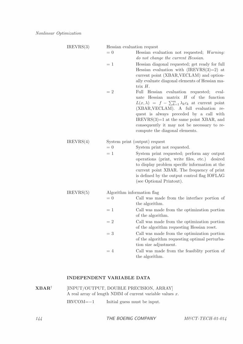
Nonlinear Optimization
IREVRS(3) Hessian evaluation request= 0 Hessian evaluation not requested; Warning:
do not change the current Hessian.
= 1 Hessian diagonal requested; get ready for fullHessian evaluation with (IREVRS(3)=2) atcurrent point (XBAR,VECLAM) and option-ally evaluate diagonal elements of Hessian ma-trix H.
= 2 Full Hessian evaluation requested; eval-uate Hessian matrix H of the functionL(x, λ) = f − ∑m
k=1 λkck at current point(XBAR,VECLAM). A full evaluation re-quest is always preceded by a call withIREVRS(3)=1 at the same point XBAR, andconsequently it may not be necessary to re-compute the diagonal elements.
IREVRS(4) System print (output) request= 0 System print not requested.
= 1 System print requested; perform any outputoperations (print, write files, etc.) desiredto display problem specific information at thecurrent point XBAR. The frequency of printis defined by the output control flag IOFLAG(see Optional Printout).
IREVRS(5) Algorithm information flag= 0 Call was made from the interface portion of
the algorithm.
= 1 Call was made from the optimization portionof the algorithm.
= 2 Call was made from the optimization portionof the algorithm requesting Hessian reset.
= 3 Call was made from the optimization portionof the algorithm requesting optimal perturba-tion size adjustment.
= 4 Call was made from the feasiblity portion ofthe algorithm.
INDEPENDENT VARIABLE DATA
XBAR† [INPUT/OUTPUT, DOUBLE PRECISION, ARRAY]A real array of length NDIM of current variable values x.
IRVCOM=−1 Initial guess must be input.
144 THE BOEING COMPANY M&CT-TECH-01-014

Subprograms for Optimization
IRVCOM=0 Final point is output.
IRVCOM=1 Intermediate iteration points are output.
XLWR† [INPUT, DOUBLE PRECISION, ARRAY]A real array of length NDIM containing the variable lower bounds xL. For variablesthat have no lower bound set xLi ≤ −.01/HDMCON(5). See Section 2.2 of theBCSLIB Manual [2] for HDMCON.
XUPR† [INPUT, DOUBLE PRECISION, ARRAY]A real array of length NDIM containing the variable upper bounds xU . For variablesthat have no upper bound set xUi ≥ .01/HDMCON(5).
ISTATV† [INPUT/OUTPUT, INTEGER, ARRAY]An integer array of length NDIM indicating variable status. On input ISTATVdefines an estimate of the active variable bounds, and on output ISTATV definesthe bounds active at the solution.
ISTATV(i)= 0 Variable is strictly feasible, i.e. xLi < xi < xUi.
ISTATV(i)= 1 Variable lower bound is active, i.e. xLi = xi.
ISTATV(i)= 2 Variable upper bound is active, i.e. xi = xUi.
ISTATV(i)= 3 Fixed permanently.
ISTATV(i)= 10 Output only: Violated variable lower bound, i.e. xLi−δc > xi.
ISTATV(i)= 20 Output only: Violated variable upper bound, i.e. xi > xUi+δc.
ISTATV(i)= 30 Output only: Violated fixed variable. Either xi < xLi − δc orxi > xUi + δc.
When ISTATV(i) = 3 it is necessary that xLi = xUi, where xLi = XLWR(i)and xUi = XUPR(i). When ISTATV(i) 6= 3, it is necessary that xLi < xUi with|xLi − xUi| > δc.
VECNU# [INPUT/OUTPUT, DOUBLE PRECISION, ARRAY]An array of length NDIM of bound multipliers ν.
NDIM† [INPUT, INTEGER]Number of variables n, where 1 ≤ NDIM.
OBJECTIVE FUNCTION DATA
FBAR‡ [INPUT, DOUBLE PRECISION]The objective function evaluated at XBAR, f(XBAR).
DELF‡ [INPUT, DOUBLE PRECISION, ARRAY]A real array of length NDIM containing the gradient g of FBAR at XBAR.
M&CT-TECH-01-014 THE BOEING COMPANY 145
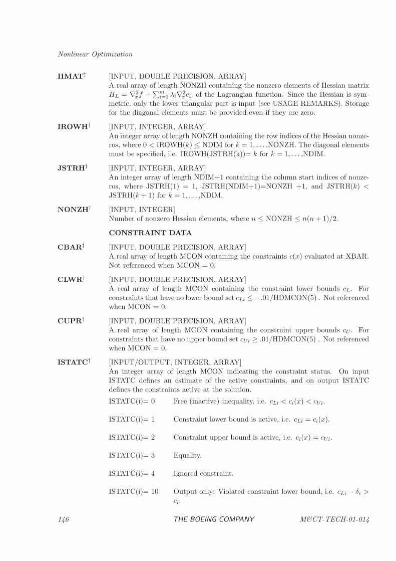
Nonlinear Optimization
HMAT‡ [INPUT, DOUBLE PRECISION, ARRAY]A real array of length NONZH containing the nonzero elements of Hessian matrixHL = ∇2
xf −∑mi=1 λi∇2
x ci. of the Lagrangian function. Since the Hessian is sym-metric, only the lower triangular part is input (see USAGE REMARKS). Storagefor the diagonal elements must be provided even if they are zero.
IROWH† [INPUT, INTEGER, ARRAY]An integer array of length NONZH containing the row indices of the Hessian nonze-ros, where 0 < IROWH(k) ≤ NDIM for k = 1, . . . ,NONZH. The diagonal elementsmust be specified, i.e. IROWH(JSTRH(k))= k for k = 1, . . . ,NDIM.
JSTRH† [INPUT, INTEGER, ARRAY]An integer array of length NDIM+1 containing the column start indices of nonze-ros, where JSTRH(1) = 1, JSTRH(NDIM+1)=NONZH +1, and JSTRH(k) <JSTRH(k + 1) for k = 1, . . . ,NDIM.
NONZH† [INPUT, INTEGER]Number of nonzero Hessian elements, where n ≤ NONZH ≤ n(n+ 1)/2.
CONSTRAINT DATA
CBAR‡ [INPUT, DOUBLE PRECISION, ARRAY]A real array of length MCON containing the constraints c(x) evaluated at XBAR.Not referenced when MCON = 0.
CLWR† [INPUT, DOUBLE PRECISION, ARRAY]A real array of length MCON containing the constraint lower bounds cL. Forconstraints that have no lower bound set cLi ≤ −.01/HDMCON(5) . Not referencedwhen MCON = 0.
CUPR† [INPUT, DOUBLE PRECISION, ARRAY]A real array of length MCON containing the constraint upper bounds cU . Forconstraints that have no upper bound set cUi ≥ .01/HDMCON(5) . Not referencedwhen MCON = 0.
ISTATC† [INPUT/OUTPUT, INTEGER, ARRAY]An integer array of length MCON indicating the constraint status. On inputISTATC defines an estimate of the active constraints, and on output ISTATCdefines the constraints active at the solution.
ISTATC(i)= 0 Free (inactive) inequality, i.e. cLi < ci(x) < cUi.
ISTATC(i)= 1 Constraint lower bound is active, i.e. cLi = ci(x).
ISTATC(i)= 2 Constraint upper bound is active, i.e. ci(x) = cUi.
ISTATC(i)= 3 Equality.
ISTATC(i)= 4 Ignored constraint.
ISTATC(i)= 10 Output only: Violated constraint lower bound, i.e. cLi − δc >ci.
146 THE BOEING COMPANY M&CT-TECH-01-014
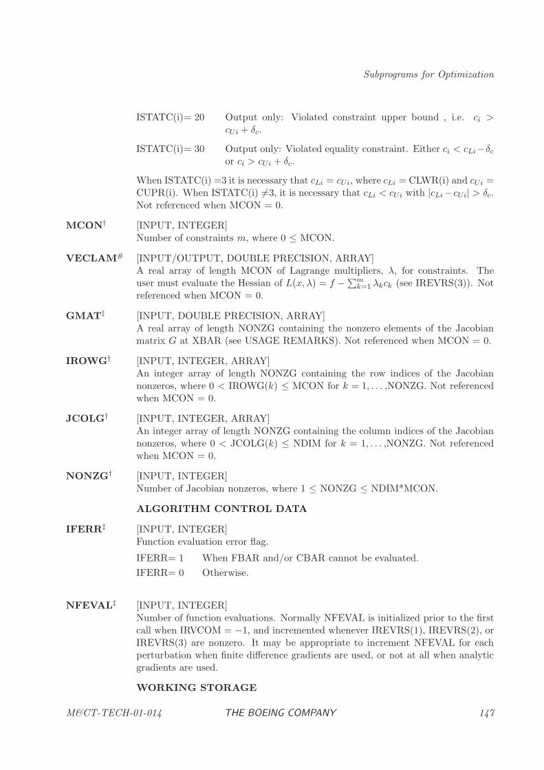
Subprograms for Optimization
ISTATC(i)= 20 Output only: Violated constraint upper bound , i.e. ci >cUi + δc.
ISTATC(i)= 30 Output only: Violated equality constraint. Either ci < cLi−δcor ci > cUi + δc.
When ISTATC(i) =3 it is necessary that cLi = cUi, where cLi = CLWR(i) and cUi =CUPR(i). When ISTATC(i) 6=3, it is necessary that cLi < cUi with |cLi−cUi| > δc.Not referenced when MCON = 0.
MCON† [INPUT, INTEGER]Number of constraints m, where 0 ≤ MCON.
VECLAM# [INPUT/OUTPUT, DOUBLE PRECISION, ARRAY]A real array of length MCON of Lagrange multipliers, λ, for constraints. Theuser must evaluate the Hessian of L(x, λ) = f −∑m
k=1 λkck (see IREVRS(3)). Notreferenced when MCON = 0.
GMAT‡ [INPUT, DOUBLE PRECISION, ARRAY]A real array of length NONZG containing the nonzero elements of the Jacobianmatrix G at XBAR (see USAGE REMARKS). Not referenced when MCON = 0.
IROWG† [INPUT, INTEGER, ARRAY]An integer array of length NONZG containing the row indices of the Jacobiannonzeros, where 0 < IROWG(k) ≤ MCON for k = 1, . . . ,NONZG. Not referencedwhen MCON = 0.
JCOLG† [INPUT, INTEGER, ARRAY]An integer array of length NONZG containing the column indices of the Jacobiannonzeros, where 0 < JCOLG(k) ≤ NDIM for k = 1, . . . ,NONZG. Not referencedwhen MCON = 0.
NONZG† [INPUT, INTEGER]Number of Jacobian nonzeros, where 1 ≤ NONZG ≤ NDIM*MCON.
ALGORITHM CONTROL DATA
IFERR‡ [INPUT, INTEGER]Function evaluation error flag.
IFERR= 1 When FBAR and/or CBAR cannot be evaluated.
IFERR= 0 Otherwise.
NFEVAL‡ [INPUT, INTEGER]Number of function evaluations. Normally NFEVAL is initialized prior to the firstcall when IRVCOM = −1, and incremented whenever IREVRS(1), IREVRS(2), orIREVRS(3) are nonzero. It may be appropriate to increment NFEVAL for eachperturbation when finite difference gradients are used, or not at all when analyticgradients are used.
WORKING STORAGE
M&CT-TECH-01-014 THE BOEING COMPANY 147
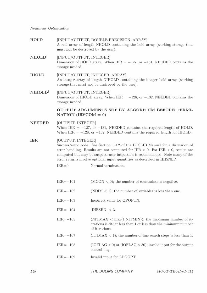
Nonlinear Optimization
HOLD [INPUT/OUTPUT, DOUBLE PRECISION, ARRAY]A real array of length NHOLD containing the hold array (working storage thatmust not be destroyed by the user).
NHOLD† [INPUT/OUTPUT, INTEGER]Dimension of HOLD array. When IER = −127, or −131, NEEDED contains thestorage needed.
IHOLD [INPUT/OUTPUT, INTEGER, ARRAY]An integer array of length NIHOLD containing the integer hold array (workingstorage that must not be destroyed by the user).
NIHOLD† [INPUT/OUTPUT, INTEGER]Dimension of IHOLD array. When IER = −128, or −132, NEEDED contains thestorage needed.
OUTPUT ARGUMENTS SET BY ALGORITHM BEFORE TERMI-NATION (IRVCOM = 0)
NEEDED [OUTPUT, INTEGER]When IER = −127, or −131, NEEDED contains the required length of HOLD.When IER = −128, or −132, NEEDED contains the required length for IHOLD.
IER [OUTPUT, INTEGER]Success/error code. See Section 1.4.2 of the BCSLIB Manual for a discussion oferror handling. Results are not computed for IER < 0. For IER > 0, results arecomputed but may be suspect; user inspection is recommended. Note many of theerror returns involve optional input quantities as described in HHSNLP.
IER=0 Normal termination.
IER=−101 (MCON < 0); the number of constraints is negative.
IER=−102 (NDIM < 1); the number of variables is less than one.
IER=−103 Incorrect value for QPOPTN.
IER=−104 |IHESHN| > 3.
IER=−105 (NITMAX < max(1,NITMIN)); the maximum number of it-erations is either less than 1 or less than the minimum numberof iterations.
IER=−107 (IT1MAX < 1); the number of line search steps is less than 1.
IER=−108 (IOFLAG< 0) or (IOFLAG > 30); invalid input for the outputcontrol flag.
IER=−109 Invalid input for ALGOPT.
148 THE BOEING COMPANY M&CT-TECH-01-014
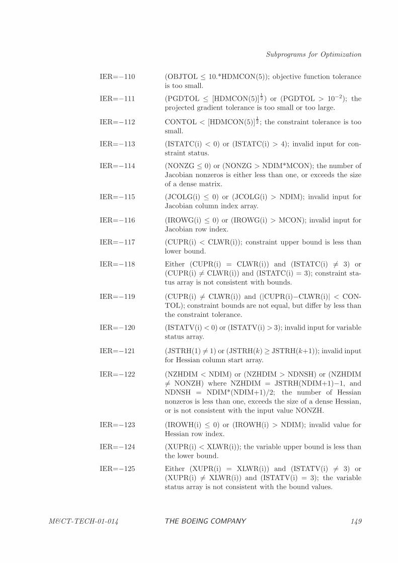
Subprograms for Optimization
IER=−110 (OBJTOL ≤ 10.*HDMCON(5)); objective function toleranceis too small.
IER=−111 (PGDTOL ≤ [HDMCON(5)]12 ) or (PGDTOL > 10−2); the
projected gradient tolerance is too small or too large.
IER=−112 CONTOL < [HDMCON(5)]12 ; the constraint tolerance is too
small.
IER=−113 (ISTATC(i) < 0) or (ISTATC(i) > 4); invalid input for con-straint status.
IER=−114 (NONZG ≤ 0) or (NONZG > NDIM*MCON); the number ofJacobian nonzeros is either less than one, or exceeds the sizeof a dense matrix.
IER=−115 (JCOLG(i) ≤ 0) or (JCOLG(i) > NDIM); invalid input forJacobian column index array.
IER=−116 (IROWG(i) ≤ 0) or (IROWG(i) > MCON); invalid input forJacobian row index.
IER=−117 (CUPR(i) < CLWR(i)); constraint upper bound is less thanlower bound.
IER=−118 Either (CUPR(i) = CLWR(i)) and (ISTATC(i) 6= 3) or(CUPR(i) 6= CLWR(i)) and (ISTATC(i) = 3); constraint sta-tus array is not consistent with bounds.
IER=−119 (CUPR(i) 6= CLWR(i)) and (|CUPR(i)−CLWR(i)| < CON-TOL); constraint bounds are not equal, but differ by less thanthe constraint tolerance.
IER=−120 (ISTATV(i)< 0) or (ISTATV(i) > 3); invalid input for variablestatus array.
IER=−121 (JSTRH(1) 6= 1) or (JSTRH(k) ≥ JSTRH(k+1)); invalid inputfor Hessian column start array.
IER=−122 (NZHDIM < NDIM) or (NZHDIM > NDNSH) or (NZHDIM6= NONZH) where NZHDIM = JSTRH(NDIM+1)−1, andNDNSH = NDIM*(NDIM+1)/2; the number of Hessiannonzeros is less than one, exceeds the size of a dense Hessian,or is not consistent with the input value NONZH.
IER=−123 (IROWH(i) ≤ 0) or (IROWH(i) > NDIM); invalid value forHessian row index.
IER=−124 (XUPR(i) < XLWR(i)); the variable upper bound is less thanthe lower bound.
IER=−125 Either (XUPR(i) = XLWR(i)) and (ISTATV(i) 6= 3) or(XUPR(i) 6= XLWR(i)) and (ISTATV(i) = 3); the variablestatus array is not consistent with the bound values.
M&CT-TECH-01-014 THE BOEING COMPANY 149
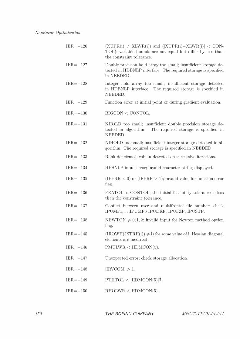
Nonlinear Optimization
IER=−126 (XUPR(i) 6= XLWR(i)) and (|XUPR(i)−XLWR(i)| < CON-TOL); variable bounds are not equal but differ by less thanthe constraint tolerance.
IER=−127 Double precision hold array too small; insufficient storage de-tected in HDBNLP interface. The required storage is specifiedin NEEDED.
IER=−128 Integer hold array too small; insufficient storage detectedin HDBNLP interface. The required storage is specified inNEEDED.
IER=−129 Function error at initial point or during gradient evaluation.
IER=−130 BIGCON < CONTOL.
IER=−131 NHOLD too small; insufficient double precision storage de-tected in algorithm. The required storage is specified inNEEDED.
IER=−132 NIHOLD too small; insufficient integer storage detected in al-gorithm. The required storage is specified in NEEDED.
IER=−133 Rank deficient Jacobian detected on successive iterations.
IER=−134 HHSNLP input error; invalid character string displayed.
IER=−135 (IFERR < 0) or (IFERR > 1); invalid value for function errorflag.
IER=−136 FEATOL < CONTOL; the initial feasibility tolerance is lessthan the constraint tolerance.
IER=−137 Conflict between user and multifrontal file number; checkIPUMF1,. . .,IPUMF6 IPUDRF, IPUFZF, IPUSTF.
IER=−138 NEWTON 6= 0, 1, 2; invalid input for Newton method optionflag.
IER=−145 (IROWH(JSTRH(i)) 6= i) for some value of i; Hessian diagonalelements are incorrect.
IER=−146 PMULWR < HDMCON(5).
IER=−147 Unexpected error; check storage allocation.
IER=−148 |IRVCOM| > 1.
IER=−149 PTHTOL < [HDMCON(5)]12 .
IER=−150 RHOLWR < HDMCON(5).
150 THE BOEING COMPANY M&CT-TECH-01-014
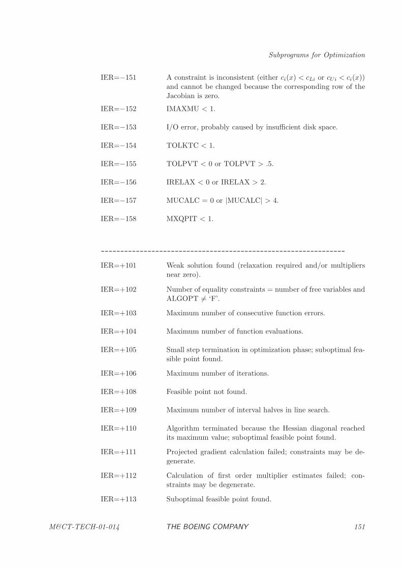
Subprograms for Optimization
IER=−151 A constraint is inconsistent (either ci(x) < cLi or cUi < ci(x))and cannot be changed because the corresponding row of theJacobian is zero.
IER=−152 IMAXMU < 1.
IER=−153 I/O error, probably caused by insufficient disk space.
IER=−154 TOLKTC < 1.
IER=−155 TOLPVT < 0 or TOLPVT > .5.
IER=−156 IRELAX < 0 or IRELAX > 2.
IER=−157 MUCALC = 0 or |MUCALC| > 4.
IER=−158 MXQPIT < 1.
---------------------------------------------------------------
IER=+101 Weak solution found (relaxation required and/or multipliersnear zero).
IER=+102 Number of equality constraints = number of free variables andALGOPT 6= ‘F’.
IER=+103 Maximum number of consecutive function errors.
IER=+104 Maximum number of function evaluations.
IER=+105 Small step termination in optimization phase; suboptimal fea-sible point found.
IER=+106 Maximum number of iterations.
IER=+108 Feasible point not found.
IER=+109 Maximum number of interval halves in line search.
IER=+110 Algorithm terminated because the Hessian diagonal reachedits maximum value; suboptimal feasible point found.
IER=+111 Projected gradient calculation failed; constraints may be de-generate.
IER=+112 Calculation of first order multiplier estimates failed; con-straints may be degenerate.
IER=+113 Suboptimal feasible point found.
M&CT-TECH-01-014 THE BOEING COMPANY 151
Nonlinear Optimization
IER=+114 Barrier NLP failed with unexpected error.
IER=+115 CONTOL > OBJTOL; convergence tolerances may be inap-propriate.
IER=+116 Uphill direction detected in line search.
IER=+117 Reduced objective function is linear.
IER=+118 Both cLi ≤ −.01/HDMCON(5) and cUi ≥ .01/HDMCON(5);constraints ignored.
IER=+119 Terminate after diagnostic line search.
IER=+121 Terminate after postoptimality analysis.
IER=+704 Sparse or dense parameter defaults may cause poor algorithmperformance.
† Variable set when IRVCOM=−1, and not changed by user thereafter‡ Variable set when IRVCOM=+1, as required by IREVRS(*)# Variable optionally set when IRVCOM=−1, and not changed by user thereafter
USAGE REMARKS
Sparse Matrix Input
Hessian Matrix. The user must supply the Hessian matrix of the following Lagrangian function:
L(x, λ) = f −m∑
k=1
λkck
that is,
L(XBAR,VECLAM) = FBAR - VECLAM(1)*CBAR(1) - . . . - VECLAM(MCON)*CBAR(MCON) .
Consider the following example in which n = 3:
H =
1.1 0 3 .10 2.2 0
3.1 0 3.3
Since the Hessian is a symmetric matrix only the lower triangular portion must be specified. Forthis example NDIM = 3 and NONZH = 4 = [JSTRH(NDIM+1)−1]. The nonzero values arespecified as HMAT(*) = (1.1, 3.1, 2.2, 3.3). The row indices are IROWH(*) = (1, 3, 2, 3), andthe column start indices are JSTRH(*) = (1, 3, 4, 5). Notice that the element in row 1, column 3is not specified. Also observe that the diagonal elements must always be included in the Hessiansparsity pattern even if the elements are zero. Additional information on sparse matrix formats isfound in BCSLIB-EXT [1].
152 THE BOEING COMPANY M&CT-TECH-01-014
Subprograms for Optimization
Jacobian Matrix. The user must specify the nonzero elements in the Jacobian matrix when required.Consider the following example in five variables n = 5 and three constraints m = 3:
G =
0 0 1.3 0 1.5
2.1 0 0 0 00 0 3.3 0 0
For this example NDIM = 5, MCON = 3, and the number of nonzeros NONZG = 4. The nonzeroarray is GMAT(*) = (2.1, 1.3, 3.3, 1.5). The row indices are IROWG(*) = (2, 1, 3, 1), and thecolumn indices are JCOLG(*) = (1, 3, 3, 5). Additional information on sparse matrix formats isfound in BCSLIB-EXT [1].
Unconstrained Problems
When the problem is unconstrained the user must set MCON = 0. The following constraint relatedquantities will not be referenced: CBAR, CLWR, CUPR, ISTATC, VECLAM, GMAT, IROWG,JCOLG, and NONZG. Since these quantities must appear as arguments in the call to HDBNLP,dummy values may be utilized.
OPTIONAL INPUT
In addition to the required arguments, there are a number of optional arguments that can be spec-ified for subroutine HDBNLP. All optional inputs are specified by calls to subroutine HHSNLP. Itshould be emphasized that it is not necessary to call HHSNLP if the default values are appropriate.
OPTIONAL PRINTOUT
The level of printed output from HSBNLP is controlled by the variables IOFLAG and IPUNLPwhich are set by calls to HHSNLP. The standard level of output which corresponds to IOFLAG= 10 is the default for HSBNLP. A complete description of the iteration output options is found inSection 2.2.
EXAMPLE
Find the values of the independent variables x = (x1, x2, x3, x4) to minimize the objective function
f(x) = 100(x2 − x21)
2 + (1 − x1)2 + 100(x4 − x2
3)2 + (1 − x3)
2
subject to the two constraints
x1x2 ≤ 1
2
−1
2≤ x1 + x3 ≤ 1
2
and the bounds−2 ≤ xk ≤ 2
for k = 1, 2, 3, 4 beginning at the initial point x = (−1, 2,−1, 2). For this example the gradientvector is
g = ∇xf =
−400x1(x2 − x21) − 2(1 − x1)
200(x2 − x21)
−400x3(x4 − x23) − 2(1 − x3)
200(x4 − x23)
M&CT-TECH-01-014 THE BOEING COMPANY 153
Nonlinear Optimization
and the Jacobian matrix is
G =
[∇xcT1
∇xcT2
]=
[x2 x1 0 01 0 1 0
].
It is also necessary to supply the Hessian matrix
∇2xL = ∇2
xf − λ1∇2xc1 − λ2∇2
x c2
where
∇2xf =
1200x21 − 400x2 + 2 −400x1 0 0−400x1 200 0 0
0 0 1200x23 − 400x4 + 2 −400x3
0 0 −400x3 200
with
∇2xc1 =
0 1 0 01 0 0 00 0 0 00 0 0 0
and ∇2xc2 = 0. Note: this example also illustrates the use of the “Terse Output” option by the call
to HHSNLP with “IOFLAG = 1”.
SAMPLE PROGRAM (exbnlp.f) 8
PROGRAM EXAMPL
C
C PROGRAM TO ILLUSTRATE THE USE OF THE SPARSE NONLINEAR
C PROGRAMMING ALGORITHM HDBNLP
C
IMPLICIT DOUBLE PRECISION (A-H,O-Z)
C
PARAMETER (NDIM=4, MCON=2)
PARAMETER (NONZH=6, NONZG=4)
PARAMETER (NHOLD=5000,NIHOLD=5000)
C
DIMENSION IREVRS(5),XBAR(NDIM),XLWR(NDIM),XUPR(NDIM),
$ ISTATV(NDIM),VECNU(NDIM),DELF(NDIM),HMAT(NONZH),
$ IROWH(NONZH),JSTRH(NDIM+1),CBAR(MCON),CLWR(MCON),
$ CUPR(MCON),ISTATC(MCON),VECLAM(MCON),
$ GMAT(NONZG),IROWG(NONZG),JCOLG(NONZG)
DIMENSION HOLD(NHOLD),IHOLD(NIHOLD)
C
C INITIALIZE REVERSE COMMUNICATION CONTROL FLAG
C
ICC = -1
C
C ----------------------------------------------------------------------
8For long-word-length computers, a single precision version of the SAMPLE PROGRAM must be used. See
Section 1.4.7 for further discussion.
154 THE BOEING COMPANY M&CT-TECH-01-014
Subprograms for Optimization
C
C INDEPENDENT VARIABLE DATA
C
C ----INITIAL GUESS
XBAR(1) = -1.0D0
XBAR(2) = 2.0D0
XBAR(3) = -1.0D0
XBAR(4) = 2.0D0
C ----BOUNDS
CALL DFILL(NDIM,-2.D0,XLWR,1)
CALL DFILL(NDIM,2.D0,XUPR,1)
C ----VARIABLE STATUS
CALL IFILL(NDIM,0,ISTATV,1)
C
C ----------------------------------------------------------------------
C
C OBJECTIVE FUNCTION DATA
C
C ----HESSIAN SPARSITY PATTERN (ROW INDICES)
IROWH(1) = 1
IROWH(2) = 2
IROWH(3) = 2
IROWH(4) = 3
IROWH(5) = 4
IROWH(6) = 4
C ----HESSIAN SPARSITY PATTERN (COLUMN START INDICES)
JSTRH(1) = 1
JSTRH(2) = 3
JSTRH(3) = 4
JSTRH(4) = 6
JSTRH(5) = 7
C
C ----------------------------------------------------------------------
C
C CONSTRAINT DATA
C
C ----BOUNDS
CLWR(1) = -1.D0/HDMCON(5)
CUPR(1) = .5D0
CLWR(2) = -.5D0
CUPR(2) = .5D0
C ----CONSTRAINT STATUS
CALL IFILL(MCON,0,ISTATC,1)
C ----JACOBIAN SPARSITY PATTERN (ROW INDICES)
IROWG(1) = 1
IROWG(2) = 2
IROWG(3) = 1
IROWG(4) = 2
M&CT-TECH-01-014 THE BOEING COMPANY 155
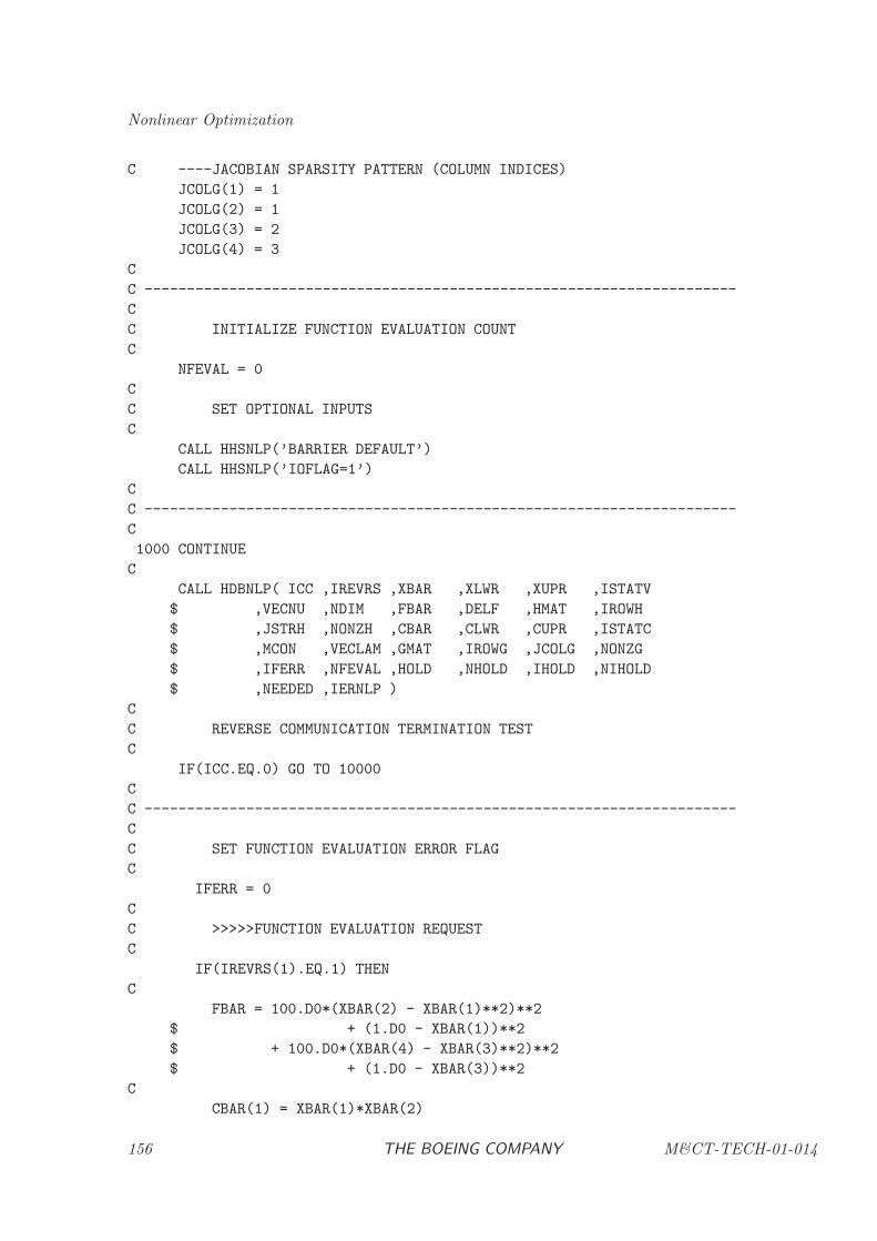
Nonlinear Optimization
C ----JACOBIAN SPARSITY PATTERN (COLUMN INDICES)
JCOLG(1) = 1
JCOLG(2) = 1
JCOLG(3) = 2
JCOLG(4) = 3
C
C ----------------------------------------------------------------------
C
C INITIALIZE FUNCTION EVALUATION COUNT
C
NFEVAL = 0
C
C SET OPTIONAL INPUTS
C
CALL HHSNLP(’BARRIER DEFAULT’)
CALL HHSNLP(’IOFLAG=1’)
C
C ----------------------------------------------------------------------
C
1000 CONTINUE
C
CALL HDBNLP( ICC ,IREVRS ,XBAR ,XLWR ,XUPR ,ISTATV
$ ,VECNU ,NDIM ,FBAR ,DELF ,HMAT ,IROWH
$ ,JSTRH ,NONZH ,CBAR ,CLWR ,CUPR ,ISTATC
$ ,MCON ,VECLAM ,GMAT ,IROWG ,JCOLG ,NONZG
$ ,IFERR ,NFEVAL ,HOLD ,NHOLD ,IHOLD ,NIHOLD
$ ,NEEDED ,IERNLP )
C
C REVERSE COMMUNICATION TERMINATION TEST
C
IF(ICC.EQ.0) GO TO 10000
C
C ----------------------------------------------------------------------
C
C SET FUNCTION EVALUATION ERROR FLAG
C
IFERR = 0
C
C >>>>>FUNCTION EVALUATION REQUEST
C
IF(IREVRS(1).EQ.1) THEN
C
FBAR = 100.D0*(XBAR(2) - XBAR(1)**2)**2
$ + (1.D0 - XBAR(1))**2
$ + 100.D0*(XBAR(4) - XBAR(3)**2)**2
$ + (1.D0 - XBAR(3))**2
C
CBAR(1) = XBAR(1)*XBAR(2)
156 THE BOEING COMPANY M&CT-TECH-01-014
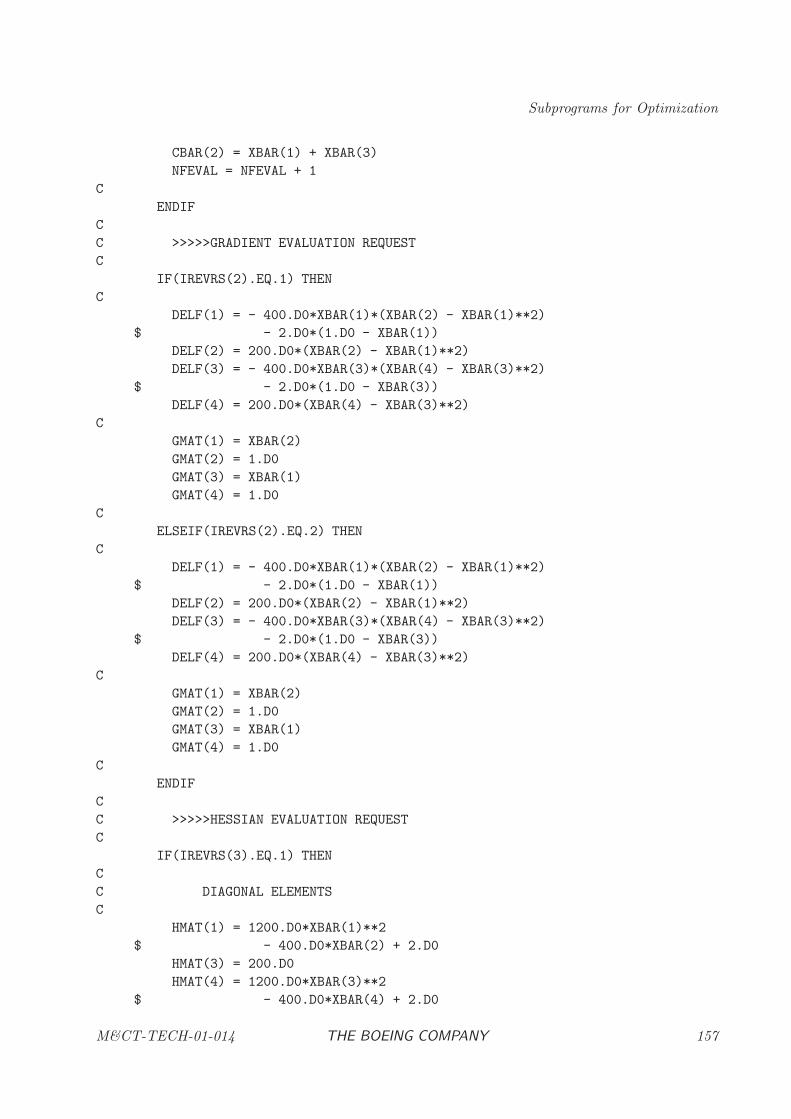
Subprograms for Optimization
CBAR(2) = XBAR(1) + XBAR(3)
NFEVAL = NFEVAL + 1
C
ENDIF
C
C >>>>>GRADIENT EVALUATION REQUEST
C
IF(IREVRS(2).EQ.1) THEN
C
DELF(1) = - 400.D0*XBAR(1)*(XBAR(2) - XBAR(1)**2)
$ - 2.D0*(1.D0 - XBAR(1))
DELF(2) = 200.D0*(XBAR(2) - XBAR(1)**2)
DELF(3) = - 400.D0*XBAR(3)*(XBAR(4) - XBAR(3)**2)
$ - 2.D0*(1.D0 - XBAR(3))
DELF(4) = 200.D0*(XBAR(4) - XBAR(3)**2)
C
GMAT(1) = XBAR(2)
GMAT(2) = 1.D0
GMAT(3) = XBAR(1)
GMAT(4) = 1.D0
C
ELSEIF(IREVRS(2).EQ.2) THEN
C
DELF(1) = - 400.D0*XBAR(1)*(XBAR(2) - XBAR(1)**2)
$ - 2.D0*(1.D0 - XBAR(1))
DELF(2) = 200.D0*(XBAR(2) - XBAR(1)**2)
DELF(3) = - 400.D0*XBAR(3)*(XBAR(4) - XBAR(3)**2)
$ - 2.D0*(1.D0 - XBAR(3))
DELF(4) = 200.D0*(XBAR(4) - XBAR(3)**2)
C
GMAT(1) = XBAR(2)
GMAT(2) = 1.D0
GMAT(3) = XBAR(1)
GMAT(4) = 1.D0
C
ENDIF
C
C >>>>>HESSIAN EVALUATION REQUEST
C
IF(IREVRS(3).EQ.1) THEN
C
C DIAGONAL ELEMENTS
C
HMAT(1) = 1200.D0*XBAR(1)**2
$ - 400.D0*XBAR(2) + 2.D0
HMAT(3) = 200.D0
HMAT(4) = 1200.D0*XBAR(3)**2
$ - 400.D0*XBAR(4) + 2.D0
M&CT-TECH-01-014 THE BOEING COMPANY 157
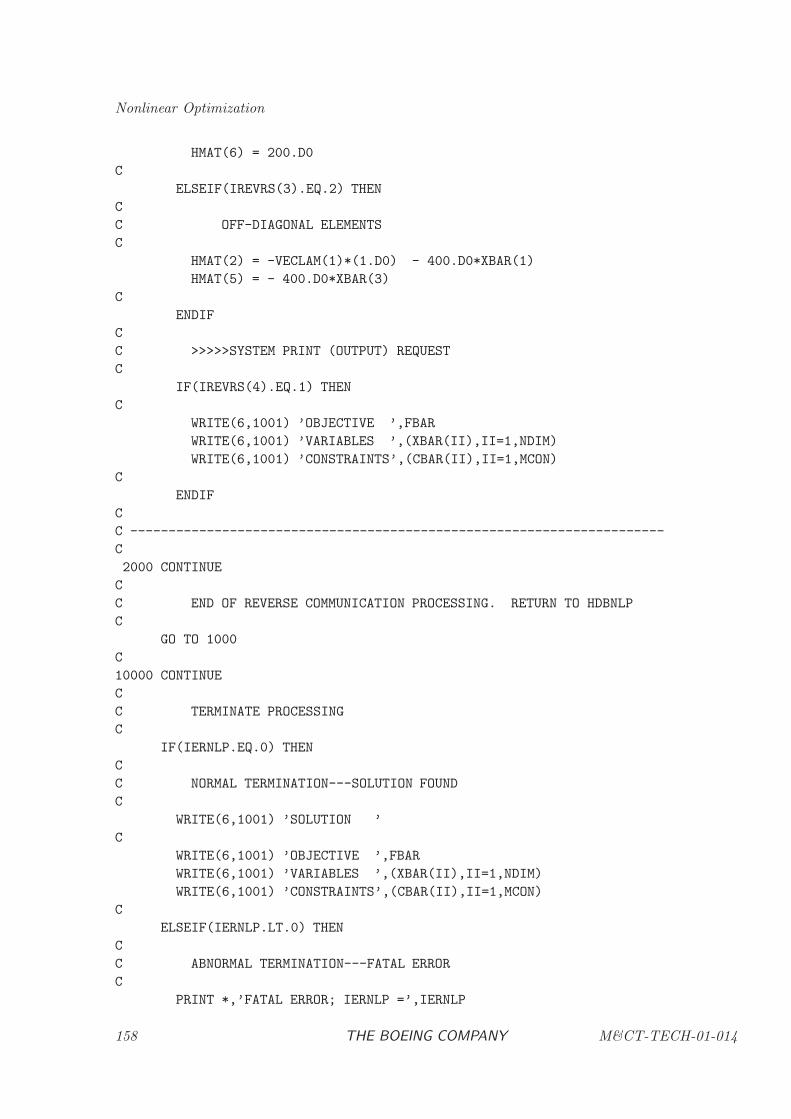
Nonlinear Optimization
HMAT(6) = 200.D0
C
ELSEIF(IREVRS(3).EQ.2) THEN
C
C OFF-DIAGONAL ELEMENTS
C
HMAT(2) = -VECLAM(1)*(1.D0) - 400.D0*XBAR(1)
HMAT(5) = - 400.D0*XBAR(3)
C
ENDIF
C
C >>>>>SYSTEM PRINT (OUTPUT) REQUEST
C
IF(IREVRS(4).EQ.1) THEN
C
WRITE(6,1001) ’OBJECTIVE ’,FBAR
WRITE(6,1001) ’VARIABLES ’,(XBAR(II),II=1,NDIM)
WRITE(6,1001) ’CONSTRAINTS’,(CBAR(II),II=1,MCON)
C
ENDIF
C
C ----------------------------------------------------------------------
C
2000 CONTINUE
C
C END OF REVERSE COMMUNICATION PROCESSING. RETURN TO HDBNLP
C
GO TO 1000
C
10000 CONTINUE
C
C TERMINATE PROCESSING
C
IF(IERNLP.EQ.0) THEN
C
C NORMAL TERMINATION---SOLUTION FOUND
C
WRITE(6,1001) ’SOLUTION ’
C
WRITE(6,1001) ’OBJECTIVE ’,FBAR
WRITE(6,1001) ’VARIABLES ’,(XBAR(II),II=1,NDIM)
WRITE(6,1001) ’CONSTRAINTS’,(CBAR(II),II=1,MCON)
C
ELSEIF(IERNLP.LT.0) THEN
C
C ABNORMAL TERMINATION---FATAL ERROR
C
PRINT *,’FATAL ERROR; IERNLP =’,IERNLP
158 THE BOEING COMPANY M&CT-TECH-01-014

Subprograms for Optimization
C
ELSE
C
C ABNORMAL TERMINATION---WARNING. EVALUATION OF RESULTS RECOMMENDED!
C
PRINT *,’WARNING MESSAGE; IERNLP =’,IERNLP
C
ENDIF
C
1001 FORMAT(5X,A11,5X,4G17.8)
C
STOP
END
OUTPUT FROM SAMPLE PROGRAM
Optimization
It Lnfltr KT Cond Step Levnbrg Cmplmt Barrier Violtn |Grdl| Obj Log-Barrier Fn
(1) 1 5.0E+04 2.5E-02 0.0E+00 0.0E+00 1.4E-01 1.5E+00 2.5E+02 2.0E+02 2.008936E+02
(2) 2 8.2E+06 1.0E+00 1.0E+00 1.4E-01 1.4E-01 1.5E+00 2.4E+02 2.0E+02 2.020735E+02
(3) 1 3.1E+05 6.6E-01 1.0E+00 2.3E-01 1.4E-02 6.9E-01 2.3E+02 9.9E+01 9.872009E+01
(4) 1 2.3E+06 1.0E+00 1.0E+00 2.0E-01 1.4E-02 2.1E-01 2.2E+02 4.8E+01 4.832725E+01
(5) 1 1.1E+06 1.0E+00 5.0E-01 4.4E-02 1.4E-02 9.1E-03 1.3E+02 9.1E+00 9.167177E+00
(6) 1 7.7E+03 1.0E+00 1.5E-01 3.0E-02 1.4E-02 4.4E-03 3.9E+01 4.2E+00 4.190492E+00
(7) 2 3.6E+03 1.0E+00 1.5E-02 2.3E-01 1.4E-02 3.5E-03 3.9E+00 3.7E+00 3.674143E+00
(8) 2 5.1E+02 1.0E+00 1.5E-02 8.9E-03 1.4E-02 8.3E-02 1.5E+01 3.2E+00 3.152611E+00
(9) 1 5.7E+02 1.0E+00 7.7E-03 4.1E-03 1.4E-02 2.2E-02 1.2E+01 2.6E+00 2.583827E+00
(10) 2 7.1E+02 3.8E-01 3.8E-03 1.0E-02 1.4E-02 5.4E-02 1.2E+01 2.0E+00 1.983696E+00
(11) 2 2.1E+03 1.0E+00 1.9E-03 1.4E-02 1.4E-02 3.3E-02 7.7E+00 1.7E+00 1.735478E+00
(12) 1 1.3E+03 8.1E-01 8.3E-04 1.8E-02 1.4E-02 2.7E-04 3.3E+00 1.5E+00 1.437484E+00
(13) 1 1.4E+04 1.0E+00 4.1E-04 1.3E-02 1.4E-02 2.5E-03 2.9E+00 1.3E+00 1.335245E+00
(14) 1 7.7E+02 1.0E+00 1.9E-04 1.4E-03 1.2E-02 9.4E-04 1.5E+00 1.2E+00 1.211659E+00
(15) 1 7.0E+02 1.0E+00 9.3E-05 1.1E-04 1.2E-02 1.3E-03 1.3E+00 1.2E+00 1.166334E+00
(16) 1 4.6E+02 1.0E+00 2.7E-05 6.1E-06 1.2E-02 8.4E-04 3.8E-01 1.1E+00 1.144744E+00
(17) 1 4.2E+02 1.0E+00 1.4E-05 7.1E-06 1.2E-02 7.1E-04 3.3E-01 1.1E+00 1.138631E+00
(18) 1 3.3E+02 1.0E+00 1.1E-07 1.1E-02 1.2E-03 8.1E-05 2.7E-02 1.1E+00 1.137412E+00
(19) 1 1.8E+03 1.0E+00 0.0E+00 1.2E-03 1.2E-04 3.4E-05 1.4E-02 1.1E+00 1.126633E+00
(20) 1 1.8E+04 1.0E+00 0.0E+00 1.1E-04 1.2E-05 3.2E-07 1.1E-04 1.1E+00 1.125183E+00
(21) 1 1.8E+05 1.0E+00 0.0E+00 1.2E-05 1.5E-09 1.5E-09 6.0E-07 1.1E+00 1.125012E+00
(22) 1 1.8E+05 1.0E+00 0.0E+00 1.4E-10 1.5E-09 1.5E-11 1.2E-07 1.1E+00 1.125000E+00
-------------------------------------------------------------------------------------------
| |
| BARNLP ALGORITHM PERFORMANCE STATISTICS |
| |
| Total CPU Time.....................................................+4.383216E-02 |
| |
| Number of Function Calls......................................................22 |
| Number of Gradient Calls......................................................23 |
| Number of Hessian Calls.......................................................20 |
| Total Number of Function Evaluations..........................................22 |
| |
| Storage Needed in HOLD Array.................................................762 |
| Storage Needed in IHOLD Array................................................141 |
| |
-------------------------------------------------------------------------------------------
M&CT-TECH-01-014 THE BOEING COMPANY 159

Nonlinear Optimization
SOLUTION
OBJECTIVE 1.1250000
VARIABLES 0.25000000 0.62499999E-01 0.25000000 0.62500000E-01
CONSTRAINTS 0.15625000E-01 0.50000000
160 THE BOEING COMPANY M&CT-TECH-01-014
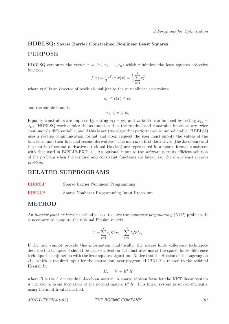
Subprograms for Optimization
HDBLSQ: Sparse Barrier Constrained Nonlinear Least Squares
PURPOSE
HDBLSQ computes the vector x = (x1, x2, . . . , xn) which minimizes the least squares objectivefunction
f(x) =1
2rT (x)r(x) =
1
2
ℓ∑
i=1
r2i
where r(x) is an ℓ-vector of residuals, subject to the m nonlinear constraints
cL ≤ c(x) ≤ cU
and the simple boundsxL ≤ x ≤ xU
Equality constraints are imposed by setting cLi = cUi and variables can be fixed by setting xLi =xUi. HDBLSQ works under the assumption that the residual and constraint functions are twicecontinuously differentiable, and if this is not true algorithm performance is unpredictable. HDBLSQuses a reverse communication format and upon request the user must supply the values of thefunctions, and their first and second derivatives. The matrix of first derivatives (the Jacobian) andthe matrix of second derivatives (residual Hessian) are represented in a sparse format consistentwith that used in BCSLIB-EXT [1]. An optional input to the software permits efficient solutionof the problem when the residual and constraint functions are linear, i.e. the linear least squaresproblem.
RELATED SUBPROGRAMS
HDBNLP Sparse Barrier Nonlinear Programming
HHSNLP Sparse Nonlinear Programming Input Procedure
METHOD
An interior point or barrier method is used to solve the nonlinear programming (NLP) problem. Itis necessary to compute the residual Hessian matrix
V =ℓ∑
i=1
ri∇2ri −m∑
i=1
λi∇2ci.
If the user cannot provide this information analytically, the sparse finite difference techniquesdescribed in Chapter 3 should be utilized. Section 4.4 illustrates use of the sparse finite differencetechnique in conjunction with the least squares algorithm. Notice that the Hessian of the LagrangianHL, which is required input for the sparse nonlinear program HDBNLP is related to the residualHessian by
HL = V +RTR
where R is the ℓ× n residual Jacobian matrix. A sparse tableau form for the KKT linear systemis utilized to avoid formation of the normal matrix RTR. This linear system is solved efficientlyusing the multifrontal method.
M&CT-TECH-01-014 THE BOEING COMPANY 161
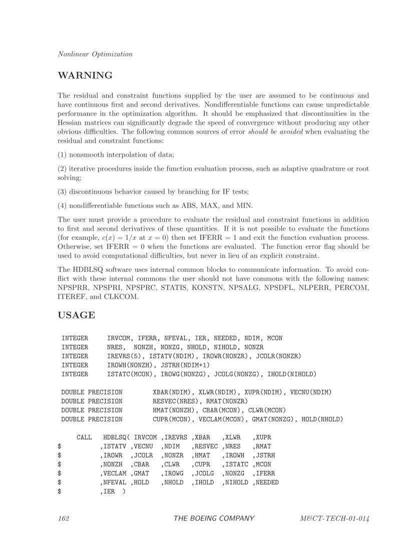
Nonlinear Optimization
WARNING
The residual and constraint functions supplied by the user are assumed to be continuous andhave continuous first and second derivatives. Nondifferentiable functions can cause unpredictableperformance in the optimization algorithm. It should be emphasized that discontinuities in theHessian matrices can significantly degrade the speed of convergence without producing any otherobvious difficulties. The following common sources of error should be avoided when evaluating theresidual and constraint functions:
(1) nonsmooth interpolation of data;
(2) iterative procedures inside the function evaluation process, such as adaptive quadrature or rootsolving;
(3) discontinuous behavior caused by branching for IF tests;
(4) nondifferentiable functions such as ABS, MAX, and MIN.
The user must provide a procedure to evaluate the residual and constraint functions in additionto first and second derivatives of these quantities. If it is not possible to evaluate the functions(for example, c(x) = 1/x at x = 0) then set IFERR = 1 and exit the function evaluation process.Otherwise, set IFERR = 0 when the functions are evaluated. The function error flag should beused to avoid computational difficulties, but never in lieu of an explicit constraint.
The HDBLSQ software uses internal common blocks to communicate information. To avoid con-flict with these internal commons the user should not have commons with the following names:NPSPRR, NPSPRI, NPSPRC, STATIS, KONSTN, NPSALG, NPSDFL, NLPERR, PERCOM,ITEREF, and CLKCOM.
USAGE
INTEGER IRVCOM, IFERR, NFEVAL, IER, NEEDED, NDIM, MCON
INTEGER NRES, NONZH, NONZG, NHOLD, NIHOLD, NONZR
INTEGER IREVRS(5), ISTATV(NDIM), IROWR(NONZR), JCOLR(NONZR)
INTEGER IROWH(NONZH), JSTRH(NDIM+1)
INTEGER ISTATC(MCON), IROWG(NONZG), JCOLG(NONZG), IHOLD(NIHOLD)
DOUBLE PRECISION XBAR(NDIM), XLWR(NDIM), XUPR(NDIM), VECNU(NDIM)
DOUBLE PRECISION RESVEC(NRES), RMAT(NONZR)
DOUBLE PRECISION HMAT(NONZH), CBAR(MCON), CLWR(MCON)
DOUBLE PRECISION CUPR(MCON), VECLAM(MCON), GMAT(NONZG), HOLD(NHOLD)
CALL HDBLSQ( IRVCOM ,IREVRS ,XBAR ,XLWR ,XUPR
$ ,ISTATV ,VECNU ,NDIM ,RESVEC ,NRES ,RMAT
$ ,IROWR ,JCOLR ,NONZR ,HMAT ,IROWH ,JSTRH
$ ,NONZH ,CBAR ,CLWR ,CUPR ,ISTATC ,MCON
$ ,VECLAM ,GMAT ,IROWG ,JCOLG ,NONZG ,IFERR
$ ,NFEVAL ,HOLD ,NHOLD ,IHOLD ,NIHOLD ,NEEDED
$ ,IER )
162 THE BOEING COMPANY M&CT-TECH-01-014
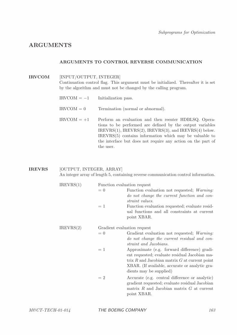
Subprograms for Optimization
ARGUMENTS
ARGUMENTS TO CONTROL REVERSE COMMUNICATION
IRVCOM [INPUT/OUTPUT, INTEGER]Continuation control flag. This argument must be initialized. Thereafter it is setby the algorithm and must not be changed by the calling program.
IRVCOM = −1 Initialization pass.
IRVCOM = 0 Termination (normal or abnormal).
IRVCOM = +1 Perform an evaluation and then reenter HDBLSQ. Opera-tions to be performed are defined by the output variablesIREVRS(1), IREVRS(2), IREVRS(3), and IREVRS(4) below.IREVRS(5) contains information which may be valuable tothe interface but does not require any action on the part ofthe user.
IREVRS [OUTPUT, INTEGER, ARRAY]An integer array of length 5, containing reverse communication control information.
IREVRS(1) Function evaluation request= 0 Function evaluation not requested; Warning:
do not change the current function and con-straint values.
= 1 Function evaluation requested; evaluate resid-ual functions and all constraints at currentpoint XBAR.
IREVRS(2) Gradient evaluation request= 0 Gradient evaluation not requested; Warning:
do not change the current residual and con-straint and Jacobians.
= 1 Approximate (e.g. forward difference) gradi-ent requested; evaluate residual Jacobian ma-trix R and Jacobian matrix G at current pointXBAR. (If available, accurate or analytic gra-dients may be supplied)
= 2 Accurate (e.g. central difference or analytic)gradient requested; evaluate residual Jacobianmatrix R and Jacobian matrix G at currentpoint XBAR.
M&CT-TECH-01-014 THE BOEING COMPANY 163
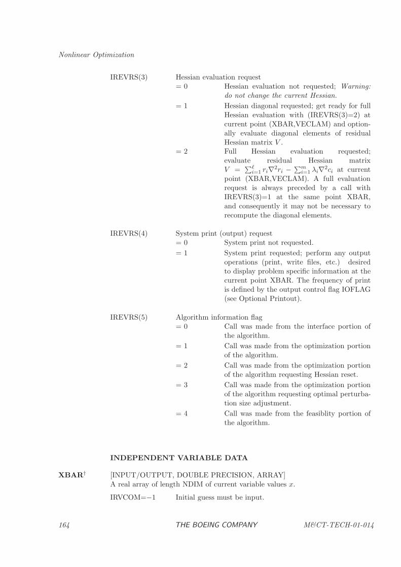
Nonlinear Optimization
IREVRS(3) Hessian evaluation request= 0 Hessian evaluation not requested; Warning:
do not change the current Hessian.
= 1 Hessian diagonal requested; get ready for fullHessian evaluation with (IREVRS(3)=2) atcurrent point (XBAR,VECLAM) and option-ally evaluate diagonal elements of residualHessian matrix V .
= 2 Full Hessian evaluation requested;evaluate residual Hessian matrixV =
∑ℓi=1 ri∇2ri −
∑mi=1 λi∇2ci at current
point (XBAR,VECLAM). A full evaluationrequest is always preceded by a call withIREVRS(3)=1 at the same point XBAR,and consequently it may not be necessary torecompute the diagonal elements.
IREVRS(4) System print (output) request= 0 System print not requested.
= 1 System print requested; perform any outputoperations (print, write files, etc.) desiredto display problem specific information at thecurrent point XBAR. The frequency of printis defined by the output control flag IOFLAG(see Optional Printout).
IREVRS(5) Algorithm information flag= 0 Call was made from the interface portion of
the algorithm.
= 1 Call was made from the optimization portionof the algorithm.
= 2 Call was made from the optimization portionof the algorithm requesting Hessian reset.
= 3 Call was made from the optimization portionof the algorithm requesting optimal perturba-tion size adjustment.
= 4 Call was made from the feasiblity portion ofthe algorithm.
INDEPENDENT VARIABLE DATA
XBAR† [INPUT/OUTPUT, DOUBLE PRECISION, ARRAY]A real array of length NDIM of current variable values x.
IRVCOM=−1 Initial guess must be input.
164 THE BOEING COMPANY M&CT-TECH-01-014
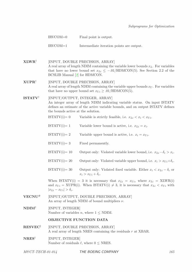
Subprograms for Optimization
IRVCOM=0 Final point is output.
IRVCOM=1 Intermediate iteration points are output.
XLWR† [INPUT, DOUBLE PRECISION, ARRAY]A real array of length NDIM containing the variable lower bounds xL. For variablesthat have no lower bound set xLi ≤ −.01/HDMCON(5). See Section 2.2 of theBCSLIB Manual [2] for HDMCON.
XUPR† [INPUT, DOUBLE PRECISION, ARRAY]A real array of length NDIM containing the variable upper bounds xU . For variablesthat have no upper bound set xUi ≥ .01/HDMCON(5).
ISTATV† [INPUT/OUTPUT, INTEGER, ARRAY]An integer array of length NDIM indicating variable status. On input ISTATVdefines an estimate of the active variable bounds, and on output ISTATV definesthe bounds active at the solution.
ISTATV(i)= 0 Variable is strictly feasible, i.e. xLi < xi < xUi.
ISTATV(i)= 1 Variable lower bound is active, i.e. xLi = xi.
ISTATV(i)= 2 Variable upper bound is active, i.e. xi = xUi.
ISTATV(i)= 3 Fixed permanently.
ISTATV(i)= 10 Output only: Violated variable lower bound, i.e. xLi−δc > xi.
ISTATV(i)= 20 Output only: Violated variable upper bound, i.e. xi > xUi+δc.
ISTATV(i)= 30 Output only: Violated fixed variable. Either xi < xLi − δc orxi > xUi + δc.
When ISTATV(i) = 3 it is necessary that xLi = xUi, where xLi = XLWR(i)and xUi = XUPR(i). When ISTATV(i) 6= 3, it is necessary that xLi < xUi with|xLi − xUi| > δc.
VECNU# [INPUT/OUTPUT, DOUBLE PRECISION, ARRAY]An array of length NDIM of bound multipliers ν.
NDIM† [INPUT, INTEGER]Number of variables n, where 1 ≤ NDIM.
OBJECTIVE FUNCTION DATA
RESVEC‡ [INPUT, DOUBLE PRECISION, ARRAY]A real array of length NRES containing the residuals r at XBAR.
NRES† [INPUT, INTEGER]Number of residuals ℓ, where 0 ≤ NRES.
M&CT-TECH-01-014 THE BOEING COMPANY 165
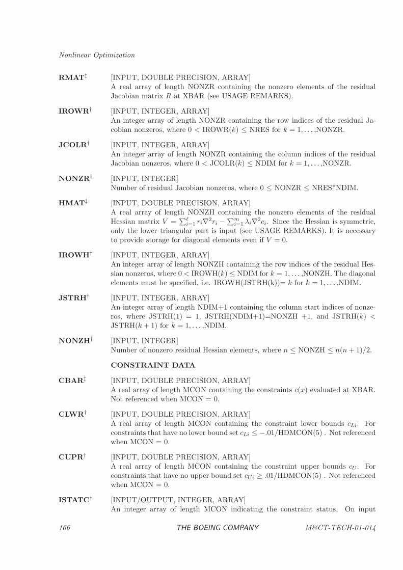
Nonlinear Optimization
RMAT‡ [INPUT, DOUBLE PRECISION, ARRAY]A real array of length NONZR containing the nonzero elements of the residualJacobian matrix R at XBAR (see USAGE REMARKS).
IROWR† [INPUT, INTEGER, ARRAY]An integer array of length NONZR containing the row indices of the residual Ja-cobian nonzeros, where 0 < IROWR(k) ≤ NRES for k = 1, . . . ,NONZR.
JCOLR† [INPUT, INTEGER, ARRAY]An integer array of length NONZR containing the column indices of the residualJacobian nonzeros, where 0 < JCOLR(k) ≤ NDIM for k = 1, . . . ,NONZR.
NONZR† [INPUT, INTEGER]Number of residual Jacobian nonzeros, where 0 ≤ NONZR ≤ NRES*NDIM.
HMAT‡ [INPUT, DOUBLE PRECISION, ARRAY]A real array of length NONZH containing the nonzero elements of the residualHessian matrix V =
∑ℓi=1 ri∇2ri −
∑mi=1 λi∇2ci. Since the Hessian is symmetric,
only the lower triangular part is input (see USAGE REMARKS). It is necessaryto provide storage for diagonal elements even if V = 0.
IROWH† [INPUT, INTEGER, ARRAY]An integer array of length NONZH containing the row indices of the residual Hes-sian nonzeros, where 0 < IROWH(k) ≤ NDIM for k = 1, . . . ,NONZH. The diagonalelements must be specified, i.e. IROWH(JSTRH(k))= k for k = 1, . . . ,NDIM.
JSTRH† [INPUT, INTEGER, ARRAY]An integer array of length NDIM+1 containing the column start indices of nonze-ros, where JSTRH(1) = 1, JSTRH(NDIM+1)=NONZH +1, and JSTRH(k) <JSTRH(k + 1) for k = 1, . . . ,NDIM.
NONZH† [INPUT, INTEGER]Number of nonzero residual Hessian elements, where n ≤ NONZH ≤ n(n+ 1)/2.
CONSTRAINT DATA
CBAR‡ [INPUT, DOUBLE PRECISION, ARRAY]A real array of length MCON containing the constraints c(x) evaluated at XBAR.Not referenced when MCON = 0.
CLWR† [INPUT, DOUBLE PRECISION, ARRAY]A real array of length MCON containing the constraint lower bounds cLi. Forconstraints that have no lower bound set cLi ≤ −.01/HDMCON(5) . Not referencedwhen MCON = 0.
CUPR† [INPUT, DOUBLE PRECISION, ARRAY]A real array of length MCON containing the constraint upper bounds cU . Forconstraints that have no upper bound set cUi ≥ .01/HDMCON(5) . Not referencedwhen MCON = 0.
ISTATC† [INPUT/OUTPUT, INTEGER, ARRAY]An integer array of length MCON indicating the constraint status. On input
166 THE BOEING COMPANY M&CT-TECH-01-014
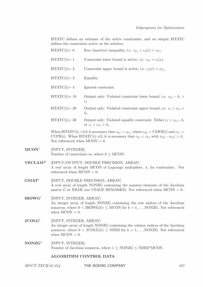
Subprograms for Optimization
ISTATC defines an estimate of the active constraints, and on output ISTATCdefines the constraints active at the solution.
ISTATC(i)= 0 Free (inactive) inequality, i.e. cLi < ci(x) < cUi.
ISTATC(i)= 1 Constraint lower bound is active, i.e. cLi = ci(x).
ISTATC(i)= 2 Constraint upper bound is active, i.e. ci(x) = cUi.
ISTATC(i)= 3 Equality.
ISTATC(i)= 4 Ignored constraint.
ISTATC(i)= 10 Output only: Violated constraint lower bound, i.e. cLi − δc >ci.
ISTATC(i)= 20 Output only: Violated constraint upper bound, i.e. ci > cUi +δc.
ISTATC(i)= 30 Output only: Violated equality constraint. Either ci < cLi−δcor ci > cUi + δc.
When ISTATC(i) =3 it is necessary that cLi = cUi, where cLi = CLWR(i) and cUi =CUPR(i). When ISTATC(i) 6=3, it is necessary that cLi < cUi with |cLi−cUi| > δc.Not referenced when MCON = 0.
MCON† [INPUT, INTEGER]Number of constraints m, where 0 ≤ MCON.
VECLAM# [INPUT/OUTPUT, DOUBLE PRECISION, ARRAY]A real array of length MCON of Lagrange multipliers, λ, for constraints. Notreferenced when MCON = 0.
GMAT‡ [INPUT, DOUBLE PRECISION, ARRAY]A real array of length NONZG containing the nonzero elements of the Jacobianmatrix G at XBAR (see USAGE REMARKS). Not referenced when MCON = 0.
IROWG† [INPUT, INTEGER, ARRAY]An integer array of length NONZG containing the row indices of the Jacobiannonzeros, where 0 < IROWG(k) ≤ MCON for k = 1, . . . ,NONZG. Not referencedwhen MCON = 0.
JCOLG† [INPUT, INTEGER, ARRAY]An integer array of length NONZG containing the column indices of the Jacobiannonzeros, where 0 < JCOLG(k) ≤ NDIM for k = 1, . . . ,NONZG. Not referencedwhen MCON = 0.
NONZG† [INPUT, INTEGER]Number of Jacobian nonzeros, where 1 ≤ NONZG ≤ NDIM*MCON.
ALGORITHM CONTROL DATA
M&CT-TECH-01-014 THE BOEING COMPANY 167
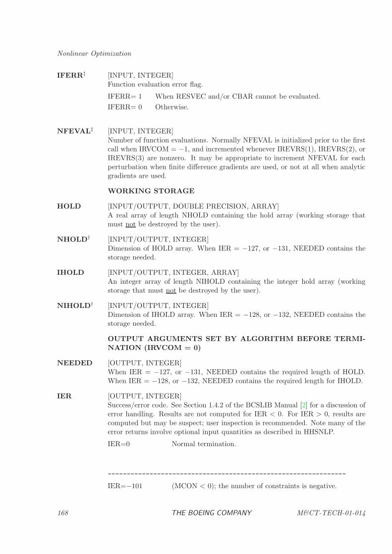
Nonlinear Optimization
IFERR‡ [INPUT, INTEGER]Function evaluation error flag.
IFERR= 1 When RESVEC and/or CBAR cannot be evaluated.
IFERR= 0 Otherwise.
NFEVAL‡ [INPUT, INTEGER]Number of function evaluations. Normally NFEVAL is initialized prior to the firstcall when IRVCOM = −1, and incremented whenever IREVRS(1), IREVRS(2), orIREVRS(3) are nonzero. It may be appropriate to increment NFEVAL for eachperturbation when finite difference gradients are used, or not at all when analyticgradients are used.
WORKING STORAGE
HOLD [INPUT/OUTPUT, DOUBLE PRECISION, ARRAY]A real array of length NHOLD containing the hold array (working storage thatmust not be destroyed by the user).
NHOLD† [INPUT/OUTPUT, INTEGER]Dimension of HOLD array. When IER = −127, or −131, NEEDED contains thestorage needed.
IHOLD [INPUT/OUTPUT, INTEGER, ARRAY]An integer array of length NIHOLD containing the integer hold array (workingstorage that must not be destroyed by the user).
NIHOLD† [INPUT/OUTPUT, INTEGER]Dimension of IHOLD array. When IER = −128, or −132, NEEDED contains thestorage needed.
OUTPUT ARGUMENTS SET BY ALGORITHM BEFORE TERMI-NATION (IRVCOM = 0)
NEEDED [OUTPUT, INTEGER]When IER = −127, or −131, NEEDED contains the required length of HOLD.When IER = −128, or −132, NEEDED contains the required length for IHOLD.
IER [OUTPUT, INTEGER]Success/error code. See Section 1.4.2 of the BCSLIB Manual [2] for a discussion oferror handling. Results are not computed for IER < 0. For IER > 0, results arecomputed but may be suspect; user inspection is recommended. Note many of theerror returns involve optional input quantities as described in HHSNLP.
IER=0 Normal termination.
---------------------------------------------------------------
IER=−101 (MCON < 0); the number of constraints is negative.
168 THE BOEING COMPANY M&CT-TECH-01-014
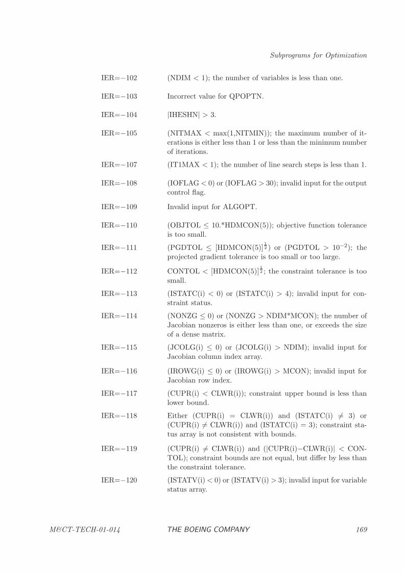
Subprograms for Optimization
IER=−102 (NDIM < 1); the number of variables is less than one.
IER=−103 Incorrect value for QPOPTN.
IER=−104 |IHESHN| > 3.
IER=−105 (NITMAX < max(1,NITMIN)); the maximum number of it-erations is either less than 1 or less than the minimum numberof iterations.
IER=−107 (IT1MAX < 1); the number of line search steps is less than 1.
IER=−108 (IOFLAG< 0) or (IOFLAG > 30); invalid input for the outputcontrol flag.
IER=−109 Invalid input for ALGOPT.
IER=−110 (OBJTOL ≤ 10.*HDMCON(5)); objective function toleranceis too small.
IER=−111 (PGDTOL ≤ [HDMCON(5)]12 ) or (PGDTOL > 10−2); the
projected gradient tolerance is too small or too large.
IER=−112 CONTOL < [HDMCON(5)]12 ; the constraint tolerance is too
small.
IER=−113 (ISTATC(i) < 0) or (ISTATC(i) > 4); invalid input for con-straint status.
IER=−114 (NONZG ≤ 0) or (NONZG > NDIM*MCON); the number ofJacobian nonzeros is either less than one, or exceeds the sizeof a dense matrix.
IER=−115 (JCOLG(i) ≤ 0) or (JCOLG(i) > NDIM); invalid input forJacobian column index array.
IER=−116 (IROWG(i) ≤ 0) or (IROWG(i) > MCON); invalid input forJacobian row index.
IER=−117 (CUPR(i) < CLWR(i)); constraint upper bound is less thanlower bound.
IER=−118 Either (CUPR(i) = CLWR(i)) and (ISTATC(i) 6= 3) or(CUPR(i) 6= CLWR(i)) and (ISTATC(i) = 3); constraint sta-tus array is not consistent with bounds.
IER=−119 (CUPR(i) 6= CLWR(i)) and (|CUPR(i)−CLWR(i)| < CON-TOL); constraint bounds are not equal, but differ by less thanthe constraint tolerance.
IER=−120 (ISTATV(i)< 0) or (ISTATV(i) > 3); invalid input for variablestatus array.
M&CT-TECH-01-014 THE BOEING COMPANY 169
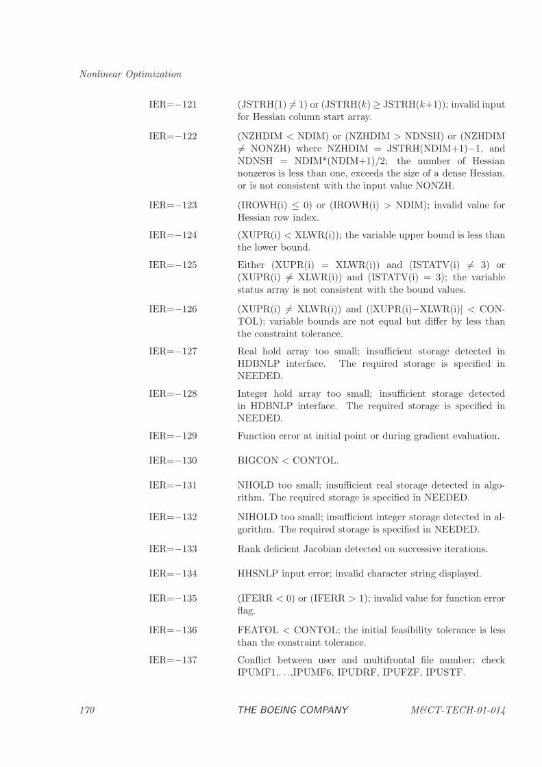
Nonlinear Optimization
IER=−121 (JSTRH(1) 6= 1) or (JSTRH(k) ≥ JSTRH(k+1)); invalid inputfor Hessian column start array.
IER=−122 (NZHDIM < NDIM) or (NZHDIM > NDNSH) or (NZHDIM6= NONZH) where NZHDIM = JSTRH(NDIM+1)−1, andNDNSH = NDIM*(NDIM+1)/2; the number of Hessiannonzeros is less than one, exceeds the size of a dense Hessian,or is not consistent with the input value NONZH.
IER=−123 (IROWH(i) ≤ 0) or (IROWH(i) > NDIM); invalid value forHessian row index.
IER=−124 (XUPR(i) < XLWR(i)); the variable upper bound is less thanthe lower bound.
IER=−125 Either (XUPR(i) = XLWR(i)) and (ISTATV(i) 6= 3) or(XUPR(i) 6= XLWR(i)) and (ISTATV(i) = 3); the variablestatus array is not consistent with the bound values.
IER=−126 (XUPR(i) 6= XLWR(i)) and (|XUPR(i)−XLWR(i)| < CON-TOL); variable bounds are not equal but differ by less thanthe constraint tolerance.
IER=−127 Real hold array too small; insufficient storage detected inHDBNLP interface. The required storage is specified inNEEDED.
IER=−128 Integer hold array too small; insufficient storage detectedin HDBNLP interface. The required storage is specified inNEEDED.
IER=−129 Function error at initial point or during gradient evaluation.
IER=−130 BIGCON < CONTOL.
IER=−131 NHOLD too small; insufficient real storage detected in algo-rithm. The required storage is specified in NEEDED.
IER=−132 NIHOLD too small; insufficient integer storage detected in al-gorithm. The required storage is specified in NEEDED.
IER=−133 Rank deficient Jacobian detected on successive iterations.
IER=−134 HHSNLP input error; invalid character string displayed.
IER=−135 (IFERR < 0) or (IFERR > 1); invalid value for function errorflag.
IER=−136 FEATOL < CONTOL; the initial feasibility tolerance is lessthan the constraint tolerance.
IER=−137 Conflict between user and multifrontal file number; checkIPUMF1,. . .,IPUMF6, IPUDRF, IPUFZF, IPUSTF.
170 THE BOEING COMPANY M&CT-TECH-01-014
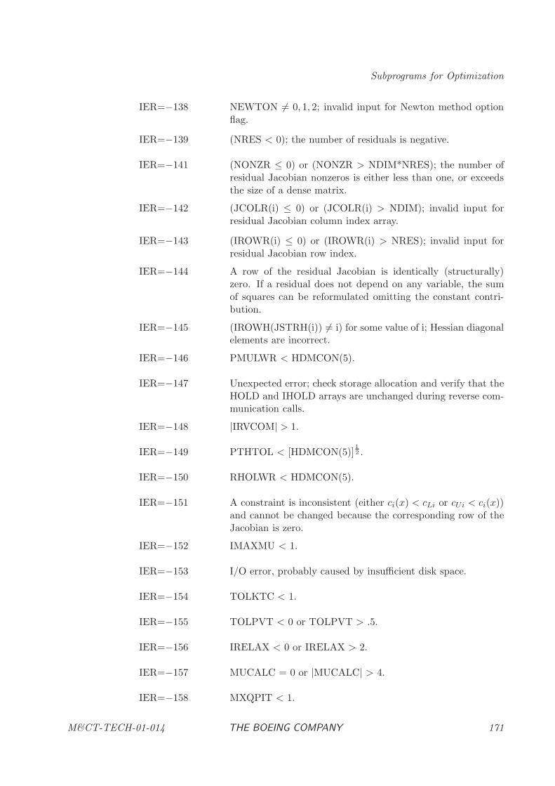
Subprograms for Optimization
IER=−138 NEWTON 6= 0, 1, 2; invalid input for Newton method optionflag.
IER=−139 (NRES < 0); the number of residuals is negative.
IER=−141 (NONZR ≤ 0) or (NONZR > NDIM*NRES); the number ofresidual Jacobian nonzeros is either less than one, or exceedsthe size of a dense matrix.
IER=−142 (JCOLR(i) ≤ 0) or (JCOLR(i) > NDIM); invalid input forresidual Jacobian column index array.
IER=−143 (IROWR(i) ≤ 0) or (IROWR(i) > NRES); invalid input forresidual Jacobian row index.
IER=−144 A row of the residual Jacobian is identically (structurally)zero. If a residual does not depend on any variable, the sumof squares can be reformulated omitting the constant contri-bution.
IER=−145 (IROWH(JSTRH(i)) 6= i) for some value of i; Hessian diagonalelements are incorrect.
IER=−146 PMULWR < HDMCON(5).
IER=−147 Unexpected error; check storage allocation and verify that theHOLD and IHOLD arrays are unchanged during reverse com-munication calls.
IER=−148 |IRVCOM| > 1.
IER=−149 PTHTOL < [HDMCON(5)]12 .
IER=−150 RHOLWR < HDMCON(5).
IER=−151 A constraint is inconsistent (either ci(x) < cLi or cUi < ci(x))and cannot be changed because the corresponding row of theJacobian is zero.
IER=−152 IMAXMU < 1.
IER=−153 I/O error, probably caused by insufficient disk space.
IER=−154 TOLKTC < 1.
IER=−155 TOLPVT < 0 or TOLPVT > .5.
IER=−156 IRELAX < 0 or IRELAX > 2.
IER=−157 MUCALC = 0 or |MUCALC| > 4.
IER=−158 MXQPIT < 1.
M&CT-TECH-01-014 THE BOEING COMPANY 171
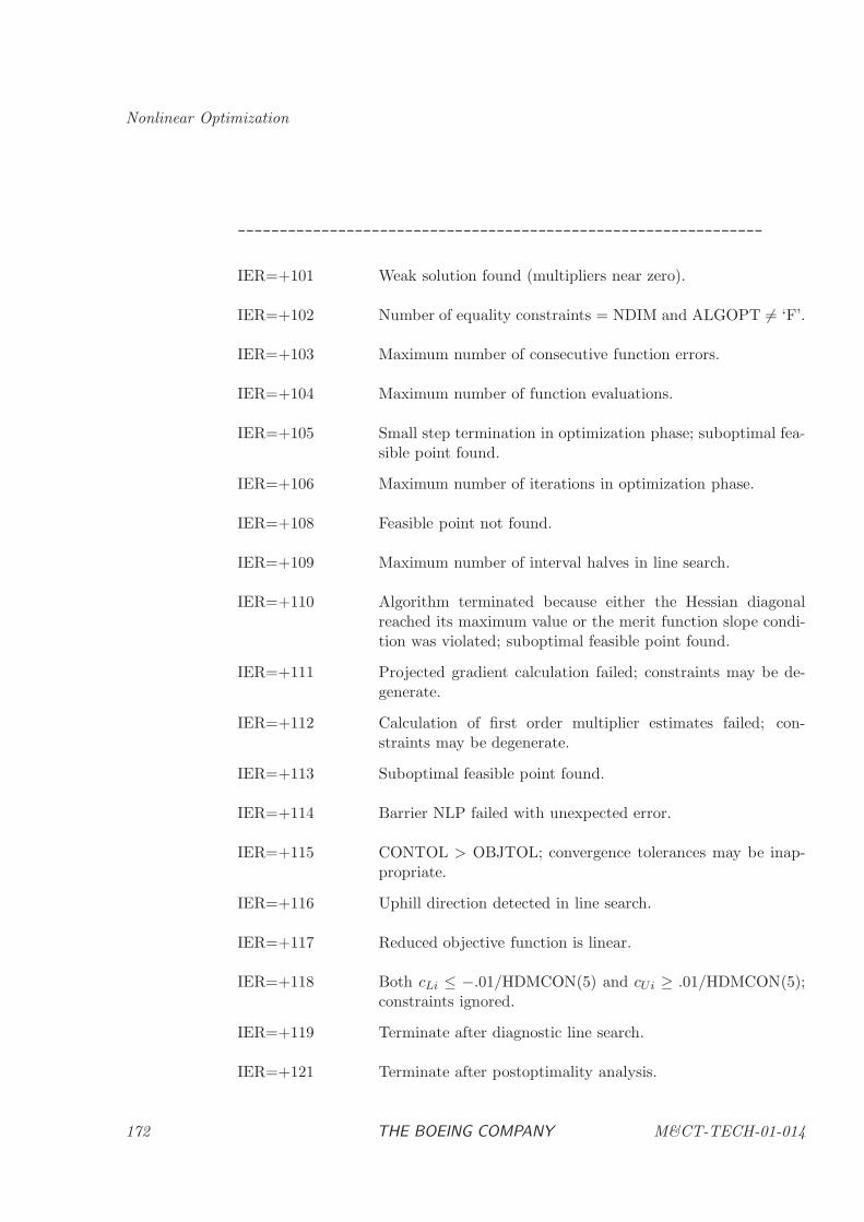
Nonlinear Optimization
---------------------------------------------------------------
IER=+101 Weak solution found (multipliers near zero).
IER=+102 Number of equality constraints = NDIM and ALGOPT 6= ‘F’.
IER=+103 Maximum number of consecutive function errors.
IER=+104 Maximum number of function evaluations.
IER=+105 Small step termination in optimization phase; suboptimal fea-sible point found.
IER=+106 Maximum number of iterations in optimization phase.
IER=+108 Feasible point not found.
IER=+109 Maximum number of interval halves in line search.
IER=+110 Algorithm terminated because either the Hessian diagonalreached its maximum value or the merit function slope condi-tion was violated; suboptimal feasible point found.
IER=+111 Projected gradient calculation failed; constraints may be de-generate.
IER=+112 Calculation of first order multiplier estimates failed; con-straints may be degenerate.
IER=+113 Suboptimal feasible point found.
IER=+114 Barrier NLP failed with unexpected error.
IER=+115 CONTOL > OBJTOL; convergence tolerances may be inap-propriate.
IER=+116 Uphill direction detected in line search.
IER=+117 Reduced objective function is linear.
IER=+118 Both cLi ≤ −.01/HDMCON(5) and cUi ≥ .01/HDMCON(5);constraints ignored.
IER=+119 Terminate after diagnostic line search.
IER=+121 Terminate after postoptimality analysis.
172 THE BOEING COMPANY M&CT-TECH-01-014
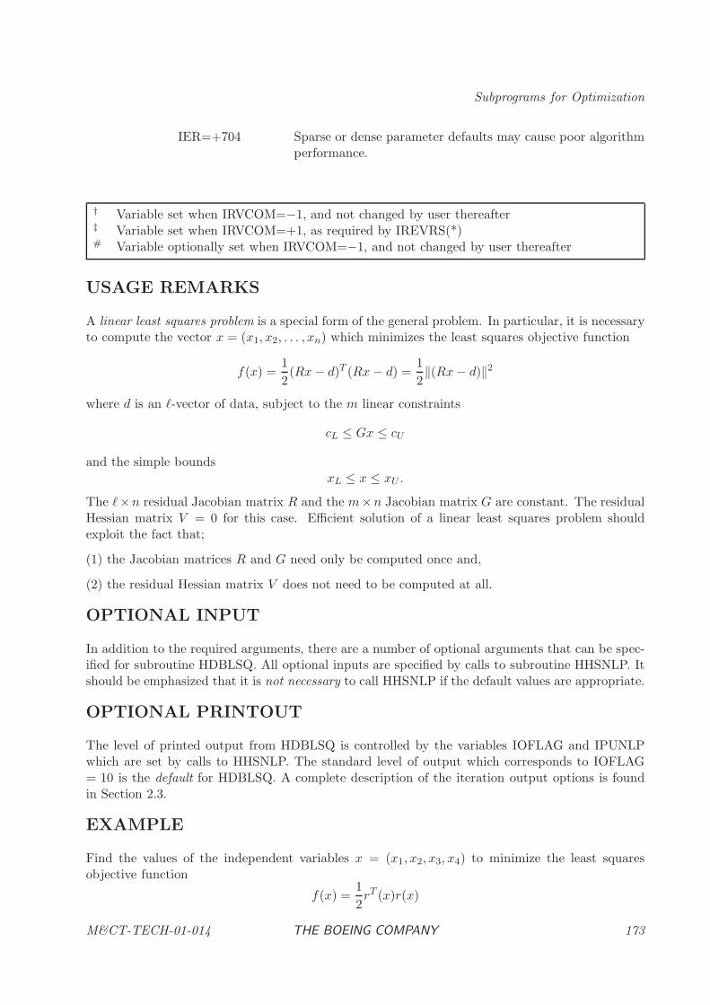
Subprograms for Optimization
IER=+704 Sparse or dense parameter defaults may cause poor algorithmperformance.
† Variable set when IRVCOM=−1, and not changed by user thereafter‡ Variable set when IRVCOM=+1, as required by IREVRS(*)# Variable optionally set when IRVCOM=−1, and not changed by user thereafter
USAGE REMARKS
A linear least squares problem is a special form of the general problem. In particular, it is necessaryto compute the vector x = (x1, x2, . . . , xn) which minimizes the least squares objective function
f(x) =1
2(Rx− d)T (Rx− d) =
1
2‖(Rx− d)‖2
where d is an ℓ-vector of data, subject to the m linear constraints
cL ≤ Gx ≤ cU
and the simple boundsxL ≤ x ≤ xU .
The ℓ×n residual Jacobian matrix R and the m×n Jacobian matrix G are constant. The residualHessian matrix V = 0 for this case. Efficient solution of a linear least squares problem shouldexploit the fact that;
(1) the Jacobian matrices R and G need only be computed once and,
(2) the residual Hessian matrix V does not need to be computed at all.
OPTIONAL INPUT
In addition to the required arguments, there are a number of optional arguments that can be spec-ified for subroutine HDBLSQ. All optional inputs are specified by calls to subroutine HHSNLP. Itshould be emphasized that it is not necessary to call HHSNLP if the default values are appropriate.
OPTIONAL PRINTOUT
The level of printed output from HDBLSQ is controlled by the variables IOFLAG and IPUNLPwhich are set by calls to HHSNLP. The standard level of output which corresponds to IOFLAG= 10 is the default for HDBLSQ. A complete description of the iteration output options is foundin Section 2.3.
EXAMPLE
Find the values of the independent variables x = (x1, x2, x3, x4) to minimize the least squaresobjective function
f(x) =1
2rT (x)r(x)
M&CT-TECH-01-014 THE BOEING COMPANY 173
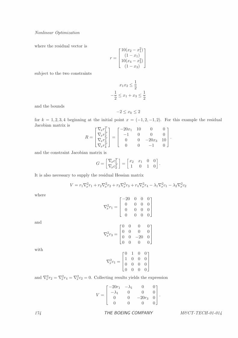
Nonlinear Optimization
where the residual vector is
r =
10(x2 − x21)
(1 − x1)10(x4 − x2
3)(1 − x3)
subject to the two constraints
x1x2 ≤ 1
2
−1
2≤ x1 + x3 ≤ 1
2
and the bounds
−2 ≤ xk ≤ 2
for k = 1, 2, 3, 4 beginning at the initial point x = (−1, 2,−1, 2). For this example the residualJacobian matrix is
R =
∇xrT1
∇xrT2
∇xrT3
∇xrT4
=
−20x1 10 0 0−1 0 0 00 0 −20x3 100 0 −1 0
.
and the constraint Jacobian matrix is
G =
[∇xcT1
∇xcT2
]=
[x2 x1 0 01 0 1 0
].
It is also necessary to supply the residual Hessian matrix
V = r1∇2xr1 + r2∇2
xr2 + r3∇2xr3 + r4∇2
xr4 − λ1∇2xc1 − λ2∇2
xc2
where
∇2xr1 =
−20 0 0 00 0 0 00 0 0 00 0 0 0
and
∇2xr3 =
0 0 0 00 0 0 00 0 −20 00 0 0 0
with
∇2xc1 =
0 1 0 01 0 0 00 0 0 00 0 0 0
and ∇2xr2 = ∇2
xr4 = ∇2x c2 = 0. Collecting results yields the expression
V =
−20r1 −λ1 0 0−λ1 0 0 00 0 −20r3 00 0 0 0
.
174 THE BOEING COMPANY M&CT-TECH-01-014
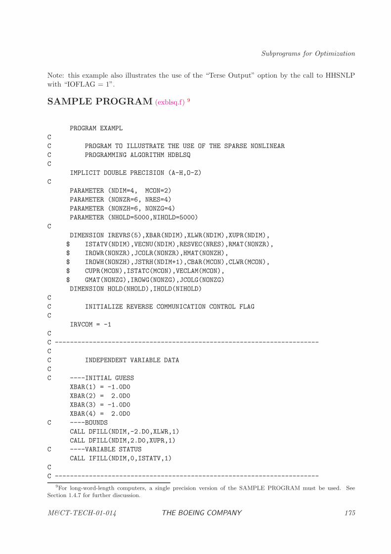
Subprograms for Optimization
Note: this example also illustrates the use of the “Terse Output” option by the call to HHSNLPwith “IOFLAG = 1”.
SAMPLE PROGRAM (exblsq.f) 9
PROGRAM EXAMPL
C
C PROGRAM TO ILLUSTRATE THE USE OF THE SPARSE NONLINEAR
C PROGRAMMING ALGORITHM HDBLSQ
C
IMPLICIT DOUBLE PRECISION (A-H,O-Z)
C
PARAMETER (NDIM=4, MCON=2)
PARAMETER (NONZR=6, NRES=4)
PARAMETER (NONZH=6, NONZG=4)
PARAMETER (NHOLD=5000,NIHOLD=5000)
C
DIMENSION IREVRS(5),XBAR(NDIM),XLWR(NDIM),XUPR(NDIM),
$ ISTATV(NDIM),VECNU(NDIM),RESVEC(NRES),RMAT(NONZR),
$ IROWR(NONZR),JCOLR(NONZR),HMAT(NONZH),
$ IROWH(NONZH),JSTRH(NDIM+1),CBAR(MCON),CLWR(MCON),
$ CUPR(MCON),ISTATC(MCON),VECLAM(MCON),
$ GMAT(NONZG),IROWG(NONZG),JCOLG(NONZG)
DIMENSION HOLD(NHOLD),IHOLD(NIHOLD)
C
C INITIALIZE REVERSE COMMUNICATION CONTROL FLAG
C
IRVCOM = -1
C
C ----------------------------------------------------------------------
C
C INDEPENDENT VARIABLE DATA
C
C ----INITIAL GUESS
XBAR(1) = -1.0D0
XBAR(2) = 2.0D0
XBAR(3) = -1.0D0
XBAR(4) = 2.0D0
C ----BOUNDS
CALL DFILL(NDIM,-2.D0,XLWR,1)
CALL DFILL(NDIM,2.D0,XUPR,1)
C ----VARIABLE STATUS
CALL IFILL(NDIM,0,ISTATV,1)
C
C ----------------------------------------------------------------------
9For long-word-length computers, a single precision version of the SAMPLE PROGRAM must be used. See
Section 1.4.7 for further discussion.
M&CT-TECH-01-014 THE BOEING COMPANY 175
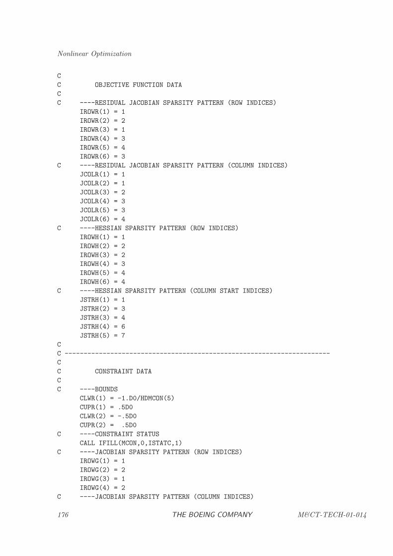
Nonlinear Optimization
C
C OBJECTIVE FUNCTION DATA
C
C ----RESIDUAL JACOBIAN SPARSITY PATTERN (ROW INDICES)
IROWR(1) = 1
IROWR(2) = 2
IROWR(3) = 1
IROWR(4) = 3
IROWR(5) = 4
IROWR(6) = 3
C ----RESIDUAL JACOBIAN SPARSITY PATTERN (COLUMN INDICES)
JCOLR(1) = 1
JCOLR(2) = 1
JCOLR(3) = 2
JCOLR(4) = 3
JCOLR(5) = 3
JCOLR(6) = 4
C ----HESSIAN SPARSITY PATTERN (ROW INDICES)
IROWH(1) = 1
IROWH(2) = 2
IROWH(3) = 2
IROWH(4) = 3
IROWH(5) = 4
IROWH(6) = 4
C ----HESSIAN SPARSITY PATTERN (COLUMN START INDICES)
JSTRH(1) = 1
JSTRH(2) = 3
JSTRH(3) = 4
JSTRH(4) = 6
JSTRH(5) = 7
C
C ----------------------------------------------------------------------
C
C CONSTRAINT DATA
C
C ----BOUNDS
CLWR(1) = -1.D0/HDMCON(5)
CUPR(1) = .5D0
CLWR(2) = -.5D0
CUPR(2) = .5D0
C ----CONSTRAINT STATUS
CALL IFILL(MCON,0,ISTATC,1)
C ----JACOBIAN SPARSITY PATTERN (ROW INDICES)
IROWG(1) = 1
IROWG(2) = 2
IROWG(3) = 1
IROWG(4) = 2
C ----JACOBIAN SPARSITY PATTERN (COLUMN INDICES)
176 THE BOEING COMPANY M&CT-TECH-01-014
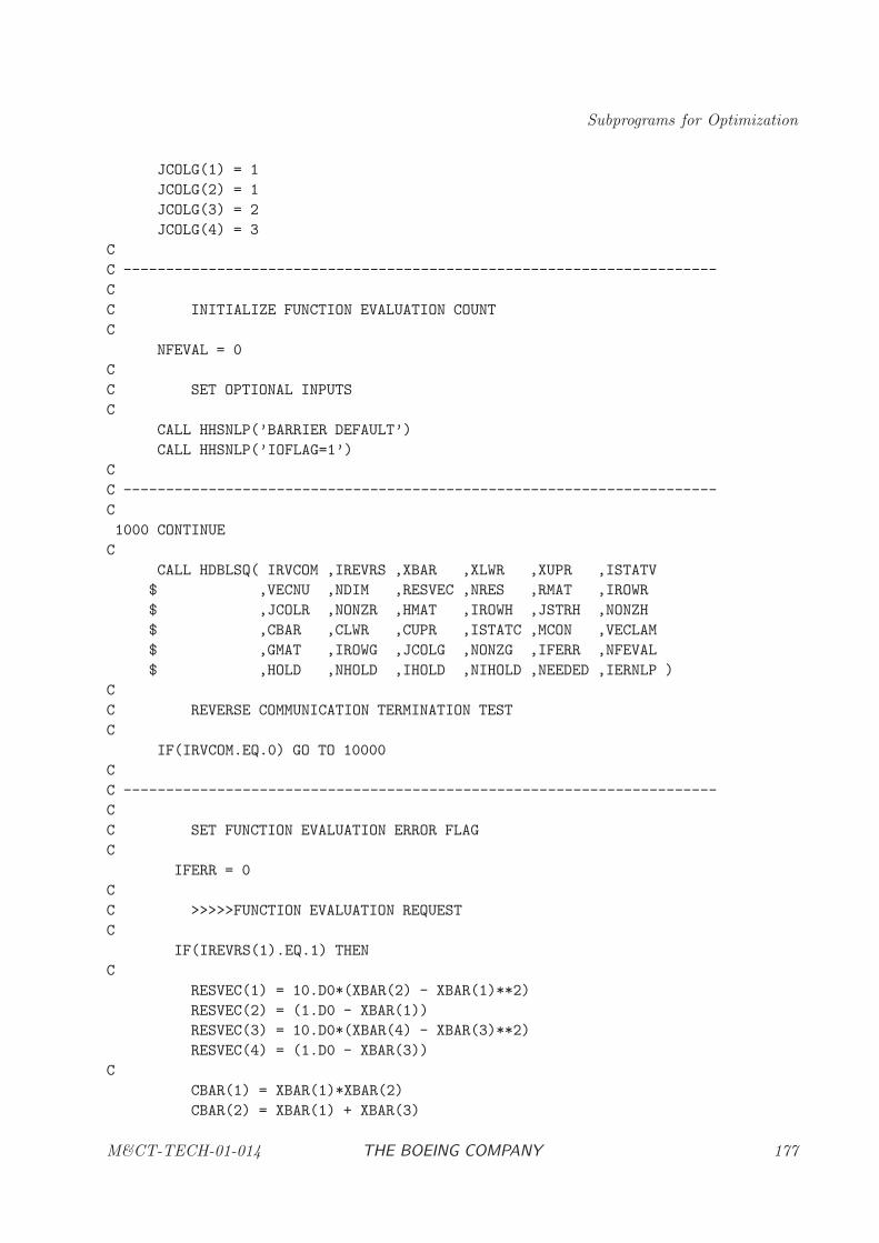
Subprograms for Optimization
JCOLG(1) = 1
JCOLG(2) = 1
JCOLG(3) = 2
JCOLG(4) = 3
C
C ----------------------------------------------------------------------
C
C INITIALIZE FUNCTION EVALUATION COUNT
C
NFEVAL = 0
C
C SET OPTIONAL INPUTS
C
CALL HHSNLP(’BARRIER DEFAULT’)
CALL HHSNLP(’IOFLAG=1’)
C
C ----------------------------------------------------------------------
C
1000 CONTINUE
C
CALL HDBLSQ( IRVCOM ,IREVRS ,XBAR ,XLWR ,XUPR ,ISTATV
$ ,VECNU ,NDIM ,RESVEC ,NRES ,RMAT ,IROWR
$ ,JCOLR ,NONZR ,HMAT ,IROWH ,JSTRH ,NONZH
$ ,CBAR ,CLWR ,CUPR ,ISTATC ,MCON ,VECLAM
$ ,GMAT ,IROWG ,JCOLG ,NONZG ,IFERR ,NFEVAL
$ ,HOLD ,NHOLD ,IHOLD ,NIHOLD ,NEEDED ,IERNLP )
C
C REVERSE COMMUNICATION TERMINATION TEST
C
IF(IRVCOM.EQ.0) GO TO 10000
C
C ----------------------------------------------------------------------
C
C SET FUNCTION EVALUATION ERROR FLAG
C
IFERR = 0
C
C >>>>>FUNCTION EVALUATION REQUEST
C
IF(IREVRS(1).EQ.1) THEN
C
RESVEC(1) = 10.D0*(XBAR(2) - XBAR(1)**2)
RESVEC(2) = (1.D0 - XBAR(1))
RESVEC(3) = 10.D0*(XBAR(4) - XBAR(3)**2)
RESVEC(4) = (1.D0 - XBAR(3))
C
CBAR(1) = XBAR(1)*XBAR(2)
CBAR(2) = XBAR(1) + XBAR(3)
M&CT-TECH-01-014 THE BOEING COMPANY 177
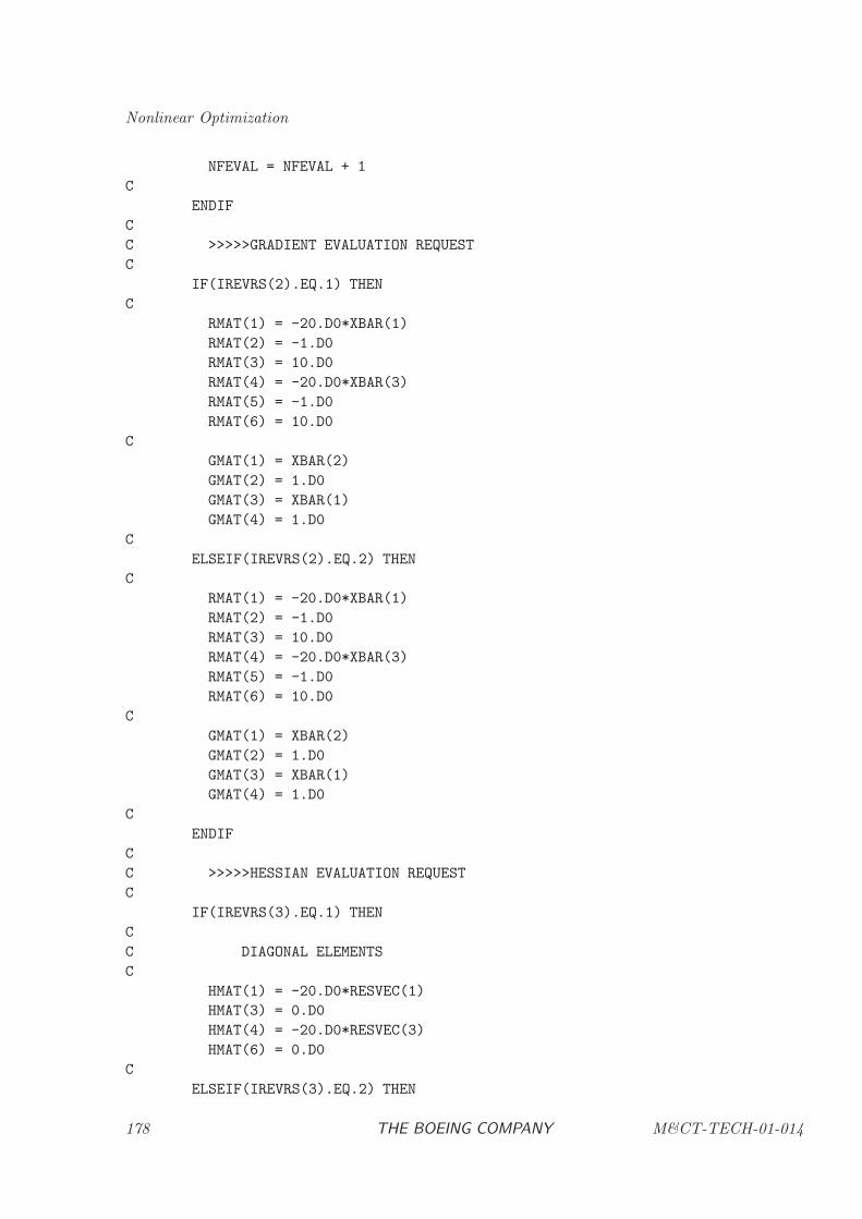
Nonlinear Optimization
NFEVAL = NFEVAL + 1
C
ENDIF
C
C >>>>>GRADIENT EVALUATION REQUEST
C
IF(IREVRS(2).EQ.1) THEN
C
RMAT(1) = -20.D0*XBAR(1)
RMAT(2) = -1.D0
RMAT(3) = 10.D0
RMAT(4) = -20.D0*XBAR(3)
RMAT(5) = -1.D0
RMAT(6) = 10.D0
C
GMAT(1) = XBAR(2)
GMAT(2) = 1.D0
GMAT(3) = XBAR(1)
GMAT(4) = 1.D0
C
ELSEIF(IREVRS(2).EQ.2) THEN
C
RMAT(1) = -20.D0*XBAR(1)
RMAT(2) = -1.D0
RMAT(3) = 10.D0
RMAT(4) = -20.D0*XBAR(3)
RMAT(5) = -1.D0
RMAT(6) = 10.D0
C
GMAT(1) = XBAR(2)
GMAT(2) = 1.D0
GMAT(3) = XBAR(1)
GMAT(4) = 1.D0
C
ENDIF
C
C >>>>>HESSIAN EVALUATION REQUEST
C
IF(IREVRS(3).EQ.1) THEN
C
C DIAGONAL ELEMENTS
C
HMAT(1) = -20.D0*RESVEC(1)
HMAT(3) = 0.D0
HMAT(4) = -20.D0*RESVEC(3)
HMAT(6) = 0.D0
C
ELSEIF(IREVRS(3).EQ.2) THEN
178 THE BOEING COMPANY M&CT-TECH-01-014
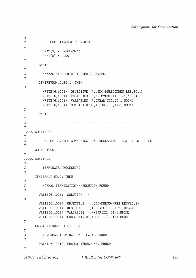
Subprograms for Optimization
C
C OFF-DIAGONAL ELEMENTS
C
HMAT(2) = -VECLAM(1)
HMAT(5) = 0.D0
C
ENDIF
C
C >>>>>SYSTEM PRINT (OUTPUT) REQUEST
C
IF(IREVRS(4).EQ.1) THEN
C
WRITE(6,1001) ’OBJECTIVE ’,.5D0*DNRSQ(NRES,RESVEC,1)
WRITE(6,1001) ’RESIDUALS ’,(RESVEC(II),II=1,NRES)
WRITE(6,1001) ’VARIABLES ’,(XBAR(II),II=1,NDIM)
WRITE(6,1001) ’CONSTRAINTS’,(CBAR(II),II=1,MCON)
C
ENDIF
C
C ----------------------------------------------------------------------
C
2000 CONTINUE
C
C END OF REVERSE COMMUNICATION PROCESSING. RETURN TO HDBLSQ
C
GO TO 1000
C
10000 CONTINUE
C
C TERMINATE PROCESSING
C
IF(IERNLP.EQ.0) THEN
C
C NORMAL TERMINATION---SOLUTION FOUND
C
WRITE(6,1001) ’SOLUTION ’
C
WRITE(6,1001) ’OBJECTIVE ’,.5D0*DNRSQ(NRES,RESVEC,1)
WRITE(6,1001) ’RESIDUALS ’,(RESVEC(II),II=1,NRES)
WRITE(6,1001) ’VARIABLES ’,(XBAR(II),II=1,NDIM)
WRITE(6,1001) ’CONSTRAINTS’,(CBAR(II),II=1,MCON)
C
ELSEIF(IERNLP.LT.0) THEN
C
C ABNORMAL TERMINATION---FATAL ERROR
C
PRINT *,’FATAL ERROR; IERNLP =’,IERNLP
C
M&CT-TECH-01-014 THE BOEING COMPANY 179
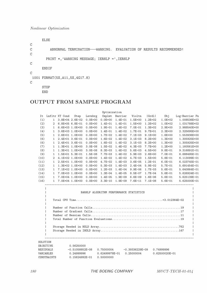
Nonlinear Optimization
ELSE
C
C ABNORMAL TERMINATION---WARNING. EVALUATION OF RESULTS RECOMMENDED!
C
PRINT *,’WARNING MESSAGE; IERNLP =’,IERNLP
C
ENDIF
C
1001 FORMAT(5X,A11,5X,4G17.8)
C
STOP
END
OUTPUT FROM SAMPLE PROGRAM
Optimization
It Lnfltr KT Cond Step Levnbrg Cmplmt Barrier Violtn |Grdl| Obj Log-Barrier Fn
(1) 1 3.8E+04 2.6E-02 0.0E+00 0.0E+00 1.4E-01 1.5E+00 1.2E+02 1.0E+02 1.008536E+02
(2) 2 6.8E+05 6.8E-01 0.0E+00 1.4E-01 1.4E-01 1.5E+00 1.2E+02 1.0E+02 1.031788E+02
(3) 1 6.6E+03 1.0E+00 0.0E+00 1.9E-01 1.4E-02 7.0E-01 1.3E+02 2.9E+00 2.988540E+00
(4) 1 3.6E+03 1.0E+00 0.0E+00 1.4E-01 1.4E-02 1.7E-01 9.7E+01 2.3E+00 2.325695E+00
(5) 1 2.6E+01 1.0E+00 0.0E+00 1.7E-02 1.4E-02 7.1E-03 9.1E+00 1.6E+00 1.553936E+00
(6) 1 2.4E+01 3.6E-01 0.0E+00 1.6E-02 1.4E-02 3.1E-03 8.2E+00 1.3E+00 1.305925E+00
(6) 1 2.4E+01 3.6E-01 0.0E+00 1.6E-02 1.4E-02 3.1E-03 8.2E+00 1.3E+00 1.305925E+00
(7) 1 1.3E+01 1.0E+00 3.0E-08 1.5E-02 1.4E-02 4.3E-03 7.7E+00 1.2E+00 1.160561E+00
(8) 1 1.3E+01 1.0E+00 3.0E-08 8.3E-03 1.4E-02 5.6E-03 4.5E+00 9.8E-01 9.316891E-01
(9) 1 1.5E+01 5.3E-01 1.5E-08 7.7E-03 1.4E-02 5.9E-03 2.6E+00 7.0E-01 6.688495E-01
(10) 2 4.1E+02 1.0E+00 0.0E+00 1.4E-02 1.4E-02 4.7E-03 1.5E+00 5.8E-01 6.113099E-01
(11) 1 2.5E+01 1.0E+00 0.0E+00 4.7E-02 1.4E-03 3.6E-05 1.2E-01 6.0E-01 6.023745E-01
(12) 1 1.3E+02 1.0E+00 0.0E+00 5.3E-03 1.4E-03 2.4E-04 5.9E-02 5.7E-01 5.691454E-01
(13) 1 7.1E+02 1.0E+00 0.0E+00 1.2E-03 1.4E-04 9.9E-06 1.7E-03 5.6E-01 5.640864E-01
(14) 1 7.0E+03 1.0E+00 0.0E+00 1.3E-04 1.4E-05 8.5E-07 1.7E-04 5.6E-01 5.626924E-01
(15) 1 7.0E+04 1.0E+00 0.0E+00 1.4E-05 1.9E-09 6.6E-09 1.6E-06 5.6E-01 5.625139E-01
(16) 1 7.0E+04 1.0E+00 0.0E+00 3.3E-10 1.9E-09 7.6E-11 7.1E-08 5.6E-01 5.625000E-01
-------------------------------------------------------------------------------------------
| |
| BARNLP ALGORITHM PERFORMANCE STATISTICS |
| |
| Total CPU Time.....................................................+3.012364E-02 |
| |
| Number of Function Calls......................................................19 |
| Number of Gradient Calls......................................................17 |
| Number of Hessian Calls.......................................................11 |
| Total Number of Function Evaluations..........................................19 |
| |
| Storage Needed in HOLD Array.................................................762 |
| Storage Needed in IHOLD Array................................................147 |
| |
-------------------------------------------------------------------------------------------
SOLUTION
OBJECTIVE 0.56250000
RESIDUALS -0.51058852E-08 0.75000004 -0.39336229E-09 0.74999996
VARIABLES 0.24999996 0.62499978E-01 0.25000004 0.62500020E-01
CONSTRAINTS 0.15624992E-01 0.50000000
180 THE BOEING COMPANY M&CT-TECH-01-014
Subprograms for Optimization
HDBLPQ: Sparse Barrier Quadratic Programming
PURPOSE
HDBLPQ computes the vector x = (x1, x2, . . . , xn) which minimizes the quadratic function
cTx+1
2xTHx
subject to the m linear constraints
bL ≤ Ax ≤ bU ,
and the simple bounds
xL ≤ x ≤ xU
Equality constraints are imposed by setting bLi = bUi and variables can be fixed by setting xLi =xUi. A linear programming problem can be solved by setting H = 0. HDBLPQ works underthe assumption that the quadratic programming problem has a unique, finite solution. Thus, itis assumed that the projected Hessian matrix is positive definite at the solution. The matrix offirst derivatives (the Jacobian) and the matrix of second derivatives (Hessian) are represented in asparse format consistent with that used in BCSLIB-EXT [1].
RELATED SUBPROGRAMS
HDSQSH Sparse Quadratic Programming
HHSNLP Sparse Nonlinear Programming Input Procedure
METHOD
An interior point or barrier method is used to solve the quadratic programming (QP) problem.The quadratic programming algorithm requires the Hessian matrix H and the Jacobian matrix A,both which must be specified in a sparse format. The barrier method is efficient because it avoidsthe computational complexity of active set methods when there are many inequality constraints,by using a log-barrier transformation. The large sparse KKT system is solved efficiently using themultifrontal algorithm described in BCSLIB-EXT [1]. The algorithm incorporates a nonlinear filterfor globalization.
WARNING
The projected Hessian matrix is assumed to be positive definite at the solution, i.e. with thecorrect active constraints. If this is not true, the software will detect an incorrect value for thematrix inertia and modify the Hessian matrix.
The HDBLPQ software uses internal common blocks to communicate information. To avoid con-flict with these internal commons the user should not have commons with the following names:NPSPRR, NPSPRI, NPSPRC, STATIS, KONSTN, NPSALG, NPSDFL, NLPERR, PERCOM,ITEREF, and CLKCOM.
USAGE
M&CT-TECH-01-014 THE BOEING COMPANY 181
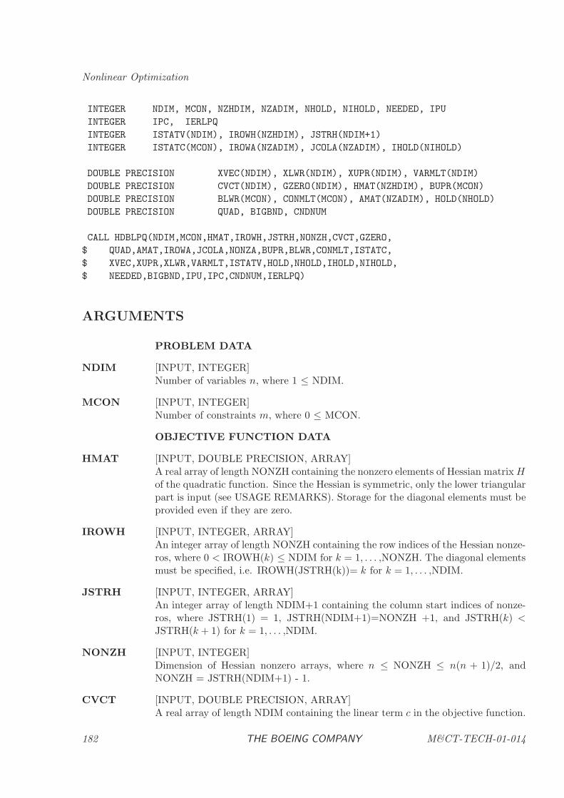
Nonlinear Optimization
INTEGER NDIM, MCON, NZHDIM, NZADIM, NHOLD, NIHOLD, NEEDED, IPU
INTEGER IPC, IERLPQ
INTEGER ISTATV(NDIM), IROWH(NZHDIM), JSTRH(NDIM+1)
INTEGER ISTATC(MCON), IROWA(NZADIM), JCOLA(NZADIM), IHOLD(NIHOLD)
DOUBLE PRECISION XVEC(NDIM), XLWR(NDIM), XUPR(NDIM), VARMLT(NDIM)
DOUBLE PRECISION CVCT(NDIM), GZERO(NDIM), HMAT(NZHDIM), BUPR(MCON)
DOUBLE PRECISION BLWR(MCON), CONMLT(MCON), AMAT(NZADIM), HOLD(NHOLD)
DOUBLE PRECISION QUAD, BIGBND, CNDNUM
CALL HDBLPQ(NDIM,MCON,HMAT,IROWH,JSTRH,NONZH,CVCT,GZERO,
$ QUAD,AMAT,IROWA,JCOLA,NONZA,BUPR,BLWR,CONMLT,ISTATC,
$ XVEC,XUPR,XLWR,VARMLT,ISTATV,HOLD,NHOLD,IHOLD,NIHOLD,
$ NEEDED,BIGBND,IPU,IPC,CNDNUM,IERLPQ)
ARGUMENTS
PROBLEM DATA
NDIM [INPUT, INTEGER]Number of variables n, where 1 ≤ NDIM.
MCON [INPUT, INTEGER]Number of constraints m, where 0 ≤ MCON.
OBJECTIVE FUNCTION DATA
HMAT [INPUT, DOUBLE PRECISION, ARRAY]A real array of length NONZH containing the nonzero elements of Hessian matrixHof the quadratic function. Since the Hessian is symmetric, only the lower triangularpart is input (see USAGE REMARKS). Storage for the diagonal elements must beprovided even if they are zero.
IROWH [INPUT, INTEGER, ARRAY]An integer array of length NONZH containing the row indices of the Hessian nonze-ros, where 0 < IROWH(k) ≤ NDIM for k = 1, . . . ,NONZH. The diagonal elementsmust be specified, i.e. IROWH(JSTRH(k))= k for k = 1, . . . ,NDIM.
JSTRH [INPUT, INTEGER, ARRAY]An integer array of length NDIM+1 containing the column start indices of nonze-ros, where JSTRH(1) = 1, JSTRH(NDIM+1)=NONZH +1, and JSTRH(k) <JSTRH(k + 1) for k = 1, . . . ,NDIM.
NONZH [INPUT, INTEGER]Dimension of Hessian nonzero arrays, where n ≤ NONZH ≤ n(n + 1)/2, andNONZH = JSTRH(NDIM+1) - 1.
CVCT [INPUT, DOUBLE PRECISION, ARRAY]A real array of length NDIM containing the linear term c in the objective function.
182 THE BOEING COMPANY M&CT-TECH-01-014
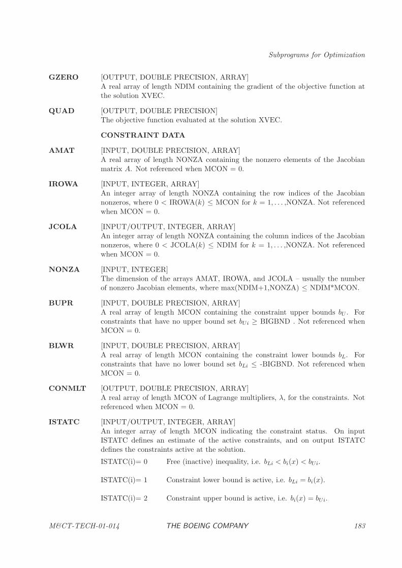
Subprograms for Optimization
GZERO [OUTPUT, DOUBLE PRECISION, ARRAY]A real array of length NDIM containing the gradient of the objective function atthe solution XVEC.
QUAD [OUTPUT, DOUBLE PRECISION]The objective function evaluated at the solution XVEC.
CONSTRAINT DATA
AMAT [INPUT, DOUBLE PRECISION, ARRAY]A real array of length NONZA containing the nonzero elements of the Jacobianmatrix A. Not referenced when MCON = 0.
IROWA [INPUT, INTEGER, ARRAY]An integer array of length NONZA containing the row indices of the Jacobiannonzeros, where 0 < IROWA(k) ≤ MCON for k = 1, . . . ,NONZA. Not referencedwhen MCON = 0.
JCOLA [INPUT/OUTPUT, INTEGER, ARRAY]An integer array of length NONZA containing the column indices of the Jacobiannonzeros, where 0 < JCOLA(k) ≤ NDIM for k = 1, . . . ,NONZA. Not referencedwhen MCON = 0.
NONZA [INPUT, INTEGER]The dimension of the arrays AMAT, IROWA, and JCOLA – usually the numberof nonzero Jacobian elements, where max(NDIM+1,NONZA) ≤ NDIM*MCON.
BUPR [INPUT, DOUBLE PRECISION, ARRAY]A real array of length MCON containing the constraint upper bounds bU . Forconstraints that have no upper bound set bUi ≥ BIGBND . Not referenced whenMCON = 0.
BLWR [INPUT, DOUBLE PRECISION, ARRAY]A real array of length MCON containing the constraint lower bounds bL. Forconstraints that have no lower bound set bLi ≤ -BIGBND. Not referenced whenMCON = 0.
CONMLT [OUTPUT, DOUBLE PRECISION, ARRAY]A real array of length MCON of Lagrange multipliers, λ, for the constraints. Notreferenced when MCON = 0.
ISTATC [INPUT/OUTPUT, INTEGER, ARRAY]An integer array of length MCON indicating the constraint status. On inputISTATC defines an estimate of the active constraints, and on output ISTATCdefines the constraints active at the solution.
ISTATC(i)= 0 Free (inactive) inequality, i.e. bLi < bi(x) < bUi.
ISTATC(i)= 1 Constraint lower bound is active, i.e. bLi = bi(x).
ISTATC(i)= 2 Constraint upper bound is active, i.e. bi(x) = bUi.
M&CT-TECH-01-014 THE BOEING COMPANY 183
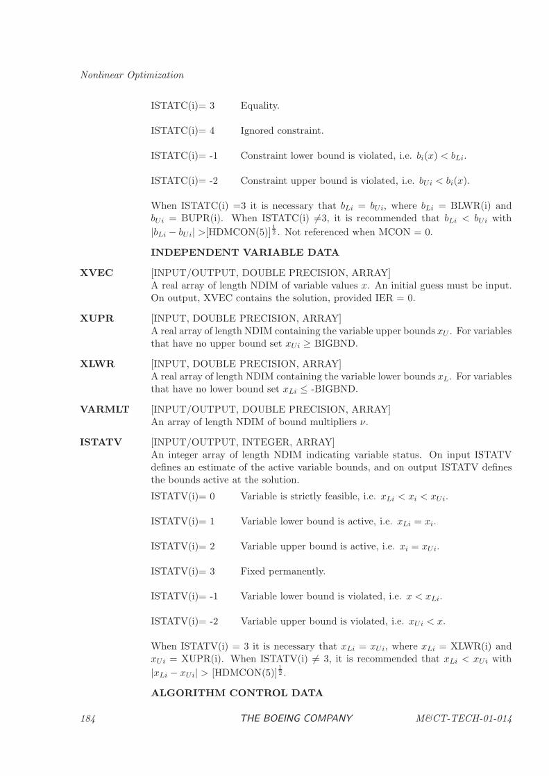
Nonlinear Optimization
ISTATC(i)= 3 Equality.
ISTATC(i)= 4 Ignored constraint.
ISTATC(i)= -1 Constraint lower bound is violated, i.e. bi(x) < bLi.
ISTATC(i)= -2 Constraint upper bound is violated, i.e. bUi < bi(x).
When ISTATC(i) =3 it is necessary that bLi = bUi, where bLi = BLWR(i) andbUi = BUPR(i). When ISTATC(i) 6=3, it is recommended that bLi < bUi with
|bLi − bUi| >[HDMCON(5)]12 . Not referenced when MCON = 0.
INDEPENDENT VARIABLE DATA
XVEC [INPUT/OUTPUT, DOUBLE PRECISION, ARRAY]A real array of length NDIM of variable values x. An initial guess must be input.On output, XVEC contains the solution, provided IER = 0.
XUPR [INPUT, DOUBLE PRECISION, ARRAY]A real array of length NDIM containing the variable upper bounds xU . For variablesthat have no upper bound set xUi ≥ BIGBND.
XLWR [INPUT, DOUBLE PRECISION, ARRAY]A real array of length NDIM containing the variable lower bounds xL. For variablesthat have no lower bound set xLi ≤ -BIGBND.
VARMLT [INPUT/OUTPUT, DOUBLE PRECISION, ARRAY]An array of length NDIM of bound multipliers ν.
ISTATV [INPUT/OUTPUT, INTEGER, ARRAY]An integer array of length NDIM indicating variable status. On input ISTATVdefines an estimate of the active variable bounds, and on output ISTATV definesthe bounds active at the solution.
ISTATV(i)= 0 Variable is strictly feasible, i.e. xLi < xi < xUi.
ISTATV(i)= 1 Variable lower bound is active, i.e. xLi = xi.
ISTATV(i)= 2 Variable upper bound is active, i.e. xi = xUi.
ISTATV(i)= 3 Fixed permanently.
ISTATV(i)= -1 Variable lower bound is violated, i.e. x < xLi.
ISTATV(i)= -2 Variable upper bound is violated, i.e. xUi < x.
When ISTATV(i) = 3 it is necessary that xLi = xUi, where xLi = XLWR(i) andxUi = XUPR(i). When ISTATV(i) 6= 3, it is recommended that xLi < xUi with
|xLi − xUi| > [HDMCON(5)]12 .
ALGORITHM CONTROL DATA
184 THE BOEING COMPANY M&CT-TECH-01-014
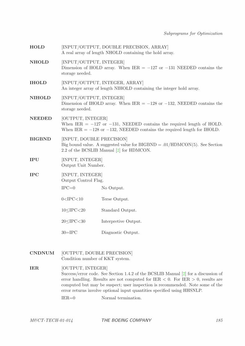
Subprograms for Optimization
HOLD [INPUT/OUTPUT, DOUBLE PRECISION, ARRAY]A real array of length NHOLD containing the hold array.
NHOLD [INPUT/OUTPUT, INTEGER]Dimension of HOLD array. When IER = −127 or −131 NEEDED contains thestorage needed.
IHOLD [INPUT/OUTPUT, INTEGER, ARRAY]An integer array of length NIHOLD containing the integer hold array.
NIHOLD [INPUT/OUTPUT, INTEGER]Dimension of IHOLD array. When IER = −128 or −132, NEEDED contains thestorage needed.
NEEDED [OUTPUT, INTEGER]When IER = −127 or −131, NEEDED contains the required length of HOLD.When IER = −128 or −132, NEEDED contains the required length for IHOLD.
BIGBND [INPUT, DOUBLE PRECISION]Big bound value. A suggested value for BIGBND = .01/HDMCON(5). See Section2.2 of the BCSLIB Manual [2] for HDMCON.
IPU [INPUT, INTEGER]Output Unit Number.
IPC [INPUT, INTEGER]Output Control Flag.
IPC=0 No Output.
0<IPC<10 Terse Output.
10≤IPC<20 Standard Output.
20≤IPC<30 Interpretive Output.
30=IPC Diagnostic Output.
CNDNUM [OUTPUT, DOUBLE PRECISION]Condition number of KKT system.
IER [OUTPUT, INTEGER]Success/error code. See Section 1.4.2 of the BCSLIB Manual [2] for a discussion oferror handling. Results are not computed for IER < 0. For IER > 0, results arecomputed but may be suspect; user inspection is recommended. Note some of theerror returns involve optional input quantities specified using HHSNLP.
IER=0 Normal termination.
M&CT-TECH-01-014 THE BOEING COMPANY 185
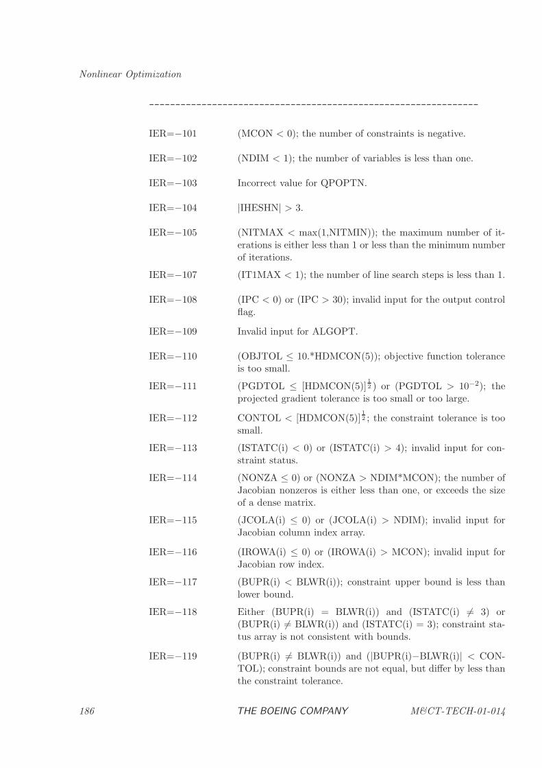
Nonlinear Optimization
---------------------------------------------------------------
IER=−101 (MCON < 0); the number of constraints is negative.
IER=−102 (NDIM < 1); the number of variables is less than one.
IER=−103 Incorrect value for QPOPTN.
IER=−104 |IHESHN| > 3.
IER=−105 (NITMAX < max(1,NITMIN)); the maximum number of it-erations is either less than 1 or less than the minimum numberof iterations.
IER=−107 (IT1MAX < 1); the number of line search steps is less than 1.
IER=−108 (IPC < 0) or (IPC > 30); invalid input for the output controlflag.
IER=−109 Invalid input for ALGOPT.
IER=−110 (OBJTOL ≤ 10.*HDMCON(5)); objective function toleranceis too small.
IER=−111 (PGDTOL ≤ [HDMCON(5)]12 ) or (PGDTOL > 10−2); the
projected gradient tolerance is too small or too large.
IER=−112 CONTOL < [HDMCON(5)]12 ; the constraint tolerance is too
small.
IER=−113 (ISTATC(i) < 0) or (ISTATC(i) > 4); invalid input for con-straint status.
IER=−114 (NONZA ≤ 0) or (NONZA > NDIM*MCON); the number ofJacobian nonzeros is either less than one, or exceeds the sizeof a dense matrix.
IER=−115 (JCOLA(i) ≤ 0) or (JCOLA(i) > NDIM); invalid input forJacobian column index array.
IER=−116 (IROWA(i) ≤ 0) or (IROWA(i) > MCON); invalid input forJacobian row index.
IER=−117 (BUPR(i) < BLWR(i)); constraint upper bound is less thanlower bound.
IER=−118 Either (BUPR(i) = BLWR(i)) and (ISTATC(i) 6= 3) or(BUPR(i) 6= BLWR(i)) and (ISTATC(i) = 3); constraint sta-tus array is not consistent with bounds.
IER=−119 (BUPR(i) 6= BLWR(i)) and (|BUPR(i)−BLWR(i)| < CON-TOL); constraint bounds are not equal, but differ by less thanthe constraint tolerance.
186 THE BOEING COMPANY M&CT-TECH-01-014
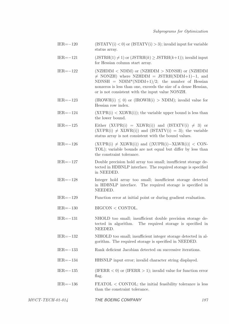
Subprograms for Optimization
IER=−120 (ISTATV(i)< 0) or (ISTATV(i) > 3); invalid input for variablestatus array.
IER=−121 (JSTRH(1) 6= 1) or (JSTRH(k) ≥ JSTRH(k+1)); invalid inputfor Hessian column start array.
IER=−122 (NZHDIM < NDIM) or (NZHDIM > NDNSH) or (NZHDIM6= NONZH) where NZHDIM = JSTRH(NDIM+1)−1, andNDNSH = NDIM*(NDIM+1)/2; the number of Hessiannonzeros is less than one, exceeds the size of a dense Hessian,or is not consistent with the input value NONZH.
IER=−123 (IROWH(i) ≤ 0) or (IROWH(i) > NDIM); invalid value forHessian row index.
IER=−124 (XUPR(i) < XLWR(i)); the variable upper bound is less thanthe lower bound.
IER=−125 Either (XUPR(i) = XLWR(i)) and (ISTATV(i) 6= 3) or(XUPR(i) 6= XLWR(i)) and (ISTATV(i) = 3); the variablestatus array is not consistent with the bound values.
IER=−126 (XUPR(i) 6= XLWR(i)) and (|XUPR(i)−XLWR(i)| < CON-TOL); variable bounds are not equal but differ by less thanthe constraint tolerance.
IER=−127 Double precision hold array too small; insufficient storage de-tected in HDBNLP interface. The required storage is specifiedin NEEDED.
IER=−128 Integer hold array too small; insufficient storage detectedin HDBNLP interface. The required storage is specified inNEEDED.
IER=−129 Function error at initial point or during gradient evaluation.
IER=−130 BIGCON < CONTOL.
IER=−131 NHOLD too small; insufficient double precision storage de-tected in algorithm. The required storage is specified inNEEDED.
IER=−132 NIHOLD too small; insufficient integer storage detected in al-gorithm. The required storage is specified in NEEDED.
IER=−133 Rank deficient Jacobian detected on successive iterations.
IER=−134 HHSNLP input error; invalid character string displayed.
IER=−135 (IFERR < 0) or (IFERR > 1); invalid value for function errorflag.
IER=−136 FEATOL < CONTOL; the initial feasibility tolerance is lessthan the constraint tolerance.
M&CT-TECH-01-014 THE BOEING COMPANY 187
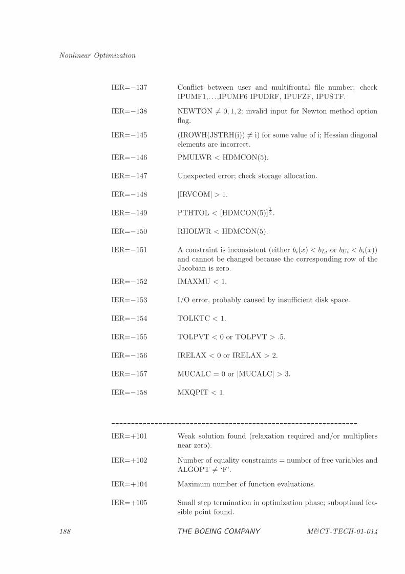
Nonlinear Optimization
IER=−137 Conflict between user and multifrontal file number; checkIPUMF1,. . .,IPUMF6 IPUDRF, IPUFZF, IPUSTF.
IER=−138 NEWTON 6= 0, 1, 2; invalid input for Newton method optionflag.
IER=−145 (IROWH(JSTRH(i)) 6= i) for some value of i; Hessian diagonalelements are incorrect.
IER=−146 PMULWR < HDMCON(5).
IER=−147 Unexpected error; check storage allocation.
IER=−148 |IRVCOM| > 1.
IER=−149 PTHTOL < [HDMCON(5)]12 .
IER=−150 RHOLWR < HDMCON(5).
IER=−151 A constraint is inconsistent (either bi(x) < bLi or bUi < bi(x))and cannot be changed because the corresponding row of theJacobian is zero.
IER=−152 IMAXMU < 1.
IER=−153 I/O error, probably caused by insufficient disk space.
IER=−154 TOLKTC < 1.
IER=−155 TOLPVT < 0 or TOLPVT > .5.
IER=−156 IRELAX < 0 or IRELAX > 2.
IER=−157 MUCALC = 0 or |MUCALC| > 3.
IER=−158 MXQPIT < 1.
---------------------------------------------------------------
IER=+101 Weak solution found (relaxation required and/or multipliersnear zero).
IER=+102 Number of equality constraints = number of free variables andALGOPT 6= ‘F’.
IER=+104 Maximum number of function evaluations.
IER=+105 Small step termination in optimization phase; suboptimal fea-sible point found.
188 THE BOEING COMPANY M&CT-TECH-01-014
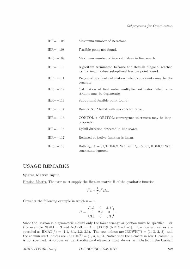
Subprograms for Optimization
IER=+106 Maximum number of iterations.
IER=+108 Feasible point not found.
IER=+109 Maximum number of interval halves in line search.
IER=+110 Algorithm terminated because the Hessian diagonal reachedits maximum value; suboptimal feasible point found.
IER=+111 Projected gradient calculation failed; constraints may be de-generate.
IER=+112 Calculation of first order multiplier estimates failed; con-straints may be degenerate.
IER=+113 Suboptimal feasible point found.
IER=+114 Barrier NLP failed with unexpected error.
IER=+115 CONTOL > OBJTOL; convergence tolerances may be inap-propriate.
IER=+116 Uphill direction detected in line search.
IER=+117 Reduced objective function is linear.
IER=+118 Both bLi ≤ −.01/HDMCON(5) and bUi ≥ .01/HDMCON(5);constraints ignored.
USAGE REMARKS
Sparse Matrix Input
Hessian Matrix. The user must supply the Hessian matrix H of the quadratic function
cTx+1
2xTHx.
Consider the following example in which n = 3:
H =
1.1 0 3 .10 2.2 0
3.1 0 3.3
.
Since the Hessian is a symmetric matrix only the lower triangular portion must be specified. Forthis example NDIM = 3 and NONZH = 4 = [JSTRH(NDIM+1)−1]. The nonzero values arespecified as HMAT(*) = (1.1, 3.1, 2.2, 3.3). The row indices are IROWH(*) = (1, 3, 2, 3), andthe column start indices are JSTRH(*) = (1, 3, 4, 5). Notice that the element in row 1, column 3is not specified. Also observe that the diagonal elements must always be included in the Hessian
M&CT-TECH-01-014 THE BOEING COMPANY 189
Nonlinear Optimization
sparsity pattern even if the elements are zero. Additional information on sparse matrix formats isfound in BCSLIB-EXT [1].
Jacobian Matrix. The user must specify the nonzero elements in the Jacobian matrix when required.Consider the following example in five variables n = 5 and three constraints m = 3:
A =
0 0 1.3 0 1.5
2.1 0 0 0 00 0 3.3 0 0
For this example NDIM = 5, MCON = 3, and the number of nonzeros NONZA = 4. The matrixcan be specified in two formats. The nonzero array is AMAT(*) = (2.1, 1.3, 3.3, 1.5). The rowindices are IROWA(*) = (2, 1, 3, 1), and the column indices are JCOLA(*) = (1, 3, 3, 5). Note thatsufficient storage must be provided in the array JCOLA to accomodate at least NDIM+1 values.Additional information on sparse matrix formats is found in BCSLIB-EXT [1].
Unconstrained Problems
When the problem is unconstrained the user must set MCON = 0. The following constraint relatedquantities will not be referenced: BLWR, BUPR, ISTATC, CONMLT, AMAT, IROWA, JCOLA,and NONZA. Since these quantities must appear as arguments in the call to HDBLPQ, dummyvalues may be utilized.
OPTIONAL INPUT
In addition to the required arguments, there are a number of optional arguments that can bespecified for subroutine HDBLPQ. All optional inputs are specified by calls to subroutine HHSNLP.It should be emphasized that it is not necessary to call HHSNLP to set default values.
OPTIONAL PRINTOUT
The level of printed output from HDBLPQ is controlled by the variables IPC and IPU. The defaultfor HDBLPQ is to have no output which corresponds to IPC = 0.
EXAMPLE
Find the values of the independent variables x = (x1, x2, x3, x4) to minimize the objective function
f(x) = cTx+1
2xTHx
subject to the constraints
bL ≤ Ax ≤ bU ,
where bTL = (−∞,−.5) and bTU = (.5, .5). The solution must also satisfy the bounds
−2 ≤ xk ≤ 2
for k = 1, 2, 3, 4 and as an initial guess select x = (−1, 2,−1, 2). For this example the vector
cT = [400, 200, 400, 200]
190 THE BOEING COMPANY M&CT-TECH-01-014
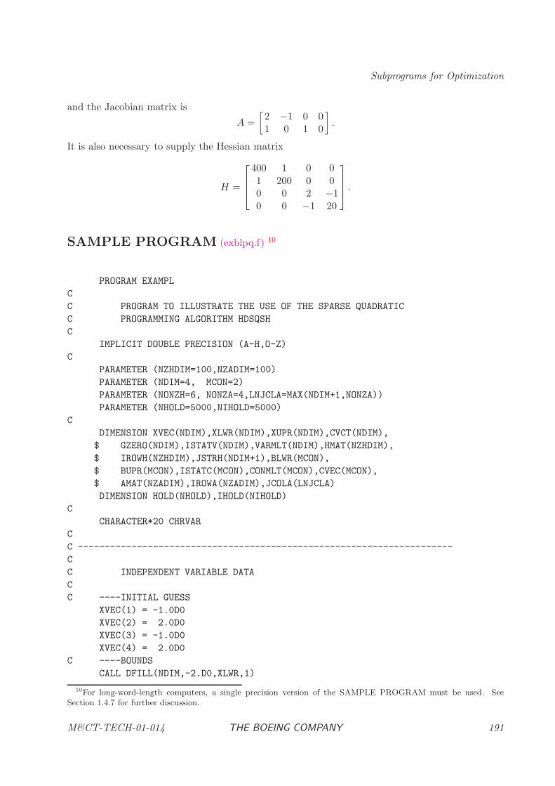
Subprograms for Optimization
and the Jacobian matrix is
A =
[2 −1 0 01 0 1 0
].
It is also necessary to supply the Hessian matrix
H =
400 1 0 01 200 0 00 0 2 −10 0 −1 20
.
SAMPLE PROGRAM (exblpq.f) 10
PROGRAM EXAMPL
C
C PROGRAM TO ILLUSTRATE THE USE OF THE SPARSE QUADRATIC
C PROGRAMMING ALGORITHM HDSQSH
C
IMPLICIT DOUBLE PRECISION (A-H,O-Z)
C
PARAMETER (NZHDIM=100,NZADIM=100)
PARAMETER (NDIM=4, MCON=2)
PARAMETER (NONZH=6, NONZA=4,LNJCLA=MAX(NDIM+1,NONZA))
PARAMETER (NHOLD=5000,NIHOLD=5000)
C
DIMENSION XVEC(NDIM),XLWR(NDIM),XUPR(NDIM),CVCT(NDIM),
$ GZERO(NDIM),ISTATV(NDIM),VARMLT(NDIM),HMAT(NZHDIM),
$ IROWH(NZHDIM),JSTRH(NDIM+1),BLWR(MCON),
$ BUPR(MCON),ISTATC(MCON),CONMLT(MCON),CVEC(MCON),
$ AMAT(NZADIM),IROWA(NZADIM),JCOLA(LNJCLA)
DIMENSION HOLD(NHOLD),IHOLD(NIHOLD)
C
CHARACTER*20 CHRVAR
C
C ----------------------------------------------------------------------
C
C INDEPENDENT VARIABLE DATA
C
C ----INITIAL GUESS
XVEC(1) = -1.0D0
XVEC(2) = 2.0D0
XVEC(3) = -1.0D0
XVEC(4) = 2.0D0
C ----BOUNDS
CALL DFILL(NDIM,-2.D0,XLWR,1)
10For long-word-length computers, a single precision version of the SAMPLE PROGRAM must be used. See
Section 1.4.7 for further discussion.
M&CT-TECH-01-014 THE BOEING COMPANY 191
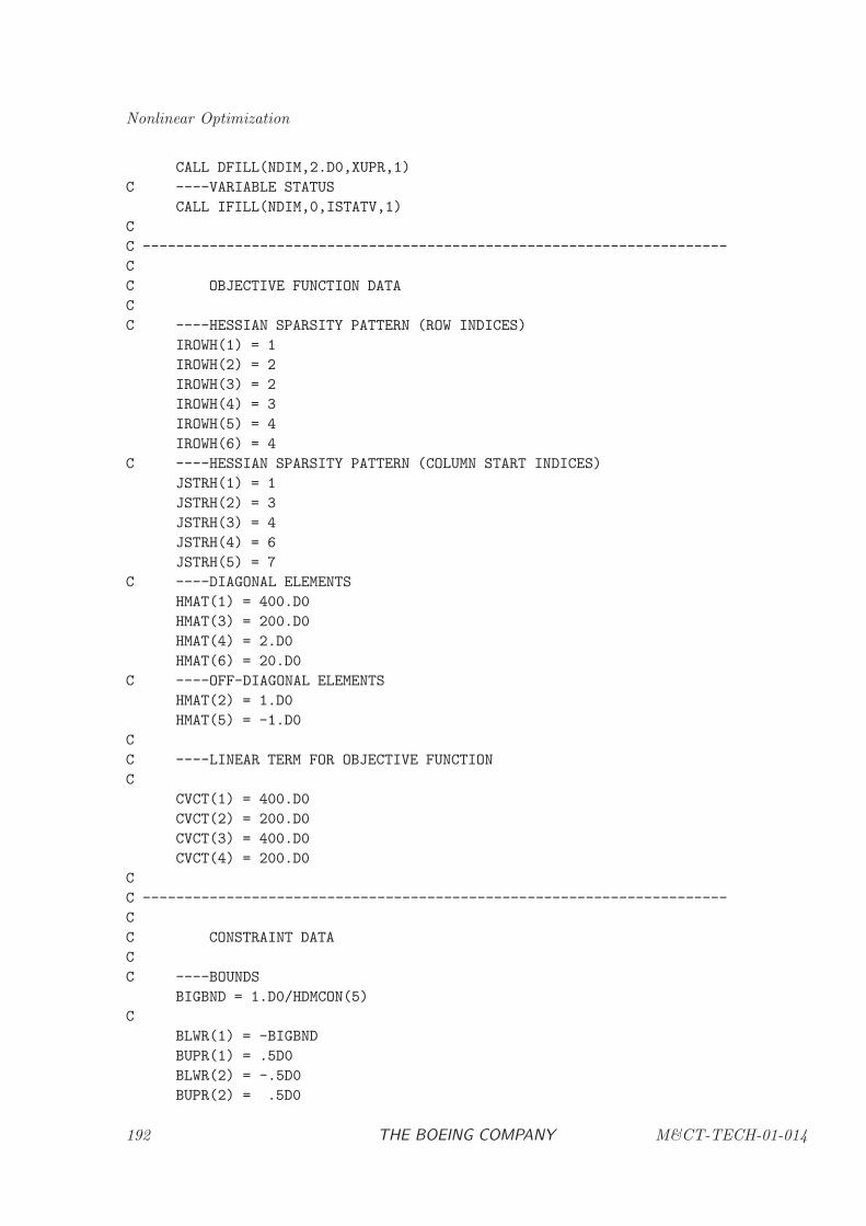
Nonlinear Optimization
CALL DFILL(NDIM,2.D0,XUPR,1)
C ----VARIABLE STATUS
CALL IFILL(NDIM,0,ISTATV,1)
C
C ----------------------------------------------------------------------
C
C OBJECTIVE FUNCTION DATA
C
C ----HESSIAN SPARSITY PATTERN (ROW INDICES)
IROWH(1) = 1
IROWH(2) = 2
IROWH(3) = 2
IROWH(4) = 3
IROWH(5) = 4
IROWH(6) = 4
C ----HESSIAN SPARSITY PATTERN (COLUMN START INDICES)
JSTRH(1) = 1
JSTRH(2) = 3
JSTRH(3) = 4
JSTRH(4) = 6
JSTRH(5) = 7
C ----DIAGONAL ELEMENTS
HMAT(1) = 400.D0
HMAT(3) = 200.D0
HMAT(4) = 2.D0
HMAT(6) = 20.D0
C ----OFF-DIAGONAL ELEMENTS
HMAT(2) = 1.D0
HMAT(5) = -1.D0
C
C ----LINEAR TERM FOR OBJECTIVE FUNCTION
C
CVCT(1) = 400.D0
CVCT(2) = 200.D0
CVCT(3) = 400.D0
CVCT(4) = 200.D0
C
C ----------------------------------------------------------------------
C
C CONSTRAINT DATA
C
C ----BOUNDS
BIGBND = 1.D0/HDMCON(5)
C
BLWR(1) = -BIGBND
BUPR(1) = .5D0
BLWR(2) = -.5D0
BUPR(2) = .5D0
192 THE BOEING COMPANY M&CT-TECH-01-014
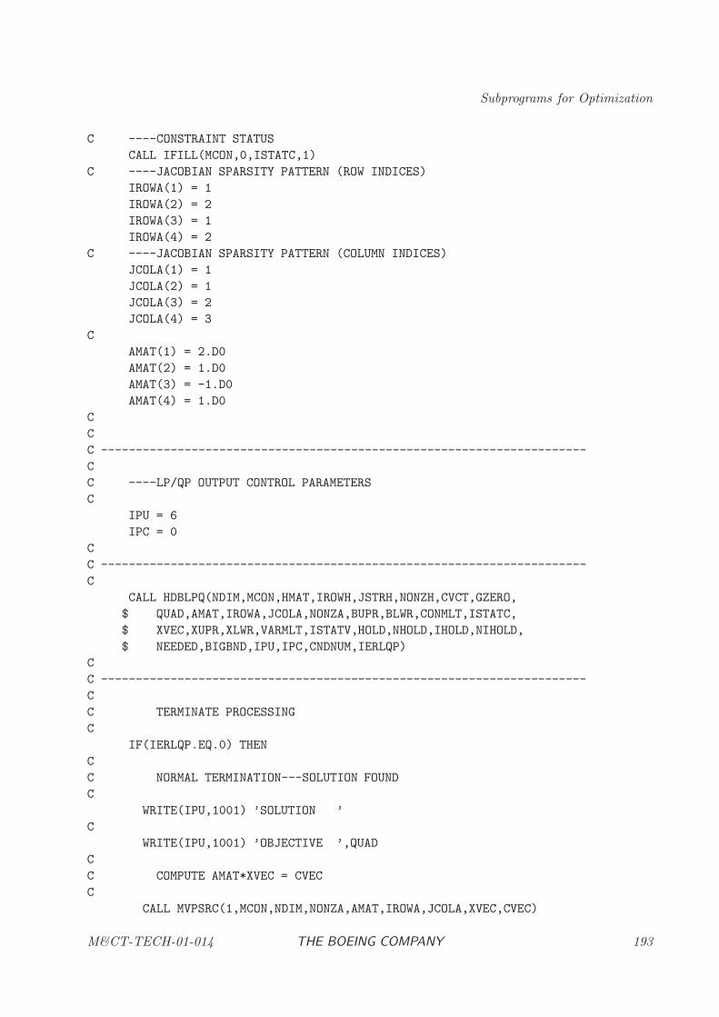
Subprograms for Optimization
C ----CONSTRAINT STATUS
CALL IFILL(MCON,0,ISTATC,1)
C ----JACOBIAN SPARSITY PATTERN (ROW INDICES)
IROWA(1) = 1
IROWA(2) = 2
IROWA(3) = 1
IROWA(4) = 2
C ----JACOBIAN SPARSITY PATTERN (COLUMN INDICES)
JCOLA(1) = 1
JCOLA(2) = 1
JCOLA(3) = 2
JCOLA(4) = 3
C
AMAT(1) = 2.D0
AMAT(2) = 1.D0
AMAT(3) = -1.D0
AMAT(4) = 1.D0
C
C
C ----------------------------------------------------------------------
C
C ----LP/QP OUTPUT CONTROL PARAMETERS
C
IPU = 6
IPC = 0
C
C ----------------------------------------------------------------------
C
CALL HDBLPQ(NDIM,MCON,HMAT,IROWH,JSTRH,NONZH,CVCT,GZERO,
$ QUAD,AMAT,IROWA,JCOLA,NONZA,BUPR,BLWR,CONMLT,ISTATC,
$ XVEC,XUPR,XLWR,VARMLT,ISTATV,HOLD,NHOLD,IHOLD,NIHOLD,
$ NEEDED,BIGBND,IPU,IPC,CNDNUM,IERLQP)
C
C ----------------------------------------------------------------------
C
C TERMINATE PROCESSING
C
IF(IERLQP.EQ.0) THEN
C
C NORMAL TERMINATION---SOLUTION FOUND
C
WRITE(IPU,1001) ’SOLUTION ’
C
WRITE(IPU,1001) ’OBJECTIVE ’,QUAD
C
C COMPUTE AMAT*XVEC = CVEC
C
CALL MVPSRC(1,MCON,NDIM,NONZA,AMAT,IROWA,JCOLA,XVEC,CVEC)
M&CT-TECH-01-014 THE BOEING COMPANY 193
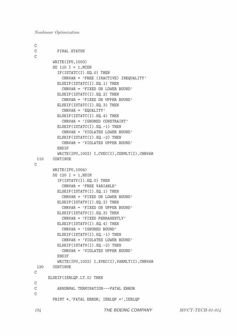
Nonlinear Optimization
C
C FINAL STATUS
C
WRITE(IPU,1003)
DO 110 I = 1,MCON
IF(ISTATC(I).EQ.0) THEN
CHRVAR = ’FREE (INACTIVE) INEQUALITY’
ELSEIF(ISTATC(I).EQ.1) THEN
CHRVAR = ’FIXED ON LOWER BOUND’
ELSEIF(ISTATC(I).EQ.2) THEN
CHRVAR = ’FIXED ON UPPER BOUND’
ELSEIF(ISTATC(I).EQ.3) THEN
CHRVAR = ’EQUALITY’
ELSEIF(ISTATC(I).EQ.4) THEN
CHRVAR = ’IGNORED CONSTRAINT’
ELSEIF(ISTATC(I).EQ.-1) THEN
CHRVAR = ’VIOLATES LOWER BOUND’
ELSEIF(ISTATC(I).EQ.-2) THEN
CHRVAR = ’VIOLATES UPPER BOUND’
ENDIF
WRITE(IPU,1002) I,CVEC(I),CONMLT(I),CHRVAR
110 CONTINUE
C
WRITE(IPU,1004)
DO 120 I = 1,NDIM
IF(ISTATV(I).EQ.0) THEN
CHRVAR = ’FREE VARIABLE’
ELSEIF(ISTATV(I).EQ.1) THEN
CHRVAR = ’FIXED ON LOWER BOUND’
ELSEIF(ISTATV(I).EQ.2) THEN
CHRVAR = ’FIXED ON UPPER BOUND’
ELSEIF(ISTATV(I).EQ.3) THEN
CHRVAR = ’FIXED PERMANENTLY’
ELSEIF(ISTATV(I).EQ.4) THEN
CHRVAR = ’IGNORED BOUND’
ELSEIF(ISTATV(I).EQ.-1) THEN
CHRVAR = ’VIOLATES LOWER BOUND’
ELSEIF(ISTATV(I).EQ.-2) THEN
CHRVAR = ’VIOLATES UPPER BOUND’
ENDIF
WRITE(IPU,1002) I,XVEC(I),VARMLT(I),CHRVAR
120 CONTINUE
C
ELSEIF(IERLQP.LT.0) THEN
C
C ABNORMAL TERMINATION---FATAL ERROR
C
PRINT *,’FATAL ERROR; IERLQP =’,IERLQP
194 THE BOEING COMPANY M&CT-TECH-01-014
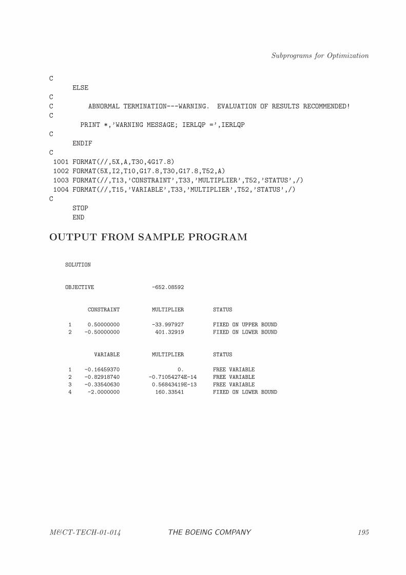
Subprograms for Optimization
C
ELSE
C
C ABNORMAL TERMINATION---WARNING. EVALUATION OF RESULTS RECOMMENDED!
C
PRINT *,’WARNING MESSAGE; IERLQP =’,IERLQP
C
ENDIF
C
1001 FORMAT(//,5X,A,T30,4G17.8)
1002 FORMAT(5X,I2,T10,G17.8,T30,G17.8,T52,A)
1003 FORMAT(//,T13,’CONSTRAINT’,T33,’MULTIPLIER’,T52,’STATUS’,/)
1004 FORMAT(//,T15,’VARIABLE’,T33,’MULTIPLIER’,T52,’STATUS’,/)
C
STOP
END
OUTPUT FROM SAMPLE PROGRAM
SOLUTION
OBJECTIVE -652.08592
CONSTRAINT MULTIPLIER STATUS
1 0.50000000 -33.997927 FIXED ON UPPER BOUND
2 -0.50000000 401.32919 FIXED ON LOWER BOUND
VARIABLE MULTIPLIER STATUS
1 -0.16459370 0. FREE VARIABLE
2 -0.82918740 -0.71054274E-14 FREE VARIABLE
3 -0.33540630 0.56843419E-13 FREE VARIABLE
4 -2.0000000 160.33541 FIXED ON LOWER BOUND
M&CT-TECH-01-014 THE BOEING COMPANY 195
Nonlinear Optimization
HHSNLP: Sparse Nonlinear Programming Input Procedure
PURPOSE
HHSNLP is a utility subroutine used to define optional inputs for the suite of nonlinear program-ming algorithms: for the SQP methods HDNLPD, HDNLPR, HDSNLP, HDSLSQ and HDSQSH;or the barrier methods HDBNPD, HDBNPR, HDBNLP, HDBLSQ and HDBLPQ.
RELATED SUBPROGRAMS
HDNLPD Dense Nonlinear Programming
HDNLPR Dense Nonlinear Programming–Reverse Communication Format
HDSNLP Sparse Nonlinear Programming
HDSLSQ Sparse Constrained Nonlinear Least Squares
HDSQSH Sparse Quadratic Programming
HDBNPD Dense Barrier Nonlinear Programming
HDBNPR Dense Barrier Nonlinear Programming–Reverse Communication Format
HDBNLP Sparse Barrier Nonlinear Programming
HDBLSQ Sparse Barrier Constrained Nonlinear Least Squares
HDBNLP Sparse Barrier Nonlinear Programming
METHOD
Subroutine HHSNLP must be called once for every optional parameter to be set. The input toHHSNLP must be a single character variable of length not to exceed 80 characters. The string iscase insensitive and is assumed to have the following format:
’ symbol = value ’
The symbol must be one of the valid mnemonics defined below; see ARGUMENTS. Informationcontained in the character string is communicated to the sparse nonlinear programming algorithmsHDSNLP, HDSLSQ, HDNLPR, HDNLPD, HDSQSH, HDBNPD, HDBNPR, HDBNLP, and HD-BLPQ via one of five commons:
NPSPRR Real variable inputs
NPSPRI Integer variable inputs
NPSPRC Character variable inputs.
BNPSPR Real variable inputs
BNPSPI Integer variable inputs
The character string must have an equals sign “=” to separate the symbol from the value. Theonly exceptions to this rule are when symbol = ’SUMMARY’, ’SPARSE DEFAULT’, ’DENSE DEFAULT’,
196 THE BOEING COMPANY M&CT-TECH-01-014
Subprograms for Optimization
’BARRIER DEFAULT’, ’OPTION’, or ’FULL OPTIONS’. The value portion of the string can containinteger, real (single or double precision), or character values.
All parameters not specified by the user are automatically set to their default values. Any optionalparameters that are set by the user are not altered by algorithms HDSNLP, HDSLSQ, HDNLPR,HDNLPD, HDSQSH, HDBNPD, HDBNPR, HDBNLP, and HDBLPQ and hence changes to theoptions are cumulative. Therefore, any input changes made by the user will remain in effect untilthey are explicitly reset by another call to HHSNLP. Many of the optional inputs are used bothby the SQP algorithms (HDSNLP, HDSLSQ, HDNLPR, HDNLPD, HDSQSH) and the barrieralgorithms (HDBNPD, HDBNPR, HDBNLP, HDBLPQ). Input parameters that apply only to theSQP algorithms are indicated as “SQP Only.” Similarly, input parameters that are applicable tothe barrier algorithms are denoted by “Barrier Only.”
There are two possible sources for error when using HHSNLP;
(1) The character string input to HHSNLP is invalid,
(2) The character string input to HHSNLP is valid, but the value is incorrect for algorithms HD-SNLP, HDSLSQ, HDNLPR, HDNLPD, HDSQSH, HDBNPD, HDBNPR, HDBNLP, and HDBLPQ.
Errors encountered by HHSNLP as a result of incorrect character strings (class 1) are communicatedto the user by a call to the BCSLIB error handler HHERR, followed by a call to HHERRX to displaythe incorrect string. A list of the character string errors is given below (see ARGUMENTS). Inputerrors caused by an incorrect value (i.e. class 2) are detected by algorithms HDSNLP, HDSLSQ,HDNLPR, HDNLPD, HDSQSH, HDBNPD, HDBNPR, HDBNLP, and HDBLPQ when they arecalled and the information is communicated to the user by the appropriate error return flag.
USAGE
CHARACTER STRING*k
CALL HHSNLP(STRING)
ARGUMENTS
STRING [INPUT, CHARACTER]Character variable of length k where k ≤ 80, of the form STRING(1:k) = ’symbol= value’.
Convergence and Termination Tolerances
The following optional inputs can be used to control convergence and termination:
Symbol Default Description
CONTOL ǫ12 Constraint tolerance, δc ≥ ǫ
12 , where ǫ = HDMCON(5).
OBJTOL 10−7 Objective function tolerance, δo, where δo ≥ max (10ǫ, δc)
PGDTOL 10−5 Projected gradient tolerance, δp, where 10ǫ < δp ≤ .01
MAXNFE 10000 Maximum number of function evaluations.NITMAX 100 Maximum number of iterations. NITMAX ≥ max (1,NITMIN).
NITMIN 0 Minimum number of iterations.
M&CT-TECH-01-014 THE BOEING COMPANY 197
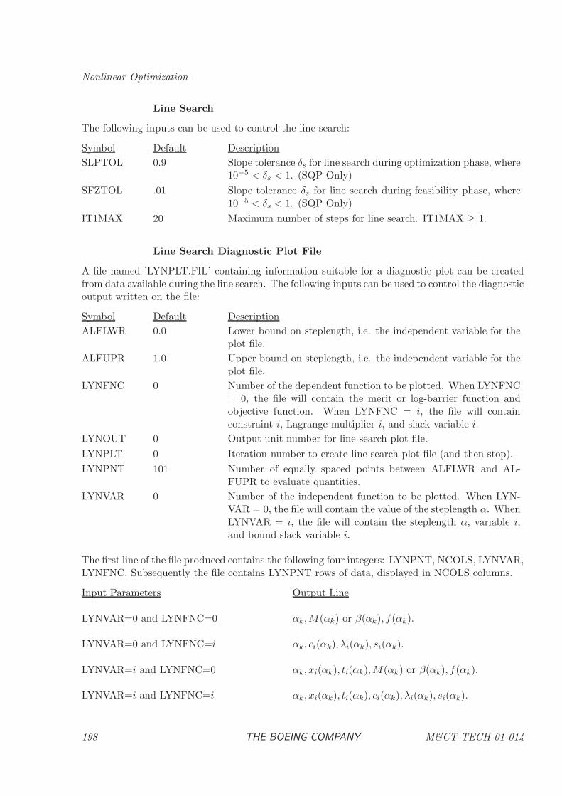
Nonlinear Optimization
Line Search
The following inputs can be used to control the line search:
Symbol Default Description
SLPTOL 0.9 Slope tolerance δs for line search during optimization phase, where10−5 < δs < 1. (SQP Only)
SFZTOL .01 Slope tolerance δs for line search during feasibility phase, where10−5 < δs < 1. (SQP Only)
IT1MAX 20 Maximum number of steps for line search. IT1MAX ≥ 1.
Line Search Diagnostic Plot File
A file named ’LYNPLT.FIL’ containing information suitable for a diagnostic plot can be createdfrom data available during the line search. The following inputs can be used to control the diagnosticoutput written on the file:
Symbol Default Description
ALFLWR 0.0 Lower bound on steplength, i.e. the independent variable for theplot file.
ALFUPR 1.0 Upper bound on steplength, i.e. the independent variable for theplot file.
LYNFNC 0 Number of the dependent function to be plotted. When LYNFNC= 0, the file will contain the merit or log-barrier function andobjective function. When LYNFNC = i, the file will containconstraint i, Lagrange multiplier i, and slack variable i.
LYNOUT 0 Output unit number for line search plot file.
LYNPLT 0 Iteration number to create line search plot file (and then stop).
LYNPNT 101 Number of equally spaced points between ALFLWR and AL-FUPR to evaluate quantities.
LYNVAR 0 Number of the independent function to be plotted. When LYN-VAR = 0, the file will contain the value of the steplength α. WhenLYNVAR = i, the file will contain the steplength α, variable i,and bound slack variable i.
The first line of the file produced contains the following four integers: LYNPNT, NCOLS, LYNVAR,LYNFNC. Subsequently the file contains LYNPNT rows of data, displayed in NCOLS columns.
Input Parameters Output Line
LYNVAR=0 and LYNFNC=0 αk,M(αk) or β(αk), f(αk).
LYNVAR=0 and LYNFNC=i αk, ci(αk), λi(αk), si(αk).
LYNVAR=i and LYNFNC=0 αk, xi(αk), ti(αk),M(αk) or β(αk), f(αk).
LYNVAR=i and LYNFNC=i αk, xi(αk), ti(αk), ci(αk), λi(αk), si(αk).
198 THE BOEING COMPANY M&CT-TECH-01-014
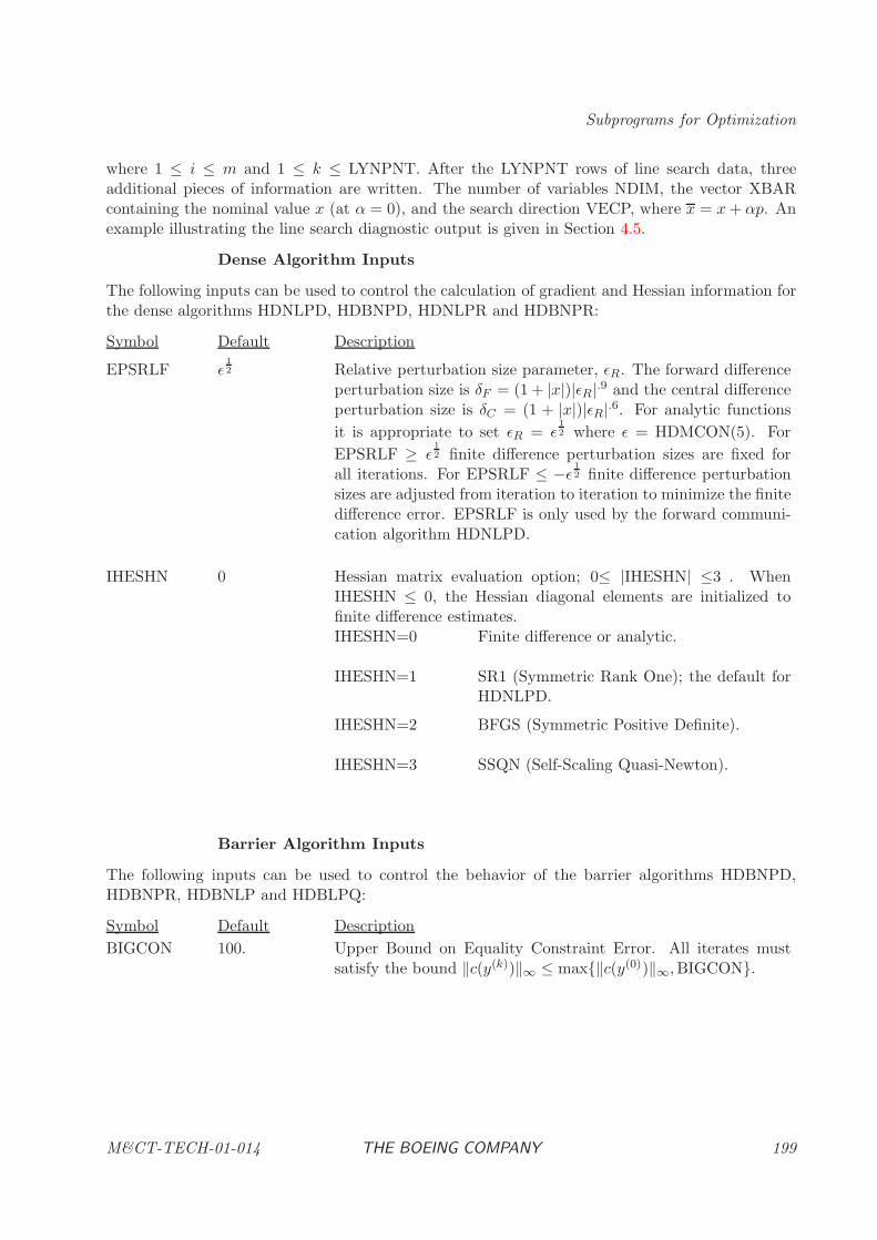
Subprograms for Optimization
where 1 ≤ i ≤ m and 1 ≤ k ≤ LYNPNT. After the LYNPNT rows of line search data, threeadditional pieces of information are written. The number of variables NDIM, the vector XBARcontaining the nominal value x (at α = 0), and the search direction VECP, where x = x+ αp. Anexample illustrating the line search diagnostic output is given in Section 4.5.
Dense Algorithm Inputs
The following inputs can be used to control the calculation of gradient and Hessian information forthe dense algorithms HDNLPD, HDBNPD, HDNLPR and HDBNPR:
Symbol Default Description
EPSRLF ǫ12 Relative perturbation size parameter, ǫR. The forward difference
perturbation size is δF = (1 + |x|)|ǫR|.9 and the central differenceperturbation size is δC = (1 + |x|)|ǫR|.6. For analytic functions
it is appropriate to set ǫR = ǫ12 where ǫ = HDMCON(5). For
EPSRLF ≥ ǫ12 finite difference perturbation sizes are fixed for
all iterations. For EPSRLF ≤ −ǫ 12 finite difference perturbation
sizes are adjusted from iteration to iteration to minimize the finitedifference error. EPSRLF is only used by the forward communi-cation algorithm HDNLPD.
IHESHN 0 Hessian matrix evaluation option; 0≤ |IHESHN| ≤3 . WhenIHESHN ≤ 0, the Hessian diagonal elements are initialized tofinite difference estimates.IHESHN=0 Finite difference or analytic.
IHESHN=1 SR1 (Symmetric Rank One); the default forHDNLPD.
IHESHN=2 BFGS (Symmetric Positive Definite).
IHESHN=3 SSQN (Self-Scaling Quasi-Newton).
Barrier Algorithm Inputs
The following inputs can be used to control the behavior of the barrier algorithms HDBNPD,HDBNPR, HDBNLP and HDBLPQ:
Symbol Default Description
BIGCON 100. Upper Bound on Equality Constraint Error. All iterates mustsatisfy the bound ‖c(y(k))‖∞ ≤ max{‖c(y(0))‖∞,BIGCON}.
M&CT-TECH-01-014 THE BOEING COMPANY 199
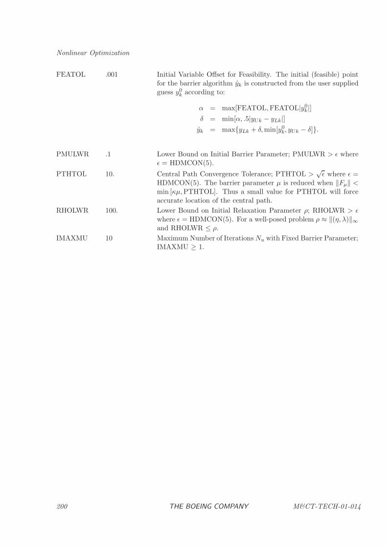
Nonlinear Optimization
FEATOL .001 Initial Variable Offset for Feasibility. The initial (feasible) pointfor the barrier algorithm yk is constructed from the user suppliedguess y0
k according to:
α = max[FEATOL,FEATOL|y0k|]
δ = min[α, .5|yUk − yLk|]yk = max{yLk + δ,min[y0
k, yUk − δ]}.
PMULWR .1 Lower Bound on Initial Barrier Parameter; PMULWR > ǫ whereǫ = HDMCON(5).
PTHTOL 10. Central Path Convergence Tolerance; PTHTOL >√ǫ where ǫ =
HDMCON(5). The barrier parameter µ is reduced when ‖Fµ‖ <min [κµ,PTHTOL]. Thus a small value for PTHTOL will forceaccurate location of the central path.
RHOLWR 100. Lower Bound on Initial Relaxation Parameter ρ; RHOLWR > ǫwhere ǫ = HDMCON(5). For a well-posed problem ρ ≈ ‖(η, λ)‖∞and RHOLWR ≤ ρ.
IMAXMU 10 Maximum Number of IterationsNu with Fixed Barrier Parameter;IMAXMU ≥ 1.
200 THE BOEING COMPANY M&CT-TECH-01-014
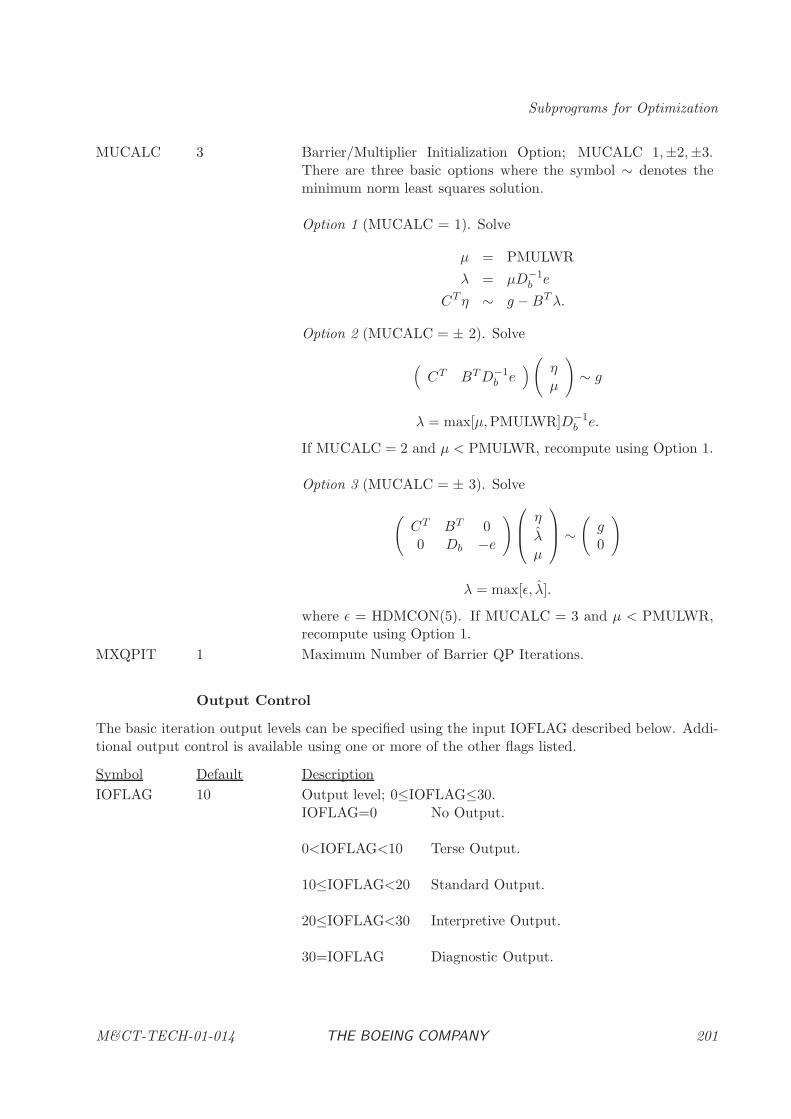
Subprograms for Optimization
MUCALC 3 Barrier/Multiplier Initialization Option; MUCALC 1,±2,±3.There are three basic options where the symbol ∼ denotes theminimum norm least squares solution.
Option 1 (MUCALC = 1). Solve
µ = PMULWR
λ = µD−1b e
CTη ∼ g −BTλ.
Option 2 (MUCALC = ± 2). Solve
(CT BTD−1
b e)( η
µ
)
∼ g
λ = max[µ,PMULWR]D−1b e.
If MUCALC = 2 and µ < PMULWR, recompute using Option 1.
Option 3 (MUCALC = ± 3). Solve
(CT BT 00 Db −e
)
η
λµ
∼(g0
)
λ = max[ǫ, λ].
where ǫ = HDMCON(5). If MUCALC = 3 and µ < PMULWR,recompute using Option 1.
MXQPIT 1 Maximum Number of Barrier QP Iterations.
Output Control
The basic iteration output levels can be specified using the input IOFLAG described below. Addi-tional output control is available using one or more of the other flags listed.
Symbol Default Description
IOFLAG 10 Output level; 0≤IOFLAG≤30.IOFLAG=0 No Output.
0<IOFLAG<10 Terse Output.
10≤IOFLAG<20 Standard Output.
20≤IOFLAG<30 Interpretive Output.
30=IOFLAG Diagnostic Output.
M&CT-TECH-01-014 THE BOEING COMPANY 201
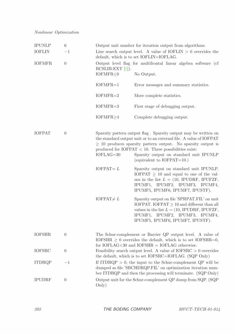
Nonlinear Optimization
IPUNLP 6 Output unit number for iteration output from algorithms.
IOFLIN −1 Line search output level. A value of IOFLIN > 0 overrides thedefault, which is to set IOFLIN=IOFLAG.
IOFMFR 0 Output level flag for multifrontal linear algebra software (cfBCSLIB-EXT [1]).IOFMFR≤0 No Output.
IOFMFR=1 Error messages and summary statistics.
IOFMFR=2 More complete statistics.
IOFMFR=3 First stage of debugging output.
IOFMFR≥4 Complete debugging output.
IOFPAT 0 Sparsity pattern output flag . Sparsity output may be written onthe standard output unit or to an external file. A value of IOFPAT≥ 10 produces sparsity pattern output. No sparsity output isproduced for IOFPAT < 10. Three possibilities exist:IOFLAG=30 Sparsity output on standard unit IPUNLP
(equivalent to IOFPAT=10.)
IOFPAT= L Sparsity output on standard unit IPUNLP.IOFPAT ≥ 10 and equal to one of the val-ues in the list L = (10, IPUDRF, IPUFZF,IPUMF1, IPUMF2, IPUMF3, IPUMF4,IPUMF5, IPUMF6, IPUMF7, IPUSTF).
IOFPAT 6= L Sparsity output on file ’SPRPAT.FIL’ on unitIOFPAT. IOFPAT ≥ 10 and different than allvalues in the list L = (10, IPUDRF, IPUFZF,IPUMF1, IPUMF2, IPUMF3, IPUMF4,IPUMF5, IPUMF6, IPUMF7, IPUSTF).
IOFSHR 0 The Schur-complement or Barrier QP output level. A value ofIOFSHR ≥ 0 overrides the default, which is to set IOFSHR=0,for IOFLAG<30 and IOFSHR = IOFLAG otherwise.
IOFSRC 0 Feasibility search output level. A value of IOFSRC > 0 overridesthe default, which is to set IOFSRC=IOFLAG. (SQP Only)
ITDRQP −1 If ITDRQP > 0, the input to the Schur-complement QP will bedumped as file ’SRCHDRQP.FIL’ on optimization iteration num-ber ITDRQP and then the processing will terminate. (SQP Only)
IPUDRF 0 Output unit for the Schur-complement QP dump from SQP. (SQPOnly)
202 THE BOEING COMPANY M&CT-TECH-01-014
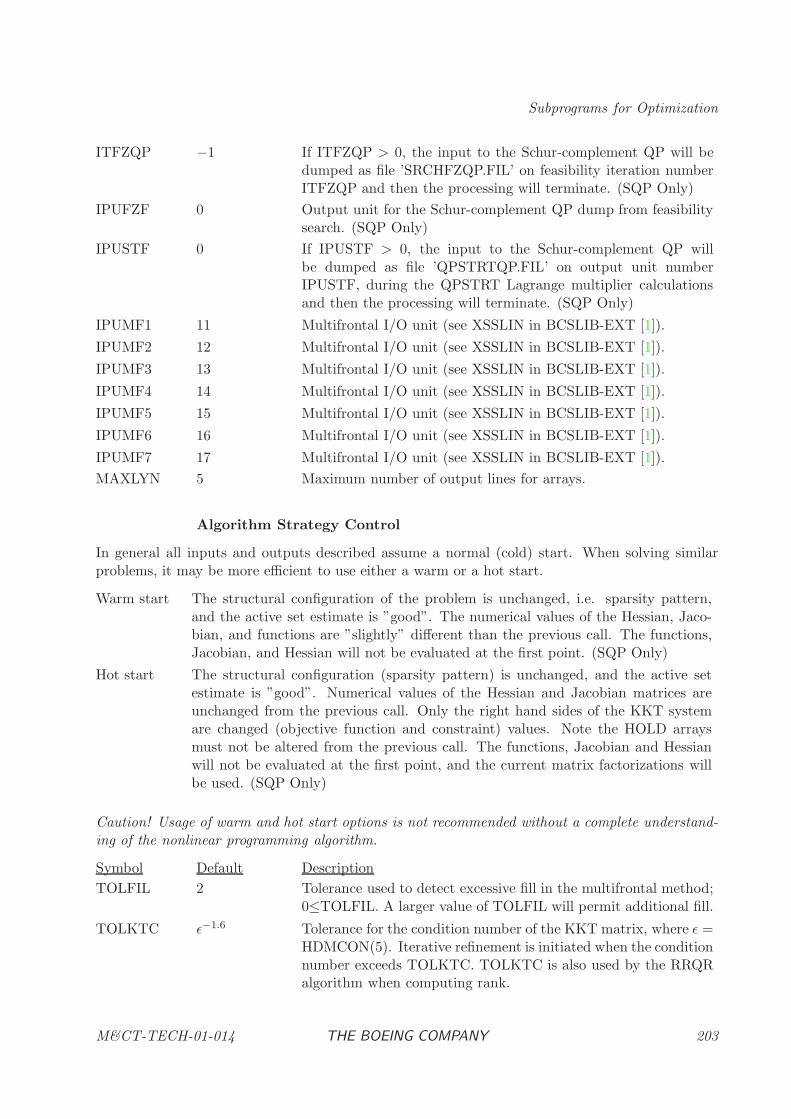
Subprograms for Optimization
ITFZQP −1 If ITFZQP > 0, the input to the Schur-complement QP will bedumped as file ’SRCHFZQP.FIL’ on feasibility iteration numberITFZQP and then the processing will terminate. (SQP Only)
IPUFZF 0 Output unit for the Schur-complement QP dump from feasibilitysearch. (SQP Only)
IPUSTF 0 If IPUSTF > 0, the input to the Schur-complement QP willbe dumped as file ’QPSTRTQP.FIL’ on output unit numberIPUSTF, during the QPSTRT Lagrange multiplier calculationsand then the processing will terminate. (SQP Only)
IPUMF1 11 Multifrontal I/O unit (see XSSLIN in BCSLIB-EXT [1]).
IPUMF2 12 Multifrontal I/O unit (see XSSLIN in BCSLIB-EXT [1]).
IPUMF3 13 Multifrontal I/O unit (see XSSLIN in BCSLIB-EXT [1]).
IPUMF4 14 Multifrontal I/O unit (see XSSLIN in BCSLIB-EXT [1]).
IPUMF5 15 Multifrontal I/O unit (see XSSLIN in BCSLIB-EXT [1]).
IPUMF6 16 Multifrontal I/O unit (see XSSLIN in BCSLIB-EXT [1]).
IPUMF7 17 Multifrontal I/O unit (see XSSLIN in BCSLIB-EXT [1]).
MAXLYN 5 Maximum number of output lines for arrays.
Algorithm Strategy Control
In general all inputs and outputs described assume a normal (cold) start. When solving similarproblems, it may be more efficient to use either a warm or a hot start.
Warm start The structural configuration of the problem is unchanged, i.e. sparsity pattern,and the active set estimate is ”good”. The numerical values of the Hessian, Jaco-bian, and functions are ”slightly” different than the previous call. The functions,Jacobian, and Hessian will not be evaluated at the first point. (SQP Only)
Hot start The structural configuration (sparsity pattern) is unchanged, and the active setestimate is ”good”. Numerical values of the Hessian and Jacobian matrices areunchanged from the previous call. Only the right hand sides of the KKT systemare changed (objective function and constraint) values. Note the HOLD arraysmust not be altered from the previous call. The functions, Jacobian and Hessianwill not be evaluated at the first point, and the current matrix factorizations willbe used. (SQP Only)
Caution! Usage of warm and hot start options is not recommended without a complete understand-ing of the nonlinear programming algorithm.
Symbol Default Description
TOLFIL 2 Tolerance used to detect excessive fill in the multifrontal method;0≤TOLFIL. A larger value of TOLFIL will permit additional fill.
TOLKTC ǫ−1.6 Tolerance for the condition number of the KKT matrix, where ǫ =HDMCON(5). Iterative refinement is initiated when the conditionnumber exceeds TOLKTC. TOLKTC is also used by the RRQRalgorithm when computing rank.
M&CT-TECH-01-014 THE BOEING COMPANY 203
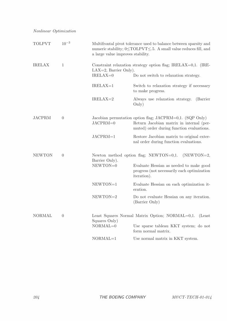
Nonlinear Optimization
TOLPVT 10−3 Multifrontal pivot tolerance used to balance between sparsity andnumeric stability; 0≤TOLPVT≤.5. A small value reduces fill, anda large value improves stability.
IRELAX 1 Constraint relaxation strategy option flag; IRELAX=0,1. (IRE-LAX=2, Barrier Only).IRELAX=0 Do not switch to relaxation strategy.
IRELAX=1 Switch to relaxation strategy if necessaryto make progress.
IRELAX=2 Always use relaxation strategy. (BarrierOnly)
JACPRM 0 Jacobian permutation option flag; JACPRM=0,1. (SQP Only)JACPRM=0 Return Jacobian matrix in internal (per-
muted) order during function evaluations.
JACPRM=1 Restore Jacobian matrix to original exter-nal order during function evaluations.
NEWTON 0 Newton method option flag; NEWTON=0,1. (NEWTON=2,Barrier Only).NEWTON=0 Evaluate Hessian as needed to make good
progress (not necessarily each optimizationiteration).
NEWTON=1 Evaluate Hessian on each optimization it-eration.
NEWTON=2 Do not evaluate Hessian on any iteration.(Barrier Only)
NORMAL 0 Least Squares Normal Matrix Option; NORMAL=0,1. (LeastSquares Only)NORMAL=0 Use sparse tableau KKT system; do not
form normal matrix.
NORMAL=1 Use normal matrix in KKT system.
204 THE BOEING COMPANY M&CT-TECH-01-014
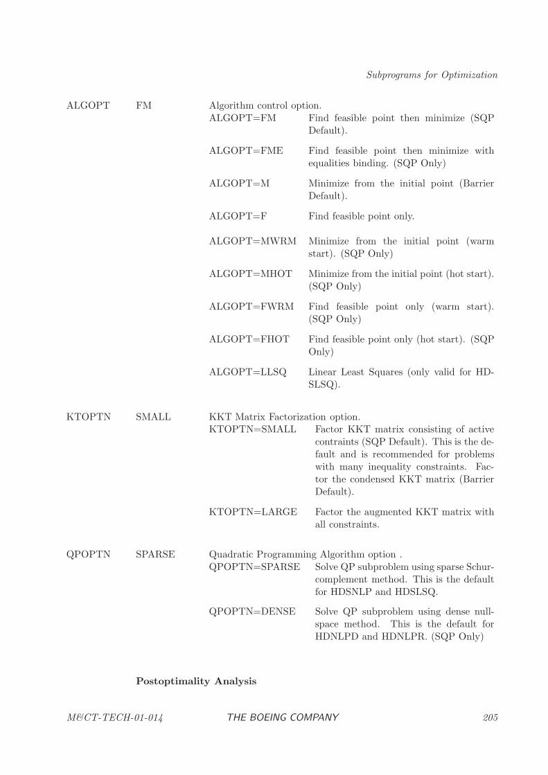
Subprograms for Optimization
ALGOPT FM Algorithm control option.ALGOPT=FM Find feasible point then minimize (SQP
Default).
ALGOPT=FME Find feasible point then minimize withequalities binding. (SQP Only)
ALGOPT=M Minimize from the initial point (BarrierDefault).
ALGOPT=F Find feasible point only.
ALGOPT=MWRM Minimize from the initial point (warmstart). (SQP Only)
ALGOPT=MHOT Minimize from the initial point (hot start).(SQP Only)
ALGOPT=FWRM Find feasible point only (warm start).(SQP Only)
ALGOPT=FHOT Find feasible point only (hot start). (SQPOnly)
ALGOPT=LLSQ Linear Least Squares (only valid for HD-SLSQ).
KTOPTN SMALL KKT Matrix Factorization option.KTOPTN=SMALL Factor KKT matrix consisting of active
contraints (SQP Default). This is the de-fault and is recommended for problemswith many inequality constraints. Fac-tor the condensed KKT matrix (BarrierDefault).
KTOPTN=LARGE Factor the augmented KKT matrix withall constraints.
QPOPTN SPARSE Quadratic Programming Algorithm option .QPOPTN=SPARSE Solve QP subproblem using sparse Schur-
complement method. This is the defaultfor HDSNLP and HDSLSQ.
QPOPTN=DENSE Solve QP subproblem using dense null-space method. This is the default forHDNLPD and HDNLPR. (SQP Only)
Postoptimality Analysis
M&CT-TECH-01-014 THE BOEING COMPANY 205
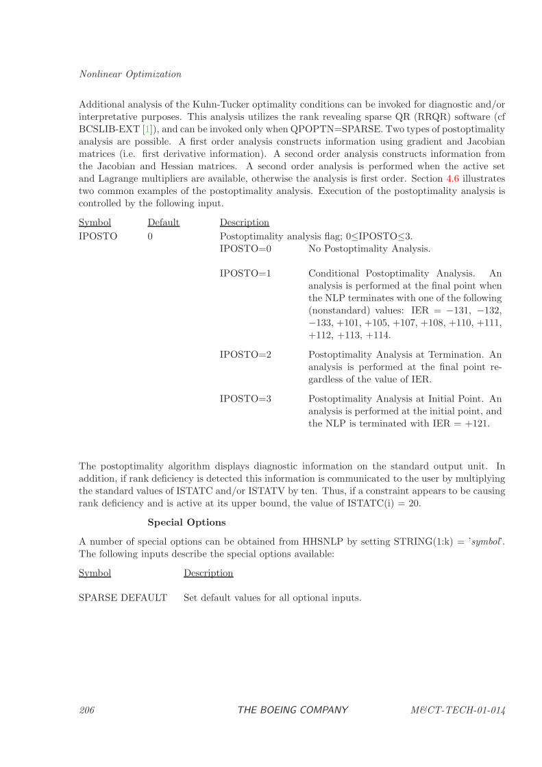
Nonlinear Optimization
Additional analysis of the Kuhn-Tucker optimality conditions can be invoked for diagnostic and/orinterpretative purposes. This analysis utilizes the rank revealing sparse QR (RRQR) software (cfBCSLIB-EXT [1]), and can be invoked only when QPOPTN=SPARSE. Two types of postoptimalityanalysis are possible. A first order analysis constructs information using gradient and Jacobianmatrices (i.e. first derivative information). A second order analysis constructs information fromthe Jacobian and Hessian matrices. A second order analysis is performed when the active setand Lagrange multipliers are available, otherwise the analysis is first order. Section 4.6 illustratestwo common examples of the postoptimality analysis. Execution of the postoptimality analysis iscontrolled by the following input.
Symbol Default Description
IPOSTO 0 Postoptimality analysis flag; 0≤IPOSTO≤3.IPOSTO=0 No Postoptimality Analysis.
IPOSTO=1 Conditional Postoptimality Analysis. Ananalysis is performed at the final point whenthe NLP terminates with one of the following(nonstandard) values: IER = −131, −132,−133, +101, +105, +107, +108, +110, +111,+112, +113, +114.
IPOSTO=2 Postoptimality Analysis at Termination. Ananalysis is performed at the final point re-gardless of the value of IER.
IPOSTO=3 Postoptimality Analysis at Initial Point. Ananalysis is performed at the initial point, andthe NLP is terminated with IER = +121.
The postoptimality algorithm displays diagnostic information on the standard output unit. Inaddition, if rank deficiency is detected this information is communicated to the user by multiplyingthe standard values of ISTATC and/or ISTATV by ten. Thus, if a constraint appears to be causingrank deficiency and is active at its upper bound, the value of ISTATC(i) = 20.
Special Options
A number of special options can be obtained from HHSNLP by setting STRING(1:k) = ’symbol’.The following inputs describe the special options available:
Symbol Description
SPARSE DEFAULT Set default values for all optional inputs.
206 THE BOEING COMPANY M&CT-TECH-01-014
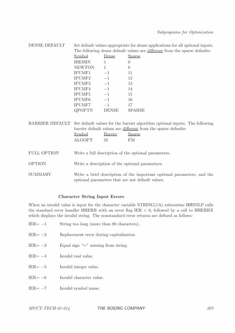
Subprograms for Optimization
DENSE DEFAULT Set default values appropriate for dense applications for all optional inputs.The following dense default values are different from the sparse defaults:Symbol Dense Sparse
IHESHN 1 0NEWTON 1 0IPUMF1 −1 11IPUMF2 −1 12IPUMF3 −1 13IPUMF4 −1 14IPUMF5 −1 15IPUMF6 −1 16IPUMF7 −1 17QPOPTN DENSE SPARSE
BARRIER DEFAULT Set default values for the barrier algorithm optional inputs. The followingbarrier default values are different from the sparse defaults:Symbol Barrier Sparse
ALGOPT M FM
FULL OPTION Write a full description of the optional parameters.
OPTION Write a description of the optional parameters.
SUMMARY Write a brief description of the important optional parameters, and theoptional parameters that are not default values.
Character String Input Errors
When an invalid value is input for the character variable STRING(1:k) subroutine HHSNLP callsthe standard error handler HHERR with an error flag IER < 0, followed by a call to HHERRXwhich displays the invalid string. The nonstandard error returns are defined as follows:
IER= −1 String too long (more than 80 characters).
IER= −2 Replacement error during capitalization.
IER= −3 Equal sign “=” missing from string.
IER= −4 Invalid real value.
IER= −5 Invalid integer value.
IER= −6 Invalid character value.
IER= −7 Invalid symbol name.
M&CT-TECH-01-014 THE BOEING COMPANY 207
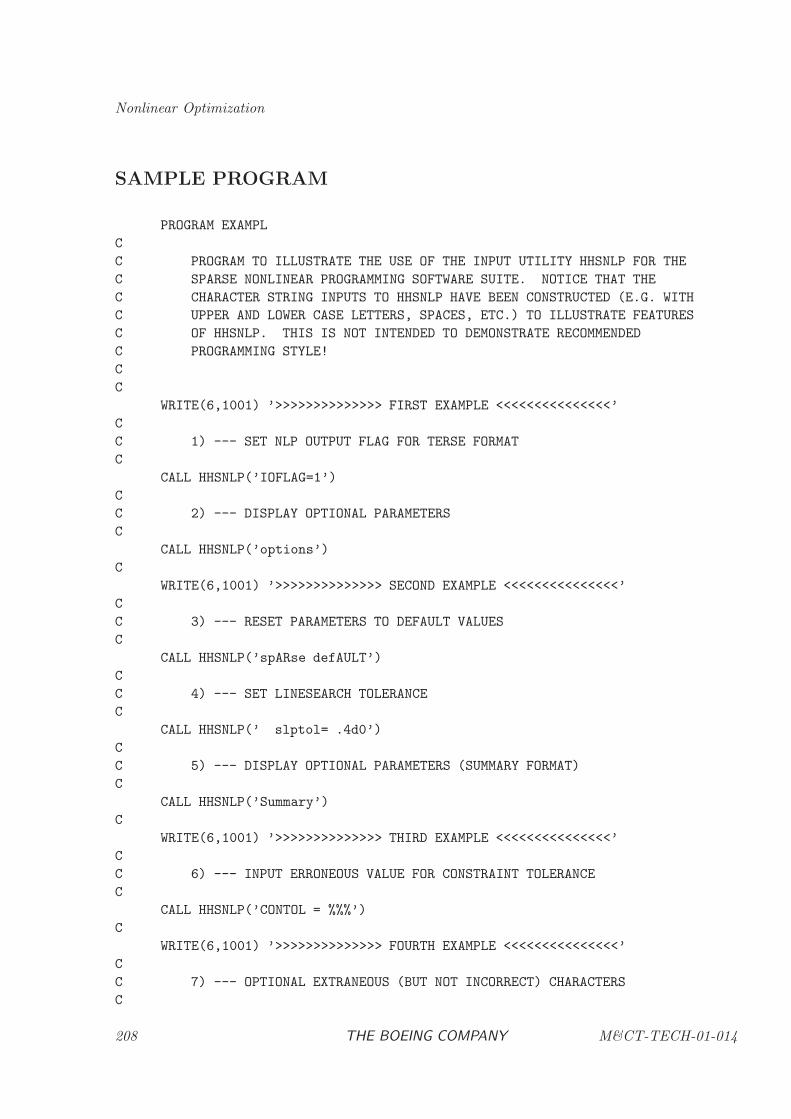
Nonlinear Optimization
SAMPLE PROGRAM
PROGRAM EXAMPL
C
C PROGRAM TO ILLUSTRATE THE USE OF THE INPUT UTILITY HHSNLP FOR THE
C SPARSE NONLINEAR PROGRAMMING SOFTWARE SUITE. NOTICE THAT THE
C CHARACTER STRING INPUTS TO HHSNLP HAVE BEEN CONSTRUCTED (E.G. WITH
C UPPER AND LOWER CASE LETTERS, SPACES, ETC.) TO ILLUSTRATE FEATURES
C OF HHSNLP. THIS IS NOT INTENDED TO DEMONSTRATE RECOMMENDED
C PROGRAMMING STYLE!
C
C
WRITE(6,1001) ’>>>>>>>>>>>>>> FIRST EXAMPLE <<<<<<<<<<<<<<<’
C
C 1) --- SET NLP OUTPUT FLAG FOR TERSE FORMAT
C
CALL HHSNLP(’IOFLAG=1’)
C
C 2) --- DISPLAY OPTIONAL PARAMETERS
C
CALL HHSNLP(’options’)
C
WRITE(6,1001) ’>>>>>>>>>>>>>> SECOND EXAMPLE <<<<<<<<<<<<<<<’
C
C 3) --- RESET PARAMETERS TO DEFAULT VALUES
C
CALL HHSNLP(’spARse defAULT’)
C
C 4) --- SET LINESEARCH TOLERANCE
C
CALL HHSNLP(’ slptol= .4d0’)
C
C 5) --- DISPLAY OPTIONAL PARAMETERS (SUMMARY FORMAT)
C
CALL HHSNLP(’Summary’)
C
WRITE(6,1001) ’>>>>>>>>>>>>>> THIRD EXAMPLE <<<<<<<<<<<<<<<’
C
C 6) --- INPUT ERRONEOUS VALUE FOR CONSTRAINT TOLERANCE
C
CALL HHSNLP(’CONTOL = %%%’)
C
WRITE(6,1001) ’>>>>>>>>>>>>>> FOURTH EXAMPLE <<<<<<<<<<<<<<<’
C
C 7) --- OPTIONAL EXTRANEOUS (BUT NOT INCORRECT) CHARACTERS
C
208 THE BOEING COMPANY M&CT-TECH-01-014
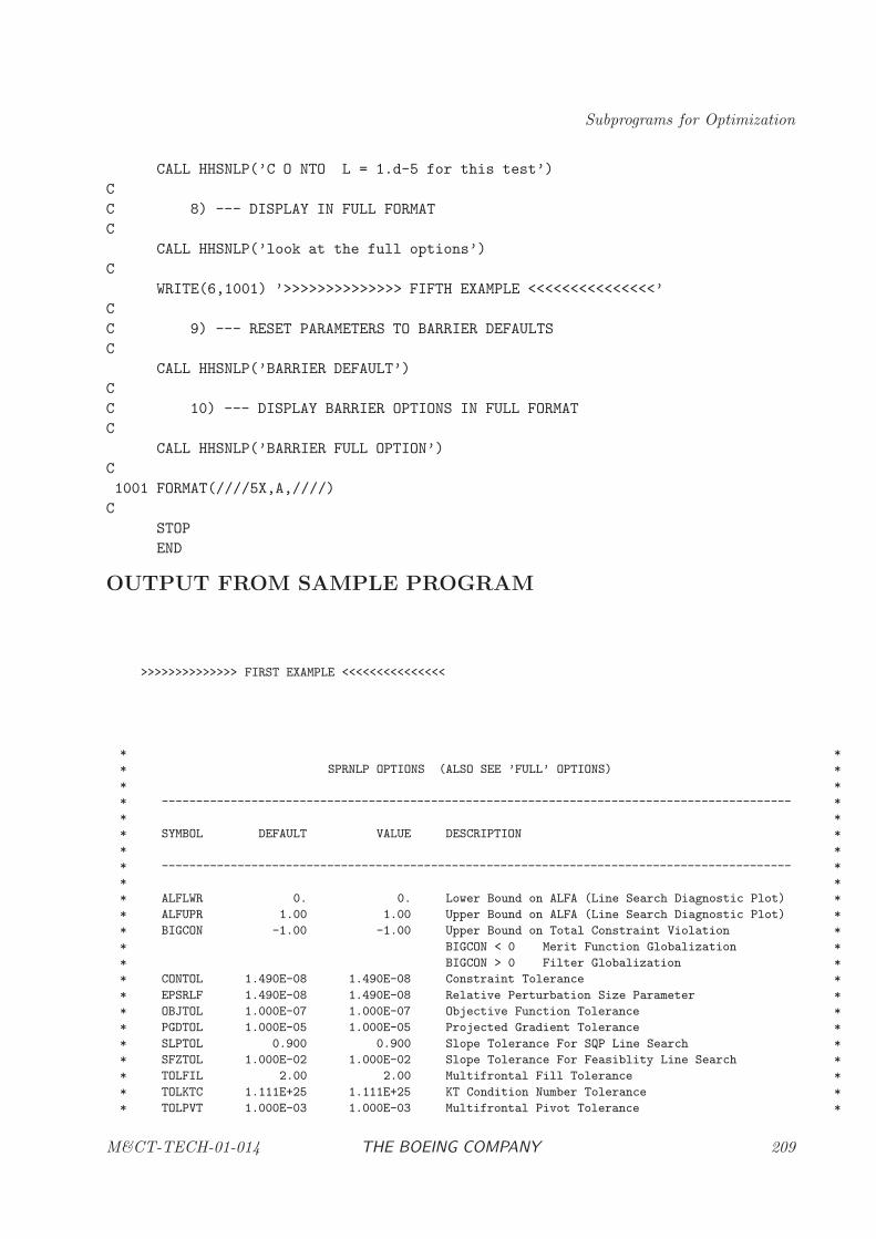
Subprograms for Optimization
CALL HHSNLP(’C O NTO L = 1.d-5 for this test’)
C
C 8) --- DISPLAY IN FULL FORMAT
C
CALL HHSNLP(’look at the full options’)
C
WRITE(6,1001) ’>>>>>>>>>>>>>> FIFTH EXAMPLE <<<<<<<<<<<<<<<’
C
C 9) --- RESET PARAMETERS TO BARRIER DEFAULTS
C
CALL HHSNLP(’BARRIER DEFAULT’)
C
C 10) --- DISPLAY BARRIER OPTIONS IN FULL FORMAT
C
CALL HHSNLP(’BARRIER FULL OPTION’)
C
1001 FORMAT(////5X,A,////)
C
STOP
END
OUTPUT FROM SAMPLE PROGRAM
>>>>>>>>>>>>>> FIRST EXAMPLE <<<<<<<<<<<<<<<
* *
* SPRNLP OPTIONS (ALSO SEE ’FULL’ OPTIONS) *
* *
* ------------------------------------------------------------------------------------------- *
* *
* SYMBOL DEFAULT VALUE DESCRIPTION *
* *
* ------------------------------------------------------------------------------------------- *
* *
* ALFLWR 0. 0. Lower Bound on ALFA (Line Search Diagnostic Plot) *
* ALFUPR 1.00 1.00 Upper Bound on ALFA (Line Search Diagnostic Plot) *
* BIGCON -1.00 -1.00 Upper Bound on Total Constraint Violation *
* BIGCON < 0 Merit Function Globalization *
* BIGCON > 0 Filter Globalization *
* CONTOL 1.490E-08 1.490E-08 Constraint Tolerance *
* EPSRLF 1.490E-08 1.490E-08 Relative Perturbation Size Parameter *
* OBJTOL 1.000E-07 1.000E-07 Objective Function Tolerance *
* PGDTOL 1.000E-05 1.000E-05 Projected Gradient Tolerance *
* SLPTOL 0.900 0.900 Slope Tolerance For SQP Line Search *
* SFZTOL 1.000E-02 1.000E-02 Slope Tolerance For Feasiblity Line Search *
* TOLFIL 2.00 2.00 Multifrontal Fill Tolerance *
* TOLKTC 1.111E+25 1.111E+25 KT Condition Number Tolerance *
* TOLPVT 1.000E-03 1.000E-03 Multifrontal Pivot Tolerance *
M&CT-TECH-01-014 THE BOEING COMPANY 209
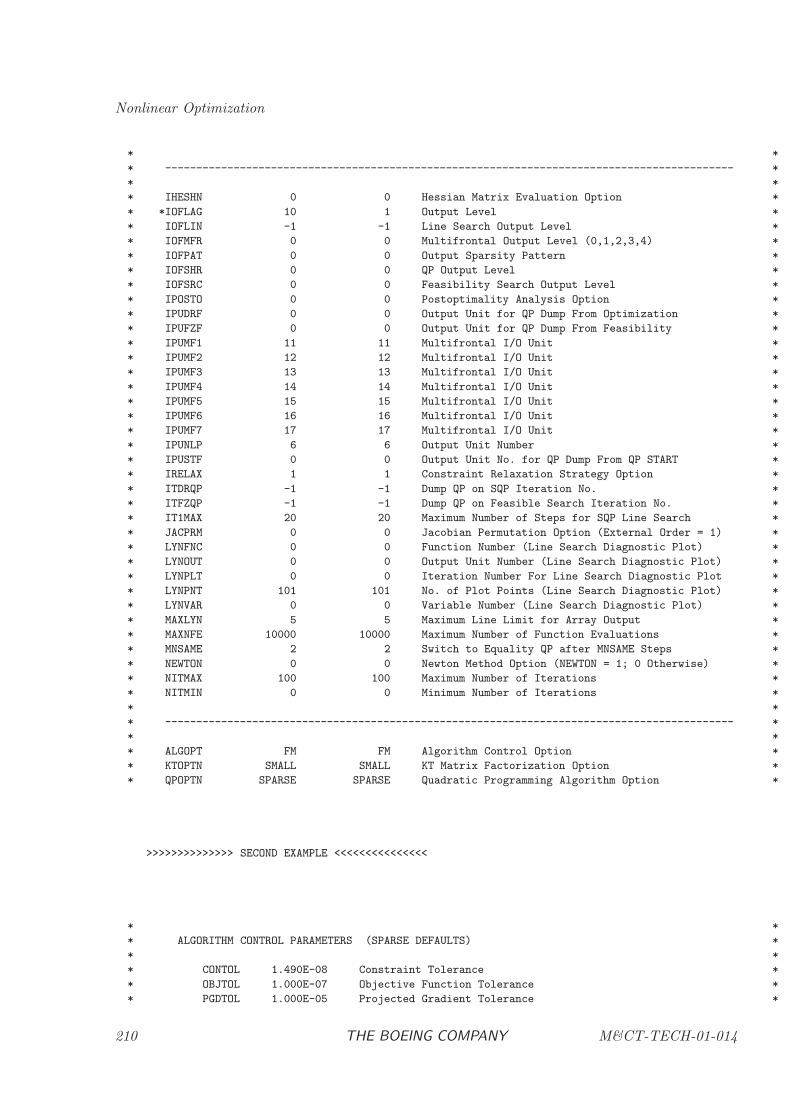
Nonlinear Optimization
* *
* ------------------------------------------------------------------------------------------- *
* *
* IHESHN 0 0 Hessian Matrix Evaluation Option *
* *IOFLAG 10 1 Output Level *
* IOFLIN -1 -1 Line Search Output Level *
* IOFMFR 0 0 Multifrontal Output Level (0,1,2,3,4) *
* IOFPAT 0 0 Output Sparsity Pattern *
* IOFSHR 0 0 QP Output Level *
* IOFSRC 0 0 Feasibility Search Output Level *
* IPOSTO 0 0 Postoptimality Analysis Option *
* IPUDRF 0 0 Output Unit for QP Dump From Optimization *
* IPUFZF 0 0 Output Unit for QP Dump From Feasibility *
* IPUMF1 11 11 Multifrontal I/O Unit *
* IPUMF2 12 12 Multifrontal I/O Unit *
* IPUMF3 13 13 Multifrontal I/O Unit *
* IPUMF4 14 14 Multifrontal I/O Unit *
* IPUMF5 15 15 Multifrontal I/O Unit *
* IPUMF6 16 16 Multifrontal I/O Unit *
* IPUMF7 17 17 Multifrontal I/O Unit *
* IPUNLP 6 6 Output Unit Number *
* IPUSTF 0 0 Output Unit No. for QP Dump From QP START *
* IRELAX 1 1 Constraint Relaxation Strategy Option *
* ITDRQP -1 -1 Dump QP on SQP Iteration No. *
* ITFZQP -1 -1 Dump QP on Feasible Search Iteration No. *
* IT1MAX 20 20 Maximum Number of Steps for SQP Line Search *
* JACPRM 0 0 Jacobian Permutation Option (External Order = 1) *
* LYNFNC 0 0 Function Number (Line Search Diagnostic Plot) *
* LYNOUT 0 0 Output Unit Number (Line Search Diagnostic Plot) *
* LYNPLT 0 0 Iteration Number For Line Search Diagnostic Plot *
* LYNPNT 101 101 No. of Plot Points (Line Search Diagnostic Plot) *
* LYNVAR 0 0 Variable Number (Line Search Diagnostic Plot) *
* MAXLYN 5 5 Maximum Line Limit for Array Output *
* MAXNFE 10000 10000 Maximum Number of Function Evaluations *
* MNSAME 2 2 Switch to Equality QP after MNSAME Steps *
* NEWTON 0 0 Newton Method Option (NEWTON = 1; 0 Otherwise) *
* NITMAX 100 100 Maximum Number of Iterations *
* NITMIN 0 0 Minimum Number of Iterations *
* *
* ------------------------------------------------------------------------------------------- *
* *
* ALGOPT FM FM Algorithm Control Option *
* KTOPTN SMALL SMALL KT Matrix Factorization Option *
* QPOPTN SPARSE SPARSE Quadratic Programming Algorithm Option *
>>>>>>>>>>>>>> SECOND EXAMPLE <<<<<<<<<<<<<<<
* *
* ALGORITHM CONTROL PARAMETERS (SPARSE DEFAULTS) *
* *
* CONTOL 1.490E-08 Constraint Tolerance *
* OBJTOL 1.000E-07 Objective Function Tolerance *
* PGDTOL 1.000E-05 Projected Gradient Tolerance *
210 THE BOEING COMPANY M&CT-TECH-01-014
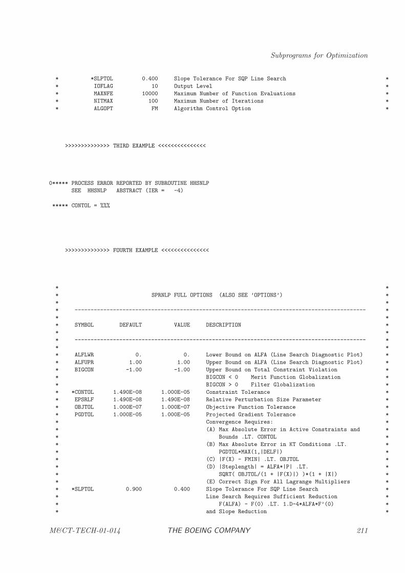
Subprograms for Optimization
* *SLPTOL 0.400 Slope Tolerance For SQP Line Search *
* IOFLAG 10 Output Level *
* MAXNFE 10000 Maximum Number of Function Evaluations *
* NITMAX 100 Maximum Number of Iterations *
* ALGOPT FM Algorithm Control Option *
>>>>>>>>>>>>>> THIRD EXAMPLE <<<<<<<<<<<<<<<
0***** PROCESS ERROR REPORTED BY SUBROUTINE HHSNLP
SEE HHSNLP ABSTRACT (IER = -4)
***** CONTOL = %%%
>>>>>>>>>>>>>> FOURTH EXAMPLE <<<<<<<<<<<<<<<
* *
* SPRNLP FULL OPTIONS (ALSO SEE ’OPTIONS’) *
* *
* ------------------------------------------------------------------------------------------- *
* *
* SYMBOL DEFAULT VALUE DESCRIPTION *
* *
* ------------------------------------------------------------------------------------------- *
* *
* ALFLWR 0. 0. Lower Bound on ALFA (Line Search Diagnostic Plot) *
* ALFUPR 1.00 1.00 Upper Bound on ALFA (Line Search Diagnostic Plot) *
* BIGCON -1.00 -1.00 Upper Bound on Total Constraint Violation *
* BIGCON < 0 Merit Function Globalization *
* BIGCON > 0 Filter Globalization *
* *CONTOL 1.490E-08 1.000E-05 Constraint Tolerance *
* EPSRLF 1.490E-08 1.490E-08 Relative Perturbation Size Parameter *
* OBJTOL 1.000E-07 1.000E-07 Objective Function Tolerance *
* PGDTOL 1.000E-05 1.000E-05 Projected Gradient Tolerance *
* Convergence Requires: *
* (A) Max Absolute Error in Active Constraints and *
* Bounds .LT. CONTOL *
* (B) Max Absolute Error in KT Conditions .LT. *
* PGDTOL*MAX(1,|DELF|) *
* (C) |F(X) - FMIN| .LT. OBJTOL *
* (D) |Steplength| = ALFA*|P| .LT. *
* SQRT( OBJTOL/(1 + |F(X)|) )*(1 + |X|) *
* (E) Correct Sign For All Lagrange Multipliers *
* *SLPTOL 0.900 0.400 Slope Tolerance For SQP Line Search *
* Line Search Requires Sufficient Reduction *
* F(ALFA) - F(0) .LT. 1.D-4*ALFA*F’(0) *
* and Slope Reduction *
M&CT-TECH-01-014 THE BOEING COMPANY 211
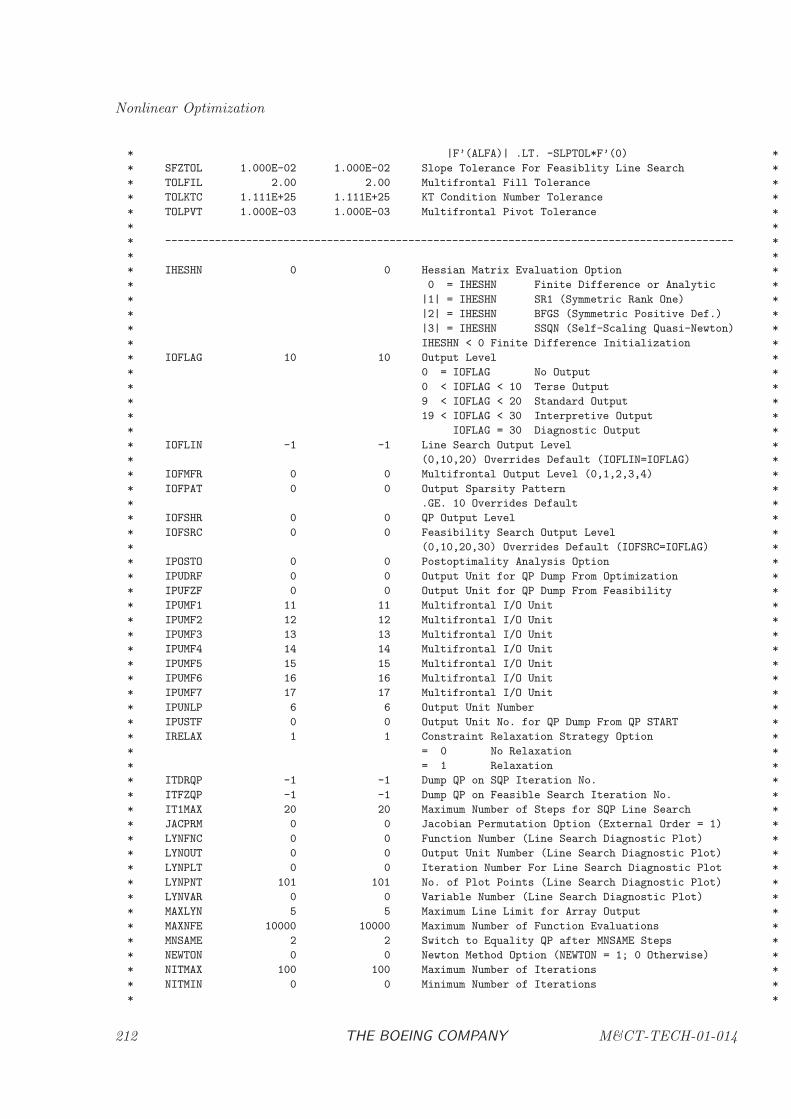
Nonlinear Optimization
* |F’(ALFA)| .LT. -SLPTOL*F’(0) *
* SFZTOL 1.000E-02 1.000E-02 Slope Tolerance For Feasiblity Line Search *
* TOLFIL 2.00 2.00 Multifrontal Fill Tolerance *
* TOLKTC 1.111E+25 1.111E+25 KT Condition Number Tolerance *
* TOLPVT 1.000E-03 1.000E-03 Multifrontal Pivot Tolerance *
* *
* ------------------------------------------------------------------------------------------- *
* *
* IHESHN 0 0 Hessian Matrix Evaluation Option *
* 0 = IHESHN Finite Difference or Analytic *
* |1| = IHESHN SR1 (Symmetric Rank One) *
* |2| = IHESHN BFGS (Symmetric Positive Def.) *
* |3| = IHESHN SSQN (Self-Scaling Quasi-Newton) *
* IHESHN < 0 Finite Difference Initialization *
* IOFLAG 10 10 Output Level *
* 0 = IOFLAG No Output *
* 0 < IOFLAG < 10 Terse Output *
* 9 < IOFLAG < 20 Standard Output *
* 19 < IOFLAG < 30 Interpretive Output *
* IOFLAG = 30 Diagnostic Output *
* IOFLIN -1 -1 Line Search Output Level *
* (0,10,20) Overrides Default (IOFLIN=IOFLAG) *
* IOFMFR 0 0 Multifrontal Output Level (0,1,2,3,4) *
* IOFPAT 0 0 Output Sparsity Pattern *
* .GE. 10 Overrides Default *
* IOFSHR 0 0 QP Output Level *
* IOFSRC 0 0 Feasibility Search Output Level *
* (0,10,20,30) Overrides Default (IOFSRC=IOFLAG) *
* IPOSTO 0 0 Postoptimality Analysis Option *
* IPUDRF 0 0 Output Unit for QP Dump From Optimization *
* IPUFZF 0 0 Output Unit for QP Dump From Feasibility *
* IPUMF1 11 11 Multifrontal I/O Unit *
* IPUMF2 12 12 Multifrontal I/O Unit *
* IPUMF3 13 13 Multifrontal I/O Unit *
* IPUMF4 14 14 Multifrontal I/O Unit *
* IPUMF5 15 15 Multifrontal I/O Unit *
* IPUMF6 16 16 Multifrontal I/O Unit *
* IPUMF7 17 17 Multifrontal I/O Unit *
* IPUNLP 6 6 Output Unit Number *
* IPUSTF 0 0 Output Unit No. for QP Dump From QP START *
* IRELAX 1 1 Constraint Relaxation Strategy Option *
* = 0 No Relaxation *
* = 1 Relaxation *
* ITDRQP -1 -1 Dump QP on SQP Iteration No. *
* ITFZQP -1 -1 Dump QP on Feasible Search Iteration No. *
* IT1MAX 20 20 Maximum Number of Steps for SQP Line Search *
* JACPRM 0 0 Jacobian Permutation Option (External Order = 1) *
* LYNFNC 0 0 Function Number (Line Search Diagnostic Plot) *
* LYNOUT 0 0 Output Unit Number (Line Search Diagnostic Plot) *
* LYNPLT 0 0 Iteration Number For Line Search Diagnostic Plot *
* LYNPNT 101 101 No. of Plot Points (Line Search Diagnostic Plot) *
* LYNVAR 0 0 Variable Number (Line Search Diagnostic Plot) *
* MAXLYN 5 5 Maximum Line Limit for Array Output *
* MAXNFE 10000 10000 Maximum Number of Function Evaluations *
* MNSAME 2 2 Switch to Equality QP after MNSAME Steps *
* NEWTON 0 0 Newton Method Option (NEWTON = 1; 0 Otherwise) *
* NITMAX 100 100 Maximum Number of Iterations *
* NITMIN 0 0 Minimum Number of Iterations *
* *
212 THE BOEING COMPANY M&CT-TECH-01-014
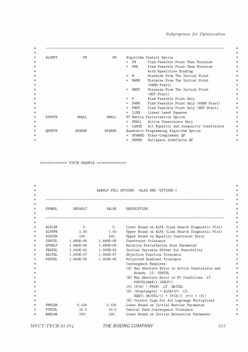
Subprograms for Optimization
* ------------------------------------------------------------------------------------------- *
* *
* ALGOPT FM FM Algorithm Control Option *
* = FM Find Feasible Point Then Minimize *
* = FME Find Feasible Point Then Minimize *
* With Equalities Binding *
* = M Minimize From The Initial Point *
* = MWRM Minimize From The Initial Point *
* (WARM Start) *
* = MHOT Minimize From The Initial Point *
* (HOT Start) *
* = F Find Feasible Point Only *
* = FWRM Find Feasible Point Only (WARM Start) *
* = FHOT Find Feasible Point Only (HOT Start) *
* = LLSQ Linear Least Squares *
* KTOPTN SMALL SMALL KT Matrix Factorization Option *
* = SMALL Active Constraints Only *
* = LARGE All Equality and Inequality Constraints *
* QPOPTN SPARSE SPARSE Quadratic Programming Algorithm Option *
* = SPARSE Schur-Complement QP *
* = DENSE Nullspace Indefinite QP *
>>>>>>>>>>>>>> FIFTH EXAMPLE <<<<<<<<<<<<<<<
* *
* BARNLP FULL OPTIONS (ALSO SEE ’OPTIONS’) *
* *
* ------------------------------------------------------------------------------------------- *
* *
* SYMBOL DEFAULT VALUE DESCRIPTION *
* *
* ------------------------------------------------------------------------------------------- *
* *
* ALFLWR 0. 0. Lower Bound on ALFA (Line Search Diagnostic Plot) *
* ALFUPR 1.00 1.00 Upper Bound on ALFA (Line Search Diagnostic Plot) *
* BIGCON 100. 100. Upper Bound on Equality Constraint Error *
* CONTOL 1.490E-08 1.490E-08 Constraint Tolerance *
* EPSRLF 1.490E-08 1.490E-08 Relative Perturbation Size Parameter *
* FEATOL 1.000E-02 1.000E-02 Initial Variable Offset for Feasibility *
* OBJTOL 1.000E-07 1.000E-07 Objective Function Tolerance *
* PGDTOL 1.000E-05 1.000E-05 Projected Gradient Tolerance *
* Convergence Requires: *
* (A) Max Absolute Error in Active Constraints and *
* Bounds .LT. CONTOL *
* (B) Max Absolute Error in KT Conditions .LT. *
* PGDTOL*MAX(1,|DELF|) *
* (C) |F(X) - FMIN| .LT. OBJTOL *
* (D) |Steplength| = ALFA*|P| .LT. *
* SQRT( OBJTOL/(1 + |F(X)|) )*(1 + |X|) *
* (E) Correct Sign For All Lagrange Multipliers *
* PMULWR 0.100 0.100 Lower Bound on Initial Barrier Parameter *
* PTHTOL 10.0 10.0 Central Path Convergence Tolerance *
* RHOLWR 100. 100. Lower Bound on Initial Relaxation Parameter *
M&CT-TECH-01-014 THE BOEING COMPANY 213
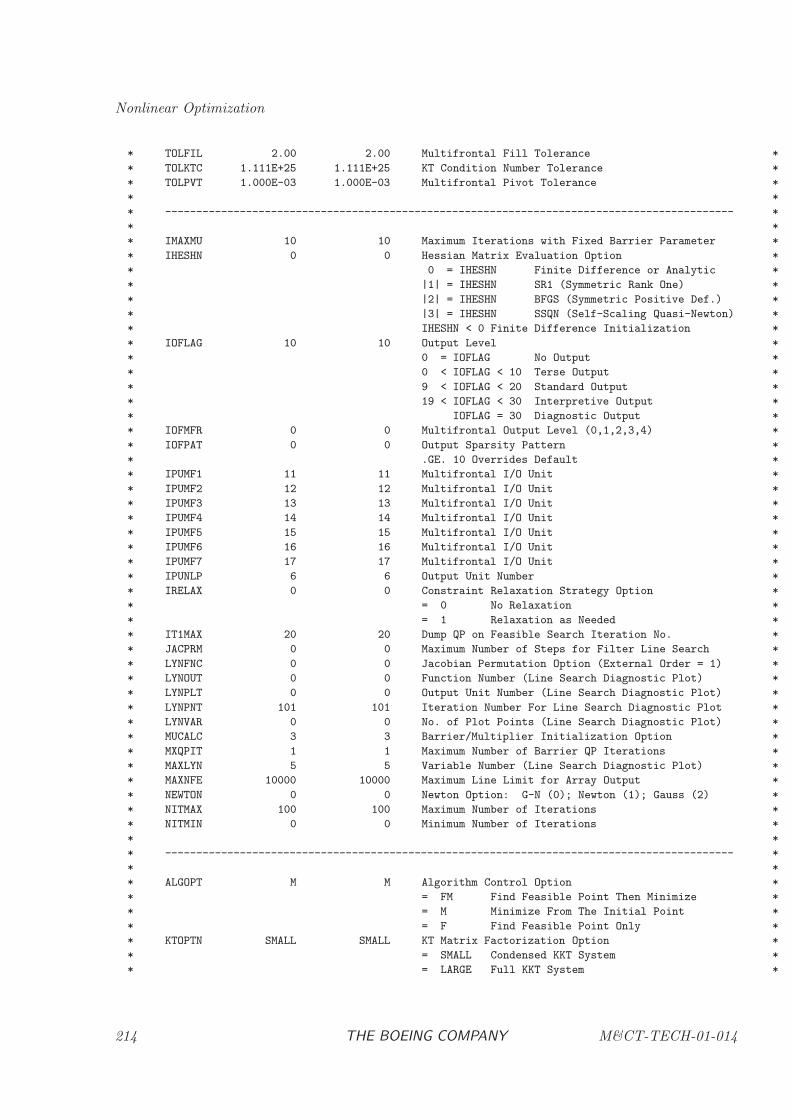
Nonlinear Optimization
* TOLFIL 2.00 2.00 Multifrontal Fill Tolerance *
* TOLKTC 1.111E+25 1.111E+25 KT Condition Number Tolerance *
* TOLPVT 1.000E-03 1.000E-03 Multifrontal Pivot Tolerance *
* *
* ------------------------------------------------------------------------------------------- *
* *
* IMAXMU 10 10 Maximum Iterations with Fixed Barrier Parameter *
* IHESHN 0 0 Hessian Matrix Evaluation Option *
* 0 = IHESHN Finite Difference or Analytic *
* |1| = IHESHN SR1 (Symmetric Rank One) *
* |2| = IHESHN BFGS (Symmetric Positive Def.) *
* |3| = IHESHN SSQN (Self-Scaling Quasi-Newton) *
* IHESHN < 0 Finite Difference Initialization *
* IOFLAG 10 10 Output Level *
* 0 = IOFLAG No Output *
* 0 < IOFLAG < 10 Terse Output *
* 9 < IOFLAG < 20 Standard Output *
* 19 < IOFLAG < 30 Interpretive Output *
* IOFLAG = 30 Diagnostic Output *
* IOFMFR 0 0 Multifrontal Output Level (0,1,2,3,4) *
* IOFPAT 0 0 Output Sparsity Pattern *
* .GE. 10 Overrides Default *
* IPUMF1 11 11 Multifrontal I/O Unit *
* IPUMF2 12 12 Multifrontal I/O Unit *
* IPUMF3 13 13 Multifrontal I/O Unit *
* IPUMF4 14 14 Multifrontal I/O Unit *
* IPUMF5 15 15 Multifrontal I/O Unit *
* IPUMF6 16 16 Multifrontal I/O Unit *
* IPUMF7 17 17 Multifrontal I/O Unit *
* IPUNLP 6 6 Output Unit Number *
* IRELAX 0 0 Constraint Relaxation Strategy Option *
* = 0 No Relaxation *
* = 1 Relaxation as Needed *
* IT1MAX 20 20 Dump QP on Feasible Search Iteration No. *
* JACPRM 0 0 Maximum Number of Steps for Filter Line Search *
* LYNFNC 0 0 Jacobian Permutation Option (External Order = 1) *
* LYNOUT 0 0 Function Number (Line Search Diagnostic Plot) *
* LYNPLT 0 0 Output Unit Number (Line Search Diagnostic Plot) *
* LYNPNT 101 101 Iteration Number For Line Search Diagnostic Plot *
* LYNVAR 0 0 No. of Plot Points (Line Search Diagnostic Plot) *
* MUCALC 3 3 Barrier/Multiplier Initialization Option *
* MXQPIT 1 1 Maximum Number of Barrier QP Iterations *
* MAXLYN 5 5 Variable Number (Line Search Diagnostic Plot) *
* MAXNFE 10000 10000 Maximum Line Limit for Array Output *
* NEWTON 0 0 Newton Option: G-N (0); Newton (1); Gauss (2) *
* NITMAX 100 100 Maximum Number of Iterations *
* NITMIN 0 0 Minimum Number of Iterations *
* *
* ------------------------------------------------------------------------------------------- *
* *
* ALGOPT M M Algorithm Control Option *
* = FM Find Feasible Point Then Minimize *
* = M Minimize From The Initial Point *
* = F Find Feasible Point Only *
* KTOPTN SMALL SMALL KT Matrix Factorization Option *
* = SMALL Condensed KKT System *
* = LARGE Full KKT System *
214 THE BOEING COMPANY M&CT-TECH-01-014
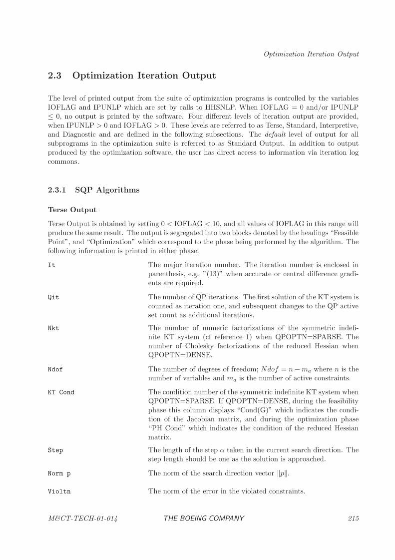
Optimization Iteration Output
2.3 Optimization Iteration Output
The level of printed output from the suite of optimization programs is controlled by the variablesIOFLAG and IPUNLP which are set by calls to HHSNLP. When IOFLAG = 0 and/or IPUNLP≤ 0, no output is printed by the software. Four different levels of iteration output are provided,when IPUNLP > 0 and IOFLAG > 0. These levels are referred to as Terse, Standard, Interpretive,and Diagnostic and are defined in the following subsections. The default level of output for allsubprograms in the optimization suite is referred to as Standard Output. In addition to outputproduced by the optimization software, the user has direct access to information via iteration logcommons.
2.3.1 SQP Algorithms
Terse Output
Terse Output is obtained by setting 0 < IOFLAG < 10, and all values of IOFLAG in this range willproduce the same result. The output is segregated into two blocks denoted by the headings “FeasiblePoint”, and “Optimization” which correspond to the phase being performed by the algorithm. Thefollowing information is printed in either phase:
It The major iteration number. The iteration number is enclosed inparenthesis, e.g. ”(13)” when accurate or central difference gradi-ents are required.
Qit The number of QP iterations. The first solution of the KT system iscounted as iteration one, and subsequent changes to the QP activeset count as additional iterations.
Nkt The number of numeric factorizations of the symmetric indefi-nite KT system (cf reference 1) when QPOPTN=SPARSE. Thenumber of Cholesky factorizations of the reduced Hessian whenQPOPTN=DENSE.
Ndof The number of degrees of freedom; Ndof = n−ma where n is thenumber of variables and ma is the number of active constraints.
KT Cond The condition number of the symmetric indefinite KT system whenQPOPTN=SPARSE. If QPOPTN=DENSE, during the feasibilityphase this column displays “Cond(G)” which indicates the condi-tion of the Jacobian matrix, and during the optimization phase“PH Cond” which indicates the condition of the reduced Hessianmatrix.
Step The length of the step α taken in the current search direction. Thestep length should be one as the solution is approached.
Norm p The norm of the search direction vector ‖p‖.
Violtn The norm of the error in the violated constraints.
M&CT-TECH-01-014 THE BOEING COMPANY 215
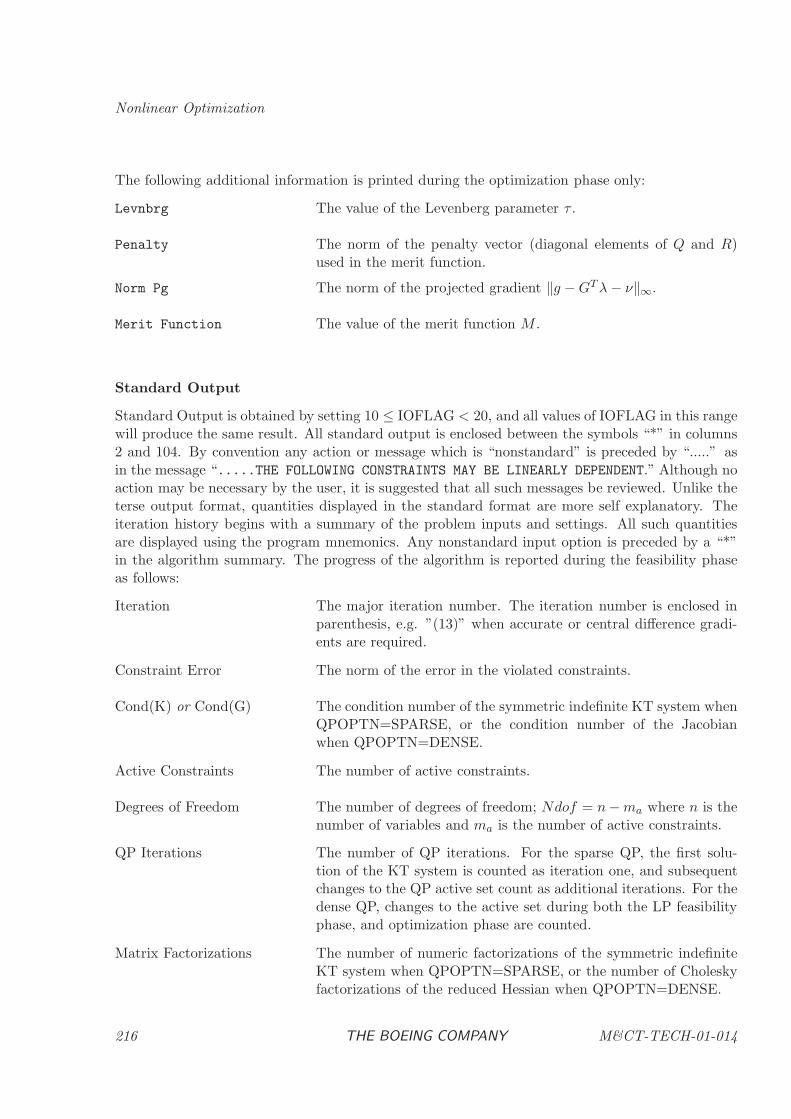
Nonlinear Optimization
The following additional information is printed during the optimization phase only:
Levnbrg The value of the Levenberg parameter τ .
Penalty The norm of the penalty vector (diagonal elements of Q and R)used in the merit function.
Norm Pg The norm of the projected gradient ‖g −GTλ− ν‖∞.
Merit Function The value of the merit function M .
Standard Output
Standard Output is obtained by setting 10 ≤ IOFLAG < 20, and all values of IOFLAG in this rangewill produce the same result. All standard output is enclosed between the symbols “*” in columns2 and 104. By convention any action or message which is “nonstandard” is preceded by “.....” asin the message “.....THE FOLLOWING CONSTRAINTS MAY BE LINEARLY DEPENDENT.” Although noaction may be necessary by the user, it is suggested that all such messages be reviewed. Unlike theterse output format, quantities displayed in the standard format are more self explanatory. Theiteration history begins with a summary of the problem inputs and settings. All such quantitiesare displayed using the program mnemonics. Any nonstandard input option is preceded by a “*”in the algorithm summary. The progress of the algorithm is reported during the feasibility phaseas follows:
Iteration The major iteration number. The iteration number is enclosed inparenthesis, e.g. ”(13)” when accurate or central difference gradi-ents are required.
Constraint Error The norm of the error in the violated constraints.
Cond(K) or Cond(G) The condition number of the symmetric indefinite KT system whenQPOPTN=SPARSE, or the condition number of the Jacobianwhen QPOPTN=DENSE.
Active Constraints The number of active constraints.
Degrees of Freedom The number of degrees of freedom; Ndof = n−ma where n is thenumber of variables and ma is the number of active constraints.
QP Iterations The number of QP iterations. For the sparse QP, the first solu-tion of the KT system is counted as iteration one, and subsequentchanges to the QP active set count as additional iterations. For thedense QP, changes to the active set during both the LP feasibilityphase, and optimization phase are counted.
Matrix Factorizations The number of numeric factorizations of the symmetric indefiniteKT system when QPOPTN=SPARSE, or the number of Choleskyfactorizations of the reduced Hessian when QPOPTN=DENSE.
216 THE BOEING COMPANY M&CT-TECH-01-014

Optimization Iteration Output
During the optimization phase the following additional information is printed
Projected Gradient The norm of the projected gradient ‖g −GTλ− ν‖∞.
Objective Function The value of the objective function f(x).
Equality Error The norm of the error in the equality constraints.
Inequality Error The norm of the error in the violated inequality constraints.
Merit Function The value of the merit function M .
Penalty Weight Norm The norm of the penalty vector (diagonal elements of Q and R)used in the merit function.
Levenberg Parameter The value of the Levenberg parameter τ .
Min. Eigenvalue The Gerschgorin bound for the minimum eigenvalue of HL.
Max. Eigenvalue The Gerschgorin bound for the maximum eigenvalue of HL.
A line search is used during both the optimization and feasibility phase to adjust the steplength α.A single line of the form
Model Line Search ........Step: iter .....ALFA = α
is printed which contains the following information about the line search:
Model The model used to predict the steplength. The models are:Quadratic quadratic polynomial to predict minimum;
Cubic cubic polynomial to predict minimum;
Quadratic Cliff quadratic polynomial to predict location of cliff;
Cubic Cliff cubic polynomial to predict location of cliff;
Bisection bisect the interval to predict minimum;
Backtrack step reduction when a function error is encountered;
iter the line search step number;
α the length of the step in the search direction p.
M&CT-TECH-01-014 THE BOEING COMPANY 217
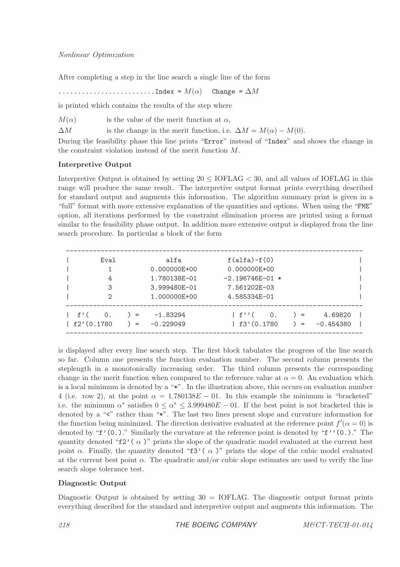
Nonlinear Optimization
After completing a step in the line search a single line of the form
.........................Index = M(α) Change = ∆M
is printed which contains the results of the step where
M(α) is the value of the merit function at α,
∆M is the change in the merit function, i.e. ∆M = M(α) −M(0).
During the feasibility phase this line prints “Error” instead of “Index” and shows the change inthe constraint violation instead of the merit function M .
Interpretive Output
Interpretive Output is obtained by setting 20 ≤ IOFLAG < 30, and all values of IOFLAG in thisrange will produce the same result. The interpretive output format prints everything describedfor standard output and augments this information. The algorithm summary print is given in a“full” format with more extensive explanation of the quantities and options. When using the “FME”option, all iterations performed by the constraint elimination process are printed using a formatsimilar to the feasibility phase output. In addition more extensive output is displayed from the linesearch procedure. In particular a block of the form
-----------------------------------------------------------------------------
| Eval alfa f(alfa)-f(0) |
| 1 0.000000E+00 0.000000E+00 |
| 4 1.780138E-01 -2.196746E-01 * |
| 3 3.999480E-01 7.561202E-03 |
| 2 1.000000E+00 4.585334E-01 |
-----------------------------------------------------------------------------
| f’( 0. ) = -1.83294 | f’’( 0. ) = 4.69820 |
| f2’(0.1780 ) = -0.229049 | f3’(0.1780 ) = -0.454380 |
-----------------------------------------------------------------------------
is displayed after every line search step. The first block tabulates the progress of the line searchso far. Column one presents the function evaluation number. The second column presents thesteplength in a monotonically increasing order. The third column presents the correspondingchange in the merit function when compared to the reference value at α = 0. An evaluation whichis a local minimum is denoted by a “*”. In the illustration above, this occurs on evaluation number4 (i.e. row 2), at the point α = 1.780138E − 01. In this example the minimum is “bracketed”i.e. the minimum α∗ satisfies 0 ≤ α∗ ≤ 3.999480E − 01. If the best point is not bracketed this isdenoted by a “<” rather than “*”. The last two lines present slope and curvature information forthe function being minimized. The direction derivative evaluated at the reference point f ′(α = 0) isdenoted by “f’(0.).” Similarly the curvature at the reference point is denoted by “f’’(0.).” Thequantity denoted “f2’( α )” prints the slope of the quadratic model evaluated at the current bestpoint α. Finally, the quantity denoted “f3’( α )” prints the slope of the cubic model evaluatedat the current best point α. The quadratic and/or cubic slope estimates are used to verify the linesearch slope tolerance test.
Diagnostic Output
Diagnostic Output is obtained by setting 30 = IOFLAG. The diagnostic output format printseverything described for the standard and interpretive output and augments this information. The
218 THE BOEING COMPANY M&CT-TECH-01-014
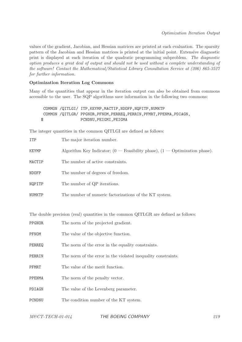
Optimization Iteration Output
values of the gradient, Jacobian, and Hessian matrices are printed at each evaluation. The sparsitypattern of the Jacobian and Hessian matrices is printed at the initial point. Extensive diagnosticprint is displayed at each iteration of the quadratic programming subproblem. The diagnosticoption produces a great deal of output and should not be used without a complete understanding ofthe software! Contact the Mathematical/Statistical Library Consultation Service at (206) 865-3527for further information.
Optimization Iteration Log Commons
Many of the quantities that appear in the iteration output can also be obtained from commonsaccessible to the user. The SQP algorithms save information in the following two commons:
COMMON /QITLGI/ ITP,KEYMP,MACTIP,NDOFP,NQPITP,NUMKTP
COMMON /QITLGR/ PPGNOR,PFNOM,PERREQ,PERRIN,PFMRT,PPENMA,PDIAGN,
$ PCNDNU,PEIGMI,PEIGMA
The integer quantities in the common QITLGI are defined as follows:
ITP The major iteration number.
KEYMP Algorithm Key Indicator; (0 — Feasibility phase), (1 — Optimization phase).
MACTIP The number of active constraints.
NDOFP The number of degrees of freedom.
NQPITP The number of QP iterations.
NUMKTP The number of numeric factorizations of the KT system.
The double precision (real) quantities in the common QITLGR are defined as follows:
PPGNOR The norm of the projected gradient.
PFNOM The value of the objective function.
PERREQ The norm of the error in the equality constraints.
PERRIN The norm of the error in the violated inequality constraints.
PFMRT The value of the merit function.
PPENMA The norm of the penalty vector.
PDIAGN The value of the Levenberg parameter.
PCNDNU The condition number of the KT system.
M&CT-TECH-01-014 THE BOEING COMPANY 219
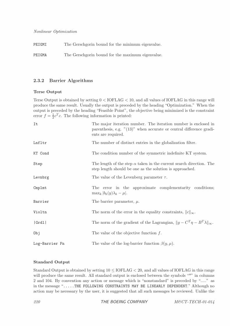
Nonlinear Optimization
PEIGMI The Gerschgorin bound for the minimum eigenvalue.
PEIGMA The Gerschgorin bound for the maximum eigenvalue.
2.3.2 Barrier Algorithms
Terse Output
Terse Output is obtained by setting 0 < IOFLAG < 10, and all values of IOFLAG in this range willproduce the same result. Usually the output is preceded by the heading “Optimization.” When theoutput is preceded by the heading “Feasible Point”, the objective being minimized is the constrainterror f = 1
2cT c. The following information is printed:
It The major iteration number. The iteration number is enclosed inparenthesis, e.g. ”(13)” when accurate or central difference gradi-ents are required.
Lnfltr The number of distinct entries in the globalization filter.
KT Cond The condition number of the symmetric indefinite KT system.
Step The length of the step α taken in the current search direction. Thestep length should be one as the solution is approached.
Levnbrg The value of the Levenberg parameter τ .
Cmplmt The error in the approximate complementarity conditions;maxk |bk(y)λk − µ|.
Barrier The barrier parameter, µ.
Violtn The norm of the error in the equality constraints, ‖c‖∞.
|Grdl| The norm of the gradient of the Lagrangian, ‖g − CTη −BTλ‖∞.
Obj The value of the objective function f .
Log-Barrier Fn The value of the log-barrier function β(y, µ).
Standard Output
Standard Output is obtained by setting 10 ≤ IOFLAG < 20, and all values of IOFLAG in this rangewill produce the same result. All standard output is enclosed between the symbols “*” in columns2 and 104. By convention any action or message which is “nonstandard” is preceded by “.....” asin the message “.....THE FOLLOWING CONSTRAINTS MAY BE LINEARLY DEPENDENT.” Although noaction may be necessary by the user, it is suggested that all such messages be reviewed. Unlike the
220 THE BOEING COMPANY M&CT-TECH-01-014
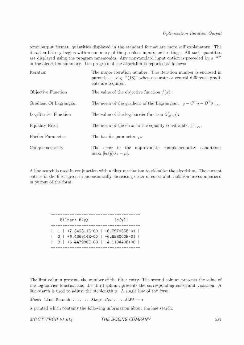
Optimization Iteration Output
terse output format, quantities displayed in the standard format are more self explanatory. Theiteration history begins with a summary of the problem inputs and settings. All such quantitiesare displayed using the program mnemonics. Any nonstandard input option is preceded by a “*”in the algorithm summary. The progress of the algorithm is reported as follows:
Iteration The major iteration number. The iteration number is enclosed inparenthesis, e.g. ”(13)” when accurate or central difference gradi-ents are required.
Objective Function The value of the objective function f(x).
Gradient Of Lagrangian The norm of the gradient of the Lagrangian, ‖g − CTη −BTλ‖∞.
Log-Barrier Function The value of the log-barrier function β(y, µ).
Equality Error The norm of the error in the equality constraints, ‖c‖∞.
Barrier Parameter The barrier parameter, µ.
Complementarity The error in the approximate complementarity conditions;maxk |bk(y)λk − µ|.
A line search is used in conjunction with a filter mechanism to globalize the algorithm. The currententries in the filter given in monotonically increasing order of constraint violation are summarizedin output of the form:
--------------------------------------
Filter: B(y) |c(y)|
--------------------------------------
| 1 | +7.342311E+00 | +6.797935E-01 |
| 2 | +6.436914E+00 | +6.898000E-01 |
| 3 | +6.447988E+00 | +4.110440E+00 |
--------------------------------------
The first column presents the number of the filter entry. The second column presents the value ofthe log-barrier function and the third column presents the corresponding constraint violation. Aline search is used to adjust the steplength α. A single line of the form
Model Line Search ........Step: iter .....ALFA = α
is printed which contains the following information about the line search:
M&CT-TECH-01-014 THE BOEING COMPANY 221
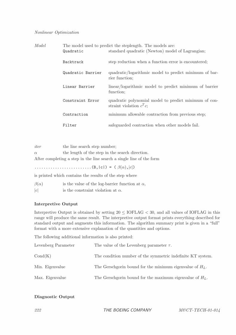
Nonlinear Optimization
Model The model used to predict the steplength. The models are:Quadratic standard quadratic (Newton) model of Lagrangian;
Backtrack step reduction when a function error is encountered;
Quadratic Barrier quadratic/logarithmic model to predict minimum of bar-rier function;
Linear Barrier linear/logarithmic model to predict minimum of barrierfunction;
Constraint Error quadratic polynomial model to predict minimum of con-straint violation cT c;
Contraction minimum allowable contraction from previous step;
Filter safeguarded contraction when other models fail.
iter the line search step number;
α the length of the step in the search direction.
After completing a step in the line search a single line of the form
.........................(B,|c|) = ( β(α),|c|)
is printed which contains the results of the step where
β(α) is the value of the log-barrier function at α,
|c| is the constraint violation at α.
Interpretive Output
Interpretive Output is obtained by setting 20 ≤ IOFLAG < 30, and all values of IOFLAG in thisrange will produce the same result. The interpretive output format prints everything described forstandard output and augments this information. The algorithm summary print is given in a “full”format with a more extensive explanation of the quantities and options.
The following additional information is also printed:
Levenberg Parameter The value of the Levenberg parameter τ .
Cond(K) The condition number of the symmetric indefinite KT system.
Min. Eigenvalue The Gerschgorin bound for the minimum eigenvalue of HL.
Max. Eigenvalue The Gerschgorin bound for the maximum eigenvalue of HL.
Diagnostic Output
222 THE BOEING COMPANY M&CT-TECH-01-014
Reverse Communication Program Structure
Diagnostic Output is obtained by setting 30 = IOFLAG. The diagnostic output format printseverything described for the standard and interpretive output and augments this information. Thevalues of the gradient, Jacobian, and Hessian matrices are printed at each evaluation. The sparsitypattern of the Jacobian and Hessian matrices is printed at the initial point. Extensive diagnosticprint is displayed at each iteration of the quadratic programming subproblem. The diagnosticoption produces a great deal of output and should not be used without a complete understanding ofthe software! Contact the Mathematical/Statistical Library Consultation Service at (206) 865-3527for further information.
2.4 Reverse Communication Program Structure
The reverse communication structure of subroutine HDSNLP (and the related routines HDNLPRand HDSLSQ) permits the user a great deal of flexibility when implementing an application. Typi-cally the optimization software is called directly from either a main program or high level executiveroutine. This format permits the user to supply gradient and Hessian information using a techniqueappropriate for the application. This format is also useful when the application is implementedin a multitasking environment, since the function and/or gradient evaluations can be executed ondifferent platforms. To aid the user with a reverse communication implementation, a flow chartpresenting the various operations is presented in Figure 2-1.
M&CT-TECH-01-014 THE BOEING COMPANY 223
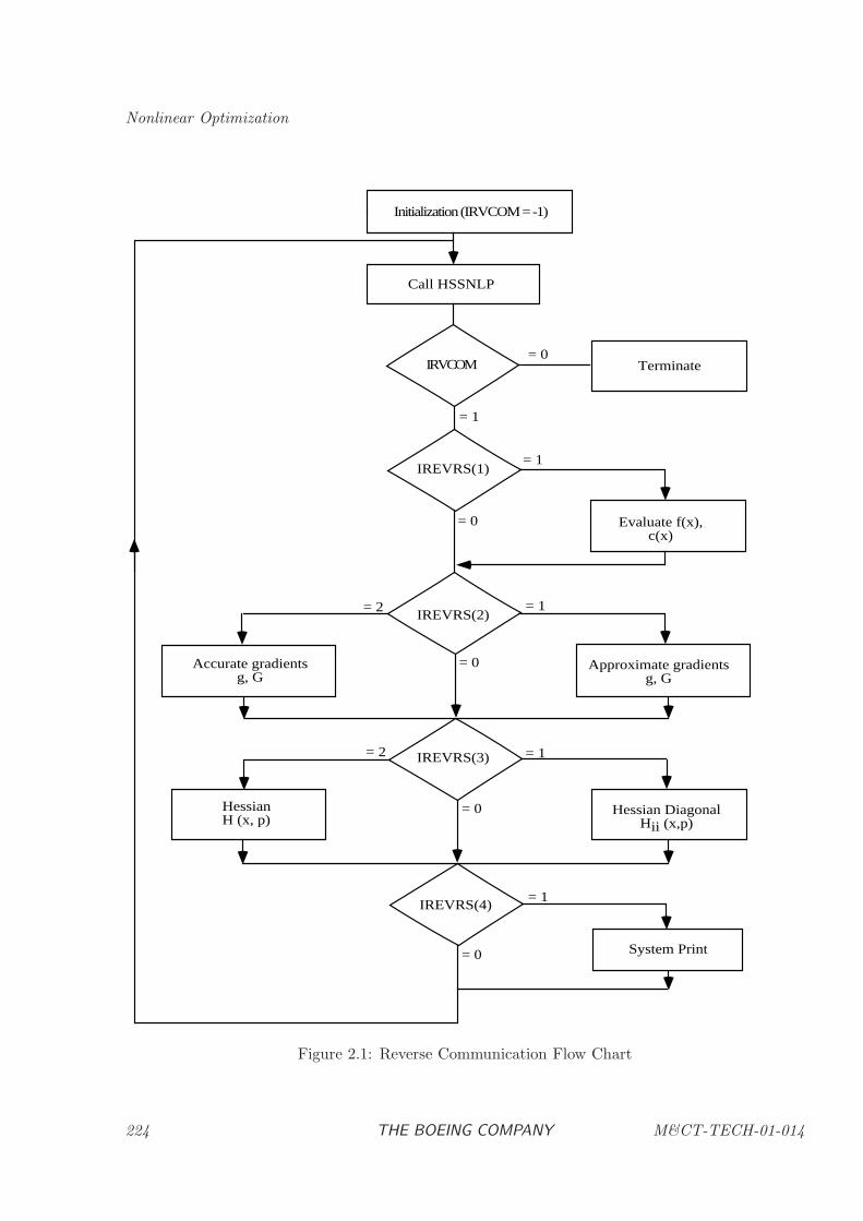
Nonlinear Optimization
Initialization (IRVCOM = -1)
Call HSSNLP
IRVCOM
IREVRS(1)
Terminate
Evaluate f(x),c(x)
Approximate gradientsg, G
Hessian DiagonalHii (x,p)
System Print
HessianH (x, p)
Accurate gradientsg, G
IREVRS(2)
IREVRS(3)
IREVRS(4)
= 0
= 1
= 0
= 1
= 0
= 1
= 0
= 1
= 0
= 2
= 2
= 1
Figure 2.1: Reverse Communication Flow Chart
224 THE BOEING COMPANY M&CT-TECH-01-014
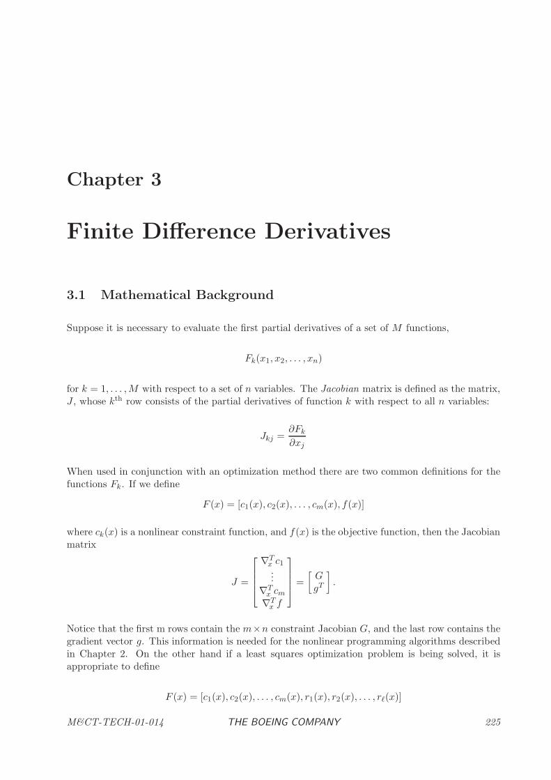
Chapter 3
Finite Difference Derivatives
3.1 Mathematical Background
Suppose it is necessary to evaluate the first partial derivatives of a set of M functions,
Fk(x1, x2, . . . , xn)
for k = 1, . . . ,M with respect to a set of n variables. The Jacobian matrix is defined as the matrix,J , whose kth row consists of the partial derivatives of function k with respect to all n variables:
Jkj =∂Fk
∂xj
When used in conjunction with an optimization method there are two common definitions for thefunctions Fk. If we define
F (x) = [c1(x), c2(x), . . . , cm(x), f(x)]
where ck(x) is a nonlinear constraint function, and f(x) is the objective function, then the Jacobianmatrix
J =
∇Tx c1...
∇Tx cm∇T
x f
=
[GgT
].
Notice that the first m rows contain the m×n constraint Jacobian G, and the last row contains thegradient vector g. This information is needed for the nonlinear programming algorithms describedin Chapter 2. On the other hand if a least squares optimization problem is being solved, it isappropriate to define
F (x) = [c1(x), c2(x), . . . , cm(x), r1(x), r2(x), . . . , rℓ(x)]
M&CT-TECH-01-014 THE BOEING COMPANY 225
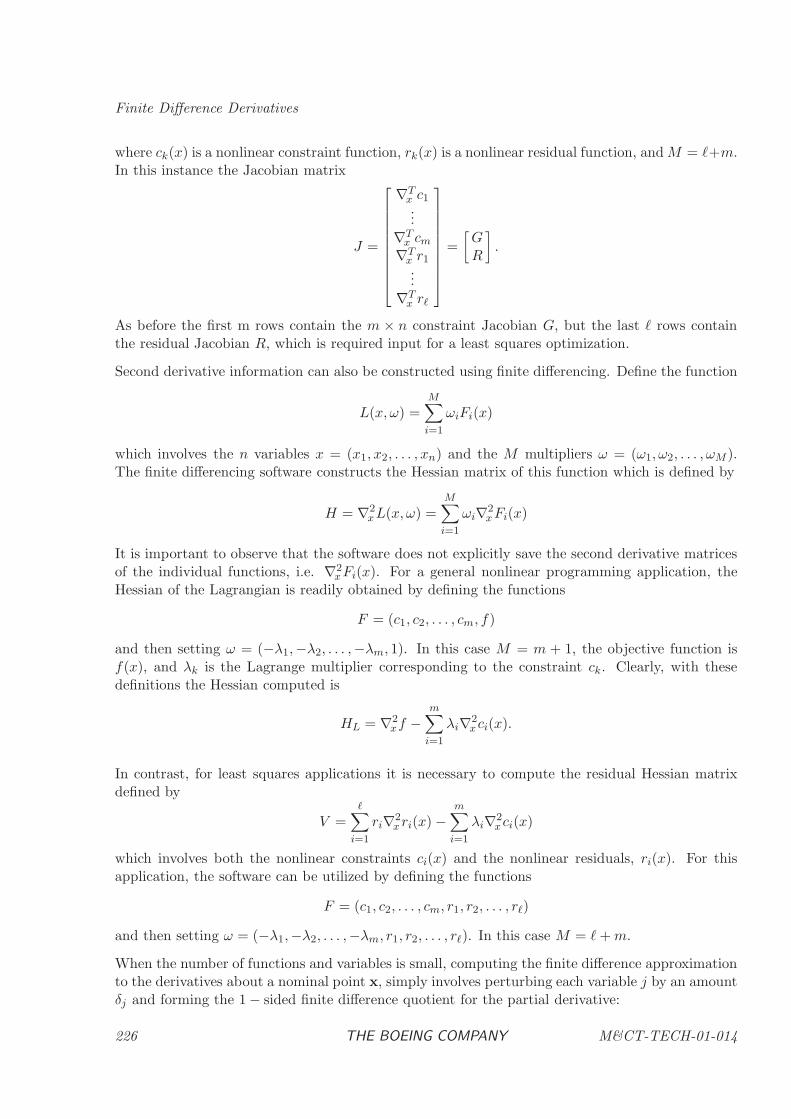
Finite Difference Derivatives
where ck(x) is a nonlinear constraint function, rk(x) is a nonlinear residual function, andM = ℓ+m.In this instance the Jacobian matrix
J =
∇Tx c1...
∇Tx cm
∇Tx r1...
∇Tx rℓ
=
[GR
].
As before the first m rows contain the m × n constraint Jacobian G, but the last ℓ rows containthe residual Jacobian R, which is required input for a least squares optimization.
Second derivative information can also be constructed using finite differencing. Define the function
L(x, ω) =M∑
i=1
ωiFi(x)
which involves the n variables x = (x1, x2, . . . , xn) and the M multipliers ω = (ω1, ω2, . . . , ωM ).The finite differencing software constructs the Hessian matrix of this function which is defined by
H = ∇2xL(x, ω) =
M∑
i=1
ωi∇2xFi(x)
It is important to observe that the software does not explicitly save the second derivative matricesof the individual functions, i.e. ∇2
xFi(x). For a general nonlinear programming application, theHessian of the Lagrangian is readily obtained by defining the functions
F = (c1, c2, . . . , cm, f)
and then setting ω = (−λ1,−λ2, . . . ,−λm, 1). In this case M = m + 1, the objective function isf(x), and λk is the Lagrange multiplier corresponding to the constraint ck. Clearly, with thesedefinitions the Hessian computed is
HL = ∇2xf −
m∑
i=1
λi∇2xci(x).
In contrast, for least squares applications it is necessary to compute the residual Hessian matrixdefined by
V =ℓ∑
i=1
ri∇2xri(x) −
m∑
i=1
λi∇2xci(x)
which involves both the nonlinear constraints ci(x) and the nonlinear residuals, ri(x). For thisapplication, the software can be utilized by defining the functions
F = (c1, c2, . . . , cm, r1, r2, . . . , rℓ)
and then setting ω = (−λ1,−λ2, . . . ,−λm, r1, r2, . . . , rℓ). In this case M = ℓ+m.
When the number of functions and variables is small, computing the finite difference approximationto the derivatives about a nominal point x, simply involves perturbing each variable j by an amountδj and forming the 1 − sided finite difference quotient for the partial derivative:
226 THE BOEING COMPANY M&CT-TECH-01-014
Mathematical Background
∂Fk
∂xj=Fk(x + δjej) − Fk(x)
δj+O(δj)
or for 2 − sided finite difference derivatives:
∂Fk
∂xj=Fk(x + δjej) − Fk(x − δjej)
2δj+O(δ2j )
for k = 1, . . . ,m and j = 1, . . . , n, where x = (x1, x2, . . . , xn) and ej is a unit vector in the jth
coordinate direction. The notation O(rp) means that the difference between the left side and thefirst term on the right side is proportional to rp as r → 0. For obvious reasons, the first expressionis often referred to as a forward difference estimate and the second is called a central differenceapproximation. The trade-off between these formulae is that the second provides a more accurateapproximation at the expense of an extra function evaluation per derivative.
For large problems with hundreds to thousands of variables, perturbing each variable individuallybecomes impractical because of the expense of evaluating the functions so many times. It is afortunate occurrence that many large problems are also sparse, that is, the number of nonzeroelements Jkj in the Jacobian matrix for the system is a relatively small percentage of the totalnumber of elements in the matrix. In these cases derivatives can be computed more efficientlyby grouping variables together and simultaneously perturbing all variables in the set, a techniquecalled sparse differencing.
Definition: The Sparsity Pattern of a matrix is a list of the locations of the nonzero elements inthe matrix.
One way to specify the sparsity pattern is to list the nonzero elements, aij, in a matrix by givingeach location as a triple: (i, j, aij). In general this list does not need to be ordered in any particularmanner, although it could be permuted into row or column order. If the matrix has been orderedby columns (or rows), a second more storage efficient description is possible. The list now consistsof only two entries: (i, aij) or (j, aij) with a separate vector pointing to the starting location ofeach column (row) in the list. An example of this format is given in the USAGE REMARKS forsubroutine HJSFDI. Each representation can be convenient in certain situations.
In the following presentation it will be assumed that the nonzeros in the Jacobian matrix aredescribed by a triple, where the row number is the number of the dependent function whosederivatives are being computed, the column number is the number of the independent variable,and the value is the corresponding value of the partial derivative. The Hessian matrix, Hk, of athe function Fk is the matrix of second partial derivatives of the function with respect to all ofthe independent variables. Since it will be assumed that the functions are sufficiently differentiablethat the mixed partial derivatives are equal, i.e.
∂2Fk
∂xi∂xj=
∂2Fk
∂xj∂xi,
the Hessian matrix is symmetric. Thus only the lower (upper) triangular portion of the matrixneeds to be specified for the complete description. It will be convenient to express this matrix inthe second sparse form, where each element is specified as a row number and value with pointersto the beginning of each column.
Index Set Generation - HJSFDI
M&CT-TECH-01-014 THE BOEING COMPANY 227
Finite Difference Derivatives
Definition: An Index Set is a subset of the problem variable indices such that no two variablesbelonging to the set affect the same dependent function. (No two columns in the matrix corre-sponding to variable numbers in the index set have a nonzero element in the same row.) Stateddifferently, and index set is a subset of the columns of the Jacobian, with the property that thereis at most one nonzero element per row.
The definition of an index set allows all variables within it to be perturbed simultaneously, sincethere will be at most one variable in the set effecting each function. The partial derivative of thefunction with respect to that variable can be approximated by a difference quotient. As a simpleexample consider the set of 3 functions depending on 3 variables, x = (x1, x2, x3):
F1(x) = F1(x1)F2(x) = F2(x2)F3(x) = F3(x3)
In this case the only index set is I1 = {1, 2, 3}. To find all the partial derivatives we need onlythe single evaluation at the point, xp = (x1 + δ1, x2 + δ2, x3 + δ3). The partial derivatives may beobtained as:
∂F1
∂x1≈ F1(xp) − F1(x)
δ1∂F2
∂x2≈ F2(xp) − F2(x)
δ2∂F3
∂x3≈ F3(xp) − F3(x)
δ3
The example above shows that if the Jacobian matrix sparsity pattern is diagonal, then one pertur-bation is sufficient to generate the Jacobian matrix independent of how many variables are involved.For a general banded matrix the number of perturbations is no larger than the band width.
In general, a perturbation of index set, Ij , will mean that every variable in the set is perturbed byits corresponding perturbation size,
∆j =∑
p∈Ij
δpep
The standard formulae for forward and central difference approximations still hold when the indi-vidual variable perturbations, δpep are replaced with index set perturbations, ∆j . Using index setperturbations to obtain the partial derivatives is called Sparse Differencing.
For a general sparse matrix the computation of the index sets can be done in a number of ways.The simplest method is one developed by Curtis, Powell, and Reid (CPR) (see references). Itplaces the first column in the first index set and then sweeps over the rest of the matrix placingadditional columns in the developing index set if there are no row conflicts with the columns alreadyselected. Although the method is efficient, the drawback is that it is dependent on the ordering ofthe columns, and in general will not yield the minimum number of index sets required to generatethe Jacobian. The CPR method is implemented in subroutine HJSFDI. A more sophisticatedmethod relates the problem to that of graph coloring, and is discribed by Coleman and More (seereferences).
It is relatively easy to obtain a lower bound for the number of index sets which will be required forany specific problem. One merely notes from the definition of an index set that the variables which
228 THE BOEING COMPANY M&CT-TECH-01-014
Mathematical Background
affect any particular dependent function (row) must be in different sets to avoid a conflict. Thus alower bound to the number of index sets is the maximum number of nonzero elements in any row.
The first observation obtained from this lower bound is that if a single function depends on allthe variables, the number of index sets will equal the number of variables. In this case sparsedifferencing will reduce to the dense method of perturbing every variable, thereby nullifying anyadvantage of sparse differencing. The only recourse in this case is to see if the partial derivativesin the dense rows can be determined analytically or by some other method. Removing these rowsfrom the problem will then allow the remaining rows to be determined by sparse differencing.
A second observation from the definition of an index set is that if a variable affects every dependentfunction (row), then that variable must be in its own index set to avoid row conflict with all othervariables. This case is not as serious as the one above if the number of dense columns is relativelysmall, for the total number of index sets could still be substantially smaller than the total numberof variables.
Note that the computation of the index sets is based solely on the sparsity pattern of the Jacobianmatrix which must be input to subroutine HJSFDI in the row/column format for describing thelocation of the nonzero elements. Thus only the structure of the functional dependencies affectsthe index set computation. Determining the sparsity pattern for a particular problem may be asubstantial task for the user of this subroutine.
The Jacobian Matrix - HDSFDJ and HDDFDJ
For dense applications subroutine HDDFDJ can be used to construct the Jacobian matrix. Forsparse applications once the index sets have been determined, subroutine HDSFDJ can be used tocompute the Jacobian matrix by sparse differences. To do this efficiently, a column ordering of thesparsity pattern is maintained internally. It is assumed that the perturbation sizes have been setappropriately prior to the call so that sufficiently accurate derivatives will be obtained. A centraldifference option is also included for the cases where accuracy is of paramount concern. The finitedifference approximations to the derivatives for dense matrices can be generalized by replacing thecomputation with single variable perturbations by index set perturbations. Thus for each nonzerorow i of a column j ∈ Γk, the forward difference approximation is
Jij ≈1
δj
[Fi(x + ∆k) − Fi(x)
]
and the central difference approximation is
Jij ≈1
2δj
[Fi(x + ∆k) − Fi(x −∆k)
].
For dense applications the number of index sets is equal to the number of variables and ∆k = δkek.
To allow for maximum flexibility in the manner in which the functions are computed, subroutinesHDSFDJ and HDDFDJ use a reverse communication technique. This means that the subroutinewill not directly call a user subroutine (thus requiring a fixed argument list), but will instead returnto the calling program each time a new function evaluation is to be performed. After the evaluation,the finite difference routine must be called again with the new function values at the perturbedpoint. See the usage examples to obtain a more detailed look at how reverse communication isused.
M&CT-TECH-01-014 THE BOEING COMPANY 229
Finite Difference Derivatives
Sparsity Pattern Check - HDSFDC
The sparsity pattern of the Jacobian defines the location of the nonzero derivatives, Jkj = ∂Fk
∂xj.
The pattern can be incorrect in one of two ways:
1. A particular element Jkj can be included in the nonzero list even though the partial derivativeis identically zero.
2. A particular element Jkj is not included in the nonzero list even though the partial derivativeis nonzero.
The first case, namely specifying a nonzero location in the matrix when in fact there is no functionaldependence, is not a serious error. Under these circumstances the index set determination will stillbe correct, with the computed value of the derivative being within truncation error of zero. Thepenalty for this error is computational efficiency. By incorrectly specifying extra elements, it ispossible that more index sets will be needed than are necessary. This in turn will increase thenumber of function evaluations required to compute the relevant derivatives.
On the other hand, omitting a nonzero element location from the sparsity pattern may causeserious problems. In this case it possible to obtain an incorrect partition of the variables into indexsets, which will lead to the incorrect calculation of some of the partial derivatives. To illustratethis, consider the case where F7 = F7(x1, x3) but the (7, 3) location is missing from the sparsitypattern. In this case, variables 1 and 3 might both be placed erroneously in the first index set ifno other function in the problem depended simultaneously on these variables. Then the Jacobiancomputation would approximate the partial of function 7 with respect to variable 1 as:
∂F7
∂x1≈ F7(x1 + δ1, x3 + δ3) − F7(x1, x3)
δ1
=∂F7
∂x1+∂F7
∂x3
δ3δ1
+O(δ1, δ23/δ1)
In other words, the partial derivative ∂F7∂x3
would not be computed and a linear combination ofthe actual derivatives affecting F7 would be mistaken for a single partial derivative. Unless thelinear combination was so large that its size would catch the eye as being a potential error, themiscomputed derivatives would go unnoticed. However, if the matrix is being used by an iterativemethod, the error in the partial derivative will lead to a reduction in the rate of convergence ofthe method, and possibly to the inability to converge the problem. For these reasons, a subroutinewhich attempts to check for missing nonzero elements is included in the sparse difference package(HDSFDC).
In general, the brute force method of perturbing every variable independently to obtain the denseJacobian and then inspecting for nonzero locations will be too expensive for all but the smallestproblems. Instead, the assumption will be made that the number of missing elements is small, andthat a consistency check of the index sets generated using the input sparsity pattern will revealpotential missing elements.
The search for missing elements uses two perturbations of each index set with different sets ofcoefficients. Consider the two perturbations of the first index set given by:
xp1 = x +∑
i∈I1δiei
xp2 = x +∑
i∈I1αiδiei
230 THE BOEING COMPANY M&CT-TECH-01-014
Mathematical Background
Now suppose function Fk was specified as depending only on variable j in the first index set andform the difference,
[Fk(xp2) − Fk(x)] − αj [Fk(xp1) − Fk(x)] =∑
i∈I1
(αi − αj)∂Fk
∂xiδi +O(δ2)
If in fact Fk depended only on element j in the index set, then the summation on the right handside would be zero, and the difference would therefore be of second order. On the other hand, ifFk depended additionally on any other variables in the index set, the difference above would be offirst order in the perturbation size. The size of the difference can therefore be used to estimate ifthere are elements in the sparsity pattern that are missing.
Under the assumption that at most one element is missing in row k for any particular index set,it is possible to estimate which variable in the set also affects the row by using one additionalperturbation. To see this, assume that variable xq is the only other variable in the first index setwhich also affects function k. Then the difference equation reduces to
[Fk(xp2) − Fk(x)] − αj [Fk(xp1) − Fk(x)] = (αq − αj)∂Fk
∂xqδq +O(δ2)
Let the third perturbation be given by
xp3 = x +∑
i∈I1
1
αiδiei
Then the difference for perturbation 3 will be
[Fk(xp3) − Fk(x)] − 1
αj[Fk(xp1) − Fk(x)] = (
1
αq− 1
αj)∂Fk
∂xqδq +O(δ2)
Now forming the ratio of the first perturbation with αj times the second perturbation yields
r = −αq +O(δ2)
Thus the coefficient of the perturbation in the missing variable has been isolated, and if it issufficiently different from the other coefficients, the missing variable can be inferred. The estimatewill be incorrect if more than one element is missing in the row. The total time for the sparsitypattern check will therefore not exceed the cost of calculating three 1-sided Jacobian matrices.
The Hessian Matrix - HDSFDH and HDDFDH
Subroutine HDSFDH is provided to compute the Hessian matrix of any function, L, which canbe written as a linear combination of the finite difference functions whose index sets have beencomputed by HJSFDI. Subroutine HDDFDH is a simplified version of HDSFDH which does notexploit sparsity. In either case,
L(x, ω) =M∑
i=1
ωiFi(x)
HDSFDH and HDDFDH directly compute the Hessian of L, rather than the individual Hessians.This enables a substantial savings in storage. To directly compute the Hessian of one of thefunctions, Fp, the user needs only to set ωp = 1 and ωk = 0, k 6= p.
M&CT-TECH-01-014 THE BOEING COMPANY 231
Finite Difference Derivatives
The computation is divided into two passes which have been found to be convenient for optimizationapplications. The first pass computes a central difference estimate of the Jacobian matrix of thefunctions along with the diagonal of the Hessian matrix. Working quantities are also stored on thispass which will be needed on the second pass when the off-diagonal elements of the Hessian arecomputed. It is important to note that the same index sets are used for both Jacobian and Hessiancalculations. If it is not necessary to construct finite difference estimates for the Jacobian, moreefficient sparse difference techniques exist which exploit the symmetry of the Hessian.
The Hessian of the function L can be formed by perturbing each index set in combination with everyother index set. For a standard dense Hessian matrix, all second derivatives can be determined bypairwise perturbation of the variables according to the formula
∂2Fk
∂xi∂xj≈ Fk(x + δiei + δjej) + Fk(x) − Fk(x + δiei) − Fk(x + δjej)
δiδj
for i 6= j and,∂2Fk
∂x2i
≈ Fk(x + δiei) + Fk(x − δiei) − 2Fk(x)
δ2i
for i = j using the perturbations +δiei and −δiei. This procedure is implemented in the densesoftware HDDFDH. In the sparse case (i.e. HDSFDH) these formulae also hold when the individualvariable perturbations δjej are replaced by full index set perturbations ∆j .
The reason the above formula will hold when the index set containing xi is perturbed simultaneouslywith the set containing xj follows from the definition of index sets. For if the second partial ∂2Fk
∂xi∂xj
is not identically zero, then it must be the case that neither of the first partials of Fk with respect toxi or xj are identically zero. This implies that the sparsity pattern for the kth row of the Jacobiancontains nonzeros in columns i and j, which requires that i and j be in distinct index sets sincei 6= j. By applying this argument to all dependent functions it is clear that when two index setsare perturbed, there can be at most one resulting second partial derivative generated for each Fk.
This relationship between nonzero locations in the Hessian matrix and those in the Jacobian matrix,J , can be used as a consistency check between the sparsity patterns of the two matrices. Considerthe sparsity pattern of the normal matrix:
N = JTJ
Nij =m∑
k=1
∂Fk
∂xi
∂Fk
∂xj
The matrix element Nij is potentially nonzero if there is at least one function k which depends onboth xi and xj. In general this function k will have a mixed second partial depending on these twovariables and therefore the same element will occur as a nonzero in the Hessian of the Lagrangian.When HJSFDI is asked to generate the Hessian pattern, it will generate the most general pattern,that of N .
On the other hand, if the user inputs a Hessian pattern, it will be compared with N . There arethen three possibilities in the comparison:
1. Input elements appearing in N will be accepted.
2. Input elements not appearing in N will be flagged as being ‘unreachable’.
232 THE BOEING COMPANY M&CT-TECH-01-014

Mathematical Background
3. Elements in N that are not included in the given Hessian sparsity pattern, will be flagged as‘separable’.
Cases 2 and 3 are not necessarily indications that the Hessian sparsity pattern is incorrect. Perfectlylegitimate second partial derivatives can be generated when there are elements corresponding tothese cases.
M&CT-TECH-01-014 THE BOEING COMPANY 233
Finite Difference Derivatives
If a Hessian element, Hij, is flagged as unreachable, the computed value loaded at that locationwill always be zero. However, assuming the given Hessian pattern is correct, it could also be anindication of a Jacobian input error. This is due to the above argument showing that at leastone function, Fk, will have nonzeros with respect to the two variables, i and j. Thus, both of theelements (k, i) and (k, j) should have appeared in the Jacobian pattern, and apparently did not,since the element Nij was not found.
A location flagged as separable indicates that a function which was specified as depending simul-taneously on two variables is really the sum of two terms, each term depending on only one ofthe variables. This presents a possibility for reducing the number of index sets by splitting theseparable function into two parts, computing the finite difference derivatives of the parts, and thensumming to get the whole.
Since the Hessian has been shown to consist of perturbing each pair of index sets, it can be generatedwith nI(nI +1)/2 perturbations where nI is the number of index sets. Although this number growsquadratically with the number of index sets, it is substantially less than the number for generatinga dense Hessian, n(n+ 1)/2 where n is the number of variables.
Sparse Matrix Print - HDSFDP
HDSFDP is a utility which has been included in the sparse difference package to print rows, columns,or the entire finite difference Jacobian and Hessian matrices. The usefulness of this subroutine liesmainly in the fact that the index set array for sparse differences contains both row and columnrepresentations of the matrices in most cases. This allows an efficient way to print these matricesby either row or column. It should be noted that if HJSFDI was called with the Jacobian onlyoption, printing by row will require an exhaustive search in order to find the required elements forprinting. It is therefore recommended that only selected rows, rather than the entire matrix, beprinted in this case.
234 THE BOEING COMPANY M&CT-TECH-01-014
Subprograms for Finite Differences
3.2 Subprograms for Finite Differences
Dense Differences
HDDFDJ: Dense Finite Difference Jacobian—Reverse Communication Format . . . . . . . . 236
HDDFDH: Finite Difference Jacobian and Hessian—Reverse Communication Format . . . . . 245
Sparse Differences
HJSFDI: Generate Sparse Finite Difference Index Sets . . . . . . . . . . . . . . . . . . . . . . 256
HDSFDJ: Sparse Finite Difference Jacobian—Reverse Communication Format . . . . . . . . 263
HDSFDH: Sparse Finite Difference Jacobian/Hessian—Reverse Communication Format . . . 276
HDSFDC: Check Sparsity Pattern for Missing Elements—Reverse Communication Format . 288
HDSFDP: Print Out Sparse Matrix . . . . . . . . . . . . . . . . . . . . . . . . . . . . . . . . 293
M&CT-TECH-01-014 THE BOEING COMPANY 235
Finite Difference Derivatives
HDDFDJ: Dense Finite Difference Jacobian—Reverse Communication Format
PURPOSE
HDDFDJ computes a finite difference approximation to the dense Jacobian matrix of a set ofdependent functions with respect to a set of independent variables. Forward or central differencescan be computed using a fixed perturbation size.
RELATED SUBPROGRAMS
HDSFDJ Compute Sparse Finite Difference Jacobian—Reverse Communication Format
METHOD
The Jacobian is given by
J =
∂f1
∂x1
∂f1
∂x2. . . ∂f1
∂xn∂f2
∂x1
∂f2
∂x2. . . ∂f2
∂xn
......
. . ....
∂fm
∂x1
∂fm
∂x2. . . ∂fm
∂xn
.
Each variable is perturbed one at a time from the given nominal values, and the correspondingfunction values are obtained. The finite differences can be computed using either forward (1-sided)differences:
∂fk
∂xj≈ fk(x + ~δj) − fk(x)
δj
or central (2-sided) differences:
∂fk
∂xj≈ fk(x + ~δj) − fk(x − ~δj)
2δj
for k = 1, . . . ,m and j = 1, . . . , n, where x = (x1, x2, . . . , xn) and ~δj = δj ej with ej a unit vectorin the jth coordinate axis.
Note that the more accurate central difference approximations require twice as many functionevaluations as the forward difference estimates.
USAGE
INTEGER ICC, NROW, NCOL, IFERR, ISTOR, MSGLVL, IPU, IDTYPE, NHOLD, IER
DOUBLE PRECISION CJAC(NROW*NCOL), PRTSYZ(NCOL), XBAR(NCOL), FBAR(NROW), HOLD(NHOLD)
DOUBLE PRECISION PRTMIN
CALL HDDFDJ(ICC,NROW,NCOL,CJAC,PRTSYZ,PRTMIN,XBAR,FBAR,
1 IFERR,ISTOR,MSGLVL,IPU,IDTYPE,HOLD,NHOLD,IER)
ARGUMENTS
236 THE BOEING COMPANY M&CT-TECH-01-014
Subprograms for Finite Differences
ICC [INPUT/OUTPUT, INTEGER]Initial/continue call code; see USAGE REMARKS for explanation. ICC is set to−1 by the user on the initialization call and must not be changed by the usersubsequently. On output, ICC contains process status information and directionsto the user:
ICC=1 Continue flag; evaluate f(x) for the x variable values returned inXBAR and call HDDFDJ again with ICC = 1.
ICC=0 Termination flag; check the value of IER for success/error status.
NROW [INPUT, INTEGER]Number of rows in the finite difference Jacobian matrix; NROW ≥ 1.
NCOL [INPUT, INTEGER]Number of columns in the finite difference Jacobian matrix; NCOL ≥ 1.
CJAC [OUTPUT, DOUBLE PRECISION, ARRAY]If ICC = 0 and IER ≥ 0, CJAC contains the finite difference approximation to theJacobian matrix, stored as specified by the parameter ISTOR. CJAC must not bemodified by the user during the Jacobian calculation process.
PRTSYZ [INPUT/OUTPUT, DOUBLE PRECISION, ARRAY]Perturbation sizes, ~δ, for the x variable values. PRTSYZ(j) is the perturbation sizefor XBAR(j); |PRTSYZ(j)| ≥ PRTMIN. The perturbation sizes are only reducedwhen a function error, signalled by IFERR 6= 0, prevents a successful finite dif-ference computation. PRTSYZ must be specified by the user on the initializationcall and not subsequently changed by the user. A recommended initial value forPRTSYZ(j) is 10−5 max [1, x(j)].
PRTMIN [INPUT, DOUBLE PRECISION]Minimum absolute perturbation size for any variable xj ;10∗HDMCON(5) ≤ PRTMIN ≤ min1≤j≤NCOL|PRTSYZ(j)|. HDDFDJ will not re-duce any |PRTSYZ(j)| below PRTMIN during the Jacobian computations. PRT-MIN must be specified by the user on the initialization call and not subsequentlychanged. A recommended initial value for PRTMIN is
√HDMCON(5). Setting
PRTMIN less than this value will result in a warning message.
XBAR [INPUT/OUTPUT, DOUBLE PRECISION, ARRAY]Independent variable values x. The current use of XBAR depends on the value ofICC:
ICC=−1 XBAR must be initialized to the nominal point, that is, the x valuefor which the Jacobian is to be computed.
ICC=1 XBAR contains a perturbed point at which a function evaluationis required.
ICC=0 XBAR contains the nominal point, restored by HDDFDJ.
M&CT-TECH-01-014 THE BOEING COMPANY 237
Finite Difference Derivatives
XBAR must be specified by the user on the initialization call and not subsequentlychanged by the user. See USAGE REMARKS.
FBAR [INPUT/OUTPUT, DOUBLE PRECISION, ARRAY]Dependent function values f(x). The current use of FBAR depends on the valueof ICC (see USAGE REMARKS):
|ICC|=1 FBAR must be set by the user to the values of the function at thecurrent value of XBAR.
ICC=0 FBAR contains the values of the function at the nominal point,restored by HDDFDJ.
IFERR [INPUT, INTEGER]Function error flag. This variable is used to communicate a function error thatoccurred when the user evaluated f(x).
IFERR=0 The evaluation of f(x) was successful.
IFERR 6=0 An error occurred in evaluating f(x).
IFERR must be 0 on the initialization call. This implies that the function must bevalid at the nominal point. See USAGE REMARKS.
ISTOR [INPUT, INTEGER]Finite difference Jacobian storage scheme.
ISTOR=0 Finite difference Jacobian is stored as a single array of lengthNROW*NCOL. The value of the Jacobian in row i and columnj is stored in CJAC(k) where k = i+ (j − 1)*NROW.
ISTOR=1 Finite difference Jacobian is partitioned into two contiguous arrays.The function array FBAR is partitioned as f = (c1, c2, . . . , cm, F ),where the constraints are stored in the first m elements, and theobjective is stored as the last element. The value of the con-straint Jacobian ∂ci
∂xjis stored in CJAC(k) where k = i + (j −
1)*(NROW−1). The objective gradient ∂F∂xj
is stored in CJAC(k)
where k =NCOL*(NROW−1) + j.
MSGLVL [INPUT, INTEGER]Level of diagnostic print.
MSGLVL≤0 Suppress all output.
MSGLVL=1 Print error messages and some diagnostic information about re-duced perturbation sizes.
238 THE BOEING COMPANY M&CT-TECH-01-014
Subprograms for Finite Differences
MSGLVL≥2 Print complete diagnostic output, including additional perturba-tion information and the norm of the Jacobian.Note: Matrix norms are computed for output purposes only andresult in some extra computation.
IPU [INPUT, INTEGER]Fortran logical unit number to which diagnostic output will be written. It is as-sumed that this unit has been opened by the user prior to the call to HDDFDJ ifMSGLVL > 0.
IDTYPE [INPUT, INTEGER]Derivative type; IDTYPE = 1 or 2. IDTYPE is only referenced on the initializationcall.
IDTYPE=1 Use forward finite differences.IDTYPE=2 Use central finite differences; this results in more accurate finite
differences.
HOLD [INPUT/OUTPUT, DOUBLE PRECISION, ARRAY]Hold array of length NHOLD. This array must not be changed by the user betweensuccessive calls to HDDFDJ when the Jacobian is being computed. After theJacobian computation is complete (ICC = 0), this array can be used elsewhere asa work array.
NHOLD [INPUT, INTEGER]The length of the HOLD array. NHOLD ≥ (2∗NROW+NCOL).
IER [OUTPUT, INTEGER]Success/error code. See Section 1.4.2 of the BCSLIB manual for a discussion oferror handling. For IER < 0, ICC has been set to 0, and at least part of theCJAC array has been clobbered with HDMCON(1). See the BCSLIB manual forHDMCON.
IER=0 Success, results computed.
IER=1 PRTMIN <√
HDMCON(5).
IER=−1 Invalid initial/continue call code; ICC 6= −1 or 1.
IER=−2 NROW < 1.
IER=−3 IDTYPE ≤ 0 or IDTYPE > 2.
IER=−4 NHOLD too small; NHOLD ≥ 2∗NROW+NCOL.
IER=−5 For ICC = −1, IFERR 6= 0. There must not be a function errorat the nominal point.
M&CT-TECH-01-014 THE BOEING COMPANY 239
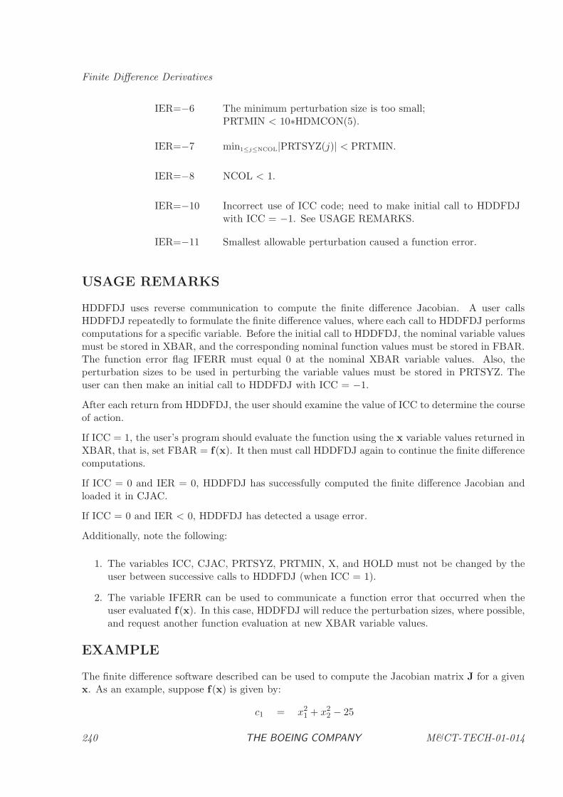
Finite Difference Derivatives
IER=−6 The minimum perturbation size is too small;PRTMIN < 10∗HDMCON(5).
IER=−7 min1≤j≤NCOL|PRTSYZ(j)| < PRTMIN.
IER=−8 NCOL < 1.
IER=−10 Incorrect use of ICC code; need to make initial call to HDDFDJwith ICC = −1. See USAGE REMARKS.
IER=−11 Smallest allowable perturbation caused a function error.
USAGE REMARKS
HDDFDJ uses reverse communication to compute the finite difference Jacobian. A user callsHDDFDJ repeatedly to formulate the finite difference values, where each call to HDDFDJ performscomputations for a specific variable. Before the initial call to HDDFDJ, the nominal variable valuesmust be stored in XBAR, and the corresponding nominal function values must be stored in FBAR.The function error flag IFERR must equal 0 at the nominal XBAR variable values. Also, theperturbation sizes to be used in perturbing the variable values must be stored in PRTSYZ. Theuser can then make an initial call to HDDFDJ with ICC = −1.
After each return from HDDFDJ, the user should examine the value of ICC to determine the courseof action.
If ICC = 1, the user’s program should evaluate the function using the x variable values returned inXBAR, that is, set FBAR = f(x). It then must call HDDFDJ again to continue the finite differencecomputations.
If ICC = 0 and IER = 0, HDDFDJ has successfully computed the finite difference Jacobian andloaded it in CJAC.
If ICC = 0 and IER < 0, HDDFDJ has detected a usage error.
Additionally, note the following:
1. The variables ICC, CJAC, PRTSYZ, PRTMIN, X, and HOLD must not be changed by theuser between successive calls to HDDFDJ (when ICC = 1).
2. The variable IFERR can be used to communicate a function error that occurred when theuser evaluated f(x). In this case, HDDFDJ will reduce the perturbation sizes, where possible,and request another function evaluation at new XBAR variable values.
EXAMPLE
The finite difference software described can be used to compute the Jacobian matrix J for a givenx. As an example, suppose f(x) is given by:
c1 = x21 + x2
2 − 25
240 THE BOEING COMPANY M&CT-TECH-01-014
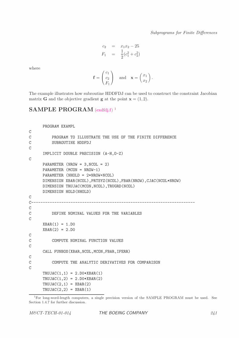
Subprograms for Finite Differences
c2 = x1x2 − 25
F1 =1
2(c21 + c22)
where
f =
c1c2F1
and x =
(x1
x2
).
The example illustrates how subroutine HDDFDJ can be used to construct the constraint Jacobianmatrix G and the objective gradient g at the point x = (1, 2).
SAMPLE PROGRAM (exdfdj.f) 1
PROGRAM EXAMPL
C
C PROGRAM TO ILLUSTRATE THE USE OF THE FINITE DIFFERENCE
C SUBROUTINE HDDFDJ
C
IMPLICIT DOUBLE PRECISION (A-H,O-Z)
C
PARAMETER (NROW = 3,NCOL = 2)
PARAMETER (MCON = NROW-1)
PARAMETER (NHOLD = 2*NROW+NCOL)
DIMENSION XBAR(NCOL),PRTSYZ(NCOL),FBAR(NROW),CJAC(NCOL*NROW)
DIMENSION TRUJAC(MCON,NCOL),TRUGRD(NCOL)
DIMENSION HOLD(NHOLD)
C
C-----------------------------------------------------------------------
C
C DEFINE NOMINAL VALUES FOR THE VARIABLES
C
XBAR(1) = 1.D0
XBAR(2) = 2.D0
C
C COMPUTE NOMINAL FUNCTION VALUES
C
CALL FUNBOX(XBAR,NCOL,MCON,FBAR,IFERR)
C
C COMPUTE THE ANALYTIC DERIVATIVES FOR COMPARISON
C
TRUJAC(1,1) = 2.D0*XBAR(1)
TRUJAC(1,2) = 2.D0*XBAR(2)
TRUJAC(2,1) = XBAR(2)
TRUJAC(2,2) = XBAR(1)
1For long-word-length computers, a single precision version of the SAMPLE PROGRAM must be used. See
Section 1.4.7 for further discussion.
M&CT-TECH-01-014 THE BOEING COMPANY 241
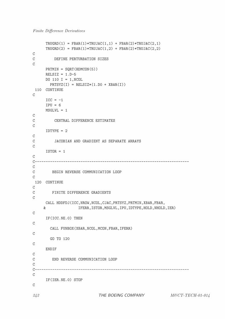
Finite Difference Derivatives
TRUGRD(1) = FBAR(1)*TRUJAC(1,1) + FBAR(2)*TRUJAC(2,1)
TRUGRD(2) = FBAR(1)*TRUJAC(1,2) + FBAR(2)*TRUJAC(2,2)
C
C DEFINE PERTURBATION SIZES
C
PRTMIN = SQRT(HDMCON(5))
RELSIZ = 1.D-5
DO 110 I = 1,NCOL
PRTSYZ(I) = RELSIZ*(1.D0 + XBAR(I))
110 CONTINUE
C
ICC = -1
IPU = 6
MSGLVL = 1
C
C CENTRAL DIFFERENCE ESTIMATES
C
IDTYPE = 2
C
C JACOBIAN AND GRADIENT AS SEPARATE ARRAYS
C
ISTOR = 1
C
C-----------------------------------------------------------------------
C
C BEGIN REVERSE COMMUNICATION LOOP
C
120 CONTINUE
C
C FINITE DIFFERENCE GRADIENTS
C
CALL HDDFDJ(ICC,NROW,NCOL,CJAC,PRTSYZ,PRTMIN,XBAR,FBAR,
& IFERR,ISTOR,MSGLVL,IPU,IDTYPE,HOLD,NHOLD,IER)
C
IF(ICC.NE.0) THEN
C
CALL FUNBOX(XBAR,NCOL,MCON,FBAR,IFERR)
C
GO TO 120
C
ENDIF
C
C END REVERSE COMMUNICATION LOOP
C
C-----------------------------------------------------------------------
C
IF(IER.NE.0) STOP
C
242 THE BOEING COMPANY M&CT-TECH-01-014
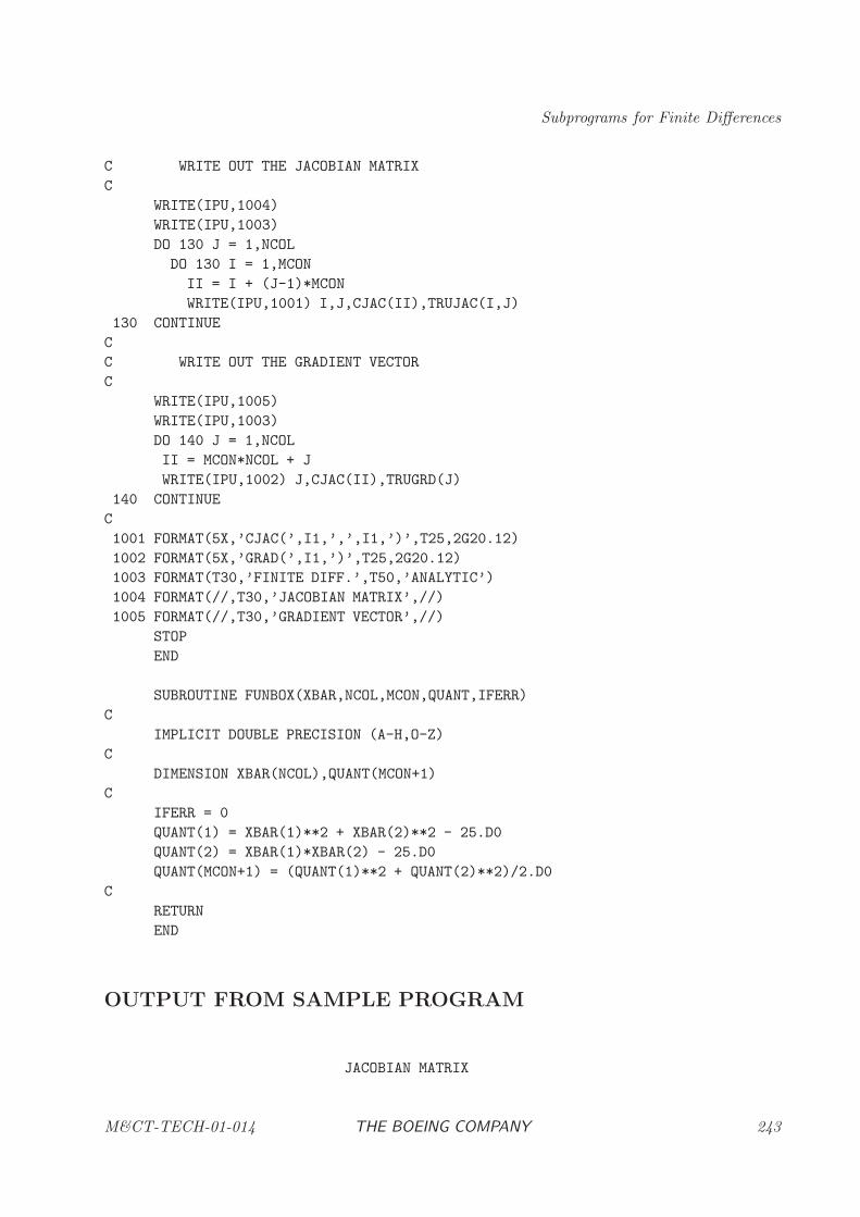
Subprograms for Finite Differences
C WRITE OUT THE JACOBIAN MATRIX
C
WRITE(IPU,1004)
WRITE(IPU,1003)
DO 130 J = 1,NCOL
DO 130 I = 1,MCON
II = I + (J-1)*MCON
WRITE(IPU,1001) I,J,CJAC(II),TRUJAC(I,J)
130 CONTINUE
C
C WRITE OUT THE GRADIENT VECTOR
C
WRITE(IPU,1005)
WRITE(IPU,1003)
DO 140 J = 1,NCOL
II = MCON*NCOL + J
WRITE(IPU,1002) J,CJAC(II),TRUGRD(J)
140 CONTINUE
C
1001 FORMAT(5X,’CJAC(’,I1,’,’,I1,’)’,T25,2G20.12)
1002 FORMAT(5X,’GRAD(’,I1,’)’,T25,2G20.12)
1003 FORMAT(T30,’FINITE DIFF.’,T50,’ANALYTIC’)
1004 FORMAT(//,T30,’JACOBIAN MATRIX’,//)
1005 FORMAT(//,T30,’GRADIENT VECTOR’,//)
STOP
END
SUBROUTINE FUNBOX(XBAR,NCOL,MCON,QUANT,IFERR)
C
IMPLICIT DOUBLE PRECISION (A-H,O-Z)
C
DIMENSION XBAR(NCOL),QUANT(MCON+1)
C
IFERR = 0
QUANT(1) = XBAR(1)**2 + XBAR(2)**2 - 25.D0
QUANT(2) = XBAR(1)*XBAR(2) - 25.D0
QUANT(MCON+1) = (QUANT(1)**2 + QUANT(2)**2)/2.D0
C
RETURN
END
OUTPUT FROM SAMPLE PROGRAM
JACOBIAN MATRIX
M&CT-TECH-01-014 THE BOEING COMPANY 243

Finite Difference Derivatives
FINITE DIFF. ANALYTIC
CJAC(1,1) 1.99999999992 2.00000000000
CJAC(2,1) 1.99999999992 2.00000000000
CJAC(1,2) 4.00000000003 4.00000000000
CJAC(2,2) 0.999999999962 1.00000000000
GRADIENT VECTOR
FINITE DIFF. ANALYTIC
GRAD(1) -85.9999999975 -86.0000000000
GRAD(2) -102.999999996 -103.000000000
244 THE BOEING COMPANY M&CT-TECH-01-014
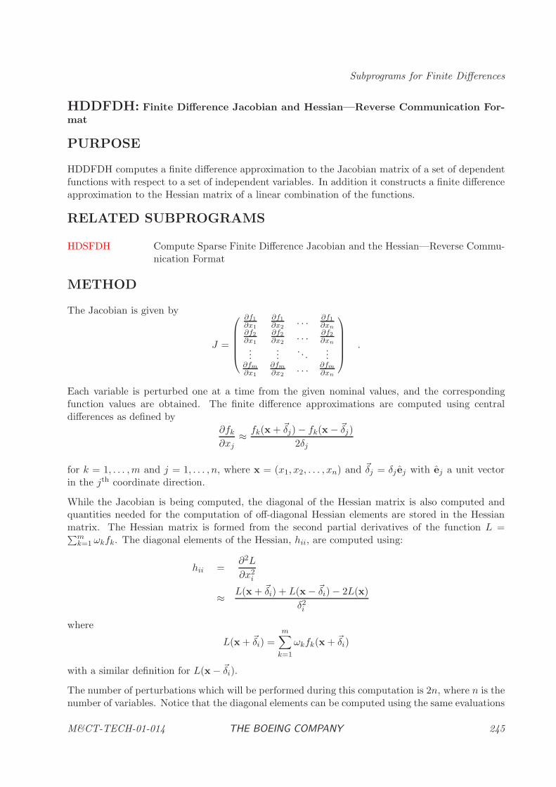
Subprograms for Finite Differences
HDDFDH: Finite Difference Jacobian and Hessian—Reverse Communication For-mat
PURPOSE
HDDFDH computes a finite difference approximation to the Jacobian matrix of a set of dependentfunctions with respect to a set of independent variables. In addition it constructs a finite differenceapproximation to the Hessian matrix of a linear combination of the functions.
RELATED SUBPROGRAMS
HDSFDH Compute Sparse Finite Difference Jacobian and the Hessian—Reverse Commu-nication Format
METHOD
The Jacobian is given by
J =
∂f1
∂x1
∂f1
∂x2. . . ∂f1
∂xn∂f2
∂x1
∂f2
∂x2. . . ∂f2
∂xn
......
. . ....
∂fm
∂x1
∂fm
∂x2. . . ∂fm
∂xn
.
Each variable is perturbed one at a time from the given nominal values, and the correspondingfunction values are obtained. The finite difference approximations are computed using centraldifferences as defined by
∂fk
∂xj≈ fk(x + ~δj) − fk(x − ~δj)
2δj
for k = 1, . . . ,m and j = 1, . . . , n, where x = (x1, x2, . . . , xn) and ~δj = δj ej with ej a unit vectorin the jth coordinate direction.
While the Jacobian is being computed, the diagonal of the Hessian matrix is also computed andquantities needed for the computation of off-diagonal Hessian elements are stored in the Hessianmatrix. The Hessian matrix is formed from the second partial derivatives of the function L =∑m
k=1 ωkfk. The diagonal elements of the Hessian, hii, are computed using:
hii =∂2L
∂x2i
≈ L(x + ~δi) + L(x− ~δi) − 2L(x)
δ2i
where
L(x + ~δi) =m∑
k=1
ωkfk(x + ~δi)
with a similar definition for L(x− ~δi).
The number of perturbations which will be performed during this computation is 2n, where n is thenumber of variables. Notice that the diagonal elements can be computed using the same evaluations
M&CT-TECH-01-014 THE BOEING COMPANY 245
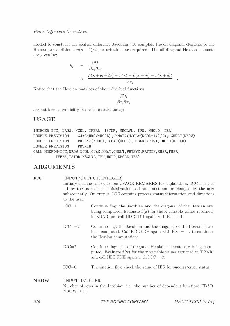
Finite Difference Derivatives
needed to construct the central difference Jacobian. To complete the off-diagonal elements of theHessian, an additional n(n − 1)/2 perturbations are required. The off-diagonal Hessian elementsare given by:
hij =∂2L
∂xi∂xj
≈ L(x + ~δi + ~δj) + L(x) − L(x + ~δi) − L(x + ~δj)
δiδj.
Notice that the Hessian matrices of the individual functions
∂2fk
∂xi∂xj
are not formed explicitly in order to save storage.
USAGE
INTEGER ICC, NROW, NCOL, IFERR, ISTOR, MSGLVL, IPU, NHOLD, IER
DOUBLE PRECISION CJAC(NROW*NCOL), HMAT((NCOL*(NCOL+1))/2), CMULT(NROW)
DOUBLE PRECISION PRTSYZ(NCOL), XBAR(NCOL), FBAR(NROW), HOLD(NHOLD)
DOUBLE PRECISION PRTMIN
CALL HDDFDH(ICC,NROW,NCOL,CJAC,HMAT,CMULT,PRTSYZ,PRTMIN,XBAR,FBAR,
1 IFERR,ISTOR,MSGLVL,IPU,HOLD,NHOLD,IER)
ARGUMENTS
ICC [INPUT/OUTPUT, INTEGER]Initial/continue call code; see USAGE REMARKS for explanation. ICC is set to−1 by the user on the initialization call and must not be changed by the usersubsequently. On output, ICC contains process status information and directionsto the user:
ICC=1 Continue flag; the Jacobian and the diagonal of the Hessian arebeing computed. Evaluate f(x) for the x variable values returnedin XBAR and call HDDFDH again with ICC = 1.
ICC=−2 Continue flag; the Jacobian and the diagonal of the Hessian havebeen computed. Call HDDFDH again with ICC = −2 to continuethe Hessian computations.
ICC=2 Continue flag; the off-diagonal Hessian elements are being com-puted. Evaluate f(x) for the x variable values returned in XBARand call HDDFDH again with ICC = 2.
ICC=0 Termination flag; check the value of IER for success/error status.
NROW [INPUT, INTEGER]Number of rows in the Jacobian, i.e. the number of dependent functions FBAR;NROW ≥ 1..
246 THE BOEING COMPANY M&CT-TECH-01-014
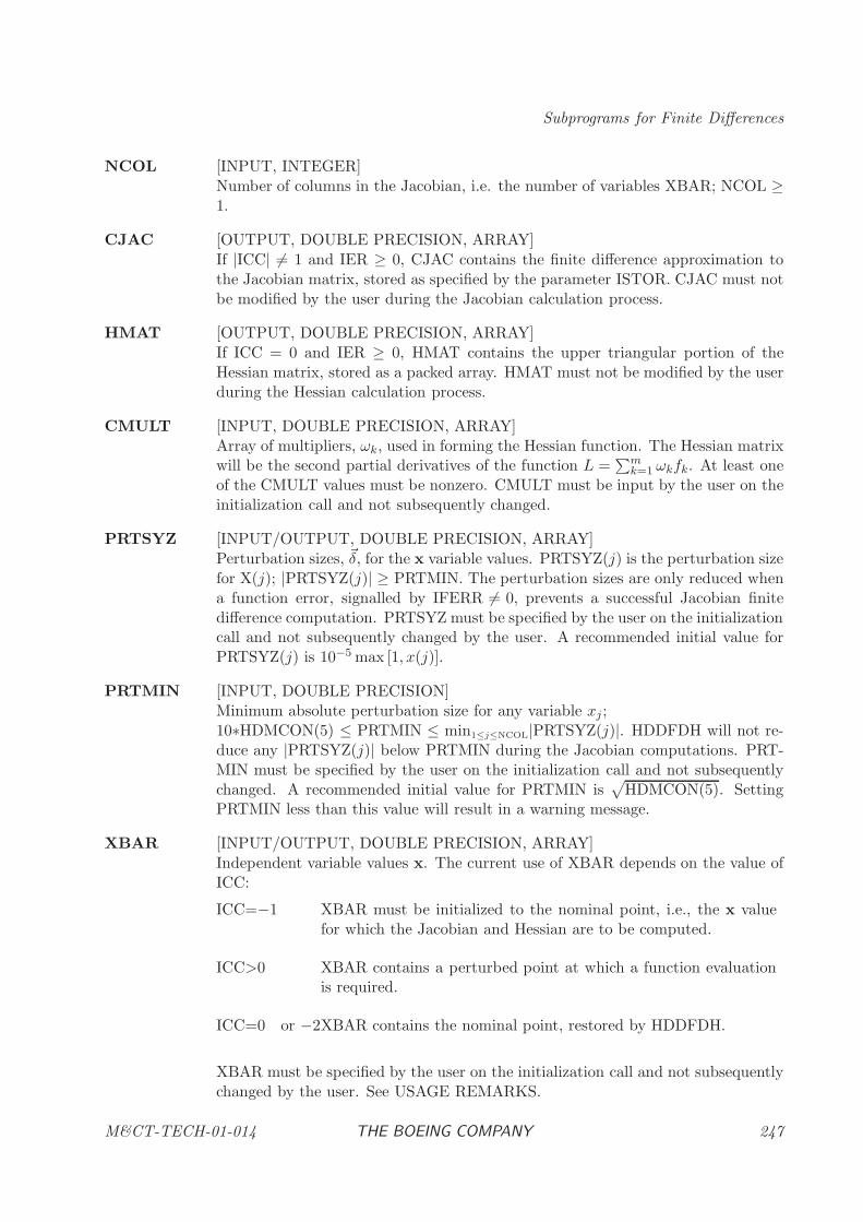
Subprograms for Finite Differences
NCOL [INPUT, INTEGER]Number of columns in the Jacobian, i.e. the number of variables XBAR; NCOL ≥1.
CJAC [OUTPUT, DOUBLE PRECISION, ARRAY]If |ICC| 6= 1 and IER ≥ 0, CJAC contains the finite difference approximation tothe Jacobian matrix, stored as specified by the parameter ISTOR. CJAC must notbe modified by the user during the Jacobian calculation process.
HMAT [OUTPUT, DOUBLE PRECISION, ARRAY]If ICC = 0 and IER ≥ 0, HMAT contains the upper triangular portion of theHessian matrix, stored as a packed array. HMAT must not be modified by the userduring the Hessian calculation process.
CMULT [INPUT, DOUBLE PRECISION, ARRAY]Array of multipliers, ωk, used in forming the Hessian function. The Hessian matrixwill be the second partial derivatives of the function L =
∑mk=1 ωkfk. At least one
of the CMULT values must be nonzero. CMULT must be input by the user on theinitialization call and not subsequently changed.
PRTSYZ [INPUT/OUTPUT, DOUBLE PRECISION, ARRAY]Perturbation sizes, ~δ, for the x variable values. PRTSYZ(j) is the perturbation sizefor X(j); |PRTSYZ(j)| ≥ PRTMIN. The perturbation sizes are only reduced whena function error, signalled by IFERR 6= 0, prevents a successful Jacobian finitedifference computation. PRTSYZ must be specified by the user on the initializationcall and not subsequently changed by the user. A recommended initial value forPRTSYZ(j) is 10−5 max [1, x(j)].
PRTMIN [INPUT, DOUBLE PRECISION]Minimum absolute perturbation size for any variable xj ;10∗HDMCON(5) ≤ PRTMIN ≤ min1≤j≤NCOL|PRTSYZ(j)|. HDDFDH will not re-duce any |PRTSYZ(j)| below PRTMIN during the Jacobian computations. PRT-MIN must be specified by the user on the initialization call and not subsequentlychanged. A recommended initial value for PRTMIN is
√HDMCON(5). Setting
PRTMIN less than this value will result in a warning message.
XBAR [INPUT/OUTPUT, DOUBLE PRECISION, ARRAY]Independent variable values x. The current use of XBAR depends on the value ofICC:
ICC=−1 XBAR must be initialized to the nominal point, i.e., the x valuefor which the Jacobian and Hessian are to be computed.
ICC>0 XBAR contains a perturbed point at which a function evaluationis required.
ICC=0 or −2XBAR contains the nominal point, restored by HDDFDH.
XBAR must be specified by the user on the initialization call and not subsequentlychanged by the user. See USAGE REMARKS.
M&CT-TECH-01-014 THE BOEING COMPANY 247
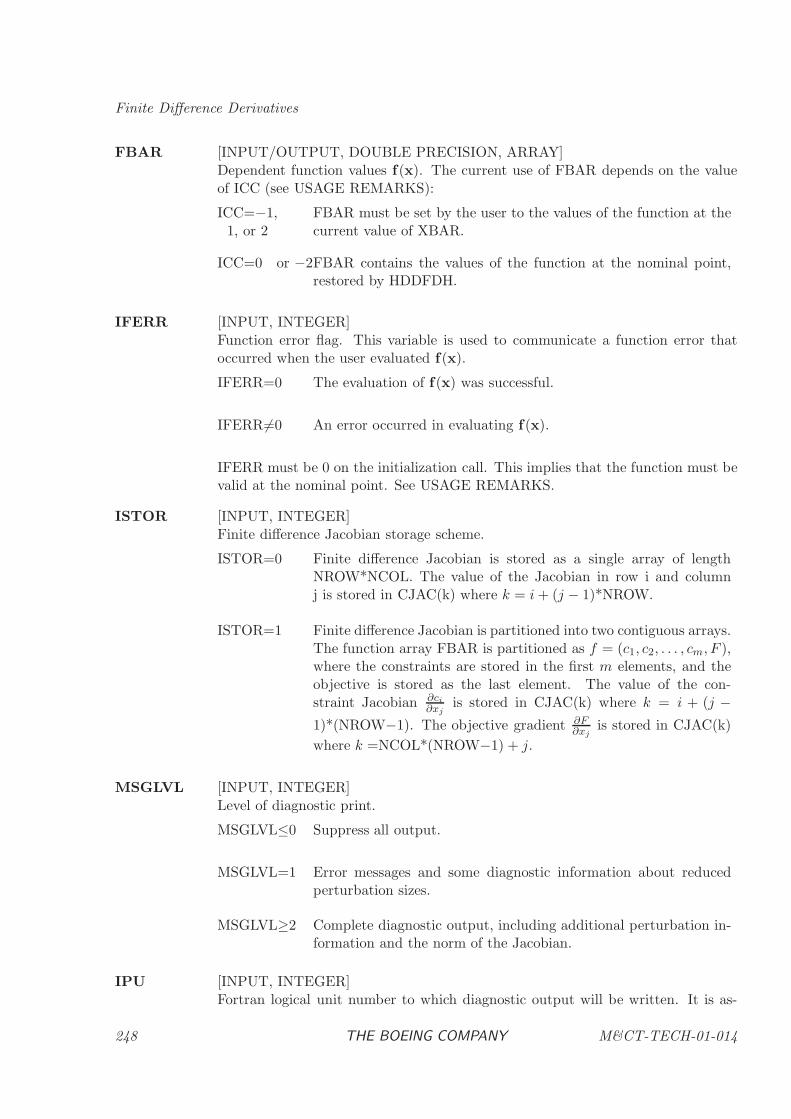
Finite Difference Derivatives
FBAR [INPUT/OUTPUT, DOUBLE PRECISION, ARRAY]Dependent function values f(x). The current use of FBAR depends on the valueof ICC (see USAGE REMARKS):
ICC=−1,1, or 2
FBAR must be set by the user to the values of the function at thecurrent value of XBAR.
ICC=0 or −2FBAR contains the values of the function at the nominal point,restored by HDDFDH.
IFERR [INPUT, INTEGER]Function error flag. This variable is used to communicate a function error thatoccurred when the user evaluated f(x).
IFERR=0 The evaluation of f(x) was successful.
IFERR 6=0 An error occurred in evaluating f(x).
IFERR must be 0 on the initialization call. This implies that the function must bevalid at the nominal point. See USAGE REMARKS.
ISTOR [INPUT, INTEGER]Finite difference Jacobian storage scheme.
ISTOR=0 Finite difference Jacobian is stored as a single array of lengthNROW*NCOL. The value of the Jacobian in row i and columnj is stored in CJAC(k) where k = i+ (j − 1)*NROW.
ISTOR=1 Finite difference Jacobian is partitioned into two contiguous arrays.The function array FBAR is partitioned as f = (c1, c2, . . . , cm, F ),where the constraints are stored in the first m elements, and theobjective is stored as the last element. The value of the con-straint Jacobian ∂ci
∂xjis stored in CJAC(k) where k = i + (j −
1)*(NROW−1). The objective gradient ∂F∂xj
is stored in CJAC(k)
where k =NCOL*(NROW−1) + j.
MSGLVL [INPUT, INTEGER]Level of diagnostic print.
MSGLVL≤0 Suppress all output.
MSGLVL=1 Error messages and some diagnostic information about reducedperturbation sizes.
MSGLVL≥2 Complete diagnostic output, including additional perturbation in-formation and the norm of the Jacobian.
IPU [INPUT, INTEGER]Fortran logical unit number to which diagnostic output will be written. It is as-
248 THE BOEING COMPANY M&CT-TECH-01-014
Subprograms for Finite Differences
sumed that this unit has been opened by the user prior to the call to HDDFDH ifMSGLVL > 0.
HOLD [INPUT/OUTPUT, DOUBLE PRECISION, ARRAY]Hold array of length NHOLD. This array must not be changed by the user betweensuccessive calls to HDDFDH when the Jacobian and Hessian matrices are beingcomputed. After the Jacobian and Hessian computations are complete (ICC = 0),this array can be used elsewhere as a work array.
NHOLD [INPUT, INTEGER]The length of the HOLD array. NHOLD ≥ 2∗(NROW+NCOL).
IER [OUTPUT, INTEGER]Success/error code. See Section 1.4.2 of the BCSLIB manual for a discussion oferror handling. For IER < 0, ICC has been set to 0, and at least part of theCJAC and HMAT arrays have been clobbered with HDMCON(1). See the BCSLIBmanual for HDMCON. Note, however, that for IER = −21, −22, and −23, theCJAC array is not clobbered and contains the computed Jacobian matrix.
IER=0 Success, results computed.
IER=1 PRTMIN <√
HDMCON(5).
IER=4 The CMULT array is all zeros; no need to compute the Hessianmatrix. If only the Jacobian matrix is needed, use HDDFDJ.
IER=−1 Invalid initial/continue call code; ICC 6= −2, −1, 1, or 2.
IER=−2 NROW < 1.
IER=−4 NHOLD too small; the number of words needed is given by theprinted error message.
IER=−5 For ICC = −1 or −2, IFERR 6= 0. There must not be a functionerror at the nominal point.
IER=−6 The minimum perturbation size is too small;PRTMIN < 10∗HDMCON(5).
IER=−7 min1≤j≤NCOL|PRTSYZ(j)| < PRTMIN.
IER=−8 NCOL < 1.
IER=−10 Incorrect use of ICC code; make sure that an initial call toHDDFDH with ICC = −1 is made prior to the Jacobian and Hes-sian diagonal computations (ICC = 1). See USAGE REMARKS.
M&CT-TECH-01-014 THE BOEING COMPANY 249
Finite Difference Derivatives
IER=−11 Smallest allowable perturbation caused a function error.
IER=−20 Incorrect use of ICC code; make sure that a call to HDDFDHwith ICC = −2 is made after the Jacobian and Hessian diagonalcomputations (ICC = 1) and prior to the off-diagonal Hessian com-putations (ICC = 2). See USAGE REMARKS.
IER=−21 Inconsistency in nominal variable values detected. The same nom-inal values must be used in XBAR for ICC = −1 and −2, andthe HOLD array must not be changed between successive calls toHDDFDH. In spite of this, the Jacobian matrix was successfullycomputed for the nominal values supplied when HDDFDH wascalled with ICC = −1.
IER=−22 Inconsistency in nominal function values detected. The same nom-inal values must be used in FBAR for ICC = −1 and −2, andthe HOLD array must not be changed between successive calls toHDDFDH. In spite of this, the Jacobian matrix was successfullycomputed for the nominal values supplied when HDDFDH wascalled with ICC = −1.
IER=−23 A function error occurred while computing the off-diagonal Hessianelements. The computation of the Hessian was not completed. TheJacobian matrix, on the other hand, was successfully computed andis stored in CJAC.
USAGE REMARKS
HDDFDH uses reverse communication to compute the Jacobian and Hessian matrices. A user callsHDDFDH repeatedly to formulate the Jacobian and Hessian values, where each call to HDDFDHperforms computations for a particular variable. Before the initial call to HDDFDH, the nominalvariable values must be stored in XBAR, and the corresponding nominal function values must bestored in FBAR. The function error flag IFERR must equal 0 at the nominal XBAR variable values.Also, the perturbation sizes used in perturbing the variable values must be stored in PRTSYZ. Theuser can then make an initial call to HDDFDH with ICC = −1.
After each return from HDDFDH, the user should examine the value of ICC to determine thecourse of action.
If ICC = 1 or 2, the user’s program should evaluate the function using the x variable values returnedin XBAR, that is, set FBAR = f(x). It then must call HDDFDH again with the same value ofICC to continue the Jacobian and Hessian computations.
If ICC = −2, the Jacobian and the diagonal elements of the Hessian have been computed. To con-tinue the Hessian computation, the user’s program can simply call HDDFDH again with ICC = −2.
If ICC = 0 and IER = 0, HDDFDH has successfully computed the Jacobian and Hessian matricesand loaded them in CJAC and HMAT, respectively.
If ICC = 0 and IER < 0, HDDFDH has detected a usage error.
250 THE BOEING COMPANY M&CT-TECH-01-014
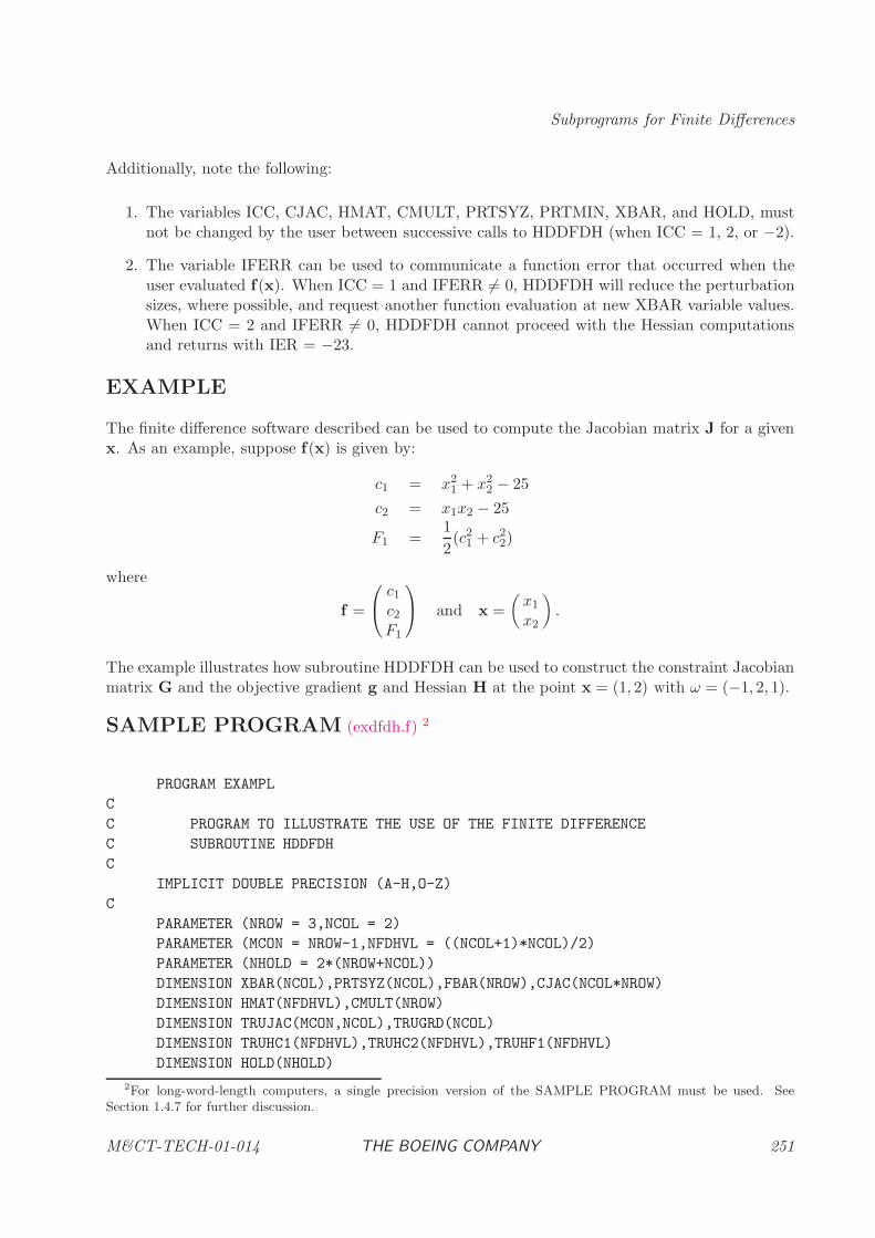
Subprograms for Finite Differences
Additionally, note the following:
1. The variables ICC, CJAC, HMAT, CMULT, PRTSYZ, PRTMIN, XBAR, and HOLD, mustnot be changed by the user between successive calls to HDDFDH (when ICC = 1, 2, or −2).
2. The variable IFERR can be used to communicate a function error that occurred when theuser evaluated f(x). When ICC = 1 and IFERR 6= 0, HDDFDH will reduce the perturbationsizes, where possible, and request another function evaluation at new XBAR variable values.When ICC = 2 and IFERR 6= 0, HDDFDH cannot proceed with the Hessian computationsand returns with IER = −23.
EXAMPLE
The finite difference software described can be used to compute the Jacobian matrix J for a givenx. As an example, suppose f(x) is given by:
c1 = x21 + x2
2 − 25
c2 = x1x2 − 25
F1 =1
2(c21 + c22)
where
f =
c1c2F1
and x =
(x1
x2
).
The example illustrates how subroutine HDDFDH can be used to construct the constraint Jacobianmatrix G and the objective gradient g and Hessian H at the point x = (1, 2) with ω = (−1, 2, 1).
SAMPLE PROGRAM (exdfdh.f) 2
PROGRAM EXAMPL
C
C PROGRAM TO ILLUSTRATE THE USE OF THE FINITE DIFFERENCE
C SUBROUTINE HDDFDH
C
IMPLICIT DOUBLE PRECISION (A-H,O-Z)
C
PARAMETER (NROW = 3,NCOL = 2)
PARAMETER (MCON = NROW-1,NFDHVL = ((NCOL+1)*NCOL)/2)
PARAMETER (NHOLD = 2*(NROW+NCOL))
DIMENSION XBAR(NCOL),PRTSYZ(NCOL),FBAR(NROW),CJAC(NCOL*NROW)
DIMENSION HMAT(NFDHVL),CMULT(NROW)
DIMENSION TRUJAC(MCON,NCOL),TRUGRD(NCOL)
DIMENSION TRUHC1(NFDHVL),TRUHC2(NFDHVL),TRUHF1(NFDHVL)
DIMENSION HOLD(NHOLD)
2For long-word-length computers, a single precision version of the SAMPLE PROGRAM must be used. See
Section 1.4.7 for further discussion.
M&CT-TECH-01-014 THE BOEING COMPANY 251
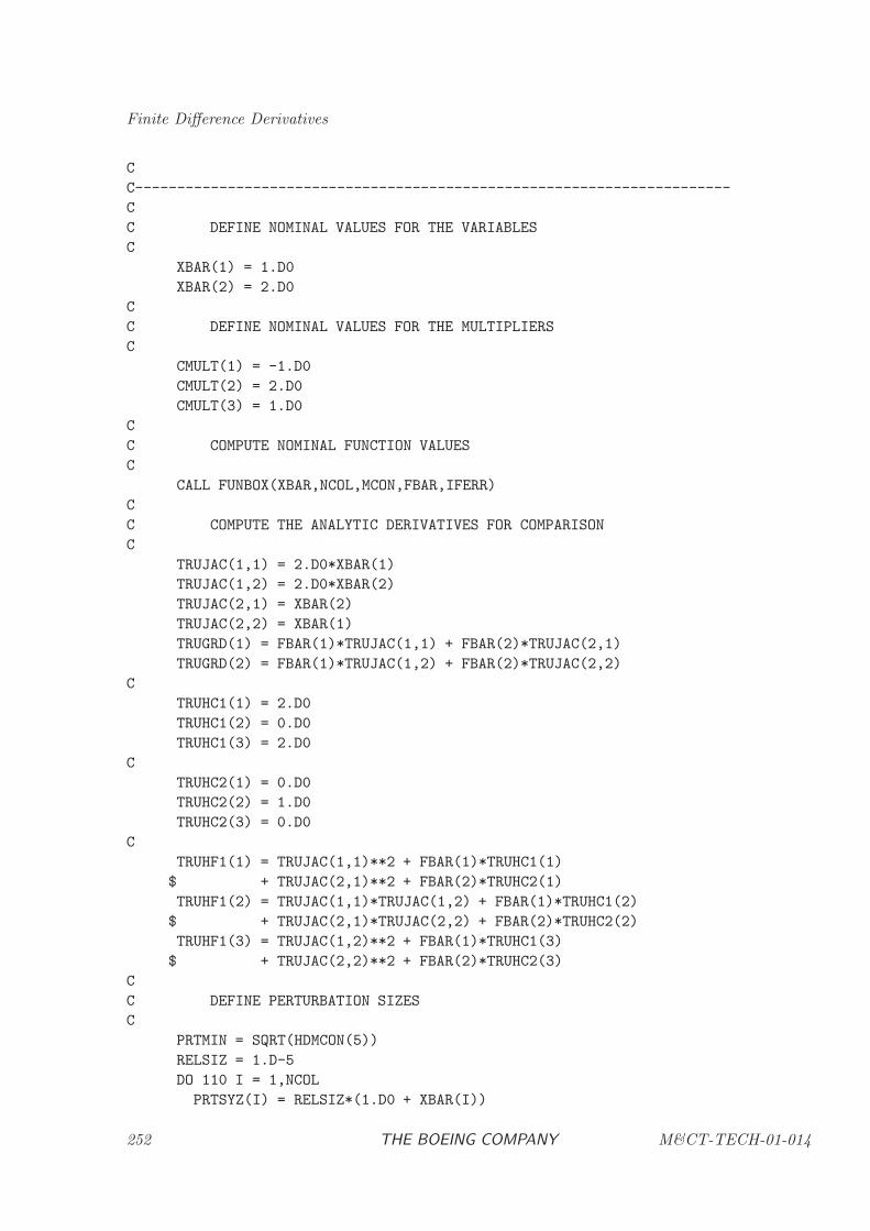
Finite Difference Derivatives
C
C-----------------------------------------------------------------------
C
C DEFINE NOMINAL VALUES FOR THE VARIABLES
C
XBAR(1) = 1.D0
XBAR(2) = 2.D0
C
C DEFINE NOMINAL VALUES FOR THE MULTIPLIERS
C
CMULT(1) = -1.D0
CMULT(2) = 2.D0
CMULT(3) = 1.D0
C
C COMPUTE NOMINAL FUNCTION VALUES
C
CALL FUNBOX(XBAR,NCOL,MCON,FBAR,IFERR)
C
C COMPUTE THE ANALYTIC DERIVATIVES FOR COMPARISON
C
TRUJAC(1,1) = 2.D0*XBAR(1)
TRUJAC(1,2) = 2.D0*XBAR(2)
TRUJAC(2,1) = XBAR(2)
TRUJAC(2,2) = XBAR(1)
TRUGRD(1) = FBAR(1)*TRUJAC(1,1) + FBAR(2)*TRUJAC(2,1)
TRUGRD(2) = FBAR(1)*TRUJAC(1,2) + FBAR(2)*TRUJAC(2,2)
C
TRUHC1(1) = 2.D0
TRUHC1(2) = 0.D0
TRUHC1(3) = 2.D0
C
TRUHC2(1) = 0.D0
TRUHC2(2) = 1.D0
TRUHC2(3) = 0.D0
C
TRUHF1(1) = TRUJAC(1,1)**2 + FBAR(1)*TRUHC1(1)
$ + TRUJAC(2,1)**2 + FBAR(2)*TRUHC2(1)
TRUHF1(2) = TRUJAC(1,1)*TRUJAC(1,2) + FBAR(1)*TRUHC1(2)
$ + TRUJAC(2,1)*TRUJAC(2,2) + FBAR(2)*TRUHC2(2)
TRUHF1(3) = TRUJAC(1,2)**2 + FBAR(1)*TRUHC1(3)
$ + TRUJAC(2,2)**2 + FBAR(2)*TRUHC2(3)
C
C DEFINE PERTURBATION SIZES
C
PRTMIN = SQRT(HDMCON(5))
RELSIZ = 1.D-5
DO 110 I = 1,NCOL
PRTSYZ(I) = RELSIZ*(1.D0 + XBAR(I))
252 THE BOEING COMPANY M&CT-TECH-01-014
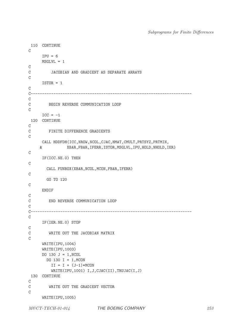
Subprograms for Finite Differences
110 CONTINUE
C
IPU = 6
MSGLVL = 1
C
C JACOBIAN AND GRADIENT AS SEPARATE ARRAYS
C
ISTOR = 1
C
C-----------------------------------------------------------------------
C
C BEGIN REVERSE COMMUNICATION LOOP
C
ICC = -1
120 CONTINUE
C
C FINITE DIFFERENCE GRADIENTS
C
CALL HDDFDH(ICC,NROW,NCOL,CJAC,HMAT,CMULT,PRTSYZ,PRTMIN,
& XBAR,FBAR,IFERR,ISTOR,MSGLVL,IPU,HOLD,NHOLD,IER)
C
IF(ICC.NE.0) THEN
C
CALL FUNBOX(XBAR,NCOL,MCON,FBAR,IFERR)
C
GO TO 120
C
ENDIF
C
C END REVERSE COMMUNICATION LOOP
C
C-----------------------------------------------------------------------
C
IF(IER.NE.0) STOP
C
C WRITE OUT THE JACOBIAN MATRIX
C
WRITE(IPU,1004)
WRITE(IPU,1003)
DO 130 J = 1,NCOL
DO 130 I = 1,MCON
II = I + (J-1)*MCON
WRITE(IPU,1001) I,J,CJAC(II),TRUJAC(I,J)
130 CONTINUE
C
C WRITE OUT THE GRADIENT VECTOR
C
WRITE(IPU,1005)
M&CT-TECH-01-014 THE BOEING COMPANY 253
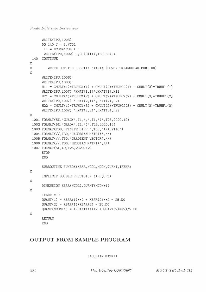
Finite Difference Derivatives
WRITE(IPU,1003)
DO 140 J = 1,NCOL
II = MCON*NCOL + J
WRITE(IPU,1002) J,CJAC(II),TRUGRD(J)
140 CONTINUE
C
C WRITE OUT THE HESSIAN MATRIX (LOWER TRIANGULAR PORTION)
C
WRITE(IPU,1006)
WRITE(IPU,1003)
H11 = CMULT(1)*TRUHC1(1) + CMULT(2)*TRUHC2(1) + CMULT(3)*TRUHF1(1)
WRITE(IPU,1007) ’HMAT(1,1)’,HMAT(1),H11
H21 = CMULT(1)*TRUHC1(2) + CMULT(2)*TRUHC2(2) + CMULT(3)*TRUHF1(2)
WRITE(IPU,1007) ’HMAT(2,1)’,HMAT(2),H21
H22 = CMULT(1)*TRUHC1(3) + CMULT(2)*TRUHC2(3) + CMULT(3)*TRUHF1(3)
WRITE(IPU,1007) ’HMAT(2,2)’,HMAT(3),H22
C
1001 FORMAT(5X,’CJAC(’,I1,’,’,I1,’)’,T25,2G20.12)
1002 FORMAT(5X,’GRAD(’,I1,’)’,T25,2G20.12)
1003 FORMAT(T30,’FINITE DIFF.’,T50,’ANALYTIC’)
1004 FORMAT(//,T30,’JACOBIAN MATRIX’,//)
1005 FORMAT(//,T30,’GRADIENT VECTOR’,//)
1006 FORMAT(//,T30,’HESSIAN MATRIX’,//)
1007 FORMAT(5X,A9,T25,2G20.12)
STOP
END
SUBROUTINE FUNBOX(XBAR,NCOL,MCON,QUANT,IFERR)
C
IMPLICIT DOUBLE PRECISION (A-H,O-Z)
C
DIMENSION XBAR(NCOL),QUANT(MCON+1)
C
IFERR = 0
QUANT(1) = XBAR(1)**2 + XBAR(2)**2 - 25.D0
QUANT(2) = XBAR(1)*XBAR(2) - 25.D0
QUANT(MCON+1) = (QUANT(1)**2 + QUANT(2)**2)/2.D0
C
RETURN
END
OUTPUT FROM SAMPLE PROGRAM
JACOBIAN MATRIX
254 THE BOEING COMPANY M&CT-TECH-01-014
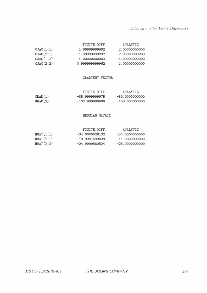
Subprograms for Finite Differences
FINITE DIFF. ANALYTIC
CJAC(1,1) 1.99999999992 2.00000000000
CJAC(2,1) 1.99999999992 2.00000000000
CJAC(1,2) 4.00000000003 4.00000000000
CJAC(2,2) 0.999999999962 1.00000000000
GRADIENT VECTOR
FINITE DIFF. ANALYTIC
GRAD(1) -85.9999999975 -86.0000000000
GRAD(2) -102.999999996 -103.000000000
HESSIAN MATRIX
FINITE DIFF. ANALYTIC
HMAT(1,1) -34.0000028132 -34.0000000000
HMAT(2,1) -10.9997699838 -11.0000000000
HMAT(2,2) -24.9999882524 -25.0000000000
M&CT-TECH-01-014 THE BOEING COMPANY 255
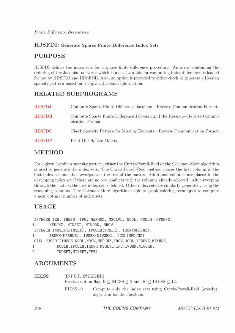
Finite Difference Derivatives
HJSFDI: Generate Sparse Finite Difference Index Sets
PURPOSE
HJSFDI defines the index sets for a sparse finite difference procedure. An array containing theordering of the Jacobian nonzeros which is most favorable for computing finite differences is loadedfor use by HDSFDJ and HDSFDH. Also, an option is provided to either check or generate a Hessiansparsity pattern based on the given Jacobian information.
RELATED SUBPROGRAMS
HDSFDJ Compute Sparse Finite Difference Jacobian—Reverse Communication Format
HDSFDH Compute Sparse Finite Difference Jacobian and the Hessian—Reverse Commu-nication Format
HDSFDC Check Sparsity Pattern for Missing Elements—Reverse Communication Format
HDSFDP Print Out Sparse Matrix
METHOD
For a given Jacobian sparsity pattern, either the Curtis-Powell-Reid or the Coleman-More algorithmis used to generate the index sets. The Curtis-Powell-Reid method places the first column in thefirst index set and then sweeps over the rest of the matrix. Additional columns are placed in thedeveloping index set if there are no row conflicts with the columns already selected. After sweepingthrough the matrix, the first index set is defined. Other index sets are similarly generated, using theremaining columns. The Coleman-More algorithm exploits graph coloring techniques to computea near optimal number of index sets.
USAGE
INTEGER IER, IHESS, IPU, MAXHNZ, MSGLVL, NCOL, NCOLH, NFDHNZ,
1 NFDJNZ, NINSET, NIWORK, NROW
INTEGER INDSET(NINSET), IPCOLH(NCOLH), IROW(NFDJNZ),
1 IROWH(MAXHNZ), IWORK(NIWORK), JCOL(NFDJNZ)
CALL HJSFDI(IHESS,NCOL,NROW,NFDJNZ,IROW,JCOL,NFDHNZ,MAXHNZ,
1 NCOLH,IPCOLH,IROWH,MSGLVL,IPU,IWORK,NIWORK,
2 INDSET,NINSET,IER)
ARGUMENTS
IHESS [INPUT, INTEGER]Hessian option flag; 0 ≤ IHESS ≤ 2 and 10 ≤ IHESS ≤ 12.
IHESS=0 Compute only the index sets using Curtis-Powell-Reid (greedy)algorithm for the Jacobian.
256 THE BOEING COMPANY M&CT-TECH-01-014
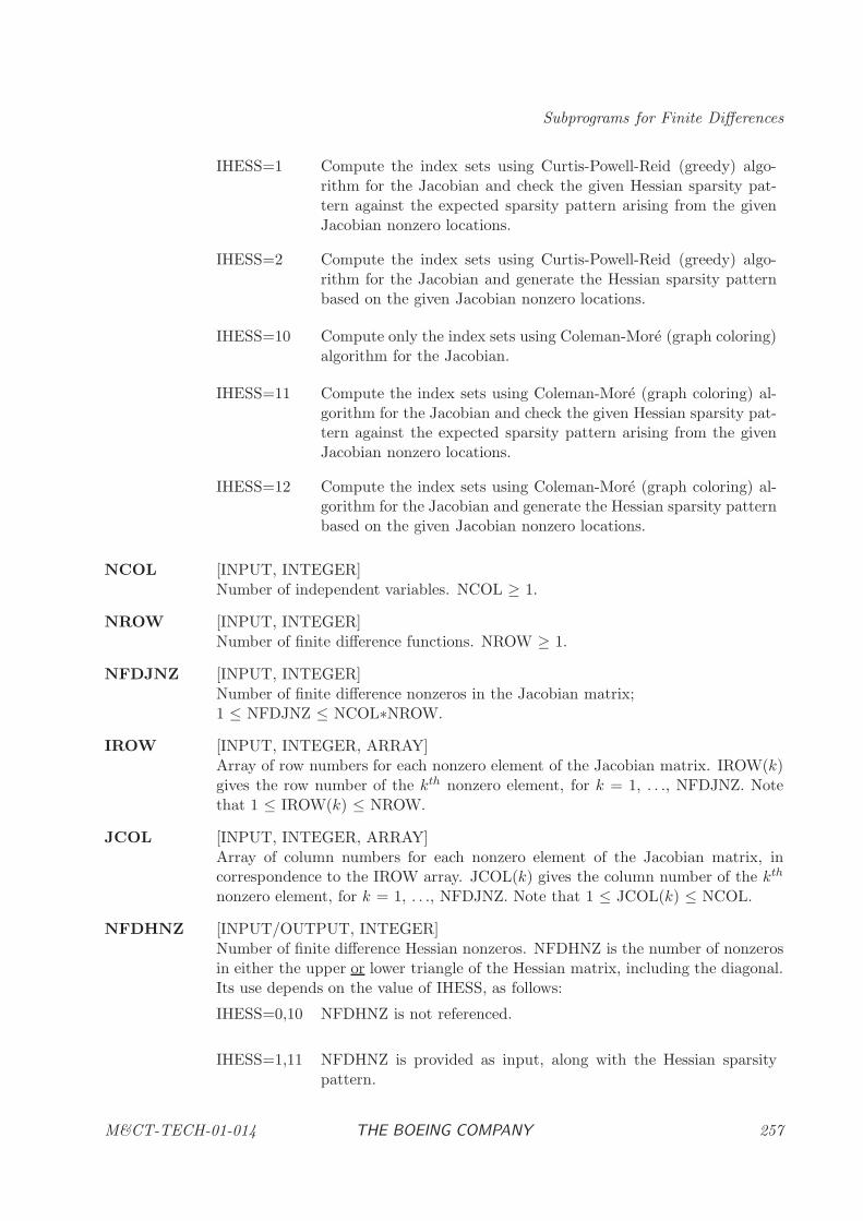
Subprograms for Finite Differences
IHESS=1 Compute the index sets using Curtis-Powell-Reid (greedy) algo-rithm for the Jacobian and check the given Hessian sparsity pat-tern against the expected sparsity pattern arising from the givenJacobian nonzero locations.
IHESS=2 Compute the index sets using Curtis-Powell-Reid (greedy) algo-rithm for the Jacobian and generate the Hessian sparsity patternbased on the given Jacobian nonzero locations.
IHESS=10 Compute only the index sets using Coleman-More (graph coloring)algorithm for the Jacobian.
IHESS=11 Compute the index sets using Coleman-More (graph coloring) al-gorithm for the Jacobian and check the given Hessian sparsity pat-tern against the expected sparsity pattern arising from the givenJacobian nonzero locations.
IHESS=12 Compute the index sets using Coleman-More (graph coloring) al-gorithm for the Jacobian and generate the Hessian sparsity patternbased on the given Jacobian nonzero locations.
NCOL [INPUT, INTEGER]Number of independent variables. NCOL ≥ 1.
NROW [INPUT, INTEGER]Number of finite difference functions. NROW ≥ 1.
NFDJNZ [INPUT, INTEGER]Number of finite difference nonzeros in the Jacobian matrix;1 ≤ NFDJNZ ≤ NCOL∗NROW.
IROW [INPUT, INTEGER, ARRAY]Array of row numbers for each nonzero element of the Jacobian matrix. IROW(k)gives the row number of the kth nonzero element, for k = 1, . . ., NFDJNZ. Notethat 1 ≤ IROW(k) ≤ NROW.
JCOL [INPUT, INTEGER, ARRAY]Array of column numbers for each nonzero element of the Jacobian matrix, incorrespondence to the IROW array. JCOL(k) gives the column number of the kth
nonzero element, for k = 1, . . ., NFDJNZ. Note that 1 ≤ JCOL(k) ≤ NCOL.
NFDHNZ [INPUT/OUTPUT, INTEGER]Number of finite difference Hessian nonzeros. NFDHNZ is the number of nonzerosin either the upper or lower triangle of the Hessian matrix, including the diagonal.Its use depends on the value of IHESS, as follows:
IHESS=0,10 NFDHNZ is not referenced.
IHESS=1,11 NFDHNZ is provided as input, along with the Hessian sparsitypattern.
M&CT-TECH-01-014 THE BOEING COMPANY 257
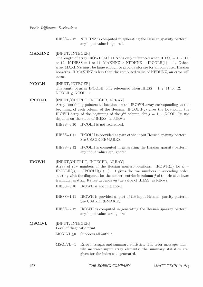
Finite Difference Derivatives
IHESS=2,12 NFDHNZ is computed in generating the Hessian sparsity pattern;any input value is ignored.
MAXHNZ [INPUT, INTEGER]The length of array IROWH; MAXHNZ is only referenced when IHESS = 1, 2, 11,or 12. If IHESS = 1 or 11, MAXHNZ ≥ NFDHNZ + IPCOLH(1) − 1. Other-wise, MAXHNZ must be large enough to provide storage for all computed Hessiannonzeros. If MAXHNZ is less than the computed value of NFDHNZ, an error willoccur.
NCOLH [INPUT, INTEGER]The length of array IPCOLH; only referenced when IHESS = 1, 2, 11, or 12.NCOLH ≥ NCOL+1.
IPCOLH [INPUT/OUTPUT, INTEGER, ARRAY]Array containing pointers to locations in the IROWH array corresponding to thebeginning of each column of the Hessian. IPCOLH(j) gives the location in theIROWH array of the beginning of the jth column, for j = 1,. . .,NCOL. Its usedepends on the value of IHESS, as follows:
IHESS=0,10 IPCOLH is not referenced.
IHESS=1,11 IPCOLH is provided as part of the input Hessian sparsity pattern.See USAGE REMARKS.
IHESS=2,12 IPCOLH is computed in generating the Hessian sparsity pattern;any input values are ignored.
IROWH [INPUT/OUTPUT, INTEGER, ARRAY]Array of row numbers of the Hessian nonzero locations. IROWH(k) for k =IPCOLH(j), . . . , IPCOLH(j + 1) − 1 gives the row numbers in ascending order,starting with the diagonal, for the nonzero entries in column j of the Hessian lowertriangular matrix. Its use depends on the value of IHESS, as follows:
IHESS=0,10 IROWH is not referenced.
IHESS=1,11 IROWH is provided as part of the input Hessian sparsity pattern.See USAGE REMARKS.
IHESS=2,12 IROWH is computed in generating the Hessian sparsity pattern;any input values are ignored.
MSGLVL [INPUT, INTEGER]Level of diagnostic print.
MSGLVL≤0 Suppress all output.
MSGLVL=1 Error messages and summary statistics. The error messages iden-tify incorrect input array elements; the summary statistics aregiven for the index sets generated.
258 THE BOEING COMPANY M&CT-TECH-01-014
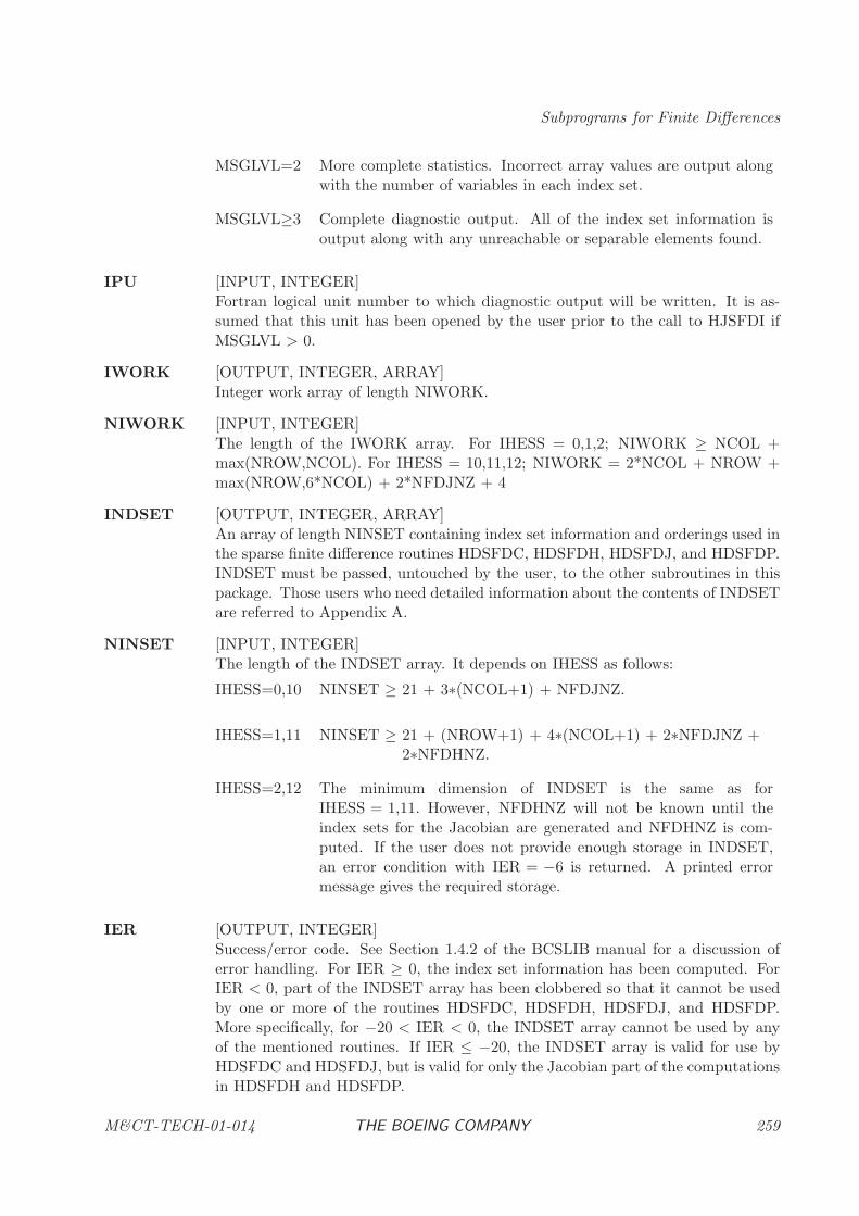
Subprograms for Finite Differences
MSGLVL=2 More complete statistics. Incorrect array values are output alongwith the number of variables in each index set.
MSGLVL≥3 Complete diagnostic output. All of the index set information isoutput along with any unreachable or separable elements found.
IPU [INPUT, INTEGER]Fortran logical unit number to which diagnostic output will be written. It is as-sumed that this unit has been opened by the user prior to the call to HJSFDI ifMSGLVL > 0.
IWORK [OUTPUT, INTEGER, ARRAY]Integer work array of length NIWORK.
NIWORK [INPUT, INTEGER]The length of the IWORK array. For IHESS = 0,1,2; NIWORK ≥ NCOL +max(NROW,NCOL). For IHESS = 10,11,12; NIWORK = 2*NCOL + NROW +max(NROW,6*NCOL) + 2*NFDJNZ + 4
INDSET [OUTPUT, INTEGER, ARRAY]An array of length NINSET containing index set information and orderings used inthe sparse finite difference routines HDSFDC, HDSFDH, HDSFDJ, and HDSFDP.INDSET must be passed, untouched by the user, to the other subroutines in thispackage. Those users who need detailed information about the contents of INDSETare referred to Appendix A.
NINSET [INPUT, INTEGER]The length of the INDSET array. It depends on IHESS as follows:
IHESS=0,10 NINSET ≥ 21 + 3∗(NCOL+1) + NFDJNZ.
IHESS=1,11 NINSET ≥ 21 + (NROW+1) + 4∗(NCOL+1) + 2∗NFDJNZ +2∗NFDHNZ.
IHESS=2,12 The minimum dimension of INDSET is the same as forIHESS = 1,11. However, NFDHNZ will not be known until theindex sets for the Jacobian are generated and NFDHNZ is com-puted. If the user does not provide enough storage in INDSET,an error condition with IER = −6 is returned. A printed errormessage gives the required storage.
IER [OUTPUT, INTEGER]Success/error code. See Section 1.4.2 of the BCSLIB manual for a discussion oferror handling. For IER ≥ 0, the index set information has been computed. ForIER < 0, part of the INDSET array has been clobbered so that it cannot be usedby one or more of the routines HDSFDC, HDSFDH, HDSFDJ, and HDSFDP.More specifically, for −20 < IER < 0, the INDSET array cannot be used by anyof the mentioned routines. If IER ≤ −20, the INDSET array is valid for use byHDSFDC and HDSFDJ, but is valid for only the Jacobian part of the computationsin HDSFDH and HDSFDP.
M&CT-TECH-01-014 THE BOEING COMPANY 259
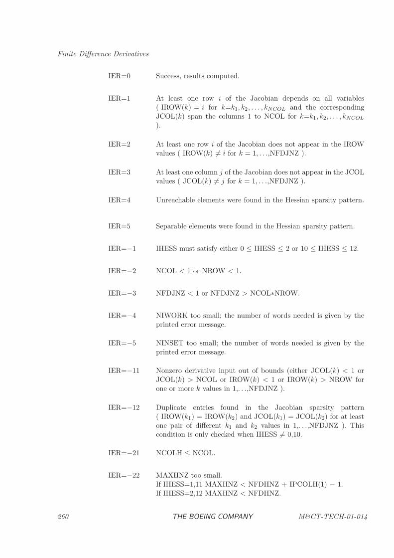
Finite Difference Derivatives
IER=0 Success, results computed.
IER=1 At least one row i of the Jacobian depends on all variables( IROW(k) = i for k=k1, k2, . . . , kNCOL and the correspondingJCOL(k) span the columns 1 to NCOL for k=k1, k2, . . . , kNCOL
).
IER=2 At least one row i of the Jacobian does not appear in the IROWvalues ( IROW(k) 6= i for k = 1, . . .,NFDJNZ ).
IER=3 At least one column j of the Jacobian does not appear in the JCOLvalues ( JCOL(k) 6= j for k = 1, . . .,NFDJNZ ).
IER=4 Unreachable elements were found in the Hessian sparsity pattern.
IER=5 Separable elements were found in the Hessian sparsity pattern.
IER=−1 IHESS must satisfy either 0 ≤ IHESS ≤ 2 or 10 ≤ IHESS ≤ 12.
IER=−2 NCOL < 1 or NROW < 1.
IER=−3 NFDJNZ < 1 or NFDJNZ > NCOL∗NROW.
IER=−4 NIWORK too small; the number of words needed is given by theprinted error message.
IER=−5 NINSET too small; the number of words needed is given by theprinted error message.
IER=−11 Nonzero derivative input out of bounds (either JCOL(k) < 1 orJCOL(k) > NCOL or IROW(k) < 1 or IROW(k) > NROW forone or more k values in 1,. . .,NFDJNZ ).
IER=−12 Duplicate entries found in the Jacobian sparsity pattern( IROW(k1) = IROW(k2) and JCOL(k1) = JCOL(k2) for at leastone pair of different k1 and k2 values in 1,. . .,NFDJNZ ). Thiscondition is only checked when IHESS 6= 0,10.
IER=−21 NCOLH ≤ NCOL.
IER=−22 MAXHNZ too small.If IHESS=1,11 MAXHNZ < NFDHNZ + IPCOLH(1) − 1.If IHESS=2,12 MAXHNZ < NFDHNZ.
260 THE BOEING COMPANY M&CT-TECH-01-014
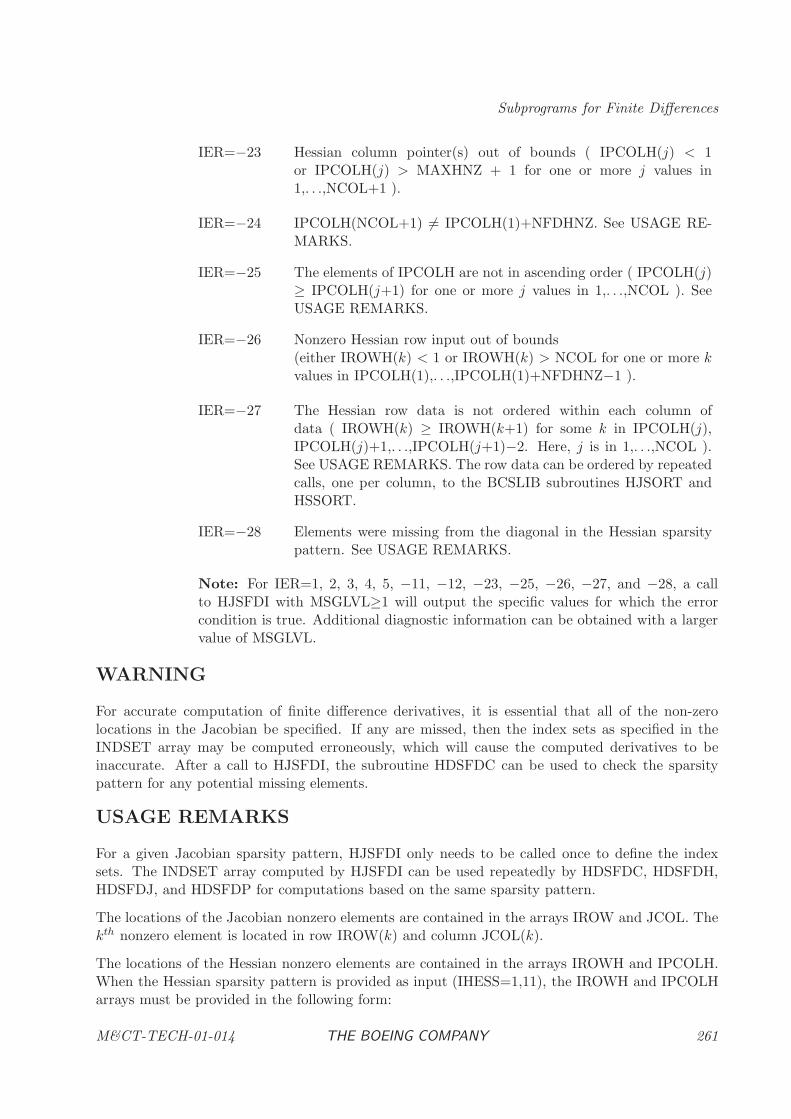
Subprograms for Finite Differences
IER=−23 Hessian column pointer(s) out of bounds ( IPCOLH(j) < 1or IPCOLH(j) > MAXHNZ + 1 for one or more j values in1,. . .,NCOL+1 ).
IER=−24 IPCOLH(NCOL+1) 6= IPCOLH(1)+NFDHNZ. See USAGE RE-MARKS.
IER=−25 The elements of IPCOLH are not in ascending order ( IPCOLH(j)≥ IPCOLH(j+1) for one or more j values in 1,. . .,NCOL ). SeeUSAGE REMARKS.
IER=−26 Nonzero Hessian row input out of bounds(either IROWH(k) < 1 or IROWH(k) > NCOL for one or more kvalues in IPCOLH(1),. . .,IPCOLH(1)+NFDHNZ−1 ).
IER=−27 The Hessian row data is not ordered within each column ofdata ( IROWH(k) ≥ IROWH(k+1) for some k in IPCOLH(j),IPCOLH(j)+1,. . .,IPCOLH(j+1)−2. Here, j is in 1,. . .,NCOL ).See USAGE REMARKS. The row data can be ordered by repeatedcalls, one per column, to the BCSLIB subroutines HJSORT andHSSORT.
IER=−28 Elements were missing from the diagonal in the Hessian sparsitypattern. See USAGE REMARKS.
Note: For IER=1, 2, 3, 4, 5, −11, −12, −23, −25, −26, −27, and −28, a callto HJSFDI with MSGLVL≥1 will output the specific values for which the errorcondition is true. Additional diagnostic information can be obtained with a largervalue of MSGLVL.
WARNING
For accurate computation of finite difference derivatives, it is essential that all of the non-zerolocations in the Jacobian be specified. If any are missed, then the index sets as specified in theINDSET array may be computed erroneously, which will cause the computed derivatives to beinaccurate. After a call to HJSFDI, the subroutine HDSFDC can be used to check the sparsitypattern for any potential missing elements.
USAGE REMARKS
For a given Jacobian sparsity pattern, HJSFDI only needs to be called once to define the indexsets. The INDSET array computed by HJSFDI can be used repeatedly by HDSFDC, HDSFDH,HDSFDJ, and HDSFDP for computations based on the same sparsity pattern.
The locations of the Jacobian nonzero elements are contained in the arrays IROW and JCOL. Thekth nonzero element is located in row IROW(k) and column JCOL(k).
The locations of the Hessian nonzero elements are contained in the arrays IROWH and IPCOLH.When the Hessian sparsity pattern is provided as input (IHESS=1,11), the IROWH and IPCOLHarrays must be provided in the following form:
M&CT-TECH-01-014 THE BOEING COMPANY 261
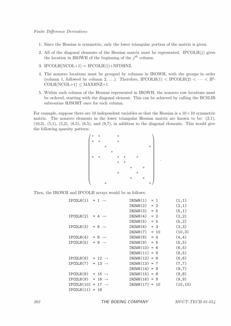
Finite Difference Derivatives
1. Since the Hessian is symmetric, only the lower triangular portion of the matrix is given.
2. All of the diagonal elements of the Hessian matrix must be represented. IPCOLH(j) givesthe location in IROWH of the beginning of the jth column.
3. IPCOLH(NCOL+1) = IPCOLH(1)+NFDHNZ.
4. The nonzero locations must be grouped by columns in IROWH, with the groups in order(column 1, followed by column 2, . . .). Therefore, IPCOLH(1) < IPCOLH(2) < · · · < IP-COLH(NCOL+1) ≤ MAXHNZ+1.
5. Within each column of the Hessian represented in IROWH, the nonzero row locations mustbe ordered, starting with the diagonal element. This can be achieved by calling the BCSLIBsubroutine HJSORT once for each column.
For example, suppose there are 10 independent variables so that the Hessian is a 10×10 symmetricmatrix. The nonzero elements in the lower triangular Hessian matrix are known to be: (2,1),(10,3), (5,1), (5,2), (8,5), (6,5), and (9,7), in addition to the diagonal elements. This would givethe following sparsity pattern:
∗ ∗ ∗∗ ∗ ∗
∗ ∗∗
∗ ∗ ∗ ∗ ∗∗ ∗
∗ ∗∗ ∗
∗ ∗∗ ∗
.
Then, the IROWH and IPCOLH arrays would be as follows:
IPCOLH(1) = 1 → IROWH(1) = 1 (1,1)
IROWH(2) = 2 (2,1)
IROWH(3) = 5 (5,1)
IPCOLH(2) = 4 → IROWH(4) = 2 (2,2)
IROWH(5) = 5 (5,2)
IPCOLH(3) = 6 → IROWH(6) = 3 (3,3)
IROWH(7) = 10 (10,3)
IPCOLH(4) = 8 → IROWH(8) = 4 (4,4)
IPCOLH(5) = 9 → IROWH(9) = 5 (5,5)
IROWH(10) = 6 (6,5)
IROWH(11) = 8 (8,5)
IPCOLH(6) = 12 → IROWH(12) = 6 (6,6)
IPCOLH(7) = 13 → IROWH(13) = 7 (7,7)
IROWH(14) = 9 (9,7)
IPCOLH(8) = 15 → IROWH(15) = 8 (8,8)
IPCOLH(9) = 16 → IROWH(16) = 9 (9,9)
IPCOLH(10) = 17 → IROWH(17) = 10 (10,10)
IPCOLH(11) = 18
262 THE BOEING COMPANY M&CT-TECH-01-014
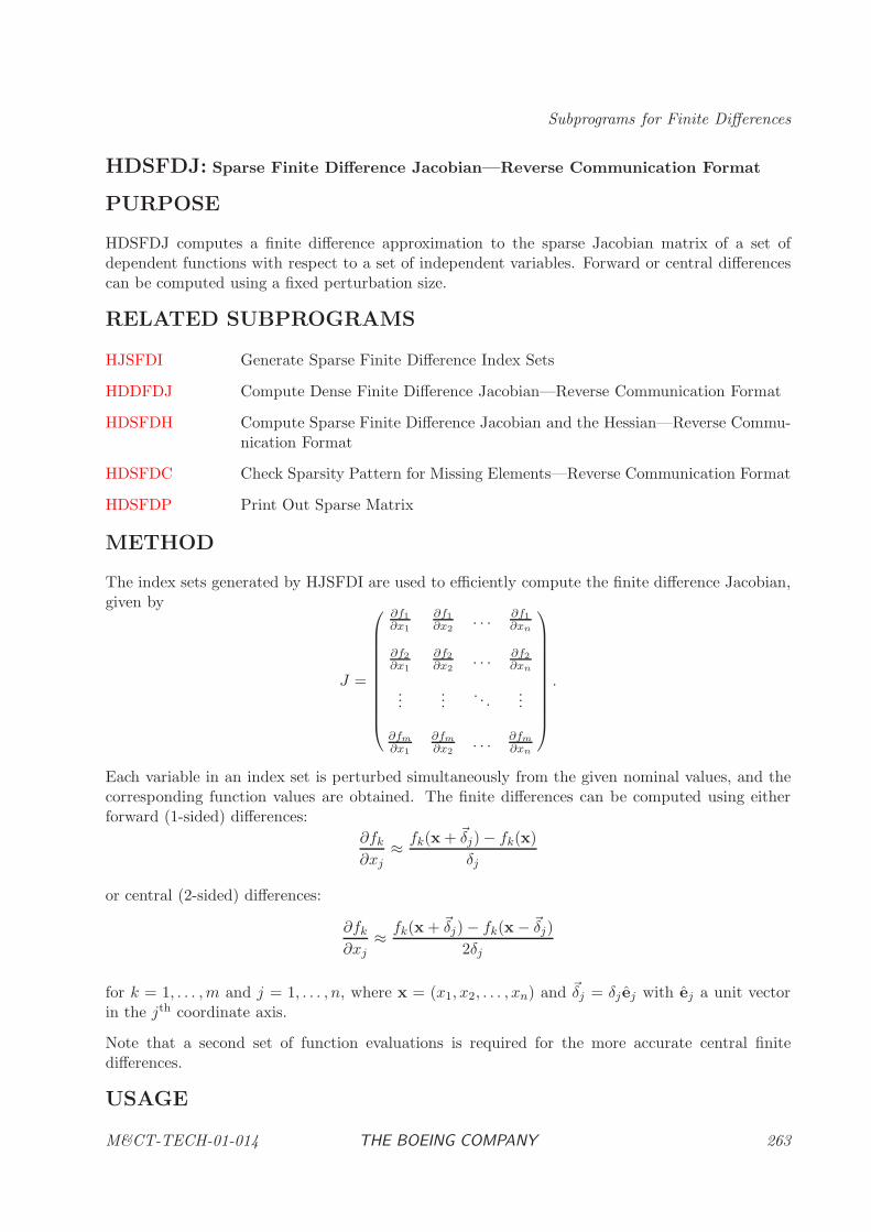
Subprograms for Finite Differences
HDSFDJ: Sparse Finite Difference Jacobian—Reverse Communication Format
PURPOSE
HDSFDJ computes a finite difference approximation to the sparse Jacobian matrix of a set ofdependent functions with respect to a set of independent variables. Forward or central differencescan be computed using a fixed perturbation size.
RELATED SUBPROGRAMS
HJSFDI Generate Sparse Finite Difference Index Sets
HDDFDJ Compute Dense Finite Difference Jacobian—Reverse Communication Format
HDSFDH Compute Sparse Finite Difference Jacobian and the Hessian—Reverse Commu-nication Format
HDSFDC Check Sparsity Pattern for Missing Elements—Reverse Communication Format
HDSFDP Print Out Sparse Matrix
METHOD
The index sets generated by HJSFDI are used to efficiently compute the finite difference Jacobian,given by
J =
∂f1
∂x1
∂f1
∂x2. . . ∂f1
∂xn
∂f2
∂x1
∂f2
∂x2. . . ∂f2
∂xn
......
. . ....
∂fm
∂x1
∂fm
∂x2. . . ∂fm
∂xn
.
Each variable in an index set is perturbed simultaneously from the given nominal values, and thecorresponding function values are obtained. The finite differences can be computed using eitherforward (1-sided) differences:
∂fk
∂xj≈ fk(x + ~δj) − fk(x)
δj
or central (2-sided) differences:
∂fk
∂xj≈ fk(x + ~δj) − fk(x − ~δj)
2δj
for k = 1, . . . ,m and j = 1, . . . , n, where x = (x1, x2, . . . , xn) and ~δj = δj ej with ej a unit vectorin the jth coordinate axis.
Note that a second set of function evaluations is required for the more accurate central finitedifferences.
USAGE
M&CT-TECH-01-014 THE BOEING COMPANY 263
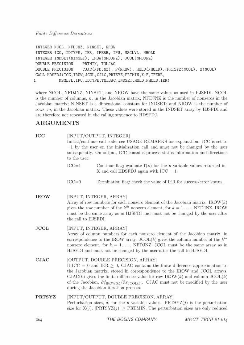
Finite Difference Derivatives
INTEGER NCOL, NFDJNZ, NINSET, NROW
INTEGER ICC, IDTYPE, IER, IFERR, IPU, MSGLVL, NHOLD
INTEGER INDSET(NINSET), IROW(NFDJNZ), JCOL(NFDJNZ)
DOUBLE PRECISION PRTMIN, TOLJAC
DOUBLE PRECISION CJAC(NFDJNZ), F(NROW), HOLD(NHOLD), PRTSYZ(NCOL), X(NCOL)
CALL HDSFDJ(ICC,IROW,JCOL,CJAC,PRTSYZ,PRTMIN,X,F,IFERR,
1 MSGLVL,IPU,IDTYPE,TOLJAC,INDSET,HOLD,NHOLD,IER)
where NCOL, NFDJNZ, NINSET, and NROW have the same values as used in HJSFDI. NCOLis the number of columns, n, in the Jacobian matrix; NFDJNZ is the number of nonzeros in theJacobian matrix; NINSET is a dimensional constant for INDSET; and NROW is the number ofrows, m, in the Jacobian matrix. These values were stored in the INDSET array by HJSFDI andare therefore not repeated in the calling sequence to HDSFDJ.
ARGUMENTS
ICC [INPUT/OUTPUT, INTEGER]Initial/continue call code; see USAGE REMARKS for explanation. ICC is set to−1 by the user on the initialization call and must not be changed by the usersubsequently. On output, ICC contains process status information and directionsto the user:
ICC=1 Continue flag; evaluate f(x) for the x variable values returned inX and call HDSFDJ again with ICC = 1.
ICC=0 Termination flag; check the value of IER for success/error status.
IROW [INPUT, INTEGER, ARRAY]Array of row numbers for each nonzero element of the Jacobian matrix. IROW(k)gives the row number of the kth nonzero element, for k = 1, . . ., NFDJNZ. IROWmust be the same array as in HJSFDI and must not be changed by the user afterthe call to HJSFDI.
JCOL [INPUT, INTEGER, ARRAY]Array of column numbers for each nonzero element of the Jacobian matrix, incorrespondence to the IROW array. JCOL(k) gives the column number of the kth
nonzero element, for k = 1, . . ., NFDJNZ. JCOL must be the same array as inHJSFDI and must not be changed by the user after the call to HJSFDI.
CJAC [OUTPUT, DOUBLE PRECISION, ARRAY]If ICC = 0 and IER ≥ 0, CJAC contains the finite difference approximation tothe Jacobian matrix, stored in correspondence to the IROW and JCOL arrays.CJAC(k) gives the finite difference value for row IROW(k) and column JCOL(k)of the Jacobian, ∂fIROW(k)/∂xJCOL(k). CJAC must not be modified by the userduring the Jacobian iteration process.
PRTSYZ [INPUT/OUTPUT, DOUBLE PRECISION, ARRAY]Perturbation sizes, ~δ, for the x variable values. PRTSYZ(j) is the perturbationsize for X(j); |PRTSYZ(j)| ≥ PRTMIN. The perturbation sizes are only reduced
264 THE BOEING COMPANY M&CT-TECH-01-014
Subprograms for Finite Differences
when a function error, signalled by IFERR 6= 0, prevents a successful finite dif-ference computation. Furthermore, a reduction in perturbation sizes is done onlyfor variables in the current index set. PRTSYZ must be specified by the user onthe initialization call and not subsequently changed by the user. A recommendedinitial value for PRTSYZ(j) is 10−5 max [1, x(j)].
PRTMIN [INPUT, DOUBLE PRECISION]Minimum absolute perturbation size for any variable xj ;10∗HDMCON(5) ≤ PRTMIN ≤ min1≤j≤NCOL|PRTSYZ(j)|. HDSFDJ will not re-duce any |PRTSYZ(j)| below PRTMIN during the Jacobian computations. PRT-MIN must be specified by the user on the initialization call and not subsequentlychanged. A recommended initial value for PRTMIN is
√HDMCON(5). Setting
PRTMIN less than this value will result in a warning message.
X [INPUT/OUTPUT, DOUBLE PRECISION, ARRAY]Independent variable values x. The current use of X depends on the value of ICC:
ICC=−1 X must be initialized to the nominal point, that is, the x value forwhich the Jacobian is to be computed.
ICC=1 X contains a perturbed point at which a function evaluation isrequired.
ICC=0 X contains the nominal point, restored by HDSFDJ.
X must be specified by the user on the initialization call and not subsequentlychanged by the user. See USAGE REMARKS.
F [INPUT/OUTPUT, DOUBLE PRECISION, ARRAY]Dependent function values f(x). The current use of F depends on the value of ICC(see USAGE REMARKS):
|ICC|=1 F must be set by the user to the values of the function at thecurrent value of X.
ICC=0 F contains the values of the function at the nominal point, restoredby HDSFDJ.
IFERR [INPUT, INTEGER]Function error flag. This variable is used to communicate a function error thatoccurred when the user evaluated f(x).
IFERR=0 The evaluation of f(x) was successful.
IFERR 6=0 An error occurred in evaluating f(x).
IFERR must be 0 on the initialization call. This implies that the function must bevalid at the nominal point. See USAGE REMARKS.
MSGLVL [INPUT, INTEGER]Level of diagnostic print.
M&CT-TECH-01-014 THE BOEING COMPANY 265
Finite Difference Derivatives
MSGLVL≤0 Suppress all output.
MSGLVL=1 Print error messages and some diagnostic information about re-duced perturbation sizes.
MSGLVL≥2 Print complete diagnostic output, including additional perturba-tion information and the norm of the Jacobian.Note: Matrix norms are computed for output purposes only andresult in some extra computation.
IPU [INPUT, INTEGER]Fortran logical unit number to which diagnostic output will be written. It is as-sumed that this unit has been opened by the user prior to the call to HDSFDJ ifMSGLVL > 0.
IDTYPE [INPUT, INTEGER]Derivative type; IDTYPE = 1 or 2. IDTYPE is only referenced on the initializationcall.
IDTYPE=1 Use forward finite differences.IDTYPE=2 Use central finite differences; this results in more accurate finite
differences.
TOLJAC [INPUT, DOUBLE PRECISION]Tolerance for row and column norms; TOLJAC ≥ 0. If MSGLVL ≥ 2, any rowsfor which max1≤j≤n|∂fk
∂xj| ≤ TOLJAC and any columns for which max1≤k≤m|∂fk
∂xj| ≤
TOLJAC will be identified in the output file. If MSGLVL < 2, TOLJAC is notused by HDSFDJ.
INDSET [INPUT/OUTPUT, INTEGER, ARRAY]An array containing the index set information generated by HJSFDI. This arraymust not be changed by the user between the call to HJSFDI and the initial callto HDSFDJ and also must not be changed by the user between successive calls toHDSFDJ.
HOLD [INPUT/OUTPUT, DOUBLE PRECISION, ARRAY]Hold array of length NHOLD. This array must not be changed by the user betweensuccessive calls to HDSFDJ when the Jacobian is being computed. After the Ja-cobian computation is complete (ICC = 0), this array can be used elsewhere as awork array.
NHOLD [INPUT, INTEGER]The length of the HOLD array. NHOLD ≥ (2∗NROW+NCOL), where NROWand NCOL are the same values used in HJSFDI.
IER [OUTPUT, INTEGER]Success/error code. See Section 1.4.2 of the BCSLIB manual for a discussion oferror handling. For IER < 0, ICC has been set to 0, and at least part of theCJAC array has been clobbered with HDMCON(1). See the BCSLIB manual forHDMCON.
266 THE BOEING COMPANY M&CT-TECH-01-014
Subprograms for Finite Differences
IER=0 Success, results computed.
IER=1 PRTMIN <√
HDMCON(5).
IER=2 MSGLVL ≥ 2 and TOLJAC< 0. No matrix norms were computed.
IER=3 MSGLVL ≥ 2 and at least one row or column norm is ≤ TOLJAC.
IER=−1 Invalid initial/continue call code; ICC 6= −1 or 1.
IER=−2 Invalid INDSET array—the INDSET array must not be changedbetween the call to HJSFDI and the initial call to HDSFDJ andalso must not be changed between successive calls to HDSFDJ.
IER=−3 IDTYPE ≤ 0 or IDTYPE > 2.
IER=−4 NHOLD too small; the number of words needed is given by theprinted error message.
IER=−5 For ICC = −1, IFERR 6= 0. There must not be a function errorat the nominal point.
IER=−6 The minimum perturbation size is too small;PRTMIN < 10∗HDMCON(5).
IER=−7 min1≤j≤NCOL|PRTSYZ(j)| < PRTMIN.
IER=−10 Incorrect use of ICC code; need to make initial call to HDSFDJwith ICC = −1. See USAGE REMARKS.
IER=−11 Smallest allowable perturbation caused a function error.
USAGE REMARKS
HDSFDJ uses reverse communication to compute the finite difference Jacobian. A user callsHDSFDJ repeatedly to formulate the finite difference values, where each call to HDSFDJ performscomputations based on a particular index set. Before the initial call to HDSFDJ, the nominalvariable values must be stored in X, and the corresponding nominal function values must be storedin F. The function error flag IFERR must equal 0 at the nominal X variable values. Also, theperturbation sizes to be used in perturbing the variable values must be stored in PRTSYZ. Theuser can then make an initial call to HDSFDJ with ICC = −1.
After each return from HDSFDJ, the user should examine the value of ICC to determine the courseof action.
M&CT-TECH-01-014 THE BOEING COMPANY 267
Finite Difference Derivatives
If ICC = 1, the user’s program should evaluate the function using the x variable values returnedin X, that is, set F = f(x). It then must call HDSFDJ again to continue the finite differencecomputations.
If ICC = 0 and IER = 0, HDSFDJ has successfully computed the finite difference Jacobian andloaded it in CJAC.
If ICC = 0 and IER < 0, HDSFDJ has detected a usage error.
Additionally, note the following:
1. The IROW and JCOL arrays must be the same arrays as used in HJSFDI.
2. The variables ICC, IROW, JCOL, CJAC, PRTSYZ, PRTMIN, X, INDSET, and HOLD mustnot be changed by the user between successive calls to HDSFDJ (when ICC = 1).
3. The variable IFERR can be used to communicate a function error that occurred when theuser evaluated f(x). In this case, HDSFDJ will reduce the perturbation sizes, where possible,and request another function evaluation at new X variable values.
EXAMPLE
The sparse finite difference software described can be used to compute the Jacobian matrix Jk fora given x(k). As an example, suppose f(x) is given by:
f1 = x21 + 4x2
f2 = 2x1x3 + 1f3 = x4 + x5
f4 = 2x2
+ x4
f5 = x21 − x2
5
where
f =
f1
f2
f3
f4
f5
and x =
x1
x2
x3
x4
x5
.
In order to use HDSFDJ to compute the Jacobian matrix, the sparsity pattern of the Jacobian,i.e., its nonzero locations, must be identified. From the definition of f(x) in (3.2), the location ofnonzero partial derivatives in the Jacobian results in the following sparsity pattern:
∗ ∗∗ ∗
∗ ∗∗ ∗
∗ ∗
.
The example program given below illustrates how the Jacobian matrix J would be computed asone step of solving f(x) = 0 for x, with f as defined in (3.2). The Jacobian is computed for threedifferent values of x, the third of which happens to be a solution to f(x) = 0.
268 THE BOEING COMPANY M&CT-TECH-01-014
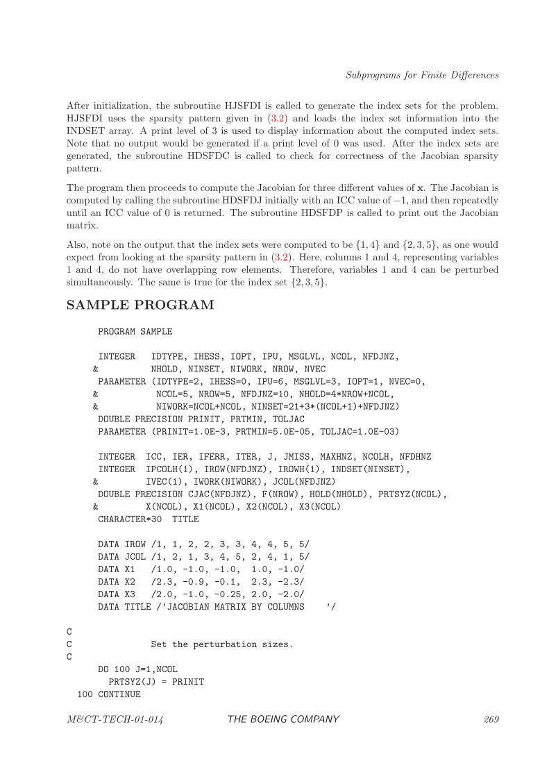
Subprograms for Finite Differences
After initialization, the subroutine HJSFDI is called to generate the index sets for the problem.HJSFDI uses the sparsity pattern given in (3.2) and loads the index set information into theINDSET array. A print level of 3 is used to display information about the computed index sets.Note that no output would be generated if a print level of 0 was used. After the index sets aregenerated, the subroutine HDSFDC is called to check for correctness of the Jacobian sparsitypattern.
The program then proceeds to compute the Jacobian for three different values of x. The Jacobian iscomputed by calling the subroutine HDSFDJ initially with an ICC value of −1, and then repeatedlyuntil an ICC value of 0 is returned. The subroutine HDSFDP is called to print out the Jacobianmatrix.
Also, note on the output that the index sets were computed to be {1, 4} and {2, 3, 5}, as one wouldexpect from looking at the sparsity pattern in (3.2). Here, columns 1 and 4, representing variables1 and 4, do not have overlapping row elements. Therefore, variables 1 and 4 can be perturbedsimultaneously. The same is true for the index set {2, 3, 5}.
SAMPLE PROGRAM
PROGRAM SAMPLE
INTEGER IDTYPE, IHESS, IOPT, IPU, MSGLVL, NCOL, NFDJNZ,
& NHOLD, NINSET, NIWORK, NROW, NVEC
PARAMETER (IDTYPE=2, IHESS=0, IPU=6, MSGLVL=3, IOPT=1, NVEC=0,
& NCOL=5, NROW=5, NFDJNZ=10, NHOLD=4*NROW+NCOL,
& NIWORK=NCOL+NCOL, NINSET=21+3*(NCOL+1)+NFDJNZ)
DOUBLE PRECISION PRINIT, PRTMIN, TOLJAC
PARAMETER (PRINIT=1.0E-3, PRTMIN=5.0E-05, TOLJAC=1.0E-03)
INTEGER ICC, IER, IFERR, ITER, J, JMISS, MAXHNZ, NCOLH, NFDHNZ
INTEGER IPCOLH(1), IROW(NFDJNZ), IROWH(1), INDSET(NINSET),
& IVEC(1), IWORK(NIWORK), JCOL(NFDJNZ)
DOUBLE PRECISION CJAC(NFDJNZ), F(NROW), HOLD(NHOLD), PRTSYZ(NCOL),
& X(NCOL), X1(NCOL), X2(NCOL), X3(NCOL)
CHARACTER*30 TITLE
DATA IROW /1, 1, 2, 2, 3, 3, 4, 4, 5, 5/
DATA JCOL /1, 2, 1, 3, 4, 5, 2, 4, 1, 5/
DATA X1 /1.0, -1.0, -1.0, 1.0, -1.0/
DATA X2 /2.3, -0.9, -0.1, 2.3, -2.3/
DATA X3 /2.0, -1.0, -0.25, 2.0, -2.0/
DATA TITLE /’JACOBIAN MATRIX BY COLUMNS ’/
C
C Set the perturbation sizes.
C
DO 100 J=1,NCOL
PRTSYZ(J) = PRINIT
100 CONTINUE
M&CT-TECH-01-014 THE BOEING COMPANY 269
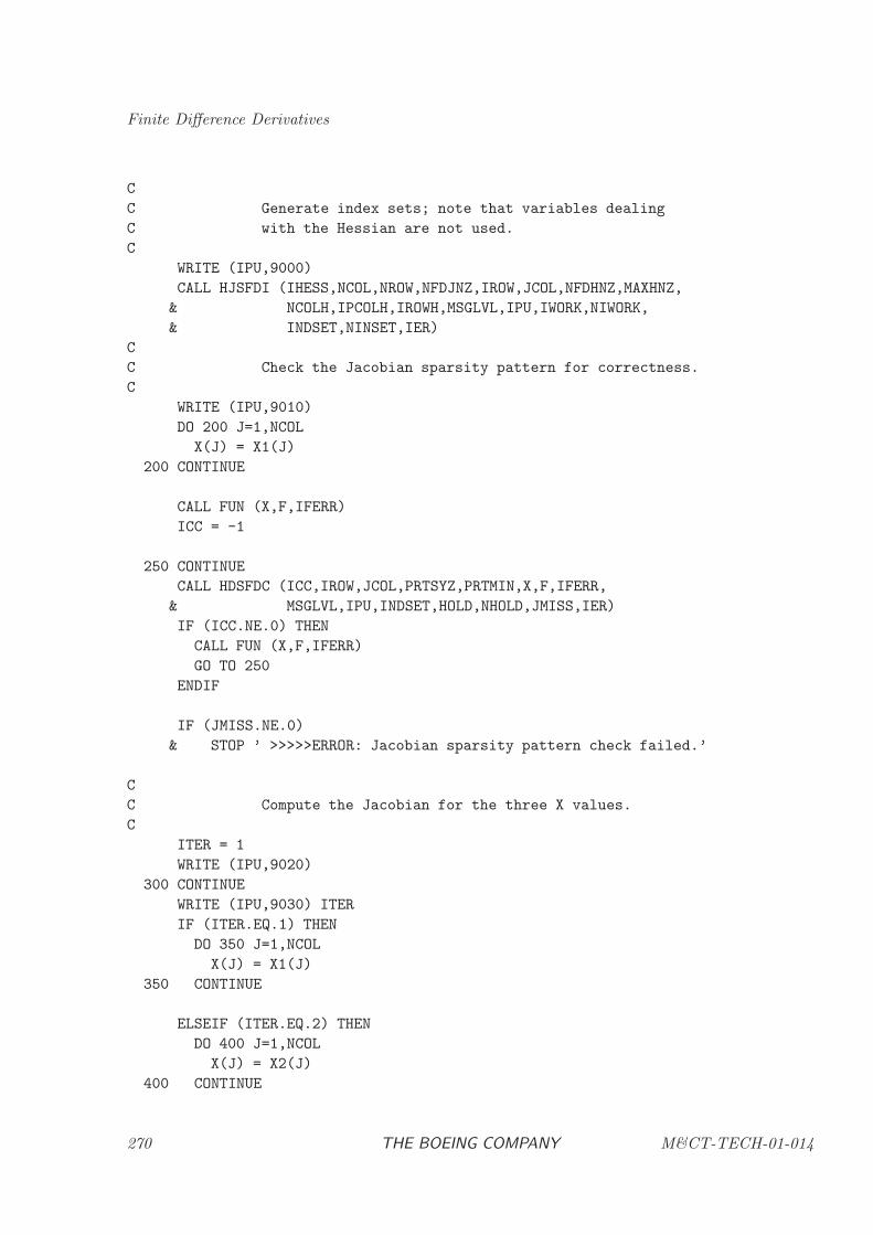
Finite Difference Derivatives
C
C Generate index sets; note that variables dealing
C with the Hessian are not used.
C
WRITE (IPU,9000)
CALL HJSFDI (IHESS,NCOL,NROW,NFDJNZ,IROW,JCOL,NFDHNZ,MAXHNZ,
& NCOLH,IPCOLH,IROWH,MSGLVL,IPU,IWORK,NIWORK,
& INDSET,NINSET,IER)
C
C Check the Jacobian sparsity pattern for correctness.
C
WRITE (IPU,9010)
DO 200 J=1,NCOL
X(J) = X1(J)
200 CONTINUE
CALL FUN (X,F,IFERR)
ICC = -1
250 CONTINUE
CALL HDSFDC (ICC,IROW,JCOL,PRTSYZ,PRTMIN,X,F,IFERR,
& MSGLVL,IPU,INDSET,HOLD,NHOLD,JMISS,IER)
IF (ICC.NE.0) THEN
CALL FUN (X,F,IFERR)
GO TO 250
ENDIF
IF (JMISS.NE.0)
& STOP ’ >>>>>ERROR: Jacobian sparsity pattern check failed.’
C
C Compute the Jacobian for the three X values.
C
ITER = 1
WRITE (IPU,9020)
300 CONTINUE
WRITE (IPU,9030) ITER
IF (ITER.EQ.1) THEN
DO 350 J=1,NCOL
X(J) = X1(J)
350 CONTINUE
ELSEIF (ITER.EQ.2) THEN
DO 400 J=1,NCOL
X(J) = X2(J)
400 CONTINUE
270 THE BOEING COMPANY M&CT-TECH-01-014
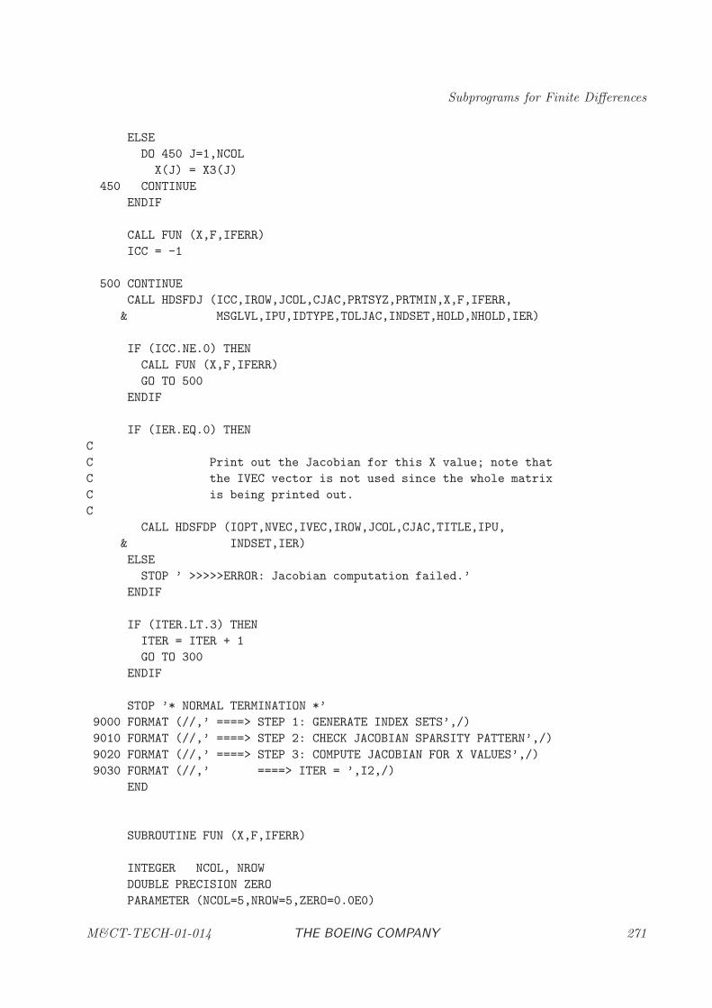
Subprograms for Finite Differences
ELSE
DO 450 J=1,NCOL
X(J) = X3(J)
450 CONTINUE
ENDIF
CALL FUN (X,F,IFERR)
ICC = -1
500 CONTINUE
CALL HDSFDJ (ICC,IROW,JCOL,CJAC,PRTSYZ,PRTMIN,X,F,IFERR,
& MSGLVL,IPU,IDTYPE,TOLJAC,INDSET,HOLD,NHOLD,IER)
IF (ICC.NE.0) THEN
CALL FUN (X,F,IFERR)
GO TO 500
ENDIF
IF (IER.EQ.0) THEN
C
C Print out the Jacobian for this X value; note that
C the IVEC vector is not used since the whole matrix
C is being printed out.
C
CALL HDSFDP (IOPT,NVEC,IVEC,IROW,JCOL,CJAC,TITLE,IPU,
& INDSET,IER)
ELSE
STOP ’ >>>>>ERROR: Jacobian computation failed.’
ENDIF
IF (ITER.LT.3) THEN
ITER = ITER + 1
GO TO 300
ENDIF
STOP ’* NORMAL TERMINATION *’
9000 FORMAT (//,’ ====> STEP 1: GENERATE INDEX SETS’,/)
9010 FORMAT (//,’ ====> STEP 2: CHECK JACOBIAN SPARSITY PATTERN’,/)
9020 FORMAT (//,’ ====> STEP 3: COMPUTE JACOBIAN FOR X VALUES’,/)
9030 FORMAT (//,’ ====> ITER = ’,I2,/)
END
SUBROUTINE FUN (X,F,IFERR)
INTEGER NCOL, NROW
DOUBLE PRECISION ZERO
PARAMETER (NCOL=5,NROW=5,ZERO=0.0E0)
M&CT-TECH-01-014 THE BOEING COMPANY 271
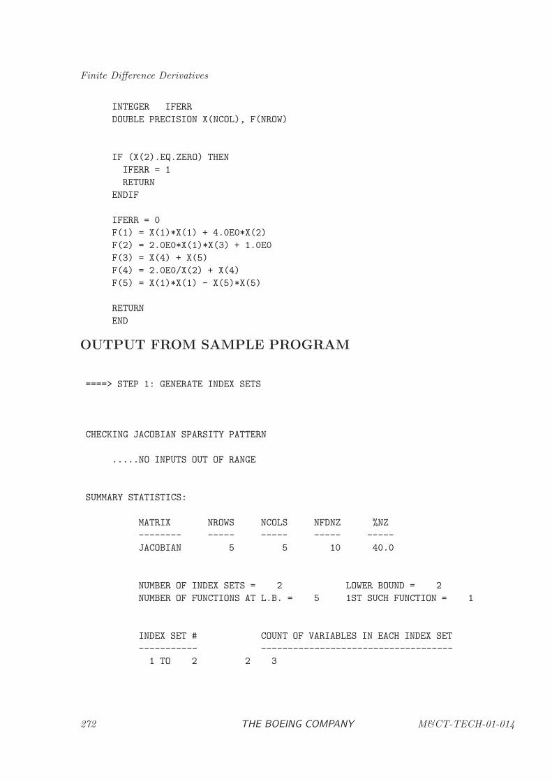
Finite Difference Derivatives
INTEGER IFERR
DOUBLE PRECISION X(NCOL), F(NROW)
IF (X(2).EQ.ZERO) THEN
IFERR = 1
RETURN
ENDIF
IFERR = 0
F(1) = X(1)*X(1) + 4.0E0*X(2)
F(2) = 2.0E0*X(1)*X(3) + 1.0E0
F(3) = X(4) + X(5)
F(4) = 2.0E0/X(2) + X(4)
F(5) = X(1)*X(1) - X(5)*X(5)
RETURN
END
OUTPUT FROM SAMPLE PROGRAM
====> STEP 1: GENERATE INDEX SETS
CHECKING JACOBIAN SPARSITY PATTERN
.....NO INPUTS OUT OF RANGE
SUMMARY STATISTICS:
MATRIX NROWS NCOLS NFDNZ %NZ
-------- ----- ----- ----- -----
JACOBIAN 5 5 10 40.0
NUMBER OF INDEX SETS = 2 LOWER BOUND = 2
NUMBER OF FUNCTIONS AT L.B. = 5 1ST SUCH FUNCTION = 1
INDEX SET # COUNT OF VARIABLES IN EACH INDEX SET
----------- ------------------------------------
1 TO 2 2 3
272 THE BOEING COMPANY M&CT-TECH-01-014
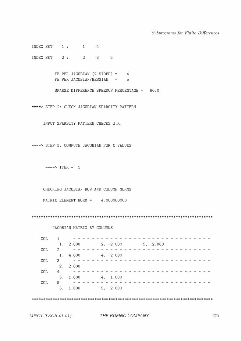
Subprograms for Finite Differences
INDEX SET 1 : 1 4
INDEX SET 2 : 2 3 5
FE PER JACOBIAN (2-SIDED) = 4
FE PER JACOBIAN/HESSIAN = 5
SPARSE DIFFERENCE SPEEDUP PERCENTAGE = 60.0
====> STEP 2: CHECK JACOBIAN SPARSITY PATTERN
INPUT SPARSITY PATTERN CHECKS O.K.
====> STEP 3: COMPUTE JACOBIAN FOR X VALUES
====> ITER = 1
CHECKING JACOBIAN ROW AND COLUMN NORMS
MATRIX ELEMENT NORM = 4.000000000
******************************************************************************
JACOBIAN MATRIX BY COLUMNS
COL 1 - - - - - - - - - - - - - - - - - - - - - - - - - - - - - -
1, 2.000 2, -2.000 5, 2.000
COL 2 - - - - - - - - - - - - - - - - - - - - - - - - - - - - - -
1, 4.000 4, -2.000
COL 3 - - - - - - - - - - - - - - - - - - - - - - - - - - - - - -
2, 2.000
COL 4 - - - - - - - - - - - - - - - - - - - - - - - - - - - - - -
3, 1.000 4, 1.000
COL 5 - - - - - - - - - - - - - - - - - - - - - - - - - - - - - -
3, 1.000 5, 2.000
******************************************************************************
M&CT-TECH-01-014 THE BOEING COMPANY 273
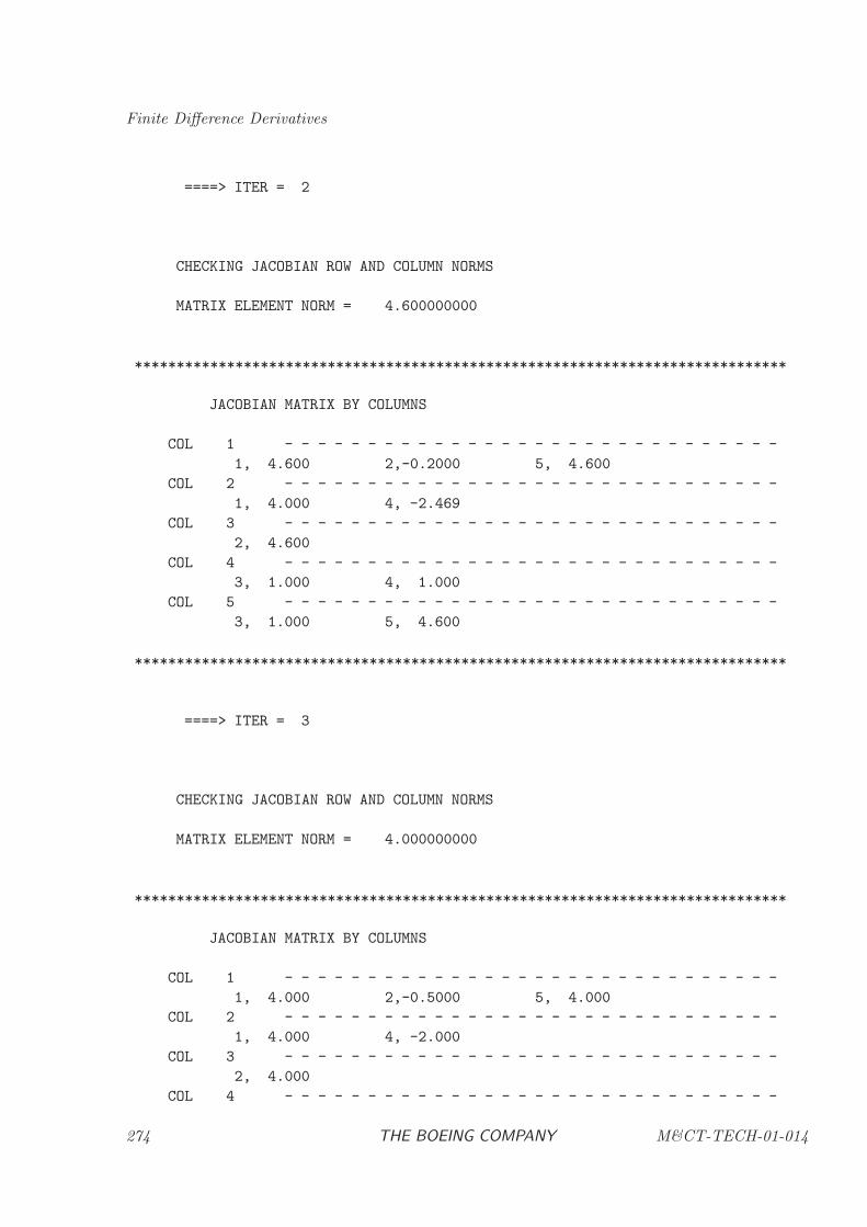
Finite Difference Derivatives
====> ITER = 2
CHECKING JACOBIAN ROW AND COLUMN NORMS
MATRIX ELEMENT NORM = 4.600000000
******************************************************************************
JACOBIAN MATRIX BY COLUMNS
COL 1 - - - - - - - - - - - - - - - - - - - - - - - - - - - - - -
1, 4.600 2,-0.2000 5, 4.600
COL 2 - - - - - - - - - - - - - - - - - - - - - - - - - - - - - -
1, 4.000 4, -2.469
COL 3 - - - - - - - - - - - - - - - - - - - - - - - - - - - - - -
2, 4.600
COL 4 - - - - - - - - - - - - - - - - - - - - - - - - - - - - - -
3, 1.000 4, 1.000
COL 5 - - - - - - - - - - - - - - - - - - - - - - - - - - - - - -
3, 1.000 5, 4.600
******************************************************************************
====> ITER = 3
CHECKING JACOBIAN ROW AND COLUMN NORMS
MATRIX ELEMENT NORM = 4.000000000
******************************************************************************
JACOBIAN MATRIX BY COLUMNS
COL 1 - - - - - - - - - - - - - - - - - - - - - - - - - - - - - -
1, 4.000 2,-0.5000 5, 4.000
COL 2 - - - - - - - - - - - - - - - - - - - - - - - - - - - - - -
1, 4.000 4, -2.000
COL 3 - - - - - - - - - - - - - - - - - - - - - - - - - - - - - -
2, 4.000
COL 4 - - - - - - - - - - - - - - - - - - - - - - - - - - - - - -
274 THE BOEING COMPANY M&CT-TECH-01-014

Subprograms for Finite Differences
3, 1.000 4, 1.000
COL 5 - - - - - - - - - - - - - - - - - - - - - - - - - - - - - -
3, 1.000 5, 4.000
******************************************************************************
M&CT-TECH-01-014 THE BOEING COMPANY 275
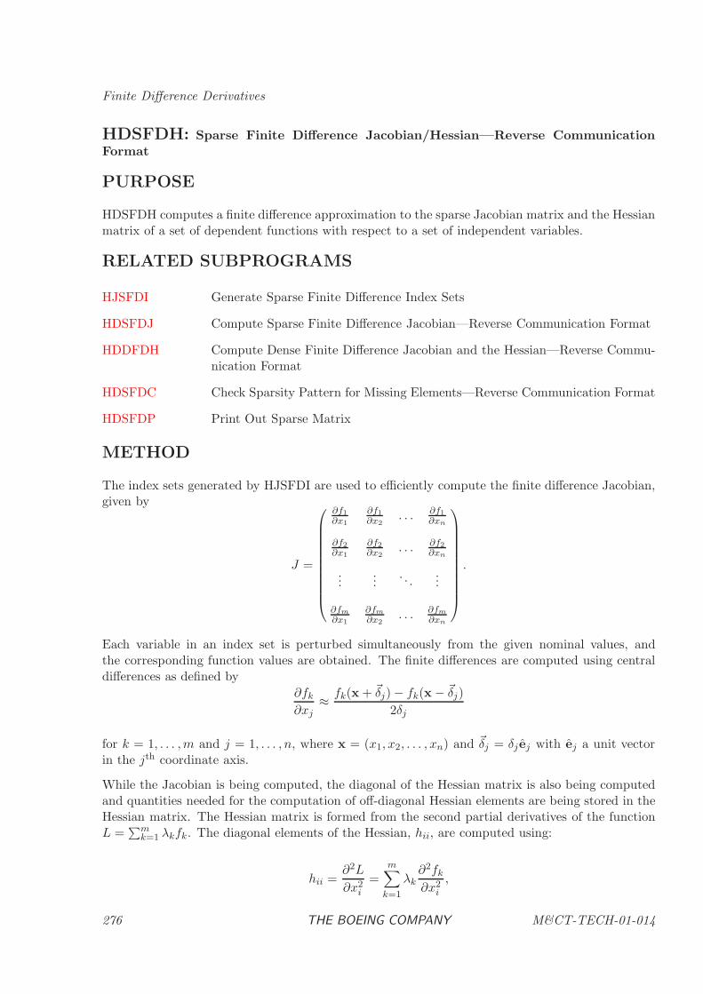
Finite Difference Derivatives
HDSFDH: Sparse Finite Difference Jacobian/Hessian—Reverse CommunicationFormat
PURPOSE
HDSFDH computes a finite difference approximation to the sparse Jacobian matrix and the Hessianmatrix of a set of dependent functions with respect to a set of independent variables.
RELATED SUBPROGRAMS
HJSFDI Generate Sparse Finite Difference Index Sets
HDSFDJ Compute Sparse Finite Difference Jacobian—Reverse Communication Format
HDDFDH Compute Dense Finite Difference Jacobian and the Hessian—Reverse Commu-nication Format
HDSFDC Check Sparsity Pattern for Missing Elements—Reverse Communication Format
HDSFDP Print Out Sparse Matrix
METHOD
The index sets generated by HJSFDI are used to efficiently compute the finite difference Jacobian,given by
J =
∂f1
∂x1
∂f1
∂x2. . . ∂f1
∂xn
∂f2∂x1
∂f2∂x2
. . . ∂f2∂xn
......
. . ....
∂fm
∂x1
∂fm
∂x2. . . ∂fm
∂xn
.
Each variable in an index set is perturbed simultaneously from the given nominal values, andthe corresponding function values are obtained. The finite differences are computed using centraldifferences as defined by
∂fk
∂xj≈ fk(x + ~δj) − fk(x − ~δj)
2δj
for k = 1, . . . ,m and j = 1, . . . , n, where x = (x1, x2, . . . , xn) and ~δj = δj ej with ej a unit vectorin the jth coordinate axis.
While the Jacobian is being computed, the diagonal of the Hessian matrix is also being computedand quantities needed for the computation of off-diagonal Hessian elements are being stored in theHessian matrix. The Hessian matrix is formed from the second partial derivatives of the functionL =
∑mk=1 λkfk. The diagonal elements of the Hessian, hii, are computed using:
hii =∂2L
∂x2i
=m∑
k=1
λk∂2fk
∂x2i
,
276 THE BOEING COMPANY M&CT-TECH-01-014
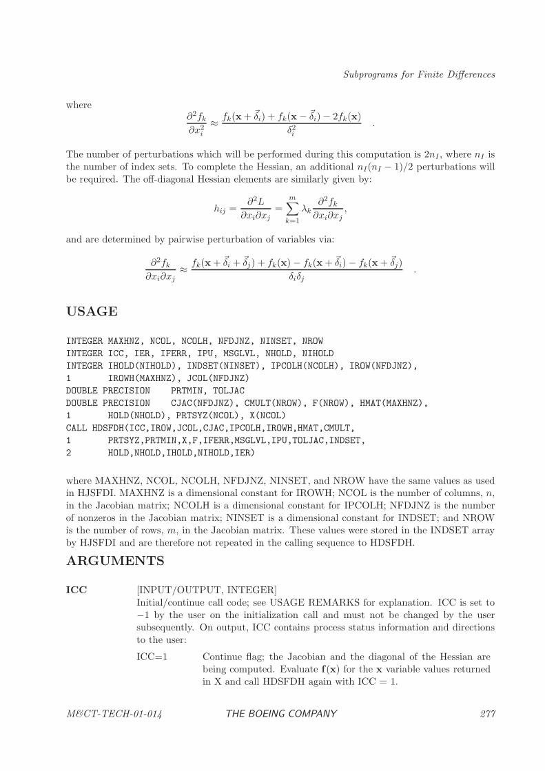
Subprograms for Finite Differences
where∂2fk
∂x2i
≈ fk(x + ~δi) + fk(x − ~δi) − 2fk(x)
δ2i.
The number of perturbations which will be performed during this computation is 2nI , where nI isthe number of index sets. To complete the Hessian, an additional nI(nI − 1)/2 perturbations willbe required. The off-diagonal Hessian elements are similarly given by:
hij =∂2L
∂xi∂xj=
m∑
k=1
λk∂2fk
∂xi∂xj,
and are determined by pairwise perturbation of variables via:
∂2fk
∂xi∂xj≈ fk(x + ~δi + ~δj) + fk(x) − fk(x + ~δi) − fk(x + ~δj)
δiδj.
USAGE
INTEGER MAXHNZ, NCOL, NCOLH, NFDJNZ, NINSET, NROW
INTEGER ICC, IER, IFERR, IPU, MSGLVL, NHOLD, NIHOLD
INTEGER IHOLD(NIHOLD), INDSET(NINSET), IPCOLH(NCOLH), IROW(NFDJNZ),
1 IROWH(MAXHNZ), JCOL(NFDJNZ)
DOUBLE PRECISION PRTMIN, TOLJAC
DOUBLE PRECISION CJAC(NFDJNZ), CMULT(NROW), F(NROW), HMAT(MAXHNZ),
1 HOLD(NHOLD), PRTSYZ(NCOL), X(NCOL)
CALL HDSFDH(ICC,IROW,JCOL,CJAC,IPCOLH,IROWH,HMAT,CMULT,
1 PRTSYZ,PRTMIN,X,F,IFERR,MSGLVL,IPU,TOLJAC,INDSET,
2 HOLD,NHOLD,IHOLD,NIHOLD,IER)
where MAXHNZ, NCOL, NCOLH, NFDJNZ, NINSET, and NROW have the same values as usedin HJSFDI. MAXHNZ is a dimensional constant for IROWH; NCOL is the number of columns, n,in the Jacobian matrix; NCOLH is a dimensional constant for IPCOLH; NFDJNZ is the numberof nonzeros in the Jacobian matrix; NINSET is a dimensional constant for INDSET; and NROWis the number of rows, m, in the Jacobian matrix. These values were stored in the INDSET arrayby HJSFDI and are therefore not repeated in the calling sequence to HDSFDH.
ARGUMENTS
ICC [INPUT/OUTPUT, INTEGER]Initial/continue call code; see USAGE REMARKS for explanation. ICC is set to−1 by the user on the initialization call and must not be changed by the usersubsequently. On output, ICC contains process status information and directionsto the user:
ICC=1 Continue flag; the Jacobian and the diagonal of the Hessian arebeing computed. Evaluate f(x) for the x variable values returnedin X and call HDSFDH again with ICC = 1.
M&CT-TECH-01-014 THE BOEING COMPANY 277
Finite Difference Derivatives
ICC=−2 Continue flag; the Jacobian and the diagonal of the Hessian havebeen computed. Call HDSFDH again with ICC = −2 to continuethe Hessian computations.
ICC=2 Continue flag; the off-diagonal Hessian elements are being com-puted. Evaluate f(x) for the x variable values returned in X andcall HDSFDH again with ICC = 2.
ICC=0 Termination flag; check the value of IER for success/error status.
IROW [INPUT, INTEGER, ARRAY]Array of row numbers for each nonzero element of the Jacobian matrix. IROW(k)gives the row number of the kth nonzero element, for k = 1, . . ., NFDJNZ. IROWmust be the same array as in HJSFDI and must not be changed by the user afterthe call to HJSFDI.
JCOL [INPUT, INTEGER, ARRAY]Array of column numbers for each nonzero element of the Jacobian matrix, incorrespondence to the IROW array. JCOL(k) gives the column number of the kth
nonzero element, for k = 1, . . ., NFDJNZ. JCOL must be the same array as inHJSFDI and must not be changed by the user after the call to HJSFDI.
CJAC [OUTPUT, DOUBLE PRECISION, ARRAY]If |ICC| 6= 1 and IER≥0, CJAC contains the finite difference approximation tothe Jacobian matrix, stored in correspondence to the IROW and JCOL arrays.CJAC(k) gives the finite difference value for row IROW(k) and column JCOL(k)of the Jacobian, ∂fIROW(k)/∂xJCOL(k). CJAC must not be modified by the userduring the Jacobian iteration process.
IPCOLH [INPUT, INTEGER, ARRAY]Array containing pointers to locations in the IROWH array corresponding to thebeginning of each column of the Hessian. IPCOLH(j) gives the location in theIROWH array of the beginning of the jth column, for j = 1, . . ., NCOL. IPCOLHmust be the same array as in HJSFDI and must not be changed by the user afterthe call to HJSFDI.
IROWH [INPUT, INTEGER, ARRAY]Array of row numbers of the Hessian nonzero locations. IROWH(k) for k =IPCOLH(j), . . ., IPCOLH(j+1)−1 gives the row numbers in ascending order, start-ing with the diagonal, for the nonzero entries in column j of the Hessian lowertriangular matrix. IROWH must be the same array as in HJSFDI and must notbe changed by the user after the call to HJSFDI.
HMAT [OUTPUT, DOUBLE PRECISION, ARRAY]If ICC = 0 and IER ≥ 0, HMAT contains the Hessian values, stored in corre-spondence to the IROWH array and IPCOLH pointer array. HMAT(k) gives theHessian value for row IROWH(k) and column j of the Hessian matrix, where jis the largest index in 1, . . ., NCOL with IPCOLH(j) ≤ k. HMAT must not bemodified by the user during the Hessian iteration process.
278 THE BOEING COMPANY M&CT-TECH-01-014
Subprograms for Finite Differences
CMULT [INPUT, DOUBLE PRECISION, ARRAY]Array of multipliers, λk, used in forming the Hessian function. The Hessian matrixwill be the second partial derivatives of the function L =
∑mk=1 λkfk. At least one
of the CMULT values must be nonzero. CMULT must be input by the user on theinitialization call and not subsequently changed.
PRTSYZ [INPUT/OUTPUT, DOUBLE PRECISION, ARRAY]Perturbation sizes, ~δ, for the x variable values. PRTSYZ(j) is the perturbationsize for X(j); |PRTSYZ(j)| ≥ PRTMIN. The perturbation sizes are only reducedwhen a function error, signalled by IFERR 6= 0, prevents a successful Jacobianfinite difference computation. Furthermore, a reduction in perturbation sizes isdone only for variables in the current index set. PRTSYZ must be specified bythe user on the initialization call and not subsequently changed by the user. Arecommended initial value for PRTSYZ(j) is 10−5 max [1, x(j)].
PRTMIN [INPUT, DOUBLE PRECISION]Minimum absolute perturbation size for any variable xj ;10∗HDMCON(5) ≤ PRTMIN ≤ min1≤j≤NCOL|PRTSYZ(j)|. HDSFDH will not re-duce any |PRTSYZ(j)| below PRTMIN during the Jacobian computations. PRT-MIN must be specified by the user on the initialization call and not subsequentlychanged. A recommended initial value for PRTMIN is
√HDMCON(5). Setting
PRTMIN less than this value will result in a warning message.
X [INPUT/OUTPUT, DOUBLE PRECISION, ARRAY]Independent variable values x. The current use of X depends on the value of ICC:
ICC=−1 X must be initialized to the nominal point, i.e., the x value forwhich the Jacobian and Hessian are to be computed.
ICC>0 X contains a perturbed point at which a function evaluation isrequired.
ICC=0 or −2X contains the nominal point, restored by HDSFDH.
X must be specified by the user on the initialization call and not subsequentlychanged by the user. See USAGE REMARKS.
F [INPUT/OUTPUT, DOUBLE PRECISION, ARRAY]Dependent function values f(x). The current use of F depends on the value of ICC(see USAGE REMARKS):
ICC=−1,1, or 2
F must be set by the user to the values of the function at thecurrent value of X.
ICC=0 or −2F contains the values of the function at the nominal point, restoredby HDSFDH.
IFERR [INPUT, INTEGER]Function error flag. This variable is used to communicate a function error thatoccurred when the user evaluated f(x).
M&CT-TECH-01-014 THE BOEING COMPANY 279
Finite Difference Derivatives
IFERR=0 The evaluation of f(x) was successful.
IFERR 6=0 An error occurred in evaluating f(x).
IFERR must be 0 on the initialization call. This implies that the function must bevalid at the nominal point. See USAGE REMARKS.
MSGLVL [INPUT, INTEGER]Level of diagnostic print.
MSGLVL≤0 Suppress all output.
MSGLVL=1 Error messages and some diagnostic information about reducedperturbation sizes.
MSGLVL≥2 Complete diagnostic output, including additional perturbation in-formation and the norm of the Jacobian.Note: Jacobian matrix norms are computed for output purposesonly and result in some extra computation.
IPU [INPUT, INTEGER]Fortran logical unit number to which diagnostic output will be written. It is as-sumed that this unit has been opened by the user prior to the call to HDSFDH ifMSGLVL > 0.
TOLJAC [INPUT, DOUBLE PRECISION]Comparison tolerance for Jacobian row and column norms; TOLJAC ≥ 0. IfMSGLVL ≥ 2, any rows for which max1≤j≤n|∂fk
∂xj| ≤ TOLJAC and any columns
for which max1≤k≤m|∂fk
∂xj| ≤ TOLJAC will be identified in the output file. If
MSGLVL < 2, TOLJAC is not used by HDSFDH.
INDSET [INPUT/OUTPUT, INTEGER, ARRAY]An array containing the index set information generated by HJSFDI. This arraymust not be changed by the user between the call to HJSFDI and the initial callto HDSFDH and also must not be changed by the user between successive calls toHDSFDH.
HOLD [INPUT/OUTPUT, DOUBLE PRECISION, ARRAY]Hold array of length NHOLD. This array must not be changed by the user betweensuccessive calls to HDSFDH when the Jacobian and Hessian matrices are beingcomputed. After the Jacobian and Hessian computations are complete (ICC = 0),this array can be used elsewhere as a work array.
NHOLD [INPUT, INTEGER]The length of the HOLD array. NHOLD ≥ 2∗(NROW+NCOL), where NROWand NCOL are the same values used in HJSFDI.
IHOLD [INPUT/OUTPUT, INTEGER, ARRAY]Integer hold array of length NIHOLD. This array must not be changed by the user
280 THE BOEING COMPANY M&CT-TECH-01-014
Subprograms for Finite Differences
between successive calls to HDSFDH when the Jacobian and Hessian matrices arebeing computed. After the Jacobian and Hessian computations are complete (ICC= 0), this array can be used elsewhere as a work array.
NIHOLD [INPUT, INTEGER]The length of the IHOLD array. NIHOLD ≥ NROW, where NROW is the samevalue used in HJSFDI.
IER [OUTPUT, INTEGER]Success/error code. See Section 1.4.2 of the BCSLIB manual for a discussion oferror handling. For IER < 0, ICC has been set to 0, and at least part of theCJAC and HMAT arrays have been clobbered with HDMCON(1). See the BCSLIBmanual for HDMCON. Note, however, that for IER = −21, −22, and −23, theCJAC array is not clobbered and contains the computed Jacobian matrix.
IER=0 Success, results computed.
IER=1 PRTMIN <√
HDMCON(5).
IER=2 MSGLVL ≥ 2 and TOLJAC< 0. No matrix norms were computed.
IER=3 MSGLVL ≥ 2 and at least one row or column norm of the Jacobianis ≤ TOLJAC.
IER=4 The CMULT array is all zeros; no need to compute the Hessianmatrix. If only the Jacobian matrix is needed, use HDSFDJ.
IER=−1 Invalid initial/continue call code; ICC 6= −2, −1, 1, or 2.
IER=−2 Invalid INDSET array—the INDSET array must not be changedbetween the call to HJSFDI and the initial call to HDSFDH andalso must not be changed between successive calls to HDSFDH.
IER=−3 NIHOLD too small; the number of words needed is given by theprinted error message.
IER=−4 NHOLD too small; the number of words needed is given by theprinted error message.
IER=−5 For ICC = −1 or −2, IFERR 6= 0. There must not be a functionerror at the nominal point.
IER=−6 The minimum perturbation size is too small;PRTMIN < 10∗HDMCON(5).
IER=−7 min1≤j≤NCOL|PRTSYZ(j)| < PRTMIN.
M&CT-TECH-01-014 THE BOEING COMPANY 281
Finite Difference Derivatives
IER=−10 Incorrect use of ICC code; make sure that an initial call toHDSFDH with ICC = −1 is made prior to the Jacobian and Hes-sian diagonal computations (ICC = 1). See USAGE REMARKS.
IER=−11 Smallest allowable perturbation caused a function error.
IER=−20 Incorrect use of ICC code; make sure that a call to HDSFDH withICC = −2 is made after the Jacobian and Hessian diagonal com-putations (ICC = 1) and prior to the off-diagonal Hessian compu-tations (ICC = 2). See USAGE REMARKS.
IER=−21 Inconsistency in nominal variable values detected. The same nomi-nal values must be used in X for ICC = −1 and −2, and the HOLDarray must not be changed between successive calls to HDSFDH.In spite of this, the Jacobian matrix was successfully computed forthe nominal values supplied when HDSFDH was called with ICC= −1.
IER=−22 Inconsistency in nominal function values detected. The same nom-inal values must be used in F for ICC = −1 and −2, and the HOLDarray must not be changed between successive calls to HDSFDH.In spite of this, the Jacobian matrix was successfully computed forthe nominal values supplied when HDSFDH was called with ICC= −1.
IER=−23 A function error occurred while computing the off-diagonal Hessianelements. The computation of the Hessian was not completed. TheJacobian matrix, on the other hand, was successfully computed andis stored in CJAC.
USAGE REMARKS
HDSFDH uses reverse communication to compute the Jacobian and Hessian matrices. A user callsHDSFDH repeatedly to formulate the Jacobian and Hessian values, where each call to HDSFDHperforms computations based on a particular index set. Before the initial call to HDSFDH, thenominal variable values must be stored in X, and the corresponding nominal function values mustbe stored in F. The function error flag IFERR must equal 0 at the nominal X variable values. Also,the perturbation sizes to be used in perturbing the variable values must be stored in PRTSYZ. Theuser can then make an initial call to HDSFDH with ICC = −1.
After each return from HDSFDH, the user should examine the value of ICC to determine the courseof action.
If ICC = 1 or 2, the user’s program should evaluate the function using the x variable values returnedin X, that is, set F = f(x). It then must call HDSFDH again with the same value of ICC to continuethe Jacobian and Hessian computations.
282 THE BOEING COMPANY M&CT-TECH-01-014
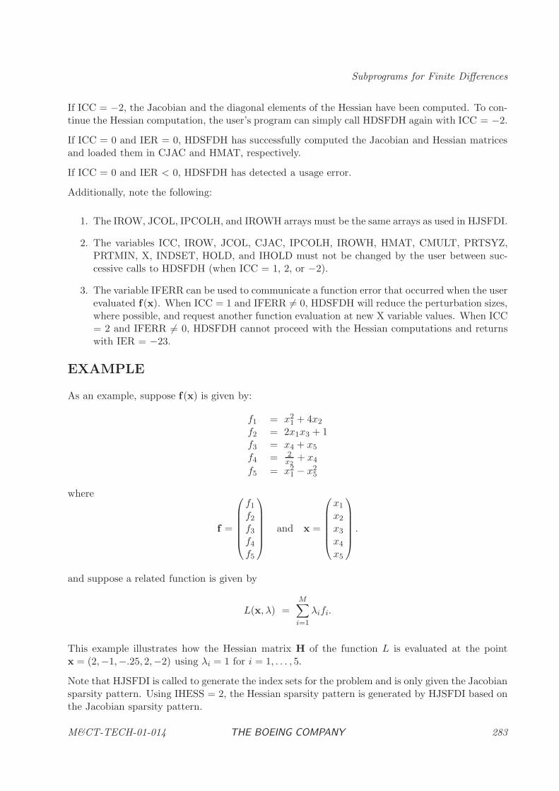
Subprograms for Finite Differences
If ICC = −2, the Jacobian and the diagonal elements of the Hessian have been computed. To con-tinue the Hessian computation, the user’s program can simply call HDSFDH again with ICC = −2.
If ICC = 0 and IER = 0, HDSFDH has successfully computed the Jacobian and Hessian matricesand loaded them in CJAC and HMAT, respectively.
If ICC = 0 and IER < 0, HDSFDH has detected a usage error.
Additionally, note the following:
1. The IROW, JCOL, IPCOLH, and IROWH arrays must be the same arrays as used in HJSFDI.
2. The variables ICC, IROW, JCOL, CJAC, IPCOLH, IROWH, HMAT, CMULT, PRTSYZ,PRTMIN, X, INDSET, HOLD, and IHOLD must not be changed by the user between suc-cessive calls to HDSFDH (when ICC = 1, 2, or −2).
3. The variable IFERR can be used to communicate a function error that occurred when the userevaluated f(x). When ICC = 1 and IFERR 6= 0, HDSFDH will reduce the perturbation sizes,where possible, and request another function evaluation at new X variable values. When ICC= 2 and IFERR 6= 0, HDSFDH cannot proceed with the Hessian computations and returnswith IER = −23.
EXAMPLE
As an example, suppose f(x) is given by:
f1 = x21 + 4x2
f2 = 2x1x3 + 1f3 = x4 + x5
f4 = 2x2
+ x4
f5 = x21 − x2
5
where
f =
f1
f2
f3
f4
f5
and x =
x1
x2
x3
x4
x5
.
and suppose a related function is given by
L(x, λ) =M∑
i=1
λifi.
This example illustrates how the Hessian matrix H of the function L is evaluated at the pointx = (2,−1,−.25, 2,−2) using λi = 1 for i = 1, . . . , 5.
Note that HJSFDI is called to generate the index sets for the problem and is only given the Jacobiansparsity pattern. Using IHESS = 2, the Hessian sparsity pattern is generated by HJSFDI based onthe Jacobian sparsity pattern.
M&CT-TECH-01-014 THE BOEING COMPANY 283
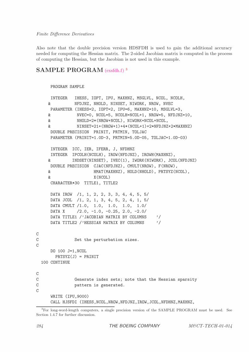
Finite Difference Derivatives
Also note that the double precision version HDSFDH is used to gain the additional accuracyneeded for computing the Hessian matrix. The 2-sided Jacobian matrix is computed in the processof computing the Hessian, but the Jacobian is not used in this example.
SAMPLE PROGRAM (exsfdh.f) 3
PROGRAM SAMPLE
INTEGER IHESS, IOPT, IPU, MAXHNZ, MSGLVL, NCOL, NCOLH,
& NFDJNZ, NHOLD, NINSET, NIWORK, NROW, NVEC
PARAMETER (IHESS=2, IOPT=2, IPU=6, MAXHNZ=10, MSGLVL=3,
& NVEC=0, NCOL=5, NCOLH=NCOL+1, NROW=5, NFDJNZ=10,
& NHOLD=2*(NROW+NCOL), NIWORK=NCOL+NCOL,
& NINSET=21+(NROW+1)+4*(NCOL+1)+2*NFDJNZ+2*MAXHNZ)
DOUBLE PRECISION PRINIT, PRTMIN, TOLJAC
PARAMETER (PRINIT=1.0D-3, PRTMIN=5.0D-05, TOLJAC=1.0D-03)
INTEGER ICC, IER, IFERR, J, NFDHNZ
INTEGER IPCOLH(NCOLH), IROW(NFDJNZ), IROWH(MAXHNZ),
& INDSET(NINSET), IVEC(1), IWORK(NIWORK), JCOL(NFDJNZ)
DOUBLE PRECISION CJAC(NFDJNZ), CMULT(NROW), F(NROW),
& HMAT(MAXHNZ), HOLD(NHOLD), PRTSYZ(NCOL),
& X(NCOL)
CHARACTER*30 TITLE1, TITLE2
DATA IROW /1, 1, 2, 2, 3, 3, 4, 4, 5, 5/
DATA JCOL /1, 2, 1, 3, 4, 5, 2, 4, 1, 5/
DATA CMULT /1.0, 1.0, 1.0, 1.0, 1.0/
DATA X /2.0, -1.0, -0.25, 2.0, -2.0/
DATA TITLE1 /’JACOBIAN MATRIX BY COLUMNS ’/
DATA TITLE2 /’HESSIAN MATRIX BY COLUMNS ’/
C
C Set the perturbation sizes.
C
DO 100 J=1,NCOL
PRTSYZ(J) = PRINIT
100 CONTINUE
C
C Generate index sets; note that the Hessian sparsity
C pattern is generated.
C
WRITE (IPU,9000)
CALL HJSFDI (IHESS,NCOL,NROW,NFDJNZ,IROW,JCOL,NFDHNZ,MAXHNZ,
3For long-word-length computers, a single precision version of the SAMPLE PROGRAM must be used. See
Section 1.4.7 for further discussion.
284 THE BOEING COMPANY M&CT-TECH-01-014
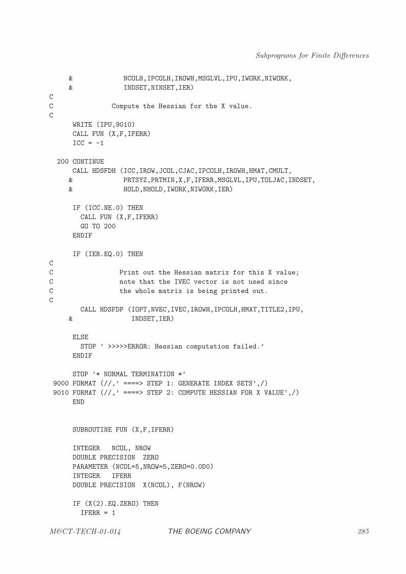
Subprograms for Finite Differences
& NCOLH,IPCOLH,IROWH,MSGLVL,IPU,IWORK,NIWORK,
& INDSET,NINSET,IER)
C
C Compute the Hessian for the X value.
C
WRITE (IPU,9010)
CALL FUN (X,F,IFERR)
ICC = -1
200 CONTINUE
CALL HDSFDH (ICC,IROW,JCOL,CJAC,IPCOLH,IROWH,HMAT,CMULT,
& PRTSYZ,PRTMIN,X,F,IFERR,MSGLVL,IPU,TOLJAC,INDSET,
& HOLD,NHOLD,IWORK,NIWORK,IER)
IF (ICC.NE.0) THEN
CALL FUN (X,F,IFERR)
GO TO 200
ENDIF
IF (IER.EQ.0) THEN
C
C Print out the Hessian matrix for this X value;
C note that the IVEC vector is not used since
C the whole matrix is being printed out.
C
CALL HDSFDP (IOPT,NVEC,IVEC,IROWH,IPCOLH,HMAT,TITLE2,IPU,
& INDSET,IER)
ELSE
STOP ’ >>>>>ERROR: Hessian computation failed.’
ENDIF
STOP ’* NORMAL TERMINATION *’
9000 FORMAT (//,’ ====> STEP 1: GENERATE INDEX SETS’,/)
9010 FORMAT (//,’ ====> STEP 2: COMPUTE HESSIAN FOR X VALUE’,/)
END
SUBROUTINE FUN (X,F,IFERR)
INTEGER NCOL, NROW
DOUBLE PRECISION ZERO
PARAMETER (NCOL=5,NROW=5,ZERO=0.0D0)
INTEGER IFERR
DOUBLE PRECISION X(NCOL), F(NROW)
IF (X(2).EQ.ZERO) THEN
IFERR = 1
M&CT-TECH-01-014 THE BOEING COMPANY 285
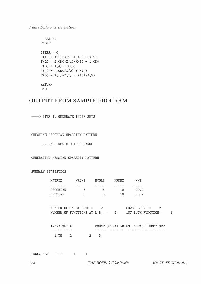
Finite Difference Derivatives
RETURN
ENDIF
IFERR = 0
F(1) = X(1)*X(1) + 4.0D0*X(2)
F(2) = 2.0D0*X(1)*X(3) + 1.0D0
F(3) = X(4) + X(5)
F(4) = 2.0D0/X(2) + X(4)
F(5) = X(1)*X(1) - X(5)*X(5)
RETURN
END
OUTPUT FROM SAMPLE PROGRAM
====> STEP 1: GENERATE INDEX SETS
CHECKING JACOBIAN SPARSITY PATTERN
.....NO INPUTS OUT OF RANGE
GENERATING HESSIAN SPARSITY PATTERN
SUMMARY STATISTICS:
MATRIX NROWS NCOLS NFDNZ %NZ
-------- ----- ----- ----- -----
JACOBIAN 5 5 10 40.0
HESSIAN 5 5 10 66.7
NUMBER OF INDEX SETS = 2 LOWER BOUND = 2
NUMBER OF FUNCTIONS AT L.B. = 5 1ST SUCH FUNCTION = 1
INDEX SET # COUNT OF VARIABLES IN EACH INDEX SET
----------- ------------------------------------
1 TO 2 2 3
INDEX SET 1 : 1 4
286 THE BOEING COMPANY M&CT-TECH-01-014
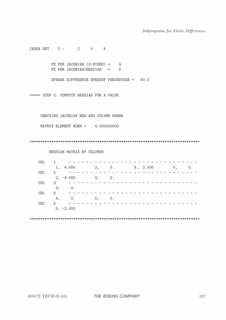
Subprograms for Finite Differences
INDEX SET 2 : 2 3 5
FE PER JACOBIAN (2-SIDED) = 4
FE PER JACOBIAN/HESSIAN = 5
SPARSE DIFFERENCE SPEEDUP PERCENTAGE = 60.0
====> STEP 2: COMPUTE HESSIAN FOR X VALUE
CHECKING JACOBIAN ROW AND COLUMN NORMS
MATRIX ELEMENT NORM = 4.000000000
******************************************************************************
HESSIAN MATRIX BY COLUMNS
COL 1 - - - - - - - - - - - - - - - - - - - - - - - - - - - - - -
1, 4.000 2, 0. 3, 2.000 5, 0.
COL 2 - - - - - - - - - - - - - - - - - - - - - - - - - - - - - -
2, -4.000 4, 0.
COL 3 - - - - - - - - - - - - - - - - - - - - - - - - - - - - - -
3, 0.
COL 4 - - - - - - - - - - - - - - - - - - - - - - - - - - - - - -
4, 0. 5, 0.
COL 5 - - - - - - - - - - - - - - - - - - - - - - - - - - - - - -
5, -2.000
******************************************************************************
M&CT-TECH-01-014 THE BOEING COMPANY 287
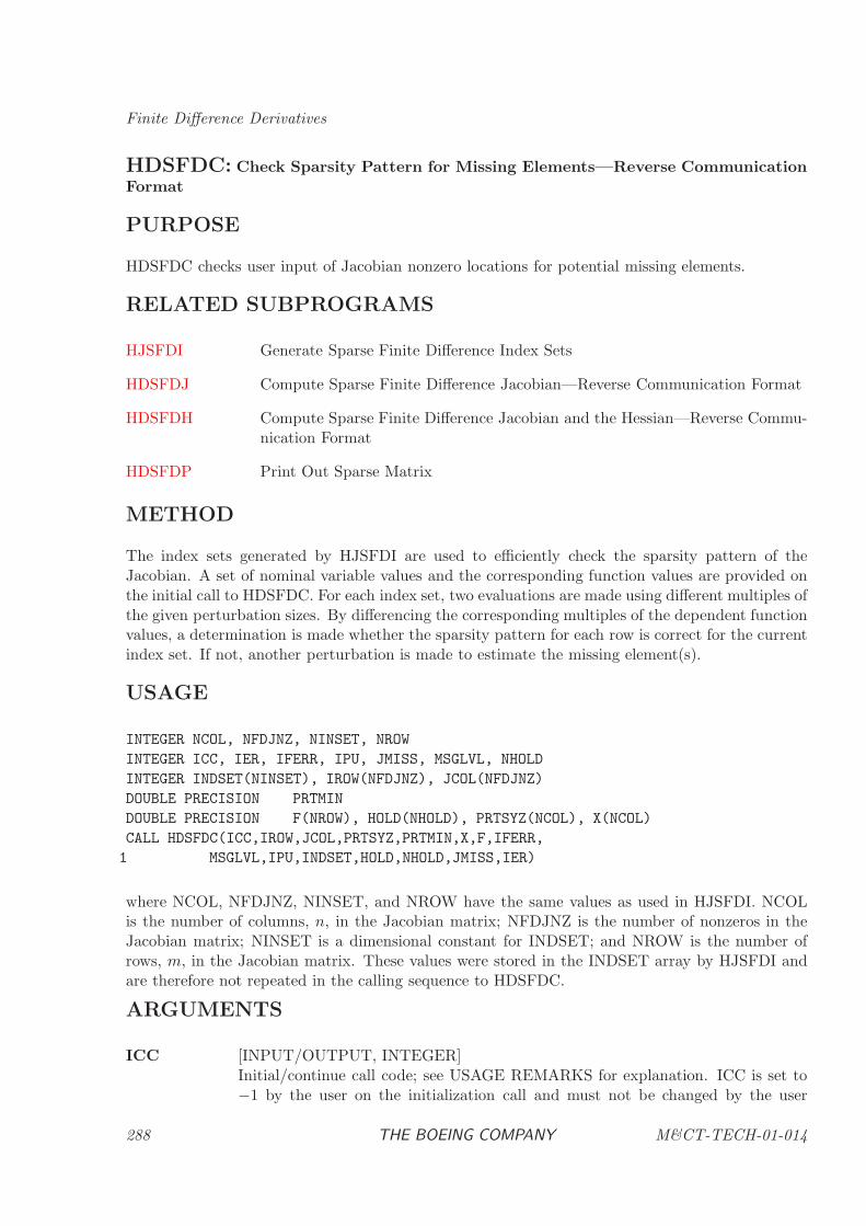
Finite Difference Derivatives
HDSFDC: Check Sparsity Pattern for Missing Elements—Reverse CommunicationFormat
PURPOSE
HDSFDC checks user input of Jacobian nonzero locations for potential missing elements.
RELATED SUBPROGRAMS
HJSFDI Generate Sparse Finite Difference Index Sets
HDSFDJ Compute Sparse Finite Difference Jacobian—Reverse Communication Format
HDSFDH Compute Sparse Finite Difference Jacobian and the Hessian—Reverse Commu-nication Format
HDSFDP Print Out Sparse Matrix
METHOD
The index sets generated by HJSFDI are used to efficiently check the sparsity pattern of theJacobian. A set of nominal variable values and the corresponding function values are provided onthe initial call to HDSFDC. For each index set, two evaluations are made using different multiples ofthe given perturbation sizes. By differencing the corresponding multiples of the dependent functionvalues, a determination is made whether the sparsity pattern for each row is correct for the currentindex set. If not, another perturbation is made to estimate the missing element(s).
USAGE
INTEGER NCOL, NFDJNZ, NINSET, NROW
INTEGER ICC, IER, IFERR, IPU, JMISS, MSGLVL, NHOLD
INTEGER INDSET(NINSET), IROW(NFDJNZ), JCOL(NFDJNZ)
DOUBLE PRECISION PRTMIN
DOUBLE PRECISION F(NROW), HOLD(NHOLD), PRTSYZ(NCOL), X(NCOL)
CALL HDSFDC(ICC,IROW,JCOL,PRTSYZ,PRTMIN,X,F,IFERR,
1 MSGLVL,IPU,INDSET,HOLD,NHOLD,JMISS,IER)
where NCOL, NFDJNZ, NINSET, and NROW have the same values as used in HJSFDI. NCOLis the number of columns, n, in the Jacobian matrix; NFDJNZ is the number of nonzeros in theJacobian matrix; NINSET is a dimensional constant for INDSET; and NROW is the number ofrows, m, in the Jacobian matrix. These values were stored in the INDSET array by HJSFDI andare therefore not repeated in the calling sequence to HDSFDC.
ARGUMENTS
ICC [INPUT/OUTPUT, INTEGER]Initial/continue call code; see USAGE REMARKS for explanation. ICC is set to−1 by the user on the initialization call and must not be changed by the user
288 THE BOEING COMPANY M&CT-TECH-01-014
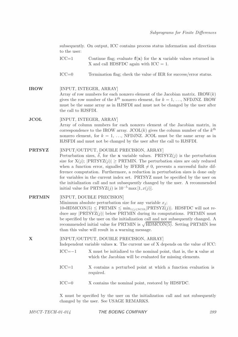
Subprograms for Finite Differences
subsequently. On output, ICC contains process status information and directionsto the user:
ICC=1 Continue flag; evaluate f(x) for the x variable values returned inX and call HDSFDC again with ICC = 1.
ICC=0 Termination flag; check the value of IER for success/error status.
IROW [INPUT, INTEGER, ARRAY]Array of row numbers for each nonzero element of the Jacobian matrix. IROW(k)gives the row number of the kth nonzero element, for k = 1, . . ., NFDJNZ. IROWmust be the same array as in HJSFDI and must not be changed by the user afterthe call to HJSFDI.
JCOL [INPUT, INTEGER, ARRAY]Array of column numbers for each nonzero element of the Jacobian matrix, incorrespondence to the IROW array. JCOL(k) gives the column number of the kth
nonzero element, for k = 1, . . ., NFDJNZ. JCOL must be the same array as inHJSFDI and must not be changed by the user after the call to HJSFDI.
PRTSYZ [INPUT/OUTPUT, DOUBLE PRECISION, ARRAY]Perturbation sizes, ~δ, for the x variable values. PRTSYZ(j) is the perturbationsize for X(j); |PRTSYZ(j)| ≥ PRTMIN. The perturbation sizes are only reducedwhen a function error, signalled by IFERR 6= 0, prevents a successful finite dif-ference computation. Furthermore, a reduction in perturbation sizes is done onlyfor variables in the current index set. PRTSYZ must be specified by the user onthe initialization call and not subsequently changed by the user. A recommendedinitial value for PRTSYZ(j) is 10−5 max [1, x(j)].
PRTMIN [INPUT, DOUBLE PRECISION]Minimum absolute perturbation size for any variable xj ;10∗HDMCON(5) ≤ PRTMIN ≤ min1≤j≤NCOL|PRTSYZ(j)|. HDSFDC will not re-duce any |PRTSYZ(j)| below PRTMIN during its computations. PRTMIN mustbe specified by the user on the initialization call and not subsequently changed. Arecommended initial value for PRTMIN is
√HDMCON(5). Setting PRTMIN less
than this value will result in a warning message.
X [INPUT/OUTPUT, DOUBLE PRECISION, ARRAY]Independent variable values x. The current use of X depends on the value of ICC:
ICC=−1 X must be initialized to the nominal point, that is, the x value atwhich the Jacobian will be evaluated for missing elements.
ICC=1 X contains a perturbed point at which a function evaluation isrequired.
ICC=0 X contains the nominal point, restored by HDSFDC.
X must be specified by the user on the initialization call and not subsequentlychanged by the user. See USAGE REMARKS.
M&CT-TECH-01-014 THE BOEING COMPANY 289
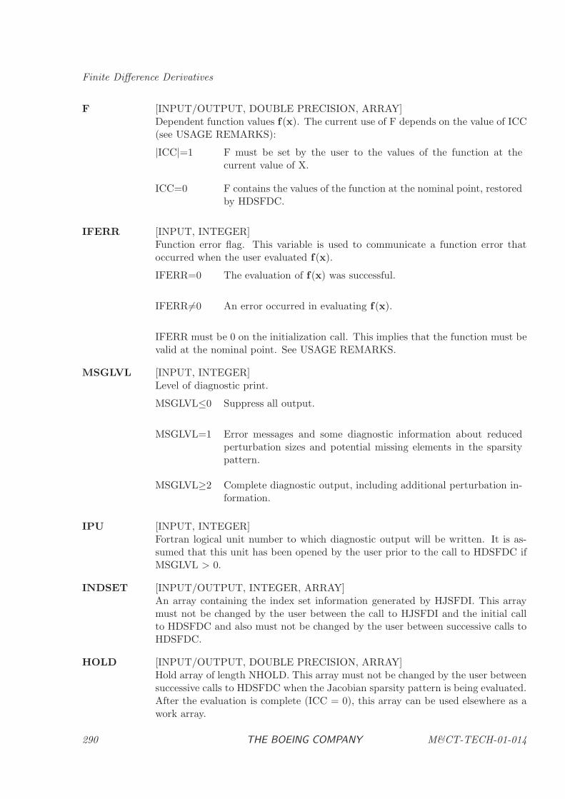
Finite Difference Derivatives
F [INPUT/OUTPUT, DOUBLE PRECISION, ARRAY]Dependent function values f(x). The current use of F depends on the value of ICC(see USAGE REMARKS):
|ICC|=1 F must be set by the user to the values of the function at thecurrent value of X.
ICC=0 F contains the values of the function at the nominal point, restoredby HDSFDC.
IFERR [INPUT, INTEGER]Function error flag. This variable is used to communicate a function error thatoccurred when the user evaluated f(x).
IFERR=0 The evaluation of f(x) was successful.
IFERR 6=0 An error occurred in evaluating f(x).
IFERR must be 0 on the initialization call. This implies that the function must bevalid at the nominal point. See USAGE REMARKS.
MSGLVL [INPUT, INTEGER]Level of diagnostic print.
MSGLVL≤0 Suppress all output.
MSGLVL=1 Error messages and some diagnostic information about reducedperturbation sizes and potential missing elements in the sparsitypattern.
MSGLVL≥2 Complete diagnostic output, including additional perturbation in-formation.
IPU [INPUT, INTEGER]Fortran logical unit number to which diagnostic output will be written. It is as-sumed that this unit has been opened by the user prior to the call to HDSFDC ifMSGLVL > 0.
INDSET [INPUT/OUTPUT, INTEGER, ARRAY]An array containing the index set information generated by HJSFDI. This arraymust not be changed by the user between the call to HJSFDI and the initial callto HDSFDC and also must not be changed by the user between successive calls toHDSFDC.
HOLD [INPUT/OUTPUT, DOUBLE PRECISION, ARRAY]Hold array of length NHOLD. This array must not be changed by the user betweensuccessive calls to HDSFDC when the Jacobian sparsity pattern is being evaluated.After the evaluation is complete (ICC = 0), this array can be used elsewhere as awork array.
290 THE BOEING COMPANY M&CT-TECH-01-014
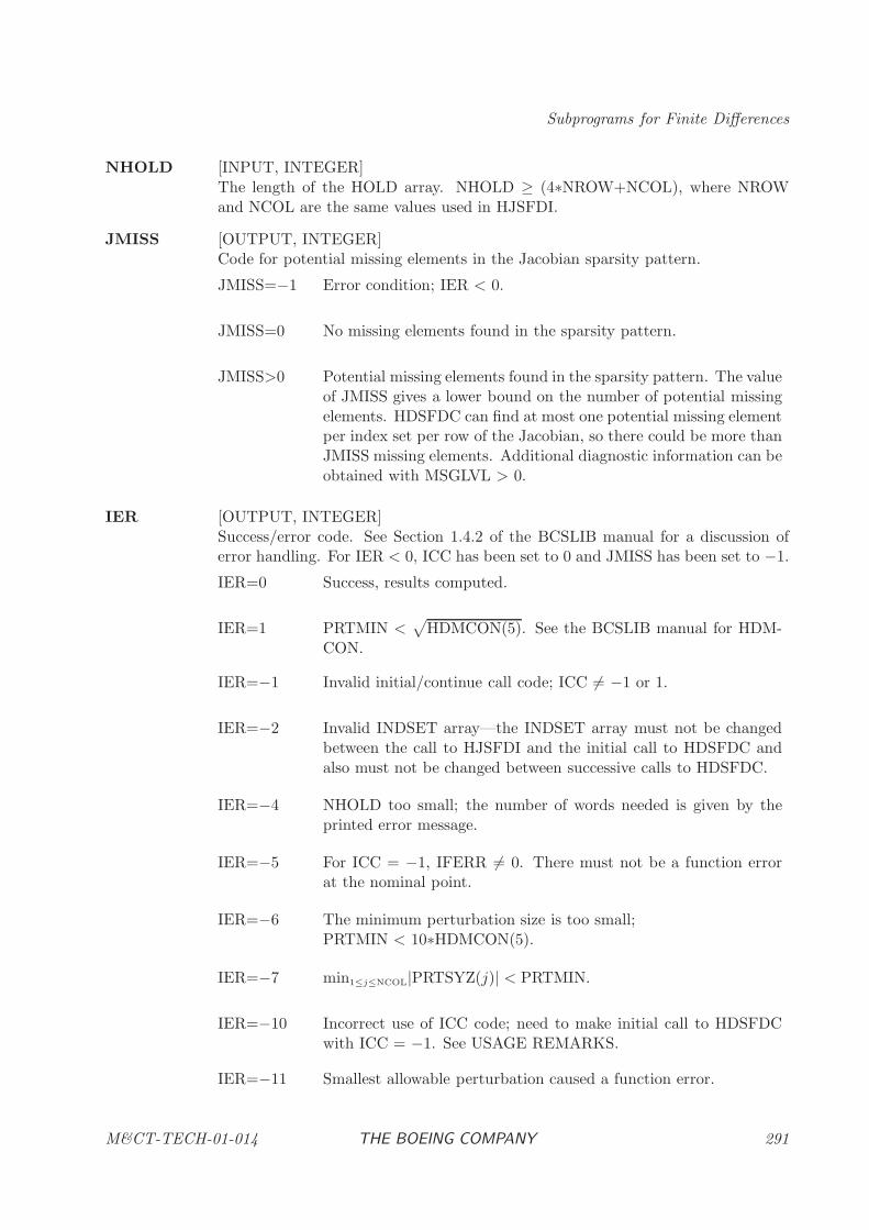
Subprograms for Finite Differences
NHOLD [INPUT, INTEGER]The length of the HOLD array. NHOLD ≥ (4∗NROW+NCOL), where NROWand NCOL are the same values used in HJSFDI.
JMISS [OUTPUT, INTEGER]Code for potential missing elements in the Jacobian sparsity pattern.
JMISS=−1 Error condition; IER < 0.
JMISS=0 No missing elements found in the sparsity pattern.
JMISS>0 Potential missing elements found in the sparsity pattern. The valueof JMISS gives a lower bound on the number of potential missingelements. HDSFDC can find at most one potential missing elementper index set per row of the Jacobian, so there could be more thanJMISS missing elements. Additional diagnostic information can beobtained with MSGLVL > 0.
IER [OUTPUT, INTEGER]Success/error code. See Section 1.4.2 of the BCSLIB manual for a discussion oferror handling. For IER < 0, ICC has been set to 0 and JMISS has been set to −1.
IER=0 Success, results computed.
IER=1 PRTMIN <√
HDMCON(5). See the BCSLIB manual for HDM-CON.
IER=−1 Invalid initial/continue call code; ICC 6= −1 or 1.
IER=−2 Invalid INDSET array—the INDSET array must not be changedbetween the call to HJSFDI and the initial call to HDSFDC andalso must not be changed between successive calls to HDSFDC.
IER=−4 NHOLD too small; the number of words needed is given by theprinted error message.
IER=−5 For ICC = −1, IFERR 6= 0. There must not be a function errorat the nominal point.
IER=−6 The minimum perturbation size is too small;PRTMIN < 10∗HDMCON(5).
IER=−7 min1≤j≤NCOL|PRTSYZ(j)| < PRTMIN.
IER=−10 Incorrect use of ICC code; need to make initial call to HDSFDCwith ICC = −1. See USAGE REMARKS.
IER=−11 Smallest allowable perturbation caused a function error.
M&CT-TECH-01-014 THE BOEING COMPANY 291
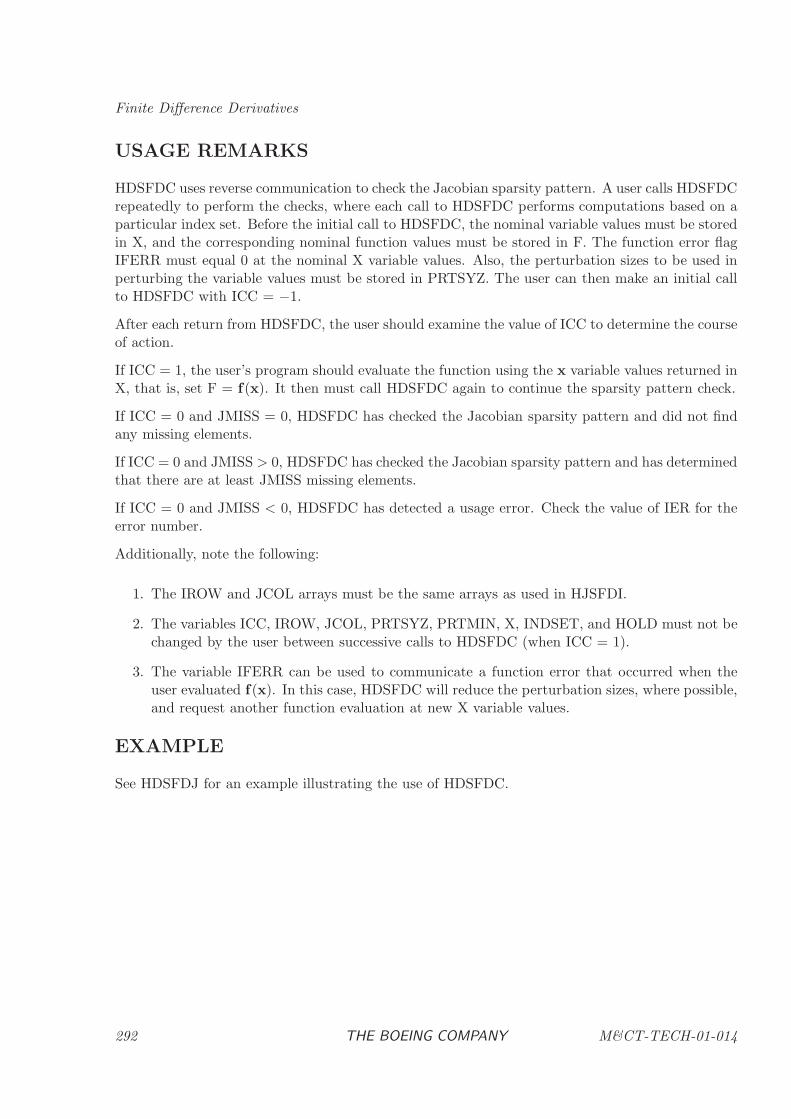
Finite Difference Derivatives
USAGE REMARKS
HDSFDC uses reverse communication to check the Jacobian sparsity pattern. A user calls HDSFDCrepeatedly to perform the checks, where each call to HDSFDC performs computations based on aparticular index set. Before the initial call to HDSFDC, the nominal variable values must be storedin X, and the corresponding nominal function values must be stored in F. The function error flagIFERR must equal 0 at the nominal X variable values. Also, the perturbation sizes to be used inperturbing the variable values must be stored in PRTSYZ. The user can then make an initial callto HDSFDC with ICC = −1.
After each return from HDSFDC, the user should examine the value of ICC to determine the courseof action.
If ICC = 1, the user’s program should evaluate the function using the x variable values returned inX, that is, set F = f(x). It then must call HDSFDC again to continue the sparsity pattern check.
If ICC = 0 and JMISS = 0, HDSFDC has checked the Jacobian sparsity pattern and did not findany missing elements.
If ICC = 0 and JMISS > 0, HDSFDC has checked the Jacobian sparsity pattern and has determinedthat there are at least JMISS missing elements.
If ICC = 0 and JMISS < 0, HDSFDC has detected a usage error. Check the value of IER for theerror number.
Additionally, note the following:
1. The IROW and JCOL arrays must be the same arrays as used in HJSFDI.
2. The variables ICC, IROW, JCOL, PRTSYZ, PRTMIN, X, INDSET, and HOLD must not bechanged by the user between successive calls to HDSFDC (when ICC = 1).
3. The variable IFERR can be used to communicate a function error that occurred when theuser evaluated f(x). In this case, HDSFDC will reduce the perturbation sizes, where possible,and request another function evaluation at new X variable values.
EXAMPLE
See HDSFDJ for an example illustrating the use of HDSFDC.
292 THE BOEING COMPANY M&CT-TECH-01-014
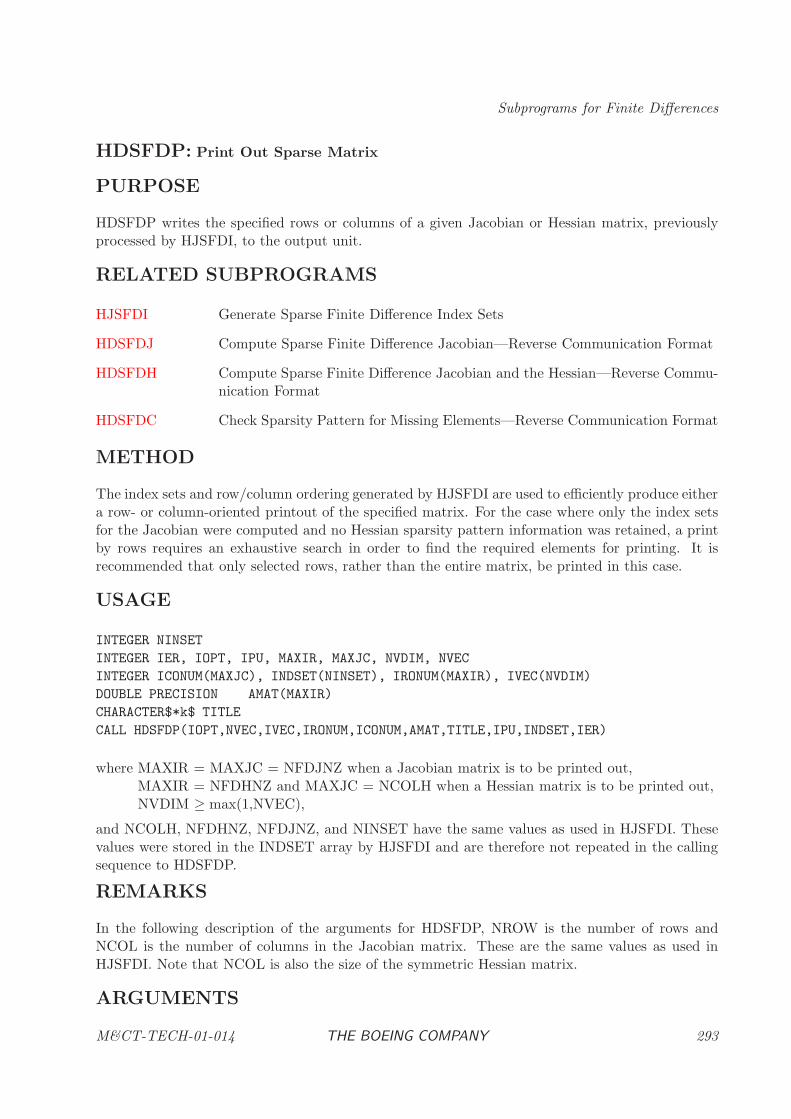
Subprograms for Finite Differences
HDSFDP: Print Out Sparse Matrix
PURPOSE
HDSFDP writes the specified rows or columns of a given Jacobian or Hessian matrix, previouslyprocessed by HJSFDI, to the output unit.
RELATED SUBPROGRAMS
HJSFDI Generate Sparse Finite Difference Index Sets
HDSFDJ Compute Sparse Finite Difference Jacobian—Reverse Communication Format
HDSFDH Compute Sparse Finite Difference Jacobian and the Hessian—Reverse Commu-nication Format
HDSFDC Check Sparsity Pattern for Missing Elements—Reverse Communication Format
METHOD
The index sets and row/column ordering generated by HJSFDI are used to efficiently produce eithera row- or column-oriented printout of the specified matrix. For the case where only the index setsfor the Jacobian were computed and no Hessian sparsity pattern information was retained, a printby rows requires an exhaustive search in order to find the required elements for printing. It isrecommended that only selected rows, rather than the entire matrix, be printed in this case.
USAGE
INTEGER NINSET
INTEGER IER, IOPT, IPU, MAXIR, MAXJC, NVDIM, NVEC
INTEGER ICONUM(MAXJC), INDSET(NINSET), IRONUM(MAXIR), IVEC(NVDIM)
DOUBLE PRECISION AMAT(MAXIR)
CHARACTER$*k$ TITLE
CALL HDSFDP(IOPT,NVEC,IVEC,IRONUM,ICONUM,AMAT,TITLE,IPU,INDSET,IER)
where MAXIR = MAXJC = NFDJNZ when a Jacobian matrix is to be printed out,MAXIR = NFDHNZ and MAXJC = NCOLH when a Hessian matrix is to be printed out,NVDIM ≥ max(1,NVEC),
and NCOLH, NFDHNZ, NFDJNZ, and NINSET have the same values as used in HJSFDI. Thesevalues were stored in the INDSET array by HJSFDI and are therefore not repeated in the callingsequence to HDSFDP.
REMARKS
In the following description of the arguments for HDSFDP, NROW is the number of rows andNCOL is the number of columns in the Jacobian matrix. These are the same values as used inHJSFDI. Note that NCOL is also the size of the symmetric Hessian matrix.
ARGUMENTS
M&CT-TECH-01-014 THE BOEING COMPANY 293
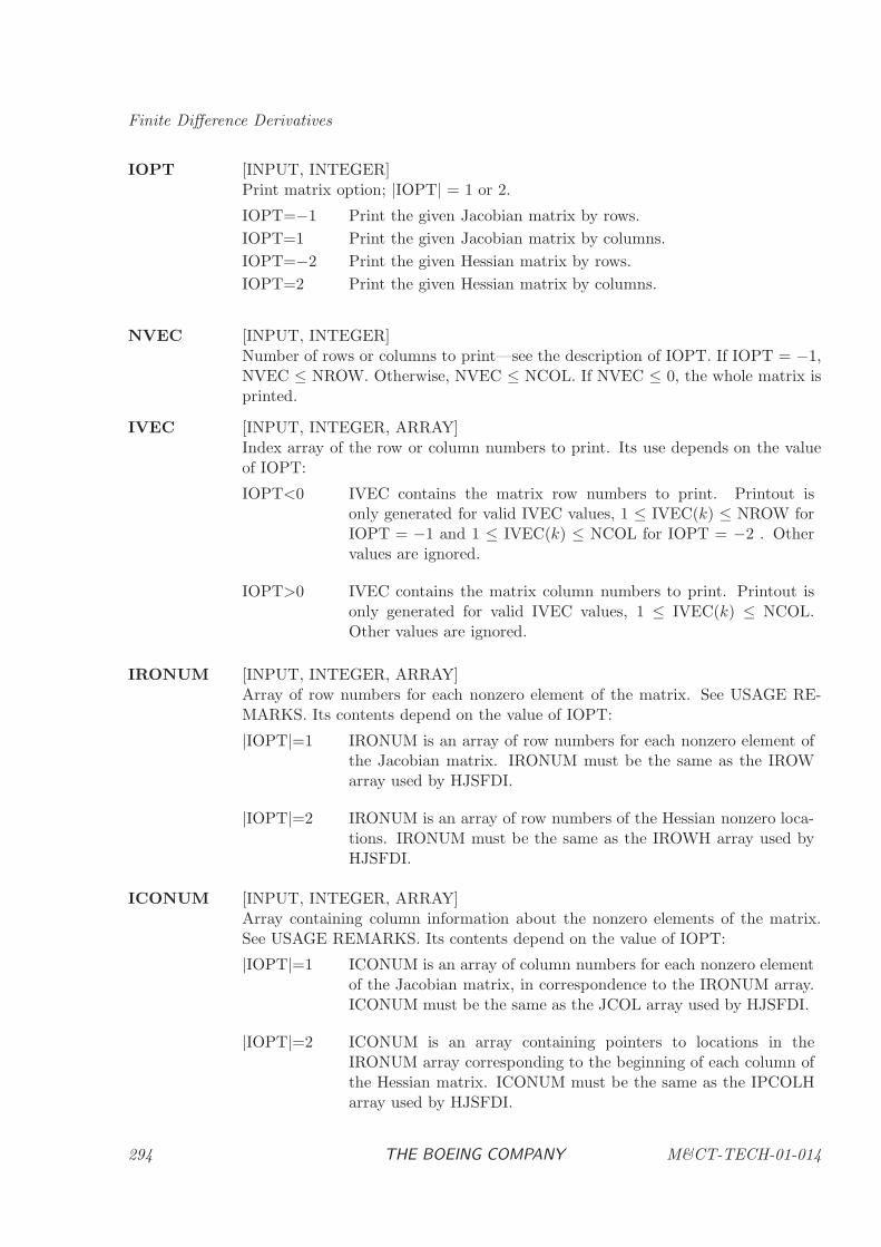
Finite Difference Derivatives
IOPT [INPUT, INTEGER]Print matrix option; |IOPT| = 1 or 2.
IOPT=−1 Print the given Jacobian matrix by rows.
IOPT=1 Print the given Jacobian matrix by columns.
IOPT=−2 Print the given Hessian matrix by rows.
IOPT=2 Print the given Hessian matrix by columns.
NVEC [INPUT, INTEGER]Number of rows or columns to print—see the description of IOPT. If IOPT = −1,NVEC ≤ NROW. Otherwise, NVEC ≤ NCOL. If NVEC ≤ 0, the whole matrix isprinted.
IVEC [INPUT, INTEGER, ARRAY]Index array of the row or column numbers to print. Its use depends on the valueof IOPT:
IOPT<0 IVEC contains the matrix row numbers to print. Printout isonly generated for valid IVEC values, 1 ≤ IVEC(k) ≤ NROW forIOPT = −1 and 1 ≤ IVEC(k) ≤ NCOL for IOPT = −2 . Othervalues are ignored.
IOPT>0 IVEC contains the matrix column numbers to print. Printout isonly generated for valid IVEC values, 1 ≤ IVEC(k) ≤ NCOL.Other values are ignored.
IRONUM [INPUT, INTEGER, ARRAY]Array of row numbers for each nonzero element of the matrix. See USAGE RE-MARKS. Its contents depend on the value of IOPT:
|IOPT|=1 IRONUM is an array of row numbers for each nonzero element ofthe Jacobian matrix. IRONUM must be the same as the IROWarray used by HJSFDI.
|IOPT|=2 IRONUM is an array of row numbers of the Hessian nonzero loca-tions. IRONUM must be the same as the IROWH array used byHJSFDI.
ICONUM [INPUT, INTEGER, ARRAY]Array containing column information about the nonzero elements of the matrix.See USAGE REMARKS. Its contents depend on the value of IOPT:
|IOPT|=1 ICONUM is an array of column numbers for each nonzero elementof the Jacobian matrix, in correspondence to the IRONUM array.ICONUM must be the same as the JCOL array used by HJSFDI.
|IOPT|=2 ICONUM is an array containing pointers to locations in theIRONUM array corresponding to the beginning of each column ofthe Hessian matrix. ICONUM must be the same as the IPCOLHarray used by HJSFDI.
294 THE BOEING COMPANY M&CT-TECH-01-014
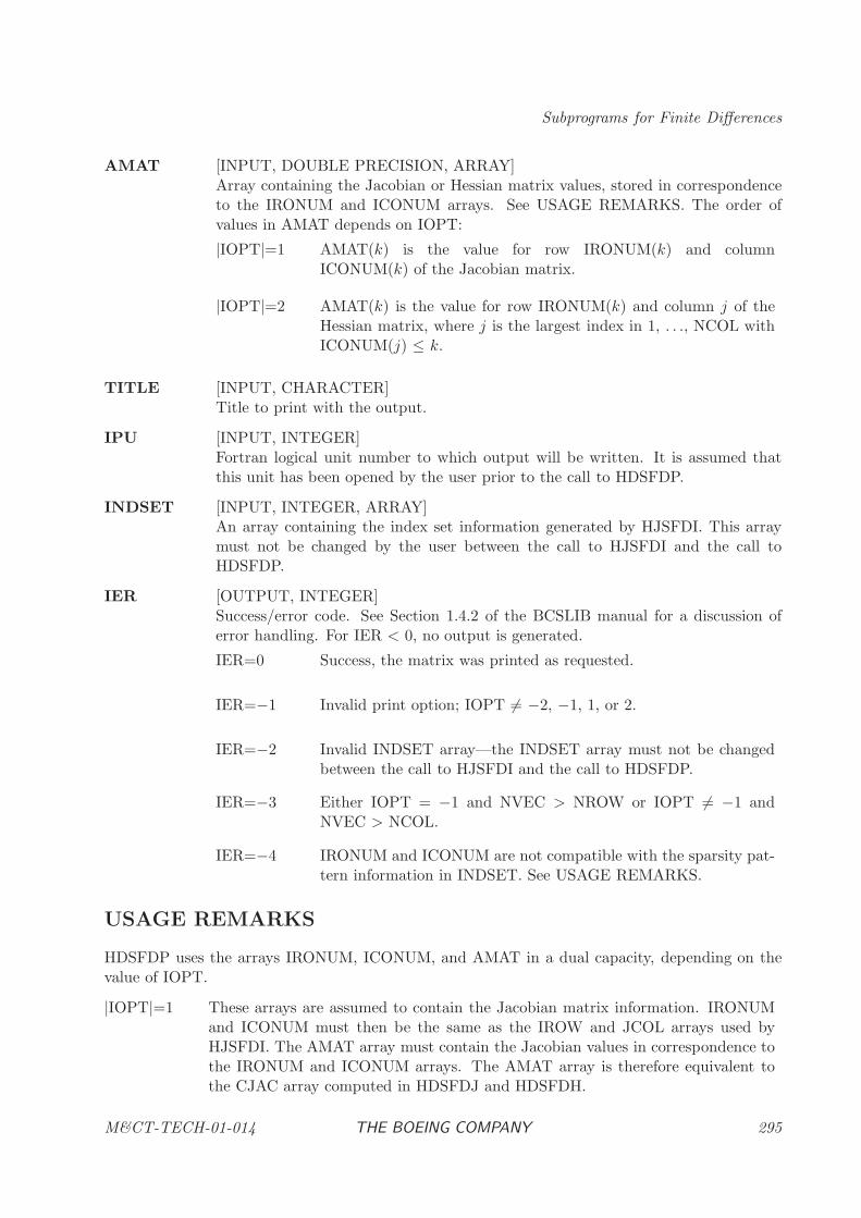
Subprograms for Finite Differences
AMAT [INPUT, DOUBLE PRECISION, ARRAY]Array containing the Jacobian or Hessian matrix values, stored in correspondenceto the IRONUM and ICONUM arrays. See USAGE REMARKS. The order ofvalues in AMAT depends on IOPT:
|IOPT|=1 AMAT(k) is the value for row IRONUM(k) and columnICONUM(k) of the Jacobian matrix.
|IOPT|=2 AMAT(k) is the value for row IRONUM(k) and column j of theHessian matrix, where j is the largest index in 1, . . ., NCOL withICONUM(j) ≤ k.
TITLE [INPUT, CHARACTER]Title to print with the output.
IPU [INPUT, INTEGER]Fortran logical unit number to which output will be written. It is assumed thatthis unit has been opened by the user prior to the call to HDSFDP.
INDSET [INPUT, INTEGER, ARRAY]An array containing the index set information generated by HJSFDI. This arraymust not be changed by the user between the call to HJSFDI and the call toHDSFDP.
IER [OUTPUT, INTEGER]Success/error code. See Section 1.4.2 of the BCSLIB manual for a discussion oferror handling. For IER < 0, no output is generated.
IER=0 Success, the matrix was printed as requested.
IER=−1 Invalid print option; IOPT 6= −2, −1, 1, or 2.
IER=−2 Invalid INDSET array—the INDSET array must not be changedbetween the call to HJSFDI and the call to HDSFDP.
IER=−3 Either IOPT = −1 and NVEC > NROW or IOPT 6= −1 andNVEC > NCOL.
IER=−4 IRONUM and ICONUM are not compatible with the sparsity pat-tern information in INDSET. See USAGE REMARKS.
USAGE REMARKS
HDSFDP uses the arrays IRONUM, ICONUM, and AMAT in a dual capacity, depending on thevalue of IOPT.
|IOPT|=1 These arrays are assumed to contain the Jacobian matrix information. IRONUMand ICONUM must then be the same as the IROW and JCOL arrays used byHJSFDI. The AMAT array must contain the Jacobian values in correspondence tothe IRONUM and ICONUM arrays. The AMAT array is therefore equivalent tothe CJAC array computed in HDSFDJ and HDSFDH.
M&CT-TECH-01-014 THE BOEING COMPANY 295

Finite Difference Derivatives
|IOPT|=2 These arrays are assumed to contain the Hessian matrix information. IRONUMand ICONUM must then be the same as the IROWH and IPCOLH arrays used byHJSFDI. The AMAT array must contain the Hessian values in correspondence tothe IRONUM and ICONUM arrays. The AMAT array is therefore equivalent tothe HMAT array computed in HDSFDH.
EXAMPLE
See HDSFDJ and HDSFDH for an example illustrating the use of HDSFDC.
296 THE BOEING COMPANY M&CT-TECH-01-014
Chapter 4
Advanced Usage Examples
4.1 Introduction—Advanced Application Examples
The optimization and derivative software described in the preceding chapters can be utilized tosolve very complex problems. While it is not feasible to anticipate all possible uses for the suite ofroutines, a number of typical situations are illustrated in this chapter. The first three examples inSections 4.2, 4.3, and 4.4 illustrate how the optimization software can be used in conjunction withthe finite difference derivative software. The last two examples in Sections 4.5 and 4.6 illustratehow the diagnostic capabilities of the algorithm can be exploited to interpret
M&CT-TECH-01-014 THE BOEING COMPANY 297
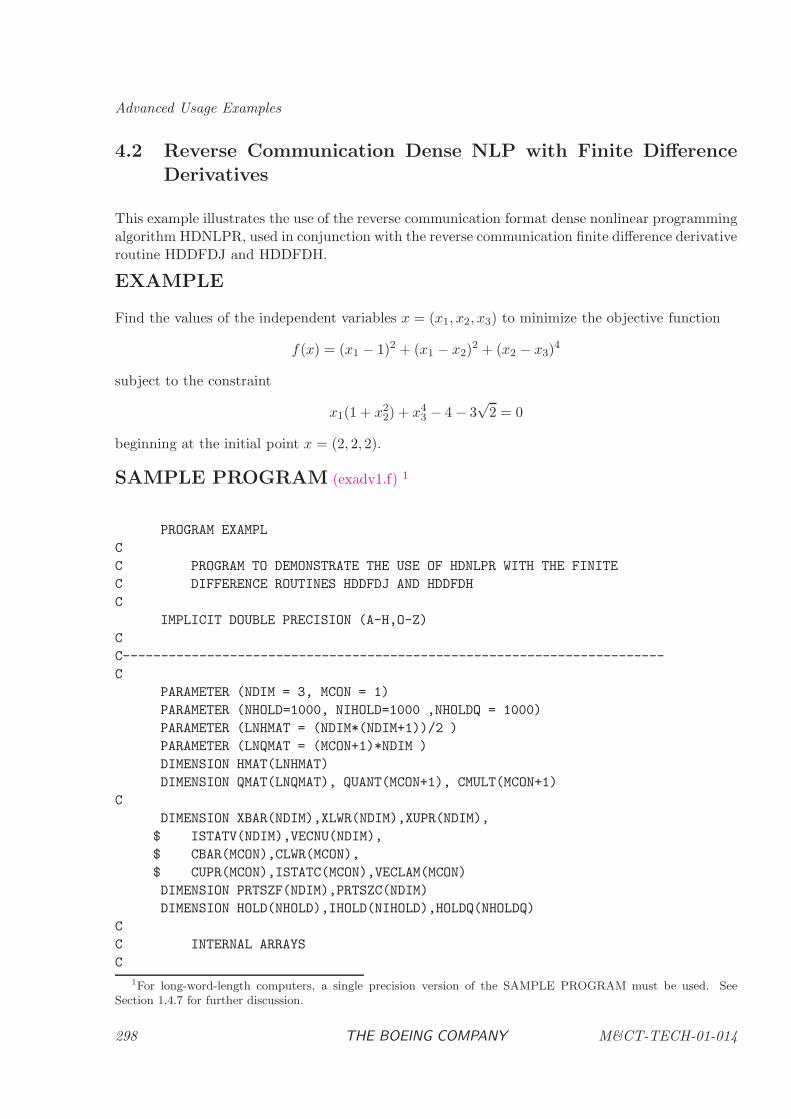
Advanced Usage Examples
4.2 Reverse Communication Dense NLP with Finite Difference
Derivatives
This example illustrates the use of the reverse communication format dense nonlinear programmingalgorithm HDNLPR, used in conjunction with the reverse communication finite difference derivativeroutine HDDFDJ and HDDFDH.
EXAMPLE
Find the values of the independent variables x = (x1, x2, x3) to minimize the objective function
f(x) = (x1 − 1)2 + (x1 − x2)2 + (x2 − x3)
4
subject to the constraint
x1(1 + x22) + x4
3 − 4 − 3√
2 = 0
beginning at the initial point x = (2, 2, 2).
SAMPLE PROGRAM (exadv1.f) 1
PROGRAM EXAMPL
C
C PROGRAM TO DEMONSTRATE THE USE OF HDNLPR WITH THE FINITE
C DIFFERENCE ROUTINES HDDFDJ AND HDDFDH
C
IMPLICIT DOUBLE PRECISION (A-H,O-Z)
C
C-----------------------------------------------------------------------
C
PARAMETER (NDIM = 3, MCON = 1)
PARAMETER (NHOLD=1000, NIHOLD=1000 ,NHOLDQ = 1000)
PARAMETER (LNHMAT = (NDIM*(NDIM+1))/2 )
PARAMETER (LNQMAT = (MCON+1)*NDIM )
DIMENSION HMAT(LNHMAT)
DIMENSION QMAT(LNQMAT), QUANT(MCON+1), CMULT(MCON+1)
C
DIMENSION XBAR(NDIM),XLWR(NDIM),XUPR(NDIM),
$ ISTATV(NDIM),VECNU(NDIM),
$ CBAR(MCON),CLWR(MCON),
$ CUPR(MCON),ISTATC(MCON),VECLAM(MCON)
DIMENSION PRTSZF(NDIM),PRTSZC(NDIM)
DIMENSION HOLD(NHOLD),IHOLD(NIHOLD),HOLDQ(NHOLDQ)
C
C INTERNAL ARRAYS
C
1For long-word-length computers, a single precision version of the SAMPLE PROGRAM must be used. See
Section 1.4.7 for further discussion.
298 THE BOEING COMPANY M&CT-TECH-01-014
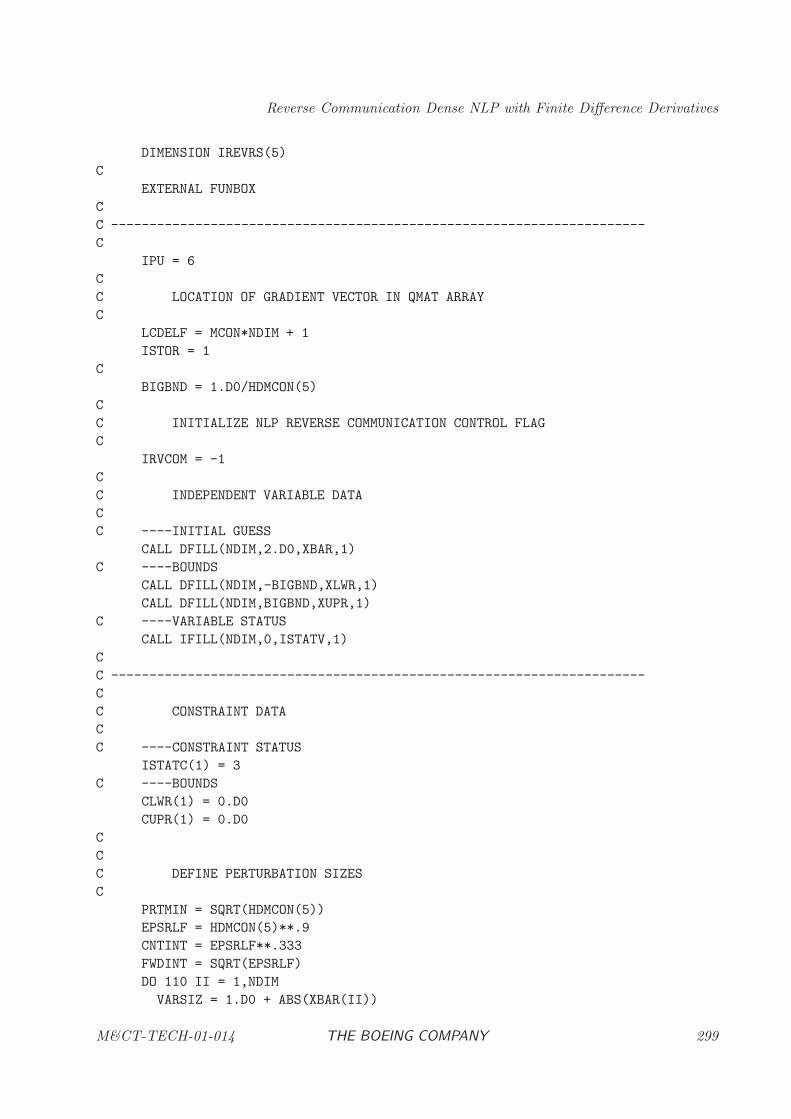
Reverse Communication Dense NLP with Finite Difference Derivatives
DIMENSION IREVRS(5)
C
EXTERNAL FUNBOX
C
C ----------------------------------------------------------------------
C
IPU = 6
C
C LOCATION OF GRADIENT VECTOR IN QMAT ARRAY
C
LCDELF = MCON*NDIM + 1
ISTOR = 1
C
BIGBND = 1.D0/HDMCON(5)
C
C INITIALIZE NLP REVERSE COMMUNICATION CONTROL FLAG
C
IRVCOM = -1
C
C INDEPENDENT VARIABLE DATA
C
C ----INITIAL GUESS
CALL DFILL(NDIM,2.D0,XBAR,1)
C ----BOUNDS
CALL DFILL(NDIM,-BIGBND,XLWR,1)
CALL DFILL(NDIM,BIGBND,XUPR,1)
C ----VARIABLE STATUS
CALL IFILL(NDIM,0,ISTATV,1)
C
C ----------------------------------------------------------------------
C
C CONSTRAINT DATA
C
C ----CONSTRAINT STATUS
ISTATC(1) = 3
C ----BOUNDS
CLWR(1) = 0.D0
CUPR(1) = 0.D0
C
C
C DEFINE PERTURBATION SIZES
C
PRTMIN = SQRT(HDMCON(5))
EPSRLF = HDMCON(5)**.9
CNTINT = EPSRLF**.333
FWDINT = SQRT(EPSRLF)
DO 110 II = 1,NDIM
VARSIZ = 1.D0 + ABS(XBAR(II))
M&CT-TECH-01-014 THE BOEING COMPANY 299
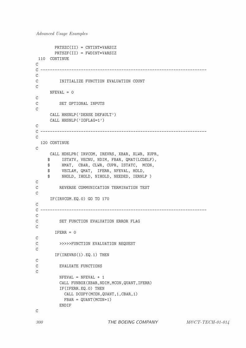
Advanced Usage Examples
PRTSZC(II) = CNTINT*VARSIZ
PRTSZF(II) = FWDINT*VARSIZ
110 CONTINUE
C
C ----------------------------------------------------------------------
C
C INITIALIZE FUNCTION EVALUATION COUNT
C
NFEVAL = 0
C
C SET OPTIONAL INPUTS
C
CALL HHSNLP(’DENSE DEFAULT’)
CALL HHSNLP(’IOFLAG=1’)
C
C ----------------------------------------------------------------------
C
120 CONTINUE
C
CALL HDNLPR( IRVCOM, IREVRS, XBAR, XLWR, XUPR,
$ ISTATV, VECNU, NDIM, FBAR, QMAT(LCDELF),
$ HMAT, CBAR, CLWR, CUPR, ISTATC, MCON,
$ VECLAM, QMAT, IFERR, NFEVAL, HOLD,
$ NHOLD, IHOLD, NIHOLD, NEEDED, IERNLP )
C
C REVERSE COMMUNICATION TERMINATION TEST
C
IF(IRVCOM.EQ.0) GO TO 170
C
C ----------------------------------------------------------------------
C
C SET FUNCTION EVALUATION ERROR FLAG
C
IFERR = 0
C
C >>>>>FUNCTION EVALUATION REQUEST
C
IF(IREVRS(1).EQ.1) THEN
C
C EVALUATE FUNCTIONS
C
NFEVAL = NFEVAL + 1
CALL FUNBOX(XBAR,NDIM,MCON,QUANT,IFERR)
IF(IFERR.EQ.0) THEN
CALL DCOPY(MCON,QUANT,1,CBAR,1)
FBAR = QUANT(MCON+1)
ENDIF
C
300 THE BOEING COMPANY M&CT-TECH-01-014
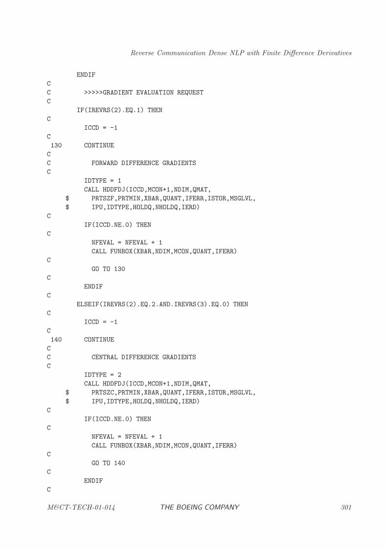
Reverse Communication Dense NLP with Finite Difference Derivatives
ENDIF
C
C >>>>>GRADIENT EVALUATION REQUEST
C
IF(IREVRS(2).EQ.1) THEN
C
ICCD = -1
C
130 CONTINUE
C
C FORWARD DIFFERENCE GRADIENTS
C
IDTYPE = 1
CALL HDDFDJ(ICCD,MCON+1,NDIM,QMAT,
$ PRTSZF,PRTMIN,XBAR,QUANT,IFERR,ISTOR,MSGLVL,
$ IPU,IDTYPE,HOLDQ,NHOLDQ,IERD)
C
IF(ICCD.NE.0) THEN
C
NFEVAL = NFEVAL + 1
CALL FUNBOX(XBAR,NDIM,MCON,QUANT,IFERR)
C
GO TO 130
C
ENDIF
C
ELSEIF(IREVRS(2).EQ.2.AND.IREVRS(3).EQ.0) THEN
C
ICCD = -1
C
140 CONTINUE
C
C CENTRAL DIFFERENCE GRADIENTS
C
IDTYPE = 2
CALL HDDFDJ(ICCD,MCON+1,NDIM,QMAT,
$ PRTSZC,PRTMIN,XBAR,QUANT,IFERR,ISTOR,MSGLVL,
$ IPU,IDTYPE,HOLDQ,NHOLDQ,IERD)
C
IF(ICCD.NE.0) THEN
C
NFEVAL = NFEVAL + 1
CALL FUNBOX(XBAR,NDIM,MCON,QUANT,IFERR)
C
GO TO 140
C
ENDIF
C
M&CT-TECH-01-014 THE BOEING COMPANY 301
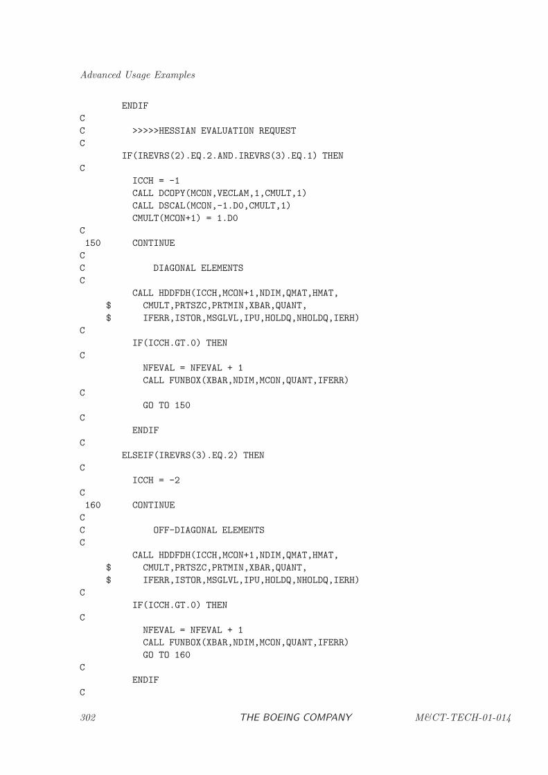
Advanced Usage Examples
ENDIF
C
C >>>>>HESSIAN EVALUATION REQUEST
C
IF(IREVRS(2).EQ.2.AND.IREVRS(3).EQ.1) THEN
C
ICCH = -1
CALL DCOPY(MCON,VECLAM,1,CMULT,1)
CALL DSCAL(MCON,-1.D0,CMULT,1)
CMULT(MCON+1) = 1.D0
C
150 CONTINUE
C
C DIAGONAL ELEMENTS
C
CALL HDDFDH(ICCH,MCON+1,NDIM,QMAT,HMAT,
$ CMULT,PRTSZC,PRTMIN,XBAR,QUANT,
$ IFERR,ISTOR,MSGLVL,IPU,HOLDQ,NHOLDQ,IERH)
C
IF(ICCH.GT.0) THEN
C
NFEVAL = NFEVAL + 1
CALL FUNBOX(XBAR,NDIM,MCON,QUANT,IFERR)
C
GO TO 150
C
ENDIF
C
ELSEIF(IREVRS(3).EQ.2) THEN
C
ICCH = -2
C
160 CONTINUE
C
C OFF-DIAGONAL ELEMENTS
C
CALL HDDFDH(ICCH,MCON+1,NDIM,QMAT,HMAT,
$ CMULT,PRTSZC,PRTMIN,XBAR,QUANT,
$ IFERR,ISTOR,MSGLVL,IPU,HOLDQ,NHOLDQ,IERH)
C
IF(ICCH.GT.0) THEN
C
NFEVAL = NFEVAL + 1
CALL FUNBOX(XBAR,NDIM,MCON,QUANT,IFERR)
GO TO 160
C
ENDIF
C
302 THE BOEING COMPANY M&CT-TECH-01-014
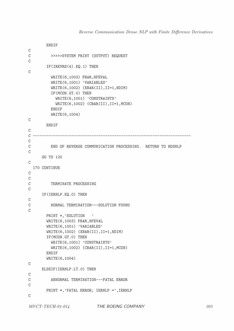
Reverse Communication Dense NLP with Finite Difference Derivatives
ENDIF
C
C >>>>>SYSTEM PRINT (OUTPUT) REQUEST
C
IF(IREVRS(4).EQ.1) THEN
C
WRITE(6,1003) FBAR,NFEVAL
WRITE(6,1001) ’VARIABLES’
WRITE(6,1002) (XBAR(II),II=1,NDIM)
IF(MCON.GT.0) THEN
WRITE(6,1001) ’CONSTRAINTS’
WRITE(6,1002) (CBAR(II),II=1,MCON)
ENDIF
WRITE(6,1004)
C
ENDIF
C
C ----------------------------------------------------------------------
C
C END OF REVERSE COMMUNICATION PROCESSING. RETURN TO HDSNLP
C
GO TO 120
C
170 CONTINUE
C
C
C TERMINATE PROCESSING
C
IF(IERNLP.EQ.0) THEN
C
C NORMAL TERMINATION---SOLUTION FOUND
C
PRINT *,’SOLUTION ’
WRITE(6,1003) FBAR,NFEVAL
WRITE(6,1001) ’VARIABLES’
WRITE(6,1002) (XBAR(II),II=1,NDIM)
IF(MCON.GT.0) THEN
WRITE(6,1001) ’CONSTRAINTS’
WRITE(6,1002) (CBAR(II),II=1,MCON)
ENDIF
WRITE(6,1004)
C
ELSEIF(IERNLP.LT.0) THEN
C
C ABNORMAL TERMINATION---FATAL ERROR
C
PRINT *,’FATAL ERROR; IERNLP =’,IERNLP
C
M&CT-TECH-01-014 THE BOEING COMPANY 303
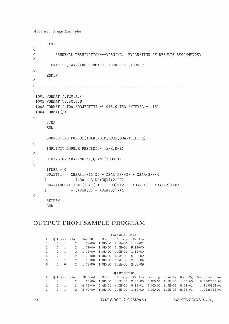
Advanced Usage Examples
ELSE
C
C ABNORMAL TERMINATION---WARNING. EVALUATION OF RESULTS RECOMMENDED!
C
PRINT *,’WARNING MESSAGE; IERNLP =’,IERNLP
C
ENDIF
C
C-----------------------------------------------------------------------
C
1001 FORMAT(/,T20,A,/)
1002 FORMAT(T5,5G16.6)
1003 FORMAT(/,T20,’OBJECTIVE =’,G16.6,T60,’NFEVAL =’,I5)
1004 FORMAT(/)
C
STOP
END
SUBROUTINE FUNBOX(XBAR,NDIM,MCON,QUANT,IFERR)
C
IMPLICIT DOUBLE PRECISION (A-H,O-Z)
C
DIMENSION XBAR(NDIM),QUANT(MCON+1)
C
IFERR = 0
QUANT(1) = XBAR(1)*(1.D0 + XBAR(2)**2) + XBAR(3)**4
$ - 4.D0 - 3.D0*SQRT(2.D0)
QUANT(MCON+1) = (XBAR(1) - 1.D0)**2 + (XBAR(1) - XBAR(2))**2
$ + (XBAR(2) - XBAR(3))**4
C
RETURN
END
OUTPUT FROM SAMPLE PROGRAM
Feasible Point
It Qit Nkt Ndof Cond(G) Step Norm p Violtn
1 1 1 2 1.0E+00 1.0E+00 5.3E-01 1.8E+01
2 2 1 2 1.0E+00 1.0E+00 3.4E-01 5.3E+00
3 2 1 2 1.0E+00 1.0E+00 1.0E-01 1.1E+00
4 2 1 2 1.0E+00 1.0E+00 6.4E-03 5.8E-02
5 2 1 2 1.0E+00 1.0E+00 2.2E-05 2.0E-04
6 0 0 2 1.0E+00 1.0E+00 2.2E-05 2.3E-09
Optimization
It Qit Nkt Ndof PH Cond Step Norm p Violtn Levnbrg Penalty Norm Pg Merit Function
1 2 1 2 1.0E+00 1.0E+00 1.8E+00 2.3E-09 0.0E+00 1.5E-08 1.6E+00 6.988735E-01
2 2 1 2 4.7E+00 3.4E-01 6.5E-01 8.9E-01 0.0E+00 1.5E-08 8.4E-01 1.919590E-01
3 2 1 2 3.4E+00 1.0E+00 3.5E-01 1.1E+00 0.0E+00 1.5E-08 8.8E-01 1.033876E-01
304 THE BOEING COMPANY M&CT-TECH-01-014
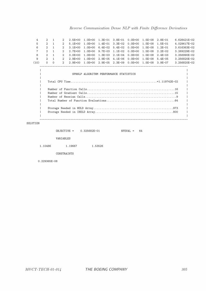
Reverse Communication Dense NLP with Finite Difference Derivatives
4 2 1 2 2.5E+00 1.0E+00 1.3E-01 3.8E-01 0.0E+00 1.5E-08 2.8E-01 6.628421E-02
5 2 1 2 5.1E+00 1.0E+00 1.4E-01 3.3E-02 0.0E+00 1.5E-08 1.5E-01 4.029617E-02
6 2 1 2 3.1E+00 1.0E+00 6.4E-02 5.4E-02 0.0E+00 1.5E-08 1.2E-01 3.616363E-02
7 2 1 2 2.7E+00 1.0E+00 9.7E-03 1.1E-02 0.0E+00 1.5E-08 2.2E-02 3.269229E-02
8 2 1 2 3.0E+00 1.0E+00 1.3E-03 2.1E-04 0.0E+00 1.5E-08 2.4E-03 3.256990E-02
9 2 1 2 2.9E+00 1.0E+00 2.9E-05 4.1E-06 0.0E+00 1.5E-08 5.4E-05 3.256820E-02
(10) 0 0 2 2.9E+00 1.0E+00 2.9E-05 2.3E-09 0.0E+00 1.5E-08 3.9E-07 3.256820E-02
-------------------------------------------------------------------------------------------
| |
| SPRNLP ALGORITHM PERFORMANCE STATISTICS |
| |
| Total CPU Time.....................................................+1.119742E-02 |
| |
| Number of Function Calls......................................................16 |
| Number of Gradient Calls......................................................15 |
| Number of Hessian Calls........................................................9 |
| Total Number of Function Evaluations..........................................64 |
| |
| Storage Needed in HOLD Array.................................................973 |
| Storage Needed in IHOLD Array................................................800 |
| |
-------------------------------------------------------------------------------------------
SOLUTION
OBJECTIVE = 0.325682E-01 NFEVAL = 64
VARIABLES
1.10486 1.19667 1.53526
CONSTRAINTS
0.229365E-08
M&CT-TECH-01-014 THE BOEING COMPANY 305
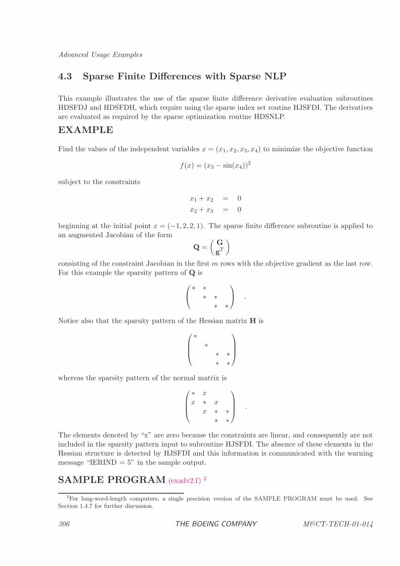
Advanced Usage Examples
4.3 Sparse Finite Differences with Sparse NLP
This example illustrates the use of the sparse finite difference derivative evaluation subroutinesHDSFDJ and HDSFDH, which require using the sparse index set routine HJSFDI. The derivativesare evaluated as required by the sparse optimization routine HDSNLP.
EXAMPLE
Find the values of the independent variables x = (x1, x2, x3, x4) to minimize the objective function
f(x) = (x3 − sin(x4))2
subject to the constraints
x1 + x2 = 0
x2 + x3 = 0
beginning at the initial point x = (−1, 2, 2, 1). The sparse finite difference subroutine is applied toan augmented Jacobian of the form
Q =
(GgT
)
consisting of the constraint Jacobian in the first m rows with the objective gradient as the last row.For this example the sparsity pattern of Q is
∗ ∗
∗ ∗∗ ∗
.
Notice also that the sparsity pattern of the Hessian matrix H is
∗∗
∗ ∗∗ ∗
whereas the sparsity pattern of the normal matrix is
∗ xx ∗ x
x ∗ ∗∗ ∗
.
The elements denoted by “x” are zero because the constraints are linear, and consequently are notincluded in the sparsity pattern input to subroutine HJSFDI. The absence of these elements in theHessian structure is detected by HJSFDI and this information is communicated with the warningmessage “IERIND = 5” in the sample output.
SAMPLE PROGRAM (exadv2.f) 2
2For long-word-length computers, a single precision version of the SAMPLE PROGRAM must be used. See
Section 1.4.7 for further discussion.
306 THE BOEING COMPANY M&CT-TECH-01-014
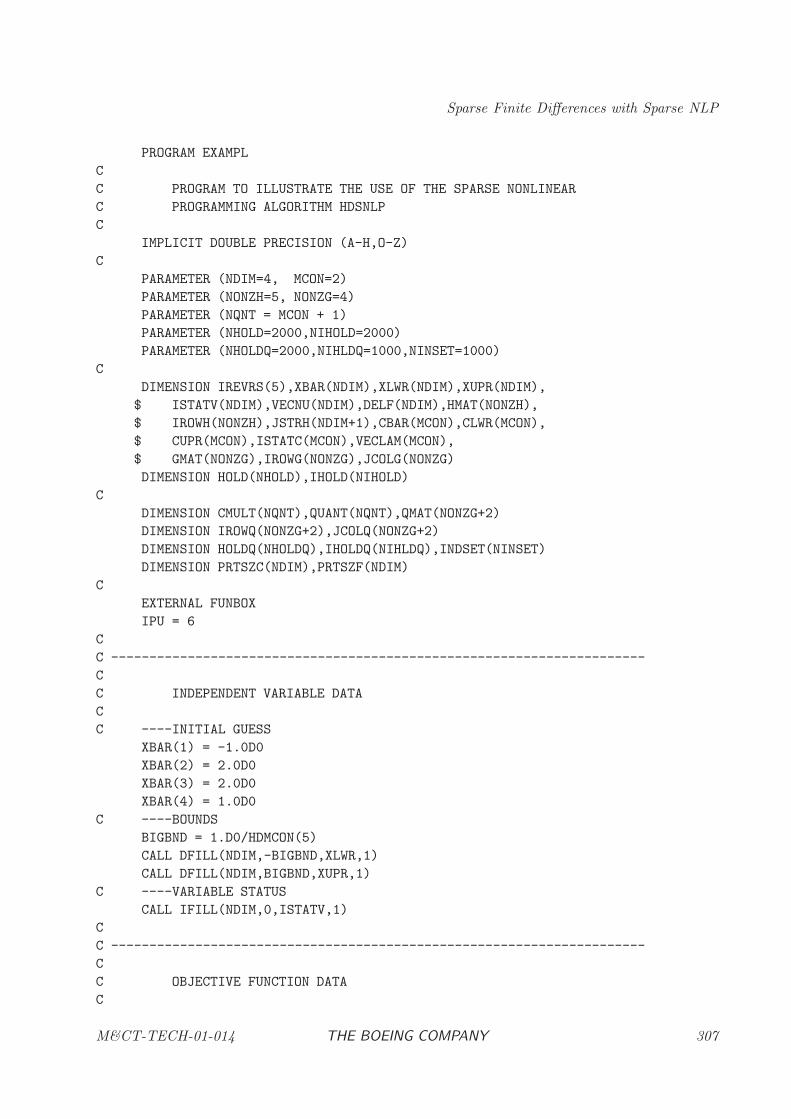
Sparse Finite Differences with Sparse NLP
PROGRAM EXAMPL
C
C PROGRAM TO ILLUSTRATE THE USE OF THE SPARSE NONLINEAR
C PROGRAMMING ALGORITHM HDSNLP
C
IMPLICIT DOUBLE PRECISION (A-H,O-Z)
C
PARAMETER (NDIM=4, MCON=2)
PARAMETER (NONZH=5, NONZG=4)
PARAMETER (NQNT = MCON + 1)
PARAMETER (NHOLD=2000,NIHOLD=2000)
PARAMETER (NHOLDQ=2000,NIHLDQ=1000,NINSET=1000)
C
DIMENSION IREVRS(5),XBAR(NDIM),XLWR(NDIM),XUPR(NDIM),
$ ISTATV(NDIM),VECNU(NDIM),DELF(NDIM),HMAT(NONZH),
$ IROWH(NONZH),JSTRH(NDIM+1),CBAR(MCON),CLWR(MCON),
$ CUPR(MCON),ISTATC(MCON),VECLAM(MCON),
$ GMAT(NONZG),IROWG(NONZG),JCOLG(NONZG)
DIMENSION HOLD(NHOLD),IHOLD(NIHOLD)
C
DIMENSION CMULT(NQNT),QUANT(NQNT),QMAT(NONZG+2)
DIMENSION IROWQ(NONZG+2),JCOLQ(NONZG+2)
DIMENSION HOLDQ(NHOLDQ),IHOLDQ(NIHLDQ),INDSET(NINSET)
DIMENSION PRTSZC(NDIM),PRTSZF(NDIM)
C
EXTERNAL FUNBOX
IPU = 6
C
C ----------------------------------------------------------------------
C
C INDEPENDENT VARIABLE DATA
C
C ----INITIAL GUESS
XBAR(1) = -1.0D0
XBAR(2) = 2.0D0
XBAR(3) = 2.0D0
XBAR(4) = 1.0D0
C ----BOUNDS
BIGBND = 1.D0/HDMCON(5)
CALL DFILL(NDIM,-BIGBND,XLWR,1)
CALL DFILL(NDIM,BIGBND,XUPR,1)
C ----VARIABLE STATUS
CALL IFILL(NDIM,0,ISTATV,1)
C
C ----------------------------------------------------------------------
C
C OBJECTIVE FUNCTION DATA
C
M&CT-TECH-01-014 THE BOEING COMPANY 307
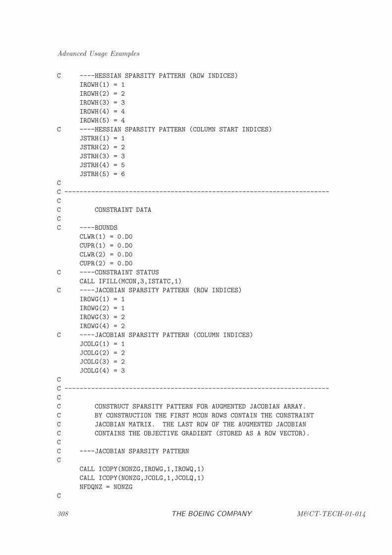
Advanced Usage Examples
C ----HESSIAN SPARSITY PATTERN (ROW INDICES)
IROWH(1) = 1
IROWH(2) = 2
IROWH(3) = 3
IROWH(4) = 4
IROWH(5) = 4
C ----HESSIAN SPARSITY PATTERN (COLUMN START INDICES)
JSTRH(1) = 1
JSTRH(2) = 2
JSTRH(3) = 3
JSTRH(4) = 5
JSTRH(5) = 6
C
C ----------------------------------------------------------------------
C
C CONSTRAINT DATA
C
C ----BOUNDS
CLWR(1) = 0.D0
CUPR(1) = 0.D0
CLWR(2) = 0.D0
CUPR(2) = 0.D0
C ----CONSTRAINT STATUS
CALL IFILL(MCON,3,ISTATC,1)
C ----JACOBIAN SPARSITY PATTERN (ROW INDICES)
IROWG(1) = 1
IROWG(2) = 1
IROWG(3) = 2
IROWG(4) = 2
C ----JACOBIAN SPARSITY PATTERN (COLUMN INDICES)
JCOLG(1) = 1
JCOLG(2) = 2
JCOLG(3) = 2
JCOLG(4) = 3
C
C ----------------------------------------------------------------------
C
C CONSTRUCT SPARSITY PATTERN FOR AUGMENTED JACOBIAN ARRAY.
C BY CONSTRUCTION THE FIRST MCON ROWS CONTAIN THE CONSTRAINT
C JACOBIAN MATRIX. THE LAST ROW OF THE AUGMENTED JACOBIAN
C CONTAINS THE OBJECTIVE GRADIENT (STORED AS A ROW VECTOR).
C
C ----JACOBIAN SPARSITY PATTERN
C
CALL ICOPY(NONZG,IROWG,1,IROWQ,1)
CALL ICOPY(NONZG,JCOLG,1,JCOLQ,1)
NFDQNZ = NONZG
C
308 THE BOEING COMPANY M&CT-TECH-01-014
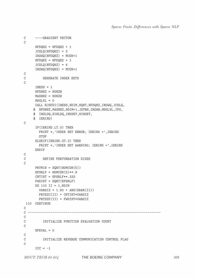
Sparse Finite Differences with Sparse NLP
C ----GRADIENT VECTOR
C
NFDQNZ = NFDQNZ + 1
JCOLQ(NFDQNZ) = 3
IROWQ(NFDQNZ) = MCON+1
NFDQNZ = NFDQNZ + 1
JCOLQ(NFDQNZ) = 4
IROWQ(NFDQNZ) = MCON+1
C
C GENERATE INDEX SETS
C
IHESS = 1
NFDHNZ = NONZH
MAXHNZ = NONZH
MSGLVL = 0
CALL HJSFDI(IHESS,NDIM,NQNT,NFDQNZ,IROWQ,JCOLQ,
$ NFDHNZ,MAXHNZ,NDIM+1,JSTRH,IROWH,MSGLVL,IPU,
$ IHOLDQ,NIHLDQ,INDSET,NINSET,
$ IERIND)
C
IF(IERIND.LT.0) THEN
PRINT *,’INDEX SET ERROR; IERIND =’,IERIND
STOP
ELSEIF(IERIND.GT.0) THEN
PRINT *,’INDEX SET WARNING; IERIND =’,IERIND
ENDIF
C
C DEFINE PERTURBATION SIZES
C
PRTMIN = SQRT(HDMCON(5))
EPSRLF = HDMCON(5)**.9
CNTINT = EPSRLF**.333
FWDINT = SQRT(EPSRLF)
DO 110 II = 1,NDIM
VARSIZ = 1.D0 + ABS(XBAR(II))
PRTSZC(II) = CNTINT*VARSIZ
PRTSZF(II) = FWDINT*VARSIZ
110 CONTINUE
C
C ----------------------------------------------------------------------
C
C INITIALIZE FUNCTION EVALUATION COUNT
C
NFEVAL = 0
C
C INITIALIZE REVERSE COMMUNICATION CONTROL FLAG
C
ICC = -1
M&CT-TECH-01-014 THE BOEING COMPANY 309
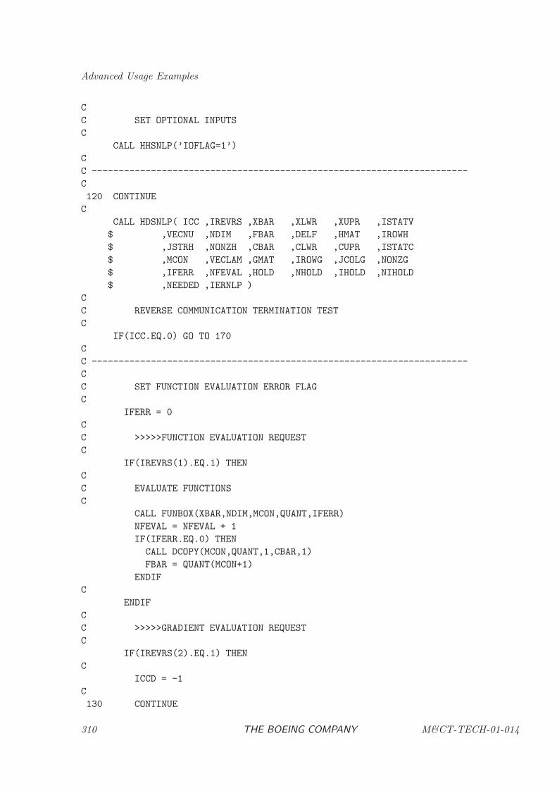
Advanced Usage Examples
C
C SET OPTIONAL INPUTS
C
CALL HHSNLP(’IOFLAG=1’)
C
C ----------------------------------------------------------------------
C
120 CONTINUE
C
CALL HDSNLP( ICC ,IREVRS ,XBAR ,XLWR ,XUPR ,ISTATV
$ ,VECNU ,NDIM ,FBAR ,DELF ,HMAT ,IROWH
$ ,JSTRH ,NONZH ,CBAR ,CLWR ,CUPR ,ISTATC
$ ,MCON ,VECLAM ,GMAT ,IROWG ,JCOLG ,NONZG
$ ,IFERR ,NFEVAL ,HOLD ,NHOLD ,IHOLD ,NIHOLD
$ ,NEEDED ,IERNLP )
C
C REVERSE COMMUNICATION TERMINATION TEST
C
IF(ICC.EQ.0) GO TO 170
C
C ----------------------------------------------------------------------
C
C SET FUNCTION EVALUATION ERROR FLAG
C
IFERR = 0
C
C >>>>>FUNCTION EVALUATION REQUEST
C
IF(IREVRS(1).EQ.1) THEN
C
C EVALUATE FUNCTIONS
C
CALL FUNBOX(XBAR,NDIM,MCON,QUANT,IFERR)
NFEVAL = NFEVAL + 1
IF(IFERR.EQ.0) THEN
CALL DCOPY(MCON,QUANT,1,CBAR,1)
FBAR = QUANT(MCON+1)
ENDIF
C
ENDIF
C
C >>>>>GRADIENT EVALUATION REQUEST
C
IF(IREVRS(2).EQ.1) THEN
C
ICCD = -1
C
130 CONTINUE
310 THE BOEING COMPANY M&CT-TECH-01-014
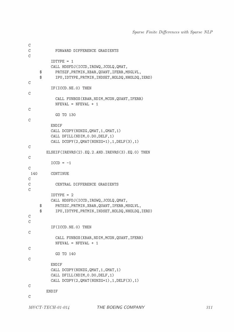
Sparse Finite Differences with Sparse NLP
C
C FORWARD DIFFERENCE GRADIENTS
C
IDTYPE = 1
CALL HDSFDJ(ICCD,IROWQ,JCOLQ,QMAT,
$ PRTSZF,PRTMIN,XBAR,QUANT,IFERR,MSGLVL,
$ IPU,IDTYPE,PRTMIN,INDSET,HOLDQ,NHOLDQ,IERD)
C
IF(ICCD.NE.0) THEN
C
CALL FUNBOX(XBAR,NDIM,MCON,QUANT,IFERR)
NFEVAL = NFEVAL + 1
C
GO TO 130
C
ENDIF
CALL DCOPY(NONZG,QMAT,1,GMAT,1)
CALL DFILL(NDIM,0.D0,DELF,1)
CALL DCOPY(2,QMAT(NONZG+1),1,DELF(3),1)
C
ELSEIF(IREVRS(2).EQ.2.AND.IREVRS(3).EQ.0) THEN
C
ICCD = -1
C
140 CONTINUE
C
C CENTRAL DIFFERENCE GRADIENTS
C
IDTYPE = 2
CALL HDSFDJ(ICCD,IROWQ,JCOLQ,QMAT,
$ PRTSZC,PRTMIN,XBAR,QUANT,IFERR,MSGLVL,
$ IPU,IDTYPE,PRTMIN,INDSET,HOLDQ,NHOLDQ,IERD)
C
C
IF(ICCD.NE.0) THEN
C
CALL FUNBOX(XBAR,NDIM,MCON,QUANT,IFERR)
NFEVAL = NFEVAL + 1
C
GO TO 140
C
ENDIF
CALL DCOPY(NONZG,QMAT,1,GMAT,1)
CALL DFILL(NDIM,0.D0,DELF,1)
CALL DCOPY(2,QMAT(NONZG+1),1,DELF(3),1)
C
ENDIF
C
M&CT-TECH-01-014 THE BOEING COMPANY 311
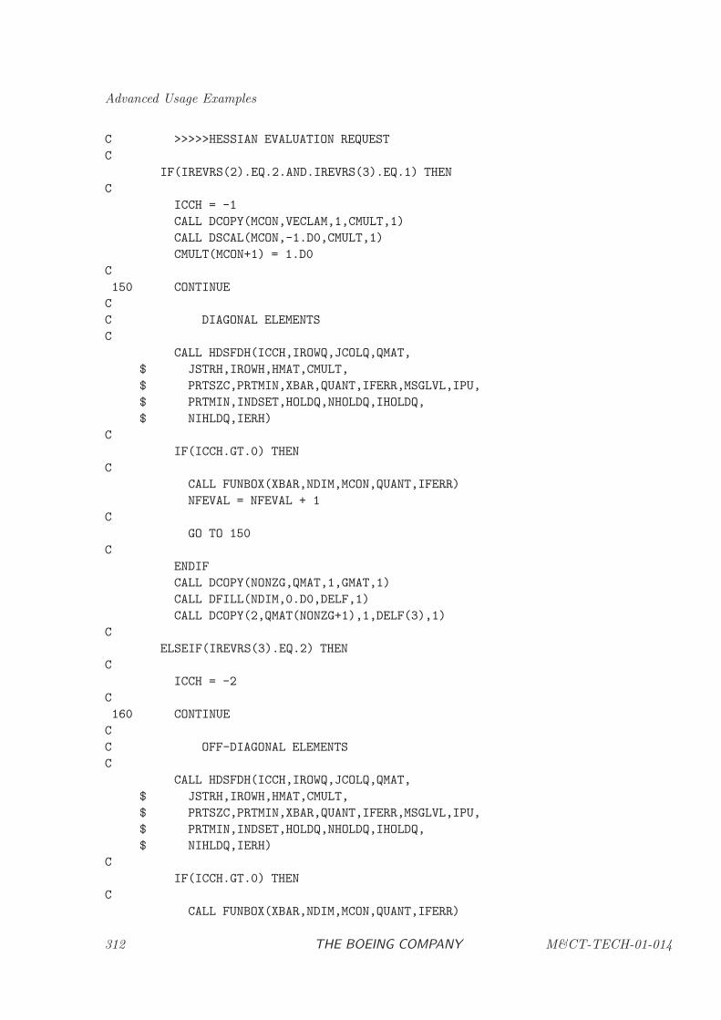
Advanced Usage Examples
C >>>>>HESSIAN EVALUATION REQUEST
C
IF(IREVRS(2).EQ.2.AND.IREVRS(3).EQ.1) THEN
C
ICCH = -1
CALL DCOPY(MCON,VECLAM,1,CMULT,1)
CALL DSCAL(MCON,-1.D0,CMULT,1)
CMULT(MCON+1) = 1.D0
C
150 CONTINUE
C
C DIAGONAL ELEMENTS
C
CALL HDSFDH(ICCH,IROWQ,JCOLQ,QMAT,
$ JSTRH,IROWH,HMAT,CMULT,
$ PRTSZC,PRTMIN,XBAR,QUANT,IFERR,MSGLVL,IPU,
$ PRTMIN,INDSET,HOLDQ,NHOLDQ,IHOLDQ,
$ NIHLDQ,IERH)
C
IF(ICCH.GT.0) THEN
C
CALL FUNBOX(XBAR,NDIM,MCON,QUANT,IFERR)
NFEVAL = NFEVAL + 1
C
GO TO 150
C
ENDIF
CALL DCOPY(NONZG,QMAT,1,GMAT,1)
CALL DFILL(NDIM,0.D0,DELF,1)
CALL DCOPY(2,QMAT(NONZG+1),1,DELF(3),1)
C
ELSEIF(IREVRS(3).EQ.2) THEN
C
ICCH = -2
C
160 CONTINUE
C
C OFF-DIAGONAL ELEMENTS
C
CALL HDSFDH(ICCH,IROWQ,JCOLQ,QMAT,
$ JSTRH,IROWH,HMAT,CMULT,
$ PRTSZC,PRTMIN,XBAR,QUANT,IFERR,MSGLVL,IPU,
$ PRTMIN,INDSET,HOLDQ,NHOLDQ,IHOLDQ,
$ NIHLDQ,IERH)
C
IF(ICCH.GT.0) THEN
C
CALL FUNBOX(XBAR,NDIM,MCON,QUANT,IFERR)
312 THE BOEING COMPANY M&CT-TECH-01-014
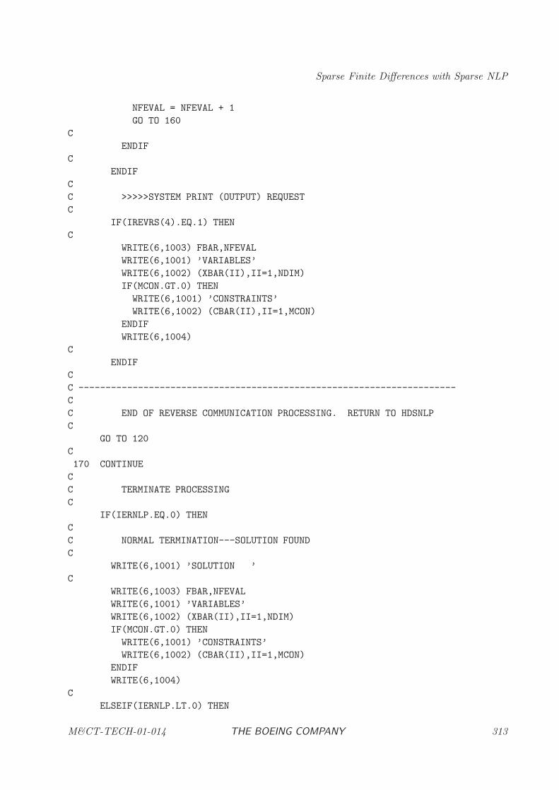
Sparse Finite Differences with Sparse NLP
NFEVAL = NFEVAL + 1
GO TO 160
C
ENDIF
C
ENDIF
C
C >>>>>SYSTEM PRINT (OUTPUT) REQUEST
C
IF(IREVRS(4).EQ.1) THEN
C
WRITE(6,1003) FBAR,NFEVAL
WRITE(6,1001) ’VARIABLES’
WRITE(6,1002) (XBAR(II),II=1,NDIM)
IF(MCON.GT.0) THEN
WRITE(6,1001) ’CONSTRAINTS’
WRITE(6,1002) (CBAR(II),II=1,MCON)
ENDIF
WRITE(6,1004)
C
ENDIF
C
C ----------------------------------------------------------------------
C
C END OF REVERSE COMMUNICATION PROCESSING. RETURN TO HDSNLP
C
GO TO 120
C
170 CONTINUE
C
C TERMINATE PROCESSING
C
IF(IERNLP.EQ.0) THEN
C
C NORMAL TERMINATION---SOLUTION FOUND
C
WRITE(6,1001) ’SOLUTION ’
C
WRITE(6,1003) FBAR,NFEVAL
WRITE(6,1001) ’VARIABLES’
WRITE(6,1002) (XBAR(II),II=1,NDIM)
IF(MCON.GT.0) THEN
WRITE(6,1001) ’CONSTRAINTS’
WRITE(6,1002) (CBAR(II),II=1,MCON)
ENDIF
WRITE(6,1004)
C
ELSEIF(IERNLP.LT.0) THEN
M&CT-TECH-01-014 THE BOEING COMPANY 313
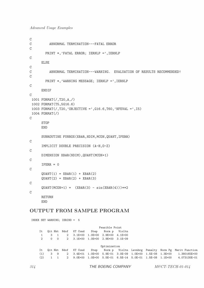
Advanced Usage Examples
C
C ABNORMAL TERMINATION---FATAL ERROR
C
PRINT *,’FATAL ERROR; IERNLP =’,IERNLP
C
ELSE
C
C ABNORMAL TERMINATION---WARNING. EVALUATION OF RESULTS RECOMMENDED!
C
PRINT *,’WARNING MESSAGE; IERNLP =’,IERNLP
C
ENDIF
C
1001 FORMAT(/,T20,A,/)
1002 FORMAT(T5,5G16.6)
1003 FORMAT(/,T20,’OBJECTIVE =’,G16.6,T60,’NFEVAL =’,I5)
1004 FORMAT(/)
C
STOP
END
SUBROUTINE FUNBOX(XBAR,NDIM,MCON,QUANT,IFERR)
C
IMPLICIT DOUBLE PRECISION (A-H,O-Z)
C
DIMENSION XBAR(NDIM),QUANT(MCON+1)
C
IFERR = 0
C
QUANT(1) = XBAR(1) + XBAR(2)
QUANT(2) = XBAR(2) + XBAR(3)
C
QUANT(MCON+1) = (XBAR(3) - sin(XBAR(4)))**2
C
RETURN
END
OUTPUT FROM SAMPLE PROGRAM
INDEX SET WARNING; IERIND = 5
Feasible Point
It Qit Nkt Ndof KT Cond Step Norm p Violtn
1 3 1 2 3.1E+00 1.0E+00 2.9E+00 4.1E+00
2 0 0 2 3.1E+00 1.0E+00 2.9E+00 3.1E-09
Optimization
It Qit Nkt Ndof KT Cond Step Norm p Violtn Levnbrg Penalty Norm Pg Merit Function
(1) 3 9 2 3.4E+01 1.0E+00 5.9E-01 3.0E-09 1.0E+00 1.5E-08 1.3E+00 1.380165E+00
(2) 1 1 2 9.0E+00 1.0E+00 5.5E-01 6.5E-14 5.0E-01 1.5E-08 1.1E+00 4.073135E-01
314 THE BOEING COMPANY M&CT-TECH-01-014
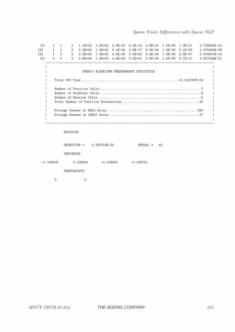
Sparse Finite Differences with Sparse NLP
(3) 1 1 2 1.1E+02 1.0E+00 4.5E-02 6.5E-14 4.6E-02 1.5E-08 1.0E-01 2.729025E-03
[4] 1 1 2 5.2E+03 1.0E+00 9.1E-04 2.8E-17 9.0E-04 1.5E-08 2.1E-03 1.074082E-06
[5] 1 2 2 2.8E+06 1.0E+00 4.9E-05 0.0E+00 3.9E-06 1.5E-08 8.9E-07 2.003607E-13
(6) 0 0 2 2.8E+06 1.0E+00 4.9E-05 0.0E+00 3.9E-06 1.5E-08 9.7E-11 3.257546E-21
-------------------------------------------------------------------------------------------
| |
| SPRNLP ALGORITHM PERFORMANCE STATISTICS |
| |
| Total CPU Time.....................................................+2.210767E-02 |
| |
| Number of Function Calls.......................................................7 |
| Number of Gradient Calls.......................................................8 |
| Number of Hessian Calls........................................................5 |
| Total Number of Function Evaluations..........................................40 |
| |
| Storage Needed in HOLD Array.................................................385 |
| Storage Needed in IHOLD Array.................................................27 |
| |
-------------------------------------------------------------------------------------------
SOLUTION
OBJECTIVE = 0.325755E-20 NFEVAL = 40
VARIABLES
-0.106500 0.106500 -0.106500 -0.106702
CONSTRAINTS
0. 0.
M&CT-TECH-01-014 THE BOEING COMPANY 315
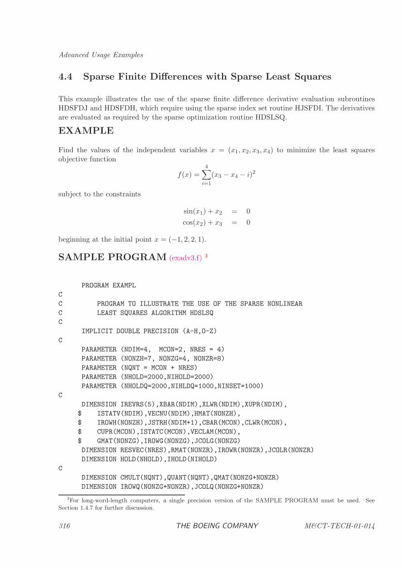
Advanced Usage Examples
4.4 Sparse Finite Differences with Sparse Least Squares
This example illustrates the use of the sparse finite difference derivative evaluation subroutinesHDSFDJ and HDSFDH, which require using the sparse index set routine HJSFDI. The derivativesare evaluated as required by the sparse optimization routine HDSLSQ.
EXAMPLE
Find the values of the independent variables x = (x1, x2, x3, x4) to minimize the least squaresobjective function
f(x) =4∑
i=1
(x3 − x4 − i)2
subject to the constraints
sin(x1) + x2 = 0
cos(x2) + x3 = 0
beginning at the initial point x = (−1, 2, 2, 1).
SAMPLE PROGRAM (exadv3.f) 3
PROGRAM EXAMPL
C
C PROGRAM TO ILLUSTRATE THE USE OF THE SPARSE NONLINEAR
C LEAST SQUARES ALGORITHM HDSLSQ
C
IMPLICIT DOUBLE PRECISION (A-H,O-Z)
C
PARAMETER (NDIM=4, MCON=2, NRES = 4)
PARAMETER (NONZH=7, NONZG=4, NONZR=8)
PARAMETER (NQNT = MCON + NRES)
PARAMETER (NHOLD=2000,NIHOLD=2000)
PARAMETER (NHOLDQ=2000,NIHLDQ=1000,NINSET=1000)
C
DIMENSION IREVRS(5),XBAR(NDIM),XLWR(NDIM),XUPR(NDIM),
$ ISTATV(NDIM),VECNU(NDIM),HMAT(NONZH),
$ IROWH(NONZH),JSTRH(NDIM+1),CBAR(MCON),CLWR(MCON),
$ CUPR(MCON),ISTATC(MCON),VECLAM(MCON),
$ GMAT(NONZG),IROWG(NONZG),JCOLG(NONZG)
DIMENSION RESVEC(NRES),RMAT(NONZR),IROWR(NONZR),JCOLR(NONZR)
DIMENSION HOLD(NHOLD),IHOLD(NIHOLD)
C
DIMENSION CMULT(NQNT),QUANT(NQNT),QMAT(NONZG+NONZR)
DIMENSION IROWQ(NONZG+NONZR),JCOLQ(NONZG+NONZR)
3For long-word-length computers, a single precision version of the SAMPLE PROGRAM must be used. See
Section 1.4.7 for further discussion.
316 THE BOEING COMPANY M&CT-TECH-01-014
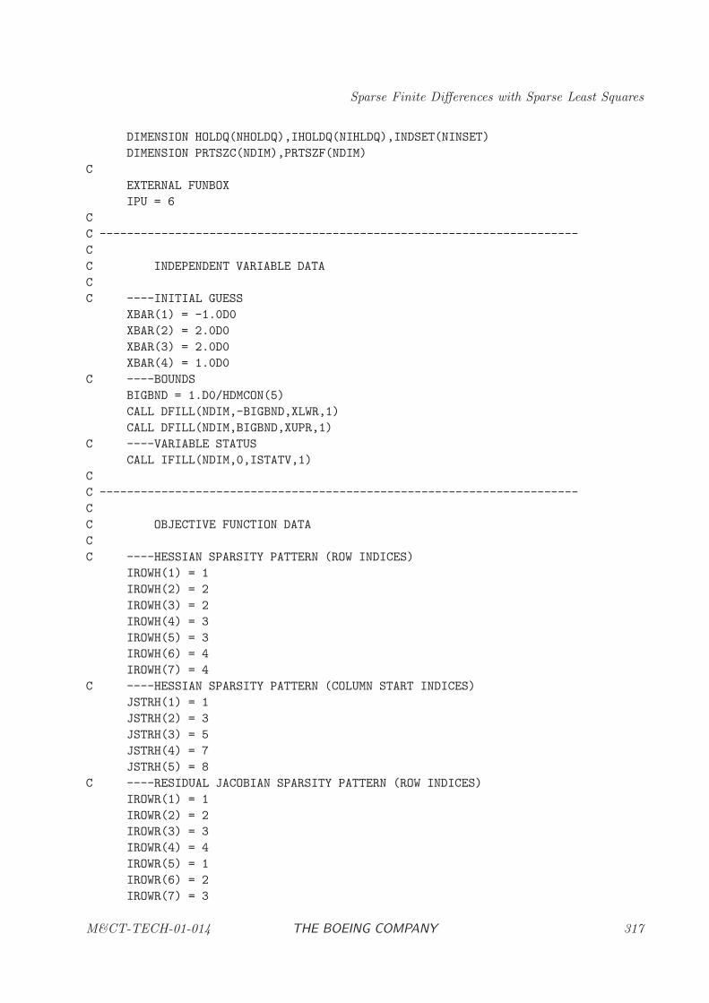
Sparse Finite Differences with Sparse Least Squares
DIMENSION HOLDQ(NHOLDQ),IHOLDQ(NIHLDQ),INDSET(NINSET)
DIMENSION PRTSZC(NDIM),PRTSZF(NDIM)
C
EXTERNAL FUNBOX
IPU = 6
C
C ----------------------------------------------------------------------
C
C INDEPENDENT VARIABLE DATA
C
C ----INITIAL GUESS
XBAR(1) = -1.0D0
XBAR(2) = 2.0D0
XBAR(3) = 2.0D0
XBAR(4) = 1.0D0
C ----BOUNDS
BIGBND = 1.D0/HDMCON(5)
CALL DFILL(NDIM,-BIGBND,XLWR,1)
CALL DFILL(NDIM,BIGBND,XUPR,1)
C ----VARIABLE STATUS
CALL IFILL(NDIM,0,ISTATV,1)
C
C ----------------------------------------------------------------------
C
C OBJECTIVE FUNCTION DATA
C
C ----HESSIAN SPARSITY PATTERN (ROW INDICES)
IROWH(1) = 1
IROWH(2) = 2
IROWH(3) = 2
IROWH(4) = 3
IROWH(5) = 3
IROWH(6) = 4
IROWH(7) = 4
C ----HESSIAN SPARSITY PATTERN (COLUMN START INDICES)
JSTRH(1) = 1
JSTRH(2) = 3
JSTRH(3) = 5
JSTRH(4) = 7
JSTRH(5) = 8
C ----RESIDUAL JACOBIAN SPARSITY PATTERN (ROW INDICES)
IROWR(1) = 1
IROWR(2) = 2
IROWR(3) = 3
IROWR(4) = 4
IROWR(5) = 1
IROWR(6) = 2
IROWR(7) = 3
M&CT-TECH-01-014 THE BOEING COMPANY 317
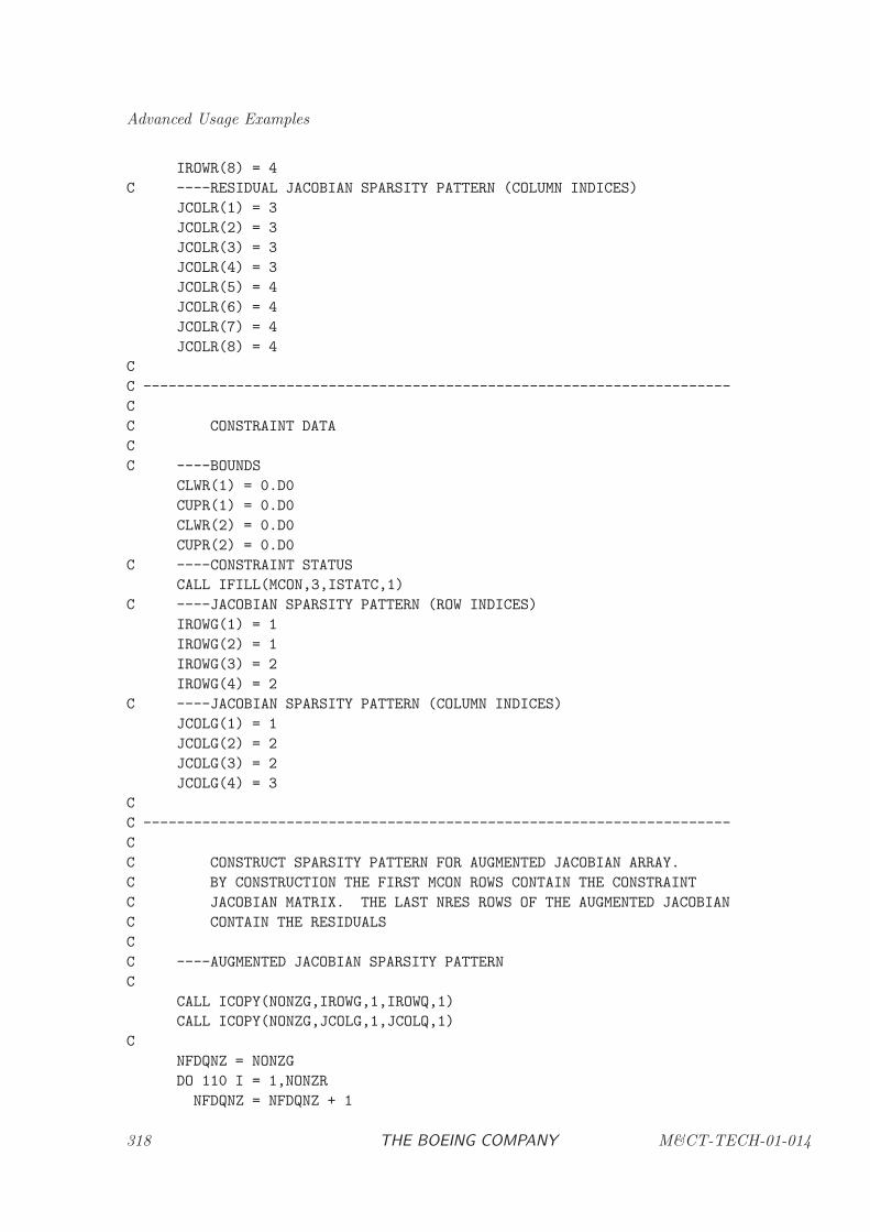
Advanced Usage Examples
IROWR(8) = 4
C ----RESIDUAL JACOBIAN SPARSITY PATTERN (COLUMN INDICES)
JCOLR(1) = 3
JCOLR(2) = 3
JCOLR(3) = 3
JCOLR(4) = 3
JCOLR(5) = 4
JCOLR(6) = 4
JCOLR(7) = 4
JCOLR(8) = 4
C
C ----------------------------------------------------------------------
C
C CONSTRAINT DATA
C
C ----BOUNDS
CLWR(1) = 0.D0
CUPR(1) = 0.D0
CLWR(2) = 0.D0
CUPR(2) = 0.D0
C ----CONSTRAINT STATUS
CALL IFILL(MCON,3,ISTATC,1)
C ----JACOBIAN SPARSITY PATTERN (ROW INDICES)
IROWG(1) = 1
IROWG(2) = 1
IROWG(3) = 2
IROWG(4) = 2
C ----JACOBIAN SPARSITY PATTERN (COLUMN INDICES)
JCOLG(1) = 1
JCOLG(2) = 2
JCOLG(3) = 2
JCOLG(4) = 3
C
C ----------------------------------------------------------------------
C
C CONSTRUCT SPARSITY PATTERN FOR AUGMENTED JACOBIAN ARRAY.
C BY CONSTRUCTION THE FIRST MCON ROWS CONTAIN THE CONSTRAINT
C JACOBIAN MATRIX. THE LAST NRES ROWS OF THE AUGMENTED JACOBIAN
C CONTAIN THE RESIDUALS
C
C ----AUGMENTED JACOBIAN SPARSITY PATTERN
C
CALL ICOPY(NONZG,IROWG,1,IROWQ,1)
CALL ICOPY(NONZG,JCOLG,1,JCOLQ,1)
C
NFDQNZ = NONZG
DO 110 I = 1,NONZR
NFDQNZ = NFDQNZ + 1
318 THE BOEING COMPANY M&CT-TECH-01-014
Sparse Finite Differences with Sparse Least Squares
IROWQ(NFDQNZ) = IROWR(I) + MCON
JCOLQ(NFDQNZ) = JCOLR(I)
110 CONTINUE
C
C GENERATE INDEX SETS
C
LCRMAT = NFDQNZ - NONZR + 1
IHESS = 1
NFDHNZ = NONZH
MAXHNZ = NONZH
MSGLVL = 0
CALL HJSFDI(IHESS,NDIM,NQNT,NFDQNZ,IROWQ,JCOLQ,
$ NFDHNZ,MAXHNZ,NDIM+1,JSTRH,IROWH,MSGLVL,IPU,
$ IHOLDQ,NIHLDQ,INDSET,NINSET,
$ IERIND)
C
IF(IERIND.LT.0) THEN
PRINT *,’INDEX SET ERROR; IERIND =’,IERIND
STOP
ELSEIF(IERIND.GT.0) THEN
PRINT *,’INDEX SET WARNING; IERIND =’,IERIND
ENDIF
C
C DEFINE PERTURBATION SIZES
C
PRTMIN = SQRT(HDMCON(5))
EPSRLF = HDMCON(5)**.9
CNTINT = EPSRLF**.333
FWDINT = SQRT(EPSRLF)
DO 120 II = 1,NDIM
VARSIZ = 1.D0 + ABS(XBAR(II))
PRTSZC(II) = CNTINT*VARSIZ
PRTSZF(II) = FWDINT*VARSIZ
120 CONTINUE
C
C ----------------------------------------------------------------------
C
C INITIALIZE FUNCTION EVALUATION COUNT
C
NFEVAL = 0
C
C INITIALIZE REVERSE COMMUNICATION CONTROL FLAG
C
ICC = -1
C
C SET OPTIONAL INPUTS
C
CALL HHSNLP(’IOFLAG=1’)
M&CT-TECH-01-014 THE BOEING COMPANY 319
Advanced Usage Examples
C
C ----------------------------------------------------------------------
C
130 CONTINUE
C
CALL HDSLSQ( ICC ,IREVRS ,XBAR ,XLWR ,XUPR ,ISTATV
$ ,VECNU ,NDIM ,RESVEC ,NRES ,RMAT ,IROWR
$ ,JCOLR ,NONZR ,HMAT ,IROWH ,JSTRH ,NONZH
$ ,CBAR ,CLWR ,CUPR ,ISTATC ,MCON ,VECLAM
$ ,GMAT ,IROWG ,JCOLG ,NONZG ,IFERR ,NFEVAL
$ ,HOLD ,NHOLD ,IHOLD ,NIHOLD ,NEEDED ,IERNLP )
C
C REVERSE COMMUNICATION TERMINATION TEST
C
IF(ICC.EQ.0) GO TO 180
C
C ----------------------------------------------------------------------
C
C SET FUNCTION EVALUATION ERROR FLAG
C
IFERR = 0
C
C >>>>>FUNCTION EVALUATION REQUEST
C
IF(IREVRS(1).EQ.1) THEN
C
C EVALUATE FUNCTIONS
C
CALL FUNBOX(XBAR,NDIM,NQNT,QUANT,IFERR)
NFEVAL = NFEVAL + 1
IF(IFERR.EQ.0) THEN
CALL DCOPY(MCON,QUANT,1,CBAR,1)
CALL DCOPY(NRES,QUANT(MCON+1),1,RESVEC,1)
ENDIF
C
ENDIF
C
C >>>>>GRADIENT EVALUATION REQUEST
C
IF(IREVRS(2).EQ.1) THEN
C
ICCD = -1
C
140 CONTINUE
C
C FORWARD DIFFERENCE GRADIENTS
C
IDTYPE = 1
320 THE BOEING COMPANY M&CT-TECH-01-014
Sparse Finite Differences with Sparse Least Squares
CALL HDSFDJ(ICCD,IROWQ,JCOLQ,QMAT,
$ PRTSZF,PRTMIN,XBAR,QUANT,IFERR,MSGLVL,
$ IPU,IDTYPE,PRTMIN,INDSET,HOLDQ,NHOLDQ,IERD)
C
IF(ICCD.NE.0) THEN
C
CALL FUNBOX(XBAR,NDIM,NQNT,QUANT,IFERR)
NFEVAL = NFEVAL + 1
C
GO TO 140
C
ENDIF
IF(MCON.GT.0) CALL DCOPY(NONZG,QMAT,1,GMAT,1)
CALL DCOPY(NONZR,QMAT(LCRMAT),1,RMAT,1)
C
ELSEIF(IREVRS(2).EQ.2.AND.IREVRS(3).EQ.0) THEN
C
ICCD = -1
C
150 CONTINUE
C
C CENTRAL DIFFERENCE GRADIENTS
C
IDTYPE = 2
CALL HDSFDJ(ICCD,IROWQ,JCOLQ,QMAT,
$ PRTSZC,PRTMIN,XBAR,QUANT,IFERR,MSGLVL,
$ IPU,IDTYPE,PRTMIN,INDSET,HOLDQ,NHOLDQ,IERD)
C
C
IF(ICCD.NE.0) THEN
C
CALL FUNBOX(XBAR,NDIM,NQNT,QUANT,IFERR)
NFEVAL = NFEVAL + 1
C
GO TO 150
C
ENDIF
IF(MCON.GT.0) CALL DCOPY(NONZG,QMAT,1,GMAT,1)
CALL DCOPY(NONZR,QMAT(LCRMAT),1,RMAT,1)
C
ENDIF
C
C >>>>>HESSIAN EVALUATION REQUEST
C
IF(IREVRS(2).EQ.2.AND.IREVRS(3).EQ.1) THEN
C
ICCH = -1
CALL DCOPY(MCON,VECLAM,1,CMULT,1)
M&CT-TECH-01-014 THE BOEING COMPANY 321
Advanced Usage Examples
CALL DSCAL(MCON,-1.D0,CMULT,1)
CALL DCOPY(NRES,RESVEC,1,CMULT(MCON+1),1)
C
160 CONTINUE
C
C DIAGONAL ELEMENTS
C
CALL HDSFDH(ICCH,IROWQ,JCOLQ,QMAT,
$ JSTRH,IROWH,HMAT,CMULT,
$ PRTSZC,PRTMIN,XBAR,QUANT,IFERR,MSGLVL,IPU,
$ PRTMIN,INDSET,HOLDQ,NHOLDQ,IHOLDQ,
$ NIHLDQ,IERH)
C
IF(ICCH.GT.0) THEN
C
CALL FUNBOX(XBAR,NDIM,NQNT,QUANT,IFERR)
NFEVAL = NFEVAL + 1
C
GO TO 160
C
ENDIF
IF(MCON.GT.0) CALL DCOPY(NONZG,QMAT,1,GMAT,1)
CALL DCOPY(NONZR,QMAT(LCRMAT),1,RMAT,1)
C
ELSEIF(IREVRS(3).EQ.2) THEN
C
ICCH = -2
C
170 CONTINUE
C
C OFF-DIAGONAL ELEMENTS
C
CALL HDSFDH(ICCH,IROWQ,JCOLQ,QMAT,
$ JSTRH,IROWH,HMAT,CMULT,
$ PRTSZC,PRTMIN,XBAR,QUANT,IFERR,MSGLVL,IPU,
$ PRTMIN,INDSET,HOLDQ,NHOLDQ,IHOLDQ,
$ NIHLDQ,IERH)
C
IF(ICCH.GT.0) THEN
C
CALL FUNBOX(XBAR,NDIM,NQNT,QUANT,IFERR)
NFEVAL = NFEVAL + 1
GO TO 170
C
ENDIF
C
IF(MCON.GT.0) CALL DCOPY(NONZG,QMAT,1,GMAT,1)
CALL DCOPY(NONZR,QMAT(LCRMAT),1,RMAT,1)
322 THE BOEING COMPANY M&CT-TECH-01-014
Sparse Finite Differences with Sparse Least Squares
C
ENDIF
C
C >>>>>SYSTEM PRINT (OUTPUT) REQUEST
C
IF(IREVRS(4).EQ.1) THEN
C
WRITE(6,1003) .5D0*DDOT(NRES,RESVEC,1,RESVEC,1),NFEVAL
WRITE(6,1001) ’VARIABLES’
WRITE(6,1002) (XBAR(II),II=1,NDIM)
IF(MCON.GT.0) THEN
WRITE(6,1001) ’CONSTRAINTS’
WRITE(6,1002) (CBAR(II),II=1,MCON)
ENDIF
WRITE(6,1004)
C
ENDIF
C
C ----------------------------------------------------------------------
C
C END OF REVERSE COMMUNICATION PROCESSING. RETURN TO HDSNLP
C
GO TO 130
C
180 CONTINUE
C
C TERMINATE PROCESSING
C
IF(IERNLP.EQ.0) THEN
C
C NORMAL TERMINATION---SOLUTION FOUND
C
WRITE(6,1001) ’SOLUTION ’
C
WRITE(6,1003) .5D0*DDOT(NRES,RESVEC,1,RESVEC,1),NFEVAL
WRITE(6,1001) ’VARIABLES’
WRITE(6,1002) (XBAR(II),II=1,NDIM)
IF(MCON.GT.0) THEN
WRITE(6,1001) ’CONSTRAINTS’
WRITE(6,1002) (CBAR(II),II=1,MCON)
ENDIF
WRITE(6,1004)
C
ELSEIF(IERNLP.LT.0) THEN
C
C ABNORMAL TERMINATION---FATAL ERROR
C
PRINT *,’FATAL ERROR; IERNLP =’,IERNLP
M&CT-TECH-01-014 THE BOEING COMPANY 323
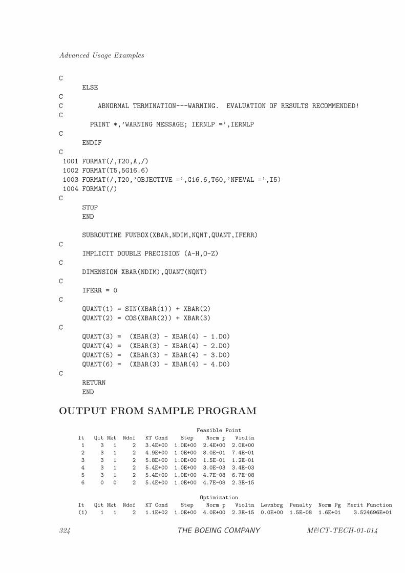
Advanced Usage Examples
C
ELSE
C
C ABNORMAL TERMINATION---WARNING. EVALUATION OF RESULTS RECOMMENDED!
C
PRINT *,’WARNING MESSAGE; IERNLP =’,IERNLP
C
ENDIF
C
1001 FORMAT(/,T20,A,/)
1002 FORMAT(T5,5G16.6)
1003 FORMAT(/,T20,’OBJECTIVE =’,G16.6,T60,’NFEVAL =’,I5)
1004 FORMAT(/)
C
STOP
END
SUBROUTINE FUNBOX(XBAR,NDIM,NQNT,QUANT,IFERR)
C
IMPLICIT DOUBLE PRECISION (A-H,O-Z)
C
DIMENSION XBAR(NDIM),QUANT(NQNT)
C
IFERR = 0
C
QUANT(1) = SIN(XBAR(1)) + XBAR(2)
QUANT(2) = COS(XBAR(2)) + XBAR(3)
C
QUANT(3) = (XBAR(3) - XBAR(4) - 1.D0)
QUANT(4) = (XBAR(3) - XBAR(4) - 2.D0)
QUANT(5) = (XBAR(3) - XBAR(4) - 3.D0)
QUANT(6) = (XBAR(3) - XBAR(4) - 4.D0)
C
RETURN
END
OUTPUT FROM SAMPLE PROGRAM
Feasible Point
It Qit Nkt Ndof KT Cond Step Norm p Violtn
1 3 1 2 3.4E+00 1.0E+00 2.4E+00 2.0E+00
2 3 1 2 4.9E+00 1.0E+00 8.0E-01 7.4E-01
3 3 1 2 5.8E+00 1.0E+00 1.5E-01 1.2E-01
4 3 1 2 5.4E+00 1.0E+00 3.0E-03 3.4E-03
5 3 1 2 5.4E+00 1.0E+00 4.7E-08 6.7E-08
6 0 0 2 5.4E+00 1.0E+00 4.7E-08 2.3E-15
Optimization
It Qit Nkt Ndof KT Cond Step Norm p Violtn Levnbrg Penalty Norm Pg Merit Function
(1) 1 1 2 1.1E+02 1.0E+00 4.0E+00 2.3E-15 0.0E+00 1.5E-08 1.6E+01 3.524696E+01
324 THE BOEING COMPANY M&CT-TECH-01-014
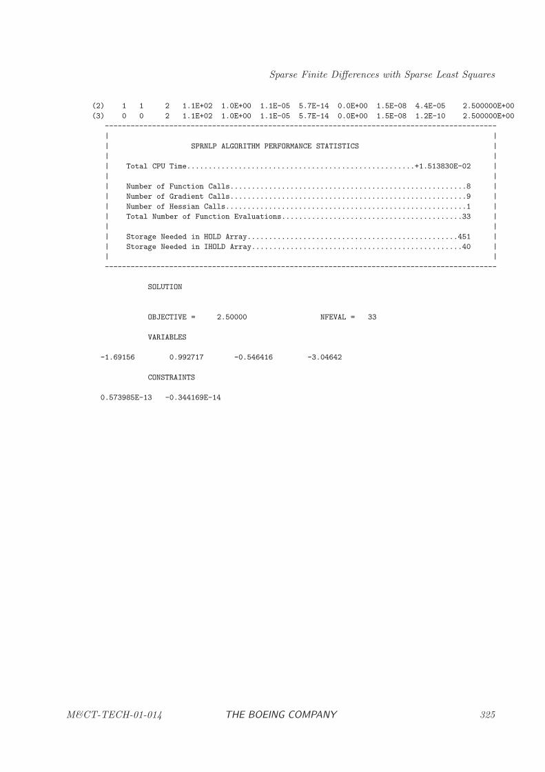
Sparse Finite Differences with Sparse Least Squares
(2) 1 1 2 1.1E+02 1.0E+00 1.1E-05 5.7E-14 0.0E+00 1.5E-08 4.4E-05 2.500000E+00
(3) 0 0 2 1.1E+02 1.0E+00 1.1E-05 5.7E-14 0.0E+00 1.5E-08 1.2E-10 2.500000E+00
-------------------------------------------------------------------------------------------
| |
| SPRNLP ALGORITHM PERFORMANCE STATISTICS |
| |
| Total CPU Time.....................................................+1.513830E-02 |
| |
| Number of Function Calls.......................................................8 |
| Number of Gradient Calls.......................................................9 |
| Number of Hessian Calls........................................................1 |
| Total Number of Function Evaluations..........................................33 |
| |
| Storage Needed in HOLD Array.................................................451 |
| Storage Needed in IHOLD Array.................................................40 |
| |
-------------------------------------------------------------------------------------------
SOLUTION
OBJECTIVE = 2.50000 NFEVAL = 33
VARIABLES
-1.69156 0.992717 -0.546416 -3.04642
CONSTRAINTS
0.573985E-13 -0.344169E-14
M&CT-TECH-01-014 THE BOEING COMPANY 325
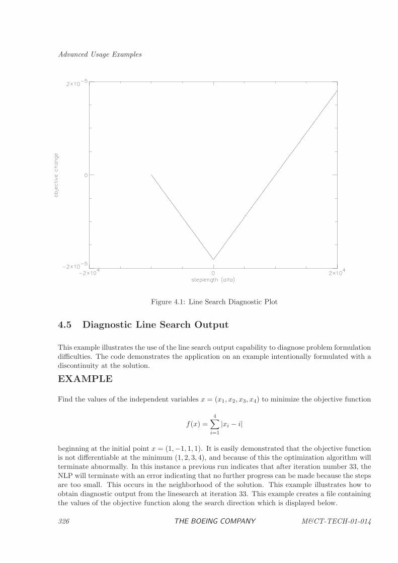
Advanced Usage Examples
Figure 4.1: Line Search Diagnostic Plot
4.5 Diagnostic Line Search Output
This example illustrates the use of the line search output capability to diagnose problem formulationdifficulties. The code demonstrates the application on an example intentionally formulated with adiscontinuity at the solution.
EXAMPLE
Find the values of the independent variables x = (x1, x2, x3, x4) to minimize the objective function
f(x) =4∑
i=1
|xi − i|
beginning at the initial point x = (1,−1, 1, 1). It is easily demonstrated that the objective functionis not differentiable at the minimum (1, 2, 3, 4), and because of this the optimization algorithm willterminate abnormally. In this instance a previous run indicates that after iteration number 33, theNLP will terminate with an error indicating that no further progress can be made because the stepsare too small. This occurs in the neighborhood of the solution. This example illustrates how toobtain diagnostic output from the linesearch at iteration 33. This example creates a file containingthe values of the objective function along the search direction which is displayed below.
326 THE BOEING COMPANY M&CT-TECH-01-014
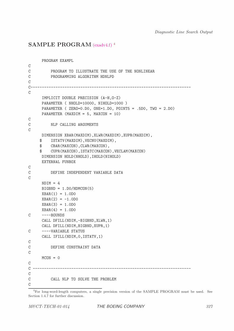
Diagnostic Line Search Output
SAMPLE PROGRAM (exadv4.f) 4
PROGRAM EXAMPL
C
C PROGRAM TO ILLUSTRATE THE USE OF THE NONLINEAR
C PROGRAMMING ALGORITHM HDNLPD
C
C-----------------------------------------------------------------------
C
IMPLICIT DOUBLE PRECISION (A-H,O-Z)
PARAMETER ( NHOLD=10000, NIHOLD=1000 )
PARAMETER ( ZERO=0.D0, ONE=1.D0, POINT5 = .5D0, TWO = 2.D0)
PARAMETER (MAXDIM = 5, MAXCON = 10)
C
C NLP CALLING ARGUMENTS
C
DIMENSION XBAR(MAXDIM),XLWR(MAXDIM),XUPR(MAXDIM),
$ ISTATV(MAXDIM),VECNU(MAXDIM),
$ CBAR(MAXCON),CLWR(MAXCON),
$ CUPR(MAXCON),ISTATC(MAXCON),VECLAM(MAXCON)
DIMENSION HOLD(NHOLD),IHOLD(NIHOLD)
EXTERNAL FUNBOX
C
C DEFINE INDEPENDENT VARIABLE DATA
C
NDIM = 4
BIGBND = 1.D0/HDMCON(5)
XBAR(1) = 1.0D0
XBAR(2) = -1.0D0
XBAR(3) = 1.0D0
XBAR(4) = 1.0D0
C ----BOUNDS
CALL DFILL(NDIM,-BIGBND,XLWR,1)
CALL DFILL(NDIM,BIGBND,XUPR,1)
C ----VARIABLE STATUS
CALL IFILL(NDIM,0,ISTATV,1)
C
C DEFINE CONSTRAINT DATA
C
MCON = 0
C
C ----------------------------------------------------------------------
C
C CALL NLP TO SOLVE THE PROBLEM
C
4For long-word-length computers, a single precision version of the SAMPLE PROGRAM must be used. See
Section 1.4.7 for further discussion.
M&CT-TECH-01-014 THE BOEING COMPANY 327
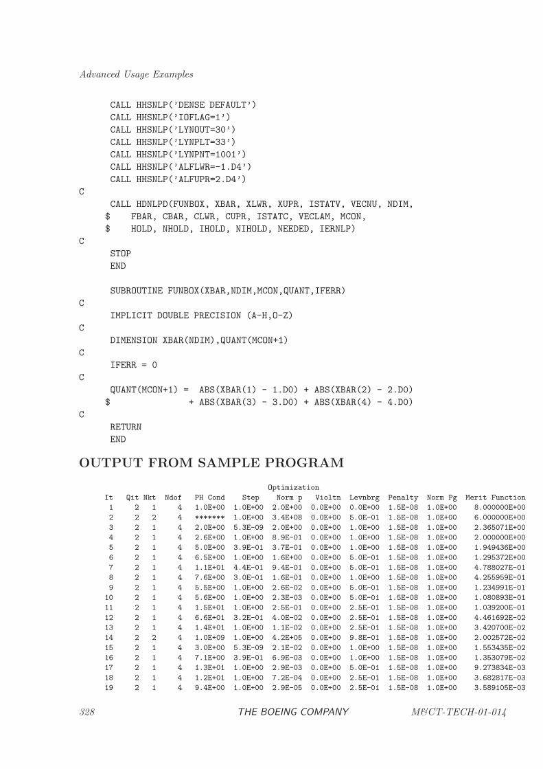
Advanced Usage Examples
CALL HHSNLP(’DENSE DEFAULT’)
CALL HHSNLP(’IOFLAG=1’)
CALL HHSNLP(’LYNOUT=30’)
CALL HHSNLP(’LYNPLT=33’)
CALL HHSNLP(’LYNPNT=1001’)
CALL HHSNLP(’ALFLWR=-1.D4’)
CALL HHSNLP(’ALFUPR=2.D4’)
C
CALL HDNLPD(FUNBOX, XBAR, XLWR, XUPR, ISTATV, VECNU, NDIM,
$ FBAR, CBAR, CLWR, CUPR, ISTATC, VECLAM, MCON,
$ HOLD, NHOLD, IHOLD, NIHOLD, NEEDED, IERNLP)
C
STOP
END
SUBROUTINE FUNBOX(XBAR,NDIM,MCON,QUANT,IFERR)
C
IMPLICIT DOUBLE PRECISION (A-H,O-Z)
C
DIMENSION XBAR(NDIM),QUANT(MCON+1)
C
IFERR = 0
C
QUANT(MCON+1) = ABS(XBAR(1) - 1.D0) + ABS(XBAR(2) - 2.D0)
$ + ABS(XBAR(3) - 3.D0) + ABS(XBAR(4) - 4.D0)
C
RETURN
END
OUTPUT FROM SAMPLE PROGRAM
Optimization
It Qit Nkt Ndof PH Cond Step Norm p Violtn Levnbrg Penalty Norm Pg Merit Function
1 2 1 4 1.0E+00 1.0E+00 2.0E+00 0.0E+00 0.0E+00 1.5E-08 1.0E+00 8.000000E+00
2 2 2 4 ******* 1.0E+00 3.4E+08 0.0E+00 5.0E-01 1.5E-08 1.0E+00 6.000000E+00
3 2 1 4 2.0E+00 5.3E-09 2.0E+00 0.0E+00 1.0E+00 1.5E-08 1.0E+00 2.365071E+00
4 2 1 4 2.6E+00 1.0E+00 8.9E-01 0.0E+00 1.0E+00 1.5E-08 1.0E+00 2.000000E+00
5 2 1 4 5.0E+00 3.9E-01 3.7E-01 0.0E+00 1.0E+00 1.5E-08 1.0E+00 1.949436E+00
6 2 1 4 6.5E+00 1.0E+00 1.6E+00 0.0E+00 5.0E-01 1.5E-08 1.0E+00 1.295372E+00
7 2 1 4 1.1E+01 4.4E-01 9.4E-01 0.0E+00 5.0E-01 1.5E-08 1.0E+00 4.788027E-01
8 2 1 4 7.6E+00 3.0E-01 1.6E-01 0.0E+00 1.0E+00 1.5E-08 1.0E+00 4.255959E-01
9 2 1 4 5.5E+00 1.0E+00 2.6E-02 0.0E+00 5.0E-01 1.5E-08 1.0E+00 1.234991E-01
10 2 1 4 5.6E+00 1.0E+00 2.3E-03 0.0E+00 5.0E-01 1.5E-08 1.0E+00 1.080893E-01
11 2 1 4 1.5E+01 1.0E+00 2.5E-01 0.0E+00 2.5E-01 1.5E-08 1.0E+00 1.039200E-01
12 2 1 4 6.6E+01 3.2E-01 4.0E-02 0.0E+00 2.5E-01 1.5E-08 1.0E+00 4.461692E-02
13 2 1 4 1.4E+01 1.0E+00 1.1E-02 0.0E+00 2.5E-01 1.5E-08 1.0E+00 3.420700E-02
14 2 2 4 1.0E+09 1.0E+00 4.2E+05 0.0E+00 9.8E-01 1.5E-08 1.0E+00 2.002572E-02
15 2 1 4 3.0E+00 5.3E-09 2.1E-02 0.0E+00 1.0E+00 1.5E-08 1.0E+00 1.553435E-02
16 2 1 4 7.1E+00 3.9E-01 6.9E-03 0.0E+00 1.0E+00 1.5E-08 1.0E+00 1.353079E-02
17 2 1 4 1.3E+01 1.0E+00 2.9E-03 0.0E+00 5.0E-01 1.5E-08 1.0E+00 9.273834E-03
18 2 1 4 1.2E+01 1.0E+00 7.2E-04 0.0E+00 2.5E-01 1.5E-08 1.0E+00 3.682817E-03
19 2 1 4 9.4E+00 1.0E+00 2.9E-05 0.0E+00 2.5E-01 1.5E-08 1.0E+00 3.589105E-03
328 THE BOEING COMPANY M&CT-TECH-01-014
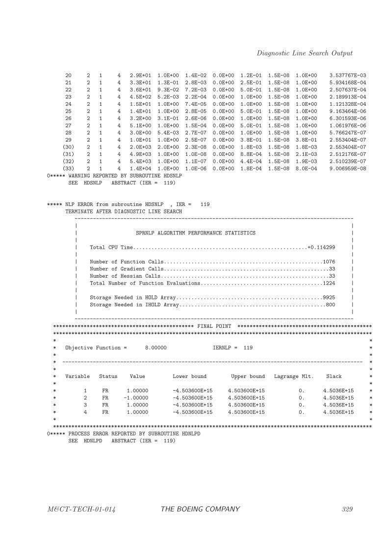
Diagnostic Line Search Output
20 2 1 4 2.9E+01 1.0E+00 1.4E-02 0.0E+00 1.2E-01 1.5E-08 1.0E+00 3.537767E-03
21 2 1 4 3.3E+01 1.3E-01 2.8E-03 0.0E+00 2.5E-01 1.5E-08 1.0E+00 5.934168E-04
22 2 1 4 3.6E+01 9.3E-02 7.2E-03 0.0E+00 5.0E-01 1.5E-08 1.0E+00 2.507637E-04
23 2 1 4 4.5E+02 5.2E-03 2.2E-04 0.0E+00 1.0E+00 1.5E-08 1.0E+00 2.189913E-04
24 2 1 4 1.5E+01 1.0E+00 7.4E-05 0.0E+00 1.0E+00 1.5E-08 1.0E+00 1.121328E-04
25 2 1 4 1.4E+01 1.0E+00 2.8E-05 0.0E+00 5.0E-01 1.5E-08 1.0E+00 9.163464E-06
26 2 1 4 3.2E+00 3.1E-01 2.6E-06 0.0E+00 1.0E+00 1.5E-08 1.0E+00 6.301593E-06
27 2 1 4 5.1E+00 1.0E+00 1.5E-04 0.0E+00 5.0E-01 1.5E-08 1.0E+00 1.061976E-06
28 2 1 4 3.0E+00 5.4E-03 2.7E-07 0.0E+00 1.0E+00 1.5E-08 1.0E+00 5.766247E-07
29 2 1 4 1.0E+01 1.0E+00 2.5E-07 0.0E+00 3.8E-01 1.5E-08 3.8E-01 2.553404E-07
(30) 2 1 4 2.0E+03 2.0E+00 2.3E-08 0.0E+00 1.8E-03 1.5E-08 1.8E-03 2.553404E-07
(31) 2 1 4 4.9E+03 1.0E+00 1.0E-08 0.0E+00 8.8E-04 1.5E-08 2.1E-03 2.512176E-07
(32) 2 1 4 5.4E+03 1.0E+00 1.1E-07 0.0E+00 4.4E-04 1.5E-08 1.9E-03 2.510239E-07
(33) 2 1 4 1.4E+04 1.0E+00 1.0E-06 0.0E+00 1.8E-04 1.5E-08 8.0E-04 9.006959E-08
0***** WARNING REPORTED BY SUBROUTINE HDSNLP
SEE HDSNLP ABSTRACT (IER = 119)
***** NLP ERROR from subroutine HDSNLP , IER = 119
TERMINATE AFTER DIAGNOSTIC LINE SEARCH
-------------------------------------------------------------------------------------------
| |
| SPRNLP ALGORITHM PERFORMANCE STATISTICS |
| |
| Total CPU Time.........................................................+0.114299 |
| |
| Number of Function Calls....................................................1076 |
| Number of Gradient Calls......................................................33 |
| Number of Hessian Calls.......................................................33 |
| Total Number of Function Evaluations........................................1224 |
| |
| Storage Needed in HOLD Array................................................9925 |
| Storage Needed in IHOLD Array................................................800 |
| |
-------------------------------------------------------------------------------------------
********************************************** FINAL POINT ********************************************
********************************************************************************************************
* *
* Objective Function = 8.00000 IERNLP = 119 *
* *
* -------------------------------------------------------------------------------------------------- *
* *
* Variable Status Value Lower bound Upper bound Lagrange Mlt. Slack *
* *
* 1 FR 1.00000 -4.503600E+15 4.503600E+15 0. 4.5036E+15 *
* 2 FR -1.00000 -4.503600E+15 4.503600E+15 0. 4.5036E+15 *
* 3 FR 1.00000 -4.503600E+15 4.503600E+15 0. 4.5036E+15 *
* 4 FR 1.00000 -4.503600E+15 4.503600E+15 0. 4.5036E+15 *
* *
********************************************************************************************************
0***** PROCESS ERROR REPORTED BY SUBROUTINE HDNLPD
SEE HDNLPD ABSTRACT (IER = 119)
M&CT-TECH-01-014 THE BOEING COMPANY 329
Advanced Usage Examples
4.6 Problem Diagnostics using Postoptimality Analysis
This example illustrates the use of the postoptimality analysis capability to diagnose problemformulation difficulties. The code demonstrates the application on two different problems, bothintentionally formulated with known anomolies.
EXAMPLE
Problem 1
Find the values of the independent variables x = (x1, x2, x3, x4) to minimize the objective function
f(x) = (x3 − x4)2
subject to the constraints
x1 + x2 = 0
x2 + x3 = 0
beginning at the initial point x = (1,−1, 1, 1). It is easily demonstrated that whenever x1 =−x2 = x3 = x4 the constraints are satisfied and the objective is minimized. Since there are aninfinite number of solutions this is an example of a singular optimization problem. The reducedHessian matrix for this example is not positive definite. This singularity causes the linear systemdefining the necessary conditions (the KT system) to be rank deficient. When the postoptimalityanalysis is utilized a rank revealing sparse QR is applied to the KT system, and a rank deficiencyis detected. Notice that the rank deficiency is attributed to a column which is redundant, that is,it can be written as a linear combination of the other columns. The function box for this problemis implemented in subroutine FUNBX1.
Problem 2
Find the values of the independent variables x = (x1, x2, x3, x4) to minimize the objective function
f(x) = x21 + x2
2 + x23 + x2
4
subject to the constraints
x1 + x2 = 0
2(x1 + x2) = 0
beginning at the initial point x = (2,−1, 1, 1). It is easily demonstrated that the constraints arelinearly dependent since one is a multiple of the other. For this example the constraints do notsatisfy what is referred to as the “constraint qualification test,” and in this case it is not possibleto compute Lagrange multipliers. When the postoptimality analysis is utilized the rank deficiencyis attributed to a row of the Jacobian matrix. This row is considered redundant since it can bewritten as a linear combination of the other rows. The function box for this problem is implementedin subroutine FUNBX2.
SAMPLE PROGRAM (exadv5.f) 5
5For long-word-length computers, a single precision version of the SAMPLE PROGRAM must be used. See
Section 1.4.7 for further discussion.
330 THE BOEING COMPANY M&CT-TECH-01-014
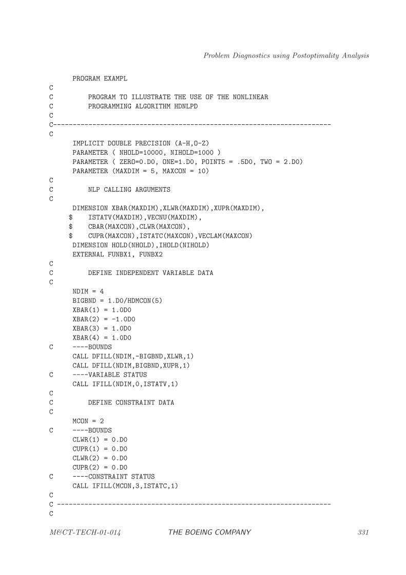
Problem Diagnostics using Postoptimality Analysis
PROGRAM EXAMPL
C
C PROGRAM TO ILLUSTRATE THE USE OF THE NONLINEAR
C PROGRAMMING ALGORITHM HDNLPD
C
C-----------------------------------------------------------------------
C
IMPLICIT DOUBLE PRECISION (A-H,O-Z)
PARAMETER ( NHOLD=10000, NIHOLD=1000 )
PARAMETER ( ZERO=0.D0, ONE=1.D0, POINT5 = .5D0, TWO = 2.D0)
PARAMETER (MAXDIM = 5, MAXCON = 10)
C
C NLP CALLING ARGUMENTS
C
DIMENSION XBAR(MAXDIM),XLWR(MAXDIM),XUPR(MAXDIM),
$ ISTATV(MAXDIM),VECNU(MAXDIM),
$ CBAR(MAXCON),CLWR(MAXCON),
$ CUPR(MAXCON),ISTATC(MAXCON),VECLAM(MAXCON)
DIMENSION HOLD(NHOLD),IHOLD(NIHOLD)
EXTERNAL FUNBX1, FUNBX2
C
C DEFINE INDEPENDENT VARIABLE DATA
C
NDIM = 4
BIGBND = 1.D0/HDMCON(5)
XBAR(1) = 1.0D0
XBAR(2) = -1.0D0
XBAR(3) = 1.0D0
XBAR(4) = 1.0D0
C ----BOUNDS
CALL DFILL(NDIM,-BIGBND,XLWR,1)
CALL DFILL(NDIM,BIGBND,XUPR,1)
C ----VARIABLE STATUS
CALL IFILL(NDIM,0,ISTATV,1)
C
C DEFINE CONSTRAINT DATA
C
MCON = 2
C ----BOUNDS
CLWR(1) = 0.D0
CUPR(1) = 0.D0
CLWR(2) = 0.D0
CUPR(2) = 0.D0
C ----CONSTRAINT STATUS
CALL IFILL(MCON,3,ISTATC,1)
C
C ----------------------------------------------------------------------
C
M&CT-TECH-01-014 THE BOEING COMPANY 331
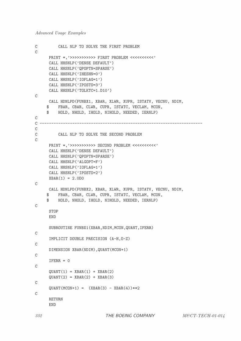
Advanced Usage Examples
C CALL NLP TO SOLVE THE FIRST PROBLEM
C
PRINT *,’>>>>>>>>>>> FIRST PROBLEM <<<<<<<<<<’
CALL HHSNLP(’DENSE DEFAULT’)
CALL HHSNLP(’QPOPTN=SPARSE’)
CALL HHSNLP(’IHESHN=0’)
CALL HHSNLP(’IOFLAG=1’)
CALL HHSNLP(’IPOSTO=3’)
CALL HHSNLP(’TOLKTC=1.D10’)
C
CALL HDNLPD(FUNBX1, XBAR, XLWR, XUPR, ISTATV, VECNU, NDIM,
$ FBAR, CBAR, CLWR, CUPR, ISTATC, VECLAM, MCON,
$ HOLD, NHOLD, IHOLD, NIHOLD, NEEDED, IERNLP)
C
C ----------------------------------------------------------------------
C
C CALL NLP TO SOLVE THE SECOND PROBLEM
C
PRINT *,’>>>>>>>>>>> SECOND PROBLEM <<<<<<<<<<’
CALL HHSNLP(’DENSE DEFAULT’)
CALL HHSNLP(’QPOPTN=SPARSE’)
CALL HHSNLP(’ALGOPT=F’)
CALL HHSNLP(’IOFLAG=1’)
CALL HHSNLP(’IPOSTO=2’)
XBAR(1) = 2.0D0
C
CALL HDNLPD(FUNBX2, XBAR, XLWR, XUPR, ISTATV, VECNU, NDIM,
$ FBAR, CBAR, CLWR, CUPR, ISTATC, VECLAM, MCON,
$ HOLD, NHOLD, IHOLD, NIHOLD, NEEDED, IERNLP)
C
STOP
END
SUBROUTINE FUNBX1(XBAR,NDIM,MCON,QUANT,IFERR)
C
IMPLICIT DOUBLE PRECISION (A-H,O-Z)
C
DIMENSION XBAR(NDIM),QUANT(MCON+1)
C
IFERR = 0
C
QUANT(1) = XBAR(1) + XBAR(2)
QUANT(2) = XBAR(2) + XBAR(3)
C
QUANT(MCON+1) = (XBAR(3) - XBAR(4))**2
C
RETURN
END
332 THE BOEING COMPANY M&CT-TECH-01-014
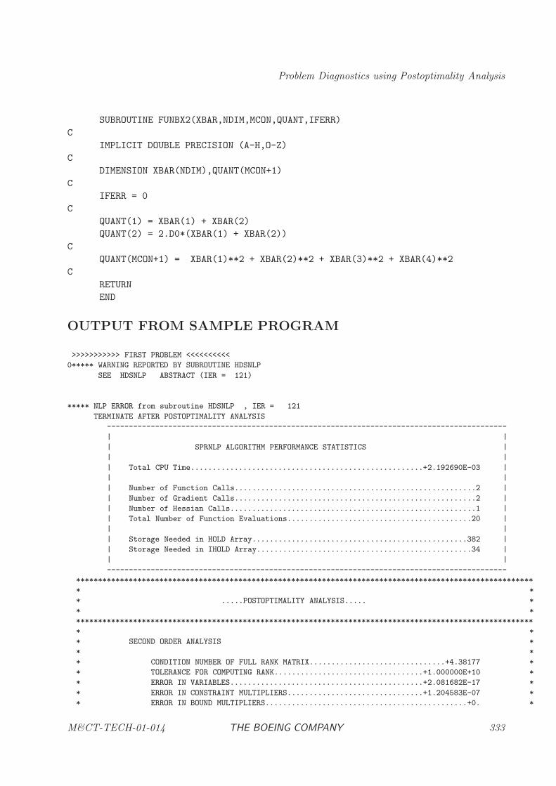
Problem Diagnostics using Postoptimality Analysis
SUBROUTINE FUNBX2(XBAR,NDIM,MCON,QUANT,IFERR)
C
IMPLICIT DOUBLE PRECISION (A-H,O-Z)
C
DIMENSION XBAR(NDIM),QUANT(MCON+1)
C
IFERR = 0
C
QUANT(1) = XBAR(1) + XBAR(2)
QUANT(2) = 2.D0*(XBAR(1) + XBAR(2))
C
QUANT(MCON+1) = XBAR(1)**2 + XBAR(2)**2 + XBAR(3)**2 + XBAR(4)**2
C
RETURN
END
OUTPUT FROM SAMPLE PROGRAM
>>>>>>>>>>> FIRST PROBLEM <<<<<<<<<<
0***** WARNING REPORTED BY SUBROUTINE HDSNLP
SEE HDSNLP ABSTRACT (IER = 121)
***** NLP ERROR from subroutine HDSNLP , IER = 121
TERMINATE AFTER POSTOPTIMALITY ANALYSIS
-------------------------------------------------------------------------------------------
| |
| SPRNLP ALGORITHM PERFORMANCE STATISTICS |
| |
| Total CPU Time.....................................................+2.192690E-03 |
| |
| Number of Function Calls.......................................................2 |
| Number of Gradient Calls.......................................................2 |
| Number of Hessian Calls........................................................1 |
| Total Number of Function Evaluations..........................................20 |
| |
| Storage Needed in HOLD Array.................................................382 |
| Storage Needed in IHOLD Array.................................................34 |
| |
-------------------------------------------------------------------------------------------
********************************************************************************************************
* *
* .....POSTOPTIMALITY ANALYSIS..... *
* *
********************************************************************************************************
* *
* SECOND ORDER ANALYSIS *
* *
* CONDITION NUMBER OF FULL RANK MATRIX...............................+4.38177 *
* TOLERANCE FOR COMPUTING RANK..................................+1.000000E+10 *
* ERROR IN VARIABLES............................................+2.081682E-17 *
* ERROR IN CONSTRAINT MULTIPLIERS...............................+1.204583E-07 *
* ERROR IN BOUND MULTIPLIERS..............................................+0. *
M&CT-TECH-01-014 THE BOEING COMPANY 333
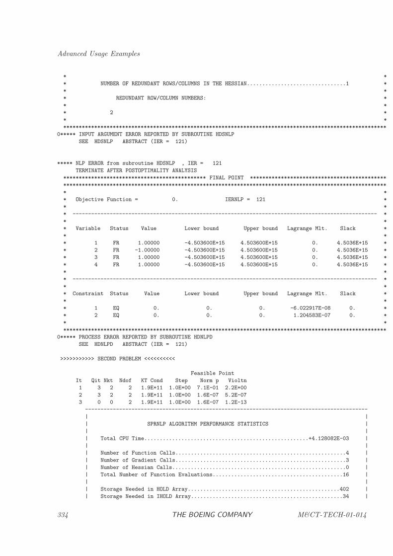
Advanced Usage Examples
* *
* NUMBER OF REDUNDANT ROWS/COLUMNS IN THE HESSIAN................................1 *
* *
* REDUNDANT ROW/COLUMN NUMBERS: *
* *
* 2 *
* *
********************************************************************************************************
0***** INPUT ARGUMENT ERROR REPORTED BY SUBROUTINE HDSNLP
SEE HDSNLP ABSTRACT (IER = 121)
***** NLP ERROR from subroutine HDSNLP , IER = 121
TERMINATE AFTER POSTOPTIMALITY ANALYSIS
********************************************** FINAL POINT ********************************************
********************************************************************************************************
* *
* Objective Function = 0. IERNLP = 121 *
* *
* -------------------------------------------------------------------------------------------------- *
* *
* Variable Status Value Lower bound Upper bound Lagrange Mlt. Slack *
* *
* 1 FR 1.00000 -4.503600E+15 4.503600E+15 0. 4.5036E+15 *
* 2 FR -1.00000 -4.503600E+15 4.503600E+15 0. 4.5036E+15 *
* 3 FR 1.00000 -4.503600E+15 4.503600E+15 0. 4.5036E+15 *
* 4 FR 1.00000 -4.503600E+15 4.503600E+15 0. 4.5036E+15 *
* *
* -------------------------------------------------------------------------------------------------- *
* *
* Constraint Status Value Lower bound Upper bound Lagrange Mlt. Slack *
* *
* 1 EQ 0. 0. 0. -6.022917E-08 0. *
* 2 EQ 0. 0. 0. 1.204583E-07 0. *
* *
********************************************************************************************************
0***** PROCESS ERROR REPORTED BY SUBROUTINE HDNLPD
SEE HDNLPD ABSTRACT (IER = 121)
>>>>>>>>>>> SECOND PROBLEM <<<<<<<<<<
Feasible Point
It Qit Nkt Ndof KT Cond Step Norm p Violtn
1 3 2 2 1.9E+11 1.0E+00 7.1E-01 2.2E+00
2 3 2 2 1.9E+11 1.0E+00 1.6E-07 5.2E-07
3 0 0 2 1.9E+11 1.0E+00 1.6E-07 1.2E-13
-------------------------------------------------------------------------------------------
| |
| SPRNLP ALGORITHM PERFORMANCE STATISTICS |
| |
| Total CPU Time.....................................................+4.128082E-03 |
| |
| Number of Function Calls.......................................................4 |
| Number of Gradient Calls.......................................................3 |
| Number of Hessian Calls........................................................0 |
| Total Number of Function Evaluations..........................................16 |
| |
| Storage Needed in HOLD Array.................................................402 |
| Storage Needed in IHOLD Array.................................................34 |
334 THE BOEING COMPANY M&CT-TECH-01-014
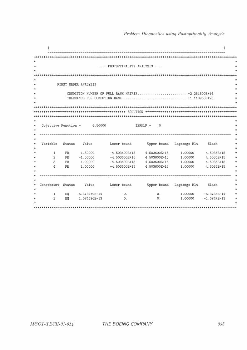
Problem Diagnostics using Postoptimality Analysis
| |
-------------------------------------------------------------------------------------------
********************************************************************************************************
* *
* .....POSTOPTIMALITY ANALYSIS..... *
* *
********************************************************************************************************
* *
* FIRST ORDER ANALYSIS *
* *
* CONDITION NUMBER OF FULL RANK MATRIX..........................+2.251800E+16 *
* TOLERANCE FOR COMPUTING RANK..................................+1.110953E+25 *
* *
********************************************************************************************************
*********************************************** SOLUTION ***********************************************
********************************************************************************************************
* *
* Objective Function = 6.50000 IERNLP = 0 *
* *
* -------------------------------------------------------------------------------------------------- *
* *
* Variable Status Value Lower bound Upper bound Lagrange Mlt. Slack *
* *
* 1 FR 1.50000 -4.503600E+15 4.503600E+15 1.00000 4.5036E+15 *
* 2 FR -1.50000 -4.503600E+15 4.503600E+15 1.00000 4.5036E+15 *
* 3 FR 1.00000 -4.503600E+15 4.503600E+15 1.00000 4.5036E+15 *
* 4 FR 1.00000 -4.503600E+15 4.503600E+15 1.00000 4.5036E+15 *
* *
* -------------------------------------------------------------------------------------------------- *
* *
* Constraint Status Value Lower bound Upper bound Lagrange Mlt. Slack *
* *
* 1 EQ 5.373479E-14 0. 0. 1.00000 -5.3735E-14 *
* 2 EQ 1.074696E-13 0. 0. 1.00000 -1.0747E-13 *
* *
********************************************************************************************************
M&CT-TECH-01-014 THE BOEING COMPANY 335

Advanced Usage Examples
336 THE BOEING COMPANY M&CT-TECH-01-014
Chapter 5
Optimal Control Background
Problem Definition
An optimal control problem can be formulated as a collection of N phases. In general, the inde-
pendent variable t for phase k is defined in the region t(k)I ≤ t ≤ t
(k)F . For many applications the
independent variable t is time, and the phases are sequential, that is t(k+1)I = t
(k)F , however neither
of these assumptions is required. Within phase k the dynamics of the system are described by aset of dynamic variables
z =
[y(k)(t)
u(k)(t)
]
made up of the n(k)y state variables and the n
(k)u control variables respectively. In addition the
dynamics may incorporate the n(k)p parameters p(k) which are not dependent on t. For clarity
we drop the phase-dependent notation from the remaining discussion, however it is important toremember that many complex problem descriptions require different dynamics and/or constraintswithin each phase, and the approach accommodates this requirement.
Typically the dynamics of the system are defined by a set of ordinary differential equations writtenin explicit form, which are referred to as the state equations
y = f [y(t), u(t), p, t]
where y is the ny dimension state vector. Initial conditions at time tI are defined by
ψIℓ ≤ ψ[y(tI), u(tI), p, tI ] ≤ ψIu
where ψ[y(tI), u(tI), p, tI ] ≡ ψI and terminal conditions at the final time tF are defined by
ψFℓ ≤ ψ[y(tF ), u(tF ), p, tF ] ≤ ψFu
where ψ[y(tF ), u(tF ), p, tF ] ≡ ψF . In addition the solution must satisfy algebraic path constraintsof the form
gℓ ≤ g[y(t), u(t), p, t] ≤ gu,
where g is a vector of size ng. The algebraic constraints are of the form
g[y(t), u(t), p, t] = α⊤v + β⊤a[v, t]
M&CT-TECH-01-014 THE BOEING COMPANY 337
Optimal Control Background
where
v =
y(t)u(t)p
.
The constraint definition can include analytic terms involving α⊤v where the (ny +nu +np) vectorα is constant, as well as linear combinations of the na auxiliary functions ak(v) for k = 0, . . . , na
where the coefficients βk are nonzero constants. By convention, a path constraint with a singlenonlinear term a0(y, u, p, t) has no auxiliary functions (na = 0). Observe that each individual pathconstraint may have a different number of auxiliary functions and analytic terms. Simple boundscan be imposed on the state variables
yℓ ≤ y(t) ≤ yu,
the control variables
uℓ ≤ u(t) ≤ uu,
and the parameters
pℓ ≤ p ≤ pu.
Note that an equality constraint can be imposed if the upper and lower bounds are equal, e.g.(gℓ)k = (gu)k for some k.
Finally it may be convenient to evaluate expressions of the form
∫ tF
tI
q[y(t), u(t), p, t]dt
which involve the quadrature functions q. Collectively we refer to those functions evaluated duringthe phase, namely,
F (t) =
f [y(t), u(t), p, t]g[y(t), u(t), p, t]q[y(t), u(t), p, t]a[y(t), u(t), p, t]
as the vector of continuous functions. Similarly functions evaluated at a specific point (i.e. thephase boundary) such as the boundary conditions ψ[y(tI), u(tI), p, tI ] and ψ[y(tF ), u(tF ), p, tF ] arereferred to as point functions.
The basic optimal control problem is to determine the n(k)u -dimensional control vectors u(k)(t) and
parameters p(k) to minimize the performance index
J = φ[y(t
(1)I ), t
(1)I , y(t
(1)F ), p(1), t
(1)F , . . . , y(t
(N)I ), t
(N)I , y(t
(N)F ), p(N), t
(N)F
]
+N∑
k=1
∫ t(k)F
t(k)I
q(k)[y(k)(t), u(k)(t), p(k), t]dt.
Notice that the objective function may depend on quantities computed in each of the N phases.
The above formulation can also accommodate implicit differential equations of the form,
f [y(t), y(t), u(t), p, t] = 0.
338 THE BOEING COMPANY M&CT-TECH-01-014
A simple substitution turns the implicit equation above into the semi-explicit differential-algebraic(DAE) system,
y = w0 = f [y(t), w(t), u(t), p, t]
In the semi-explicit form, w are considered another set of algebraic variables, and the functionsdefining the implicit differential equations now become algebraic path conditions.
Transcription Formulation
The basic approach for solving the optimal control problem by transcription has been presented indetail elsewhere (cf. Ref [5]). All approaches divide the time interval into ns segments
tI < t1 < t2 < . . . < tF = tns ,
where the points are referred to as node, mesh or grid points. Define the number of mesh pointsas M ≡ ns + 1. Let us introduce the notation yk ≡ y(tk) to indicate the value of the state variableat a grid point. In like fashion denote the control at a grid point by uk ≡ u(tk). In addition somediscretization schemes require values for the variables at the midpoint of an interval, and we denotethese quantities by yk ≡ y(t) and uk ≡ u(t) with t = 1
2(tk + tk−1). The SOCS software providesa number of different discretization schemes. Each scheme produces a distinct set of nonlinearprogramming (NLP) variables and constraints.
For the trapezoidal discretization, the NLP variables are
x = [y0, u0, y1, u1, . . . , yF , uF , p, tI , tF ]⊤ .
The state equations are approximately satisfied by setting the defects
ζk = yk − yk−1 −hk
2[fk + fk−1]
to zero for k = 1, . . . , ns. The step size is denoted by hk ≡ tk − tk−1, and the right hand side of thedifferential equations are given by fk ≡ f [y(tk), u(tk), p, tk].
For the Compressed Hermite-Simpson discretization scheme, the NLP variables are
x = [y0, u0, u0, y1, u1, u1, . . . , yF , uF , p, tI , tF ]⊤ .
The defects for this discretization are given by
ζk = yk − yk−1 −hk
6
[fk + 4fk + fk−1
]
wherefk = f [yk, uk, p, t]
with
yk =1
2[yk−1 + yk] +
hk
8[fk−1 − fk]
for k = 1, . . . , ns.
An alternate form of this discretization scheme referred to as Separated Hermite-Simpson, has thefollowing NLP variables
x = [y0, u0, y0, u0, y1, u1, y1, u1, . . . , yF , uF , p, tI , tF ]⊤ .
M&CT-TECH-01-014 THE BOEING COMPANY 339
Optimal Control Background
The defects for this discretization are given by
ζk = yk − yk−1 −hk
6
[fk + 4fk + fk−1
]
and
ζk = yk − 1
2[yk−1 + yk] −
hk
8[fk−1 − fk]
wherefk = f [yk, uk, p, t]
for k = 1, . . . , ns.
For the fourth order Runge-Kutta discretization scheme, the NLP variables are the same as theCompressed Hermite-Simpson method. The defects for this discretization are given by
ζk = yk − yk−1 −1
6[k1 + 2k2 + 2k3 + k4]
wherek1 = hkf(yk−1, uk−1, p, tk−1)k2 = hkf(yk−1 + k1/2, uk, p, t)k3 = hkf(yk−1 + k2/2, uk, p, t)k4 = hkf(yk−1 + k3, uk, p, tk)
for k = 1, . . . , ns.
As a result of the transcription the optimal control constraints are replaced by the NLP constraints
cℓ ≤ c(x) ≤ cu,
wherec(x) = [ζ1, ζ2, . . . , ζF , ψI , ψF , g0, g1, . . . , gF ]⊤
withcℓ = [0, . . . , 0, ψIℓ, ψFℓ, gℓ, . . . , gℓ]
⊤
and a corresponding definition of cu. The Separated Hermite-Simpson discretization also includesζk as constraints. The first nyns equality constraints require that the defect vectors from each ofthe ns segments be zero thereby approximately satisfying the differential equations. The boundaryconditions are enforced directly by the equality constraints on ψ, and the nonlinear path constraintsare imposed at the grid points. Note that nonlinear equality path constraints are enforced by settingcℓ = cu
In a similar fashion the state and control variable bounds become simple bounds on the NLPvariables. The path constraints and variable bounds are always imposed at the grid points forall discretization schemes. For the Hermite-Simpson, and Runge-Kutta discretization methods thepath constraints and variable bounds are also imposed at the interval midpoints.
The nonlinear programming (NLP) problem can be stated as follows: Find the n-vector x whichminimizes the objective function J subject to the constraints on c. This large, sparse NLP canbe solved efficiently using either a sequential quadratic programming (SQP) method or an interiorpoint (barrier) method.
To summarize, there are three primary operations that are performed when solving an optimalcontrol problem using a transcription method. Briefly the approach is as follows:
340 THE BOEING COMPANY M&CT-TECH-01-014
Direct Transcription Transcribe the optimal control problem into a nonlinear programming(NLP) problem by discretization;
Sparse Nonlinear Program Solve the sparse NLP using either a sequential quadratic program-ming or an interior-point (barrier) method.
Mesh Refinement Assess the accuracy of the approximation (i.e. the finite dimensional problem),and if necessary refine the discretization, and then repeat the optimization steps.
It is worth noting that the method is a “direct” transcription because it is not necessary to explicitlyconstruct the optimal control necessary conditions, i.e. the adjoint equations and the PontryaginMaximum Principle. However, if the adjoint equations are available the SOCS software can be usedto efficiently solve the boundary value problem.
The Parameter Estimation Problem
The parameter estimation problem has a different objective function than the optimal controlproblem. The basic parameter estimation problem is to determine the np-dimensional vector p tominimize the least squares performance index
J =1
2r⊤r.
where r is the ℓ-dimensional residual vector. Components of the residual vector can be of twoforms. State residuals are of the form
rk = wij [yi(θij) − yij]
where yi(θij) is the value of state variable i computed at time θij and yij is the observed value atthe same point. Algebraic residuals are of the form
rk = wij [ui(θij) − uij ]
where ui(θij) is the value of algebraic variable i computed at time θij and uij is the observed valueat the same point. The quantities wij are residual scale weights. It is required that data evaluationpoints satisfy
tI ≤ θij ≤ tF .
We refer to yij and uij as the discrete data functions. Often the evaluation points are arrangedmonotonically, that is θi,j ≤ θi,j+1. It is also common to have many variables evaluated at the sametime, e.g. θi,j = θi+1,j. Neither of these assumptions are necessary for our software however theinitial and final (phase) times tI and tF must be fixed.
It is worth noting that more complicated problem descriptions can be accommodated by the for-mulation given. For example, suppose it is required to minimize the expression
F =1
2
N∑
k=1
[ω(y, u, p, θk) − ωk]⊤Λ[ω(y, u, p, θk) − ωk]
where ωk are the observed values of the function ω at the times θk and Λ is the inverse covariancematrix of these quantities. Since the positive definite matrix can be factored as Λ = Q⊤Q we candefine a new set of algebraic variables
v(t) = Qω(y, u, p, t)
vk = Qωk.
M&CT-TECH-01-014 THE BOEING COMPANY 341
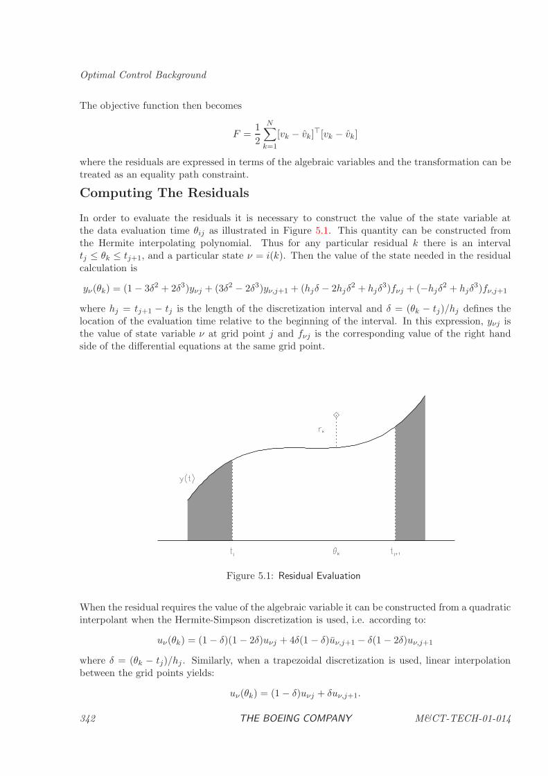
Optimal Control Background
The objective function then becomes
F =1
2
N∑
k=1
[vk − vk]⊤[vk − vk]
where the residuals are expressed in terms of the algebraic variables and the transformation can betreated as an equality path constraint.
Computing The Residuals
In order to evaluate the residuals it is necessary to construct the value of the state variable atthe data evaluation time θij as illustrated in Figure 5.1. This quantity can be constructed fromthe Hermite interpolating polynomial. Thus for any particular residual k there is an intervaltj ≤ θk ≤ tj+1, and a particular state ν = i(k). Then the value of the state needed in the residualcalculation is
yν(θk) = (1 − 3δ2 + 2δ3)yνj + (3δ2 − 2δ3)yν,j+1 + (hjδ − 2hjδ2 + hjδ
3)fνj + (−hjδ2 + hjδ
3)fν,j+1
where hj = tj+1 − tj is the length of the discretization interval and δ = (θk − tj)/hj defines thelocation of the evaluation time relative to the beginning of the interval. In this expression, yνj isthe value of state variable ν at grid point j and fνj is the corresponding value of the right handside of the differential equations at the same grid point.
Figure 5.1: Residual Evaluation
When the residual requires the value of the algebraic variable it can be constructed from a quadraticinterpolant when the Hermite-Simpson discretization is used, i.e. according to:
uν(θk) = (1 − δ)(1 − 2δ)uνj + 4δ(1 − δ)uν,j+1 − δ(1 − 2δ)uν,j+1
where δ = (θk − tj)/hj . Similarly, when a trapezoidal discretization is used, linear interpolationbetween the grid points yields:
uν(θk) = (1 − δ)uνj + δuν,j+1.
342 THE BOEING COMPANY M&CT-TECH-01-014
It is important to observe that the residuals are computed by interpolation and do not have anydirect affect on the location of the discretization grid points. This is often referred to as denseoutput in methods for numerical integration (c.f. [19]).
Problem Scaling
The optimal control problem variables and constraints in an attempt to improve the conditioningand efficiency of the underlying nonlinear programming problem. Thus the NLP solves a problemin terms of the scaled variables:
xi = wixi + si
and the scaled functions:ci = wici
F = woF.
Although there are many ways to compute the weights one possibility is to use scaling to improvethe Jacobian conditioning. When the original constraint is 0 = g(y, u, t) and ‖∇g‖ 6= 0 then onecan set w = 1/‖∇g‖ and define the scaled constraint 0 = g(y, u, t) = wg(y, u, t). With this choice,the gradient of the scaled constraint is ‖∇g‖ = 1. Unfortunately, gradient information can besignificantly different between the initial iterate and the solution. The automatic scaling procedureconstructs the scale weights at the initial point, and then recomputes the scaling at the solutionto the first mesh refinement problem. In addition this technique is used in conjunction with thefollowing SOCS scaling heuristics:
Rule 1: Scale from a control perspective, e.g. state variable y4(t) has the same scale for all gridpoints.
Rule 2: Variable Scaling
1. estimate the largest/smallest variable value from
(a) user input upper/lower bound, or if not available
(b) user specified initial guess
2. normalize and shift the variables. When (a) and (b) provide no information defaultscaling to 1.
Rule 3: ODE Defect Scaling
1. Set ODE defect scaling to state variable scaling, or optionally
2. choose it to normalize the defect gradients
Rule 4: Algebraic and Boundary Constraint Scaling
1. estimate the largest/smallest constraint value from user input upper/lower bound
2. optionally, estimate and/or compute the Jacobian
3. normalize the constraint.
4. When bounds provide no information set scaling to 1.
M&CT-TECH-01-014 THE BOEING COMPANY 343

Optimal Control Background
344 THE BOEING COMPANY M&CT-TECH-01-014
Chapter 6
Optimal Control Software
6.1 Overview of Sparse Optimal Control Software
The software for solving optimal control and parameter estimation problems can be grouped intofour distinct classes:
1. the optimal control routines namely HDSOCS or HDSOPE, which are called by the user to solvean optimal control or parameter estimation problem, and the input routine HHSOCS;
2. the user supplied subroutines needed to define the optimal control or parameter estimationproblem, and;
3. the optimization software needed to solve a sparse nonlinear programming subproblem, and;
4. the optimal control utility software available for special analysis and applications.
The first three sections of this chapter describe the optimal control routines in the SOCS package.The primary SOCS routine HDSOCS (p. 351) and a procedure for defining optional algorithm pa-rameters HHSOCS (p. 365) are both discussed. The parameter estimation software HDSOPE (p.358) is also described. The next six sections provide a description of the user supplied optimal con-trol routines. Specifically the user must define the problem using a routine generically referred toas ODEINP (p. 384). An initial guess can be supplied in the a routine referred to as ODEIGS (p.381). Subroutine ODERHS (p. 409) permits the user to define the right hand sides of the rel-evant differential-algebraic equations, and nonlinear boundary conditions can be constructed insubroutine ODEPTF (p. 405). Optional output can be constructed in subroutine ODEPRT (p.401). Parameter estimation problems require input of the measurement data using subroutineDDLOAD (p. 378). The SOCS program utilizes the sparse NLP and sparse finite difference soft-ware described in Chapters 2 and 3. The SOCS user does not need to call the optimization and/orfinite difference software, however, optional input to this software may be useful. The final sectionsof this chapter describe a collection of useful utility procedures available in the SOCS library, thatare commonly needed for many applications. In particular subroutines AUXOUT (p. 418), OC-SEVL (p. 439), OCSRNG (p. 445) and OCSTAU (p. 447) are output utility routines. SubroutineCTLSTA (p. 429) can be used to monitor the status of the software and subroutine LINKST (p.435) is useful for linking dynamic variables across a phase boundary. Subroutines FYLFMT (p.432), and RST2SP (p. 461), are utility routines for manipulation of the B-spline solution files
M&CT-TECH-01-014 THE BOEING COMPANY 345
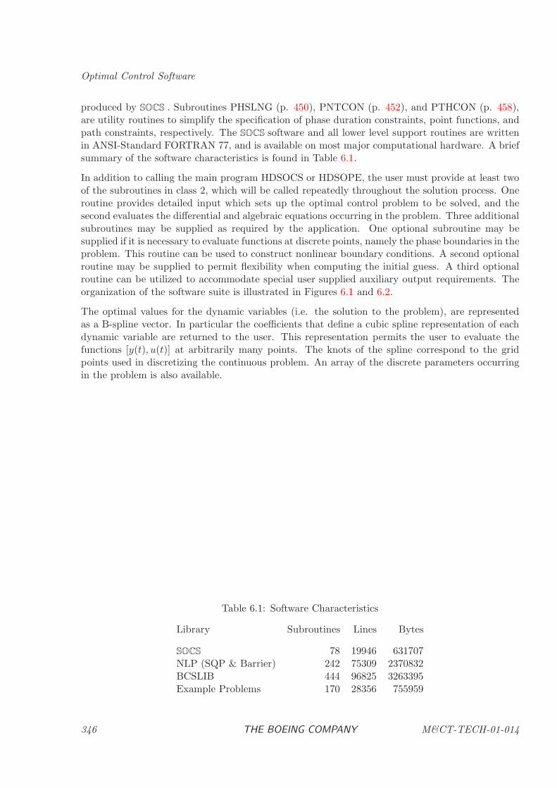
Optimal Control Software
produced by SOCS . Subroutines PHSLNG (p. 450), PNTCON (p. 452), and PTHCON (p. 458),are utility routines to simplify the specification of phase duration constraints, point functions, andpath constraints, respectively. The SOCS software and all lower level support routines are writtenin ANSI-Standard FORTRAN 77, and is available on most major computational hardware. A briefsummary of the software characteristics is found in Table 6.1.
In addition to calling the main program HDSOCS or HDSOPE, the user must provide at least twoof the subroutines in class 2, which will be called repeatedly throughout the solution process. Oneroutine provides detailed input which sets up the optimal control problem to be solved, and thesecond evaluates the differential and algebraic equations occurring in the problem. Three additionalsubroutines may be supplied as required by the application. One optional subroutine may besupplied if it is necessary to evaluate functions at discrete points, namely the phase boundaries in theproblem. This routine can be used to construct nonlinear boundary conditions. A second optionalroutine may be supplied to permit flexibility when computing the initial guess. A third optionalroutine can be utilized to accommodate special user supplied auxiliary output requirements. Theorganization of the software suite is illustrated in Figures 6.1 and 6.2.
The optimal values for the dynamic variables (i.e. the solution to the problem), are representedas a B-spline vector. In particular the coefficients that define a cubic spline representation of eachdynamic variable are returned to the user. This representation permits the user to evaluate thefunctions [y(t), u(t)] at arbitrarily many points. The knots of the spline correspond to the gridpoints used in discretizing the continuous problem. An array of the discrete parameters occurringin the problem is also available.
Table 6.1: Software Characteristics
Library Subroutines Lines Bytes
SOCS 78 19946 631707NLP (SQP & Barrier) 242 75309 2370832BCSLIB 444 96825 3263395Example Problems 170 28356 755959
346 THE BOEING COMPANY M&CT-TECH-01-014
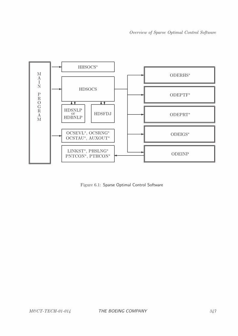
Overview of Sparse Optimal Control Software
MAIN
PROGRAM
HHSOCS∗
HDSOCS
HDSNLPor
HDBNLPHDSFDJ
OCSEVL∗, OCSRNG∗
OCSTAU∗, AUXOUT∗
LINKST∗, PHSLNG∗
PNTCON∗, PTHCON∗
ODERHS∗
ODEPTF∗
ODEPRT∗
ODEIGS∗
ODEINP
-
-
-
-
-�
-
-
-
?6 ?6
Figure 6.1: Sparse Optimal Control Software
M&CT-TECH-01-014 THE BOEING COMPANY 347
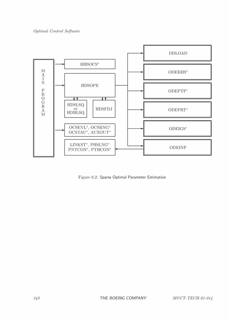
Optimal Control Software
MAIN
PROGRAM
HHSOCS∗
HDSOPE
HDSLSQor
HDBLSQHDSFDJ
OCSEVL∗, OCSRNG∗
OCSTAU∗, AUXOUT∗
LINKST∗, PHSLNG∗
PNTCON∗, PTHCON∗
DDLOAD
ODERHS∗
ODEPTF∗
ODEPRT∗
ODEIGS∗
ODEINP
-
-
-
-
-
-�
-
-
-
?6 ?6
Figure 6.2: Sparse Optimal Parameter Estimation
348 THE BOEING COMPANY M&CT-TECH-01-014
Subprograms for Optimal Control
6.2 Subprograms for Optimal Control
HDSOCS: Sparse Optimal Control . . . . . . . . . . . . . . . . . . . . . . . . . . . . . . . . . 351
HDSOPE: Sparse Optimal Parameter Estimation . . . . . . . . . . . . . . . . . . . . . . . . . 358
HHSOCS: Sparse Optimal Control Input Procedure . . . . . . . . . . . . . . . . . . . . . . . 365
DDLOAD: Discrete Data Load . . . . . . . . . . . . . . . . . . . . . . . . . . . . . . . . . . . 378
ODEIGS: Optimal Control Initial Guess . . . . . . . . . . . . . . . . . . . . . . . . . . . . . . 381
ODEINP: Optimal Control Problem Definition . . . . . . . . . . . . . . . . . . . . . . . . . . 384
ODEPRT: Optimal Control Print . . . . . . . . . . . . . . . . . . . . . . . . . . . . . . . . . . 401
ODEPTF: Optimal Control Point Function Evaluation . . . . . . . . . . . . . . . . . . . . . . 405
ODERHS: Optimal Control Right Hand Side Evaluation . . . . . . . . . . . . . . . . . . . . . 409
AUTOLK: Auto Link Variable Utility . . . . . . . . . . . . . . . . . . . . . . . . . . . . . . . 414
AUTOPL: Auto Phase Length Constraint Utility . . . . . . . . . . . . . . . . . . . . . . . . . 416
AUXOUT: Auxiliary Output Utility . . . . . . . . . . . . . . . . . . . . . . . . . . . . . . . . 418
BSPDEF: B-Spline Algebraic Variable Utility . . . . . . . . . . . . . . . . . . . . . . . . . . . 422
CTLFIL: Optimal Control Input From a File . . . . . . . . . . . . . . . . . . . . . . . . . . . 427
CTLSTA: Optimal Control Software Status Utility . . . . . . . . . . . . . . . . . . . . . . . . 429
FETCH: Variable Retrieval Utility . . . . . . . . . . . . . . . . . . . . . . . . . . . . . . . . . 430
FYLFMT: Restart File Format Conversion Utility . . . . . . . . . . . . . . . . . . . . . . . . 432
LINKST: Optimal Control Linkage Utility . . . . . . . . . . . . . . . . . . . . . . . . . . . . . 435
NUMGRD: Gridpoint Evaluation Utility . . . . . . . . . . . . . . . . . . . . . . . . . . . . . . 437
OCSEVL: Optimal Control Solution Evaluation Utility . . . . . . . . . . . . . . . . . . . . . 439
OCSGRD: Optimal Control Solution Grid Evaluation Utility . . . . . . . . . . . . . . . . . . 443
OCSRNG: Optimal Control Solution Range Utility . . . . . . . . . . . . . . . . . . . . . . . . 445
OCSTAU: Optimal Control Solution Spline Evaluation Utility . . . . . . . . . . . . . . . . . . 447
PHSLNG: Optimal Control Phase Duration Utility . . . . . . . . . . . . . . . . . . . . . . . . 450
PNTCON: Optimal Control Point Constraint Utility . . . . . . . . . . . . . . . . . . . . . . . 452
PTHAUX: Path Constraint with Auxiliary Functions . . . . . . . . . . . . . . . . . . . . . . 455
PTHCON: Path Constraint Utility . . . . . . . . . . . . . . . . . . . . . . . . . . . . . . . . . 458
RST2SP: Restart File to Spline Array Utility . . . . . . . . . . . . . . . . . . . . . . . . . . . 461
SCTFIL: Save an Optimal Control Input File . . . . . . . . . . . . . . . . . . . . . . . . . . . 463
M&CT-TECH-01-014 THE BOEING COMPANY 349

Optimal Control Software
TRMAUX: Terminate Auxiliary Function Construction . . . . . . . . . . . . . . . . . . . . . 465
WATCH: Variable Monitor Utility . . . . . . . . . . . . . . . . . . . . . . . . . . . . . . . . . 467
350 THE BOEING COMPANY M&CT-TECH-01-014
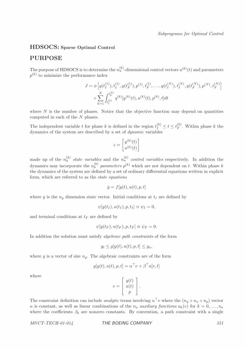
Subprograms for Optimal Control
HDSOCS: Sparse Optimal Control
PURPOSE
The purpose of HDSOCS is to determine the n(k)u -dimensional control vectors u(k)(t) and parameters
p(k) to minimize the performance index
J = φ[y(t
(1)I ), t
(1)I , y(t
(1)F ), p(1), t
(1)F , . . . , y(t
(N)I ), t
(N)I , y(t
(N)F ), p(N), t
(N)F
]
+N∑
k=1
∫ t(k)F
t(k)I
q(k)[y(k)(t), u(k)(t), p(k), t]dt
where N is the number of phases. Notice that the objective function may depend on quantitiescomputed in each of the N phases.
The independent variable t for phase k is defined in the region t(k)I ≤ t ≤ t
(k)F . Within phase k the
dynamics of the system are described by a set of dynamic variables
z =
[y(k)(t)
u(k)(t)
]
made up of the n(k)y state variables and the n
(k)u control variables respectively. In addition the
dynamics may incorporate the n(k)p parameters p(k) which are not dependent on t. Within phase k
the dynamics of the system are defined by a set of ordinary differential equations written in explicitform, which are referred to as the state equations
y = f [y(t), u(t), p, t]
where y is the ny dimension state vector. Initial conditions at tI are defined by
ψ[y(tI), u(tI), p, tI ] ≡ ψI = 0,
and terminal conditions at tF are defined by
ψ[y(tF ), u(tF ), p, tF ] ≡ ψF = 0.
In addition the solution must satisfy algebraic path constraints of the form
gℓ ≤ g[y(t), u(t), p, t] ≤ gu,
where g is a vector of size ng. The algebraic constraints are of the form
g[y(t), u(t), p, t] = α⊤v + β⊤a[v, t]
where
v =
y(t)u(t)p
.
The constraint definition can include analytic terms involving α⊤v where the (ny +nu +np) vectorα is constant, as well as linear combinations of the na auxiliary functions ak(v) for k = 0, . . . , na
where the coefficients βk are nonzero constants. By convention, a path constraint with a single
M&CT-TECH-01-014 THE BOEING COMPANY 351
Optimal Control Software
nonlinear term a0(y, u, p, t) has no auxiliary functions (na = 0). Observe that each individual pathconstraint may have a different number of auxiliary functions and analytic terms. Simple boundscan be imposed on the state variables
yℓ ≤ y(t) ≤ yu,
the control variablesuℓ ≤ u(t) ≤ uu,
and the parameterspℓ ≤ p ≤ pu.
Note that a path variable equality constraint can be imposed if the upper and lower bounds areequal, e.g. (gℓ)k = (gu)k for some k.
Finally it may be convenient to evaluate expressions of the form
∫ tF
tI
q[y(t), u(t), p, t]dt
which involve the quadrature functions q. Collectively we refer to those functions evaluated duringthe phase, namely,
F (t) =
f [y(t), u(t), p, t]g[y(t), u(t), p, t]q[y(t), u(t), p, t]a[y(t), u(t), p, t]
as the vector of continuous functions. Similarly functions evaluated at the beginning or end of aphase such as the boundary conditions ψ[y(tI), u(tI), p, tI ] and ψ[y(tF ), u(tF ), p, tF ] are referred toas point functions.
RELATED SUBPROGRAMS
HHSNLP Sparse Nonlinear Programming Input Procedure
HDSNLP Sparse Nonlinear Programming
HDBNLP Sparse Barrier Nonlinear Programming
HHSOCS Sparse Optimal Control Input Procedure
HDSOPE Sparse Optimal Parameter Estimation
METHOD
The optimal control problem is solved using a direct transcription method. The basic steps in theapproach are as follows:
1. Direct Transcription. Transcribe the optimal control problem into a nonlinear program-ming (NLP) problem by discretization;
2. Sparse Nonlinear Program. Solve the sparse NLP using either a sequential quadraticprogramming (SQP) or an interior-point (barrier) method;
352 THE BOEING COMPANY M&CT-TECH-01-014
Subprograms for Optimal Control
3. Mesh Refinement. Assess the accuracy of the approximation (i.e. the finite dimensionalproblem), and if necessary refine the discretization, and then repeat the optimization steps.
The SOCS software provides a number of discretization techniques including, trapezoidal, Hermite-Simpson, and Runge-Kutta methods. The sparse nonlinear programming problem can be solvedusing either a sequential quadratic programming (SQP) approach or an interior-point (barrier)method. There are a number of issues which determine the efficiency of the NLP. First, theJacobian matrix (of first derivatives) and the Hessian matrix (of second derivatives) needed tosolve the NLP are large and sparse, and SOCS automatically constructs the sparsity structure.Second, it is necessary to compute the Hessian matrix HL and within SOCS sparse finite differencetechniques are utilized. Third, the sparse NLP subproblem can be solved efficiently using a sparseSchur-Complement Method or a primal-dual barrier method. The SOCS software also incorporatesa technique for computing the discretization error and if necessary refining the mesh to reduce thiserror.
WARNING
The direct transcription method implemented in the SOCS software yields approximate solutionsfor the state and control functions. The technique is appropriate when the control variables arecontinuous and the state variables have continuous first derivatives. If the solution to the optimalcontrol problem cannot be represented in this form, unpredictable performance in the numericalmethods may be observed. Furthermore the technique may be inappropriate for solving differential-algebraic systems with global index greater than one. This situation can occur either because ofthe presence of state variable path constraints and/or singular arcs in the solution. Many of thesesituations can be circumvented by reformulation of the underlying problem to exploit the multi-phase capability of the SOCS software.
The user supplied functions which define the objective function, path constraints, point functions,and differential equations are all assumed to be continuous and have continuous first and secondderivatives. Non-differentiable functions can cause unpredictable performance in the optimizationalgorithm. It should be emphasized that discontinuities in the second derivatives can significantlydegrade the speed of convergence without producing any other obvious difficulties. The followingcommon sources of error should be avoided when evaluating the objective and constraint functions:
(1) non-smooth interpolation of data;
(2) iterative procedures inside the function evaluation process, such as adaptive quadrature or rootsolving;
(3) discontinuous behavior caused by branching for IF tests;
(4) non-differentiable functions such as ABS, MAX, and MIN.
The user must provide procedures to evaluate the continuous and point functions. If it is notpossible to evaluate the functions the user can communicate this information to the algorithmusing the function error flag IFERR as described below.
USAGE
M&CT-TECH-01-014 THE BOEING COMPANY 353
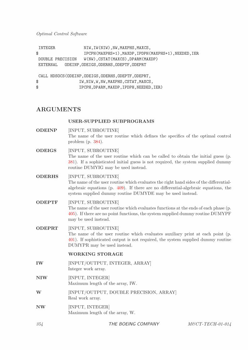
Optimal Control Software
INTEGER NIW,IW(NIW),NW,MAXPHS,MAXCS,
$ IPCPH(MAXPHS+1),MAXDP,IPDPH(MAXPHS+1),NEEDED,IER
DOUBLE PRECISION W(NW),CSTAT(MAXCS),DPARM(MAXDP)
EXTERNAL ODEINP,ODEIGS,ODERHS,ODEPTF,ODEPRT
CALL HDSOCS(ODEINP,ODEIGS,ODERHS,ODEPTF,ODEPRT,
$ IW,NIW,W,NW,MAXPHS,CSTAT,MAXCS,
$ IPCPH,DPARM,MAXDP,IPDPH,NEEDED,IER)
ARGUMENTS
USER-SUPPLIED SUBPROGRAMS
ODEINP [INPUT, SUBROUTINE]The name of the user routine which defines the specifics of the optimal controlproblem (p. 384).
ODEIGS [INPUT, SUBROUTINE]The name of the user routine which can be called to obtain the initial guess (p.381). If a sophisticated initial guess is not required, the system supplied dummyroutine DUMYIG may be used instead.
ODERHS [INPUT, SUBROUTINE]The name of the user routine which evaluates the right hand sides of the differential-algebraic equations (p. 409). If there are no differential-algebraic equations, thesystem supplied dummy routine DUMYDE may be used instead.
ODEPTF [INPUT, SUBROUTINE]The name of the user routine which evaluates functions at the ends of each phase (p.405). If there are no point functions, the system supplied dummy routine DUMYPFmay be used instead.
ODEPRT [INPUT, SUBROUTINE]The name of the user routine which evaluates auxiliary print at each point (p.401). If sophisticated output is not required, the system supplied dummy routineDUMYPR may be used instead.
WORKING STORAGE
IW [INPUT/OUTPUT, INTEGER, ARRAY]Integer work array.
NIW [INPUT, INTEGER]Maximum length of the array, IW.
W [INPUT/OUTPUT, DOUBLE PRECISION, ARRAY]Real work array.
NW [INPUT, INTEGER]Maximum length of the array, W.
354 THE BOEING COMPANY M&CT-TECH-01-014
Subprograms for Optimal Control
OPTIMAL CONTROL ARGUMENTS
MAXPHS [INPUT, INTEGER]Maximum number of phases permitted.
CSTAT [INPUT/OUTPUT, DOUBLE PRECISION, ARRAY]Array containing the B-spline coefficient vectors for each phase in the optimal con-trol problem. The coefficients for phase k are stored in CSTAT(k1),. . ., CSTAT(k2)where k1 = IPCPH(k) and k2 = IPCPH(k+1) −1. An initial guess for the contin-uous functions [y(t), u(t)] can be specified if CSTAT is input and the initializationflag INIT = 3 is set in subroutine ODEINP. After terminating the final value forthe continuous variables [y(t), u(t)] is represented in B-spline format and the arrayCSTAT is output.
MAXCS [INPUT, INTEGER]Maximum length of the array, CSTAT.
IPCPH [INPUT/OUTPUT, INTEGER, ARRAY]Array of pointers to the beginning of the B-spline coefficient vectors for each phase.
DPARM [INPUT/OUTPUT, DOUBLE PRECISION, ARRAY]Array containing the values of discrete parameters.
MAXDP [INPUT, INTEGER]Maximum length of the array, DPARM.
IPDPH [INPUT/OUTPUT, INTEGER, ARRAY]Array of pointers to the beginning of the discrete parameters in effect on eachphase.
NEEDED [OUTPUT, INTEGER]Storage needed in one of the arrays IW, W, CSTAT, DPARM, IPDPH, or IPCPH.When IER 6= 0 to indicate that HDSOCS has failed to compute a solution, an errormessage will be printed. Section 6.5 describes the optimal control error messages.NEEDED contains the required value for one of the quantities NIW, NW, MAXCS,MAXDP, or MAXPHS.
IER [OUTPUT, INTEGER]Error return flag; IER = 0 for a successful termination. When IER 6= 0 to indicatethat HDSOCS has failed to compute a solution, an error message will be printed.Section 6.5 describes the optimal control error messages.
USAGE REMARKS
Optimal Solution B-spline Representation
The optimal values for the continuous functions are represented in terms of a common B-splinebasis. The continuous functions can be written as
[y(t)u(t)
]≈[y(t)u(t)
]=
N∑
i=1
αiBi(t)
M&CT-TECH-01-014 THE BOEING COMPANY 355
Optimal Control Software
where the functions Bi(t) form a basis for C0 cubic B-splines. By construction the state variablesare C1 cubics and the control will be either C0 quadratic or linear functions, even though they arerepresented in the space of C0 cubic B-splines.
After SOCS has terminated successfully, the coefficients αi which define the optimal solution arereturned to the user in the CSTAT array. The utility routine OCSEVL (p. 439) can be used toevaluate the solution at an arbitrary point. The utility routine AUXOUT (p. 418) can be usedto create an output file from the information in the CSTAT array. For a multiphase problem theCSTAT array contains the B-spline coefficients for all phases stored in a single contiguous array,with the beginning of the data for phase k defined by the integer array IPCPH.
OPTIONAL INPUT
In addition to the required arguments, there are a number of optional arguments that can bespecified for subroutine HDSOCS. There are three ways that optional inputs can be specified tothe SOCS software. The first method is to call the input subroutine HHSOCS (p. 365). Thesecond method which can be used to define input for the sparse NLP is to call the input routineHHSNLP (p. 196). The third approach is to read an input file by utilizing subroutine CTLFIL (p.427). It should be emphasized that it is not necessary to call HHSOCS, HHSNLP or CTLFIL ifthe default values are appropriate.
Usage of the routine HHSOCS is described on page 365. The sole argument of the routine is acharacter string of the form ’symbol = value’, where ’symbol’ is the mnemonic for a variable namewhich is to be set, and ’value’ is the corresponding integer, floating point, or character constant tobe used. Exceptions to this form are the character strings, ’DEFAULT’, ’OPTIONS’, and ’FULLOPTIONS’. The preceding strings, or those representing mnemonics, can be in upper, lower, ormixed case.
Sample calls to HHSOCS are of the form:
CALL HHSOCS(’IPUOCP = 11’)
CALL HHSOCS(’odetol = 1.e-04’)
The sparse nonlinear programming algorithms HDSNLP (p. 51) and HDBNLP (p. 141) which arecalled by HDSOCS utilize a similar input mechanism. In fact, there are two functionally equivalentmethods for setting the sparse NLP options. The first approach is to directly call the sparse NLPinput procedure HHSNLP (p. 196) from the main program. The second approach is to call theSOCS input procedure HHSOCS (p. 365), with the special string ’HHSNLP:symbol = value’. Thefollowing examples illustrate the options:
C
C THE FOLLOWING CALL TO THE SPARSE NLP
C
CALL HHSNLP(’ALGOPT = FM’)
C
C IS EQUIVALENT TO
356 THE BOEING COMPANY M&CT-TECH-01-014
Subprograms for Optimal Control
C
CALL HHSOCS(’HHSNLP:ALGOPT = FM’)
C
C----------------------------
C
C THE FOLLOWING CALL TO THE SPARSE NLP
C
CALL HHSNLP(’MAXNFE = 100’)
C
C IS EQUIVALENT TO
C
CALL HHSOCS(’HHSNLP:MAXNFE = 100’)
C
Another way of setting optimal control values is through the routine, CTLFIL. This routine willread a user specified file where each line corresponds to a character string like those describedabove.
CHARACTER*80 FILNAM
INTEGER INUNIT
CALL CTLFIL(INUNIT,FILNAM)
OPTIONAL PRINTOUT
The level of printed output from HDSOCS is controlled by the variables IPGRD, IPNLP, IPODEand IPUOCP which are set by calls to HHSOCS. A complete description of the iteration outputoptions is found in Section 6.6.
M&CT-TECH-01-014 THE BOEING COMPANY 357
Optimal Control Software
HDSOPE: Sparse Optimal Parameter Estimation
PURPOSE
The purpose of HDSOPE is to determine the n(k)u -dimensional control vectors u(k)(t) and parameters
p(k) to minimize the performance index
J =1
2r⊤r
where r is the L-dimensional residual vector. The form of the residual vector is defined below.Notice that the objective function may depend on quantities computed in each of the N phases.
The independent variable t for phase k is defined in the region t(k)I ≤ t ≤ t
(k)F . Within phase k the
dynamics of the system are described by a set of dynamic variables
z =
[y(k)(t)
u(k)(t)
]
made up of the n(k)y state variables and the n
(k)u control variables respectively. In addition the
dynamics may incorporate the n(k)p parameters p(k) which are not dependent on t. Within phase k
the dynamics of the system are defined by a set of ordinary differential equations written in explicitform, which are referred to as the state equations
y = f [y(t), u(t), p, t]
where y is the ny dimension state vector. Initial conditions at tI are defined by
ψ[y(tI), u(tI), p, tI ] ≡ ψI = 0,
and terminal conditions at tF are defined by
ψ[y(tF ), u(tF ), p, tF ] ≡ ψF = 0.
In addition the solution must satisfy algebraic path constraints of the form
gℓ ≤ g[y(t), u(t), p, t] ≤ gu,
where g is a vector of size ng. The algebraic constraints are of the form
g[y(t), u(t), p, t] = α⊤v + β⊤a[v, t]
where
v =
y(t)u(t)p
.
The constraint definition can include analytic terms involving α⊤v where the (ny +nu +np) vectorα is constant, as well as linear combinations of the na auxiliary functions ak(v) for k = 0, . . . , na
where the coefficients βk are nonzero constants. By convention, a path constraint with a singlenonlinear term a0(y, u, p, t) has no auxiliary functions (na = 0). Observe that each individual pathconstraint may have a different number of auxiliary functions and analytic terms. Simple boundscan be imposed on the state variables
yL ≤ y(t) ≤ yU ,
358 THE BOEING COMPANY M&CT-TECH-01-014
Subprograms for Optimal Control
the control variables
uL ≤ u(t) ≤ uU ,
and the parameters
pL ≤ p ≤ pU .
Note that a path variable equality constraint can be imposed if the upper and lower bounds areequal, e.g. (gL)k = (gU )k for some k.
Components of the residual vector can be of two forms. State residuals on phase k are of the form
rℓ = wij
[y
(k)i (θij) − y
(k)ij
]
where y(k)i (θij) is the value of state variable i computed at time θij and yij is the observed value at
the same point. Algebraic residuals are of the form
rℓ = wij
[u
(k)i (θij) − u
(k)ij
]
where u(k)i (θij) is the value of algebraic variable i computed at time θij and u
(k)ij is the observed
value at the same point. The quantities wij are residual scale weights. It is required that dataevaluation points satisfy
t(k)I ≤ θ
(k)ij ≤ t
(k)F .
Often the evaluation points are arranged monotonically, that is θi,j ≤ θi,j+1. It is also common tohave many variables evaluated at the same time, e.g. θi,j = θi+1,j. Neither of these assumptions
are necessary for the software, however the initial and final phase times t(k)I and t
(k)F must be fixed.
RELATED SUBPROGRAMS
HHSNLP Sparse Nonlinear Programming Input Procedure
HDSLSQ Sparse Constrained Nonlinear Least Squares
HDBLSQ Sparse Barrier Constrained Nonlinear Least Squares
HHSOCS Sparse Optimal Control Input Procedure
METHOD
The parameter estimation problem is solved using a direct transcription method. The basic stepsin the approach are as follows:
1. Direct Transcription. Transcribe the parameter estimation problem into a nonlinear pro-gramming (NLP) problem by discretization;
2. Sparse Nonlinear Program. Solve the sparse NLP using a sequential quadratic program-ming (SQP) method;
3. Mesh Refinement. Assess the accuracy of the approximation (i.e. the finite dimensionalproblem), and if necessary refine the discretization, and then repeat the optimization steps.
M&CT-TECH-01-014 THE BOEING COMPANY 359
Optimal Control Software
The SOCS software provides a number of discretization techniques including, trapezoidal, Hermite-Simpson, and Runge-Kutta methods. The sparse nonlinear programming problem is solved using asequential quadratic programming (SQP) approach. There are a number of issues which determinethe efficiency of the NLP. First, the Jacobian matrix (of first derivatives) and the Hessian matrix(of second derivatives) needed to solve the NLP are large and sparse, and SOCS automaticallyconstructs the sparsity structure. Second, it is necessary to compute the Hessian matrix HL andwithin SOCS sparse finite difference techniques are utilized. Third, the sparse NLP subproblem canbe solved efficiently using a sparse Schur-Complement Method. The SOCS software also incorporatesa technique for computing the discretization error and if necessary refining the mesh to reduce thiserror.
WARNING
The direct transcription method implemented in the SOCS software yields approximate solutionsfor the state and control functions. The technique is appropriate when the control variables arecontinuous and the state variables have continuous first derivatives. If the solution to the parameterestimation problem cannot be represented in this form, unpredictable performance in the numericalmethods may be observed. Furthermore the technique may be inappropriate for solving differential-algebraic systems with global index greater than one. This situation can occur either because ofthe presence of state variable path constraints and/or singular arcs in the solution. Many of thesesituations can be circumvented by reformulation of the underlying problem to exploit the multi-phase capability of the SOCS software.
The user supplied functions which define the objective function, path constraints, point functions,and differential equations are all assumed to be continuous and have continuous first and secondderivatives. Non-differentiable functions can cause unpredictable performance in the optimizationalgorithm. It should be emphasized that discontinuities in the second derivatives can significantlydegrade the speed of convergence without producing any other obvious anomalies. The followingcommon sources of error should be avoided when evaluating the objective and constraint functions:
(1) non-smooth interpolation of data;
(2) iterative procedures inside the function evaluation process, such as adaptive quadrature or rootsolving;
(3) discontinuous behavior caused by branching for IF tests;
(4) non-differentiable functions such as ABS, MAX, and MIN.
The user must provide procedures to evaluate the continuous and point functions. If it is notpossible to evaluate the functions the user can communicate this information to the algorithmusing the function error flag IFERR as described below.
USAGE
INTEGER NIW,IW(NIW),NW,MAXPHS,MAXCS,
$ IPCPH(MAXPHS+1),MAXDP,IPDPH(MAXPHS+1),NEEDED,IER
DOUBLE PRECISION W(NW),CSTAT(MAXCS),DPARM(MAXDP)
EXTERNAL ODEINP,ODEIGS,ODERHS,ODEPTF,ODEPRT,DDLOAD
360 THE BOEING COMPANY M&CT-TECH-01-014
Subprograms for Optimal Control
CALL HDSOPE(ODEINP,ODEIGS,ODERHS,ODEPTF,ODEPRT,DDLOAD,
$ IW,NIW,W,NW,MAXPHS,CSTAT,MAXCS,
$ IPCPH,DPARM,MAXDP,IPDPH,NEEDED,IER)
ARGUMENTS
USER-SUPPLIED SUBPROGRAMS
ODEINP [INPUT, SUBROUTINE]The name of the user routine which defines the specifics of the parameter estimationproblem to solve (p. 384).
ODEIGS [INPUT, SUBROUTINE]The name of the user routine which can be called to obtain the initial guess (p.381). If a sophisticated initial guess is not required, the system supplied dummyroutine DUMYIG may be used instead.
ODERHS [INPUT, SUBROUTINE]The name of the user routine which evaluates the right hand sides of the differential-algebraic equations (p. 409). If there are no differential-algebraic equations, thesystem supplied dummy routine DUMYDE may be used instead.
ODEPTF [INPUT, SUBROUTINE]The name of the user routine which evaluates functions at the ends of each phase (p.405). If there are no point functions, the system supplied dummy routine DUMYPFmay be used instead.
ODEPRT [INPUT, SUBROUTINE]The name of the user routine which evaluates auxiliary print at each point (p.401). If sophisticated output is not required, the system supplied dummy routineDUMYPR may be used instead.
DDLOAD [INPUT, SUBROUTINE]The name of the user routine which loads the discrete data values (p. 378).
WORKING STORAGE
IW [INPUT/OUTPUT, INTEGER, ARRAY]Integer work array.
NIW [INPUT, INTEGER]Maximum length of the array, IW.
W [INPUT/OUTPUT, DOUBLE PRECISION, ARRAY]Real work array.
NW [INPUT, INTEGER]Maximum length of the array, W.
PARAMETER ESTIMATION ARGUMENTS
M&CT-TECH-01-014 THE BOEING COMPANY 361
Optimal Control Software
MAXPHS [INPUT, INTEGER]Maximum number of phases permitted.
CSTAT [INPUT/OUTPUT, DOUBLE PRECISION, ARRAY]Array containing the B-spline coefficient vectors for each phase in the parameterestimation problem. The coefficients for phase k are stored in CSTAT(k1),. . .,CSTAT(k2) where k1 = IPCPH(k) and k2 = IPCPH(k + 1) −1. An initial guessfor the continuous functions [y(t), u(t)] can be specified if CSTAT is input and theinitialization flag INIT = 3 is set in subroutine ODEINP. After terminating thefinal value for the continuous variables [y(t), u(t)] is represented in B-spline formatand the array CSTAT is output.
MAXCS [INPUT, INTEGER]Maximum length of the array, CSTAT.
IPCPH [INPUT/OUTPUT, INTEGER, ARRAY]Array of pointers to the beginning of the B-spline coefficient vectors for each phase.
DPARM [INPUT/OUTPUT, DOUBLE PRECISION, ARRAY]Array containing the values of discrete parameters.
MAXDP [INPUT, INTEGER]Maximum length of the array, DPARM.
IPDPH [INPUT/OUTPUT, INTEGER, ARRAY]Array of pointers to the beginning of the discrete parameters in effect on eachphase.
NEEDED [OUTPUT, INTEGER]Storage needed in one of the arrays IW, W, CSTAT, DPARM, IPDPH, or IPCPH.When IER 6= 0 to indicate that HDSOPE has failed to compute a solution, anerror message will be printed. Section 6.5 describes the parameter estimation errormessages. NEEDED contains the required value for one of the quantities NIW,NW, MAXCS, MAXDP, or MAXPHS.
IER [OUTPUT, INTEGER]Error return flag; IER = 0 for a successful termination. When IER 6= 0 to indicatethat HDSOPE has failed to compute a solution, an error message will be printed.Section 6.5 describes the parameter estimation error messages.
USAGE REMARKS
Optimal Solution B-spline Representation
The optimal values for the continuous functions are represented in terms of a common B-splinebasis. The continuous functions can be written as
[y(t)u(t)
]≈[y(t)u(t)
]=
N∑
i=1
αiBi(t)
362 THE BOEING COMPANY M&CT-TECH-01-014
Subprograms for Optimal Control
where the functions Bi(t) form a basis for C0 cubic B-splines. By construction the state variablesare C1 cubics and the control will be either C0 quadratic or linear functions, even though they arerepresented in the space of C0 cubic B-splines.
After SOCS has terminated successfully, the coefficients αi which define the optimal solution arereturned to the user in the CSTAT array. The utility routine OCSEVL (p. 439) can be used toevaluate the solution at an arbitrary point. The utility routine AUXOUT (p. 418) can be usedto create an output file from the information in the CSTAT array. For a multi-phase problem theCSTAT array contains the B-spline coefficients for all phases stored in a single contiguous array,with the beginning of the data for phase k defined by the integer array IPCPH.
OPTIONAL INPUT
In addition to the required arguments, there are a number of optional arguments that can bespecified for subroutine HDSOPE. There are three ways that optional inputs can be specified tothe SOCS software. The first method is to call the input subroutine HHSOCS (p. 365). Thesecond method which can be used to define input for the sparse NLP is to call the input routineHHSNLP (p. 196). The third approach is to read an input file by utilizing subroutine CTLFIL (p.427). It should be emphasized that it is not necessary to call HHSOCS, HHSNLP or CTLFIL ifthe default values are appropriate.
Usage of the routine HHSOCS is described on page 365. The sole argument of the routine is acharacter string of the form ’symbol = value’, where ’symbol’ is the mnemonic for a variable namewhich is to be set, and ’value’ is the corresponding integer, floating point, or character constant tobe used. Exceptions to this form are the character strings, ’DEFAULT’, ’OPTIONS’, and ’FULLOPTIONS’. The preceding strings, or those representing mnemonics, can be in upper, lower, ormixed case.
Sample calls to HHSOCS are of the form:
CALL HHSOCS(’IPUOCP = 11’)
CALL HHSOCS(’odetol = 1.e-04’)
The sparse nonlinear programming algorithms HDSLSQ (p. 70) and HDBLSQ (p. 161) which arecalled by HDSOPE utilize an input mechanism similar to the other optimization algorithms in thelibrary. In fact, there are two functionally equivalent methods for setting the sparse NLP options.The first approach is to directly call the sparse NLP input procedure HHSNLP (p. 196) from themain program. The second approach is to call the SOCS input procedure HHSOCS (p. 365), withthe special strings ’HHSNLP:symbol = value’. The following examples illustrate the options:
C
C THE FOLLOWING CALL TO THE SPARSE NLP
C
CALL HHSNLP(’ALGOPT = FM’)
C
C IS EQUIVALENT TO
M&CT-TECH-01-014 THE BOEING COMPANY 363
Optimal Control Software
C
CALL HHSOCS(’HHSNLP:ALGOPT = FM’)
C
C----------------------------
C
C THE FOLLOWING CALL TO THE SPARSE NLP
C
CALL HHSNLP(’MAXNFE = 100’)
C
C IS EQUIVALENT TO
C
CALL HHSOCS(’HHSNLP:MAXNFE = 100’)
C
Another way of setting parameter estimation values is through the routine, CTLFIL. This routinewill read a user specified file where each line corresponds to a character string like those describedabove.
CHARACTER*80 FILNAM
INTEGER INUNIT
CALL CTLFIL(INUNIT,FILNAM)
OPTIONAL PRINTOUT
The level of printed output from HDSOPE is controlled by the variables IPGRD, IPNLP, IPODEand IPUOCP which are set by calls to HHSOCS. A complete description of the iteration outputoptions is found in Section 6.6.
364 THE BOEING COMPANY M&CT-TECH-01-014
Subprograms for Optimal Control
HHSOCS: Sparse Optimal Control Input Procedure
PURPOSE
HHSOCS is a utility subroutine used to define optional inputs for the sparse optimal control softwareSOCS implemented in subroutine HDSOCS and HDSOPE.
RELATED SUBPROGRAMS
HDSOCS Sparse Optimal Control
HDSOPE Sparse Optimal Parameter Estimation
HDSNLP Sparse Nonlinear Programming
HDBNLP Sparse Barrier Nonlinear Programming
HDSLSQ Sparse Constrained Nonlinear Least Squares
HDBLSQ Sparse Barrier Constrained Nonlinear Least Squares
HHSNLP Sparse Nonlinear Programming Input Procedure
METHOD
Subroutine HHSOCS must be called once for every optional parameter to be set. The input toHHSOCS must be a single character variable of length not to exceed 80 characters. The string iscase insensitive and is assumed to have the following format:
’ symbol = value ’
The symbol must be one of the valid mnemonics defined below; see ARGUMENTS. Informationcontained in the character string is communicated to the sparse optimal control algorithm HDSOCSand sparse optimal parameter estimation algorithm HDSOPE via three internal commons. Thecharacter string must have an equals sign “=” to separate the symbol from the value. The onlyexceptions to this rule are when symbol = ’DEFAULT, or ’OPTIONS’. The value portion of the stringcan contain integer, real (single or double precision), or character values.
The sparse nonlinear programming algorithms called by HDSOCS and HDSOPE utilize a similarinput mechanism. In fact, there are two functionally equivalent methods for setting the sparse NLPoptions. The first approach is to directly call the sparse NLP input procedure HHSNLP (p. 196)from the main program. The second approach is to call the SOCS input procedure HHSOCS, witheither of the special string
’HHSNLP:symbol = value’.
All parameters not specified by the user are automatically set to their default values. Any optionalparameters that are set by the user are not altered by algorithms HDSOCS, HDSOPE, HDBNLP,HDBLSQ, HDSLSQ and HDSNLP, and hence changes to the options are cumulative. Thereforeany input changes made by the user will remain in effect until they are explicitly reset by anothercall to HHSOCS (or HHSNLP).
There are two possible sources for error when using HHSOCS;
M&CT-TECH-01-014 THE BOEING COMPANY 365
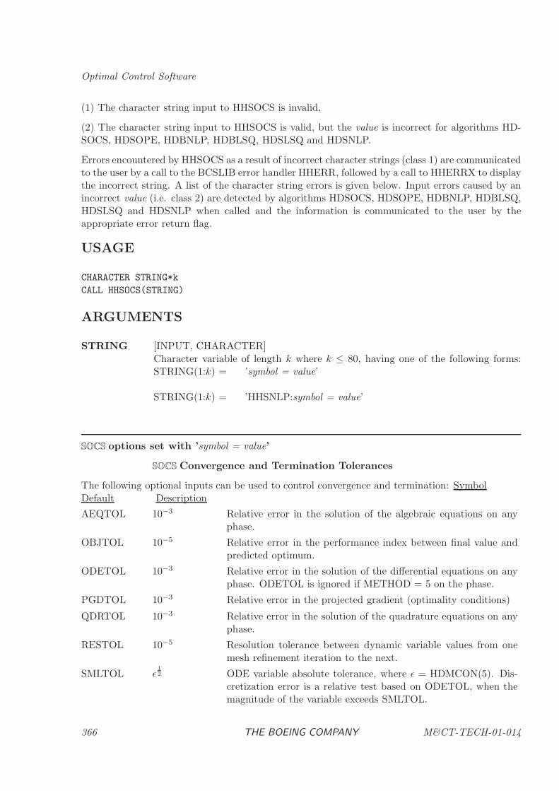
Optimal Control Software
(1) The character string input to HHSOCS is invalid,
(2) The character string input to HHSOCS is valid, but the value is incorrect for algorithms HD-SOCS, HDSOPE, HDBNLP, HDBLSQ, HDSLSQ and HDSNLP.
Errors encountered by HHSOCS as a result of incorrect character strings (class 1) are communicatedto the user by a call to the BCSLIB error handler HHERR, followed by a call to HHERRX to displaythe incorrect string. A list of the character string errors is given below. Input errors caused by anincorrect value (i.e. class 2) are detected by algorithms HDSOCS, HDSOPE, HDBNLP, HDBLSQ,HDSLSQ and HDSNLP when called and the information is communicated to the user by theappropriate error return flag.
USAGE
CHARACTER STRING*k
CALL HHSOCS(STRING)
ARGUMENTS
STRING [INPUT, CHARACTER]Character variable of length k where k ≤ 80, having one of the following forms:STRING(1:k) = ’symbol = value’
STRING(1:k) = ’HHSNLP:symbol = value’
SOCS options set with ’symbol = value’
SOCS Convergence and Termination Tolerances
The following optional inputs can be used to control convergence and termination: SymbolDefault Description
AEQTOL 10−3 Relative error in the solution of the algebraic equations on anyphase.
OBJTOL 10−5 Relative error in the performance index between final value andpredicted optimum.
ODETOL 10−3 Relative error in the solution of the differential equations on anyphase. ODETOL is ignored if METHOD = 5 on the phase.
PGDTOL 10−3 Relative error in the projected gradient (optimality conditions)
QDRTOL 10−3 Relative error in the solution of the quadrature equations on anyphase.
RESTOL 10−5 Resolution tolerance between dynamic variable values from onemesh refinement iteration to the next.
SMLTOL ǫ12 ODE variable absolute tolerance, where ǫ = HDMCON(5). Dis-
cretization error is a relative test based on ODETOL, when themagnitude of the variable exceeds SMLTOL.
366 THE BOEING COMPANY M&CT-TECH-01-014
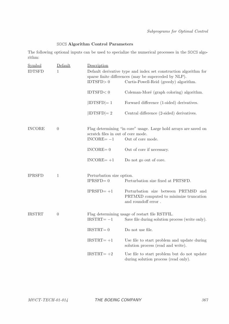
Subprograms for Optimal Control
SOCS Algorithm Control Parameters
The following optional inputs can be used to specialize the numerical processes in the SOCS algo-rithm:
Symbol Default Description
IDTSFD 1 Default derivative type and index set construction algorithm forsparse finite differences (may be superceded by NLP).IDTSFD> 0 Curtis-Powell-Reid (greedy) algorithm.
IDTSFD< 0 Coleman-More (graph coloring) algorithm.
|IDTSFD|= 1 Forward difference (1-sided) derivatives.
|IDTSFD|= 2 Central difference (2-sided) derivatives.
INCORE 0 Flag determining “in core” usage. Large hold arrays are saved onscratch files in out of core mode.INCORE= −1 Out of core mode.
INCORE= 0 Out of core if necessary.
INCORE= +1 Do not go out of core.
IPRSFD 1 Perturbation size option.IPRSFD= 0 Perturbation size fixed at PRTSFD.
IPRSFD= +1 Perturbation size between PRTMSD andPRTMXD computed to minimize truncationand roundoff error .
IRSTRT 0 Flag determining usage of restart file RSTFIL.IRSTRT= −1 Save file during solution process (write only).
IRSTRT= 0 Do not use file.
IRSTRT= +1 Use file to start problem and update duringsolution process (read and write).
IRSTRT= +2 Use file to start problem but do not updateduring solution process (read only).
M&CT-TECH-01-014 THE BOEING COMPANY 367
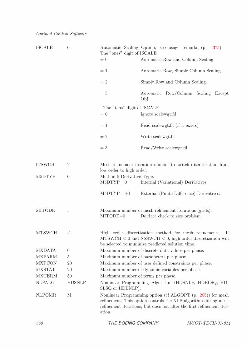
Optimal Control Software
ISCALE 0 Automatic Scaling Option; see usage remarks (p. 375).The ”ones” digit of ISCALE
= 0 Automatic Row and Column Scaling.
= 1 Automatic Row, Simple Column Scaling.
= 2 Simple Row and Column Scaling.
= 3 Automatic Row/Column Scaling ExceptObj.
The ”tens” digit of ISCALE
= 0 Ignore scalewgt.fil
= 1 Read scalewgt.fil (if it exists)
= 2 Write scalewgt.fil
= 3 Read/Write scalewgt.fil
ITSWCH 2 Mesh refinement iteration number to switch discretization fromlow order to high order.
M5DTYP 0 Method 5 Derivative Type.M5DTYP= 0 Internal (Variational) Derivatives.
M5DTYP= +1 External (Finite Difference) Derivatives.
MITODE 5 Maximum number of mesh refinement iterations (grids).MITODE=0 Do data check to size problem.
MTSWCH -1 High order discretization method for mesh refinement. IfMTSWCH < 0 and NSSWCH < 0, high order discretization willbe selected to minimize predicted solution time.
MXDATA 0 Maximum number of discrete data values per phase.
MXPARM 5 Maximum number of parameters per phase.
MXPCON 20 Maximum number of user defined constraints per phase.
MXSTAT 20 Maximum number of dynamic variables per phase.
MXTERM 50 Maximum number of terms per phase.
NLPALG HDSNLP Nonlinear Programming Algorithm (HDSNLP, HDBLSQ, HD-SLSQ or HDBNLP).
NLPOMR M Nonlinear Programming option (cf ALGOPT (p. 205)) for meshrefinement. This option controls the NLP algorithm during meshrefinement iterations, but does not alter the first refinement iter-ation.
368 THE BOEING COMPANY M&CT-TECH-01-014
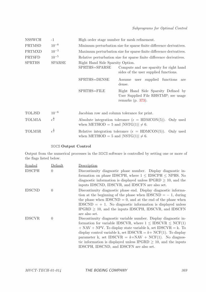
Subprograms for Optimal Control
NSSWCH -1 High order stage number for mesh refinement.
PRTMSD 10−8 Minimum perturbation size for sparse finite difference derivatives.
PRTMXD 10−3 Maximum perturbation size for sparse finite difference derivatives.
PRTSFD 10−5 Relative perturbation size for sparse finite difference derivatives.
SPRTHS SPARSE Right Hand Side Sparsity Option.SPRTHS=SPARSE Compute and use sparsity for right hand
sides of the user supplied functions.
SPRTHS=DENSE Assume user supplied functions aredense.
SPRTHS=FILE Right Hand Side Sparsity Defined byUser Supplied File RHSTMP; see usageremarks (p. 373).
TOLJSD 10−6 Jacobian row and column tolerance for print.
TOLM5A ǫ12 Absolute integration tolerance (ǫ = HDMCON(5)). Only used
when METHOD = 5 and |NSTG(1)| 6= 6.
TOLM5R ǫ12 Relative integration tolerance (ǫ = HDMCON(5)). Only used
when METHOD = 5 and |NSTG(1)| 6= 6.
SOCS Output Control
Output from the numerical processes in the SOCS software is controlled by setting one or more ofthe flags listed below.
Symbol Default Description
IDSCPH 0 Discontinuity diagnostic phase number. Display diagnostic in-formation on phase IDSCPH, where 1 ≤ IDSCPH ≤ NPHS. Nodiagnostic information is displayed unless IPGRD ≥ 10, and theinputs IDSCND, IDSCVR, and IDSCFN are also set.
IDSCND 0 Discontinuity diagnostic phase end. Display diagnostic informa-tion at the beginning of the phase when IDSCND = − 1, duringthe phase when IDSCND = 0, and at the end of the phase whenIDSCND = + 1. No diagnostic information is displayed unlessIPGRD ≥ 10, and the inputs IDSCPH, IDSCVR, and IDSCFNare also set.
IDSCVR 0 Discontinuity diagnostic variable number. Display diagnostic in-formation for variable IDSCVR, where 1 ≤ IDSCVR ≤ NCF(1)+ NAV + NPV. To display state variable k, set IDSCVR = k. Todisplay control variable k, set IDSCVR = k+ NCF(1). To displayparameter k, set IDSCVR = k+NAV + NCF(1). No diagnos-tic information is displayed unless IPGRD ≥ 10, and the inputsIDSCPH, IDSCND, and IDSCFN are also set.
M&CT-TECH-01-014 THE BOEING COMPANY 369
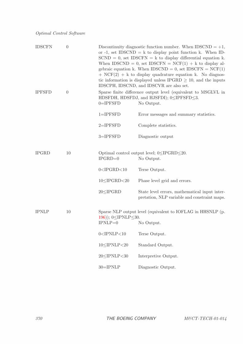
Optimal Control Software
IDSCFN 0 Discontinuity diagnostic function number. When IDSCND = +1,or -1, set IDSCND = k to display point function k. When ID-SCND = 0, set IDSCFN = k to display differential equation k.When IDSCND = 0, set IDSCFN = NCF(1) + k to display al-gebraic equation k. When IDSCND = 0, set IDSCFN = NCF(1)+ NCF(2) + k to display quadrature equation k. No diagnos-tic information is displayed unless IPGRD ≥ 10, and the inputsIDSCPH, IDSCND, and IDSCVR are also set.
IPFSFD 0 Sparse finite difference output level (equivalent to MSGLVL inHDSFDH, HDSFDJ, and HJSFDI); 0≤IPFSFD≤3.0=IPFSFD No Output.
1=IPFSFD Error messages and summary statistics.
2=IPFSFD Complete statistics.
3=IPFSFD Diagnostic output
IPGRD 10 Optimal control output level; 0≤IPGRD≤20.IPGRD=0 No Output.
0<IPGRD<10 Terse Output.
10≤IPGRD<20 Phase level grid and errors.
20≤IPGRD State level errors, mathematical input inter-pretation, NLP variable and constraint maps.
IPNLP 10 Sparse NLP output level (equivalent to IOFLAG in HHSNLP (p.196)); 0≤IPNLP≤30.IPNLP=0 No Output.
0<IPNLP<10 Terse Output.
10≤IPNLP<20 Standard Output.
20≤IPNLP<30 Interpretive Output.
30=IPNLP Diagnostic Output.
370 THE BOEING COMPANY M&CT-TECH-01-014
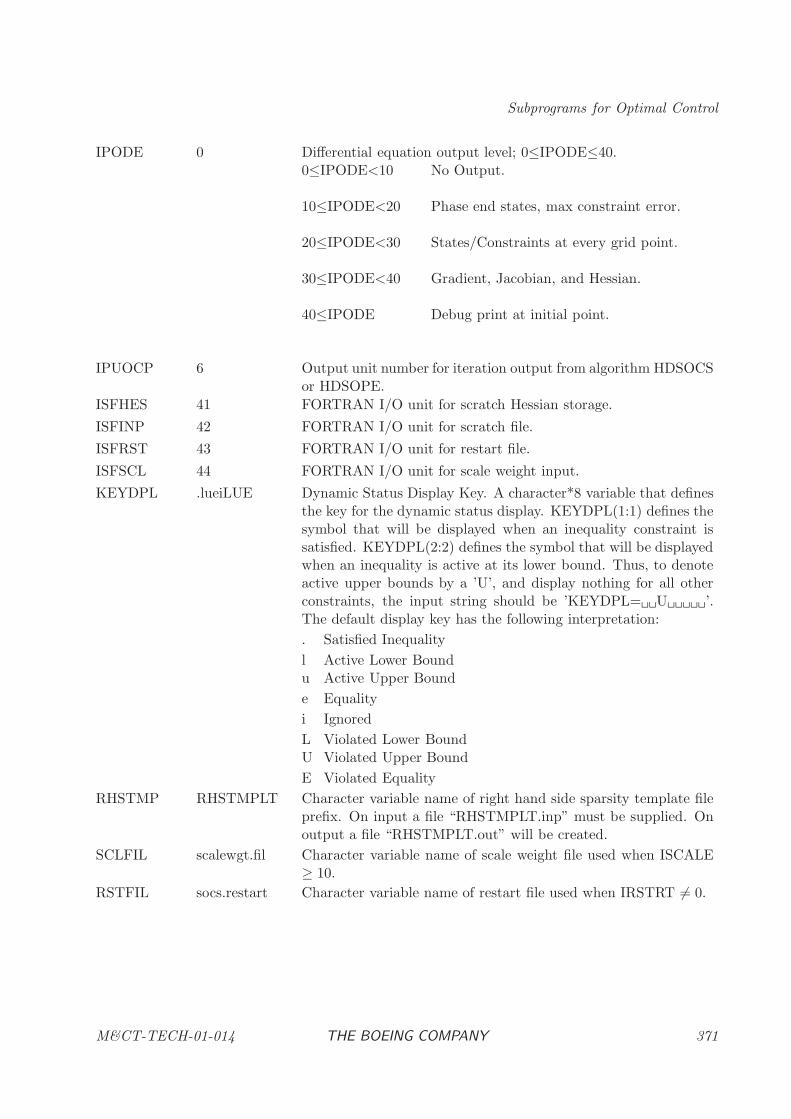
Subprograms for Optimal Control
IPODE 0 Differential equation output level; 0≤IPODE≤40.0≤IPODE<10 No Output.
10≤IPODE<20 Phase end states, max constraint error.
20≤IPODE<30 States/Constraints at every grid point.
30≤IPODE<40 Gradient, Jacobian, and Hessian.
40≤IPODE Debug print at initial point.
IPUOCP 6 Output unit number for iteration output from algorithm HDSOCSor HDSOPE.
ISFHES 41 FORTRAN I/O unit for scratch Hessian storage.
ISFINP 42 FORTRAN I/O unit for scratch file.
ISFRST 43 FORTRAN I/O unit for restart file.
ISFSCL 44 FORTRAN I/O unit for scale weight input.
KEYDPL .lueiLUE Dynamic Status Display Key. A character*8 variable that definesthe key for the dynamic status display. KEYDPL(1:1) defines thesymbol that will be displayed when an inequality constraint issatisfied. KEYDPL(2:2) defines the symbol that will be displayedwhen an inequality is active at its lower bound. Thus, to denoteactive upper bounds by a ’U’, and display nothing for all otherconstraints, the input string should be ’KEYDPL= U ’.The default display key has the following interpretation:
. Satisfied Inequality
l Active Lower Boundu Active Upper Bound
e Equality
i Ignored
L Violated Lower BoundU Violated Upper Bound
E Violated Equality
RHSTMP RHSTMPLT Character variable name of right hand side sparsity template fileprefix. On input a file “RHSTMPLT.inp” must be supplied. Onoutput a file “RHSTMPLT.out” will be created.
SCLFIL scalewgt.fil Character variable name of scale weight file used when ISCALE≥ 10.
RSTFIL socs.restart Character variable name of restart file used when IRSTRT 6= 0.
M&CT-TECH-01-014 THE BOEING COMPANY 371
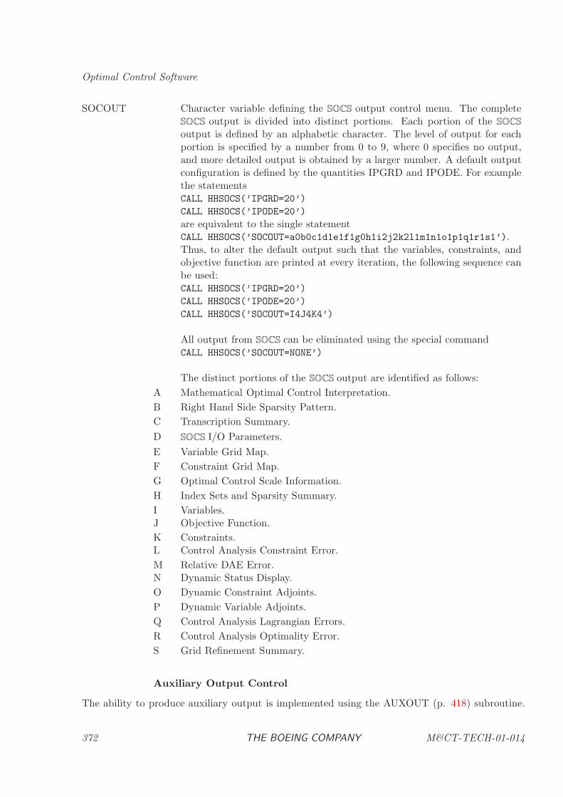
Optimal Control Software
SOCOUT Character variable defining the SOCS output control menu. The completeSOCS output is divided into distinct portions. Each portion of the SOCS
output is defined by an alphabetic character. The level of output for eachportion is specified by a number from 0 to 9, where 0 specifies no output,and more detailed output is obtained by a larger number. A default outputconfiguration is defined by the quantities IPGRD and IPODE. For examplethe statementsCALL HHSOCS(’IPGRD=20’)
CALL HHSOCS(’IPODE=20’)
are equivalent to the single statementCALL HHSOCS(’SOCOUT=a0b0c1d1e1f1g0h1i2j2k2l1m1n1o1p1q1r1s1’).Thus, to alter the default output such that the variables, constraints, andobjective function are printed at every iteration, the following sequence canbe used:CALL HHSOCS(’IPGRD=20’)
CALL HHSOCS(’IPODE=20’)
CALL HHSOCS(’SOCOUT=I4J4K4’)
All output from SOCS can be eliminated using the special commandCALL HHSOCS(’SOCOUT=NONE’)
The distinct portions of the SOCS output are identified as follows:
A Mathematical Optimal Control Interpretation.
B Right Hand Side Sparsity Pattern.
C Transcription Summary.
D SOCS I/O Parameters.
E Variable Grid Map.
F Constraint Grid Map.
G Optimal Control Scale Information.
H Index Sets and Sparsity Summary.
I Variables.J Objective Function.
K Constraints.L Control Analysis Constraint Error.
M Relative DAE Error.N Dynamic Status Display.
O Dynamic Constraint Adjoints.
P Dynamic Variable Adjoints.
Q Control Analysis Lagrangian Errors.
R Control Analysis Optimality Error.
S Grid Refinement Summary.
Auxiliary Output Control
The ability to produce auxiliary output is implemented using the AUXOUT (p. 418) subroutine.
372 THE BOEING COMPANY M&CT-TECH-01-014
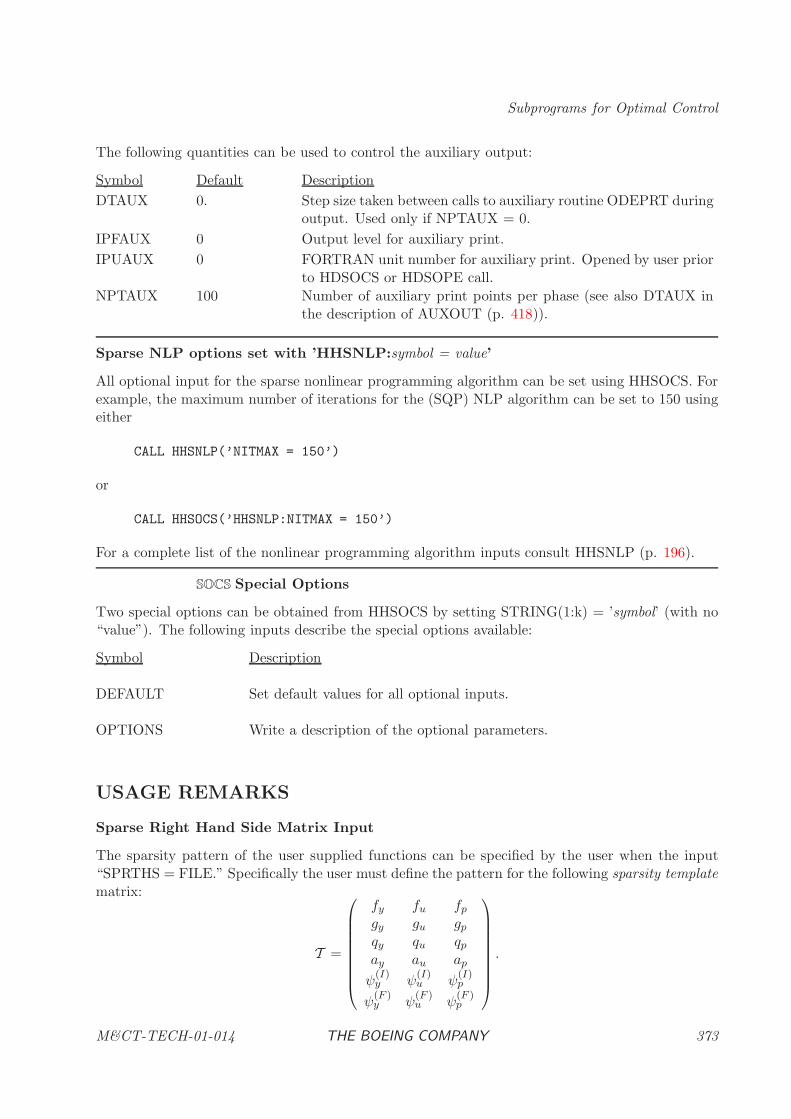
Subprograms for Optimal Control
The following quantities can be used to control the auxiliary output:
Symbol Default Description
DTAUX 0. Step size taken between calls to auxiliary routine ODEPRT duringoutput. Used only if NPTAUX = 0.
IPFAUX 0 Output level for auxiliary print.
IPUAUX 0 FORTRAN unit number for auxiliary print. Opened by user priorto HDSOCS or HDSOPE call.
NPTAUX 100 Number of auxiliary print points per phase (see also DTAUX inthe description of AUXOUT (p. 418)).
Sparse NLP options set with ’HHSNLP:symbol = value’
All optional input for the sparse nonlinear programming algorithm can be set using HHSOCS. Forexample, the maximum number of iterations for the (SQP) NLP algorithm can be set to 150 usingeither
CALL HHSNLP(’NITMAX = 150’)
or
CALL HHSOCS(’HHSNLP:NITMAX = 150’)
For a complete list of the nonlinear programming algorithm inputs consult HHSNLP (p. 196).
SOCS Special Options
Two special options can be obtained from HHSOCS by setting STRING(1:k) = ’symbol’ (with no“value”). The following inputs describe the special options available:
Symbol Description
DEFAULT Set default values for all optional inputs.
OPTIONS Write a description of the optional parameters.
USAGE REMARKS
Sparse Right Hand Side Matrix Input
The sparsity pattern of the user supplied functions can be specified by the user when the input“SPRTHS = FILE.” Specifically the user must define the pattern for the following sparsity templatematrix:
T =
fy fu fp
gy gu gp
qy qu qpay au ap
ψ(I)y ψ
(I)u ψ
(I)p
ψ(F )y ψ
(F )u ψ
(F )p
.
M&CT-TECH-01-014 THE BOEING COMPANY 373
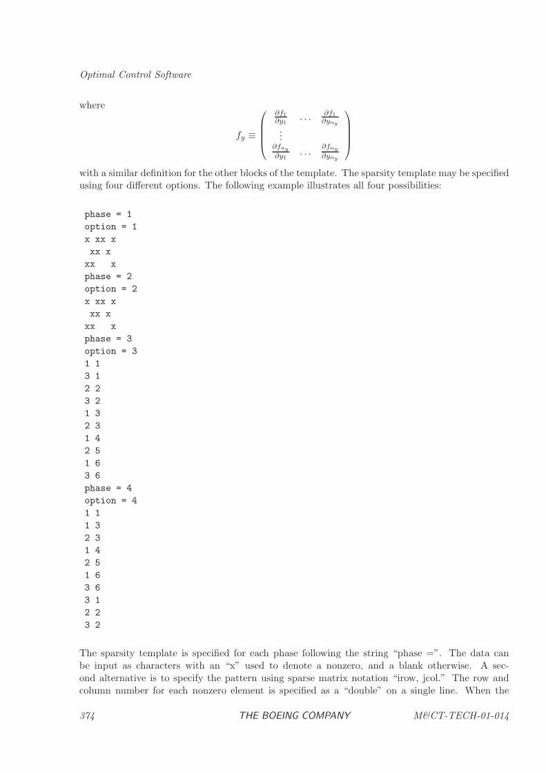
Optimal Control Software
where
fy ≡
∂f1
∂y1. . . ∂f1
∂yny
...∂fny
∂y1. . .
∂fny
∂yny
with a similar definition for the other blocks of the template. The sparsity template may be specifiedusing four different options. The following example illustrates all four possibilities:
phase = 1
option = 1
x xx x
xx x
xx x
phase = 2
option = 2
x xx x
xx x
xx x
phase = 3
option = 3
1 1
3 1
2 2
3 2
1 3
2 3
1 4
2 5
1 6
3 6
phase = 4
option = 4
1 1
1 3
2 3
1 4
2 5
1 6
3 6
3 1
2 2
3 2
The sparsity template is specified for each phase following the string “phase =”. The data canbe input as characters with an “x” used to denote a nonzero, and a blank otherwise. A sec-ond alternative is to specify the pattern using sparse matrix notation “irow, jcol.” The row andcolumn number for each nonzero element is specified as a “double” on a single line. When the
374 THE BOEING COMPANY M&CT-TECH-01-014
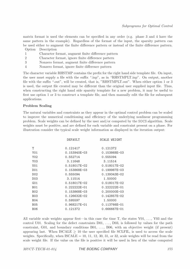
Subprograms for Optimal Control
matrix format is used the elements can be specified in any order (e.g. phase 3 and 4 have thesame pattern in the example). Regardless of the format of the input, the sparsity pattern canbe used either to augment the finite difference pattern or instead of the finite difference pattern.Option Description1 Character format, augment finite difference pattern2 Character format, ignore finite difference pattern3 Nonzero format, augment finite difference pattern4 Nonzero format, ignore finite difference pattern
The character variable RHSTMP contains the prefix for the right hand side template file. On input,the user must supply a file with the suffix “.inp”, as in “RHSTMPLT.inp”. On output, anotherfile with the suffix “.out”, will be created, that is, ”RHSTMPLT.out”. When either option 1 or 3is used, the output file created may be different than the original user supplied input file. Thus,when constructing the right hand side sparsity template for a new problem, it may be useful tofirst use option 1 or 3 to construct a template file, and then manually edit the file for subsequentapplications.
Problem Scaling
The natural variables and constraints as they appear in the optimal control problem can be scaledto improve the numerical conditioning and efficiency of the underlying nonlinear programmingproblem. Scale weights can be defined by the user and/or computed by the SOCS algorithm. Scaleweights must be positive, and are defined for each variable and constraint present on a phase. Forillustration consider the typical scale weight information as displayed in the iteration output:
DEFAULT SCALE WEIGHT
T 0.121417 0.121372
Y01 0.153940E-03 0.153868E-03
Y02 0.552714 0.555094
Y03 3.11648 3.11514
U01 0.518017E-02 0.518017E-02
D01 0.153868E-03 0.199987E-03
D02 0.555094 0.139343E-02
D03 3.11514 1.50000
G01 0.518017E-02 0.518017E-02
B01 0.222222E-01 0.222222E-01
B02 0.153868E-03 0.200000E-03
B03 0.126632E-02 0.142857E-02
B04 0.595597 1.50000
B05 0.968217E-01 0.113766E-01
B06 0.121372 0.666667E-01
All variable scale weights appear first—in this case the time T, the states Y01, . . . , Y03 and thecontrol U01. Scaling for the defect constraints D01, . . . , D03, is followed by values for the pathconstraint, G01, and boundary conditions B01, . . . , B06, with an objective weight (if present)appearing last. When ISCALE ≥ 10 the user specified file SCLFIL, is used to access the scaleweights. Specifically, when ISCALE = 10, 11, 12, 30, 31, or 32, scale weights will be read from thescale weight file. If the value on the file is positive it will be used in lieu of the value computed
M&CT-TECH-01-014 THE BOEING COMPANY 375

Optimal Control Software
by SOCS . On the other hand if the value on the file is negative it will not be used, and SOCS
will compute a scale weight. When ISCALE ≥ 20 the scale weight file will be written to the namespecified by SCLFIL.
376 THE BOEING COMPANY M&CT-TECH-01-014
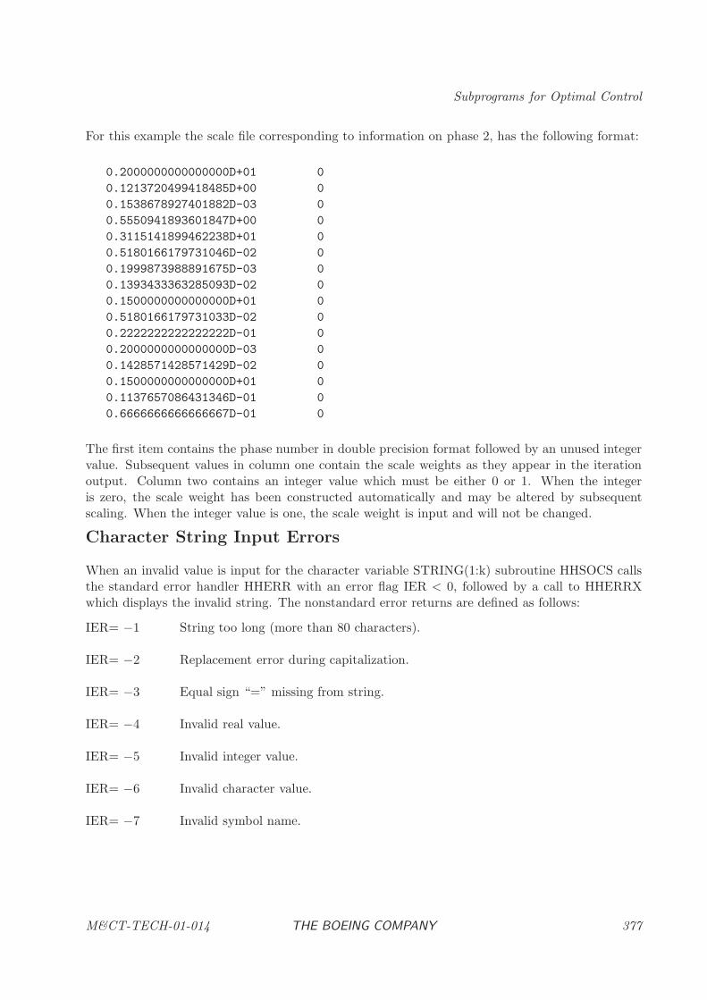
Subprograms for Optimal Control
For this example the scale file corresponding to information on phase 2, has the following format:
0.2000000000000000D+01 0
0.1213720499418485D+00 0
0.1538678927401882D-03 0
0.5550941893601847D+00 0
0.3115141899462238D+01 0
0.5180166179731046D-02 0
0.1999873988891675D-03 0
0.1393433363285093D-02 0
0.1500000000000000D+01 0
0.5180166179731033D-02 0
0.2222222222222222D-01 0
0.2000000000000000D-03 0
0.1428571428571429D-02 0
0.1500000000000000D+01 0
0.1137657086431346D-01 0
0.6666666666666667D-01 0
The first item contains the phase number in double precision format followed by an unused integervalue. Subsequent values in column one contain the scale weights as they appear in the iterationoutput. Column two contains an integer value which must be either 0 or 1. When the integeris zero, the scale weight has been constructed automatically and may be altered by subsequentscaling. When the integer value is one, the scale weight is input and will not be changed.
Character String Input Errors
When an invalid value is input for the character variable STRING(1:k) subroutine HHSOCS callsthe standard error handler HHERR with an error flag IER < 0, followed by a call to HHERRXwhich displays the invalid string. The nonstandard error returns are defined as follows:
IER= −1 String too long (more than 80 characters).
IER= −2 Replacement error during capitalization.
IER= −3 Equal sign “=” missing from string.
IER= −4 Invalid real value.
IER= −5 Invalid integer value.
IER= −6 Invalid character value.
IER= −7 Invalid symbol name.
M&CT-TECH-01-014 THE BOEING COMPANY 377
Optimal Control Software
6.3 User-Supplied Subprograms for Optimal Control
DDLOAD: Discrete Data Load
PURPOSE
DDLOAD is a user-supplied subroutine that loads values for the discrete data functions needed todefine the parameter estimation objective function. Specifically the routine supplies the values yij,the weights wij and the corresponding evaluation times θij used to construct the residual
rk = wij [yi(θij) − yij]
in addition to the values θij and uij which define the residual
rk = wij [ui(θij) − uij ] .
For applications that use the parameter estimation software HDSOPE but have no discrete data,the system supplied dummy routine, DUMYDE may be used in the calling arguments to HDSOPE.This routine is not used by the optimal control algorithm HDSOCS.
RELATED SUBPROGRAMS
HDSOPE Sparse Optimal Parameter Estimation
HHSOCS Sparse Optimal Control Input Procedure
ODEINP Optimal Control Problem Definition
ODEIGS Optimal Control Initial Guess
ODEPTF Optimal Control Point Function Evaluation
ODEPRT Optimal Control Print
METHOD
DDLOAD is a generic name for this routine, and the actual routine name must be declared as anexternal in the main program and placed in the calling list to subroutine HDSOPE.
On a specific phase the fundamental input to this routine is the number of the discrete data functionbeing loaded. DDLOAD must load either the values θij , wij and yij or the values θij, wij and uij .In either case DDLOAD must also supply the total number of discrete data values (NDATA) andthe corresponding number of the dynamic variable. Data is always supplied as a triple, i.e.
(θij , yij, wij)
for a fixed value of i, and j = 1, . . . ,Nd. The function evaluation error flag, IFERR, should be setto zero if the data is supplied successfully. Otherwise, IFERR can be set to any nonzero value todesignate that the data can not be supplied for the current inputs.
WARNING
378 THE BOEING COMPANY M&CT-TECH-01-014
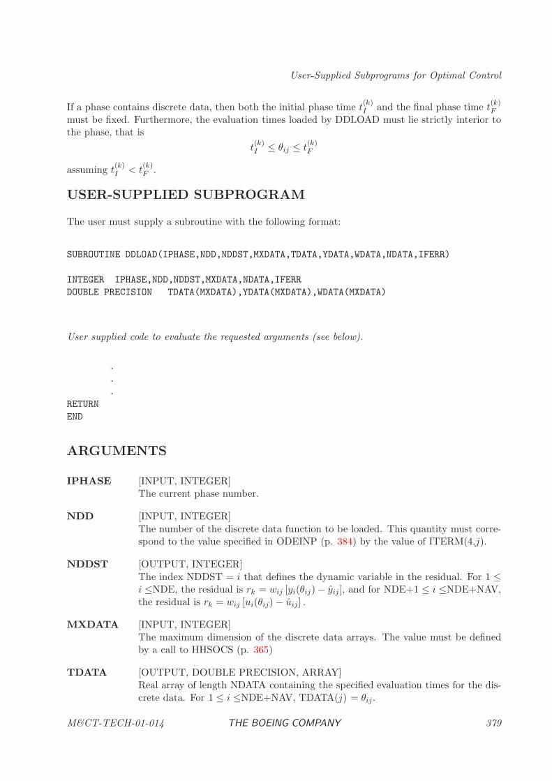
User-Supplied Subprograms for Optimal Control
If a phase contains discrete data, then both the initial phase time t(k)I and the final phase time t
(k)F
must be fixed. Furthermore, the evaluation times loaded by DDLOAD must lie strictly interior tothe phase, that is
t(k)I ≤ θij ≤ t
(k)F
assuming t(k)I < t
(k)F .
USER-SUPPLIED SUBPROGRAM
The user must supply a subroutine with the following format:
SUBROUTINE DDLOAD(IPHASE,NDD,NDDST,MXDATA,TDATA,YDATA,WDATA,NDATA,IFERR)
INTEGER IPHASE,NDD,NDDST,MXDATA,NDATA,IFERR
DOUBLE PRECISION TDATA(MXDATA),YDATA(MXDATA),WDATA(MXDATA)
User supplied code to evaluate the requested arguments (see below).
.
.
.
RETURN
END
ARGUMENTS
IPHASE [INPUT, INTEGER]The current phase number.
NDD [INPUT, INTEGER]The number of the discrete data function to be loaded. This quantity must corre-spond to the value specified in ODEINP (p. 384) by the value of ITERM(4,j).
NDDST [OUTPUT, INTEGER]The index NDDST = i that defines the dynamic variable in the residual. For 1 ≤i ≤NDE, the residual is rk = wij [yi(θij) − yij], and for NDE+1 ≤ i ≤NDE+NAV,the residual is rk = wij [ui(θij) − uij] .
MXDATA [INPUT, INTEGER]The maximum dimension of the discrete data arrays. The value must be definedby a call to HHSOCS (p. 365)
TDATA [OUTPUT, DOUBLE PRECISION, ARRAY]Real array of length NDATA containing the specified evaluation times for the dis-crete data. For 1 ≤ i ≤NDE+NAV, TDATA(j) = θij.
M&CT-TECH-01-014 THE BOEING COMPANY 379
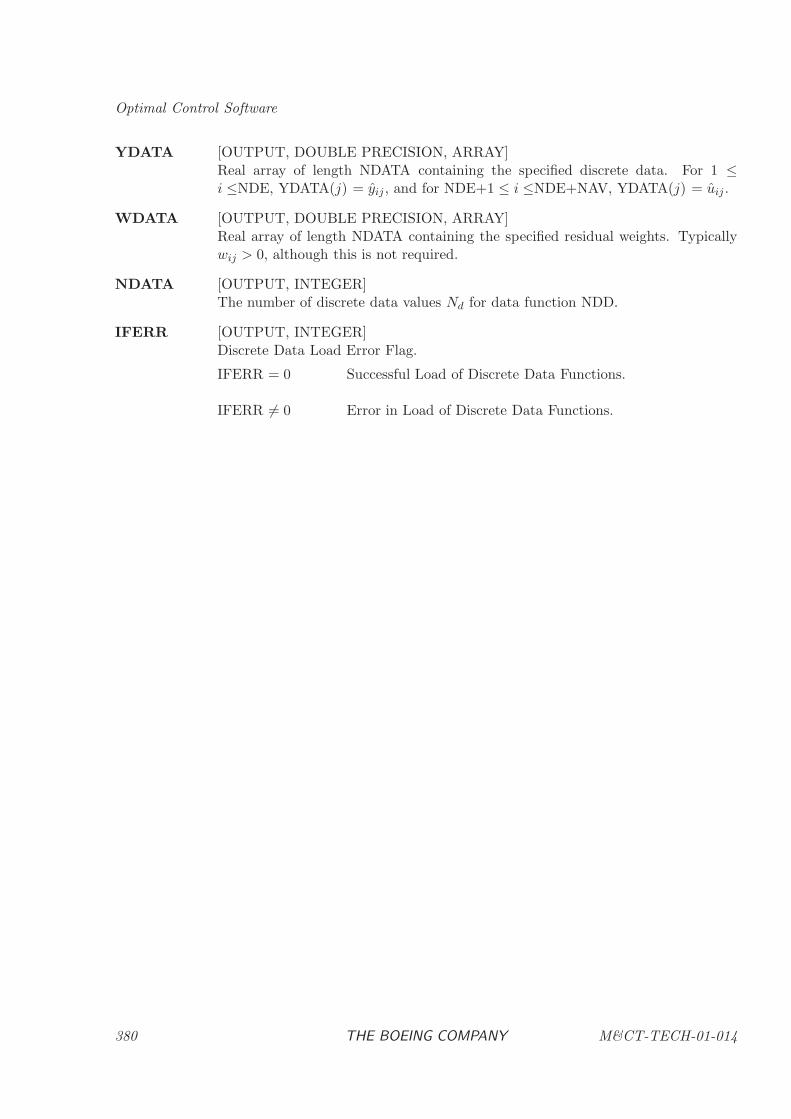
Optimal Control Software
YDATA [OUTPUT, DOUBLE PRECISION, ARRAY]Real array of length NDATA containing the specified discrete data. For 1 ≤i ≤NDE, YDATA(j) = yij , and for NDE+1 ≤ i ≤NDE+NAV, YDATA(j) = uij .
WDATA [OUTPUT, DOUBLE PRECISION, ARRAY]Real array of length NDATA containing the specified residual weights. Typicallywij > 0, although this is not required.
NDATA [OUTPUT, INTEGER]The number of discrete data values Nd for data function NDD.
IFERR [OUTPUT, INTEGER]Discrete Data Load Error Flag.
IFERR = 0 Successful Load of Discrete Data Functions.
IFERR 6= 0 Error in Load of Discrete Data Functions.
380 THE BOEING COMPANY M&CT-TECH-01-014
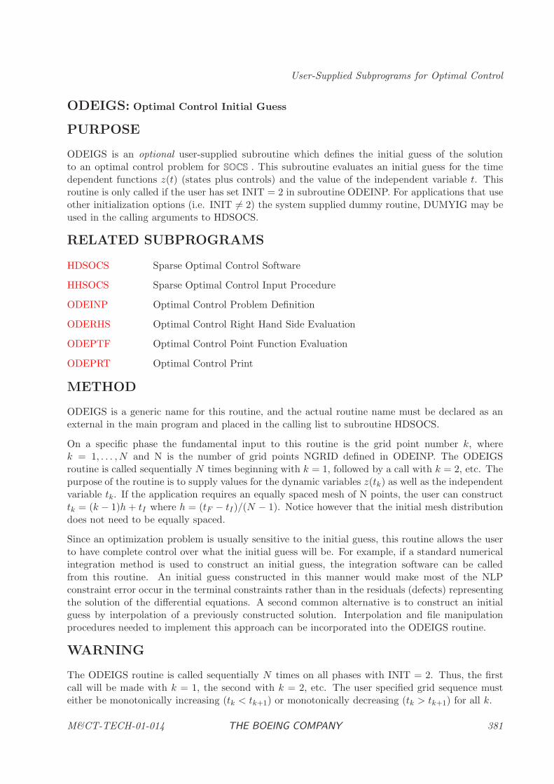
User-Supplied Subprograms for Optimal Control
ODEIGS: Optimal Control Initial Guess
PURPOSE
ODEIGS is an optional user-supplied subroutine which defines the initial guess of the solutionto an optimal control problem for SOCS . This subroutine evaluates an initial guess for the timedependent functions z(t) (states plus controls) and the value of the independent variable t. Thisroutine is only called if the user has set INIT = 2 in subroutine ODEINP. For applications that useother initialization options (i.e. INIT 6= 2) the system supplied dummy routine, DUMYIG may beused in the calling arguments to HDSOCS.
RELATED SUBPROGRAMS
HDSOCS Sparse Optimal Control Software
HHSOCS Sparse Optimal Control Input Procedure
ODEINP Optimal Control Problem Definition
ODERHS Optimal Control Right Hand Side Evaluation
ODEPTF Optimal Control Point Function Evaluation
ODEPRT Optimal Control Print
METHOD
ODEIGS is a generic name for this routine, and the actual routine name must be declared as anexternal in the main program and placed in the calling list to subroutine HDSOCS.
On a specific phase the fundamental input to this routine is the grid point number k, wherek = 1, . . . , N and N is the number of grid points NGRID defined in ODEINP. The ODEIGSroutine is called sequentially N times beginning with k = 1, followed by a call with k = 2, etc. Thepurpose of the routine is to supply values for the dynamic variables z(tk) as well as the independentvariable tk. If the application requires an equally spaced mesh of N points, the user can constructtk = (k − 1)h+ tI where h = (tF − tI)/(N − 1). Notice however that the initial mesh distributiondoes not need to be equally spaced.
Since an optimization problem is usually sensitive to the initial guess, this routine allows the userto have complete control over what the initial guess will be. For example, if a standard numericalintegration method is used to construct an initial guess, the integration software can be calledfrom this routine. An initial guess constructed in this manner would make most of the NLPconstraint error occur in the terminal constraints rather than in the residuals (defects) representingthe solution of the differential equations. A second common alternative is to construct an initialguess by interpolation of a previously constructed solution. Interpolation and file manipulationprocedures needed to implement this approach can be incorporated into the ODEIGS routine.
WARNING
The ODEIGS routine is called sequentially N times on all phases with INIT = 2. Thus, the firstcall will be made with k = 1, the second with k = 2, etc. The user specified grid sequence musteither be monotonically increasing (tk < tk+1) or monotonically decreasing (tk > tk+1) for all k.
M&CT-TECH-01-014 THE BOEING COMPANY 381
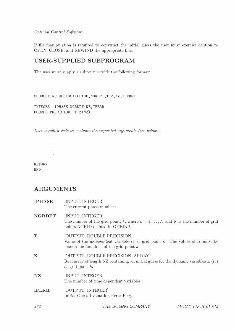
Optimal Control Software
If file manipulation is required to construct the initial guess the user must exercise caution toOPEN, CLOSE, and REWIND the appropriate files.
USER-SUPPLIED SUBPROGRAM
The user must supply a subroutine with the following format:
SUBROUTINE ODEIGS(IPHASE,NGRDPT,T,Z,NZ,IFERR)
INTEGER IPHASE,NGRDPT,NZ,IFERR
DOUBLE PRECISION T,Z(NZ)
User supplied code to evaluate the requested arguments (see below).
.
.
.
RETURN
END
ARGUMENTS
IPHASE [INPUT, INTEGER]The current phase number.
NGRDPT [INPUT, INTEGER]The number of the grid point, k, where k = 1, . . . ,N and N is the number of gridpoints NGRID defined in ODEINP.
T [OUTPUT, DOUBLE PRECISION]Value of the independent variable tk at grid point k. The values of tk must bemonotonic functions of the grid point k.
Z [OUTPUT, DOUBLE PRECISION, ARRAY]Real array of length NZ containing an initial guess for the dynamic variables zk(tk)at grid point k.
NZ [INPUT, INTEGER]The number of time dependent variables.
IFERR [OUTPUT, INTEGER]Initial Guess Evaluation Error Flag.
382 THE BOEING COMPANY M&CT-TECH-01-014
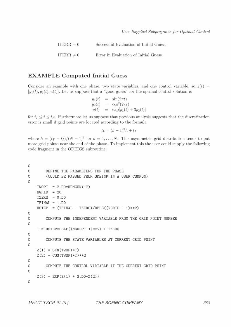
User-Supplied Subprograms for Optimal Control
IFERR = 0 Successful Evaluation of Initial Guess.
IFERR 6= 0 Error in Evaluation of Initial Guess.
EXAMPLE Computed Initial Guess
Consider an example with one phase, two state variables, and one control variable, so z(t) =[y1(t), y2(t), u(t)]. Let us suppose that a “good guess” for the optimal control solution is
y1(t) = sin(2πt)y2(t) = cos2(2πt)u(t) = exp[y1(t) + 3y2(t)]
for tI ≤ t ≤ tF . Furthermore let us suppose that previous analysis suggests that the discretizationerror is small if grid points are located according to the formula
tk = (k − 1)2h+ tI
where h = (tF − tI)/(N − 1)2 for k = 1, . . . ,N . This asymmetric grid distribution tends to putmore grid points near the end of the phase. To implement this the user could supply the followingcode fragment in the ODEIGS subroutine:
C
C DEFINE THE PARAMETERS FOR THE PHASE
C (COULD BE PASSED FROM ODEINP IN A USER COMMON)
C
TWOPI = 2.D0*HDMCON(12)
NGRID = 20
TZERO = 0.D0
TFINAL = 1.D0
HSTEP = (TFINAL - TZERO)/DBLE((NGRID - 1)**2)
C
C COMPUTE THE INDEPENDENT VARIABLE FROM THE GRID POINT NUMBER
C
T = HSTEP*DBLE((NGRDPT-1)**2) + TZERO
C
C COMPUTE THE STATE VARIABLES AT CURRENT GRID POINT
C
Z(1) = SIN(TWOPI*T)
Z(2) = COS(TWOPI*T)**2
C
C COMPUTE THE CONTROL VARIABLE AT THE CURRENT GRID POINT
C
Z(3) = EXP(Z(1) + 3.D0*Z(2))
C
M&CT-TECH-01-014 THE BOEING COMPANY 383
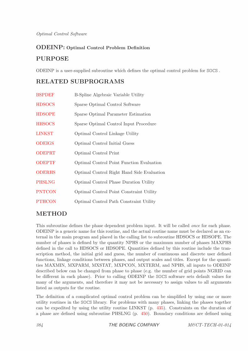
Optimal Control Software
ODEINP: Optimal Control Problem Definition
PURPOSE
ODEINP is a user-supplied subroutine which defines the optimal control problem for SOCS .
RELATED SUBPROGRAMS
BSPDEF B-Spline Algebraic Variable Utility
HDSOCS Sparse Optimal Control Software
HDSOPE Sparse Optimal Parameter Estimation
HHSOCS Sparse Optimal Control Input Procedure
LINKST Optimal Control Linkage Utility
ODEIGS Optimal Control Initial Guess
ODEPRT Optimal Control Print
ODEPTF Optimal Control Point Function Evaluation
ODERHS Optimal Control Right Hand Side Evaluation
PHSLNG Optimal Control Phase Duration Utility
PNTCON Optimal Control Point Constraint Utility
PTHCON Optimal Control Path Constraint Utility
METHOD
This subroutine defines the phase dependent problem input. It will be called once for each phase.ODEINP is a generic name for this routine, and the actual routine name must be declared as an ex-ternal in the main program and placed in the calling list to subroutine HDSOCS or HDSOPE. Thenumber of phases is defined by the quantity NPHS or the maximum number of phases MAXPHSdefined in the call to HDSOCS or HDSOPE. Quantities defined by this routine include the tran-scription method, the initial grid and guess, the number of continuous and discrete user definedfunctions, linkage conditions between phases, and output scales and titles. Except for the quanti-ties MAXMIN, MXPARM, MXSTAT, MXPCON, MXTERM, and NPHS, all inputs to ODEINPdescribed below can be changed from phase to phase (e.g. the number of grid points NGRID canbe different in each phase). Prior to calling ODEINP the SOCS software sets default values formany of the arguments, and therefore it may not be necessary to assign values to all argumentslisted as outputs for the routine.
The definition of a complicated optimal control problem can be simplified by using one or moreutility routines in the SOCS library. For problems with many phases, linking the phases togethercan be expedited by using the utility routine LINKST (p. 435). Constraints on the duration ofa phase are defined using subroutine PHSLNG (p. 450). Boundary conditions are defined using
384 THE BOEING COMPANY M&CT-TECH-01-014
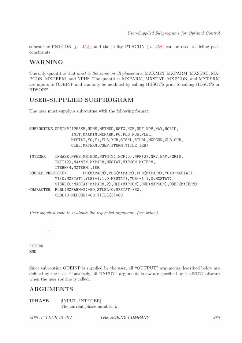
User-Supplied Subprograms for Optimal Control
subroutine PNTCON (p. 452), and the utility PTHCON (p. 458) can be used to define pathconstraints.
WARNING
The only quantities that must be the same on all phases are: MAXMIN, MXPARM, MXSTAT, MX-PCON, MXTERM, and NPHS. The quantities MXPARM, MXSTAT, MXPCON, and MXTERMare inputs to ODEINP and can only be modified by calling HHSOCS prior to calling HDSOCS orHDSOPE.
USER-SUPPLIED SUBPROGRAM
The user must supply a subroutine with the following format:
SUBROUTINE ODEINP(IPHASE,NPHS,METHOD,NSTG,NCF,NPF,NPV,NAV,NGRID,
INIT,MAXMIN,MXPARM,P0,PLB,PUB,PLBL,
MXSTAT,Y0,Y1,YLB,YUB,STSKL,STLBL,MXPCON,CLB,CUB,
CLBL,MXTERM,COEF,ITERM,TITLE,IER)
INTEGER IPHASE,NPHS,METHOD,NSTG(2),NCF(5),NPF(2),NPV,NAV,NGRID,
INIT(2),MAXMIN,MXPARM,MXSTAT,MXPCON,MXTERM,
ITERM(4,MXTERM),IER
DOUBLE PRECISION P0(MXPARM),PLB(MXPARM),PUB(MXPARM),Y0(0:MXSTAT),
Y1(0:MXSTAT),YLB(-1:1,0:MXSTAT),YUB(-1:1,0:MXSTAT),
STSKL(0:MXSTAT+MXPARM,2),CLB(MXPCON),CUB(MXPCON),COEF(MXTERM)
CHARACTER PLBL(MXPARM+2)*80,STLBL(0:MXSTAT)*80,
CLBL(0:MXPCON)*80,TITLE(3)*60
User supplied code to evaluate the requested arguments (see below).
.
.
.
RETURN
END
Since subroutine ODEINP is supplied by the user, all “OUTPUT” arguments described below aredefined by the user. Conversely, all “INPUT” arguments below are specified by the SOCS softwarewhen the user routine is called.
ARGUMENTS
IPHASE [INPUT, INTEGER]The current phase number, k.
M&CT-TECH-01-014 THE BOEING COMPANY 385
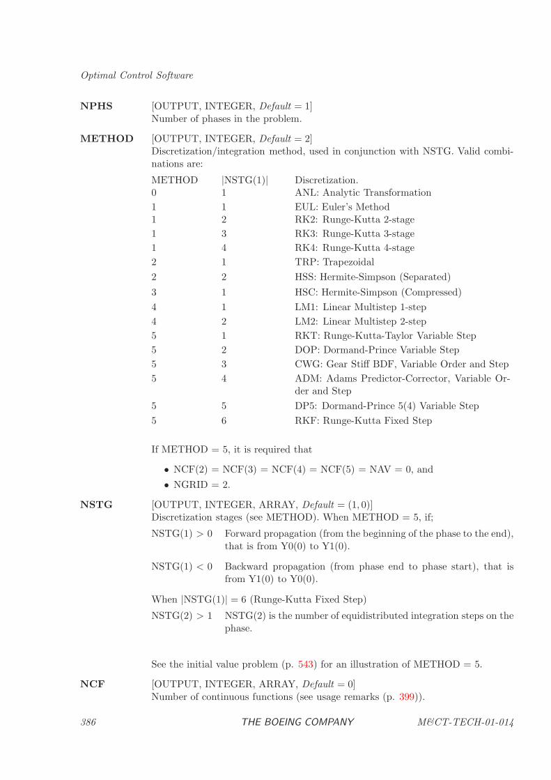
Optimal Control Software
NPHS [OUTPUT, INTEGER, Default = 1]Number of phases in the problem.
METHOD [OUTPUT, INTEGER, Default = 2]Discretization/integration method, used in conjunction with NSTG. Valid combi-nations are:
METHOD |NSTG(1)| Discretization.0 1 ANL: Analytic Transformation
1 1 EUL: Euler’s Method1 2 RK2: Runge-Kutta 2-stage
1 3 RK3: Runge-Kutta 3-stage
1 4 RK4: Runge-Kutta 4-stage
2 1 TRP: Trapezoidal
2 2 HSS: Hermite-Simpson (Separated)
3 1 HSC: Hermite-Simpson (Compressed)
4 1 LM1: Linear Multistep 1-step
4 2 LM2: Linear Multistep 2-step
5 1 RKT: Runge-Kutta-Taylor Variable Step
5 2 DOP: Dormand-Prince Variable Step
5 3 CWG: Gear Stiff BDF, Variable Order and Step
5 4 ADM: Adams Predictor-Corrector, Variable Or-der and Step
5 5 DP5: Dormand-Prince 5(4) Variable Step
5 6 RKF: Runge-Kutta Fixed Step
If METHOD = 5, it is required that
• NCF(2) = NCF(3) = NCF(4) = NCF(5) = NAV = 0, and
• NGRID = 2.
NSTG [OUTPUT, INTEGER, ARRAY, Default = (1, 0)]Discretization stages (see METHOD). When METHOD = 5, if;
NSTG(1) > 0 Forward propagation (from the beginning of the phase to the end),that is from Y0(0) to Y1(0).
NSTG(1) < 0 Backward propagation (from phase end to phase start), that isfrom Y1(0) to Y0(0).
When |NSTG(1)| = 6 (Runge-Kutta Fixed Step)
NSTG(2) > 1 NSTG(2) is the number of equidistributed integration steps on thephase.
See the initial value problem (p. 543) for an illustration of METHOD = 5.
NCF [OUTPUT, INTEGER, ARRAY, Default = 0]Number of continuous functions (see usage remarks (p. 399)).
386 THE BOEING COMPANY M&CT-TECH-01-014
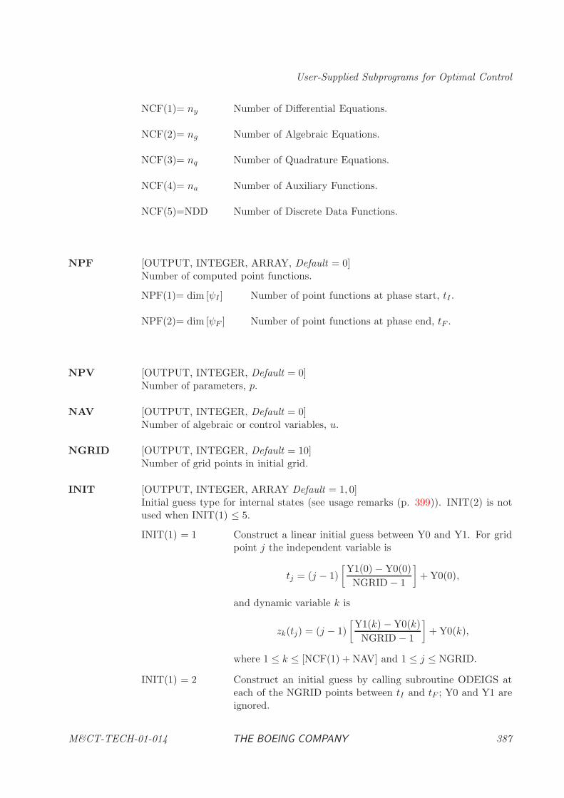
User-Supplied Subprograms for Optimal Control
NCF(1)= ny Number of Differential Equations.
NCF(2)= ng Number of Algebraic Equations.
NCF(3)= nq Number of Quadrature Equations.
NCF(4)= na Number of Auxiliary Functions.
NCF(5)=NDD Number of Discrete Data Functions.
NPF [OUTPUT, INTEGER, ARRAY, Default = 0]Number of computed point functions.
NPF(1)= dim [ψI ] Number of point functions at phase start, tI .
NPF(2)= dim [ψF ] Number of point functions at phase end, tF .
NPV [OUTPUT, INTEGER, Default = 0]Number of parameters, p.
NAV [OUTPUT, INTEGER, Default = 0]Number of algebraic or control variables, u.
NGRID [OUTPUT, INTEGER, Default = 10]Number of grid points in initial grid.
INIT [OUTPUT, INTEGER, ARRAY Default = 1, 0]Initial guess type for internal states (see usage remarks (p. 399)). INIT(2) is notused when INIT(1) ≤ 5.
INIT(1) = 1 Construct a linear initial guess between Y0 and Y1. For gridpoint j the independent variable is
tj = (j − 1)
[Y1(0) − Y0(0)
NGRID − 1
]+ Y0(0),
and dynamic variable k is
zk(tj) = (j − 1)
[Y1(k) − Y0(k)
NGRID − 1
]+ Y0(k),
where 1 ≤ k ≤ [NCF(1) + NAV] and 1 ≤ j ≤ NGRID.
INIT(1) = 2 Construct an initial guess by calling subroutine ODEIGS ateach of the NGRID points between tI and tF ; Y0 and Y1 areignored.
M&CT-TECH-01-014 THE BOEING COMPANY 387
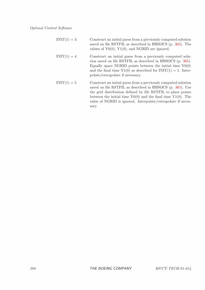
Optimal Control Software
INIT(1) = 3 Construct an initial guess from a previously computed solutionsaved on file RSTFIL as described in HHSOCS (p. 365). Thevalues of Y0(0), Y1(0), and NGRID are ignored.
INIT(1) = 4 Construct an initial guess from a previously computed solu-tion saved on file RSTFIL as described in HHSOCS (p. 365).Equally space NGRID points between the initial time Y0(0)and the final time Y1(0) as described for INIT(1) = 1. Inter-polate/extrapolate if necessary.
INIT(1) = 5 Construct an initial guess from a previously computed solutionsaved on file RSTFIL as described in HHSOCS (p. 365). Usethe grid distribution defined by file RSTFIL to place pointsbetween the initial time Y0(0) and the final time Y1(0). Thevalue of NGRID is ignored. Interpolate/extrapolate if neces-sary.
388 THE BOEING COMPANY M&CT-TECH-01-014
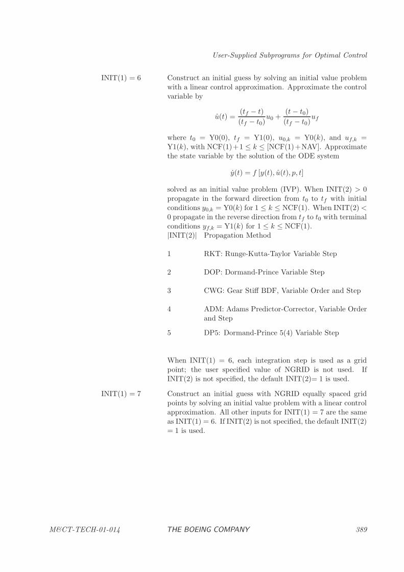
User-Supplied Subprograms for Optimal Control
INIT(1) = 6 Construct an initial guess by solving an initial value problemwith a linear control approximation. Approximate the controlvariable by
u(t) =(tf − t)
(tf − t0)u0 +
(t− t0)
(tf − t0)uf
where t0 = Y0(0), tf = Y1(0), u0,k = Y0(k), and uf,k =Y1(k), with NCF(1)+1 ≤ k ≤ [NCF(1)+NAV]. Approximatethe state variable by the solution of the ODE system
y(t) = f [y(t), u(t), p, t]
solved as an initial value problem (IVP). When INIT(2) > 0propagate in the forward direction from t0 to tf with initialconditions y0,k = Y0(k) for 1 ≤ k ≤ NCF(1). When INIT(2) <0 propagate in the reverse direction from tf to t0 with terminalconditions yf,k = Y1(k) for 1 ≤ k ≤ NCF(1).|INIT(2)| Propagation Method
1 RKT: Runge-Kutta-Taylor Variable Step
2 DOP: Dormand-Prince Variable Step
3 CWG: Gear Stiff BDF, Variable Order and Step
4 ADM: Adams Predictor-Corrector, Variable Orderand Step
5 DP5: Dormand-Prince 5(4) Variable Step
When INIT(1) = 6, each integration step is used as a gridpoint; the user specified value of NGRID is not used. IfINIT(2) is not specified, the default INIT(2)= 1 is used.
INIT(1) = 7 Construct an initial guess with NGRID equally spaced gridpoints by solving an initial value problem with a linear controlapproximation. All other inputs for INIT(1) = 7 are the sameas INIT(1) = 6. If INIT(2) is not specified, the default INIT(2)= 1 is used.
M&CT-TECH-01-014 THE BOEING COMPANY 389
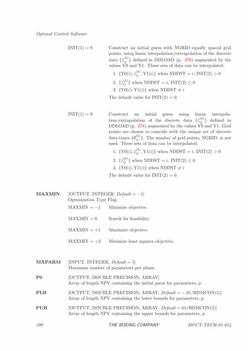
Optimal Control Software
INIT(1) = 8 Construct an initial guess with NGRID equally spaced gridpoints, using linear interpolation/extrapolation of the discrete
data {z(k)ij } defined in DDLOAD (p. 378) augmented by the
values Y0 and Y1. Three sets of data can be interpolated.
1. {Y0(i), z(k)ij ,Y1(i)} when NDDST = i, INIT(2) > 0
2. {z(k)ij } when NDDST = i, INIT(2) ≤ 0
3. {Y0(i),Y1(i)} when NDDST 6= i
The default value for INIT(2) = 0.
INIT(1) = 9 Construct an initial guess using linear interpola-
tion/extrapolation of the discrete data {z(k)ij } defined in
DDLOAD (p. 378) augmented by the values Y0 and Y1. Gridpoints are chosen to coincide with the unique set of discrete
data times {θ(k)ij }. The number of grid points, NGRID, is not
used. Three sets of data can be interpolated.
1. {Y0(i), z(k)ij ,Y1(i)} when NDDST = i, INIT(2) > 0
2. {z(k)ij } when NDDST = i, INIT(2) ≤ 0
3. {Y0(i),Y1(i)} when NDDST 6= i
The default value for INIT(2) = 0.
MAXMIN [OUTPUT, INTEGER, Default = −1]Optimization Type Flag.
MAXMIN = −1 Minimize objective.
MAXMIN = 0 Search for feasibility.
MAXMIN = +1 Maximize objective.
MAXMIN = +2 Minimize least squares objective.
MXPARM [INPUT, INTEGER, Default = 5]Maximum number of parameters per phase.
P0 [OUTPUT, DOUBLE PRECISION, ARRAY]Array of length NPV containing the initial guess for parameters, p.
PLB [OUTPUT, DOUBLE PRECISION, ARRAY, Default = −.01/HDMCON(5)]Array of length NPV containing the lower bounds for parameters, p.
PUB [OUTPUT, DOUBLE PRECISION, ARRAY, Default =.01/HDMCON(5)]Array of length NPV containing the upper bounds for parameters, p.
390 THE BOEING COMPANY M&CT-TECH-01-014
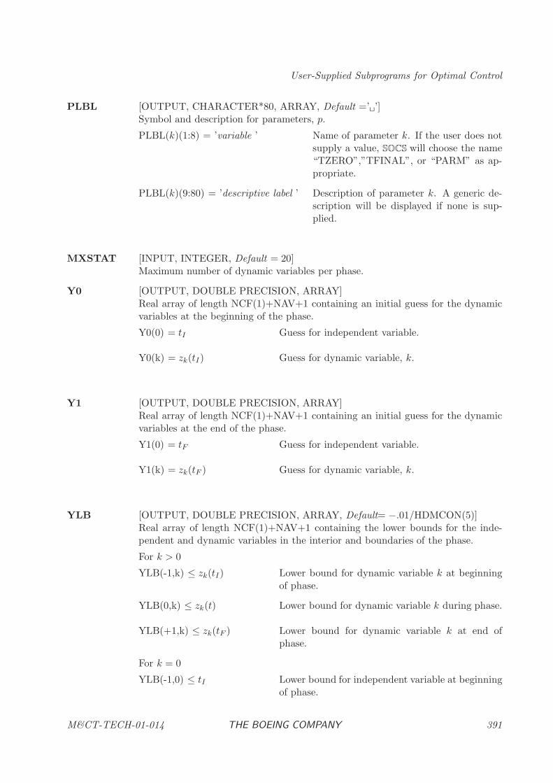
User-Supplied Subprograms for Optimal Control
PLBL [OUTPUT, CHARACTER*80, ARRAY, Default =’ ’]Symbol and description for parameters, p.
PLBL(k)(1:8) = ’variable ’ Name of parameter k. If the user does notsupply a value, SOCS will choose the name“TZERO”,”TFINAL”, or “PARM” as ap-propriate.
PLBL(k)(9:80) = ’descriptive label ’ Description of parameter k. A generic de-scription will be displayed if none is sup-plied.
MXSTAT [INPUT, INTEGER, Default = 20]Maximum number of dynamic variables per phase.
Y0 [OUTPUT, DOUBLE PRECISION, ARRAY]Real array of length NCF(1)+NAV+1 containing an initial guess for the dynamicvariables at the beginning of the phase.
Y0(0) = tI Guess for independent variable.
Y0(k) = zk(tI) Guess for dynamic variable, k.
Y1 [OUTPUT, DOUBLE PRECISION, ARRAY]Real array of length NCF(1)+NAV+1 containing an initial guess for the dynamicvariables at the end of the phase.
Y1(0) = tF Guess for independent variable.
Y1(k) = zk(tF ) Guess for dynamic variable, k.
YLB [OUTPUT, DOUBLE PRECISION, ARRAY, Default= −.01/HDMCON(5)]Real array of length NCF(1)+NAV+1 containing the lower bounds for the inde-pendent and dynamic variables in the interior and boundaries of the phase.
For k > 0
YLB(-1,k) ≤ zk(tI) Lower bound for dynamic variable k at beginningof phase.
YLB(0,k) ≤ zk(t) Lower bound for dynamic variable k during phase.
YLB(+1,k) ≤ zk(tF ) Lower bound for dynamic variable k at end ofphase.
For k = 0
YLB(-1,0) ≤ tI Lower bound for independent variable at beginningof phase.
M&CT-TECH-01-014 THE BOEING COMPANY 391
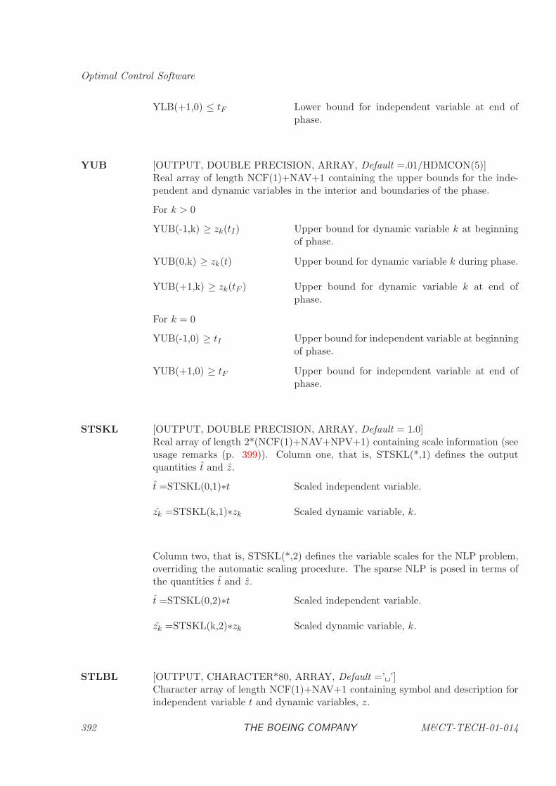
Optimal Control Software
YLB(+1,0) ≤ tF Lower bound for independent variable at end ofphase.
YUB [OUTPUT, DOUBLE PRECISION, ARRAY, Default =.01/HDMCON(5)]Real array of length NCF(1)+NAV+1 containing the upper bounds for the inde-pendent and dynamic variables in the interior and boundaries of the phase.
For k > 0
YUB(-1,k) ≥ zk(tI) Upper bound for dynamic variable k at beginningof phase.
YUB(0,k) ≥ zk(t) Upper bound for dynamic variable k during phase.
YUB(+1,k) ≥ zk(tF ) Upper bound for dynamic variable k at end ofphase.
For k = 0
YUB(-1,0) ≥ tI Upper bound for independent variable at beginningof phase.
YUB(+1,0) ≥ tF Upper bound for independent variable at end ofphase.
STSKL [OUTPUT, DOUBLE PRECISION, ARRAY, Default = 1.0]Real array of length 2*(NCF(1)+NAV+NPV+1) containing scale information (seeusage remarks (p. 399)). Column one, that is, STSKL(*,1) defines the outputquantities t and z.
t =STSKL(0,1)∗t Scaled independent variable.
zk =STSKL(k,1)∗zk Scaled dynamic variable, k.
Column two, that is, STSKL(*,2) defines the variable scales for the NLP problem,overriding the automatic scaling procedure. The sparse NLP is posed in terms ofthe quantities t and z.
t =STSKL(0,2)∗t Scaled independent variable.
zk =STSKL(k,2)∗zk Scaled dynamic variable, k.
STLBL [OUTPUT, CHARACTER*80, ARRAY, Default =’ ’]Character array of length NCF(1)+NAV+1 containing symbol and description forindependent variable t and dynamic variables, z.
392 THE BOEING COMPANY M&CT-TECH-01-014
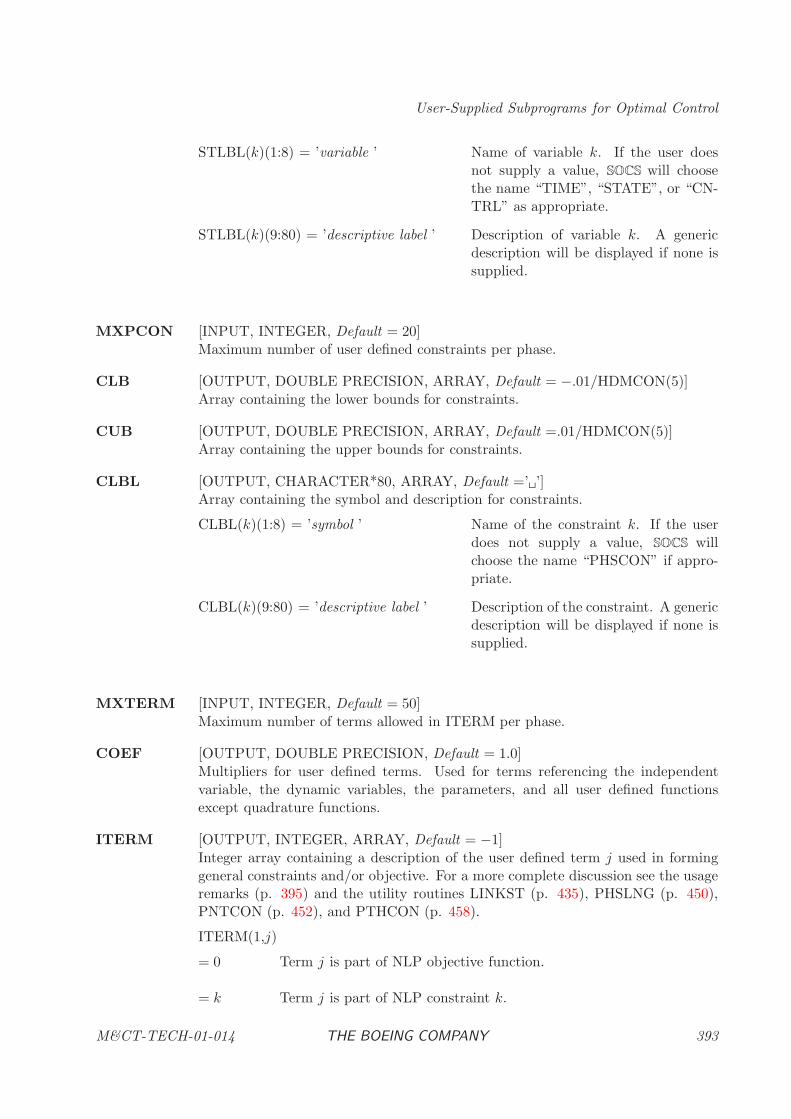
User-Supplied Subprograms for Optimal Control
STLBL(k)(1:8) = ’variable ’ Name of variable k. If the user doesnot supply a value, SOCS will choosethe name “TIME”, “STATE”, or “CN-TRL” as appropriate.
STLBL(k)(9:80) = ’descriptive label ’ Description of variable k. A genericdescription will be displayed if none issupplied.
MXPCON [INPUT, INTEGER, Default = 20]Maximum number of user defined constraints per phase.
CLB [OUTPUT, DOUBLE PRECISION, ARRAY, Default = −.01/HDMCON(5)]Array containing the lower bounds for constraints.
CUB [OUTPUT, DOUBLE PRECISION, ARRAY, Default =.01/HDMCON(5)]Array containing the upper bounds for constraints.
CLBL [OUTPUT, CHARACTER*80, ARRAY, Default =’ ’]Array containing the symbol and description for constraints.
CLBL(k)(1:8) = ’symbol ’ Name of the constraint k. If the userdoes not supply a value, SOCS willchoose the name “PHSCON” if appro-priate.
CLBL(k)(9:80) = ’descriptive label ’ Description of the constraint. A genericdescription will be displayed if none issupplied.
MXTERM [INPUT, INTEGER, Default = 50]Maximum number of terms allowed in ITERM per phase.
COEF [OUTPUT, DOUBLE PRECISION, Default = 1.0]Multipliers for user defined terms. Used for terms referencing the independentvariable, the dynamic variables, the parameters, and all user defined functionsexcept quadrature functions.
ITERM [OUTPUT, INTEGER, ARRAY, Default = −1]Integer array containing a description of the user defined term j used in forminggeneral constraints and/or objective. For a more complete discussion see the usageremarks (p. 395) and the utility routines LINKST (p. 435), PHSLNG (p. 450),PNTCON (p. 452), and PTHCON (p. 458).
ITERM(1,j)
= 0 Term j is part of NLP objective function.
= k Term j is part of NLP constraint k.
M&CT-TECH-01-014 THE BOEING COMPANY 393
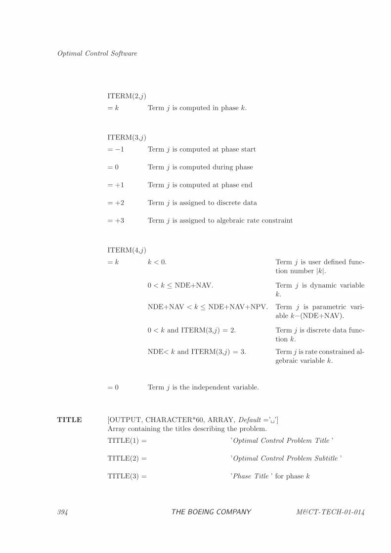
Optimal Control Software
ITERM(2,j)
= k Term j is computed in phase k.
ITERM(3,j)
= −1 Term j is computed at phase start
= 0 Term j is computed during phase
= +1 Term j is computed at phase end
= +2 Term j is assigned to discrete data
= +3 Term j is assigned to algebraic rate constraint
ITERM(4,j)
= k k < 0. Term j is user defined func-tion number |k|.
0 < k ≤ NDE+NAV. Term j is dynamic variablek.
NDE+NAV < k ≤ NDE+NAV+NPV. Term j is parametric vari-able k−(NDE+NAV).
0 < k and ITERM(3,j) = 2. Term j is discrete data func-tion k.
NDE< k and ITERM(3,j) = 3. Term j is rate constrained al-gebraic variable k.
= 0 Term j is the independent variable.
TITLE [OUTPUT, CHARACTER*60, ARRAY, Default =’ ’]Array containing the titles describing the problem.
TITLE(1) = ’Optimal Control Problem Title ’
TITLE(2) = ’Optimal Control Problem Subtitle ’
TITLE(3) = ’Phase Title ’ for phase k
394 THE BOEING COMPANY M&CT-TECH-01-014
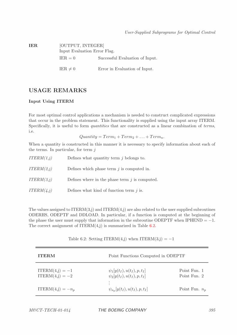
User-Supplied Subprograms for Optimal Control
IER [OUTPUT, INTEGER]Input Evaluation Error Flag.
IER = 0 Successful Evaluation of Input.
IER 6= 0 Error in Evaluation of Input.
USAGE REMARKS
Input Using ITERM
For most optimal control applications a mechanism is needed to construct complicated expressionsthat occur in the problem statement. This functionality is supplied using the input array ITERM.Specifically, it is useful to form quantities that are constructed as a linear combination of terms,i.e.
Quantity = Term1 + Term2 + . . .+ Termn.
When a quantity is constructed in this manner it is necessary to specify information about each ofthe terms. In particular, for term j
ITERM(1,j) Defines what quantity term j belongs to.
ITERM(2,j) Defines which phase term j is computed in.
ITERM(3,j) Defines where in the phase term j is computed.
ITERM(4,j) Defines what kind of function term j is.
The values assigned to ITERM(3,j) and ITERM(4,j) are also related to the user supplied subroutinesODERHS, ODEPTF and DDLOAD. In particular, if a function is computed at the beginning ofthe phase the user must supply that information in the subroutine ODEPTF when IPHEND = −1.The correct assignment of ITERM(4,j) is summarized in Table 6.2.
Table 6.2: Setting ITERM(4,j) when ITERM(3,j) = −1
ITERM Point Functions Computed in ODEPTF
ITERM(4,j) = −1 ψ1[y(tI), u(tI), p, tI ] Point Fun. 1ITERM(4,j) = −2 ψ2[y(tI), u(tI), p, tI ] Point Fun. 2
...ITERM(4,j) = −np ψnp [y(tI), u(tI), p, tI ] Point Fun. np
M&CT-TECH-01-014 THE BOEING COMPANY 395
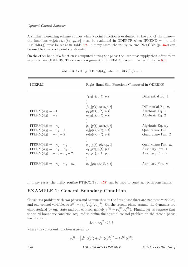
Optimal Control Software
A similar referencing scheme applies when a point function is evaluated at the end of the phase—the functions ψk[y(tF ), u(tF ), p, tF ] must be evaluated in ODEPTF when IPHEND = +1 andITERM(4,j) must be set as in Table 6.2. In many cases, the utility routine PNTCON (p. 452) canbe used to construct point constraints.
On the other hand, if a function is computed during the phase the user must supply that informationin subroutine ODERHS. The correct assignment of ITERM(4,j) is summarized in Table 6.3.
Table 6.3: Setting ITERM(4,j) when ITERM(3,j) = 0
ITERM Right Hand Side Functions Computed in ODERHS
f1[y(t), u(t), p, t] Differential Eq. 1...fny [y(t), u(t), p, t] Differential Eq. ny
ITERM(4,j) = −1 g1[y(t), u(t), p, t] Algebraic Eq. 1ITERM(4,j) = −2 g2[y(t), u(t), p, t] Algebraic Eq. 2
...ITERM(4,j) = −ng gng [y(t), u(t), p, t] Algebraic Eq. ng
ITERM(4,j) = −ng − 1 q1[y(t), u(t), p, t] Quadrature Fun. 1ITERM(4,j) = −ng − 2 q2[y(t), u(t), p, t] Quadrature Fun. 2
...ITERM(4,j) = −ng − nq qnq [y(t), u(t), p, t] Quadrature Fun. nq
ITERM(4,j) = −ng − nq − 1 a1[y(t), u(t), p, t] Auxiliary Fun. 1ITERM(4,j) = −ng − nq − 2 a2[y(t), u(t), p, t] Auxiliary Fun. 2
...ITERM(4,j) = −ng − nq − na ana [y(t), u(t), p, t] Auxiliary Fun. na
In many cases, the utility routine PTHCON (p. 458) can be used to construct path constraints.
EXAMPLE 1: General Boundary Condition
Consider a problem with two phases and assume that on the first phase there are two state variables,
and one control variable, so z(1) = (y(1)1 , y
(1)2 , u
(1)1 ). On the second phase assume the dynamics are
characterized by one state and one control, namely z(2) = (y(2)1 , u
(2)1 ). Finally, let us suppose that
the third boundary condition required to define the optimal control problem on the second phasehas the form
2.4 ≤ ψ(2)3 ≤ 3.7
where the constraint function is given by
ψ(2)3 =
[y
(1)1 (t
(1)F ) + y
(1)2 (t
(1)F )]2
− 4u(2)1 (t
(2)I )
396 THE BOEING COMPANY M&CT-TECH-01-014
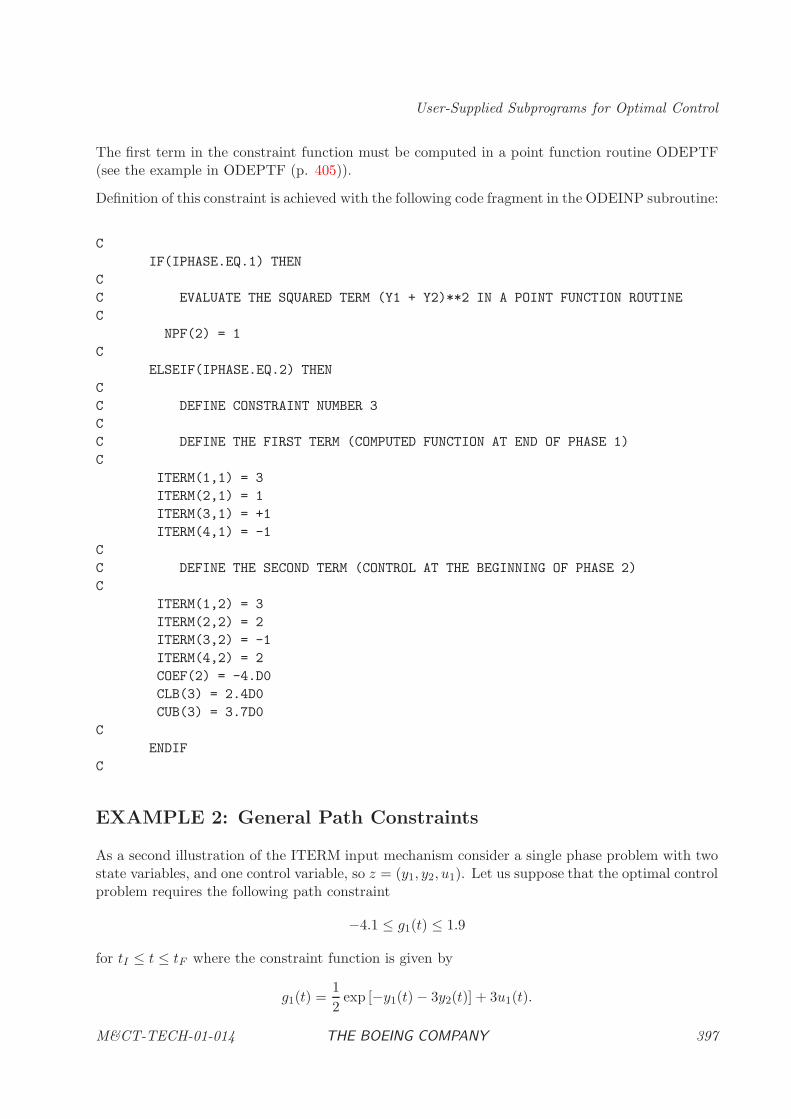
User-Supplied Subprograms for Optimal Control
The first term in the constraint function must be computed in a point function routine ODEPTF(see the example in ODEPTF (p. 405)).
Definition of this constraint is achieved with the following code fragment in the ODEINP subroutine:
C
IF(IPHASE.EQ.1) THEN
C
C EVALUATE THE SQUARED TERM (Y1 + Y2)**2 IN A POINT FUNCTION ROUTINE
C
NPF(2) = 1
C
ELSEIF(IPHASE.EQ.2) THEN
C
C DEFINE CONSTRAINT NUMBER 3
C
C DEFINE THE FIRST TERM (COMPUTED FUNCTION AT END OF PHASE 1)
C
ITERM(1,1) = 3
ITERM(2,1) = 1
ITERM(3,1) = +1
ITERM(4,1) = -1
C
C DEFINE THE SECOND TERM (CONTROL AT THE BEGINNING OF PHASE 2)
C
ITERM(1,2) = 3
ITERM(2,2) = 2
ITERM(3,2) = -1
ITERM(4,2) = 2
COEF(2) = -4.D0
CLB(3) = 2.4D0
CUB(3) = 3.7D0
C
ENDIF
C
EXAMPLE 2: General Path Constraints
As a second illustration of the ITERM input mechanism consider a single phase problem with twostate variables, and one control variable, so z = (y1, y2, u1). Let us suppose that the optimal controlproblem requires the following path constraint
−4.1 ≤ g1(t) ≤ 1.9
for tI ≤ t ≤ tF where the constraint function is given by
g1(t) =1
2exp [−y1(t) − 3y2(t)] + 3u1(t).
M&CT-TECH-01-014 THE BOEING COMPANY 397
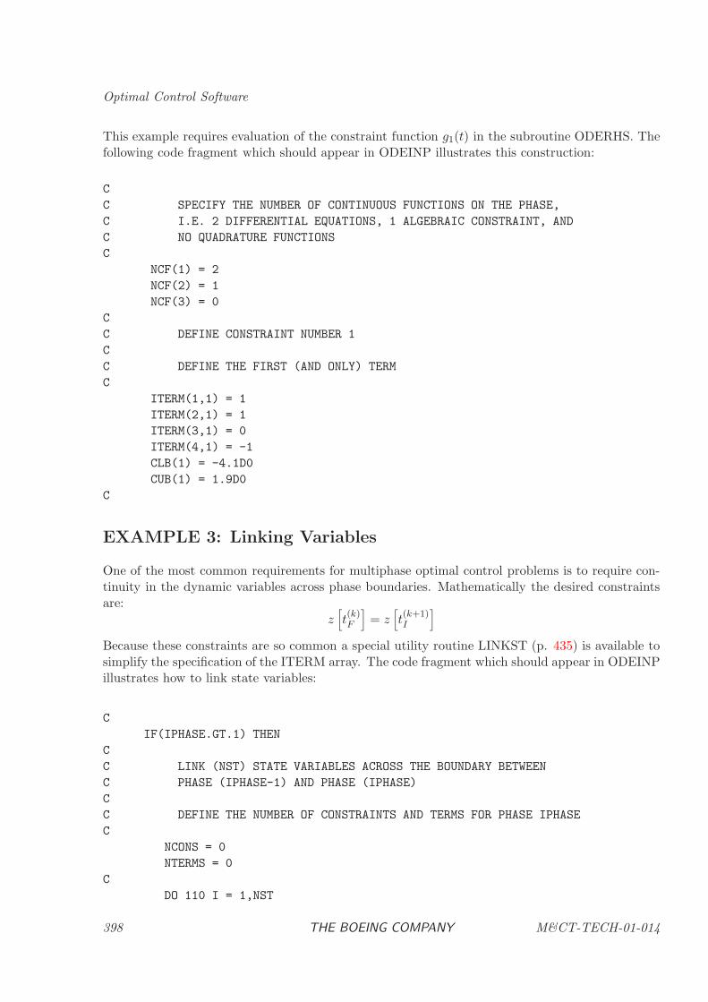
Optimal Control Software
This example requires evaluation of the constraint function g1(t) in the subroutine ODERHS. Thefollowing code fragment which should appear in ODEINP illustrates this construction:
C
C SPECIFY THE NUMBER OF CONTINUOUS FUNCTIONS ON THE PHASE,
C I.E. 2 DIFFERENTIAL EQUATIONS, 1 ALGEBRAIC CONSTRAINT, AND
C NO QUADRATURE FUNCTIONS
C
NCF(1) = 2
NCF(2) = 1
NCF(3) = 0
C
C DEFINE CONSTRAINT NUMBER 1
C
C DEFINE THE FIRST (AND ONLY) TERM
C
ITERM(1,1) = 1
ITERM(2,1) = 1
ITERM(3,1) = 0
ITERM(4,1) = -1
CLB(1) = -4.1D0
CUB(1) = 1.9D0
C
EXAMPLE 3: Linking Variables
One of the most common requirements for multiphase optimal control problems is to require con-tinuity in the dynamic variables across phase boundaries. Mathematically the desired constraintsare:
z[t(k)F
]= z
[t(k+1)I
]
Because these constraints are so common a special utility routine LINKST (p. 435) is available tosimplify the specification of the ITERM array. The code fragment which should appear in ODEINPillustrates how to link state variables:
C
IF(IPHASE.GT.1) THEN
C
C LINK (NST) STATE VARIABLES ACROSS THE BOUNDARY BETWEEN
C PHASE (IPHASE-1) AND PHASE (IPHASE)
C
C DEFINE THE NUMBER OF CONSTRAINTS AND TERMS FOR PHASE IPHASE
C
NCONS = 0
NTERMS = 0
C
DO 110 I = 1,NST
398 THE BOEING COMPANY M&CT-TECH-01-014
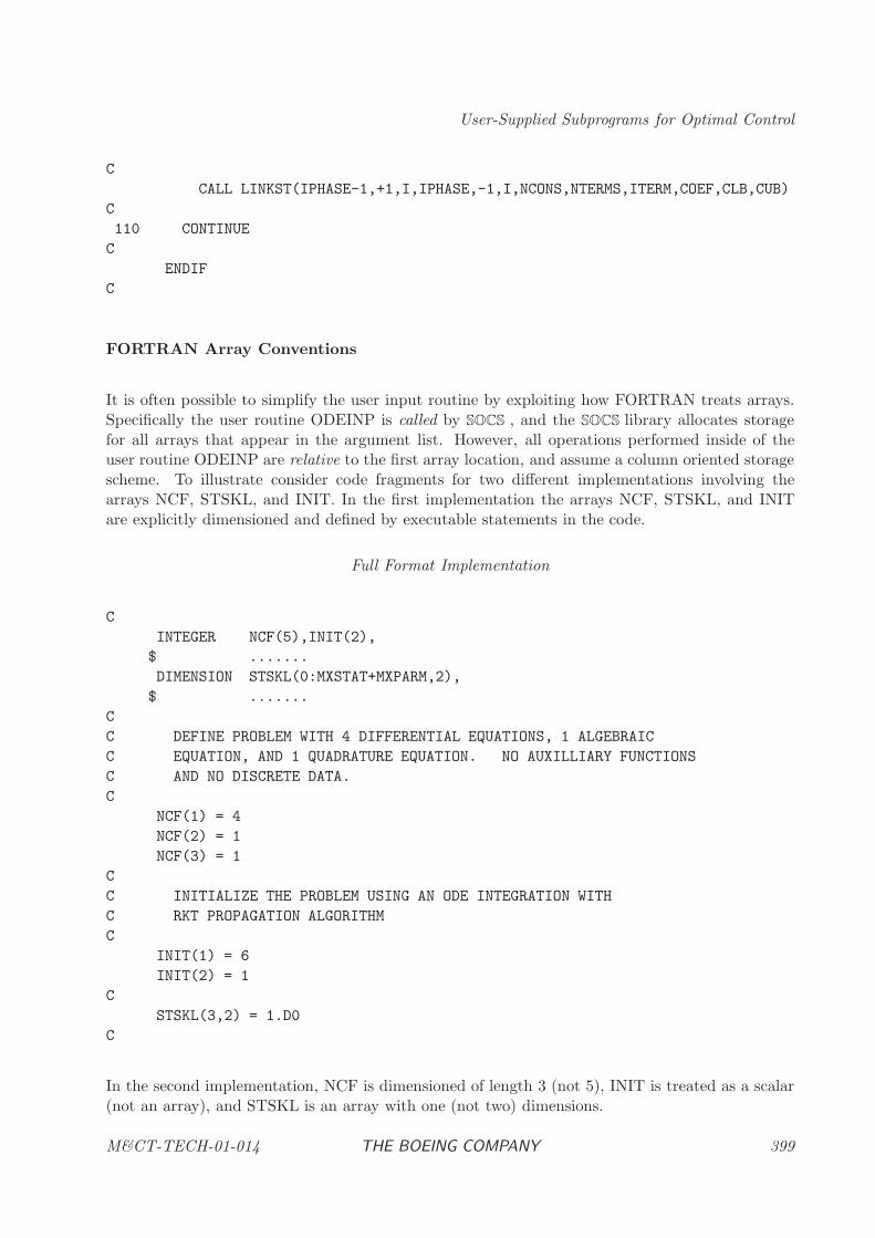
User-Supplied Subprograms for Optimal Control
C
CALL LINKST(IPHASE-1,+1,I,IPHASE,-1,I,NCONS,NTERMS,ITERM,COEF,CLB,CUB)
C
110 CONTINUE
C
ENDIF
C
FORTRAN Array Conventions
It is often possible to simplify the user input routine by exploiting how FORTRAN treats arrays.Specifically the user routine ODEINP is called by SOCS , and the SOCS library allocates storagefor all arrays that appear in the argument list. However, all operations performed inside of theuser routine ODEINP are relative to the first array location, and assume a column oriented storagescheme. To illustrate consider code fragments for two different implementations involving thearrays NCF, STSKL, and INIT. In the first implementation the arrays NCF, STSKL, and INITare explicitly dimensioned and defined by executable statements in the code.
Full Format Implementation
C
INTEGER NCF(5),INIT(2),
$ .......
DIMENSION STSKL(0:MXSTAT+MXPARM,2),
$ .......
C
C DEFINE PROBLEM WITH 4 DIFFERENTIAL EQUATIONS, 1 ALGEBRAIC
C EQUATION, AND 1 QUADRATURE EQUATION. NO AUXILLIARY FUNCTIONS
C AND NO DISCRETE DATA.
C
NCF(1) = 4
NCF(2) = 1
NCF(3) = 1
C
C INITIALIZE THE PROBLEM USING AN ODE INTEGRATION WITH
C RKT PROPAGATION ALGORITHM
C
INIT(1) = 6
INIT(2) = 1
C
STSKL(3,2) = 1.D0
C
In the second implementation, NCF is dimensioned of length 3 (not 5), INIT is treated as a scalar(not an array), and STSKL is an array with one (not two) dimensions.
M&CT-TECH-01-014 THE BOEING COMPANY 399
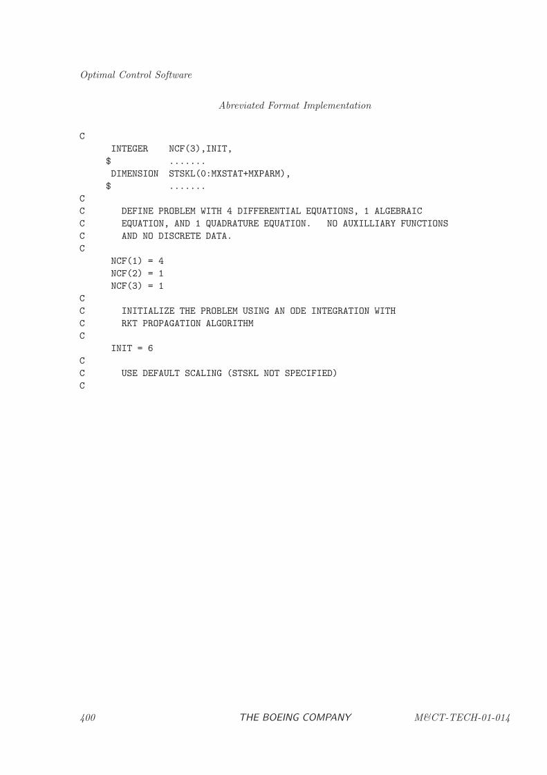
Optimal Control Software
Abreviated Format Implementation
C
INTEGER NCF(3),INIT,
$ .......
DIMENSION STSKL(0:MXSTAT+MXPARM),
$ .......
C
C DEFINE PROBLEM WITH 4 DIFFERENTIAL EQUATIONS, 1 ALGEBRAIC
C EQUATION, AND 1 QUADRATURE EQUATION. NO AUXILLIARY FUNCTIONS
C AND NO DISCRETE DATA.
C
NCF(1) = 4
NCF(2) = 1
NCF(3) = 1
C
C INITIALIZE THE PROBLEM USING AN ODE INTEGRATION WITH
C RKT PROPAGATION ALGORITHM
C
INIT = 6
C
C USE DEFAULT SCALING (STSKL NOT SPECIFIED)
C
400 THE BOEING COMPANY M&CT-TECH-01-014
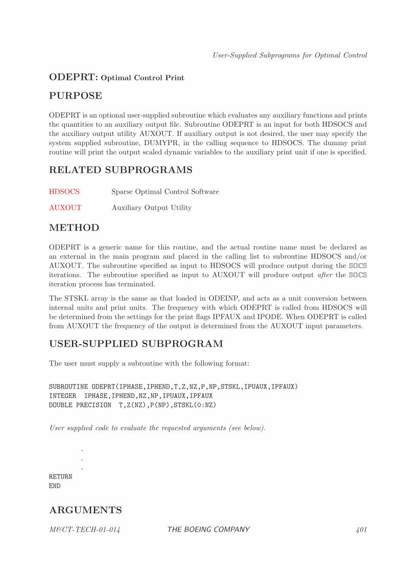
User-Supplied Subprograms for Optimal Control
ODEPRT: Optimal Control Print
PURPOSE
ODEPRT is an optional user-supplied subroutine which evaluates any auxiliary functions and printsthe quantities to an auxiliary output file. Subroutine ODEPRT is an input for both HDSOCS andthe auxiliary output utility AUXOUT. If auxiliary output is not desired, the user may specify thesystem supplied subroutine, DUMYPR, in the calling sequence to HDSOCS. The dummy printroutine will print the output scaled dynamic variables to the auxiliary print unit if one is specified.
RELATED SUBPROGRAMS
HDSOCS Sparse Optimal Control Software
AUXOUT Auxiliary Output Utility
METHOD
ODEPRT is a generic name for this routine, and the actual routine name must be declared asan external in the main program and placed in the calling list to subroutine HDSOCS and/orAUXOUT. The subroutine specified as input to HDSOCS will produce output during the SOCS
iterations. The subroutine specified as input to AUXOUT will produce output after the SOCS
iteration process has terminated.
The STSKL array is the same as that loaded in ODEINP, and acts as a unit conversion betweeninternal units and print units. The frequency with which ODEPRT is called from HDSOCS willbe determined from the settings for the print flags IPFAUX and IPODE. When ODEPRT is calledfrom AUXOUT the frequency of the output is determined from the AUXOUT input parameters.
USER-SUPPLIED SUBPROGRAM
The user must supply a subroutine with the following format:
SUBROUTINE ODEPRT(IPHASE,IPHEND,T,Z,NZ,P,NP,STSKL,IPUAUX,IPFAUX)
INTEGER IPHASE,IPHEND,NZ,NP,IPUAUX,IPFAUX
DOUBLE PRECISION T,Z(NZ),P(NP),STSKL(0:NZ)
User supplied code to evaluate the requested arguments (see below).
.
.
.
RETURN
END
ARGUMENTS
M&CT-TECH-01-014 THE BOEING COMPANY 401
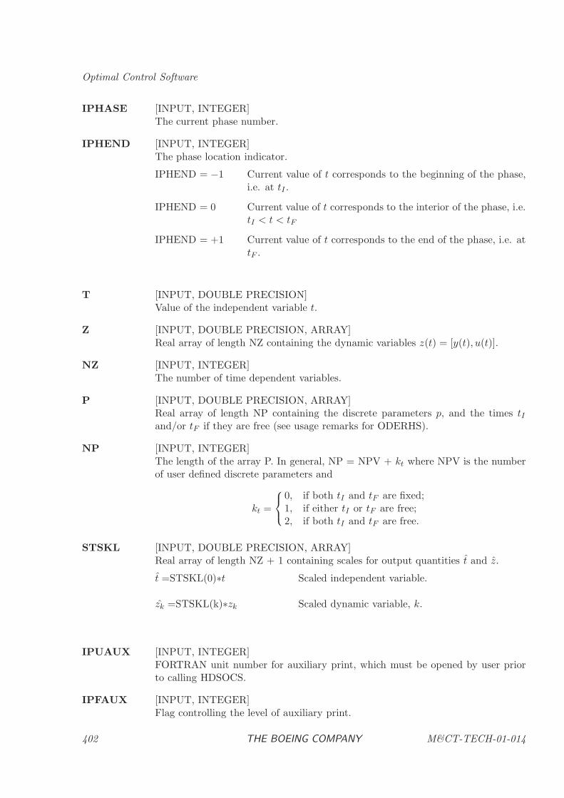
Optimal Control Software
IPHASE [INPUT, INTEGER]The current phase number.
IPHEND [INPUT, INTEGER]The phase location indicator.
IPHEND = −1 Current value of t corresponds to the beginning of the phase,i.e. at tI .
IPHEND = 0 Current value of t corresponds to the interior of the phase, i.e.tI < t < tF
IPHEND = +1 Current value of t corresponds to the end of the phase, i.e. attF .
T [INPUT, DOUBLE PRECISION]Value of the independent variable t.
Z [INPUT, DOUBLE PRECISION, ARRAY]Real array of length NZ containing the dynamic variables z(t) = [y(t), u(t)].
NZ [INPUT, INTEGER]The number of time dependent variables.
P [INPUT, DOUBLE PRECISION, ARRAY]Real array of length NP containing the discrete parameters p, and the times tIand/or tF if they are free (see usage remarks for ODERHS).
NP [INPUT, INTEGER]The length of the array P. In general, NP = NPV + kt where NPV is the numberof user defined discrete parameters and
kt =
0, if both tI and tF are fixed;1, if either tI or tF are free;2, if both tI and tF are free.
STSKL [INPUT, DOUBLE PRECISION, ARRAY]Real array of length NZ + 1 containing scales for output quantities t and z.
t =STSKL(0)∗t Scaled independent variable.
zk =STSKL(k)∗zk Scaled dynamic variable, k.
IPUAUX [INPUT, INTEGER]FORTRAN unit number for auxiliary print, which must be opened by user priorto calling HDSOCS.
IPFAUX [INPUT, INTEGER]Flag controlling the level of auxiliary print.
402 THE BOEING COMPANY M&CT-TECH-01-014
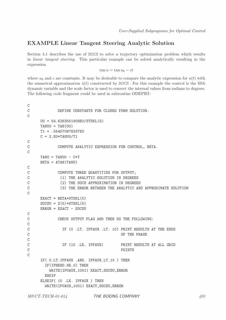
User-Supplied Subprograms for Optimal Control
EXAMPLE Linear Tangent Steering Analytic Solution
Section 4.1 describes the use of SOCS to solve a trajectory optimization problem which resultsin linear tangent steering. This particular example can be solved analytically resulting in theexpression
tanu = tan u0 − ct
where u0 and c are constants. It may be desirable to compare the analytic expression for u(t) withthe numerical approximation u(t) constructed by SOCS . For this example the control is the fifthdynamic variable and the scale factor is used to convert the internal values from radians to degrees.The following code fragment could be used in subroutine ODEPRT:
C
C DEFINE CONSTANTS FOR CLOSED FORM SOLUTION.
C
U0 = 54.6263551908E0/STSKL(5)
TANU0 = TAN(U0)
T1 = .554570878337E0
C = 2.E0*TANU0/T1
C
C COMPUTE ANALYTIC EXPRESSION FOR CONTROL, BETA.
C
TANU = TANU0 - C*T
BETA = ATAN(TANU)
C
C COMPUTE THREE QUANTITIES FOR OUTPUT;
C (1) THE ANALYTIC SOLUTION IN DEGREES
C (2) THE SOCS APPROXIMATION IN DEGREES
C (3) THE ERROR BETWEEN THE ANALYTIC AND APPROXIMATE SOLUTION
C
EXACT = BETA*STSKL(5)
SOCSU = Z(5)*STSKL(5)
ERROR = EXACT - SOCSU
C
C CHECK OUTPUT FLAG AND THEN DO THE FOLLOWING:
C
C IF (0 .LT. IPFAUX .LT. 10) PRINT RESULTS AT THE ENDS
C OF THE PHASE
C
C IF (10 .LE. IPFAUX) PRINT RESULTS AT ALL GRID
C POINTS
C
IF( 0.LT.IPFAUX .AND. IPFAUX.LT.10 ) THEN
IF(IPHEND.NE.0) THEN
WRITE(IPUAUX,1001) EXACT,SOCSU,ERROR
ENDIF
ELSEIF( 10 .LE. IPFAUX ) THEN
WRITE(IPUAUX,1001) EXACT,SOCSU,ERROR
M&CT-TECH-01-014 THE BOEING COMPANY 403

Optimal Control Software
ENDIF
C
1001 FORMAT(T5,’EXACT =’,G16.6,T40,’SOCSU =’,G16.6,T75,’ERROR =’,G16.6)
C
404 THE BOEING COMPANY M&CT-TECH-01-014
User-Supplied Subprograms for Optimal Control
ODEPTF: Optimal Control Point Function Evaluation
PURPOSE
ODEPTF is an optional user-supplied subroutine which evaluates the point functions which occurat either the beginning or end of each phase. This routine is only called if the user has input anonzero value for either NPF(1) or NPF(2) in subroutine ODEINP. For applications that do notrequire evaluation of point functions the system supplied dummy routine, DUMYPF may be usedin the calling arguments to HDSOCS.
RELATED SUBPROGRAMS
HDSOCS Sparse Optimal Control Software
HHSOCS Sparse Optimal Control Input Procedure
ODEINP Optimal Control Problem Definition
ODEIGS Optimal Control Initial Guess
ODERHS Optimal Control Right Hand Side Evaluation
ODEPRT Optimal Control Print
METHOD
ODEPTF is a generic name for this routine, and the actual routine name must be declared as anexternal in the main program and placed in the calling list to subroutine HDSOCS.
At the beginning of a specific phase the fundamental inputs to this routine are values for theindependent variable tI , the dependent functions z(tI) (states plus controls), and the constantparameters, p. From this information, ODEPTF must evaluate the point functions
ψ[y(tI), u(tI), p, tI ].
Similarly, at the end of the phase, using input values for the independent variable tF , the dependentfunctions z(tF ) (states plus controls), and the constant parameters, p, ODEPTF must evaluate thepoint functions
ψ[y(tF ), u(tF ), p, tF ].
Note that the number of point functions computed at the beginning of the phase NPF(1) andthe number of point functions at the end of the phase NPF(2) are both defined in ODEINP. Thecomputed values for the point functions must be stored in the output array PSI in the orderconsistent with the definition of the ITERM array which is also defined in ODEINP. Thus a termwhich was input as (ITERM(2,K)=2, ITERM(3,K)=1, ITERM(4,K)=-5), should be loaded intoPSI(5) when ODEPTF is called with IPHASE=2 and IPHEND=1.
It may not be possible to evaluate the point functions for some arguments [y(tI), u(tI), p, tI ] and/or[y(tF ), u(tF ), p, tF ]. The function evaluation error flag, IFERR, should be set to zero if the righthand side evaluation is successful. Otherwise, IFERR can be set to any nonzero value to designatethat the point function can not be evaluated for the current inputs. It may be useful for the user
M&CT-TECH-01-014 THE BOEING COMPANY 405
Optimal Control Software
to set the flag to different values depending on the type of input error so that the system print ofthe error number will have meaning in the user’s context.
WARNING
The functions loaded in PSI should only depend on computations involving input values of T,Z,Pand constants of the problem.
The functions computed in ODEPTF as supplied by the user are assumed to be continuous andhave continuous first and second derivatives. Nondifferentiable functions can cause unpredictableperformance in the optimization algorithm. It should be emphasized that discontinuities in thesecond derivatives of these functions can significantly degrade the speed of convergence withoutproducing any other obvious difficulties. The following common sources of error should be avoidedwhen evaluating the point functions:
(1) nonsmooth interpolation of data;
(2) iterative procedures inside the function evaluation process, such as adaptive quadrature or rootsolving;
(3) discontinuous behavior caused by branching for IF tests;
(4) nondifferentiable functions such as ABS, MAX, and MIN.
The most common source of difficulty encountered when using SOCS is nonsmooth interpolation oftabular data. DO NOT USE LINEAR INTERPOLATION OF TABULAR DATA!
USER-SUPPLIED SUBPROGRAM
The user must supply a subroutine with the following format:
SUBROUTINE ODEPTF(IPHASE,IPHEND,T,Z,NZ,P,NP,PSI,NPSI,IFERR)
INTEGER IPHASE,IPHEND,NZ,NP,NPSI,IFERR
DOUBLE PRECISION T,Z(NZ),P(NP),PSI(NPSI)
User supplied code to evaluate the requested arguments (see below).
.
.
.
RETURN
END
ARGUMENTS
IPHASE [INPUT, INTEGER]The current phase number.
IPHEND [INPUT, INTEGER]The phase end indicator.
406 THE BOEING COMPANY M&CT-TECH-01-014
User-Supplied Subprograms for Optimal Control
IPHEND = −1 Point function evaluated at the beginning of the phase, i.e. attI .
IPHEND = +1 Point function evaluated at the end of the phase, i.e. at tF .
T [INPUT, DOUBLE PRECISION]Value of the independent variable t, (either tI or tF ).
Z [INPUT, DOUBLE PRECISION, ARRAY]Real array of length NZ containing the dynamic variables z(t) = [y(t), u(t)].
NZ [INPUT, INTEGER]The number of time dependent variables.
P [INPUT, DOUBLE PRECISION, ARRAY]Real array of length NP containing the discrete parameters p, and the times tIand/or tF if they are free (see usage remarks for ODERHS).
NP [INPUT, INTEGER]The length of the array P. In general, NP = NPV + kt where NPV is the numberof user defined discrete parameters and
kt =
0, if both tI and tF are fixed;1, if either tI or tF are free;2, if both tI and tF are free.
PSI [OUTPUT, DOUBLE PRECISION, ARRAY]Real array of length NPSI containing the computed values for the point functionsψ(t).
ψ(t) = ψ[y(tI), u(tI), p, tI ]. When IPHEND = −1
ψ(t) = ψ[y(tF ), u(tF ), p, tF ]. When IPHEND = +1
NPSI [INPUT, INTEGER]The number of point functions.
NPSI = NPF(1) When IPHEND = −1
NPSI = NPF(2) When IPHEND = +1
IFERR [OUTPUT, INTEGER]Point Function Evaluation Error Flag.
IFERR = 0 Successful Evaluation of Point Functions.
IFERR 6= 0 Error in Evaluation of Point Functions.
M&CT-TECH-01-014 THE BOEING COMPANY 407
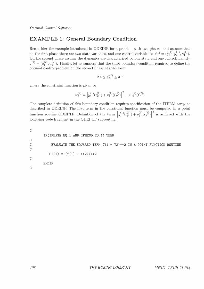
Optimal Control Software
EXAMPLE 1: General Boundary Condition
Reconsider the example introduced in ODEINP for a problem with two phases, and assume that
on the first phase there are two state variables, and one control variable, so z(1) = (y(1)1 , y
(1)2 , u
(1)1 ).
On the second phase assume the dynamics are characterized by one state and one control, namely
z(2) = (y(2)1 , u
(2)1 ). Finally, let us suppose that the third boundary condition required to define the
optimal control problem on the second phase has the form
2.4 ≤ ψ(2)3 ≤ 3.7
where the constraint function is given by
ψ(2)3 =
[y
(1)1 (t
(1)F ) + y
(1)2 (t
(1)F )]2
− 4u(2)1 (t
(2)I )
The complete definition of this boundary condition requires specification of the ITERM array asdescribed in ODEINP. The first term in the constraint function must be computed in a point
function routine ODEPTF. Definition of the term[y
(1)1 (t
(1)F ) + y
(1)2 (t
(1)F )]2
is achieved with the
following code fragment in the ODEPTF subroutine:
C
IF(IPHASE.EQ.1.AND.IPHEND.EQ.1) THEN
C
C EVALUATE THE SQUARED TERM (Y1 + Y2)**2 IN A POINT FUNCTION ROUTINE
C
PSI(1) = (Y(1) + Y(2))**2
C
ENDIF
C
408 THE BOEING COMPANY M&CT-TECH-01-014
User-Supplied Subprograms for Optimal Control
ODERHS: Optimal Control Right Hand Side Evaluation
PURPOSE
ODERHS is a user-supplied subroutine which evaluates the right hand sides of the differentialequations, the algebraic equations, the quadrature functions, and the auxiliary functions for eachinput value of the independent variable t, the dependent functions z(t) (states plus controls),and the constant parameters, p. For applications that do not require evaluation of differentialequations, algebraic equations, quadrature functions or auxiliary functions the system supplieddummy routine, DUMYDE may be used in the calling arguments to HDSOCS or HDSOPE.
RELATED SUBPROGRAMS
HDSOCS Sparse Optimal Control Software
HDSOPE Sparse Optimal Parameter Estimation
HHSOCS Sparse Optimal Control Input Procedure
ODEINP Optimal Control Problem Definition
ODEIGS Optimal Control Initial Guess
ODEPTF Optimal Control Point Function Evaluation
ODEPRT Optimal Control Print
METHOD
ODERHS is a generic name for this routine, and the actual routine name must be declared as anexternal in the main program and placed in the calling list to subroutine HDSOCS or HDSOPE.
On a specific phase the fundamental inputs to this routine are values for the independent variablet, the dependent functions z(t) (states plus controls), and the constant parameters, p. From thisinformation, ODERHS must evaluate the continuous functions
F (t) =
f [y(t), u(t), p, t]g[y(t), u(t), p, t]q[y(t), u(t), p, t]a[y(t), u(t), p, t]
.
The continuous functions are made up of the right hand sides of the differential equations
y = f [y(t), u(t), p, t]
and the functions g and a defining the path constraints
gℓ ≤ g[y(t), u(t), p, t] ≤ gu,
where g is a vector of size ng. The algebraic constraints are of the form
g[y(t), u(t), p, t] = α0g[v, t] + α⊤v + β⊤a[v, t]
M&CT-TECH-01-014 THE BOEING COMPANY 409
Optimal Control Software
where
v =
y(t)u(t)p
.
The constraint definition can include analytic terms involving α⊤v where the (ny +nu +np) vectorα is constant, as well as linear combinations of the na auxiliary functions ak(v) where β is constant.The continuous functions also include the quadrature functions appearing as integrands in theexpression ∫ tF
tI
q[y(t), u(t), p, t]dt.
Note that the array of continuous functions F (t) must be defined with the values of NCF(1) differen-tial equations stored first, followed by NCF(2) path constraints. The NCF(3) quadrature functionsare stored next and the NCF(4) auxiliary functions last. The partitioning of the continuous functionarray F (t) is defined in subroutine ODEINP by the array NCF.
The SOCS software may request an evaluation of the continuous functions for any value of t in therange tI ≤ t ≤ tF . The function evaluation error flag, IFERR, should be set to zero if the righthand side evaluation is successful. Otherwise, IFERR can be set to any nonzero value to designatethat the differential-algebraic system can not be evaluated for the current inputs. It may be usefulfor the user to set the flag to different values depending on the type of input error so that thesystem print of the error number will have meaning in the user’s context.
USAGE REMARKS
For some applications it is convenient to define the continuous functions in terms of relative times τfrom the beginning or end of the phase, e.g. τ = t−tI or τ = tF −t. Suppose the number of discreteparameters is np. If the initial or final times have been specified as variables in ODEINP, then theywill also appear in the parameter array after the user defined parameters. Thus, if tI is variable,then tI = P (np+1). If the final time of the phase, tF , is also variable, then tF = P (np+2). In caseswhere tI is fixed, but tF is free, tF = P (np + 1). This information in the parameter array permitsthe user to compute the relative time τ from the input value of t, thereby allowing construction ofdifferential equations depending on the relative time since the beginning of the phase, or the timeto go until the end of the phase.
WARNING
The system of differential-algebraic equations may be different on each phase, but may not bechanged within a phase. Thus the number of dependent functions, z(t), and parameters, p, canvary from phase to phase.
The functions computed in ODERHS supplied by the user are assumed to be continuous andhave continuous first and second derivatives. Nondifferentiable functions can cause unpredictableperformance in the optimization algorithm. It should be emphasized that discontinuities in thesecond derivatives of these functions can significantly degrade the speed of convergence withoutproducing any other obvious difficulties. The following common sources of error should be avoidedwhen evaluating the right hand side functions:
(1) nonsmooth interpolation of data;
410 THE BOEING COMPANY M&CT-TECH-01-014
User-Supplied Subprograms for Optimal Control
(2) iterative procedures inside the function evaluation process, such as adaptive quadrature or rootsolving;
(3) discontinuous behavior caused by branching for IF tests;
(4) nondifferentiable functions such as ABS, MAX, and MIN.
The most common source of difficulty encountered when using SOCS is nonsmooth interpolation oftabular data. DO NOT USE LINEAR INTERPOLATION OF TABULAR DATA!
USER-SUPPLIED SUBPROGRAM
The user must supply a subroutine with the following format:
SUBROUTINE ODERHS(IPHASE,T,Z,NZ,P,NP,F,NF,IFERR)
INTEGER IPHASE,NZ,NP,NF,IFERR
DOUBLE PRECISION T,Z(NZ),P(NP),F(NF)
User supplied code to evaluate the requested arguments (see below).
.
.
.
RETURN
END
ARGUMENTS
IPHASE [INPUT, INTEGER]The current phase number.
T [INPUT, DOUBLE PRECISION]Value of the independent variable t.
Z [INPUT, DOUBLE PRECISION, ARRAY]Real array of length NZ containing the dynamic variables z(t) = [y(t), u(t)].
NZ [INPUT, INTEGER]The number of time dependent variables.
P [INPUT, DOUBLE PRECISION, ARRAY]Real array of length NP containing the discrete parameters p, and the times tIand/or tF if they are free (see usage remarks).
NP [INPUT, INTEGER]The length of the array P. In general, NP = NPV + kt where NPV is the number
M&CT-TECH-01-014 THE BOEING COMPANY 411
Optimal Control Software
of user defined discrete parameters and
kt =
0, if both tI and tF are fixed;1, if either tI or tF are free;2, if both tI and tF are free.
F [OUTPUT, DOUBLE PRECISION, ARRAY]Real array of length NF containing the computed values for the continuous func-tions F (t).
NF [INPUT, INTEGER]The number of continuous functions, NF = NCF(1) + NCF(2) + NCF(3) +NCF(4).
IFERR [OUTPUT, INTEGER]Continuous Function Evaluation Error Flag.
IFERR = 0 Successful Evaluation of Continuous Functions.
IFERR 6= 0 Error in Evaluation of Continuous Functions.
EXAMPLE 2: General Path Constraints
As an illustration let us reconsider the problem introduced in ODEINP. For this single phaseexample there are two state variables, and one control variable, so z = (y1, y2, u1). The dynamicsof the system are described by the differential equations
y1 = −uy1
y2 = uy1 − ρuky2
where the constants ρ > 0 and k > 0. As before suppose that the optimal control problem requiresthe following path constraint
−4.1 ≤ g1(t) ≤ 1.9
for tI ≤ t ≤ tF where the constraint function is given by
g1(t) =1
2exp [−y1(t) − 3y2(t)] + 3u1(t).
For this example the user supplied subroutine ODERHS must evaluate the right hand side of thedifferential equations and the constraint function g1(t). The following code fragment illustrates thisconstruction:
C
C DEFINE THE PROBLEM PARAMETERS
C
RHO = 2.5E0
EXPON = 1.5E0
Y1 = Z(1)
412 THE BOEING COMPANY M&CT-TECH-01-014

User-Supplied Subprograms for Optimal Control
Y2 = Z(2)
U = Z(3)
C
C CONSTRUCT THE RIGHT HAND SIDES OF THE DIFFERENTIAL EQUATIONS
C
F(1) = - U*Y1
F(2) = U*Y1 - RHO*Y2*(U**EXPON)
C
C CONSTRUCT THE PATH CONSTRAINT FUNCTION
C
F(3) = EXP(-Y1 - 3.E0*Y2)/2.E0 + 3.E0*U
C
M&CT-TECH-01-014 THE BOEING COMPANY 413
Optimal Control Software
6.4 Utility Subprograms for Optimal Control
AUTOLK: Auto Link Variable Utility
PURPOSE
AUTOLK is a utility routine which can be used in the user-supplied ODEINP subroutine to linkvariables from one phase to another.
RELATED SUBPROGRAMS
ODEINP Optimal Control Problem Definition
LINKST Optimal Control Linkage Utility
METHOD
Subroutine AUTOLK is a utility routine which is called from the user supplied input routineODEINP. A single call to the routine will construct the inputs necessary to define a linkage con-straint in one of the forms
’name1 < name2’’name1 = name2’’name1 > name2’
Note that the character string “<” is used to denote the mathematical operation “≤”, and similarly“≥” is denoted by “>”. Both name1 and name2 are character variables having the following format
name1 = ”symbol@phaseE”.
The character substring ’symbol’ defines the name of the variable that is to be linked. The substring’symbol’ of maximum length 8 is
• case sensitive (i.e. TIME is not the same as time)
• must exactly match a user specified label quantity STLBL or PLBL.
The substring ’phase’ is the numeric phase number for the desired variable and must be precededby the symbol @.
The substring ’E’ denotes which end of the phase is linked.
• The beginning of a phase is denoted by E = i or E = I.
• The end of a phase is denoted by E = f or E = F .
For example the statement
call autolk(’VEL@1f = VEL@2I’)
414 THE BOEING COMPANY M&CT-TECH-01-014

Utility Subprograms for Optimal Control
executed in the user input routine ODEINP, will link the user defined variable VEL at the end ofphase 1, to the same variable at the beginning of phase 2. Each call to AUTOLK will construct aconstraint using the ITERM array. Multiple calls to the utility will create successive linkage con-straints in the order same order AUTOLK is called. For example four successive calls to AUTOLKwill construct four linkage constraints, e.g.
| (B02) | LINK1 | TIME@2I > TIME@1F |
| (B03) | LINK2 | HALT@1F = HALT@2I |
| (B04) | LINK3 | VEL@1F = VEL@2I |
| (B05) | LINK4 | MASS@1F = MASS@2I |
USAGE
CALL AUTOLK(’string’)
ARGUMENTS
STRING [INPUT, CHARACTER*80]Character string containing the linkage condition of the form ’name1 = name2’ asdescribed in method.
M&CT-TECH-01-014 THE BOEING COMPANY 415
Optimal Control Software
AUTOPL: Auto Phase Length Constraint Utility
PURPOSE
AUTOPL is a utility routine which can be used in the user-supplied ODEINP subroutine to con-strain the length of a phase.
RELATED SUBPROGRAMS
ODEINP Optimal Control Problem Definition
PHSLNG Optimal Control Phase Duration Utility
METHOD
Subroutine AUTOPL is a utility routine which is called from the user supplied input routineODEINP. A single call to the routine will construct the inputs necessary to constrain the length(duration) of a phase. Specifically bounds of the following form can be imposed:
∆t = a
∆t ≤ a
∆t ≥ a
a = ∆t
a ≤ ∆t
a ≥ ∆t
a ≤ ∆t ≤ b
a ≥ ∆t ≥ b
where ∆t = tF − tI and tI is the time (i.e. independent variable) at the beginning of the phase,and tF is the time at the end of the phase. Typically tI ≤ tF however the procedure can also beapplied when tI ≥ tF . The phase duration or length ∆t is denoted by the case insensitive characterstring PHSLNG. The fixed bounds a and b can be specified using any character format that has anumeric representation, i.e. integer, real, or double precision. The following examples are all valid:
call autopl(’1 < PHSLNG’)
call autopl(’14.d0 > PHSLNG > .1’)
call autopl(’PHSLNG = 27.35e-2’)
Note that the character string “<” is used to denote the mathematical operation “≤”, and similarly“≥” is denoted by “>”. Regardless of the format, the routine AUTOPL cannot be called more thanonce per phase from the user input routine ODEINP. A call to AUTOPL will construct a constraintusing the ITERM array. If either the initial or final time is fixed by user specified bounds, theconstraint limits will be shifted accordingly. For example suppose that tI = 2. which is implementedin ODEINP by setting
YLB(-1,0)=2.
YUB(-1,0)=2.
416 THE BOEING COMPANY M&CT-TECH-01-014
Utility Subprograms for Optimal Control
Furthermore suppose the phase length is constrained using the following statement in ODEINP
call autopl(’5 < PHSLNG’)
These conditions can be simplified as follows
a ≤ ∆t
5 ≤ tF − tI
5 ≤ tF − 2
7 ≤ tF
and the final constraint construction will reflect this simplification.
USAGE
CALL AUTOPL(’string’)
ARGUMENTS
STRING [INPUT, CHARACTER*80]Character string containing the linkage condition of the form ’name1 = name2’ asdescribed in method.
M&CT-TECH-01-014 THE BOEING COMPANY 417
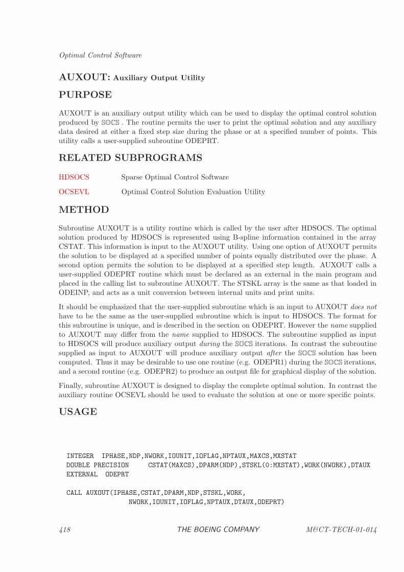
Optimal Control Software
AUXOUT: Auxiliary Output Utility
PURPOSE
AUXOUT is an auxiliary output utility which can be used to display the optimal control solutionproduced by SOCS . The routine permits the user to print the optimal solution and any auxiliarydata desired at either a fixed step size during the phase or at a specified number of points. Thisutility calls a user-supplied subroutine ODEPRT.
RELATED SUBPROGRAMS
HDSOCS Sparse Optimal Control Software
OCSEVL Optimal Control Solution Evaluation Utility
METHOD
Subroutine AUXOUT is a utility routine which is called by the user after HDSOCS. The optimalsolution produced by HDSOCS is represented using B-spline information contained in the arrayCSTAT. This information is input to the AUXOUT utility. Using one option of AUXOUT permitsthe solution to be displayed at a specified number of points equally distributed over the phase. Asecond option permits the solution to be displayed at a specified step length. AUXOUT calls auser-supplied ODEPRT routine which must be declared as an external in the main program andplaced in the calling list to subroutine AUXOUT. The STSKL array is the same as that loaded inODEINP, and acts as a unit conversion between internal units and print units.
It should be emphasized that the user-supplied subroutine which is an input to AUXOUT does nothave to be the same as the user-supplied subroutine which is input to HDSOCS. The format forthis subroutine is unique, and is described in the section on ODEPRT. However the name suppliedto AUXOUT may differ from the name supplied to HDSOCS. The subroutine supplied as inputto HDSOCS will produce auxiliary output during the SOCS iterations. In contrast the subroutinesupplied as input to AUXOUT will produce auxiliary output after the SOCS solution has beencomputed. Thus it may be desirable to use one routine (e.g. ODEPR1) during the SOCS iterations,and a second routine (e.g. ODEPR2) to produce an output file for graphical display of the solution.
Finally, subroutine AUXOUT is designed to display the complete optimal solution. In contrast theauxiliary routine OCSEVL should be used to evaluate the solution at one or more specific points.
USAGE
INTEGER IPHASE,NDP,NWORK,IOUNIT,IOFLAG,NPTAUX,MAXCS,MXSTAT
DOUBLE PRECISION CSTAT(MAXCS),DPARM(NDP),STSKL(0:MXSTAT),WORK(NWORK),DTAUX
EXTERNAL ODEPRT
CALL AUXOUT(IPHASE,CSTAT,DPARM,NDP,STSKL,WORK,
NWORK,IOUNIT,IOFLAG,NPTAUX,DTAUX,ODEPRT)
418 THE BOEING COMPANY M&CT-TECH-01-014
Utility Subprograms for Optimal Control
ARGUMENTS
IPHASE [INPUT, INTEGER]The current phase number.
CSTAT [INPUT, DOUBLE PRECISION, ARRAY]The spline array for the current phase.
DPARM [INPUT, DOUBLE PRECISION, ARRAY]The discrete parameter array for the current phase.
NDP [INPUT, INTEGER]The number of discrete parameters.
STSKL [INPUT, DOUBLE PRECISION, ARRAY]Real array containing scales for output quantities t and z.
t =STSKL(0)∗t Scaled independent variable.
zk =STSKL(k)∗zk Scaled dynamic variable, k.
WORK [INPUT, DOUBLE PRECISION, ARRAY]Real work array.
NWORK [INPUT, INTEGER]Length of work array.
IOUNIT [INPUT, INTEGER]FORTRAN unit number for auxiliary print, which must be opened by user priorto calling AUXOUT.
IOFLAG [INPUT, INTEGER]Flag controlling the level of auxiliary print.
NPTAUX [INPUT, INTEGER]The number of output points in the interval tI ≤ t ≤ tF . There are three types ofoutput possible.
NPTAUX > 0 Subroutine ODEPRT will be called at NPTAUXequally spaced points in the phase.
NPTAUX = 0 andDTAUX > 0
Subroutine ODEPRT will be called at pointsspaced DTAUX apart in the phase.
NPTAUX < 0 Subroutine ODEPRT will be called at the gridpoints in the phase.
M&CT-TECH-01-014 THE BOEING COMPANY 419
Optimal Control Software
DTAUX [INPUT, INTEGER]The step length between print points used only when NPTAUX = 0. SubroutineODEPRT will be called for all values of k = 0, 1, . . . such that tk ≤ tF wheretk = k∗DTAUX+tI , and the final point printed will always be tF .
ODEPRT [INPUT, SUBROUTINE]The name of the user routine which evaluates auxiliary print at each point. Ifsophisticated output is not required, the system supplied dummy routine DUMYPRmay be used instead. See Section 3.3
EXAMPLE Creating a Plot File of the Solution
To illustrate the usage of the AUXOUT procedure, suppose that an optimal control problem hasbeen solved using HDSOCS. Most graphics software requires as input a file containing the quantitiesto be displayed. The system supplied output routine DUMYPR must be declared using an externalstatement, and will produce a file containing the independent variable followed by all dynamicvariables. The following code fragement which must be executed after calling HDSOCS will producea file suitable for plotting:
C
C OPEN A PLOT FILE ON UNIT 31 CALLED ’TSTSPR.PLT’
C
IPLT = 31
OPEN(IPLT,FILE=’TSTSPR.PLT’,STATUS=’UNKNOWN’)
C
C DEFINE THE NUMBER OF PLOT POINTS AND SET STEPSIZE ZERO
C
NPLPTS = 100
DTAUX = ZERO
C
C SET THE AUXILIARY PRINT FLAG (VALUE CONSISTENT WITH
C OUTPUT SUBROUTINE)
C
IPFAUX = 10
C
C SET THE PHASE TO ONE, AND COMPUTE THE NUMBER OF
C DEPENDENT PARAMETERS ON THE PHASE
C
IPH = 1
NDP = IPDPH(IPH+1) - IPDPH(IPH)
C
C SET THE PRINT SCALE WEIGHTS TO ONE FOR THE NDYN DYNAMIC
C VARIABLES
C
NDYN = 20
CALL DFILL(NDYN,1.E0,STSKL,1)
C
C CREATE THE FILE BY CALLING AUXOUT
420 THE BOEING COMPANY M&CT-TECH-01-014

Utility Subprograms for Optimal Control
C
CALL AUXOUT(IPH,CSTAT,DPARM,NDP,STSKL,WORK,NRW,IPLT,
& IPFAUX,NPLPTS,DTAUX,DUMYPR)
C
C CLOSE THE PLOT FILE
C
CLOSE(IPLT)
M&CT-TECH-01-014 THE BOEING COMPANY 421
Optimal Control Software
BSPDEF: B-Spline Algebraic Variable Utility
PURPOSE
BSPDEF is a utility routine which can be used to construct a cubic B-spline representation foran algebraic variable during a phase. It must be called from the user supplied input routineODEINP (p. 384), and will define the required SOCS input for the construction.
RELATED SUBPROGRAMS
HDSOCS Sparse Optimal Control Software
HDSOPE Sparse Optimal Parameter Estimation
ODEINP Optimal Control Problem Definition
ODERHS Optimal Control Right Hand Side Evaluation
METHOD
Subroutine BSPDEF is a utility routine that is called by the user from ODEINP. BSPDEF willconstruct the necessary SOCS information to represent an algebaic variable by a cubic B-spline.Specifically,
u(t) = c0B0(t) + c1B1(t) + ...+ cnBn(t)
where Bj(t) are the cubic B-spline basis functions.
This requires four distinct operations:
1. u(t) is defined as an algebraic variable
2. c0, c1, . . . , cn are defined as parameters
3. c0B0(t) . . . cnBn(t) are defined as analytic terms
4. The following path constraint is constructed
0 = u(t) − [c0B0(t) + c1B1(t) + ...+ cnBn(t)] = g(t)
The user can also supply a label to identify the variable. The B-spline representation is a continuous,
differentiable (C1) cubic with internal knots equally spaced between the initial phase time t(k)I and
the final phase time t(k)F . Since the B-spline terms cjBj(t) are treated analytically, derivatives with
respect to the optimization parameters cj are also computed analytically, and the number of finitedifference index sets is not affected.
Since a number of SOCS input quantities are incremented when BSPDEF is called, it is importantthat the user properly initializes these quantities in ODEINP (p. 384). Also since a B-spline con-struction introduces a path constraint the user supplied routine ODERHS (p. 409) must computea (trivial) path function gj [y(t), u(t), p, t] = 0 (cf Table 6.3) in the same order as defined by callsto BSPDEF. For a B-spline construction with Ns segments, BSPDEF introduces np = (2Ns + 2)parameters, and the user must ensure that the value of MXPARM is sufficiently large.
422 THE BOEING COMPANY M&CT-TECH-01-014
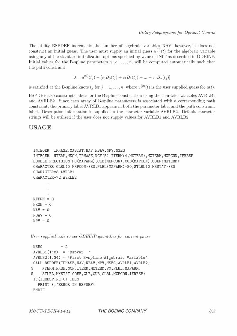
Utility Subprograms for Optimal Control
The utility BSPDEF increments the number of algebraic variables NAV, however, it does notconstruct an initial guess. The user must supply an initial guess u(0)(t) for the algebraic variableusing any of the standard initialization options specified by value of INIT as described in ODEINP.Initial values for the B-spline parameters c0, c1, . . . , cn will be computed automatically such thatthe path constraint
0 = u(0)(tj) − [c0B0(tj) + c1B1(tj) + ...+ cnBn(tj)]
is satisfied at the B-spline knots tj for j = 1, . . . , n, where u(0)(t) is the user supplied guess for u(t).
BSPDEF also constructs labels for the B-spline construction using the character variables AVRLB1and AVRLB2. Since each array of B-spline parameters is associated with a corresponding pathconstraint, the primary label AVRLB1 appears in both the parameter label and the path constraintlabel. Description information is supplied in the character variable AVRLB2. Default characterstrings will be utilized if the user does not supply values for AVRLB1 and AVRLB2.
USAGE
INTEGER IPHASE,MXSTAT,NAV,NBAV,NPV,NSEG
INTEGER NTERM,NKON,IPHASE,NCF(5),ITERM(4,MXTERM),MXTERM,MXPCON,IERBSP
DOUBLE PRECISION P0(MXPARM),CLB(MXPCON),CUB(MXPCON),COEF(MXTERM)
CHARACTER CLBL(0:MXPCON)*80,PLBL(MXPARM)*80,STLBL(0:MXSTAT)*80
CHARACTER*8 AVRLB1
CHARACTER*72 AVRLB2
.
.
.
NTERM = 0
NKON = 0
NAV = 0
NBAV = 0
NPV = 0
User supplied code to set ODEINP quantities for current phase
NSEG = 2
AVRLB1(1:8) = ’BspVar ’
AVRLB2(1:34) = ’First B-spline Algebraic Variable’
CALL BSPDEF(IPHASE,NAV,NBAV,NPV,NSEG,AVRLB1,AVRLB2,
$ NTERM,NKON,NCF,ITERM,MXTERM,P0,PLBL,MXPARM,
$ STLBL,MXSTAT,COEF,CLB,CUB,CLBL,MXPCON,IERBSP)
IF(IERBSP.NE.0) THEN
PRINT *,’ERROR IN BSPDEF’
ENDIF
M&CT-TECH-01-014 THE BOEING COMPANY 423
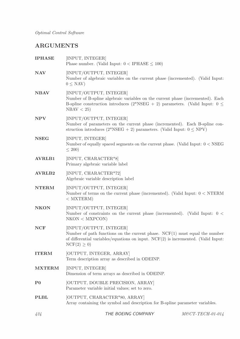
Optimal Control Software
ARGUMENTS
IPHASE [INPUT, INTEGER]Phase number. (Valid Input: 0 < IPHASE ≤ 100)
NAV [INPUT/OUTPUT, INTEGER]Number of algebraic variables on the current phase (incremented). (Valid Input:0 ≤ NAV)
NBAV [INPUT/OUTPUT, INTEGER]Number of B-spline algebraic variables on the current phase (incremented). EachB-spline construction introduces (2*NSEG + 2) parameters. (Valid Input: 0 ≤NBAV < 25)
NPV [INPUT/OUTPUT, INTEGER]Number of parameters on the current phase (incremented). Each B-spline con-struction introduces (2*NSEG + 2) parameters. (Valid Input: 0 ≤ NPV)
NSEG [INPUT, INTEGER]Number of equally spaced segments on the current phase. (Valid Input: 0 < NSEG≤ 200)
AVRLB1 [INPUT, CHARACTER*8]Primary algebraic variable label
AVRLB2 [INPUT, CHARACTER*72]Algebraic variable description label
NTERM [INPUT/OUTPUT, INTEGER]Number of terms on the current phase (incremented). (Valid Input: 0 < NTERM< MXTERM)
NKON [INPUT/OUTPUT, INTEGER]Number of constraints on the current phase (incremented). (Valid Input: 0 <NKON < MXPCON)
NCF [INPUT/OUTPUT, INTEGER]Number of path functions on the current phase. NCF(1) must equal the numberof differential variables/equations on input. NCF(2) is incremented. (Valid Input:NCF(2) ≥ 0)
ITERM [OUTPUT, INTEGER, ARRAY]Term description array as described in ODEINP.
MXTERM [INPUT, INTEGER]Dimension of term arrays as described in ODEINP.
P0 [OUTPUT, DOUBLE PRECISION, ARRAY]Parameter variable initial values; set to zero.
PLBL [OUTPUT, CHARACTER*80, ARRAY]Array containing the symbol and description for B-spline parameter variables.
424 THE BOEING COMPANY M&CT-TECH-01-014
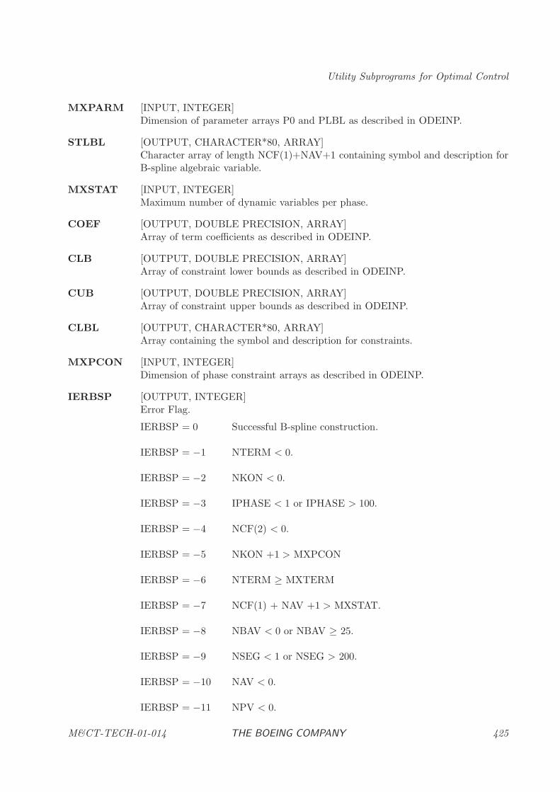
Utility Subprograms for Optimal Control
MXPARM [INPUT, INTEGER]Dimension of parameter arrays P0 and PLBL as described in ODEINP.
STLBL [OUTPUT, CHARACTER*80, ARRAY]Character array of length NCF(1)+NAV+1 containing symbol and description forB-spline algebraic variable.
MXSTAT [INPUT, INTEGER]Maximum number of dynamic variables per phase.
COEF [OUTPUT, DOUBLE PRECISION, ARRAY]Array of term coefficients as described in ODEINP.
CLB [OUTPUT, DOUBLE PRECISION, ARRAY]Array of constraint lower bounds as described in ODEINP.
CUB [OUTPUT, DOUBLE PRECISION, ARRAY]Array of constraint upper bounds as described in ODEINP.
CLBL [OUTPUT, CHARACTER*80, ARRAY]Array containing the symbol and description for constraints.
MXPCON [INPUT, INTEGER]Dimension of phase constraint arrays as described in ODEINP.
IERBSP [OUTPUT, INTEGER]Error Flag.
IERBSP = 0 Successful B-spline construction.
IERBSP = −1 NTERM < 0.
IERBSP = −2 NKON < 0.
IERBSP = −3 IPHASE < 1 or IPHASE > 100.
IERBSP = −4 NCF(2) < 0.
IERBSP = −5 NKON +1 > MXPCON
IERBSP = −6 NTERM ≥ MXTERM
IERBSP = −7 NCF(1) + NAV +1 > MXSTAT.
IERBSP = −8 NBAV < 0 or NBAV ≥ 25.
IERBSP = −9 NSEG < 1 or NSEG > 200.
IERBSP = −10 NAV < 0.
IERBSP = −11 NPV < 0.
M&CT-TECH-01-014 THE BOEING COMPANY 425

Optimal Control Software
IERBSP = −12 MXPARM too small.
426 THE BOEING COMPANY M&CT-TECH-01-014
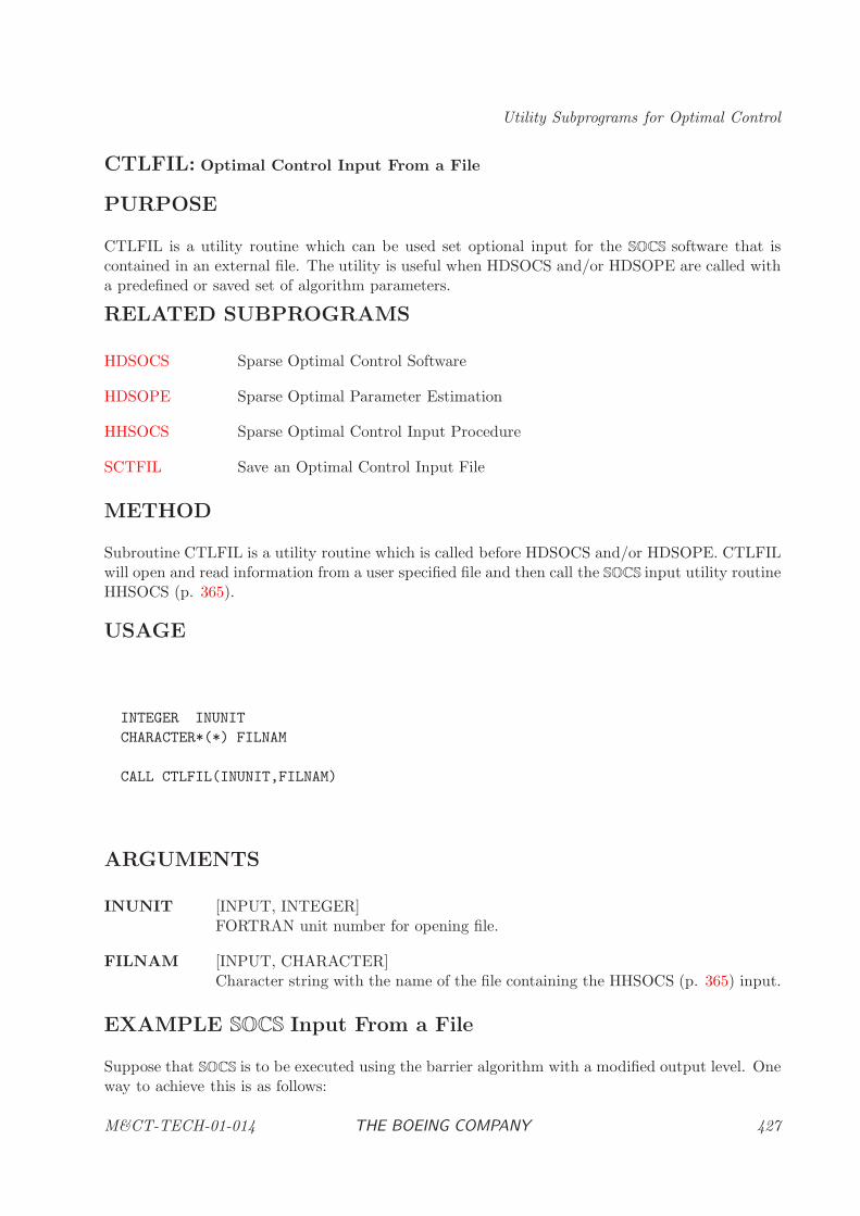
Utility Subprograms for Optimal Control
CTLFIL: Optimal Control Input From a File
PURPOSE
CTLFIL is a utility routine which can be used set optional input for the SOCS software that iscontained in an external file. The utility is useful when HDSOCS and/or HDSOPE are called witha predefined or saved set of algorithm parameters.
RELATED SUBPROGRAMS
HDSOCS Sparse Optimal Control Software
HDSOPE Sparse Optimal Parameter Estimation
HHSOCS Sparse Optimal Control Input Procedure
SCTFIL Save an Optimal Control Input File
METHOD
Subroutine CTLFIL is a utility routine which is called before HDSOCS and/or HDSOPE. CTLFILwill open and read information from a user specified file and then call the SOCS input utility routineHHSOCS (p. 365).
USAGE
INTEGER INUNIT
CHARACTER*(*) FILNAM
CALL CTLFIL(INUNIT,FILNAM)
ARGUMENTS
INUNIT [INPUT, INTEGER]FORTRAN unit number for opening file.
FILNAM [INPUT, CHARACTER]Character string with the name of the file containing the HHSOCS (p. 365) input.
EXAMPLE SOCS Input From a File
Suppose that SOCS is to be executed using the barrier algorithm with a modified output level. Oneway to achieve this is as follows:
M&CT-TECH-01-014 THE BOEING COMPANY 427
Optimal Control Software
C
CALL HHSOCS(’NLPALG=HDBNLP’)
CALL HHSOCS(’HDBNLP:BARRIER DEFAULT’)
CALL HHSOCS(’HDBNLP:IOFLAG=20’)
C
CALL HDSOCS(.....
C
An equivalent technique is as follows:
C
CALL CTLFIL(35,’/home/socsinput.fil’)
C
CALL HDSOCS(.....
C
where the file “/home/socsinput.fil” contains the following information:
nlpalg=hdbnlp
hdbnlp:barrier default
hdbnlp:ioflag = 20
The file “/home/socsinput.fil” can be created manually or by using the companion utility routineSCTFIL (p. 463).
428 THE BOEING COMPANY M&CT-TECH-01-014
Utility Subprograms for Optimal Control
CTLSTA: Optimal Control Software Status Utility
PURPOSE
CTLSTA is a utility routine which can be used to retrieve and optionally display the status of theSOCS software following execution. The utility is useful when HHSOCS has been called with theiteration output turned off, but SOCS returns with an error. In this case CTLSTA can be called toretrieve the complete error message, without rerunning the application.
RELATED SUBPROGRAMS
HDSOCS Sparse Optimal Control Software
METHOD
Subroutine CTLSTA is a utility routine which is called after HDSOCS. CTLSTA will retrieve andoptionally display information contained in commons used by the SOCS library.
USAGE
INTEGER IPF,IPU,IERCTL
CALL CTLSTA(IPF,IPU,IERCTL)
ARGUMENTS
IPF [INPUT, INTEGER]The print level flag (> 0 for output).
IPU [INPUT, INTEGER]FORTRAN unit number for printing messages.
IERCTL [INPUT, INTEGER]The SOCS error return flag.
EXAMPLE Diagnostic Messages
If HDSOCS is executed with all output turned off, no error messages will be displayed. To assureretrieval of error messages the following statement can be executed after HDSOCS has terminated:
C
IF (IER.NE.0) CALL CTLSTA(10,IPU,IERCTL)
C
M&CT-TECH-01-014 THE BOEING COMPANY 429
Optimal Control Software
FETCH: Variable Retrieval Utility
PURPOSE
FETCH is a utility routine which can be used to retrieve the numerical value(s) of variables specifiedby the companion utility WATCH (p. 467). It must be called from the main program aftertermination of SOCS or SOPE.
RELATED SUBPROGRAMS
WATCH Variable Monitor Utility
METHOD
Subroutine FETCH is a utility routine that is called by the user from the main program. Unlikethe companion utility WATCH, it cannot be called from the user input routine ODEINP. FETCHhas a single input argument, a character string, which is the name of the variable to be retrieved.The input string to FETCH must identical to the input string monitored by WATCH. The inputstring also must be identical to the desired output name which is derived from one of the userspecified label quantities STLBL, PLBL, or CLBL. The string must not exceed 80 characters andis of the following form:
’symbol@phase’
The character substring ’symbol’ defines the name of the variable that is to be monitored. Thesubstring ’symbol’ is:
• case sensitive (i.e. TIME is not the same as time)
• must exactly match the desired output name which is derived from a user specified labelquantity STLBL, PLBL, or CLBL.
The substring ’phase’ is the numeric phase number for the desired variable and must be precededby the symbol @. A global quantity with no explicit phase number can be specified by a characterstring of the form ’symbol’ or ’symbol@0’.
The FETCH utility retrieves the numerical values of the requested quantity at the solution (ortermination) of a run. As such, it must be called after HDSOCS or HDSOPE. An attempt tofetch a particular quantity must be preceded by a call to the WATCH (p. 467) utility. The valuesretrieved are stored in an array and can be used for additional calculations or processing.
USAGE
INTEGER LNVRVL,NUMVAL,IERGET
DOUBLE PRECISION VRVAL(LNVRVL)
CHARACTER*80 VRNAME
.
.
.
430 THE BOEING COMPANY M&CT-TECH-01-014
Utility Subprograms for Optimal Control
User main program call to HDSOCS or HDSOPE
VRNAME = ‘Variable’
CALL FETCH(VRNAME,LNVRVL,VRVAL,NUMVAL,IERGET)
IF(IERGET.NE.0) THEN
PRINT *,’ERROR IN FETCH’
ENDIF
ARGUMENTS
VRNAME [INPUT, CHARACTER*80]Character string containing variable name of the form ’symbol@phase’
LNVRVL [INPUT, INTEGER]Maximum length of the array VRVAL
VRVAL [OUTPUT, DOUBLE PRECISION, ARRAY]Array of of length NUMVAL containing numerical values of the requested variable.
NUMVAL [OUTPUT, INTEGER]Length of the array VRVAL (NUMVAL ≥ 1)
IERGET [OUTPUT, INTEGER]Error Flag.
IERGET = 0 Successful retrieval. VRVAL contains the requested values.
IERGET = −1 VRNAME is too short.
IERGET = −2 Input string in VRNAME is not found.
IERGET = −3 Input phase number is invalid.
IERGET = −4 Valid name not currently implemented in SOCS .
IERGET = −5 NUMVAL > LNVRVL
IERGET = −6 NUMVAL < 1
M&CT-TECH-01-014 THE BOEING COMPANY 431
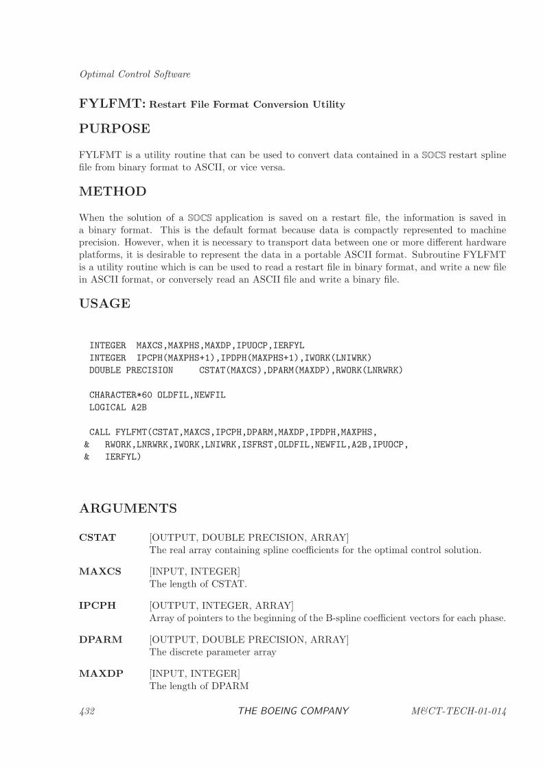
Optimal Control Software
FYLFMT: Restart File Format Conversion Utility
PURPOSE
FYLFMT is a utility routine that can be used to convert data contained in a SOCS restart splinefile from binary format to ASCII, or vice versa.
METHOD
When the solution of a SOCS application is saved on a restart file, the information is saved ina binary format. This is the default format because data is compactly represented to machineprecision. However, when it is necessary to transport data between one or more different hardwareplatforms, it is desirable to represent the data in a portable ASCII format. Subroutine FYLFMTis a utility routine which is can be used to read a restart file in binary format, and write a new filein ASCII format, or conversely read an ASCII file and write a binary file.
USAGE
INTEGER MAXCS,MAXPHS,MAXDP,IPUOCP,IERFYL
INTEGER IPCPH(MAXPHS+1),IPDPH(MAXPHS+1),IWORK(LNIWRK)
DOUBLE PRECISION CSTAT(MAXCS),DPARM(MAXDP),RWORK(LNRWRK)
CHARACTER*60 OLDFIL,NEWFIL
LOGICAL A2B
CALL FYLFMT(CSTAT,MAXCS,IPCPH,DPARM,MAXDP,IPDPH,MAXPHS,
& RWORK,LNRWRK,IWORK,LNIWRK,ISFRST,OLDFIL,NEWFIL,A2B,IPUOCP,
& IERFYL)
ARGUMENTS
CSTAT [OUTPUT, DOUBLE PRECISION, ARRAY]The real array containing spline coefficients for the optimal control solution.
MAXCS [INPUT, INTEGER]The length of CSTAT.
IPCPH [OUTPUT, INTEGER, ARRAY]Array of pointers to the beginning of the B-spline coefficient vectors for each phase.
DPARM [OUTPUT, DOUBLE PRECISION, ARRAY]The discrete parameter array
MAXDP [INPUT, INTEGER]The length of DPARM
432 THE BOEING COMPANY M&CT-TECH-01-014
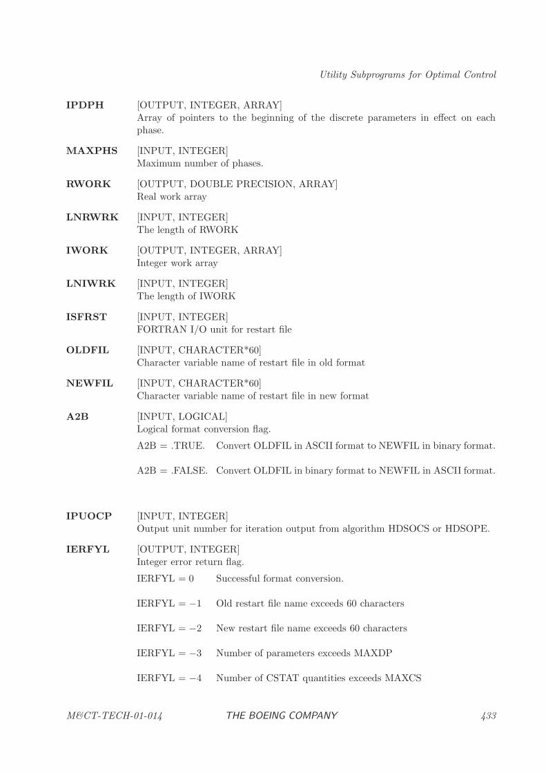
Utility Subprograms for Optimal Control
IPDPH [OUTPUT, INTEGER, ARRAY]Array of pointers to the beginning of the discrete parameters in effect on eachphase.
MAXPHS [INPUT, INTEGER]Maximum number of phases.
RWORK [OUTPUT, DOUBLE PRECISION, ARRAY]Real work array
LNRWRK [INPUT, INTEGER]The length of RWORK
IWORK [OUTPUT, INTEGER, ARRAY]Integer work array
LNIWRK [INPUT, INTEGER]The length of IWORK
ISFRST [INPUT, INTEGER]FORTRAN I/O unit for restart file
OLDFIL [INPUT, CHARACTER*60]Character variable name of restart file in old format
NEWFIL [INPUT, CHARACTER*60]Character variable name of restart file in new format
A2B [INPUT, LOGICAL]Logical format conversion flag.
A2B = .TRUE. Convert OLDFIL in ASCII format to NEWFIL in binary format.
A2B = .FALSE. Convert OLDFIL in binary format to NEWFIL in ASCII format.
IPUOCP [INPUT, INTEGER]Output unit number for iteration output from algorithm HDSOCS or HDSOPE.
IERFYL [OUTPUT, INTEGER]Integer error return flag.
IERFYL = 0 Successful format conversion.
IERFYL = −1 Old restart file name exceeds 60 characters
IERFYL = −2 New restart file name exceeds 60 characters
IERFYL = −3 Number of parameters exceeds MAXDP
IERFYL = −4 Number of CSTAT quantities exceeds MAXCS
M&CT-TECH-01-014 THE BOEING COMPANY 433

Optimal Control Software
IERFYL = −5 Number of RWORK quantities exceeds LNRWRK
IERFYL = −6 Number of IWORK quantities exceeds LNIWRK
IERFYL = −7 Number of phases exceeds MAXPHS
434 THE BOEING COMPANY M&CT-TECH-01-014
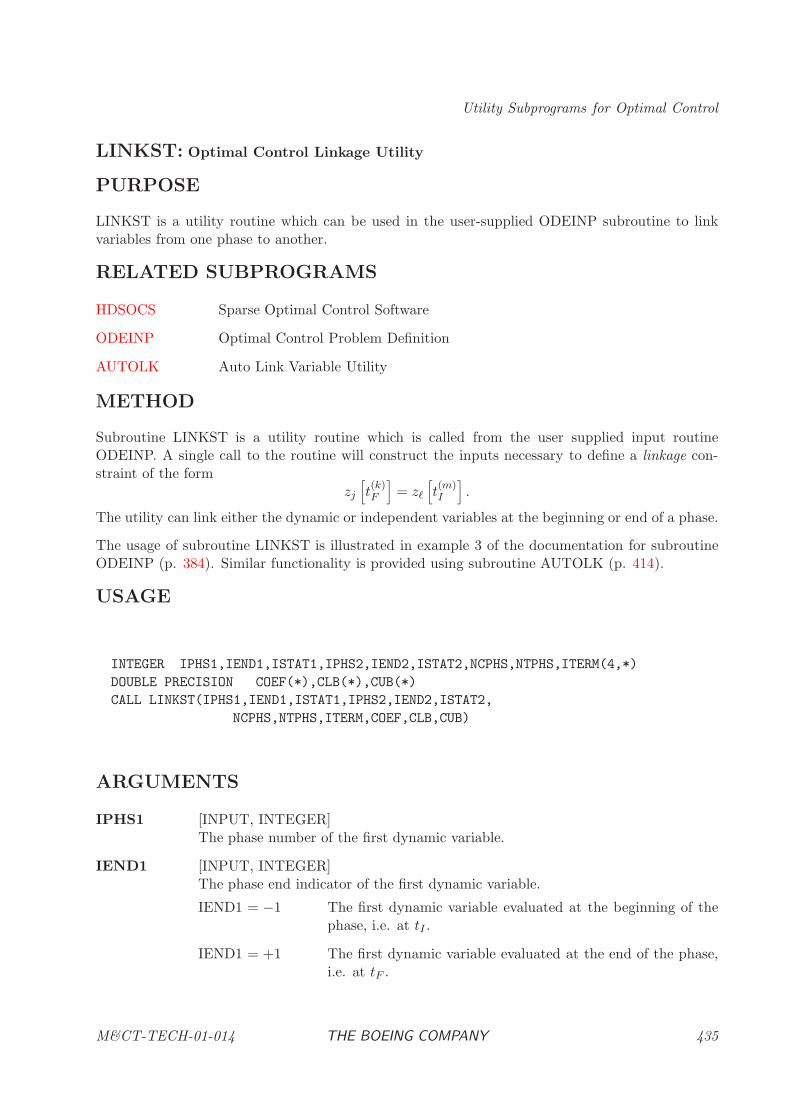
Utility Subprograms for Optimal Control
LINKST: Optimal Control Linkage Utility
PURPOSE
LINKST is a utility routine which can be used in the user-supplied ODEINP subroutine to linkvariables from one phase to another.
RELATED SUBPROGRAMS
HDSOCS Sparse Optimal Control Software
ODEINP Optimal Control Problem Definition
AUTOLK Auto Link Variable Utility
METHOD
Subroutine LINKST is a utility routine which is called from the user supplied input routineODEINP. A single call to the routine will construct the inputs necessary to define a linkage con-straint of the form
zj[t(k)F
]= zℓ
[t(m)I
].
The utility can link either the dynamic or independent variables at the beginning or end of a phase.
The usage of subroutine LINKST is illustrated in example 3 of the documentation for subroutineODEINP (p. 384). Similar functionality is provided using subroutine AUTOLK (p. 414).
USAGE
INTEGER IPHS1,IEND1,ISTAT1,IPHS2,IEND2,ISTAT2,NCPHS,NTPHS,ITERM(4,*)
DOUBLE PRECISION COEF(*),CLB(*),CUB(*)
CALL LINKST(IPHS1,IEND1,ISTAT1,IPHS2,IEND2,ISTAT2,
NCPHS,NTPHS,ITERM,COEF,CLB,CUB)
ARGUMENTS
IPHS1 [INPUT, INTEGER]The phase number of the first dynamic variable.
IEND1 [INPUT, INTEGER]The phase end indicator of the first dynamic variable.
IEND1 = −1 The first dynamic variable evaluated at the beginning of thephase, i.e. at tI .
IEND1 = +1 The first dynamic variable evaluated at the end of the phase,i.e. at tF .
M&CT-TECH-01-014 THE BOEING COMPANY 435

Optimal Control Software
ISTAT1 [INPUT, INTEGER]The number of the first dynamic variable.
IPHS2 [INPUT, INTEGER]The phase number of the second dynamic variable.
IEND2 [INPUT, INTEGER]The phase end indicator of the second dynamic variable.
IEND2 = −1 The second dynamic variable evaluated at the beginning of thephase, i.e. at tI .
IEND2 = +1 The second dynamic variable evaluated at the end of the phase,i.e. at tF .
ISTAT2 [INPUT, INTEGER]The number of the second dynamic variable.
NCPHS [INPUT/OUTPUT, INTEGER]Running number of constraints on the current phase.
NTPHS [INPUT/OUTPUT, INTEGER]Running number of terms on the current phase.
ITERM [INPUT/OUTPUT, INTEGER, ARRAY]Term description array as described in ODEINP.
COEF [INPUT/OUTPUT, DOUBLE PRECISION, ARRAY]Array of term coefficients as described in ODEINP.
CLB [INPUT/OUTPUT, DOUBLE PRECISION, ARRAY]Array of constraint lower bounds as described in ODEINP.
CUB [INPUT/OUTPUT, DOUBLE PRECISION, ARRAY]Array of constraint upper bounds as described in ODEINP.
436 THE BOEING COMPANY M&CT-TECH-01-014
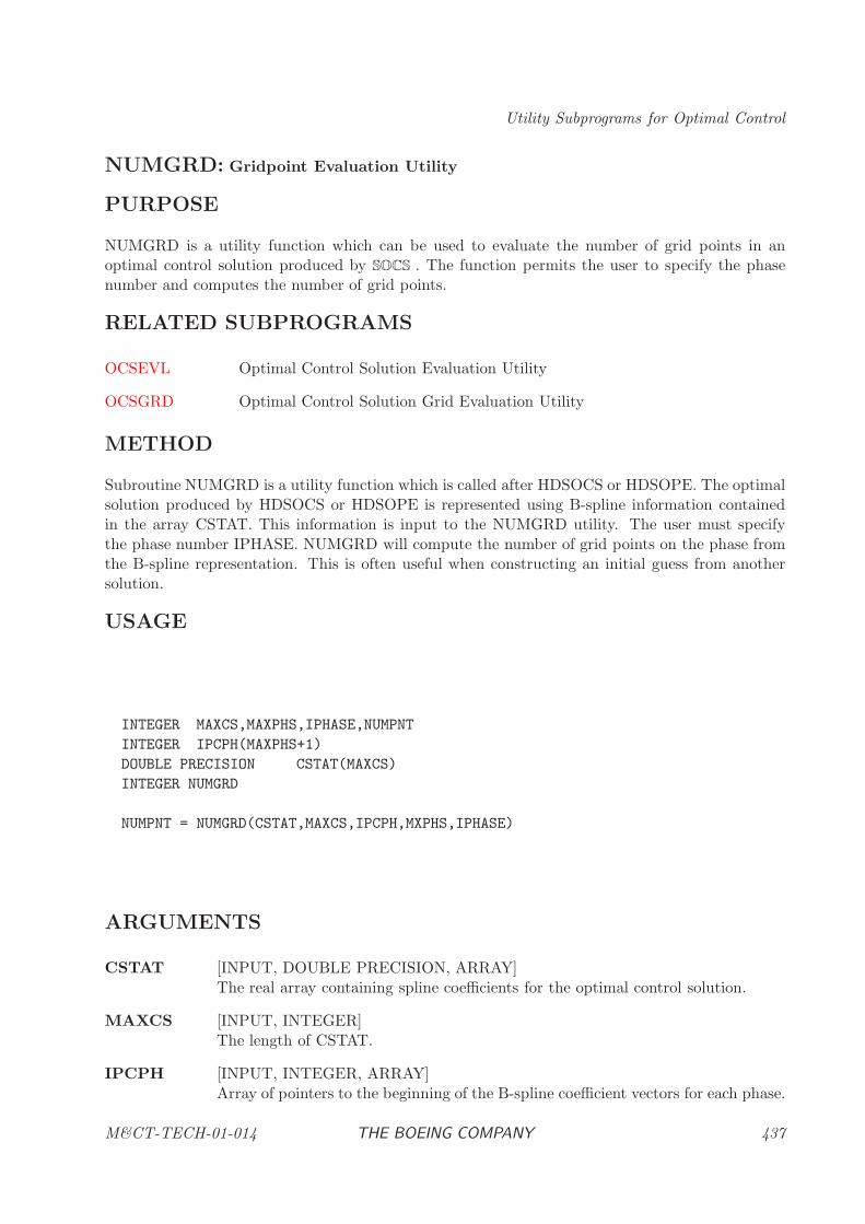
Utility Subprograms for Optimal Control
NUMGRD: Gridpoint Evaluation Utility
PURPOSE
NUMGRD is a utility function which can be used to evaluate the number of grid points in anoptimal control solution produced by SOCS . The function permits the user to specify the phasenumber and computes the number of grid points.
RELATED SUBPROGRAMS
OCSEVL Optimal Control Solution Evaluation Utility
OCSGRD Optimal Control Solution Grid Evaluation Utility
METHOD
Subroutine NUMGRD is a utility function which is called after HDSOCS or HDSOPE. The optimalsolution produced by HDSOCS or HDSOPE is represented using B-spline information containedin the array CSTAT. This information is input to the NUMGRD utility. The user must specifythe phase number IPHASE. NUMGRD will compute the number of grid points on the phase fromthe B-spline representation. This is often useful when constructing an initial guess from anothersolution.
USAGE
INTEGER MAXCS,MAXPHS,IPHASE,NUMPNT
INTEGER IPCPH(MAXPHS+1)
DOUBLE PRECISION CSTAT(MAXCS)
INTEGER NUMGRD
NUMPNT = NUMGRD(CSTAT,MAXCS,IPCPH,MXPHS,IPHASE)
ARGUMENTS
CSTAT [INPUT, DOUBLE PRECISION, ARRAY]The real array containing spline coefficients for the optimal control solution.
MAXCS [INPUT, INTEGER]The length of CSTAT.
IPCPH [INPUT, INTEGER, ARRAY]Array of pointers to the beginning of the B-spline coefficient vectors for each phase.
M&CT-TECH-01-014 THE BOEING COMPANY 437

Optimal Control Software
MAXPHS [INPUT, INTEGER]Maximum number of phases.
IPHASE [INPUT, INTEGER]The phase number.
NUMPNT [OUTPUT, INTEGER]The number of grid points on phase IPHASE
438 THE BOEING COMPANY M&CT-TECH-01-014
Utility Subprograms for Optimal Control
OCSEVL: Optimal Control Solution Evaluation Utility
PURPOSE
OCSEVL is a utility routine which can be used to evaluate the optimal control solution produced bySOCS . The routine permits the user to specify the value of the independent variable t and computethe optimal state vector y(t) and control vector u(t). The routine also computes the beginning andend of the phase, as well as the discrete parameter values.
RELATED SUBPROGRAMS
HDSOCS Sparse Optimal Control Software
OCSGRD Optimal Control Solution Grid Evaluation Utility
OCSTAU Optimal Control Solution Spline Evaluation Utility
AUXOUT Auxiliary Output Utility
METHOD
Subroutine OCSEVL is a utility routine which is called after HDSOCS or HDSOPE. The optimalsolution produced by HDSOCS or HDSOPE is represented using B-spline information containedin the array CSTAT. This information is input to the OCSEVL utility. The user must specify thephase number IPHASE and the desired evaluation point t. From the phase number OCSEVL firstcomputes the initial time tI and final time tF for the phase. If the specified time is not within thephase i.e. either t < tI or t > tF the state and control are not evaluated and an error return isset. On the other hand if tI ≤ t ≤ tF the specified time is within the phase, and OCSEVL willevaluate the B-spline representation for the dynamic variables and return the computed values forthe optimal state vector y(t) and control vector u(t).
The primary function of OCSEVL is to evaluate the solution at a few points. Subroutine AUX-OUT may be more appropriate when a complete time history of the solution is desired for displaypurposes.
USAGE
INTEGER MAXPHS,MAXCS,MAXDP,NWORK,IPHASE,NUMZV,LNZVEC,NUMPV,LNPVEC,IEROCS
INTEGER IPCPH(MAXPHS+1),IPDPH(MAXPHS+1)
DOUBLE PRECISION CSTAT(MAXCS),DPARM(MAXDP),WORK(NWORK)
DOUBLE PRECISION ZVEC(LNZVEC),PVEC(LNPVEC)
DOUBLE PRECISION TIME,TZERO,TFINAL
CALL OCSEVL(MAXPHS,CSTAT,MAXCS,IPCPH,DPARM,MAXDP,IPDPH,
WORK,NWORK,IPHASE,TIME,TZERO,TFINAL,ZVEC,NUMZV,LNZVEC,
PVEC,NUMPV,LNPVEC,IEROCS)
M&CT-TECH-01-014 THE BOEING COMPANY 439
Optimal Control Software
ARGUMENTS
MAXPHS [INPUT, INTEGER]Maximum number of phases.
CSTAT [INPUT, DOUBLE PRECISION, ARRAY]The real array containing spline coefficients for the optimal control solution.
MAXCS [INPUT, INTEGER]The length of CSTAT.
IPCPH [INPUT, INTEGER, ARRAY]Array of pointers to the beginning of the B-spline coefficient vectors for each phase.
DPARM [INPUT, DOUBLE PRECISION, ARRAY]The discrete parameter array.
MAXDP [INPUT, INTEGER]The length of DPARM.
IPDPH [INPUT, INTEGER, ARRAY]Array of pointers to the beginning of the discrete parameters in effect on eachphase.
WORK [INPUT, DOUBLE PRECISION, ARRAY]Real work array.
NWORK [INPUT, INTEGER]Length of work array. NWORK ≥ 2*LNZVEC + 19
IPHASE [INPUT, INTEGER]The phase number.
TIME [INPUT, DOUBLE PRECISION]The independent variable value t.
TZERO [OUTPUT, DOUBLE PRECISION]The phase start time tI .
TFINAL [OUTPUT, DOUBLE PRECISION]The phase end time tF .
ZVEC [OUTPUT, DOUBLE PRECISION, ARRAY]Real array containing the dynamic variables z(t) = [y(t), u(t)] evaluated at t whenIEROCS = 0.
NUMZV [OUTPUT, INTEGER]The length of ZVEC.
LNZVEC [INPUT, INTEGER]The maximum length of ZVEC.
440 THE BOEING COMPANY M&CT-TECH-01-014
Utility Subprograms for Optimal Control
PVEC [OUTPUT, DOUBLE PRECISION, ARRAY]Real array containing the discrete parameters p evaluated when IEROCS = 0.
NUMPV [OUTPUT, INTEGER]The length of PVEC.
LNPVEC [INPUT, INTEGER]The maximum length of PVEC.
IEROCS [OUTPUT, INTEGER]Integer error return flag.
IEROCS = 0 Successful evaluation of z(t), tI and tF .
IEROCS = +1 Input value of t is outside the phase, i.e. eithert > tF and z(t) is linearly extrapolated from z(tF )or t < tI and z(t) is linearly extrapolated fromz(tI).
IEROCS = −1 MAXPHS < 1
IEROCS = −2 NUMZV > LNZVEC
IEROCS = −3 NUMPV > LNPVEC
IEROCS = −4 IPHASE < 0 or IPHASE > MAXPHS
IEROCS = −5 NWORK < 2*LNZVEC + 19
−100 ≥ IEROCS ≥ −152 Spline evaluation error at tI . Consult HDSPVLdocumentation in BCSLIB, with IER = IEROCS+ 100
−200 ≥ IEROCS ≥ −252 Spline evaluation error at tF . Consult HDSPVLdocumentation in BCSLIB, with IER = IEROCS+ 200
−300 ≥ IEROCS ≥ −352 Spline evaluation error at t. Consult HDSPVL doc-umentation in BCSLIB, with IER = IEROCS +300
EXAMPLE Evaluating the Solution
To illustrate the usage of the OCSEVL procedure, suppose that an optimal control problem hasbeen solved using HDSOCS or HDSOPE. It is then desirable to perform additional calculationswhich require the values the dynamic variables at a specific point. The following code fragementwhich must be executed after calling HDSOCS or HDSOPE will evaluate the solution:
C
M&CT-TECH-01-014 THE BOEING COMPANY 441

Optimal Control Software
C THE FOLLOWING SEQUENCE CAN BE USED TO EVALUATE THE
C SOLUTION AT THE SPECIFIED VALUE OF TIME IN PHASE 6
C
TIME = 8700.E0
IPHASE = 6
C
CALL OCSEVL(MAXPHS,CSTAT,MAXCS,IPCPH,DPARM,MAXDP,IPDPH,
& WORK,NWORK,IPHASE,TIME,TZERO,TFINAL,ZVEC,NUMZV,LNZVEC,
& PVEC,NUMPV,LNPVEC,IEROCS)
C
IF(IEROCS.EQ.0) THEN
C
C SOLUTION EVALUATED AT THE REQUESTED POINT; PRINT RESULTS
C
PRINT *,’IEROCS =’, IEROCS
PRINT *,’TZERO,TIME,TFINAL’,TZERO,TIME,TFINAL
PRINT *,’ZVEC’,(ZVEC(IZ),IZ=1,NUMZV)
PRINT *,’PVEC’,(PVEC(IZ),IZ=1,NUMPV)
C
ELSEIF(IEROCS.EQ.1) THEN
C
C REQUESTED POINT IS NOT IN PHASE 6; PRINT PHASE BOUNDARIES
C
PRINT *,’IEROCS =’, IEROCS
PRINT *,’TZERO,TFINAL’,TZERO,TFINAL
C
ELSE
C
C INPUT AND/OR EVALUATION ERROR
C
PRINT *,’IEROCS =’, IEROCS
C
ENDIF
442 THE BOEING COMPANY M&CT-TECH-01-014
Utility Subprograms for Optimal Control
OCSGRD: Optimal Control Solution Grid Evaluation Utility
PURPOSE
OCSGRD is a utility routine which can be used to evaluate the optimal control solution producedby SOCS . The routine permits the user to specify the grid point number and compute the optimalstate vector y(t) and control vector u(t).
RELATED SUBPROGRAMS
OCSEVL Optimal Control Solution Evaluation Utility
OCSTAU Optimal Control Solution Spline Evaluation Utility
NUMGRD Gridpoint Evaluation Utility
METHOD
Subroutine OCSGRD is a utility routine which is called after HDSOCS or HDSOPE. The optimalsolution produced by HDSOCS or HDSOPE is represented using B-spline information containedin the array CSTAT. This information is input to the OCSGRD utility. The user must specify thephase number IPHASE and the desired grid point number IGRDPT.
The primary function of OCSGRD is to evaluate the solution at the gridpoints of a previoussolution. This is often useful when constructing an initial guess from another solution.
USAGE
INTEGER MAXCS,MAXPHS,NWORK,IPHASE,IGRDPT,LNZVEC,IEROCS
INTEGER IPCPH(MAXPHS+1)
DOUBLE PRECISION CSTAT(MAXCS),WORK(NWORK)
DOUBLE PRECISION ZVEC(0:LNZVEC)
CALL OCSGRD(CSTAT,MAXCS,IPCPH,MAXPHS,WORK,NWORK,IPHASE,
$ IGRDPT,ZVEC,LNZVEC,IEROCS)
ARGUMENTS
CSTAT [INPUT, DOUBLE PRECISION, ARRAY]The real array containing spline coefficients for the optimal control solution.
MAXCS [INPUT, INTEGER]The length of CSTAT.
M&CT-TECH-01-014 THE BOEING COMPANY 443
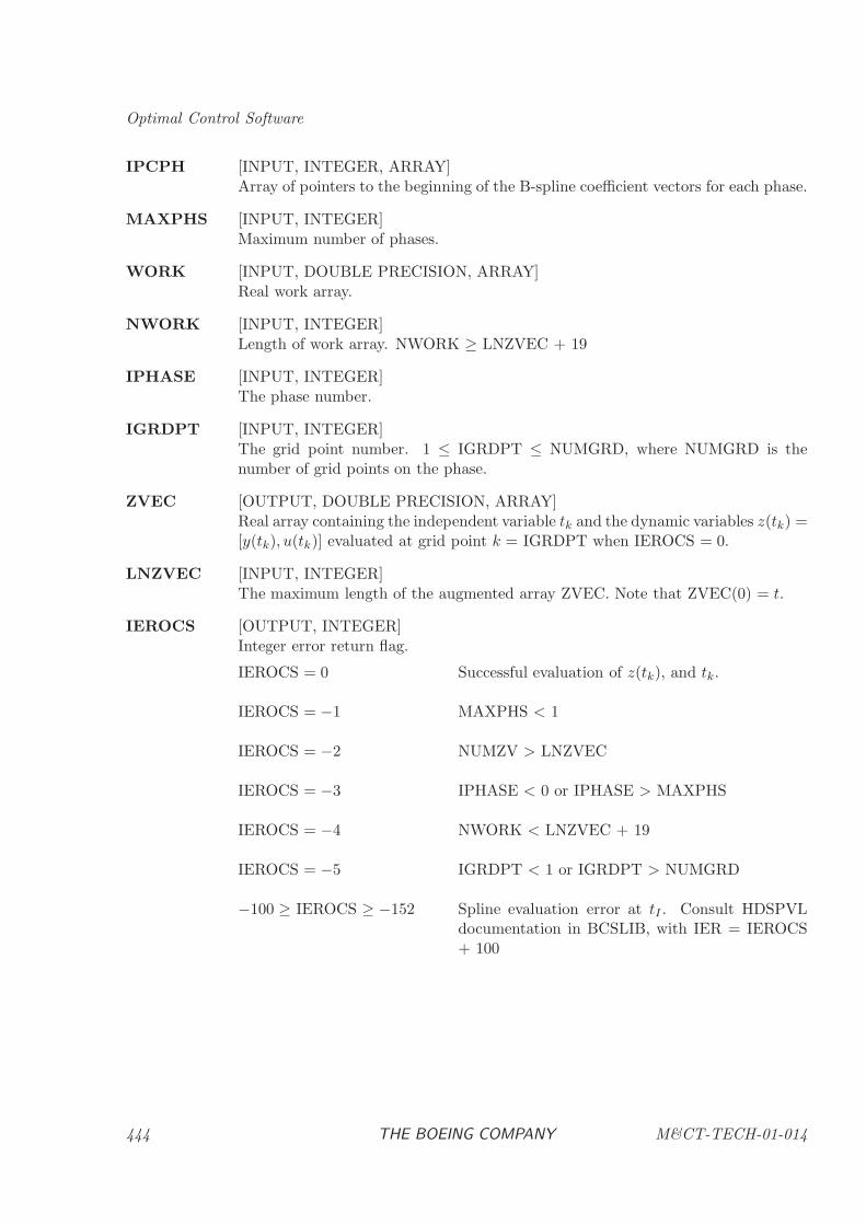
Optimal Control Software
IPCPH [INPUT, INTEGER, ARRAY]Array of pointers to the beginning of the B-spline coefficient vectors for each phase.
MAXPHS [INPUT, INTEGER]Maximum number of phases.
WORK [INPUT, DOUBLE PRECISION, ARRAY]Real work array.
NWORK [INPUT, INTEGER]Length of work array. NWORK ≥ LNZVEC + 19
IPHASE [INPUT, INTEGER]The phase number.
IGRDPT [INPUT, INTEGER]The grid point number. 1 ≤ IGRDPT ≤ NUMGRD, where NUMGRD is thenumber of grid points on the phase.
ZVEC [OUTPUT, DOUBLE PRECISION, ARRAY]Real array containing the independent variable tk and the dynamic variables z(tk) =[y(tk), u(tk)] evaluated at grid point k = IGRDPT when IEROCS = 0.
LNZVEC [INPUT, INTEGER]The maximum length of the augmented array ZVEC. Note that ZVEC(0) = t.
IEROCS [OUTPUT, INTEGER]Integer error return flag.
IEROCS = 0 Successful evaluation of z(tk), and tk.
IEROCS = −1 MAXPHS < 1
IEROCS = −2 NUMZV > LNZVEC
IEROCS = −3 IPHASE < 0 or IPHASE > MAXPHS
IEROCS = −4 NWORK < LNZVEC + 19
IEROCS = −5 IGRDPT < 1 or IGRDPT > NUMGRD
−100 ≥ IEROCS ≥ −152 Spline evaluation error at tI . Consult HDSPVLdocumentation in BCSLIB, with IER = IEROCS+ 100
444 THE BOEING COMPANY M&CT-TECH-01-014
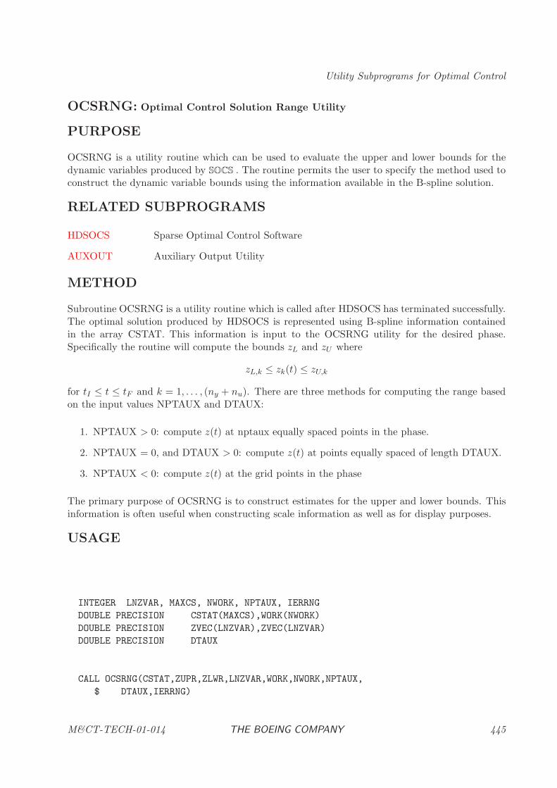
Utility Subprograms for Optimal Control
OCSRNG: Optimal Control Solution Range Utility
PURPOSE
OCSRNG is a utility routine which can be used to evaluate the upper and lower bounds for thedynamic variables produced by SOCS . The routine permits the user to specify the method used toconstruct the dynamic variable bounds using the information available in the B-spline solution.
RELATED SUBPROGRAMS
HDSOCS Sparse Optimal Control Software
AUXOUT Auxiliary Output Utility
METHOD
Subroutine OCSRNG is a utility routine which is called after HDSOCS has terminated successfully.The optimal solution produced by HDSOCS is represented using B-spline information containedin the array CSTAT. This information is input to the OCSRNG utility for the desired phase.Specifically the routine will compute the bounds zL and zU where
zL,k ≤ zk(t) ≤ zU,k
for tI ≤ t ≤ tF and k = 1, . . . , (ny + nu). There are three methods for computing the range basedon the input values NPTAUX and DTAUX:
1. NPTAUX > 0: compute z(t) at nptaux equally spaced points in the phase.
2. NPTAUX = 0, and DTAUX > 0: compute z(t) at points equally spaced of length DTAUX.
3. NPTAUX < 0: compute z(t) at the grid points in the phase
The primary purpose of OCSRNG is to construct estimates for the upper and lower bounds. Thisinformation is often useful when constructing scale information as well as for display purposes.
USAGE
INTEGER LNZVAR, MAXCS, NWORK, NPTAUX, IERRNG
DOUBLE PRECISION CSTAT(MAXCS),WORK(NWORK)
DOUBLE PRECISION ZVEC(LNZVAR),ZVEC(LNZVAR)
DOUBLE PRECISION DTAUX
CALL OCSRNG(CSTAT,ZUPR,ZLWR,LNZVAR,WORK,NWORK,NPTAUX,
$ DTAUX,IERRNG)
M&CT-TECH-01-014 THE BOEING COMPANY 445
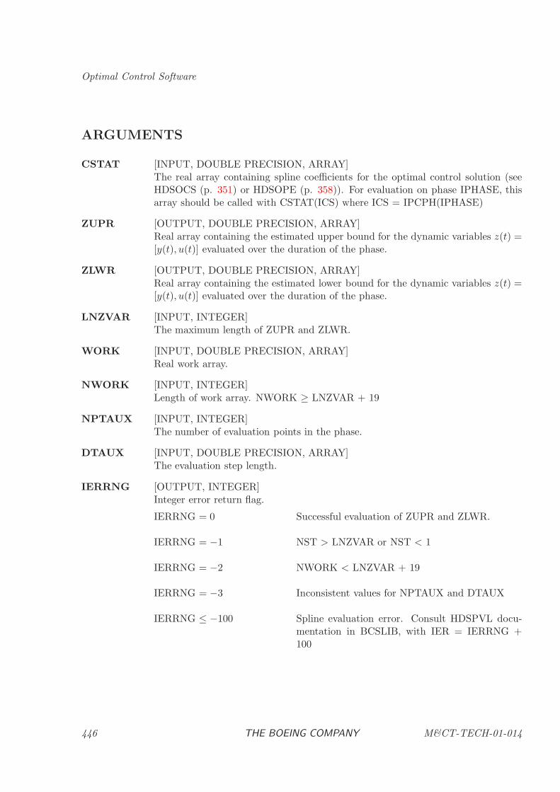
Optimal Control Software
ARGUMENTS
CSTAT [INPUT, DOUBLE PRECISION, ARRAY]The real array containing spline coefficients for the optimal control solution (seeHDSOCS (p. 351) or HDSOPE (p. 358)). For evaluation on phase IPHASE, thisarray should be called with CSTAT(ICS) where ICS = IPCPH(IPHASE)
ZUPR [OUTPUT, DOUBLE PRECISION, ARRAY]Real array containing the estimated upper bound for the dynamic variables z(t) =[y(t), u(t)] evaluated over the duration of the phase.
ZLWR [OUTPUT, DOUBLE PRECISION, ARRAY]Real array containing the estimated lower bound for the dynamic variables z(t) =[y(t), u(t)] evaluated over the duration of the phase.
LNZVAR [INPUT, INTEGER]The maximum length of ZUPR and ZLWR.
WORK [INPUT, DOUBLE PRECISION, ARRAY]Real work array.
NWORK [INPUT, INTEGER]Length of work array. NWORK ≥ LNZVAR + 19
NPTAUX [INPUT, INTEGER]The number of evaluation points in the phase.
DTAUX [INPUT, DOUBLE PRECISION, ARRAY]The evaluation step length.
IERRNG [OUTPUT, INTEGER]Integer error return flag.
IERRNG = 0 Successful evaluation of ZUPR and ZLWR.
IERRNG = −1 NST > LNZVAR or NST < 1
IERRNG = −2 NWORK < LNZVAR + 19
IERRNG = −3 Inconsistent values for NPTAUX and DTAUX
IERRNG ≤ −100 Spline evaluation error. Consult HDSPVL docu-mentation in BCSLIB, with IER = IERRNG +100
446 THE BOEING COMPANY M&CT-TECH-01-014
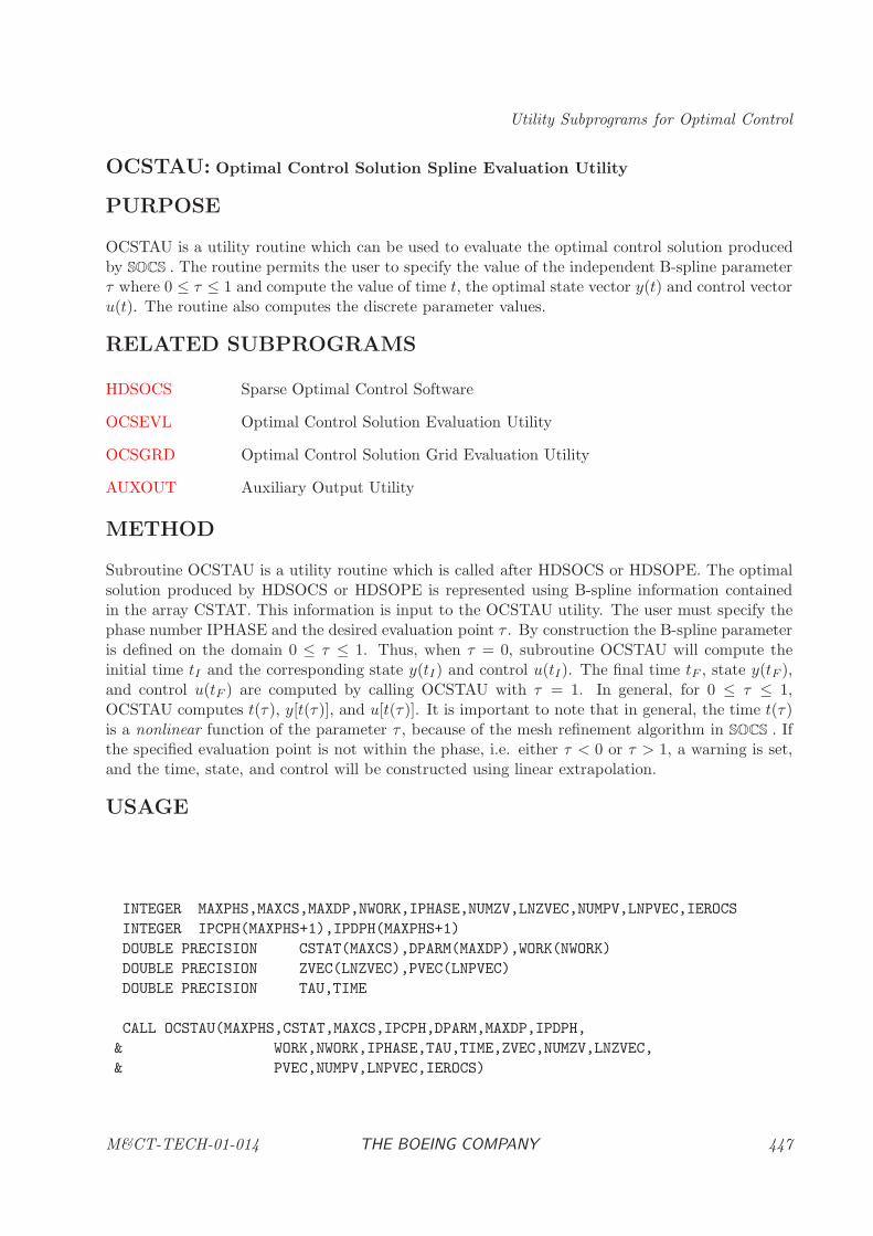
Utility Subprograms for Optimal Control
OCSTAU: Optimal Control Solution Spline Evaluation Utility
PURPOSE
OCSTAU is a utility routine which can be used to evaluate the optimal control solution producedby SOCS . The routine permits the user to specify the value of the independent B-spline parameterτ where 0 ≤ τ ≤ 1 and compute the value of time t, the optimal state vector y(t) and control vectoru(t). The routine also computes the discrete parameter values.
RELATED SUBPROGRAMS
HDSOCS Sparse Optimal Control Software
OCSEVL Optimal Control Solution Evaluation Utility
OCSGRD Optimal Control Solution Grid Evaluation Utility
AUXOUT Auxiliary Output Utility
METHOD
Subroutine OCSTAU is a utility routine which is called after HDSOCS or HDSOPE. The optimalsolution produced by HDSOCS or HDSOPE is represented using B-spline information containedin the array CSTAT. This information is input to the OCSTAU utility. The user must specify thephase number IPHASE and the desired evaluation point τ . By construction the B-spline parameteris defined on the domain 0 ≤ τ ≤ 1. Thus, when τ = 0, subroutine OCSTAU will compute theinitial time tI and the corresponding state y(tI) and control u(tI). The final time tF , state y(tF ),and control u(tF ) are computed by calling OCSTAU with τ = 1. In general, for 0 ≤ τ ≤ 1,OCSTAU computes t(τ), y[t(τ)], and u[t(τ)]. It is important to note that in general, the time t(τ)is a nonlinear function of the parameter τ , because of the mesh refinement algorithm in SOCS . Ifthe specified evaluation point is not within the phase, i.e. either τ < 0 or τ > 1, a warning is set,and the time, state, and control will be constructed using linear extrapolation.
USAGE
INTEGER MAXPHS,MAXCS,MAXDP,NWORK,IPHASE,NUMZV,LNZVEC,NUMPV,LNPVEC,IEROCS
INTEGER IPCPH(MAXPHS+1),IPDPH(MAXPHS+1)
DOUBLE PRECISION CSTAT(MAXCS),DPARM(MAXDP),WORK(NWORK)
DOUBLE PRECISION ZVEC(LNZVEC),PVEC(LNPVEC)
DOUBLE PRECISION TAU,TIME
CALL OCSTAU(MAXPHS,CSTAT,MAXCS,IPCPH,DPARM,MAXDP,IPDPH,
& WORK,NWORK,IPHASE,TAU,TIME,ZVEC,NUMZV,LNZVEC,
& PVEC,NUMPV,LNPVEC,IEROCS)
M&CT-TECH-01-014 THE BOEING COMPANY 447
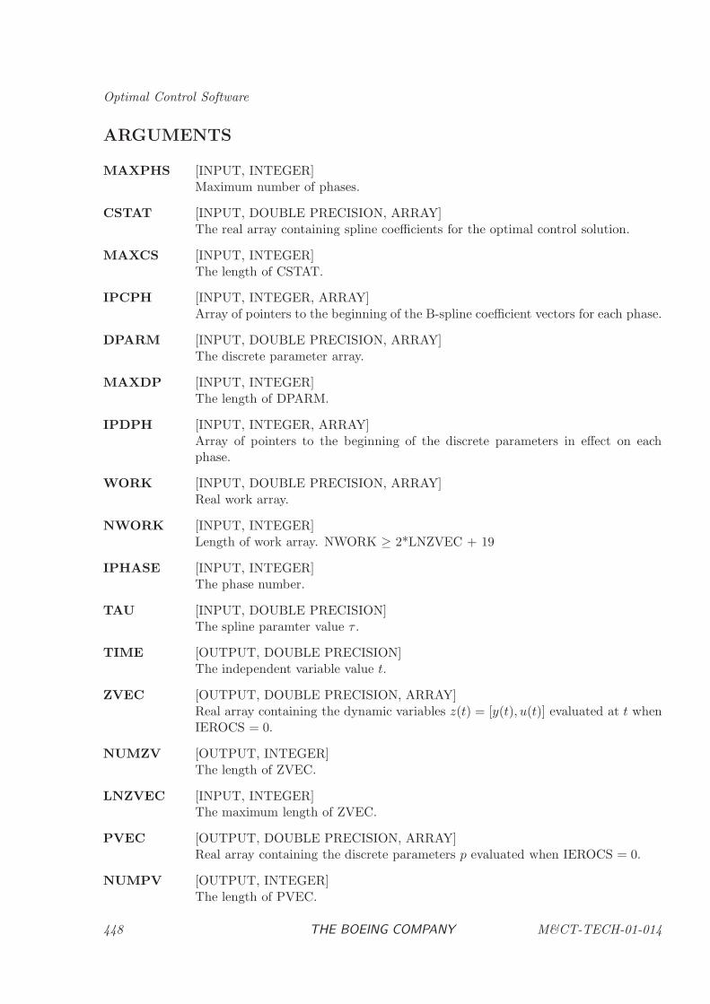
Optimal Control Software
ARGUMENTS
MAXPHS [INPUT, INTEGER]Maximum number of phases.
CSTAT [INPUT, DOUBLE PRECISION, ARRAY]The real array containing spline coefficients for the optimal control solution.
MAXCS [INPUT, INTEGER]The length of CSTAT.
IPCPH [INPUT, INTEGER, ARRAY]Array of pointers to the beginning of the B-spline coefficient vectors for each phase.
DPARM [INPUT, DOUBLE PRECISION, ARRAY]The discrete parameter array.
MAXDP [INPUT, INTEGER]The length of DPARM.
IPDPH [INPUT, INTEGER, ARRAY]Array of pointers to the beginning of the discrete parameters in effect on eachphase.
WORK [INPUT, DOUBLE PRECISION, ARRAY]Real work array.
NWORK [INPUT, INTEGER]Length of work array. NWORK ≥ 2*LNZVEC + 19
IPHASE [INPUT, INTEGER]The phase number.
TAU [INPUT, DOUBLE PRECISION]The spline paramter value τ .
TIME [OUTPUT, DOUBLE PRECISION]The independent variable value t.
ZVEC [OUTPUT, DOUBLE PRECISION, ARRAY]Real array containing the dynamic variables z(t) = [y(t), u(t)] evaluated at t whenIEROCS = 0.
NUMZV [OUTPUT, INTEGER]The length of ZVEC.
LNZVEC [INPUT, INTEGER]The maximum length of ZVEC.
PVEC [OUTPUT, DOUBLE PRECISION, ARRAY]Real array containing the discrete parameters p evaluated when IEROCS = 0.
NUMPV [OUTPUT, INTEGER]The length of PVEC.
448 THE BOEING COMPANY M&CT-TECH-01-014
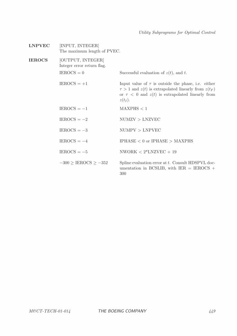
Utility Subprograms for Optimal Control
LNPVEC [INPUT, INTEGER]The maximum length of PVEC.
IEROCS [OUTPUT, INTEGER]Integer error return flag.
IEROCS = 0 Successful evaluation of z(t), and t.
IEROCS = +1 Input value of τ is outside the phase, i.e. eitherτ > 1 and z(t) is extrapolated linearly from z(tF )or τ < 0 and z(t) is extrapolated linearly fromz(tI).
IEROCS = −1 MAXPHS < 1
IEROCS = −2 NUMZV > LNZVEC
IEROCS = −3 NUMPV > LNPVEC
IEROCS = −4 IPHASE < 0 or IPHASE > MAXPHS
IEROCS = −5 NWORK < 2*LNZVEC + 19
−300 ≥ IEROCS ≥ −352 Spline evaluation error at t. Consult HDSPVL doc-umentation in BCSLIB, with IER = IEROCS +300
M&CT-TECH-01-014 THE BOEING COMPANY 449

Optimal Control Software
PHSLNG: Optimal Control Phase Duration Utility
PURPOSE
PHSLNG is a utility routine which can be used to construct constraints on the duration of a phase.It is typically called from the user supplied input routine ODEINP (p. 384). Specifically, the utilitycan be used to construct constraints of the form:
pL ≤ t(k)F − t
(k)I ≤ pU
where t(k)F is the final time for phase k, and t
(k)I is the initial time for phase k. Often the phase
duration pL will be positive to ensure that t(k)F > t
(k)I .
RELATED SUBPROGRAMS
HDSOCS Sparse Optimal Control Software
HDSOPE Sparse Optimal Parameter Estimation
ODEINP Optimal Control Problem Definition
AUTOPL Auto Phase Length Constraint Utility
METHOD
Subroutine PHSLNG is a utility routine which is called by the user (usually from ODEINP).PHSLNG will construct a constraint on the phase duration by proper definition of the SOCS inputquantities. Similar functionality is available using routine AUTOPL (p. 416).
The Goddard Rocket test problem (p. 538) illustrates the use of this utility routine.
USAGE
INTEGER NTERM,NKON,IPHASE,ITERM(4,MXTERM),MXTERM,MXPCON,IERLNG
DOUBLE PRECISION CLB(MXPCON),CUB(MXPCON),COEF(MXTERM),PHSLWR,PHSUPR
CHARACTER CLBL(0:MXPCON)*80
CALL PHSLNG(NTERM,NKON,IPHASE,ITERM,MXTERM,COEF,
$ CLB,CUB,CLBL,MXPCON,PHSLWR,PHSUPR,IERLNG)
ARGUMENTS
NTERM [INPUT/OUTPUT, INTEGER]Running number of terms on the current phase.
450 THE BOEING COMPANY M&CT-TECH-01-014
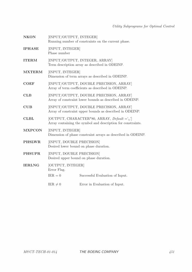
Utility Subprograms for Optimal Control
NKON [INPUT/OUTPUT, INTEGER]Running number of constraints on the current phase.
IPHASE [INPUT, INTEGER]Phase number
ITERM [INPUT/OUTPUT, INTEGER, ARRAY]Term description array as described in ODEINP.
MXTERM [INPUT, INTEGER]Dimension of term arrays as described in ODEINP.
COEF [INPUT/OUTPUT, DOUBLE PRECISION, ARRAY]Array of term coefficients as described in ODEINP.
CLB [INPUT/OUTPUT, DOUBLE PRECISION, ARRAY]Array of constraint lower bounds as described in ODEINP.
CUB [INPUT/OUTPUT, DOUBLE PRECISION, ARRAY]Array of constraint upper bounds as described in ODEINP.
CLBL [OUTPUT, CHARACTER*80, ARRAY, Default =’ ’]Array containing the symbol and description for constraints.
MXPCON [INPUT, INTEGER]Dimension of phase constraint arrays as described in ODEINP.
PHSLWR [INPUT, DOUBLE PRECISION]Desired lower bound on phase duration.
PHSUPR [INPUT, DOUBLE PRECISION]Desired upper bound on phase duration.
IERLNG [OUTPUT, INTEGER]Error Flag.
IER = 0 Successful Evaluation of Input.
IER 6= 0 Error in Evaluation of Input.
M&CT-TECH-01-014 THE BOEING COMPANY 451
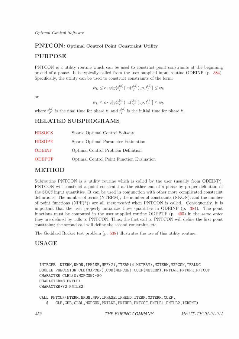
Optimal Control Software
PNTCON: Optimal Control Point Constraint Utility
PURPOSE
PNTCON is a utility routine which can be used to construct point constraints at the beginningor end of a phase. It is typically called from the user supplied input routine ODEINP (p. 384).Specifically, the utility can be used to construct constraints of the form:
ψL ≤ c · ψ[y(t(k)I ), u(t
(k)I ), p, t
(k)I ] ≤ ψU
orψL ≤ c · ψ[y(t
(k)F ), u(t
(k)F ), p, t
(k)F ] ≤ ψU
where t(k)F is the final time for phase k, and t
(k)I is the initial time for phase k.
RELATED SUBPROGRAMS
HDSOCS Sparse Optimal Control Software
HDSOPE Sparse Optimal Parameter Estimation
ODEINP Optimal Control Problem Definition
ODEPTF Optimal Control Point Function Evaluation
METHOD
Subroutine PNTCON is a utility routine which is called by the user (usually from ODEINP).PNTCON will construct a point constraint at the either end of a phase by proper definition ofthe SOCS input quantities. It can be used in conjunction with other more complicated constraintdefinitions. The number of terms (NTERM), the number of constraints (NKON), and the numberof point functions (NPF(*)) are all incremented when PNTCON is called. Consequently, it isimportant that the user properly initializes these quantities in ODEINP (p. 384). The pointfunctions must be computed in the user supplied routine ODEPTF (p. 405) in the same orderthey are defined by calls to PNTCON. Thus, the first call to PNTCON will define the first pointconstraint; the second call will define the second constraint, etc.
The Goddard Rocket test problem (p. 538) illustrates the use of this utility routine.
USAGE
INTEGER NTERM,NKON,IPHASE,NPF(2),ITERM(4,MXTERM),MXTERM,MXPCON,IERLNG
DOUBLE PRECISION CLB(MXPCON),CUB(MXPCON),COEF(MXTERM),PNTLWR,PNTUPR,PNTCOF
CHARACTER CLBL(0:MXPCON)*80
CHARACTER*8 PNTLB1
CHARACTER*72 PNTLB2
CALL PNTCON(NTERM,NKON,NPF,IPHASE,IPHEND,ITERM,MXTERM,COEF,
$ CLB,CUB,CLBL,MXPCON,PNTLWR,PNTUPR,PNTCOF,PNTLB1,PNTLB2,IERPNT)
452 THE BOEING COMPANY M&CT-TECH-01-014
Utility Subprograms for Optimal Control
ARGUMENTS
NTERM [INPUT/OUTPUT, INTEGER]Running number of terms on the current phase.
NKON [INPUT/OUTPUT, INTEGER]Running number of constraints on the current phase.
NPF [INPUT/OUTPUT, INTEGER]Number of point functions on the current phase. When IPHEND=-1, NPF(1) isincremented. When IPHEND=+1, NPF(2) is incremented.
IPHASE [INPUT, INTEGER]Phase number
IPHEND [INPUT, INTEGER]Phase end where point constraint is imposed. When IPHEND=-1, constraint is
imposed at t(k)I . When IPHEND=+1, constraint is imposed at t
(k)F .
ITERM [OUTPUT, INTEGER, ARRAY]Term description array as described in ODEINP.
MXTERM [INPUT, INTEGER]Dimension of term arrays as described in ODEINP.
COEF [OUTPUT, DOUBLE PRECISION, ARRAY]Array of term coefficients as described in ODEINP.
CLB [OUTPUT, DOUBLE PRECISION, ARRAY]Array of constraint lower bounds as described in ODEINP.
CUB [OUTPUT, DOUBLE PRECISION, ARRAY]Array of constraint upper bounds as described in ODEINP.
CLBL [OUTPUT, CHARACTER*80, ARRAY, Default =’ ’]Array containing the symbol and description for constraints.
MXPCON [INPUT, INTEGER]Dimension of phase constraint arrays as described in ODEINP.
PNTLWR [INPUT, DOUBLE PRECISION]Desired lower bound ψL on point constraint.
PNTUPR [INPUT, DOUBLE PRECISION]Desired upper bound ψU on point constraint.
PNTCOF [INPUT, DOUBLE PRECISION]Desired coefficient c on point function.
PNTLB1 [INPUT, CHARACTER*8]Primary point constraint label.
M&CT-TECH-01-014 THE BOEING COMPANY 453

Optimal Control Software
PNTLB2 [INPUT, CHARACTER*72]Point constraint description label.
IERPNT [OUTPUT, INTEGER]Error Flag.
IER = 0 Successful construction of point constraint.
IER 6= 0 Error in construction of point constraint.
454 THE BOEING COMPANY M&CT-TECH-01-014
Utility Subprograms for Optimal Control
PTHAUX: Path Constraint with Auxiliary Functions
PURPOSE
PTHAUX is a utility routine which can be used to construct path constraints involving auxiliaryfunctions during a phase. It is typically called from the user supplied input routine ODEINP (p.384). Specifically, the utility can be used to construct a constraint for phase k defined in the region
t(k)I ≤ t ≤ t
(k)F of the form:
gL ≤ g[y(t), u(t), p, t] ≤ gU ,
where
g[y(t), u(t), p, t] = α⊤v + β⊤a[v, t]
and
v =
y(t)u(t)p
.
The utility can be used to construct linear combinations of the na auxiliary functions ak(v) fork = 0, . . . , na where the coefficients βk are nonzero constants. By convention, a path constraintwith a single nonlinear term a0(y, u, p, t) has no auxiliary functions (na = 0) and in this case it issimpler to use the utility routine PTHCON (p. 458). The complete constraint definition can includeanalytic terms involving α⊤v where the (ny + nu + np) vector α is constant. Analytic terms mustbe constructed in ODEINP immediately after calling the PTHAUX utility, and the constructionprocess is terminated by calling a second utility TRMAUX (p. 465). Observe that each individualpath constraint may have a different number of auxiliary functions and analytic terms.
RELATED SUBPROGRAMS
HDSOCS Sparse Optimal Control Software
HDSOPE Sparse Optimal Parameter Estimation
ODEINP Optimal Control Problem Definition
ODERHS Optimal Control Right Hand Side Evaluation
METHOD
Subroutine PTHAUX is a utility routine which is called by the user (usually from ODEINP).The constraint definition must be completed by a call to the routine TRMAUX (p. 465). ThePTHAUX/TRMAUX call pairs will construct a path constraint involving auxiliary functions duringthe phase by proper definition of the SOCS input quantities. They can be used in conjunction withother more complicated constraint definitions. The number of terms (NTERM), the number ofconstraints (NKON), and the number of algebraic functions (NCF(2)), are all incremented by thePTHAUX calls. Consequently, it is important that the user properly initializes these quantitiesin ODEINP (p. 384). The user supplied routine ODERHS (p. 409) must compute the path andauxiliary functions in the same order as they are defined by calls to PTHAUX. Thus, the first callto PTHAUX will define the first path constraint and define which auxiliary functions are linked toit; the second call will define the second constraint and associated auxiliary functions, etc.
M&CT-TECH-01-014 THE BOEING COMPANY 455
Optimal Control Software
The Van der Pol Oscillator test problem (p. 538) illustrates the use of this utility routine.
USAGE
INTEGER NTERM,NKON,IPHASE,NCF(5),ITERM(4,MXTERM),MXTERM,MXPCON,
$ IERPTH,NUMAUX
DOUBLE PRECISION CLB(MXPCON),CUB(MXPCON),COEF(MXTERM),AUXCOF(NUMAUX),
$ PTHLWR,PTHUPR,PTHCOF
CHARACTER CLBL(0:MXPCON)*80
CHARACTER*8 PTHLB1
CHARACTER*72 PTHLB2
CALL PTHAUX(NTERM,NKON,NCF,IPHASE,ITERM,MXTERM,COEF,
$ CLB,CUB,CLBL,MXPCON,NUMAUX,AUXCOF,PTHLWR,PTHUPR,PTHCOF,
$ PTHLB1,PTHLB2,IERPTH)
ARGUMENTS
NTERM [INPUT/OUTPUT, INTEGER]Running number of terms on the current phase.
NKON [INPUT/OUTPUT, INTEGER]Running number of constraints on the current phase.
NCF [INPUT/OUTPUT, INTEGER]Number of path functions on the current phase. NCF(2) is incremented. NCF(4)is not incremented by PTHAUX.
IPHASE [INPUT, INTEGER]Phase number
ITERM [OUTPUT, INTEGER, ARRAY]Term description array as described in ODEINP.
MXTERM [INPUT, INTEGER]Dimension of term arrays as described in ODEINP.
COEF [OUTPUT, DOUBLE PRECISION, ARRAY]Array of term coefficients as described in ODEINP.
CLB [OUTPUT, DOUBLE PRECISION, ARRAY]Array of constraint lower bounds as described in ODEINP.
CUB [OUTPUT, DOUBLE PRECISION, ARRAY]Array of constraint upper bounds as described in ODEINP.
456 THE BOEING COMPANY M&CT-TECH-01-014
Utility Subprograms for Optimal Control
CLBL [OUTPUT, CHARACTER*80, ARRAY, Default =’ ’]Array containing the symbol and description for constraints.
MXPCON [INPUT, INTEGER]Dimension of phase constraint arrays as described in ODEINP.
NUMAUX [INPUT, INTEGER]Number of auxiliary functions linked to constraint NKON.
NUMAUX < 0 Set all coefficients to AUXCOF(1).
NUMAUX > 0 Use coefficient vector AUXCOF.
AUXCOF [INPUT, DOUBLE PRECISION, ARRAY]Array of auxiliary function coefficients βk.
PTHLWR [INPUT, DOUBLE PRECISION]Desired lower bound gL on path constraint.
PTHUPR [INPUT, DOUBLE PRECISION]Desired upper bound gU on path constraint.
PTHCOF [INPUT, DOUBLE PRECISION]Desired coefficient β0 on path function.
PTHLB1 [INPUT, CHARACTER*8]Primary path constraint label.
PTHLB2 [INPUT, CHARACTER*72]Path constraint description label.
IERPTH [OUTPUT, INTEGER]Error Flag.
IER = 0 Successful construction of path constraint.
IER 6= 0 Error in construction of path constraint.
M&CT-TECH-01-014 THE BOEING COMPANY 457
Optimal Control Software
PTHCON: Path Constraint Utility
PURPOSE
PTHCON is a utility routine which can be used to construct path constraints during a phase. Itis typically called from the user supplied input routine ODEINP (p. 384). Specifically, the utilitycan be used to construct constraints of the form:
gL ≤ c · g[y(t), u(t), p, t] ≤ gU ,
for phase k defined in the region t(k)I ≤ t ≤ t
(k)F . This utility should not be used when the problem
definition requires the use of auxiliary functions.
RELATED SUBPROGRAMS
HDSOCS Sparse Optimal Control Software
HDSOPE Sparse Optimal Parameter Estimation
ODEINP Optimal Control Problem Definition
ODERHS Optimal Control Right Hand Side Evaluation
METHOD
Subroutine PTHCON is a utility routine that is called by the user (usually from ODEINP). PTH-CON will construct a path constraint during the phase by proper definition of the SOCS inputquantities. It can be used in conjunction with other more complicated constraint definitions. Thenumber of terms (NTERM), the number of constraints (NKON), and the number of algebraicfunctions (NCF(2)) are all incremented when PTHCON is called. Consequently, it is importantthat the user properly initializes these quantities in ODEINP (p. 384). The user supplied routineODERHS (p. 409) must compute the path functions in the same order they are defined by callsto PTHCON. Thus, the first call to PTHCON will define the first path constraint; the second callwill define the second constraint, etc.
WARNING This utility should not be used if any path constraint involves an auxiliary function.
The Goddard Rocket test problem (p. 538) illustrates the use of this utility routine.
USAGE
INTEGER NTERM,NKON,IPHASE,NCF(5),ITERM(4,MXTERM),MXTERM,MXPCON,IERPTH
DOUBLE PRECISION CLB(MXPCON),CUB(MXPCON),COEF(MXTERM),PTHLWR,PTHUPR,PTHCOF
CHARACTER CLBL(0:MXPCON)*80
CHARACTER*8 PTHLB1
CHARACTER*72 PTHLB2
CALL PTHCON(NTERM,NKON,NCF,IPHASE,ITERM,MXTERM,COEF,
$ CLB,CUB,CLBL,MXPCON,PTHLWR,PTHUPR,PTHCOF,PTHLB1,PTHLB2,IERPTH)
458 THE BOEING COMPANY M&CT-TECH-01-014
Utility Subprograms for Optimal Control
ARGUMENTS
NTERM [INPUT/OUTPUT, INTEGER]Running number of terms on the current phase.
NKON [INPUT/OUTPUT, INTEGER]Running number of constraints on the current phase.
NCF [INPUT/OUTPUT, INTEGER]Number of path functions on the current phase. NCF(2) is incremented.
IPHASE [INPUT, INTEGER]Phase number
ITERM [OUTPUT, INTEGER, ARRAY]Term description array as described in ODEINP.
MXTERM [INPUT, INTEGER]Dimension of term arrays as described in ODEINP.
COEF [OUTPUT, DOUBLE PRECISION, ARRAY]Array of term coefficients as described in ODEINP.
CLB [OUTPUT, DOUBLE PRECISION, ARRAY]Array of constraint lower bounds as described in ODEINP.
CUB [OUTPUT, DOUBLE PRECISION, ARRAY]Array of constraint upper bounds as described in ODEINP.
CLBL [OUTPUT, CHARACTER*80, ARRAY, Default =’ ’]Array containing the symbol and description for constraints.
MXPCON [INPUT, INTEGER]Dimension of phase constraint arrays as described in ODEINP.
PTHLWR [INPUT, DOUBLE PRECISION]Desired lower bound gL on path constraint.
PTHUPR [INPUT, DOUBLE PRECISION]Desired upper bound gU on path constraint.
PTHCOF [INPUT, DOUBLE PRECISION]Desired coefficient c on path function.
PTHLB1 [INPUT, CHARACTER*8]Primary path constraint label.
PTHLB2 [INPUT, CHARACTER*72]Path constraint description label.
M&CT-TECH-01-014 THE BOEING COMPANY 459

Optimal Control Software
IERPTH [OUTPUT, INTEGER]Error Flag.
IER = 0 Successful construction of path constraint.
IER 6= 0 Error in construction of path constraint.
460 THE BOEING COMPANY M&CT-TECH-01-014
Utility Subprograms for Optimal Control
RST2SP: Restart File to Spline Array Utility
PURPOSE
RST2SP is a utility routine that can be used to read information from a SOCS restart spline file,into the spline storage arrays.
METHOD
Subroutine RST2SP is a utility routine which is called to read information from a previously createdSOCS restart file. The information is stored into the arrays used to represent the optimal controlsolution in B-spline format. This is often useful when constructing an initial guess from anothersolution.
USAGE
INTEGER MAXCS,MAXPHS,MAXDP,IPUOCP,IERRST
INTEGER IPCPH(MAXPHS+1),IPDPH(MAXPHS+1)
DOUBLE PRECISION CSTAT(MAXCS),DPARM(MAXDP)
CHARACTER*60 RSTFIL
CALL RST2SP(RSTFIL,ISFRST,CSTAT,MAXCS,DPARM,MAXDP,IPCPH,
& IPDPH,MAXPHS,IERRST)
ARGUMENTS
RSTFIL [INPUT, CHARACTER*60]Character variable name of restart file
ISFRST [INPUT, INTEGER]FORTRAN I/O unit for restart file
CSTAT [OUTPUT, DOUBLE PRECISION, ARRAY]The real array containing spline coefficients for the optimal control solution.
MAXCS [INPUT, INTEGER]The length of CSTAT.
DPARM [OUTPUT, DOUBLE PRECISION, ARRAY]The discrete parameter array
MAXDP [INPUT, INTEGER]The length of DPARM
M&CT-TECH-01-014 THE BOEING COMPANY 461
Optimal Control Software
IPCPH [OUTPUT, INTEGER, ARRAY]Array of pointers to the beginning of the B-spline coefficient vectors for each phase.
IPDPH [OUTPUT, INTEGER, ARRAY]Array of pointers to the beginning of the discrete parameters in effect on eachphase.
MAXPHS [INPUT, INTEGER]Maximum number of phases.
IERRST [OUTPUT, INTEGER]Integer error return flag.
IERRST = 0 Successful restoration of restart spline information.
IERRST = −1 Restart file name exceeds 60 characters
IERRST = −2 Number of parameters exceeds MAXDP
IERRST = −3 Number of CSTAT quantities exceeds MAXCS
IERRST = −4 Number of phases exceeds MAXPHS
462 THE BOEING COMPANY M&CT-TECH-01-014
Utility Subprograms for Optimal Control
SCTFIL: Save an Optimal Control Input File
PURPOSE
SCTFIL is a utility routine which can be used to save a file containing a particular configuration ofoptional inputs for the SOCS software. The utility is useful when it is desirable to save a particularset of algorithm parameters for a subsequent application of HDSOCS and/or HDSOPE.
RELATED SUBPROGRAMS
HDSOCS Sparse Optimal Control Software
HDSOPE Sparse Optimal Parameter Estimation
HHSOCS Sparse Optimal Control Input Procedure
CTLFIL Optimal Control Input From a File
METHOD
Subroutine SCTFIL is a utility routine which is called from the users main program to save aparticular configuration of algorithm parameters. SCTFIL is intended to be used in conjunctionwith subroutine CTLFIL (p. 427) for a subsequent call to HDSOCS and/or HDSOPE. SCTFILwill write information from the SOCS parameter common to a user specified file.
USAGE
INTEGER INUNIT
CHARACTER*(*) FILNAM
CALL SCTFIL(INUNIT,FILNAM)
ARGUMENTS
INUNIT [INPUT, INTEGER]FORTRAN unit number for opening file.
FILNAM [INPUT, CHARACTER]Character string with the name of the file containing the HHSOCS (p. 365) input.
EXAMPLE Save SOCS Input Parameters on a File
Suppose that SOCS is to be executed using the barrier algorithm with a modified output level. Oneway to achieve this is as follows:
M&CT-TECH-01-014 THE BOEING COMPANY 463

Optimal Control Software
C
CALL HHSOCS(’NLPALG=HDBNLP’)
CALL HHSOCS(’HDBNLP:BARRIER DEFAULT’)
CALL HHSOCS(’HDBNLP:IOFLAG=20’)
C
CALL HDSOCS(.....
C
This collection of algorithm inputs can be saved for subsequent use as follows:
C
CALL HHSOCS(’NLPALG=HDBNLP’)
CALL HHSOCS(’HDBNLP:BARRIER DEFAULT’)
CALL HHSOCS(’HDBNLP:IOFLAG=20’)
C
CALL SCTFIL(35,’/home/socsinput.fil’)
C
CALL HDSOCS(.....
C
where the file “/home/socsinput.fil” contains the following information:
nlpalg=hdbnlp
hdbnlp:barrier default
hdbnlp:ioflag = 20
A subsequent run with the same algorithm settings can then be invoked as follows:
C
CALL CTLFIL(35,’/home/socsinput.fil’)
C
CALL HDSOCS(.....
C
464 THE BOEING COMPANY M&CT-TECH-01-014
Utility Subprograms for Optimal Control
TRMAUX: Terminate Auxiliary Function Construction
PURPOSE
TRMAUX is a utility routine that is used to complete the construction of path constraints involvingauxiliary functions during a phase. It is typically called from the user supplied input routineODEINP (p. 384) after calling the utility PTHAUX (p. 455). Specifically, the utility can be usedto complete construction for path constraints of the form:
gL ≤ g[y(t), u(t), p, t] ≤ gU ,
whereg[y(t), u(t), p, t] = α⊤v + β⊤a[v, t]
and
v =
y(t)u(t)p
.
The utility can be used to complete constructions that involve linear combinations of the na auxiliaryfunctions ak(v) for k = 0, . . . , na where the coefficients βk are nonzero constants. By convention, apath constraint with a single nonlinear term a0(y, u, p, t) has no auxiliary functions (na = 0) and inthis case it is simpler to use the utility routine PTHCON (p. 458). The total constraint definitioncan include analytic terms involving α⊤v where the (ny + nu + np) vector α is constant. Analyticterms must be constructed in ODEINP immediately after calling the PTHAUX utility and beforecalling TRMAUX.
RELATED SUBPROGRAMS
HDSOCS Sparse Optimal Control Software
HDSOPE Sparse Optimal Parameter Estimation
ODEINP Optimal Control Problem Definition
ODERHS Optimal Control Right Hand Side Evaluation
METHOD
Subroutine TRMAUX is a utility routine which is called by the user (usually from ODEINP) afterone or more calls to the utility PTHAUX (p. 455). PTHAUX must first be called to construct theprimary path constraint definition and define the auxiliary functions linked to each path constraint.TRMAUX then completes the construction of the path constraint involving auxiliary functions byproper definition of the SOCS input quantities. It can be used in conjunction with other morecomplicated constraint definitions. The number of terms (NTERM), and the number of auxiliaryfunctions (NCF(4)) are both incremented when TRMAUX is called. Consequently, it is importantthat the user properly initializes these quantities in ODEINP (p. 384). The user supplied routineODERHS (p. 409) must compute the path and auxiliary functions in the same order they aredefined by calls to PTHAUX.
The Van der Pol Oscillator test problem (p. 538) illustrates the use of this utility routine.
USAGE
M&CT-TECH-01-014 THE BOEING COMPANY 465
Optimal Control Software
INTEGER NTERM,IPHASE,NCF(5),ITERM(4,MXTERM),MXTERM,IERPTH
DOUBLE PRECISION COEF(MXTERM)
CALL TRMAUX(NTERM,NCF,IPHASE,ITERM,MXTERM,COEF,IERPTH)
ARGUMENTS
NTERM [INPUT/OUTPUT, INTEGER]Running number of terms on the current phase.
NCF [INPUT/OUTPUT, INTEGER]Number of auxiliary functions on the current phase. NCF(4) is incremented.
IPHASE [INPUT, INTEGER]Phase number
ITERM [OUTPUT, INTEGER, ARRAY]Term description array as described in ODEINP.
MXTERM [INPUT, INTEGER]Dimension of term arrays as described in ODEINP.
COEF [OUTPUT, DOUBLE PRECISION, ARRAY]Array of term coefficients as described in ODEINP.
IERPTH [OUTPUT, INTEGER]Error Flag.
IER = 0 Successful completion of path constraint with auxiliary func-tion.
IER 6= 0 Error in completion of path constraint with auxiliary function.
466 THE BOEING COMPANY M&CT-TECH-01-014
Utility Subprograms for Optimal Control
WATCH: Variable Monitor Utility
PURPOSE
WATCH is a utility routine that is used to monitor a variable for subsequent retrieval by the fetchutility, FETCH (p. 430). It must be called from the user supplied input routine ODEINP (p. 384).
RELATED SUBPROGRAMS
FETCH Variable Retrieval Utility
METHOD
Subroutine WATCH is a utility routine that is called by the user from ODEINP. WATCH has asingle argument, a character string, which is the name of the variable to be retrieved. The stringmust not exceed 80 characters and is of the following form:
’symbol@phase’
The character substring ’symbol’ defines the name of the variable that is to be monitored. Thesubstring ’symbol’ is:
• case sensitive (i.e. TIME is not the same as time)
• must exactly match the desired output name which is derived from a user specified labelquantity STLBL, PLBL, or CLBL.
The substring ’phase’ is the numeric phase number for the desired variable and must be precededby the symbol @. A global quantity with no explicit phase number can be specified by a characterstring of the form ’symbol’ or ’symbol@0’.
Referring to the Goddard Rocket Problem (p. 538) the following examples are valid uses of theWATCH utility:
Command Description
call watch(’VEL@2’) Velocity v(t) during phase 2call watch(’T3BEG@3’) Parameter t3 (beginning) phase 3call watch(’SINGLR_a@2’) Singular arc algebraic constraint g(t) during phase 2call watch(’TIME_M@2’) Time at interval midpoints during phase 2call watch(’L_HALT@1’) Discrete altitude adjoint during phase 1
The FETCH (p. 430) utility which retrieves data, must be preceded by a call to the WATCHutility.
ARGUMENTS
STRING [INPUT, CHARACTER*80]Monitor variable label
M&CT-TECH-01-014 THE BOEING COMPANY 467
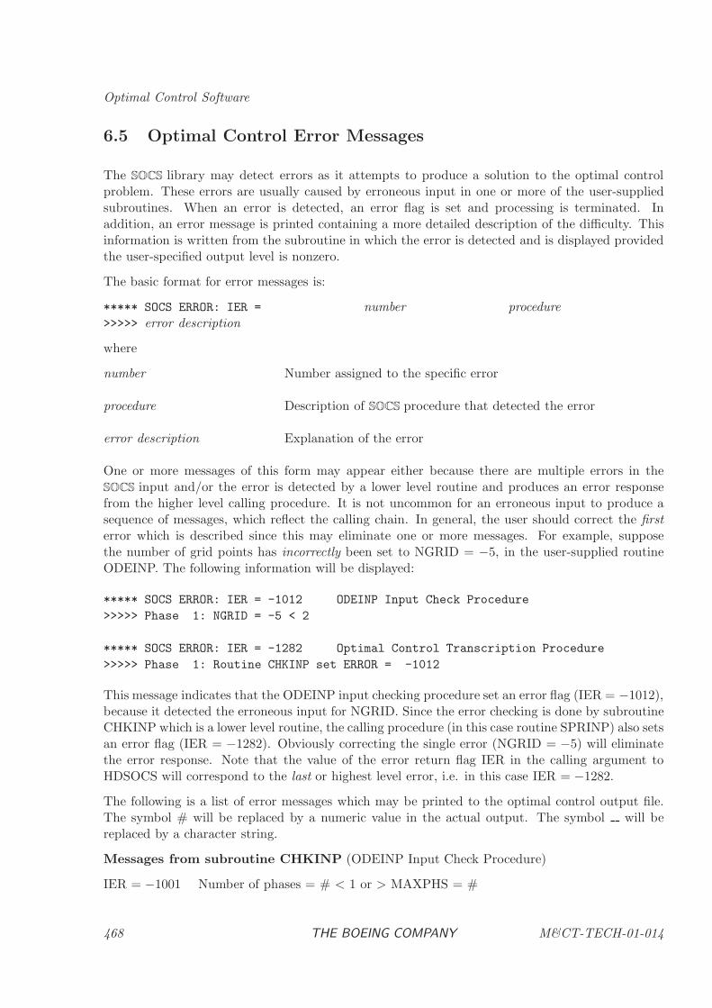
Optimal Control Software
6.5 Optimal Control Error Messages
The SOCS library may detect errors as it attempts to produce a solution to the optimal controlproblem. These errors are usually caused by erroneous input in one or more of the user-suppliedsubroutines. When an error is detected, an error flag is set and processing is terminated. Inaddition, an error message is printed containing a more detailed description of the difficulty. Thisinformation is written from the subroutine in which the error is detected and is displayed providedthe user-specified output level is nonzero.
The basic format for error messages is:
***** SOCS ERROR: IER = number procedure>>>>> error description
where
number Number assigned to the specific error
procedure Description of SOCS procedure that detected the error
error description Explanation of the error
One or more messages of this form may appear either because there are multiple errors in theSOCS input and/or the error is detected by a lower level routine and produces an error responsefrom the higher level calling procedure. It is not uncommon for an erroneous input to produce asequence of messages, which reflect the calling chain. In general, the user should correct the firsterror which is described since this may eliminate one or more messages. For example, supposethe number of grid points has incorrectly been set to NGRID = −5, in the user-supplied routineODEINP. The following information will be displayed:
***** SOCS ERROR: IER = -1012 ODEINP Input Check Procedure
>>>>> Phase 1: NGRID = -5 < 2
***** SOCS ERROR: IER = -1282 Optimal Control Transcription Procedure
>>>>> Phase 1: Routine CHKINP set ERROR = -1012
This message indicates that the ODEINP input checking procedure set an error flag (IER = −1012),because it detected the erroneous input for NGRID. Since the error checking is done by subroutineCHKINP which is a lower level routine, the calling procedure (in this case routine SPRINP) also setsan error flag (IER = −1282). Obviously correcting the single error (NGRID = −5) will eliminatethe error response. Note that the value of the error return flag IER in the calling argument toHDSOCS will correspond to the last or highest level error, i.e. in this case IER = −1282.
The following is a list of error messages which may be printed to the optimal control output file.The symbol # will be replaced by a numeric value in the actual output. The symbol will bereplaced by a character string.
Messages from subroutine CHKINP (ODEINP Input Check Procedure)
IER = −1001 Number of phases = # < 1 or > MAXPHS = #
468 THE BOEING COMPANY M&CT-TECH-01-014

Optimal Control Error Messages
IER = −1002 Phase #: ODE hold array length = # need #
IER = −1003 Phase #: METHOD = # is invalid.
IER = −1004 Phase #: METHOD = # NSTG = # is invalid.
IER = −1005 Phase #: NCF(1) = # < 0
IER = −1006 Phase #: NCF(2) = # < 0
IER = −1007 Phase #: NCF(3) = # < 0
IER = −1008 Phase #: NPF(1) = # < 0
IER = −1009 Phase #: NPF(2) = # < 0
IER = −1010 Phase #: NPV = # < 0 or > MXPARM = #
IER = −1011 Phase #: NAV = # < 0
IER = −1012 Phase #: NGRID = # < 2
IER = −1013 Phase #: INIT = # < 1 or > 3
IER = −1014 Phase #: MAXMIN = # < -1 or > +1
IER = −1015 Phase #: Parm #: Upper bound # less than lower bound #
IER = −1016 Phase #: More than # parameters loaded.
IER = −1017 Phase #: Parm #, not initialized.
IER = −1018 Phase #: Quadrature equations not allowed with RK integration.
IER = −1019 Phase #: NDE+NAV = # > MXSTAT = #
IER = −1020 Phase #, state #: Upper bound # less than lower bound #
IER = −1021 Phase #: More than # states loaded.
IER = −1022 Phase #: More than # state scales loaded.
IER = −1023 Phase #: term # refers to future phase #
IER = −1024 Phase #: term # END = # must be -1,0,1
IER = −1025 Phase #: term # STATE = # does not match any of # states on phase #
M&CT-TECH-01-014 THE BOEING COMPANY 469
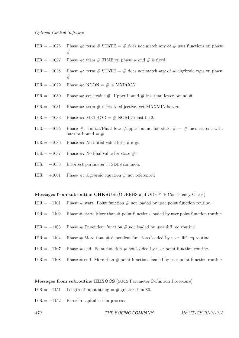
Optimal Control Software
IER = −1026 Phase #: term # STATE = # does not match any of # user functions on phase#
IER = −1027 Phase #: term # TIME on phase # end # is fixed.
IER = −1028 Phase #: term # STATE = # does not match any of # algebraic eqns on phase#
IER = −1029 Phase #: NCON = # > MXPCON
IER = −1030 Phase #: constraint #: Upper bound # less than lower bound #
IER = −1031 Phase #: term # refers to objective, yet MAXMIN is zero.
IER = −1033 Phase #: METHOD = # NGRID must be 2.
IER = −1035 Phase #: Initial/Final lower/upper bound for state # = # inconsistent withinterior bound = #
IER = −1036 Phase #: No initial value for state #.
IER = −1037 Phase #: No final value for state #.
IER = −1038 Incorrect parameter in SOCS common.
IER = +1001 Phase #: algebraic equation # not referenced
Messages from subroutine CHKSUB (ODERHS and ODEPTF Consistency Check)
IER = −1101 Phase # start. Point function # not loaded by user point function routine.
IER = −1102 Phase # start. More than # point functions loaded by user point function routine.
IER = −1103 Phase # Dependent function # not loaded by user diff. eq routine.
IER = −1104 Phase # More than # dependent functions loaded by user diff. eq routine.
IER = −1107 Phase # end. Point function # not loaded by user point function routine.
IER = −1108 Phase # end. More than # point functions loaded by user point function routine.
Messages from subroutine HHSOCS (SOCS Parameter Definition Procedure)
IER = −1151 Length of input string = # greater than 80.
IER = −1152 Error in capitalization process.
470 THE BOEING COMPANY M&CT-TECH-01-014
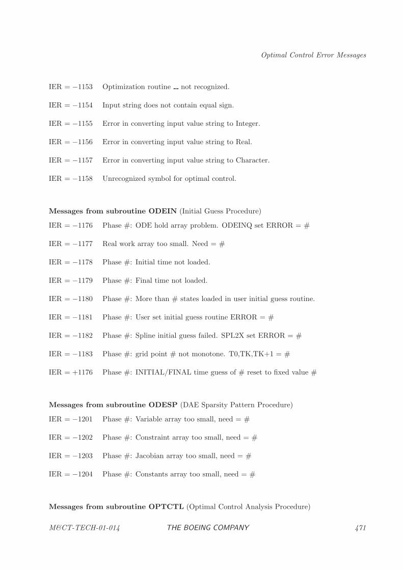
Optimal Control Error Messages
IER = −1153 Optimization routine not recognized.
IER = −1154 Input string does not contain equal sign.
IER = −1155 Error in converting input value string to Integer.
IER = −1156 Error in converting input value string to Real.
IER = −1157 Error in converting input value string to Character.
IER = −1158 Unrecognized symbol for optimal control.
Messages from subroutine ODEIN (Initial Guess Procedure)
IER = −1176 Phase #: ODE hold array problem. ODEINQ set ERROR = #
IER = −1177 Real work array too small. Need = #
IER = −1178 Phase #: Initial time not loaded.
IER = −1179 Phase #: Final time not loaded.
IER = −1180 Phase #: More than # states loaded in user initial guess routine.
IER = −1181 Phase #: User set initial guess routine ERROR = #
IER = −1182 Phase #: Spline initial guess failed. SPL2X set ERROR = #
IER = −1183 Phase #: grid point # not monotone. T0,TK,TK+1 = #
IER = +1176 Phase #: INITIAL/FINAL time guess of # reset to fixed value #
Messages from subroutine ODESP (DAE Sparsity Pattern Procedure)
IER = −1201 Phase #: Variable array too small, need = #
IER = −1202 Phase #: Constraint array too small, need = #
IER = −1203 Phase #: Jacobian array too small, need = #
IER = −1204 Phase #: Constants array too small, need = #
Messages from subroutine OPTCTL (Optimal Control Analysis Procedure)
M&CT-TECH-01-014 THE BOEING COMPANY 471
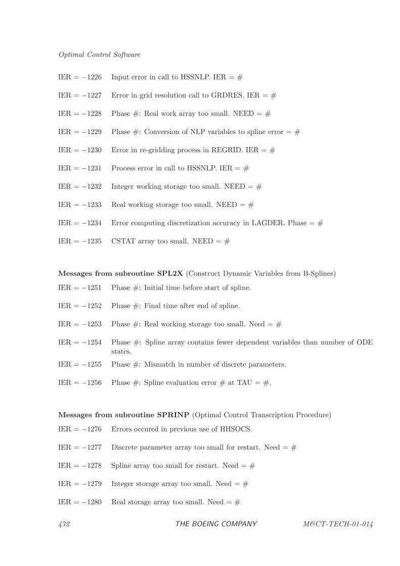
Optimal Control Software
IER = −1226 Input error in call to HSSNLP. IER = #
IER = −1227 Error in grid resolution call to GRDRES. IER = #
IER = −1228 Phase #: Real work array too small. NEED = #
IER = −1229 Phase #: Conversion of NLP variables to spline error = #
IER = −1230 Error in re-gridding process in REGRID. IER = #
IER = −1231 Process error in call to HSSNLP. IER = #
IER = −1232 Integer working storage too small. NEED = #
IER = −1233 Real working storage too small. NEED = #
IER = −1234 Error computing discretization accuracy in LAGDER. Phase = #
IER = −1235 CSTAT array too small. NEED = #
Messages from subroutine SPL2X (Construct Dynamic Variables from B-Splines)
IER = −1251 Phase #: Initial time before start of spline.
IER = −1252 Phase #: Final time after end of spline.
IER = −1253 Phase #: Real working storage too small. Need = #
IER = −1254 Phase #: Spline array contains fewer dependent variables than number of ODEstates.
IER = −1255 Phase #: Mismatch in number of discrete parameters.
IER = −1256 Phase #: Spline evaluation error # at TAU = #.
Messages from subroutine SPRINP (Optimal Control Transcription Procedure)
IER = −1276 Errors occured in previous use of HHSOCS.
IER = −1277 Discrete parameter array too small for restart. Need = #
IER = −1278 Spline array too small for restart. Need = #
IER = −1279 Integer storage array too small. Need = #
IER = −1280 Real storage array too small. Need = #
472 THE BOEING COMPANY M&CT-TECH-01-014
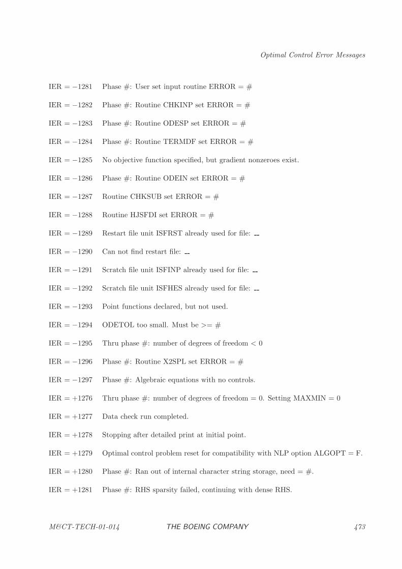
Optimal Control Error Messages
IER = −1281 Phase #: User set input routine ERROR = #
IER = −1282 Phase #: Routine CHKINP set ERROR = #
IER = −1283 Phase #: Routine ODESP set ERROR = #
IER = −1284 Phase #: Routine TERMDF set ERROR = #
IER = −1285 No objective function specified, but gradient nonzeroes exist.
IER = −1286 Phase #: Routine ODEIN set ERROR = #
IER = −1287 Routine CHKSUB set ERROR = #
IER = −1288 Routine HJSFDI set ERROR = #
IER = −1289 Restart file unit ISFRST already used for file:
IER = −1290 Can not find restart file:
IER = −1291 Scratch file unit ISFINP already used for file:
IER = −1292 Scratch file unit ISFHES already used for file:
IER = −1293 Point functions declared, but not used.
IER = −1294 ODETOL too small. Must be >= #
IER = −1295 Thru phase #: number of degrees of freedom < 0
IER = −1296 Phase #: Routine X2SPL set ERROR = #
IER = −1297 Phase #: Algebraic equations with no controls.
IER = +1276 Thru phase #: number of degrees of freedom = 0. Setting MAXMIN = 0
IER = +1277 Data check run completed.
IER = +1278 Stopping after detailed print at initial point.
IER = +1279 Optimal control problem reset for compatibility with NLP option ALGOPT = F.
IER = +1280 Phase #: Ran out of internal character string storage, need = #.
IER = +1281 Phase #: RHS sparsity failed, continuing with dense RHS.
M&CT-TECH-01-014 THE BOEING COMPANY 473
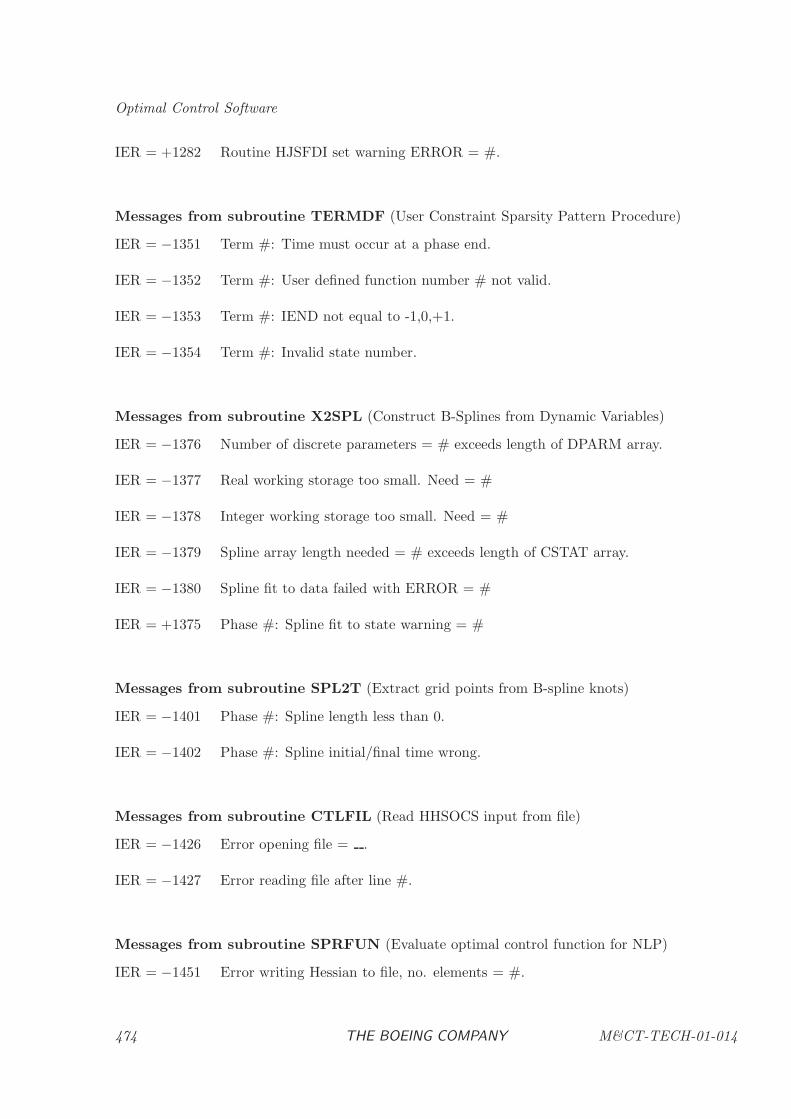
Optimal Control Software
IER = +1282 Routine HJSFDI set warning ERROR = #.
Messages from subroutine TERMDF (User Constraint Sparsity Pattern Procedure)
IER = −1351 Term #: Time must occur at a phase end.
IER = −1352 Term #: User defined function number # not valid.
IER = −1353 Term #: IEND not equal to -1,0,+1.
IER = −1354 Term #: Invalid state number.
Messages from subroutine X2SPL (Construct B-Splines from Dynamic Variables)
IER = −1376 Number of discrete parameters = # exceeds length of DPARM array.
IER = −1377 Real working storage too small. Need = #
IER = −1378 Integer working storage too small. Need = #
IER = −1379 Spline array length needed = # exceeds length of CSTAT array.
IER = −1380 Spline fit to data failed with ERROR = #
IER = +1375 Phase #: Spline fit to state warning = #
Messages from subroutine SPL2T (Extract grid points from B-spline knots)
IER = −1401 Phase #: Spline length less than 0.
IER = −1402 Phase #: Spline initial/final time wrong.
Messages from subroutine CTLFIL (Read HHSOCS input from file)
IER = −1426 Error opening file = .
IER = −1427 Error reading file after line #.
Messages from subroutine SPRFUN (Evaluate optimal control function for NLP)
IER = −1451 Error writing Hessian to file, no. elements = #.
474 THE BOEING COMPANY M&CT-TECH-01-014
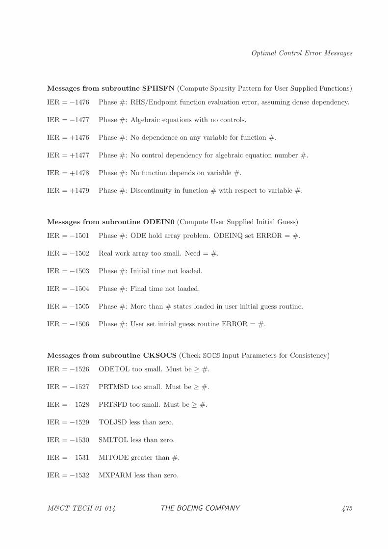
Optimal Control Error Messages
Messages from subroutine SPHSFN (Compute Sparsity Pattern for User Supplied Functions)
IER = −1476 Phase #: RHS/Endpoint function evaluation error, assuming dense dependency.
IER = −1477 Phase #: Algebraic equations with no controls.
IER = +1476 Phase #: No dependence on any variable for function #.
IER = +1477 Phase #: No control dependency for algebraic equation number #.
IER = +1478 Phase #: No function depends on variable #.
IER = +1479 Phase #: Discontinuity in function # with respect to variable #.
Messages from subroutine ODEIN0 (Compute User Supplied Initial Guess)
IER = −1501 Phase #: ODE hold array problem. ODEINQ set ERROR = #.
IER = −1502 Real work array too small. Need = #.
IER = −1503 Phase #: Initial time not loaded.
IER = −1504 Phase #: Final time not loaded.
IER = −1505 Phase #: More than # states loaded in user initial guess routine.
IER = −1506 Phase #: User set initial guess routine ERROR = #.
Messages from subroutine CKSOCS (Check SOCS Input Parameters for Consistency)
IER = −1526 ODETOL too small. Must be ≥ #.
IER = −1527 PRTMSD too small. Must be ≥ #.
IER = −1528 PRTSFD too small. Must be ≥ #.
IER = −1529 TOLJSD less than zero.
IER = −1530 SMLTOL less than zero.
IER = −1531 MITODE greater than #.
IER = −1532 MXPARM less than zero.
M&CT-TECH-01-014 THE BOEING COMPANY 475
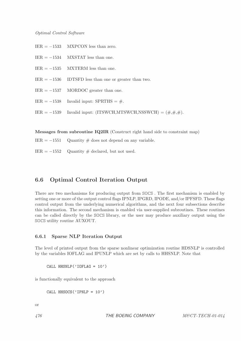
Optimal Control Software
IER = −1533 MXPCON less than zero.
IER = −1534 MXSTAT less than one.
IER = −1535 MXTERM less than one.
IER = −1536 IDTSFD less than one or greater than two.
IER = −1537 MORDOC greater than one.
IER = −1538 Invalid input: SPRTHS = #.
IER = −1539 Invalid input: (ITSWCH,MTSWCH,NSSWCH) = (#,#,#).
Messages from subroutine IQ2IR (Construct right hand side to constraint map)
IER = −1551 Quantity # does not depend on any variable.
IER = −1552 Quantity # declared, but not used.
6.6 Optimal Control Iteration Output
There are two mechanisms for producing output from SOCS . The first mechanism is enabled bysetting one or more of the output control flags IPNLP, IPGRD, IPODE, and/or IPFSFD. These flagscontrol output from the underlying numerical algorithms, and the next four subsections describethis information. The second mechanism is enabled via user-supplied subroutines. These routinescan be called directly by the SOCS library, or the user may produce auxiliary output using theSOCS utility routine AUXOUT.
6.6.1 Sparse NLP Iteration Output
The level of printed output from the sparse nonlinear optimization routine HDSNLP is controlledby the variables IOFLAG and IPUNLP which are set by calls to HHSNLP. Note that
CALL HHSNLP(’IOFLAG = 10’)
is functionally equivalent to the approach
CALL HHSOCS(’IPNLP = 10’)
or
476 THE BOEING COMPANY M&CT-TECH-01-014
Optimal Control Iteration Output
CALL HHSOCS(’HHSNLP:IOFLAG = 10’)
For clarity in presentation the discussion in this subsection will only refer to IOFLAG. For a morecomplete understanding of the NLP output the reader should consult Section 2.3.
When IOFLAG = 0 and/or IPUNLP ≤ 0, no output is printed by HDSNLP. Four different levelsof iteration output are provided, when IPUNLP > 0 and IOFLAG > 0. These levels are referredto as Terse, Standard, Interpretive, and Diagnostic and are defined in the following subsections.The default level of output is referred to as Standard Output. For a complete discussion of NLPiteration output consult Section 2.3.
6.6.2 Optimal Control Output
When IPGRD = 0 and/or IPUOCP ≤ 0, no output is printed by HDSOCS. Three different levelsof optimal control output are provided, when IPUOCP > 0 and IPGRD > 0. These levels arereferred to as Terse, Standard, and Interpretive and are defined in the following subsections. Thedefault level of output is IPGRD = 10 and is referred to as Standard Output.
Terse Output
Terse Output is obtained by setting 0 < IPGRD < 10, and all values of IPGRD in this range willproduce the same result. The first block of output which appears after the SOCS logo, is of theform:
ODE = title(1)
GOAL = title(2)
where
title(1) The user defined problem title as input in TITLE(1) in ODEINP.
title(2) The user defined problem subtitle as input in TITLE(2) in ODEINP.
The beginning of a particular mesh refinement iteration is denoted by a delimiting banner of theform:
========================================================================================================
========================================================================================================
========================================================================================================
====================================== REFINEMENT ITERATION 1 =========================================
========================================================================================================
========================================================================================================
========================================================================================================
The next block of output describes the particulars for the specific transcription used on the currentrefinement iteration. A typical output summary is:
TRANSCRIPTION SUMMARY:
M&CT-TECH-01-014 THE BOEING COMPANY 477
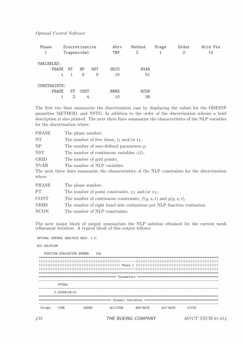
Optimal Control Software
Phase Discretization Abrv Method Stage Order Grid Pts
1 Trapezoidal TRP 2 1 2 10
VARIABLES:
PHASE NT NP NST GRID NVAR
1 1 0 5 10 51
CONSTRAINTS:
PHASE PT CONT NRHS NCON
1 2 4 10 38
The first two lines summarize the discretization case by displaying the values for the ODEINPquantities METHOD, and NSTG. In addition to the order of the discretization scheme a briefdescription is also printed. The next three lines summarize the characteristics of the NLP variablesfor the discretization where
PHASE The phase number,
NT The number of free times, tI and/or tF ,
NP The number of user-defined parameters p,
NST The number of continuous variables z(t),
GRID The number of grid points,
NVAR The number of NLP variables.The next three lines summarize the characteristics of the NLP constraints for the discretizationwhere
PHASE The phase number,
PT The number of point constraints, ψI and/or ψF ,
CONT The number of continuous constraints, f(y, u, t) and g(y, u, t),
NRHS The number of right hand side evaluations per NLP function evaluation,
NCON The number of NLP constraints.
The next major block of output summarizes the NLP solution obtained for the current meshrefinement iteration. A typical block of this output follows:
OPTIMAL CONTROL ANALYSIS GRID 1.0:
NLP SOLUTION:
FUNCTION EVALUATION NUMBER 164
========================================================================================================
|||||||||||||||||||||||||||||||||||||||||||||||---------||||||||||||||||||||||||||||||||||||||||||||||||
||||||||||||||||||||||||||||||||||||||||||||||| Phase 1 ||||||||||||||||||||||||||||||||||||||||||||||||
|||||||||||||||||||||||||||||||||||||||||||||||---------||||||||||||||||||||||||||||||||||||||||||||||||
========================================================================================================
============================================= Parameters ===============================================
--------------------------------------------------------------------------------------------------------
TFINAL
--------------------------------------------------------------------------------------------------------
5.5028814E-01
========================================================================================================
========================================== Dynamic Variables ===========================================
--------------------------------------------------------------------------------------------------------
Gridpt TIME RANGE ALTITUDE RNG-RATE ALT-RATE PITCH
478 THE BOEING COMPANY M&CT-TECH-01-014
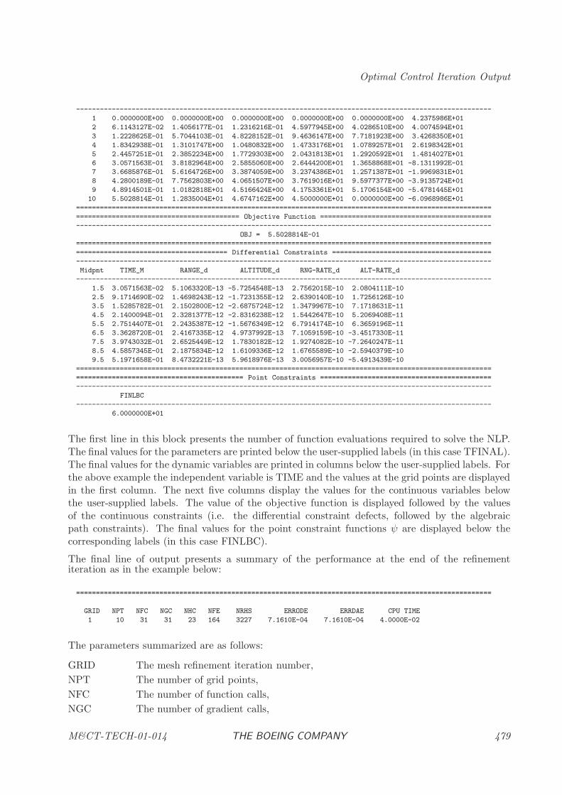
Optimal Control Iteration Output
--------------------------------------------------------------------------------------------------------
1 0.0000000E+00 0.0000000E+00 0.0000000E+00 0.0000000E+00 0.0000000E+00 4.2375986E+01
2 6.1143127E-02 1.4056177E-01 1.2316216E-01 4.5977945E+00 4.0286510E+00 4.0074594E+01
3 1.2228625E-01 5.7044103E-01 4.8228152E-01 9.4636147E+00 7.7181923E+00 3.4268350E+01
4 1.8342938E-01 1.3101747E+00 1.0480832E+00 1.4733176E+01 1.0789257E+01 2.6198342E+01
5 2.4457251E-01 2.3852234E+00 1.7729303E+00 2.0431813E+01 1.2920592E+01 1.4814027E+01
6 3.0571563E-01 3.8182964E+00 2.5855060E+00 2.6444200E+01 1.3658868E+01 -8.1311992E-01
7 3.6685876E-01 5.6164726E+00 3.3874059E+00 3.2374386E+01 1.2571387E+01 -1.9969831E+01
8 4.2800189E-01 7.7562803E+00 4.0651507E+00 3.7619016E+01 9.5977377E+00 -3.9135724E+01
9 4.8914501E-01 1.0182818E+01 4.5166424E+00 4.1753361E+01 5.1706154E+00 -5.4781445E+01
10 5.5028814E-01 1.2835004E+01 4.6747162E+00 4.5000000E+01 0.0000000E+00 -6.0968986E+01
========================================================================================================
========================================= Objective Function ===========================================
--------------------------------------------------------------------------------------------------------
OBJ = 5.5028814E-01
========================================================================================================
====================================== Differential Constraints ========================================
--------------------------------------------------------------------------------------------------------
Midpnt TIME_M RANGE_d ALTITUDE_d RNG-RATE_d ALT-RATE_d
--------------------------------------------------------------------------------------------------------
1.5 3.0571563E-02 5.1063320E-13 -5.7254548E-13 2.7562015E-10 2.0804111E-10
2.5 9.1714690E-02 1.4698243E-12 -1.7231355E-12 2.6390140E-10 1.7256126E-10
3.5 1.5285782E-01 2.1502800E-12 -2.6875724E-12 1.3479967E-10 7.1718631E-11
4.5 2.1400094E-01 2.3281377E-12 -2.8316238E-12 1.5442647E-10 5.2069408E-11
5.5 2.7514407E-01 2.2435387E-12 -1.5676349E-12 6.7914174E-10 6.3659196E-11
6.5 3.3628720E-01 2.4167335E-12 4.9737992E-13 7.1059159E-10 -3.4517330E-11
7.5 3.9743032E-01 2.6525449E-12 1.7830182E-12 1.9274082E-10 -7.2640247E-11
8.5 4.5857345E-01 2.1875834E-12 1.6109336E-12 1.6765589E-10 -2.5940379E-10
9.5 5.1971658E-01 8.4732221E-13 5.9618976E-13 3.0056957E-10 -5.4913439E-10
========================================================================================================
========================================== Point Constraints ===========================================
--------------------------------------------------------------------------------------------------------
FINLBC
--------------------------------------------------------------------------------------------------------
6.0000000E+01
The first line in this block presents the number of function evaluations required to solve the NLP.The final values for the parameters are printed below the user-supplied labels (in this case TFINAL).The final values for the dynamic variables are printed in columns below the user-supplied labels. Forthe above example the independent variable is TIME and the values at the grid points are displayedin the first column. The next five columns display the values for the continuous variables belowthe user-supplied labels. The value of the objective function is displayed followed by the valuesof the continuous constraints (i.e. the differential constraint defects, followed by the algebraicpath constraints). The final values for the point constraint functions ψ are displayed below thecorresponding labels (in this case FINLBC).
The final line of output presents a summary of the performance at the end of the refinementiteration as in the example below:
========================================================================================================
GRID NPT NFC NGC NHC NFE NRHS ERRODE ERRDAE CPU TIME
1 10 31 31 23 164 3227 7.1610E-04 7.1610E-04 4.0000E-02
The parameters summarized are as follows:
GRID The mesh refinement iteration number,
NPT The number of grid points,
NFC The number of function calls,
NGC The number of gradient calls,
M&CT-TECH-01-014 THE BOEING COMPANY 479
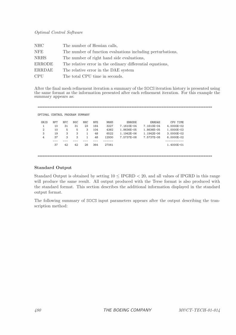
Optimal Control Software
NHC The number of Hessian calls,
NFE The number of function evaluations including perturbations,
NRHS The number of right hand side evaluations,
ERRODE The relative error in the ordinary differential equations,
ERRDAE The relative error in the DAE system
CPU The total CPU time in seconds.
After the final mesh refinement iteration a summary of the SOCS iteration history is presented usingthe same format as the information presented after each refinement iteration. For this example thesummary appears as:
========================================================================================================
OPTIMAL CONTROL PROGRAM SUMMARY
GRID NPT NFC NGC NHC NFE NRHS ERRODE ERRDAE CPU TIME
1 10 31 31 23 164 3227 7.1610E-04 7.1610E-04 4.0000E-02
2 10 5 5 3 104 4382 1.8636E-05 1.8636E-05 1.0000E-02
3 19 3 3 1 48 6522 1.1942E-06 1.1942E-06 3.0000E-02
4 37 3 3 1 48 12930 7.5737E-08 7.5737E-08 6.0000E-02
--- --- --- --- --- ------ -----------
37 42 42 28 364 27061 1.4000E-01
========================================================================================================
Standard Output
Standard Output is obtained by setting 10 ≤ IPGRD < 20, and all values of IPGRD in this rangewill produce the same result. All output produced with the Terse format is also produced withthe standard format. This section describes the additional information displayed in the standardoutput format.
The following summary of SOCS input parameters appears after the output describing the tran-scription method:
480 THE BOEING COMPANY M&CT-TECH-01-014
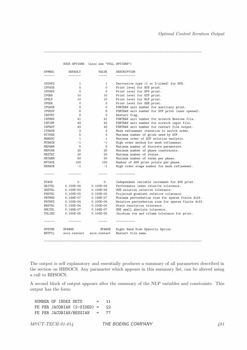
Optimal Control Iteration Output
------------------------------------------------------------------------------------------
SOCS OPTIONS (also see "FULL OPTIONS")
SYMBOL DEFAULT VALUE DESCRIPTION
------ ------- ----- -----------
IDTSFD 1 1 Derivative type (1 or 2-sided) for SFD.
IPFAUX 0 0 Print level for AUX print.
IPFSFD 0 0 Print level for SFD print.
IPGRD 10 10 Print level for OCP print.
IPNLP 10 10 Print level for NLP print.
IPODE 0 0 Print level for ODE print.
IPUAUX 0 0 FORTRAN unit number for auxiliary print.
IPUOCP 6 6 FORTRAN unit number for OCP print (user opened).
IRSTRT 0 0 Restart flag.
ISFHES 41 41 FORTRAN unit number for scratch Hessian file.
ISFINP 42 42 FORTRAN unit number for scratch input file.
ISFRST 43 43 FORTRAN unit number for restart file output.
ITSWCH 2 2 Mesh refinement iteration to switch order.
MITODE 5 5 Maximum number of grids used by OCP.
MORDOC 1 1 Maximum order of OCP solution analysis.
MTSWCH -1 -1 High order method for mesh refinement.
MXPARM 5 5 Maximum number of discrete parameters.
MXPCON 20 20 Maximum number of phase constraints.
MXSTAT 20 20 Maximum number of states.
MXTERM 50 50 Maximum number of terms per phase.
NPTAUX 100 100 Number of AUX print points per phase.
NSSWCH -1 -1 High order stage number for mesh refinement.
------ ------- ----- -----------
DTAUX 0. 0. Independent variable increment for AUX print.
OBJTOL 0.100E-04 0.100E-04 Performance index relative tolerance.
ODETOL 0.100E-02 0.100E-06 ODE solution relative tolerance.
PGDTOL 0.100E-02 0.100E-02 Projected gradient relative tolerance.
PRTMSD 0.149E-07 0.149E-07 Minimum perturbation size for sparse finite diff.
PRTSFD 0.100E-04 0.100E-04 Relative perturbation size for sparse finite diff.
RESTOL 0.100E-04 0.100E-04 State resolution tolerance.
SMLTOL 0.149E-07 0.149E-07 ODE small absolute tolerance.
TOLJSD 0.100E-05 0.100E-05 Jacobian row and column tolerance for print.
------ ------- ----- -----------
SPRTHS SPARSE SPARSE Right Hand Side Sparsity Option.
RSTFIL socs.restart socs.restart Restart file name.
------------------------------------------------------------------------------------------
The output is self explanatory and essentially produces a summary of all parameters described inthe section on HHSOCS. Any parameter which appears in this summary list, can be altered usinga call to HHSOCS.
A second block of output appears after the summary of the NLP variables and constraints. Thisoutput has the form:
NUMBER OF INDEX SETS = 11
FE PER JACOBIAN (2-SIDED) = 22
FE PER JACOBIAN/HESSIAN = 77
M&CT-TECH-01-014 THE BOEING COMPANY 481
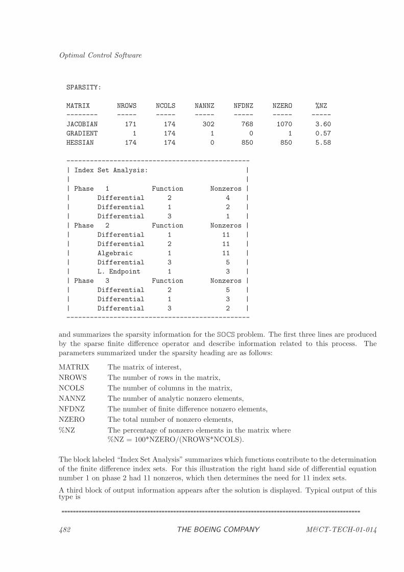
Optimal Control Software
SPARSITY:
MATRIX NROWS NCOLS NANNZ NFDNZ NZERO %NZ
-------- ----- ----- ----- ----- ----- -----
JACOBIAN 171 174 302 768 1070 3.60
GRADIENT 1 174 1 0 1 0.57
HESSIAN 174 174 0 850 850 5.58
-----------------------------------------------
| Index Set Analysis: |
| |
| Phase 1 Function Nonzeros |
| Differential 2 4 |
| Differential 1 2 |
| Differential 3 1 |
| Phase 2 Function Nonzeros |
| Differential 1 11 |
| Differential 2 11 |
| Algebraic 1 11 |
| Differential 3 5 |
| L. Endpoint 1 3 |
| Phase 3 Function Nonzeros |
| Differential 2 5 |
| Differential 1 3 |
| Differential 3 2 |
-----------------------------------------------
and summarizes the sparsity information for the SOCS problem. The first three lines are producedby the sparse finite difference operator and describe information related to this process. Theparameters summarized under the sparsity heading are as follows:
MATRIX The matrix of interest,
NROWS The number of rows in the matrix,
NCOLS The number of columns in the matrix,
NANNZ The number of analytic nonzero elements,
NFDNZ The number of finite difference nonzero elements,
NZERO The total number of nonzero elements,
%NZ The percentage of nonzero elements in the matrix where%NZ = 100*NZERO/(NROWS*NCOLS).
The block labeled “Index Set Analysis” summarizes which functions contribute to the determinationof the finite difference index sets. For this illustration the right hand side of differential equationnumber 1 on phase 2 had 11 nonzeros, which then determines the need for 11 index sets.
A third block of output information appears after the solution is displayed. Typical output of thistype is
========================================================================================================
482 THE BOEING COMPANY M&CT-TECH-01-014
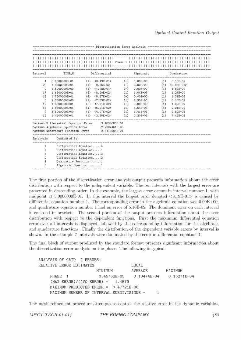
Optimal Control Iteration Output
==================================== Discretization Error Analysis =====================================
--------------------------------------------------------------------------------------------------------
========================================================================================================
|||||||||||||||||||||||||||||||||||||||||||||||---------||||||||||||||||||||||||||||||||||||||||||||||||
||||||||||||||||||||||||||||||||||||||||||||||| Phase 1 ||||||||||||||||||||||||||||||||||||||||||||||||
|||||||||||||||||||||||||||||||||||||||||||||||---------||||||||||||||||||||||||||||||||||||||||||||||||
========================================================================================================
Interval TIME_M Differential Algebraic Quadrature
--------------------------------------------------------------------------------------------------------
1 5.0000000E-01 (1) <3.19E-01> (-) 0.00E+00 (1) 5.10E-02
20 1.9500000E+01 (1) 9.66E-02 (-) 0.00E+00 (1) <2.84E-01>
2 1.5000000E+00 (1) <1.28E-01> (-) 0.00E+00 (1) 1.82E-02
17 1.6500000E+01 (4) <8.40E-02> (1) 1.04E-07 (1) 1.27E-02
18 1.7500000E+01 (4) <8.27E-02> (-) 0.00E+00 (1) 1.31E-02
3 2.5000000E+00 (1) <7.53E-02> (1) 4.95E-06 (1) 3.18E-02
19 1.8500000E+01 (3) <7.01E-02> (-) 0.00E+00 (1) 1.09E-02
16 1.5500000E+01 (4) <6.51E-02> (1) 4.64E-06 (1) 2.21E-02
4 3.5000000E+00 (1) <4.07E-02> (1) 1.41E-03 (1) 9.80E-03
15 1.4500000E+01 (1) <2.55E-02> (1) 2.20E-03 (1) 7.46E-03
--------------------------------------------------------------------------------------------------------
Maximum Differential Equation Error 3.1899685E-01
Maximum Algebraic Equation Error 2.2007461E-03
Maximum Quadrature Function Error 2.8410504E-01
--------------------------------------------------------------------------------------------------------
Intervals Dominated By:
--------------------------------------------------------------------------------------------------------
7 Differential Equation.....4
7 Differential Equation.....1
3 Differential Equation.....3
2 Differential Equation.....2
1 Quadrature Function.......1
0 Algebraic Equation........1
--------------------------------------------------------------------------------------------------------
The first portion of the discretization error analysis output presents information about the errordistribution with respect to the independent variable. The ten intervals with the largest error arepresented in descending order. In the example, the largest error occurs in interval number 1, withmidpoint at 5.0000000E-01. In this interval the largest error denoted <3.19E-01> is caused bydifferential equation number 1. The corresponding error in the algebraic equation was 0.00E+00,and quadrature equation number 1 had an error of 5.10E-02. The dominant error on each intervalis enclosed in brackets. The second portion of the output presents information about the errordistribution with respect to the dependent functions. First the maximum differential equationerror over all intervals is displayed, followed by the corresponding information for the algebraic,and quadrature functions. Finally the distribution of the dependent variable errors by interval isshown. In the example 7 intervals were dominated by the error in differential equation 4.
The final block of output produced by the standard format presents significant information aboutthe discretization error analysis on the phase. The following is typical:
ANALYSIS OF GRID 2 ERRORS:
RELATIVE ERROR ESTIMATES LOCAL
MINIMUM AVERAGE MAXIMUM
PHASE 1 0.46762E-05 0.10474E-04 0.15271E-04
(MAX ERROR)/(AVG ERROR) = 1.4579
MAXIMUM PREDICTED ERROR = 0.47721E-06
MAXIMUM NUMBER OF INTERVAL SUBDIVISIONS = 1
The mesh refinement procedure attempts to control the relative error in the dynamic variables.
M&CT-TECH-01-014 THE BOEING COMPANY 483
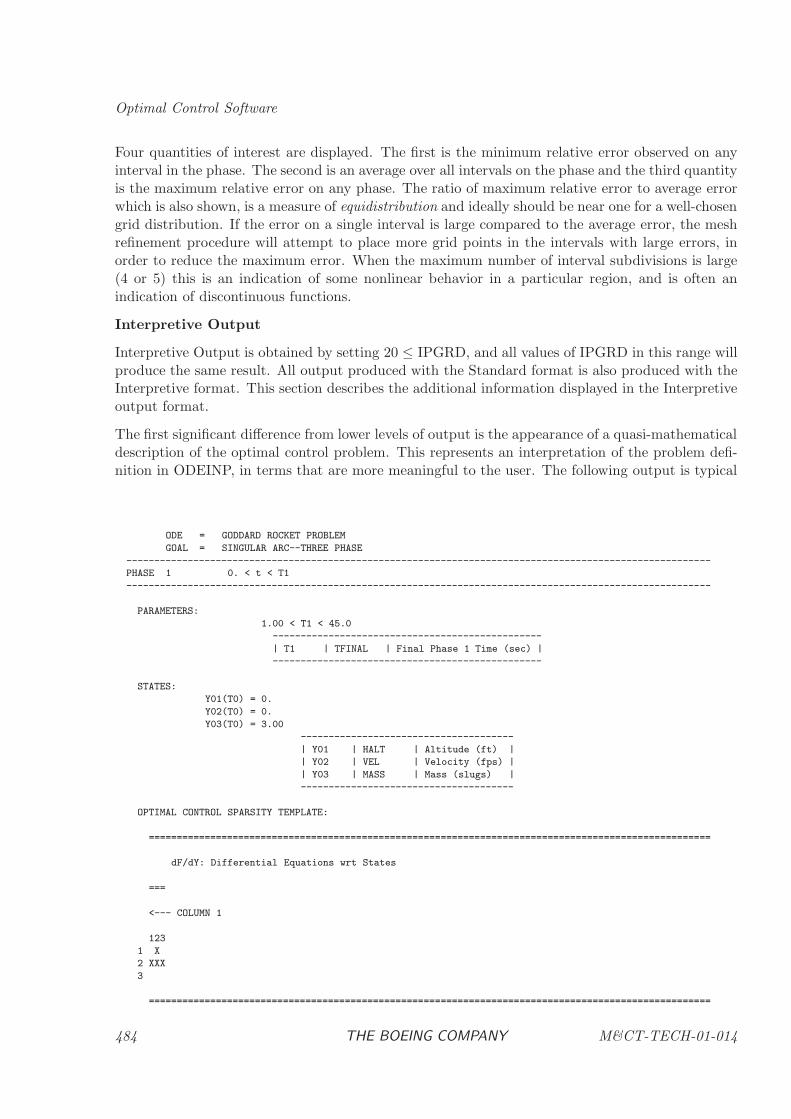
Optimal Control Software
Four quantities of interest are displayed. The first is the minimum relative error observed on anyinterval in the phase. The second is an average over all intervals on the phase and the third quantityis the maximum relative error on any phase. The ratio of maximum relative error to average errorwhich is also shown, is a measure of equidistribution and ideally should be near one for a well-chosengrid distribution. If the error on a single interval is large compared to the average error, the meshrefinement procedure will attempt to place more grid points in the intervals with large errors, inorder to reduce the maximum error. When the maximum number of interval subdivisions is large(4 or 5) this is an indication of some nonlinear behavior in a particular region, and is often anindication of discontinuous functions.
Interpretive Output
Interpretive Output is obtained by setting 20 ≤ IPGRD, and all values of IPGRD in this range willproduce the same result. All output produced with the Standard format is also produced with theInterpretive format. This section describes the additional information displayed in the Interpretiveoutput format.
The first significant difference from lower levels of output is the appearance of a quasi-mathematicaldescription of the optimal control problem. This represents an interpretation of the problem defi-nition in ODEINP, in terms that are more meaningful to the user. The following output is typical
ODE = GODDARD ROCKET PROBLEM
GOAL = SINGULAR ARC--THREE PHASE
--------------------------------------------------------------------------------------------------------
PHASE 1 0. < t < T1
--------------------------------------------------------------------------------------------------------
PARAMETERS:
1.00 < T1 < 45.0
------------------------------------------------
| T1 | TFINAL | Final Phase 1 Time (sec) |
------------------------------------------------
STATES:
Y01(T0) = 0.
Y02(T0) = 0.
Y03(T0) = 3.00
--------------------------------------
| Y01 | HALT | Altitude (ft) |
| Y02 | VEL | Velocity (fps) |
| Y03 | MASS | Mass (slugs) |
--------------------------------------
OPTIMAL CONTROL SPARSITY TEMPLATE:
====================================================================================================
dF/dY: Differential Equations wrt States
===
<--- COLUMN 1
123
1 X
2 XXX
3
====================================================================================================
484 THE BOEING COMPANY M&CT-TECH-01-014
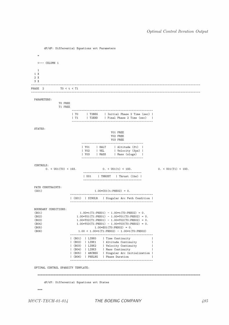
Optimal Control Iteration Output
dF/dP: Differential Equations wrt Parameters
=
<--- COLUMN 1
1
1 X
2 X
3 X
--------------------------------------------------------------------------------------------------------
PHASE 2 T0 < t < T1
--------------------------------------------------------------------------------------------------------
PARAMETERS:
T0 FREE
T1 FREE
--------------------------------------------------
| T0 | T2BEG | Initial Phase 2 Time (sec) |
| T1 | T2END | Final Phase 2 Time (sec) |
--------------------------------------------------
STATES:
Y01 FREE
Y02 FREE
Y03 FREE
--------------------------------------
| Y01 | HALT | Altitude (ft) |
| Y02 | VEL | Velocity (fps) |
| Y03 | MASS | Mass (slugs) |
--------------------------------------
CONTROLS:
0. < U01(T0) < 193. 0. < U01(t) < 193. 0. < U01(T1) < 193.
------------------------------------
| U01 | THRUST | Thrust (lbs) |
------------------------------------
PATH CONSTRAINTS:
(G01) 1.00*C01(t:PHS02) = 0.
---------------------------------------------------
| (G01) | SINGLR | Singular Arc Path Condition |
---------------------------------------------------
BOUNDARY CONDITIONS:
(B01) 1.00*t(T1:PHS01) - 1.00*t(T0:PHS02) = 0.
(B02) 1.00*Y01(T1:PHS01) - 1.00*Y01(T0:PHS02) = 0.
(B03) 1.00*Y02(T1:PHS01) - 1.00*Y02(T0:PHS02) = 0.
(B04) 1.00*Y03(T1:PHS01) - 1.00*Y03(T0:PHS02) = 0.
(B05) 1.00*E01(T0:PHS02) = 0.
(B06) 1.00 < 1.00*t(T1:PHS02) - 1.00*t(T0:PHS02)
---------------------------------------------------
| (B01) | LINK0 | Time Continuity |
| (B02) | LINK1 | Altitude Continuity |
| (B03) | LINK2 | Velocity Continuity |
| (B04) | LINK3 | Mass Continuity |
| (B05) | ARCBEG | Singular Arc Initialization |
| (B06) | PHSLNG | Phase Duration |
---------------------------------------------------
OPTIMAL CONTROL SPARSITY TEMPLATE:
====================================================================================================
dF/dY: Differential Equations wrt States
===
M&CT-TECH-01-014 THE BOEING COMPANY 485
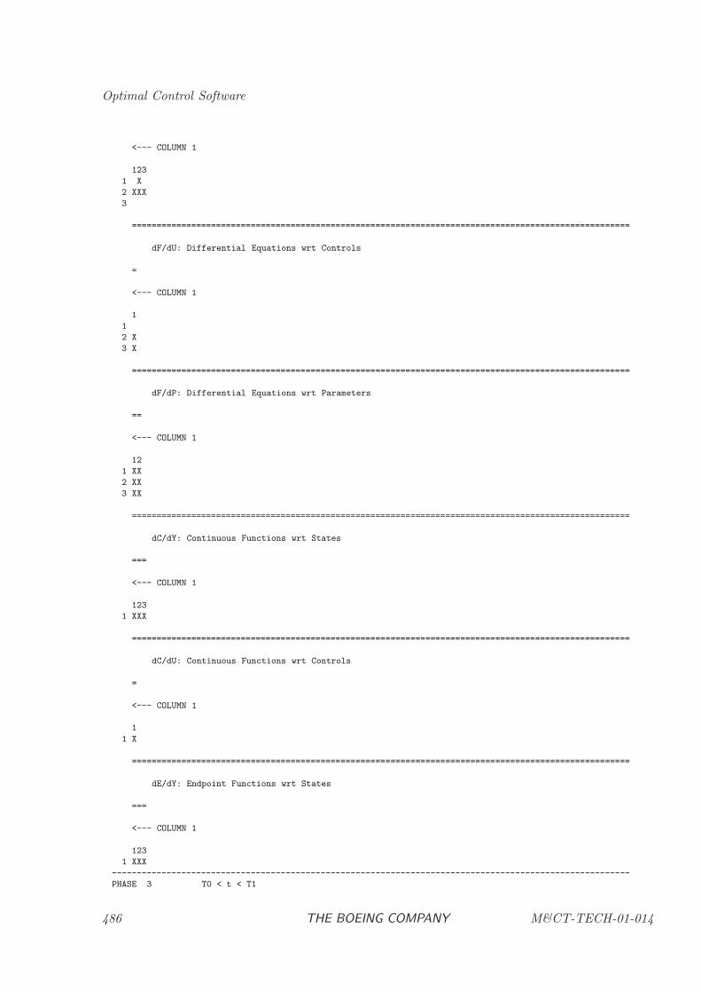
Optimal Control Software
<--- COLUMN 1
123
1 X
2 XXX
3
====================================================================================================
dF/dU: Differential Equations wrt Controls
=
<--- COLUMN 1
1
1
2 X
3 X
====================================================================================================
dF/dP: Differential Equations wrt Parameters
==
<--- COLUMN 1
12
1 XX
2 XX
3 XX
====================================================================================================
dC/dY: Continuous Functions wrt States
===
<--- COLUMN 1
123
1 XXX
====================================================================================================
dC/dU: Continuous Functions wrt Controls
=
<--- COLUMN 1
1
1 X
====================================================================================================
dE/dY: Endpoint Functions wrt States
===
<--- COLUMN 1
123
1 XXX
--------------------------------------------------------------------------------------------------------
PHASE 3 T0 < t < T1
486 THE BOEING COMPANY M&CT-TECH-01-014
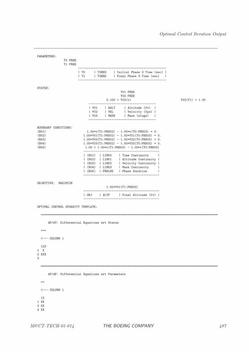
Optimal Control Iteration Output
--------------------------------------------------------------------------------------------------------
PARAMETERS:
T0 FREE
T1 FREE
--------------------------------------------------
| T0 | T3BEG | Initial Phase 3 Time (sec) |
| T1 | T3END | Final Phase 3 Time (sec) |
--------------------------------------------------
STATES:
Y01 FREE
Y02 FREE
0.100 < Y03(t) Y03(T1) = 1.00
--------------------------------------
| Y01 | HALT | Altitude (ft) |
| Y02 | VEL | Velocity (fps) |
| Y03 | MASS | Mass (slugs) |
--------------------------------------
BOUNDARY CONDITIONS:
(B01) 1.00*t(T1:PHS02) - 1.00*t(T0:PHS03) = 0.
(B02) 1.00*Y01(T1:PHS02) - 1.00*Y01(T0:PHS03) = 0.
(B03) 1.00*Y02(T1:PHS02) - 1.00*Y02(T0:PHS03) = 0.
(B04) 1.00*Y03(T1:PHS02) - 1.00*Y03(T0:PHS03) = 0.
(B05) 1.00 < 1.00*t(T1:PHS03) - 1.00*t(T0:PHS03)
-------------------------------------------
| (B01) | LINK0 | Time Continuity |
| (B02) | LINK1 | Altitude Continuity |
| (B03) | LINK2 | Velocity Continuity |
| (B04) | LINK3 | Mass Continuity |
| (B05) | PHSLNG | Phase Duration |
-------------------------------------------
OBJECTIVE: MAXIMIZE
1.00*Y01(T1:PHS03)
-------------------------------------------
| OBJ | ALTF | Final Altitude (ft) |
-------------------------------------------
OPTIMAL CONTROL SPARSITY TEMPLATE:
====================================================================================================
dF/dY: Differential Equations wrt States
===
<--- COLUMN 1
123
1 X
2 XXX
3
====================================================================================================
dF/dP: Differential Equations wrt Parameters
==
<--- COLUMN 1
12
1 XX
2 XX
3 XX
M&CT-TECH-01-014 THE BOEING COMPANY 487
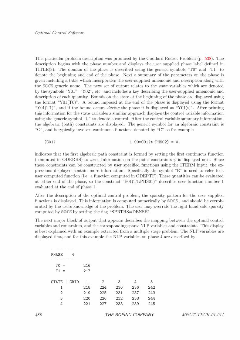
Optimal Control Software
This particular problem description was produced by the Goddard Rocket Problem (p. 538). Thedescription begins with the phase number and displays the user supplied phase label defined inTITLE(3). The domain of the phase is described using the generic symbols “T0” and “T1” todenote the beginning and end of the phase. Next a summary of the parameters on the phase isgiven including a table which incorporates the user-supplied mnemonic and description along withthe SOCS generic name. The next set of output relates to the state variables which are denotedby the symbols “Y01”, “Y02”, etc. and includes a key describing the user-supplied mnemonic anddescription of each quantity. Bounds on the state at the beginning of the phase are displayed usingthe format “Y01(T0)”. A bound imposed at the end of the phase is displayed using the format“Y01(T1)”, and if the bound occurs during the phase it is displayed as “Y01(t)”. After printingthis information for the state variables a similiar approach displays the control variable informationusing the generic symbol “U” to denote a control. After the control variable summary information,the algebraic (path) constraints are displayed. The generic symbol for an algebraic constraint is“G”, and it typically involves continuous functions denoted by “C” so for example
(G01) 1.00*C01(t:PHS02) = 0.
indicates that the first algebraic path constraint is formed by setting the first continuous function(computed in ODERHS) to zero. Information on the point constraints ψ is displayed next. Sincethese constraints can be constructed by user specified functions using the ITERM input, the ex-pressions displayed contain more information. Specifically the symbol “E” is used to refer to auser computed function (i.e. a function computed in ODEPTF). These quantities can be evaluatedat either end of the phase, so the construct “E01(T1:PHS01)” describes user function number 1evaluated at the end of phase 1.
After the description of the optimal control problem, the sparsity pattern for the user suppliedfunctions is displayed. This information is computed numerically by SOCS , and should be corrob-orated by the users knowledge of the problem. The user may override the right hand side sparsitycomputed by SOCS by setting the flag “SPRTHS=DENSE”.
The next major block of output that appears describes the mapping between the optimal controlvariables and constraints, and the corresponding sparse NLP variables and constraints. This displayis best explained with an example extracted from a multiple stage problem. The NLP variables aredisplayed first, and for this example the NLP variables on phase 4 are described by:
----------
PHASE 4
----------
T0 = 216
T1 = 217
STATE | GRID 1 2 3 4 5
1 218 224 230 236 242
2 219 225 231 237 243
3 220 226 232 238 244
4 221 227 233 239 245
488 THE BOEING COMPANY M&CT-TECH-01-014
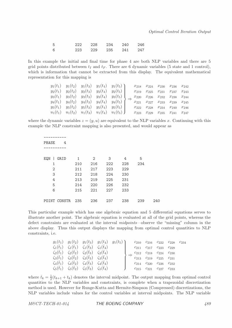
Optimal Control Iteration Output
5 222 228 234 240 246
6 223 229 235 241 247
In this example the initial and final time for phase 4 are both NLP variables and there are 5grid points distributed between tI and tF . There are 6 dynamic variables (5 state and 1 control),which is information that cannot be extracted from this display. The equivalent mathematicalrepresentation for this mapping is
y1(t1) y1(t2) y1(t3) y1(t4) y1(t5)y2(t1) y2(t2) y2(t3) y2(t4) y2(t5)y3(t1) y3(t2) y3(t3) y3(t4) y3(t5)y4(t1) y4(t2) y4(t3) y4(t4) y4(t5)y5(t1) y5(t2) y5(t3) y5(t4) y5(t5)u1(t1) u1(t2) u1(t3) u1(t4) u1(t5)
⇒
x218 x224 x230 x236 x242
x219 x225 x231 x237 x243
x220 x226 x232 x238 x244
x221 x227 x233 x239 x245
x222 x228 x234 x240 x246
x223 x229 x235 x241 x247
where the dynamic variables z = (y, u) are equivalent to the NLP variables x. Continuing with thisexample the NLP constraint mapping is also presented, and would appear as
----------
PHASE 4
----------
EQN | GRID 1 2 3 4 5
1 210 216 222 228 234
2 211 217 223 229
3 212 218 224 230
4 213 219 225 231
5 214 220 226 232
6 215 221 227 233
POINT CONSTR 235 236 237 238 239 240
This particular example which has one algebraic equation and 5 differential equations serves toillustrate another point. The algebraic equation is evaluated at all of the grid points, whereas thedefect constraints are evaluated at the interval midpoints—observe the “missing” column in theabove display. Thus this output displays the mapping from optimal control quantities to NLPconstraints, i.e.
g1(t1) g1(t2) g1(t3) g1(t4) g1(t5)ζ1(t1) ζ1(t1) ζ1(t3) ζ1(t4)ζ2(t1) ζ2(t2) ζ2(t3) ζ2(t4)ζ3(t1) ζ3(t2) ζ3(t3) ζ3(t4)ζ4(t1) ζ4(t2) ζ4(t3) ζ4(t4)ζ5(t1) ζ5(t2) ζ5(t3) ζ5(t4)
⇒
c210 c216 c222 c228 c234c211 c217 c223 c229c212 c218 c224 c230c213 c219 c225 c231c214 c220 c226 c232c215 c221 c227 c233
where tk = 12 (tk+1 + tk) denotes the interval midpoint. The output mapping from optimal control
quantities to the NLP variables and constraints, is complete when a trapezoidal discretizationmethod is used. However for Runge-Kutta and Hermite-Simpson (Compressed) discretizations, theNLP variables include values for the control variables at interval midpoints. The NLP variable
M&CT-TECH-01-014 THE BOEING COMPANY 489
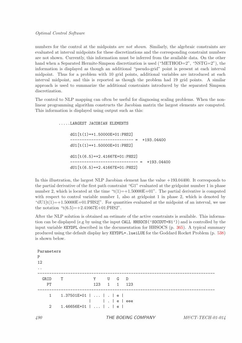
Optimal Control Software
numbers for the control at the midpoints are not shown. Similarly, the algebraic constraints areevaluated at interval midpoints for these discretizations and the corresponding constraint numbersare not shown. Currently, this information must be inferred from the available data. On the otherhand when a Separated Hermite-Simpson discretization is used (“METHOD=2”, “NSTG=2”), theinformation is displayed as though an additional “pseudo-grid” point is present at each intervalmidpoint. Thus for a problem with 10 grid points, additional variables are introduced at eachinterval midpoint, and this is reported as though the problem had 19 grid points. A similarapproach is used to summarize the additional constraints introduced by the separated Simpsondiscretization.
The control to NLP mapping can often be useful for diagnosing scaling problems. When the non-linear programming algorithm constructs the Jacobian matrix the largest elements are computed.This information is displayed using output such as this:
.....LARGEST JACOBIAN ELEMENTS
dG1[t(1)=+1.50000E+01:PHS2]
--------------------------- = +193.04400
dU1[t(1)=+1.50000E+01:PHS2]
dG1[t(6.5)=+2.41667E+01:PHS2]
----------------------------- = +193.04400
dU1[t(6.5)=+2.41667E+01:PHS2]
In this illustration, the largest NLP Jacobian element has the value +193.04400. It corresponds tothe partial derivative of the first path constraint “G1” evaluated at the gridpoint number 1 in phasenumber 2, which is located at the time “t(1)=+1.50000E+01”. The partial derivative is computedwith respect to control variable number 1, also at gridpoint 1 in phase 2, which is denoted by“dU1[t(1)=+1.50000E+01:PHS2]”. For quantities evaluated at the midpoint of an interval, we usethe notation “t(6.5)=+2.41667E+01:PHS2”.
After the NLP solution is obtained an estimate of the active constraints is available. This informa-tion can be displayed (e.g by using the input CALL HHSOCS(’SOCOUT=N1’)) and is controlled by theinput variable KEYDPL described in the documentation for HHSOCS (p. 365). A typical summaryproduced using the default display key KEYDPL=.lueiLUE for the Goddard Rocket Problem (p. 538)is shown below.
Parameters
P
12
..
----------------------------------------------------------------------------
GRID T Y U G D
PT 123 1 1 123
----------------------------------------------------------------------------
1 1.37501E+01 | ... | . | e |
| | . | e | eee
2 1.46656E+01 | ... | . | e |
490 THE BOEING COMPANY M&CT-TECH-01-014
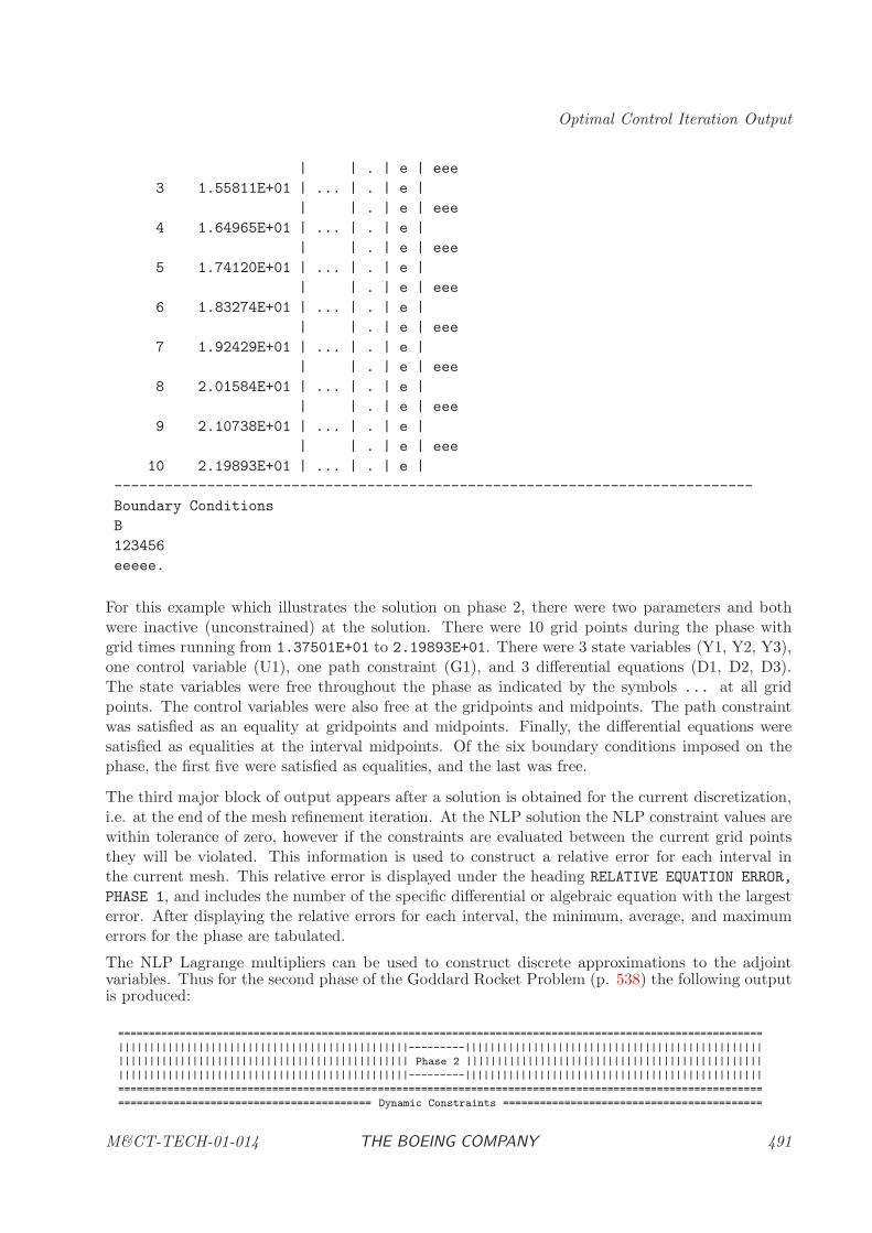
Optimal Control Iteration Output
| | . | e | eee
3 1.55811E+01 | ... | . | e |
| | . | e | eee
4 1.64965E+01 | ... | . | e |
| | . | e | eee
5 1.74120E+01 | ... | . | e |
| | . | e | eee
6 1.83274E+01 | ... | . | e |
| | . | e | eee
7 1.92429E+01 | ... | . | e |
| | . | e | eee
8 2.01584E+01 | ... | . | e |
| | . | e | eee
9 2.10738E+01 | ... | . | e |
| | . | e | eee
10 2.19893E+01 | ... | . | e |
----------------------------------------------------------------------------
Boundary Conditions
B
123456
eeeee.
For this example which illustrates the solution on phase 2, there were two parameters and bothwere inactive (unconstrained) at the solution. There were 10 grid points during the phase withgrid times running from 1.37501E+01 to 2.19893E+01. There were 3 state variables (Y1, Y2, Y3),one control variable (U1), one path constraint (G1), and 3 differential equations (D1, D2, D3).The state variables were free throughout the phase as indicated by the symbols ... at all gridpoints. The control variables were also free at the gridpoints and midpoints. The path constraintwas satisfied as an equality at gridpoints and midpoints. Finally, the differential equations weresatisfied as equalities at the interval midpoints. Of the six boundary conditions imposed on thephase, the first five were satisfied as equalities, and the last was free.
The third major block of output appears after a solution is obtained for the current discretization,i.e. at the end of the mesh refinement iteration. At the NLP solution the NLP constraint values arewithin tolerance of zero, however if the constraints are evaluated between the current grid pointsthey will be violated. This information is used to construct a relative error for each interval inthe current mesh. This relative error is displayed under the heading RELATIVE EQUATION ERROR,
PHASE 1, and includes the number of the specific differential or algebraic equation with the largesterror. After displaying the relative errors for each interval, the minimum, average, and maximumerrors for the phase are tabulated.
The NLP Lagrange multipliers can be used to construct discrete approximations to the adjointvariables. Thus for the second phase of the Goddard Rocket Problem (p. 538) the following outputis produced:
========================================================================================================
|||||||||||||||||||||||||||||||||||||||||||||||---------||||||||||||||||||||||||||||||||||||||||||||||||
||||||||||||||||||||||||||||||||||||||||||||||| Phase 2 ||||||||||||||||||||||||||||||||||||||||||||||||
|||||||||||||||||||||||||||||||||||||||||||||||---------||||||||||||||||||||||||||||||||||||||||||||||||
========================================================================================================
========================================= Dynamic Constraints ==========================================
M&CT-TECH-01-014 THE BOEING COMPANY 491
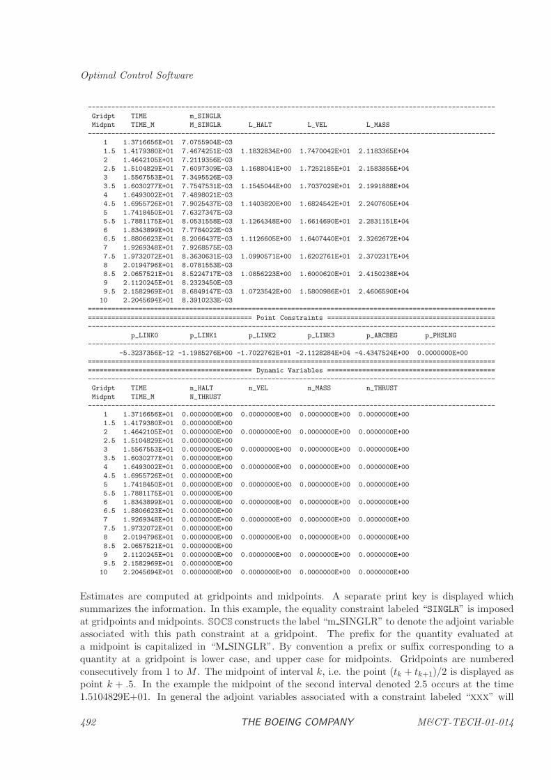
Optimal Control Software
--------------------------------------------------------------------------------------------------------
Gridpt TIME m_SINGLR
Midpnt TIME_M M_SINGLR L_HALT L_VEL L_MASS
--------------------------------------------------------------------------------------------------------
1 1.3716656E+01 7.0755904E-03
1.5 1.4179380E+01 7.4674251E-03 1.1832834E+00 1.7470042E+01 2.1183365E+04
2 1.4642105E+01 7.2119356E-03
2.5 1.5104829E+01 7.6097309E-03 1.1688041E+00 1.7252185E+01 2.1583855E+04
3 1.5567553E+01 7.3495526E-03
3.5 1.6030277E+01 7.7547531E-03 1.1545044E+00 1.7037029E+01 2.1991888E+04
4 1.6493002E+01 7.4898021E-03
4.5 1.6955726E+01 7.9025437E-03 1.1403820E+00 1.6824542E+01 2.2407605E+04
5 1.7418450E+01 7.6327347E-03
5.5 1.7881175E+01 8.0531558E-03 1.1264348E+00 1.6614690E+01 2.2831151E+04
6 1.8343899E+01 7.7784022E-03
6.5 1.8806623E+01 8.2066437E-03 1.1126605E+00 1.6407440E+01 2.3262672E+04
7 1.9269348E+01 7.9268575E-03
7.5 1.9732072E+01 8.3630631E-03 1.0990571E+00 1.6202761E+01 2.3702317E+04
8 2.0194796E+01 8.0781553E-03
8.5 2.0657521E+01 8.5224717E-03 1.0856223E+00 1.6000620E+01 2.4150238E+04
9 2.1120245E+01 8.2323450E-03
9.5 2.1582969E+01 8.6849147E-03 1.0723542E+00 1.5800986E+01 2.4606590E+04
10 2.2045694E+01 8.3910233E-03
========================================================================================================
========================================== Point Constraints ===========================================
--------------------------------------------------------------------------------------------------------
p_LINK0 p_LINK1 p_LINK2 p_LINK3 p_ARCBEG p_PHSLNG
--------------------------------------------------------------------------------------------------------
-5.3237356E-12 -1.1985276E+00 -1.7022762E+01 -2.1128284E+04 -4.4347524E+00 0.0000000E+00
========================================================================================================
========================================== Dynamic Variables ===========================================
--------------------------------------------------------------------------------------------------------
Gridpt TIME n_HALT n_VEL n_MASS n_THRUST
Midpnt TIME_M N_THRUST
--------------------------------------------------------------------------------------------------------
1 1.3716656E+01 0.0000000E+00 0.0000000E+00 0.0000000E+00 0.0000000E+00
1.5 1.4179380E+01 0.0000000E+00
2 1.4642105E+01 0.0000000E+00 0.0000000E+00 0.0000000E+00 0.0000000E+00
2.5 1.5104829E+01 0.0000000E+00
3 1.5567553E+01 0.0000000E+00 0.0000000E+00 0.0000000E+00 0.0000000E+00
3.5 1.6030277E+01 0.0000000E+00
4 1.6493002E+01 0.0000000E+00 0.0000000E+00 0.0000000E+00 0.0000000E+00
4.5 1.6955726E+01 0.0000000E+00
5 1.7418450E+01 0.0000000E+00 0.0000000E+00 0.0000000E+00 0.0000000E+00
5.5 1.7881175E+01 0.0000000E+00
6 1.8343899E+01 0.0000000E+00 0.0000000E+00 0.0000000E+00 0.0000000E+00
6.5 1.8806623E+01 0.0000000E+00
7 1.9269348E+01 0.0000000E+00 0.0000000E+00 0.0000000E+00 0.0000000E+00
7.5 1.9732072E+01 0.0000000E+00
8 2.0194796E+01 0.0000000E+00 0.0000000E+00 0.0000000E+00 0.0000000E+00
8.5 2.0657521E+01 0.0000000E+00
9 2.1120245E+01 0.0000000E+00 0.0000000E+00 0.0000000E+00 0.0000000E+00
9.5 2.1582969E+01 0.0000000E+00
10 2.2045694E+01 0.0000000E+00 0.0000000E+00 0.0000000E+00 0.0000000E+00
Estimates are computed at gridpoints and midpoints. A separate print key is displayed whichsummarizes the information. In this example, the equality constraint labeled “SINGLR” is imposedat gridpoints and midpoints. SOCS constructs the label “m SINGLR” to denote the adjoint variableassociated with this path constraint at a gridpoint. The prefix for the quantity evaluated ata midpoint is capitalized in “M SINGLR”. By convention a prefix or suffix corresponding to aquantity at a gridpoint is lower case, and upper case for midpoints. Gridpoints are numberedconsecutively from 1 to M . The midpoint of interval k, i.e. the point (tk + tk+1)/2 is displayed aspoint k + .5. In the example the midpoint of the second interval denoted 2.5 occurs at the time1.5104829E+01. In general the adjoint variables associated with a constraint labeled “xxx” will
492 THE BOEING COMPANY M&CT-TECH-01-014
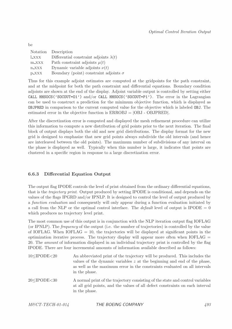
Optimal Control Iteration Output
be
Notation Descriptionl xxx Differential constraint adjoints λ(t)m xxx Path constraint adjoints µ(t)n xxx Dynamic variable adjoints ν(t)p xxx Boundary (point) constraint adjoints σ
Thus for this example adjoint estimates are computed at the gridpoints for the path constraint,and at the midpoint for both the path constraint and differential equations. Boundary conditionadjoints are shown at the end of the display. Adjoint variable output is controlled by setting eitherCALL HHSOCS(’SOCOUT=O1’) and/or CALL HHSOCS(’SOCOUT=P1’). The error in the Lagrangiancan be used to construct a prediction for the minimum objective function, which is displayed asOBJPRED in comparison to the current computed value for the objective which is labeled OBJ. Theestimated error in the objective function is ERROBJ = |OBJ - OBJPRED|.
After the discretization error is computed and displayed the mesh refinement procedure can utilizethis information to compute a new distribution of grid points prior to the next iteration. The finalblock of output displays both the old and new grid distributions. The display format for the newgrid is designed to emphasize that new grid points always subdivide the old intervals (and henceare interleaved between the old points). The maximum number of subdivisions of any interval onthe phase is displayed as well. Typically when this number is large, it indicates that points areclustered in a specific region in response to a large discretization error.
6.6.3 Differential Equation Output
The output flag IPODE controls the level of print obtained from the ordinary differential equations,that is the trajectory print. Output produced by setting IPODE is conditional, and depends on thevalues of the flags IPGRD and/or IPNLP. It is designed to control the level of output produced bya function evaluation and consequently will only appear during a function evaluation initiated bya call from the NLP or the optimal control interface. The default level of output is IPODE = 0which produces no trajectory level print.
The most common use of this output is in conjunction with the NLP iteration output flag IOFLAG(or IPNLP). The frequency of the output (i.e. the number of trajectories) is controlled by the valueof IOFLAG. When IOFLAG = 10, the trajectories will be displayed at significant points in theoptimization iterative process. The trajectory display will appear more often when IOFLAG =20. The amount of information displayed in an individual trajectory print is controlled by the flagIPODE. There are four incremental amounts of information available described as follows:
10≤IPODE<20 An abbreviated print of the trajectory will be produced. This includes thevalues of the dynamic variables z at the beginning and end of the phase,as well as the maximum error in the constraints evaluated on all intervalsin the phase.
20≤IPODE<30 A normal print of the trajectory consisting of the state and control variablesat all grid points, and the values of all defect constraints on each intervalin the phase.
M&CT-TECH-01-014 THE BOEING COMPANY 493
Optimal Control Software
30≤IPODE<40 The normal trajectory print obtained with IPODE = 20, is augmentedby the gradient vector, Jacobian matrix, and Hessian matrix displayed insparse format.
40≤IPODE All of the output obtained with IPODE = 30, is augmented by extensive di-agnostic information about each variable and constraint at the initial point.After information is displayed, SOCS terminates with an error condition.
6.6.4 Sparse Finite Difference Output
The output flag IPFSFD controls the level of print obtained from the sparse finite difference subrou-tines. This flag is identical to the quantity MSGLVL described in the documentation for subroutinesHDSFDH, HDSFDJ, and HSSFDI which is fully described in Section 3.2. The default level of outputis IPFSFD = 0 which produces no print from these routines.
494 THE BOEING COMPANY M&CT-TECH-01-014
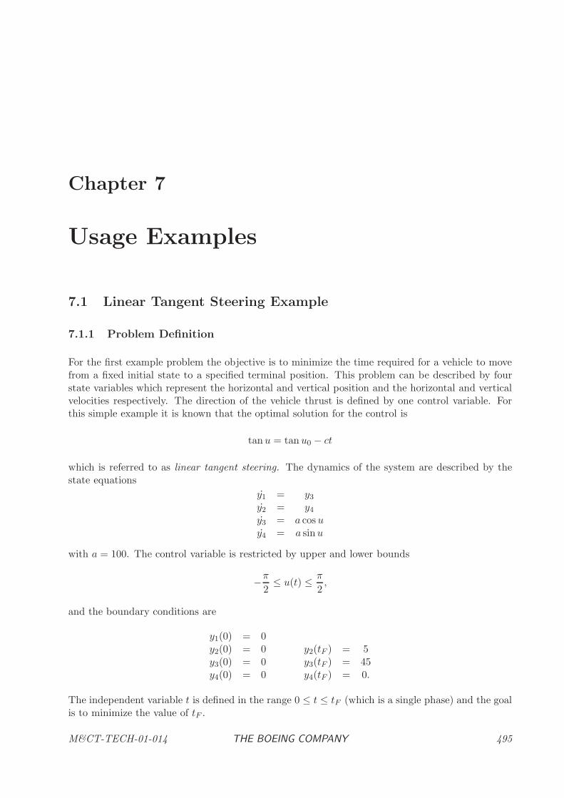
Chapter 7
Usage Examples
7.1 Linear Tangent Steering Example
7.1.1 Problem Definition
For the first example problem the objective is to minimize the time required for a vehicle to movefrom a fixed initial state to a specified terminal position. This problem can be described by fourstate variables which represent the horizontal and vertical position and the horizontal and verticalvelocities respectively. The direction of the vehicle thrust is defined by one control variable. Forthis simple example it is known that the optimal solution for the control is
tanu = tan u0 − ct
which is referred to as linear tangent steering. The dynamics of the system are described by thestate equations
y1 = y3
y2 = y4
y3 = a cos uy4 = a sinu
with a = 100. The control variable is restricted by upper and lower bounds
−π2≤ u(t) ≤ π
2,
and the boundary conditions are
y1(0) = 0y2(0) = 0 y2(tF ) = 5y3(0) = 0 y3(tF ) = 45y4(0) = 0 y4(tF ) = 0.
The independent variable t is defined in the range 0 ≤ t ≤ tF (which is a single phase) and the goalis to minimize the value of tF .
M&CT-TECH-01-014 THE BOEING COMPANY 495
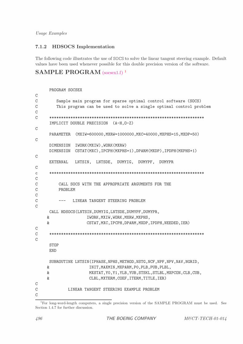
Usage Examples
7.1.2 HDSOCS Implementation
The following code illustrates the use of SOCS to solve the linear tangent steering example. Defaultvalues have been used whenever possible for this double precision version of the software.
SAMPLE PROGRAM (socsex1.f) 1
PROGRAM SOCSEX
C
C Sample main program for sparse optimal control software (SOCS)
C This program can be used to solve a single optimal control problem
C
C ******************************************************************
IMPLICIT DOUBLE PRECISION (A-H,O-Z)
C
PARAMETER (MXIW=600000,MXRW=1000000,MXC=40000,MXPHS=15,MXDP=50)
C
DIMENSION IWORK(MXIW),WORK(MXRW)
DIMENSION CSTAT(MXC),IPCPH(MXPHS+1),DPARM(MXDP),IPDPH(MXPHS+1)
C
EXTERNAL LNTSIN, LNTSDE, DUMYIG, DUMYPF, DUMYPR
C
c ******************************************************************
C
C CALL SOCS WITH THE APPROPRIATE ARGUMENTS FOR THE
C PROBLEM
C
C --- LINEAR TANGENT STEERING PROBLEM
C
CALL HDSOCS(LNTSIN,DUMYIG,LNTSDE,DUMYPF,DUMYPR,
& IWORK,MXIW,WORK,MXRW,MXPHS,
& CSTAT,MXC,IPCPH,DPARM,MXDP,IPDPH,NEEDED,IER)
C
C ******************************************************************
C
STOP
END
SUBROUTINE LNTSIN(IPHASE,NPHS,METHOD,NSTG,NCF,NPF,NPV,NAV,NGRID,
& INIT,MAXMIN,MXPARM,P0,PLB,PUB,PLBL,
& MXSTAT,Y0,Y1,YLB,YUB,STSKL,STLBL,MXPCON,CLB,CUB,
& CLBL,MXTERM,COEF,ITERM,TITLE,IER)
C
C LINEAR TANGENT STEERING EXAMPLE PROBLEM
C
1For long-word-length computers, a single precision version of the SAMPLE PROGRAM must be used. See
Section 1.4.7 for further discussion.
496 THE BOEING COMPANY M&CT-TECH-01-014
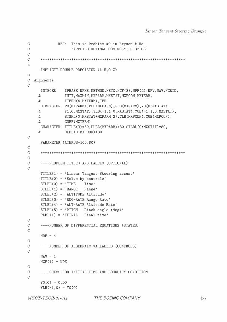
Linear Tangent Steering Example
C REF: This is Problem #9 in Bryson & Ho
C "APPLIED OPTIMAL CONTROL", P.82-83.
C
C ******************************************************************
c
IMPLICIT DOUBLE PRECISION (A-H,O-Z)
C
C Arguments:
C
INTEGER IPHASE,NPHS,METHOD,NSTG,NCF(3),NPF(2),NPV,NAV,NGRID,
& INIT,MAXMIN,MXPARM,MXSTAT,MXPCON,MXTERM,
& ITERM(4,MXTERM),IER
DIMENSION P0(MXPARM),PLB(MXPARM),PUB(MXPARM),Y0(0:MXSTAT),
& Y1(0:MXSTAT),YLB(-1:1,0:MXSTAT),YUB(-1:1,0:MXSTAT),
& STSKL(0:MXSTAT+MXPARM,2),CLB(MXPCON),CUB(MXPCON),
& COEF(MXTERM)
CHARACTER TITLE(3)*60,PLBL(MXPARM)*80,STLBL(0:MXSTAT)*80,
& CLBL(0:MXPCON)*80
C
PARAMETER (ATHRUS=100.D0)
C
C ******************************************************************
C
C ----PROBLEM TITLES AND LABELS (OPTIONAL)
C
TITLE(1) = ’Linear Tangent Steering ascent’
TITLE(2) = ’Solve by controls’
STLBL(0) = ’TIME Time’
STLBL(1) = ’RANGE Range’
STLBL(2) = ’ALTITUDE Altitude’
STLBL(3) = ’RNG-RATE Range Rate’
STLBL(4) = ’ALT-RATE Altitude Rate’
STLBL(5) = ’PITCH Pitch angle (deg)’
PLBL(1) = ’TFINAL Final time’
C
C ----NUMBER OF DIFFERENTIAL EQUATIONS (STATES)
C
NDE = 4
C
C ----NUMBER OF ALGEBRAIC VARIABLES (CONTROLS)
C
NAV = 1
NCF(1) = NDE
C
C ----GUESS FOR INITIAL TIME AND BOUNDARY CONDITION
C
Y0(0) = 0.D0
YLB(-1,0) = Y0(0)
M&CT-TECH-01-014 THE BOEING COMPANY 497
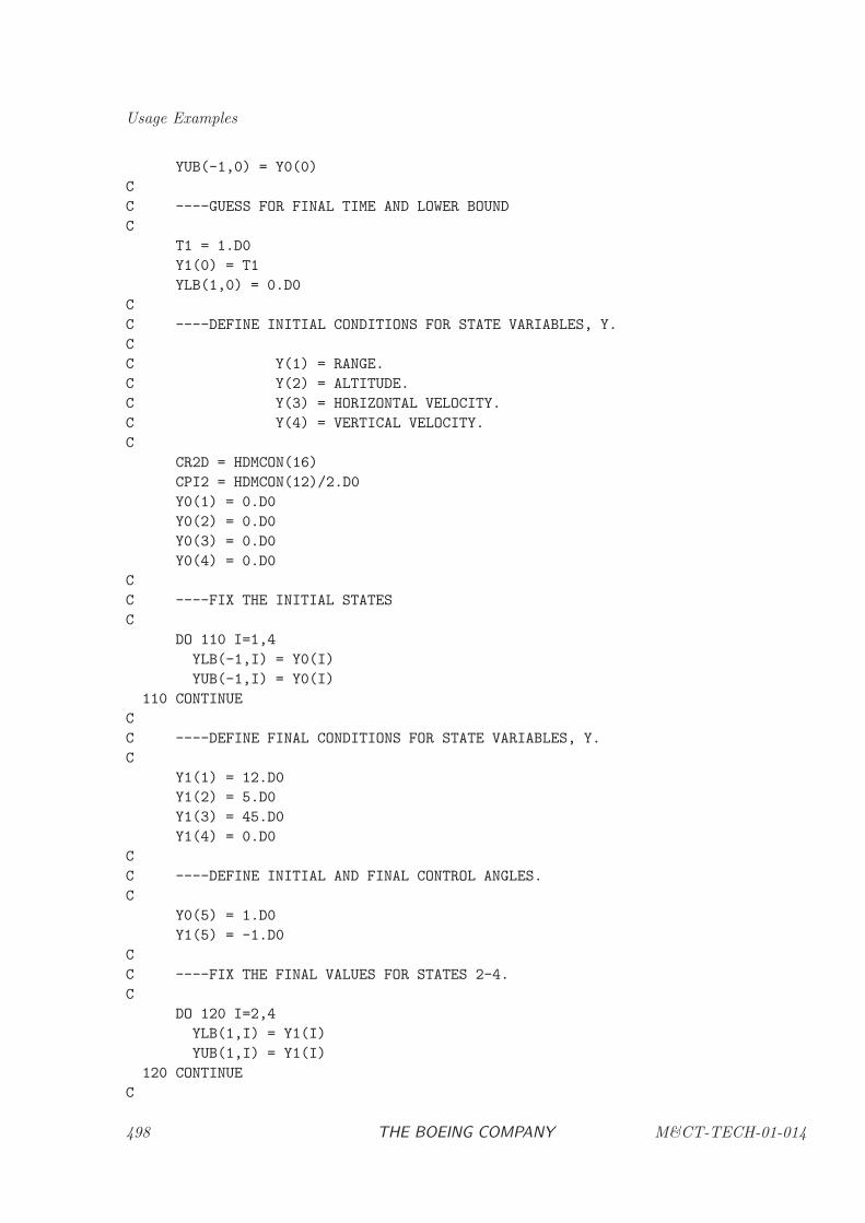
Usage Examples
YUB(-1,0) = Y0(0)
C
C ----GUESS FOR FINAL TIME AND LOWER BOUND
C
T1 = 1.D0
Y1(0) = T1
YLB(1,0) = 0.D0
C
C ----DEFINE INITIAL CONDITIONS FOR STATE VARIABLES, Y.
C
C Y(1) = RANGE.
C Y(2) = ALTITUDE.
C Y(3) = HORIZONTAL VELOCITY.
C Y(4) = VERTICAL VELOCITY.
C
CR2D = HDMCON(16)
CPI2 = HDMCON(12)/2.D0
Y0(1) = 0.D0
Y0(2) = 0.D0
Y0(3) = 0.D0
Y0(4) = 0.D0
C
C ----FIX THE INITIAL STATES
C
DO 110 I=1,4
YLB(-1,I) = Y0(I)
YUB(-1,I) = Y0(I)
110 CONTINUE
C
C ----DEFINE FINAL CONDITIONS FOR STATE VARIABLES, Y.
C
Y1(1) = 12.D0
Y1(2) = 5.D0
Y1(3) = 45.D0
Y1(4) = 0.D0
C
C ----DEFINE INITIAL AND FINAL CONTROL ANGLES.
C
Y0(5) = 1.D0
Y1(5) = -1.D0
C
C ----FIX THE FINAL VALUES FOR STATES 2-4.
C
DO 120 I=2,4
YLB(1,I) = Y1(I)
YUB(1,I) = Y1(I)
120 CONTINUE
C
498 THE BOEING COMPANY M&CT-TECH-01-014
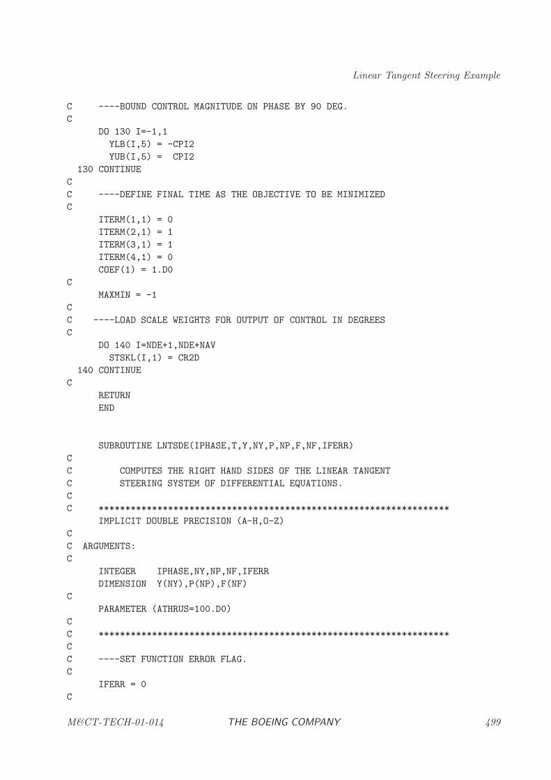
Linear Tangent Steering Example
C ----BOUND CONTROL MAGNITUDE ON PHASE BY 90 DEG.
C
DO 130 I=-1,1
YLB(I,5) = -CPI2
YUB(I,5) = CPI2
130 CONTINUE
C
C ----DEFINE FINAL TIME AS THE OBJECTIVE TO BE MINIMIZED
C
ITERM(1,1) = 0
ITERM(2,1) = 1
ITERM(3,1) = 1
ITERM(4,1) = 0
COEF(1) = 1.D0
C
MAXMIN = -1
C
C ----LOAD SCALE WEIGHTS FOR OUTPUT OF CONTROL IN DEGREES
C
DO 140 I=NDE+1,NDE+NAV
STSKL(I,1) = CR2D
140 CONTINUE
C
RETURN
END
SUBROUTINE LNTSDE(IPHASE,T,Y,NY,P,NP,F,NF,IFERR)
C
C COMPUTES THE RIGHT HAND SIDES OF THE LINEAR TANGENT
C STEERING SYSTEM OF DIFFERENTIAL EQUATIONS.
C
C ******************************************************************
IMPLICIT DOUBLE PRECISION (A-H,O-Z)
C
C ARGUMENTS:
C
INTEGER IPHASE,NY,NP,NF,IFERR
DIMENSION Y(NY),P(NP),F(NF)
C
PARAMETER (ATHRUS=100.D0)
C
C ******************************************************************
C
C ----SET FUNCTION ERROR FLAG.
C
IFERR = 0
C
M&CT-TECH-01-014 THE BOEING COMPANY 499
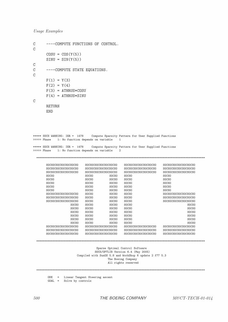
Usage Examples
C ----COMPUTE FUNCTIONS OF CONTROL.
C
COSU = COS(Y(5))
SINU = SIN(Y(5))
C
C ----COMPUTE STATE EQUATIONS.
C
F(1) = Y(3)
F(2) = Y(4)
F(3) = ATHRUS*COSU
F(4) = ATHRUS*SINU
C
RETURN
END
***** SOCS WARNING: IER = 1478 Compute Sparsity Pattern for User Supplied Functions
>>>>> Phase 1: No function depends on variable 1
***** SOCS WARNING: IER = 1478 Compute Sparsity Pattern for User Supplied Functions
>>>>> Phase 1: No function depends on variable 2
========================================================================================================
SOCSOCSOCSOCSOCSOCSO SOCSOCSOCSOCSOCSOCSO SOCSOCSOCSOCSOCSOCSO SOCSOCSOCSOCSOCSOCSO
SOCSOCSOCSOCSOCSOCSO SOCSOCSOCSOCSOCSOCSO SOCSOCSOCSOCSOCSOCSO SOCSOCSOCSOCSOCSOCSO
SOCSOCSOCSOCSOCSOCSO SOCSOCSOCSOCSOCSOCSO SOCSOCSOCSOCSOCSOCSO SOCSOCSOCSOCSOCSOCSO
SOCSO SOCSO SOCSO SOCSO SOCSO
SOCSO SOCSO SOCSO SOCSO SOCSO
SOCSO SOCSO SOCSO SOCSO SOCSO
SOCSO SOCSO SOCSO SOCSO SOCSO
SOCSO SOCSO SOCSO SOCSO SOCSO
SOCSOCSOCSOCSOCSOCSO SOCSO SOCSO SOCSO SOCSOCSOCSOCSOCSOCSO
SOCSOCSOCSOCSOCSOCSO SOCSO SOCSO SOCSO SOCSOCSOCSOCSOCSOCSO
SOCSOCSOCSOCSOCSOCSO SOCSO SOCSO SOCSO SOCSOCSOCSOCSOCSOCSO
SOCSO SOCSO SOCSO SOCSO SOCSO
SOCSO SOCSO SOCSO SOCSO SOCSO
SOCSO SOCSO SOCSO SOCSO SOCSO
SOCSO SOCSO SOCSO SOCSO SOCSO
SOCSO SOCSO SOCSO SOCSO SOCSO
SOCSO SOCSO SOCSO SOCSO SOCSO
SOCSOCSOCSOCSOCSOCSO SOCSOCSOCSOCSOCSOCSO SOCSOCSOCSOCSOCSOCSO SOCSOCSOCSOCSOCSOCSO
SOCSOCSOCSOCSOCSOCSO SOCSOCSOCSOCSOCSOCSO SOCSOCSOCSOCSOCSOCSO SOCSOCSOCSOCSOCSOCSO
SOCSOCSOCSOCSOCSOCSO SOCSOCSOCSOCSOCSOCSO SOCSOCSOCSOCSOCSOCSO SOCSOCSOCSOCSOCSOCSO
========================================================================================================
Sparse Optimal Control Software
SOCS/OPTLIB Version 6.4 (May 2005)
Compiled with SunOS 5.8 and WorkShop 6 update 2 f77 5.3
The Boeing Company
All rights reserved
========================================================================================================
ODE = Linear Tangent Steering ascent
GOAL = Solve by controls
500 THE BOEING COMPANY M&CT-TECH-01-014
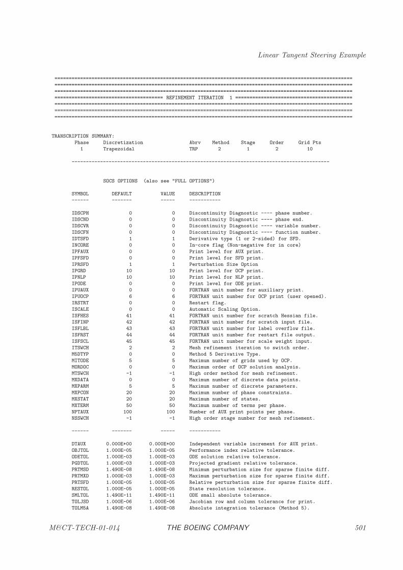
Linear Tangent Steering Example
========================================================================================================
========================================================================================================
========================================================================================================
====================================== REFINEMENT ITERATION 1 =========================================
========================================================================================================
========================================================================================================
========================================================================================================
TRANSCRIPTION SUMMARY:
Phase Discretization Abrv Method Stage Order Grid Pts
1 Trapezoidal TRP 2 1 2 10
------------------------------------------------------------------------------------------
SOCS OPTIONS (also see "FULL OPTIONS")
SYMBOL DEFAULT VALUE DESCRIPTION
------ ------- ----- -----------
IDSCPH 0 0 Discontinuity Diagnostic ---- phase number.
IDSCND 0 0 Discontinuity Diagnostic ---- phase end.
IDSCVR 0 0 Discontinuity Diagnostic ---- variable number.
IDSCFN 0 0 Discontinuity Diagnostic ---- function number.
IDTSFD 1 1 Derivative type (1 or 2-sided) for SFD.
INCORE 0 0 In-core flag (Non-negative for in core)
IPFAUX 0 0 Print level for AUX print.
IPFSFD 0 0 Print level for SFD print.
IPRSFD 1 1 Perturbation Size Option
IPGRD 10 10 Print level for OCP print.
IPNLP 10 10 Print level for NLP print.
IPODE 0 0 Print level for ODE print.
IPUAUX 0 0 FORTRAN unit number for auxiliary print.
IPUOCP 6 6 FORTRAN unit number for OCP print (user opened).
IRSTRT 0 0 Restart flag.
ISCALE 0 0 Automatic Scaling Option.
ISFHES 41 41 FORTRAN unit number for scratch Hessian file.
ISFINP 42 42 FORTRAN unit number for scratch input file.
ISFLBL 43 43 FORTRAN unit number for label overflow file.
ISFRST 44 44 FORTRAN unit number for restart file output.
ISFSCL 45 45 FORTRAN unit number for scale weight input.
ITSWCH 2 2 Mesh refinement iteration to switch order.
M5DTYP 0 0 Method 5 Derivative Type.
MITODE 5 5 Maximum number of grids used by OCP.
MORDOC 0 0 Maximum order of OCP solution analysis.
MTSWCH -1 -1 High order method for mesh refinement.
MXDATA 0 0 Maximum number of discrete data points.
MXPARM 5 5 Maximum number of discrete parameters.
MXPCON 20 20 Maximum number of phase constraints.
MXSTAT 20 20 Maximum number of states.
MXTERM 50 50 Maximum number of terms per phase.
NPTAUX 100 100 Number of AUX print points per phase.
NSSWCH -1 -1 High order stage number for mesh refinement.
------ ------- ----- -----------
DTAUX 0.000E+00 0.000E+00 Independent variable increment for AUX print.
OBJTOL 1.000E-05 1.000E-05 Performance index relative tolerance.
ODETOL 1.000E-03 1.000E-03 ODE solution relative tolerance.
PGDTOL 1.000E-03 1.000E-03 Projected gradient relative tolerance.
PRTMSD 1.490E-08 1.490E-08 Minimum perturbation size for sparse finite diff.
PRTMXD 1.000E-03 1.000E-03 Maximum perturbation size for sparse finite diff.
PRTSFD 1.000E-05 1.000E-05 Relative perturbation size for sparse finite diff.
RESTOL 1.000E-05 1.000E-05 State resolution tolerance.
SMLTOL 1.490E-11 1.490E-11 ODE small absolute tolerance.
TOLJSD 1.000E-06 1.000E-06 Jacobian row and column tolerance for print.
TOLM5A 1.490E-08 1.490E-08 Absolute integration tolerance (Method 5).
M&CT-TECH-01-014 THE BOEING COMPANY 501
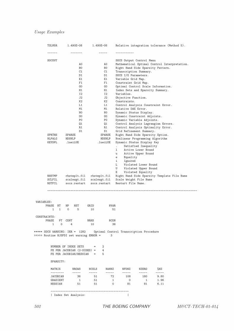
Usage Examples
TOLM5R 1.490E-08 1.490E-08 Relative integration tolerance (Method 5).
------ ------- ----- -----------
SOCOUT SOCS Output Control Menu
A0 A0 Mathematical Optimal Control Interpretation.
B0 B0 Right Hand Side Sparsity Pattern.
C1 C1 Transcription Summary.
D1 D1 SOCS I/O Parameters.
E1 E1 Variable Grid Map.
F1 F1 Constraint Grid Map.
G0 G0 Optimal Control Scale Information.
H1 H1 Index Sets and Sparsity Summary.
I2 I2 Variables.
J2 J2 Objective Function.
K2 K2 Constraints.
L1 L1 Control Analysis Constraint Error.
M1 M1 Relative DAE Error.
N0 N0 Dynamic Status Display.
O0 O0 Dynamic Constraint Adjoints.
P0 P0 Dynamic Variable Adjoints.
Q1 Q1 Control Analysis Lagrangian Errors.
R1 R1 Control Analysis Optimality Error.
S1 S1 Grid Refinement Summary.
SPRTHS SPARSE SPARSE Right Hand Side Sparsity Option.
NLPALG HDSNLP HDSNLP Nonlinear Programming Algorithm
KEYDPL .lueiLUE .lueiLUE Dynamic Status Display Key
. Satisfied Inequality
l Active Lower Bound
u Active Upper Bound
e Equality
i Ignored
L Violated Lower Bound
U Violated Upper Bound
E Violated Equality
RHSTMP rhstmplt.fil rhstmplt.fil Right Hand Side Sparsity Template File Name
SCLFIL scalewgt.fil scalewgt.fil Scale Weight File Name
RSTFIL socs.restart socs.restart Restart File Name.
------------------------------------------------------------------------------------------
VARIABLES:
PHASE NT NP NST GRID NVAR
1 1 0 5 10 51
CONSTRAINTS:
PHASE PT CONT NRHS NCON
1 0 4 10 36
***** SOCS WARNING: IER = 1282 Optimal Control Transcription Procedure
>>>>> Routine HJSFDI set warning ERROR = 3
NUMBER OF INDEX SETS = 2
FE PER JACOBIAN (2-SIDED) = 4
FE PER JACOBIAN/HESSIAN = 5
SPARSITY:
MATRIX NROWS NCOLS NANNZ NFDNZ NZERO %NZ
-------- ----- ----- ----- ----- ----- -----
JACOBIAN 36 51 72 108 180 9.80
GRADIENT 1 51 1 0 1 1.96
HESSIAN 51 51 0 81 81 6.11
-----------------------------------------------
| Index Set Analysis: |
502 THE BOEING COMPANY M&CT-TECH-01-014
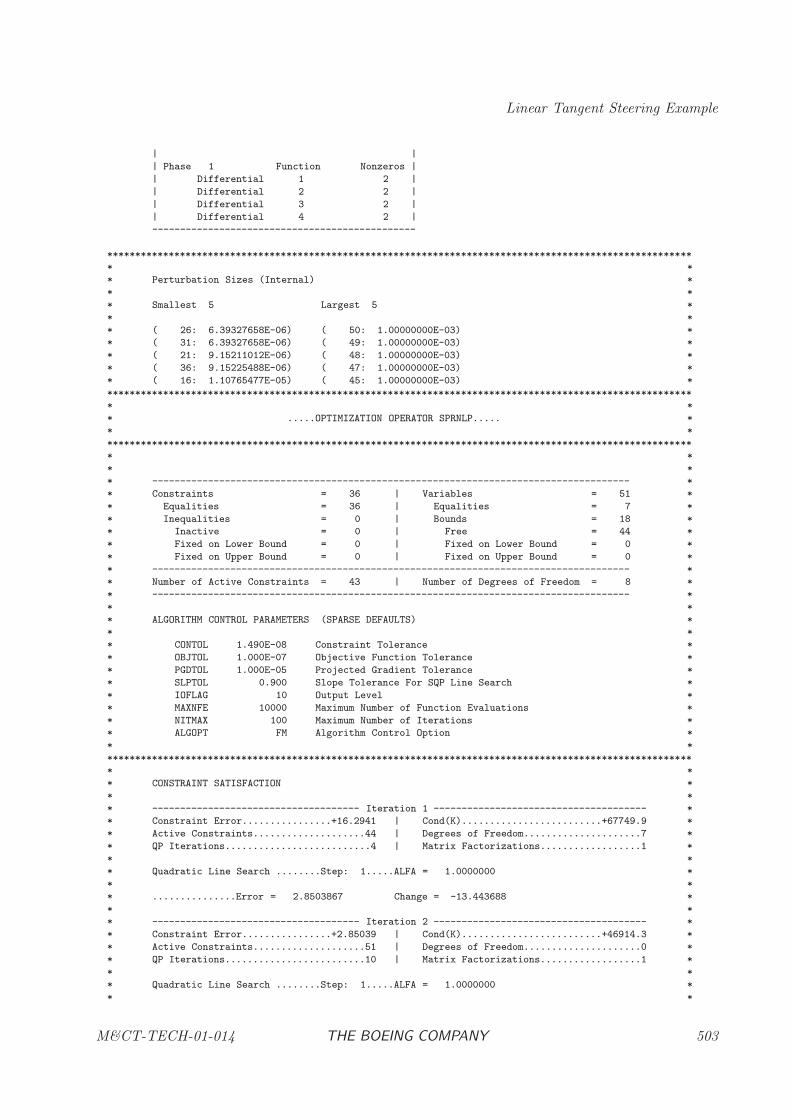
Linear Tangent Steering Example
| |
| Phase 1 Function Nonzeros |
| Differential 1 2 |
| Differential 2 2 |
| Differential 3 2 |
| Differential 4 2 |
-----------------------------------------------
********************************************************************************************************
* *
* Perturbation Sizes (Internal) *
* *
* Smallest 5 Largest 5 *
* *
* ( 26: 6.39327658E-06) ( 50: 1.00000000E-03) *
* ( 31: 6.39327658E-06) ( 49: 1.00000000E-03) *
* ( 21: 9.15211012E-06) ( 48: 1.00000000E-03) *
* ( 36: 9.15225488E-06) ( 47: 1.00000000E-03) *
* ( 16: 1.10765477E-05) ( 45: 1.00000000E-03) *
********************************************************************************************************
* *
* .....OPTIMIZATION OPERATOR SPRNLP..... *
* *
********************************************************************************************************
* *
* *
* ------------------------------------------------------------------------------------- *
* Constraints = 36 | Variables = 51 *
* Equalities = 36 | Equalities = 7 *
* Inequalities = 0 | Bounds = 18 *
* Inactive = 0 | Free = 44 *
* Fixed on Lower Bound = 0 | Fixed on Lower Bound = 0 *
* Fixed on Upper Bound = 0 | Fixed on Upper Bound = 0 *
* ------------------------------------------------------------------------------------- *
* Number of Active Constraints = 43 | Number of Degrees of Freedom = 8 *
* ------------------------------------------------------------------------------------- *
* *
* ALGORITHM CONTROL PARAMETERS (SPARSE DEFAULTS) *
* *
* CONTOL 1.490E-08 Constraint Tolerance *
* OBJTOL 1.000E-07 Objective Function Tolerance *
* PGDTOL 1.000E-05 Projected Gradient Tolerance *
* SLPTOL 0.900 Slope Tolerance For SQP Line Search *
* IOFLAG 10 Output Level *
* MAXNFE 10000 Maximum Number of Function Evaluations *
* NITMAX 100 Maximum Number of Iterations *
* ALGOPT FM Algorithm Control Option *
* *
********************************************************************************************************
* *
* CONSTRAINT SATISFACTION *
* *
* ------------------------------------- Iteration 1 -------------------------------------- *
* Constraint Error................+16.2941 | Cond(K).........................+67749.9 *
* Active Constraints....................44 | Degrees of Freedom.....................7 *
* QP Iterations..........................4 | Matrix Factorizations..................1 *
* *
* Quadratic Line Search ........Step: 1.....ALFA = 1.0000000 *
* *
* ...............Error = 2.8503867 Change = -13.443688 *
* *
* ------------------------------------- Iteration 2 -------------------------------------- *
* Constraint Error................+2.85039 | Cond(K).........................+46914.3 *
* Active Constraints....................51 | Degrees of Freedom.....................0 *
* QP Iterations.........................10 | Matrix Factorizations..................1 *
* *
* Quadratic Line Search ........Step: 1.....ALFA = 1.0000000 *
* *
M&CT-TECH-01-014 THE BOEING COMPANY 503
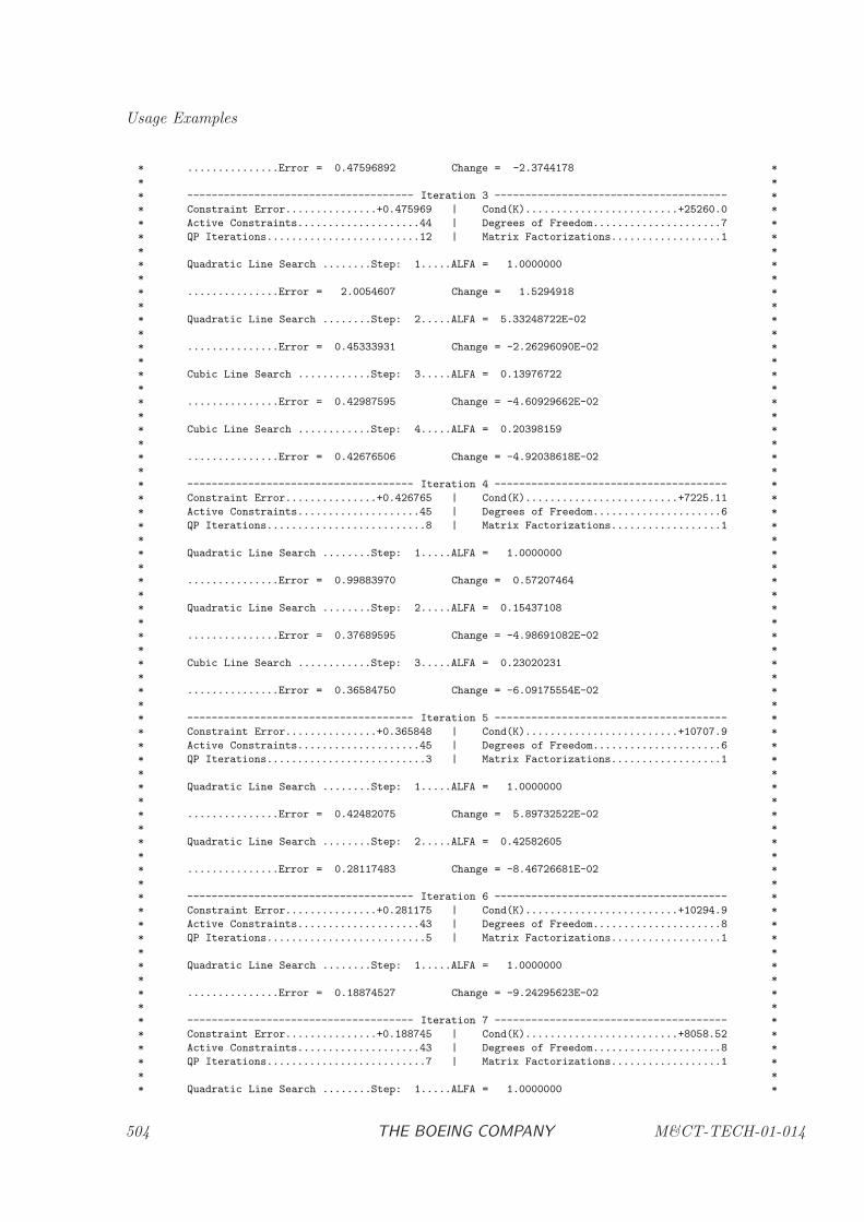
Usage Examples
* ...............Error = 0.47596892 Change = -2.3744178 *
* *
* ------------------------------------- Iteration 3 -------------------------------------- *
* Constraint Error...............+0.475969 | Cond(K).........................+25260.0 *
* Active Constraints....................44 | Degrees of Freedom.....................7 *
* QP Iterations.........................12 | Matrix Factorizations..................1 *
* *
* Quadratic Line Search ........Step: 1.....ALFA = 1.0000000 *
* *
* ...............Error = 2.0054607 Change = 1.5294918 *
* *
* Quadratic Line Search ........Step: 2.....ALFA = 5.33248722E-02 *
* *
* ...............Error = 0.45333931 Change = -2.26296090E-02 *
* *
* Cubic Line Search ............Step: 3.....ALFA = 0.13976722 *
* *
* ...............Error = 0.42987595 Change = -4.60929662E-02 *
* *
* Cubic Line Search ............Step: 4.....ALFA = 0.20398159 *
* *
* ...............Error = 0.42676506 Change = -4.92038618E-02 *
* *
* ------------------------------------- Iteration 4 -------------------------------------- *
* Constraint Error...............+0.426765 | Cond(K).........................+7225.11 *
* Active Constraints....................45 | Degrees of Freedom.....................6 *
* QP Iterations..........................8 | Matrix Factorizations..................1 *
* *
* Quadratic Line Search ........Step: 1.....ALFA = 1.0000000 *
* *
* ...............Error = 0.99883970 Change = 0.57207464 *
* *
* Quadratic Line Search ........Step: 2.....ALFA = 0.15437108 *
* *
* ...............Error = 0.37689595 Change = -4.98691082E-02 *
* *
* Cubic Line Search ............Step: 3.....ALFA = 0.23020231 *
* *
* ...............Error = 0.36584750 Change = -6.09175554E-02 *
* *
* ------------------------------------- Iteration 5 -------------------------------------- *
* Constraint Error...............+0.365848 | Cond(K).........................+10707.9 *
* Active Constraints....................45 | Degrees of Freedom.....................6 *
* QP Iterations..........................3 | Matrix Factorizations..................1 *
* *
* Quadratic Line Search ........Step: 1.....ALFA = 1.0000000 *
* *
* ...............Error = 0.42482075 Change = 5.89732522E-02 *
* *
* Quadratic Line Search ........Step: 2.....ALFA = 0.42582605 *
* *
* ...............Error = 0.28117483 Change = -8.46726681E-02 *
* *
* ------------------------------------- Iteration 6 -------------------------------------- *
* Constraint Error...............+0.281175 | Cond(K).........................+10294.9 *
* Active Constraints....................43 | Degrees of Freedom.....................8 *
* QP Iterations..........................5 | Matrix Factorizations..................1 *
* *
* Quadratic Line Search ........Step: 1.....ALFA = 1.0000000 *
* *
* ...............Error = 0.18874527 Change = -9.24295623E-02 *
* *
* ------------------------------------- Iteration 7 -------------------------------------- *
* Constraint Error...............+0.188745 | Cond(K).........................+8058.52 *
* Active Constraints....................43 | Degrees of Freedom.....................8 *
* QP Iterations..........................7 | Matrix Factorizations..................1 *
* *
* Quadratic Line Search ........Step: 1.....ALFA = 1.0000000 *
504 THE BOEING COMPANY M&CT-TECH-01-014
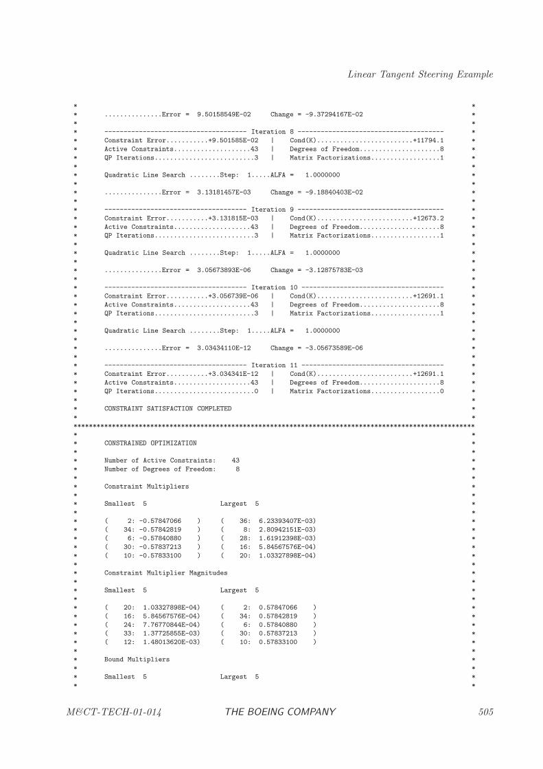
Linear Tangent Steering Example
* *
* ...............Error = 9.50158549E-02 Change = -9.37294167E-02 *
* *
* ------------------------------------- Iteration 8 -------------------------------------- *
* Constraint Error...........+9.501585E-02 | Cond(K).........................+11794.1 *
* Active Constraints....................43 | Degrees of Freedom.....................8 *
* QP Iterations..........................3 | Matrix Factorizations..................1 *
* *
* Quadratic Line Search ........Step: 1.....ALFA = 1.0000000 *
* *
* ...............Error = 3.13181457E-03 Change = -9.18840403E-02 *
* *
* ------------------------------------- Iteration 9 -------------------------------------- *
* Constraint Error...........+3.131815E-03 | Cond(K).........................+12673.2 *
* Active Constraints....................43 | Degrees of Freedom.....................8 *
* QP Iterations..........................3 | Matrix Factorizations..................1 *
* *
* Quadratic Line Search ........Step: 1.....ALFA = 1.0000000 *
* *
* ...............Error = 3.05673893E-06 Change = -3.12875783E-03 *
* *
* ------------------------------------- Iteration 10 ------------------------------------- *
* Constraint Error...........+3.056739E-06 | Cond(K).........................+12691.1 *
* Active Constraints....................43 | Degrees of Freedom.....................8 *
* QP Iterations..........................3 | Matrix Factorizations..................1 *
* *
* Quadratic Line Search ........Step: 1.....ALFA = 1.0000000 *
* *
* ...............Error = 3.03434110E-12 Change = -3.05673589E-06 *
* *
* ------------------------------------- Iteration 11 ------------------------------------- *
* Constraint Error...........+3.034341E-12 | Cond(K).........................+12691.1 *
* Active Constraints....................43 | Degrees of Freedom.....................8 *
* QP Iterations..........................0 | Matrix Factorizations..................0 *
* *
* CONSTRAINT SATISFACTION COMPLETED *
* *
********************************************************************************************************
* *
* CONSTRAINED OPTIMIZATION *
* *
* Number of Active Constraints: 43 *
* Number of Degrees of Freedom: 8 *
* *
* Constraint Multipliers *
* *
* Smallest 5 Largest 5 *
* *
* ( 2: -0.57847066 ) ( 36: 6.23393407E-03) *
* ( 34: -0.57842819 ) ( 8: 2.80942151E-03) *
* ( 6: -0.57840880 ) ( 28: 1.61912398E-03) *
* ( 30: -0.57837213 ) ( 16: 5.84567576E-04) *
* ( 10: -0.57833100 ) ( 20: 1.03327898E-04) *
* *
* Constraint Multiplier Magnitudes *
* *
* Smallest 5 Largest 5 *
* *
* ( 20: 1.03327898E-04) ( 2: 0.57847066 ) *
* ( 16: 5.84567576E-04) ( 34: 0.57842819 ) *
* ( 24: 7.76770844E-04) ( 6: 0.57840880 ) *
* ( 33: 1.37725855E-03) ( 30: 0.57837213 ) *
* ( 12: 1.48013620E-03) ( 10: 0.57833100 ) *
* *
* Bound Multipliers *
* *
* Smallest 5 Largest 5 *
* *
M&CT-TECH-01-014 THE BOEING COMPANY 505
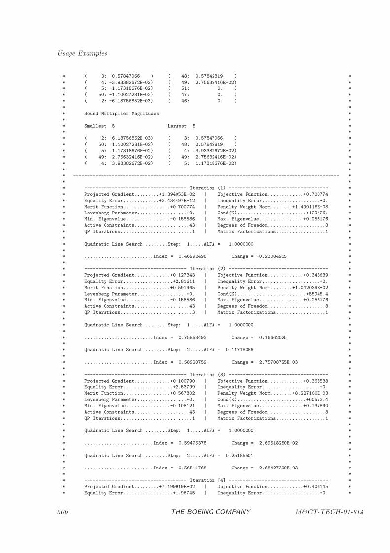
Usage Examples
* ( 3: -0.57847066 ) ( 48: 0.57842819 ) *
* ( 4: -3.93382672E-02) ( 49: 2.75632416E-02) *
* ( 5: -1.17318676E-02) ( 51: 0. ) *
* ( 50: -1.10027281E-02) ( 47: 0. ) *
* ( 2: -6.18756852E-03) ( 46: 0. ) *
* *
* Bound Multiplier Magnitudes *
* *
* Smallest 5 Largest 5 *
* *
* ( 2: 6.18756852E-03) ( 3: 0.57847066 ) *
* ( 50: 1.10027281E-02) ( 48: 0.57842819 ) *
* ( 5: 1.17318676E-02) ( 4: 3.93382672E-02) *
* ( 49: 2.75632416E-02) ( 49: 2.75632416E-02) *
* ( 4: 3.93382672E-02) ( 5: 1.17318676E-02) *
* *
* ------------------------------------------------------------------------------------------------ *
* *
* ------------------------------------- Iteration (1) ------------------------------------ *
* Projected Gradient.........+1.394053E-02 | Objective Function.............+0.700774 *
* Equality Error.............+2.434497E-12 | Inequality Error.....................+0. *
* Merit Function.................+0.700774 | Penalty Weight Norm........+1.490116E-08 *
* Levenberg Parameter..................+0. | Cond(K).........................+129426. *
* Min. Eigenvalue................-0.158586 | Max. Eigenvalue................+0.256176 *
* Active Constraints....................43 | Degrees of Freedom.....................8 *
* QP Iterations..........................1 | Matrix Factorizations..................1 *
* *
* Quadratic Line Search ........Step: 1.....ALFA = 1.0000000 *
* *
* .........................Index = 0.46992496 Change = -0.23084915 *
* *
* ------------------------------------- Iteration (2) ------------------------------------ *
* Projected Gradient.............+0.127343 | Objective Function.............+0.345639 *
* Equality Error..................+2.81611 | Inequality Error.....................+0. *
* Merit Function.................+0.591965 | Penalty Weight Norm........+1.042039E-02 *
* Levenberg Parameter..................+0. | Cond(K).........................+55945.4 *
* Min. Eigenvalue................-0.158586 | Max. Eigenvalue................+0.256176 *
* Active Constraints....................43 | Degrees of Freedom.....................8 *
* QP Iterations..........................3 | Matrix Factorizations..................1 *
* *
* Quadratic Line Search ........Step: 1.....ALFA = 1.0000000 *
* *
* .........................Index = 0.75858493 Change = 0.16662025 *
* *
* Quadratic Line Search ........Step: 2.....ALFA = 0.11718086 *
* *
* .........................Index = 0.58920759 Change = -2.75708725E-03 *
* *
* ------------------------------------- Iteration (3) ------------------------------------ *
* Projected Gradient.............+0.100790 | Objective Function.............+0.365538 *
* Equality Error..................+2.53799 | Inequality Error.....................+0. *
* Merit Function.................+0.567802 | Penalty Weight Norm........+8.227100E-03 *
* Levenberg Parameter..................+0. | Cond(K).........................+60573.4 *
* Min. Eigenvalue................-0.108121 | Max. Eigenvalue................+0.137890 *
* Active Constraints....................43 | Degrees of Freedom.....................8 *
* QP Iterations..........................1 | Matrix Factorizations..................1 *
* *
* Quadratic Line Search ........Step: 1.....ALFA = 1.0000000 *
* *
* .........................Index = 0.59475378 Change = 2.69518250E-02 *
* *
* Quadratic Line Search ........Step: 2.....ALFA = 0.25185501 *
* *
* .........................Index = 0.56511768 Change = -2.68427390E-03 *
* *
* ------------------------------------- Iteration [4] ------------------------------------ *
* Projected Gradient.........+7.199919E-02 | Objective Function.............+0.406145 *
* Equality Error..................+1.96745 | Inequality Error.....................+0. *
506 THE BOEING COMPANY M&CT-TECH-01-014
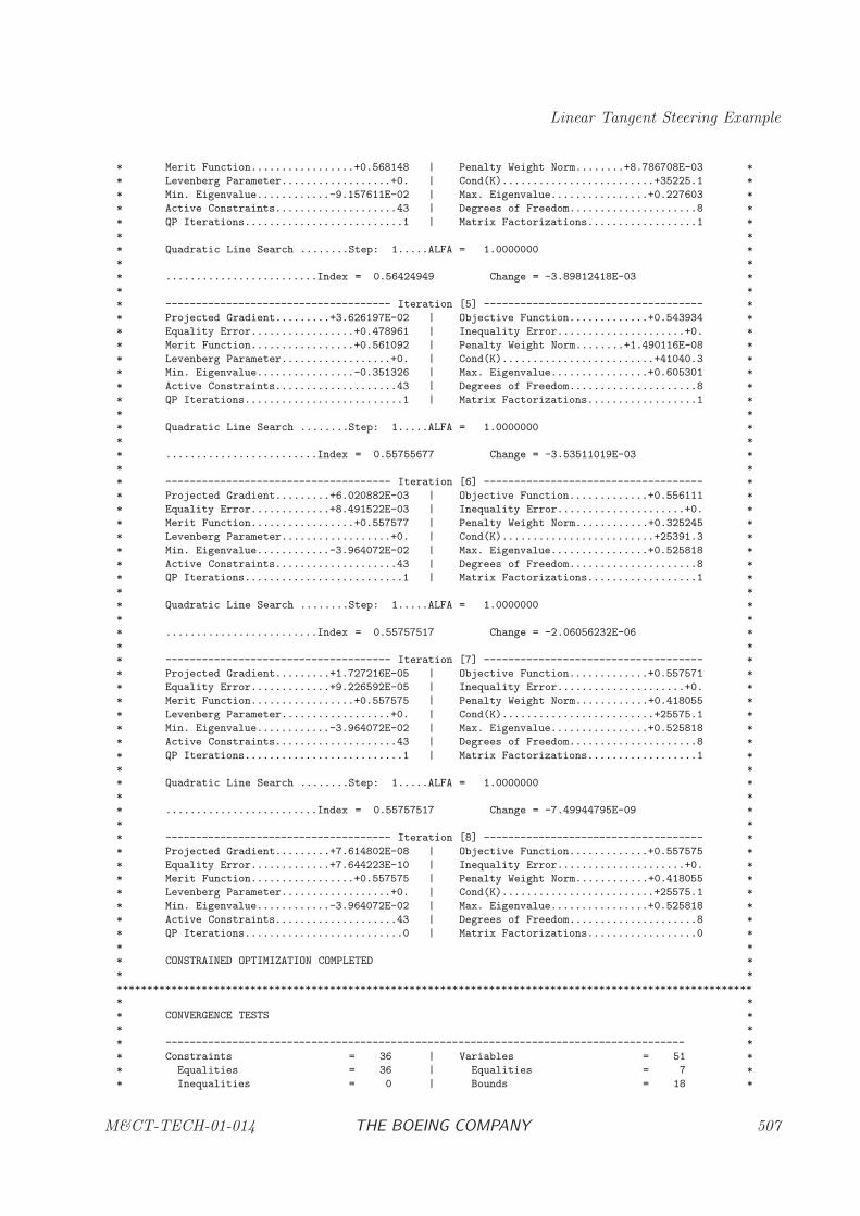
Linear Tangent Steering Example
* Merit Function.................+0.568148 | Penalty Weight Norm........+8.786708E-03 *
* Levenberg Parameter..................+0. | Cond(K).........................+35225.1 *
* Min. Eigenvalue............-9.157611E-02 | Max. Eigenvalue................+0.227603 *
* Active Constraints....................43 | Degrees of Freedom.....................8 *
* QP Iterations..........................1 | Matrix Factorizations..................1 *
* *
* Quadratic Line Search ........Step: 1.....ALFA = 1.0000000 *
* *
* .........................Index = 0.56424949 Change = -3.89812418E-03 *
* *
* ------------------------------------- Iteration [5] ------------------------------------ *
* Projected Gradient.........+3.626197E-02 | Objective Function.............+0.543934 *
* Equality Error.................+0.478961 | Inequality Error.....................+0. *
* Merit Function.................+0.561092 | Penalty Weight Norm........+1.490116E-08 *
* Levenberg Parameter..................+0. | Cond(K).........................+41040.3 *
* Min. Eigenvalue................-0.351326 | Max. Eigenvalue................+0.605301 *
* Active Constraints....................43 | Degrees of Freedom.....................8 *
* QP Iterations..........................1 | Matrix Factorizations..................1 *
* *
* Quadratic Line Search ........Step: 1.....ALFA = 1.0000000 *
* *
* .........................Index = 0.55755677 Change = -3.53511019E-03 *
* *
* ------------------------------------- Iteration [6] ------------------------------------ *
* Projected Gradient.........+6.020882E-03 | Objective Function.............+0.556111 *
* Equality Error.............+8.491522E-03 | Inequality Error.....................+0. *
* Merit Function.................+0.557577 | Penalty Weight Norm............+0.325245 *
* Levenberg Parameter..................+0. | Cond(K).........................+25391.3 *
* Min. Eigenvalue............-3.964072E-02 | Max. Eigenvalue................+0.525818 *
* Active Constraints....................43 | Degrees of Freedom.....................8 *
* QP Iterations..........................1 | Matrix Factorizations..................1 *
* *
* Quadratic Line Search ........Step: 1.....ALFA = 1.0000000 *
* *
* .........................Index = 0.55757517 Change = -2.06056232E-06 *
* *
* ------------------------------------- Iteration [7] ------------------------------------ *
* Projected Gradient.........+1.727216E-05 | Objective Function.............+0.557571 *
* Equality Error.............+9.226592E-05 | Inequality Error.....................+0. *
* Merit Function.................+0.557575 | Penalty Weight Norm............+0.418055 *
* Levenberg Parameter..................+0. | Cond(K).........................+25575.1 *
* Min. Eigenvalue............-3.964072E-02 | Max. Eigenvalue................+0.525818 *
* Active Constraints....................43 | Degrees of Freedom.....................8 *
* QP Iterations..........................1 | Matrix Factorizations..................1 *
* *
* Quadratic Line Search ........Step: 1.....ALFA = 1.0000000 *
* *
* .........................Index = 0.55757517 Change = -7.49944795E-09 *
* *
* ------------------------------------- Iteration [8] ------------------------------------ *
* Projected Gradient.........+7.614802E-08 | Objective Function.............+0.557575 *
* Equality Error.............+7.644223E-10 | Inequality Error.....................+0. *
* Merit Function.................+0.557575 | Penalty Weight Norm............+0.418055 *
* Levenberg Parameter..................+0. | Cond(K).........................+25575.1 *
* Min. Eigenvalue............-3.964072E-02 | Max. Eigenvalue................+0.525818 *
* Active Constraints....................43 | Degrees of Freedom.....................8 *
* QP Iterations..........................0 | Matrix Factorizations..................0 *
* *
* CONSTRAINED OPTIMIZATION COMPLETED *
* *
********************************************************************************************************
* *
* CONVERGENCE TESTS *
* *
* ------------------------------------------------------------------------------------- *
* Constraints = 36 | Variables = 51 *
* Equalities = 36 | Equalities = 7 *
* Inequalities = 0 | Bounds = 18 *
M&CT-TECH-01-014 THE BOEING COMPANY 507
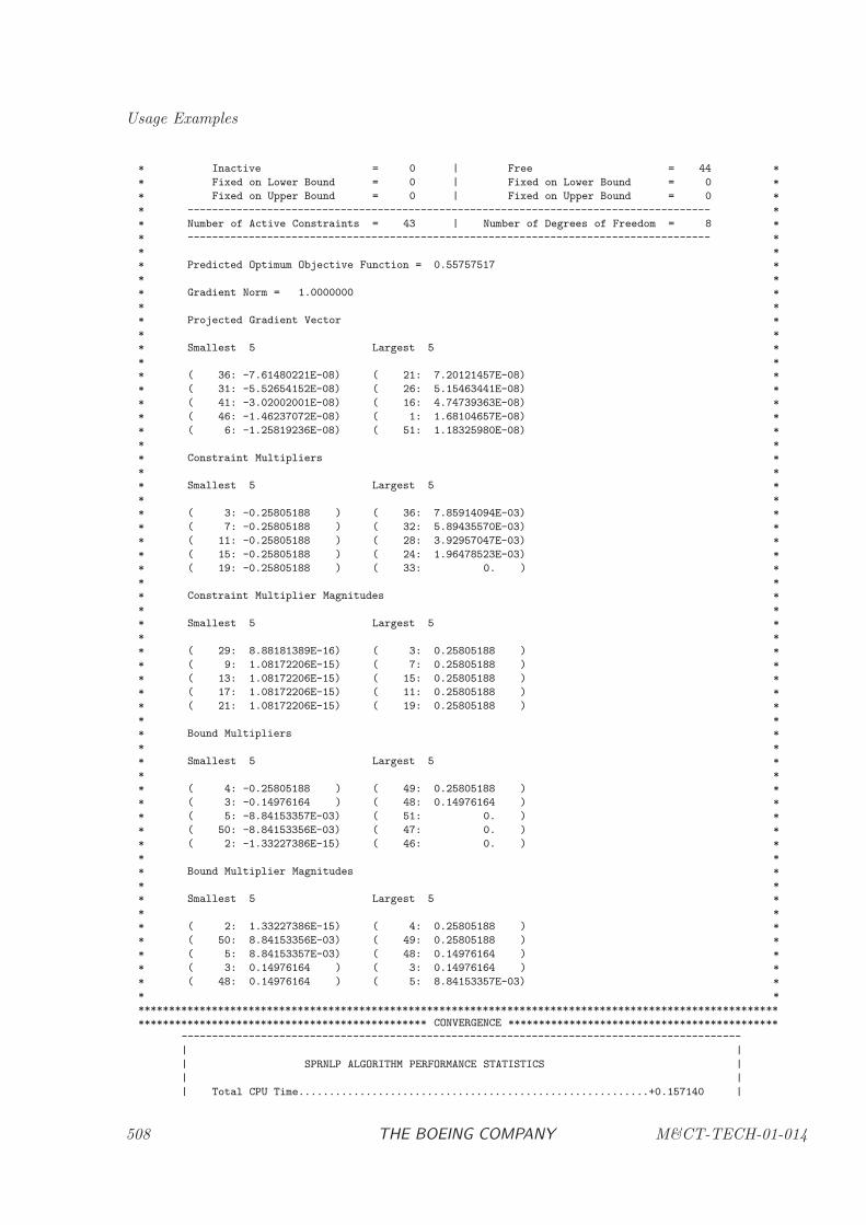
Usage Examples
* Inactive = 0 | Free = 44 *
* Fixed on Lower Bound = 0 | Fixed on Lower Bound = 0 *
* Fixed on Upper Bound = 0 | Fixed on Upper Bound = 0 *
* ------------------------------------------------------------------------------------- *
* Number of Active Constraints = 43 | Number of Degrees of Freedom = 8 *
* ------------------------------------------------------------------------------------- *
* *
* Predicted Optimum Objective Function = 0.55757517 *
* *
* Gradient Norm = 1.0000000 *
* *
* Projected Gradient Vector *
* *
* Smallest 5 Largest 5 *
* *
* ( 36: -7.61480221E-08) ( 21: 7.20121457E-08) *
* ( 31: -5.52654152E-08) ( 26: 5.15463441E-08) *
* ( 41: -3.02002001E-08) ( 16: 4.74739363E-08) *
* ( 46: -1.46237072E-08) ( 1: 1.68104657E-08) *
* ( 6: -1.25819236E-08) ( 51: 1.18325980E-08) *
* *
* Constraint Multipliers *
* *
* Smallest 5 Largest 5 *
* *
* ( 3: -0.25805188 ) ( 36: 7.85914094E-03) *
* ( 7: -0.25805188 ) ( 32: 5.89435570E-03) *
* ( 11: -0.25805188 ) ( 28: 3.92957047E-03) *
* ( 15: -0.25805188 ) ( 24: 1.96478523E-03) *
* ( 19: -0.25805188 ) ( 33: 0. ) *
* *
* Constraint Multiplier Magnitudes *
* *
* Smallest 5 Largest 5 *
* *
* ( 29: 8.88181389E-16) ( 3: 0.25805188 ) *
* ( 9: 1.08172206E-15) ( 7: 0.25805188 ) *
* ( 13: 1.08172206E-15) ( 15: 0.25805188 ) *
* ( 17: 1.08172206E-15) ( 11: 0.25805188 ) *
* ( 21: 1.08172206E-15) ( 19: 0.25805188 ) *
* *
* Bound Multipliers *
* *
* Smallest 5 Largest 5 *
* *
* ( 4: -0.25805188 ) ( 49: 0.25805188 ) *
* ( 3: -0.14976164 ) ( 48: 0.14976164 ) *
* ( 5: -8.84153357E-03) ( 51: 0. ) *
* ( 50: -8.84153356E-03) ( 47: 0. ) *
* ( 2: -1.33227386E-15) ( 46: 0. ) *
* *
* Bound Multiplier Magnitudes *
* *
* Smallest 5 Largest 5 *
* *
* ( 2: 1.33227386E-15) ( 4: 0.25805188 ) *
* ( 50: 8.84153356E-03) ( 49: 0.25805188 ) *
* ( 5: 8.84153357E-03) ( 48: 0.14976164 ) *
* ( 3: 0.14976164 ) ( 3: 0.14976164 ) *
* ( 48: 0.14976164 ) ( 5: 8.84153357E-03) *
* *
********************************************************************************************************
*********************************************** CONVERGENCE ********************************************
-------------------------------------------------------------------------------------------
| |
| SPRNLP ALGORITHM PERFORMANCE STATISTICS |
| |
| Total CPU Time.........................................................+0.157140 |
508 THE BOEING COMPANY M&CT-TECH-01-014
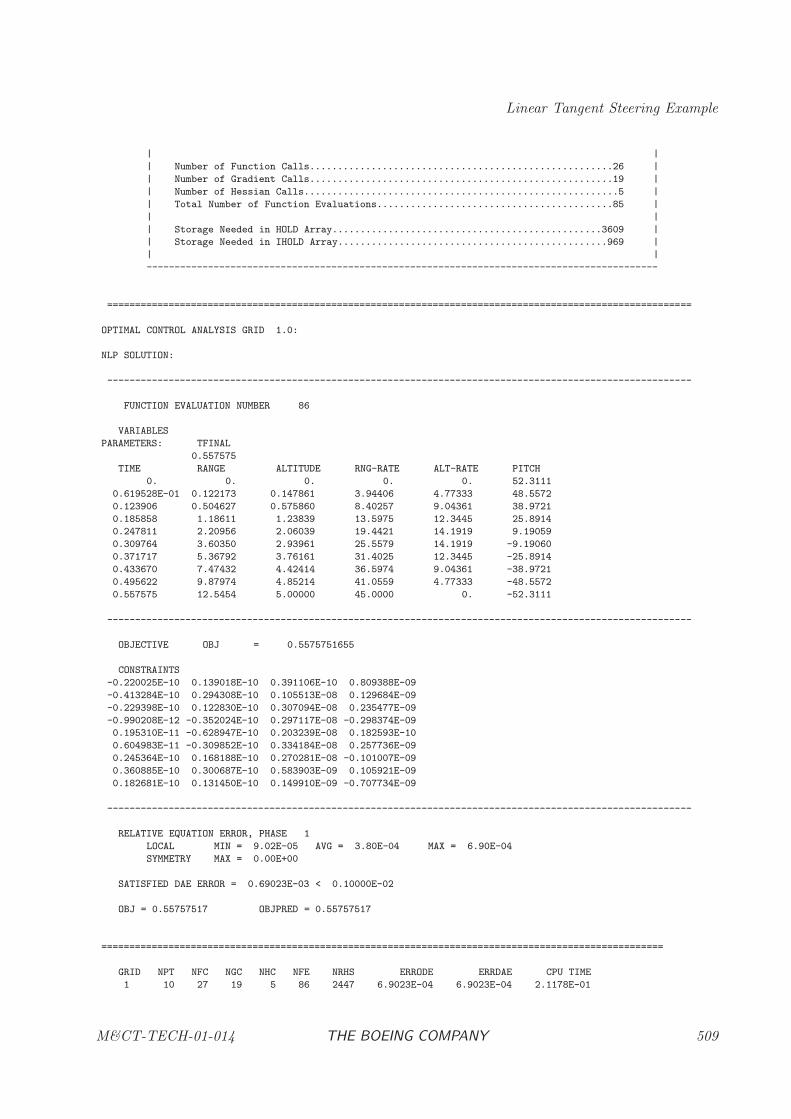
Linear Tangent Steering Example
| |
| Number of Function Calls......................................................26 |
| Number of Gradient Calls......................................................19 |
| Number of Hessian Calls........................................................5 |
| Total Number of Function Evaluations..........................................85 |
| |
| Storage Needed in HOLD Array................................................3609 |
| Storage Needed in IHOLD Array................................................969 |
| |
-------------------------------------------------------------------------------------------
========================================================================================================
OPTIMAL CONTROL ANALYSIS GRID 1.0:
NLP SOLUTION:
--------------------------------------------------------------------------------------------------------
FUNCTION EVALUATION NUMBER 86
VARIABLES
PARAMETERS: TFINAL
0.557575
TIME RANGE ALTITUDE RNG-RATE ALT-RATE PITCH
0. 0. 0. 0. 0. 52.3111
0.619528E-01 0.122173 0.147861 3.94406 4.77333 48.5572
0.123906 0.504627 0.575860 8.40257 9.04361 38.9721
0.185858 1.18611 1.23839 13.5975 12.3445 25.8914
0.247811 2.20956 2.06039 19.4421 14.1919 9.19059
0.309764 3.60350 2.93961 25.5579 14.1919 -9.19060
0.371717 5.36792 3.76161 31.4025 12.3445 -25.8914
0.433670 7.47432 4.42414 36.5974 9.04361 -38.9721
0.495622 9.87974 4.85214 41.0559 4.77333 -48.5572
0.557575 12.5454 5.00000 45.0000 0. -52.3111
--------------------------------------------------------------------------------------------------------
OBJECTIVE OBJ = 0.5575751655
CONSTRAINTS
-0.220025E-10 0.139018E-10 0.391106E-10 0.809388E-09
-0.413284E-10 0.294308E-10 0.105513E-08 0.129684E-09
-0.229398E-10 0.122830E-10 0.307094E-08 0.235477E-09
-0.990208E-12 -0.352024E-10 0.297117E-08 -0.298374E-09
0.195310E-11 -0.628947E-10 0.203239E-08 0.182593E-10
0.604983E-11 -0.309852E-10 0.334184E-08 0.257736E-09
0.245364E-10 0.168188E-10 0.270281E-08 -0.101007E-09
0.360885E-10 0.300687E-10 0.583903E-09 0.105921E-09
0.182681E-10 0.131450E-10 0.149910E-09 -0.707734E-09
--------------------------------------------------------------------------------------------------------
RELATIVE EQUATION ERROR, PHASE 1
LOCAL MIN = 9.02E-05 AVG = 3.80E-04 MAX = 6.90E-04
SYMMETRY MAX = 0.00E+00
SATISFIED DAE ERROR = 0.69023E-03 < 0.10000E-02
OBJ = 0.55757517 OBJPRED = 0.55757517
====================================================================================================
GRID NPT NFC NGC NHC NFE NRHS ERRODE ERRDAE CPU TIME
1 10 27 19 5 86 2447 6.9023E-04 6.9023E-04 2.1178E-01
M&CT-TECH-01-014 THE BOEING COMPANY 509
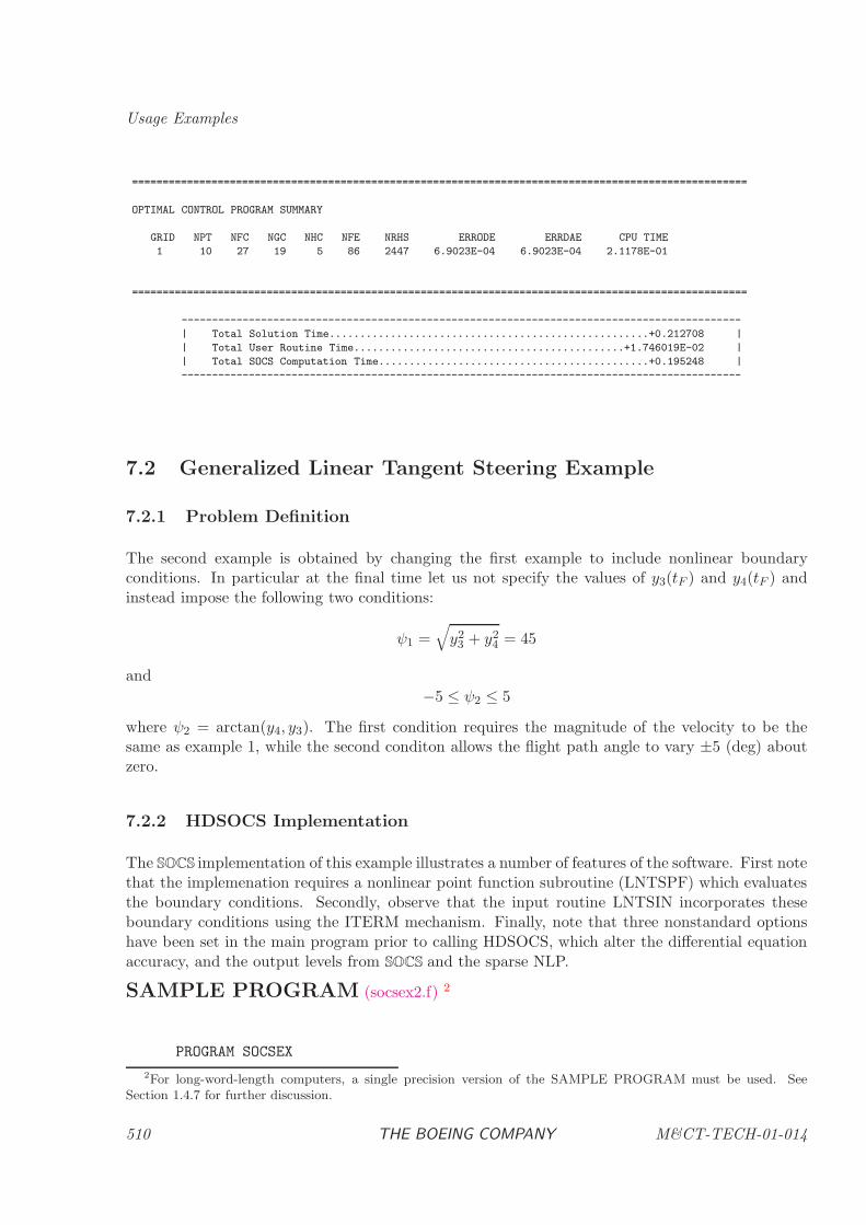
Usage Examples
====================================================================================================
OPTIMAL CONTROL PROGRAM SUMMARY
GRID NPT NFC NGC NHC NFE NRHS ERRODE ERRDAE CPU TIME
1 10 27 19 5 86 2447 6.9023E-04 6.9023E-04 2.1178E-01
====================================================================================================
-------------------------------------------------------------------------------------------
| Total Solution Time....................................................+0.212708 |
| Total User Routine Time............................................+1.746019E-02 |
| Total SOCS Computation Time............................................+0.195248 |
-------------------------------------------------------------------------------------------
7.2 Generalized Linear Tangent Steering Example
7.2.1 Problem Definition
The second example is obtained by changing the first example to include nonlinear boundaryconditions. In particular at the final time let us not specify the values of y3(tF ) and y4(tF ) andinstead impose the following two conditions:
ψ1 =√y23 + y2
4 = 45
and
−5 ≤ ψ2 ≤ 5
where ψ2 = arctan(y4, y3). The first condition requires the magnitude of the velocity to be thesame as example 1, while the second conditon allows the flight path angle to vary ±5 (deg) aboutzero.
7.2.2 HDSOCS Implementation
The SOCS implementation of this example illustrates a number of features of the software. First notethat the implemenation requires a nonlinear point function subroutine (LNTSPF) which evaluatesthe boundary conditions. Secondly, observe that the input routine LNTSIN incorporates theseboundary conditions using the ITERM mechanism. Finally, note that three nonstandard optionshave been set in the main program prior to calling HDSOCS, which alter the differential equationaccuracy, and the output levels from SOCS and the sparse NLP.
SAMPLE PROGRAM (socsex2.f) 2
PROGRAM SOCSEX
2For long-word-length computers, a single precision version of the SAMPLE PROGRAM must be used. See
Section 1.4.7 for further discussion.
510 THE BOEING COMPANY M&CT-TECH-01-014
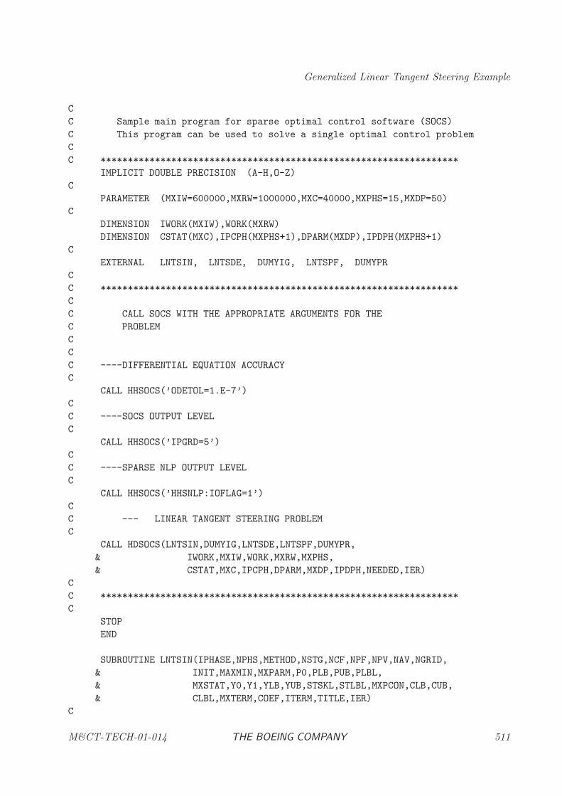
Generalized Linear Tangent Steering Example
C
C Sample main program for sparse optimal control software (SOCS)
C This program can be used to solve a single optimal control problem
C
C ******************************************************************
IMPLICIT DOUBLE PRECISION (A-H,O-Z)
C
PARAMETER (MXIW=600000,MXRW=1000000,MXC=40000,MXPHS=15,MXDP=50)
C
DIMENSION IWORK(MXIW),WORK(MXRW)
DIMENSION CSTAT(MXC),IPCPH(MXPHS+1),DPARM(MXDP),IPDPH(MXPHS+1)
C
EXTERNAL LNTSIN, LNTSDE, DUMYIG, LNTSPF, DUMYPR
C
C ******************************************************************
C
C CALL SOCS WITH THE APPROPRIATE ARGUMENTS FOR THE
C PROBLEM
C
C
C ----DIFFERENTIAL EQUATION ACCURACY
C
CALL HHSOCS(’ODETOL=1.E-7’)
C
C ----SOCS OUTPUT LEVEL
C
CALL HHSOCS(’IPGRD=5’)
C
C ----SPARSE NLP OUTPUT LEVEL
C
CALL HHSOCS(’HHSNLP:IOFLAG=1’)
C
C --- LINEAR TANGENT STEERING PROBLEM
C
CALL HDSOCS(LNTSIN,DUMYIG,LNTSDE,LNTSPF,DUMYPR,
& IWORK,MXIW,WORK,MXRW,MXPHS,
& CSTAT,MXC,IPCPH,DPARM,MXDP,IPDPH,NEEDED,IER)
C
C ******************************************************************
C
STOP
END
SUBROUTINE LNTSIN(IPHASE,NPHS,METHOD,NSTG,NCF,NPF,NPV,NAV,NGRID,
& INIT,MAXMIN,MXPARM,P0,PLB,PUB,PLBL,
& MXSTAT,Y0,Y1,YLB,YUB,STSKL,STLBL,MXPCON,CLB,CUB,
& CLBL,MXTERM,COEF,ITERM,TITLE,IER)
C
M&CT-TECH-01-014 THE BOEING COMPANY 511
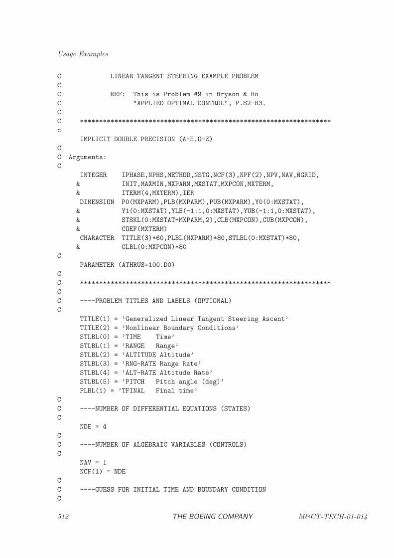
Usage Examples
C LINEAR TANGENT STEERING EXAMPLE PROBLEM
C
C REF: This is Problem #9 in Bryson & Ho
C "APPLIED OPTIMAL CONTROL", P.82-83.
C
C ******************************************************************
c
IMPLICIT DOUBLE PRECISION (A-H,O-Z)
C
C Arguments:
C
INTEGER IPHASE,NPHS,METHOD,NSTG,NCF(3),NPF(2),NPV,NAV,NGRID,
& INIT,MAXMIN,MXPARM,MXSTAT,MXPCON,MXTERM,
& ITERM(4,MXTERM),IER
DIMENSION P0(MXPARM),PLB(MXPARM),PUB(MXPARM),Y0(0:MXSTAT),
& Y1(0:MXSTAT),YLB(-1:1,0:MXSTAT),YUB(-1:1,0:MXSTAT),
& STSKL(0:MXSTAT+MXPARM,2),CLB(MXPCON),CUB(MXPCON),
& COEF(MXTERM)
CHARACTER TITLE(3)*60,PLBL(MXPARM)*80,STLBL(0:MXSTAT)*80,
& CLBL(0:MXPCON)*80
C
PARAMETER (ATHRUS=100.D0)
C
C ******************************************************************
C
C ----PROBLEM TITLES AND LABELS (OPTIONAL)
C
TITLE(1) = ’Generalized Linear Tangent Steering Ascent’
TITLE(2) = ’Nonlinear Boundary Conditions’
STLBL(0) = ’TIME Time’
STLBL(1) = ’RANGE Range’
STLBL(2) = ’ALTITUDE Altitude’
STLBL(3) = ’RNG-RATE Range Rate’
STLBL(4) = ’ALT-RATE Altitude Rate’
STLBL(5) = ’PITCH Pitch angle (deg)’
PLBL(1) = ’TFINAL Final time’
C
C ----NUMBER OF DIFFERENTIAL EQUATIONS (STATES)
C
NDE = 4
C
C ----NUMBER OF ALGEBRAIC VARIABLES (CONTROLS)
C
NAV = 1
NCF(1) = NDE
C
C ----GUESS FOR INITIAL TIME AND BOUNDARY CONDITION
C
512 THE BOEING COMPANY M&CT-TECH-01-014
Generalized Linear Tangent Steering Example
Y0(0) = 0.D0
YLB(-1,0) = Y0(0)
YUB(-1,0) = Y0(0)
C
C ----GUESS FOR FINAL TIME AND LOWER BOUND
C
T1 = 1.D0
Y1(0) = T1
YLB(1,0) = 0.D0
C
C ----RADIANS TO DEGREES CONVERSION FACTOR
C
CR2D = HDMCON(16)
C
C ----PI/2 FACTOR
C
CPI2 = HDMCON(12)/2.D0
C
C ----DEFINE INITIAL CONDITIONS FOR STATE VARIABLES, Y.
C
C Y(1) = RANGE.
C Y(2) = ALTITUDE.
C Y(3) = HORIZONTAL VELOCITY.
C Y(4) = VERTICAL VELOCITY.
C
Y0(1) = 0.D0
Y0(2) = 0.D0
Y0(3) = 0.D0
Y0(4) = 0.D0
C
C ----FIX THE INITIAL STATES
C
DO 110 I=1,4
YLB(-1,I) = Y0(I)
YUB(-1,I) = Y0(I)
110 CONTINUE
C
C ----DEFINE FINAL CONDITIONS FOR STATE VARIABLES, Y.
C
Y1(1) = 12.D0
Y1(2) = 5.D0
Y1(3) = 45.D0
Y1(4) = 0.D0
C
C ----DEFINE INITIAL AND FINAL CONTROL ANGLES.
C
Y0(5) = 1.D0
Y1(5) = -1.D0
M&CT-TECH-01-014 THE BOEING COMPANY 513
Usage Examples
C
C ----FIX THE FINAL VALUES FOR STATE 2
C
YLB(1,2) = Y1(2)
YUB(1,2) = Y1(2)
C
C ----INITIALIZE RUNNING COUNTER FOR THE NUMBER OF TERMS AND THE
C NUMBER OF CONSTRAINTS ON THIS PHASE
C
NTERM = 0
NKON = 0
C
C ----DEFINE CONSTRAINT ON FINAL VELOCITY MAGNITUDE
C
NTERM = NTERM + 1
NKON = NKON + 1
ITERM(1,NTERM) = NKON
ITERM(2,NTERM) = 1
ITERM(3,NTERM) = 1
ITERM(4,NTERM) = -NKON
COEF(NTERM) = 1.D0
CLB(NKON) = 45.D0
CUB(NKON) = 45.D0
C
C ----DEFINE CONSTRAINT ON FINAL FLIGHT PATH DIRECTION
C
NTERM = NTERM + 1
NKON = NKON + 1
ITERM(1,NTERM) = NKON
ITERM(2,NTERM) = 1
ITERM(3,NTERM) = 1
ITERM(4,NTERM) = -NKON
COEF(NTERM) = 1.D0
CLB(NKON) = -5.D0
CUB(NKON) = 5.D0
C
C ----DEFINE THE NUMBER OF POINT FUNCTIONS AT THE END OF PHASE
C
NPF(2) = NKON
C
C ----BOUND CONTROL MAGNITUDE ON PHASE BY 90 DEG.
C
DO 120 I=-1,1
YLB(I,5) = -CPI2
YUB(I,5) = CPI2
120 CONTINUE
C
C ----DEFINE FINAL TIME AS THE OBJECTIVE TO BE MINIMIZED
514 THE BOEING COMPANY M&CT-TECH-01-014
Generalized Linear Tangent Steering Example
C
NTERM = NTERM + 1
ITERM(1,NTERM) = 0
ITERM(2,NTERM) = 1
ITERM(3,NTERM) = 1
ITERM(4,NTERM) = 0
COEF(NTERM) = 1.D0
C
MAXMIN = -1
C
C ----LOAD SCALE WEIGHTS FOR OUTPUT OF CONTROL IN DEGREES
C
DO 130 I=NDE+1,NDE+NAV
STSKL(I,1) = CR2D
130 CONTINUE
C
RETURN
END
SUBROUTINE LNTSDE(IPHASE,T,Y,NY,P,NP,F,NF,IFERR)
C
C COMPUTES THE RIGHT HAND SIDES OF THE LINEAR TANGENT
C STEERING SYSTEM OF DIFFERENTIAL EQUATIONS.
C
C ******************************************************************
IMPLICIT DOUBLE PRECISION (A-H,O-Z)
C
C ARGUMENTS:
C
INTEGER IPHASE,NY,NP,NF,IFERR
DIMENSION Y(NY),P(NP),F(NF)
C
PARAMETER (ATHRUS=100.D0)
C
C ******************************************************************
C
C ----SET FUNCTION ERROR FLAG.
C
IFERR = 0
C
C ----COMPUTE FUNCTIONS OF CONTROL.
C
COSU = COS(Y(5))
SINU = SIN(Y(5))
C
C ----COMPUTE STATE EQUATIONS.
C
M&CT-TECH-01-014 THE BOEING COMPANY 515
Usage Examples
F(1) = Y(3)
F(2) = Y(4)
F(3) = ATHRUS*COSU
F(4) = ATHRUS*SINU
C
RETURN
END
SUBROUTINE LNTSPF(IPHASE,IPHEND,T,Y,NY,P,NP,PSI,NPSI,IFERR)
C
C Computes terminal constraint for the linear tangent
C steering problem.
C
C ******************************************************************
IMPLICIT DOUBLE PRECISION (A-H,O-Z)
C
C Arguments:
C
INTEGER IPHASE,IPHEND,NY,NP,NPSI,IFERR
DIMENSION Y(NY),P(NP),PSI(NPSI)
C
C ******************************************************************
C
IFERR = 0
C
IF (IPHEND.EQ.1) THEN
C
C COMPUTE THE VELOCITY MAGNITUDE
C
VELMAG = SQRT(Y(3)**2 + Y(4)**2)
PSI(1) = VELMAG
C
C COMPUTE THE FLIGHT PATH ANGLE (DEG)
C
CR2D = HDMCON(16)
PSI(2) = CR2D*ATAN2(Y(4),Y(3))
C
ENDIF
C
RETURN
END
***** SOCS WARNING: IER = 1478 Compute Sparsity Pattern for User Supplied Functions
>>>>> Phase 1: No function depends on variable 1
***** SOCS WARNING: IER = 1478 Compute Sparsity Pattern for User Supplied Functions
>>>>> Phase 1: No function depends on variable 2
516 THE BOEING COMPANY M&CT-TECH-01-014
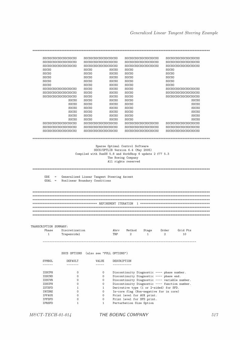
Generalized Linear Tangent Steering Example
========================================================================================================
SOCSOCSOCSOCSOCSOCSO SOCSOCSOCSOCSOCSOCSO SOCSOCSOCSOCSOCSOCSO SOCSOCSOCSOCSOCSOCSO
SOCSOCSOCSOCSOCSOCSO SOCSOCSOCSOCSOCSOCSO SOCSOCSOCSOCSOCSOCSO SOCSOCSOCSOCSOCSOCSO
SOCSOCSOCSOCSOCSOCSO SOCSOCSOCSOCSOCSOCSO SOCSOCSOCSOCSOCSOCSO SOCSOCSOCSOCSOCSOCSO
SOCSO SOCSO SOCSO SOCSO SOCSO
SOCSO SOCSO SOCSO SOCSO SOCSO
SOCSO SOCSO SOCSO SOCSO SOCSO
SOCSO SOCSO SOCSO SOCSO SOCSO
SOCSO SOCSO SOCSO SOCSO SOCSO
SOCSOCSOCSOCSOCSOCSO SOCSO SOCSO SOCSO SOCSOCSOCSOCSOCSOCSO
SOCSOCSOCSOCSOCSOCSO SOCSO SOCSO SOCSO SOCSOCSOCSOCSOCSOCSO
SOCSOCSOCSOCSOCSOCSO SOCSO SOCSO SOCSO SOCSOCSOCSOCSOCSOCSO
SOCSO SOCSO SOCSO SOCSO SOCSO
SOCSO SOCSO SOCSO SOCSO SOCSO
SOCSO SOCSO SOCSO SOCSO SOCSO
SOCSO SOCSO SOCSO SOCSO SOCSO
SOCSO SOCSO SOCSO SOCSO SOCSO
SOCSO SOCSO SOCSO SOCSO SOCSO
SOCSOCSOCSOCSOCSOCSO SOCSOCSOCSOCSOCSOCSO SOCSOCSOCSOCSOCSOCSO SOCSOCSOCSOCSOCSOCSO
SOCSOCSOCSOCSOCSOCSO SOCSOCSOCSOCSOCSOCSO SOCSOCSOCSOCSOCSOCSO SOCSOCSOCSOCSOCSOCSO
SOCSOCSOCSOCSOCSOCSO SOCSOCSOCSOCSOCSOCSO SOCSOCSOCSOCSOCSOCSO SOCSOCSOCSOCSOCSOCSO
========================================================================================================
Sparse Optimal Control Software
SOCS/OPTLIB Version 6.4 (May 2005)
Compiled with SunOS 5.8 and WorkShop 6 update 2 f77 5.3
The Boeing Company
All rights reserved
========================================================================================================
ODE = Generalized Linear Tangent Steering Ascent
GOAL = Nonlinear Boundary Conditions
========================================================================================================
========================================================================================================
========================================================================================================
====================================== REFINEMENT ITERATION 1 =========================================
========================================================================================================
========================================================================================================
========================================================================================================
TRANSCRIPTION SUMMARY:
Phase Discretization Abrv Method Stage Order Grid Pts
1 Trapezoidal TRP 2 1 2 10
------------------------------------------------------------------------------------------
SOCS OPTIONS (also see "FULL OPTIONS")
SYMBOL DEFAULT VALUE DESCRIPTION
------ ------- ----- -----------
IDSCPH 0 0 Discontinuity Diagnostic ---- phase number.
IDSCND 0 0 Discontinuity Diagnostic ---- phase end.
IDSCVR 0 0 Discontinuity Diagnostic ---- variable number.
IDSCFN 0 0 Discontinuity Diagnostic ---- function number.
IDTSFD 1 1 Derivative type (1 or 2-sided) for SFD.
INCORE 0 0 In-core flag (Non-negative for in core)
IPFAUX 0 0 Print level for AUX print.
IPFSFD 0 0 Print level for SFD print.
IPRSFD 1 1 Perturbation Size Option
M&CT-TECH-01-014 THE BOEING COMPANY 517
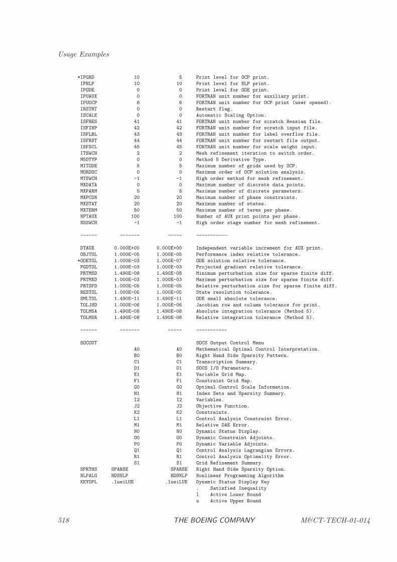
Usage Examples
*IPGRD 10 5 Print level for OCP print.
IPNLP 10 10 Print level for NLP print.
IPODE 0 0 Print level for ODE print.
IPUAUX 0 0 FORTRAN unit number for auxiliary print.
IPUOCP 6 6 FORTRAN unit number for OCP print (user opened).
IRSTRT 0 0 Restart flag.
ISCALE 0 0 Automatic Scaling Option.
ISFHES 41 41 FORTRAN unit number for scratch Hessian file.
ISFINP 42 42 FORTRAN unit number for scratch input file.
ISFLBL 43 43 FORTRAN unit number for label overflow file.
ISFRST 44 44 FORTRAN unit number for restart file output.
ISFSCL 45 45 FORTRAN unit number for scale weight input.
ITSWCH 2 2 Mesh refinement iteration to switch order.
M5DTYP 0 0 Method 5 Derivative Type.
MITODE 5 5 Maximum number of grids used by OCP.
MORDOC 0 0 Maximum order of OCP solution analysis.
MTSWCH -1 -1 High order method for mesh refinement.
MXDATA 0 0 Maximum number of discrete data points.
MXPARM 5 5 Maximum number of discrete parameters.
MXPCON 20 20 Maximum number of phase constraints.
MXSTAT 20 20 Maximum number of states.
MXTERM 50 50 Maximum number of terms per phase.
NPTAUX 100 100 Number of AUX print points per phase.
NSSWCH -1 -1 High order stage number for mesh refinement.
------ ------- ----- -----------
DTAUX 0.000E+00 0.000E+00 Independent variable increment for AUX print.
OBJTOL 1.000E-05 1.000E-05 Performance index relative tolerance.
*ODETOL 1.000E-03 1.000E-07 ODE solution relative tolerance.
PGDTOL 1.000E-03 1.000E-03 Projected gradient relative tolerance.
PRTMSD 1.490E-08 1.490E-08 Minimum perturbation size for sparse finite diff.
PRTMXD 1.000E-03 1.000E-03 Maximum perturbation size for sparse finite diff.
PRTSFD 1.000E-05 1.000E-05 Relative perturbation size for sparse finite diff.
RESTOL 1.000E-05 1.000E-05 State resolution tolerance.
SMLTOL 1.490E-11 1.490E-11 ODE small absolute tolerance.
TOLJSD 1.000E-06 1.000E-06 Jacobian row and column tolerance for print.
TOLM5A 1.490E-08 1.490E-08 Absolute integration tolerance (Method 5).
TOLM5R 1.490E-08 1.490E-08 Relative integration tolerance (Method 5).
------ ------- ----- -----------
SOCOUT SOCS Output Control Menu
A0 A0 Mathematical Optimal Control Interpretation.
B0 B0 Right Hand Side Sparsity Pattern.
C1 C1 Transcription Summary.
D1 D1 SOCS I/O Parameters.
E1 E1 Variable Grid Map.
F1 F1 Constraint Grid Map.
G0 G0 Optimal Control Scale Information.
H1 H1 Index Sets and Sparsity Summary.
I2 I2 Variables.
J2 J2 Objective Function.
K2 K2 Constraints.
L1 L1 Control Analysis Constraint Error.
M1 M1 Relative DAE Error.
N0 N0 Dynamic Status Display.
O0 O0 Dynamic Constraint Adjoints.
P0 P0 Dynamic Variable Adjoints.
Q1 Q1 Control Analysis Lagrangian Errors.
R1 R1 Control Analysis Optimality Error.
S1 S1 Grid Refinement Summary.
SPRTHS SPARSE SPARSE Right Hand Side Sparsity Option.
NLPALG HDSNLP HDSNLP Nonlinear Programming Algorithm
KEYDPL .lueiLUE .lueiLUE Dynamic Status Display Key
. Satisfied Inequality
l Active Lower Bound
u Active Upper Bound
518 THE BOEING COMPANY M&CT-TECH-01-014
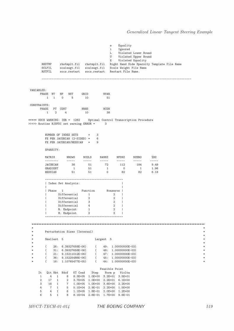
Generalized Linear Tangent Steering Example
e Equality
i Ignored
L Violated Lower Bound
U Violated Upper Bound
E Violated Equality
RHSTMP rhstmplt.fil rhstmplt.fil Right Hand Side Sparsity Template File Name
SCLFIL scalewgt.fil scalewgt.fil Scale Weight File Name
RSTFIL socs.restart socs.restart Restart File Name.
------------------------------------------------------------------------------------------
VARIABLES:
PHASE NT NP NST GRID NVAR
1 1 0 5 10 51
CONSTRAINTS:
PHASE PT CONT NRHS NCON
1 2 4 10 38
***** SOCS WARNING: IER = 1282 Optimal Control Transcription Procedure
>>>>> Routine HJSFDI set warning ERROR = 3
NUMBER OF INDEX SETS = 3
FE PER JACOBIAN (2-SIDED) = 6
FE PER JACOBIAN/HESSIAN = 9
SPARSITY:
MATRIX NROWS NCOLS NANNZ NFDNZ NZERO %NZ
-------- ----- ----- ----- ----- ----- -----
JACOBIAN 38 51 72 112 184 9.49
GRADIENT 1 51 1 0 1 1.96
HESSIAN 51 51 0 82 82 6.18
-----------------------------------------------
| Index Set Analysis: |
| |
| Phase 1 Function Nonzeros |
| Differential 1 2 |
| Differential 2 2 |
| Differential 3 2 |
| Differential 4 2 |
| R. Endpoint 1 2 |
| R. Endpoint 2 2 |
-----------------------------------------------
********************************************************************************************************
* *
* Perturbation Sizes (Internal) *
* *
* Smallest 5 Largest 5 *
* *
* ( 26: 6.39327658E-06) ( 49: 1.00000000E-03) *
* ( 31: 6.39327658E-06) ( 48: 1.00000000E-03) *
* ( 21: 9.15211012E-06) ( 47: 1.00000000E-03) *
* ( 36: 9.15225488E-06) ( 45: 1.00000000E-03) *
* ( 16: 1.10765477E-05) ( 44: 1.00000000E-03) *
Feasible Point
It Qit Nkt Ndof KT Cond Step Norm p Violtn
1 4 1 8 8.3E+05 1.0E+00 3.2E+01 3.5E+01
2 17 1 2 3.7E+05 1.0E+00 2.2E+01 6.1E+00
3 18 1 7 1.0E+05 1.0E+00 3.6E+00 2.2E+00
4 7 1 5 5.1E+04 2.9E-01 2.2E+00 1.5E+00
5 4 1 6 1.1E+05 1.8E-01 2.0E+00 1.2E+00
6 5 1 8 8.1E+04 2.6E-01 1.7E+00 9.6E-01
M&CT-TECH-01-014 THE BOEING COMPANY 519
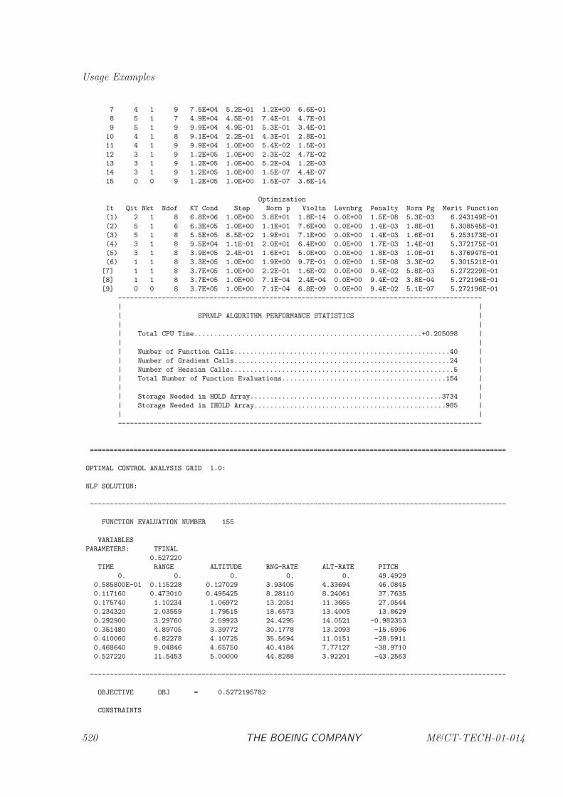
Usage Examples
7 4 1 9 7.5E+04 5.2E-01 1.2E+00 6.6E-01
8 5 1 7 4.9E+04 4.5E-01 7.4E-01 4.7E-01
9 5 1 9 9.9E+04 4.9E-01 5.3E-01 3.4E-01
10 4 1 8 9.1E+04 2.2E-01 4.3E-01 2.8E-01
11 4 1 9 9.9E+04 1.0E+00 5.4E-02 1.5E-01
12 3 1 9 1.2E+05 1.0E+00 2.3E-02 4.7E-02
13 3 1 9 1.2E+05 1.0E+00 5.2E-04 1.2E-03
14 3 1 9 1.2E+05 1.0E+00 1.5E-07 4.4E-07
15 0 0 9 1.2E+05 1.0E+00 1.5E-07 3.6E-14
Optimization
It Qit Nkt Ndof KT Cond Step Norm p Violtn Levnbrg Penalty Norm Pg Merit Function
(1) 2 1 8 6.8E+06 1.0E+00 3.8E+01 1.8E-14 0.0E+00 1.5E-08 5.3E-03 6.243149E-01
(2) 5 1 6 6.3E+05 1.0E+00 1.1E+01 7.6E+00 0.0E+00 1.4E-03 1.8E-01 5.308545E-01
(3) 5 1 8 5.5E+05 8.5E-02 1.9E+01 7.1E+00 0.0E+00 1.4E-03 1.6E-01 5.253173E-01
(4) 3 1 8 9.5E+04 1.1E-01 2.0E+01 6.4E+00 0.0E+00 1.7E-03 1.4E-01 5.372175E-01
(5) 3 1 8 3.9E+05 2.4E-01 1.6E+01 5.0E+00 0.0E+00 1.8E-03 1.0E-01 5.376947E-01
(6) 1 1 8 3.3E+05 1.0E+00 1.9E+00 9.7E-01 0.0E+00 1.5E-08 3.3E-02 5.301521E-01
[7] 1 1 8 3.7E+05 1.0E+00 2.2E-01 1.6E-02 0.0E+00 9.4E-02 5.8E-03 5.272229E-01
[8] 1 1 8 3.7E+05 1.0E+00 7.1E-04 2.4E-04 0.0E+00 9.4E-02 3.8E-04 5.272196E-01
[9] 0 0 8 3.7E+05 1.0E+00 7.1E-04 6.8E-09 0.0E+00 9.4E-02 5.1E-07 5.272196E-01
-------------------------------------------------------------------------------------------
| |
| SPRNLP ALGORITHM PERFORMANCE STATISTICS |
| |
| Total CPU Time.........................................................+0.205098 |
| |
| Number of Function Calls......................................................40 |
| Number of Gradient Calls......................................................24 |
| Number of Hessian Calls........................................................5 |
| Total Number of Function Evaluations.........................................154 |
| |
| Storage Needed in HOLD Array................................................3734 |
| Storage Needed in IHOLD Array................................................985 |
| |
-------------------------------------------------------------------------------------------
========================================================================================================
OPTIMAL CONTROL ANALYSIS GRID 1.0:
NLP SOLUTION:
--------------------------------------------------------------------------------------------------------
FUNCTION EVALUATION NUMBER 155
VARIABLES
PARAMETERS: TFINAL
0.527220
TIME RANGE ALTITUDE RNG-RATE ALT-RATE PITCH
0. 0. 0. 0. 0. 49.4929
0.585800E-01 0.115228 0.127029 3.93405 4.33694 46.0845
0.117160 0.473010 0.495425 8.28110 8.24061 37.7635
0.175740 1.10234 1.06972 13.2051 11.3665 27.0544
0.234320 2.03559 1.79515 18.6573 13.4005 13.8629
0.292900 3.29760 2.59923 24.4295 14.0521 -0.982353
0.351480 4.89705 3.39772 30.1778 13.2093 -15.6996
0.410060 6.82278 4.10725 35.5694 11.0151 -28.5911
0.468640 9.04846 4.65750 40.4184 7.77127 -38.9710
0.527220 11.5453 5.00000 44.8288 3.92201 -43.2563
--------------------------------------------------------------------------------------------------------
OBJECTIVE OBJ = 0.5272195782
CONSTRAINTS
520 THE BOEING COMPANY M&CT-TECH-01-014
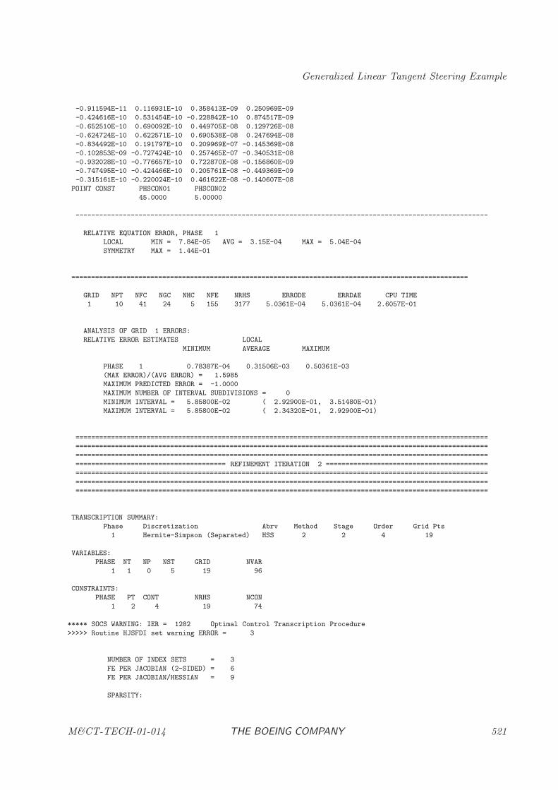
Generalized Linear Tangent Steering Example
-0.911594E-11 0.116931E-10 0.358413E-09 0.250969E-09
-0.424616E-10 0.531454E-10 -0.228842E-10 0.874517E-09
-0.652510E-10 0.690092E-10 0.449705E-08 0.129726E-08
-0.624724E-10 0.622571E-10 0.690538E-08 0.247694E-08
-0.834492E-10 0.191797E-10 0.209969E-07 -0.145369E-08
-0.102853E-09 -0.727424E-10 0.257465E-07 -0.340531E-08
-0.932028E-10 -0.776657E-10 0.722870E-08 -0.156860E-09
-0.747495E-10 -0.424466E-10 0.205761E-08 -0.449369E-09
-0.315161E-10 -0.220024E-10 0.461622E-08 -0.140607E-08
POINT CONST PHSCON01 PHSCON02
45.0000 5.00000
--------------------------------------------------------------------------------------------------------
RELATIVE EQUATION ERROR, PHASE 1
LOCAL MIN = 7.84E-05 AVG = 3.15E-04 MAX = 5.04E-04
SYMMETRY MAX = 1.44E-01
====================================================================================================
GRID NPT NFC NGC NHC NFE NRHS ERRODE ERRDAE CPU TIME
1 10 41 24 5 155 3177 5.0361E-04 5.0361E-04 2.6057E-01
ANALYSIS OF GRID 1 ERRORS:
RELATIVE ERROR ESTIMATES LOCAL
MINIMUM AVERAGE MAXIMUM
PHASE 1 0.78387E-04 0.31506E-03 0.50361E-03
(MAX ERROR)/(AVG ERROR) = 1.5985
MAXIMUM PREDICTED ERROR = -1.0000
MAXIMUM NUMBER OF INTERVAL SUBDIVISIONS = 0
MINIMUM INTERVAL = 5.85800E-02 ( 2.92900E-01, 3.51480E-01)
MAXIMUM INTERVAL = 5.85800E-02 ( 2.34320E-01, 2.92900E-01)
========================================================================================================
========================================================================================================
========================================================================================================
====================================== REFINEMENT ITERATION 2 =========================================
========================================================================================================
========================================================================================================
========================================================================================================
TRANSCRIPTION SUMMARY:
Phase Discretization Abrv Method Stage Order Grid Pts
1 Hermite-Simpson (Separated) HSS 2 2 4 19
VARIABLES:
PHASE NT NP NST GRID NVAR
1 1 0 5 19 96
CONSTRAINTS:
PHASE PT CONT NRHS NCON
1 2 4 19 74
***** SOCS WARNING: IER = 1282 Optimal Control Transcription Procedure
>>>>> Routine HJSFDI set warning ERROR = 3
NUMBER OF INDEX SETS = 3
FE PER JACOBIAN (2-SIDED) = 6
FE PER JACOBIAN/HESSIAN = 9
SPARSITY:
M&CT-TECH-01-014 THE BOEING COMPANY 521
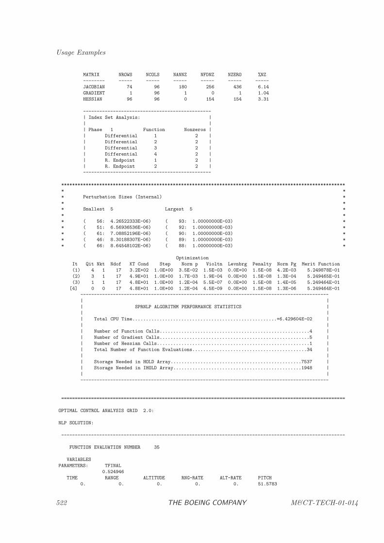
Usage Examples
MATRIX NROWS NCOLS NANNZ NFDNZ NZERO %NZ
-------- ----- ----- ----- ----- ----- -----
JACOBIAN 74 96 180 256 436 6.14
GRADIENT 1 96 1 0 1 1.04
HESSIAN 96 96 0 154 154 3.31
-----------------------------------------------
| Index Set Analysis: |
| |
| Phase 1 Function Nonzeros |
| Differential 1 2 |
| Differential 2 2 |
| Differential 3 2 |
| Differential 4 2 |
| R. Endpoint 1 2 |
| R. Endpoint 2 2 |
-----------------------------------------------
********************************************************************************************************
* *
* Perturbation Sizes (Internal) *
* *
* Smallest 5 Largest 5 *
* *
* ( 56: 4.26522333E-06) ( 93: 1.00000000E-03) *
* ( 51: 6.56936536E-06) ( 92: 1.00000000E-03) *
* ( 61: 7.08852196E-06) ( 90: 1.00000000E-03) *
* ( 46: 8.30188307E-06) ( 89: 1.00000000E-03) *
* ( 66: 8.64548102E-06) ( 88: 1.00000000E-03) *
Optimization
It Qit Nkt Ndof KT Cond Step Norm p Violtn Levnbrg Penalty Norm Pg Merit Function
(1) 4 1 17 3.2E+02 1.0E+00 3.5E-02 1.5E-03 0.0E+00 1.5E-08 4.2E-03 5.249878E-01
(2) 3 1 17 4.9E+01 1.0E+00 1.7E-03 1.9E-04 0.0E+00 1.5E-08 1.3E-04 5.249465E-01
(3) 1 1 17 4.8E+01 1.0E+00 1.2E-04 5.5E-07 0.0E+00 1.5E-08 1.4E-05 5.249464E-01
[4] 0 0 17 4.8E+01 1.0E+00 1.2E-04 4.5E-09 0.0E+00 1.5E-08 1.3E-06 5.249464E-01
-------------------------------------------------------------------------------------------
| |
| SPRNLP ALGORITHM PERFORMANCE STATISTICS |
| |
| Total CPU Time.....................................................+6.429604E-02 |
| |
| Number of Function Calls.......................................................4 |
| Number of Gradient Calls.......................................................5 |
| Number of Hessian Calls........................................................1 |
| Total Number of Function Evaluations..........................................34 |
| |
| Storage Needed in HOLD Array................................................7537 |
| Storage Needed in IHOLD Array...............................................1948 |
| |
-------------------------------------------------------------------------------------------
========================================================================================================
OPTIMAL CONTROL ANALYSIS GRID 2.0:
NLP SOLUTION:
--------------------------------------------------------------------------------------------------------
FUNCTION EVALUATION NUMBER 35
VARIABLES
PARAMETERS: TFINAL
0.524946
TIME RANGE ALTITUDE RNG-RATE ALT-RATE PITCH
0. 0. 0. 0. 0. 51.5783
522 THE BOEING COMPANY M&CT-TECH-01-014
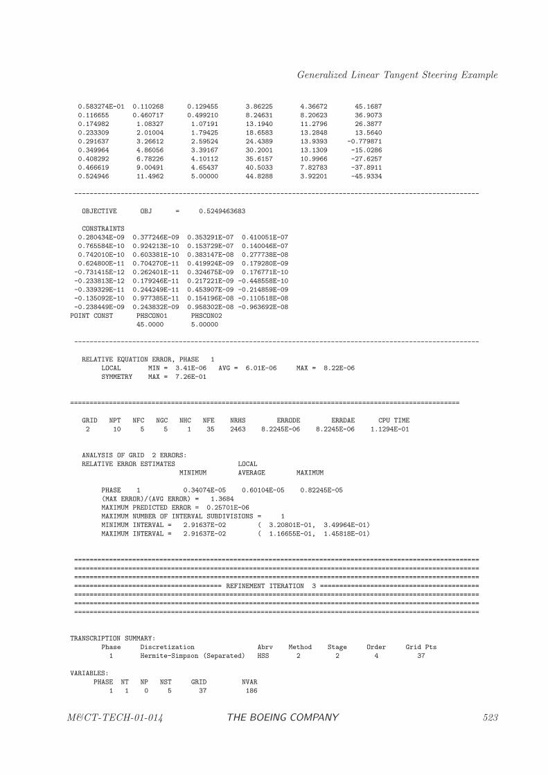
Generalized Linear Tangent Steering Example
0.583274E-01 0.110268 0.129455 3.86225 4.36672 45.1687
0.116655 0.460717 0.499210 8.24631 8.20623 36.9073
0.174982 1.08327 1.07191 13.1940 11.2796 26.3877
0.233309 2.01004 1.79425 18.6583 13.2848 13.5640
0.291637 3.26612 2.59524 24.4389 13.9393 -0.779871
0.349964 4.86056 3.39167 30.2001 13.1309 -15.0286
0.408292 6.78226 4.10112 35.6157 10.9966 -27.6257
0.466619 9.00491 4.65437 40.5033 7.82783 -37.8911
0.524946 11.4962 5.00000 44.8288 3.92201 -45.9334
--------------------------------------------------------------------------------------------------------
OBJECTIVE OBJ = 0.5249463683
CONSTRAINTS
0.280434E-09 0.377246E-09 0.353291E-07 0.410051E-07
0.765584E-10 0.924213E-10 0.153729E-07 0.140046E-07
0.742010E-10 0.603381E-10 0.383147E-08 0.277738E-08
0.624800E-11 0.704270E-11 0.419924E-09 0.179280E-09
-0.731415E-12 0.262401E-11 0.324675E-09 0.176771E-10
-0.233813E-12 0.179246E-11 0.217221E-09 -0.448558E-10
-0.339329E-11 0.244249E-11 0.453907E-09 -0.214859E-09
-0.135092E-10 0.977385E-11 0.154196E-08 -0.110518E-08
-0.238449E-09 0.243832E-09 0.958302E-08 -0.963692E-08
POINT CONST PHSCON01 PHSCON02
45.0000 5.00000
--------------------------------------------------------------------------------------------------------
RELATIVE EQUATION ERROR, PHASE 1
LOCAL MIN = 3.41E-06 AVG = 6.01E-06 MAX = 8.22E-06
SYMMETRY MAX = 7.26E-01
====================================================================================================
GRID NPT NFC NGC NHC NFE NRHS ERRODE ERRDAE CPU TIME
2 10 5 5 1 35 2463 8.2245E-06 8.2245E-06 1.1294E-01
ANALYSIS OF GRID 2 ERRORS:
RELATIVE ERROR ESTIMATES LOCAL
MINIMUM AVERAGE MAXIMUM
PHASE 1 0.34074E-05 0.60104E-05 0.82245E-05
(MAX ERROR)/(AVG ERROR) = 1.3684
MAXIMUM PREDICTED ERROR = 0.25701E-06
MAXIMUM NUMBER OF INTERVAL SUBDIVISIONS = 1
MINIMUM INTERVAL = 2.91637E-02 ( 3.20801E-01, 3.49964E-01)
MAXIMUM INTERVAL = 2.91637E-02 ( 1.16655E-01, 1.45818E-01)
========================================================================================================
========================================================================================================
========================================================================================================
====================================== REFINEMENT ITERATION 3 =========================================
========================================================================================================
========================================================================================================
========================================================================================================
TRANSCRIPTION SUMMARY:
Phase Discretization Abrv Method Stage Order Grid Pts
1 Hermite-Simpson (Separated) HSS 2 2 4 37
VARIABLES:
PHASE NT NP NST GRID NVAR
1 1 0 5 37 186
M&CT-TECH-01-014 THE BOEING COMPANY 523
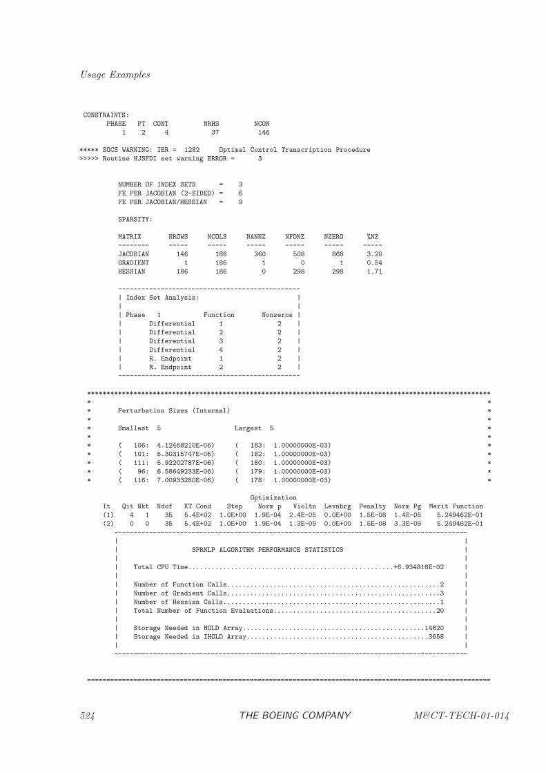
Usage Examples
CONSTRAINTS:
PHASE PT CONT NRHS NCON
1 2 4 37 146
***** SOCS WARNING: IER = 1282 Optimal Control Transcription Procedure
>>>>> Routine HJSFDI set warning ERROR = 3
NUMBER OF INDEX SETS = 3
FE PER JACOBIAN (2-SIDED) = 6
FE PER JACOBIAN/HESSIAN = 9
SPARSITY:
MATRIX NROWS NCOLS NANNZ NFDNZ NZERO %NZ
-------- ----- ----- ----- ----- ----- -----
JACOBIAN 146 186 360 508 868 3.20
GRADIENT 1 186 1 0 1 0.54
HESSIAN 186 186 0 298 298 1.71
-----------------------------------------------
| Index Set Analysis: |
| |
| Phase 1 Function Nonzeros |
| Differential 1 2 |
| Differential 2 2 |
| Differential 3 2 |
| Differential 4 2 |
| R. Endpoint 1 2 |
| R. Endpoint 2 2 |
-----------------------------------------------
********************************************************************************************************
* *
* Perturbation Sizes (Internal) *
* *
* Smallest 5 Largest 5 *
* *
* ( 106: 4.12468210E-06) ( 183: 1.00000000E-03) *
* ( 101: 5.30315747E-06) ( 182: 1.00000000E-03) *
* ( 111: 5.92202787E-06) ( 180: 1.00000000E-03) *
* ( 96: 6.58649233E-06) ( 179: 1.00000000E-03) *
* ( 116: 7.00933280E-06) ( 178: 1.00000000E-03) *
Optimization
It Qit Nkt Ndof KT Cond Step Norm p Violtn Levnbrg Penalty Norm Pg Merit Function
(1) 4 1 35 5.4E+02 1.0E+00 1.9E-04 2.4E-05 0.0E+00 1.5E-08 1.4E-05 5.249462E-01
(2) 0 0 35 5.4E+02 1.0E+00 1.9E-04 1.3E-09 0.0E+00 1.5E-08 3.3E-09 5.249462E-01
-------------------------------------------------------------------------------------------
| |
| SPRNLP ALGORITHM PERFORMANCE STATISTICS |
| |
| Total CPU Time.....................................................+6.934816E-02 |
| |
| Number of Function Calls.......................................................2 |
| Number of Gradient Calls.......................................................3 |
| Number of Hessian Calls........................................................1 |
| Total Number of Function Evaluations..........................................20 |
| |
| Storage Needed in HOLD Array...............................................14820 |
| Storage Needed in IHOLD Array...............................................3658 |
| |
-------------------------------------------------------------------------------------------
========================================================================================================
524 THE BOEING COMPANY M&CT-TECH-01-014
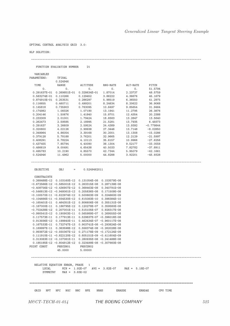
Generalized Linear Tangent Steering Example
OPTIMAL CONTROL ANALYSIS GRID 3.0:
NLP SOLUTION:
--------------------------------------------------------------------------------------------------------
FUNCTION EVALUATION NUMBER 21
VARIABLES
PARAMETERS: TFINAL
0.524946
TIME RANGE ALTITUDE RNG-RATE ALT-RATE PITCH
0. 0. 0. 0. 0. 51.5794
0.291637E-01 0.269851E-01 0.328634E-01 1.87014 2.23737 48.5759
0.583274E-01 0.110266 0.129452 3.86222 4.36676 45.1679
0.874910E-01 0.253531 0.286297 5.98519 6.36550 41.2975
0.116655 0.460711 0.499201 8.24634 8.20622 36.9068
0.145818 0.735903 0.763095 10.6497 9.85654 31.9464
0.174982 1.08326 1.07190 13.1941 11.2795 26.3876
0.204146 1.50676 1.41840 15.8701 12.4354 20.2388
0.233309 2.01001 1.79424 18.6583 13.2847 13.5640
0.262473 2.59585 2.18995 21.5281 13.7935 6.49373
0.291637 3.26609 2.59524 24.4389 13.9392 -0.779844
0.320800 4.02126 2.99938 27.3446 13.7148 -8.02850
0.349964 4.86054 3.39168 30.2001 13.1308 -15.0286
0.379128 5.78188 3.76201 32.9665 12.2129 -21.5997
0.408291 6.78224 4.10113 35.6157 10.9966 -27.6256
0.437455 7.85794 4.40090 38.1304 9.52177 -33.0558
0.466619 9.00491 4.65438 40.5033 7.82782 -37.8911
0.495783 10.2190 4.85570 42.7344 5.95079 -42.1661
0.524946 11.4962 5.00000 44.8288 3.92201 -45.9328
--------------------------------------------------------------------------------------------------------
OBJECTIVE OBJ = 0.5249462011
CONSTRAINTS
0.268488E-12 0.103160E-12 0.131054E-08 0.153579E-08
-0.672566E-12 -0.585001E-12 0.263315E-08 0.287139E-08
-0.408756E-12 -0.436907E-12 0.368463E-08 0.340791E-08
-0.546813E-12 -0.948061E-12 0.205836E-08 0.171509E-08
-0.100570E-11 -0.622974E-12 0.500663E-09 0.324660E-09
-0.104666E-11 -0.934530E-12 0.615083E-10 0.398384E-10
-0.165401E-11 0.464351E-12 0.806606E-08 0.355131E-08
-0.167000E-11 0.186795E-12 0.120278E-07 0.359580E-08
-0.702438E-12 0.207001E-11 0.515105E-07 0.928317E-08
-0.990541E-12 0.190903E-11 0.565989E-07 0.269555E-08
0.117573E-11 0.177913E-11 0.529837E-07 -0.396016E-08
0.913936E-12 0.199840E-11 0.462434E-07 -0.960117E-08
0.167533E-11 0.732747E-13 0.903741E-08 -0.293824E-08
0.169997E-11 0.363598E-12 0.558374E-08 -0.262028E-08
0.993872E-12 -0.930367E-12 0.271178E-09 -0.172124E-09
0.111910E-11 -0.822120E-12 0.605151E-09 -0.411604E-09
0.313083E-12 -0.107081E-11 0.280935E-08 -0.241488E-08
0.185185E-12 -0.804912E-12 0.323499E-08 -0.307660E-08
POINT CONST PHSCON01 PHSCON02
45.0000 5.00000
--------------------------------------------------------------------------------------------------------
RELATIVE EQUATION ERROR, PHASE 1
LOCAL MIN = 1.92E-07 AVG = 3.82E-07 MAX = 5.18E-07
SYMMETRY MAX = 3.83E-02
====================================================================================================
GRID NPT NFC NGC NHC NFE NRHS ERRODE ERRDAE CPU TIME
M&CT-TECH-01-014 THE BOEING COMPANY 525
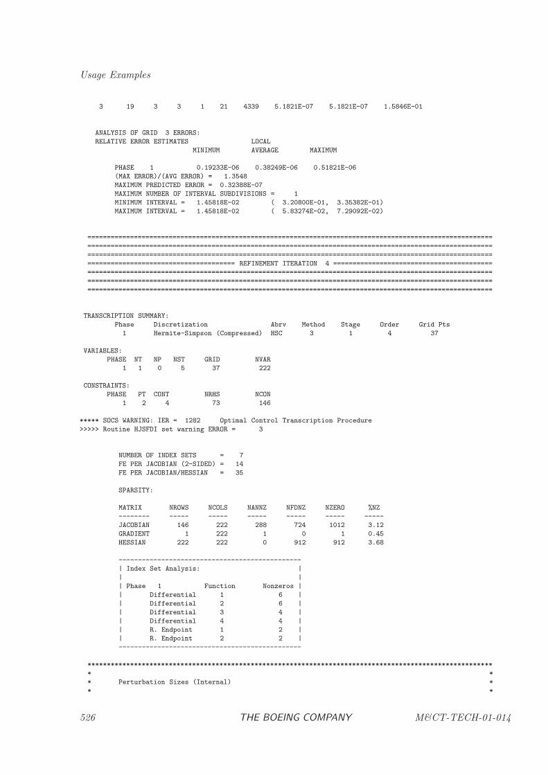
Usage Examples
3 19 3 3 1 21 4339 5.1821E-07 5.1821E-07 1.5846E-01
ANALYSIS OF GRID 3 ERRORS:
RELATIVE ERROR ESTIMATES LOCAL
MINIMUM AVERAGE MAXIMUM
PHASE 1 0.19233E-06 0.38249E-06 0.51821E-06
(MAX ERROR)/(AVG ERROR) = 1.3548
MAXIMUM PREDICTED ERROR = 0.32388E-07
MAXIMUM NUMBER OF INTERVAL SUBDIVISIONS = 1
MINIMUM INTERVAL = 1.45818E-02 ( 3.20800E-01, 3.35382E-01)
MAXIMUM INTERVAL = 1.45818E-02 ( 5.83274E-02, 7.29092E-02)
========================================================================================================
========================================================================================================
========================================================================================================
====================================== REFINEMENT ITERATION 4 =========================================
========================================================================================================
========================================================================================================
========================================================================================================
TRANSCRIPTION SUMMARY:
Phase Discretization Abrv Method Stage Order Grid Pts
1 Hermite-Simpson (Compressed) HSC 3 1 4 37
VARIABLES:
PHASE NT NP NST GRID NVAR
1 1 0 5 37 222
CONSTRAINTS:
PHASE PT CONT NRHS NCON
1 2 4 73 146
***** SOCS WARNING: IER = 1282 Optimal Control Transcription Procedure
>>>>> Routine HJSFDI set warning ERROR = 3
NUMBER OF INDEX SETS = 7
FE PER JACOBIAN (2-SIDED) = 14
FE PER JACOBIAN/HESSIAN = 35
SPARSITY:
MATRIX NROWS NCOLS NANNZ NFDNZ NZERO %NZ
-------- ----- ----- ----- ----- ----- -----
JACOBIAN 146 222 288 724 1012 3.12
GRADIENT 1 222 1 0 1 0.45
HESSIAN 222 222 0 912 912 3.68
-----------------------------------------------
| Index Set Analysis: |
| |
| Phase 1 Function Nonzeros |
| Differential 1 6 |
| Differential 2 6 |
| Differential 3 4 |
| Differential 4 4 |
| R. Endpoint 1 2 |
| R. Endpoint 2 2 |
-----------------------------------------------
********************************************************************************************************
* *
* Perturbation Sizes (Internal) *
* *
526 THE BOEING COMPANY M&CT-TECH-01-014
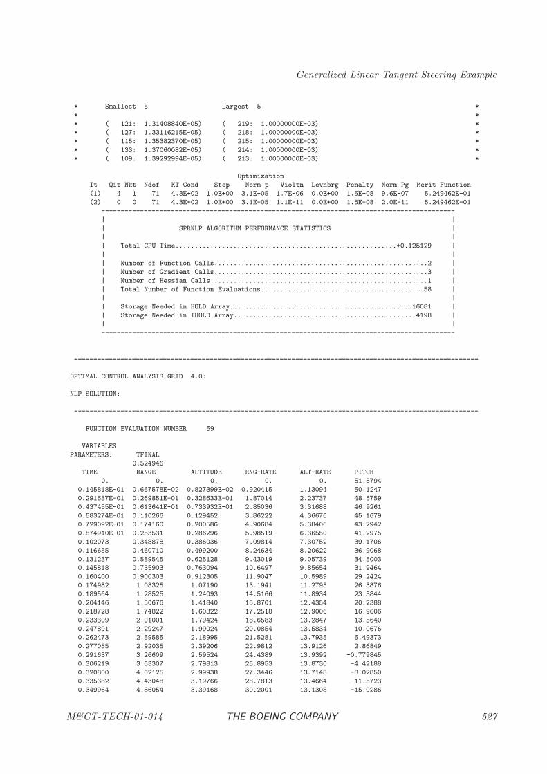
Generalized Linear Tangent Steering Example
* Smallest 5 Largest 5 *
* *
* ( 121: 1.31408840E-05) ( 219: 1.00000000E-03) *
* ( 127: 1.33116215E-05) ( 218: 1.00000000E-03) *
* ( 115: 1.35382370E-05) ( 215: 1.00000000E-03) *
* ( 133: 1.37060082E-05) ( 214: 1.00000000E-03) *
* ( 109: 1.39292994E-05) ( 213: 1.00000000E-03) *
Optimization
It Qit Nkt Ndof KT Cond Step Norm p Violtn Levnbrg Penalty Norm Pg Merit Function
(1) 4 1 71 4.3E+02 1.0E+00 3.1E-05 1.7E-06 0.0E+00 1.5E-08 9.6E-07 5.249462E-01
(2) 0 0 71 4.3E+02 1.0E+00 3.1E-05 1.1E-11 0.0E+00 1.5E-08 2.0E-11 5.249462E-01
-------------------------------------------------------------------------------------------
| |
| SPRNLP ALGORITHM PERFORMANCE STATISTICS |
| |
| Total CPU Time.........................................................+0.125129 |
| |
| Number of Function Calls.......................................................2 |
| Number of Gradient Calls.......................................................3 |
| Number of Hessian Calls........................................................1 |
| Total Number of Function Evaluations..........................................58 |
| |
| Storage Needed in HOLD Array...............................................16081 |
| Storage Needed in IHOLD Array...............................................4198 |
| |
-------------------------------------------------------------------------------------------
========================================================================================================
OPTIMAL CONTROL ANALYSIS GRID 4.0:
NLP SOLUTION:
--------------------------------------------------------------------------------------------------------
FUNCTION EVALUATION NUMBER 59
VARIABLES
PARAMETERS: TFINAL
0.524946
TIME RANGE ALTITUDE RNG-RATE ALT-RATE PITCH
0. 0. 0. 0. 0. 51.5794
0.145818E-01 0.667578E-02 0.827399E-02 0.920415 1.13094 50.1247
0.291637E-01 0.269851E-01 0.328633E-01 1.87014 2.23737 48.5759
0.437455E-01 0.613641E-01 0.733932E-01 2.85036 3.31688 46.9261
0.583274E-01 0.110266 0.129452 3.86222 4.36676 45.1679
0.729092E-01 0.174160 0.200586 4.90684 5.38406 43.2942
0.874910E-01 0.253531 0.286296 5.98519 6.36550 41.2975
0.102073 0.348878 0.386036 7.09814 7.30752 39.1706
0.116655 0.460710 0.499200 8.24634 8.20622 36.9068
0.131237 0.589545 0.625128 9.43019 9.05739 34.5003
0.145818 0.735903 0.763094 10.6497 9.85654 31.9464
0.160400 0.900303 0.912305 11.9047 10.5989 29.2424
0.174982 1.08325 1.07190 13.1941 11.2795 26.3876
0.189564 1.28525 1.24093 14.5166 11.8934 23.3844
0.204146 1.50676 1.41840 15.8701 12.4354 20.2388
0.218728 1.74822 1.60322 17.2518 12.9006 16.9606
0.233309 2.01001 1.79424 18.6583 13.2847 13.5640
0.247891 2.29247 1.99024 20.0854 13.5834 10.0676
0.262473 2.59585 2.18995 21.5281 13.7935 6.49373
0.277055 2.92035 2.39206 22.9812 13.9126 2.86849
0.291637 3.26609 2.59524 24.4389 13.9392 -0.779845
0.306219 3.63307 2.79813 25.8953 13.8730 -4.42188
0.320800 4.02125 2.99938 27.3446 13.7148 -8.02850
0.335382 4.43048 3.19766 28.7813 13.4664 -11.5723
0.349964 4.86054 3.39168 30.2001 13.1308 -15.0286
M&CT-TECH-01-014 THE BOEING COMPANY 527
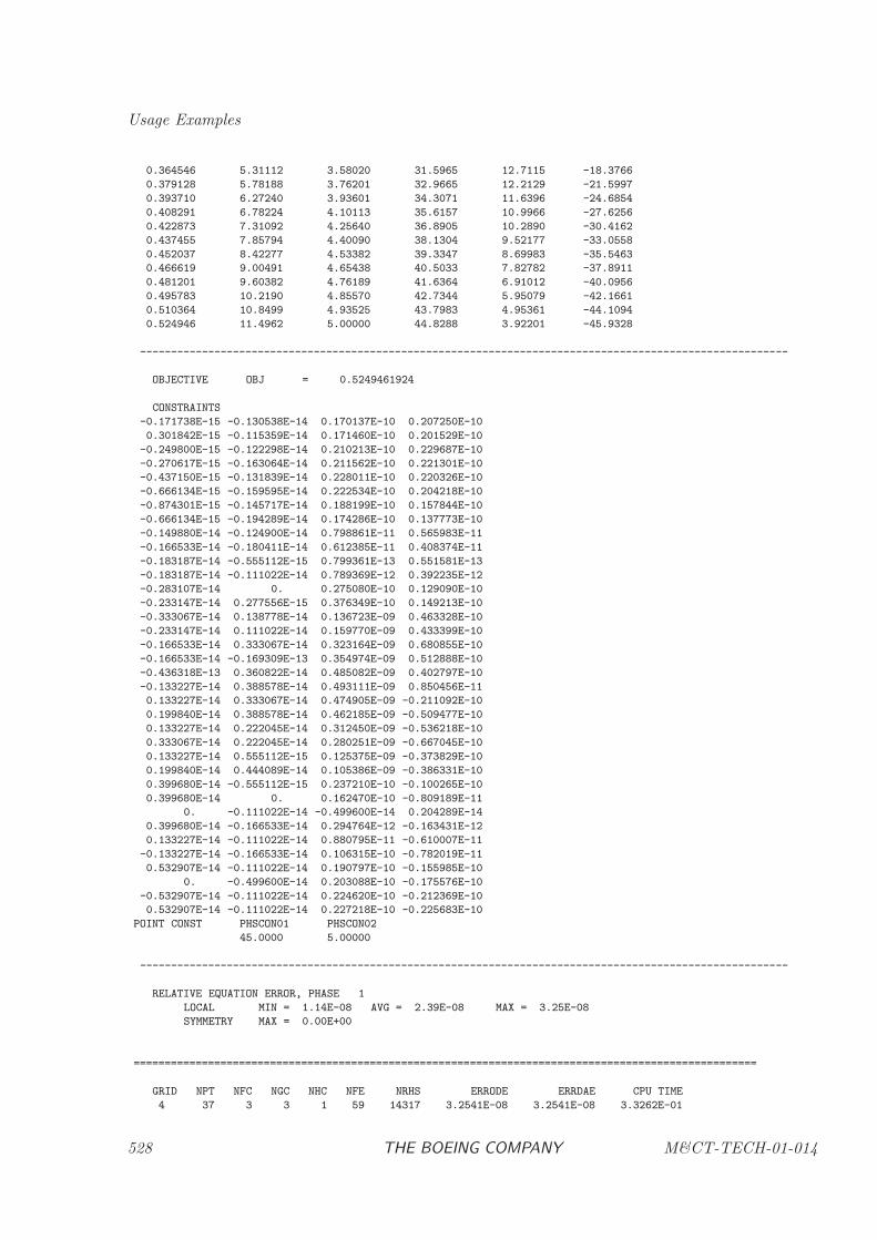
Usage Examples
0.364546 5.31112 3.58020 31.5965 12.7115 -18.3766
0.379128 5.78188 3.76201 32.9665 12.2129 -21.5997
0.393710 6.27240 3.93601 34.3071 11.6396 -24.6854
0.408291 6.78224 4.10113 35.6157 10.9966 -27.6256
0.422873 7.31092 4.25640 36.8905 10.2890 -30.4162
0.437455 7.85794 4.40090 38.1304 9.52177 -33.0558
0.452037 8.42277 4.53382 39.3347 8.69983 -35.5463
0.466619 9.00491 4.65438 40.5033 7.82782 -37.8911
0.481201 9.60382 4.76189 41.6364 6.91012 -40.0956
0.495783 10.2190 4.85570 42.7344 5.95079 -42.1661
0.510364 10.8499 4.93525 43.7983 4.95361 -44.1094
0.524946 11.4962 5.00000 44.8288 3.92201 -45.9328
--------------------------------------------------------------------------------------------------------
OBJECTIVE OBJ = 0.5249461924
CONSTRAINTS
-0.171738E-15 -0.130538E-14 0.170137E-10 0.207250E-10
0.301842E-15 -0.115359E-14 0.171460E-10 0.201529E-10
-0.249800E-15 -0.122298E-14 0.210213E-10 0.229687E-10
-0.270617E-15 -0.163064E-14 0.211562E-10 0.221301E-10
-0.437150E-15 -0.131839E-14 0.228011E-10 0.220326E-10
-0.666134E-15 -0.159595E-14 0.222534E-10 0.204218E-10
-0.874301E-15 -0.145717E-14 0.188199E-10 0.157844E-10
-0.666134E-15 -0.194289E-14 0.174286E-10 0.137773E-10
-0.149880E-14 -0.124900E-14 0.798861E-11 0.565983E-11
-0.166533E-14 -0.180411E-14 0.612385E-11 0.408374E-11
-0.183187E-14 -0.555112E-15 0.799361E-13 0.551581E-13
-0.183187E-14 -0.111022E-14 0.789369E-12 0.392235E-12
-0.283107E-14 0. 0.275080E-10 0.129090E-10
-0.233147E-14 0.277556E-15 0.376349E-10 0.149213E-10
-0.333067E-14 0.138778E-14 0.136723E-09 0.463328E-10
-0.233147E-14 0.111022E-14 0.159770E-09 0.433399E-10
-0.166533E-14 0.333067E-14 0.323164E-09 0.680855E-10
-0.166533E-14 -0.169309E-13 0.354974E-09 0.512888E-10
-0.436318E-13 0.360822E-14 0.485082E-09 0.402797E-10
-0.133227E-14 0.388578E-14 0.493111E-09 0.850456E-11
0.133227E-14 0.333067E-14 0.474905E-09 -0.211092E-10
0.199840E-14 0.388578E-14 0.462185E-09 -0.509477E-10
0.133227E-14 0.222045E-14 0.312450E-09 -0.536218E-10
0.333067E-14 0.222045E-14 0.280251E-09 -0.667045E-10
0.133227E-14 0.555112E-15 0.125375E-09 -0.373829E-10
0.199840E-14 0.444089E-14 0.105386E-09 -0.386331E-10
0.399680E-14 -0.555112E-15 0.237210E-10 -0.100265E-10
0.399680E-14 0. 0.162470E-10 -0.809189E-11
0. -0.111022E-14 -0.499600E-14 0.204289E-14
0.399680E-14 -0.166533E-14 0.294764E-12 -0.163431E-12
0.133227E-14 -0.111022E-14 0.880795E-11 -0.610007E-11
-0.133227E-14 -0.166533E-14 0.106315E-10 -0.782019E-11
0.532907E-14 -0.111022E-14 0.190797E-10 -0.155985E-10
0. -0.499600E-14 0.203088E-10 -0.175576E-10
-0.532907E-14 -0.111022E-14 0.224620E-10 -0.212369E-10
0.532907E-14 -0.111022E-14 0.227218E-10 -0.225683E-10
POINT CONST PHSCON01 PHSCON02
45.0000 5.00000
--------------------------------------------------------------------------------------------------------
RELATIVE EQUATION ERROR, PHASE 1
LOCAL MIN = 1.14E-08 AVG = 2.39E-08 MAX = 3.25E-08
SYMMETRY MAX = 0.00E+00
====================================================================================================
GRID NPT NFC NGC NHC NFE NRHS ERRODE ERRDAE CPU TIME
4 37 3 3 1 59 14317 3.2541E-08 3.2541E-08 3.3262E-01
528 THE BOEING COMPANY M&CT-TECH-01-014
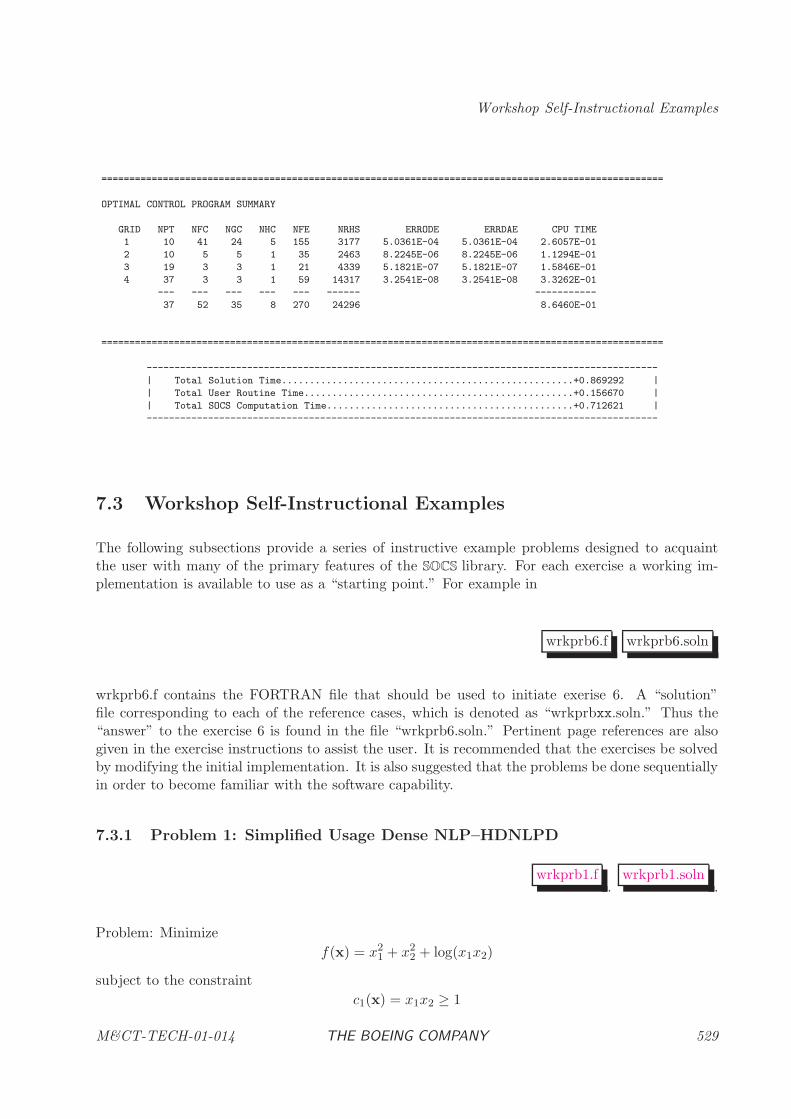
Workshop Self-Instructional Examples
====================================================================================================
OPTIMAL CONTROL PROGRAM SUMMARY
GRID NPT NFC NGC NHC NFE NRHS ERRODE ERRDAE CPU TIME
1 10 41 24 5 155 3177 5.0361E-04 5.0361E-04 2.6057E-01
2 10 5 5 1 35 2463 8.2245E-06 8.2245E-06 1.1294E-01
3 19 3 3 1 21 4339 5.1821E-07 5.1821E-07 1.5846E-01
4 37 3 3 1 59 14317 3.2541E-08 3.2541E-08 3.3262E-01
--- --- --- --- --- ------ -----------
37 52 35 8 270 24296 8.6460E-01
====================================================================================================
-------------------------------------------------------------------------------------------
| Total Solution Time....................................................+0.869292 |
| Total User Routine Time................................................+0.156670 |
| Total SOCS Computation Time............................................+0.712621 |
-------------------------------------------------------------------------------------------
7.3 Workshop Self-Instructional Examples
The following subsections provide a series of instructive example problems designed to acquaintthe user with many of the primary features of the SOCS library. For each exercise a working im-plementation is available to use as a “starting point.” For example in
wrkprb6.f wrkprb6.soln
wrkprb6.f contains the FORTRAN file that should be used to initiate exerise 6. A “solution”file corresponding to each of the reference cases, which is denoted as “wrkprbxx.soln.” Thus the“answer” to the exercise 6 is found in the file “wrkprb6.soln.” Pertinent page references are alsogiven in the exercise instructions to assist the user. It is recommended that the exercises be solvedby modifying the initial implementation. It is also suggested that the problems be done sequentiallyin order to become familiar with the software capability.
7.3.1 Problem 1: Simplified Usage Dense NLP–HDNLPD
wrkprb1.f.
wrkprb1.soln.
Problem: Minimize
f(x) = x21 + x2
2 + log(x1x2)
subject to the constraint
c1(x) = x1x2 ≥ 1
M&CT-TECH-01-014 THE BOEING COMPANY 529
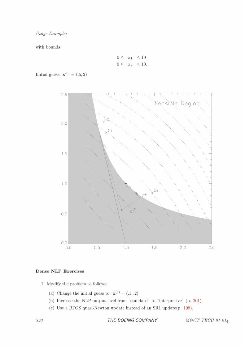
Usage Examples
with bounds
0 ≤ x1 ≤ 10
0 ≤ x2 ≤ 10.
Initial guess: x(0) = (.5, 2)
Dense NLP Exercises
1. Modify the problem as follows:
(a) Change the initial guess to: x(0) = (.1, .2)
(b) Increase the NLP output level from “standard” to “interpretive” (p. 201).
(c) Use a BFGS quasi-Newton update instead of an SR1 update(p. 199).
530 THE BOEING COMPANY M&CT-TECH-01-014
Workshop Self-Instructional Examples
2. Modify the previous case as follows:
(a) Use the Schur-complement sparse QP (p. 205).
(b) Use a finite difference Hessian (p. 199).
3. Use the default algorithm with “interpretive” line search output (p. 202) to solve the (modi-fied) problem: Minimize
f(x) = x21 + x2
2
subject to
x21x2 − 1 ≥ 0
x2 ≤ −.1
with no bounds on the variables. Use the initial guess: x(0) = (.5, 2)
7.3.2 Problem 2: Reverse Communication Dense NLP–HDNLPR
wrkprb2.f.
wrkprb2.soln.
1. Modify the reference problem as follows:
(a) Increase the NLP output level from “terse” to “interpretive” (p. 201).
(b) Use the exact Hessian matrix (p. 199).
(c) Change constraint number 1 from x1x2 ≤ 1/2 to
x1x22 ≤ 1/2
(d) Display the quantity x1x2 in addition to previous output using IREVRS(4)(p. 36).
2. Modify the previous case as follows:
(a) Display the Jacobian and Hessian matrices (p. 201)
(b) Set the iteration limit to one (p. 197).
(c) Set the algorithm option to “M” (p. 205).
7.3.3 Problem 3: Sparse NLP–HDSNLP
wrkprb3.f.
wrkprb3.soln.
M&CT-TECH-01-014 THE BOEING COMPANY 531
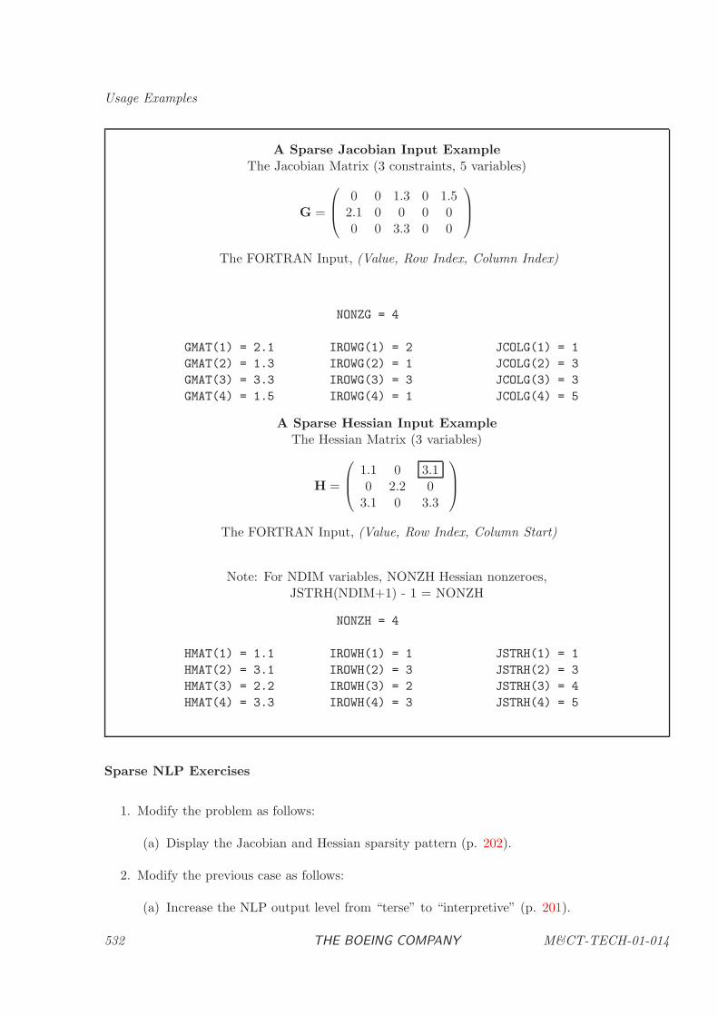
Usage Examples
A Sparse Jacobian Input ExampleThe Jacobian Matrix (3 constraints, 5 variables)
G =
0 0 1.3 0 1.5
2.1 0 0 0 00 0 3.3 0 0
The FORTRAN Input, (Value, Row Index, Column Index)
NONZG = 4
GMAT(1) = 2.1 IROWG(1) = 2 JCOLG(1) = 1
GMAT(2) = 1.3 IROWG(2) = 1 JCOLG(2) = 3
GMAT(3) = 3.3 IROWG(3) = 3 JCOLG(3) = 3
GMAT(4) = 1.5 IROWG(4) = 1 JCOLG(4) = 5
A Sparse Hessian Input ExampleThe Hessian Matrix (3 variables)
H =
1.1 0 3.10 2.2 0
3.1 0 3.3
The FORTRAN Input, (Value, Row Index, Column Start)
Note: For NDIM variables, NONZH Hessian nonzeroes,JSTRH(NDIM+1) - 1 = NONZH
NONZH = 4
HMAT(1) = 1.1 IROWH(1) = 1 JSTRH(1) = 1
HMAT(2) = 3.1 IROWH(2) = 3 JSTRH(2) = 3
HMAT(3) = 2.2 IROWH(3) = 2 JSTRH(3) = 4
HMAT(4) = 3.3 IROWH(4) = 3 JSTRH(4) = 5
Sparse NLP Exercises
1. Modify the problem as follows:
(a) Display the Jacobian and Hessian sparsity pattern (p. 202).
2. Modify the previous case as follows:
(a) Increase the NLP output level from “terse” to “interpretive” (p. 201).
532 THE BOEING COMPANY M&CT-TECH-01-014
Workshop Self-Instructional Examples
(b) Change constraint number 1 from x1x2 ≤ 1/2 to
x1x4 ≤ 1/2
7.3.4 Problem 4: Sparse Least Squares–HDSLSQ
wrkprb4.f.
wrkprb4.soln.
Sparse Least Squares Exercises
1. Modify the reference problem as follows:
(a) Display the Jacobian and Hessian sparsity pattern (p. 202)
(b) Increase the NLP output level from “terse” to “standard” (p. 201).
2. Modify the previous case as follows:
(a) Use the linear least squares algorithm option (p. 205)
(b) Change constraint number 1 from x1x2 ≤ 1/2 to
x1 + x2 ≤ 1/2
(c) Change the residual vector to
r =
10(x2 − 2x1)(1 − x1)
10(x4 − 2x3)(1 − x3)
7.3.5 Problem 5: Reverse Communication NLP, Finite Difference Gradients
wrkprb5.f.
wrkprb5.soln.
Exercises
1. Modify the problem as follows:
(a) Use the sparse QP (p. 205)
(b) Use a finite difference Hessian (p. 199)
(c) Do a postoptimality analysis at the solution (p. 206)
(d) Set the KKT condition number tolerance to 1.d10 (p. 203)
(e) Increase the NLP output level from “terse” to “standard” (p. 201).
(f) Change constraint number 1 tox1 − x3 = 0
(g) Change the objective function to
f(x) = (x1 − x2)2 + (x2 − x3)
4
M&CT-TECH-01-014 THE BOEING COMPANY 533
Usage Examples
7.3.6 Problem 6: Sparse NLP with Sparse Finite Differences
wrkprb6.f.
wrkprb6.soln.
Exercises
1. Modify the problem as follows:
(a) Increase the sparse difference output level (i.e. set MSGLVL=3) (p. 265)
(b) Increase the NLP output level from “terse” to “standard” (p. 201).
(c) Display the sparsity pattern (p. 202)
7.3.7 Problem 7: One Phase Example
wrkprb7.f.
wrkprb7.soln.
Linear Tangent Steering Example Ref. [11]Solve the following problem:Objective: Minimize the final time tfState Equations:
y1 = y3
y2 = y4
y3 = a cos u
y4 = a sinu
where a = 100 and
−π2≤ u(t) ≤ π
2
Boundary Conditions: y1(0) = y2(0) = y3(0) = y4(0) = 0 and y2(tf ) = 5, y3(tf ) = 45, y4(tf ) = 0.
Setting SOCS Parameters–Exercises
1. Modify the example problem as follows:
(a) Set the relative accuracy in the differential equations to 1.d-7 (p. 366).
(b) Change the optimal control output level to “interpretive” (i.e. level 20) (p. 370)
2. Modify the previous case as follows:
(a) Eliminate the SOCS output for menu items; (e, f, g, k, l, m, n, o, p, q, r) (p. 372).
(b) Display the NLP Jacobian and Hessian sparsity (p. 202)
534 THE BOEING COMPANY M&CT-TECH-01-014

Workshop Self-Instructional Examples
7.3.8 Problem 8: User Routines Example
wrkprb8.f.
wrkprb8.soln.
The User Routines–Exercises
1. Modify the previous case to make the final differential equation (p. 409)
y4 = a sinu− g0
[h0
y2 + h0
]2
where g0 = 32.2 and h0 = 3500
2. Modify the previous case to impose the boundary condition (p. 384)
y2(tf ) = 6
3. Modify the previous case to impose the control path bounds (p. 384)
−π3≤ u(t) ≤ π
3
and display the inequality switching times (p. 372).
7.3.9 Problem 9: Path Constraint Example
wrkprb9.f.
wrkprb9.soln.
Path Constraints–Exercise (p. 409), (p. 458)Solve the following problem:Objective: Minimize the final time tfState Equations:
y1 = y3
y2 = y4
y3 = a cos u
y4 = a sinu
where a = 100 and
−π2≤ u(t) ≤ π
2
Path Constraint:
a sinu(t) ≤ 60
Boundary Conditions: y1(0) = y2(0) = y3(0) = y4(0) = 0 and y2(tf ) = 5, y3(tf ) = 45, y4(tf ) = 0.
M&CT-TECH-01-014 THE BOEING COMPANY 535
Usage Examples
7.3.10 Problem 10: Quadrature Example
wrkprb10.f.
wrkprb10.soln.
Quadrature Functions–Exercise (p. 384), (p. 409)Solve the following problem:Objective: Minimize the “energy”
J =
∫ tf
0u2(t)dt
State Equations:
y1 = y3
y2 = y4
y3 = a cos u
y4 = a sinu
where a = 100 and
−π2≤ u(t) ≤ π
2
Boundary Conditions: y1(0) = y2(0) = y3(0) = y4(0) = 0 and y2(tf ) = 5, y3(tf ) = 45, y4(tf ) = 0.
7.3.11 Problem 11: Point Function Example
wrkprb11.f.
wrkprb11.soln.
Point Functions–Exercise (p. 384), (p. 405), (p. 452)Solve the following problem:Objective: Minimize the final time tfState Equations:
y1 = y3
y2 = y4
y3 = a cos u
y4 = a sinu
where a = 100 and
−π2≤ u(t) ≤ π
2
Boundary Conditions: y1(0) = y2(0) = y3(0) = y4(0) = 0 and y3(tf ) = 45, y4(tf ) = 0 and
y1(tf )y2(tf ) ≥ 60
536 THE BOEING COMPANY M&CT-TECH-01-014
Workshop Self-Instructional Examples
7.3.12 Problem 12: Initial Guess Example
wrkprb12.f.
wrkprb12.soln.
Initial Guess–Exercise (p. 384), (p. 381)Solve the previous problem with the following modifications:
1. Compute “exact” initial guess (provided in subroutine EXACKT) (p. 387).
2. Set the discretization method to Hermite-Simpson (Compressed) (p. 386)
3. Set the initial number of grid points to 15 (p. 387)
4. Use NLP option “M” (p. 205)
7.3.13 Problem 13: Auxilliary Output Example
wrkprb13.f.
wrkprb13.soln.
Auxilliary Output–ExerciseModify the previous problem to display the analytic solution at the grid points.
1. Use subroutine EXACKT to compute the analytic solution.
2. Use IPUAUX=6 (p. 365), to display auxilliary output interspersed with the standard output(p. 401)
3. Force the NLP to be a Newton method–i.e. recompute the Hessian every step! (p. 204)
7.3.14 Problem 14: Two Phase Example
wrkprb14.f.
Two Phase Example (p. 384), (p. 409), (p. 435)
Phase 1: (Burn) 0 ≤ t ≤ t1State Equations:
y1 = y3
y2 = y4
y3 = a cos u
y4 = a sinu− g0
[h0
y2 + h0
]2
M&CT-TECH-01-014 THE BOEING COMPANY 537
Usage Examples
where a = 100, g0 = 32.2 and h0 = 3500 with −π2 ≤ u(t) ≤ π
2Boundary Conditions: y1(0) = y2(0) = y3(0) = y4(0) = 0 and y2(t1) = 5, y3(t1) = 45, y4(t1) = 0.
Phase 2: (Coast) t1 ≤ t ≤ 1State Equations:
y1 = y3
y2 = y4
y3 = 0
y4 = −g0[
h0
y2 + h0
]2
Boundary Conditions: Continuity for all states and time at t1 (the boundary between phase 1 and2). (p. 435).
Solve the following problem:Objective: Minimize the final burn time t1
Note: This example does not have a file “wrkprb14.soln.”
7.4 SOCS Demonstration/Test Examples
A more extensive collection of test problems that illustrate many of the features of the SOCS softwareare available in source code form. This section briefly describes the features of the problems.
7.4.1 Zermelo’s Problem
zermelo.f.
This classical example illustrates how SOCS can be applied to a very simple problem. It is describedin Reference [11].
7.4.2 Goddard Rocket Problem
templt.f.
This is a three phase problem containing a singular arc phase, which is modeled using an algebraicpath constraint. This problem is described in Section 4.10.1 of Reference [5].
7.4.3 Van der Pol Oscillator Problem
vpolex.f.
538 THE BOEING COMPANY M&CT-TECH-01-014
SOCS Demonstration/Test Examples
This problem is formulated in eight mathematically equivalent ways to demonstrate various SOCS
implementation options using analytic terms and auxiliary functions.�
�
�
�Formulation 1
Consider a problem with two state variables and one control described by the system
y1 = y2
y2 = (1 − y21)y2 − y1 + u. (7.1)
The goal is to minimize
J =
∫ 5
0(y2
1 + y22 + u2)dt
subject to the boundary conditions y1(0) = 1 and y2(0) = 0 and state bound
−4 ≤ y2(t).
�
�
�
�Formulation 2
Introduce a new algebraic variable v = (1 − y21)y2 and replace (7.1) with
y1 = y2
y2 = v − y1 + u
0 = v − y2 + y21y2. (7.2)
SOCS Implementationcontinuous function (NCF(2)=1), β0a0(y, u, p, t) v
analytic term −y2
auxiliary function (NCF(4)=1), β1a1(y, u, p, t) y21y2
�
�
�
�Formulation 3
Introduce a new algebraic variable v = (1 − y21)y2 and replace (7.1) with
y1 = y2
y2 = v − y1 + u
0 = v − (1 − y21)y2. (7.3)
SOCS Implementationcontinuous function (NCF(2)=1), β0a0(y, u, p, t) v
auxiliary function (NCF(4)=1), β1a1(y, u, p, t) −(1 − y21)y2
�
�
�
�Formulation 4
Introduce a new algebraic variable v = (1 − y21)y2 and replace (7.1) with
y1 = y2
y2 = v − y1 + u
0 = v − (1 − y21)y2. (7.4)
M&CT-TECH-01-014 THE BOEING COMPANY 539
Usage Examples
SOCS Implementationcontinuous function (NCF(2)=1), β0a0(y, u, p, t) v − (1 − y2
1)y2
�
�
�
�Formulation 5
Introduce a new algebraic variable v = (1 − y21)y2 and replace (7.1) with
y1 = y2
y2 = v − y1 + u
0 = v + y21y2 − y2. (7.5)
SOCS Implementationcontinuous function (NCF(2)=1), β0a0(y, u, p, t) v + y2
1y2
analytic term −y2
�
�
�
�Formulation 6
Introduce a new algebraic variable v = (1 − y21)y2 − y1 + u and replace (7.1) with
y1 = y2
y2 = v
0 = (1 − y21)y2 − y1 + u− v. (7.6)
SOCS Implementationcontinuous function (NCF(2)=1), β0a0(y, u, p, t) (1 − y2
1)y2 − y1
analytic term u
analytic term −v
�
�
�
�Formulation 7
This formulation implements an indirect solution method using three distinct phases. In additionto the state equations defined by (7.1) the optimality conditions are formed explicitly. The problemhas a first order state constraint s(t) = −y2(t) − 4 ≤ 0, so the Hamiltonian is
H = u2 + y21 + y2
2 + λ1y2 + λ2[(1 − y21)y2 − y1 + u] + µ[−(1 − y2
1)y2 + y1 − u] (7.7)
where the first derivative of the path constraint s = −y2 = −(1− y21)y2 + y1 −u appears in H. The
adjoint equations are
λ1 = −2y1 + 2y1y2λ2 + λ2 − µ(2y1y2 + 1) (7.8)
λ2 = −2y2 − λ1 + λ2(y21 − 1) + µ(1 − y2
1). (7.9)
The optimal control is
u(t) =
−λ2/2 0 ≤ t ≤ t1(y2
1 − 1)y2 + y1 t1 ≤ t ≤ t2−λ2/2 t2 ≤ t ≤ 5
(7.10)
540 THE BOEING COMPANY M&CT-TECH-01-014
SOCS Demonstration/Test Examples
with optimal multiplier given by
µ(t) =
0 0 ≤ t ≤ t12(y2
1 − 1)y2 + 2y1 + λ2 t1 ≤ t ≤ t20 t2 ≤ t ≤ 5.
(7.11)
The switching structure is determined by the tangency condition
0 = s
= −y2
= −(1 − y21)y2 + y1 − u
= (y21 − 1)y2 + y1 + λ2/2 (7.12)
which is enforced immediately before entering the boundary arc at t = t−1 and immediately afterleaving the boundary arc at point t = t+2 . The location of the exit point is also defined by enforcingthe switching condition µ(t−2 ) = 0.�
�
�
�Formulation 8
This formulation is identical to (7.1) except that the simple bound on the state is treated as thepath constraint s(t) = −y2(t) − 4 ≤ 0.
7.4.4 Maximum Crossrange Space Shuttle Reentry Problem
shutle.f.
This single phase problem is described in Section 5.1 of Reference [5].
7.4.5 Minimum Time to Climb Problem
clymex.files.
This single phase problem is described in Section 5.2 of Reference [5], and illustrates the use ofminimum curvature data fitting software. The file contains both the FORTRAN code and therelevant data files.
7.4.6 Low-Thrust Orbit Transfer
lthrst.f.
This single phase problem using modified equinoctial coordinates is described in Section 5.3 ofReference [5].
M&CT-TECH-01-014 THE BOEING COMPANY 541
Usage Examples
7.4.7 Two-Burn Orbit Transfer
twobrn.f.
This multiple phase problem illustrates the use of analytic phase propagation, as well as modifiedequinoctial coordinates. A shooting method formulation is also demonstrated. It is described inSection 5.4 of Reference [5].
7.4.8 Industrial Robot
robot.f.
This nine phase problem illustrates how state constrained multibody problems can be solved. It isdescribed in Section 5.5 of Reference [5].
7.4.9 Multibody Mechanism
skwzer.f.
This example illustrates how SOCS can be applied to an index-three differential-algebraic system.It is described in Section 5.6 of Reference [5].
7.4.10 Heat Flow–Parabolic PDE
heatfl.f.
This example illustrates how SOCS can be applied to a parabolic partial differential equation usingthe method of lines. It is described in Section 4.6.10 of Reference [5].
7.4.11 Embedding (Homotopy) Example Problem
embed.f.
This example demonstrates how to construct a solution to a series of related problems using anembedding or homotopy method. The approach can be especially useful when computing an initialguess for a very complex problem or when performing a parameter study that requires manysolutions of a similiar nature. The specific example mimics the behavior of a numerical integrationalgorithm, to compute the solution of an initial value problem.
542 THE BOEING COMPANY M&CT-TECH-01-014
SOCS Demonstration/Test Examples
7.4.12 Orbit Determination (Parameter Estimation) Example Problem
lambrt.f.
This example demonstrates the use of the SOCS parameter estimation software for a classical orbitdetermination problem. Three cases are illustrated including:
• determination of an orbit from two position vectors and time (Lambert’s problem)
• determination of an orbit from position vectors with and without noise.
7.4.13 First-Order Irreversible Chain Reaction Parameter Estimation Problem
foicex.files.
This problem illustrates the SOCS parameter estimation software for a chemical process application.Three cases are illustrated including:
• A single phase formultion
• A multi-phase (multiple observation) formulation
• A multi-phase explicit model (curve fitting) solution.
The file contains both the FORTRAN code and the relevant data files.
7.4.14 Initial Value and Shooting Method Example Problems
ivptst.f.
This example demonstrates the use of the SOCS initial value and shooting method capability. Aseries of cases are illustrated including:
• forward and backward propagation of a simple initial value problem
• construction of an initial guess for a collocation method from an integrated (initial value)problem
• solution of Linear Tangent Steering problem using a multiphase shooting method.
M&CT-TECH-01-014 THE BOEING COMPANY 543

Usage Examples
544 THE BOEING COMPANY M&CT-TECH-01-014
Chapter 8
Spline Data Approximations
8.1 Overview of Data Fitting and Approximation
Many optimization, optimal control, and parameter estimation applications involve problems thatare specified in terms of tabular data. All optimization algorithms require that the objective andconstraints be sufficiently smooth to insure convergence and consequently it is recommended thattabular data be represented by functions with continuous first and second derivatives. For tabularfunctions of a single independent variable we consider
s(x) =n∑
k=1
ckBk(x)
where Bk(x) are referred to as B-spline basis functions. Tabular functions with more than oneindependent variable can be represented using a tensor product spline, e.g. in two dimensions
s(x, y) =m∑
j=1
n∑
k=1
cj,kBj(x)Bk(y).
When dealing with spline approximations, in general there are two distinct operations of interestto the user.
Construction of the spline coefficients {ck} or {cj,k} using the given tabular data, and;
Evaluation of the spline approximation at a specified value of the independent variable(s).
It is important to note that these operations are completely independent of each other. In fact it isusually preferable to construct the approximation (i.e. compute {cj,k}) just once. Many evaluationsof the spline models can then be performed very quickly. A complete description of data fittingand approximation using B-splines can be found in Chapter 4 of the BCSLIB Manual [2]. Thesubroutines described in this chapter focus on two particular aspects of interest for optimizationapplications. The first section describes software for the construction of smooth approximationsfrom tabular data. In particular, the coefficients {cj,k} are computed by solving a large sparse opti-mization problem which is achieved using the software described in Chapter 2. The second sectiondescribes software for rapid evaluation of spline approximations, which is particularly importantfor many optimal control applications.
M&CT-TECH-01-014 THE BOEING COMPANY 545
Spline Data Approximations
8.2 Subprograms for Tensor Product Spline Approximations of
Multvariate Data
Spline Construction Subprograms
HDMGDI: Tensor Product Spline Interpolation of Gridded Data . . . . . . . . . . . . . . . . 547
HDGDWH: Tensor Product Spline Approximation of Gridded Data with Holes . . . . . . . . 556
HDCMVS: Constrained Tensor Product Approximation of Multivariate Data . . . . . . . . . 567
Spline Evaluation Subprograms
HDNPVL: Evaluation of a Tensor Product Spline . . . . . . . . . . . . . . . . . . . . . . . . . 586
HDENVL: Spline Evaluation with Extrapolation . . . . . . . . . . . . . . . . . . . . . . . . . 593
HDFNVL: Fast Spline Evaluation without Error Checking . . . . . . . . . . . . . . . . . . . . 601
HDFEVL: Fast Spline Evaluation with Extrapolation, but without Error Checking . . . . . . 607
546 THE BOEING COMPANY M&CT-TECH-01-014
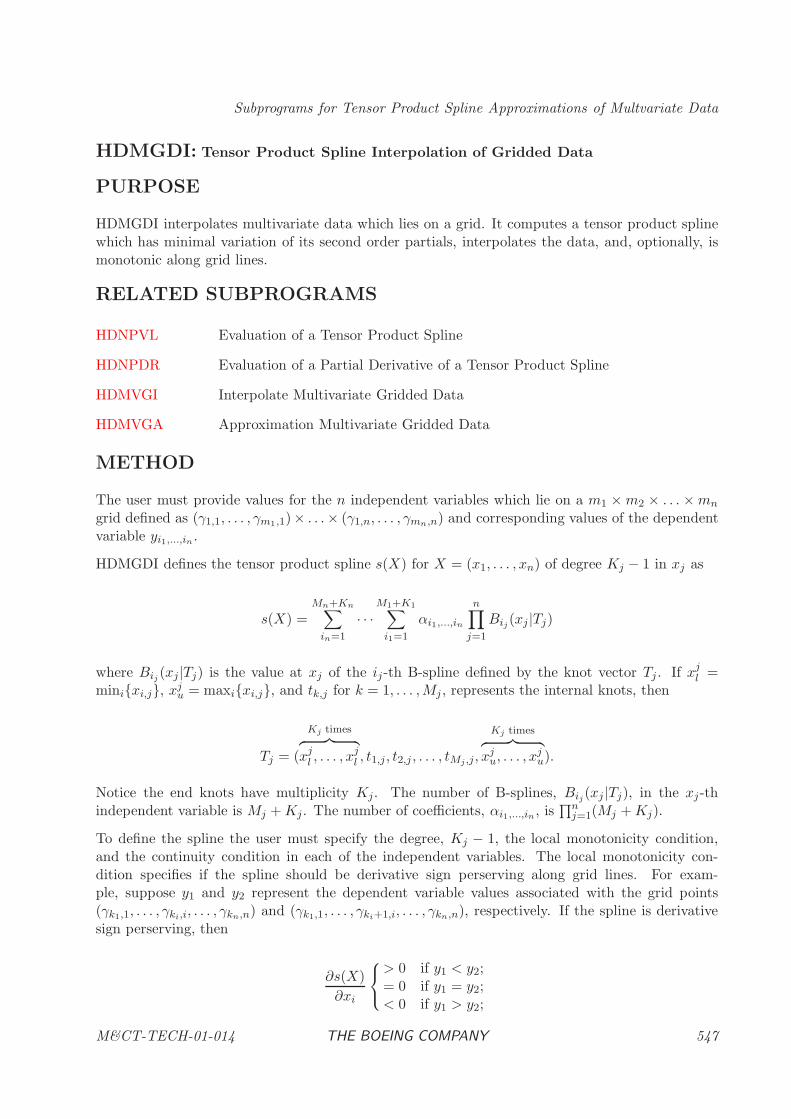
Subprograms for Tensor Product Spline Approximations of Multvariate Data
HDMGDI: Tensor Product Spline Interpolation of Gridded Data
PURPOSE
HDMGDI interpolates multivariate data which lies on a grid. It computes a tensor product splinewhich has minimal variation of its second order partials, interpolates the data, and, optionally, ismonotonic along grid lines.
RELATED SUBPROGRAMS
HDNPVL Evaluation of a Tensor Product Spline
HDNPDR Evaluation of a Partial Derivative of a Tensor Product Spline
HDMVGI Interpolate Multivariate Gridded Data
HDMVGA Approximation Multivariate Gridded Data
METHOD
The user must provide values for the n independent variables which lie on a m1 ×m2 × . . . ×mn
grid defined as (γ1,1, . . . , γm1,1)× . . .× (γ1,n, . . . , γmn,n) and corresponding values of the dependentvariable yi1,...,in .
HDMGDI defines the tensor product spline s(X) for X = (x1, . . . , xn) of degree Kj − 1 in xj as
s(X) =Mn+Kn∑
in=1
· · ·M1+K1∑
i1=1
αi1,...,in
n∏
j=1
Bij(xj |Tj)
where Bij (xj|Tj) is the value at xj of the ij-th B-spline defined by the knot vector Tj . If xjl =
mini{xi,j}, xju = maxi{xi,j}, and tk,j for k = 1, . . . ,Mj , represents the internal knots, then
Tj = (
Kj times︷ ︸︸ ︷xj
l , . . . , xjl , t1,j, t2,j , . . . , tMj ,j,
Kj times︷ ︸︸ ︷xj
u, . . . , xju).
Notice the end knots have multiplicity Kj. The number of B-splines, Bij(xj |Tj), in the xj-thindependent variable is Mj +Kj. The number of coefficients, αi1,...,in , is
∏nj=1(Mj +Kj).
To define the spline the user must specify the degree, Kj − 1, the local monotonicity condition,and the continuity condition in each of the independent variables. The local monotonicity con-dition specifies if the spline should be derivative sign perserving along grid lines. For exam-ple, suppose y1 and y2 represent the dependent variable values associated with the grid points(γk1,1, . . . , γki,i, . . . , γkn,n) and (γk1,1, . . . , γki+1,i, . . . , γkn,n), respectively. If the spline is derivativesign perserving, then
∂s(X)
∂xi
> 0 if y1 < y2;= 0 if y1 = y2;< 0 if y1 > y2;
M&CT-TECH-01-014 THE BOEING COMPANY 547
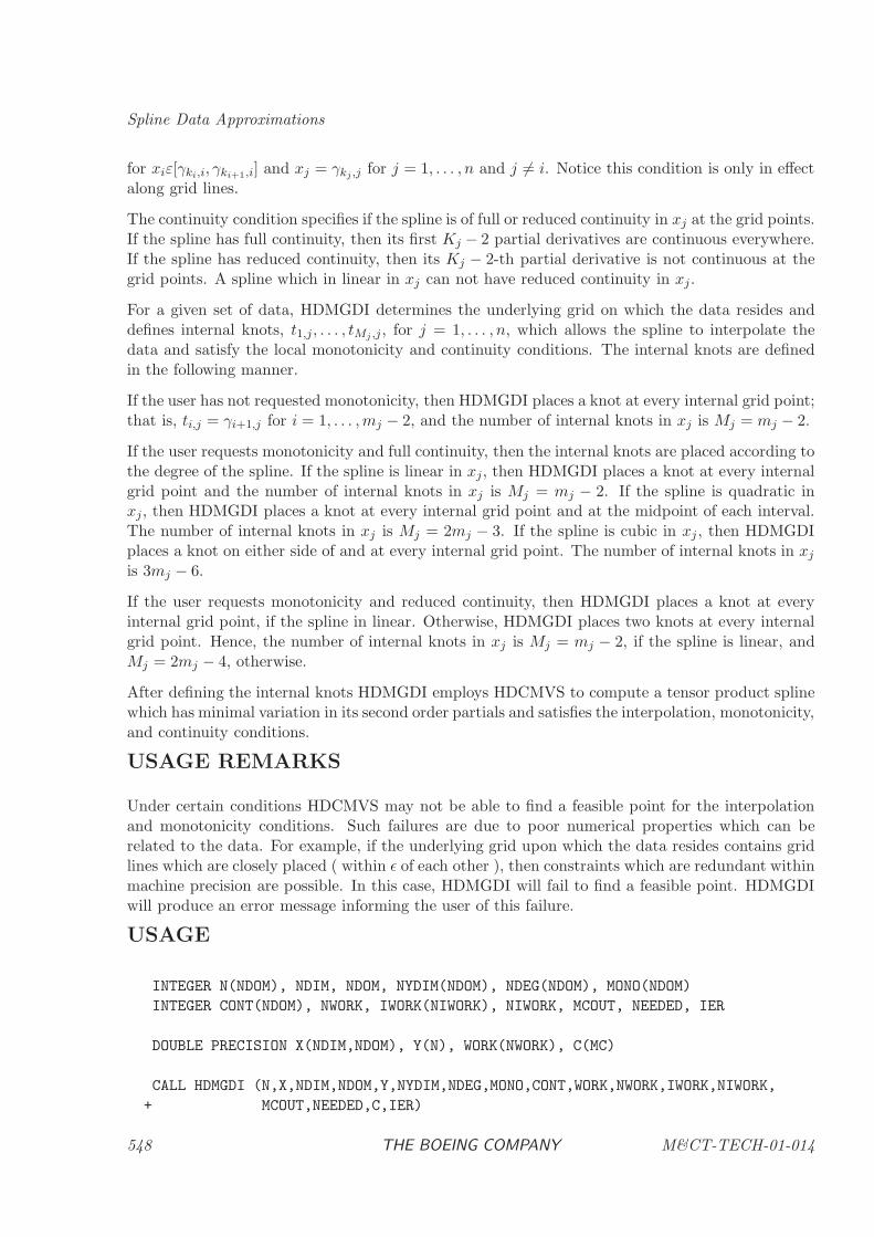
Spline Data Approximations
for xiε[γki,i, γki+1,i] and xj = γkj ,j for j = 1, . . . , n and j 6= i. Notice this condition is only in effectalong grid lines.
The continuity condition specifies if the spline is of full or reduced continuity in xj at the grid points.If the spline has full continuity, then its first Kj − 2 partial derivatives are continuous everywhere.If the spline has reduced continuity, then its Kj − 2-th partial derivative is not continuous at thegrid points. A spline which in linear in xj can not have reduced continuity in xj.
For a given set of data, HDMGDI determines the underlying grid on which the data resides anddefines internal knots, t1,j, . . . , tMj ,j, for j = 1, . . . , n, which allows the spline to interpolate thedata and satisfy the local monotonicity and continuity conditions. The internal knots are definedin the following manner.
If the user has not requested monotonicity, then HDMGDI places a knot at every internal grid point;that is, ti,j = γi+1,j for i = 1, . . . ,mj − 2, and the number of internal knots in xj is Mj = mj − 2.
If the user requests monotonicity and full continuity, then the internal knots are placed according tothe degree of the spline. If the spline is linear in xj, then HDMGDI places a knot at every internalgrid point and the number of internal knots in xj is Mj = mj − 2. If the spline is quadratic inxj, then HDMGDI places a knot at every internal grid point and at the midpoint of each interval.The number of internal knots in xj is Mj = 2mj − 3. If the spline is cubic in xj , then HDMGDIplaces a knot on either side of and at every internal grid point. The number of internal knots in xj
is 3mj − 6.
If the user requests monotonicity and reduced continuity, then HDMGDI places a knot at everyinternal grid point, if the spline in linear. Otherwise, HDMGDI places two knots at every internalgrid point. Hence, the number of internal knots in xj is Mj = mj − 2, if the spline is linear, andMj = 2mj − 4, otherwise.
After defining the internal knots HDMGDI employs HDCMVS to compute a tensor product splinewhich has minimal variation in its second order partials and satisfies the interpolation, monotonicity,and continuity conditions.
USAGE REMARKS
Under certain conditions HDCMVS may not be able to find a feasible point for the interpolationand monotonicity conditions. Such failures are due to poor numerical properties which can berelated to the data. For example, if the underlying grid upon which the data resides contains gridlines which are closely placed ( within ǫ of each other ), then constraints which are redundant withinmachine precision are possible. In this case, HDMGDI will fail to find a feasible point. HDMGDIwill produce an error message informing the user of this failure.
USAGE
INTEGER N(NDOM), NDIM, NDOM, NYDIM(NDOM), NDEG(NDOM), MONO(NDOM)
INTEGER CONT(NDOM), NWORK, IWORK(NIWORK), NIWORK, MCOUT, NEEDED, IER
DOUBLE PRECISION X(NDIM,NDOM), Y(N), WORK(NWORK), C(MC)
CALL HDMGDI (N,X,NDIM,NDOM,Y,NYDIM,NDEG,MONO,CONT,WORK,NWORK,IWORK,NIWORK,
+ MCOUT,NEEDED,C,IER)
548 THE BOEING COMPANY M&CT-TECH-01-014
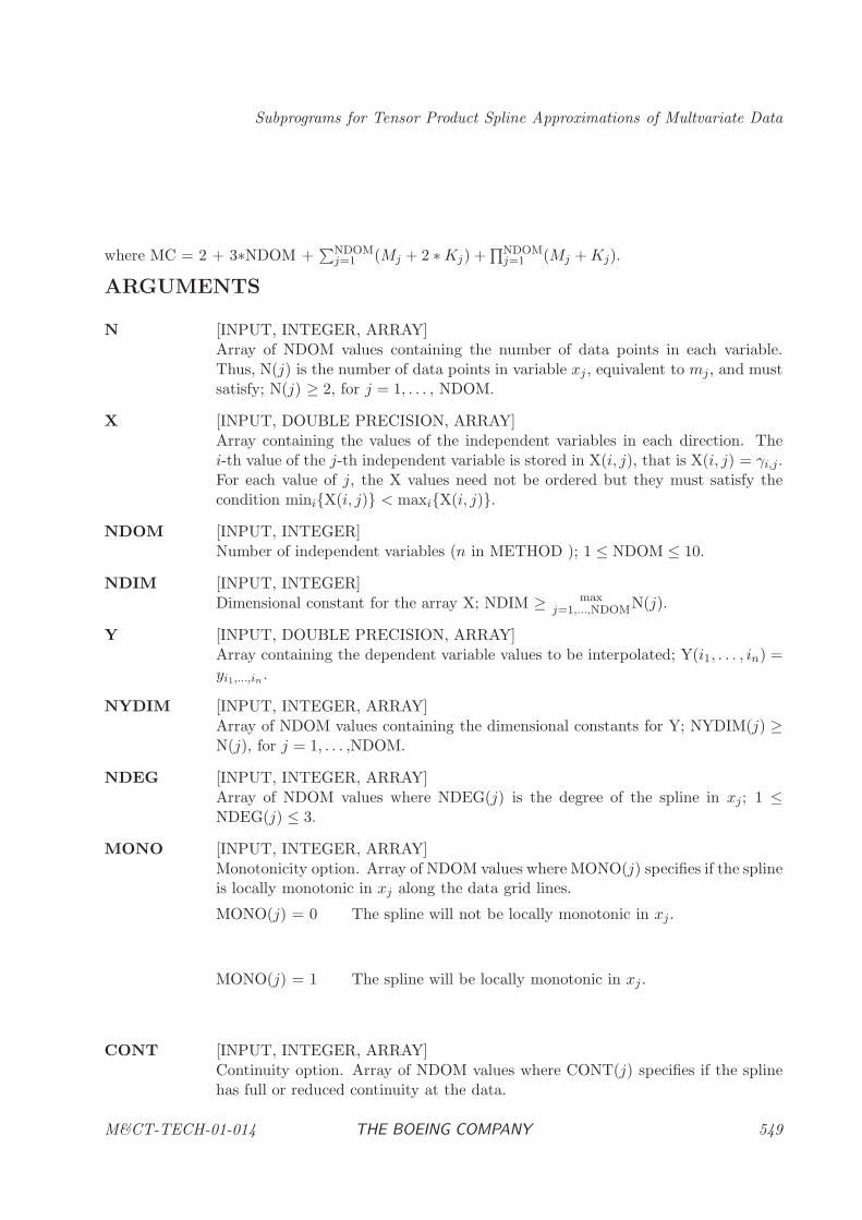
Subprograms for Tensor Product Spline Approximations of Multvariate Data
where MC = 2 + 3∗NDOM +∑NDOM
j=1 (Mj + 2 ∗Kj) +∏NDOM
j=1 (Mj +Kj).
ARGUMENTS
N [INPUT, INTEGER, ARRAY]Array of NDOM values containing the number of data points in each variable.Thus, N(j) is the number of data points in variable xj , equivalent to mj, and mustsatisfy; N(j) ≥ 2, for j = 1, . . . , NDOM.
X [INPUT, DOUBLE PRECISION, ARRAY]Array containing the values of the independent variables in each direction. Thei-th value of the j-th independent variable is stored in X(i, j), that is X(i, j) = γi,j.For each value of j, the X values need not be ordered but they must satisfy thecondition mini{X(i, j)} < maxi{X(i, j)}.
NDOM [INPUT, INTEGER]Number of independent variables (n in METHOD ); 1 ≤ NDOM ≤ 10.
NDIM [INPUT, INTEGER]Dimensional constant for the array X; NDIM ≥ max
j=1,...,NDOMN(j).
Y [INPUT, DOUBLE PRECISION, ARRAY]Array containing the dependent variable values to be interpolated; Y(i1, . . . , in) =yi1,...,in .
NYDIM [INPUT, INTEGER, ARRAY]Array of NDOM values containing the dimensional constants for Y; NYDIM(j) ≥N(j), for j = 1, . . . ,NDOM.
NDEG [INPUT, INTEGER, ARRAY]Array of NDOM values where NDEG(j) is the degree of the spline in xj; 1 ≤NDEG(j) ≤ 3.
MONO [INPUT, INTEGER, ARRAY]Monotonicity option. Array of NDOM values where MONO(j) specifies if the splineis locally monotonic in xj along the data grid lines.
MONO(j) = 0 The spline will not be locally monotonic in xj.
MONO(j) = 1 The spline will be locally monotonic in xj .
CONT [INPUT, INTEGER, ARRAY]Continuity option. Array of NDOM values where CONT(j) specifies if the splinehas full or reduced continuity at the data.
M&CT-TECH-01-014 THE BOEING COMPANY 549
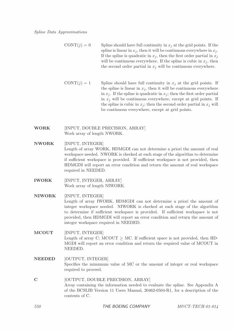
Spline Data Approximations
CONT(j) = 0 Spline should have full continuity in xj at the grid points. If thespline is linear in xj, then it will be continuous everywhere in xj .If the spline is quadratic in xj, then the first order partial in xj
will be continuous everywhere. If the spline is cubic in xj , thenthe second order partial in xj will be continuous everywhere.
CONT(j) = 1 Spline should have full continuity in xj at the grid points. Ifthe spline is linear in xj, then it will be continuous everywherein xj . If the spline is quadratic in xj; then the first order partialin xj will be continuous everywhere, except at grid points. Ifthe spline is cubic in xj; then the second order partial in xj willbe continuous everywhere, except at grid points.
WORK [INPUT, DOUBLE PRECISION, ARRAY]Work array of length NWORK.
NWORK [INPUT, INTEGER]Length of array WORK, HDMGDI can not determine a priori the amount of realworkspace needed. NWORK is checked at each stage of the algorithm to determineif sufficient workspace is provided. If sufficient workspace is not provided, thenHDMGDI will report an error condition and return the amount of real workspacerequired in NEEDED.
IWORK [INPUT, INTEGER, ARRAY]Work array of length NIWORK.
NIWORK [INPUT, INTEGER]Length of array IWORK, HDMGDI can not determine a priori the amount ofinteger workspace needed. NIWORK is checked at each stage of the algorithmto determine if sufficient workspace is provided. If sufficient workspace is notprovided, then HDMGDI will report an error condition and return the amount ofinteger workspace required in NEEDED.
MCOUT [INPUT, INTEGER]Length of array C; MCOUT ≥ MC. If sufficient space is not provided, then HD-MGDI will report an error condition and return the required value of MCOUT inNEEDED.
NEEDED [OUTPUT, INTEGER]Specifies the minumum value of MC or the amount of integer or real workspacerequired to proceed.
C [OUTPUT, DOUBLE PRECISION, ARRAY]Array containing the information needed to evaluate the spline. See Appendix Aof the BCSLIB Version 11 Users Manual, 20462-0504-R1, for a description of thecontents of C.
550 THE BOEING COMPANY M&CT-TECH-01-014
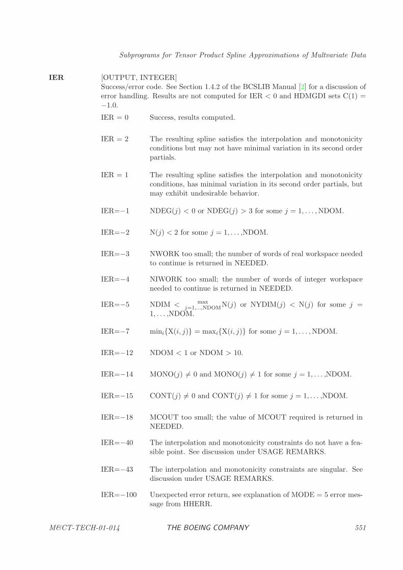
Subprograms for Tensor Product Spline Approximations of Multvariate Data
IER [OUTPUT, INTEGER]Success/error code. See Section 1.4.2 of the BCSLIB Manual [2] for a discussion oferror handling. Results are not computed for IER < 0 and HDMGDI sets C(1) =−1.0.
IER = 0 Success, results computed.
IER = 2 The resulting spline satisfies the interpolation and monotonicityconditions but may not have minimal variation in its second orderpartials.
IER = 1 The resulting spline satisfies the interpolation and monotonicityconditions, has minimal variation in its second order partials, butmay exhibit undesirable behavior.
IER=−1 NDEG(j) < 0 or NDEG(j) > 3 for some j = 1, . . . ,NDOM.
IER=−2 N(j) < 2 for some j = 1, . . . ,NDOM.
IER=−3 NWORK too small; the number of words of real workspace neededto continue is returned in NEEDED.
IER=−4 NIWORK too small; the number of words of integer workspaceneeded to continue is returned in NEEDED.
IER=−5 NDIM < maxj=1,...,NDOMN(j) or NYDIM(j) < N(j) for some j =
1, . . . ,NDOM.
IER=−7 mini{X(i, j)} = maxi{X(i, j)} for some j = 1, . . . ,NDOM.
IER=−12 NDOM < 1 or NDOM > 10.
IER=−14 MONO(j) 6= 0 and MONO(j) 6= 1 for some j = 1, . . . ,NDOM.
IER=−15 CONT(j) 6= 0 and CONT(j) 6= 1 for some j = 1, . . . ,NDOM.
IER=−18 MCOUT too small; the value of MCOUT required is returned inNEEDED.
IER=−40 The interpolation and monotonicity constraints do not have a fea-sible point. See discussion under USAGE REMARKS.
IER=−43 The interpolation and monotonicity constraints are singular. Seediscussion under USAGE REMARKS.
IER=−100 Unexpected error return, see explanation of MODE = 5 error mes-sage from HHERR.
M&CT-TECH-01-014 THE BOEING COMPANY 551
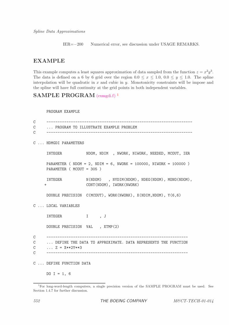
Spline Data Approximations
IER=−200 Numerical error, see discussion under USAGE REMARKS.
EXAMPLE
This example computes a least squares approximation of data sampled from the function z = x2y3.The data is defined on a 6 by 6 grid over the region 0.0 ≤ x ≤ 1.0, 0.0 ≤ y ≤ 1.0. The splineinterpolation will be quadratic in x and cubic in y. Monotonicity constraints will be impose andthe spline will have full continuity at the grid points in both independent variables.
SAMPLE PROGRAM (exmgdi.f) 1
PROGRAM EXAMPLE
C ------------------------------------------------------------------
C ... PROGRAM TO ILLUSTRATE EXAMPLE PROBLEM
C ------------------------------------------------------------------
C ... HDMGDI PARAMETERS
INTEGER NDOM, NDIM , NWORK, NIWORK, NEEDED, MCOUT, IER
PARAMETER ( NDOM = 2, NDIM = 6, NWORK = 100000, NIWORK = 100000 )
PARAMETER ( MCOUT = 305 )
INTEGER N(NDOM) , NYDIM(NDOM), NDEG(NDOM), MONO(NDOM),
+ CONT(NDOM), IWORK(NWORK)
DOUBLE PRECISION C(MCOUT), WORK(NWORK), X(NDIM,NDOM), Y(6,6)
C ... LOCAL VARIABLES
INTEGER I , J
DOUBLE PRECISION VAL , XTMP(2)
C ----------------------------------------------------------------
C ... DEFINE THE DATA TO APPROXIMATE. DATA REPRESENTS THE FUNCTION
C ... Z = X**2Y**3
C ----------------------------------------------------------------
C ... DEFINE FUNCTION DATA
DO I = 1, 6
1For long-word-length computers, a single precision version of the SAMPLE PROGRAM must be used. See
Section 1.4.7 for further discussion.
552 THE BOEING COMPANY M&CT-TECH-01-014
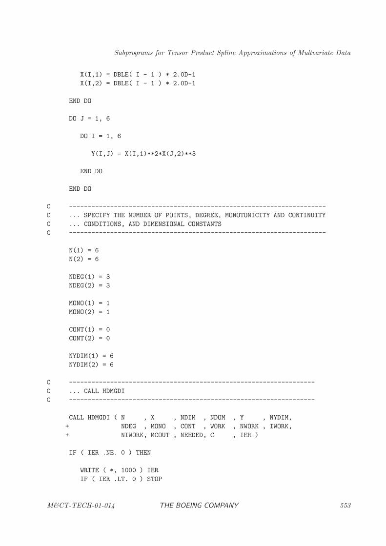
Subprograms for Tensor Product Spline Approximations of Multvariate Data
X(I,1) = DBLE( I - 1 ) * 2.0D-1
X(I,2) = DBLE( I - 1 ) * 2.0D-1
END DO
DO J = 1, 6
DO I = 1, 6
Y(I,J) = X(I,1)**2*X(J,2)**3
END DO
END DO
C ---------------------------------------------------------------------
C ... SPECIFY THE NUMBER OF POINTS, DEGREE, MONOTONICITY AND CONTINUITY
C ... CONDITIONS, AND DIMENSIONAL CONSTANTS
C ---------------------------------------------------------------------
N(1) = 6
N(2) = 6
NDEG(1) = 3
NDEG(2) = 3
MONO(1) = 1
MONO(2) = 1
CONT(1) = 0
CONT(2) = 0
NYDIM(1) = 6
NYDIM(2) = 6
C ------------------------------------------------------------------
C ... CALL HDMGDI
C ------------------------------------------------------------------
CALL HDMGDI ( N , X , NDIM , NDOM , Y , NYDIM,
+ NDEG , MONO , CONT , WORK , NWORK , IWORK,
+ NIWORK, MCOUT , NEEDED, C , IER )
IF ( IER .NE. 0 ) THEN
WRITE ( *, 1000 ) IER
IF ( IER .LT. 0 ) STOP
M&CT-TECH-01-014 THE BOEING COMPANY 553
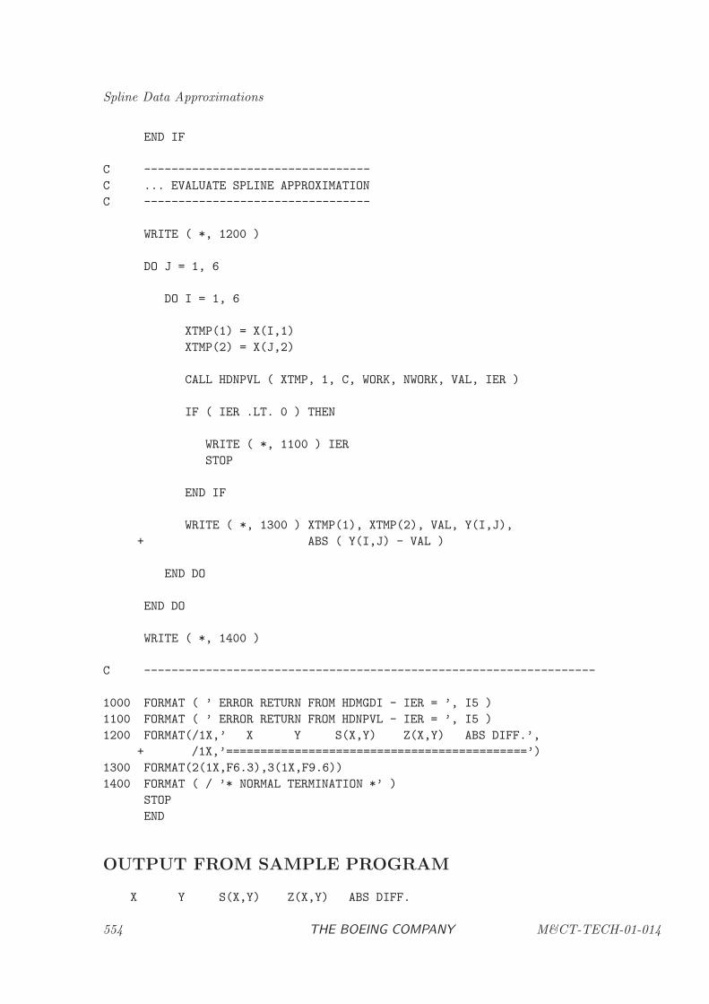
Spline Data Approximations
END IF
C ---------------------------------
C ... EVALUATE SPLINE APPROXIMATION
C ---------------------------------
WRITE ( *, 1200 )
DO J = 1, 6
DO I = 1, 6
XTMP(1) = X(I,1)
XTMP(2) = X(J,2)
CALL HDNPVL ( XTMP, 1, C, WORK, NWORK, VAL, IER )
IF ( IER .LT. 0 ) THEN
WRITE ( *, 1100 ) IER
STOP
END IF
WRITE ( *, 1300 ) XTMP(1), XTMP(2), VAL, Y(I,J),
+ ABS ( Y(I,J) - VAL )
END DO
END DO
WRITE ( *, 1400 )
C ------------------------------------------------------------------
1000 FORMAT ( ’ ERROR RETURN FROM HDMGDI - IER = ’, I5 )
1100 FORMAT ( ’ ERROR RETURN FROM HDNPVL - IER = ’, I5 )
1200 FORMAT(/1X,’ X Y S(X,Y) Z(X,Y) ABS DIFF.’,
+ /1X,’============================================’)
1300 FORMAT(2(1X,F6.3),3(1X,F9.6))
1400 FORMAT ( / ’* NORMAL TERMINATION *’ )
STOP
END
OUTPUT FROM SAMPLE PROGRAM
X Y S(X,Y) Z(X,Y) ABS DIFF.
554 THE BOEING COMPANY M&CT-TECH-01-014
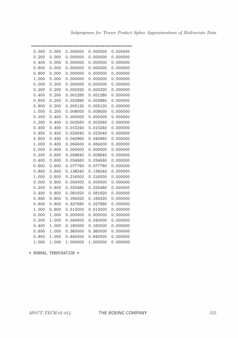
Subprograms for Tensor Product Spline Approximations of Multvariate Data
============================================
0.000 0.000 0.000000 0.000000 0.000000
0.200 0.000 0.000000 0.000000 0.000000
0.400 0.000 0.000000 0.000000 0.000000
0.600 0.000 0.000000 0.000000 0.000000
0.800 0.000 0.000000 0.000000 0.000000
1.000 0.000 0.000000 0.000000 0.000000
0.000 0.200 0.000000 0.000000 0.000000
0.200 0.200 0.000320 0.000320 0.000000
0.400 0.200 0.001280 0.001280 0.000000
0.600 0.200 0.002880 0.002880 0.000000
0.800 0.200 0.005120 0.005120 0.000000
1.000 0.200 0.008000 0.008000 0.000000
0.000 0.400 0.000000 0.000000 0.000000
0.200 0.400 0.002560 0.002560 0.000000
0.400 0.400 0.010240 0.010240 0.000000
0.600 0.400 0.023040 0.023040 0.000000
0.800 0.400 0.040960 0.040960 0.000000
1.000 0.400 0.064000 0.064000 0.000000
0.000 0.600 0.000000 0.000000 0.000000
0.200 0.600 0.008640 0.008640 0.000000
0.400 0.600 0.034560 0.034560 0.000000
0.600 0.600 0.077760 0.077760 0.000000
0.800 0.600 0.138240 0.138240 0.000000
1.000 0.600 0.216000 0.216000 0.000000
0.000 0.800 0.000000 0.000000 0.000000
0.200 0.800 0.020480 0.020480 0.000000
0.400 0.800 0.081920 0.081920 0.000000
0.600 0.800 0.184320 0.184320 0.000000
0.800 0.800 0.327680 0.327680 0.000000
1.000 0.800 0.512000 0.512000 0.000000
0.000 1.000 0.000000 0.000000 0.000000
0.200 1.000 0.040000 0.040000 0.000000
0.400 1.000 0.160000 0.160000 0.000000
0.600 1.000 0.360000 0.360000 0.000000
0.800 1.000 0.640000 0.640000 0.000000
1.000 1.000 1.000000 1.000000 0.000000
* NORMAL TERMINATION *
M&CT-TECH-01-014 THE BOEING COMPANY 555
Spline Data Approximations
HDGDWH: Tensor Product Spline Approximation of Gridded Data with Holes
PURPOSE
HDGDWH approximates multivariate data which lies on a grid but contains regions of missingdata. It computes a tensor product spline which has minimal variation of its second order partials,approximates the data within a user specified tolerance and, optionally, is locally monotonic alonggrid lines.
RELATED SUBPROGRAMS
HDNPVL Evaluation of a Tensor Product Spline
HDNPDR Evaluation of a Partial Derivative of a Tensor Product Spline
HDMVGI Interpolate Multivariate Gridded Data
HDMVGA Approximation Multivariate Gridded Data
METHOD
The user must provide values for the n independent variables Xℓ = (x1,ℓ, . . . , xn,ℓ), correspond-ing values of the dependent variable yℓ, and corresponding values of the absolute tolerance δℓ,for ℓ = 1, . . . ,N. The points Xℓ should be a subset of a grid defined by (γ1,1, . . . , γ1,m1) × . . . ×(γn,1, . . . , γn,mn).
HDGDWH defines the tensor product spline s(X) for X = (x1, . . . , xn) of degree Ki − 1 in xi as
s(X) =Mn+Kn∑
jn=1
· · ·M1+K1∑
j1=1
αj1,...,jn
n∏
i=1
Bji(xi|Ti)
where Bji(xi|Ti) is the value at xi of the ji-th B-spline defined by the knot vector Ti. If xi
l =minℓ{xi,ℓ}, xi
u = maxℓ{xi,ℓ}, and ti,k for k = 1, . . . ,Mi, represents the internal knots, then
Ti = (
Ki times︷ ︸︸ ︷xi
l , . . . , xil , ti,1, ti,2, . . . , ti,Mi
,
Ki times︷ ︸︸ ︷xi
u, . . . , xiu).
Notice the end knots have multiplicity Ki. The number of B-splines, Bji(xi|Ti), in the xi-th
independent variable is Mi +Ki. The number of coefficients, αj1,...,jn , is∏n
i=1(Mi +Ki).
HDGDWH computes the tensor product spline coefficients αj1,...,jn , such that s(X) satisfies theconstraints
yℓ − δℓ ≤ s(Xℓ) ≤ yℓ + δℓ
for ℓ = 1, . . . ,N.
To define the spline the user must specify the degree, Ki − 1, the local monotonicity condition, andthe continuity condition in each of the independent variables.
556 THE BOEING COMPANY M&CT-TECH-01-014
Subprograms for Tensor Product Spline Approximations of Multvariate Data
The local monotonicity condition specifies if the spline should be derivative sign perserving alonggrid lines. For example, suppose y1 and y2 represent the dependent variable values associatedwith the grid points (γ1,k1 , . . . , γi,ki
, . . . , γn,kn) and (γ1,k1 , . . . , γi,ki+1, . . . , γn,kn
), respectively. If thespline is derivative sign perserving, then
∂s(X)
∂xi
> 0 if y1 < y2;= 0 if y1 = y2;< 0 if y1 > y2;
for xi ∈ [γi,ki, γi,ki+1
] and xj = γj,kjfor j = 1, . . . , n and j 6= i. Note: This condition is only in
effect along grid lines.
The continuity condition specifies if the spline is of full or reduced continuity in xi at the grid points.If the spline has full continuity, then its first Ki − 2 partial derivatives are continuous everywhere.If the spline has reduced continuity, then its Ki − 2-th partial derivative is not continuous at thegrid points. A spline which in linear in xi can not have reduced continuity in xi.
For a given set of data, HDGDWH determines the underlying grid on which the data resides anddefines internal knots, ti,1, . . . , ti,Mi
, for i = 1, . . . , n, which allows the spline to approximate thedata and satisfy the local monotonicity and continuity conditions. The internal knots are definedin the following manner.
If the user has not requested monotonicity, then HDGDWH places a knot at every internal gridpoint; that is, ti,j = γi,j+1 for j = 1, . . . ,mi−2, and the number of internal knots in xi isMi = mi−2.
If the user requests monotonicity and full continuity, then the internal knots are placed according tothe degree of the spline. If the spline is linear in xi, then HDGDWH places a knot at every internalgrid point and the number of internal knots in xi is Mi = mi − 2. If the spline is quadratic in xi,then HDGDWH places a knot at every internal grid point and at the midpoint of each interval.The number of internal knots in xi is Mi = 2mi − 3. If the spline is cubic in xi, then HDGDWHplaces a knot on either side of and at every internal grid point. The number of internal knots in xi
is 3mi − 6.
If the user requests monotonicity and reduced continuity, then HDGDWH places a knot at everyinternal grid point, if the spline in linear. Otherwise, HDGDWH places two knots at every internalgrid point. Hence, the number of internal knots in xi is Mi = mi − 2, if the spline is linear, andMi = 2mi − 4, otherwise.
In addition to the approximation, monotinicty and continuity conditions; the use can specify alower bound sl, and an upper bound su, on the spline approximation. HDGDWH will compute aspline s(X) which satisfies the condition
sl ≤ s(X) ≤ su
for values of X in regions without data. The only way to insure the spline approximation satisfiesthe above relation in independent variable regions which contain data is to impose monotonicityconstraints in at least one of the independent variables.
After defining the internal knots and determing the constraints to satisfy the approximation andmonotinicity conditions, HDGDWH employs HDCMVS to compute a tensor product spline which
M&CT-TECH-01-014 THE BOEING COMPANY 557
Spline Data Approximations
has minimal variation in its second order partials and satisfies the approximation, monotonicity,and continuity conditions.
USAGE REMARKS
Under certain conditions HDCMVS may not be able to find a feasible point for the approximationand monotonicity conditions. Such failures are due to poor numerical properties which may berelated to the data. For example, if the underlying grid upon which the data resides contains gridlines which are close ( within ǫ of each other ), then constraints which are redundant within machineprecision are possible. Also, if the dependent variable has some extreme derivative variation, thenit can be difficult to satisfy the local monotonicity conditions and the approximation conditions forsmall values of δℓ. In either case HDGDWH may fail to find a feasible point or produce a singularset of constraints. HDGDWH will report these conditions with an error message.
USAGE
INTEGER N, NDIM, NDOM, ITOL, NDEG(NDOM), MONO(NDOM), CONT(NDOM)
INTEGER IBND, NWORK, IWORK(NIWORK), NIWORK, MCOUT, NEEDED, IER
DOUBLE PRECISION ABSTOL(N), BOUNDS(2), X(NDIM,NDOM), Y(N), WORK(NWORK), C(MC)
CALL HDGDWH (N,X,NDIM,NDOM,Y,ITOL,ABSTOL,NDEG,MONO,CONT,IBND,BOUNDS,
+ WORK,NWORK,IWORK,NIWORK,MCOUT,NEEDED,C,IER)
where MC = 2 + 3∗NDOM +∑NDOM
i=1 (Mi + 2 ∗Ki) +∏NDOM
i=1 (Mi +Ki).
ARGUMENTS
N [INPUT, INTEGER]Number of data points; N ≥ 2.
X [INPUT, DOUBLE PRECISION, ARRAY]Two-dimensional array containing the N values of the independent variables inthe x1 through xNDOM directions which are stored in the first through NDOMcolumns of X, respectively. This array need not be ordered but it must representN distinct points and satisfy the condition minℓ{X(ℓ, i)} < maxℓ{X(ℓ, i)} for i =1, . . . ,NDOM.
NDIM [INPUT, INTEGER]Dimensional constant for the array X; NDIM ≥ N.
NDOM [INPUT, INTEGER]Number of independent variables (n in METHOD ); 1 ≤ NDOM ≤ 10.
Y [INPUT, DOUBLE PRECISION, ARRAY]Array of N values of the dependent variable y in correspondence with the X array.
ITOL [INPUT, INTEGER]Absolute tolerance option flag;
558 THE BOEING COMPANY M&CT-TECH-01-014
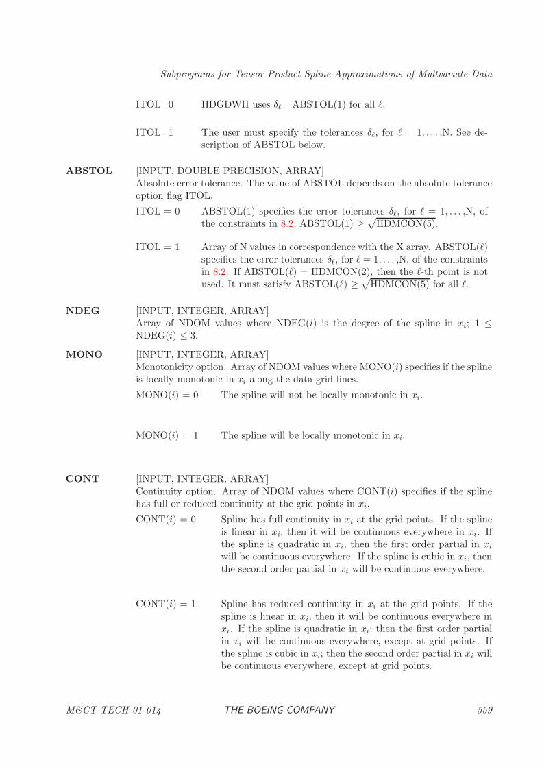
Subprograms for Tensor Product Spline Approximations of Multvariate Data
ITOL=0 HDGDWH uses δℓ =ABSTOL(1) for all ℓ.
ITOL=1 The user must specify the tolerances δℓ, for ℓ = 1, . . . ,N. See de-scription of ABSTOL below.
ABSTOL [INPUT, DOUBLE PRECISION, ARRAY]Absolute error tolerance. The value of ABSTOL depends on the absolute toleranceoption flag ITOL.
ITOL = 0 ABSTOL(1) specifies the error tolerances δℓ, for ℓ = 1, . . . ,N, ofthe constraints in 8.2; ABSTOL(1) ≥
√HDMCON(5).
ITOL = 1 Array of N values in correspondence with the X array. ABSTOL(ℓ)specifies the error tolerances δℓ, for ℓ = 1, . . . ,N, of the constraintsin 8.2. If ABSTOL(ℓ) = HDMCON(2), then the ℓ-th point is notused. It must satisfy ABSTOL(ℓ) ≥
√HDMCON(5) for all ℓ.
NDEG [INPUT, INTEGER, ARRAY]Array of NDOM values where NDEG(i) is the degree of the spline in xi; 1 ≤NDEG(i) ≤ 3.
MONO [INPUT, INTEGER, ARRAY]Monotonicity option. Array of NDOM values where MONO(i) specifies if the splineis locally monotonic in xi along the data grid lines.
MONO(i) = 0 The spline will not be locally monotonic in xi.
MONO(i) = 1 The spline will be locally monotonic in xi.
CONT [INPUT, INTEGER, ARRAY]Continuity option. Array of NDOM values where CONT(i) specifies if the splinehas full or reduced continuity at the grid points in xi.
CONT(i) = 0 Spline has full continuity in xi at the grid points. If the splineis linear in xi, then it will be continuous everywhere in xi. Ifthe spline is quadratic in xi, then the first order partial in xi
will be continuous everywhere. If the spline is cubic in xi, thenthe second order partial in xi will be continuous everywhere.
CONT(i) = 1 Spline has reduced continuity in xi at the grid points. If thespline is linear in xi, then it will be continuous everywhere inxi. If the spline is quadratic in xi; then the first order partialin xi will be continuous everywhere, except at grid points. Ifthe spline is cubic in xi; then the second order partial in xi willbe continuous everywhere, except at grid points.
M&CT-TECH-01-014 THE BOEING COMPANY 559
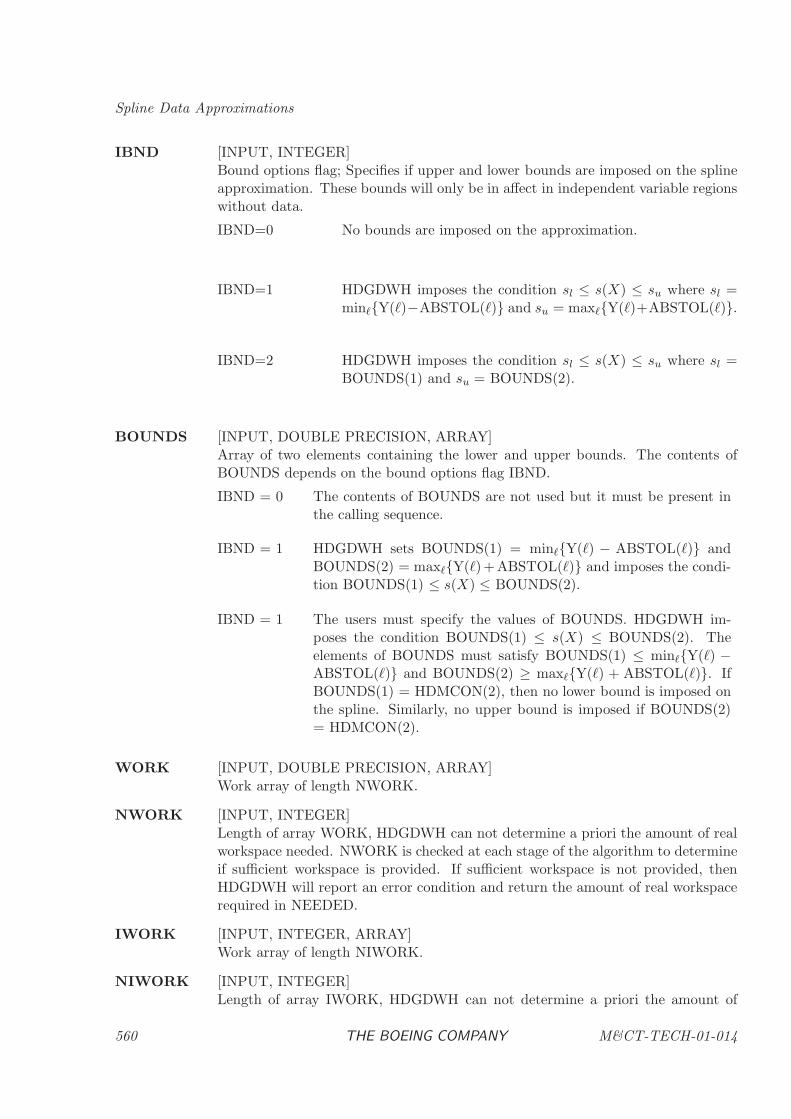
Spline Data Approximations
IBND [INPUT, INTEGER]Bound options flag; Specifies if upper and lower bounds are imposed on the splineapproximation. These bounds will only be in affect in independent variable regionswithout data.
IBND=0 No bounds are imposed on the approximation.
IBND=1 HDGDWH imposes the condition sl ≤ s(X) ≤ su where sl =minℓ{Y(ℓ)−ABSTOL(ℓ)} and su = maxℓ{Y(ℓ)+ABSTOL(ℓ)}.
IBND=2 HDGDWH imposes the condition sl ≤ s(X) ≤ su where sl =BOUNDS(1) and su = BOUNDS(2).
BOUNDS [INPUT, DOUBLE PRECISION, ARRAY]Array of two elements containing the lower and upper bounds. The contents ofBOUNDS depends on the bound options flag IBND.
IBND = 0 The contents of BOUNDS are not used but it must be present inthe calling sequence.
IBND = 1 HDGDWH sets BOUNDS(1) = minℓ{Y(ℓ) − ABSTOL(ℓ)} andBOUNDS(2) = maxℓ{Y(ℓ)+ABSTOL(ℓ)} and imposes the condi-tion BOUNDS(1) ≤ s(X) ≤ BOUNDS(2).
IBND = 1 The users must specify the values of BOUNDS. HDGDWH im-poses the condition BOUNDS(1) ≤ s(X) ≤ BOUNDS(2). Theelements of BOUNDS must satisfy BOUNDS(1) ≤ minℓ{Y(ℓ) −ABSTOL(ℓ)} and BOUNDS(2) ≥ maxℓ{Y(ℓ) + ABSTOL(ℓ)}. IfBOUNDS(1) = HDMCON(2), then no lower bound is imposed onthe spline. Similarly, no upper bound is imposed if BOUNDS(2)= HDMCON(2).
WORK [INPUT, DOUBLE PRECISION, ARRAY]Work array of length NWORK.
NWORK [INPUT, INTEGER]Length of array WORK, HDGDWH can not determine a priori the amount of realworkspace needed. NWORK is checked at each stage of the algorithm to determineif sufficient workspace is provided. If sufficient workspace is not provided, thenHDGDWH will report an error condition and return the amount of real workspacerequired in NEEDED.
IWORK [INPUT, INTEGER, ARRAY]Work array of length NIWORK.
NIWORK [INPUT, INTEGER]Length of array IWORK, HDGDWH can not determine a priori the amount of
560 THE BOEING COMPANY M&CT-TECH-01-014
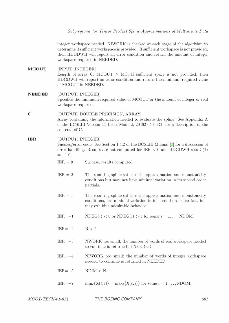
Subprograms for Tensor Product Spline Approximations of Multvariate Data
integer workspace needed. NIWORK is checked at each stage of the algorithm todetermine if sufficient workspace is provided. If sufficient workspace is not provided,then HDGDWH will report an error condition and return the amount of integerworkspace required in NEEDED.
MCOUT [INPUT, INTEGER]Length of array C; MCOUT ≥ MC. If sufficient space is not provided, thenHDGDWH will report an error condition and return the minimum required valueof MCOUT in NEEDED.
NEEDED [OUTPUT, INTEGER]Specifies the minimum required value of MCOUT or the amount of integer or realworkspace required.
C [OUTPUT, DOUBLE PRECISION, ARRAY]Array containing the information needed to evaluate the spline. See Appendix Aof the BCSLIB Version 11 Users Manual, 20462-0504-R1, for a description of thecontents of C.
IER [OUTPUT, INTEGER]Success/error code. See Section 1.4.2 of the BCSLIB Manual [2] for a discussion oferror handling. Results are not computed for IER < 0 and HDGDWH sets C(1)= −1.0.
IER = 0 Success, results computed.
IER = 2 The resulting spline satisfies the approximation and monotonicityconditions but may not have minimal variation in its second orderpartials.
IER = 1 The resulting spline satisfies the approximation and monotonicityconditions, has minimal variation in its second order partials, butmay exhibit undesirable behavior.
IER=−1 NDEG(i) < 0 or NDEG(i) > 3 for some i = 1, . . . ,NDOM.
IER=−2 N < 2.
IER=−3 NWORK too small; the number of words of real workspace neededto continue is returned in NEEDED.
IER=−4 NIWORK too small; the number of words of integer workspaceneeded to continue is returned in NEEDED.
IER=−5 NDIM < N.
IER=−7 minℓ{X(ℓ, i)} = maxℓ{X(ℓ, i)} for some i = 1, . . . ,NDOM.
M&CT-TECH-01-014 THE BOEING COMPANY 561
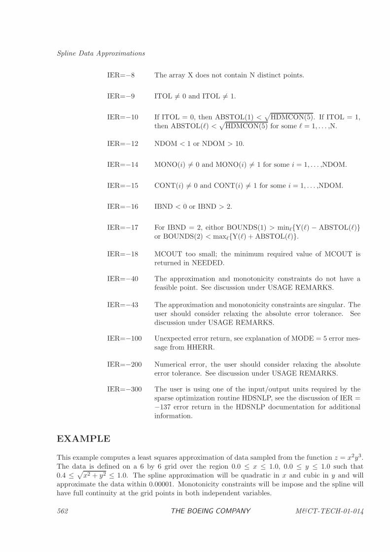
Spline Data Approximations
IER=−8 The array X does not contain N distinct points.
IER=−9 ITOL 6= 0 and ITOL 6= 1.
IER=−10 If ITOL = 0, then ABSTOL(1) <√
HDMCON(5). If ITOL = 1,then ABSTOL(ℓ) <
√HDMCON(5) for some ℓ = 1, . . . ,N.
IER=−12 NDOM < 1 or NDOM > 10.
IER=−14 MONO(i) 6= 0 and MONO(i) 6= 1 for some i = 1, . . . ,NDOM.
IER=−15 CONT(i) 6= 0 and CONT(i) 6= 1 for some i = 1, . . . ,NDOM.
IER=−16 IBND < 0 or IBND > 2.
IER=−17 For IBND = 2, eithor BOUNDS(1) > minℓ{Y(ℓ) − ABSTOL(ℓ)}or BOUNDS(2) < maxℓ{Y(ℓ) + ABSTOL(ℓ)}.
IER=−18 MCOUT too small; the minimum required value of MCOUT isreturned in NEEDED.
IER=−40 The approximation and monotonicity constraints do not have afeasible point. See discussion under USAGE REMARKS.
IER=−43 The approximation and monotonicity constraints are singular. Theuser should consider relaxing the absolute error tolerance. Seediscussion under USAGE REMARKS.
IER=−100 Unexpected error return, see explanation of MODE = 5 error mes-sage from HHERR.
IER=−200 Numerical error, the user should consider relaxing the absoluteerror tolerance. See discussion under USAGE REMARKS.
IER=−300 The user is using one of the input/output units required by thesparse optimization routine HDSNLP, see the discussion of IER =−137 error return in the HDSNLP documentation for additionalinformation.
EXAMPLE
This example computes a least squares approximation of data sampled from the function z = x2y3.The data is defined on a 6 by 6 grid over the region 0.0 ≤ x ≤ 1.0, 0.0 ≤ y ≤ 1.0 such that0.4 ≤
√x2 + y2 ≤ 1.0. The spline approximation will be quadratic in x and cubic in y and will
approximate the data within 0.00001. Monotonicity constraints will be impose and the spline willhave full continuity at the grid points in both independent variables.
562 THE BOEING COMPANY M&CT-TECH-01-014
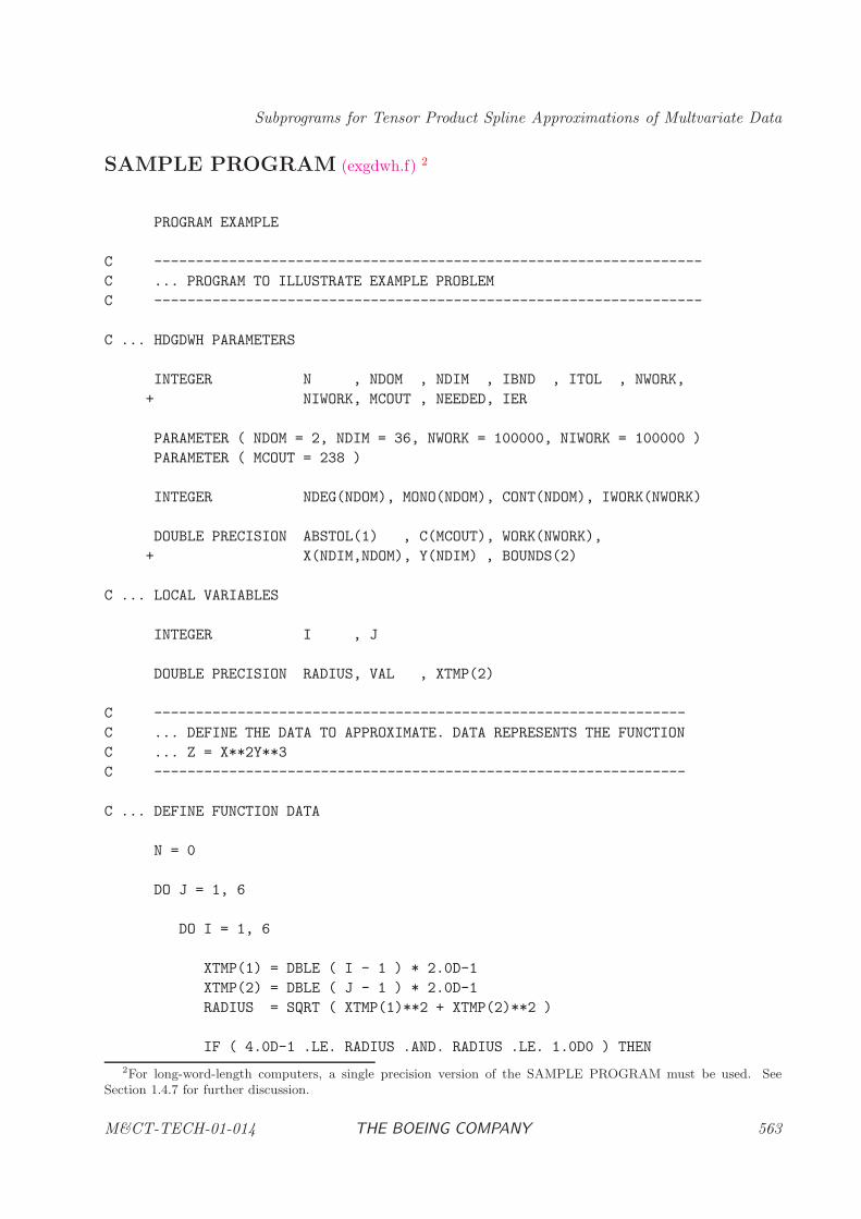
Subprograms for Tensor Product Spline Approximations of Multvariate Data
SAMPLE PROGRAM (exgdwh.f) 2
PROGRAM EXAMPLE
C ------------------------------------------------------------------
C ... PROGRAM TO ILLUSTRATE EXAMPLE PROBLEM
C ------------------------------------------------------------------
C ... HDGDWH PARAMETERS
INTEGER N , NDOM , NDIM , IBND , ITOL , NWORK,
+ NIWORK, MCOUT , NEEDED, IER
PARAMETER ( NDOM = 2, NDIM = 36, NWORK = 100000, NIWORK = 100000 )
PARAMETER ( MCOUT = 238 )
INTEGER NDEG(NDOM), MONO(NDOM), CONT(NDOM), IWORK(NWORK)
DOUBLE PRECISION ABSTOL(1) , C(MCOUT), WORK(NWORK),
+ X(NDIM,NDOM), Y(NDIM) , BOUNDS(2)
C ... LOCAL VARIABLES
INTEGER I , J
DOUBLE PRECISION RADIUS, VAL , XTMP(2)
C ----------------------------------------------------------------
C ... DEFINE THE DATA TO APPROXIMATE. DATA REPRESENTS THE FUNCTION
C ... Z = X**2Y**3
C ----------------------------------------------------------------
C ... DEFINE FUNCTION DATA
N = 0
DO J = 1, 6
DO I = 1, 6
XTMP(1) = DBLE ( I - 1 ) * 2.0D-1
XTMP(2) = DBLE ( J - 1 ) * 2.0D-1
RADIUS = SQRT ( XTMP(1)**2 + XTMP(2)**2 )
IF ( 4.0D-1 .LE. RADIUS .AND. RADIUS .LE. 1.0D0 ) THEN
2For long-word-length computers, a single precision version of the SAMPLE PROGRAM must be used. See
Section 1.4.7 for further discussion.
M&CT-TECH-01-014 THE BOEING COMPANY 563
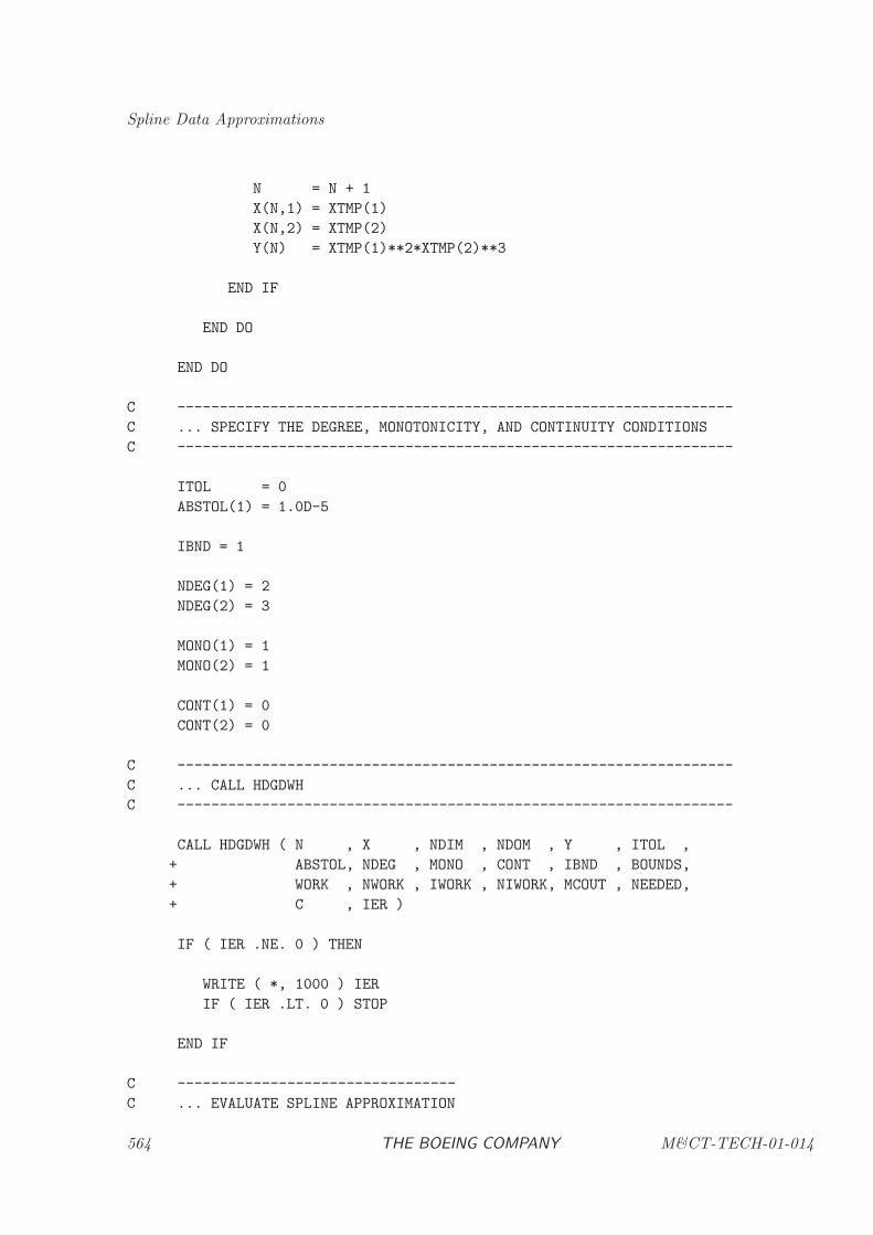
Spline Data Approximations
N = N + 1
X(N,1) = XTMP(1)
X(N,2) = XTMP(2)
Y(N) = XTMP(1)**2*XTMP(2)**3
END IF
END DO
END DO
C ------------------------------------------------------------------
C ... SPECIFY THE DEGREE, MONOTONICITY, AND CONTINUITY CONDITIONS
C ------------------------------------------------------------------
ITOL = 0
ABSTOL(1) = 1.0D-5
IBND = 1
NDEG(1) = 2
NDEG(2) = 3
MONO(1) = 1
MONO(2) = 1
CONT(1) = 0
CONT(2) = 0
C ------------------------------------------------------------------
C ... CALL HDGDWH
C ------------------------------------------------------------------
CALL HDGDWH ( N , X , NDIM , NDOM , Y , ITOL ,
+ ABSTOL, NDEG , MONO , CONT , IBND , BOUNDS,
+ WORK , NWORK , IWORK , NIWORK, MCOUT , NEEDED,
+ C , IER )
IF ( IER .NE. 0 ) THEN
WRITE ( *, 1000 ) IER
IF ( IER .LT. 0 ) STOP
END IF
C ---------------------------------
C ... EVALUATE SPLINE APPROXIMATION
564 THE BOEING COMPANY M&CT-TECH-01-014
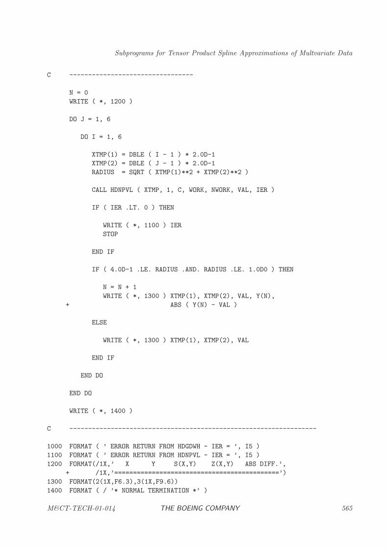
Subprograms for Tensor Product Spline Approximations of Multvariate Data
C ---------------------------------
N = 0
WRITE ( *, 1200 )
DO J = 1, 6
DO I = 1, 6
XTMP(1) = DBLE ( I - 1 ) * 2.0D-1
XTMP(2) = DBLE ( J - 1 ) * 2.0D-1
RADIUS = SQRT ( XTMP(1)**2 + XTMP(2)**2 )
CALL HDNPVL ( XTMP, 1, C, WORK, NWORK, VAL, IER )
IF ( IER .LT. 0 ) THEN
WRITE ( *, 1100 ) IER
STOP
END IF
IF ( 4.0D-1 .LE. RADIUS .AND. RADIUS .LE. 1.0D0 ) THEN
N = N + 1
WRITE ( *, 1300 ) XTMP(1), XTMP(2), VAL, Y(N),
+ ABS ( Y(N) - VAL )
ELSE
WRITE ( *, 1300 ) XTMP(1), XTMP(2), VAL
END IF
END DO
END DO
WRITE ( *, 1400 )
C ------------------------------------------------------------------
1000 FORMAT ( ’ ERROR RETURN FROM HDGDWH - IER = ’, I5 )
1100 FORMAT ( ’ ERROR RETURN FROM HDNPVL - IER = ’, I5 )
1200 FORMAT(/1X,’ X Y S(X,Y) Z(X,Y) ABS DIFF.’,
+ /1X,’============================================’)
1300 FORMAT(2(1X,F6.3),3(1X,F9.6))
1400 FORMAT ( / ’* NORMAL TERMINATION *’ )
M&CT-TECH-01-014 THE BOEING COMPANY 565
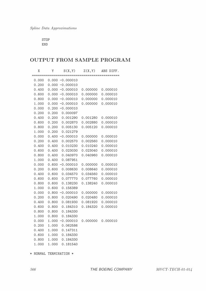
Spline Data Approximations
STOP
END
OUTPUT FROM SAMPLE PROGRAM
X Y S(X,Y) Z(X,Y) ABS DIFF.
============================================
0.000 0.000 -0.000010
0.200 0.000 -0.000010
0.400 0.000 -0.000010 0.000000 0.000010
0.600 0.000 -0.000010 0.000000 0.000010
0.800 0.000 -0.000010 0.000000 0.000010
1.000 0.000 -0.000010 0.000000 0.000010
0.000 0.200 -0.000010
0.200 0.200 0.000097
0.400 0.200 0.001290 0.001280 0.000010
0.600 0.200 0.002870 0.002880 0.000010
0.800 0.200 0.005130 0.005120 0.000010
1.000 0.200 0.021279
0.000 0.400 -0.000010 0.000000 0.000010
0.200 0.400 0.002570 0.002560 0.000010
0.400 0.400 0.010230 0.010240 0.000010
0.600 0.400 0.023030 0.023040 0.000010
0.800 0.400 0.040970 0.040960 0.000010
1.000 0.400 0.087951
0.000 0.600 -0.000010 0.000000 0.000010
0.200 0.600 0.008630 0.008640 0.000010
0.400 0.600 0.034570 0.034560 0.000010
0.600 0.600 0.077770 0.077760 0.000010
0.800 0.600 0.138230 0.138240 0.000010
1.000 0.600 0.156389
0.000 0.800 -0.000010 0.000000 0.000010
0.200 0.800 0.020490 0.020480 0.000010
0.400 0.800 0.081930 0.081920 0.000010
0.600 0.800 0.184310 0.184320 0.000010
0.800 0.800 0.184330
1.000 0.800 0.184330
0.000 1.000 -0.000010 0.000000 0.000010
0.200 1.000 0.062586
0.400 1.000 0.147311
0.600 1.000 0.184330
0.800 1.000 0.184330
1.000 1.000 0.181540
* NORMAL TERMINATION *
566 THE BOEING COMPANY M&CT-TECH-01-014
Subprograms for Tensor Product Spline Approximations of Multvariate Data
HDCMVS: Constrained Tensor Product Approximation of Multivariate Data
PURPOSE
HDCMVS computes a tensor product spline approximation of multivariate data. The approxima-tion can be either: a least squares approximation; a weighted least squares approximation; or anapproximation with minimal variation of its first or second order partials, which is within an userspecified tolerance of the data. Additionally, HDCMVS allows the user to define constraints on thespline and its partial derivatives.
RELATED SUBPROGRAMS
HDNPVL Evaluation of a Tensor Product Spline
HDNPDR Evaluation of a Partial Derivative of a Tensor Product Spline
HDTPSA Tensor Product Spline Approximation of Two-Dimensional Data
HDMVGA Approximation Multivariate Gridded Data
METHOD
To specify the data the user must provide values for the n independent variablesXℓ = (x1,ℓ, . . . , xn,ℓ)and corresponding values of the dependent variable yℓ, for ℓ = 1, . . . ,N. The dependent variabledata yℓ can represent either function values or partial derivative values. In the latter case the usermust specify the indices of the partial derivative, (γ1,ℓ, . . . , γn,ℓ), which yℓ represents.
HDCMVS defines the tensor product spline s(X) for X = (x1, . . . , xn) of degree Ki − 1 in xi as
s(X) =Mn+Kn∑
jn=1
· · ·M1+K1∑
j1=1
Aj1,...,jn
n∏
i=1
Bji(xi|Ti)
where Bji(xi|Ti) is the value at xi of the ji-th B-spline defined by the knot vector Ti. If xi
l =minℓ{xi,ℓ}, xi
u = maxℓ{xi,ℓ}, and ti,k for k = 1, . . . ,Mi, represents the internal knots, then
Ti = (
Ki times︷ ︸︸ ︷xi
l, . . . , xil , ti,1, ti,2, . . . , ti,Mi
,
Ki times︷ ︸︸ ︷xi
u, . . . , xiu)
Notice the end knots have multiplicity Ki. The number of B-splines, Bji(xi|Ti), in the xi-th
independent variable is Mi +Ki. The number of coefficients, Aj1,...,jn , is∏n
i=1(Mi +Ki).
To define the spline the user must specify the degree, Ki−1, in each of the independent variables and,optionally, the internal knots. Then for a given set of data (Xℓ, yℓ) and, optionally, spline partialderivative indices (γ1,ℓ, . . . , γn,ℓ); HDCMVS will compute a tensor product spline approximation ofthe data. The spline approximation can be either: a least squares approximation of the data; aweighted least squares approximation of the data; an approximation with minimal variation of itsfirst order partials, which is within an user specified tolerance of the data; or an approximation
M&CT-TECH-01-014 THE BOEING COMPANY 567
Spline Data Approximations
with minimal variation of its second order partials, which is within an user specified tolerance ofthe data. The user selects one of these options with the approximation option flag.
For the first two options HDCMVS computes the coefficients A = (Aj1,...,jn)T which minimize
E(A) =N∑
ℓ=1
wℓ
(
yℓ −∂s(γ1,ℓ+...,+γn,ℓ)
∂xγ1,ℓ1 · · · ∂xγn,ℓ
n
(Xℓ)
)2
.
If the spline is a least squares approximation, then wℓ = 1.0 for all ℓ. A weighted least squaresapproximation is obtained by specifying wℓ ≥ 0.0, for ℓ = 1, . . . ,N. For the latter two options theuser specifies error tolerances, ǫℓ ≥ 0, and HDCMVS computes the coefficients A which minimizeeither
E(A) =
∫ (∂s(X)
∂x1
)2
dx1 + · · · +∫ (
∂s(X)
∂xn
)2
dxn
or
E(A) =
∫ (∂2s(X)
∂2x1
)2
dx1 + · · · +∫ (
∂2s(X)
∂2xn
)2
dxn
subject to the constraints
yℓ − ǫℓ ≤∂s(γ1,ℓ+...+γn,ℓ)
∂xγ1,ℓ1 · · · ∂xγn,ℓ
n
(Xℓ) ≤ yℓ + ǫℓ
for ℓ = 1, . . . ,N.
Independent of which of the above four options is chosen, the user can impose constraints on thespline. These constraints are of the form
∂s(λ1,j+...+λn,j)(X)
∂xλ1,j
1 · · · ∂xλn,jn
{≥≤=
}
gj(X)
for j = 1, . . . ,NCON. The indices λ1,j through λn,j specify the order of the partial derivative inx1 through xn, respectively, that is bounded by gj(X). The bounds gj(X) are either univariate ormultivariate splines. If gj(X) is an univariate spline, which depends on xi, then it must be of theform
gj(xi) =
mi,j∑
li=1
βliGli(xi|Si)
where Gli(xi|Si) are B-splines of order ki,j defined by the knot vector Si. If gj(X) is a multivariatespline, then it must be of the form
568 THE BOEING COMPANY M&CT-TECH-01-014
Subprograms for Tensor Product Spline Approximations of Multvariate Data
gj(X) =
mnj,j∑
lnj=1
· · ·m1,j∑
l1=1
βl1,...,lnj
nj∏
i=1
Gli(xi|Si)
where Gli(xi|Si) are B-splines of order ki,j defined by the knot vector Si; nj is the number ofindependent variables for gj(X), which must satisfy nj ≤ n; and X is a vector of nj elements.
Whenever nj < n the user must specify the indices of the independent variables for gj(X) andvalues for the remaining independent variables. For example, suppose the user wishes to impose aconstraint on a spline s(X) which is a function of three variables, (x, y, z). If the bounding splineg(X) associated with the constraint is a function of the variables (x, z), then the user must speciifythe value of y at which the constraint is imposed.
For a given approximation option and set of constraints, HDCMVS formulates a linearly constrainedquadratic programming problem in the following manner. First, HDCMVS defines a set of tensorproduct B-splines
Φj1,...,jn(X) =n∏
i=1
Cji(xi|Λi)
which forms a common basis for the spline s(X), the NCON partial derivatives of the spline, andthe NCON constraint splines gj(X). The Cji
(xi|Λi)’s , for ji = 1, . . . ,Mci, are B-splines of order
Kciwhere
Kci= max{Ki,
max
j{ki,j}}
and
Mci≤
NCON∑
j=1
(mi,j ∗ (Kci− ki,j + 1) + (Mi +Ki) ∗ (Kci
−Ki + 1)) .
After defining the common tensor product basis the constraints represented by Equation (8.2) areconverted into linear constraints of the form
l1l2...
lNCON
≤
D1
D2...
DNCON
A ≤
u1
u2...
uNCON
where DjA are the coefficients of the partial derivative of the spline s(X) with respect to thecommon tensor product B-splines Φj1,...,jn(X). The vectors lj and uj are the coefficients of theconstraint splines gj(X) with respect to the common tensor product B-splines. If the j-th constraintis an equality constraint, then lj = uj .
Then, HDCMVS employs either the sparse nonlinear optimization package HDSNLP or HDBNLPto solve the quadratic programming problem, minimize E(A) subject to the linear constraints
M&CT-TECH-01-014 THE BOEING COMPANY 569
Spline Data Approximations
defined by Equation (8.2). HDSNLP or HDBNLP are designed to locate the minimum of a quadraticfunction subject to linear constraints. They utilize sparse linear algebra techniques and are capableof solving large sparse optimization problems. See HDSNLP (p. 51) or HDBNLP (p. 141) for moreinformation.
HDCMVS provides the user with an option to regularize rank deficient problems. A problem isconsidered rank deficient if the location of the data, the placement of the internal knots, and theselected approximation option do not uniquely define the spline coefficients. Three options areprovided for handling rank deficient problems.
If the first option is chosen, then HDCMVS will not determine if the problem is rank deficient. Ifthe second option is chosen, then HDCMVS will inform the user of any rank deficiencies via theerror return code. In either case the problem is not regularized. If the third option is chosen, thenthe problem is regularized in the following manner.
First, HDCMVS determines the spline coefficients which are not uniquely defined by the dataand approximation option. Then two optimizations are performed. During the first optimization,the spline coefficients which minimized the approximation option and satisfy the constraints arecomputed. The second optimization computes the coefficients which minimize the second partialderivative with respect to each independent variable and satisfies the constraints. During the secondoptimization the spline coefficeints which were uniquely defined by the data remain fixed and equalto their previously computed values. If the second optimization fails, then HDCMVS returns theresult of the first optimzation.
USAGE REMARKS
Whether or not a set of spline coefficients which satisfies the constraints exists depends on the typeof constraints, the constraint splines, and the internal knots of the spline approximation. Thatis, a feasible point may exists for some values of the internal knots but not for others. Therefore,the user must define a set of knots which allow sufficient flexibility for the spline to satisfy theconstraints.
Also, the optimization routines HDSNLP and HDBNLP require upper and lower bounds for thespline coefficients. HDCMVS imposes the bounds
−105δy ≤ αj1,...,jn − minℓ{yℓ} ≤ 105δy
where δy = maxℓ{yℓ} − minℓ{yℓ}. If a bound is active at the solution, then HDCMVS will informthe user via the error return code. In this case, the user should consider imposing additionalconstraints on the spline approximation.
WARNING
It may be neccessary for HDCMVS to create scratch files to hold information required to define theconstraint Jacobian. These binary files are associated with input/output units 18 and 19. Theseinput/output units are reserved for HDCMVS and can not be utilized by the user. If an erroroccurs while accessing these input/output units, then HDCMVS reports an error condition.
USAGE
570 THE BOEING COMPANY M&CT-TECH-01-014
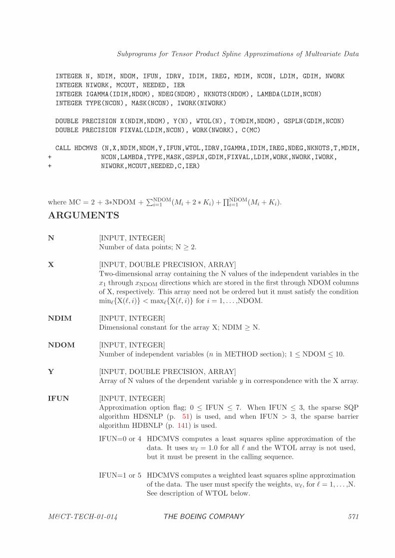
Subprograms for Tensor Product Spline Approximations of Multvariate Data
INTEGER N, NDIM, NDOM, IFUN, IDRV, IDIM, IREG, MDIM, NCON, LDIM, GDIM, NWORK
INTEGER NIWORK, MCOUT, NEEDED, IER
INTEGER IGAMMA(IDIM,NDOM), NDEG(NDOM), NKNOTS(NDOM), LAMBDA(LDIM,NCON)
INTEGER TYPE(NCON), MASK(NCON), IWORK(NIWORK)
DOUBLE PRECISION X(NDIM,NDOM), Y(N), WTOL(N), T(MDIM,NDOM), GSPLN(GDIM,NCON)
DOUBLE PRECISION FIXVAL(LDIM,NCON), WORK(NWORK), C(MC)
CALL HDCMVS (N,X,NDIM,NDOM,Y,IFUN,WTOL,IDRV,IGAMMA,IDIM,IREG,NDEG,NKNOTS,T,MDIM,
+ NCON,LAMBDA,TYPE,MASK,GSPLN,GDIM,FIXVAL,LDIM,WORK,NWORK,IWORK,
+ NIWORK,MCOUT,NEEDED,C,IER)
where MC = 2 + 3∗NDOM +∑NDOM
i=1 (Mi + 2 ∗Ki) +∏NDOM
i=1 (Mi +Ki).
ARGUMENTS
N [INPUT, INTEGER]Number of data points; N ≥ 2.
X [INPUT, DOUBLE PRECISION, ARRAY]Two-dimensional array containing the N values of the independent variables in thex1 through xNDOM directions which are stored in the first through NDOM columnsof X, respectively. This array need not be ordered but it must satisfy the conditionminℓ{X(ℓ, i)} < maxℓ{X(ℓ, i)} for i = 1, . . . ,NDOM.
NDIM [INPUT, INTEGER]Dimensional constant for the array X; NDIM ≥ N.
NDOM [INPUT, INTEGER]Number of independent variables (n in METHOD section); 1 ≤ NDOM ≤ 10.
Y [INPUT, DOUBLE PRECISION, ARRAY]Array of N values of the dependent variable y in correspondence with the X array.
IFUN [INPUT, INTEGER]Approximation option flag; 0 ≤ IFUN ≤ 7. When IFUN ≤ 3, the sparse SQPalgorithm HDSNLP (p. 51) is used, and when IFUN > 3, the sparse barrieralgorithm HDBNLP (p. 141) is used.
IFUN=0 or 4 HDCMVS computes a least squares spline approximation of thedata. It uses wℓ = 1.0 for all ℓ and the WTOL array is not used,but it must be present in the calling sequence.
IFUN=1 or 5 HDCMVS computes a weighted least squares spline approximationof the data. The user must specify the weights, wℓ, for ℓ = 1, . . . ,N.See description of WTOL below.
M&CT-TECH-01-014 THE BOEING COMPANY 571
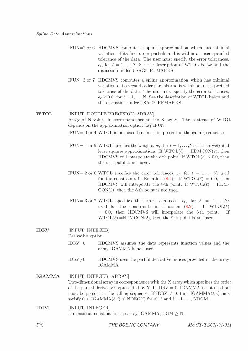
Spline Data Approximations
IFUN=2 or 6 HDCMVS computes a spline approximation which has minimalvariation of its first order partials and is within an user specifiedtolerance of the data. The user must specify the error tolerances,ǫℓ, for ℓ = 1, . . . ,N. See the description of WTOL below and thediscussion under USAGE REMARKS.
IFUN=3 or 7 HDCMVS computes a spline approximation which has minimalvariation of its second order partials and is within an user specifiedtolerance of the data. The user must specify the error tolerances,ǫℓ ≥ 0.0, for ℓ = 1, . . . ,N. See the description of WTOL below andthe discussion under USAGE REMARKS.
WTOL [INPUT, DOUBLE PRECISION, ARRAY]Array of N values in correspondence to the X array. The contents of WTOLdepends on the approximation option flag IFUN.
IFUN= 0 or 4 WTOL is not used but must be present in the calling sequence.
IFUN= 1 or 5 WTOL specifies the weights, wℓ, for ℓ = 1, . . . ,N; used for weightedleast squares approximations. If WTOL(ℓ) = HDMCON(2), thenHDCMVS will interpolate the ℓ-th point. If WTOL(ℓ) ≤ 0.0, thenthe ℓ-th point is not used.
IFUN= 2 or 6 WTOL specifies the error tolerances, ǫℓ, for ℓ = 1, . . . ,N; usedfor the constraints in Equation (8.2). If WTOL(ℓ) = 0.0, thenHDCMVS will interpolate the ℓ-th point. If WTOL(ℓ) = HDM-CON(2), then the ℓ-th point is not used.
IFUN= 3 or 7 WTOL specifies the error tolerances, ǫℓ, for ℓ = 1, . . . ,N;used for the constraints in Equation (8.2). If WTOL(ℓ)= 0.0, then HDCMVS will interpolate the ℓ-th point. IfWTOL(ℓ) =HDMCON(2), then the ℓ-th point is not used.
IDRV [INPUT, INTEGER]Derivative option.
IDRV=0 HDCMVS assumes the data represents function values and thearray IGAMMA is not used.
IDRV6=0 HDCMVS uses the partial derivative indices provided in the arrayIGAMMA.
IGAMMA [INPUT, INTEGER, ARRAY]Two-dimensional array in correspondence with the X array which specifies the orderof the partial derivative represented by Y. If IDRV = 0, IGAMMA is not used butmust be present in the calling sequence. If IDRV 6= 0, then IGAMMA(ℓ, i) mustsatisfy 0 ≤ IGAMMA(ℓ, i) ≤ NDEG(i) for all ℓ and i = 1, . . . , NDOM.
IDIM [INPUT, INTEGER]Dimensional constant for the array IGAMMA; IDIM ≥ N.
572 THE BOEING COMPANY M&CT-TECH-01-014
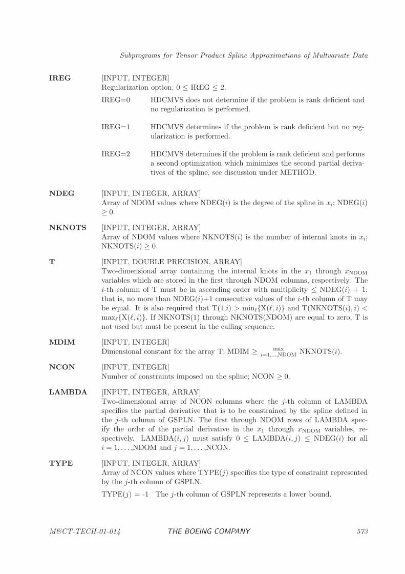
Subprograms for Tensor Product Spline Approximations of Multvariate Data
IREG [INPUT, INTEGER]Regularization option; 0 ≤ IREG ≤ 2.
IREG=0 HDCMVS does not determine if the problem is rank deficient andno regularization is performed.
IREG=1 HDCMVS determines if the problem is rank deficient but no reg-ularization is performed.
IREG=2 HDCMVS determines if the problem is rank deficient and performsa second optimization which minimizes the second partial deriva-tives of the spline, see discussion under METHOD.
NDEG [INPUT, INTEGER, ARRAY]Array of NDOM values where NDEG(i) is the degree of the spline in xi; NDEG(i)≥ 0.
NKNOTS [INPUT, INTEGER, ARRAY]Array of NDOM values where NKNOTS(i) is the number of internal knots in xi;NKNOTS(i) ≥ 0.
T [INPUT, DOUBLE PRECISION, ARRAY]Two-dimensional array containing the internal knots in the x1 through xNDOM
variables which are stored in the first through NDOM columns, respectively. Thei-th column of T must be in ascending order with multiplicity ≤ NDEG(i) + 1;that is, no more than NDEG(i)+1 consecutive values of the i-th column of T maybe equal. It is also required that T(1,i) > minℓ{X(ℓ, i)} and T(NKNOTS(i), i) <maxℓ{X(ℓ, i)}. If NKNOTS(1) through NKNOTS(NDOM) are equal to zero, T isnot used but must be present in the calling sequence.
MDIM [INPUT, INTEGER]Dimensional constant for the array T; MDIM ≥ max
i=1,...,NDOM NKNOTS(i).
NCON [INPUT, INTEGER]Number of constraints imposed on the spline; NCON ≥ 0.
LAMBDA [INPUT, INTEGER, ARRAY]Two-dimensional array of NCON columns where the j-th column of LAMBDAspecifies the partial derivative that is to be constrained by the spline defined inthe j-th column of GSPLN. The first through NDOM rows of LAMBDA spec-ify the order of the partial derivative in the x1 through xNDOM variables, re-spectively. LAMBDA(i, j) must satisfy 0 ≤ LAMBDA(i, j) ≤ NDEG(i) for alli = 1, . . . ,NDOM and j = 1, . . . ,NCON.
TYPE [INPUT, INTEGER, ARRAY]Array of NCON values where TYPE(j) specifies the type of constraint representedby the j-th column of GSPLN.
TYPE(j) = -1 The j-th column of GSPLN represents a lower bound.
M&CT-TECH-01-014 THE BOEING COMPANY 573
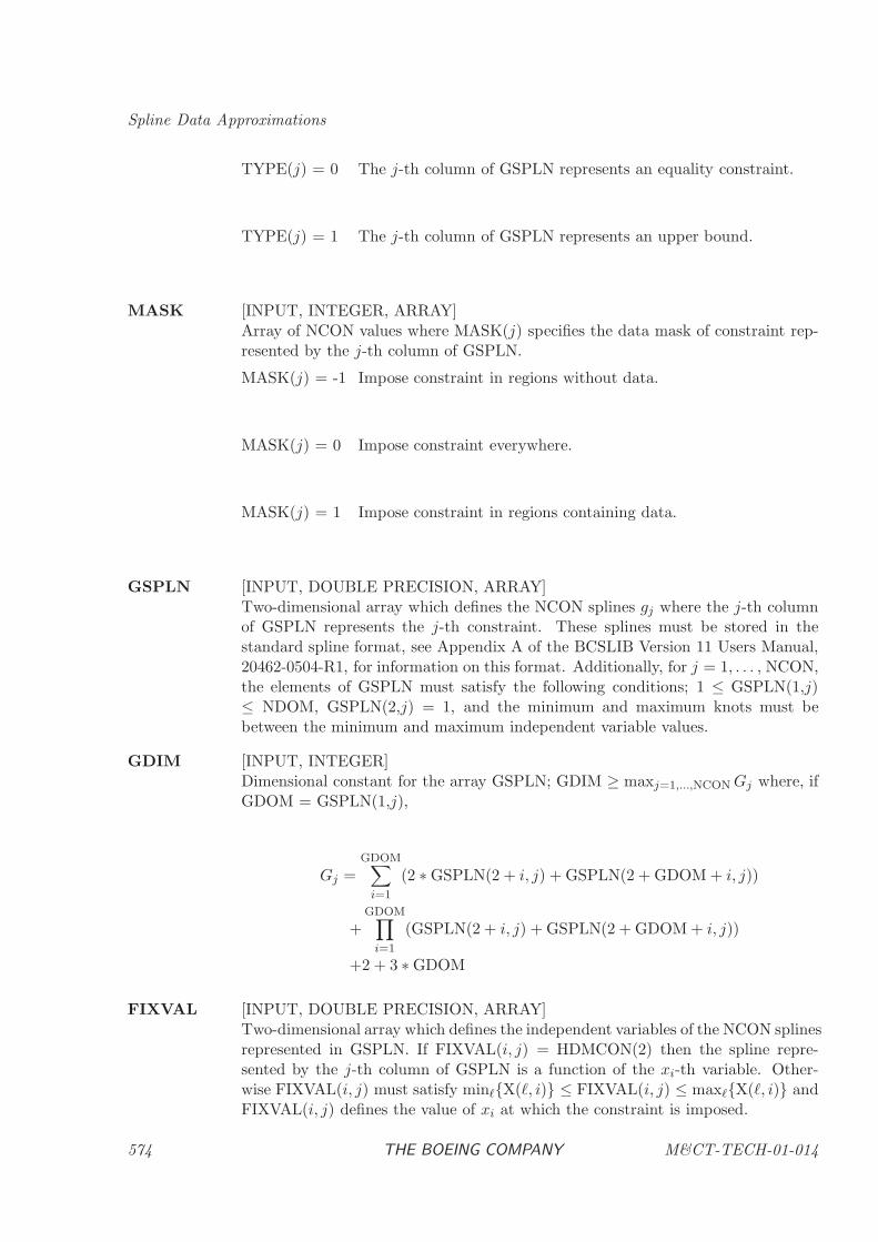
Spline Data Approximations
TYPE(j) = 0 The j-th column of GSPLN represents an equality constraint.
TYPE(j) = 1 The j-th column of GSPLN represents an upper bound.
MASK [INPUT, INTEGER, ARRAY]Array of NCON values where MASK(j) specifies the data mask of constraint rep-resented by the j-th column of GSPLN.
MASK(j) = -1 Impose constraint in regions without data.
MASK(j) = 0 Impose constraint everywhere.
MASK(j) = 1 Impose constraint in regions containing data.
GSPLN [INPUT, DOUBLE PRECISION, ARRAY]Two-dimensional array which defines the NCON splines gj where the j-th columnof GSPLN represents the j-th constraint. These splines must be stored in thestandard spline format, see Appendix A of the BCSLIB Version 11 Users Manual,20462-0504-R1, for information on this format. Additionally, for j = 1, . . . , NCON,the elements of GSPLN must satisfy the following conditions; 1 ≤ GSPLN(1,j)≤ NDOM, GSPLN(2,j) = 1, and the minimum and maximum knots must bebetween the minimum and maximum independent variable values.
GDIM [INPUT, INTEGER]Dimensional constant for the array GSPLN; GDIM ≥ maxj=1,...,NCONGj where, ifGDOM = GSPLN(1,j),
Gj =GDOM∑
i=1
(2 ∗ GSPLN(2 + i, j) + GSPLN(2 + GDOM + i, j))
+GDOM∏
i=1
(GSPLN(2 + i, j) + GSPLN(2 + GDOM + i, j))
+2 + 3 ∗ GDOM
FIXVAL [INPUT, DOUBLE PRECISION, ARRAY]Two-dimensional array which defines the independent variables of the NCON splinesrepresented in GSPLN. If FIXVAL(i, j) = HDMCON(2) then the spline repre-sented by the j-th column of GSPLN is a function of the xi-th variable. Other-wise FIXVAL(i, j) must satisfy minℓ{X(ℓ, i)} ≤ FIXVAL(i, j) ≤ maxℓ{X(ℓ, i)} andFIXVAL(i, j) defines the value of xi at which the constraint is imposed.
574 THE BOEING COMPANY M&CT-TECH-01-014
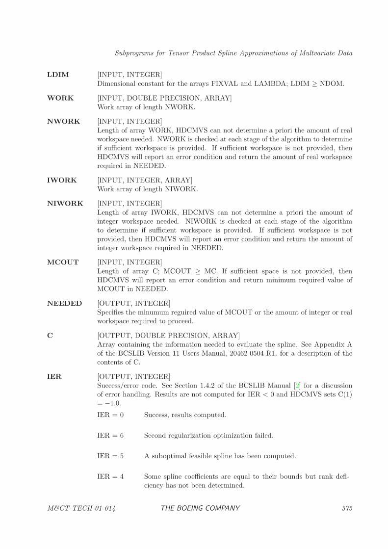
Subprograms for Tensor Product Spline Approximations of Multvariate Data
LDIM [INPUT, INTEGER]Dimensional constant for the arrays FIXVAL and LAMBDA; LDIM ≥ NDOM.
WORK [INPUT, DOUBLE PRECISION, ARRAY]Work array of length NWORK.
NWORK [INPUT, INTEGER]Length of array WORK, HDCMVS can not determine a priori the amount of realworkspace needed. NWORK is checked at each stage of the algorithm to determineif sufficient workspace is provided. If sufficient workspace is not provided, thenHDCMVS will report an error condition and return the amount of real workspacerequired in NEEDED.
IWORK [INPUT, INTEGER, ARRAY]Work array of length NIWORK.
NIWORK [INPUT, INTEGER]Length of array IWORK, HDCMVS can not determine a priori the amount ofinteger workspace needed. NIWORK is checked at each stage of the algorithmto determine if sufficient workspace is provided. If sufficient workspace is notprovided, then HDCMVS will report an error condition and return the amount ofinteger workspace required in NEEDED.
MCOUT [INPUT, INTEGER]Length of array C; MCOUT ≥ MC. If sufficient space is not provided, thenHDCMVS will report an error condition and return minimum required value ofMCOUT in NEEDED.
NEEDED [OUTPUT, INTEGER]Specifies the minumum reguired value of MCOUT or the amount of integer or realworkspace required to proceed.
C [OUTPUT, DOUBLE PRECISION, ARRAY]Array containing the information needed to evaluate the spline. See Appendix Aof the BCSLIB Version 11 Users Manual, 20462-0504-R1, for a description of thecontents of C.
IER [OUTPUT, INTEGER]Success/error code. See Section 1.4.2 of the BCSLIB Manual [2] for a discussionof error handling. Results are not computed for IER < 0 and HDCMVS sets C(1)= −1.0.
IER = 0 Success, results computed.
IER = 6 Second regularization optimization failed.
IER = 5 A suboptimal feasible spline has been computed.
IER = 4 Some spline coefficients are equal to their bounds but rank defi-ciency has not been determined.
M&CT-TECH-01-014 THE BOEING COMPANY 575
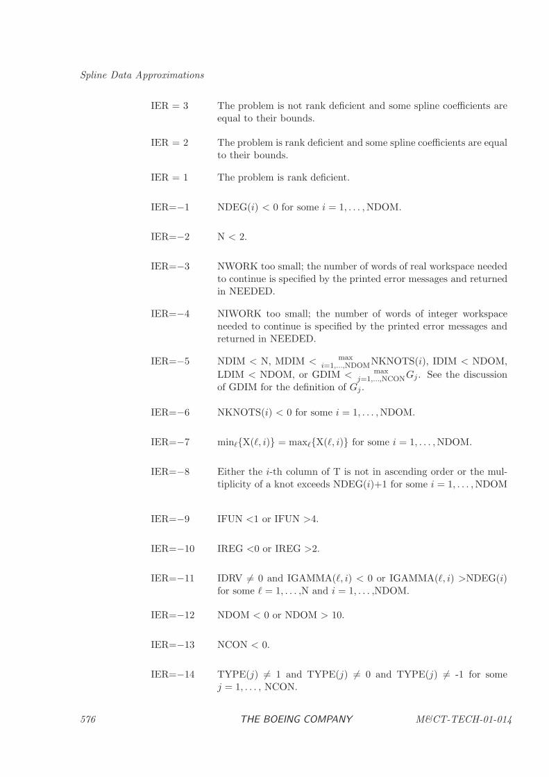
Spline Data Approximations
IER = 3 The problem is not rank deficient and some spline coefficients areequal to their bounds.
IER = 2 The problem is rank deficient and some spline coefficients are equalto their bounds.
IER = 1 The problem is rank deficient.
IER=−1 NDEG(i) < 0 for some i = 1, . . . ,NDOM.
IER=−2 N < 2.
IER=−3 NWORK too small; the number of words of real workspace neededto continue is specified by the printed error messages and returnedin NEEDED.
IER=−4 NIWORK too small; the number of words of integer workspaceneeded to continue is specified by the printed error messages andreturned in NEEDED.
IER=−5 NDIM < N, MDIM < maxi=1,...,NDOMNKNOTS(i), IDIM < NDOM,
LDIM < NDOM, or GDIM < maxj=1,...,NCONGj . See the discussion
of GDIM for the definition of Gj .
IER=−6 NKNOTS(i) < 0 for some i = 1, . . . ,NDOM.
IER=−7 minℓ{X(ℓ, i)} = maxℓ{X(ℓ, i)} for some i = 1, . . . ,NDOM.
IER=−8 Either the i-th column of T is not in ascending order or the mul-tiplicity of a knot exceeds NDEG(i)+1 for some i = 1, . . . ,NDOM
IER=−9 IFUN <1 or IFUN >4.
IER=−10 IREG <0 or IREG >2.
IER=−11 IDRV 6= 0 and IGAMMA(ℓ, i) < 0 or IGAMMA(ℓ, i) >NDEG(i)for some ℓ = 1, . . . ,N and i = 1, . . . ,NDOM.
IER=−12 NDOM < 0 or NDOM > 10.
IER=−13 NCON < 0.
IER=−14 TYPE(j) 6= 1 and TYPE(j) 6= 0 and TYPE(j) 6= -1 for somej = 1, . . . , NCON.
576 THE BOEING COMPANY M&CT-TECH-01-014
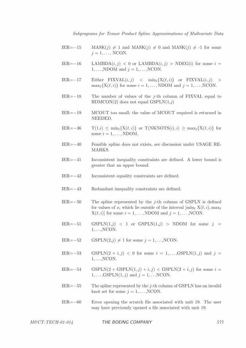
Subprograms for Tensor Product Spline Approximations of Multvariate Data
IER=−15 MASK(j) 6= 1 and MASK(j) 6= 0 and MASK(j) 6= -1 for somej = 1, . . . , NCON.
IER=−16 LAMBDA(i, j) < 0 or LAMBDA(i, j) > NDEG(i) for some i =1, . . . ,NDOM and j = 1, . . . ,NCON.
IER=−17 Either FIXVAL(i, j) < minℓ{X(ℓ, i)} or FIXVAL(i, j) >maxℓ{X(ℓ, i)} for some i = 1, . . . ,NDOM and j = 1, . . . ,NCON.
IER=−18 The number of values of the j-th column of FIXVAL equal toHDMCON(2) does not equal GSPLN(1,j)
IER=−19 MCOUT too small; the value of MCOUT required is returned inNEEDED.
IER=−36 T(1,i) ≤ minℓ{X(ℓ, i)} or T(NKNOTS(i), i) ≥ maxℓ{X(ℓ, i)} forsome i = 1, . . . ,NDOM.
IER=−40 Feasible spline does not exists, see discussion under USAGE RE-MARKS.
IER=−41 Inconsistent inequality constraints are defined. A lower bound isgreater that an upper bound.
IER=−42 Inconsistent equality constraints are defined.
IER=−43 Redundant inequality constraints are defined.
IER=−50 The spline represented by the j-th column of GSPLN is definedfor values of xi which lie outside of the interval [minℓ X(ℓ, i),maxℓ
X(ℓ, i)] for some i = 1, . . . ,NDOM and j = 1, . . . ,NCON.
IER=−51 GSPLN(1,j) < 1 or GSPLN(1,j) > NDOM for some j =1, . . .,NCON.
IER=−52 GSPLN(2,j) 6= 1 for some j = 1, . . .,NCON.
IER=−53 GSPLN(2 + i, j) < 0 for some i = 1, . . . ,GSPLN(1, j) and j =1, . . .,NCON.
IER=−54 GSPLN(2 + GSPLN(1, j) + i, j) < GSPLN(2 + i, j) for some i =1, . . . ,GSPLN(1, j) and j = 1, . . .NCON.
IER=−55 The spline represented by the j-th column of GSPLN has an invalidknot set for some j = 1, . . . ,NCON.
IER=−60 Error opening the scratch file associated with unit 19. The usermay have previously opened a file associated with unit 19.
M&CT-TECH-01-014 THE BOEING COMPANY 577
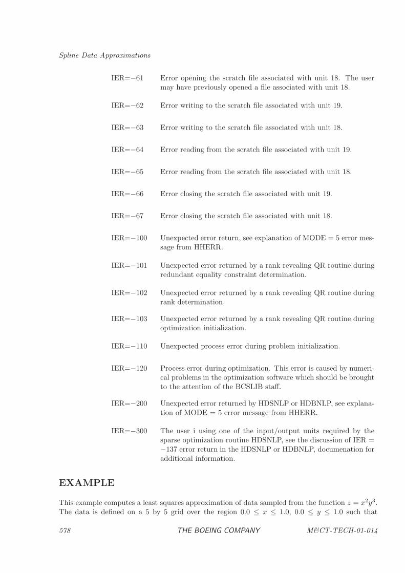
Spline Data Approximations
IER=−61 Error opening the scratch file associated with unit 18. The usermay have previously opened a file associated with unit 18.
IER=−62 Error writing to the scratch file associated with unit 19.
IER=−63 Error writing to the scratch file associated with unit 18.
IER=−64 Error reading from the scratch file associated with unit 19.
IER=−65 Error reading from the scratch file associated with unit 18.
IER=−66 Error closing the scratch file associated with unit 19.
IER=−67 Error closing the scratch file associated with unit 18.
IER=−100 Unexpected error return, see explanation of MODE = 5 error mes-sage from HHERR.
IER=−101 Unexpected error returned by a rank revealing QR routine duringredundant equality constraint determination.
IER=−102 Unexpected error returned by a rank revealing QR routine duringrank determination.
IER=−103 Unexpected error returned by a rank revealing QR routine duringoptimization initialization.
IER=−110 Unexpected process error during problem initialization.
IER=−120 Process error during optimization. This error is caused by numeri-cal problems in the optimization software which should be broughtto the attention of the BCSLIB staff.
IER=−200 Unexpected error returned by HDSNLP or HDBNLP, see explana-tion of MODE = 5 error message from HHERR.
IER=−300 The user i using one of the input/output units required by thesparse optimization routine HDSNLP, see the discussion of IER =−137 error return in the HDSNLP or HDBNLP, documenation foradditional information.
EXAMPLE
This example computes a least squares approximation of data sampled from the function z = x2y3.The data is defined on a 5 by 5 grid over the region 0.0 ≤ x ≤ 1.0, 0.0 ≤ y ≤ 1.0 such that
578 THE BOEING COMPANY M&CT-TECH-01-014
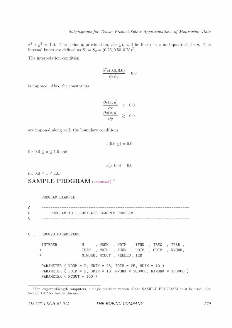
Subprograms for Tensor Product Spline Approximations of Multvariate Data
x2 + y2 = 1.0. The spline approximation, s(x, y), will be linear in x and quadratic in y. Theinternal knots are defined as S1 = S2 = (0.25, 0.50, 0.75)T .
The interpolation condition
∂2s(0.0, 0.0)
∂x∂y= 0.0
is imposed. Also, the constraints
∂s(x, y)
∂x≥ 0.0
∂s(x, y)
∂y≥ 0.0.
are imposed along with the boundary conditions
s(0.0, y) = 0.0
for 0.0 ≤ y ≤ 1.0 and
s(x, 0.0) = 0.0
for 0.0 ≤ x ≤ 1.0.
SAMPLE PROGRAM (excmvs.f) 3
PROGRAM EXAMPLE
C ------------------------------------------------------------------
C ... PROGRAM TO ILLUSTRATE EXAMPLE PROBLEM
C ------------------------------------------------------------------
C ... HDCMVS PARAMETERS
INTEGER N , NDOM , NDIM , IFUN , IREG , IPAR ,
+ IDIM , MDIM , NCON , LDIM , GDIM , NWORK,
+ NIWORK, MCOUT , NEEDED, IER
PARAMETER ( NDOM = 2, NDIM = 25, IDIM = 25, MDIM = 10 )
PARAMETER ( LDIM = 2, GDIM = 13, NWORK = 100000, NIWORK = 100000 )
PARAMETER ( MCOUT = 100 )
3For long-word-length computers, a single precision version of the SAMPLE PROGRAM must be used. See
Section 1.4.7 for further discussion.
M&CT-TECH-01-014 THE BOEING COMPANY 579
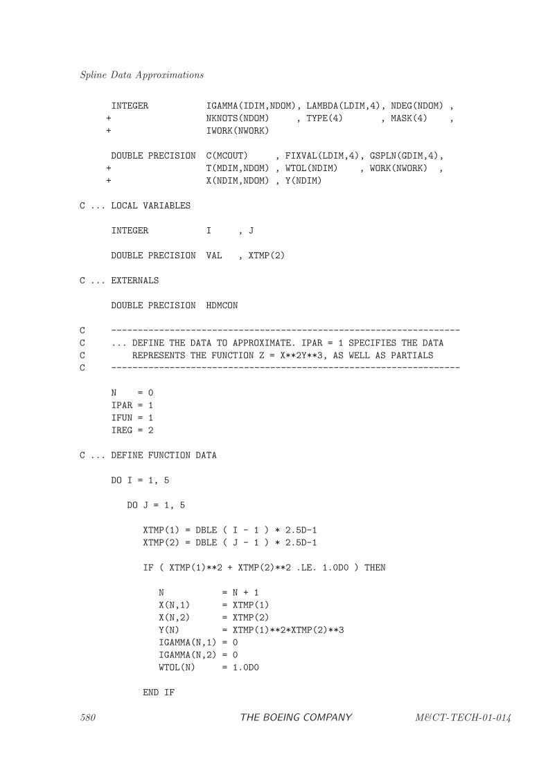
Spline Data Approximations
INTEGER IGAMMA(IDIM,NDOM), LAMBDA(LDIM,4), NDEG(NDOM) ,
+ NKNOTS(NDOM) , TYPE(4) , MASK(4) ,
+ IWORK(NWORK)
DOUBLE PRECISION C(MCOUT) , FIXVAL(LDIM,4), GSPLN(GDIM,4),
+ T(MDIM,NDOM) , WTOL(NDIM) , WORK(NWORK) ,
+ X(NDIM,NDOM) , Y(NDIM)
C ... LOCAL VARIABLES
INTEGER I , J
DOUBLE PRECISION VAL , XTMP(2)
C ... EXTERNALS
DOUBLE PRECISION HDMCON
C ------------------------------------------------------------------
C ... DEFINE THE DATA TO APPROXIMATE. IPAR = 1 SPECIFIES THE DATA
C REPRESENTS THE FUNCTION Z = X**2Y**3, AS WELL AS PARTIALS
C ------------------------------------------------------------------
N = 0
IPAR = 1
IFUN = 1
IREG = 2
C ... DEFINE FUNCTION DATA
DO I = 1, 5
DO J = 1, 5
XTMP(1) = DBLE ( I - 1 ) * 2.5D-1
XTMP(2) = DBLE ( J - 1 ) * 2.5D-1
IF ( XTMP(1)**2 + XTMP(2)**2 .LE. 1.0D0 ) THEN
N = N + 1
X(N,1) = XTMP(1)
X(N,2) = XTMP(2)
Y(N) = XTMP(1)**2*XTMP(2)**3
IGAMMA(N,1) = 0
IGAMMA(N,2) = 0
WTOL(N) = 1.0D0
END IF
580 THE BOEING COMPANY M&CT-TECH-01-014
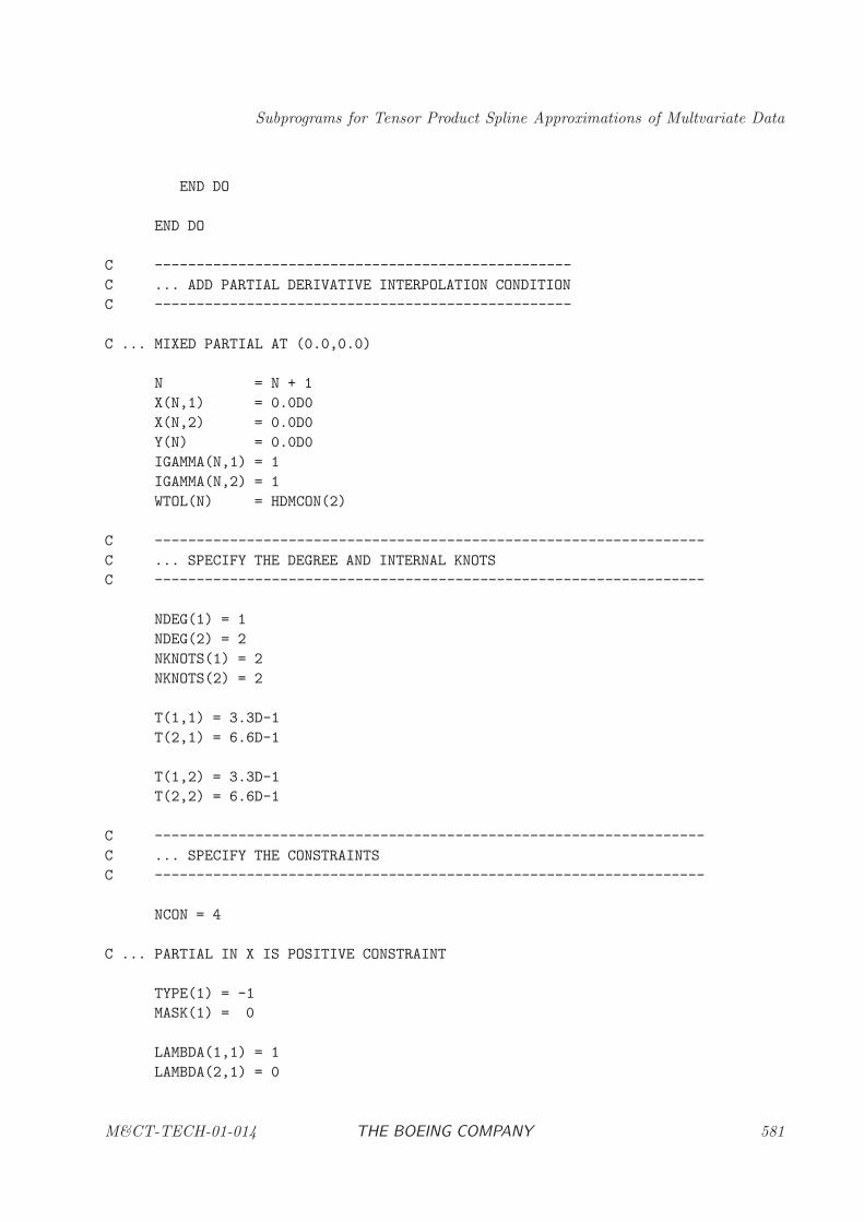
Subprograms for Tensor Product Spline Approximations of Multvariate Data
END DO
END DO
C --------------------------------------------------
C ... ADD PARTIAL DERIVATIVE INTERPOLATION CONDITION
C --------------------------------------------------
C ... MIXED PARTIAL AT (0.0,0.0)
N = N + 1
X(N,1) = 0.0D0
X(N,2) = 0.0D0
Y(N) = 0.0D0
IGAMMA(N,1) = 1
IGAMMA(N,2) = 1
WTOL(N) = HDMCON(2)
C ------------------------------------------------------------------
C ... SPECIFY THE DEGREE AND INTERNAL KNOTS
C ------------------------------------------------------------------
NDEG(1) = 1
NDEG(2) = 2
NKNOTS(1) = 2
NKNOTS(2) = 2
T(1,1) = 3.3D-1
T(2,1) = 6.6D-1
T(1,2) = 3.3D-1
T(2,2) = 6.6D-1
C ------------------------------------------------------------------
C ... SPECIFY THE CONSTRAINTS
C ------------------------------------------------------------------
NCON = 4
C ... PARTIAL IN X IS POSITIVE CONSTRAINT
TYPE(1) = -1
MASK(1) = 0
LAMBDA(1,1) = 1
LAMBDA(2,1) = 0
M&CT-TECH-01-014 THE BOEING COMPANY 581
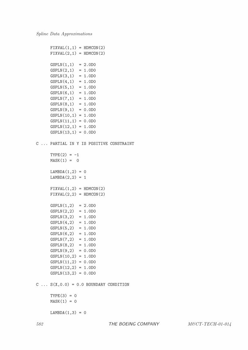
Spline Data Approximations
FIXVAL(1,1) = HDMCON(2)
FIXVAL(2,1) = HDMCON(2)
GSPLN(1,1) = 2.0D0
GSPLN(2,1) = 1.0D0
GSPLN(3,1) = 1.0D0
GSPLN(4,1) = 1.0D0
GSPLN(5,1) = 1.0D0
GSPLN(6,1) = 1.0D0
GSPLN(7,1) = 1.0D0
GSPLN(8,1) = 1.0D0
GSPLN(9,1) = 0.0D0
GSPLN(10,1) = 1.0D0
GSPLN(11,1) = 0.0D0
GSPLN(12,1) = 1.0D0
GSPLN(13,1) = 0.0D0
C ... PARTIAL IN Y IS POSITIVE CONSTRAINT
TYPE(2) = -1
MASK(1) = 0
LAMBDA(1,2) = 0
LAMBDA(2,2) = 1
FIXVAL(1,2) = HDMCON(2)
FIXVAL(2,2) = HDMCON(2)
GSPLN(1,2) = 2.0D0
GSPLN(2,2) = 1.0D0
GSPLN(3,2) = 1.0D0
GSPLN(4,2) = 1.0D0
GSPLN(5,2) = 1.0D0
GSPLN(6,2) = 1.0D0
GSPLN(7,2) = 1.0D0
GSPLN(8,2) = 1.0D0
GSPLN(9,2) = 0.0D0
GSPLN(10,2) = 1.0D0
GSPLN(11,2) = 0.0D0
GSPLN(12,2) = 1.0D0
GSPLN(13,2) = 0.0D0
C ... S(X,0.0) = 0.0 BOUNDARY CONDITION
TYPE(3) = 0
MASK(1) = 0
LAMBDA(1,3) = 0
582 THE BOEING COMPANY M&CT-TECH-01-014
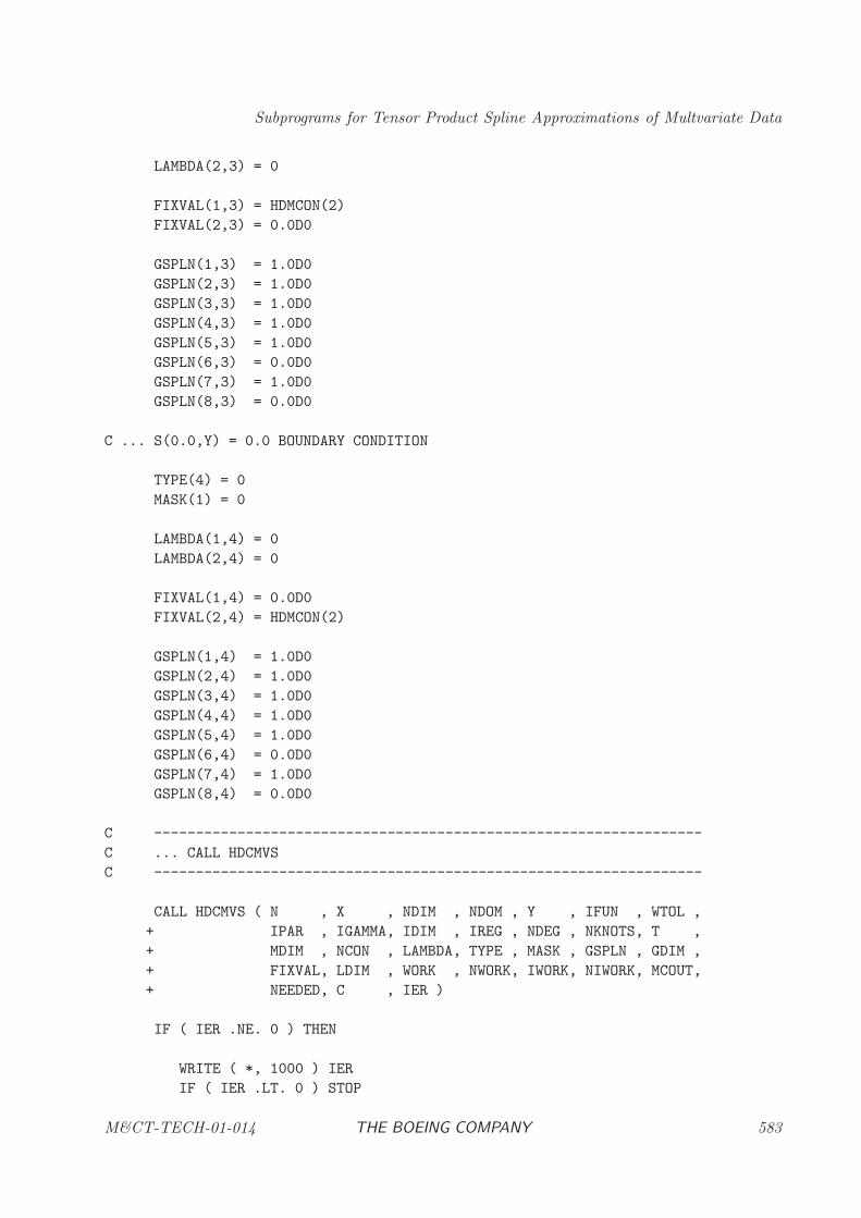
Subprograms for Tensor Product Spline Approximations of Multvariate Data
LAMBDA(2,3) = 0
FIXVAL(1,3) = HDMCON(2)
FIXVAL(2,3) = 0.0D0
GSPLN(1,3) = 1.0D0
GSPLN(2,3) = 1.0D0
GSPLN(3,3) = 1.0D0
GSPLN(4,3) = 1.0D0
GSPLN(5,3) = 1.0D0
GSPLN(6,3) = 0.0D0
GSPLN(7,3) = 1.0D0
GSPLN(8,3) = 0.0D0
C ... S(0.0,Y) = 0.0 BOUNDARY CONDITION
TYPE(4) = 0
MASK(1) = 0
LAMBDA(1,4) = 0
LAMBDA(2,4) = 0
FIXVAL(1,4) = 0.0D0
FIXVAL(2,4) = HDMCON(2)
GSPLN(1,4) = 1.0D0
GSPLN(2,4) = 1.0D0
GSPLN(3,4) = 1.0D0
GSPLN(4,4) = 1.0D0
GSPLN(5,4) = 1.0D0
GSPLN(6,4) = 0.0D0
GSPLN(7,4) = 1.0D0
GSPLN(8,4) = 0.0D0
C ------------------------------------------------------------------
C ... CALL HDCMVS
C ------------------------------------------------------------------
CALL HDCMVS ( N , X , NDIM , NDOM , Y , IFUN , WTOL ,
+ IPAR , IGAMMA, IDIM , IREG , NDEG , NKNOTS, T ,
+ MDIM , NCON , LAMBDA, TYPE , MASK , GSPLN , GDIM ,
+ FIXVAL, LDIM , WORK , NWORK, IWORK, NIWORK, MCOUT,
+ NEEDED, C , IER )
IF ( IER .NE. 0 ) THEN
WRITE ( *, 1000 ) IER
IF ( IER .LT. 0 ) STOP
M&CT-TECH-01-014 THE BOEING COMPANY 583
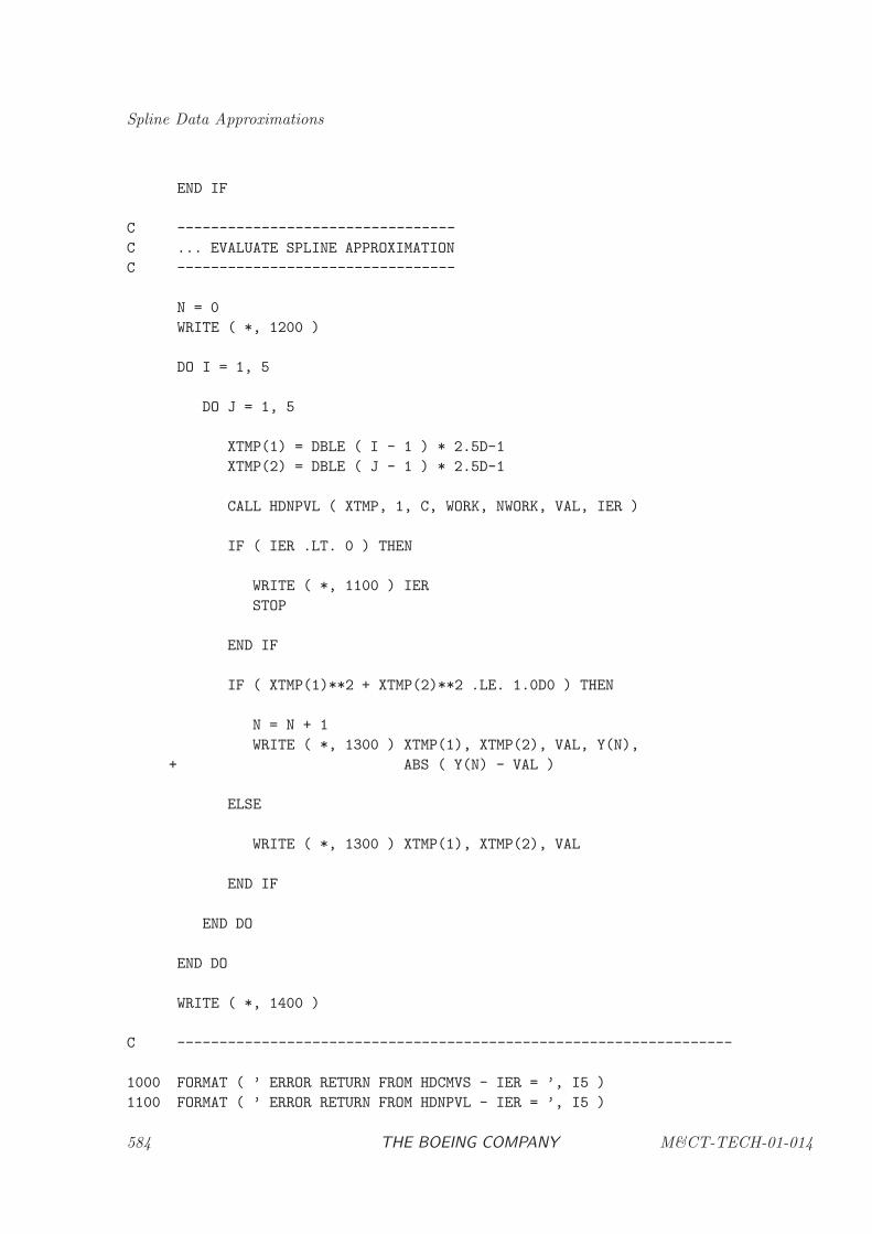
Spline Data Approximations
END IF
C ---------------------------------
C ... EVALUATE SPLINE APPROXIMATION
C ---------------------------------
N = 0
WRITE ( *, 1200 )
DO I = 1, 5
DO J = 1, 5
XTMP(1) = DBLE ( I - 1 ) * 2.5D-1
XTMP(2) = DBLE ( J - 1 ) * 2.5D-1
CALL HDNPVL ( XTMP, 1, C, WORK, NWORK, VAL, IER )
IF ( IER .LT. 0 ) THEN
WRITE ( *, 1100 ) IER
STOP
END IF
IF ( XTMP(1)**2 + XTMP(2)**2 .LE. 1.0D0 ) THEN
N = N + 1
WRITE ( *, 1300 ) XTMP(1), XTMP(2), VAL, Y(N),
+ ABS ( Y(N) - VAL )
ELSE
WRITE ( *, 1300 ) XTMP(1), XTMP(2), VAL
END IF
END DO
END DO
WRITE ( *, 1400 )
C ------------------------------------------------------------------
1000 FORMAT ( ’ ERROR RETURN FROM HDCMVS - IER = ’, I5 )
1100 FORMAT ( ’ ERROR RETURN FROM HDNPVL - IER = ’, I5 )
584 THE BOEING COMPANY M&CT-TECH-01-014
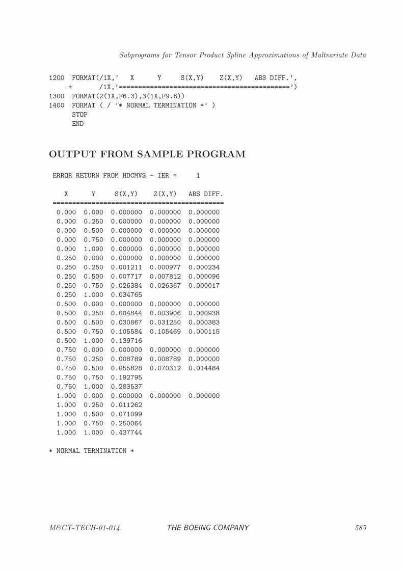
Subprograms for Tensor Product Spline Approximations of Multvariate Data
1200 FORMAT(/1X,’ X Y S(X,Y) Z(X,Y) ABS DIFF.’,
+ /1X,’============================================’)
1300 FORMAT(2(1X,F6.3),3(1X,F9.6))
1400 FORMAT ( / ’* NORMAL TERMINATION *’ )
STOP
END
OUTPUT FROM SAMPLE PROGRAM
ERROR RETURN FROM HDCMVS - IER = 1
X Y S(X,Y) Z(X,Y) ABS DIFF.
============================================
0.000 0.000 0.000000 0.000000 0.000000
0.000 0.250 0.000000 0.000000 0.000000
0.000 0.500 0.000000 0.000000 0.000000
0.000 0.750 0.000000 0.000000 0.000000
0.000 1.000 0.000000 0.000000 0.000000
0.250 0.000 0.000000 0.000000 0.000000
0.250 0.250 0.001211 0.000977 0.000234
0.250 0.500 0.007717 0.007812 0.000096
0.250 0.750 0.026384 0.026367 0.000017
0.250 1.000 0.034765
0.500 0.000 0.000000 0.000000 0.000000
0.500 0.250 0.004844 0.003906 0.000938
0.500 0.500 0.030867 0.031250 0.000383
0.500 0.750 0.105584 0.105469 0.000115
0.500 1.000 0.139716
0.750 0.000 0.000000 0.000000 0.000000
0.750 0.250 0.008789 0.008789 0.000000
0.750 0.500 0.055828 0.070312 0.014484
0.750 0.750 0.192795
0.750 1.000 0.283537
1.000 0.000 0.000000 0.000000 0.000000
1.000 0.250 0.011262
1.000 0.500 0.071099
1.000 0.750 0.250064
1.000 1.000 0.437744
* NORMAL TERMINATION *
M&CT-TECH-01-014 THE BOEING COMPANY 585
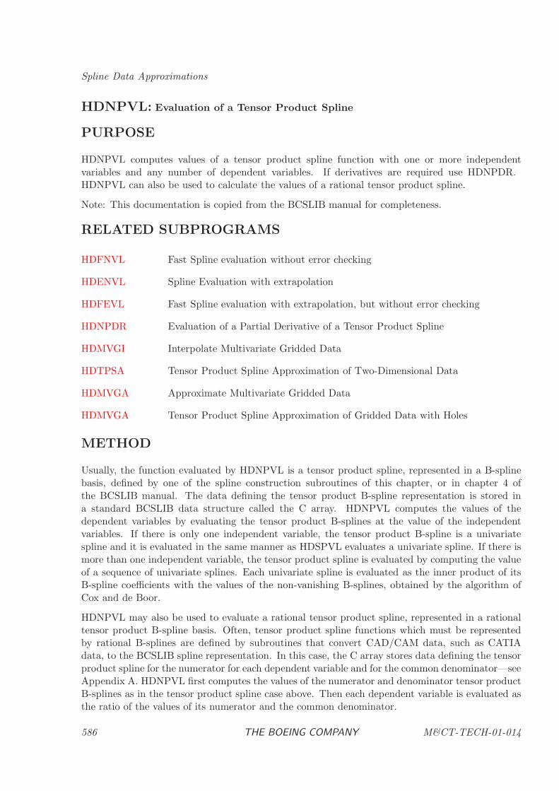
Spline Data Approximations
HDNPVL: Evaluation of a Tensor Product Spline
PURPOSE
HDNPVL computes values of a tensor product spline function with one or more independentvariables and any number of dependent variables. If derivatives are required use HDNPDR.HDNPVL can also be used to calculate the values of a rational tensor product spline.
Note: This documentation is copied from the BCSLIB manual for completeness.
RELATED SUBPROGRAMS
HDFNVL Fast Spline evaluation without error checking
HDENVL Spline Evaluation with extrapolation
HDFEVL Fast Spline evaluation with extrapolation, but without error checking
HDNPDR Evaluation of a Partial Derivative of a Tensor Product Spline
HDMVGI Interpolate Multivariate Gridded Data
HDTPSA Tensor Product Spline Approximation of Two-Dimensional Data
HDMVGA Approximate Multivariate Gridded Data
HDMVGA Tensor Product Spline Approximation of Gridded Data with Holes
METHOD
Usually, the function evaluated by HDNPVL is a tensor product spline, represented in a B-splinebasis, defined by one of the spline construction subroutines of this chapter, or in chapter 4 ofthe BCSLIB manual. The data defining the tensor product B-spline representation is stored ina standard BCSLIB data structure called the C array. HDNPVL computes the values of thedependent variables by evaluating the tensor product B-splines at the value of the independentvariables. If there is only one independent variable, the tensor product B-spline is a univariatespline and it is evaluated in the same manner as HDSPVL evaluates a univariate spline. If there ismore than one independent variable, the tensor product spline is evaluated by computing the valueof a sequence of univariate splines. Each univariate spline is evaluated as the inner product of itsB-spline coefficients with the values of the non-vanishing B-splines, obtained by the algorithm ofCox and de Boor.
HDNPVL may also be used to evaluate a rational tensor product spline, represented in a rationaltensor product B-spline basis. Often, tensor product spline functions which must be representedby rational B-splines are defined by subroutines that convert CAD/CAM data, such as CATIAdata, to the BCSLIB spline representation. In this case, the C array stores data defining the tensorproduct spline for the numerator for each dependent variable and for the common denominator—seeAppendix A. HDNPVL first computes the values of the numerator and denominator tensor productB-splines as in the tensor product spline case above. Then each dependent variable is evaluated asthe ratio of the values of its numerator and the common denominator.
586 THE BOEING COMPANY M&CT-TECH-01-014
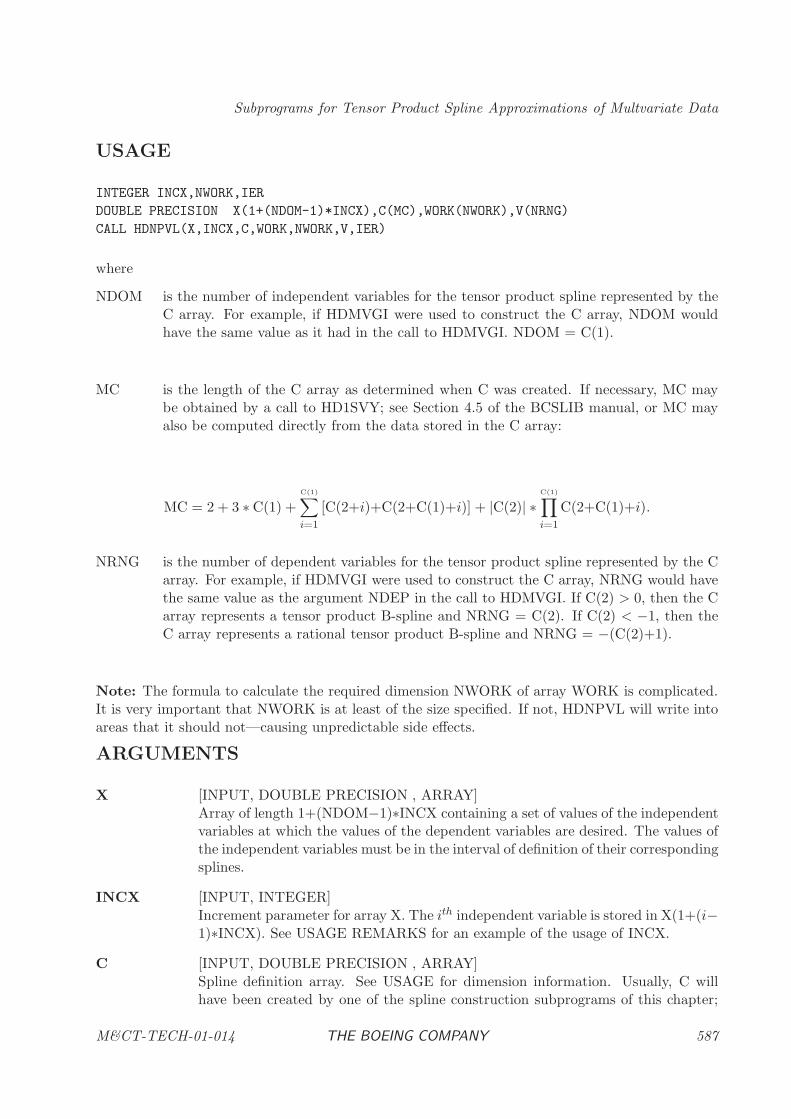
Subprograms for Tensor Product Spline Approximations of Multvariate Data
USAGE
INTEGER INCX,NWORK,IER
DOUBLE PRECISION X(1+(NDOM-1)*INCX),C(MC),WORK(NWORK),V(NRNG)
CALL HDNPVL(X,INCX,C,WORK,NWORK,V,IER)
where
NDOM is the number of independent variables for the tensor product spline represented by theC array. For example, if HDMVGI were used to construct the C array, NDOM wouldhave the same value as it had in the call to HDMVGI. NDOM = C(1).
MC is the length of the C array as determined when C was created. If necessary, MC maybe obtained by a call to HD1SVY; see Section 4.5 of the BCSLIB manual, or MC mayalso be computed directly from the data stored in the C array:
MC = 2 + 3 ∗ C(1) +C(1)∑
i=1
[C(2+i)+C(2+C(1)+i)] + |C(2)| ∗C(1)∏
i=1
C(2+C(1)+i).
NRNG is the number of dependent variables for the tensor product spline represented by the Carray. For example, if HDMVGI were used to construct the C array, NRNG would havethe same value as the argument NDEP in the call to HDMVGI. If C(2) > 0, then the Carray represents a tensor product B-spline and NRNG = C(2). If C(2) < −1, then theC array represents a rational tensor product B-spline and NRNG = −(C(2)+1).
Note: The formula to calculate the required dimension NWORK of array WORK is complicated.It is very important that NWORK is at least of the size specified. If not, HDNPVL will write intoareas that it should not—causing unpredictable side effects.
ARGUMENTS
X [INPUT, DOUBLE PRECISION , ARRAY]Array of length 1+(NDOM−1)∗INCX containing a set of values of the independentvariables at which the values of the dependent variables are desired. The values ofthe independent variables must be in the interval of definition of their correspondingsplines.
INCX [INPUT, INTEGER]Increment parameter for array X. The ith independent variable is stored in X(1+(i−1)∗INCX). See USAGE REMARKS for an example of the usage of INCX.
C [INPUT, DOUBLE PRECISION , ARRAY]Spline definition array. See USAGE for dimension information. Usually, C willhave been created by one of the spline construction subprograms of this chapter;
M&CT-TECH-01-014 THE BOEING COMPANY 587
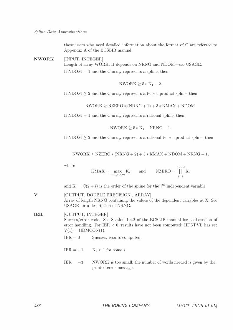
Spline Data Approximations
those users who need detailed information about the format of C are referred toAppendix A of the BCSLIB manual.
NWORK [INPUT, INTEGER]Length of array WORK. It depends on NRNG and NDOM—see USAGE.
If NDOM = 1 and the C array represents a spline, then
NWORK ≥ 5 ∗ K1 − 2.
If NDOM ≥ 2 and the C array represents a tensor product spline, then
NWORK ≥ NZERO ∗ (NRNG + 1) + 3 ∗ KMAX + NDOM.
If NDOM = 1 and the C array represents a rational spline, then
NWORK ≥ 5 ∗ K1 + NRNG − 1.
If NDOM ≥ 2 and the C array represents a rational tensor product spline, then
NWORK ≥ NZERO ∗ (NRNG + 2) + 3 ∗ KMAX + NDOM + NRNG + 1,
where
KMAX = maxi=1,NDOM
Ki and NZERO =NDOM∏
i=2
Ki
and Ki = C(2 + i) is the order of the spline for the ith independent variable.
V [OUTPUT, DOUBLE PRECISION , ARRAY]Array of length NRNG containing the values of the dependent variables at X. SeeUSAGE for a description of NRNG.
IER [OUTPUT, INTEGER]Success/error code. See Section 1.4.2 of the BCSLIB manual for a discussion oferror handling. For IER < 0, results have not been computed; HDNPVL has setV(1) = HDMCON(1).
IER = 0 Success, results computed.
IER = −1 Ki < 1 for some i.
IER = −3 NWORK is too small; the number of words needed is given by theprinted error message.
588 THE BOEING COMPANY M&CT-TECH-01-014
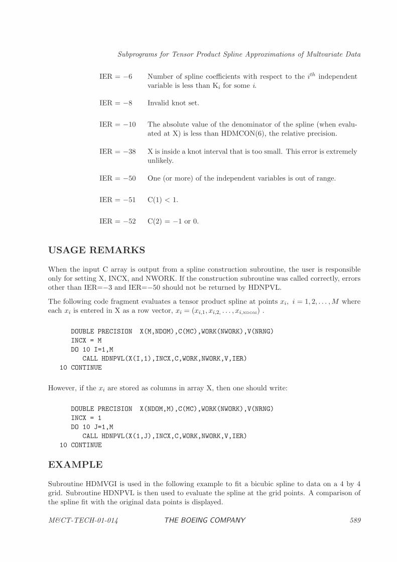
Subprograms for Tensor Product Spline Approximations of Multvariate Data
IER = −6 Number of spline coefficients with respect to the ith independentvariable is less than Ki for some i.
IER = −8 Invalid knot set.
IER = −10 The absolute value of the denominator of the spline (when evalu-ated at X) is less than HDMCON(6), the relative precision.
IER = −38 X is inside a knot interval that is too small. This error is extremelyunlikely.
IER = −50 One (or more) of the independent variables is out of range.
IER = −51 C(1) < 1.
IER = −52 C(2) = −1 or 0.
USAGE REMARKS
When the input C array is output from a spline construction subroutine, the user is responsibleonly for setting X, INCX, and NWORK. If the construction subroutine was called correctly, errorsother than IER=−3 and IER=−50 should not be returned by HDNPVL.
The following code fragment evaluates a tensor product spline at points xi, i = 1, 2, . . . ,M whereeach xi is entered in X as a row vector, xi = (xi,1, xi,2, . . . , xi,NDOM) .
DOUBLE PRECISION X(M,NDOM),C(MC),WORK(NWORK),V(NRNG)
INCX = M
DO 10 I=1,M
CALL HDNPVL(X(I,1),INCX,C,WORK,NWORK,V,IER)
10 CONTINUE
However, if the xi are stored as columns in array X, then one should write:
DOUBLE PRECISION X(NDOM,M),C(MC),WORK(NWORK),V(NRNG)
INCX = 1
DO 10 J=1,M
CALL HDNPVL(X(1,J),INCX,C,WORK,NWORK,V,IER)
10 CONTINUE
EXAMPLE
Subroutine HDMVGI is used in the following example to fit a bicubic spline to data on a 4 by 4grid. Subroutine HDNPVL is then used to evaluate the spline at the grid points. A comparison ofthe spline fit with the original data points is displayed.
M&CT-TECH-01-014 THE BOEING COMPANY 589
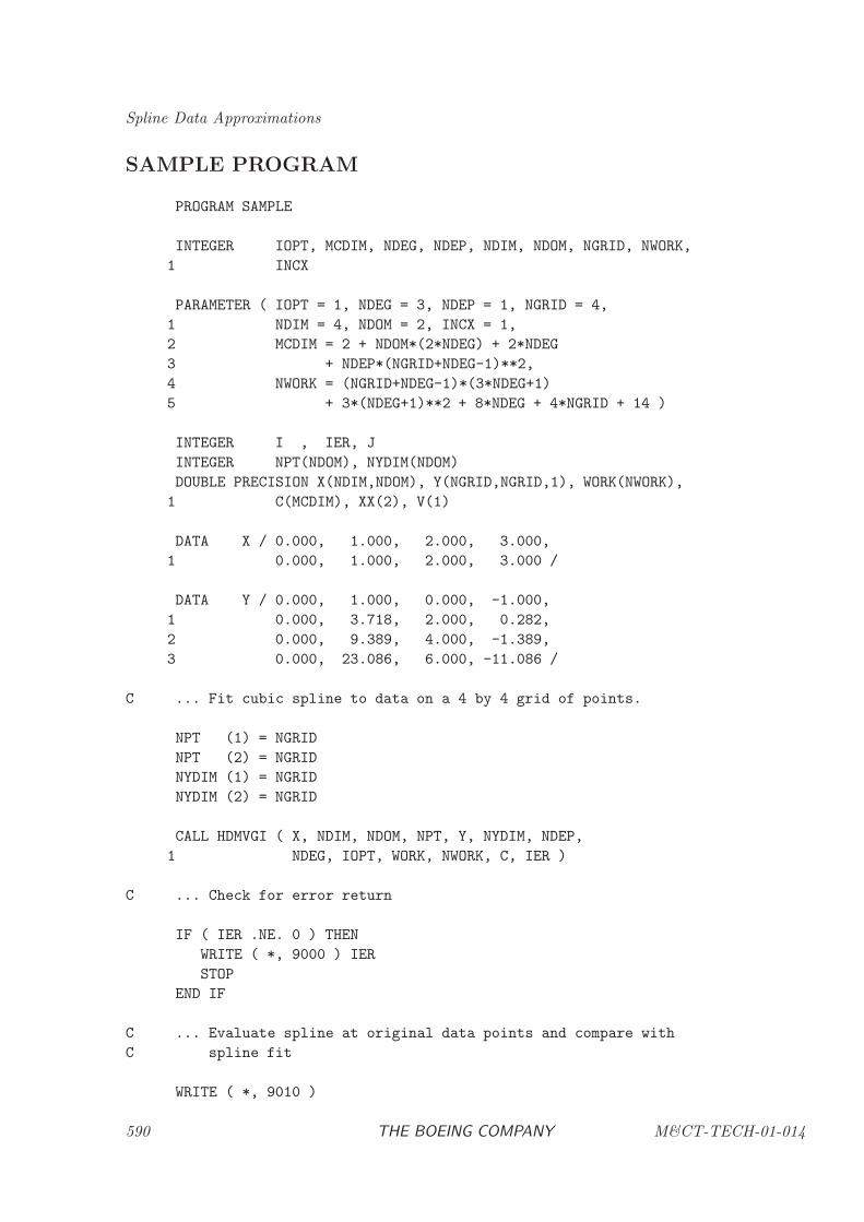
Spline Data Approximations
SAMPLE PROGRAM
PROGRAM SAMPLE
INTEGER IOPT, MCDIM, NDEG, NDEP, NDIM, NDOM, NGRID, NWORK,
1 INCX
PARAMETER ( IOPT = 1, NDEG = 3, NDEP = 1, NGRID = 4,
1 NDIM = 4, NDOM = 2, INCX = 1,
2 MCDIM = 2 + NDOM*(2*NDEG) + 2*NDEG
3 + NDEP*(NGRID+NDEG-1)**2,
4 NWORK = (NGRID+NDEG-1)*(3*NDEG+1)
5 + 3*(NDEG+1)**2 + 8*NDEG + 4*NGRID + 14 )
INTEGER I , IER, J
INTEGER NPT(NDOM), NYDIM(NDOM)
DOUBLE PRECISION X(NDIM,NDOM), Y(NGRID,NGRID,1), WORK(NWORK),
1 C(MCDIM), XX(2), V(1)
DATA X / 0.000, 1.000, 2.000, 3.000,
1 0.000, 1.000, 2.000, 3.000 /
DATA Y / 0.000, 1.000, 0.000, -1.000,
1 0.000, 3.718, 2.000, 0.282,
2 0.000, 9.389, 4.000, -1.389,
3 0.000, 23.086, 6.000, -11.086 /
C ... Fit cubic spline to data on a 4 by 4 grid of points.
NPT (1) = NGRID
NPT (2) = NGRID
NYDIM (1) = NGRID
NYDIM (2) = NGRID
CALL HDMVGI ( X, NDIM, NDOM, NPT, Y, NYDIM, NDEP,
1 NDEG, IOPT, WORK, NWORK, C, IER )
C ... Check for error return
IF ( IER .NE. 0 ) THEN
WRITE ( *, 9000 ) IER
STOP
END IF
C ... Evaluate spline at original data points and compare with
C spline fit
WRITE ( *, 9010 )
590 THE BOEING COMPANY M&CT-TECH-01-014
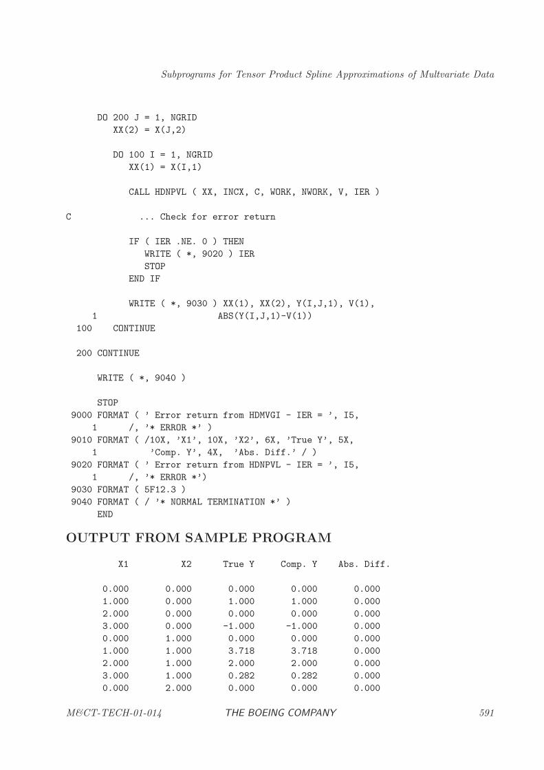
Subprograms for Tensor Product Spline Approximations of Multvariate Data
DO 200 J = 1, NGRID
XX(2) = X(J,2)
DO 100 I = 1, NGRID
XX(1) = X(I,1)
CALL HDNPVL ( XX, INCX, C, WORK, NWORK, V, IER )
C ... Check for error return
IF ( IER .NE. 0 ) THEN
WRITE ( *, 9020 ) IER
STOP
END IF
WRITE ( *, 9030 ) XX(1), XX(2), Y(I,J,1), V(1),
1 ABS(Y(I,J,1)-V(1))
100 CONTINUE
200 CONTINUE
WRITE ( *, 9040 )
STOP
9000 FORMAT ( ’ Error return from HDMVGI - IER = ’, I5,
1 /, ’* ERROR *’ )
9010 FORMAT ( /10X, ’X1’, 10X, ’X2’, 6X, ’True Y’, 5X,
1 ’Comp. Y’, 4X, ’Abs. Diff.’ / )
9020 FORMAT ( ’ Error return from HDNPVL - IER = ’, I5,
1 /, ’* ERROR *’)
9030 FORMAT ( 5F12.3 )
9040 FORMAT ( / ’* NORMAL TERMINATION *’ )
END
OUTPUT FROM SAMPLE PROGRAM
X1 X2 True Y Comp. Y Abs. Diff.
0.000 0.000 0.000 0.000 0.000
1.000 0.000 1.000 1.000 0.000
2.000 0.000 0.000 0.000 0.000
3.000 0.000 -1.000 -1.000 0.000
0.000 1.000 0.000 0.000 0.000
1.000 1.000 3.718 3.718 0.000
2.000 1.000 2.000 2.000 0.000
3.000 1.000 0.282 0.282 0.000
0.000 2.000 0.000 0.000 0.000
M&CT-TECH-01-014 THE BOEING COMPANY 591

Spline Data Approximations
1.000 2.000 9.389 9.389 0.000
2.000 2.000 4.000 4.000 0.000
3.000 2.000 -1.389 -1.389 0.000
0.000 3.000 0.000 0.000 0.000
1.000 3.000 23.086 23.086 0.000
2.000 3.000 6.000 6.000 0.000
3.000 3.000 -11.086 -11.086 0.000
* NORMAL TERMINATION *
592 THE BOEING COMPANY M&CT-TECH-01-014
Subprograms for Tensor Product Spline Approximations of Multvariate Data
HDENVL: Spline Evaluation with Extrapolation
PURPOSE
HDENVL computes values of a tensor product spline function with one or more independentvariables and any number of dependent variables. This routine also uses linear extrapolation if theuser tries to evaluate the tensor product spline outside of the range of the independent variables.HDENVL can also be used to calculate the values of a rational tensor product spline.
RELATED SUBPROGRAMS
HDNPVL Evaluation of a Tensor Product Spline
HDFNVL Fast Spline Evaluation without Error Checking
HDFEVL Fast Spline Evaluation with Extrapolation, but without Error Checking
HDNPDR Evaluation of a Partial Derivative of a Tensor Product Spline
HDMVGI Interpolate Multivariate Gridded Data
HDTPSA Tensor Product Spline Approximation of Two-Dimensional Data
HDMVGA Approximate Multivariate Gridded Data
HDMVGA Tensor Product Spline Approximation of Gridded Data with Holes
METHOD
This function is an extension of HDNPVL. If a point at which the tensor product spline needs tobe evaluated lies within the range of the spline, this routine directly calls HDNPVL. Otherwise, alinear extrapolation is used. This is done by finding the appropriate point on the boundary of therange of the spline, and calculating the value and first derivative of the spline at that point. Thisinformation is then used to calculate a linear extrapolation.
M&CT-TECH-01-014 THE BOEING COMPANY 593
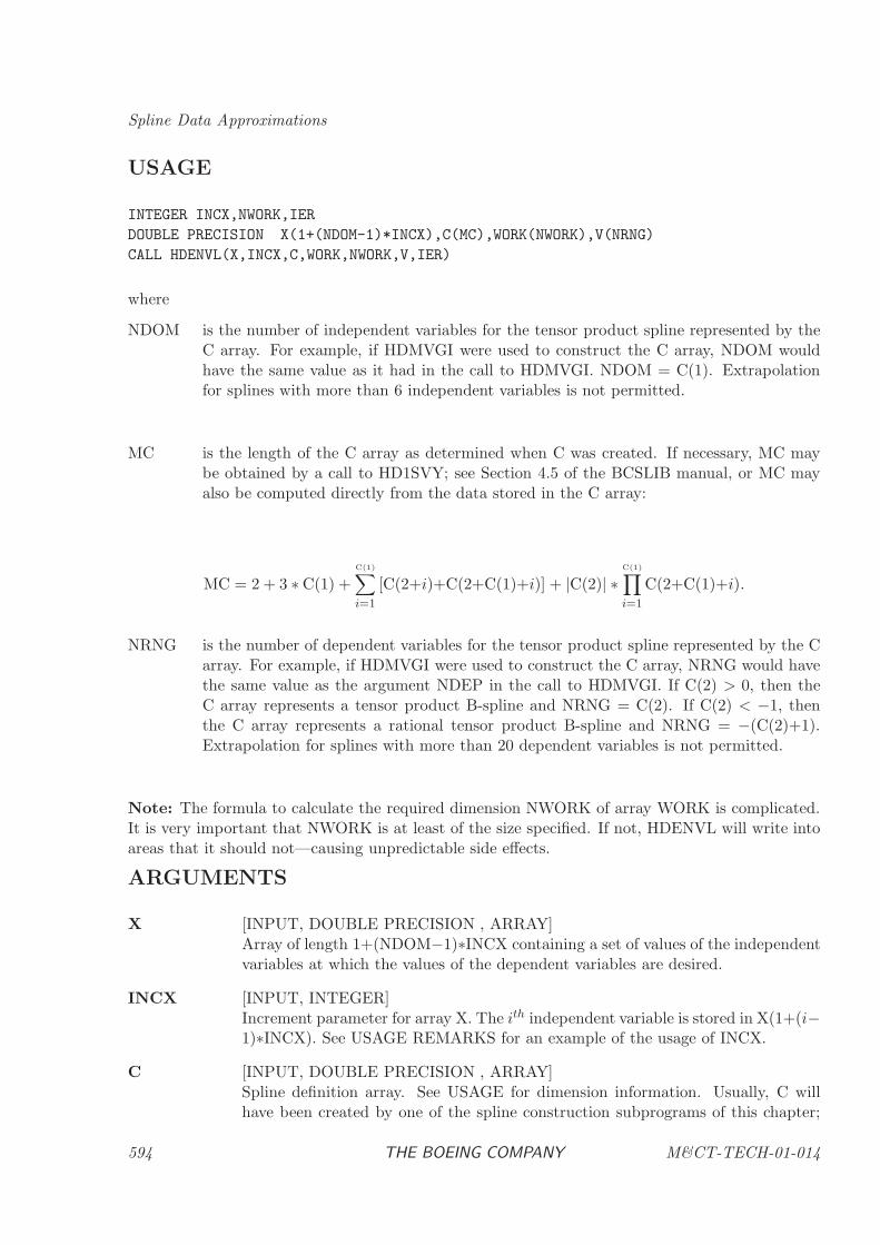
Spline Data Approximations
USAGE
INTEGER INCX,NWORK,IER
DOUBLE PRECISION X(1+(NDOM-1)*INCX),C(MC),WORK(NWORK),V(NRNG)
CALL HDENVL(X,INCX,C,WORK,NWORK,V,IER)
where
NDOM is the number of independent variables for the tensor product spline represented by theC array. For example, if HDMVGI were used to construct the C array, NDOM wouldhave the same value as it had in the call to HDMVGI. NDOM = C(1). Extrapolationfor splines with more than 6 independent variables is not permitted.
MC is the length of the C array as determined when C was created. If necessary, MC maybe obtained by a call to HD1SVY; see Section 4.5 of the BCSLIB manual, or MC mayalso be computed directly from the data stored in the C array:
MC = 2 + 3 ∗ C(1) +C(1)∑
i=1
[C(2+i)+C(2+C(1)+i)] + |C(2)| ∗C(1)∏
i=1
C(2+C(1)+i).
NRNG is the number of dependent variables for the tensor product spline represented by the Carray. For example, if HDMVGI were used to construct the C array, NRNG would havethe same value as the argument NDEP in the call to HDMVGI. If C(2) > 0, then theC array represents a tensor product B-spline and NRNG = C(2). If C(2) < −1, thenthe C array represents a rational tensor product B-spline and NRNG = −(C(2)+1).Extrapolation for splines with more than 20 dependent variables is not permitted.
Note: The formula to calculate the required dimension NWORK of array WORK is complicated.It is very important that NWORK is at least of the size specified. If not, HDENVL will write intoareas that it should not—causing unpredictable side effects.
ARGUMENTS
X [INPUT, DOUBLE PRECISION , ARRAY]Array of length 1+(NDOM−1)∗INCX containing a set of values of the independentvariables at which the values of the dependent variables are desired.
INCX [INPUT, INTEGER]Increment parameter for array X. The ith independent variable is stored in X(1+(i−1)∗INCX). See USAGE REMARKS for an example of the usage of INCX.
C [INPUT, DOUBLE PRECISION , ARRAY]Spline definition array. See USAGE for dimension information. Usually, C willhave been created by one of the spline construction subprograms of this chapter;
594 THE BOEING COMPANY M&CT-TECH-01-014
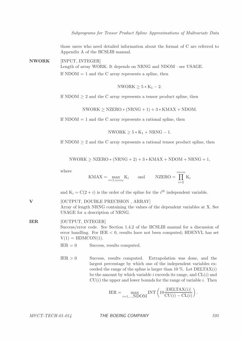
Subprograms for Tensor Product Spline Approximations of Multvariate Data
those users who need detailed information about the format of C are referred toAppendix A of the BCSLIB manual.
NWORK [INPUT, INTEGER]Length of array WORK. It depends on NRNG and NDOM—see USAGE.
If NDOM = 1 and the C array represents a spline, then
NWORK ≥ 5 ∗ K1 − 2.
If NDOM ≥ 2 and the C array represents a tensor product spline, then
NWORK ≥ NZERO ∗ (NRNG + 1) + 3 ∗ KMAX + NDOM.
If NDOM = 1 and the C array represents a rational spline, then
NWORK ≥ 5 ∗ K1 + NRNG − 1.
If NDOM ≥ 2 and the C array represents a rational tensor product spline, then
NWORK ≥ NZERO ∗ (NRNG + 2) + 3 ∗ KMAX + NDOM + NRNG + 1,
where
KMAX = maxi=1,NDOM
Ki and NZERO =NDOM∏
i=2
Ki
and Ki = C(2 + i) is the order of the spline for the ith independent variable.
V [OUTPUT, DOUBLE PRECISION , ARRAY]Array of length NRNG containing the values of the dependent variables at X. SeeUSAGE for a description of NRNG.
IER [OUTPUT, INTEGER]Success/error code. See Section 1.4.2 of the BCSLIB manual for a discussion oferror handling. For IER < 0, results have not been computed; HDENVL has setV(1) = HDMCON(1).
IER = 0 Success, results computed.
IER > 0 Success, results computed. Extrapolation was done, and thelargest percentage by which one of the independent variables ex-ceeded the range of the spline is larger than 10 %. Let DELTAX(i)be the amount by which variable i exceeds its range, and CL(i) andCU(i) the upper and lower bounds for the range of variable i. Then
IER = maxi=1,...,NDOM
INT
(10
|DELTAX(i)|CU(i) − CL(i)
).
M&CT-TECH-01-014 THE BOEING COMPANY 595

Spline Data Approximations
IER = −1 Ki < 1 for some i.
IER = −3 NWORK is too small; the number of words needed is given by theprinted error message.
IER = −6 Number of spline coefficients with respect to the ith independentvariable is less than Ki for some i.
IER = −8 Invalid knot set.
IER = −10 The absolute value of the denominator of the spline (when evalu-ated at X) is less than HDMCON(6), the relative precision.
IER = −38 X is inside a knot interval that is too small. This error is extremelyunlikely.
IER = −51 C(1) < 1.
IER = −52 C(2) = −1 or 0.
IER = −100 NDOM > 6. Extrapolation for splines with more than 6 indepen-dent variables is not permitted. Contact SOCS support if this erroroccurs.
IER = −101 NRNG > 20. Extrapolation for splines with more than 20 depen-dent variables is not permitted. Contact SOCS support if this erroroccurs.
IER = −200 An error occurred while trying to extrapolate. One reason mightbe insufficient workspace. Increase NWORK.
USAGE REMARKS
When the input C array is output from a spline construction subroutine, the user is responsibleonly for setting X, INCX, and NWORK. If the construction subroutine was called correctly, errorsother than IER=−3, IER=−100, IER=−101, or IER=−200 should not be returned by HDENVL.
The following code fragment evaluates a tensor product spline at points xi, i = 1, 2, . . . ,M whereeach xi is entered in X as a row vector, xi = (xi,1, xi,2, . . . , xi,NDOM) .
DOUBLE PRECISION X(M,NDOM),C(MC),WORK(NWORK),V(NRNG)
INCX = M
DO 10 I=1,M
CALL HDENVL(X(I,1),INCX,C,WORK,NWORK,V,IER)
10 CONTINUE
However, if the xi are stored as columns in array X, then one should write:
596 THE BOEING COMPANY M&CT-TECH-01-014

Subprograms for Tensor Product Spline Approximations of Multvariate Data
DOUBLE PRECISION X(NDOM,M),C(MC),WORK(NWORK),V(NRNG)
INCX = 1
DO 10 J=1,M
CALL HDENVL(X(1,J),INCX,C,WORK,NWORK,V,IER)
10 CONTINUE
EXAMPLE
Subroutine HDMVGI is used in the following example to fit a bicubic spline to data on a 4 by 4grid. Subroutine HDENVL is then used to evaluate the spline at the grid points. A comparison ofthe spline fit with the original data points is displayed. We also evaluate the spline at some pointsoutside of the range of the data to test the extrapolation.
SAMPLE PROGRAM
PROGRAM SAMPLE
INTEGER IOPT, MCDIM, NDEG, NDEP, NDIM, NDOM, NGRID, NWORK,
1 INCX
PARAMETER ( IOPT = 1, NDEG = 3, NDEP = 1, NGRID = 4,
1 NDIM = 4, NDOM = 2, INCX = 1,
2 MCDIM = 2 + NDOM*(2*NDEG) + 2*NDEG
3 + NDEP*(NGRID+NDEG-1)**2,
4 NWORK = (NGRID+NDEG-1)*(3*NDEG+1)
5 + 3*(NDEG+1)**2 + 8*NDEG + 4*NGRID + 14 )
INTEGER I , IER, J
INTEGER NPT(NDOM), NYDIM(NDOM)
DOUBLE PRECISION X(NDIM,NDOM), Y(NGRID,NGRID,1), WORK(NWORK),
1 C(MCDIM), XX(2), V(1)
DATA X / 0.000, 1.000, 2.000, 3.000,
1 0.000, 1.000, 2.000, 3.000 /
DATA Y / 0.000, 1.000, 0.000, -1.000,
1 0.000, 3.718, 2.000, 0.282,
2 0.000, 9.389, 4.000, -1.389,
3 0.000, 23.086, 6.000, -11.086 /
C ... Fit cubic spline to data on a 4 by 4 grid of points.
NPT (1) = NGRID
NPT (2) = NGRID
NYDIM (1) = NGRID
NYDIM (2) = NGRID
CALL HDMVGI ( X, NDIM, NDOM, NPT, Y, NYDIM, NDEP,
M&CT-TECH-01-014 THE BOEING COMPANY 597

Spline Data Approximations
1 NDEG, IOPT, WORK, NWORK, C, IER )
C ... Check for error return
IF ( IER .NE. 0 ) THEN
WRITE ( *, 9000 ) IER
STOP
END IF
C ... Evaluate spline at original data points and compare with
C spline fit
WRITE ( *, 9010 )
DO 200 J = 1, NGRID
XX(2) = X(J,2)
DO 100 I = 1, NGRID
XX(1) = X(I,1)
CALL HDENVL ( XX, INCX, C, WORK, NWORK, V, IER )
C ... Check for error return
IF ( IER .NE. 0 ) THEN
WRITE ( *, 9020 ) IER
STOP
END IF
WRITE ( *, 9030 ) XX(1), XX(2), Y(I,J,1), V(1),
1 ABS(Y(I,J,1)-V(1))
100 CONTINUE
200 CONTINUE
C ... Evaluate spline at data points outside of the region
C defined by the data points to check extrapolation...
WRITE ( *, 10010 )
DO 1200 J = NGRID, NGRID
XX(2) = X(J,2)+0.1D0*X(J,2)
DO 1100 I = 1, NGRID
XX(1) = X(I,1)
CALL HDENVL ( XX, INCX, C, WORK, NWORK, V, IER )
598 THE BOEING COMPANY M&CT-TECH-01-014

Subprograms for Tensor Product Spline Approximations of Multvariate Data
C ... Check for error return
IF ( IER .NE. 0 ) THEN
WRITE ( *, 9020 ) IER
STOP
END IF
WRITE ( *, 10030 ) XX(1), XX(2), V(1)
1100 CONTINUE
1200 CONTINUE
WRITE ( *, 9040 )
STOP
9000 FORMAT ( ’ Error return from HDMVGI - IER = ’, I5,
1 /, ’* ERROR *’ )
9010 FORMAT ( /10X, ’X1’, 10X, ’X2’, 6X, ’True Y’, 5X,
1 ’Comp. Y’, 4X, ’Abs. Diff.’ / )
9020 FORMAT ( ’ Error return from HDENVL - IER = ’, I5,
1 /, ’* ERROR *’)
9030 FORMAT ( 5F12.3 )
9040 FORMAT ( / ’* NORMAL TERMINATION *’ )
10010 FORMAT ( /10X, ’X1’, 10X, ’X2’, 6X, ’Comp. Y’ / )
10030 FORMAT ( 3F12.3 )
END
OUTPUT FROM SAMPLE PROGRAM
X1 X2 True Y Comp. Y Abs. Diff.
0.000 0.000 0.000 0.000 0.000
1.000 0.000 1.000 1.000 0.000
2.000 0.000 0.000 0.000 0.000
3.000 0.000 -1.000 -1.000 0.000
0.000 1.000 0.000 0.000 0.000
1.000 1.000 3.718 3.718 0.000
2.000 1.000 2.000 2.000 0.000
3.000 1.000 0.282 0.282 0.000
0.000 2.000 0.000 0.000 0.000
1.000 2.000 9.389 9.389 0.000
2.000 2.000 4.000 4.000 0.000
3.000 2.000 -1.389 -1.389 0.000
0.000 3.000 0.000 0.000 0.000
1.000 3.000 23.086 23.086 0.000
2.000 3.000 6.000 6.000 0.000
3.000 3.000 -11.086 -11.086 0.000
M&CT-TECH-01-014 THE BOEING COMPANY 599

Spline Data Approximations
X1 X2 Comp. Y
0.000 3.300 0.000
1.000 3.300 29.496
2.000 3.300 6.600
3.000 3.300 -16.296
* NORMAL TERMINATION *
600 THE BOEING COMPANY M&CT-TECH-01-014
Subprograms for Tensor Product Spline Approximations of Multvariate Data
HDFNVL: Fast Spline Evaluation without Error Checking
PURPOSE
HDFNVL computes values of a tensor product spline function with one or more independent vari-ables and any number of dependent variables. This method only performs limited error checking. Itshould only be used if a user is certain that the splines he passes are valid, and that the workspaceis large enough. The user is advised to use the corresponding routine HDNPVL during productdevelopment. HDNPVL is slower than HDFNVL, but performs error checking.
Furthermore, if the number of independent variables is larger then 3, this routine calls HDNPVLinternally. In this case the user is again advised to directly call HDNPVL. Note that both routineshave the same calling sequence. If derivatives are required use HDNPDR. HDFNVL can also beused to calculate the values of a rational tensor product spline—see Appendix A of the BCSLIBuser manual.
RELATED SUBPROGRAMS
HDNPVL Evaluation of a Tensor Product Spline
HDENVL Spline Evaluation with Extrapolation
HDFEVL Fast Spline Evaluation with Extrapolation, but without Error Checking
HDNPDR Evaluation of a Partial Derivative of a Tensor Product Spline
HDMVGI Interpolate Multivariate Gridded Data
HDTPSA Tensor Product Spline Approximation of Two-Dimensional Data
HDMVGA Approximate Multivariate Gridded Data
METHOD
HDFNVL is very similar to HDNPVL, except that it does not perform many error checks, andit uses a faster method if the number of independent variables is between one and three. If thenumber of independent variables is larger, this method calls HDNPVL. For more details on themethod see the documentation to HDNPVL.
USAGE
INTEGER INCX,NWORK,IER
DOUBLE PRECISION X(1+(NDOM-1)*INCX),C(MC),WORK(NWORK),V(NRNG)
CALL HDFNVL(X,INCX,C,WORK,NWORK,V,IER)
where
NDOM is the number of independent variables for the tensor product spline represented by theC array. For example, if HDMVGI were used to construct the C array, NDOM wouldhave the same value as it had in the call to HDMVGI. NDOM = C(1).
M&CT-TECH-01-014 THE BOEING COMPANY 601
Spline Data Approximations
MC is the length of the C array as determined when C was created. If necessary, MC maybe obtained by a call to HD1SVY; see Section 4.5 in the BCSLIB manual, or MC mayalso be computed directly from the data stored in the C array:
MC = 2 + 3 ∗ C(1) +C(1)∑
i=1
[C(2+i)+C(2+C(1)+i)] + |C(2)| ∗C(1)∏
i=1
C(2+C(1)+i).
NRNG is the number of dependent variables for the tensor product spline represented by the Carray. For example, if HDMVGI were used to construct the C array, NRNG would havethe same value as the argument NDEP in the call to HDMVGI. If C(2) > 0, then the Carray represents a tensor product B-spline and NRNG = C(2). If C(2) < −1, then theC array represents a rational tensor product B-spline and NRNG = −(C(2)+1).
Note: The formula to calculate the required dimension NWORK of array WORK is complicated.It is very important that NWORK is at least of the size specified. If not, HDFNVL will write intoareas that it should not—causing unpredictable side effects.
ARGUMENTS
X [INPUT, DOUBLE PRECISION , ARRAY]Array of length 1+(NDOM−1)∗INCX containing a set of values of the independentvariables at which the values of the dependent variables are desired. The values ofthe independent variables must be in the interval of definition of their correspondingsplines.
INCX [INPUT, INTEGER]Increment parameter for array X. The ith independent variable is stored in X(1+(i−1)∗INCX). See USAGE REMARKS for an example of the usage of INCX.
C [INPUT, DOUBLE PRECISION , ARRAY]Spline definition array. See USAGE for dimension information. See BCSLIB man-ual for a description of the contents of C. Usually, C will have been created byone of the spline construction subprograms like HDGDWH; those users who needdetailed information about the format of C are referred to Appendix A in theBCSLIB manual.
NWORK [INPUT, INTEGER]Length of array WORK. It depends on NRNG and NDOM—see USAGE.
If NDOM = 1 and the C array represents a spline, then
NWORK ≥ 5 ∗ K1 − 2.
If NDOM ≥ 2 and the C array represents a tensor product spline, then
NWORK ≥ NZERO ∗ (NRNG + 1) + 3 ∗ KMAX + NDOM.
602 THE BOEING COMPANY M&CT-TECH-01-014
Subprograms for Tensor Product Spline Approximations of Multvariate Data
If NDOM = 1 and the C array represents a rational spline, then
NWORK ≥ 5 ∗ K1 + NRNG − 1.
If NDOM ≥ 2 and the C array represents a rational tensor product spline, then
NWORK ≥ NZERO ∗ (NRNG + 2) + 3 ∗ KMAX + NDOM + NRNG + 1,
where
KMAX = maxi=1,NDOM
Ki and NZERO =NDOM∏
i=2
Ki
and Ki = C(2 + i) is the order of the spline for the ith independent variable.
V [OUTPUT, DOUBLE PRECISION , ARRAY]Array of length NRNG containing the values of the dependent variables at X. SeeUSAGE for a description of NRNG.
IER [OUTPUT, INTEGER]Success/error code. See Section 1.4.2 of the BCSLIB manual for a discussion oferror handling. For IER < 0, results have not been computed; HDFNVL has setV(1) = HDMCON(1). Note that no errors except IER = −50 will be detected bythis routine if the number of independent variables is less than 4. The user shouldonly use this method if he is sure that these errors cannot happen. Otherwise, heshould use HDNPVL instead.
IER = 0 Success, results computed.
IER = −1 Ki < 1 for some i.
IER = −3 NWORK is too small; the number of words needed is given by theprinted error message.
IER = −6 Number of spline coefficients with respect to the ith independentvariable is less than Ki for some i.
IER = −8 Invalid knot set.
IER = −10 The absolute value of the denominator of the spline (when evalu-ated at X) is less than HDMCON(6), the relative precision.
IER = −38 X is inside a knot interval that is too small. This error is extremelyunlikely.
IER = −50 One (or more) of the independent variables is out of range.
IER = −51 C(1) < 1.
M&CT-TECH-01-014 THE BOEING COMPANY 603
Spline Data Approximations
IER = −52 C(2) = −1 or 0.
USAGE REMARKS
When the input C array is output from a spline construction subroutine, the user is responsible onlyfor setting X, INCX, and NWORK. If the construction subroutine was called correctly, errors otherthan IER=−3 and IER=−50 should not be returned by HDFNVL. If the number of independentvariables is between 1 and 3, the error IER=−3 will not be detected, and unpredictable behaviorof the program could result. The user is responsible to ensure that enough workspace is available.
The following code fragment evaluates a tensor product spline at points xi, i = 1, 2, . . . ,M whereeach xi is entered in X as a row vector, xi = (xi,1, xi,2, . . . , xi,NDOM) .
DOUBLE PRECISION X(M,NDOM),C(MC),WORK(NWORK),V(NRNG)
INCX = M
DO 10 I=1,M
CALL HDFNVL(X(I,1),INCX,C,WORK,NWORK,V,IER)
10 CONTINUE
However, if the xi are stored as columns in array X, then one should write:
DOUBLE PRECISION X(NDOM,M),C(MC),WORK(NWORK),V(NRNG)
INCX = 1
DO 10 J=1,M
CALL HDFNVL(X(1,J),INCX,C,WORK,NWORK,V,IER)
10 CONTINUE
EXAMPLE
Subroutine HDMVGI is used in the following example to fit a bicubic spline to data on a 4 by 4grid. Subroutine HDFNVL is then used to evaluate the spline at the grid points. A comparison ofthe spline fit with the original data points is displayed.
SAMPLE PROGRAM
PROGRAM SAMPLE
INTEGER IOPT, MCDIM, NDEG, NDEP, NDIM, NDOM, NGRID, NWORK,
1 INCX
PARAMETER ( IOPT = 1, NDEG = 3, NDEP = 1, NGRID = 4,
1 NDIM = 4, NDOM = 2, INCX = 1,
2 MCDIM = 2 + NDOM*(2*NDEG) + 2*NDEG
3 + NDEP*(NGRID+NDEG-1)**2,
4 NWORK = (NGRID+NDEG-1)*(3*NDEG+1)
5 + 3*(NDEG+1)**2 + 8*NDEG + 4*NGRID + 14 )
604 THE BOEING COMPANY M&CT-TECH-01-014
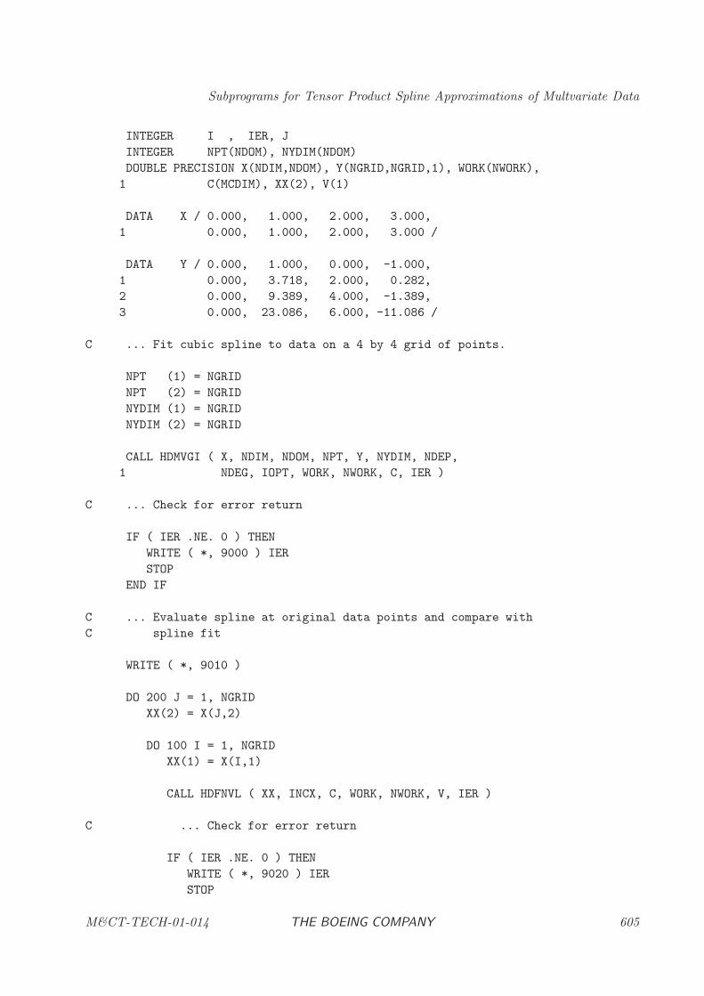
Subprograms for Tensor Product Spline Approximations of Multvariate Data
INTEGER I , IER, J
INTEGER NPT(NDOM), NYDIM(NDOM)
DOUBLE PRECISION X(NDIM,NDOM), Y(NGRID,NGRID,1), WORK(NWORK),
1 C(MCDIM), XX(2), V(1)
DATA X / 0.000, 1.000, 2.000, 3.000,
1 0.000, 1.000, 2.000, 3.000 /
DATA Y / 0.000, 1.000, 0.000, -1.000,
1 0.000, 3.718, 2.000, 0.282,
2 0.000, 9.389, 4.000, -1.389,
3 0.000, 23.086, 6.000, -11.086 /
C ... Fit cubic spline to data on a 4 by 4 grid of points.
NPT (1) = NGRID
NPT (2) = NGRID
NYDIM (1) = NGRID
NYDIM (2) = NGRID
CALL HDMVGI ( X, NDIM, NDOM, NPT, Y, NYDIM, NDEP,
1 NDEG, IOPT, WORK, NWORK, C, IER )
C ... Check for error return
IF ( IER .NE. 0 ) THEN
WRITE ( *, 9000 ) IER
STOP
END IF
C ... Evaluate spline at original data points and compare with
C spline fit
WRITE ( *, 9010 )
DO 200 J = 1, NGRID
XX(2) = X(J,2)
DO 100 I = 1, NGRID
XX(1) = X(I,1)
CALL HDFNVL ( XX, INCX, C, WORK, NWORK, V, IER )
C ... Check for error return
IF ( IER .NE. 0 ) THEN
WRITE ( *, 9020 ) IER
STOP
M&CT-TECH-01-014 THE BOEING COMPANY 605
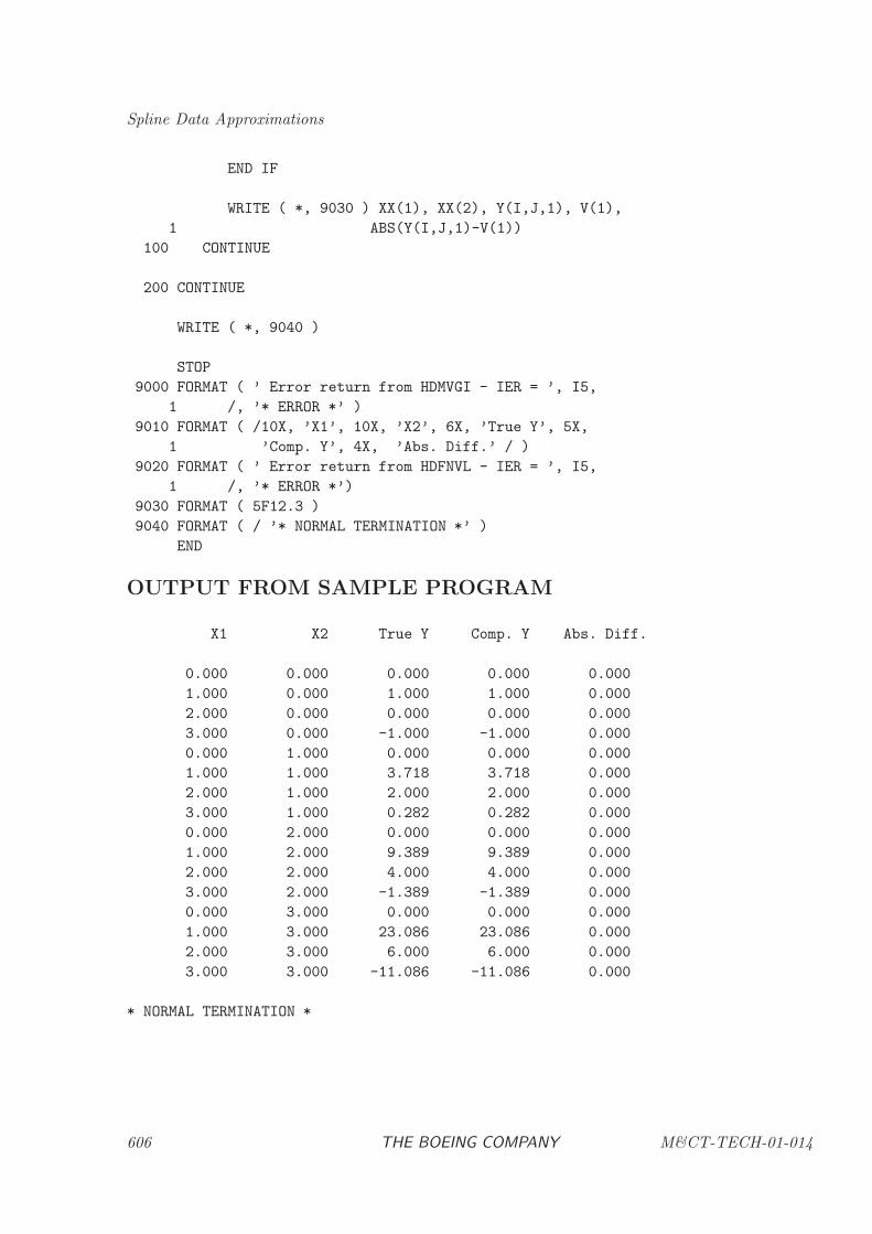
Spline Data Approximations
END IF
WRITE ( *, 9030 ) XX(1), XX(2), Y(I,J,1), V(1),
1 ABS(Y(I,J,1)-V(1))
100 CONTINUE
200 CONTINUE
WRITE ( *, 9040 )
STOP
9000 FORMAT ( ’ Error return from HDMVGI - IER = ’, I5,
1 /, ’* ERROR *’ )
9010 FORMAT ( /10X, ’X1’, 10X, ’X2’, 6X, ’True Y’, 5X,
1 ’Comp. Y’, 4X, ’Abs. Diff.’ / )
9020 FORMAT ( ’ Error return from HDFNVL - IER = ’, I5,
1 /, ’* ERROR *’)
9030 FORMAT ( 5F12.3 )
9040 FORMAT ( / ’* NORMAL TERMINATION *’ )
END
OUTPUT FROM SAMPLE PROGRAM
X1 X2 True Y Comp. Y Abs. Diff.
0.000 0.000 0.000 0.000 0.000
1.000 0.000 1.000 1.000 0.000
2.000 0.000 0.000 0.000 0.000
3.000 0.000 -1.000 -1.000 0.000
0.000 1.000 0.000 0.000 0.000
1.000 1.000 3.718 3.718 0.000
2.000 1.000 2.000 2.000 0.000
3.000 1.000 0.282 0.282 0.000
0.000 2.000 0.000 0.000 0.000
1.000 2.000 9.389 9.389 0.000
2.000 2.000 4.000 4.000 0.000
3.000 2.000 -1.389 -1.389 0.000
0.000 3.000 0.000 0.000 0.000
1.000 3.000 23.086 23.086 0.000
2.000 3.000 6.000 6.000 0.000
3.000 3.000 -11.086 -11.086 0.000
* NORMAL TERMINATION *
606 THE BOEING COMPANY M&CT-TECH-01-014
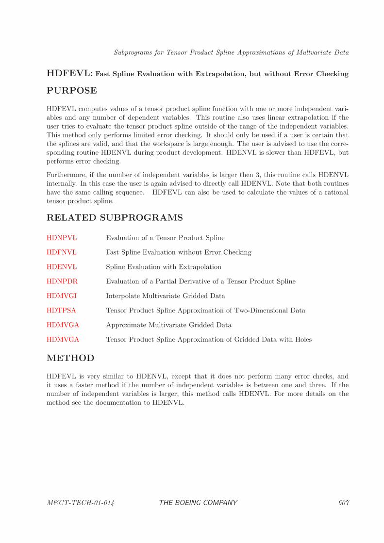
Subprograms for Tensor Product Spline Approximations of Multvariate Data
HDFEVL: Fast Spline Evaluation with Extrapolation, but without Error Checking
PURPOSE
HDFEVL computes values of a tensor product spline function with one or more independent vari-ables and any number of dependent variables. This routine also uses linear extrapolation if theuser tries to evaluate the tensor product spline outside of the range of the independent variables.This method only performs limited error checking. It should only be used if a user is certain thatthe splines are valid, and that the workspace is large enough. The user is advised to use the corre-sponding routine HDENVL during product development. HDENVL is slower than HDFEVL, butperforms error checking.
Furthermore, if the number of independent variables is larger then 3, this routine calls HDENVLinternally. In this case the user is again advised to directly call HDENVL. Note that both routineshave the same calling sequence. HDFEVL can also be used to calculate the values of a rationaltensor product spline.
RELATED SUBPROGRAMS
HDNPVL Evaluation of a Tensor Product Spline
HDFNVL Fast Spline Evaluation without Error Checking
HDENVL Spline Evaluation with Extrapolation
HDNPDR Evaluation of a Partial Derivative of a Tensor Product Spline
HDMVGI Interpolate Multivariate Gridded Data
HDTPSA Tensor Product Spline Approximation of Two-Dimensional Data
HDMVGA Approximate Multivariate Gridded Data
HDMVGA Tensor Product Spline Approximation of Gridded Data with Holes
METHOD
HDFEVL is very similar to HDENVL, except that it does not perform many error checks, andit uses a faster method if the number of independent variables is between one and three. If thenumber of independent variables is larger, this method calls HDENVL. For more details on themethod see the documentation to HDENVL.
M&CT-TECH-01-014 THE BOEING COMPANY 607
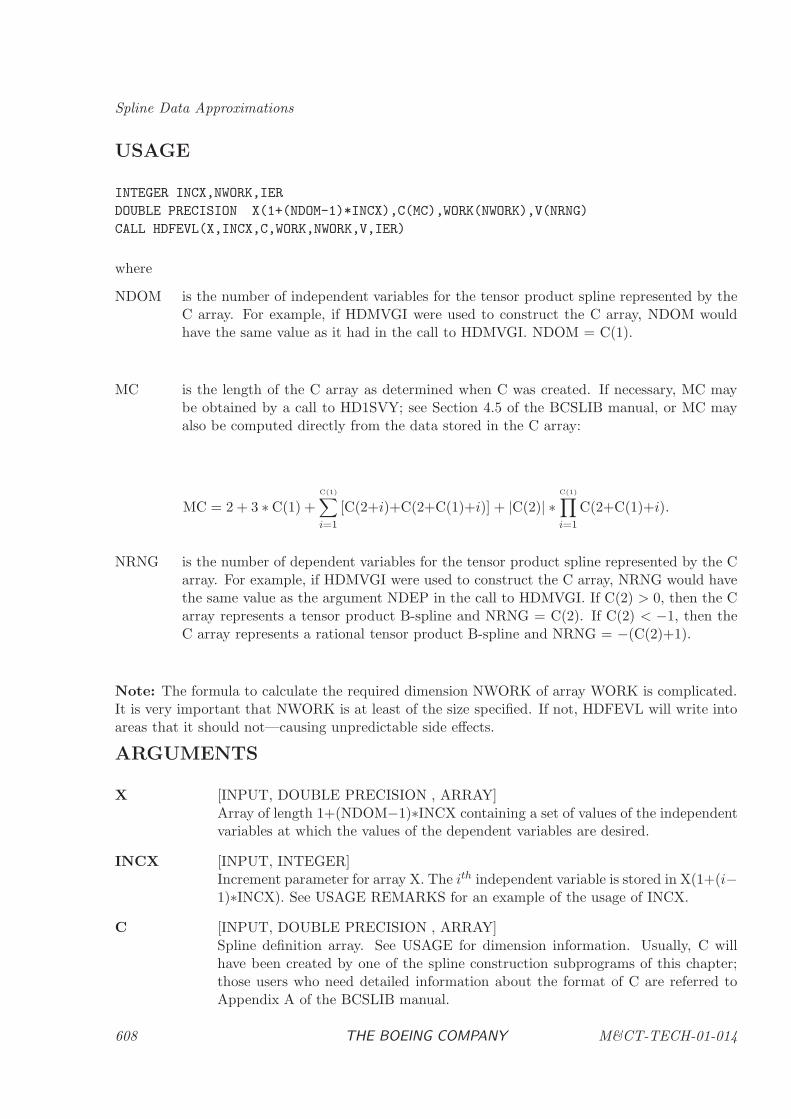
Spline Data Approximations
USAGE
INTEGER INCX,NWORK,IER
DOUBLE PRECISION X(1+(NDOM-1)*INCX),C(MC),WORK(NWORK),V(NRNG)
CALL HDFEVL(X,INCX,C,WORK,NWORK,V,IER)
where
NDOM is the number of independent variables for the tensor product spline represented by theC array. For example, if HDMVGI were used to construct the C array, NDOM wouldhave the same value as it had in the call to HDMVGI. NDOM = C(1).
MC is the length of the C array as determined when C was created. If necessary, MC maybe obtained by a call to HD1SVY; see Section 4.5 of the BCSLIB manual, or MC mayalso be computed directly from the data stored in the C array:
MC = 2 + 3 ∗ C(1) +C(1)∑
i=1
[C(2+i)+C(2+C(1)+i)] + |C(2)| ∗C(1)∏
i=1
C(2+C(1)+i).
NRNG is the number of dependent variables for the tensor product spline represented by the Carray. For example, if HDMVGI were used to construct the C array, NRNG would havethe same value as the argument NDEP in the call to HDMVGI. If C(2) > 0, then the Carray represents a tensor product B-spline and NRNG = C(2). If C(2) < −1, then theC array represents a rational tensor product B-spline and NRNG = −(C(2)+1).
Note: The formula to calculate the required dimension NWORK of array WORK is complicated.It is very important that NWORK is at least of the size specified. If not, HDFEVL will write intoareas that it should not—causing unpredictable side effects.
ARGUMENTS
X [INPUT, DOUBLE PRECISION , ARRAY]Array of length 1+(NDOM−1)∗INCX containing a set of values of the independentvariables at which the values of the dependent variables are desired.
INCX [INPUT, INTEGER]Increment parameter for array X. The ith independent variable is stored in X(1+(i−1)∗INCX). See USAGE REMARKS for an example of the usage of INCX.
C [INPUT, DOUBLE PRECISION , ARRAY]Spline definition array. See USAGE for dimension information. Usually, C willhave been created by one of the spline construction subprograms of this chapter;those users who need detailed information about the format of C are referred toAppendix A of the BCSLIB manual.
608 THE BOEING COMPANY M&CT-TECH-01-014
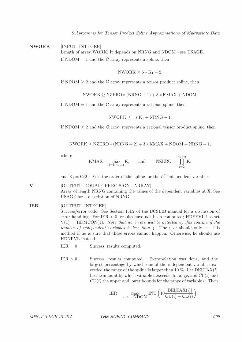
Subprograms for Tensor Product Spline Approximations of Multvariate Data
NWORK [INPUT, INTEGER]Length of array WORK. It depends on NRNG and NDOM—see USAGE.
If NDOM = 1 and the C array represents a spline, then
NWORK ≥ 5 ∗ K1 − 2.
If NDOM ≥ 2 and the C array represents a tensor product spline, then
NWORK ≥ NZERO ∗ (NRNG + 1) + 3 ∗ KMAX + NDOM.
If NDOM = 1 and the C array represents a rational spline, then
NWORK ≥ 5 ∗ K1 + NRNG − 1.
If NDOM ≥ 2 and the C array represents a rational tensor product spline, then
NWORK ≥ NZERO ∗ (NRNG + 2) + 3 ∗ KMAX + NDOM + NRNG + 1,
where
KMAX = maxi=1,NDOM
Ki and NZERO =NDOM∏
i=2
Ki
and Ki = C(2 + i) is the order of the spline for the ith independent variable.
V [OUTPUT, DOUBLE PRECISION , ARRAY]Array of length NRNG containing the values of the dependent variables at X. SeeUSAGE for a description of NRNG.
IER [OUTPUT, INTEGER]Success/error code. See Section 1.4.2 of the BCSLIB manual for a discussion oferror handling. For IER < 0, results have not been computed; HDFEVL has setV(1) = HDMCON(1). Note that no errors will be detected by this routine if thenumber of independent variables is less than 4. The user should only use thismethod if he is sure that these errors cannot happen. Otherwise, he should useHDNPVL instead.
IER = 0 Success, results computed.
IER > 0 Success, results computed. Extrapolation was done, and thelargest percentage by which one of the independent variables ex-ceeded the range of the spline is larger than 10 %. Let DELTAX(i)be the amount by which variable i exceeds its range, and CL(i) andCU(i) the upper and lower bounds for the range of variable i. Then
IER = maxi=1,...,NDOM
INT
(10
|DELTAX(i)|CU(i) − CL(i)
).
M&CT-TECH-01-014 THE BOEING COMPANY 609
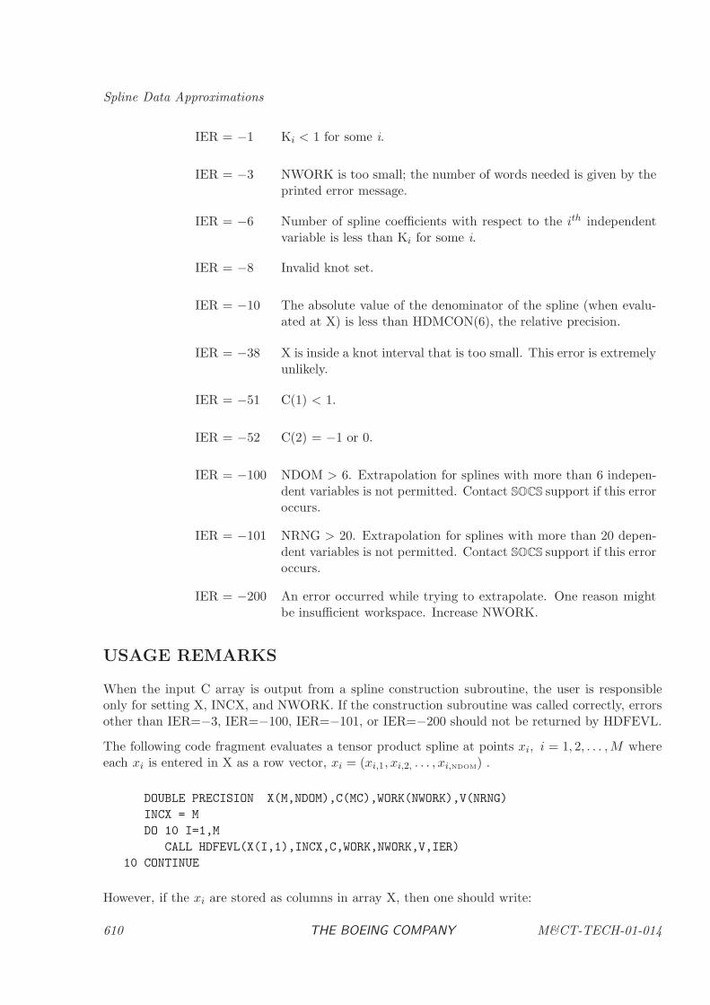
Spline Data Approximations
IER = −1 Ki < 1 for some i.
IER = −3 NWORK is too small; the number of words needed is given by theprinted error message.
IER = −6 Number of spline coefficients with respect to the ith independentvariable is less than Ki for some i.
IER = −8 Invalid knot set.
IER = −10 The absolute value of the denominator of the spline (when evalu-ated at X) is less than HDMCON(6), the relative precision.
IER = −38 X is inside a knot interval that is too small. This error is extremelyunlikely.
IER = −51 C(1) < 1.
IER = −52 C(2) = −1 or 0.
IER = −100 NDOM > 6. Extrapolation for splines with more than 6 indepen-dent variables is not permitted. Contact SOCS support if this erroroccurs.
IER = −101 NRNG > 20. Extrapolation for splines with more than 20 depen-dent variables is not permitted. Contact SOCS support if this erroroccurs.
IER = −200 An error occurred while trying to extrapolate. One reason mightbe insufficient workspace. Increase NWORK.
USAGE REMARKS
When the input C array is output from a spline construction subroutine, the user is responsibleonly for setting X, INCX, and NWORK. If the construction subroutine was called correctly, errorsother than IER=−3, IER=−100, IER=−101, or IER=−200 should not be returned by HDFEVL.
The following code fragment evaluates a tensor product spline at points xi, i = 1, 2, . . . ,M whereeach xi is entered in X as a row vector, xi = (xi,1, xi,2, . . . , xi,NDOM) .
DOUBLE PRECISION X(M,NDOM),C(MC),WORK(NWORK),V(NRNG)
INCX = M
DO 10 I=1,M
CALL HDFEVL(X(I,1),INCX,C,WORK,NWORK,V,IER)
10 CONTINUE
However, if the xi are stored as columns in array X, then one should write:
610 THE BOEING COMPANY M&CT-TECH-01-014
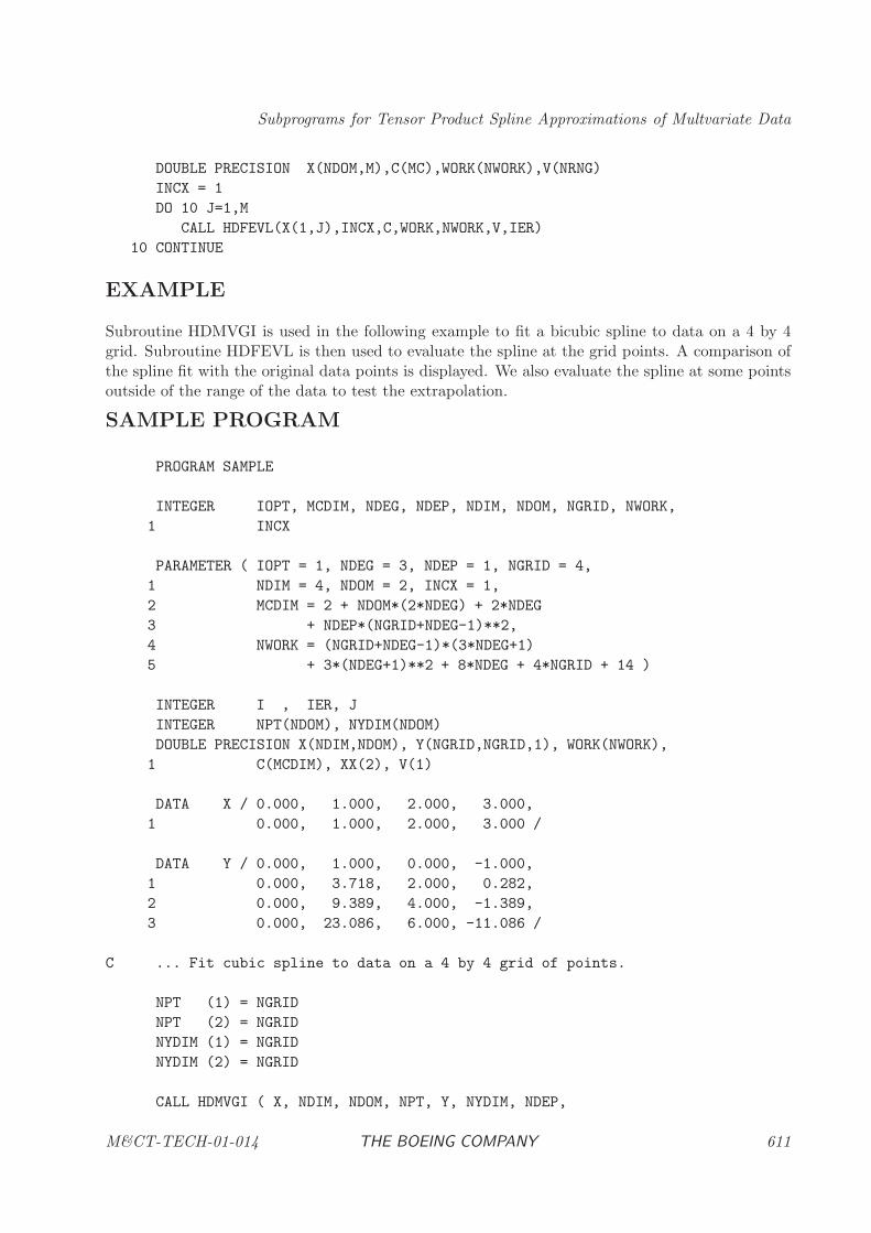
Subprograms for Tensor Product Spline Approximations of Multvariate Data
DOUBLE PRECISION X(NDOM,M),C(MC),WORK(NWORK),V(NRNG)
INCX = 1
DO 10 J=1,M
CALL HDFEVL(X(1,J),INCX,C,WORK,NWORK,V,IER)
10 CONTINUE
EXAMPLE
Subroutine HDMVGI is used in the following example to fit a bicubic spline to data on a 4 by 4grid. Subroutine HDFEVL is then used to evaluate the spline at the grid points. A comparison ofthe spline fit with the original data points is displayed. We also evaluate the spline at some pointsoutside of the range of the data to test the extrapolation.
SAMPLE PROGRAM
PROGRAM SAMPLE
INTEGER IOPT, MCDIM, NDEG, NDEP, NDIM, NDOM, NGRID, NWORK,
1 INCX
PARAMETER ( IOPT = 1, NDEG = 3, NDEP = 1, NGRID = 4,
1 NDIM = 4, NDOM = 2, INCX = 1,
2 MCDIM = 2 + NDOM*(2*NDEG) + 2*NDEG
3 + NDEP*(NGRID+NDEG-1)**2,
4 NWORK = (NGRID+NDEG-1)*(3*NDEG+1)
5 + 3*(NDEG+1)**2 + 8*NDEG + 4*NGRID + 14 )
INTEGER I , IER, J
INTEGER NPT(NDOM), NYDIM(NDOM)
DOUBLE PRECISION X(NDIM,NDOM), Y(NGRID,NGRID,1), WORK(NWORK),
1 C(MCDIM), XX(2), V(1)
DATA X / 0.000, 1.000, 2.000, 3.000,
1 0.000, 1.000, 2.000, 3.000 /
DATA Y / 0.000, 1.000, 0.000, -1.000,
1 0.000, 3.718, 2.000, 0.282,
2 0.000, 9.389, 4.000, -1.389,
3 0.000, 23.086, 6.000, -11.086 /
C ... Fit cubic spline to data on a 4 by 4 grid of points.
NPT (1) = NGRID
NPT (2) = NGRID
NYDIM (1) = NGRID
NYDIM (2) = NGRID
CALL HDMVGI ( X, NDIM, NDOM, NPT, Y, NYDIM, NDEP,
M&CT-TECH-01-014 THE BOEING COMPANY 611
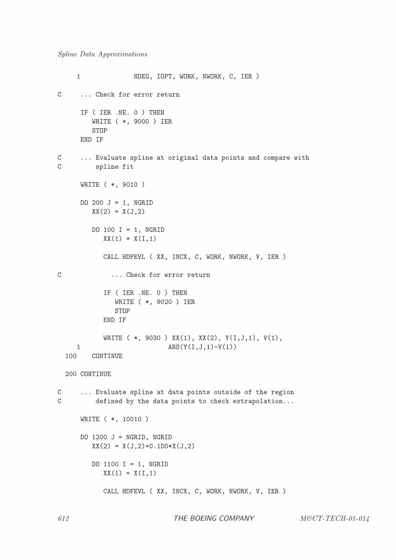
Spline Data Approximations
1 NDEG, IOPT, WORK, NWORK, C, IER )
C ... Check for error return
IF ( IER .NE. 0 ) THEN
WRITE ( *, 9000 ) IER
STOP
END IF
C ... Evaluate spline at original data points and compare with
C spline fit
WRITE ( *, 9010 )
DO 200 J = 1, NGRID
XX(2) = X(J,2)
DO 100 I = 1, NGRID
XX(1) = X(I,1)
CALL HDFEVL ( XX, INCX, C, WORK, NWORK, V, IER )
C ... Check for error return
IF ( IER .NE. 0 ) THEN
WRITE ( *, 9020 ) IER
STOP
END IF
WRITE ( *, 9030 ) XX(1), XX(2), Y(I,J,1), V(1),
1 ABS(Y(I,J,1)-V(1))
100 CONTINUE
200 CONTINUE
C ... Evaluate spline at data points outside of the region
C defined by the data points to check extrapolation...
WRITE ( *, 10010 )
DO 1200 J = NGRID, NGRID
XX(2) = X(J,2)+0.1D0*X(J,2)
DO 1100 I = 1, NGRID
XX(1) = X(I,1)
CALL HDFEVL ( XX, INCX, C, WORK, NWORK, V, IER )
612 THE BOEING COMPANY M&CT-TECH-01-014
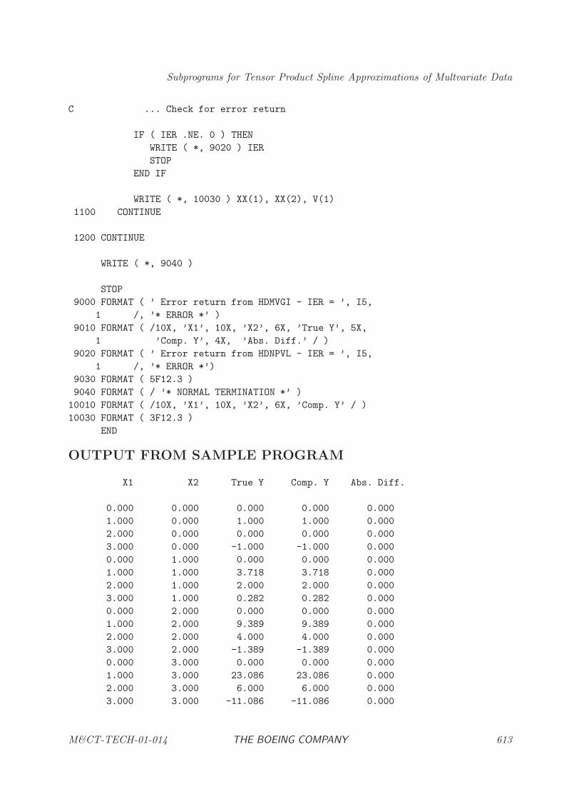
Subprograms for Tensor Product Spline Approximations of Multvariate Data
C ... Check for error return
IF ( IER .NE. 0 ) THEN
WRITE ( *, 9020 ) IER
STOP
END IF
WRITE ( *, 10030 ) XX(1), XX(2), V(1)
1100 CONTINUE
1200 CONTINUE
WRITE ( *, 9040 )
STOP
9000 FORMAT ( ’ Error return from HDMVGI - IER = ’, I5,
1 /, ’* ERROR *’ )
9010 FORMAT ( /10X, ’X1’, 10X, ’X2’, 6X, ’True Y’, 5X,
1 ’Comp. Y’, 4X, ’Abs. Diff.’ / )
9020 FORMAT ( ’ Error return from HDNPVL - IER = ’, I5,
1 /, ’* ERROR *’)
9030 FORMAT ( 5F12.3 )
9040 FORMAT ( / ’* NORMAL TERMINATION *’ )
10010 FORMAT ( /10X, ’X1’, 10X, ’X2’, 6X, ’Comp. Y’ / )
10030 FORMAT ( 3F12.3 )
END
OUTPUT FROM SAMPLE PROGRAM
X1 X2 True Y Comp. Y Abs. Diff.
0.000 0.000 0.000 0.000 0.000
1.000 0.000 1.000 1.000 0.000
2.000 0.000 0.000 0.000 0.000
3.000 0.000 -1.000 -1.000 0.000
0.000 1.000 0.000 0.000 0.000
1.000 1.000 3.718 3.718 0.000
2.000 1.000 2.000 2.000 0.000
3.000 1.000 0.282 0.282 0.000
0.000 2.000 0.000 0.000 0.000
1.000 2.000 9.389 9.389 0.000
2.000 2.000 4.000 4.000 0.000
3.000 2.000 -1.389 -1.389 0.000
0.000 3.000 0.000 0.000 0.000
1.000 3.000 23.086 23.086 0.000
2.000 3.000 6.000 6.000 0.000
3.000 3.000 -11.086 -11.086 0.000
M&CT-TECH-01-014 THE BOEING COMPANY 613

Spline Data Approximations
X1 X2 Comp. Y
0.000 3.300 0.000
1.000 3.300 29.496
2.000 3.300 6.600
3.000 3.300 -16.296
* NORMAL TERMINATION *
614 THE BOEING COMPANY M&CT-TECH-01-014
Chapter 9
Getting Started
The SOCS library provides considerable flexibility both in problem formulation and solution options.This flexibility is achieved by using subroutines which are supplied by the user to define the problemand solution characteristics. Although there is no obvious way to relieve the user of this burdenthere are some guidelines that are generally helpful.
Perhaps the most important first step is to carefully formulate the optimal control problem. Itis usually extremely helpful to write down the mathematical description of the problem, even ifsome of the details are omitted. Special attention should be given to identifying the variables andconstraints.
With a mathematical formulation in hand the next step is to implement the necessary software.The user must supply subroutines ODEINP and ODERHS and possibly may need the routinesODEPTF, ODEIGS, and ODEPRT. It is suggested that the subroutines be written in the followingorder:
1. ODERHS—right hand side of differential-algebraic equations
2. ODEINP—problem description, method, options, etc.
3. ODEPTF—nonlinear point functions, computed quantities, etc.
4. ODEIGS—special purpose initial guess
5. ODEPRT—special purpose output.
Usually by writing the subroutines to evaluate the differential and algebraic equations, the user isforced to identify the fundamental quantities (i.e. state and control variables). Once this informa-tion has been established constructing the problem description in the ODEINP routine is relativelystraightforward. Often a simplified version of the desired problem can be tested using the SOCS
dummy subroutines DUMYPF, DUMYIG, and DUMYPR in lieu of the other required software.
If possible modify a working example, e.g. (p. 538).
For applications with many phases write one phase at a time!
For applications with many constraints write one constraint at a time!
M&CT-TECH-01-014 THE BOEING COMPANY 615

Getting Started
DO NOT USE LINEAR INTERPOLATION OF TABULAR DATA. (p. 545)
Do not use embedded iterations when evaluating the point functions and/or differential equations.
Become familiar with the SOCS library by solving the workshop problems (p. 529).
616 THE BOEING COMPANY M&CT-TECH-01-014
Appendix A
Interface with the NPSOLOptimization Algorithm
The NPSOL optimization algorithm is a widely used software tool which is appropriate for solv-ing dense nonlinear programming problems. Similar functionality is provided by the subprogramHDNLPD described in Section 2.2. In order to clarify the comparison, this appendix describes howthe principal interface requirements for NPSOL are related to those for HDNLPD.
Both HDNLPD, and NPSOL require the user to supply the software which computes values of theconstraint and objective functions. There are two primary differences between the algorithms:
(1) HDNLPD requires the user to supply a single subroutine FUNBOX which evaluates the problemfunctions. NPSOL requires the user to supply two subroutines, namely CONFUN which evaluatesthe constraint functions, and OBJFUN which evaluates the objective function.
(2) HDNLPD requires the user to set a function error flag IFERR which indicates successful eval-uation of the problem functions. NPSOL does not provide this capability and consequently doesnot accommodate regions of incomputability in the problem functions.
For applications that do not have need for the function error flag the following code illustrates howthe HDNLPD subroutine FUNBOX is related to the NPSOL routines CONFUN and OBJFUN.
SUBROUTINE FUNBOX(XBAR,NDIM,MCON,QUANT,IFERR)
C
IMPLICIT DOUBLE PRECISION (A-H,O-Z)
C
DIMENSION XBAR(NDIM),QUANT(MCON+1)
C
IFERR = 0
C
MODE = 0
NSTATE = 0
CALL CONFUN(MODE,MCON,NDIM,MCON,NEEDC,XBAR,QUANT,
& DUMMY,NSTATE)
M&CT-TECH-01-014 THE BOEING COMPANY 617

Interface with the NPSOL Optimization Algorithm
C
CALL OBJFUN(MODE,NDIM,XBAR,QUANT(MCON+1),DUMMY,NSTATE)
C
RETURN
END
618 THE BOEING COMPANY M&CT-TECH-01-014
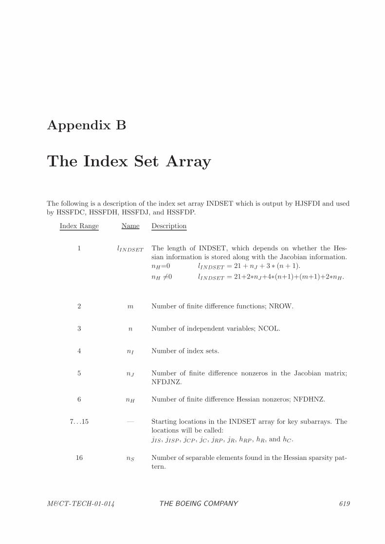
Appendix B
The Index Set Array
The following is a description of the index set array INDSET which is output by HJSFDI and usedby HSSFDC, HSSFDH, HSSFDJ, and HSSFDP.
Index Range Name Description
1 lINDSET The length of INDSET, which depends on whether the Hes-sian information is stored along with the Jacobian information.nH=0 lINDSET = 21 + nJ + 3 ∗ (n+ 1).
nH 6=0 lINDSET = 21+2∗nJ+4∗(n+1)+(m+1)+2∗nH.
2 m Number of finite difference functions; NROW.
3 n Number of independent variables; NCOL.
4 nI Number of index sets.
5 nJ Number of finite difference nonzeros in the Jacobian matrix;NFDJNZ.
6 nH Number of finite difference Hessian nonzeros; NFDHNZ.
7. . .15 — Starting locations in the INDSET array for key subarrays. Thelocations will be called:jIS , jISP , jCP , jC , jRP , jR, hRP , hR, and hC .
16 nS Number of separable elements found in the Hessian sparsity pat-tern.
M&CT-TECH-01-014 THE BOEING COMPANY 619

The Index Set Array
17 icom Set and used by HSSFDC, HSSFDJ, and HSSFDH for keepingtrack of initial vs. continue calls in the reverse communication.
18. . .20 — Future expansion.
jIS . . . jIS + n− 1 ~JIS The indices of the independent variables ordered by index set.
jISP . . . jISP + nI~JISP Pointers into the ~JIS subarray for the beginning of each index
set.
jCP . . . jCP + n ~JCP Pointers into the ~JC subarray locating the start of the indicescorresponding to each column of the Jacobian.
jC . . . jC + nJ − 1 ~JC The indices of the nonzero locations in the Jacobian matrix or-dered by column.
jRP . . . jRP +m ~JRP Pointers into the ~JR subarray locating the start of the indicescorresponding to each row of the Jacobian.
jR . . . jR + nJ − 1 ~JR The indices of the nonzero locations in the Jacobian matrix or-dered by row.
620 THE BOEING COMPANY M&CT-TECH-01-014

Index Range Name Description
hRP . . . hRP + n ~HRP Pointers into the ~HR subarray locating the start of the indicescorresponding to each row of the Hessian.
hR . . . hR + nH − 1 ~HR The indices of the nonzero locations in the Hessian matrix or-dered by row.
hC . . . hC + nH − 1 ~HC The column indices for the Hessian matrix.
lINDSET CS A check sum; must be equal to m+ n+ nJ for a valid INDSETarray.
M&CT-TECH-01-014 THE BOEING COMPANY 621

The Index Set Array
622 THE BOEING COMPANY M&CT-TECH-01-014
Appendix C
The MATLAB Toolbox
C.1 Introduction
This document describes toolboxes for the MATLAB environment that are based on the successfuloptimization library OPTLIB from The Boeing Company. Currently, the toolboxes provide inter-faces to the dense nonlinear optimization capabilities of OPTLIB, to the subprograms for tensorproduct spline approximations of multivariate data, and to several spline evaluation routines. Somemathematical background for these routines is given in this document, more detailed informationcan be found in the documentation of the FORTRAN routines [10].
Chapter C.2 describes briefly the dense nonlinear optimization routines. Chapter 8 discusses allspline related routines, beginning with routines to approximate multivariate data, continuing withroutines for the evaluation of these splines, and finishing with some utilities to export these splinesto FORTRAN.
Chapter C.6 concludes this document by describing some more detailed examples of the use of thespline functions.
C.2 Nonlinear optimization
M&CT-TECH-01-014 THE BOEING COMPANY 623
The MATLAB Toolbox
SOCS NLP: Local Optimization Method
PURPOSE
SOCS NLP is a MATLAB Toolbox for calling the dense nonlinear programming tool from theBoeing’s state-of-the-art SOCS package (http://www.boeing.com/phantom/socs/). Its main func-tion, SOCS NLP is a traditional forward communication code. A reverse communication code,callHDNLPR, is also available.
RELATED SUBPROGRAMS
SOCS NLP INIT Initialize the SOCS NLP parameters.
callHDNLPR Calls the OPTLIB dense reverse communication solvers, HDNLPRand HDBNPR.
callHDDFDJ Calls the OPTLIB finite difference derivative code HDDFDJ.
callHDDFDH Calls the OPTLIB finite difference derivative code HDDFDH.
METHOD
For a detailed description of the optimization methods used see the SOCS manual.
USAGE REMARKS
If SOCS NLP returns with a solution, this solution might only be a local solution. See the SOCSmanual for more details on this.
USAGE
[x, cval, fval, nFunEvals, errCode] = socs nlp(FUN, x0, opts)
[x, cval, fval, nFunEvals, errCode] = socs nlp(FUN, x0, opts, p1, p2, ...)
The first input argument FUN is the name or handle to the functions file, which contains the codefor evaluating the objective and constraints (and optionally, their derivatives) at a given point. Adetailed description of this function is given separately below. The argument opts is a structurecontaining optimization and problem parameters, which must be initialized prior to the call tosocs nlp. The function SOCS NLP INIT can be used to do this.
The arguments, p1, p2, ..., are optional parameters that are passed into the function to be opti-mized, in the case where additional parameters are required to evaluate the function. For equalityconstraints, set the upper and lower bounds to the same value.
ARGUMENTS
x [OUTPUT, DOUBLE, ARRAY]Final solution vector.
624 THE BOEING COMPANY M&CT-TECH-01-014
Nonlinear optimization
cval [OUTPUT, DOUBLE, ARRAY]Vector of constraint function values at the solution.
fval [OUTPUT, DOUBLE]Objective function value at the solution.
nFunEvals [OUTPUT, INTEGER]Number of function evaluations required to obtain the final solution.
errCode [OUTPUT, INTEGER]Error code returned from OPTLIB (0 = no error). See OPTLIB manual for fulldescription of the error code.
FUN [INPUT, STRING]name or handle to the file containing the objective and constraint functions.
x0 [INPUT, DOUBLE, ARRAY]Initial guess at the solution.
opts [INPUT, STRUCT]Structure with optional inputs to SOCS NLP. Options contained in this structureare described in detail under SOCS NLP INIT.
p1, p2, . . . [INPUT, ANY]Additional arguments for FUN, which can be of any type. These are generally pa-rameters that must be included in the evaluation of objective/constraint equations,but they are not optimized. See section on funbox for further details.
EXAMPLE 1
This example solves the optimization problem
min(x1 − 1)2 + (x1 − x2)2 + (x2 − x3)
4 (C.1)
subject tox1(1 + x2
2) + x43 − 4 − 3
√2 = 0. (C.2)
SAMPLE PROGRAM DRIVER
%SOCS_NLP_EXAMPLE is a sample driver to use SOCS_NLP.
%
% min (x(1)-1)^2 + (x(1)-x(2))^2 + (x(2)-x(3))^4
% s.t. x(1)*(1+x(2)^2) + x(3)^4 - 4 - 3*sqrt(2) = 0
%
% Select test problem, initial point, and variable/constraint bounds
f = @funbox;
x0 = [2; 5; -3];
Options.clwr = 0;
Options.cupr = 0;
M&CT-TECH-01-014 THE BOEING COMPANY 625
The MATLAB Toolbox
% Select algorithmic options
Options.optimizer = ’sqp’;
Options.HessUpdate = ’SR1’;
Options.OutputLevel = 0;
Options.Jacobian = ’off’;
Options.Hessian = ’off’;
Options.MaxFunEvals = 10000;
Options.MaxIter = 100;
Options.MaxIterLS = 20;
% Initialize and call optimizer
opts = socs_nlp_init(length(x0),length(Options.cupr),Options);
[x,cval,fval,nFunEvals,errCode] = socs_nlp(f,x0,opts)
SAMPLE PROGRAM
%===============================================================================
% funbox: Sample functions file used for testing of SOCS_NLP solver.
% ------------------------------------------------------------------------------
% VARIABLES:
% fx = objective function value at x
% cx = constraint function values at x
% dfx = gradient of objective function at x
% dcx = Jacobian of constraints at x
% x = point being evaluated
%===============================================================================
function [fx,cx,dfx,dcx] = funbox(x)
fx = (x(1) - 1)^2 + (x(1) - x(2))^2 + (x(2) - x(3))^4;
cx = x(1)*(1 + x(2)^2) + x(3)^4 - 4 - 3*sqrt(2);
dfx = [2*(x(1)-1)+2*(x(1) - x(2)); ...
-2*(x(1)-x(2))+4*(x(2)-x(3))^3;
-4*(x(2)-x(3))^3];
dcx = [1 + x(2)^2; 2*x(1)*x(2); 4*x(3)^3];
return
OUTPUT FROM SAMPLE PROGRAM
>> socs_nlp_example
x =
1.104859034205678
1.196674180655277
1.535262258200661
626 THE BOEING COMPANY M&CT-TECH-01-014

Nonlinear optimization
cval =
1.253397385880817e-010
fval =
0.032568200256415
nfeval =
281
iernlp =
0
M&CT-TECH-01-014 THE BOEING COMPANY 627
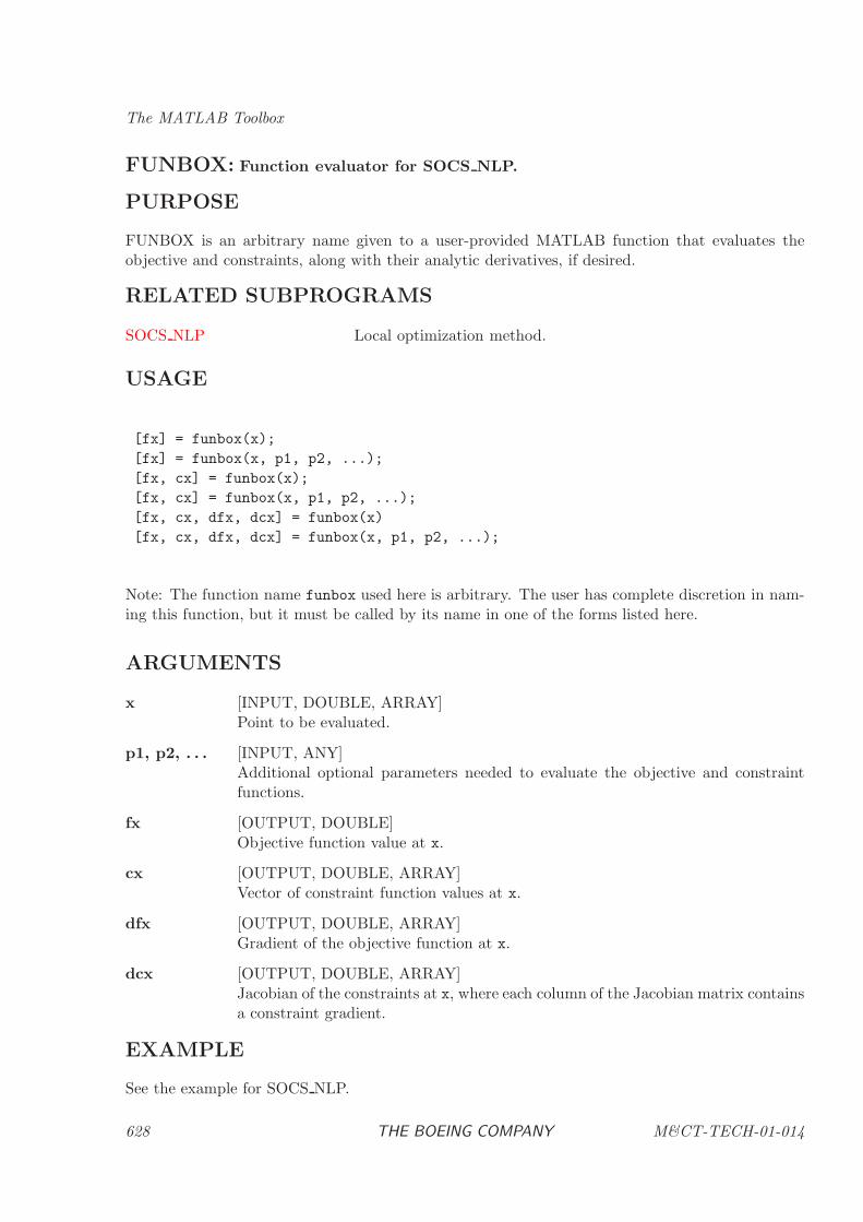
The MATLAB Toolbox
FUNBOX: Function evaluator for SOCS NLP.
PURPOSE
FUNBOX is an arbitrary name given to a user-provided MATLAB function that evaluates theobjective and constraints, along with their analytic derivatives, if desired.
RELATED SUBPROGRAMS
SOCS NLP Local optimization method.
USAGE
[fx] = funbox(x);
[fx] = funbox(x, p1, p2, ...);
[fx, cx] = funbox(x);
[fx, cx] = funbox(x, p1, p2, ...);
[fx, cx, dfx, dcx] = funbox(x)
[fx, cx, dfx, dcx] = funbox(x, p1, p2, ...);
Note: The function name funbox used here is arbitrary. The user has complete discretion in nam-ing this function, but it must be called by its name in one of the forms listed here.
ARGUMENTS
x [INPUT, DOUBLE, ARRAY]Point to be evaluated.
p1, p2, . . . [INPUT, ANY]Additional optional parameters needed to evaluate the objective and constraintfunctions.
fx [OUTPUT, DOUBLE]Objective function value at x.
cx [OUTPUT, DOUBLE, ARRAY]Vector of constraint function values at x.
dfx [OUTPUT, DOUBLE, ARRAY]Gradient of the objective function at x.
dcx [OUTPUT, DOUBLE, ARRAY]Jacobian of the constraints at x, where each column of the Jacobian matrix containsa constraint gradient.
EXAMPLE
See the example for SOCS NLP.
628 THE BOEING COMPANY M&CT-TECH-01-014
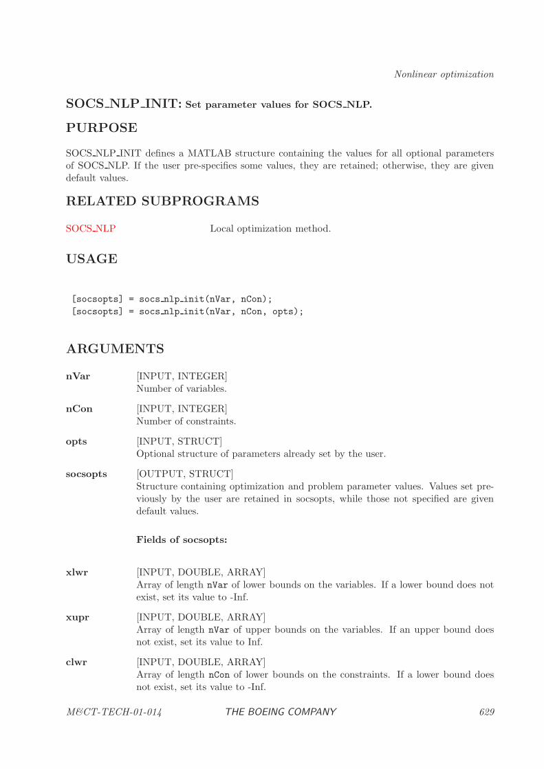
Nonlinear optimization
SOCS NLP INIT: Set parameter values for SOCS NLP.
PURPOSE
SOCS NLP INIT defines a MATLAB structure containing the values for all optional parametersof SOCS NLP. If the user pre-specifies some values, they are retained; otherwise, they are givendefault values.
RELATED SUBPROGRAMS
SOCS NLP Local optimization method.
USAGE
[socsopts] = socs nlp init(nVar, nCon);
[socsopts] = socs nlp init(nVar, nCon, opts);
ARGUMENTS
nVar [INPUT, INTEGER]Number of variables.
nCon [INPUT, INTEGER]Number of constraints.
opts [INPUT, STRUCT]Optional structure of parameters already set by the user.
socsopts [OUTPUT, STRUCT]Structure containing optimization and problem parameter values. Values set pre-viously by the user are retained in socsopts, while those not specified are givendefault values.
Fields of socsopts:
xlwr [INPUT, DOUBLE, ARRAY]Array of length nVar of lower bounds on the variables. If a lower bound does notexist, set its value to -Inf.
xupr [INPUT, DOUBLE, ARRAY]Array of length nVar of upper bounds on the variables. If an upper bound doesnot exist, set its value to Inf.
clwr [INPUT, DOUBLE, ARRAY]Array of length nCon of lower bounds on the constraints. If a lower bound doesnot exist, set its value to -Inf.
M&CT-TECH-01-014 THE BOEING COMPANY 629
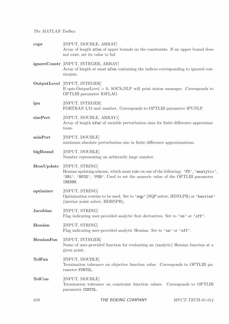
The MATLAB Toolbox
cupr [INPUT, DOUBLE, ARRAY]Array of length nCon of upper bounds on the constraints. If an upper bound doesnot exist, set its value to Inf.
ignoreConstr [INPUT, INTEGER, ARRAY]Array of length at most nCon containing the indices corresponding to ignored con-straints.
OutputLevel [INPUT, INTEGER]If opts.OutputLevel > 0, SOCS NLP will print status messages. Corresponds toOPTLIB parameter IOFLAG.
ipu [INPUT, INTEGER]FORTRAN I/O unit number. Corresponds to OPTLIB parameter IPUNLP.
sizePert [INPUT, DOUBLE, ARRAY)]Array of length nVar of variable perturbation sizes for finite difference approxima-tions.
minPert [INPUT, DOUBLE]minimum absolute perturbation size in finite difference approximations.
bigBound [INPUT, DOUBLE]Number representing an arbitrarily large number.
HessUpdate [INPUT, STRING]Hessian updating scheme, which must take on one of the following: ’FD’, ’analytic’,’SR1’, ’BFGS’, ’PSB’. Used to set the numeric value of the OPTLIB parameterIHESHN.
optimizer [INPUT, STRING]Optimization routine to be used. Set to ’sqp’ (SQP solver, HDNLPR) or ’barrier’(interior point solver, HDBNPR).
Jacobian [INPUT, STRING]Flag indicating user-provided analytic first derivatives. Set to ’on’ or ’off’.
Hessian [INPUT, STRING]Flag indicating user-provided analytic Hessian. Set to ’on’ or ’off’.
HessianFun [INPUT, INTEGER]Name of user-provided function for evaluating an (analytic) Hessian function at agiven point.
TolFun [INPUT, DOUBLE]Termination tolerance on objective function value. Corresponds to OPTLIB pa-rameter FUNTOL.
TolCon [INPUT, DOUBLE]Termination tolerance on constraint function values. Corresponds to OPTLIBparameter CONTOL.
630 THE BOEING COMPANY M&CT-TECH-01-014
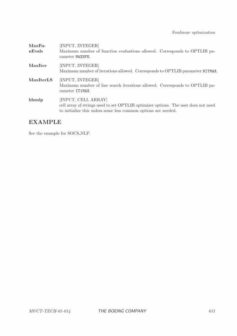
Nonlinear optimization
MaxFu-nEvals
[INPUT, INTEGER]Maximum number of function evaluations allowed. Corresponds to OPTLIB pa-rameter MAXNFE.
MaxIter [INPUT, INTEGER]Maximum number of iterations allowed. Corresponds to OPTLIB parameter NITMAX.
MaxIterLS [INPUT, INTEGER]Maximum number of line search iterations allowed. Corresponds to OPTLIB pa-rameter IT1MAX.
hhsnlp [INPUT, CELL ARRAY]cell array of strings used to set OPTLIB optimizer options. The user does not needto initialize this unless some less common options are needed.
EXAMPLE
See the example for SOCS NLP.
M&CT-TECH-01-014 THE BOEING COMPANY 631
The MATLAB Toolbox
callHDNLPR: Shell for calling HDNLPR or HDBNPR.
PURPOSE
callHDNLPR is a MATLAB shell for calling the dense, reverse communication OPTLIB solvers,HDNLPR and HDBNPR.
RELATED SUBPROGRAMS
SOCS NLP Local optimization method.
callHDDFDJ Shell for calling HDDFDJ
callHDDFDH Shell for calling HDDFDH
USAGE
[iCode, iReverse, x, Hold, errCode]
= callHDNLPR(iCode, x, xLower, xUpper, nX, fx, dfx, Hx, cx, ...
cLower, cUpper, nC, Jx, errFunc, nFunc, Hold, iUnit, optimizer)
[iCode, iReverse, x, Hold, errCode]
= callHDNLPR(iCode, x, xLower, xUpper, nX, fx, dfx, Hx, cx,
cLower, cUpper, nC, Jx, errFunc, nFunc, Hold, iUnit, ...
optimizer, s1, s2, ...)
In the argument list below, equivalent HDNLPR/HDBNPR arguments are given in Courier fonteither in the first line of the description or (in the case of a structure) in parentheses immediatelyafter its usage.
ARGUMENTS
iCode [INPUT/OUTPUT, INTEGER, IRVCOM ]Continuation control flag.
iReverse [OUTPUT, INTEGER, ARRAY, IREVRS ]An integer array of length 5, containing reverse communication control information.
errCode [OUTPUT, INTEGER, IER ]Success/error code.
x [INPUT/OUTPUT, DOUBLE, ARRAY, XBAR ]Array of length nX of current variable values.
xLower [INPUT, DOUBLE, ARRAY, XLWR ]Array of length nX of variable lower bounds.
632 THE BOEING COMPANY M&CT-TECH-01-014
Nonlinear optimization
xUpper [INPUT, DOUBLE, ARRAY, XUPR ]Array of length nX of variable upper bounds.
nX [INPUT, INTEGER, NDIM ]Number of variables.
fx [INPUT, DOUBLE, FBAR ]Objective function value at x.
dfx [INPUT, DOUBLE, ARRAY, DELF ]Array of length nX containing the gradient of the objective function value at x.
Hx [INPUT, DOUBLE, ARRAY, HMAT ]Array of size nX × nC containing the Hessian of the Lagrangian function at x.
cx [INPUT, DOUBLE, ARRAY, CBAR ]Array of length nC of constraint function values at x.
cLower [INPUT, DOUBLE, ARRAY, CLWR ]Array of length nC of constraint lower bounds.
cUpper [INPUT, DOUBLE, ARRAY, CUPR ]Array of length nC of constraint upper bounds.
nC [INPUT, INTEGER, MCON ]Number of constraints.
Jx [INPUT, DOUBLE, ARRAY, GMAT ]Array of size nX × nC containing the Jacobian of the constraints at x, each columnbeing a constraint gradient.
errFunc [INPUT, INTEGER, IFERR ]Function evaluation error flag.
nFunc [INPUT, INTEGER, NFEVAL ]Cumulative number of function evaluations.
Hold [INPUT/OUTPUT, STRUCT]A structure of intermediate data initialized by the user but not modified thereafter.Hold.Real (HOLD) is large array of length Hold.nReal (NHOLD) of intermediatedouble precision data. Hold.Int (IHOLD) is a large array of length Hold.nInt(NIHOLD) of intermediate integer data. Hold.needed (NEEDED) is an output inte-ger containing the required size for either Hold.nReal or Hold.nInt, depending onthe value of ErrCode. Hold.iStatusX (ISTATV) is an integer array of length nX
containing status of each variable relative to its bounds. Hold.iStatusC (ISTATC)is an integer array of length nC containing status of each constraint relative to itsbound. Hold.xMult (VECNU) is an array of length nX containing Lagrange multi-pliers for each variable’s bounds. Hold.cMult (VECLAM) is an array of length nC
containing Lagrange multipliers for each constraint.
iUnit [INPUT, INTEGER, IPU ]FORTRAN I/O unit number.
M&CT-TECH-01-014 THE BOEING COMPANY 633

The MATLAB Toolbox
optimizer [INPUT, STRING]String identifying which OPTLIB optimization routine is to be called. A value of“sqp” calls HDNLPR, and a value of “barrier” calls HDBNPR.
s1, s2, . . . [INPUT, STRINGS]Optional arguments are string codes passed into the OPTLIB subroutine HHSNLP,which sets various algorithmic options for the optimizer.
EXAMPLE
The SOCS NLP function is an example of the use of this code.
634 THE BOEING COMPANY M&CT-TECH-01-014
Nonlinear optimization
callHDDFDJ: Shell for calling HDDFDJ.
PURPOSE
callHDDFDJ is a MATLAB shell for the OPTLIB subroutine HDDFDJ, a reverse communicationcode for computing finite difference objective and constraint gradients.
RELATED SUBPROGRAMS
SOCS NLP Local optimization method.
callHDDFDH Shell for calling HDDFDH
USAGE
[iCode,Jx,x,fx,Options,Hold,errCode] = ...
callHDDFDJ(iCode,nRows,nColumns,Jx,x,fx,Options,Hold,nHold)
In the argument list below, equivalent HDDFDJ arguments are given in Courier font either in thefirst line of the description or (in the case of a structure) in parentheses immediately after its usage.
ARGUMENTS
iCode [INPUT/OUTPUT, INTEGER, IRVCOM ]Continuation control flag.
Jx [INPUT/OUTPUT, DOUBLE, ARRAY, CJAC ]Array of size n ×m containing the Jacobian of the constraints at x, each columnbeing a constraint gradient.
x [INPUT/OUTPUT, DOUBLE, ARRAY, XBAR ]Array of length n of current variable values.
fx [INPUT/OUTPUT, DOUBLE, FBAR ]Objective function value at x.
Options [INPUT/OUTPUT, STRUCT]A structure of user options. Options.sizePert (PRTSYZ) is a real array of lengthn containing each variable’s perturbation size used in the finite difference calcula-tions. Options.minPert (PRTMIN) is a positive double precision scalar containingthe minimum absolute perturbation size. Options.errFunc (IFERR) is an integercontaining the function evaluation error flag. Options.iStore (ISTOR) is an integerrepresenting the Jacobian storage scheme. Options.iDiag (MSGLVL) is an integerrepresenting the level of diagnostic output to be generated. Options.iUnit (IPU)is an integer representing the FORTRAN I/O unit number. Options.typeFD(IDTYPE) is an integer representing the type of finite difference approximation tobe used.
M&CT-TECH-01-014 THE BOEING COMPANY 635
The MATLAB Toolbox
Hold [INPUT/OUTPUT, DOUBLE, ARRAY, HOLD ]Array of intermediate double precision data that the user must initialize but notmodify thereafter.
nHold [INPUT, INTEGER, NHOLD ]Length of Hold.
errCode [OUTPUT, INTEGER, IER ]Success/error code.
nRows [INPUT, INTEGER, NROW ]Number of rows in the Jacobian matrix.
nColumns [INPUT, INTEGER, NCOL ]Number of columns in the Jacobian matrix.
EXAMPLE
The SOCS NLP function is an example of the use of this code.
636 THE BOEING COMPANY M&CT-TECH-01-014
Nonlinear optimization
callHDDFDH: Shell for calling HDDFDH.
PURPOSE
callHDDFDH is a MATLAB shell for the OPTLIB subroutine HDDFDH, a reverse communicationcode for computing a finite difference Jacobian of a set of real-valued functions and the Hessian ofa linear combination of the functions at a given point.
RELATED SUBPROGRAMS
SOCS NLP Local optimization method.
callHDDFDJ Shell for calling HDDFDJ
USAGE
[iCode,Jx,Hx,x,fx,Options,Hold,errCode] = ...
callHDDFDH(iCode,nRows,nColumns,Jx,Hx,x,fx,Options,Hold,nHold)
In the argument list below, equivalent HDDFDH arguments are given in Courier font either in thefirst line of the description or (in the case of a structure) in parentheses immediately after its usage.
ARGUMENTS
iCode [INPUT/OUTPUT, INTEGER, IRVCOM ]Continuation control flag.
Jx [INPUT/OUTPUT, DOUBLE, ARRAY, CJAC ]Array of size n ×m containing the Jacobian of the constraints at x, each columnbeing a constraint gradient.
Hx [INPUT/OUTPUT, DOUBLE, ARRAY, HMAT ]Array of size n× n containing the Hessian at x.
x [INPUT/OUTPUT, DOUBLE, ARRAY, XBAR ]Array of length n of current variable values.
fx [INPUT/OUTPUT, DOUBLE, FBAR ]Objective function value at x.
Options [INPUT/OUTPUT, STRUCT]A structure of user options. Options.sizePert (PRTSYZ) is a real array of lengthn containing each variable’s perturbation size used in the finite difference calcula-tions. Options.minPert (PRTMIN) is a positive double precision scalar containingthe minimum absolute perturbation size. Options.errFunc (IFERR) is an inte-ger containing the function evaluation error flag. Options.iStore (ISTOR) is aninteger representing the Jacobian storage scheme. Options.iDiag (MSGLVL) is an
M&CT-TECH-01-014 THE BOEING COMPANY 637
The MATLAB Toolbox
integer representing the level of diagnostic output to be generated. Options.iUnit(IPU) is an integer representing the FORTRAN I/O unit number. Options.cMult(CMULT) is a vector of length m of multipliers used in forming the Hessian function.
Hold [INPUT/OUTPUT, DOUBLE, ARRAY, HOLD ]Array of intermediate double precision data that the user must initialize but notmodify thereafter.
nHold [INPUT, INTEGER, NHOLD ]Length of Hold.
errCode [OUTPUT, INTEGER, IER ]Success/error code.
nRows [INPUT, INTEGER, NROW ]Number of rows in the Jacobian matrix.
nColumns [INPUT, INTEGER, NCOL ]Number of columns in the Jacobian matrix.
EXAMPLE
The SOCS NLP function is an example of the use of this code.
638 THE BOEING COMPANY M&CT-TECH-01-014
Spline Data Approximations
C.3 Spline Data Approximations
C.4 Overview of Data Fitting and Approximation
Many optimization, optimal control, and parameter estimation applications involve problems thatare specified in terms of tabular data. All optimization algorithms require that the objective andconstraints be sufficiently smooth to insure convergence and consequently it is recommended thattabular data be represented by functions with continuous first and second derivatives. For tabularfunctions of a single independent variable we consider
s(x) =n∑
k=1
ckBk(x)
where Bk(x) are referred to as B-spline basis functions. Tabular functions with more than oneindependent variable can be represented using a tensor product spline, e.g. in two dimensions
s(x, y) =m∑
j=1
n∑
k=1
cj,kBj(x)Bk(y).
When dealing with spline approximations, in general there are two distinct operations of interestto the user.
Construction of the spline coefficients {ck} or {cj,k} using the given tabular data, and;
Evaluation of the spline approximation at a specified value of the independent variable(s).
It is important to note that these operations are completely independent of each other. In fact it isusually preferable to construct the approximation (i.e. compute {cj,k}) just once. Many evaluationsof the spline models can then be performed very quickly. A complete description of data fittingand approximation using B-splines can be found in Chapter 4 of the BCSLIB Manual [2]. Thesubroutines described in this chapter focus on two particular aspects of interest for optimizationapplications. The first section describes software for the construction of smooth approximationsfrom tabular data. In particular, the coefficients {cj,k} are computed by solving a large sparseoptimization problem which is achieved using the software described in Chapter 2 of the SOCSmanual. The second section describes software for rapid evaluation of spline approximations, whichis particularly important for many optimal control applications.
M&CT-TECH-01-014 THE BOEING COMPANY 639
The MATLAB Toolbox
C.5 Subprograms for Tensor Product Spline Approximations of
Multivariate Data
BCSLIB GDWH: Tensor Product Spline Approximation of Gridded Data withHoles
PURPOSE
BCSLIB GDWH approximates multivariate data which lies on a grid but contains regions of missingdata. It computes a tensor product spline which has minimal variation of its second order partials,approximates the data within a user specified tolerance and, optionally, is locally monotonic alonggrid lines.
RELATED SUBPROGRAMS
BCSLIB GDWH INIT Initialize the optional argument opts to standard values.
BCSLIB NPVL Evaluation of a Tensor Product Spline.
BCSLIB GRIDDATA Two-dimensional approximation using BCSLIB GDWH.
BCSLIB GRIDDATAN N -dimensional approximation using BCSLIB GDWH.
METHOD
The user must provide values for the n independent variables Xℓ = (x1,ℓ, . . . , xn,ℓ), correspond-ing values of the dependent variable yℓ, and corresponding values of the absolute tolerance δℓ,for ℓ = 1, . . . ,N. The points Xℓ should be a subset of a grid defined by (γ1,1, . . . , γ1,m1) × . . . ×(γn,1, . . . , γn,mn).
BCSLIB GDWH defines the tensor product spline s(X) for X = (x1, . . . , xn) of degree Ki − 1 inxi as
s(X) =Mn+Kn∑
jn=1
· · ·M1+K1∑
j1=1
αj1,...,jn
n∏
i=1
Bji(xi|Ti)
where Bji(xi|Ti) is the value at xi of the ji-th B-spline defined by the knot vector Ti. If xi
l =minℓ{xi,ℓ}, xi
u = maxℓ{xi,ℓ}, and ti,k for k = 1, . . . ,Mi, represents the internal knots, then
Ti = (
Ki times︷ ︸︸ ︷xi
l , . . . , xil , ti,1, ti,2, . . . , ti,Mi
,
Ki times︷ ︸︸ ︷xi
u, . . . , xiu).
Notice the end knots have multiplicity Ki. The number of B-splines, Bji(xi|Ti), in the xi-th
independent variable is Mi +Ki. The number of coefficients, αj1,...,jn , is∏n
i=1(Mi +Ki).
BCSLIB GDWH computes the tensor product spline coefficients αj1,...,jn , such that s(X) satisfiesthe constraints
640 THE BOEING COMPANY M&CT-TECH-01-014
Subprograms for Tensor Product Spline Approximations of Multivariate Data
yℓ − δℓ ≤ s(Xℓ) ≤ yℓ + δℓ
for ℓ = 1, . . . ,N.
To define the spline the user must specify the degree, Ki − 1, the local monotonicity condition, andthe continuity condition in each of the independent variables.
The local monotonicity condition specifies if the spline should be derivative sign preserving alonggrid lines. For example, suppose y1 and y2 represent the dependent variable values associatedwith the grid points (γ1,k1 , . . . , γi,ki
, . . . , γn,kn) and (γ1,k1 , . . . , γi,ki+1, . . . , γn,kn
), respectively. If thespline is derivative sign preserving, then
∂s(X)
∂xi
> 0 if y1 < y2;= 0 if y1 = y2;< 0 if y1 > y2;
for xi ∈ [γi,ki, γi,ki+1
] and xj = γj,kjfor j = 1, . . . , n and j 6= i. This means if three grid points
next to each other along a grid line have the same value, the spline approximation will be constantbetween these three points along this gridline. Note: This condition is only in effect along gridlines.
The continuity condition specifies if the spline is of full or reduced continuity in xi at the grid points.If the spline has full continuity, then its first Ki − 2 partial derivatives are continuous everywhere.If the spline has reduced continuity, then its Ki − 2-th partial derivative is not continuous at thegrid points. A spline which in linear in xi can not have reduced continuity in xi.
For a given set of data, BCSLIB GDWH determines the underlying grid on which the data residesand defines internal knots, ti,1, . . . , ti,Mi
, for i = 1, . . . , n, which allows the spline to approximate thedata and satisfy the local monotonicity and continuity conditions. The internal knots are definedin the following manner.
If the user has not requested monotonicity, then BCSLIB GDWH places a knot at every internalgrid point; that is, ti,j = γi,j+1 for j = 1, . . . ,mi − 2, and the number of internal knots in xi isMi = mi − 2.
If the user requests monotonicity and full continuity, then the internal knots are placed accordingto the degree of the spline. If the spline is linear in xi, then BCSLIB GDWH places a knot at everyinternal grid point and the number of internal knots in xi is Mi = mi − 2. If the spline is quadraticin xi, then BCSLIB GDWH places a knot at every internal grid point and at the midpoint of eachinterval. The number of internal knots in xi is Mi = 2mi − 3. If the spline is cubic in xi, thenBCSLIB GDWH places a knot on either side of and at every internal grid point. The number ofinternal knots in xi is 3mi − 6.
If the user requests monotonicity and reduced continuity, then BCSLIB GDWH places a knot atevery internal grid point, if the spline in linear. Otherwise, BCSLIB GDWH places two knots atevery internal grid point. Hence, the number of internal knots in xi is Mi = mi − 2, if the spline islinear, and Mi = 2mi − 4, otherwise.
In addition to the approximation, monotonicity and continuity conditions the user can specifya lower bound sl, and an upper bound su, on the spline approximation. BCSLIB GDWH will
M&CT-TECH-01-014 THE BOEING COMPANY 641
The MATLAB Toolbox
compute a spline s(X) which satisfies the condition
sl ≤ s(X) ≤ su
for all X.
After defining the internal knots and determining the constraints to satisfy the approximationand monotonicity conditions, BCSLIB GDWH employs a BCSLIB specific optimization methodto compute a tensor product spline which has minimal variation in its second order partials andsatisfies the approximation, monotonicity, and continuity conditions.
USAGE REMARKS
Under certain conditions the internal optimization method may not be able to find a feasiblepoint for the approximation and monotonicity conditions. Such failures are due to poor numericalproperties which may be related to the data. For example, if the underlying grid upon which thedata resides contains grid lines which are close ( within ǫ of each other ), then constraints which areredundant within machine precision are possible. Also, if the dependent variable has some extremederivative variation, then it can be difficult to satisfy the local monotonicity conditions and theapproximation conditions for small values of δℓ. In either case BCSLIB GDWH may fail to find afeasible point or produce a singular set of constraints. BCSLIB GDWH will report these conditionswith an error message.
USAGE
[ans_spline, ier] = bcslib gdwh(x, y, opts);
or
ans_spline = bcslib gdwh(x, y, opts);
Note that opts is an optional input argument. If the user wants to change any of the settings,he should initialize opts with a call to BCSLIB GDWH INIT, and then only change the necessarysettings. Nevertheless, it is possible to only set part of the structure of opts, and BCSLIB GDWHwill set undefined properties to standard values.
ARGUMENTS
x [INPUT, ]Two-dimensional array of size (m,n). x contains the m values of the independentvariables in the x1 to xn directions which are stored in the first through n-th columnof x, respectively. This array need not be ordered but it must represent m distinctpoints and satisfy the condition
minlx(l, i) < max
lx(l, i) for i = 1, . . . , n.
642 THE BOEING COMPANY M&CT-TECH-01-014
Subprograms for Tensor Product Spline Approximations of Multivariate Data
Note the following conditions on m and n:
m ≥ 2 and 1 ≤ n ≤ 10.
y [INPUT, ]Array of m values of dependent variable y in correspondence with the x array.
opts [INPUT, ]structure with optional input to BCSLIB GDWH.
opts.abstol [INPUT, ]Absolute Error tolerance. The use of abstol depends on its dimension.
Optional, set to 1.0e-5 if not given.
If abstol is a scalar, abstol specifies the error tolerances for all constraints. Notethat abstol ≥ √
ǫ, where ǫ is the Matlab constant describing the floating pointrelative accuracy.
If abstol is a vector, it must have dimension m in correspondence with the x array.Abstol(l) specifies the error tolerances for l = 1, . . . ,m of the constraints.
If abstol(l) = Inf, then the l-th point is not used. It must satisfy abstol(l) ≥ √ǫ
for all l.
opts.ndeg [INPUT, ]Array of n values where ndeg(i) is the degree of the spline in xi; 1 ≤ndeg(i)≤ 3.
Optional, set to all 3 if not given.
opts.mono [INPUT, ]Monotonicity option. Array of n values where mono(i) specifies if the spline islocally monotonic in xi along the data grid lines.
Optional, set to all 1 if not given.
mono(i) = 0 The spline will not be locally monotonic in xi.
mono(i) = 1 The spline will be locally monotonic in xi.
opts.cont [INPUT, ]Continuity option. Array of n values where cont(i) specifies if the spline has fullor reduced continuity at the grid points in xi.
Optional, set to all 0 if not given.
cont(i) = 0 The spline has full continuity in xi at the grid points. If the splineis linear in xi, then it will be continuous everywhere in xi. If thespline is quadratic in xi, then the first order partial in xi will becontinuous everywhere. If the spline is cubic in xi, then the secondorder partial in xi will be continuous everywhere.
cont(i) = 1 The spline has reduced continuity in xi at the grid points. If thespline is linear in xi, then it will be continuous everywhere in xi. Ifthe spline is quadratic in xi, then the first order partial in xi willbe continuous everywhere, except at grid points. If the spline iscubic in xi, then the second order partial in xi will be continuouseverywhere, except at grid points.
M&CT-TECH-01-014 THE BOEING COMPANY 643
The MATLAB Toolbox
opts.ibnd [INPUT, ]Bound options flag.
Optional, set to 0 if not given.
ibnd = 0 No bounds are imposed on the approximation.
ibnd = 1 BCSLIB GDWH imposes the condition sl ≤ s(x) ≤ su where sl =minl y(l) and su = maxl y(l).
ibnd = 2 BCSLIB GDWH imposes the condition sl ≤ s(x) ≤ su wheresl =bounds(1) and su =bounds(2).
opts.bounds [INPUT, ]Array of two elements containing the lower and upper bounds. The content ofbounds depends on the bound options flag ibnd.
Optional, set to (0,0) if not given.
ibnd = 0 The contents of bounds are not used and bounds can be omitted.ibnd = 1 BCSLIB GDWH sets bounds(1) = minl y(l) and bounds(2) =
maxl y(l).
ibnd = 2 The user must specify the values of bounds. BCSLIB GDWHimposes the condition bounds(1)≤ s(x) ≤ bounds(2). The ele-ments of bounds must satisfy bounds(1) ≤ minl y(l) and bounds(2)≥ maxl y(l).If bounds(1) = -Inf, then no lower bound is imposed on the spline.Similarly, no upper bound is imposed if bounds(2) = Inf.
ans spline [OUTPUT, ]A Matlab structure containing spline information.
ier [OUTPUT, ]Success / Error code. For ier < 0, results have not been computed and BC-SLIB GDWH sets c(1) = -1.0.
ier = 0 Success, results computed.
ier = 1 The resulting spline satisfies the approximation and monotonicityconditions, has minimal variation in its second order partials, butmay not exhibit desirable behavior.
ier = 2 The resulting spline satisfies the approximation and monotonicityconditions but may not have minimal variation in its second orderpartials.
ier = -1 opts.ndeg(i) < 0 or opts.ndeg(i) > 3 for some i.
ier = -2 Number of points given smaller then 2.
ier = -3,-4,-18 An internal work array is too small. Contact the software provider.
ier = -7 min(x(:, i)) = max(x(:, i)).
ier = -8 The array x does not contain n distinct points.
ier = -10 opts.abstol is too small.
ier = -12 Number of independent variables n < 1 or n > 10.
644 THE BOEING COMPANY M&CT-TECH-01-014
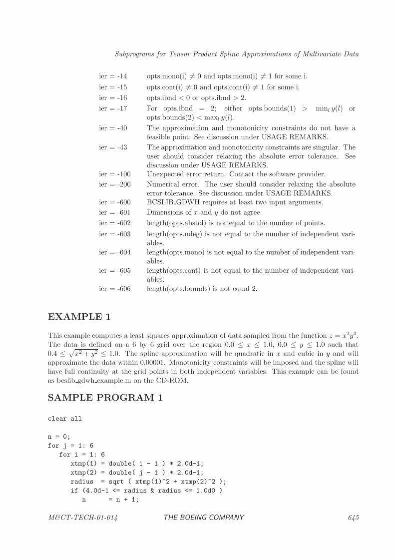
Subprograms for Tensor Product Spline Approximations of Multivariate Data
ier = -14 opts.mono(i) 6= 0 and opts.mono(i) 6= 1 for some i.
ier = -15 opts.cont(i) 6= 0 and opts.cont(i) 6= 1 for some i.
ier = -16 opts.ibnd < 0 or opts.ibnd > 2.
ier = -17 For opts.ibnd = 2; either opts.bounds(1) > minl y(l) oropts.bounds(2) < maxl y(l).
ier = -40 The approximation and monotonicity constraints do not have afeasible point. See discussion under USAGE REMARKS.
ier = -43 The approximation and monotonicity constraints are singular. Theuser should consider relaxing the absolute error tolerance. Seediscussion under USAGE REMARKS.
ier = -100 Unexpected error return. Contact the software provider.
ier = -200 Numerical error. The user should consider relaxing the absoluteerror tolerance. See discussion under USAGE REMARKS.
ier = -600 BCSLIB GDWH requires at least two input arguments.
ier = -601 Dimensions of x and y do not agree.
ier = -602 length(opts.abstol) is not equal to the number of points.
ier = -603 length(opts.ndeg) is not equal to the number of independent vari-ables.
ier = -604 length(opts.mono) is not equal to the number of independent vari-ables.
ier = -605 length(opts.cont) is not equal to the number of independent vari-ables.
ier = -606 length(opts.bounds) is not equal 2.
EXAMPLE 1
This example computes a least squares approximation of data sampled from the function z = x2y3.The data is defined on a 6 by 6 grid over the region 0.0 ≤ x ≤ 1.0, 0.0 ≤ y ≤ 1.0 such that0.4 ≤
√x2 + y2 ≤ 1.0. The spline approximation will be quadratic in x and cubic in y and will
approximate the data within 0.00001. Monotonicity constraints will be imposed and the spline willhave full continuity at the grid points in both independent variables. This example can be foundas bcslib gdwh example.m on the CD-ROM.
SAMPLE PROGRAM 1
clear all
n = 0;
for j = 1: 6
for i = 1: 6
xtmp(1) = double( i - 1 ) * 2.0d-1;
xtmp(2) = double( j - 1 ) * 2.0d-1;
radius = sqrt ( xtmp(1)^2 + xtmp(2)^2 );
if (4.0d-1 <= radius & radius <= 1.0d0 )
n = n + 1;
M&CT-TECH-01-014 THE BOEING COMPANY 645
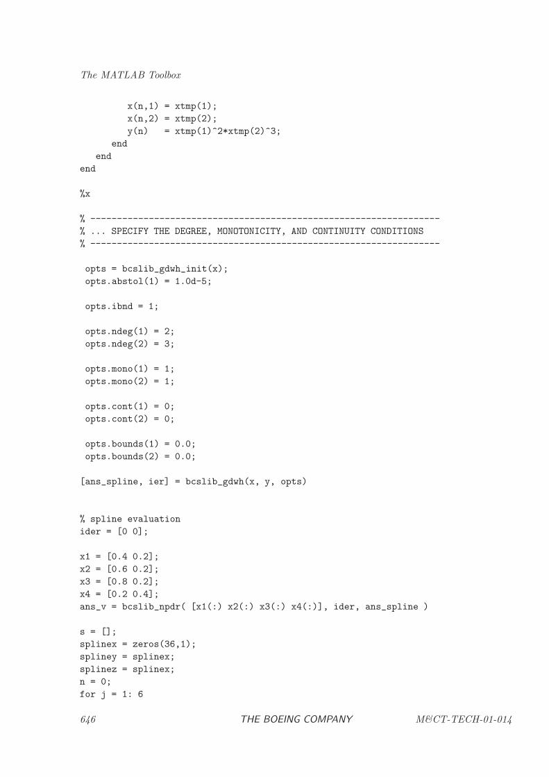
The MATLAB Toolbox
x(n,1) = xtmp(1);
x(n,2) = xtmp(2);
y(n) = xtmp(1)^2*xtmp(2)^3;
end
end
end
%x
% ------------------------------------------------------------------
% ... SPECIFY THE DEGREE, MONOTONICITY, AND CONTINUITY CONDITIONS
% ------------------------------------------------------------------
opts = bcslib_gdwh_init(x);
opts.abstol(1) = 1.0d-5;
opts.ibnd = 1;
opts.ndeg(1) = 2;
opts.ndeg(2) = 3;
opts.mono(1) = 1;
opts.mono(2) = 1;
opts.cont(1) = 0;
opts.cont(2) = 0;
opts.bounds(1) = 0.0;
opts.bounds(2) = 0.0;
[ans_spline, ier] = bcslib_gdwh(x, y, opts)
% spline evaluation
ider = [0 0];
x1 = [0.4 0.2];
x2 = [0.6 0.2];
x3 = [0.8 0.2];
x4 = [0.2 0.4];
ans_v = bcslib_npdr( [x1(:) x2(:) x3(:) x4(:)], ider, ans_spline )
s = [];
splinex = zeros(36,1);
spliney = splinex;
splinez = splinex;
n = 0;
for j = 1: 6
646 THE BOEING COMPANY M&CT-TECH-01-014
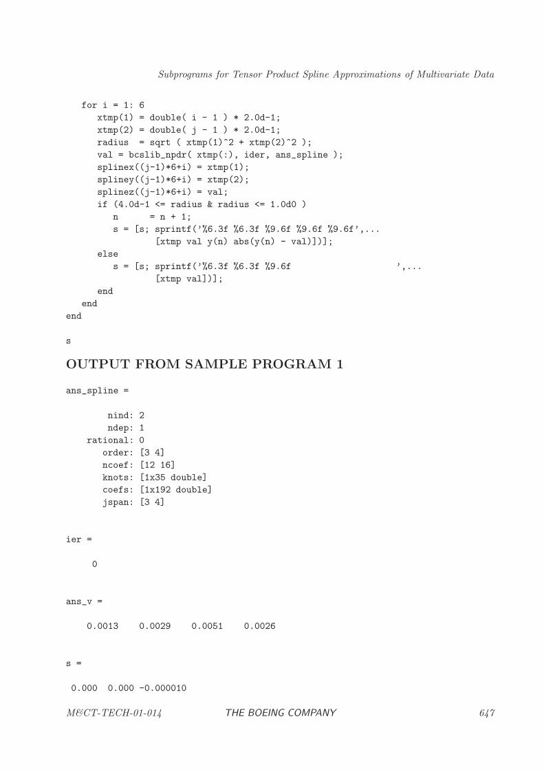
Subprograms for Tensor Product Spline Approximations of Multivariate Data
for i = 1: 6
xtmp(1) = double( i - 1 ) * 2.0d-1;
xtmp(2) = double( j - 1 ) * 2.0d-1;
radius = sqrt ( xtmp(1)^2 + xtmp(2)^2 );
val = bcslib_npdr( xtmp(:), ider, ans_spline );
splinex((j-1)*6+i) = xtmp(1);
spliney((j-1)*6+i) = xtmp(2);
splinez((j-1)*6+i) = val;
if (4.0d-1 <= radius & radius <= 1.0d0 )
n = n + 1;
s = [s; sprintf(’%6.3f %6.3f %9.6f %9.6f %9.6f’,...
[xtmp val y(n) abs(y(n) - val)])];
else
s = [s; sprintf(’%6.3f %6.3f %9.6f ’,...
[xtmp val])];
end
end
end
s
OUTPUT FROM SAMPLE PROGRAM 1
ans_spline =
nind: 2
ndep: 1
rational: 0
order: [3 4]
ncoef: [12 16]
knots: [1x35 double]
coefs: [1x192 double]
jspan: [3 4]
ier =
0
ans_v =
0.0013 0.0029 0.0051 0.0026
s =
0.000 0.000 -0.000010
M&CT-TECH-01-014 THE BOEING COMPANY 647
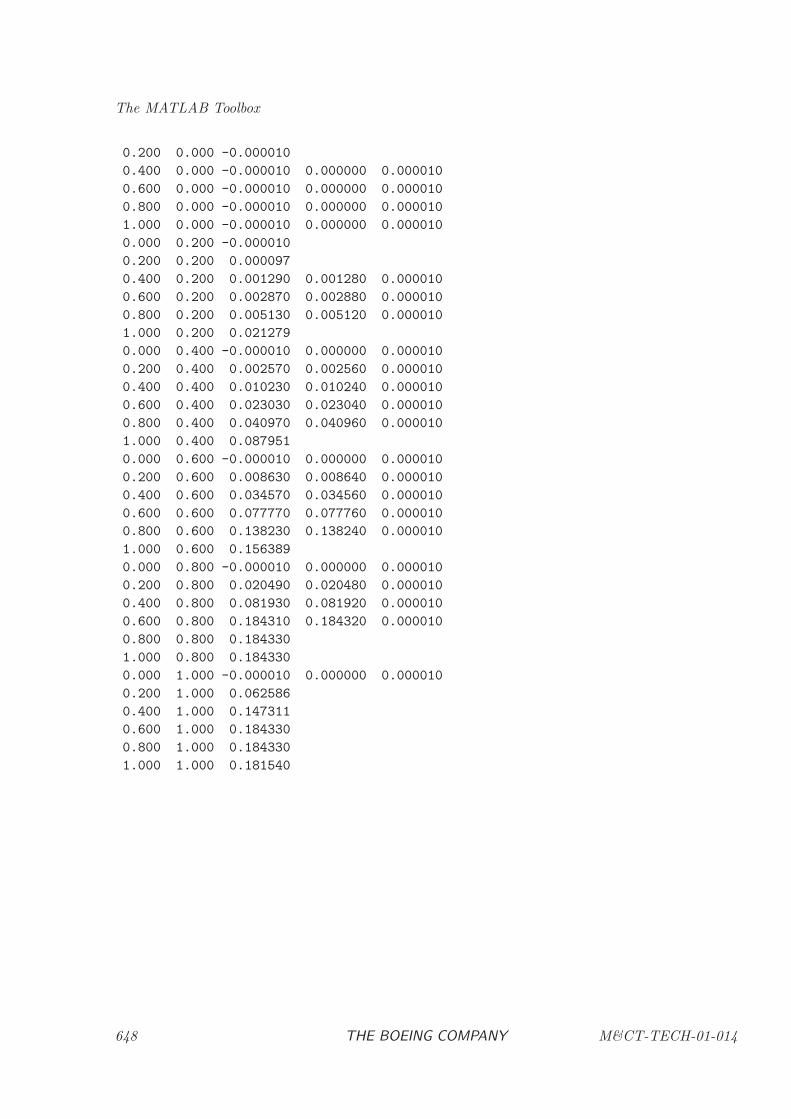
The MATLAB Toolbox
0.200 0.000 -0.000010
0.400 0.000 -0.000010 0.000000 0.000010
0.600 0.000 -0.000010 0.000000 0.000010
0.800 0.000 -0.000010 0.000000 0.000010
1.000 0.000 -0.000010 0.000000 0.000010
0.000 0.200 -0.000010
0.200 0.200 0.000097
0.400 0.200 0.001290 0.001280 0.000010
0.600 0.200 0.002870 0.002880 0.000010
0.800 0.200 0.005130 0.005120 0.000010
1.000 0.200 0.021279
0.000 0.400 -0.000010 0.000000 0.000010
0.200 0.400 0.002570 0.002560 0.000010
0.400 0.400 0.010230 0.010240 0.000010
0.600 0.400 0.023030 0.023040 0.000010
0.800 0.400 0.040970 0.040960 0.000010
1.000 0.400 0.087951
0.000 0.600 -0.000010 0.000000 0.000010
0.200 0.600 0.008630 0.008640 0.000010
0.400 0.600 0.034570 0.034560 0.000010
0.600 0.600 0.077770 0.077760 0.000010
0.800 0.600 0.138230 0.138240 0.000010
1.000 0.600 0.156389
0.000 0.800 -0.000010 0.000000 0.000010
0.200 0.800 0.020490 0.020480 0.000010
0.400 0.800 0.081930 0.081920 0.000010
0.600 0.800 0.184310 0.184320 0.000010
0.800 0.800 0.184330
1.000 0.800 0.184330
0.000 1.000 -0.000010 0.000000 0.000010
0.200 1.000 0.062586
0.400 1.000 0.147311
0.600 1.000 0.184330
0.800 1.000 0.184330
1.000 1.000 0.181540
648 THE BOEING COMPANY M&CT-TECH-01-014
Subprograms for Tensor Product Spline Approximations of Multivariate Data
BCSLIB GDWH INIT: Set standard values for optional parameters.
PURPOSE
BCSLIB GDWH INIT defines a Matlab structure containing the standard values for all optionalparameters of BCSLIB GDWH.
RELATED SUBPROGRAMS
BCSLIB GDWH Tensor Product Spline Approximation of Gridded Data with Holes
BCSLIB GRIDDATA Two-dimensional approximation using BCSLIB GDWH.
BCSLIB GRIDDATAN N -dimensional approximation using BCSLIB GDWH.
USAGE
[opts] = bcslib gdwh init(x);
ARGUMENTS
x [INPUT, ]Two-dimensional array of size (m,n). This x must have the same dimensions asthe x used with BCSLIB GDWH.
opts [OUTPUT, ]A Matlab structure containing standard values for the optional parameters.
EXAMPLE
See the example for BCSLIB GDWH.
M&CT-TECH-01-014 THE BOEING COMPANY 649
The MATLAB Toolbox
BCSLIB GRIDDATA: Bivariate Spline Approximation and Evaluation.
PURPOSE
BCSLIB GRIDDATA approximates multivariate data which lies on a grid but contains regionsof missing data. It computes a tensor product spline which has minimal variation of its secondorder partials, approximates the data within a user specified tolerance and, optionally, is locallymonotonic along grid lines. It then evaluates this spline at points specified by the user. Note thatif the same approximation will be used many times, the user should only calculate the spline oncewith BCSLIB GDWH and then evaluate the spline repeatedly using BCSLIB NPDR. This willsignificantly speed up the computations.
RELATED SUBPROGRAMS
BCSLIB GDWH INIT Initialize the optional argument opts to standard values.
BCSLIB GDWH Tensor Product Spline Approximation of Gridded Data with Holes
BCSLIB NPVL Evaluation of a Tensor Product Spline.
BCSLIB GRIDDATAN N -dimensional approximation using BCSLIB GDWH.
METHOD
This method combines the two methods BCSLIB GDWH and BCSLIB NPDR into one, easier touse method, for bivariate data. It can be used with the same calling sequence as the Matlab internalinterpolation method.
USAGE
zi = bcslib_griddata(x,y,z,xi,yi,method,opts)
or
[xi,yi,zi] = bcslib_griddata(x,y,z,xi,yi,method,opts)
Note that method and opts are optional input arguments. If the user wants to change any ofthe settings, he should initialize opts with a call to BCSLIB GDWH INIT, and then only changethe necessary settings. Nevertheless, it is possible to only set part of the structure of opts, andBCSLIB GRIDDATA will set undefined properties to standard values.
ARGUMENTS
x,y [INPUT, ]Vectors of size m. x and y contain the m values of the independent variables in
650 THE BOEING COMPANY M&CT-TECH-01-014
Subprograms for Tensor Product Spline Approximations of Multivariate Data
the x and y direction. These vectors need not be ordered but they must representm distinct points and satisfy the condition
minlx(l) < max
lx(l) and min
ly(l) < max
ly(l)
Note that at least two points need to be provided.
z [INPUT, ]Array of m values of dependent variable z in correspondence with the x and yvectors.
xi,yi [INPUT, ]Points at which the spline will be evaluated. The corresponding values will bestored in zi. xi and yi can be row and column vectors, respectively. In this casethey specify matrices with constant columns and constant rows, respectively.
method [INPUT, ]specifies the degree of the spline. Note that when using this option, the degree willbe the same in the x and y direction. Possible options are
’linear’ - Use linear splines.
’quadratic’ - Use quadratic splines.
’cubic’ - Use cubic splines.
If you want to define different degrees for the spline, set method to an empty stringand define the degrees for each direction using opts.
opts [INPUT, ]structure with optional input to BCSLIB GDWH.
opts.abstol [INPUT, ]Absolute Error tolerance. The use of abstol depends on its dimension.
Optional, set to 1.0e-5 if not given.
If abstol is a scalar, abstol specifies the error tolerances for all constraints. Notethat abstol ≥ √
ǫ, where ǫ is the Matlab constant describing the floating pointrelative accuracy.
If abstol is a vector, it must have dimension m in correspondence with the x array.Abstol(l) specifies the error tolerances for l = 1, . . . ,m of the constraints.
If abstol(l) = Inf, then the l-th point is not used. It must satisfy abstol(l) ≥ √ǫ
for all l.
opts.ndeg [INPUT, ]Array of n values where ndeg(i) is the degree of the spline in xi; 1 ≤ndeg(i)≤ 3.
Optional, set to all 2 if not given.
opts.mono [INPUT, ]Monotonicity option. Array of n values where mono(i) specifies if the spline islocally monotonic in xi along the data grid lines.
Optional, set to all 1 if not given.
M&CT-TECH-01-014 THE BOEING COMPANY 651
The MATLAB Toolbox
mono(i) = 0 The spline will not be locally monotonic in xi.
mono(i) = 1 The spline will be locally monotonic in xi.
opts.cont [INPUT, ]Continuity option. Array of n values where cont(i) specifies if the spline has fullor reduced continuity at the grid points in xi.
Optional, set to all 0 if not given.
cont(i) = 0 The spline has full continuity in xi at the grid points. If the splineis linear in xi, then it will be continuous everywhere in xi. If thespline is quadratic in xi, then the first order partial in xi will becontinuous everywhere. If the spline is cubic in xi, then the secondorder partial in xi will be continuous everywhere.
cont(i) = 1 The spline has reduced continuity in xi at the grid points. If thespline is linear in xi, then it will be continuous everywhere in xi. Ifthe spline is quadratic in xi, then the first order partial in xi willbe continuous everywhere, except at grid points. If the spline iscubic in xi, then the second order partial in xi will be continuouseverywhere, except at grid points.
opts.ibnd [INPUT, ]Bound options flag.
Optional, set to 0 if not given.
ibnd = 0 No bounds are imposed on the approximation.
ibnd = 1 BCSLIB GDWH imposes the condition sl ≤ s(x) ≤ su where sl =minl y(l) and su = maxl y(l).
ibnd = 2 BCSLIB GDWH imposes the condition sl ≤ s(x) ≤ su wheresl =bounds(1) and su =bounds(2).
opts.bounds [INPUT, ]Array of two elements containing the lower and upper bounds. The content ofbounds depends on the bound options flag ibnd.
Optional, set to (0,0) if not given.
ibnd = 0 The contents of bounds are not used and bounds can be omitted.ibnd = 1 BCSLIB GDWH sets bounds(1) = minl y(l) and bounds(2) =
maxl y(l).
ibnd = 2 The user must specify the values of bounds. BCSLIB GDWHimposes the condition bounds(1)≤ s(x) ≤ bounds(2). The ele-ments of bounds must satisfy bounds(1) ≤ minl y(l) and bounds(2)≥ maxl y(l).If bounds(1) = Inf, then no lower bound is imposed on the spline.Similarly, no upper bound is imposed if bounds(2) = Inf.
zi [OUTPUT, ]Value of the approximated surface at the points specified in xi,yi.
652 THE BOEING COMPANY M&CT-TECH-01-014
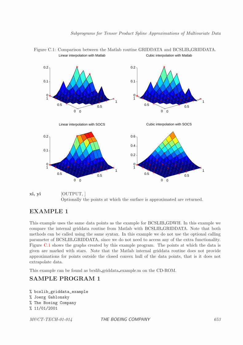
Subprograms for Tensor Product Spline Approximations of Multivariate Data
Figure C.1: Comparison between the Matlab routine GRIDDATA and BCSLIB GRIDDATA.
00.5
1
0
0.5
10
0.1
0.2
Linear interpolation with Matlab
00.5
1
0
0.5
10
0.1
0.2
Cubic interpolation with Matlab
00.5
1
0
0.5
10
0.1
0.2
Linear interpolation with SOCS
00.5
1
0
0.5
10
0.2
0.4
0.6
Cubic interpolation with SOCS
xi, yi [OUTPUT, ]Optionally the points at which the surface is approximated are returned.
EXAMPLE 1
This example uses the same data points as the example for BCSLIB GDWH. In this example wecompare the internal griddata routine from Matlab with BCSLIB GRIDDATA. Note that bothmethods can be called using the same syntax. In this example we do not use the optional callingparameter of BCSLIB GRIDDATA, since we do not need to access any of the extra functionality.Figure C.1 shows the graphs created by this example program. The points at which the data isgiven are marked with stars. Note that the Matlab internal griddata routine does not provideapproximations for points outside the closed convex hull of the data points, that is it does notextrapolate data.
This example can be found as bcslib griddata example.m on the CD-ROM.
SAMPLE PROGRAM 1
% bcslib_griddata_example
% Joerg Gablonsky
% The Boeing Company
% 11/01/2001
M&CT-TECH-01-014 THE BOEING COMPANY 653
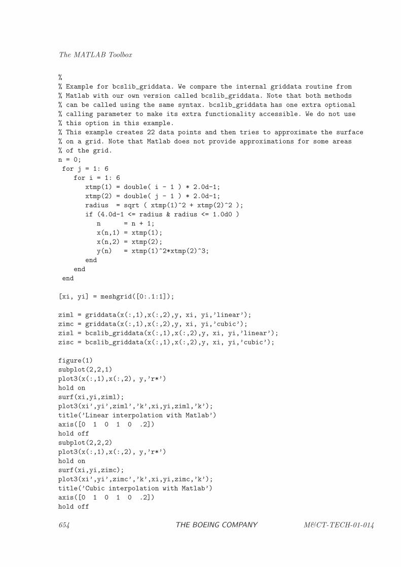
The MATLAB Toolbox
%
% Example for bcslib_griddata. We compare the internal griddata routine from
% Matlab with our own version called bcslib_griddata. Note that both methods
% can be called using the same syntax. bcslib_griddata has one extra optional
% calling parameter to make its extra functionality accessible. We do not use
% this option in this example.
% This example creates 22 data points and then tries to approximate the surface
% on a grid. Note that Matlab does not provide approximations for some areas
% of the grid.
n = 0;
for j = 1: 6
for i = 1: 6
xtmp(1) = double( i - 1 ) * 2.0d-1;
xtmp(2) = double( j - 1 ) * 2.0d-1;
radius = sqrt ( xtmp(1)^2 + xtmp(2)^2 );
if (4.0d-1 <= radius & radius <= 1.0d0 )
n = n + 1;
x(n,1) = xtmp(1);
x(n,2) = xtmp(2);
y(n) = xtmp(1)^2*xtmp(2)^3;
end
end
end
[xi, yi] = meshgrid([0:.1:1]);
ziml = griddata(x(:,1),x(:,2),y, xi, yi,’linear’);
zimc = griddata(x(:,1),x(:,2),y, xi, yi,’cubic’);
zisl = bcslib_griddata(x(:,1),x(:,2),y, xi, yi,’linear’);
zisc = bcslib_griddata(x(:,1),x(:,2),y, xi, yi,’cubic’);
figure(1)
subplot(2,2,1)
plot3(x(:,1),x(:,2), y,’r*’)
hold on
surf(xi,yi,ziml);
plot3(xi’,yi’,ziml’,’k’,xi,yi,ziml,’k’);
title(’Linear interpolation with Matlab’)
axis([0 1 0 1 0 .2])
hold off
subplot(2,2,2)
plot3(x(:,1),x(:,2), y,’r*’)
hold on
surf(xi,yi,zimc);
plot3(xi’,yi’,zimc’,’k’,xi,yi,zimc,’k’);
title(’Cubic interpolation with Matlab’)
axis([0 1 0 1 0 .2])
hold off
654 THE BOEING COMPANY M&CT-TECH-01-014
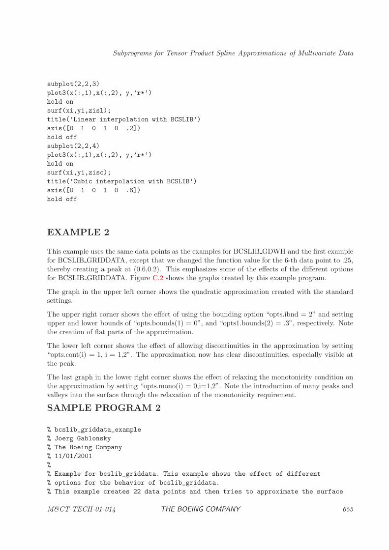
Subprograms for Tensor Product Spline Approximations of Multivariate Data
subplot(2,2,3)
plot3(x(:,1),x(:,2), y,’r*’)
hold on
surf(xi,yi,zisl);
title(’Linear interpolation with BCSLIB’)
axis([0 1 0 1 0 .2])
hold off
subplot(2,2,4)
plot3(x(:,1),x(:,2), y,’r*’)
hold on
surf(xi,yi,zisc);
title(’Cubic interpolation with BCSLIB’)
axis([0 1 0 1 0 .6])
hold off
EXAMPLE 2
This example uses the same data points as the examples for BCSLIB GDWH and the first examplefor BCSLIB GRIDDATA, except that we changed the function value for the 6-th data point to .25,thereby creating a peak at (0.6,0.2). This emphasizes some of the effects of the different optionsfor BCSLIB GRIDDATA. Figure C.2 shows the graphs created by this example program.
The graph in the upper left corner shows the quadratic approximation created with the standardsettings.
The upper right corner shows the effect of using the bounding option “opts.ibnd = 2” and settingupper and lower bounds of “opts.bounds(1) = 0”, and “opts1.bounds(2) = .3”, respectively. Notethe creation of flat parts of the approximation.
The lower left corner shows the effect of allowing discontinuities in the approximation by setting“opts.cont(i) = 1, i = 1,2”. The approximation now has clear discontinuities, especially visible atthe peak.
The last graph in the lower right corner shows the effect of relaxing the monotonicity condition onthe approximation by setting “opts.mono(i) = 0,i=1,2”. Note the introduction of many peaks andvalleys into the surface through the relaxation of the monotonicity requirement.
SAMPLE PROGRAM 2
% bcslib_griddata_example
% Joerg Gablonsky
% The Boeing Company
% 11/01/2001
%
% Example for bcslib_griddata. This example shows the effect of different
% options for the behavior of bcslib_griddata.
% This example creates 22 data points and then tries to approximate the surface
M&CT-TECH-01-014 THE BOEING COMPANY 655
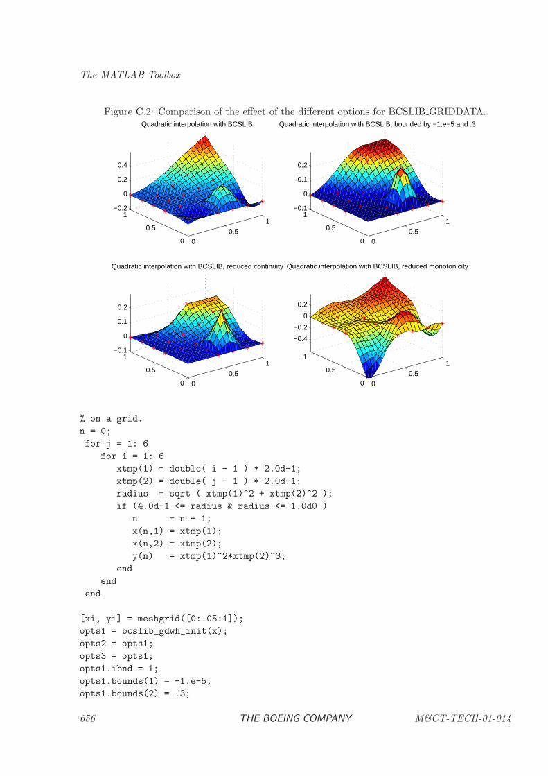
The MATLAB Toolbox
Figure C.2: Comparison of the effect of the different options for BCSLIB GRIDDATA.
00.5
1
0
0.5
1−0.2
0
0.2
0.4
Quadratic interpolation with BCSLIB
00.5
1
0
0.5
1−0.1
0
0.1
0.2
Quadratic interpolation with BCSLIB, bounded by −1.e−5 and .3
00.5
1
0
0.5
1−0.1
0
0.1
0.2
Quadratic interpolation with BCSLIB, reduced continuity
00.5
1
0
0.5
1
−0.4
−0.2
0
0.2
Quadratic interpolation with BCSLIB, reduced monotonicity
% on a grid.
n = 0;
for j = 1: 6
for i = 1: 6
xtmp(1) = double( i - 1 ) * 2.0d-1;
xtmp(2) = double( j - 1 ) * 2.0d-1;
radius = sqrt ( xtmp(1)^2 + xtmp(2)^2 );
if (4.0d-1 <= radius & radius <= 1.0d0 )
n = n + 1;
x(n,1) = xtmp(1);
x(n,2) = xtmp(2);
y(n) = xtmp(1)^2*xtmp(2)^3;
end
end
end
[xi, yi] = meshgrid([0:.05:1]);
opts1 = bcslib_gdwh_init(x);
opts2 = opts1;
opts3 = opts1;
opts1.ibnd = 1;
opts1.bounds(1) = -1.e-5;
opts1.bounds(2) = .3;
656 THE BOEING COMPANY M&CT-TECH-01-014
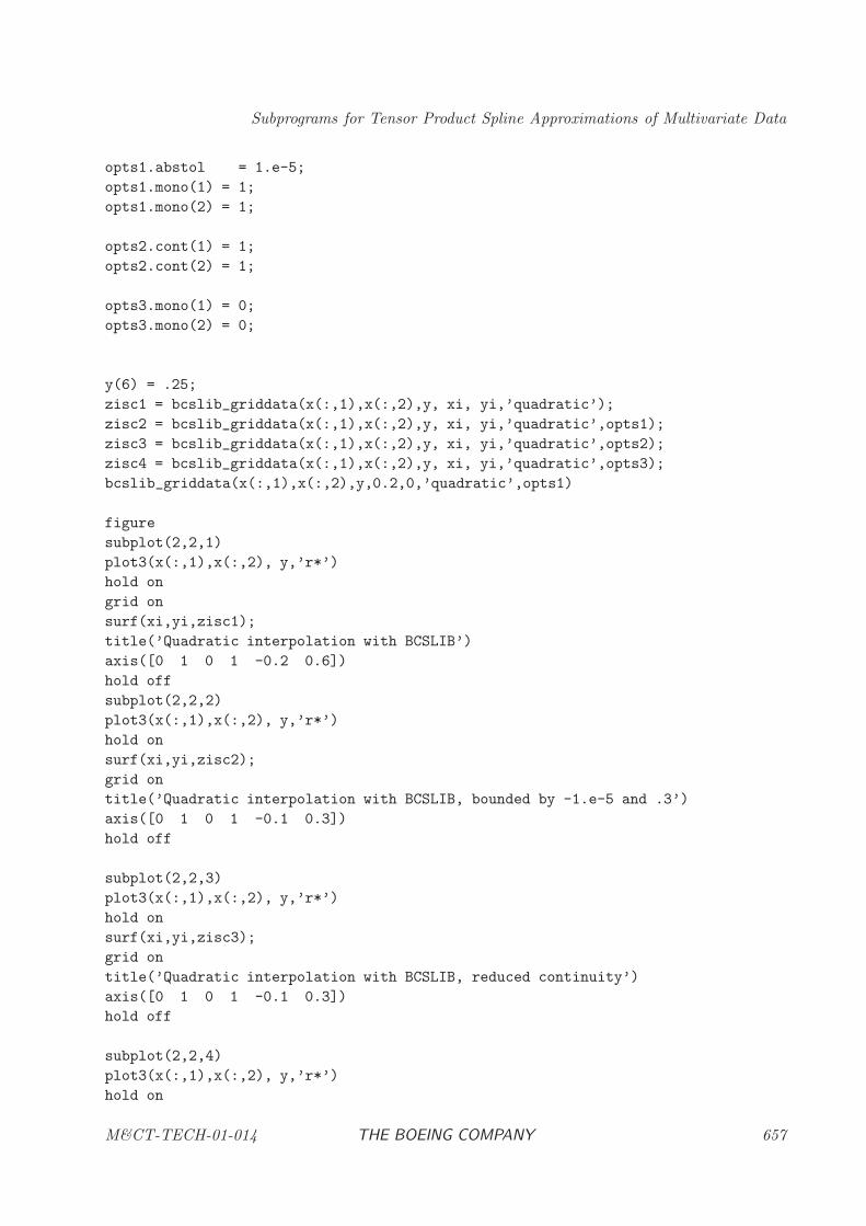
Subprograms for Tensor Product Spline Approximations of Multivariate Data
opts1.abstol = 1.e-5;
opts1.mono(1) = 1;
opts1.mono(2) = 1;
opts2.cont(1) = 1;
opts2.cont(2) = 1;
opts3.mono(1) = 0;
opts3.mono(2) = 0;
y(6) = .25;
zisc1 = bcslib_griddata(x(:,1),x(:,2),y, xi, yi,’quadratic’);
zisc2 = bcslib_griddata(x(:,1),x(:,2),y, xi, yi,’quadratic’,opts1);
zisc3 = bcslib_griddata(x(:,1),x(:,2),y, xi, yi,’quadratic’,opts2);
zisc4 = bcslib_griddata(x(:,1),x(:,2),y, xi, yi,’quadratic’,opts3);
bcslib_griddata(x(:,1),x(:,2),y,0.2,0,’quadratic’,opts1)
figure
subplot(2,2,1)
plot3(x(:,1),x(:,2), y,’r*’)
hold on
grid on
surf(xi,yi,zisc1);
title(’Quadratic interpolation with BCSLIB’)
axis([0 1 0 1 -0.2 0.6])
hold off
subplot(2,2,2)
plot3(x(:,1),x(:,2), y,’r*’)
hold on
surf(xi,yi,zisc2);
grid on
title(’Quadratic interpolation with BCSLIB, bounded by -1.e-5 and .3’)
axis([0 1 0 1 -0.1 0.3])
hold off
subplot(2,2,3)
plot3(x(:,1),x(:,2), y,’r*’)
hold on
surf(xi,yi,zisc3);
grid on
title(’Quadratic interpolation with BCSLIB, reduced continuity’)
axis([0 1 0 1 -0.1 0.3])
hold off
subplot(2,2,4)
plot3(x(:,1),x(:,2), y,’r*’)
hold on
M&CT-TECH-01-014 THE BOEING COMPANY 657

The MATLAB Toolbox
surf(xi,yi,zisc4);
title(’Quadratic interpolation with BCSLIB, reduced monotonicity’)
axis([0 1 0 1 -0.6 .4])
grid on
hold off
658 THE BOEING COMPANY M&CT-TECH-01-014
Subprograms for Tensor Product Spline Approximations of Multivariate Data
BCSLIB GRIDDATAN: Multivariate Spline Approximation and Evaluation.
PURPOSE
BCSLIB GRIDDATAN approximates multivariate data which lies on a grid but contains regionsof missing data. It computes a tensor product spline which has minimal variation of its secondorder partials, approximates the data within a user specified tolerance and, optionally, is locallymonotonic along grid lines. It then evaluates this spline at points specified by the user. This is theN -dimensional version of BCSLIB GRIDDATA.
RELATED SUBPROGRAMS
BCSLIB GDWH INIT Initialize the optional argument opts to standard values.
BCSLIB GDWH Tensor Product Spline Approximation of Gridded Data with Holes
BCSLIB NPVL Evaluation of a Tensor Product Spline.
BCSLIB GRIDDATA Two-dimensional approximation using BCSLIB GDWH.
METHOD
This method combines the two methods BCSLIB GDWH and BCSLIB NPDR into one, easier touse method. It can be used with the same calling sequence as the Matlab internal interpolationmethod GRIDDATAN.
USAGE
yi = bcslib griddatan(x,y,xi,method,opts)
Note that method and opts are optional input arguments. If the user wants to change any ofthe settings, he should initialize opts with a call to BCSLIB GDWH INIT, and then only changethe necessary settings. Nevertheless, it is possible to only set part of the structure of opts, andBCSLIB GRIDDATAN will set undefined properties to standard values.
ARGUMENTS
x [INPUT, ]Two-dimensional array of size (m,n). x contains the m values of the independentvariables in the x1 to xn directions which are stored in the first through n-th columnof x, respectively. This array need not be ordered but it must represent m distinctpoints and satisfy the condition
minlx(l, i) < max
lx(l, i) for i = 1, . . . , n.
M&CT-TECH-01-014 THE BOEING COMPANY 659
The MATLAB Toolbox
Note the following conditions on m and n:
m ≥ 2 and 1 ≤ n ≤ 10.
y [INPUT, ]Array of m values of dependent variable y in correspondence with the x array.
xi [INPUT, ]Array of size p by m, representing p points at which the spline will be evaluated.The corresponding values will be stored in yi. xi can be nonuniform.
method [INPUT, ]specifies the degree of the spline. Note that when using this option, the degree willbe the same in the x and y direction. Possible options are
’linear’ - Use linear splines.
’quadratic’ - Use quadratic splines.
’cubic’ - Use cubic splines.
If you want to define different degrees for the spline, set method to ” and definethe degrees for each direction using opts.
opts [INPUT, ]structure with optional input to BCSLIB GDWH.
opts.abstol [INPUT, ]Absolute Error tolerance. The use of abstol depends on its dimension.
Optional, set to 1.0e-5 if not given.
If abstol is a scalar, abstol specifies the error tolerances for all constraints. Notethat abstol ≥ √
ǫ, where ǫ is the Matlab constant describing the floating pointrelative accuracy.
If abstol is a vector, it must have dimension m in correspondence with the x array.Abstol(l) specifies the error tolerances for l = 1, . . . ,m of the constraints.
If abstol(l) = Inf, then the l-th point is not used. It must satisfy abstol(l) ≥ √ǫ
for all l.
opts.ndeg [INPUT, ]Array of n values where ndeg(i) is the degree of the spline in xi; 1 ≤ndeg(i)≤ 3.
Optional, set to all 2 if not given.
opts.mono [INPUT, ]Monotonicity option. Array of n values where mono(i) specifies if the spline islocally monotonic in xi along the data grid lines.
Optional, set to all 1 if not given.
mono(i) = 0 The spline will not be locally monotonic in xi.
mono(i) = 1 The spline will be locally monotonic in xi.
660 THE BOEING COMPANY M&CT-TECH-01-014
Subprograms for Tensor Product Spline Approximations of Multivariate Data
opts.cont [INPUT, ]Continuity option. Array of n values where cont(i) specifies if the spline has fullor reduced continuity at the grid points in xi.
Optional, set to all 0 if not given.
cont(i) = 0 The spline has full continuity in xi at the grid points. If the splineis linear in xi, then it will be continuous everywhere in xi. If thespline is quadratic in xi, then the first order partial in xi will becontinuous everywhere. If the spline is cubic in xi, then the secondorder partial in xi will be continuous everywhere.
cont(i) = 1 The spline has reduced continuity in xi at the grid points. If thespline is linear in xi, then it will be continuous everywhere in xi. Ifthe spline is quadratic in xi, then the first order partial in xi willbe continuous everywhere, except at grid points. If the spline iscubic in xi, then the second order partial in xi will be continuouseverywhere, except at grid points.
opts.ibnd [INPUT, ]Bound options flag.
Optional, set to 0 if not given.
ibnd = 0 No bounds are imposed on the approximation.
ibnd = 1 BCSLIB GDWH imposes the condition sl ≤ s(x) ≤ su where sl =minl y(l) and su = maxl y(l).
ibnd = 2 BCSLIB GDWH imposes the condition sl ≤ s(x) ≤ su wheresl =bounds(1) and su =bounds(2).
opts.bounds [INPUT, ]Array of two elements containing the lower and upper bounds. The content ofbounds depends on the bound options flag ibnd.
Optional, set to (0,0) if not given.
ibnd = 0 The contents of bounds are not used and bounds can be omitted.ibnd = 1 BCSLIB GDWH sets bounds(1) = minl y(l) and bounds(2) =
maxl y(l).
ibnd = 2 The user must specify the values of bounds. BCSLIB GDWHimposes the condition bounds(1)≤ s(x) ≤ bounds(2). The ele-ments of bounds must satisfy bounds(1) ≤ minl y(l) and bounds(2)≥ maxl y(l).If bounds(1) = Inf, then no lower bound is imposed on the spline.Similarly, no upper bound is imposed if bounds(2) = Inf.
yi [OUTPUT, ]Value of the approximated surface at the points specified in xi.
M&CT-TECH-01-014 THE BOEING COMPANY 661
The MATLAB Toolbox
BCSLIB NPVL: Evaluation of a Tensor Product Spline
PURPOSE
BCSLIB NPVL computes values of a tensor product spline function with one or more independentvariables and any number of dependent variables. If derivatives are required use BCSLIB NPDR.BCSLIB NPVL can also be used to calculate the values of a rational tensor product spline.
RELATED SUBPROGRAMS
BCSLIB FNVL Fast evaluation of a Tensor Product Spline without error checking
BCSLIB ENVL Evaluation of a Tensor Product Spline with extrapolation
BCSLIB FEVL Fast evaluation of a Tensor Product Spline with extrapolation,but without error checking
BCSLIB GDWH INIT Initialize the optional argument opts to standard values.
BCSLIB GDWH Tensor Product Spline Approximation of Gridded Data with Holes
BCSLIB GRIDDATA Two-dimensional approximation using BCSLIB GDWH.
BCSLIB GRIDDATAN N -dimensional approximation using BCSLIB GDWH.
METHOD
Usually, the function evaluated by BCSLIB NPVL is a tensor product spline, represented in a B-spline basis, defined by one of the spline construction subroutines of this chapter. The data definingthe tensor product B-spline representation is stored either in a Matlab structure, or in a standardBCSLIB data structure called the C array. BCSLIB NPVL computes the values of the dependentvariables by evaluating the tensor product B-splines at the value of the independent variables. Thetensor product spline is evaluated by computing the value of a sequence of univariate splines. Eachunivariate spline is evaluated as the inner product of its B-spline coefficients with the values of thenon-vanishing B-splines, obtained by the algorithm of Cox and de Boor.
BCSLIB NPVL may also be used to evaluate a rational tensor product spline, represented in arational tensor product B-spline basis. Often, tensor product spline functions which must berepresented by rational B-splines are defined by subroutines that convert CAD/CAM data, such asCATIA data, to the BCSLIB spline representation. In this case, the C array stores data definingthe tensor product spline for the numerator for each dependent variable and for the commondenominator—see Appendix A of the BCSLIB manual. BCSLIB NPVL first computes the valuesof the numerator and denominator tensor product B-splines as in the tensor product spline caseabove. Then each dependent variable is evaluated as the ratio of the values of its numerator andthe common denominator.
USAGE
[ans_v, ier] = bcslib_npvl(x, s),
662 THE BOEING COMPANY M&CT-TECH-01-014
Subprograms for Tensor Product Spline Approximations of Multivariate Data
or
ans_v = bcslib_npvl(x, s)
ARGUMENTS
x [INPUT, ]Two-dimensional array of size (m,n). X contains the points where the spline shouldbe evaluated. The values of the independent variables must be in the interval ofdefinition of their corresponding splines.
s [INPUT, ]Spline definition. This definition can have two forms. The first is a Matlab structureas is returned by the spline creation routines such as BCSLIB GDWH. The secondform is an array. This array corresponds to the C array used in Fortran BCSLIBroutines. If a spline is evaluated many times, the user should convert the splinestructure with the help of BCSLIB CONVERTSPLINE to an array:
s = bcslib convertspline(spline);
where spline is a (Matlab) structure. Calling BCSLIB NPVL with the array insteadon the structure increases the performance.
ans v [OUTPUT, ]Two-dimensional array of size (k, n). ANS V contains the calculated values of thespline at the points specified in X.
ier [OUTPUT, ]Success / Error code. For ier < 0, results have not been computed and BC-SLIB NPVL has set ANS V(1) = HDMCON(1).
ier = 0 Success, results computed.
ier = −1 Order of the spline in some direction is lower than 1.
ier = −6 Number of spline coefficients with respect to the ith independentvariable is less than its order for some i.
ier = −8 Invalid knot set.
ier = −10 The absolute value of the denominator of the spline (when evalu-ated at X) is less than epsilon, the relative precision.
ier = −38 X is inside a knot interval that is too small.
ier = −50 One (or more) of the independent variables is out of range.
ier = −51 C(1) < 1.
M&CT-TECH-01-014 THE BOEING COMPANY 663
The MATLAB Toolbox
ier = −52 C(2) = −1 or 0.
USAGE REMARKS
If an error other than the listed ones occurs, please contact the software provider.
EXAMPLE
Subroutine BCSLIB GDWH is used in the following example to fit a spline to data. SubroutineBCSLIB NPVL is then used to evaluate the spline at the grid points. A comparison of the splinefit with the original data points is displayed.
SAMPLE PROGRAM
n = 0;
for j = 1: 6
for i = 1: 6
xtmp(1) = double( i - 1 ) * 2.0d-1;
xtmp(2) = double( j - 1 ) * 2.0d-1;
radius = sqrt ( xtmp(1)^2 + xtmp(2)^2 );
if (4.0d-1 <= radius & radius <= 1.0d0 )
n = n + 1;
x(n,1) = xtmp(1);
x(n,2) = xtmp(2);
y(n) = xtmp(1)^2*xtmp(2)^3;
end
end
end
opts = bcslib_gdwh_init(x);
opts.abstol(1) = 1.0d-7;
ans_spline = bcslib_gdwh(x, y’, opts);
s = [’x(1) x(2) val y abs(y-val)’];
n = 0;
for j = 1: 3
for i = 1: 3
xtmp(1) = double( i - 1 ) * 4.0d-1;
xtmp(2) = double( j - 1 ) * 4.0d-1;
radius = sqrt ( xtmp(1)^2 + xtmp(2)^2 );
val = bcslib_npvl( xtmp(:), ans_spline );
if (4.0d-1 <= radius & radius <= 1.0d0 )
n = n + 1;
s = [s; sprintf(’%6.3f %6.3f %9.6f %9.6f %9.6f’,...
[xtmp val y(n) abs(y(n) - val)])];
else
s = [s; sprintf(’%6.3f %6.3f %9.6f ’,[xtmp val])];
end
end
664 THE BOEING COMPANY M&CT-TECH-01-014
Subprograms for Tensor Product Spline Approximations of Multivariate Data
end
s
OUTPUT FROM SAMPLE PROGRAM
x(1) x(2) val y abs(y-val)
0.000 0.000 -0.000297
0.400 0.000 -0.000000 0.000000 0.000000
0.800 0.000 -0.000000 0.000000 0.000000
0.000 0.400 -0.000000 0.000000 0.000000
0.400 0.400 0.010240 0.000000 0.010240
0.800 0.400 0.040960 0.001280 0.039680
0.000 0.800 -0.000000 0.002880 0.002880
0.400 0.800 0.081920 0.005120 0.076800
0.800 0.800 0.266164
M&CT-TECH-01-014 THE BOEING COMPANY 665
The MATLAB Toolbox
BCSLIB FNVL: Fast Evaluation of a Tensor Product Spline without error check-ing
PURPOSE
BCSLIB FNVL computes values of a tensor product spline function with one or more independentvariables and any number of dependent variables. This method only performs limited error checking.It should only be used if a user is certain that the splines he passes are valid, and that the workspaceis large enough. The user is advised to use the corresponding routine BCSLIB NPVL during productdevelopment. BCSLIB NPVL is slower than BCSLIB FNVL, but performs error checking.
Furthermore, if the number of independent variables is larger then 3, this routine calls BC-SLIB NPVL internally. In this case the user is again advised to directly call BCSLIB NPVL. Notethat both routines have the same calling sequence. If derivatives are required use BCSLIB NPDR.BCSLIB FNVL can also be used to calculate the values of a rational tensor product spline—see
Appendix A of the BCSLIB user manual.
RELATED SUBPROGRAMS
BCSLIB NPVL Evaluation of a Tensor Product Spline
BCSLIB ENVL Evaluation of a Tensor Product Spline with extrapolation
BCSLIB FEVL Fast evaluation of a Tensor Product Spline with extrapolation,but without error checking
BCSLIB GDWH INIT Initialize the optional argument opts to standard values.
BCSLIB GDWH Tensor Product Spline Approximation of Gridded Data with Holes
BCSLIB GRIDDATA Two-dimensional approximation using BCSLIB GDWH.
BCSLIB GRIDDATAN N -dimensional approximation using BCSLIB GDWH.
METHOD
BCSLIB FNVL is very similar to BCSLIB NPVL, except that it does not perform many errorchecks, and it uses a faster method if the number of independent variables is between one andthree. If the number of independent variables is larger, this method calls BCSLIB NPVL. For moredetails on the method see the documentation to BCSLIB NPVL.
USAGE
[ans_v, ier] = bcslib_fnvl(x, s),
or
ans_v = bcslib_fnvl(x, s)
ARGUMENTS
666 THE BOEING COMPANY M&CT-TECH-01-014
Subprograms for Tensor Product Spline Approximations of Multivariate Data
x [INPUT, ]Two-dimensional array of size (m,n). X contains the points where the spline shouldbe evaluated. The values of the independent variables must be in the interval ofdefinition of their corresponding splines.
s [INPUT, ]Spline definition. This definition can have two forms. The first is a Matlab structureas is returned by the spline creation routines such as BCSLIB GDWH. The secondform is an array. This array corresponds to the C array used in Fortran BCSLIBroutines. If a spline is evaluated many times, the user should convert the splinestructure with the help of BCSLIB CONVERTSPLINE to an array:
s = bcslib convertspline(spline);
where spline is a (Matlab) structure. Calling BCSLIB FNVL with the array insteadon the structure increases the performance.
ans v [OUTPUT, ]Two-dimensional array of size (k, n). ANS V contains the calculated values of thespline at the points specified in X.
ier [OUTPUT, ]Success / Error code. For ier < 0, results have not been computed and BC-SLIB FNVL has set ANS V(1) = HDMCON(1). Note that no errors other than-50 will be detected by this method if the number of independent variables is be-tween 1 and 3. The user should only use this method if he is sure that these errorscannot happen. Otherwise, he should use BCSLIB NPVL instead.
ier = 0 Success, results computed.
ier = −1 Order of the spline in some direction is lower than 1.
ier = −6 Number of spline coefficients with respect to the ith independentvariable is less than its order for some i.
ier = −8 Invalid knot set.
ier = −10 The absolute value of the denominator of the spline (when evalu-ated at X) is less than epsilon, the relative precision.
ier = −38 X is inside a knot interval that is too small.
ier = −50 One (or more) of the independent variables is out of range.
ier = −51 C(1) < 1.
ier = −52 C(2) = −1 or 0.
M&CT-TECH-01-014 THE BOEING COMPANY 667
The MATLAB Toolbox
USAGE REMARKS
If an error other than the listed ones occurs, please contact the software provider.
EXAMPLE
Subroutine BCSLIB GDWH is used in the following example to fit a spline to data. SubroutineBCSLIB FNVL is then used to evaluate the spline at the grid points. A comparison of the splinefit with the original data points is displayed.
SAMPLE PROGRAM
n = 0;
for j = 1: 6
xtmp(2) = double( j - 1 ) * 2.0d-1;
for i = 1: 6
xtmp(1) = double( i - 1 ) * 2.0d-1;
radius = sqrt ( xtmp(1)^2 + xtmp(2)^2 );
if (4.0d-1 <= radius & radius <= 1.0d0 )
n = n + 1;
x(n,1:2) = xtmp;
y(n) = xtmp(1)^2*xtmp(2)^3;
end
end
end
opts = bcslib_gdwh_init(x);
opts.abstol(1) = 1.0d-7;
ans_spline = bcslib_gdwh(x, y, opts);
s = [’x(1) x(2) val y abs(y-val)’];
n = 0;
for j = 1: 3
for i = 1: 3
xtmp(1) = double( i - 1 ) * 4.0d-1;
xtmp(2) = double( j - 1 ) * 4.0d-1;
radius = sqrt ( xtmp(1)^2 + xtmp(2)^2 );
val = bcslib_fnvl( xtmp(:), ans_spline );
if (4.0d-1 <= radius & radius <= 1.0d0 )
n = n + 1;
s = [s; sprintf(’%6.3f %6.3f %9.6f %9.6f %9.6f’,...
[xtmp val y(n) abs(y(n) - val)])];
else
s = [s; sprintf(’%6.3f %6.3f %9.6f ’,[xtmp val])];
end
end
end
s
668 THE BOEING COMPANY M&CT-TECH-01-014
Subprograms for Tensor Product Spline Approximations of Multivariate Data
OUTPUT FROM SAMPLE PROGRAM
x(1) x(2) val y abs(y-val)
0.000 0.000 -0.000297
0.400 0.000 -0.000000 0.000000 0.000000
0.800 0.000 -0.000000 0.000000 0.000000
0.000 0.400 -0.000000 0.000000 0.000000
0.400 0.400 0.010240 0.000000 0.010240
0.800 0.400 0.040960 0.001280 0.039680
0.000 0.800 -0.000000 0.002880 0.002880
0.400 0.800 0.081920 0.005120 0.076800
0.800 0.800 0.266164
M&CT-TECH-01-014 THE BOEING COMPANY 669
The MATLAB Toolbox
BCSLIB ENVL: Evaluation of a Tensor Product Spline with extrapolation
PURPOSE
BCSLIB ENVL computes values of a tensor product spline function with one or more independentvariables and any number of dependent variables. This routine also uses linear extrapolation if theuser tries to evaluate the tensor product spline outside of the range of the independent variables.BCSLIB ENVL can also be used to calculate the values of a rational tensor product spline—see
Appendix A of the BCSLIB user manual.
RELATED SUBPROGRAMS
BCSLIB NPVL Evaluation of a Tensor Product Spline
BCSLIB FNVL Fast evaluation of a Tensor Product Spline without error checking
BCSLIB FEVL Fast evaluation of a Tensor Product Spline with extrapolation,but without error checking
BCSLIB GDWH INIT Initialize the optional argument opts to standard values.
BCSLIB GDWH Tensor Product Spline Approximation of Gridded Data with Holes
BCSLIB GRIDDATA Two-dimensional approximation using BCSLIB GDWH.
BCSLIB GRIDDATAN N -dimensional approximation using BCSLIB GDWH.
METHOD
This function is an extension of BCSLIB NPVL. If a point at which the tensor product splineneeds to be evaluated lies within the range of the spline, this routine directly calls BCSLIB NPVL.Otherwise, a linear extrapolation is used. This is done by finding the appropriate point on theboundary of the range of the spline, and calculating the value and first derivative of the spline atthat point. This information is then used to calculate a linear extrapolation.
USAGE
[ans_v, ier] = bcslib_envl(x, s),
or
ans_v = bcslib_envl(x, s)
ARGUMENTS
x [INPUT, ]Two-dimensional array of size (m,n). X contains the points where the spline shouldbe evaluated. The values of the independent variables must be in the interval ofdefinition of their corresponding splines.
670 THE BOEING COMPANY M&CT-TECH-01-014
Subprograms for Tensor Product Spline Approximations of Multivariate Data
s [INPUT, ]Spline definition. This definition can have two forms. The first is a Matlab structureas is returned by the spline creation routines such as BCSLIB GDWH. The secondform is an array. This array corresponds to the C array used in Fortran BCSLIBroutines. If a spline is evaluated many times, the user should convert the splinestructure with the help of BCSLIB CONVERTSPLINE to an array:
s = bcslib convertspline(spline);
where spline is a (Matlab) structure. Calling BCSLIB ENVL with the array insteadon the structure increases the performance.
ans v [OUTPUT, ]Two-dimensional array of size (k, n). ANS V contains the calculated values of thespline at the points specified in X.
ier [OUTPUT, ]Success / Error code. For ier < 0, results have not been computed and BC-SLIB ENVL has set ANS V(1) = HDMCON(1).
ier = 0 Success, results computed.
ier > 0 Success, results computed. Extrapolation was done, and thelargest percentage by which one of the independent variables ex-ceeded the range of the spline is larger than 10 %. Let DELTAX(i)be the amount by which variable i exceeds its range, and CL(i) andCU(i) the upper and lower bounds for the range of variable i. Then
IER = maxi=1,...,m
INT
(10
|DELTAX(i)|CU(i) − CL(i)
).
ier = −1 Order of the spline in some direction is lower than 1.
ier = −6 Number of spline coefficients with respect to the ith independentvariable is less than its order for some i.
ier = −8 Invalid knot set.
ier = −10 The absolute value of the denominator of the spline (when evalu-ated at X) is less than epsilon, the relative precision.
ier = −38 X is inside a knot interval that is too small.
ier = −51 C(1) < 1.
ier = −52 C(2) = −1 or 0.
M&CT-TECH-01-014 THE BOEING COMPANY 671
The MATLAB Toolbox
ier = −100 m > 6. If extrapolation is needed, m must be smaller or equal6, that is, the number of independent variables is restricted to atmost six. Contact the software vendor if this error occurs.
ier = −101 k > 20. If extrapolation is needed, k must be smaller or equal 20,that is, the number of dependent variables is restricted to at mosttwenty. Contact the software vendor if this error occurs.
ier = −200 An error occurred while trying to extrapolate. Contact the soft-ware vendor if this error occurs.
USAGE REMARKS
If an error other than the listed ones occurs, please contact the software provider.
EXAMPLE
Subroutine BCSLIB GDWH is used in the following example to fit a spline to data. SubroutineBCSLIB ENVL is then used to evaluate the spline at the grid points. A comparison of the splinefit with the original data points is displayed. We furthermore evaluate the spline also at some otherpoints outside the range to test the linear extrapolation.
SAMPLE PROGRAM
n = 0;
for j = 1: 6
xtmp(2) = double( j - 1 ) * 2.0d-1;
for i = 1: 6
xtmp(1) = double( i - 1 ) * 2.0d-1;
radius = sqrt ( xtmp(1)^2 + xtmp(2)^2 );
if (4.0d-1 <= radius & radius <= 1.0d0 )
n = n + 1;
x(n,1:2) = xtmp;
y(n) = xtmp(1)^2*xtmp(2)^3;
end
end
end
opts = bcslib_gdwh_init(x);
opts.abstol(1) = 1.0d-7;
ans_spline = bcslib_gdwh(x, y, opts);
s = [’x(1) x(2) val y abs(y-val)’];
n = 0;
for j = 1: 3
for i = 1: 3
xtmp(1) = double( i - 1 ) * 4.0d-1;
xtmp(2) = double( j - 1 ) * 4.0d-1;
radius = sqrt ( xtmp(1)^2 + xtmp(2)^2 );
672 THE BOEING COMPANY M&CT-TECH-01-014
Subprograms for Tensor Product Spline Approximations of Multivariate Data
val = bcslib_envl( xtmp(:), ans_spline );
if (4.0d-1 <= radius & radius <= 1.0d0 )
n = n + 1;
s = [s; sprintf(’%6.3f %6.3f %9.6f %9.6f %9.6f’,...
[xtmp val y(n) abs(y(n) - val)])];
else
s = [s; sprintf(’%6.3f %6.3f %9.6f ’,[xtmp val])];
end
end
end
j = 1;
xtmp(2) = -1.4;
for i = 1: 3
xtmp(1) = double( i - 1 ) * 4.0d-1;
[val,ier] = bcslib_envl( xtmp(:), ans_spline );
s = [s; sprintf(’%6.3f %6.3f %9.6f ’,[xtmp val])];
end
s
OUTPUT FROM SAMPLE PROGRAM
x(1) x(2) val y abs(y-val)
0.000 0.000 -0.000297
0.400 0.000 -0.000000 0.000000 0.000000
0.800 0.000 -0.000000 0.000000 0.000000
0.000 0.400 -0.000000 0.000000 0.000000
0.400 0.400 0.010240 0.000000 0.010240
0.800 0.400 0.040960 0.001280 0.039680
0.000 0.800 -0.000000 0.002880 0.002880
0.400 0.800 0.081920 0.005120 0.076800
0.800 0.800 0.266164
0.000 -1.400 0.002055
0.400 -1.400 -0.000000
0.800 -1.400 -0.007673
M&CT-TECH-01-014 THE BOEING COMPANY 673
The MATLAB Toolbox
BCSLIB FEVL: Evaluation of a Tensor Product Spline with extrapolation
PURPOSE
BCSLIB FEVL computes values of a tensor product spline function with one or more independentvariables and any number of dependent variables. This routine also uses linear extrapolation if theuser tries to evaluate the tensor product spline outside of the range of the independent variables.This method only performs limited error checking. It should only be used if a user is certainthat the splines are valid, and that the workspace is large enough. The user is advised to use thecorresponding routine BCSLIB ENVL during product development. BCSLIB ENVL is slower thanBCSLIB FEVL, but performs error checking.
Furthermore, if the number of independent variables is larger then 3, this routine calls BC-SLIB ENVL internally. In this case the user is again advised to directly call BCSLIB ENVL. Notethat both routines have the same calling sequence. BCSLIB FEVL can also be used to calculatethe values of a rational tensor product spline—see Appendix A of the BCSLIB user manual.
RELATED SUBPROGRAMS
BCSLIB NPVL Evaluation of a Tensor Product Spline
BCSLIB FNVL Fast evaluation of a Tensor Product Spline without error checking
BCSLIB ENVL Evaluation of a Tensor Product Spline with extrapolation
BCSLIB GDWH INIT Initialize the optional argument opts to standard values.
BCSLIB GDWH Tensor Product Spline Approximation of Gridded Data with Holes
BCSLIB GRIDDATA Two-dimensional approximation using BCSLIB GDWH.
BCSLIB GRIDDATAN N -dimensional approximation using BCSLIB GDWH.
METHOD
BCSLIB FEVL is very similar to BCSLIB ENVL, except that it does not perform many errorchecks, and it uses a faster method if the number of independent variables is between one andthree. If the number of independent variables is larger, this method calls BCSLIB ENVL. For moredetails on the method see the documentation to BCSLIB ENVL.
USAGE
[ans_v, ier] = bcslib_fevl(x, s),
or
ans_v = bcslib_fevl(x, s)
674 THE BOEING COMPANY M&CT-TECH-01-014
Subprograms for Tensor Product Spline Approximations of Multivariate Data
ARGUMENTS
x [INPUT, ]Two-dimensional array of size (m,n). X contains the points where the spline shouldbe evaluated. The values of the independent variables must be in the interval ofdefinition of their corresponding splines.
s [INPUT, ]Spline definition. This definition can have two forms. The first is a Matlab structureas is returned by the spline creation routines such as BCSLIB GDWH. The secondform is an array. This array corresponds to the C array used in Fortran BCSLIBroutines. If a spline is evaluated many times, the user should convert the splinestructure with the help of BCSLIB CONVERTSPLINE to an array:
s = bcslib convertspline(spline);
where spline is a (Matlab) structure. Calling BCSLIB FEVL with the array insteadon the structure increases the performance.
ans v [OUTPUT, ]Two-dimensional array of size (k, n). ANS V contains the calculated values of thespline at the points specified in X.
ier [OUTPUT, ]Success / Error code. For ier < 0, results have not been computed and BC-SLIB FEVL has set ANS V(1) = HDMCON(1). Note that no errors other than-50 will be detected by this method if the number of independent variables is be-tween 1 and 3. The user should only use this method if he is sure that these errorscannot happen. Otherwise, he should use BCSLIB NPVL instead.
ier = 0 Success, results computed.
ier > 0 Success, results computed. Extrapolation was done, and thelargest percentage by which one of the independent variables ex-ceeded the range of the spline is larger than 10 %. Let DELTAX(i)be the amount by which variable i exceeds its range, and CL(i) andCU(i) the upper and lower bounds for the range of variable i. Then
IER = maxi=1,...,m
INT
(10
|DELTAX(i)|CU(i) − CL(i)
).
ier = −1 Order of the spline in some direction is lower than 1.
ier = −6 Number of spline coefficients with respect to the ith independentvariable is less than its order for some i.
ier = −8 Invalid knot set.
M&CT-TECH-01-014 THE BOEING COMPANY 675
The MATLAB Toolbox
ier = −10 The absolute value of the denominator of the spline (when evalu-ated at X) is less than epsilon, the relative precision.
ier = −38 X is inside a knot interval that is too small.
ier = −51 C(1) < 1.
ier = −52 C(2) = −1 or 0.
ier = −100 m > 6. If extrapolation is needed, m must be smaller or equal6, that is, the number of independent variables is restricted to atmost six. Contact the software vendor if this error occurs.
ier = −101 k > 20. If extrapolation is needed, k must be smaller or equal 20,that is, the number of dependent variables is restricted to at mosttwenty. Contact the software vendor if this error occurs.
ier = −200 An error occurred while trying to extrapolate. Contact the soft-ware vendor if this error occurs.
USAGE REMARKS
If an error other than the listed ones occurs, please contact the software provider.
EXAMPLE
Subroutine BCSLIB GDWH is used in the following example to fit a spline to data. SubroutineBCSLIB FEVL is then used to evaluate the spline at the grid points. A comparison of the splinefit with the original data points is displayed. We furthermore evaluate the spline also at some otherpoints outside the range to test the linear extrapolation.
SAMPLE PROGRAM
n = 0;
for j = 1: 6
xtmp(2) = double( j - 1 ) * 2.0d-1;
for i = 1: 6
xtmp(1) = double( i - 1 ) * 2.0d-1;
radius = sqrt ( xtmp(1)^2 + xtmp(2)^2 );
if (4.0d-1 <= radius & radius <= 1.0d0 )
n = n + 1;
x(n,1:2) = xtmp;
y(n) = xtmp(1)^2*xtmp(2)^3;
end
end
end
676 THE BOEING COMPANY M&CT-TECH-01-014
Subprograms for Tensor Product Spline Approximations of Multivariate Data
opts = bcslib_gdwh_init(x);
opts.abstol(1) = 1.0d-7;
ans_spline = bcslib_gdwh(x, y, opts);
s = [’x(1) x(2) val y abs(y-val)’];
n = 0;
for j = 1: 3
for i = 1: 3
xtmp(1) = double( i - 1 ) * 4.0d-1;
xtmp(2) = double( j - 1 ) * 4.0d-1;
radius = sqrt ( xtmp(1)^2 + xtmp(2)^2 );
val = bcslib_fevl( xtmp(:), ans_spline );
if (4.0d-1 <= radius & radius <= 1.0d0 )
n = n + 1;
s = [s; sprintf(’%6.3f %6.3f %9.6f %9.6f %9.6f’,...
[xtmp val y(n) abs(y(n) - val)])];
else
s = [s; sprintf(’%6.3f %6.3f %9.6f ’,[xtmp val])];
end
end
end
j = 1;
xtmp(2) = -1.4;
for i = 1: 3
xtmp(1) = double( i - 1 ) * 4.0d-1;
[val,ier] = bcslib_fevl( xtmp(:), ans_spline );
s = [s; sprintf(’%6.3f %6.3f %9.6f ’,[xtmp val])];
end
s
OUTPUT FROM SAMPLE PROGRAM
x(1) x(2) val y abs(y-val)
0.000 0.000 -0.000297
0.400 0.000 -0.000000 0.000000 0.000000
0.800 0.000 -0.000000 0.000000 0.000000
0.000 0.400 -0.000000 0.000000 0.000000
0.400 0.400 0.010240 0.000000 0.010240
0.800 0.400 0.040960 0.001280 0.039680
0.000 0.800 -0.000000 0.002880 0.002880
0.400 0.800 0.081920 0.005120 0.076800
0.800 0.800 0.266164
0.000 -1.400 0.002055
0.400 -1.400 -0.000000
0.800 -1.400 -0.007673
M&CT-TECH-01-014 THE BOEING COMPANY 677
The MATLAB Toolbox
BCSLIB CONVERTSPLINE: Convert Matlab structure spline informationinto an array
PURPOSE
BCSLIB CONVERTSPLINE converts a Matlab structure containing spline information into anarray. This array can then be saved and used to read the spline description into a FORTRANprogram. See also BCSLIB WRITESPLINE, which creates an ASCII file containing the descriptionof the spline.
RELATED SUBPROGRAMS
BCSLIB GDWH Tensor Product Spline Approximation of Gridded Data with Holes
BCSLIB WRITESPLINE Write Matlab spline information to a FORTRAN accessible file.
USAGE
splinearray = bcslib convertspline(ans spline)
ARGUMENTS
ans spline [INPUT, ]A Matlab structure containing spline information.
splinearray [OUTPUT, ]An array containing information about the spline.
678 THE BOEING COMPANY M&CT-TECH-01-014
Subprograms for Tensor Product Spline Approximations of Multivariate Data
BCSLIB WRITESPLINE: Write Matlab spline information to a FORTRANaccessible file.
PURPOSE
BCSLIB WRITESPLINE creates an ASCII file containing the description of the spline.
RELATED SUBPROGRAMS
BCSLIB GDWH Tensor Product Spline Approximation of Gridded Data with Holes
BCSLIB CONVERTSPLINE Convert Matlab structure spline information into an array
USAGE
bcslib writespline(ans spline, filename)
ARGUMENTS
ans spline [INPUT, ]A Matlab structure containing spline information.
filename [INPUT, ]The name of the file to save the spline information.
EXAMPLE 1
This example creates a spline in Matlab using example 1 for BCSLIB GDWH. It then saves thisspline to a ASCII file named matlab.out. This file is read by the FORTRAN program exreadspline.f,which evaluates the spline at the same points as the Matlab example 1.
This example can be found as bcslib writespline example.m and exreadspline.f on the CD-ROM.We only report the output of the FORTRAN code here.
SAMPLE PROGRAM 1
bcslib_gdwh_example;
bcslib_writespline(ans_spline,’matlab.out’);
M&CT-TECH-01-014 THE BOEING COMPANY 679
The MATLAB Toolbox
SAMPLE PROGRAM 2
PROGRAM EXAMPLE
C ------------------------------------------------------------------
C ... PROGRAM TO ILLUSTRATE HOW TO READ IN A SPLINE CREATED WITH
C ... MATLAB
C ------------------------------------------------------------------
C ... HDGDWH PARAMETERS
INTEGER N , NDOM , NDIM , NWORK,
+ NIWORK, MCOUT , IER
PARAMETER ( NDOM = 2, NDIM = 36, NWORK = 100000, NIWORK = 100000 )
PARAMETER ( MCOUT = 238 )
DOUBLE PRECISION C(MCOUT), WORK(NWORK),
+ Y(NDIM)
C ... LOCAL VARIABLES
INTEGER I , J
DOUBLE PRECISION RADIUS, VAL , XTMP(2)
C ----------------------------------------------------------------
C ... DEFINE THE DATA TO APPROXIMATE. DATA REPRESENTS THE FUNCTION
C ... Z = X**2Y**3
C ----------------------------------------------------------------
C ... DEFINE FUNCTION DATA
N = 0
DO J = 1, 6
DO I = 1, 6
XTMP(1) = DBLE ( I - 1 ) * 2.0D-1
XTMP(2) = DBLE ( J - 1 ) * 2.0D-1
RADIUS = SQRT ( XTMP(1)**2 + XTMP(2)**2 )
IF ( 4.0D-1 .LE. RADIUS .AND. RADIUS .LE. 1.0D0 ) THEN
N = N + 1
Y(N) = XTMP(1)**2*XTMP(2)**3
END IF
END DO
END DO
C ----------------------------------------------
C ... READ IN THE SPLINE DATA CREATED BY MATLAB.
C ----------------------------------------------
OPEN(UNIT = 32, FILE = ’matlab.out’)
I = 1
4242 READ(32,*,END=5000) C(I)
I = I + 1
GOTO 4242
5000 CLOSE(32)
C ---------------------------------
C ... EVALUATE SPLINE APPROXIMATION
C ---------------------------------
N = 0
WRITE ( *, 1200 )
680 THE BOEING COMPANY M&CT-TECH-01-014
Subprograms for Tensor Product Spline Approximations of Multivariate Data
DO J = 1, 6
DO I = 1, 6
XTMP(1) = DBLE ( I - 1 ) * 2.0D-1
XTMP(2) = DBLE ( J - 1 ) * 2.0D-1
RADIUS = SQRT ( XTMP(1)**2 + XTMP(2)**2 )
CALL HDNPVL ( XTMP, 1, C, WORK, NWORK, VAL, IER )
IF ( IER .LT. 0 ) THEN
WRITE ( *, 1100 ) IER
STOP
END IF
IF ( 4.0D-1 .LE. RADIUS .AND. RADIUS .LE. 1.0D0 ) THEN
N = N + 1
WRITE ( *, 1300 ) XTMP(1), XTMP(2), VAL, Y(N),
+ ABS ( Y(N) - VAL )
ELSE
WRITE ( *, 1300 ) XTMP(1), XTMP(2), VAL
END IF
END DO
END DO
WRITE ( *, 1400 )
C ------------------------------------------------------------------
1100 FORMAT ( ’ ERROR RETURN FROM HDNPVL - IER = ’, I5 )
1200 FORMAT(/1X,’ X Y S(X,Y) Z(X,Y) ABS DIFF.’,
+ /1X,’============================================’)
1300 FORMAT(2(1X,F6.3),3(1X,F9.6))
1400 FORMAT ( / ’* NORMAL TERMINATION *’ )
STOP
END
OUTPUT FROM SAMPLE PROGRAM 1
X Y S(X,Y) Z(X,Y) ABS DIFF.
============================================
0.000 0.000 -0.000010
0.200 0.000 -0.000010
0.400 0.000 -0.000010 0.000000 0.000010
0.600 0.000 -0.000010 0.000000 0.000010
0.800 0.000 -0.000010 0.000000 0.000010
1.000 0.000 -0.000010 0.000000 0.000010
0.000 0.200 -0.000010
0.200 0.200 0.000097
0.400 0.200 0.001290 0.001280 0.000010
0.600 0.200 0.002870 0.002880 0.000010
0.800 0.200 0.005130 0.005120 0.000010
1.000 0.200 0.021279
0.000 0.400 -0.000010 0.000000 0.000010
0.200 0.400 0.002570 0.002560 0.000010
0.400 0.400 0.010230 0.010240 0.000010
M&CT-TECH-01-014 THE BOEING COMPANY 681
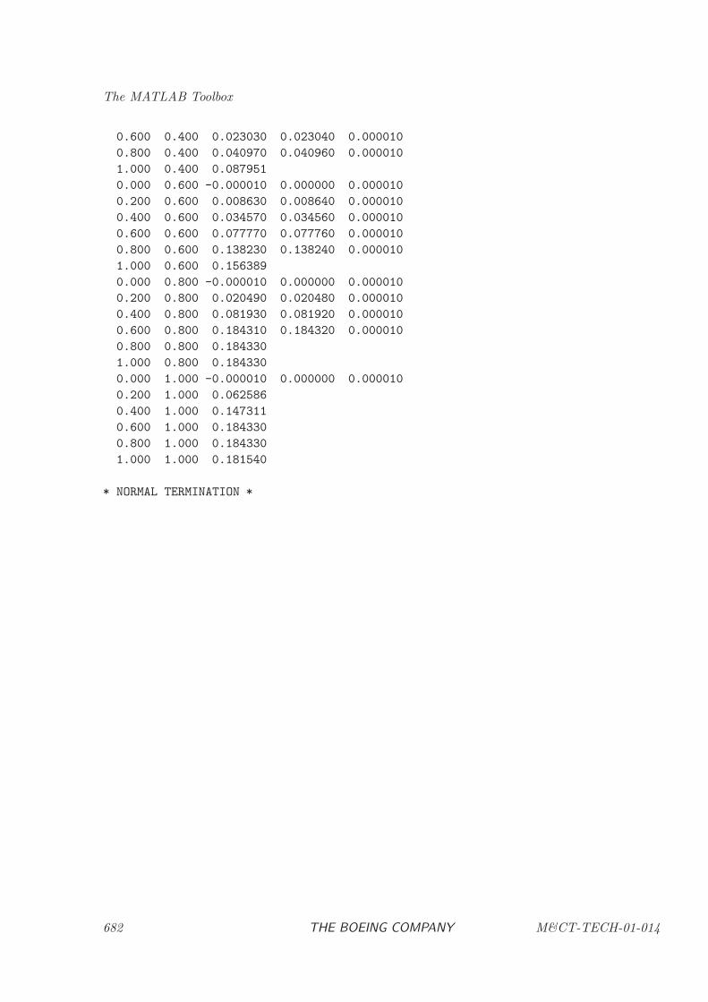
The MATLAB Toolbox
0.600 0.400 0.023030 0.023040 0.000010
0.800 0.400 0.040970 0.040960 0.000010
1.000 0.400 0.087951
0.000 0.600 -0.000010 0.000000 0.000010
0.200 0.600 0.008630 0.008640 0.000010
0.400 0.600 0.034570 0.034560 0.000010
0.600 0.600 0.077770 0.077760 0.000010
0.800 0.600 0.138230 0.138240 0.000010
1.000 0.600 0.156389
0.000 0.800 -0.000010 0.000000 0.000010
0.200 0.800 0.020490 0.020480 0.000010
0.400 0.800 0.081930 0.081920 0.000010
0.600 0.800 0.184310 0.184320 0.000010
0.800 0.800 0.184330
1.000 0.800 0.184330
0.000 1.000 -0.000010 0.000000 0.000010
0.200 1.000 0.062586
0.400 1.000 0.147311
0.600 1.000 0.184330
0.800 1.000 0.184330
1.000 1.000 0.181540
* NORMAL TERMINATION *
682 THE BOEING COMPANY M&CT-TECH-01-014
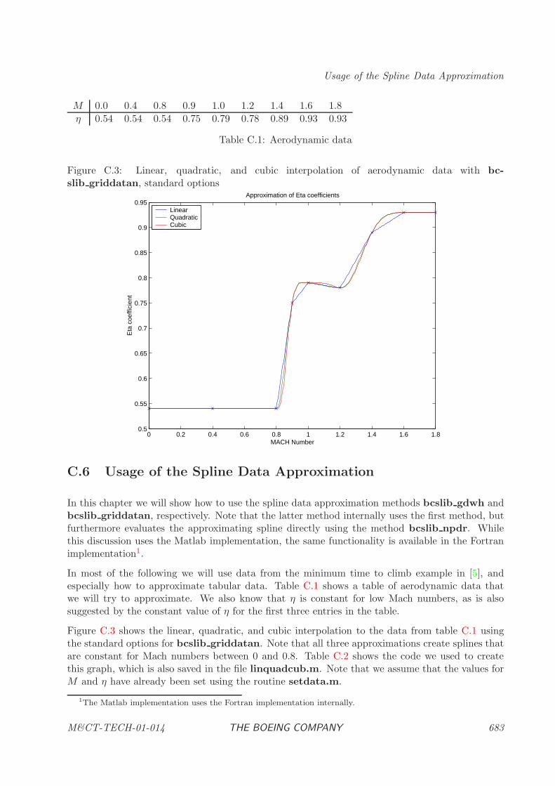
Usage of the Spline Data Approximation
M 0.0 0.4 0.8 0.9 1.0 1.2 1.4 1.6 1.8
η 0.54 0.54 0.54 0.75 0.79 0.78 0.89 0.93 0.93
Table C.1: Aerodynamic data
Figure C.3: Linear, quadratic, and cubic interpolation of aerodynamic data with bc-slib griddatan, standard options
0 0.2 0.4 0.6 0.8 1 1.2 1.4 1.6 1.80.5
0.55
0.6
0.65
0.7
0.75
0.8
0.85
0.9
0.95Approximation of Eta coefficients
MACH Number
Eta
coe
ffici
ent
LinearQuadraticCubic
C.6 Usage of the Spline Data Approximation
In this chapter we will show how to use the spline data approximation methods bcslib gdwh andbcslib griddatan, respectively. Note that the latter method internally uses the first method, butfurthermore evaluates the approximating spline directly using the method bcslib npdr. Whilethis discussion uses the Matlab implementation, the same functionality is available in the Fortranimplementation1.
In most of the following we will use data from the minimum time to climb example in [5], andespecially how to approximate tabular data. Table C.1 shows a table of aerodynamic data thatwe will try to approximate. We also know that η is constant for low Mach numbers, as is alsosuggested by the constant value of η for the first three entries in the table.
Figure C.3 shows the linear, quadratic, and cubic interpolation to the data from table C.1 usingthe standard options for bcslib griddatan. Note that all three approximations create splines thatare constant for Mach numbers between 0 and 0.8. Table C.2 shows the code we used to createthis graph, which is also saved in the file linquadcub.m. Note that we assume that the values forM and η have already been set using the routine setdata.m.
1The Matlab implementation uses the Fortran implementation internally.
M&CT-TECH-01-014 THE BOEING COMPANY 683
The MATLAB Toolbox
Mz_lin = bcslib_griddatan(M’,eta’,Mdiff,’linear’);
Mz_quad = bcslib_griddatan(M’,eta’,Mdiff,’quadratic’);
Mz_cubic = bcslib_griddatan(M’,eta’,Mdiff,’cubic’);
plot(Mdiff, Mz_lin, Mdiff, Mz_quad, Mdiff, Mz_cubic);
title(’Approximation of Eta coefficients’)
xlabel(’MACH Number’);
ylabel(’Eta coefficient’);
legend( ’Linear’,’Quadratic’,’Cubic’,2);
hold on
plot(M,eta,’x’);
hold off
Table C.2: Matlab code to calculate linear, quadratic, and cubic approximations.
The first option we will explore is the error tolerance. Tabular data is most of the time createdby taking measurements. This implies that the tabular data is not exact, but includes errors. Theapproximation routine allows the user to specify error bounds in the measurement. The first wayto do this assumes that the error bounds are constant for all data points. If this is the case, theuser can set opts.abstol to these bounds. Figure C.4 and Table C.3 show a plot of this and thecorresponding code taken from cubicconsterr.m.
In this plot we show an error bar for each data point signaling the range that the approximation isallowed to vary. Note that by using this error tolerance (or bounds), the approximation betweenthe fifth and sixth data point becomes constant.
In the next example we actually perturb the tabular data to show the effect this has on theapproximation with tight error tolerance (i.e. the standard setting), and how the use of a loosererror tolerance allows the approximation to keep the desired features. We only perturb the firstentry by subtracting .005, and the second entry by adding .007.
Figure C.5 and Table C.4 show a plot of this and the corresponding code taken from cubicme-serr.m. Note that the approximation with standard error bounds bends to interpolate all datapoints, whereas the approximation with looser constant error tolerance is constant through the firstthree data points.
Sometimes measurements have varying precision depending on where in their range a measurementis taken. For the next example, we assume that the instrument used to measure η is relativelyimprecise for low Mach numbers, but very precise for higher Mach numbers. The approximationmethod allows the user to define an error tolerance for each individual data point. We use thisfeature in the next example to define loose tolerances for the first three data points, and stricttolerances for all other.
Figure C.6 and Table C.5 show a plot of this and the corresponding code taken from cubicmeser-radj.m. The two approximations only differ significantly for the first three data points.
The next example examines another option the user can specify. This option controls the lo-
684 THE BOEING COMPANY M&CT-TECH-01-014
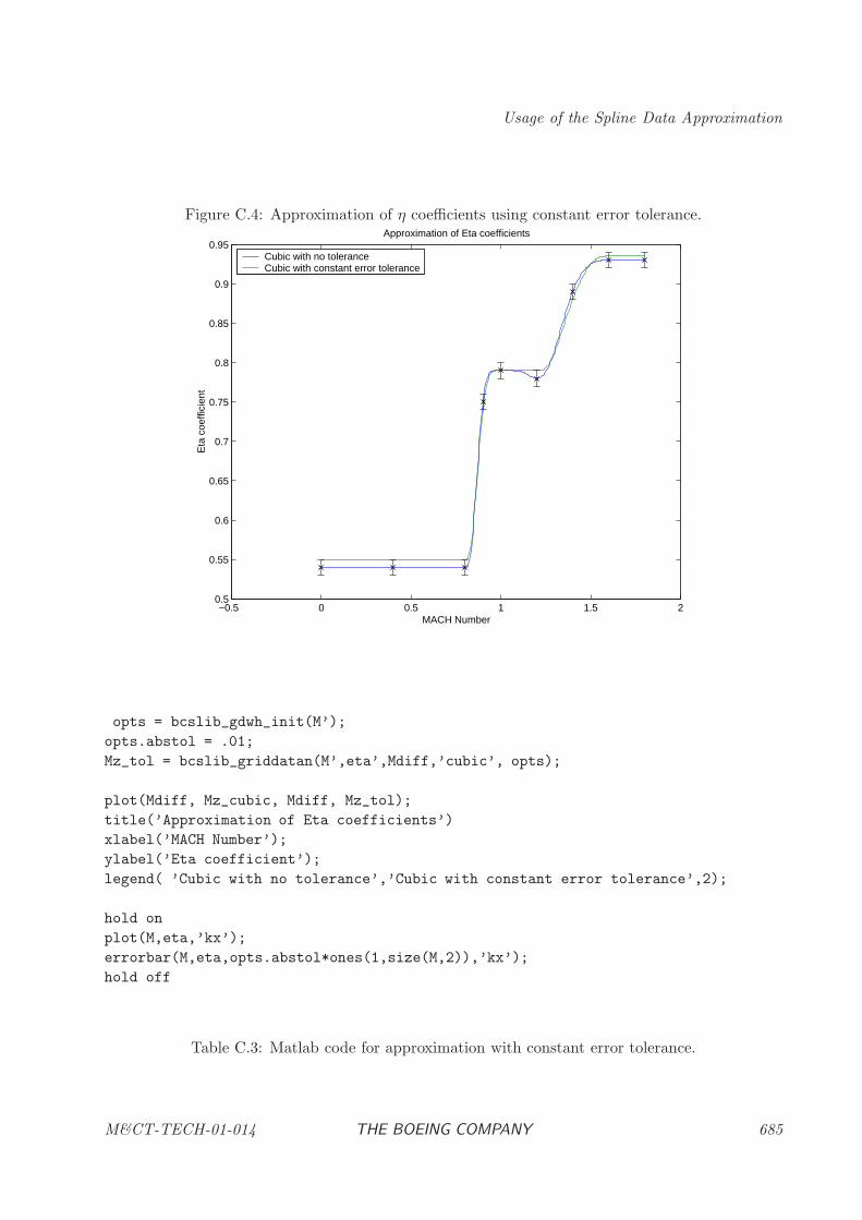
Usage of the Spline Data Approximation
Figure C.4: Approximation of η coefficients using constant error tolerance.
−0.5 0 0.5 1 1.5 20.5
0.55
0.6
0.65
0.7
0.75
0.8
0.85
0.9
0.95Approximation of Eta coefficients
MACH Number
Eta
coe
ffici
ent
Cubic with no toleranceCubic with constant error tolerance
opts = bcslib_gdwh_init(M’);
opts.abstol = .01;
Mz_tol = bcslib_griddatan(M’,eta’,Mdiff,’cubic’, opts);
plot(Mdiff, Mz_cubic, Mdiff, Mz_tol);
title(’Approximation of Eta coefficients’)
xlabel(’MACH Number’);
ylabel(’Eta coefficient’);
legend( ’Cubic with no tolerance’,’Cubic with constant error tolerance’,2);
hold on
plot(M,eta,’kx’);
errorbar(M,eta,opts.abstol*ones(1,size(M,2)),’kx’);
hold off
Table C.3: Matlab code for approximation with constant error tolerance.
M&CT-TECH-01-014 THE BOEING COMPANY 685
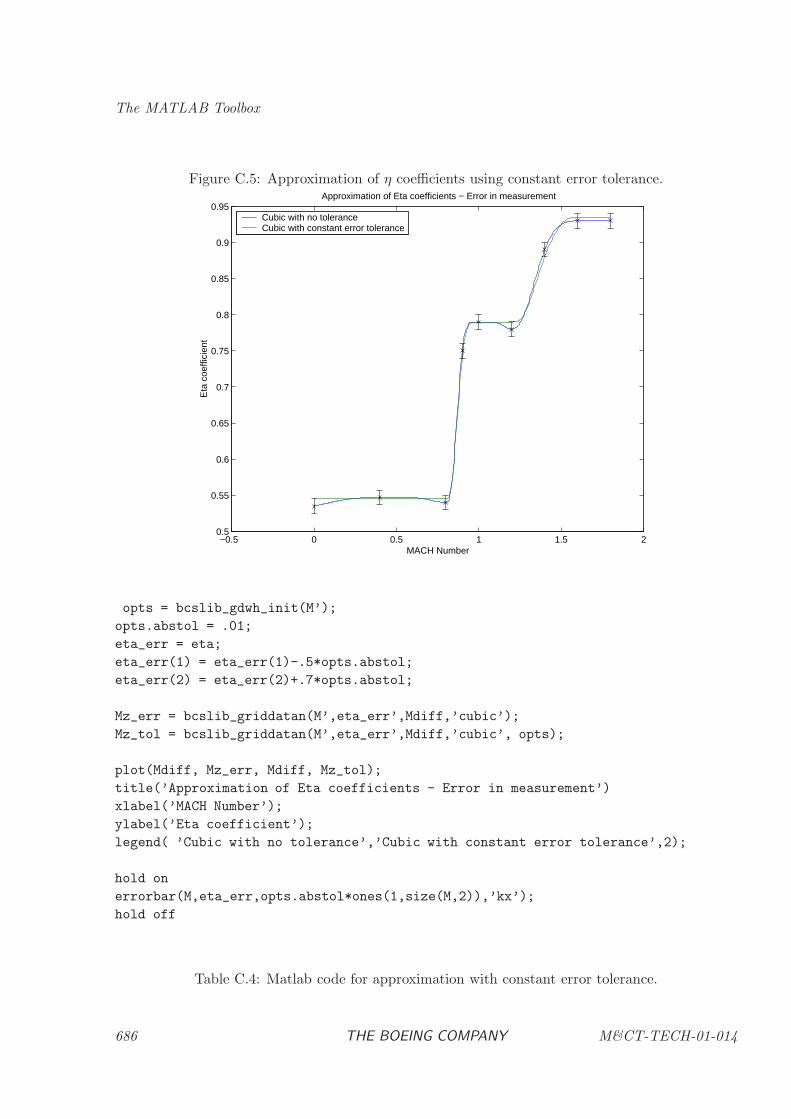
The MATLAB Toolbox
Figure C.5: Approximation of η coefficients using constant error tolerance.
−0.5 0 0.5 1 1.5 20.5
0.55
0.6
0.65
0.7
0.75
0.8
0.85
0.9
0.95Approximation of Eta coefficients − Error in measurement
MACH Number
Eta
coe
ffici
ent
Cubic with no toleranceCubic with constant error tolerance
opts = bcslib_gdwh_init(M’);
opts.abstol = .01;
eta_err = eta;
eta_err(1) = eta_err(1)-.5*opts.abstol;
eta_err(2) = eta_err(2)+.7*opts.abstol;
Mz_err = bcslib_griddatan(M’,eta_err’,Mdiff,’cubic’);
Mz_tol = bcslib_griddatan(M’,eta_err’,Mdiff,’cubic’, opts);
plot(Mdiff, Mz_err, Mdiff, Mz_tol);
title(’Approximation of Eta coefficients - Error in measurement’)
xlabel(’MACH Number’);
ylabel(’Eta coefficient’);
legend( ’Cubic with no tolerance’,’Cubic with constant error tolerance’,2);
hold on
errorbar(M,eta_err,opts.abstol*ones(1,size(M,2)),’kx’);
hold off
Table C.4: Matlab code for approximation with constant error tolerance.
686 THE BOEING COMPANY M&CT-TECH-01-014
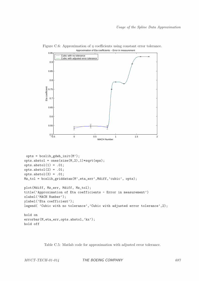
Usage of the Spline Data Approximation
Figure C.6: Approximation of η coefficients using constant error tolerance.
−0.5 0 0.5 1 1.5 20.5
0.55
0.6
0.65
0.7
0.75
0.8
0.85
0.9
0.95Approximation of Eta coefficients − Error in measurement
MACH Number
Eta
coe
ffici
ent
Cubic with no toleranceCubic with adjusted error tolerance
opts = bcslib_gdwh_init(M’);
opts.abstol = ones(size(M,2),1)*sqrt(eps);
opts.abstol(1) = .01;
opts.abstol(2) = .01;
opts.abstol(3) = .01;
Mz_tol = bcslib_griddatan(M’,eta_err’,Mdiff,’cubic’, opts);
plot(Mdiff, Mz_err, Mdiff, Mz_tol);
title(’Approximation of Eta coefficients - Error in measurement’)
xlabel(’MACH Number’);
ylabel(’Eta coefficient’);
legend( ’Cubic with no tolerance’,’Cubic with adjusted error tolerance’,2);
hold on
errorbar(M,eta_err,opts.abstol,’kx’);
hold off
Table C.5: Matlab code for approximation with adjusted error tolerance.
M&CT-TECH-01-014 THE BOEING COMPANY 687
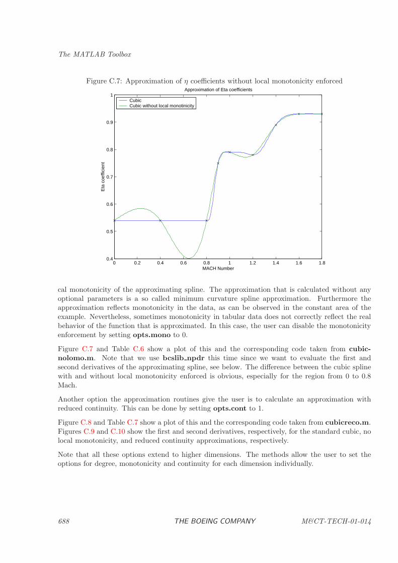
The MATLAB Toolbox
Figure C.7: Approximation of η coefficients without local monotonicity enforced
0 0.2 0.4 0.6 0.8 1 1.2 1.4 1.6 1.80.4
0.5
0.6
0.7
0.8
0.9
1Approximation of Eta coefficients
MACH Number
Eta
coe
ffici
ent
CubicCubic without local monotinicity
cal monotonicity of the approximating spline. The approximation that is calculated without anyoptional parameters is a so called minimum curvature spline approximation. Furthermore theapproximation reflects monotonicity in the data, as can be observed in the constant area of theexample. Nevertheless, sometimes monotonicity in tabular data does not correctly reflect the realbehavior of the function that is approximated. In this case, the user can disable the monotonicityenforcement by setting opts.mono to 0.
Figure C.7 and Table C.6 show a plot of this and the corresponding code taken from cubic-nolomo.m. Note that we use bcslib npdr this time since we want to evaluate the first andsecond derivatives of the approximating spline, see below. The difference between the cubic splinewith and without local monotonicity enforced is obvious, especially for the region from 0 to 0.8Mach.
Another option the approximation routines give the user is to calculate an approximation withreduced continuity. This can be done by setting opts.cont to 1.
Figure C.8 and Table C.7 show a plot of this and the corresponding code taken from cubicreco.m.Figures C.9 and C.10 show the first and second derivatives, respectively, for the standard cubic, nolocal monotonicity, and reduced continuity approximations, respectively.
Note that all these options extend to higher dimensions. The methods allow the user to set theoptions for degree, monotonicity and continuity for each dimension individually.
688 THE BOEING COMPANY M&CT-TECH-01-014
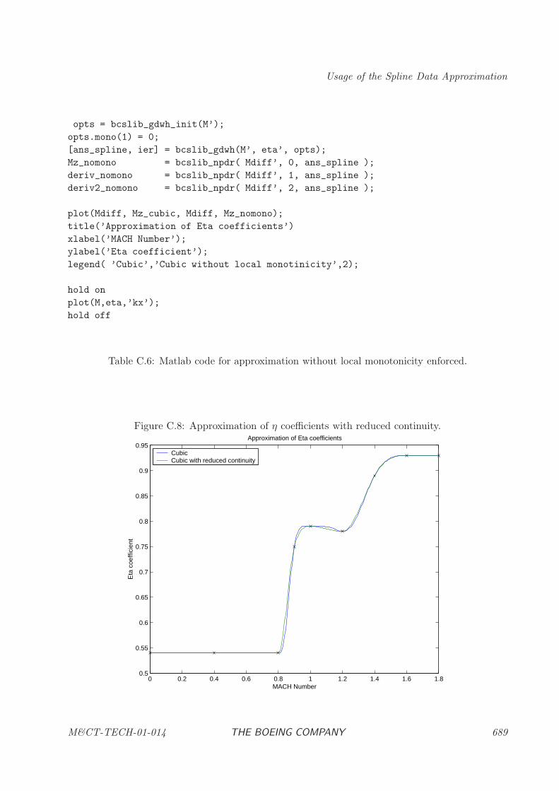
Usage of the Spline Data Approximation
opts = bcslib_gdwh_init(M’);
opts.mono(1) = 0;
[ans_spline, ier] = bcslib_gdwh(M’, eta’, opts);
Mz_nomono = bcslib_npdr( Mdiff’, 0, ans_spline );
deriv_nomono = bcslib_npdr( Mdiff’, 1, ans_spline );
deriv2_nomono = bcslib_npdr( Mdiff’, 2, ans_spline );
plot(Mdiff, Mz_cubic, Mdiff, Mz_nomono);
title(’Approximation of Eta coefficients’)
xlabel(’MACH Number’);
ylabel(’Eta coefficient’);
legend( ’Cubic’,’Cubic without local monotinicity’,2);
hold on
plot(M,eta,’kx’);
hold off
Table C.6: Matlab code for approximation without local monotonicity enforced.
Figure C.8: Approximation of η coefficients with reduced continuity.
0 0.2 0.4 0.6 0.8 1 1.2 1.4 1.6 1.80.5
0.55
0.6
0.65
0.7
0.75
0.8
0.85
0.9
0.95Approximation of Eta coefficients
MACH Number
Eta
coe
ffici
ent
CubicCubic with reduced continuity
M&CT-TECH-01-014 THE BOEING COMPANY 689
The MATLAB Toolbox
[ans_spline, ier] = bcslib_gdwh(M’, eta’);
Mz_cubic = bcslib_npdr( Mdiff’, 0, ans_spline );
deriv_cubic = bcslib_npdr( Mdiff’, 1, ans_spline );
deriv2_cubic = bcslib_npdr( Mdiff’, 2, ans_spline );
opts = bcslib_gdwh_init(M’);
opts.cont(1) = 1;
[ans_spline, ier] = bcslib_gdwh(M’, eta’, opts);
Mz_nocont = bcslib_npdr( Mdiff’, 0, ans_spline );
deriv_nocont = bcslib_npdr( Mdiff’, 1, ans_spline );
deriv2_nocont = bcslib_npdr( Mdiff’, 2, ans_spline );
plot(Mdiff, Mz_cubic, Mdiff, Mz_nocont);
title(’Approximation of Eta coefficients’)
xlabel(’MACH Number’);
ylabel(’Eta coefficient’);
legend( ’Cubic’,’Cubic with reduced continuity’,2);
hold on
plot(M,eta,’kx’);
hold off
Table C.7: Matlab code for approximation with reduced continuity.
690 THE BOEING COMPANY M&CT-TECH-01-014
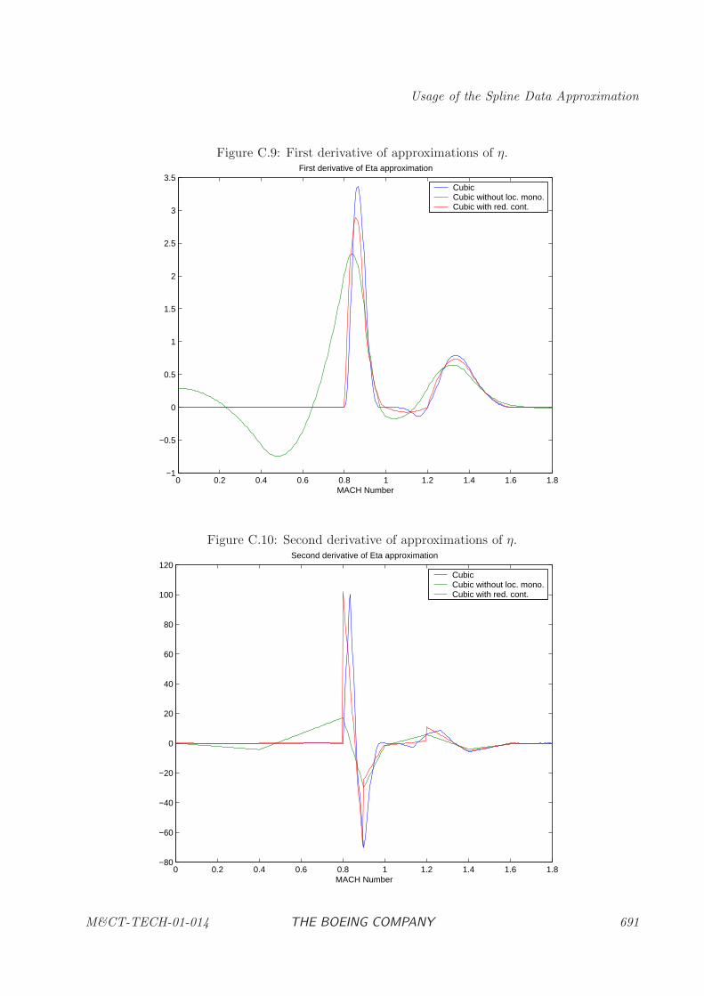
Usage of the Spline Data Approximation
Figure C.9: First derivative of approximations of η.
0 0.2 0.4 0.6 0.8 1 1.2 1.4 1.6 1.8−1
−0.5
0
0.5
1
1.5
2
2.5
3
3.5First derivative of Eta approximation
MACH Number
CubicCubic without loc. mono.Cubic with red. cont.
Figure C.10: Second derivative of approximations of η.
0 0.2 0.4 0.6 0.8 1 1.2 1.4 1.6 1.8−80
−60
−40
−20
0
20
40
60
80
100
120Second derivative of Eta approximation
MACH Number
CubicCubic without loc. mono.Cubic with red. cont.
M&CT-TECH-01-014 THE BOEING COMPANY 691

The MATLAB Toolbox
692 THE BOEING COMPANY M&CT-TECH-01-014
BIBLIOGRAPHY
Bibliography
[1] BCSLIB-EXT Mathematical Library, The Boeing Extended Mathematical Subprogram Li-brary. Mathematics and Engineering Analysis Library Report 20462-0520-R3, Boeing Infor-mation and Support Services, The Boeing Company, PO Box 3707, Seattle, WA 98124-2207,December 1993.
[2] BCSLIB Mathematical/Statistical Library, Fortran Version, User’s Guide. Mathematics andEngineering Analysis Library Report 20462-0516-R14, Boeing Information and Support Ser-vices, The Boeing Company, PO Box 3707, Seattle, WA 98124-2207, June 1993.
[3] John T. Betts. Trajectory Optimization Using Sparse Sequential Quadratic Programming.In Roland Bulirsch, Angelo Miele, Josef Stoer, and Klaus H. Well, editors, Optimal Control,volume 111 of International Series of Numerical Mathematics, pages 115–128, Basel, 1993.Birkhauser Verlag.
[4] John T. Betts. Issues in the Direct Transcription of Optimal Control Problems to SparseNonlinear Programs. In Roland Bulirsch and Dieter Kraft, editors, Computational OptimalControl, volume 115 of International Series of Numerical Mathematics, pages 3–18. BirkhauserVerlag, Basel, 1994.
[5] John T. Betts. Practical Methods for Optimal Control using Nonlinear Programming. Societyfor Industrial and Applied Mathematics, Philadelphia, PA., 2001.
[6] John T. Betts, Samuel K. Eldersveld, Paul D. Frank, and John G. Lewis. An Interior-PointNonlinear Programming Algorithm for Very Large Scale Optimization. In Lorenz T. Biegler,Omar Ghattas, Matthias Heinkenschloss, and Bart van Bloemen Waanders, editors, Large-Scale PDE-Constrained Optimization, pages 184–198. Springer-Verlag, Berlin, 2003.
[7] John T. Betts and Paul D. Frank. A Sparse Nonlinear Optimization Algorithm. Journal ofOptimization Theory and Applications, 82(3):519–541, September 1994.
[8] John T. Betts and William P. Huffman. Application of Sparse Nonlinear Programming toTrajectory Optimization. AIAA Journal of Guidance, Control, and Dynamics, 15(1):198–206,January–February 1992.
[9] John T. Betts and William P. Huffman. Path Constrained Trajectory Optimization UsingSparse Sequential Quadratic Programming. AIAA Journal of Guidance, Control, and Dynam-ics, 16(1):59–68, January–February 1993.
[10] John T. Betts and William P. Huffman. Sparse Optimal Control Software SOCS . Mathematicsand Engineering Analysis Technical Document MEA-LR-085, Boeing Information and SupportServices, The Boeing Company, PO Box 3707, Seattle, WA 98124-2207, July 1997.
M&CT-TECH-01-014 THE BOEING COMPANY 693
BIBLIOGRAPHY
[11] Arthur E. Bryson, Jr. and Yu-Chi Ho. Applied Optimal Control. John Wiley & Sons, NewYork, NY, 1975.
[12] Thomas F. Coleman and Jorge J. More. Estimation of Sparse Jacobian Matrices and GraphColoring Problems. SIAM Journal on Numerical Analysis, 20:187–209, 1983.
[13] A. R. Curtis, M. J. D. Powell, and J. K. Reid. On the Estimation of Sparse Jacobian Matrices.Journal of the Institute of Mathematics and Applications, 13:117–120, 1974.
[14] Ernst D. Dickmanns. Efficient Convergence and Mesh Refinement Strategies for Solving Gen-eral Ordinary Two-point Boundary Value Problems by Collocated Hermite Approximation.2nd IFAC Workshop on Optimisation, Oberpfaffenhofen, September 1980.
[15] Paul J. Enright and Bruce A. Conway. Optimal Finite-thrust Spacecraft Trajectories UsingCollocation and Nonlinear Programming. AIAA Journal of Guidance, Control, and Dynamics,14(5):981–985, 1991.
[16] Philip E. Gill, Walter Murray, and Michael A. Saunders. Users Guide for QPOPT (Version 1):a Fortran Package for Quadratic Programming. Technical Report Report NA 95-1, Departmentof Mathematics, University of California, San Diego.
[17] Philip E. Gill, Walter Murray, Michael A. Saunders, and Margaret H. Wright. Some TheoreticalProperties of an Augmented Lagrangian Merit Function. Technical Report Report SOL 86-6,Department of Operations Research, Stanford University, April 1986.
[18] Philip E. Gill, Walter Murray, Michael A. Saunders, and Margaret H. Wright. A Schur-complement Method for Sparse Quadratic Programming. Technical Report Report SOL 87-12,Department of Operations Research, Stanford University, October 1987.
[19] E. Hairer, S. P. Norsett, and G. Wanner. Solving Ordinary Differential Equations I NonstiffProblems. Springer-Verlag, New York, New York, 1993.
[20] Charles R. Hargraves and Stephen W. Paris. Direct Trajectory Optimization Using NonlinearProgramming and Collocation. AIAA Journal of Guidance, Control, and Dynamics, 10(4):338–342, July–August 1987.
[21] Oskar von Stryk. Numerical Solution of Optimal Control Problems by Direct Collocation.In Roland Bulirsch, Angelo Miele, Josef Stoer, and Klaus H. Well, editors, Optimal Control,volume 111 of International Series of Numerical Mathematics, pages 129–143, Basel, 1993.Birkhauser Verlag.
I-694 THE BOEING COMPANY M&CT-TECH-01-014
INDEX
Index
Evaluation
of a tensor product spline, 586, 651fast, 601, 655, 659, 663
of a tensor product spline with extrapola-tion, 593
fast, 607
Splinestensor product, 586, 593, 601, 607, 651, 655,
659, 663
Subprograms
AUTOLK, 414
AUTOPL, 416AUXOUT, 418
BCSLIBCONVERTSPLINE, 667
BCSLIBENVL, 659
BCSLIBFEVL, 663BCSLIBFNVL, 655
BCSLIBGDWH, 629
BCSLIBGDWHINIT, 638
BCSLIBGRIDDATA, 639BCSLIBGRIDDATAN, 648
BCSLIBNPVL, 651
BCSLIBWRITESPLINE, 668
BSPDEF, 422CTLFIL, 427
CTLSTA, 429
DDLOAD, 378
FETCH, 430FYLFMT, 432
HDBLPQ, 181
HDBLSQ, 161
HDBNLP, 141HDBNPD, 107
HDBNPR, 123
HDCMVS, 567
HDDFDH, 245HDDFDJ, 236
HDENVL, 593
HDFEVL, 607
HDFNVL, 601HDGDWH, 556
HDMGDI, 547HDNLPD, 14HDNLPR, 33HDNPVL, 586
HDSFDC, 288HDSFDH, 276HDSFDJ, 263
HDSFDP, 293HDSLSQ, 70HDSNLP, 51HDSNPV, 105
HDSOCS, 351HDSOPE, 358HDSQSH, 91HHSNLP, 196
HHSOCS, 365HJSFDI, 256LINKST, 435
NUMGRD, 437OCSEVL, 439OCSGRD, 443OCSRNG, 445
OCSTAU, 447ODEIGS, 381ODEINP, 384
ODEPRT, 401ODEPTF, 405ODERHS, 409PHSLNG, 450
PNTCON, 452PTHAUX, 455PTHCON, 458
RST2SP, 461SCTFIL, 463SOCSNLP, 624SOCSNLPINIT, 627
TRMAUX, 465WATCH, 467
M&CT-TECH-01-014 THE BOEING COMPANY I-695

INDEX
Tensor product splinesevaluation, 586, 651evaluation with extrapolation, 593fast evaluation, 601, 655, 659, 663fast evaluation with extrapolation, 607
I-696 THE BOEING COMPANY M&CT-TECH-01-014