Socio-Economic Status, Income, & Wealth

Dimitrios Christelis, Tullio Jappelli, Omar Paccagnella and Guglielmo Weber

16 February 2006 Acknowledgements: The SHARE data collection has been primarily funded by the European Commission through the 5th framework programme (project QLK6-CT-2001-00360 in the thematic programme Quality of Life). Additional funding came from the US National Institute on Aging (U01 AG09740-13S2, P01 AG005842, P01 AG08291, P30 AG12815, Y1-AG-4553-01 and OGHA 04-064). Data collection in Austria (through the Austrian Science Fund, FWF), Belgium (through the Belgian Science Policy Office) and Switzerland (through BBW/OFES/UFES) was nationally funded. The SHARE data set is introduced in Börsch-Supan et al. (2005); methodological details are contained in Börsch-Supan and Jürges (2005). Dimitris Christelis and Tullio Jappelli: University of Salerno and CSEF Omar Paccagnella and Guglielmo Weber: Department of Economics, University of Padua

2

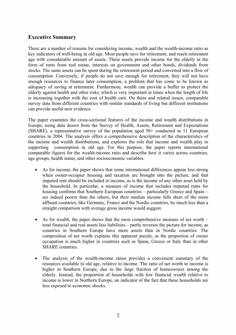
Executive Summary There are a number of reasons for considering income, wealth and the wealth-income ratio as key indicators of well-being in old age. Most people save for retirement, and reach retirement age with considerable amount of assets. These assets provide income for the elderly in the form of rents from real estate, interests on government and other bonds, dividends from stocks. The same assets can be spent during the retirement period and converted into a flow of consumption. Conversely, if people do not save enough for retirement, they will not have enough resources to finance later consumption, a problem that has come to be known as adequacy of saving at retirement. Furthermore, wealth can provide a buffer to protect the elderly against health and other risks, which is very important at times when the length of life is increasing together with the cost of health care. On these and related issues, comparable survey data from different countries with similar standards of living but different institutions can provide useful new evidence.

The paper examines the cross-sectional features of the income and wealth distributions in Europe, using data drawn from the Survey of Health, Assets, Retirement and Expectations (SHARE), a representative survey of the population aged 50+ conducted in 11 European countries in 2004. The analysis offers a comprehensive description of the characteristics of the income and wealth distributions, and explores the role that income and wealth play in supporting consumption in old age. For this purpose, the paper reports international comparable figures for the wealth-income ratio and describe how it varies across countries, age groups, health status, and other socioeconomic variables.

• As for income, the paper shows that some international differences appear less strong

when owner-occupier housing and taxation are brought into the picture, and that imputed rent should be included in income, as is the income of any other asset held by the household. In particular, a measure of income that includes imputed rents for housing confirms that Southern European countries – particularly Greece and Spain – are indeed poorer than the others, but their median income falls short of the more affluent countries, like Germany, France and the Nordic countries, by much less than a straight comparison with average gross income would suggest.

• As for wealth, the paper shows that the most comprehensive measure of net worth –

total financial and real assets less liabilities – partly reverses the picture for income, as countries in Southern Europe have more assets than in Nordic countries. The composition of net worth explains this apparent puzzle, as the proportion of owner occupation is much higher in countries such as Spain, Greece or Italy than in other SHARE countries.

• The analysis of the wealth-income ratios provides a convenient summary of the

resources available to old age, relative to income. The ratio of net worth to income is higher in Southern Europe, due to the large fraction of homeowners among the elderly. Instead, the proportion of households with low financial wealth relative to income is lower in Northern Europe, an indicator of the fact that these households are less exposed to economic shocks.

3

1. Introduction

In this paper we examine the cross-sectional features of the income and wealth distributions in Europe, using data drawn from the Survey of Health, Assets, Retirement and Expectations (SHARE), a representative survey of the population aged 50+ conducted in 11 countries in 2004. The purpose of our analysis is to offer a comprehensive description of the characteristics of the income and wealth distributions, and to explore the role that income and wealth have to support consumption in old age. For this purpose, we reporting international comparable figures for the wealth-income ratio and describe how it varies across countries, age groups, health status, and other socioeconomic variables.

Because of the demographic trends, the resources available for the elderly and their saving behaviour are central to the current policy debate. While income is an important determinant of current well-being, assets are a key indicator of future, sustainable consumption of the elderly. SHARE allows the study of the composition of income and wealth around and after retirement, and the extent to which the wealth of the elderly is annuitized through pensions, social security, and health insurance.

There are a number of reasons for considering income, wealth and the wealth-income ratio as key indicators of well-being in old age. Most people save for retirement, and reach retirement age with considerable amount of assets. These assets provide income for the elderly in the form of rents from real estate, interests on government and other bonds, dividends from stocks. The same assets can be spent during the retirement period and converted into a flow of consumption. Conversely, if people do not save enough for retirement, they will not have enough resources to finance later consumption, a problem that has come to be known as adequacy of saving at retirement. Furthermore, wealth can provide a buffer to protect the elderly against health and other risks, which is very important at times when the length of life is increasing together with the cost of health care.

On these and related issues, SHARE provides fresh evidence in comparative fashion. The paper starts out describing income and wealth and distributions (Sections 2 and 3, respectively), and then turn to examining the distribution of the wealth-income ratio (Section 4). Section 5 concludes. The Appendix reports detailed definitions and imputation procedures for income and wealth. 2. The income of the elderly

Social scientists and economists have always shown a keen interest in income, for instance in their studies of economic inequality and poverty, and in most surveys containing questions on economic and social well-being, the only measure of access to economic resources is income. Indeed, income is an important (arguably, the most important) component of any measure of access to economic resources, thus deserving careful investigation on its own. For this reason, in this section we present statistics on household income as recorded in SHARE in a number of different dimensions.

In almost all EU policy statements income per capita statistics are core indicators for public policy. But our analysis reveals that coarse income measures mask important differences that are due to differences in purchasing power, in household size, in taxation, in

4

the services provided by owner-occupied housing. Only after allowance is made for all these factors, can we compare incomes across countries in a meaningful way.

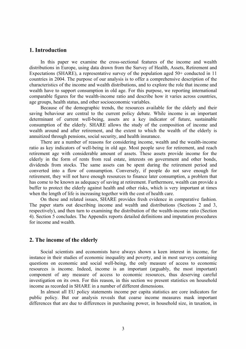
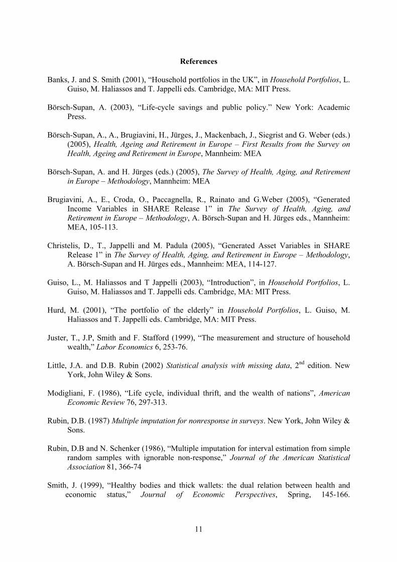
Insert Figure 1 – Average and median gross household income

In Figure 1 we summarise graphically some of the income differences found across SHARE countries by reporting average and median gross household income in its basic definition (excluding imputed rent from owner occupation – current exchange rates have been used to translate national currencies in Euros, where applicable). Average income exceeds € 45,000 in three countries (Denmark, the Netherlands, Switzerland), it lies between € 30,000 and € 45,000 in Austria, France, Germany and Sweden, it is below € 30,000 in Italy as well as in Greece and Spain.

Median income may be a better indicator of access to economic resources, as averages are heavily affected by the right tail of the distribution. In fact, Figure 1 shows that for all countries median income is much lower than average income, and that the difference is by no means constant. So Sweden replaces the Netherlands among the top three countries in terms of median income; among the lower income countries, Spain’s median income is less than half of Italy’s, whereas Austria and Italy appear quite close.

Next, we provide systematic evidence on ways in which income varies across countries, by looking at its various sources and by assessing the relevance of corrections for differences in purchasing power, household size and taxation. We shall also argue that some international differences appear less strong when owner-occupier housing is brought into the picture. All these adjustments can be implemented in the SHARE data in a consistent manner, and this makes this data set a particularly valuable source of information for policy analysis. 2.1. Income components

The SHARE questionnaire contains a number of questions on individual incomes, such as earnings, pensions and transfers, and a few questions on incomes that can only be recorded at the household level. The former are asked to all eligible individuals. The latter are asked to one particular respondent, and include items such as rents and housing benefits received, as well as an estimate of all individual incomes of non-eligible household members.1

SHARE is the only European – wide data set that collects the gross amount for all income components in a consistent way. Total household income is the sum of some incomes at the individual level and some at the household level. Lump-sum payments and financial support provided by parents, relatives or other people are excluded. The basic definition used here reflects money income before taxes on a yearly base (2003) and includes only regular payments.

The coarse income data require some adjustments before they can be used. First, imputations are needed for missing income items. Secondly, a correction must be made for differences in purchasing power across countries – to this end, we use OECD PPP exchange rates (that apply also within the Euro area) to turn nominal incomes into real incomes.

The issue of imputation is particularly relevant for income. In fact, household income is the sum of a very large number of items: for most of these, we have an exact record provided 1 Interest and dividend income is sometimes recorded at the individual level (when respondents keep their finances separate), but more often at the household level, and we therefore always treat it as a household level item (known as “capital income”). We should stress that household income does not include capital gains on financial or real assets.

5

by the respondent, but for some others such amount is not available. However, when respondents refused or were not able to provide an exact answer to a question on a particular income or asset component, they were routinely asked unfolding brackets questions (was this income higher/lower than a certain threshold?). These answers place the income in a certain range, but an exact value needs to be imputed. Imputations were made using a conditional hot-deck procedure: missing income items were randomly replaced with income records from households from the same country, same income range (where available) or sex and age (where such range was not available).2

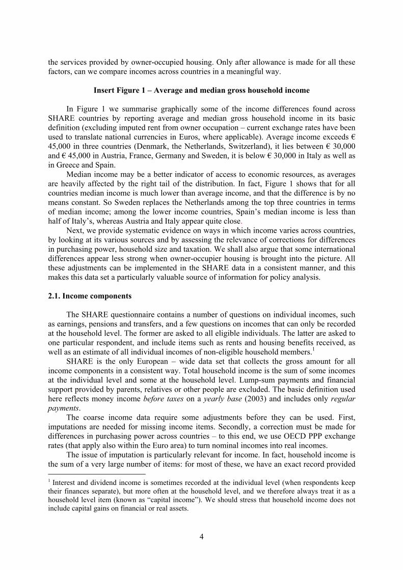
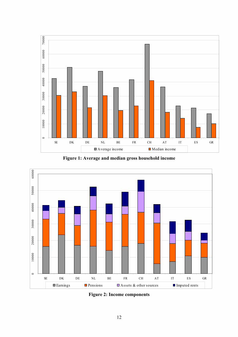
Insert Figure 2: Income components

Figure 2 shows the importance of different income components. We correct average gross income for purchasing power differences, and include in gross income imputed rent from owner occupation. Imputed rent is a relatively small item in Nordic countries, as well as in Germany, Greece and Austria, but it is quite important in France, Italy and Spain. This is consistent with the notion that in countries where credit markets are not well developed, but house prices are high, many elderly individuals are house-rich but cash-poor. However, imputed rent is also a highly volatile measure, being based on the market value of the main residence, and its average may be heavily influenced by the business cycle, as indeed capital income.

Two other striking features emerge when we look at Figure 2. First, earnings are the largest item in Denmark, Germany and Switzerland, whilst pensions play the biggest role in Austria and the Netherlands. Such differences may be due to differences in pension payments or in retirement ages across countries. Secondly, the residual item (that is mostly made of income from other members) is relatively small, except in Switzerland and the Netherlands. 2.2. Towards a better income measure

We have already stressed that average gross household income is a relatively

unsatisfactory measure of individuals’ access to economic resources and shown how different median income is from average income. In this section, we document the role of corrections for differences in purchasing power and in household size. We also show how to account for owner occupation housing (through imputed rent) and for tax and social security contributions paid. These two income /components are particularly important, as they vary greatly across countries, age and income groups.

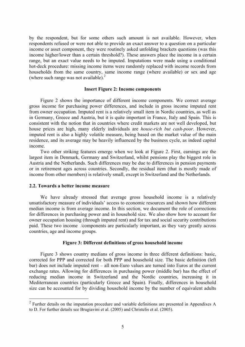
Figure 3: Different definitions of gross household income

Figure 3 shows country medians of gross income in three different definitions: basic,

corrected for PPP and corrected for both PPP and household size. The basic definition (left bar) does not include imputed rent – all non-Euro values are turned into Euros at the current exchange rates. Allowing for differences in purchasing power (middle bar) has the effect of reducing median income in Switzerland and the Nordic countries, increasing it in Mediterranean countries (particularly Greece and Spain). Finally, differences in household size can be accounted for by dividing household income by the number of equivalent adults

2 Further details on the imputation procedure and variable definitions are presented in Appendixes A to D. For further details see Brugiavini et al. (2005) and Christelis et al. (2005).

6

(EA, based on OECD scale – right bar). The resulting statistic comes close to the notion of per-capita income that is required for policy analysis, and shows that SHARE countries can be divided in three groups: Nordic countries, Switzerland and the Netherlands enjoy the highest gross income, followed by France, Belgium and Germany. Austria, Italy, and particularly Greece and Spain have the lowest gross income as defined here.

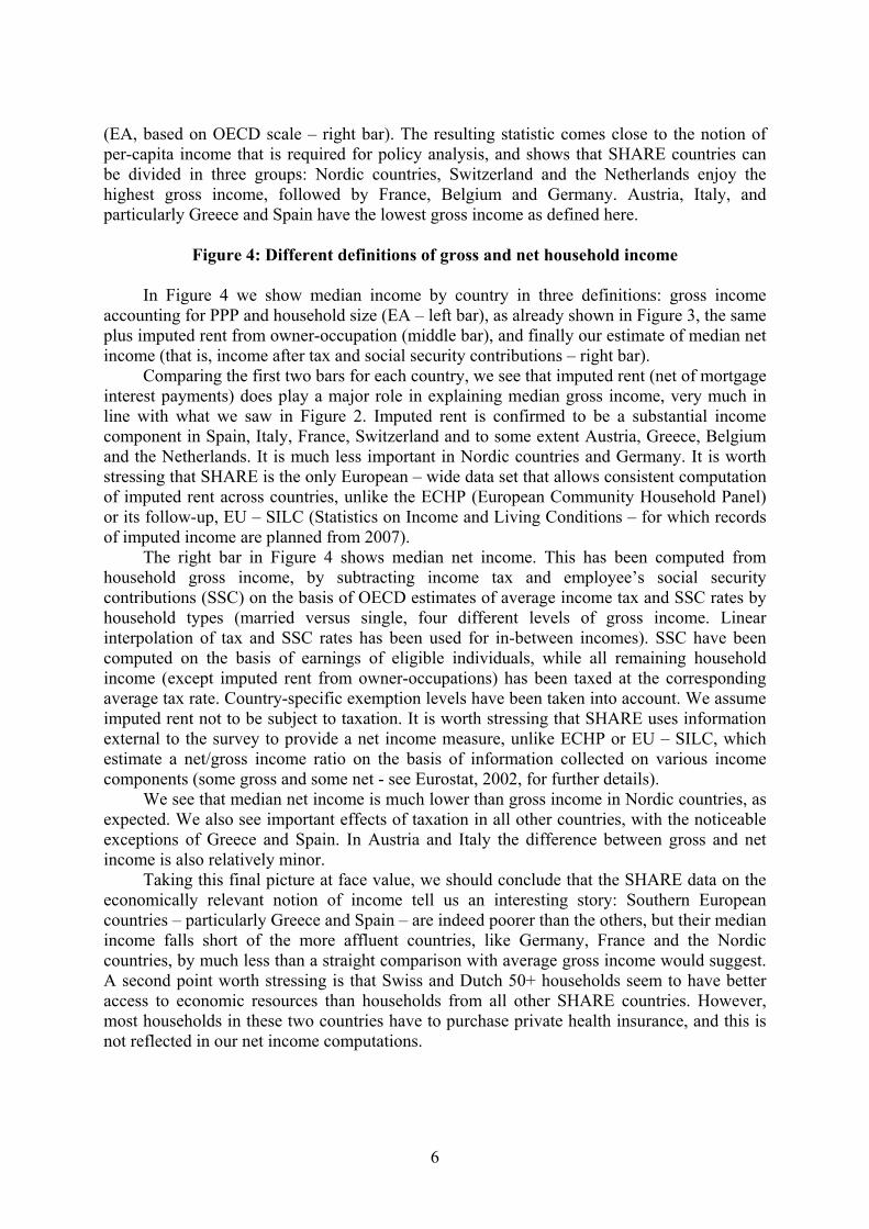
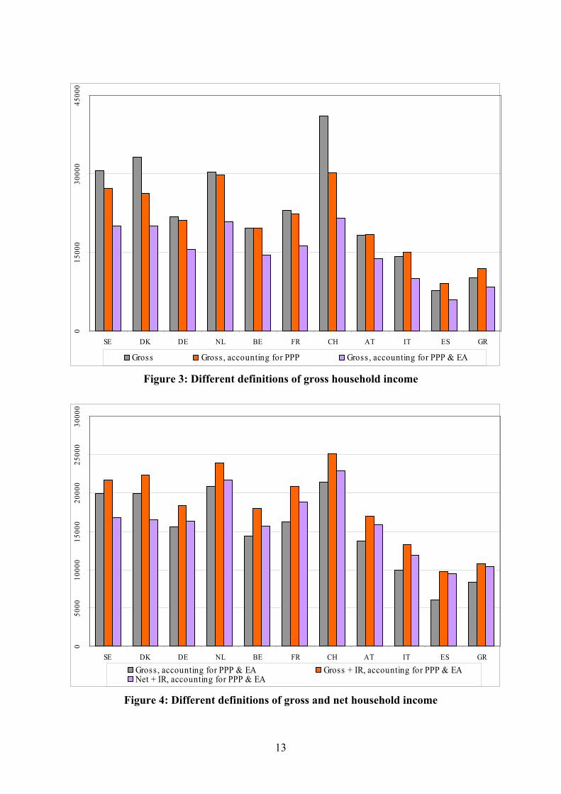
Figure 4: Different definitions of gross and net household income

In Figure 4 we show median income by country in three definitions: gross income accounting for PPP and household size (EA – left bar), as already shown in Figure 3, the same plus imputed rent from owner-occupation (middle bar), and finally our estimate of median net income (that is, income after tax and social security contributions – right bar).

Comparing the first two bars for each country, we see that imputed rent (net of mortgage interest payments) does play a major role in explaining median gross income, very much in line with what we saw in Figure 2. Imputed rent is confirmed to be a substantial income component in Spain, Italy, France, Switzerland and to some extent Austria, Greece, Belgium and the Netherlands. It is much less important in Nordic countries and Germany. It is worth stressing that SHARE is the only European – wide data set that allows consistent computation of imputed rent across countries, unlike the ECHP (European Community Household Panel) or its follow-up, EU – SILC (Statistics on Income and Living Conditions – for which records of imputed income are planned from 2007).

The right bar in Figure 4 shows median net income. This has been computed from household gross income, by subtracting income tax and employee’s social security contributions (SSC) on the basis of OECD estimates of average income tax and SSC rates by household types (married versus single, four different levels of gross income. Linear interpolation of tax and SSC rates has been used for in-between incomes). SSC have been computed on the basis of earnings of eligible individuals, while all remaining household income (except imputed rent from owner-occupations) has been taxed at the corresponding average tax rate. Country-specific exemption levels have been taken into account. We assume imputed rent not to be subject to taxation. It is worth stressing that SHARE uses information external to the survey to provide a net income measure, unlike ECHP or EU – SILC, which estimate a net/gross income ratio on the basis of information collected on various income components (some gross and some net - see Eurostat, 2002, for further details).

We see that median net income is much lower than gross income in Nordic countries, as expected. We also see important effects of taxation in all other countries, with the noticeable exceptions of Greece and Spain. In Austria and Italy the difference between gross and net income is also relatively minor.

Taking this final picture at face value, we should conclude that the SHARE data on the economically relevant notion of income tell us an interesting story: Southern European countries – particularly Greece and Spain – are indeed poorer than the others, but their median income falls short of the more affluent countries, like Germany, France and the Nordic countries, by much less than a straight comparison with average gross income would suggest. A second point worth stressing is that Swiss and Dutch 50+ households seem to have better access to economic resources than households from all other SHARE countries. However, most households in these two countries have to purchase private health insurance, and this is not reflected in our net income computations.

7

3. Wealth and wealth composition

Assets, both real and financial, can be spent during the retirement period and converted into a flow of consumption. Assets are therefore a measure of the resources on which retired individuals can rely to finance future consumption or to pass to future generations. Here we provide basic facts on wealth amounts and composition of the elderly in Europe.

The SHARE questionnaire covers a wide range of financial and real assets, from which one can calculate wealth and its components, and is designed to make the asset definition comparable across countries. Financial assets include seven broad categories: bank and other transaction accounts, government and corporate bonds, stocks, mutual funds, individual retirement accounts, contractual savings for housing, and life insurance policies. The real assets are primary and other residences, own business and vehicles. The asset module in SHARE has also questions on household liabilities, such as mortgages and other debts on cars, credit cards or towards banks, building societies and other financial institutions. As for the income questions, for financial assets and liabilities, if the point value is not available, financial respondents are routed into unfolding brackets.3

The detailed asset and liabilities questions contained in SHARE can be used to construct an indicator of the well being of the elderly as the sum of all financial and real assets, minus liabilities, a summary indicator of all resources that are available to household members. These assets can be used to finance normal retirement consumption, to buffer health and other risks the elderly face, or can be left as a bequest to future generations. To ensure cross-country comparability, the amounts are corrected for differences in the purchasing power of money across countries. In order to avoid the effect on cross-country comparison of households with influential values for wealth, we report medians rather than means of the relevant indicators.

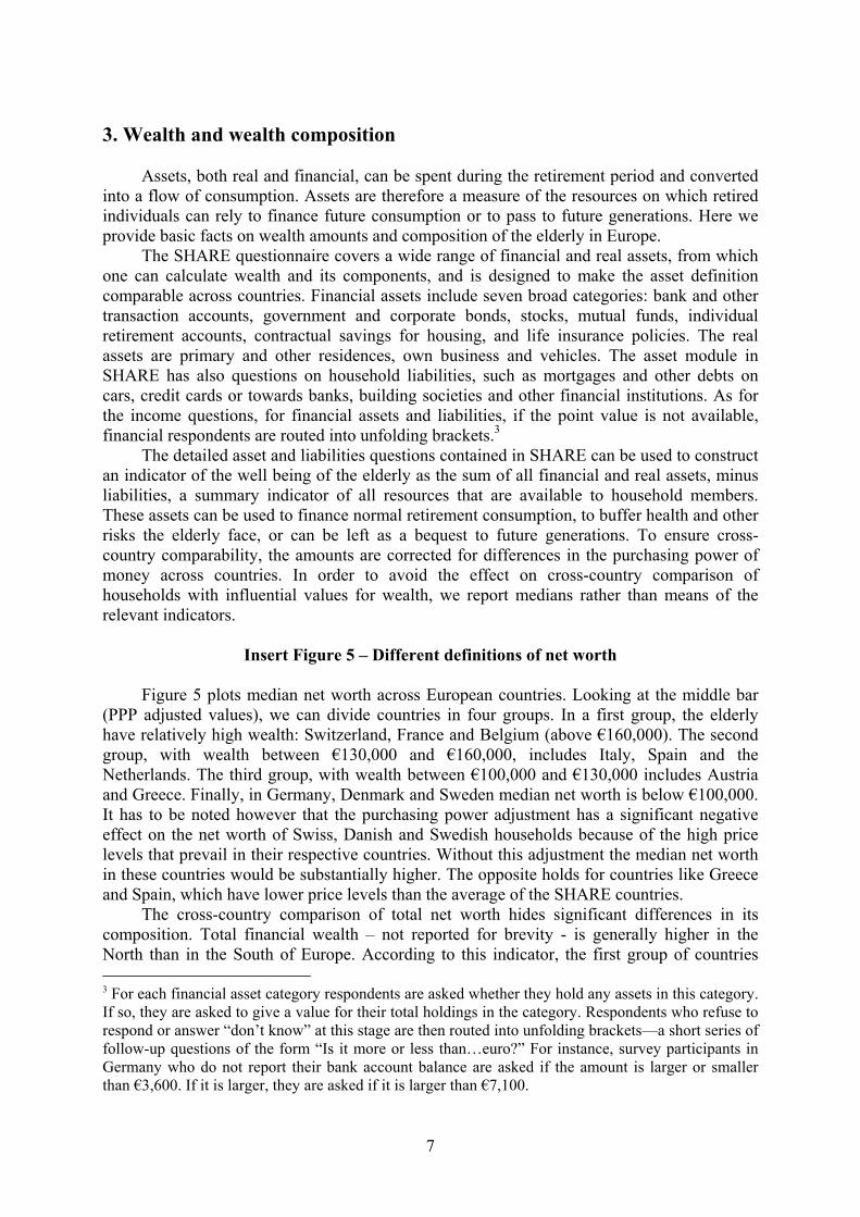
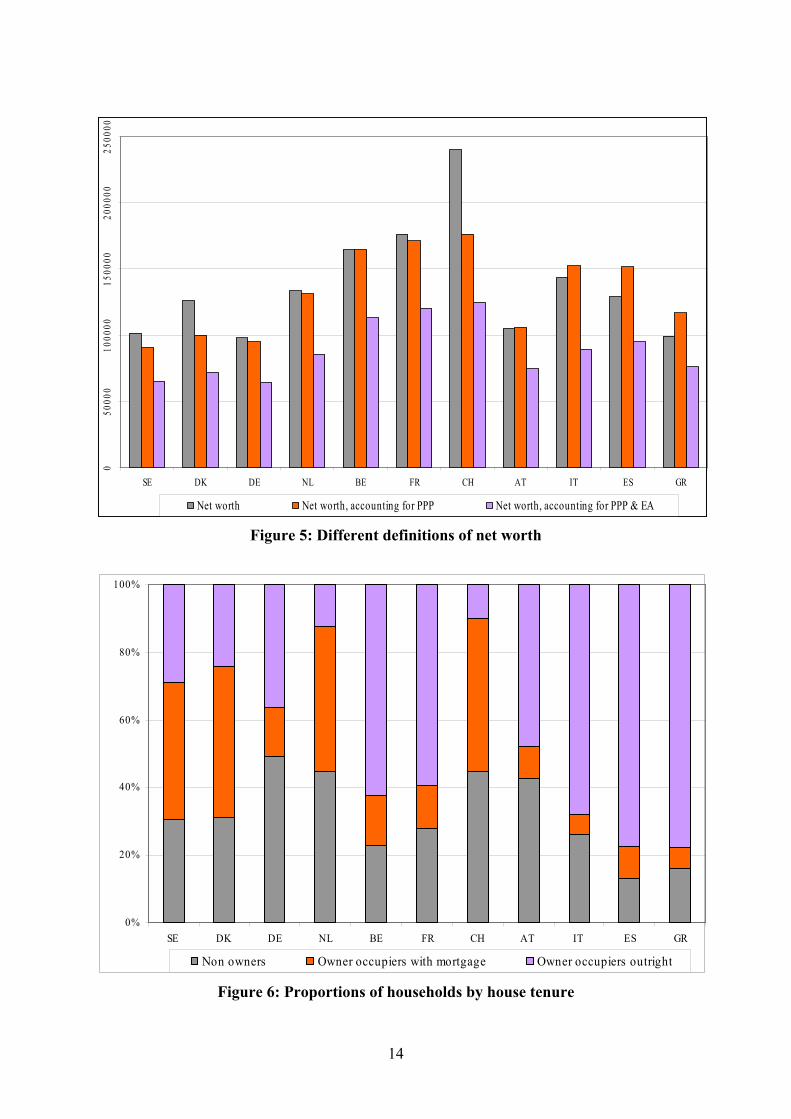
Insert Figure 5 – Different definitions of net worth

Figure 5 plots median net worth across European countries. Looking at the middle bar (PPP adjusted values), we can divide countries in four groups. In a first group, the elderly have relatively high wealth: Switzerland, France and Belgium (above €160,000). The second group, with wealth between €130,000 and €160,000, includes Italy, Spain and the Netherlands. The third group, with wealth between €100,000 and €130,000 includes Austria and Greece. Finally, in Germany, Denmark and Sweden median net worth is below €100,000. It has to be noted however that the purchasing power adjustment has a significant negative effect on the net worth of Swiss, Danish and Swedish households because of the high price levels that prevail in their respective countries. Without this adjustment the median net worth in these countries would be substantially higher. The opposite holds for countries like Greece and Spain, which have lower price levels than the average of the SHARE countries.

The cross-country comparison of total net worth hides significant differences in its composition. Total financial wealth – not reported for brevity - is generally higher in the North than in the South of Europe. According to this indicator, the first group of countries 3 For each financial asset category respondents are asked whether they hold any assets in this category. If so, they are asked to give a value for their total holdings in the category. Respondents who refuse to respond or answer “don’t know” at this stage are then routed into unfolding brackets—a short series of follow-up questions of the form “Is it more or less than…euro?” For instance, survey participants in Germany who do not report their bank account balance are asked if the amount is larger or smaller than €3,600. If it is larger, they are asked if it is larger than €7,100.

8

(financial wealth above €20,000) includes Switzerland and Sweden. Next come France, Belgium, Germany and Netherlands (between €10,000 and €20,000). The group of countries with lower level of median financial wealth per household (less than €10,000) includes Austria, Italy, Greece and Spain. These low amounts for the Mediterranean countries and Austria reflect in part the very low ownership rate in those countries of any financial assets other than bank accounts (e.g., in Greece) and in part the relative high weight of residential and other real estate wealth (e.g., in Italy and Spain).

A comparison between the two pictures makes it clear that the cross-country distribution of gross financial assets does not parallel that of net worth. While the elderly have relatively little financial wealth in Italy and Spain, it is precisely in these countries that we see the highest levels of total net worth. The reason is that real estate, and primary residence in particular, makes for a large chunk of wealth in Italy, Spain and other countries. While the elderly in these countries may more often rely on family and social support, this still raises an issue of adequacy of saving if pension income is limited and reverse mortgage markets are underdeveloped, since financial assets can be a very important vehicle for countering the financial difficulties of old age.

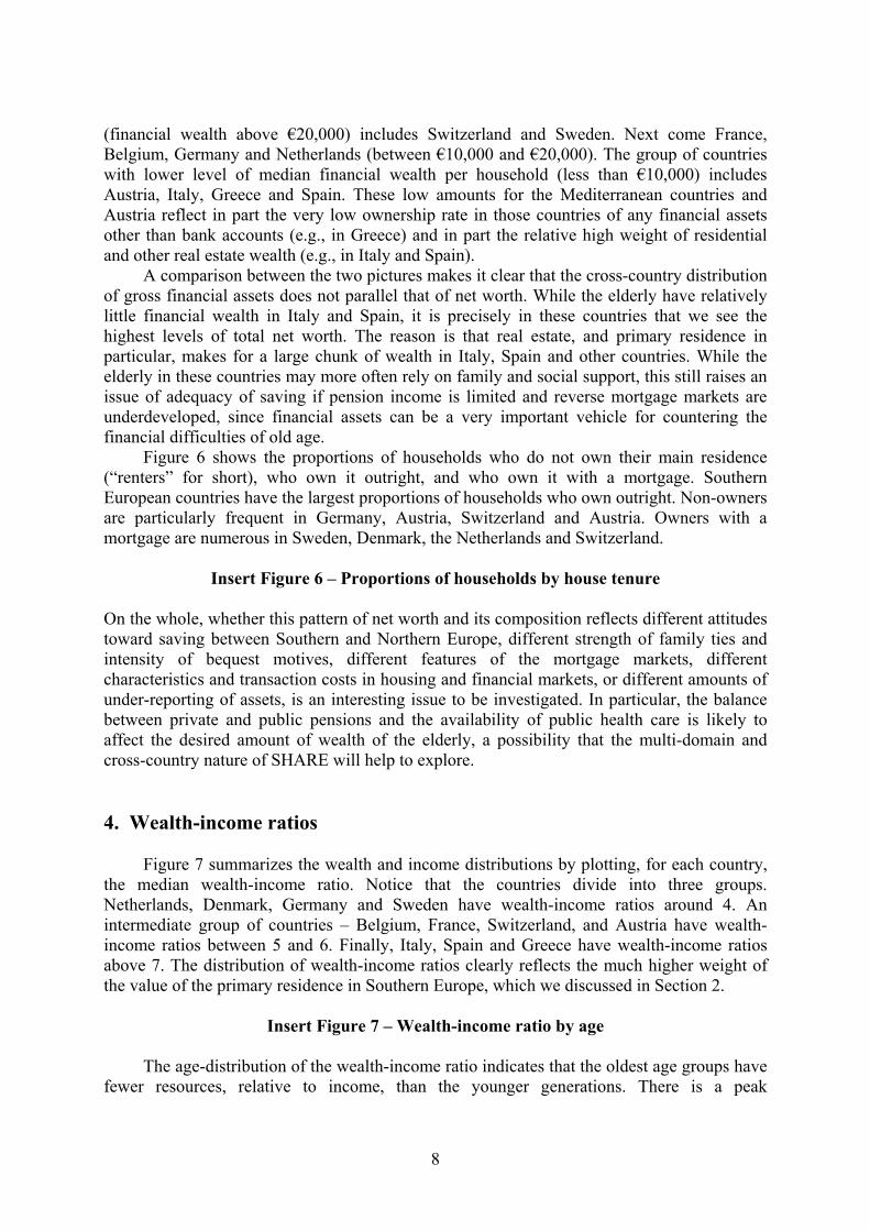
Figure 6 shows the proportions of households who do not own their main residence (“renters” for short), who own it outright, and who own it with a mortgage. Southern European countries have the largest proportions of households who own outright. Non-owners are particularly frequent in Germany, Austria, Switzerland and Austria. Owners with a mortgage are numerous in Sweden, Denmark, the Netherlands and Switzerland.

Insert Figure 6 – Proportions of households by house tenure On the whole, whether this pattern of net worth and its composition reflects different attitudes toward saving between Southern and Northern Europe, different strength of family ties and intensity of bequest motives, different features of the mortgage markets, different characteristics and transaction costs in housing and financial markets, or different amounts of under-reporting of assets, is an interesting issue to be investigated. In particular, the balance between private and public pensions and the availability of public health care is likely to affect the desired amount of wealth of the elderly, a possibility that the multi-domain and cross-country nature of SHARE will help to explore. 4. Wealth-income ratios

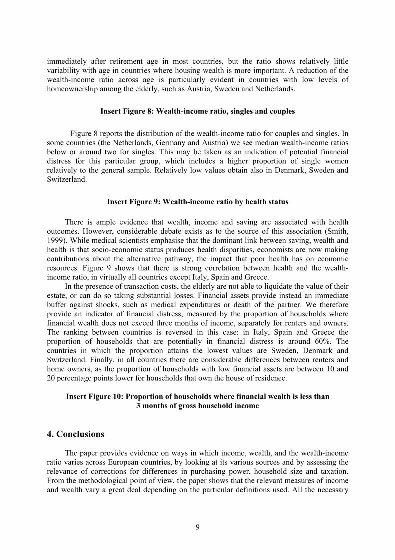
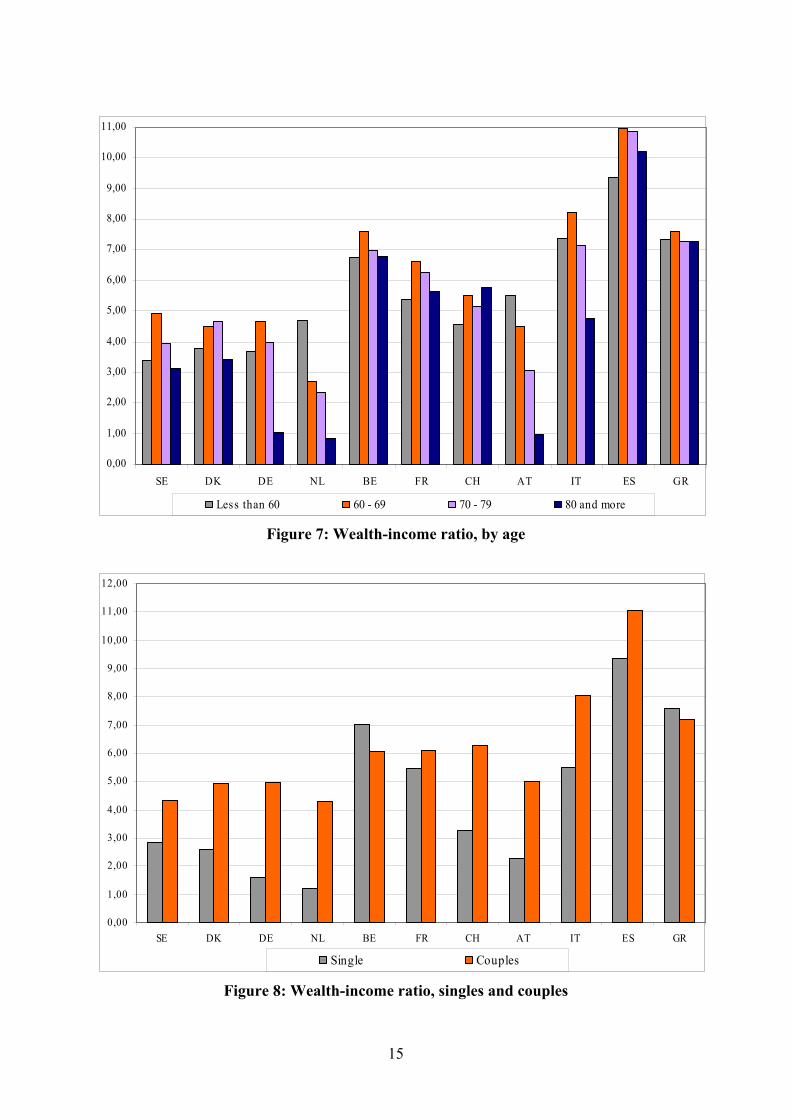
Figure 7 summarizes the wealth and income distributions by plotting, for each country, the median wealth-income ratio. Notice that the countries divide into three groups. Netherlands, Denmark, Germany and Sweden have wealth-income ratios around 4. An intermediate group of countries – Belgium, France, Switzerland, and Austria have wealth-income ratios between 5 and 6. Finally, Italy, Spain and Greece have wealth-income ratios above 7. The distribution of wealth-income ratios clearly reflects the much higher weight of the value of the primary residence in Southern Europe, which we discussed in Section 2.

Insert Figure 7 – Wealth-income ratio by age

The age-distribution of the wealth-income ratio indicates that the oldest age groups have

fewer resources, relative to income, than the younger generations. There is a peak

9

immediately after retirement age in most countries, but the ratio shows relatively little variability with age in countries where housing wealth is more important. A reduction of the wealth-income ratio across age is particularly evident in countries with low levels of homeownership among the elderly, such as Austria, Sweden and Netherlands.

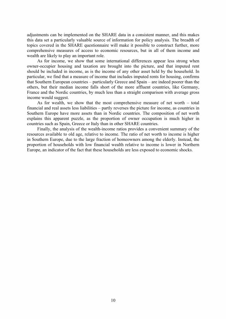
Insert Figure 8: Wealth-income ratio, singles and couples

Figure 8 reports the distribution of the wealth-income ratio for couples and singles. In

some countries (the Netherlands, Germany and Austria) we see median wealth-income ratios below or around two for singles. This may be taken as an indication of potential financial distress for this particular group, which includes a higher proportion of single women relatively to the general sample. Relatively low values obtain also in Denmark, Sweden and Switzerland.

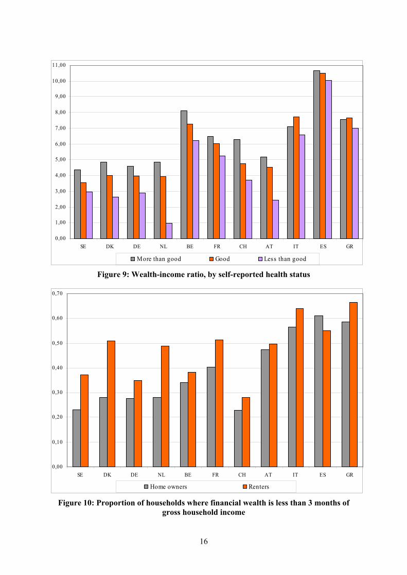
Insert Figure 9: Wealth-income ratio by health status

There is ample evidence that wealth, income and saving are associated with health

outcomes. However, considerable debate exists as to the source of this association (Smith, 1999). While medical scientists emphasise that the dominant link between saving, wealth and health is that socio-economic status produces health disparities, economists are now making contributions about the alternative pathway, the impact that poor health has on economic resources. Figure 9 shows that there is strong correlation between health and the wealth-income ratio, in virtually all countries except Italy, Spain and Greece.

In the presence of transaction costs, the elderly are not able to liquidate the value of their estate, or can do so taking substantial losses. Financial assets provide instead an immediate buffer against shocks, such as medical expenditures or death of the partner. We therefore provide an indicator of financial distress, measured by the proportion of households where financial wealth does not exceed three months of income, separately for renters and owners. The ranking between countries is reversed in this case: in Italy, Spain and Greece the proportion of households that are potentially in financial distress is around 60%. The countries in which the proportion attains the lowest values are Sweden, Denmark and Switzerland. Finally, in all countries there are considerable differences between renters and home owners, as the proportion of households with low financial assets are between 10 and 20 percentage points lower for households that own the house of residence.

Insert Figure 10: Proportion of households where financial wealth is less than 3 months of gross household income

4. Conclusions

The paper provides evidence on ways in which income, wealth, and the wealth-income ratio varies across European countries, by looking at its various sources and by assessing the relevance of corrections for differences in purchasing power, household size and taxation. From the methodological point of view, the paper shows that the relevant measures of income and wealth vary a great deal depending on the particular definitions used. All the necessary

10

adjustments can be implemented on the SHARE data in a consistent manner, and this makes this data set a particularly valuable source of information for policy analysis. The breadth of topics covered in the SHARE questionnaire will make it possible to construct further, more comprehensive measures of access to economic resources, but in all of them income and wealth are likely to play an important role.

As for income, we show that some international differences appear less strong when owner-occupier housing and taxation are brought into the picture, and that imputed rent should be included in income, as is the income of any other asset held by the household. In particular, we find that a measure of income that includes imputed rents for housing, confirms that Southern European countries – particularly Greece and Spain – are indeed poorer than the others, but their median income falls short of the more affluent countries, like Germany, France and the Nordic countries, by much less than a straight comparison with average gross income would suggest.

As for wealth, we show that the most comprehensive measure of net worth – total financial and real assets less liabilities – partly reverses the picture for income, as countries in Southern Europe have more assets than in Nordic countries. The composition of net worth explains this apparent puzzle, as the proportion of owner occupation is much higher in countries such as Spain, Greece or Italy than in other SHARE countries.

Finally, the analysis of the wealth-income ratios provides a convenient summary of the resources available to old age, relative to income. The ratio of net worth to income is higher in Southern Europe, due to the large fraction of homeowners among the elderly. Instead, the proportion of households with low financial wealth relative to income is lower in Northern Europe, an indicator of the fact that these households are less exposed to economic shocks.

11

References Banks, J. and S. Smith (2001), “Household portfolios in the UK”, in Household Portfolios, L.

Guiso, M. Haliassos and T. Jappelli eds. Cambridge, MA: MIT Press. Börsch-Supan, A. (2003), “Life-cycle savings and public policy.” New York: Academic

Press. Börsch-Supan, A., A., Brugiavini, H., Jürges, J., Mackenbach, J., Siegrist and G. Weber (eds.)

(2005), Health, Ageing and Retirement in Europe – First Results from the Survey on Health, Ageing and Retirement in Europe, Mannheim: MEA

Börsch-Supan, A. and H. Jürges (eds.) (2005), The Survey of Health, Aging, and Retirement

in Europe – Methodology, Mannheim: MEA Brugiavini, A., E., Croda, O., Paccagnella, R., Rainato and G.Weber (2005), “Generated

Income Variables in SHARE Release 1” in The Survey of Health, Aging, and Retirement in Europe – Methodology, A. Börsch-Supan and H. Jürges eds., Mannheim: MEA, 105-113.

Christelis, D., T., Jappelli and M. Padula (2005), “Generated Asset Variables in SHARE

Release 1” in The Survey of Health, Aging, and Retirement in Europe – Methodology, A. Börsch-Supan and H. Jürges eds., Mannheim: MEA, 114-127.

Guiso, L., M. Haliassos and T Jappelli (2003), “Introduction”, in Household Portfolios, L.

Guiso, M. Haliassos and T. Jappelli eds. Cambridge, MA: MIT Press. Hurd, M. (2001), “The portfolio of the elderly” in Household Portfolios, L. Guiso, M.

Haliassos and T. Jappelli eds. Cambridge, MA: MIT Press. Juster, T., J.P, Smith and F. Stafford (1999), “The measurement and structure of household

wealth,” Labor Economics 6, 253-76. Little, J.A. and D.B. Rubin (2002) Statistical analysis with missing data, 2nd edition. New

York, John Wiley & Sons. Modigliani, F. (1986), “Life cycle, individual thrift, and the wealth of nations”, American

Economic Review 76, 297-313. Rubin, D.B. (1987) Multiple imputation for nonresponse in surveys. New York, John Wiley &

Sons. Rubin, D.B and N. Schenker (1986), “Multiple imputation for interval estimation from simple

random samples with ignorable non-response,” Journal of the American Statistical Association 81, 366-74

Smith, J. (1999), “Healthy bodies and thick wallets: the dual relation between health and

economic status,” Journal of Economic Perspectives, Spring, 145-166.

12

010

000

2000

030

000

4000

050

000

6000

070

000

SE DK DE NL BE FR CH AT IT ES GR

Average income Median income

Figure 1: Average and median gross household income

010

000

2000

030

000

4000

050

000

6000

0

SE DK DE NL BE FR CH AT IT ES GR

Earnings Pensions Assets & other sources Imputed rents

Figure 2: Income components

13

015

000

3000

045

000

SE DK DE NL BE FR CH AT IT ES GR

Gross Gross , accounting for PPP Gross , accounting for PPP & EA

Figure 3: Different definitions of gross household income

050

0010

000

1500

020

000

2500

030

000

SE DK DE NL BE FR CH AT IT ES GR

Gross , accounting for PPP & EA Gross + IR, accounting for PPP & EANet + IR, accounting for PPP & EA

Figure 4: Different definitions of gross and net household income

14

050

000

1000

0015

0000

2000

0025

0000

SE DK DE NL BE FR CH AT IT ES GR

Net worth Net worth, accounting for PPP Net worth, accounting for PPP & EA

Figure 5: Different definitions of net worth

0%

20%

40%

60%

80%

100%

SE DK DE NL BE FR CH AT IT ES GR

Non owners Owner occupiers with mortgage Owner occupiers outright

Figure 6: Proportions of households by house tenure

15

0,00

1,00

2,00

3,00

4,00

5,00

6,00

7,00

8,00

9,00

10,00

11,00

SE DK DE NL BE FR CH AT IT ES GR

Less than 60 60 - 69 70 - 79 80 and more

Figure 7: Wealth-income ratio, by age

0,00

1,00

2,00

3,00

4,00

5,00

6,00

7,00

8,00

9,00

10,00

11,00

12,00

SE DK DE NL BE FR CH AT IT ES GR

Single Couples

Figure 8: Wealth-income ratio, singles and couples

16

0,00

1,00

2,00

3,00

4,00

5,00

6,00

7,00

8,00

9,00

10,00

11,00

SE DK DE NL BE FR CH AT IT ES GR

More than good Good Less than good

Figure 9: Wealth-income ratio, by self-reported health status

0,00

0,10

0,20

0,30

0,40

0,50

0,60

0,70

SE DK DE NL BE FR CH AT IT ES GR

Home owners Renters

Figure 10: Proportion of households where financial wealth is less than 3 months of gross household income

17

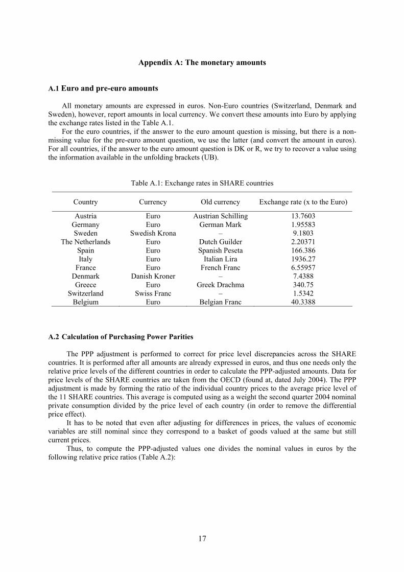
Appendix A: The monetary amounts A.1 Euro and pre-euro amounts

All monetary amounts are expressed in euros. Non-Euro countries (Switzerland, Denmark and Sweden), however, report amounts in local currency. We convert these amounts into Euro by applying the exchange rates listed in the Table A.1.

For the euro countries, if the answer to the euro amount question is missing, but there is a non-missing value for the pre-euro amount question, we use the latter (and convert the amount in euros). For all countries, if the answer to the euro amount question is DK or R, we try to recover a value using the information available in the unfolding brackets (UB).

Table A.1: Exchange rates in SHARE countries

Country Currency Old currency Exchange rate (x to the Euro)

Austria Euro Austrian Schilling 13.7603 Germany Euro German Mark 1.95583 Sweden Swedish Krona – 9.1803

The Netherlands Euro Dutch Guilder 2.20371 Spain Euro Spanish Peseta 166.386 Italy Euro Italian Lira 1936.27

France Euro French Franc 6.55957 Denmark Danish Kroner – 7.4388 Greece Euro Greek Drachma 340.75

Switzerland Swiss Franc – 1.5342 Belgium Euro Belgian Franc 40.3388

A.2 Calculation of Purchasing Power Parities

The PPP adjustment is performed to correct for price level discrepancies across the SHARE countries. It is performed after all amounts are already expressed in euros, and thus one needs only the relative price levels of the different countries in order to calculate the PPP-adjusted amounts. Data for price levels of the SHARE countries are taken from the OECD (found at, dated July 2004). The PPP adjustment is made by forming the ratio of the individual country prices to the average price level of the 11 SHARE countries. This average is computed using as a weight the second quarter 2004 nominal private consumption divided by the price level of each country (in order to remove the differential price effect).

It has to be noted that even after adjusting for differences in prices, the values of economic variables are still nominal since they correspond to a basket of goods valued at the same but still current prices.

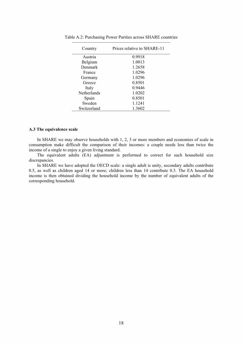
Thus, to compute the PPP-adjusted values one divides the nominal values in euros by the following relative price ratios (Table A.2):

18

Table A.2: Purchasing Power Parities across SHARE countries

Country Prices relative to SHARE-11

Austria 0.9918 Belgium 1.0013 Denmark 1.2658 France 1.0296

Germany 1.0296 Greece 0.8501 Italy 0.9446

Netherlands 1.0202 Spain 0.8501

Sweden 1.1241 Switzerland 1.3602

A.3 The equivalence scale

In SHARE we may observe households with 1, 2, 3 or more members and economies of scale in consumption make difficult the comparison of their incomes: a couple needs less than twice the income of a single to enjoy a given living standard.

The equivalent adults (EA) adjustment is performed to correct for such household size discrepancies.

In SHARE we have adopted the OECD scale: a single adult is unity, secondary adults contribute 0.5, as well as children aged 14 or more; children less than 14 contribute 0.3. The EA household income is then obtained dividing the household income by the number of equivalent adults of the corresponding household.

19

Appendix B: Calculation and imputation of income variables B.1 Definitions

Total household income is the sum of some incomes at the individual level and some at the household level. The basic definition used in the SHARE project reflects money income before taxes on a yearly base (2003) and includes only regular payments. Home business, lump-sum payments and financial support provided by parents, relatives or other people are not included. The SHARE definition of income does not include ”other types of debts”, because we are not able to separate the amount of the debts on cars and other vehicles from the total amount of debts.

B.1.1 Amounts

The available data at the individual level include: i) Income from employment (ep205_) ii) Income from self-employment or work for a family business (ep207_) iii) Income from (public or private) pensions or invalidity or unemployment benefits (ep074_,

ep078_, ep208_) iv) Income from alimony or other private regular payments (ep094_) v) Income from long-term care insurance (only for Austria and Germany) (ep086_) The available data at the household level include: vi) Income from other household members not interviewed (hh002_) vii) Income from other payments, such as housing allowances, child benefits, poverty relief,

etc. (hh011_) viii) Income actually received from secondary homes, holiday homes or real estate, land or

forestry (ho030_) ix) Interest from bank accounts, transaction accounts or saving accounts (as005_) x) Interest from government or corporate bonds (as009_) xi) Dividend from stocks or shares (as015_) xii) Interest or dividend from mutual funds or managed investment accounts (as058_) xiii) Imputed rent (only for homeowners), based on the self-assessed home value minus the net

residual value of the debt (payments for mortgages or loans). The interest rate used for imputed rents is fixed at 4% for all countries (ho015_, ho024_) 4

Questions may refer to different time frames. Employment and self-employment income amounts

are asked directly as approximate yearly amounts. In contrast, the annual amount of income received from a specific pension or a specific regular payment needs to be calculated from 3 variables: average payment in 2003, the period covered by the payment, and the number of months in which the respondent has received that income payment in 2003. Long term care insurance income is asked as monthly amount. All household level incomes (except imputed rents which are calculated) are asked directly as approximate yearly amounts. B.1.2 Flag variables

We generate different types of flag variables, depending on the characteristics of the variables they are associated with.

4 We have decided to impute rents for homeowners because they may represent a large fraction of resources at old age.

20

Labels of the flag variables of an amount variable (e.g. earnings or pensions) that follows an ownership question and for which unfolding bracket sequence is possible:

1 Valid response: The respondent provides a valid response (in Euro or non-Euro). 2 Complete bracket: The respondent answers ‘refuse’ or ‘don’t know’ on the amount-question

enters the unfolding bracket sequence and follows it until the end. We include here answers of the ‘about’ category.

3 Incomplete bracket: The respondent answers ‘refuse’ or ‘don’t know’ on the amount-question, enters the unfolding bracket sequence and at least provides a valid answer to the first question but does not finish this sequence for some reason. At some point in the sequence the respondent answers ‘refuse’ or ‘don’t know’.

5 No value/bracket: The respondent answers ‘refuse’ or ‘don’t know’ on the amount-question, enters the unfolding bracket sequence but does no provide a valid answer to the first question and does not finish this sequence for some reason.

6 No ownership: This respondent is not asked the amount question. The respondent answers in a previous question that he or she does not own this item or has no such source of income.

7 rf / dk ownership: This respondent is not asked the amount question. The respondent answers in a previous question on ownership ‘refuse’ or ‘don’t know’.

9 No respondent for this module: The questionnaire identifies the household, housing and financial respondent. If this household, housing and financial respondent does not answer the specific CAPI-module (e.g. a financial respondent does not answer the AS module), this flag is up.

Labels of the flag variables of a composed amount variable (e.g. household income):

0 Does not apply 5 1 No imputations: The respondent provides valid responses to all questions on which this

composed variable is based. Hence no imputations are needed. 5 Some imputations: The respondent does not provide valid responses to all questions on

which this composed variable is based and some imputations are needed to construct this variable.

11 Imputation failed: The hot-deck procedure may fail – it happens very rarely - because there are no donors that can be used for that specific interval

B.2 Imputation

We perform two types of imputations: imputations on amount variables, using the unfolding brackets (UBs) information and the hot-deck method, and imputations on frequency variables, using regression methods.

B.2.1 Unfolding brackets

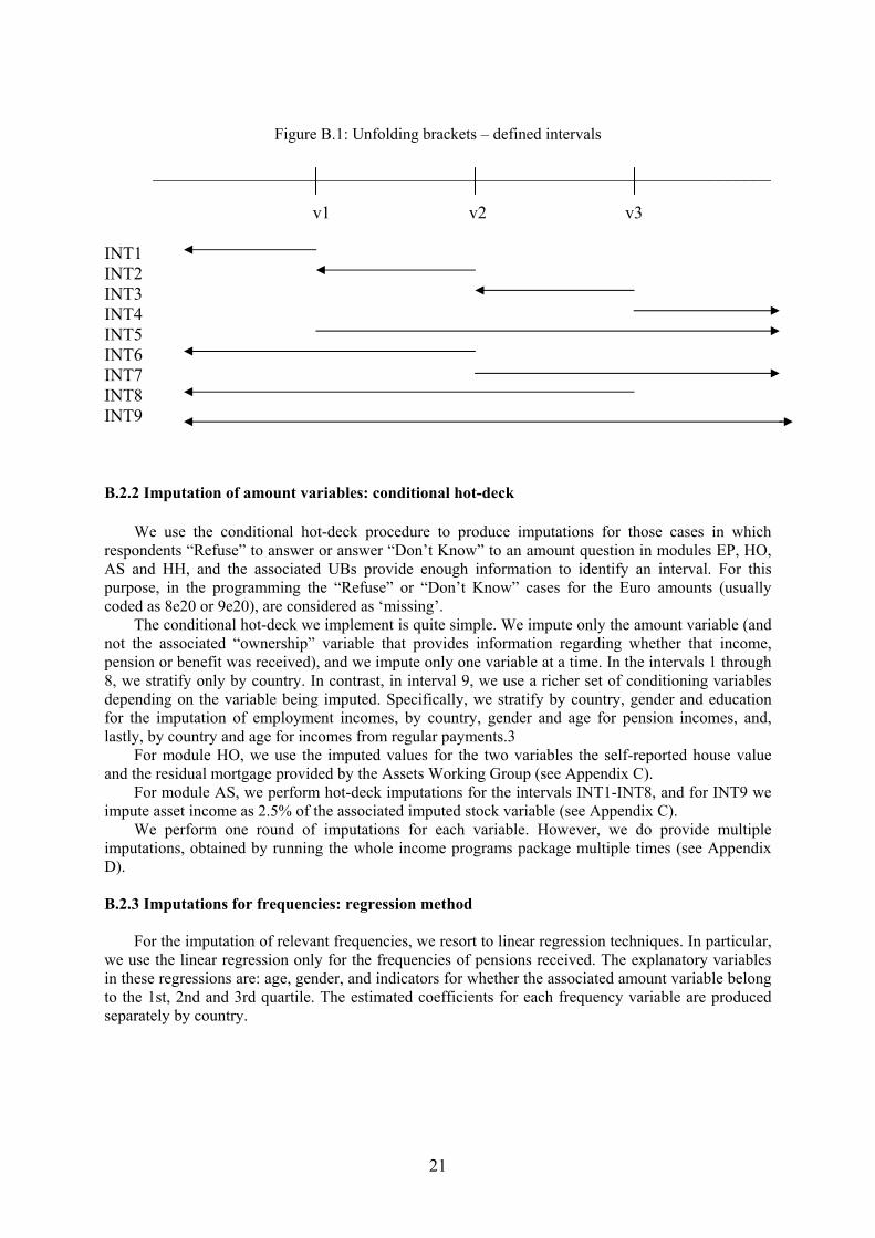
The three bracket cut-off values (v1,v2,v3) define 9 intervals (INT1,…INT9), depicted in Figure B.1.

5 The amount question is asked only if the respondent answer “yes” to the associated ownership question. “Does not apply” in this context means that the associated ownership variable is not “yes”.

21

Figure B.1: Unfolding brackets – defined intervals

______________________________________________________________________ v1 v2 v3 INT1 INT2 INT3 INT4 INT5 INT6 INT7 INT8 INT9

B.2.2 Imputation of amount variables: conditional hot-deck

We use the conditional hot-deck procedure to produce imputations for those cases in which respondents “Refuse” to answer or answer “Don’t Know” to an amount question in modules EP, HO, AS and HH, and the associated UBs provide enough information to identify an interval. For this purpose, in the programming the “Refuse” or “Don’t Know” cases for the Euro amounts (usually coded as 8e20 or 9e20), are considered as ‘missing’.

The conditional hot-deck we implement is quite simple. We impute only the amount variable (and not the associated “ownership” variable that provides information regarding whether that income, pension or benefit was received), and we impute only one variable at a time. In the intervals 1 through 8, we stratify only by country. In contrast, in interval 9, we use a richer set of conditioning variables depending on the variable being imputed. Specifically, we stratify by country, gender and education for the imputation of employment incomes, by country, gender and age for pension incomes, and, lastly, by country and age for incomes from regular payments.3

For module HO, we use the imputed values for the two variables the self-reported house value and the residual mortgage provided by the Assets Working Group (see Appendix C).

For module AS, we perform hot-deck imputations for the intervals INT1-INT8, and for INT9 we impute asset income as 2.5% of the associated imputed stock variable (see Appendix C).

We perform one round of imputations for each variable. However, we do provide multiple imputations, obtained by running the whole income programs package multiple times (see Appendix D).

B.2.3 Imputations for frequencies: regression method

For the imputation of relevant frequencies, we resort to linear regression techniques. In particular, we use the linear regression only for the frequencies of pensions received. The explanatory variables in these regressions are: age, gender, and indicators for whether the associated amount variable belong to the 1st, 2nd and 3rd quartile. The estimated coefficients for each frequency variable are produced separately by country.

22

Appendix C: Calculation and imputation of wealth variables C.1 Definitions

Respondents in SHARE are all household members aged 50 and over, plus their spouses, regardless of age. Financial and housing respondents are those household members most responsible for financial and housing matters, respectively. This is done to save time and avoid duplications. For instance, in a couple the financial questions are preferably answered by one person only, unless finances are not jointly managed, in which case each household member is treated as a separate financial unit. C.1.1 Amounts

First, the following individual-level magnitudes are generated (the question names to which they

correspond are in parentheses):

i) Value of the primary residence (HO024_) ii) Value of the mortgage (HO015_) iii) Value of other real estate (HO027_) iv) Value of bank accounts (AS003_) v) Value of government and corporate bond holdings (AS007_) vi) Value of stock holdings (AS011_) vii) Value of mutual fund holdings (AS017_) viii) Value of individual retirement accounts (AS021_, AS024) ix) Value of the contractual savings for housing (AS027_) x) Value of life insurance policies (AS030_) xi) Value of owned business, including the non-owned part of it (AS042_) xii) Owned share of own business (AS044_) xiii) Value of owned cars (AS051_) xiv) Value of financial liabilities (AS055_)

By multiplying xi) by xii) above one obtains:

xv) Value of owned share of own business.

In addition, we impute the value of risky assets, which we define to be direct stock holdings, and the percentage of holdings in mutual funds and individual retirement accounts that are invested in stocks. Unfortunately we cannot directly observe the latter two quantities. We have however questions for both mutual funds (AS019_) and individual retirement accounts (AS023_, AS026_), which give information on whether the amount invested is mostly in stocks, roughly equally in stocks and bonds or mostly in bonds. We impute respectively to these three possible answers the following percentages of investment in stocks: 75%, 50% and 25%. Using this imputation we construct:

xvi) Value of holdings of risky financial assets

At a second stage, the individual-level variables i, ii, iii, iv, v, vi, vii, viii, ix, x, xiii, xiv, xv and xvi defined above are summed over all household members in order to generate the corresponding household-level variables. In addition we generate the following household-level aggregates:

xvii) Real assets are defined as the sum of the value of the primary residence net of the

mortgage on it, the value of other real estate, the owned share of own business and the owned cars.

23

xviii) Gross financial assets are equal to the sum of the values of bank accounts, government and corporate bonds, stocks, mutual funds, individual retirement accounts, contractual savings for housing and life insurance policies owned by the household.

xix) Net financial assets are equal to gross financial assets minus financial liabilities. xx) Net worth is equal to the sum of real and net financial assets

C.1.2 Flags

In addition to generating the variables for the amounts of wealth related items, we need to generate also their corresponding flag variable, which contains information about how the amount variables were constructed. For individual-level variables the flag variable takes the following values:

1 - Continuous answer: the respondent answered with a positive or negative value to

the amount question, and there was no need to amend her answer in any respect. 2 - Complete Bracket: the respondent did not want or did not know how to answer the

amount question, but then entered into the unfolding bracket procedure and successfully completed it.

3 - Incomplete Bracket: the respondent did not want or did not know how to answer the amount question, entered into the unfolding bracket procedure but did not complete it.

5 - Refusal to start the bracket sequence: the respondent did not want or did not know how to answer the amount question, and again refused or did not know how to answer the first unfolding bracket question.

6 - No ownership: the respondent does not own the item. 7 - Refusal/Don't know on ownership question: the respondent refused or did not know

how to answer the question on ownership that precedes the amount question for each item.

9 - Is not a financial respondent: the respondent is not the designated financial respondent for the household and does not report any amount for the item.

10 - Negative values, 0s, implausibly low positive values, wrong currency answers, very high outliers: this broad category includes cases for which it was decided that the values were so implausible as to be a result of some mistake or an alternative form of refusal to answer the question. For these cases we used imputation to fill in the values.

Some additional clarifications are needed for the last value of the flag variable. We treated

negative values as implausible, with the exception of bank accounts and the value of own business. The balance of the former can be negative because of overdrafts for example, and the latter’s value can be negative when the assets of the business are less than its liabilities.

There are some cases for which the amount is stated to be zero, while the ownership variable is positive. We think that this might be an indication of refusal to answer the amount question, without going into the unfolding brackets procedure. We consider these cases to be missing and we impute them.

The threshold below which a positive value was deemed to be implausible differs by item but is the same for each country. The values by item are (in euros): 5000 for the primary residence, 500 for the mortgage, 1000 for other real estate, 500 for bonds, mutual funds, individual retirement accounts, contractual savings for housing and life insurance, 1000 for the value of the own business, 250 euros for cars. We set no minimum positive threshold for the values of bank accounts, stocks and financial liabilities.

For countries that have adopted the euro as their currency (i.e. Austria, Belgium, France, Germany, Greece, Italy, Netherlands, Spain), the respondent can give an answer to an amount question

24

either in euros or in pre-euro currency. Unfortunately, some answers in pre-euro currency are entered by mistake as an answer in euros. Given that the exchange rate of the old currency to the euro is always greater than one (see Table A.1), this mistake can basically be detected only for answers with unusually high values and for countries for which the euro conversion exchange rate is very high, namely Italy (exchange rate equal to 1936.27), Greece (340.75), Spain (166.39), and possibly Austria (13.76) and Sweden (9.18). In determining whether an answer is entered in the wrong currency column we also take into account whether the respondent has answered other questions in pre-euro currency. When the answer is deemed to having been entered in the wrong currency, we divide by the exchange rate.

Finally, after correcting for an wrong currency entry, we are still left with some implausibly high outliers, which are detected by inspection. We set them to missing and impute them, conditional on being on the highest bracket.

C.2 Imputation

Imputation is performed using the hotdeck imputation package in STATA, which is based on the approximate Bayesian bootstrap described in Rubin and Schenker (1986). This procedure requires the classification (by some variables) of the non-missing observations in cells, from which bootstrap samples are drawn and values from these samples are used to impute the missing observations in each cell. In choosing the number of variables to define the cells we faced a trade-off. The higher this number is, the better the match between the missing and the non-missing observations, but the smaller is the number of observations with non-missing values within the cell.

We use multiple imputation during which the hotdeck procedure creates five different values for each missing one. This is done by drawing five samples with replacement from the cells of non-missing observations. Further details are given in Appendix D. C.2.1 Imputation of Ownership Variables

Each question about the amount of an item is preceded by a corresponding question about

whether this item is owned or not. The ownership questions corresponding to each asset are:

i) Primary residence – HO002_ ii) Mortgage – HO013_ iii) Other Real Estate – HO026_ iv) Bank accounts, bonds, stocks, mutual funds, respondent’s individual retirement

account, contractual savings for housing, life insurance – AS002_1, AS002_2, AS002_3, AS002_4, AS002_5, AS002_6, AS002_7, AS002_8

v) Individual retirement account of the respondent’s spouse: AS020_ vi) Own business – AS041_ vii) Cars – AS049_ viii) Financial Liabilities – AS054_1, AS054_2, AS054_3, AS054_4, AS054_5,

AS054_6, AS054_7, AS054_8

If an individual gives a response of don’t know or refuses to answer the ownership question, then ownership is imputed. In addition there are households in which no individual gives any response for the housing (question HO002_), financial assets (question AS001_) or financial liabilities (question AS053_) section. In that case ownership is imputed for the designated household head. The imputation is done using country and age as classificatory variables for the hotdeck procedure.

25

C.2.2 Imputation of Amount Variables The amount is imputed in the following cases, once the ownership question has an original or

imputed positive value:

i) When the ownership is imputed and the result is positive (flag variable equals 7). ii) When the individual gives a response of don’t know/refusal and either does not start

the unfolding brackets procedure (flag variable equals 5), or does not complete it (flag variable equals 3), or completes it without giving a specific amount as an approximate answer (the value of the flag variable equals 2, which is however the value also if the approximate amount is given during the unfolding bracket procedure).

iii) When the original answer is an illegitimate negative value, a zero while the ownership answer is positive, an implausibly low positive value, a wrong currency answer or a very high outlier (flag variable equals 10).

In the end we divided the variables into three groups according to the criteria by which the cell

classification for imputation was made (all imputations were made separately for each country):

i) Housing, bank accounts and cars. These variables contained numerous positive non-missing values, reflecting the wide ownership of the corresponding assets. In the case in which we did not know the bracket value we used age as an additional variable. When we knew the bracket value, we used it together with age.

ii) Mortgage. We needed to link the value of the mortgage to the value of the underlying house, in order to avoid as much as possible the case where the imputed value of the mortgage was greater than the value of the house. Thus, when we did not know the bracket value of the mortgage, we used the bracket value of the house as a classificatory variable; when we knew the bracket value of the mortgage we used it for the imputation. We left out the bracket value of the house because its inclusion would have made the cells too thin.

iii) Other real estate, bonds, stocks, mutual funds, individual retirement accounts, contractual savings for housing, life insurance, own business and owned share thereof and financial liabilities. These variables exhibited relatively few positive non-missing values. We used age to define the imputation cells when we did not know the bracket value, while we used the bracket value for their definition when we knew it.

Following convention, we use a male as the household head, provided his record is in the first two

observations of a given household, since typically these are the lines where members of a couple or primary respondents are listed. If there’s no male listed in the first two observations, we pick the first female listed as head. Having designated the household head, we had to decide whether to use the individual’s or the household head’s information (e.g. age) in order to classify each missing value into cells. Using the individual’s characteristics assumes that s/he plays the most significant part in determining the value of (a potentially household-level) variable. On the other hand, the head’s information can be more useful in cases where the head does not respond and the answer is provided by someone else purely for convenience reasons. We chose to use the individual’s information when the individual is the head or another household member in a household where the head gives a response. If the head does not respond then the first respondent with missing values is assigned the head’s information, while any further respondents’ answers are imputed using their own information.

26

Appendix D: Multiple Imputations

Statistical inference with missing data is an important applied problem, because missing data (planned or unplanned) are commonly encountered in practice. Multiple imputations (MI) is one of the available procedures for analysing data sets with missing values entries (Little and Rubin, 2002).

MI is the technique that replaces each missing value with M (M=2 or more) acceptable values representing a distribution of possibilities. The M values are ordered in the sense that the first components of the vectors for the missing values are used to create one completed data set, the second components of the vectors for the missing values are used to create the second completed data set and so on. Thus, the M imputations for each missing datum create M complete data sets. Standard complete-data methods can be used to analyse each data set.

Advantages of MI:

o MI allows to analyse completed data sets (standard methods may be used). o In many contexts the data collector is different from the data analyst, but data collector may have

access to more and better information about non-respondents than the data analyst. This kind of information can often improve the imputed values.

o MI allows data collectors to reflect their uncertainty as to which values to impute: the resulting M complete-data analyses can be easily combined to create an inference that validly reflects sampling variability because of the missing values.

o If the method to create imputations is 'proper' (Rubin, 1987), then the resulting inferences will be statistically valid.

o Using MI, the missing data problem can be handled once, rather than many times, by the users. This implies consistency of the data-bases across users and a consequent consistency of answers from identical analyses. We generated five values for each missing one by running the same program five different times

using a different seed to perform the hotdeck imputation in each run of the program. Thus we generated five different implicate datasets which have identical values when these were not originally missing and potentially five different values for the missing cases.

It is fundamental to always take into account the fact that we have five different datasets when performing any kind of analysis. This means that one should not use just one of the five datasets nor one should concatenate all five and treat them as one. Rather, one should perform the analysis on each dataset separately and then combine the results from all five datasets using the results of Rubin (1987); see also Little and Rubin (2002) for a recent survey.

Let m=1,….,M index the imputation run (with M in our case equal to 5) and let m be mβ̂ our estimate of interest (e.g. sample median, regression coefficient etc.) from the mth implicate dataset. Then the estimate using all M implicate datasets is just the average of the M separate estimates, i.e.

∑=

=M

m mM M 1ˆ1

ββ

The variance of this estimate consists of two parts. Let Vm be the variance estimated from the mth

implicate dataset. Then the first magnitude one needs to compute is the average of all M variances, which constitutes the within-imputation variance, i.e.

∑=

=M

mmM VWV M 1

1

The second magnitude one needs to compute is the between-imputation variance, which is given

by:

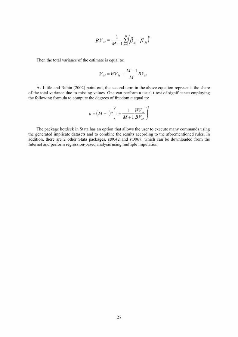
27

( )∑=

−−

=M

mMmM MBV

1

2ˆ1

1ββ

Then the total variance of the estimate is equal to:

MMM BVM

MWVV1+

+=

As Little and Rubin (2002) point out, the second term in the above equation represents the share

of the total variance due to missing values. One can perform a usual t-test of significance employing the following formula to compute the degrees of freedom n equal to:

( )2

111*1

+

+−=M

m

BVWV

MMn

The package hotdeck in Stata has an option that allows the user to execute many commands using

the generated implicate datasets and to combine the results according to the aforementioned rules. In addition, there are 2 other Stata packages, st0042 and st0067, which can be downloaded from the Internet and perform regression-based analysis using multiple imputation.