Test

Sociedad de Estadística e Investigación Operativa

Volume 14, Number 2. December 2005

Intrinsic Credible Regions: An Objective Bayesian

Approach to Interval EstimationJose M. Bernardo

Departamento de Estadıstica e I. O.

Universidad de Valencia, Spain

Sociedad de Estadıstica e Investigacion OperativaTest (2005) Vol. 14, No. 2, pp. 317–384

Sociedad de Estadıstica e Investigacion OperativaTest (2005) Vol. 14, No. 2, pp. 317–384

Intrinsic Credible Regions: An Objective Bayesian

Approach to Interval Estimation

Jose M. Bernardo∗

Departamento de Estadıstica e I. O.

Universidad de Valencia, Spain

Abstract

This paper defines intrinsic credible regions, a method to produce objectiveBayesian credible regions which only depends on the assumed model and the avail-able data. Lowest posterior loss (LPL) regions are defined as Bayesian credibleregions which contain values of minimum posterior expected loss; they dependboth on the loss function and on the prior specification. An invariant, information-theory based loss function, the intrinsic discrepancy, is argued to be appropriatefor scientific communication. Intrinsic credible regions are the lowest posterior lossregions with respect to the intrinsic discrepancy loss and the appropriate referenceprior. The proposed procedure is completely general, and it is invariant under bothreparametrization and marginalization. The exact derivation of intrinsic credibleregions often requires numerical integration, but good analytical approximations areprovided. Special attention is given to one-dimensional intrinsic credible intervals;their coverage properties show that they are always approximate (and sometimesexact) frequentist confidence intervals. The method is illustrated with a number ofexamples.

Key Words: Amount of information, intrinsic discrepancy, Bayesian asymptotics,confidence intervals, Fisher information, HPD regions, interval estimation, Jeffreyspriors, LPL regions, objective priors, reference priors, point estimation, probabilitycentred intervals, region estimation.

AMS subject classification: Primary 62F15; Secondary 62F25, 62B10.

1 Introduction and notation

This paper is mainly concerned with statistical inference problems suchas occur in scientific investigation. Those problems are typically solved

∗Correspondence to: Jose M. Bernardo. Departamento de Estadıstica e I.O., Facul-tad de Matematicas, 46100-Burjassot, Spain. E-mail: jose.m.bernardo@uv.es

Work partially supported by grant MTM2004-05956 of MEC, Madrid, Spain

318 J. M. Bernardo

conditional on the assumption that a particular statistical model is an ap-propriate description of the probabilistic mechanism which has generatedthe data, and the choice of that model naturally involves an element ofsubjectivity. It has become standard practice however, to describe as “ob-jective” any statistical analysis which only depends on the model assumedand the data observed. In this precise sense (and only in this sense) thispaper provides an “objective” procedure to Bayesian region estimation.

Foundational arguments (Bernardo and Smith, 1994; de Finetti, 1970;Savage, 1954) dictate that scientists should elicit a unique (joint) priordistribution on all unknown elements of the problem on the basis of allavailable information, and use Bayes theorem to combine this with the in-formation provided by the data, encapsulated in the likelihood function,to obtain a joint posterior distribution. Standard probability theory maythen be used to derive from this joint posterior the posterior distributionof the quantity of interest; mathematically this is the final result of thestatistical analysis. Unfortunately however, elicitation of the joint prior isa formidable task, specially in realistic models with many nuisance param-eters which rarely have a simple interpretation, or in scientific inference,where some sort of consensus on the elicited prior would obviously be re-quired. In this context, the (unfortunately very frequent) naıve use ofsimple proper “flat” priors (often a limiting form of a conjugate family)as presumed “noninformative” priors often hides important unwarrantedassumptions which may easily dominate, or even invalidate, the analysis:see e.g., Berger (2000), and references therein. The uncritical (ab)use ofsuch “flat” priors should be strongly discouraged. An appropriate referenceprior (Berger and Bernardo, 1992c; Bernardo, 1979b, 2005b) should insteadbe used.

As mentioned above, from a Bayesian viewpoint, the final outcome of aproblem of inference about any unknown quantity is simply the posteriordistribution of that quantity. Thus, given some data x and conditions C, allthat can be said about any function θ(ω) of the parameter vector ω whichgovern the model is contained in the posterior distribution p(θ |x, C), andall that can be said about some function y of future observations from thesame model is contained in its posterior predictive distribution p(y |x, C).Indeed (Bernardo, 1979a), Bayesian inference is a decision problem wherethe action space is the class of those posterior probability distributions ofthe quantity of interest which are compatible with accepted assumptions.

Intrinsic Credible Regions 319

However, to make it easier for the user to assimilate the appropri-ate conclusions, it is often convenient to summarize the information con-tained in the posterior distribution, while retaining as much of the infor-mation as possible. This is conveniently done by providing sets of pos-sible values of the quantity of interest which, in the light of the data,are likely to be “close” to its true value. The pragmatic importance ofthese region estimates should not be underestimated; see Guttman (1970),Blyth (1986), Efron (1987), Hahn and Meeker (1991), Burdick and Gray-bill (1992), Eberly and Casella (2003), and references therein, for somemonographic works on this topic. In this paper, a new objective Bayesiansolution to this region estimation problem is proposed and analyzed.

1.1 Notation

It will be assumed that probability distributions may be described throughtheir probability density functions, and no notational distinction will bemade between a random quantity and the particular values that it maytake. Bold italic roman fonts are used for observable random vectors (typ-ically data) and bold italic greek fonts for unobservable random vectors(typically parameters); lower case is used for variables and upper case cal-ligraphic for their dominion sets. Moreover, the standard mathematicalconvention of referring to functions, say fx and gx of x ∈ X , respectivelyby f(x) and g(x) will be used throughout. Thus, the conditional proba-bility density of data x ∈ X given θ will be represented by either px |θ orp(x |θ), with p(x |θ) ≥ 0 and

∫

Xp(x |θ) dx = 1, and the posterior distri-

bution of θ ∈ Θ given x will be represented by either pθ |x or p(θ |x), withp(θ |x) ≥ 0 and

∫

Θp(θ |x) dθ = 1. This admittedly imprecise notation will

greatly simplify the exposition. If the random vectors are discrete, thesefunctions naturally become probability mass functions, and integrals overtheir values become sums. Density functions of specific distributions aredenoted by appropriate names. Thus, if x is an observable random variablewith a normal distribution of mean µ and variance σ2, its probability den-sity function will be denoted N(x |µ, σ). If the posterior distribution of µ isStudent with location x, scale s, and n degrees of freedom, its probabilitydensity function will be denoted St(µ |x, s, n).

320 J. M. Bernardo

1.2 Problem statement

The argument is always defined in terms of some parametric model ofthe general form M ≡ p(x |ω), x ∈ X , ω ∈ Ω, which describes theconditions under which data have been generated. Thus, data x are as-sumed to consist of one observation of the random vector x ∈ X , withprobability density p(x |ω), for some ω ∈ Ω. Often, but not necessar-ily, data will consist of a random sample x = y1, . . . ,yn of fixed size nfrom some distribution with, say, density p(y |ω), y ∈ Y , in which casep(x |ω) =

∏nj=1 p(yj |ω), and X = Yn.

Let θ = θ(ω) ∈ Θ be some vector of interest; without loss of generality,the assumed model M may be reparametrized in the form

M ≡ p(x |θ,λ), x ∈ X , θ ∈ Θ, λ ∈ Λ , (1.1)

where λ is some vector of nuisance parameters; this is often simply referredto as “model” p(x |θ,λ). Conditional on the assumed model, all validBayesian inferential statements about the value of θ are encapsulated in itsposterior distribution

p(θ |x) ∝∫

Λ

p(x |θ,λ) p(θ,λ) dλ, (1.2)

which combines the information provided by the data x with any otherinformation about θ contained in the prior density p(θ,λ).

With no commonly agreed prior information on (θ,λ) the referenceprior function for the quantity of interest, a mathematical description ofthat situation which maximizes the missing information about the quantityof interest θ which will be denoted by π(θ)π(λ |θ), should be used to obtainthe corresponding reference posterior,

π(θ |x) ∝ π(θ)

∫

Λ

p(x |θ,λ) π(λ |θ) dλ. (1.3)

To describe the inferential content of the posterior distribution p(θ |x)of the quantity of interest and, in particular, that of the reference posteriorπ(θ |x), it is often convenient to quote regions R ⊂ Θ of given (posterior)probability under p(θ |x), often called credible regions.

This paper concentrates on credible regions for parameter values. How-ever, the ideas may be extended to prediction problems by using the pos-

Intrinsic Credible Regions 321

terior predictive density of the quantity y to be predicted, namely p(y |x)=

∫

Ω p(y |ω) p(ω |x) dω, in place of the posterior density of θ.

Definition 1.1 (Credible region). A (posterior) q-credible region forθ ∈ Θ is a subset Rq(x,Θ) of the parameter space Θ such that,

Rq(x,Θ) ⊂ Θ,

∫

Rq(x,Θ)p(θ |x) dθ = q, 0 < q ≤ 1.

Thus, given data x, the true value of θ belongs to Rq(x,Θ) with (posterior)probability q.

If there is no danger of confusion, dependence on available data x andexplicit mention of the parametrization used will both be dropped from thenotation, and a q-credible region Rq(x,Θ) will simply be denoted by Rq.

Credible regions are invariant under reparametrization. Thus, for anyq-credible region Rq(x,Θ) for θ and for any one-to-one transformationφ = φ(θ) ∈ φ(Θ) = Φ of the parameter θ, Rq(x,Φ) = φRq(x,Θ) isa q-credible region for φ. However, for any given q there are generallyinfinitely many credible regions. Many efforts have been devoted to theselection of an appropriate credible region.

Sometimes, credible regions are selected to have minimum size (length,area, volume), resulting in highest posterior density (HPD) regions, whereall points in the region have larger posterior probability density than allpoints outside. However, HPD regions are not invariant under reparametri-zation: the image Rq(x,Φ) = φRq(x,Θ) of a HPD q-credible region for θ

will be a q-credible region for φ, but will not generally be HPD. Thus, theapparently intuitive idea behind the definition of HPD regions is found tobe illusory, for it totally depends on the (arbitrary) parametrization chosento describe the problem.

In one dimensional problems, posterior quantiles are often used as analternative to HPD regions to specify credible regions. Thus, if θq = θq(x)is the posterior q-quantile of θ, then Rq(x,Θ) = θ; θ ≤ θq is a one-sided,typically unique q-credible interval, and it is invariant under reparametriza-tion. Posterior quantiles may be used to define probability centred q-credibleintervals of the form

Rq(x,Θ) = θ; θ(1−q)/2 ≤ θ ≤ θ(1+q)/2,

322 J. M. Bernardo

so that there is the same probability, namely (1− q)/2, that the true valueof θ is at either side of the interval. Probability centred intervals are easierto compute, and they are often quoted in preference to HPD regions. How-ever, probability centred credible intervals are only really appealing whenthe posterior density has a unique interior mode and, moreover, they havea crucial limitation: they are not uniquely defined in problems with morethan one dimension.

Example 1.1 (Credible intervals for a binomial parameter). Con-sider a set x = x1, . . . , xn of n independent Bernoulli observations withparameter θ ∈ Θ = (0, 1), so that p(x | θ) = θx(1− θ)1−x, and the likelihoodfunction is p(x | θ) = θr(1 − θ)n−r, with r =

∑nj=1 xj. The reference prior,

which in this case is also Jeffreys prior, is π(θ) = Be(θ | 12 ,

12), and the refer-

ence posterior is π(θ | r, n) = Be(θ | r+ 12 , n−r+ 1

2) ∝ θr−1/2(1−θ)n−r−1/2.A (posterior) q-credible region for θ is any subset of Rq of (0, 1) such that∫

RqBe(θ | r + 1

2 , n− r + 12) dθ = q.

Consider now the one-to-one (variance stabilizing) reparametrizationφ = 2arcsin

√θ, φ ∈ Φ = (0, π), so that θ = sin2(φ/2). Changing variables,

the reference posterior density of φ is

π(φ | r, n) =π(θ | r, n)

|∂φ(θ)/∂θ|

∣

∣

∣

∣

θ=sin2(φ/2)

∝ (sin2[φ/2])r(cos2[φ/2])n−r, (1.4)

which conveys precisely the same information that π(θ | r, n). Clearly, if theset Rq(r, n,Θ) is a q-credible region for θ then Rq(r, n,Φ) = φRq(r, n,Θ)will be a q-credible region for φ; however, if Rq(r, n,Θ) is HPD for θ, thenRq(r, n,Φ) will generally not be HPD for φ.

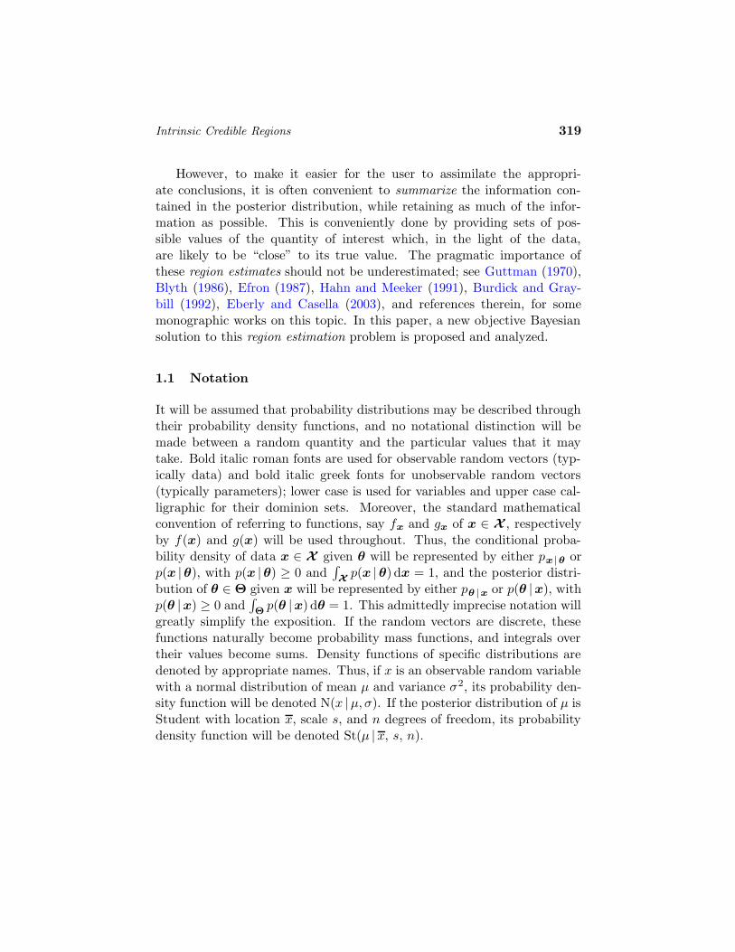
For a numerical illustration, consider the case n = 10, r = 2, so that thereference posterior is the beta density Be(θ | 2.5, 8.5) represented in the leftpanel of Figure 1. Numerical integration or the use of the incomplete betaintegral shows that the 0.95 HPD credible interval is the set (0.023, 0.462) ofthose θ values whose posterior density is larger than 0.585 (shaded regionin that figure). The reference posterior of φ, given by Equation (1.4), isshown on the right panel of Figure 1; the θ-HPD interval transforms intoφ[(0.023, 0.462)] = (0.308, 1.495) which is a 0.95-credible interval for φ,but clearly not HPD. The 0.95 probability centred credible interval for θis (0.044, 0.503), slightly to the right of the HPD interval. Consider nowthe case n = 10, r = 0, so that no successes have been observed in tentrials. The reference posteriors densities of θ and φ are now both monotone

Intrinsic Credible Regions 323

0 0.2 0.4 0.6 0.8 1

Θ

ΠHΘ È2,10L

0 0.5 1 1.5 2 2.5 3

Φ

ΠHΦÈ2,10L

Figure 1: HPD credible regions do not remain HPD under reparametrization.

0 0.2 0.4 0.6 0.8 1Θ

ΠHΘ È0,10L

0 0.5 1 1.5 2 2.5 3

Φ

ΠHΦÈ0,10L

Figure 2: Probability centred credible intervals are not appropriate if posteriors

have not a unique interior mode.

decreasing from zero (see Figure 2). The HPD interval for θ is (0, 0.170);this transforms into φ[(0, 0.170)] = (0, 0.852), which now is also HPD in φ.Clearly, probability centred intervals do not make much intuitive sense inthis case, for they would leave out the neighbourhood of zero, which is byfar the region more likely to contain the true parameter value.

324 J. M. Bernardo

Conventional frequentist theory fails to produce a convincing confidenceinterval in this (very simple) example. Indeed, since data are discrete, anexact non-randomized confidence interval of level 1 − q does not exist formost q-values. On the other hand the frequentist coverage of (exact) ob-jective q-credible intervals may generally be shown to be q + O(n−1); thus,Bayesian q-credible regions typically produce approximate confidence inter-vals of level 1 − q. See Section 5 for further discussion.

As the preceding example illustrates, even in simple one-dimensionalproblems, there is no generally agreed solution on the appropriate choiceof credible regions. As one would expect, the situation only gets worse inmany dimensions.

In the next section, a decision theory argument is used to propose anew procedure for the selection of credible intervals, a procedure designedto overcome the problems discussed above.

2 Lowest posterior loss (LPL) credible regions

Let θ ∈ Θ be some vector of interest and suppose that available data x areassumed to consist of one observation from

M ≡ p(x |θ,λ), x ∈ X , θ ∈ Θ, λ ∈ Λ ,where λ ∈ Λ is some vector of nuisance parameters. Let p(θ,λ) the thejoint prior for (θ,λ), let p(θ |x) ∝

∫

Λp(x |θ,λ) p(θ,λ) dλ be the corre-

sponding marginal posterior for θ, and let `θ0,θ the loss to be sufferedif a particular value θ0 ∈ Θ of the parameter were used as a proxy for theunknown true value of θ in the specific application under consideration.The expected loss from using θ0 is then

lθ0 |x = Eθ |x[`θ0,θ] =

∫

Θ

`θ0,θ p(θ |x) dθ (2.1)

and the optimal (Bayes) estimate of θ with respect to this loss (given theassumed prior), is

θ∗(x) = arg infθ0∈Θ

lθ0 |x. (2.2)

As mentioned before, with no commonly agreed prior information on (θ,ω)the prior p(θ,λ) will typically be taken to be the reference prior functionfor the quantity of interest, π(θ)π(ω |θ).

Intrinsic Credible Regions 325

More generally, the loss to be suffered if θ0 were used as a proxy for θ

could also depend on the true value of the nuisance parameter λ. In thiscase, the loss function would be of the general form `θ0, (θ,λ) and theexpected loss from using θ0 would be

lθ0 |x =

∫

Θ

∫

Λ

`θ0, (θ,λ) p(θ,λ |x) dθ dλ, (2.3)

where p(θ,λ |x) ∝ p(x |θ,λ) p(θ,λ) is the joint posterior of (θ,λ).

With a loss structure precisely defined, coherence dictates that param-eter values with smaller expected loss should always be preferred. For rea-sonable loss functions, a typically unique credible region may be selectedas a lowest posterior loss (LPL) region, where all points in the region havesmaller posterior expected loss than all points outside.

Definition 2.1 (Lowest posterior loss credible region). Let data x

consist of one observation from M ≡ p(x |θ,λ),x ∈ X ,θ ∈ Θ,λ ∈ Λ,and let `θ0, (θ,λ) be the loss to be suffered if θ0 were used as a proxyfor θ. A lowest posterior loss q-credible region is a subset R`

q = R`q(x,Θ)

of the parameter space Θ such that,

(i).∫

R`qp(θ |x) dθ = q,

(ii). ∀θi ∈ R`q, ∀θj /∈ R`

q, l(θi |x) ≤ l(θj |x),

where l(θi |x) =∫

Θ

∫

Λ`θi, (θ,λ) p(θ,λ |x) dθ dλ.

Lowest posterior loss regions obviously depend on the particular lossfunction used. In principle, any loss function could be used. However, inscientific inference one would expect the loss function to be invariant underone-to-one reparametrization. Indeed, if θ is a positive quantity of interest,the loss suffered from using θ0 instead of the true value of θ should be pre-cisely the same the same as, say, the loss suffered from using log θ0 insteadof log θ. Moreover, the (arbitrary) parameter is only a label for the model.Thus, for any one-to-one transformation φ = φ(θ) in Φ = Φ(Θ), the modelp(x |θ), x ∈ X , θ ∈ Θ is precisely the same as the (reparametrized)model p(x |φ), x ∈ X , φ ∈ Φ; the conclusions to be derived from avail-able data x should be precisely the same whether one chooses to work interms of θ or in terms of φ. Thus, in scientific inference, where only truth

326 J. M. Bernardo

is supposed to matter, the loss suffered `θ0,θ from using θ0 instead of θ

should not measure the (irrelevant) discrepancy in the parameter space Θbetween the parameter values θ0 and θ, but the (relevant) discrepancy inthe appropriate functional space between the models px | θ0

and px |θ whichthey label. Such a loss function, of general form `θ0,θ = `px |θ0

, px | θ,will obviously be invariant under one-to-one reparametrizations, so that forany such transformation φ = φ(θ), one will have `θ0,θ = `φ0,φ, withφ0 = φ(θ0), as required.

Loss functions which depend on the models they label rather than on theparameters themselves are known as intrinsic loss functions (Robert, 1996).This concept is not related to the concepts of “intrinsic Bayes factors” and“intrinsic priors” introduced by Berger and Pericchi (1996).

Definition 2.2 (Intrinsic loss function). Consider the probability modelM ≡ p(x |ω), x ∈ X , ω ∈ Ω . An intrinsic loss function for M is asymmetric, non-negative function `ω0,ω of the general form

`ω0,ω = `ω,ω0 = `px |w0, px |w

which is zero if, and only if, p(x |ω0) = p(x |ω) almost everywhere.

Well known examples of intrinsic loss functions include the L1 norm,

`1ω0,ω =

∫

X|p(x |ω0) − p(x |ω)|dx (2.4)

and the L∞ norm

`∞ω0,ω = supx∈X

|p(x |ω0) − p(x |ω)|. (2.5)

All intrinsic loss functions are invariant under reparametrization, but theythey are not necessarily invariant under one-to-one transformations of x.Thus, `1 in Equation (2.4) is invariant in this sense, but `∞ in Equation (2.5)is not. Intrinsic loss functions which are invariant under one-to-one trans-formations of the data are typically also invariant under reduction to suf-ficient statistics. For example, if t = t(x) ∈ T is sufficient for the modelunder consideration, so that p(x |ω) = p(t |ω) p(s | t), where s = s(x) is

Intrinsic Credible Regions 327

an ancillary statistic, the intrinsic `1 loss becomes

`1ω0,ω =

∫

Xp(x |ω)

∣

∣

∣

∣

p(x |ω0)

p(x |ω)− 1

∣

∣

∣

∣

dx

=

∫

Tp(t |ω)

∣

∣

∣

∣

p(t |ω0)

p(t |ω)− 1

∣

∣

∣

∣

dt

=

∫

T|p(t |ω0) − p(t |ω)|dt.

Hence, the `1 loss would be the same whether one uses the full modelp(x |ω) or the marginal model p(t |ω) induced by the sampling distributionof the sufficient statistic t. The loss `∞ however is not invariant is thisstatistically important sense.

The conclusions to be derived from any data set x should obviously thesame as those derived from reduction to any sufficient statistic; hence, onlyintrinsic loss functions which are invariant under reduction by sufficiencyshould really be considered.

Example 2.1 (Credible intervals for a binomial parameter (con-tinued)). Consider again the problem considered in Example 1.1 and takethe `1 loss function of Equation (2.4). Since this loss is invariant under re-duction to a sufficient statistic, the expected loss from using θ0 rather thanθ may be found using the sampling distribution p(r | θ) = Bi(r |n, θ) of thesufficient statistic r. This yields

l1θ0 | r, n =

∫ 1

0`1θ0, θBe(θ | r + 1

2 , n− r + 12) dθ

`1θ0, θ =

n∑

r=0

|Bi(r |n, θ0) − Bi(r |n, θ)|.

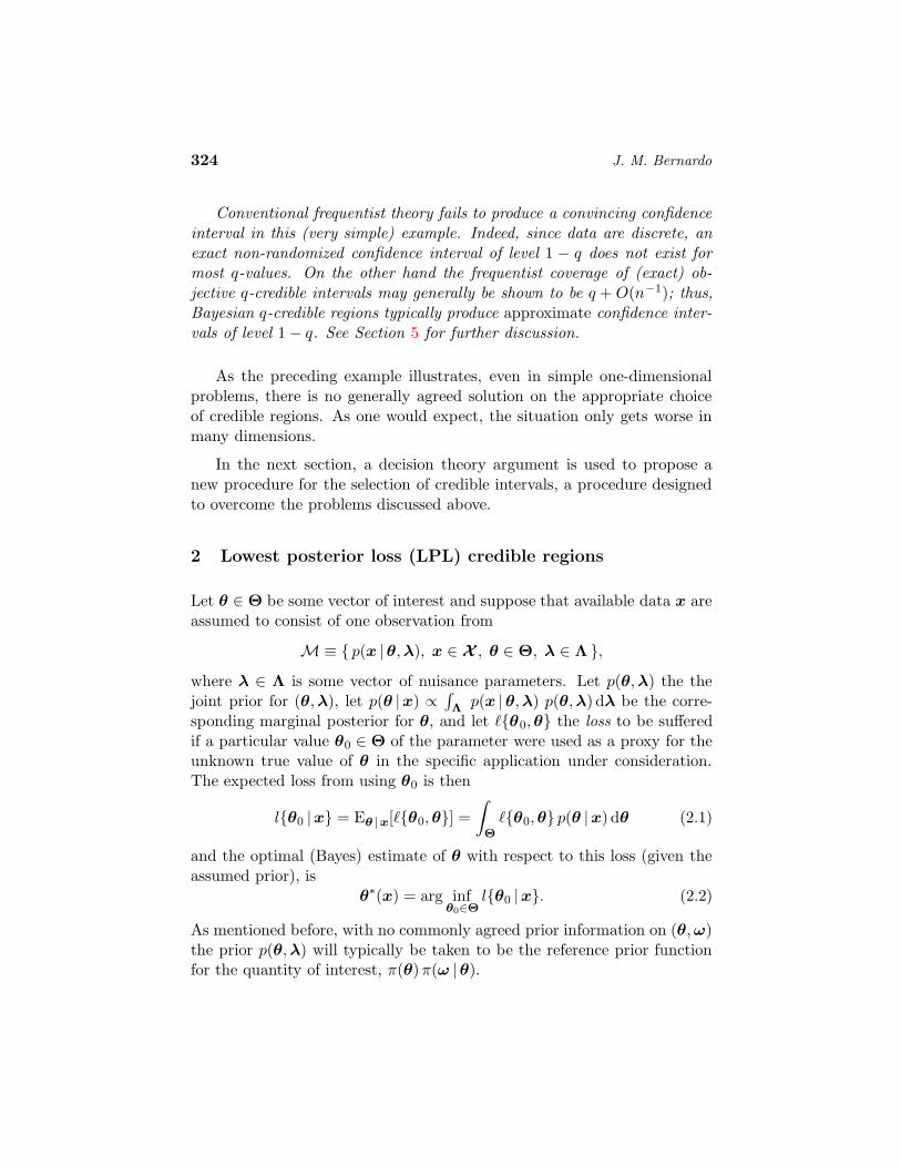
The expected loss l1θ0 | r, n is shown in the upper panel of Figure 3 forthe case r = 2 and n = 10 discussed before. This has a unique minimumat θ∗ = 0.210 which is therefore the Bayes estimator for this loss (markedwith a solid dot in the lower panel of Figure 3). The 0.95-LPL credibleinterval for this loss is numerically found to consist of the set (0.037, 0.482)whose expected loss is lower than 1.207 (shaded region in the lower panel ofFigure 3). Since intrinsic loss functions are invariant under reparametriza-tions, the Bayes estimate φ∗ and LPL q-credible region of some one-to-one

328 J. M. Bernardo

0 0.2 0.4 0.6 0.8 1

0.5

1.5

2.5

Θ

ΠHΘ È2,10L

0 0.2 0.4 0.6 0.8 1

0.5

1

1.5

2

Θ0

l1 HΘ0 È2,10L

Figure 3: Bayes estimator and LPL 0.95-credible region for a binomial parameter

using the L1 intrinsic loss.

function of φ will simply be φ(θ∗) and φ[R`q(r, n,Θ)]. For the variance-

stabilizing transformation φ(θ) = 2 arcsin√θ already considered in Exam-

ple 1.1 these are, respectively, 0.952 and (0.385, 1.535).

Notice that if one were to use a conventional, not invariant loss func-tion, the results would not be invariant under reparametrization. For in-stance, with a quadratic loss `θ0, θ = (θ0 − θ)2, the Bayes estimator isthe posterior mean, E[θ | r, n] = 0.227; similarly, the Bayes estimator forφ would be its posterior mean E[φ | r, n] = 0.965, which is different fromφ(0.227) = 0.994; credible regions would be similarly inconsistent. Yet, itwould be hard to argue, say to a quality engineer, that your best guess forthe proportion of defective items is θ∗, but that your best guess for log θ isnot log θ∗.

Intrinsic Credible Regions 329

In the next section, a particular, invariant intrinsic loss, the intrinsicdiscrepancy will be introduced. It is argued that this provides a far betterconventional loss function of choice for mathematical statistics than theubiquitous, overused quadratic loss.

3 The intrinsic discrepancy loss

Probability theory makes frequent use of divergence measures between prob-ability distributions. The total variation distance, Hellinger distance, Kull-back-Leibler logarithmic divergence, and Jeffreys logarithmic divergenceare all frequently cited; see, for example, Kullback (1968), and Gutierrez-Pena (1992) for precise definitions and properties. Each of those divergencemeasures may be used to define a type of convergence. It has been found,however, that the behaviour of many important limiting processes, in bothprobability theory and statistical inference, is better described in terms ofanother information-theory related divergence measure, the intrinsic dis-crepancy (Bernardo and Rueda, 2002), which is now defined and illustrated.

Definition 3.1 (Intrinsic discrepancy). Consider two probability dis-tributions of a random vector x ∈ X , specified by their density functionsp1(x), x ∈ X 1 ⊂ X , and p2(x), x ∈ X 2 ⊂ X , with either identical ornested supports. The intrinsic discrepancy δp1, p2 between p1 and p2 is

δp1, p2 = min

∫

X 1

p1(x) logp1(x)

p2(x)dx,

∫

X 2

p2(x) logp2(x)

p1(x)dx

, (3.1)

provided one of the integrals (or sums) is finite. The intrinsic discrepancyδF1,F2 between two families F1 and F2 of probability distributions is theminimum intrinsic discrepancy between their elements,

δF1,F2 = infp1∈F1, p2∈F2

δp1, p2. (3.2)

It is immediate from Definition 3.1 that the intrinsic discrepancy be-tween two probability distributions may be written in terms of their twopossible directed divergences (Kullback and Leibler, 1951) as

δp2, p1 = min

κp2 | p1, κp1 | p2

(3.3)

where the κpj | pi’s are the non-negative quantities defined by

κpj | pi =

∫

X i

pi(x) logpi(x)

pj(x)dx, with X i ⊆ X j. (3.4)

330 J. M. Bernardo

which are invariant under one-to-one transformations of x. Since κpj | piis the expected value of the logarithm of the density (or probability) ratiofor pi against pj when pi is true, it also follows from Definition 3.1 that, if p1

and p2 describe two alternative models, one of which is assumed to generatethe data, their intrinsic discrepancy δp1, p2 is the minimum expected log-likelihood ratio in favour of the model which generates the data (the “true”model).

The intrinsic discrepancy δp1, p2 is a divergence measure (i.e., it issymmetric, non-negative and zero iff p1 = p2 a.e.) with two added impor-tant properties which make it virtually unique: (i) the intrinsic discrepancyis still defined when the supports are strictly nested; hence, the intrinsicdiscrepancy δp, p between, say a distribution p with support on R andits approximation p with support on some compact subset [a, b] may becomputed; and (ii) the intrinsic discrepancy is additive for independentobservations. As a consequence of (ii), the intrinsic discrepancy δθ1, θ2between two possible joint models

∏nj=1 p1(xj | θ1) and

∏nj=1 p2(xj | θ2) for a

random sample x = x1, . . . , xn is simply n times the discrepancy betweenp1(x | θ1) and p2(x | θ2).

Theorem 3.1 (Properties of the intrinsic discrepancy). Let p1 and p2

be any two probability densities for the random vector x ∈ X with ei-ther identical or nested supports X 1 and X 2. Their intrinsic discrepancyδp1, p2 is

(i). Symmetric: δp1, p2 = δp2, p1

(ii). Non-negative: δp1, p2 ≥ 0, andδp1, p2 = 0 if, and only if, p1(x) = p2(x) a.e.

(iii). Defined for strictly nested supports:if X i ⊂ X j, then δpi, pj = δpj , pi = κpj | pi.

(iv). Invariant: If z = z(x) is one-to-one and qi(z) is the probability den-sity of z induced by pi(x), then δp1, p2 = δq1, q2

(v). Additive for independent observations: If x = y1, . . . ,yn, andpi(x) =

∏nl=1 qi(yl), then δp1, p2 = n δq1, q2.

Proof. (i) From Definition 3.1, δp1, p2 is obviously symmetric. (ii) More-over, δp1, p2 = minκp1 | p2, κp2 | p1; but κpi | pj is non-negative

Intrinsic Credible Regions 331

(use the inequality logw ≤ w − 1 with w = pi/pj , multiply by pj and inte-grate), and vanishes if (and only if) pi(x) = pj(x) almost everywhere. (iii)If p1(x) and p2(x) have strictly nested supports, one of the two directed di-vergences will not be finite, and their intrinsic discrepancy simply reduces tothe other directed divergence. (iv) The new densities are qi(x) = pi(x)/|J |,where J is the jacobian of the transformation; hence,

κqi | qj =

∫

Z

pj(x) |J | log pj(x) |J |pi(x) |J | dz =

∫

X

pj(x) logpj(x)

pi(x)dx

which is κpi | pj. (v) Under independence, pi(x) =∏n

j=1 qi(yj); thus

κpi | pj =

∫

Yn

n∏

l=1

qj(yl) log

∏nl=1 qj(yl)

∏nl=1 qi(yl)

dy1 . . . dyl

= n

∫

Y

qj(y) logqj(y)

qi(y)dy = n κqi | qj

and the result follows from Definition 3.1.

The statistically important additive property is essentially unique tologarithmic discrepancies; it is basically a consequence of two facts (i)the joint density of independent random quantities is the product of theirmarginals, and (ii) the logarithm is the only analytic function which trans-forms products into sums.

The intrinsic discrepancy may be used to define a new type of conver-gence for probability distributions which finds many applications in bothprobability theory and Bayesian inference.

Definition 3.2 (Intrinsic convergence). A sequence of probability dis-tributions specified by their density functions pi(x)∞i=1 is said to convergeintrinsically to a probability distribution with density p(x) whenever thesequence of their intrinsic discrepancies δ(pi, p)∞i=1 converges to zero.

Example 3.1 (Poisson approximation to a Binomial distribution).The intrinsic discrepancy between a Binomial distribution with probabilityfunction Bi(r |n, θ) and its Poisson approximation Po(r |n θ), is

δBi,Po |n, θ =

n∑

r=0

Bi(r |n, θ) logBi(r |n, θ)Po(r |n θ)

,

332 J. M. Bernardo

since the second sum in Definition 3.1 diverges. It may easily be verified thatlimn→∞ δBi,Po |n, λ/n = 0 and limθ→0 δBi,Po |λ/θ, θ = 0; thus, thesequences of Binomials Bi(r |n, λ/n) and Bi(r |λ/θi, θi) both intrinsicallyconverge to a Poisson Po(r |λ) when n→ ∞ and θi → 0, respectively. No-tice however that in the approximation a Binomial Bi(r |n, θ) by a PoissonPo(r |n θ) the roles of n and θ are very far from similar; the crucial con-dition for the approximation to work is that the value of θ must be small,while the value of n is largely irrelevant. Indeed, as shown in Figure 4,limθ→0 δBi,Po |n, θ = 0, for all n > 0, so arbitrarily good approxima-tions are possible with any n, provided θ is sufficiently small. However,limn→∞ δBi,Po |n, θ = 1

2 [−θ− log(1− θ)] for all θ > 0; thus, for fixed θ,the quality of the approximation cannot improve over a certain limit, nomatter how large n might be.

0.1 0.2 0.3 0.4 0.5

0

0.05

0.1

0.15 n=1

n=3n=5n=¥

Θ

∆ HBi, Po È n, Θ <

Figure 4: Intrinsic discrepancy δBi,Po |n, θ between a Binomial Bi(r |n, θ) and

a Poisson Po(r |nθ) as a function of θ, for n = 1, 3, 5 and ∞.

Definition 3.3 (Intrinsic discrepancy loss). For any given parametricmodel M = p(x |ω), x ∈ X , ω ∈ Ω, the intrinsic discrepancy loss asso-ciated to the use of ω0 as a proxy for ω is the intrinsic discrepancy

δxω0,ω = δpx |w0, px |w

between the models identified by ω0 and ω. More generally, if ω = (θ,λ),so that the model is M ≡ p(x |θ,λ), x ∈ X , θ ∈ Θ, λ ∈ Λ, the intrinsicdiscrepancy loss associated to the use of θ0 as a proxy for θ is the intrinsicdiscrepancy

δxθ0, (θ,λ) = infλ0∈Λ

δpx |θ0,λ0, px |θ,λ

Intrinsic Credible Regions 333

between the assumed model p(x |θ,λ), and its closest element in the familyp(x |θ0,λ0),λ0 ∈ Λ.

Example 3.2 (Intrinsic discrepancy loss in a Binomial model). Theintrinsic discrepancy loss δrθ0, θ |n associated to the use of θ0 as a proxyfor θ with Binomial Bi(r |n, θ) data is

δrθ0, θ |n = n δxθ0, θ, (3.5)

δxθ0, θ = min[κθ0 | θ, κθ | θ0 ]

κ(θi | θj) = θj log[θj/θi] + (1 − θj) log[(1 − θj)/(1 − θi)],

where δxθ0, θ is the intrinsic discrepancy between Bernoulli random vari-ables with parameters θ0 and θ. The intrinsic loss function δxθ0, θ isrepresented in Figure 5.

0.20.4

0.60.8

0.20.4

0.60.8

0

2

4

6

0.20.4

0.60.8

0.20.4

0.60.8

∆x 8Θ0 ,Θ <

Θ0

Θ

Figure 5: Intrinsic discrepancy loss δxθ0, θ from using θ0 as a proxy for θ in a

binomial setting.

The intrinsic discrepancy loss, was introduced by Bernardo and Rueda(2002) in the context of hypothesis testing. It is an intrinsic loss function(Definition 2.2) and, hence, it is invariant under reparametrization. More-over, as one would surely require, (i) the intrinsic discrepancy between

334 J. M. Bernardo

two elements of a parametric family of distributions is also invariant un-der marginalization to the model induced by the sampling distribution ofany sufficient statistic, and (ii) the intrinsic discrepancy loss is additive forconditionally independent observations. More precisely,

Theorem 3.2 (Properties of the intrinsic discrepancy loss). Con-sider model M ≡ p(x |θ,λ), x ∈ X , θ ∈ Θ, λ ∈ Λ and let δxθ0, (θ,λ)be the loss associated to the use of θ0 as a proxy for θ.

(i). Consistent marginalization: If t(x) ∈ T is sufficient for M, thenδtθ0, (θ,λ) = δxθ0, (θ,λ). In particular, δxθ0, (θ,λ) is in-variant under one-to-one transformations of x.

(ii). Additivity: If x = y1, . . . ,yn and the yj’s are independent given(θ,λ), then δxθ0, (θ,λ) =

∑nj=1 δyj

θ0, (θ,λ). If they are alsoidentically distributed, then δxθ0, (θ,λ) = n δyθ0, (θ,λ).

Proof. (i) If t(x) ∈ T is sufficient for M and s(x) is an ancillary statistic,so that, in terms of ω = (θ,λ), p(x |ω) = p(t |ω) p(s | t), the requireddirected divergences κp(x |ωi) | p(x |ωj) may be written as

∫

X

p(t |ωj) p(s | t) logp(t |ωj) p(s | t)p(t |ωi) p(s | t)

dx =

∫

T

p(t |ωj) logp(t |ωj)

p(t |ωi)dt.

It follows that the intrinsic discrepancy loss δxθ0, (θ,λ) calculated fromthe full model is the same as the intrinsic discrepancy δtθ0, (θ,λ) calcu-lated from the marginal model p(t |θ,λ), t ∈ T , θ ∈ Θ, λ ∈ Λ inducedby the sufficient statistic. (ii) Additivity is a direct consequence of the laststatement in Theorem 3.1.

Computation of intrinsic loss functions in well-behaved problems maybe simplified by the use of the result below:

Theorem 3.3 (Computation of the intrinsic loss function). Considera model M ≡ p(x |θ,λ), x ∈ X , θ ∈ Θ, λ ∈ Λ such that the support ofp(x |θ,λ) is convex for all pairs (θ,λ). Then

δxθ0, (θ,λ) = infλ0∈Λ

δpx | θ0,λ0, px | θ,λ

= min

infλ0∈Λ

κ(θ,λ |θ0,λ0), infλ0∈Λ

κ(θ0,λ0 |θ,λ)

.

Intrinsic Credible Regions 335

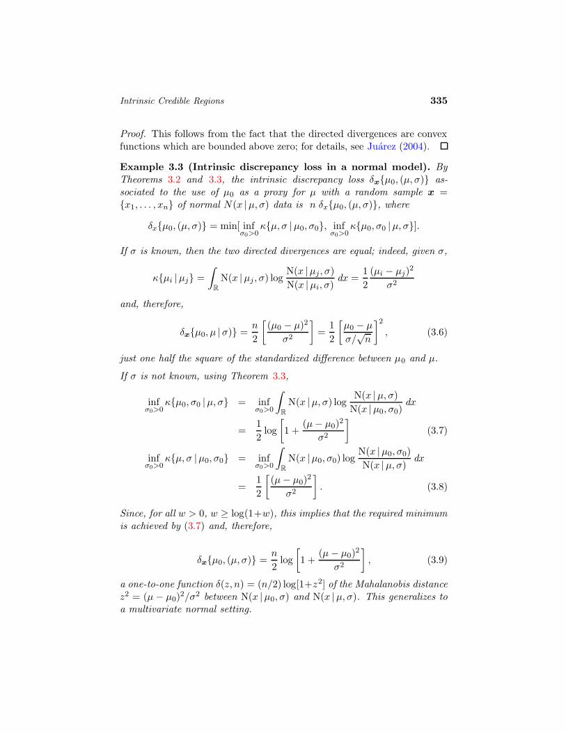
Proof. This follows from the fact that the directed divergences are convexfunctions which are bounded above zero; for details, see Juarez (2004).

Example 3.3 (Intrinsic discrepancy loss in a normal model). ByTheorems 3.2 and 3.3, the intrinsic discrepancy loss δxµ0, (µ, σ) as-sociated to the use of µ0 as a proxy for µ with a random sample x =x1, . . . , xn of normal N(x |µ, σ) data is n δxµ0, (µ, σ), where

δxµ0, (µ, σ) = min[ infσ0>0

κµ, σ |µ0, σ0, infσ0>0

κµ0, σ0 |µ, σ].

If σ is known, then the two directed divergences are equal; indeed, given σ,

κµi |µj =

∫

R

N(x |µj , σ) logN(x |µj , σ)

N(x |µi, σ)dx =

1

2

(µi − µj)2

σ2

and, therefore,

δxµ0, µ |σ) =n

2

[

(µ0 − µ)2

σ2

]

=1

2

[

µ0 − µ

σ/√n

]2

, (3.6)

just one half the square of the standardized difference between µ0 and µ.

If σ is not known, using Theorem 3.3,

infσ0>0

κµ0, σ0 |µ, σ = infσ0>0

∫

R

N(x |µ, σ) logN(x |µ, σ)

N(x |µ0, σ0)dx

=1

2log

[

1 +(µ− µ0)

2

σ2

]

(3.7)

infσ0>0

κµ, σ |µ0, σ0 = infσ0>0

∫

R

N(x |µ0, σ0) logN(x |µ0, σ0)

N(x |µ, σ)dx

=1

2

[

(µ− µ0)2

σ2

]

. (3.8)

Since, for all w > 0, w ≥ log(1+w), this implies that the required minimumis achieved by (3.7) and, therefore,

δxµ0, (µ, σ) =n

2log

[

1 +(µ− µ0)

2

σ2

]

, (3.9)

a one-to-one function δ(z, n) = (n/2) log[1+z2] of the Mahalanobis distancez2 = (µ− µ0)

2/σ2 between N(x |µ0, σ) and N(x |µ, σ). This generalizes toa multivariate normal setting.

336 J. M. Bernardo

-10 -5 0 5 10

0

1

2

3

4

5

z

∆x 8z,1<

∆x 8z,2<∆x 8z,10<

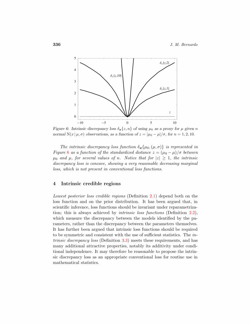
Figure 6: Intrinsic discrepancy loss δxz, n of using µ0 as a proxy for µ given n

normal N(x |µ, σ) observations, as a function of z = |µ0 − µ|/σ, for n = 1, 2, 10.

The intrinsic discrepancy loss function δxµ0, (µ, σ) is represented inFigure 6 as a function of the standardized distance z = (µ0 − µ)/σ betweenµ0 and µ, for several values of n. Notice that for |z| ≥ 1, the intrinsicdiscrepancy loss is concave, showing a very reasonable decreasing marginalloss, which is not present in conventional loss functions.

4 Intrinsic credible regions

Lowest posterior loss credible regions (Definition 2.1) depend both on theloss function and on the prior distribution. It has been argued that, inscientific inference, loss functions should be invariant under reparametriza-tion; this is always achieved by intrinsic loss functions (Definition 2.2),which measure the discrepancy between the models identified by the pa-rameters, rather than the discrepancy between the parameters themselves.It has further been argued that intrinsic loss functions should be requiredto be symmetric and consistent with the use of sufficient statistics. The in-trinsic discrepancy loss (Definition 3.3) meets these requirements, and hasmany additional attractive properties, notably its additivity under condi-tional independence. It may therefore be reasonable to propose the intrin-sic discrepancy loss as an appropriate conventional loss for routine use inmathematical statistics.

Intrinsic Credible Regions 337

On the other hand, as already mentioned in the introduction, scientificcommunication typically requires the use of some sort objective prior, onewhich captures, in a well-defined sense, the notion of the prior having aminimal effect, relative to the data in the final inference. This should be aconventional prior to be used when a default specification, having a claim tobeing non-influential in the sense described above, is required. In the longhistorical quest for these objective priors several requirements have emergedwhich may reasonably be requested as necessary properties of any proposedsolution; this includes generality, consistency under reparametrization, con-sistency under marginalization, and consistent sampling properties. Ref-erence analysis, introduced by Bernardo (1979b) and further developedBerger and Bernardo (1989, 1992a,b,c), appears to be the only availablemethod to derive objective prior functions which satisfy all these desider-ata. For an introduction to reference analysis, see Bernardo and Ramon(1998); for a recent review of reference analysis, see Bernardo (2005b).

The Bayes estimator which corresponds to the intrinsic discrepancy lossand the appropriate reference prior is the intrinsic estimator. Introduced byBernardo and Juarez (2003), this is a completely general objective Bayesianestimator, which is invariant under reparametrization.

Definition 4.1 (Intrinsic estimate). Consider data x which consist ofone observation from M ≡ p(x |θ,λ), x ∈ X , θ ∈ Θ, λ ∈ Λ, and letδxθ0, (θ,λ) be the intrinsic discrepancy loss to be suffered if θ0 were usedas a proxy for θ. The intrinsic estimate of θ

θ∗(x) = arg minθi∈Θ

d(θi |x),

is that parameter value which minimizes the reference posterior expectedintrinsic loss d(θi |x), where

d(θi |x) =

∫

Θ

∫

Λ

δxθi, (θ,λ)π(θ,λ |x) dθ dλ, (4.1)

π(θ,λ |x) ∝ p(x |θ,λ)π(λ |θ)π(θ), (4.2)

and π(λ |θ)π(θ) is the joint reference prior of (θ,λ) when θ is the quantityof interest.

Moving from point estimation to region estimation, intrinsic credibleregions are defined as the lowest posterior loss credible regions which cor-respond to the use of the intrinsic discrepancy loss and the appropriate

338 J. M. Bernardo

reference prior. As one would expect, the intrinsic estimate is contained inall intrinsic credible regions.

Definition 4.2 (Intrinsic credible region). Consider data x which con-sist of one observation from M ≡ p(x |θ,λ), x ∈ X , θ ∈ Θ, λ ∈ Λ,and let δxθ0, (θ,λ) be the intrinsic discrepancy loss to be suffered if θ0

were used as a proxy for θ. An intrinsic q-credible region is a subsetR∗

q = R∗q(x,Θ) ⊂ Θ of the parameter space Θ such that,

(i).∫

R∗

qπ(θ |x) dθ = q,

(ii). ∀θi ∈ R∗q , ∀θj /∈ R∗

q , d(θi |x) ≤ d(θj |x),

where d(θi |x), the reference intrinsic posterior expected loss from using θ i

as a proxy for the value of the parameter, is given by Equation (4.1).

The analytical expression of the intrinsic discrepancy loss δxθ0, (θ,λ)is often complicated and, hence, exact computation of its posterior expecta-tion, d(θi |x) typically requires numerical integration. Although these daysthis is seldom a serious practical problem, it is both theoretically interestingand pragmatically useful to derive appropriate asymptotic approximations.Attention to approximations will be limited here to one-dimensional reg-ular models, but the results may be extended to both non-regular andmultiparameter problems.

Let data x = x1, . . . , xn, xj ∈ X , consist of a random sample of size nfrom a distribution p(x | θ) with one continuous parameter θ ∈ Θ ⊂ R.Under appropriate regularity conditions, there exists a unique maximumlikelihood estimator θn = θn(x) whose sampling distribution is asymptot-ically normal with mean θ and variance i−1(θ)/n, where i(θ) is Fisher’sinformation function,

i(θ) = −∫

Xp(x | θ) ∂2

∂θ2log p(x | θ) dx. (4.3)

Moreover, the function defined by the indefinite integral

φ(θ) =

∫

√

i(θ) dθ (4.4)

provides a variance stabilizing transformation. Indeed, it is easily veri-fied that, under the assumed conditions, the maximum likelihood estimate

Intrinsic Credible Regions 339

φn = φn(x) is asymptotically normal with mean φ = φ(θ) and variance1/n, and that the approximate marginal model

p(φn |φ) = N(φn |φ, 1/√n), φ ∈ Φ = φ(Θ),

is asymptotically equivalent to the original model p(x | θ) =∏n

j=1 p(xj | θ).It follows that φ asymptotically behaves as location parameter and, hence,the reference prior for φ is the uniform prior π(φ) = 1. All this suggeststhat φ(θ) is, in a sense, a fairly natural parametrization for the model.

More generally, if θn = θn(x) is an asymptotically sufficient, consis-tent estimator of θ whose asymptotic sampling distribution is p(θn | θ), thereference prior for θ is (Bernardo and Smith, 1994, Section 5.4)

π(θ) = p(θn | θ)∣

∣

∣

∣

θn=θ

(4.5)

and, therefore, the reference prior of the monotone transformation definedby the indefinite integral φ(θ) =

∫

π(θ) dθ is π(φ) = π(θ)/|∂φ/∂θ| = 1, auniform prior.

The reference parametrization of a probability model is defined as thatfor which the reference prior is uniform:

Definition 4.3 (Reference parametrization). Let x = x1, . . . , xn bea random sample from M = p(x | θ), x ∈ X , θ ∈ Θ and let θn = θn(x)be an asymptotically sufficient, consistent estimator of θ whose asymptoticsampling distribution is p(θn | θ). A reference parametrization for model Mis then defined by the indefinite integral

φ(θ) =

∫

π(θ) dθ, where π(θ) = p(θn | θ)∣

∣

∣

∣

θn=θ

. (4.6)

When the sample space X does not depend on θ and the likelihoodfunction p(x | θ) is twice differentiable as a function of θ, the sampling dis-tribution of maximum-likelihood estimator θ is often asymptotically normalwith variance i−1(θ)/n, where i(θ) is Fisher’s information function given byEquation (4.3); see, e.g., Schervish (1995, Section 7.3.5) for precise condi-tions. In this case, the reference parametrization is given by Equation (4.4),and this may be used to obtain analytical approximations. More generally,if a model has an asymptotically sufficient, consistent estimator of θ whosesampling distribution is asymptotically normal, a reference parametrization

340 J. M. Bernardo

may be used to obtain a simple asymptotic approximation to its intrinsicdiscrepancy loss δx(θ0, θ), and to the corresponding reference posterior ex-pectation d(θ0 |x). This provides analytical asymptotic approximations tothe required credible regions.

Theorem 4.1 (Asymptotic approximations). Let x = x1, . . . , xn bea random sample from M = p(x | θ), x ∈ X , θ ∈ Θ and let θn = θn(x)be an asymptotically sufficient, consistent estimator of θ whose samplingdistribution is asymptotically normal N(θn | θ, s(θ)/

√n). Then,

(i). The reference prior for θ is π(θ) = s−1(θ), a reference parametriza-tion is φ(θ) =

∫

s−1(θ) dθ, the reference prior for φ is π(φ) = 1, andthe reference posterior of φ, in terms of the inverse function θ(φ), isπ(φ |x) ∝ px | θ(φ) |∂θ(φ)/∂φ|.

(ii). The intrinsic discrepancy loss is

δx(θ0, θ) = n2

[

φ(θ0) − φ(θ)]2

+ o(1).

(iii). The expected posterior loss isd(θ0 |x) = n

2

[

σ2φ(x) + µφ(x) − φ(θ0)2

]

+ o(1),

where µφ(x) and σ2φ(x) are, respectively, the mean and variance of

the reference posterior distribution of φ, π(φ |x).

(iv). The intrinsic estimator of φ is µφ(x) + o(1), and the intrinsic esti-mator of θ is θ∗(x) = θµφ(x) + o(1)

(v). The intrinsic q-credible region of φ is the interval[φq0(x), φq1(x)] = µφ(x) ± zq σφ(x) + o(1),where zq is the (q + 1)/2 normal quantile.

The intrinsic q-credible region of θ is the interval[θq0(x), θq1(x)] = θ [φq0(x), φq1(x)] + o(1).

Proof. (i) is an immediate application of Equation (4.5), Definition 4.3 andstandard probability calculus. (ii) Under the assumed conditions, the sam-pling distribution of φn(x) will be, for sufficiently large n, approximatelynormal N(φn |φ, 1/√n). Since the intrinsic discrepancy loss is invariantunder marginalization (Theorem 3.2), δx(θ0, θ) = δφn

(φ0, φ) and, usingEquation (3.6) of Example 3.3,

δφn(φ0, φ) ≈ δxN(φn |φ0, 1/

√n), N(φn |φ, 1/

√n) =

n

2(φ0 − φ)2.

Intrinsic Credible Regions 341

(iii) Using the invariance of the intrinsic discrepancy loss under reparametri-zation,

d(θ0 |x) =

∫

Θδx(θ0, θ)π(θ |x) dθ =

∫

Φδx(φ0, φ)π(φ |x) dφ

≈∫

Φ

n

2(φ0 − φ)2 π(φ |x) dφ

=n

2

[

E(φ− µφ)2 + (µφ − φ0)2]

=n

2

[

σ2φ + (µφ − φ0)

2]

,

where φ0 = φ(θ0). (iv) As a function of φ0, d(φ0 |x) is minimised whenφ0 = µφ and, hence this provides the intrinsic estimate of φ; by invari-ance, the intrinsic estimate of θ is simply θ(µφ), where θ(φ) is the inversefunction of φ(θ). (v) Since the expected intrinsic loss d(φ0 |x) is symmet-ric around µφ, all lowest posterior loss credible regions will be symmetricaround µφ Hence, the intrinsic q-credible interval for φ will be of the formR∗

q(x,Φ) = µφ ± zq σφ, with zq chosen such that

∫ µφ+zq σφ

µφ−zq σφ

π(φ |x) dφ = q.

Moreover, since φn(x) is asymptotically sufficient, and its sampling distri-bution is asymptotically normal, the reference posterior distribution of φwill also be asymptotically normal and, therefore, zq will approximately bethe (q + 1)/2 quantile of the standard normal distribution. By invariance,the intrinsic q-credible interval for θ will simply be given by inverse imageof q-credible interval for φ, R∗

q(x,Θ) = θR∗q(x,Φ).

The posterior moments µφ(x) and σ2φ(x) of the reference parameter

required in Theorem 4.1 may often be obtained analytically. If this isnot the case, the delta method may be used to derive µφ(x) and σ2

φ(x) interms of the (typically easier to obtain) reference posterior mean µθ(x) andreference posterior variance σ2

θ(x) of the original parameter θ:

µφ(x) ≈ φµθ(x) + 12 σ

2θ(x)φ′′µθ(x) (4.7)

σ2φ(x) ≈ σ2

θ(x) [φ′µθ(x)]2 (4.8)

(see e.g., Schervish (1995, Section 7.1.3) for precise conditions). The deltamethod yields a particularly simple approximation for the posterior vari-ance of the reference parameter. Indeed, σ2

θ ≈ s(θn)/n and φ′

(θ) = s(θ);

342 J. M. Bernardo

hence, using Equation (4.8), σ2φ ≈ 1/n. This provides much simpler (but

less precise) approximations than those in Theorem 4.1.

Corollary 4.1. Under the conditions of Theorem 4.1, simpler (less precise)approximations are given by:

(i). d(θ0 |x) ≈ 12 + n

2

[

µφ(x) − φ(θ0)]2

(ii). θ∗ ≈ θµφ(x)

(iii). R∗q(x,Φ) ≈ µφ(x) ± zq/

√n, R∗

q(x,Θ) = θR∗q(x,Φ),

where zq is the (q+1)/2 quantile of the standard normal distribution.

(iv). If µφ(x) is not analytically available, it may be approximated in termsof the first reference posterior moments of θ, µθ(x) and σθ(x), byµφ(x) ≈ φµθ(x) + 1

2 σ2θ(x)φ

′′µθ(x)

As illustrated below, Corollary 4.1 may actually provide reasonable approx-imations even with rather small sample sizes.

Example 4.1 (Credible intervals for a binomial parameter (contin-ued)). Consider again the problem considered in Examples 1.1, 2.1 and 3.2,and use the corresponding intrinsic discrepancy loss (Equation 3.5). Thereference prior is π(θ) = θ−1/2(1 − θ)−1/2, and the reference posterior isπ(θ | r, n) = Be(θ | r + 1

2 , n − r + 12). The reference posterior expected loss

from using θ0 rather than θ will be

dθ0 | r, n = n

∫ 1

0δxθ0, θBe(θ | r + 1

2 , n− r + 12) dθ.

Simple numerical algorithms may be used to obtain the intrinsic estimate,namely the value of θ0 which minimizes dθ0 | r, n, and intrinsic credibleintervals, that is the lowest posterior loss intervals with the required poste-rior probability.

The function dθ0 | r, n is represented in the upper panel of Figure 7for the case r = 0 and n = 10 discussed before. This is minimized byθ∗ = 0.031, which is therefore the intrinsic estimate; the result may becompared with the maximum-likelihood estimate θ = 0, utterly useless inthis case. Similarly, for r = 1 and n = 10 the intrinsic estimate is foundto be θ∗ = 0.123; by invariance, the intrinsic estimate of any one to onefunction ψ = ψ(θ) is simply ψ(θ∗); thus the intrinsic estimate of, say θ2, is

Intrinsic Credible Regions 343

0 0.05 0.1 0.15 0.2 0.25 0.30

5

10

15

20

25

30

Θ

ΠHΘ È0,10L

0 0.05 0.1 0.15 0.2 0.25 0.3

0.5

1

1.5

2

2.5

Θ0

dHΘ0 È0,10L

Figure 7: Reference posterior density, intrinsic estimate and intrinsic 0.95-credible

region for a binomial parameter, given n = 10 and r = 0.

θ∗2 = 0.015; this may be compared with the corresponding unbiased estimateof θ2, which is r(r−1)/n(n−1) and hence zero in this particular case,a rather obtuse estimation for the square of the proportion of somethingwhich has actually been observed one in ten times. For r = 2, n = 10 theintrinsic estimate is θ∗ = 0.218, somewhere between the posterior median(0.210) and the the posterior mean (0.227).

Intrinsic credible regions are also easily found numerically. Thus, forr = 0 and n = 10, the 0.95 intrinsic credible interval for θ is (0, 0.170)(shaded region in Figure 7); in this case, this is also the HPD interval. Forr = 2 and n = 10 the 0.95 intrinsic credible interval is (0.032, 0.474), veryclose to (0.037, 0.482), the LPL 0.95-credible interval which corresponds tothe L1 loss (see Example 2.1).

344 J. M. Bernardo

Since the reference prior for this problem is π(θ) = θ−1/2(1 − θ)−1/2, areference parameter is φ(θ) =

∫

π(θ) dθ = 2arcsin√θ, with inverse func-

tion θ(φ) = sin2(φ/2). Changing variables, the reference posterior of thereference parameter φ is Equation (1.4), a distribution whose first momentsdo not have a simple analytical expression. The use of Corollary 4.1 withthe exact reference posterior moments of θ, µθ = (r + 1/2)/(n + 1) andσ2

θ = µθ(1 − µθ)/(n+ 2) leads, with φ′

(θ) = θ−1/2(1 − θ)−1/2 and φ′′

(θ) =12 (2θ − 1) θ−3/2(1 − θ)−3/2, to simple analytical approximations for the in-trinsic estimates and the intrinsic credible regions. In particular, with r = 2and n = 10, µθ = 0.227, σ2

θ = 0.015, and the delta method yields µφ ≈ 0.967and θ∗ = θ(µφ) ≈ 0.216, quite close to the exact value 0.218. MoreoverR∗

0.95(Θ) ≈ θ (0.967 ± 1.96 × 1/√

10) = (0.030, 0.508), close to its ex-act value (0.032, 0.474). As one would expect the approximation is not thatgood in extreme cases, when either r = 0 or r = n. For instance, with r = 0and n = 10, Corollary 4.1 yields θ∗ ≈ 0.028 and R∗

0.95(Θ) ≈ (0.020, 0.213),compared with the exact values 0.031 and (0, 0.170) respectively.

Example 4.2 (Intrinsic credible interval for the normal mean).Consider a random sample x = x1, . . . , xn from a normal distributionN(x |µ, σ), and let x = Σjxj/n, and s2 = Σj(xj −x)2/n be the correspond-ing mean and variance. The reference prior when µ is the parameter ofinterest is π(µ)π(σ |µ) = σ−1, and the corresponding joint reference poste-rior is

π(µ, σ |x) = π(µ, σ |x) = N[µ |x, σ/√n] Ga−1/2[σ | 1

2(n− 1), 12n s

2]

∝ σ−(n+1) exp[− n

σ2s2 + (x− µ)2]. (4.9)

Thus, using Equation (3.9), the reference posterior expected intrinsic lossfrom using µ0 as a proxy for µ is

d(µ0 |x) =

∫ ∞

∞

∫ ∞

0

n

2log

[

1 +(µ− µ0)

2

σ2

]

π(µ, σ |x) dµ dσ. (4.10)

As one could expect, and may directly be verified by appropriate changeof variables in Equation (4.10), this is a symmetric function of µ0 − x.It follows that q-credible regions for µ must be centred at x. Moreover,the (marginal) reference posterior of µ is Student St(µ|x, s/

√n− 1, n− 1).

Consequently, the intrinsic q-credible interval for the normal mean µ is

R∗q(x,R) = x± tq(n− 1) s/

√n− 1

Intrinsic Credible Regions 345

where tq(n− 1) is the (q + 1)/2 quantile of a standard Student distributionwith n− 1 degrees of freedom. As one could expect in this example, this isalso the HPD interval, and the frequentist confidence interval of level 1−q.

0.5 1 1.5 2 2.5 3 3.5 4

0

1

2

3

4

Μ0

dH Μ0 Èx,s,nL

Figure 8: Expected intrinsic loss from using µi as a proxy for a normal mean,

given n = 10 observations, with x = 2.165 and s = 1.334.

Figure 8 describes the behaviour of d(µ0 |x) given n = 10 observations,simulated from N(x | 2, 1) which yielded x = 2.165 and s = 1.334. Theintrinsic estimate is obviously x (marked with a solid dot) and the 0.95intrinsic credible interval consists of values (1.159, 3.171) whose intrinsicposterior expected loss is smaller than 2.151.

5 Frequentist coverage

As Example 4.2 illustrates, the frequentist coverage probabilities of theq-credible regions which may be derived from objective posterior distribu-tions are sometimes identical to their posterior probabilities. This exactnumerical agreement is however the exception, not the norm. Nevertheless,for large sample sizes, Bayesian credible intervals are always approximateconfidence intervals. Although this is an asymptotic property, it has beenfound that, even for moderate samples, the frequentist coverage of referenceq-credible regions, i.e., credible regions based of the reference posterior dis-tribution, is usually very close to q. This means that, in many problems,

346 J. M. Bernardo

reference q-credible regions are also approximate frequentist confidence in-tervals with significance level 1−q; thus, under repeated sampling from thesame model, the proportion of reference q-credible regions containing thetrue value of the parameter will be approximately q.

More precisely, let data x = x1, . . . , xn consist of n independent ob-servations from the one parameter model M = p(x | θ), x ∈ X , θ ∈ Θ, andlet θq(x, pθ) denote the q-quantile of the posterior p(θ |x) ∝ p(x | θ) p(θ)which corresponds to the prior p(θ); thus,

Pr[

θ ≤ θq(x, pθ) |x]

=

∫

θ≤θq(x, pθ)p(θ |x) dθ = q.

and, for any fixed data x, Rq(x) = θ; θ ≤ θq(x, pθ) is a left q-credibleregion for θ. For fixed θ, consider now Rq(x) as a function of x. Standardasymptotic theory may be used to establish that, for any sufficiently regularpair pθ, M of prior pθ and model M, the coverage probability of Rq(x)converges to q as n→ ∞. Specifically, for all sufficiently regular priors,

Pr[

θq(x, pθ) ≥ θ | θ]

=

∫

x; θq(x, pθ)≥θp(x | θ) dx = q +O(n−1/2).

In a pioneering paper, Welch and Peers (1963) established that in the caseof the one-parameter regular models for continuous data Jeffreys prior,which in this case is also the reference prior, π(θ) ∝ i(θ)1/2, is the onlyprior which further satisfies

Pr[

θq(x, πθ) ≥ θ | θ]

= q +O(n−1);

Hartigan (1966) later showed that the coverage probabilities of one-dimen-sional two-sided Bayesian posterior credible intervals satisfy this type of ap-proximation to O(n−1) for all sufficiently regular prior functions. Moreover,Hartigan (1983, p. 79) showed that the result of Welch and Peers (1963)on one-sided posterior credible intervals may be extended to one-parametermodels for discrete data by using appropriate continuity corrections.

This all means that reference priors are often probability matching pri-ors, that is, priors for which the coverage probabilities of posterior credibleintervals are asymptotically closer to their posterior probabilities than thosederived from any other prior; see Datta and Sweeting (2005) for a recentreview on this topic.

Intrinsic Credible Regions 347

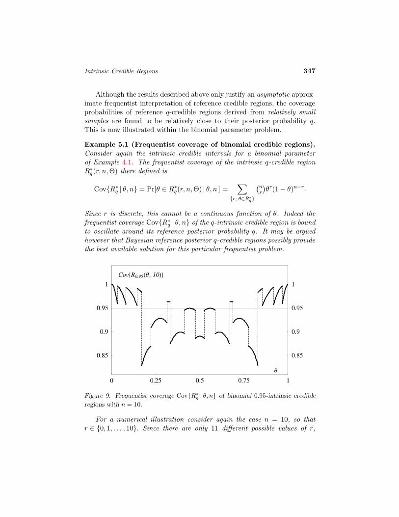
Although the results described above only justify an asymptotic approx-imate frequentist interpretation of reference credible regions, the coverageprobabilities of reference q-credible regions derived from relatively smallsamples are found to be relatively close to their posterior probability q.This is now illustrated within the binomial parameter problem.

Example 5.1 (Frequentist coverage of binomial credible regions).Consider again the intrinsic credible intervals for a binomial parameterof Example 4.1. The frequentist coverage of the intrinsic q-credible regionR∗

q(r, n,Θ) there defined is

CovR∗q | θ, n = Pr[θ ∈ R∗

q(r, n,Θ) | θ, n ] =∑

r; θ∈R∗

q

(nr

)

θr(1 − θ)n−r.

Since r is discrete, this cannot be a continuous function of θ. Indeed thefrequentist coverage CovR∗

q | θ, n of the q-intrinsic credible region is boundto oscillate around its reference posterior probability q. It may be arguedhowever that Bayesian reference posterior q-credible regions possibly providethe best available solution for this particular frequentist problem.

0 0.25 0.5 0.75 1

0.85

0.9

0.95

1

0.85

0.9

0.95

1

Θ

Cov8R0.95HΘ , 10L<

Figure 9: Frequentist coverage CovR∗

q | θ, n of binomial 0.95-intrinsic credible

regions with n = 10.

For a numerical illustration consider again the case n = 10, so thatr ∈ 0, 1, . . . , 10. Since there are only 11 different possible values of r,

348 J. M. Bernardo

Table 1: Intrinsic estimates and intrinsic 0.95-credible intervals for the parameter θ

of a binomial distribution Bi(r |n, θ), with n = 10.

r θ∗(r, 10) R∗q(r, n,Θ)

0 0.032 (0.000, 0.171)

1 0.124 (0.000, 0.331)

2 0.218 (0.033, 0.474)

3 0.314 (0.082, 0.588)

4 0.408 (0.145, 0.686)

5 0.500 (0.224, 0.776)

6 0.592 (0.314, 0.855)

7 0.686 (0.412, 0.918)

8 0.782 (0.526, 0.967)

9 0.876 (0.669, 1.000)

10 0.968 (0.829, 1.000)

there are only 11 distinct intrinsic 0.95-credible intervals; those are listedin Table 1. If the true value of θ were, say, 0.25, it would be containedin the intrinsic credible region R∗

q(r, n,Θ) if, and only if, r ∈ 1, 2, 3, 4, 5,and this would happen with probability

CovR∗0.95 | θ = 0.25, n = 10 =

5∑

r=1

Bi(r | θ = 0.25, n = 10) = 0.934.

Figure 9 represents the frequentist coverage CovR∗q | θ, n as a function

of θ for q = 0.95 and n = 10. It may be appreciated the proportionCovR∗

0.95 | θ, n of intrinsic 0.95-credible intervals which may be expected tocontain the true value of θ under repeated sampling oscillates rather wildlyaround its posterior probability 0.95, with discontinuities at the points whichdefine the credible regions. Naturally, CovR∗

q | θ, n will converge to q forall θ values as n → ∞, but very large n values would be necessary for agood approximation, especially for extreme values of θ.

6 Further Examples

The canonical binomial and normal examples have systematically been usedabove to illustrate the ideas presented. In this final section a wider rangeof examples is presented.

Intrinsic Credible Regions 349

6.1 Exponential data

Consider a random sample x = x1, . . . , xn from an exponential distribu-tion Ex(x | θ) = θe−xθ, and let t =

∑nj=1 xj .

The exponential intrinsic discrepancy loss is

δx(θ0, θ) = n min[κθ | θ0, κθ0 | θ]

κθi | θj =

∫ ∞

0Ex(x | θj) log

Ex(x | θj)

Ex(x | θi)dx

= g(θi/θj),

where g(x) is the linlog function, the positive distance

g(x) = (x− 1) − log x, (6.1)

between log x and its tangent at x = 1. Hence,

δx(θ0, θ) = n δx(θ0, θ), δx(θ0, θ) =

g(θ0/θ) θ0 ≤ θ,g(θ/θ0) θ0 > θ.

A related loss function, `σ20 , σ

2 = g(σ20/σ

2), often referred to as theentropy loss, was used by Brown (1968) (who attributed this to C. Stein) asan alternative to the quadratic loss in point estimation of scale parameters.

The reference prior (which here is also Jeffreys prior) is π(θ) = θ−1, andthe corresponding reference posterior is π(θ |x) = Ga(θ |n, t) ∝ θn−1e−nt.Hence, the posterior loss d(θ0 |x) from using θ0 as a proxy for θ is

d(θ0 |x) = d(θ0 | t, n) = n

∫ ∞

0δx(θ0, θ)Ga(θ |n, t) dθ.

Figure 10 describes the behaviour of d(θo |x) given n = 12 observations,simulated from Ex(x | 2), which yielded t = 4.88. The intrinsic estimateis 2.364 (marked with a solid dot), and the intrinsic 0.95-credible intervalconsists of the values (1.328, 4.198) whose posterior expected loss is smallerthan 1.954.

A reference parameter for this problem is φ(θ) =∫

π(θ) dθ = log θ, andits posterior mean may be analytically obtained as

µφ =

∫ ∞

0log θ Ga(θ |n, t) dθ = ψ(n) − log t (6.2)

350 J. M. Bernardo

0 1 2 3 4 5 6 7

0

0.5

1

1.5

2

2.5

3

Θ0

dHΘo È4.88,12L

Figure 10: Expected intrinsic loss from using θ0 as a proxy for the parameter θ of

an exponential distribution, given n = 12 observations, with x = t/n = 0.407. The

intrinsic estimate is θ∗ = 2.364, the intrinsic 0.95-credible region is (1.328, 4.198).

where ψ(·) is the digamma function. Using Equation (6.2) in Corollary 4.1,with t = 4.88 and n = 12, yields µφ = 0.858, and hence, θ∗ ≈ exp[µφ] =2.357 very close to its exact value 2.364, even though the sample size,n = 12, is rather small. Moreover,

R∗0.95 ≈ (exp[µφ − 1.96/

√n], exp[µφ + 1.96/

√n]) = (1.339, 4.151)

quite close again to the exact intrinsic region (1.328, 4.198).

In this problem, all reference posterior credible regions are exact fre-quentist confidence intervals. Indeed, changing variables, the referenceposterior distribution of τ = t θ is Ga(τ |n, 1); on the other hand, thesampling distribution of t is Ga(t |n, θ) and, therefore, the sampling distri-bution of s = t θ is Ga(s |n, 1). Thus, the reference posterior distributionof t θ, as a function of θ, is precisely the same as the sampling distribu-tion of t θ, as a function of t; consequently, for any region R(t) ⊂ Θ,Pr[θ ∈ R(t) | t, n] = Pr[θ ∈ R(t) | θ, n].

6.2 Uniform data

Consider a random sample x = x1, . . . , xn from a uniform distributionUn(x | θ) = θ−1, 0 ≤ x ≤ θ, θ > 0, and let t = maxx1, . . . , xn. Notice that

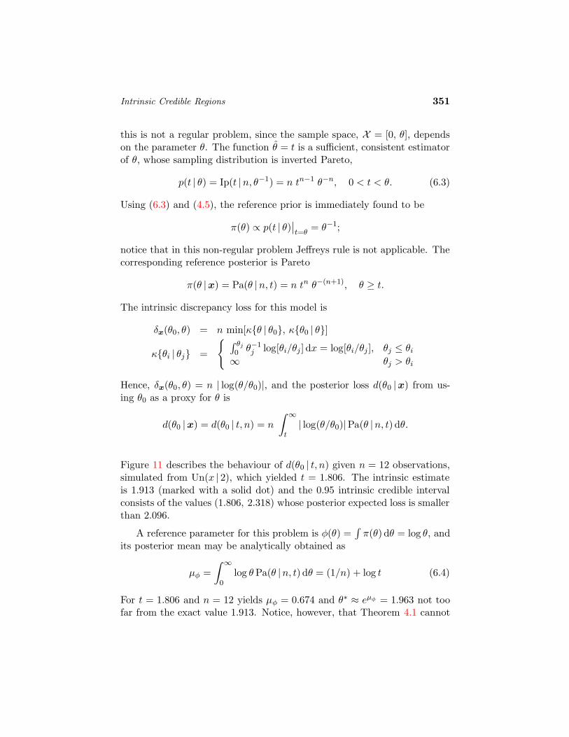
Intrinsic Credible Regions 351

this is not a regular problem, since the sample space, X = [0, θ], dependson the parameter θ. The function θ = t is a sufficient, consistent estimatorof θ, whose sampling distribution is inverted Pareto,

p(t | θ) = Ip(t |n, θ−1) = n tn−1 θ−n, 0 < t < θ. (6.3)

Using (6.3) and (4.5), the reference prior is immediately found to be

π(θ) ∝ p(t | θ)∣

∣

t=θ= θ−1;

notice that in this non-regular problem Jeffreys rule is not applicable. Thecorresponding reference posterior is Pareto

π(θ |x) = Pa(θ |n, t) = n tn θ−(n+1), θ ≥ t.

The intrinsic discrepancy loss for this model is

δx(θ0, θ) = n min[κθ | θ0, κθ0 | θ]

κθi | θj =

∫ θj

0 θ−1j log[θi/θj ] dx = log[θi/θj ], θj ≤ θi

∞ θj > θi

Hence, δx(θ0, θ) = n | log(θ/θ0)|, and the posterior loss d(θ0 |x) from us-ing θ0 as a proxy for θ is

d(θ0 |x) = d(θ0 | t, n) = n

∫ ∞

t| log(θ/θ0)|Pa(θ |n, t) dθ.

Figure 11 describes the behaviour of d(θ0 | t, n) given n = 12 observations,simulated from Un(x | 2), which yielded t = 1.806. The intrinsic estimateis 1.913 (marked with a solid dot) and the 0.95 intrinsic credible intervalconsists of the values (1.806, 2.318) whose posterior expected loss is smallerthan 2.096.

A reference parameter for this problem is φ(θ) =∫

π(θ) dθ = log θ, andits posterior mean may be analytically obtained as

µφ =

∫ ∞

0log θPa(θ |n, t) dθ = (1/n) + log t (6.4)

For t = 1.806 and n = 12 yields µφ = 0.674 and θ∗ ≈ eµφ = 1.963 not toofar from the exact value 1.913. Notice, however, that Theorem 4.1 cannot

352 J. M. Bernardo

1.8 2 2.2 2.4 2.6

0

0.5

1

1.5

2

2.5

3

Θ0

dHΘ0 È1.806,12L

Figure 11: Expected intrinsic loss from using θ0 as a proxy for the parameter θ of

a uniform distribution, given n = 12 observations, with t = maxxj = 1.806. The

intrinsic estimate is θ∗ = 1.913, the intrinsic 0.95-credible region is (1.806, 2.318).

be applied to this problem, since neither the sampling distribution of theconsistent estimator t, nor the posterior distribution of φ are asymptoticallynormal. In fact, the posterior variance of φ is (exactly) 1/n2; this is O(n−2)rather than O(n−1), as obtained in regular models.

Once again, all reference posterior credible regions in this problem areexact frequentist confidence intervals. Indeed, changing variables, the ref-erence posterior distribution of τ = θ/t is Pareto, Pa(τ |n, 1); on the otherhand, the sampling distribution of t is inverted Pareto Ip(t |n, θ−1) and,therefore, the sampling distribution of s = θ/t is also Pa(s |n, 1). Hence,the reference posterior distribution of θ/t as a function of θ is precisely thesame as the sampling distribution of θ/t as a function of t and thus, forany region R(t) ⊂ Θ, Pr[θ ∈ R(t) | t, n] = Pr[θ ∈ R(t) | θ, n].

6.3 Normal mean and variance

Consider a random sample x = x1, . . . , xn from a normal distributionN(x |µ, σ), and let θ = (µ, σ) be the (bivariate) quantity of interest. Theintrinsic discrepancy loss for this model is

δxθ0,θ = δx(µ0, σ0), (µ, σ)

Intrinsic Credible Regions 353

= n min[κ(µ0, σ0) | (µ, σ), κ(µ, σ) | (µ0, σ0)]

with

κ(µi, σi) | (µj , σj =1

2

[

g

(

σ2j

σ2i

)

+(µi − µj)

2

σ2i

]

, (6.5)

where g(x) = (x− 1) − log x is, again, the linlog function; this yields

δx(µ0, σ0), (µ, σ) =

n κ(µ, σ) | (µ0, σ0), σ ≥ σ0

n κ(µ0, σ0) | (µ, σ), σ < σ0.(6.6)

The normal is a location-scale model and, thus (Bernardo, 2005b), the ref-erence prior is π(µ, σ) = σ−1. The corresponding (joint) reference posteriordistribution, π(µ, σ |x), is given in Equation (4.9).

The reference posterior expected intrinsic loss from using (µ0, σ0) as aproxy for (µ, σ) is then

d(µ0, σ0 |x) =

∫ ∞

0

∫ ∞

−∞δx(µ0, σ0), (µ, σ)π(µ, σ |x) dµdσ.

This is a convex surface with a unique minimum at the intrinsic estimate

µ∗(x), σ∗(x) = arg minµ0∈R,σ0>0

d(µ0, σ0 |x) = x, σ∗(s, n) (6.7)

where σ∗ is of the form σ∗(s, n) = kn s and, hence, it is an affine equivariantestimator. With n = 2, σ∗(x1, x2) ≈ (

√5/2) |x1−x2|; for moderate or large

sample sizes,

σ∗(s, n) = kn s ≈√

n

n− 2s. (6.8)

Since intrinsic estimation is invariant under reparametrization, the intrinsicestimator of the variance is simply (σ∗)2 ≈ n s2/(n−2), slightly larger thanboth the mle estimator s2, and the unbiased estimator n s2/(n− 1).

Intrinsic credible regions are obtained by projecting into the (µ0, σ0)plane the intersections of the surface d(µ0, σ0 |x) with horizontal planes.

Figure 12 describes the behaviour of d(µ0, σ0 |x) given n = 25 observations,simulated from N(x | 0, 1), which yielded x = 0.024 and s = 1.077. Theresulting surface has a unique minimum at (µ∗, σ∗) = (0.024, 1.133), whichis the intrinsic estimate; notice that

µ∗ = x, σ∗ ≈ s√

n/(n− 2) = 1.123.

354 J. M. Bernardo

-0.5

0

0.5

0.751

1.251.5

1.75

0

0.1

0.2

0.3

-0.5

0

0.5

0.751

1.251.5

1.75

d8 Μ0 ,Σ0 È data<

Σ0

Μ0

Figure 12: Expected intrinsic loss from using (µ0, σ0) as a proxy for the param-

eters (µ, σ) of a normal distribution, given n = 25 observations, with x = 0.024

and s = 1.077.

Figure 13 represents the corresponding intrinsic estimate and contours ofintrinsic q-credible regions, for q = 0.50, 0.95 and 0.99. For instance, R∗

0.95

(middle contour in the figure) is the set of µ0, σ0 points whose intrinsicexpected loss is not larger that 0.134.

Notice finally that all reference posterior credible regions in this problemare, once more, exact frequentist confidence intervals. Indeed, for all n, thejoint reference posterior distribution of

µ− x

σ/√n× n s2

σ2(6.9)

as a function of (µ, σ) is precisely the same as its sampling distribution asa function of (x, s2). Thus, for any region R = R(m, s, n) ⊂ R × R

+, onemust have Pr[(µ, σ) ∈ R |m, s, n] = Pr[(µ, σ) ∈ R |µ, σ, n].

Intrinsic Credible Regions 355

-1 -0.5 0 0.5 1

0.5

1

1.5

2

Μ

Σ

Figure 13: Intrinsic estimate (solid dot) and intrinsic q-credible regions (q = 0.50,

0.95 and 0.99) for the parameters (µ, σ) of a normal distribution, given n = 25

observations, with x = 0.024 and s = 1.077.

DISCUSSION

George CasellaDepartment of Statistics

University of Florida, USA

1 Introduction

The vagaries of email originally sent Professor Bernardo’s paper into Limborather than Florida, and because of that, my time to prepare this discussionwas limited. As a result, I decided to concentrate on one aspect of the paper,that having to do with discrete intervals.

First, let me say that Professor Bernardo has, once again, brought us afundamentally new way of approaching a problem, an approach that is notonly extremely insightful, but also is likely to lead to even more develop-ments in objective Bayesian analysis. The coupling of interval construction

356 G. Casella

with lowest posterior loss is a very intriguing concept, and the argumentfor using an intrinsic loss is compelling.

There is one point about loss functions that I really like. ProfessorBernardo notes that a loss `θ0,θ should be measuring the distance be-tween the models p(x|θ0) and p(x|θ), not the distance between θ0 and θ,which is often irrelevant to an inference. This is an excellent principle tofocus on in any decision problem. Results that are not invariant to 1 − 1transformations can sometimes be interesting in theory, but they tend tobe less useful in practice.

2 Convincing Confidence Intervals

Professor Bernardo states that in the binomial problem “Conventional fre-quentist theory fails to provide a convincing confidence interval” (my ital-ics), and then comments on the limitations imposed by the discreteness ofthe problem. It is not clear what a “convincing” confidence interval is -it seems to me that any confidence interval that maintains its guaranteedconfidence level is convincing. It is also unclear to me, and has been for along time, why the fact that the problem is discrete automatically bringsabout criticism.

The discreteness of the data is a limitation. When we impose a contin-uous criterion, satisfying such a criterion will often require more than thedata can provide. This is not a fault of any procedure, simply a limitationof the data. The fact that in discrete problems a confidence interval cannotattain exact level q is not a cause for criticism.

However, what is a cause for criticism is the reliance on Bayesian in-tervals being approximate frequentist intervals. Although it is true that insome cases the frequentist coverage may be of the order q + O(n−1), thatO may be so big as to not be useful.

3 Binomial Confidence Intervals

Now I would like to focus on Example 5.1 (also note the companion Exam-ples 1.1, 3.2, and 4.1). Professor Bernardo is not happy with the frequentistanswer here (or anywhere, I dare say!) however, I claim that in this case thebest frequentist region provides a very acceptable Bayesian region, whilethe objective Bayesian region fails as a frequentist region.

Intrinsic Credible Regions 357

First of all, what is the “best” frequentist answer? To me, it is theprocedure of Blyth and Still (1983) (see also Casella, 1986). This procedureworks within the limitations of the discrete binomial problem to produceintervals that are not only short, but enjoy a number of other desirableproperties, including equivariance. Figure 1 shows the Blyth-Still intervalsalong with the Bernardo intervals for the case n = 10.

0 2 4 6 8 10

0.0

0.2

0.4

0.6

0.8

1.0

r

thet

a

0 2 4 6 8 10

0.0

0.2

0.4

0.6

0.8

1.0

0 2 4 6 8 10

0.0

0.2

0.4

0.6

0.8

1.0

0 2 4 6 8 10

0.0

0.2

0.4

0.6

0.8

1.0

Figure 1: For n = 10, binomial intervals of Bernardo (dashed) and Blyth-Still

(solid). The Bernardo intervals are 95% Bayesian credible intervals, and the Blyth-

Still intervals are 95% frequentist intervals.

It is interesting that the intervals are so close, but we notice that theBlyth-Still intervals are a bit longer than the Bernardo intervals. Indeed,if we compare the procedures using the sum of the lengths as a measureof size, we find that the sum of the lengths of the Blyth-Still intervalsis 5.20, while that of the Bernardo intervals is 4.53. However, one of thecriteria that the Blyth-Still intervals satisfy is that, among level q confidenceintervals, they minimize the sum of the lengths. Therefore, we know thatthe Bernardo intervals cannot maintain level q and, indeed, from Bernardo’sFigure 9 we see that this is indeed the case. Even though the Bernardointervals are approximate frequentist intervals, the approximation is really

358 G. Casella

quite poor. The nominal 95% interval can have coverage probability as lowas 83% (reading off the graph) which is quite unacceptable. Moreover, thefluctuations in the coverage probability are quite large, ranging from a lowof 83% to a high of 100%

0.0 0.2 0.4 0.6 0.8 1.0

0.95

0.96

0.97

0.98

0.99

1.00

theta

Cove

rage

Figure 2: For n = 10, coverage probabilities of the 95% Blyth-Still intervals.

The frequentist intervals, although not convincing to Professor Bernar-do, do a fine job of controlling the coverage probability within the con-straints of a discrete problem. As an illustration, compare Bernardo’s Fig-ure 9 with Figure 2, showing the coverage probability of the Blyth-Still95% interval. Although there is fluctuation in the probabilities, they areabove 95%, making a true confidence interval, and the range of probabil-ities ranges only from 95% to 100%, displaying much less variability thanthe Bernardo intervals.

Finally, lets look at how the Blyth-Still intervals fare as Bayesian cred-ible regions. Using the reference prior, we can produce Table 1. There wesee that they are, indeed, 95% credible intervals. Although the credibleprobabilities are not exactly 95% for each value of r, they are uniformlygreater than r, varying in the range .951 − .989.

Intrinsic Credible Regions 359

Table 1: Credible probabilities of the 95% Blyth-Still confidence intervals

r 0 1 2 3 4 5

Prob .989 .979 .971 .959 .964 .951

r 6 7 8 9 10

Prob .964 .959 .971 .979 .989

What to conclude from all of this? As a long-time frequentist, it issupremely gratifying to see the wide development of objective Bayesianinference, which is defined by Professor Bernardo as a statistical analysisthat only depends on the model and the observed data. With one moresmall step, we might include the sample space and then objective Bayesianswill attain the ultimate objective goal of being frequentists!

But, on a more serious note, we see that in “objective” inference, thereis a desire to have a procedure perform well on Bayesian (post-data) and fre-quentist (pre-data) criteria. What my illustration was supposed to demon-strate is that one can construct an acceptable objective Bayesian procedurenot just by starting from a Bayesian derivation and then checking frequen-tist properties, but also by starting from a frequentist derivation and thenchecking Bayesian properties.

Edward I. GeorgeDepartment of Statistics

University of Pennsylvania, USA

Let me begin by congratulating Professor Bernardo on a deep method-ological contribution that is based on important recent foundational con-siderations. I must admit that I was skeptical when I began to read thispaper, thinking that this would simply be a new recipe for credible regionswith little in the way of compelling justification. Much to my surprise,the proposed approach has both a compelling motivation and turns out, atleast in some cases, to dovetail nicely with frequentist procedures that areroutinely used. Going further, I would recommend these intrinsic credibleregions as the new default in the absence of reliable prior information.

As I understand it, the general goal of the objective Bayes approach is todevise default Bayesian procedures that require minimal, if any, subjective

360 E. I. George

input. Towards this end, the basic problem in this paper is to come up withan objective Bayesian methodology for the construction of credible regionsfor an unknown parameter function value θ(ω).

At the heart of the objective Bayesian approach is the choice of prior,and in this regard, a key development has been the default reference priorapproach put forward by Professor Bernardo and his collaborators. Theseattractive reference priors are an essential ingredient for the proposed con-struction of intrinsic credible regions in so far as they are used to obtain thereference posterior. However, the central issue tackled in this paper is howto extract from the reference posterior a unique set of values which are in ameaningful sense “closest” to θ(ω). As Professor Bernardo correctly pointsout, HPD regions are unappealing because of a lack of reparametrizationinvariance, and posterior quantile regions may easily exclude sets of highestposterior concentration.

Instead, Professor Bernardo proposes using a Lowest Posterior Loss(LPL) region, effectively a neighborhood of the minimum posterior ex-pected loss estimate. I much prefer such an approach because it treats theregion estimation problem as an extension of the decision theoretic treat-ment of the point estimation problem. Although a companion coveragereport of (1 −α)% probability, frequentist or Bayesian, is valuable, I thinkit has incorrectly been given too much primacy as a construction criterion.I believe a practitioner is best served by a region containing point estimatesthat are superior to point estimates outside the region, which is preciselywhat LPL is about. I don’t think it is wise to sacrifice this property simplyto gain a more accurate coverage estimate.

Having settled on LPL, the problem becomes one of choosing a lossfunction that is essentially objective. For this purpose, Professor Bernardoargues convincingly that attention must be restricted to the so-called in-trinsic losses, losses that are parametrization invariant and so depend onlyon discrepancies between models. I agree. Further, divergence measuresare natural candidates for such losses. Especially attractive is the KL di-vergence which as Professor Bernardo notes is invariant under sample spacetransformation, see also George and McCulloch (1993). However, the lackof symmetry of the KL divergence is problematic for the construction ofLPL regions. By proposing instead to use the intrinsic discrepancy loss,Professor Bernardo gets to “have his cake and eat it too”. The intrinsicdiscrepancy essentially symmetrizes the KL divergence without relinquish-

Intrinsic Credible Regions 361

ing many of its wonderful features. And I much prefer this symmetrizationto the standard alternative approach of a weighted sum of the two directedKL divergences.

The examples in Section 3 nicely illustrate how intrinsic discrepanciesbetween distributions can depend dramatically upon different regions inthe parameter space. Indeed, Example 3.1 shows how clearly the intrin-sic discrepancy reveals regions of asymptotic equivalence and nonequiva-lence between the binomial and Poisson models. To me, this highlights theneed to avoid arbitrary loss functions for the construction of LPL regions.Further investigation into other potential uses of the intrinsic discrepancyseems to be a fertile new research direction.

Thus, Professor Bernardo arrives at his definition of an intrinsic credi-ble region – namely an LPL region based on intrinsic discrepancy loss andthe appropriate reference prior – very reasonable and well motivated. ButI then was astonished to see what came next. Applied to several importantexamples, namely the normal mean, the exponential, the uniform, and thenormal mean and variance, the intrinsic credible regions are all also exactfrequentist confidence intervals. These intrinsic credible regions they notonly contain a best set of point estimates, but their coverage can be con-veyed in an objectively meaningful way. I suspect that further investigationof this agreement may shed valuable new light on the always fascinatinginterface between Bayesian and frequentist methods. I wonder if ProfessorBernardo can pinpoint the essential reason behind this matching propertyof intrinsic credible regions in these cases, and if he has any sense of howbroadly it will it occur?

The frequentists coverage properties of the intrinsic credible regions forthe discrete binomial distribution are not as nice, but this is fundamentallya general problem of all interval estimation reports for discrete distribu-tions, see Brown et al. (2001). My sense is that a different type of reportis needed in such cases, for example, see Geyer and Meeden (2005). In anycase, the asymptotic agreement with frequentist coverage is reassuring.

It is clear that when reliable prior subjective information is unavail-able, a Bayesian analysis must turn to non-subjective considerations. Forthis purpose Professor Bernardo has made wonderful use of the invarianceproperties of information theoretic measures. It is interesting that suchinvariance is typically lacking in fully subjective Bayesian methods.

362 J. Giron and E. Moreno

In closing, I must apologize to Professor Bernardo for being so positiveabout his paper, as it hardly gives him anything to argue about in hisrejoinder. But that is the price for having such a good idea.

Javier GironDepartment of Statistics

University of Malaga, SpainElıas Moreno

Department of StatisticsUniversity of Granada, Spain

The advantage of a unifying approach to the basic inference problems,as the one carried out by Professor Bernardo in this and previous papers onintrinsic estimation and testing, (see Bernardo, 2001) is always welcomedand, in this respect, we cannot help but congratulate Professor Bernardofor his proposal.

Highest posterior density regions (HPD’s) are, as Professor Bernardocorrectly asserts in his paper, a tool we employ to summarize a given pos-terior density π(θ |x). Sometimes the mode, mean and standard deviationare also reported.

A natural question to be answered before giving credit to the intrinsiccredible regions proposed in the paper is the following: do we need to replaceHPD’s with another region? Professor Bernardo asserts that HPD’s arenot coherent in the sense of not being invariant under reparametrization.Therefore, the consequence for him is that a different region is needed. But,not so fast!

Given a one-to-one differentiable transformation α = g(θ) the posteriordensity of α is

π(α |x) = π(g−1(α) |x)|J|, (1)

where |J| stands for the determinant of the Jacobian of the inverse map-ping. Then, HPD’s for the parameter α are obtained from the posteriordistribution π(α |x). What is wrong with this?

Professor Bernardo claims that the HPD’s are not coherent because theq-HPD for α does not coincide with the g-transformation of the q-HPDfor θ. This is obviously due to the fact that the Jacobian in Equation (1)

Intrinsic Credible Regions 363

is not constant unless g be linear. We do not think this coherent notionto be of such a fundamental nature, and we find such a requirement ratherartificial.

In fact, q-HPD regions are a good summary of the posterior density andthey are defined in the same spirit as the likelihood sets notion. These setshave been proved to enjoy very nice properties (Cano et al., 1987; Piccinato,1984; Wasserman, 1989).

But intrinsic credible regions rely more on the properties of the intrinsicloss discrepancy than on the form of the posterior. Thus, the computationof intrinsic credible regions appears as a somewhat contrived artifact toassure coherence, i.e. invariance, rather than a means to show off nicecharacteristics of the posterior density for a given parametrization. Fur-ther, the metric or scale of the expected intrinsic loss is in units of informa-tion δ∗, while intrinsic credible regions are measured in a probabilistic scaleq; consequently, in order to compute intrinsic credible regions the expectedintrinsic loss has to be calibrated in terms of the probabilistic content q.

Though for one-dimensional parameters when the expected intrinsicloss is pseudoconvex and the posterior density is unimodal HPD’s and in-trinsic credible regions are intervals, contours in more than one dimension,obtained from the expected intrinsic loss may be very different from theones obtained from the posterior density, whatever the parametrization,specially in higher dimensions. This might be very disturbing, and it is the(sometimes very high) price one has to pay to preserve invariance; for thisreason, we believe that credible regions should capture the properties of theposterior density not those of the expected intrinsic loss. We note that theabove comments apply to any other loss function we would consider appro-priate for the estimation problem, as the differences between the contoursof the posterior risk and the posterior density can be very substantial.

One point of some concern is the fact that, as shown in the binomialExample 4.1 and the uniform example in Section 6.1, the reference pos-terior expected intrinsic loss displayed in Figures 7 and 11, respectively,though they are convex they are not increasing. This means that for verysmall values of q the intrinsic credible intervals do not contain values ina small neighborhood of 0, thus ruling out a set of points with highestposterior density; furthermore, this problem also holds for any monotonictransformation of the parameter θ.

364 J. Giron and E. Moreno

It might be argued that intrinsic credible regions do only make sense forthe usual large values of q, say 0.95 and 0.99, but from a formal standpointthe behavior of the intrinsic credible regions should be consistent whateverthe value of q.

On the other hand, as the two statistical problems of testing a sharphypothesis of the form H0 : θ = θ0 and computing a credible region in theparameter space Ω both use the reference posterior expected intrinsic lossin a similar way, it is apparent that there exists a duality between the twoproblems in the same sense as in the classical approach and in the Bayesianone advocated by Lindley (1970, pp. 56–69). In fact, to reject the nullH0 : θ = θ0 is equivalent to see if the reference posterior expected intrinsicloss d(θ0 |x) is greater that some suitable positive value δ∗, where δ∗ is theexpected utility of accepting the null hypothesis when it is true. This isobviously equivalent to rejecting the null whenever θ0 does not belong tothe credible region R∗

q for some q which depends on δ∗ defined by

R∗q = θ; d(θ |x) < δ∗.

In some sense the computation of δ∗, which is carried out conditioningon the null hypothesis, resembles that of computing a p-value in frequentisttesting.

Thus, from Bernardo’s approach, intrinsic testing of sharp null hypoth-esis and intrinsic credible regions are equivalent procedures as there is a oneto one mapping between δ∗’s and q’s. Further, this mapping depends en-tirely on the reference posterior expected intrinsic loss, thus differing fromLindley’s approach to significance testing.

While this approach has many advantages —the most important onebeing that no new prior but the reference prior is to be used for estimationand testing and, in some sense, provides a Bayesian simple mechanism forsignificance testing from a statistical viewpoint—, the issue of practicalsignificance seems to be missing in this approach as we believe that pointor interval estimation is quite a different statistical problem than that oftesting sharp nulls, and this in turn means that using a prior different fromthe reference one which may take into account the sharp null to be testedmakes sense in this setting.

Intrinsic Credible Regions 365

Daniel PenaDepartamento de Estadıstica

Universidad Carlos III de Madrid, Spain

This article presents an objective way to obtain confidence intervals fora parameter. In Bayesian inference this problem has not received much at-tention and the Bayesian literature usually has stressed that the posteriorprobability for the parameter incorporates all the information about it andfrom this posterior probability it is straightforward to obtain a q-credibleinterval, that is, a region on the support of the random variable with hasa probability equal to q. Among all the infinite regions that can be built anatural criterion is that values inside the interval must have higher proba-bility than values outside, but in order to apply this rule it is well known, seefor instance Lindley (1970, p. 35), that we have to decide which parameteris to be used, as this rule is not invariant under one-to-one transformationsof the parameter.

In this article an objective solution is proposed to solve this ambiguity.The procedure is to use a reference prior and a reference loss function andone key contribution in this paper is the use of the intrinsic discrepancyloss, introduced by Bernardo and Rueda (2002) for hypothesis testing. Theauthor has to be congratulated for proposing a clear and objective way tosolve this ambiguity in building credible regions.

The intrinsic discrepancy is defined as the minimum of κ(p2 | p1) andκ(p1 | p2) where

κ(p2 | p1) =

∫

p1(x) logp1(x)

p2(x)dx ≥ 0

is the Kullback-Leibler information in favor of p1 against p2. This measureis invariant under reparametrization and also with respect to one to onetransformations of the variable. It is also additive for independent observa-tions. These properties are shared with the divergence κ(p2 | p1)+κ(p1 | p2),introduced by Kullblack and Leibler. However it has the advantage overthe later that it is well defined when one of the two measures of informa-tion is infinite. To avoid this problem, Kullback (1968) assumed that thetwo probability measures were absolutely continuous with respect to eachother, so that the two integrals could exist. The intrinsic discrepancy does

366 D. Pena

not need this constrain and therefore it has a wider applicability. However,in the application considered in this paper, building credible regions, it isto be expected that the two probability measures used verify Kullback con-ditions, that is they are absolutely continuous with respect to each other,and therefore this property may not be crucial. Assuming that in mostcases both discrepancies can be used, which are the advantages for build-ing credible regions of the intrinsic discrepancy with respect to the standardKullblack Leibler divergence?, how different the results would be of usingone instead of the other?

The derivation of intrinsic credible regions may be complicated and mayrequire numerical integration and thus an interesting contribution from thepoint of view of applications is Theorem 4.1, where simple asymptotic ap-proximations are obtained. This result will facilitate the use of the pre-sented theory in practice.

My final comments on this interesting and though-provoking paper areon three directions. First, it would be useful to have a better understandingof the advantages of the proposed approach over the standard HPD regions.Suppose that I have a HPD region for θ. Would it be possible to computea measure of the maximum loss that we may have if we translate this HPDfor θ to build a credible interval for a one-to-one transformation of theparameter φ? From my point of view in order to convince people to usethese ideas is important to provide some bounds of the advantages that wemay obtain with respect to conventional methods.

Second, how this ideas can be extended for building prediction credi-ble regions for future values of the observed random variable of interest?As in the Bayesian approach parameters are random variables, I supposethe extension is straightforward but it would be interesting to have somecomments on this topic.

Third, how these ideas can be extended for dependent observationsas, for instance, time series or spatial data? When the data have somedependency structure prediction of the observed random variable is usuallythe key problem, and an approach to develop prediction intervals whichdoes not depend on the parametrization could be very appealing. For timeseries a popular measure of information is the mutual information or relativeentropy (Joe, 1989) given by

K(x, y) =

∫ ∫

f(x, y) logf(x, y)

f(x)f(y)dxdy,

Intrinsic Credible Regions 367

which is nonnegative and it is zero only if the two variables are independent.This measure has been used to build a test of independence (Robinson,1991), identifying lags in the relationship in nonlinear time series model-ing (Granger and Lin, 1994) or building measures of general dependencyamong vector random variables (Pena and van der Linde, 2005), among oth-ers applications. Taking p1(x) = f(x, y) and p2(x) = f(x)f(y) the intrinsicdiscrepancy between dependency and independency of the two random vari-ables x and y can be defined and this idea might be used for credible regionsand hypothesis testing in time series. It would be interesting to explore thispossibility.

Finally I would like to congratulate the author for a very interestingpiece of research.

Judith Rousseau and Christian P. RobertCEREMADE, Universite Paris Dauphine

and CREST, INSEE, France

In this paper, Professor Bernardo presents a unified and structured ob-jective approach to (decisional) statistical inference, based on informationtheoretic ideas he has used previously to define reference priors. He fo-cusses here on the estimation of credible regions, keeping those values ofthe parameter that are the least costly rather than the most probable, asin HPD regions. This is an interesting and novel approach to an efficientconstruction of credible regions when lacking a decision-theoretic basis. Asnoted in Casella et al. (1993, 1994) (see also Robert, 2001, Section 5.5.3,for a review), the classical decision-theoretic approaches to credible regionsare quite behind their counterpart for point estimation and testing and in-corporating loss perspectives in credible sets was then suggested in Robertand Casella (1994).

1 On invariance: link with HPD regions

A possible drawback of HPD regions, in particular in objective contexts,is their lack of invariance under reparameterization as was pointed out byProfessor Bernardo. Obviously, HPD regions are defined in terms of avolume-under-fixed-coverage loss and they do minimize the volume among

368 J. Rousseau and C. P. Robert

q-credible regions. The lack of invariance hence stems from the lack of in-variance in the definition of the volume, which is based on the Lebesguemeasure for the considered parametrization θ. Therefore, simply consider-ing a different type of volume based on an invariant measure would resultin an HPD region that is invariant under reparameterization. A naturalinvariant measure in this setup is Jeffreys’ measure, due to its geometricand information interpretations (among others). The resulting HPD regionis thus constructed as the region C that minimizes

∫

C

√

i(θ)dθ, u.c. P π[C|X] ≥ q. (1)

This region also corresponds to the transform of the (usual) HPD regionconstructed using the reference parametrization as defined by ProfessorBernardo.

Note that, in the above construction, there is absolutely no need inhaving the prior be Jeffreys prior and this construction could be used in(partially) informative setups. It is also interesting to note that, in regularcases, the above HPD region is asymptotically equivalent to the intrinsiccredible region of Professor Bernardo. Which of both approaches is themost appealing is probably a question of taste or depends on how they willbe used.

On a more philosophical basis, we think that invariance is less com-pelling an argument for (credible) regions than for point estimations. In-deed, while it is difficult to sell to a customer that the estimator of h(θ) isnot necessarily the transform h(θ) of the estimator θ of θ, the transformof a crebible region does remain a credible region, even though it is notalways the optimal region. Moreover, invariance under reparameterizationshould be weighted against shape poor modifications. Indeed, if we imposethat the credible region Ch on h(θ) is the transform by h of the credibleregion Cid on θ, we get exposed to strange shapes for less regular functionsh! For instance, if the transform h is not monotonic (but still one-to-one),it is possible to obtain the transform of a credible interval as a collection ofseveral disjoint intervals, always a puzzling feature! Connexity (and maybeto some extent convexity) should be part of the constraints on a credibleregion.

Intrinsic Credible Regions 369

2 Asymptotic coverage : matching properties

Under regularity properties, the HPD region defined by (1) is a second ordermatching region for any smooth prior π, in the sense that its frequentistcoverage is equal to its posterior coverage to the order O(n−1). Third ordercoverage does not necessarily apply for Jeffreys’ prior, though (see Dattaand Mukerjee, 2004 or Rousseau, 1997). As Bernardo’s intrinsic credibleregion is asymptotically equivalent to the HPD region defined by (1) thereis a chance that second order matching is satisfied, which would explain thegood small sample properties mentioned in the paper. In particular, theperturbation due to using the intrinsic loss, compared to using the posteriordensity, is of order O(n−1), so second order asymptotics should be the samebetween (1) and the intrinsic credible region.

Investing further the higher order matching properties of this credibleregion would be worthwhile though. Regarding the discrete case, how-ever, things are more complicated than what was mentioned by ProfessorBernardo since there is usually no matching to orders higher than O(n−1/2)or sometimes o(n−1/2) for higher dimensional cases. Whether referenceposterior q-credible regions provide the best available solution for this par-ticular problem is somehow doubtful as there are many criteria which couldreasonably be considered for comparing credible regions or their approxi-mations in the discrete case, see Brown et al. (2002).

3 Computations

Adopting this approach to credible set construction obviously makes lifeharder than computing HPD regions: while HPD regions do simply re-quire the derivation of a posterior level % for the set θ : π(θ|x) ≥ %to have coverage q, an intrinsic credible set involves the intrinsic loss—not easily computed outside exponential families—, the posterior intrinsicloss—possibly integrated over a large dimensional space—, the posteriorcoverage of the corresponding region and at last the bound on d(θ|x) thatgarantees q coverage. In large dimensional settings or outside exponentialframeworks, the tasks simply seems too formidable to be contemplated, es-pecially given that standard numerical features like convexification cannotbe taken for granted since the credible region is not necessarily convex oreven connected.

370 J. M. Bernardo

Rejoinder by J. M. Bernardo

I am most grateful to the editors for inviting so many fine statisticians tocomment on this paper, and to the discussants for their kind remarks andthought-provoking comments. I will try to provide a personalized answerto each of them.

1 Casella

I am obviously flattered by the opening paragraphs of Professor Casella’scomment, and I am glad to read that he appreciates the importance of re-quiring that statistical procedures should be invariant under reparametriza-tion.

Given his mainly frequentist standpoint, it is not surprising that hefinds convincing a confidence interval even if this cannot exactly obtaina required level. He claims that this is a consequence of the limitationimposed by the discreteness of the data and, mathematically, this is cer-tainly true. My point, however, is that, since the parameter is continuous,one should expect to be able to provide region estimates for the parameterin a continuous manner, and this obviously requires a Bayesian approach.It may be argued that what scientists need is a set of parameter valueswhich, given the available data, may be expected to be close to the truevalue; the average properties under sampling of the procedure are certainlyworth investigating but, I believe, they should not be the overwhelmingconsideration.

We should all be grateful to Professor Casella for the detailed com-parison between the solution to interval estimation of a binomial param-eter proposed in the paper and that of Blyth-Still (that Professor Casellaconsiders the best frequentist answer), for this provides a nice examplewhere the practical implications of foundational issues may usefully be dis-cussed. I should first mention an important foundational difference: whilethe Bayesian approach provides general procedures, which may be applied

Intrinsic Credible Regions 371

without modification to any particular example, good frequentist proce-dures often require a great deal of ingenuity to taylor the procedure tothe specific needs of the example (“adhockeries” in de Finetti, 1970, ter-minology); this is clearly demonstrated by the long history of frequentistconfidence intervals in the binomial case.

The practical differences between the two solutions compared mirrortheir very different foundational basis. Indeed, if one takes the frequentistview that the criterion is to have at least 95% coverage with a minimumlength, then Blyth-Still solution does a very good job and, as one couldexpect, this produces longer intervals than the Bayesian solution, with pos-terior probability larger than 0.95. If, on the other hand, one takes theBayesian view that the criterion is to have precisely 0.95 posterior proba-bility, one has shorter intervals with an average 95% coverage. ProfessorCasella finds a particular 83% coverage unacceptable from a frequentistviewpoint if 95% was the desired level; I similarly find unacceptable froma Bayesian viewpoint a posterior probability 0.989 if 0.95 was required.I suspect that the two methods would give very close numerical answersif either the Bayesian procedure were set to a credible level equal to theaverage confidence level reached by the frequentist procedure or, alterna-tively, if the frequentist procedure were set to a confidence level equal tothe minimum coverage attained by the Bayesian procedure.

The main difference however, is not numerical but foundational; it doesnot lie with the numerical differences (in many other examples, as illus-trated in the paper, the numbers are precisely equal) but with their inter-pretation. The main point, I believe, is whether a scientist is best served bya given interval estimate and the knowledge, that had he obtained the datahe had not, the resulting intervals would have contained the true value95% of the time, or by a (possibly different) interval and the knowledgethe he is entitled to a 0.95 measure of uncertainty, in a (0, 1) scale, thatthis particular interval contains the true value. I firmly believe that mostscientists, if given the choice, would prefer the second scenario.

That said, I must applaud Professor Casella’s suggestion that frequen-tist statisticians should check the Bayesian properties of their proposals.As this paper illustrates, good Bayesian and frequentist solutions are of-ten numerically very close, and both paradigms (and their fertile interface)should make part of any decent education in mathematical statistics.

372 J. M. Bernardo

2 George

I must warmly thank Professor George for his excellent review of the moti-vation and contents of the paper. As he states in the last paragraph of hiscomment, it hardly leaves me anything to argue about!

Professor George wonders about the essential reasons behind the match-ing properties of intrinsic credible regions. The set of examples I have cho-sen to include possibly has an over-representation of exact matching cases.Indeed, except for the binomial case (where, as in any problem with dis-crete data, exact matching is impossible), all the other examples show exactmatching in the sense that the frequentist coverage of q-credible regions isexactly q for any sample size. In all these examples, this is due to theexistence of a pivotal quantity whose sampling distribution as a functionof the data is precisely the same as its reference posterior distribution as afunction of the parameters. I suspect the existence of such a pivotal quan-tity is the basic condition for exact matching to exist; related pioneeringpapers are Lindley (1958) and Barnard (1980). Whether or not the refer-ence posterior of the pivotal quantity (whenever this exists) is always thesame as its sampling distribution is an interesting open problem. I wouldthink that this is probably true (under appropriate regularity conditions) inone-dimensional problems, but I doubt that such a result would generalizeto multivariate settings. More work is certainly needed in that direction.

A superficial reading of the exact matching properties may however leadto think that, when pivotal quantities do exist, intrinsic credible regions givethe same numerical result than conventional frequentist confidence sets,but this is certainly not the case. Indeed, q-credible regions may well haveexact q-coverage and yet be numerically very different from the commonfrequentist q-confidence sets. For instance, the conventional q-confidenceinterval for the normal variance when the mean is unknown, based on aprobability centred interval on the χ2

n−1 distribution of the pivotal quantityns2/σ2, is

Cq =

[

ns2

Qn−1(1 + q)/2), ns2

Qn−1(1 − q)/2

]

(1)

whereQνp is the p-quantile of a χ2n−1 distribution. On the other hand, ex-

tending the results in (Bernardo, 2005a) to region estimation, the q-intrinsic

Intrinsic Credible Regions 373

credible region is the set R∗q of the σ2

i values such that∫

R∗

q

π(σ2 |n, s2) dσ2 = q, ∀σ2i ∈ R∗

q , ∀σ2j /∈ R∗

q , d(σ2i |n, s2) ≤ d(σ2

j |n, s2)

where π(σ2 |n, s2), the reference posterior of σ2, is an inverted gammaIg(σ2 | (n− 1)/2, ns2/2),

d(σ2i |n, s2) =

1

2

∫ ∞

0δ

(

σ2i τ

ns2

)

χ2(τ |n− 1) dτ, (2)

and δ(θ) = g(θ) if θ < 1, δ(θ) = g(θ−1) if θ > 1, with g(x) = (x− 1) − log x.Using the results in Theorem 4.1, this may approximated by

R∗q ≈ exp

[(

log[ns2

2] − ψ(

n− 1

2)

)

± zq

√

ψ′(n− 1

2)

]

, (3)

where ψ(·) is the digamma function, and zq is the standard normal quantileof order (1+ q)/2. Using Stirling to approximate the polygamma functionsthis further reduces to

R∗q ≈ exp

[(

1

n− 1+ log

n s2

n− 1

)

± zq

√2n

n− 1

]

. (4)

With a simulated sample of size n = 20 from a N(x | 0, 1) distribution,which yielded x = 0.069 and s2 = 0.889, the conventional 0.95-confidenceset for σ2 is C0.95 = (0.5376, 1.9828), while the exact intrinsic intervalis R∗

0.95 = (0.5109, 1.8739), the approximation (3) yields (0.5104, 1.8840),and (4) gives (0.5102, 1.8812). As one would expect, the differences betweenconfidence sets and credible regions increase as the sample size decreases.To show an extreme case, with only two observations, x1 = −1 and x2 = 1,the 0.95-confidence set is C0.95 = (0.398, 2037), while the intrinsic interval isthe far better centred R∗

0.95 = (0.004, 509); even in this extreme case the ap-proximation (3) is useful, yielding (0.092, 554), while (4) gives (0.108, 274).Again, the dual behaviour of the pivotal quantity ns2/σ2 guarantees in thisexample that the coverage probability of a Bayesian credible interval Rq,and reference posterior probability of a frequentist confidence interval Cq

are both exactly q, whatever the sample size.

3 Giron and Moreno

Professors Giron and Moreno question the use of the emotionally chargedadjective “incoherent” to refer to the lack of invariance under one-to-one

374 J. M. Bernardo

reparametrization shown by HPD intervals, which was the terminology Iused in the first draft of this paper. They are probably right, and I havereplaced this by simply “non-invariant” is the final version. That said,I still believe invariance under (irrelevant) one-to-one reparametrizationshould be a requirement for any statistical procedure, an in particular, thisshould be a property of appropriate region estimators.

Professors Giron and Moreno suggest that the use of an invariant lossfunction may be a contrived artifact to achieve invariance rather than ameans to show the properties of the posterior. I disagree. They seem tomiss the point that any feature of the posterior which is not invariant underreparametrization is completely illusory, since the parametrization is arbi-trary. Points with relatively large posterior density in one parametrizationmay well correspond to points with relatively low posterior density in an-other. The need for invariant interval regions stems from the fact that themain objective of a region estimate, which is to give the scientist a set ofvalues of the parameter of interest which (given the available data) couldreasonably be expected to be close to the true value, requires invariance.Would anyone be happy to report a set of, say, credible speed values for aremote galaxy given available measurements to a group of scientists work-ing in speed units, and a different set to another group working in a logscale?

I have chosen to define the low posterior loss regions in terms of cred-ible regions to facilitate comparison with conventional interval estimates.However, there is no need to specify the threshold level δ∗ indirectly, inprobability terms, as implied by a posterior probability content. Indeed, δ∗

may directly be specified in terms of the maximum expected loss one isprepared to suffer. If the intrinsic discrepancy loss is used, this simplymeans to exclude from the region estimate those parameter values whichlabel models leading to expected log-likelihood ratios against them largerthan δ∗. As Professors Giron and Moreno correctly point out this is closelyrelated to precise hypothesis testing and, in hypothesis testing, it leads toa different (and I would claim better) solution than the conventional Bayesfactor approach. There is no space here however to discuss this importantissue, and the interested reader is referred to Bernardo and Rueda (2002)and Bernardo (2005b).

Professors Giron and Moreno find disturbing the fact that the contoursobtained from LDL regions may be very different, specially in higher di-

Intrinsic Credible Regions 375

mensions, from those of HPD regions. It is difficult to argue without anyspecific example in mind, but what I would definitely find disturbing is toinclude in a region estimate parameter values with large expected losses.The crucial difference between focusing attention on probability densityrather than expected loss is well illustrated by one of their final comments.The show concern on the fact, illustrated by Example 4.1, that high densityparameter values, such as zero in a binomial situation when no successeshave been observed, may be excluded from an intrinsic credible intervalwith an small credible level. Thus, in the n = 10, r = 0 case discussedin the paper, the 0.50-intrinsic credible interval is (0.006, 0.070), and thisexcludes the parameter values close to 0, although the posterior densityof θ is monotonically decreasing from 0. Notice, however, that very fewstatisticians would consider the point estimator θ = 0, which is both themaximum likelihood estimate and the posterior mode in this case, any-thing but useless; thus, most would use some sort of correction to obtainan strictly positive point estimate of θ and, indeed, the intrinsic point es-timate in this case (see Example 4.1) is θ∗ = 0.031. It is then natural toexpect that if an small set of good estimates of θ is desired, these shouldconcentrate in a small neighbourhood of the optimal choice, which is θ∗.The important point to notice is that values around θ∗ have a lower ex-pected loss than the more likely values around zero. In practice, this meansthat, after observing r = 0 successes in n trials, if one were to act as if thetrue model were Bi(r | θ, n) it would be safer to act as if θ were close toθ∗, the intrinsic estimate, than to act as if θ were close to 0, the posteriormode. This is, I believe, an eminently sensible conclusion.

4 Pena

Professor Pena wonders whether the results would be very different if, inthose cases where both directed divergences are finite, the conventionalsymmetric logarithmic divergence (already suggested by Jeffreys)

`J(p1, p2) = κp1 | p2 + κp2 | p1

were used instead of the intrinsic loss in Definition 3.1; I would expect thetwo solutions in that case to be pretty similar. However, as illustratedby the uniform data example of Section 6.2, there are many interestingproblems where one of the directed divergences is infinite, and I believe oneshould strive for theories which are as generally applicable as possible. As

376 J. M. Bernardo

illustrated by the Poisson approximation to the Binomial (see Example 3.1),the intrinsic discrepancy may be applied to important statistical problemswhere Jeffreys divergence cannot.

As stated, Definition 4.2 may be applied to any type of data, includ-ing those with dependent observations. Indeed, p(x |θ,λ) stands for thejoint distribution of the observed data x (although in all the examples con-sidered x has been assumed to be a random sample from some underlyingdistribution). If Professor Pena, a known expert in dependent data, decidedto try out a particular example with dependent observations, we would allbe grateful.

Professor Pena makes the interesting suggestion of providing a measureof the expected loss from using a HPD region instead of the optimal LDLregion. The posterior expected loss from using any particular value θ i asa proxy for the unknown value of the parameter is given by d(θ i |x), inEquation (4.1). Thus, an upper bound of the expected loss increase fromusing a region estimate Rq(x,Θ) rather than the optimal region R∗(x,Θ)would be the (necessarily positive) quantity

∆(Rq) = supθi∈Rq

d(θi |x) − supθi∈R∗

q

d(θi |x).

Simple approximations to ∆(Rq) should be available from the results ofTheorem 4.1. A possible use of ∆(Rq) would be to check the possible lossesassociated to the use of HPD regions in alternative parametrizations. Itfollows from Theorem 4.1 that under regularity conditions, the best choicewould be the reference parametrization since, in that case, intrinsic credibleregions are approximate (and often exact) HPD regions.

Derivation of credible sets for prediction is certainly a natural extensionof the proposed theory. This is not directly contemplated in Definition 4.2but, as Professor Pena suggests, the main ideas may be indeed applied. Ina prediction situation, the loss from using a predictive density px(·) as afunction of the value x eventually observed may be argued to be of the form

`px(·), x = − a log px(x) + b, a > 0, b ∈ R,

for, under regularity conditions, the logarithmic scoring rule is the onlyproper local scoring rule (Bernardo, 1979a). The best possible predictivedensity is obviously the actual model p(x |θ). Hence, as a function of θ,the loss suffered from predicting a particular value x0 would be of the form

`x0,θ = − a log p(x0 |θ) + b, a > 0, b ∈ R.

Intrinsic Credible Regions 377

To set an origin for the loss scale, let xθ be some good estimate of x given θ,say the mean, the mode or the median of p(x |θ), which is arbitrarily givenzero loss. In this case, `xθ,θ = − a log p(xθ |θ)+ b = 0, and solving for byields b = a log p(xθ |θ). Hence, as a function of θ, the loss suffered frompredicting any other value x0 would be

`x0,θ = a logp(xθ |θ)

p(x0 |θ), a > 0. (5)

The corresponding reference posterior expected loss,

l(x0 |x) =

∫

Θ

`x0,θπ(θ |x) dθ, (6)

is invariant under both one-to-one reparametrization and one-to-one trans-formation of the observable x. I would suggest that a function of theform (5) is an appropriate loss function for prediction. Using the expectedloss (6) in Definition 2.1, the corresponding lower posterior loss (LPL) q-credible predictive region would be a subset Rq(x,X ) of X such that

∫

Rq

px(x |x) dx = q, ∀xi ∈ Rq, ∀xj /∈ Rq, l(xi |x) ≤ l(xj |x).

For example, in the exponential example of Section 6.1, with the conditionalmean xθ = E[x | θ] = θ−1 used to set the origin of the loss scale, the referenceposterior expected loss (6) is easily found to be d(x0 | t, n) = x0 n/t − 1,where t is the sum of the observations. Since this is an increasing function ofx0, the LPL q-credible predictive interval would be of the form Rq = (0, a),where a = a(q, t, n) is such that

∫ a0 p(x | t, n) dx = q, and p(x | t, n) is the

reference posterior predictive density,

p(x | t, n) =Γ(n+ 1)

Γ(n)

tn

(t+ x)n, x > 0.

Analytical integration and some algebra yields the q-predictive interval

Rq =(

0, [(1 − q)−1/n − 1] t)

.

For the numerical illustration considered in Section 6.1, where n = 12 andt = 4.88, the LPL 0.95-credible predictive interval (which in this case isalso HPD) is R0.95(x,X ) = (0, 1.384).

378 J. M. Bernardo

In his final comment, Professor Pena refers the the relative entropy,that is the directed logarithmic divergence of the product of the marginalsfrom the joint distribution, as a sensible measure of dependence. This is aparticular case (Bernardo, 2005b) of the intrinsic dependency,

min

[∫

X

∫

Yp(x,y) log

p(x,y)

p(x)p(y)dy dx,

∫

X

∫

Yp(x)p(y) log

p(x)p(y)

p(x,y)dy dx

]

which reduces to the relative entropy (the first integral above) under reg-ularity conditions, but may be seen to behave better in non-regular cases.Professor Pena suggests the use of a dependency measure as the basis for aprediction loss function. This is an interesting idea, well worth exploring.

5 Rousseau and Robert

Professors Rousseau and Robert describe a solution to invariant region es-timation that, when applicable, is simple and elegant. As they point out,this is the usual HPD region obtained using the reference parametrizationand thus, their proposal is asymptotically equivalent to ours. Notice, how-ever, that there are many important non-regular problems where Jeffreysprior does not exist and hence, their method could not be used.

They correctly point out that there is no need in their construction touse Jeffreys’ as a formal prior and that their construction could be used in(partially) informative setups. We note in passing that this is also the casewith intrinsic credible regions: as stated in Definition 2.1, q-credible lowestposterior loss regions may be found conditional to a posterior probability qobtained from any desired prior. Indeed, their construction may be formallyseen a particular case or lowest posterior loss regions where the (invariant)loss function is taken to be the volume based on Jeffreys’ measure.

Professors Rousseau and Robert argue that in region estimation invari-ance should be weighted against shape poor modifications, and suggestthat connexity should be part of the constraints on a credible region. Idisagree. For instance, a non-connected region might be the only sensibleoption if, say, the posterior distribution is strongly bimodal. The particularparametrization of the problem is irrelevant and thus, as a basic founda-tional point, the procedure should be independent of the parametrization.It is certainly true that connected, convex regions may be easier to under-stand but, precisely because the procedure is invariant under reparametriza-tion, one is free to choose that parametrization where the required regions

Intrinsic Credible Regions 379

look better. This will often be the reference parametrization where, asmentioned above, intrinsic regions will be nearly HPD.

Professors Rousseau and Robert refer to the matching properties ofboth their suggestion and the (asymptotically equivalent) intrinsic regions.While it is certainly nice to know that, asymptotically, the expected pro-portion of q-credible regions containing the true value is q, I believe thattoo much emphasis on numerical coincidence with confidence regions ismisplaced. Indeed, there is a large class of problems (Gleser and Hwang,1987), which includes for instance the region estimation of the ratio of nor-mal means, where frequentist confidence regions may be both useless andmisleading, and therefore, one does not want to approximate these.

I certainly share Professors Rousseau and Robert concern with compu-tational issues: this is why I invested some effort in deriving approximatesolutions. However, I believe that one should derive what the optimalprocedure should be, and then try to find clever ways to obtain either nu-merical solutions or analytical approximations to the optimal procedure,rather than using a simple alternative (say a quadratic loss) just becauseit it easier to compute, even if it may be shown to be less than appropriatefor the problem considered.

References

Barnard, G. A. (1980). Pivotal inference and the Bayesian controversy(with discussion). In J. M. Bernardo, M. H. DeGroot, D. V. Lindley,and A. F. M. Smith, eds., Bayesian Statistics 1 , pp. 295–318. UniversityPress, Valencia.

Berger, J. O. (2000). Bayesian analysis: A look at today and thoughts oftomorrow. Journal of the American Statististical Association, 95:1269–1276.

Berger, J. O. and Bernardo, J. M. (1989). Estimating a product ofmeans: Bayesian analysis with reference priors. Journal of the AmericanStatististical Association, 84:200–207.

Berger, J. O. and Bernardo, J. M. (1992a). On the developmentof reference priors (with discussion). In J. M. Bernardo, J. O. Berger,A. P. Dawid, and A. F. M. Smith, eds., Bayesian Statistics 4 , pp. 35–60.Oxford University Press, Oxford.

380 J. M. Bernardo

Berger, J. O. and Bernardo, J. M. (1992b). Ordered group referencepriors with applications to a multinomial problem. Biometrika, 79:25–37.

Berger, J. O. and Bernardo, J. M. (1992c). Reference priors ina variance components problem. In P. K. Goel and N. S. Iyengar,eds., Bayesian Analysis in Statistics and Econometrics, pp. 323–340.Springer–Verlag, Berlin.

Berger, J. O. and Pericchi, L. R. (1996). The intrinsic Bayes factorfor model selection and prediction. Journal of the American StatististicalAssociation, 91:109–122.

Bernardo, J. M. (1979a). Expected information as expected utility. TheAnnals of Statistics, 7:686–690.

Bernardo, J. M. (1979b). Reference posterior distributions for Bayesianinference (with discussion). Journal of the Royal Statistical Society. Se-ries B , 41:113–147. Reprinted in Bayesian Inference (N. G. Polson andG. C. Tiao, eds.), Edward Elgar, Brookfield, VT, 1995, pp. 229–263.

Bernardo, J. M. (1997). Non-informative priors do not exist (with dis-cussion). Journal of Statistical Planning and Inference, 65:159–189.

Bernardo, J. M. (2001). Un programa de sıntesis para la ensenanzauniversitaria de la estadıstica matematica contemporanea. Revista dela Real Academia de Ciencias Exactas, Fısicas y Naturales (Espana),95(1–2):87–105.

Bernardo, J. M. (2005a). Intrinsic point estimation of the normal vari-ance. In S. K. Upadhyay, U. Singh, and D. K. Dey, eds., BayesianStatistics and its Applications. Anamaya Pub, New Delhi. In press.

Bernardo, J. M. (2005b). Reference analysis. In D. Dey and C. R. Rao,eds., Bayesian Thinking, Modeling and Computation, vol. 25 of Handbookof Statistics. North Holland, Amsterdam. In press.

Bernardo, J. M. and Juarez, M. (2003). Intrinsic estimation. In J. M.Bernardo, M. J. Bayarri, J. O. Berger, A. P. Dawid, D. Heckerman,A. F. M. Smith, and M. West, eds., Bayesian Statistics 7 , pp. 465–476.Oxford University Press, Oxford.

Intrinsic Credible Regions 381

Bernardo, J. M. and Ramon, J. M. (1998). An introduction to Bayesianreference analysis: Inference on the ratio of multinomial parameters.Journal of the Royal Statistical Society. Series D. The Statistician, 47:1–35.

Bernardo, J. M. and Rueda, R. (2002). Bayesian hypothesis testing: Areference approach. International Statistical Review , 70:351–372.

Bernardo, J. M. and Smith, A. F. M. (1994). Bayesian Theory . JohnWiley & Sons, Chichester.

Blyth, C. R. (1986). Approximate binomial confidence limits. Journal ofthe American Statististical Association, 81:843–855.

Blyth, C. R. and Still, H. A. (1983). Binomial confidence intervals.Journal of the American Statistical Association, 78:108–116.

Brown, L. (1968). Inadmissibility of the usual estimators of scale param-eters in problems with unknown location and scale parameters. Annalsof Mathematics and Statistics, 39:29–48.

Brown, L. D., Cai, T. T., and DasGupta, A. (2001). Interval esti-mation for a binomial proportion (with discussion). Statistical Science,16:101–133.

Brown, L. D., Cai, T. T., and DasGupta, A. (2002). Confidence in-tervals for a binomial proportion and Edgeworth expansion. The Annalsof Statistics, 30(1):160–201.

Burdick, R. K. and Graybill, F. A. (1992). Confidence Intervals onVariance Components. Marcel Dekker, New York.

Cano, J. A., Hernandez, A., and Moreno, E. (1987). A note onmaximized likelihood sets. European Journal of Operational Research,32:291–293.

Casella, G. (1986). Refining binomial confidence intervals. The CanadianJournal of Statistics, 14:113–129.

Casella, G., Hwang, J. T., and Robert, C. P. (1993). A paradox indecision-theoretic set estimation. Statistica Sinica, 3:141–155.

382 J. M. Bernardo

Casella, G., Hwang, J. T., and Robert, C. P. (1994). Loss functionfor set estimation. In J. O. Berger and S. S. Gupta, eds., StatisticalDecision Theory and Related Topics, V , pp. 237–252. Springer Verlag,New York.

Datta, G. S. and Mukerjee, R. (2004). Probability Matching Pri-ors: Higher Order Asymptotics, vol. 178 of Lecture Notes in Statistics.Springer Verlag, New York.

Datta, G. S. and Sweeting, T. (2005). Probability matching priors. InD. Dey and C. R. Rao, eds., Bayesian Thinking, Modeling and Compu-tation, vol. 25 of Handbook of Statistics. North Holland, Amsterdam. Inpress.

de Finetti, B. (1970). Teoria delle Probabilita. Einaudi, Turin. En-glish translation as Theory of Probability in 1974, John Wiley & Sons,Chichester.

Eberly, L. E. and Casella, G. (2003). Estimating Bayesian credibleintervals. Journal of Statistical Planning and Inference, 112:115–132.

Efron, B. (1987). Better bootstrap confidence intervals (with discussion).Journal of the American Statististical Association, 82:171–200.

George, E. I. and McCulloch, R. E. (1993). On obtaining invariantprior distributions. Journal of Statistical Planning and Inference, 37:169–179.

Geyer, C. J. and Meeden, G. D. (2005). Fuzzy and randomized con-fidence intervals and p-values (with discussion). Statistical Science. Toappear.

Gleser, L. and Hwang, J. T. (1987). The nonexistence of 100(1 − α)confidence sets of finite expected diameter in errors-in-variable and re-lated models. The Annals of Statistics, 15:1351–1362.

Granger, C. and Lin, J.-L. (1994). Using the mutual information coef-ficient to identify lags in nonlinear models. The Journal of Time seriesAnalysis, 15(4):371–384.

Gutierrez-Pena, E. (1992). Expected logarithmic divergence for expo-nential families. In J. M. Bernardo, J. O. Berger, A. P. Dawid, and

Intrinsic Credible Regions 383

A. F. M. Smith, eds., Bayesian Statistics 4 , pp. 669–674. Oxford Uni-versity Press, Oxford.

Guttman, I. (1970). Statistical Tolerance Regions: Classical and Bayes-ian. Griffin, London.

Hahn, G. J. and Meeker, W. Q. (1991). Statistical Intervals. JohnWiley & Sons, Chichester.

Hartigan, J. A. (1966). Note on the confidence prior of Welch and Peers.Journal of the Royal Statistical Society. Series B , 28:55–56.

Hartigan, J. A. (1983). Bayes Theory . Springer–Verlag, Berlin.

Joe, H. (1989). Relative entropy measures of multivariate dependence.The Journal of American Statistical Association, 405:157–164.

Juarez, M. (2004). Metodos Bayesianos Objetivos de Estimacion y Con-traste de Hipotesis. PhD Thesis, Universidad de Valencia, Spain.

Kullback, S. (1968). Information Theory and Statistics. Dover, NewYork, 2nd ed. Reprinted in 1978, Peter Smith, Gloucester, MA.

Kullback, S. and Leibler, R. A. (1951). On information and sufficiency.Annals of Mathematics and Statistics, 22:79–86.

Lindley, D. V. (1958). Fiducial distribution and Bayes’ Theorem. Journalof the Royal Statistical Society. Series B , 20:102–107.

Lindley, D. V. (1970). Introduction to Probability and Statistics froma Bayesian Viewpoint. Part 2: Inference. Cambridge University Press,Cambridge.

Pena, D. and van der Linde, A. (2005). General measures of variabilityand dependence for multivariate continuous distribution. Manuscriptsubmitted for publication.

Piccinato, L. (1984). A Bayesian property of the likelihood sets. Statis-tica, 3:367–372.

Robert, C. P. (1996). Intrinsic loss functions. Theory and Decision,40:192–214.

384 J. M. Bernardo

Robert, C. P. (2001). The Bayesian Choice. Springer Verlag, New York,2nd ed.

Robert, C. P. and Casella, G. (1994). Distance penalized losses fortesting and confidence set evaluation. Test , 3(1):163–182.

Robinson, P. (1991). Consistent nonparametric entropy-based testing.Review of Economic Studies, 58:437–453.

Rousseau, J. (1997). Expansions of penalized likelihood ratio statis-tics and consequences on matching priors for HPD regions. Tech. rep.,CREST, INSEE, Paris.

Savage, L. J. (1954). The Foundations of Statistics. John Wiley & Sons,New York. Second edition in 1972, Dover, New York.

Schervish, M. J. (1995). Theory of Statistics. Springer–Verlag, Berlin.

Wasserman, L. (1989). A robust Bayesian interpretation of likelihoodregions. The Annals of Statistics, 17:1387–1393.

Welch, B. L. and Peers, H. W. (1963). On formulae for confidencepoints based on intervals of weighted likelihoods. Journal of the RoyalStatistical Society. Series B , 25:318–329.