Embed Size (px)
Citation preview
Social Stratification and Education:
Case Studies Analysing Social Survey Data
Roxanne Connelly
Thesis submitted for the degree of Doctor of Philosophy
School of Applied Social Science
University of Stirling
2013

i
Author’s Declaration
I declare that this thesis is a presentation of my original work and has not been submitted for any
other degree or award. The work was completed under the supervision of Professor Vernon Gayle
and Professor Paul Lambert and conducted at the University of Stirling, Scotland.
Roxanne Connelly

Abstract
Social Stratification is an enduring influence in contemporary societies which shapes many
outcomes over the lifecourse. Social Stratification is also a key mechanism by which social
inequalities are transmitted from one generation to the next. This thesis presents a set of inter-
related case studies which explore social stratification in contemporary Britain. This thesis focuses
on the analysis of an appropriate set of large scale social survey datasets, which contain detailed
micro-level data.
The thesis begins with a detailed review of one area of social survey research practice which has
been neglected, namely the measurement and operationalisation of ‘key variables’. Three case
studies are then presented which undertake original analyses using five different large-scale social
survey resources. Throughout this thesis detailed consideration of the operationalisation of
variables is made and a range of statistical modelling approaches are employed to address middle
range theories regarding the processes of social stratification.
Case study one focuses on cognitive inequalities in the early years of childhood. This case study
builds on research which has indicated that social stratification impacts on the cognitive perform-
ance of young children. This chapter makes the original contribution of charting the extent of social
inequalities on childhood cognitive abilities between three British birth cohorts. There are clear
patterns of social inequality within each cohort. Between the cohorts there is also evidence that
the association between socio-economic advantage and childhood cognitive capability have
remained largely stable over the post-war period, in spite of the raft of policy measures that have
been floated to tackle social inequality.
Case study two investigates the recent sociological idea that there is a ‘middle’ group of young
people who are absent in sociological inquiries. This chapter sets out to explore the existence of a
‘middle’ group based on their socio-economic characteristics. This case study focuses on school
GCSE examination performance, and finds that performance is highly stratified by parental
occupational positions. The analysis provided no persuasive evidence of the existence of a
‘middle’, mediocre or ordinary group of young people. The analytical benefits of studying the full
attainment spectrum are emphasised, over a priori categorisation.
Case study three combines the analysis of intra-generational and inter-generational status
attainment perspectives by studying the influences of social origins, educational attainment and
cognitive abilities across the occupational lifecourse. This case study tests theoretical ideas
regarding the importance of these three areas of influence over time. This case study therefore
presents a detailed picture of social stratification processes. The results highlight that much more
variation in occupational positions is observed between individuals, rather than across an individ-
ual’s lifecourse. The influence of social origins, educational attainment and cognitive ability on
occupational positions appear to decrease across an individual’s occupational lifecourse.
A brief afterword that showcases a sensitivity analysis is presented at the end of the thesis. This
brief exposition is provided to illustrate the potential benefit of undertaking sensitivity analyses
when developing research which operationalises key variables in social stratification. It is argued
that such an activity is beneficial and informative and should routinely be undertaken within

sociological analyses of social surveys. The thesis concludes with a brief reflection on large-scale
survey research and statistical modelling and comments on potential areas for future research.

Acknowledgements
This work was supported by an Economic and Social Research Council Studentship.
I would like to thank all the survey respondents from the five social survey datasets analysed in
this thesis. I would also like to thank those who have funded these data collection endeavours,
and the UK Data Service for providing me with these data.
I gratefully acknowledge my supervisors Professor Vernon Gayle and Professor Paul Lambert for
their outstanding support throughout this process. I will forever be indebted to Vernon and Paul for
everything which they have taught me.
I am also grateful to Dr Chris Playford, Dr Kevin Ralston and Dr Susan Murray for their compan-
ionship and encouragement.
Finally I would like to thank my family for their support and encouragement.
Publications arising from this thesis
The following is a list of peer-reviewed publications that are based on empirical work in this thesis:
Connelly, R. (2012). Social Stratification and Cognitive Ability: An assessment of the influence of
childhood ability test scores and family background on occupational position across the lifespan.
In Lambert, P., Connelly, R., Blackburn, R., & Gayle, V (Eds.). (2012). Social Stratification: Trends
and Processes (pp. 101-114). Farnham: Ashgate.
Connelly, R., Murray, S. & Gayle, V. (2013). Young People and School GCSE Attainment:
Exploring the 'Middle'. Sociological Research Online, Vol. 18, No. 1.
Contents
1. Introduction ............................................................................................................................. 16
2. Modelling Key Variables in Social Science Research: Measures of Occupation, Education and Ethnicity .................................................................................................................................. 20
2.1 Introduction .................................................................................................................. 20
2.2 Occupation ................................................................................................................... 24
2.2.1 Introduction ..................................................................................................... 24
2.2.2 Occupation Versus Income ............................................................................. 26
2.2.3 Coding Occupational Data .............................................................................. 28
2.2.4 Social Class Schemes ..................................................................................... 30
2.2.5 Social Stratification Scales .............................................................................. 38
2.2.6 ‘Microclass’ Approaches .................................................................................. 42
2.2.7 The Great British Class Survey ....................................................................... 44
2.2.8 Relationships with Demographic Structure and Social Changes ..................... 47
2.2.9 Conclusion ...................................................................................................... 52
2.3 Education ..................................................................................................................... 54
2.3.1 Introduction ..................................................................................................... 54
2.3.2 Measures of Education .................................................................................... 56
2.3.3 Further Complications in Studying Educational Measures .............................. 66
2.3.4 Conclusion ...................................................................................................... 71
2.4 Ethnicity ........................................................................................................................ 73
2.4.1 Introduction ..................................................................................................... 73
2.4.2 Data on Ethnicity ............................................................................................. 76
2.4.3 Change Over Time .......................................................................................... 81
2.4.4 Measurement Approaches .............................................................................. 82
2.4.5 Relationships to Other Categories ................................................................... 84
2.4.6 Conclusion ...................................................................................................... 88
2.5 Statistical Modelling of Social Science Variables ......................................................... 88
2.5.1 The Reference Category Problem ................................................................... 88
2.5.2 Spuriousness, Collinearity and Effect Summaries ........................................... 89
2.5.3 Interactions ...................................................................................................... 91
2.5.4 Nonlinear Transformations .............................................................................. 92
2.6 Documentation for Replication ..................................................................................... 93
2.7 Sensitivity Analysis ....................................................................................................... 95
2.8 Overall Conclusion ....................................................................................................... 97
3. Cognitive Inequality in the Early Years: Three British Birth Cohorts ....................................... 99
3.1 Introduction .................................................................................................................. 99
3.2 Cognitive Ability .......................................................................................................... 101
3.3 The Context for Change in Cognitive Inequality ......................................................... 104
3.4 Data and Methodology ............................................................................................... 105
3.4.1 Structural Equation Modelling........................................................................ 105
3.4.2 The British Birth Cohort Studies .................................................................... 107
3.4.3 Measures of Cognitive Ability ........................................................................ 112
3.4.4 Measuring Social Advantage ......................................................................... 115
3.4.5 Structure of Analysis ..................................................................................... 119
3.5 Results ....................................................................................................................... 120
3.5.1 National Child Development Study ................................................................ 121
3.5.2 British Cohort Study ...................................................................................... 123
3.5.3 Millennium Cohort Study ............................................................................... 123
3.5.4 Cross Cohort Comparisons ........................................................................... 128
3.6 Discussion and Conclusions....................................................................................... 131
4. Social Stratification and School GCSE Attainment: Exploring the 'Middle' ............................ 136
4.1 Introduction ................................................................................................................ 136
4.2 The ‘Missing’ Middle ................................................................................................... 140
4.3 The General Certificate of Secondary Education (GCSE) .......................................... 145
4.3.1 GCSE Results and Gender ........................................................................... 146
4.3.2 GCSE Results and Social Advantage ........................................................... 147
4.3.3 GCSE Results and Ethnicity .......................................................................... 148
4.3.4 Measuring School GCSE Attainment ............................................................ 149
4.4 Exploring the ‘Middle’ with the British Household Panel Data .................................... 150
4.4.1 The British Household Panel Survey ............................................................. 151
4.4.2 Structure of Analysis (BHPS) ........................................................................ 154
4.4.3 Explanatory Variables (BHPS) ...................................................................... 155
4.4.4 The Consequences of ‘Middle’ Level GCSE Attainment (BHPS) .................. 156
4.4.5 Characterising ‘Middle’ Level GCSE Attainment (BHPS) .............................. 159
4.4.6 Further Exploring the ‘Middle’ (BHPS) ........................................................... 163
4.5 Exploring the ‘Middle’ with the Youth Cohort Study of England and Wales ................ 171
4.5.1 The Youth Cohort Study of England and Wales ............................................ 172
4.5.2 Structure of Analysis (YCS) ........................................................................... 173
4.5.3 Explanatory Variables (YCS) ......................................................................... 174
4.5.4 The Consequences of ‘Middle’ Level GCSE Attainment (YCS) ..................... 176
4.5.5 Characterising ‘Middle’ Level GCSE Attainment (YCS) ................................. 179
4.5.6 The Growing ‘Middle’ Group? (YCS) ............................................................. 186
4.5.7 Further Exploring the ‘Middle’ ........................................................................ 188
4.6 Discussion and Conclusions....................................................................................... 203
5. Education, Ability and Social Origins Across the Occupational Lifespan .............................. 206
5.1 Introduction ................................................................................................................ 206
5.2 Meritocracy ................................................................................................................. 210
5.3 Linking Inter- and Intra-generational Mobility Analysis ............................................... 212
5.4 Longitudinal Processes: Cognitive Ability, Education and Social Background Across the Lifecourse ................................................................................................................... 215
5.5 Data and Methodology ............................................................................................... 218
5.5.1 The National Child Development Study ......................................................... 219
5.5.2 Modelling Strategy ......................................................................................... 225
5.6 Results ....................................................................................................................... 228
5.6.1 Descriptive Statistics ..................................................................................... 228
5.6.2 Analyses in a Cross-Sectional Framework .................................................... 234
5.6.3 Analyses in a Panel Data Framework ........................................................... 240
5.7 Discussion and Conclusions....................................................................................... 259
6. An Afterword – A Sensitivity Analysis of Social Background, Educational and Occupational Attainment............................................................................................................................. 262
6.1 Sensitivity Analysis ..................................................................................................... 262
6.2 Data ............................................................................................................................ 263
6.3 Results ....................................................................................................................... 264
7. Conclusions .......................................................................................................................... 276
7.1 Introduction ................................................................................................................ 276
7.2 Substantive Conclusions ............................................................................................ 277
7.3 Social Survey Data Analysis....................................................................................... 280
7.4 Closing Remarks ........................................................................................................ 282
List of Tables
Table 2.1: The Goldthorpe Class Scheme (Erikson & Goldthorpe, 1992, pp. 38-39). ................... 35
Table 2.2: The National Statistics Socio-economic Classification (NS-SEC). ................................ 36
Table 2.3: The Comparative Analysis of Social Mobility in Industrial National (CASMIN) with UK
qualification examples (Schneider, 2011). ..................................................................................... 63
Table 2.4: The 2011 International Standard Classification of Education (ISCED) (UNESCO, 1997).
...................................................................................................................................................... 64
Table 2.5: Office for National Statistics Ethnicity codes based on the 2011 UK census (Office for
National Statistics, 2013). .............................................................................................................. 78
Table 3.1: The cognitive ability tests analyses in each cohort. .................................................... 112
Table 3.2: The Relative Scales of Parental Educational Attainment for each cohort. .................. 119
Table 3.3: Structural Equation Models using the National Child Development Study (1958). ..... 122
Table 3.4: Structural Equation Models using the British Birth Cohort Study (1970). .................... 124
Table 3.5: Structural Equation Models using the Millennium Study Age 5 (2000). ...................... 125
Table 3.6: Structural Equation Models using the Millennium Study Age 7 (2000). ...................... 126
Table 3.7: Structural Equation Models using the Millennium Cohort Study Ages 5 and 7 combined
(2000). ......................................................................................................................................... 127
Table 3.8: Z-Test results for comparison of the coefficients in each cohort. ................................ 131
Table 4.1: The characteristics of BHPS sample. ......................................................................... 157
Table 4.2. Main economic activity (age 18) by GCSE attainment. ............................................... 158
Table 4.3.Main economic activity (age 20) by GCSE attainment. ................................................ 158
Table 4.4. Bivariate analysis of the characteristics associated with GCSE attainment ................ 160
Table 4.5: Multinomial logistic regression of GCSE (A*-C) attainment categories. ...................... 161
Table 4.6: Alternative measures of the ‘Middle’ category school GCSE attainment and participation
in education Age 17. .................................................................................................................... 164
Table 4.7: Summary statistics of the number of GCSEs attained (Grades A*-C). ....................... 166
Table 4.8: Poisson model of the number of GCSEs attained (Grades A*-C). .............................. 167
Table 4.9: Zero-inflated Poisson model of the number of GCSEs attained (Grades A*-C). ......... 169
Table 4.10: The characteristics of YCS sample. .......................................................................... 175
Table 4.11: Summary measures of GCSE attainment. ................................................................ 176
Table 4.12: GCSE attainment by respondent’s characteristics (YCS Sample). ........................... 180
Table 4.13: Multinomial Logistic Regression Model of GCSE Attainment (Survey Weighted). .... 182
Table 4.14: Model estimation information for Multinomial Logistic Regression Models of GCSE 183
Table 4.15: Alternative Measures of ‘Middle’ Category GCSE Attainment Year 11 (Unweighted
Models). ...................................................................................................................................... 189
Table 4.16: Stereotype Logit Model of Number of GCSEs (Grades A*-C) (Survey Weighted). ... 192
Table 4.17: Summary measures of GCSE attainment of number of GCSEs A*-C and GCSE point
score (Unweighted). .................................................................................................................... 195
Table 4.18: Mean number of GCSEs A*-C and mean GCSE point score by respondent’s
characteristics (Survey Weighted Means). .................................................................................. 196
Table 4.19: Poisson Regression Model of the number of GCSEs attained ................................. 197
Table 4.20: Zero-inflated Poisson Regression Model of the number of GCSEs attained ............ 198
Table 4.21: Linear Regression Model of GCSE point score) (Survey Weighted). ....................... 202
Table 5.1: Summary statistics for cohort members’ CAMSIS score at each time point. .............. 228
Table 5.2: Panel data summary statistics for cohort members’ CAMSIS scores. ........................ 230
Table 5.3: Summary statistics for parents’ education. ................................................................. 230
Table 5.4: Summary statistics for ability test scores. ................................................................... 231
Table 5.5: Summary statistics for cohort members’ level of education at each time point. .......... 232
Table 5.6: Panel tabulation for educational attainment. ............................................................... 233
Table 5.7: Cross-sectional OLS regression models of CAMSIS (Male Cohort Members). .......... 236
Table 5.8: Cross-sectional OLS regression models of CAMSIS (Female Cohort Members). ...... 237
Table 5.9: Cross-sectional Ordered Logit Regression Models of Educational Attainment. .......... 238
Table 5.10: Pooled OLS models of CAMSIS scores across time points, with robust standard
errors. .......................................................................................................................................... 242
Table 5.11: Correlation of the residuals from the Pooled OLS model. ......................................... 244
Table 5.12: Growth curve models of CAMSIS scores across time points with time interactions
(male cohort members). .............................................................................................................. 252
Table 5.13: Growth curve models of CAMSIS scores across time points with time interactions
(female cohort members). ........................................................................................................... 254
Table 6.1: The characteristics of BHPS sample. ......................................................................... 265
Table 6.2: Ordered Logistic Regression Model of Highest Educational Qualification (Parent’s
CAMSIS). .................................................................................................................................... 267
Table 6.3: Ordered Logistic Regression Model of Highest Educational Qualification (Parents NS-
SEC). ........................................................................................................................................... 269
Table 6.5: Linear Regression Model of Destination CAMSIS score. ........................................... 272
Table 6.6: Model fit criteria for the different occupation-based measured of parental social
advantage. .................................................................................................................................. 275
List of Figures
Figure 2.1: Depiction of the impact of educational expansion in the UK, taken from Lambert
(2012b) based upon analysis of the ‘Slow Degrees’ dataset used by Lambert et al. (2007). ........ 68
Figure 3.1: The Structural Equation Model estimated for each cohort. ........................................ 107
Figure 4.1: School GCSE attainment (Grades A*-C). .................................................................. 165
Figure 4.2: The explanatory power of GCSE attainment measures in logistic regression models of
participation in education at age 20. ............................................................................................ 170
Figure 4.3: Participation in post-compulsory education by GCSE attainment (YCS sample). ..... 177
Figure 4.4: Main activity age 18-19 by GCSE attainment (YCS sample). .................................... 178
Figure 4.5: GCSE attainment by YCS cohort. ............................................................................. 187
Figure 4.6: Number of GCSEs grade A*-C by YCS cohort. ......................................................... 190
Figure 4.7: Proportion in education age 16-17 by number of GCSEs. ......................................... 191
Figure 5.1: Summary statistics for the cohort members’ CAMSIS scores at each time point. ..... 229
Figure 5.2: Adjusted R2 statistics from cross sectional models of CAMSIS scores at each time
point. ........................................................................................................................................... 240
Figure 5.3: Mean occupational trajectory of the cohort members, with the individual trajectories of
15 randomly chosen cohort members. ........................................................................................ 246
Figure 5.4: Mean occupational trajectory of the male cohort members. ...................................... 246
Figure 5.5: Mean occupational trajectory of the female cohort members. ................................... 247
Figure 6.1: Educational attainment for Men and Women born from 1930 to 1979. ..................... 266
Figure 6.2: Logit Coefficients with Quasi Standard Errors for the parent’s NS-SEC variable in the
model estimating educational attainment. ................................................................................... 270

Figure 6.3: Linear Regression Coefficients with Quasi Standard Errors for the parent’s NS-SEC
variable in the model estimating destination occupational position. ............................................ 273
CHAPTER ONE INTRODUCTION
16
1. Introduction
“Inequality in one generation affects inequality in the next. The resources that are
available to us growing up as children affect the success of our schooling, and so our
eventual occupational careers, and the lifestyles that we adopt as adults. However,
this means there is also impact on the next generation, since our social position in-
fluences the resources to which our children have access, and to their life-chances
too” (Bottero, 2010, p. 137).
Social Stratification is understood as a system of social structures through which social inequali-
ties persist and are reproduced (Bottero, 2005). This thesis is located within the field of social
stratification which has traditionally been a central concern for sociologists interested in the nature
of inequalities in industrial societies. This thesis is a programme of empirical work that uses a
number of large-scale social survey datasets to explore a subset of themes and issues that locate
within the broader remit of social stratification research.
The survey is a flexible tool (Kiecolt and Nathan, 1985), and the UK research community has at its
disposal a vast quantity of existing data which can be used to investigate a range of topics.
Particularly, the widespread collection of socio-economic information within the majority of social
surveys makes these resources lucrative for performing analyses to widen our knowledge of
socio-economic inequalities and the processes of social stratification. As Freese (2009, p. 29)
notes, social survey resources are ‘indispensible tools for characterizing populations, and clear-
CHAPTER ONE INTRODUCTION
17
eyed and conscientious survey research has afforded all kinds of subtle insights into the workings
of social life not otherwise available’.
This thesis begins with a detailed review of the operationalisation and measurement of key
stratification related variables in social survey research. Numerous analysts have voiced their
dismay that researchers often place more interest and concern on statistical analysis techniques
than the careful consideration of the variables that are used in quantitative analyses (Blumer,
1956; Bulmer, Gibbs, & Hyman, 2010b; Burgess, 1986; Lambert, et al., 2011; Stacey, 1969). This
first chapter focuses on three key variables, education, occupation and ethnicity because they are
central to stratification research in countries like Britain. An overview of alternative measurement
schemes is provided along with further discussions regarding the complexities of modelling key
social science variables (e.g. specificity, inter-relations amongst variables and measurement
scaling).
Following from the initial discussion of key variables in stratification research, three empirical case
studies are presented based on the detailed analysis of existing social survey data. Merton (1957)
advances a persuasive theoretical argument which implores empirical researchers to engage with
middle range theories. Merton deploys the term ‘middle range theory’ to describe a level between
minor working hypotheses and abstract grand theories. The overall goal of this thesis is to explore
a set of themes and issues related to social stratification in contemporary Britain using existing
large scale datasets and advanced statistical methods. Employing Merton’s conception of middle
range sociological thinking has obvious appeal and is far better suited than an appeal to grand,
and often abstract, social theory.
CHAPTER ONE INTRODUCTION
18
The first case study relates to cognitive inequalities in early childhood. This chapter undertakes
analysis of three British Birth cohorts, The National Child Development Study (1958), The British
Cohort Study (1970) and The Millennium Cohort Study (2000/01). This case study focuses on the
early cognitive development of these cohort members, particularly at ages 5 and 7. This case
study builds on existing research which highlights the association between family socio-economic
advantage and childhood cognitive test scores (for example Cunha and Heckman, 2009; Duncan
et al., 1998; Gottfried et al., 2003; Smith et al., 1997). This chapter intends to make an original
contribution by charting differences and similarities in the extent of social inequalities in childhood
cognitive abilities between three cohorts.
The second case study focuses on testing a popular idea which has recently emerged within the
sociology of youth. Roberts (2011) suggests that there is ‘missing middle’ group of young people
who merit increased research focus. The overall goal of this case study is the obvious, yet
frequently overlooked, Mertonian idea of establishing the existence of a theoretical phenomenon
(Merton 1987). The British Household Panel Survey and the Youth Cohort Study of England and
Wales are analysed in this case study. The focus is on school GCSE examination performance,
because these are standard qualifications which mark the first educational branching point for
young people growing up in England and Wales.
Case study three combines the analysis of intra-generational and inter-generational status
attainment perspectives by studying the influences of social origins, educational attainment and
cognitive abilities throughout the occupational lifecourse. Much of the classic work establishing the
persistent influence of social origins on life-course outcomes has relied on cross-sectional data
(e.g. Blau and Duncan, 1967; Erikson and Goldthorpe, 1992; Glass, 1954; Goldthorpe et al.,

CHAPTER ONE INTRODUCTION
19
1987). The analysis in this case study makes use of the longitudinal structure of the National Child
Development Study, this ongoing study has followed individuals born in 1958 and provides
information on their cognitive abilities in childhood, educational attainment and occupational
positions at multiple points in time across the adult lifecourse. The analyses in this chapter employ
advanced panel data analytical techniques. These sophisticated models are utilised to investigate
the influence of social origins, educational attainment and cognitive ability at multiple points in the
adult lifecourse. Orthodox economic theories of career progression suggest that employers have
selective pieces of information on workers in the early part of their career. These pieces of
information will include educational qualifications and social origins. Farber and Gibbons (1996)
for example argue that further information which may indicate true capabilities is only available as
an individual’s career progresses (see Farber and Gibbons, 1996). Therefore it is theorised that
education and social origins will exert their greatest influence early in an individual’s career,
whereas cognitive ability will exert its greatest influence later in an individual’s career. The overall
aim of this case study is to explore these theoretical claims directly.
Following the three case studies a brief afterword presents the results of a short set of sensitivity
analyses. The impact of the occupation-based variables used to represent parental socio-
economic position is considered in models estimating educational and occupational attainment. A
claim that is made is that sensitivity analyses should routinely be part of social survey research
practice. The afterword illustrates how a sensitivity analysis of the effects of alternative parental
socio-economic measures might be orchestrated.
CHAPTER TWO MODELLING KEY VARIABLES
20
2. Modelling Key Variables in Social Science Research: Measures of Occupation, Education and Ethnicity
2.1 Introduction
Social survey research hinges on the collection of data in the form of measured variables, and its
summary through statistical analysis of the ‘relationships between variables’ (e.g. Marsh, 1982). In
the last decades, methodological innovations and analysis options in survey research have rapidly
developed, alongside increasing computer power and software capabilities for the sophisticated
analysis of the large volumes of micro-data which we now have at our disposal. These methodo-
logical advances in social survey data analysis are well documented, and social researchers are
becoming increasingly able to deploy relatively complex and specialised statistical modelling
techniques. Yet the results of analyses can only be as good as the measures which underlie them.
Whilst it is normal for most survey studies to have a good justification for the way in which the
variables most central to their analysis are operationalised, there are certain ‘key variables’ –
measures within social surveys that are routinely recorded and feature in a great many analyses,
whether as explanatory or outcome variables – for which measurement and operationalisation is
sometimes only briefly considered (and often inappropriately simplified). Indeed, from the 1950s to
the present day, social survey methodologists have heralded the same warning on several
occasions - that the construction and careful analysis of such ‘key variables’ has habitually been
overlooked in literature and practice (Blumer, 1956; Bulmer, Gibbs, & Hyman, 2010b; Burgess,
1986; Lambert, et al., 2011; Stacey, 1969).
CHAPTER TWO MODELLING KEY VARIABLES
21
The purpose of this chapter is to provide an overview of the measurement options available for the
analysis of three ‘key variables’, namely measures based upon occupation, education and
ethnicity. There are, of course, many more variables (e.g. gender, age, health, wellbeing, relig-
iousity) which could be considered in detail. The three variables chosen as the focus of this
chapter are utilised very widely in social survey research either as explanatory or dependent
variables, they are also variables for which a range of measurement options are available.
Furthermore, there is a degree of debate over how these three variables should be operational-
ised and the complexities of the use of these variables are often overlooked in practice. This
chapter builds on the reviews of Stacey (1969), Burgess (1986) and the more recent contribution
of Bulmer et al. (2010b) and discusses contemporary approaches and issues in the construction
and modelling of these measures.
The manner in which a variable is constructed relies upon the decisions of the analyst and
subsequently influences the form and outcomes of statistical models. The best research publica-
tions ought to show evidence of evaluation of alternative measures and careful documentation of
the route taken, which can easily be made available to the reader through electronic sources
(Dale, 2006). This is especially important in areas of the social sciences where there are many
and, often disputed, measurement alternatives, thus leading to complex possibilities for the
construction of variables. This situation often leads to popular social science variables (e.g. social
class) being described as ‘soft’, in comparison to the ‘hard’ variables (e.g. income) which routinely
feature in economics and demography (see Bulmer et al., 2010a).
It is widely noted that the data preparation and variable construction stage of the research process
is the most time consuming. Methodologists generally recommend that researchers should take
CHAPTER TWO MODELLING KEY VARIABLES
22
their time in constructing measures from a survey dataset in a clear, assiduous manner with every
operation carefully documented through well annotated software command files (e.g. Long, 2009).
If this is achieved, a clear trace of the variable construction process is developed which is readily
replicable in the future, and after which the statistical analysis stage of the research can usually
progress relatively swiftly. A common complaint, however, concerning social science research
projects, is that the activities of variable construction are often neither well documented nor
replicable by others (e.g. Treiman, 2009). This typically arises for two reasons. The first is the sub-
optimal exploitation of software (for instance, due to researchers not using command files at all, or
using them in a poorly organised sequence). This poor practice arguably represents long-term
shortcomings in the training and information organisation skills of survey researchers (e.g. Long,
2009). The second issue, which this review hopes to address, is researchers’ lack of awareness
(or at a minimum, their lack of inclination) to seek out, engage with, and ideally re-use, existing
approaches to variable constructions. Researchers frequently invent new variable constructions
‘on the fly’ during the research process, in a manner which makes documentation and replication
very difficult (see Lambert et al., 2007b).
There ought to be good news with regards to variable construction in social surveys, insofar as
many social scientists have already put a great deal of effort into the production of carefully
constructed and tested measures. A key tenet in social survey research, therefore, which should
allow for the incremental development of substantive social science, comparability between
studies, as well as a degree of tested validity and reliability, is that researchers ought to use
suitable existing standardised measures in their analysis, rather than seeking to create new, often
ad hoc, measures.

CHAPTER TWO MODELLING KEY VARIABLES
23
In most situations there are a range of suitable pre-existing variable constructions to choose from,
and this is particularly true of ‘key measures’ in the social sciences. Typically, there are one or
more ‘official’ classifications (e.g. the measurement format recommended by national government)
and which can usually be found on versions of government sponsored datasets. There are also
alternative academic recommendations and working standards, which may serve to supplement,
or rival, the official classifications. In this chapter the form and utility of alternative measures which
can be used to represent measures of occupations, education and ethnicity will be discussed. It is
ordinarily the case that several variable constructions are plausible. Sensitivity analysis is there-
fore encouraged to evaluate the multiple measures and their impact upon the substantive
conclusions and explanatory power of analyses (Dale, 2006). Approaches to sensitivity analysis
and its documentation are expanded upon in the last sections of this chapter.
Looking beyond the initial stage of variable construction, frequently overlooked issues which relate
to the treatment of key social science variables in the development of statistical models are also
highlighted below. There are several issues in the specification of regression models which can
greatly influence the way that the effects of variables are assessed, including for instance the
recoding and merging of sparse categories, the specification or otherwise of interaction effects,
the consideration of non-linear effects for continuous measures, and attention to the specification
of the reference category when utilising categorical measures. The advantages of scaling cate-
gorical variables, in particular, are highlighted, since there are many scenarios where the detailed
categorical data recorded on social science variables is not well incorporated into a statistical
analysis, but practices could be improved upon if scaling were considered. Indeed, an emergent
theme in these discussions is the trade-off between model parsimony and the thorough represen-
tation of patterns in the data.
CHAPTER TWO MODELLING KEY VARIABLES
24
2.2 Occupation
“The occupational structure in modern industrial society not only constitutes an
important foundation for the main dimensions of stratification but also serves
as the connecting link between different institutions and spheres of social life,
and therein lies its great significance.” (Blau et al., 1967, pp. 6-7)
2.2.1 Introduction
Occupational information is collected in the majority of major social surveys, and is arguably one
of the most important pieces of information a social scientist can know about an individual (see
Blau et al., 1967). Bechhofer (1969) highlights three ways in which an individual’s occupation can
be used in social research: first, for the study of individuals from a particular occupation (e.g.
levels of stress amongst teachers); second, for the study of jobs and work content itself (e.g. the
focus of the ‘sociology of work’); and third, as an indicator of an individual’s position within the
social hierarchy.
The third use of occupational data for the study of social stratification is the focus here, as it is the
most common way in which occupational information is exploited. Occupational data is routinely
used as an indicator of an individual’s or household’s relative level of social advantage - as
Willmott and Young (1960, p. 145) state, “we are not so much interested in the person’s job as a
job, but as an indication of the kind of background the job gives him or her”. Indeed, in industrial-
ised societies occupations are held to be our most powerful single indicator of levels of material
reward, social standing and life chances (Parkin, 1971). Recent sociological analyses have also
CHAPTER TWO MODELLING KEY VARIABLES
25
highlighted how occupations can provide clear indicators of lifestyle and cultural preferences
(Chan, 2010a).
Though an important source of information, the way in which researchers have used occupational
data has not been overly consistent. Lambert and Bihagen (2012) for instance claim that upwards
of a thousand different measures based upon occupations have been used in the contemporary
social sciences. This surfeit of measurement implementations may initially seem daunting for
researchers and, adding complexity, many of the measures are grounded in competing schools of
thought and theoretical perspectives. In practice, research studies almost never operationalise
and compare many different measurement options, but instead usually select a particular measure
and work with it throughout (whether for theoretical or operational reasons). The proliferation of
different measures largely arises from new studies using and recommending different ways of
measuring occupational positions. Nevertheless, the prevailing methodological advice is that
researchers should utilise existing measurement options whenever possible, and should avoid
producing their own ad hoc measures without strong justification (e.g. Bechhofer, 1969; Lambert
et al., 2012). This is because it is highly likely that a suitable measure already exists. The adoption
of an existing measure saves the analyst time and effort, and the use of measures that have
agreed standards, and can be replicated, is also firmly within the spirit of cumulative scientific
endeavour (Lambert et al., 2012).
The following sections describe the options available when undertaking analyses with occupation-
based variables. This overview begins with an outline of how to handle raw occupational data,
followed by an introduction to three forms of occupation-based measures; social class schemes,
the micro-class scheme, and social stratification scales. In addition, occupation-based measures
CHAPTER TWO MODELLING KEY VARIABLES
26
for international comparisons are described. This section concludes with a discussion of the
implications of age, gender and ‘specificity’ when utilising and interpreting occupational variables.
2.2.2 Occupation Versus Income
As an initial point of reflection however, some analysts might question the focus on the use of
occupational data as an indicator of relative social advantage, when the majority of social survey
datasets also contain information regarding income. Hauser and Warren (1997) contend that the
social sciences have been suffering from a pre-occupation with measures of income and poverty.
This focus possibly stems from the assumed utility of monetary measures for policy analysis,
impact or ‘real world’ relevance, and might also reflect the relative disciplinary esteem of the field
of economics within the social sciences.
An economic focus may have diverted some social survey researchers from major and conse-
quential dimensions of social inequality which are not captured by focusing on the purely
economic dimension (see Bourguignon, 2006; Goldthorpe, 2012). Indeed, a number of sociologi-
cal studies have suggested that occupation-based socio-economic classification measures have
improved empirical power, and have more favourable consistency through time, when compared
with income-based measures, as for instance by Rose and Pevalin (2003, p. 39):
CHAPTER TWO MODELLING KEY VARIABLES
27
“…we would also argue that the use of SECs [socio-economic classifications]
in research is not simply to act as a proxy for income where income data
themselves are unavailable. We use SECs [socio-economic classifications]
because they are measures designed to help us identify key forms of social re-
lations to which income is merely epiphenomenal.”
Furthermore, Jenkins and Van Kerm (2009) note that measures of income and poverty level are
sensitive to ‘churning’ within the income distribution which may not truly relate to manifest changes
in lifestyle or life chances (see also Jarvis and Jenkins, 1997). In contrast, occupational measures
can provide a more stable indication of relative position in the social hierarchy (Lambert and
Gayle, 2009).
On a practical level, occupational information is a salient aspect of an individual’s consciousness,
and survey respondents are readily willing and able to provide detailed descriptions of their
occupation (Coxon and Jones, 1978). In survey data collection, rates of refusal and non-response
are higher for income questions than for occupation questions (Hauser et al., 1997). Indeed,
detailed occupational information can also be accurately provided by proxy survey respondents in
a manner not readily achieved with income data. Moreover, the use of occupational information
need not preclude the inclusion of the unemployed, or those out of the labour market. Previous
occupations, or the occupations of relatives, significant others, or other household members can
be successfully used as suitable proxies in almost all circumstances (see Lambert et al., 2012).

CHAPTER TWO MODELLING KEY VARIABLES
28
2.2.3 Coding Occupational Data
A great deal of care and effort is put into the curation of social surveys, and data providers will
derive ‘ready to use’ key variables from the information which they collect. Therefore, many social
surveys deposited in the UK Data Service1 for analysis will already include a range of occupation-
based measures. Nevertheless, the responsibility will always fall on the researcher to prepare the
available data for their specific analytical purposes. Given the large number of occupation-based
measures available, the researcher’s desired operationalisation may not be available in the
deposited data and they may have to derive their required variable autonomously.
The raw occupational information in major UK social surveys is stored in the form of Standardised
Occupational Classification (‘SOC’) codes (e.g. Office for National Statistics, 2010b), and is often
augmented with additional employment information such as employment status (e.g. self-
employed or supervisory). SOC codes are produced by matching original textual occupational
descriptions with a standardised list of occupations. It is extremely important that a researcher
maintains detailed occupational data in the form of SOC codes, rather than coding occupation-
based measures (e.g. social class schemes) directly from textual descriptions. Without detailed
occupational information, testing for comparability between occupational measures is impossible,
and precise occupational details are lost (Lambert, 2002a).
The coding of SOC codes can be a time consuming and costly exercise. However, the burden is
greatly reduced through the use of computer assisted and computer automated coding procedures
1 The UK Data Archive digitally houses the largest collection of social survey data in the UK, including the majority of the UK’s major social surveys. The UK Data Archive can be accessed here: http://ukdataservice.ac.uk/.

CHAPTER TWO MODELLING KEY VARIABLES
29
(Elias, 1997; Elias et al., 1993). The Computer Aided Structured Coding Tool2 (CASCOT) is an
online resource for the quick and reliable coding of occupational descriptions, developed by the
Institute of Employment Research at the University of Warwick (Jones, 2004). The CASCOT
program compares the words in descriptions of occupations with the words in standardised
occupational classifications and presents a list of recommended matches. CASCOT also provides
a score for the matches representing the degree of certainty that the given occupational code is
correct.
Schemes of SOC codes are updated periodically and the current nationally specific UK scheme is
SOC20103,4 (Office for National Statistics, 2010a). Equally ISCO-885, the International Standard
Classification of Occupations (International Labour Organization, 2010 Accessed:12/12/2013) is
also widely used in both cross-national and nationally specific survey datasets (Bergman and
Joye, 2005). ISCO-88 represents an important effort to develop internationally comparable SOC
codes, which facilitate cross-national comparisons in social survey research (Elias, 1997).
The means to convert SOC codes and employment status data into standardised occupational
measures is typically supplied in a listing of SOC codes alongside the corresponding occupation-
based measure. This may take the form of a table, textual description, statistical software com-
mand file, or a matrix of data for match merging (see Lambert et al., 2012 for a more extended
2 CASCOT can be accessed here: http://www2.warwick.ac.uk/fac/soc/ier/software/cascot/ 3 Although SOC2010 is the most up to date UK scheme, surveys and coding guidelines may be based on previous schemes such as SOC2000, SOC90 or CO80. 4 Further details of SOC2010 are available here: http://www.ons.gov.uk/ons/guide-method/classifications/currentstandardclassifications/soc2010/index.html. 5 Further details of ISCO-88 are available here: http://www.ilo.org/public/english/bureau/stat/isco/isco88/index.htm.
CHAPTER TWO MODELLING KEY VARIABLES
30
description). In order to carry out these operations the researcher will require basic skills in syntax
based data manipulation, notable introductions to which include Treiman (2009 chapter 4) and
Mitchell (2010).
Coding resources for occupational measures can be found in paper publications (e.g.
Ganzeboom, 1996), specific occupational measure websites (e.g. Ganzeboom and Treiman, 2010
Accessed:12/12/2013; Lambert, 2012a Accessed:12/12/2013) or the online portal facility,
‘GEODE’ (Lambert, 2012b; Lambert, Gayle, et al., 2007; Lambert, Tan, Gayle, Sinnott, & Prandy,
2006). The Grid Enabled Occupational Data Environment6 (GEODE) is a tool which provides a
library of occupational information sources, and the means by which social survey researchers
can produce a range of occupation-based measures. At the GEODE portal, social survey re-
searchers can access, in at a unified location, a range of information regarding the coding of
occupational measures. With SOC codes and a wealth of modern coding strategies for occupa-
tional measures at an analyst’s disposal, what remains now is the decision of which occupation-
based measure to utilise.
2.2.4 Social Class Schemes
Social Class based schemes are by far the most prevalent conceptualisation of occupation-based
measures of inequality in the UK, and there are a myriad of social class schemes informed by
varied theoretical standpoints (see Crompton, 2008). Wright (2005), for instance, distinguished
between groups of social class measures which could be classified as Marxist7, Weberian and
6 The GEODE portal can be accessed here: http://www.geode.stir.ac.uk/. 7 Marxist approaches are not widely used in contemporary social survey research. Marxist approaches to social class also differ from the mainstream social class schemes described in this chapter as they do not
CHAPTER TWO MODELLING KEY VARIABLES
31
Durkhiemian in their approach, whilst popular recent sociological analyses introduce consumption
and lifestyle factors into the definition of social class categories in a way that could be defined as
Bourdieusian (e.g. Savage et al., 2013). In any case, whatever their origins, the overall basis of a
social class scheme is “the division of the population into unequally rewarded categories”
(Crompton, 2008, p. 49). Notably, social class schemes are not necessarily hierarchical, although
often a general ordinal structure is evident (Carlsson, 1958; Glass, 1954).
view occupations as the main basis of the system of social stratification. From the Marxist perspective, occupations are considered to represent only the ‘technical’ divisions of labour (i.e. activities or functions of occupations). Marxist class schemes consider the social relations of economic production as the real basis upon which class groups can be defined (Wright and Perrone, 1977). From the Marxist perspective the class structure is held to be based on three underlying relations of production: the ownership of the means of production; the purchase of labour from others; and the sale of labour. Wright is the most renowned proponent of the Marxist based class approach and has developed a class scheme based on these three relations of production and, in the the most recent version of his class scheme, these are combined with a focus on assets (Wright, 1989; Wright, 1997; Wright, 2005; Wright et al., 1982; Wright and Martin, 1987; Wright et al., 1977). In Wright’s class scheme assets are seen as the tools of the process of exploitation or as commodities which are exploited (e.g. the assets of the most advantaged classes are the means of production and the assets of the least advantaged are their skills in labour which can be sold). In its most recent form, Wright’s Class scheme comprises of twelve categories which reflect the extent of: ownership of the means of production (i.e. bourgeoisie, small employer, and petty bourgeoisie, defined according to the number of employees); and low, medium and high levels of skills and organisational assets (i.e. control over means of administration). In practice this scheme has been reduced to either an eight (Wright and Cho, 1992) or seven (Western and Wright, 1994) category scheme for practical reasons (e.g. small sample sizes). Empirical research has indicated that the application of Marxist social class schemes can offer additional insights into the processes of social stratification and inequality. Aldrich and Weiss (1981) have shown that being in the most advantaged Marxian class position, irrespective of other factors such as education and occupational skills, results in higher incomes. Robinson and Kelley (1979) found separate mobility patterns in terms of Marxian class position and occupational status. Those individuals who attain the highest Marxian class position are likely to have parents of this class; however those who attain a high occupa-tional status are likely to have parents with high educational qualifications. These studies suggest that an individual’s position in relation to the means of production may provide additional insights into the proc-esses of social stratification than measures based purely on occupations. Nevertheless Kerbo (2000) highlights that Marxian social classes do not explain everything that is to be known about social stratifica-tion and Crompton (2008) notes that in practical terms Wright’s Marxian class schemes are very similar to widely used occupation-based class measures. On a theoretical level Rose and Marshall (1986) and Marshall et al. (1989) have highlighted that Wright’s scheme has moved away from a true Marxian basis and incorporates many orthodox Weberian concepts which Wright has argued against. Particularly, the use of ‘assets’ is congruent with Weber’s view of individuals as differentiated according to the services they offer on the market (i.e. occupations), therefore the use of assets may directly contradict the Marxist theoretical stance on the underlying basis of class (Marshall et al., 1989; Rose et al., 1986).
CHAPTER TWO MODELLING KEY VARIABLES
32
Many of the earliest published social class schemes focussed upon differences in the skill levels of
occupations, and defined social categories in those terms. Skill categories were sometimes
calculated in terms of typical qualification requirements, but their identification was also often
associated with evaluations of the relative prestige or social standing, as in the evolution of the
UK’s long standing ‘Registrar General’s Social Class Classification’ (e.g. Szreter, 1984). In many
nations, skill-based schemes have declined in popularity in recent decades, though there is some
evidence that they remain empirically very powerful tools (e.g. Tahlin, 2007). A recent international
standard skill-based measure is frequently used in sociology and in economics (Elias and
McKnight, 2001).
The work of John Goldthorpe, leading to the ‘Goldthorpe’ or ‘Erikson-Goldthorpe-Portocarero’
(EGP) scheme (Erikson et al., 1979) has, arguably, generated the most influential social class
scheme in sociology and allied disciplines (Evans, 1992). The EGP scheme embodies a set of
theoretical principles which have been incorporated in several refinements to this measure over
time (see Goldthorpe, 1997; Goldthorpe and McKnight, 2006). Notable examples include the
CASMIN scheme (Erikson et al., 1992), influential modified versions of the scheme such as used
by Heath and colleagues in the UK (e.g. Heath and McMahon, 2005; Heath and Payne, 1999), the
derivation supported for international comparisons by Ganzeboom and Treiman (1996), the UK’s
National Statistics Socio-Economic Classification (Rose et al., 2003) and the European Socio-
Economic Classification (Rose and Harrison, 2007). In line with the EGP perspective, employment
relations within the labour market are held to be of key importance to the allocation of individuals
into social class categories (Erikson et al., 1992, pp. 36-45). Individuals within a social class are
considered to share similar ‘market situation’ (e.g. levels of income, economic security, chances
for economic advancement) and ‘work situation’ (e.g. authority and control) (Goldthorpe, 1980).
CHAPTER TWO MODELLING KEY VARIABLES
33
Accordingly, those individuals within a social class are thought to hold similar lifestyles and life
chances.
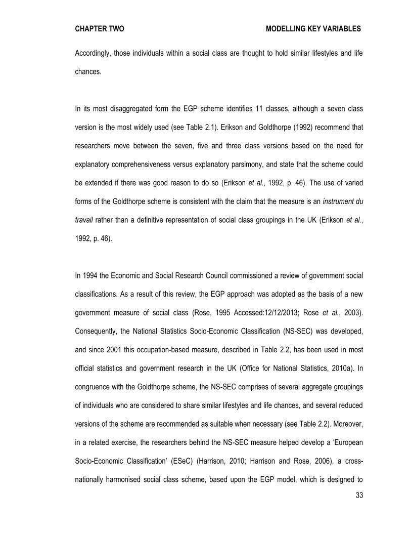
In its most disaggregated form the EGP scheme identifies 11 classes, although a seven class
version is the most widely used (see Table 2.1). Erikson and Goldthorpe (1992) recommend that
researchers move between the seven, five and three class versions based on the need for
explanatory comprehensiveness versus explanatory parsimony, and state that the scheme could
be extended if there was good reason to do so (Erikson et al., 1992, p. 46). The use of varied
forms of the Goldthorpe scheme is consistent with the claim that the measure is an instrument du
travail rather than a definitive representation of social class groupings in the UK (Erikson et al.,
1992, p. 46).
In 1994 the Economic and Social Research Council commissioned a review of government social
classifications. As a result of this review, the EGP approach was adopted as the basis of a new
government measure of social class (Rose, 1995 Accessed:12/12/2013; Rose et al., 2003).
Consequently, the National Statistics Socio-Economic Classification (NS-SEC) was developed,
and since 2001 this occupation-based measure, described in Table 2.2, has been used in most
official statistics and government research in the UK (Office for National Statistics, 2010a). In
congruence with the Goldthorpe scheme, the NS-SEC comprises of several aggregate groupings
of individuals who are considered to share similar lifestyles and life chances, and several reduced
versions of the scheme are recommended as suitable when necessary (see Table 2.2). Moreover,
in a related exercise, the researchers behind the NS-SEC measure helped develop a ‘European
Socio-Economic Classification’ (ESeC) (Harrison, 2010; Harrison and Rose, 2006), a cross-
nationally harmonised social class scheme, based upon the EGP model, which is designed to
CHAPTER TWO MODELLING KEY VARIABLES
34
facilitate comparative research. ESeC8 comprises a nine-class categorical measure, with recom-
mended reduced versions of five or three classes, which can be readily operationalised from data
coded into the three-digit version of the ISCO occupational unit group scheme. The ‘ESeC’
scheme has the potential to be widely used in international research, though other versions of the
EGP scheme have also been exploited in cross-nationally comparative studies (e.g. Blossfeld and
Hofmeister, 2005a; Breen, 2004; Erikson et al., 1992; Ganzeboom, 1996).
8 Full details of the ESeC scheme are available here: https://www.iser.essex.ac.uk/archives/esec/user-guide.

35
Table 2.1: The Goldthorpe Class Scheme (Erikson & Goldthorpe, 1992, pp. 38-39).
Full Version Collapsed Versions
Seven-class version Five-class version Three-class version
I Higher-grade professionals, administrators and officials; managers in large industrial establish-ments; large proprietors
I+II Service class: professionals, administra-tors and managers; higher-grade technicians; supervisors of non-manual workers
I-III White-collar workers
I-III+ IVa+b
Non-manual workers
II Lower-grade professionals, administrators and officials; higher-grade technicians; managers in small industrial establishments; supervisors of non-manual employees
IIIa Routine non-manual employees, higher grade (administration and commerce)
III Routine non-manual workers: routine non-manual employees in administration and commerce; sales personnel; other rank-and-file service workers
IIIb Routine non-manual employees, lower grade (sales and services)
IVa Small proprietors, artisans, etc., with employees IVa+b
Petty bourgeoisie: small properties and artisans, etc., with and without employees
IVa+b Petty bourgeoisie IVb Small proprietors, artisans, etc., without
employees IVc Farmers and smallholders; other self-employed
workers in primary production IVc Farmers: farmers and small holders and
other self-employed workers in primary production
IVc+VIIb
Farm workers
IVc+VIIb Farm workers
V Lower-grade technicians; supervisors of manual workers
V+VI Skilled workers: lower-grade technicians; supervisors of manual workers; skilled manual workers
V+VI Skilled workers
V+VI+ VIIa
Manual workers
VI Skilled manual workers VIIa Semi-skilled and unskilled manual workers (not
in agriculture, etc.) VIIa Non-skilled workers: semi-and unskilled
manual workers (not in agriculture, etc.) VIIa Non-skilled
workers
VIIb Agricultural workers and other workers in primary production
VIIb Agricultural labourers: agricultural and other workers in primary production

CHAPTER TWO MODELLING KEY VARIABLES
36
Table 2.2: The National Statistics Socio-economic Classification (NS-SEC).
Eight-class version Five-class version Three-class version
1 Higher managerial, administrative and professional occupations
1 Higher managerial, administrative and professional occupations
1 Higher managerial, administrative and profes-sional occupations
1.1 Large employers and higher managerial and administrative occupa-tions
1.2 Higher professional occupations
2 Lower managerial, administrative and professional occupations
3 Intermediate occupations 2 Intermediate occupations 2 Intermediate occupations 4 Small employers and
own account workers 3 Small employers and own
account workers 5 Lower supervisory and
technical occupations 4 Lower supervisory and
technical occupations 3 Routine and manual
occupations 6 Semi-routine occupations 5 Semi-routine and routine
occupations 7 Routine occupations 8 Never worked and long-
term unemployed
The Goldthorpe social class scheme and its derivatives are widely used in British sociology, and
several studies have provided evidence of acceptable construct9 and criterion10 validity for this
measure (e.g. Evans, 1992; Evans and Mills, 1998; Evans and Mills, 2000). Nevertheless, these
social class schemes have also been evaluated critically. Kelley (1973) questions the degree of
within-class homogeneity in social class categories, and highlights that individuals placed within
the same social class can hold very different positions within social hierarchies, a sentiment
echoed by Blackburn and Prandy (1997) and Bergman and Joye (2005). Meanwhile, Penn (1981),
Hout and Hauser (1992b) and Blackburn and Prandy (1997), amongst others, have argued that
9 Construct validity is based on the assessment of whether a measure reflects the underlying construct of interest (Cronbach and Meehl, 1955). 10 Criterion validity is based on the assessment of whether a measure behaves in the expected fashion, given the theory underlying of measure (Carmines and Zeller, 1979)
CHAPTER TWO MODELLING KEY VARIABLES
37
the EGP scheme’s categories downplay relatively more important aspects of the structure of
social stratification, most notably the key element of hierarchy.
It is necessary to note at this point that for some groups of contemporary sociologists the notion of
class, and particularly its continued relevance, is greatly disputed. Against the backdrop of a vast
quantity of work charting class-based inequalities (e.g. Erikson et al., 1979; Erikson et al., 1992;
Goldthorpe et al., 1980; Goldthorpe et al., 1987; Wright, 1997), a parallel stream of literature has
claimed that “class as a concept is ceasing to do any useful work” (Pahl, 1989, p. 710) and is
indeed ‘dead’ (e.g. Clark and Seymour, 1991; Holton and Turner, 1989; Joyce, 1995; Kingston,
1994; Lee and Turner, 1996; Pakulski and Waters, 1996). These theories generally argue that the
lives and experiences of individuals in modern society are too fluid and transient, and too influ-
enced by the processes of globalisation to fit within class categories. Pakulski and Waters (1996)
account of the ‘death of class’ centres on three main ideas: that the extent to which individuals can
be categorised in classes varies over time; that class based divisions peaked in industrial society
and have been declining since; and that although there are inequalities in modern society these
are not aligned with class categories.
There are however a number of weaknesses in the ‘end of class’ thesis. Goldthorpe and Marshall
(1992) note that the concept of class which is being attacked is a concept which is never clearly
defined and is most aligned to the Marxist tradition which does not represent contemporary
mainstream class analysis. The sophistication and development of class analysis is largely
overlooked by those who argue that class is dead, and is often represented in a caricatured and
simplistic manner (Goldthorpe et al., 1992). The notion of change in the influence of class, the
declining importance of class, and the role of other variables such as gender and ethnicity are all
CHAPTER TWO MODELLING KEY VARIABLES
38
central concerns in class analysis. Indeed, perhaps the central theme in modern class analysis is
the study of the extent to which the influence of social class has decreased over time in relation to
major economic and social change (e.g. the decline of heavy manufacturing, the growth of the
service sector, reduced job security, increasing levels of educational attainment). Yet, whilst class
analysts have researched these issues in depth, the ‘death of class’ theorists have provided little
convincing evidence to support their argument. Goldthorpe et al. (1992) have noted that there has
been no attempt to provide longitudinal evidence of change in the nature or influence of class to
provide adequate support for the ‘death of class’ argument. Many theoretical sociologists have
also continued to describe the importance and relevance of class in contemporary society
(Giddens, 1981; Sayer, 2005; Skeggs, 1997).
2.2.5 Social Stratification Scales
Occupational measures are generally separated into two forms, those which represent categorical
class based structures, described above, and those which comprise of gradational scales. Rather
than placing individuals into categories based on their occupations, social stratification scales
place individuals at some point on a continuous hierarchy (Bergman et al., 2005). Social stratifica-
tion scales also differ from class schemes as they generally assume that the varied features of
occupational groups can be represented in a single dimension, typically labelled ‘status’ or more
generally ‘relative social advantage’ (Jonsson et al., 2009).
An example of a social stratification scale is the Cambridge Social Interaction and Stratification
Scale (CAMSIS) (Prandy, 1990; Stewart et al., 1980). This scale is based on the theoretical idea
that there is a stratification order derived from a hierarchical structure of advantage (and disadvan-
tage) arising from the unequal distribution of social, cultural and economic resources.

CHAPTER TWO MODELLING KEY VARIABLES
39
According to the CAMSIS approach, individuals are embedded in social networks of relationships
within which they engage in social, cultural, political and economic interactions. These social
interactions are qualitatively and quantitatively different depending on the social distance of the
social actors. The idea of the centrality of ‘social space’ is not unique to the CAMSIS approach,
and has a long history in the sociological literature. Sorokin (1927, p. 6), for example, states that
“man’s social position is the totality of his relationships towards all groups of a population, within
each of them, towards its members”. Chan (2010b) describes another recent project in construct-
ing occupational scales based upon social interaction patterns which uses a very similar approach
to the CAMSIS perspective.
Patterns of social interaction between occupations are uncovered by looking at the frequency of
links between people in different occupations. Links are typically defined either by friendship or by
marriage/cohabitation, and the CAMSIS scale is formed through statistical analysis of ‘dimensions’
within the social interaction structure11 (Prandy, 1999). The scores are derived separately, for a
number of different ‘versions’. Different versions exist for different countries, different time periods,
and for different occupational base unit schemes within a country. It is also a standard outcome of
the methods used that different scores are obtained for men and women.
An unusual feature of the CAMSIS approach is that CAMSIS scales are calculated empirically for
the society at hand, and different CAMSIS scales exist for different countries and time periods.
Different CAMSIS scales can also be generated for men and women, and for other important
socio-demographic differences if desired (e.g. ethnic groups or regions). This quality of ‘specificity’
11 Detailed guidance for the translation of occupational codes and employment status information into CAMSIS measures can be found on the project’s website: http://www.camsis.stir.ac.uk/.
CHAPTER TWO MODELLING KEY VARIABLES
40
has some attractions (see Lambert et al., 2008), but also introduces complexity into the approach.
The majority of other occupational scales have not been constructed in this manner, and arguably
make for easier measurement tools in many scenarios.
Two particularly popular alternative stratification scales (see Ganzeboom and Treiman, 1996;
Ganzeboom and Treiman, 2003) are SIOPS (the Standard International Occupational Prestige
Scale) and ISEI (the International Socio-economic Index). SIOPS is devised by taking survey
information on prestige ratings given by respondents to samples of jobs, and calculating averages
within and across societies (Treiman, 1977). Treiman’s original analysis compared ratings across
over 60 societies, and drew the important conclusion that variation from society to society, and
over time, in the prestige allocated to occupations was minimal – often dubbed the ‘Treiman
constant’ within sociology12 (Hout and DiPrete, 2006). SIOPS provides a hierarchical ranking from
the least to the most esteemed occupations according to average ratings, and scores are shown
to correlate strongly with both the socioeconomic circumstances and the socio-cultural behaviour
of individuals. ISEI on the other hand uses an empirical approach to calculate scores for occupa-
tions based upon their average profiles in terms of the income and educational qualifications held
by their incumbents (adjusting for age profiles). It follows a long tradition of socio-economic
indexes for occupations based upon these two measures (e.g. Duncan, 1961), but again makes
12 Coxon and Jones (1978; 1979a; 1979b) have critiqued Treiman’s approach at length, based on analyses which focus on the cognitive issues involved when asking individuals to rank occupations. Coxon and Jones considered the types of distinctions people might draw between occupations. They experimented with tasks such as asking respondents to sort occupations into groups and asking the respondents to describe the criteria by which occupations could be ordered. They argue that these evaluative tasks should have preceded Treiman’s protocol to rank the occupations by prestige, in order to ensure the respondents had a clear basis by which to rank the occupations (Coxon et al., 1978). Coxon and Jones (1978; 1979a; 1979b) also present evidence that the ranking of occupations can vary between individuals and groups which may be overlooked when producing average rankings or scales. For example, individual’s exhibit a pattern of ‘occupational egoism’ whereby they give more favourable ratings to their own occupations and occupations similar to their own (Coxon et al., 1978)
CHAPTER TWO MODELLING KEY VARIABLES
41
the important generalisation that a cross-national hierarchy of socio-economic scores can be
effectively calculated and applied across countries (Ganzeboom et al., 1992).
The CAMSIS scales, SIOPS and ISEI are relatively popular stratification scales in contemporary
sociology, but many others are available. Further examples include scales based only upon the
average income of occupations (e.g. Sobek, 1995), upon career prospects in terms of average
wage growth (Bihagen and Ohls, 2004), or upon job quality or desirability (e.g. Jencks et al., 1988;
Mills, 2007). As continuous measures, all scales lead to numeric values being attached to occupa-
tions, but the relative meaning of a specific value is largely only established in comparison with
other occupations (for instance, the CAMSIS scales are usually standardised to a mean of 50 and
standard deviation of 15 in each version, but the SIOPS and ISEI measures are scaled in terms of
their original measurement and they typically have a mean of around 40, and standard deviation
of around 14, in a nationally representative sample). As described above, CAMSIS scales tend to
be specific to particular societies whereas ISEI and SIOPS are designed to be ‘universal’ (i.e. the
same scores are applicable to the same occupations across societies). However, this operational
difference is not necessarily related to the underlying theoretical basis of the scale (prestige and
socio-economic indexes, for instance, have often been calculated on a specific basis for different
countries and time periods, and a universal version of a CAMSIS scale has been advocated by De
Luca et al., 2010).
A major attraction of all scale approaches, however, is the relative parsimony which may be
attributed to them in most circumstances. It is claimed that scales measure the major elements of
social stratification in occupations, but they typically need only a single parameter (i.e. for a linear
effect) or two parameters (i.e. for a curvilinear effect) to summarise their influence in a modelling
CHAPTER TWO MODELLING KEY VARIABLES
42
approach. In many circumstances this parsimoniousness offers a major improvement over social
class schemes, which feature many discrete categories and typically require the specification of
categorical outcome models, or dummy variable effects, in a modelling approach. This advantage
is exacerbated, moreover, when interaction effects are considered. In many social processes, for
example, it would be typical that social stratification effects would interact with both age and
gender, but the specification of interaction effects of this nature with class schemes is much more
cumbersome than with stratification scales.
2.2.6 ‘Microclass’ Approaches
Recently Grusky and colleagues (Grusky and Sorensen, 2001; Grusky and Sørensen, 1998;
Grusky and Weeden, 2006) have provided a very powerful critique of traditional social class
schemes which has led to the development of the 'microclass' model. This novel perspective
suggests that the categorical approach of class schemes is desirable, but that there are far more
important categorical divisions than are conventionally depicted through ‘big class’ schemes (i.e.
measures such as the EGP scheme, which feature a low number of large social class categories).
The microclass alternative is to define a much larger number of classes based upon institutional-
ised occupational divisions, generating ‘microclass’ schemes which typically feature around 100
different classes. Grusky and Sørensen (1998) contend that traditional social class schemes fail to
represent detailed aggregate social structures, whilst also arguing that the social structure is also
not adequately represented by uni-dimensional hierarchical scales13. Due to their attention to
13 Micro-classes (i.e. many class categories) differ from gradational scales (i.e. many scaling points) as gradational scales are based on an asset which varies quantitatively between incumbents (e.g. a higher value on a prestige scale represents a higher level of prestige and the amount of prestige increases in a unidimensional manner throughout the scale). In the case of micro-classes the characteristics of the categories may vary quantitatively and also qualitatively (e.g. in the type of cultural capital). The differentia-
CHAPTER TWO MODELLING KEY VARIABLES
43
detailed differences in the division of labour, ‘microclass’ schemes have been associated with a
‘Durkhiemian’ approach to class analysis (Wright, 2005), and a number of studies have now
demonstrated their empirical validity (e.g. Jonsson et al., 2009; Weeden and Grusky, 2005).
Full details of the micro-class scheme can be found on the microclass project homepage14
(Grusky et al., 2012 Accessed:12/12/2013). The central attraction of the microclass approach is
that there may be important empirical ‘action’ between the large categories of ‘big’ social class
schemes, described above, and individual occupations themselves. Microclasses are formed at
the level of institutionalised occupations (e.g. plumber, baker, doctor) rather than agglomerate
classes (e.g. skilled manual workers, or professionals), and as such have opportunities to capture
substantially more empirical variance than other aggregate measures (Jonsson et al., 2009). The
many categories involved in the microclass approach, however, introduce significant operational
complexities for many forms of statistical analysis. Furthermore, Goldthorpe (2002) has high-
lighted that the disaggregate model makes traditional modes of theoretical explanation difficult to
achieve. Accordingly, the microclass model has not been widely used in social science. As
methods of statistical analysis evolve, in ways which allow for less problematic control for disag-
gregate units, the prevalence of ‘microclass’ usage may change.
tion between micro-classes and the assets which they have do not necessarily follow a strict unidimen-sional pattern and may not allow for a clear hierarchy. In statistical analyses which have used microclasses a combination of distinctive parameters for each micro-class category and a scaled unidimensional effect have been incorporated in the same analysis (Jonsson et al., 2009). 14See: http://www.classmobility.org/.
CHAPTER TWO MODELLING KEY VARIABLES
44
2.2.7 The Great British Class Survey
At this point it is also relevant to discuss a further new social class scheme which results from the
‘Great British Class Survey’ (GBCS) (Savage et al., 2013). Savage et al. (2013) propose a new
model of social class based on Bourdieu’s concepts of: economic capital (e.g. income and
wealth); cultural capital (e.g. engagement with cultural goods and activities); and social capital
(e.g. social contacts and networks) (Bourdieu, 1984). In order to construct this new scheme these
concepts have been measured in a survey in much more detail than they are generally covered in
multi-purpose social survey datasets. These measures include: household income, savings,
property value, the number of social contacts held and the occupations of these social contacts,
engagement with ‘highbrow culture’ (e.g. visiting museums or listening to classical music) and
engagement with ‘emerging cultural capital’ (i.e. activities once considered ‘lowbrow culture’ but
that may now be quite widely engaged with, such as using social network websites, going to the
gym or playing computer games).
Unlike the measures of social class and social stratification described in the preceding sections,
this new scheme does not use occupations as its main basis, however occupation does play a
role (i.e. an individual’s social contacts are defined by their occupation). Rather than holding
occupations as the main basis of the opportunity structure, Bourdieu (1984) argues that his three
capitals can be used to explain the processes of social reproduction. Based on this theory Savage
et al. (2013) contend that by measuring the varying degrees to which individuals’ hold these
capitals, a far more informative social class scheme can be developed than the traditional occupa-
tion-based measures in wide use, particularly the National Statistics Socio-Economic
Classification described above.
CHAPTER TWO MODELLING KEY VARIABLES
45
At the present time Savage et al. (2013) have only published one paper from what has been a
major project of data collection, and the latent class approach used to construct their scheme is
not described in much depth, although more detailed results are promised shortly. The study was
based on a web-based survey hosted by the British Broadcasting Corporation (BBC) which
received 161,400 responses. However as is frequently found when using web-based surveys
(Cobanoglu et al., 2001; Couper, 2000), these data were highly skewed and were completed
largely by more advantaged individuals. The main analysis upon which the GBCS is based
therefore makes use of a subsequent face-to-face survey completed by a quota sample of only
1,026 individuals. From these data a latent class model identified seven ‘new’ classes: the elite,
the established middle class, the technical middle class, new affluent workers, the traditional
working class, the emergent service workers and the precariat. Nevertheless, Payne (2013) has
noted that these seven ‘new’ classes are very similar to the NS-SEC categories, with the added
distinction of the ‘elite’, and do not represent a revolutionary re-working of the conceptualisation of
social class.
At present there is little peer-reviewed published critique of the approach (with the exception of
Payne, 2013), however several online web blogs from well known figures in the field suggest that
a number of published critiques are likely to be forthcoming shortly (Lambert and Griffiths, 2013
Accessed:12/12/2013; Mills, 2013 Accessed:12/12/2013; Rose and Harrison, 2013
Accessed:12/12/2013). One key critique launched against the GBCS concerns the analysis
strategy, Rose and Harrison describe the technique used quite harshly as “not very insightful data-
mining” (Rose et al., 2013 Accessed:12/12/2013) and note that quite different classes could have
emerged if different measures had been used. Lambert and Griffiths (2013 Accessed:12/12/2013)
echo this sentiment and suggest that given the small sample size the seven category latent class
CHAPTER TWO MODELLING KEY VARIABLES
46
solution could be an artefact, and could indeed change if a larger dataset was used. Indeed
McCutcheon and Hagenaars (1997) note that making the distinction between categories, when
utilising a latent class approach, should be driven by sound theoretical interpretation, however the
classes selected in the GBCS have been selected on largely statistical grounds. Lambert et al.
(2013 Accessed:12/12/2013) also question the decision to seek out categories of social class
membership at all where the detailed measures of capital may be better retained as a metric
variable, the reasoning as to why discrete categories of individuals should be apparent is not
addressed by Savage et al. (2013). Indeed it seems unfortunate to seek to reduce the information
in the detailed measures that have been taken of the three capitals to a small number of catego-
ries, which inevitably contain a degree of within category variation. This may hamper Savage et
al.’s (2013) plan to use the insights of Bourdieu to produce of clearer picture of social inequality
than that currently available.
A further critique of the GBCS approach is the association between membership of the GBCS
categories and age (i.e. the emergent service workers and the affluent workers seem to be
characterised by their youth). The problem of unintended correlations between measures and
extraneous factors is important and will be described in detail later in this chapter. Mills (2013
Accessed:12/12/2013) suggests that the correlation between GBCS class membership and age or
life course stage is evidence of a validity problem in the measures used (Mills, 2013
Accessed:12/12/2013). One might question whether the measures used hold measurement
equivalence between individual’s of varying ages and indeed whether cohort effects are influenc-
ing the measurement of these three capitals (i.e. the cultural activities which people engage with
and the extent to which they are ‘highbrow’ may change over time). Lambert et al. (2013
Accessed:12/12/2013) also note concerns over the correlation with age for the identification of an
CHAPTER TWO MODELLING KEY VARIABLES
47
individual’s position in the stratification structure (e.g. for use in studies of social mobility), how-
ever they suggest that this feature of the scheme could also have some advantages when we are
specifically interested in an individual’s current circumstances.
In the context of the present chapter which focuses on the processes and practicalities of using
existing survey data to produce measures for analysis which can be replicated and used by
others, this scheme reaches a major stumbling block in that it would be impractical to collect the
detailed information required to produce this new social class measure in every mainstream social
survey. Nevertheless, we are yet to see the extent to which this new scheme offers increased
explanatory power over existing measures when applied to the study of social phenomenon, and
indeed the insights which it can provide over and above existing measures, we therefore need to
review future publications of the GBCS to fully appreciate its contribution. Due to the lack of
availability of existing survey data which contain detailed measures of Bourdieu’s three capitals it
would be of great value and in the spirit of cumulative scientific endeavour if the GBCS survey
data were to be made available to other researchers to foster further debate and the development
of this measure.
2.2.8 Relationships with Demographic Structure and Social Changes
An important consideration when analysing occupation-based measures is whether there are
substantial but unintended correlations between the measure and extraneous factors such as age,
gender, region and, if relevant, time period. Most occupation-based measures show moderate
correlations with each of these factors and if ignored there is a danger that a story expressed in
terms of occupations is summarising a spurious effect due to a relation with another variable (e.g.
CHAPTER TWO MODELLING KEY VARIABLES
48
age or gender) (Lambert et al., 2008; Prandy, 1986). Recently Lambert et al. (2008) explored
three ‘social contexts’ over which occupation-based social classifications can be ‘specific’, namely
time periods, countries and gender. They argued that whilst temporal change in the meaning of
occupations is slight, gender differences in occupational distributions are so entrenched that they
should be considered fundamental to the evaluation of occupation-based measures (see also
Prandy, 1986).
In a multivariate analysis, it is reasonably straightforward to incorporate main effects for measures
of such factors (e.g. age and gender) which ought to substantially control for these spurious
effects. However, it is surprisingly common to see results in social statistics which do not incorpo-
rate such controls. There is often a good substantive case to be made that an interaction effect
between the factors, potentially of a non-linear nature, may exist. However, it remains relatively
rare for analysts to consider all possible interaction terms with occupation-based measures
(particularly when the occupation-based measure is of a categorical form).
A further way in which relations with age and gender may be accounted for is to design ‘specific’
occupation-based measures, whereby the incumbents of the same occupations could be given
different positions dependent upon their age or gender. Examples include the gender-specific
CAMSIS scales, or the social class scheme for women’s jobs as recommended by Martin and
Roberts (1984).
There are large and persistent differences in the occupations held by men and women which are
of consequence to the performance of occupation-based measures (Hauser et al., 1997). Black-
burn, Racko and Jarman (2009) and Jarman, Blackburn and Racko (2012) highlight that there are
CHAPTER TWO MODELLING KEY VARIABLES
49
two dimensions to gender differences in occupations. Namely, the vertical dimension of difference,
without inequality, and the horizontal dimension of inequality. Most occupation-based measures
emphasise differences of a vertical character, and despite the influence of horizontal gender
segregation, the consequences are not explicit in their representation of social inequality. There-
fore, caution must be placed on the nature in which women are distributed across the categories
of class schemes. This issue is particularly important for research which purports to study vertical
dimensions of gender difference (i.e. gender inequalities), yet fails to consider the comparability of
measures at a horizontal level (e.g. occupational gender segregation).
Attention to age differences in occupational classifications has received less consideration.
Several recently advocated occupation-based measures are known to have strong associations
with age (e.g. Kunst and Roskam, 2010), and multidimensional measures of stratification that
incorporate occupational differences (e.g. Hennig and Liao, 2013; Savage et al., 2013) are
strongly linked to age differences (to the point that spurious conclusions are possible).
There is clearly a compelling case for controlling for age and age interactions when using occupa-
tion-based measures (noting that the age effect might not be linear in nature). Another simple,
albeit partial, solution has been to restrict analysis to samples of certain age groups. An argument
expressed by, amongst others, Goldthorpe et al. (1987, p. 51), is that most adults reach a point of
‘occupational maturity’, around about the age of 35, after which it is relatively unlikely they will
experience major changes in their occupational position. Accordingly, many analyses using
occupational measures have been restricted to samples of older adults. Though in practice most
studies have used lower thresholds than the age of 35, whilst other authors have suggested that,
CHAPTER TWO MODELLING KEY VARIABLES
50
over time, the appropriate age of occupational maturity is likely to rise higher (e.g. Tampubolon
and Savage, 2012).
Another way of addressing age dependence in occupational circumstances may be to try to
construct summary measures of occupational position which themselves take account of the
career trajectories. This can be achieved through the detailed analysis of the career history of an
individual (e.g. Tampubolon et al., 2012), or by developing measures which try to profile the
average career development of occupations (e.g. Bihagen et al., 2004; Stewart et al., 1980).
However, whilst it is certainly conceivable that different occupation-based measures could be
constructed for different age groups (e.g. specific CAMSIS versions for, conceivably, those over
and those under the age of ‘occupational maturity’); this is a relatively complex approach which
hasn’t previously been widely employed.
Such issues raise the more general question of whether ‘specificity’ in occupational classifications
(i.e. the calculation of different measures for different groups in the data) is ordinarily a positive or
negative feature. There are in fact no influential methodological positions which deny such a
possibility on a priori grounds. For instance, Goldthorpe’s influential works (e.g. Goldthorpe,
2000), which instantiate the methodological preferences of many empirically oriented social
survey researchers, have stressed the value in making measurements contingent upon national
and temporal contexts. Many sociological theories and hypotheses are predicated on changing
social conditions across countries, time periods, or gender (e.g. modernisation theory see Blau et
al., 1967). To a certain extent specificity is required to best represent this change (Lambert et al.,
2008). Nevertheless, specificity raises clear operational difficulties and has not been employed in
many analytical studies.
CHAPTER TWO MODELLING KEY VARIABLES
51
A further related debate in using occupation-based measures is whether the occupational meas-
ure should be associated with an individual’s current (or last) occupation in isolation from other
knowledge about their circumstances, or whether occupations from household sharers or other
influential people should be used. Classically this is expressed as the debate between ‘individual’,
‘dominance’ and ‘conventional’ approaches to social classification (e.g. Erikson, 1984). The
individual approach uses the current job, the ‘dominance’ approach measures all jobs in the
current household and allocates individuals to the economically dominant occupation (i.e. that
which contributes the most to the household circumstances, usually the one with the longer hours
of work); and the ‘conventional’ approach allocates on the basis of the occupation of the ‘conven-
tional head of household’ (most commonly, the oldest employed male in the household).
Another alternative is simply to incorporate multiple variables indicating both own occupations and
those of household sharers, but debates on the optimal approach to allocating individuals in the
context of household information remain unresolved (Crompton et al., 2007). Increasing access to
detailed survey data often means that alternatives to the individualist approach can be operation-
alised by reasonably simple file matching techniques utilising household information. Whilst it
would be good practice to operationalise and compare alternative measurement strategies, in
practice it is relatively unusual to see an applied study which does so.
Lastly, an enduring problem in studying occupational measures relates to attempts to make
comparisons over time in a context when the occupational distribution itself is likely to have shifted
substantially. The time frames of interest to those studying social change are usually quite
substantial (for example, comparisons between ‘young’ and ‘old’ birth cohorts which effectively
span 50-100 years of social history are common). Over such periods, extended ‘structural mobility’
CHAPTER TWO MODELLING KEY VARIABLES
52
is likely to occur - typified in the UK by a pronounced shift from manufacturing to service employ-
ment through the twentieth century (e.g. Crafts et al., 2007). In general, comparisons over time in
occupational positions can be thought of as unsatisfactory. Statistical techniques exist to control
for distributional changes, isolating the ‘net’ change in patterns after allowing for structural change
through time (esp. Erikson et al., 1992), but these are not always adopted in all analyses, and
might in any case be controlling too strongly (e.g. Payne, 2012b). It is arguably in terms of
historical change that a ‘specific’ approach is most appealing, potentially providing a tool which
‘standardises’ occupational positions (in a similar way to adjusting measures of income for
inflation in temporal comparisons). When not employed, however, it should be thought of as
imperative that analyses of social change give detailed descriptive results and reflections upon the
scale of structural change in occupational positions through time, and their relation to the phe-
nomena under investigation.
2.2.9 Conclusion
The examples above highlight different approaches to the measurement of occupations and
comment upon some of the most salient issues in using variables based upon occupations. For
further information, there are many extended reviews covering the use of occupation-based
measures (e.g. Bechhofer, 1969; Bukodi et al., 2011; Hauser et al., 1997; Jonsson et al., 2009;
Lambert et al., 2012; Marsh, 1986; Rose and Harrison, 2010; Rose and O'Reilly, 1998).
Many occupation-based measures have different theoretical foundations (e.g. Wright, 2005), and
a widespread claim is that the theoretical origins of measures relate directly to their empirical
properties (e.g. Bukodi et al., 2011). Nevertheless, contemporary empirical analyses suggest that
CHAPTER TWO MODELLING KEY VARIABLES
53
theoretical perspectives associated with occupation-based measures of social stratification are not
necessarily greatly influential upon the results of an analysis (see Gayle and Lambert, 2011). It is,
perhaps, important to bear in mind that for many social science researchers it is the substantive
results and utility of research which is important, rather than the production of detailed theoretical
discussions. Gayle and Lambert (2011) demonstrated, for example, that in the analysis of filial
educational attainment a large proportion of the influence of social inequality is accounted for with
a crude simplified version of an occupational-based measure, and that the differences in interpre-
tation associated with using alternative occupational measures in the analysis was minimal. In
such regard, the exact occupation-based measure may not matter hugely to overall results (see
also Marsh, 1986; Penn, 1981). Arguably, perhaps a more important concern may be whether or
not the functional form of the measure facilitates its use in reasonably sophisticated statistical
models, such as in specifying interactions effects – as discussed above. Scales based on occupa-
tions have much more favourable features in this regard, and accordingly it may often be realistic
to encourage more use of occupation-based scales rather than categorical class schemes or other
approaches.

CHAPTER TWO MODELLING KEY VARIABLES
54
2.3 Education
“[T]he question of how to measure education and qualifications – or indeed
what ‘measure’ means – raises interesting issues…since there is no agreed
standard way of categorising educational qualifications” (Prandy et al., 2004,
p. 4)
2.3.1 Introduction
Though there are no agreed standard educational measures, there are certainly plenty of com-
monly used conventions for summarising differences in educational levels within or between
countries. Below is a review of some of the most important measures, and some of the critical
analytical issues to consider when working with variables based upon educational qualifications.
Similarly to the GEODE service providing access to information on measures of occupations, the
Data Management through E-Social Science (DAMES) Node runs an online portal designed to
serve as a repository for research information resources on educational qualifications, ‘GEEDE’
(Grid Enabled Educational Data Environment15). This site is one of several locations from which
metadata on educational qualifications and other supplementary information is available to others,
and this facility was used to retrieve information for use in this thesis. Critically, it is more common
than not that social science datasets feature records related to educational qualifications and that
these are of potential relevance to an analysis. The challenge for most researchers is identifying
and implementing appropriate derived measures which are suitably informed by major features of
the social structure such as expansion of educational provision and attainment through time.
15See: www.dames.org.uk/geede.

CHAPTER TWO MODELLING KEY VARIABLES
55
There are at least three aspects of educational attainment which are commonly measured or of
interest to analysis. The majority of survey studies on the effects of measured education have
focused on the effects of either the number of years of schooling, or the educational qualifications
gained (Feinstein et al., 2008). However, there are fundamental distinctions between these
constructs that matter for how the analyst thinks about and evaluates the effects of education.
Years of schooling is typically measured at a metric level variable, whereas measures of qualifica-
tions are usually operationalised by differentiating between a number of categories. It can be
argued that there is a third category of information, namely concerned with detailed features of the
quality or type of education, such as the exact institution attended or precise grades attained by
subject type (Feinstein et al., 2008). Key ‘qualitative’ features of educational attainment can be
considered in terms of learning ethos, pedagogy, curricula or assessment (Feinstein et al., 2008).
Additionally, more broadly, the social relations imbued by the experience of a given educational
context are also of importance (Feinstein et al., 2008).
In general terms, measures based on years of schooling are most commonly used in econometric
analyses, but are a less standard feature of sociological studies. Measures are typically con-
structed by collecting data on years of schooling directly from respondents, though it is also
possible to calculate the average years of schooling for different qualification categories then use
these values as measures at the individual level. This type of approach is known as ‘effect
proportional scaling’ (see Treiman, 2009). Years of education can be used as a functional proxy
for educational attainment, however it provides no information regarding the type or quality of
schooling (e.g. academic versus vocational), or indeed whether learning and educational ad-
vancement took place throughout the period of education recorded (Feinstein et al., 2008).
CHAPTER TWO MODELLING KEY VARIABLES
56
As an alternative measure, typologies of qualifications gained tend to be highly correlated with the
length of educational participation. In most nations it is necessary to attain entry level qualifica-
tions to proceed to the next stage of learning, therefore those with a greater quantity of education
(i.e. years of schooling) will also tend to have higher levels of qualification. Many different typolo-
gies are available, and it can be difficult to tease out the separate effects of participation and
qualification. Nevertheless, it is important to make the distinction between years of education and
actual qualifications gained, since it is qualifications and not educational experience that are
deemed to hold ‘signalling effects’, which can lead to socio-economic dividends (Feinstein et al.,
2008).
Another feature of the focus on the years of schooling or qualifications as measures of education
is that the benefits of learning at different stages of the lifecourse are overlooked. If the benefits of
education are mostly concentrated on their socio-economic returns in the workplace, then earlier,
standard educational trajectories may be of most value. Education may also imbue benefits
related to resilience and identity for those who study later in the lifecourse (Cunha et al., 2006;
Feinstein et al., 2008). Surprisingly little is known about these trade-offs in the dividends to
education, which may represent an important dimension of the influence of educational attainment
on social outcomes.
2.3.2 Measures of Education
Most social surveys collect information on education. Education is a powerful explanatory factor
influencing success in the labour market, and is related to further social, health and economic
outcomes (Jenkins and Siedler, 2007). Of course, education is also a key focus of research in
CHAPTER TWO MODELLING KEY VARIABLES
57
itself. Despite the key importance of education in social survey research the process and theory
surrounding the construction of education based measures has not received the same degree of
focus as occupation-based measures (Schneider, 2008). Several techniques exist including
constructing measures of the time spent in education (i.e. years of education), the construction of
different taxonomies of educational categories based on qualifications data, and scaling tech-
niques to attribute scores to educational attainments (e.g. Buis, 2010).
The data collected within social surveys usually comprise a set of questions covering the educa-
tional qualifications of a nation, as well as more general questions regarding the age at which an
individual left full-time education (Schneider, 2008). There are a great number of complexities
when using these pieces of information to create a measure suitable for use in a statistical model.
Stewart, Prandy and Blackburn (1980) describe great diversity in the UK education system. For
example, the education systems and qualification frameworks differ between each of the UK’s
constituent countries. Indeed, there is a great deal of migration between UK constituent countries
making it difficult to track an individual’s educational experiences (Schneider, 2011), and the
vocational education system in the UK is diverse and weakly regulated making it difficult to
determine the level and standard of vocational qualifications16 (Schneider, 2011).
Above all, there has also been a great deal of change over time in educational systems, both in
the UK and elsewhere. The form, structure, content and level of educational qualifications have
changed drastically over the last century, and continue to change regularly. For survey research-
ers, therefore, if the analysis sample contains individuals of different ages they will, most likely, all
16 See also: https://www.qaa.ac.uk/standardsandquality/otherrefpoints/Qualsboundaries09.pdf for full details of the plethora of educational qualifications in the UK.
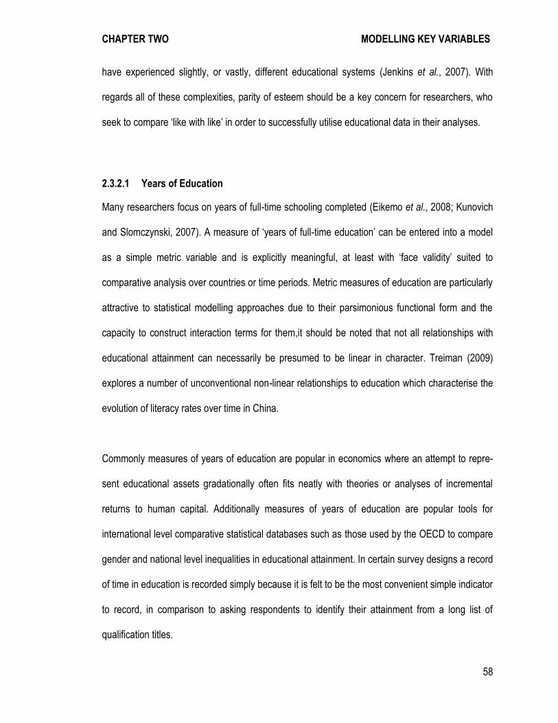
CHAPTER TWO MODELLING KEY VARIABLES
58
have experienced slightly, or vastly, different educational systems (Jenkins et al., 2007). With
regards all of these complexities, parity of esteem should be a key concern for researchers, who
seek to compare ‘like with like’ in order to successfully utilise educational data in their analyses.
2.3.2.1 Years of Education
Many researchers focus on years of full-time schooling completed (Eikemo et al., 2008; Kunovich
and Slomczynski, 2007). A measure of ‘years of full-time education’ can be entered into a model
as a simple metric variable and is explicitly meaningful, at least with ‘face validity’ suited to
comparative analysis over countries or time periods. Metric measures of education are particularly
attractive to statistical modelling approaches due to their parsimonious functional form and the
capacity to construct interaction terms for them,it should be noted that not all relationships with
educational attainment can necessarily be presumed to be linear in character. Treiman (2009)
explores a number of unconventional non-linear relationships to education which characterise the
evolution of literacy rates over time in China.
Commonly measures of years of education are popular in economics where an attempt to repre-
sent educational assets gradationally often fits neatly with theories or analyses of incremental
returns to human capital. Additionally measures of years of education are popular tools for
international level comparative statistical databases such as those used by the OECD to compare
gender and national level inequalities in educational attainment. In certain survey designs a record
of time in education is recorded simply because it is felt to be the most convenient simple indicator
to record, in comparison to asking respondents to identify their attainment from a long list of
qualification titles.
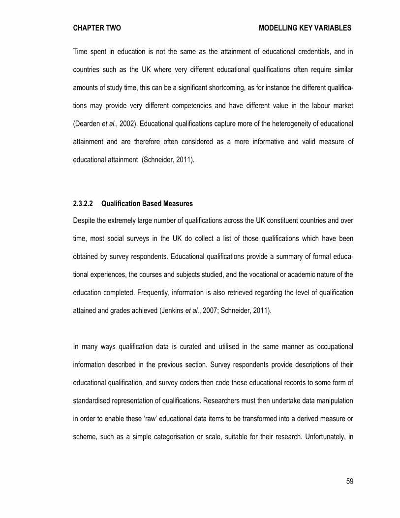
CHAPTER TWO MODELLING KEY VARIABLES
59
Time spent in education is not the same as the attainment of educational credentials, and in
countries such as the UK where very different educational qualifications often require similar
amounts of study time, this can be a significant shortcoming, as for instance the different qualifica-
tions may provide very different competencies and have different value in the labour market
(Dearden et al., 2002). Educational qualifications capture more of the heterogeneity of educational
attainment and are therefore often considered as a more informative and valid measure of
educational attainment (Schneider, 2011).
2.3.2.2 Qualification Based Measures
Despite the extremely large number of qualifications across the UK constituent countries and over
time, most social surveys in the UK do collect a list of those qualifications which have been
obtained by survey respondents. Educational qualifications provide a summary of formal educa-
tional experiences, the courses and subjects studied, and the vocational or academic nature of the
education completed. Frequently, information is also retrieved regarding the level of qualification
attained and grades achieved (Jenkins et al., 2007; Schneider, 2011).
In many ways qualification data is curated and utilised in the same manner as occupational
information described in the previous section. Survey respondents provide descriptions of their
educational qualification, and survey coders then code these educational records to some form of
standardised representation of qualifications. Researchers must then undertake data manipulation
in order to enable these ‘raw’ educational data items to be transformed into a derived measure or
scheme, such as a simple categorisation or scale, suitable for their research. Unfortunately, in
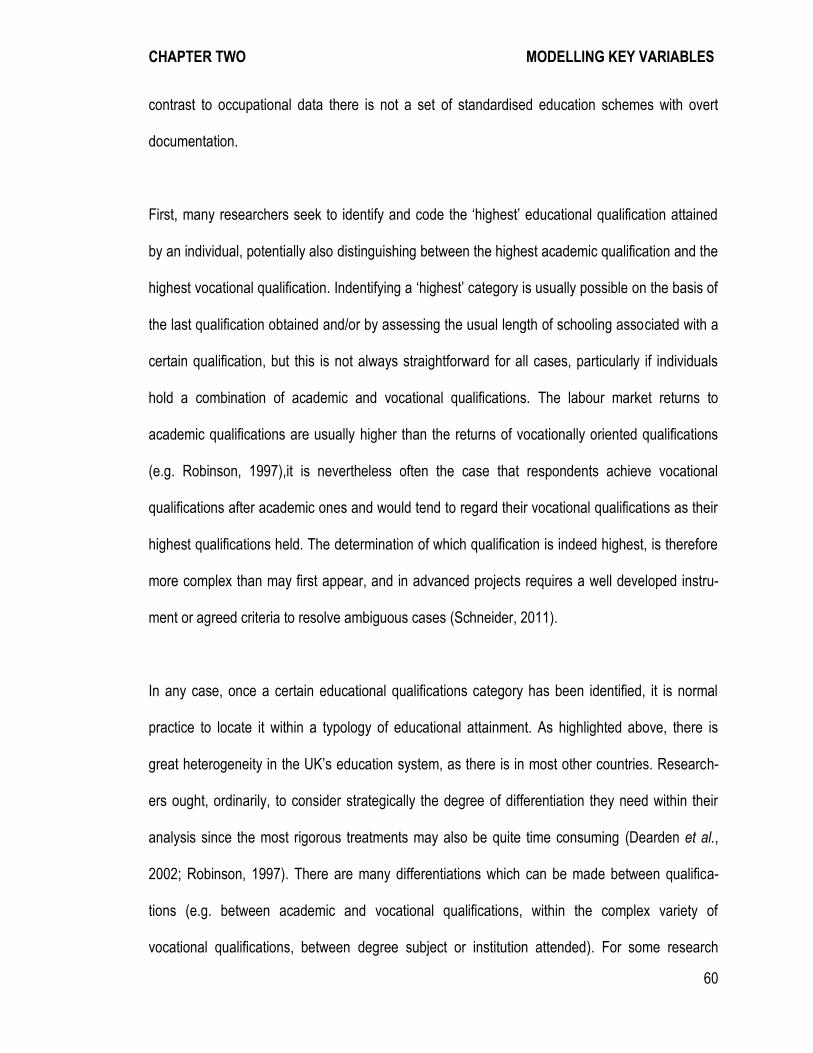
CHAPTER TWO MODELLING KEY VARIABLES
60
contrast to occupational data there is not a set of standardised education schemes with overt
documentation.
First, many researchers seek to identify and code the ‘highest’ educational qualification attained
by an individual, potentially also distinguishing between the highest academic qualification and the
highest vocational qualification. Indentifying a ‘highest’ category is usually possible on the basis of
the last qualification obtained and/or by assessing the usual length of schooling associated with a
certain qualification, but this is not always straightforward for all cases, particularly if individuals
hold a combination of academic and vocational qualifications. The labour market returns to
academic qualifications are usually higher than the returns of vocationally oriented qualifications
(e.g. Robinson, 1997),it is nevertheless often the case that respondents achieve vocational
qualifications after academic ones and would tend to regard their vocational qualifications as their
highest qualifications held. The determination of which qualification is indeed highest, is therefore
more complex than may first appear, and in advanced projects requires a well developed instru-
ment or agreed criteria to resolve ambiguous cases (Schneider, 2011).
In any case, once a certain educational qualifications category has been identified, it is normal
practice to locate it within a typology of educational attainment. As highlighted above, there is
great heterogeneity in the UK’s education system, as there is in most other countries. Research-
ers ought, ordinarily, to consider strategically the degree of differentiation they need within their
analysis since the most rigorous treatments may also be quite time consuming (Dearden et al.,
2002; Robinson, 1997). There are many differentiations which can be made between qualifica-
tions (e.g. between academic and vocational qualifications, within the complex variety of
vocational qualifications, between degree subject or institution attended). For some research
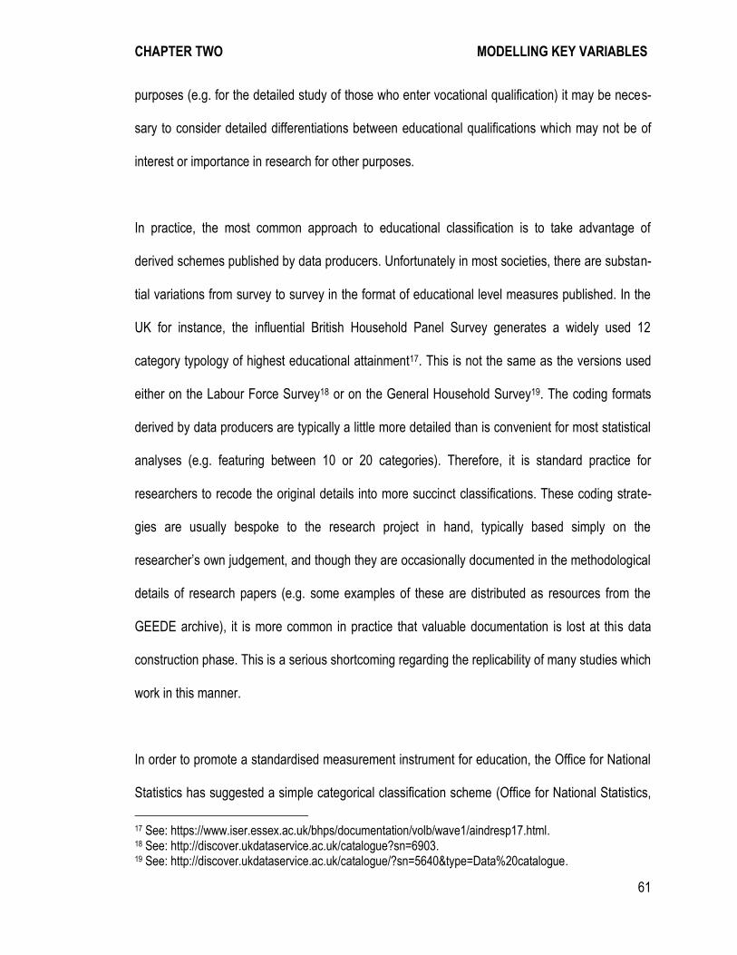
CHAPTER TWO MODELLING KEY VARIABLES
61
purposes (e.g. for the detailed study of those who enter vocational qualification) it may be neces-
sary to consider detailed differentiations between educational qualifications which may not be of
interest or importance in research for other purposes.
In practice, the most common approach to educational classification is to take advantage of
derived schemes published by data producers. Unfortunately in most societies, there are substan-
tial variations from survey to survey in the format of educational level measures published. In the
UK for instance, the influential British Household Panel Survey generates a widely used 12
category typology of highest educational attainment17. This is not the same as the versions used
either on the Labour Force Survey18 or on the General Household Survey19. The coding formats
derived by data producers are typically a little more detailed than is convenient for most statistical
analyses (e.g. featuring between 10 or 20 categories). Therefore, it is standard practice for
researchers to recode the original details into more succinct classifications. These coding strate-
gies are usually bespoke to the research project in hand, typically based simply on the
researcher’s own judgement, and though they are occasionally documented in the methodological
details of research papers (e.g. some examples of these are distributed as resources from the
GEEDE archive), it is more common in practice that valuable documentation is lost at this data
construction phase. This is a serious shortcoming regarding the replicability of many studies which
work in this manner.
In order to promote a standardised measurement instrument for education, the Office for National
Statistics has suggested a simple categorical classification scheme (Office for National Statistics,
17 See: https://www.iser.essex.ac.uk/bhps/documentation/volb/wave1/aindresp17.html. 18 See: http://discover.ukdataservice.ac.uk/catalogue?sn=6903. 19 See: http://discover.ukdataservice.ac.uk/catalogue/?sn=5640&type=Data%20catalogue.
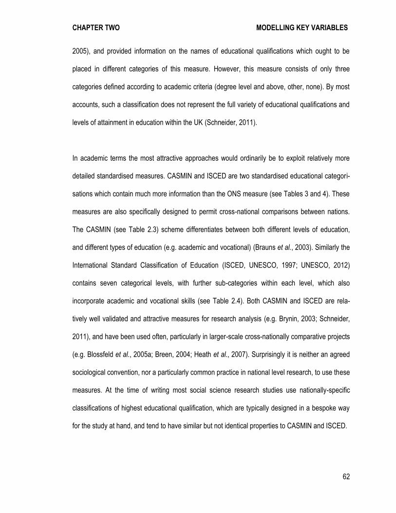
CHAPTER TWO MODELLING KEY VARIABLES
62
2005), and provided information on the names of educational qualifications which ought to be
placed in different categories of this measure. However, this measure consists of only three
categories defined according to academic criteria (degree level and above, other, none). By most
accounts, such a classification does not represent the full variety of educational qualifications and
levels of attainment in education within the UK (Schneider, 2011).
In academic terms the most attractive approaches would ordinarily be to exploit relatively more
detailed standardised measures. CASMIN and ISCED are two standardised educational categori-
sations which contain much more information than the ONS measure (see Tables 3 and 4). These
measures are also specifically designed to permit cross-national comparisons between nations.
The CASMIN (see Table 2.3) scheme differentiates between both different levels of education,
and different types of education (e.g. academic and vocational) (Brauns et al., 2003). Similarly the
International Standard Classification of Education (ISCED, UNESCO, 1997; UNESCO, 2012)
contains seven categorical levels, with further sub-categories within each level, which also
incorporate academic and vocational skills (see Table 2.4). Both CASMIN and ISCED are rela-
tively well validated and attractive measures for research analysis (e.g. Brynin, 2003; Schneider,
2011), and have been used often, particularly in larger-scale cross-nationally comparative projects
(e.g. Blossfeld et al., 2005a; Breen, 2004; Heath et al., 2007). Surprisingly it is neither an agreed
sociological convention, nor a particularly common practice in national level research, to use these
measures. At the time of writing most social science research studies use nationally-specific
classifications of highest educational qualification, which are typically designed in a bespoke way
for the study at hand, and tend to have similar but not identical properties to CASMIN and ISCED.

CHAPTER TWO MODELLING KEY VARIABLES
63
Table 2.3: The Comparative Analysis of Social Mobility in Industrial National (CASMIN) with UK qualification examples (Schneider, 2011).
Description UK Qualification Examples
1a Inadequately completed general elementary education
no qualification
1b Inadequately completed general elementary education
GCSE grades D‐G, SCE standard grades 4‐7
1c Basic vocational qualification or general elementary education and basic vocational qualification
Basic Skills qualification, Key Skills qualification, YT/YTP certificate, City and Guilds other, RSA other, SCOTVEC modules or equivalent, BTEC first or general certificate, GNVQ/GSVQ foundation level, NVQ/SVQ level 1 or equivalent
2a Intermediate vocational qualification or intermediate general education plus basic vocational qualification
BTEC/SCOTVEC first or general diploma, City and Guilds craft, RSA diploma, GNVQ intermediate, NVQ/SVQ level 2 or equivalent
2b Intermediate general qualification GCSE grade A‐C or equivalent, SCE standard
grades 1‐3 2c (Voc)
Intermediate general qualification OND/ONC, BTEC/SCOTVEC national, GNVQ advanced, NVQ/SVQ level 3
2c (Gen)
Full general maturity certificate AS level or equivalent, A level or equivalent, SCE higher or equivalent, Scottish 6th year certificate (CSYS)
3a Lower tertiary certificate HNC/HND, BTEC higher etc, NVQ/SVQ level 4 3b Higher tertiary certificate University/CNAA Bachelor Degree, Higher degree,
Doctorate, NVQ/SVQ level 5

CHAPTER TWO MODELLING KEY VARIABLES
64
Table 2.4: The 2011 International Standard Classification of Education (ISCED) (UNESCO, 1997).
Description Description
0 Pre-primary education The initial stage of organised instruction; school or centre based, designed for children aged at least three years
1 Primary education Begins between five and seven years of age, start of compulsory education
2 Lower secondary education Continues the basic programmes of the primary level, although teaching is typically more subject-focused. Usually, the end of this level coincides with the end of compulsory education.
3 Upper secondary education Generally begins at the end of compulsory educa-tion. The entrance age is typically 15 or 16 years. Requires entrance qualifications, Instruction is often more subject-oriented than at ISCED level 2.
4 Post-secondary non-tertiary education Between upper secondary and tertiary education. This level serves to broaden the knowledge of ISCED level 3 graduates. Typical examples are programmes designed to prepare pupils for studies at level 5 or programmes designed to prepare pupils for direct labour market entry.
5 Tertiary education (first stage) Entry to these programmes normally requires the successful completion of ISCED level 3 or 4.
6 Tertiary education (second stage) Reserved for tertiary studies that lead to an ad-vanced research qualification (i.e. Ph.D. or doctorate).
2.3.2.3 Scaling Educational Measures
An alternative approach to the categorisation of highest educational qualifications is their scaling
based upon some relevant criteria (e.g. the average study time needed to achieve them, or the
average income or occupational attainment of those with the relevant qualification). Despite the
great heterogeneity in educational attainment, the educational system represents an ordinal
gradation of attainment which can be represented on an approximately hierarchical vertical scale
(Chauvel, 2002). Buis (2010) has demonstrated methods for producing a scale of education,
based upon the association between educational qualifications and other positive outcomes (e.g.
more advantaged jobs and higher incomes). Based on these associations a large number of
educational qualifications can be attributed to a metric level of education, whilst the very exercise

CHAPTER TWO MODELLING KEY VARIABLES
65
of scaling can itself provide revealing insights into the character of educational inequalities (e.g.
Buis, 2010; Lambert, 2012c).
Treiman (e.g. 1975; 1977) for example advocated influential ways of achieving ‘effect proportional
scaling’ for both occupational and educational measures, and continues to justify this position in
recent writing (e.g. Treiman, 2007; Treiman, 2009). Many contemporary European sociologists
however seem to eschew scaling approaches, often apparently conflating them with American,
functionalist arguments and crude approaches to measuring social phenomena. Chauvel (2002),
for instance argues that the nature of educational attainment is too complex, heterogeneous and
multi-dimensional to represent on a uni-dimensional scale of educational attainment and con-
cludes that scaling educational attainment may hide complex qualitative aspects of attainment.
The majority of European studies seem, in practice, to adopt this position through their favouring
of bespoke categorical schemes. Nevertheless, complex heterogeneity in qualifications is also
hidden when large categorical groupings are used. Moreover, the functional form of categorical
measures introduce many other simplifications to analysis which are not associated with scaling
approaches, namely the difficulty of adapting classification categories to changes through time in
the relative prevalence of qualifications, and the difficulty of calculating arithmetically standardised
scores, and terms such as interaction effects, with categorical data. Scaling approaches for
educational qualifications offer many important attractions, and might therefore seem to have
been wrongly neglected by the European predilection for categorisation.

CHAPTER TWO MODELLING KEY VARIABLES
66
2.3.3 Further Complications in Studying Educational Measures
A variety of further complications are well-recognised in the analysis of educational data. On a
general level, the categorisation of educational qualifications into categories can be criticised if it
leads to combining dissimilar qualifications into the same category. Possible simplification occurs
not just at the stage of constructing derived schemes based on a longer list of qualification types,
but also during the initial enumeration of data on educational level. For instance, a survey respon-
dent might describe that they have a University degree, but surveys do not usually record
information on which institution they attended, the subject studied, or the class of degree awarded.
All of these ‘qualitative’ details are typically important in some circumstances.
The greatest enduring challenge to working with educational data reflects the long-term expansion
of the education system, which leads to redefinitions in the types of qualifications held, as well as
typical study periods, and could also lead to changes in the relative social value which can be
attributed to educational qualifications. This is known as the process of ‘credential inflation’
(Blackburn and Jarman, 1992). The scale of educational expansion has been dramatic and
sustained through time. Consistently, for more than one hundred years, the average educational
profile has increased substantially from each decennial cohort to cohort (Glennerster, 2001;
Greenaway and Haynes, 2003). In turn the relative returns to educational qualifications have
adjusted accordingly (see Figure 2.1). The credential inflation thesis predicts that as the supply of
highly educated labour increases, for example in the UK over the course of the twentieth century,
the value of educational qualifications decrease (Van de Werfhorst and Andersen, 2005). Creden-
tial inflation is particularly difficult to deal with when categorical schemes of educational
qualifications are used, since the implication is that the same categories over time may change in
their relative meaning. On the other hand, scaling approaches are arguably better positioned here

CHAPTER TWO MODELLING KEY VARIABLES
67
because they accommodate arithmetic scaling according to the relevant birth cohort or time period
(i.e. the scale score given to, say, a postgraduate qualification could be set lower for more recent
birth cohorts than earlier ones). With regard to statistical modelling approaches, the dramatic
scale of educational expansion at a minimum raises the case for calculating interaction terms
between educational level and birth cohort, and/or estimating structurally separate models for
different birth cohorts. Nevertheless, many studies which use educational measures within
statistical models do not incorporate such controls, often, because of the relative complexity of
setting up interactions with categorical education variables.
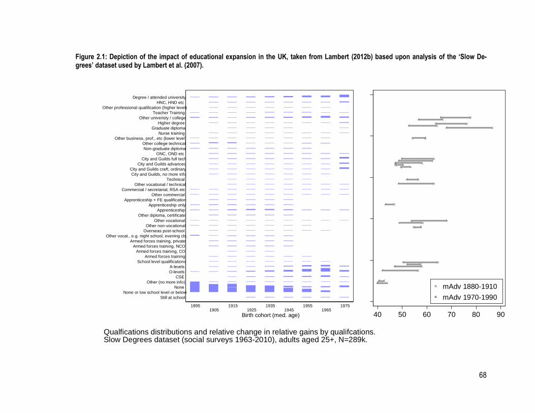
68
Figure 2.1: Depiction of the impact of educational expansion in the UK, taken from Lambert (2012b) based upon analysis of the ‘Slow De-grees’ dataset used by Lambert et al. (2007).
Still at school
None or low school level or below
None
Other (no more info)
CSE
O-levels
A-levels
School level qualifications
Armed forces training
Armed forces training, CO
Armed forces training, NCO
Armed forces training, private
Other vocat., e.g. night school, evening cls.
Overseas post-school
Other non-vocational
Other vocational
Other diploma, certificate
Apprenticeship
Apprenticeship only
Apprenticeship + FE qualification
Other commercial
Commercial / secretarial, RSA etc
Other vocational / technical
Technical
City and Guilds, no more info
City and Guilds craft, ordinary
City and Guilds advanced
City and Guilds full tech
ONC, OND etc
Non-graduate diploma
Other college technical
Other business, prof., etc (lower level)
Nurse training
Graduate diploma
Higher degree
Other univeristy / college
Teacher Training
Other professional qualification (higher level)
HNC, HND etc
Degree / attended university
1895 1905
1915 1925
1935 1945
1955 1965
1975
Birth cohort (med. age) 40 50 60 70 80 90
mAdv 1880-1910
mAdv 1970-1990
Qualfications distributions and relative change in relative gains by qualifcations. Slow Degrees dataset (social surveys 1963-2010), adults aged 25+, N=289k.
CHAPTER TWO MODELLING KEY VARIABLES
69
Educational expansion also raises two further issues for the measurement of education. First as
the value of education changes there is a risk that internal heterogeneity within categories may
change. Categorisations of educational qualifications may conflate varying levels of education by
placing qualifications with similar titles and descriptions in the same category when their real
importance in relation to each other may change. For instance, many educational categorisations
combine together all forms of University degree, but over time the components within that classifi-
cation have changed dramatically in countries like the UK. One example is the disproportionate
expansion in postgraduate courses and in vocational courses such as nursing. When a scaling
approach is used this problem may be alleviated although not eliminated. It may be possible to
adjust the scale scores according to the overall composition of the categories being scaled.
However, the integrity of the scale will be affected if the changes in composition affect some
educational categories more than others (Buis, 2010).
Second, the role of educational heterogeneity may have become more important over time in
general. For instance, according to the theory of ‘effectively maintained inequality’ (Lucas, 2001),
as the population becomes more highly educated a greater range of factors must be used in order
to differentiate individuals (e.g. grades, subjects studied, institution attended). In particular, the
role of less overt aspects of educational experience discussed earlier (e.g. provision of soft skills,
socialisation and personality development) can be expected to change as the distribution of
educational qualifications changes itself.
Gender may also play a significant role in the effects and interpretation of an educational meas-
ure. Dearden et al. (2002) highlight the influence of gender in their research on the returns to
qualifications. Women tend to receive greater rewards in return to academic qualifications, and in
CHAPTER TWO MODELLING KEY VARIABLES
70
particular degree level education, compared to men. When considering vocational qualifications
there are complex patterns of varying returns to precise vocational qualifications for men and
women. These outcomes are interrelated to the strongly differentiated patterns of occupational
distribution by gender as discussed in the previous section. For example, whilst women may be far
over-represented on Nursing degree courses, men are far over-represented on Engineering
degree courses. If the intention of a piece of research is to fully understand patterns of inequality,
such differences in the distributions of men and women within the diverse range of academic and
vocational qualifications is a key consideration which must be made.
Lastly, whilst most of the approaches described above are based upon classifying a single
qualification which has been identified as the ‘highest’, this is not the only plausible strategy for
taking account of data on educational qualifications. On the contrary, it is often possible to take
advantage of information about all of, or a relevant selection of, the different qualifications held by
people in some manner. This tradition is particularly well developed in educational research at the
school level, where various strategies are available for summarising the profile of school qualifica-
tions achieved by individuals, but it is less common to see similar principles applied to
summarising the qualifications held by adults (a notable exception is McIntosh, 2006).
In some instances, it might be plausible to construct a ‘cumulative’ educational index by adding
together the information about different qualifications held in a categorical or arithmetic way.
Various creative approaches could be adopted as relevant to the research question, for instance,
a categorical classification for a study within interest in global communication might enable an
analyst to place respondents with both a University degree and a school level qualification in a
foreign language in a separate category from those with a University degree but no languages

CHAPTER TWO MODELLING KEY VARIABLES
71
qualification. A metric summary might add together the scores given to each qualification of
relevance, in a similar manner to the way in which school level exam scores are often added
together to provide an index measure. Other creative examples of using data on more than one
qualification include Playford’s (2011) analysis which defined latent classes of educational
attainment according to school level exam subjects and grades, or Connelly’s (2012) research
which disaggregated a category of ‘University degree’ according to level of performance in A-level
results (the construction of this measure is discussed in chapter 6). Certainly there is ample
evidence to suggest that such differentiations can be influential upon the results of analysis. As an
example, Dearden et al.’s (2002) analyses of the National Child Development Study and the
Labour Force Survey suggest that ‘A-level’20 attainment tends to maintain its influence regardless
of whether a respondent goes on to further academic or vocational education, or indeed whether
they leave education at this point, whilst the returns to ‘O-levels’21 are greatest in the labour
market when they are followed by vocational qualifications, and lose value when individuals obtain
further academic qualifications. By such accounts, information on these qualifications all contrib-
utes to an, albeit disjointed and semi-ordinal, characterisation of progression through the
educational system.
2.3.4 Conclusion
A key issue, which has been highlighted throughout the preceding sections, is the degree of
heterogeneity in educational qualifications and how this is considered in educational measures.
Educational qualifications are only the tip of the iceberg when it comes to understanding an
20 The advanced level of secondary school qualifications taken at age 17 or 18 in England and Wales. 21 The lower level of secondary school qualifications completed in England and Wales at age 16 until the late 1980s. They are similar in structure to GCSE examinations.
CHAPTER TWO MODELLING KEY VARIABLES
72
individual’s educational experience and competencies. Field of education, part-time vs. full-time
study, grades and type of institution are all further dimensions of educational experience and
attainment which can be considered alongside any conceptualisation of the key variable of
education in social research.
Clearly there are the complexities, benefits and drawbacks to adopting approaches to measure-
ment which either used categorisations or scaling approaches, and no prescription as to the use of
either measure is offered in this chapter. Two other recommendations are however easier to
make. First, given the vast range of alternative treatments, there is a compelling argument to say
that researchers should always endeavour to operationalise more than one measure, and com-
pare their properties in a sensitivity analysis prior to research. This could be expected to minimise
the dangers of drawing unrealistic conclusions due to inadequate classification strategies. This
process ought not to be overly demanding for contemporary survey researchers given the prolif-
eration of information resources such as GEEDE which provide guidance on possible
operationalisations, and it is particularly compelling if the researcher uses a measure which was
constructed in a bespoke way for the analysis (i.e. they have the opportunity to also operationalise
a existing measure as used in other studies and compare its properties). Second, given the
dramatic scale of educational expansion through time, it is hard to ever justify ignoring birth-cohort
differences in the distribution of educational qualifications, even though this is often done in
practice. On the contrary, social researchers ought to expect by default to consider birth cohort
interactions between the effects of education and other outcomes.
CHAPTER TWO MODELLING KEY VARIABLES
73
2.4 Ethnicity
“We shall class ‘ethnic groups’ those human groups that entertain a subjective
belief in their common descent because of colonisation and migration; this be-
lief must be important for the propagation of group formation: conversely, it
does not matter whether or not an objective blood relationship exists” (Weber,
1978 p.389)
2.4.1 Introduction
Of the three key variables discussed in this chapter, ethnicity is the most challenging to measure
effectively in social survey research. There is no consensus on what constitutes an ethnic group,
and the concept of ethnicity is potentially subjective and multi-dimensional. For instance, in the
UK, the measurement of ethnicity in social surveys often incorporates differences of nationality,
national origins, language use and religious background. Ethnic group classification and member-
ship has also been fraught with political difficulties (Bulmer, 2010), not least because, much more
so than with occupation and education, ethnic group membership is subjectively meaningful to the
survey respondent. Platt (2011, p. 69), for example, describes ethnicity as ‘self-conscious and
claimed identities’. Bulmer (1996) also highlights the self-reflective and self-conscious elements of
ethnic identity:
CHAPTER TWO MODELLING KEY VARIABLES
74
“An ethnic group is a collectivity within a larger population having real or puta-
tive common ancestry, memories of a shared past, and a cultural focus upon
one or more symbolic elements which define the group’s identity, such as kin-
ship, religion, language, shared territory, nationality or physical appearance.
Members of an ethnic group are conscious of belonging to an ethnic group”
(Bulmer, 1996, p. 35)
Additionally, the relationship between ethnicity and immigration raises major challenges of
measurement consistency through time. In a society like the UK, for example, ‘ethnic groups’ often
have distinctive demographic profiles linked to their immigrant origins (Peach, 1997), and the most
relevant ways of identifying, sampling and categorising minority groups can change substantially
in short periods of time because of this. Lastly, in many populations of interest, multiple potentially
interesting categories of ethnicity are held by only a small proportion of individuals, meaning that
conventional sampling methods yield only low numbers of cases for many minority groups.
Accordingly, when surveys do not have sufficient numbers of cases representing selected groups,
analysts often feel they have no alternative but to ignore or simplify the information for the pur-
poses of analysis. It is common practice in the UK to see ethnicity information summarised by the
dichotomy of ‘White’ and ‘Non-white’, even though most theorists studying ethnicity would regard
this as a gross oversimplification. Despite these many challenges, it is clear that measures of
ethnicity can explain substantial patterns of social inequality, and that ethnicity itself is of rele-
vance to a great many sociological enquiries. It is therefore highly relevant to explore in
methodological terms the ways that social survey analysts are able to represent this variable in
their research.
CHAPTER TWO MODELLING KEY VARIABLES
75
Nevertheless, whilst it is clearly a relevant concept of analysis, it is not the case that all social
surveys collect measures which capture ethnic differences, nor that all of the measures used
identify the same categories. In the UK, the 1991 census was the first decennial census to
measure ‘ethnicity’ as a concept which was distinguished from country of birth, and it is only since
that period that it has been reasonably common in the UK to incorporate measures of ethnicity,
usually based upon census schemes, in other social surveys. Existing measures usually offer
respondents a short range of categories typically alongside an option to reject the categories and,
if desired, give a textual description of their preferred ethnic identity instead (Gardener and
Connolly, 2005).
To define ethnicity, many sociologists follow Weber (1978) in referring mainly to points of personal
reference as uniting principles for ethnic groups (e.g. perceptions of common descent, history, fate
and culture). Usually these characteristics also include aspects of language, physical appearance
and religion. Hale (2004), for instance, describes ethnic groups as perceiving commonalities which
lead to ethnic identities:
“…‘ethnic identity’ (or ethnicity) is that set of personal points of reference, thick
and thin, that involve what we call “ethnic” distinctions between people. An
“ethnic group” is thus a set of people who have common points of reference to
these ethnic dimensions of the social world and who perceive that they indeed
have these things in common and that these similarities are captured by a la-
bel, the ethnic group’s name” (Hale, 2004 p.473)
CHAPTER TWO MODELLING KEY VARIABLES
76
In the UK and the United States, this definition is reasonably congruent with the dominant meas-
ures of ethnicity used in official statistics, which are based upon subjective identity with categories
which are felt to capture major constellations of these qualities. In the UK, the official definition is
mainly expressed in terms of country of origin and skin colour. In the US, the major categories are
defined in terms of skin colour and genetic ancestry. Nevertheless, in both societies there have
been many methodological reviews concerning the way in which ethnicity is measured in official
classifications, with numerous inconsistencies in existing definitions identified, and alternative
proposals offered (for the UK, see for instance Aspinall, 2009; Ballard, 1997; Brown, 2006).
The review below describes the major ways in which ethnicity is measured and exploited in social
surveys in the UK and beyond. As in many other countries there are numerous alternative
strategies, many of which in methodological terms might not be thought satisfactory.
2.4.2 Data on Ethnicity
Contemporary Britain is an increasingly ethnically diverse nation by virtue of substantial flows of
immigration, and increasing levels of inter-ethnic marriage and partnership formation. Conse-
quently, there is considerable need for information resources on the measurement and analysis of
ethnicity. As with the GEODE and GEEDE systems highlighted above, the DAMES research Node
developed an online portal, ‘GEMDE’ (‘Grid Enabled ethnic Minority Data Environment, see
www.dames.org.uk/gemde), which is designed to bring together, store, and distribute to others,
information about the measurement and understanding of ethnicity, such as copies of data
processing commands and definitional taxonomies.
CHAPTER TWO MODELLING KEY VARIABLES
77
Collecting data on ethnicity is a challenge because ethnic identity is subjectively meaningful to the
individual and it is multi-faceted and can also be changeable. Data on ethnicity in large scale
government surveys has often included one or more of the following categories; country of birth,
nationality, parents’ country of birth, national/geographical origin, race and religion. Although each
category can be an aspect of ethnic identification, for a variety of reasons they are not as useful
when taken separately. In the UK, measures which have been used in social surveys since the
1990’s have usually sought to identify a small selection of categories which cross-cut the above
‘referents’ in a statistically parsimonious way. The categorisation of ethnicity used in the 2011
census, for example (see Table 2.5), shown below, includes categories which combine national
origins, skin colour and geographical affiliations. Needless to say, a wide range of opinion exists
on whether ethnicity can be reliably characterised in this way in order to reflect the most salient
categories of group identity. In the UK at least, however, it is ordinarily felt that placement into the
categories is most appropriately done through self-assessment (Aspinall, 2011).
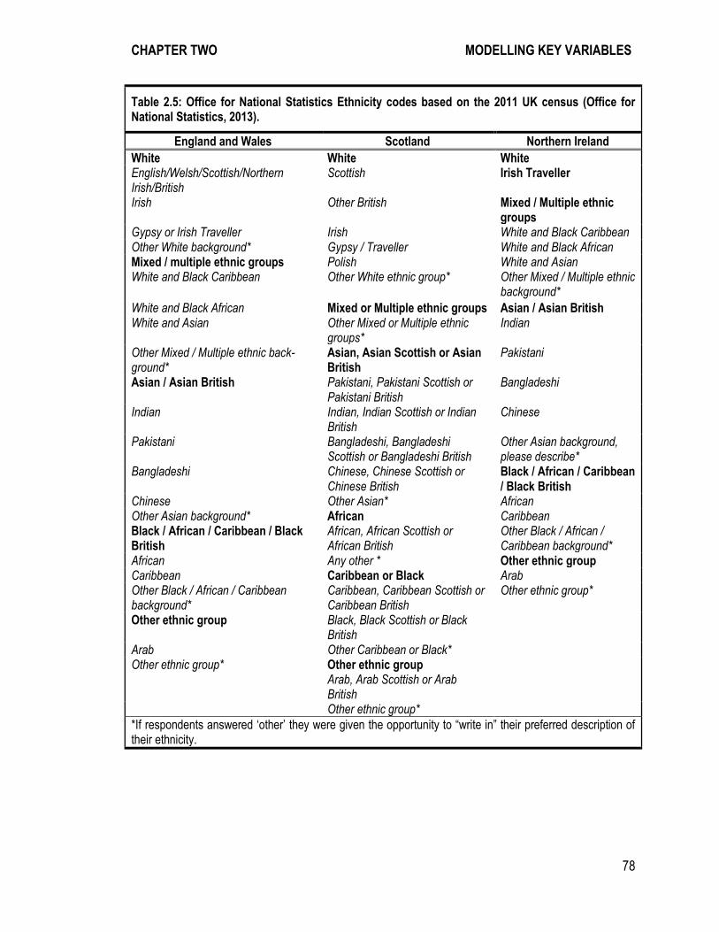
CHAPTER TWO MODELLING KEY VARIABLES
78
Table 2.5: Office for National Statistics Ethnicity codes based on the 2011 UK census (Office for National Statistics, 2013).
England and Wales Scotland Northern Ireland
White White White English/Welsh/Scottish/Northern Irish/British
Scottish Irish Traveller
Irish Other British Mixed / Multiple ethnic groups
Gypsy or Irish Traveller Irish White and Black Caribbean Other White background* Gypsy / Traveller White and Black African Mixed / multiple ethnic groups Polish White and Asian White and Black Caribbean Other White ethnic group* Other Mixed / Multiple ethnic
background*
White and Black African Mixed or Multiple ethnic groups Asian / Asian British White and Asian Other Mixed or Multiple ethnic
groups* Indian
Other Mixed / Multiple ethnic back-ground*
Asian, Asian Scottish or Asian British
Pakistani
Asian / Asian British Pakistani, Pakistani Scottish or Pakistani British
Bangladeshi
Indian Indian, Indian Scottish or Indian British
Chinese
Pakistani Bangladeshi, Bangladeshi Scottish or Bangladeshi British
Other Asian background, please describe*
Bangladeshi Chinese, Chinese Scottish or Chinese British
Black / African / Caribbean / Black British
Chinese Other Asian* African Other Asian background* African Caribbean Black / African / Caribbean / Black British
African, African Scottish or African British
Other Black / African / Caribbean background*
African Any other * Other ethnic group Caribbean Caribbean or Black Arab Other Black / African / Caribbean background*
Caribbean, Caribbean Scottish or Caribbean British
Other ethnic group*
Other ethnic group Black, Black Scottish or Black British
Arab Other Caribbean or Black* Other ethnic group* Other ethnic group Arab, Arab Scottish or Arab
British
Other ethnic group*
*If respondents answered ‘other’ they were given the opportunity to “write in” their preferred description of their ethnicity.
CHAPTER TWO MODELLING KEY VARIABLES
79
The 2011 census question itself represents a development upon earlier UK Census measures of
ethnicity. For example, the 1991 Census did not include a specific ‘mixed’ ethnic group category,
based on research which indicated that individuals of ‘mixed’ heritage preferred not to separate or
distinguish themselves on that basis (Sillitoe, 1987). However, the 2011 census provided the
opportunity to indicate ‘mixed’ ethnicity, and also provide a more detailed description, by means of
a written response.
A difficulty in the analysis of ethnicity in the UK is often a lack of adequate sample size of ethnic
minorities in social surveys. By virtue of the relative size of ethnic populations in the UK, often
even in large social surveys, some ethnic minority populations cannot be studied in isolation due
to concerns over under-representativeness, statistical power and also confidentiality. Frequently,
researchers respond by seeking to identify data with sufficiently large sample sizes to minimise
problems of sparse representation, such as Census datasets, very large sample surveys such as
Labour Force Surveys, or surveys with large ‘boost’ samples22. Indeed, survey selection is a
crucial consideration for projects with an interest in analysing ethnicity. If the sample is to be
divided by other variables such as age, sex or employment status, as well as ethnicity, a large
sample will ensure better coverage in each sub-group.
The UK offers a wealth of multi-purpose surveys that can be used to analyse the experiences of
different ethnic groups and to highlight inequalities between them. The most suitable are ordinarily
those surveys with minority ‘boost samples’, or other particularly large social surveys which have
22 A boost sample comprises of an additional set of interviews carried out with a specific sub-group of the survey population. Boosts are carried out in order to produce a larger sample size for analysis of specific sub-groups. If boost samples are added to the main sample, the data should be weighted to restore the proportions of the different groups in the population sampled.
CHAPTER TWO MODELLING KEY VARIABLES
80
high coverage of minority groups. Of the former, the Policy Studies Institute surveys have been of
great historical influence (Brown, 1984; Modood et al., 1997), and recent decades have seen the
rise and fall of the Home Office Citizenship Survey (Attwood et al., 2003), as well as the introduc-
tion of substantial ethnic minority coverage in the ‘Understanding Society’ panel study (Nandi and
Platt, 2009). The UK Census and Labour Force Survey are the most widely used sources, though
even smaller surveys are increasingly analysed, after aggregation, for ethnicity effects.
Another way around problems of small sample size is to aggregate ethnicity categories. This is
frequently done, but is also frequently criticised. For example, it is common practice to aggregate
data regarding Indian, Pakistani, Bangladeshi and other Asian populations due to their small
sample sizes. However, there may be important differences between these groups, for example,
when considering women’s employment. Employment patterns for Indian women are very different
from other women in this aggregate ‘South Asian’ category (Dale, 2008). Therefore, it is important
that combined ethnic populations show similar patterns on the outcome of interest. In general,
rather than combining categories inappropriately, it is better to show a category in a table while
indicating that data for that category have been omitted because of small sample sizes (even if
this results in gaps in the evidence base for informing policy).
There is also evidence to suggest that there may be ethnicity specific patterns of non-response in
social survey data collection. Ethnic groups can have different levels of unit non-response,
propensity to take part in a survey, therefore patterns of participation and the use of post-
stratification weights should always be carefully considered (Feskens et al., 2006; Feskens et al.,
2007).
CHAPTER TWO MODELLING KEY VARIABLES
81
2.4.3 Change Over Time
Substantial ethnic differences continue to be displayed across a wide range of outcomes in the
UK, for example, major empirical enquiries have consistently shown strong ethnic differences in
socio-economic, biosocial, cultural and behavioural outcomes (e.g. Brown, 1984; Finney and
Simpson, 2009; Jones, 1993; Modood et al., 1997). Whilst there is long term stability in the
salience of ethnicity to social science investigation, the availability of data on ethnicity itself varies
over time, including by being linked to trends in contemporary research interest. In recent years in
the UK, religious affiliation has been increasingly recorded in social surveys in combination with
ethnic identity. Furthermore, institutions such as the ONS have added the measurement of
national identity as part of its methodological toolkit, no doubt reflecting the growth of Scotland,
Wales and Northern Ireland as more autonomous units within the United Kingdom of Great Britain
and Ireland. Equally, over time there is increasing demand from social scientists for more refined
ethnicity data for smaller sub-groups, as traditional ‘broad brush’ categorisations are frequently
criticised as over-simplifications (Bulmer, 2010).
A major source of literature on the quantitative analysis of ethnicity has concerned its consistent
measurement through time. Commonly, prescriptions have been given to suggest how to most
effectively make temporal comparisons between measures which are not recorded in an identical
way through time (e.g. Platt et al., 2005; Simpson and Akinwale, 2006). The endeavour is often
regarded as problematic and many sociologists maintain that equivalent categories simply cannot
be identified. Alternatively, certain methodological solutions for specific scenarios have also been
proposed. For example, Burton et al. (2010) argue that multiple response questions on ethnicity
can be kept stable through time whilst allowing different derived categories to be generated from
CHAPTER TWO MODELLING KEY VARIABLES
82
them. Platt (2005) exploits administrative data to link records on the ethnic categorisations
allocated to the same individuals in different data sources over an extended period of time.
Lambert (2002b) has also proposed a scaling strategy applied to ethnic groups which would allow
the possibility that in different time periods the scale locations for what may nominally be the same
categories could change.
Evidence suggests that ethnic identities, however defined or measured, will tend to change over
time. Therefore, quite legitimately, for a proportion of the population, a person may record them-
selves as one ethnic group at one time and another on a subsequent occasion (Platt et al., 2005).
Such changes depend upon personal, social and political attitudes and developments. Despite the
variable nature of ethnic identity, and structural changes which influence the development of
ethnic boundaries, measures of ethnicity in social surveys tend to focus on largely fixed and
unsophisticated ethnic categories (Burton et al., 2010). Some analysts, have become frustrated
with the lack of consistency and detail, rejecting survey measures of ethnicity as inadequate and
uninformative (Burton et al., 2010). Yet there remains substantial demand for ethnicity measures
in order to engage with issues of ethnicity in survey research.
2.4.4 Measurement Approaches
The most broad-minded approach to ethnic reporting, ‘open’ response reporting, would allow
individuals to provide a detailed description of their ethnic identity. However, these data would be
of questionable utility for empirical analysis. Nevertheless, there are also problems with categori-
cal measures of ethnicity; there may be a degree of heterogeneity within ethnic group categories
which is concealed in a fixed category social survey measure (i.e. the ‘fallacy of homogeneity’).
CHAPTER TWO MODELLING KEY VARIABLES
83
Categories with a large degree of within-group heterogeneity may introduce error in the conclu-
sions of the effects of ethnicity if these unmeasured elements of the categories correlate with the
research outcomes (Campbell, 1989; Stanfield, 1993).
Furthermore, asking survey respondents to identify themselves on the basis of a single, mutually
exclusive, category may overlook some important dimensions of ethnicity. As described above,
ethnicity is a multi-dimensional concept which includes a number of elements (e.g. ancestry,
national identity, religion and country of birth) (Aspinall, 2011). Importantly, there is evidence that
different dimensions of ethnic identity may vary across groups. For example, when providing
descriptions of their ethnicity in free-text responses, Black groups in the 1991 and 2001 censuses
were found to emphasise their national identity (i.e. being British) as a central element of their
ethnicity (Office for National Statistics, 2006). Meanwhile, South Asian groups have been found to
emphasise their religion as a central element of their ethnicity (Modood et al., 1994).
Multiple response questions offer a possible solution to improve the representation of the multiple
dimensions of ethnicity (e.g. Burton et al., 2010). Allowing multiple responses across differing
characteristics of ethnic identity and ethnic group membership allows the respondents to have
more control over the expression of various elements of their ethnic identity, and have proved
popular (e.g. Burton et al., 2010). Multiple response measures also reduce the perception that the
individual is being asked to summarise the complexity of their identity into a single box (Burton et
al., 2010). Analytically, multiple responses will allow the researcher to investigate the features of
ethnicity which divide and unite different groups (Burton et al., 2010). The multiple response
approach allows for increased flexibility, and detailed insights.
CHAPTER TWO MODELLING KEY VARIABLES
84
2.4.5 Relationships to Other Categories
Alongside independent definitional issues, an important consideration in most analyses of ethnicity
is the way in which ethnic categories are linked to other important differences between people. In
multivariate survey research, a common statistical objective is to isolate the relative influence of
background factors in order to identify the distinctive empirical associates with a variable of
interest (i.e. a measure of ethnicity), net of other factors. In the case of measures of ethnicity,
there are strong correlations between ethnic categories and many other socio-demographic
differences, so particular care is needed in order to avoid drawing spurious conclusions about
ethnic differences. This issue will be further elaborated on below. First and foremost, in many
societies the age profiles of the different minority ethnic groups vary substantially, and this can
account for many other differences seen between ethnic groups. Substantial age differences arise,
ordinarily, due to the immigrant-cohort background of minority groups across societies. It has been
common for ethnic minority groups to form through concentrated waves of immigration, leading to
strong cohort demographic patterns (Fryer, 1984; Hansen, 2000; Panayi, 1999; Spencer, 1997).
Certain socio-economic measures, such as income, and most outcomes related to health, vary
substantially according to age, and because certain ethnic groups have younger age structures
than others there is a pressing need to control for these differences in age when analysing data
(for details on the age profiles of ethnic groups in the UK see Haskey, 1996; Scott et al., 2001). In
modelling approaches, additional controls for age effects may often be adequate, but it should
also be considered that the ageing process itself may vary by ethnicity group, so interaction terms
between age and ethnicity are, in theory at least, justified. In many analyses, it is descriptive
results which are at increased risk of spurious findings, where ideally age-standardised descriptive
results ought to be presented, though this not commonly done in practice (Treiman, 2009).

CHAPTER TWO MODELLING KEY VARIABLES
85
Other complicating factors of obvious relevance to studying ethnicity concern immigration itself:
whether or not individuals are born in the country of residence, and related features such as
whether or not they are fluent in the host country language, how long if relevant their family have
been resident in the country, or whether they received educational qualifications or vocational
training from the host country or elsewhere. Even within ethnic groups one would ordinarily expect
to find differences between people born in the host society and immigrants. These patterns may,
in turn, affect important outcomes such as chances in the labour market. In the social sciences,
there is a large analytical literature on the differences between the experiences of immigrants and
those born in the host society. The literature has described differences across the spectrum of
social life such as in social, human and economic capital (e.g. Alba and Nee, 2003; Castles and
Miller, 2009). At a minimum, statistical analysis should be expected to separate people born in the
host society from those born elsewhere and to investigate the main effects, and ordinarily interac-
tion effects with ethnic identity. In addition, one important convention in the area is to characterise
survey respondents into different ‘immigrant generations’, typically the ‘first generation’ of immi-
grants are those born abroad, the ‘second generation’ are those born in the host society whose
parents were born abroad, and other categories are occasionally identified such as the ‘third’ and
‘subsequent generations’. In some cases researchers also define the ‘1.5 generation’ (i.e. those
who were born abroad but moved to the host society as young children and had the bulk of their
schooling there) (see, for example, Quirke et al., 2010). In many circumstances, an analysis of
ethnicity which neglects immigrant status would be highly unsatisfactory, even though it may be
feasible given the way many measures of ethnicity are defined.
In some nations, the UK being a prime example, there are pronounced ethnic differences in
settlement patterns within the country (Finney et al., 2009; Ratcliffe, 1997). For example, urban
CHAPTER TWO MODELLING KEY VARIABLES
86
areas in London, the Midlands, the North East and the North West have much higher ethnic
minority populations than elsewhere. The extent and consequences of regional segregation are
sometimes exaggerated (c.f. Finney et al., 2009), but from a statistical analytical perspective there
is again a pressing case to control for, or otherwise consider, geographical issues when studying
patterns of ethnic difference. Conventionally, higher level regional measures can be recorded and
entered into analysis to attempt to separate geographical from ethnic effects. Alternative analytical
solutions can also be considered, for instance, it could be argued that comparisons between
minority ethnic groups and the majority should only be made between ‘matching’ members based
on their geographical location. For example, Feng (2012) restricted her analysis to comparisons
between minority groups and ‘urban whites’ in an effort to avoid spurious conclusions.
A wider regional difference in the role of measures of ethnicity concerns national differences
themselves. The contemporary social sciences are characterised by a great deal of interest in
conducting cross-nationally comparative analyses with survey data. In principle the analysis of
ethnicity is an intrinsically international theme, given its relationship with international migration.
Because different countries have very different histories of immigration, it proves difficult to
consistently analyse ethnic differences in cross-nationally comparative analyses. A strategy
sometimes followed is to identify and compare minorities from the same origin background in
different countries (e.g. Crul and Vermeulen, 2003; Model, 2005). This can still be unsatisfactory
because, even in this scenario, it is unlikely that the differences between migrants from the same
nation who settled in different countries are largely independent of other factors. Some alternative
reviews have suggested specific measurement instruments being applied consistently through
countries (e.g. Aspinall, 2007; Hoffmeyer-Zlotnik, 2003; Lambert, 2005), but the most common
CHAPTER TWO MODELLING KEY VARIABLES
87
comparative strategy is simply to study different ethnic minority groups in different countries, and
make only carefully qualified comparisons (e.g. Heath et al., 2007).
Lastly, there is a strong but not determinant relationship between ethnicity and religious group.
Religion is itself a problematic measure, potentially confusing for example between belief, partici-
pation and affiliation (e.g. Brierley, 2010). In many countries however, certain religions are strongly
linked to ethnic and/or immigrant groups, and accordingly in some circumstances measures of
ethnicity are sometimes used as if they could be a proxy for measures of religion (Platt, 2011). In a
multivariate analysis it would again, ideally, be possible to control for both measures of ethnicity
and religion separately, and their interaction if relevant, but this is not ordinarily supported by
sufficient cases from all relevant combinations (Platt, 2005). Scaling solutions have been sug-
gested as one alternative, for instance whereby a score is given to ‘Muslim Indian’ which is
different to that given to ‘Hindu Indian’ and so forth (e.g. Lambert, 2002b). More commonly,
however, survey researchers using ethnicity categories seek simply to contextualise their descrip-
tion of findings in the knowledge of the strong relationship between religion and ethnicity (Modood
et al., 1997).
CHAPTER TWO MODELLING KEY VARIABLES
88
2.4.6 Conclusion
There is probably much less consistency within the social sciences, and much less existing
advice, on how the concept of ethnicity is theorised and operationalised within social survey
research projects, in comparison to uses of measures of occupations and educational qualifica-
tions. Like those two concepts, however, there are similar challenges concerned with spurious
correlations with other factors, consistency through time, and the consistent documentation of
methods used. In the UK at least, the relatively small size of ethnic minority groups have perhaps
insulated the concept from extensive incorporation into statistical analyses, but recent expansions
in quantitative data resources, in particular the ‘Understanding Society’ survey and growing use of
administrative datasets, seem likely to change that situation and make the consistent treatment of
variables measuring ethnicity a greater priority than has been seen in the past.
2.5 Statistical Modelling of Social Science Variables
The previous sections focus on the selection and construction of key standardised variables in
social research. A further focus of this chapter, however, is to highlight important issues for the
implementation of these ‘key variables’ in statistical modelling analyses. This section highlights
several issues which are of generic importance for good quality modelling of social science
variables.
2.5.1 The Reference Category Problem
The ‘reference category problem’ refers to a known, but seldom fully addressed, problem of
comparison in statistical modelling, whereby the effects of categorical variables in statistical
models are typically reported in terms of comparison either with a reference category or with a
CHAPTER TWO MODELLING KEY VARIABLES
89
suitably defined “mean effect” (Firth, 2003). With the conventional presentation of categorical
effects, and without the full variance-covariance matrix available to readers, one is often unable to
decipher the comparison of interest (i.e. a comparison which does not involve the “reference
category”). Furthermore, the comparison of studies which have investigated the same categorical
variable, but presented different “reference categories”, is impossible (Firth, 2003). An alternative
presentation of categorical effects, in terms of “quasi standard errors”, overcomes this problem in
an efficient manner (Firth, 2003).
Solutions to the reference category problem have been presented in several recent methodologi-
cal papers (e.g. Firth, 2000; Firth, 2003; Firth and Menezes, 2004). Notably, Gayle and Lambert
(2007) provided an accessible description of this approach, and developed a number of Stata and
SPSS syntax files to help social science researchers produce and present quasi-variance in their
work, including an Excel calculator to assist in the statistical calculation of quasi-variance
(www.longitudinal.stir.ac.uk/qv/). Needless to say, the complex categorical functional forms
ordinarily used to describe measures of each of the ‘key variables’ described above make the
reference category problem particularly relevant, especially when interactions are calculated.
Accordingly, the case for attention to this issue when working with measures of occupation,
education or ethnicity is especially compelling.
2.5.2 Spuriousness, Collinearity and Effect Summaries
One reason why ‘key variables’ are ‘key’ in social science studies is because they tend to have
strong relationships with lots of other things. In many ways this is a positive feature for statistical
CHAPTER TWO MODELLING KEY VARIABLES
90
analysis, but it does raise questions of how to address potential statistical problems associated
with strong correlations amongst explanatory variables.
A first concern, often mentioned above, lies with spurious effects: the relation between ethnicity
and age, for example, is often strong enough that a correlation between ethnicity and another
outcome might reflect a spurious relationship with age, if age hasn’t otherwise been controlled for.
The same applies to the relationship between birth cohort and educational qualification, and in
some circumstances, the relation between occupation and gender. Ordinarily, it is adequate for
researchers to be aware of the concern and introduce controls if required, though as mentioned
above it is also commonly desirable to fit interaction effects, though in practice this is often
overlooked by researchers.
Collinearity problems, which might arise when there are sufficiently large correlations amongst
explanatory variables, mean that interpretation becomes problematic or unreliable. In the areas
discussed above, the relationship between ethnicity and religion is potentially problematic, since in
many countries there can be an almost perfect association between some component categories.
In addition, for socio-economic outcomes, it can often be problematic to attempt to use both
occupation and education as explanatory variables, if the association between categories of the
two is very close. In some scenarios, also, the multiple alternative measures based on occupation
encourage some researchers to include more than one derived measure as an explanatory
variable in the same model. As with all examples of potential collinearity, such instances might not
be problematic, if the underlying data is sufficiently rich, but it certainly makes a case for close
attention to the consistency of effects.

CHAPTER TWO MODELLING KEY VARIABLES
91
A final example of where the importance of key variables can potentially complicate statistical
results concerns the well-known problems of comparison in reporting the effects of variables in
regression models with non-linear outcomes (e.g. logit models) (see Karlson et al., 2010; Mood,
2010). These models have fixed variances. Therefore the estimate of the x1 variable will change
as a result of the addition of x2 even when they are uncorrelated.
2.5.3 Interactions
Models can be defined to include a numerous interaction terms that can be put into a model, and
multiple degrees of the interaction are possible. For example, you can construct three-way or even
higher order interactions. But, there is a trade-off, in terms of parsimony and interpretability. Multi-
way interactions become very difficult to interpret, and they also require complex theories to justify
their inclusion in a model, as well as reducing model power. In this regard, key variables are
especially problematic as there are numerous substantive scenarios where interaction effects with
them are relevant, the operationalisation of which can be especially demanding if the variables are
represented in a categorical functional form.
One prescription mentioned already above is, wherever possible, to use a metric rather than a
categorical form, as this greatly improves the parsimony of interaction effects. This approach has
been advocated for occupation and education, and in some scenarios it can even be applicable
for exploring the effects of ethnicity (e.g. scaling ethnic groups according to linguistic distance from
the host society). Another common recommendation is to calculate structurally separate models
for different categories, rather than using interaction terms in a single model, as is common in
economics. The statistical results may ultimately prove equivalent, but the interpretation of
CHAPTER TWO MODELLING KEY VARIABLES
92
separate but related models is made potentially easier (in particular, regression constraints can be
used here to force the effects of some variables to be the same across models if that is desired).
One last approach, relevant to the theme of interaction effects which has not been previously
discussed is the possibility of modelling categorical differences related to key variables through
more advanced Generalised Linear Mixed Models (GLMM) models. Gelman and Hill (2007)
suggest comparing the comparative aspects of different groupings of a categorical x variable by
estimating models that partition the variance of the outcome across levels of the x variable. This is
achieved by estimating a random effects model where the random effect represents levels of the
observed x variable. Expressed alternatively this transforms the categories of the x variable from
the fixed to random part of the model. The standard tools of random effects models make it easy
to assess the magnitude of influence of the categorical variable and the scale of interactions in the
form of ‘random coefficients’ or ‘random slopes’ models. This strategy is not routinely employed in
social research but appears to be insightful.
2.5.4 Nonlinear Transformations
Furthermore, it is often the case that the standard linear model is inappropriate for a given set of
data, such as if the relationship between the independent variables and dependent variables is
nonlinear. In such cases, the analyst can utilise suitable transformations of the independent and/or
dependent variables. In particular, regarding the ‘key variables’ discussed above, it may well be
productive to perform transformations on variables in order to linearise the relationship being
explored.
CHAPTER TWO MODELLING KEY VARIABLES
93
Various transformations are sometimes performed, such as power transformations (i.e. squaring
and cubing the variable), or using a log transformation. In some cases, the relationships between
variables are highly complex and not captured with simple variable transformations. In this
scenario, analysts can consider the use a spline function. Splines can be implemented quite easily
(i.e. using dummy variables and polynomial expressions), although they can lead to quite compli-
cated interpretations. Utilising splines results in a series of linear or curvilinear associations, with
points of disjuncture (i.e. knots) where the degree of association is changed in a ‘piecewise
manner’ (see Marsh and Cormier, 2002).
Though non-linear transformations can be difficult to approach, there are in fact very many
situations in the social sciences when they make for a useful explanation (Treiman, 2009). In
particular, in the case of exploring trends through time in relationships with educational and/or
occupational measures, it is plausible that the relationship follows some form of non-linear step
relationship, which can be captured by a non-linear transformation, and would be described sub-
optimally without such an adjustment.
2.6 Documentation for Replication
Throughout the preceding sections of this chapter two elements of good research practice have
been alluded to, which are essential for the effective construction and use of key variables in
social research. First, the use of a textual command language in exploiting statistical software
(e.g. using ‘do files’ in Stata or ‘syntax’ in SPSS), which allows the researcher to create a clear
record of data operations (see also Kohler and Kreuter, 2012; Long, 2009; Treiman, 2009).
Second, the use of existing resources to construct alternative measures and compare them with a
CHAPTER TWO MODELLING KEY VARIABLES
94
sensitivity analysis in order to assess the effectiveness and influence of competing measures.
Taken together, these support the important quality of ‘documentation for replication’ in scientific
research: clear documentation through syntax alongside thorough evaluation of alternative
measures provides a clear marker of high quality research.
Advances in computer power and statistical software have allowed social survey researchers to
dramatically increase the scale, complexity and sophistication of their analyses. The production of
textual command based analyses is the key to providing an accurate record of data operations
and to contribute to the enablement of measures into standardised and validated instruments in
the wider research community. Treiman (2009) states that researchers should all carryout analy-
ses using syntactical commands, and keep a log of manipulations which are performed on the
data. Moreover, key to producing successful textual command files is the use of extensive
comments to describe the work which has been undertaken and why this has been done.
Textual command files allow the researcher to modify their analyses, create and re-do computa-
tions efficiently, however the key advantage is the resource which syntax files produce for the
replication of the analysis, by the primary researcher, and indeed for others to have access to the
extent of details required to fully replicate a piece of analysis. For example, it is generally not
feasible in a journal article, or even a longer publication, to present all the intricate details of social
survey research in order to fully appreciate each stage which has been undertaken to carry a
social survey data set from ‘raw’ data to data analysis, but a well-documented command file can
readily achieve this through electronic documentation or archiving (Freese, 2007).
CHAPTER TWO MODELLING KEY VARIABLES
95
More generally, the ‘workflow of data analysis’ (Long, 2009) is a term used to describe the entire
process of data analysis including planning of an analysis, cleaning the variables ready for
analysis, creating new variables, producing and presenting statistical analyses. It is possible to
design a workflow record which covers each of these steps within a coherent textual command file
(Long, 2009), with documentation which links it to data files and supporting documents which can
be archived for later use and, indeed, for distribution to others. In terms of the analysis of key
social science variables, the important stage in the workflow will be the cleaning of data and the
production of new variables. There will be many ways to do this, often raising quite complex and
extended requirements, which is a compelling reason for the documentation of decisions within
the command workflow.
2.7 Sensitivity Analysis
With such a large number of measures based on occupation, education and ethnicity, it may seem
like a daunting task to select the correct measure for an analysis. However as has been stressed
above, a sensible and defensible solution may be to select not one but several different opera-
tionalisations of the measures, at least in the early stages of research. Throughout this chapter it
has been suggested that operationalising a measure of occupation, education and ethnicity is not
necessarily a simple case of selecting one superlative measure; there may be many plausible
measures to derive, often of quite different functional forms (e.g. categories vs. scaling), and
potentially with quite substantial, or only very slight, variations . Given adequate access to
information resources (e.g. as is available, for instance, from the three services ‘GEODE’,
‘GEEDE’ and ‘GEMDE’ discussed above), a good solution would clearly be to construct more than
CHAPTER TWO MODELLING KEY VARIABLES
96
one measure, then compare, through sensitivity analysis, the influence of utilising competing
measures.
Sensitivity analysis is the process of investigating the influence which small perturbations to a
model (e.g. the use different operationalisations of variable) have on substantive results (i.e. the
influence and effect of variables). Several sensitivity analyses have already been discussed in
previous sections of this chapter, for instance comparisons of occupation-based measures
presented by Lambert and Bihagen (2012), Bukodi et al. (2011) and Gayle and Lambert (2011),
and the comparison of measures of education presented by Feinstein et al. (2003). In most
circumstances, however, a new sensitivity analysis is probably required for each new project,
since the particular features of different measures are likely to be different for different outcomes
or application areas. The process of conducting a sensitivity analysis can seem burdensome and
uninspiring, however, modern software capabilities mean that at least in principle it is now quite
easy to re-run analyses using different candidate measures, whilst more generic sensitivity
analysis is of considerable scientific importance since it can bring confidence, and inspire confi-
dence in, research. Indeed, in the same way in which analysts put a great deal of effort into
comparing the results of different forms of statistical analysis, the same could and should be true
of comparisons of measures based on alternative key social science variables. The hope is that
the substantive results of research are relatively robust and stable under the various operationali-
sations of key variables.
CHAPTER TWO MODELLING KEY VARIABLES
97
2.8 Overall Conclusion
The aim of this chapter was to provide an overview of the measurement options for the analysis of
three key social science variables (i.e. occupations, education and ethnicity). This chapter builds
on previous reviews by focussing on issues related to the statistical modelling of these variables,
and providing more general guidance for the selection and operationalisation of variables in the
modelling process. It is not the intention of this chapter to highlight a single superior or preferred
measure for each key variable. Instead, the information provided is intended to raise awareness of
the multitude of measurement options and to encourage the derivation and consideration of
multiple plausible measures for the research question at hand.
Lambert and Bihagen (2012) present guiding principles for the analysis of occupational measures,
which are in the spirit of contemporary social survey research and apply more widely to the study
of other key social science variables. First, measurement decisions and operationalisation
techniques should be embedded in the literature and based on the cumulate development of
social science. Second, the researchers’ decisions and their methods of variable operationalisa-
tion should be documented to allow others to test, validate and build upon their efforts in the spirit
of cumulative scientific endeavour. Finally, sensitivity analysis should be employed to understand
the impact of the researcher’s measurement decisions on their substantive conclusions, before the
decision over which measurement method best suits the research is made.
There remain many contemporary challenges in analysing key variables. The context of vastly
increasing levels of access to microdata, including new large scale social surveys and increasing
availability of administratively collected data for research analysis, alongside major expansions in
access to cross-nationally comparative data, all increase the difficulty of researchers understand-
CHAPTER TWO MODELLING KEY VARIABLES
98
ing measures from study to study, and using them consistently. Indeed, alongside the proliferation
of data the contemporary social sciences are also characterised by the proliferation of research
publications. This further raises challenges for researchers who do wish to review and follow the
strategies used in other analyses. Trends towards interdisciplinary collaborations also raise
challenges in the consistent summary of social science measures. In recent years, for instance,
sociologists have commented critically on how economists and health researchers have entered
what were traditionally sociological domains, and have adapted existing measures to their
traditions (Goldthorpe, 2010). A long standing challenge in the area of variable operationalisations
is associated with the more rapid development of statistical analysis opportunities in comparison
to measurement recommendations – for example, as new techniques of statistical analysis are
pioneered and promoted to others, their proponents are rarely worried to ensure that well docu-
mented and effective underlying variables are exploited. On the other hand, of course, the
development of new internet resources for information sharing regarding operationalisations, such
as the ‘GESDE’ services described above and related academic innovations (e.g. ADLS, 2012
Accessed: 01/05/2012), alongside other institutional changes in research sectors which are
designed to improve the dissemination of research resources and relevant documentation such as
moves towards open access publication and dissemination of data resources, clearly provide
exciting opportunities for improvements to the handling of variables in survey research. Analysts
often navigate through the abundance of options by being, arbitrarily, selective, using convenient
variables, and disregarding more intricate variable construction literatures. Though pragmatic it
may not lead to good science. Above, this chapter has argued that resources exist in the social
sciences to sustain more effective operationalisations of variables, and there are compelling
reasons for researchers to better exploit them.
CHAPTER THREE CASE STUDY ONE
99
3. Cognitive Inequality in the Early Years: Three British Birth Cohorts
“Give me a child until he is seven and I will give you the man.”
(attrib.) St. Francis Xavier (1506 – 1552)
3.1 Introduction
Cognitive ability is strongly associated with social stratification and education, performance on
cognitive ability tests in childhood is widely found to be associated with later educational attain-
ment (see Bartels et al., 2002; Deary et al., 2007b; Jencks, 1979; MacKintosh, 1998; Sternberg et
al., 2001), as well as occupational positions in adulthood (see Jensen, 1998, p. 293; Mascie-
Taylor and Gibson, 1978; Nettle, 2003; Schmidt and Hunter, 2004; Tittle and Rotolo, 2000, see
also chapter 5 of this thesis). At the same time, cognitive ability test scores are associated with an
individual’s origin socio-economic position (see Cunha et al., 2009; Duncan et al., 1998; Gottfried
et al., 2003; Noble et al., 2005; Smith et al., 1997). As such, cognitive ability can be viewed as an
intermediary variable in the process of social stratification, and has featured in models of status
attainment (Blau et al., 1967; Duncan et al., 1972; Erikson and Jonsson, 1998; Sewell, 1980) and
inter-generational mobility more generally (Breen and Goldthorpe, 2001; Saunders, 1996;
Saunders, 2010).
When seeking to identify the nature of social inequalities, social stratification researchers have
generally focussed on one of a number prominent life outcomes, such as attainment in standard-
ised examinations in secondary school (e.g. Connolly, 2006a; Jackson et al., 2007) or participation
CHAPTER THREE CASE STUDY ONE
100
in higher education (e.g. Blackburn et al., 1992; Forsyth and Furlong, 2003), transitions from
education to employment (e.g. Gayle, 2005; Gayle et al., 2009a) or occupational outcomes (e.g.
Erikson et al., 1992; Goldthorpe, 1980). This chapter however, focuses on cognitive ability which
is a socially stratified outcome, apparent at a very young age. As an intermediary variable in the
social stratification process, this chapter investigates the association between a child’s cognitive
ability test scores and their family socio-economic status, in order to contribute to the understand-
ing of this very early stage of the social stratification process.
Previous research using representative UK data has consistently demonstrated the association
between parental socio-economic positions and the cognitive abilities of their offspring. McCulloch
and Joshi (2001) have demonstrated that children, born in 1958, from economically disadvantaged
families show poor cognitive test performance. For children born in 1970, Feinstein (2003) finds
significant social class differences in cognitive test performance at as young as 22 months. In
Feinstein’s study, social class inequalities in cognitive test performance were also found to be
persistent and pervasive when the sample members’ performance was measured again at age 42
months, 5 and 10 years. Furthermore, in a contemporary sample of young people growing up in
the UK, the Millennium Cohort Study, numerous studies have shown that children from disadvan-
taged social backgrounds perform worse on cognitive ability tests than their more advantaged
peers at very young ages (i.e. age 3, 5 and 7 years) (see Blanden et al., 2007; Blanden and
Machin, 2010; Dickerson and Popli, 2012; Goodman and Gregg, 2010; Schoon et al., 2010;
Schoon et al., 2011).
This chapter is based on the analysis of three British birth cohort studies, the National Child
Development Study (NCDS), the British Cohort Study (BCS) and the Millennium Cohort Study
CHAPTER THREE CASE STUDY ONE
101
(MCS). These large scale longitudinal surveys are ongoing and follow infants born in 1958, 1970
and 2000 respectively. A vast quantity of research regarding educational inequalities and social
mobility trends in the UK is based on comparisons between the two mature cohorts considered
here (e.g. Blanden et al., 2004a; Blanden et al., 2005; Blanden et al., 2013; Blanden and Machin,
2004b; Goldthorpe and Jackson, 2007; Machin and Vignoles, 2004; Tampubolon et al., 2012). A
key concern in social stratification research is change over time in inequalities such as education
(Breen et al., 2010; Shavit and Blossfeld, 1991; Shavit et al., 2007) and occupational attainment
(Breen, 2004; Erikson et al., 1992). Building on the tradition of cross-cohort comparisons, this
chapter represents one the first attempts to compare the MCS with both the NCDS and BCS. The
research question to be addressed is: has the association between social advantage and child-
hood cognitive ability test scores changed over time?
3.2 Cognitive Ability
Before the analysis proceeds, it is necessary to define the nature of cognitive abilities, particularly
as this phenomenon is not widely accepted outside of psychology (Nash, 2003). The aim of
cognitive ability tests are to “provide an objective measure of the individual differences in cognitive
abilities that undoubtedly exist within society” (Deary et al., 2007b, p. 13). As Neisser et al. (1995,
p. 77) state:
“Individuals differ from one another in their ability to understand complex ideas, to
adapt effectively to the environment, to learn from experience, to engage in various
forms of reasoning, to overcome obstacles by taking thought.”
CHAPTER THREE CASE STUDY ONE
102
Cognitive ability tests are well validated measures of individual differences of cognitive capability
(Deary et al., 2007b; Sternberg et al., 2001). Cognitive ability test scores have real world rele-
vance as they go on to independently influence a range of important life outcomes; including
educational attainment (Deary et al., 2007b) and adult occupational positions (Hauser, 2002;
Ritchie and Bates, 2013). Therefore it seems evident that performance on cognitive ability tests
and, specifically, social inequalities in cognitive performance warrant research focus. The influ-
ence of cognitive abilities have featured in models of status attainment and social mobility (Blau et
al., 1967; Breen et al., 2001; Breen and Goldthorpe, 1999). Nevertheless, the consideration of
individual differences was once a more central theme in social stratification research (see Halsey,
1958).
In mainstream sociological enquiry, the view that individual differences in cognitive capabilities are
either non-existent, or un-important is widespread (Nash, 2001). In the classic work, Learning to
Labour, Willis (1977, p. 59) asserts that the cultural perspective is a “much better model for
explaining social mobility than in the mechanistic undialectical notion of ‘intelligence’”. Similarly
Bourdieu (1993, p. 178) states that:
“I think one should purely and simply refuse to accept the problem of the biological or
social foundation of ‘intelligence’, in which psychologists have allowed themselves to
be trapped.”
In a more recent work regarding the experiences of the working class, Jones (2011, p. 172)
responds to the idea that certain children might be ‘brighter’ than others:
CHAPTER THREE CASE STUDY ONE
103
“It is the cards stacked against working-class kids that are to blame, not their genetic
make-up”.
These frequently voiced perceptions indicate two possible weaknesses in the mainstream ap-
proach to the consideration of cognitive abilities in social stratification. First, in each of the cases
quoted above, these statements are made without supporting evidence, or attempts to explain the
volume of previous literature which highlight social inequalities in cognitive ability test scores.
Ignorance of this parallel literature questions the scientific strength of these critiques.
Second, the quotes also indicate a perception of the concept of cognitive ability as a biological or
genetic trait, which exists in isolation from social influences. A useful concept which may help
address this concern is ‘Cognitive Capital’. This new concept emphasises that cognitive abilities
are “an asset to be acquired rather than a fixed attribute embedded in the human organism at
conception” (Bynner and Wadsworth, 2010, p. 299). The use of this concept may make cognitive
abilities more palatable to sociologists. Moreover, the concept of Cognitive Capital also empha-
sises that individual differences in cognitive abilities emerge through an interaction between the
brain and social environment (Flynn, 2012; Turkheimer et al., 2003). In fact, the prominent
psychologist J.R. Flynn (2012, p. 159) highlights his concern regarding “the isolation of the study
of intelligence from an awareness of the social context within which all human behaviour occurs”.
Flynn further argues that the ‘sociological imagination’ should be central to the study of cognitive
inequalities between social groups (Flynn, 2012).

CHAPTER THREE CASE STUDY ONE
104
3.3 The Context for Change in Cognitive Inequality
“While the nineteenth century was distinguished by the introduction of primary edu-
cation for all and the twentieth century by the introduction of secondary education for
all, so the early part of the twenty first century should be marked by the introduction
of pre-school provision for the under fives…”
(Gordon Brown, Chancellor of the Exchequer 2004 Comprehensive Spending Review)
The vast expansion in the education system over the second half of the twentieth century has
been widely recognised (Clark et al., 2005; Hansen and Vignoles, 2005; Stewart et al., 1980).
There were also developments in the provision of pre-school education for 3 and 4 year olds in
this period, although at a much slower rate. The 1944 Education Act recommended that universal
education should include pre-school provision, however due to economic constraints this was not
realised. Throughout the 1950s and 1960s state provision of educational opportunities for young
children remained elusive (Nutbrown et al., 2008).
During the 1960s there was a growing awareness of the benefits of socialisation and early
intellectual stimulation for the development of young children. In 1960 the Pre-School Playgroup
Movement was formed by mothers in response to the lack of state provision for pre-school
education, this movement proved extremely successful and gained funding from the Nuffield
Foundation and the Department of Education and Science (Whitbread, 1972). In 1972 the White
Paper ‘Education: A Framework for Expansion’ included the provision for nursery school classes
for children from the age of three, however nursery education continued to be a neglected and
underdeveloped element of the education system (Kwon, 2002). In 1996 the Conservative

CHAPTER THREE CASE STUDY ONE
105
government emphasised their commitment for pre-school children to achieve a range of ‘learning
goals’ before they started school, and a complex voucher system for Nursery school attendance
was introduced (Kwon, 2002). It was during the late 1990s, however, that the major period of
development in pre-school education occurred. The labour government placed significant empha-
sis on reducing the inequalities experienced by young children, they introduced directly funded
part-time nursery education, within primary schools, for all 4 year olds and they also increased the
provision of nursery education for 3 year olds (Kwon, 2002).
A further policy development which may have impacted on the cognitive inequalities of young
children at the turn of the 21st century was the Sure Start Initiative. Sure Start Programmes were
wide ranging parenting and child support services set up in deprived geographical areas, they
provide childcare, children’s activities, parenting support services and health services. The overall
aim of the Sure Start Programme was to enhance the intellectual and social skills of children from
disadvantaged families, improve their health and wellbeing, and generally to prepare them
children to enter school on an even footing with their more advantaged peers (Feinstein and
Duckworth, 2006; Rutter, 2006).
3.4 Data and Methodology
3.4.1 Structural Equation Modelling
Changes in the associations between social advantage and cognitive ability will be examined in
three birth cohorts. To assess the extent to which the association between the cohort members’
level of advantage and their cognitive abilities have changed over time, this study will utilise
Structural Equation Modelling (SEM). The SEM technique can be described as a combination of
CHAPTER THREE CASE STUDY ONE
106
factor analysis and regression analysis (Hox and Bechger, 1998). SEMs can incorporate both
latent factors and observed variables, and it is this feature which makes the SEM technique most
suitable for the present analyses (Hox et al., 1998). In seeking to compare the three cohorts,
complexity was encountered because of the lack of identical measures in the data, described in
more detail below. The use of latent variables in SEMs allows for the comparison of theoretical
concepts of interest (e.g. cognitive ability), which are formed using different manifest measures
(i.e. different ability tests in each cohort) (Bollen, 1989).
Figure 3.1 illustrates the associations which will be tested in each cohort. The diagram uses the
standard SEM conventions (Hox et al., 1998; Mueller, 1996). Latent variables (i.e. parents’
advantage and cognitive ability) are represented by ovals, and manifest variables (e.g. test
scores) are represented by oblongs. The single headed arrow represents the influence of the
latent variable of parental social advantage on the latent variable of ability. In conventional
analysis terms the estimation of each latent variable can be thought of as a factor model, and the
relation between the latent variable of advantage and the latent variable of ability can be thought
of as a regression model (Hox et al., 1998).
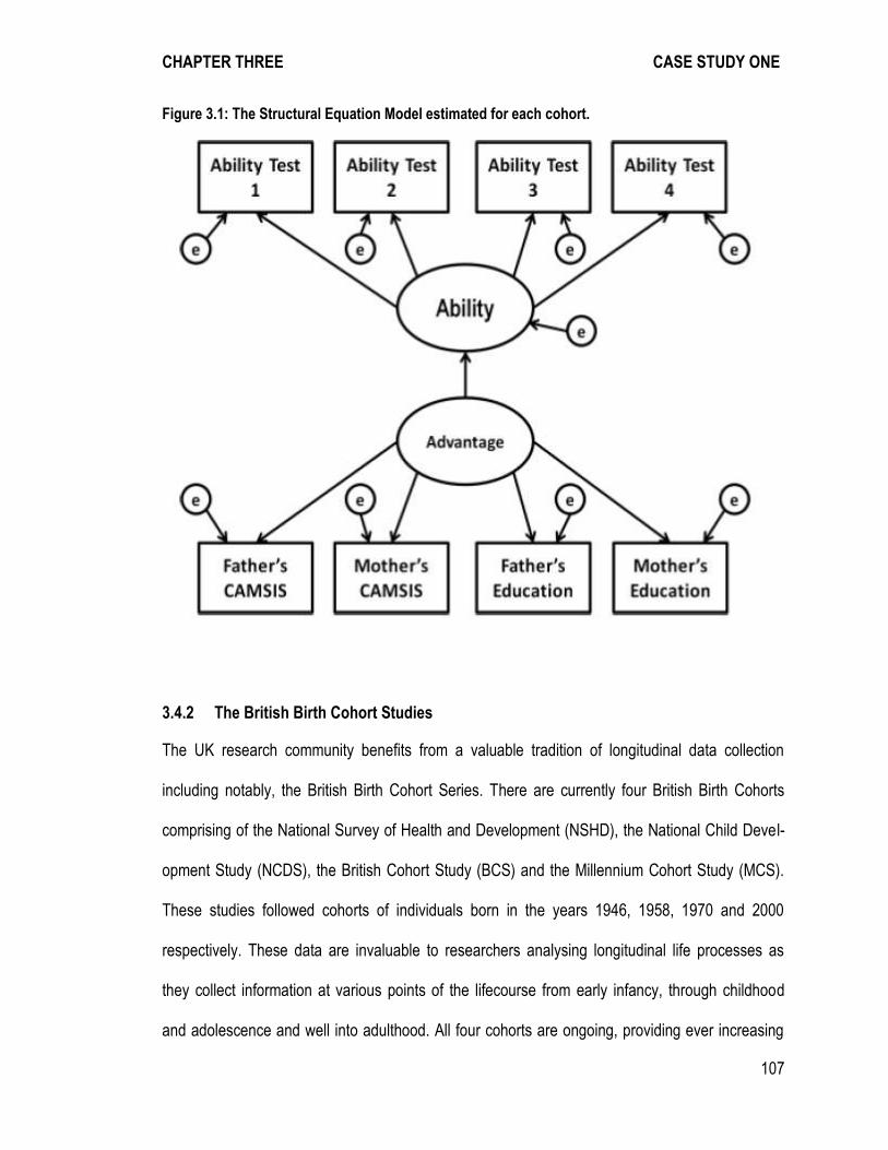
CHAPTER THREE CASE STUDY ONE
107
Figure 3.1: The Structural Equation Model estimated for each cohort.
3.4.2 The British Birth Cohort Studies
The UK research community benefits from a valuable tradition of longitudinal data collection
including notably, the British Birth Cohort Series. There are currently four British Birth Cohorts
comprising of the National Survey of Health and Development (NSHD), the National Child Devel-
opment Study (NCDS), the British Cohort Study (BCS) and the Millennium Cohort Study (MCS).
These studies followed cohorts of individuals born in the years 1946, 1958, 1970 and 2000
respectively. These data are invaluable to researchers analysing longitudinal life processes as
they collect information at various points of the lifecourse from early infancy, through childhood
and adolescence and well into adulthood. All four cohorts are ongoing, providing ever increasing

CHAPTER THREE CASE STUDY ONE
108
volumes of data on the life outcomes and experiences of the cohort members. One of the aims of
the most recent cohort, the MCS, was “to collect data which would foster comparisons with other
cohort studies” (Hansen, 2008, p. 9). This chapter fulfils this aim by seeking to compare the
inequalities in cognitive skills of the children in this contemporary cohort, with the inequalities in
cognitive skills observed in children of the same age 30 and 42 years earlier, in the BCS and
NCDS studies.
Data from the three most recent cohorts the MCS, BCS and NCDS, are accessible from the UK
Data Archive. These datasets are the most suitable resources available to investigate the re-
search question of this chapter. The data include a range of information on the socio-economic
environment of the cohort members, as well as their scores on a number of cognitive tests
administered in early childhood. Comparisons between these three cohorts are far from straight-
forward. Identical information is not collected in each cohort, and considerations must be made as
to the equivalence of variables over this long period of time, these issues will be discussed later in
this section.
3.4.2.1 The National Child Development Study
The National Child Development Study was initiated as the Perinatal Mortality Survey, which
collected data on all babies born in England, Scotland and Wales from the 3rd to 9th of March
1958. The sample also incorporated new immigrant children born on the specified dates, when the
CHAPTER THREE CASE STUDY ONE
109
sample was revisited at ages 7, 11 and 1623 (Dodgeon et al., 2006). The second sweep of NCDS
data collection occurred when the cohort members were aged seven. At this age the cohort
members completed several cognitive ability tests, described in more detail below, which were
administered at the cohort member’s school by a teacher. Data on the socio-economic environ-
ment of the cohort member was collected at ages 7, 11 and 16 by means of a parent interview.
3.4.2.2 The British Cohort Study
The British Birth Cohort Study was initiated as the British Births Study, and the sample comprises
of all babies born in England, Scotland, Wales and Northern Ireland from the 5th to the 11th of April
1970 (Institute of Child Health, 1970). At ages 5, 10 and 16 the BCS sample also incorporated
new immigrants born on the specified dates24. In the 1975 (age 5) sweep of the BCS the cohort
members completed a series of cognitive tests which were administered at home, by a health
visitor. The health visitors were trained for their role in data collection and were provided with
lengthy guidelines and procedures to follow. Data regarding the socio-economic environment of
the cohort member was collected at ages 5, 10 and 16 by means of a structured parental inter-
view.
23 Full information regarding the NCDS sample and data collection procedure is provided on the NCDS website, accessed here: http://www.cls.ioe.ac.uk/page.aspx?&sitesectionid=779&sitesectiontitle=User+guides+to+the+NCDS+age+7+dataset. 24 Full details of the BCS samples and data collection procedures are provided on the BCS website accessed here: http://www.cls.ioe.ac.uk/page.aspx?&sitesectionid=803&sitesectiontitle=BCS+1975.
CHAPTER THREE CASE STUDY ONE
110
3.4.2.3 The Millennium Cohort Study
After a 30 year gap, the Millennium Cohort Study was initiated and provides information on a
cohort of individuals from Scotland, England, Wales and Northern Ireland. The structure of the
sample of the MCS differs in many ways from the samples of its predecessors, the NCDS and
BCS25. First, the sampling frame utilised for the MCS did not comprise all babies born in the UK in
a given period. The sampling frame comprised of all families eligible to claim child benefit,
although this is not a means tested benefit it does exclude those for whom the UK is not their
permanent residence (e.g. stationed military families from abroad and Asylum seekers). Plewis
(2007a) notes that these excluded populations are very much in the minority and should not
jeopardise the quality of the MCS sample.
Second, the MCS did not comprise of babies born in a single week. In England and Wales babies
born between September 2000 and August 2001 were included in the sample, and in Scotland
and Northern Ireland babies born from the end of November 2000 to the start of January 2002
were eligible for selection (Dex and Joshi, 2004). As a result, MCS cohort members are born over
a period of more than one year. Differences in the age of the cohort members may have implica-
tions when considering the development of young children, therefore care is taken to control for
the cohort members’ ages in the analyses of the MCS data in this chapter.
Furthermore, the MCS is based on a probability sample. The NCDS and BCS studies effectively
attempted to collect a systematic sample of all babies in their sampling frame. The MCS sample
was further stratified to increase the probability of selection of children in disadvantaged areas,
25 Full details of the MCS samples and data collection procedures are provided on the BCS website accessed here: http://www.cls.ioe.ac.uk/page.aspx?&sitesectionid=952&sitesectiontitle=About+the+sample.
CHAPTER THREE CASE STUDY ONE
111
and areas with large populations of ethnic minorities (Ketende and Jones, 2011). Stata’s survey
package (i.e. -svy- commands) is utilised to account for the complex sampling design of the MCS
in all the analyses presented in this chapter. Weights are used to account for the sampling
structure and also to correct for non-response (Plewis, 2007b).
A further complexity in the analysis of the MCS data is that parental responses are documented as
relating to a ‘main’ or ‘partner’ respondent, in comparison to the NCDS and BCS studies which
specifically document the responses of mother figures and father figures. The vast majority of
‘main’ respondents in the MCS are the cohort members’ natural mothers (Hansen, 2010), however
this is not always the case and one can not always assume that the ‘main’ respondent is the same
individual across survey sweeps. To produce the analytic MCS sample utilised in this chapter, the
‘household grid’ data file of the MCS was utilised to identify the relationship of the ‘main’ and
‘partner’ respondents to the cohort member. Only ‘main’ and ‘partner’ respondents identified as
mother and father figures to the cohort member (e.g. natural parent, step-parent, or adopted
parent) were retained, and variables were attributed to the mother figure or father figure of the
cohort member based on their relationship to the cohort member and their gender.
A further point of departure between the MCS and the older cohort studies is that the first sweep
of data collection in the MCS took place when the baby was around 9 months old, and not at birth.
Retrospective information was, however, collected regarding pregnancy and the first months of the
cohort members’ lives. The cohort members were then revisited at 3 years, 5 years, and 7 years.
Cognitive tests were administered to the cohort members at each of these sweeps, by a trained
interviewer. Cognitive ability tests completed by MCS members are considered at both ages 5 and
7, and are described in detail below. Using both the age 5 and age 7 sweeps of the MCS will
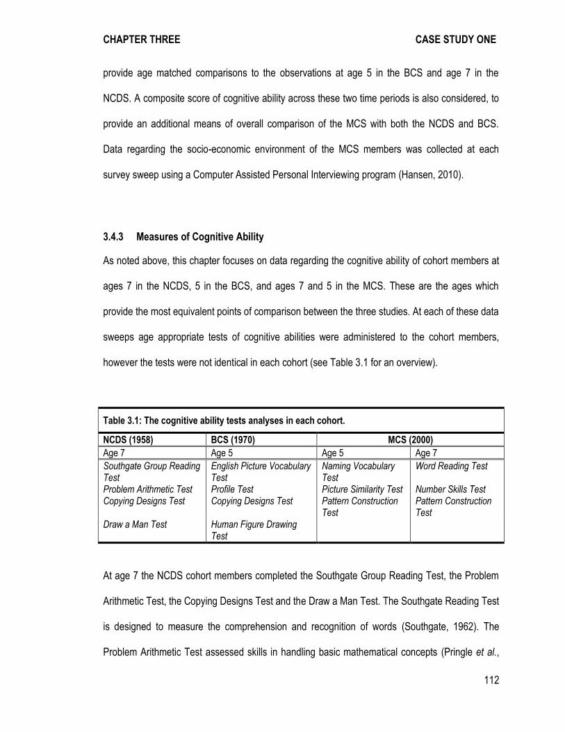
CHAPTER THREE CASE STUDY ONE
112
provide age matched comparisons to the observations at age 5 in the BCS and age 7 in the
NCDS. A composite score of cognitive ability across these two time periods is also considered, to
provide an additional means of overall comparison of the MCS with both the NCDS and BCS.
Data regarding the socio-economic environment of the MCS members was collected at each
survey sweep using a Computer Assisted Personal Interviewing program (Hansen, 2010).
3.4.3 Measures of Cognitive Ability
As noted above, this chapter focuses on data regarding the cognitive ability of cohort members at
ages 7 in the NCDS, 5 in the BCS, and ages 7 and 5 in the MCS. These are the ages which
provide the most equivalent points of comparison between the three studies. At each of these data
sweeps age appropriate tests of cognitive abilities were administered to the cohort members,
however the tests were not identical in each cohort (see Table 3.1 for an overview).
Table 3.1: The cognitive ability tests analyses in each cohort.
NCDS (1958) BCS (1970) MCS (2000)
Age 7 Age 5 Age 5 Age 7
Southgate Group Reading Test
English Picture Vocabulary Test
Naming Vocabulary Test
Word Reading Test
Problem Arithmetic Test Profile Test Picture Similarity Test Number Skills Test Copying Designs Test Copying Designs Test Pattern Construction
Test Pattern Construction Test
Draw a Man Test Human Figure Drawing Test
At age 7 the NCDS cohort members completed the Southgate Group Reading Test, the Problem
Arithmetic Test, the Copying Designs Test and the Draw a Man Test. The Southgate Reading Test
is designed to measure the comprehension and recognition of words (Southgate, 1962). The
Problem Arithmetic Test assessed skills in handling basic mathematical concepts (Pringle et al.,
CHAPTER THREE CASE STUDY ONE
113
1966). The Copying Designs Test required the cohort member to copy pictures of basic shapes
and is an indicator of perceptuo-motor ability (Pringle et al., 1966). The Draw a Man Test simply
asks the cohort member to draw a picture of man, which is then scored based on various criteria
such as proportion and the presence of detailed features. The results of this test can indicate
general levels of ability as well as perceptual skills (Goodenough, 1926).
At age 5 the BCS cohort members again completed the Copying Designs Test, as well as the
Human Figure Drawing Test which is equivalent to the Draw a Man Test. The cohort members
also completed a further drawing test, the Profile Test, where they copied a picture of the profile of
a face. The English Picture Vocabulary Test was also completed, and requires the child to point to
a picture which matches a given word, this test is designed to provide an assessment of the cohort
members’ verbal intelligence (Brimer and Dunn, 1962).
Cognitive assessments in the MCS are considered at ages 5 and 7. The tests completed in the
MCS were all sub-scales of the British Ability Scales, a collection of cognitive ability tests designed
to measure ability in childhood (Elliott et al., 1978). At age 5 the cohort members completed the
Naming Vocabulary Test, where they are asked to name objects from pictures. This test aims to
assess expressive language ability as well as underlying cognitive skills, such as the ability to
retrieve words from long term memory and to attach verbal labels to pictures (Hansen, 2010). The
Picture Similarities Test involves selecting a picture to complete a sequence, and aims to assess
problem solving skills (Hansen, 2010). At age 5 the MCS cohort members also completed a
Pattern Construction Test, where they were required to reproduce a pattern using cubes. This test
is designed to assess visual-spatial skills (Hansen, 2010). The Pattern Construction Test was
CHAPTER THREE CASE STUDY ONE
114
completed again at age 7, alongside a Word Reading Test. At age 7 the MCS cohort members
also completed a Number Skills Test (Hansen, 2010).
For each of the tests, age standardised versions are utilised based on the cohorts members’ age
at interview in months. These age-standardised versions of the tests are then standardised to
have a mean of 0 and standard deviation of 1. The Number Skills Test completed at age 7 in the
MCS can not be standardised by age because there are no age-based norms for this test, but it is
standardised to have a mean of 0 and a standard deviation of 1, therefore giving an indication of
the cohort member’s overall relative level of performance.
In the Structural Equation Model estimated in this chapter (see Figure 3.1) the ability test scores at
each age are used to represent an a single underlying latent concept of ability26. The test scores
of cohort members have been treated in a similar manner in previous research in the field. Using
Principal Components Analysis, Feinstein (2003) has produced a composite score based on the
ability test performance of subsamples of the BCS cohort at 22 months and 42 months of age.
Jones and Schoon (2008) have also utilised Principal Components Analysis to produce an overall
score of cognitive performance for children in the MCS, a procedure also employed by Blanden,
Katz and Redmond (2012).
26 There is heated debate concerning whether a single underlying dimension of cognitive ability exists, or whether individual differences in cognitive capacity are better represented by multiple dimensions (Garner, 1983; Sternberg, 1985). However, Deary et al.’s (2010) review of the contemporary evidence indicates that people who perform well in one domain of cognitive ability perform well in the others. Therefore a uni-dimensional latent variable of ability, in the models estimated in this chapter, is justified.
CHAPTER THREE CASE STUDY ONE
115
3.4.4 Measuring Social Advantage
The second latent variable analysed in this chapter is a measure of the relative socio-economic
advantage of the cohort member’s family. This latent variable is based on the occupational
position of the cohort member’s parents, and parents’ highest level of education27. However, the
year of birth of the cohort members’ parents spans almost the entire 20th century, a period which
witnessed structural change in occupational opportunities and vast educational expansion
(Glennerster, 2001; Greenaway et al., 2003). Therefore, detailed considerations need to be made
to ensure that the variables indicating parental occupational position and parental education in
each cohort maintain ‘meaning equivalence’ over time (Lambert et al., 2012). There may be
differences in the treatment of the variables in each time period, however this is to ensure that the
relative positions of the cohort member’s families can be meaningfully compared between cohorts.
3.4.4.1 Parent’s Occupational Position
In line with Lambert et al. (2007c) to maintain the equivalent meaning of occupational position over
time, focus is placed on the hierarchical element of stratification. CAMSIS scores are used to
represent the relative social advantage of the cohort member’s mother and father. These scores
are standardised within each cohort to have a mean of 50 and a standard deviation of 15. There-
fore mothers and fathers with different occupations can be attributed different relative positions,
taking into account changes in the occupational structure (Lambert et al., 2008).
27 Ideally a range of identical measures would be available in these three studies in order to facilitate a detailed comparison (e.g. detailed educational variables described in chapter two and further variables indicating lifestyle and parenting behaviours), however limited comparable measures are available. In this chapter we therefore focus on a limited number of variables and consider their comparability over time in detail.
CHAPTER THREE CASE STUDY ONE
116
Detailed occupational information which allows for the coding of parental CAMSIS scores in the
NCDS and BCS has only recently become available, whereas detailed parental occupational
information is available for every wave of the MCS. Gregg (2012) has deposited SOC codes for
NCDS fathers in 1969, when the cohort member was 11 years old. SOC codes have also been
deposited for BCS mothers and fathers in 1980, when the cohort member was 10 years old.
These newly deposited SOC codes are an invaluable resource, with the previously available
information consisting of a Socio-economic Group Measure which could be recoded to an estima-
tion of the Goldthorpe Class Scheme. However SOC codes are only available at age 10 and 11, a
few years older than the age at which the cognitive test scores were collected. Data is not yet
available on the MCS at this age, therefore the occupational position of parents in the MCS is
taken at the same time as the cognitive tests are collected (i.e. parental positions at age 5 are
considered when analysing age 5 test performance, and positions are age 7 are considered when
analysing age 7 test performance).
A further point of departure is that SOC codes are only available for fathers in the NCDS, whereas
information is available for mothers and fathers in the BCS and MCS cohorts. As a result two SEM
models are estimated for each cohort, one including only father’s CAMSIS to allow for the fairest
comparison to the NCDS, and a second which combines the additional information provided by
the mothers’ CAMSIS. If a social class measure was used to represent parental advantage in the
three cohorts these points of departure could have been avoided, however social class schemes
do not allow for clear considerations of hierarchy and are subject to complex structural change
over time (Prandy, 1998; Rytina, 2000).
CHAPTER THREE CASE STUDY ONE
117
3.4.4.2 Parent’s Education
The vast expansion of educational provision throughout the 20th century is well documented
(Glennerster, 2001; Greenaway et al., 2003). A consequence of educational expansion is that the
‘meaning’ of parental educational qualifications, in terms of the level of advantage which they
indicate, might change over time. The positional good theory indicates that the relative value of
educational categories will alter based on the relative advantage which the educational level
imbues (e.g. in terms of value in the labour market) (Hirsch, 1976).
In the first stage of coding the parents’ occupational information measurement equivalence is
ensured by focusing on the age at which the cohort members’ parents left education, as this is the
only measure of education available in all three cohorts. Information regarding qualifications
gained is available in the BCS, and NVQ level of qualifications is available in the MCS but no
comparable information is available in the NCDS.
Cheng and Egerton (2007, p. 207) have developed a comparable measure of educational level
based on the CASMIN educational scheme for the comparison of the NCDS and BCS. This
operationalisation is used here for the NCDS, BCS and MCS. Age at which mother and fathers left
school is used to record the parents’ highest level of education:
1) Upper tertiary (CASMIN 3b) – left school at age 21 or above
2) Lower Tertiary (CASMIN 3a) – left school age 19 to 20
3) Full Secondary (CASMIN 2c) – left school age 16 to 18
4) Intermediate Secondary or below (CASMIN 2ab, 1) - left school age 15 or below
CHAPTER THREE CASE STUDY ONE
118
Although this is a comparable measure for each of the three cohorts consideration is also required
as to the ‘meaning equivalence’ of these categories over time. Schroder and Ganzeboom (2009)
highlight that it is not the absolute value of an individual’s educational attainment which is impor-
tant, rather an indication of the relative value of the educational credentials within a given social
context, as described in position good theory (Hirsch, 1976). Sorensen (1979) represented the
relative structure of educational inequality based on the cumulative percentile distribution of
education in different cohorts. Olneck and Kim (1989) produced a scale of educational attainment
based on how close to the top of the educational distribution an individual’s level of education fell.
For the purposes of the analyses in this chapter parents’ educational attainment in each cohort is
transformed into a relative scale based on the prevalence of a level of education amongst parents
in each cohort. Educational qualifications are given a relative value based on the proportion of
mothers and fathers who do not also have that level of qualification28. The relative scales of
parental education are summarised in Table 3.2.
28 The parents of the cohort members vary greatly in their ages, ideally the relative score would compare the parents with counterparts of the same age however there are not sufficient observations to meaning-fully make these comparisons.

CHAPTER THREE CASE STUDY ONE
119
Table 3.2: The Relative Scales of Parental Educational Attainment for each cohort.
1958 Cohort 1970 Cohort MCS Cohort Age 5 MCS Cohort Age 7
Father’s Education CASMIN 3b 96.30% 93.00% 75.31% 74.56% CASMIN 3a 92.18% 91.09% 69.24% 68.42% CASMIN 2c 78.81% 66.46% 06.57% 06.36% CASMIN 2ab, 1 00.00% 00.00% 00.00% 00.00% Mother’s Education CASMIN 3b 98.00% 96.48% 79.93% 79.41% CASMIN 3a 94.35% 94.34% 71.68% 71.07% CASMIN 2c 78.60% 65.83% 05.05% 04.85% CASMIN 2ab, 1 00.00% 00.00% 00.00% 00.00%
Notes: A relative scale of highest educational level based on the percentage of cohort member’s parents who have a level of education level below each CASMIN category.
3.4.5 Structure of Analysis
Changes in the associations between parental advantage and childhood cognitive ability are
modelled using SEMs. The model estimated is presented in Figure 3.1. As mentioned above, two
models are estimated, one that contains fathers CAMSIS only and a second which contains both
Mothers’ and Fathers’ CAMSIS where available. Mothers’ and Fathers’ relative level of education
is entered in all models as a manifest indicator of social advantage. A number of cognitive tests
are used to indicate the latent variable of ability. These tests are not the same across cohorts and
have been described above (see Table 3.1). The analytic sample is based on a complete case
analysis of all the information available on the variables considered in each cohort. The complex
survey structure of the MCS was accounted for using the appropriate weights. Weighted and non-
weighted results were compared but they are highly similar and only weighted results are pre-
sented.
Several model fit criteria were used to assess the models, the chi square statistic is presented
however it is overly sensitive to sample size and will almost always be positive in large sample
CHAPTER THREE CASE STUDY ONE
120
sizes (Hox et al., 1998). The samples used in these analyses are large, and the chi square
statistic is significant in all model estimations. Therefore more suitable model fit criteria are also
considered. The Root Mean Square Error of Approximation gives an approximation of discrepancy
in model fit per degrees of freedom, values of less than 0.05 indicate a good fit (Hooper et al.,
2008). The Comparative Fit Index is also presented with values over 0.95 indicating a good fit.
The R2 of the whole model is also presented and indicated the amount of variance explained by
the model.
3.5 Results
The models for each cohort are considered separately, and then the models will be comparedbe-
tween cohorts to address the research question, has the association between socio-economic
advantage and cognitive ability scores in the early years changed over time?

CHAPTER THREE CASE STUDY ONE
121
3.5.1 National Child Development Study
Table 3.3. presents the estimates for the SEM model shown in Figure 3.1, which was estimated
separately for each cohort. The coefficients refer to standardised regression coefficients ceteris
paribus. The top panel of the model shows the pathway coefficients, the relationship between the
latent variable of advantage and the latent variable of ability. This is known as the structural
model. The Middle panel shows the relationship between the latent variables and their indicators
which is known as the measurement model. The bottom panel presents the model fit criteria
discussed above.
Looking first at the measurement model, the measured variables all loaded strongly on the latent
variables, and CFI and RMSEA statistics indicate the model is a good fit. Looking to the structural
model, the relative social advantage of the cohort member’s family had a positive association with
their cognitive ability test scores. Overall the model explains between 74% and 75% of the
variance in cognitive ability test scores.
The model was repeated separately for male and female cohort members, due to concerns that
the rate of cognitive development for male and female cohort members may be different (Deary et
al., 2007a; Dykiert et al., 2009). The coefficients in the male and female models were compared
using Z-tests which indicate that there are no significant differences in the patterns observed for
boys and girls.
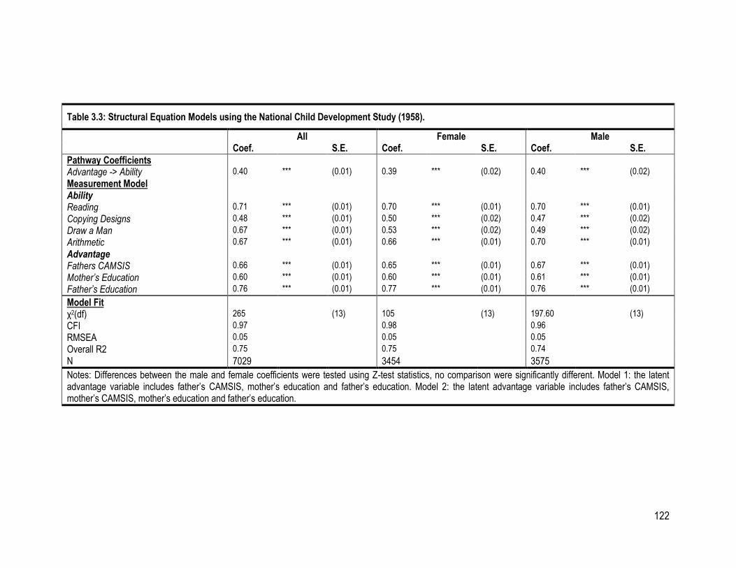
122
Table 3.3: Structural Equation Models using the National Child Development Study (1958).
All Female Male Coef. S.E. Coef. S.E. Coef. S.E.
Pathway Coefficients
Advantage -> Ability 0.40 *** (0.01) 0.39 *** (0.02) 0.40 *** (0.02)
Measurement Model
Ability
Reading 0.71 *** (0.01) 0.70 *** (0.01) 0.70 *** (0.01)
Copying Designs 0.48 *** (0.01) 0.50 *** (0.02) 0.47 *** (0.02)
Draw a Man 0.67 *** (0.01) 0.53 *** (0.02) 0.49 *** (0.02)
Arithmetic 0.67 *** (0.01) 0.66 *** (0.01) 0.70 *** (0.01)
Advantage
Fathers CAMSIS 0.66 *** (0.01) 0.65 *** (0.01) 0.67 *** (0.01)
Mother’s Education 0.60 *** (0.01) 0.60 *** (0.01) 0.61 *** (0.01)
Father’s Education 0.76 *** (0.01) 0.77 *** (0.01) 0.76 *** (0.01)
Model Fit
χ2(df) 265 (13) 105 (13) 197.60 (13)
CFI 0.97 0.98 0.96
RMSEA 0.05 0.05 0.05
Overall R2 0.75 0.75 0.74
N 7029 3454 3575
Notes: Differences between the male and female coefficients were tested using Z-test statistics, no comparison were significantly different. Model 1: the latent advantage variable includes father’s CAMSIS, mother’s education and father’s education. Model 2: the latent advantage variable includes father’s CAMSIS, mother’s CAMSIS, mother’s education and father’s education.
CHAPTER THREE CASE STUDY ONE
123
3.5.2 British Cohort Study
Table 3.4 gives the estimates for the SEM model using the British Cohort Study Data. Again these
models showed satisfactory fit, indicated by the CFI and RMSEA statistics. Looking to the meas-
urement model each of the cognitive ability tests load significantly on the latent variable of ability,
and parents occupation and CAMSIS load significantly on the latent variable of advantage. With
the addition of mother’s CAMSIS, this manifest variable loads significantly on the latent variable of
advantage. Although the overall R2 for the model only increases marginally when this additional
variable is included, suggesting that much of the variance in the model has already been ac-
counted for by father’s CAMSIS and education. Overall the models explain between 76% and 78%
of the variance in cognitive ability test scores. There is a positive significant association between
the latent variable of advantage and the latent variable of ability, and this is not significantly
different between boys and girls.
3.5.3 Millennium Cohort Study
Models for the Millennium Cohort Study are presented for cognitive ability tests administered at
age 5 (see Table 3.5), age 7 (see Table 3.6) and for the two sets of ability tests together (see
Table 3.7). These models are weighted to account for the complex survey structure of the MCS. In
order to present model fit statistics for these weighted models, estimates of the model fit are
provided from non-weighted models, a practice advocated by Treiman (2009).
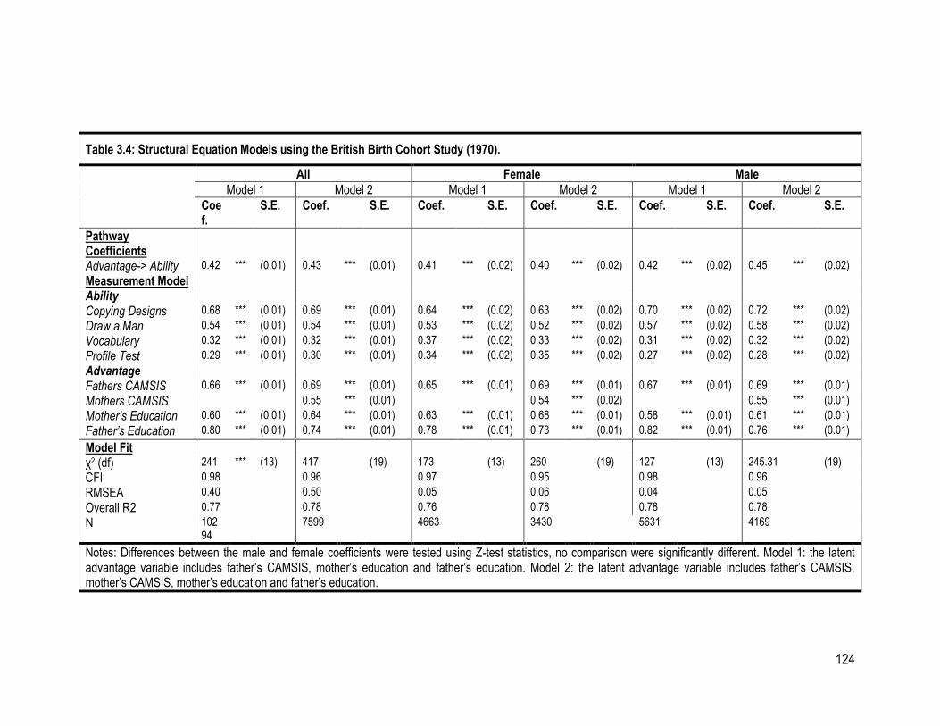
124
Table 3.4: Structural Equation Models using the British Birth Cohort Study (1970).
All Female Male
Model 1 Model 2 Model 1 Model 2 Model 1 Model 2
Coef.
S.E. Coef. S.E. Coef. S.E. Coef. S.E. Coef. S.E. Coef. S.E.
Pathway Coefficients
Advantage-> Ability 0.42 *** (0.01) 0.43 *** (0.01) 0.41 *** (0.02) 0.40 *** (0.02) 0.42 *** (0.02) 0.45 *** (0.02)
Measurement Model
Ability
Copying Designs 0.68 *** (0.01) 0.69 *** (0.01) 0.64 *** (0.02) 0.63 *** (0.02) 0.70 *** (0.02) 0.72 *** (0.02)
Draw a Man 0.54 *** (0.01) 0.54 *** (0.01) 0.53 *** (0.02) 0.52 *** (0.02) 0.57 *** (0.02) 0.58 *** (0.02)
Vocabulary 0.32 *** (0.01) 0.32 *** (0.01) 0.37 *** (0.02) 0.33 *** (0.02) 0.31 *** (0.02) 0.32 *** (0.02)
Profile Test 0.29 *** (0.01) 0.30 *** (0.01) 0.34 *** (0.02) 0.35 *** (0.02) 0.27 *** (0.02) 0.28 *** (0.02)
Advantage
Fathers CAMSIS 0.66 *** (0.01) 0.69 *** (0.01) 0.65 *** (0.01) 0.69 *** (0.01) 0.67 *** (0.01) 0.69 *** (0.01)
Mothers CAMSIS 0.55 *** (0.01) 0.54 *** (0.02) 0.55 *** (0.01)
Mother’s Education 0.60 *** (0.01) 0.64 *** (0.01) 0.63 *** (0.01) 0.68 *** (0.01) 0.58 *** (0.01) 0.61 *** (0.01)
Father’s Education 0.80 *** (0.01) 0.74 *** (0.01) 0.78 *** (0.01) 0.73 *** (0.01) 0.82 *** (0.01) 0.76 *** (0.01)
Model Fit
χ2 (df) 241 *** (13) 417 (19) 173 (13) 260 (19) 127 (13) 245.31 (19)
CFI 0.98 0.96 0.97 0.95 0.98 0.96
RMSEA 0.40 0.50 0.05 0.06 0.04 0.05
Overall R2 0.77 0.78 0.76 0.78 0.78 0.78
N 10294
7599 4663 3430 5631 4169
Notes: Differences between the male and female coefficients were tested using Z-test statistics, no comparison were significantly different. Model 1: the latent advantage variable includes father’s CAMSIS, mother’s education and father’s education. Model 2: the latent advantage variable includes father’s CAMSIS, mother’s CAMSIS, mother’s education and father’s education.
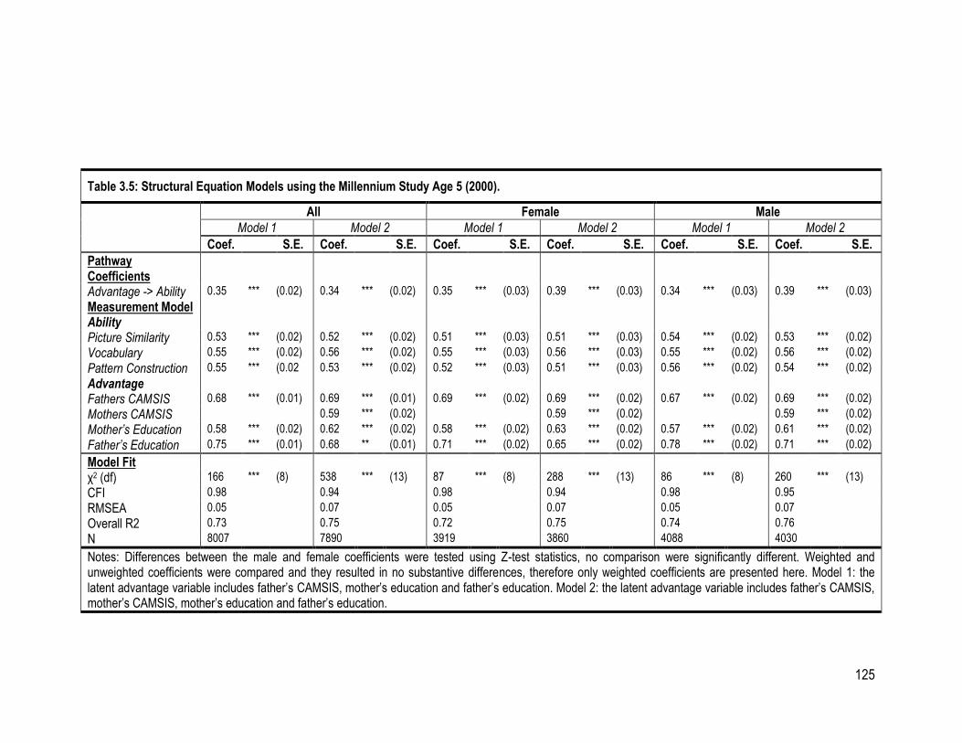
125
Table 3.5: Structural Equation Models using the Millennium Study Age 5 (2000).
All Female Male
Model 1 Model 2 Model 1 Model 2 Model 1 Model 2
Coef. S.E. Coef. S.E. Coef. S.E. Coef. S.E. Coef. S.E. Coef. S.E.
Pathway Coefficients
Advantage -> Ability 0.35 *** (0.02) 0.34 *** (0.02) 0.35 *** (0.03) 0.39 *** (0.03) 0.34 *** (0.03) 0.39 *** (0.03)
Measurement Model
Ability
Picture Similarity 0.53 *** (0.02) 0.52 *** (0.02) 0.51 *** (0.03) 0.51 *** (0.03) 0.54 *** (0.02) 0.53 *** (0.02)
Vocabulary 0.55 *** (0.02) 0.56 *** (0.02) 0.55 *** (0.03) 0.56 *** (0.03) 0.55 *** (0.02) 0.56 *** (0.02)
Pattern Construction 0.55 *** (0.02 0.53 *** (0.02) 0.52 *** (0.03) 0.51 *** (0.03) 0.56 *** (0.02) 0.54 *** (0.02)
Advantage
Fathers CAMSIS 0.68 *** (0.01) 0.69 *** (0.01) 0.69 *** (0.02) 0.69 *** (0.02) 0.67 *** (0.02) 0.69 *** (0.02)
Mothers CAMSIS 0.59 *** (0.02) 0.59 *** (0.02) 0.59 *** (0.02)
Mother’s Education 0.58 *** (0.02) 0.62 *** (0.02) 0.58 *** (0.02) 0.63 *** (0.02) 0.57 *** (0.02) 0.61 *** (0.02)
Father’s Education 0.75 *** (0.01) 0.68 ** (0.01) 0.71 *** (0.02) 0.65 *** (0.02) 0.78 *** (0.02) 0.71 *** (0.02)
Model Fit
χ2 (df) 166 *** (8) 538 *** (13) 87 *** (8) 288 *** (13) 86 *** (8) 260 *** (13)
CFI 0.98 0.94 0.98 0.94 0.98 0.95
RMSEA 0.05 0.07 0.05 0.07 0.05 0.07
Overall R2 0.73 0.75 0.72 0.75 0.74 0.76
N 8007 7890 3919 3860 4088 4030
Notes: Differences between the male and female coefficients were tested using Z-test statistics, no comparison were significantly different. Weighted and unweighted coefficients were compared and they resulted in no substantive differences, therefore only weighted coefficients are presented here. Model 1: the latent advantage variable includes father’s CAMSIS, mother’s education and father’s education. Model 2: the latent advantage variable includes father’s CAMSIS, mother’s CAMSIS, mother’s education and father’s education.
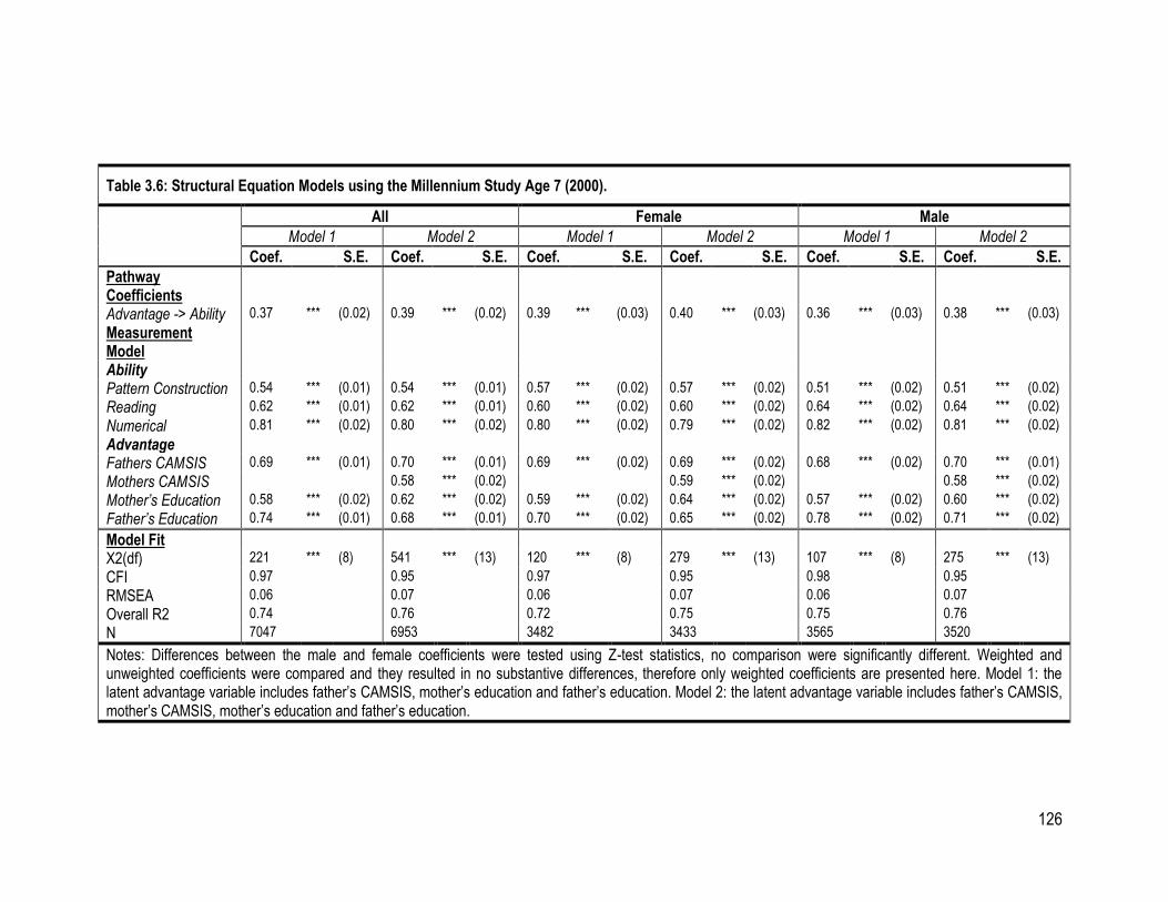
126
Table 3.6: Structural Equation Models using the Millennium Study Age 7 (2000).
All Female Male
Model 1 Model 2 Model 1 Model 2 Model 1 Model 2
Coef. S.E. Coef. S.E. Coef. S.E. Coef. S.E. Coef. S.E. Coef. S.E.
Pathway Coefficients
Advantage -> Ability 0.37 *** (0.02) 0.39 *** (0.02) 0.39 *** (0.03) 0.40 *** (0.03) 0.36 *** (0.03) 0.38 *** (0.03)
Measurement Model
Ability
Pattern Construction 0.54 *** (0.01) 0.54 *** (0.01) 0.57 *** (0.02) 0.57 *** (0.02) 0.51 *** (0.02) 0.51 *** (0.02)
Reading 0.62 *** (0.01) 0.62 *** (0.01) 0.60 *** (0.02) 0.60 *** (0.02) 0.64 *** (0.02) 0.64 *** (0.02)
Numerical 0.81 *** (0.02) 0.80 *** (0.02) 0.80 *** (0.02) 0.79 *** (0.02) 0.82 *** (0.02) 0.81 *** (0.02)
Advantage
Fathers CAMSIS 0.69 *** (0.01) 0.70 *** (0.01) 0.69 *** (0.02) 0.69 *** (0.02) 0.68 *** (0.02) 0.70 *** (0.01)
Mothers CAMSIS 0.58 *** (0.02) 0.59 *** (0.02) 0.58 *** (0.02)
Mother’s Education 0.58 *** (0.02) 0.62 *** (0.02) 0.59 *** (0.02) 0.64 *** (0.02) 0.57 *** (0.02) 0.60 *** (0.02)
Father’s Education 0.74 *** (0.01) 0.68 *** (0.01) 0.70 *** (0.02) 0.65 *** (0.02) 0.78 *** (0.02) 0.71 *** (0.02)
Model Fit
X2(df) 221 *** (8) 541 *** (13) 120 *** (8) 279 *** (13) 107 *** (8) 275 *** (13)
CFI 0.97 0.95 0.97 0.95 0.98 0.95
RMSEA 0.06 0.07 0.06 0.07 0.06 0.07
Overall R2 0.74 0.76 0.72 0.75 0.75 0.76
N 7047 6953 3482 3433 3565 3520
Notes: Differences between the male and female coefficients were tested using Z-test statistics, no comparison were significantly different. Weighted and unweighted coefficients were compared and they resulted in no substantive differences, therefore only weighted coefficients are presented here. Model 1: the latent advantage variable includes father’s CAMSIS, mother’s education and father’s education. Model 2: the latent advantage variable includes father’s CAMSIS, mother’s CAMSIS, mother’s education and father’s education.
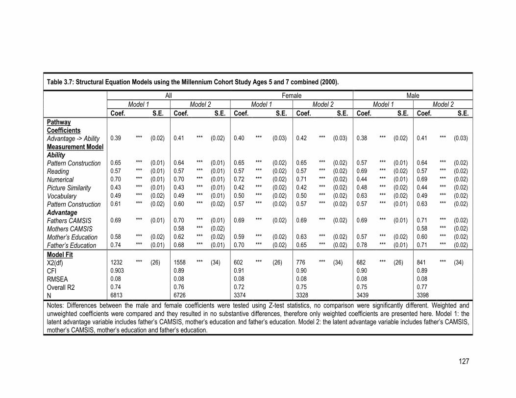
127
Table 3.7: Structural Equation Models using the Millennium Cohort Study Ages 5 and 7 combined (2000).
All Female Male
Model 1 Model 2 Model 1 Model 2 Model 1 Model 2
Coef. S.E. Coef. S.E. Coef. S.E. Coef. S.E. Coef. S.E. Coef. S.E.
Pathway Coefficients
Advantage -> Ability 0.39 *** (0.02) 0.41 *** (0.02) 0.40 *** (0.03) 0.42 *** (0.03) 0.38 *** (0.02) 0.41 *** (0.03)
Measurement Model
Ability
Pattern Construction 0.65 *** (0.01) 0.64 *** (0.01) 0.65 *** (0.02) 0.65 *** (0.02) 0.57 *** (0.01) 0.64 *** (0.02)
Reading 0.57 *** (0.01) 0.57 *** (0.01) 0.57 *** (0.02) 0.57 *** (0.02) 0.69 *** (0.02) 0.57 *** (0.02)
Numerical 0.70 *** (0.01) 0.70 *** (0.01) 0.72 *** (0.02) 0.71 *** (0.02) 0.44 *** (0.01) 0.69 *** (0.02)
Picture Similarity 0.43 *** (0.01) 0.43 *** (0.01) 0.42 *** (0.02) 0.42 *** (0.02) 0.48 *** (0.02) 0.44 *** (0.02)
Vocabulary 0.49 *** (0.02) 0.49 *** (0.01) 0.50 *** (0.02) 0.50 *** (0.02) 0.63 *** (0.02) 0.49 *** (0.02)
Pattern Construction 0.61 *** (0.02) 0.60 *** (0.02) 0.57 *** (0.02) 0.57 *** (0.02) 0.57 *** (0.01) 0.63 *** (0.02)
Advantage
Fathers CAMSIS 0.69 *** (0.01) 0.70 *** (0.01) 0.69 *** (0.02) 0.69 *** (0.02) 0.69 *** (0.01) 0.71 *** (0.02)
Mothers CAMSIS 0.58 *** (0.02) 0.58 *** (0.02)
Mother’s Education 0.58 *** (0.02) 0.62 *** (0.02) 0.59 *** (0.02) 0.63 *** (0.02) 0.57 *** (0.02) 0.60 *** (0.02)
Father’s Education 0.74 *** (0.01) 0.68 *** (0.01) 0.70 *** (0.02) 0.65 *** (0.02) 0.78 *** (0.01) 0.71 *** (0.02)
Model Fit
X2(df) 1232 *** (26) 1558 *** (34) 602 *** (26) 776 *** (34) 682 *** (26) 841 *** (34)
CFI 0.903 0.89 0.91 0.90 0.90 0.89
RMSEA 0.08 0.08 0.08 0.08 0.08 0.08
Overall R2 0.74 0.76 0.72 0.75 0.75 0.77
N 6813 6726 3374 3328 3439 3398
Notes: Differences between the male and female coefficients were tested using Z-test statistics, no comparison were significantly different. Weighted and unweighted coefficients were compared and they resulted in no substantive differences, therefore only weighted coefficients are presented here. Model 1: the latent advantage variable includes father’s CAMSIS, mother’s education and father’s education. Model 2: the latent advantage variable includes father’s CAMSIS, mother’s CAMSIS, mother’s education and father’s education.
CHAPTER THREE CASE STUDY ONE
128
At age 5, 7 (and the combined score), the test scores loaded significantly on the latent variable of
ability and the measures of family advantage loaded significantly on the latent variable of advan-
tage. In the age 5 model the CFI and RMSEA statistics indicate that this model is a good fit. In the
age 7 and combined model, the RMSEA were a little too large to indicate good model fit although
the CFI statistics indicate that these models are satisfactory. In each MCS model around 72% and
77% of the variance in the model is accounted for. The addition of mother’s CAMSIS increases
the proportion of variance explained slightly in each case. Looking to the structural model, there is
a positive significant association between social advantage and cognitive ability test scores in
each set of models.
Looking at the models of the NCDS, BCS and MCS separately it is clear that these results
replicate previous findings which have shown that the performance of children on tests of cogni-
tive skills in early childhood is significantly influenced by their level of relative social advantage
(e.g. Blanden et al., 2007; Blanden et al., 2010; Dickerson et al., 2012; Feinstein, 2003; Goodman
et al., 2010; Schoon et al., 2010; Schoon et al., 2011).
3.5.4 Cross Cohort Comparisons
The research question posed in this chapter seeks to investigate whether the association between
parental social advantage and child ability test scores has changed over time. First looking to the
proportion of variance explained in each model, 74% to 75% is explained in the oldest cohort
(NCDS), 76% to 78% in the BCS cohort and 72% to 76% in the MCS cohort. Comparison of the
proportion of variance explained gives only a very general overview of how the models compare

CHAPTER THREE CASE STUDY ONE
129
and shows no convincing or clear indication of noticeable change in the amount of variance in
ability test scores accounted for by social advantage in each cohort.
The standardised regression coefficients linking the latent variable of advantage and the latent
variable of ability are compared using Z-tests, to indicate if statistical differences are apparent. As
discussed above the fairest comparisons are between the NCDS who were age 7 when their
ability data was collected and the age 7 sweep of the MCS data. Likewise the BCS data was
collected at age 5 and therefore the fairest comparisons can therefore be made between the BCS
and MCS age 5 sweep. Table 3.8 shows the results of significant tests (Z-tests) between the
standardised coefficients in each cohort. Looking to the NCDS and MCS at age 7 there is no
significant difference between the regression coefficients representing the association between
parental advantage and ability scores. Looking at the BCS and MCS at age 5 results there is
some evidence of a decrease in the association between advantage and ability between these two
time points. Overall there appears to be no significant difference between the coefficients of the
NCDS and MCS, and despite tentative evidence of a reduction in the association between the
NCDS and MCS, comparisons between the NCDS and all other MCS sweeps indicate no change.
A decrease is apparent between the BCS and both the MCS at age 5 and 7, this is also most
notable when for the male cohort members.
Over the greatest period of time (NCDS vs. MCS) there is an indication of little change in the
association, although a decrease is observed within this period between the BCS and MCS. This
significant difference is less apparent when mother’s CAMSIS is added to the model. The overall
amount of variance explained changes very little between the three cohorts and the manifest
variables for social origins load strongly on ability test scores in each cohort. Overall, there is no

CHAPTER THREE CASE STUDY ONE
130
clear evidence of a reduction in the association between social background and cognitive test
scores.
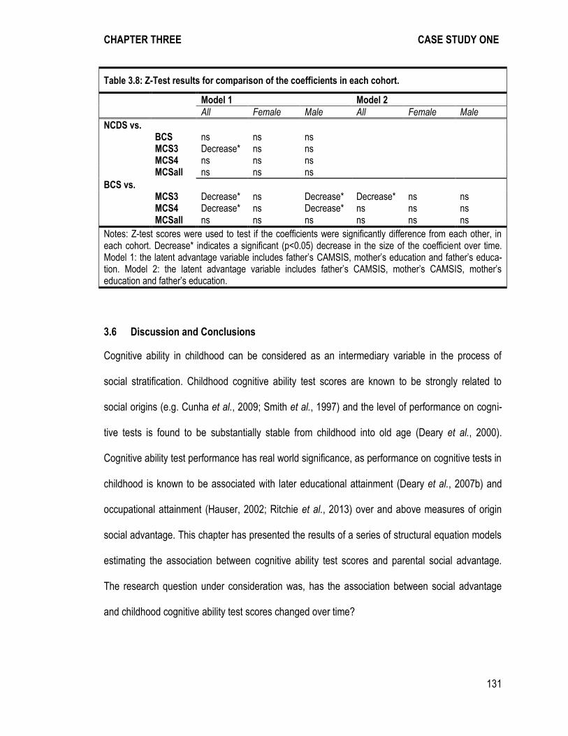
CHAPTER THREE CASE STUDY ONE
131
Table 3.8: Z-Test results for comparison of the coefficients in each cohort.
Model 1 Model 2
All Female Male All Female Male
NCDS vs. BCS ns ns ns MCS3 Decrease* ns ns MCS4 ns ns ns MCSall ns ns ns
BCS vs. MCS3 Decrease* ns Decrease* Decrease* ns ns MCS4 Decrease* ns Decrease* ns ns ns MCSall ns ns ns ns ns ns
Notes: Z-test scores were used to test if the coefficients were significantly difference from each other, in each cohort. Decrease* indicates a significant (p<0.05) decrease in the size of the coefficient over time. Model 1: the latent advantage variable includes father’s CAMSIS, mother’s education and father’s educa-tion. Model 2: the latent advantage variable includes father’s CAMSIS, mother’s CAMSIS, mother’s education and father’s education.
3.6 Discussion and Conclusions
Cognitive ability in childhood can be considered as an intermediary variable in the process of
social stratification. Childhood cognitive ability test scores are known to be strongly related to
social origins (e.g. Cunha et al., 2009; Smith et al., 1997) and the level of performance on cogni-
tive tests is found to be substantially stable from childhood into old age (Deary et al., 2000).
Cognitive ability test performance has real world significance, as performance on cognitive tests in
childhood is known to be associated with later educational attainment (Deary et al., 2007b) and
occupational attainment (Hauser, 2002; Ritchie et al., 2013) over and above measures of origin
social advantage. This chapter has presented the results of a series of structural equation models
estimating the association between cognitive ability test scores and parental social advantage.
The research question under consideration was, has the association between social advantage
and childhood cognitive ability test scores changed over time?
CHAPTER THREE CASE STUDY ONE
132
Overall what is clear from the results is that cognitive abilities measured in early childhood (i.e.
age 5 or 7) are strongly associated with family social advantage, indicated by parental education
and parental CAMSIS scores. In each cohort there was a significant positive association between
a latent variable representing family advantage and a latent variable representing cognitive ability.
Comparing the three cohorts, there is no striking evidence to suggest either a notable decrease or
increase in the association between social origins and cognitive ability scores. Tentatively, there is
evidence for a decrease between the BCS (1970) and MCS (2000) cohorts. Overall in comparing
the NCDS (1958) and MCS (2000) there appears to be stability in the association between social
advantage and childhood cognitive ability test scores.
The widespread provision of pre-school education by the Labour government seemed to provide
the context through which young children from all social backgrounds would be able to improve
their cognitive skills. However, as Gottfredson (2005) highlights, policy changes which aim
improve the cognitive abilities of all children will counter intuitively increase differences in perform-
ance between groups. Through the provision of universal pre-school education, the more
advantaged children will still continue to improve their skills and they may also improve more than
their disadvantaged counterparts given their already higher level of ability (Gottfredson, 2005).
The Labour government also introduced focussed programmes to improve the cognitive abilities of
the most disadvantaged children which should have acted to readdress cognitive inequality,
nevertheless although the Sure Start programme is reported to have been successful in improving
parenting behaviours and health, it does not seem to have had a clear impact on the cognitive
abilities of the children (Department for Education, 2010). Children from disadvantaged families
continue to enter school with lower levels of cognitive capability, which sets them apart from their
more advantaged peers, even at only 5 or 7 years of age.
CHAPTER THREE CASE STUDY ONE
133
These findings paint a pessimistic picture for the longer term egalitarian goals of reducing ine-
qualities in educational attainment and indeed in reducing inequalities in the occupational
attainment process. Children with low cognitive skills in childhood are unlikely to overcome these
initial disadvantages in their development (Jerrim and Vignoles, 2012) and as they progress
through more demanding stages of education gaps in ability tend to increase (Gottfredson, 2005).
There is a growing stream of debate in political discourse which seeks to lay the blame of the
social reproduction of cognitive inequalities upon parents, in a recent speech Prime Minister David
Cameron has stated:
“…the differences in child outcomes between a child born in poverty and a child born
in wealth are no longer statistically significant when both have been raised by ‘confi-
dent and able’ parents. It would be over the top to say that it is to social science
when E=MC2 was to physics… That discovery defined the laws of relativity; this one
is the new law for social mobility.” (Cameron, 2010 Accessed: 12/12/2013)
In the UK the Conservative government that took office in 2010 have developed a strong focus on
individualistic causes for the inequalities faced by children and young people from disadvantaged
backgrounds. In the wake of the 2011 London riots, Cameron stated that the clear cause of the
violent revolt of young people in London was “...a lack of proper parenting, a lack of proper
upbringing...” (Cameron, 2011). Policies have been introduced with the aim of reducing ‘bad’
parenting and encouraging traditional family structures, such as the trialing of parenting classes
for the parents of children under five and relationship support services for parents when they have
their first child. The notion of a breakdown in the upbringing of children falls within the framework
CHAPTER THREE CASE STUDY ONE
134
of political and media discourse on ‘New Social Mobility’ (Payne, 2012a; Payne, 2012c). This
discourse has overlooked the complexity of research on social mobility to present a misguided
picture of clear and certain decline in social mobility, and has largely ignored sociological insights
on the stratifying influence of the social structure (Payne, 2012a; Payne, 2012c). Little emphasis
has been placed on the structural and labour market influences on social mobility, as Payne
(2012c, p. 69) states “it is not the case that more mobility will reduce social inequality: rather
reducing social inequality will increase social mobility”.
The analyses in this chapter have indicated that social origins appear to have exerted a stable
influence on the cognitive outcomes of children over a period of 42 years. If parenting practices,
related to socio-economic position had altered drastically in recent decades, to impede the
success of the more recent cohorts, great differences should have been apparent in the strength
of association between social origins and cognitive inequalities over time, this was not the case
and therefore it is unlikely that a breakdown in parenting is a clear explanation for patterns of
inequality in educational or occupational attainment.
Limitations in the comparable variables across the cohort studies meant that the analyses in this
chapter could not be extended to study possible mechanisms in the social reproduction of cogni-
tive inequalities. Although the results have made an informative and useful contribution to the
literature, Lieberson (1985, pp. 213-219) highlights for example, the importance of using quantita-
tive data to show “what is happening” before the attempt to explain “why it is happening”.
Research which has analysed possible mechanisms explaining cognitive inequalities within single
cohorts have highlighted that parenting behaviours and skills do not fully explain ongoing social

CHAPTER THREE CASE STUDY ONE
135
inequalities. For example, following analysis of the MCS, Sullivan, Ketende and Joshi (2013, p.
17) state:
“Parents’ social class and education reflect not just what parents do, but also what
they have – and what they have is not just money. Other classed resources including
cultural and cognitive resources matter too…”
Finally, from reviewing the research which has analysed the Millennium Cohort Study the analyses
in this chapter appear to represent the first attempt to compare the Millennium Cohort Study with
both the British Cohort Study and the National Child Study. This exercise has not been without its
difficulties. Although the cohort studies are designed to facilitate research on social change,
developments and differences between the surveys make cross cohort comparisons between the
mature cohorts (i.e. the NCDS and the BCS) and the ‘contemporary’ child cohort (MCS) problem-
atic. In this chapter care has been taken to operationalise variables which aid the comparability of
measurement between the studies. This has been a good first step into the foray of three cohort
comparisons which will become increasingly important as the MCS sample sit their first standard-
ised examinations and begin to leave education. These later life outcomes will perhaps be better
suited, in terms of comparability, for three cohort comparisons. These cohort studies represent a
valuable resource which provides the opportunity to link influences on the individual cohort
member’s outcomes throughout their whole life period. The considerations made in this chapter in
terms of measuring parents’ education levels and occupational position will be an important
foundation for future cross-cohort comparisons.
CHAPTER FOUR CASE STUDY TWO
136
4. Social Stratification and School GCSE Attainment: Exploring the 'Middle'
4.1 Introduction
In two recent papers, Roberts (2011; 2012) contends that there has been oversight in the study of
the outcomes and transitions of ‘ordinary’ young people. It is argued that the research agenda has
been characterised by a dualistic focus on educationally successful young people and those who
are excluded or disconnected from the education system altogether. Roberts (2011) employs the
term ‘missing middle’ to describe the ‘ordinary’ young people who are absent from the polarised
focus of the current research programme. In Brown’s terms (1987, p. 1) these young people could
be described as the “ordinary working class pupils who neither leave their names engraved on the
school honours board nor gouge them into the top of their desks”.
Roberts (2011) appeals to researchers to better document the educational experiences of ‘ordi-
nary’ young people, through the secondary analysis of large-scale datasets, in order to establish
the social characteristics and qualification level of the ‘missing middle’ (2011, p. 22). A vast
quantity of previous research has demonstrated that educational attainment is highly stratified by
social characteristics in a persistent manner (see Shavit et al., 1991), therefore this chapter
focuses on establishing the relations between social characteristics (e.g. social class, gender and
ethnicity) and ‘middle’ levels of attainment. This chapter investigates this ‘missing middle’ concept
using nationally representative social survey data, with a specific focus on General Certificate of
Secondary Education (GCSE) attainment. There is currently a dearth of previous research which
has attempted to identify the characteristics of the theorised ‘middle’ group. As a starting point for
CHAPTER FOUR CASE STUDY TWO
137
the analysis of the ‘missing middle’, the underlying theoretical principal of the ‘missing middle’ will
be examined.
The ‘missing middle’ theory is, first, a reflective assertion on the form and history of the discipline
of sociology itself. The theory suggests that the research focus of sociologists has neglected an
important group of young people, the ‘middle’, due to a penchant for the study of young people on
the margins of attainment (i.e. the educationally successful young people, and the educationally
unsuccessful young people). This assertion, for the neglect of research on the ‘middle’, lays blame
upon sociologists for needlessly neglecting a group of young people from the research agenda.
The absence of the ‘middle’ from sociological research can be assessed with a review of the
literature. Notably, if the research agenda is considered in the context of educational develop-
ments and transformations in the youth labour market, justification can be found for a dualistic
focus on the educational experiences of young people. Second, the ‘missing middle’ theory also
implies that there is a distinct ‘middle’ group of young people, who are different from other young
people, and for that reason warrant explicit and increased research attention. Building on the
‘missing middle’ theory of S. Roberts (2011), K. Roberts (2013) describes the nature of the
‘middle’ group and their increasing vulnerability in Britain today, however he does not scrutinise
his theoretical assertions with any form of empirical analysis.
Rather than merely accepting the theoretical assertions of the ‘missing middle’, it is necessary to
compare the theory with empirical evidence. The focus of this chapter follows the practice of
‘establishing the phenomenon’, described by Merton (1987, p. 2):
CHAPTER FOUR CASE STUDY TWO
138
“…it need hardly be said that before one proceeds to explain or to interpret a phe-
nomenon, it is advisable to establish that the phenomenon actually exists, that it is
enough of a regularity to require and to allow explanation” (Merton, 1987, p. 2)
Merton suggests that ‘establishing the phenomenon’ is a regularly neglected, yet central, element
of sociological enquiry. In the context of this chapter, the practice of ‘establishing the phenome-
non’ emphasises that before one seeks to document and describe the distinct experiences of the
‘missing middle’, one must determine if the ‘middle’ group presents a distinct, and substantively
interesting, collective of young people. The desire to fully establish the nature of theoretical
concepts, such as the ‘missing middle’, is sometimes criticised as ‘mere empiricism’ (Merton,
1957). However, as Goldthorpe (2000, pp. 152-153) highlights, tasks of ‘establishing the phe-
nomenon’ represent one of the key linkages between sociology and statistics, and that the
analysis of large scale quantitative data is the most reliable means for demonstrating the exis-
tence of social phenomenon. The assessment of the ‘missing middle’ theory in this chapter should
therefore be viewed as a prime example of cumulative social scientific endeavour, and of the
effective manner in which social survey data can be used to assess the viability of contemporary
social theory. The main focus of this chapter is, therefore, the research question: Is there a
‘middle’ group of ordinary young people that can be characterised by their social and educational
characteristics?
As an aside, there may be an additional manner in which the ‘middle’ has been neglected in
sociological enquiry. The NS-SEC social class measure, described in chapter two, is one of the
most widely used measures of social class in the UK; however a weakness of this measure is that
it is not strictly ordinal and therefore is often used in a reduced form in analyses which combines
CHAPTER FOUR CASE STUDY TWO
139
the middle categories. The NS-SEC differentiates between social classes based on employment
relations which capture qualitative differences between groups of people. It is not recommended
that the NS-SEC categories been ordered based on a single component as this would compro-
mise the theoretical clarity of the measure (Rose and Pevalin, 2005). Social classes may be
advantaged or disadvantaged in different ways, higher professionals and managers in large
organisations can be considered as holding broadly equal positions, as do intermediate employ-
ees and the self-employed, both these groups can, however, be considered as holding more
advantaged positions when compared with the working class. The five-, six-, eight- and nine-
category versions of the NS-SEC all contain categories which can be considered as holding
similar positions, it is only by combing categories down to the three-category version that a
hierarchical scale is achieved. Analysts who reduce the NS-SEC to this degree will be able to
attain a hierarchical measure; however this comes at the cost of combining many qualitatively
different categories into one ‘middle’ group. The study of this aggregate ‘middle’ group is likely to
make insights into the nature of the outcomes of the ‘middle’ unclear and could disguise important
distinctions within this category. A solution could be to use a clearly ordinal measure (e.g.
CAMSIS, described in chapter two) in order to study detailed differentiation across the social
structure. Nevertheless, the issue of the possible oversight of the ‘middle’ in class terms is not the
focus of this chapter, which deals with the missing middle in Robert’s (2011) original terms (i.e. the
‘middle’ in relation to educational attainment).
This chapter will continue with a brief description of the focus of mainstream research literature
regarding educational attainment, in order to clarify the extent to which the study of the educa-
tional experiences and outcomes of ‘ordinary’ young people have been overlooked. GCSE
attainment, as the focus of the analyses in this chapter, will then be discussed. Next, two streams
CHAPTER FOUR CASE STUDY TWO
140
of analysis will be presented. The first investigates the ‘missing middle’ of GCSE attainment using
the British Household Panel Survey, and the second extends these analyses using the Youth
Cohort Study of England and Wales. This chapter will provide conclusions as to the extent to
which a ‘middle’ group of young people is evident, and the utility of the ‘missing middle’ concept
will be assessed.
4.2 The ‘Missing’ Middle
The concept of the ‘missing middle’ is not novel in youth research, a plea for an increased focus
on non-spectacular young people was also voiced in the 1980s (Brown, 1987; Jenkins, 1983). As
a result, and partly as a response to perceived elitism in the focus of British academia, research
effort was intentionally turned to ‘ordinary kids’ in this period (for example see Brown, 1987;
Jenkins, 1983; Pye, 1988). More recently, France (2007) again highlighted the need to extend the
study of ‘ordinary’ and ‘unspectacular’ young people and, as stated above, Roberts (2011; 2012)
has echoed this concern.
It is far from straightforward to state that a ‘middle’ group of young people has been neglected
from the field of sociology as a whole. Assessment of the extent of neglect of ‘ordinary’ young
people in the literature is extremely complex, as research regarding educational attainment, youth
transitions and the experiences of young people falls within multiple fragmented sub-disciplines.
The study of youth and youth transitions is the focus of the ‘sociology of youth’, the main field
upon which Roberts (2011; 2012) builds his argument. However, the mainstay of research on
education is located within the sub-discipline of the ‘sociology of education’ and, similarly, re-
search on youth employment (and unemployment) is frequently located within the ‘sociology of
CHAPTER FOUR CASE STUDY TWO
141
work’. At the same time, youth research is sometimes located in ‘Gender Studies’ and other areas
of sociology. This section therefore proceeds with a brief review of a number of key areas of
literature which relate to the conception of the ‘missing middle’ in terms of the educational attain-
ment of young people.
The UK education system underwent great development and expansion over the second half of
the twentieth century, and the background against which young people grew up was transformed
by dramatic changes in employment, unemployment, training and access to welfare benefits
(Furlong and Cartmel, 2007; Gayle et al., 2009b; Wyn and Dwyer, 2000). These developments
had an organising influence on the focus of sociological research. To a great extent, a review of
the literature supports the claim that the study of ‘ordinary’ young people has been neglected.
Expansion of post-compulsory education has concentrated research efforts on educationally
‘successful’ young people. In the decades following the Second World War the vast majority of
young people in the UK left education at the first opportunity (Furlong et al., 2007). Banks et al.
(1992) note that there was always a minority of young people who remained in education for long
periods of time before entering the labour market. However, in more recent decades, official data
illustrates that an increasing proportion of young people remain in education after the compulsory
school leaving age (see Department of Employment, 1993; Further Education Funding Council,
2000; Social Trends, 2006). The provision of further education expanded in the 1980s (Further
Education Funding Council, 1997; Hyland and Merril, 2003; Smithers and Robinson, 2000).
Participation in post-compulsory education has, therefore, been the focus of sociological analyses
(notable examples include Biggart and Furlong, 1996; Cregan, 2001; Gray et al., 1993; McVicar
and Rice, 2000; Paterson and Raffe, 1995). There has also been an extension in the provision of
CHAPTER FOUR CASE STUDY TWO
142
educational opportunities throughout the lifecourse, the study of which has been located with the
wider sub-area of ‘lifelong learning’ (see Field, 2000).
The closing decades of the twentieth century also saw the UK move away from a system of elite,
to a system of mass higher education (Daniel, 1993; Dearing, 1997; Tight, 2009). There are now a
large number of universities, and record numbers of young people enter higher education.
Accordingly, researchers have been prolific in studying participation and issues associated with
inequality in higher education (examples include Archer et al., 2003; Connor, 2001; Forsyth et al.,
2003; Gorard, 2005; Paterson, 1997; Reay et al., 2005). Much research attention has concen-
trated on the young people who have made the successful transition to the highest reaches of
educational provision.
There is ample evidence that within the sociology of youth and education there has been a long
running orientation towards the analysis of ‘underachievement’ (for example see Corrigan, 1979;
Douglas, 1964; Douglas et al., 1968; Lacey, 1970; Rutter, 1979; Wedge and Prosser, 1973; Willis,
1977). In general, the developments in education that were introduced in the last quarter of a
century largely targeted low attainment and low rates of participation, consequently the research
agenda also shifted focus to young people with low levels of attainment and participation. The
introduction of explicit attainment targets and the publication of league tables and other perform-
ance information for schools also guided the focus of research to those young people who were
failing to meet basic standards. As Goldstein (1997) asserts, during the 1980s and early 1990s,
considerable attention was given to school effectiveness research, and to the production and use
‘performance indicators’ as measures of school efficiency. Ordinary pupils, making modest,
average or satisfactory progress, were not the focus of these accounts.
CHAPTER FOUR CASE STUDY TWO
143
Changes in the youth labour market may also have influenced research focus. Historically, school
leavers entered a restricted but buoyant selection of industrial and occupational sectors (Ashton et
al., 1982). The 1980s, however, witnessed demise in the youth labour market. The reduction in
labour-intensive industries (e.g. the manufacturing sector) was accompanied with organisational
restructuring, technology changes, and a reduced demand for routine clerical workers, which have
all been associated with the reduction in employment opportunities for young school leavers
(Furlong et al., 2007; Gospel, 1995; Maguire and Maguire, 1997). Consequently, the jobs avail-
able for young school leavers became increasingly precarious, with low-skill requirements and
high workforce turn-over (Green and Owen, 2006; MacDonald and Marsh, 2005; Quintini et al.,
2007).
As a result of these labour market changes, the nature and effectiveness of vocational education
was increasingly studied (see Bash and Green, 1995; Brown and Evans, 1994; Hodkinson and
Sparkes, 1995). Youth training programmes became widespread and youth training received a
reasonably large amount of analytical attention (see Chapman and Tooze, 1987; Deakin, 1996;
Raffe, 1982; Raffe, 1983; Roberts, 1984; Stoney and Lines, 1987). Research focus was increas-
ingly placed on young people with ‘low skills’ (Chitty, 1991; Whiteside, 1992). More recent policy
initiatives aimed at training young workers with low skills (e.g. Modern Apprenticeships) have also
been the subject of a number of analyses (see Brockmann et al., 2010; Fuller and Unwin, 2003a;
Fuller and Unwin, 2003b; Fuller and Unwin, 2004; Gospel and Fuller, 1998; Gray and Morgan,
1998). Young people termed NEET (Not in Education, Employment or Training) have also
received a significant amount of research attention (notable examples include Bynner and
Parsons, 2002; Furlong, 2006; Popham, 2003 Accessed:12/12/2013; Robson, 2011; Williamson,
2010).In summary, notably, the expansion of educational provision, and the demise of the youth
CHAPTER FOUR CASE STUDY TWO
144
labour market, over the last decades of the twentieth century are undeniable. These develop-
ments have, logically, influenced the focus of research agendas in sociology. The expansion of
the further and higher education sectors has led to new patterns and trends in educational
participation, and has galvanised a group of educationally ‘successful’ young people who remain
in education past the compulsory school leaving age, and complete further and higher educational
qualifications. Conversely, there has also been a strong research programme in relation to young
people who ‘underachieve’ in the education system. This focus may have increased due to the
proliferation of league tables and school effectiveness research. The collapse of the youth market
has also led to an increased focus on young people with low skills, precarious employment and
those young people who are outwith education, employment and training. Taken together these
developments imply some confirmation of a polarised focus on the educational attainments of
young people. Research agendas do appear to have concentrated on young people who are
educationally successful, and complete higher levels of educational qualifications, as well as those
young people who have not experienced educational success.
Nevertheless, to fully evaluate the concept of the ‘missing middle’, evidence of a lack of explicit
research focus is not sufficient. The evaluation also requires an assessment of whether the
‘missing middle’ is a meaningful grouping. To assess the utility of the ‘missing middle’ concept an
evaluation is required as to the extent to which the ‘middle’ group represents a distinct faction of
young people whose educational outcomes can not be explained by the insights of research on
their more- and less- educationally successful counterparts. It is therefore contended that whether
or not there is a neglected ‘middle’ group should largely be an empirical question.

CHAPTER FOUR CASE STUDY TWO
145
4.3 The General Certificate of Secondary Education (GCSE)
The analyses in this chapter focus specifically on General Certificate of Secondary Education
(GCSE) examination results. Introduced by the Education Reform Act 1988, the General Certifi-
cate of Secondary Education (GCSE) is the standard qualification undertaken at the end of
compulsory school (in year 11) by pupils in England and Wales (Department for Education, 1985;
Mobley et al., 1986; North, 1987). GCSEs are usually a mixture of both assessed coursework and
examinations (Ashford et al., 1993). Commonly, each subject is assessed separately and a
subject specific GCSE is awarded. Courses are ordinarily spread over school years 10 and 11
(age 15-16) and pupils study for about nine GCSE subjects, which will include core subjects (e.g.
English, Maths and Science) and non-core subjects. Each GCSE subject is graded using discrete
ordered categories. Originally the highest grade was grade A, and the lowest grade G, but in 1994
a higher grade of A* was introduced (Yang and Woodhouse, 2001).
School GCSE attainment is worthy of sociological attention for numerous reasons. Educational
qualifications gained at school continue to be a motor that propels young people along alternative
pathways. Indeed Noah and Eckstein (1992) state that, while particular examinations have come
and gone during the past forty years, the underlying social and educational significance of school
examinations has been preserved.
As a result of the widespread comprehensivisation of secondary schools in England and Wales,
the diet of GCSE examinations marks the first major branching point in a young person’s educa-
tional career. GCSEs are often the only educational qualifications gained by young people who
choose to leave education at the minimum age (Leckie and Goldstein, 2009). Furthermore, there
is a clear relationship between poor school GCSE performance, unemployment and low rates of
CHAPTER FOUR CASE STUDY TWO
146
participation in further education (1999). Young people’s experiences at school and their school
qualification levels are strong determinants of their future success in both education and employ-
ment (Babb, 2005; Jones et al., 2003; Murray, 2011). Through the detailed examination of panel
data, Murray (2011) reports that the negative effects of poor GCSE attainment follow young
people into early adulthood. Jones et al. (2003) also clearly illustrates that workers with poor
school level qualifications (e.g. GCSEs) have less favourable labour market outcomes.
School GCSE attainment is strongly related to participation in immediate post-compulsory educa-
tion (Payne, 1995; Payne, 2000; Payne, 2001b; Payne, 2003).The progressive structure of the
British education system means that poor GCSE attainment is a considerable obstacle which
often prevents young people, with poor results, from progressing to more advanced educational
qualifications. GCSE attainment is strongly related to participation in post-compulsory education
(Payne, 1995; Payne, 2000; Payne, 2001a; Payne, 2003). Importantly, GCSEs are the main entry
requirement for courses at National Qualification Framework29 Level 3. This level includes General
Certificate of Education Advanced Levels (GCE A’ Level), which are a typical entry requirement for
university courses. GCSEs are also the minimum educational qualification for many jobs (Leading
Learning and Skills, 2006).
4.3.1 GCSE Results and Gender
GCSE attainment is highly stratified by the characteristics of the pupil (for example see Connolly,
2006a). During the 1970s and 1980s the primary focus of research on gender in the field of
29 The National Qualification Framework was developed to allow for the comparison of the plethora of educational qualifications available in England, Wales and Northern Ireland. Full details are available here: http://www.ofqual.gov.uk/qualifications-and-assessments/qualification-frameworks/
CHAPTER FOUR CASE STUDY TWO
147
education was on girls (Warrington and Younger, 2000). The overall message was that expecta-
tions, aspirations and choices were structured along traditional gender lines to the disadvantage of
young women (see for example Deem, 1980; Griffin, 1985; Sharpe, 1976). Since the introduction
of GCSEs female pupils have out-performed their male counterparts and continue to do so
(Department for Education and Skills, 2007). The situation is now reversed and there is currently
growing concern about the under-achievement of boys (Younger and Warrington, 2005).
Epstein et al. (1998, p. 11) note that the under-achievement of boys is “a strongly classed and
racialised phenomenon” and therefore boys and girls should not be considered as homogenous
groups (Connolly, 2006b; Lucey and Walkerdine, 2000). Models of the main and additive effects of
gender with social class and ethnicity have indicated that gender differences are overshadowed
by far greater disparities in relation to social advantage and ethnicity (Demack et al., 2000;
Gillborn and Mirza, 2000).
4.3.2 GCSE Results and Social Advantage
The differential levels of educational attainment achieved by pupils from less advantaged social
backgrounds is persistent, and has been well documented (for example see Blackburn and Marsh,
1991; Goldthorpe and Jackson, 2008; Halsey et al., 1980; Savage and Egerton, 1997; Shavit et
al., 1991). As Demack et al. (2000) note, the relationship between school GCSE attainment and
social background is striking both in the magnitude of the differences in attainment between pupils
from advantaged and disadvantaged backgrounds, and in the rigid and persistent nature of these
inequalities. Notably, multivariate analyses of nationally representative youth data highlight that
the effects of parental social class on school GCSE attainment are much stronger than the gender
CHAPTER FOUR CASE STUDY TWO
148
effects which receive widespread publicity (Drew et al., 1992; Gayle et al., 2003; Gayle et al.,
2009b).
4.3.3 GCSE Results and Ethnicity
Significant ethnic group differences in school GCSE attainment are also apparent (see
Bhattacharyya et al., 2003; Drew, 1995; Drew and Gray, 1990; Drew et al., 1992; Rothon, 2007).
The overall pattern is not simply one of ethnic disadvantage. Pupils from some ethnic groups, for
example those of Indian and Chinese origin, outperform their white counterparts. Conversely,
pupils of Black and Pakistani origins do less well than white pupils (Department for Education,
2012). Only white pupils have experienced the, widely reported, year on year improvement in
GCSE attainment from 1988 to 1997 (Gillborn et al., 2000). In the same period there was, in fact,
a relative decline in the GCSE attainment of pupils from African-Caribbean and Paki-
stani/Bangladeshi backgrounds (Gillborn et al., 2000).
The effects of ethnicity remain even when a pupil’s social class background is controlled for,
suggesting that ethnic inequalities in GCSE attainment are not merely due to socio-economic
inequalities between the ethnic groups (Jackson, 2012). However these patterns are not uniform,
for African-Caribbean pupils for example, the social class interaction is much less pronounced
than with other ethnic groups (Gillborn et al., 2000). Indeed, Gillborn and Mirza (2000) note that
African-Caribbean pupils from relatively advantaged backgrounds show similar levels of GCSE
attainment to their white counterparts from less advantaged social backgrounds.
CHAPTER FOUR CASE STUDY TWO
149
4.3.4 Measuring School GCSE Attainment
As Prandy et al. (2004, p. 4) state, “the question of how to measure education and qualifications –
or indeed what ‘measure’ means – raises interesting issues…since there is no agreed standard
way of categorising educational qualifications”. Furthermore, an individual’s educational attain-
ment, as measured by highest level of qualification, is only a narrow representation of their
educational experience (Smith, 1995) as discussed in Chapter Two.
Assessing GCSE attainment can be particularly problematic. Researchers often seek to represent
education with a vertical, hierarchically ordered, measure (Schneider, 2011). However, pupils
study many subjects and the GCSE award is for the individual subject studied (Ashford et al.,
1993). Furthermore, the GCSE for each subject is given an alphabetical rather than a numerical
grade, and therefore there is no clear and simple method of aggregation. This means that there is
no single, or agreed, measure of GCSE attainment. One plausible way to demarcate GCSE
performance is to consider the standard GCSE benchmark, the attainment of five or more GCSEs
at grades A* - C. This benchmark is used in school performance league tables and is regarded as
an indicator of a successful level of attainment (see Leckie et al., 2009). The benchmark measure
is routinely employed in a wide variety of social science applications (e.g. Connolly, 2006a; Gayle
et al., 2003; Sullivan et al., 2011; Tunstall et al., 2011).
The aim of this chapter is to study, specifically, those young people who achieve ordinary,
moderate, or ‘middle’ levels of GCSE qualifications. The ‘middle’ group is considered to be neither
well qualified, nor completely unqualified. However, there is no clear point at which to demarcate
‘middle’ levels of GCSE performance. The benchmark level of GCSE attainment (i.e. five or more
GCSEs at grades A* - C) is taken as the starting point in operationalising a measure of ‘middle’

CHAPTER FOUR CASE STUDY TWO
150
attainment in this chapter. The analysis begins by constructing a measure of GCSE attainment
with a ‘middle’ group of moderately qualified young people. Those young people who have
obtained some GCSEs (i.e. one to four) at grades A*-C, but who have not achieved the standard
benchmark of five or more GCSEs at grades A*-C, are considered as an initial group of ‘middle’
attainners.
To summarise, in line with Roberts (2011; 2012) theory, a tripartite categorisation of young people
is initially studied:
The ‘unsuccessful’ young people – who attain no school GCSEs at grades A*-C
The ‘missing middle’ – who attain one to four school GCSEs at grades A*-C
The ‘successful’ young people – who attain five or more school GCSEs at grades A*-C
(the national benchmark for school GCSE attainment)
Following this initial operationalisation of the ‘middle’ group of young people, in relation to GCSE
attainment, the presence of a distinct middle group will be investigated by permuting this definition
of the ‘middle’.
4.4 Exploring the ‘Middle’ with the British Household Panel Data
Roberts (2011, p. 22) contends that the detailed study of the nature and characteristics of the
‘middle’ group of young people is achievable through the secondary analysis of social survey data
sets. However, identifying a single dataset with the required variables, a suitable sample of young
people, and a sufficient sample size is not straightforward. In order to fully investigate the theoreti-
cal concept of the ‘missing middle’, this chapter comprises of two series of analyses. The first is
CHAPTER FOUR CASE STUDY TWO
151
based on the British Household Panel Survey (BHPS), and the second is based on the Youth
Cohort Study of England and Wales (YCS).
4.4.1 The British Household Panel Survey
Although the BHPS is not specifically a youth dataset, it offers great potential for studying the lives
of young people growing up in Britain. It is particularly appropriate for studying young people
growing up in the 1990s, directly after GCSEs were introduced (Gayle, 2005). Gayle, Lambert and
Murray (2009b) and more recently Murray (2011) have successfully undertaken youth research
using BHPS data.
The BHPS is a nationally representative survey of individuals within households which was
conducted from 1991 to 2008, and has since been subsumed into Understanding Society (The UK
Household Longitudinal Survey). The BHPS comprises of annual sweeps of data collection from
approximately ten thousand individuals living within over five thousand households. From 1994,
data were also collected on children aged eleven to fifteen living in the BHPS households, known
as the youth panel. When a household member reached age sixteen they entered the adult
sample of the BHPS and undertook the full annual adult interview (Taylor et al., 2010). This
feature means there is great potential for following young people through the youth period and into
adulthood using these data.
The analytic sample utilised in this chapter consists of young BHPS members who participated in
the youth panel, and subsequently aged into the adult BHPS sample at sixteen. To present a
coherent picture of a contemporary cohort, the analytic sample includes only individuals from
CHAPTER FOUR CASE STUDY TWO
152
England and Wales born in the 1980s. These young people were undertaking their GCSEs from
1996 to 2005, and are therefore a suitable sample for the study of the attainment in GCSE
examinations which were introduced in 1988. Information regarding the young person’s parents
and household when they were undertaking their GCSE courses is linked with their school GCSE
attainment. The longitudinal structure of the BHPS data is then utilised to link this information to
details concerning subsequent educational activities and employment in early adulthood. The
BHPS provides a relatively long outlook on the outcomes of this sample of young people, which is
required to assess the influence of GCSE attainment on subsequent educational participation and
employment.
Weighting is encouraged for BHPS analyses, to adjust for a two-stage stratified sample design
(Taylor, 2009). Initially, the BHPS sample was selected using an equal probability selection
mechanism (‘epsem’), which would not require weighting for sample design. In later waves of the
survey, however, booster samples increased the probability of certain households being selected
for inclusion (e.g. households in Wales, Scotland and Northern Ireland). The highly experienced
data analysts Angrist and Pischke concede that ‘few things are as confusing to applied research-
ers as the role of sample weights. Even now, 20 years post Ph.D., we read the section of the
Stata manual on weighting with some dismay’ (Angrist and Pischke, 2009, p. 66). There is little in
the way of a clear prescription on when to use weights in empirical analyses. For example
Pfefferman (1993) and Deaton (1997) offer two different perspectives.
Surveys such as the British Household Panel Survey are deposited with several weights, whereas
the Youth Cohort Study is deposited with only one weight per sweep. The current position adopted
here is that weighted estimates are most suitable when a point estimate, such as a mean or a
CHAPTER FOUR CASE STUDY TWO
153
proportion, is being reported. For example it would make little sense to report the unweighted
proportion of pupils gaining five or more GCSEs at grades A*-C using the YCS data. The un-
weighted proportion would be inconsistent with national figures and therefore would at best lead to
confusion. This is a clear example of when sample survey information is being used to ‘gross-up’
to a population figure. Using sample survey weights in other situations is less clear cut however.
Large-scale surveys such as the BHPS deposit weights with the data that provide adjustment for
both non-response and for attrition. It is sensible for any researcher to consider the effects that
non-response has on their analyses. The cross-sectional (i.e. wave specific) weights that are
deposited with the BHPS are suitable to ‘gross-up’ samples, for example to reflect national
patterns. The longitudinal weights are suitable for use in longitudinal analyses. By their nature
these longitudinal weights can only be constructed for balanced panels.
Views on the appropriateness of sample weights in regression models vary. On the one hand
there are sampling statisticians that suggest that weights should always be used, although in
practice some techniques cannot be used on weighted data. Similarly certain summary measures
such as goodness of fit measures cannot be estimated for some models when the data are
weighted (for example it is not currently possible to estimate BIC statistics for some statistical
models with non-continuous outcomes). This is a clear drawback to using weighted regression.
By contrast survey data analysts within economics generally do not use survey weights in regres-
sion models. Part of the intuition is that the regression model is recovering an underlying or ‘true’
value of a parameter and this can be achieved without the application of survey weights. Econo-
mists tend to emphasise that it is more important to construct an appropriate theoretically informed
CHAPTER FOUR CASE STUDY TWO
154
regression model. It is also worth noting that survey weights are not magic bullets. Survey weights
are estimates and they are made up of components. The weights that are deposited with surveys
are usually very general and many other formulations would be possible.
In the current work using the subsample of young people growing up in BHPS households it is not
clear which of the deposited weights would be most suited to the analyses. It is clear that weight-
ing in the BHPS is most critical when the regional booster samples are used. This is because the
survey over-samples certain geographical regions. In this present chapter we restrict the analysis
to young people growing up within the English and Welsh education system. In practice these
young people are ‘Essex’ Original Sample Members and therefore this avoids the problems
associated with weighting for the boosted samples.
Remembering that weights can do harm as well as good, an unweighted analysis has been
preferred for the BHPS data. This issue is touched on in a very recent paper by Solon, Haider and
Woodridge (2013). In the analysis of the YCS, which is a nationally representative sample of year
11 pupils we use the sample survey weights as these weights more obviously assist with the
‘grossing up’.
4.4.2 Structure of Analysis (BHPS)
The analyses of the BHPS first assumes that the ‘missing middle’, as operationalised above (i.e.
no GCSEs A*-C, 1-4 GCSEs A*-C, and 5+ GCSEs A*-C), is a meaningful sociological concept.
Therefore the transitions of the ‘middle’ group of young people, in terms of their economic activity
at age eighteen and twenty, are initially documented. Next, answering Roberts (2011) call for
CHAPTER FOUR CASE STUDY TWO
155
researchers to establish the social characteristics of the ‘missing middle’, the analyses proceed
with bivariate statistics and a multinomial logistic regression model to consider the characteristics
which determine membership of the ‘middle’ group, relative to membership of the ‘unsuccessful’ or
‘successful’ educational groups.
In order to fully answer the research question of this chapter, is there a ‘middle’ group of ordinary
young people that can be characterised by their social and educational characteristics?, the
analyses move to more comprehensive evaluation of the nature of the ‘middle’ group in GCSE
attainment. Alternative operationalisations of the ‘middle’ group are considered, and the analyses
move to consideration of the distribution of GCSE attainment as a continuous measure rather than
a limited categorical measure.
4.4.3 Explanatory Variables (BHPS)
A strength of using the BHPS data is that it contains a wealth of information on the young person’s
household, socio-economic and demographic characteristics. It also contains measures collected
directly from the young person’s parents and step-parents. The existing research literature clearly
indicates that GCSE attainment is stratified by the characteristics of the young person. In seeking
to characterise the ‘middle’ group, the analyses therefore focus on explanatory variables which
are implicated, as significantly influential, in previous studies of school GCSE attainment (i.e.
gender, parental social class, parental education and housing tenure) (see Connolly, 2006a;
Demack et al., 2000; Drew, 1995; Drew et al., 1992; Gayle et al., 2003; Gayle et al., 2009a;
Sullivan et al., 2011). The characteristics of the BHPS sample are outlined in Table 4.1.
CHAPTER FOUR CASE STUDY TWO
156
The BHPS is a general, nationally representative, household dataset, and therefore its coverage
of minority ethnic groups is correspondingly low. Due to the small sample sizes of ethnic groups, it
is, unfortunately, not possible to undertake statistically meaningful analyses concerning ethnicity
using subtests of the BHPS data. As outlined above, ethnicity has been highlighted as a key
stratifying dimension in the study of GCSE attainment, but cannot be investigated using these
data (see Bhattacharyya et al., 2003; Drew, 1995; Drew et al., 1990; Drew et al., 1992; Rothon,
2007). The later YCS analyses will allow a full consideration of ethnicity effects.
4.4.4 The Consequences of ‘Middle’ Level GCSE Attainment (BHPS)
In order to understand the utility of the ‘missing middle’ concept, the consequences of ‘middle’
attainment, in terms of subsequent economic activity, is considered. There is a significant
relationship between school GCSE attainment and the young person’s main economic activity at
age eighteen (see Table 4.2). Fifteen percent of pupils with no school GCSEs at grades A*-C
were unemployed at age eighteen compared with ten percent of those with 1-4 GCSEs at grades
A*-C (i.e. the ‘middle’ group), and only eight percent of those that had achieved the benchmark of
five or more GCSEs at grades A*-C. Sixty two percent of young people with ‘middle’ levels of
GCSE attainment (i.e. 1-4 GCSEs at grades A*-C) were employed. Over fifty percent of young
people who attained the benchmark of five or more GCSEs at grades A*-C were in education at
age eighteen.

CHAPTER FOUR CASE STUDY TWO
157
Table 4.1: The characteristics of BHPS sample.
Variable Category All
Frequency (Column %) GCSE Attainment None (No GCSEs Grade A*-C) 265(37) Middle (1-4 GCSEs Grade A*-C) 131(18) Benchmark (5+ GCSEs Grade A*-C) 317(44) Gender Female 349(49) Male 364(51) Parental Social Class (3 Category NS-SEC) Routine/Manual 227(32) Intermediate 146(20) Managerial/Professional 340(48) Parental Education None 77(11) Sub-Degree (i.e. school level qualifications) 496(69) Degree Level 140(20) Housing Tenure Renters (Private & Local Authority) 124(17) Home Owners 589(83) Economic Activity at age 17 Not in Education 173(30) Education 399(70) Economic Activity at age 20 Unemployed1 48(10) Employed 134(23) Education 399(70)
Notes: British Household Panel Survey, Born in the 1980s, England and Wales, unweighted data, n= 713. 1The ‘Unemployed’ category also includes sample members who are otherwise out of the labour market.
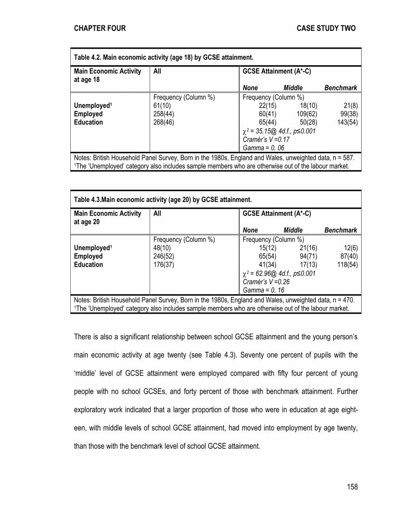
CHAPTER FOUR CASE STUDY TWO
158
Table 4.2. Main economic activity (age 18) by GCSE attainment.
Main Economic Activity at age 18
All GCSE Attainment (A*-C)
None Middle Benchmark
Frequency (Column %) Frequency (Column %) Unemployed1 61(10) 22(15) 18(10) 21(8) Employed 258(44) 60(41) 109(62) 99(38) Education 268(46) 65(44) 50(28) 143(54) 2 = 35.15@ 4d.f., p≤0.001
Cramér’s V =0.17 Gamma = 0. 06
Notes: British Household Panel Survey, Born in the 1980s, England and Wales, unweighted data, n = 587. 1The ‘Unemployed’ category also includes sample members who are otherwise out of the labour market.
Table 4.3.Main economic activity (age 20) by GCSE attainment.
Main Economic Activity at age 20
All GCSE Attainment (A*-C)
None Middle Benchmark
Frequency (Column %) Frequency (Column %) Unemployed1 48(10) 15(12) 21(16) 12(6) Employed 246(52) 65(54) 94(71) 87(40) Education 176(37) 41(34) 17(13) 118(54) 2 = 62.96@ 4d.f., p≤0.001
Cramér’s V =0.26 Gamma = 0. 16
Notes: British Household Panel Survey, Born in the 1980s, England and Wales, unweighted data, n = 470. 1The ‘Unemployed’ category also includes sample members who are otherwise out of the labour market.
There is also a significant relationship between school GCSE attainment and the young person’s
main economic activity at age twenty (see Table 4.3). Seventy one percent of pupils with the
‘middle’ level of GCSE attainment were employed compared with fifty four percent of young
people with no school GCSEs, and forty percent of those with benchmark attainment. Further
exploratory work indicated that a larger proportion of those who were in education at age eight-
een, with middle levels of school GCSE attainment, had moved into employment by age twenty,
than those with the benchmark level of school GCSE attainment.
CHAPTER FOUR CASE STUDY TWO
159
Taken together, these initial results indicate that having moderate, or ‘middle’, levels of school
GCSE attainment has distinct consequences for young people’s economic and educational activity
in early adulthood. The ‘middle’ group appear to be more likely to be in employment at age
eighteen and twenty than both the low attaining, and benchmark groups. The ‘middle’ group were
also less likely to be in education at age eighteen and twenty than both the low attaining, and
benchmark groups. Successful GCSE attainners (i.e. the ‘benchmark’ group) are likely to still be
engaged in higher education at age twenty. On the other hand, less educationally successful
young people (i.e. the ‘none’ group) may be attempting to catch up with their peers, or indeed
‘sheltering’ in education (Biggart et al., 1996). Although it may seem tempting to continue with
extended interpretation of the importance of the ‘missing middle’ as an analytical concept, in line
with the research question, it is first necessary to determine the extent to which the ‘middle’
represents a distinctive and substantively meaningful grouping.
4.4.5 Characterising ‘Middle’ Level GCSE Attainment (BHPS)
The analysis now turns to describing the characteristics of young people who attain ‘middle’ levels
of the school GCSE attainment. Bivariate relationships between the key explanatory factors and
school GCSE attainment are reported in Table 4.4. Overall, female pupils perform better than
males, and parental social class, parental education and housing tenure are all significant. In line
with previous research, young people from more advantaged backgrounds are more likely to
reach the ‘benchmark’ level of attainment, and are less likely to fail to gain any GCSEs at grades
A*-C (see Drew et al., 1992; Gayle et al., 2003; Gayle et al., 2009b).
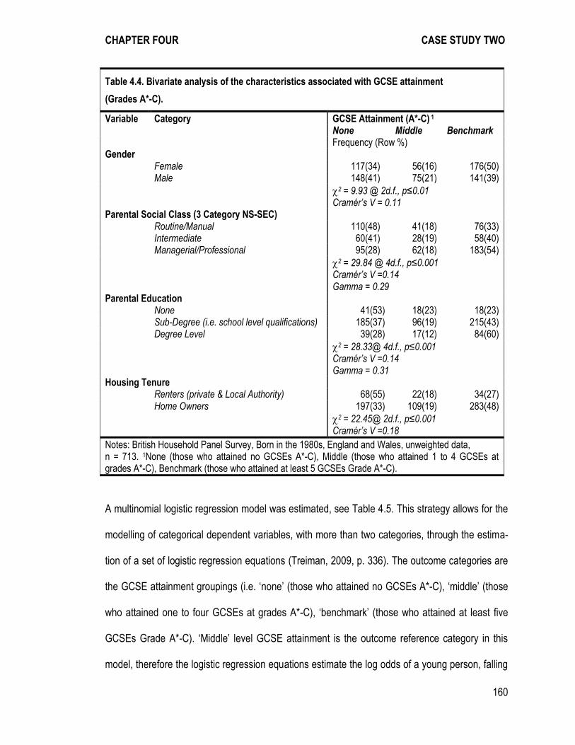
CHAPTER FOUR CASE STUDY TWO
160
Table 4.4. Bivariate analysis of the characteristics associated with GCSE attainment
(Grades A*-C).
Variable Category GCSE Attainment (A*-C) 1 None Middle Benchmark Frequency (Row %) Gender Female 117(34) 56(16) 176(50) Male 148(41) 75(21) 141(39) 2 = 9.93 @ 2d.f., p≤0.01
Cramér’s V = 0.11 Parental Social Class (3 Category NS-SEC) Routine/Manual 110(48) 41(18) 76(33) Intermediate 60(41) 28(19) 58(40) Managerial/Professional 95(28) 62(18) 183(54) 2 = 29.84 @ 4d.f., p≤0.001
Cramér’s V =0.14 Gamma = 0.29
Parental Education None 41(53) 18(23) 18(23) Sub-Degree (i.e. school level qualifications) 185(37) 96(19) 215(43) Degree Level 39(28) 17(12) 84(60) 2 = 28.33@ 4d.f., p≤0.001
Cramér’s V =0.14 Gamma = 0.31
Housing Tenure Renters (private & Local Authority) 68(55) 22(18) 34(27) Home Owners 197(33) 109(19) 283(48) 2 = 22.45@ 2d.f., p≤0.001
Cramér’s V =0.18
Notes: British Household Panel Survey, Born in the 1980s, England and Wales, unweighted data, n = 713. 1None (those who attained no GCSEs A*-C), Middle (those who attained 1 to 4 GCSEs at grades A*-C), Benchmark (those who attained at least 5 GCSEs Grade A*-C).
A multinomial logistic regression model was estimated, see Table 4.5. This strategy allows for the
modelling of categorical dependent variables, with more than two categories, through the estima-
tion of a set of logistic regression equations (Treiman, 2009, p. 336). The outcome categories are
the GCSE attainment groupings (i.e. ‘none’ (those who attained no GCSEs A*-C), ‘middle’ (those
who attained one to four GCSEs at grades A*-C), ‘benchmark’ (those who attained at least five
GCSEs Grade A*-C). ‘Middle’ level GCSE attainment is the outcome reference category in this
model, therefore the logistic regression equations estimate the log odds of a young person, falling
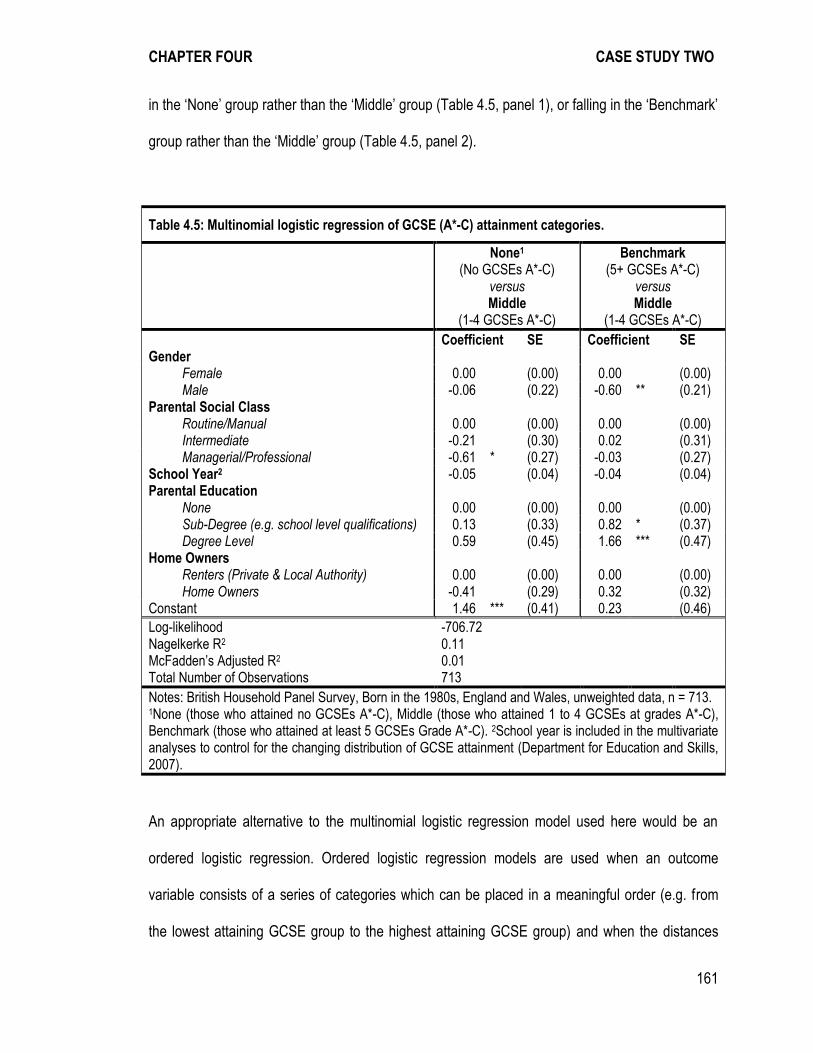
CHAPTER FOUR CASE STUDY TWO
161
in the ‘None’ group rather than the ‘Middle’ group (Table 4.5, panel 1), or falling in the ‘Benchmark’
group rather than the ‘Middle’ group (Table 4.5, panel 2).
Table 4.5: Multinomial logistic regression of GCSE (A*-C) attainment categories.
None1 (No GCSEs A*-C)
versus Middle
(1-4 GCSEs A*-C)
Benchmark (5+ GCSEs A*-C)
versus Middle
(1-4 GCSEs A*-C)
Coefficient SE Coefficient SE Gender Female 0.00 (0.00) 0.00 (0.00) Male -0.06 (0.22) -0.60 ** (0.21) Parental Social Class Routine/Manual 0.00 (0.00) 0.00 (0.00) Intermediate -0.21 (0.30) 0.02 (0.31) Managerial/Professional -0.61 * (0.27) -0.03 (0.27) School Year2 -0.05 (0.04) -0.04 (0.04) Parental Education None 0.00 (0.00) 0.00 (0.00) Sub-Degree (e.g. school level qualifications) 0.13 (0.33) 0.82 * (0.37) Degree Level 0.59 (0.45) 1.66 *** (0.47) Home Owners Renters (Private & Local Authority) 0.00 (0.00) 0.00 (0.00) Home Owners -0.41 (0.29) 0.32 (0.32) Constant 1.46 *** (0.41) 0.23 (0.46)
Log-likelihood -706.72 Nagelkerke R2 0.11 McFadden’s Adjusted R2 0.01 Total Number of Observations 713
Notes: British Household Panel Survey, Born in the 1980s, England and Wales, unweighted data, n = 713. 1None (those who attained no GCSEs A*-C), Middle (those who attained 1 to 4 GCSEs at grades A*-C), Benchmark (those who attained at least 5 GCSEs Grade A*-C). 2School year is included in the multivariate analyses to control for the changing distribution of GCSE attainment (Department for Education and Skills, 2007).
An appropriate alternative to the multinomial logistic regression model used here would be an
ordered logistic regression. Ordered logistic regression models are used when an outcome
variable consists of a series of categories which can be placed in a meaningful order (e.g. from
the lowest attaining GCSE group to the highest attaining GCSE group) and when the distances

CHAPTER FOUR CASE STUDY TWO
162
between these categories are arbitrary. The categories of the outcome variable in an ordered
logistic regression model are considered to represent a continuous latent variable which is
unobserved and the coefficients of the model indicate the extent of change in this latent variable
for a one unit change in the independent variable (Treiman, 2009, p. 342). However the ordered
logistic regression model does not identify specific differences between the categories of the
outcome variable. As the specific focus of this chapter is the investigation of the differences
between the ‘middle’ group and other groups, the multinomial logistic regression model is
considered more appropriate. This model assumes that the categories are not in a meaningful
order and therefore presents comparisons between between the categories of the outcome
variable. These comparisons allow us to specifically consider the differences between the ‘middle’
group and the ‘none’ and ‘benchmark’ categories.
Overall, the model indicates that there is no clear pattern that identifies ‘no GCSE’ school attain-
ment rather than ‘middle’ attainment (see Table 4.5, panel 1). Pupils with managerial/professional
parents are significantly less likely not to gain any GCSEs at grades A*-C. Again, no overwhelm-
ing pattern of associations identifies ‘benchmark’ group membership (i.e. five or more GCSEs at
grades A*-C), rather than ‘middle’ group membership (see Table 5.5, panel 2). There are both
gender and parental education effects relating to the attainment of the benchmark level rather
than the ‘middle’ category. Young males are significantly more likely to be in the ‘middle’ category.
Pupils with more educated parents are significantly more likely to achieve the GCSE benchmark
(e.g. Connolly, 2006a; Gayle et al., 2003). Nevertheless, a strong pattern fails to be detected in
the log odds of middle group membership, rather than membership of the less and more educa-
tionally successful groups.
CHAPTER FOUR CASE STUDY TWO
163
4.4.6 Further Exploring the ‘Middle’ (BHPS)
The multinomial regression model fails to identify a definitive pattern of membership of the ‘middle’
category based on the young person’s characteristics. Therefore, the ‘middle’ group categorisation
needs to be further investigated, in order to identify if a distinct ‘middle’ group of young people
exists. The benchmark of five or more GCSEs at grades A*-C is widely recognised, but it is largely
an administrative measure. In order to operationalise the ‘middle’ in these analyses the attainment
of one to four GCSEs at grades A*-C was selected as indicative of ‘middle’ level attainment. This
is a defensible measure of ‘middle’ attainment, and it indicates that a pupil is neither unqualified
nor well qualified. Nevertheless, to fully address the research question the consideration of
additional operationalisations is required to further test this concept.
Various analyses have demonstrated that school GCSE attainment is central to participation in
post-compulsory education (e.g. Babb, 2005; Drew et al., 1992; Gayle et al., 2000; Gayle et al.,
2003; Jones et al., 2003; Murray, 2011; Rice, 1999). Therefore, a series of logistic regression
models, with the outcome measure being participation in education at age 17, compared to all
other activities, were estimated. An overall goodness of fit measure for each model is reported in
Table 4.6. This exercise leads to the conclusion that the operationalisation of a ‘middle’ category
of one to four GCSEs at grades A*-C performs relatively well. Alternative measures that include
pupils with either five or six GCSEs at grades A*-C do not have increased explanatory power.
There is a very slight increase in the adjusted R2 value when the middle category is extended to
include pupils with seven GCSEs at grades A*-C. However, this level of attainment is considered
too high to reasonably constitute a ‘middle’ or moderate level of attainment.
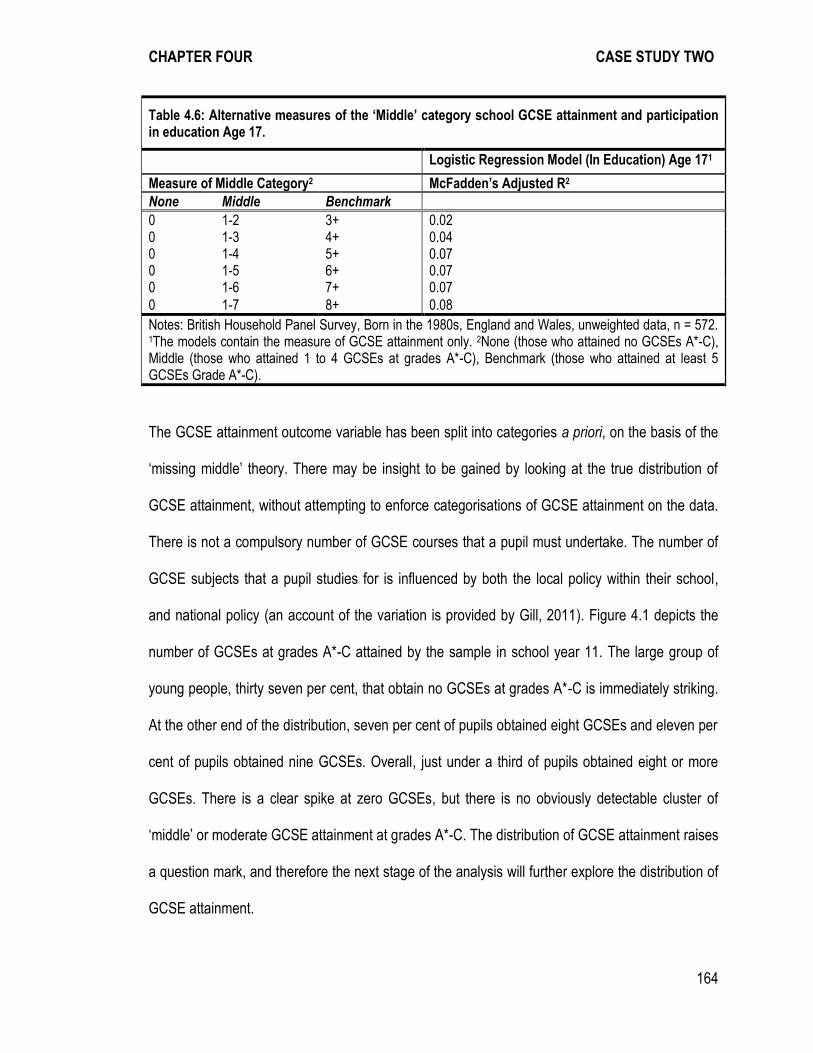
CHAPTER FOUR CASE STUDY TWO
164
Table 4.6: Alternative measures of the ‘Middle’ category school GCSE attainment and participation in education Age 17.
Logistic Regression Model (In Education) Age 171
Measure of Middle Category2 McFadden’s Adjusted R2
None Middle Benchmark
0 1-2 3+ 0.02 0 1-3 4+ 0.04 0 1-4 5+ 0.07 0 1-5 6+ 0.07 0 1-6 7+ 0.07
0 1-7 8+ 0.08
Notes: British Household Panel Survey, Born in the 1980s, England and Wales, unweighted data, n = 572. 1The models contain the measure of GCSE attainment only. 2None (those who attained no GCSEs A*-C), Middle (those who attained 1 to 4 GCSEs at grades A*-C), Benchmark (those who attained at least 5 GCSEs Grade A*-C).
The GCSE attainment outcome variable has been split into categories a priori, on the basis of the
‘missing middle’ theory. There may be insight to be gained by looking at the true distribution of
GCSE attainment, without attempting to enforce categorisations of GCSE attainment on the data.
There is not a compulsory number of GCSE courses that a pupil must undertake. The number of
GCSE subjects that a pupil studies for is influenced by both the local policy within their school,
and national policy (an account of the variation is provided by Gill, 2011). Figure 4.1 depicts the
number of GCSEs at grades A*-C attained by the sample in school year 11. The large group of
young people, thirty seven per cent, that obtain no GCSEs at grades A*-C is immediately striking.
At the other end of the distribution, seven per cent of pupils obtained eight GCSEs and eleven per
cent of pupils obtained nine GCSEs. Overall, just under a third of pupils obtained eight or more
GCSEs. There is a clear spike at zero GCSEs, but there is no obviously detectable cluster of
‘middle’ or moderate GCSE attainment at grades A*-C. The distribution of GCSE attainment raises
a question mark, and therefore the next stage of the analysis will further explore the distribution of
GCSE attainment.
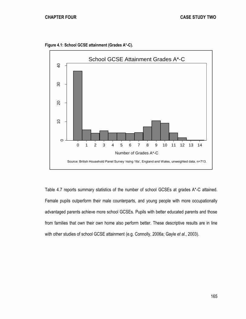
CHAPTER FOUR CASE STUDY TWO
165
Figure 4.1: School GCSE attainment (Grades A*-C).
Table 4.7 reports summary statistics of the number of school GCSEs at grades A*-C attained.
Female pupils outperform their male counterparts, and young people with more occupationally
advantaged parents achieve more school GCSEs. Pupils with better educated parents and those
from families that own their own home also perform better. These descriptive results are in line
with other studies of school GCSE attainment (e.g. Connolly, 2006a; Gayle et al., 2003).
010
20
30
40
Perc
ent
0 1 2 3 4 5 6 7 8 9 10 11 12 13 14
Number of Grades A*-C
Source: British Household Panel Survey ‘rising 16s’, England and Wales, unweighted data, n=713.
School GCSE Attainment Grades A*-C
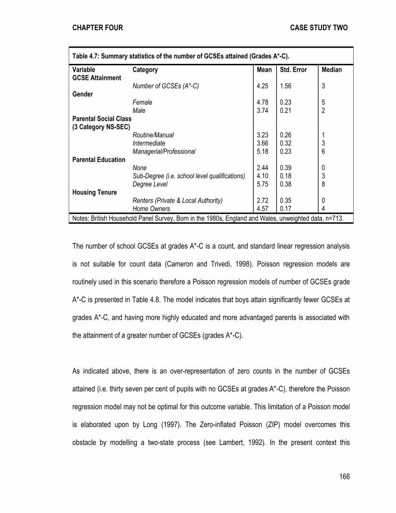
CHAPTER FOUR CASE STUDY TWO
166
Table 4.7: Summary statistics of the number of GCSEs attained (Grades A*-C).
Variable Category Mean Std. Error Median GCSE Attainment Number of GCSEs (A*-C) 4.25 1.56 3 Gender Female 4.78 0.23 5 Male 3.74 0.21 2 Parental Social Class (3 Category NS-SEC)
Routine/Manual 3.23 0.26 1 Intermediate 3.66 0.32 3 Managerial/Professional 5.18 0.23 6 Parental Education None 2.44 0.39 0 Sub-Degree (i.e. school level qualifications) 4.10 0.18 3 Degree Level 5.75 0.38 8 Housing Tenure Renters (Private & Local Authority) 2.72 0.35 0 Home Owners 4.57 0.17 4
Notes: British Household Panel Survey, Born in the 1980s, England and Wales, unweighted data, n=713.
The number of school GCSEs at grades A*-C is a count, and standard linear regression analysis
is not suitable for count data (Cameron and Trivedi, 1998). Poisson regression models are
routinely used in this scenario therefore a Poisson regression models of number of GCSEs grade
A*-C is presented in Table 4.8. The model indicates that boys attain significantly fewer GCSEs at
grades A*-C, and having more highly educated and more advantaged parents is associated with
the attainment of a greater number of GCSEs (grades A*-C).
As indicated above, there is an over-representation of zero counts in the number of GCSEs
attained (i.e. thirty seven per cent of pupils with no GCSEs at grades A*-C), therefore the Poisson
regression model may not be optimal for this outcome variable. This limitation of a Poisson model
is elaborated upon by Long (1997). The Zero-inflated Poisson (ZIP) model overcomes this
obstacle by modelling a two-state process (see Lambert, 1992). In the present context this
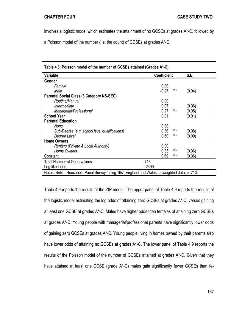
CHAPTER FOUR CASE STUDY TWO
167
involves a logistic model which estimates the attainment of no GCSEs at grades A*-C, followed by
a Poisson model of the number (i.e. the count) of GCSEs at grades A*-C.
Table 4.8: Poisson model of the number of GCSEs attained (Grades A*-C).
Variable Coefficient S.E.
Gender Female 0.00 Male -0.27 *** (0.04) Parental Social Class (3 Category NS-SEC) Routine/Manual 0.00 Intermediate 0.07 (0.06) Managerial/Professional 0.27 *** (0.05) School Year 0.01 (0.01) Parental Education None 0.00 Sub-Degree (e.g. school level qualifications) 0.36 *** (0.08) Degree Level 0.60 *** (0.09) Home Owners Renters (Private & Local Authority) 0.00 Home Owners 0.35 *** (0.06) Constant 0.69 *** (0.06)
Total Number of Observations 713 Log-likelihood -2490
Notes: British Household Panel Survey ‘rising 16s’, England and Wales, unweighted data, n=713.
Table 4.9 reports the results of the ZIP model. The upper panel of Table 4.9 reports the results of
the logistic model estimating the log odds of attaining zero GCSEs at grades A*-C, versus gaining
at least one GCSE at grades A*-C. Males have higher odds than females of attaining zero GCSEs
at grades A*-C. Young people with managerial/professional parents have significantly lower odds
of gaining zero GCSEs at grades A*-C. Young people living in homes owned by their parents also
have lower odds of attaining no GCSEs at grades A*-C. The lower panel of Table 4.9 reports the
results of the Poisson model of the number of GCSEs attained at grades A*-C. Given that they
have attained at least one GCSE (grade A*-C) males gain significantly fewer GCSEs than fe-
CHAPTER FOUR CASE STUDY TWO
168
males. Parental education levels are significant. Pupils with more educated parents gain more
GCSEs at grades A*-C.
The message emerging from the model is that the predictors are not common across the two
stages. There is clearly a group of young people that do not gain any GCSEs (at grades A*-C) and
this group is less likely to be female or from a more advantaged family. The second group attain
some GCSEs at grades A*-C and their school GCSE attainment is better understood as a lying
along a continuum. Females in this group perform better than males and higher levels of parental
education are also positively influential.
The relative explanatory power of alternative measures of school GCSE attainment is considered
next (see Figure 4.2). The focus on relative explanatory power of alternative measures of GCSE
attainment in logistic regression models of participation in education at age twenty are considered.
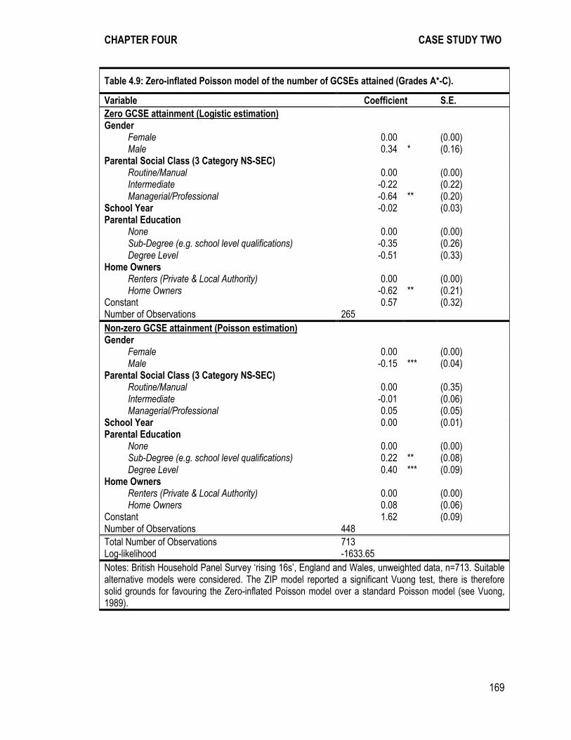
CHAPTER FOUR CASE STUDY TWO
169
Table 4.9: Zero-inflated Poisson model of the number of GCSEs attained (Grades A*-C).
Variable Coefficient S.E.
Zero GCSE attainment (Logistic estimation) Gender Female 0.00 (0.00) Male 0.34 * (0.16) Parental Social Class (3 Category NS-SEC) Routine/Manual 0.00 (0.00) Intermediate -0.22 (0.22) Managerial/Professional -0.64 ** (0.20) School Year -0.02 (0.03) Parental Education None 0.00 (0.00) Sub-Degree (e.g. school level qualifications) -0.35 (0.26) Degree Level -0.51 (0.33) Home Owners Renters (Private & Local Authority) 0.00 (0.00) Home Owners -0.62 ** (0.21) Constant 0.57 (0.32) Number of Observations 265*
Non-zero GCSE attainment (Poisson estimation) Gender Female 0.00 (0.00) Male -0.15 *** (0.04) Parental Social Class (3 Category NS-SEC) Routine/Manual 0.00 (0.35) Intermediate -0.01 (0.06) Managerial/Professional 0.05 (0.05) School Year 0.00 (0.01) Parental Education None 0.00 (0.00) Sub-Degree (e.g. school level qualifications) 0.22 ** (0.08) Degree Level 0.40 *** (0.09) Home Owners Renters (Private & Local Authority) 0.00 (0.00) Home Owners 0.08 (0.06) Constant 1.62 (0.09) Number of Observations 448
Total Number of Observations 713 Log-likelihood -1633.65
Notes: British Household Panel Survey ‘rising 16s’, England and Wales, unweighted data, n=713. Suitable alternative models were considered. The ZIP model reported a significant Vuong test, there is therefore solid grounds for favouring the Zero-inflated Poisson model over a standard Poisson model (see Vuong, 1989).

CHAPTER FOUR CASE STUDY TWO
170
Figure 4.2 reports the adjusted R2 values for four measures of GCSE attainment, and a Bayesian
Information Criterion statistic (BIC) as a measure of goodness of fit which also reflects model
parsimony (see Raftery, 1995). Model A includes a crude binary measure of attainment (any
GCSEs at grades A*-C). Model B uses the familiar benchmark of five or more GCSEs at grades
A*-C and is an improvement on Model A. Model C includes a middle category of 1-4 GCSEs at
grades A*-C, it offers no improvement in explanatory power and is less parsimonious than Model
B. Model D includes the count of GCSEs at grades A*-C, it has increased explanatory power and
is more parsimonious than the three previous models. This result is further encouragement that
the number of GCSEs at grades A*-C should be preferred in many analyses.
Figure 4.2: The explanatory power of GCSE attainment measures in logistic regression models of participation in education at age 20.
-23
20
-23
10
-23
00
-22
90
-22
80
-22
70
BIC
(S
olid
Tria
ng
les)
.02
.04
.06
.08
.1
McF
ad
de
n’s
Ad
juste
d R
2 (
Ho
llow
Cir
cle
s)
A B C DModel
Model A: 0, 1+ GCSEs A*-C (2 Category)Model B: 0-4, 5+ GCSEs A*-C (2 Category)Model C: 0, 1-4, 5+ GCSEs A*-C (3 Category)Model D: Number of GCSEs A*-C (Continuous) Note: British Household Panel Survey ‘rising 16s’, England and Wales, unweighted data, n=470.
GCSE Attainment MeasuresIn Education Age 20
CHAPTER FOUR CASE STUDY TWO
171
4.5 Exploring the ‘Middle’ with the Youth Cohort Study of England and Wales
The British Household Panel Survey provides a sample of young people who have completed
GCSE examinations and can be followed into their early twenties. However, the BHPS is not a
specialised youth dataset and therefore the sample of relevant respondents in the BHPS is small
and restricted (Murray, 2011). The representativeness of the relevant BHPS sample may therefore
be sub-optimal. The BHPS sample does not provide sufficient analytic power to examine the
influence of ethnicity, which is described above as an important stratifying concept in GCSE
attainment (see Bhattacharyya et al., 2003; Drew, 1995; Drew et al., 1990; Drew et al., 1992;
Rothon, 2007).
To ensure the generalisability of the findings of this chapter, the concept of the ‘missing middle’ is
also examined using a large-scale nationally representative specialised youth dataset, the Youth
Cohort Study of England and Wales (YCS). The YCS dataset does not provide the ‘long-run’
insight into the transitions of young people, seen above in the BHPS, which followed young people
into their twenties and continues to follow the sample members who have been subsumed into the
United Kingdom Household Longitudinal Survey. The YCS represents a ‘short panel’ of data
collection, with many cohorts followed for around three years each. However, the YCS provides a
suitable resource to augment the BHPS analyses. Furthermore, the multiple cohort structure of
YCS, described in more detail below, allows for a superior assessment of the changes in the
nature of ‘missing middle’ over a period of time.
CHAPTER FOUR CASE STUDY TWO
172
4.5.1 The Youth Cohort Study of England and Wales
The Youth Cohort Study of England and Wales (YCS) is a specialist youth dataset which has
been successfully used to explore educational attainment (Connolly, 2006a; Demack et al., 2000;
Drew, 1995; Drew et al., 1992; Gayle et al., 2003; Gayle et al., 2009b; Sullivan et al., 2011). The
YCS is a major longitudinal study that began in the mid-1980s, and was designed to monitor the
activities of young people as they reach the minimum school leaving age and make transitions into
further education, employment or otherwise (BMRB Social Research, 2008). The young person is
first surveyed about six months after they complete year eleven of school (i.e. at age sixteen to
seventeen), with follow-up sweeps taking place on at least two subsequent occasions30 (Croxford,
2005). Data have been collected for a number of cohorts of young people as they reach the end of
compulsory schooling, therefore the YCS provides the opportunity to undertake cross-cohort
comparisons (Croxford, 2006).
The YCS can be a challenging dataset to work with, the survey has been collected by a number of
different organisations and changes to question wording, measurement techniques and coding
over the years have lead to questionable parity of esteem between cohorts. Additionally, the
standard of data documentation for the YCS is also considered to be of poor quality, which
impedes the research process (Croxford, 2006).
To overcome these difficulties, the analyses in this chapter make use of a harmonised dataset
comprising of YCS cohorts from 1984 to 2002, developed by Croxford et al. (2005). To provide a
clear sample this chapter utilises only the cohorts of young people who reached the compulsory
30 Each cohort was re-visited for at least two (e.g. the 1994 cohort), sometimes three (e.g. the 1991 cohort) or four sweeps (e.g. the 2009 cohort). The follow up sweeps generally take place annually, although there are exceptions. This varying structure and poor data documentation adds additional complexity to the data.
CHAPTER FOUR CASE STUDY TWO
173
school leaving age in 1990, 1993, 1995, 1997 and 1999 respectively. The earlier YCS cohorts
were too young to have undertaken GCSE examinations, and these cohorts also lacked sufficient
parental occupational information to operationalise their social class positions and therefore they
are excluded from the analytic sample. The analytic sample is also based only on those young
people who attended state secondary schools in England and Wales. Since 1990, the YCS
employs a single-stage random sample. The sample is comprised of young people in year eleven
of all state and private secondary schools in England and Wales, whose birthdays fall on a
selection of dates. This sampling strategy is designed to give a random sample of year eleven
pupils. However, there is a large degree of survey non-response in the YCS, therefore weighting
is used to compensate for non-response bias (Croxford et al., 2005). The harmonised dataset
provides three weighting variables for individuals in each cohort, which are used to weight
outcome variables at each of the three sweeps.
4.5.2 Structure of Analysis (YCS)
The YCS analyses replicate and extend the considerations made using the BHPS. The analysis
begins by looking at the consequences of ‘middle’ level GCSE attainment in relation to economic
activities at age 16-17 and 18-19. Then bivariate statistics, and a multinomial logistic regression
model is utilised to evaluate the social characteristics of the ‘middle’ group. The structure of the
YCS data also provides the opportunity to consider the possibility of an increasing ‘middle’ group
of young people over time.
Moving to the evaluation of the ‘middle’ concept, alternative formulations of the ‘middle’ are again
considered. The nature of the distribution of GCSE attainment is considered using the number of
CHAPTER FOUR CASE STUDY TWO
174
GCSEs grade A*-C attained, as well as a points score of GCSE attainment. A stereotype regres-
sion model considers the ordinal nature of the distribution of GCSE attainment, and a Zero-inflated
Poisson explores the social characteristics which determine GCSE attainment. Finally, a linear
regression model is used to evaluate GCSE point score attainment.
4.5.3 Explanatory Variables (YCS)
In characterising the ‘middle’, the analysis of the YCS focuses on a set of established explanatory
variables that have been implicated in previous studies of GCSE attainment, and youth outcomes
more widely (for example Connolly, 2006a; Demack et al., 2000; Drew, 1995; Drew et al., 1992;
Gayle et al., 2003; Gayle et al., 2009b; Sullivan et al., 2011). In comparison to the BHPS analy-
ses, above, the larger sample size of the YCS data facilitates the analysis of additional variables
(e.g. ethnicity). The characteristics of the YCS sample are reported in Table 4.10. The Summary
information for the three category school GCSE attainment measure is provided in Table 4.11.
The YCS survey (weighted) proportions are in line with national figures for the benchmark of 5+
GCSEs at grades A*-C for the time period (see Department for Children, 2009).
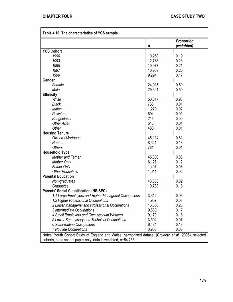
CHAPTER FOUR CASE STUDY TWO
175
Table 4.10: The characteristics of YCS sample.
n
Proportion (weighted)
YCS Cohort 1990 10,268 0.19
1993 12,788 0.23 1995 10,977 0.21 1997 10,909 0.20 1999 9,294 0.17 Gender
Female 24,915 0.50 Male 29,321 0.50 Ethnicity
White 50,317 0.93 Black 738 0.01 Indian 1,279 0.02 Pakistani 694 0.01 Bangladeshi 215 0.00 Other Asian 513 0.01 Other 480 0.01 Housing Tenure
Owned / Mortgage 45,114 0.81 Renters 8,341 0.18 Others 781 0.01 Household Type
Mother and Father 45,600 0.83 Mother Only 6,128 0.12 Father Only 1,497 0.03 Other Household 1,011 0.02 Parental Education
Non-graduates 43,503 0.82 Graduates 10,733 0.18 Parents' Social Classification (NS-SEC) 1.1 Large Employers and Higher Managerial Occupations 3,312 0.06 1.2 Higher Professional Occupations 4,957 0.08 2 Lower Managerial and Professional Occupations 13,306 0.23 3 Intermediate Occupations 9,560 0.17 4 Small Employers and Own Account Workers 9,170 0.18 5 Lower Supervisory and Technical Occupations 3,594 0.07 6 Semi-routine Occupations 6,434 0.13 7 Routine Occupations 3,903 0.08
Notes: Youth Cohort Study of England and Wales, harmonised dataset (Croxford et al., 2005), selected cohorts, state school pupils only, data is weighted, n=54,236.
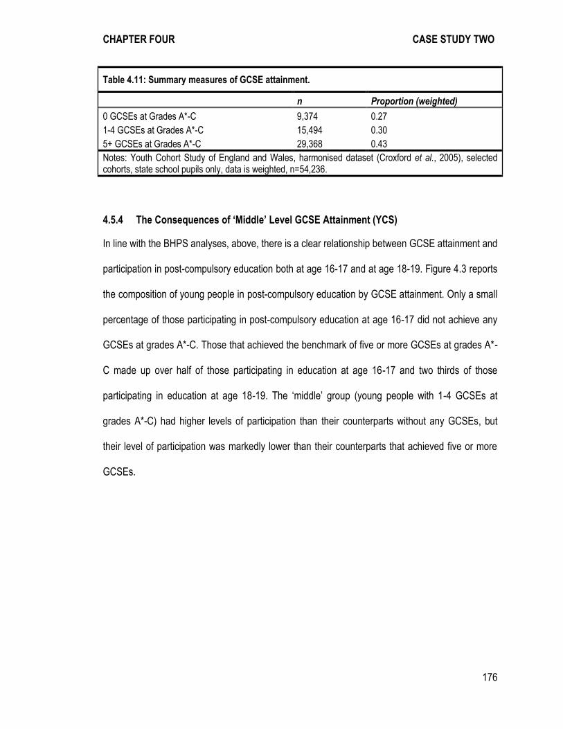
CHAPTER FOUR CASE STUDY TWO
176
Table 4.11: Summary measures of GCSE attainment.
n Proportion (weighted)
0 GCSEs at Grades A*-C 9,374 0.27
1-4 GCSEs at Grades A*-C 15,494 0.30
5+ GCSEs at Grades A*-C 29,368 0.43
Notes: Youth Cohort Study of England and Wales, harmonised dataset (Croxford et al., 2005), selected cohorts, state school pupils only, data is weighted, n=54,236.
4.5.4 The Consequences of ‘Middle’ Level GCSE Attainment (YCS)
In line with the BHPS analyses, above, there is a clear relationship between GCSE attainment and
participation in post-compulsory education both at age 16-17 and at age 18-19. Figure 4.3 reports
the composition of young people in post-compulsory education by GCSE attainment. Only a small
percentage of those participating in post-compulsory education at age 16-17 did not achieve any
GCSEs at grades A*-C. Those that achieved the benchmark of five or more GCSEs at grades A*-
C made up over half of those participating in education at age 16-17 and two thirds of those
participating in education at age 18-19. The ‘middle’ group (young people with 1-4 GCSEs at
grades A*-C) had higher levels of participation than their counterparts without any GCSEs, but
their level of participation was markedly lower than their counterparts that achieved five or more
GCSEs.
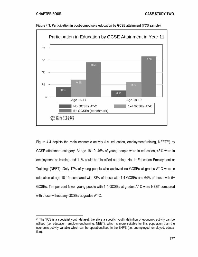
CHAPTER FOUR CASE STUDY TWO
177
Figure 4.3: Participation in post-compulsory education by GCSE attainment (YCS sample).
Figure 4.4 depicts the main economic activity (i.e. education, employment/training, NEET31) by
GCSE attainment category. At age 18-19, 46% of young people were in education, 43% were in
employment or training and 11% could be classified as being ‘Not in Education Employment or
Training’ (NEET). Only 17% of young people who achieved no GCSEs at grades A*-C were in
education at age 18-19, compared with 33% of those with 1-4 GCSEs and 64% of those with 5+
GCSEs. Ten per cent fewer young people with 1-4 GCSEs at grades A*-C were NEET compared
with those without any GCSEs at grades A*-C.
31 The YCS is a specialist youth dataset, therefore a specific ‘youth’ definition of economic activity can be utilised (i.e. education, employment/training, NEET), which is more suitable for this population than the economic activity variable which can be operationalised in the BHPS (i.e. unemployed, employed, educa-tion).
0.16
0.28
0.56
0.10
0.24
0.66
0.2
.4.6
.8
Pro
port
ion (
surv
ey w
eig
hte
d)
Age 16-17 Age 18-19
Age 16-17 n=54,236Age 18-19 n=29,033
Participation in Education by GCSE Attainment in Year 11
No GCSEs A*-C 1-4 GCSEs A*-C
5+ GCSEs (benchmark)

CHAPTER FOUR CASE STUDY TWO
178
Figure 4.4: Main activity age 18-19 by GCSE attainment (YCS sample).
Unlike the BHPS results, there is no evidence from the YCS data of increased educational
participation for the lowest achieving GCSE group (i.e. see Table 4.2 and Table 4.3). The differ-
ence in the pattern of results may be accounted for by the small BHPS sample size leading to
distortion. A suitable degree of caution was placed on the initial BHPS analyses, regarding the
consequences of ‘Middle’ GCSE attainment, as the results may have been a consequence of the
manner in which the outcome variable (GCSE attainment) was categorised. The more powerful
YCS sample may be better placed to assess the utility of the ‘missing middle’ concept, and
certainly highlights that there is not a distinct pattern of post-compulsory education participation,
for the ‘middle’ group. The ‘middle’ groups’ level of participation in education and employ-
ment/training, and their propensity to be NEET at age 18-19, does not demonstrate any notable
distinct pattern. The participation of the 'middle’ is placed systematically between their more and
0.64 0.30 0.07
0.33 0.56 0.12
0.17 0.61 0.22
0.46 0.43 0.11
0 .2 .4 .6 .8 1Proportion (survey weighted)
5+ GCSEs
1-4 GCSEs
No GCSEs
Overall
n=29,033
by GCSE Attainment in Year 11
Main Activity Age 18-19
Education Employment/Training
NEET
CHAPTER FOUR CASE STUDY TWO
179
less educationally successful peers (i.e. somewhat more likely to be NEET and less likely to be in
education than the ‘benchmark’ group, and somewhat less likely to be NEET and more likely to be
education than the ‘none’ group).
4.5.5 Characterising ‘Middle’ Level GCSE Attainment (YCS)
Table 4.12 outlines the exploratory (bivariate) relationships between the outcome variable i.e. the
three category GCSE measure, and each of the explanatory variables. All of the relationships are
significant (p<.05). Overall, Table 4.12 indicates that ‘middle’ levels of GCSE attainment are
stratified by gender, ethnicity, housing tenure, household composition, parental education and
family socioeconomic classification. Females outperformed males in relation to achieving the
benchmark of 5+ GCSEs at grades A*-C, although about the same proportion of males and
females fell into the ‘middle’ category. Thirty per cent of white young people were in the middle
category. The same proportion of young people of Indian origin achieved the middle level of
GCSE attainment, but a lower proportion of those classified as other Asians were in this category.
Conversely a higher proportion of young people from black, Pakistani, Bangladeshi and other
minority ethnic backgrounds were in the ‘Middle’ category. There were some GCSE attainment
differences between young people from families with different housing tenure and of different
household compositions. A larger proportion of young people with more qualified parents achieved
the benchmark of 5+ GCSEs at grades A*-C, and ten per cent fewer achieved 1-4 A*-C grades.
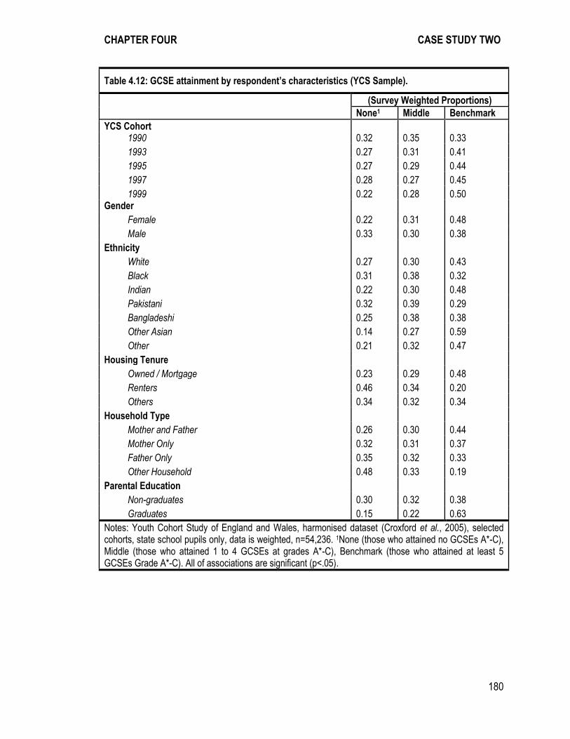
CHAPTER FOUR CASE STUDY TWO
180
Table 4.12: GCSE attainment by respondent’s characteristics (YCS Sample).
(Survey Weighted Proportions)
None1 Middle Benchmark
YCS Cohort 1990 0.32 0.35 0.33
1993 0.27 0.31 0.41
1995 0.27 0.29 0.44
1997 0.28 0.27 0.45
1999 0.22 0.28 0.50 Gender
Female 0.22 0.31 0.48
Male 0.33 0.30 0.38
Ethnicity White 0.27 0.30 0.43
Black 0.31 0.38 0.32
Indian 0.22 0.30 0.48
Pakistani 0.32 0.39 0.29
Bangladeshi 0.25 0.38 0.38
Other Asian 0.14 0.27 0.59
Other 0.21 0.32 0.47
Housing Tenure Owned / Mortgage 0.23 0.29 0.48
Renters 0.46 0.34 0.20
Others 0.34 0.32 0.34
Household Type Mother and Father 0.26 0.30 0.44
Mother Only 0.32 0.31 0.37
Father Only 0.35 0.32 0.33
Other Household 0.48 0.33 0.19
Parental Education Non-graduates 0.30 0.32 0.38
Graduates 0.15 0.22 0.63
Notes: Youth Cohort Study of England and Wales, harmonised dataset (Croxford et al., 2005), selected cohorts, state school pupils only, data is weighted, n=54,236. 1None (those who attained no GCSEs A*-C), Middle (those who attained 1 to 4 GCSEs at grades A*-C), Benchmark (those who attained at least 5 GCSEs Grade A*-C). All of associations are significant (p<.05).
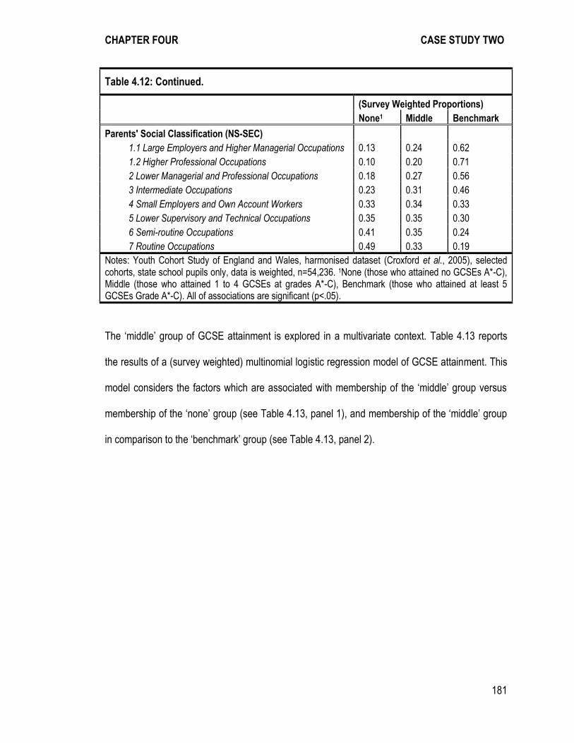
CHAPTER FOUR CASE STUDY TWO
181
Table 4.12: Continued.
(Survey Weighted Proportions)
None1 Middle Benchmark
Parents' Social Classification (NS-SEC) 1.1 Large Employers and Higher Managerial Occupations 0.13 0.24 0.62
1.2 Higher Professional Occupations 0.10 0.20 0.71
2 Lower Managerial and Professional Occupations 0.18 0.27 0.56
3 Intermediate Occupations 0.23 0.31 0.46
4 Small Employers and Own Account Workers 0.33 0.34 0.33
5 Lower Supervisory and Technical Occupations 0.35 0.35 0.30
6 Semi-routine Occupations 0.41 0.35 0.24
7 Routine Occupations 0.49 0.33 0.19
Notes: Youth Cohort Study of England and Wales, harmonised dataset (Croxford et al., 2005), selected cohorts, state school pupils only, data is weighted, n=54,236. 1None (those who attained no GCSEs A*-C), Middle (those who attained 1 to 4 GCSEs at grades A*-C), Benchmark (those who attained at least 5 GCSEs Grade A*-C). All of associations are significant (p<.05).
The ‘middle’ group of GCSE attainment is explored in a multivariate context. Table 4.13 reports
the results of a (survey weighted) multinomial logistic regression model of GCSE attainment. This
model considers the factors which are associated with membership of the ‘middle’ group versus
membership of the ‘none’ group (see Table 4.13, panel 1), and membership of the ‘middle’ group
in comparison to the ‘benchmark’ group (see Table 4.13, panel 2).
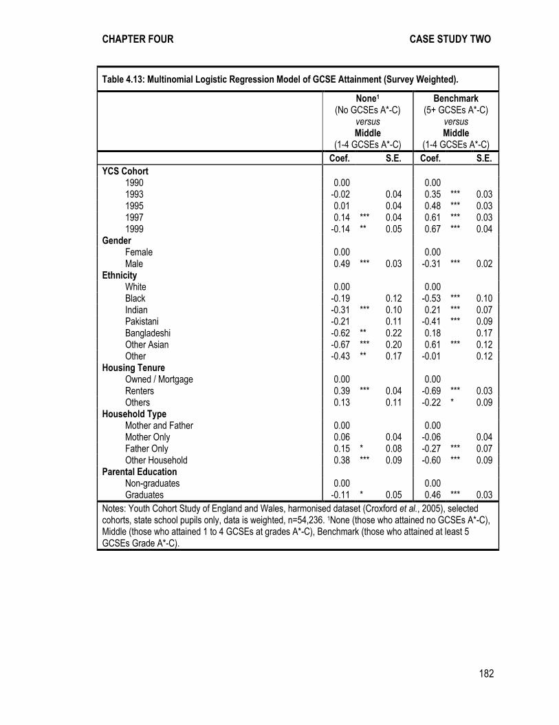
CHAPTER FOUR CASE STUDY TWO
182
Table 4.13: Multinomial Logistic Regression Model of GCSE Attainment (Survey Weighted).
None1 (No GCSEs A*-C)
versus Middle
(1-4 GCSEs A*-C)
Benchmark (5+ GCSEs A*-C)
versus Middle
(1-4 GCSEs A*-C)
Coef. S.E. Coef.
S.E.
YCS Cohort
1990 0.00
0.00 1993 -0.02 0.04 0.35 *** 0.03
1995 0.01 0.04 0.48 *** 0.03 1997 0.14 *** 0.04 0.61 *** 0.03 1999 -0.14 ** 0.05 0.67 *** 0.04 Gender
Female 0.00
0.00 Male 0.49 *** 0.03 -0.31 *** 0.02
Ethnicity
White 0.00
0.00 Black -0.19 0.12 -0.53 *** 0.10
Indian -0.31 *** 0.10 0.21 *** 0.07 Pakistani -0.21 0.11 -0.41 *** 0.09 Bangladeshi -0.62 ** 0.22 0.18
0.17
Other Asian -0.67 *** 0.20 0.61 *** 0.12 Other -0.43 ** 0.17 -0.01
0.12
Housing Tenure
Owned / Mortgage 0.00
0.00 Renters 0.39 *** 0.04 -0.69 *** 0.03
Others 0.13 0.11 -0.22 * 0.09 Household Type
Mother and Father 0.00
0.00 Mother Only 0.06 0.04 -0.06
0.04 Father Only 0.15 * 0.08 -0.27 *** 0.07 Other Household 0.38 *** 0.09 -0.60 *** 0.09 Parental Education
Non-graduates 0.00
0.00 Graduates -0.11 * 0.05 0.46 *** 0.03
Notes: Youth Cohort Study of England and Wales, harmonised dataset (Croxford et al., 2005), selected cohorts, state school pupils only, data is weighted, n=54,236. 1None (those who attained no GCSEs A*-C), Middle (those who attained 1 to 4 GCSEs at grades A*-C), Benchmark (those who attained at least 5 GCSEs Grade A*-C).

CHAPTER FOUR CASE STUDY TWO
183
Table 4.13: Continued.
None1 (No GCSEs A*-C)
versus Middle
(1-4 GCSEs A*-C)
Benchmark (5+ GCSEs A*-C)
versus Middle
(1-4 GCSEs A*-C)
Coef. S.E. Coef.
S.E.
Parents' Social Classification (NS-SEC)
1.1 Large Employers and Higher Managerial
Occupations -0.24 * 0.09 0.40 *** 0.05
1.2 Higher Professional Occupations -0.35 *** 0.09 0.64 *** 0.05
2 Lower Managerial and Professional Occupations -0.09 0.05 0.25 *** 0.03
3 Intermediate Occupations 0.00
0.00
4 Small Employers and Own Account Workers 0.26 *** 0.05 -0.41 *** 0.04 5 Lower Supervisory and Technical Occupations 0.29 *** 0.06 -0.48 *** 0.05 6 Semi-routine Occupations 0.41 *** 0.05 -0.66 *** 0.04 7 Routine Occupations 0.61 *** 0.05 -0.75 *** 0.05 Constant -0.64 *** 0.05 0.17 *** 0.03
Log likelihood (unweighted model) -49001 Pseudo R Squared (unweighted model) 0.09 BIC (unweighted model) 98547
Notes: Youth Cohort Study of England and Wales, harmonised dataset (Croxford et al., 2005), selected cohorts, state school pupils only, data is weighted, n=54,236. 1None (those who attained no GCSEs A*-C), Middle (those who attained 1 to 4 GCSEs at grades A*-C), Benchmark (those who attained at least 5 GCSEs Grade A*-C).
Table 4.14: Model estimation information for Multinomial Logistic Regression Models of GCSE
Attainment (Unweighted Models).
BIC Statistic Change in Deviance Change in d.f.
Null 107788 Null + YCS Cohort 106531 1344 8 Null + Gender 107353 457 2 Null + Ethnicity 107730 188 12 Null + Housing Tenure 104947 2885 4 Null + Household Type 107272 581 6 Null + Parental Education 105691 2118 2 Null + Parents’ Social Classification (NS-SEC) 102033 5907 14
Notes: Youth Cohort Study of England and Wales, harmonised dataset (Croxford et al., 2005), selected cohorts, state school pupils only, n=54,236. 1Outcome: None (those who attained no GCSEs A*-C), Middle (those who attained 1 to 4 GCSEs at grades A*-C), Benchmark (those who attained at least 5 GCSEs Grade A*-C).
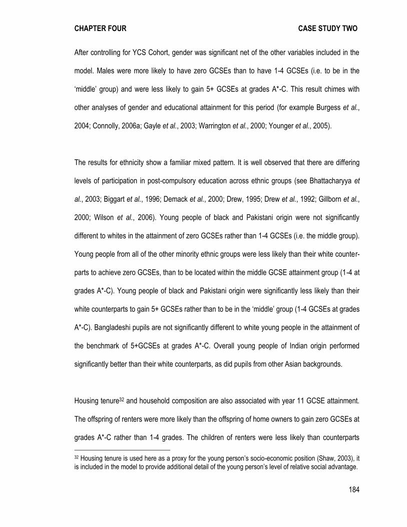
CHAPTER FOUR CASE STUDY TWO
184
After controlling for YCS Cohort, gender was significant net of the other variables included in the
model. Males were more likely to have zero GCSEs than to have 1-4 GCSEs (i.e. to be in the
‘middle’ group) and were less likely to gain 5+ GCSEs at grades A*-C. This result chimes with
other analyses of gender and educational attainment for this period (for example Burgess et al.,
2004; Connolly, 2006a; Gayle et al., 2003; Warrington et al., 2000; Younger et al., 2005).
The results for ethnicity show a familiar mixed pattern. It is well observed that there are differing
levels of participation in post-compulsory education across ethnic groups (see Bhattacharyya et
al., 2003; Biggart et al., 1996; Demack et al., 2000; Drew, 1995; Drew et al., 1992; Gillborn et al.,
2000; Wilson et al., 2006). Young people of black and Pakistani origin were not significantly
different to whites in the attainment of zero GCSEs rather than 1-4 GCSEs (i.e. the middle group).
Young people from all of the other minority ethnic groups were less likely than their white counter-
parts to achieve zero GCSEs, than to be located within the middle GCSE attainment group (1-4 at
grades A*-C). Young people of black and Pakistani origin were significantly less likely than their
white counterparts to gain 5+ GCSEs rather than to be in the ‘middle’ group (1-4 GCSEs at grades
A*-C). Bangladeshi pupils are not significantly different to white young people in the attainment of
the benchmark of 5+GCSEs at grades A*-C. Overall young people of Indian origin performed
significantly better than their white counterparts, as did pupils from other Asian backgrounds.
Housing tenure32 and household composition are also associated with year 11 GCSE attainment.
The offspring of renters were more likely than the offspring of home owners to gain zero GCSEs at
grades A*-C rather than 1-4 grades. The children of renters were less likely than counterparts
32 Housing tenure is used here as a proxy for the young person’s socio-economic position (Shaw, 2003), it is included in the model to provide additional detail of the young person’s level of relative social advantage.
CHAPTER FOUR CASE STUDY TWO
185
whose parents were home owners to gain 5+ GCSEs. Household composition was significant
overall. Young people in mother only households were not significantly different to their counter-
parts living in households with both parents. Those in father only, and in other households,
performed less well at GCSE. These findings are consistent with earlier YCS based results (see
Drew et al., 1990; Gayle et al., 2003). The offspring of more educated parents had significantly
better levels of GCSE attainment. This result is consistent with other studies and earlier YCS
results (Drew, 1995; Drew et al., 1992; Gayle et al., 2003). Taken together these results point
towards the overall effect of living in a more advantaged home background on GCSE attainment.
Parental socioeconomic classifications, which are measured through parental occupations, are
central to explaining patterns of GCSE attainment. Table 4.14 indicates that the addition of the
NS-SEC variable lead to the greatest change in deviance33 compared to the Null model and the
lowest BIC statistic34.
Compared with young people who have parents in Intermediate Occupations (NS-SEC 3), those
with parents who are either Large Employers or Higher Managers (NS-SEC 1.1), or Higher
Professionals (NS-SEC 1.2) are less likely to gain zero GCSEs at grades A*-C. Those young
people with parents who are Lower Managers and Professionals (NS-SEC 2) are not significantly
different to those with parents in Intermediate Occupations (NS-SEC 3). Young people with
parents in NS-SEC 1.1, 1.2 and 2 are all more likely to gain 5+ GCSEs than to attain 1-4 GCSEs
33 Deviance is the error sum of squares divided by the population variance; it measures the difference in “fit” between nested models. A change in deviance indicates a relative improvement in the level of explana-tion offered by the model (Dunteman and Ho, 2006, p. 32). 34 The Bayesian Information Criterion (BIC) is based on the log likelihood of a model along with considera-tion of the number of parameters and sample size. Smaller BIC values are deemed to represent better model fit (Raftery, 1995; Treiman, 2009, p. 133).
CHAPTER FOUR CASE STUDY TWO
186
at grades A* - C. Young people with parents in NS-SEC categories 4, 5, 6 and 7 are all more likely
to gain no GCSEs than 1-4 GCSEs at grades A*-C. They are also more likely to be in the middle
category (with 1-4 GCSEs) than gaining the benchmark 5+ GCSES at grades A*-C. The pattern of
the relationship between parental occupations and GCSE attainment accords with the often
documented view that those from more occupationally advantaged backgrounds perform better
(Connolly, 2006a; Demack et al., 2000; Drew, 1995; Drew et al., 1992; Gayle et al., 2003; Gayle et
al., 2009b).
These initial results intimate that there are some defining characteristics of the ‘middle’ group. This
‘middle’ group is more likely to be male, and be from a lower attaining minority ethnic group. It is
less likely that their parents are homeowners or graduates and they are more likely to come from
less occupationally advantaged families. These initial findings lend support to the conception of a
‘middle’ group of ordinary young people with moderate levels of GCSE attainment, and maps onto
participation in immediate post-compulsory education and activities in early adulthood. Equally,
the characteristics of those in the middle group do not demonstrate any distinctive elements, other
than being placed between the ‘successful’ and ‘unsuccessful’ groups. It is therefore possible that
the tripartite categorisation is simply bisecting an underlying distribution of the GCSE attainment,
rather than meaningful and distinct groupings. In line with the research question, this will be
considered in more detail below.
4.5.6 The Growing ‘Middle’ Group? (YCS)
The rising levels of GCSE attainment over the course of the 1990s are documented in official
figures (see Social Trends, 2001). A further feature of Roberts (2011) ‘missing middle’ concept is
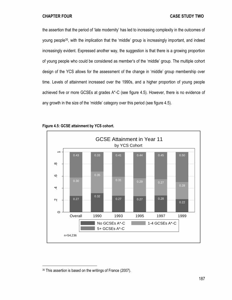
CHAPTER FOUR CASE STUDY TWO
187
the assertion that the period of ‘late modernity’ has led to increasing complexity in the outcomes of
young people35, with the implication that the ‘middle’ group is increasingly important, and indeed
increasingly evident. Expressed another way, the suggestion is that there is a growing proportion
of young people who could be considered as member’s of the ‘middle’ group. The multiple cohort
design of the YCS allows for the assessment of the change in ‘middle’ group membership over
time. Levels of attainment increased over the 1990s, and a higher proportion of young people
achieved five or more GCSEs at grades A*-C (see figure 4.5). However, there is no evidence of
any growth in the size of the ‘middle’ category over this period (see figure 4.5).
Figure 4.5: GCSE attainment by YCS cohort.
35 This assertion is based on the writings of France (2007).
0.27
0.30
0.43
0.32
0.35
0.33
0.27
0.31
0.41
0.27
0.29
0.44
0.28
0.27
0.45
0.22
0.28
0.50
0.2
.4.6
.81
Pro
port
ion (
surv
ey w
eig
hte
d)
Overall 1990 1993 1995 1997 1999
n=54,236
by YCS Cohort
GCSE Attainment in Year 11
No GCSEs A*-C 1-4 GCSEs A*-C
5+ GCSEs A*-C
CHAPTER FOUR CASE STUDY TWO
188
4.5.7 Further Exploring the ‘Middle’
As in the BHPS analyses, the results so far, depend on the operationalisation of the ‘middle’ group
which has been used. The analysis will therefore proceed with a more comprehensive exploration
of ‘middle’ levels of school GCSE attainment. The benchmark of 5+ GCSEs at grades A*-C is
widely used, but is largely an administrative standard.
Table 4.15 presents a sensitivity analysis of alternative formulations of the ‘middle’ category. The
overall summaries of series of logistic regression models are reported, the outcome variable is
participation in post-compulsory education at age 16-17. When the middle category is 1-2 GCSEs
(Grades A*-C) the R2 = 0.15, compared with R2 = 0.18, when the ‘middle’ category is 1-4 GCSEs
at grades A*-C. When the ‘middle’ category is extended to include 5 or 6 GCSEs at grades A*-C
there is no overall improvement in the explanation of participation in education at age 16-17. The
results are similar for the multinomial logistic regression models of main activity at age 18-19. The
emerging message is that 1-4 GCSEs at grades A*-C is a plausible construction for the ‘middle’
category of moderately qualified young people.
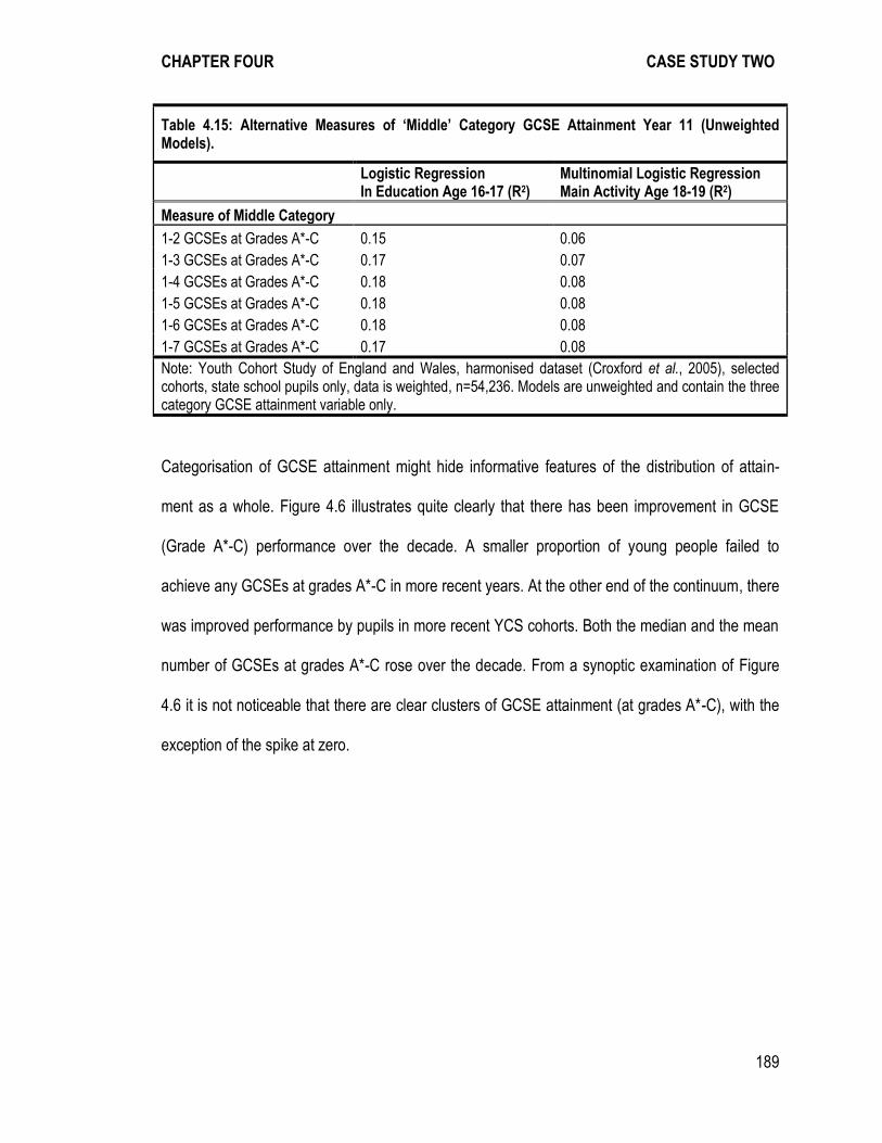
CHAPTER FOUR CASE STUDY TWO
189
Table 4.15: Alternative Measures of ‘Middle’ Category GCSE Attainment Year 11 (Unweighted Models).
Logistic Regression In Education Age 16-17 (R2)
Multinomial Logistic Regression Main Activity Age 18-19 (R2)
Measure of Middle Category
1-2 GCSEs at Grades A*-C 0.15 0.06
1-3 GCSEs at Grades A*-C 0.17 0.07
1-4 GCSEs at Grades A*-C 0.18 0.08
1-5 GCSEs at Grades A*-C 0.18 0.08
1-6 GCSEs at Grades A*-C 0.18 0.08
1-7 GCSEs at Grades A*-C 0.17 0.08
Note: Youth Cohort Study of England and Wales, harmonised dataset (Croxford et al., 2005), selected cohorts, state school pupils only, data is weighted, n=54,236. Models are unweighted and contain the three category GCSE attainment variable only.
Categorisation of GCSE attainment might hide informative features of the distribution of attain-
ment as a whole. Figure 4.6 illustrates quite clearly that there has been improvement in GCSE
(Grade A*-C) performance over the decade. A smaller proportion of young people failed to
achieve any GCSEs at grades A*-C in more recent years. At the other end of the continuum, there
was improved performance by pupils in more recent YCS cohorts. Both the median and the mean
number of GCSEs at grades A*-C rose over the decade. From a synoptic examination of Figure
4.6 it is not noticeable that there are clear clusters of GCSE attainment (at grades A*-C), with the
exception of the spike at zero.

CHAPTER FOUR CASE STUDY TWO
190
Figure 4.6: Number of GCSEs grade A*-C by YCS cohort.
To explore this issue further Figure 4.7 reports the proportion of young people in education at age
16-17 by the number of A*-C grade GCSEs that they obtained. There was a positive relationship
between the number of GCSEs at grades A*-C and participation in education at age 16-17. Those
with no GCSEs had lower levels of participation, and this appears to be a distinctive group of
young people. The ‘middle’ group with 1-4 GCSEs at grades A*-C (marked with a ▲) do not
appear to be tightly bunched and it is not obvious that they form a distinctive educational cluster.
0.1
.2.3
Pro
port
ion (
surv
ey w
eig
hte
d)
0 1 2 3 4 5 6 7 8 9 10 11 12n=54,236
by YCS Cohort
No of GCSEs A*-C in Year 11
1990 1993
1995 1997
1999
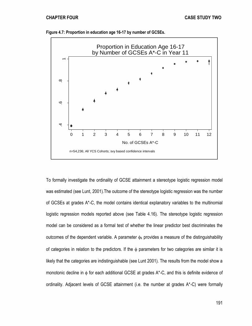
CHAPTER FOUR CASE STUDY TWO
191
Figure 4.7: Proportion in education age 16-17 by number of GCSEs.
To formally investigate the ordinality of GCSE attainment a stereotype logistic regression model
was estimated (see Lunt, 2001).The outcome of the stereotype logistic regression was the number
of GCSEs at grades A*-C, the model contains identical explanatory variables to the multinomial
logistic regression models reported above (see Table 4.16). The stereotype logistic regression
model can be considered as a formal test of whether the linear predictor best discriminates the
outcomes of the dependent variable. A parameter k provides a measure of the distinguishability
of categories in relation to the predictors. If the parameters for two categories are similar it is
likely that the categories are indistinguishable (see Lunt 2001). The results from the model show a
monotonic decline in for each additional GCSE at grades A*-C, and this is definite evidence of
ordinality. Adjacent levels of GCSE attainment (i.e. the number at grades A*-C) were formally
.4.6
.81
Pro
port
ion (
surv
ey w
eig
hte
d)
0 1 2 3 4 5 6 7 8 9 10 11 12
No. of GCSEs A*-C
n=54,236; All YCS Cohorts; svy based confidence intervals
Proportion in Education Age 16-17by Number of GCSEs A*-C in Year 11
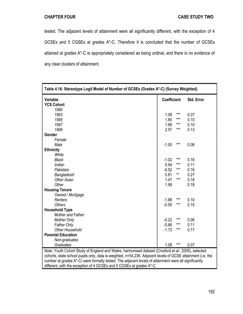
CHAPTER FOUR CASE STUDY TWO
192
tested. The adjacent levels of attainment were all significantly different, with the exception of 4
GCSEs and 5 CGSEs at grades A*-C. Therefore it is concluded that the number of GCSEs
attained at grades A*-C is appropriately considered as being ordinal, and there is no evidence of
any clear clusters of attainment.
Table 4.16: Stereotype Logit Model of Number of GCSEs (Grades A*-C) (Survey Weighted).
Variable Coefficient Std. Error YCS Cohort
1990 1993 1.08 *** 0.07
1995 1.80 *** 0.10 1997 1.66 *** 0.10 1999 2.57 *** 0.13 Gender
Female Male -1.00 *** 0.06
Ethnicity White Black -1.02 *** 0.16
Indian 0.54 *** 0.11 Pakistani -0.52 *** 0.16 Bangladeshi 0.81 ** 0.27 Other Asian 1.47 *** 0.18 Other 1.99
0.18
Housing Tenure Owned / Mortgage Renters -1.88 *** 0.10
Others -0.55 *** 0.15 Household Type
Mother and Father Mother Only -0.22 *** 0.06
Father Only -0.66 *** 0.11 Other Household -1.73 *** 0.17 Parental Education
Non-graduates Graduates 1.08 *** 0.07
Note: Youth Cohort Study of England and Wales, harmonised dataset (Croxford et al., 2005), selected cohorts, state school pupils only, data is weighted, n=54,236. Adjacent levels of GCSE attainment (i.e. the number at grades A*-C) were formally tested. The adjacent levels of attainment were all significantly different, with the exception of 4 GCSEs and 5 CGSEs at grades A*-C.
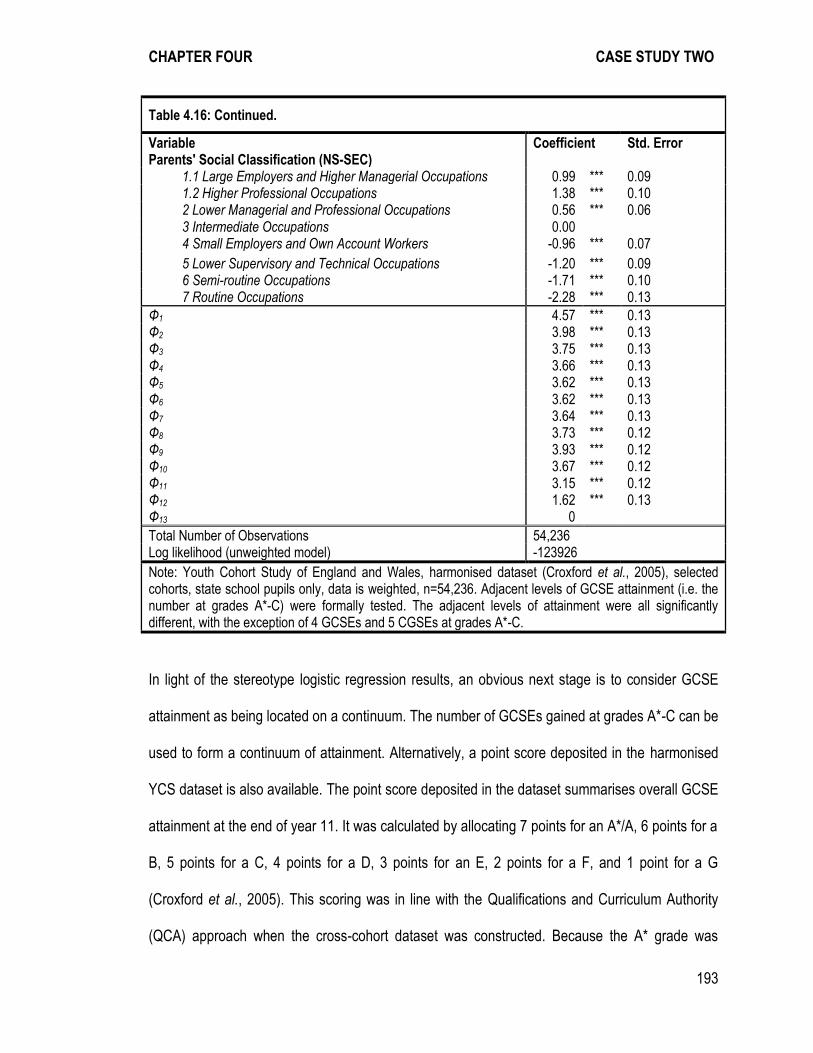
CHAPTER FOUR CASE STUDY TWO
193
Table 4.16: Continued.
Variable Coefficient Std. Error Parents' Social Classification (NS-SEC)
1.1 Large Employers and Higher Managerial Occupations 0.99 *** 0.09 1.2 Higher Professional Occupations 1.38 *** 0.10 2 Lower Managerial and Professional Occupations 0.56 *** 0.06 3 Intermediate Occupations 0.00
4 Small Employers and Own Account Workers -0.96 *** 0.07
5 Lower Supervisory and Technical Occupations -1.20 *** 0.09 6 Semi-routine Occupations -1.71 *** 0.10 7 Routine Occupations -2.28 *** 0.13
Φ1 4.57 *** 0.13 Φ2 3.98 *** 0.13 Φ3 3.75 *** 0.13 Φ4 3.66 *** 0.13 Φ5 3.62 *** 0.13 Φ6 3.62 *** 0.13 Φ7 3.64 *** 0.13 Φ8 3.73 *** 0.12 Φ9 3.93 *** 0.12 Φ10 3.67 *** 0.12 Φ11 3.15 *** 0.12 Φ12 1.62 *** 0.13 Φ13 0
Total Number of Observations 54,236 Log likelihood (unweighted model) -123926 Note: Youth Cohort Study of England and Wales, harmonised dataset (Croxford et al., 2005), selected
cohorts, state school pupils only, data is weighted, n=54,236. Adjacent levels of GCSE attainment (i.e. the number at grades A*-C) were formally tested. The adjacent levels of attainment were all significantly different, with the exception of 4 GCSEs and 5 CGSEs at grades A*-C.
In light of the stereotype logistic regression results, an obvious next stage is to consider GCSE
attainment as being located on a continuum. The number of GCSEs gained at grades A*-C can be
used to form a continuum of attainment. Alternatively, a point score deposited in the harmonised
YCS dataset is also available. The point score deposited in the dataset summarises overall GCSE
attainment at the end of year 11. It was calculated by allocating 7 points for an A*/A, 6 points for a
B, 5 points for a C, 4 points for a D, 3 points for an E, 2 points for a F, and 1 point for a G
(Croxford et al., 2005). This scoring was in line with the Qualifications and Curriculum Authority
(QCA) approach when the cross-cohort dataset was constructed. Because the A* grade was
CHAPTER FOUR CASE STUDY TWO
194
introduced midway through the data series, a grade A and a grade A* are awarded the same
score. Yang and Woodhouse (2001) adopt the same strategy to splice GCSE data spanning the
introduction of the A* grade.
The points score is capped at 84 points (i.e. the equivalent of twelve GCSEs at grade A*/A). This
approach was chosen to limit the effects of pupils achieving higher scores simply as a function of
having taken more GCSEs. Webber and Butler (2007) used a similar approach on the advice of
DfES officials. More recently, some official statistics have capped the points score based on the
best eight GCSEs. Other alternative approaches have been employed for example Haque and
Bell (2001) convert GCSE attainment into numerical scores (A*=8, A=7…U=0) and calculate a
mean GCSE score for each pupil. They chose this approach because they believe that this helps
to prevent discrimination against pupils who have taken fewer GCSEs as a result of their school’s
internal policy.
The Qualifications and Curriculum Authority have more recently developed a scoring system
which awards an A* 58 points, an A 52 points, a B 46 points, a C 40 points, a D 34 points, an E 28
points, a F 22 points, and a G 16 points.36 It is not possible to recode the GCSE scores in the
dataset onto the new QCA scale. Because the new and old scores for each GCSE grade are
similarly spaced, the overall substantive interpretations of analyses that use the new scoring
system will not be dramatically altered. Ideally, the analysis would include sensitivity analyses of
additional alternative GCSE attainment score measures; however such measures cannot be
effectively derived from data. The overall summary statistics of the number of GCSEs at grades
A*-C, and the GCSE points score are reported in table 4.17.
36 See: http://www.education.gov.uk/schools/performance/secondary_11/PointsScoreAllocation2011.pdf.
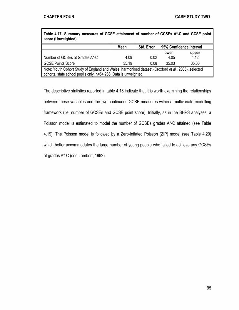
CHAPTER FOUR CASE STUDY TWO
195
Table 4.17: Summary measures of GCSE attainment of number of GCSEs A*-C and GCSE point score (Unweighted).
Mean Std. Error 95% Confidence Interval
lower upper Number of GCSEs at Grades A*-C 4.09 0.02 4.05 4.12
GCSE Points Score 35.19 0.08 35.03 35.36
Note: Youth Cohort Study of England and Wales, harmonised dataset (Croxford et al., 2005), selected cohorts, state school pupils only, n=54,236. Data is unweighted.
The descriptive statistics reported in table 4.18 indicate that it is worth examining the relationships
between these variables and the two continuous GCSE measures within a multivariate modelling
framework (i.e. number of GCSEs and GCSE point score). Initially, as in the BHPS analyses, a
Poisson model is estimated to model the number of GCSEs grades A*-C attained (see Table
4.19). The Poisson model is followed by a Zero-inflated Poisson (ZIP) model (see Table 4.20)
which better accommodates the large number of young people who failed to achieve any GCSEs
at grades A*-C (see Lambert, 1992).
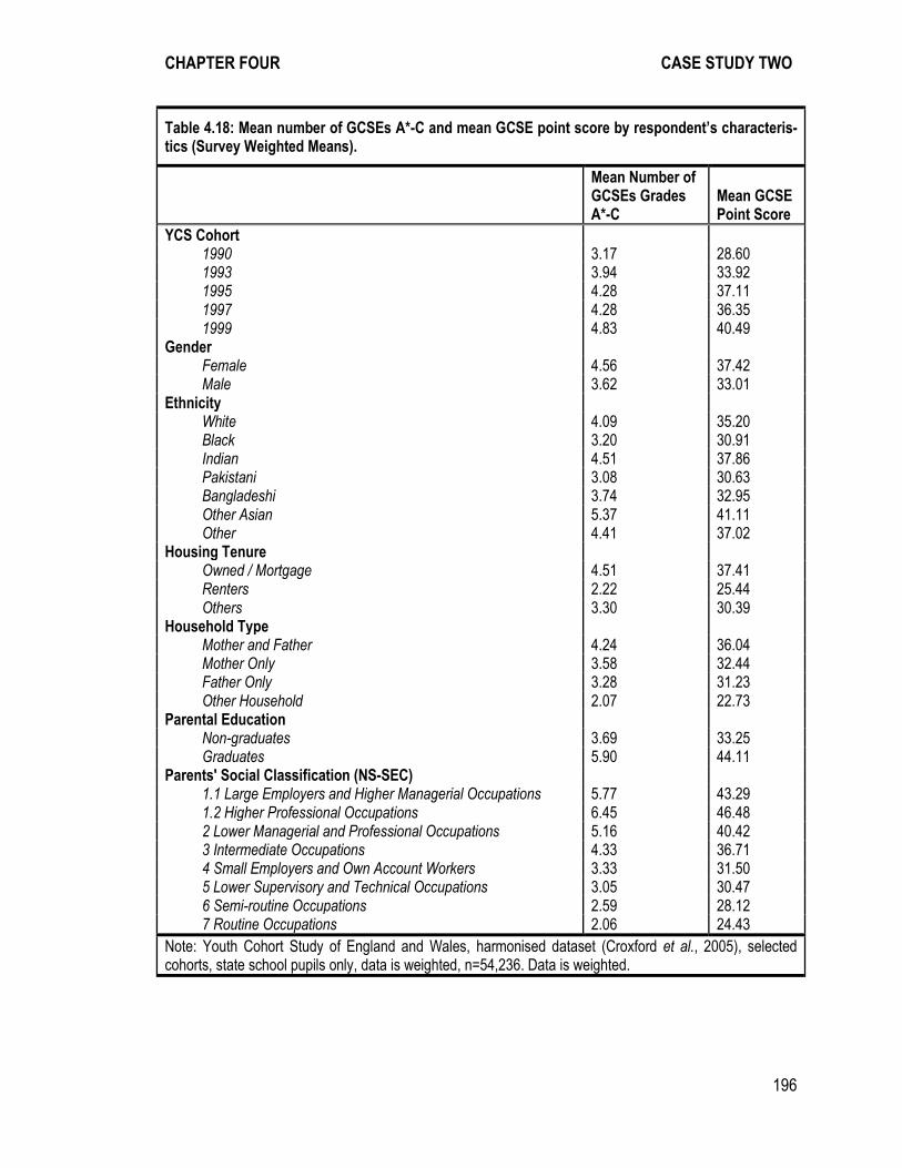
CHAPTER FOUR CASE STUDY TWO
196
Table 4.18: Mean number of GCSEs A*-C and mean GCSE point score by respondent’s characteris-tics (Survey Weighted Means).
Mean Number of GCSEs Grades A*-C
Mean GCSE Point Score
YCS Cohort 1990 3.17 28.60
1993 3.94 33.92 1995 4.28 37.11 1997 4.28 36.35 1999 4.83 40.49 Gender
Female 4.56 37.42 Male 3.62 33.01 Ethnicity
White 4.09 35.20 Black 3.20 30.91 Indian 4.51 37.86 Pakistani 3.08 30.63 Bangladeshi 3.74 32.95 Other Asian 5.37 41.11 Other 4.41 37.02 Housing Tenure
Owned / Mortgage 4.51 37.41 Renters 2.22 25.44 Others 3.30 30.39 Household Type
Mother and Father 4.24 36.04 Mother Only 3.58 32.44 Father Only 3.28 31.23 Other Household 2.07 22.73 Parental Education
Non-graduates 3.69 33.25 Graduates 5.90 44.11 Parents' Social Classification (NS-SEC)
1.1 Large Employers and Higher Managerial Occupations 5.77 43.29 1.2 Higher Professional Occupations 6.45 46.48 2 Lower Managerial and Professional Occupations 5.16 40.42 3 Intermediate Occupations 4.33 36.71 4 Small Employers and Own Account Workers 3.33 31.50 5 Lower Supervisory and Technical Occupations 3.05 30.47 6 Semi-routine Occupations 2.59 28.12 7 Routine Occupations 2.06 24.43
Note: Youth Cohort Study of England and Wales, harmonised dataset (Croxford et al., 2005), selected cohorts, state school pupils only, data is weighted, n=54,236. Data is weighted.
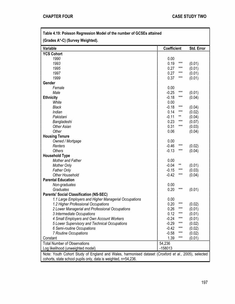
CHAPTER FOUR CASE STUDY TWO
197
Table 4.19: Poisson Regression Model of the number of GCSEs attained
(Grades A*-C) (Survey Weighted).
Variable Coefficient Std. Error
YCS Cohort 1990 0.00
1993 0.19 *** (0.01) 1995 0.27 *** (0.01) 1997 0.27 *** (0.01) 1999 0.37 *** (0.01) Gender
Female 0.00 Male -0.25 *** (0.01)
Ethnicity -0.18 *** (0.04) White 0.00
Black -0.18 *** (0.04) Indian 0.14 *** (0.02) Pakistani -0.11 ** (0.04) Bangladeshi 0.23 *** (0.07) Other Asian 0.31 *** (0.03) Other 0.06
(0.04)
Housing Tenure Owned / Mortgage 0.00
Renters -0.46 *** (0.02) Others -0.13 *** (0.04) Household Type
Mother and Father 0.00 Mother Only -0.04 ** (0.01)
Father Only -0.15 *** (0.03) Other Household -0.42 *** (0.04) Parental Education
Non-graduates 0.00 Graduates 0.20 *** (0.01)
Parents' Social Classification (NS-SEC) 1.1 Large Employers and Higher Managerial Occupations 0.00
1.2 Higher Professional Occupations 0.20 *** (0.02) 2 Lower Managerial and Professional Occupations 0.26 *** (0.01) 3 Intermediate Occupations 0.12 *** (0.01) 4 Small Employers and Own Account Workers -0.24 *** (0.01) 5 Lower Supervisory and Technical Occupations -0.29 *** (0.02) 6 Semi-routine Occupations -0.42 *** (0.02) 7 Routine Occupations -0.58 *** (0.02) Constant 1.39 *** (0.01)
Total Number of Observations 54,236 Log likelihood (unweighted model) -158013 Note: Youth Cohort Study of England and Wales, harmonised dataset (Croxford et al., 2005), selected
cohorts, state school pupils only, data is weighted, n=54,236.
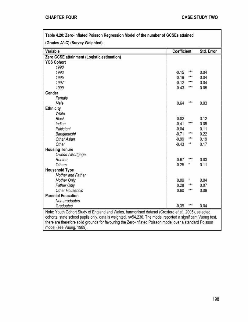
CHAPTER FOUR CASE STUDY TWO
198
Table 4.20: Zero-inflated Poisson Regression Model of the number of GCSEs attained
(Grades A*-C) (Survey Weighted).
Variable Coefficient Std. Error
Zero GCSE attainment (Logistic estimation) YCS Cohort 1990 1993 -0.15 *** 0.04
1995 -0.19 *** 0.04 1997 -0.12 *** 0.04 1999 -0.43 *** 0.05 Gender
Female Male 0.64 *** 0.03
Ethnicity White Black 0.02
0.12
Indian -0.41 *** 0.09 Pakistani -0.04
0.11
Bangladeshi -0.71 *** 0.22 Other Asian -0.99 *** 0.19 Other -0.43 ** 0.17 Housing Tenure
Owned / Mortgage Renters 0.67 *** 0.03
Others 0.25 * 0.11 Household Type
Mother and Father Mother Only 0.09 * 0.04
Father Only 0.28 *** 0.07 Other Household 0.60 *** 0.09 Parental Education
Non-graduates Graduates -0.39 *** 0.04
Note: Youth Cohort Study of England and Wales, harmonised dataset (Croxford et al., 2005), selected cohorts, state school pupils only, data is weighted, n=54,236. The model reported a significant Vuong test, there are therefore solid grounds for favouring the Zero-inflated Poisson model over a standard Poisson model (see Vuong, 1989).
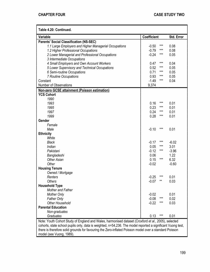
CHAPTER FOUR CASE STUDY TWO
199
Table 4.20: Continued.
Variable Coefficient Std. Error
Parents' Social Classification (NS-SEC) 1.1 Large Employers and Higher Managerial Occupations -0.50 *** 0.08
1.2 Higher Professional Occupations -0.79 *** 0.08 2 Lower Managerial and Professional Occupations -0.24 *** 0.05 3 Intermediate Occupations
4 Small Employers and Own Account Workers 0.47 *** 0.04 5 Lower Supervisory and Technical Occupations 0.52 *** 0.05 6 Semi-routine Occupations 0.71 *** 0.05 7 Routine Occupations 0.93 *** 0.05 Constant -1.49 *** 0.04 Number of Observations 9,374
Non-zero GCSE attainment (Poisson estimation) YCS Cohort 1990 1993 0.16 *** 0.01
1995 0.23 *** 0.01 1997 0.24 *** 0.01 1999 0.28 *** 0.01 Gender
Female Male -0.10 *** 0.01
Ethnicity White Black -0.17 *** -6.02
Indian 0.05 *** 3.01 Pakistani -0.12 *** -3.96 Bangladeshi 0.06
1.22
Other Asian 0.15 *** 6.32 Other -0.02
-0.60
Housing Tenure Owned / Mortgage Renters -0.25 *** 0.01
Others -0.07 ** 0.03 Household Type
Mother and Father Mother Only -0.02
0.01
Father Only -0.08 *** 0.02 Other Household -0.22 *** 0.03 Parental Education
Non-graduates Graduates 0.13 *** 0.01
Note: Youth Cohort Study of England and Wales, harmonised dataset (Croxford et al., 2005), selected cohorts, state school pupils only, data is weighted, n=54,236. The model reported a significant Vuong test, there is therefore solid grounds for favouring the Zero-inflated Poisson model over a standard Poisson model (see Vuong, 1989).
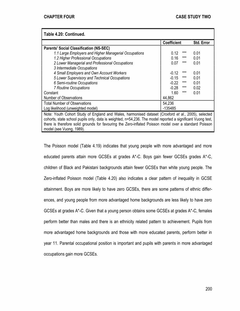
CHAPTER FOUR CASE STUDY TWO
200
Table 4.20: Continued.
Coefficient Std. Error
Parents' Social Classification (NS-SEC) 1.1 Large Employers and Higher Managerial Occupations 0.12 *** 0.01
1.2 Higher Professional Occupations 0.16 *** 0.01 2 Lower Managerial and Professional Occupations 0.07 *** 0.01 3 Intermediate Occupations
4 Small Employers and Own Account Workers -0.12 *** 0.01 5 Lower Supervisory and Technical Occupations -0.15 *** 0.01 6 Semi-routine Occupations -0.22 *** 0.01 7 Routine Occupations -0.28 *** 0.02 Constant 1.60 *** 0.01 Number of Observations 44,862
Total Number of Observations 54,236 Log likelihood (unweighted model) -135485 Note: Youth Cohort Study of England and Wales, harmonised dataset (Croxford et al., 2005), selected
cohorts, state school pupils only, data is weighted, n=54,236. The model reported a significant Vuong test, there is therefore solid grounds for favouring the Zero-inflated Poisson model over a standard Poisson model (see Vuong, 1989).
The Poisson model (Table 4.19) indicates that young people with more advantaged and more
educated parents attain more GCSEs at grades A*-C. Boys gain fewer GCSEs grades A*-C,
children of Black and Pakistani backgrounds attain fewer GCSEs than white young people. The
Zero-inflated Poisson model (Table 4.20) also indicates a clear pattern of inequality in GCSE
attainment. Boys are more likely to have zero GCSEs, there are some patterns of ethnic differ-
ences, and young people from more advantaged home backgrounds are less likely to have zero
GCSEs at grades A*-C. Given that a young person obtains some GCSEs at grades A*-C, females
perform better than males and there is an ethnicity related pattern to achievement. Pupils from
more advantaged home backgrounds and those with more educated parents, perform better in
year 11. Parental occupational position is important and pupils with parents in more advantaged
occupations gain more GCSEs.
CHAPTER FOUR CASE STUDY TWO
201
The modelling results indicate that GCSE attainment is reasonably considered as being located
on a continuum. Thus, there is mounting evidence that there are no clear clusters or groups of
GCSE attainment. There is increasing evidence that there is not a ‘middle’ group of young people
that is characteristically different from other groups of young people.
The overall mean GCSE points score was 35.19. There was not an extreme spike at zero points,
this is because many of the pupils that fail to achieve any GCSEs at grades A*-C are awarded
points for subjects for which they gain awards at grades D-G. The linear regression (Table 4.21)
models GCSE attainment point score. There is a significant gender gap and a mixed pattern of
achievement across the minority ethnic groups. Young people with more educated parents scored
higher on average, and pupils from more advantaged home backgrounds also performed better.
The effect of parental occupational position was dramatic and those pupils with parents in less
advantaged occupational positions performed significantly less well, ceteris paribus.
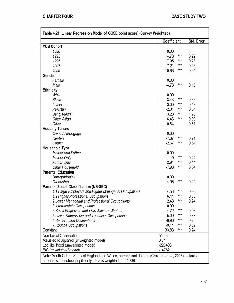
CHAPTER FOUR CASE STUDY TWO
202
Table 4.21: Linear Regression Model of GCSE point score) (Survey Weighted).
Coefficient Std. Error
YCS Cohort
1990 0.00
1993 4.78 *** 0.22 1995 7.95 *** 0.23 1997 7.21 *** 0.23 1999 10.88 *** 0.24 Gender
Female 0.00
Male -4.73 *** 0.15 Ethnicity
White 0.00
Black -3.43 *** 0.65 Indian 3.00 *** 0.49 Pakistani -2.01 *** 0.64 Bangladeshi 3.28 ** 1.28 Other Asian 6.46 *** 0.89 Other 0.84
0.81
Housing Tenure
Owned / Mortgage 0.00
Renters -7.37 *** 0.21 Others -2.67 *** 0.64 Household Type
Mother and Father 0.00
Mother Only -1.19 *** 0.24 Father Only -2.94 *** 0.44 Other Household -7.98 *** 0.54 Parental Education
Non-graduates 0.00
Graduates 4.95 *** 0.22 Parents' Social Classification (NS-SEC)
1.1 Large Employers and Higher Managerial Occupations 4.53 *** 0.36 1.2 Higher Professional Occupations 6.44 *** 0.33 2 Lower Managerial and Professional Occupations 2.43 *** 0.24 3 Intermediate Occupations 0.00
4 Small Employers and Own Account Workers -4.72 *** 0.26 5 Lower Supervisory and Technical Occupations -5.09 *** 0.33 6 Semi-routine Occupations -6.96 *** 0.28 7 Routine Occupations -9.14 *** 0.32 Constant 33.83 *** 0.24
Number of Observations 54,236 Adjusted R Squared (unweighted model) 0.24 Log likelihood (unweighted model) -223408 BIC (unweighted model) -14762
Note: Youth Cohort Study of England and Wales, harmonised dataset (Croxford et al., 2005), selected cohorts, state school pupils only, data is weighted, n=54,236.
CHAPTER FOUR CASE STUDY TWO
203
4.6 Discussion and Conclusions
School attainment plays a central and critical role in young people’s educational and employment
trajectories. Furthermore, the 1990s are an important period that followed structural changes in
the British secondary school system, including the introduction of GCSEs in England and Wales.
This chapter has presented the results of a series of exploratory analyses of GCSE attainment in
the 1990s using the British Household Panel Survey and the Youth Cohort Study of England and
Wales. The analysis was motivated by the desire to explore the cogency of the theoretical idea of
the ‘missing middle’ through the research question, Is there a ‘middle’ group of ordinary young
people that can be characterised by their social and educational characteristics? Therefore, the
utility of studying a categorised ‘middle’ group of young people, as advocated by Roberts (2011),
has been assessed.
Overall, what is clear from the results, and should not be overlooked, is that multiple dimensions
of educational inequality are apparent in the GCSE attainment of these samples. Boys tend to
achieve fewer GCSEs at grades A*-C, and young people from Black and Pakistani backgrounds
also achieve fewer GCSEs at grades A*-C. There is a clear social gradient in GCSE attainment,
with children from the least advantaged social groups attaining fewest GCSEs at grades A*-C.
The 1990s witnessed an overall pattern of improvement in GCSE examination results (see Social
Trends, 2001), evident in the YCS data. However, in general, girls performed better than boys and
there were some marked differences in attainment for pupils from the main minority ethnic groups.
A striking result is the impact of parental socio-economic positions and the other variables
associated with the young person’s home background. This is particularly important as much of
the popular discourse associated with differences in school attainment focuses on gender differ-
ences, rather than differences between pupils from dissimilar social backgrounds.
CHAPTER FOUR CASE STUDY TWO
204
A sizeable proportion of young people failed to gain any GCSEs at grades A*-C. This is obviously
far short of the benchmark target, and is consequential because those without school level
qualifications usually have fewer choices and chances in later life than their better qualified
counterparts. Nevertheless, Roberts (2011) rightly contends that a bifurcated conceptualisation of
the outcomes and experiences of youth is not adequate. As a solution he argues for the detailed
analysis of a third category, comprising ordinary or non-spectacular young people, the ‘middle’.
Attempts to model membership of the ‘middle’ group fail to provide convincing evidence that there
are distinctive, or discrete, categories of GCSE attainment. There appear to be no crisp bounda-
ries that mark out a ‘middle’ category of moderate GCSE attainment. With the exception of the
sharp spike of young people that were unsuccessful in gaining any GCSEs at grades A*-C, no
clear cohesive GCSE attainment groups are evident. The replication of the patterns in both the
BHPS and the YCS provide persuasive evidence that the results are robust. To answer the
research question posed at the start of this chapter, here does not appear to be a ‘middle’ group
of ordinary young people that can be characterised by their social and educational characteristics.
The results of the attempt to ‘establish the phenomenon’ of the ‘missing middle’ suggest that
researchers exercise a suitable degree of caution before making additional claims about the
GCSE attainment of ‘ordinary’ young people.
The analyses indicate that there are clear benefits to understanding school attainment as being
located upon a continuum, and that measures which reflect the heterogeneity of GCSE perform-
ance as fully as possible should be preferred. These include continuous measures such as the
number of GCSEs gained at grades A*-C. Altman (2006) contends that the categorisation of
variables can provide enticing simplicity, but this is gained at a cost. The drawbacks of categorisa-
tion are demonstrated in the greater explanatory power for the continuous variables considered in
CHAPTER FOUR CASE STUDY TWO
205
this chapter. Categorisation of variables which have an underlying continuous distribution, such as
GCSE attainment, leads to loss of information (Altman, 2006). By categorising GCSE attainment,
the extent of variation between groups may be underestimated, and a misleading degree of
homogeneity within groups is implied. Notably, categorisation is not necessary for the techniques
of modern social survey analysis, and continuous measures often lend themselves to the simplest
types of analysis (i.e. the linear regression model presented as the final piece of analysis in this
chapter) (Sauerbrei and Royston, 2010).
In many social surveys only crude measures of educational attainment are available. For many
analyses a detailed measure of GCSE school attainment will not be available, and therefore a
simplified categorical measure will have to be utilised. In such circumstances it is recommended
that categorical GCSE attainment measures should not be understood as substantively meaning-
ful categories. Rather they should be considered as coarse groupings of a more continuous
measure.
In conclusion, there was an initial theoretical attraction to the idea of a ‘middle’ group of ordinary
young people. It is undeniable that sociologists should pay research attention to ‘ordinary’ young
people with moderate, or unspectacular, levels of school attainment. The tripartite categorisation
of young people may however disguise the heterogeneity of young people’s characteristics and
outcomes, in the same manner as a bifurcated conceptualisation. The analyses in this chapter
highlight that there is much to be gained by understanding the educational experiences, character-
istics and qualifications of young people across the full spectrum of attainment.
CHAPTER FIVE CASE STUDY THREE
206
5. Education, Ability and Social Origins Across the Occupational Lifespan
“The occupational achievement process is a change process. Few persons’
status and income remain constant over their lifetime.” (Sorensen, 1975, p. 470)
5.1 Introduction
Much of the classic work establishing the persistent influence of social origins on life-course
outcomes has relied on cross-sectional data (e.g. Blau et al., 1967; Erikson et al., 1992; Glass,
1954; Goldthorpe et al., 1987). Research focus has been placed largely on the relationship
between parent’s class position and that of the respondent at a single point in time. Some re-
search has sought to appreciate the changeable nature of occupational attainment, notably the
‘status attainment’ models that are especially popular in the United States (esp. Blau et al., 1967;
Sewell and Hauser, 1975). In the ‘status attainment’ modelling tradition a single intermediary
position, that of first job or of occupational aspirations, is incorporated within an assessment of the
influence of social background upon current or last job. In the class analysis approach more
popular in European sociology (esp. Breen, 2004; Erikson et al., 1992; Goldthorpe et al., 1987), a
two-point comparison between parental and current jobs is analysed, since it is argued that
occupational achievement at one point in time should (for adults over a certain age37) prove an
adequate proxy of long-term occupational circumstances (e.g. Goldthorpe et al., 1987, p. 57). This
assumption is potentially problematic, and results in important information regarding the proc-
37 An argument expressed by, amongst others, Goldthorpe et al. (1987, p. 51), is that most adults reach a point of ‘occupational maturity’, around about the age of 35, after which it is relatively unlikely they will experience major changes in their occupational position.
CHAPTER FIVE CASE STUDY THREE
207
esses of occupational attainment across the lifecourse being aggregated into a single indicator
(Featherman and Selbee, 1988; Goldthorpe, 1980; Sorensen, 1986).
The detailed consideration of occupational transitions across the lifecourse can be achieved
through the analysis of prospective or retrospective data on the occupational positions held by the
same person over time. There have been striking developments in statistical analysis techniques
and statistical software capabilities over the last two decades which lend themselves to the
detailed modelling of repeated measures. These techniques are suited for the detailed analysis of
multiple observations of occupational position across the lifecourse, or ‘intra-generational mobility’.
Importantly, for research on social stratification and inequality, it is possible to conceive of a
longitudinal outcome defined in terms of intra-generational mobility, whereby the ways in which
the effects of education, ability and social origins played out across the lifecourse might lead to
different intra-generational profiles or trajectories. It has been reasonably common for researchers
to examine such influences upon certain aspects of intra-generational mobility (e.g. transitions into
and out of poverty, or between full-time and part-time employment) (e.g. Blossfeld et al., 2005b;
Jenkins, 2011). However, it has been less common for sociologists to attempt to summarise intra-
generational transitions within the context of an analysis of stratification outcomes in general
terms. From this perspective, the motivation would be to improve upon the measurement of
stratification outcomes by using a characterisation of the outcome which is informed by the history
of intra-generational mobility, rather than just the most recent occupation. Though occasionally
explored before (e.g. Featherman, 1971; Featherman and Hauser, 1978; Hauser et al., 1999;
Hillmert, 2010; Tampubolon et al., 2012), such approaches have not yet become mainstream
analytical strategies, and have rarely been applied to UK data.
CHAPTER FIVE CASE STUDY THREE
208
Taking account of intra-generational mobility is particularly relevant to research on the reproduc-
tion of social inequality, because a number of theories and a substantial amount of research
suggests that occupational inequalities will persist or even increase over the life course. Central to
the analysis of intra-generational mobility is aging effects, and possible cohort change in aging
effects (Miech et al., 2003). Age is an important factor in social stratification, and there is a
considerable association between age and levels of social and economic advantage (Foner, 1979;
Riley, 1987). As O’Rand (1996, p. 188) notes: “age is an independent social basis for social
differentiation and inequality that interacts with political and economic institutions to allocate
resources across age groups even within other ascriptive groups such as class, gender and race”.
One clear mechanism for age-related social stratification concerns how people tend to be pro-
moted into more senior positions as they grow older. Ageing effects, moreover, are known to work
in different ways for people in different social positions, so much so that patterns of age-related
progression (e.g. career advancement prospects in a given occupation) have been used to define
or justify ways of measuring stratification itself (e.g. Bihagen et al., 2004; Goldthorpe et al., 2006).
Furthermore, factors that affect the attainment of occupational positions (e.g. education, social
origins and ability), may exert differing influences on occupational positions throughout the
lifecourse (Warren, 2001). Childhood characteristics, family influences, educational attainment,
adult family roles, and work lives are closely intertwined. It is therefore rational to conceive of the
process of occupational attainment as contingent on the influence and interaction of a range of
factors derived from across all points of the lifecourse (Warren, 2001). From this perspective,
analyses of occupational attainment that only consider the current or last occupations of a sample
of individuals at best neglect age-related changes, and at worst give a misleading impression of
CHAPTER FIVE CASE STUDY THREE
209
the overall experience of individuals, since results may depend to an important extent on the age
and birth cohort of the sample (Warren, 2001).
The study of social mobility aims to progress our understanding of the mechanisms which underlie
social inequality. Social mobility research has largely made the distinction between intra-
generational mobility (e.g. trajectories across the lifecourse) or inter-generational mobility (i.e. the
comparison of occupational positions between parents and children). Our understanding of intra-
and inter-generational social mobility could be enhanced by considering social mobility as a
mixture of both of these processes. For example, the support received from one’s parents may not
only influence the initial transition into employment and the early career stages, but may also
influence an individual’s occupational position throughout the lifecourse. Additionally, occupational
trajectories themselves may determine important outcomes (i.e. economic holdings, experience,
networks and expert knowledge) that can transmitted from parents to children.
Although there have been some examples of studies which summarise inter-generational influ-
ences in a way which is informed by data on intra-generational mobility (e.g. Blau et al., 1967), it
remains the case that most inter-generational social mobility studies incorporate little or no
account of intra-generational change within their analysis. Although longitudinal intra-generational
data could be exploited, most analysts have been persuaded by analyses, such as those of
Erikson and Goldthorpe (1992, Chapter 8), which suggest that social reproduction can adequately
be summarised by comparing parental background with current or last occupational position alone
as long as the age of occupational maturity has been reached.

CHAPTER FIVE CASE STUDY THREE
210
This chapter explores whether there is additional insight to be gained by studying the determi-
nants of occupational standing across the life course in an inter-generational analysis. The
National Child Development Study is used to investigate the trends and differentials in intra-
generational socio-economic position with regards social background, educational attainment and
childhood cognitive ability test scores. The ultimate aim of this chapter is to assess the influence
of social background, educational attainment and cognitive ability on occupational position in
adulthood, not at one point in time, but across a period of time.
This analysis is approached by investigating the role of social background, education and meas-
ured ability upon the development of the cohort members’ careers from their mid-twenties through
to age fifty. Age is an important factor in the achievement of advantaged social positions, as
analysed through cohort studies, as different points of contact may correspond to different stages
in the career. Therefore, it could be expected that an investigation which considers social position
across age may produce a clearer picture of the processes of social stratification than investiga-
tions which focus on changes between cohorts or generations (Warren, 2001; Warren et al.,
2002). The contribution of the present chapter is to specifically consider the role of social origins,
educational attainment and childhood cognitive ability test scores on occupational position at
several points in time.
5.2 Meritocracy
Research regarding the influence of social background, education and cognitive ability on occupa-
tional attainment, which is the focus of this chapter, is closely associated with the concept of
meritocracy. A meritocratic system is a popular political ideal whereby social position is achieved
CHAPTER FIVE CASE STUDY THREE
211
through “ability and effort”38, (Young, 1958, p. 94). Literature concerning cognitive ability and
occupational position in the British context has focused on the empirical testing of the extent to
which a meritocratic system of occupational selection is evident in Britain today and in past eras39.
Using the National Child Development Study (NCDS), Saunders (1995; 1996; Saunders, 2010)
asserts that the levels of inter-generational mobility observed closely match the levels expected in
a model of stratification based upon ability. Similarly, Nettle (2003) conducted correlational
analysis of ability and occupational attainment in the NCDS and found evidence of a largely open
society stratified according to ability. Breen and Goldthorpe’s (2001; 1999) interpretation, on the
other hand, emphasises that adult social position is influenced largely through origin socio-
economic position and education, with ability playing only a minimal role. The debate is further
complicated as Breen and Goldthorpe (1999) note that it is not merely the different methods used
38 Although political discourse, particularly under the Blair administration, has used the term ‘meritocracy’ as a positive political ideal, the negative consequences of a system of social selection based purely on ability and effort have also been emphasised (see Young, 1958; Young, 2001). 39 There are many features of the relationship between social origins and destinations which can be described in more detail, particularly in relation to the processes of educational attainment. For example, Willis (1977) famously described the antagonistic relationship which working class boys had with their education, which often led to disengagement and disinterest in educational attainment. This cultural approach to understanding processes of educational disadvantage has been highlighted more recently by Reay (2006) who described the alienation and disaffection of working class children. More advantaged children and young people also benefit from their parent’s knowledge of the education system and cultural capital. More advantaged parents often engage in focussed organised parenting practices to develop their children’s skills, encourage a wide-range of cultured interests and foster an appreciation of education. Lareau (2011) describes these middle class parenting practices as ‘concerted cultivation’. The processes by which working class young people are disadvantaged in the education system have been highlighted clearly in relation to higher education participation. Bradley et al. (2011) have described how the parents of working class students are particularly frightened by the prospect of debt, may encour-age their children to attend local universities and can have limited knowledge of higher education, whereas more advantaged parents can provide more support and guidance. As a result, more advantaged young people have smoother routes into higher education, are less likely to be unhappy with their chosen course and attend more prestigious universities (Bradley et al., 2011). Furthermore, once at university, disadvan-taged young people can have trouble integrating into the university environment leading to increased risk of drop out (Bradley et al., 2011; Crozier et al., 2010; Reay et al., 2010). Overall, advantaged parents have many skills and resources at their disposal in order to increase the chances that their offspring are successful in education and the labour market (Devine, 2004).
CHAPTER FIVE CASE STUDY THREE
212
for analysis of the role of ability which has led to disagreement, but also that different conclusions
can logically be reached from the same results. Overall the debate, although ongoing, tends to
indicate that ability does appear to exert a significant influence upon socio-economic outcomes,
and that ability will enable occupational attainment. However, social opportunity, economic
resources and, chiefly, education seem to exert a major moderating influence on the process of
social stratification. These findings are comparable to the conclusions reached in Blau and
Duncan’s (1967) monograph which highlighted the theoretical and empirical importance of
cognitive ability variables, alongside social origins and education, in models of occupational
attainment in the North American context.
Informed by similar interests, this chapter explores the temporal dynamics of the concept of
meritocratic attainment. Following papers such as Tampubolon and Savage (2012) who suggest
that class fractions may have specific mobility trajectories, it is conceivable that an analysis of
‘merit variables’ from an intra-generational perspective may reveal different and additional
evidence to those previous studies, cited above, which have used a single cross-sectional
outcome.
5.3 Linking Inter- and Intra-generational Mobility Analysis
As noted above, early inter-generational mobility studies often incorporated a limited account of
intra-generational mobility by comparing the influence of background upon both current occupa-
tion, and the first occupation held after leaving education (e.g. Blau et al., 1967). More complex
models were not thought readily possible, both in terms of statistical techniques and data re-
sources. The expansion of high-quality longitudinal data resources over the last decades has
CHAPTER FIVE CASE STUDY THREE
213
prompted more ambitious attempts to integrate intra-generational data within inter-generational
studies. As one notable example, Tampubolon and Savage (2012) used latent class growth
analysis techniques to analyse the trajectories of members of the National Child Development
Study and the British Cohort Study. They identified several latent trajectory profiles, membership
to which was largely determined by social class of origin. They also found notable gender differ-
ences, beyond a certain age the male trajectories became stable, whereas women showed more
complex patterns of instability, and a lack of long-term attachment to occupational positions
(Tampubolon et al., 2012).
Nevertheless, the analysis of intra-generational data presents problems. Panel data may not
provide complete information on mobility or status changes, whilst retrospective questionnaires
about previous career history are only occasionally implemented in social surveys, and feature
problems of recall bias (Hassan, 2006). Tampubolon and Savage’s (2012) analysis compares two
UK birth cohorts (born in 1958 and 1970), which has the advantage of featuring a reasonably
extended lifecourse coverage, at least for the older cohort. However this analysis could be
criticised for conflating age and cohort effects, and lacking coverage for other individuals, outwith
these two specific years of birth. The analysis in this chapter also uses also birth cohort data;
therefore one must recognise the limitations of generalisation from this specific birth cohort to
wider population level age and cohort processes.
Alongside the approach of Tampubolon and Savage (2012), which seeks to characterise the
entire intra-generational profile (see also Sturgis and Sullivan, 2008), another group of studies
incorporating aspects of career data in inter-generational mobility research are worth distinguish-
ing. Attention to the first job obtained, and its relation to the current or most recently measured job,
CHAPTER FIVE CASE STUDY THREE
214
has been a common feature of stratification and social mobility studies for some time. In earlier
generations of research, first job was seen as an important intermediary in linking from educa-
tional attainment to occupational outcomes in the status attainment approach (e.g. Blau et al.,
1967), and marked one of several factors through which the impact of parental background was
transmitted into final outcomes. Similar conclusions, moreover, were found in class mobility
studies (e.g. Goldthorpe et al., 1987, Chapter 5), though here the relative gain from studying first
occupations was not thought to be substantial. By using the National Child Development Study in
this chapter, it is possible to focus upon a longer sequence of career histories than the first job
alone.
In more recent literature, similar themes have often been found, but greater emphasis has been
placed on the differences between the trajectories of men and women, rather than the influence of
a number of variables at different points of the lifecourse. For example, Bukodi and Dex (2009)
analysed the impact of holding ‘bad jobs’ (defined by pay) at career entry, on later occupations.
They found that men were more likely to escape these ‘bad jobs’ and enter stable improved
employment, whereas women who advanced beyond these ‘bad jobs’ had more transient patterns
of employment and were more likely to experience downward movements in their intra-
generational mobility profile (see also Golsch, 2006; Jacobs, 1999). In this chapter the role of
gender will be considered, as the studies above have highlighted that differences are apparent in
the trajectories of men and women. However, the focus is placed on a different perspective of the
insights provided by intra-generational analyses. Instead of describing the trajectories apparent for
different social groups, this chapter will analyse the differing importance of the variables of social
origins, education and cognitive ability at different points of the lifecourse to better understand the
process of social stratification.
CHAPTER FIVE CASE STUDY THREE
215
5.4 Longitudinal Processes: Cognitive Ability, Education and Social Background Across the Lifecourse
Regardless of more detailed explanation and investigation, what is clear from the outset in studies
of cognitive abilities and social position is that performance on cognitive ability tests correlates
with both origin social position in childhood and destination social position in adulthood (Nettle,
2003; Saunders, 1995; Thienpont and Verleye, 2003). Such general relationships, however, may
conceal the processes by which cognitive ability influences occupational attainment. Farber and
Gibbons (1996) present a model of learning about worker ability in which they emphasise that, at
labour market entry, educational qualifications are likely to convey only partial information about
the worker’s attributes. Employers only receive a full picture of the employees’ productive ability
after they begin employment, beyond which intuitive theory suggests that occupational position
will be increasingly determined by demonstrated abilities in the workplace rather than educational
qualifications (Warren, 2001).
Early in the career where indicators of job performance are lacking, educational qualifications may
exert a greater influence. The model implies that those with greater cognitive ability, regardless of
indicators from family background or educational qualifications, will be enabled to achieve higher
occupational position through their superior performance in the workplace. In line with this theory,
Farber and Gibbons’ (1996) analysis of the National Longitudinal Survey of Youth found that
variables indicating ability, but unobserved by employers, are increasingly correlated with wages
as time spent in the labour market increases. It appears, therefore, that those with more demon-
strated ability in employment might have an added benefit as their careers progress and their
advantages accumulate.
CHAPTER FIVE CASE STUDY THREE
216
In previous cohort studies, childhood indications of cognitive ability are found to be substantially
stable from childhood into old age (Deary et al., 2000). This study seeks to investigate the effects
of these cognitive abilities measured at a young age, upon progress in socio-economic position in
adult life. The opponent theory would suggest that no such progressive accumulation across the
lifecourse occurs, and instead that abilities related to occupational performance gained in adoles-
cence and through participation in higher education will exert the overwhelming influence upon
socio-economic outcomes.
Previous studies of influences upon social position across the life-course are largely based on the
US context; however they provide a basis for understanding the processes which might be
observed with UK data. US studies have indicated that the effects of education decline with age,
although educational qualifications continue to exert a significant effect upon educational position
throughout the lifespan. The greatest influence of educational qualifications upon occupational
position is observed at an early point in the occupational career (Featherman, 1971; Warren et al.,
2002). The influence of family background is seen to remain reasonably stable or decrease across
the life-course (Warren et al., 2002). In general, the effects of cognitive ability on occupation
appear to remain fairly stable or increase only modestly across the life course, and the effect
overall tends to be consistently small throughout (Hauser et al., 1999; Warren, 2001; Warren et
al., 2002).
With UK data, Deary et al. (2005) found ability test scores collected at age 11 to be more strongly
related to socio-economic position in middle age, than socio-economic position indicated by initial
occupation, suggesting that an individual’s socio-economic position comes to increasingly repre-
sent their true ability as their career progresses. This sentiment is also discussed in Nettle’s
CHAPTER FIVE CASE STUDY THREE
217
(2003) correlational analysis of occupational position and childhood ability test scores. Similarly,
Currie and Thomas (2001) also established that ability scores of NCDS cohort members at age 7
were better predictors of both income and employment status at age 33 than at age 23.
Measures of educational attainment appear to be associated with occupational position through-
out the lifecourse, but the associations between educational attainment and occupational position
have been found to be greater earlier in the career (Featherman, 1971; Warren et al., 2002). This
literature suggests that the association between occupation and educational attainment declines
across the lifecourse, whereas the association with cognitive ability increases or remains rea-
sonably stable (Currie et al., 2001; Deary et al., 2005; Hauser et al., 1999; Warren, 2001; Warren
et al., 2002).
The previous literature, from the US context, has indicated that the effects of social background on
occupational positions remain constant or decline with age to a small degree (Blau et al., 1967;
Featherman, 1971; Featherman et al., 1978; Kelley, 1973). More recently, Hauser Sheridan and
Warren (1999), Warren, Hauser and Sheridan (2002) and Warren (2001) argued that the effects of
social background are mediated largely through educational attainment and cognitive ability,
which have both been shown to be associated with social origins (i.e. see Case Studies One and
Two). From such evidence, it can be expected that empirical associations will ordinarily be
identified between measures of social origins and later occupational attainment. It can also be
expected that these associations will vary, and may diminish, when other measures of circum-
stances are also incorporated into analyses.

CHAPTER FIVE CASE STUDY THREE
218
The contribution to the literature of the empirical analyses presented in this chapter is to specifi-
cally consider, with UK data, the influence of cognitive ability, social origins and education on
occupational position of adult cohort members at several follow-up opportunities. This research is
guided by the following hypotheses:
Family background and education will exert their greatest influence at the early stages of
the occupational career. The association of family background and education with occu-
pational position will weaken as the career progresses.
Cognitive ability test scores will exert their greatest influence at the later stages of the oc-
cupational career. The association of cognitive ability with occupational position will
strengthen as the career progresses.
5.5 Data and Methodology
The UK is relatively rich in the availability of longitudinal data on the occupational positions of
individuals over a period of time. To answer the research question of this chapter, intra-
generational information on occupational positions is required along with information regarding
cognitive ability. The British Birth Cohort Studies (i.e. the 1946 National Survey of Health and
Development, the 1958 National Child Development Study, and the 1970 British Birth Cohort
Study40) provide a resource which links childhood information, and various psychological tests
conducted during childhood and adolescence, with adult occupational outcomes. This chapter
focuses on the National Child Development Study (NCDS) which provides information on the
occupational outcomes of cohort members up to age 50. The NCDS is also the dataset used in
many previous studies of inter-generational mobility and ‘meritocracy’ in the UK (see Blanden et
40 The youngest British birth cohort, the Millennium Cohort Study, will also provide a valuable data resource for the study occupational outcomes in the future.

CHAPTER FIVE CASE STUDY THREE
219
al., 2005; Blanden et al., 2004b; Breen et al., 2001; Breen et al., 1999; Currie et al., 2001;
Dearden, 1999; Feinstein et al., 2004; Nettle, 2003; Saunders, 1995; Saunders, 1996; Saunders,
2002; Saunders, 2010).
5.5.1 The National Child Development Study
The National Child Development Study is an ongoing survey of a cohort of babies born in one
week in 1958, and was introduced in detail in chapter three which focused on the cognitive
development of the cohort members in childhood. This chapter revisits the cohort members later
in their lifecourse, from age 23. In total outcomes at five time points are considered: age 23
(1981), 33 (1991), 42 (2000), 46 (2004) and 50 (2008).
Attrition is often a problem in longitudinal studies and the NCDS is not an exception. The NCDS
has suffered attrition, cohort members have left the sample and cohort members are not present
in every sweep considered. Detailed analyses of attrition and non-response in the NCDS have
indicated that the survey remains largely representative, and that no major biases have been
introduced into the sample (Hawkes and Plewis, 2006; Nathan, 1999). These strong results
suggest that a complete case analysis, which is conducted in this chapter, is scientifically defensi-
ble.
A technique which could be used to tackle survey non-response is multiple imputation (Carpenter
and Plewis, 2011; Goldstein, 2009). Multiple imputation allocates values to missing observations
based on information which is available in the dataset. Rather than just filling in one value,
multiple imputation produces many versions of the data and probabilities of a given value are used
to fill in the missingness. In the analysis of survey data with item non-response, multiple imputa-
CHAPTER FIVE CASE STUDY THREE
220
tion is an attractive method which presents the possibility to maintain the original sample size.
However, with longitudinal social survey data including complex patterns of attrition and non-
response, the use of multiple imputation is still in its infancy and is beyond the scope of routinely
available social science packages. Carpenter and Kenward (2012) and Allison (1999) note that it
is better to undertake complete case analysis than to attempt an ad hoc imputation. When
undertaking analyses of large scale social survey data with missingness, it is still possible to
recover sensible estimates (e.g. an unbiased regression coefficient) but with the smaller sample
size there is a risk that standard errors will be too large. This may possibly result in overlooking a
significant effect; however in practice this problem will not be too dramatic when using large scale
social survey data.
5.5.1.1 Occupational Position
Occupational position in adulthood is represented with the Cambridge Social Interaction and
Stratification scale (CAMSIS) (see Prandy and Lambert, 2003). Standard Occupational Classifica-
tion codes (SOC) and employment status were used to derive the CAMSIS scores at each time
point. The standard classification of occupations has changed three times over this period; from
the ‘Classification of Occupations 1980’, to the ‘Standard Occupational Classification 1990’, and to
the ‘Standard Occupational Classification 2000’. The newly deposited ‘Occupational Coding for
the National Child Development Study (1969, 1991-2008) and the 1970 British Cohort Study
(1980, 2000-2008)’ data set, deposited in the UK Data Archive by Gregg (2012), vastly improves
the quality of occupational information available in the NCDS. This dataset provides SOC2000
codes for the occupations of NCDS cohort members at ages 33, 42, 46 and 50. The availability of
these new comparable SOC codes provides the basis to produce perfectly comparable CAMSIS
scores for these four sweeps of NCDS data. Information regarding occupations in the 1981 sweep
CHAPTER FIVE CASE STUDY THREE
221
of the NCDS is limited to ‘Classification of Occupations 1980’ codes (CO80). There is not currently
any standardised method of converting between CO80 and SOC2000 codes. Therefore, although
the age 23 CAMSIS scores represent the relative social advantage of cohort members at this age,
intra-generational changes between this observation and later observations may, to some extent,
represent structural changes as a result of differences in the coding mechanisms available, in
addition to true changes in the intra-generational profiles of the cohort members.
The observations of occupational position analysed are both right and left censored. Those young
people who left school at the first opportunity (i.e. 16 years) would have already spent 7 years in
the work place by the first observation considered in this chapter (i.e. age 23), and may have
already experienced intra-generational mobility in this time. Likewise, beyond age 50 it is still
possible that the cohort members may experience intra-generational mobility. Age 23 was
selected as the first observation to allow for the inclusion of sample members who participated in
higher education. Nevertheless, although the observations studied here will not cover the whole
occupational lifecourse of all cohort members, the five observations of occupational position
provide information on the occupational trajectories of the cohort members over 27 years, cover-
ing a large period of the occupational lifecourse.
5.5.1.2 Social Background
The cohort member’s father’s CAMSIS scores were also derived by accessing standard occupa-
tional codes available in the newly deposited occupational information dataset (Gregg, 2012). In
addition to details regarding the cohort member’s occupational positions in adulthood, this dataset
also includes a variable providing detailed occupational information (SOC2000 codes) of fathers in

CHAPTER FIVE CASE STUDY THREE
222
1969, when the cohort member was 11 years old. Previously, occupational information on NCDS
parents was only available in the form of Socio-Economic Groups, from which much more limited
opportunities were available for constructing occupation-based social classifications. Unfortu-
nately, due to limitations in the data collected on the employment activities of the NCDS cohort
members’ mothers, only information regarding father’s occupational position is available.
Information regarding NCDS parent’s education is in the form of the age at which the cohort
member’s mother and father left education, provided in the data as a categorised variable. In line
with the method described in chapter three, parents’ education leaving age was converted into a
four category version of the CASMIN educational scheme utilising a data operationalisation
method devised by Cheng and Egerton (2007):
1) Upper Tertiary (CASMIN 3b) – those who left full-time education at age 21 or above,
2) Lower Tertiary (CASMIN 3a) – those who left full-time education at age 19 to 20,
3) Full Secondary (CASMIN 2c) – those who left full-time education at age 16 to 18.
4) Intermediate Secondary or below (CASMIN 2ab, 1) – those who left education at age 15 or
below.
A single parental education variable is then formed based on the highest educational level of the
cohort members’ parents. Though other measures of educational level may have been desirable,
this scheme ought nevertheless to provide a reliable indication of the level of education which the
cohort members’ parents experienced. It should also be noted that for NCDS parents the legal
school leaving age varied depending on their age. Parents who were 25 or younger at the birth of
the cohort member were subject to a legal school leaving age of 15, those who were over 25 were

CHAPTER FIVE CASE STUDY THREE
223
subject to a legal school leaving age of 14, therefore the lower two categories vary to take into
account the age profile of the NCDS parents.
5.5.1.3 Cognitive Ability
The primary concept explored in this paper is cognitive ability. Hauser (2002) highlights that the
use of psychological measures of cognitive abilities have become overly conflated with the notion
of merit, and an array of variables describing ability and personality are likely to represent a more
thorough picture of the social and economic concept of merit. Nevertheless, cognitive ability is an
important component of merit, and is in any case a variable of interest in its own right. Cognitive
ability tests, such as those used in the NCDS, though controversial, can be presented as well
validated measures of individual differences of cognitive capability (Deary et al., 2007b; Sternberg
et al., 2001).
The NCDS sample completed a General Ability Test at age 11, and this measure has been
described as a good proxy for intelligence (Douglas, 1967). As a result of this General Ability Test
each cohort member was given an overall ability score, which was standardised for use in the
present analyses. Whilst cognitive ability is measured here only in childhood, it is noted that
indications of an individual’s cognitive ability are found to be substantially stable from childhood
into old age (Deary et al., 2000).
Historically, many sociological studies have not attempted to incorporate measures of cognitive
ability within their analysis. For some, this occurs simply due to political and ideological biases
within the mainstream sociological paradigm (e.g. Saunders, 2010), though there are certainly
counter-examples of sociological analyses which consider the concept and its implications directly
CHAPTER FIVE CASE STUDY THREE
224
(e.g. Jackson, 2006; Swift, 2005). One possibility is that caution regarding the consideration of
individual differences in human characteristics and capabilities in social stratification research may
rest mainly on unease concerning the implication of a non-random distribution of these traits, and
the implications which this may have with regard to social policies (e.g. Jencks and Tach, 2006;
Swift, 2005). Nevertheless, fears that biologically biased variables are not amenable to change
seem to be unfounded, as previous research on this topic has clearly demonstrated that the
effects of cognitive variables operate largely through interaction with environment and opportunity,
and by no means entail a fixed or predetermined state (Fulker and Cherny, 1995; Jencks et al.,
2006; Udry, 1995). Therefore, empirical testing of the dynamic relations of cognitive variables and
more conventional social and economic factors may offer a fruitful contribution to the understand-
ing of how various influences determine an individual’s socio-economic position in adulthood. In
any case, as noted above, whatever is measured as ‘cognitive ability’ in the NCDS is of intrinsic
interest itself, and of relevance to engaging with other studies in the field.
5.5.1.4 Educational Attainment
Data regarding the cohort members’ education is retrieved from each of the adult survey sweeps
considered (i.e. age 23, 33, 42, 46 and 50). Cohort members’ education therefore has a ‘time-
varying’ quality and takes account of those cohort members who achieved higher qualifications
throughout the lifecourse. The measure used is based upon the National Vocational Qualification
levels41, using a derivation technique outlined in Breen and Goldthorpe (2001). This measure
41 The National Vocational Qualification Levels are a standardised classification scheme of qualifications in England and Wales (termed the Scottish Vocational Qualifications in Scotland). The lowest categories represent basic qualifications, progressing through school level qualifications, up to degree level qualifica-tions and higher. For more details see: http://ofqual.gov.uk/qualifications-and-assessments/qualification-frameworks/.
CHAPTER FIVE CASE STUDY THREE
225
comprises of 6 categories ranging from no qualifications to degree level qualifications (or higher).
In addition, in order to consider a more detailed representation of educational attainment42, the
highest educational category (i.e. degree or higher) is further differentiated by high school exami-
nation results (i.e. A-Level or equivalent). Performance on the three best A-Levels (or equivalent)
was used to produce an A-Level score. Based on this score, three categories of A-level perform-
ance were distinguished, and then the highest NVQ level (degree) was disaggregated into three
groups (i.e. high, medium and low A-Level attainment). The derivation of this enhanced measure
of education aims to demonstrate the manner in which multiple sources of educational information
can be combined to produce a more detailed measure of educational attainment. This measure is
designed to serve as a proxy indicator of the relative heterogeneity in detailed educational
credentials likely to be incorporated in the ‘degree’ category43.
5.5.2 Modelling Strategy
The focus of this chapter is on linear mixed-effects modelling for continuous outcomes (i.e.
CAMSIS scores), where the multiple records from the same individual (at ages 23, 33, 42, 46 and
50) are regarded as repeated measures clustered within the individual. This well-known formula-
tion, also often called the ‘random effects’ or ‘multilevel’ model for repeated contacts data, allows
a single model process to describe the overall patterns of relationships between variables across
time points, which can serve to characterise the longitudinal relationships between observed
42 To fully represent education one would ideally include information regarding grades, subjects and, in the case of post-school qualifications, the prestige and standard of educational institution attended. 43 A-Level or equivalent qualifications are the pre-requisite for entry into Higher education in the UK. Those cohort members with a better standard of A-Levels are likely to have undertaken more prestigious courses (e.g. medicine or law), and attended more prestigious institutions (e.g. Russell Group universities).
CHAPTER FIVE CASE STUDY THREE
226
occupational positions within cases (Goldstein, 1995; Hox, 2010; Rabe-Hesketh and Skrondal,
2012).
Though it is more common to fit the mixed effects panel model to panel data which has more
points of contact, and shorter intervals between contact points, there are few intrinsic difficulties
raised by the larger gap between contact points (i.e. the 10 year gap between age 23 and 33) in
the NCDS. In particular, the form of mixed-effects model used here, the ‘growth curve’ model, in
which explanatory variables for time are added to the model, followed by additional terms which
allow for the possibility of variations in the effects of time from person to person, modelled through
the error structure, is readily adapted to panel data frameworks which feature only a few points in
time (Hedeker and Gibbons, 2006).
Growth curve models are a commonly used special case of mixed-effects models. Here the focus
is on modelling variations in growth (or decline) over time between individual’s occupational
positions, which is achieved by including random coefficients of time to represent individual growth
trajectories. Growth curve analysis is well suited to examine occupational standing over the
lifecourse because it allows for characterisations of the occupational trajectories held by individu-
als (Rabe-Hesketh et al., 2012). The methodology explicitly models variation in trajectories from
person to person. Therefore, this method can, in principal, be used to retrieve estimates of
occupational trajectories for every individual in a given sample, though in practice the large
volume of trajectories, obtained by analysing model residuals, would be difficult to summarise
further and interpret.
CHAPTER FIVE CASE STUDY THREE
227
The variation in trajectories is characterised by estimating variation in intercept, slope, and
curvature terms associated with the effects of time upon the outcome, here serving to summarise
the trajectory of occupational position over time (Miech et al., 2003). Importantly, for this applica-
tion, growth curve models can also accommodate flat trajectories (i.e. where the individual’s
CAMSIS does not change over time) (Curran et al., 2010b).To examine whether social groups
differ in terms of their occupational trajectories, the methodology can also provide estimates of the
influence of specified variables (e.g. origin social position) upon variations in growth curves. By
comparison, where cross-sectional research has focused on occupational differences across
demographic groups at one point in time, fitting growth curve models in this way allows this study
to examine the extent to which these differences may change over the lifecourse (Miech et al.,
2003).
The analyses in this chapter commence with a presentation of descriptive statistics describing the
outcome and explanatory variables to be analysed. The data are then modelled from a cross-
sectional perspective (i.e. at each time point). Next, the data is pooled and growth curve models
are estimated for male and female cohort members, main effects are considered, followed by the
interaction of the variables of interest (i.e. cognitive ability, education and social origins) with time.
Interpretation of the interaction of the effects of the key variables considered as the cohort
members age is the main basis by which the proposed research hypotheses will be assessed.
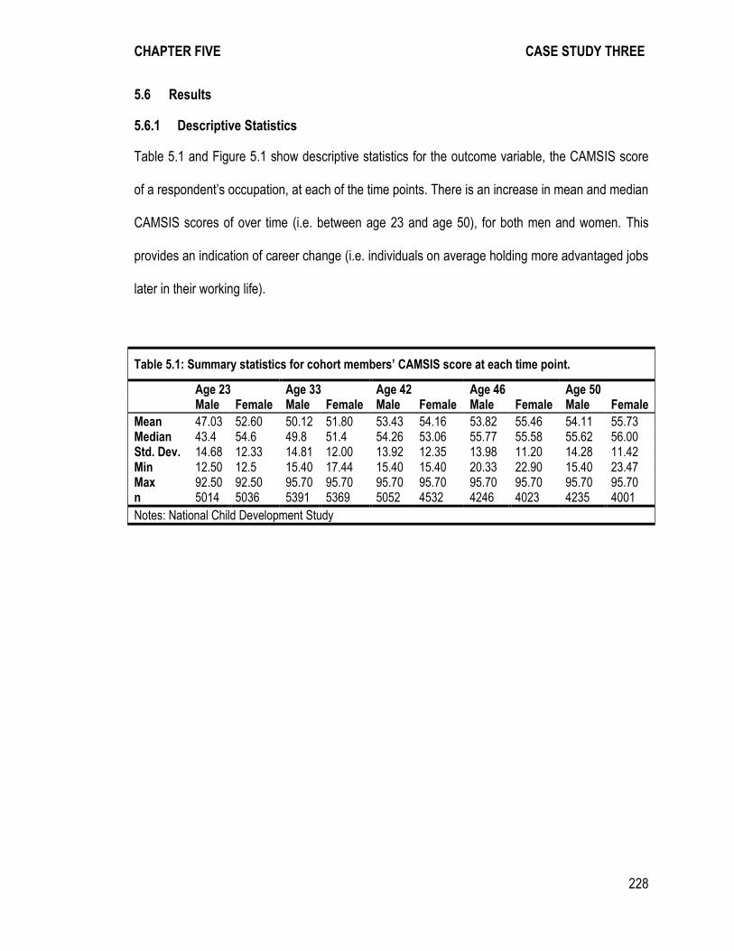
CHAPTER FIVE CASE STUDY THREE
228
5.6 Results
5.6.1 Descriptive Statistics
Table 5.1 and Figure 5.1 show descriptive statistics for the outcome variable, the CAMSIS score
of a respondent’s occupation, at each of the time points. There is an increase in mean and median
CAMSIS scores of over time (i.e. between age 23 and age 50), for both men and women. This
provides an indication of career change (i.e. individuals on average holding more advantaged jobs
later in their working life).
Table 5.1: Summary statistics for cohort members’ CAMSIS score at each time point.
Age 23 Age 33 Age 42 Age 46 Age 50 Male Female Male Female Male Female Male Female Male Female
Mean 47.03 52.60 50.12 51.80 53.43 54.16 53.82 55.46 54.11 55.73 Median 43.4 54.6 49.8 51.4 54.26 53.06 55.77 55.58 55.62 56.00 Std. Dev. 14.68 12.33 14.81 12.00 13.92 12.35 13.98 11.20 14.28 11.42 Min 12.50 12.5 15.40 17.44 15.40 15.40 20.33 22.90 15.40 23.47 Max 92.50 92.50 95.70 95.70 95.70 95.70 95.70 95.70 95.70 95.70 n 5014 5036 5391 5369 5052 4532 4246 4023 4235 4001
Notes: National Child Development Study
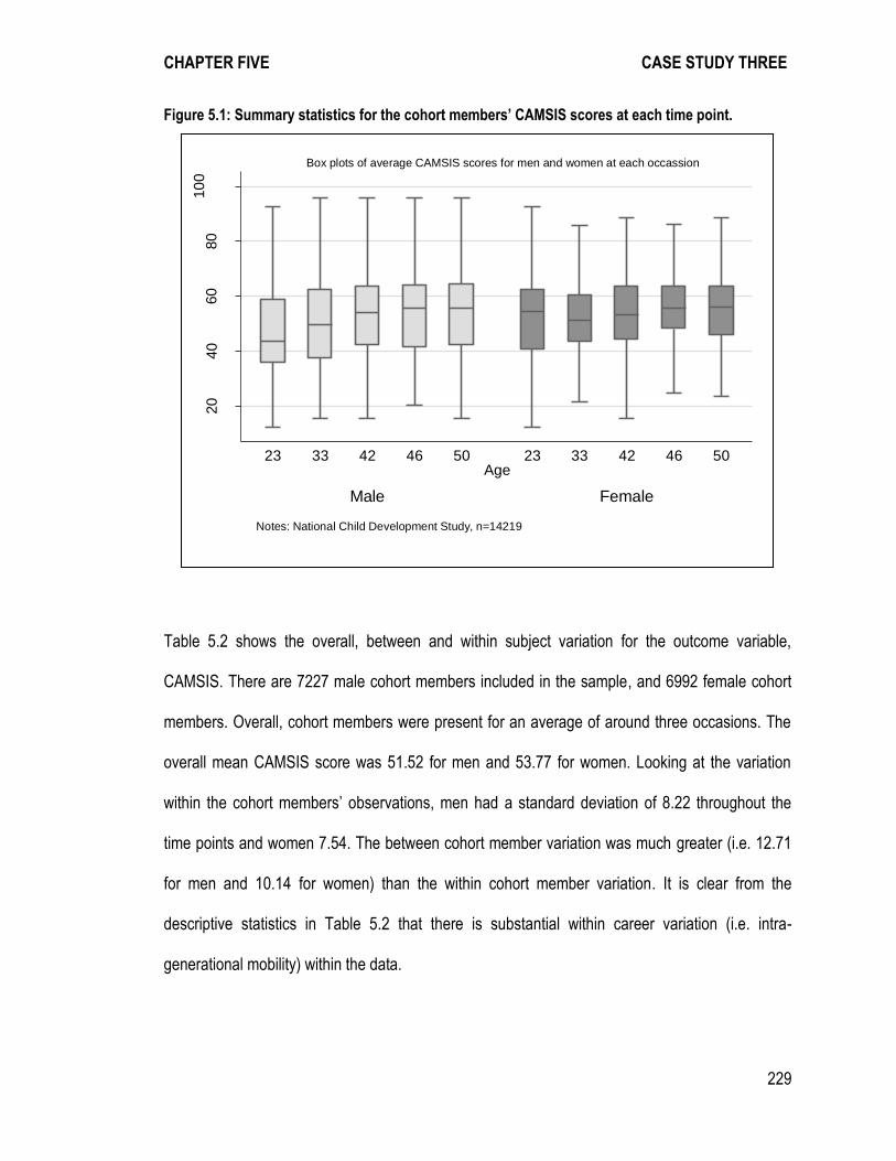
CHAPTER FIVE CASE STUDY THREE
229
Figure 5.1: Summary statistics for the cohort members’ CAMSIS scores at each time point.
Table 5.2 shows the overall, between and within subject variation for the outcome variable,
CAMSIS. There are 7227 male cohort members included in the sample, and 6992 female cohort
members. Overall, cohort members were present for an average of around three occasions. The
overall mean CAMSIS score was 51.52 for men and 53.77 for women. Looking at the variation
within the cohort members’ observations, men had a standard deviation of 8.22 throughout the
time points and women 7.54. The between cohort member variation was much greater (i.e. 12.71
for men and 10.14 for women) than the within cohort member variation. It is clear from the
descriptive statistics in Table 5.2 that there is substantial within career variation (i.e. intra-
generational mobility) within the data.
20
40
60
80
10
0
Ave
rag
e C
AM
SIS
Sco
re
Male Female
23 33 42 46 50 23 33 42 46 50Age
Notes: National Child Development Study, n=14219
Box plots of average CAMSIS scores for men and women at each occassion
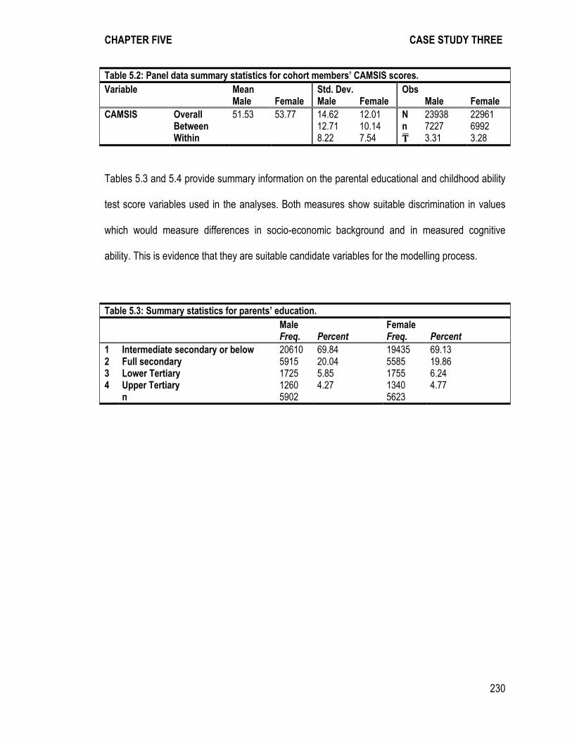
CHAPTER FIVE CASE STUDY THREE
230
Table 5.2: Panel data summary statistics for cohort members’ CAMSIS scores.
Variable Mean Std. Dev. Obs Male Female Male Female Male Female
CAMSIS Overall 51.53 53.77 14.62 12.01 N 23938 22961 Between 12.71 10.14 n 7227 6992 Within 8.22 7.54 3.31 3.28
Tables 5.3 and 5.4 provide summary information on the parental educational and childhood ability
test score variables used in the analyses. Both measures show suitable discrimination in values
which would measure differences in socio-economic background and in measured cognitive
ability. This is evidence that they are suitable candidate variables for the modelling process.
Table 5.3: Summary statistics for parents’ education.
Male Female Freq. Percent Freq. Percent
1 Intermediate secondary or below 20610 69.84 19435 69.13 2 Full secondary 5915 20.04 5585 19.86 3 Lower Tertiary 1725 5.85 1755 6.24 4 Upper Tertiary 1260 4.27 1340 4.77 n 5902 5623

CHAPTER FIVE CASE STUDY THREE
231
Table 5.4: Summary statistics for ability test scores.
Male Female
Mean -0.07 0.07 Median -0.06 0.13 Std. Dev. 1.01 0.98 Min -2.66 -2.66 Max 2.23 2.29 n 7254 6878
Notes: The cohort members’ ability test scores have been standardised to a mean of 0 and a standard deviation of 1.
Tables 5.5 and 5.6 summarise the relatively complicated data on the cohort members’ educational
attainment which is used in the models. It can be seen that in comparison with the educational
levels of the cohort members’ parents (Table 5.3), cohort members hold relatively higher levels of
educational qualifications (Table 5.5). Variation across the life-course in educational attainment,
though incorporated in the modelling strategy, is relatively slight. In Table 5.5 only minor changes
in the overall distribution of qualifications over time are apparent.
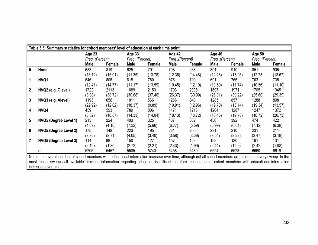
232
Table 5.5: Summary statistics for cohort members’ level of education at each time point.
Age 23 Age 33 Age 42 Age 46 Age 50 Freq .(Percent) Freq .(Percent) Freq .(Percent) Freq .(Percent) Freq .(Percent) Male Female Male Female Male Female Male Female Male Female
0 None 683 (13.12)
819 (15.01)
625 (11.35)
791 (13.78)
798 (12.36)
938 (14.48)
801 (12.28)
910 (13.95)
851 (12.78)
905 (13.67)
1 NVQ1 646 (12.41)
806 (14.77)
615 (11.17)
780 (13.59)
675 (10.45)
790 (12.19)
691 (10.59)
766 (11.74)
703 (10.56)
735 (11.10)
2 NVQ2 (e.g. Olevel) 1722 (3.08)
2113 (38.72)
1689 (30.68)
2150 (37.46)
1703 (26.37)
2008 (30.99)
1697 (26.01)
1971 (30.22)
1705 (25.60)
1945 (29.39)
3 NVQ3 (e.g. Alevel) 1193 (22.92)
656 (12.02)
1011 (18.37)
566 (9.89)
1286 (19.91)
840 (12.96)
1285 (19.70)
857 (13.14)
1288 (19.34)
898 (13.57)
4 NVQ4 459 (8.82)
593 (10.87)
789 (14.33)
806 (14.04)
1171 (18.13)
1213 (18.72)
1204 (18.45)
1287 (19.73)
1247 (18.72)
1372 (20.73)
5 NVQ5 (Degree Level 1) 213 (4.09)
224 (4.10)
403 (7.32)
325 (5.66)
437 (6.77)
362 (5.59)
456 (6.99)
392 (6.01)
474 (7.12)
422 (6.38)
6 NVQ5 (Degree Level 2) 175 (3.36)
148 (2.71)
223 (4.05)
195 (3.40)
231 (3.58)
200 (3.09)
231 (3.54)
210 (3.22)
231 (3.47)
211 (3.19)
7 NVQ5 (Degree Level 3) 114 (2.19)
98 (1.80)
150 (2.72)
127 (2.21)
157 (2.43)
129 (1.99)
159 (2.44)
130 (1.99)
161 (2.42)
131 (1.98)
n 5205 5457 5505 5740 6458 6480 6524 6523 6660 6619
Notes: the overall number of cohort members with educational information increase over time, although not all cohort members are present in every sweep. In the most recent sweeps all available previous information regarding education is utilised therefore the number of cohort members with educational information increases over time.
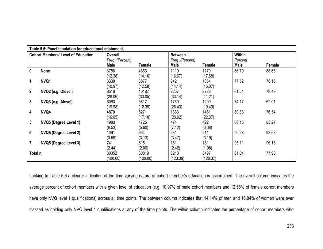
233
Table 5.6: Panel tabulation for educational attainment.
Cohort Members’ Level of Education Overall Between Within Freq .(Percent) Freq .(Percent) Percent Male Female Male Female Male Female
0 None 3758 (12.38)
4363 (14.16)
1110 (16.67)
1170 (17.68)
86.79 88.68
1 NVQ1 3330 (10.97)
3877 (12.58)
942 (14.14)
1064 (16.07)
77.52 78.16
2 NVQ2 (e.g. Olevel) 8516 (28.06)
10187 (33.05)
2207 (33.14)
2728 (41.21)
81.51 78.49
3 NVQ3 (e.g. Alevel) 6063 (19.98)
3817 (12.39)
1760 (26.43)
1290 (19.49)
74.17 62.01
4 NVQ4 4870 (16.05)
5271 (17.10)
1333 (20.02)
1481 (22.37)
80.88 76.54
5 NVQ5 (Degree Level 1) 1983 (6.53)
1725 (5.60)
474 (7.12)
422 (6.38)
86.15 83.27
6 NVQ5 (Degree Level 2) 1091 (3.59)
964 (3.13)
231 (3.47)
211 (3.19)
96.28 93.68
7 NVQ5 (Degree Level 3) 741 (2.44)
615 (2.00)
161 (2.42)
131 (1.98)
95.11 96.18
Total n 30352 (100.00)
30819 (100.00)
8218 (123.39)
8497 (128.37)
81.04 77.90
Looking to Table 5.6 a clearer indication of the time-varying nature of cohort member’s education is ascertained. The overall column indicates the
average percent of cohort members with a given level of education (e.g. 10.97% of male cohort members and 12.58% of female cohort members
have only NVQ level 1 qualifications) across all time points. The between column indicates that 14.14% of men and 16.04% of women were ever
classed as holding only NVQ level 1 qualifications at any of the time points. The within column indicates the percentage of cohort members who
234
have always held a given level of education, across all time points. Overall, 77.52% of men and 78.16% of women have held NVQ level 1 qualifica-
tions at every time point. High internal stability in educational levels is apparent, and there are only a low number of occurrences of individuals
holding more than one educational level (i.e. improving their educational level) at different points in time.
5.6.2 Analyses in a Cross-Sectional Framework
As the first stage in the modelling process, ‘cross-sectional’ models of the CAMSIS scores of the cohort members are estimated. For each time point
(i.e. ages 23, 33, 42, 46 and 50) a standard linear regression model was estimated for the cohort members’ CAMSIS score at that age. The full
regression results are reported in Table 5.7 for men and Table 5.8 for women. For male cohort members’ father’s CAMSIS scores, cohort member’s
education and ability all exerted positive significant effects on CAMSIS scores at each of the five ages. For women educational attainment and
cognitive ability variables also exerted a positive significant relationship at each time point. However for women at ages 42, 46 and age 50 father’s
CAMSIS score was no longer significant. This finding provides tentative evidence to support the hypothesis that the association between social
background and occupational positions will weaken across the lifecourse. Furthermore evidence is also found, in line with the findings of Hauser
Sheridan and Warren (1999), Warren, Hauser and Sheridan (2002) and Warren (2001), that social origins may continue to exert an effect on
occupational outcomes at these later stages of the lifecourse indirectly through education. Ordered Logistic Regression Models were also estimated
for the educational attainment of the cohort members (Table 5.9), these models indicated that, educational attainment was significantly influenced by

235
father’s CAMSIS score and ability. Notably far clearer patterns are apparent in the influence of parental education on cohort members education in
comparison with the attainment of occupational positions.
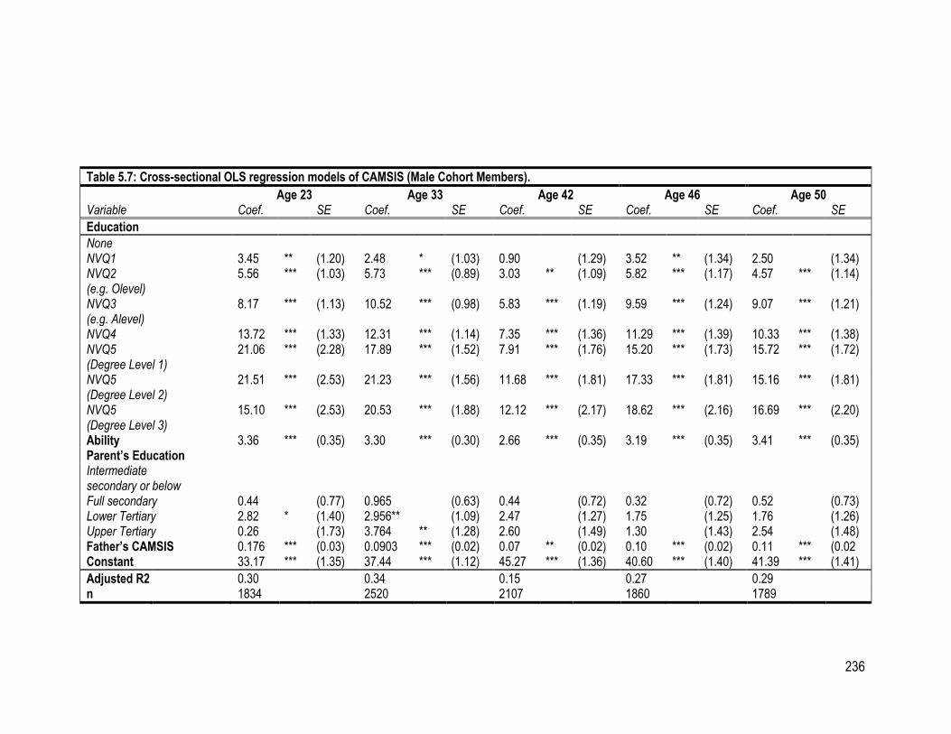
236
Table 5.7: Cross-sectional OLS regression models of CAMSIS (Male Cohort Members).
Age 23 Age 33 Age 42 Age 46 Age 50 Variable Coef. SE Coef. SE Coef. SE Coef. SE Coef. SE
Education
None NVQ1 3.45 ** (1.20) 2.48 * (1.03) 0.90 (1.29) 3.52 ** (1.34) 2.50 (1.34) NVQ2 (e.g. Olevel)
5.56 *** (1.03) 5.73 *** (0.89) 3.03 ** (1.09) 5.82 *** (1.17) 4.57 *** (1.14)
NVQ3 (e.g. Alevel)
8.17 *** (1.13) 10.52 *** (0.98) 5.83 *** (1.19) 9.59 *** (1.24) 9.07 *** (1.21)
NVQ4 13.72 *** (1.33) 12.31 *** (1.14) 7.35 *** (1.36) 11.29 *** (1.39) 10.33 *** (1.38) NVQ5 (Degree Level 1)
21.06 *** (2.28) 17.89 *** (1.52) 7.91 *** (1.76) 15.20 *** (1.73) 15.72 *** (1.72)
NVQ5 (Degree Level 2)
21.51 *** (2.53) 21.23 *** (1.56) 11.68 *** (1.81) 17.33 *** (1.81) 15.16 *** (1.81)
NVQ5 (Degree Level 3)
15.10 *** (2.53) 20.53 *** (1.88) 12.12 *** (2.17) 18.62 *** (2.16) 16.69 *** (2.20)
Ability 3.36 *** (0.35) 3.30 *** (0.30) 2.66 *** (0.35) 3.19 *** (0.35) 3.41 *** (0.35) Parent’s Education Intermediate secondary or below
Full secondary 0.44 (0.77) 0.965 (0.63) 0.44 (0.72) 0.32 (0.72) 0.52 (0.73) Lower Tertiary 2.82 * (1.40) 2.956** (1.09) 2.47 (1.27) 1.75 (1.25) 1.76 (1.26) Upper Tertiary 0.26 (1.73) 3.764 ** (1.28) 2.60 (1.49) 1.30 (1.43) 2.54 (1.48) Father’s CAMSIS 0.176 *** (0.03) 0.0903 *** (0.02) 0.07 ** (0.02) 0.10 *** (0.02) 0.11 *** (0.02 Constant 33.17 *** (1.35) 37.44 *** (1.12) 45.27 *** (1.36) 40.60 *** (1.40) 41.39 *** (1.41)
Adjusted R2 0.30 0.34 0.15 0.27 0.29 n 1834 2520 2107 1860 1789
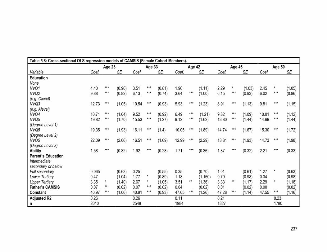
237
Table 5.8: Cross-sectional OLS regression models of CAMSIS (Female Cohort Members).
Age 23 Age 33 Age 42 Age 46 Age 50 Variable Coef. SE Coef. SE Coef. SE Coef. SE Coef. SE
Education None NVQ1 4.40 *** (0.90) 3.51 *** (0.81) 1.96 (1.11) 2.29 * (1.03) 2.45 * (1.05) NVQ2 (e.g. Olevel)
9.88 *** (0.82) 6.13 *** (0.74) 3.64 *** (1.00) 6.15 *** (0.93) 6.02 *** (0.96)
NVQ3 (e.g. Alevel)
12.73 *** (1.05) 10.54 *** (0.93) 5.93 *** (1.23) 8.91 *** (1.13) 9.81 *** (1.15)
NVQ4 10.71 *** (1.04) 9.52 *** (0.92) 6.49 *** (1.21) 9.82 *** (1.09) 10.01 *** (1.12) NVQ5 (Degree Level 1)
19.82 *** (1.70) 15.53 *** (1.27) 9.12 *** (1.62) 13.80 *** (1.44) 14.69 *** (1.44)
NVQ5 (Degree Level 2)
19.35 *** (1.93) 16.11 *** (1.4) 10.05 *** (1.89) 14.74 *** (1.67) 15.30 *** (1.72)
NVQ5 (Degree Level 3)
22.09 *** (2.66) 16.51 *** (1.69) 12.99 *** (2.29) 13.81 *** (1.93) 14.73 *** (1.98)
Ability 1.58 *** (0.32) 1.92 *** (0.28) 1.71 *** (0.36) 1.87 *** (0.32) 2.21 *** (0.33) Parent’s Education Intermediate secondary or below
Full secondary 0.065 (0.63) 0.25 (0.55) 0.35 (0.70) 1.01 (0.61) 1.27 * (0.63) Lower Tertiary 0.47 (1.04) 1.77 * (0.89) 1.18 (1.160) 0.79 (0.98) 0.34 (0.98) Upper Tertiary 3.35 * (1.40) 2.67 * (1.05) 3.51 ** (1.36) 3.33 ** (1.17) 2.29 * (1.18) Father’s CAMSIS 0.07 ** (0.02) 0.07 *** (0.02) 0.04 (0.02) 0.01 (0.02) 0.00 (0.02) Constant 40.97 *** (1.06) 40.91 *** (0.93) 47.05 *** (1.26) 47.28 *** (1.14) 47.55 *** (1.16)
Adjusted R2 0.26 0.26 0.11 0.21 0.23 n 2010 2548 1984 1827 1780
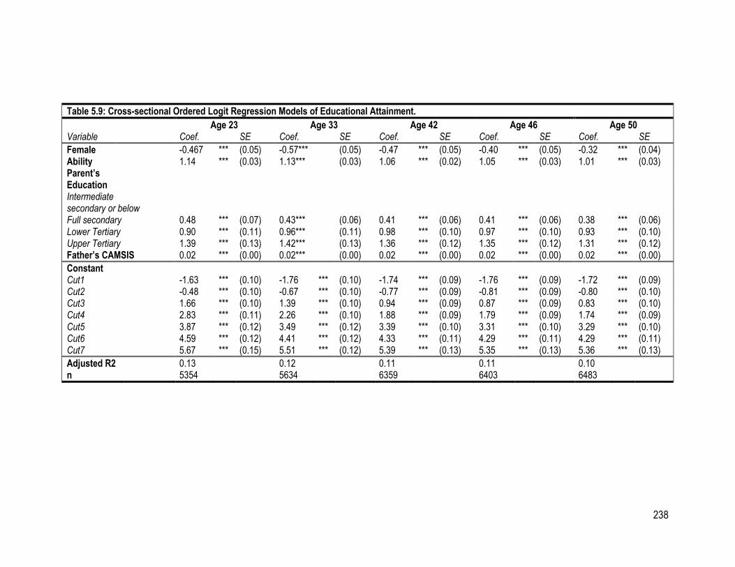
238
Table 5.9: Cross-sectional Ordered Logit Regression Models of Educational Attainment.
Age 23 Age 33 Age 42 Age 46 Age 50 Variable Coef. SE Coef. SE Coef. SE Coef. SE Coef. SE
Female -0.467 *** (0.05) -0.57*** (0.05) -0.47 *** (0.05) -0.40 *** (0.05) -0.32 *** (0.04) Ability 1.14 *** (0.03) 1.13*** (0.03) 1.06 *** (0.02) 1.05 *** (0.03) 1.01 *** (0.03) Parent’s Education
Intermediate secondary or below
Full secondary 0.48 *** (0.07) 0.43*** (0.06) 0.41 *** (0.06) 0.41 *** (0.06) 0.38 *** (0.06) Lower Tertiary 0.90 *** (0.11) 0.96*** (0.11) 0.98 *** (0.10) 0.97 *** (0.10) 0.93 *** (0.10) Upper Tertiary 1.39 *** (0.13) 1.42*** (0.13) 1.36 *** (0.12) 1.35 *** (0.12) 1.31 *** (0.12) Father’s CAMSIS 0.02 *** (0.00) 0.02*** (0.00) 0.02 *** (0.00) 0.02 *** (0.00) 0.02 *** (0.00)
Constant Cut1 -1.63 *** (0.10) -1.76 *** (0.10) -1.74 *** (0.09) -1.76 *** (0.09) -1.72 *** (0.09) Cut2 -0.48 *** (0.10) -0.67 *** (0.10) -0.77 *** (0.09) -0.81 *** (0.09) -0.80 *** (0.10) Cut3 1.66 *** (0.10) 1.39 *** (0.10) 0.94 *** (0.09) 0.87 *** (0.09) 0.83 *** (0.10) Cut4 2.83 *** (0.11) 2.26 *** (0.10) 1.88 *** (0.09) 1.79 *** (0.09) 1.74 *** (0.09) Cut5 3.87 *** (0.12) 3.49 *** (0.12) 3.39 *** (0.10) 3.31 *** (0.10) 3.29 *** (0.10) Cut6 4.59 *** (0.12) 4.41 *** (0.12) 4.33 *** (0.11) 4.29 *** (0.11) 4.29 *** (0.11) Cut7 5.67 *** (0.15) 5.51 *** (0.12) 5.39 *** (0.13) 5.35 *** (0.13) 5.36 *** (0.13)
Adjusted R2 0.13 0.12 0.11 0.11 0.10 n 5354 5634 6359 6403 6483
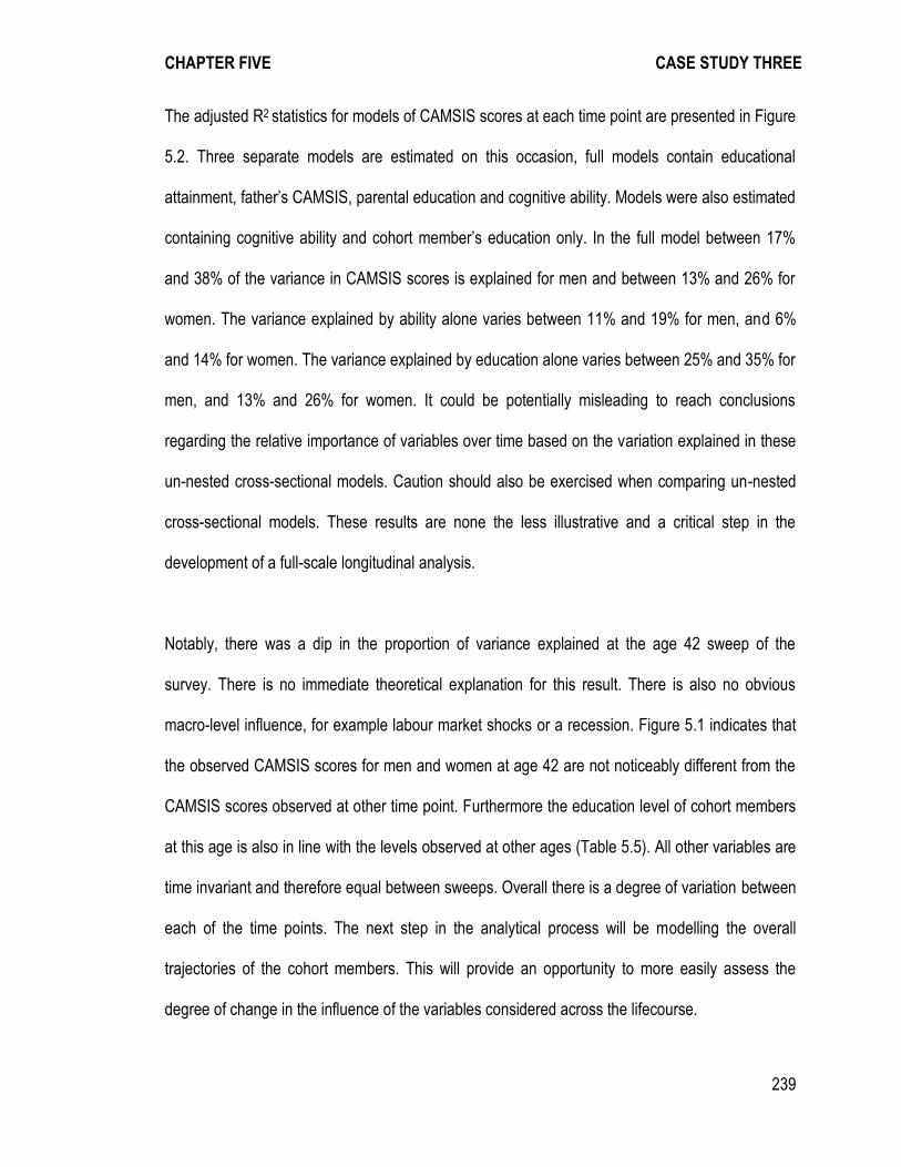
CHAPTER FIVE CASE STUDY THREE
239
The adjusted R2 statistics for models of CAMSIS scores at each time point are presented in Figure
5.2. Three separate models are estimated on this occasion, full models contain educational
attainment, father’s CAMSIS, parental education and cognitive ability. Models were also estimated
containing cognitive ability and cohort member’s education only. In the full model between 17%
and 38% of the variance in CAMSIS scores is explained for men and between 13% and 26% for
women. The variance explained by ability alone varies between 11% and 19% for men, and 6%
and 14% for women. The variance explained by education alone varies between 25% and 35% for
men, and 13% and 26% for women. It could be potentially misleading to reach conclusions
regarding the relative importance of variables over time based on the variation explained in these
un-nested cross-sectional models. Caution should also be exercised when comparing un-nested
cross-sectional models. These results are none the less illustrative and a critical step in the
development of a full-scale longitudinal analysis.
Notably, there was a dip in the proportion of variance explained at the age 42 sweep of the
survey. There is no immediate theoretical explanation for this result. There is also no obvious
macro-level influence, for example labour market shocks or a recession. Figure 5.1 indicates that
the observed CAMSIS scores for men and women at age 42 are not noticeably different from the
CAMSIS scores observed at other time point. Furthermore the education level of cohort members
at this age is also in line with the levels observed at other ages (Table 5.5). All other variables are
time invariant and therefore equal between sweeps. Overall there is a degree of variation between
each of the time points. The next step in the analytical process will be modelling the overall
trajectories of the cohort members. This will provide an opportunity to more easily assess the
degree of change in the influence of the variables considered across the lifecourse.
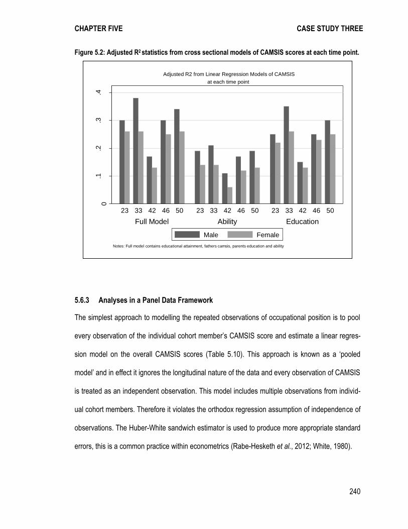
CHAPTER FIVE CASE STUDY THREE
240
Figure 5.2: Adjusted R2 statistics from cross sectional models of CAMSIS scores at each time point.
5.6.3 Analyses in a Panel Data Framework
The simplest approach to modelling the repeated observations of occupational position is to pool
every observation of the individual cohort member’s CAMSIS score and estimate a linear regres-
sion model on the overall CAMSIS scores (Table 5.10). This approach is known as a ‘pooled
model’ and in effect it ignores the longitudinal nature of the data and every observation of CAMSIS
is treated as an independent observation. This model includes multiple observations from individ-
ual cohort members. Therefore it violates the orthodox regression assumption of independence of
observations. The Huber-White sandwich estimator is used to produce more appropriate standard
errors, this is a common practice within econometrics (Rabe-Hesketh et al., 2012; White, 1980).
0.1
.2.3
.4
Adju
ste
d R
2
Full Model Ability Education
23 33 42 46 50 23 33 42 46 50 23 33 42 46 50
Notes: Full model contains educational attainment, fathers camsis, parents education and ability
at each time point
Adjusted R2 from Linear Regression Models of CAMSIS
Male Female

CHAPTER FIVE CASE STUDY THREE
241
Table 5.10 presents the results of the pooled regression model of CAMSIS scores across all time
points. The model indicates that higher levels of education are associated with higher CAMSIS
scores, education also seems to exert the largest independent influence on occupational posi-
tions. This is in line with previous research such as Muller and Shavit (see Muller and Shavit,
1998) which has described education as the main moderator in the process of social stratification.
In line with the previous literature cognitive ability also demonstrated a significant positive associa-
tion with CAMSIS scores. Parents’ education and fathers’ CAMSIS scores are also significantly
associated with CAMSIS scores in adulthood.
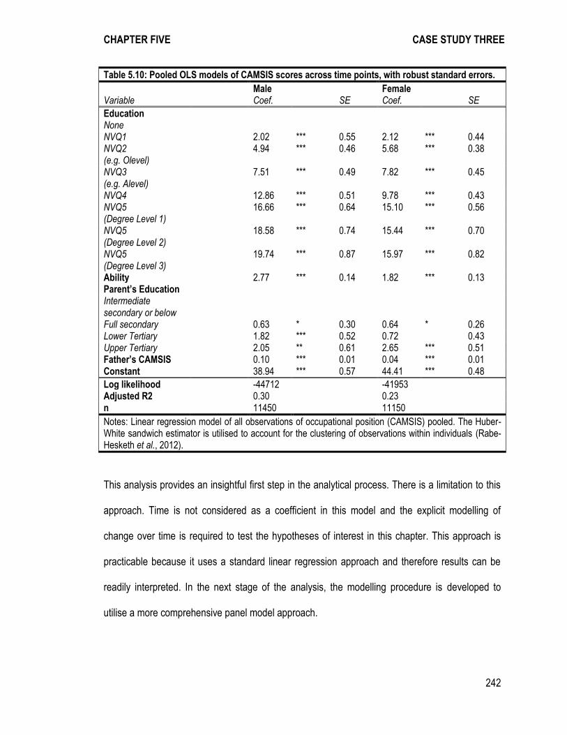
CHAPTER FIVE CASE STUDY THREE
242
Table 5.10: Pooled OLS models of CAMSIS scores across time points, with robust standard errors.
Male Female Variable Coef. SE Coef. SE
Education None NVQ1 2.02 *** 0.55 2.12 *** 0.44 NVQ2 (e.g. Olevel)
4.94 *** 0.46 5.68 *** 0.38
NVQ3 (e.g. Alevel)
7.51 *** 0.49 7.82 *** 0.45
NVQ4 12.86 *** 0.51 9.78 *** 0.43 NVQ5 (Degree Level 1)
16.66 *** 0.64 15.10 *** 0.56
NVQ5 (Degree Level 2)
18.58 *** 0.74 15.44 *** 0.70
NVQ5 (Degree Level 3)
19.74 *** 0.87 15.97 *** 0.82
Ability 2.77 *** 0.14 1.82 *** 0.13 Parent’s Education Intermediate secondary or below
Full secondary 0.63 * 0.30 0.64 * 0.26 Lower Tertiary 1.82 *** 0.52 0.72 0.43 Upper Tertiary 2.05 ** 0.61 2.65 *** 0.51 Father’s CAMSIS 0.10 *** 0.01 0.04 *** 0.01 Constant 38.94 *** 0.57 44.41 *** 0.48
Log likelihood -44712 -41953 Adjusted R2 0.30 0.23 n 11450 11150
Notes: Linear regression model of all observations of occupational position (CAMSIS) pooled. The Huber-White sandwich estimator is utilised to account for the clustering of observations within individuals (Rabe-Hesketh et al., 2012).
This analysis provides an insightful first step in the analytical process. There is a limitation to this
approach. Time is not considered as a coefficient in this model and the explicit modelling of
change over time is required to test the hypotheses of interest in this chapter. This approach is
practicable because it uses a standard linear regression approach and therefore results can be
readily interpreted. In the next stage of the analysis, the modelling procedure is developed to
utilise a more comprehensive panel model approach.
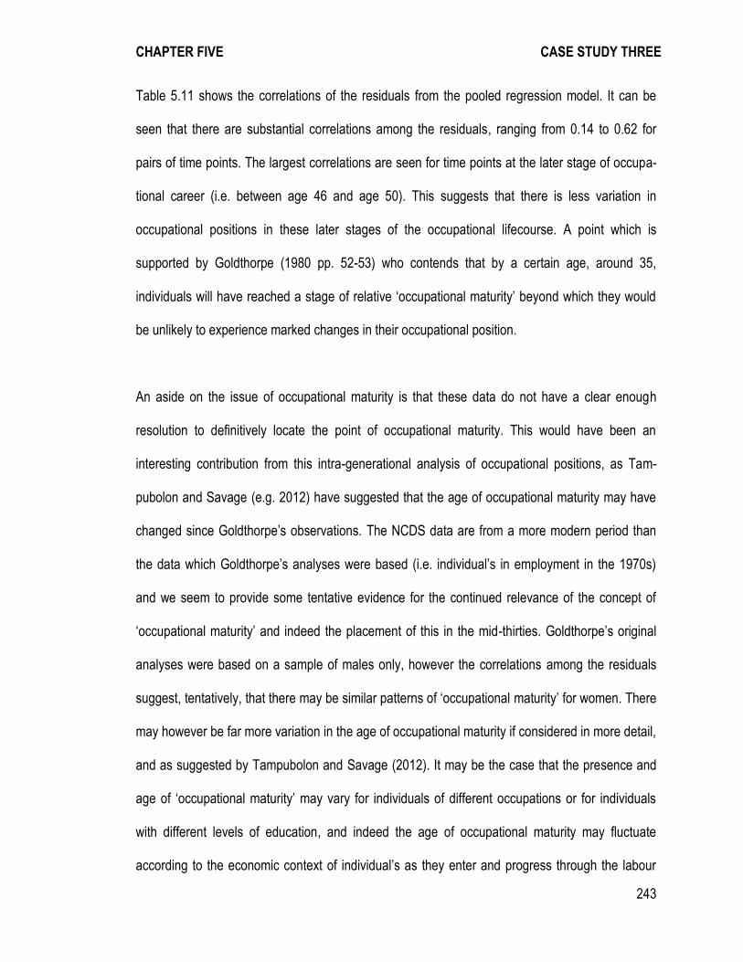
CHAPTER FIVE CASE STUDY THREE
243
Table 5.11 shows the correlations of the residuals from the pooled regression model. It can be
seen that there are substantial correlations among the residuals, ranging from 0.14 to 0.62 for
pairs of time points. The largest correlations are seen for time points at the later stage of occupa-
tional career (i.e. between age 46 and age 50). This suggests that there is less variation in
occupational positions in these later stages of the occupational lifecourse. A point which is
supported by Goldthorpe (1980 pp. 52-53) who contends that by a certain age, around 35,
individuals will have reached a stage of relative ‘occupational maturity’ beyond which they would
be unlikely to experience marked changes in their occupational position.
An aside on the issue of occupational maturity is that these data do not have a clear enough
resolution to definitively locate the point of occupational maturity. This would have been an
interesting contribution from this intra-generational analysis of occupational positions, as Tam-
pubolon and Savage (e.g. 2012) have suggested that the age of occupational maturity may have
changed since Goldthorpe’s observations. The NCDS data are from a more modern period than
the data which Goldthorpe’s analyses were based (i.e. individual’s in employment in the 1970s)
and we seem to provide some tentative evidence for the continued relevance of the concept of
‘occupational maturity’ and indeed the placement of this in the mid-thirties. Goldthorpe’s original
analyses were based on a sample of males only, however the correlations among the residuals
suggest, tentatively, that there may be similar patterns of ‘occupational maturity’ for women. There
may however be far more variation in the age of occupational maturity if considered in more detail,
and as suggested by Tampubolon and Savage (2012). It may be the case that the presence and
age of ‘occupational maturity’ may vary for individuals of different occupations or for individuals
with different levels of education, and indeed the age of occupational maturity may fluctuate
according to the economic context of individual’s as they enter and progress through the labour
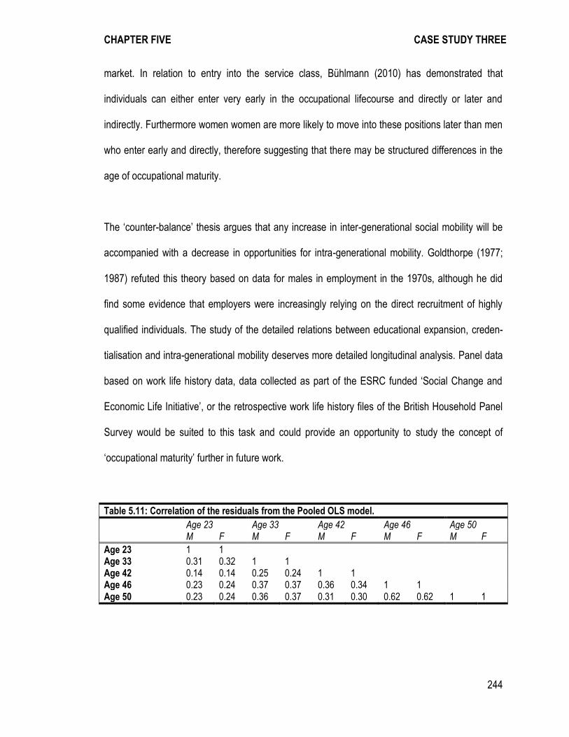
CHAPTER FIVE CASE STUDY THREE
244
market. In relation to entry into the service class, Bühlmann (2010) has demonstrated that
individuals can either enter very early in the occupational lifecourse and directly or later and
indirectly. Furthermore women women are more likely to move into these positions later than men
who enter early and directly, therefore suggesting that there may be structured differences in the
age of occupational maturity.
The ‘counter-balance’ thesis argues that any increase in inter-generational social mobility will be
accompanied with a decrease in opportunities for intra-generational mobility. Goldthorpe (1977;
1987) refuted this theory based on data for males in employment in the 1970s, although he did
find some evidence that employers were increasingly relying on the direct recruitment of highly
qualified individuals. The study of the detailed relations between educational expansion, creden-
tialisation and intra-generational mobility deserves more detailed longitudinal analysis. Panel data
based on work life history data, data collected as part of the ESRC funded ‘Social Change and
Economic Life Initiative’, or the retrospective work life history files of the British Household Panel
Survey would be suited to this task and could provide an opportunity to study the concept of
‘occupational maturity’ further in future work.
Table 5.11: Correlation of the residuals from the Pooled OLS model.
Age 23 Age 33 Age 42 Age 46 Age 50 M F M F M F M F M F
Age 23 1 1 Age 33 0.31 0.32 1 1 Age 42 0.14 0.14 0.25 0.24 1 1 Age 46 0.23 0.24 0.37 0.37 0.36 0.34 1 1 Age 50 0.23 0.24 0.36 0.37 0.31 0.30 0.62 0.62 1 1

CHAPTER FIVE CASE STUDY THREE
245
5.6.3.1 Growth Curve Models
The analyses now move to a multilevel framework, and specifically to the use of growth curve
models described above (Section 5.5.2). Growth curve models attempt to estimate “between-
person differences in within-person change” (Curran et al., 2010a, p. 121). Growth curve models
explicitly model the trajectories of individuals over time and can be used to indicate how trajecto-
ries differ in relation to covariates (e.g. cognitive ability, social origins and education). A random
coefficient growth curve model is estimated which allows for individual specific regression lines
(i.e. slopes) and individual specific intercepts. A model is first estimated with main effects only, for
men and women separately, and then interaction terms are included to investigate how the effects
of the key covariates (i.e. cognitive ability, education and father’s CAMSIS) change between the
observed ages (see Table 5.12 for men and Table 5.13 for women).
The first task, in specifying the growth curve models was to consider the shape of the sample’s
average trajectories of CAMSIS scores over time. Figure 5.3 shows the spread of CAMSIS scores
at each time point, with the mean overall trajectory of the sample, and the trajectories of 15
randomly chosen cohort members. It is apparent that there is variability in CAMSIS scores
between individuals at each time point, and there is also variability over time in the way the cohort
members’ CAMSIS scores are changing. Some individual’s are increasing their CAMSIS over
time, some are decreasing and some have stable intra-generational trajectories. Some cohort
members have highly volatile trajectories. The overall mean trajectory indicates an increase in
CAMSIS scores over time (also shown in Figure 5.1). However the variable nature of the individual
trajectories emphasises the need to utilise a modelling approach which allows for variation in the
intercepts and slopes for each cohort member.
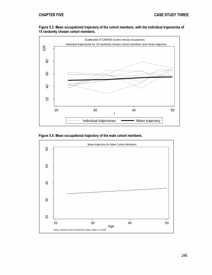
CHAPTER FIVE CASE STUDY THREE
246
Figure 5.3: Mean occupational trajectory of the cohort members, with the individual trajectories of 15 randomly chosen cohort members.
Figure 5.4: Mean occupational trajectory of the male cohort members.
20
40
60
80
10
0
CA
MS
IS
20 30 40 50t
Individual trajectories Mean trajectory
Notes: National Child Development Study, n=14219
individual trajectories for 15 randomly chosen cohort members and mean trajectory
Scatterplot of CAMSIS scores versus occassions;
20
30
40
50
60
CA
MS
IS
20 30 40 50Age
Notes: National Child Development Study, Males, n=11450
Mean trajectory for Male Cohort Members
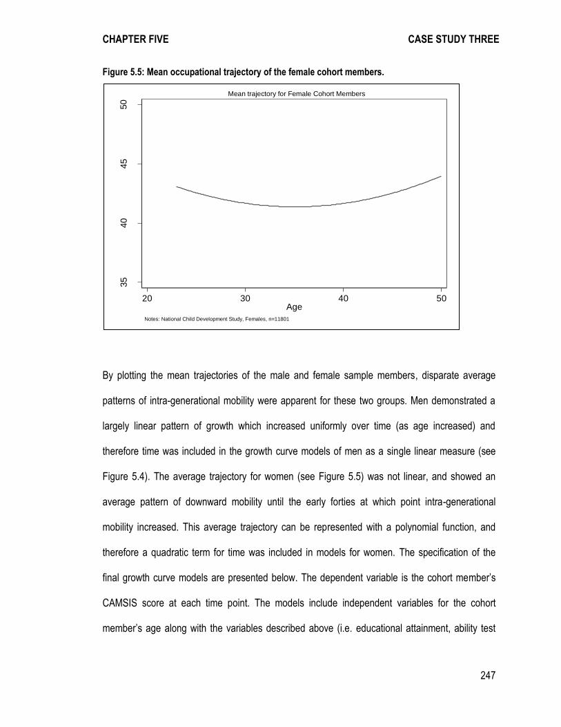
CHAPTER FIVE CASE STUDY THREE
247
Figure 5.5: Mean occupational trajectory of the female cohort members.
By plotting the mean trajectories of the male and female sample members, disparate average
patterns of intra-generational mobility were apparent for these two groups. Men demonstrated a
largely linear pattern of growth which increased uniformly over time (as age increased) and
therefore time was included in the growth curve models of men as a single linear measure (see
Figure 5.4). The average trajectory for women (see Figure 5.5) was not linear, and showed an
average pattern of downward mobility until the early forties at which point intra-generational
mobility increased. This average trajectory can be represented with a polynomial function, and
therefore a quadratic term for time was included in models for women. The specification of the
final growth curve models are presented below. The dependent variable is the cohort member’s
CAMSIS score at each time point. The models include independent variables for the cohort
member’s age along with the variables described above (i.e. educational attainment, ability test
35
40
45
50
CA
MS
IS
20 30 40 50Age
Notes: National Child Development Study, Females, n=11801
Mean trajectory for Female Cohort Members
CHAPTER FIVE CASE STUDY THREE
248
score, parent’s highest education and father’s CAMSIS). The subscript ‘i’ refers to the individual
cohort member and ‘t’ refers to the time point.
For Male Cohort Members:
CAMSISit = β1 + β2ageit + β3Educationt + β4Abilityt + β5Parent’sEducationt + β6Father’sCAMSISt +
U1t +U2tageit + εit
For Female Cohort Members:
CAMSISit = β1 + β2ageit + β3age2it + β4Educationt + β5Abilityt + β4Parent’sEducationt +
β4Father’sCAMSISt + U1t +U2tageit + εit
The differences between the average intra-generational trajectories for men and women, and
particularly the downward mobility of women have been highlighted in the previous literature, in
particular studies based on different measures of intra-generational mobility (i.e. pay) (e.g. Bukodi
et al., 2009; Golsch, 2006; Jacobs, 1999). The average downward mobility of women over the
lifecourse has been associated with the different social roles held by women in relation to child-
birth and parenting (see Joshi and Dex, 1999). Many commentators have attributed the downward
mobility patterns of mothers in relation to sub-optimal provision of parental leave, affordable
childcare or family friendly working arrangements (Joshi et al., 1999), whereas other sociological
perspectives have emphasised women’s choice and preferences (Hakim, 2000). It is not within the
remit of the present chapter to consider the differences between men and women in detail,
however the NCDS would provide a suitable data resource to investigate gender differences in
intra-generational mobility further.
CHAPTER FIVE CASE STUDY THREE
249
It is also plausible that differences in average trajectories may also have emerged if alternative
models were estimated. Theoretically it might be plausible to model different trajectories for cohort
members who originated from more- or less- advantaged families or those holding different
education levels, or indeed different cognitive ability groupings. Bruegel and Perrons (Bruegel and
Perrons, 1998) show that men and women are not homogenous groups and, for example, the
workplace experiences of advantaged and disadvantaged women (and mothers) have been
shown to vary greatly. Within the growth curve modelling framework additional covariates can be
introduced into the random part of the model, therefore estimating random trajectories for multiple
covariates (e.g. individuals with different educational levels).
In the next stage of the analysis attempts were made to estimate a series of more comprehensive
models that test a range of these potential effects. These models are computationally intensive. At
the current time these models can be estimated with standard statistical software such as Stata,
using the –xtmixed- family. However the NCDS dataset is large both in terms of observations, time
points and covariates. In practice these models do not converge and therefore estimates cannot
be recovered. This is routinely a problem when mass point quadrature is used to estimate models
(Jeliazkov and Lee, 2010). It is conceivable that increases in computing power may lead to a
solution to this impasse in the future. Another possibility is that software will be able to commence
searching the likelihood surface using starting values from simpler models. Another future possi-
bility is that alternative estimation procedures such as MCMC might prove a useful alternative. At
the current time this is not possible and beyond the capability of existing software and standard
computers.

CHAPTER FIVE CASE STUDY THREE
250
A further additional modelling strategy would involve the use of a lagged dependent variable (i.e. a
dynamic panel model). In this model an individual’s previous CAMSIS score would be entered as
a predictor of their current CAMSIS score at each time point. This model specification makes
theoretical sense in relation to the concept of ‘cumulative advantage’, also known as the ‘Matthew
Effect’. This concept was first demonstrated in the study of successful careers in science, and
suggests that advantages early in the career will result in even greater advantages later in the
career, as positive outcomes accrue as a result of previous success (Merton, 1968). The cumula-
tive advantage concept has proven to be informative in the study of inequalities across the
lifecourse in the German labour market (Hillmert, 2012). However, this additional complexity
resulted in the model again failing to converge, most likely for the reasons described above, and
therefore the estimates could not be recovered. This approach would also have several weak-
nessnesses when applied to the present data. First, the use of a lagged dependent variable would
only make clear sense when the spacing between time points was equal and therefore we could
interpret the influence of the lagged dependent variable uniformly across the occupational career.
The time points or ages observed in the NCDS are widely spaced and vary from as much as a 10
year gap to as little as a 4 year gap, as we would expect much more variation over 10 years than
4 years the use of a lagged dependent variable is not ideal in this scenario (Rabe-Hesketh et al.,
2012). Furthermore, a lagged dependent variable would also reduce the number of time points
available as the first time point would be missing its lag and would therefore be discarded. The
problem of missing data in this unbalanced panel model would also be very much increased with
the use of a lagged dependent variable. Cases with data missing at one time point would also
become missing at the subsequent time point due to the lack of information available to estimate
the lagged effect (Rabe-Hesketh et al., 2012).
CHAPTER FIVE CASE STUDY THREE
251
Looking now to the growth curve models (see Tables 5.12 and 5.13) the coefficients presented
first (e.g. qualification, ability, parents’ education) form the fixed part of the model, and indicate the
average association between each covariate and CAMSIS scores. In line with the results of the
cross-sectional models and pooled model education has a positive significant association with
CAMSIS scores, alongside cognitive ability, parents’ education and father’s CAMSIS for both men
and women. Only the contrast of parental education between the lowest and highest was signifi-
cant for men, and only the contrast between the lowest and the two highest parental education
categories were significant for women however.
The time variable, and time plus time squared variable for women, indicates the average trajecto-
ries which are demonstrated in Figures 5.5 and 5.6. For men (Table 5.12) the random effects
parameters indicate that there is a considerable estimated random intercept standard deviation,
the standard deviation of the constant = 12.53. The standard deviation of the residual also
indicates that there was a large deviation of the CAMSIS scores from the average slope estimated
as the constant in the fixed effects part of the mode, the standard deviation of the residual = 9.14.
The standard deviation of time indicates that the increase in CAMSIS scores over time was on
average of 0.3 standard deviations. Therefore it is apparent that the deviation between cohort
members observations is far greater than the deviation within cohort members’ observations. The
correlation with time and the constant is negative (-0.83) indicating that intra-generational gains
(i.e. CAMSIS score increases) decreased over time.
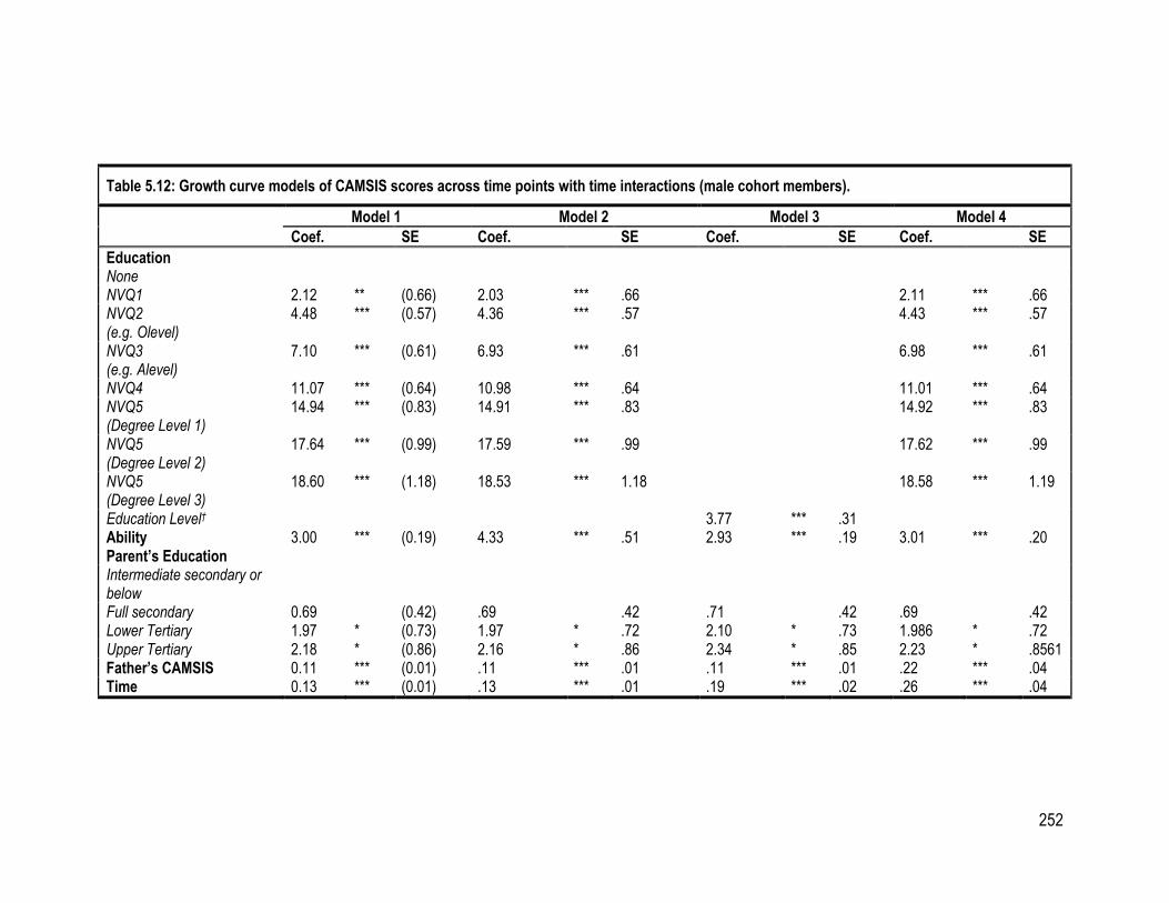
252
Table 5.12: Growth curve models of CAMSIS scores across time points with time interactions (male cohort members).
Model 1 Model 2 Model 3 Model 4
Coef. SE Coef. SE Coef. SE Coef. SE
Education None NVQ1 2.12 ** (0.66) 2.03 *** .66 2.11 *** .66 NVQ2 (e.g. Olevel)
4.48 *** (0.57) 4.36 *** .57 4.43 *** .57
NVQ3 (e.g. Alevel)
7.10 *** (0.61) 6.93 *** .61 6.98 *** .61
NVQ4 11.07 *** (0.64) 10.98 *** .64 11.01 *** .64 NVQ5 (Degree Level 1)
14.94 *** (0.83) 14.91 *** .83 14.92 *** .83
NVQ5 (Degree Level 2)
17.64 *** (0.99) 17.59 *** .99 17.62 *** .99
NVQ5 (Degree Level 3)
18.60 *** (1.18) 18.53 *** 1.18 18.58 *** 1.19
Education Level† 3.77 *** .31 Ability 3.00 *** (0.19) 4.33 *** .51 2.93 *** .19 3.01 *** .20 Parent’s Education Intermediate secondary or below
Full secondary 0.69 (0.42) .69 .42 .71 .42 .69 .42 Lower Tertiary 1.97 * (0.73) 1.97 * .72 2.10 * .73 1.986 * .72 Upper Tertiary 2.18 * (0.86) 2.16 * .86 2.34 * .85 2.23 * .8561 Father’s CAMSIS 0.11 *** (0.01) .11 *** .01 .11 *** .01 .22 *** .04 Time 0.13 *** (0.01) .13 *** .01 .19 *** .02 .26 *** .04
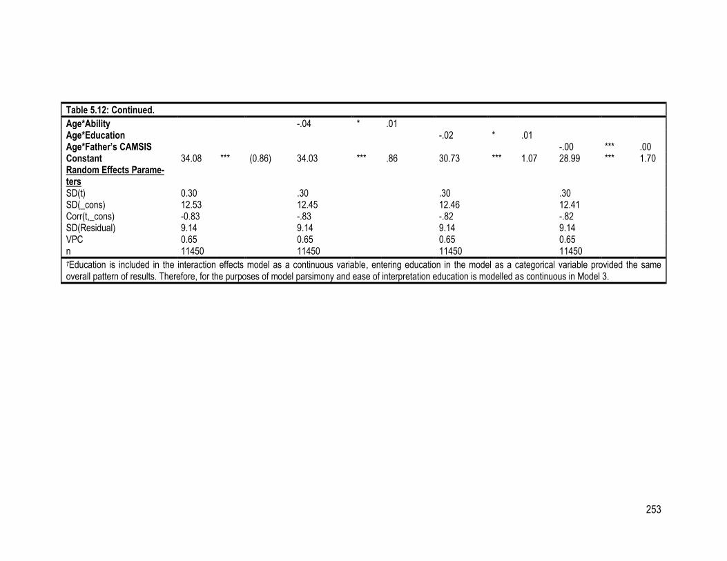
253
Table 5.12: Continued.
Age*Ability -.04 * .01 Age*Education -.02 * .01 Age*Father’s CAMSIS -.00 *** .00 Constant 34.08 *** (0.86) 34.03 *** .86 30.73 *** 1.07 28.99 *** 1.70 Random Effects Parame-ters
SD(t) 0.30 .30 .30 .30 SD(_cons) 12.53 12.45 12.46 12.41 Corr(t,_cons) -0.83 -.83 -.82 -.82 SD(Residual) 9.14 9.14 9.14 9.14 VPC 0.65 0.65 0.65 0.65 n 11450 11450 11450 11450 †Education is included in the interaction effects model as a continuous variable, entering education in the model as a categorical variable provided the same overall pattern of results. Therefore, for the purposes of model parsimony and ease of interpretation education is modelled as continuous in Model 3.
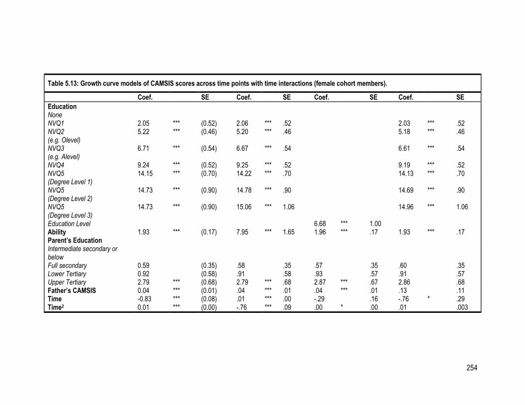
254
Table 5.13: Growth curve models of CAMSIS scores across time points with time interactions (female cohort members).
Coef. SE Coef. SE Coef. SE Coef. SE
Education None NVQ1 2.05 *** (0.52) 2.06 *** .52 2.03 *** .52 NVQ2 (e.g. Olevel)
5.22 *** (0.46) 5.20 *** .46 5.18 *** .46
NVQ3 (e.g. Alevel)
6.71 *** (0.54) 6.67 *** .54 6.61 *** .54
NVQ4 9.24 *** (0.52) 9.25 *** .52 9.19 *** .52 NVQ5 (Degree Level 1)
14.15 *** (0.70) 14.22 *** .70 14.13 *** .70
NVQ5 (Degree Level 2)
14.73 *** (0.90) 14.78 *** .90 14.69 *** .90
NVQ5 (Degree Level 3)
14.73 *** (0.90) 15.06 *** 1.06 14.96 *** 1.06
Education Level 6.68 *** 1.00 Ability 1.93 *** (0.17) 7.95 *** 1.65 1.96 *** .17 1.93 *** .17 Parent’s Education Intermediate secondary or below
Full secondary 0.59 (0.35) .58 .35 .57 .35 .60 .35 Lower Tertiary 0.92 (0.58) .91 .58 .93 .57 .91 .57 Upper Tertiary 2.79 *** (0.68) 2.79 *** .68 2.87 *** .67 2.86 .68 Father’s CAMSIS 0.04 *** (0.01) .04 *** .01 .04 *** .01 .13 .11 Time -0.83 *** (0.08) .01 *** .00 -.29 .16 -.76 * .29 Time2 0.01 *** (0.00) -.76 *** .09 .00 * .00 .01 .003
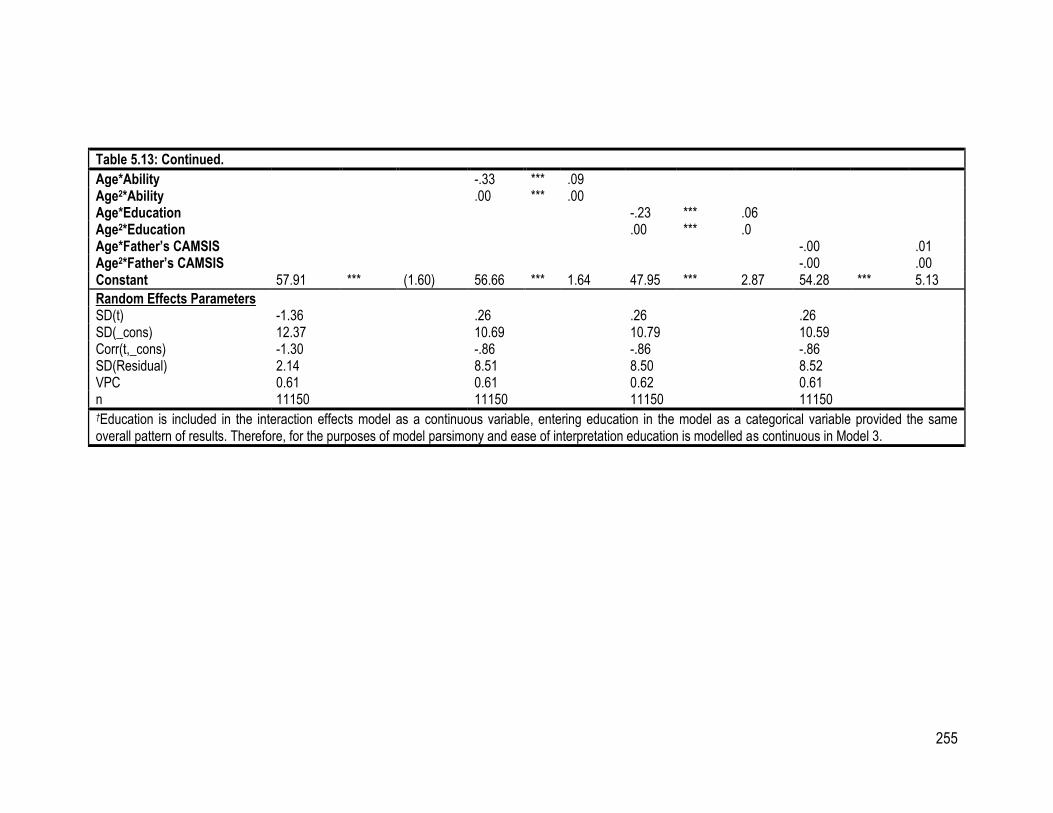
255
Table 5.13: Continued.
Age*Ability -.33 *** .09 Age2*Ability .00 *** .00 Age*Education -.23 *** .06 Age2*Education .00 *** .0 Age*Father’s CAMSIS -.00 .01 Age2*Father’s CAMSIS -.00 .00 Constant 57.91 *** (1.60) 56.66 *** 1.64 47.95 *** 2.87 54.28 *** 5.13
Random Effects Parameters SD(t) -1.36 .26 .26 .26 SD(_cons) 12.37 10.69 10.79 10.59 Corr(t,_cons) -1.30 -.86 -.86 -.86 SD(Residual) 2.14 8.51 8.50 8.52 VPC 0.61 0.61 0.62 0.61 n 11150 11150 11150 11150 †Education is included in the interaction effects model as a continuous variable, entering education in the model as a categorical variable provided the same overall pattern of results. Therefore, for the purposes of model parsimony and ease of interpretation education is modelled as continuous in Model 3.
CHAPTER FIVE CASE STUDY THREE
256
Table 5.13 also shows the growth curve model for women, the models contain the quadratic effect
for age as the women’s trajectory is shown to be curved. In line with the patterns indicated in the
cross-sectional and pooled models, educational attainment, cognitive ability test scores, parents’
education and father’s CAMSIS are all significantly associated with the cohort member’s CAMSIS
scores. In line with the trajectories described the female cohort members showed a mean de-
crease in their CAMSIS score per observation by a standard deviation of -1.36. There was also a
large amount of estimated random intercept standard deviation for women (12.37). Again the
correlation between the intercept and slope indicate that there are smaller average gains in
CAMSIS score at the later time points.
A further piece of information available in the random effects parameters of the growth curve
models presented is the Variance Partition Coefficient or the intra-class correlation (ICC). The
VPC can be thought of as the “extent of clustering” in the data (Goldstein et al., 2002). Tables
5.12 and 5.13 indicate that the variance explained in these two models by the individual level (i.e.
higher level) of the model is quite large, 65% for men and 60% for women, suggesting that
individual differences between the cohort members are extremely important in explaining change
in adult CAMSIS scores over time.
The aim of this chapter is to consider if the effects of social origins, educational attainment and
childhood cognitive ability test scores change as the cohort members’ age. Therefore a considera-
tion is required of the interaction of these covariates with time. Tables 5.12 and 5.13 present
models, for male and female cohort members respectively, which include interactions between
time (or age) and cognitive ability test scores, educational level and father’s CAMSIS. For women,

CHAPTER FIVE CASE STUDY THREE
257
who demonstrate a curve trajectory interaction terms are estimated between both time and the
quadratic function of time.
Previous studies have suggested that the association between cognitive ability and occupational
positions may increase across the lifecourse or remain largely stable (Currie et al., 2001; Deary et
al., 2005; Hauser et al., 1999; Warren, 2001; Warren et al., 2002). For male cohort members the
association between ability test scores and occupational position decreased over time significantly
(Table 5.12). The same result was also demonstrated for the female cohort members (Table 5.13).
The previous literature suggested that educational qualifications will be more strongly associated
with occupational scores early in lifecourse (Featherman, 1971; Warren et al., 2002). For the male
cohort members a decreasing association between age and education was found, as age in-
creased the association between the cohort member’s education and their CAMSIS score
decreased. For female cohort members the age and age squared interactions considered together
also indicate a decreasing association between education and CAMSIS scores as the cohort
member’s occupational career progresses.
The previous literature has also suggested that the influence of social origins will remain stable or
decrease across the lifecourse (Warren et al., 2002). The cross-sectional models provided
tentative evidence in the initial analyses that effect of social origins waned. Looking to the growth
curve models, male cohort members showed a significant decrease in the association between
social origins and CAMSIS scores, although the coefficient is small and therefore the decrease in
the effect is minimal. The growth curve model for the women again showed a significant decrease
in the association between social origins and outcome CAMSIS scores.In summary consideration
CHAPTER FIVE CASE STUDY THREE
258
of growth curve models estimating individual intercepts and slopes for each cohort member
demonstrated the importance of social origins, cognitive ability and educational attainment across
the lifecourse. The coefficients for these covariates in the fixed part of the model indicated that
overall between-individual differences could be accounted for by these often studied key variables
in social stratification research. However there was large variation in the CAMSIS scores between
individuals, differences between individuals standard deviations for the intercepts of the model
(the cohort members starting CAMSIS score) were larger than for standard deviations indicating
individual change in CAMSIS scores over time. In testing the specific hypotheses of this chapter,
evidence was found to support the contention that social origins and education will become less
influential in the attainment of occupational positions throughout the career. Counter to expecta-
tions, however, the interaction effects indicated that the effect of cognitive ability also decreased
across the lifecourse.

CHAPTER FIVE CASE STUDY THREE
259
5.7 Discussion and Conclusions
Social stratification research has focused largely on examining the relationships between vari-
ables such as education and origin social advantage on the occupational position of individuals at
one point of their occupational lifecourse. Far less is known is known about what happens as
individuals navigate throughout their occupational careers, and what influences intra-generational
mobility as the career progresses. Furthermore, even less is known about the interrelations
between measures of inter-generational mobility and intra-generational mobility. The analyses in
this chapter sought to contribute to the literature on intra-generational processes of social stratifi-
cation by studying the effects of social origins, education and cognitive ability on adult
occupational positions at multiple time points.
First, the results of this chapter highlighted the importance of between group differences in
educational attainment, ability test scores and social origins highlight the continued importance of
inter-generational studies of social stratification. The analyses indicate the importance of the inter-
generation influence of parents’ socioeconomic positions on the occupational outcomes of
individuals across the lifecourse. Furthermore the greatest variances were observed between
individuals and not within individuals over time. Therefore a great deal of the variance involved in
the analysis of between group differences in occupational attainment will be captured by the
analysis of data sampled from a point in the mature occupational phase. This is a useful and
practical finding for social stratification researchers.
This is not to suggest that the study of intra-generational mobility is not without significant value.
The main focus of this chapter questioned the extent to which social origins, educational attain-
ment and cognitive ability scores would change in their influence across the lifecourse. These
CHAPTER FIVE CASE STUDY THREE
260
hypotheses were informed by theory and previous work in the North American context (Farber et
al., 1996; Featherman et al., 1988; Hauser, 2010; Warren, 2001; Warren et al., 2002). The
influence of education was seen to decrease along with the influence of social origins. This is
contrary to Farber and Gibbons (1996) theory that effect of ability would increase as the cohort
member’s career progresses and they are able to demonstrate their capabilities. These findings
have quite pessimistic implications for those people who made sub-optimal transitions into
employment and are trying to ‘work their way up’. The initial differences between the occupational
positions of the cohort members were larger than the changes which they made across the
lifecourse. This suggests that much of the differences between individuals may be accounted for
early in the career. Merton’s (1988) observations regarding ‘cumulative advantages’ across
careers suggest that initial advantages may more easily lead to future advantages which may
enable individuals to progress at different rates based on their initial positions. An important
feature of these analyses were the contingent nature of the variables in the model. It was sug-
gested that although the influence of social origins waned as the career progressed, the influence
of social background was still pervasive due to its influence on the cohort members’ ability test
scores and educational attainment (Hauser et al., 1999; Warren, 2001; Warren et al., 2002).
These results detail the cohort-specific effects of the National Child Development Study. Ryder
(1965) described how cohorts are nested within their own particular temporal, social, political and
historical context. Britain has undergone some structural changes for example in the economy and
in patterns of female participation in the labour market, at the same time there has been wide-
spread social stability. An acid test of the particularity of the NCDS cohort would be a comparison
with the BCS cohort once age matched data are available for these individuals. Ultimately com-

CHAPTER FIVE CASE STUDY THREE
261
parisons with more recent cohorts such as the Millennium Cohort Study and ALSPAC will be
possible in future decades.
CHAPTER SIX AFTERWORD
262
6. An Afterword – A Sensitivity Analysis of Social Background, Educational and Occupational Attainment
“Another way to gain confidence – and inspire confidence on the part of your reader
– that your results are robust is to conduct sensitivity analysis…” (Treiman, 2009, p.
402)
In this short section a brief note is provided which examines the influences of social background
on educational and occupational attainment using data on adults in the British Household Panel
Survey. This afterword is intended to provide an example of a sensitivity analysis using social
survey data.
6.1 Sensitivity Analysis
Sensitivity analysis is the process of investigating the influence which small perturbations to a
statistical analysis (e.g. the use different operationalisations of variables) can have on the sub-
stantive results of a study. Sensitivity analysis is described in detail in chapter two (section 2.7).
Sensitivity analysis is encouraged in order to ensure that the results of a statistical investigation
are robust, and therefore that substantive conclusions based on social survey research are
reliable. An example of a published sensitivity analysis in the field of social stratification research
is Hout and Hauser’s (1992a) critique of Erikson and Goldthorpe’s classic sociological monograph,
the Constant Flux (1992). Hout and Hauser (1992a) expressed their concern over the sensitivity of
the findings of the Constant Flux to the statistical analysis techniques utilised and the social class
measure employed. This afterword presents the results of regression models which consider
CHAPTER SIX AFTERWORD
263
change over time in the influence of social origins on educational and occupational attainment, the
sensitivity of the results to the measure of parental occupational position utilised is investigated.
6.2 Data
These brief analyses are based on the British Household Panel Survey, a full description of the
BHPS data is provided in chapter 4 (section 4.4.1). The BHPS is nationally representative survey
of individuals within households that was conducted annually from 1991 to 2008. The analytical
sample is based on BHPS members present in the 2003 sweep of data collection, as this was the
only wave of the survey which collected the parental education details required in this analysis.
The analytical sample includes BHPS members from England and Wales44. In the analysis of the
cohort members’ educational attainment only sample members aged 25 and over were included in
the sample45. For the analysis of the attainment of occupational position only sample members
aged 35 and over were included46. BHPS sample members born from 1930 to 1979 were retained
in the sample, this wide age range allows for the analysis of trends in educational and occupa-
tional attainment over time. These analyses are weighted using cross-sectional survey weights
(see section 4.4.1.for an extended discussion on the use of weights).
Three different occupation-based measures are used to represent parental occupational positions,
CAMSIS, NS-SEC and the Chan-Goldthorpe Status scale. The ‘Cambridge Social Interaction and
44 There is a great deal of similarity between the education systems in the four nations of the UK, as well as their development over the 20st century. However, the systems do remain disparate and educational developments did not occur in sync (Raffe et al., 1999). Therefore, to provide a more focussed analysis, only BHPS members from England and Wales are included in the analytical sample. 45 This selection was made to ensure that sample members who were completing degree level qualifica-tions had a representative educational level recorded. 46 This selection was made as it was the intention to represent the position of sample members at a mature stage of their occupational career (see Goldthorpe, 1980 pp. 52-53).
CHAPTER SIX AFTERWORD
264
Stratification Scale’ (CAMSIS) is a continuous social stratification scale which represents ‘relative
social advantage (Prandy, 1990; Stewart et al., 1980). The ‘National Statistics Socio-Economic
Classification’ (NS-SEC) is a social class scheme developed from the ‘Erikson-Goldthorpe-
Portocarero’ perspective (Chan and Goldthorpe, 2004). The ‘Chan-Goldthorpe Status Scale’ is
purported to measure the ‘status’ dimension of social hierarchy (Chan et al., 2004).
6.3 Results
The descriptive characteristics of the analytical sample are reported in Table 6.1. Figure 6.1
shows the distribution of educational attainment by the decade of birth. Overall, the educational
attainment of both men and women has increased since the 1930s, in line with the widely reported
trends in educational expansion over this period (see Galinda-Rueda and Vignoles, 2005; Hansen
et al., 2005; Stewart et al., 1980).
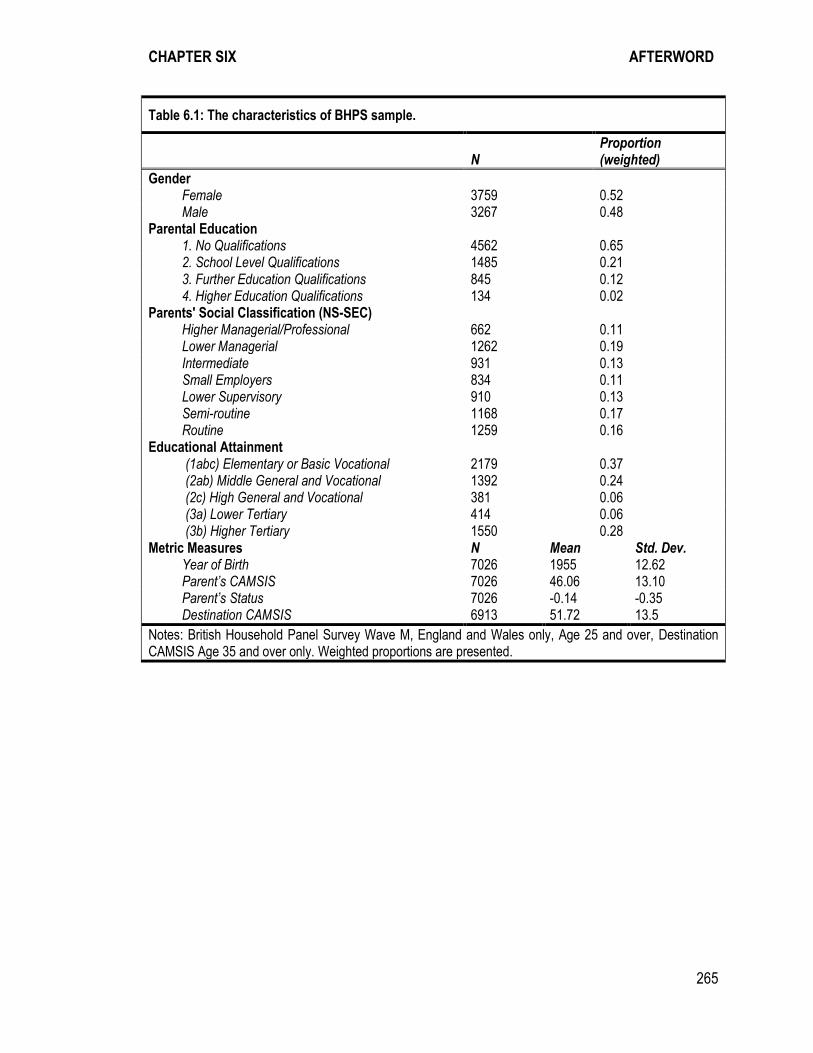
CHAPTER SIX AFTERWORD
265
Table 6.1: The characteristics of BHPS sample.
N
Proportion (weighted)
Gender Female 3759 0.52
Male 3267 0.48 Parental Education
1. No Qualifications 4562 0.65 2. School Level Qualifications 1485 0.21 3. Further Education Qualifications 845 0.12 4. Higher Education Qualifications 134 0.02 Parents' Social Classification (NS-SEC)
Higher Managerial/Professional 662 0.11 Lower Managerial 1262 0.19 Intermediate 931 0.13 Small Employers 834 0.11 Lower Supervisory 910 0.13 Semi-routine 1168 0.17 Routine 1259 0.16 Educational Attainment
(1abc) Elementary or Basic Vocational 2179 0.37 (2ab) Middle General and Vocational 1392 0.24 (2c) High General and Vocational 381 0.06 (3a) Lower Tertiary 414 0.06 (3b) Higher Tertiary 1550 0.28 Metric Measures N Mean Std. Dev. Year of Birth 7026 1955 12.62 Parent’s CAMSIS 7026 46.06 13.10 Parent’s Status 7026 -0.14 -0.35 Destination CAMSIS 6913 51.72 13.5
Notes: British Household Panel Survey Wave M, England and Wales only, Age 25 and over, Destination CAMSIS Age 35 and over only. Weighted proportions are presented.

CHAPTER SIX AFTERWORD
266
Figure 6.1: Educational attainment for Men and Women born from 1930 to 1979.
In the next step of the analyses level of educational attainment47 is investigated using an ordered
logistic regression model (see Long, 1997). Table 6.2 reports the results of the ordered logistic
model48. The level of education increases with year of birth, parent’s CAMSIS score and parent’s
education. Women are significantly less well qualified than their male counterparts overall during
this period. Model 2 in Table 6.249. reports the significant but very small interaction effect of year
47 Level of educational attainment is represented using a reduced form the CASMIN educational scheme (Schneider, 2011). 48 The proportional odds assumption of the ordered logistic regression model was tested using a Brant test. The Brant test indicated that the Proportional Odds assumption was not violated, therefore an Ordered Logistic Regression model was appropriate (Treiman, 2009). 49 Figure 6.2 provides a demonstration of the use of quansi-variance to identify significant differences between the levels of a categorical variable.
0 20 40 60 80 100percent of category
1970-1979
1960-1969
1950-1959
1940-1949
1930-1939
Male
None
Low (e.g. O Level)
Medium (e.g. A Level)
Degree
0 20 40 60 80 100percent of category
1970-1979
1960-1969
1950-1959
1940-1949
1930-1939
Female
None
Low (e.g. O Level)
Medium (e.g. A Level)
Degree
Source: British Household Panel Study Wave M (Unweighted)
by decade of birth
Distribution of Highest Level of Education

CHAPTER SIX AFTERWORD
267
of birth and parental CAMSIS. This negative effect suggests a weakening relationship between
parental background and educational attainment.
Table 6.2: Ordered Logistic Regression Model of Highest Educational Qualification (Parent’s CAMSIS).
Model 1 Model 2 Variable Coef. S.E. Coef. S.E.
Year of Birth 0.02 *** (0.00) 0.05 *** (0.01) Parent’s CAMSIS 0.03 *** (0.00) 0.06 *** (0.01) Parental Education
1. No Qualifications
2. School Level Qualifications 0.39 *** (0.08) 0.39 *** (0.07)
3. Further Education Qualifications 0.39 *** (0.09) 0.40 *** (0.08)
4. Higher Education Qualifications 0.65 * (0.31) 0.49 *** (0.09) Gender Male 0.00 (0.00) 0.00 (0.00) Female -0.32 *** (0.06) 0.73 * (0.30) Interaction Year of Birth*Parent’s CAMSIS -0.00 ** (0.00)
Cut Points Middle General and Vocational 1.96 *** (0.18) 3.34 *** (0.51) High General and Vocational 3.05 *** (0.19) 4.43 *** (0.52) Lower Tertiary 3.32 *** (0.19) 4.70 *** (0.52) Higher Tertiary 3.64 *** (0.19) 5.03 *** (0.52)
Number of Observations 5929 5929 Pseudo R Squared (unweighted model) 0.05 0.05 BIC (unweighted model) -35251 -35261
Notes: British Household Panel Survey Wave M, England and Wales only, Age 25 and over. Models are weighted.
In the spirit of undertaking sensitivity analyses, these models are now re-estimated with alternative
parental socio-economic measures. Table 6.3 reports an insignificant interaction between parental
background and year of birth using NS-SEC. Table 6.4 reports a significant (p<.05) interaction
between parental background and year of birth using the Chan-Goldthorpe status scale.
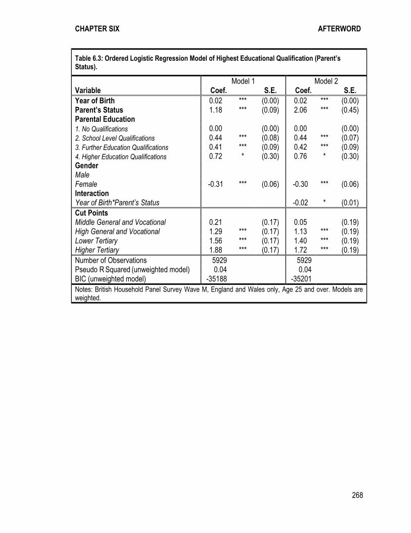
CHAPTER SIX AFTERWORD
268
Table 6.3: Ordered Logistic Regression Model of Highest Educational Qualification (Parent’s Status).
Model 1 Model 2 Variable Coef. S.E. Coef. S.E.
Year of Birth 0.02 *** (0.00) 0.02 *** (0.00) Parent’s Status 1.18 *** (0.09) 2.06 *** (0.45) Parental Education
1. No Qualifications 0.00 (0.00) 0.00 (0.00)
2. School Level Qualifications 0.44 *** (0.08) 0.44 *** (0.07)
3. Further Education Qualifications 0.41 *** (0.09) 0.42 *** (0.09)
4. Higher Education Qualifications 0.72 * (0.30) 0.76 * (0.30) Gender Male Female -0.31 *** (0.06) -0.30 *** (0.06) Interaction Year of Birth*Parent’s Status -0.02 * (0.01)
Cut Points Middle General and Vocational 0.21 (0.17) 0.05 (0.19) High General and Vocational 1.29 *** (0.17) 1.13 *** (0.19) Lower Tertiary 1.56 *** (0.17) 1.40 *** (0.19) Higher Tertiary 1.88 *** (0.17) 1.72 *** (0.19)
Number of Observations 5929 5929 Pseudo R Squared (unweighted model) 0.04 0.04 BIC (unweighted model) -35188 -35201
Notes: British Household Panel Survey Wave M, England and Wales only, Age 25 and over. Models are weighted.
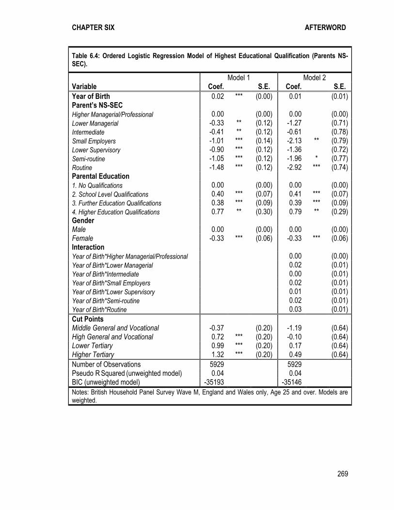
CHAPTER SIX AFTERWORD
269
Table 6.4: Ordered Logistic Regression Model of Highest Educational Qualification (Parents NS-SEC).
Model 1 Model 2 Variable Coef. S.E. Coef. S.E.
Year of Birth 0.02 *** (0.00) 0.01 (0.01) Parent’s NS-SEC
Higher Managerial/Professional 0.00 (0.00) 0.00 (0.00)
Lower Managerial -0.33 ** (0.12) -1.27 (0.71)
Intermediate -0.41 ** (0.12) -0.61 (0.78)
Small Employers -1.01 *** (0.14) -2.13 ** (0.79)
Lower Supervisory -0.90 *** (0.12) -1.36 (0.72)
Semi-routine -1.05 *** (0.12) -1.96 * (0.77)
Routine -1.48 *** (0.12) -2.92 *** (0.74) Parental Education
1. No Qualifications 0.00 (0.00) 0.00 (0.00)
2. School Level Qualifications 0.40 *** (0.07) 0.41 *** (0.07)
3. Further Education Qualifications 0.38 *** (0.09) 0.39 *** (0.09)
4. Higher Education Qualifications 0.77 ** (0.30) 0.79 ** (0.29) Gender Male 0.00 (0.00) 0.00 (0.00) Female -0.33 *** (0.06) -0.33 *** (0.06) Interaction
Year of Birth*Higher Managerial/Professional 0.00 (0.00)
Year of Birth*Lower Managerial 0.02 (0.01)
Year of Birth*Intermediate 0.00 (0.01)
Year of Birth*Small Employers 0.02 (0.01)
Year of Birth*Lower Supervisory 0.01 (0.01)
Year of Birth*Semi-routine 0.02 (0.01)
Year of Birth*Routine 0.03 (0.01)
Cut Points Middle General and Vocational -0.37 (0.20) -1.19 (0.64) High General and Vocational 0.72 *** (0.20) -0.10 (0.64) Lower Tertiary 0.99 *** (0.20) 0.17 (0.64) Higher Tertiary 1.32 *** (0.20) 0.49 (0.64)
Number of Observations 5929 5929 Pseudo R Squared (unweighted model) 0.04 0.04 BIC (unweighted model) -35193 -35146
Notes: British Household Panel Survey Wave M, England and Wales only, Age 25 and over. Models are weighted.
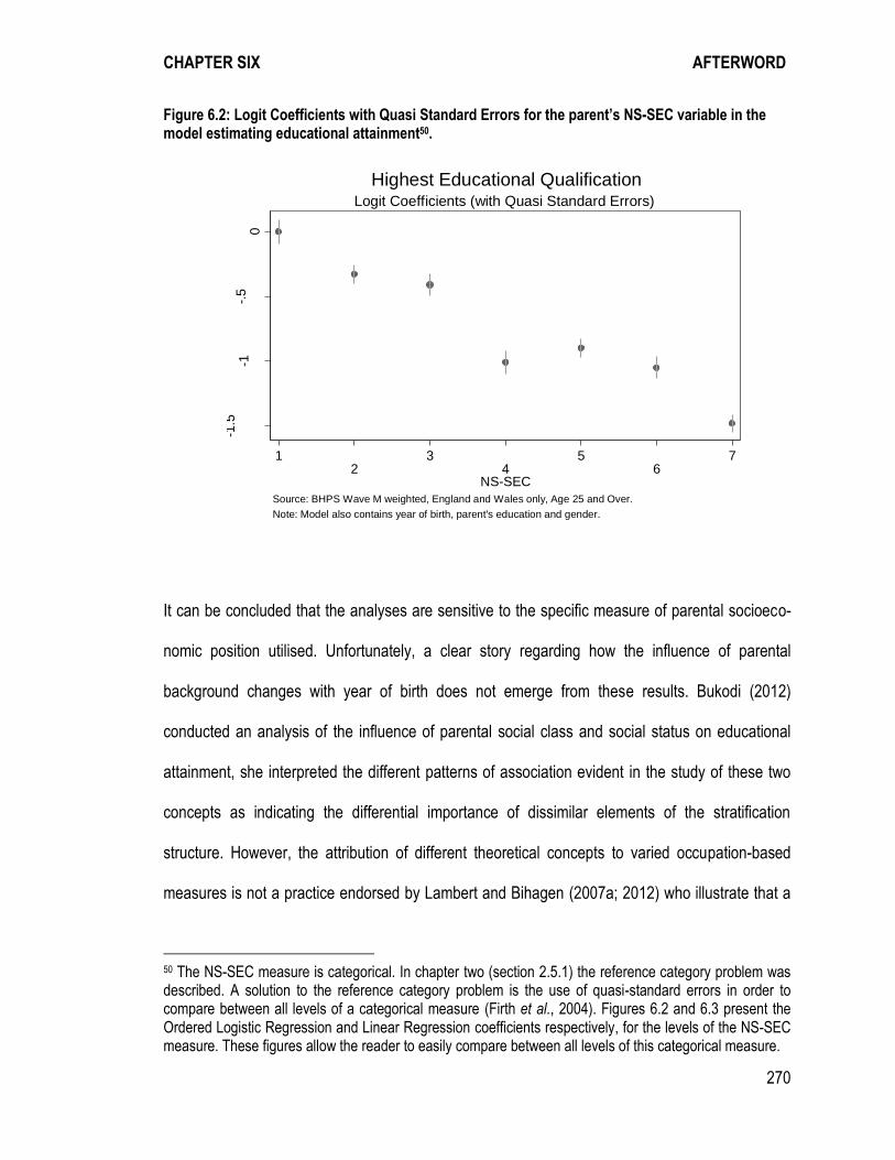
CHAPTER SIX AFTERWORD
270
Figure 6.2: Logit Coefficients with Quasi Standard Errors for the parent’s NS-SEC variable in the model estimating educational attainment50.
It can be concluded that the analyses are sensitive to the specific measure of parental socioeco-
nomic position utilised. Unfortunately, a clear story regarding how the influence of parental
background changes with year of birth does not emerge from these results. Bukodi (2012)
conducted an analysis of the influence of parental social class and social status on educational
attainment, she interpreted the different patterns of association evident in the study of these two
concepts as indicating the differential importance of dissimilar elements of the stratification
structure. However, the attribution of different theoretical concepts to varied occupation-based
measures is not a practice endorsed by Lambert and Bihagen (2007a; 2012) who illustrate that a
50 The NS-SEC measure is categorical. In chapter two (section 2.5.1) the reference category problem was described. A solution to the reference category problem is the use of quasi-standard errors in order to compare between all levels of a categorical measure (Firth et al., 2004). Figures 6.2 and 6.3 present the Ordered Logistic Regression and Linear Regression coefficients respectively, for the levels of the NS-SEC measure. These figures allow the reader to easily compare between all levels of this categorical measure.
-1.5
-1-.
50
12
34
56
7
NS-SEC
Source: BHPS Wave M weighted, England and Wales only, Age 25 and Over.
Note: Model also contains year of birth, parent's education and gender.
Logit Coefficients (with Quasi Standard Errors)
Highest Educational Qualification

CHAPTER SIX AFTERWORD
271
very wide range of socioeconomic measures perform similarly in a variety of empirical applica-
tions. It is therefore concluded that these results are sensitive to the use of different occupation-
based measures of social stratification. These analyses illustrate the research value of sensitivity
analysis, as suggested in chapter 2.
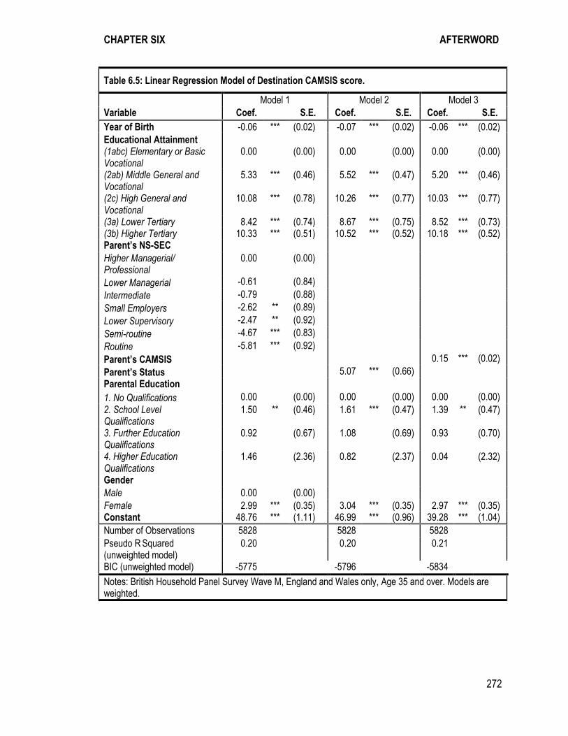
CHAPTER SIX AFTERWORD
272
Table 6.5: Linear Regression Model of Destination CAMSIS score.
Model 1 Model 2 Model 3 Variable Coef. S.E. Coef. S.E. Coef. S.E.
Year of Birth -0.06 *** (0.02) -0.07 *** (0.02) -0.06 *** (0.02) Educational Attainment (1abc) Elementary or Basic Vocational
0.00 (0.00) 0.00 (0.00) 0.00 (0.00)
(2ab) Middle General and Vocational
5.33 *** (0.46) 5.52 *** (0.47) 5.20 *** (0.46)
(2c) High General and Vocational
10.08 *** (0.78) 10.26 *** (0.77) 10.03 *** (0.77)
(3a) Lower Tertiary 8.42 *** (0.74) 8.67 *** (0.75) 8.52 *** (0.73) (3b) Higher Tertiary 10.33 *** (0.51) 10.52 *** (0.52) 10.18 *** (0.52) Parent’s NS-SEC Higher Managerial/ Professional
0.00 (0.00)
Lower Managerial -0.61 (0.84)
Intermediate -0.79 (0.88)
Small Employers -2.62 ** (0.89)
Lower Supervisory -2.47 ** (0.92)
Semi-routine -4.67 *** (0.83)
Routine -5.81 *** (0.92)
Parent’s CAMSIS 0.15 *** (0.02)
Parent’s Status 5.07 *** (0.66) Parental Education
1. No Qualifications 0.00 (0.00) 0.00 (0.00) 0.00 (0.00) 2. School Level Qualifications
1.50 ** (0.46) 1.61 *** (0.47) 1.39 ** (0.47)
3. Further Education Qualifications
0.92 (0.67) 1.08 (0.69) 0.93 (0.70)
4. Higher Education Qualifications
1.46 (2.36) 0.82 (2.37) 0.04 (2.32)
Gender Male 0.00 (0.00) Female 2.99 *** (0.35) 3.04 *** (0.35) 2.97 *** (0.35) Constant 48.76 *** (1.11) 46.99 *** (0.96) 39.28 *** (1.04)
Number of Observations 5828 5828 5828 Pseudo R Squared
(unweighted model) 0.20 0.20 0.21
BIC (unweighted model) -5775 -5796 -5834
Notes: British Household Panel Survey Wave M, England and Wales only, Age 35 and over. Models are weighted.
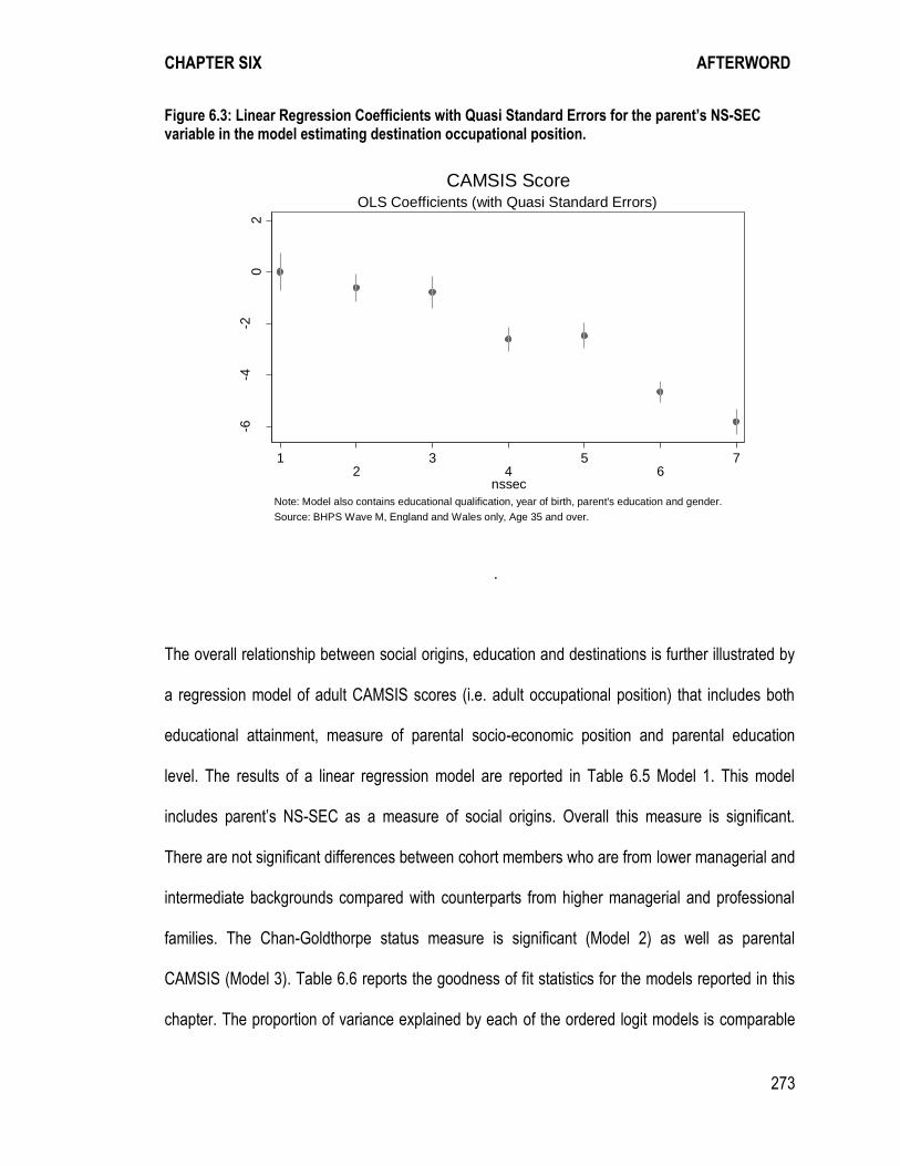
CHAPTER SIX AFTERWORD
273
Figure 6.3: Linear Regression Coefficients with Quasi Standard Errors for the parent’s NS-SEC variable in the model estimating destination occupational position.
.
The overall relationship between social origins, education and destinations is further illustrated by
a regression model of adult CAMSIS scores (i.e. adult occupational position) that includes both
educational attainment, measure of parental socio-economic position and parental education
level. The results of a linear regression model are reported in Table 6.5 Model 1. This model
includes parent’s NS-SEC as a measure of social origins. Overall this measure is significant.
There are not significant differences between cohort members who are from lower managerial and
intermediate backgrounds compared with counterparts from higher managerial and professional
families. The Chan-Goldthorpe status measure is significant (Model 2) as well as parental
CAMSIS (Model 3). Table 6.6 reports the goodness of fit statistics for the models reported in this
chapter. The proportion of variance explained by each of the ordered logit models is comparable
-6-4
-20
2
12
34
56
7
nssec
Note: Model also contains educational qualification, year of birth, parent's education and gender.
Source: BHPS Wave M, England and Wales only, Age 35 and over.
OLS Coefficients (with Quasi Standard Errors)
CAMSIS Score
CHAPTER SIX AFTERWORD
274
and each model is similarly parsimonious (measured by the BIC statistic). The proportion of
variance explained by each of the linear regression models is comparable and equally parsimoni-
ous. In conducting sensitivity analysis, the hope is that perturbations to the analysis will lead to the
same substantive conclusions, indicating a robust analysis. In the linear regression models, the
outlay of effort employed to undertake the sensitivity analysis was not especially rewarded,
however such judgments cannot be made a priori.
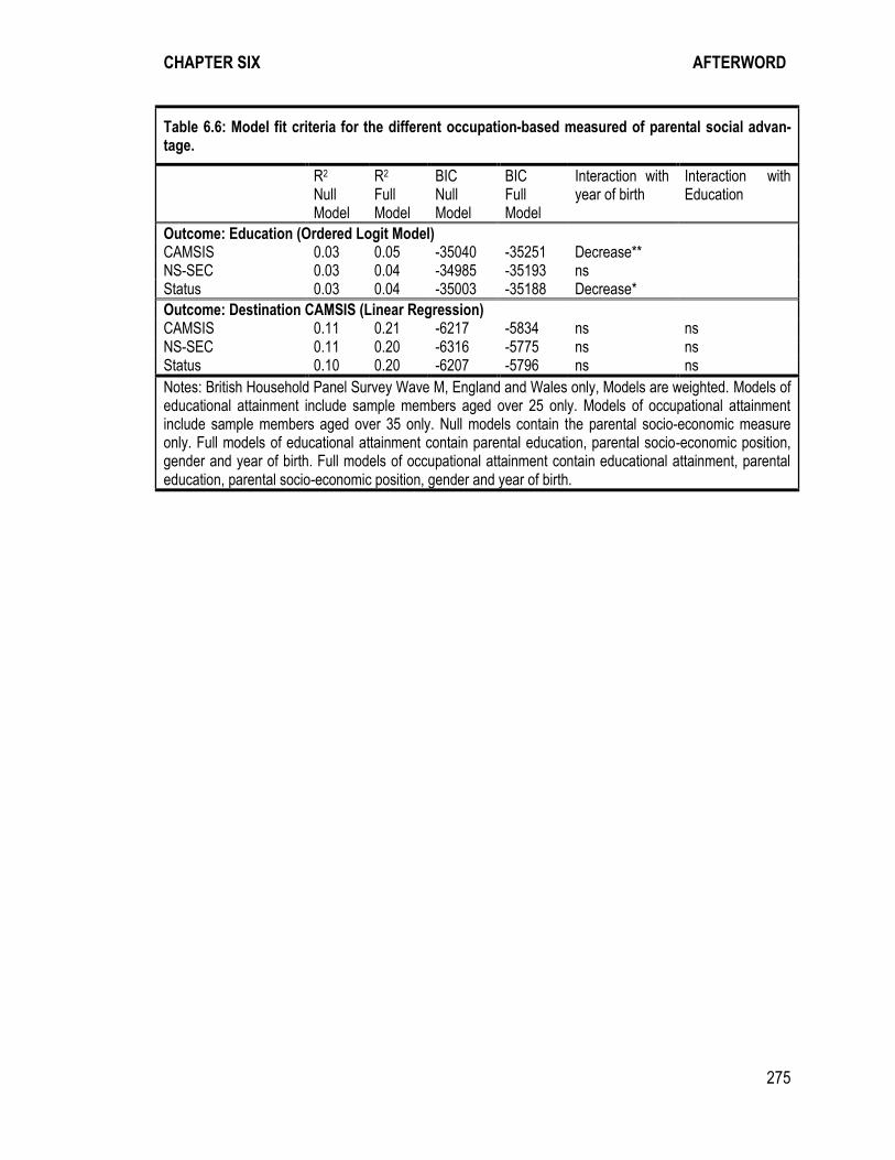
CHAPTER SIX AFTERWORD
275
Table 6.6: Model fit criteria for the different occupation-based measured of parental social advan-tage.
R2 Null Model
R2 Full Model
BIC Null Model
BIC Full Model
Interaction with year of birth
Interaction with Education
Outcome: Education (Ordered Logit Model) CAMSIS 0.03 0.05 -35040 -35251 Decrease** NS-SEC 0.03 0.04 -34985 -35193 ns Status 0.03 0.04 -35003 -35188 Decrease*
Outcome: Destination CAMSIS (Linear Regression) CAMSIS 0.11 0.21 -6217 -5834 ns ns NS-SEC 0.11 0.20 -6316 -5775 ns ns Status 0.10 0.20 -6207 -5796 ns ns
Notes: British Household Panel Survey Wave M, England and Wales only, Models are weighted. Models of educational attainment include sample members aged over 25 only. Models of occupational attainment include sample members aged over 35 only. Null models contain the parental socio-economic measure only. Full models of educational attainment contain parental education, parental socio-economic position, gender and year of birth. Full models of occupational attainment contain educational attainment, parental education, parental socio-economic position, gender and year of birth.
CHAPTER SEVEN CONCLUSIONS
276
7. Conclusions
Social relations are “highly resistant to change: those groupings who enjoy positions
of superior advantage and disadvantage cannot be expected to yield them up without
a struggle, but will rather typically seek to exploit the resources they can command in
order to preserve their superiority.” (Goldthorpe et al., 1980, p. 28)
7.1 Introduction
Despite the more obvious examples of social change in the western educated industrial rich
developed societies, this programme of empirical work fails to provide compelling evidence that
contemporary Britain is no longer still highly socially stratified. The overall orientation of this thesis
has been the practical empirical analysis of contemporary large-scale social survey data using
advanced statistical methods. From the outset the goal was to develop a series of detailed original
case studies relating to social stratification in contemporary Britain. The theoretical endeavour was
informed by the modest, but important, Mertonian conception of drawing on ‘middle range’ theory
(Merton, 1957). The thesis has therefore not engaged directly with ‘grand’ sociological theory. This
is because the aim has been to establish what Goldthorpe (2000) terms as ‘empirical regularities’.

CHAPTER SEVEN CONCLUSIONS
277
7.2 Substantive Conclusions
Case study one focuses on cognitive inequalities in the early years of childhood. This case study
builds on research which has indicated that social stratification impacts on the cognitive perform-
ance of young children. This chapter makes the original contribution of charting the extent of
social inequalities on childhood cognitive abilities between the UK birth cohorts. There are clear
patterns of social inequality within each of the cohorts. Between the cohorts there is also evidence
that the association between socio-economic advantage and childhood cognitive capability have
remained largely stable over the post-war period. This finding is both striking and alarming given
the widespread nature of numerous policies which have been implemented during this period
specifically to combat social inequality.
There was tentative evidence of a decrease in the influence of social origins on cognitive abilities
for the BCS and MCS but this finding was not robust and the overall pattern in the data was one of
stability. This finding indicates that the influence of social inequalities on cognitive ability is not a
new phenomenon. This is a subtle but important finding because recent popular and political
discourse suggests that such differences are largely a result of family breakdown and changes to
traditional family structure (e.g. Cameron, 2010 Accessed: 12/12/2013).
Case study two investigated the theoretical idea of a middle group of young people. Detailed
analysis of the Youth Cohort Study of England and Wales, which is a nationally representative
specialised youth dataset, and an analysis of the British Household Panel Survey, which provides
information on young people growing up in contemporary British households, failed to provide
convincing evidence that there is a middle group of young people with mediocre levels of GCSE
school attainment. The detailed multivariate analysis highlights that it is more appropriate to

CHAPTER SEVEN CONCLUSIONS
278
understand school educational attainment as being located on a continuum rather than there
being distinctive clusters or educational groups with clear and crisp boundaries.
Case study three combined analyses of both intra-generational and inter-generational occupa-
tional attainment. Through an analysis of social origins, educational attainment and cognitive
abilities throughout the occupational lifecourse advanced multivariate analyses of the occupational
lifecourse were undertaken. The results reported that much more variation in occupational
positions is observed between individuals compared with intra-generation mobility across the adult
occupational lifecourse. This finding chimes with the general theoretical idea advanced by
Goldthorpe et al. (1987, p. 51) that workers reach a stage of occupational maturity after which
there is a prolonged state of occupational stability. Unsurprisingly therefore the influence of social
origins, educational attainment and cognitive ability are most salient in the early phase of the
occupational lifecourse. The declining influence of cognitive ability is counter to studies such as
Farber and Gibbons (1996) which suggest that cognitive ability will increasingly relate to labour
market success as the lifecourse proceeds.
This thesis has been structured around a focus on the nature of social stratification at three stages
of the lifecourse: the entry to primary school, school leaving age and early adulthood, and the
occupational life course. These three case studies have emphasised clear and persistent patterns
of inequality throughout the life course in relation to educational attainment and social stratification
and highlight the importance of the life course approach for understanding the nature and com-
plexity of social inequalities. Elder (1994) describes the life course as a ‘multilevel phenomenon’
which involves: developmental pathways; pathways through social institutions (e.g. education);
and individual trajectories which vary in their timing and ordering. Life course studies, including the
CHAPTER SEVEN CONCLUSIONS
279
research presented in this thesis, indicate that inequalities are reinforced throughout these
pathways and inequalities arise as a result of what came before and the specific transitions which
have been made. Mills’ (1959, p. 149) influential work emphasised the importance of understand-
ing inequalities across an individual’s life course, highlighting the significance of “the study of
biography, of history, and of the problems of their intersection within social structure”.
In Boudon’s (1974) terms this thesis has focused largely on ‘primary effects’ in the transmission of
inequalities between generations, i.e. the influence of social origins on test performance or
educational attainment. Boudon (1974) also described the nature of ‘secondary effects’ which are
the educational choices that children and families make despite their prior attainment. Even given
the same level of educational attainment children from more disadvantaged backgrounds may be
less likely to make the transition to higher levels of education (see Jackson et al., 2007). In future
studies the focus on ‘secondary effects’ in addition to the widely studied ‘primary effects’ may
provide further insights into the influence of social background on choices and transitions which
can go on to influence further life course outcomes (e.g. occupational attainment).
The study of the processes of social stratification throughout the life course could also be devel-
oped through a focus on the cumulative nature of advantages and disadvantages. Merton’s (1968)
concept of cumulative advantage is very relevant to life course studies and suggests that advan-
tages early in the career will result in even greater advantages later in the career, as positive
outcomes accrue as a result of previous success. This concept can be applied more widely and is
synonymous with Heckman’s descriptions of the developmental processes of human capital
formation. Heckman (2008, p. 2) has stated that “Life cycle skill formation is dynamic in nature.
Skill begets skill; motivation begets motivation. Motivation cross-fosters skill and skill cross-fosters
CHAPTER SEVEN CONCLUSIONS
280
motivation”. Cumulative advantages and disadvantages may be inextricably linked in the devel-
opment of the skills, characteristics and credentials necessary to alleviate educational and
occupational inequalities later in the life course. Taken together these examples of the complexity
of inequalities across the life course emphasise the process of the social reproduction of inequali-
ties as a complex and inter-related system of multiple inequalities across many points in an
individual’s life. Inequalities in educational attainment and inequalities in the attainment of occupa-
tional positions must therefore be considered within a framework of a chain of interconnected
stages of inequality.
7.3 Social Survey Data Analysis
This programme of work has demonstrated that the incorporation of key variables in social
stratification research requires thought. It is not simply the case that variables can routinely, or
even worse carelessly, be included in statistical models. It is a truism to assert that social science
theory should guide the statistical model building process. The importance of guidelines that help
to inform the development of statistical models should not be under-emphasised however. This
should include clear ideas about the nature of measures, their effectiveness, reliability, validity and
replicability. This is an aspect of research methods, and the data analytical process that is not
currently highlighted (especially in methodological texts).
The role and potential benefits of sensitivity analyses are attractive. This practice has appeal
when several, potentially competing, measures are available. It also has merit when comparing a
range of results, for example from models with weighted and unweighted data, or models based
on complete case analyses and models based on multiple imputation methods. The use of
CHAPTER SEVEN CONCLUSIONS
281
sensitivity analyses is not routine within sociology, but would add to the scientific rigour of analy-
ses. The importance of sensitivity analysis dovetails with a more general position advanced in
Dale (2006) who argues for greater transparency in reporting the detail of both the data and the
methods used in survey data analysis. She argues that this not only enables replication but also
allows a much more critical appraisal of the research than is usually possible. A similar call for
standards of replication in sociology is made by Freese (2007).
The ‘Occupational Coding’ data file recently developed by Gregg (2012) provides is an extremely
beneficial recent addition to the data available in the National Child Development Study and
British Cohort Study. This is an important infrastructural resource which helps facilitate the
analyses in case study one. This information will provide the basis to facilitate future cross-cohort
comparisons which seek to compare the influence of occupation-based socioeconomic classifica-
tions and also look at occupations in finer resolution. At the current time there is an emerging
sociological perspective that suggests that there may be important patterns of social stratification
which are located between traditional large scale or agglomerate social classes and individual
occupations, which are known as micro-classes (Grusky et al., 2001). At the current time little is
known about the role that micro-classes might play in either inter-generational reproduction in
contemporary Britain or across the occupational lifecourse. Such investigations might plausibly be
a fruitful area for further investigation. However a large outlay of effort will be required to construct
suitable measures of micro-class membership in existing large scale survey datasets.
Extended searches suggest that the analysis in case study one represents one of the first at-
tempts to conduct a three cohort comparison using the Millennium Cohort Study and both the
earlier British birth cohorts. Detailed consideration was therefore paid to ‘measurement equiva-
CHAPTER SEVEN CONCLUSIONS
282
lence’ between the studies, particularly in relation to the organisational changes which took place
over this period in the occupational structure and in the increasing overall levels of education.
These changes influence the operationalisation of comparable measures of parental occupational
positions and educational level.
In the coming decades changes to the occupational structure may also impact the adult outcomes
of current members of the Millennium Cohort study. It is anticipated that these considerations will
continue to be important as the MCS matures and further cross-cohort comparisons are con-
ducted in the analysis of social stratification. It is anticipated that the Millennium Cohort Study will
prove a particularly useful social survey resource for future social stratification research, as it
represents the first nationally representative cohort study for thirty years and will allow researchers
to link early years information with outcomes in adulthood.
7.4 Closing Remarks
In summary the purpose of this research was to provide three detailed case studies investigating
original elements of enquiry in the field of social stratification. In addition, the thesis also aimed to
demonstrate the value of existing social survey resources in producing original research outputs.
The first chapter has highlighted that there are a number of complex considerations to be made in
the process of social survey research. Social survey research is hard work, a lot of effort goes into
the preparation of survey data even before the analysis stage can proceed. The application of
statistical models to social survey data is a rapidly developing field. The estimation of statistical
models suitable for complex survey data analysis is nontrivial and computationally demanding.
However, the results of social survey research are invaluable in elucidating the true patterns of

CHAPTER SEVEN CONCLUSIONS
283
inequality in a population. The results of this thesis have demonstrated the pervasive influence of
social stratification on the lives of individuals in the UK today. Inequalities in cognitive abilities are
apparent in children even as they enter school, and inequalities are seen to remain as individuals
progress through the educational system, and indeed as they progress throughout their occupa-
tional careers. This thesis has made a distinctive and original contribution to sociology by clearly
demonstrating the enduring influence of social stratification across the lifecourse in contemporary
Britain.
284
References
ADLS. (2012). P-ADLS: Portal of the Administrative Data Liaison Service. [Online]. Available at: http://www.adls.ac.uk/padls/. [Last accessed 01/05/2012].
Alba, R. and Nee, V. (2003). Remaking the American Mainstream: Assimilation and Contemporary Immigration. Cambridge, MA: Harvard University Press.
Aldrich, H. and Weiss, J. (1981). 'Differentiation within the U.S. Capitalist Class: Workforce Size and Income Differences'. American Sociological Review, 46, 279-289.
Allison, P. D. (1999). Multiple imputation for missing data: A cautionary tale: Philadelphia.
Alpin, C., Shackleton, J. and Walsh, S. (2009). 'Over- and undereducation in the UK graduate labour market'. Studies in Higher Education, 23 (1), 17-34.
Altman, D. (2006). 'The cost of dichotomising continuous variables'. British Medical Journal, 332 (7549), 1080.
Angrist, J. and Pischke, J. (2009). Mostly Harmless Econometrics: An Empiricists Companion. Princeton: Princeton University Press.
Archer, L., Hutchings, M. and Ross, A. (2003). Higher Education and Social Class - Issues of exclusion and inclusion. London: Routledge Falmer.
Ashford, S., Gray, J. and Tranmer, M. (1993). The introduction of GCSE exams and changes in post-16 participation. Research Paper No. 23. Sheffield: Department of Employment.
Ashton, D., Maguire, M. and Garland, V. (1982). Youth in the Labour Market, Research Paper No.34. Sheffield: Department of Employment.
Aspinall, P. J. (2007). 'Approaches to developing an improved cross-national understanding of concepts and terms relating to ethnicity and race'. International Sociology, 22 (1), 41-70.
Aspinall, P. J. (2009). 'The Future of Ethnicity Classifications'. Journal of Ethnic and Migration Studies, 35 (9), 1417-1435.
285
Aspinall, P. J. (2011). 'The utility and validity for public health of ethnicity categorization in the 1991, 2001 and 2011 British Censuses'. Public Health, 125, 680-687.
Attwood, C., Singh, G., Prime, D. and Creasy, R. (2003). 2001 Home Office Citizenship Survey: people, families and communities. London: Home Office Research, Development and Statistics Directorate.
Babb, P. (2005). A Summary of Focus on Social Inequalities. London: Office for National Statistics.
Ball, S. (2004). The Routledge-Falmer Reader In Sociology Of Education. London: Francis Taylor Group.
Ballard, R. (1997). 'The construction of a conceptual vision: 'ethnic groups' and the 1991 UK Census''. Ethnic and Racial Studies, 20 (1), 182-194.
Banks, M., Bates, I., Breakwell, G., Bynner, J., Emler, N., Jamieson, L. and Roberts, K. (1992). Careers and Identities. Milton Keynes: Open University of Press.
Bartels, M., Rietveld, M., Van Baal, G. and Boomsma, D. (2002). 'Heritability of educational achievement in 12-year-olds and the overlap with cognitive ability'. Twin Research, 5, 544-554.
Bash, L. and Green, A. (1995). Youth, Education and Work. London: Kogan Page.
Bechhofer, F. (1969). 'Occupations'. In M. Stacey (Ed.), Comparability in Social Research (pp. 94-122). London: Heinemann.
Bergman, M. M. and Joye, D. (2005). Comparison Social Stratification Schemata: CASMSIS, CSP-CH, Goldthorpe, ISCO-88, Treiman, and Wright. University of Cambridge: Cambridge Studies in Social Research, No10.
Bhattacharyya, G., Ison, L. and Blair, M. (2003). Minority Ethnic Attainment and Participation in Education and Training: The evidence. London: Department for Education and Skills.
Biggart, A. and Furlong, A. (1996). 'Educating 'discouraged workers' - Cultural diversity in the upper secondary school.'. British Journal of Sociology of Education, 17 (3), 253-266.
286
Bihagen, E. and Ohls, M. (2004). Towards a Definition of Dead-End Jobs: Empirically derived measures of dead-end-jobs using Swedish Data, Work, Employment and Society Conference.
Blackburn, R. M. and Jarman, J. (1992). 'Changing Inequalities in Access to Higher Education'. Sociological Research Group University of Cambridge, Working Paper No.12.
Blackburn, R. M. and Marsh, C. (1991). 'Education and Social Class: Revisiting the 1944 Education Act with Fixed Marginals'. The British Journal of Sociology, 42 (4), 507-536.
Blackburn, R. M. and Prandy, K. (1997). 'The Reproduction of Social Inequality'. Sociology, 31 (3), 491-509.
Blanden, J., Goodman, A., Gregg, P. and Machin, S. (2004a). 'Changes in Intergenerational mobility in Britain'. In M. Corak (Ed.), Generational Income Mobility in North America and Europe. Cambridge: Cambridge University Press.
Blanden, J., Gregg, P. and Machin, S. (2005). 'Educational Inequality and Intergenerational Mobility'. In S. Machin and A. Vignoles (Eds), What's The Good of Education? The Economics of Education In The UK. (pp. 99-114). Princeton: Princeton University Press.
Blanden, J., Gregg, P. and Macmillan, L. (2007). 'Accounting for intergenerational income persistence: non-cognitive skills, ability and education'. Economic Journal, 117, 43-60.
Blanden, J., Gregg, P. and Macmillan, L. (2013). 'Intergenerational persistence in income and social class: the effect of within-group inequality'. Journal of the Royal Statistical Society: Series A (Statistics in Society), 176 (2), 541-563.
Blanden, J., Katz, I. and Redmond, G. (2012). 'Family Background and Child Outcomes'. In J. Ermisch, M. Jantti and T. Smeeding (Eds), From Parents To Children: The Intergenerational Transmission of Advantage. New York: Russell Sage Foundation.
Blanden, J. and Machin, S. (2004b). 'Educational Inequality and the Expansion of UK Higher Education'. Scottish Journal of Political Economy, 51 (2), 20.
Blanden, J. and Machin, S. (2010). Millennium Cohort Study Briefing 13: Intergenerational inequality in early years assessments. London: Institute for Education.
287
Blau, P. and Duncan, O. (1967). The American Occupational Structure. London: John Wiley and Sons.
Blossfeld, H. and Hofmeister, H. (2005a). GLOBALIFE - Life Courses in the Globalization Process: Final Report. Bamberg, Germany: Faculty of Social and Economic Science, Otto Freidrich University of Bamberg.
Blossfeld, H., Klijzing, E., Mills, M. and Kurz, K. (2005b). Globalization, Uncertainty and Youth in Society. London: Routledge.
BMRB Social Research (2008). Youth Cohort Study - Cohort 13 Sweep 1 Technical Report. London: BMRB Social Research.
Bollen, K. (1989). Structural Equations with Latent Variables. New York: Wiley.
Bottero, W. (2005). Stratification: Social Division and Inequality. London: Routledge.
Bottero, W. (2010). 'What is Social Stratification?'. In A. Giddens and A. Sutton (Eds), Sociology: Introductory Readings (pp. 137-142). Cambridge: Polity Press.
Boudon, R. (1974). Education, Opportunity and Social Inequality. New York: Wiley.
Bourdieu, P. (1984). Distinction. London: Routledge.
Bourdieu, P. (1993). Sociology in Question. London: Sage.
Bourguignon, F. (2006). 'From Income to Endowments: The Difficult Task of Expanding the Income Poverty Paradigm'. In D. B. Grusky and R. Kanbur (Eds), Poverty and Inequality (pp. 76-102). Stanford: Stanford.
Bradley, H., Ingram, N. and Abrahams, J. (2011). Gateways to success?: the influence of class on transitions into higher education. Paper presented at the British Educational Research Association (BERA) Annual Conference 2011.
Brauns, H., Scherer, S. and Steinmann, S. (2003). 'The CASMIN educational classification in international comparative research'. In J. H. P. Hoffmeyer-Zlotnik and C. Wolf (Eds), Advances in cross-national comparison: A European working book for demographic and socio-economic variables (pp. 221-244). London: Kluwer.
288
Breen, R. (Ed.) (2004), Social Mobility in Europe. Oxford: Oxford University Press.
Breen, R. and Goldthorpe, J. (2001). 'Class, Mobility and Merit: The experience of Two Birth Cohorts'. European Sociological Review, 17 (2), 81-101.
Breen, R. and Goldthorpe, J. H. (1999). 'Class Inequality and Meritocracy: A Critique of Saunders ad an Alternative Analysis'. British Journal of Sociology, 50 (1), 1-27.
Breen, R., Luijkx, R., Muller, W. and Pollak, R. (2010). 'Long-term Trends in Educational Inequality in Europe: Class Inequalities and Gender Differences'. European Sociological Review, 26 (1), 31-48.
Brierley, P. (2010). 'Measuring Religious Behaviour'. In M. Bulmer, J. Gibbs and L. Hyman (Eds), Social Measurement through Social Surveys: An Applied Approach. Aldershot: Ashgate.
Brimer, M. and Dunn, L. (1962). English Picture Vocabulary Test. London: Education Evaluation Enterprises.
Brockmann, M., Clarke, L. and Winch, C. (2010). 'The Apprenticeship Framework in England: a new beginning or a continuing sham?'. Journal of Education and Work, 7 (2), 6-7.
Brown, A. and Evans, K. (1994). 'Changing the training culture: lessons from Anglo-German comparisons of vocational education and training'. British Journal of Education and Work, 7 (2), 6-7.
Brown, C. (1984). Black and White Britain: The Third PSI Survey. Aldershot: Gower.
Brown, M. (2006). Measuring Ethnic Differences: are surveys up the job?, CCSR Working Paper 2006-09.
Brown, P. (1987). Schooling ordinary kinds; inequality, unemployment and the new vocationalism. London: Tavistock.
Bruegel, I. and Perrons, D. (1998). 'Deregulation and women's employment: the diverse experience of women in Britain'. Feminist Economics, 4 (1), 103-125.
Brynin, M. (2003). 'Using CASMIN: The Effect of Education on Wages in Britain and Germany'. In J. H. P. Hoffmeyer-Zlotnik and A. Wolf (Eds), Advances in Cross-National Comparison: A
289
European Working Book for Demographic and Socio-Economic Variables (pp. 327-344). New York: Kluwer Academic.
Bühlmann, F. (2010). 'Routes into the British Service Class Feeder Logics According to Gender and Occupational Groups'. Sociology, 44 (2), 195-212.
Buis, M. L. (2010). Inequality of Educational Outcome and Inequality of Educational Opportunity in the Netherlands during the 20th Century. VU University, Amsterdam.
Bukodi, E. and Dex, S. (2009). 'Bad Start: Is There a Way Up? Gender Differences in the Effect of Initial Occupation on Early Career Mobility in Britain'. European Sociological Review, 26 (4), 431-446.
Bukodi, E., Dex, S. and Goldthorpe, J. (2011). 'The conceptualisation and measurement of occupational hierarchies: a review, a proposal and some illustrative analyses'. Quality and Quantity, 45 (3), 623-639.
Bukodi, E. and Goldthorpe, J. (2012). 'Decomposing 'Social Origins': The Effects of Parents' Class, Status, and Education on the Educational Attainment of Their Children'. European Sociological Review, Advance Online Access.
Bulmer, H. (2010). 'Measuring Race and Ethnicity'. In M. Bulmer, J. Gibbs and L. Hyman (Eds), Social Measurement through Social Surveys: An Applied Approach (pp. 109-126). Farnham: Ashgate.
Bulmer, M. (1996). 'The ethnic group question in the 1991 census of population'. In J. Coleman and J. Salt (Eds), Ethnicity in the 1991 Census, Vol. 1 (pp. 33-62). London: HMSO.
Bulmer, M., Gibbs, J. and Hyman, L. (2010a). 'Introduction'. In M. Bulmer, J. Gibbs and L. Hyman (Eds), Social measurement through social surveys: an applied approach (pp. 1-9). Farnham: Ashgate.
Bulmer, M., Gibbs, J. and Hyman, L. (Eds) (2010b), Social Measurement through Social Surveys: An Applied Approach. Farnham: Ashgate.
Burgess, R. (Ed.) (1986), Key Variables in Social Investigation. London: Routledge and Kegan Paul.
290
Burgess, S., McConnell, B., Propper, C. and Wilson, D. (2004). 'Girls Rock, Boys Roll: An Analysis of the Age 14-16 Gender Gap in English Schools'. Scottish Journal of Political Economy, 51 (2), 209-229.
Burton, J., Nandi, A. and Platt, L. (2010). 'Measuring ethnicity: challenges and opportunities for survey research'. Ethnic and Racial Studies, 33 (8), 1332-1349.
Bynner, J. and Parsons, S. (2002). 'Social Exclusion and the Transition from School to Work: The Case of Young People Not in Education, Employment or Training (NEET)'. Journal of Vocational Behaviour, 60, 289-309.
Bynner, J. and Wadsworth, M. (2010). 'Cognitive Capital: The case for a construct'. Longitudinal and Life Course Studies, 1 (3), 297-304.
Cameron, A. C. and Trivedi, P. K. (1998). Regression Analysis of Count Data. Cambridge: Cambridge University Press.
Cameron, D. (2010). Speech: 'Supporting Parents'. [Online]. Available at: http://www.demos.co.uk/files/cameronspeechjan2010.pdf. [Last accessed 12/12/2013].
Cameron, D. (2011). PM statement on violence in England. London: Cabinet Office and Prime Minister's Office.
Campbell, P. B. (1989). The hidden discriminator: sex and race bias in educational research. Newton, MA: WEEA Publishing Center.
Carlsson, G. (1958). Social Mobility and Class Structure. Lund: Gleerups.
Carmines, E. G. and Zeller, R. A. (1979). Reliability and Validity Assessment. Thousand Oaks: Sage.
Carpenter, J. and Kenward, M. (2012). Multiple imputation and its application: John Wiley & Sons.
Carpenter, J. and Plewis, I. (2011). 'Analysing Longitudinal Studies with Non-response: Issues and Statistical Methods'. In M. Williams and W. P. Vogt (Eds), The Sage Handbook of Innovation in Social Research Methods. London: Sage.
291
Castles, S. and Miller, M. J. (2009). The Age of Migration: International Population Movements in the Modern World. Basingstoke: Palgrave MacMillan.
Chan, T. W. (Ed.) (2010a), Social Status and Cultural Consumption. Cambridge: Cambridge University Press.
Chan, T. W. (2010b). 'The social status scale: Its construction and properties'. In T. W. Chan (Ed.), Social Status and Cultural Consumption (pp. 28-56). Cambridge: Cambridge University Press.
Chan, T. W. and Goldthorpe, J. (2004). 'Is There a Status Order in Contemporary British Society? Evidence from the Occupational Structure of Friendship.'. European Sociological Review, 20 (5), 383-401.
Chapman, P. and Tooze, M. (1987). Youth Unemployment in the United Kingdom. Aldershot: Avebury.
Chauvel, L. (2002). 'Educational Inequalities: Distribution of Knowledge, Social Origins and Social Outcomes'. In Y. Lemel and H. H. Noll (Eds), Changing Structures of Inequality: A Comparative Perspective (pp. 219-249). Montreal: McGill-Queens UP.
Cheng, Y. and Egerton, M. (2007). 'Great Britain: Higher Education Expansion and Reform - Changing Educational Inequalities'. In Y. Shavit, R. Arum and A. Gamoran (Eds), Stratification in Higher Education: A Comparative Study. Stanford: Stanford University Press.
Chitty, C. (1991). Post-16 Education: Studies in access and achievement. London: Kogan Page.
Clark, D., Conlon, G. and Galindo-Rueda, F. (2005). 'Post-Compulsory Education And Qualification Attainment'. In K. Hansen and A. Vignoles (Eds), What's The Good Of Education? The Economics Of Education In The UK. (pp. 71-98). Princeton: Princeton University Press.
Clark, T. N. and Seymour, M. L. (1991). 'Are Social Classes Dying?'. International Sociology, 6, 397-410.
Cobanoglu, C., Warde, B. and Moreo, P. J. (2001). 'A comparison of mail, fax and web-based survey methods'. International journal of market research, 43 (4), 441-452.
292
Connelly, R. (2012). 'Social stratification and cognitive ability: An assessment of the influence of childhood ability test scores and family background on occupational position across the lifespan'. In P. S. Lambert, R. Connelly, M. Blackburn and V. Gayle (Eds), Social Stratification: Trends and Processes (pp. 101-113). Aldershot: Ashgate.
Connolly, P. (2006a). 'The Effects of Social Class and Ethnicity on Gender Differences in GCSE Attainment: A secondary analysis of the Youth Cohort Study of England and Wales 1997-2001.'. British Educational Research Journal, 32 (1), 3-21.
Connolly, P. (2006b). 'Summary Statistics, Educational Achievement Gaps and the Ecological Fallacy.'. Oxford Review of Education, 32 (2), 235-252.
Connor, H. (2001). 'Deciding for or Against Participation in Higher Education: The Views of Young People from Lower Social Class Backgrounds'. Higher Education Quarterly, 55, 204-224.
Corrigan, P. (1979). Schooling the Smash Street Kids. London: Macmillan.
Couper, M. P. (2000). 'Review: Web surveys: A review of issues and approaches'. The Public Opinion Quarterly, 64 (4), 464-494.
Coxon, A. P. M. and Jones, C. L. (1978). The Images of Occupational Prestige. London: Macmillan.
Coxon, A. P. M. and Jones, C. L. (1979a). Class and Hierarchy: The Social Meaning of Occupations. London: Macmillan.
Coxon, A. P. M. and Jones, C. L. (1979b). Measurement and Meaning: Techniques and Methods of Studying Occupational Cognition. London: Macmillan.
Crafts, N., Gazeley, I. and Newell, A. (2007). Work and Pay in 20th Century Britain. Oxford: Oxford University Press.
Cregan, C. (2001). 'What happened to the labour market for early school-leavers in Britain?'. Industrial Relations Journal, 32 (2), 126-135.
Crompton, R. (2008). Class and Stratification. Cambridge: Polity Press.
293
Crompton, R., Lewis, S. and Lyonette, C. (2007). Women, Men, Work and Family in Europe. Basingstoke: Palgrave.
Cronbach, L. J. and Meehl, P. E. (1955). 'Construct Validity in Psychological Tests'. Psychological Bulletin, 52, 281-302.
Croxford, L. (2005). The Youth Cohort Study Survey Data, EYT Working Paper No. 5. Edinburgh: Centre for Educational Sociology, University of Edinburgh.
Croxford, L. (2006). The Youth Cohort Surveys - How Good Is The Evidence? Special CES Briefing No. 38. Edinburgh: Centre for Educational Sociology.
Croxford, L., Iannelli, C. and Shapira, M. (2005). Documentation of the Youth Cohort Time-Series Datasets, ESRC Research Project on Education and Youth Transitions in England, Wales and Scotland, 1984-2002. Centre for Educational Sociology, University of Edinburgh.
Crozier, G., Reay, D. and Clayton, J. (2010). 'The socio-cultural and learning experiences of working-class students in higher education'. In M. E. David (Ed.), Improving Learning by Widening Participation in Higher Education (pp. 62-74). London: Routledge.
Crul, M. and Vermeulen, H. (2003). 'The Second Generation in Europe'. International Migration Review, 37 (4), 965-986.
Cunha, F. and Heckman, J. (2009). The Economics and Psychology of Inequality and Human Development, NBER Working Paper No. 14695. Cambridge: National Bureau of Economic Research.
Cunha, F., Heckman, J., Lochner, L. and Masterov, D. (2006). 'Interpreting the Evidence on Life Cycle Skill Formation'. In E. Hanushek and F. Welch (Eds), Handbook of the Economics of Education (pp. 697-805). Amsterdam: North-Holland.
Curran, P., Obeidat, K. and Losardo, D. (2010a). 'Tools of the Trade: Twelve Frequently Asked Questions About Growth Curve Modeling'. Journal of Cognition and Development, 11 (2), 121-136.
Curran, P. J., Obeidat, K. and Losardo, D. (2010b). 'Twelve Frequently Asked Questions About Growth Curve Modeling'. Journal of Cognition and Development, 11 (2), 121-136.
294
Currie, J. and Thomas, D. (2001). 'Early test scores, socioeconomic status, school quality and future outcomes'. Research in Labor Economics, 20, 103-132.
Dale, A. (2006). 'Quality Issues with Survey Research'. International Journal of Social Research Methodology, 9 (2), 143-158.
Dale, A. (2008). Migration, marriage and employment amongst Indian, Pakistani and Bangladeshi residents in the UK, CCSR Working Paper 2008-02. University of Manchester: Cathie Marsh Centre for Census and Survey Research.
Daniel, J. (1993). 'The Challenge of Mass Higher Education'. Studies in Higher Education, 18 (2), 197-203.
De Luca, D., Meraviglia, C. and Ganzeboom, H. (2010). ICAM: The International CAMSIS Scale, International Research Association, Research Committee 28 Conference. Haifa.
Deakin, B. (1996). The Youth Labour Market in Britain: The Role of Intervention. Cambridge: Cambridge University Press.
Dearden, L. (1999). 'The effects of families and ability on men's education and earnings in Britain'. Labour Economics, 6, 551-567.
Dearden, L., McIntosh, S., Myck, M. and Vignoles, A. (2002). 'The Returns to Academic and Vocational Qualifications in Britain'. Bulletin of Economic Research, 54 (3), 249-274.
Dearing, R. (1997). Higher Education in the Learning Society, Report of the National Committee of Inquiry into Higher Education. London: Her Majesty's Stationary Office.
Deary, I., Penke, L. and Johnson, W. (2010). 'The neuroscience of human intelligence differences'. Nature Reviews Neuroscience, 11 (201-211).
Deary, I., Strand, S., Smith, P. and Fernances, C. (2007a). 'Intelligence, childhood and educational achievement'. Intelligence, 35, 13-21.
Deary, I., Strand, S., Smith, P. and Fernandes, C. (2007b). 'Intelligence and educational achievement'. Intelligence, 35, 13-21.

295
Deary, I., Taylor, M., Hart, C., Wilson, V., Smith, D., Blane, D. and Starr, J. (2005). 'Intergenerational Social Mobility And Mid-Life Status Attainment: Influences of Childhood Intelligence, Childhood Social Factors, and Education.'. Intelligence, 33 (5), 455-472.
Deary, I., Whalley, L., Lemmon, H., Crawford, J. and Starr, J. (2000). 'The stability of individual differences in mental ability from childhood to old age: follow-up of the 1932 Scottish Mental Survey'. Intelligence, 28 (1), 49-55.
Deaton, A. (1997). The Analysis of Household Surveys: A microeconometric approach to development policy. Baltimore: The Johns Hopkins University Press.
Deem, R. (1980). Schooling for Women's Work. London: Routledge and Kegan Paul.
Demack, S., Drew, D. and Grimsley, M. (2000). 'Minding the Gap: Ethnic, gender and social class differences in attainment at 16, 1988-95'. Race Ethnicity and Education, 3 (2), 117-143.
Department for Children, S. a. F. (2009). GCSE and equivalent examination results in England 2007/08 (Revised), SFR 02/2009. London.
Department for Education. (1985). General Certificate of Secondary Education: A general introduction. London: Her Majesty's Stationary Office.
Department for Education. (2010). The impact of Sure Start local programmes on five year olds and their families, Research Report DFE-RR067. London: Department for Education.
Department for Education. (2012). GCSE and Equivalent Attainment by Pupils Characteristics in England 2010/11. London: Department for Education.
Department for Education and Skills. (2007). Gender and Education: The evidence on pupils in England. Nottingham: Department for Education and Skills.
Department of Employment. (1993). Labour Market and Skill Trends (Vol. Skills and Enterprise Network): Nottingham.
Devine, F. (2004). Class Practices: How Parent's Help Their Children Get Good Jobs. Cambridge: cambridge University Press.
296
Dex, S. and Joshi, H. (2004). Millennium Cohort Study First Study: A User's Guide to Initial Findings. Institute of Education, University of London: Centre for Longitudinal Studies.
Dickerson, A. and Popli, G. (2012). Persistent Poverty and Children's Cognitive Development, CLS Working Paper 2012/2. London: Centre for Longitudinal Studies.
Dodgeon, B., Elliott, J., Johnson, J. and Shepherd, P. (2006). National Child Development Study: User Guide Institute of Education, University of London: Centre for Longitudinal Studies.
Douglas, J. W. B. (1964). The Home and the School: A study of ability and attainment in the primary school. London: MacGibbon and Kee.
Douglas, J. W. B. (1967). The home and the school. London: Panther Books.
Douglas, J. W. B., Ross, J. M. and Simpson, H. R. (1968). All our future. London: Davies.
Drew, D. (1995). 'Race', Education and Work: The Statistics of Inequality. Aldershot: Avebury.
Drew, D. and Gray, J. (1990). 'The Fifth Year Examination Results of Black Young People in England and Wales'. Educational Research, 32 (3), 107-117.
Drew, D., Gray, J. and Sime, F. (1992). Against the Odds: The Education and Labour Market Experiences of Black Young People, Youth Cohort Series No. 19. Sheffield: Training, Agency Research and Development Series.
Duncan, G., Yeung, W., J., B.-G. and Smith, J. (1998). 'How much does childhood poverty affect the lifechances of children?'. American Sociological Review, 63, 406-423.
Duncan, O. D. (1961). 'A Socioeconomic Index for All Occupations'. In A. J. Reiss (Ed.), Occupations and Social Status (pp. 109-138). New York: Free Press.
Duncan, O. D., Featherman, D. and Duncan, B. (1972). Socioeconomic Background and Achievement. New York: Academic Press.
Dunteman, G. and Ho, M. (2006). An Introduction to Generalized Linear Models. London: Sage.
297
Dykiert, D., Gale, C. and Deary, I. (2009). 'Are apparent differences in mean IQ scores created in part by sample restriction and increased male variance?'. Intelligence, 37 (1), 42-47.
Eikemo, T. A., Huisman, M., Bambra, C. and Kunst, A. E. (2008). 'Health inequalities according to educational levels in different welfare regimes: a comparison of 23 European countries'. Sociology of Health and Illness, 30 (4), 565-582.
Elder, G. H. (1994). 'Time, Human Agency and Social Change: Perspectives on the Life Course'. Social Psychology Quarterly, 57 (1), 4-15.
Elias, P. (1997). Occupational Classification (ISCO-88): Concepts, Methods, Reliability, Validity and Cross-National Comparability. OECD Labour Market and Social Policy Occasional Papers No. 20: OECD Publishing.
Elias, P., Halstead, K. and Prandy, K. (1993). Computer Assisted Standard Occupational Classification. London: HMSO.
Elias, P. and McKnight, A. (2001). 'Skill measurement in official statistics: recent developments in the UK and the rest of Europe'. Oxford Economic Papers, New Series, 53 (3), 508-540.
Elliott, C., Murray, D. and Pearson, L. (1978). British Ability Scales. London: National Foundation for Educational Research.
Epstein, D., Elwood, J., Hey, V. and Maw, J. (1998). 'Schoolboy Frictions: Feminism And 'Failing' Boys'. In D. Epstein, J. Elwood, V. Hey and J. Maw (Eds), Failing Boys? Issues in gender and achievement. Buckingham: Open University Press.
Erikson, R. (1984). 'Social Class of Men, Women and Families.'. Sociology, 18 (4), 500-514.
Erikson, R., Goldthorpe, J. and Portocarero, L. (1979). 'Intergenerational Class Mobility in Three Western Societies: England, France, and Sweden'. British Journal of Sociology, 30 (4), 415-41.
Erikson, R. and Goldthorpe, J. H. (1992). The Constant Flux: A Study of Class Mobility in Industrial Societies. Oxford: Clarendon.
298
Erikson, R. and Jonsson, J. O. (1998). 'Social Origin as an Interest-Bearing Asset: Family Background and Labour Market Rewards Among Employees in Sweden'. Acta Sociologica, 41 (1), 19-36.
Evans, G. (1992). 'Testing the Validity of the Goldthorpe Class Schema'. European Sociological Review, 8 (3), 211-232.
Evans, G. and Mills, C. (1998). 'Identifying Class Structure: A Latent Class Analysis of the Criterion-Related and Construct Validity of the Goldthorpe Class Schema'. European Sociological Review, 14 (1), 87-106.
Evans, G. and Mills, C. (2000). 'In search of the wage-labour/service contract: new evidence on the validity of the Goldthorpe class schema'. British Journal of Sociology, 51 (4), 641-661.
Farber, H. and Gibbons, R. (1996). 'Learning and Wage Dynamics'. The Quarterly Journal of Economics, 111 (4), 1007-1047.
Featherman, D. (1971). 'A Research Note: A Social Structural Model for the Socioeconomic Career'. The American Journal of Sociology, 77 (2), 293-304.
Featherman, D. and Hauser, R. (1978). Opportunity and Change. New York: Academic Press.
Featherman, D. and Selbee, L. (1988). 'Class Formation and Class Mobility: A New Approach from the Counts from the Life History Data'. In M. Riley (Ed.), Social Structure and Human Lives. Newbury Park, CA: Sage.
Feinstein, L. (2003). 'Inequality in the Early Cognitive Development of British Children in the 1970 Cohort'. Economica, 70 (277), 73-97.
Feinstein, L. and Duckworth, K. (2006). Development in the early years: Its importance for school performance and adult outcomes. London: Centre for Research on the Wider Benefits of Learning.
Feinstein, L., Duckworth, K. and Sabates, R. (2004). A Model of the Intergenerational Transmission of Educational Success. London: Centre for Research on the Wider Benefits of Learning.
299
Feinstein, L., Duckworth, K. and Sabates, R. (2008). Education and the Family: passing success across the generations. London: Routledge.
Feinstein, L., Hammond, L., Woods, J., Preston, J. and Bynner, J. (2003). The contribution of adult learning to health and social capital, Wider Benefits of Learning Research Report No. 8. Centre for Research on the Wider Benefits of Learning: Institute of Education.
Feng, X. (2012). Ethnic inequalities in social mobility at the neighbourhood scale. PhD Thesis. University of St Andrews, St Andrews.
Feskens, R., Hox, J. J., Lensvelt-Mulders, G. and Schmeets, H. (2006). 'Collecting Data among Ethnic Minorities in an International Perspective'. Field Methods, 18 (3), 284-304.
Feskens, R., Hox, J. J., Lensvelt-Mulders, G. and Schmeets, H. (2007). 'Nonresponse Among Ethnic Minorities: A Multivariate Analysis'. Journal of Official Statistics, 23 (3), 387-408.
Field, J. (2000). Lifelong Learning and the New Educational Order. Stoke on Trent: Trentham Books Limited.
Finney, N. and Simpson, L. (2009). 'Sleepwalking to segregation'? Challenging myths about race and migration. Bristol: Policy Press.
Firth, D. (2000). 'Quasi-variances in Xlisp-Stat and on the Web'. Journal of Statistical Software, 5.4, 1-13.
Firth, D. (2003). 'Overcoming the Reference Category Problem in the Presentation of Statistical Models'. Sociological Methodology, 33 (1), 1-18.
Firth, D. and Menezes, R. (2004). 'Quasi-variances'. Biometrika, 91 (1), 65-80.
Flynn, J. R. (2012). Are We Getting Smarter? Rising IQ in the Twenty-First Century. Cambridge: Cambridge University Press.
Foner, A. (1979). 'Ascribed and Achieved Bases of Stratification'. Annual Review of Sociology, 5, 219-242.
Forsyth, A. and Furlong, A. (2003). 'Access to Higher Education and Disadvantaged Young People'. British Educational Research Journal, 29 (2), 205-225.

300
France, A. (2007). Understanding youth in late modernity. Buckingham: Open University Press.
Freese, J. (2007). 'Replication Standards for Quantitative Social Science: Why Not Sociology?'. Sociological Methods and Research, 36 (2), 153-171.
Freese, J. (2009). 'Secondary Analysis of Large Social Surveys'. In E. Hargittai (Ed.), Research Confidential. Ann Arbor, MI: University of Michigan Press.
Fryer, P. (1984). Staying Power: The history of black people in Britain. London: Pluto Press.
Fulker, D. and Cherny, S. (1995). 'Genetic and environmental influences on cognition during childhood'. Population Research and Policy Review, 14, 283-300.
Fuller, A. and Unwin, L. (2003a). 'Creating a Modern Apprenticeship: A critique of the UK's multi-sector, social inclusion approach'. Journal of Education and Work, 16 (1), 5-25.
Fuller, A. and Unwin, L. (2003b). 'Learning as Apprentices in the Contemporary UK Workplace: creating and managing expansive and restrictive participation'. Journal of Education and Work, 16 (4), 407-426.
Fuller, A. and Unwin, L. (2004). Expecting too much? Modern apprenticeship: Purposes, participation and attainment, Nuffield Review of 14-19 Education and Training, Working Paper 10.
Furlong, A. (2006). 'Not a very NEET solution: representing problematic labour market transitions among early school-leavers'. Work, Employment and Society, 20 (3), 553-569.
Furlong, A. and Cartmel, F. (2007). Young People and Social Change: new perspectives. Berkshire: Open University Press/McGraw Hill.
Further Education Funding Council. (1997). Widening Participation in Further Education: Statistical Evidence. London: Her Majesty's Stationary Office.
Further Education Funding Council. (2000). Citizenship for 16-19 Year Olds in Education and Training. Coventry: Further Education Funding Council.
301
Galinda-Rueda, F. and Vignoles, A. (2005). The heterogeneous effect of selection in secondary schools: understanding the changing role of ability. London: Centre for the Economics of Education, London School of Economics.
Ganzeboom, H. B. G. (1996). 'Internationally Comparable Measures of Occupational Status for the 1988 International Standard Classification of Occupations'. Social Science Research, 25, 201-239.
Ganzeboom, H. B. G., D Graaf, P. M. and Treiman, D. J. (1992). 'A standard international socio-economic index of occupational status'. Social Science Research, 21 (1-56).
Ganzeboom, H. B. G. and Treiman, D. J. (1996). 'Internationally Comparable Measures of Occupational Status for the 1988 International Standard Classification of Occupations'. Social Science Research, 25 (3), 201-235.
Ganzeboom, H. B. G. and Treiman, D. J. (2003). 'Three Internationally Standardised Measures for Comparative Research on Occupational Status'. In J. H. P. Hoffmeyer-Zlotnik and C. Wolf (Eds), Advances in Cross-National Comparison: A European Working Book for Demographic and Socio-Economic Variables (pp. 159-193). New York: Kluwer Academic.
Ganzeboom, H. B. G. and Treiman, D. J. (2010). International Stratification and Mobility File: Conversion Tools. [Online]. Available at: http://www.harryganzeboom.nl/ismf/index.htm. [Last accessed 12/12/2013].
Gardener, D. and Connolly, H. (2005). Who are the 'Other' ethnic groups? London: Office for National Statistics.
Garner, H. (1983). Frames of Mind: The Theory of Multiple. New York: Basic Books.
Gayle, V. (2005). 'Youth transitions'. In J. Ermisch and R. E. Wright (Eds), Changing Scotland: Evidence from the British Household Panel Survey. Bristol: Policy Press.
Gayle, V., Berridge, D. and Davies, R. B. (2000). 'Young People's Routes to Higher Education: Exploring Social Processes with Longitudinal Data'. Higher Education Review, 33 (1), 47-64.
Gayle, V., Berridge, D. and Davies, R. B. (2003). Econometric Analysis of the Demand for Higher Education, Research Report 472. London: Department for Education and Skills Research Series.
302
Gayle, V. and Lambert, P. (2007). 'Using Quasi-Variance To Communicate Sociological Results From Statistical Models'. Sociology, 41 (6), 1191-1208.
Gayle, V. and Lambert, P. (2011). An analysis of detailed parental occupational differences and their effects on children's school attainment in Britain., ISA Research Committee 28 Spring Meeting. University of Essex.
Gayle, V., Lambert, P. and Murray, S. (2009a). 'School-to-Work in the 1990s: Modelling Transitions with large-scale datasets'. In R. Brooks (Ed.), Transitions from Education to Work: New Perspectives from Europe and Beyond. London: Palgrave Macmillan.
Gayle, V., Lambert, P. and Murray, S. J. (2009b). Growing Up in the 1990s – An exploration of the educational experiences of cohorts of Rising 16s in the British Household Panel Survey, British Household Panel Survey Conference, 9th - 11th July, University of Essex. University of Essex.
Gelman, A. and Hill, J. (2007). Data Analysis using Regression and Multilevel/Hierarchical Models. Cambridge: Cambridge University Press.
Giddens, A. (1981). The Class Structure of the Advanced Societies. London: Hutchinson.
Gill, T. (2011). Uptake of GCSE subjects 2010, Statistics Report Series No. 35. Cambridge: Cambridge Assessment.
Gillborn, D. and Mirza, H. (2000). Educational Inequality. Mapping Race, Class and Gender. A Synthesis of Research Evidence. (pp. 1-31). London: Office for Standards in Education.
Glass, D. V. (1954). Social Mobility in Britain. London: Routledge.
Glennerster, H. (2001). United Kingdom Education 1997-2001, CASE Paper 50: Centre for Analysis of Social Exclusion.
Goldstein, H. (1995). Multilevel Statistical Models. London: Edward Arnold.
Goldstein, H. (1997). 'Methods in School Effectiveness Research'. School Effectiveness and School Improvement and International Journal of Research, Policy and Practice, 8 (4), 369-395.
303
Goldstein, H. (2009). 'Handlind attrition and non-response in longitudinal data'. Longitudinal and Life Course Studies, 1 (1), 63-72.
Goldstein, H., Browne, W. and Rasbash, J. (2002). 'Partitioning variation in multilevel models'. Understanding Statistics, 1 (223-231).
Goldthorpe, J. (1980). Social Mobility and Class Structure in Modern Britain. Oxford: Clarendon.
Goldthorpe, J. (1997). 'The "Goldthorpe" Class Schema: Some Observations on Conceptual and Operational Issues in Relation to the ESRC Review of Government Social Classification'. In D. Rose and K. O'Reilly (Eds), Constructing Classes: Towards a New Social Classification for the UK. Swindon: ESRC/ONS.
Goldthorpe, J. (2000). On Sociology: Numbers, Narratives, and the Integration of Research and Theory. Oxford: Oxford University Press.
Goldthorpe, J. (2002). 'Occupational Sociology, Yes: Class Analysis, No: Comment on Grusky and Weeden's Research Agenda'. Acta Sociological, 45, 211-217.
Goldthorpe, J. (2010). 'Analysing Social Inequality: A Critique of Two Recent Contributions from Economics and Epidemiology'. European Sociological Review, 26 (6), 731-744.
Goldthorpe, J. (2012). 'Back to Class and Status: Or Why a Sociological View of Social Inequality Should Be Reasserted'. Revista Espanola de Investigaciones Sociologicas, 137, 201-216.
Goldthorpe, J. and Jackson, M. (2007). 'Intergenerational Class Mobility in Contemporary Britain: Political Concerns And Empirical Findings'. The British Journal of Sociology, 58 (4), 525-546.
Goldthorpe, J. and Jackson, M. (2008). 'Problems of an Education-Based Meritocracy'. In A. Lareau and D. Conley (Eds), Social Class: How Does it Work? London: Russell Sage.
Goldthorpe, J. and Llewellyn, C. (1977). 'Class Mobility in Modern Britain: Three Theses Examined'. Sociology, 11, 257-287.
Goldthorpe, J., Llewellyn, C. and Payne, C. (1980). Social Mobility and Class Structure in Modern Britain. Oxford: Oxford University Press.

304
Goldthorpe, J., Llewellyn, C. and Payne, C. (1987). Social Mobility and Class Structure in Modern Britain. Oxford: Clarendon Press.
Goldthorpe, J. and Marshall, G. (1992). 'The Promising Future of Class Analysis: A Response to Recent Critiques'. Sociology, 26 (3), 381-400.
Goldthorpe, J. and McKnight, A. (2006). 'The Economic Basis of Social Class'. In S. L. Morgan, D. B. Grusky and G. S. Fields (Eds), Mobility and Inequality (pp. 109-136). Stanford: Stanford University Press.
Golsch, K. (2006). 'The process of globalization and women's careers in Britain'. In H. Blossfeld and H. Hofmeister (Eds), Globalization, Uncertainty and Women's Careers: An International Comparison. Cheltenham: Edward Elgar.
Goodenough, F. (1926). Measurement of Intelligence by Drawings. New York: World Book Company.
Goodman, A. and Gregg, P. (2010). Poorer children's educational attainment: how important are attitudes and behaviour. London: Joseph Rowntree Foundation.
Gorard, S. (2005). 'Where shall we widen it? Higher Education and the Age Participation Rate in Wales'. Higher Education Quarterly, 59, 3-18.
Gospel, H. F. (1995). 'The decline of apprenticeship training in Britain'. Industrial Relations Journal, 26 (1), 32-44.
Gospel, H. F. and Fuller, A. (1998). 'The Modern Apprenticeship Training in Britain'. Industrial Relations Journal, 26 (1), 32-44.
Gottfredson, L. (2005). 'Social consequences of group differences in cognitive ability'. In C. Flores-Mendoza (Ed.), Introducau a psicologia das diferncas individuais. Porto Allegre: ArtMed Publishers.
Gottfried, A., Gottfried, A., Bathurst, K., Guerin, D. and Parramore, M. (2003). 'Socioeconomic status in children's development and family environment: infancy through adolescence'. In M. Bornstein and R. Bradley (Eds), Socioeconomic status, parenting and child development (Vol. 189-207). Mahwah: Lawrence Erlbaum.
305
Gray, D. and Morgan, M. (1998). 'Modern Apprenticeships: filling the skills gap?'. Journal of Vocational Education and Training, 50 (1), 123-134.
Gray, J., Jesson, D. and Tranmer, M. (1993). Boosting post-16 participation in full-time education. A study of some key factors, Employment Department Research Series, Youth Cohort Report No. 20.
Green, A. E. and Owen, D. W. (2006). The geography of poor skills and access to work. York: Joseph Rowntree Foundation.
Greenaway, D. and Haynes, M. (2003). 'Funding higher education in the UK: the role of fees and loans'. Economic Journal, 113, F150-167.
Gregg, P. (2012). Occupational Coding for the National Child Development Study (1969, 1991-2008) and the 1970 British Cohort Study (1980, 2000-2008). SN 7023. Colchester: UK Data Archive.
Griffin, C. (1985). Typical girls? Young women from school to the job market. London: Routledge and Kegan Paul.
Grusky, D. B., Jonsson, J. O., Di Carlo, M. and Pollack, R. (2012). The Microclass Project Homepage. [Online]. Available at: http://www.classmobility.org/. [Last accessed 12/12/2013].
Grusky, D. B. and Sorensen, J. B. (2001). '"Are there big social classes?"'. In D. B. Grusky (Ed.), Social Stratification: Class, Race, and Gender in Sociological Perspective (pp. 183-194). Boulder: Westview Press.
Grusky, D. B. and Sørensen, J. B. (1998). 'Can class analysis be salvaged?'. American Journal of Sociology, 103 (5), 1187-1234.
Grusky, D. B. and Weeden, K. A. (2006). 'Does the sociological approach to studying social mobility have a future?'. In S. L. Morgan, D. B. Grusky and G. S. Fields (Eds), Mobility and Inequality. Stanford: Stanford University Press.
Hakim, C. (2000). Work-Lifestyle Choices in the 21st Century. Oxford: Oxford University Press.
Hale, H. E. (2004). 'Explaining Ethnicity'. Comparative Political Studies, 37 (4), 458-485.
306
Halsey, A. (1958). 'Genetics, social structure and intelligence'. British Journal of Sociology of Education, 20, 15-28.
Halsey, A., Heath, A. and Ridge, J. (1980). Origins And Destinations. Family, Class and Education in Modern Britain. Oxford: Clarendon Press.
Hansen, K. (Ed.) (2008), Millennium Cohort Study First, Second and Third Surveys: A Guide to the Datasets. London: Centre for Longitudinal Studies.
Hansen, K. (Ed.) (2010), Millennium Cohort Study First, Second, Third and Fourth Surveys. A Guide to the Datasets (Fifth ed.). London: Centre for Longitudinal Studies, Institute of Education, University of London.
Hansen, K. and Vignoles, A. (2005). 'The United Kingdom Education System in a Comparative Context'. In S. Machin and A. Vignoles (Eds), What's the Good of Education? The Economics of Education in the UK (pp. 13-34). Princeton: Princeton University of Press.
Hansen, R. (2000). Citizenship and Immigration in Post-war Britain. Oxford: Oxford University Press.
Haque, Z. and Bell, J. (2001). 'Evaluating Performances of Minority Ethnic Pupils in Secondary Schools'. Oxford Review of Education, 27 (3), 357-368.
Harrison, E. (2010). 'Measuring Social Class'. In M. Bulmer, J. Gibbs and L. Hyman (Eds), Social Measurement through Social Surveys: An Applied Approach (pp. 89-108). Farnham: Ashgate.
Harrison, E. and Rose, D. (2006). The European Socio-economic Classification (ESeC) User Guide. Colchester: University of Essex.
Haskey, J. (1996). 'The ethnic minority populations of Great Britain: their estimated sizes and age profiles'. Population Trends, 84, 33-39.
Hassan, E. (2006). 'Recall Bias can be a Threat to Retrospective Research Designs'. The Internet Journal of Epidemiology, 3 (2).
Hauser, R. (2002). 'Meritocracy, Cognitive Ability, and the Sources of Occupational Success'. CDE Working Paper No. 98-07.
307
Hauser, R. (2010). 'Causes and Consequences of Cognitive Functioning Across the Life Course'. Educational Researcher, 39 (2), 95-109.
Hauser, R., Sheridan, J. and Warren, J. (1999). 'Socioeconomic Achievement of Siblings in the Life Course: New Findings from the Wisconsin Longitudinal Study'. Research on Aging, 21, 338-378.
Hauser, R. M. and Warren, J. R. (1997). 'Socioeconomic indexes for occupations: A review, update, and critique'. Sociological Methodology, 27, 177-298.
Hawkes, D. and Plewis, I. (2006). 'Modelling non-response in the National Child Development Study'. Journal of the Royal Statistical Society: Series A (Statistics in Society), 169, 479-491.
Heath, A., Cheung, S. Y. and Smith, S. W. (2007). Unequal Chances: Ethnic Minorities in Western Labour Markets. Oxford: Oxford University Press.
Heath, A. and McMahon, D. (2005). 'Social Mobility of Ethnic Minorities'. In G. C. Loury, T. Modood and M. Teles (Eds), Ethnicity, Social Mobility and Public Policy: Comparing the US and UK (pp. 393-413). Cambridge: Cambridge University Press.
Heath, A. and Payne, C. (1999). Twentieth Century Trend in Social Mobility in Britain, Working Paper 70 of CRESR. Department of Sociology, University of Oxford: Centre for Research into Elections and Social Trends.
Heckman, J. J. (2008). 'Schools, Skills and Synapses'. Economic Inquiry, 46 (3), 1-63.
Hedeker, D. and Gibbons, R. (2006). Longitudinal Data Analysis. Hoboken, NJ: John Wiley and Sons.
Hennig, C. and Liao, T. F. (2013). 'How to find an appropriate clustering for mixed type variables with application to socio-economic stratification'. Journal of the Royal Statistical Society Series C, (Forthcoming 2013).
Hillmert, S. (2010). Cumulative Inequality Along the Life Course. Long-term Trends on the German Labour Market, ESOC Working Paper 1/2010. Tubingen: University of Tubingen.

308
Hillmert, S. (2012). 'Cumulative Inequalities Along the Life Course: Long-Term Trends in the German Labour Market'. In P. Lambert, R. Connelly, B. Blackburn and V. Gayle (Eds), Social Stratification: Trends and Processes (pp. 69-84). Farnham: Ashgate.
Hirsch, F. (1976). Social Limits to Growth. London: Routledge and Kegan Paul.
Hodkinson, P. and Sparkes, A. (1995). 'Markets and vouchers: the inadequacy of individualist policies for vocational education and training in England and Wales'. Journal of Education Policy, 10 (2), 189-207.
Hoffmeyer-Zlotnik, J. H. P. (2003). 'How to Measure Race and Ethnicity'. In J. H. P. Hoffmeyer-Zlotnik and C. Wolf (Eds), Advances in Cross-National Comparison: A European Working Book for Demographic and Socio-Economic Variables (pp. 267-277). New York: Kluwer Academic.
Holton, R. J. and Turner, B. S. (1989). 'Has Class Analysis a Future? Max Weber and the challenge of Liberalism to Gemeinschaftlich accounts of class'. In R. J. Holton and B. S. Turner (Eds), Max Weber on Economics and Society (pp. 160-196). London: Routledge.
Hooper, D., Coughlan, J. and Mullen, M. (2008). 'Structural Equation Modelling: Guidelines for Determining Model Fit'. THe Electronic Journal of Business Research Methods, 6 (1), 53-60.
Hout, H. and Hauser, R. (1992a). 'Symmetry and hierarchy in social mobility: A methodological analysis of the CAMSIN model of class mobility'. European Sociological Review, 8 (3), 239-266.
Hout, M. and DiPrete, T. A. (2006). 'What Have We Learned? RC28's Contributions To Knowledge About Social Stratification.'. Research in Social Stratification and Mobility, 24, 1-20.
Hout, M. and Hauser, R. M. (1992b). 'Symmetry and hierarchy in social mobility: a methodological analysis of the CASMIN model of class mobility'. European Sociological Review, 8, 239-266.
Hox, J. J. (2010). Multilevel Analysis: Techniques and Applications. New York: Routledge.
Hox, J. J. and Bechger, T. M. (1998). 'An Introduction to Structural Equation Modeling'. Family Science Review, 11, 354-373.
309
Husen, T. (1975). Social Influences Of Educational Attainment. Research Perspectives In Educational Equality. Washington: Organisation for Economic Co-Operation and Development.
Hyland, T. and Merril, B. (2003). The Changing Face of Further Education - Lifelong Learning, Inclusion and Community Values in Further Education. London: Routledge.
Institute of Child Health. (1970). The 1970 Birth Cohort. University of Bristol: Institute of Child Health.
International Labour Organization. (2010). International Standard Classification of Occupations. [Online]. Available at: http://www.ilo.org/public/english/bureau/stat/isco/index.htm. [Last accessed 12/12/2013].
Jackson, M. (2006). 'Personality Traits and Occupational Attainment'. European Sociological Review, 22 (2), 187-199.
Jackson, M. (2012). 'Bold Choices: How Ethnic Inequalities in Educational Attainment are Suppressed'. Oxford Review of Education, 38 (2), 189-208.
Jackson, M., Erikson, R., Goldthorpe, J. H. and Yaish, M. (2007). 'Primary and Secondary Effects in Class Differentials in Educational Attainment: The Transition to A-Level Courses in England and Wales'. Acta Sociologica, 50 (3), 211-229.
Jacobs, S. (1999). 'Trends in women's career patterns and in gender in occupational mobility in Britain'. Gender, Work and Organization, 6, 32-46.
Jarman, J., Blackburn, M. and Racko, G. (2012). 'The Dimensions of Occupational Gender Segregation in Industrial Countries'. Sociology, 46 (6), 1003-1019.
Jarvis, S. and Jenkins, S. P. (1997). 'Low income dynamics in 1990s Britain'. Fiscal Studies, 18, 123-143.
Jeliazkov, I. and Lee, E. (2010). 'MCMC perspectives on simulated likelihood estimation'. In R. Greene and R. Hill (Eds), Maximum Simulated Likelihood Methods and Applications (Advances in Econometrics, Volume 26) (pp. 3-39). London: Emerald Group Publishing.
310
Jencks, C. (1979). Who gets ahead?: The determinants of economic success in America. New York: Basic Books.
Jencks, C., Perman, L. and Rainwater, L. (1988). 'What Is a Good Job? A New Measure of Labor-Market Success'. American Journal of Sociology, 93 (6), 1322-1357.
Jencks, C. and Tach, L. (2006). 'Would Equal Opportunity Mean More Mobility'. In S. Morgan, D. Grusky and G. Fields (Eds), Mobility and Inequality: Frontiers of Research from Sociology and Economics (pp. 23-58). Stanford: Stanford University Press.
Jenkins, R. (1983). Lads, citizens, and ordinary kids: working class youth lifestyles in Belfast. London: Routledge and Kegan Paul.
Jenkins, S. (2011). Changing Fortunes: Income Mobility and Poverty Dynamics in Britain. Oxford: Oxford University Press.
Jenkins, S. and Siedler, T. (2007). Using Household Panel Data to Understand the Intergenerational Transmission Of Poverty. (CPRC Working Paper 74). Colchester: Institute for Social and Economic Research.
Jenkins, S. and Van Kerm, P. (2009). 'The Measurement of Economic Inequality'. In W. Salverda, B. Nolvan and T. Smeeding (Eds), Economic Inequality (pp. 40-69). Oxford: Oxford University Press.
Jensen, A. (1998). The g factor: The science of mental ability. Westport: Praeger.
Jerrim, J. and Vignoles, A. (2012). 'Social mobility, regression to the mean and the cognitive development of high ability children from disadvantaged homes'. Journal of the Royal Statistical Society: Series A (Statistics in Society), Online Preview.
Jones, E. and Schoon, I. (2008). 'Child Cognition and Behaviour'. In K. Hansen and H. Joshi (Eds), Millennium Cohort Study. Third Survey: A User's Guide to Initial Findings. Institute of Education, University of London: Centre for Longitudinal Studies.
Jones, J., Joyce, M. and Thomas, J. (2003). 'Non-employment and labour availability'. Bank of England Quarterly Bulletin, Autumn, 291-303.
Jones, O. (2011). Chavs: The Demonization of the Working Class. London: Verso.
311
Jones, R. (2004). CASCOT (Computer Aided Structured COding Tool). Warwick: University of Warwick.
Jones, T. (1993). Britain's Ethnic Minorities: An analysis of the Labour Force Survey. London: Policy Studies Institute.
Jonsson, J. O., Grusky, D. B., Di Carlo, M., Pollack, R. and Brinton, M. C. (2009). 'Microclass Mobility: Social Reproduction in Four Countries'. American Journal of Sociology, 114 (4), 977-1036.
Joshi, H. and Dex, S. (1999). 'Careers and motherhood: policies for compatibility'. Cambridge Journal of Economics, 23, 641-659.
Joyce, P. (1995). Class. Oxford: Oxford University Press.
Karlson, K. B., Holm, A. and Breen, R. (2010). Total, Direct and Indirect Effects in Logit Models, CSER Working Paper 0005. Aarhus: Aarhus University, Centre for Strategic Educational Research.
Kelley, J. (1973). 'Causal chain models for the socioeconomic career'. American Sociological Review, 38 (4), 481-493.
Kerbo, H. R. (2000). Social Stratification and Inequality: Class Conflict in Historical, Comparative, and Global Perspective. New York: McGraw Hill.
Ketende, S. and Jones, E. (2011). The Millennium Cohort Study: User Guide to Analysing MCS Data using Stata. Institute of Education, University of London: Centre for Longitudinal Studies.
Kiecolt, K. and Nathan, L. (1985). Secondary Analysis of Survey Data, Quantitative Applications in the Social Sciences. London: Sage.
Kingston, P. W. (1994). 'Are There Classes in the United States?'. In R. Althauser and M. Wallace (Eds), Research in Social Stratification and Mobility Volume 13 (pp. 3-41). Greenwich: JAI Press.
Kohler, H. P. and Kreuter, F. (2012). Data Analysis using Stata. (Third Edition ed.). College Station, Tx: Stata Press.
312
Kunovich, S. and Slomczynski, K. M. (2007). 'Systems of distribution and a sense of equity: A multilevel analysis of meritocratic attitudes in post-industrial societies'. European Sociological Review, 23 (5), 649-663.
Kunst, A. E. and Roskam, A. J. (2010). 'Using the ESeC to describe socio-economic inequalities in health in Europe'. In D. Rose and E. Harrison (Eds), Social Class in Europe: An introduction to the European Socio-economic Classification. London: Routledge.
Kwon, Y. (2002). 'Changing Curriculum for Early Childhood Education in England'. Early Childhood Research and Practice, 4 (2).
Lacey, C. (1970). Hightown Grammar. Manchester: Manchester University Press.
Lambert, D. (1992). 'Zero-inflated Poisson regression, with an application to defects in manufacturing'. Technometrics, 34, 1-34.
Lambert, P. (2002a). 'Handling occupational information'. Building Research Capacity, 4, 9-12.
Lambert, P. (2012a). CAMSIS: Social Interaction and Stratification Scale. [Online]. Available at: http://www.camsis.stir.ac.uk/. [Last accessed 12/12/2013].
Lambert, P. (2012b). Dealing with key variables in social research: New options, ESRC DAMES node workshop in 'operationalising social science variables using the GEODE, GEMDE and GEEDE services'. University of Stirling.
Lambert, P. and Bihagen, E. (2007a). Concepts and Measures: Empirical evidence on the interpretation of ESeC and other occupation-based social classifications., RC28 Summer Meeting. Montreal.
Lambert, P. and Bihagen, E. (2012). 'Stratification Research and Occupation-Based Social Classifications'. In P. Lambert, R. Connelly, R. M. Blackburn and V. Gayle (Eds), Social Stratification: Trends and Processes (pp. 13-28). Farnham: Ashgate.
Lambert, P. and Gayle, V. (2009). 'Escape from Poverty' and Occupations, British Household Panel Survey Conference. University of Essex.

313
Lambert, P., Gayle, V., Tan, L., Turner, K., Sinnott, R. and Prandy, K. (2007b). 'Data Curation Standards and Social Science Occupational Information Resources'. The International Journal of Digital Curation, 2 (1), 73-91.
Lambert, P. and Griffiths, D. (2013). Seven new social classes? [Online]. Available at: http://pullingapartproject.wordpress.com/2013/04/04/seven-new-social-classes/. [Last accessed 12/12/2013].
Lambert, P., Prandy, K. and Bottero, W. (2007c). 'By Slow Degrees: Two Centuries of Social Reproduction and Mobility in Britain'. Sociological Research Online, 12 (1).
Lambert, P., Tan, L., Prandy, K., Gayle, V. and Bergman, M. M. (2008). 'The importance of specificity in occupation-based social classifications'. International Journal of Sociology and Social Policy, 28 (5/6), 179-192.
Lambert, P. S. (2002b). Quantitative Representations of Ethnic Difference?, International Sociological Association Research Committee 28. Oxford.
Lambert, P. S. (2005). 'Ethnicity and the Comparative Analysis of Contemporary Survey Data'. In J. H. P. Hoffmeyer-Zlotnik and S. Harkness (Eds), Methodological Aspects in Cross-National Research (pp. 259-277). Manheim: ZUMA.
Lambert, P. S. (2012c). Comparative scaling of educational categories by homogamy - Analysis of UK data from the BHPS Technical Paper 2012-1 of the DAMES Node, Data Management through e-Social Science. Stirling: Stirling University.
Lareau, A. (2011). Unequal childhoods: Class, race, and family life: University of California Pr.
Leading Learning and Skills. (2006). GCSE Drop-Outs 'Unemployable'. London: Leading Learning and Skills.
Leckie, G. and Goldstein, H. (2009). 'The limitations of Using School League Tables to Inform School Choice'. Centre for Marker and Public Organisation Working Paper Series No. 09/208.
Lee, D. J. and Turner, B. S. (1996). Conflicts about Class: Debating Inequality in Late Industrialism. London: Longman.
314
Lieberson, S. (1985). Making it Count: The Improvement of Social Research and Theory. Los Angeles: University of California Press.
Long, J. S. (1997). Regression Models for Categorical and Limited Dependent Variables. London: Sage.
Long, J. S. (2009). The Workflow of Data Analysis Using Stata. College Station: Stata Press.
Lucas, S. R. (2001). 'Effectively Maintained Inequality: Education Transitions, Track Mobility, and Social Background Effects'. American Journal of Sociology, 106 (6), 1642-1690.
Lucey, H. and Walkerdine, V. (2000). 'Boys' Underachievement: Social Class and Changing Masculinities'. In T. Cox (Ed.), Combating Educational Disadvantage: Meeting the Needs of Vulnerable Children. London: Falmer Press.
Lunt, M. (2001). 'Stereotype Ordinal Regression'. Stata Technical Bulletin, 10, 298-307.
MacDonald, R. and Marsh, J. (2005). Disconnected Youth? Growing up in Britain's Poor Neighbourhoods. Basingstoke: Palgrave.
Machin, S. and Vignoles, A. (2004). 'Educational Inequality: The Widening Socio-Economic Gap'. Fiscal Studies, 25 (2), 22.
MacKintosh, N. J. (1998). IQ and Human Intelligence. Oxford: Oxford University Press.
Maguire, M. and Maguire, S. (1997). 'Young people and the labour market'. In R. MacDonald (Ed.), Youth, and the Underclass and Social Exclusion. London: Routledge.
Marsh, C. (1982). The Survey Method: The Contribution of surveys to sociological explanation. London: Allen and Unwin.
Marsh, C. (1986). 'Social Class and Occupation'. In R. Burgess (Ed.), Key Variables in Social Investigation (pp. 123-152). London: Routledge and Kegan Hall.
Marsh, L. C. and Cormier, D. R. (2002). Spline Regression Models. London: Sage.
315
Marshall, G., Newby, H., Rose, D. and Vogler, C. (1989). Social class in modern Britain: Routledge.
Martin, J. and Roberts, C. (1984). Women and Employment: A lifetime perspective. London: HMSO.
Mascie-Taylor, C. and Gibson, J. (1978). 'Social mobility and IQ components'. Journal of Biosocial Science, 10, 263-276.
McCulloch, A. and Joshi, H. (2001). 'Neighbourhood and family influences on the cognitive ability of children in the British National Child Development Study'. Social Science and Medicine, 53 (5), 579-591.
McCutcheon, A. L. and Hagenaars, J. A. (1997). 'Comparative social research with multi-sample latent class models'. Applications of latent trait and latent class models in the social sciences, 266-277.
McIntosh, S. (2006). 'Further Analysis of the Returns to Academic and Vocational Qualifications'. Oxford Bulletin of Economics and Statistic, 68 (2), 225-251.
McVicar, D. and Rice, P. (2000). Participation in Further Education in England and Wales: An analysis of post-war trends. Southampton: University of Southampton.
Merton, R. K. (1957). Social Theory and Social Structure. New York: Free Press of Glencoe.
Merton, R. K. (1968). 'The Matthew Effect in Science: The Reward and Communication System in Science'. Science, 199, 55-63.
Merton, R. K. (1987). 'Three Fragments From a Sociologist's Notebook: Establishing the Phenomenon, Specified Ignorance, and Strategic Research Materials'. Annual Review of Sociology, 13, 1-28.
Merton, R. K. (1988). 'The Matthew Effect in Science, II: Cumulative Advantage and the Symbolism of Intellectual Property'. Isis, 79 (4), 606-623.
Miech, R., Eaton, W. and Liang, K. (2003). 'Occupational Stratification Over the Life Course: A Comparison of Occupational Trajectories Across Race and Gender During the 1980s and 1990s'. Work and Occupations, 30, 440-473.
316
Mills, C. (2007). 'Unequal Jobs: Job quality and job satisfaction'. In P. McGovern, S. Hill, C. Mills and M. White (Eds), Market, Class and Employment (pp. 233-282). Oxford: Oxford University Press.
Mills, C. (2013). The Great British Class Fiasco. [Online]. Available at: http://oxfordsociology.blogspot.co.uk/2013/04/the-great-british-class-fiasco.html. [Last accessed 12/12/2013].
Mitchell, M. (2010). Data Management Using Stata: A Practical Handbook. College Station: Stata Press.
Mobley, M., Emerson, C., Goddard, Y., Goodwin, S. and Letch, R. (1986). All about GCSE. London: Heinemann.
Model, S. (2005). 'Non-White Origins, Anglo Destinations: Immigrants in the US and Britain'. In G. C. Loury, T. Modood and M. Teles (Eds), Ethnicity, Social Mobility and Public Policy in the United States and United Kingdom (pp. 363-392). Cambridge: Cambridge University Press.
Modood, T., Beishon, S. and Virdee, S. (1994). Changing ethnic identities. London: Policy Studies Institute.
Modood, T., Berthoud, R., Lakey, J., Nazroo, J. Y., Smith, P., Virdee, S. and Beishon, S. (1997). Ethnic Minorities in Britain: Diversity and Disadvantage. London: Policy Studies Institute.
Mood, C. (2010). 'Logistic Regression: Why we cannot do what we think we can do, and what we can do about it'. European Sociological Review, 26 (1), 67-82.
Mueller, R. (1996). Basic Principles of Structural Equation Modeling. New York: Springer.
Muller, W. and Shavit, Y. (1998). 'The Institutional Embeddedness of the Stratification Process'. In Y. Shavit and W. Muller (Eds), From School to Work. Oxford: Clarendon.
Murray, S. J. (2011). Growing up in the 1990s: Tracks and trajectories of the 'Rising 16's': A longitudinal analysis using the British Household Panel Survey. PhD Thesis, University of Stirling, Stirling.
317
Nandi, A. and Platt, L. (2009). Developing Ethnic Identity Questions for Understanding Society, the UK Household Longitudinal Study. University of Essex: Understanding Society Working Paper Series No. 2009-09.
Nash, R. (2001). 'Class, 'Ability' and Attainment: A problem for the sociology of education'. British Journal of Sociology of Education, 22 (2), 189-202.
Nash, R. (2003). 'Inequality/Difference in New Zealand Education: social reproduction and the cognitive habitus'. International Studies in Sociology of Education, 13 (2), 171-193.
Nathan, G. (1999). A Review of Sample Attrition and Representativeness in Three Longitudinal Surveys. Government Statistical Service Methodology Series No. 13. London: Office for National Statistics.
Neisser, U., Boodoo, G., Bouchard, T., Boykin, A., Brody, N., Ceci, S., Halpern, D., Loehlin, J., Perloff, R., Sternberg, R. and Urbina, S. (1995). 'Intelligence: Knowns And Unknowns'. American Psychologist, 51 (2), 77-101.
Nettle, D. (2003). 'Intelligence and Class Mobility in the British Population'. British Journal Of Psychology, 94, 551-561.
Noah, H. and Eckstein, M. (1992). 'The Two Faces of Examinations: A Comparative and International Perspective'. In M. Eckstein and H. Noah (Eds), Examinations: Comparative and International Studies (pp. 147-170). Oxford: Pergamon Press.
Noble, K., Norman, M. and Farah, M. (2005). 'Neurocognitive correlated of socioeconomic status in Kindergarten children'. Developmental Science, 8 (1), 74-87.
North, J. (1987). The GCSE: An Examination. London: The Clarridge Press.
Nutbrown, C., Clough, P. and Selbie, P. (2008). Early Childhood Education: History, Philosophy and Experience. London: Sage.
O'Rand, A. (1996). 'The precious and the precocious: understanding cumulative disadvantage and cumulative advantage over the life course'. The Gerontologist, 36, 230-238.
Office for National Statistics (2005). Harmonised Concepts and Questions for Social Data Sources: Primary Standards: Office for National Statistics.

318
Office for National Statistics. (2006). A guide to comparing 1991 and 2001 Census ethnic group data. London: ONS.
Office for National Statistics. (2010a). SOC2010. Volume 3: NS-SEC User Manual. In O. f. N. Statistics (ed). London: Office for National Statistics.
Office for National Statistics. (2010b). Standard Occupational Classification 2010. Volume 1: Structure and Descriptions of Unit Groups. Basingstoke: Palgrave Macmillan.
Olneck, R. and Kim, K. (1989). 'High School Completion and Men's Incomes: An Apparent Anomaly'. Sociology of Education, 62 (3), 193-207.
Pahl, R. E. (1989). 'Is the Emperor Naked? Some Questions on the Adequacy of Sociological Theory in Urban and Regional Research'. International Journal of Urban and Regional Research, 13, 709-720.
Pakulski, J. and Waters, M. (1996). 'The Death of Class'. Theory and Society, 25, 667-691.
Panayi, P. (1999). The impact of immigration: A documentary history of the effects and experiences of immigrants in Britain since 1945. Manchester: Manchester University Press.
Parkin, F. (1971). Class Inequality and Political Order: Social Stratification in Capitalist and Communist Societies. New York: Praeger.
Paterson, L. (1997). 'Trends in Higher Education Participation in Scotland'. Higher Education Quarterly, 51, 29-48.
Paterson, L. and Raffe, D. (1995). ''Staying-on' in Full-Time Education in Scotland 1985-1991'. Oxford Review of Education, 21 (1), 3-23.
Payne, C. (2012a). 'Labouring Under a Misapprehension: Politicians' Perceptions and the Realities of Structural Social Mobility in Britain, 1995-2010'. In P. Lambert, R. Connelly, B. Blackburn and V. Gayle (Eds), Social Stratification: Trends and Processes. Farnham: Ashgate.
Payne, G. (2012b). 'Labouring under a misapprehension? Politicians' perceptions and the realities of structural social mobility in Britain, 1995-2010'. In P. S. Lambert, R. Connelly, M.
319
Blackburn and V. Gayle (Eds), Social Stratification: Trends and Processes (pp. 223-242). Aldershot: Ashgate.
Payne, G. (2012c). 'A New Social Mobility? The political redefinition of a sociological problem'. Contemporary Social Science, 7 (1), 55-71.
Payne, G. (2013). 'Models of Contemporary Social Class: The Great British Class Survey'. Methodological Innovations Online, 8 (1), 3-17.
Payne, J. (1995). Routes Beyond Compulsory Schooling, Youth Cohort Report No. 31. Employment Department Research Series.
Payne, J. (2000). Progress of Low Achievers after Age 16: An Analysis of Data from the England and Wales Youth Cohort Study, Research Report No. 185. Department of Education and Employment.
Payne, J. (2001a). Patterns of Participation in Full-Time Education after 16: An Analysis of The England and Wales Youth Cohort Study. London: Department for Education and Skills.
Payne, J. (2001b). Work-based Training for Young People: Data from the England and Wales Youth Cohort Study, Research Report No. 276. Department for Education and Skills Research Series.
Payne, J. (2003). Vocational Pathways at Age 16-19, Research Report No. 501. Department for Education and Skills Research Series.
Peach, C. (Ed.) (1997), Ethnicity in the 1991 Census, Volume 2: The Ethnic Minority Populations of Great Britain. London: HMSO.
Penn, R. D. (1981). 'The Nuffield Class Categorisation'. Sociology, 15 (2), 265-271.
Pfeffermann, D. (1993). 'The Role of Sampling Weights When Modeling Survey Data'. International Statistical Review, 61 (2), 317-337.
Platt, L. (2005). Migration and Social Mobility: The Life Chances of Britain's Minority Ethnic Communities. Bristol: The Policy Press.
Platt, L. (2011). Understanding Inequalities: Stratification and Difference. Cambridge: Polity Press.
320
Platt, L., Simpson, L. and Akinwale, B. (2005). 'Stability and change in ethnic groups in England and Wales'. Population Trends, 121, 35-46.
Playford, C. J. (2011). The role of families in the stratification of attainment: Parental occupations, parental education and family structure in the 1990s. PhD Thesis, University of Stirling, Stirling.
Plewis, I. (2007a). The Millennium Cohort Study First Survey: Technical Reporting on Sampling. University of London, Institute of Education: Centre for Longitudinal Studies.
Plewis, I. (2007b). The Millennium Cohort Study: Technical Report on Sampling. Institute of Education, University of London: Centre for Longitudinal Studies.
Popham, I. (2003). Tackling NEETs. Connexions national evaluation and research strategy. [Online]. Available at: http://www.dartmouth.edu/~blnchflr/papers/speech379paper.pdf. [Last accessed 12/12/2013].
Prandy, K. (1986). 'Similarities of Life-Style and the Occupations of Women'. In R. Crompton and M. Mann (Eds), Gender and Stratification (pp. 137-153). Cambridge: Polity Press.
Prandy, K. (1990). 'The revised Cambridge scale of occupations'. Sociology, 24 (629-655).
Prandy, K. (1998). 'Class and continuity in social reproduction: an empirical investigation'. The Sociological Review, 46 (2), 340-364.
Prandy, K. (1999). 'The Social Interaction Approach to the Measurement and analysis of Social Stratification'. International Journal of Sociology and Social Policy, 19, 204-236.
Prandy, K. and Lambert, P. (2003). 'Marriage, Social Distance and the Social Space: An Alternative Derivation and Validation of the Cambridge Scale'. Sociology, 37 (3), 397-411.
Prandy, K., Unt, M. and Lambert, P. (2004). Not by degrees: Education and social reproduction in twentieth-century Britain, International Sociological Association Research Committee 28 on Social Stratification and Mobility. Neuchatel, Switzerland.
Pringle, M., Butler, N. and Davie, R. (1966). 11,000 Seven Year Olds. London: Longmans.
321
Pye, J. (1988). Invisible Children: Who are the real losers in school? Oxford: Oxford University Press.
Quintini, G., Martin, P. and Martin, S. (2007). The Changing Nature of the School to Work Transition Process in OECD Countries, Discussion Paper 2582 (Vol. Institute for the Study of Labor): Bonn.
Quirke, E., Potter, R. and Conway, D. (2010). 'Transnationalism and the Caribbean Community in the UK: Theoretical Perspectives'. The Open Geography Journal, 3, 1-14.
Rabe-Hesketh, S. and Skrondal, A. (2012). Multilevel and Longitudinal Modeling Using Stata. Volume I: Continuous Responses. College Station: Stata Press.
Raffe, D. (1982). 'YOP and the future of the YTS'. In D. Raffe (Ed.), Fourteen to Eighteen - The changing pattern of schooling in Scotland. Aberdeen: Aberdeen University Press.
Raffe, D. (1983). Education and the Youth Labour Market. Basingstoke: Falmer Press.
Raffe, D., Brannen, K., Croxford, L. and Martin, C. (1999). 'Comparing England, Scotland, Wales and Northern Ireland: The case for 'home internationals' in comparative research'. Comparative Education, 35 (1), 9-25.
Raftery, A. E. (1995). 'Bayesian Model Selection in Social Research'. Sociological Methodology, 25, 111-163.
Ratcliffe, P. (1997). Ethnicity in the 1991 Census, Volume 3: Social Geography and Ethnicity in Britain: Geographical spread, spatial concentration and internal migration. London: HMSO.
Reay, D. (2006). 'The Zombie Stalking English Schools: Social Class and Educational Inequality'. British Journal of Educational Studies, 54 (3), 288-307.
Reay, D., Crozier, G. and Clayton, J. (2010). '‘Fitting in’or ‘standing out’: working‐class students in UK higher education'. British Educational Research Journal, 36 (1), 107-124.
Reay, D., David, M. E. and Ball, S. (2005). Degrees of Choice: social class, race and gender in higher education. Stoke on Trent: Trentham Books.
322
Rice, P. (1999). 'The impact of local labour markets on investment in higher education: evidence from the England and Wales Youth Cohort Studies'. Journal of Population Economics, 12, 287-312.
Riley, M. (1987). 'On the Significance of Age in Sociology'. American Sociological Review, 52 (1), 1-14.
Ritchie, S. and Bates, T. (2013). 'Enduring Links from Childhood Mathematics and Reading Achievement to Adult Socioeconomic Status'. Psychological Science, Online Preview.
Roberts, K. (1984). School Leavers and their Prospects - Youth and the Labour Market in the 1980s. Milton Keynes: Open University Press.
Roberts, K. (2013). 'Education to Work Transitions: How the Old Middle Went Missing and Why the New Middle Remains Elusive'. Sociological Research Online, 18 (1), 3.
Roberts, S. (2011). 'Beyond 'NEET' and 'tidy' pathways: considering the 'missing middle' of youth transition studies'. Journal of Youth Studies, 14 (1), 21-39.
Roberts, S. (2012). 'I just got on with it: the educational experiences of ordinary, yet overlooked boys'. British Journal of Sociology of Education, 22 (2), 203-221.
Robinson, P. (1997). The Myth of Parity of Esteem: Earnings and Qualifications, London School of Economics, Discussion Paper No. 354. Centre for Economic Performance, London School of Economics.
Robinson, R. and Kelley, J. (1979). 'Class as Conceived by Marx and Dahrendorf: Effects of Income Inequality, Class Sconsciousness, and Class Conflict in the United States and Great Britain'. American Sociological Review, 44, 38-58.
Robson, K. (2011). 'Predictors and Outcomes of Becoming NEET in Europe'. In P. Attewell and K. Newman (Eds), Growing Gaps: Educational Inequality around the World. Oxford: Oxford University Press.
Rose, D. (1995). Social Research Update: Official Social Classification in the UK. [Online]. Available at: http://sru.soc.surrey.ac.uk/SRU9.html. [Last accessed 12/12/2013].
323
Rose, D. and Harrison, E. (2007). 'The European Socio-economic Classification: A New Social Class Scheme for Comparative European Research'. European Societies, 9 (3), 459-490.
Rose, D. and Harrison, E. (Eds) (2010), Social Class in Europe: An Introduction to the European Socio-economic Classification. London: Routledge.
Rose, D. and Harrison, E. (2013). The Guardian: Letters. Little solidarity over the question of social class. [Online]. Available at: http://www.theguardian.com/society/2013/apr/05/solidarity-question-social-class.
Rose, D. and Marshall, G. (1986). 'Constructing the (W) right Classes'. Sociology, 20 (3), 440-455.
Rose, D. and O'Reilly, K. (1998). 'The Economic and Social Research Council review of government social classifications'. Journal of the Royal Statistical Society Series A: Statistics in Society, 161 (1), 2-4.
Rose, D. and Pevalin, D. J. (2003). 'The NS-SEC Explained'. In D. Rose and D. J. Pevalin (Eds), A Researcher's Guide to the National Statistics Socio-economic Classification (pp. 28-43). London: Sage.
Rose, D. and Pevalin, D. J. (2005). The National Statistics Socio-Economic Classification: Origins, Development and Use. Colchester: University of Essex.
Rothon, C. (2007). 'Can achievement differentials be explained by social class alone? An examination of minority ethnic educational performance in England and Wales at the end of compulsory schooling'. Ethnicities, 7 (3), 306-322.
Rutter, M. (1979). 'Protective factors in children's responses to stress and disadvantage'. In M. W. Kent and J. E. Rolf (Eds), Primary Prevention in Psychotherapy: Social Competence in Children. Hanover: University Press of New England.
Rutter, M. (2006). 'Is Sure Start and Effective Preventive Intervention?'. Child and Adolescent Mental Health, 11 (3), 135-141.
Ryder, N. (1965). 'The cohort as a concept in the study of social change'. American Sociological Review, 98, 169-192.
324
Rytina, S. (2000). A Keynote of hierarchy, and echo of class: the fine texture of mobility in England and Wales, Fifth International Conference on Logic and Methodology RC33. Cologne.
Sauerbrei, W. and Royston, P. (2010). 'Continuous Variables: To Categorize or to Model?'. In C. Reading (Ed.), Data and context in statistics education: Towards an evidence-based society. Proceedings of the Eighth International Conference on Teaching Statistics. Voorburg: International Statistical Institute.
Saunders, P. (1995). 'Might Britain Be A Meritocracy?'. Sociology, 29 (1), 19.
Saunders, P. (1996). Unequal But Fair? A Study Of Class Barriers In Britain. London: Institute for Economic Affairs.
Saunders, P. (2002). 'Reflections On The Meritocracy Debate In Britain: A Response To Richard Breen And John Goldthorpe'. British Journal of Sociology, 53 (4), 559-575.
Saunders, P. (2010). Social Mobility Myths. London: Cromwell Press Group.
Savage, M., Devine, F., Cunningham, N., Taylor, M., Li, Y., Hjellbrekke, J., Le Roux, B., Friedman, S. and Miles, A. (2013). 'A new model of social class: Findings from the BBC's Great British Class Survey Experiment'. Sociology.
Savage, M. and Egerton, M. (1997). 'Social Mobility, Individual Ability and the Inheritance of Class Inequality'. Sociology, 31 (4), 645-672.
Sayer, A. (2005). The Moral Significance of Class. Cambridge: Cambridge University Press.
Schmidt, F. and Hunter, J. (2004). 'General Mental Ability in the World of Work: Occupational Attainment and Job Performance'. Journal of Personality and Social Psychology, 86 (1), 162-173.
Schneider, S. (2008). Nominal comparability is not enough: Evaluating cross-national measures of educational attainment using ISER scores. Oxford: University of Oxford.
Schneider, S. (2011). Measuring Educational Attainment. Survey Question Bank: Topic Overview 6.
325
Schoon, I., Jones, E., Cheng, H. and Maughan, B. (2010). 'Resilience in children's development'. In K. Hansen, H. Joshi and S. Dex (Eds), Children of the 21st Century: The first five years. Bristol: Policy Press.
Schoon, I., Jones, E., Cheng, H. and Maughan, B. (2011). 'Family hardship, family instability and cognitive development'. Journal of Epidemiology and Community Health, 643 (1), 239-266.
Schroder, H. and Ganzeboom, H. (2009). Measuring and Modelling Education Levels in European Societies, European Consortium for Sociological Research. Paris.
Scott, A., Pearce, D. and Goldblatt, P. (2001). 'The sizes and characteristics of the minority ethnic populations of Great Britain - latest estimates'. Population Trends, 105, 6-15.
Sewell, W. (1980). 'The Wisconsin longitudinal study of social and psychological factors in aspirations and achievements'. In A. Kerckhoff (Ed.), Research in Sociology of Education and Socialisation. Greenwich: Jai Press.
Sewell, W. and Hauser, R. (1975). Education, Occupation and Earnings: Achievement in the Early Career. New York: Academic Press.
Sharpe, S. (1976). Just Like a Girl: How girls learn to be women. Harmondsworth: Penguin.
Shavit, Y. and Blossfeld, H. (1991). Persistent Inequality: Changing Educational Attainment in Thirteen Countries. Boulder, Colorado: Westview Press.
Shavit, Y., Yaisch, M. and Bar-Haim, E. (2007). 'The Persistence Of Persistent Inequality'. In S. Scherer, R. Pollack, G. Otte and M. Gangl (Eds), From origin to destination: Trends and mechanisms in social stratification research. Frankfurt: Campus Verlag.
Shaw, M. (2003). 'Housing and Public Health'. Annual Review of Public Health, 25, 397-418.
Sillitoe, K. (1987). Asking About Race. London: Office of Population Censuses and Surveys.
Simpson, L. and Akinwale, B. (2006). Quantifying Stability and Change in Ethnic Group, CCSR Working Paper 2006-05. Manchester: University of Manchester.
326
Skeggs, B. (1997). 'Classifying Practices: Representations, Capitals and Recognitions'. In P. Mahony and C. Zmroczek (Eds), Class Matters. London: Taylor & Francis.
Smith, J., Brooks-Gunn, J. and Klebanov, P. (1997). 'Consequences of living in poverty for young children's cognitive and verbal ability and early school achievement'. In G. Duncan and J. Brooks-Gunn (Eds), Consequences of growing up poor. New York: Russell Sage.
Smith, T. W. (1995). 'Some aspects of measuring education'. Social Science Research, 24 (3), 215-242.
Smithers, A. and Robinson, P. (2000). Coping with Teacher Shortages. London: National Union Teachers.
Sobek, M. (1995). 'The comparability of occupations and the generation of income scores'. Historical Methods, 28 (1), 47-51.
Social Trends. (2001). Volume No. 31. London: Office for National Statistics.
Social Trends. (2006). Volume No. 36. London: Office for National Statistics.
Solon, G., Haider, S. and Woodridge, J. (2013). What Are We Weighting For? Working Paper 18859. Cambridge: National Bureau of Economic Research.
Sorensen, A. (1975). 'The Structure of Intragenerational Mobility'. American Sociological Review, 40 (4), 456-471.
Sorensen, A. (1979). 'A Model and a Metric for the Analysis of the Intragenerational Status Attainment Process.'. American Journal of Sociology, 85 (2), 361-384.
Sorensen, A. (1986). 'Theory and Methodology in Social Stratification'. In U. Himmelstrand (Ed.), The Sociology of Structure and Action. New York: Sage.
Sorokin, P. (1927). Social and Cultural Mobility. New York: Free Press.
Southgate, V. (1962). Southgate Group Reading Tests: Manual of Instructions. London: University of London Press.
327
Spencer, I. R. G. (1997). British Immigration Policy Since 1939: The making of multi-racial Britain. London: Routledge.
Stacey, M. (Ed.) (1969), Comparability in Social Research. London: Heinemann.
Stanfield, J. H. (1993). 'Methodological reflections: An introduction'. In H. H. Stanfield and R. J. Dennis (Eds), Handbook of qualitative research (pp. 175-188). Thousand Oaks, CA: Sage.
Sternberg, R. (1985). Beyond IQ. New York: Cambridge University Press.
Sternberg, R., Grigorenko, E. and Bundy, D. (2001). 'The predictive value of IQ'. Merrill-Palmer Quarterly, 47 (1), 1-41.
Stewart, A., Prandy, K. and Blackburn, R. M. (1980). Social Stratification and Occupations. New York: Holmes and Meier Publishers.
Stoney, S. and Lines, A. (1987). Youth Training Scheme: The Impact of Further Education. London: NFER-Nelson.
Sturgis, P. and Sullivan, L. (2008). 'Exploring social mobility with latent trajectory groups'. Journal of the Royal Statistical Society: Series A (Statistics in Society), 171 (1), 65-88.
Sullivan, A., Joshi, H. and Leonard, D. (2011). 'Single-sex schooling and labour market outcomes'. Oxford Review of Education, 37 (3), 311-332.
Sullivan, A., Ketende, S. and Joshi, H. (2013). 'Social Class and Inequalities in Early Cognitive Scores'. Sociology, 29, Online Preview.
Swift, A. (2005). 'Justice, Luck and the Family: The Intergenerational Transmission of Economic Advantage from a Normative Perspective'. In S. Bowles, H. Gintis and M. Groves (Eds), Unequal Chances: Family Background and Economic Success (pp. 256-276). London: Russell Sage.
Szreter, S. R. S. (1984). 'The genesis of the Registrar-General: social classification of occupations'. British Journal of Sociology, 35 (4), 522-546.
328
Tahlin, M. (2007). 'Skills and Wages in European Labour Markets'. In D. Gallie (Ed.), Employment Regimes and The Quality of Work. Oxford: Oxford University Press.
Tampubolon, G. and Savage, M. (2012). 'Intergenerational and Intragenerational Social Mobility in Britain'. In P. S. Lambert, R. Connelly, M. Blackburn and V. Gayle (Eds), Social Stratification: Trends and Processes (pp. 115-131). Aldershot: Ashgate.
Taylor, M. (Ed.) (2009), Household Panel Survey User Manual. Volume A: Introduction, Technical Report and Appendices. Colchester: University of Essex.
Taylor, M. F., Brice, J., Buck, N. and Prentice-Lane, E. (2010). British Household Panel Survey User Manual Volume A: Introduction, Technical Report and Appendices. Colchester: University of Essex.
Thienpont, K. and Verleye, G. (2003). 'Cognitive Ability And Occupational Status In A British Cohort'. Journal of Biosocial Science, 36, 333-349.
Tight, M. (2009). The Development of Higher Education in the United Kingdom since 1945. Maidenhead: Open University Press.
Tittle, C. and Rotolo, T. (2000). 'IQ and stratification: An empirical evaluation of Herrnstein and Murray's social change argument'. Social Forces, 79, 1-28.
Treiman, D. J. (1977). Occupational Prestige in Comparative Perspective. New York: Academic Press.
Treiman, D. J. (2007). 'The Legacy of Apartheid: Racial Inequalities in the New South Africa'. In A. F. Heath and S. Y. Cheung (Eds), Unequal Chances: Ethnic Minorities in Western Labour Markets. Oxford: Oxford University Press.
Treiman, D. J. (2009). Quantitative Data Analysis: Doing Social Research to Test Ideas. San Francisco: John Wiley & Sons.
Tunstall, R., Lupton, R., Kneale, D. and Jenkins, A. (2011). Growing up in social housing in the new millennium: Housing, neighbourhoods and early outcomes for children born in 2000, CASE paper 142. London: CASE.
329
Turkheimer, E., Haley, A., Waldron, M., D'Onofrio, B. and Gottesman, I. (2003). 'Socioeconomic Status Modifies Heritability Of IQ In Young Children'. Psychological Science, 14 (6), 623-628.
Udry, J. (1995). 'Policy and ethical implications of biosocial research'. Population Research and Policy Review, 14, 347-357.
UNESCO. (1997). International Standard Classification of Education: ISCED 1997. Montreal: UNESCO-UIS.
UNESCO. (2012). International Standard Classification of Education, ISCED 2011. Montreal: UNESCO Institute for Statistics.
Van de Werfhorst, H. G. and Andersen, R. (2005). 'Social Background, Credential Inflation and Educational Strategies'. Acta Sociologica, 48 (4), 321-340.
Vuong, Q. H. (1989). 'Likelihood ratio tests for model selection and non-nested hypotheses'. Econometrica, 57, 307-333.
Warren, J. (2001). 'Changes with Age in the Process of Occupational Stratification'. Social Science Research, 30, 264-288.
Warren, J., Hauser, R. and Sheridan, J. (2002). 'Occupational stratification across the life course: evidence from the Wisconsin longitudinal study'. American Sociological Review, 67 (432-455).
Warrington, M. and Younger, M. (2000). 'The Other Side of the Gender Gap'. Gender and Education, 12 (4), 493-508.
Webber, R. and Butler, T. (2007). 'Classifying pupils by where they live: How well does this predict variations in their GCSE results?'. Urban Studies, 44 (7), 1229-1253.
Weber, M. (1978). Economy and Society. Berkley: University of California Press.
Wedge, D. and Prosser, H. (1973). Born to Fail? London: Arrow Books and National Children's Bureau.

330
Weeden, K. A. and Grusky, D. B. (2005). 'The Case for a New Class Map'. American Journal of Sociology, 111 (1), 141-212.
Western, M. and Wright, E. O. (1994). 'The Permeability of Class Boudaries to Intergenerational Mobility among Men in the United States, Canada, Norway, and Sweden.'. American Sociological Review, 59, 606-629.
Whitbread, N. (1972). The Evolution of the Nursery-Infant School: A history of infant and nursery education in Britain 1800-1970. London: Routledge and Kegan Paul.
White, H. (1980). 'A heteroskedasticity-consistent covariance matrix estimator and a direct test for heteroskedasticity'. Econometrica, 48, 817-838.
Whiteside, T. (1992). 'The Alliance and the Shaping of the Agenda'. In T. Whiteside, A. Sutton and T. Everton (Eds), 16-19 Changes in Education and Training. London: David Fulton.
Williamson, H. (2010). 'Delivering a 'NEET' Solution: An essay on an apparently intractable problem'. In S. Upton (Ed.), Engaging Wales' Disengaged Youth. Cardiff: Institute of Welsh Affairs.
Willis, P. (1977). Learning to Labour: How Working-Class Kids Get Working-Class Jobs. New York: Colombia University Press.
Willmott, P. and Young, M. (1960). Family and class in a London Suburb. London: Routledge and Kegan Paul.
Wilson, D., Burgess, R. and Briggs, A. (2006). The Dynamics of School Attainment of England’s Minorities, CASE paper 105. London: CASE.
Wright, E. O. (1989). The Debate on Classes. Verso: London.
Wright, E. O. (1997). Class Counts. Cambridge: Cambridge University Press.
Wright, E. O. (2005). Approaches to Class Analysis. Cambridge: Cambridge University Press.
Wright, E. O. and Cho, D. (1992). 'The Relative Permeability of Class Boundaries to Cross-Class Friendships: A Comparative Study of the United States, Canada, Sweden, and Norway.'. American Sociological Review, 57, 85-102.
331
Wright, E. O., Costello, C., Hachen, D. and Sprague, J. (1982). 'The American Class Structure'. American Sociological Review, 47, 709-726.
Wright, E. O. and Martin, B. (1987). 'The Transformation of the American Class Structure, 1960-1980'. American Sociological Review, 93, 1-29.
Wright, E. O. and Perrone, L. (1977). 'Marxist class categories and income inequality'. American Sociological Review, 32-55.
Wright Mills, C. (1959). The Sociological Imagination. Oxford: Oxford University Press.
Wyn, J. and Dwyer, P. (2000). 'New Patterns of Youth Transitions in Education'. International Social Science Journal, 52 (164), 147-159.
Yang, M. and Woodhouse, G. (2001). 'Progress from GCSE to A and AS level: institutional and gender differences and trends over time'. British Educational Research Journal, 27, 245-267.
Young, M. (1958). The Rise of Meritocracy 1870-2033. London: Penguin Books.
Young, M. (June 29th 2001, 2001). 'Down With Meritocracy'. The Guardian.
Younger, M. and Warrington, M. (2005). Rising Boys' Achievement, Research Report 636. London: Department for Education and Skills.