1

Social Security Taxation and Compliance: The Chinese Evidence

Jie Mao Lei Zhang Jing Zhao*

June 21, 2012

PRELIMINARY AND INCOMPLETE: PLEASE DO NOT CITE OR CIRCULATE

Abstract

This paper estimates the impact of payroll tax rate on social security compliance in urban China. The social security system for urban employees has a few salient features that may induce non-compliance, including high statutory contribution rate, weak link between contribution and benefits, system fragmentation both geographically and across occupation, and quite weak enforcement by local government. We examine both the decision to participate in the system and if so to what extent to underreporting taxable salary. Taking advantage of the variation in statutory payroll tax rate across cities and over time, we conduct empirical analysis on the 2002-2006 individual data and on 2004-2006 firm data. We find that higher payroll tax rate reduces the possibility of participation and reduces the ratio of taxable salary to total labor compensation. The elasticity of participation is 0.18 and 0.11 from individual and firm data, and elasticity of taxable salary ratio is 0.18 and 0.62 from individual and firm data. Moreover, taxable salary ratio of individuals who are more likely to move to a public-sector job is more sensitive to payroll tax rate, but their participation is not. Larger firms are more likely to comply, and foreign-owned firms are more likely to comply than SOEs and domestic private firms.

                                                               * Mao: School of International Trade and Economics, University of International Business and Economics,and National Institute for Fiscal Studies, Tsinghua University, phdmaojie@gmail.com. Zhang: corresponding author, Antai College of Economics and Management, Shanghai Jiao Tong University, and National Institute for Fiscal Studies, Tsinghua University, zlei89@gmail.com. Zhao: School of Economics and Management, Tsinghua University, lcjwolf@126.com. We thank Alan Auerbach, Chong-En Bai, Jin Feng, Lixin He, and Emmanual Saez for helpful comments and discussions, and Hongbin Li and Binzhen Wu for help with the Urban Household Survey data. Part of the work was completed when Lei Zhang was a visiting scholar at the Economics Department of UC-Berkeley.

  2

1. Introduction

Compliance figures importantly in both the theory and the practice of taxation. It has

fundamental implications for the efficiency and equity features of a tax system. Recent empirical

studies take it as an essential behavioral response that contributes to the elasticity of taxable

income, a sufficient statistic to gauge the overall efficiency of taxation. The variation in the

degree of compliance by individuals of different characteristics can potentially undermine the

intended redistribution attribute of a tax system. Compliance should be given particular

consideration in designing a tax system in developing countries, where the enforcement is

relatively weak. This paper studies the non-compliance of social security taxation by firms and

employees in urban China – how it responds to payroll tax rate and other aspects of the system.

China started to create a new, unified social security system for firm employees in the

urban area in 1997, including pension, health care, unemployment, injury, and maternity leave

programs.1 It has several salient features. First, the statutory payroll tax rate is high. While

varying across regions and over time, it is generally more than 30% of total labor cost and can

reach more than 40% in some areas in some years, higher than that in all but a few OECD

countries (OECD 2011a, 2011b). Second, the social security benefits are low and at best loosely

linked to individual contributions. It is also very difficult to transfer benefits across

administrative regions. Third, it covers only a segment of urban employees; in particular,

employees of the public sector (government and non-profit public institutions) continue to be

covered by a separate and more generous social security system. The first two features combined

provide strong incentives for employers and employees to collude to avoid the social security

taxation. The third feature is likely to provide additional incentives of tax avoidance to                                                                1 This social security system initially only covers firm employees in the formal sector; only much later are employees in the informal sector and urban residents not in the labor force encouraged and then required to participate in the system, and they are subject to different contribution and benefit rules.

  3

individuals who are more mobile from the private to the public sector.

We estimate the responsiveness of avoidance behavior to payroll tax rate, taking

advantage of the significant variation in statutory payroll tax rate across cities and over time and

given that the benefit formula set by the central government remains unchanged till very recently.

We also explore the heterogeneous responses by different types of individuals and firms. We

consider two behavioral responses: whether to participate in the social security system and if so

to what extent to under-report taxable salary, measured by the ratio between taxable salary and

total labor compensation. We conduct our empirical analysis for both employees using the 2002-

2006 Urban Household Survey data and firms using the 2004-2006 Firm Census data. While we

argue that the city statutory payroll tax rate is likely exogenous to the tax avoidance behavior, in

the empirical model we control for province-specific time trend, city fixed effects, and a wide

range of time-varying city characteristics to remove confounding factors that may be related to

both city payroll tax rate and individual and firm behavior. In addition, we control for a rich set

of individual and firm characteristics in the respective analyses.

Our main findings are the following. First, analyses for both individuals and firms

indicate that payroll tax rate has a negative and significant effect on the likelihood of

participation in the social security system and on the ratio between taxable salary and total labor

compensation. The estimates are robust to controlling for province-by-year and city fixed effects

and time-varying city characteristics. Evaluated at the sample means, the elasticity of

participation with respect to payroll tax rate is 0.18 and 0.11 from individual and firm

regressions respectively, and the elasticity of ratio between taxable salary and total labor

compensation is 0.18 and 0.62 from individual and firm analyses respectively. The relative size

of the two elasticities from the two data is consistent with the general conception that firms may

  4

not register all their employees, particularly migrant workers, in the social security system.

Additionally, firms may apply a still lower tax base to their share of the contribution as it bears

an even weaker connection to employees’ future benefits. Both types of behavior are plausibly

more sensitive to payroll tax rate than individual wage structure. Second, payroll tax rate has an

even larger negative impact on the ratio between taxable salary and total labor compensation for

individuals who are more capable of moving to a public sector job, such as young people with at

least a college education through selective national exams and firm executives with certain

career experiences through job reassignment, but their participation is not differentially affected

by tax rate. Thus, the distortion comes from both the high statutory payroll tax rate and the

fragmented nature of the urban social security system. Third, larger firms, especially larger

foreign owned firms, are less sensitive to the payroll tax rate. This is likely an outcome of

stronger enforcement of taxation, payroll or otherwise, on these firms.

This paper is related to a growing literature that studies tax compliance. Saez, Slemrod,

and Giertz (2012) survey recent work on the responses of individual taxable income to marginal

tax rate, with avoidance and evasion an important determinant of the size of the elasticity of

taxable income (ETI).2 Most of the papers surveyed concern the U.S. experience with a few

about European countries. They find much evidence that ETI is higher for high-income

individuals with more access to avoidance opportunities. Studies of tax compliance in

developing countries focus primarily on firms’ response to business taxation.3 Fisman and Wei

(2004) use the difference between Hong Kong’s reported exports to China and China’s reported

imports from Hong Kong to measure tax evasion. They find that Chinese firms show                                                                2 Allingham and Sandmo (1972) provide a seminal theoretical analysis of tax evasion. Early empirical estimates of elasticity of taxable income include Feldstein (1995, 1999), Gruber and Saez (2002). See Slemrod and Yitzhaki (2002) for a comprehensive review of earlier work. 3 An exception is Gorodnichenko et al. (2009), who find that Russian’s 2001 flat tax income tax reform that reduces the marginal tax rate to a flat rate of 13% leads to large and significant reductions in tax evasion resulting from improved voluntary compliance.

  5

significantly higher tax evasion when tariff rate increases. Similarly, Mishra et al. (2008) find

that increases in tariff rate reduce compliance by Indian firms. Other papers study how firm

characteristics affect corporate tax avoidance. For example, Desai, Dyck, and Zingales (2007)

find in Russian Data and a cross-country analysis that corporate governance affects the

sensitivity of tax avoidance to tax rate; Cai and Liu (2009) find that Chinese firms operating in

more competitive markets engage in more corporate tax avoidance by underreporting profits.4

Social security contribution avoidance is widespread and documented in many

developing countries where tax rate is high and enforcement is weak, and it has caused critical

social security financing problems in these countries (Nitsch and Schwarzer 1995, Cottani and

Demarco 1998, and Bailery and Turner 2001). Since its beginning, China’s social security system

has been criticized by scholars (for example, Zhao and Xu 2001, Diamond et al. 2005, and

Feldstein and Liebman 2006) for its incentive problems, and anecdotes of avoidance and evasion

are much reported in news media. This paper is the first rigorous analysis of the effects of payroll

tax rate on avoidance. While it is intrinsically difficult to measure tax avoidance, our approach

combines three pieces of information – payroll tax payment, statutory payroll tax rate, and total

labor compensation – to calculate the gap between reported taxable salary and total labor

compensation, and we find a relatively large avoidance response to tax rate. Since tax avoidance

is strongly institution-dependent, our findings from an alternative institutional context enrich the

empirical evidence about the effect of tax rate on tax avoidance, which has hitherto chiefly

focused on a few developed countries.

Our findings have important implications for the direction of further reforms of China’s

                                                               4 Another strand of literature studies corporate tax avoidance in an open economy with capital mobility across countries. For example, differences in corporate tax rates among countries may affect the investment location of international companies and hence countries’ tax revenue. See the survey by Gordon and Hines (2002).

  6

social security system. The overall findings suggest that reducing payroll tax rate and

strengthening the link between contribution and benefits are likely to improve compliance.

China’s 2010 Social Security Law stipulates a much stronger contribution-benefits link including

better portability of benefits, and it would be valuable to explore the effect of this change on

compliance. The contrast between employee and firm responses suggest that firms fail to enroll

many of its employees, most likely migrant workers. Due to data limitation, we are unable to

determine whether this failure is due to firms’ unwillingness to enroll their workers or workers’

unwillingness to participate. Policy implications for these two scenarios would be quite different;

for example, if the latter is the dominant cause, a more effective policy may provide more

information about the portability of the benefits and to simplify the paperwork for transferring

benefits. The heterogeneity of responses by different types of employees suggests that an

integration of different social security systems for different occupations is highly desirable.

More generally, our findings suggest that the strategies for improving tax compliance

may be very different for developed and developing countries. While papers (Saez 2010, Klevin

et al. 2011, among others) indicate that third-party reporting greatly improves individual income

tax compliance in developed countries, this does not appears to be the case for developing

countries. In most of the social security systems, employers are responsible for contributing on

behalf of their employees and withholding contributions from pay, but payroll tax avoidance is

pervasive. A better design of policies that is based on first principle and that provides more

incentives to taxpayers to voluntarily comply would be warranted. For example, Kumler,

Verhoogen, and Frias (2011) find that the 1997 Mexican pension reform that gives workers more

incentives to ensure accurate reporting their wages leads to a significant decline in

underreporting of wages by firms.

  7

The rest of the paper proceeds as follows. In the next section, we describe the evolution

and detail the major characteristics of the Chinese social security system. Section 3 discusses the

empirical strategy. Section 4 describes the data sources and summary statistics. Section 5

presents estimates from individual data of the impact of the payroll tax rate on participation and

labor compensation structure, both overall and heterogeneous impacts on different types of

individuals. Section 6 reports estimates from firm data, which corroborate and add to findings

from individual data. Section 7 concludes.

2. Background

In the centrally planned economy before economic reforms started in 1978, all urban employees

of state-owned enterprises (SOEs), government, and non-profit public institutions receive a

defined-benefit pension and other social security benefits from their employers financed by a

pay-as-you-go (PAYG) system. While benefits of public-sector employees continue to be

financed by the general fiscal revenue, this unfunded employer-sponsored arrangement became

unsustainable for firm employees with the progress of SOE reforms that aim to force firms to be

more responsive to market incentives. Meanwhile, employees in the fast-growing non-state firms

are in general not covered by any social insurance programs. Starting in the mid 1980s, pension

reforms are experimented in a few provinces such as Guangdong, Shanghai, and Sichuan (Chen

2004). The State Council Decrees No. 33 of 1991 and No. 6 of 1995 set the foundation for a

decentralized pension system for formal-sector employees in the urban area, and the State

Council Decree No. 26 of 1997 further unified the provisions of this pension system. The State

Council has since issued succeeding decrees to expand the pension program to cover urban

informal-sector workers (Decree No. 38 of 2005) and to create other social security programs

such as medical insurance for urban employees (Decree No. 44 of 1998). The two-decade long

  8

efforts lead to the 2010 Social Security Law that encompasses all aspects of social security

programs including pension, medical insurance, unemployment, injury, and maternity and for

both urban and rural residents. For urban employees, the largest program is the pension program,

which is the focus of the discussion below.

2.1 Pension Program

The social security pension program for urban private-sector employees is financed and

administered by local governments under the general guideline of the State Council. It has two

components: a social pool and an individual account. The 1997 Decree stipulates that the

employer contribution be less than 20% of salary and decreasing overtime, and the employee

contribution be no less than 4% of salary and gradually increasing to 8%; of all contributions

11% goes into the individual account and the rest to the social pool.5 Individuals contributing for

at least 15 years are eligible for benefits, and the monthly pension is the sum of two parts: an

annuity equal to 20% of monthly local average salary financed from the social pool and one one-

hundred and twentieth of the individual account balance for ten years.6 Individuals contributing

for less than 15 years are not eligible for the benefit from the social pool and will receive a lump-

sum payment of the balance of their individual account at retirement.7 The 2005 Decree reduces

the contribution to individual account to 8% of salary and stipulates that it entirely come from

employee contribution, but it maintains the general provisions for employer contribution. It also

                                                               5 For individuals whose salary is below 60% or above 300% of local average salary of the previous year, their respective tax base is 60% and 300% of local average salary of the previous year. This continues to hold up to the writing of this paper. 6 This is the benefit formula for individuals joining the labor force after the issuance of Decree No. 26 of 1997 (new people). Eligibility of employees already in the labor force before 1997 (middle people) depends on their year of experience before 1997 and year of contribution after 1997; they receive the same benefit from the social pool as the new people, a transition benefit financed from the social pool, and benefits from individual account. Retirees in 1997 (old people) continue to receive a pension based on their salary at retirement with annual adjustment; this is also financed from the social pool. 7 The 2010 Social Security Law gives these individuals the option of making extra years of contribution even after they have retired so that they will become eligible for the benefit from the social pool.

  9

introduces a formula that relates the benefit to the length and amount of individual contribution

and, for the benefit from individual account, retirement age and urban life expectancy.

Several important features of the pension program warrant further discussion. First, the

28% benchmark payroll tax rate set by the State Council is high; it is deemed necessary both to

finance the benefits of current and soon-to-be retirees (the legacy debt) and to create a funded

pension program for the young workers. Expecting low compliance, at least initially, policy

makers also believed that a high rate was needed to generate adequate funds. Second, the

benefits from the social pool is highly redistributive, while the individual account is virtually a

notional account that is assigned a low, nominal interest rate equal to the savings account rate,

about 3% in most years. Third, the pension program is financed and administered at the city level

in all but a few provinces. While the benefit is portable de jure, in practice, the paperwork is so

burdensome that most movers choose to withdraw the funds from and close their individual

account and forego the potential benefit from the social pool. Another dimension of the system

fragmentation is the parallel and more generous pension program for public-sector employers.

Individuals moving to a public-sector job will be eligible for the public pension benefit but lose

all their contributions in the private-sector. Fourth, since the deficit in the local social security

funds will be made up for by local general fiscal revenue and central government transfers, local

governments may not have a particularly strong incentive to enforce the social security

contribution. Indeed, only a small number of firms are audited, and if found not to comply, firms

just pay the tax arrears. Punishment is rare.

To sum up, we hypothesize that the high payroll tax rate, low returns to individual

account, and the weak link between benefits and contribution may create strong incentives for

employers and employees to collude to avoid the social security contribution. The system

  10

fragmentation exacerbates the problem by incentivizing extra avoidance by more mobile

employees. Avoidance in practice is facilitated by the weak enforcement of local governments.

2.2 Other Components of the Social Security Programs

The second largest program for urban employees is the medical insurance program created by the

1998 State Council Decree No. 44. It is again a decentralized program administered by city

governments. The benchmark contribution rate is 6% and 2% of salary by employers and

employees respectively, which may vary across regions and be adjusted over time. Employee

contribution and about 30% of employer contribution go into the individual account that may pay

for drugs and out-patient care; the rest forms the social pool to reimburse for in-patient care with

a maximum payment about four times the annual local average salary.8

Other programs include unemployment insurance, workers’ injury, and maternity leave,

with a total combined employer and employee contribution no more than 5% of salary. Bundling

these programs, in particular the medical insurance program, with the pension program may

alleviate the avoidance incentive associated with the pension program alone, as the benefits are

more current.9

2.3 Sources of Variation in Payroll Tax Rate

To estimate the effect of payroll tax rate on compliance, we rely on the variation in the total

payroll tax rates for all social security programs across cities and over time. Understanding the

sources of this variation is essential to judge the validity of our identification strategy.

While the social security system is designed by the State Council, it is administered by

local, mostly city, governments. City governments have the discretion to set local payroll tax

                                                               8 The maximum reimbursement payment is currently about six times the annual local average salary. 9 Both employees and employers also contribute to an individual housing allowance account that can be withdrawn when employees purchase a house; the contribution rate is about 10% of salary by each party. This program is administered by a different government agency from the social security programs. Anecdotal evidence indicates that the salary base of the housing allowance program is larger than that for the social security programs.

  11

rates around the general guideline of the State Council. First, employer contribution rate to the

pension program varies. Employer contribution largely forms the local social pool, which pays

for the pension of current and soon-to-be retirees; these people spend all or most of their working

life under the centrally planned economy with an unfunded pension system. This “legacy debt” is

an important determinant of the pension contribution rate at any given time. For example, in

2002, the employer rate is 23.5% in Shenyang of Liaoning Province, one of China’s most

important old industrial cities, while it is 14% in Shenzhen of Guangdong Province, a new,

booming city with a large working population. Additionally, cities are required to maintain only

a minimum annual surplus in their social pool; thus, city governments may adjust the employer

rate based on local economic and wage growth, the pension coverage, and the account balance

from the previous year.

Second, employer contribution rate to the medical insurance program varies with the

increase in the benchmark reimbursement level set by the State Council. It also varies with the

local economic and wage growth to meet the minimum surplus requirement.

Third, employee contribution rate to the pension program varies over time. It is 3-4% in

most cities in 1998, and is officially required to increase by 1 percentage point every two years to

eventually reach 8%. However, cities are allowed to choose their own growth rate based on local

wage growth rate.10

Finally, cities may temporarily reduce the payroll tax rate to encourage compliance,

especially participation. This is considered necessary by the local officials as they are responsible

for expanding coverage of the social security system.11

                                                               10 Up to 2005, as the employee contribution increases, employer contribution may decrease because the total contribution to the individual account is fixed at 11%. 11 In response to the 2008 global financial crisis, some cities also temporarily reduce the payroll tax rate as a stimulus to local economy. For example, Ningbo of Zhejiang Province reduces the employer pension contribution

  12

To summarize, the variation in the city payroll tax rate largely reflects the policy rules

and local economic situations. These factors may or may not have a direct bearing on the

compliance behavior of firms and individuals. In the empirical analysis, we show that our

estimates are robust to controlling for these factors.

3. Empirical Strategy

In China’s social security system where firms are responsible for enrolling their employees and

submitting payroll taxes to the social security administering agency, payroll tax avoidance is first

and foremost a firm effort to lower its total labor cost and maximize profits. However because

firms also bear the risk of punishment if detected, for example, as a result of internal whistle

blowing, avoidance is more plausible if employees collude with firms. We believe this to be the

case in China – under the policy rules employees may well expect future benefits from social

security to be lower than returns from other savings options.

We focus on two types of avoidance behavior: whether to participate in the social security

system and, if so, to what extent to underreport taxable salary; they can be measure by both

individual and firm data. First, firms may choose not to participate or, when participating, only

enroll a subset of employees, which may be purely a firm decision or one made at the request of

employees. Second, while the State Council Decrees state that the social security taxable salary

be total individual salary including (1) basic salary (or hourly and piece rate wage), (2) bonuses,

and (3) subsidies and allowances, in practice local officials commonly interpret it as including

only the first two and part or none of the third, leaving firms ample opportunity to design

individual compensation structures to minimize social security tax burden. We measure the

degree of underreporting with the ratio between social security taxable salary and total labor

                                                                                                                                                                                                         from 20% to 12% in 2008. See http://www.cnnb.com.cn/nbbang/system/2008/12/19/005924946.shtml .

  13

compensation.12 Because a participating firm may not enroll all its employees, the ratio

calculated from the firm data may be substantially smaller than that calculated from the

employee data.

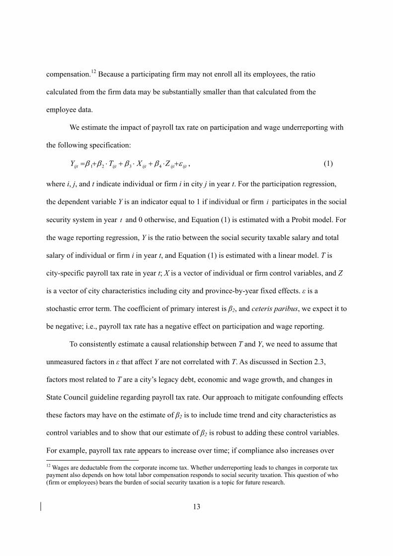
We estimate the impact of payroll tax rate on participation and wage underreporting with

the following specification:

ijtijtijtijtijt ZXTY 4321 , (1)

where i, j, and t indicate individual or firm i in city j in year t. For the participation regression,

the dependent variable Y is an indicator equal to 1 if individual or firm i participates in the social

security system in year t and 0 otherwise, and Equation (1) is estimated with a Probit model. For

the wage reporting regression, Y is the ratio between the social security taxable salary and total

salary of individual or firm i in year t, and Equation (1) is estimated with a linear model. T is

city-specific payroll tax rate in year t; X is a vector of individual or firm control variables, and Z

is a vector of city characteristics including city and province-by-year fixed effects. ε is a

stochastic error term. The coefficient of primary interest is β2, and ceteris paribus, we expect it to

be negative; i.e., payroll tax rate has a negative effect on participation and wage reporting.

To consistently estimate a causal relationship between T and Y, we need to assume that

unmeasured factors in ε that affect Y are not correlated with T. As discussed in Section 2.3,

factors most related to T are a city’s legacy debt, economic and wage growth, and changes in

State Council guideline regarding payroll tax rate. Our approach to mitigate confounding effects

these factors may have on the estimate of β2 is to include time trend and city characteristics as

control variables and to show that our estimate of β2 is robust to adding these control variables.

For example, payroll tax rate appears to increase over time; if compliance also increases over                                                                12 Wages are deductable from the corporate income tax. Whether underreporting leads to changes in corporate tax payment also depends on how total labor compensation responds to social security taxation. This question of who (firm or employees) bears the burden of social security taxation is a topic for future research.

  14

time because of more awareness of individuals or more diligent enforcement by local

governments, we may under-estimate the negative effect of payroll tax rate on compliance. We

control for province-specific time trend to address this concern. We use city fixed effects to

control for constant city-specific factors that may be related to both payroll tax rate and

compliance. For example, cities in the rusty belt tend to have a larger legacy debt and hence

higher payroll tax rate; meanwhile, these cities may exhibit lower compliance because of the

large number of under-employed workers (lay-offs or Xiagang Zhigong) who can easily fall

through the bureaucratic crack. Time-varying city characteristics include real GDP per capita,

average salary, adult illiterate rate, population, and fiscal capacity. In particular, fiscal capacity,

the ratio between general tax revenue and GDP, may to some extent reflect the effort and efficacy

of local government tax enforcement.

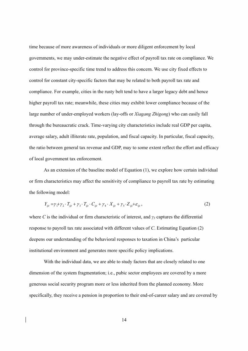
As an extension of the baseline model of Equation (1), we explore how certain individual

or firm characteristics may affect the sensitivity of compliance to payroll tax rate by estimating

the following model:

ijtijtijtijtijtijtijt ZXCTTY 54321 , (2)

where C is the individual or firm characteristic of interest, and γ3 captures the differential

response to payroll tax rate associated with different values of C. Estimating Equation (2)

deepens our understanding of the behavioral responses to taxation in China’s particular

institutional environment and generates more specific policy implications.

With the individual data, we are able to study factors that are closely related to one

dimension of the system fragmentation; i.e., pubic sector employees are covered by a more

generous social security program more or less inherited from the planned economy. More

specifically, they receive a pension in proportion to their end-of-career salary and are covered by

  15

a much more generous public medical insurance program.13 Additionally, an individual loses all

his social security contribution when moving from a firm job to a public sector job. Thus, ceteris

paribus, individuals who are potentially able to move to a public sector position may respond

more strongly to the payroll tax rate.

We consider individual characteristics that are associated with two routes to move to a

public sector job. First, young people aged between 18 and 35 with at least a 4-year college

education are eligible to take a highly competitive, national examination that selects public

servants. Second, firm executives who have had sufficiently extensive experience in the private

sector may be reassigned to a government position where their expertise is considered relevant

for policy making. We use the combination of age and current position to capture this possibility.

An alternative story that cannot be separated is that older executives may try to game the system

by consciously seeking a government position – they essentially exchange a few years of higher

salary in the private sector for the substantially more generous public-sector pension for the rest

of their life.

Another dimension of the system fragmentation is geographical. Because of the

administrative barriers to transfer benefits, individuals who are more mobile such as migrant

workers may comply less for any given level of payroll tax rate. Unfortunately, the individual

data contain mostly locally registered residents (individuals with Hukou), which prevent us from

directly testing this channel of differential responses. Nevertheless, the contrast between the

estimate of β2 in Equation (1) from the individual analysis and that from the firm analysis sheds

light on its importance. We discuss this in more detail in Section 6.

                                                               13 For example, public sector employees with more than 30 years of work experience receive at least 85% of the sum of their basic salary and post salary. The disparity in pension between a firm retiree and a government retiree has widened substantially over the past two decades. In 1990, the average annual pension is 1,664 Yuan and 2,006 Yuan for a firm retiree and a government retiree respectively; by 2005, the respective numbers are 8,803 Yuan and 18,410 Yuan (Zheng 2010), all in current RMB.

  16

We also explore how different types of firms respond differentially to the payroll tax rate.

One firm feature we consider is firm size. Klevin et al. (2009) show theoretically that larger

firms are more likely to comply with corporate taxation because of the higher likelihood of

whistle blowing by disgruntled employees. We test if this holds in the Chinese environment

where much less effort is spent on tax auditing than in more advanced economies. Another firm

feature we investigate is ownership – whether privately-owned and foreign-owned firms are

more sensitive than SOEs to payroll tax rate. Finally, we combine ownership and firm size.

These analyses may have important implications for where to target auditing effort.

4. Data and Summary Statistics

4.1 Data Sources

Ideally, we would like to use matched employer-employee data to examine the interaction

between firms and individuals in the decision of tax avoidance. With this unavailable, we use

individual data and firm data to study the responses of the two sides separately.

The individual data come from the annual Urban Household Survey (UHS) conducted by

the National Bureau of Statistics (NBS) of China. The UHS uses a stratified random sampling

method to select households to be representative of the urban population.14 Selected households

are required to report the demographic and income information of each member and to keep a

diary of itemized expenditure. We use survey data for the years 2002-2006, when detailed

information about social security contribution is available. This and information on individuals’

total labor compensation, and combined with statutory payroll tax rate, allow us to back out the

ratio between taxable salary and total salary – a measure of wage underreporting. While the

UHS covers all provincial units (including directly administered metropolises), due to restricted

                                                               14 The UHS does not survey households of migrant workers mostly because they lack a fixed residence; it also under-samples the extremely wealthy households due to lack of access to their residence.

  17

access to the full data our sample is a subset of nine provinces: Beijing, Liaoning, Zhejiang,

Anhui, Hubei, Guangdong, Sichuan, Shaanxi, and Gansu, which are picked from the three

broadly defined regions in China (costal, central, and western) and are representative of the

national urban population. We drop Liaoning and Shaanxi from the empirical analysis because a

key macroeconomic variable – annual city social security funds revenue – is missing.15 Our

sample thus includes on average about 12,000 households from just below 100 cities each year.

The majority of the households are composed of two parents and a child. The UHS sample is by

design a rotating panel with one third of households replaced each year; however, the survey

does not provide adequate information that allows us to precisely match households over time, so

we treat the sample primarily as repeated cross sections. Nevertheless, we construct a panel data

set by matching household basic information such as household size, age, gender and nationality

for each household member; this is used only for robustness analysis.

We restrict our analytical sample to individuals employed by firms in the formal sector.

For most of the sample period, participation in the social security system is mandatory for

formal-sector employees but is voluntary for those working in the informal sectors. In our data,

the participation rate is 78% and 28% for the formal-sector and informal-sector workers

respectively. We believe that the behavioral responses to payroll tax rate by the two groups of

individuals are rather different and should be studied separately. We lose about one fifth of

working adults due to this sample restriction. We further drop individuals reporting an annual

total earning lower than the annual minimum wage of 3600 Yuan,16 accounting for 1% of formal-

sector employees.

The firm data come from the Annual Census of Industrial Enterprises maintained by the

                                                               15 In the case of Shaanxi, this information is missing because it achieved the provincial social pool in 2000. Thus only provincial social security funds revenue is recorded. 16 The average minimum wage in our sample is around 300 Yuan per month, equivalently to 3600 Yuan per year.

  18

NBS. We use data from 2004 to 2006 for the same seven provinces as the individual analysis.

The data set includes all the State-Owned Enterprises (SOEs) and non-SOEs with annual sales

over 5 million Yuan (“above scale”), about 600,000 US dollars during the sample period, in the

mining, manufacturing, and electricity and utility sectors. The data contain basic information

about firm characteristics and many of the financial variables from three accounting statements –

balance sheet, income statement, and cash flow statement. In particular it includes information

on firms’ total salary payable and contributions to social security pension and medical insurance

programs, allowing us to estimate the underreporting of taxable salary from firm side. We restrict

our sample to firms with at least 20 employees and obtain an unbalanced panel with more than

100,000 firms in each of the three years.

We also collect city-level socio-economic data from various publications such as China

City Statistics Yearbooks and Municipal Public Finance Statistics Yearbooks. These include GDP

per capita, industrial structure, average wage, population, adult illiterate rate, general fiscal

capacity, and social security funds revenue.

4.2 Variable Definition

The most important explanatory variable for our analysis is the city statutory payroll tax rate. For

most of the cities in our sample, however, this information is not published. We therefore back it

out using publicly available aggregate soico-economic variables as follows:

salary average annual*sector formal in tsparticipan No.

revenue fundssecurity social annualT

salary average annual*rate coverage*sector formal in employees No.

revenue fundssecurity social annual . (3)

The numerator is the total annual social security funds revenue of a city, and the denominator is

the total annual salary of formal-sector contributors of the city; the ratio is approximately the

statutory payroll tax rate. All variables but coverage rate in the second row of Equation (3) are

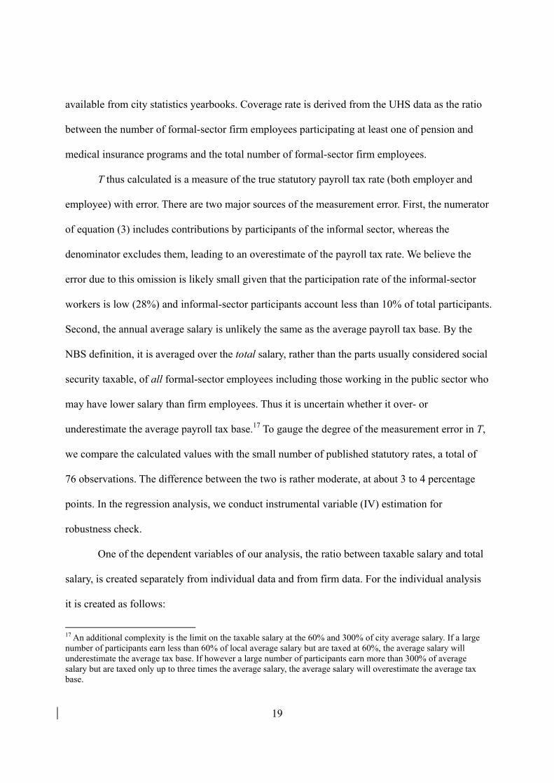
  19

available from city statistics yearbooks. Coverage rate is derived from the UHS data as the ratio

between the number of formal-sector firm employees participating at least one of pension and

medical insurance programs and the total number of formal-sector firm employees.

T thus calculated is a measure of the true statutory payroll tax rate (both employer and

employee) with error. There are two major sources of the measurement error. First, the numerator

of equation (3) includes contributions by participants of the informal sector, whereas the

denominator excludes them, leading to an overestimate of the payroll tax rate. We believe the

error due to this omission is likely small given that the participation rate of the informal-sector

workers is low (28%) and informal-sector participants account less than 10% of total participants.

Second, the annual average salary is unlikely the same as the average payroll tax base. By the

NBS definition, it is averaged over the total salary, rather than the parts usually considered social

security taxable, of all formal-sector employees including those working in the public sector who

may have lower salary than firm employees. Thus it is uncertain whether it over- or

underestimate the average payroll tax base.17 To gauge the degree of the measurement error in T,

we compare the calculated values with the small number of published statutory rates, a total of

76 observations. The difference between the two is rather moderate, at about 3 to 4 percentage

points. In the regression analysis, we conduct instrumental variable (IV) estimation for

robustness check.

One of the dependent variables of our analysis, the ratio between taxable salary and total

salary, is created separately from individual data and from firm data. For the individual analysis

it is created as follows:

                                                               17 An additional complexity is the limit on the taxable salary at the 60% and 300% of city average salary. If a large number of participants earn less than 60% of local average salary but are taxed at 60%, the average salary will underestimate the average tax base. If however a large number of participants earn more than 300% of average salary but are taxed only up to three times the average salary, the average salary will overestimate the average tax base.

  20

salary totalannual individual

salary taxableannual individualratio

salary totalannual individual

rate tax payroll eon/employecontributisecurity social annual individual

salary totalannual individual

0.2625)*on/(Tcontributisecurity social annual individual . (4)

In the last row of Equation (4), the information on individual annual social security contribution

and annual total salary is directly available from the UHS data, T is payroll tax rate just

calculated using Equation (3), and the factor 0.2625 is the share of employee social security

contribution specified by the State Council. In this process, we first drop the top and bottom 1%

of the calculated payroll tax rate; we then drop individuals whose annual social security

contribution is lower than what would be predicted at minimum wage, which account for about

5% of formal-sector firm employees.

From the firm data, the ratio between taxable salary and total salary is calculated as

follows:

salary totalannual firm

salary taxableannual firmratio

salary totalannual firm

medical&pensionfor rate tax payroller ons/employcontributi medical&pension annual firm

salary totalannual firm

0.2950.26*0.2625)-(1*ons/(Tcontributi health&pension annual firm

. (5)

In the last row of Equation (5), the information on firm annual pension and medical insurance

contribution and annual total salary is directly available from the Firm Census data, T is payroll

tax rate from Equation (3), the factor 1-0.2625 is the share of employer social security

contribution, and the factor 0.26/0.295 is the share of firm pension and medical insurance

contribution out of firm total social security contribution to all five programs, also specified by

  21

the State Council. In this process, we again drop the top and bottom 1% of the calculated payroll

tax rate, and we then drop firms with an average total salary lower than minimum wage, about

1% of all observations.

For both the individual and firm data, we define a dummy variable indicating whether an

individual or a firm participates in the social security system, taking the value 1 for participating

and 0 otherwise. A participant is one with positive social security contributions. The definition of

other variables used in the analysis is self-explanatory.

4.3 Descriptive Statistics

Table 1 reports summary statistics of individual characteristics. Panel A focuses on the sample

for the analysis of participation decision including all firm employees in the formal sector; we

restrict the payroll tax rate to be less than 1. Panel B focuses on the analytical sample of wage

underreporting including only formal-sector firm employees contributing to social security; we

restrict the payroll tax rate to be less than 1, the ratio between taxable salary and total salary to be

less than 1, and the ratio between taxable salary and city average salary to be between 0.6 and 3.

Of the 49120 observations in Panel A, 78.67% participates in the social security system.

The vast majority of individuals (98.4%) are registered local urban residents (with local Hukou).

57% of the individuals are male and they are slightly more likely to participate in social security

than females. Individuals with at least a 4-year college education account for 12.33% of the

sample, of which 4.98% are between 18 and 35 years of age and hence are eligible for the

national civil servant exam. College educated people are significantly more likely to participate

in social security (84.2%) than those with less education (77.9%). Executives account for 5.2%

of the sample, of which 1.14% are below 40 years of age and 4% are between 40 and the

mandatory retirement age. Additionally, 21.3% of individuals are ordinary white collar worker,

  22

39.8% are blue collar worker, and the occupation of the remaining is uncertain. Executives and

other white collar workers have similar participation rate (82.3% and 85.2% respectively), which

is significantly higher than that of the blue collar workers, at 74%. The majority of the sample

work in state-owned enterprises, and their participation rate of 83.56% is about 21 percentage

points higher than that of employees in collectively owned firms and 14 percentage points higher

than that of employees in domestic privately owned and foreign owned firms.18

The payroll tax rate for this sample has a mean of 0.36 and standard deviation of 0.17.

Figure 1 depicts the distribution of the payroll tax rate, while Figure 2 depicts the distribution of

the residual of payroll tax rate after removing the province-specific time trend and city fixed

effects. From Figure 2, there appears to be considerable within-city variation in payroll tax rate

over time, which is essential for our empirical analysis. The distribution of payroll tax rate for

the Panel B sample is almost identical; this is expected as the two samples include almost the

same cities in each year. Figure 3 shows that the distribution of payroll tax rate faced by

participants is slightly to the left of that faced by non-participants, suggesting a negative

relationship between participation and payroll tax rate.

The sample in Panel B includes 7314 individuals. Their average total salary, measured in

constant 2002 RMB, is 26,878 Yuan. Individuals with at least a 4-year college education earn an

average of 34,874 Yuan per year, about 9600 Yuan higher than those of lower education levels.

The average total salary of executives is 35150 Yuan, about 6300 Yuan higher than ordinary

white collar workers, and about 12600 Yuan higher than blue collar workers. The average total

salary of SOE employees is 25963 Yuan, 2400 Yuan higher than employees of collectively                                                                18 There is a discrepancy in firm ownership structure between the individual data and the firm data. One reason is that the former is self-reported while the latter is from the firm registration form, and individuals in the UHS may not have accurate information about the registered ownership type of their employers. Another reason is that the firm data only include mining, manufacturing, and electricity and utility industries, whereas the UHS data may include individuals working in other sectors such as banking, construction, and retailing. We believe that the firm data provide more accurate information about the ownership composition of the industrial sector.

  23

owned firms, but about 5100 Yuan lower than employees of private and foreign owned firms.

The ratio between taxable salary and total salary is 0.7 overall. There appears to be a

negative relationship between taxable salary ratio and payroll tax rate, as shown in Figure 4: The

distribution of ratio for above-median payroll tax rates is substantially to the left of that for

below-median payroll tax rates.

Individuals with higher total salary are also more likely to have a flexible pay structure,

with relatively larger share in the form of various subsidies and allowances; therefore we expect

their taxable salary ratio to be lower. While individuals employed in firms of different

ownerships show similar taxable salary ratio, this conjecture is born out in all other cases. For

example, the ratio is 0.65 for college-educated and 0.72 for those with less than a college

education. Figure 5 illustrates the entire distribution of taxable salary ratio for the two groups,

and as expected, the distribution of college-educated is considerably to the left.19 Additionally,

Figure 6 shows that the gap in the ratio distribution between the two education groups grows

wider with the increase in payroll tax rate: the gap is much larger at the top quartile payroll tax

rate than at the bottom quartile. Thus, Figures 5-6 provide clear visual evidence that the taxable

salary ratio differs by education, and the difference is even more salient at higher payroll tax rate.

The average ratio of executives is 0.63, close to that of ordinary white collar workers

(0.67), and both are much lower than that of blue collar workers (0.76). Figures 7-8 demonstrate

similar relationships as for education groups: the ratio distribution of executives is much to the

left of that for other types of employees, and the gap is larger at higher payroll tax rates.

In Figures 9-12, we present similar figures for those eligible for the national civil servant

exam (college education and aged between 18 and 35) and those ineligible, and for those with a

                                                               19 We also graph the distribution of the payroll tax rate by education level and find that different groups face nearly the same payroll tax rate distribution. Thus, the difference in the taxable salary ratio between groups is not due to differences in payroll tax rate, but due to education difference.

  24

higher possibility of moving to a public-sector job at late career (executives aged between 40 and

the mandatory retirement age) and others. In both cases, individuals who are potentially more

able to move to a public-sector job have a lower taxable salary ratio, and the gap between the

two respective groups widens as payroll tax rate gets higher.

Table 2 reports summary statistics of firm characteristics. In Panel A, the sample is for

the participation analysis, and we restrict the payroll tax rate to be less than one. Of the 187,333

observations, 67% participates in the social security system, somewhat smaller than the

individual participation rate. SOEs account for 6.2% of the sample, and their participation rate is

80.8%, similar to that of foreign-owned firms. The majority of firms are domestic privately

owned, but their participation rate is much lower, at 63.2%. The average employment of the

sample firms is 2100, and firms with larger employment have higher participation rate: it is just

below 60% for the bottom quartile of firms (smallest employment) and 75% for the top quartile

of firms. The average payroll tax rate for this sample is 0.42 with a standard deviation of 0.14.

The sample in Panel B is that for the wage reporting analysis. Here we further restrict the

ratio between taxable salary and total salary to be no greater than one, and the sample size is

111,997. The average ratio between taxable salary and total salary is 0.34, much smaller than that

observed in the individual data. One reason for this discrepancy is that a participating firm may

not enroll every employee in the social security system. Because the individual data include

almost all registered local urban residents, we suspect many of the employees not enrolled by

firms are migrant workers. These workers are either in a disadvantaged position when bargaining

with firms for benefits or unwilling to enroll due to the barriers when transferring benefits across

regions. Another reason for this discrepancy is that firms may report an even lower total taxable

salary because their contributions mostly go into the social pool and bear little relationship to

  25

employees’ future pension benefits. In the next two sections, we show that the wage reporting

response to payroll tax rate by individuals is indeed quite different from that by firms.

SOEs on average exhibit a significantly higher taxable salary ratio (0.52) than both

domestic private and foreign firms, who have similar ratios, 0.32 and 0.35 respectively. The ratio

however is not significantly different across firms of different employment levels.

Table 3 reports summary statistics of time-varying city characteristics for the sample in

Panel A of Table 1; they are similar for other samples in Tables 1 and 2. On average, the per

capita GDP is 23,080 Yuan, with 18,650 Yuan goes to individual salary. City value-added comes

mostly from the industrial and service sectors. Local tax revenue accounts for about 6% of GDP

(fiscal capacity), which is much lower than the revenue share in national GDP, consistent with

the fact that the central government collects most of the tax revenue. The average population is

3.4 million, with about 6% of illiterate adults. There is a great deal of variation in all these

variables.

5. Estimation Results from Individual Data

This section reports estimation results from the individual data. We first report our baseline

estimates of the impact of payroll tax rate on participation and the wage reporting decisions. We

discuss results of various sensitivity analyses. We then report estimation results of heterogeneous

responses to payroll tax rate by different types of individuals that are specific to China’s

fragmented social security system.

5.1 Participation and Payroll Tax Rate

Table 4 reports the estimation results of equation (1) for the participation decision. All columns

use the sample of formal-sector firm employees, while Columns 2-8 further restrict the payroll

tax rate to be less than one. All reported estimates are marginal effects, and standard errors are

  26

robust standard errors clustered at city level.

Columns 1-2 report the estimate on payroll tax rate without including any control

variables; they are -0.26 and -0.32 respectively, and both are significant at 1% level. Since

payroll tax rate is measured with error, the smaller estimate in Column 1 suggests that the

measurement error issue is perhaps more serious without the sample restriction in other columns,

and it is possible that we underestimate the effect of payroll tax rate even with this restriction.

Column 3 controls for key individual characteristics including education, age, occupation,

and ownership of the firm one work in, and Column 4 adds additional individual control

variables such as gender, marital status, registered residence status, and the industry one works in.

The estimate on payroll tax rate is similar in the two columns and is not significantly different

from that in Column 2. When we control for province-specific time trend in Column 5, the

estimate is significantly larger in absolute value. This suggests that there may be an increasing

trend in both the payroll tax rate and the social security coverage rate, and not controlling for this

trend leads to an underestimate of the negative effect of payroll tax rate on participation. Column

6 further controls for city fixed effects, and Column 7 adds controls of time-varying city

characteristics including per capita GDP, average wage of formal sector employees, fiscal

capacity, etc. The estimate on payroll tax rate barely changes.

Most pronounced in Table 4 is that the estimate on payroll tax rate in all columns is

negative and significant; in particular, once province-by-year fixed effects are controlled for,

controlling for additional city characteristics does not alter the estimate on payroll tax rate. This

robustness lends us confidence that the estimated effect of the payroll tax rate on participation is

not likely to reflect the influences of other unmeasured confounding factors.

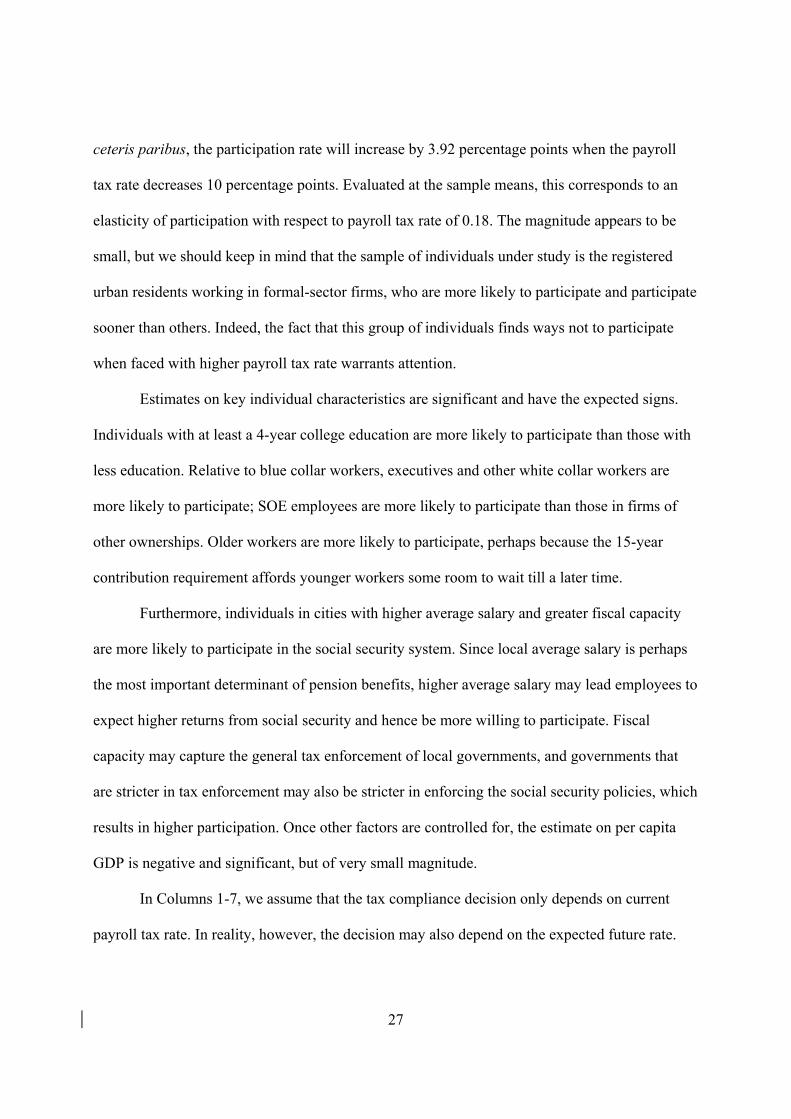
Consider the estimate in Column 7; if we extrapolate its implication to the city-level,

  27

ceteris paribus, the participation rate will increase by 3.92 percentage points when the payroll

tax rate decreases 10 percentage points. Evaluated at the sample means, this corresponds to an

elasticity of participation with respect to payroll tax rate of 0.18. The magnitude appears to be

small, but we should keep in mind that the sample of individuals under study is the registered

urban residents working in formal-sector firms, who are more likely to participate and participate

sooner than others. Indeed, the fact that this group of individuals finds ways not to participate

when faced with higher payroll tax rate warrants attention.

Estimates on key individual characteristics are significant and have the expected signs.

Individuals with at least a 4-year college education are more likely to participate than those with

less education. Relative to blue collar workers, executives and other white collar workers are

more likely to participate; SOE employees are more likely to participate than those in firms of

other ownerships. Older workers are more likely to participate, perhaps because the 15-year

contribution requirement affords younger workers some room to wait till a later time.

Furthermore, individuals in cities with higher average salary and greater fiscal capacity

are more likely to participate in the social security system. Since local average salary is perhaps

the most important determinant of pension benefits, higher average salary may lead employees to

expect higher returns from social security and hence be more willing to participate. Fiscal

capacity may capture the general tax enforcement of local governments, and governments that

are stricter in tax enforcement may also be stricter in enforcing the social security policies, which

results in higher participation. Once other factors are controlled for, the estimate on per capita

GDP is negative and significant, but of very small magnitude.

In Columns 1-7, we assume that the tax compliance decision only depends on current

payroll tax rate. In reality, however, the decision may also depend on the expected future rate.

  28

For example, if it is difficult to withdraw once one has participated in the social security system,

a higher expected future rate may deter current participation. Column 8 reports estimation results

controlling for the expectation of payroll tax rate for the next year, which is measured by the

actual payroll tax rate in the next year. The sample includes data for 2002-2005. The estimate on

the expected payroll tax rate is positive but insignificant, and its inclusion only slightly changes

the estimates on the current payroll tax rate and control variables. Thus it appears that

expectation does not play an important role here.

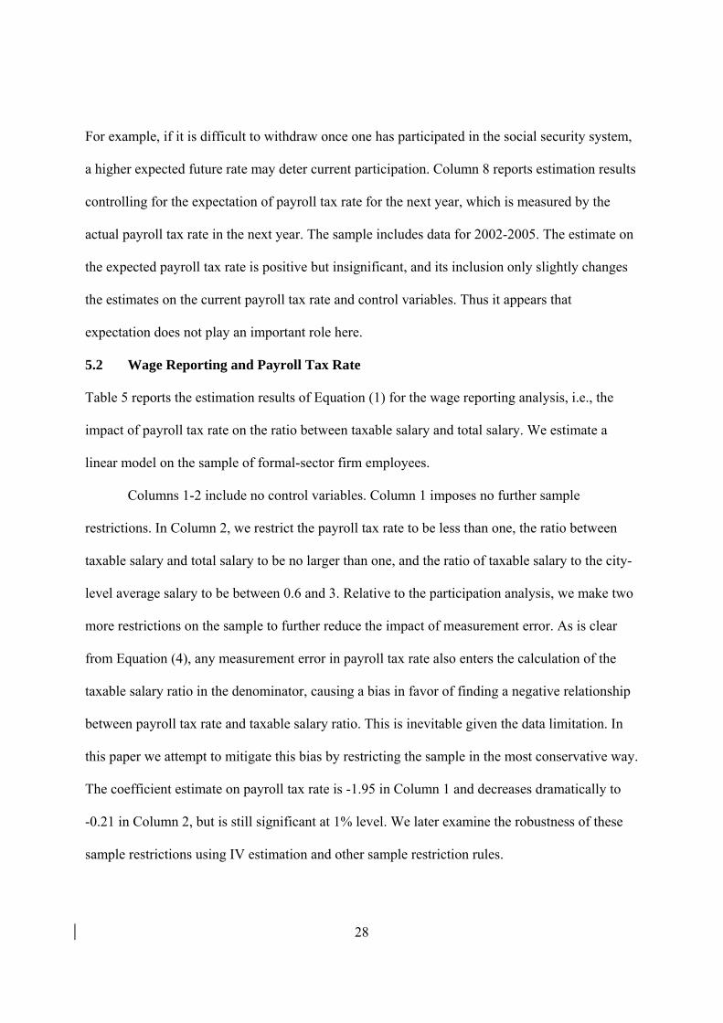
5.2 Wage Reporting and Payroll Tax Rate

Table 5 reports the estimation results of Equation (1) for the wage reporting analysis, i.e., the

impact of payroll tax rate on the ratio between taxable salary and total salary. We estimate a

linear model on the sample of formal-sector firm employees.

Columns 1-2 include no control variables. Column 1 imposes no further sample

restrictions. In Column 2, we restrict the payroll tax rate to be less than one, the ratio between

taxable salary and total salary to be no larger than one, and the ratio of taxable salary to the city-

level average salary to be between 0.6 and 3. Relative to the participation analysis, we make two

more restrictions on the sample to further reduce the impact of measurement error. As is clear

from Equation (4), any measurement error in payroll tax rate also enters the calculation of the

taxable salary ratio in the denominator, causing a bias in favor of finding a negative relationship

between payroll tax rate and taxable salary ratio. This is inevitable given the data limitation. In

this paper we attempt to mitigate this bias by restricting the sample in the most conservative way.

The coefficient estimate on payroll tax rate is -1.95 in Column 1 and decreases dramatically to

-0.21 in Column 2, but is still significant at 1% level. We later examine the robustness of these

sample restrictions using IV estimation and other sample restriction rules.

  29

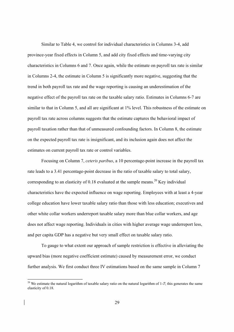
Similar to Table 4, we control for individual characteristics in Columns 3-4, add

province-year fixed effects in Column 5, and add city fixed effects and time-varying city

characteristics in Columns 6 and 7. Once again, while the estimate on payroll tax rate is similar

in Columns 2-4, the estimate in Column 5 is significantly more negative, suggesting that the

trend in both payroll tax rate and the wage reporting is causing an underestimation of the

negative effect of the payroll tax rate on the taxable salary ratio. Estimates in Columns 6-7 are

similar to that in Column 5, and all are significant at 1% level. This robustness of the estimate on

payroll tax rate across columns suggests that the estimate captures the behavioral impact of

payroll taxation rather than that of unmeasured confounding factors. In Column 8, the estimate

on the expected payroll tax rate is insignificant, and its inclusion again does not affect the

estimates on current payroll tax rate or control variables.

Focusing on Column 7, ceteris paribus, a 10 percentage-point increase in the payroll tax

rate leads to a 3.41 percentage-point decrease in the ratio of taxable salary to total salary,

corresponding to an elasticity of 0.18 evaluated at the sample means.20 Key individual

characteristics have the expected influence on wage reporting. Employees with at least a 4-year

college education have lower taxable salary ratio than those with less education; executives and

other white collar workers underreport taxable salary more than blue collar workers, and age

does not affect wage reporting. Individuals in cities with higher average wage underreport less,

and per capita GDP has a negative but very small effect on taxable salary ratio.

To gauge to what extent our approach of sample restriction is effective in alleviating the

upward bias (more negative coefficient estimate) caused by measurement error, we conduct

further analysis. We first conduct three IV estimations based on the same sample in Column 7

                                                               20 We estimate the natural logarithm of taxable salary ratio on the natural logarithm of 1-T; this generates the same elasticity of 0.18.

  30

using different instrumental variables for payroll tax rage; we then apply different sample

restrictions and conduct OLS estimations on these different samples.

Columns 9-11 of Table 5 report the IV estimations. Our first IV is the employee pension

contribution rate calculated from information on individual pension contributions from the UHS

data. More specifically, it is the ratio between contributions of all participants in a city and the

product of the number of participants and city average salary. Our second IV is the sum of the

employee pension and medical insurance contribution rates, with the latter calculated similarly.

Insofar as the measurement error in the two employee contribution rates is not perfectly

correlated with the measurement in the payroll tax rate, they can be used to deal with the

measurement error problem in the payroll tax rate. Results using these two IVs (Columns 9-10)

are similar: the IV estimates on payroll tax rate are negative and of larger magnitude than

estimate in Column 7; however they are not significant. The first stage estimate on each IV is

positive and significant. In Column 11 we report the results using the third IV. We first create a

panel data set by matching key information of a household and of each member of the household

with the same household identification code; we then employ city dummies as instruments as

Gruber (1997). The assumption is that the error term in the payroll tax rate measure does not

systematically vary with city; or in other words, the error term varies over time within a city. The

IV estimate on payroll tax rate is -1.3 and significant at 1% level; the Sargan’s test rejects weak

IV. Thus, while none of the IVs are prefect, they jointly suggest that the negative estimates in the

first eight columns in Table 5 are not an artifact due to measurement error in payroll tax rate.

For the second set of robustness checks, we estimate the same model in Column 7 of

Table 5 using alternative samples. The results are reported in Tables 6. We continue to focus on

formal-sector firm employees. In Columns 1-4 we restrict the payroll tax rate to be below one

  31

and then impose other constraints on each column. Column 1 limits the ratio between taxable

salary and total salary to be no more than 1; Columns 2-4 all start from the sample in Column 1

and further restrict the ratio between taxable salary and city average salary to be less than 3

(Column 2), greater than 0.6 (Column 3), and between 0.6 and 3 (Column 4) respectively.

Sample in Column 4 is the same as that in Columns 2-7 of Table 5. We note that the sample size

does not change much between Columns 1 and 2, but drops substantially in Column 3. In

Columns 5-8, we first restrict the payroll tax rate to be less than 0.6 – as shown in Figure 1, a

very small number of observations have a payroll tax rate higher than 0.6, and we treat these as

extreme values. We then impose further sample restrictions in the same manner as for Columns

1-4. Estimate on payroll tax rate is negative and significant at 1% level in all columns, and all

estimates are of similar magnitude. These results suggest that the sample restriction rules in

Table 5 are not overly restrictive, and the magnitude of the estimate there provides a reasonably

sound guidance about the true effect of payroll tax rate on wage reporting.21

In December, 2005, the State Council Decree No. 38 changes the benefit formula to make

benefits from the social pool a function of length and amount of individual contribution;

meanwhile, it reduces the funds assigned to individual account to 8%. Both are effective at the

beginning of 2006. We explore whether the policy changes affect the participation and wage

reporting behavior in 2006 by estimating Equation (1) using data from 2002-2005. The results

are reported in Appendix Table A2. The magnitude of the results is similar to those for the 2002-

2006 data, and the two sets of results are not significantly different from each other.22

5.3 Heterogeneity due to System Fragmentation                                                                21 In the first three columns of Table A1, we report IV estimates for the sample used in Column 8 of Table 6 using the same IVs as in Columns 9-11 of Table 5, and the results are similar. 22 In the first two columns of Appendix Tables A3 and A4, we report estimation results using the 2002-2006 and 2002-2005 panel data respectively, controlling for unobserved individual characteristics with individual fixed effects. The results are similar in the two tables, and the magnitude of the estimate is larger than that from the pooled cross section data for the respective period.

  32

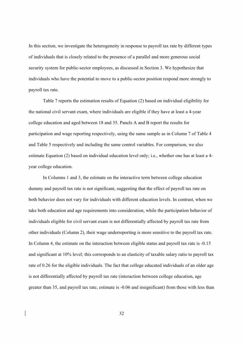
In this section, we investigate the heterogeneity in response to payroll tax rate by different types

of individuals that is closely related to the presence of a parallel and more generous social

security system for public-sector employees, as discussed in Section 3. We hypothesize that

individuals who have the potential to move to a public-sector position respond more strongly to

payroll tax rate.

Table 7 reports the estimation results of Equation (2) based on individual eligibility for

the national civil servant exam, where individuals are eligible if they have at least a 4-year

college education and aged between 18 and 35. Panels A and B report the results for

participation and wage reporting respectively, using the same sample as in Column 7 of Table 4

and Table 5 respectively and including the same control variables. For comparison, we also

estimate Equation (2) based on individual education level only; i.e., whether one has at least a 4-

year college education.

In Columns 1 and 3, the estimate on the interactive term between college education

dummy and payroll tax rate is not significant, suggesting that the effect of payroll tax rate on

both behavior does not vary for individuals with different education levels. In contrast, when we

take both education and age requirements into consideration, while the participation behavior of

individuals eligible for civil servant exam is not differentially affected by payroll tax rate from

other individuals (Column 2), their wage underreporting is more sensitive to the payroll tax rate.

In Column 4, the estimate on the interaction between eligible status and payroll tax rate is -0.15

and significant at 10% level; this corresponds to an elasticity of taxable salary ratio to payroll tax

rate of 0.26 for the eligible individuals. The fact that college educated individuals of an older age

is not differentially affected by payroll tax rate (interaction between college education, age

greater than 35, and payroll tax rate, estimate is -0.06 and insignificant) from those with less than

  33

college education suggests that this is not because higher income people have more room to

underreport taxable incomes.23 One reason that the eligible individuals do not respond differently

in participation behavior is perhaps that participation is more of a firm decision and individuals

have less discretion. In contrast, given their incentives, eligible individuals may be more able to

bargain with employers over their compensation structure.

Table 8 presents the estimation results for Equation (2) based on individual ability to

change to a public-sector job at late career, where individuals are more “able” if they are firm

executives and aged between 40 and the mandatory retirement age.24 Panels A and B report the

results for participation and wage reporting respectively, using the same samples and including

the same control variables as in Table 7. For comparison, we also estimate Equation (2) based on

individual occupation only – executive, ordinary white collar, and blue collar.

Columns 1 and 2 show that relative to blue collar workers, participation of executives and

white collar workers is less sensitive to payroll tax rate, and among the blue collar workers,

participation of younger workers is less sensitive to payroll tax rate than older workers. In

Column 2, the elasticity of participation to payroll tax rate is 0.25 for older blue collar workers.

Other than older blue collar workers, payroll tax rate does not differentially affect the

participation probability of other groups – estimates on the interactive terms are not significantly

different. One explanation for the greater sensitivity of participation to payroll tax rate of the

older blue collar workers is that they are more likely to belong to the “middle people” category

discussed in Footnote 6 and their retirement benefits are less affected by their own contributions,

particularly in view of their low earnings relative to other groups of the same age.25

                                                               23 All individuals with at least a college education is greater than 18 years of age; the average of total salary is 35,400 Yuan and 34,100 Yuan for those aged above 35 and below 35 respectively. 24 We use age 45 as the late career cutoff and the results are similar. 25 The average total salary of individuals between 40 and the mandatory retirement age is 28,300 Yuan, 22,300 Yuan,

  34

For the wage reporting analysis, estimates on the interactions between occupation

dummies and payroll tax rate are not significant in Column 3, indicating that occupation alone

dose not affect the sensitivity of wage reporting to payroll tax rate. In Column 4, the estimate on

the interaction between older executive dummy (relative to older blue collar workers) and

payroll tax rate is -0.18 and significant at 10% level, implying a taxable salary elasticity to

payroll tax rate of 0.29 for this group. The estimates on all other interactive terms with payroll

tax rate are insignificant, and they are all significantly different from the estimate on the older

executive-payroll tax rate interaction. Because older executives have the highest total salary,26

one concern is that they have more room to underreport salary faced with a higher payroll tax

rate. Because the difference in the age gap of total salary between the two occupation groups is

similar, we test whether the difference in response between older executives and younger

executives is the same as that between older and younger other white collar workers, assuming

response difference is linear in total salary. The p-value for this F-test is 0.07, allowing us to

reject the null hypothesis with sufficient confidence. Thus the stronger response to payroll tax

rate by older executives is not due to their higher salary.27

In sum, findings in Tables 7-8 suggest strongly that individuals who have the potential to

move to a public sector job are more likely to underreport taxable salary when faced with a

higher payroll tax rate.

6. Estimation Results from Firm Data

In this section, we perform the participation and wage reporting analyses using firm data; the

results corroborate the findings from individual data and enhance our understanding of firm                                                                                                                                                                                                          and 13,700 Yuan for executives, other white collar workers, and blue collar workers respectively. 26 The average total salary is 28,300 Yuan, 26,500 Yuan, 22,300 Yuan, and 20,900 Yuan for older executives, younger executives, older other white collar workers, and younger other white collar workers respectively. 27 In Appendix Tables A1-A4, we conduct the heterogeneity analysis of wage reporting behavior for the sample of Column 8 of Table 6, pooled cross sections for 2002-2005, and panel data for 2002-2005 and 2002-2006 separately, the results are generally consistent with findings in Tables 7-8.

  35

avoidance behavior of payroll taxation.

The results are reported in Table 9. Panels A and B report the estimates for the

participation and wage reporting analysis respectively. In Panel A, we restrict the payroll tax rate

to be less than one; In Panel B, we further restrict the firm ratio between taxable salary and total

salary to be no more than one. All columns control for basic firm characteristics, province-year

and city fixed effects, and time-varying city characteristics.

6.1 Baseline Results

In Column 1, the estimate on payroll tax rate is -0.19 and significant at 1% level, corresponds to

an elasticity of participation of 0.11 with respect to payroll tax rate when evaluated at the sample

means. Estimates on control variables are significant and have expected signs. Firms with larger

work force and in operation for longer time are more likely to participate; relative to state-owned

enterprises (SOEs), domestic private firms are less likely to participate, while foreign owned

firms are slightly more likely to participate in the social security system. Additionally, firms in

cities with higher average wage and greater per capita GDP are more likely to participate.

Estimate in Column 5 shows that payroll tax rate has a negative effect on firm taxable salary

ratio: the estimate is -0.51 and significant at 1% level. This corresponds to an elasticity of taxable

salary to payroll tax rate of 0.62. While firms of different ownerships have similar taxable salary

ratio, larger firms underreport more, perhaps because larger firms are more able to report labor

cost in different categories.

Compared to the baseline results from individual data (Column 7 of Table 4 and Table 5),

firm participation elasticity is somewhat smaller (0.11 v. 0.18), but the elasticity of taxable salary

is much larger for firms than for individuals (0.62 v. 0.18). These are consistent with the choices

faced by individuals and firms. On the one hand, individuals may choose to work for a non-

  36

participating firm or choose not to participate (such as older blue collar workers discussed earlier)

when working for a participating firm; this additional option may render their participation

behavior more responsive to payroll tax rate. On the other hand, faced with a higher payroll tax

rate, firms could choose to enroll fewer employees in the social security system, as well as

adjusting the compensation structure of enrollees. As a result, firm taxable salary ratio is more

responsive to payroll tax rate than individual taxable salary ratio.

The large discrepancy in the elasticity of taxable salary between firms and individuals is

consistent with the fact that individuals in the UHS data are registered local urban residents,

whereas firms may hire many migrant workers. The latter may be less willing to participate in

the social security system because of the high barriers in transferring benefits across regions;

they may be less covered also because they are in a disadvantaged position when bargaining with

firms for benefits. Regardless, this implies that to improve compliance, in both coverage and

accurate wage reporting, the policy makers should pay particular attention to firms that hire large

numbers of migrant workers.

Another possibility that may contribute to this large discrepancy is that firms may simply

underreport the aggregate taxable salary to a larger extent. First, this is less visible to individual

employees and less likely to be reported to the government agency. Second, even if individual

employees are aware of this activity, because it most goes into the social pool, firm contribution

has less relation to individual future benefits. Thus enforcing full contribution by firms is more

difficult.

6.2 Heterogeneity by Firm Size and Ownership

We first investigate whether firms of different sizes respond differentially to payroll tax rate. We

use employment to measure firm size and interact it with payroll tax rate. Estimate on the

  37

interaction between employment and payroll tax rate in Column 2 is positive and significant,

suggesting that larger firms’ participation is less sensitive to payroll tax rate. Indeed, larger firms

tend to participate more with increases in payroll tax rate, perhaps due to stronger enforcement

on these firms at higher rates. Estimate on the interactive term in Column 6, however, is

insignificant; thus payroll tax rate has no differential effects on wage reporting of participating

firms of different sizes. We also interact indicators for quartiles of firm size with payroll tax rate

to allow firm response to payroll tax rate to vary nonlinearly with firm size, and the results are

similar. In sum, our findings are broadly consistent with the theoretical prediction of Kleven et al.

(2009) that larger firms are more likely to comply with taxation.

We next explore whether firms of different ownerships respond differentially to payroll

tax rate. The estimation results in Column 3 indicate that payroll tax rate has no effect on

participation of SOEs and foreign-owned firms and a negative and significant effect on

participation of domestic private firms.28 Meanwhile, estimates in Column 7 suggest that for

participating firms, payroll tax rate has a negative effect on taxable salary ratio regardless of

ownership, but it is more adverse for SOEs’ than for domestic private firms foreign owned firms.

Finally, we add a full set of interactive terms between firm size, firm ownership, and payroll

tax rate in Columns 4 and 8. Estimates in Column 4 suggest that payroll tax rate has a negative

effect on participation of private firms regardless of size; payroll tax rate has no effect on

participation of SOEs regardless of size; and for a wide range of firm size, higher payroll tax

rates induce more participation by foreign-owned firms. Estimates in Column 8 suggest that

payroll tax rate has a negative effect on the taxable salary ratio of SOEs regardless of size;

however, for both the domestic private and foreign-owned firms, the negative effect of payroll

                                                               28 The sum of estimates on payroll tax rate and on the interaction between private ownership dummy and payroll tax rate is negative and significantly different form zero.

  38

tax rate on taxable salary decreases with firm size, likely because large private and foreign firms

are subject to stricter tax auditing by the government. These findings can potentially provide

guidance as to the target of payroll tax enforcement: while government should pay attention to

participation of domestic private firms, it should perhaps exert more effort to insure full coverage

of employees and accurate reporting of taxable salary by participating firms, in particular SOEs

and relatively small domestic private firms.

To summarize, the findings from the firm data are in line with those from individual data.

They both indicate that increases in payroll tax rate reduce the likelihood of participation and

increase the degree of underreporting of taxable salary. There are interesting heterogeneities in

response by both individuals and firms, which have important policy implications.

7. Conclusion

TO BE COMPLETED.

  39

References: Allingham, Michael G. and Agnar Sandmo (1972). “Income Tax Evasion: A Theoretical Analysis.” Journal of Public Economics. 1 (3-4), 323-338. Bailey, Clive and John Turner (2001). “Strategies to Reduce Contribution Evasion in Social Security Financing.” World Development, 29 (2): 385-393. Cai, Hongbin and Qiao Liu (2009). “Competition and Corporate Tax Avoidance: Evidence from Chinese Industrial Firms.” Economic Journal, 119 (537): 764-795. Chen, Vivian Y. (2004). “A Macro Analysis of China Pension Pooling System - Incentive Issues and Financial Problem.” International Conference on Pensions in Asia: Incentives, Compliance and Their Role in Retirement, Organized by PIE and COE/RES, Hitotsubashi University. Cottani, Joaquin and Gustavo Demarco (1998). “The Shift to a Funded Social Security System: the Case of Argentina.” In Martin Feldstein, eds., Privatizing social security. Chicago: University of Chicago Press, 177-212. Desai, Mihir A., Alexander Dyck, and Luigi Zingales (2007). “Theft and Taxes.” Journal of Financial Economics, 84 (3): 591-623. Feldstein, Martin (1995). “The Effect of Marginal Tax Rates on Taxable Income: a Panel Study of the 1986 Tax Reform Act.” Journal of Political Economy, 103(3): 551-572. Feldstein, Martin (1999). “Tax Avoidance and the Deadweight Loss of the Income Tax.” Review of Economics and Statistics, 81 (4): 674-680. Feldstein, Martin (2003). “Banking, Budgets, and Pensions: Some Priorities for Chinese Policy.” Remarks presented at the China Development Forum 2003 of the Development Research Center of the State Council of the People’s Republic of China. Feldstein, Martin and Jeffrey Liebman (2006). “Realizing the Potential of China’s Social Security Pension System.” China Economic Times, February 24. Fisman, Raymond and Shang-Jin Wei (2004). “Tax Rates and Tax Evasion: Evidence from ‘Missing Imports’ in China.” Journal of Political Economy, 112 (2): 471-496. Gordon, Roger H. and James R. Hines (2002). “International Taxation.” In Alan Auerbach and Martin Feldstein, eds., Handbook of Public Economics, Elsevier, 1935-1995. Gorodnichenko, Yuriy, Jorge Martinez-Vazquez, and Klara Sabirianova Peter (2009). “Myth and Reality of Flat Tax Reform: Micro Estimates of Tax Evasion Response and Welfare Effects in Russia.” Journal of Political Economy, 117(3): 504-554. Gruber, Jonathan (1997). “The Incidence of Payroll Taxation: Evidence from Chile.” Journal of

  40

Labor Economics, 15(3), S72-101. Mishra, Prachi, Arvind Subramanian, and Petia Topalova (2008). “Tariffs, Enforcement, and Custom Evasion: Evidence from India.” Journal of Public Economics, 92 (10-11): 1907-1925. Nitsch, Manfred and Helmut Schwarzer (1995). “Recent Developments in Financing Social Security in Latin America.” Issues in Social Protection Discussion Paper No.1, International Labor Organization. Nyland, Chris, Russell Smyth, and Cherrie Jiuhua Zhu (2005). “What Determines the Extent to which Employers Will Comply with Their Social Security Obligations? Evidence from Chinese Firm Level Data.” Monash University Working Paper 14/05. OECD (2011a). Taxation: Key Tables from OECD. http://www.oecd-ilibrary.org/taxation/taxation-key-tables-from-oecd_20758510. OECD (2011b). Pensions at a Glance 2011: Retirement-Income Systems in OECD and G20 Countries. www.oecd.org/els/social/pensions/PAG. Saez, Emmanuel (2010). “Do Taxpayers Bunch at Kink Points?” American Economic Journal: Economic Policy, 2: 180-212. Saez, Emmanuel, Joel Slemrod, and Seth H. Giertz (2012). “The Elasticity of Taxable Income with Respect to Marginal Tax Rates: a Critical Review.” Journal of Economic Literature, 50(1): 3-50. Slemrod, Joel (2004). “Economics of Corporate Tax Selfishness”, National Tax Journal, 57(4), 877-899. Slemrod, Joel and Shlomo Yitzhaki (2002). “Tax Avoidance, Evasion, and Administration.” In Alan Auerbach and Martin Feldstein, eds., Handbook of Public Economics, Elsevier, 1423-1470. Zhao, Yaohui and Jianguo Xu (2001). “Incentive Problem in China’s Urban Pension Reform.” China Economic Quarterly, 1(1): 193: 206 (in Chinese). Zheng, Bingwen (2010). “The Development of Social Security System and Its Institutional Changes in the People’s Republic of China.” In Jiagui Chen and Yanzhong Wang, eds., China Social Security System Development Report: Building an Equal Treatment Social Security System, Social Science Academy Press (in Chinese).

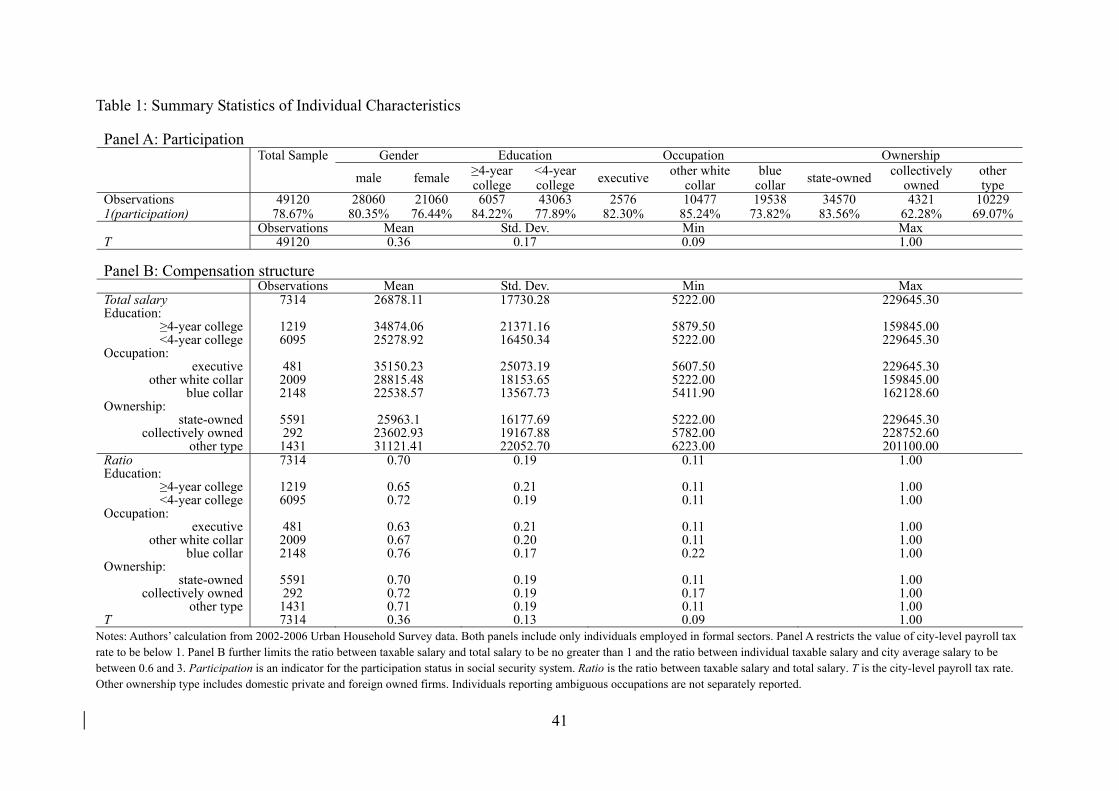
  41

Table 1: Summary Statistics of Individual Characteristics

Panel A: Participation Gender Education Occupation Ownership

Total Sample

male female ≥4-year college

<4-year college executive other white

collar blue

collar state-owned collectively owned

other type

Observations 49120 28060 21060 6057 43063 2576 10477 19538 34570 4321 10229 1(participation) 78.67% 80.35% 76.44% 84.22% 77.89% 82.30% 85.24% 73.82% 83.56% 62.28% 69.07% Observations Mean Std. Dev. Min Max T 49120 0.36 0.17 0.09 1.00 Panel B: Compensation structure Observations Mean Std. Dev. Min Max Total salary 7314 26878.11 17730.28 5222.00 229645.30 Education:

≥4-year college <4-year college

1219 6095

34874.06 25278.92

21371.16 16450.34

5879.50 5222.00

159845.00 229645.30

Occupation: executive

other white collar blue collar

481 2009 2148

35150.23 28815.48 22538.57

25073.19 18153.65 13567.73

5607.50 5222.00 5411.90

229645.30 159845.00 162128.60

Ownership: state-owned

collectively owned other type

5591 292 1431

25963.1

23602.93 31121.41

16177.69 19167.88 22052.70

5222.00 5782.00 6223.00

229645.30 228752.60 201100.00

Ratio 7314 0.70 0.19 0.11 1.00 Education:

≥4-year college <4-year college

1219 6095

0.65 0.72

0.21 0.19

0.11 0.11

1.00 1.00

Occupation: executive

other white collar blue collar

481 2009 2148

0.63 0.67 0.76

0.21 0.20 0.17

0.11 0.11 0.22

1.00 1.00 1.00

Ownership: state-owned

collectively owned other type

5591 292 1431

0.70 0.72 0.71

0.19 0.19 0.19

0.11 0.17 0.11

1.00 1.00 1.00

T 7314 0.36 0.13 0.09 1.00 Notes: Authors’ calculation from 2002-2006 Urban Household Survey data. Both panels include only individuals employed in formal sectors. Panel A restricts the value of city-level payroll tax rate to be below 1. Panel B further limits the ratio between taxable salary and total salary to be no greater than 1 and the ratio between individual taxable salary and city average salary to be between 0.6 and 3. Participation is an indicator for the participation status in social security system. Ratio is the ratio between taxable salary and total salary. T is the city-level payroll tax rate. Other ownership type includes domestic private and foreign owned firms. Individuals reporting ambiguous occupations are not separately reported.

  42

Table 2: Summary Statistics of Firm Characteristics

Panel A: Participation Ownership Employment

Total Sample state-owned private FDI Quartile 1 Quartile 2 Quartile 3 Quartile 4

Observations 187333 11648 141424 34261 47352 46824 46501 46656 1(participation) 67.00% 80.80% 63.16% 78.14% 59.95% 64.98% 68.03% 75.15% Observations Mean Std. Dev. Min Max T 187333 0.42 0.14 0.11 1.00 Employment (Thousand) 187333 0.21 0.97 0.02 113.04 years in operation 187333 8.29 8.92 0.00 106.00 Panel B: Compensation Structure Observations Mean Std. Dev. Min Max Ratio 111997 0.34 0.23 0.00 1.00 Ownership:

state-owned private

FDI

5967

81800 24230

0.52 0.32 0.35

0.26 0.22 0.23

0.01 0.00 0.01

1.00 1.00 1.00

Employment: Quartile 1 Quartile 2 Quartile 3 Quartile 4

28542 28454 27196 27805

0.36 0.33 0.33 0.34

0.23 0.22 0.23 0.24

0.01 0.00 0.00 0.01

1.00 1.00 1.00 1.00

Notes: Authors’ calculation from the 2004-2006 census of above-scale firms (all state-owned firms and firms of other ownership types with annual sales greater than 5 Million Yuan). In both panels, we restrict firms to have at least 20 employees. Panel A restricts the value of the city-level payroll tax rate to be below 1. Panel B further limits the ratio between taxable salary and total salary to be no greater than 1.Participation is an indicator for a firm’s participation status in social security system. Employment is firm employment in thousand. Ratio is the ratio between taxable salary and total salary. We group firms by employment quartiles, with quartile 1 indicating firms with the smallest employment. Since the summary statistics of T, employment, and years in operation are similar for the sample of firms in Panel A and Panel B, we only report those in Panel A.

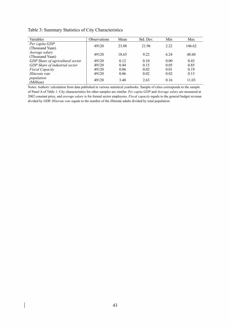
  43

Table 3: Summary Statistics of City Characteristics Variables Observations Mean Std. Dev. Min Max Per capita GDP (Thousand Yuan) 49120 23.08 21.96 2.22 146.62

Average salary (Thousand Yuan) 49120 18.65 9.22 6.24 48.60

GDP Share of agricultural sector 49120 0.12 0.10 0.00 0.43 GDP Share of industrial sector 49120 0.44 0.15 0.05 0.85 Fiscal Capacity 49120 0.06 0.02 0.01 0.19 Illiterate rate 49120 0.06 0.02 0.02 0.13 population (Million) 49120 3.40 2.63 0.16 11.03

Notes: Authors’ calculation from data published in various statistical yearbooks. Sample of cities corresponds to the sample of Panel A of Table 1. City characteristics for other samples are similar. Per capita GDP and Average salary are measured at 2002 constant price, and average salary is for formal sector employees. Fiscal capacity equals to the general budget revenue divided by GDP. Illiterate rate equals to the number of the illiterate adults divided by total population.

  44

Table 4: Payroll Tax Rate and Participation in Social Security System

Dependent Variable: 1(participation)

(1) (2) (3) (4) (5) (6) (7) (8)

Expectation

T -0.264** [0.038]

-0.321** [0.048]

-0.298** [0.049]

-0.290** [0.050]

-0.379** [0.046]

-0.386** [0.056]

-0.392** [0.056]

-0.426** [0.054]

expectation of T 0.028 [0.050]

1(edu≥4-year college) 0.031* [0.012]

0.043** [0.010]

0.040** [0.010]

0.037** [0.010]

0.037** [0.010]

0.046** [0.011]

age 0.004** [0.000]

0.002** [0.001]

0.001** [0.000]

0.002** [0.000]

0.002** [0.000]

0.002** [0.000]

1(occu=executive) 0.018 [0.023]

0.040* [0.019]

0.041* [0.018]

0.050** [0.016]

0.049** [0.016]

0.058** [0.016]

1(occu=other white collar)

0.083** [0.010]

0.098** [0.009]

0.097** [0.008]

0.095** [0.008]

0.095** [0.008]

0.097** [0.009]

1(occu=uncertain) 0.035** [0.010]

0.050** [0.008]

0.049** [0.007]

0.054** [0.007]

0.053** [0.007]

0.064** [0.007]

1(ownership=state-owned)

0.113** [0.014]

0.120** [0.015]

0.150** [0.017]

0.169** [0.014]

0.169** [0.014]

0.167** [0.016]

1(ownership=collectively owned)

-0.054** [0.019]

-0.060** [0.020]

-0.038+ [0.020]

-0.011 [0.020]

-0.011 [0.020]

-0.019 [0.022]

Other individual-level control variables

No No No Yes Yes Yes Yes Yes

City-level control variables

No No No No No No Yes Yes

City FE No No No No No Yes Yes Yes Province FE*Year FE No No No No Yes Yes Yes Yes Observations 50494 49244 49244 49244 49244 49224 49120 35597 Pseudo R-square 0.022 0.019 0.062 0.079 0.093 0.133 0.133 0.138

Notes: A probit model is employed, and all coefficients are marginal effects. Robust standard errors in the brackets are clustered at city level. ** is significant at 1% level. * is significant at 5% level. + is significant at 10% level.

Sample includes individuals employed in formal-sector firms from the pooled data of 2002-2006 Urban Household Survey. We restrict the value of the city-level payroll tax rate to be below 1 for Columns 2-8. The omitted occupation type is blue collar, the omitted education type is below 4-year college, and the omitted ownership type is other type (domestic private and foreign owned firms). Other individual-level control variables include gender, marital status, registered residence status, and the industry individuals work in. City-level control variables include GDP per capita, average salary, GDP shares of agricultural and industrial sectors, fiscal capacity, adult illiterate rate, and population.

  45

Table 5: Payroll Tax Rate and Ratio of Taxable Salary Relative to Total Salary

Dependent Var: ratio (1) (2) (3) (4) (5) (6) (7) (8)

Expectation (9) IV1

(10) IV2

(11) IV3

T -1.954** [0.354]

-0.207** [0.052]

-0.232** [0.050]

-0.249** [0.048]

-0.334** [0.057]

-0.367** [0.075]

-0.341** [0.065]

-0.363** [0.071]

-0.619 [0.918]

-0.590 [0.905]

-1.314** [0.232]

expectation of T 0.092

[0.062]

1(edu≥4-year college) -0.042** [0.009]

-0.036** [0.008]

-0.042** [0.008]

-0.044** [0.007]

-0.044** [0.007]

-0.045** [0.009]

-0.043** [0.007]

-0.043** [0.007]

0.037 [0.078]

age 0.000 [0.000]

0.001+ [0.000]

0.001 [0.000]

0.001 [0.000]

0.001 [0.000]

0.001 [0.000]

0.001 [0.000]

0.001 [0.000]

-0.006 [0.006]

1(occu=executive) -0.127** [0.017]

-0.109** [0.017]

-0.107** [0.014]

-0.099** [0.014]

-0.098** [0.015]

-0.106** [0.016]

-0.098** [0.015]

-0.098** [0.015]

-0.100 [0.061]

1(occu=other white collar) -0.083** [0.010]

-0.069** [0.009]

-0.065** [0.009]

-0.056** [0.009]

-0.056** [0.009]

-0.059** [0.010]

-0.056** [0.009]

-0.056** [0.009]

-0.109* [0.051]

1(occu=uncertain) -0.070** [0.009]

-0.058** [0.009]

-0.052** [0.008]

-0.042** [0.008]

-0.042** [0.008]

-0.039** [0.008]

-0.042** [0.008]

-0.042** [0.008]

-0.052 [0.042]

1(ownership=state-owned) -0.005 [0.007]

0.010 [0.007]

0.011 [0.008]

0.003 [0.008]

0.002 [0.008]

0.002 [0.010]

0.001 [0.008]

0.001 [0.008]

-0.042 [0.058]

1(ownership=collectively owned)

-0.001 [0.013]

0.009 [0.013]

0.020 [0.013]

0.020 [0.013]

0.020 [0.013]

0.034* [0.016]

0.016 [0.017]

0.017 [0.018]

-0.190** [0.070]

Other individual-level control variables

No No No Yes Yes Yes Yes Yes Yes Yes Yes

City-level control variables No No No No No No Yes Yes Yes Yes Yes City FE No No No No No Yes Yes Yes Yes Yes Yes Province*Year FE No No No No Yes Yes Yes Yes Yes Yes Yes Observations 37330 7324 7324 7324 7324 7324 7314 5250 7312 7311 2090 Adjusted R-square 0.116 0.020 0.076 0.093 0.128 0.183 0.183 0.195 0.178 0.179 0.070

Notes: Robust standard errors in the brackets are clustered at city level. ** is significant at 1% level. * is significant at 5% level. + is significant at 10% level. Sample includes individuals employed in formal sectors from the pooled data of 2002-2006 Urban Household Survey (UHS). We restrict value of the city-level payroll tax rate to be below

1, value of the ratio between taxable salary and total salary to be no greater than 1, and ratio between individual taxable salary and city-level average salary to be between 0.6 and 3 for Columns 2-12. The omitted occupation type is blue collar, the omitted education type is below 4-year college, and the omitted ownership type is other type.

Column (8) is the log-log specification, and the main independent variable is the natural logarithm of 1-T. Column (9) introduces the expectation of T as an independent variable measured by the payroll tax rate in the next year. Column (10) is an IV regression, and IV1 is the employees’ average pension contribution rate calculated from the UHS data. Column (11) is an IV regression, and IV2 is the sum of the employees’ average pension contribution rate and health contribution rate calculated from UHS data. Column (12) is an IV regression using a panel of individuals. We create the panel from the original pooled data and use city dummies as instrument variables for the city-level payroll tax rates. The F-statistic of the first stage regression is 8472.28. Other individual and city control variables are the same as in Table 4.

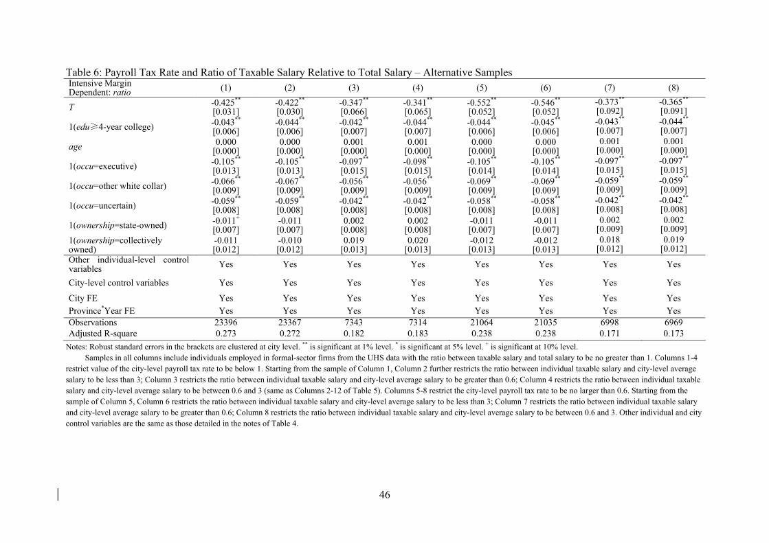
  46

Table 6: Payroll Tax Rate and Ratio of Taxable Salary Relative to Total Salary – Alternative Samples Intensive Margin Dependent: ratio (1) (2) (3) (4) (5) (6) (7) (8)

T -0.425** [0.031]

-0.422** [0.030]

-0.347** [0.066]

-0.341** [0.065]

-0.552** [0.052]

-0.546** [0.052]

-0.373** [0.092]

-0.365** [0.091]

1(edu≥4-year college) -0.043** [0.006]

-0.044** [0.006]

-0.042** [0.007]

-0.044** [0.007]

-0.044** [0.006]

-0.045** [0.006]

-0.043** [0.007]

-0.044** [0.007]

age 0.000 [0.000]

0.000 [0.000]

0.001 [0.000]

0.001 [0.000]

0.000 [0.000]

0.000 [0.000]

0.001 [0.000]

0.001 [0.000]

1(occu=executive) -0.105** [0.013]

-0.105** [0.013]

-0.097** [0.015]

-0.098** [0.015]

-0.105** [0.014]

-0.105** [0.014]

-0.097** [0.015]

-0.097** [0.015]

1(occu=other white collar) -0.066** [0.009]

-0.067** [0.009]

-0.056** [0.009]

-0.056** [0.009]

-0.069** [0.009]

-0.069** [0.009]

-0.059** [0.009]

-0.059** [0.009]

1(occu=uncertain) -0.059** [0.008]

-0.059** [0.008]

-0.042** [0.008]

-0.042** [0.008]

-0.058** [0.008]

-0.058** [0.008]

-0.042** [0.008]

-0.042** [0.008]

1(ownership=state-owned) -0.011+ [0.007]

-0.011 [0.007]

0.002 [0.008]

0.002 [0.008]

-0.011 [0.007]

-0.011 [0.007]

0.002 [0.009]

0.002 [0.009]

1(ownership=collectively owned)

-0.011 [0.012]

-0.010 [0.012]

0.019 [0.013]

0.020 [0.013]

-0.012 [0.013]

-0.012 [0.013]

0.018 [0.012]

0.019 [0.012]

Other individual-level control variables Yes Yes Yes Yes Yes Yes Yes Yes

City-level control variables Yes Yes Yes Yes Yes Yes Yes Yes

City FE Yes Yes Yes Yes Yes Yes Yes Yes Province*Year FE Yes Yes Yes Yes Yes Yes Yes Yes Observations 23396 23367 7343 7314 21064 21035 6998 6969 Adjusted R-square 0.273 0.272 0.182 0.183 0.238 0.238 0.171 0.173

Notes: Robust standard errors in the brackets are clustered at city level. ** is significant at 1% level. * is significant at 5% level. + is significant at 10% level. Samples in all columns include individuals employed in formal-sector firms from the UHS data with the ratio between taxable salary and total salary to be no greater than 1. Columns 1-4

restrict value of the city-level payroll tax rate to be below 1. Starting from the sample of Column 1, Column 2 further restricts the ratio between individual taxable salary and city-level average salary to be less than 3; Column 3 restricts the ratio between individual taxable salary and city-level average salary to be greater than 0.6; Column 4 restricts the ratio between individual taxable salary and city-level average salary to be between 0.6 and 3 (same as Columns 2-12 of Table 5). Columns 5-8 restrict the city-level payroll tax rate to be no larger than 0.6. Starting from the sample of Column 5, Column 6 restricts the ratio between individual taxable salary and city-level average salary to be less than 3; Column 7 restricts the ratio between individual taxable salary and city-level average salary to be greater than 0.6; Column 8 restricts the ratio between individual taxable salary and city-level average salary to be between 0.6 and 3. Other individual and city control variables are the same as those detailed in the notes of Table 4.

  47

Table 7: Heterogeneity One – Eligibility for National Civil Service Exam

(1) (2) (3) (4)

Panel A:

Dep Var: 1(participation) Panel B:

Dep Var: ratio

T -0.399** [0.054]

-0.414** [0.058]

-0.329** [0.066]

-0.317** [0.067]

1(edu≥4-year college)*T 0.077

[0.057] -0.072 [0.055]

1(edu≥4-year college) 0.010

[0.027] -0.018 [0.019]

1(edu≥4-year college)*1(18≤age≤35)*T 0.079 [0.062] -0.148+

[0.083]

1(edu≥4-year college)*1(age<18 or age>35)*T 0.103 [0.070] -0.058

[0.072]

1(edu<4-year college)*1(18≤age≤35)*T 0.053 [0.048] -0.077

[0.059]

1(edu≥4-year college)*1(18≤age≤35) -0.016 [0.028] 0.007

[0.030]

1(edu≥4-year college)*1(age<18 or age>35) -0.019 [0.035] -0.029

[0.025]

1(edu<4-year college)*1(18≤age≤35) -0.069** [0.026] 0.015

[0.023]

Individual-level control variables Yes Yes Yes Yes

City-level control variables Yes Yes Yes Yes City FE Yes Yes Yes Yes

Province*Year FE Yes Yes Yes Yes Observations 49120 49120 7314 7314 Pseudo R-square/Adjusted R-square 0.133 0.134 0.184 0.184

Notes: Robust standard errors in the brackets are clustered at city level. ** is significant at 1% level. * is significant at 5% level. + is significant at 10% level.

Columns 1-2 report marginal effects from a probit model; the dependent variable is the indicator for whether on participates in the social security system. Sample is the same as that in Columns 2-7 of Table 4. In Columns 3-4, the dependent variable is the ratio between individual taxable salary and total salary. Sample is the same as that in Columns 2-12 of Table 5. Only coefficients of interest are reported. The omitted education type is below 4-year college, and the omitted type of education*age is below 4-year college and outside the age range of [18, 35]. Control variables include individual occupation, ownership of firm one works in, and other individual and city control variables detailed in the note of Table 4.

  48

Table 8: Heterogeneity Two – Ability to Move to Public Sector at Late Career

(1) (2) (3) (4)

Panel A: Dep Var: 1(participation)

Panel B: Dep Var: ratio

T -0.446** [0.053]

-0.516** [0.059]

-0.346** [0.077]

-0.317** [0.073]

1(occu=executive)*T 0.111 [0.082] -0.099

[0.091]

1(occu=other white collar)*T 0.139** [0.042] 0.004

[0.068]

1(occu=executive) 0.012 [0.039] -0.065+

[0.036]

1(occu=other white collar) 0.051** [0.017] -0.058*

[0.025]

1(occu=executive)*1(40≤age< MRA)*T 0.172+ [0.092] -0.179+

[0.094]

1(occu=executive)*1(age< 40)*T 0.179 [0.120] 0.007

[0.187]

1(occu=other white collar)*1(40≤age< MRA)*T 0.222** [0.068] 0.027

[0.074]

1(occu=other white collar)*1(age< 40)*T 0.193** [0.054] -0.123

[0.082]

1(occu=blue collar)*1(age<40)*T 0.161** [0.048] -0.082

[0.077]

1(occu=executive)*1(40≤age< MRA) -0.022 [0.052] -0.049

[0.037]

1(occu=executive)*1(age< 40) -0.005 [0.051] -0.097

[0.062]

1(occu=other white collar)*1(40≤age< MRA) 0.014 [0.028] -0.073**

[0.027]

1(occu=other white collar)*1(age< 40) 0.006 [0.024] -0.024

[0.029]

1(occu=blue collar)*1(age<40) -0.107** [0.026] 0.008

[0.031] Individual-level control variables Yes Yes Yes Yes

City-level control variables Yes Yes Yes Yes

City FE Yes Yes Yes Yes Province*Year FE Yes Yes Yes Yes

Observations 49120 49120 7314 7314

Pseudo R-square/Adjusted R-square 0.134 0.135 0.183 0.185

Notes: Robust standard errors in the brackets are clustered at city level. ** is significant at 1% level. * is significant at 5% level. + is significant at 10% level.

Columns 1-2 report marginal effects from a probit model; the dependent variable is the indicator for whether on participates in the social security system. Sample is the same as that in Columns 2-7 of Table 4. In Columns 3-4, the dependent variable is the ratio between individual taxable salary and total salary. Sample is the same as that in Columns 2-7 of Table 5. Only coefficients of interest are reported. The omitted occupation type is blue collar, and the omitted type of occupation*age is blue collar and age between 40 and the mandatory retirement age. Mandatory retirement age (MRA) is 60 for males and 55 for females. Control variables include individual education, ownership of firm one works in, and other individual and city control variables detailed in the note of Table 4

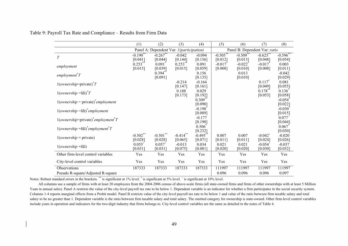
  49

Table 9: Payroll Tax Rate and Compliance – Results from Firm Data

(1) (2) (3) (4) (5) (6) (7) (8)

Panel A: Dependent Var: 1(participation) Panel B: Dependent Var: ratio

T -0.190** [0.041]

-0.267** [0.044]

-0.042 [0.144]

-0.094 [0.156]

-0.505** [0.012]

-0.509** [0.013]

-0.625** [0.048]

-0.596** [0.054]

employment 0.253** [0.015]

0.091* [0.039]

0.253** [0.015]

0.091 [0.059]

-0.017* [0.008]

-0.022* [0.010]

-0.017* [0.008]

0.003 [0.011]

employment*T 0.394** [0.091] 0.156

[0.135] 0.013 [0.010] -0.042

[0.029]

1(ownership=private)*T -0.214 [0.147]

-0.164 [0.161] 0.117*

[0.049] 0.081

[0.055]

1(ownership =fdi)*T 0.188 [0.173]

0.029 [0.192] 0.178**

[0.053] 0.136* [0.058]

1(ownership = private)*employment 0.309** [0.090] -0.054*

[0.022]

1(ownership =fdi)*employment -0.198* [0.089] -0.030*

[0.015]

1(ownership=private)*employment*T -0.177 [0.198] 0.077+

[0.044]

1(ownership =fdi)*employment*T 0.506* [0.232] 0.067*

[0.030]

1(ownership = private) -0.502** [0.028]

-0.501** [0.028]

-0.414** [0.065]

-0.495** [0.071]

0.007 [0.011]

0.007 [0.011]

-0.042+ [0.024]

-0.020 [0.026]

1(ownership =fdi) 0.055+ [0.031]

0.057+ [0.031]

-0.013 [0.075]

0.034 [0.081]

0.021 [0.020]

0.021 [0.020]

-0.054+ [0.030]

-0.037 [0.032]

Other firm-level control variables Yes Yes Yes Yes Yes Yes Yes Yes

City-level control variables Yes Yes Yes Yes Yes Yes Yes Yes

Observations 187333 187333 187333 187333 111997 111997 111997 111997 Pseudo R-square/Adjusted R-square 0.096 0.096 0.096 0.097

Notes: Robust standard errors in the brackets. ** is significant at 1% level. * is significant at 5% level. + is significant at 10% level. All columns use a sample of firms with at least 20 employees from the 2004-2006 census of above-scale firms (all state-owned firms and firms of other ownerships with at least 5 Million

Yuan in annual sales). Panel A restricts the value of the city-level payroll tax rate to be below 1. Dependent variable is an indicator for whether a firm participates in the social security system. Columns 1-4 reports marginal effects from a Probit model. Panel B restricts value of the city-level payroll tax rate to be below 1 and value of the ratio between firm taxable salary and total salary to be no greater than 1. Dependent variable is the ratio between firm taxable salary and total salary. The omitted category for ownership is state-owned. Other firm-level control variables include years in operation and indicators for the two-digit industry that firms belongs to. City-level control variables are the same as detailed in the notes of Table 4.

  50

Table A1: Robustness Tests Using an Alternative Sample

(1) (2) (3) (4) (5)

Dependent Variable: ratio IV1 IV2 IV3 Mechanism1 Mechanism2

T -0.565 [0.806]

-0.548 [0.775]

-1.694** [0.237]

-0.319** [0.094]

-0.298** [0.094]

IV first stage 0.635** [0.072]

0.587** [0.066]

1(edu≥4-year college)*1(18≤age≤35)*T -0.219* [0.094]

1(edu≥4-year college)*1(age<18 or age>35)*T -0.118 [0.074]

1(edu<4-year college)*1(18≤age≤35)*T -0.107 [0.080]

1(occu=executive)*1(40≤age< MRA)*T -0.182 [0.118]

1(occu=executive)*1(age< 40)*T -0.119 [0.226]

1(occu= other white collar)*1(40≤age<MRA)*T -0.102 [0.084]

1(occu= other white collar)*1(age< 40)*T -0.198* [0.099]

1(occu= blue collar)*1(age<40)*T -0.137 [0.103]

1(ownership=state-owned)*T

1(ownership=collectively owned)*T

Observations 6967 6966 1962 6969 6969 Adjusted R-square 0.171 0.171 0.084 0.174 0.175

Notes: Robust standard errors in the brackets are clustered at city level. ** is significant at 1% level. * is significant at 5% level. + is significant at 10% level. Sample includes individuals employed in the formal sectors, with the value of the city-level payroll tax rate no greater than 0.6, the ratio between taxable salary and total salary no greater than

1, and the ratio between individual taxable salary and the city-level average salary between 0.6 and 3. Column 1 is an IV regression, where IV1 is the employees’ average pension contribution rate calculated by from the UHS data data. Column 2 is an IV regression, where IV2 is the sum of the employees’ average pension contribution rate and health insurance contribution rate calculated from the UHS data. Column 3 is an IV regression using the panel data created from the original pooled data, where IV3 is the city dummies. In the first stage, the F statistic is 9276.52. Columns 4-6 are results for mechanisms 1-3, respectively, see notes in Tables 7-9. All specifications control for province*year and city FEs and all individual and city control variables. Individual and city control variables are the same as those detailed in the notes of Table 4.

  51

Table A2: Robustness Tests Using 2002-2005 Pooled Data from Urban Household Survey Data

(1)

Baseline (2)

Baseline (3)

Mechanism 1 (4)

Mechanism 2

Panel A:

Dep Var: 1(participation) Panel B: Dep Var: ratio

T -0.417** [0.061]

-0.366** [0.076]

-0.343** [0.079]

-0.319** [0.087]

1(edu≥4-year college)*1(18≤age≤35)*T -0.214* [0.084]

1(edu≥4-year college)*1(age<18 or age>35)*T -0.015 [0.084]

1(edu<4-year college)*1(18≤age≤35)*T -0.105 [0.067]

1(occu=executive)*1(40≤age< MRA)*T -0.220* [0.106]

1(occu=executive)*1(age< 40)*T -0.096 [0.186]

1(occu= other white collar)*1(40≤age< MRA)*T -0.011 [0.068]

1(occu= other white collar)*1(age< 40)*T -0.171* [0.079]

1(occu= blue collar)*1(age<40)*T -0.120 [0.086]

1(ownership=state-owned)*T

1(ownership=collectively owned)*T

Observations 37471 5585 5585 5585 Pseudo R-square/ Adjusted R-square 0.142 0.184 0.185 0.187

Notes: Robust standard errors in the brackets are clustered at city level. ** is significant at 1% level. * is significant at 5% level. + is significant at 10% level. Sample is the pooled data from the 2002-2005 UHS data. Only individuals employed in formal sectors are included. Panel A restricts value of the city-level payroll tax rate to be below 1.

Dependent variable is an indicator for whether one participates in the social security system. Marginal effects from a Probit model are reported in Column 1. Panel B further restricts value of the ratio between taxable salary and total salary to be no larger than 1 and ratio between individual taxable salary and the city-level average salary to be between 0.6 and 3. Dependent variable is the ratio between taxable salary and total salary. We use a fixed effect model. Columns 3-5 report results for Mechanisms 1-3 respectively; see notes in Tables 7-9. All specifications control for province*year and city FEs and all individual and city control variables as detailed in the notes of Table 4.

  52

Table A3: Robustness Tests Using 2002-2006 Panel Data from Urban Household Survey Data

(1)

Baseline (2)

Baseline (3)

Mechanism 1 (4)

Mechanism 2

Panel A:

Dep Var: 1(participation) Panel B: Dep Var: ratio

T -0.314** [0.043]

-0.772** [0.115]

-0.655** [0.125]

-0.695** [0.169]

1(edu≥4-year college)*1(18≤age≤35)*T -0.152 [0.307]

1(edu≥4-year college)*1(age<18 or age>35)*T -0.175 [0.297]

1(edu<4-year college)*1(18≤age≤35)*T -0.270* [0.126]

1(occu=executive)*1(40≤age< MRA)*T -0.016 [0.325]

1(occu=executive)*1(age< 40)*T 0.831* [0.394]

1(occu= other white collar)*1(40≤age< MRA)*T 0.209 [0.214]

1(occu= other white collar)*1(age< 40)*T -0.144 [0.242]

1(occu= blue collar)*1(age<40)*T -0.039 [0.244]

1(ownership=state-owned)*T

1(ownership=collectively owned)*T

Observations 28196 4272 4272 4272 Pseudo R-square/ Adjusted R-square 0.092 0.171 0.165 0.172

Notes: Robust standard errors in the brackets are clustered at city level. ** is significant at 1% level. * is significant at 5% level. + is significant at 10% level. Sample is the panel data created from the original pooled data from the 2002-2006 UHS data. Only individuals employed in formal sectors are included. Panel A restricts value of the city-

level payroll tax rate to be below 1. Dependent variable is an indicator for whether one participates in the social security system. Marginal effects from a Probit model are reported in Column 1. Panel B further restricts value of the ratio between taxable salary and total salary to be no larger than 1 and ratio between individual taxable salary and the city-level average salary to be between 0.6 and 3. Dependent variable is the ratio between taxable salary and total salary. We use a fixed effect model. Columns 3-5 report results for Mechanisms 1-3 respectively; see notes in Tables 7-9. All specifications control for all individual and city control variables as detailed in the notes of Table 4.

  53

Table A4: Robustness Tests Using 2002-2005 Panel Data from Urban Household Survey Data

(1)

Baseline (2)

Baseline (3)

Mechanism 1 (4)

Mechanism 2

Panel A:

Dep Var: 1(participation) Panel B: Dep Var: ratio

T -0.369** [0.042]

-0.797** [0.161]

-0.549** [0.178]

-0.555* [0.268]

1(edu≥4-year college)*1(18≤age≤35)*T -0.265 [0.239]

1(edu≥4-year college)*1(age<18 or age>35)*T -0.526 [0.338]

1(edu<4-year college)*1(18≤age≤35)*T -0.254 [0.155]

1(occu=executive)*1(40≤age< MRA)*T -0.084 [0.598]

1(occu=executive)*1(age< 40)*T 0.871+ [0.440]

1(occu= other white collar)*1(40≤age< MRA)*T 0.108 [0.249]

1(occu= other white collar)*1(age< 40)*T -0.376 [0.349]

1(occu= blue collar)*1(age<40)*T -0.102 [0.316]

1(ownership=state-owned)*T

1(ownership=collectively owned)*T

Observations 15710 2412 2412 2412 Pseudo R-square/ Adjusted R-square 0.110 0.177 0.154 0.171

Notes: Robust standard errors in the brackets are clustered at city level. ** is significant at 1% level. * is significant at 5% level. + is significant at 10% level. Sample is the panel data created from the original pooled data from the 2002-2006 UHS data. Only individuals employed in formal sectors are included. Panel A restricts value of the city-

level payroll tax rate to be below 1. Dependent variable is an indicator for whether one participates in the social security system. Marginal effects from a Probit model are reported in Column 1. Panel B further restricts value of the ratio between taxable salary and total salary to be no larger than 1 and ratio between individual taxable salary and the city-level average salary to be between 0.6 and 3. Dependent variable is the ratio between taxable salary and total salary. We use a fixed effect model. Columns 3-5 report results for Mechanisms 1-3 respectively; see notes in Tables 7-9. All specifications control for all individual and city control variables as detailed in the notes of Table 4.

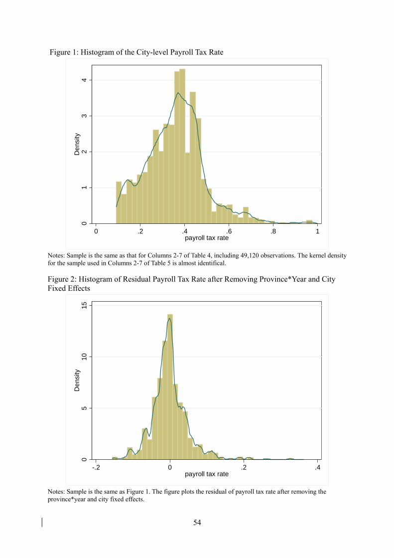
  54

Figure 1: Histogram of the City-level Payroll Tax Rate

01

23

4D

ens

ity

0 .2 .4 .6 .8 1payroll tax rate

Notes: Sample is the same as that for Columns 2-7 of Table 4, including 49,120 observations. The kernel density for the sample used in Columns 2-7 of Table 5 is almost identifical. Figure 2: Histogram of Residual Payroll Tax Rate after Removing Province*Year and City Fixed Effects

05

1015

De

nsity

-.2 0 .2 .4payroll tax rate

Notes: Sample is the same as Figure 1. The figure plots the residual of payroll tax rate after removing the province*year and city fixed effects.

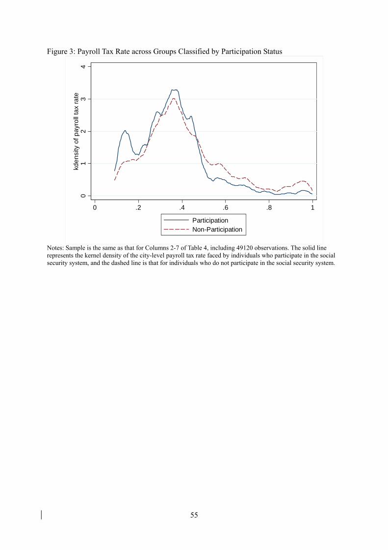
  55

Figure 3: Payroll Tax Rate across Groups Classified by Participation Status

01

23

4kd

en

sity

of

pa

yro

ll ta

x ra

te

0 .2 .4 .6 .8 1

ParticipationNon-Participation

Notes: Sample is the same as that for Columns 2-7 of Table 4, including 49120 observations. The solid line represents the kernel density of the city-level payroll tax rate faced by individuals who participate in the social security system, and the dashed line is that for individuals who do not participate in the social security system.

  56

Figure 4: Ratio between Taxable Salary and Total Salary for Different Levels of Payroll Tax Rate

0.5

11.

52

kde

nsity

of r

atio

0 .2 .4 .6 .8 1

Below Median of Payroll Tax RateAbove Median of Payroll Tax Rate

Notes: Sample is the same as Figure 1. The solid line represents the kernel density of ratio between taxable salary and total salary when the payroll tax rate is above the median of its distribution, and the dashed line is that for payroll tax rate below the median.

  57

Figure 5: Ratio between Taxable Salary and Total Salary by Education Level

0.5

11.

52

kde

nsity

of r

atio

0 .2 .4 .6 .8 1

Education Level not Lower than UndergraduateEducation Level Lower than Undergraduate

Notes: Sample is the same as Figure 1. The solid line represents the kenel density of the ratio bewteen taxable salary and total salary for individuals with at least a 4-year college education, and the dashed line is that for individuals with less than a 4-year college education. Figure 6: Ratio between Taxable Salary and Total Salary for Three Levels of Payroll Tax Rates by Education Level

Notes: Same as Figure 5.

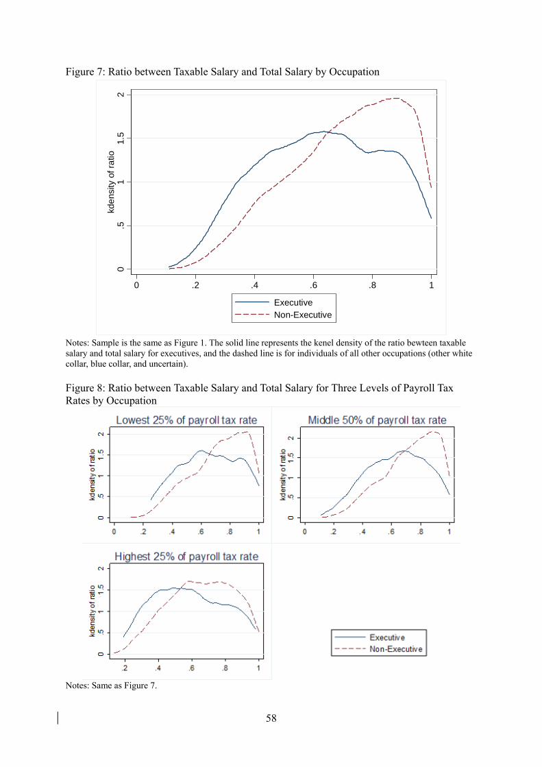
  58

Figure 7: Ratio between Taxable Salary and Total Salary by Occupation

0.5

11.

52

kde

nsity

of r

atio

0 .2 .4 .6 .8 1

ExecutiveNon-Executive

Notes: Sample is the same as Figure 1. The solid line represents the kenel density of the ratio bewteen taxable salary and total salary for executives, and the dashed line is for individuals of all other occupations (other white collar, blue collar, and uncertain). Figure 8: Ratio between Taxable Salary and Total Salary for Three Levels of Payroll Tax Rates by Occupation

Notes: Same as Figure 7.

  59

Figure 9: Ratio between Taxable Salary and Total Salary by Eligibility for National Civil Servant Exam

0.5

11.

52

kde

nsity

of r

atio

0 .2 .4 .6 .8 1

EligibleIneligible

Notes: Sample is the same as Figure 1. The solid line represents the kernel density of the ratio between taxable salary and total salary for individuals eligible for national civil servant exam (at least 4-year college education and aged between 18 to 35), and the dashed line is that for individuals ineligible for the exam. Figure 10: Ratio between Taxable Salary and Total Salary for Three Levels of Payroll Tax Rates by Eligibility for National Civil Service Exam

Notes: Same as Figure 9.

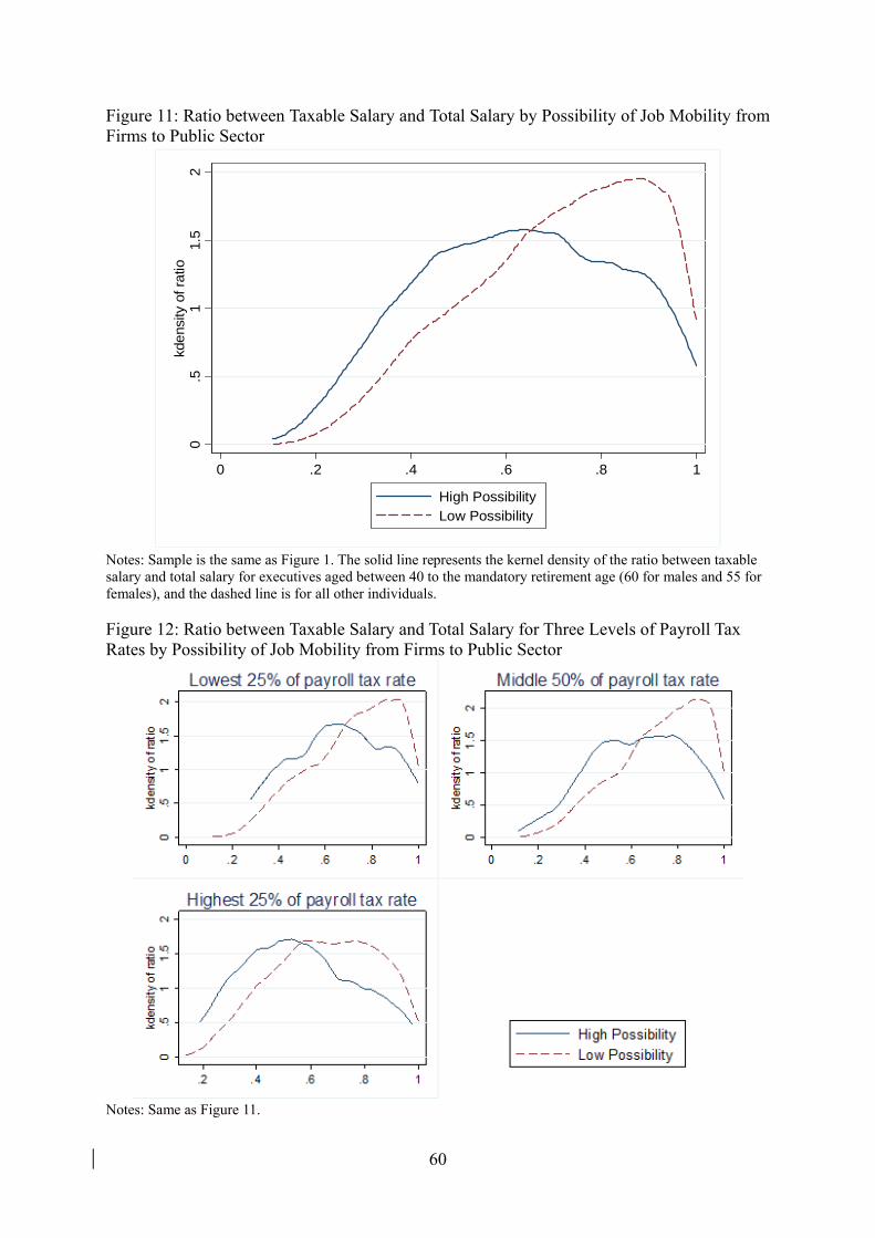
  60

Figure 11: Ratio between Taxable Salary and Total Salary by Possibility of Job Mobility from Firms to Public Sector

0.5

11.

52

kdens

ity o

f ratio

0 .2 .4 .6 .8 1

High PossibilityLow Possibility

Notes: Sample is the same as Figure 1. The solid line represents the kernel density of the ratio between taxable salary and total salary for executives aged between 40 to the mandatory retirement age (60 for males and 55 for females), and the dashed line is for all other individuals. Figure 12: Ratio between Taxable Salary and Total Salary for Three Levels of Payroll Tax Rates by Possibility of Job Mobility from Firms to Public Sector

Notes: Same as Figure 11.