Embed Size (px)
Citation preview

Social Science Models
What elements (at least two) are necessary for a “social science model”?
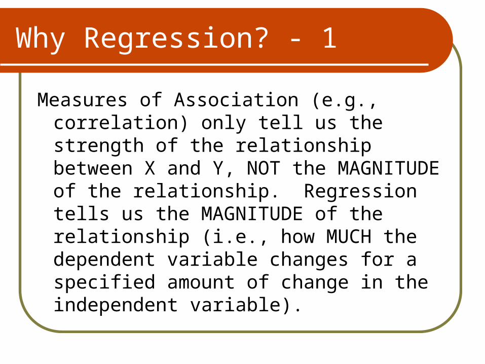
Why Regression? - 1
Measures of Association (e.g., correlation) only tell us the strength of the relationship between X and Y, NOT the MAGNITUDE of the relationship. Regression tells us the MAGNITUDE of the relationship (i.e., how MUCH the dependent variable changes for a specified amount of change in the independent variable).
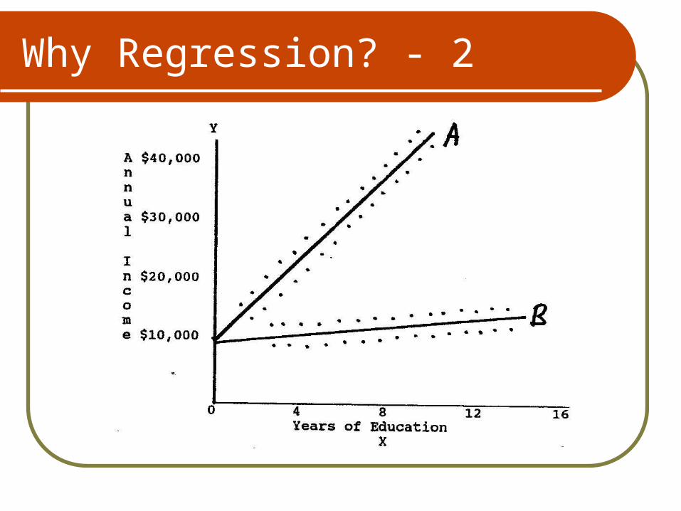
Why Regression? - 2

Why Regression? - 3
Properties that our estimate of the magnitude will adhere to:
1. Unbiased – on average our estimate will be the “true” value of the
magnitude.
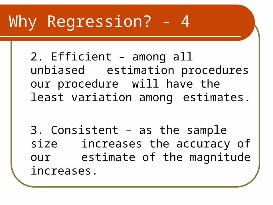
Why Regression? - 4
2. Efficient – among all unbiased estimation procedures our procedure will have the least variation among estimates.
3. Consistent – as the sample size increases the accuracy of our estimate of the magnitude increases.

Linear Regression I:Scatterplots and Regression Lines
SAT scores and graduation ratesLooking at a scatterplotFitting a regression lineWhat does it mean?
Other factors that affect graduation ratesConfound: reputationOther independent variables

SAT Scores and Graduation Rates -1
To test the hypothesis that colleges with smarter students have higher graduation rates, I will look at data from 148 colleges in the United States.
SAT Scores Graduation Rates
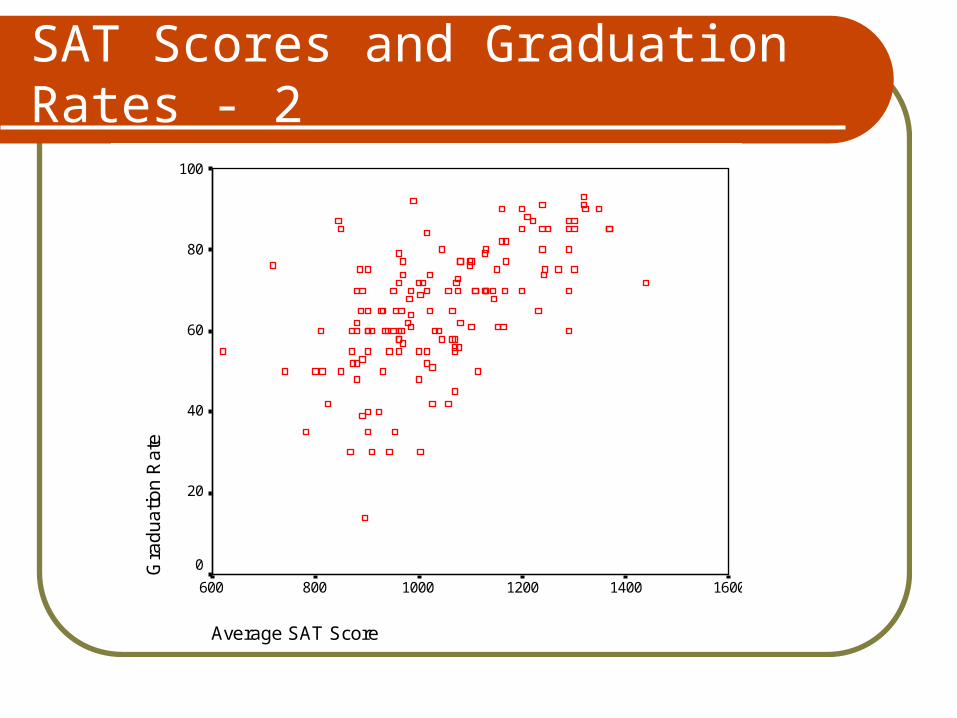
SAT Scores and Graduation Rates - 2
Average SAT Score
1600140012001000800600
Gra
du
atio
n R
ate
100
80
60
40
20
0

SAT Scores and Graduation Rates - 3
We can summarize the direction and strength of a relationship between two variables by calculating “r,” the correlation.
If we want to know more about the relationship, we can fit a “regression line” to the scatterplot.

SAT Scores and Graduation Rates -4
Average SAT Score
1600140012001000800600
Gra
du
atio
n R
ate
100
80
60
40
20
0 Rsq = 0.3454

SAT Scores and Graduation Rates -5A regression line summarizes how much
the dependent variable (graduation rates) changes when the independent variable (SAT scores) increases.The line gives you a “predicted value” of
graduation rates for a college with a given average SAT score.
To make this prediction as good as possible, the line minimizes vertical distances between the line and the data points.

SAT Scores and Graduation Rates -6 – DON’T WRITE THE FORMULA!
Like all lines, a regression line can be summarized with this formula:
y = a + b•x
where:
b = slope of line or “regression coefficient”
a = the intercept, or the value of y when x=0
Regression Theory - 1
We want to “explain” the variation in graduation rates among universities.
We could just use the mean graduation rate as a prediction of each university’s graduation rate.
However, even with many cases, we often do not observe multiple cases at the same value of x. Thus, no average graduation rate for a particular average SAT score.

Regression Theory - 2
We might think the value of “y” (graduation rates) we observe is conditional on the value of “x” (SAT scores).
Take the mean of y at each value of xWe essentially have a frequency
distribution for the values y can take on for each value of x
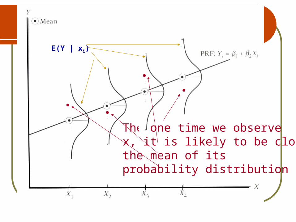
E(Y | xi)
The one time we observex, it is likely to be close tothe mean of itsprobability distribution
SAT Scores and Graduation Rates -7
The regression coefficient for the effect of SAT scores on graduation rates is 0.06.
This is the predicted effect on graduation rates when SAT scores go up by one unit.
This means that comparing one college to another college where average SATs were 100 points higher should lead to a graduation rate that is 6 percentage points higher.

Other Factors Affecting Grad Rates - 1
The school’s reputation could be a confound: a school with a good rep might attract smart students and want to keep its reputation high by graduating them.
Year school was founded
20001900180017001600
Gra
du
atio
n R
ate
100
80
60
40
20
0 Rsq = 0.1900

Other Factors Affecting Grad Rates – 2-Which Relationship is Negative?
Student/faculty ratio
3020100
Gra
du
atio
n R
ate
100
80
60
40
20
0 Rsq = 0.1491
In-state Tuition
14000120001000080006000400020000G
rad
ua
tion
Ra
te
100
80
60
40
20
0 Rsq = 0.3596
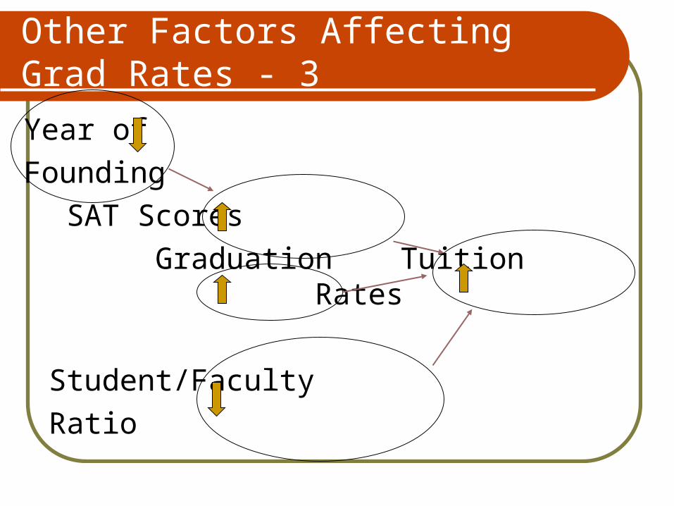
Other Factors Affecting Grad Rates - 3
Year of
Founding
SAT Scores
Graduation Tuition Rates
Student/Faculty
Ratio

Multiple Regression - 1
The impact of one independent variable on the dependent variable may change as other independent variables are included in the model (i.e., the same equation). The following example will demonstrate this.

Multiple Regression - 2
Tax = Percentage of times the senator voted in favor of federal tax changes
where over 50% of the benefits went to households earning less than the median family income on 76 amendments to the Tax Reform Act of 1976 (my first attempt at looking at the impact of political parties on income inequality – too long ago!). This is the dependent variable in the analysis ahead.

Multiple Regression - 3
Cons = Percentage of times the senator voted for positions favored by the Americans for Constitutional Action (a conservative interest group)
Note: What assumption about vote value does using a percentage measure make?
Multiple Regression - 4
Party = Senator’s party affiliation
(1 = Democrat; 0 = Republican)
Stinc = median household income in
the senator’s state in thousands of dollars (i.e., $10,200 is entered as 10.2)
What’s the “median”?

Multiple Regression - 5
Source | SS df MS Number of obs = 100
-------------+------------------------------ F( 1, 98) = 176.36
Model | 52533.9423 1 52533.9423 Prob > F = 0.0000
Residual | 29192.8977 98 297.886711 R-squared = 0.6428
-------------+------------------------------ Adj R-squared = 0.6392
Total | 81726.84 99 825.523636 Root MSE = 17.259
------------------------------------------------------------------------------
tax | Coef. Std. Err. t P>|t| [95% Conf. Interval]
-------------+----------------------------------------------------------------
cons | -.73731 .055521 -13.28 0.000 -.84749 -.62713
_cons | 72.42727 2.603626 27.82 0.000 67.26046 77.59409
------------------------------------------------------------------------------
Note: _cons is the y-intercept. Can you interpret the above Stata output? Why might multiple regression be useful?

Multiple Regression - 6
Example from the 300Reader: Value of “b”:
(1) if you use the senator’s conservatism to explain tax voting: -.737
(2) if you use the senator’s party to explain tax voting: 35.293
(3) if you use the median family income
in the senator’s state to explain tax voting: 2.867
CAN YOU INTERPRET EACH “b”?
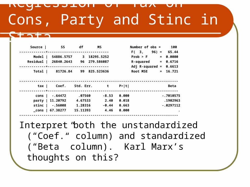
Regression of Tax on Cons, Party and Stinc in Stata
Source | SS df MS Number of obs = 100
-------------+------------------------------ F( 3, 96) = 65.44
Model | 54886.5757 3 18295.5252 Prob > F = 0.0000
Residual | 26840.2643 96 279.586087 R-squared = 0.6716
-------------+------------------------------ Adj R-squared = 0.6613
Total | 81726.84 99 825.523636 Root MSE = 16.721
------------------------------------------------------------------------------
tax | Coef. Std. Err. t P>|t| Beta
-------------+----------------------------------------------------------------
cons | -.64472 .07560 -8.53 0.000 -.7010575
party | 11.20792 4.67533 2.40 0.018 .1902963
stinc | -.56008 1.28316 -0.44 0.663 -.0297112
_cons | 67.38277 15.11393 4.46 0.000 .
------------------------------------------------------------------------------
Interpret both the unstandardized (“Coef.” column) and standardized (“Beta” column). Karl Marx’s thoughts on this?

Multiple Regression - Interpretation
Notice how much smaller the impact of senator party identification is when senator ideology is in the same equation. Also, note that the sign (i.e., direction of the relationship) for state median family income changes from positive to negative once all three independent variables are in the same equation.

Multiple Regression – Prediction - 1
From the previous output we know the following: “a” = 67.382, the impact of senator conservatism = -.644, the impact of senator party affiliation = 11.207 and the impact of the median household income in the senator’s state = -.560. Senator #1’s scores on the three independent variables are as follows: conservatism = 26, party affiliation = 1 and state median household income = 7.4 (i.e., $7,400 in 1970).
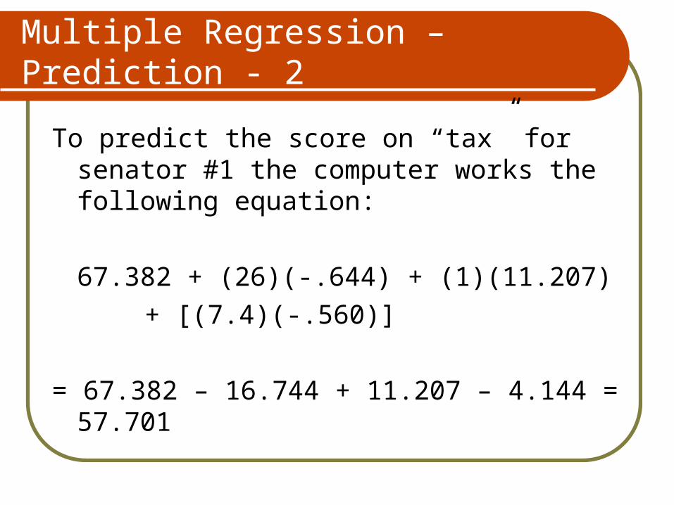
Multiple Regression – Prediction - 2
To predict the score on “tax” for senator #1 the computer works the following equation:
67.382 + (26)(-.644) + (1)(11.207)
+ [(7.4)(-.560)]
= 67.382 – 16.744 + 11.207 – 4.144 = 57.701

Multiple Regression – Prediction - 3
Senator #1 is “predicted” to support the poor 57.701% of the time . Since senator #1 “actually” supported the poor on 54% of their tax votes, the prediction error (“e” or “residual”) for senator #1 is: 54 - 57.701 = -3.701
The computer then squares this value (i.e.,
-3.701 x -3.701 = 13.69). The computer performs this same operation for all 100 senators. The sum of the squared prediction errors for all 100 senators is 26,840.
Multiple Regression – Prediction - 4
If any of the values of the coefficients (i.e., 67.382, -.644, 11.207 or -.560) were changed, the sum of the squared prediction errors would have been greater than 26,840. This is known as the “least squared errors principle.”

Regression Model Performance - 1
Let’s see how well our regression model performed. From the following we know that the mean score on “tax” is 46.5 (i.e., the average senator supported the poor/middle class 46.5% of the time).
Variable | Obs Mean Std. Dev.
-------------+----------------------------------------------
tax | 100 46.54 28.73193
Regression Model Performance - 2
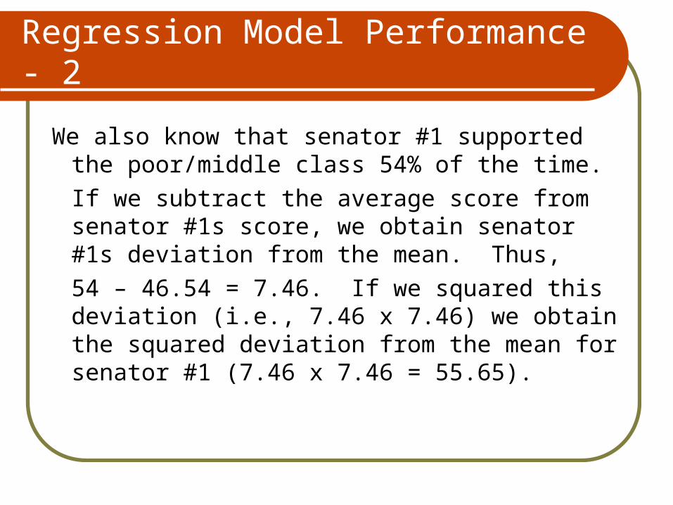
We also know that senator #1 supported the poor/middle class 54% of the time.
If we subtract the average score from senator #1s score, we obtain senator #1s deviation from the mean. Thus,
54 – 46.54 = 7.46. If we squared this deviation (i.e., 7.46 x 7.46) we obtain the squared deviation from the mean for senator #1 (7.46 x 7.46 = 55.65).

Regression Model Performance - 3
If we repeat this process for all remaining 99 senators and add this total, we obtain the total variation in the dependent variable that we could explain: 81,776. From the previous discussion we know that the total squared prediction errors equal 26,840. If take [1 – (26,840/81,776 = 1 - .328 = 67.1) we find that variation in senator conservatism, party affiliation and state median household income explained 67.1% of the variation in senatorial voting on tax legislation.

Multicollinearity
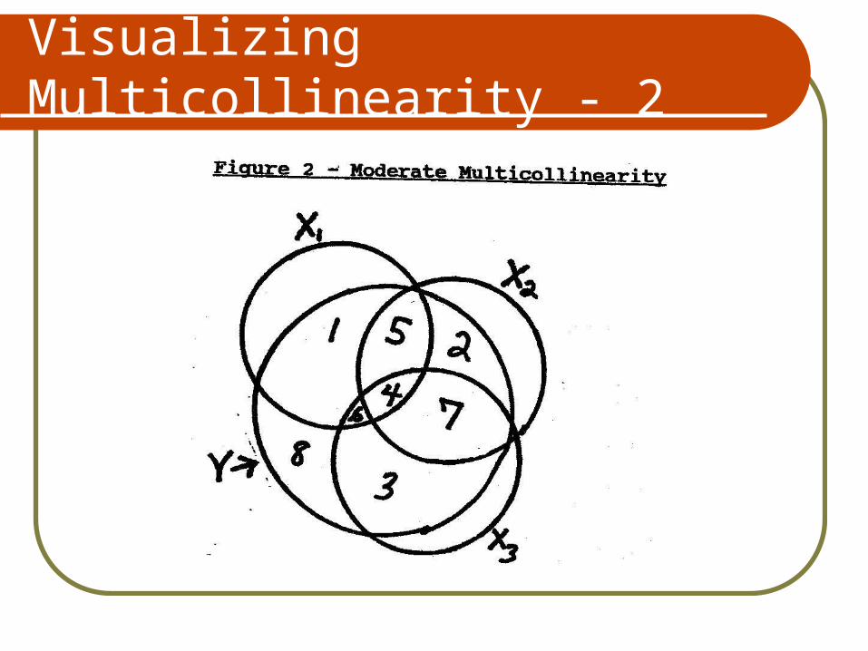
An independent variable may be statistically insignificant because it is highly correlated with one, or more, of the other independent variables. For example, perhaps state median family income is highly correlated with senator conservatism (e.g., if wealthier states elected more conservative senators). Multicollinearity is a lack of information rather than a lack of data.

Visualizing Multicollinearity - 1
Visualizing Multicollinearity - 2

Visualizing Multicollinearity - 3

Multicollinearity Check in Stata
1 - 1/vif yields the percentage of the variation in one independent explained by all the other independent variables.
Variable | VIF 1/VIF
-------------+----------------------
cons | 1.98 0.506218
party | 1.84 0.542894
stinc | 1.35 0.738325
What would Karl Marx think now?

Multicollinearity - Interpretation
Unfortunately for Karl Marx, only 26% of the variation in state median family income is explained by the variation in senator conservatism and senator party affiliation (1- .738 = .262). Since this is low (i.e., well below the .70 threshold mentioned in the readings), Marx can’t legitimately claim high multicollinearity undermined his hypothesis.
Bread and Peace Model - 1
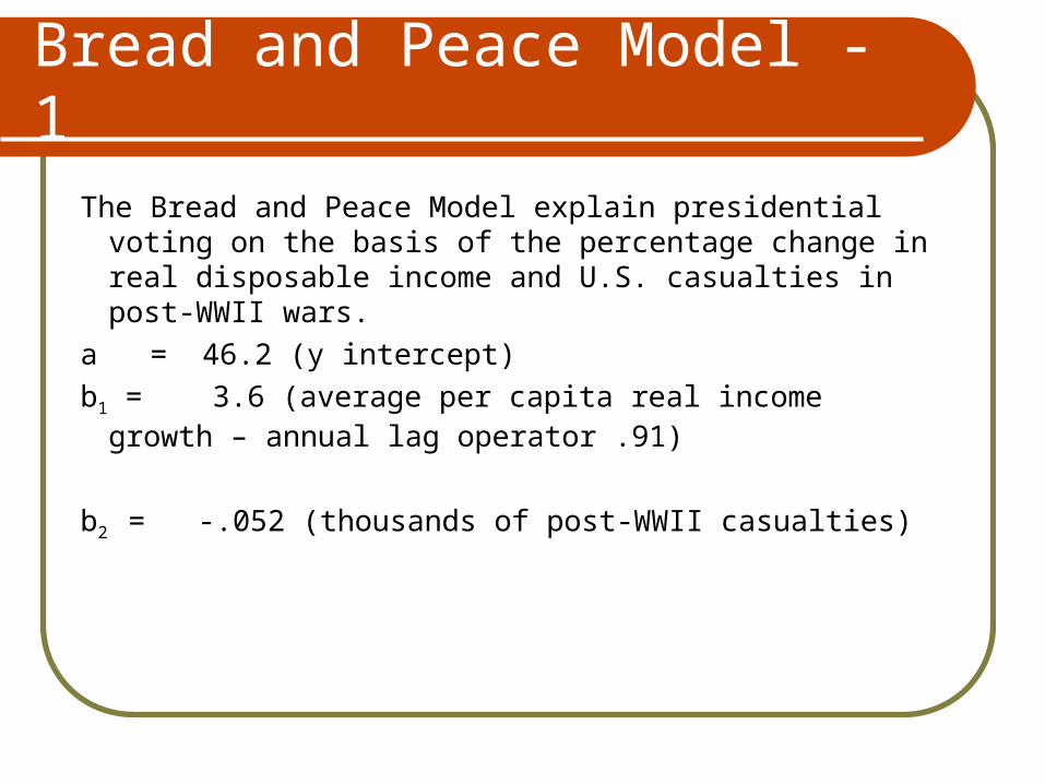
The Bread and Peace Model explain presidential voting on the basis of the percentage change in real disposable income and U.S. casualties in post-WWII wars.
a = 46.2 (y intercept)
b1 = 3.6 (average per capita real income growth – annual lag operator .91)
b2 = -.052 (thousands of post-WWII casualties)
Bread and Peace Model - 2
1956
1960
19641972
1976
1980
1984
1988
1992
1996
20002004
1952
1968
2008
4045
5055
6065
Incu
mbe
nt s
har
e of
two-
part
y vo
te (
%)
-2 -1 0 1 2 3 4 5 6 7 8 9 10 11 12 13 14 15 16
Real income growth and military fatalities combined
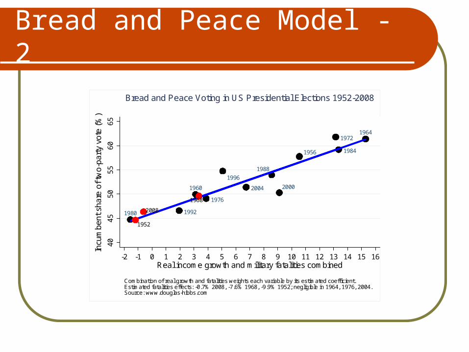
Combination of real growth and fatalities weights each variable by its estimated coefficient.Estimated fatalities effects: -0.7% 2008, -7.6% 1968, -9.9% 1952; negligible in 1964, 1976, 2004.Source: www.douglas-hibbs.com
Bread and Peace Voting in US Presidential Elections 1952-2008

Government Benefits - 1
The following slide contains the percentage of people who (a) benefit from various programs, and (b) claim in response to a government survey that they 'have not used a government social program.’ Government social programs are stigmatized as “welfare.” But many people benefit from such programs without realizing it. This results in a likely underprovision of such benefits.

Government Benefits - 2
529 or Coverdell - 64.3
Home mortgage interest deduction - 60.0
Hope or Lifetime Learning Tax Credit- 59.6
Student Loans - 53.3
Child and Dependent Tax Credit - 51.7
Earned income tax credit - 47.1
Pell Grants – 43.1
Medicare – 39.8
Food Stamps – 25.4


Regression in Value Added Teacher Evaluations – LA Times - 3/28/11
The general formula for the "linear mixed model" used in her district is a string of symbols and letters more than 80 characters long: y = Xβ + Zv + ε where β is a p-by-1 vector of fixed effects; X is an n-by-p matrix; v is a q-by-1 vector of random effects; Z is an n-by-q matrix; E(v) = 0, Var(v) = G; E(ε) = 0, Var(ε) = R; Cov(v,ε) = 0. V = Var(y) = Var(y - Xβ) = Var(Zv + ε) = ZGZT + R. In essence, value-added analysis involves looking at each student's past test scores to predict future scores. The difference between the prediction and students' actual scores each year is the estimated "value" that the teacher added — or subtracted.

California Election 2010 - 1
Given the correlations below, what should you expect
in the regression table on the next slide where the dependent variable is “boxer 10” (percent
of county vote for Boxer in 2010)?
correlate boxer10 brown10 coll00 medinc08
(obs=58)
| boxer10 brown10 coll00 medinc08
-------------+------------------------------------
boxer10 | 1.0000
brown10 | 0.9788 1.0000
coll00 | 0.7422 0.6885 1.0000
medinc08 | 0.6022 0.5401 0.8321 1.0000