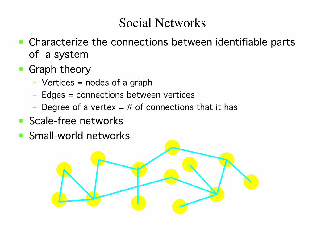
Social Networks• Characterize the connections between identifiable parts

of a system• Graph theory

– Vertices = nodes of a graph– Edges = connections between vertices– Degree of a vertex = # of connections that it has

• Scale-free networks• Small-world networks

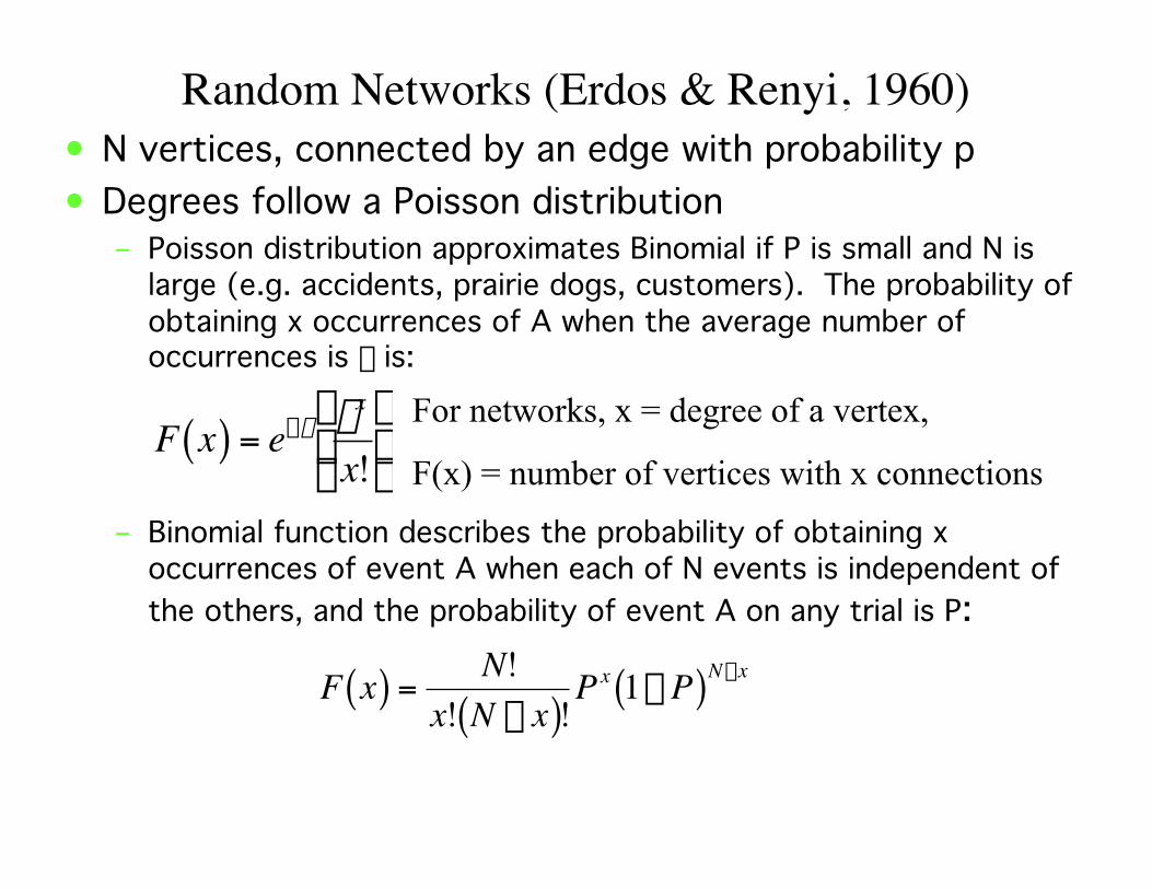
Random Networks (Erdos & Renyi, 1960)• N vertices, connected by an edge with probability p• Degrees follow a Poisson distribution

– Poisson distribution approximates Binomial if P is small and N islarge (e.g. accidents, prairie dogs, customers). The probability ofobtaining x occurrences of A when the average number ofoccurrences is l is:

– Binomial function describes the probability of obtaining xoccurrences of event A when each of N events is independent ofthe others, and the probability of event A on any trial is P:

†

F x( ) = e-l lx

x!Ê

Ë Á

ˆ

¯ ˜

†

F x( ) =N!

x! N - x( )!Px 1- P( )N-x

For networks, x = degree of a vertex,

F(x) = number of vertices with x connections

Poisson distribution of degrees in a random network

m= l

l=Where N = Number of vertices, p = probability of each pair ofvertices being connected, k= number of edgesProbability of finding a highly connected vertex decreasesexponentially for k >> average k

†

l = N N -1k

Ê

Ë Á

ˆ

¯ ˜ pk 1- p( )N-1-k

Scale-free Networks• Very uneven distribution of connections. Some nodes

have very high degrees of connectivity (hubs), while mosthave small degrees

• Scale-free means that the description of a system doesnot change as a function of the magnification (scale)used to view the system– fractals = self similar patterns with fractional dimensionality– Power law distribution of degrees: high connectivity is unlikely but

occurs more often than predicted by random network

• Power laws show up as straight lines when plotted on log-logcoordinates, with the slope of the line = -a

• Power laws are scale free because if x is rescaled (multiplied by aconstant), then P(x) is still proportional to x-a

– if P(x) = x-2, then P(10*x) is still proportional to x-2. P(x)= 10-2 * x-2

†

P(x) µ x-a

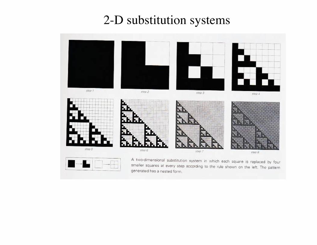
2-D substitution systems

Cantor’s Set

A = 1/3, N= 2, so D=log(2)/log(3)

A = 1/9, N= 4, so D=log(4)/log(9)

†

A =13T

Ê

Ë Á

ˆ

¯ ˜ , N = 2T ,D =

log 2T( )log 3T( )

=T log(2)T log(3)

@ 0.6309

Dimensionality is between 0 and 1

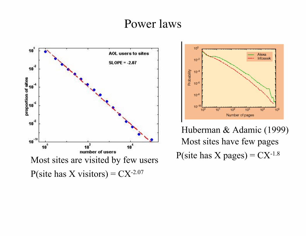
Power laws

A mathematical relation that forms linear plots when datais transformed into log-log coordinates

Very few sites have many users

Power laws

Huberman & Adamic (1999)Most sites have few pages

Most sites are visited by few users

P(site has X visitors) = CX-2.07

P(site has X pages) = CX-1.8

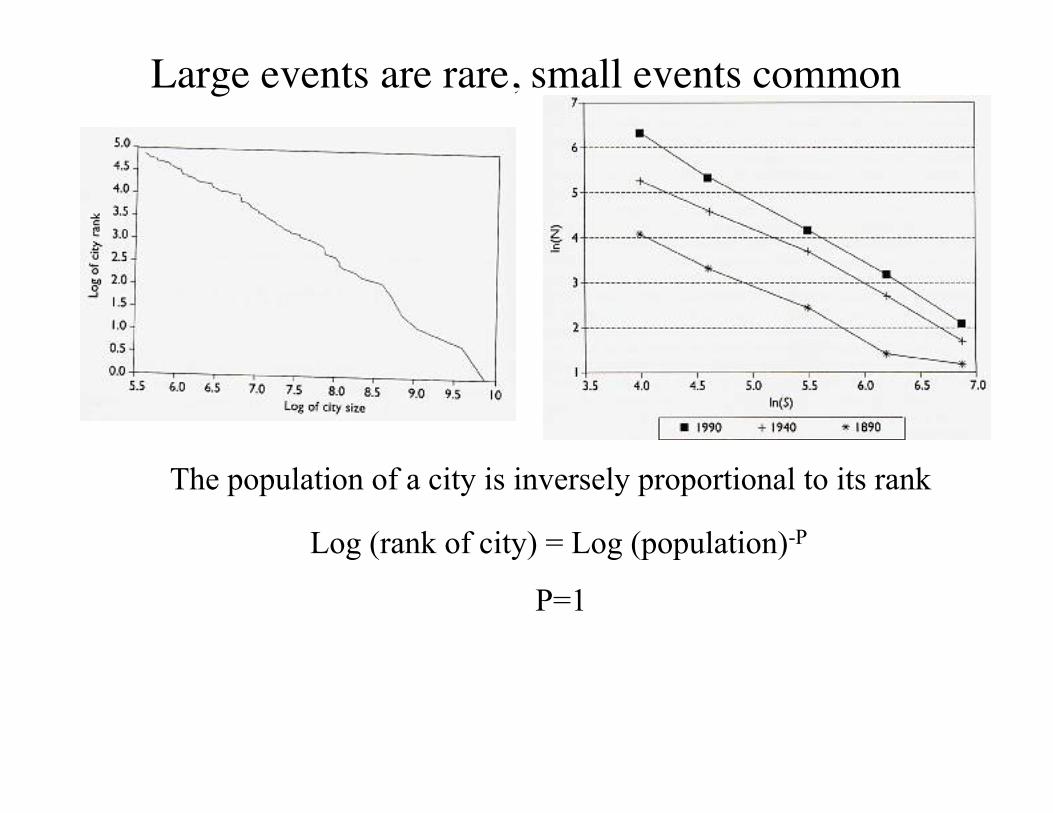
Large events are rare, small events common

The population of a city is inversely proportional to its rank

Log (rank of city) = Log (population)-P

P=1

Log (probability of word) = Log (rank of word)-P

P=1

Zipf’s Law

Power Law in Bibliometrics

Ln (citations to Goldstone) = Ln (rank of citation)-1.59

Ln (Rank)3.53.02.52.01.51.0.50.0-.5

7

6

5

4

3

2

1

0

-1

Observed

Y=X^-1.59L

n(ci

tatio

ns)

Power Law in Baby namesSocial Security data, 1990s

Michael 21243 Ashley 14108Christopher 16421 Jessica 14090Matthew 15851 Emily 10345Joshua 14973 Sarah 10109Jacob 13086 Samantha 10096Andrew 12281 Brittany 9016Daniel 12178 Amanda 8982Nicholas 12072 Elizabeth 7745Tyler 11739 Taylor 7329Joseph 11646 Megan 7266

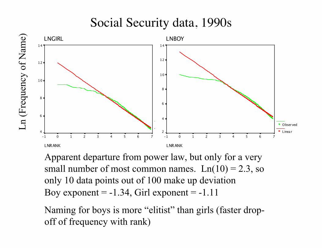
Social Security data, 1990sLNGIRL

LNRANK76543210-1

14

12

10

8

6

4ObservedLinear

LNBOY

LNRANK76543210-1

14

12

10

8

6

4

2ObservedLinear

Apparent departure from power law, but only for a verysmall number of most common names. Ln(10) = 2.3, soonly 10 data points out of 100 make up deviationBoy exponent = -1.34, Girl exponent = -1.11

Naming for boys is more “elitist” than girls (faster drop-off of frequency with rank)

Ln

(Fre

quen

cy o

f N

ame)

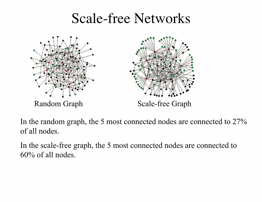
Scale-free Networks

Random Graph Scale-free Graph

In the random graph, the 5 most connected nodes are connected to 27%of all nodes.

In the scale-free graph, the 5 most connected nodes are connected to60% of all nodes.

Colorado Springs High-risk Sex Contacts

l=-1.3

Barabasi & Albert, 1999

P(k)~k-g

A = actor collaborations, N=212,250 edges, average connectivity<k> = 28.78, exponent g = 2.3

B = WWW, N = 325,729, <k> = 5.46, g = 2.3

C = Power grid, N = 4941, <k> = 2.67, g = 4

Redner (1998): probability that a paper is cited k times ~ k-3

•Number of nodes having k links toother nodes (degree k) scales as apower law: k-g

•Exponent g is in the interval 2-3 formost real networks.•Example: The Bell Labs call graph:Calls made between 53 millionphone numbers in a single day•Aiello, W., F. Chung and L. Lu, 2000 Proc. 32ndACM Symp. Theor. Comp.

Number of callers to a number

Freq

uenc

y

Most numbers are called by only a few people

Where do scale free networks come from?• Growth plus preferential attachment

– Growth - networks do not start with all vertices established.Rather, networks accumulate vertices with time

– Preferential attachment - a vertex that already has a large numberof edges connecting it to other vertices will tend to attract stillmore edges. Rich get richer.

• well known actors get more parts• well cited papers get more citations

• Formal model– Growth: start with m0 vertices, and add new vertices one by one,

each with m edges– Preferential attachment: probability that new vertex will connect

to Vertex i is based on ki the degree of I:– Predicts g = 3

• to generalize, use directed graphs, or edge deletion

†

P ki( ) =ki

k jj

Â

Properties of scale free networks• Robust to network failures (Albert, Jeong, & Barabasi, 2000)

– Networks tend to stay connected, and average path lengthcontinues to be small, if random vertices are deleted

– The probability of deleting a hub (vertex with high k) is small• Vulnerable to targeted attacks

– Targeted attacks specifically remove hubs– This is a positive property for negative networks

• Decrease spread of AIDS by changing behavior of a small number ofhighly connected individuals

• Basic model does not predict high degrees of clustering– vertices connected to a vertex are often directly connected

themselves. Clustering coeficient:

Ei = number of edges between i’s neighbors

ki = degree of vertex iCred=2*2/3*2=.667

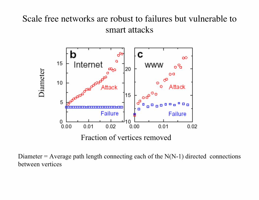
Scale free networks are robust to failures but vulnerable tosmart attacks

Fraction of vertices removed

Diameter = Average path length connecting each of the N(N-1) directed connectionsbetween vertices

Dia

met

er

Hubs make the network fragile to node disruption

Hubs make the network fragile to node disruption

Degree, Clustering, & Path Length

Albert & Barabasi (2002)

Power law exponents, degree, path length

(g=2 is equivalent to Zipf’s law with exponent of 1)

Small World Networks• Elements of a system are frequently connected to each other via a

short path– Milgram’s lost letter experiments (from Omaha to Boston stock broker)

– Six-degrees of separation to Kevin Bacon and Paul Erdos• Regular Lattices

– Vertices only connected to their neighbors (ring-worlds)– “Large world” networks because one must go through many

intermediaries to form some paths. Path length is proportional to n/2k(n=# vertices, k = degree)

• Random graphs– Vertices connected randomly– Average path length is short, proportional to ln(n)/ln(k)– Unfortunately network has no clusters/cliques

• Small world networks (Watts & Strogatz, 1998)– Intermediates between regular and random graphs– degree has a poisson distribution (like random graphs)

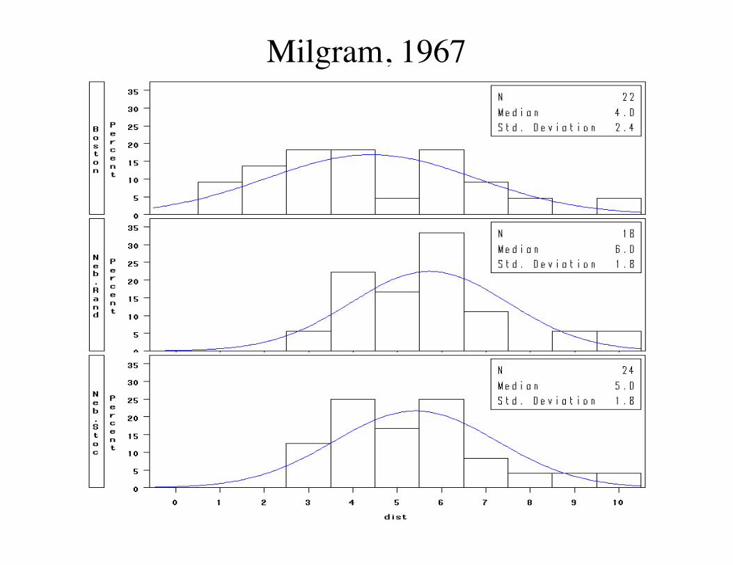
Milgram, 1967

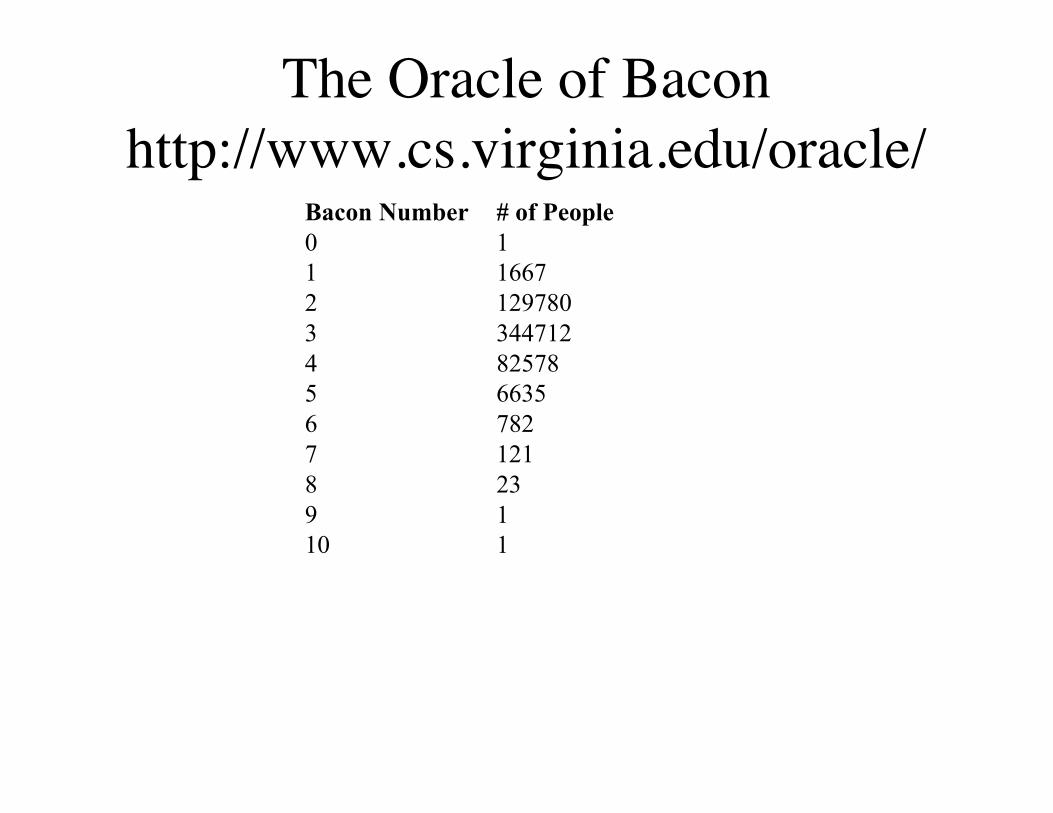
The Oracle of Baconhttp://www.cs.virginia.edu/oracle/

Bacon Number # of People0 1 1 1667 2 129780 3 344712 4 82578 5 6635 6 782 7 121 8 23 9 1 10 1

Small World Networks

Constructing a small world network (Watts, 1999)

Start with regular graph

Rewire each edge with probability p

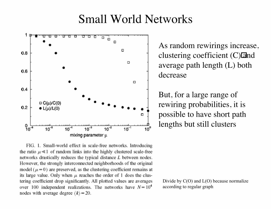
Small World Networks

As random rewirings increase,clustering coefficient (C)!andaverage path length (L) bothdecrease

But, for a large range ofrewiring probabilities, it ispossible to have short pathlengths but still clusters

Divide by C(O) and L(O) because normalizeaccording to regular graph

Small world networks frequently occur (Watts & Strogatz, 1998)

Disease infection: If only a few long-range connections, diseasesspread very quickly (path length is short)

Biochemical Networks

Protein Interaction Networkof common Yeast cellSaccharomyces CerevisiaeJeong, et al., 2001,Nature 411, 41.

• Links between9/11 hijackersand knownassociates.

• (Courtesy ofValdis Krebs,UncloakingTerrorist Networks,First Monday 7, no4, April 2002)

Al-Quaeda

Open issues in social networks• Integrating properties of scale free and small world networks

– Clusters– Hubs

• Ways of characterizing elements in a network