Embed Size (px)
Citation preview
SOCIAL MOBILITY AND INTRA-REGIONAL INCOME DISTRIBUTION ACROSS EU MEMBER STATES
Nº 2008CE160AT054/2008CE16CAT017
DG REGIONAL POLICY
Final Report Date: July 2010
30 St Paul’s Square, Birmingham, B3 1QZ
Tel: 0121 233 8900; Fax: 0121 212 0308
www.ghkint.com
Social Mobility and Intra-Regional Income Distribution Across EU Member States
2
Document Control
Document Title
Social Mobility and Intra-Regional Income Distribution Across EU Member States- Revised Final Report
Job No. 30256192
Prepared by Nick Bozeat, Pat Irving, Xavi Ramos, Mate Peter Vincze, Carmen Juravle, David Jesuit
Checked by Nick Bozeat
Date July 2010
Responsible Administrator:
Dr Alessandro Ferrara,
Unit C3, Economic and Quantitative Analysis, Additionality, DG Regional Policy,
European Commission, CSM2 1/73,
Brussels,1049,Belgium Phone: 0032.2.299.76.39
Fax: 0032.2.299.46.84
E-mail: [email protected]
CONTENTS
3
CONTENTS EXECUTIVE SUMMARY.............................................................................................................7 Approach .....................................................................................................................................8 Key constraints and assumptions..............................................................................................10 Main findings..............................................................................................................................11 Interpersonal income distribution...............................................................................................11 Social mobility............................................................................................................................16 Income distribution and social mobility ......................................................................................21 Income mobility and public supplies ..........................................................................................28 Pointers for future policy............................................................................................................33 Recommendations for further work ...........................................................................................34 1 INTRODUCTION .................................................................................................................37 1.1 Study Aims and objectives............................................................................................37 1.2 Regional policy, social mobility and income distribution...............................................37 1.3 Method of approach......................................................................................................39 1.3.1 Interpersonal income distribution...................................................................................40 1.3.2 Social mobility................................................................................................................40 1.3.3 Income distribution and social mobility..........................................................................41 1.3.4 Income mobility and public supplies ..............................................................................42 1.3.5 Policy analysis ...............................................................................................................42 1.4 Structure of the Report .................................................................................................43 2 INTERPERSONAL INCOME DISTRIBUTION....................................................................47 2.1 Introduction ...................................................................................................................47 2.2 Theoretical analysis ......................................................................................................47 2.2.1 Definitions and indexes of income distribution ..............................................................47 2.2.2 The assessment of alternative measures of interpersonal income distribution ............51 2.2.3 Key conclusions.............................................................................................................54 2.3 Quantitative Analysis of interpersonal income distribution ...........................................54 2.3.1 Empirical evidence from the literature ...........................................................................54 2.3.2 Results of quantitative analysis undertaken for the assignment ...................................67 2.3.3 Suggestions for improving the measurement of income inequality...............................73 2.3.4 Summary and key conclusions......................................................................................73 3 SOCIAL MOBILITY.............................................................................................................75 3.1 Introduction ...................................................................................................................75 3.2 Theoretical Analysis......................................................................................................75 3.2.1 Key concepts of social mobility......................................................................................75 3.2.2 The assessment of alternative definitions of social mobility..........................................85 3.3 Quantitative analysis of social mobility .........................................................................90 3.3.1 Intra-generational income mobility: Empirical evidence from the literature...................90 3.3.2 Results of the quantitative analysis undertaken in this assignment ..............................92 3.3.3 Individual and household characteristics affecting income mobility ..............................96 3.3.4 Other evidence on factors influencing intra-generational mobility.................................98 3.3.5 Inter-generational Social mobility: empirical evidence from the literature .....................99
Social Mobility and Intra-Regional Income Distribution Across EU Member States
4
3.3.6 National and regional intergenerational social mobility: findings of the quantitative analysis of this assignment......................................................................................................102 3.3.7 Factors influencing inter-generational social mobility..................................................107 3.3.8 Influencing social mobility at regional level .................................................................110 3.3.9 Suggestions for improving the measurement of Social Mobility..................................110 3.3.10 Summary .....................................................................................................................110 4 INCOME DISTRIBUTION AND SOCIAL MOBILITY (INCOME DISTRIBUTION DYNAMICS) ............................................................................................................................113 4.1 Introduction .................................................................................................................113 4.2 Theoretical analysis ....................................................................................................113 4.3 Quantitative analysis of social mobility and income distribution.................................118 4.3.1 Evidence Social mobility and income distribution from the literature ..........................118 4.3.2 Evidence on social mobility and income distribution from this assignment.................118 4.3.3 Suggestions to improve the measurement of the relationship between income mobility and income distribution............................................................................................................122 4.4 Summary.....................................................................................................................122 5 RELATING INCOME MOBILITY AND PUBLIC SUPPLIES ............................................123 5.1 Introduction .................................................................................................................123 5.2 The difficulties of relating public expenditure to income distribution and mobility ......124 5.3 The effects of public expenditure analogous to ECP..................................................125 5.4 Evidence from the literature on the distributional effects of ECP expenditure ...........128 5.4.1 Research and technological development (R&TD), innovation and entrepreneurship129 5.4.2 Information society.......................................................................................................130 5.4.3 Transport .....................................................................................................................131 5.4.4 Energy .........................................................................................................................133 5.4.5 Environmental protection and risk prevention .............................................................133 5.4.6 Tourism........................................................................................................................135 5.4.7 Culture .........................................................................................................................135 5.4.8 Urban and rural regeneration ......................................................................................136 5.4.9 Increasing the adaptability of workers and firms, enterprises and entrepreneurs.......136 5.4.10 Improving access to employment and sustainability ...................................................136 5.4.11 Improving the social inclusion of less-favoured persons.............................................137 5.4.12 Improving human capital .............................................................................................137 5.4.13 Investment in social infrastructure ...............................................................................138 5.4.14 Mobilisation for reforms in the fields of employment and inclusion .............................139 5.4.15 Strengthening institutional capacity at national, regional and local level ....................140 5.4.16 Reduction of additional costs hindering the outermost regions development.............140 5.4.17 Technical assistance ...................................................................................................140 5.4.18 Estimates of the distribution effects of ECP categories of expenditure.......................140 5.5 The household income effects of ECP expenditure ...................................................146 5.6 The effects of alternative ECP resource allocations on income distribution ..............147 5.7 The effects of ECP expenditure on social mobility .....................................................149 5.8 Recommendations......................................................................................................150 5.9 Summary.....................................................................................................................150 6 POINTERS FOR FUTURE POLICY..................................................................................153 6.1 Introduction .................................................................................................................153
CONTENTS
5
6.2 European Union Cohesion Policy ...............................................................................153 6.3 Pointers for future policy .............................................................................................153 6.4 Recommendations for further work.............................................................................155 LIST OF COUNTRY ABBREVIATIONS .................................................................................159 LIST OF OTHER ABBREVIATIONS ......................................................................................160 REFERENCES ........................................................................................................................162 ANNEX 1 INCOME INEQUALITY AT NATIONAL AND REGIONAL LEVELS .....................175 ANNEX 2 CLASSIFICATIONS USED IN THE STUDY OF INTER GENERATIONAL SOCIAL MOBILITY.................................................................................................................191 ANNEX 3 EXPLANATION OF REGRESSION ANALYSIS....................................................195 ANNEX 4 ESTIMATING ECP RELATED PUBLIC EXPENDITURE AT REGIONAL LEVEL .....................................................................................................................................205 ANNEX 5 CASE STUDIES SHOWING THE RESULTS OF THE SIMULATIONS ................219 ANNEX 6 MAPS ILLUSTRATING MAIN FINDINGS FOR COUNTRIES AND REGIONS ....229

EXECUTIVE SUMMARY
7
EXECUTIVE SUMMARY This is the Final Report on social mobility and intra-regional income distribution across EU Member States. The report has been prepared by GHK on behalf of the Directorate General Regional Policy (DG REGIO). The work has been undertaken under the guidance of a Steering Group comprising officers of DG REGIO, Directorate General Employment, social Affairs and Equal Opportunities (DG EMPL) and Directorate General Economic and Financial Affairs (DG ECFIN) and the three members of the Scientific Committee comprising: Valentino Dardanoni, Stephen Jenkins and Jacques Silber.
The overall purpose of the study is to assess the current state of social mobility and income distribution across the EU at the national and regional levels. The study focuses on the extent to which social mobility (both short term income mobility and changes of social status between generations) affects income distribution.
More particularly the objectives of the study are:
To provide an economic analysis and literature review of: the relationships between social mobility and the potential for social mobility and income distribution; and, the determinants of social mobility;
To provide a quantitative analysis of the trends in social mobility and income distribution and the influence of different variables (determinants) on income distribution and social mobility across EU Member States and regions; and
To identify, on the basis of the economic and quantitative analyses the implications for policy and policy instruments that could be used to enhance social mobility and potential social mobility.
The Tender Specifications stressed that the study should cover, as far as is practical, the whole of EU27, and NUTS2 regions, and preferably the time scale over which study findings and data are reviewed should allow for the consideration of inter-generational social mobility.
Regional policy, social mobility and income distribution
Article 158 of the EC Treaty establishes that in order to strengthen its economic and social cohesion, the Community aims to reduce disparities between levels of development of EU regions.
The European Union Cohesion Policy (ECP) for the period 2007-2013 has three objectives: the ‘Convergence objective’ that promotes growth-enhancing conditions and factors leading to convergence for the least-developed Member States and regions; the ‘Regional Competitiveness and Employment objective’ that aims to strengthen competitiveness and attractiveness, as well as employment elsewhere in the EU; and, the ‘European Territorial Co-operation objective’. The amount available under the ‘Convergence objective’ is EUR 282.8 billion. The allocation for the ‘Regional Competitiveness and Employment objective’ is EUR 55 billion.
Amongst the factors that may influence the ‘Convergence’ and ‘Regional Competitiveness and Employment’ objectives, and regional GDP per capita, are: interpersonal income distribution at regional level at a particular point in time; changes in the social status of individuals that can in turn affect their earnings potential; and, the changes in interpersonal income distribution over time.
Certainly, social mobility and the related concept of social fluidity are important to economic development and increasing social inclusion. At the same time income inequality is associated with a number of societal outcomes that reduce social welfare. Both social mobility and income distribution can be affected by ECP.
Social Mobility and Intra-Regional Income Distribution Across EU Member States
8
The work is also timely because of the specific reference to the need to address social exclusion in the new EU Treaty and because of the recent review of region policy (Barca, 2009) and the questions it raised over the extent to which regional policy should be focussed on the ‘social task’ bearing in mind the progress in reducing regional disparities but persistent problems related to income inequality including lack of social inclusion, poverty and the risk of poverty. Indeed, the report comments on the relative low levels of ECP resources earmarked to address these needs. This study has explored the consequences for income inequality of changing ECP resource allocations.
Approach
The work was based on a review of relevant theoretical and empirical research in the economic and sociological traditions and quantitative analysis that has identified income distribution, social mobility and public supplies in EU Member States at the national and regional levels and the relationships between then. These relationships have been used to develop simulations to explore the possible consequences of changes in resource allocation within ECP on social (income) mobility and income distribution. The simulations provide estimates of the effects of increases or decreases of expenditure on the main ECP categories: physical infrastructure; human resources; RTD; and, aids to productive investment and expenditure categories that are likely to be ‘pro-lower and middle income groups’ within each region.
Measuring interpersonal income distribution at the regional level requires the definition of a measure of income; an appropriate indicator of income distribution; and, data from sufficiently large household surveys. The preferred measure of income adopted on the recommendation of the Steering Group is ‘net of tax (household) income and benefits’. The alternatives indicators of income distribution have been reviewed. Emphasis has been placed on indicators of equality/inequality rather than indicators of poverty on the recommendation of the Scientific Committee because the study is concerned with income distribution across the full range of incomes. As the study is concerned with the whole of the EU and with comparisons between regions it has been necessary to rely upon datasets that are comparable across the EU. The main datasets that have been used to measure interpersonal income distribution are as follows:
The European Union Statistics on Income and Living Conditions (EU-SILC);
Luxembourg Income Study (LIS); and
European Community Household Panel (ECHP).
Social mobility concerns the changes in the social class of individuals over time. A distinction is made between inter-generational social mobility and intra-generational social mobility. The latter normally focuses on income mobility because it provides a good indicator of individual or household progress and can be measured over several years. Measuring social mobility requires: an appropriate indicator that includes a proxy for social status (class, occupation, income etc) and a defined timescale; and, either ‘panel’ surveys within which the same individuals/households are surveyed on more than one occasion or (less reliable) surveys in which individuals/households are asked about previous social status. The emphasis in the study, stressed by the Steering Group, has been on measuring intra-generational income mobility. The alternative indicators of social mobility have been assessed. The main datasets that have been used to measure intra-generational social (income) mobility in the EU and at regional level are as follows:
EU-SILC 2005-2007;
The Cross-National Equivalent File 1980-2007 (CNEF);
ECHP.
EXECUTIVE SUMMARY
9
Each of these datasets provides panel data tracing the income situation of individual households’ overtime. The literature provides various estimates of inter-generational mobility for some EU countries. The EU-SILC 2005 module, that asked retrospective questions, has been used to explore inter-generational social mobility at the regional level.
Changes in income distribution amongst panels of households at the national and regional levels have been considered so that the relationships between income inequality and income mobility can be explored. The influence of individual or household characteristics and regional level contextual factors on changes in household income and hence income distribution has also been explored though regression analysis.
The individual or household-level factors considered include: the gender and age of the household head; the number of adults and children in the household and the change in their number over a two-year period; the number of persons with at least upper-secondary education in the household, and the change in full or part time employment.
The regional contextual factors considered include: GDP per capita; business sector investment in RTD (BERD), the share of economically active population, unemployment rate, the regional density of motorways, other roads and railway lines, the proportion of students (ISCED levels 5-6) in the population, as well as the relative endowment of the region with hospital beds.
The data sources used to measure social mobility, particularly EU- SILC, are the most up to date and include information on each of the potential individual and household determinants.
The relationship between income mobility and public supplies has been explored to assess the potential of ECP expenditure to influence income mobility and hence income distribution. The potential relationships were explored by: regressing income mobility against of actual public expenditure per capita (including those equivalent to the ECP expenditure) at the regional and national levels; reviewing relevant literature; and, developing reasoned arguments as to the likely distributional effects of different categories of ECP expenditure.
The focus of the policy analysis was on exploring the consequences of alternative allocations of ECP resources on social mobility and income distribution. Information on actual ECP resource allocations for the period 2007-2013 from DG REGIO has been used.
Nine broad simulations have been considered:
X% pro rata increase in ECP expenditure
X% pro rata decrease in ECP expenditure
X% increase in ECP categories relating to physical infrastructure, and corresponding decreases in all other categories.
X% increase in ECP categories relating to human resources infrastructure, and corresponding decreases in all other categories.
X% increase in ECP categories relating to research and technological development (R&TD), and corresponding decreases in all other categories.
X% increase in ECP categories relating to aids to productive sector and corresponding decreases in all other categories.
X% increase in allocations to ECP categories that are pro lower and middle income groups and corresponding decreases in all other categories, assuming moderate distribution effects.
X% increase in allocations to ECP categories that are pro lower and middle income groups and corresponding decreases in all other categories, assuming high distribution effects.
Social Mobility and Intra-Regional Income Distribution Across EU Member States
10
X% increase in allocations to ECP categories that are pro lower and middle income groups and corresponding decreases in all other categories, assuming very high distribution effects.
These simulations have been chosen in order to explore the possible effects of changes in ECP resource allocation decisions on income mobility and income distribution. The latter three simulations explore the possible effects of resource allocation adjustments that are likely to be pro poor whilst applying different assumptions as to the extent to which particular sub categories of ECP expenditure are likely to benefit lower income groups. Whilst neither reducing income inequality nor improving the benefits to lower income groups are explicit ECP objectives, such effects may be of interest to those at the national and regional levels responsible for regional policy because much of the disparities between income groups accrue at the intra rather than inter regional levels.
The effects on income distribution to quintile income groups of the simulations have been estimated. The simulation model developed allows for changes in the value X. The simulations have been used to assess the extent to which changes in the allocations affect income distribution and lead to significant changes in the Gini coefficient.
In addition, consideration has been given to the ways in which ECP resources might influence the contextual, household and individual factors that affect, in particular, upward social mobility. The results of the application of the method are illustrated in a number of case studies.
Key constraints and assumptions
Before presenting the main findings of the study it is important to emphasis the key constraints faced and the key assumptions underpinning the analysis. The Tender Specifications requested a study in three parts: economic analysis; quantitative analysis and policy analysis. The relationships between social mobility, income distribution and public supplies, and in particular ECP type expenditure, have not been thoroughly researched by the relevant literature, the assignment has thus innovative aspects and the conclusions drawn need to be considered a preliminary exploration of the subject. More specifically the assumptions and constraints include the following.
The preferred measure of income was ‘net of tax (household) income and benefits’. However, the main datasets available do not measure ‘non cash’ or ‘in kind’ benefits. The latter are however, important consequences of public supplies of the type provided by ECP.
The main source of data available for the quantitative analysis of intra-generational income mobility was EU-SILC. These data only allow for the measurement of household income change on a comparable basis for the period 2005-2007. This was a period of relatively high overall economic growth and of rapid change in EU12 countries. It can be argued that during the period following 2007, that has been characterized by economic crisis, the patterns of income mobility may not follow those observed between 2005 and 2007. However, the EU-SILC panel data that were used include responses from a large number of households over time which enables statistical robustness, and the analysis in the study is aimed at assessing the incremental effects of ECP and hence the findings from the 2005-2007 period may still be considered relevant.
The only data available on a comparable basis for inter-generational mobility at the regional level is that from the EU-SILC 2005 when questions were asked about family histories. Data of this type is subject to reliability problems.
ECP expenditure is limited to particular categories of public expenditure. Some categories of public expenditure that have major effects on income distribution such as social protection transfers are not eligible ECP expenditure. Thus a priori it is reasonable to assume that variations in ECP resource allocations will have relatively minor effects on income change and distribution compared with other aspects of public expenditure.
EXECUTIVE SUMMARY
11
It is assumed that the value of benefits of ECP expenditure is equivalent to the costs. It can be argued that this is a conservative assumption1. This is because much of the actual ECP expenditure is spent on investment and infrastructure projects where the benefits accruing are judged to outweigh costs and the expenditure may lead to regional multiplier effects. However, in considering the potential distribution effects of ECP expenditure the costs are assumed to equal the income benefits. Also ECP expenditure may lead or contribute to structural changes that influence social mobility and hence income distribution. However, given the limits of this study more fine tuned assumptions based on the characteristics of particular sub categories of ECP expenditure have not been applied. .
At the core of the simulation model that has been used to explore the consequences of alternative allocations of ECP expenditure are a series of assumptions concerning the distribution effects, in terms of impacts on the household incomes of different quintile income groups. The evidence to inform these assumptions is however, very limited.
Main findings
Interpersonal income distribution
Theoretical analysis: Income distribution reflects the nature and extent of inequalities in the income of individuals or households in a given society or subgroups within society. The concept may also be applied to geographical units.
There are many ways to characterise income inequality – either graphically or using various aggregate measures. The graphical methods include:
histograms, presenting the frequency of individuals belonging to separate income strata;
cumulative frequency distributions, where the frequency of individuals not surpassing a certain income level is presented; and,
the Lorenz curve, which shows the share of total income in society received by different income groups.
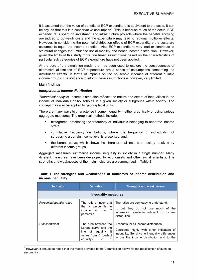
Aggregate measures summarise income inequality in society in a single number. Many different measures have been developed by economists and other social scientists. The strengths and weaknesses of the main indicators are summarised in Table 1.
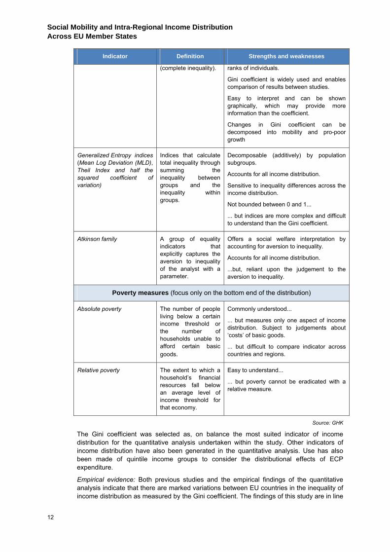
Table 1 The strengths and weaknesses of indicators of income distribution and income inequality
Indicator Definition Strengths and weaknesses
Inequality measures
Percentile/quantile ratios
The ratio of income at the X percentile to income at the Y percentile.
The ratios are very easy to understand...
... but they do not use much of the information available relevant to income distribution.
Gini coefficient The area between the Lorenz curve and the line of equality. It varies from 0 (perfect equality), to 1
Accounts for all income distribution.
Correlates highly with other indicators of inequality. Sensitive to inequality differences across the income distribution and to the
1 However, it should be noted that the model provided to the Commission allows for the modification of such an assumption.
Social Mobility and Intra-Regional Income Distribution Across EU Member States
12
Indicator Definition Strengths and weaknesses
(complete inequality). ranks of individuals.
Gini coefficient is widely used and enables comparison of results between studies.
Easy to interpret and can be shown graphically, which may provide more information than the coefficient.
Changes in Gini coefficient can be decomposed into mobility and pro-poor growth
Generalized Entropy indices (Mean Log Deviation (MLD), Theil Index and half the squared coefficient of variation)
Indices that calculate total inequality through summing the inequality between groups and the inequality within groups.
Decomposable (additively) by population subgroups.
Accounts for all income distribution.
Sensitive to inequality differences across the income distribution.
Not bounded between 0 and 1...
... but indices are more complex and difficult to understand than the Gini coefficient.
Atkinson family A group of equality indicators that explicitly captures the aversion to inequality of the analyst with a parameter.
Offers a social welfare interpretation by accounting for aversion to inequality.
Accounts for all income distribution.
...but, reliant upon the judgement to the aversion to inequality.
Poverty measures (focus only on the bottom end of the distribution)
Absolute poverty The number of people living below a certain income threshold or the number of households unable to afford certain basic goods.
Commonly understood...
... but measures only one aspect of income distribution. Subject to judgements about ‘costs’ of basic goods.
... but difficult to compare indicator across countries and regions.
Relative poverty The extent to which a household’s financial resources fall below an average level of income threshold for that economy.
Easy to understand...
... but poverty cannot be eradicated with a relative measure.
Source: GHK
The Gini coefficient was selected as, on balance the most suited indicator of income distribution for the quantitative analysis undertaken within the study. Other indicators of income distribution have also been generated in the quantitative analysis. Use has also been made of quintile income groups to consider the distributional effects of ECP expenditure.
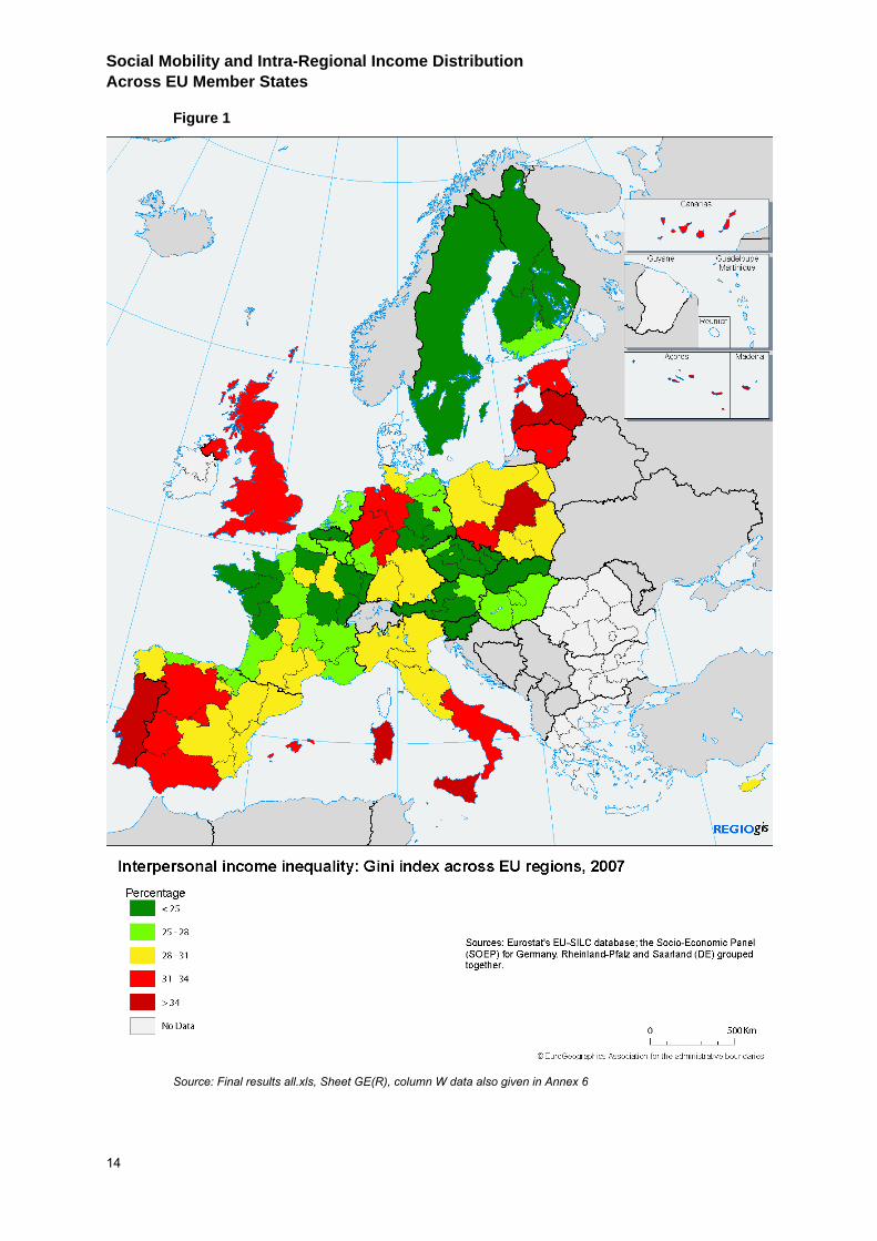
Empirical evidence: Both previous studies and the empirical findings of the quantitative analysis indicate that there are marked variations between EU countries in the inequality of income distribution as measured by the Gini coefficient. The findings of this study are in line

EXECUTIVE SUMMARY
13
with previous studies placing SE alongside SI and SK at the lower end of the inequality spectrum and PT, LT and LV at the top end. Furthermore, AT, BE, CZ, FI, FR, LU and NL form a cluster with values of the Gini coefficient below 28 percent. UK, ES, IT and EE form a cluster with higher inequality rates but lower than PT, PL and LV.
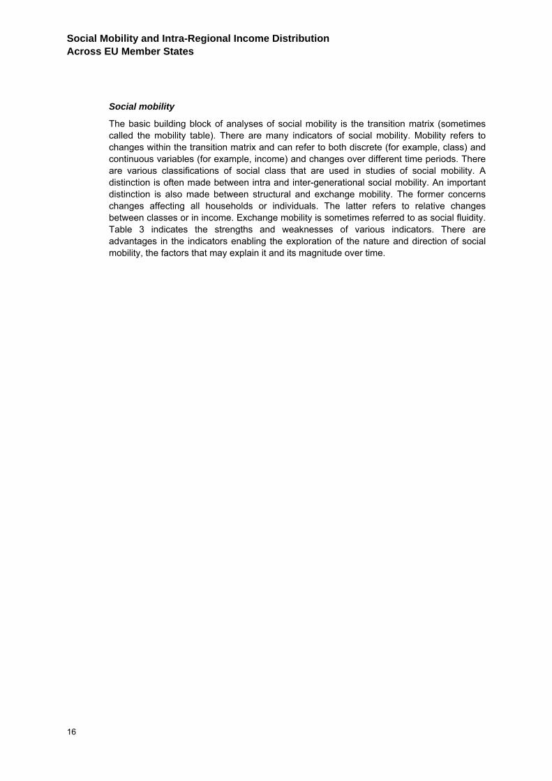
There are also marked variations in the Gini coefficients between regions in some EU countries. Capital regions tend to have greater inequality of income distribution. Figures 1 and 2 indicate the Gini coefficients and variations between and within countries. Table 2 indicates the regions/countries in the EU with the lowest and highest income inequality.
Social Mobility and Intra-Regional Income Distribution Across EU Member States
14
Figure 1
Source: Final results all.xls, Sheet GE(R), column W data also given in Annex 6
EXECUTIVE SUMMARY
15
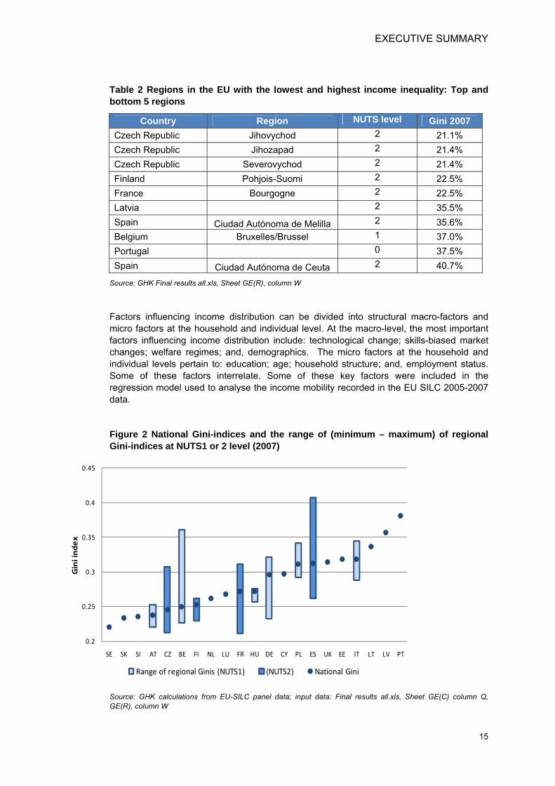
Table 2 Regions in the EU with the lowest and highest income inequality: Top and bottom 5 regions
Country Region NUTS level Gini 2007 Czech Republic Jihovychod 2 21.1% Czech Republic Jihozapad 2 21.4% Czech Republic Severovychod 2 21.4% Finland Pohjois-Suomi 2 22.5% France Bourgogne 2 22.5% Latvia 2 35.5% Spain Ciudad Autónoma de Melilla 2 35.6% Belgium Bruxelles/Brussel 1 37.0% Portugal 0 37.5% Spain Ciudad Autónoma de Ceuta 2 40.7%
Source: GHK Final results all.xls, Sheet GE(R), column W
Factors influencing income distribution can be divided into structural macro-factors and micro factors at the household and individual level. At the macro-level, the most important factors influencing income distribution include: technological change; skills-biased market changes; welfare regimes; and, demographics. The micro factors at the household and individual levels pertain to: education; age; household structure; and, employment status. Some of these factors interrelate. Some of these key factors were included in the regression model used to analyse the income mobility recorded in the EU SILC 2005-2007 data.
Figure 2 National Gini-indices and the range of (minimum – maximum) of regional Gini-indices at NUTS1 or 2 level (2007)
0.2
0.25
0.3
0.35
0.4
0.45
SE SK SI AT CZ BE FI NL LU FR HU DE CY PL ES UK EE IT LT LV PT
Gin
i in
de
x
Range of regional Ginis (NUTS1) (NUTS2) National Gini
Source: GHK calculations from EU-SILC panel data; input data: Final results all.xls, Sheet GE(C) column Q, GE(R), column W
Social Mobility and Intra-Regional Income Distribution Across EU Member States
16
Social mobility
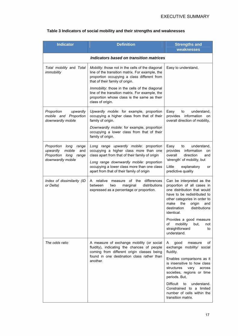
The basic building block of analyses of social mobility is the transition matrix (sometimes called the mobility table). There are many indicators of social mobility. Mobility refers to changes within the transition matrix and can refer to both discrete (for example, class) and continuous variables (for example, income) and changes over different time periods. There are various classifications of social class that are used in studies of social mobility. A distinction is often made between intra and inter-generational social mobility. An important distinction is also made between structural and exchange mobility. The former concerns changes affecting all households or individuals. The latter refers to relative changes between classes or in income. Exchange mobility is sometimes referred to as social fluidity. Table 3 indicates the strengths and weaknesses of various indicators. There are advantages in the indicators enabling the exploration of the nature and direction of social mobility, the factors that may explain it and its magnitude over time.
EXECUTIVE SUMMARY
17
Table 3 Indicators of social mobility and their strengths and weaknesses
Indicator Definition Strengths and
weaknesses
Indicators based on transition matrices
Total mobility and Total immobility
Mobility: those not in the cells of the diagonal line of the transition matrix. For example, the proportion occupying a class different from that of their family of origin.
Immobility: those in the cells of the diagonal line of the transition matrix. For example, the proportion whose class is the same as their class of origin.
Easy to understand,
Proportion upwardly mobile and Proportion downwardly mobile
Upwardly mobile: for example, proportion occupying a higher class from that of their family of origin.
Downwardly mobile: for example, proportion occupying a lower class from that of their family of origin.
Easy to understand, provides information on overall direction of mobility,
Proportion long range upwardly mobile and Proportion long range downwardly mobile
Long range upwardly mobile: proportion occupying a higher class more than one class apart from that of their family of origin
Long range downwardly mobile: proportion occupying a lower class more than one class apart from that of their family of origin
Easy to understand, provides information on overall direction and ‘strength’ of mobility, but
Little explanatory or predictive quality
Index of dissimilarity (ID or Delta)
A relative measure of the differences between two marginal distributions expressed as a percentage or proportion.
Can be interpreted as the proportion of all cases in one distribution that would have to be redistributed to other categories in order to make the origin and destination distributions identical.
Provides a good measure of mobility but, not straightforward to understand.
The odds ratio A measure of exchange mobility (or social fluidity), indicating the chances of people coming from different origin classes being found in one destination class rather than another.
A good measure of exchange mobility/ social fluidity.
Enables comparisons as it is insensitive to how class structures vary across societies, regions or time periods. But,
Difficult to understand. Constrained to a limited number of cells within the transition matrix.
Social Mobility and Intra-Regional Income Distribution Across EU Member States
18
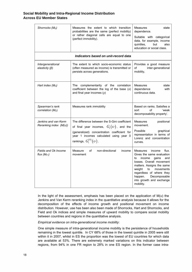
Shorrocks (MD) Measures the extent to which transition probabilities are the same (perfect mobility) or rather diagonal cells are equal to one (perfect immobility).
Measures state dependence.
Suitable with categorical data, for example, income quintiles, but also education or social class.
Indicators based on unit-record data
Intergenerational elasticity (β)
The extent to which socio-economic status (often measured as income) is transmitted or persists across generations.
Provides a good measure of inter-generational mobility,
Hart index (MH) The complementarity of the correlation coefficient between the log of the base (x) and final year incomes (y)
Measures state dependence with continuous data.
Spearman’s rank correlation (MS)
Measures rank immobility Based on ranks. Satisfies a sort of ‘weak decomposability property’.
Jenkins and van Kerm Reranking index (M(υ))
The difference between the S-Gini coefficient
of final year incomes, ( )1G υ , and the
(generalized) concentration coefficient for year 1 incomes calculated using year 0
rankings, ( ) ( )01G υ .
Measures positional movement.
Possible graphical representation in terms of Lorenz and concentration curves.
Fields and Ok Income flux (MF1)
Measure of non-directional income movement
Measures income flux. Gives the same evaluation to income gains and losses. Overall movement matters. Assigns the same weight to movements regardless of where they happen. Decomposable into growth and exchange mobility.
In the light of the assessment, emphasis has been placed on the application of M(υ) the Jenkins and Van Kerm reranking index in the quantitative analysis because it allows for the decomposition of the effects of income growth and positional movement on income distribution. However, use has been also been made of Shorrocks, Hart and Shorrocks, and Field and Ok indices and simple measures of upward mobility to compare social mobility between countries and regions in the quantitative analysis.
Empirical evidence on intra-generational income mobility:
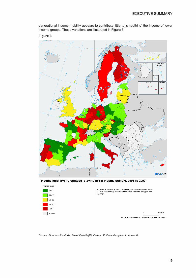
One simple measure of intra-generational income mobility is the persistence of households remaining in the lowest quintile. In CY 68% of those in the lowest quintile in 2005 were still within it in 2007, whilst in ES the proportion was the lowest of EU countries for which data are available at 53%. There are extremely marked variations on this indicator between regions, from 94% in one FR region to 28% in one ES region. In the former case intra-
EXECUTIVE SUMMARY
19
generational income mobility appears to contribute little to ‘smoothing’ the income of lower income groups. These variations are illustrated in Figure 3.
Figure 3
Source: Final results all.xls, Sheet Quintile(R), Column K. Data also given in Annex 6
Social Mobility and Intra-Regional Income Distribution Across EU Member States
20
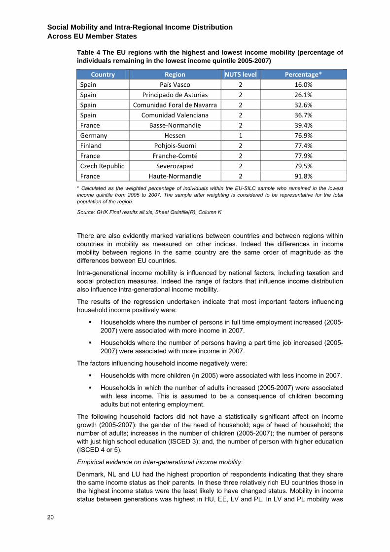
Table 4 The EU regions with the highest and lowest income mobility (percentage of individuals remaining in the lowest income quintile 2005-2007)
Country Region NUTS level Percentage* Spain País Vasco 2 16.0% Spain Principado de Asturias 2 26.1% Spain Comunidad Foral de Navarra 2 32.6% Spain Comunidad Valenciana 2 36.7% France Basse-Normandie 2 39.4% Germany Hessen 1 76.9% Finland Pohjois-Suomi 2 77.4% France Franche-Comté 2 77.9% Czech Republic Severozapad 2 79.5% France Haute-Normandie 2 91.8%
* Calculated as the weighted percentage of individuals within the EU-SILC sample who remained in the lowest income quintile from 2005 to 2007. The sample after weighting is considered to be representative for the total population of the region.
Source: GHK Final results all.xls, Sheet Quintile(R), Column K
There are also evidently marked variations between countries and between regions within countries in mobility as measured on other indices. Indeed the differences in income mobility between regions in the same country are the same order of magnitude as the differences between EU countries.
Intra-generational income mobility is influenced by national factors, including taxation and social protection measures. Indeed the range of factors that influence income distribution also influence intra-generational income mobility.
The results of the regression undertaken indicate that most important factors influencing household income positively were:
Households where the number of persons in full time employment increased (2005-2007) were associated with more income in 2007.
Households where the number of persons having a part time job increased (2005-2007) were associated with more income in 2007.
The factors influencing household income negatively were:
Households with more children (in 2005) were associated with less income in 2007.
Households in which the number of adults increased (2005-2007) were associated with less income. This is assumed to be a consequence of children becoming adults but not entering employment.
The following household factors did not have a statistically significant affect on income growth (2005-2007): the gender of the head of household; age of head of household; the number of adults; increases in the number of children (2005-2007); the number of persons with just high school education (ISCED 3); and, the number of person with higher education (ISCED 4 or 5).
Empirical evidence on inter-generational income mobility:
Denmark, NL and LU had the highest proportion of respondents indicating that they share the same income status as their parents. In these three relatively rich EU countries those in the highest income status were the least likely to have changed status. Mobility in income status between generations was highest in HU, EE, LV and PL. In LV and PL mobility was
EXECUTIVE SUMMARY
21
lowest for those in the lowest income status category. In three countries, BE, ES and IT, out of the seven within which regional comparisons were possible there were marked variations between mobility of income status between regions.
ES and PT, followed closely by AT, BE and PL have apparently the highest proportions of respondents indicating that they share the same occupational group as their father. FR and FI have the lowest proportions, but the difference between EU countries is not marked. The occupation category within which respondents were most likely to have the same category as their father was Level 2 professionals (see Annex 2 for definitions). In several countries the aggregate level of social mobility varied markedly between regions. In some countries the capital region was associated with the highest mobility.
There are marked variations in the levels of education mobility between generations. The lowest numbers indicating that they were within the same educational level as their fathers were in the UK, SE and LT. In contrast the highest numbers indicating that they were within the same level were in CZ, SK and DE. The category within which respondents were most likely to remain was ISCED level 5 (see Annex 2). In some countries, in particular ES, there were marked differences between regions in the apparent levels of inter generational education mobility.
More generally the chances of people climbing the social ladder differ between European countries. There are also marked differences in earnings elasticities between countries. Immobility tends to be greater at the higher and lower ends of the earnings spectrum. The rich stay rich whilst the poor stay poor. The pattern of mobility in former communist European countries is complex. There is some evidence that it was higher for women. The relationship between economic growth and social fluidity is unclear.
A large number of factors influence inter generational social mobility, especially: family related factors (wealth, family structure, education of parents, parental occupation, genetics and assortative mating); neighbourhood conditions; and, institutional and public policy factors particularly educational policies and reforms.
Income distribution and social mobility
The relationship between income distribution and social mobility is complex. It is possible, though unlikely, that income distribution could remain static over a period during which there had been considerable social (income) mobility. Households could simply have exchanged positions, with households from one income strata (or class) changing places with households from another. The process of measuring income distribution with cross sectional data would not in itself identify the extent of such mobility or positional movement of households. It is also possible that income distribution could change over a period during which there has been no social mobility or positional movement of households. The change in income distribution could have been simply a consequence of increased incomes within higher income groups and decreased incomes within lower income groups without households changing their relative positions or rankings. Again, the process of measuring income distribution with cross sectional data would not in itself identify the absence of such mobility or positional movement of households.
Because both the phenomena of relative income change between income groups and mobility (positional change) affect income distribution it is useful to isolate the effects of each on changes in income distribution. Relative income change or the pattern of income growth may be either pro-poor or pro-rich. This characteristic is termed progressivity and may be measured by the extent to which incomes move to or from the average. The preferred measure of inequality change put forward by Jenkins and Van Kerm (2006) allows the unravelling or decomposition of the extent to which income inequality changes are due to the pattern of income growth and to the degree of positional movement that occurs within the income distribution. This measure does however require longitudinal data before it can be applied.

Social Mobility and Intra-Regional Income Distribution Across EU Member States
22
The relationship between social mobility and interpersonal income distribution is not unidirectional and evidence is somewhat contradictory. However, one study including 9 EU countries (CY, CZ, HU, LV, West DE, PL, SK, ES and SE) indicated that that sons who grew up in more unequal countries in the 1970s were less likely to have experienced social mobility by 1999. More specifically, the authors’ estimated that a 10-percentage point rise in the Gini coefficient (ie increase in inequality) augments the intergenerational earnings correlation by between 0.07 and 0.13 (ie decrease in earnings mobility).
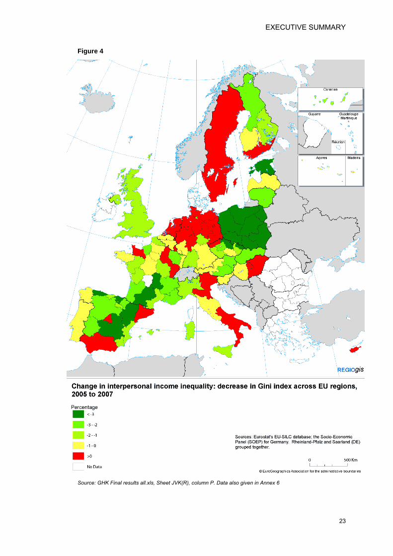
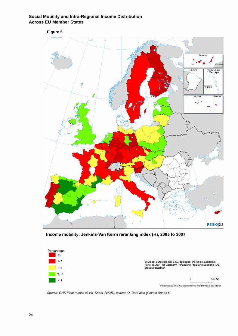
Figures 4 and 5 illustrate the changes 2005-2007 in the Gini coefficient and the extent of reranking of household income at regional level. Tables 5 and 6 indicate the EU regions with the greatest changes in inequality and highest and lowest mobility (2005-2007).
EXECUTIVE SUMMARY
23
Figure 4
Source: GHK Final results all.xls, Sheet JVK(R), column P. Data also given in Annex 6
Social Mobility and Intra-Regional Income Distribution Across EU Member States
24
Figure 5
Source: GHK Final results all.xls, Sheet JVK(R), column Q. Data also given in Annex 6
EXECUTIVE SUMMARY
25
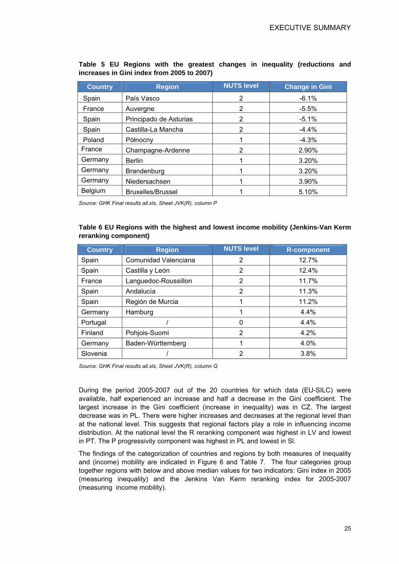
Table 5 EU Regions with the greatest changes in inequality (reductions and increases in Gini index from 2005 to 2007)
Country Region NUTS level Change in Gini Spain País Vasco 2 -6.1% France Auvergne 2 -5.5% Spain Principado de Asturias 2 -5.1% Spain Castilla-La Mancha 2 -4.4% Poland Północny 1 -4.3% France Champagne-Ardenne 2 2.90% Germany Berlin 1 3.20% Germany Brandenburg 1 3.20% Germany Niedersachsen 1 3.90% Belgium Bruxelles/Brussel 1 5.10%
Source: GHK Final results all.xls, Sheet JVK(R), column P
Table 6 EU Regions with the highest and lowest income mobility (Jenkins-Van Kerm reranking component)
Country Region NUTS level R-component Spain Comunidad Valenciana 2 12.7% Spain Castilla y León 2 12.4% France Languedoc-Roussillon 2 11.7% Spain Andalucía 2 11.3% Spain Región de Murcia 1 11.2% Germany Hamburg 1 4.4% Portugal / 0 4.4% Finland Pohjois-Suomi 2 4.2% Germany Baden-Württemberg 1 4.0% Slovenia / 2 3.8%
Source: GHK Final results all.xls, Sheet JVK(R), column Q
During the period 2005-2007 out of the 20 countries for which data (EU-SILC) were available, half experienced an increase and half a decrease in the Gini coefficient. The largest increase in the Gini coefficient (increase in inequality) was in CZ. The largest decrease was in PL. There were higher increases and decreases at the regional level than at the national level. This suggests that regional factors play a role in influencing income distribution. At the national level the R reranking component was highest in LV and lowest in PT. The P progressivity component was highest in PL and lowest in Sl.
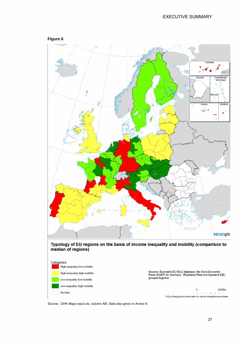
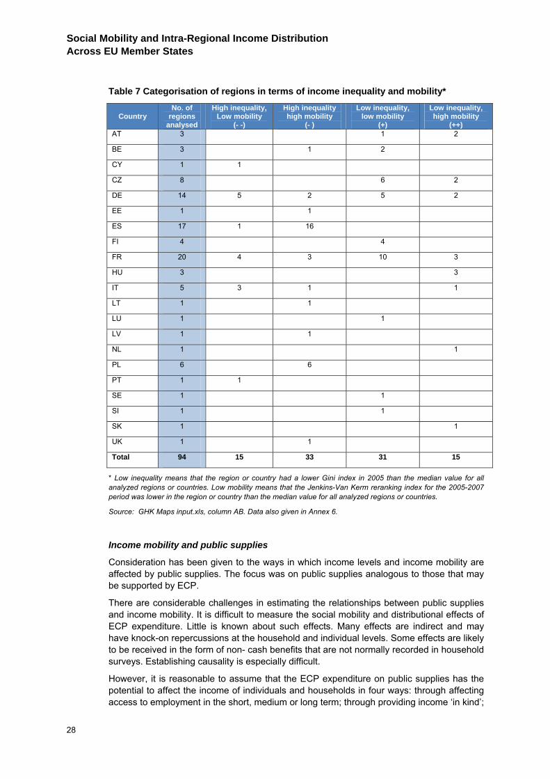
The findings of the categorization of countries and regions by both measures of inequality and (income) mobility are indicated in Figure 6 and Table 7. The four categories group together regions with below and above median values for two indicators: Gini index in 2005 (measuring inequality) and the Jenkins Van Kerm reranking index for 2005-2007 (measuring income mobility).

Social Mobility and Intra-Regional Income Distribution Across EU Member States
26
The regions where inequality is low and (income) mobility is high are concentrated in the western and central areas of continental Europe. The NL and some FR regions and part of eastern DE, SL and HU and most of AT in central Europe are of this type. The regions with relatively high inequality and low mobility are located in PT, IT and western DE, with some in FR.
Interestingly, FR, DE and IT all have regions from both the ‘extreme’ categories. Other countries for which regional level analysis was possible (ES, BE, AT, HU, PL and FI) were more homogenous.
EXECUTIVE SUMMARY
27
Figure 6
Source: GHK Maps input.xls, column AB. Data also given in Annex 6.
Social Mobility and Intra-Regional Income Distribution Across EU Member States
28
Table 7 Categorisation of regions in terms of income inequality and mobility*
Country No. of
regions analysed
High inequality, Low mobility
(- -)
High inequality high mobility
(- )
Low inequality, low mobility
(+)
Low inequality, high mobility
(++) AT 3 1 2
BE 3 1 2
CY 1 1
CZ 8 6 2
DE 14 5 2 5 2
EE 1 1
ES 17 1 16
FI 4 4
FR 20 4 3 10 3
HU 3 3
IT 5 3 1 1
LT 1 1
LU 1 1
LV 1 1
NL 1 1
PL 6 6
PT 1 1
SE 1 1
SI 1 1
SK 1 1
UK 1 1
Total 94 15 33 31 15
* Low inequality means that the region or country had a lower Gini index in 2005 than the median value for all analyzed regions or countries. Low mobility means that the Jenkins-Van Kerm reranking index for the 2005-2007 period was lower in the region or country than the median value for all analyzed regions or countries.
Source: GHK Maps input.xls, column AB. Data also given in Annex 6.
Income mobility and public supplies
Consideration has been given to the ways in which income levels and income mobility are affected by public supplies. The focus was on public supplies analogous to those that may be supported by ECP.
There are considerable challenges in estimating the relationships between public supplies and income mobility. It is difficult to measure the social mobility and distributional effects of ECP expenditure. Little is known about such effects. Many effects are indirect and may have knock-on repercussions at the household and individual levels. Some effects are likely to be received in the form of non- cash benefits that are not normally recorded in household surveys. Establishing causality is especially difficult.
However, it is reasonable to assume that the ECP expenditure on public supplies has the potential to affect the income of individuals and households in four ways: through affecting access to employment in the short, medium or long term; through providing income ‘in kind’;
EXECUTIVE SUMMARY
29
through bringing about environmental goods, health benefits or changes in property values; and, through affecting the prices of commodities and public supplies (for example, energy, transport) that may disproportionately affect one income group more than another. The orders of magnitude of ECP expenditure are large in some regional contexts and the evidence of possible mobility and distribution effects was reviewed for each sub category of ECP expenditure.
Income change 2005-2007 as observed in EU-SILC panel data was regressed against actual public expenditure at the regional level. Overall the effects were very small but the following results were obtained:
There was a significant but small association between expenditure on aids to productive investment and income growth in the lowest income quintile and a decrease in incomes amongst quintile income groups 3, 4 and 5. This suggests that aid to productive investment may have pro poor effects.
Income growth was higher in lower income groups in countries where investments in human capital were higher. This suggests that the earnings of lower income groups may be positively affected by such investments. However, the aggregate effects were very small and not statistically significant.
The levels of public expenditure on infrastructure did not significantly explain variations in income growth between quintile groups.
The levels of RTD expenditure significantly affected income, being associated with reductions in quintile 1 and increases in quintiles 3, 4 and 5.
Income distribution effects of ECP expenditure. The possible distributional effects of each sub category of ECP expenditure have been expressed in terms of the proportion of resources that would be received by each quintile income groups. As mentioned above, it has been assumed that the income benefits equate to the expenditure. There are 15 sub categories that are pro lower income groups, 23 categories that are pro middle and lower income groups, 9 sub categories that are pro middle and higher income groups and 5 sub categories that are pro higher income groups. There are 32 sub categories where there are no particular distribution effects or where any such effects are highly dependent upon complementary national or regional policies. Some of these have the potential to have pro lower and middle income groups distribution effects. The detailed income distribution assumptions for each sub category of ECP expenditure are provided in the simulation model.
A number of alternative ECP resource allocations have been considered to explore the possible income distributions effects. These simulations have been generated for all EU NUTS2 regions based on actual ECP resource allocations to each sub category for the period 2007-2013 The effects in terms of changes in household income within each quintile income group for each simulation have been estimated. For a typical region receiving a relatively high level of ECP expenditure it is evident that simulation involving 10% increases in ECP expenditure and 10% shifts in allocations between broad expenditure categories can affect household incomes significantly. The effects are most pronounced when the simulation involves increasing expenditure on the more overtly ‘pro poor’ sub categories. The simulation model developed for this assignment allows the distribution effects of varying levels of resource allocation to be considered.
For a subset of 99 countries and regions where data allow it has been possible to identify the effects of the resource allocation simulations on the Gini coefficient of inequality. By way of illustration a 10% increase in ‘pro poor’ expenditure sub categories (assuming moderate distribution effects), and a corresponding decrease in other sub categories could give rise to a discernable one percentage point reduction in the Gini coefficient in around 20% of these countries and regions.
Social Mobility and Intra-Regional Income Distribution Across EU Member States
30
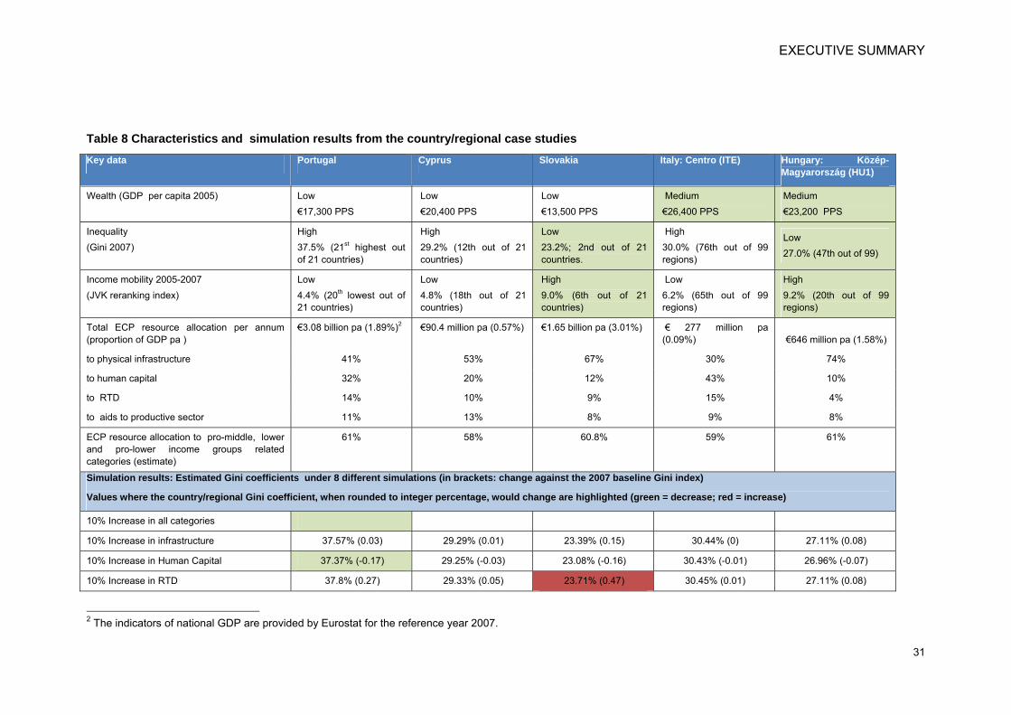
Five case studies of regions/countries with contrasting levels of inequality and (income) mobility were undertaken to explore the effects of alternative ECP resource allocations: PT, CY, SK, Centro (ITE) and Közép-Magyarország (HU1). The findings are summarized in Table 8.
The marginal effects of increased or restructured ECP expenditure on income inequality and (income) mobility vary considerably between countries or regions. Changes in the Gini coefficient are higher in regions receiving high levels of ECP resources relative to their GDP. Simulations increasing ECP expenditure by 10% yielded a reduction in the Gini coefficient of up to 3 percentage points in these countries or regions. The effects on the Gini coefficient of Cyprus and especially Centro (Italy), where ECP expenditure per GDP is lower, do not exceed 0.60 and 0.05 percentage points, respectively.
Also, the potential for reducing inequalities is higher in countries or regions where the Gini coefficient is already high, such as in PT. In lower inequality countries, such as SK, the potential seems to be lower. Only one simulated change in ECP resource allocation in one regional case study was linked to a possible increase in the Gini coefficient (when rounded to integers) This involved a stronger focus on RTD expenditure (+ 10%) in SK.
In the simulations, the estimated changes in the Gini coefficient are due to the progressivity of income growth (i.e. increases in the average incomes of households in lower income quintiles). In order to interpret these results however, it should be borne in mind that the model used allocates the same additional simulated ECP expenditure to all individuals within one income quintile. In reality, however, individuals belonging within the same quintile may differently benefit from ECP expenditure. In such a case the actual re-ranking component (that is the part of income inequality change due to income mobility) in terms of equivalised household income would change more, whilst the progressivity of income growth would change less. It has been necessary to adopt this assumption because the mobility effects are in practice influenced by individual characteristics and by other factors affecting social and income mobility in the specific region/ country concerned. In addition, however, it is also important to stress that if the average income increase due to ECP expenditure is such that all individuals of the same quintile change quintile, then mobility is recorded by the model. In conclusion, the model allows mainly for the progressivity of income growth and less for the re-ranking component of income inequality changes.
Social mobility effects of broad categories of ECP expenditure. In the light of the regression analysis undertaken the following observations were made:
Productive investment: There was a significant but small association between expenditure on aids to productive investment and income growth in the lowest income quintile and a decrease in incomes amongst quintile income groups 3, 4 and 5. This suggests that productive investment may have pro poor effects.
Human capital: Income growth was higher in lower income groups in countries where investments in human capital were higher. This suggests that the earnings of lower income groups may be positively affected by such investments. However, the aggregate effects were very small and not statistically significant.
Infrastructure: The levels of public expenditure on infrastructure did not significantly explain variations in income growth between quintile groups.
RTD: The levels of RTD expenditure significantly affected income, being associated with reductions in quintile 1 and increases in quintiles 3, 4 and 5.
EXECUTIVE SUMMARY
31
Table 8 Characteristics and simulation results from the country/regional case studies Key data Portugal Cyprus Slovakia Italy: Centro (ITE) Hungary: Közép-
Magyarország (HU1)
Wealth (GDP per capita 2005) Low €17,300 PPS
Low €20,400 PPS
Low €13,500 PPS
Medium €26,400 PPS
Medium €23,200 PPS
Inequality (Gini 2007)
High 37.5% (21st highest out of 21 countries)
High 29.2% (12th out of 21 countries)
Low 23.2%; 2nd out of 21 countries.
High 30.0% (76th out of 99 regions)
Low 27.0% (47th out of 99)
Income mobility 2005-2007 (JVK reranking index)
Low 4.4% (20th lowest out of 21 countries)
Low 4.8% (18th out of 21 countries)
High 9.0% (6th out of 21 countries)
Low 6.2% (65th out of 99 regions)
High 9.2% (20th out of 99 regions)
Total ECP resource allocation per annum (proportion of GDP pa )
€3.08 billion pa (1.89%)2 €90.4 million pa (0.57%) €1.65 billion pa (3.01%) € 277 million pa (0.09%) €646 million pa (1.58%)
to physical infrastructure 41% 53% 67% 30% 74%
to human capital 32% 20% 12% 43% 10%
to RTD 14% 10% 9% 15% 4%
to aids to productive sector 11% 13% 8% 9% 8%
ECP resource allocation to pro-middle, lower and pro-lower income groups related categories (estimate)
61% 58% 60.8% 59% 61%
Simulation results: Estimated Gini coefficients under 8 different simulations (in brackets: change against the 2007 baseline Gini index)
Values where the country/regional Gini coefficient, when rounded to integer percentage, would change are highlighted (green = decrease; red = increase)
10% Increase in all categories
10% Increase in infrastructure 37.57% (0.03) 29.29% (0.01) 23.39% (0.15) 30.44% (0) 27.11% (0.08)
10% Increase in Human Capital 37.37% (-0.17) 29.25% (-0.03) 23.08% (-0.16) 30.43% (-0.01) 26.96% (-0.07)
10% Increase in RTD 37.8% (0.27) 29.33% (0.05) 23.71% (0.47) 30.45% (0.01) 27.11% (0.08)
2 The indicators of national GDP are provided by Eurostat for the reference year 2007.
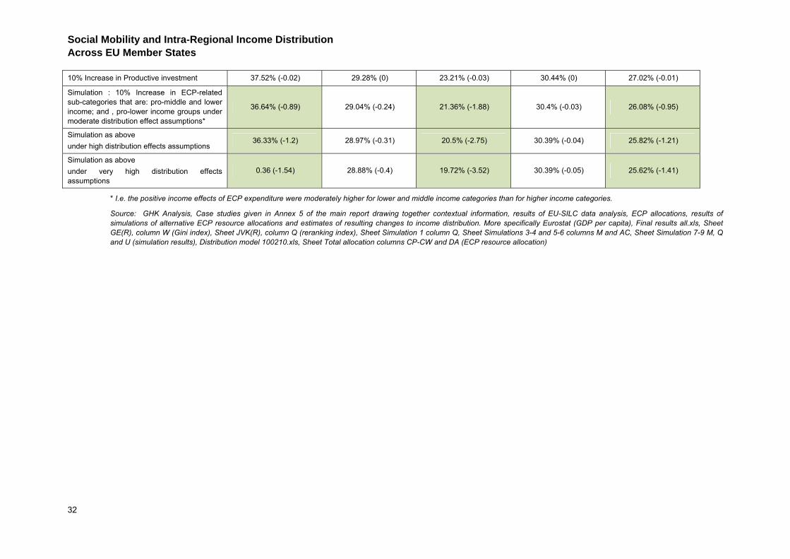
Social Mobility and Intra-Regional Income Distribution Across EU Member States
32
10% Increase in Productive investment 37.52% (-0.02) 29.28% (0) 23.21% (-0.03) 30.44% (0) 27.02% (-0.01)
Simulation : 10% Increase in ECP-related sub-categories that are: pro-middle and lower income; and , pro-lower income groups under moderate distribution effect assumptions*
36.64% (-0.89) 29.04% (-0.24) 21.36% (-1.88) 30.4% (-0.03) 26.08% (-0.95)
Simulation as above under high distribution effects assumptions
36.33% (-1.2) 28.97% (-0.31) 20.5% (-2.75) 30.39% (-0.04) 25.82% (-1.21)
Simulation as above under very high distribution effects assumptions
0.36 (-1.54) 28.88% (-0.4) 19.72% (-3.52) 30.39% (-0.05) 25.62% (-1.41)
* I.e. the positive income effects of ECP expenditure were moderately higher for lower and middle income categories than for higher income categories.
Source: GHK Analysis, Case studies given in Annex 5 of the main report drawing together contextual information, results of EU-SILC data analysis, ECP allocations, results of simulations of alternative ECP resource allocations and estimates of resulting changes to income distribution. More specifically Eurostat (GDP per capita), Final results all.xls, Sheet GE(R), column W (Gini index), Sheet JVK(R), column Q (reranking index), Sheet Simulation 1 column Q, Sheet Simulations 3-4 and 5-6 columns M and AC, Sheet Simulation 7-9 M, Q and U (simulation results), Distribution model 100210.xls, Sheet Total allocation columns CP-CW and DA (ECP resource allocation)
EXECUTIVE SUMMARY
33
Pointers for future policy
The bulk of inequality within EU Member States is accounted for by intra-regional income inequality rather that inter-regional income inequality. Thus ECP resource allocations at regional level may contribute to reducing inequality as well as regional economic growth that may lead to convergence between regions.
If ECP resources are to be used in this way, the appropriate starting point should be a clarification of the extent to which regional policy at the EU, national and regional levels aims either: to promote social mobility per se; to promote social mobility with a view to reducing income inequality through ‘pro poor growth’; or, to reduce intra regional income inequality.
ECP investment operates in concert with national public expenditure and represents a large proportion of public investment in some countries and regions. The effects of ECP investment on social mobility and income distribution depend also upon relevant national and regional policies affecting access to the outputs of ECP investment.
Promoting social mobility The policy area that is affected by ECP investment that is most likely to affect social mobility per se is education. Households with members that have achieved higher education and training levels tend to lead to further generations with similarly high levels. Higher education and training levels provide access to a wider set of employment opportunities and hence the potential for higher household income. Although ECP does not fund mainstream revenue costs of education there are a number of ways in which it may influence social mobility through changes in education and training. These include: the improvement of education infrastructure; measures to increase participation in education and training throughout the life-cycle, including action to achieve a reduction in early school leaving, and increased access to and quality of initial vocational and tertiary education and training; updating skills of training personnel with a view to innovation and a knowledge based economy; and, development of life-long learning systems and strategies in firms. Transport infrastructure may also contribute to social mobility where it improves access to education and employment opportunities to groups with hitherto low mobility. Complementary actions to address the problem of education and training being undervalued amongst some social groups are also relevant.
Promoting social mobility to reduce income inequality. The policy area within ECP that is most likely to affect social mobility and reduce intra regional income inequality is employment. The single most important factor influencing intra-generational income mobility is employment, both full time and part time. ECP has considerable scope to influence income mobility and in particular improve the incomes of those in lower income groups. The ways in which this can be achieved include through: implementing active and preventive labour market measures; creating pathways to the integration and re-entry into employment for disadvantaged people; combating discrimination in accessing and progressing in the labour market; increasing the sustainable participation and progress of women in employment to reduce gender-based segregation in the labour market (including childcare); and, actions to increase migrants’ participation in employment and thereby strengthen their social integration.
Promoting reductions in intra-regional inequality. The policy areas within ECP that are most likely to benefit poorer income groups and hence lead to reductions in intra regional inequality are environment, social inclusion and related public services. Non cash benefits, although difficult to measure, are often the potential effects of ECP interventions in these areas. The most relevant ECP investments include: the management of household and industrial waste, drinking water, water treatment, air quality, industrial sites and contaminated land, the prevention of environmental risks, housing and integrated projects for urban and rural regeneration. Other interventions are also potentially pro poor, such as
Social Mobility and Intra-Regional Income Distribution Across EU Member States
34
those in the energy field. However, the extent to which they actually contribute to reductions in intra regional inequality will strongly depend on the detailed policy design considerations.
In practice the weight of emphasis on one or other of the three priorities will be politically determined and needs to be set against issues affecting longer term structural changes within the regions concerned that can be progressed by ECP resources. A discussion of the relevance, emphasis and potential for achieving the three priorities could usefully form a component of both ex ante and ex post impact assessment of ECP interventions at the regional level. The simulation model developed as part of this assignment provides a tool that could assist in this process.
Recommendations for further work
There are several recommendations for further work to inform the key objectives of this assignment.
1. Measuring income inequality. For the purposes of enabling comprehensive comparisons via EU SILC data there would be merit in the regional identifier3 (at NUTS 1 or preferably NUTS 2 level) being included and data being made available for all EU countries. The application of uniform standards for confidentiality, data protection and quality of data in all national EU-SILC datasets would also help ensure the comparability of results.
2. Measuring benefits. None of the datasets contain information on the ‘benefits’ component of the preferred definition of income (ie ‘net of tax (household) income and benefits’). However, such benefits have a very substantial impact on citizens’ welfare; and estimates of income distribution may present a misleading picture when not accounting for such in-kind benefits. Such benefits can also be influenced by ECP expenditure. There would be merit in systematically measuring such public sector non-cash ‘benefits’ across the regions of the EU.
3. Measuring social mobility. The limited timescale and regional scope of the EU SILC panel data is a constraint on the exploration of social mobility. It is important that the EU SILC panel is maintained, that the availability of data should be extended to all EU regions and that the retrospective questions on social mobility last asked in 2005 are repeated.
4. Measuring the relationship between public expenditure and income mobility and income distribution. There would be merit in the continuing the monitoring of the relationships explored in this study and in particular the relationships between public expenditure on ECP categories, income mobility and ‘final’ income distribution. This would involve repeating the analysis annually using EU-SILC longitudinal data and refined and improved data on ECP related public expenditure at national and regional levels. There are several reasons for this. Firstly, there is scope for improving the data on relevant actual public expenditure. This assignment has used regional level expenditure data from just four countries, otherwise national level public expenditure data has been used in the regression of public supplies on income growth. The assignment has also relied on allocations of ECP expenditure (rather than actual expenditure) for the period 2007-2013. Secondly, the most comprehensive data source EU-SILC has allowed for the measuring of income change at the individual household level for only the three year period 2005-2007. This is a relatively short period of time and the results are influenced by short term fluctuations that may conceal important underlying trends. Thirdly, the key relationships may have changed since 2008, as a result of the credit and associated economic crisis. There has been a growth in unemployment and acceleration of restructuring and some income instability in the public sector. These changes may have increased the relative importance of public
3 A regional identifier indicates the region in which the household is located.
EXECUTIVE SUMMARY
35
supplies supported by the ECP. Finally, there are longer term societal trends that will impact upon the key relationships that have been illuminated by the quantitative analysis of short term income change undertaken. Key trends in the next few years include: the decline in the proportion of population of working age and concomitant increases in working life; and, reduced pressures on some infrastructure through reductions in economic growth and consumption, energy efficiency and life style changes.
5. Assessing the distributional consequences of ECP expenditure. There would be merit in undertaking more detailed analysis of the distributional effects of the types of interventions made within the ECP categories. This might involve case studies of examples of different types of ECP interventions including those in categories with explicit distributional objectives and other categories where the evidence on possible distributional effects is particularly weak. This might also usefully involve surveys and analyses that take account of the amount paid directly and indirectly by households in different income groups for public supplies supported by ECP (for example, health, education, waste management, drinking water, sewage treatment) and that identify the progressivity of these payments. Such surveys would need to identify the disposable income, amounts paid in earmarked and unearmarked taxes, insurance (where applicable) and out of pocket payments. These surveys could also help identify the non-cash benefits that accrue from ECP interventions to different income groups. Such work would be valuable because the progressivity (or otherwise) will depend upon policy and taxation arrangements that vary between countries and awareness of the progressivity effects would enable a better anticipation of the likely intra regional interpersonal distribution effects of ECP expenditure.
6. Regional case studies. It is evident both that changes within regions markedly affect inequality and that the scale and nature of social and income mobility varies markedly between different regions. The quantitative analysis undertaken in this assignment could be usefully complemented by studies that consider in more detail regions contrasting in social mobility and income inequality changes and trends and the particular regional level factors influencing this.
7. EU wide longitudinal survey study. Most ambitiously there would be merit in establishing a long term longitudinal household panel at the European level (along the lines of the ECHP that was discontinued in 2001) that could provide the basis for identifying trends in inter-generational social mobility and factors underlying these trends. A longitudinal survey at the European level should meet several requirements: a large and representative sample (sufficient for regional level analysis); repeated observations over a period of time to minimize measurement error problems that are common to the measurement of income (Jenkins and Siedler, 2007); an option to establish family links within the data; the availability of data on various variables (not only income), relevant to the inter-generational process, such as family wealth (financial and non-financial assets), employment, household composition, education, health, housing conditions etc. The longitudinal study should also follow people once they moved out of the original households. These characteristics would enable insights into key questions relevant to regional policy, such as: to what extent does intra-regional, inter-regional and transnational migration play a part in social mobility. The development of the internal market, the facilitation of transnational labour mobility and, through ECP policy, the support for cross border cooperation are factors that may encourage internal EU migration and that may reinforce forces that advantage the more developed and successful regions able to attract those that are upwardly mobile and hence constrain, in the short term at least, the achievement of the ECP convergence objective. The current EU-SILC uses a 4 year-rotating panel, therefore its use in any analysis of inter-generational mobility (and to some extent intra-generational mobility) is limited. There would also be merit in improving the provision and access to

Social Mobility and Intra-Regional Income Distribution Across EU Member States
36
national cohort panels and record register data which have been successfully used in Nordic countries.
1. INTRODUCTION
37
1 INTRODUCTION This Final Report is the final deliverable associated with contract reference Nº 2008CE160AT054/2008CE16CAT0172008 on social mobility and intra-regional income distribution across European Union (EU) Member States. It follows the submission and acceptance of the revised Inception and Interim Reports, the submission of the Draft Final Report and Revised Draft Final Report.
The report has been prepared by GHK on behalf of the Directorate General Regional Policy (DG REGIO). GHK was retained by DG REGIO following a call for tenders by open procedure. The contract entered into includes both the Tender Specifications and the proposal submitted by GHK. During the inception phase it was agreed to enhance the study team through the inclusion of Xavi Ramos and David Jesuit.
The work has been undertaken under the guidance of a Steering Group comprising officers of DG REGIO, Directorate General Employment, Social Affairs and Equal Opportunities (DG EMPL) and Directorate General Economic and Financial Affairs (DG ECFIN) and the three members of the Scientific Committee comprising: Valentino Dardanoni, Stephen Jenkins and Jacques Silber. This Final Report takes into account the written feedback from DG REGIO and members of the Scientific Committee on the Revised Draft Final Report.
1.1 Study Aims and objectives
The overall purpose of the study is to assess the current state of social mobility and income distribution across the EU at the national and regional levels. The study focuses on the extent to which social mobility (both short term income mobility and changes of social status between generations) affects income distribution.
More particularly, following the Tender Specifications the objectives of the study are:
To provide an economic analysis and literature review of: the relationships between (different types and measures of) social mobility and the potential for social mobility and (different types and measures of) income distribution; and, the determinants of social mobility. This should include: the identification of definitions and measures of social mobility; definitions and indexes of interpersonal income distribution; and the ranking of social mobility and its potential for affecting interpersonal income distribution.
To provide a quantitative analysis of the trends in social mobility and income distribution and the influence of different variables (determinants) on income distribution and social mobility across EU Member States and regions.
To identify, on the basis of the economic and quantitative analyses the implications for policy and policy instruments that could be used to enhance social mobility and potential social mobility.
The Tender Specifications (Ref Task 3.2.2) in particular stress the need to identify measures of social mobility that are functionally related to income distribution in some manner and hence could be used to predict changes in income distribution.
The Tender Specifications stressed that the study should cover, as far as is practical the whole of EU27, and NUTS2 regions, and ideally the time scale over which study findings and data are reviewed should allow for the consideration of inter-generational social mobility.
1.2 Regional policy, social mobility and income distribution
Article 158 of the EC Treaty establishes that in order to strengthen its economic and social cohesion, the Community aims to reduce disparities between levels of development of EU regions.
Social Mobility and Intra-Regional Income Distribution Across EU Member States
38
The European Union Cohesion Policy (ECP) for the period 2007-2013 has three objectives: the ‘Convergence objective’ that promotes growth-enhancing conditions and factors leading to convergence for the least-developed Member States and regions; the ‘Regional Competitiveness and Employment objective’ that aims to strengthen competitiveness and attractiveness, as well as employment elsewhere in the EU; and, the ‘European Territorial Co-operation objective’. The amount available under the ‘Convergence objective’ is EUR 282.8 billion. The allocation for the ‘Regional Competitiveness and Employment objective’ is EUR 55 billion.
Amongst the factors that may influence the ‘Convergence’ and ‘Regional Competitiveness and Employment’ objectives, and regional GDP per capita, are: interpersonal income distribution at regional level at a particular point in time; changes in the social status of individuals that can in turn affect their earnings potential; and, the changes in interpersonal income distribution over time (income dynamics).
Concerning social mobility, Galor and Tsiddon (1997) show that inter-generational mobility shapes economic growth through its effects on technological progress. In particular, intergenerational earnings mobility plays a role in mobilizing high-ability individuals into technologically advanced sectors in which growth-enhancing new technologies are developed (or adopted). In the same vein Hassler and Rodríguez Mora (2000) built a model with workers and entrepreneurs and showed that societies that exhibit larger inter-generational mobility consistently enjoy higher economic growth. They illustrated this with a hypothetical example: “Consider two ex-ante identical societies, Richland and Poorland. They have access to the same resources (both human and physical), but for historical reasons, they have different social structures. The entrepreneurial class of Poorland mainly consists of the children of previous entrepreneurs. From an intellectual point of view, they are a random sample of society’s entire population, and consequently, have average amounts of innate assets. Thus, they are not very innovative, and do not substantially change the world. Nevertheless, they confront economic challenges, and learn from these. They can explain to their children what actions were the best to take during their working life. This is sufficient to give the children of the entrepreneurs the upper hand – they will become the entrepreneurs of the next generation. Consequently, the intelligence of the entrepreneurial class of Poorland will remain on an average level. Poorlandians will have little or no growth for generations to come. In Richland, the situation is different; the entrepreneurs are the most intelligent individuals in society and they innovate and generate growth. They thus make the world change rapidly, and the information that they can pass on to their children thus depreciates so quickly that it is of no or little value. The next generation of entrepreneurs will thus be formed by the intellectually gifted and the people of Richland will enjoy consistent high growth.”
There are other relevant aspects and consequences of social mobility:
It has been taken as a good proxy for equality of opportunity.
It has an equalising effect, and thus may reduce the burden or concern for inequality overtime.
It and perceptions of it may shape preferences for redistribution policies. For example, the “prospect of upward mobility” (POUM) hypothesis suggests that not all currently poor people will support a policy that disproportionately taxes upper incomes because they may expect to move up in the income scale and therefore be hurt by such a policy.
Concerning income distribution the approach to the study assumes that the development, welfare and social progress of regions is primarily a reflection of income expressed as GDP per capita (or equivalent) and the interpersonal distribution of income at the national or regional level. Thus it is assumed that if current GDP per capita is the same in two regions, and income is more equally distributed in one region than the other, then ‘welfare’ is greater
1. INTRODUCTION
39
in the former than the latter. Thus social welfare is assumed to be a function of efficiency and equity and that there is some degree of aversion to inequality. GDP per capita has been the basis for EU regional policy resource allocation at regional level. Less attention has so far been given to interpersonal income distribution at regional level.
There is a theoretical basis for the close link between income inequality and social welfare. According to the theory of relative deprivation, individuals evaluate their level of social well-being not only in absolute terms (for example, total income available) but also in relative terms (how much they have relative to their peers). This can be expressed in terms of a social welfare function as was proposed by A. Sen in the nineteen seventies. Put another way, “an increase in mean income will lead to a higher level of social welfare, while an increase in inequality will reduce social welfare” (Wodon and Yitzhaki, 2002).
This assumption is strongly supported by the correlation between GDP and other factors that contribute to welfare and the strong association between inequality of income distribution and the incidence of a large number of social problems. Recent work using information on income distribution at the national level has demonstrated a strong correlation between income inequality and social problems reflected in for example, high teenage pregnancy rates, crime rates and the size of prison populations.
There is an ongoing debate over approaches to measuring social progress that has been brought to the fore by the advent of the threat of climate change and the credit crisis. Current work by the OECD summarises the main parameters of the debate. The work considers three areas: 1) economic aspects including: GDP, measures of income disparities, wealth created by unmeasured household production and the depletion of natural resources; 2) environmental aspects focusing on the role of sustainable development in social progress and economic performance; 3) social aspects focusing on identifying new metrics of quality of life and personal well-being (Stiglitz, 2009).
Other work including studies supported by DG REGIO has adopted the ‘capitals approach’ identifying the attributes of countries and regions in terms of their endowments of human, productive, natural and social ‘capitals’. The approach considers trade-offs between these capitals and the possibilities that certain thresholds could be reached below which development is no longer sustainable.
The relative merits of different approaches to measuring social welfare or social progress are subject to (often fierce) debate. This assignment acknowledges rather than contributes further to these debates. The purpose of this study has been to explore the occurrence and influences on income distribution and social mobility at regional and national levels.
The work is timely because the specific reference to the need to address social exclusion in the Treaty and because of the recent review of Region Policy (the Barca report) and the questions it raised over the extent to which regional policy should be focussed on the ‘social task’ bearing in mind the progress in reducing regional disparities but persistent problems related to income inequality including lack of social inclusion, poverty and risks of poverty. Indeed, the report comments on the relatively low levels of ECP resources earmarked to address these needs. This study has explored the consequences for income inequality of changing ECP resource allocations.
1.3 Method of approach
The work described in this Report is based on a review of relevant theoretical and empirical research in the economic and sociological traditions and quantitative analysis that has identified income distribution, social mobility and public supplies in EU Member States at the national and regional levels and the relationships between then. These relationships have been used to develop simulations to explore the possible consequences of changes in resource allocation within ECP on social mobility and income distribution. The simulations provide estimates of the effects of variations of expenditure on the main ECP categories: physical infrastructure; human resources; RT&D; and aids to productive investment and
Social Mobility and Intra-Regional Income Distribution Across EU Member States
40
expenditure categories that are likely to be ‘pro lower and middle income groups’ on quintile income groups within each region.
The method of approach has been influenced by both theoretical considerations and the practical constraints of data availability. A number of critical choices have also been made in developing the method of approach. The key aspects of the method of approach pertinent to each section of the report are outlined below.
1.3.1 Interpersonal income distribution
Measuring interpersonal income distribution at the regional level requires the definition of a measure of income; an appropriate indicator of income distribution; and, data from sufficiently large household surveys. The preferred measure of income adopted on the recommendation of the Steering Group is ‘net of tax (household) income and benefits’. That is income and in cash transfers and other benefits. It is acknowledged however that most available data do not include all ‘benefits’. The alternatives indicators of income distribution are reviewed in Section 2. Emphasis has been placed on indicators of equality/inequality because of the interest in social and income mobility within and between all income groups rather than indicators of poverty that focus on low income groups. As the study is concerned with the whole of the EU and with comparisons between regions it has been necessary to rely upon datasets that are comparable across the EU. The main datasets that have been used to measure interpersonal income distribution are as follows:
The European Union Statistics on Income and Living Conditions (EU-SILC): It covers 24 EU countries (plus IS and NO). There are no data for BG, RO and MT. CZ, ES, FI, FR CY, EE, LT, LU, LV provide data at NUTS2 level. There are no regional data for NL, PT and UK. The regional data for DE only includes 6 larger regions resulting from the aggregation of NUTS1 level-regions.
Luxembourg Income Study (LIS): It provides six waves of income data for up to 21 Member States: AT, BE, CZ, DE, DK, EE, ES, FI, FR, GR, HU, IE, IT, LU, NL, PL, RO, SE, SI, SK, UK (data are missing for: BG, CY, LT, LV, MT, PT); regional level analysis of income distribution is possible in some Member States. The dataset has been used to generate the Gini coefficient where possible for recent waves 5 and 6 (centred around 2000).
1.3.2 Social mobility
Social mobility concerns the changes in income or class of individuals over time. A distinction is made between inter-generational social mobility and intra-generational social mobility. The latter normally focuses on income mobility. Measuring social mobility requires: an appropriate indicator that includes a proxy for social status (class, occupation, income etc) and defined timescale; and, either ‘panel’ surveys within which the same individuals/households are surveyed on more than one occasion or (less reliable) surveys in which individuals/households are asked about previous social status. The emphasis in the study, stressed by the Steering Group, has been on measuring intra-generational income mobility. There are several reasons for this emphasis. Firstly, the timescales of ECP are relatively short and the policy options under consideration in terms of changes in ECP resource allocations are ‘tactical’ rather than ‘strategic’. Secondly, income provides a good proxy for social status. Thirdly, there is a direct link between income mobility and income distribution. Fourthly, there are no suitable data sets for comparing inter-generational social mobility at the regional level across the EU apart from the EU-SILC 2005 that relies on surveys in which individuals/households were asked about previous social status. The alternative indicators of social mobility are reviewed in Section 3.
The main datasets that have been used to measure intra-generational social (income) mobility in the EU and at regional level are as follows:
1. INTRODUCTION
41
EU-SILC: It provides longitudinal data for up to four years 2004, 2005, 2006 and 2007 for 21 EU countries. No longitudinal data are available for GR, IE, and DK. There are no data for BG, MT and RO. LU has data for 2003. The level of regional disaggregation available varied between countries. Considerable effort was required to clean the data to make it suitable for the longitudinal analysis.
The Cross-National Equivalent File 1980-2007 (CNEF): It provides good quality and harmonised longitudinal data but only for GB and DE national panels (DE-GSOEP; UK- BHPS) and regional data at NUTS1 level.
ECHP: It covers 15 EU countries for the period (1994-2001); it offers regional data, mostly at NUTS1 level (only PT, SE, UK have regional data at NUTS2); NUTS regions are grouped together for confidentiality reasons for DE, FI, IE.
The LIS is unsuitable for measuring social (income) mobility as it does not contain panel data. In practice only EU-SILC and CNEF were used in this assignment for measuring mobility.
There are few datasets providing comparable information across EU countries on inter- generational income mobility. The literature provides various estimates of inter-generational mobility for some EU countries. For example, estimates of inter-generational earnings elasticity are available for CZ, ES, DE, HU, IT, FI, FR, LV, PL, SE, SK and the UK. Estimates of inter-generational occupational mobility for 24 EU countries are provided by the European Commission 2007 Report on The Social Situation in the European Union based on the EU-SILC 2005 module. The EU-SILC 2005 module, that asked retrospective questions, has been used in this assignment to explore inter-generational social mobility at the regional level.
1.3.3 Income distribution and social mobility
Changes in income distribution amongst panels of households at the national and regional levels have been considered so that the relationships between income inequality and income mobility can be explored. The influence of individual, household and regional level contextual factors on changes in household income and hence income distribution has also been explored though regression analysis.
The individual factors considered include: the gender and age of the household head.
The household factors considered include: the number of adults and children in the household, the change in number of adults and children from 2005 to 2007; the number of persons with at least upper-secondary education in the household; as well as the change in full and in part-time employment over the period.
The regional contextual factors considered include: GDP per capita; business sector investment in RTD (BERD): the share of economically active population; unemployment rate; the regional density of motorways, other roads and railway lines; the proportion of students (ISCED levels 5-6) in the population; as well as the relative endowment of the region with hospital beds.
The data sources used to measure social mobility, particularly EU-SILC, are the most up to date and include information on each of the potential individual and household determinants. As DE was not included in the longitudinal dataset, data from the German Socio-Economic Panel (SOEP) has also been used (in the CNEF format, managed by Cornell University).
Data on the regional contextual factors, for CZ, DE, HU and PL, has been compiled from Eurostat’s NEWCRONOS database.
Social Mobility and Intra-Regional Income Distribution Across EU Member States
42
1.3.4 Income mobility and public supplies
The relationship between income mobility and public supplies has been explored to assess the potential of ECP expenditure to influence income mobility and hence income distribution. It is reasonable to assume that the ECP expenditure on public supplies has the potential to affect the income of individuals and households in four ways: through affecting access to employment in the short, medium or long term; through providing transfers ‘in kind’; through bringing about environmental goods, health benefits or changes in property values; and, through affecting the prices of commodities and public supplies (for example, energy, transport) that may disproportionately affect one income group more than another.
The potential relationships have been explored by: regressing income mobility and distribution against levels of actual public expenditure in general and in particular public expenditure equivalent to the ECP expenditure at the regional and national levels; reviewing relevant literature; and, developing reasoned arguments as to the likely distributional effects of different categories of ECP expenditure.
ECP expenditure is limited to particular categories of public expenditure. Some categories of public expenditure that have major effects on income distribution such as social protection transfers are not eligible ECP expenditure. The approach to estimating actual public expenditure equivalent to ECP expenditure has involved identifying national level expenditure in relevant Classifications of the Functions of Government (COFOG) categories for the most relevant periods. Use has also been made of data on public expenditure at the regional level that has been provided by TNO. These data are available for four countries (HU, CZ, DE and PL) for which EU-SILC data on income change 2005-2007 at the regional level are also available. The approach to estimating national and regional ECP equivalent public expenditure is elaborated in Annex 5.
1.3.5 Policy analysis
The focus of the policy analysis was on exploring the consequences of alternative allocations of ECP resources on social mobility and income distribution. Information on actual ECP resource allocations for the period 2007-2013 from DG REGIO has been used.
Nine broad simulations have been considered:
X% pro rata increase in ECP expenditure
X% pro rata decrease in ECP expenditure (the results are the inverse of the former simulation)
X% increase in ECP categories relating to physical infrastructure, and corresponding decreases in all other categories.
X% increase in ECP categories relating to human resources infrastructure, and corresponding decreases in all other categories.
X% increase in ECP categories relating to research and technological development (R&TD), and corresponding decreases in all other categories.
X% increase in ECP categories relating to aids to productive sector and corresponding decreases in all other categories.
X% increase in allocations to categories that are pro lower and middle income groups and corresponding decreases in all other categories, assuming moderate effects.
X% increase in allocations to categories that are pro lower and middle income groups and corresponding decreases in all other categories, assuming high distribution effects.
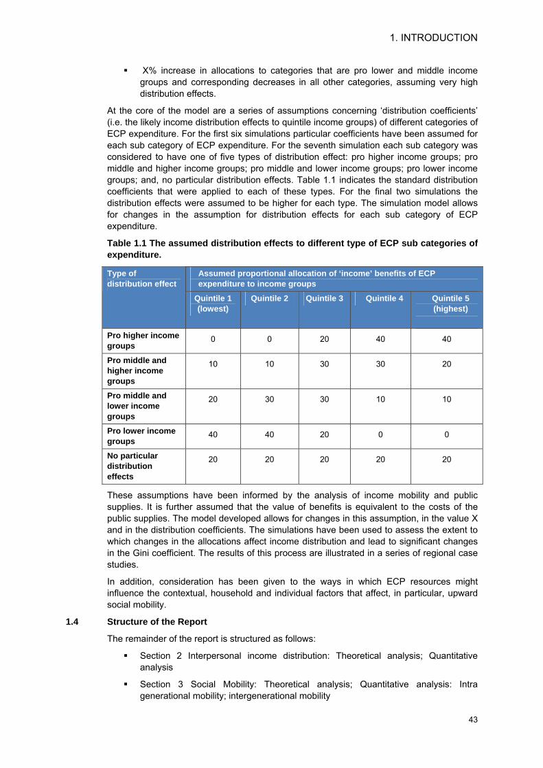
1. INTRODUCTION
43
X% increase in allocations to categories that are pro lower and middle income groups and corresponding decreases in all other categories, assuming very high distribution effects.
At the core of the model are a series of assumptions concerning ‘distribution coefficients’ (i.e. the likely income distribution effects to quintile income groups) of different categories of ECP expenditure. For the first six simulations particular coefficients have been assumed for each sub category of ECP expenditure. For the seventh simulation each sub category was considered to have one of five types of distribution effect: pro higher income groups; pro middle and higher income groups; pro middle and lower income groups; pro lower income groups; and, no particular distribution effects. Table 1.1 indicates the standard distribution coefficients that were applied to each of these types. For the final two simulations the distribution effects were assumed to be higher for each type. The simulation model allows for changes in the assumption for distribution effects for each sub category of ECP expenditure.
Table 1.1 The assumed distribution effects to different type of ECP sub categories of expenditure.
Assumed proportional allocation of ‘income’ benefits of ECP expenditure to income groups
Type of distribution effect
Quintile 1 (lowest)
Quintile 2 Quintile 3 Quintile 4 Quintile 5 (highest)
Pro higher income groups
0 0 20 40 40
Pro middle and higher income groups
10 10 30 30 20
Pro middle and lower income groups
20 30 30 10 10
Pro lower income groups
40 40 20 0 0
No particular distribution effects
20 20 20 20 20
These assumptions have been informed by the analysis of income mobility and public supplies. It is further assumed that the value of benefits is equivalent to the costs of the public supplies. The model developed allows for changes in this assumption, in the value X and in the distribution coefficients. The simulations have been used to assess the extent to which changes in the allocations affect income distribution and lead to significant changes in the Gini coefficient. The results of this process are illustrated in a series of regional case studies.
In addition, consideration has been given to the ways in which ECP resources might influence the contextual, household and individual factors that affect, in particular, upward social mobility.
1.4 Structure of the Report
The remainder of the report is structured as follows:
Section 2 Interpersonal income distribution: Theoretical analysis; Quantitative analysis
Section 3 Social Mobility: Theoretical analysis; Quantitative analysis: Intra generational mobility; intergenerational mobility
Social Mobility and Intra-Regional Income Distribution Across EU Member States
44
Section 4 Income distribution and social mobility: Theoretical analysis: Quantitative analysis
Section 5 Income mobility and public supplies: Theoretical analysis: Quantitative analysis
Section 6 Pointers for future policy
The basis for the structure of the report can be supported by a series of linked equations. In Section 2 the Gini coefficient (“single-parameter” or S-Gini) is selected as the preferred measure of income distribution. In Section 3 the mobility index chosen is derived from the Jenkins and Van Kerm equation relating income distribution and mobility as follows:
G1- G0= R-P (1) where G is the Gini coefficient (S-Gini), the subscript denotes the time period (0 denoting the base year and 1 the final year), R stands for the “reranking” component of the Jenkins-Van Kerm equation (which is a measure of income mobility), and P stands for “progressivity” of income growth (which is a measure representing the extent to which income growth was ‘pro-poor’ in the time period covered, i.e. was the income growth in poorer households relatively higher than in richer ones). From (1) it is possible to calculate the index of mobility R as the difference between two Gini indexes and the progressivity of income growth, P, that is:
R= G1-G0+P (2) From equation (1) the following can also be derived:
G1= G0+R-P (3) Equation (3) is an expression of income dynamics where the income distribution at time 1 (G1) is a function of the income distribution at time 0 (G0), the income mobility (R), and the pro-poor dimension of income growth (P). EU-SILC data for 2005-2007 have been used to assess mobility (i.e. the extent of “reranking” following Jenkins and Van Kerm as well as other indices for comparison) and income change for the countries and regions where this is possible and the results are given in Section 4.
Factors influencing income mobility have been assessed using a regression equation such as that shown as (4), separating between individual, household and regional-level characteristics (notably public supplies).
∆Yi,r=β1 Xi1+ β2Xh
2+ β3Xr3+ε (4)
Where Y stands for equivalised4 disposable household income, and the superscript i for individual with i=1,…..,I (being the unit of analysis) where i is the representative household individual (class) characterised by a specific level of income living within region r. Superscript h stands for household h=1, .., H to which the individual belongs. The individual and household level determinants shown as X1 and X2 are considered in Section 3 and the public supply endowments noted as X3, are considered in Section 5. This regression allows the identification of the individual income changes due to alternative levels and compositions of public supply. The vector Xr
3 includes calculated per capita expenditures in the region on physical infrastructure, human resources, RTD and aids to productive investment - in order to correspond with ECP expenditure categories.
By simulating ECP expenditure levels and structures different from the actual ones, it should be possible, on the basis of the regression model, to simulate the effects on household incomes over the corresponding time period. Revising the actual income differences (∆Yi,r) with new, counterfactual estimated differences (using the regression coefficients of public supplies) provide a set of new counterfactual household incomes, from
4 Revised OQCD equivalence scale
1. INTRODUCTION
45
which Gini indices can be calculated for the final year. These Gini scores may differ from the actual ones. In practice, due to the limitations of the data available, the regression model has not generated sufficiently clear and detailed findings to inform the simulations. Instead account has been taken of other studies and reasoned arguments have been developed in Section 5 to underpin the assumptions applied in the simulations.
The report is supported by the following annexes
Annex 1 Income inequality at national and regional levels
Annex 2 Classifications used in the study of inter-generational social mobility
Annex 3 Explanation of the regression analysis
Annex 4 Estimating ECP related public expenditure at national regional level
Annex 5 Regional case studies showing the results of the simulations
Annex 6 Maps illustrating the results of the quantitative analysis (prepared by DG REGIO on the basis of data provided by GHK)
In addition two Excel files have been submitted as the basis for the database required in the contract. The first includes:
Estimates of income distribution at national and regional level based on EU SILC 2005.
Estimates of intra generational income mobility and income dynamics at national and regional level based on EU SILC 2005-2007.
The national and regional level findings on inter generational social mobility
The results of the regression: Individual and household factors; and public expenditure at national and regional level in four countries (CZ, DE, HU and PL);
A second regression separately for the CZ, DE, HU and PL, which includes a set of regional contextual variables;
Correlations between intra generational income mobility and various contextual factors.
The effects of selected simulations of ECP resource allocations on income distribution and in particular the Gini coefficient at national and regional levels.
The second Excel file provides the model for estimating the income distribution effects that accrue from alternative ECP resource
The report structure is illustrated diagrammatically in Figure 1.1
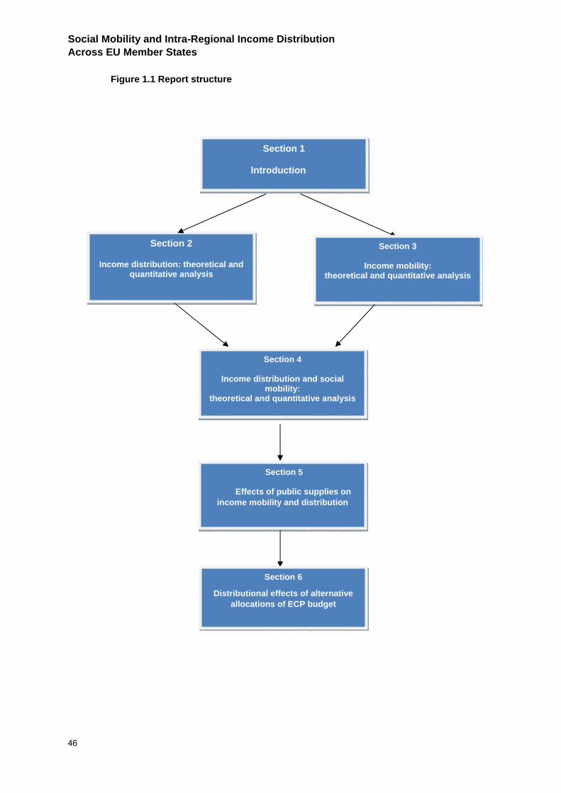
Social Mobility and Intra-Regional Income Distribution Across EU Member States
46
Figure 1.1 Report structure
Section 1
Introduction
Section 2
Income distribution: theoretical and quantitative analysis
Section 3
Income mobility: theoretical and quantitative analysis
Section 4
Income distribution and social mobility:
theoretical and quantitative analysis
Section 5
Effects of public supplies on income mobility and distribution
Section 6
Distributional effects of alternative allocations of ECP budget
2. INTERPERSONAL INCOME DISTRIBUTION
47
2 INTERPERSONAL INCOME DISTRIBUTION 2.1 Introduction
This section of the report reviews the concept, definitions and approaches to measuring interpersonal income distribution and equality. It identifies the preferred indicator for the purposes of this study. Evidence on the characteristics of and factors affecting income distribution in the EU are then reviewed.
2.2 Theoretical analysis
2.2.1 Definitions and indexes of income distribution
Income distribution reflects the nature and extent of inequalities in the income of individuals or households in a given society or subgroups within society. The concept may also be applied to geographical units.
Absolute and relative poverty
Measurements of income distribution include poverty measures, either identified as absolute or relative poverty. Absolute poverty measures the number of people living below a certain income threshold or the number of households unable to afford certain basic goods. Relative poverty, which is related to the concept of income inequality, measures the extent to which a household’s financial resources fall below an average level of income threshold for that economy (for example, the proportion of households below 40% of the median household income). If everyone's real income in an economy increases, but the income distribution stays the same, then the rate of relative poverty will also stay the same. The emphasis in this assignment is on measures of inequality rather than poverty.
Income distribution and inequality
There are many ways to characterise income distribution and inequality – either graphically or using various aggregate measures (Jenkins and Van Kerm, 2009). The first category includes:
histograms, presenting the frequency of individuals belonging to separate income strata;
cumulative frequency distributions, where the frequency of individuals not surpassing a certain income level is presented; and, as a specific subset of cumulative frequency distributions; and
the Lorenz curve, which shows for each proportion of individuals with the lowest income in society the share of total income in society they enjoy.
Aggregate measures such as the Gini coefficient and the Atkinson family of inequality measures summarise income inequality in society in a single number. Many different measures have been developed by social scientists.
Prior to measurement
Before using an index to measure income inequality, several issues have to be considered regarding the income variable, the time period, and the demographic unit.
Variable of interest: A distinction can be made between income inequality at three levels:
Inequality of earnings among employed individuals. This produces analyses of earnings inequality, pay inequality, or wage inequality.
Inequality of earnings and investment income among households. This may be termed pretax-pretransfer income inequality or market income inequality.
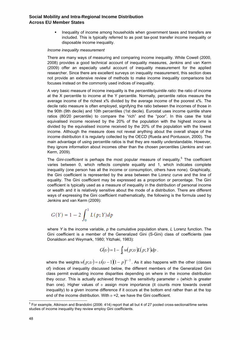
Social Mobility and Intra-Regional Income Distribution Across EU Member States
48
Inequality of income among households when government taxes and transfers are included. This is typically referred to as post tax-post transfer income inequality or disposable income inequality.
Income inequality measurement
There are many ways of measuring and comparing income inequality. While Cowell (2000, 2008) provides a good technical account of inequality measures, Jenkins and van Kerm (2009) offer an especially useful account of inequality measurement for the applied researcher. Since there are excellent surveys on inequality measurement, this section does not provide an extensive review of methods to make income inequality comparisons but focuses instead on the commonly used indices of inequality.
A very basic measure of income inequality is the percentile/quintile ratio: the ratio of income at the X percentile to income at the Y percentile. Normally, percentile ratios measure the average income of the richest x% divided by the average income of the poorest x%. The decile ratio measure is often employed, signifying the ratio between the incomes of those in the 90th (9th decile) and 10th percentiles (1st decile). Eurostat uses income quintile share ratios (80/20 percentile) to compare the “rich” and the “poor”. In this case the total equivalised income received by the 20% of the population with the highest income is divided by the equivalised income received by the 20% of the population with the lowest income. Although the measure does not reveal anything about the overall shape of the income distribution it is regularly collected by the OECD (Rueda and Pontusson, 2000). The main advantage of using percentile ratios is that they are readily understandable. However, they ignore information about incomes other than the chosen percentiles (Jenkins and van Kerm, 2009).
The Gini-coefficient is perhaps the most popular measure of inequality.5 The coefficient varies between 0, which reflects complete equality and 1, which indicates complete inequality (one person has all the income or consumption, others have none). Graphically, the Gini coefficient is represented by the area between the Lorenz curve and the line of equality. The Gini coefficient may be expressed as a proportion or percentage. The Gini coefficient is typically used as a measure of inequality in the distribution of personal income or wealth and it is relatively sensitive about the mode of a distribution. There are different ways of expressing the Gini coefficient mathematically, the following is the formula used by Jenkins and van Kerm (2009):
where Y is the income variable, p the cumulative population share, L Lorenz function. The Gini coefficient is a member of the Generalized Gini (S-Gini) class of coefficients (see Donaldson and Weymark, 1980; Yitzhaki, 1983):
( ) ( ) ( )dpYpLpwG ;;11
0∫−= υυ .
where the weights ( ) ( )( ) 211; −−−= υυυυ ppw . As it also happens with the other (classes of) indices of inequality discussed below, the different members of the Generalized Gini class permit evaluating income disparities depending on where in the income distribution they occur. This is actually achieved through the sensitivity parameter υ (which is greater than one). Higher values of υ assign more importance (it counts more towards overall inequality) to a given income difference if it occurs at the bottom end rather than at the top end of the income distribution. With υ =2, we have the Gini coefficient.
5 For example, Atkinson and Brandolini (2006: 414) report that all but 4 of 27 pooled cross-sectional/time series studies of income inequality they review employ Gini coefficients.
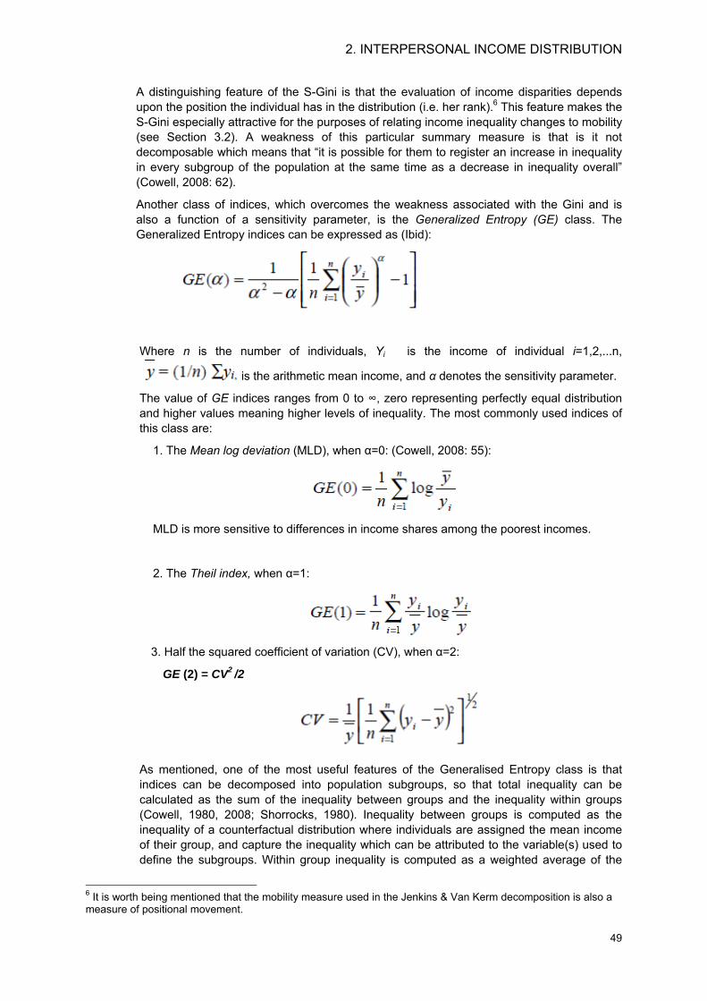
2. INTERPERSONAL INCOME DISTRIBUTION
49
A distinguishing feature of the S-Gini is that the evaluation of income disparities depends upon the position the individual has in the distribution (i.e. her rank).6 This feature makes the S-Gini especially attractive for the purposes of relating income inequality changes to mobility (see Section 3.2). A weakness of this particular summary measure is that is it not decomposable which means that “it is possible for them to register an increase in inequality in every subgroup of the population at the same time as a decrease in inequality overall” (Cowell, 2008: 62).
Another class of indices, which overcomes the weakness associated with the Gini and is also a function of a sensitivity parameter, is the Generalized Entropy (GE) class. The Generalized Entropy indices can be expressed as (Ibid):
Where n is the number of individuals, Yi is the income of individual i=1,2,...n,
is the arithmetic mean income, and α denotes the sensitivity parameter.
The value of GE indices ranges from 0 to ∞, zero representing perfectly equal distribution and higher values meaning higher levels of inequality. The most commonly used indices of this class are:
1. The Mean log deviation (MLD), when α=0: (Cowell, 2008: 55):
MLD is more sensitive to differences in income shares among the poorest incomes.
2. The Theil index, when α=1:
3. Half the squared coefficient of variation (CV), when α=2:
GE (2) = CV2 /2
As mentioned, one of the most useful features of the Generalised Entropy class is that indices can be decomposed into population subgroups, so that total inequality can be calculated as the sum of the inequality between groups and the inequality within groups (Cowell, 1980, 2008; Shorrocks, 1980). Inequality between groups is computed as the inequality of a counterfactual distribution where individuals are assigned the mean income of their group, and capture the inequality which can be attributed to the variable(s) used to define the subgroups. Within group inequality is computed as a weighted average of the
6 It is worth being mentioned that the mobility measure used in the Jenkins & Van Kerm decomposition is also a measure of positional movement.
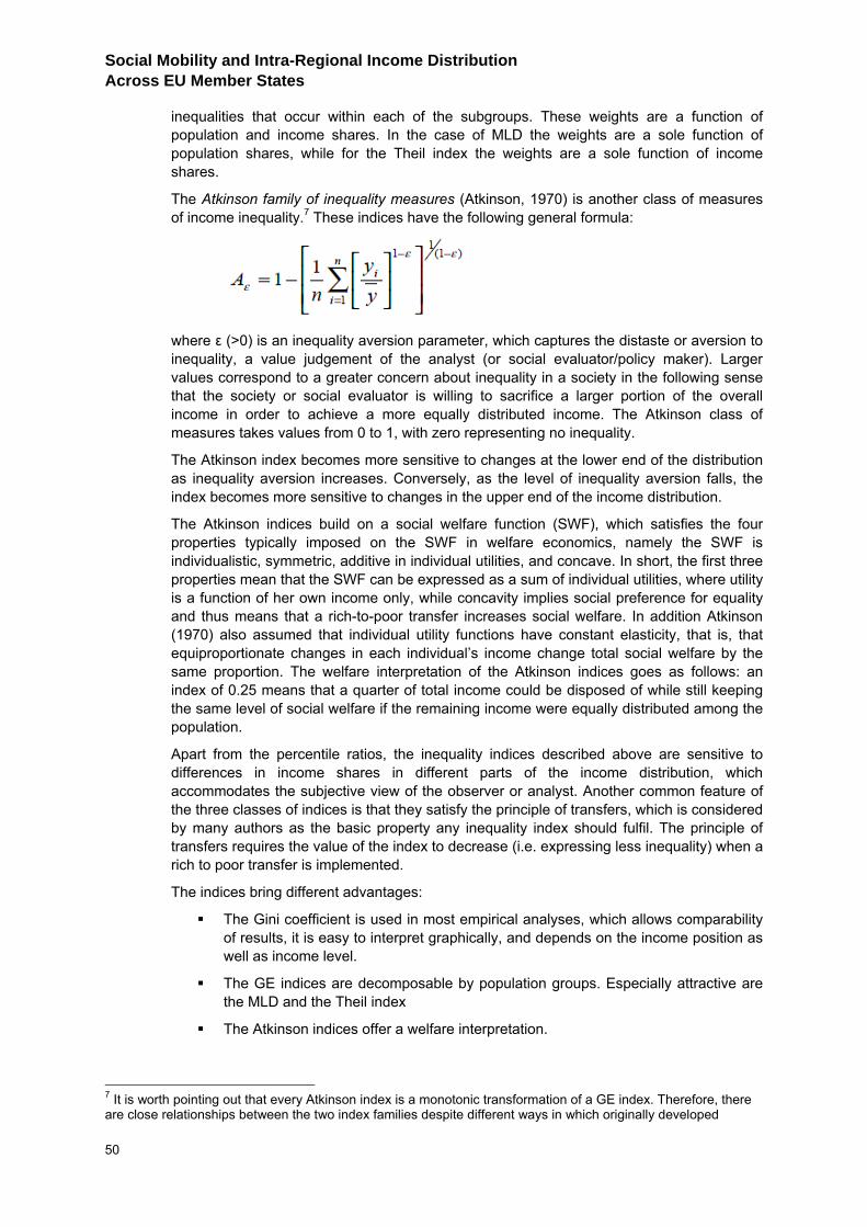
Social Mobility and Intra-Regional Income Distribution Across EU Member States
50
inequalities that occur within each of the subgroups. These weights are a function of population and income shares. In the case of MLD the weights are a sole function of population shares, while for the Theil index the weights are a sole function of income shares.
The Atkinson family of inequality measures (Atkinson, 1970) is another class of measures of income inequality.7 These indices have the following general formula:
where ε (>0) is an inequality aversion parameter, which captures the distaste or aversion to inequality, a value judgement of the analyst (or social evaluator/policy maker). Larger values correspond to a greater concern about inequality in a society in the following sense that the society or social evaluator is willing to sacrifice a larger portion of the overall income in order to achieve a more equally distributed income. The Atkinson class of measures takes values from 0 to 1, with zero representing no inequality.
The Atkinson index becomes more sensitive to changes at the lower end of the distribution as inequality aversion increases. Conversely, as the level of inequality aversion falls, the index becomes more sensitive to changes in the upper end of the income distribution.
The Atkinson indices build on a social welfare function (SWF), which satisfies the four properties typically imposed on the SWF in welfare economics, namely the SWF is individualistic, symmetric, additive in individual utilities, and concave. In short, the first three properties mean that the SWF can be expressed as a sum of individual utilities, where utility is a function of her own income only, while concavity implies social preference for equality and thus means that a rich-to-poor transfer increases social welfare. In addition Atkinson (1970) also assumed that individual utility functions have constant elasticity, that is, that equiproportionate changes in each individual’s income change total social welfare by the same proportion. The welfare interpretation of the Atkinson indices goes as follows: an index of 0.25 means that a quarter of total income could be disposed of while still keeping the same level of social welfare if the remaining income were equally distributed among the population.
Apart from the percentile ratios, the inequality indices described above are sensitive to differences in income shares in different parts of the income distribution, which accommodates the subjective view of the observer or analyst. Another common feature of the three classes of indices is that they satisfy the principle of transfers, which is considered by many authors as the basic property any inequality index should fulfil. The principle of transfers requires the value of the index to decrease (i.e. expressing less inequality) when a rich to poor transfer is implemented.
The indices bring different advantages:
The Gini coefficient is used in most empirical analyses, which allows comparability of results, it is easy to interpret graphically, and depends on the income position as well as income level.
The GE indices are decomposable by population groups. Especially attractive are the MLD and the Theil index
The Atkinson indices offer a welfare interpretation.
7 It is worth pointing out that every Atkinson index is a monotonic transformation of a GE index. Therefore, there are close relationships between the two index families despite different ways in which originally developed
2. INTERPERSONAL INCOME DISTRIBUTION
51
2.2.2 The assessment of alternative measures of interpersonal income distribution
There is no single "best" measure of income inequality. The choice of which to use depends on the focus of the analysis and on data availability. For example, some indices are more sensitive to income differences at the bottom of the distribution and others more sensitive to differences in income shares in the upper end of the distribution. According to Firebaugh (2006), the core properties that an “optimal” measure of inequality should have include:
scale-invariance: the inequality measure should not be affected when income is increased or reduced by the same rate for everyone or when income levels are measured in different units or currencies;
additive decomposability: the inequality measure for a society should be the weighted average of inequality measures of the different subgroups of that society, given that these subgroups are mutually exclusive and together they sum up to the total population. Examples for subgroups may include geographical units (for example, sub regions) or age cohorts (weights being the total population in such subgroups);
transfer principle: in its weak form, this principle says that the inequality measure should at least not increase (show greater inequality) if a certain amount of income is redistributed from an individual with higher income to one with lower income. In its stronger form, it says that the measure should decrease in such cases and increase if redistribution is taking place from a poorer individual towards a richer one.
Only the Theil index and MLD fulfil all three criteria. They also respect the principle of welfare (that is, the principle of diminishing returns): a certain amount of money (say, 100 euro) will mean less for a more affluent person than for someone with lower income. Thus a redistribution of funds at higher income levels will be less significant in resetting the value of the measure that a corresponding redistribution at lower levels would be. The Gini coefficient is scale-invariant and obeys the transfer principle, but it is not additively decomposable by population sub groups although the Generalized Gini can be decomposed into mobility and pro-poor growth. The Gini coefficient does not respect well the welfare principle.
The Tender Specifications required that the quantitative analysis included the following four exercises:
a) Studies leading to the identification of factors determining individual social status across EU Member States;
b) Studies of the evolution through time of income distributions, social mobility and of its determinants across EU Member States;
c) Assessing the relative weight of the said determinants in terms of social mobility across EU Member States;
d) Ranking income distributions using an index aiming at assessing income distributions also in terms of their potential for social mobility (by duly taking into account social mobility determinants).
Given these requirements, the alternative measures of interpersonal income distribution have been assessed against the following criteria:
Decomposability: In order to unravel the factors determining individual social status and their effect on social mobility and income distribution, either regression analysis or decomposition analysis could be applied. Thus, whether the index is decomposable by population subgroups is relevant.
Linkage to inequality: whether the index can be linked to income inequality in a simple and feasible manner.

Social Mobility and Intra-Regional Income Distribution Across EU Member States
52
(The two points (b) and (d) do not give rise to any criteria. All indices can be used to analyse trends over time).
The weaknesses and strengths including considerations of ease of understanding.
Practicality: What data (and survey methods) are required to inform the indicator?
Feasibility: Bearing in mind the current and prospective availability of data at the NUTS 2 level, what steps would need to be taken to realise the application of the indicator.
An overall assessment is also provided. Table 2.1 summaries the assessment of the indicators of income distribution and income inequality.
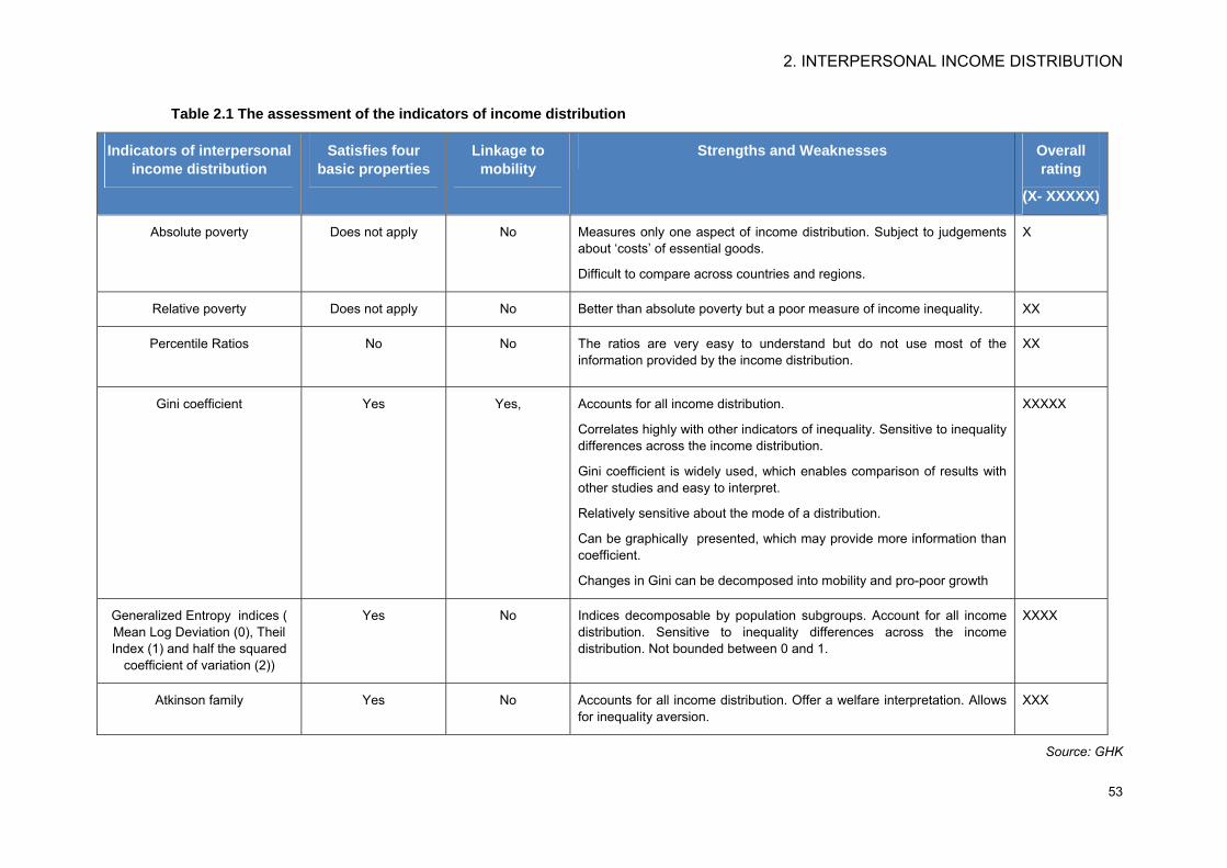
2. INTERPERSONAL INCOME DISTRIBUTION
53
Table 2.1 The assessment of the indicators of income distribution
Indicators of interpersonal income distribution
Satisfies four basic properties
Linkage to mobility
Strengths and Weaknesses Overall rating
(X- XXXXX)
Absolute poverty Does not apply No Measures only one aspect of income distribution. Subject to judgements about ‘costs’ of essential goods.
Difficult to compare across countries and regions.
X
Relative poverty Does not apply No Better than absolute poverty but a poor measure of income inequality. XX
Percentile Ratios
No No The ratios are very easy to understand but do not use most of the information provided by the income distribution.
XX
Gini coefficient Yes Yes, Accounts for all income distribution.
Correlates highly with other indicators of inequality. Sensitive to inequality differences across the income distribution.
Gini coefficient is widely used, which enables comparison of results with other studies and easy to interpret.
Relatively sensitive about the mode of a distribution.
Can be graphically presented, which may provide more information than coefficient.
Changes in Gini can be decomposed into mobility and pro-poor growth
XXXXX
Generalized Entropy indices ( Mean Log Deviation (0), Theil Index (1) and half the squared
coefficient of variation (2))
Yes No Indices decomposable by population subgroups. Account for all income distribution. Sensitive to inequality differences across the income distribution. Not bounded between 0 and 1.
XXXX
Atkinson family Yes No Accounts for all income distribution. Offer a welfare interpretation. Allows for inequality aversion.
XXX
Source: GHK
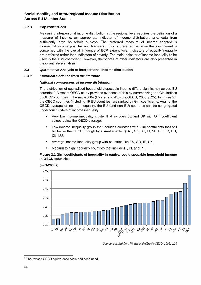
Social Mobility and Intra-Regional Income Distribution Across EU Member States
54
2.2.3 Key conclusions
Measuring interpersonal income distribution at the regional level requires the definition of a measure of income; an appropriate indicator of income distribution; and, data from sufficiently large household surveys. The preferred measure of income adopted is ‘household income post tax and transfers’. This is preferred because the assignment is concerned with the overall influence of ECP expenditure. Indicators of equality/inequality are preferred rather than indicators of poverty. The main indicator of income inequality to be used is the Gini coefficient. However, the scores of other indicators are also presented in the quantitative analysis.
2.3 Quantitative Analysis of interpersonal income distribution
2.3.1 Empirical evidence from the literature
National comparisons of income distribution
The distribution of equivalised household disposable income differs significantly across EU countries.8 A recent OECD study provides evidence of this by summarizing the Gini indices of OECD countries in the mid-2000s (Förster and d’Ercole/OECD, 2008, p.25). In Figure 2.1 the OECD countries (including 19 EU countries) are ranked by Gini coefficients. Against the OECD average of income inequality, the EU (and non-EU) countries can be congregated under four clusters of income inequality:
Very low income inequality cluster that includes SE and DK with Gini coefficient values below the OECD average.
Low income inequality group that includes countries with Gini coefficients that still fall below the OECD (though by a smaller extent): AT, CZ, SK, FI, NL, BE, FR, HU, DE, LU.
Average income inequality group with countries like ES, GR, IE, UK.
Medium to high inequality countries that include IT, PL and PT.
Figure 2.1 Gini coefficients of inequality in equivalised disposable household income in OECD countries
(mid-2000s)
Source: adapted from Förster and d’Ercole/OECD, 2008, p.25
8 The revised OECD equivalence scale had been used.
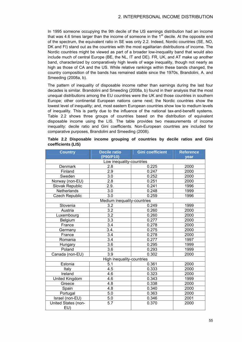
2. INTERPERSONAL INCOME DISTRIBUTION
55
In 1995 someone occupying the 9th decile of the US earnings distribution had an income that was 4.6 times larger than the income of someone in the 1st decile. At the opposite end of the spectrum, the equivalent ratio in SE was only 2.2. Indeed, Nordic countries (SE, NO, DK and FI) stand out as the countries with the most egalitarian distributions of income. The Nordic countries might be viewed as part of a broader low-inequality band that would also include much of central Europe (BE, the NL, IT and DE). FR, UK, and AT make up another band, characterized by comparatively high levels of wage inequality, though not nearly as high as those of CA and the US. While relative rankings within these bands changed, the country composition of the bands has remained stable since the 1970s, Brandolini, A. and Smeeding (2008a, b).
The pattern of inequality of disposable income rather than earnings during the last four decades is similar. Brandolini and Smeeding (2008a, b) found in their analysis that the most unequal distributions among the EU countries were the UK and those countries in southern Europe; other continental European nations came next; the Nordic countries show the lowest level of inequality; and, most eastern European countries show low to medium levels of inequality. This is partly due to the influence of the national tax-and-benefit systems. Table 2.2 shows three groups of countries based on the distribution of equivalent disposable income using the LIS. The table provides two measurements of income inequality: decile ratio and Gini coefficients. Non-European countries are included for comparative purposes, Brandolini and Smeeding (2008).
Table 2.2 Disposable income grouping of countries by decile ratios and Gini coefficients (LIS)
Country Decile ratio (P90/P10)
Gini coefficient Reference year
Low inequality-countries Denmark 2.8 0.225 2000 Finland 2.9 0.247 2000 Sweden 3.0 0.252 2000
Norway (non-EU) 2.8 0.251 2000 Slovak Republic 2.9. 0.241 1996
Netherlands 3.0 0.248 1999 Czech Republic 3.0 0.259 1996
Medium inequality-countries Slovenia 3.2 0.249 1999 Austria 3.2 0.260 2000
Luxembourg 3.2 0.260 2000 Belgium 3.3 0.277 2000 France 3.4 0.278 2000
Germany 3.4. 0.275 2000 France 3.4 0.278 2000
Romania 3.4 0.277 1997 Hungary 3.6 0.295 1999 Poland 3.6 0.293 1999
Canada (non-EU) 3.9 0.302 2000 High inequality-countries
Estonia 5.1 0.361 2000 Italy 4.5 0.333 2000
Ireland 4.6 0.323 2000 United Kingdom 4.6 0.343 1999
Greece 4.8 0.338 2000 Spain 4.8 0.340 2000
Portugal 5.0 0.363 2000 Israel (non-EU) 5.0 0.346 2001
United States (non- EU)
5.7 0.370 2000
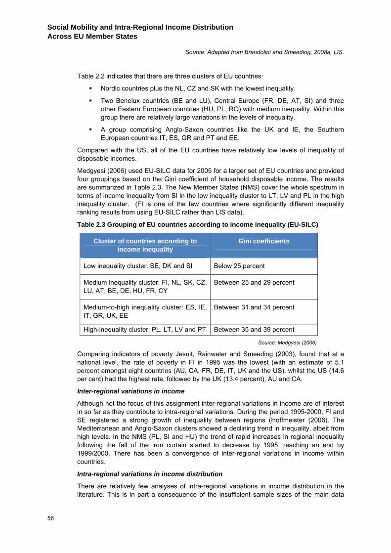
Social Mobility and Intra-Regional Income Distribution Across EU Member States
56
Source: Adapted from Brandolini and Smeeding, 2008a, LIS.
Table 2.2 indicates that there are three clusters of EU countries:
Nordic countries plus the NL, CZ and SK with the lowest inequality.
Two Benelux countries (BE and LU), Central Europe (FR, DE, AT, SI) and three other Eastern European countries (HU, PL, RO) with medium inequality. Within this group there are relatively large variations in the levels of inequality.
A group comprising Anglo-Saxon countries like the UK and IE, the Southern European countries IT, ES, GR and PT and EE.
Compared with the US, all of the EU countries have relatively low levels of inequality of disposable incomes.
Medgyesi (2006) used EU-SILC data for 2005 for a larger set of EU countries and provided four groupings based on the Gini coefficient of household disposable income. The results are summarized in Table 2.3. The New Member States (NMS) cover the whole spectrum in terms of income inequality from SI in the low inequality cluster to LT, LV and PL in the high inequality cluster. (FI is one of the few countries where significantly different inequality ranking results from using EU-SILC rather than LIS data).
Table 2.3 Grouping of EU countries according to income inequality (EU-SILC)
Cluster of countries according to income inequality
Gini coefficients
Low inequality cluster: SE, DK and SI Below 25 percent
Medium inequality cluster: FI, NL, SK, CZ, LU, AT, BE, DE, HU, FR, CY
Between 25 and 29 percent
Medium-to-high inequality cluster: ES, IE, IT, GR, UK, EE
Between 31 and 34 percent
High-inequality cluster: PL. LT, LV and PT Between 35 and 39 percent
Source: Medgyesi (2006)
Comparing indicators of poverty Jesuit, Rainwater and Smeeding (2003), found that at a national level, the rate of poverty in FI in 1995 was the lowest (with an estimate of 5.1 percent amongst eight countries (AU, CA, FR, DE, IT, UK and the US), whilst the US (14.6 per cent) had the highest rate, followed by the UK (13.4 percent), AU and CA.
Inter-regional variations in income
Although not the focus of this assignment inter-regional variations in income are of interest in so far as they contribute to intra-regional variations. During the period 1995-2000, FI and SE registered a strong growth of inequality between regions (Hoffmeister (2006). The Mediterranean and Anglo-Saxon clusters showed a declining trend in inequality, albeit from high levels. In the NMS (PL, SI and HU) the trend of rapid increases in regional inequality following the fall of the iron curtain started to decrease by 1995, reaching an end by 1999/2000. There has been a convergence of inter-regional variations in income within countries.
Intra-regional variations in income distribution
There are relatively few analyses of intra-regional variations in income distribution in the literature. This is in part a consequence of the insufficient sample sizes of the main data
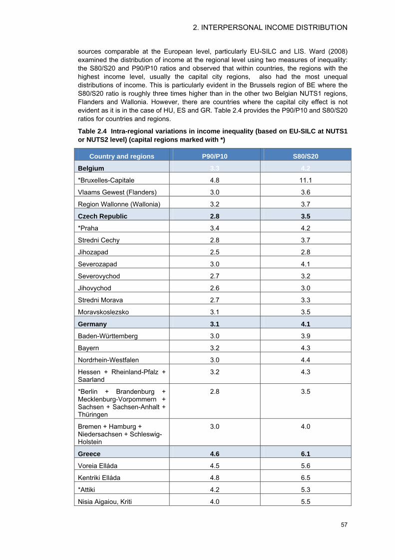
2. INTERPERSONAL INCOME DISTRIBUTION
57
sources comparable at the European level, particularly EU-SILC and LIS. Ward (2008) examined the distribution of income at the regional level using two measures of inequality: the S80/S20 and P90/P10 ratios and observed that within countries, the regions with the highest income level, usually the capital city regions, also had the most unequal distributions of income. This is particularly evident in the Brussels region of BE where the S80/S20 ratio is roughly three times higher than in the other two Belgian NUTS1 regions, Flanders and Wallonia. However, there are countries where the capital city effect is not evident as it is in the case of HU, ES and GR. Table 2.4 provides the P90/P10 and S80/S20 ratios for countries and regions.
Table 2.4 Intra-regional variations in income inequality (based on EU-SILC at NUTS1 or NUTS2 level) (capital regions marked with *)
Country and regions P90/P10 S80/S20
Belgium 3.3 4.2
*Bruxelles-Capitale 4.8 11.1
Vlaams Gewest (Flanders) 3.0 3.6
Region Wallonne (Wallonia) 3.2 3.7
Czech Republic 2.8 3.5
*Praha 3.4 4.2
Stredni Cechy 2.8 3.7
Jihozapad 2.5 2.8
Severozapad 3.0 4.1
Severovychod 2.7 3.2
Jihovychod 2.6 3.0
Stredni Morava 2.7 3.3
Moravskoslezsko 3.1 3.5
Germany 3.1 4.1
Baden-Württemberg 3.0 3.9
Bayern 3.2 4.3
Nordrhein-Westfalen 3.0 4.4
Hessen + Rheinland-Pfalz + Saarland
3.2 4.3
*Berlin + Brandenburg + Mecklenburg-Vorpommern + Sachsen + Sachsen-Anhalt + Thüringen
2.8 3.5
Bremen + Hamburg + Niedersachsen + Schleswig-Holstein
3.0 4.0
Greece 4.6 6.1
Voreia Elláda 4.5 5.6
Kentriki Elláda 4.8 6.5
*Attiki 4.2 5.3
Nisia Aigaiou, Kriti 4.0 5.5
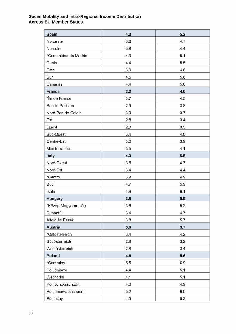
Social Mobility and Intra-Regional Income Distribution Across EU Member States
58
Spain 4.3 5.3
Noroeste 3.8 4.7
Noreste 3.8 4.4
*Comunidad de Madrid 4.3 5.1
Centro 4.4 5.5
Este 3.9 4.6
Sur 4.5 5.6
Canarias 4.4 5.6
France 3.2 4.0
*Île de France 3.7 4.5
Bassin Parisien 2.9 3.8
Nord-Pas-de-Calais 3.0 3.7
Est 2.8 3.4
Quest 2.9 3.5
Sud-Quest 3.4 4.0
Centre-Est 3.0 3.9
Méditerranée 3.5 4.1
Italy 4.3 5.5
Nord-Ovest 3.6 4.7
Nord-Est 3.4 4.4
*Centro 3.9 4.9
Sud 4.7 5.9
Isole 4.9 6.1
Hungary 3.8 5.5
*Közép-Magyarország 3.6 5.2
Dunántúl 3.4 4.7
Alföld és Észak 3.8 5.7
Austria 3.0 3.7
*Ostösterreich 3.4 4.2
Südösterreich 2.8 3.2
Westösterreich 2.8 3.4
Poland 4.6 5.6
*Centralny 5.5 6.9
Południowy 4.4 5.1
Wschodni 4.1 5.1
Północno-zachodni 4.0 4.9
Południowo-zachodni 5.2 6.0
Północny 4.5 5.3
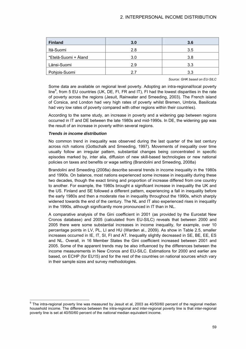
2. INTERPERSONAL INCOME DISTRIBUTION
59
Finland 3.0 3.6
Itä-Suomi 2.8 3.5
*Etelä-Suomi + Åland 3.0 3.8
Länsi-Suomi 2.9 3.3
Pohjois-Suomi 2.7 3.3 Source: GHK based on EU-SILC
Some data are available on regional level poverty. Adopting an intra-regional/local poverty line9, from 5 EU countries (UK, DE, FI, FR and IT), FI had the lowest disparities in the rate of poverty across the regions (Jesuit, Rainwater and Smeeding, 2003). The French island of Corsica, and London had very high rates of poverty whilst Bremen, Umbria, Basilicata had very low rates of poverty compared with other regions within their countries).
According to the same study, an increase in poverty and a widening gap between regions occurred in IT and DE between the late 1980s and mid-1990s. In DE, the widening gap was the result of an increase in poverty within several regions.
Trends in income distribution
No common trend in inequality was observed during the last quarter of the last century across rich nations (Gottschalk and Smeeding, 1997). Movements of inequality over time usually follow an irregular pattern, substantial changes being concentrated in specific episodes marked by, inter alia, diffusion of new skill-based technologies or new national policies on taxes and benefits or wage setting (Brandolini and Smeeding, 2008a)
Brandolini and Smeeding (2008a) describe several trends in income inequality in the 1980s and 1990s. On balance, most nations experienced some increase in inequality during these two decades, though the exact timing and proportion of increase differed from one country to another. For example, the 1980s brought a significant increase in inequality the UK and the US. Finland and SE followed a different pattern, experiencing a fall in inequality before the early 1980s and then a moderate rise in inequality throughout the 1990s, which sharply widened towards the end of the century. The NL and IT also experienced rises in inequality in the 1990s, although significantly more pronounced in IT than in NL.
A comparative analysis of the Gini coefficient in 2001 (as provided by the Eurostat New Cronos database) and 2005 (calculated from EU-SILC) reveals that between 2000 and 2005 there were some substantial increases in income inequality, for example, over 10 percentage points in LV, PL, LI and HU (Warden al., 2009). As show in Table 2.5, smaller increases occurred in IE, IT, SI, FI and AT. Inequality slightly decreased in SE, BE, EE, ES and NL. Overall, in 16 Member States the Gini coefficient increased between 2001 and 2005. Some of the apparent trends may be also influenced by the differences between the income measurements in New Cronos and EU-SILC. Estimations for 2000 and earlier are based, on ECHP (for EU15) and for the rest of the countries on national sources which vary in their sample sizes and survey methodologies.
9 The intra-regional poverty line was measured by Jesuit et al, 2003 as 40/50/60 percent of the regional median household income. The difference between the intra-regional and inter-regional poverty line is that inter-regional poverty line is set at 40/50/60 percent of the national median equivalent income.
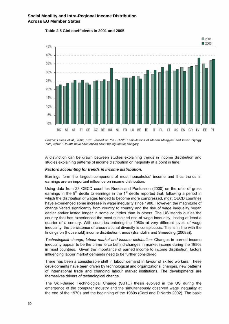
Social Mobility and Intra-Regional Income Distribution Across EU Member States
60
Table 2.5 Gini coefficients in 2001 and 2005
Source: Lelkes et al., 2009, p.21 (based on the EU-SILC calculations of Márton Medgyesi and István György Tóth) Note: * Doubts have been raised about the figures for Hungary.
A distinction can be drawn between studies explaining trends in income distribution and studies explaining patterns of income distribution or inequality at a point in time.
Factors accounting for trends in income distribution.
Earnings form the largest component of most households’ income and thus trends in earnings are an important influence on income distribution.
Using data from 23 OECD countries Rueda and Pontusson (2000) on the ratio of gross earnings in the 9th decile to earnings in the 1st decile reported that, following a period in which the distribution of wages tended to become more compressed, most OECD countries have experienced some increase in wage inequality since 1980. However, the magnitude of change varied significantly from country to country and the rise of wage inequality began earlier and/or lasted longer in some countries than in others. The US stands out as the country that has experienced the most sustained rise of wage inequality, lasting at least a quarter of a century. With countries entering the 1980s at very different levels of wage inequality, the persistence of cross-national diversity is conspicuous. This is in line with the findings on (household) income distribution trends (Brandolini and Smeeding (2008a)).
Technological change, labour market and income distribution: Changes in earned income inequality appear to be the prime force behind changes in market income during the 1980s in most countries. Given the importance of earned income to income distribution, factors influencing labour market demands need to be further considered.
There has been a considerable shift in labour demand in favour of skilled workers. These developments have been driven by technological and organizational changes, new patterns of international trade and changing labour market institutions. The developments are themselves drivers of technological change.
The Skill-Biased Technological Change (SBTC) thesis evolved in the US during the emergence of the computer industry and the simultaneously observed wage inequality at the end of the 1970s and the beginning of the 1980s (Card and DiNardo 2002). The basic
2. INTERPERSONAL INCOME DISTRIBUTION
61
idea is that new technologies, for example ICT, that improve the efficiency of the production process are “skill-biased” (Machin and van Reenen 2007) and mean that higher educated workers are more able to make use of these new technologies than less educated workers. This makes higher educated workers more attractive for employers and therefore increases the demand for them. At the same time, less educated workers become relatively less productive and are less in demand, which reduces their wages or increases unemployment within this group.
However, whilst almost all new technologies/innovations in the last decades need a high-skilled workforce that can make use of these technologies/innovations, many jobs for low skilled people cannot be replaced by the new technology. Therefore demand for this group of workers has not decreased as a consequence of the higher demand for high-skilled people. The evidence by Autor, Levy, and Murnane (2003) shows this, and used the notions “non-routine” tasks to show that the technological change favours the highly-skilled (who do the cognitive non-routine tasks that came with the new technologies) and does not affect the low skilled (who do the manual non routine tasks that are still in demand). Those who suffer are the -middle skilled workers doing the jobs characterized by routine tasks which are now replaced by the new technologies. This has been characterised as job polarisation. In support of the Autor, Levy, and Murnane (ALM) hypothesis, Goos and Manning (2007) discuss the increase in UK and US lower-tail wage inequality during the 1980s (measured in this study as 90/50 and the 50/10 percentile differentials). Their study shows that wages at the top of the distribution have been increasing relative to the median; however, the increase in the demand for low-paid non-routine jobs has not resulted in wage rises at the bottom relative to the median. One explanation is that the workers negatively affected by technology (hence, less skilled) in middling jobs have dropped into the lower-tail wage jobs. This might have raised the average level of human capital in the remaining middling jobs, accounting for the increasing wage differentials in the lower-end of the wage distribution.
The Skill-Biased Organizational Change (SBOC) thesis emphasises that technological change also leads to new organizational methods of work. In recent decades, the technological changes, mostly attributed to the development of ICT, have transformed organizations from the so-called “Taylorist Organizations” which were characterized by mass production and bureaucratic controls to more flexible forms of work (Caroli and van Reenen, 2001). The main features of these new workplaces are characterized by a wide range of changes such as a more decentralized decision making processes, Just-in-Time, Job Rotation, Teamwork or multitasking. The OECD employment outlook of 1999 paraphrased this new job design as “high performance work practices”, emphasising that these new requirements coincided with higher skill needs for workers (OECD Employment Outlook 1999).
The evolution of international trade and globalisation provide possible further explanations for a rising relative demand for skilled workers in Europe. During recent years, trade between the industrialized countries and the developing countries has risen. Emerging economies like Brazil, Russia, India and China (BRIC) play a major role in the world economy. Since the end of the 1970s increasing trade has coincided with a reduction in the relative demand for unskilled labour in developed countries. However, the importance of this factor is debatable. Skills upgrading can be observed in developing and emerging countries and Desjonqueres et al. (1999) show that skill upgrading is also present in non-trading sectors.
Given that technological development does not necessarily evolve in favour of highly-skilled workers, this suggests a more subtle interpretation of the shifts in relative labour demand. That is, a sort of endogenous Skill-Biased Technological Change thesis. It is possible that the educational upgrading of the workforce during the last decades was, to some extent, the source of technological changes and not the other way around. Firms have an incentive to adopt technology that coincides with the capacities of labour supply. A large supply of
Social Mobility and Intra-Regional Income Distribution Across EU Member States
62
skilled workers with relatively low wages could lead firms to introduce a technology their workforce can cope with. Machin and Manning (1997), describe a long-term mechanism that makes supply create its own demand. If labour markets are not perfect and employers have to invest to find the unique workers that can perfectly be matched with a specific job, they will find it easier and less risky to create jobs for workers that come from a larger group, in this case the high skilled. Intuitively, being a member of the highly-skilled workforce improves the possibility of finding employment and suggests that supply has created its own demand. Evidence on this explanation of relative shifts in labour demand for skilled workers is hard to come by. For the US it may explain why relative wages for workers with college degrees first declined in the 1960s and later on increased (Acemoglu 1998).
It is also argued that relative wages of less skilled workers are likely to have fallen because institutions that kept up wages of the less skilled became less important in the ‘new economy’ (Machin 2004). This explanation mostly figures in relation to the US and UK labour markets as these have experienced a decline of the institutions (especially a fall of the minimum wages in the US during the 1980s and a sharp decline of unionization in both countries).
Whatever the explanation the relative demand shift towards high skilled labour and to non-routine cognitive and manual tasks are partly transferred into higher wage dispersion (Machin and van Reenen 2007), even though other factors like labour market institutions, tax systems or the composition of the workforce also contribute to earnings inequality. Demographic factors may also have a minor influence.
Factors accounting for patterns of income distribution/inequality at a particular point in time
Welfare regimes and the role of the state, taxation and transfers and income distribution: One of the most commonly mentioned factors contributing to income (in)equality is the welfare regime. Whereas in the period from the end of the Second World War until the 1970s all industrialized nations showed declining income inequality, there has since been a clear divergence, with particularly marked increases in the UK, US, NL, DK, SE and AU. Other OECD countries recorded more modest increases or no change (Gottschalk and Smeeding 1997) and these differences have been attributed, to a significant extent, to differences in public policy.
Public redistribution tends to have an equalizing impact on income inequality and social transfers and taxes are known to be much higher in the Scandinavian (for example, SE) and corporatist welfare regimes (for example, DE) than in the more liberal regimes such as the UK. One illustration of this is that in 16 OECD countries, disposable incomes (post-tax and cash benefits) are more equally distributed than market incomes (ibid.). However, as Brandolini and Smeeding (2008a) show using various secondary and primary data sources, the magnitude of the equalizing impact of public redistribution varies from one country to another. Other factors (such as cross-national differences in earnings and savings) can moderate the relationship between public redistribution and income inequality. Furthermore, Mahler and Jesuit (2006) using LIS data for developed countries show that specific programmes encompassing universal benefits and targeted means-tested assistance can also have a significant redistributive impact. More specifically, fiscal redistribution arising from transfers is closely related to the size of social benefits. Fiscal redistribution is also linked to other factors such as electoral turnout, demographics and unemployment rates.
Other important factors influencing income inequality pertain to non-cash benefits such as health insurance, child care and education. Garfinkel, Rainwater and Smeeding (2006) estimate that half of welfare state transfers in rich countries are in-kind benefits. In an empirical study of ten10 rich countries in the late 1990s, the authors showed that adding to
10 The following countries were included: AU, CA, US, UK, BE, FR, DE, NL, FI and SE.
2. INTERPERSONAL INCOME DISTRIBUTION
63
the total income the value of non-cash benefits for health care and education (net of both direct and indirect taxes) drastically changes the inequality in full income between rich and poor. The equalizing impact of in-kind redistribution is particularly pronounced in the Anglo Saxon countries, which tend to be small spenders on cash but bigger spenders on in-kind benefits. Therefore, when full income (that takes into account both in-kind transfers and indirect taxes) is taken into account the difference between the most unequal nation (US) and most equal one (SE) markedly decreases.
Income and income distribution: Hoffmeister (2006) found in a study of European countries that more than a fifth (21.6%) of overall inequality was attributed to the income gap between the western and eastern halves of the EU. The differences between countries (within the areas) account for only 1.3 percent, and the differences between the regions (within the countries) for less than 1 percent of overall inequality. Three quarters of the inequality was attributed to income differences between people living in the same NUTS1 region.
The territorial distribution of power and income distribution: Research has shown decentralized political structures are an important cause of lower levels of redistribution and higher levels of inequality. However, recent research has put forward alternative interpretations of the association between fragmented fiscal structures and higher levels of inequality, arguing that the distributive effects of decentralization depend on the pre-existing territorial patterns of inequality (Beramendi 2007).
Other factors that explain patterns of income distribution: Perugini and Martino (2006) identified from the literature several determinants of income inequality: human capital endowment; structure of financial and credit markets; openness of economic systems; demographics; labour market participation; rates of unionisation and centralised bargaining; and social security systems/welfare state.
The following can also be important macro-level factors explaining differentials in the degree of, wage inequality in OECD countries (see Rueda and Pontusson 2000):
trade union density,
the centralisation of wage-bargaining decision-making structures,
the size of public sector employment,
government partisanship, and
the degree of coordination in the economy.
The relative importance of intra-regional and inter-regional income distribution to total income inequality
Literature on regional income inequality suggests that interpersonal income disparities contribute the most to the total income inequality in Europe. For example, Rodríguez-Pose, and Tselios (2009b) analysing ECHP data show that the within--region component of income inequality constituted 80 percent of the total income inequality in Europe. On a comparative basis, between-region as well as between-country levels of inequality contribute little to the total inequality. Similar results were found by Hoffmeister (2006): three quarters of the inequality reported in the EU (19 countries covered) are attributed to income differences between people living in the same NUTS1 region. Table 2.6 summarises the inter-regional and intra-regional contributions to inequality in ten EU countries listed in increasing importance of inter-regional contribution to inequality. The inter-regional contribution is greatest in IT, GR, HU and ES and lowest in AT. Between-region inequality tends to be lower in smaller countries with fewer NUTS1 regions like AT and BE.
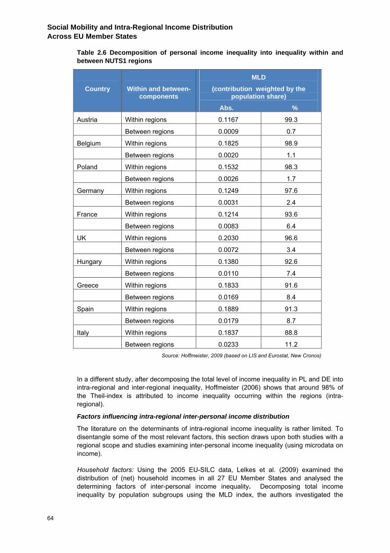
Social Mobility and Intra-Regional Income Distribution Across EU Member States
64
Table 2.6 Decomposition of personal income inequality into inequality within and between NUTS1 regions
Country
Within and between-components
MLD
(contribution weighted by the population share)
Abs. %
Austria Within regions 0.1167 99.3
Between regions 0.0009 0.7
Belgium Within regions 0.1825 98.9
Between regions 0.0020 1.1
Poland Within regions 0.1532 98.3
Between regions 0.0026 1.7
Germany Within regions 0.1249 97.6
Between regions 0.0031 2.4
France Within regions 0.1214 93.6
Between regions 0.0083 6.4
UK Within regions 0.2030 96.6
Between regions 0.0072 3.4
Hungary Within regions 0.1380 92.6
Between regions 0.0110 7.4
Greece Within regions 0.1833 91.6
Between regions 0.0169 8.4
Spain Within regions 0.1889 91.3
Between regions 0.0179 8.7
Italy Within regions 0.1837 88.8
Between regions 0.0233 11.2 Source: Hoffmeister, 2009 (based on LIS and Eurostat, New Cronos)
In a different study, after decomposing the total level of income inequality in PL and DE into intra-regional and inter-regional inequality, Hoffmeister (2006) shows that around 98% of the Theil-index is attributed to income inequality occurring within the regions (intra-regional).
Factors influencing intra-regional inter-personal income distribution
The literature on the determinants of intra-regional income inequality is rather limited. To disentangle some of the most relevant factors, this section draws upon both studies with a regional scope and studies examining inter-personal income inequality (using microdata on income).
Household factors: Using the 2005 EU-SILC data, Lelkes et al. (2009) examined the distribution of (net) household incomes in all 27 EU Member States and analysed the determining factors of inter-personal income inequality. Decomposing total income inequality by population subgroups using the MLD index, the authors investigated the
2. INTERPERSONAL INCOME DISTRIBUTION
65
impact of the following factors on income distribution: age of the head of the household; household structure; the education and the employment status of the head of the household; work intensity of the household11; and, the degree of urbanisation in the household’s place of residence. Four categories for the age of household head were used: 18–35 years; 36–49 years; 50–64 years; and, over 65 years. Household structure was grouped into five categories: a) households with a working-age head (between 18 and 64 years of age) with no children; b) with one child; c) with two children; d) with three or more children; e) households with a retirement-age head. The ‘work intensity’ of the household was defined taking into account the total number of months worked by all household members compared with the number of total workable months. The results of the decomposition show that with the exception of few countries, differences in the ages of household heads accounted for less than 5% of total inequality. Such differences in age were more important in the Nordic countries (DE, FI and SE) as well as CY and EE where there are significant income differences between different age groups, particularly between those of working age and retired. The authors suggest that the explanatory power of household structure (with children or no children) is relatively high in CZ, CY and IE. Differences in the number of children account for 8% of the total inequality in CZ and 8% in the UK, where the average income of the families with three or more dependent children is less than two-thirds of the mean income of childless households. The income differentials by household structure are explained by the differences between households headed by a working-age person or by a retired person.
However, in contrast, Brandolini, A. and G. D’Alessio (2001) concluded that differences in population structure (household size; age and sex of household head) do not explain many of the large differences in income inequality observed across countries.
Education: Rodríguez-Pose, A. and Tselios, V. (2009a) provide empirical evidence of the determinants of income inequality within 102 regions (NUTS1 or 2) of 13 EU countries.12 The study estimates income inequality (per region) as a linear function of income per capita, educational attainment and educational inequality per region.13 Educational inequality (unequal distribution of education level completed) is associated with higher income inequality within a region (Rodríguez-Pose, and Tselios, 2009a). Analysing income data at national level Lelkes et al. (2009) demonstrate that education in general accounts for income inequality to a greater extent than age and household structure: differences in education can account for up to 30% of income inequality in PT and around 20% in HU. In LT, PL, CY, LU and SI, education seems to matter at both lower and upper ends of the distribution.
Employment status: The impact of employment status of the household head varies from one country to another explaining less than 5% of income inequality in AT, LU, IT, GR and more than 15% in UK, DK and CZ. Work intensity can also account for a high proportion of the total inequality in IE, EE and BE. The results of the decomposition analysis by country groups highlight that European countries display a different structure of inequality where education is the most important factor in explaining income inequalities in the Continental Central European and Mediterranean countries, whilst employment status is the major factor of inequality in the Anglo-Saxon countries and Baltic states.
Female activity rate, female headed households and income distribution: Female economic activity rate was found to be negatively associated with income inequality within a region
11 Work intensity of the household is defined taking into account the total number of months worked by all household members, related to the number of total workable months 12 NUTS1 data for AT, BE, DK, FR, GR, IE, IT, LU, ES, SE. NUTS2 data for DE, PT, and UK. A total sample of 116.574 individuals (per wave) were surveyed, with a maximum of 124,759 individuals in 1997 and a minimum of 105,079 in 2001. 13 The study uses total net personal income data from ECHP to estimate the income inequality per region as well as regional income per capita. Income inequality within a region is calculated by taking into account each individual’s income as a proportion of total income for the entire regional population.
Social Mobility and Intra-Regional Income Distribution Across EU Member States
66
according to Rodríguez-Pose, and Tselios, (2009a). Mahler (2002) found some evidence that higher shares of female headed households within regions were associated with greater income inequality.
Unemployment and income distribution: Unemployment is positively associated with income inequality, whilst higher access to work (percentage of respondents working 15+ hours per week) is associated with lower income inequality14. The percentage of normally working respondents and the economic activity rate of the total population are negatively associated with income inequality (Rodriguez-Pose and Tselios, 2009a).
Income per capita and income distribution: The relationship between regional income per capita and income inequality is positive though not very strong. One of the explanations could be that regional economic development increases the occupational levels and earnings for the well-off rather than the whole population. However, results are not consistent. In a recent study using the same ECHP data, the authors found a non-linear relationship between income per capita and inequality (Rodríguez-Pose and Tselios, 2009b).
Income inequality in neighbour regions: Income inequality within each region is the product of intra-regional characteristics as well as the economic conditions in the neighbour regions. More specifically, regions with similar income per capita and income inequality tend to cluster (ibid.). The economic development of a region tends to diffuse across the geographically nearest regions.
Urbanisation of a region and income distribution: Increasing urbanisation (an increasing weight of the urban relative to the rural population within a region) is negatively associated with income inequality (Rodríguez-Pose, and Tselios, 2009a). However, different results were found by Hoffmeister (2006) who examined income differences between people living in the same (NUTS1) region across the EU. The regions characterised by high levels of interpersonal income inequality in Europe are usually the ones that incorporate the capital of a country or regions marked by high rates of agglomeration (such as Ostösterreich in AT, Hamburg and Berlin in DE, London in the UK, Centralny in PL). One of the explanations for this contradiction could stem from the fact that increasing weight of the urban relative to the rural population means a decreasing income inequality for the whole of the population in a region, but this does not apply to the disparities within the working population which may increase (Rodríguez-Pose, and Tselios, 2009a). Urbanisation might increase the local economic prosperity and income per capita for the local population but at the same time, it can trigger a higher earnings dispersion between the skilled employees and the less skilled, those who work in the advanced industries versus the more traditional, low paid industries. A later study using the same data (Rodríguez-Pose, and Tselios, 2009a) highlighted that there are marked differences within agglomerated and rural areas rather than between them.
Examining central and eastern European regions, Förster, Jesuit and Smeeding (2005) conclude that inter-regional income disparities, though small compared to intra-regional inequality, had grown in the decade following the collapse of the USSR. In short, “capital cities and major urban areas were mainly winners, while regions which are longer distances from central cities and which are further from their richer western neighbors characterize losers. This has led to rising differences between rich and poor regions as well” (2005: 337). In the NMS, the degree of urbanisation can explain a high percentage of inequality, between 10 and 12 percent (in LT, LV and PL). However, the explanatory role of this variable is almost negligible in EU15 (Lelkes et al., 2009). Table 2.7 indicates the extent to which urbanisation explains inequality in different countries.
14 Eurostat defines the same variable “work access” as the percentage of economic activity rate of total population.
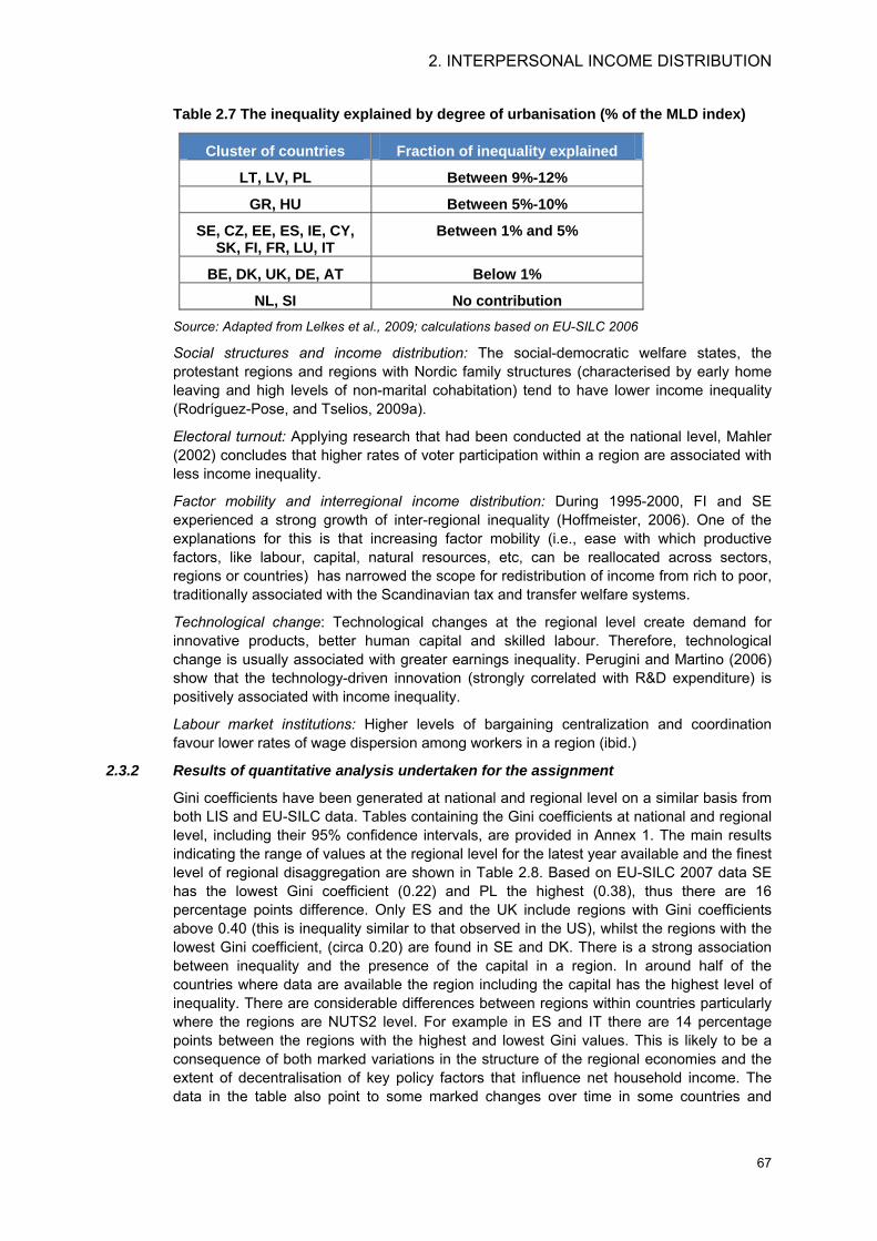
2. INTERPERSONAL INCOME DISTRIBUTION
67
Table 2.7 The inequality explained by degree of urbanisation (% of the MLD index)
Cluster of countries Fraction of inequality explained
LT, LV, PL Between 9%-12%
GR, HU Between 5%-10%
SE, CZ, EE, ES, IE, CY, SK, FI, FR, LU, IT
Between 1% and 5%
BE, DK, UK, DE, AT Below 1%
NL, SI No contribution Source: Adapted from Lelkes et al., 2009; calculations based on EU-SILC 2006
Social structures and income distribution: The social-democratic welfare states, the protestant regions and regions with Nordic family structures (characterised by early home leaving and high levels of non-marital cohabitation) tend to have lower income inequality (Rodríguez-Pose, and Tselios, 2009a).
Electoral turnout: Applying research that had been conducted at the national level, Mahler (2002) concludes that higher rates of voter participation within a region are associated with less income inequality.
Factor mobility and interregional income distribution: During 1995-2000, FI and SE experienced a strong growth of inter-regional inequality (Hoffmeister, 2006). One of the explanations for this is that increasing factor mobility (i.e., ease with which productive factors, like labour, capital, natural resources, etc, can be reallocated across sectors, regions or countries) has narrowed the scope for redistribution of income from rich to poor, traditionally associated with the Scandinavian tax and transfer welfare systems.
Technological change: Technological changes at the regional level create demand for innovative products, better human capital and skilled labour. Therefore, technological change is usually associated with greater earnings inequality. Perugini and Martino (2006) show that the technology-driven innovation (strongly correlated with R&D expenditure) is positively associated with income inequality.
Labour market institutions: Higher levels of bargaining centralization and coordination favour lower rates of wage dispersion among workers in a region (ibid.)
2.3.2 Results of quantitative analysis undertaken for the assignment
Gini coefficients have been generated at national and regional level on a similar basis from both LIS and EU-SILC data. Tables containing the Gini coefficients at national and regional level, including their 95% confidence intervals, are provided in Annex 1. The main results indicating the range of values at the regional level for the latest year available and the finest level of regional disaggregation are shown in Table 2.8. Based on EU-SILC 2007 data SE has the lowest Gini coefficient (0.22) and PL the highest (0.38), thus there are 16 percentage points difference. Only ES and the UK include regions with Gini coefficients above 0.40 (this is inequality similar to that observed in the US), whilst the regions with the lowest Gini coefficient, (circa 0.20) are found in SE and DK. There is a strong association between inequality and the presence of the capital in a region. In around half of the countries where data are available the region including the capital has the highest level of inequality. There are considerable differences between regions within countries particularly where the regions are NUTS2 level. For example in ES and IT there are 14 percentage points between the regions with the highest and lowest Gini values. This is likely to be a consequence of both marked variations in the structure of the regional economies and the extent of decentralisation of key policy factors that influence net household income. The data in the table also point to some marked changes over time in some countries and
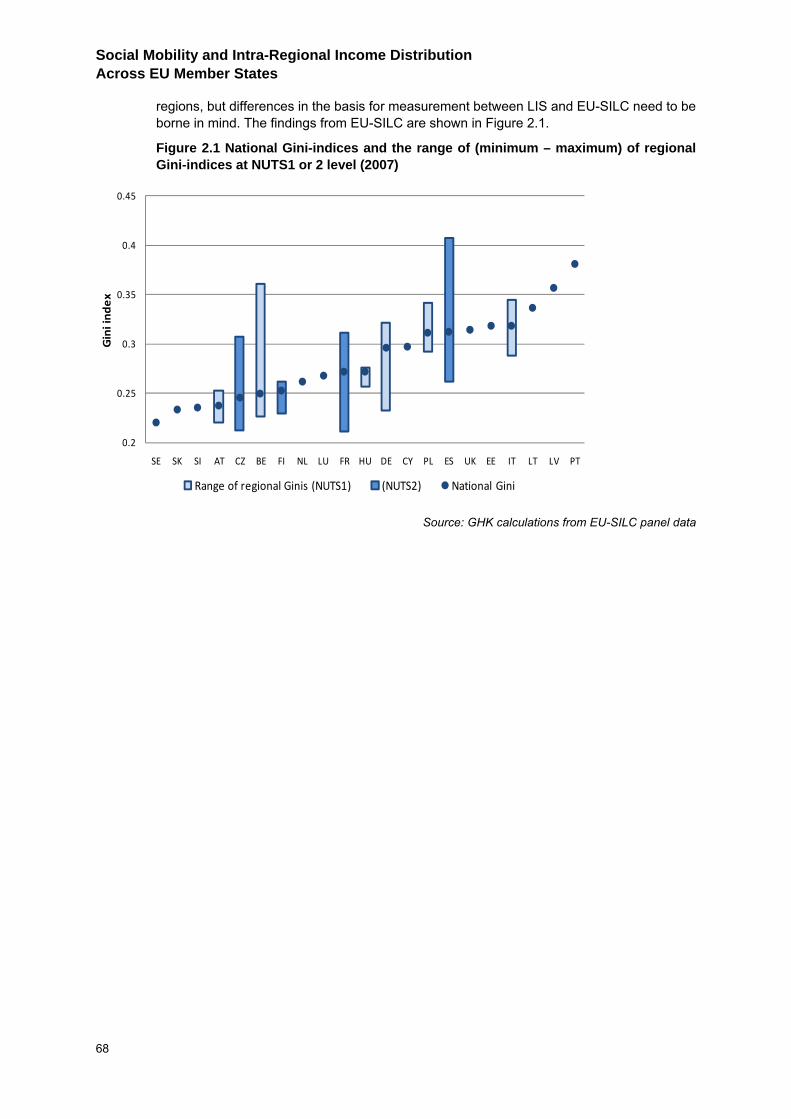
Social Mobility and Intra-Regional Income Distribution Across EU Member States
68
regions, but differences in the basis for measurement between LIS and EU-SILC need to be borne in mind. The findings from EU-SILC are shown in Figure 2.1.
Figure 2.1 National Gini-indices and the range of (minimum – maximum) of regional Gini-indices at NUTS1 or 2 level (2007)
0.2
0.25
0.3
0.35
0.4
0.45
SE SK SI AT CZ BE FI NL LU FR HU DE CY PL ES UK EE IT LT LV PT
Gin
i in
de
x
Range of regional Ginis (NUTS1) (NUTS2) National Gini
Source: GHK calculations from EU-SILC panel data
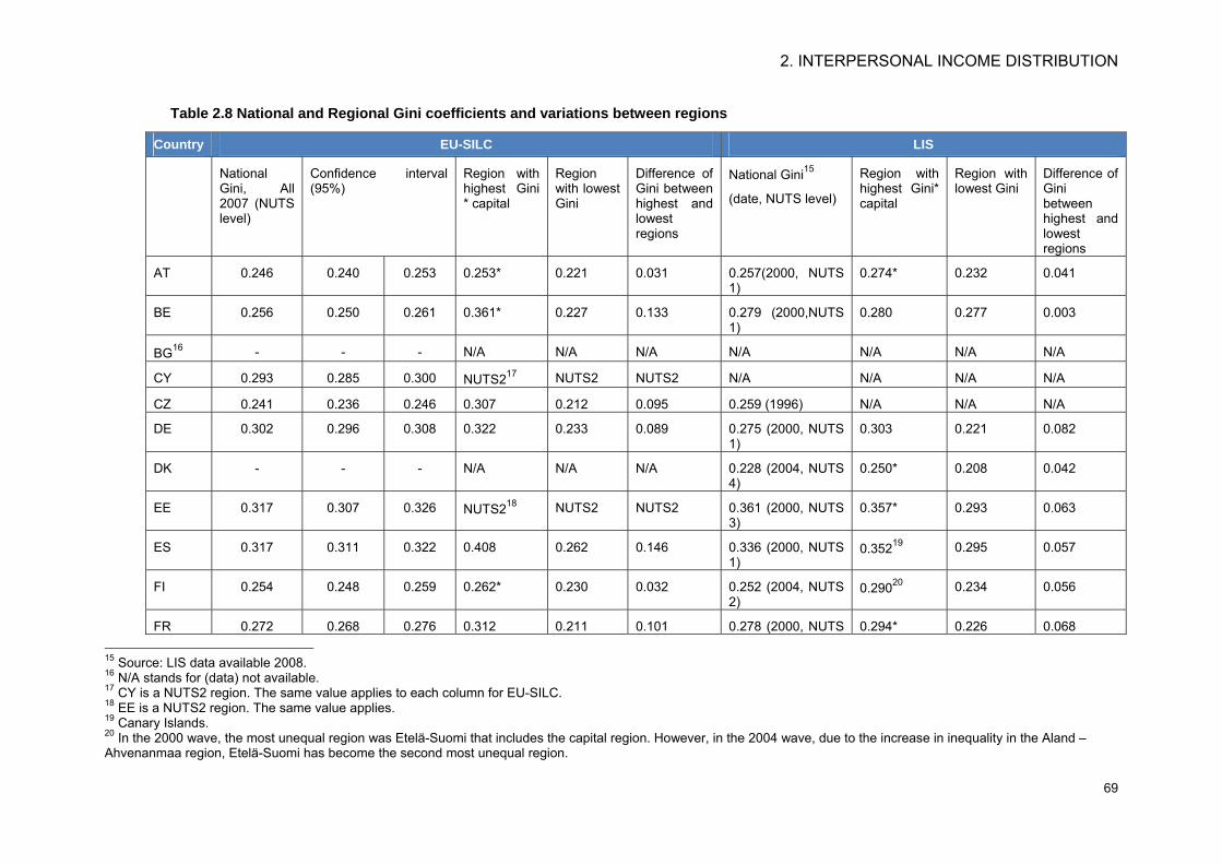
2. INTERPERSONAL INCOME DISTRIBUTION
69
Table 2.8 National and Regional Gini coefficients and variations between regions
Country EU-SILC LIS
National Gini, All 2007 (NUTS level)
Confidence interval (95%)
Region with highest Gini * capital
Region with lowest Gini
Difference of Gini between highest and lowest regions
National Gini15
(date, NUTS level)
Region with highest Gini* capital
Region with lowest Gini
Difference of Gini between highest and lowest regions
AT 0.246 0.240 0.253 0.253* 0.221 0.031 0.257(2000, NUTS 1)
0.274* 0.232 0.041
BE 0.256 0.250 0.261 0.361* 0.227 0.133 0.279 (2000,NUTS 1)
0.280 0.277 0.003
BG16 - - - N/A N/A N/A N/A N/A N/A N/A
CY 0.293 0.285 0.300 NUTS217 NUTS2 NUTS2 N/A N/A N/A N/A
CZ 0.241 0.236 0.246 0.307 0.212 0.095 0.259 (1996) N/A N/A N/A
DE 0.302 0.296 0.308 0.322 0.233 0.089 0.275 (2000, NUTS 1)
0.303 0.221 0.082
DK - - - N/A N/A N/A 0.228 (2004, NUTS 4)
0.250* 0.208 0.042
EE 0.317 0.307 0.326 NUTS218 NUTS2 NUTS2 0.361 (2000, NUTS 3)
0.357* 0.293 0.063
ES 0.317 0.311 0.322 0.408 0.262 0.146 0.336 (2000, NUTS 1)
0.35219 0.295 0.057
FI 0.254 0.248 0.259 0.262* 0.230 0.032 0.252 (2004, NUTS 2)
0.29020 0.234 0.056
FR 0.272 0.268 0.276 0.312 0.211 0.101 0.278 (2000, NUTS 0.294* 0.226 0.068 15 Source: LIS data available 2008. 16 N/A stands for (data) not available. 17 CY is a NUTS2 region. The same value applies to each column for EU-SILC. 18 EE is a NUTS2 region. The same value applies. 19 Canary Islands. 20 In the 2000 wave, the most unequal region was Etelä-Suomi that includes the capital region. However, in the 2004 wave, due to the increase in inequality in the Aland – Ahvenanmaa region, Etelä-Suomi has become the second most unequal region.
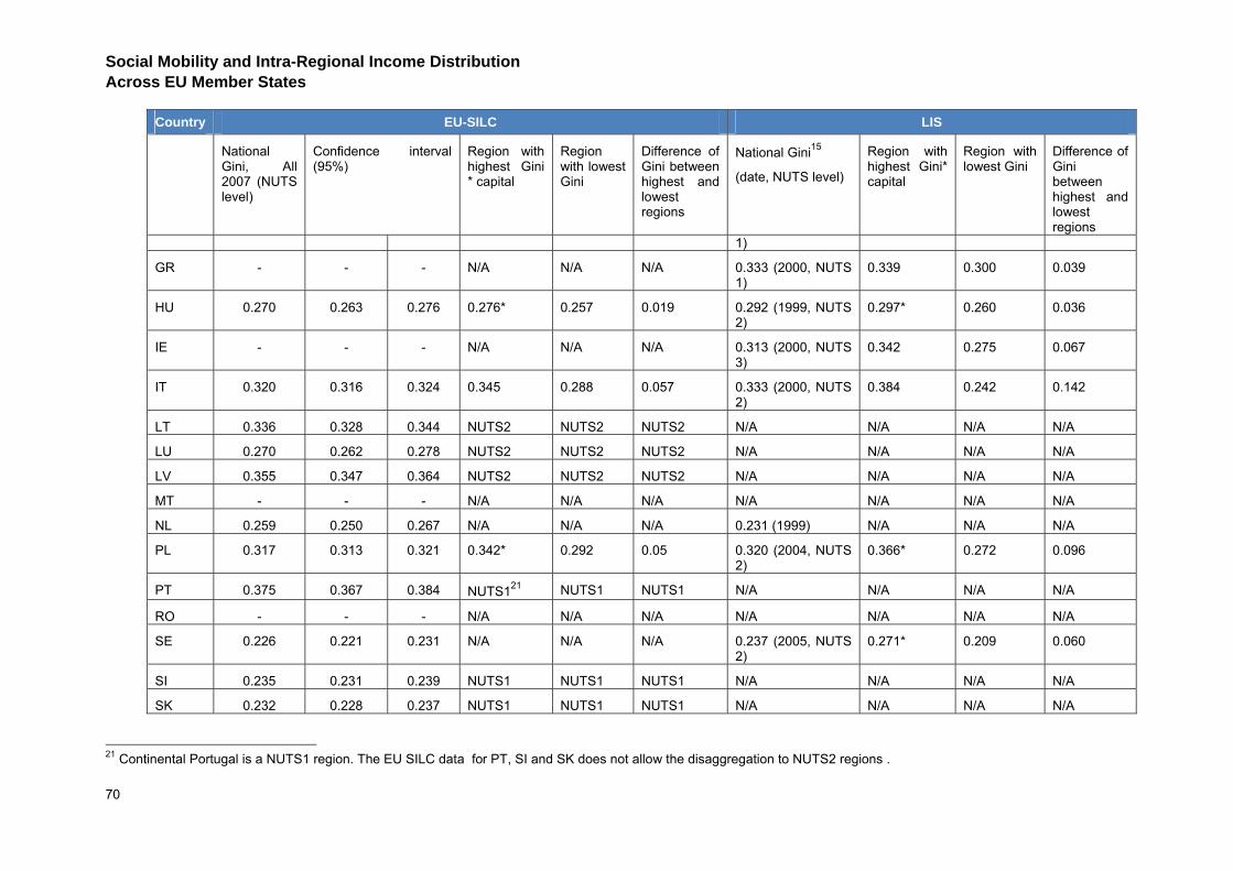
Social Mobility and Intra-Regional Income Distribution Across EU Member States
70
Country EU-SILC LIS
National Gini, All 2007 (NUTS level)
Confidence interval (95%)
Region with highest Gini * capital
Region with lowest Gini
Difference of Gini between highest and lowest regions
National Gini15
(date, NUTS level)
Region with highest Gini* capital
Region with lowest Gini
Difference of Gini between highest and lowest regions
1)
GR - - - N/A N/A N/A 0.333 (2000, NUTS 1)
0.339 0.300 0.039
HU 0.270 0.263 0.276 0.276* 0.257 0.019 0.292 (1999, NUTS 2)
0.297* 0.260 0.036
IE - - - N/A N/A N/A 0.313 (2000, NUTS 3)
0.342 0.275 0.067
IT 0.320 0.316 0.324 0.345 0.288 0.057 0.333 (2000, NUTS 2)
0.384 0.242 0.142
LT 0.336 0.328 0.344 NUTS2 NUTS2 NUTS2 N/A N/A N/A N/A
LU 0.270 0.262 0.278 NUTS2 NUTS2 NUTS2 N/A N/A N/A N/A
LV 0.355 0.347 0.364 NUTS2 NUTS2 NUTS2 N/A N/A N/A N/A
MT - - - N/A N/A N/A N/A N/A N/A N/A
NL 0.259 0.250 0.267 N/A N/A N/A 0.231 (1999) N/A N/A N/A
PL 0.317 0.313 0.321 0.342* 0.292 0.05 0.320 (2004, NUTS 2)
0.366* 0.272 0.096
PT 0.375 0.367 0.384 NUTS121 NUTS1 NUTS1 N/A N/A N/A N/A
RO - - - N/A N/A N/A N/A N/A N/A N/A
SE 0.226 0.221 0.231 N/A N/A N/A 0.237 (2005, NUTS 2)
0.271* 0.209 0.060
SI 0.235 0.231 0.239 NUTS1 NUTS1 NUTS1 N/A N/A N/A N/A
SK 0.232 0.228 0.237 NUTS1 NUTS1 NUTS1 N/A N/A N/A N/A
21 Continental Portugal is a NUTS1 region. The EU SILC data for PT, SI and SK does not allow the disaggregation to NUTS2 regions .
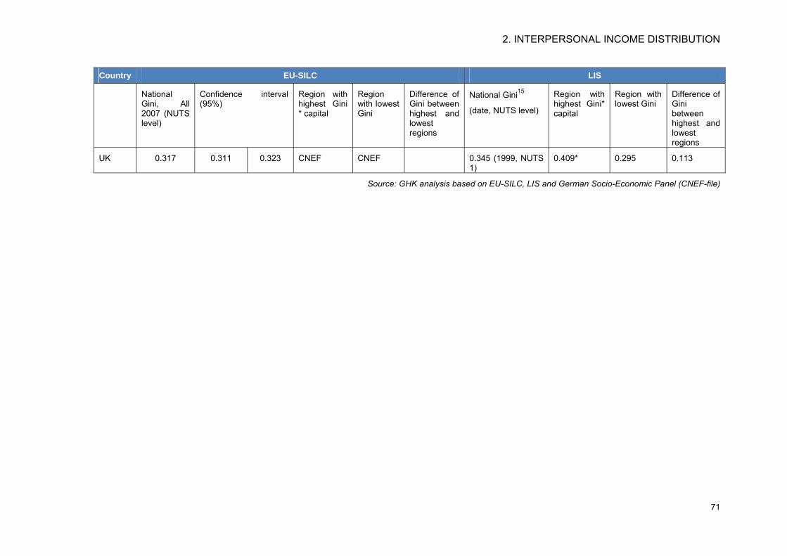
2. INTERPERSONAL INCOME DISTRIBUTION
71
Country EU-SILC LIS
National Gini, All 2007 (NUTS level)
Confidence interval (95%)
Region with highest Gini * capital
Region with lowest Gini
Difference of Gini between highest and lowest regions
National Gini15
(date, NUTS level)
Region with highest Gini* capital
Region with lowest Gini
Difference of Gini between highest and lowest regions
UK 0.317 0.311 0.323 CNEF CNEF 0.345 (1999, NUTS 1)
0.409* 0.295 0.113
Source: GHK analysis based on EU-SILC, LIS and German Socio-Economic Panel (CNEF-file)
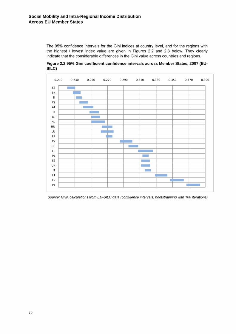
Social Mobility and Intra-Regional Income Distribution Across EU Member States
72
The 95% confidence intervals for the Gini indices at country level, and for the regions with the highest / lowest index value are given in Figures 2.2 and 2.3 below. They clearly indicate that the considerable differences in the Gini value across countries and regions.
Figure 2.2 95% Gini coefficient confidence intervals across Member States, 2007 (EU-SILC)
0.210 0.230 0.250 0.270 0.290 0.310 0.330 0.350 0.370 0.390
SE
SK
SI
CZ
AT
FI
BE
NL
HU
LU
FR
CY
DE
EE
PL
ES
UK
IT
LT
LV
PT
Source: GHK calculations from EU-SILC data (confidence intervals: bootstrapping with 100 iterations)
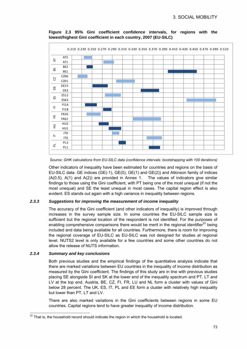
3. SOCIAL MOBILITY
73
Figure 2.3 95% Gini coefficient confidence intervals, for regions with the lowest/highest Gini coefficient in each country, 2007 (EU-SILC)
0.210 0.230 0.250 0.270 0.290 0.310 0.330 0.350 0.370 0.390 0.410 0.430 0.450 0.470 0.490 0.510
AT2AT1BE2BE1
CZ06CZ01DE15
DE3ES12ES63FI1AFI18
FR26FR62HU2HU1ITDITGPL3PL1
ATBE
CZD
EES
FIFR
HU
ITPL
Source: GHK calculations from EU-SILC data (confidence intervals: bootstrapping with 100 iterations)
Other indicators of inequality have been estimated for countries and regions on the basis of EU-SILC data. GE indices (GE(-1), GE(0), GE(1) and GE(2)) and Atkinson family of indices (A(0.5), A(1) and A(2)) are provided in Annex 1. The values of indicators give similar findings to those using the Gini coefficient, with PT being one of the most unequal (if not the most unequal) and SE the least unequal in most cases. The capital region effect is also evident. ES stands out again with a high variance in inequality between regions.
2.3.3 Suggestions for improving the measurement of income inequality
The accuracy of the Gini coefficient (and other indicators of inequality) is improved through increases in the survey sample size. In some countries the EU-SILC sample size is sufficient but the regional location of the respondent is not identified. For the purposes of enabling comprehensive comparisons there would be merit in the regional identifier22 being included and data being available for all countries. Furthermore, there is room for improving the regional coverage of EU-SILC as EU-SILC was not designed for studies at regional level. NUTS2 level is only available for a few countries and some other countries do not allow the release of NUTS information.
2.3.4 Summary and key conclusions
Both previous studies and the empirical findings of the quantitative analysis indicate that there are marked variations between EU countries in the inequality of income distribution as measured by the Gini coefficient. The findings of this study are in line with previous studies placing SE alongside SI and SK at the lower end of the inequality spectrum and PT, LT and LV at the top end. Austria, BE, CZ, FI, FR, LU and NL form a cluster with values of Gini below 28 percent. The UK, ES, IT, PL and EE form a cluster with relatively high inequality but lower than PT, LT and LV.
There are also marked variations in the Gini coefficients between regions in some EU countries. Capital regions tend to have greater inequality of income distribution.
22 That is, the household record should indicate the region in which the household is located.

Social Mobility and Intra-Regional Income Distribution Across EU Member States
74
Evidence from various studies observes factors influencing income distribution. These can be divided into structural macro-factors and micro factors at the household/individual level. At the macro-level, the most important factors influencing income distribution include: technological change; skills-biased market changes; welfare regimes; and, demographics. The micro factors at the household/individual levels pertain to: education; age; household structure; and, employment status. Some of these factors are interrelated. Some of these key factors are thus included in the regression model used to analyse income mobility recorded in the EU-SILC 2005-2007 data.
3. SOCIAL MOBILITY
75
3 SOCIAL MOBILITY 3.1 Introduction
This section of the report describes the different concepts and indicators of social mobility and assesses their relative merits for the exploration of the relationship between social mobility and intra-regional income distribution. Both intra and inter-generational social mobility are considered.
Evidence on the incidence of social mobility and in particular income mobility is reviewed and the findings of the analysis of the EU-SILC 2005-2007 panel data and EU-SILC 2005 questions on inter-generational mobility are presented. Factors influencing both intra and inter-generational social mobility are reviewed.
3.2 Theoretical Analysis
3.2.1 Key concepts of social mobility
Social mobility is defined in the Encyclopedia Britannica as the “movement of individuals, families, or groups through a system of social hierarchy or stratification” (Encyclopædia Britannica. 2009). Similar definitions are found in sociological and economic literature. For example, the Dictionary of Sociology defines social mobility as: “the movement – usually of individuals but sometimes of whole groups – between different positions within the system of social stratification in any society” (Scott and Marshall, 2005).
Several variables such as education, occupation, income or social class may be used in the analysis of social mobility. The emphasis on these variables differs across academic disciplines. Some scholars make use of continuous measures of social mobility, whilst others prefer discrete measures. Some of the indices are not applicable when a discrete variable or classification is used. Continuous variables may be broken down into groups or classes, but these are often defined ad hoc, and conclusions on social mobility may be contingent on how groups are defined.
One aspect of social mobility is income mobility. Income mobility is concerned with measuring the changes in the economic status of individuals (or their income levels) from one time period to another.
Slight variations to the above definitions exist, especially in political discourse. The 2001 discussion paper of the UK Government Office on social mobility (Aldridge, 2001) describes it as “the movement or opportunities for movement between different social groups, and the advantages and disadvantages that go with this in terms of income, security of employment, opportunities for advancement etc.” In this definition, the term is extended to cover ‘opportunities for movement’ (i.e. the chance that an individual from a socioeconomic group can move into another one).
The key concepts and measures of mobility: intra-generational mobility and inter-generational mobility; vertical and horizontal mobility; absolute and relative mobility; exchange and relative mobility are described below. Exchange and structural mobility are explained in greater detailed as they are used throughout the report.
Intra-generational (social) mobility relates to the movement of individuals or groups during their lifetime through a system of stratification or changes in income. Often the focus of studies of intra-generational mobility is on income mobility. This is the main focus of the current assignment.
Inter-generational (social) mobility of class or income compares the current socio economic characteristics of individuals, families or groups with those of their parents or those with which they originated. The focus of the characteristics may be on social class, education, occupation or earnings.
Social Mobility and Intra-Regional Income Distribution Across EU Member States
76
A distinction can also be made between social mobility within the same socio-economic status (horizontal mobility) or between different socio-economic levels (vertical mobility). Vertical mobility can be either upward or downward. Ssome categorisations of social class, such as the Cambridge Social Interaction and Stratification Scale (CASMIN)23 that group classes within levels enable this distinction.
In the literature on mobility of social class Absolute mobility refers to the absolute number of individuals who (actually) move up or down the social hierarchy. Absolute social mobility usually refers to large-scale societal changes encompassing a high number of individuals moving between different social classes (for example, the post-industrial mobility of population from blue-collar occupations to the service sector labour force).
Relative mobility refers to the chances of individuals from a certain social group attaining a different socioeconomic status24. These a priori chances may be calculated for each group on the basis of observed absolute mobility in the past, whilst accounting for shifts in the overall distribution of population between different socio-economic strata. Absolute mobility is thus the aggregate (i.e. net outcome) of individuals’ movements, reflecting shifts in the structure of the economy and society, whilst relative mobility is the movement of individuals or groups between different socio-economic strata regardless of changes in the distribution of the population25. In the sociological literature, inter-generational relative mobility is also referred to as “social fluidity”. The term was originally introduced by Erikson, Goldthorpe and Portocarero (1982) and similarly refers to the inequality between individuals from different classes in their chances of occupying one destination class rather than another (through estimating the ‘odds ratio’). The degree of social fluidity is taken as an indicator of societal openness; that is, the extent to which the chances of access to class positions are equally or unequally distributed.
However, Fields (2008) stresses that relative and absolute mobility are equivocal terms, often used by scholars with different meanings. Relative mobility can be used in the sense of “individual’s change in income relative to the income changes of others”. Alternatively, relative mobility may allude to “positional movements” i.e., changes in position from a base year to final year. Absolute mobility also lends itself to at least two meanings. It can mean either: gains and losses of income rather than income shares or positions (i.e. the magnitude of the income changes as well as their direction are taken into account); or the absolute value of income changes, irrespective of their direction. Because of the varying use of these two terms, Fields recommends their cautious use.
Measuring social mobility: The building block for studies of social mobility is the joint distribution of outcomes in two (or more) periods. When the outcome variables are categorical (e.g., CASMIN classes), social mobility is often expressed in a mobility table, also referred to as the transition/mobility table or transition matrix.
Each member of a sample (usually a sample of those of working age) is allocated to a cell within the mobility table according to current class position (destination) on the x axis and class position when he/she was growing up, usually around the age of 15, (origin) on the y axis. The mobility table thus shows the actual movements between classes and changes in class distributions. The data in the cells can be used to indicate the proportion of outflows originating from a particular class (row percentages) and the proportion of inflows from different classes (column percentages). They can also be used to estimate exchange mobility.
Several indexes of mobility and other indicators can be derived from the mobility table:
23 CASMIN is a seven class model of mobility, proposed by Erikson and Goldthorpe. For more details, see Annex. 24 The concepts of ‘absolute’ and ‘relative mobility’ are sometimes constrained to include only upward mobility. 25 The terms ‘structural’ and ‘exchange’ mobility are also used.
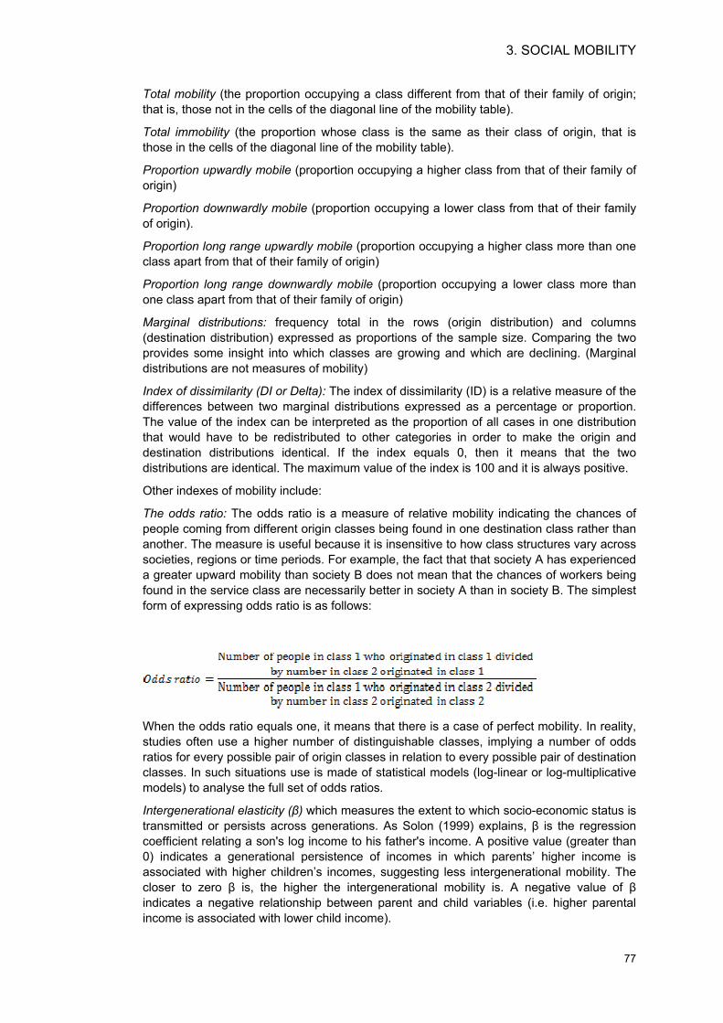
3. SOCIAL MOBILITY
77
Total mobility (the proportion occupying a class different from that of their family of origin; that is, those not in the cells of the diagonal line of the mobility table).
Total immobility (the proportion whose class is the same as their class of origin, that is those in the cells of the diagonal line of the mobility table).
Proportion upwardly mobile (proportion occupying a higher class from that of their family of origin)
Proportion downwardly mobile (proportion occupying a lower class from that of their family of origin).
Proportion long range upwardly mobile (proportion occupying a higher class more than one class apart from that of their family of origin)
Proportion long range downwardly mobile (proportion occupying a lower class more than one class apart from that of their family of origin)
Marginal distributions: frequency total in the rows (origin distribution) and columns (destination distribution) expressed as proportions of the sample size. Comparing the two provides some insight into which classes are growing and which are declining. (Marginal distributions are not measures of mobility)
Index of dissimilarity (DI or Delta): The index of dissimilarity (ID) is a relative measure of the differences between two marginal distributions expressed as a percentage or proportion. The value of the index can be interpreted as the proportion of all cases in one distribution that would have to be redistributed to other categories in order to make the origin and destination distributions identical. If the index equals 0, then it means that the two distributions are identical. The maximum value of the index is 100 and it is always positive.
Other indexes of mobility include:
The odds ratio: The odds ratio is a measure of relative mobility indicating the chances of people coming from different origin classes being found in one destination class rather than another. The measure is useful because it is insensitive to how class structures vary across societies, regions or time periods. For example, the fact that that society A has experienced a greater upward mobility than society B does not mean that the chances of workers being found in the service class are necessarily better in society A than in society B. The simplest form of expressing odds ratio is as follows:
When the odds ratio equals one, it means that there is a case of perfect mobility. In reality, studies often use a higher number of distinguishable classes, implying a number of odds ratios for every possible pair of origin classes in relation to every possible pair of destination classes. In such situations use is made of statistical models (log-linear or log-multiplicative models) to analyse the full set of odds ratios.
Intergenerational elasticity (β) which measures the extent to which socio-economic status is transmitted or persists across generations. As Solon (1999) explains, β is the regression coefficient relating a son's log income to his father's income. A positive value (greater than 0) indicates a generational persistence of incomes in which parents’ higher income is associated with higher children’s incomes, suggesting less intergenerational mobility. The closer to zero β is, the higher the intergenerational mobility is. A negative value of β indicates a negative relationship between parent and child variables (i.e. higher parental income is associated with lower child income).
Social Mobility and Intra-Regional Income Distribution Across EU Member States
78
Different socio-economic classifications
Social mobility often refers to movements between classes. Social-economic classifications can be based upon factors such as occupation, educational level, or income groups or a combination of these characteristics. Thus different forms of social mobility can be identified: occupation mobility, educational mobility - measured as the probability of someone whose father had low education attaining a university degree or the equivalent- or income mobility.
Sociologists have tended to measure social mobility by looking at changes in occupational status (Nunn et al., 2007). Research in the sociological tradition thus relies mainly on occupation/class-based categorizations. As noted by Breen and Jonsson (2005) there are various theoretical and methodological approaches regarding the concepts and classifications used. When defining social origins and destinations there are at least three commonly used frameworks: occupational prestige scales (e.g., Ganzeboom et al. 1992), socio-economic indices (SEI) (Hauser and Warren 1997), and social class typologies (Erikson and Goldthorpe, 1992; Wright, 1997). Whilst prestige scales and socio-economic indices are continuous measures, social class approaches use categorical measures. Categorical measures use discrete social classes (manual workers versus non-manual workers); continuous measures are based on interval scales or alike (e.g., occupations in the prestige scale have assigned a certain (prestige) score).
Prestige measures/scales ‘assume that objective measures of stratification can be derived from subjective perceptions of those at different levels’ (Bottero 2005). Socio-economic indices aggregate the information related to several socio-economic variables - occupation, income and education - into a single score. Social class typologies describe the structural positions that individuals occupy within the economic system, whereby individuals are given / endowed with a certain economic power and life chances (Breen and Rottman 1995). Social class therefore pertains to the market mechanisms through which life chances are distributed and social class approaches highlight inequalities in a society (Rose, 2005). The category systems that are described in this report such as the European Socio-Economic Classification (ESEC) and CASMIN encompass qualitative differences between classes. It is important to mention that ‘the classes are not consistently ordered according to some inherent hierarchical principle” (Erikson and Goldthorpe, 2002, p.33) but they do imply that certain classes are at a relative (dis)advantage. In contrast, the continuous measures of class (for example, prestige scales; SEI) are build upon a hierarchical principle of social stratification (i.e, some occupations are more “prestigious” than others). The relevance of class typologies in the context of ECP may be challenged. For example, "promoting" plumbers to office workers would register as upward socio-economic mobility, but such a change would ignore the importance of supply and demand in regional economies (where labour shortages influence the market value of occupations).
The sociological categorizations frameworks tend to use occupational information and information on employment status (to differentiate employers from the self-employed and employees) and sometimes information on sectors (for example, to distinguish farming from service sector), authority/power relations in the labour market, or expertise.
Various social mobility empirical studies that usually focus on the mobility of the occupational status employ class perspective using categorical data analysis (Breen and Breen & Luijkx (2004). On the other hand, studies analysing educational stratification and mobility processes often use SEI or prestige scales, implying linear relationships between variables (analysed, for example, through the path analysis method26). On balance, one
26 Path analysis is a statistical technique of structural equation modelling allowing the examination of a hypothesised set of relationships between one or more independent variables (continuous and/or discrete) and one or more dependent variables (discrete and/or continuous). Path analysis is used to understand the strengths of direct and indirect (linear) relationships among the set of variables.
3. SOCIAL MOBILITY
79
can say that the debate of how to conceptualize the social structure is ongoing (Erikson and Goldthorpe 1992, Grusky and Sorensen 1998, Sorensen 2000).
Categories of social class are described more fully in Annex 2.
Theories of social mobility:
The Lipset-Zetterberg (LZ) theory of mobility claims that ‘the overall pattern of social mobility appears to be much the same in the industrial societies of various western countries’ (Lipset and Bendix, 1959, p.13). The LZ thesis thus implies that countries with similar level of industrialisation have similar rates of (absolute) mobility. However, this has been widely questioned. There are two long established hypotheses about how patterns of social mobility might be expected to vary through time. The ‘liberal theory of industrialism’ or modernisation hypothesis associated with the work of Parsons, (1960), Kerr et al. (1960), argued that economic development will lead to higher rates of relative mobility and employers will increasingly recruit on the basis of merit and educational qualifications rather than ascribed characteristics and parents class. This would lead to greater openness and social fluidity, and EU countries should be tending to move in this direction. On the other hand, the Featherman, Jones, Hauser (FJH) hypothesis argues that within the advanced industrial societies, the association between origins and destinations (i.e. relative mobility) will display a basic cross-national similarity. Erikson and Goldthrope (1992) refined the FJH thesis suggesting that countries exhibit similarity in their patterns of association between origins and destinations but they may also show some deviation in the strength of this association. Both positions have received empirical support as well as faced serious challenges over the past two decades (Breen, 2004).
There have been a few attempts to develop micro-theories of social fluidity, concerned with how associations between class origins and destinations arise through the transmission of resources across generations or across lifetime. One of the most used models of exchange mobility is the “origins-education-destination triangle” that emphasises the role of educational attainment in the link between class origins and class destination.
Income mobility: key concepts and measures
Income mobility is concerned with the changes in economic status of individuals from one period to another or generation to another. That is income mobility concerns the dynamics of income distribution. Extensive reviews of the literature may be found in Atkinson, Bourguignon and Morrisson (1992), Maasoumi (1998), Solon (1999), Fields and Ok, (1999), and more recently in Burkhauser and Couch (2009). This sub-section focuses on the issues which are most relevant for the study. Before proceeding to selectively review different income mobility concepts and indices, some issues that are important for the empirical analysis are discussed.
Choice of recipient unit (of the income): usually the choice is between individuals or households. This choice may have an important bearing on the results since the family may play a smoothing role through income pooling within the household, especially in some countries (for example, the Mediterranean and NMS where households may be larger). Hence, income mobility may be greater among individuals than among households.
Structural or exchange income mobility: As with the measurement of income inequality one can take a relative view, where attention is paid to relative income changes of individuals or households (i.e., exchange mobility), or an absolute view, where absolute income changes matter (structural mobility). According to the relative approach, the degree of (relative) mobility associated to a certain transformation does not change when income is scaled up by the same factor for each and every individual (household).27 In contrast, the level of
27 To be more precise, this corresponds to the concept of weak relative mobility. Then, a mobility measure m is weakly relative if ( ) ( )m x y m x yλ λ, ,= for all λ > 0; that is, if it satisfies the property of scale invariance. Yet, when concern is only placed on the earnings shares a strong relative mobility concept is adopted. Then, a
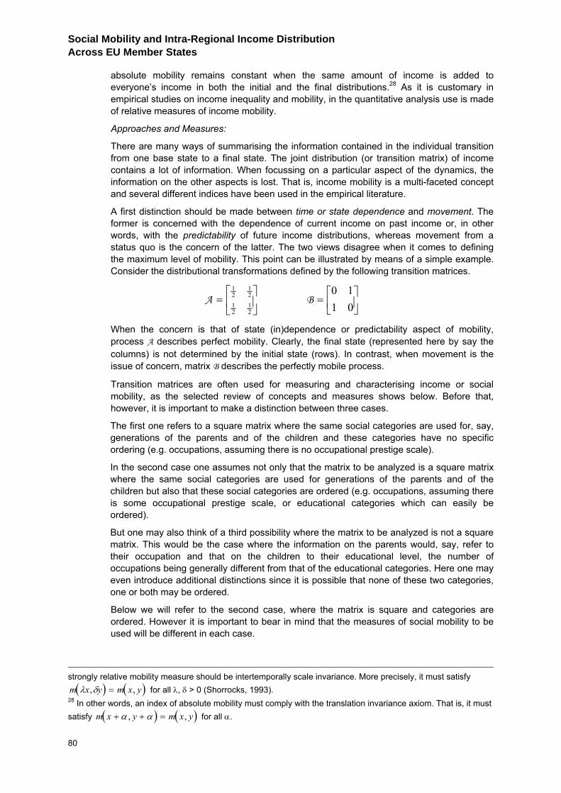
Social Mobility and Intra-Regional Income Distribution Across EU Member States
80
absolute mobility remains constant when the same amount of income is added to everyone’s income in both the initial and the final distributions.28 As it is customary in empirical studies on income inequality and mobility, in the quantitative analysis use is made of relative measures of income mobility.
Approaches and Measures:
There are many ways of summarising the information contained in the individual transition from one base state to a final state. The joint distribution (or transition matrix) of income contains a lot of information. When focussing on a particular aspect of the dynamics, the information on the other aspects is lost. That is, income mobility is a multi-faceted concept and several different indices have been used in the empirical literature.
A first distinction should be made between time or state dependence and movement. The former is concerned with the dependence of current income on past income or, in other words, with the predictability of future income distributions, whereas movement from a status quo is the concern of the latter. The two views disagree when it comes to defining the maximum level of mobility. This point can be illustrated by means of a simple example. Consider the distributional transformations defined by the following transition matrices.
A =⎡
⎣⎢
⎤
⎦⎥
12
12
12
12
B =⎡
⎣⎢⎤
⎦⎥0 11 0
When the concern is that of state (in)dependence or predictability aspect of mobility, process A describes perfect mobility. Clearly, the final state (represented here by say the columns) is not determined by the initial state (rows). In contrast, when movement is the issue of concern, matrix B describes the perfectly mobile process.
Transition matrices are often used for measuring and characterising income or social mobility, as the selected review of concepts and measures shows below. Before that, however, it is important to make a distinction between three cases.
The first one refers to a square matrix where the same social categories are used for, say, generations of the parents and of the children and these categories have no specific ordering (e.g. occupations, assuming there is no occupational prestige scale).
In the second case one assumes not only that the matrix to be analyzed is a square matrix where the same social categories are used for generations of the parents and of the children but also that these social categories are ordered (e.g. occupations, assuming there is some occupational prestige scale, or educational categories which can easily be ordered).
But one may also think of a third possibility where the matrix to be analyzed is not a square matrix. This would be the case where the information on the parents would, say, refer to their occupation and that on the children to their educational level, the number of occupations being generally different from that of the educational categories. Here one may even introduce additional distinctions since it is possible that none of these two categories, one or both may be ordered.
Below we will refer to the second case, where the matrix is square and categories are ordered. However it is important to bear in mind that the measures of social mobility to be used will be different in each case.
strongly relative mobility measure should be intertemporally scale invariance. More precisely, it must satisfy ( ) ( )m x y m x yλ δ, ,= for all λ, δ > 0 (Shorrocks, 1993).
28 In other words, an index of absolute mobility must comply with the translation invariance axiom. That is, it must satisfy ( ) ( )m x y m x y+ + =α α, , for all α.
3. SOCIAL MOBILITY
81
1. State dependence or predictability: mobility can be captured by the extent to which final income (state) depends on initial income (state). Complete state dependence, then, will occur when the original or base state fully determines the final state; for instance, when everybody has exactly the same income level in the initial and final distributions. Complete state independence is given by a situation where the probability of ending up in a particular state is the same, regardless of the origin earnings state, namely q-1, q being the number of states. In other words, each individual is facing a lottery with equiprobable outcomes. Thus, mobility may imply insecurity, uncertainty, or unpredictability, which in turn may be welfare reducing. Thus care is necessary in interpreting findings relating to state dependent income mobility.
The transition matrix is especially suitable to study the state dependence facet of mobility. When the elements of the diagonal are equal to one (and off-diagonal elements are zero) state dependence is maximal (i.e. perfect immobility), while complete state independence occurs when all transition probabilities are the same (i.e. perfect mobility). Shorrocks (1978a) suggests that a suitable index to summarise the predictability and origin (in)dependence aspects of mobility is
1)(
−−
=q
PtrqM D ,
where tr(P) denotes the trace of the transition matrix P. Shorrocks (1978a) shows that MD satisfies two basic axioms for the subset of matrices with a maximal diagonal, i.e. where the probability of staying in the same class is not smaller than the probability of moving out to another class. The first property guarantees that mobility increases as off-diagonal cells of the matrix increase, while the second one assigns the maximum value of the index (i.e. perfect mobility) to matrices with identical cells, i.e. picks up the state dependence aspect of mobility. MD could be a good index to use to estimate social mobility using a discrete variable (e.g. education, occupation, social class).
With continuous variables, such as income, origin dependence can be measured by means of the complementary of the correlation coefficient between the log of the base (x) and final year incomes (y), an index due to Hart (1983) and axiomatised by Shorrocks (1993).
( )1 log , logHM x yρ= − .
When the rank of the individual in a distribution is supposed to capture the social status of individuals, D’Agostino and Dardanoni (2009a) show that Spearman’s rank correlation index is a good measure of immobility, which satisfies a sort of ‘weak decomposability property’ that allows decomposing overall rank mobility into the rank mobility of each partition with respect to the overall distribution, where the rank of each individual is evaluated with reference to the whole distribution. This measure can be written as
( )16
1 21
2
−−= ∑ =
nnd
Mn
i iS ,
where di is the difference in the ranks of individual i in the two distributions, say, X and Y, and n is the total number of individuals. The sign of the Spearman correlation indicates the direction of association between X and Y. If Y tends to increase when X increases, the Spearman correlation coefficient is positive. If Y tends to decrease when X increases, the Spearman correlation coefficient is negative. A Spearman correlation of zero indicates perfect mobility, i.e. there is no tendency for Y to either increase or decrease when X increases. The Spearman correlation increases in magnitude as X and Y become closer to being perfect monotone functions of each other. When X and Y are perfectly monotonically related, that is there is complete immobility, the Spearman correlation coefficient becomes 1.
Social Mobility and Intra-Regional Income Distribution Across EU Member States
82
The empirical literature on intergenerational income mobility uses mostly a measure of time dependence, namely the beta coefficient of a regression of the child’s log income on the log income of the parent is a measure of time dependence (see the contributions in the special issue on intergenerational mobility of the BE Journal of Economic Policy & Analysis).
2. Movement: another aspect of mobility is movement per se. Atkinson (1981, p. 62) argues that the movement aspect of mobility may “...be viewed as an objective in its own right. Society may attach a positive weight to fluidity as such”. Again, if individual income does not change over time (absolute (im)mobility) or changes in the same proportion for all individuals (relative (im)mobility), the movement aspect of mobility will be zero. To determine maximal movement requires an accurate definition of movement. Some of the many possible definitions of movement (for an exhaustive account, see Fields, 2007) are considered below.
Positional movement: an individual experiences positional movement when she changes her position in the income scale or ladder, as measured by quintiles, deciles, ranks or classes defined in some other way. Positional movement in a population increases with the number of positional changes and/or with the length of such positional changes. Note that a person can experience relative income mobility even if her own income does not change, provided that others’ incomes change by enough so that the person in question experiences a change in position. Positional movement is conceptually very similar to exchange mobility discussed below.
A candidate measure of positional movement is the re-ranking index M(υ)
( ) ( )( ) ( )( ) ( )0 11
; ; ,z z
z z
yM w F x w F y h x y dxdyυ υ υµ
+ +
− −
⎛ ⎞⎡ ⎤= − ⎜ ⎟⎣ ⎦
⎝ ⎠∫ ∫ ,
where w(·) are social weights determined by the (normalised) position of the individual in the income distribution(s), ( )0F x and ( )1F y , and the aversion parameter υ, z- and z+ are
the lower and upper limits of the domain of the income distribution, µ1 is the mean income in the final year, and h(x,y) denotes the joint probability density function of incomes in the base and final years. The expression above shows that M(υ ) is a relative-income weighted average of changes in social weights, which are determined by rank. In particular, weights are a decreasing function of individual’s rank in the income pecking order, i.e. poorer individuals weight more than richer individuals.
This is the mobility measure used by Jenkins and Van Kerm (2006) in their decomposition of inequality trends, which is used in the quantitative analysis to relate the two distributive concepts: state dependence and inequality (see Section 4.2).
M(υ) may be also expressed as the difference between the S-Gini coefficient of final year incomes, ( )1G υ , and the (generalized) concentration coefficient29 for year 1 incomes
calculated using year 0 rankings, ( ) ( )01G υ .
( ) ( ) ( ) ( )01 1M G Gυ υ υ= −
With no reranking, individual income positions and social weights remain unchanged, Lorenz and concentration curves30 are identical, and M(υ)=0.
29 The (generalized) concentration coefficient is analogous to the generalized Gini coefficient when concentration curves are used instead of Lorenz curves. See the next footnote for a definition of a concentration curve. 30 Recall that Lorenz curves graph cumulative percentage of a variable (say post-tax income) against the cumulative population shares when population is ordered according to the same variable (i.e.post-tax income). Concentration curves instead depict the cumulative percentage of a variable (say post-tax income) against the cumulative population share ordered according to another variable (say pre-tax income). Lorenz and
3. SOCIAL MOBILITY
83
Yitzhaki and Wodon (2004), using the ‘standard’ Gini coefficient, propose the use of a related index [M(2)/G1(2)]31 as a mobility measure, which shows maximum movement when ranks of income groups are entirely reversed between the base and final distributions.
Income flux or non-directional income movement: measures the extent of fluctuation in individual’s incomes. To this approach gains and losses are weighted similarly without regard to the direction of change. Two indices have been suggested by Fields and Ok (1996 and 1999b):
∑ =−=
n
i iiF xyn
M11
1
and
∑ =−=
n
i iiF xyn
M12 loglog1
Contrary to the first index, the latter assigns greater weight to income movements that take place at the bottom part of the distribution.
D’Agostino and Dardanoni (2009b) suggest using a variation of the Euclidian distance, which they call Averaged Generalized Euclidian Distance (AGED) as index of mobility,
( )∑ =−=
n
i iiAGED ygxgn
M1
2)()(1
where g(·) is a continuous and increasing function, which they suggest to be the log function. This index is subgroups consistent and is also consistent with and exchange mobility principle, which requires that the increase in the distance between two vectors caused by any ‘order-reversing swap’ depends monotonically on the distance, in each vector, between the components (not their value) that are involved in the swap.
Directional income movement: according to this approach, direction as well as the magnitude of income changes matter for income mobility. Fields and Ok (1999b) suggest an index of directional movement, which takes into account the income level of income gainers and income losers when evaluating income changes, i.e. sensitive to the income level of the recipient.
( )∑ =−=
n
i iiDIM xyn
M1
loglog1.
3. Mobility as equaliser of longer term incomes. One of the primary motivations for economic mobility studies is to gauge the extent to which longer-term incomes are distributed more or less equally than are single-year incomes. Many economists have argued that mobility attenuates the importance of inequality since lifetime income is more even. That is, income mobility is an equalizer of longer-term incomes. Shorrocks (1978b) suggests an index of mobility, which builds on the equalizing effect of mobility. Since this approach relates cross-section to longer-term inequality it is further detailed in Section 2.2.
Does the application of different measures of income mobility matter in practice?
Clearly income mobility has many different meanings, which may be measured with different indices, but do they lead to different mobility rankings? The empirical analyses available clearly show that different concepts and measures yield different results when comparing countries (OECD, 1996 and 1997), the same country over time (Fields, Leary and Ok, 2002; Fields, 2005), or population subgroups (Buchinsky et al., 2004).
concentration curves, then are the same as long as the two distributions (pre- and post-tax incomes) rank individuals the same way, and differ as soon as there is re-ranking. 31 This means that the index is evaluated at υ =2.
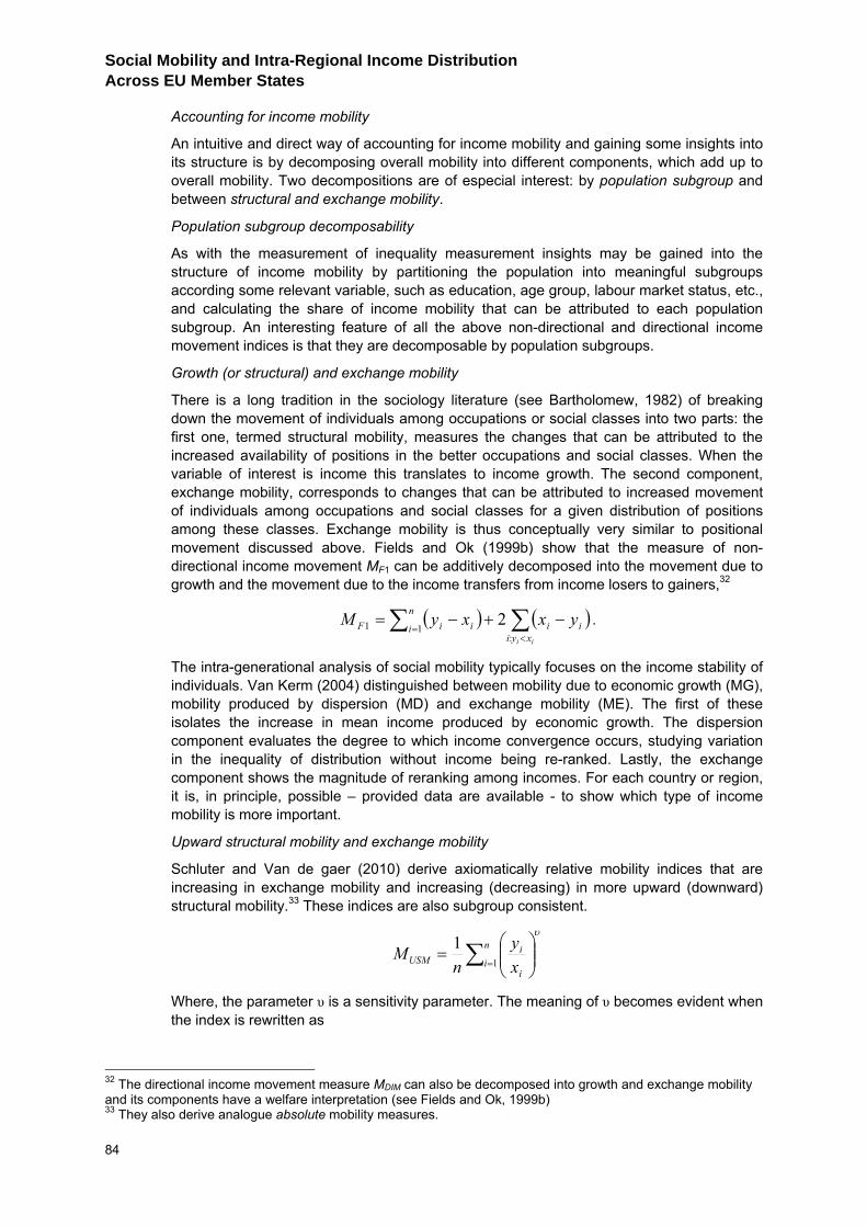
Social Mobility and Intra-Regional Income Distribution Across EU Member States
84
Accounting for income mobility
An intuitive and direct way of accounting for income mobility and gaining some insights into its structure is by decomposing overall mobility into different components, which add up to overall mobility. Two decompositions are of especial interest: by population subgroup and between structural and exchange mobility.
Population subgroup decomposability
As with the measurement of inequality measurement insights may be gained into the structure of income mobility by partitioning the population into meaningful subgroups according some relevant variable, such as education, age group, labour market status, etc., and calculating the share of income mobility that can be attributed to each population subgroup. An interesting feature of all the above non-directional and directional income movement indices is that they are decomposable by population subgroups.
Growth (or structural) and exchange mobility
There is a long tradition in the sociology literature (see Bartholomew, 1982) of breaking down the movement of individuals among occupations or social classes into two parts: the first one, termed structural mobility, measures the changes that can be attributed to the increased availability of positions in the better occupations and social classes. When the variable of interest is income this translates to income growth. The second component, exchange mobility, corresponds to changes that can be attributed to increased movement of individuals among occupations and social classes for a given distribution of positions among these classes. Exchange mobility is thus conceptually very similar to positional movement discussed above. Fields and Ok (1999b) show that the measure of non-directional income movement MF1 can be additively decomposed into the movement due to growth and the movement due to the income transfers from income losers to gainers,32
( ) ( )∑ ∑=<
−+−=n
ixyi
iiiiFii
yxxyM1
:1 2 .
The intra-generational analysis of social mobility typically focuses on the income stability of individuals. Van Kerm (2004) distinguished between mobility due to economic growth (MG), mobility produced by dispersion (MD) and exchange mobility (ME). The first of these isolates the increase in mean income produced by economic growth. The dispersion component evaluates the degree to which income convergence occurs, studying variation in the inequality of distribution without income being re-ranked. Lastly, the exchange component shows the magnitude of reranking among incomes. For each country or region, it is, in principle, possible – provided data are available - to show which type of income mobility is more important.
Upward structural mobility and exchange mobility
Schluter and Van de gaer (2010) derive axiomatically relative mobility indices that are increasing in exchange mobility and increasing (decreasing) in more upward (downward) structural mobility.33 These indices are also subgroup consistent.
υ
∑ = ⎟⎟⎠
⎞⎜⎜⎝
⎛=
n
ii
iUSM x
yn
M1
1
Where, the parameter υ is a sensitivity parameter. The meaning of υ becomes evident when the index is rewritten as
32 The directional income movement measure MDIM can also be decomposed into growth and exchange mobility and its components have a welfare interpretation (see Fields and Ok, 1999b) 33 They also derive analogue absolute mobility measures.
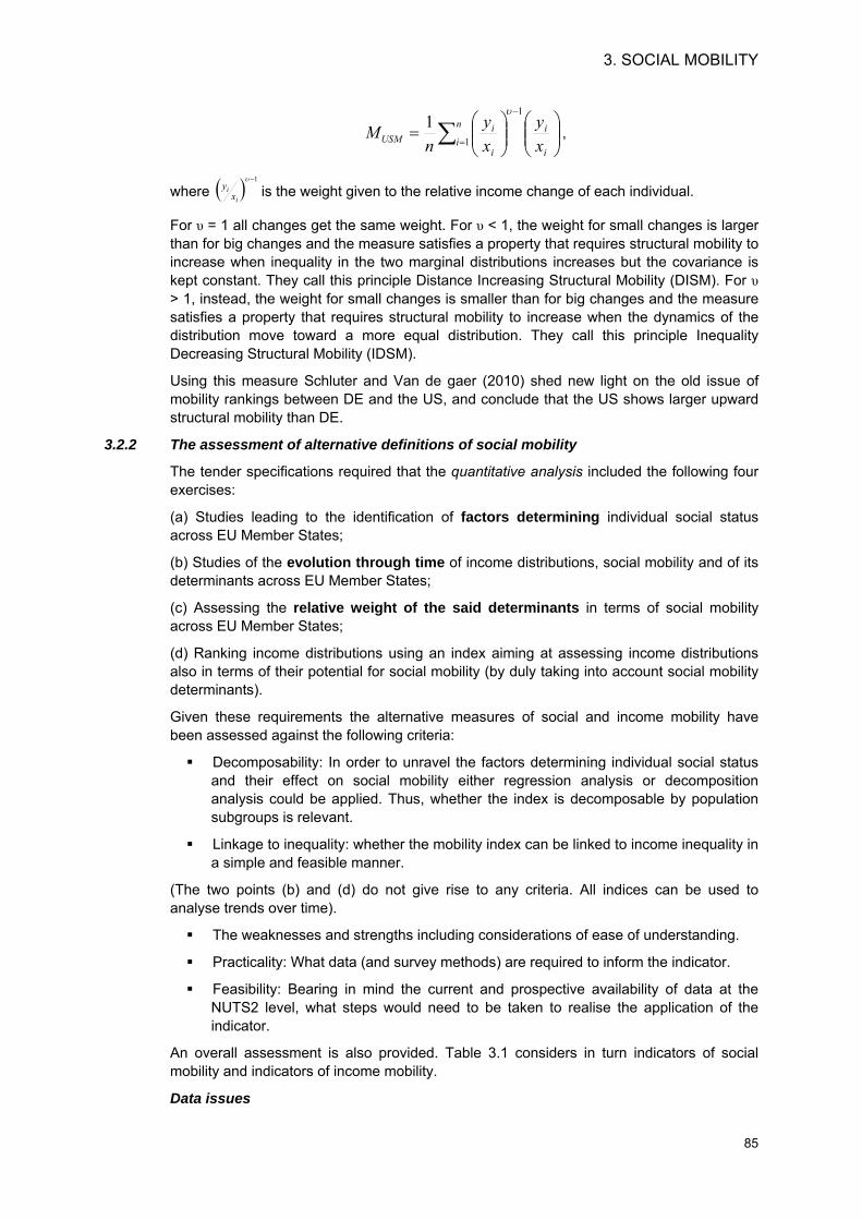
3. SOCIAL MOBILITY
85
⎟⎟⎠
⎞⎜⎜⎝
⎛⎟⎟⎠
⎞⎜⎜⎝
⎛=
−
=∑i
in
ii
iUSM x
yxy
nM
1
1
1υ
,
where ( ) 1−υ
iix
y is the weight given to the relative income change of each individual.
For υ = 1 all changes get the same weight. For υ < 1, the weight for small changes is larger than for big changes and the measure satisfies a property that requires structural mobility to increase when inequality in the two marginal distributions increases but the covariance is kept constant. They call this principle Distance Increasing Structural Mobility (DISM). For υ > 1, instead, the weight for small changes is smaller than for big changes and the measure satisfies a property that requires structural mobility to increase when the dynamics of the distribution move toward a more equal distribution. They call this principle Inequality Decreasing Structural Mobility (IDSM).
Using this measure Schluter and Van de gaer (2010) shed new light on the old issue of mobility rankings between DE and the US, and conclude that the US shows larger upward structural mobility than DE.
3.2.2 The assessment of alternative definitions of social mobility
The tender specifications required that the quantitative analysis included the following four exercises:
(a) Studies leading to the identification of factors determining individual social status across EU Member States;
(b) Studies of the evolution through time of income distributions, social mobility and of its determinants across EU Member States;
(c) Assessing the relative weight of the said determinants in terms of social mobility across EU Member States;
(d) Ranking income distributions using an index aiming at assessing income distributions also in terms of their potential for social mobility (by duly taking into account social mobility determinants).
Given these requirements the alternative measures of social and income mobility have been assessed against the following criteria:
Decomposability: In order to unravel the factors determining individual social status and their effect on social mobility either regression analysis or decomposition analysis could be applied. Thus, whether the index is decomposable by population subgroups is relevant.
Linkage to inequality: whether the mobility index can be linked to income inequality in a simple and feasible manner.
(The two points (b) and (d) do not give rise to any criteria. All indices can be used to analyse trends over time).
The weaknesses and strengths including considerations of ease of understanding.
Practicality: What data (and survey methods) are required to inform the indicator.
Feasibility: Bearing in mind the current and prospective availability of data at the NUTS2 level, what steps would need to be taken to realise the application of the indicator.
An overall assessment is also provided. Table 3.1 considers in turn indicators of social mobility and indicators of income mobility.
Data issues

Social Mobility and Intra-Regional Income Distribution Across EU Member States
86
Empirical studies of income mobility require longitudinal and good-quality data. Comparative studies also need a harmonised effort to obtain data with similar characteristics (see Lillard, 2007). However, even (ex-ante) harmonised and well-designed longitudinal data sets may encounter problems, which bias cross-national comparisons (Burkhauser and Couch, 2009). For instance, problems may arise because of unsystematic treatment of top coding (ie coding of very high incomes), usually used to preserve confidentiality, (Burkhauser et al., 2007 and Larrimore et al., 2008) or due to differential attrition problems (people from different groups drop out differently), a serious problem with the ECHP (Burkhauser and Couch, 2009).
In many European countries the longest and most important longitudinal data set is the ECHP which covers a relatively short time span (began in 1994 and was discontinued in 2001). Only few countries, such as DE and GB, have longer panels. As described in Section 1, use has been made of EU-SILC and CNEF panel data in this assignment.
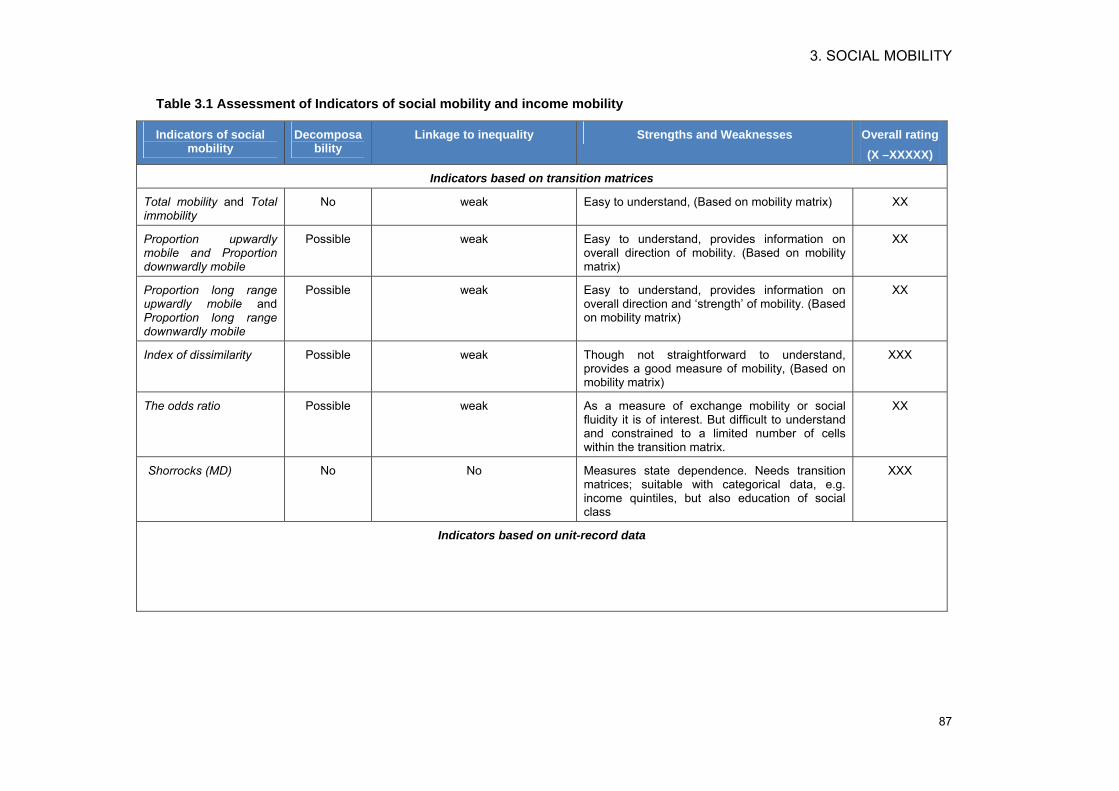
3. SOCIAL MOBILITY
87
Table 3.1 Assessment of Indicators of social mobility and income mobility
Indicators of social mobility
Decomposability
Linkage to inequality Strengths and Weaknesses Overall rating (X –XXXXX)
Indicators based on transition matrices
Total mobility and Total immobility
No weak Easy to understand, (Based on mobility matrix) XX
Proportion upwardly mobile and Proportion downwardly mobile
Possible weak Easy to understand, provides information on overall direction of mobility. (Based on mobility matrix)
XX
Proportion long range upwardly mobile and Proportion long range downwardly mobile
Possible weak Easy to understand, provides information on overall direction and ‘strength’ of mobility. (Based on mobility matrix)
XX
Index of dissimilarity Possible weak Though not straightforward to understand, provides a good measure of mobility, (Based on mobility matrix)
XXX
The odds ratio Possible weak As a measure of exchange mobility or social fluidity it is of interest. But difficult to understand and constrained to a limited number of cells within the transition matrix.
XX
Shorrocks (MD) No No Measures state dependence. Needs transition matrices; suitable with categorical data, e.g. income quintiles, but also education of social class
XXX
Indicators based on unit-record data
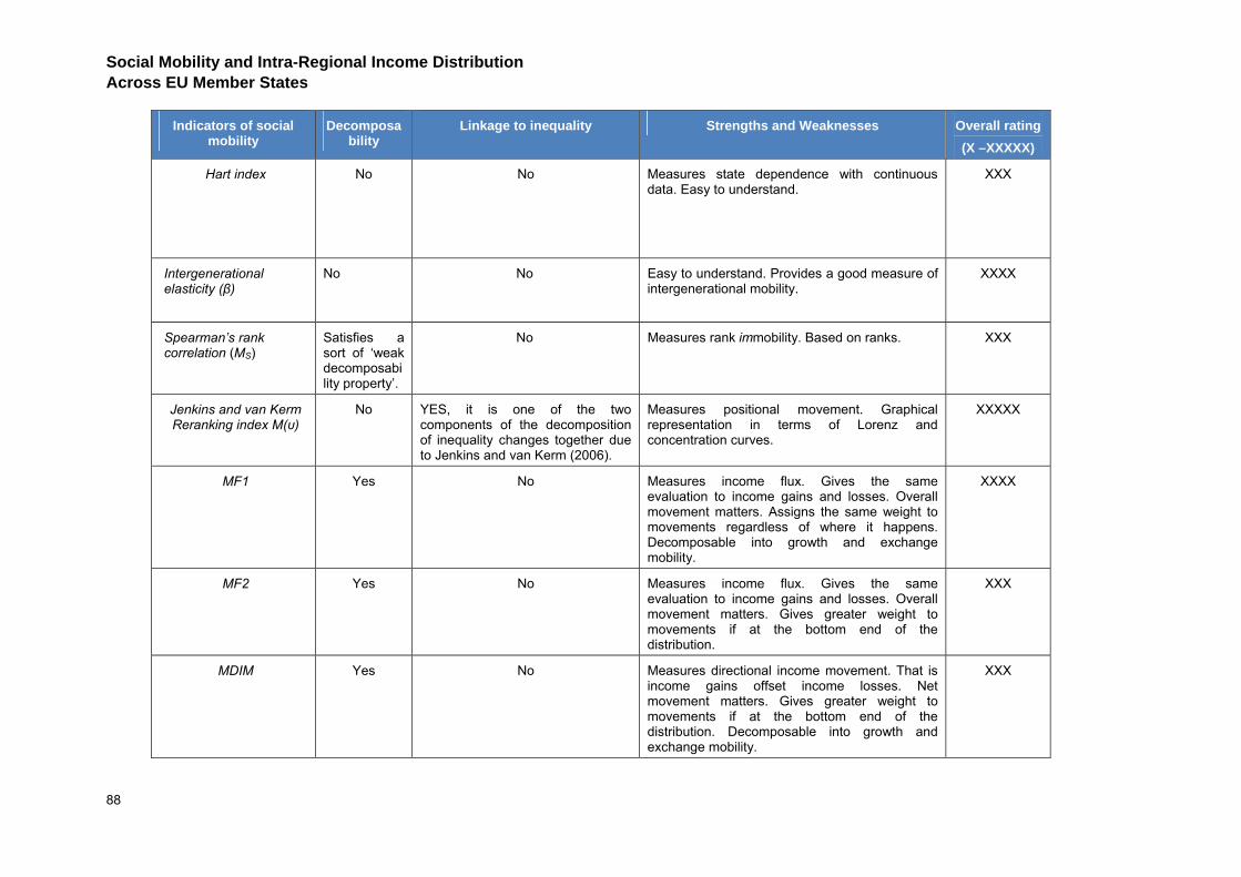
Social Mobility and Intra-Regional Income Distribution Across EU Member States
88
Indicators of social mobility
Decomposability
Linkage to inequality Strengths and Weaknesses Overall rating (X –XXXXX)
Hart index No No
Measures state dependence with continuous data. Easy to understand.
XXX
Intergenerational elasticity (β)
No No Easy to understand. Provides a good measure of intergenerational mobility.
XXXX
Spearman’s rank correlation (MS)
Satisfies a sort of ‘weak decomposability property’.
No Measures rank immobility. Based on ranks. XXX
Jenkins and van Kerm Reranking index M(υ)
No YES, it is one of the two components of the decomposition of inequality changes together due to Jenkins and van Kerm (2006).
Measures positional movement. Graphical representation in terms of Lorenz and concentration curves.
XXXXX
MF1 Yes No Measures income flux. Gives the same evaluation to income gains and losses. Overall movement matters. Assigns the same weight to movements regardless of where it happens. Decomposable into growth and exchange mobility.
XXXX
MF2 Yes No Measures income flux. Gives the same evaluation to income gains and losses. Overall movement matters. Gives greater weight to movements if at the bottom end of the distribution.
XXX
MDIM Yes No Measures directional income movement. That is income gains offset income losses. Net movement matters. Gives greater weight to movements if at the bottom end of the distribution. Decomposable into growth and exchange mobility.
XXX
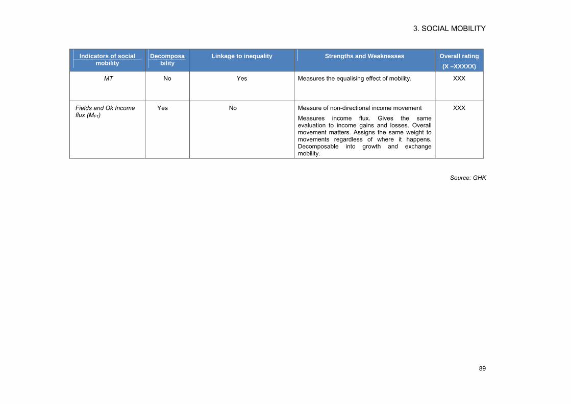
3. SOCIAL MOBILITY
89
Indicators of social mobility
Decomposability
Linkage to inequality Strengths and Weaknesses Overall rating (X –XXXXX)
MT No Yes Measures the equalising effect of mobility. XXX
Fields and Ok Income flux (MF1)
Yes No Measure of non-directional income movement
Measures income flux. Gives the same evaluation to income gains and losses. Overall movement matters. Assigns the same weight to movements regardless of where it happens. Decomposable into growth and exchange mobility.
XXX
Source: GHK
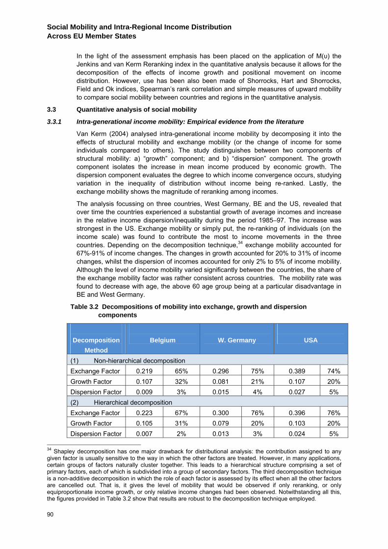
Social Mobility and Intra-Regional Income Distribution Across EU Member States
90
In the light of the assessment emphasis has been placed on the application of M(υ) the Jenkins and van Kerm Reranking index in the quantitative analysis because it allows for the decomposition of the effects of income growth and positional movement on income distribution. However, use has been also been made of Shorrocks, Hart and Shorrocks, Field and Ok indices, Spearman’s rank correlation and simple measures of upward mobility to compare social mobility between countries and regions in the quantitative analysis.
3.3 Quantitative analysis of social mobility
3.3.1 Intra-generational income mobility: Empirical evidence from the literature
Van Kerm (2004) analysed intra-generational income mobility by decomposing it into the effects of structural mobility and exchange mobility (or the change of income for some individuals compared to others). The study distinguishes between two components of structural mobility: a) “growth” component; and b) “dispersion” component. The growth component isolates the increase in mean income produced by economic growth. The dispersion component evaluates the degree to which income convergence occurs, studying variation in the inequality of distribution without income being re-ranked. Lastly, the exchange mobility shows the magnitude of reranking among incomes.
The analysis focussing on three countries, West Germany, BE and the US, revealed that over time the countries experienced a substantial growth of average incomes and increase in the relative income dispersion/inequality during the period 1985–97. The increase was strongest in the US. Exchange mobility or simply put, the re-ranking of individuals (on the income scale) was found to contribute the most to income movements in the three countries. Depending on the decomposition technique,34 exchange mobility accounted for 67%-91% of income changes. The changes in growth accounted for 20% to 31% of income changes, whilst the dispersion of incomes accounted for only 2% to 5% of income mobility. Although the level of income mobility varied significantly between the countries, the share of the exchange mobility factor was rather consistent across countries. The mobility rate was found to decrease with age, the above 60 age group being at a particular disadvantage in BE and West Germany.
Table 3.2 Decompositions of mobility into exchange, growth and dispersion components
Decomposition
Method
Belgium
W. Germany
USA
(1) Non-hierarchical decomposition Exchange Factor 0.219 65% 0.296 75% 0.389 74% Growth Factor 0.107 32% 0.081 21% 0.107 20% Dispersion Factor 0.009 3% 0.015 4% 0.027 5% (2) Hierarchical decomposition Exchange Factor 0.223 67% 0.300 76% 0.396 76% Growth Factor 0.105 31% 0.079 20% 0.103 20% Dispersion Factor 0.007 2% 0.013 3% 0.024 5%
34 Shapley decomposition has one major drawback for distributional analysis: the contribution assigned to any given factor is usually sensitive to the way in which the other factors are treated. However, in many applications, certain groups of factors naturally cluster together. This leads to a hierarchical structure comprising a set of primary factors, each of which is subdivided into a group of secondary factors. The third decomposition technique is a non-additive decomposition in which the role of each factor is assessed by its effect when all the other factors are cancelled out. That is, it gives the level of mobility that would be observed if only reranking, or only equiproportionate income growth, or only relative income changes had been observed. Notwithstanding all this, the figures provided in Table 3.2 show that results are robust to the decomposition technique employed.
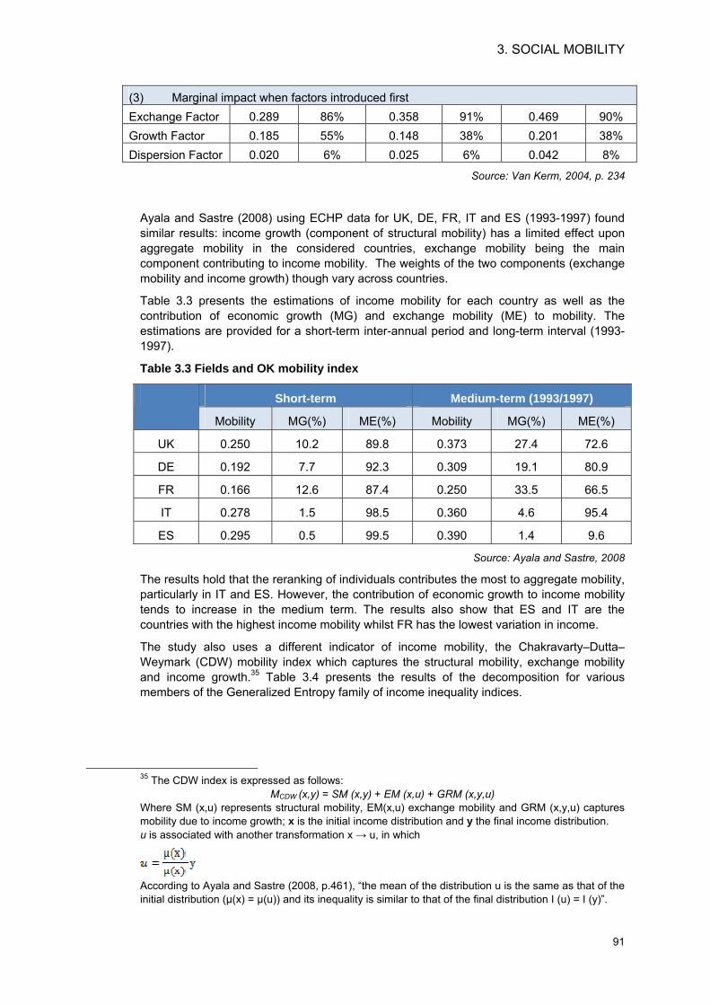
3. SOCIAL MOBILITY
91
(3) Marginal impact when factors introduced first Exchange Factor 0.289 86% 0.358 91% 0.469 90% Growth Factor 0.185 55% 0.148 38% 0.201 38% Dispersion Factor 0.020 6% 0.025 6% 0.042 8%
Source: Van Kerm, 2004, p. 234
Ayala and Sastre (2008) using ECHP data for UK, DE, FR, IT and ES (1993-1997) found similar results: income growth (component of structural mobility) has a limited effect upon aggregate mobility in the considered countries, exchange mobility being the main component contributing to income mobility. The weights of the two components (exchange mobility and income growth) though vary across countries.
Table 3.3 presents the estimations of income mobility for each country as well as the contribution of economic growth (MG) and exchange mobility (ME) to mobility. The estimations are provided for a short-term inter-annual period and long-term interval (1993-1997).
Table 3.3 Fields and OK mobility index
Short-term Medium-term (1993/1997)
Mobility MG(%) ME(%) Mobility MG(%) ME(%)
UK 0.250 10.2 89.8 0.373 27.4 72.6
DE 0.192 7.7 92.3 0.309 19.1 80.9
FR 0.166 12.6 87.4 0.250 33.5 66.5
IT 0.278 1.5 98.5 0.360 4.6 95.4
ES 0.295 0.5 99.5 0.390 1.4 9.6
Source: Ayala and Sastre, 2008
The results hold that the reranking of individuals contributes the most to aggregate mobility, particularly in IT and ES. However, the contribution of economic growth to income mobility tends to increase in the medium term. The results also show that ES and IT are the countries with the highest income mobility whilst FR has the lowest variation in income.
The study also uses a different indicator of income mobility, the Chakravarty–Dutta–Weymark (CDW) mobility index which captures the structural mobility, exchange mobility and income growth.35 Table 3.4 presents the results of the decomposition for various members of the Generalized Entropy family of income inequality indices.
35 The CDW index is expressed as follows:
MCDW (x,y) = SM (x,y) + EM (x,u) + GRM (x,y,u) Where SM (x,u) represents structural mobility, EM(x,u) exchange mobility and GRM (x,y,u) captures mobility due to income growth; x is the initial income distribution and y the final income distribution. u is associated with another transformation x → u, in which
According to Ayala and Sastre (2008, p.461), “the mean of the distribution u is the same as that of the initial distribution (µ(x) = µ(u)) and its inequality is similar to that of the final distribution I (u) = I (y)”.
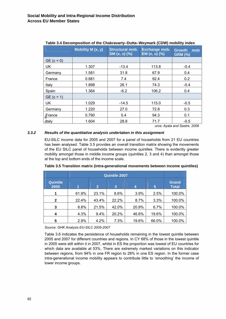
Social Mobility and Intra-Regional Income Distribution Across EU Member States
92
So
urce: Ayala and Sastre, 2008
3.3.2 Results of the quantitative analysis undertaken in this assignment
EU-SILC income data for 2005 and 2007 for a panel of households from 21 EU countries has been analysed. Table 3.5 provides an overall transition matrix showing the movements of the EU SILC panel of households between income quintiles. There is evidently greater mobility amongst those in middle income groups (quintiles 2, 3 and 4) than amongst those at the top and bottom ends of the income scale.
Table 3.5 Transition matrix (intra-generational movements between income quintiles)
Quintile 2007
Quintile 2005 1 2 3 4 5
Grand Total
1 61.9% 23.1% 8.6% 3.9% 2.5% 100.0%
2 22.4% 43.4% 22.2% 8.7% 3.3% 100.0%
3 8.8% 21.5% 42.0% 20.9% 6.7% 100.0%
4 4.3% 9.4% 20.2% 46.6% 19.6% 100.0%
5 2.9% 4.2% 7.3% 19.6% 66.0% 100.0%
Source: GHK Analysis EU-SILC 2005-2007
Table 3.6 indicates the persistence of households remaining in the lowest quintile between 2005 and 2007 for different countries and regions. In CY 68% of those in the lowest quintile in 2005 were still within it in 2007, whilst in ES the proportion was lowest of EU countries for which data are available at 53%. There are extremely marked variations on this indicator between regions, from 94% in one FR region to 28% in one ES region. In the former case intra-generational income mobility appears to contribute little to ‘smoothing’ the income of lower income groups.
Table 3.4 Decomposition of the Chakravarty–Dutta–Weymark (CDW) mobility index Mobility M (x, y) Structural mob.
SM (x, u) (%) Exchange mob. EM (x, u) (%)
Growth mob GRM (%)
GE (c = 0) UK 1.307 -13.4 113.8 -0.4 Germany 1.581 31.8 67.9 0.4 France 0.881 7.4 92.4 0.2 Italy 1.898 26.1 74.3 -0.4 Spain 1.364 -6.2 106.2 0.4 GE (c = 1) UK 1.029 -14.5 115.0 -0.5 Germany 1.220 27.0 72.8 0.3 France 0.790 5.4 94.3 0.1 Italy 1.604 28.8 71.7 -0.5
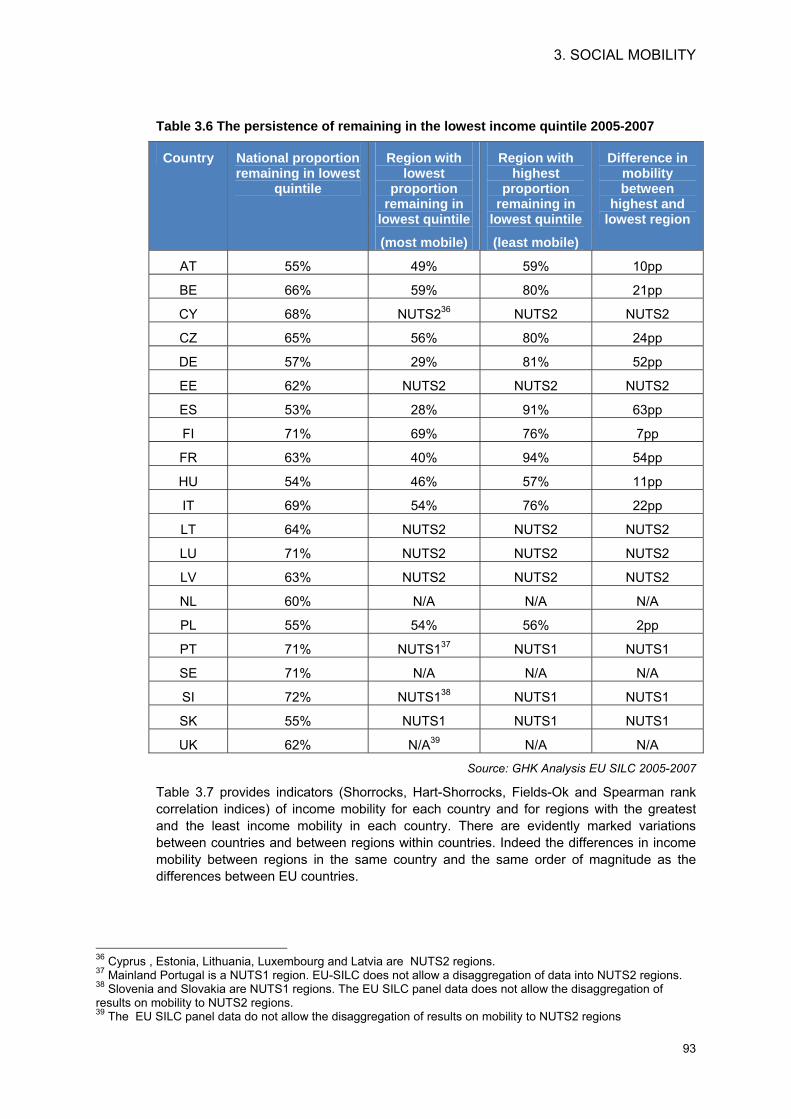
3. SOCIAL MOBILITY
93
Table 3.6 The persistence of remaining in the lowest income quintile 2005-2007
Country National proportion remaining in lowest
quintile
Region with lowest
proportion remaining in
lowest quintile
(most mobile)
Region with highest
proportion remaining in
lowest quintile
(least mobile)
Difference in mobility between
highest and lowest region
AT 55% 49% 59% 10pp
BE 66% 59% 80% 21pp
CY 68% NUTS236 NUTS2 NUTS2
CZ 65% 56% 80% 24pp
DE 57% 29% 81% 52pp
EE 62% NUTS2 NUTS2 NUTS2
ES 53% 28% 91% 63pp
FI 71% 69% 76% 7pp
FR 63% 40% 94% 54pp
HU 54% 46% 57% 11pp
IT 69% 54% 76% 22pp
LT 64% NUTS2 NUTS2 NUTS2
LU 71% NUTS2 NUTS2 NUTS2
LV 63% NUTS2 NUTS2 NUTS2
NL 60% N/A N/A N/A
PL 55% 54% 56% 2pp
PT 71% NUTS137 NUTS1 NUTS1
SE 71% N/A N/A N/A
SI 72% NUTS138 NUTS1 NUTS1
SK 55% NUTS1 NUTS1 NUTS1
UK 62% N/A39 N/A N/A
Source: GHK Analysis EU SILC 2005-2007
Table 3.7 provides indicators (Shorrocks, Hart-Shorrocks, Fields-Ok and Spearman rank correlation indices) of income mobility for each country and for regions with the greatest and the least income mobility in each country. There are evidently marked variations between countries and between regions within countries. Indeed the differences in income mobility between regions in the same country and the same order of magnitude as the differences between EU countries.
36 Cyprus , Estonia, Lithuania, Luxembourg and Latvia are NUTS2 regions. 37 Mainland Portugal is a NUTS1 region. EU-SILC does not allow a disaggregation of data into NUTS2 regions. 38 Slovenia and Slovakia are NUTS1 regions. The EU SILC panel data does not allow the disaggregation of results on mobility to NUTS2 regions. 39 The EU SILC panel data do not allow the disaggregation of results on mobility to NUTS2 regions
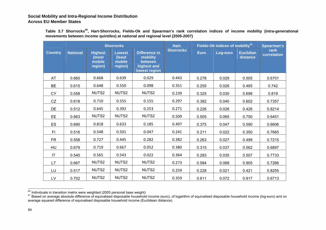
Social Mobility and Intra-Regional Income Distribution Across EU Member States
94
Table 3.7 Shorrocks40, Hart-Shorrocks, Fields-Ok and Spearman’s rank correlation indices of income mobility (intra-generational movements between income quintiles) at national and regional level (2005-2007)
Shorrocks Fields-Ok indices of mobility41
Country National
Highest (most mobile region)
Lowest (least
mobile region)
Difference in mobility between
highest and lowest region
Hart-Shorrocks Euro Log-euro Euclidian
distance
Spearman’s rank
correlation
AT 0.660 0.668 0.639 0.029 0.443 0.278 0.029 0.505 0.6701
BE 0.615 0.648 0.550 0.098 0.351 0.255 0.026 0.465 0.742
CY 0.558 NUTS2 NUTS2 NUTS2 0.239 0.325 0.030 0.698 0.819
CZ 0.618 0.710 0.555 0.155 0.297 0.382 0.040 0.602 0.7357
DE 0.512 0.645 0.392 0.253 0.271 0.226 0.026 0.426 0.8214
EE 0.663 NUTS2 NUTS2 NUTS2 0.509 0.505 0.065 0.750 0.6451
ES 0.690 0.818 0.633 0.185 0.497 0.375 0.047 0.590 0.6606
FI 0.516 0.548 0.501 0.047 0.241 0.211 0.022 0.350 0.7665
FR 0.558 0.727 0.445 0.282 0.382 0.263 0.027 0.499 0.7215
HU 0.679 0.719 0.667 0.052 0.380 0.315 0.037 0.562 0.6897
IT 0.540 0.565 0.543 0.022 0.364 0.283 0.035 0.507 0.7733
LT 0.667 NUTS2 NUTS2 NUTS2 0.273 0.584 0.068 0.905 0.7266
LU 0.517 NUTS2 NUTS2 NUTS2 0.259 0.228 0.021 0.421 0.8255
LV 0.702 NUTS2 NUTS2 NUTS2 0.359 0.611 0.072 0.917 0.6713
40 Individuals in transition matrix were weighted (2005 personal base weight) 41 Based on average absolute difference of equivalised disposable household income (euro), of logarithm of equivalised disposable household income (log-euro) and on average squared difference of equivalised disposable household income (Euclidean distance).
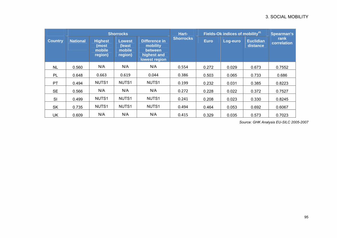
3. SOCIAL MOBILITY
95
Shorrocks Fields-Ok indices of mobility41
Country National
Highest (most mobile region)
Lowest (least
mobile region)
Difference in mobility between
highest and lowest region
Hart-Shorrocks Euro Log-euro Euclidian
distance
Spearman’s rank
correlation
NL 0.560 N/A N/A N/A 0.554 0.272 0.029 0.673 0.7552
PL 0.648 0.663 0.619 0.044 0.386 0.503 0.065 0.733 0.686
PT 0.494 NUTS1 NUTS1 NUTS1 0.199 0.232 0.031 0.385 0.8223
SE 0.566 N/A N/A N/A 0.272 0.228 0.022 0.372 0.7527
SI 0.499 NUTS1 NUTS1 NUTS1 0.241 0.208 0.023 0.330 0.8245
SK 0.735 NUTS1 NUTS1 NUTS1 0.494 0.464 0.053 0.692 0.6067
UK 0.609 N/A N/A N/A 0.415 0.329 0.035 0.573 0.7023
Source: GHK Analysis EU-SILC 2005-2007

Social Mobility and Intra-Regional Income Distribution Across EU Member States
96
7
3.3.3 Individual and household characteristics affecting income mobility
Using the EU-SILC panel data, a regression model was set up to identify the influence of selected individual and household factors on income mobility. Attempts were made to include as many as possible of the factors discussed in the relevant literature.
In this model, the change of logarithmic (equivalised42) household disposable annual income for individuals from the base year (2005) to the final year (2007) was treated as a dependent variable (i.e. the unit of analysis were individuals, potentially moving between households in the given time period). ‘Household income’ assessed is computed in the EU-SILC database as the sum for all household members of gross personal income components (including income from employment, benefits) plus gross income components at household level (including income from rental, family and other allowances, regular inter-household cash transfers, interests, dividends, profits) minus regular taxes on wealth, taxes on income, social insurance contributions and regular inter-household cash transfers paid.43 Disposable household income was top- and bottom-coded (as described in Annex 3) to mitigate the confounding effect of outliers.
This was regressed against a set of independent variables, notably:
Gender of the head of household in the base year (whether it was a woman)
Age of the head of household in the base year
Age-squared the head of household in the base year (to account for non-linear effects of age on income change)
Number of adults in the household in the base year
Number of children in the household in the base year
Difference in the number of adults in the household from the base to the final year (to account for household composition change, affecting both income and equivalisation factor)
Difference in the number of children in the household from the base to the final year (to account for household composition change, affecting the equivalisation factor)
Number of persons in household in the base year with at least upper secondary education (ISCED 3)
Number of persons in household in the base year with higher education (ISCED 4 or 5)
Change in the number of full-time employed persons in household from the base to the final year
Change in the number of part-time employed persons in household from the base to the final year (this was treated separately as its coefficient and hence its impact on expected income change was very different from those of full-time employment, whilst both were significant explanatory variables).
This regression was undertaken on the residuals from a first regression which only included country dummies on the right-hand side in order to control for very different rates in the
42 Using the revised OECD equivalence scale, assigning a weight of 1 for the first (adult) member of the household, 0.5 for each adult (i.e. above 14 years old) and 0.3 for each child (i.e. up to 13 years old). 43 The total disposable household income corresponds to variable coded ‘HY020’, whilst the equivalent household size applied as divisor is coded ‘HX050’ in EU-SILC.
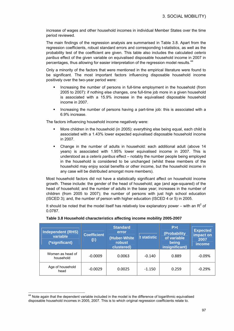
3. SOCIAL MOBILITY)
97
increase of wages and other household incomes in individual Member States over the time period reviewed.
The main findings of the regression analysis are summarised in Table 3.8. Apart from the regression coefficients, robust standard errors and corresponding t-statistics, as well as the probability test of the coefficient are given. This table also includes the calculated ceteris paribus effect of the given variable on equivalised disposable household income in 2007 in percentages, thus allowing for easier interpretation of the regression model results.44
Only a minority of the factors that were mentioned in the empirical literature were found to be significant. The most important factors influencing disposable household income positively over the two-year period were:
Increasing the number of persons in full-time employment in the household (from 2005 to 2007): if nothing else changes, one full-time job more in a given household is associated with a 15.9% increase in the equivalised disposable household income in 2007.
Increasing the number of persons having a part-time job: this is associated with a 6.9% increase.
The factors influencing household income negatively were:
More children in the household (in 2005): everything else being equal, each child is associated with a 1.43% lower expected equivalised disposable household income in 2007.
Change in the number of adults in household: each additional adult (above 14 years) is associated with 1.95% lower equivalised income in 2007. This is understood as a ceteris paribus effect – notably the number people being employed in the household is considered to be unchanged (whilst these members of the household may enjoy social benefits or other income, but the household income in any case will be distributed amongst more members).
Most household factors did not have a statistically significant affect on household income growth. These include: the gender of the head of household; age (and age-squared) of the head of household; and the number of adults in the base year; increases in the number of children (from 2005 to 2007); the number of persons with just high school education (ISCED 3); and, the number of person with higher education (ISCED 4 or 5) in 2005.
It should be noted that the model itself has relatively low explanatory power – with an R2 of 0.0787.
Table 3.8 Household characteristics affecting income mobility 2005-2007
Independent (RHS) variable
(*significant)
Coefficient (β)
Standard error
(Huber-White robust
clustered)
t statistic
P>t (Probability of variable
being insignificant)
Expected impact on
2007 income
Women as head of household -0.0009 0.0063 -0.140 0.889 -0.09%
Age of household head -0.0029 0.0025 -1.150 0.259 -0.29%
44 Note again that the dependent variable included in the model is the difference of logarithmic equivalised disposable household incomes in 2005, 2007. This is to which original regression coefficients relate to.
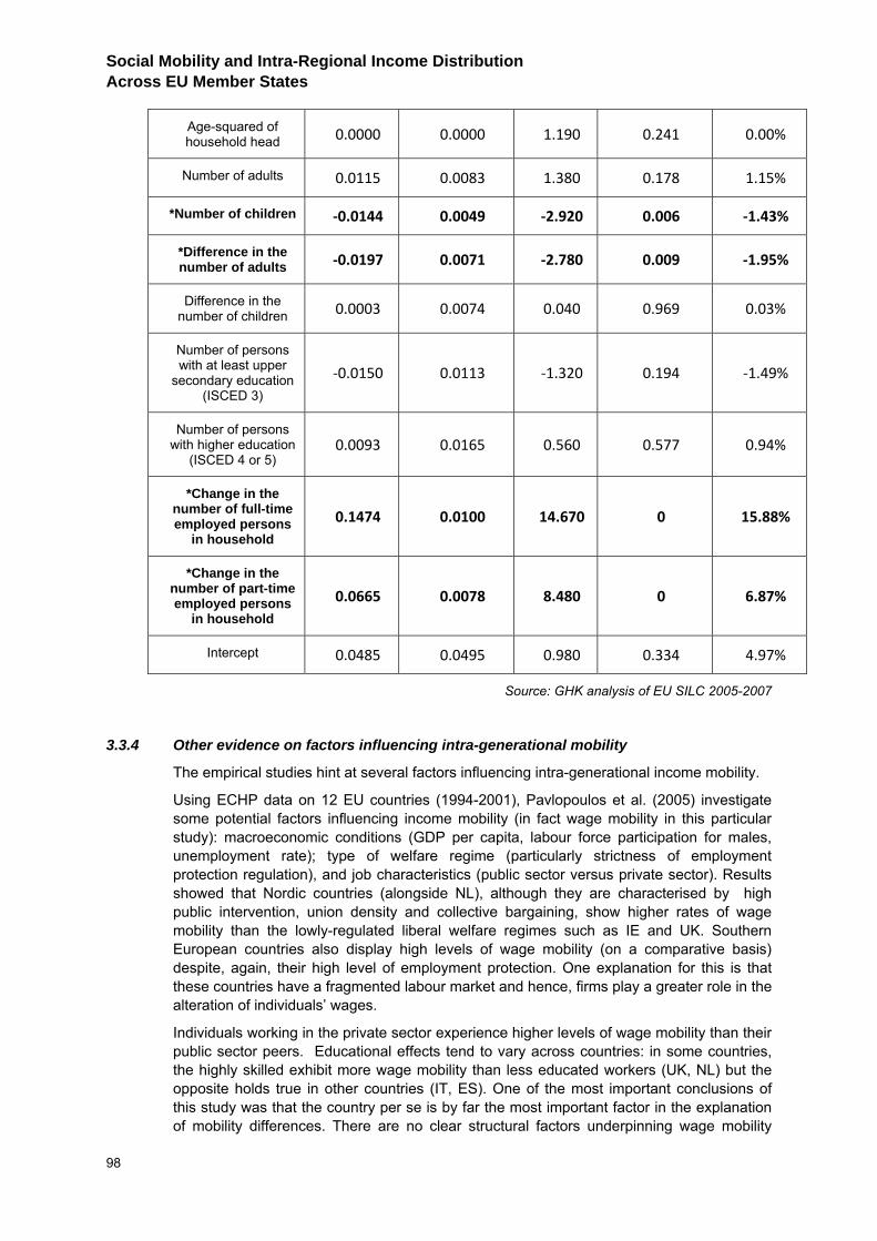
Social Mobility and Intra-Regional Income Distribution Across EU Member States
98
Age-squared of household head 0.0000 0.0000 1.190 0.241 0.00%
Number of adults 0.0115 0.0083 1.380 0.178 1.15%
*Number of children -0.0144 0.0049 -2.920 0.006 -1.43%
*Difference in the number of adults -0.0197 0.0071 -2.780 0.009 -1.95%
Difference in the number of children 0.0003 0.0074 0.040 0.969 0.03%
Number of persons with at least upper
secondary education (ISCED 3)
-0.0150 0.0113 -1.320 0.194 -1.49%
Number of persons with higher education
(ISCED 4 or 5) 0.0093 0.0165 0.560 0.577 0.94%
*Change in the number of full-time employed persons
in household 0.1474 0.0100 14.670 0 15.88%
*Change in the number of part-time employed persons
in household 0.0665 0.0078 8.480 0 6.87%
Intercept 0.0485 0.0495 0.980 0.334 4.97%
Source: GHK analysis of EU SILC 2005-2007
3.3.4 Other evidence on factors influencing intra-generational mobility
The empirical studies hint at several factors influencing intra-generational income mobility.
Using ECHP data on 12 EU countries (1994-2001), Pavlopoulos et al. (2005) investigate some potential factors influencing income mobility (in fact wage mobility in this particular study): macroeconomic conditions (GDP per capita, labour force participation for males, unemployment rate); type of welfare regime (particularly strictness of employment protection regulation), and job characteristics (public sector versus private sector). Results showed that Nordic countries (alongside NL), although they are characterised by high public intervention, union density and collective bargaining, show higher rates of wage mobility than the lowly-regulated liberal welfare regimes such as IE and UK. Southern European countries also display high levels of wage mobility (on a comparative basis) despite, again, their high level of employment protection. One explanation for this is that these countries have a fragmented labour market and hence, firms play a greater role in the alteration of individuals’ wages.
Individuals working in the private sector experience higher levels of wage mobility than their public sector peers. Educational effects tend to vary across countries: in some countries, the highly skilled exhibit more wage mobility than less educated workers (UK, NL) but the opposite holds true in other countries (IT, ES). One of the most important conclusions of this study was that the country per se is by far the most important factor in the explanation of mobility differences. There are no clear structural factors underpinning wage mobility
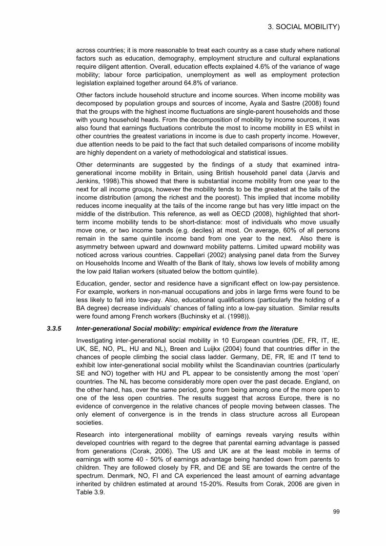
3. SOCIAL MOBILITY)
99
across countries; it is more reasonable to treat each country as a case study where national factors such as education, demography, employment structure and cultural explanations require diligent attention. Overall, education effects explained 4.6% of the variance of wage mobility; labour force participation, unemployment as well as employment protection legislation explained together around 64.8% of variance.
Other factors include household structure and income sources. When income mobility was decomposed by population groups and sources of income, Ayala and Sastre (2008) found that the groups with the highest income fluctuations are single-parent households and those with young household heads. From the decomposition of mobility by income sources, it was also found that earnings fluctuations contribute the most to income mobility in ES whilst in other countries the greatest variations in income is due to cash property income. However, due attention needs to be paid to the fact that such detailed comparisons of income mobility are highly dependent on a variety of methodological and statistical issues.
Other determinants are suggested by the findings of a study that examined intra-generational income mobility in Britain, using British household panel data (Jarvis and Jenkins, 1998).This showed that there is substantial income mobility from one year to the next for all income groups, however the mobility tends to be the greatest at the tails of the income distribution (among the richest and the poorest). This implied that income mobility reduces income inequality at the tails of the income range but has very little impact on the middle of the distribution. This reference, as well as OECD (2008), highlighted that short-term income mobility tends to be short-distance: most of individuals who move usually move one, or two income bands (e.g. deciles) at most. On average, 60% of all persons remain in the same quintile income band from one year to the next. Also there is asymmetry between upward and downward mobility patterns. Limited upward mobility was noticed across various countries. Cappellari (2002) analysing panel data from the Survey on Households Income and Wealth of the Bank of Italy, shows low levels of mobility among the low paid Italian workers (situated below the bottom quintile).
Education, gender, sector and residence have a significant effect on low-pay persistence. For example, workers in non-manual occupations and jobs in large firms were found to be less likely to fall into low-pay. Also, educational qualifications (particularly the holding of a BA degree) decrease individuals’ chances of falling into a low-pay situation. Similar results were found among French workers (Buchinsky et al. (1998)).
3.3.5 Inter-generational Social mobility: empirical evidence from the literature
Investigating inter-generational social mobility in 10 European countries (DE, FR, IT, IE, UK, SE, NO, PL, HU and NL), Breen and Luijkx (2004) found that countries differ in the chances of people climbing the social class ladder. Germany, DE, FR, IE and IT tend to exhibit low inter-generational social mobility whilst the Scandinavian countries (particularly SE and NO) together with HU and PL appear to be consistently among the most ‘open’ countries. The NL has become considerably more open over the past decade. England, on the other hand, has, over the same period, gone from being among one of the more open to one of the less open countries. The results suggest that across Europe, there is no evidence of convergence in the relative chances of people moving between classes. The only element of convergence is in the trends in class structure across all European societies.
Research into intergenerational mobility of earnings reveals varying results within developed countries with regard to the degree that parental earning advantage is passed from generations (Corak, 2006). The US and UK are at the least mobile in terms of earnings with some 40 - 50% of earnings advantage being handed down from parents to children. They are followed closely by FR, and DE and SE are towards the centre of the spectrum. Denmark, NO, FI and CA experienced the least amount of earning advantage inherited by children estimated at around 15-20%. Results from Corak, 2006 are given in Table 3.9.
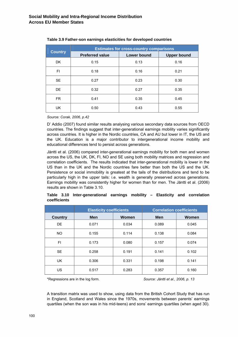
Social Mobility and Intra-Regional Income Distribution Across EU Member States
100
Table 3.9 Father-son earnings elasticities for developed countries
Estimates for cross-country comparisons Country
Preferred value Lower bound Upper bound DK 0.15 0.13 0.16
FI 0.18 0.16 0.21
SE 0.27 0.23 0.30
DE 0.32 0.27 0.35
FR 0.41 0.35 0.45
UK 0.50 0.43 0.55
Source: Corak, 2006, p.42
D’ Addio (2007) found similar results analysing various secondary data sources from OECD countries. The findings suggest that inter-generational earnings mobility varies significantly across countries. It is higher in the Nordic countries, CA and AU but lower in IT, the US and the UK. Education is a major contributor to intergenerational income mobility and educational differences tend to persist across generations.
Jäntti et al. (2006) compared inter-generational earnings mobility for both men and women across the US, the UK, DK, FI, NO and SE using both mobility matrices and regression and correlation coefficients. The results indicated that inter-generational mobility is lower in the US than in the UK and the Nordic countries fare better than both the US and the UK. Persistence or social immobility is greatest at the tails of the distributions and tend to be particularly high in the upper tails: i.e. wealth is generally preserved across generations. Earnings mobility was consistently higher for women than for men. The Jäntti et al. (2006) results are shown in Table 3.10.
Table 3.10 Inter-generational earnings mobility – Elasticity and correlation coefficients
Elasticity coefficients Correlation coefficients
Country Men Women Men Women DE 0.071 0.034 0.089 0.045
NO 0.155 0.114 0.138 0.084
FI 0.173 0.080 0.157 0.074
SE 0.258 0.191 0.141 0.102
UK 0.306 0.331 0.198 0.141
US 0.517 0.283 0.357 0.160
*Regressions are in the log form. Source: Jäntti et al., 2006, p. 13
A transition matrix was used to show, using data from the British Cohort Study that has run in England, Scotland and Wales since the 1970s, movements between parents’ earnings quartiles (when the son was in his mid-teens) and sons’ earnings quartiles (when aged 30).
3. SOCIAL MOBILITY)
101
(In the absence of earnings mobility, all children would be in the same quartile as their parents). The findings indicated that 37% of children remained in the poorest quarter as adults, whilst only 16% climbed the social ladder up to the most affluent group (Blanden, Gregg and Machin, 2005). On the other hand, 40% of the most affluent quarter remained in the top quarter in the next generation.
In SE, improvements in intergenerational social mobility (measured as mobility of occupational status organised in 9 classes) slowed down during the last quarter of the 20th century (Jonsson, 2004). Despite structural changes which saw a greater number of service-sector jobs, the movements between origin and destination classes remained largely the same. Women were the greatest winners in terms of upward mobility. Their relative mobility was mainly achieved thanks to improved access to education that meant that social origins had less of a bearing on educational attainment.
Bogdan Mach (2004) using survey data on social classes mapped into the CASMIN class schema from PL covering various years 1972, 1988 and 1994 found no change in the social mobility of men but a steady increase in the mobility of women. With regard to the total movements between origins and destinations, the findings suggest that downward mobility increased during both the state-socialism and early capitalist period. This trend impacted more on men than women. Women were also advantaged in terms of upward mobility.
Examining the rate of (CASMIN) class mobility in HU between 1973 and 2000, Róbert and Bukodi (2004) found that there was an increase in relative mobility between 1973 and 1983 for both men and women. The trend however levelled off between 1992 and 2000 after the collapse of socialism. The trend was particularly pronounced among men, though social fluidity was still greater for them in 2000 than it was in 1973. With regard to total mobility, the absolute rate of association between origins and destinations also suffered a decline with men being affected more than women. Downward mobility also increased, particularly amongst men. The study concludes that post-socialism has brought about higher income inequalities in tandem with a lower inter-generational social mobility.
A recent study carried out by the European Commission covering 24 Member States shows that educational mobility, measured as the probability of someone whose father had low education attaining a university degree or the equivalent, has increased over time across the EU, with the exception of EE, HU and SK that did not follow the same trend (European Commission, 2007). Due attention though needs to be paid to the fact that this upward trend reflects the general rise in participation in tertiary education.
Evidence on the Featherman, Jones, Hauser (FJH) or modernization hypotheses
The FJH hypothesis asserts that there is little variation between countries in their patterns of fluidity; furthermore, no systematic change of social fluidity can be envisioned. Among the most referenced studies supporting the FJH hypothesis is Erikson and Goldthorpe, 1992. Covering nine European countries, they show that despite some differences between countries in exchange mobility, these are nevertheless rather small in comparison with the broad similarities between the countries. However, in a study on intergenerational mobility of earnings, whilst Jäntti et al. (2006) suggest that all countries exhibit substantial earnings persistence across generations, contrary to the FHJ hypothesis, there are some statistically significant differences across countries.
Also contrary to the FJH hypothesis, other studies show that countries differ in their levels of exchange mobility. Breen and Luijkx (2004) who analysed 117 mobility surveys from 11 countries (including 9 EU countries) covering the period 1970-2000 show that SE, Israel and NO were the most fluid whilst DE, FR and IT were the least fluid. Most importantly, their findings suggest that there is one commonality between countries, that is, the widespread tendency towards greater fluidity (with the exception of Britain). The trend towards higher social fluidity brings supports the modernization hypothesis rather than the FJH hypothesis. Ganzeboom et al. (1989) also make a case for the modernization thesis drawing upon data
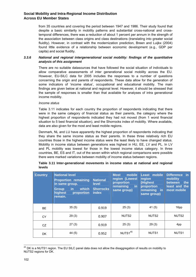
Social Mobility and Intra-Regional Income Distribution Across EU Member States
102
from 35 countries and covering the period between 1947 and 1986. Their study found that despite a basic similarity in mobility patterns and substantial cross-national and cross-temporal differences, there was a reduction of about 1 percent per annum in the strength of the association between class origins and class destinations (translating into greater social fluidity). However, in contrast with the modernization prediction, Breen and Luijkx (2004) found little evidence of a relationship between economic development (e.g., GDP per capita) and social fluidity.
3.3.6 National and regional intergenerational social mobility: findings of the quantitative analysis of this assignment
There are no suitable datasources that have followed the social situation of individuals to allow comparative assessments of inter generational social mobility across the EU. However, EU-SILC data for 2005 includes the responses to a number of questions concerning the origin and parents of respondents. These data allow for the generation of some indicators of ‘income status’, occupational and educational mobility. The main findings are given below at national and regional level. However, it should be stressed that the sample of responses is smaller than that available for analyses of intra generational income mobility.
Income status
Table 3.11 indicates for each country the proportion of respondents indicating that there were in the same category of financial status as their parents, the category where the highest proportion of respondents indicated they had not moved (from 1 worst financial situation to 5 best financial situation), and the Shorrocks index of mobility. Where available, data are also given for the most and least mobile regions.
Denmark, NL and LU have apparently the highest proportion of respondents indicating that they share the same income status as their parents. In these three relatively rich EU countries those in the highest income status were the least likely to have changed status. Mobility in income status between generations was highest in HU, EE, LV and PL. In LV and PL mobility was lowest for those in the lowest income status category. In three countries, BE, ES and IT, out of the seven within which regional comparisons were possible there were marked variations between mobility of income status between regions.
Table 3.11 Inter-generational movements in income status at national and regional levels
Country National level Proportion remaining in same group. Group in which highest proportion remain.
National level Shorrocks index
Most mobile region (Lowest proportion remaining in same group)
Least mobile region (Highest proportion remaining in same group)
Difference in mobility between the least and the most mobile
BE 35 (5) 0.919 25 (3) 41 (5) 16pp
CY 29 (3) 0.907 NUTS2 NUTS2 NUTS2
CZ 27 (3) 0.919 25 (3) 29 (3) 4pp
DK 44 (5) 0.952 NUTS145 NUTS1 NUTS1
45 DK is a NUTS1 region. The EU SILC panel data does not allow the disaggregation of results on mobility to NUTS2 regions for DK.
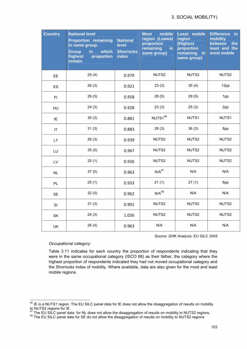
3. SOCIAL MOBILITY)
103
Country National level Proportion remaining in same group. Group in which highest proportion remain.
National level Shorrocks index
Most mobile region (Lowest proportion remaining in same group)
Least mobile region (Highest proportion remaining in same group)
Difference in mobility between the least and the most mobile
EE 25 (4) 0.979 NUTS2 NUTS2 NUTS2
ES 26 (3) 0.921 23 (3) 35 (4) 12pp
FI 29 (5) 0.958 28 (5) 29 (5) 1pp
HU 24 (3) 0.928 23 (3) 25 (3) 2pp
IE 30 (3) 0.881 NUTS146 NUTS1 NUTS1
IT 31 (3) 0.883 28 (3) 36 (3) 8pp
LT 26 (3) 0.939 NUTS2 NUTS2 NUTS2
LU 35 (5) 0.967 NUTS2 NUTS2 NUTS2
LV 25 (1) 0.926 NUTS2 NUTS2 NUTS2
NL 37 (5) 0.963 N/A47 N/A N/A
PL 25 (1) 0.933 21 (1) 27 (1) 6pp
SE 32 (5) 0.962 N/A48 N/A N/A
SI 31 (3) 0.901 NUTS2 NUTS2 NUTS2
SK 24 (3) 1.026 NUTS2 NUTS2 NUTS2
UK 26 (4) 0.963 N/A N/A N/A
Source: GHK Analysis: EU SILC 2005
Occupational category
Table 3.11 indicates for each country the proportion of respondents indicating that they were in the same occupational category (ISCO 88) as their father, the category where the highest proportion of respondents indicated they had not moved occupational category and the Shorrocks index of mobility. Where available, data are also given for the most and least mobile regions.
46 IE is a NUTS1 region. The EU SILC panel data for IE does not allow the disaggregation of results on mobility to NUTS2 regions for IE. 47 The EU SILC panel data for NL does not allow the disaggregation of results on mobility to NUTS2 regions. 48 The EU SILC panel data for SE do not allow the disaggregation of results on mobility to NUTS2 regions
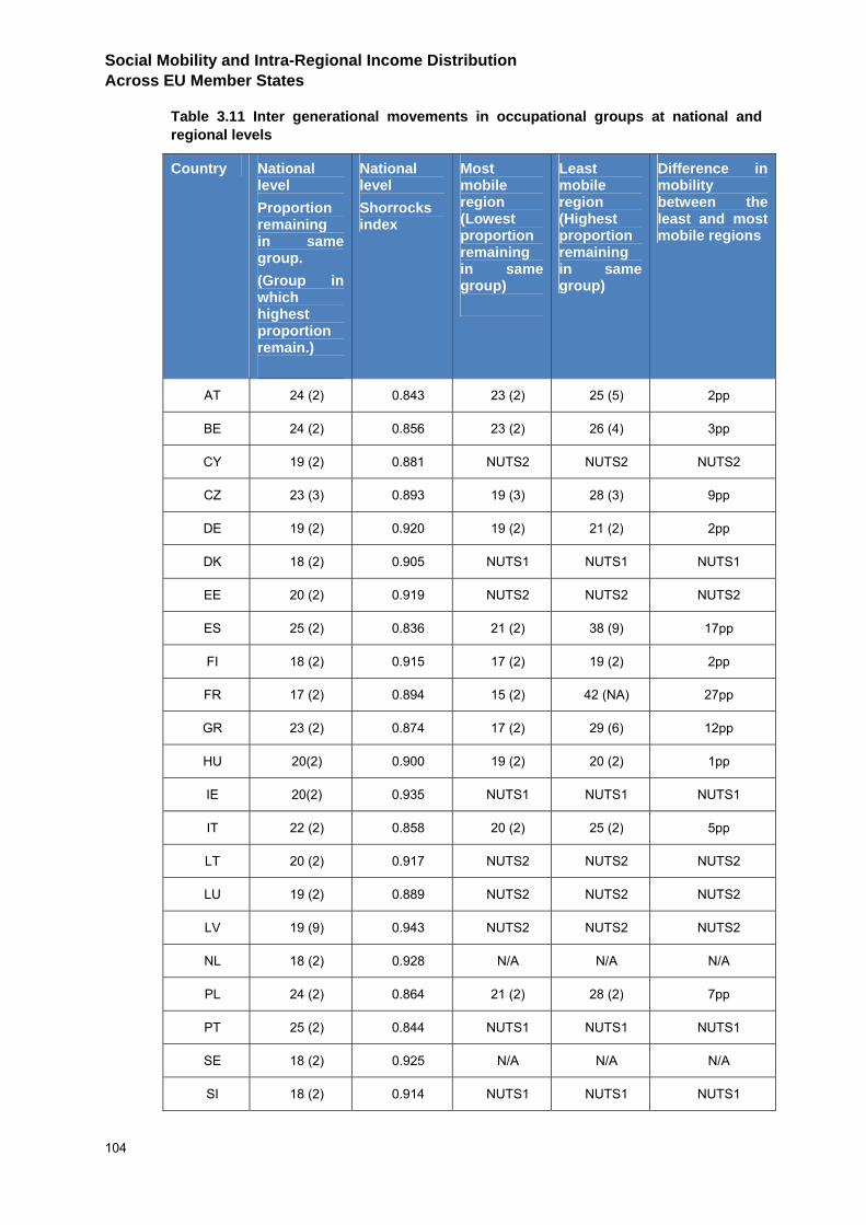
Social Mobility and Intra-Regional Income Distribution Across EU Member States
104
Table 3.11 Inter generational movements in occupational groups at national and regional levels
Country National level Proportion remaining in same group. (Group in which highest proportion remain.)
National level Shorrocks index
Most mobile region (Lowest proportion remaining in same group)
Least mobile region (Highest proportion remaining in same group)
Difference in mobility between the least and most mobile regions
AT 24 (2) 0.843 23 (2) 25 (5) 2pp
BE 24 (2) 0.856 23 (2) 26 (4) 3pp
CY 19 (2) 0.881 NUTS2 NUTS2 NUTS2
CZ 23 (3) 0.893 19 (3) 28 (3) 9pp
DE 19 (2) 0.920 19 (2) 21 (2) 2pp
DK 18 (2) 0.905 NUTS1 NUTS1 NUTS1
EE 20 (2) 0.919 NUTS2 NUTS2 NUTS2
ES 25 (2) 0.836 21 (2) 38 (9) 17pp
FI 18 (2) 0.915 17 (2) 19 (2) 2pp
FR 17 (2) 0.894 15 (2) 42 (NA) 27pp
GR 23 (2) 0.874 17 (2) 29 (6) 12pp
HU 20(2) 0.900 19 (2) 20 (2) 1pp
IE 20(2) 0.935 NUTS1 NUTS1 NUTS1
IT 22 (2) 0.858 20 (2) 25 (2) 5pp
LT 20 (2) 0.917 NUTS2 NUTS2 NUTS2
LU 19 (2) 0.889 NUTS2 NUTS2 NUTS2
LV 19 (9) 0.943 NUTS2 NUTS2 NUTS2
NL 18 (2) 0.928 N/A N/A N/A
PL 24 (2) 0.864 21 (2) 28 (2) 7pp
PT 25 (2) 0.844 NUTS1 NUTS1 NUTS1
SE 18 (2) 0.925 N/A N/A N/A
SI 18 (2) 0.914 NUTS1 NUTS1 NUTS1
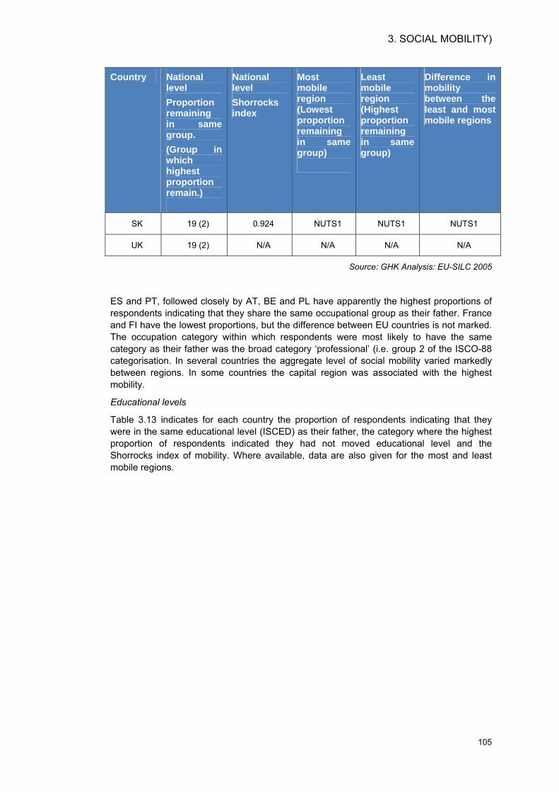
3. SOCIAL MOBILITY)
105
Country National level Proportion remaining in same group. (Group in which highest proportion remain.)
National level Shorrocks index
Most mobile region (Lowest proportion remaining in same group)
Least mobile region (Highest proportion remaining in same group)
Difference in mobility between the least and most mobile regions
SK 19 (2) 0.924 NUTS1 NUTS1 NUTS1
UK 19 (2) N/A N/A N/A N/A
Source: GHK Analysis: EU-SILC 2005
ES and PT, followed closely by AT, BE and PL have apparently the highest proportions of respondents indicating that they share the same occupational group as their father. France and FI have the lowest proportions, but the difference between EU countries is not marked. The occupation category within which respondents were most likely to have the same category as their father was the broad category ‘professional’ (i.e. group 2 of the ISCO-88 categorisation. In several countries the aggregate level of social mobility varied markedly between regions. In some countries the capital region was associated with the highest mobility.
Educational levels
Table 3.13 indicates for each country the proportion of respondents indicating that they were in the same educational level (ISCED) as their father, the category where the highest proportion of respondents indicated they had not moved educational level and the Shorrocks index of mobility. Where available, data are also given for the most and least mobile regions.
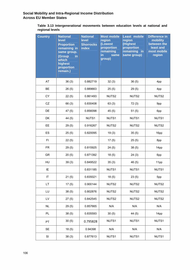
Social Mobility and Intra-Regional Income Distribution Across EU Member States
106
Table 3.13 Intergenerational movements between education levels at national and regional levels
Country National level Proportion remaining in same group. (Group in which highest proportion remain.)
National level Shorrocks index
Most mobile region (Lowest proportion remaining in same group)
Least mobile region (Highest proportion remaining in same group)
Difference in mobility
between the least and
most mobile region
AT 36 (3) 0.882719 32 (3) 36 (5) 4pp
BE 26 (5) 0.889663 25 (5) 29 (5) 4pp
CY 22 (5) 0.861493 NUTS2 NUTS2 NUTS2
CZ 66 (3) 0.830408 63 (3) 72 (3) 9pp
DE 47 (5) 0.856098 45 (5) 51 (5) 6pp
DK 44 (5) NUTS1 NUTS1 NUTS1 NUTS1
EE 29 (5) 0.916267 NUTS2 NUTS2 NUTS2
ES 25 (5) 0.820095 19 (3) 35 (5) 16pp
FI 22 (5) 17 (5) 25 (5) 8pp
FR 29 (5) 0.815925 24 (5) 38 (5) 14pp
GR 20 (5) 0.871392 18 (5) 24 (3) 6pp
HU 39 (3) 0.849522 35 (3) 46 (5) 11pp
IE 0.831185 NUTS1 NUTS1 NUTS1
IT 21 (5) 0.835021 18 (5) 23 (5) 5pp
LT 17 (5) 0.900144 NUTS2 NUTS2 NUTS2
LU 38 (5) 0.802876 NUTS2 NUTS2 NUTS2
LV 27 (5) 0.842545 NUTS2 NUTS2 NUTS2
NL 29 (5) 0.857665 N/A N/A N/A
PL 38 (5) 0.835593 30 (5) 44 (5) 14pp
PT 30 (5) 0.795828 NUTS1 NUTS1 NUTS1
SE 18 (5) 0.94398 N/A N/A N/A
SI 38 (3) 0.877613 NUTS1 NUTS1 NUTS1
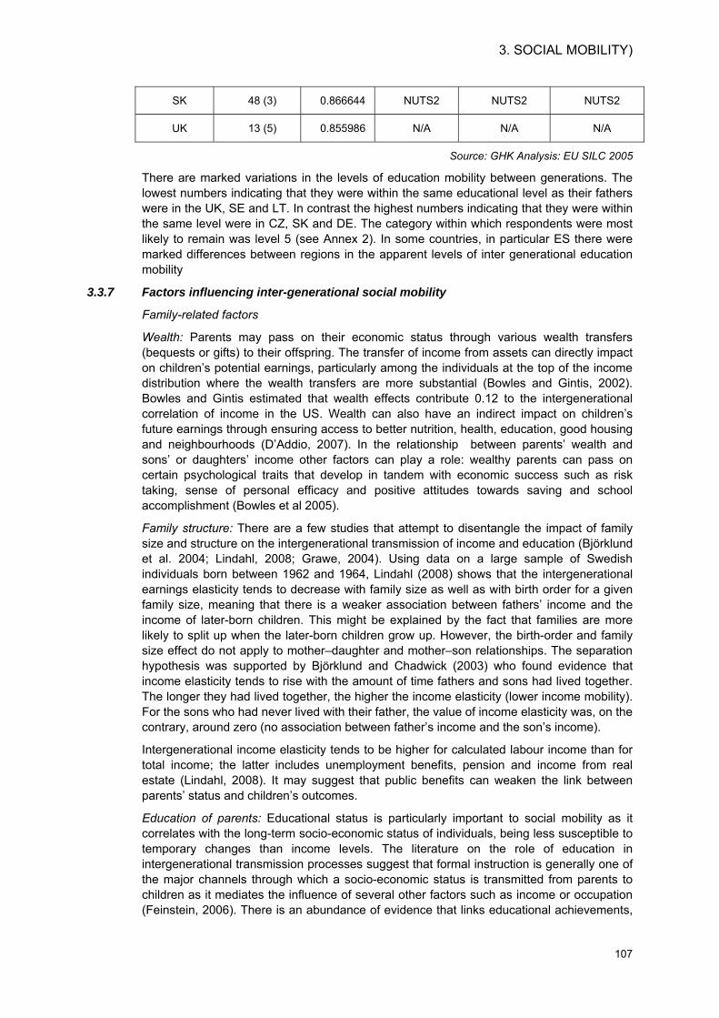
3. SOCIAL MOBILITY)
107
SK 48 (3) 0.866644 NUTS2 NUTS2 NUTS2
UK 13 (5) 0.855986 N/A N/A N/A
Source: GHK Analysis: EU SILC 2005
There are marked variations in the levels of education mobility between generations. The lowest numbers indicating that they were within the same educational level as their fathers were in the UK, SE and LT. In contrast the highest numbers indicating that they were within the same level were in CZ, SK and DE. The category within which respondents were most likely to remain was level 5 (see Annex 2). In some countries, in particular ES there were marked differences between regions in the apparent levels of inter generational education mobility
3.3.7 Factors influencing inter-generational social mobility
Family-related factors
Wealth: Parents may pass on their economic status through various wealth transfers (bequests or gifts) to their offspring. The transfer of income from assets can directly impact on children’s potential earnings, particularly among the individuals at the top of the income distribution where the wealth transfers are more substantial (Bowles and Gintis, 2002). Bowles and Gintis estimated that wealth effects contribute 0.12 to the intergenerational correlation of income in the US. Wealth can also have an indirect impact on children’s future earnings through ensuring access to better nutrition, health, education, good housing and neighbourhoods (D’Addio, 2007). In the relationship between parents’ wealth and sons’ or daughters’ income other factors can play a role: wealthy parents can pass on certain psychological traits that develop in tandem with economic success such as risk taking, sense of personal efficacy and positive attitudes towards saving and school accomplishment (Bowles et al 2005).
Family structure: There are a few studies that attempt to disentangle the impact of family size and structure on the intergenerational transmission of income and education (Björklund et al. 2004; Lindahl, 2008; Grawe, 2004). Using data on a large sample of Swedish individuals born between 1962 and 1964, Lindahl (2008) shows that the intergenerational earnings elasticity tends to decrease with family size as well as with birth order for a given family size, meaning that there is a weaker association between fathers’ income and the income of later-born children. This might be explained by the fact that families are more likely to split up when the later-born children grow up. However, the birth-order and family size effect do not apply to mother–daughter and mother–son relationships. The separation hypothesis was supported by Björklund and Chadwick (2003) who found evidence that income elasticity tends to rise with the amount of time fathers and sons had lived together. The longer they had lived together, the higher the income elasticity (lower income mobility). For the sons who had never lived with their father, the value of income elasticity was, on the contrary, around zero (no association between father’s income and the son’s income).
Intergenerational income elasticity tends to be higher for calculated labour income than for total income; the latter includes unemployment benefits, pension and income from real estate (Lindahl, 2008). It may suggest that public benefits can weaken the link between parents’ status and children’s outcomes.
Education of parents: Educational status is particularly important to social mobility as it correlates with the long-term socio-economic status of individuals, being less susceptible to temporary changes than income levels. The literature on the role of education in intergenerational transmission processes suggest that formal instruction is generally one of the major channels through which a socio-economic status is transmitted from parents to children as it mediates the influence of several other factors such as income or occupation (Feinstein, 2006). There is an abundance of evidence that links educational achievements,
Social Mobility and Intra-Regional Income Distribution Across EU Member States
108
occupational attainment and mobility processes together (D’ Addio, 2007; Blanden et al., 2005; Nunn et al., 2007). For example, using data from five EU countries (DK, SE, FI, UK and West DE), Blanden et al., 2005 show that educational attainment and the market return to education account for about 35 to 40 percent of the coefficient of intergenerational earnings elasticity. With regard to educational mobility per se, across the EU, the chances of people having tertiary education if their father had the same level are over twice as high as for people whose fathers had only basic schooling (with significantly higher odds in CZ, PL and HU where the chances are nine times higher) (European Commission, 2007).
Parental occupation: An EU study on this topic shows that there is a significantly greater chance of someone being employed in the highest level of occupation (e.g., ISCO classification-managers, professionals and technicians) if their father had the same kind of job than if he had a lower-level occupation (European Commission, 2007). However, the odds ratios vary across the EU. The countries that exhibit high odds ratio (low occupational mobility) are usually the ones with low educational mobility too (for example, CZ, PL, CY). Such studies highlight that moving from rags to riches is particularly difficult in some countries.
Genetics: The literature is not characterised by consensus. It is accepted that parents (partially) pass on their endowments to their offspring and these can encompass genetically-transmitted cognitive abilities (usually measured as IQ) that can become income-generating traits. Whilst there is robust evidence for the correlation between parents' and offspring’s scores on cognitive tests, the relationship between genetic traits and income mobility is less straightforward. For example, Bowles and Gintis (2002), in an exercise of decomposition of the intergenerational correlation coefficient of income into genetic, cultural and material (asset-based) components, found that IQ explains little in the intergenerational transmission of earnings. However, the same authors estimate that the genetic inheritance may account for almost one-third of the intergenerational correlation, suggesting that (partially) inherited traits other than cognitive skills may account for some of earnings elasticity. For example, using British cohort study data, Blanden et al. 2006 found that non-cognitive traits (that have a genetic basis) such anxiety, locus of control or aggressivity explain around 18% of the income transmission across generations.
Assortative mating: Assortative mating refers to people’s propensity to form partnerships with individuals who share similar socio-economic characteristics, in particular similar educational background (D’Addio, 2007). With regard to intergenerational mobility, the literature suggests that adults with parents of a certain socio-economic background tend to find spouses from a similar background, increasing the correlation between parents’ and children’s earnings when they are adults. Simply put, a higher degree of assortative mating between spouses (among parents and children) is associated with a lower intergenerational mobility. For example, Ermisch et al. (2006) analysed data from the German Socio-Economic Panel and the British Household Panel Survey and estimated that assortative mating accounts, on average, for about 40-50% of the covariance between parents’ and children’s own permanent family income. The explanation lies in the fact that there seems to be a strong correlation between spouses’ human capital meaning that similar background-spouses have also a similar stock of skills and knowledge to produce economic value.
Neighbourhood conditions
There are a few studies that looked into the impact of neighbourhood conditions on the intergenerational mobility of disadvantages (Palmer, 2002; Hertz, 2006; Nunn et al., 2007). Neighbourhood factors that are usually taken into account include the levels of local unemployment, benefit claimants and social housing (Nunn et al., 2007). In the UK, Palmer (2002) reported that the unemployment rate negatively impacts on children’s permanent
3. SOCIAL MOBILITY)
109
earnings, enforcing the intergenerational transmission of welfare dependency.49 It is estimated that 1% increase in the proportion of unemployed men at the local authority level in 1974 led to 1.7% decline in sons’ wages by 1991. Furthermore, some areas can be predominantly occupied by lower paid social classes and as indicated above studies show that having a father with a high-level job significantly increases children’s chances to have a similar job.
Institutional factors
Return to education and education inequalities Many studies (e.g., Johnson, 2002; Goldberger, 1989) go beyond the inter-generational transmission of income, taking into account the evidence of the transmission of education and occupation across generations as these factors are correlated with the socio-economic status of individuals. Several studies have convincingly linked inter-generational mobility to the education system. More specifically, social mobility might be linked to the differences in education attainment between people belonging to different income groups and differences in the “return” of their education in the labour market. In this case, the overall inter-generational elasticity can be decomposed into the return to education multiplied by the relationship between parental income and education, plus the unexplained persistence of income that is not transmitted through education.
The challenge of this method stems from the difficulty of interpreting such data as it is unclear whether money buys better education or better-off parents produce a more educated offspring because of other issues other than income such as good parental practices, career motivation or biases in the education system itself (Bourdieu and Passeron, 1979). There is also evidence that returns to education depend importantly on the social networks that parents can mobilise after their children finish education and look for a desirable position in the labour market. According to Boudon (1974) lower social classes tend to overestimate the costs and underestimate the benefits of education and training and therefore attached an artificially low value to education. It may be, in fact, that education has a higher value for higher socio-economic groups, as they have social connections and other resources to transform educational qualifications into an occupational status. For example, in the UK, Blanden et al. (2005) shows that the expansion of higher education since the late 1980s has disproportionately benefited those from well-off families.
This might be related to the extent to which human capital acquired through education is rewarded in the market. Compiling secondary data, D’Addio (2007) suggests that countries with higher rewards to education tend to display low intergenerational income mobility. However, looking over the associations between estimates of private returns to (upper secondary) education and intergenerational earnings, one can notice that the strength of the association varies rather widely across countries.
Solon (2004) asserts that intergenerational income mobility is enhanced in systems of public education whilst educational systems dominated by private schooling significantly reduce the chances of intergenerational earnings mobility. In FI, Pekkarinen et al. (2006) brings evidence for the role that the quality of early education plays in the intergenerational transmission of earnings. The study examined the longitudinal impact of a major educational reform in the Finnish primary and secondary education (1972-1977) on the intergenerational income mobility. Income mobility was measured as the correlation between son's earnings in 2000 and father's average earnings during 1970-1990. The reform was launched in FI with the aim to shift the tracking age in secondary education from age 10 to 16 and to impose a uniform academic curriculum up to the end of lower secondary school. The empirical evidence suggests that the educational reform reduced intergenerational income correlation by seven percentage points. Similar results were found in SE by Holmlund (2006) who examined the impact on inter generational mobility of a
49 Referenced in D’Addio, 2007.
Social Mobility and Intra-Regional Income Distribution Across EU Member States
110
Swedish educational reform of the 50s, which postponed ability tracking and extended compulsory education from seven to nine years. The results indicate that the reform spurred the intergenerational income mobility, and resulted in a lower association between the educational level of children and parents. In a study covering 12 EU countries, Comi (2004) shows that public expenditure in tertiary education is decreased income elasticity (i.e., higher public expenditure, higher income mobility).
3.3.8 Influencing social mobility at regional level
Although it has been stressed in the literature that national factors can influence patterns of social mobility it is also evident that there are marked differences between regions in the same country in both intra and inter generational social mobility. No doubt some of these variations are due to the structural characteristics of the regions and the extent to which ‘fluidity’ has developed. Amongst the ‘supply side’ factors most important to influencing inter generational social mobility is access to education. Employment (and unemployment) that is susceptible to policy influence at the regional level is the single most important factor influencing short term intra generational income and social mobility.
3.3.9 Suggestions for improving the measurement of Social Mobility
The limited timescale and regional scope of the EU SILC panel data is a constraint on the exploration of social mobility. It is important that the EU SILC panel is maintained, that the availability of data should be extended to all EU regions and that the retrospective questions on social mobility last asked in 2005 are repeated.
There would be merit in establishing a long term longitudinal household panel at the European level (along the lines of the ECHP that was discontinued in 2001) that could provide the basis for identifying trends in inter-generational social mobility and factors underlying these trends. A longitudinal survey at the European level should meet several requirements: a large and representative sample (sufficient for regional level analysis); repeated observations over a period of time to minimize measurement error problems that are common to the measurement of income (Jenkins and Siedler, 2007); an option to establish family links within the data; and, the availability of data on various variables (not only income) relevant to the inter-generational process, such as family wealth (financial and non-financial assets), employment, household composition, education, health, housing conditions etc. The longitudinal study should also follow people once they moved out of the original households. These characteristics would enable insights into key questions relevant to regional policy, such as: to what extent does intra-regional, inter-regional and transnational migration play a part in social mobility. The development of the internal market, the facilitation of transnational labour mobility and, through ECP policy, the support for cross border cooperation are factors that may encourage internal EU migration that may reinforce forces that advantage the more developed and successful regions able to attract those that are upwardly mobile and hence constrain, in the short term at least, the achievement of the ECP convergence objective. The current EU-SILC uses a 4 year-rotating panel, therefore its use in any analysis of inter-generational mobility (and to some extent intra-generational mobility) is limited. There would also be merit in improving the provision and access to national cohort panels and record register data which have been successfully used in Nordic countries.
3.3.10 Summary
The basic building block of analyses of social mobility is the transition matrix (sometimes called the mobility table). There are many indicators of social mobility. Mobility refers to changes within the transition matrix and can refer to both discrete (for example, class) and continuous variables (for example, income) and changes over different time periods. A distinction is often made between intra and intergenerational social mobility. There are various classifications of social class that are used in studies of social mobility. An important distinction is also made between structural and exchange mobility. The former
3. SOCIAL MOBILITY)
111
concerns changes affecting all households or individuals. The latter refers to relative changes between classes or in income. Exchange mobility is sometimes referred to as social fluidity. There are also other relevant concepts such as dispersion mobility. There are many indicators of social mobility. The strengths and weaknesses of various indicators have been assessed. There are advantages in the indicators enabling the exploration of the nature and direction of social mobility, the factors that may explain it and its magnitude over time.
In the light of the assessment emphasis has been placed on the application of M(υ) the Jenkins and van Kerm Reranking index in the quantitative analysis because of its close link with income distribution. However, use has been also been made of Shorrocks, Hart and Shorrocks, Field and Ok and Spearman’s rank correlation indices to compare social mobility between countries and regions in the quantitative analysis.
Empirical evidence intra generational income mobility:
One simple measure of intra generational income mobility is the persistence of households remaining in the lowest quintile. In CY 68% of those in the lowest quintile in 2005 were still within it in 2007, whilst in ES the proportion was lowest of EU countries for which data are available at 53%. There are extremely marked variations on this indicator between regions, from 94% in one FR region 28% in one ES region to. In the former case intra- generational income mobility appears to contribute little to ‘smoothing’ the income of lower income groups.
There are also evidently marked variations between countries and between regions within countries in the mobility as measured on other indices. Indeed the differences in income mobility between regions in the same country and the same order of magnitude as the differences between EU countries.
Intra-generational income mobility is influenced by national factors, including taxation and social protection measures. Indeed the range of factors that influence income distribution also influence intra-generational income mobility.
The most important factors influencing household income positively were:
Households where the number of persons in full time employment increased (2005-2007) were associated with more income in 2007.
Households where the number of persons having a part time job increased (2005-2007) were associated with more income in 2007.
Household where there are more persons with education levels above high school (i.e. ISCED 4 and 5) were associated with income growth. This may be due to the ability of those with higher education levels to progress income scales and/or command higher earnings.
The factors influencing household income negatively were:
Households with more children (in 2005) were associated with less income in 2007.
Households in which the number of adults increased (2005-2007) were associated with less income. This is assumed to be a consequence of children becoming adults but not entering employment.
The following household factors did not have a statistically significant affect on income growth (2005-2007): the gender of the head of household; age of head of household; the number of adults; increases in the number of children (2005-2007); the number of persons with just high school education (ISCED 3); and, the number of person with higher education (ISCED 4 or 5).
Social Mobility and Intra-Regional Income Distribution Across EU Member States
112
Empirical evidence inter-generational income mobility:
Denmark, NL and LU had the highest proportion of respondents indicating that they share the same income status as their parents. In these three relatively rich EU countries those in the highest income status were the least likely to have changed status. Mobility in income status between generations was highest in HU, EE, LV and PL. In LV and PL mobility was lowest for those in the lowest income status category. In three countries, BE, ES and IT, out of the seven within which regional comparisons were possible there were marked variations between mobility of income status between regions.
ES and PT, followed closely by AT, BE and PL have apparently the highest proportions of respondents indicating that they share the same occupational group as their father. FR and FI have the lowest proportions, but the difference between EU countries is not marked. The occupation category within which respondents were most likely to have the same category as their father was Level 2 professionals (see Annex 3). In several countries the aggregate level of social mobility varied markedly between regions. In some countries the capital region was associated with the highest mobility.
There are marked variations in the levels of education mobility between generations. The lowest numbers indicating that they were within the same educational level as their fathers were in the UK, SE and LT. In contrast the highest numbers indicating that they were within the same level were in CZ, SK and DE. The category within which respondents were most likely to remain was ISCED level 5 (see Annex 3). In some countries, in particular ES, there were marked differences between regions in the apparent levels of inter generational education mobility.
More generally the chances of people climbing the social ladder differ between European countries. There are also marked differences in earnings elasticities between countries. Immobility tends to be greater at the higher and lower ends of the earnings spectrum. The rich stay rich whilst the poor stay poor. The pattern of mobility in former communist European countries is complex. There is some evidence that it was higher for women. The relationship between economic growth and social fluidity is unclear.
A large number of factors influence inter generational social mobility, especially: family related factors (wealth, family structure, education of parents, parental occupation, genetics and assortative mating); neighbourhood conditions; and, institutional and public policy factors particularly educational policies and reforms.
4. INCOME DISTRIBUTION AND SOCIAL MOBILITY (INCOME DISTRIBUTION DYNAMICS)
113
4 INCOME DISTRIBUTION AND SOCIAL MOBILITY (INCOME DISTRIBUTION DYNAMICS)
4.1 Introduction
This section of the report considers further the relationship between social mobility and income distribution and more particularly the relationship between income mobility and income inequality. As with the previous sections relevant theoretical aspects are considered before the empirical evidence from the literature and this assignment is reviewed.
4.2 Theoretical analysis
Inequality trends accounted for by mobility and growth
In order to relate income mobility to inequality, use has been made of a method put forward by Jenkins and Van Kerm (2006). They propose a framework that relates inequality trends, mobility and growth patterns. More precisely they decompose inequality changes into progressivity of income growth, which measures how much income growth benefits individuals on lower incomes relative to those on higher incomes, and reranking, which measures how much changes in income positions is associated with income growth. This is considered the only method that relates a standard index of inequality (i.e, the Gini coefficient) with a mobility measure in a simple manner (see Table 3.1).
It is important to mention that the Jenkins and Van Kerm’s method is an accounting identity, and not a statistical model, as commonly used to test hypotheses by means of conditional correlations. Accounting identities allow concepts to be related by rewriting mathematical expressions into different terms, which can be given a useful interpretation. Such an exercise is called decomposing. Decompositions are usually additive, which means that the sum of all the terms or components equals the total amount of the mathematical expression that one is decomposing.
An intuitive explanation of the Jenkins and Van Kerm approach
In order to explain the intuition that lies behind the key decomposition, the simple example shown in Table 4.1 indicates how the two components (progressivity of income growth and mobility) are derived. The upper panel of this table shows an initial distribution (base year) and 4 alternative scenarios for a final year distribution. The middle panel shows the income growth of each individual while the bottom panel presents the decomposition. Note that for this simple exercise, the Gini coefficient is used, that is, the parameter υ = 2.
For the sake of simplicity, the example indicates no overall income growth, that is, where overall income does not change between the two periods. This way the example focuses on the changes that occur between the original and the final distributions.
In Scenario A there is inequality reduction due to progressivity in income growth and no mobility (nobody changes ranks). The poorest individual in the original distribution doubles his income at the expenses of the richest individual, and no one else sees their income change. That is there is a pro-poor redistribution of income, which reduces overall inequality and since there is no re-ranking, such reduction accounts for the overall reduction.
In Scenario B everyone has the same income level, i.e. there is no inequality in the final year and inequality reduction is maximal. Such a reduction is brought about by the largest progressivity, which is compatible with no changes in the income pecking order, i.e. with no mobility. In this Scenario the two richest individuals transfer income to the two poorest individuals, so that everyone has the same income level.
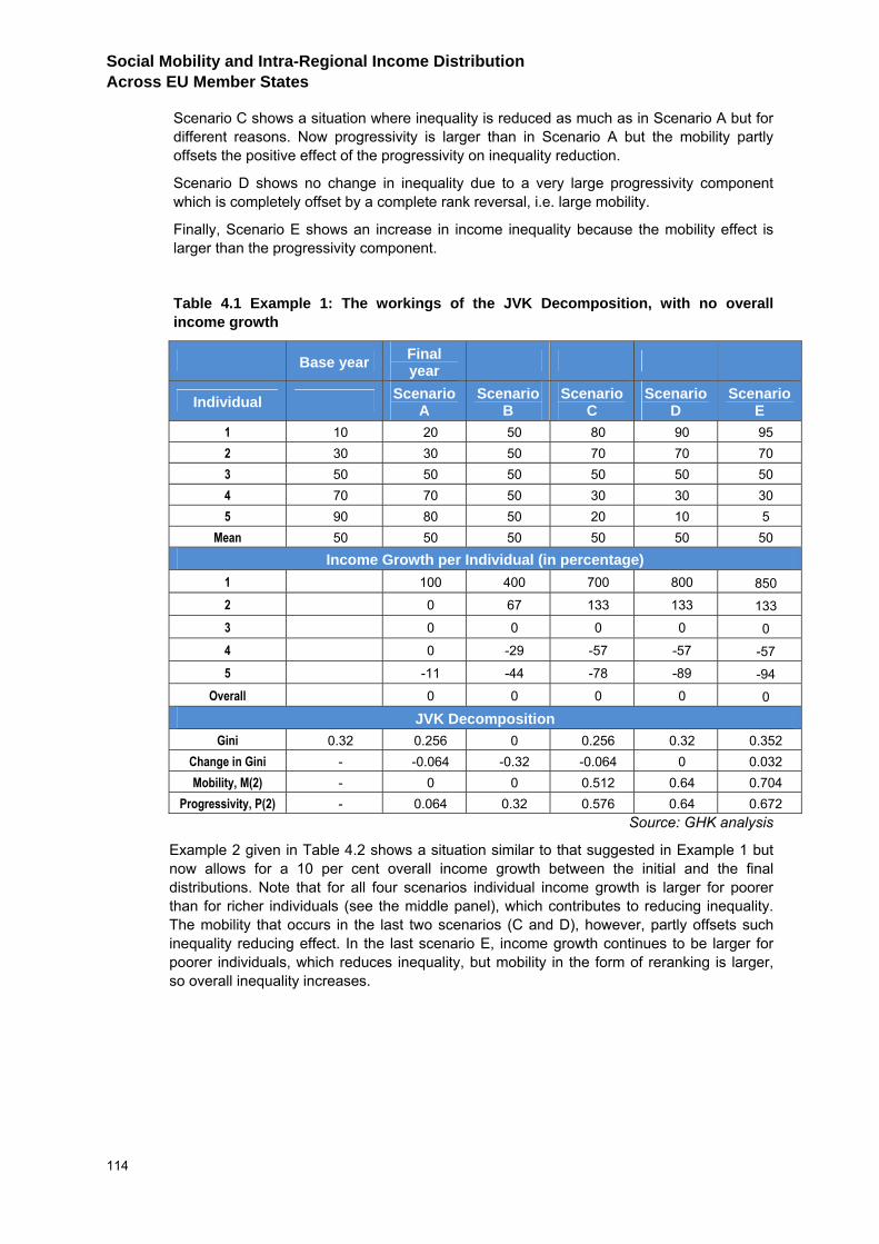
Social Mobility and Intra-Regional Income Distribution Across EU Member States
114
Scenario C shows a situation where inequality is reduced as much as in Scenario A but for different reasons. Now progressivity is larger than in Scenario A but the mobility partly offsets the positive effect of the progressivity on inequality reduction.
Scenario D shows no change in inequality due to a very large progressivity component which is completely offset by a complete rank reversal, i.e. large mobility.
Finally, Scenario E shows an increase in income inequality because the mobility effect is larger than the progressivity component.
Table 4.1 Example 1: The workings of the JVK Decomposition, with no overall income growth
Base year Final year
Individual Scenario A
Scenario B
Scenario C
Scenario D
Scenario E
1 10 20 50 80 90 95 2 30 30 50 70 70 70 3 50 50 50 50 50 50 4 70 70 50 30 30 30 5 90 80 50 20 10 5
Mean 50 50 50 50 50 50
Income Growth per Individual (in percentage) 1 100 400 700 800 850 2 0 67 133 133 133 3 0 0 0 0 0 4 0 -29 -57 -57 -57 5 -11 -44 -78 -89 -94
Overall 0 0 0 0 0
JVK Decomposition Gini 0.32 0.256 0 0.256 0.32 0.352
Change in Gini - -0.064 -0.32 -0.064 0 0.032 Mobility, M(2) - 0 0 0.512 0.64 0.704
Progressivity, P(2) - 0.064 0.32 0.576 0.64 0.672 Source: GHK analysis
Example 2 given in Table 4.2 shows a situation similar to that suggested in Example 1 but now allows for a 10 per cent overall income growth between the initial and the final distributions. Note that for all four scenarios individual income growth is larger for poorer than for richer individuals (see the middle panel), which contributes to reducing inequality. The mobility that occurs in the last two scenarios (C and D), however, partly offsets such inequality reducing effect. In the last scenario E, income growth continues to be larger for poorer individuals, which reduces inequality, but mobility in the form of reranking is larger, so overall inequality increases.
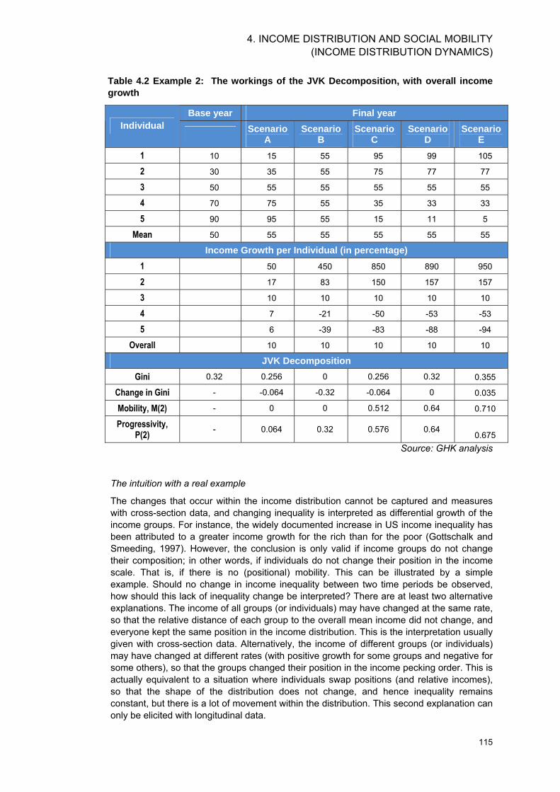
4. INCOME DISTRIBUTION AND SOCIAL MOBILITY (INCOME DISTRIBUTION DYNAMICS)
115
Table 4.2 Example 2: The workings of the JVK Decomposition, with overall income growth
Base year Final year Individual
Scenario A
Scenario B
Scenario C
Scenario D
Scenario E
1 10 15 55 95 99 105
2 30 35 55 75 77 77
3 50 55 55 55 55 55
4 70 75 55 35 33 33
5 90 95 55 15 11 5
Mean 50 55 55 55 55 55
Income Growth per Individual (in percentage) 1 50 450 850 890 950
2 17 83 150 157 157
3 10 10 10 10 10
4 7 -21 -50 -53 -53
5 6 -39 -83 -88 -94
Overall 10 10 10 10 10
JVK Decomposition Gini 0.32 0.256 0 0.256 0.32 0.355
Change in Gini - -0.064 -0.32 -0.064 0 0.035
Mobility, M(2) - 0 0 0.512 0.64 0.710
Progressivity, P(2) - 0.064 0.32 0.576 0.64
0.675 Source: GHK analysis
The intuition with a real example
The changes that occur within the income distribution cannot be captured and measures with cross-section data, and changing inequality is interpreted as differential growth of the income groups. For instance, the widely documented increase in US income inequality has been attributed to a greater income growth for the rich than for the poor (Gottschalk and Smeeding, 1997). However, the conclusion is only valid if income groups do not change their composition; in other words, if individuals do not change their position in the income scale. That is, if there is no (positional) mobility. This can be illustrated by a simple example. Should no change in income inequality between two time periods be observed, how should this lack of inequality change be interpreted? There are at least two alternative explanations. The income of all groups (or individuals) may have changed at the same rate, so that the relative distance of each group to the overall mean income did not change, and everyone kept the same position in the income distribution. This is the interpretation usually given with cross-section data. Alternatively, the income of different groups (or individuals) may have changed at different rates (with positive growth for some groups and negative for some others), so that the groups changed their position in the income pecking order. This is actually equivalent to a situation where individuals swap positions (and relative incomes), so that the shape of the distribution does not change, and hence inequality remains constant, but there is a lot of movement within the distribution. This second explanation can only be elicited with longitudinal data.
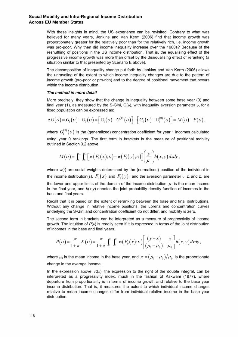
Social Mobility and Intra-Regional Income Distribution Across EU Member States
116
With these insights in mind, the US experience can be revisited. Contrary to what was believed for many years, Jenkins and Van Kerm (2006) find that income growth was proportionately greater for the relatively poor than for the relatively rich, i.e. income growth was pro-poor. Why then did income inequality increase over the 1980s? Because of the reshuffling of positions in the US income distribution. That is, the equalising effect of the progressive income growth was more than offset by the disequalising effect of reranking (a situation similar to that presented by Scenario E above).
The decomposition of inequality change put forth by Jenkins and Van Kerm (2006) allows the unraveling of the extent to which income inequality changes are due to the pattern of income growth (pro-poor or pro-rich) and to the degree of positional movement that occurs within the income distribution.
The method in more detail
More precisely, they show that the change in inequality between some base year (0) and final year (1), as measured by the S-Gini, G(υ), with inequality aversion parameter υ, for a fixed population can be expressed as:
( ) ( ) ( ) ( ) ( ) ( ) ( ) ( ) ( ) ( ) ( )0 01 0 1 1 0 1G G G G G G G M Pυ υ υ υ υ υ υ υ υ⎡ ⎤ ⎡ ⎤∆ = − = − − − = −⎣ ⎦ ⎣ ⎦ ,
where ( ) ( )01G υ is the (generalized) concentration coefficient for year 1 incomes calculated
using year 0 rankings. The first term in brackets is the measure of positional mobility outlined in Section 3.2 above
( ) ( )( ) ( )( ) ( )0 11
; ; ,z z
z z
yM w F x w F y h x y dxdyυ υ υµ
+ +
− −
⎛ ⎞⎡ ⎤= − ⎜ ⎟⎣ ⎦
⎝ ⎠∫ ∫ ,
where w(·) are social weights determined by the (normalised) position of the individual in the income distribution(s), ( )0F x and ( )1F y , and the aversion parameter υ, z- and z+ are
the lower and upper limits of the domain of the income distribution, µ1 is the mean income in the final year, and h(x,y) denotes the joint probability density function of incomes in the base and final years.
Recall that it is based on the extent of reranking between the base and final distributions. Without any change in relative income positions, the Lorenz and concentration curves underlying the S-Gini and concentration coefficient do not differ, and mobility is zero.
The second term in brackets can be interpreted as a measure of progressivity of income growth. The intuition of P(υ) is readily seen if it is expressed in terms of the joint distribution of incomes in the base and final years,
( ) ( ) ( )( ) ( )( ) ( )0
1 0 0
; ,1 1
z z
z z
y x xP K w F x h x y dxdyπ πυ υ υπ π µ µ µ
+ +
− −
⎡ ⎤−= = −⎢ ⎥+ + −⎣ ⎦
∫ ∫ ,
where µ0 is the mean income in the base year, and ( )1 0 0π µ µ µ= − is the proportionate
change in the average income.
In the expression above, K(υ), the expression to the right of the double integral, can be interpreted as a progressivity index, much in the fashion of Kakwani (1977), where departure from proportionality is in terms of income growth and relative to the base year income distribution. That is, it measures the extent to which individual income changes relative to mean income changes differ from individual relative income in the base year distribution.
4. INCOME DISTRIBUTION AND SOCIAL MOBILITY (INCOME DISTRIBUTION DYNAMICS)
117
As shown in the two simple examples above, with positive aggregate income growth (π>0), the progressivity measure P(υ) is positive if income growth is concentrated more among poorer individuals than richer ones, which decreases inequality over time, ceteris paribus. Jenkins and Van Kerm (2006) label this case as ‘pro-poor growth’. The opposite case, i.e. when income growth is mostly concentrated in the upper part of the distribution, yields a negative progressivity measure, which tends to increase inequality over time. Of course, when average income growth is negative (π<0), pro-poor growth occurs if income losses are concentrated more among richer individuals than among poorer ones, i.e. K(υ)<0.
P(υ) is then a very intuitive index, and can be thought of as a social-weighted average of the changes in (relative) incomes between base and final years, where the weights are determined by base year ranks, as the following expression shows.
( ) ( )( ) ( )01 0
; ,z z
z z
y xP w F x h x y dxdyυ υµ µ
+ +
− −
⎡ ⎤= −⎢ ⎥
⎣ ⎦∫ ∫ ,
This expression reveals that P(υ)=0 when relative incomes remain constant, that is, when everyone experiences the same growth rate.
Since the expression in (1) is an accounting identity, a change in one of the three elements (inequality change, mobility and progressivity) modifies at least another of the remaining two. For instance, inequality is reduced by progressive income growth unless more than offset by concomitant income mobility. For a given level of progressivity, higher mobility will lead to lower reduction in cross-section inequality between a base year and final year. For a given change in inequality over time, higher mobility will be associated with a greater progressivity of incomes, i.e. a growth of incomes which is more ‘pro-poor’.
As mentioned above, Jenkins and Van Kerm (2006) found that the increase in inequality both in the US (and in Germany) over the 1980s, may be accounted for by changes in the income pecking order (i.e. mobility) that have a disequalising impact, and which offsets the inequality reducing effects of a pro-poor income growth.
To study the relationship between income inequality and income mobility, equation (1) can be easily rearranged to
( ) ( ) ( ) ( )1 0G G M Pυ υ υ υ= + − (2)
Equation (2) states that final year inequality increases when base year inequality or mobility increase, and the other components remain unchanged. Inequality in the final year also increases if income growth is more ‘pro-rich’, holding the rest constant. The equation (2) has been used in the quantitative analysis (where M(υ) is also called the R (reranking) component, and P(υ) the P (progressivity) component).
An attractive feature of the decomposition is that it can be represented graphically, since it is based on Lorenz and concentration curves.
Welfare interpretations of the above decomposition is possible because the S-Gini is related to Yaari Social Welfare Function, which is additive and linear in people’s income levels, with weights determined by a function of their position in the distribution (see Yaari, 1987 and Lambert, 2001).
In short this decomposition has the advantages of being: intuitive and easy to interpret; possible to represent graphically and linked to a Social Welfare Function. It is important to recall that, as it uses generalized Gini indices, each individual’s contribution to aggregate inequality is therefore determined by both her relative income and her income rank. Moreover, inequality depends on the inequality aversion parameter, which determines the social weight given to individuals positioned in different parts of the income distribution.
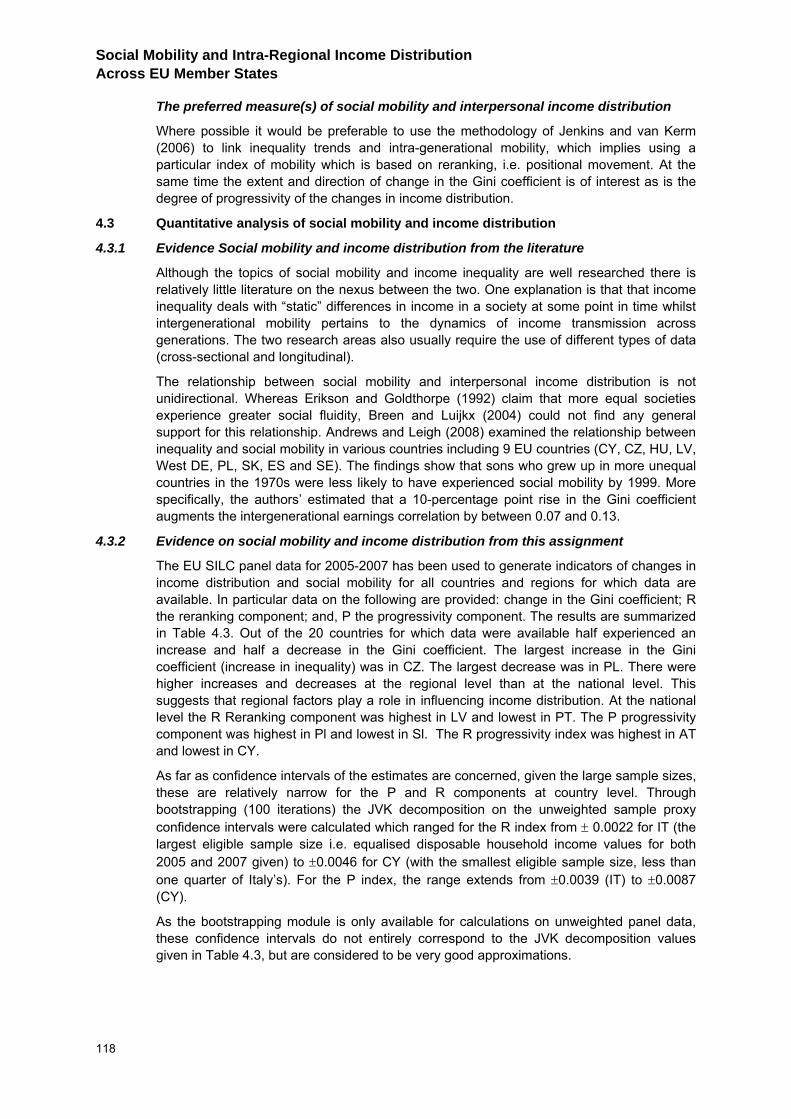
Social Mobility and Intra-Regional Income Distribution Across EU Member States
118
The preferred measure(s) of social mobility and interpersonal income distribution
Where possible it would be preferable to use the methodology of Jenkins and van Kerm (2006) to link inequality trends and intra-generational mobility, which implies using a particular index of mobility which is based on reranking, i.e. positional movement. At the same time the extent and direction of change in the Gini coefficient is of interest as is the degree of progressivity of the changes in income distribution.
4.3 Quantitative analysis of social mobility and income distribution
4.3.1 Evidence Social mobility and income distribution from the literature
Although the topics of social mobility and income inequality are well researched there is relatively little literature on the nexus between the two. One explanation is that that income inequality deals with “static” differences in income in a society at some point in time whilst intergenerational mobility pertains to the dynamics of income transmission across generations. The two research areas also usually require the use of different types of data (cross-sectional and longitudinal).
The relationship between social mobility and interpersonal income distribution is not unidirectional. Whereas Erikson and Goldthorpe (1992) claim that more equal societies experience greater social fluidity, Breen and Luijkx (2004) could not find any general support for this relationship. Andrews and Leigh (2008) examined the relationship between inequality and social mobility in various countries including 9 EU countries (CY, CZ, HU, LV, West DE, PL, SK, ES and SE). The findings show that sons who grew up in more unequal countries in the 1970s were less likely to have experienced social mobility by 1999. More specifically, the authors’ estimated that a 10-percentage point rise in the Gini coefficient augments the intergenerational earnings correlation by between 0.07 and 0.13.
4.3.2 Evidence on social mobility and income distribution from this assignment
The EU SILC panel data for 2005-2007 has been used to generate indicators of changes in income distribution and social mobility for all countries and regions for which data are available. In particular data on the following are provided: change in the Gini coefficient; R the reranking component; and, P the progressivity component. The results are summarized in Table 4.3. Out of the 20 countries for which data were available half experienced an increase and half a decrease in the Gini coefficient. The largest increase in the Gini coefficient (increase in inequality) was in CZ. The largest decrease was in PL. There were higher increases and decreases at the regional level than at the national level. This suggests that regional factors play a role in influencing income distribution. At the national level the R Reranking component was highest in LV and lowest in PT. The P progressivity component was highest in Pl and lowest in Sl. The R progressivity index was highest in AT and lowest in CY.
As far as confidence intervals of the estimates are concerned, given the large sample sizes, these are relatively narrow for the P and R components at country level. Through bootstrapping (100 iterations) the JVK decomposition on the unweighted sample proxy confidence intervals were calculated which ranged for the R index from ± 0.0022 for IT (the largest eligible sample size i.e. equalised disposable household income values for both 2005 and 2007 given) to ±0.0046 for CY (with the smallest eligible sample size, less than one quarter of Italy’s). For the P index, the range extends from ±0.0039 (IT) to ±0.0087 (CY).
As the bootstrapping module is only available for calculations on unweighted panel data, these confidence intervals do not entirely correspond to the JVK decomposition values given in Table 4.3, but are considered to be very good approximations.
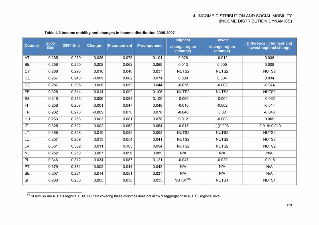
4. INCOME DISTRIBUTION AND SOCIAL MOBILITY (INCOME DISTRIBUTION DYNAMICS)
119
Table 4.3 Income mobility and changes in income distribution 2005-2007
Country 2005 Gini 2007 Gini Change R-component P-component
Highest
change region (change)
Lowest
change region (change)
Difference in highest and lowest regional change
AT 0.265 0.239 -0.026 0.075 0.101 0.026 -0.012 0.038
BE 0.258 0.250 -0.008 0.062 0.069 0.013 0.005 0.008
CY 0.288 0.298 0.010 0.046 0.037 NUTS2 NUTS2 NUTS2
CZ 0.257 0.248 -0.009 0.062 0.071 0.038 0.004 0.034
DE 0.287 0.295 0.008 0.052 0.044 -0.076 -0.002 -0.074
EE 0.328 0.314 -0.014 0.092 0.106 NUTS2 NUTS2 NUTS2
ES 0.319 0.313 -0.006 0.094 0.100 -0.066 -0.004 -0.062
FI 0.258 0.257 -0.001 0.047 0.048 -0.016 -0.002 -0.014
FR 0.282 0.273 -0.009 0.070 0.078 -0.046 0.00 -0.046
HU 0.263 0.266 0.003 0.081 0.078 0.012 -0.003 0.009
IT 0.325 0.322 -0.002 0.062 0.064 -0.013 (-)0.003 -0.016/-0.010
LT 0.358 0.348 -0.010 0.082 0.092 NUTS2 NUTS2 NUTS2
LU 0.257 0.269 0.013 0.054 0.041 NUTS2 NUTS2 NUTS2
LV 0.351 0.362 0.011 0.105 0.094 NUTS2 NUTS2 NUTS2
NL 0.252 0.259 0.007 0.096 0.089 N/A N/A N/A
PL 0.346 0.312 -0.034 0.087 0.121 -0.047 -0.029 -0.018
PT 0.379 0.381 0.002 0.044 0.042 N/A N/A N/A
SE 0.207 0.221 0.014 0.051 0.037 N/A N/A N/A
SI 0.233 0.236 0.003 0.038 0.035 NUTS1501 NUTS1 NUTS1
50 SI and SK are NUTS1 regions. EU-SILC data covering these countries does not allow disaggregation to NUTS2 regional level.
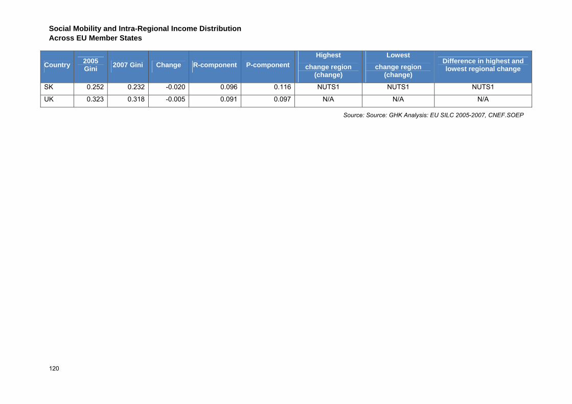
Social Mobility and Intra-Regional Income Distribution Across EU Member States
120
Country 2005 Gini 2007 Gini Change R-component P-component
Highest
change region (change)
Lowest
change region (change)
Difference in highest and lowest regional change
SK 0.252 0.232 -0.020 0.096 0.116 NUTS1 NUTS1 NUTS1
UK 0.323 0.318 -0.005 0.091 0.097 N/A N/A N/A
Source: Source: GHK Analysis: EU SILC 2005-2007, CNEF.SOEP
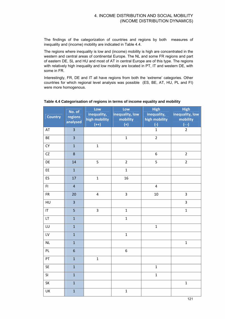
4. INCOME DISTRIBUTION AND SOCIAL MOBILITY (INCOME DISTRIBUTION DYNAMICS)
121
The findings of the categorization of countries and regions by both measures of inequality and (income) mobility are indicated in Table 4.4.
The regions where inequality is low and (income) mobility is high are concentrated in the western and central areas of continental Europe. The NL and some FR regions and part of eastern DE, SL and HU and most of AT in central Europe are of this type. The regions with relatively high inequality and low mobility are located in PT, IT and western DE, with some in FR.
Interestingly, FR, DE and IT all have regions from both the ‘extreme’ categories. Other countries for which regional level analysis was possible (ES, BE, AT, HU, PL and FI) were more homogenous.
Table 4.4 Categorisation of regions in terms of income equality and mobility
Country No. of
regions analysed
Low inequality,
high mobility (++)
Low inequality, low
mobility (+)
High inequality,
high mobility (-)
High inequality, low
mobility (- -)
AT 3 1 2
BE 3 1 2
CY 1 1
CZ 8 6 2
DE 14 5 2 5 2
EE 1 1
ES 17 1 16
FI 4 4
FR 20 4 3 10 3
HU 3 3
IT 5 3 1 1
LT 1 1
LU 1 1
LV 1 1
NL 1 1
PL 6 6
PT 1 1
SE 1 1
SI 1 1
SK 1 1
UK 1 1
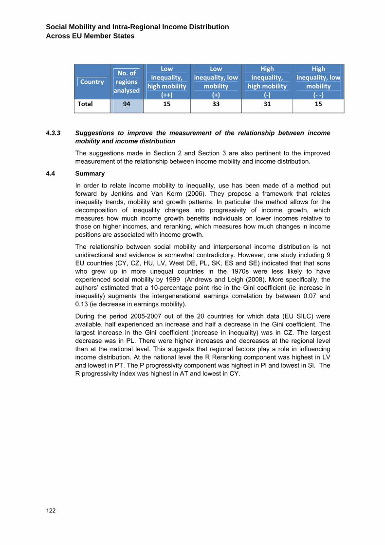
Social Mobility and Intra-Regional Income Distribution Across EU Member States
122
Country No. of
regions analysed
Low inequality,
high mobility (++)
Low inequality, low
mobility (+)
High inequality,
high mobility (-)
High inequality, low
mobility (- -)
Total 94 15 33 31 15
4.3.3 Suggestions to improve the measurement of the relationship between income mobility and income distribution
The suggestions made in Section 2 and Section 3 are also pertinent to the improved measurement of the relationship between income mobility and income distribution.
4.4 Summary
In order to relate income mobility to inequality, use has been made of a method put forward by Jenkins and Van Kerm (2006). They propose a framework that relates inequality trends, mobility and growth patterns. In particular the method allows for the decomposition of inequality changes into progressivity of income growth, which measures how much income growth benefits individuals on lower incomes relative to those on higher incomes, and reranking, which measures how much changes in income positions are associated with income growth.
The relationship between social mobility and interpersonal income distribution is not unidirectional and evidence is somewhat contradictory. However, one study including 9 EU countries (CY, CZ, HU, LV, West DE, PL, SK, ES and SE) indicated that that sons who grew up in more unequal countries in the 1970s were less likely to have experienced social mobility by 1999 (Andrews and Leigh (2008). More specifically, the authors’ estimated that a 10-percentage point rise in the Gini coefficient (ie increase in inequality) augments the intergenerational earnings correlation by between 0.07 and 0.13 (ie decrease in earnings mobility).
During the period 2005-2007 out of the 20 countries for which data (EU SILC) were available, half experienced an increase and half a decrease in the Gini coefficient. The largest increase in the Gini coefficient (increase in inequality) was in CZ. The largest decrease was in PL. There were higher increases and decreases at the regional level than at the national level. This suggests that regional factors play a role in influencing income distribution. At the national level the R Reranking component was highest in LV and lowest in PT. The P progressivity component was highest in Pl and lowest in Sl. The R progressivity index was highest in AT and lowest in CY.
5. RELATING INCOME MOBILITY AND PUBLIC SUPPLIES
123
5 RELATING INCOME MOBILITY AND PUBLIC SUPPLIES 5.1 Introduction
This Section of the report considers the ways in which income levels and income mobility are affected by public supplies. The focus is on public supplies analogous to those that may be supported by ECP. The Section begins with a review of the considerable challenges of estimating the relationships between public supplies and income mobility (Section 5.2). The Section continues with a presentation of the results of a regression undertaken where, using public expenditure data and the EU-SILC 2005-2007 data, income change has been regressed against public supplies of a type similar to the four broad categories of ECP expenditure (Section 5.3). Details of the approach to the regression are given in Annex 3. Unfortunately the findings are constrained by the quality and availability of public expenditure data at the regional level, particularly public expenditure analogous of ECP expenditure, and the relatively short time scale of the data on income change51. Furthermore, the EU-SILC data measures household cash income and transfers and not ‘in kind transfers’ of the type that are the potential consequence of much of the ECP expenditure. The results of the regression are therefore, only a partial basis on which to predict the consequences of ECP expenditure and investment. For this reason other evidence on the potential distributional consequences of ECP sub-categories of expenditure has been reviewed (Section 5.4).
The results of this review (and to a lesser extent the findings of the regression) have been used to classify the sub categories of ECP expenditure according to their distributional effects and to inform a series of simulations of the potential effects of changes in ECP resource allocations (Section 5.5). These simulations rely upon assumptions about how income derived from the ECP expenditure is received by different quintile groups that have been informed by the review. These assumptions have been applied to the actual resource allocations to countries and regions in the EU. (DG REGIO has compiled data on these allocations using a set of expenditure sub categories and categories that have been followed in the structure of Section 5.4).
A model has been used in the simulations that allocates ‘distribution coefficients’ based on these assumptions, that distribute expenditure to the income quintile groups for each sub category of ECP expenditure. The model indicates the average household income effects that would accrue in each quintile. The baseline simulation assumes that the current allocations apply. The other simulations assume variations in the total allocations (with the same allocations between categories) or reallocations between categories or different distribution coefficients. The model allows any level of resource reallocation between broad categories to be explored. The findings of the simulations reported here, which are for illustrative purposes, are however based on 10% adjustments to resource allocations.
The results of the simulations have been used to explore the potential effects of changes in resource allocations on inequality and in particular the Gini index at national and regional level (Section 5.6). The approach to the analysis is illustrated in a series of case studies giving the results of the simulations for 5 contrasting regions/countries in Annex 5.
51 Although the EU-SILC panel data include large numbers of responses which contribute to robustness and the analysis is incremental and therefore findings may be not strongly influenced by the particular economic context..
Social Mobility and Intra-Regional Income Distribution Across EU Member States
124
5.2 The difficulties of relating public expenditure to income distribution and mobility
Public policy affects individuals´ behaviour and outcomes in different ways, depending on individuals’ characteristics and current situation. For example, a policy initiative to increase women’s participation in the labour market will affect women differently depending on their educational level. Thus, to assess the impact of a policy one needs to know how it affects the different groups. This is of particular importance when one studies mobility, since mobility is concerned with the achievements of individuals relative to other individuals. In other words, average effects are not sufficient to evaluate the effects of a new policy on income (or social) mobility. Instead, one needs to estimate its effect on the different individuals or relevant groups of individuals.52 That is, to assess the impact of policy changes on mobility, one needs to have rich information about the personal characteristics of individuals, which is not readily available for this assignment.
A complete evaluation should take due account of direct and indirect effects on income. The effect of monetary transfers is usually much easier to analyse than that of public supplies. Considering the easier case, monetary transfers have a direct impact on individuals’ income, which is usually straightforward to estimate, but they may also trigger changes in labour supply, which may in turn affect individuals’ income as well.53 The magnitude of the latter indirect effect is at times difficult to estimate since, for instance, they are known to depend on the business cycle (income transfers may for instance reduce the added worker effect54 that occurs when unemployment rises) and on the institutional framework (the disincentive (income) effect on labour supply of income transfers may depend on the generosity of unemployment benefits).
Other policies that affect the determinants of income have also an indirect effect on income. Education, health or labour market policy changes, for instance, have a bearing on social mobility through the indirect effect they have on individual income. In order to estimate these indirect effects one needs to know how individuals react to the policy change, and how this change in individual behaviour affects their income (or the outcome of interest).55 Given this complexity and its relevance for this assignment, it has not been possible to pursue in this study a comprehensive analysis of the effects of public supplies of the type supplied under ECP income mobility.
Some policies provide in-kind transfers to individuals or households. Some studies have attempted to measure the incidence of these policies by calculating counterfactual distributions of income which include the share of overall expenditure that accrues to each individual or household. This exercise requires a great deal of information which is not available for this assignment and builds on a set of assumptions regarding the incidence of the expenditure among households that are difficult to test. This type of exercise does not give value for money since it is very costly to do and only provides static conclusions which do not incorporate behaviour, i.e. the approach does not allow individuals to change their behaviour as a result of the policy, and therefore do not take into account indirect effects. These exercises also ignore the causality issues explained below.
52 The variables which are relevant to define the groups will depend on the policy under evaluation. For instance, when evaluating a new training programme for long term unemployed, groups may be defined by employment status. 53 Only when monetary transfers are lump-sum (i.e. direct fix-amount income transfers given to everyone irrespective of their characteristics), there is no indirect effect and the overall effect equals the direct effect. In all other cases, one should check whether individuals modify their behaviour in any relevant way as a result of the policy change. 54 The added worker effect captures the cyclical changes in labour supply of second earners when main earners face unemployment. 55 Studies that consider only the direct effect implicitly assume then that individuals do not change their behaviour as a result of the policy.
5. RELATING INCOME MOBILITY AND PUBLIC SUPPLIES
125
When estimating the effect of public policy, causality is an important and, at times, difficult issue to measure. Simple correlations are not enough to assess the causal effects of policies that affect one of the income determinants, such as education. For instance, children of mothers who smoke during their pregnancy are known to have health problems and therefore do worse at school than children of mothers who did not smoke during the pregnancy. Smoking during pregnancy is also correlated with low educational attainment of mothers, and the education level of mothers and their children is also positively correlated. Now, to what extent is the poorer schooling attainment of these children due to the smoking during pregnancy of their mothers beyond the effect of the lower education of their mothers? To answer this question we need to know the real effect of anti-smoking policies on the educational attainment on children. If the correlation between mothers’ smoking and their children attainment is solely due to the effect of mothers’ education on the education of their children, anti-smoking policies will have no effect at all.
A complete evaluation should also consider the long term impact of public policy. Long term income effects may be especially relevant in health and education, since returns to education and health may accrue many years after the investment has taken place, as well as in the short term. Longer term effects are also relevant when the behaviour of individuals changes only in the longer term. For instance, more generous unemployment benefits may change the working attitudes of individuals in the longer term but not in the short term.
Most studies use a partial equilibrium framework and only consider and estimate immediate (or first-stage) effects, assuming that the policy affects only one market, thus ignoring or overlooking additional effects that occur in other markets. The effect of some policies, such as R&D or public infrastructure, is especially difficult to estimate because they affect many economic sectors and markets, and thus requires general equilibrium analysis, where interactions between different markets are modelled. These issues frame the quantitative analysis and its observations and the related policy pointers with respect to the effects of changes in ECP and resource allocation of social mobility and income distribution.
5.3 The effects of public expenditure analogous to ECP
Notwithstanding the difficulties mentioned above an attempt has been made to explore further the relationship between public expenditure and income mobility at the regional level. Income mobility 2005-2007 as indicated in EU-SILC panel data has been regressed against public expenditure. Public expenditure at national level in 21 countries and also additionally at regional level in four countries (DE, CZ, PL, HU) in 2007 in categories analogous to ECP expenditure was taken as independent variables. These sub categories have been regrouped into the four broad categories. The approach to this categorization is explained in Annex 4. The regression has identified the effects of the four broad categories of public expenditure on income change within each quintile household income group. The main findings of the regression are given in Table 5.1 which indicates both whether the variable significantly accounted for the variations observed and the confidence limits of these variations.
Overall the effects were very small but the following results were obtained:
There was a significant but small association between expenditure on aids to productive investment and income growth in the lowest income quintile and a decrease in incomes amongst quintile income groups 3, 4 and 5. This suggests that productive investment may have pro poor effects.
Income growth was higher in lower income groups in countries where investments in human capital were higher. This suggests that the earnings of

Social Mobility and Intra-Regional Income Distribution Across EU Member States
126
lower income groups may be positively affected by such investments. However, the aggregate effects were very small and not statistically significant.
The levels of public expenditure on infrastructure did not significantly explain variations in income growth between quintile groups.
The levels of RTD expenditure significantly affected income, being associated with reductions in quintile 1 and increases in quintiles 3, 4 and 5.
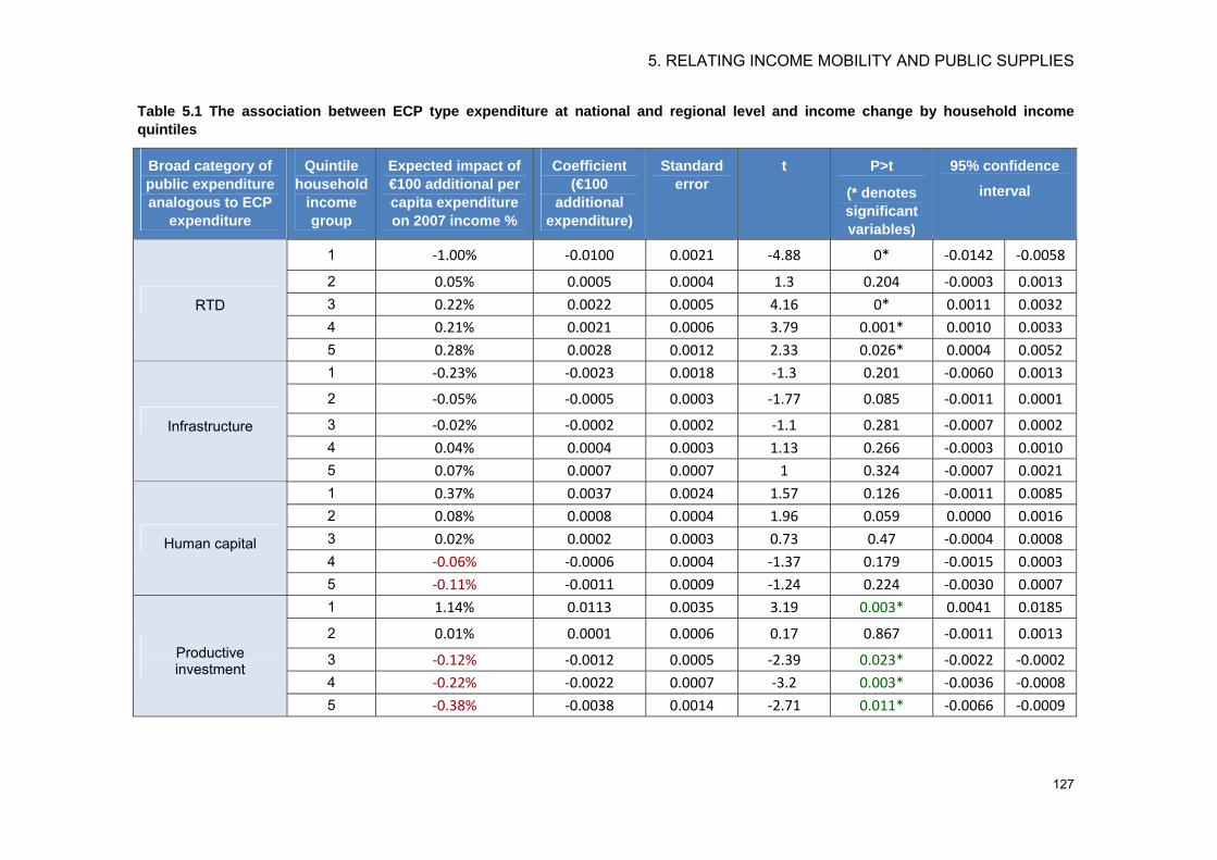
5. RELATING INCOME MOBILITY AND PUBLIC SUPPLIES
127
Table 5.1 The association between ECP type expenditure at national and regional level and income change by household income quintiles
Broad category of public expenditure analogous to ECP
expenditure
Quintile household
income group
Expected impact of €100 additional per capita expenditure on 2007 income %
Coefficient (€100
additional expenditure)
Standard error
t P>t
(* denotes significant variables)
95% confidence
interval
1 -1.00% -0.0100 0.0021 -4.88 0* -0.0142 -0.0058
2 0.05% 0.0005 0.0004 1.3 0.204 -0.0003 0.0013 3 0.22% 0.0022 0.0005 4.16 0* 0.0011 0.0032 4 0.21% 0.0021 0.0006 3.79 0.001* 0.0010 0.0033
RTD
5 0.28% 0.0028 0.0012 2.33 0.026* 0.0004 0.0052 1 -0.23% -0.0023 0.0018 -1.3 0.201 -0.0060 0.0013
2 -0.05% -0.0005 0.0003 -1.77 0.085 -0.0011 0.0001
3 -0.02% -0.0002 0.0002 -1.1 0.281 -0.0007 0.0002 4 0.04% 0.0004 0.0003 1.13 0.266 -0.0003 0.0010
Infrastructure
5 0.07% 0.0007 0.0007 1 0.324 -0.0007 0.0021 1 0.37% 0.0037 0.0024 1.57 0.126 -0.0011 0.0085 2 0.08% 0.0008 0.0004 1.96 0.059 0.0000 0.0016 3 0.02% 0.0002 0.0003 0.73 0.47 -0.0004 0.0008 4 -0.06% -0.0006 0.0004 -1.37 0.179 -0.0015 0.0003
Human capital
5 -0.11% -0.0011 0.0009 -1.24 0.224 -0.0030 0.0007 1 1.14% 0.0113 0.0035 3.19 0.003* 0.0041 0.0185
2 0.01% 0.0001 0.0006 0.17 0.867 -0.0011 0.0013
3 -0.12% -0.0012 0.0005 -2.39 0.023* -0.0022 -0.0002 4 -0.22% -0.0022 0.0007 -3.2 0.003* -0.0036 -0.0008
Productive investment
5 -0.38% -0.0038 0.0014 -2.71 0.011* -0.0066 -0.0009
Social Mobility and Intra-Regional Income Distribution Across EU Member States
128
5.4 Evidence from the literature on the distributional effects of ECP expenditure
The ECP expenditure on public supplies has the potential to affect the income of individuals and households in four ways:
Through affecting access to employment in the short, medium or long term. Much of ECP expenditure concerns capital investment that may bring benefits in terms of employment and income effects related to construction works in the short term as well as medium and long term effects.
Through providing income ‘in kind’.
Through bringing about environmental goods, health benefits or changes in property values that lead to in kind transfers. For example, both willingness to pay and hedonic pricing studies are used to provide estimates of the value of environmental goods that can be considered a source of ‘income’.
Through affecting the prices of commodities and public supplies (for example, energy, and transport). These may disproportionately affect one income group more than another.
An illustration of the importance of public supplies for income distribution is provided by an analysis in the UK, of the household income data of the Central Statistical Office (CSO). This showed that public spending on education, health services and housing subsidies (subsidies to local authority housing and housing association tenants) as well as rail and bus subsidies, school meals and welfare milk were worth significantly more for those with lower than for those with higher incomes. Indeed they were estimated as being worth almost twice as much for the bottom income quintile as for the top quintile (Evandrou et al., 1992, 1993). The analysis suggested that “final income” distribution which includes in-kind benefits is less unequal than the post-tax income and estimated that the bottom fifth of households receive only 6.9% of post-tax income but 9.9% of final income. Studies of other EU Member States reached similar conclusions. For instance, using 1995 ECHP data for Spain, Calero (2002) found that ‘in kind’ transfers in education and health have an equalising effect on the post-tax and post-transfer income distribution.
Aaberge, R. and A. Langørgen (2006) investigated the contribution of municipal in-kind benefits in 1988 amongst 2 million Norwegian families in over 400 municipalities. When all municipal services (i.e. in The Norwegian context, education, child care, health care, social services, care for the elderly and disabled, culture and related infrastructure) were taken into account, the decile groups with medium incomes receive higher in kind benefits than the lower and higher decile groups. In the cultural sector there was however, a slight weakening of inequality as the top deciles benefited most.
The ECP expenditure is divided into the following main categories:
Research and technological development (R&TD), innovation and entrepreneurship
Information society
Transport
Energy
Environmental protection and risk prevention
Tourism
Cultural

5. RELATING INCOME MOBILITY AND PUBLIC SUPPLIES
129
Urban and rural regeneration
Increasing the adaptability of workers and firms, enterprises and entrepreneurs
Improving access to employment and sustainability
Improving the social inclusion of less-favoured persons
Improving human capital
Investment in social infrastructure
Mobilisation for reforms in the fields of employment and inclusion
Strengthening institutional capacity at national, regional and local level
Reduction of additional costs hindering the outermost regions development
Technical assistance
ECP expenditure is further categorised within each of these fields. The potential effects of the ECP expenditure in each sub category are considered in the light of related research findings.
However, the following points needs to be borne in mind.
The ECP expenditure comprises only a subset of all public expenditure and public supplies and does not include public expenditure such as social transfers that have important and direct distributional effects.
For some of the ECP categories most expenditure at the national and regional levels is made by the public sector, whereas for others some, or even the majority of expenditure, is made by the private sector. The role of the market in determining the prices paid for public supplies will have an important effect on the extent to which the ECP funded public supplies impact on different income groups.
The regressive or progressive manner in which taxes are raised in order to fund public expenditure is relevant to the ‘final incomes’ of different households and influences public policy resource allocations and pricing policies.
The time scale of the effects of the public expenditure on income distribution and mobility will vary. Much of the ECP expenditure is oriented towards ‘structural’ changes in the beneficiary countries and regions that may take a considerable period to accrue. In the same vein the effects on individuals and households may be either short or long term. Effects that involve the acquisition or retention of employment are likely to contribute more to medium and long term income change and positional mobility.
The scale of the income effects may in some circumstances be greater than the scale of the public expenditure. Some ECP investments may, for example, generate multiplier effects at the local or regional levels.
Each of the categories of ECP expenditure is considered in turn below.
5.4.1 Research and technological development (R&TD), innovation and entrepreneurship
The following five sub categories of ECP expenditure:
R&TD activities in research centres
R&TD infrastructure and centres of competence in a specific technology

Social Mobility and Intra-Regional Income Distribution Across EU Member States
130
Technology transfer and improvement of cooperation networks between small businesses (SMEs), between these and other businesses and universities, post-secondary education establishments of all kinds, regional authorities, research centres and scientific and technological poles (scientific and technological parks, technopoles, etc), and
Assistance to R&TD, particularly in SMEs (including access to RTD services in research centres)
Investment in firms directly linked to research and innovation (innovative technologies, establishment of new firms by universities, existing RTD centres and firms, etc.)
are ‘likely to benefit in the short term more those in higher income groups working in RTD and Universities and those heading successful enterprises’. Innovations and new technologies tend to be driven by talent and entrepreneurship whether or not the drive is from within industry or universities. Around 30% of those working in RTD work within universities and professionals working in this area tend to be highly skilled and in higher income groups. The most significant short term effects are likely to be via increased demand for those with relevant research skills who tend to be amongst higher income groups. Moreover, the New Economic Geography (NEG) emphasises how this type of activity tends to focus employment in areas already rich in RTD assets, which tend to be high income areas. The medium and long term beneficial effects of public investment in these categories should however be felt more generally across income groups.
The category includes expenditure on:
Other measures to stimulate research and innovation and entrepreneurship in SMEs
Which is ‘likely to benefit more those in higher income groups’, through employment effects, ‘though some aspects of entrepreneurship are relevant to medium income groups’. Indeed entrepreneurship may be associated with self employment as an alternative to unemployment and thus of benefit to middle and lower income groups. Though it is reasonable to assume that research and innovation in SMEs will take place in larger SMEs led by those in higher income groups.
The category includes three further sub categories:
Advanced support services for firms and groups of firms
Assistance to SMEs for the promotion of environmentally-friendly products and production processes (introduction of effective environment managing system, adoption and use of pollution prevention technologies, integration of clean technologies into firm production
Other investment in firms
Where ‘no particular distribution effects’ can be foreseen.
5.4.2 Information society
There are three sub categories of expenditure where the distributional income effects are likely to be somewhat contradictory:
Telephone infrastructures (including broadband networks)
Information and communication technologies (access, security, interoperability, risk-prevention, research, innovation, e-content, etc.) and
Information and communication technologies (TEN-ICT)
5. RELATING INCOME MOBILITY AND PUBLIC SUPPLIES
131
On the one hand there are likely to be ‘more benefits to middle and lower income groups and lower inequality via public infrastructure’. This is evidenced for example, by the negative association between the Gini coefficient and the quality of telecommunication services (-0.34), observed by Calderón and Servén (2004). However, variations in the coverage of information and communication technologies may have distributional effects. On the other hand ‘ICT investments in companies are associated with increases in earnings inequality’. For example in the USA, Wolff, 2002, observed that investment in equipment and machinery, particular computers per person engaged in production, was strongly correlated (0.78) with household inequality.
There is one sub category within Information Society:
Services and applications for citizens (e-health, e-government, e-learning, e-inclusion, etc.)
Where ‘more benefits to middle and lower income groups’ are likely to accrue than for higher income groups. This is because such interventions should reduce the costs of access of citizens to these services and existing costs are more likely to be a barrier to lower than higher income groups. Furthermore ‘e-inclusion’ interventions are explicitly ‘pro lower income groups’. However, in the UK there is evidence to suggest that households in the higher income quartiles are more likely to use internet and benefit from e- services than those in the lower one although the ‘digital divide’ is less conspicuous in other countries such as Denmark for example (OECD, 2002)
There are two sub categories of expenditure under Information Society:
Services and applications for SMEs (e-commerce, education and training, networking, etc.)
Other measures for improving access to and efficient use of ICT by SMEs
where ‘no particular distribution effects’ can be foreseen.
5.4.3 Transport
Calderón and Servén (2004) examined the relationship between the breadth and quality of infrastructure and income inequality using a sample of 121 countries including 26 EU countries (UK was not included) and spanning the years 1960-2000. The study found that the Gini coefficient was negatively correlated with transport (-0.48 for roads, and –0.57 for roads and rail). This suggests that public investments in transport and particularly rail are strongly associated with income equality. There are various reasons why infrastructure development may disproportionately benefit the poor. There is evidence that better transportation infrastructure helps poorer individuals to gain access to additional productive opportunities (Estache, 2003). It can also decrease production and transaction costs (Gannon and Liu, 1997) and raise the value of the assets (homes, agricultural land) of the poor (Jacoby, 2000). From the UK there is evidence suggesting that commuting to work distances are increasing. People are less likely to relocate, to find a job, rather they will increase their job search area to find a job and stay put. This suggests that households are increasing their spending on travel to work. Investments in transport, particularly public transport, is therefore likely to have an increasing equalising effect
Thus there are three ECP expenditure sub categories within the transport field:
Railways
Railways (TEN-T)
Mobile rail assets, and
Social Mobility and Intra-Regional Income Distribution Across EU Member States
132
Mobile rail assets (TEN-T)
Overall investment in these sub categories is likely to be associated with income gains to middle and lower income groups. However, the TEN-T related investment may also benefit, and potentially disproportionately benefit, higher income groups making use of the high speed rail infrastructure.
Transport investments in roads involve the following ECP expenditure categories:
Motorways
Motorways (TEN-T)
National roads
Regional/local roads
Transport investments of this type are likely to be somewhat less effective in reducing inequality because the benefits tend to accrue to those owning cars and because effects on property values are likely to benefit more middle and higher income groups than those on low incomes. Using microdata on individual housing values in central cities and suburbs, Haughwout (1999) observed significant negative relationships between housing value and both highway spending and highway stocks for twenty-nine US metropolitan areas. The size of the negative effect was greater for central city housing values than for suburban housing values. One of the explanations provided suggests was that highway investments reduce the attractiveness of metropolitan area locations more than of suburban locations. Bearing in mind the above and the evidence of Calderón and Servén (2004) it is reasonable to suggest that basic roads infrastructure is likely to be pro poor through improving the access of lower income groups living in, for example, rural areas. However, roads infrastructure in urban areas that is characteristically expensive is less likely to be pro poor.
There are two ECP expenditure sub categories of transport expenditure that have a high potential to affect the incomes of middle and lower income groups they are:
Cycle tracks
Urban transport
This potential is greater if the investment in urban transport is oriented towards public transport.
One sub category of ECP expenditure:
Airports
is likely to bring more benefits to middle and higher income groups than low income groups because higher income groups travel more. For example, in the UK, the statistics provided by the Civil Aviation Authority (CAA) indicate a strong relationship between the frequency of leisure flying and the socio-economic characteristics of passengers with higher income households as well as singles, childless couples, and those with properties abroad taking more flights.
However, airports and related developments are major sources of employment and local economic activity and potential a source of construction, maintenance and service sector employment of benefit to lower income groups. They may also be associated with significant regional economic multiplier effects.
There are several ECP sub categories of transport expenditure where no particular distributional effects are likely. They are:
5. RELATING INCOME MOBILITY AND PUBLIC SUPPLIES
133
Multimodal transport
Multimodal transport (TEN-T)
Intelligent transport systems
Ports
Inland waterways (regional and local)
Inland waterways (TEN-T)
Expenditure in these areas mainly concerns the transport of goods and hence the distributional effects are likely to be minor and indirect. However, insofar as the costs of transport of goods that represent a higher proportion of the disposable income of lower income groups are reduced (for example, food) then impacts could be significant and progressive. The nature and scale of such impacts is likely to be dependent on the particular characteristics of the transport investment.
5.4.4 Energy
The sub categories of expenditure within energy are:
Electricity
Electricity (TEN-E)
Natural gas
Natural gas (TEN-E)
Petroleum products
Renewable energy: wind
Renewable energy: solar
Renewable energy: biomass
Renewable energy: hydroelectric, geothermal and other
Energy efficiency, co-generation, energy management
Calderón and Servén (2004) found a negative association between the breadth (-0.44), and quality (-0.26) of power infrastructure and the Gini coefficient. This suggests that access to in particular electricity, positively influences income equality. However, for relatively developed countries within the EU the distributional effects are not straightforward. Lower energy prices and lower consumption through energy efficiency can benefit lower income groups for whom energy costs may consume a high proportion of their disposable income. There may also be associated health benefits. However, investments in energy infrastructure particularly for renewables may be associated with higher energy prices as part of wider energy and climate change policies and/or because their commercial viability increases as a result of oil and gas price rises.
5.4.5 Environmental protection and risk prevention
Several of the sub categories of expenditure within this category are likely to be more beneficial to lower income groups than to middle and higher. They include:
Management of household and industrial waste
Management and distribution of water (drinking water)
Water treatment (waste water)
Social Mobility and Intra-Regional Income Distribution Across EU Member States
134
Air quality
Rehabilitation of industrial sites and contaminated land
Promotion of clean urban transport
Risk prevention (including the drafting and implementation of plans and measures to prevent and manage natural and technological risks)
Other measures to preserve the environment and prevent risks
Two general points can be made. Firstly, poor people tend to live closer to sources of pollution and this lowers their real incomes. For example, a hedonic pricing study undertaken by Cambridge Econometrics that the value of properties in the UK located closer to waste tips was lower than equivalent properties further away. It follows that environmental clean-up should benefit low income households disproportionately. Secondly, there is a trend to increase household charges for environmental services such as water, wastewater, and domestic waste, rather than fund these from general taxes. This can potentially lead to lower income households paying proportionately more than higher income households. Thus the ECP expenditure in these areas could have only short term positive effects on lower income groups. Taking the ECP expenditure sub categories in turn:
Household and industrial waste: Lower income groups are likely to benefit from improvements in waste disposal sites (both household and industrial waste) because many such households live close to them. Other income effects will be affected by the charging policies adopted for household waste disposal.
Drinking water: Calderón and Servén (2004) showed that improved access to safer water significantly decreases income inequality.
Air quality: Bae (1997a,b) indicated that the benefits of the policies on air quality improvement in the USA are experienced by ethnic minorities with lower household incomes and larger-size families. Those benefitting from such policies tend to live in more polluted neighbourhoods whilst the white population is concentrated in the cleaner air communities. The association between poverty and pollution has also been demonstrated by other more recent studies. For example, McLeod et al. (2008) found an overall negative relationship between air pollution exposure and social class index (the higher the exposure, the lower the social status).
Waste water treatment: Lower income groups are likely to benefit from improvements in waste water treatment plants, through for example, odour control. However, sewage treatment plants tend to be relatively isolated away from residential areas thus the number of households benefiting in this way is likely to be small. Other income effects will be affected by the charging policies adopted for household sewage treatment.
Rehabilitation of industrial sites and contaminated land: As with air quality and household waste there is a tendency for those with lower incomes to live in proximity to contaminated sites and hence they may benefit more through this type of investment.
Risk Prevention: Risk prevention measures are likely to advantage medium to lower income groups who are likely to be more vulnerable in terms of harm and potential loss of property than higher income groups. However, the lowest income groups are likely to have less to lose.
Promotion of clean urban transport: the distributional consequences are likely to be similar to those of air quality.
There are three sub categories of ECP expenditure in this field:

5. RELATING INCOME MOBILITY AND PUBLIC SUPPLIES
135
Integrated prevention and pollution control
Mitigation and adaption to climate change
Promotion of biodiversity and nature protection (including Natura 2000)
where no particular distributional effects are likely. However, integrated prevention and pollution control measures may have similar distributional consequences as air quality measures, depending on how and where the former are applied. Also whilst all income groups should benefit from measures to mitigate and adapt to climate change, worldwide the effects of climate change will be most keenly felt in poorer countries. The consequences of loss of biodiversity are likely to be felt by all income groups.
5.4.6 Tourism
There are two sub categories in this field where it is unlikely that there would be are particular distributional effects. They are:
Promotion of natural assets
Protection and development of natural heritage
Whilst they might be considered as likely to primarily benefit tourists who are themselves likely to be disproportionately drawn from middle and higher income groups the assets promoted and protected have value for all income groups. For example, there is evidence from the UK that expenditure of this type benefits middle and higher income groups. Lower income households tend not to use UK National Parks. However, tourism projects may be an important source of employment and have local and regional economic multiplier effects.
The third sub category:
Other assistance to improve tourist services,
is similarly likely to lead to improved employment prospects in tourism. Such jobs are often relatively low paid and may therefore benefit lower income groups disproportionately (Riley et al 2002). ‘Hotels and restaurants’ was the economic activity with the highest proportion of low wage earners (41%) (Eurostat, Statistics in Focus 2010)
5.4.7 Culture
There are two sub categories of expenditure in this field where the distributional effects are likely to disproportionately benefit middle and higher income groups. They are:
Protection and preservation of the cultural heritage
Development of cultural infrastructure
Such effects are likely because higher income groups are more likely to be able to afford access to the products of such expenditure and/or to have the costs of their access reduced through subsidy. Aaberge, R. and A. Langørgen (2006) investigated the contribution of municipal in-kind benefits in the culture sector to inequality and observed a weak disequalizing effect.
There is one further sub category of ECP expenditure:
Other assistance to improve cultural services
But this is insufficiently detailed and hence no particular distribution effects can be anticipated.

Social Mobility and Intra-Regional Income Distribution Across EU Member States
136
5.4.8 Urban and rural regeneration
There is only one sub category of expenditure within this field:
Integrated projects for urban and rural regeneration
The description is insufficiently detailed to anticipate the distributional effects. However, expenditure of this type tends to focus on areas (either rural or urban) facing difficulties and relatively high levels of low income groups. Thus some ‘pro poor’ distributional effects are likely.
5.4.9 Increasing the adaptability of workers and firms, enterprises and entrepreneurs
All three sub categories of expenditure in this field:
Development of life-long learning systems and strategies in firms; training and services for employees to step up their adaptability to change; promoting entrepreneurship and innovation,
Design and dissemination of innovative and more productive ways of organising work,
Development of specific services for employment, training and support in connection with restructuring of sectors and firms, and development of systems for anticipating economic changes and future requirements in terms of jobs and skills,
are likely to benefit more middle and lower income groups. The actions supported tend to be focussed on those already in employment but vulnerable to structural change. Beneficiary groups are likely to include existing employees requiring new skills, ‘older workers’ and workers benefiting from flexible working. The lowest income groups, that typically include the unemployed, will benefit less.
5.4.10 Improving access to employment and sustainability
The sub category of expenditure within this category likely to have the greatest ‘pro poor’ distributional effects is that concerned with:
Implementing active and preventive measures on the labour market
Measures of this type typically include employment services and vocational training, including training in basic skills oriented towards those who are unemployed, those who have disabilities or who are otherwise from ‘disadvantaged groups’ such as ‘female returners’ or ‘early school leavers.’ Thus lower income groups are likely to benefit more than middle and higher income groups. At best the effects should be both short and longer term.
Three sub categories are likely to benefit more middle and lower income groups:
Support for self-employment and business start-up
Measures to improve access to employment and increase sustainable participation and progress of women in employment to reduce gender-based segregation in the labour market, and to reconcile work and private life, such as facilitating access to childcare and care for dependent persons, and
Specific action to increase migrants’ participation in employment and thereby strengthen their social integration.
There are both push and pull factors influencing the incidence of self employment and business start ups. Self employment may be seen by some as an alternative to

5. RELATING INCOME MOBILITY AND PUBLIC SUPPLIES
137
unemployment. However, for the lowest income group self employment may not be a realistic option.
Female employment is an important determinant of household income and measures to improve access to and progress of women in employment are likely to markedly affect lower and middle income groups. Migrants benefiting from measures to increase their access to employment are also likely to be in lower and middle income groups.
There are two sub categories which are unlikely to have any particular direct distribution effects:
Modernisation and strengthening labour market institutions
Measures encouraging active ageing and prolonging working lives.
The modernisation and strengthening of labour market institutions should improve the efficiency of labour market institutions rather than their distributional effects. The measures encouraging active ageing and prolonging working lives are likely to be of benefit to all income groups.
5.4.11 Improving the social inclusion of less-favoured persons
The single sub category of expenditure:
Pathways to integration and re-entry into employment for disadvantaged people; combating discrimination in accessing and progressing in the labour market and promoting acceptance of diversity at the workplace,
is likely to benefit more low income groups who may otherwise be the object of discrimination. This is an overtly ‘pro poor’ category.
5.4.12 Improving human capital
Evidence on the distribution effects of investments in education and training provides various and sometimes contradictory findings.
In Finland, Pekkarinen et al. (2006) provide evidence of a positive impact on the lowest quintile on (sons’) earnings of a major educational reform in the Finnish primary and secondary education (1972-1977). Luo (2008) used quantile regression to investigate the relationship between returns to education and income distribution. Educational attainment was measured by both schooling years and the level of education attained. The study found that the return to education was higher for lower income quintiles. However, contrary results had been reported in previous studies.
Using household survey data, Evandrou et al (1992, 1993) disaggregated the total value of benefits from public spending on education, the UK National Health Service (NHS) and subsidies to local authority housing that accrued to households in different income groups. Regarding education, the study found that the middle of the income distribution reap the greatest education benefits. Also, the education benefits of the top group of the income distribution were higher than the benefits of the bottom of the distribution (ie education spending was pro-rich rather than pro-poor). Expenditure on further and higher education tended to be especially pro-rich as the top group of all households received nearly five times as much from the tertiary education as the bottom group. However, the top group received substantially less from state compulsory schooling than from further and higher education; the opposite held true for the poorer groups. One of the factors accounting for this was the greater benefits that students living away from home (usually amongst the better off) received from higher education relative to the students living at home. This is also the case for Spain (see Calero (1998)).

Social Mobility and Intra-Regional Income Distribution Across EU Member States
138
In the same vein Marical et al., 2006 looked at inter-quintile share ratios before and after inclusion of public expenditures on primary, secondary and tertiary education. The results indicated that the share of public expenditure on tertiary education accruing to people in the top income quintile was close to 30% on average, and above 40% in Belgium, Spain and Portugal. The evidence suggests that in OECD countries attendance of tertiary education (in contrast with compulsory education - primary and lower secondary education) is associated with an unequal distribution of resources, primarily because access to non-compulsory education depends on parents’ socio-economic characteristics (OECD, 2008). For example, using ECHP data for EU-15 (excl. Sweden), O’Donoghue, (2003) showed that students from richer families are more likely to attend university (cited by the Council for Employment, Income and Social Cohesion in 2003). National studies found similar results: in France, individuals from households in the highest income quintile have a probability of access to university three times higher than that of the lowest quintile (Albouy et al. 2002). In the UK, Sefton (2002) found significant differences in the use of services across income deciles, with tertiary education favouring the rich.
There is also an issue around returns to education: people from low-income groups tend to attend courses and universities that yield lower economic benefits in terms of future earnings. They are less likely to attend “elite” universities (Chevalier and Conlon, 2003) and more likely to study for a vocational than an academic qualification (Conlon, 2002).
Overall there is strong potential for expenditure in this category to influence social mobility and income distribution but realizing this potential depends upon the detailed design parameters of the interventions.
The ECP expenditure sub category:
Measures to increase participation in education and training throughout the life-cycle, including through action to achieve a reduction in early school leaving, gender-based segregation of subjects and increased access to and quality of initial vocational and tertiary education and training
is likely to bring benefits more to low income groups, particularly action to reduce early school leaving and where there is an emphasis on improving access to initial vocational and tertiary education and training for lower income groups.
The sub category:
Design, introduction and implementation of reforms in education and training systems in order to develop employability, improving the labour market relevance of initial and vocational education and training, updating skills of training personnel with a view to innovation and a knowledge based economy,
is likely to benefit more middle and lower income groups that tend to be the main beneficiaries of core expenditure of this type.
The sub category:
Developing human potential in the field of research and innovation, in particular through post-graduate studies and training of researchers, and networking activities between universities, research centres and businesses
is most likely to benefit middle and higher income groups.
5.4.13 Investment in social infrastructure
The general ‘pro poor’ importance of public supplies of this type has been emphasised above, Evandrou et al. (1992, 1993).
5. RELATING INCOME MOBILITY AND PUBLIC SUPPLIES
139
The first ECP expenditure sub category is:
Education infrastructure.
The distributional effects will very much depend on the level of education of the infrastructure. Primary, secondary and vocational education and training infrastructure are likely to benefit lower income groups more than higher education. However, as stressed above education infrastructure is just one dimension of education expenditure and the distributional and mobility effects will depend upon policies affecting the access to and use of such infrastructure.
The second sub category is:
Health infrastructure
Expenditure of this type is likely to benefit more middle and lower income groups. In a study of the UK National Health Service (NHS), Evandrou et al. (1992,1993) showed that the lowest quintile received 62% more benefits than the highest. This was both because the poorer groups tended to have more health problems but also because retired people tend to be concentrated in the bottom two groups of the income distribution. As with education infrastructure the distributional and mobility effects will depend upon policies affecting the access to and use of such infrastructure. Where the benefits of health infrastructure enable those with health problems or disabilities to increase their earnings the income mobility effects are likely to be large.
The third sub category is:
Childcare infrastructure
As with expenditure on health infrastructure this is likely to benefit more middle and low income groups as it is linked with increasing female participation in the labour market.
The fourth sub category is:
Housing infrastructure
Again this type of expenditure is likely to benefit more middle and low income groups. The Evandrou et al. (1992, 1993) study measured subsidies to local authority tenants as the difference between actual gross rents and the estimated “economic real return” on the assets. These subsidies mainly accrued to the lower income groups. Two relevant studies observed that the two bottom income quintiles in the UK benefited most from social housing receiving between 34% and 36% respectively of the total benefits (Sefton, 2002; Lakin, 2004). However, the effects of social housing on household income distribution depend on the characteristics of renters and on the estimated value of the “implicit subsidy” (Marical et al / OECD, 2008)
The final sub category:
Other social infrastructure
Is, as with the health, housing and childcare categories, likely to benefit more the middle and lower income groups.
5.4.14 Mobilisation for reforms in the fields of employment and inclusion
There is only one ECP expenditure sub category:
Promoting the partnerships, pacts and initiatives through the networking of relevant stakeholders
No particular distribution effects are anticipated. However, the orientation towards inclusion suggests some secondary effects may benefit those in lower income groups.

Social Mobility and Intra-Regional Income Distribution Across EU Member States
140
5.4.15 Strengthening institutional capacity at national, regional and local level
There is only one sub category:
Mechanism for improving good policy and programme design, monitoring and evaluation
No particular distribution effects are anticipated.
5.4.16 Reduction of additional costs hindering the outermost regions development
There are three sub categories of expenditure:
Compensation of any additional costs due to accessibility deficit and territorial fragmentation
Specific action addressed to compensate additional costs due to size market factors
Support to compensate additional costs due to climate conditions and relief difficulties
Each of these is anticipated to bring more benefits to middle and lower income groups because the additional costs due to accessibility and market size are likely to adversely affect the prices of commodities and essentials that take a disproportionate amount of the income of lower income groups. Problems due to climate conditions are also most likely to be felt by those on lower incomes less able to avoid them.
5.4.17 Technical assistance
There are two sub categories:
Preparation, implementation, monitoring and inspection
Evaluation and studies; information and communication
No particular distribution effects are anticipated.
5.4.18 Estimates of the distribution effects of ECP categories of expenditure
Bearing in mind the discussion and findings above Table 5.2 classifies each of the sub categories of ECP expenditure as follows:
Pro lower income groups
Pro middle and lower income groups
Pro middle and higher income groups
Pro higher income groups
No particular distribution effects
Amongst the latter category there are also those that are likely to have distributional consequences but the net effects are uncertain and dependent on non ECP policy factors. The possible distributional effects of each category of ECP expenditure have been expressed in terms of the proportion of resources that would be received by each quintile income groups. It has been assumed that the income benefits equate to the expenditure. The detailed income distribution assumptions for each sub category are provided in the simulation model.
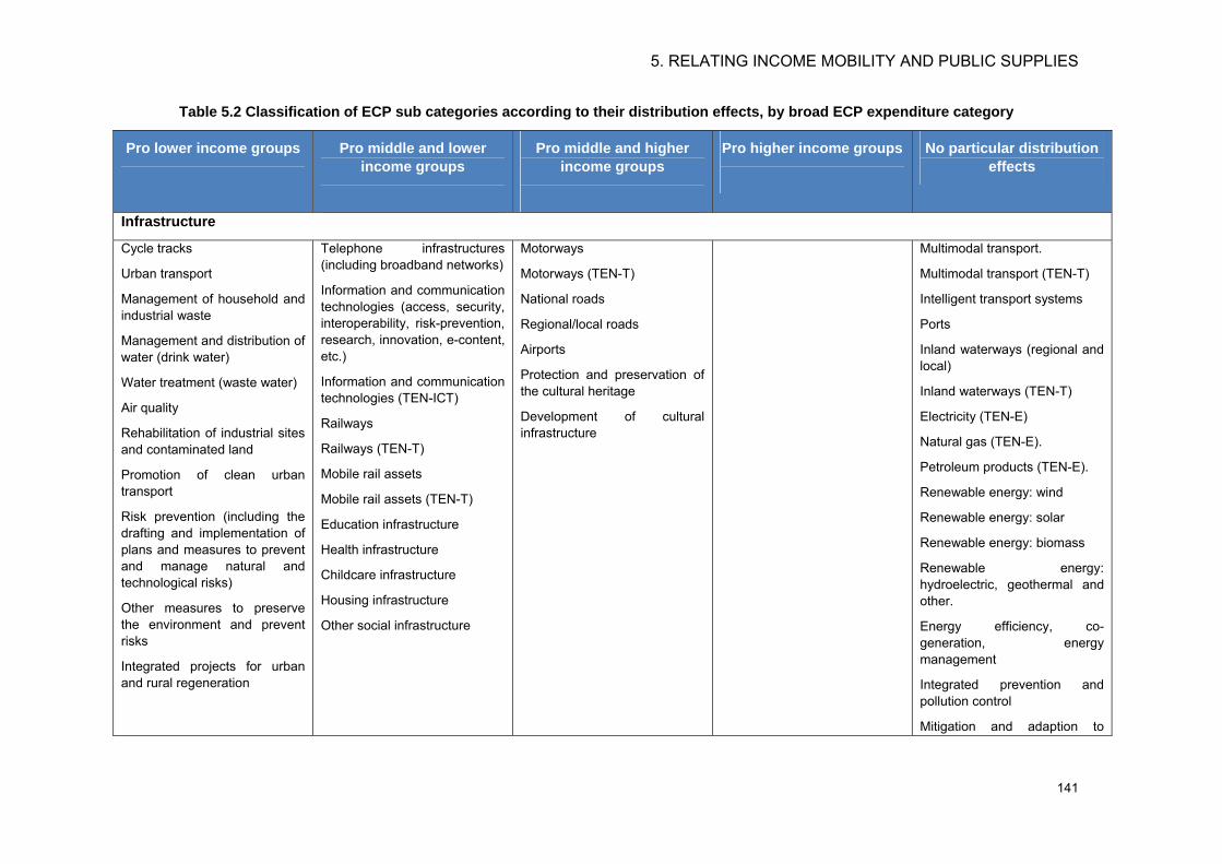
5. RELATING INCOME MOBILITY AND PUBLIC SUPPLIES
141
Table 5.2 Classification of ECP sub categories according to their distribution effects, by broad ECP expenditure category
Pro lower income groups
Pro middle and lower income groups
Pro middle and higher income groups
Pro higher income groups
No particular distribution effects
Infrastructure
Cycle tracks
Urban transport
Management of household and industrial waste
Management and distribution of water (drink water)
Water treatment (waste water)
Air quality
Rehabilitation of industrial sites and contaminated land
Promotion of clean urban transport
Risk prevention (including the drafting and implementation of plans and measures to prevent and manage natural and technological risks)
Other measures to preserve the environment and prevent risks
Integrated projects for urban and rural regeneration
Telephone infrastructures (including broadband networks)
Information and communication technologies (access, security, interoperability, risk-prevention, research, innovation, e-content, etc.)
Information and communication technologies (TEN-ICT)
Railways
Railways (TEN-T)
Mobile rail assets
Mobile rail assets (TEN-T)
Education infrastructure
Health infrastructure
Childcare infrastructure
Housing infrastructure
Other social infrastructure
Motorways
Motorways (TEN-T)
National roads
Regional/local roads
Airports
Protection and preservation of the cultural heritage
Development of cultural infrastructure
Multimodal transport.
Multimodal transport (TEN-T)
Intelligent transport systems
Ports
Inland waterways (regional and local)
Inland waterways (TEN-T)
Electricity (TEN-E)
Natural gas (TEN-E).
Petroleum products (TEN-E).
Renewable energy: wind
Renewable energy: solar
Renewable energy: biomass
Renewable energy: hydroelectric, geothermal and other.
Energy efficiency, co-generation, energy management
Integrated prevention and pollution control
Mitigation and adaption to
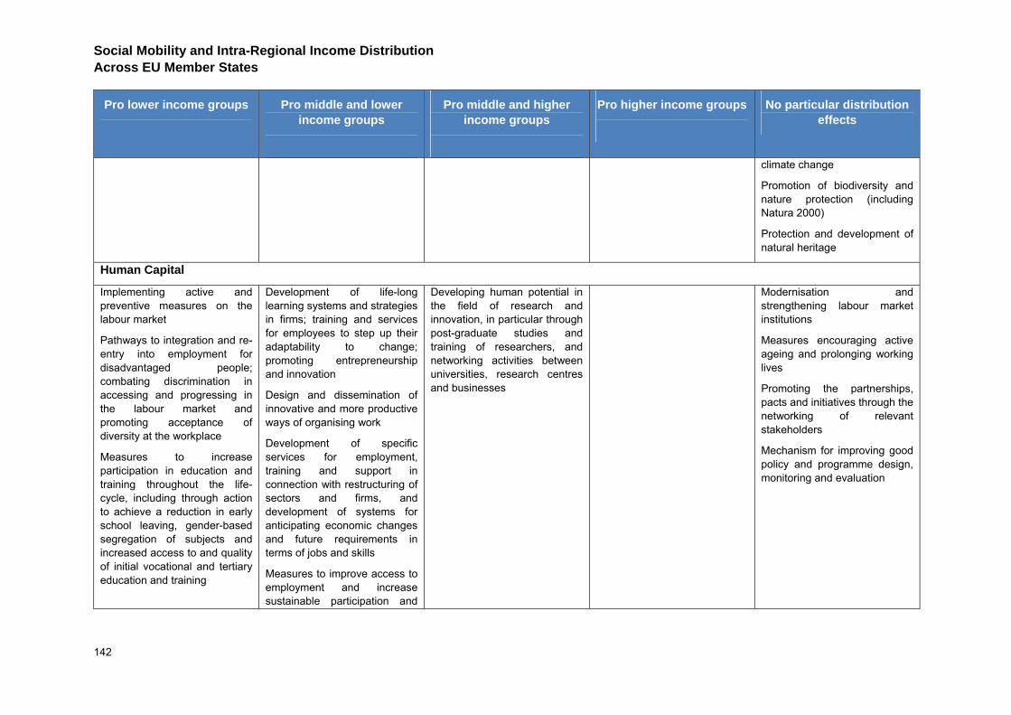
Social Mobility and Intra-Regional Income Distribution Across EU Member States
142
Pro lower income groups
Pro middle and lower income groups
Pro middle and higher income groups
Pro higher income groups
No particular distribution effects
climate change
Promotion of biodiversity and nature protection (including Natura 2000)
Protection and development of natural heritage
Human Capital
Implementing active and preventive measures on the labour market
Pathways to integration and re-entry into employment for disadvantaged people; combating discrimination in accessing and progressing in the labour market and promoting acceptance of diversity at the workplace
Measures to increase participation in education and training throughout the life-cycle, including through action to achieve a reduction in early school leaving, gender-based segregation of subjects and increased access to and quality of initial vocational and tertiary education and training
Development of life-long learning systems and strategies in firms; training and services for employees to step up their adaptability to change; promoting entrepreneurship and innovation
Design and dissemination of innovative and more productive ways of organising work
Development of specific services for employment, training and support in connection with restructuring of sectors and firms, and development of systems for anticipating economic changes and future requirements in terms of jobs and skills
Measures to improve access to employment and increase sustainable participation and
Developing human potential in the field of research and innovation, in particular through post-graduate studies and training of researchers, and networking activities between universities, research centres and businesses
Modernisation and strengthening labour market institutions
Measures encouraging active ageing and prolonging working lives
Promoting the partnerships, pacts and initiatives through the networking of relevant stakeholders
Mechanism for improving good policy and programme design, monitoring and evaluation

5. RELATING INCOME MOBILITY AND PUBLIC SUPPLIES
143
Pro lower income groups
Pro middle and lower income groups
Pro middle and higher income groups
Pro higher income groups
No particular distribution effects
progress of women in employment to reduce gender-based segregation in the labour market, and to reconcile work and private life, such as facilitating access to childcare and care for dependent persons
Specific action to increase migrants’ participation in employment and thereby strengthen their social integration
Design, introduction and implementation of reforms in education and training systems in order to develop employability, improving the labour market relevance of initial and vocational education and training, updating skills of training personnel with a view to innovation and a knowledge based economy
RTD
Other measures to stimulate research and innovation and entrepreneurship in SMEs
R&TD activities in research centres
R&TD infrastructure and centres of competence in a specific technology
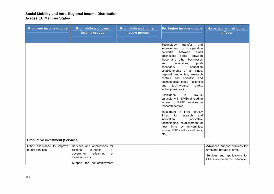
Social Mobility and Intra-Regional Income Distribution Across EU Member States
144
Pro lower income groups
Pro middle and lower income groups
Pro middle and higher income groups
Pro higher income groups
No particular distribution effects
Technology transfer and improvement of cooperation networks between small businesses (SMEs), between these and other businesses and universities, post-secondary education establishments of all kinds, regional authorities, research centres and scientific and technological poles (scientific and technological parks, technopoles, etc).
Assistance to R&TD, particularly in SMEs (including access to R&TD services in research centres)
Investment in firms directly linked to research and innovation (innovative technologies, establishment of new firms by universities, existing RTD centres and firms, etc.)
Productive investment (Services)
Other assistance to improve tourist services
Services and applications for citizens (e-health, e-government, e-learning, e-inclusion, etc.)
Support for self-employment
Advanced support services for
firms and groups of firms
Services and applications for SMEs (e-commerce, education

5. RELATING INCOME MOBILITY AND PUBLIC SUPPLIES
145
Pro lower income groups
Pro middle and lower income groups
Pro middle and higher income groups
Pro higher income groups
No particular distribution effects
and business start-up
Support to compensate additional costs due to climate conditions and relief difficulties
and training, networking, etc.)
Other measures for improving access to and efficient use of ICT by SMEs
Promotion of natural assets
Other assistance to improve cultural services
Productive investment (Industry)
Compensation of any additional costs due to accessibility deficit and territorial fragmentation
Specific action addressed to compensate additional costs due to size market factors
Assistance to SMEs for the promotion of environmentally-friendly products and production processes (introduction of effective environment managing system, adoption and use of pollution prevention technologies, integration of clean technologies into firm production
Other investment in firms
Electricity
Natural gas
Petroleum products
Source: GHK based on ECP expenditure 2007-2013
Social Mobility and Intra-Regional Income Distribution Across EU Member States
146
There are 15 sub categories are pro lower income groups, 23 categories that are pro middle and lower income groups, 9 sub categories that are pro middle and higher income groups and 5 categories that are pro higher income groups. There are 32 sub categories where there are no particular distribution effects or where any such effects are highly dependent upon complementary national or regional policies. Some of these have the potential to have pro lower and middle income distribution effects.
5.5 The household income effects of ECP expenditure
The effects on the incomes of households within quintile groups of changes in ECP resource allocation have been estimated for each NUTS2 region. Information is available on actual ECP resource allocations at the regional level for the period 2007-2013.
It is assumed that the value of benefits of ECP expenditure is equivalent to the costs. It can be argued that this is a conservative assumption. This is because much of the actual ECP expenditure is spent on investment and infrastructure projects where the benefits accruing are judged to outweigh benefits and the expenditure may lead to regional multiplier effects. However, more fine tuned assumptions based on the characteristics of particular sub categories of ECP expenditure have not been applied because of the lack of evidence to support them. The simulation model prepared as part of the assignment does however allow for such ‘multiplier’ assumptions to be varied for each category of ECP expenditure.
The income distribution effects of nine broad simulations have been estimated, the simulations concern:
(1) X% pro rata increase in ECP expenditure.
(2) X% pro rata decrease in ECP expenditure.
(3) X% increase in ECP categories relating to physical infrastructure, and corresponding decreases in all other categories.
(4) X% increase in ECP categories relating to human resources infrastructure, and corresponding decreases in all other categories.
(5) X% increase in ECP categories relating to research and technological development (R&TD), and corresponding decreases in all other categories.
(6) X% increase in ECP categories relating to aids to productive sector and corresponding decreases in all other categories.
(7) X% increase in allocations to categories that are pro lower and middle income groups and corresponding decreases in all other categories, assuming moderate distribution effects.
(8) X% increase in allocations to categories that are pro lower and middle income groups and corresponding decreases in all other categories, assuming high distribution effects.
(9) X% increase in allocations to categories that are pro lower and middle income groups and corresponding decreases in all other categories, assuming very high distribution effects.
These simulations have been chosen in order to explore the possible effects of changes in ECP resource allocation decisions on income mobility and income distribution. The latter three simulations explore the possible effects of resource allocation adjustments that are likely to be pro poor whilst applying different assumptions as to the extent to which particular sub categories of ECP expenditure are likely to benefit lower income
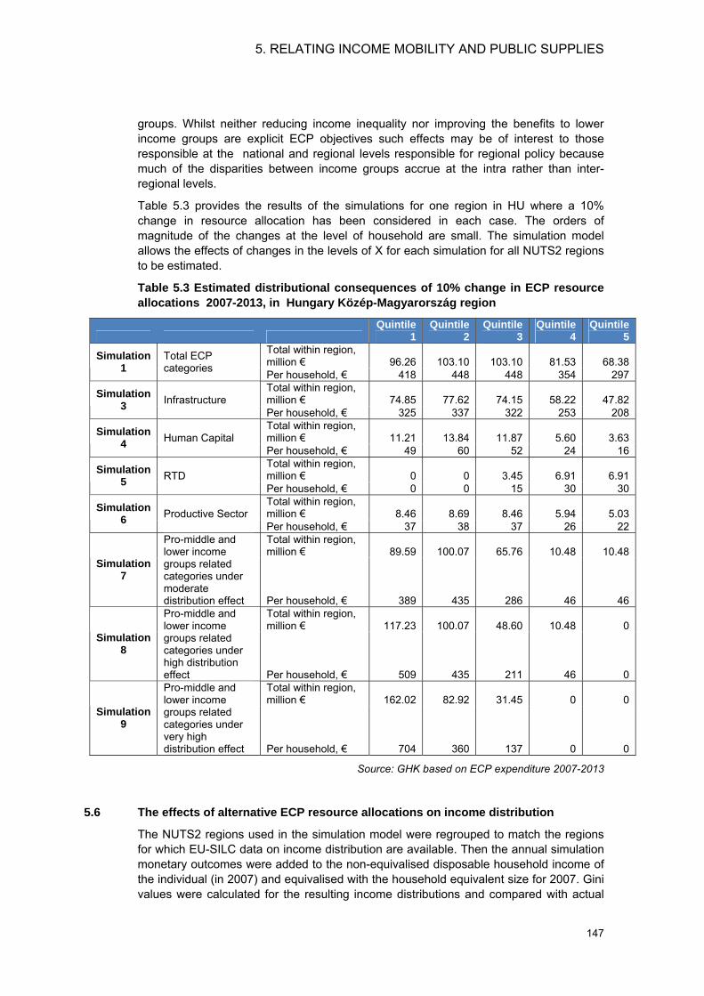
5. RELATING INCOME MOBILITY AND PUBLIC SUPPLIES
147
groups. Whilst neither reducing income inequality nor improving the benefits to lower income groups are explicit ECP objectives such effects may be of interest to those responsible at the national and regional levels responsible for regional policy because much of the disparities between income groups accrue at the intra rather than inter- regional levels.
Table 5.3 provides the results of the simulations for one region in HU where a 10% change in resource allocation has been considered in each case. The orders of magnitude of the changes at the level of household are small. The simulation model allows the effects of changes in the levels of X for each simulation for all NUTS2 regions to be estimated.
Table 5.3 Estimated distributional consequences of 10% change in ECP resource allocations 2007-2013, in Hungary Közép-Magyarország region
Quintile
1 Quintile
2 Quintile
3 Quintile
4 Quintile
5 Total within region, million € 96.26 103.10 103.10 81.53 68.38 Simulation
1 Total ECP categories Per household, € 418 448 448 354 297
Total within region, million € 74.85 77.62 74.15 58.22 47.82 Simulation
3 Infrastructure Per household, € 325 337 322 253 208 Total within region, million € 11.21 13.84 11.87 5.60 3.63 Simulation
4 Human Capital Per household, € 49 60 52 24 16 Total within region, million € 0 0 3.45 6.91 6.91 Simulation
5 RTD Per household, € 0 0 15 30 30 Total within region, million € 8.46 8.69 8.46 5.94 5.03 Simulation
6 Productive Sector Per household, € 37 38 37 26 22 Total within region, million € 89.59 100.07 65.76 10.48 10.48
Simulation 7
Pro-middle and lower income groups related categories under moderate distribution effect Per household, € 389 435 286 46 46
Total within region, million € 117.23 100.07 48.60 10.48 0
Simulation 8
Pro-middle and lower income groups related categories under high distribution effect Per household, € 509 435 211 46 0
Total within region, million € 162.02 82.92 31.45 0 0
Simulation 9
Pro-middle and lower income groups related categories under very high distribution effect Per household, € 704 360 137 0 0
Source: GHK based on ECP expenditure 2007-2013
5.6 The effects of alternative ECP resource allocations on income distribution
The NUTS2 regions used in the simulation model were regrouped to match the regions for which EU-SILC data on income distribution are available. Then the annual simulation monetary outcomes were added to the non-equivalised disposable household income of the individual (in 2007) and equivalised with the household equivalent size for 2007. Gini values were calculated for the resulting income distributions and compared with actual
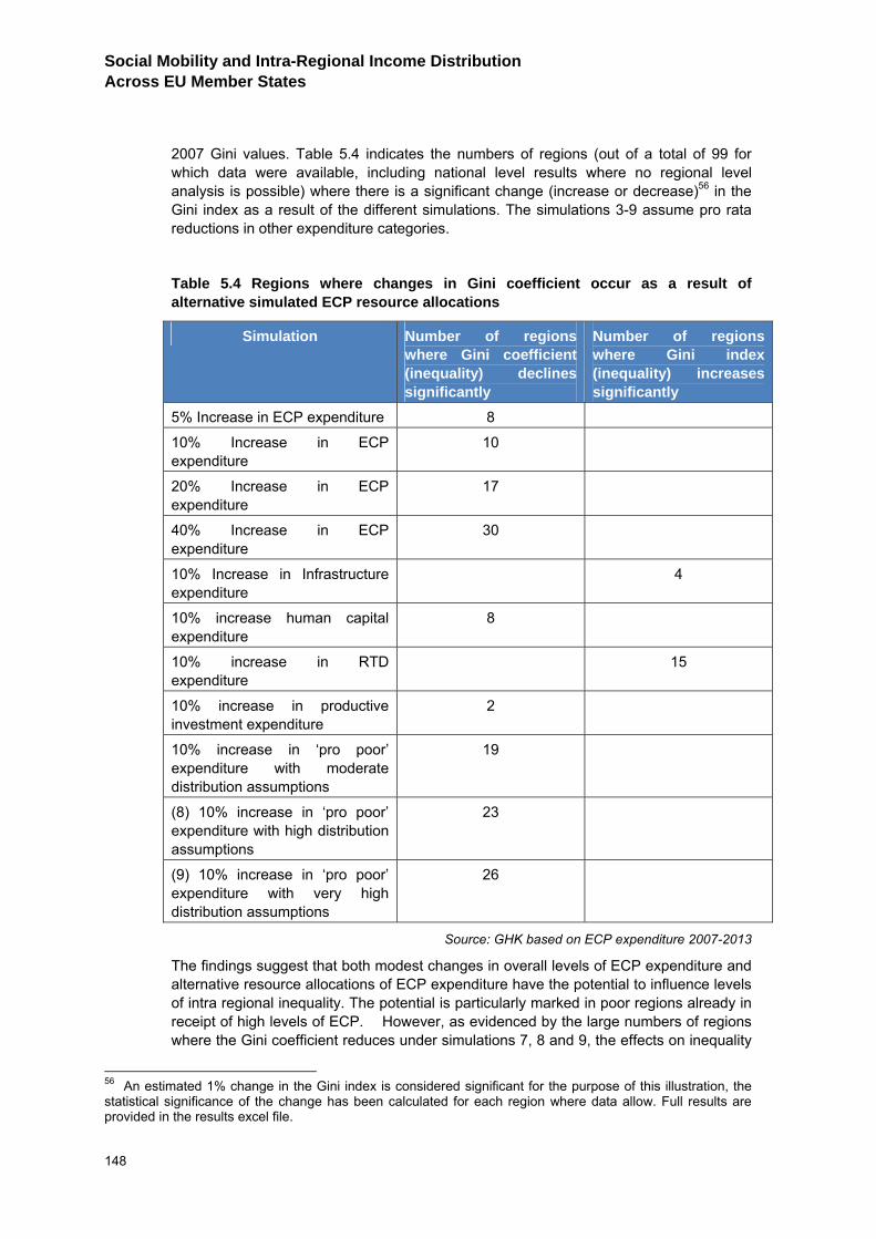
Social Mobility and Intra-Regional Income Distribution Across EU Member States
148
2007 Gini values. Table 5.4 indicates the numbers of regions (out of a total of 99 for which data were available, including national level results where no regional level analysis is possible) where there is a significant change (increase or decrease)56 in the Gini index as a result of the different simulations. The simulations 3-9 assume pro rata reductions in other expenditure categories.
Table 5.4 Regions where changes in Gini coefficient occur as a result of alternative simulated ECP resource allocations
Simulation Number of regions where Gini coefficient (inequality) declines significantly
Number of regions where Gini index (inequality) increases significantly
5% Increase in ECP expenditure 8
10% Increase in ECP expenditure
10
20% Increase in ECP expenditure
17
40% Increase in ECP expenditure
30
10% Increase in Infrastructure expenditure
4
10% increase human capital expenditure
8
10% increase in RTD expenditure
15
10% increase in productive investment expenditure
2
10% increase in ‘pro poor’ expenditure with moderate distribution assumptions
19
(8) 10% increase in ‘pro poor’ expenditure with high distribution assumptions
23
(9) 10% increase in ‘pro poor’ expenditure with very high distribution assumptions
26
Source: GHK based on ECP expenditure 2007-2013
The findings suggest that both modest changes in overall levels of ECP expenditure and alternative resource allocations of ECP expenditure have the potential to influence levels of intra regional inequality. The potential is particularly marked in poor regions already in receipt of high levels of ECP. However, as evidenced by the large numbers of regions where the Gini coefficient reduces under simulations 7, 8 and 9, the effects on inequality
56 An estimated 1% change in the Gini index is considered significant for the purpose of this illustration, the statistical significance of the change has been calculated for each region where data allow. Full results are provided in the results excel file.
5. RELATING INCOME MOBILITY AND PUBLIC SUPPLIES
149
would be considerably greater if resource allocations were explicitly designed for this purpose.
The findings are further illustrated in a series of regional case studies. Five case studies of regions with contrasting levels of inequality and (income) mobility were undertaken to explore the effects of alternative ECP resource allocations.
The marginal effects of increased or restructured ECP expenditure on income inequality and (income) mobility vary considerably between countries or regions. Changes in the Gini coefficient are higher in regions receiving high levels of ECP resources relative to their GDP. Simulations increasing ECP expenditure by 10% yielded a reduction in the Gini coefficient of up to 3 percentage point in these countries or regions. The effects on the Gini coefficient of Cyprus and especially Centro (Italy), where ECP expenditure per GDP figure is lower, do not exceed 0.60 and 0.05 percentage points, respectively.
Also, the potential for reducing inequalities is higher in countries or regions where the Gini coefficient is already high, such as in PT. In lower inequality countries, such as SK, the potential seems to be lower. Only one simulated change in ECP resource allocation in one regional case study was linked to a possible increase in the Gini coefficient (when rounded to integers). This involved a stronger focus on RTD expenditure in SK. In the simulations, the estimated changes in the Gini coefficient are due to the progressivity of income growth (i.e. increases in the average incomes of households in lower income quintiles). In order to interpret these results however, it should be borne in mind that the model used allocates the same additional simulated ECP expenditure to all individuals within one income quintile. In reality, however, individuals belonging within the same quintile may differently benefit from ECP expenditure. In such a case the actual re-ranking component (that is the part of income inequality change due to income mobility) in terms of equivalised household income would change more, whilst the progressivity of income growth would change less. It has been necessary to adopt this assumption because the mobility effects are in practice influenced by individual characteristics and by other factors affecting social and income mobility in the specific region/ country concerned. In addition, however, it is also important to stress that if the average income increase due to ECP expenditure is such that all individuals of the same quintile change quintile, then mobility is recorded by the model. In conclusion, the model allows mainly for the progressivity of income growth and less for the re-ranking component of income inequality changes.
5.7 The effects of ECP expenditure on social mobility
Consideration has been given to the ways in which ECP resources might influence the contextual, household and individual factors that affect (upward) social mobility, particularly exchange mobility (social fluidity) over and above that driven by structural change. Such mobility may in turn reduce income inequality, or at least perceptions of the unfairness of inequality.
Taking the four broad expenditure categories in turn:
Infrastructure: Transport infrastructure can reduce costs of access to employment and key services, especially education. However, the social mobility effects are likely to
Social Mobility and Intra-Regional Income Distribution Across EU Member States
150
depend upon the specific characteristics of the transport investment. Key health and education infrastructure may be particularly important for positional mobility as it may enable access to educational opportunities and health benefits that are critical to realizing opportunities for social mobility.
Human capital: Of all ECP investments those made in human capital are the most directly linked to social mobility. However, it is not just the levels of investment that matter but also the policies affecting access, cultural norms and attitudes towards investment in education by individuals and households. Investments in continuing education and training, and promoting active ageing may be effective in reducing or better managing downward social mobility.
RTD: Although the effects may be limited in scale investments in RTD at the regional level may provide opportunities for upward mobility for the most talented, including those from poorer backgrounds. However, the extent of such effects will be dependent upon how access to higher education is managed and how meritocratic the education and training systems are more generally.
Productive investments ECP productive investments whether in industry or services are less directly linked to positional mobility than the other categories of expenditure. However, insofar as such investments lead to the ‘modernization’ of the organization of productive activities and associated meritocratic effects then they may generate opportunities that can be taken by those with talent from poorer and lower status backgrounds.
5.8 Recommendations
There would be merit in undertaking more detailed analysis of the distributional effects of the types of interventions made within the ECP categories. This might involve case studies of examples of different types of ECP interventions including those in categories with explicit distributional objectives and other categories where the evidence on possible distributional effects is particularly weak. This might also usefully involve surveys and analyses that take account of the amount paid directly and indirectly by households in different income groups for public supplies supported by ECP (for example, health, education, waste management, drinking water, sewage treatment) and that identify the progressivity of these payments. Such surveys would need to identify the disposable income, amounts paid in earmarked and unearmarked taxes, insurance (where applicable) and out of pocket payments. These surveys could also help identify the non-cash benefits that accrue from ECP interventions to different income groups. Such work would be valuable because the progressivity (or otherwise) will depend upon policy and taxation arrangements that vary between countries and awareness of the progressivity effects would enable a better anticipation of the likely intra regional interpersonal distribution effects of ECP expenditure.
5.9 Summary
Consideration has been given to the ways in which income levels and income mobility are affected by public supplies. The focus was on public supplies analogous to those that may be supported by ECP.
There are considerable challenges in estimating the relationships between public supplies and income mobility. Notwithstanding these difficulties, the Section continues with a review of evidence on the distributional and mobility effects of public expenditure analogous to ECP expenditure.
It is difficult to measure the social mobility and distributional effects of ECP expenditure. Little is known about such effects. Many effects are indirect and may have knock-on
5. RELATING INCOME MOBILITY AND PUBLIC SUPPLIES
151
repercussions at the household and individual levels. Some effects are likely to be received in the form of non- cash benefits that are not normally recorded in household surveys. Establishing causality is especially difficult.
However, the orders of magnitude of ECP expenditure are large in some regional contexts and the evidence of possible mobility and distribution effects was reviewed for each sub category of ECP expenditure.
Actual income change 2005-2007 as observed in EU SILC panel data was regressed against public expenditure at the regional level. The following results were obtained:
There was a significant but very small association between expenditure on infrastructure and income growth in the lowest income quintile. This suggests that infrastructure investment may have pro-poor effects.
Income growth was higher in quintile two income groups in countries where investments in human capital were higher. This suggests that the earnings of lower income groups may be positively affected by such investments, although the aggregate effects are very small.
Levels of RTD expenditure did not significantly affect income in any quintile group, although the findings indicate some association with income decline in lower quintile groups.
Higher levels of productive investments were associated with income decline in lower quintile groups.
Income distribution effects of ECP expenditure. The possible distributional effects of each sub category of ECP expenditure have been expressed in terms of the proportion of resources that would be received by each quintile income groups. It has been assumed that the income benefits equate to the expenditure. There are 15 sub categories that are pro lower income groups, 23 categories that are pro middle and lower income groups, 9 sub categories that are pro middle and higher income groups and 5 sub categories that are pro higher income groups. There are 32 sub categories where there are no particular distribution effects or where any such effects are highly dependent upon complementary national or regional policies. Some of these have the potential to have pro lower and middle income groups distribution effects. The detailed income distribution assumptions for each sub category of ECP expenditure are provided in the simulation model.
A number of alternative ECP resource allocations have been simulated to explore the possible income distributions effects. These simulations have been generated for all EU NUTS2 regions based on actual ECP resource allocations to each sub category for the period 2007-2013. The effects in terms of changes in household income within each quintile income group for each simulation have been estimated. For a typical region receiving a relatively high level of ECP expenditure it is evident that simulation involving 10% increases in ECP expenditure and 10% shifts in allocations between broad expenditure categories can affect household incomes significantly. The effects are most pronounced when the simulation involves increasing expenditure on the more overtly pro poor sub categories. The simulation model developed for this assignment allows the distribution effects of varying levels of resource allocation to be considered.
For a subset of 99 countries and regions where data allow it has been possible to identify the effects of the resource allocation simulations on the Gini indicator of inequality. By way of illustration a 10% increase in ‘pro poor’ expenditure sub categories (assuming moderate distribution effects), and a corresponding decrease in other sub categories
Social Mobility and Intra-Regional Income Distribution Across EU Member States
152
could give rise to a discernable 1 percentage point reduction in the Gini coefficient in around 20% of these countries and regions.
Social mobility effects of broad categories of ECP expenditure. The following observations were made:
Infrastructure: Transport infrastructure can reduce costs of access to employment and key services, especially education. However, the social mobility effects are likely to depend upon the specific characteristics of the transport investment. Key health and education infrastructure may be particularly important for positional mobility.
Human capital: Of all ECP investments those made in human capital are the most directly linked to social mobility. However, it is not just the levels of investment that matter but also the policies affecting access, cultural norms and attitudes towards investment in education by individuals and households. Investments in continuing education and training, and promoting active ageing may be effective in reducing or better managing downward social mobility.
RTD: Although the effects may be limited in scale investments in RTD at the regional level may provide opportunities for upward mobility for the most talented, including those from poorer backgrounds.
Productive investments ECP productive investments whether in industry or services are less directly linked to positional mobility than the other categories of expenditure.
6. POINTERS FOR FUTURE POLICY
153
6 POINTERS FOR FUTURE POLICY 6.1 Introduction
This section of the report summaries the policy context and emerging policy conclusions and explores the implications of alternative allocations of resources within the ECP for income distribution and income mobility. Six broad scenarios are considered involving respectively: an increase and a decrease in overall resource allocation; and, increases in the resource allocations to the following areas: physical infrastructure; human resources; RTD; and, aids to the productive sector.
6.2 European Union Cohesion Policy
Article 158 of the EC Treaty establishes that in order to strengthen its economic and social cohesion, the Community aims to reduce disparities between levels of development of EU regions.
The ECP involves for the period 2007-2013, the European Fund for Regional Development (ERDF), the European Social Fund (ESF) and the Cohesion Fund (CF) which contribute to three objectives.
The ‘Convergence objective’ promotes growth-enhancing conditions and factors leading to convergence for the least-developed Member States and regions. In EU-27, this objective concerns 84 regions within 17 Member States with a total population of 154 million, and per capita GDP at less than 75 % of the Community average, and – on a “phasing-out” basis – another 16 regions with a total of 16.4 million inhabitants and a GDP only slightly above the threshold. The amount available under the ‘Convergence objective’ is EUR 282.8 billion.
Outside the convergence regions, the ‘Regional Competitiveness and Employment objective’ aims at strengthening competitiveness and attractiveness, as well as employment, through programmes that help regions to anticipate and promote economic change through innovation and the promotion of the knowledge society, entrepreneurship, the protection of the environment, the improvement of their accessibility and, adapting the workforce and investing in human resources. In EU-27, a total of 168 regions are eligible, with 314 million inhabitants. The allocation is EUR 55 billion. Regions in 19 Member States are concerned with this objective.
The ‘European Territorial Co-operation objective’ strengthens cross-border co-operation through joint local and regional initiatives, trans-national co-operation aiming at integrated territorial development, and interregional co-operation and exchange of experience. EUR 8.7 billion is available for this objective.
Amongst the factors that may influence the ‘Convergence’ and ‘Regional Competitiveness and Employment’ objectives, including regional GDP per capita, are: interpersonal income distribution at regional level at a particular point in time; the changes in interpersonal income distribution over time (income dynamics); and, changes in the social status of individuals that can in turn affect their earnings potential. The purpose of this study has been to explore the occurrence and influence of these factors.
6.3 Pointers for future policy
The bulk of inequality within EU Member States is accounted for by intra-regional income inequality rather that interregional income equality. Thus ECP resource allocations at regional level may contribute to reducing inequality as well as regional economic growth that may lead to convergence between regions.
Social Mobility and Intra-Regional Income Distribution Across EU Member States
154
If ECP resources are to be used in this way, the appropriate starting point should be a clarification of the extent to which regional policy at the EU, national and regional levels aims either: to promote social mobility per se; to promote social mobility with a view to reducing income inequality through ‘pro poor growth’; or, to reduce intra regional income inequality.
ECP investment operates in concert with national public expenditure and represents a large proportion of public investment in some countries and regions. The effects of ECP investment on social mobility and income distribution depend also upon relevant national and regional policies affecting access to the outputs of ECP investment.
Promoting social mobility The policy area that is affected by ECP investment that is most likely to affect social mobility per se is education. Households with members that have achieved higher education and training levels tend to lead to further generations with similarly high levels. Higher education and training levels provide access to a wider set of employment opportunities and hence the potential for higher household income. Although ECP does not fund mainstream revenue costs of education there are a number of ways in which it may influence social mobility through changes in education and training. These include: the improvement of education infrastructure; measures to increase participation in education and training throughout the life-cycle, including action to achieve a reduction in early school leaving, and increased access to and quality of initial vocational and tertiary education and training; updating skills of training personnel with a view to innovation and a knowledge based economy; and, development of life-long learning systems and strategies in firms. Transport infrastructure may also contribute to social mobility where it improves access to education and employment opportunities to groups with hitherto low social mobility. Complementary actions to address the problem of education and training being undervalued amongst some social groups are also relevant.
Promoting social mobility to reduce income equality. The policy area within ECP that is most likely to affect social mobility and reduce intra regional income inequality is employment. The single most important factor influencing intra-generational income mobility is employment, both full time and part time. ECP has considerable scope to influence income mobility and in particular improve the incomes of those in lower income groups. The ways in which this can be achieved include through: implementing active and preventive labour market measures; creating pathways to the integration and re-entry into employment for disadvantaged people; combating discrimination in accessing and progressing in the labour market; increasing the sustainable participation and progress of women in employment to reduce gender-based segregation in the labour market (including childcare); and, actions to increase migrants’ participation in employment and thereby strengthen their social integration.
Promoting reductions in intra regional inequality. The policy areas within ECP that are most likely to benefit poorer income groups and hence lead to reductions in intra regional inequality are environment, social inclusion and related public services. Non cash benefits, although difficult to measure, are often the potential effects of ECP interventions in these areas. The most relevant ECP investments include: the management of household and industrial waste, drinking water, water treatment, air quality, industrial sites and contaminated land, the prevention of environmental risks, housing and integrated projects for urban and rural regeneration. Other interventions are also potentially pro poor, such as those in the energy field. However, the extent to which they actually contribute to reductions in intra regional inequality will strongly depend on the detail policy design considerations.
6. POINTERS FOR FUTURE POLICY
155
In practice the weight of emphasis on one or other of the three priorities will politically determined and needs to be set against issues affecting longer term structural changes within the regions concerned that can be progressed by ECP resources. A discussion of the relevance, emphasis and potential for achieving the three priorities could usefully form a component of both ex ante and ex post impact assessment of ECP interventions at the regional level. The simulation model developed as part of this assignment provides a tool that could assist in this process.
6.4 Recommendations for further work
There are several recommendations for further work to inform the key objectives of this assignment.
1. Measuring income inequality. For the purposes of enabling comprehensive comparisons via EU SILC data there would be merit in the regional identifier57 being included and data being available for all EU countries. The application of uniform standards for confidentiality, data protection and quality of data in all national EU-SILC datasets would also help ensure the comparability of results.
2. Measuring benefits. None of the datasets contain information on the ‘benefits’ component of the preferred definition of income (ie ‘net of tax (household) income and benefits’). However, such benefits can markedly change estimates of income distribution. Such benefits can also be influenced by ECP expenditure. There would be merit in systematically measuring such non cash ‘benefits’ across the regions of the EU.
3. Measuring social mobility. The limited timescale and regional scope of the EU SILC panel data is a constraint on the exploration of social mobility. It is important that the EU SILC panel is maintained, that the availability of data should be extended to all EU regions and that the retrospective questions on social mobility last asked in 2005 are repeated.
4. Measuring the relationship between public expenditure and income mobility and income distribution. There would be merit in the continuing the monitoring of the relationships explored in this study and in particular the relationships between public expenditure on ECP categories, income mobility and ‘final’ income distribution. This would involve repeating the analysis annually using EU-SILC longitudinal data and refined and improved data on ECP related public expenditure at national and regional levels. There are several reasons for this. Firstly, there is scope for improving the data on relevant actual public expenditure. This assignment has used regional level expenditure data from just four countries, otherwise national level public expenditure data has been used in the regression of public supplies on income growth. The assignment has also relied on allocations of ECP expenditure (rather than actual expenditure) for the period 2007-2013. Secondly, the most comprehensive data source EU-SILC has allowed for the measuring of income change at the individual household level for only the three year period 2005-2007. This is a relatively short period of time and the results are influenced by short term fluctuations that may conceal important underlying trends. Thirdly, the key relationships may have changed since 2008, as a result of the credit and associated economic crisis. There has been a growth in unemployment and acceleration of restructuring and some income instability in the public sector. These changes may
57 The regional identifier indicates the region in which the household respondent in the EU SILC panel lives. This was not available for some countries.
Social Mobility and Intra-Regional Income Distribution Across EU Member States
156
have increased the relative importance of public supplies supported by the ECP. Finally, there are longer term societal trends that will impact upon the key relationships that have been illuminated by the quantitative analysis of short term income change undertaken. Key trends in the next few years include: the decline in the proportion of population of working age and concomitant increases in working life; and, reduced pressures on some infrastructure through reductions in economic growth and consumption, energy efficiency and life style changes.
5. Assessing the distributional consequences of ECP expenditure. There would be merit in undertaking more detailed analysis of the distributional effects of the types of interventions made within the ECP categories. This might involve case studies of examples of different types of ECP interventions including those in categories with explicit distributional objectives and other categories where the evidence on possible distributional effects is particularly weak. This might also usefully involve surveys and analyses that take account of the amount paid directly and indirectly by households in different income groups for public supplies supported by ECP (for example, health, education, waste management, drinking water, sewage treatment) and that identify the progressivity of these payments. Such surveys would need to identify the disposable income, amounts paid in earmarked and unearmarked taxes, insurance (where applicable) and out of pocket payments. These surveys could also help identify the non-cash benefits that accrue from ECP interventions to different income groups. Such work would be valuable because the progressivity (or otherwise) will depend upon policy and taxation arrangements that vary between countries and awareness of the progressivity effects would enable a better anticipation of the likely intra regional interpersonal distribution effects of ECP expenditure.
6. Regional case studies. It is evident both that changes within regions markedly affect inequality and that the scale and nature of social and income mobility varies markedly between different regions. The quantitative analysis undertaken in this assignment could be usefully complemented by studies that consider in more detail regions contrasting in social mobility and income inequality changes and the particular regional level factors influencing this.
7. EU wide longitudinal survey study. Most ambitiously there would be merit in establishing a long term longitudinal household panel at the European level (along the lines of the ECHP that was discontinued in 2001) that could provide the basis for identifying trends in inter-generational social mobility and factors underlying these trends. A longitudinal survey at the European level should meet several requirements: a large and representative sample (sufficient for regional level analysis); repeated observations over a period of time to minimize measurement error problems that are common to the measurement of income (Jenkins and Siedler, 2007); an option to establish family links within the data; the availability of data on various variables (not only income), relevant to the inter-generational process, such as family wealth (financial and non-financial assets), employment, household composition, education, health, housing conditions etc. The longitudinal study should also follow people once they moved out of the original households. These characteristics would enable insights into key questions relevant to regional policy, such as: to what extent does intra-regional, inter-regional and transnational migration play a part in social mobility. The development of the internal market, the facilitation of transnational labour mobility and, through ECP policy, the support for cross border cooperation are factors that may encourage internal EU migration that may reinforce forces that advantage the more developed and successful regions able to attract those that are upwardly mobile and hence constrain, in the short term at least, the achievement of the ECP convergence objective. The current EU-SILC

6. POINTERS FOR FUTURE POLICY
157
uses a 4 year-rotating panel, therefore its use in any analysis of inter-generational mobility (and to some extent intra-generational mobility) is limited. There would also be merit in improving the provision and access to national cohort panels and record register data which have been successfully used in Nordic countries.

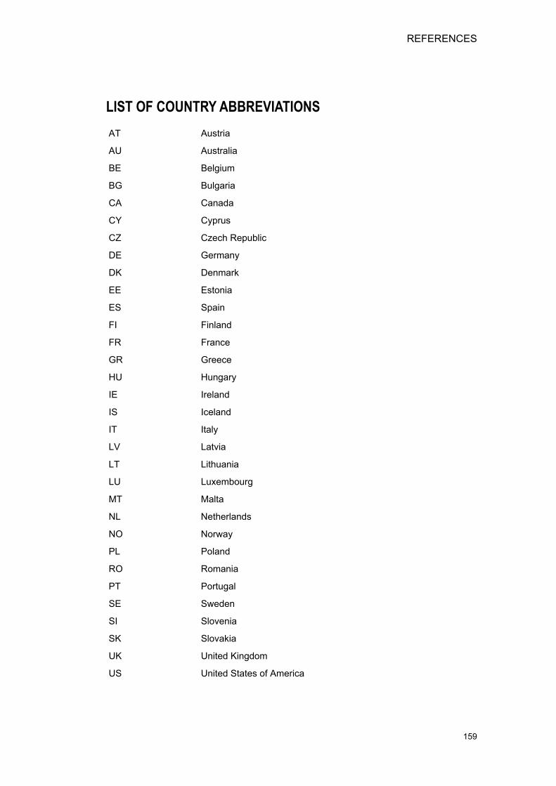
REFERENCES
159
LIST OF COUNTRY ABBREVIATIONS AT Austria
AU Australia
BE Belgium
BG Bulgaria
CA Canada
CY Cyprus
CZ Czech Republic
DE Germany
DK Denmark
EE Estonia
ES Spain
FI Finland
FR France
GR Greece
HU Hungary
IE Ireland
IS Iceland
IT Italy
LV Latvia
LT Lithuania
LU Luxembourg
MT Malta
NL Netherlands
NO Norway
PL Poland
RO Romania
PT Portugal
SE Sweden
SI Slovenia
SK Slovakia
UK United Kingdom
US United States of America

Social Mobility and Intra-Regional Income Distribution Across EU Member States
160
LIST OF OTHER ABBREVIATIONS ALM Autor, Levy & Murnane (hypothesis)
A(0.5), A(1), A(2) Atkinson family of indices
BRIC Brazil, Russia, India and China
CASMIN Comparative Analysis of Social Mobility in Industrial Nations
CAMSIS Cambridge Social Interaction and Stratification Scale
COFOG Classifications of Functions of Government
CV Coefficient of Variation
DG ECFIN Directorate General Economic and Financial Affairs
DG EMPL Directorate General Employment, Social Affairs and Equal Opportunities
DG REGIO Directorate General Regional Policy
ECHP European Community Household Panel
ECP European Cohesion Policy
ESEC European Socio-Economic Classification
EU-SILC European Union Statistics on Income and Living Conditions
FJH Featherman, Jones, Hauser (hypothesis)
GE Generalized Entropy
GSOEP German Socio-Economic Panel
ISCED International Standard Classification of Education
ISCO International Standard Classification of Occupations
LIS Luxembourg Income Study
LZ (theory) Lipset-Zetterberg (theory)
N/A Not available
ME Exchange Mobility
MLD Mean Log Deviation
NEG New Economic Geography
NMS New Member States
NUTS Nomenclature of Territorial Units for Statistics
POUM Prospect of Upward Mobility
R Reranking
RTD Research and technological development
SBOC Skill-Biased Organizational Change
SBTC Skill-Biased Technological Change
SEI Socio-Economic Indices

REFERENCES
161
SWF Social Welfare Function
TEN-ICT Trans European Network Information and communication technologies
Social Mobility and Intra-Regional Income Distribution Across EU Member States
162
REFERENCES Aaberge R. and A. Langørgen (2006), ‘Measuring the Benefits from Public Services: The Effects of Local Government Spending on the Distribution of Income in Norway’, Review of Income and Wealth. 52 (1): March.
Acemoglu, D.(1998). ‘Why Do New Technologies Complement Skills? Directed Technical Change and Wage Inequality?’ The Quarterly Journal of Economics 113 (4): pp. 1055-1089.
Adelman, I.G. (1958), ‘“A stochastic analysis of the size distribution of firms’, Journal of the American Statistical Association, 53:893-904.
Aldridge, Stephen (2001), ‘Social Mobility: A Discussion Paper’, The Cabinet Office. Available at
http ://www.cabinetoffice.gov.uk/media/cabinetoffice/strategy/assets/socialmobility.pdf
Albouy V., F. Bouton and N. Roth (2002), ’Les effets redistributifs de l’éducation: les enseignements d’une approche monétaire statique’, communication préparée pour le séminaire organisé par le CERC, la DPD et l’INSEE, Paris.
Alesina, A. and E. LaFerrara (2005), “Preferences for redistribution in the land of opportunities”, Journal of Public Economics, 89: 897–931.
Andrews, D. and A. Leigh (2007), “More Inequality, Less Social Mobility”, mimeo, Research School of Social Sciences (RSSS), Australian National University.
Atkinson, A. B. and A. Brandolini (2006) “A Panel-of-Countries Approach to Explaining Income Inequality: An Interdisciplinary Research Agenda,” In Mobility and Inequality: Frontiers of Research in Sociology and Economics. Stephen L. Morgan, David B. Grusky, Gary S. Fields (eds). Stanford University Press, 2006.
Atkinson, A. B. 1998a. Poverty in Europe, Malden, MA: Blackwell.
Atkinson, A.B. (1981), “The measurement of economic mobility”, in Inkomens Verdeling en Openbard Financien, P. Eggelshoven and L. Van Gemerden (eds.), Leiden, Het Spectrum.
Atkinson, A.B., F. Bourguignon and C. Morrisson (1992), Empirical Studies on Earnings Mobility, Harwood Academic Publishers. London.
Atoda, N. and T. Tachibanaki (1980), “Earnings distribution and inequality over time: Education versus relative position and cohort”, International Economic Review, 32: 475.
Ayala, L. and M. Sastre (2008). “The structure of income mobility: empirical evidence from five EU countries” Empirical Economics 35: 451-473.
Bae C-H (1997a), "The equity impacts of Los Angeles' air quality policies" Environment and Planning A 29(9), 1563 – 1584.
Bae, C-H (1997B). How Los Angeles’ Air Quality Policies Benefit Minorities. Journal of Environmental Planning and Management, 40(2), 235- 260, 1997
Barca (2009), An Agenda for a Reformed Cohesion Policy. Independent Report sponsored by DG REGIO.
Bartholomew, D.J. (1982), Stochastic Models for Social processes. 3rd Ed., Wiley and Sons, New York.
Bénabou, R. and E. Ok (2001), “Social mobility and the demand for redistribution. The POUM hypothesis”, Quarterly Journal of Economics, 116: 447–487.
Beramendi, P. (2007) ‘Inequality and the territorial fragmentation of solidarity’. International Organisation, vol.61(4), pp. 783-820.
REFERENCES
163
Bergman, M. and D. Joye (2001) Comparing Social Stratification Schemas: CAMSIS, CSP-CH, Goldthorpe, ISCO-88, Treiman, and Wright. Cambridge Studies in Social Research
Berthold, N. and A. Brunner. (2008),‘The struggle between Equity and Efficiency. Evidence from the LU Income Studies’. LIS Working Paper No. 498.
Björklund, A., M. Jäntti, and G. Solon (2007). ‘Nature and Nurture in the Intergenerational Transmission of Socioeconomic Status: Evidence from Swedish Children and Their Biological and Rearing Parents’. The BE Journal of Economic Analysis & Policy, Issue 2 (Advances).
Björklund, A. and L., Chadwick (2003), ’Intergenerational income mobility in permanent and separated families’, Economics Letters, Volume 80(2), pp. 239-246.
Blanden, J., P. Gregg and L., Macmillan (2006), ’Explaining Intergenerational Income Persistence: Noncognitive Skills, Ability and Education’, Working Paper n. 06/146, Centre for Market and Public Organisation.
Blanden, J., P. Gregg, and S. Machin (2005), ‘Intergenerational Mobility in Europe and North America. A Report supported by the Sutton Trust’, Centre for Economic Performance, London School of Economics.
Böheim, R.; and S. P. Jenkins,. (May 2000) ‘Do current income and annual income measures provide different pictures of Britain’s income distribution?’ ISER Working Paper 2000–16. Colchester: University of Essex.
Bottero, W. (2005) Stratification: Social Division and Inequality. London: Routledge.
Boudon, R. (1974) Education, Opportunity, and Social Inequality. New York: John Wiley,.
Bourdieu, Pierre & J. Passeron, (1979). The Inheritors: French Students and their Relation to Culture, trans. Richard Nice. Chicago: University of Chicago Press (first published 1964).
Bowles, S. and Gintis, S. (2002). ‘The inheritance of Inequality’, Journal of Economic Perspectives, Vol. 16, No. 3 (Summer, 2002), pp. 3-30.
Bowles, S., H. Gintis, and M. O. Groves (2005), ’Introduction’ in Bowles, S., H. Gintis, and M. Osborne Groves, Unequal Chances: Family Background and Economic Success, New York: Russell Sage, pp. 1-22.
Brady, D. (2002) ‘Rethinking the sociological measurement of poverty’, Luxembourg Income Study Working Paper No. 264.
Bradshaw. J and N. Finch. (2003), ’Overlaps in Dimensions of Poverty’, Journal of Social Policy, 32, 4:5113–525
Brandolini, A. and T.M. Smeeding (2008a).‘Inequality (international evidence).’ The New Palgrave Dictionary of Economics. 2nd d ed./. S. N. Durlauf and L., E. Blume. Palgrave Macmillan, 2008. The New Palgrave Dictionary of Economics Online. Palgrave Macmillan. 10 August 2009
<http://www.dictionaryofeconomics.com/article?id=pde2008_I000273> doi:10.1057/9780230226203.0788
Brandolini, A. and T. M. Smeeding. 2008(b). ’Inequality Patterns in Western Democracies: Cross-Country Differences and Changes over Time.’ in Democracy, Inequality, and Representation: A Comparative Perspective. P. Beramendi and C. J. Anderson (editors). New York: Russell Sage Foundation
Brandolini, A., E. Sierminska and T. M. Smeeding. 2006. ’The LU Wealth Study – The First Cross-Country Comparable Database for Household Wealth Research’. Journal of Economic Inequality, 4(3). 1569-1721
Social Mobility and Intra-Regional Income Distribution Across EU Member States
164
Brandolini, A. and G. D’Alessio (2001), ’Household Structure and Income Inequality’, LU Income Study Working Paper, No. 254, LU.
Breen, R. and T. Jonsson, (2005) ‘Inequality of opportunity in comparative perspective: Recent Research on Educational Attainment and Social Mobility’. Annual Review of Sociology, 31:223–43
Breen R, and R. Luijkx (2004a), Social mobility in Europe between 1970 and 2000. See Breen 2004, pp. 37–75
Breen, R. and Rottman, D. (1995a) Class Stratification: A Comparative Perspective, London: Harvester Wheatsheaf.
Breen, R. and R.Luijkx (2004), ‘Social Mobility in Europe between 1970 and 2000’, in Breen (2004) Social Mobility in Europe, Oxford University Press
Buchinsky, M., G. Fields, D. Fougère, and F. Kramarz (2003), ’Francs or ranks? Earnings mobility’in France 1967-1999, Crest working paper DP3937. Available at: http://www.ilr.cornell.edu/directory/gsf2/downloads/bffk_paper_mar03.pdf
Buchinsky, Moshe, D. Fougere and F. Kramarz (1998). ’Wage Mobility in FR: 1967-1987.’ Revue Economique 49(3): 879-890.
Burkhauser, R.V. and K.A. Couch (2009), ’Intra-generational inequality and intertemporal mobility’, in W. Salverda, B. Nolan and T.M. Smeeding (eds.) The Oxford Handbook of Economic Inequality, Oxford University Press, Oxford.
Burkhauser, R.V., F. Shuaizhang, and S.P. Jenkins (2007), ‘Using a P90/P10 ratio to measure inequality trends with the Public Use Current Population Survey: A view from inside the Census Bureau vaults’, ISER Working Paper 2007-14.
CAA (2008) ‘Recent Trends in Growth of UK Air Passenger Demand’ Report available at: http://www.caa.co.uk/default.aspx?catid=589&pagetype=90&pageid=9215
Calderón, C. and L. Servén (2004). The Effects of Infrastructure Development on Growth and Income Distribution (WP3400). Available from: econ.worldbank.org.
Calero, J. (2002), “The Distribution of Public Social Expenditure in Spain: A General Analysis with Special Reference to Age and Social Class”, Social Policy and Administration, 36 (5): 443-464]
Calero, J. (1998): El gasto publico en educación superior en España y la equidad, Hacienda Pública Española.
Cappellari, L. (2000) ’Low-Wage Mobility in the Italian Labour Market.’ International Journal of Manpower 21(3-4): 264-290.
Card, D. and J.E. Di Nardo (2002), ‘Skill-Biased Technological Change and Rising Wage Inequality: Some Problems and Puzzles’ Journal of Labor Economics, 20 (4): pp. 733-783.
Caroli, E. and J. van Reenen (2001) ‘Skill-Biased Organizational Change: Evidence From A Panel Of British and French Establishments’. The Quarterly Journal of Economics 116 (4): pp. 1449–1492.
Casali, V. and V.A. Gonzalez, V.A. (2010), ‘Statistics in Focus. Population and Social Conditions’, Eurostat, Publications Office of the European Union. Luxembourg.
Champernowne, D.G.(1953), ’A model of income distribution’, Economic Journal, 63: 318–351.
Checchi, D. and A. Filippin (2004), ‘An experimental study of the POUM hypothesis’, Research on Economic Inequality, 11: 115–136.
REFERENCES
165
Chevalier, A. and G. Conlon (2003), “Does it Pay to attend a Prestigious University?”, Centre for the Economics of Education Discussion Paper 33 and IZA Discussion Paper 848.
Comi, S. (2004). ’Intergenerational mobility in Europe: evidence from ECHP’ ChilD n. 18/2004. Available from http://www.child-centre.it
Conlon, G. (2002), ’The Determinants of Undertaking Academic and Vocational Qualifications in the UK’, Centre for the Economics of Education Discussion Paper 20.
Corak, M. (2006).’“Do Poor Children Become Poor Adults? Lessons from a Cross Country Comparison of Generational Earnings Mobility’ IZA DP No. 1993 Institute for the Study of Labor March 2006
Cowell, F. A. (2008) Measuring Inequality, Oxford University Press. http://lse.academia.edu/FrankCowell/Books/71492/Measuring-Inequality
D’Addio, A. (2007), ‘Intergenerational Transmission of Disadvantage: Mobility or Immobility across Generations? A Review of the Evidence for OECD Countries’. OECD. Delsa/elsa/wd/sem(2007)
D’Agostino, M. and V. Dardanoni (2009a). ‘The measurement of rank mobility’, Journal of Economic Theory 144, 1783—1803.
D'Agostino, M. and V. Dardanoni (2009). ‘What's So Special About Euclidean Distance? A Characterization Result with Applications to Mobility and Spatial Voting’, Social Choice and Welfare, pp. 211-233 (2009).
D’Ercole, M. And Förster, M. (2005) ‘Income distribution and poverty in OECD countries in the second half of the 1990s’. OECD Social, Employment and Migration Working Papers, Paris: OECD.
Dardanoni, V. (1995), ’Income distribution dynamics: Monotone Markov chains make light work’, Social Choice and Welfare, 12:181-192.
Dardanoni, V. and A. Forcina (1993), a’You’d better have a rich father: Testing monotone mobility matrices’, mimeo, University of Palermo.
Desjonqueres, T., S. Machin and J. van Reenen (1999), ‘Another Nail in the Coffin? Or Can the Trade Based Explanation of Changing Skill Structures Be Resurrected?’ The Scandinavian Journal of Economics, 101 (4) Industrial Policy in Open Ecomies: pp. 533-554.
DG Regional Policy (2008), ‘Convergence of EU Regions. Measures and Evolution’. Series of Working Papers on regional research and indicators produced by the Directorate-General for Regional Policy. No. 1, 2008.
O’Donoghue C. (2002) ‘The redistributive impact of education in the European Union’ Contribution to the CERC-DPD-INSEE seminar on ‘Les effets redistributifs de l’éducation : les enseignements d’une approche monétaire statique’ (The redistributive impact of education: Lessons from a static monetary approach), November 15. Cited in Council for Employment, Incoem and Socila Cohesion (2003. ‘Education and Redistribution’, Report 3. Council for Employment, Income and Social Cohesion, Paris.
EPEC (2008). ‘Impact Assessment Study on Community Instruments on International Successions and Wills’, Draft Final Report.
Erikson, R. and J. H. Goldthorpe, (2002) ’Intergenerational inequality: a sociological perspective’, Journal of Economic Perspectives 16 (3): 31-44.
Erikson R, JH. Goldthorpe (1992), The Constant Flux: A Study of Class Mobility in Industrial Societies, Oxford: Clarendon.
Erikson, R. and J. Goldthorpe. (1992), ‘The CASMIN project and the American dream’. European sociological review, 8 (3).
Social Mobility and Intra-Regional Income Distribution Across EU Member States
166
Erikson, R.,. J.H. Goldthorpe,, and L. Portocarero (1982), ‘Social Fluidity in Industrial Nations’: England, French and Swedish. The British Journal of Sociology, Vol. 33, No. 1 (Mar., 1982), 1-34.
Ermisch, J., M. Frsconi and T. Siedler (2006), ’Intergenerational Economic Mobility and Assortative Mating’, Economic Journal, Vol. 116, July, 659–679.
Encyclopædia Britannica (2009). ‘Definition of “social mobility’. Retrieved August 13, 2009, from Encyclopædia Britannica Online: http://www.britannica.com/EBchecked/topic/551322/social-mobility
Estache, A.(2003). ‘On Latin America’s Infrastructure Privatization and its Distributional Effects’, Washington, DC: The World Bank, Mimeo.
European Commission (2007) ‘The Social Situation in the European Union’. http://ec.europa.eu/employment_ social/spsi/docs/social_situation/ssr2007_en.pdf
European Commission (2008). ’New Skills for New Jobs. Anticipating and matching labour market and skills needs.’ Commission Staff Working Document accompanying the Communication from the Commission to the European Parliament, the Council, the European Economic and Social Committee and the Committee of the Regions. SEC(2008) 3058/2. Brussels.
European Commission (2008)‘Child Poverty and Well-Being in the EU’, Current status and way forward. DG Employment, Social Affairs and Equal Opportunities. Available at: http://ec.europa.eu/employment_social/spsi/docs/social_inclusion/2008/child_poverty_en.pdf.
Eurostat (2009). ‘Comparative Intermediate EU Quality Report 2007’. Available at: http://circa.europa.eu/Public/irc/dsis/eusilc/library?l=/quality_assessment/comparative_quality_1/intermediate_euqr07/_EN_1.0_&a=d
Eurostat (2003) ‘Report from the Commission to the Council and to the European Parliament on the implementation of Regulation (EC) No 1177/2003’, http://eur-lex.europa.eu/LexUriServ/LexUriServ.do?uri=COM:2008:0160:FIN:EN:PDF
Eurostat (2003) ‘Laeken indicators-detailed calculation methodology’. European Commission. Available in the Eurostat NewCronos database.
Eurostat (2005) ’The transition between ECHP and EU-SILC’. LU: Office for Official Publications of the European Communities, 2005.
Eurostat (2007), ‘Comparative EU statistics on Income and Living Conditions: Issues and Challenges’. Proceedings of the EU-SILC conference (Helsinki, 6-8 November 2006). Eurostat Working Paper Series.
Eurostat (2008), ‘Europe in Figures: Eurostat Yearbook 2008’. LU: Office for Official Publications of the European Communities.
Evandrou, M., J. Falkingham,, J. Hills, J. and J. Le Grand. (1992), ‘The distribution of welfare benefits in kind’, London School of Economics, Welfare State Programme, Discussion Paper no. WSP/68.
Evandrou, M., J. Falkingham, J. Hills and J. Le Grand (1993), ’Welfare Benefits in Kind and Income Distribution’, Fiscal Studies, Vol. 14, No. 1.
Expert Group on Household Statistics (2001), ‘Final Report and Recommendations’. Available at http://www.lisproject.org/links/canberra/finalreport.pdf.
Featherman, D.L., F.L. Jones and R.M. Hauser 1975 ’Assumptions of Social Mobility Research in the US: The Case of Occupational Status’, Social Science Research 4: 329-60.
REFERENCES
167
Feinstein, L. (2006), ’The effects of education on health: Concepts, evidence and policy implications: A review for the OECD Centre for Educational Research and Innovation (CERI)’, unpublished manuscript, OECD, Paris.
Fields, Gary S. (2008). ‘Income Mobility’ The New Palgrave Dictionary of Economics Online.
Fields, G. (2007), ‘Income mobility’. Retrieved [2 October 2009], from Cornell University, ILR School site: http://digitalcommons.ilr.cornell.edu/workingpapers/19/
Fields, G. and E. Ok (1996), ’The meaning and measurement of income mobility’, Journal of Economic Theory, 71:349-77.
Fields, G. and E. Ok (1999), ’The measurement of income mobility: An introduction to the literature’, in J. Silber (ed.) Handbook on Inequality Measurement, , London: Kluwer Academic Press.
Fields, G. and E. Ok (1999b), ’Measuring movements of incomes’, Economica, 66: 455-72.
Fields, G.S., J. Leary and E. Ok (2002), ’Stochastic dominance in mobility analysis’, Economics Letters, 75:333-9.
Fields, G.G. (2005), ’Does income mobility equalize longer-term incomes? New measures of an old concept’. Unpublished, Cornell University.
Fleurbaey, M. And F. Maniquet (2009), ’Compensation and Responsibility’ in K. J. Arrow, A. K. Sen and K. Suzumura (eds), Handbook of Social Choice and Welfare.
Förster, Michael, D. Jesuit and T. Smeeding. 2005. ‘Regional Poverty and Income Inequality in Central and Eastern Europe: Evidence from the Luxembourg Income Study.’iIn Spatial Inequality and Development, R. Kanbur and A. J. Venables (eds.), Oxford, England: Oxford University Press, 311-347.
Lakin C. (2004), ‘The effects of taxes and benefits on household income, 2002-2003’, Economic Trends 607, June.
Lasker, G.W. and C.G.N. Mascie-Taylor (1989), ’Effects of social class differences and social mobility on growth in height, weight and body mass index in a British cohort’ Annals of Human Biology, 16(1): 1-8.
Galor, O. and D. Tsiddon (1997), ’Technological Progress, Mobility, and Economic Growth’, American Economic Review, 87(3): 363-382
Gannon, C. and Z. Liu (1997) ‚Poverty and Transport.‘ Washington, DC: The World Bank, Mimeo.
Ganzeboom, H., De Graaf, P., Treiman, D., and J. De Leeuw,.(1992),‘A standard international socio- economic index of occupational status’, Social Science. Research. 21: 1-56.
Ganzeboom, H and Treiman, D. (2006) ‘Internationally Comparable Measures of Occupational Status for the 1988 International Standard Classification of Occupations’. Social Science Research 25, 201–239 (1996).
García-Peñalosa, C.; Turnovsky, S. (2005), ‘Growth and Income Inequality: A Canonical Model’, Working Paper. Available at: http://www.econ.washington.edu/user/sturn/Garcia-Turnovsky-ET.pdf
Garfinkel, I., L. Rainwater and T.M. Smeeding (2006), ’A Reexamination of Welfare State and Inequality in Rich Nations: How In-Kind Transfers and Indirect Taxes Change the Story’, Journal of Policy Analysis and Management, vol. 25, pp. 855-919.
Firebaugh, G.(2006), The New Geography of Global Income Inequality, Harvard University Press, 2006.
Social Mobility and Intra-Regional Income Distribution Across EU Member States
168
Goldberger, A. (1989), ’Economic and mechanical models of intergenerational transmission’, American Economic Review, 79, pp. 504–13.
Goldthorpe, J., M. Jackson (2005), ‘Education-Based Meritocracy: The Barriers To Its Realisation’, Working Paper. Available at: http://www.equalsoc.org/uploaded_files/regular/goldthorpe_jackson.pdf
Gordon, D. M. (1972), Theories of Poverty and Underemployment: Orthodox, Radical, and Dual Labor Market Perspectives Lexington, MA: Lexington Books.
Goos, M. N and A. Manning (2007) ‘Lousy and lovely jobs: the rising polarization of work in Britain’, Review of economics and statistics, 89 (1). Pp. 118-133.
Gottschalk, P. and S. Danziger (2005), ’Inequality of Wage Rates and Family Income in the US, 1975-2002’, Review of Income and Wealth, Vol. 51, No. 2
Gottschalk, P. and T.M. Smeeding (1997), ’Cross National Comparisons of Earnings and Income Inequality’, Journal of Economic Literature, Vol. 35, No. 2, 633-686..
Grawe N. (2004), ’Intergenerational Mobility for Whom? The Experience of High and Low Earning Sons in International Perspective’ in M.Colak (ed) Generational Income Mobility in North America and Europe, Cambridge: Cambridge University Press
Green, A., J. Preston. and J. JaanMat, (2006), Education, equality and social cohesion. A comparative analysis, Palgrave.
Grusky D.B., and J.B. Sorensen (1998), ‘Can class analysis be salvaged?’ American. Journal of Sociology. 103:1187– 234
Hagenaars, Aldi J.M. (1991),.’The Definition and Measurement of Poverty’, pp. 134-156 in Economic Inequality and Poverty: International Perspectives, Armonk, NY: M.E. Sharpe.
Harrison, E. and Rose, D. (2006)‘The European Socio-Economic Classification (EseC) User Guide’, Institute for Social and Economic Research. Available at: http://www.iser.essex.ac.uk/esec/guide/docs/UserGuide.pdf.
Hart, P.E. (1983) ’The size mobility of earnings’, Oxford Bulletin of Economics and Statistics, 45:181-93.
Hassler and M. Rodríguez (2000), ‘Intelligence, Social Mobility and Growth’, American Economic Review, 90(4): 888-908.
Hauser R.M., and J.R. Warren (1997) ‘Socioeconomic indexes for occupations: a review, update, and critique’, Socioogical Methodology27 (1):177–298.
Hauser, R.M. and D. B. Grusky (1988) ‘Cross-National Variation in Occupational Distributions, Relative Mobility Chances, and Intergenerational Shifts in Occupational Distributions’, American Sociological Review, Vol. 53, No. 5 (Oct., 1988), pp. 723-741
Heath, A and C. Payne (2000), ‘Social Mobility’, in: Halsey, A.H.; Webb, J. (ed.) Twentieth Century British Social Trends’ Macmillan
Hoffmeister, O. (2009). ’The Spatial Structure of Income Inequality in the Enlarged EU’ Review of Income and Wealth, Vol. 55, Issue 1, pp. 101-127.
Hoffmeister, O. (2006),‘Inequality of Incomes on Both Sides of the Odra: The Contribution of the Regional Dimension’ LIS Working Paper No. 439.
Haughwout, A. F. (1999) ‘Regional fiscal cooperation in metropolitan areas: An exploration.’ Journal of Policy Analysis and Management 18 (4): 579-600.
Holmlund, H. (2006), ’Intergenerational Mobility and Assortative Mating Effects of an educational reform’, Swedish Institute for Social Research working paper n. 4/2006, Stockholm University.
REFERENCES
169
Ichino, A. (2008), ‘The Political Economy of Intergenerational Income Mobility’, Working Paper. Available at: http://www.parisschoolofeconomics.eu/IMG/pdf/Ichino.pdf
Inland Revenue – Inheritance Tax’, a report by the National Audit Office, 2004.
Jacoby, H., (2000) ‘Access to Rural Markets and the Benefits of Rural Roads.’ The Economic Journal, 110, 713-37.
Jäntti, M. and B. Bratsberg,R. O. Raaum, E.Österbacka, A. Björklund and T. Eriksson (2006), ‘American Exceptionalism in a New Light: A Comparison of Intergenerational Earnings Mobility in the Nordic Countries, the UK and the US’. IZA DP No. 1938
J’arvis, S. and S. Jenkins (1998) ‘How much income mobility is there in Britain?’ The Economic Journal 108, 428-443.
Jenkins, S et al. (2009), ‘Measuring Inequality Using Censored Data: A Multiple Imputation Approach’, DIW Discussion Papers. Available at: http://www.diw.de/documents/publikationen/73/95918/dp866.pdf
Jenkins, S. and P. Van Kerm (2006) ’Trends in income inequality, pro-poor income growth, and income mobility’. Oxford Economic Papers 58, 531-548.
Jenkins, S. and P. Van Kerm (2009) ‘The measurement of Economic Inequality’ in The Oxford Handbook of Economic Inequality eds by Wiemer Salverda, Brian Nolan, and Timothy M. Smeeding.
Jenkins, S. and T. Siedler (2007) ‘Using household panel data to understand the intergenerational transmission of poverty’ Institute for Social and Economic Research University of Essex: CPRC Working Paper 74.
Jesuit, D., Rainwater, L. and I. Smeeding (2003). ’Regional poverty within rich countries’ in J. A. Bishop and Y. Amiel (eds.) Inequality, Welfare and Poverty: Theory and Measurement, , New York: Elsevier Science, 345-377.
John S. and G. Marshall (2005), A Dictionary of Sociology. Oxford University Press: Oxford Reference Online.
Jonsson, J. (2004) ‘ Equality at a Halt? Social Mobility in Sweden 1976-1999’ in: R. Breen (eds.) Social Mobility in Europe, Oxford: Oxford University Press
Johnson, P. (2002), ’Intergenerational dependence in education and income’, Applied Economic Letters, 9, pp. 159–62.
Kakwani, N. (1977), ’Measurement of tax progressivity: and international comparison’, Economic Journal, 87: 71-80.
Kerr, C., J.T. Dunlop, F.H. Harbison and C.A. Myers (1960) Industrialism and Industrial Man, Cambridge, Mass: Harvard University Press.
Lakin, C. (2004) ’The Effects of Taxes and Benefits on Household Income, 2002-2003’, Economic Trends, 607, June.
Lambert, P .J. (2001), The Distribution and Redistribution of Income, Manchester: Manchester University Press:.
Larrimore, J., R.V. Burkhauser, F. Shuaizhang, and L. Zayatz (2008), ‘Consistent cell means for topcoded incomes in the Public Use March CPS (1979-2005)’,. Department of Policy Analysis and Management, Cornell University,mimeo
Lelkes, O., M. Medgyesi and I. G. Tóth (2009) ’The Factors Affecting the Risk of Poverty and Inequalities in Income Distribution’, in T. Ward, O. Lelkes, H. Sutherland, I. G. Tóth (eds) European Inequalities: Social Inclusion and Income Distribution in the European Union, Budapest: TÁRKI Social Research Institute Inc
Social Mobility and Intra-Regional Income Distribution Across EU Member States
170
Lillard, D.R. (2007), ‘Cross-National harmonization of household panel data: concept, practice, and philosophy’, Department of Policy Analysis and Management, Cornell University, mimeo.
Lindahl, L. (2008) ‘Do birth order and family size matter for intergenerational income mobility? Evidence from SE’. Applied Economics, 40, 7.
Lipset, S.M. and R. Bendix (1959),Social mobility in industrial society. Berkely: University of California Press.
Litchfield, J. (1999) ‘Inequality: Methods and Tools’, Paper for World Bank’s Web Site on Inequality, Poverty, and Socio-economic Performance: http://www.worldbank.org/poverty/inequal/index.htm.
Luo, C. (2008) ‘The return to education and its distribution in urban China: evidence from quantile regression analysis’ China Economic Journal, Volume 1, Issue 2 July 2008 , pages 165 - 175 10.1080/17538960802076570
Maasoumi, E. (1998). On mobility. In Handbook of Applied Economic Statistics, D. Giles and A. Ullah. (eds), New York: Marcel Dekker.
Machin, S. (2004) ‘Skill-biased Technical Change and Educational Outcomes’, in G. Johnes, and J. Johnes (eds.) International handbook on the economics of education, Cheltenham: Edward Elgar.
Machin, S. and A. Manning (1997) ‘Can Supply Create Its Own Demand? Implications for Rising Skill Differentials?’ European Economic Review 41: pp. 507 – 516.
Machin, S. and J. Van Reenen (2007), ‘Changes in Wage Inequality’. Special Paper No. 18. Center for Economic Performance.
Mach, B. (2004). ’Intergenerational Mobility in Poland 1972-1988-1994’ In R. Breen (eds.) Social Mobility in Europe, Oxford: Oxford University Press
Madden, D. (2000) ‘Relative or Absolute Poverty Lines: A New Approach.’ Review of Income and Wealth 46: 181-199.
Mahler, V. A., and D. K. Jesuit (2006), Fiscal Redistribution in the Developed Countries: New Insights from the LU Income Study’, Socio-Economic Review, vol. 4, pp. 483-511.
Mahler, V. A. (2002) ‘Exploring the sub-national dimension of income inequality: An analysis of the relationship between inequality and electoral turnout in the developed countries’, International Studies Quarterly, 46(1): 117-142
Marical, F., D’ Ercole, M., Vaalavuo M. and G. Verbist (2008) ‘Publicly Provided Services and the Distribution of Households’ Economic Resources. OECD Economic Studies No. 44, 2008/1
Markandya A (1984) ‘The welfare measurement of changes in economic mobility’, Economica, 51:457–471
Medgyesi M. (2008) ’Income distribution in European countries: first reflections on the basis of EU-SILC 2005’, in I. G. Tóth, (ed.), Tárki European Social Report,. Tárki, Budapest, pp. 88-101.
Mocetti, S. (2007) ’Intergenerational Earnings Mobility in Italy,’ The Berkeley Electronic Journal of Economic Analysis & Policy: Vol. 7 : Issue 2. Nunn, A. et al (2007), ‘Factors influencing social mobility’, Department for Work and Pensions. Available at: http:// www.dwp.gov.uk/asd/asd5/rports2007-2008/rrep450.pdf
Nunn, A. Monro, S.,Kelsey, S., Bickerstaffe,T, Jassi, S., Hawtin, M. And Halliday, S-A (2008). ‘Factors influencing the inter- and intra-class mobility of Jobcentre Plus customers: a case study approach’. A report of research carried out by the Policy Research Institute on behalf of the Department for Work and Pensions.
REFERENCES
171
Nunn, A., Johnson, S., Monro, S., Bickerstaffe, T. and Kelsey, S. (2007). ’Factors influencing social mobility’, Department for Work and Pensions Research Report No 450
OECD (1996), ‘Employment Outlook 1996’, Paris: OECD.
OECD (1997), ‘Employment Outlook 1997’, Paris: OECD.
OECD (1999), ‘Employment Outlook: Giving Youth a Better Start’, Paris: OECD.
OECD (2002). ‘Measuring the Information Economy’, : Paris: OECD.
OECD (2008), ‘Growing Unequal? Income Distribution and Poverty in OECED Countries’. Paris: OECD.
Parsons. T. (1960), Structure and Process in Modern Societies, Glencoe Ill: Free Press.
Pavlopoulos, D., R. Muffels, and J.K. Vermunt, (2005), Wage Mobility in Europe. A Comparative Analysis Using restricted Multinomial Logit Regression. Quality and Quantity, forthcoming.
Pekkarinen, T., R. Uusitalo and S. Pekkala (2006), ‘Education Policy and Intergenerational Income Mobility: Evidence from the Finnish Comprehensive School Reform’, IZA DP No. 2204.
Perugini. C. and G. Martino (2006) ‘Income inequality within European regions: determinants and effects on growth’. Paper presented at the European Association for Comparative Economics Studies 9th Conference.
Piketty, T. (1995), ‘Social mobility and redistributive politics’, Quarterly Journal of Economics, 110: 551–584.
Ravallion, M. (1998), ’Poverty Lines in Theory and Practice’, Living Standards Measurement Study Working Paper, Number 133. Washington, D.C.: The World Bank.
Reed, H. (2006), ’Modelling Demographic Pressure on Poverty and Inequality’, in M. Dixon and J. Margo (eds.), Population Politics, Institute for Public Policy Research, London.
Reiner, H. and T. Siedler (2008), ’Subjective income and employment expectations and preferences for redistribution’, Economics Letters, 99: 449–453
Riley, M., Ladkin, A. and E. Szivas (2002), Tourism employment: analysis and planning, Channel View Publications.
Rodríguez-Pose A, and V. Tselios (2009a) ’Education and income inequality in the regions of the European Union’, Journal of Regional Science, 49(3): 411-437.
Rodríguez-Pose, A. and V. Tselios(2009b) ‘Mapping Regional Personal Income Distribution in Western Europe: Income Per Capita and Inequality’, Czech Journal of Economics and Finance, 59, 2009, no. 1. Available at: http://journal.fsv.cuni.cz/storage/1151_tselios.pdf
Róbert, P. and E. Bukodi (2004), ‘Changes in Intergenerational Class Mobility in Hungary, 1973-2000’ in R. Breen (eds.) Social Mobility in Europe, Oxford: Oxford University Press
Rose, D. (2005) ‘Socio-economic Classifications: Classes and Scales, Measurement and Theories’. Paper presented at the First Conference of the European Survey Research Association, Pompeu Fabra University, Barcelona, July 18-22, 2005
Rueda, D. and J. Pontusson (2000) ‘Wage inequality and varieties of capitalism’ World Politics, vol.52:350-383.
Schluter, C. and D. Van de Gaer (2010) ‘Structural mobility, exchange mobility and subgroup consistent mobility measurement, US - German mobility rankings revisited’. Review of Income and Wealth, forthcoming.
Social Mobility and Intra-Regional Income Distribution Across EU Member States
172
Scott, J. and G. Marshall (2005), A Dictionary of Sociology, Oxford University Press.and Leeds Metropolitan University
Sefton, T. (2002), ’Recent Changes in the Distribution of the Social Wage’, CASE paper 62, London School of Economics, London.
Sen, A. (1983) ’Poor, Relatively Speaking‘Oxford Economic Papers 35: 153-169; 1979.
Sen, A. (1979) ‘Issues in the Measurement of Poverty Scandinavian Journal of Economics, 81: 285-307.
Shanahan, S. E. and N. B. Tuma (1994),‘The Sociology of Distribution and Redistribution’ in N.J. Smelser and R. Swedberg (eds) The Handbook of Economic Sociology, Princeton, N.J.: Princeton University Press, pp. 733-765.
Shorrocks, A. (1976) ‘Income mobility and the Markov assumption’, Economic Journal, 86: 556-578.
Shorrocks, A. (1978a), ‘The measurement of mobility’, Econometrica, 45:1013-1024.
Shorrocks, A. (1978b), ‘Income inequality and income mobility’, Journal of Economic Theory, 19: 376-93.
Shorrocks, A. (1993), ‘On the Hart measure of income mobility’, in M. Casson & J. Creedy (eds.) Industrial Concentration and Economic Inequality, Chelstelham: Edward Elgar.
Smeeding, T. M., and L. Rainwater(2001) ’Comparing Living Standards Across Nations: Real Incomes at the Top, the Bottom and the Middle’” LIS Working Paper 266. Syracuse, New York: LU Income Study. May. http://www.lisproject.org/publications/liswps/266.pdf
Solon, G., (2004), ‘A Model of Intergenerational Mobility Variation over Time and Place’, in M. Corak(ed.), Generational Income Mobility in North America and Europe, Cambridge: Cambridge University Press, pp. 38-47.
Solon, G. (1999) ‘Intergenerational mobility in the labor market’ in O. Ashenfelter and D. Card(eds) Handbook of Labor Economics, vol. 3, . Amsterdam: North-Holland.
Sorensen A.B. (2000) ‘Towards a sounder base for class analysis’, American Journal . Sociology, Cambridge: Cambridge Univ. Press, 105:1523–58.
Stephen P. and M. Jäntti,(2005) ‘Methods for summarizing and comparing wealth distributions’, ISER Working Paper 2005-05. Colchester: University of Essex, Institute for Social and Economic Research.
Stiglitz, J. (2009) ‘Progress, what progress?’, OECD Observer, No 272 March 2009
Suyanto et al. (2007), ‘Poverty and Environmental Services: Case Study in Way Besai Watershed, Lampung Province, Indonesia’ (Available at: http://www.ecologyandsociety.org/vol12/iss2/art13/)
Townsend, P. (1980) ’Research on Poverty’ in A. B. Atkinson Wealth, Income and Inequality,. New York, Oxford University Press, pp. 299-306.
Van Kerm, P. (2004), ‘What lies behind income mobility? Reranking and distributional change in Belgium, Germany and the USA’, Economica 71: 223–239
Ward, T. (2009) ‘The Risk of Poverty and Income Distribution at the Regional Level’. in T. Ward, O. Lelkes, H. Sutherland, I. G. Tóth European Inequalities: Social Inclusion and Income Distribution in the European Union ; Budapest: TÁRKI: Social Research Institute Inc.
Watson, D, C. Whelan, C. and Maître, (2007). ‘Validating the European Socio-economic Classification: Cross-Sectional and Dynamic Analysis of Income Poverty and Lifestyle Deprivation’, ESRI Working Paper, no. 201.
REFERENCES
173
Whelan, T., D. Watson, and B. Maître, (2006). ‘Social Class Variation in Income Poverty, Deprivation and Consistent Poverty: An Analysis of EU-SILC” Eurostat and Statistics Finland International Conference on Comparative EU Statistics on Income and Living Conditions: Issues and Challenges, Helsinki, 6-7 November.
Wodon, Q; and S. Yitzhaki (2002), Inequality and Social Welfare. Published in: A Sourcebook for Poverty Reduction Strategies, 1 (2002): pp. 75-104.
Wood, A. (1998) ‘Globalisation and the rise in labour market inequalities’, The Economic Journal, 108 (450): 1463-1482.
Wright E.O. (1997) ‘Class Counts. Comparative Studies in Class Analysis’. Cambridge: Cambridge University Press.
Yaari, M. (1987), ‘The dual theory of choice under risk’, Econometrica 55: 99-115
Yokoyama and D. Gauchan (2003).‘Employment and income as influenced by adoption of orange cultivation by traditional upland farmers in Nepal’. Paper presented at the International Symposium Alternative Approaches to Enhancing Small-Scale Livelihoods and Natural Resources Management in Marginal Areas - Experience in Monsoon Asia 29 - 30 October 2003, Institute of Advanced Studies, United Nations University, Tokyo Japan
Available at: http://www.unu.edu/env/plec/marginal/proceedings/YokoyamaCH14.pdf

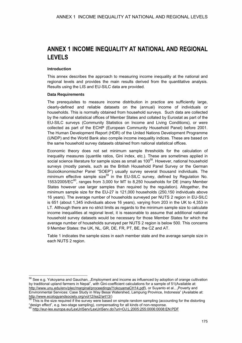
ANNEX 1 INCOME INEQUALITY AT NATIONAL AND REGIONAL LEVELS
175
ANNEX 1 INCOME INEQUALITY AT NATIONAL AND REGIONAL LEVELS Introduction
This annex describes the approach to measuring income inequality at the national and regional levels and provides the main results derived from the quantitative analysis. Results using the LIS and EU-SILC data are provided.
Data Requirements
The prerequisites to measure income distribution in practice are sufficiently large, clearly-defined and reliable datasets on the (annual) income of individuals or households. This is normally obtained from household surveys. Such data are collected by the national statistical offices of Member States and collated by Eurostat as part of the EU-SILC surveys (Community Statistics on Income and Living Conditions), or were collected as part of the ECHP (European Community Household Panel) before 2001. The Human Development Report (HDR) of the United Nations Development Programme (UNDP) and the World Bank also compile income inequality indices. These are based on the same household survey datasets obtained from national statistical offices.
Economic theory does not set minimum sample thresholds for the calculation of inequality measures (quantile ratios, Gini index, etc.). These are sometimes applied in social science literature for sample sizes as small as 10058. However, national household surveys (mostly panels, such as the British Household Panel Survey or the German Sozioökonomischer Panel “SOEP”) usually survey several thousand individuals. The minimum effective sample size59 in the EU-SILC survey, defined by Regulation No. 1553/2005/EC60, ranges from 3,000 for MT to 8,250 households for DE (many Member States however use larger samples than required by the regulation). Altogether, the minimum sample size for the EU-27 is 121,000 households (250,150 individuals above 16 years). The average number of households surveyed per NUTS 2 region in EU-SILC is 651 (about 1,345 individuals above 16 years), varying from 203 in the UK to 4,353 in LT. Although there are no strict limits as regards to the minimum sample size to calculate income inequalities at regional level, it is reasonable to assume that additional national household survey datasets would be necessary for those Member States for which the average number of households surveyed per NUTS 2 region is below 500. This concerns 9 Member States: the UK, NL, GR, DE, FR, PT, BE, the CZ and AT.
Table 1 indicates the sample sizes in each member state and the average sample size in each NUTS 2 region.
58 See e.g. Yokoyama and Gauchan, „Employment and income as influenced by adoption of orange cultivation by traditional upland farmers in Nepal”, with Gini-coefficient calculations for a sample of 51(Available at: http://www.unu.edu/env/plec/marginal/proceedings/YokoyamaCH14.pdf), or Suyanto et al., „Poverty and Environmental Services: Case Study in Way Besai Watershed, Lampung Province, Indonesia” (Available at: http://www.ecologyandsociety.org/vol12/iss2/art13/) 59 This is the size required if the survey were based on simple random sampling (accounting for the distorting “design effect”, e.g. two-stage sampling), compensating for all kinds of non-response. 60 http://eur-lex.europa.eu/LexUriServ/LexUriServ.do?uri=OJ:L:2005:255:0006:0008:EN:PDF
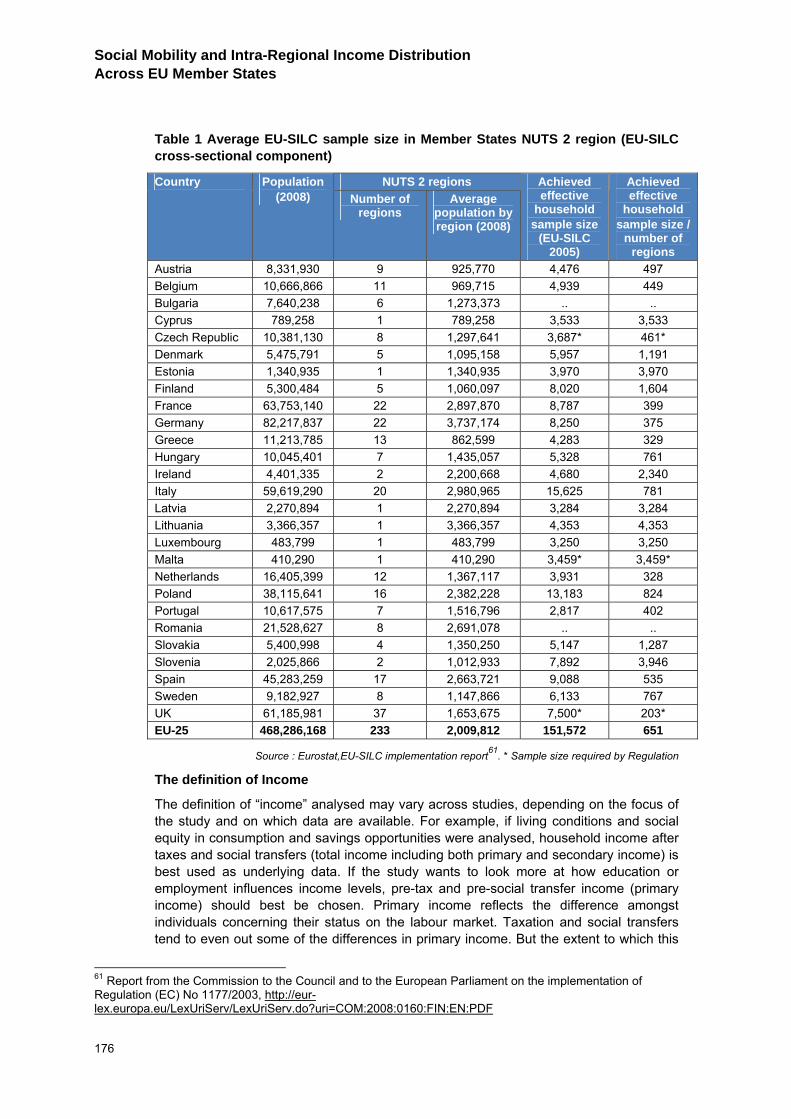
Social Mobility and Intra-Regional Income Distribution Across EU Member States
176
Table 1 Average EU-SILC sample size in Member States NUTS 2 region (EU-SILC cross-sectional component)
NUTS 2 regions Country Population (2008) Number of
regions Average
population by region (2008)
Achieved effective
household sample size
(EU-SILC 2005)
Achieved effective
household sample size /
number of regions
Austria 8,331,930 9 925,770 4,476 497 Belgium 10,666,866 11 969,715 4,939 449 Bulgaria 7,640,238 6 1,273,373 .. .. Cyprus 789,258 1 789,258 3,533 3,533 Czech Republic 10,381,130 8 1,297,641 3,687* 461* Denmark 5,475,791 5 1,095,158 5,957 1,191 Estonia 1,340,935 1 1,340,935 3,970 3,970 Finland 5,300,484 5 1,060,097 8,020 1,604 France 63,753,140 22 2,897,870 8,787 399 Germany 82,217,837 22 3,737,174 8,250 375 Greece 11,213,785 13 862,599 4,283 329 Hungary 10,045,401 7 1,435,057 5,328 761 Ireland 4,401,335 2 2,200,668 4,680 2,340 Italy 59,619,290 20 2,980,965 15,625 781 Latvia 2,270,894 1 2,270,894 3,284 3,284 Lithuania 3,366,357 1 3,366,357 4,353 4,353 Luxembourg 483,799 1 483,799 3,250 3,250 Malta 410,290 1 410,290 3,459* 3,459* Netherlands 16,405,399 12 1,367,117 3,931 328 Poland 38,115,641 16 2,382,228 13,183 824 Portugal 10,617,575 7 1,516,796 2,817 402 Romania 21,528,627 8 2,691,078 .. .. Slovakia 5,400,998 4 1,350,250 5,147 1,287 Slovenia 2,025,866 2 1,012,933 7,892 3,946 Spain 45,283,259 17 2,663,721 9,088 535 Sweden 9,182,927 8 1,147,866 6,133 767 UK 61,185,981 37 1,653,675 7,500* 203* EU-25 468,286,168 233 2,009,812 151,572 651
Source : Eurostat,EU-SILC implementation report61. * Sample size required by Regulation
The definition of Income
The definition of “income” analysed may vary across studies, depending on the focus of the study and on which data are available. For example, if living conditions and social equity in consumption and savings opportunities were analysed, household income after taxes and social transfers (total income including both primary and secondary income) is best used as underlying data. If the study wants to look more at how education or employment influences income levels, pre-tax and pre-social transfer income (primary income) should best be chosen. Primary income reflects the difference amongst individuals concerning their status on the labour market. Taxation and social transfers tend to even out some of the differences in primary income. But the extent to which this
61 Report from the Commission to the Council and to the European Parliament on the implementation of Regulation (EC) No 1177/2003, http://eur-lex.europa.eu/LexUriServ/LexUriServ.do?uri=COM:2008:0160:FIN:EN:PDF
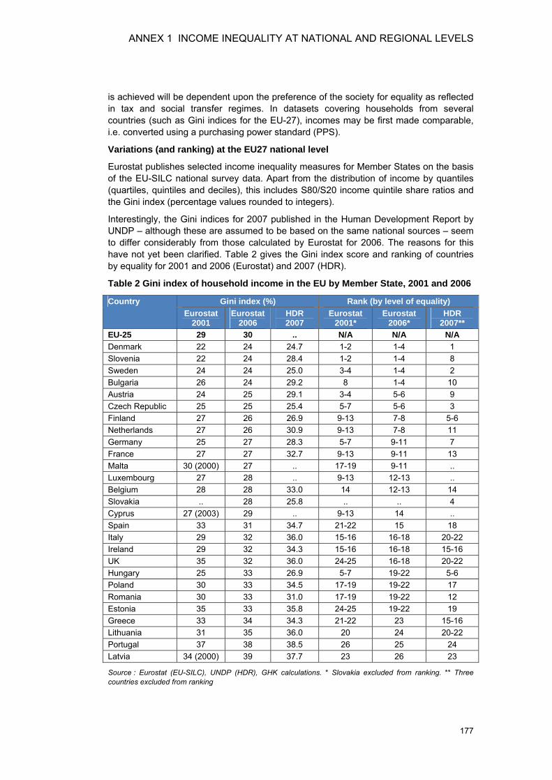
ANNEX 1 INCOME INEQUALITY AT NATIONAL AND REGIONAL LEVELS
177
is achieved will be dependent upon the preference of the society for equality as reflected in tax and social transfer regimes. In datasets covering households from several countries (such as Gini indices for the EU-27), incomes may be first made comparable, i.e. converted using a purchasing power standard (PPS).
Variations (and ranking) at the EU27 national level
Eurostat publishes selected income inequality measures for Member States on the basis of the EU-SILC national survey data. Apart from the distribution of income by quantiles (quartiles, quintiles and deciles), this includes S80/S20 income quintile share ratios and the Gini index (percentage values rounded to integers).
Interestingly, the Gini indices for 2007 published in the Human Development Report by UNDP – although these are assumed to be based on the same national sources – seem to differ considerably from those calculated by Eurostat for 2006. The reasons for this have not yet been clarified. Table 2 gives the Gini index score and ranking of countries by equality for 2001 and 2006 (Eurostat) and 2007 (HDR).
Table 2 Gini index of household income in the EU by Member State, 2001 and 2006
Gini index (%) Rank (by level of equality) Country Eurostat
2001 Eurostat
2006 HDR 2007
Eurostat 2001*
Eurostat 2006*
HDR 2007**
EU-25 29 30 .. N/A N/A N/A Denmark 22 24 24.7 1-2 1-4 1 Slovenia 22 24 28.4 1-2 1-4 8 Sweden 24 24 25.0 3-4 1-4 2 Bulgaria 26 24 29.2 8 1-4 10 Austria 24 25 29.1 3-4 5-6 9 Czech Republic 25 25 25.4 5-7 5-6 3 Finland 27 26 26.9 9-13 7-8 5-6 Netherlands 27 26 30.9 9-13 7-8 11 Germany 25 27 28.3 5-7 9-11 7 France 27 27 32.7 9-13 9-11 13 Malta 30 (2000) 27 .. 17-19 9-11 .. Luxembourg 27 28 .. 9-13 12-13 .. Belgium 28 28 33.0 14 12-13 14 Slovakia .. 28 25.8 .. .. 4 Cyprus 27 (2003) 29 .. 9-13 14 .. Spain 33 31 34.7 21-22 15 18 Italy 29 32 36.0 15-16 16-18 20-22 Ireland 29 32 34.3 15-16 16-18 15-16 UK 35 32 36.0 24-25 16-18 20-22 Hungary 25 33 26.9 5-7 19-22 5-6 Poland 30 33 34.5 17-19 19-22 17 Romania 30 33 31.0 17-19 19-22 12 Estonia 35 33 35.8 24-25 19-22 19 Greece 33 34 34.3 21-22 23 15-16 Lithuania 31 35 36.0 20 24 20-22 Portugal 37 38 38.5 26 25 24 Latvia 34 (2000) 39 37.7 23 26 23
Source : Eurostat (EU-SILC), UNDP (HDR), GHK calculations. * Slovakia excluded from ranking. ** Three countries excluded from ranking
Social Mobility and Intra-Regional Income Distribution Across EU Member States
178
The correlation between the Eurostat datasets for 2001 and 2006 is strong, 0.82. However, the Gini index values as published by Eurostat seem to be relatively volatile. In only 5 years, from 2001 to 2006, the value of the index has changed by at least 2 percentage points in 16 Member States (note that the change was very large, 8 percentage points in HU). It is not clear whether this signals real societal changes or was the result of sampling error or of the slight amendment of survey methodology (from ECHP to EU-SILC) in this period which could render the results not fully comparable.
Availability of sub-national income data
The Luxembourg Income Study (LIS) is an independent not-for-profit research institution and data archive located in the Grand Duchy of LU and is considered the foremost source of comparable cross-national income data. The LIS does not collect primary data but gathers national-level household income, budget or labour-force surveys, which include income, labour market, and demographic variables at the household- and person-level. Experts then harmonize these data in order to promote comparative research.
Data have been organized in six “waves.” The first wave begins around 1980 while wave six data are available around 2005. Although twenty-one of the twenty-seven EU Member States currently provide at least one dataset to the LIS, wave 5 data (centred around 2000) are only available for eighteen countries. Data for the most recent wave are available for just six EU Member States.
Most of the national-level surveys included in the LIS report the respondent’s state/province/municipality of residence. Sub-national information conforming to the Nomenclature of Territorial Units for Statistics (NUTS) is available for fifteen of the eighteen EU Member States included in wave 5 (data for the NL and SI lack such detail while LU has no NUTS units). The level of geographic detail included within each survey ranges from districts and municipalities (NUTS Level 4) in the CZ, DK and EE to NUTS Level 1 in AT, BE, DE, GR, ES and the UK. Accordingly, the number of sub-national units ranges from the 86 okres of the CZ to the three AT and Belgian States. In between these levels one also has the opportunity to identify households at other meaningful geographic levels, such as Italian Regions (NUTS Level 2).
Unfortunately, there are often an insufficient number of observations within NUTS levels 3 or 4 to permit statistically meaningful aggregate measures to be calculated and, as a result, confidence intervals for these estimates will be too large to permit us to make any substantive conclusions (see e.g., Osberg and Xu, 1999; Stewart, 2002; Moran, 2006). In the cases of DE and IT, in particular, even the number of households surveyed within NUTS 1 or 2 regions is too small to promote much statistical confidence in the estimates. To overcome this deficiency it is possible to aggregate household geographic locations at a higher NUTS level. For example, the Italian 2000 survey includes information about respondents at NUTS 2, which identifies Italian Regions having cultural/historical/political relevance. However, there are a few regions that have fewer than 100 observations (Val d’Aosta includes only 25 observations).
Accordingly, in order to increase the number of regional observations it is possible to aggregate households into groups of regions such as “Islands” or “Centre,” which is appropriate to NUTS Level 1. However, such classifications have little or no real significance. Thus there is a trade-off between numbers of observations gained by aggregating several regions together and the theoretical justification for working with territorial units that have some historic or political meanings. A similar trade-off also applies to DE (2000). In this country, however, data are already classified at NUTS 1. As
ANNEX 1 INCOME INEQUALITY AT NATIONAL AND REGIONAL LEVELS
179
a compromise, in the analysis of LIS data a few contiguous regions in each country have been combined in order to enable more meaningful comparisons.62
In the cases of HU (1999) and IE (2000) there are similar dilemmas. If households are aggregated at a higher NUTS level this would improve confidence in the estimates at the expense of working with meaningful geographic units. In both cases aggregate regions at lower levels were chosen, NUTS Levels 3 and 2, respectively, since aggregating them at higher levels results in rather abstract territories.63 In the case of DK, the NUTS regions were completely revised in 2007. It was decided to keep the earlier scheme rather than attempting to recombine regions into the new classification.
The income concept and other measurement issues
Table 3 provides Gini coefficients from LIS based upon after-tax-and-transfer income. More precisely, gross wages and salaries, self-employment income, cash property income, pension income, and social transfers are added, and income taxes and mandatory employee contributions are subtracted to yield household disposable income. To account for differences in household size, the standard approach of taking the square root of the number of household members (Atkinson, Rainwater, and Smeeding 1995, 21) was adopted. Moreover, following LIS conventions the LIS datasets were bottom-coded at 1 percent of equivalized mean income and top-coded at 10 times the median of non-equivalized income for the nation sample (Gottschalk and Smeeding 1997, 661). This procedure limits the effect of extreme values at either end of the distribution. Finally, all records with zero disposable incomes were exclude. These decisions are consistent with method used and recommended by the LIS Key Figures reported on the LIS web page (http://www.lisproject.org).
62 Specifically, in IT Abruzzo was combined with Molise (which were one region until 1963); Basilicata and Calabria; and Val d’Aosta with Piemonte. In Germany Bremen was combined with Niedersachsen and Schleswig-Holstein with Hamburg. The German Lander of Rheinland-Pfalz and Saarland had already been combined in the LIS survey. 63 For example, aggregating at NUTS 2 in IE would result in two regions: Border, Midland and Western; and Southern and Eastern.
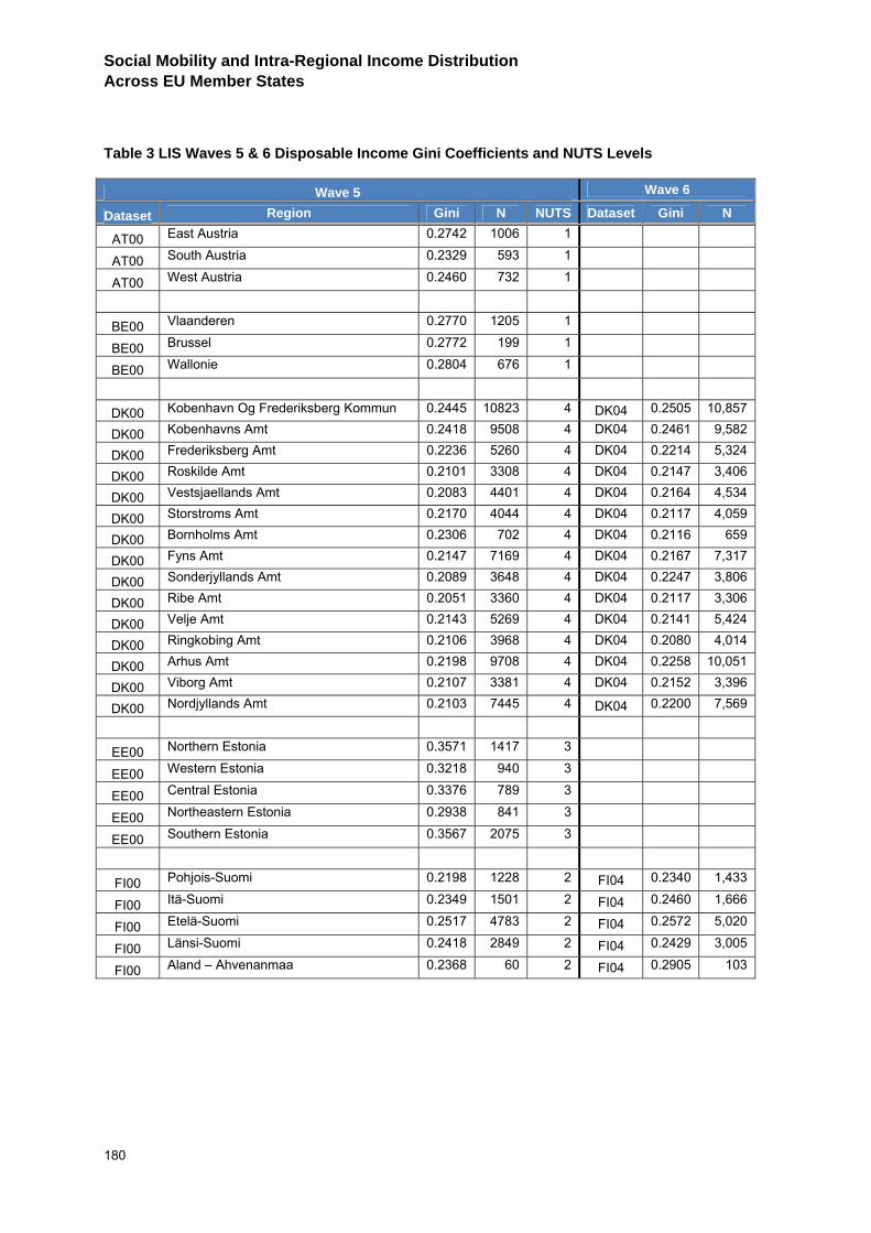
Social Mobility and Intra-Regional Income Distribution Across EU Member States
180
Table 3 LIS Waves 5 & 6 Disposable Income Gini Coefficients and NUTS Levels
Wave 5 Wave 6
Dataset Region Gini N NUTS Dataset Gini N
AT00 East Austria 0.2742 1006 1
AT00 South Austria 0.2329 593 1
AT00 West Austria 0.2460 732 1
BE00 Vlaanderen 0.2770 1205 1
BE00 Brussel 0.2772 199 1
BE00 Wallonie 0.2804 676 1
DK00 Kobenhavn Og Frederiksberg Kommun 0.2445 10823 4 DK04 0.2505 10,857
DK00 Kobenhavns Amt 0.2418 9508 4 DK04 0.2461 9,582
DK00 Frederiksberg Amt 0.2236 5260 4 DK04 0.2214 5,324
DK00 Roskilde Amt 0.2101 3308 4 DK04 0.2147 3,406
DK00 Vestsjaellands Amt 0.2083 4401 4 DK04 0.2164 4,534
DK00 Storstroms Amt 0.2170 4044 4 DK04 0.2117 4,059
DK00 Bornholms Amt 0.2306 702 4 DK04 0.2116 659
DK00 Fyns Amt 0.2147 7169 4 DK04 0.2167 7,317
DK00 Sonderjyllands Amt 0.2089 3648 4 DK04 0.2247 3,806
DK00 Ribe Amt 0.2051 3360 4 DK04 0.2117 3,306
DK00 Velje Amt 0.2143 5269 4 DK04 0.2141 5,424
DK00 Ringkobing Amt 0.2106 3968 4 DK04 0.2080 4,014
DK00 Arhus Amt 0.2198 9708 4 DK04 0.2258 10,051
DK00 Viborg Amt 0.2107 3381 4 DK04 0.2152 3,396
DK00 Nordjyllands Amt 0.2103 7445 4 DK04 0.2200 7,569
EE00 Northern Estonia 0.3571 1417 3
EE00 Western Estonia 0.3218 940 3
EE00 Central Estonia 0.3376 789 3
EE00 Northeastern Estonia 0.2938 841 3
EE00 Southern Estonia 0.3567 2075 3
FI00 Pohjois-Suomi 0.2198 1228 2 FI04 0.2340 1,433
FI00 Itä-Suomi 0.2349 1501 2 FI04 0.2460 1,666
FI00 Etelä-Suomi 0.2517 4783 2 FI04 0.2572 5,020
FI00 Länsi-Suomi 0.2418 2849 2 FI04 0.2429 3,005
FI00 Aland – Ahvenanmaa 0.2368 60 2 FI04 0.2905 103
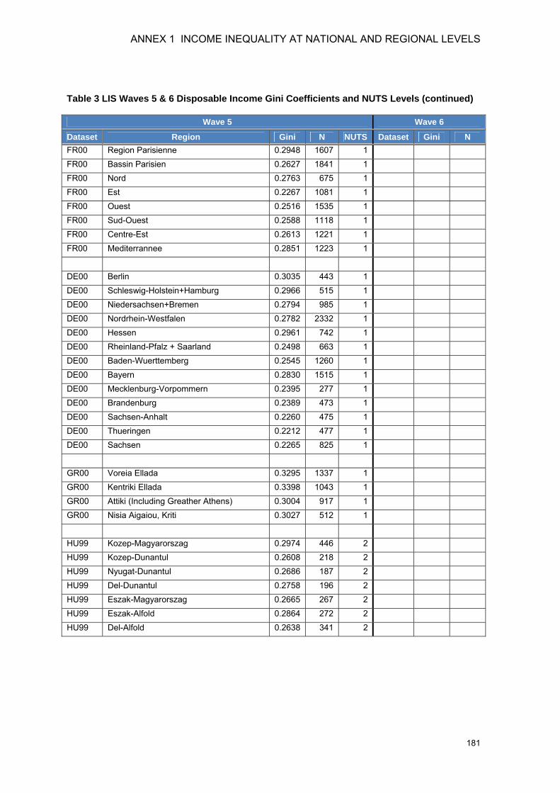
ANNEX 1 INCOME INEQUALITY AT NATIONAL AND REGIONAL LEVELS
181
Table 3 LIS Waves 5 & 6 Disposable Income Gini Coefficients and NUTS Levels (continued)
Wave 5 Wave 6
Dataset Region Gini N NUTS Dataset Gini N FR00 Region Parisienne 0.2948 1607 1 FR00 Bassin Parisien 0.2627 1841 1 FR00 Nord 0.2763 675 1 FR00 Est 0.2267 1081 1 FR00 Ouest 0.2516 1535 1 FR00 Sud-Ouest 0.2588 1118 1 FR00 Centre-Est 0.2613 1221 1 FR00 Mediterrannee 0.2851 1223 1 DE00 Berlin 0.3035 443 1 DE00 Schleswig-Holstein+Hamburg 0.2966 515 1 DE00 Niedersachsen+Bremen 0.2794 985 1 DE00 Nordrhein-Westfalen 0.2782 2332 1 DE00 Hessen 0.2961 742 1 DE00 Rheinland-Pfalz + Saarland 0.2498 663 1 DE00 Baden-Wuerttemberg 0.2545 1260 1 DE00 Bayern 0.2830 1515 1 DE00 Mecklenburg-Vorpommern 0.2395 277 1 DE00 Brandenburg 0.2389 473 1 DE00 Sachsen-Anhalt 0.2260 475 1 DE00 Thueringen 0.2212 477 1 DE00 Sachsen 0.2265 825 1 GR00 Voreia Ellada 0.3295 1337 1 GR00 Kentriki Ellada 0.3398 1043 1 GR00 Attiki (Including Greather Athens) 0.3004 917 1 GR00 Nisia Aigaiou, Kriti 0.3027 512 1 HU99 Kozep-Magyarorszag 0.2974 446 2 HU99 Kozep-Dunantul 0.2608 218 2 HU99 Nyugat-Dunantul 0.2686 187 2 HU99 Del-Dunantul 0.2758 196 2 HU99 Eszak-Magyarorszag 0.2665 267 2 HU99 Eszak-Alfold 0.2864 272 2 HU99 Del-Alfold 0.2638 341 2
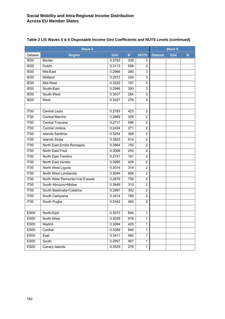
Social Mobility and Intra-Regional Income Distribution Across EU Member States
182
Table 3 LIS Waves 5 & 6 Disposable Income Gini Coefficients and NUTS Levels (continued)
Wave 5 Wave 6
Dataset Region Gini N NUTS Dataset Gini N IE00 Border 0.2750 339 3 IE00 Dublin 0.3113 558 3 IE00 Mid-East 0.2966 260 3 IE00 Midland 0.2972 200 3 IE00 Mid-West 0.3229 197 3 IE00 South-East 0.2946 300 3 IE00 South-West 0.3037 284 3 IE00 West 0.3427 278 3 IT00 Central Lazio 0.2783 423 2 IT00 Central Marche 0.2969 328 2 IT00 Central Toscana 0.2717 596 2 IT00 Central Umbria 0.2424 271 2 IT00 Islands Sardinia 0.3254 308 2 IT00 Islands Sicilia 0.3833 614 2 IT00 North East Emilia Romagna 0.2864 750 2 IT00 North East Friuli 0.3008 255 2 IT00 North East Trentino 0.2741 161 2 IT00 North East Veneto 0.3065 439 2 IT00 North West Liguria 0.3014 314 2 IT00 North West Lombardia 0.3049 858 2 IT00 North West Piemonte+Val D’aosta 0.2879 756 2 IT00 South Abruzzo+Molise 0.3849 310 2 IT00 South Basilicata+Calabria 0.2987 302 2 IT00 South Campania 0.3414 780 2 IT00 South Puglia 0.3342 460 2 ES00 North-East 0.3073 644 1 ES00 North-West 0.3029 678 1 ES00 Madrid 0.3084 425 1 ES00 Central 0.3389 840 1 ES00 East 0.3411 992 1 ES00 South 0.2957 907 1 ES00 Canary Islands 0.3529 278 1
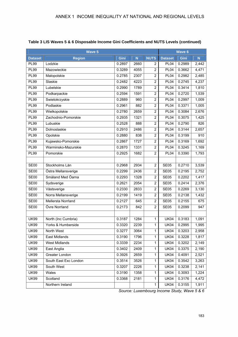
ANNEX 1 INCOME INEQUALITY AT NATIONAL AND REGIONAL LEVELS
183
Table 3 LIS Waves 5 & 6 Disposable Income Gini Coefficients and NUTS Levels (continued)
Wave 5 Wave 6
Dataset Region Gini N NUTS Dataset Gini N PL99 Lodzkie 0.2897 2660 2 PL04 0.2989 2,442 PL99 Mazowieckie 0.3289 4055 2 PL04 0.3662 4,471 PL99 Malopolskie 0.2785 2307 2 PL04 0.2982 2,485 PL99 Slaskie 0.2482 4223 2 PL04 0.2745 4,237 PL99 Lubelskie 0.2990 1789 2 PL04 0.3414 1,810 PL99 Podkarpackie 0.2594 1591 2 PL04 0.2720 1,539 PL99 Swietokrzyskie 0.2889 960 2 PL04 0.2997 1,009 PL99 Podlaskie 0.2961 882 2 PL04 0.3371 1,005 PL99 Wielkopolskie 0.2780 2659 2 PL04 0.3084 2,676 PL99 Zachodnio-Pomorskie 0.2935 1321 2 PL04 0.3075 1,425 PL99 Lubuskie 0.2528 888 2 PL04 0.2790 826 PL99 Dolnoslaskie 0.2910 2486 2 PL04 0.3144 2,657 PL99 Opolskie 0.2880 838 2 PL04 0.3199 910 PL99 Kujawsko-Pomorskie 0.2867 1727 2 PL04 0.3169 1,692 PL99 Warminsko-Mazurskie 0.2870 1331 2 PL04 0.3245 1,169 PL99 Pomorskie 0.2925 1682 2 PL04 0.3390 1,793 SE00 Stockholms Län 0.2968 2934 2 SE05 0.2710 3,539 SE00 Östra Mellansverige 0.2299 2436 2 SE05 0.2195 2,752 SE00 Småland Med Öarna 0.2293 1328 2 SE05 0.2202 1,417 SE00 Sydsverige 0.2621 2054 2 SE05 0.2414 2,376 SE00 Västsverige 0.2330 2833 2 SE05 0.2269 3,130 SE00 Norra Mellansverige 0.2199 1419 2 SE05 0.2138 1,432 SE00 Mellersta Norrland 0.2127 645 2 SE05 0.2155 675 SE00 Övre Norrland 0.2173 842 2 SE05 0.2099 947 UK99 North (Inc Cumbria) 0.3187 1284 1 UK04 0.3183 1,091 UK99 Yorks & Humberside 0.3320 2239 1 UK04 0.2995 1,995 UK99 North West 0.3277 3064 1 UK04 0.3203 2,958 UK99 East Midlands 0.3190 1796 1 UK04 0.3228 1,817 UK99 West Midlands 0.3339 2234 1 UK04 0.3202 2,149 UK99 East Anglia 0.3402 2409 1 UK04 0.3375 2,190 UK99 Greater London 0.3926 2659 1 UK04 0.4091 2,521 UK99 South East Exc London 0.3514 3526 1 UK04 0.3542 3,263 UK99 South West 0.3207 2226 1 UK04 0.3238 2,141 UK99 Wales 0.3190 1358 1 UK04 0.3093 1,224 UK99 Scotland 0.3368 2181 1 UK04 0.3176 4,472 Northern Ireland 1 UK04 0.3155 1,911
Source: Luxembourg Income Study, Wave 5 & 6

Social Mobility and Intra-Regional Income Distribution Across EU Member States
184
Alternative measures of income inequality
Table 4 provides results for alternative inequality measures - GE indices (GE(-1), GE(0), GE(1) and GE(2)) and Atkinson family of indices (A(0.5), A(1) and A(2)) - calculated for EU-SILC equivalised disposable household income data.
As mentioned in the main text, these indicators support the findings based on the single-parameter Gini index (S-Gini). Portugal is one of the most unequal (if not the most unequal) Member States of the Union, and SE the least unequal in most cases. The capital region effect is also persistent. ES stands out again with a high variance in inequality between regions.
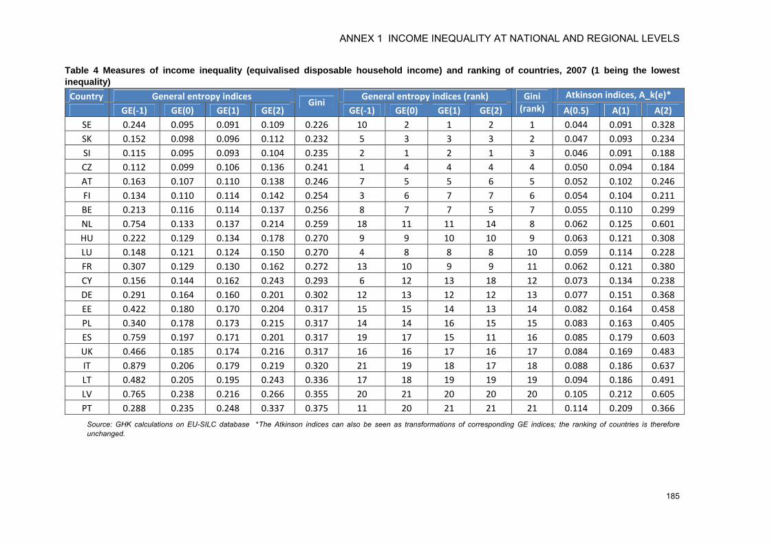
ANNEX 1 INCOME INEQUALITY AT NATIONAL AND REGIONAL LEVELS
185
Table 4 Measures of income inequality (equivalised disposable household income) and ranking of countries, 2007 (1 being the lowest inequality)
Country General entropy indices General entropy indices (rank) Atkinson indices, A_k(e)*
GE(-1) GE(0) GE(1) GE(2) Gini
GE(-1) GE(0) GE(1) GE(2) Gini
(rank) A(0.5) A(1) A(2) SE 0.244 0.095 0.091 0.109 0.226 10 2 1 2 1 0.044 0.091 0.328 SK 0.152 0.098 0.096 0.112 0.232 5 3 3 3 2 0.047 0.093 0.234 SI 0.115 0.095 0.093 0.104 0.235 2 1 2 1 3 0.046 0.091 0.188 CZ 0.112 0.099 0.106 0.136 0.241 1 4 4 4 4 0.050 0.094 0.184 AT 0.163 0.107 0.110 0.138 0.246 7 5 5 6 5 0.052 0.102 0.246 FI 0.134 0.110 0.114 0.142 0.254 3 6 7 7 6 0.054 0.104 0.211 BE 0.213 0.116 0.114 0.137 0.256 8 7 7 5 7 0.055 0.110 0.299 NL 0.754 0.133 0.137 0.214 0.259 18 11 11 14 8 0.062 0.125 0.601 HU 0.222 0.129 0.134 0.178 0.270 9 9 10 10 9 0.063 0.121 0.308 LU 0.148 0.121 0.124 0.150 0.270 4 8 8 8 10 0.059 0.114 0.228 FR 0.307 0.129 0.130 0.162 0.272 13 10 9 9 11 0.062 0.121 0.380 CY 0.156 0.144 0.162 0.243 0.293 6 12 13 18 12 0.073 0.134 0.238 DE 0.291 0.164 0.160 0.201 0.302 12 13 12 12 13 0.077 0.151 0.368 EE 0.422 0.180 0.170 0.204 0.317 15 15 14 13 14 0.082 0.164 0.458 PL 0.340 0.178 0.173 0.215 0.317 14 14 16 15 15 0.083 0.163 0.405 ES 0.759 0.197 0.171 0.201 0.317 19 17 15 11 16 0.085 0.179 0.603 UK 0.466 0.185 0.174 0.216 0.317 16 16 17 16 17 0.084 0.169 0.483 IT 0.879 0.206 0.179 0.219 0.320 21 19 18 17 18 0.088 0.186 0.637 LT 0.482 0.205 0.195 0.243 0.336 17 18 19 19 19 0.094 0.186 0.491 LV 0.765 0.238 0.216 0.266 0.355 20 21 20 20 20 0.105 0.212 0.605 PT 0.288 0.235 0.248 0.337 0.375 11 20 21 21 21 0.114 0.209 0.366
Source: GHK calculations on EU-SILC database *The Atkinson indices can also be seen as transformations of corresponding GE indices; the ranking of countries is therefore unchanged.
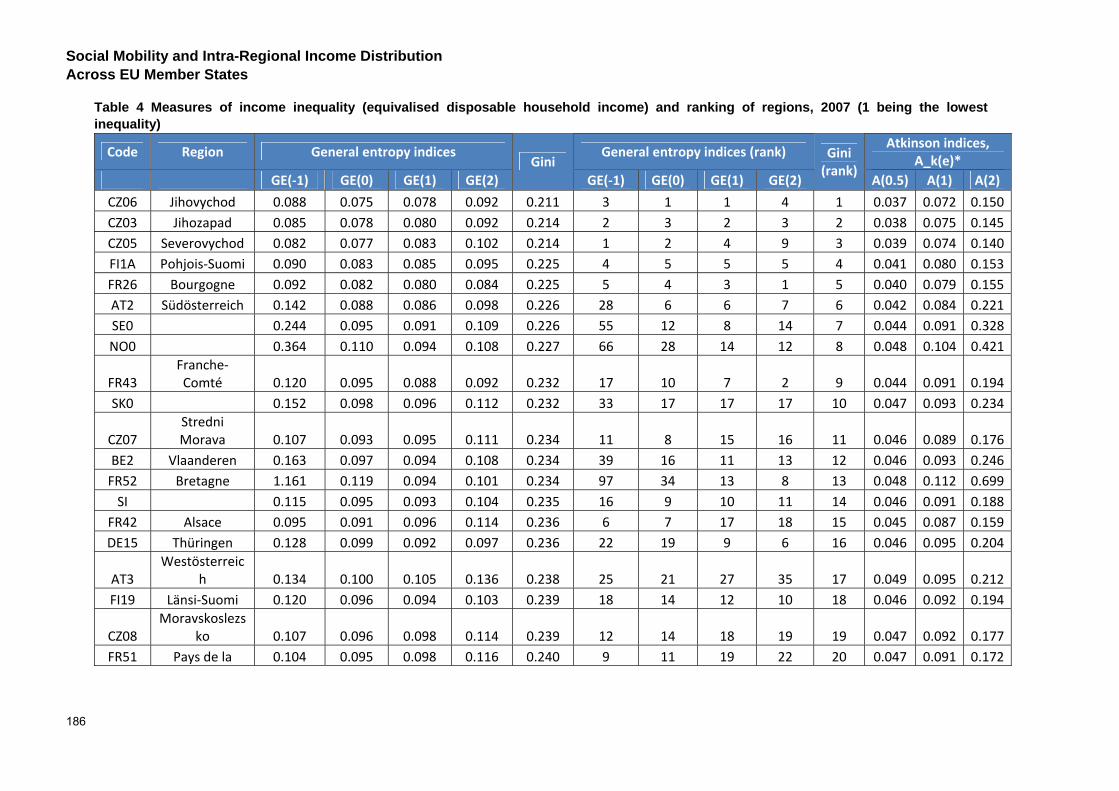
Social Mobility and Intra-Regional Income Distribution Across EU Member States
186
Table 4 Measures of income inequality (equivalised disposable household income) and ranking of regions, 2007 (1 being the lowest inequality)
Code Region General entropy indices General entropy indices (rank) Atkinson indices,
A_k(e)* GE(-1) GE(0) GE(1) GE(2)
Gini GE(-1) GE(0) GE(1) GE(2)
Gini (rank)
A(0.5) A(1) A(2)
CZ06 Jihovychod 0.088 0.075 0.078 0.092 0.211 3 1 1 4 1 0.037 0.072 0.150 CZ03 Jihozapad 0.085 0.078 0.080 0.092 0.214 2 3 2 3 2 0.038 0.075 0.145 CZ05 Severovychod 0.082 0.077 0.083 0.102 0.214 1 2 4 9 3 0.039 0.074 0.140 FI1A Pohjois-Suomi 0.090 0.083 0.085 0.095 0.225 4 5 5 5 4 0.041 0.080 0.153 FR26 Bourgogne 0.092 0.082 0.080 0.084 0.225 5 4 3 1 5 0.040 0.079 0.155 AT2 Südösterreich 0.142 0.088 0.086 0.098 0.226 28 6 6 7 6 0.042 0.084 0.221 SE0 0.244 0.095 0.091 0.109 0.226 55 12 8 14 7 0.044 0.091 0.328 NO0 0.364 0.110 0.094 0.108 0.227 66 28 14 12 8 0.048 0.104 0.421
FR43 Franche-Comté 0.120 0.095 0.088 0.092 0.232 17 10 7 2 9 0.044 0.091 0.194
SK0 0.152 0.098 0.096 0.112 0.232 33 17 17 17 10 0.047 0.093 0.234
CZ07 Stredni Morava 0.107 0.093 0.095 0.111 0.234 11 8 15 16 11 0.046 0.089 0.176
BE2 Vlaanderen 0.163 0.097 0.094 0.108 0.234 39 16 11 13 12 0.046 0.093 0.246 FR52 Bretagne 1.161 0.119 0.094 0.101 0.234 97 34 13 8 13 0.048 0.112 0.699
SI 0.115 0.095 0.093 0.104 0.235 16 9 10 11 14 0.046 0.091 0.188 FR42 Alsace 0.095 0.091 0.096 0.114 0.236 6 7 17 18 15 0.045 0.087 0.159 DE15 Thüringen 0.128 0.099 0.092 0.097 0.236 22 19 9 6 16 0.046 0.095 0.204
AT3 Westösterreic
h 0.134 0.100 0.105 0.136 0.238 25 21 27 35 17 0.049 0.095 0.212 FI19 Länsi-Suomi 0.120 0.096 0.094 0.103 0.239 18 14 12 10 18 0.046 0.092 0.194
CZ08 Moravskoslezs
ko 0.107 0.096 0.098 0.114 0.239 12 14 18 19 19 0.047 0.092 0.177 FR51 Pays de la 0.104 0.095 0.098 0.116 0.240 9 11 19 22 20 0.047 0.091 0.172
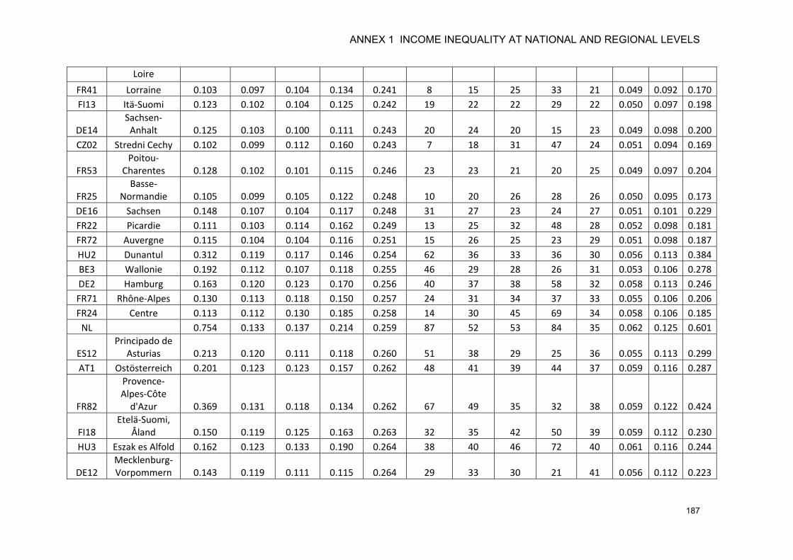
ANNEX 1 INCOME INEQUALITY AT NATIONAL AND REGIONAL LEVELS
187
Loire
FR41 Lorraine 0.103 0.097 0.104 0.134 0.241 8 15 25 33 21 0.049 0.092 0.170 FI13 Itä-Suomi 0.123 0.102 0.104 0.125 0.242 19 22 22 29 22 0.050 0.097 0.198
DE14 Sachsen-
Anhalt 0.125 0.103 0.100 0.111 0.243 20 24 20 15 23 0.049 0.098 0.200 CZ02 Stredni Cechy 0.102 0.099 0.112 0.160 0.243 7 18 31 47 24 0.051 0.094 0.169
FR53 Poitou-
Charentes 0.128 0.102 0.101 0.115 0.246 23 23 21 20 25 0.049 0.097 0.204
FR25 Basse-
Normandie 0.105 0.099 0.105 0.122 0.248 10 20 26 28 26 0.050 0.095 0.173 DE16 Sachsen 0.148 0.107 0.104 0.117 0.248 31 27 23 24 27 0.051 0.101 0.229 FR22 Picardie 0.111 0.103 0.114 0.162 0.249 13 25 32 48 28 0.052 0.098 0.181 FR72 Auvergne 0.115 0.104 0.104 0.116 0.251 15 26 25 23 29 0.051 0.098 0.187 HU2 Dunantul 0.312 0.119 0.117 0.146 0.254 62 36 33 36 30 0.056 0.113 0.384 BE3 Wallonie 0.192 0.112 0.107 0.118 0.255 46 29 28 26 31 0.053 0.106 0.278 DE2 Hamburg 0.163 0.120 0.123 0.170 0.256 40 37 38 58 32 0.058 0.113 0.246 FR71 Rhône-Alpes 0.130 0.113 0.118 0.150 0.257 24 31 34 37 33 0.055 0.106 0.206 FR24 Centre 0.113 0.112 0.130 0.185 0.258 14 30 45 69 34 0.058 0.106 0.185
NL 0.754 0.133 0.137 0.214 0.259 87 52 53 84 35 0.062 0.125 0.601
ES12 Principado de
Asturias 0.213 0.120 0.111 0.118 0.260 51 38 29 25 36 0.055 0.113 0.299 AT1 Ostösterreich 0.201 0.123 0.123 0.157 0.262 48 41 39 44 37 0.059 0.116 0.287
FR82
Provence-Alpes-Côte
d'Azur 0.369 0.131 0.118 0.134 0.262 67 49 35 32 38 0.059 0.122 0.424
FI18 Etelä-Suomi,
Åland 0.150 0.119 0.125 0.163 0.263 32 35 42 50 39 0.059 0.112 0.230 HU3 Eszak es Alfold 0.162 0.123 0.133 0.190 0.264 38 40 46 72 40 0.061 0.116 0.244
DE12 Mecklenburg-Vorpommern 0.143 0.119 0.111 0.115 0.264 29 33 30 21 41 0.056 0.112 0.223
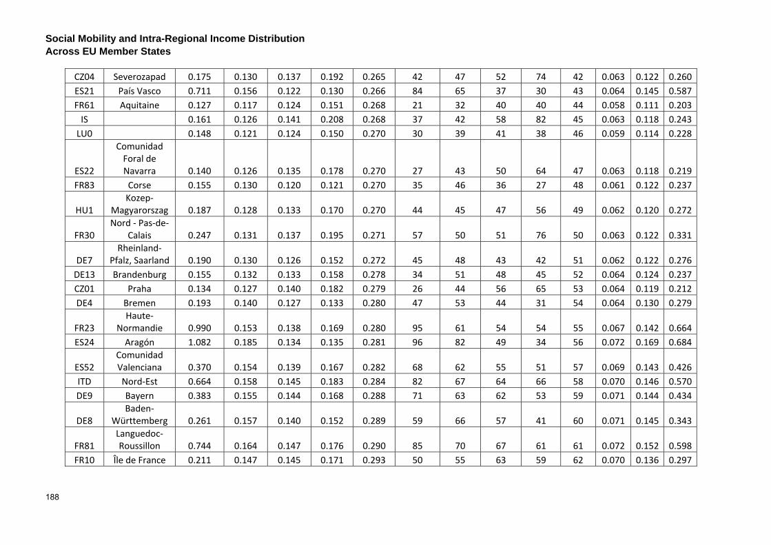
Social Mobility and Intra-Regional Income Distribution Across EU Member States
188
CZ04 Severozapad 0.175 0.130 0.137 0.192 0.265 42 47 52 74 42 0.063 0.122 0.260 ES21 País Vasco 0.711 0.156 0.122 0.130 0.266 84 65 37 30 43 0.064 0.145 0.587 FR61 Aquitaine 0.127 0.117 0.124 0.151 0.268 21 32 40 40 44 0.058 0.111 0.203
IS 0.161 0.126 0.141 0.208 0.268 37 42 58 82 45 0.063 0.118 0.243 LU0 0.148 0.121 0.124 0.150 0.270 30 39 41 38 46 0.059 0.114 0.228
ES22
Comunidad Foral de Navarra 0.140 0.126 0.135 0.178 0.270 27 43 50 64 47 0.063 0.118 0.219
FR83 Corse 0.155 0.130 0.120 0.121 0.270 35 46 36 27 48 0.061 0.122 0.237
HU1 Kozep-
Magyarorszag 0.187 0.128 0.133 0.170 0.270 44 45 47 56 49 0.062 0.120 0.272
FR30 Nord - Pas-de-
Calais 0.247 0.131 0.137 0.195 0.271 57 50 51 76 50 0.063 0.122 0.331
DE7 Rheinland-
Pfalz, Saarland 0.190 0.130 0.126 0.152 0.272 45 48 43 42 51 0.062 0.122 0.276 DE13 Brandenburg 0.155 0.132 0.133 0.158 0.278 34 51 48 45 52 0.064 0.124 0.237 CZ01 Praha 0.134 0.127 0.140 0.182 0.279 26 44 56 65 53 0.064 0.119 0.212 DE4 Bremen 0.193 0.140 0.127 0.133 0.280 47 53 44 31 54 0.064 0.130 0.279
FR23 Haute-
Normandie 0.990 0.153 0.138 0.169 0.280 95 61 54 54 55 0.067 0.142 0.664 ES24 Aragón 1.082 0.185 0.134 0.135 0.281 96 82 49 34 56 0.072 0.169 0.684
ES52 Comunidad Valenciana 0.370 0.154 0.139 0.167 0.282 68 62 55 51 57 0.069 0.143 0.426
ITD Nord-Est 0.664 0.158 0.145 0.183 0.284 82 67 64 66 58 0.070 0.146 0.570 DE9 Bayern 0.383 0.155 0.144 0.168 0.288 71 63 62 53 59 0.071 0.144 0.434
DE8 Baden-
Württemberg 0.261 0.157 0.140 0.152 0.289 59 66 57 41 60 0.071 0.145 0.343
FR81 Languedoc-Roussillon 0.744 0.164 0.147 0.176 0.290 85 70 67 61 61 0.072 0.152 0.598
FR10 Île de France 0.211 0.147 0.145 0.171 0.293 50 55 63 59 62 0.070 0.136 0.297
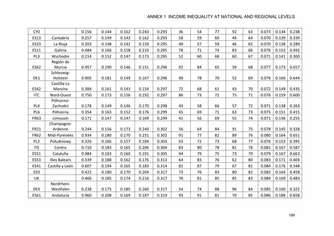
ANNEX 1 INCOME INEQUALITY AT NATIONAL AND REGIONAL LEVELS
189
CY0 0.156 0.144 0.162 0.243 0.293 36 54 77 92 63 0.073 0.134 0.238 ES13 Cantabria 0.257 0.149 0.143 0.162 0.293 58 59 60 49 64 0.070 0.139 0.339 ES23 La Rioja 0.203 0.148 0.142 0.159 0.295 49 57 59 46 65 0.070 0.138 0.289 ES11 Galicia 0.484 0.166 0.158 0.210 0.295 78 71 74 83 66 0.076 0.153 0.492 PL3 Wschodni 0.214 0.152 0.147 0.173 0.295 52 60 68 60 67 0.071 0.141 0.300
ES62 Región de
Murcia 0.957 0.190 0.146 0.151 0.296 92 84 65 39 68 0.077 0.173 0.657
DE1 Schleswig-Holstein 0.905 0.181 0.149 0.167 0.296 90 78 70 52 69 0.076 0.166 0.644
ES42 Castilla-La Mancha 0.384 0.161 0.143 0.154 0.297 72 68 61 43 70 0.072 0.149 0.435
ITC Nord-Ouest 0.750 0.173 0.156 0.192 0.297 86 73 72 75 71 0.076 0.159 0.600
PL4 Północno-Zachodni 0.178 0.149 0.146 0.170 0.298 43 58 66 57 72 0.071 0.138 0.263
PL6 Północny 0.354 0.163 0.152 0.176 0.299 65 69 71 63 73 0.075 0.151 0.415 FR63 Limousin 0.171 0.147 0.147 0.169 0.299 41 56 69 55 74 0.071 0.136 0.255
FR21 Champagne-
Ardenne 0.244 0.156 0.173 0.240 0.302 56 64 84 91 75 0.078 0.145 0.328 FR62 Midi-Pyrénées 0.934 0.180 0.170 0.231 0.302 91 77 82 89 76 0.080 0.164 0.651 PL2 Południowy 0.326 0.166 0.157 0.184 0.303 63 72 73 68 77 0.076 0.153 0.395 ITE Centro 0.710 0.183 0.165 0.206 0.304 83 80 78 81 78 0.081 0.167 0.587
ES51 Cataluña 0.984 0.183 0.160 0.191 0.305 94 79 75 73 79 0.079 0.167 0.663 ES53 Illes Balears 0.339 0.188 0.162 0.176 0.313 64 83 76 62 80 0.083 0.171 0.404 ES41 Castilla y León 0.607 0.194 0.165 0.183 0.314 81 87 79 67 81 0.084 0.176 0.548 EE0 0.422 0.180 0.170 0.204 0.317 73 76 83 80 82 0.082 0.164 0.458 UK 0.466 0.185 0.174 0.216 0.317 76 81 85 85 83 0.084 0.169 0.483
DE5 Nordrhein-Westfalen 0.238 0.175 0.185 0.260 0.317 54 74 88 96 84 0.085 0.160 0.322
ES61 Andalucía 0.960 0.208 0.169 0.187 0.319 93 91 81 70 85 0.086 0.188 0.658
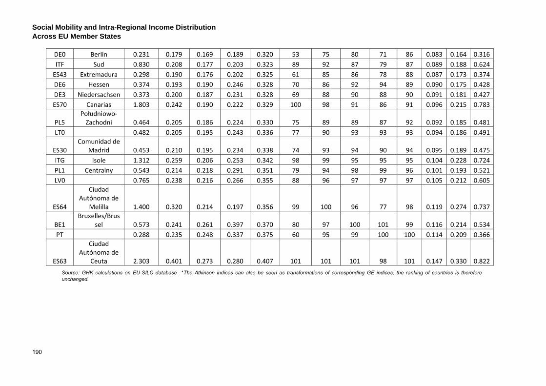
Social Mobility and Intra-Regional Income Distribution Across EU Member States
190
DE0 Berlin 0.231 0.179 0.169 0.189 0.320 53 75 80 71 86 0.083 0.164 0.316 ITF Sud 0.830 0.208 0.177 0.203 0.323 89 92 87 79 87 0.089 0.188 0.624
ES43 Extremadura 0.298 0.190 0.176 0.202 0.325 61 85 86 78 88 0.087 0.173 0.374 DE6 Hessen 0.374 0.193 0.190 0.246 0.328 70 86 92 94 89 0.090 0.175 0.428 DE3 Niedersachsen 0.373 0.200 0.187 0.231 0.328 69 88 90 88 90 0.091 0.181 0.427 ES70 Canarias 1.803 0.242 0.190 0.222 0.329 100 98 91 86 91 0.096 0.215 0.783
PL5 Południowo-
Zachodni 0.464 0.205 0.186 0.224 0.330 75 89 89 87 92 0.092 0.185 0.481 LT0 0.482 0.205 0.195 0.243 0.336 77 90 93 93 93 0.094 0.186 0.491
ES30 Comunidad de
Madrid 0.453 0.210 0.195 0.234 0.338 74 93 94 90 94 0.095 0.189 0.475 ITG Isole 1.312 0.259 0.206 0.253 0.342 98 99 95 95 95 0.104 0.228 0.724 PL1 Centralny 0.543 0.214 0.218 0.291 0.351 79 94 98 99 96 0.101 0.193 0.521 LV0 0.765 0.238 0.216 0.266 0.355 88 96 97 97 97 0.105 0.212 0.605
ES64
Ciudad Autónoma de
Melilla 1.400 0.320 0.214 0.197 0.356 99 100 96 77 98 0.119 0.274 0.737
BE1 Bruxelles/Brus
sel 0.573 0.241 0.261 0.397 0.370 80 97 100 101 99 0.116 0.214 0.534 PT 0.288 0.235 0.248 0.337 0.375 60 95 99 100 100 0.114 0.209 0.366
ES63
Ciudad Autónoma de
Ceuta 2.303 0.401 0.273 0.280 0.407 101 101 101 98 101 0.147 0.330 0.822
Source: GHK calculations on EU-SILC database *The Atkinson indices can also be seen as transformations of corresponding GE indices; the ranking of countries is therefore unchanged.
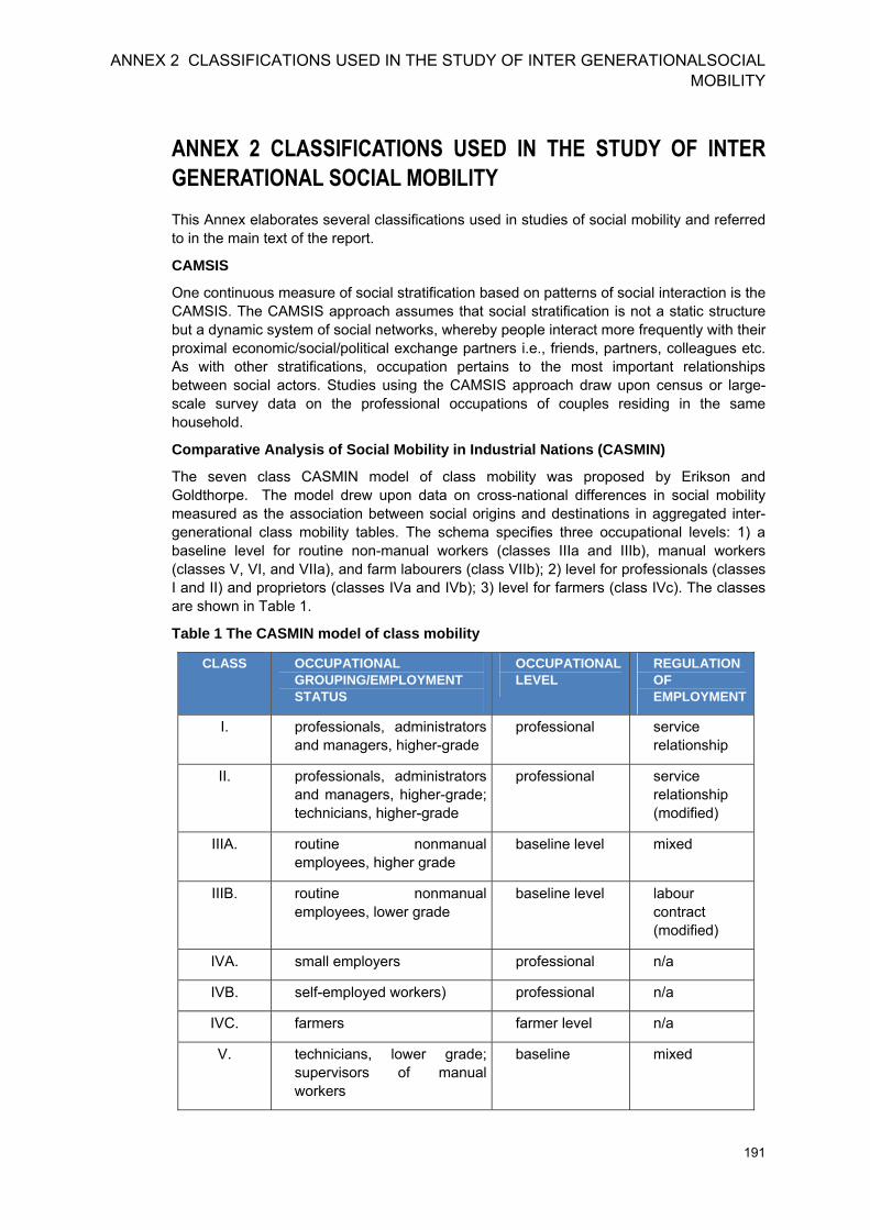
ANNEX 2 CLASSIFICATIONS USED IN THE STUDY OF INTER GENERATIONALSOCIAL MOBILITY
191
ANNEX 2 CLASSIFICATIONS USED IN THE STUDY OF INTER GENERATIONAL SOCIAL MOBILITY This Annex elaborates several classifications used in studies of social mobility and referred to in the main text of the report.
CAMSIS
One continuous measure of social stratification based on patterns of social interaction is the CAMSIS. The CAMSIS approach assumes that social stratification is not a static structure but a dynamic system of social networks, whereby people interact more frequently with their proximal economic/social/political exchange partners i.e., friends, partners, colleagues etc. As with other stratifications, occupation pertains to the most important relationships between social actors. Studies using the CAMSIS approach draw upon census or large-scale survey data on the professional occupations of couples residing in the same household.
Comparative Analysis of Social Mobility in Industrial Nations (CASMIN)
The seven class CASMIN model of class mobility was proposed by Erikson and Goldthorpe. The model drew upon data on cross-national differences in social mobility measured as the association between social origins and destinations in aggregated inter-generational class mobility tables. The schema specifies three occupational levels: 1) a baseline level for routine non-manual workers (classes IIIa and IIIb), manual workers (classes V, VI, and VIIa), and farm labourers (class VIIb); 2) level for professionals (classes I and II) and proprietors (classes IVa and IVb); 3) level for farmers (class IVc). The classes are shown in Table 1.
Table 1 The CASMIN model of class mobility
CLASS OCCUPATIONAL GROUPING/EMPLOYMENT STATUS
OCCUPATIONAL LEVEL
REGULATION OF EMPLOYMENT
I. professionals, administrators and managers, higher-grade
professional service relationship
II. professionals, administrators and managers, higher-grade; technicians, higher-grade
professional service relationship (modified)
IIIA. routine nonmanual employees, higher grade
baseline level mixed
IIIB. routine nonmanual employees, lower grade
baseline level labour contract (modified)
IVA. small employers professional n/a
IVB. self-employed workers) professional n/a
IVC. farmers farmer level n/a
V. technicians, lower grade; supervisors of manual workers
baseline mixed
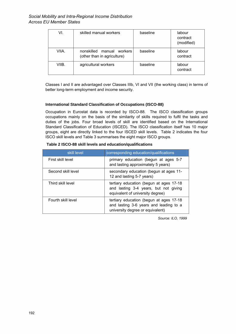
Social Mobility and Intra-Regional Income Distribution Across EU Member States
192
VI. skilled manual workers baseline labour contract (modified)
VIIA. nonskilled manual workers (other than in agriculture)
baseline labour contract
VIIB. agricultural workers baseline labour contract
Classes I and II are advantaged over Classes IIIb, VI and VII (the working class) in terms of better long-term employment and income security.
International Standard Classification of Occupations (ISCO-88)
Occupation in Eurostat data is recorded by ISCO-88. The ISCO classification groups occupations mainly on the basis of the similarity of skills required to fulfil the tasks and duties of the jobs. Four broad levels of skill are identified based on the International Standard Classification of Education (ISCED). The ISCO classification itself has 10 major groups, eight are directly linked to the four ISCED skill levels. Table 2 indicates the four ISCO skill levels and Table 3 summarises the eight major ISCO groups.
Table 2 ISCO-88 skill levels and education/qualifications
skill level corresponding education/qualifications
First skill level primary education (begun at ages 5-7 and lasting approximately 5 years)
Second skill level secondary education (begun at ages 11-12 and lasting 5-7 years)
Third skill level tertiary education (begun at ages 17-18 and lasting 3-4 years, but not giving equivalent of university degree)
Fourth skill level tertiary education (begun at ages 17-18 and lasting 3-6 years and leading to a university degree or equivalent)
Source: ILO, 1999
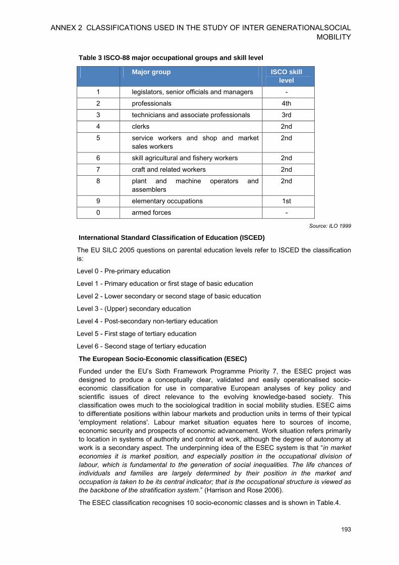
ANNEX 2 CLASSIFICATIONS USED IN THE STUDY OF INTER GENERATIONALSOCIAL MOBILITY
193
Table 3 ISCO-88 major occupational groups and skill level
Major group ISCO skill level
1 legislators, senior officials and managers -
2 professionals 4th
3 technicians and associate professionals 3rd
4 clerks 2nd
5 service workers and shop and market sales workers
2nd
6 skill agricultural and fishery workers 2nd
7 craft and related workers 2nd
8 plant and machine operators and assemblers
2nd
9 elementary occupations 1st
0 armed forces -
Source: ILO 1999
International Standard Classification of Education (ISCED)
The EU SILC 2005 questions on parental education levels refer to ISCED the classification is:
Level 0 - Pre-primary education
Level 1 - Primary education or first stage of basic education
Level 2 - Lower secondary or second stage of basic education
Level 3 - (Upper) secondary education
Level 4 - Post-secondary non-tertiary education
Level 5 - First stage of tertiary education
Level 6 - Second stage of tertiary education
The European Socio-Economic classification (ESEC)
Funded under the EU’s Sixth Framework Programme Priority 7, the ESEC project was designed to produce a conceptually clear, validated and easily operationalised socio-economic classification for use in comparative European analyses of key policy and scientific issues of direct relevance to the evolving knowledge-based society. This classification owes much to the sociological tradition in social mobility studies. ESEC aims to differentiate positions within labour markets and production units in terms of their typical 'employment relations'. Labour market situation equates here to sources of income, economic security and prospects of economic advancement. Work situation refers primarily to location in systems of authority and control at work, although the degree of autonomy at work is a secondary aspect. The underpinning idea of the ESEC system is that “in market economies it is market position, and especially position in the occupational division of labour, which is fundamental to the generation of social inequalities. The life chances of individuals and families are largely determined by their position in the market and occupation is taken to be its central indicator; that is the occupational structure is viewed as the backbone of the stratification system.” (Harrison and Rose 2006).
The ESEC classification recognises 10 socio-economic classes and is shown in Table.4.

Social Mobility and Intra-Regional Income Distribution Across EU Member States
194
Table 4: The European Socio-Economic classification
ESEC Class Common Term Employment Regulation
1 Large employers, higher grade professional, administrative and managerial occupations
Higher salariat Service relationship
2 Lower grade professional, administrative and managerial occupations and higher grade technician and supervisory occupations
Lower salariat Service relationship (modified)
3 Intermediate occupations Higher grade white collar workers
Mixed
4 Small employer and self-employed occupations (excluding agriculture etc)
Petit bourgeoisie or independents
-
5 Self employed occupations (agriculture etc)
Petit bourgeoisie or independents
-
6 Lower supervisory and lower technician occupations
Higher grade blue collar workers
Mixed
7 Lower services, sales and clerical occupations
Lower grade white collar workers
Labour Contract (modified)
8 Lower technical occupations Skilled workers Labour Contract (modified)
9 Routine occupations Semi- and non-skilled workers
Labour Contract
10 Never worked and long-term unemployed
Unemployed -
Source: E-SEC User Guide by Harrison and Rose (2006, p.5)
Related to social mobility, classes 1 and 2 are advantaged over classes 3, 6, 7, 8 and 9 in terms of long-term security of income and being less susceptible to suffering from the possible negative consequences of personnel restructuring. The top classes are also advantaged in the sense that they are less likely to suffer from fluctuations of income and they have a better prospect of upward income mobility. On the other hand, there is some evidence of downward inter-generational mobility of individuals whose parents had been in semi-skilled manual work (i.e., class 9) or skilled manual work (i.e., class 8).
Some countries such as FR and the UK have developed their own national occupational classifications and rarely use the ISCO-88 classification. For example, in FR, the occupational schema abbreviated 'PCS' ('Code des Professions - categories socio-professionnelles') is used. There are various differences between ISCO-88 and PCS e.g., the distinction between managers and professionals is not applied in PCS. Researchers in the ESEC had to code the national classifications and translated them into ISCO using certain algorithms (Rose, 2005).
ANNEX 3 EXPLANATION OF REGRESSION ANALYSIS
195
ANNEX 3 EXPLANATION OF REGRESSION ANALYSIS Base equation
A simple single-equation dynamic linear regression model (OLS) has been used to analyse the impact of public supplies on the development of household income in different income quintiles of the population, while controlling for a range of individual and household characteristics and regional contextual factors. The generic equation used for the model is the following:
(1)
This equation draws a link between the percentage change in the household income of individual i from the base to the final year and a range of explanatory variables at individual or household and regional level (the observation units are individuals in the model who might move between households between the time periods).
The dependent variable in this equation, is the difference between the logarithm of equalised disposable household income in euro at purchasing parity standard (PPS) for individual i in the final year t (i.e. 2007, this being the latest available year for which panel data was available) and the base year t – 2 (i.e. 2005, this being the first year for which sufficient data was available from the panel survey). In line with EU-SILC conventions, the modified OECD equivalence scale (1994 version) has been used.64
The right hand side of the equation contains:
• a set of time-invariate or time-dependent variables summarising individual or
household characteristics for household j ( ), such as age of the head of the household; or the change in the number of full- or part-time jobs between the base and final years;
• a set of regional contextual variables ( ) describing the characteristics of the given country or region k65 (generally in year t – 2), e.g. as the regional GDP per capita or unemployment rate (these have been only used in a separate regression analysis for a subset of countries for which regional-level public expenditure data was available: the Czech Republic, Germany, Hungary and Poland);
• a set of variables aggregating for each income quintile the value of public supply per
capita affecting them ( ) in region k. This, in effect, is the estimated regional value of public supplies in year t66, broken down into four broad categories corresponding to ECP expenditure, and multiplied by an income quintile dummy (dummy defined at national level).
is an independent and identically distributed (iid) error term.
The explanatory variables in detail are the following:
64 This assigns a weight of 1 to the first household member, 0.5 for any subsequent ‘adults’ (i.e. household members at least 14 years old) and 0.3 for ‘children’ (members up to 13 years old). In the German sample (from SOEP), ‘adults’ were defined as being at least 15 years old, and, correspondingly, ‘children’ as being up to 14 years old. 65 Depending on the level of regional breakdown of available panel data. 66 2007 was the only year for which a regionalisation of public supplies for four countries (CZ, DE, HU, PL) was available.

Social Mobility and Intra-Regional Income Distribution Across EU Member States
196
Table 1 List of explanatory variables
Variable code
Variable name Description
Individual/household-level variables
hhheadsex05 Sex of the household head
The sex of the head of the household (household status 2005), defined as a binary variable taking the value 0 for male and 1 for female heads. The head of household was assumed to be the person who in the EU-SILC survey was indicated to be ‘primarily responsible for accommodation’.
hhheadage05 Age of household head The age of the head of household in 2005 in years (the age of most individuals above 80 in the sample years was coded as 80).
hhheadag205 Age-squared of household head
adults05 Number of adults The number of adults (14+ years; 15+ years in the German sample) in the household of the individual in 2005
children05 Number of children The number of children (13- years; 14- years in the German sample) in the household of the individual in 2005
dadults Change in number of adults
The change in the number of adults in the household of the individual from 2005 to 2007
dchildren Change in number of children
The change in the number of children (13- years) in the household of the individual from 2005 to 2007
hhisced3 Upper-secondary education (ISCED3)
The number of persons in the household of the individual (for EU-SILC: who are currently not learning) whose highest educational attainment was upper-secondary (ISCED 3) in 2005
hhisced45 Post-secondary/tertiary education (ISCED4 and 5)
The number of persons in the household of the individual (for EU-SILC: who are currently not learning) whose highest educational attainment was post-secondary or tertiary (ISCED 3) in 2005
dhhft Change in household full-time employment
The change in the number of persons in the household of the individual who were full-time employed from 2005 to 2007
dhhpt Change in household part-time employment
The change in the number of persons in the household of the individual who were part-time employed from 2005 to 2007
Regional contextual variables (only for a subset of countries)
loggdp05 Log-GDP/capita The logarithm of regional GDP per capita (in euro at PPS)
logberdcap Log-BERD/capita The logarithm of business expenditure on R&D (BERD) per capita in the region (in euro at PPS)
econact05 Economic activity The economic activity rate in the region in the 15-74
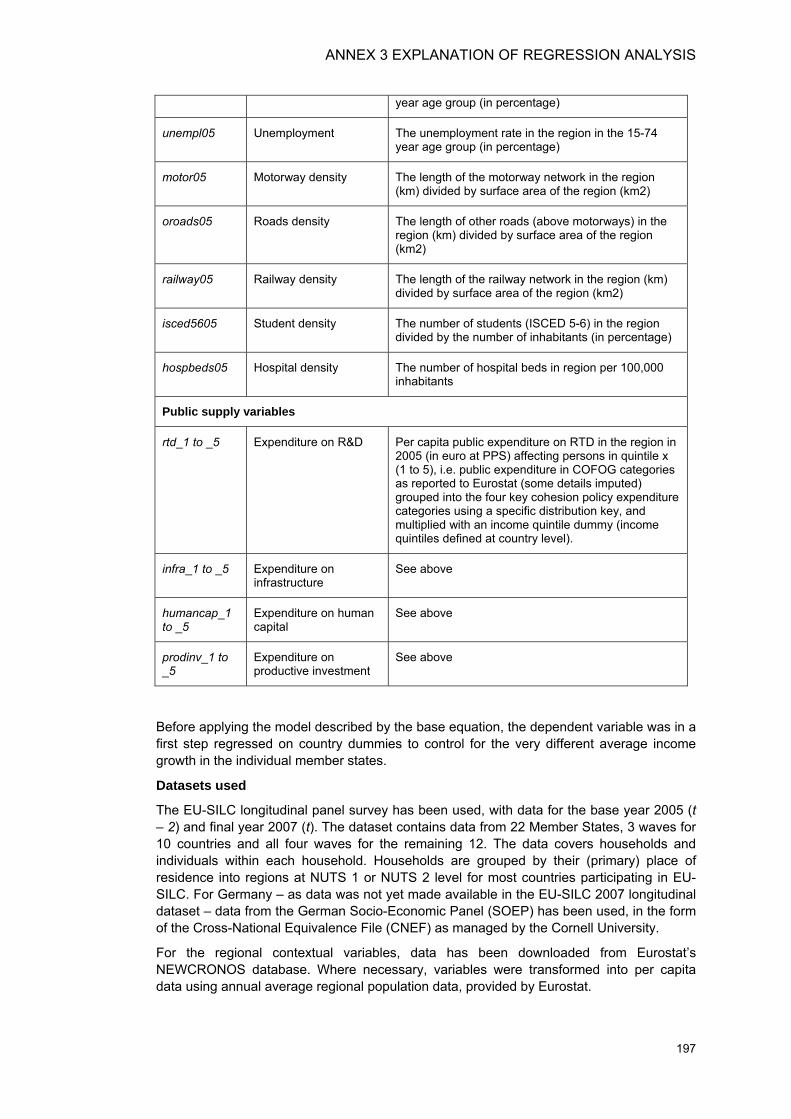
ANNEX 3 EXPLANATION OF REGRESSION ANALYSIS
197
year age group (in percentage)
unempl05 Unemployment The unemployment rate in the region in the 15-74 year age group (in percentage)
motor05 Motorway density The length of the motorway network in the region (km) divided by surface area of the region (km2)
oroads05 Roads density The length of other roads (above motorways) in the region (km) divided by surface area of the region (km2)
railway05 Railway density The length of the railway network in the region (km) divided by surface area of the region (km2)
isced5605 Student density The number of students (ISCED 5-6) in the region divided by the number of inhabitants (in percentage)
hospbeds05 Hospital density The number of hospital beds in region per 100,000 inhabitants
Public supply variables
rtd_1 to _5 Expenditure on R&D Per capita public expenditure on RTD in the region in 2005 (in euro at PPS) affecting persons in quintile x (1 to 5), i.e. public expenditure in COFOG categories as reported to Eurostat (some details imputed) grouped into the four key cohesion policy expenditure categories using a specific distribution key, and multiplied with an income quintile dummy (income quintiles defined at country level).
infra_1 to _5 Expenditure on infrastructure
See above
humancap_1 to _5
Expenditure on human capital
See above
prodinv_1 to _5
Expenditure on productive investment
See above
Before applying the model described by the base equation, the dependent variable was in a first step regressed on country dummies to control for the very different average income growth in the individual member states.
Datasets used
The EU-SILC longitudinal panel survey has been used, with data for the base year 2005 (t – 2) and final year 2007 (t). The dataset contains data from 22 Member States, 3 waves for 10 countries and all four waves for the remaining 12. The data covers households and individuals within each household. Households are grouped by their (primary) place of residence into regions at NUTS 1 or NUTS 2 level for most countries participating in EU-SILC. For Germany – as data was not yet made available in the EU-SILC 2007 longitudinal dataset – data from the German Socio-Economic Panel (SOEP) has been used, in the form of the Cross-National Equivalence File (CNEF) as managed by the Cornell University.
For the regional contextual variables, data has been downloaded from Eurostat’s NEWCRONOS database. Where necessary, variables were transformed into per capita data using annual average regional population data, provided by Eurostat.
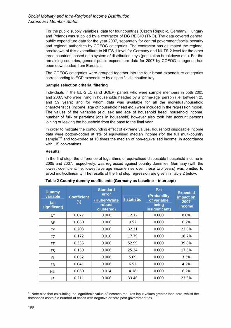
Social Mobility and Intra-Regional Income Distribution Across EU Member States
198
For the public supply variables, data for four countries (Czech Republic, Germany, Hungary and Poland) was supplied by a contractor of DG REGIO (TNO). The data covered general public expenditure data for the year 2007, separately for central government/social security and regional authorities by COFOG categories. The contractor has estimated the regional breakdown of this expenditure to NUTS 1 level for Germany and NUTS 2 level for the other three countries, based on a system of distribution keys (population breakdown etc.). For the remaining countries, general public expenditure data for 2007 by COFOG categories has been downloaded from Eurostat.
The COFOG categories were grouped together into the four broad expenditure categories corresponding to ECP expenditure by a specific distribution key.
Sample selection criteria, filtering
Individuals in the EU-SILC (and SOEP) panels who were sample members in both 2005 and 2007, who were living in households headed by a ‘prime-age’ person (i.e. between 25 and 59 years) and for whom data was available for all the individual/household characteristics (income, age of household head etc.) were included in the regression model. The values of the variables (e.g. sex and age of household head, household income, number of full- or part-time jobs in household) however also took into account persons joining or leaving the household from the base to the final year.
In order to mitigate the confounding effect of extreme values, household disposable income data were bottom-coded at 1% of equivalised median income (for the full multi-country sample)67 and top-coded at 10 times the median of non-equivalised income, in accordance with LIS conventions.
Results
In the first step, the difference of logarithms of equivalised disposable household income in 2005 and 2007, respectively, was regressed against country dummies. Germany (with the lowest coefficient, i.e. lowest average income rise over these two years) was omitted to avoid multicollinearity. The results of the first step regression are given in Table 2 below.
Table 2 Country dummy coefficients (Germany as baseline – intercept)
Dummy variable
(all significant)
Coefficient (β)
Standard error
(Huber-White robust
clustered)
t statistic
P>t (Probability of variable
being insignificant)
Expected impact on
2007 income
AT 0.077 0.006 12.12 0.000 8.0%
BE 0.060 0.006 9.52 0.000 6.2%
CY 0.203 0.006 32.21 0.000 22.6%
CZ 0.172 0.010 17.79 0.000 18.7%
EE 0.335 0.006 52.99 0.000 39.8%
ES 0.159 0.006 25.24 0.000 17.3%
FI 0.032 0.006 5.09 0.000 3.3%
FR 0.041 0.006 6.52 0.000 4.2%
HU 0.060 0.014 4.18 0.000 6.2%
IS 0.211 0.006 33.46 0.000 23.5%
67 Note also that calculating the logarithmic value of incomes requires input values greater than zero, whilst the databases contain a number of cases with negative or zero post-government tax.
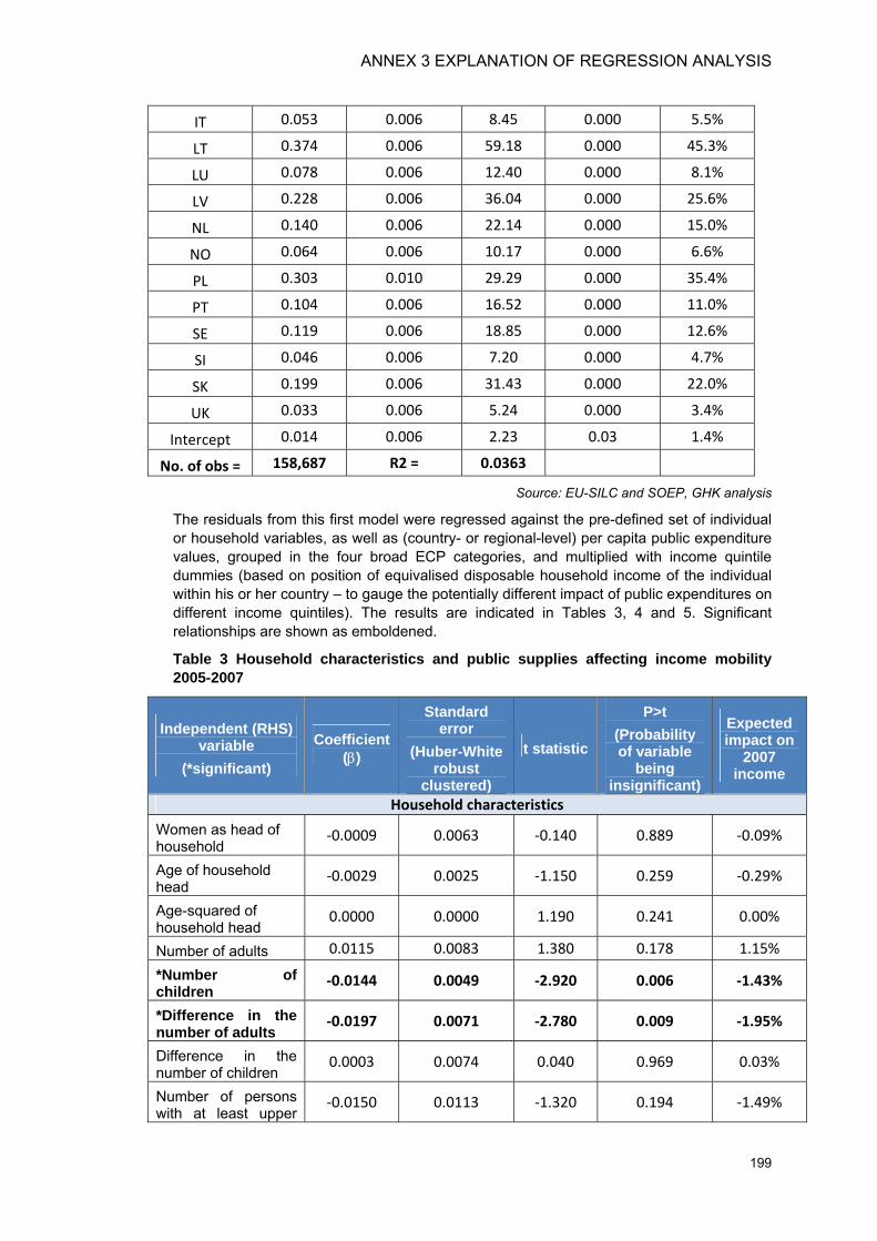
ANNEX 3 EXPLANATION OF REGRESSION ANALYSIS
199
IT 0.053 0.006 8.45 0.000 5.5%
LT 0.374 0.006 59.18 0.000 45.3%
LU 0.078 0.006 12.40 0.000 8.1%
LV 0.228 0.006 36.04 0.000 25.6%
NL 0.140 0.006 22.14 0.000 15.0%
NO 0.064 0.006 10.17 0.000 6.6%
PL 0.303 0.010 29.29 0.000 35.4%
PT 0.104 0.006 16.52 0.000 11.0%
SE 0.119 0.006 18.85 0.000 12.6%
SI 0.046 0.006 7.20 0.000 4.7%
SK 0.199 0.006 31.43 0.000 22.0%
UK 0.033 0.006 5.24 0.000 3.4%
Intercept 0.014 0.006 2.23 0.03 1.4%
No. of obs = 158,687 R2 = 0.0363
Source: EU-SILC and SOEP, GHK analysis
The residuals from this first model were regressed against the pre-defined set of individual or household variables, as well as (country- or regional-level) per capita public expenditure values, grouped in the four broad ECP categories, and multiplied with income quintile dummies (based on position of equivalised disposable household income of the individual within his or her country – to gauge the potentially different impact of public expenditures on different income quintiles). The results are indicated in Tables 3, 4 and 5. Significant relationships are shown as emboldened.
Table 3 Household characteristics and public supplies affecting income mobility 2005-2007
Independent (RHS) variable
(*significant)
Coefficient (β)
Standard error
(Huber-White robust
clustered)
t statistic
P>t (Probability of variable
being insignificant)
Expected impact on
2007 income
Household characteristics
Women as head of household
-0.0009 0.0063 -0.140 0.889 -0.09%
Age of household head
-0.0029 0.0025 -1.150 0.259 -0.29%
Age-squared of household head
0.0000 0.0000 1.190 0.241 0.00%
Number of adults 0.0115 0.0083 1.380 0.178 1.15%
*Number of children
-0.0144 0.0049 -2.920 0.006 -1.43%
*Difference in the number of adults
-0.0197 0.0071 -2.780 0.009 -1.95%
Difference in the number of children
0.0003 0.0074 0.040 0.969 0.03%
Number of persons with at least upper
-0.0150 0.0113 -1.320 0.194 -1.49%
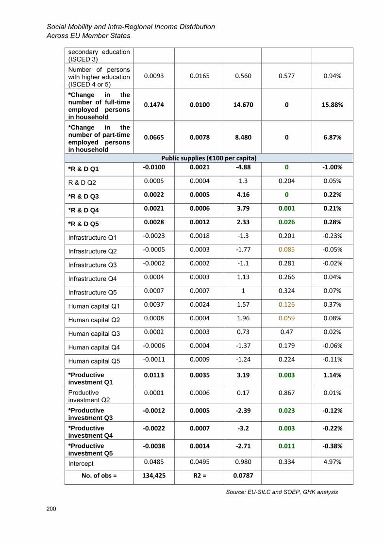
Social Mobility and Intra-Regional Income Distribution Across EU Member States
200
secondary education (ISCED 3) Number of persons with higher education (ISCED 4 or 5)
0.0093 0.0165 0.560 0.577 0.94%
*Change in the number of full-time employed persons in household
0.1474 0.0100 14.670 0 15.88%
*Change in the number of part-time employed persons in household
0.0665 0.0078 8.480 0 6.87%
Public supplies (€100 per capita)
*R & D Q1 -0.0100 0.0021 -4.88 0 -1.00%
R & D Q2 0.0005 0.0004 1.3 0.204 0.05%
*R & D Q3 0.0022 0.0005 4.16 0 0.22%
*R & D Q4 0.0021 0.0006 3.79 0.001 0.21%
*R & D Q5 0.0028 0.0012 2.33 0.026 0.28%
Infrastructure Q1 -0.0023 0.0018 -1.3 0.201 -0.23%
Infrastructure Q2 -0.0005 0.0003 -1.77 0.085 -0.05%
Infrastructure Q3 -0.0002 0.0002 -1.1 0.281 -0.02%
Infrastructure Q4 0.0004 0.0003 1.13 0.266 0.04%
Infrastructure Q5 0.0007 0.0007 1 0.324 0.07%
Human capital Q1 0.0037 0.0024 1.57 0.126 0.37%
Human capital Q2 0.0008 0.0004 1.96 0.059 0.08%
Human capital Q3 0.0002 0.0003 0.73 0.47 0.02%
Human capital Q4 -0.0006 0.0004 -1.37 0.179 -0.06%
Human capital Q5 -0.0011 0.0009 -1.24 0.224 -0.11%
*Productive investment Q1
0.0113 0.0035 3.19 0.003 1.14%
Productive investment Q2
0.0001 0.0006 0.17 0.867 0.01%
*Productive investment Q3
-0.0012 0.0005 -2.39 0.023 -0.12%
*Productive investment Q4
-0.0022 0.0007 -3.2 0.003 -0.22%
*Productive investment Q5
-0.0038 0.0014 -2.71 0.011 -0.38%
Intercept 0.0485 0.0495 0.980 0.334 4.97%
No. of obs = 134,425 R2 = 0.0787
Source: EU-SILC and SOEP, GHK analysis
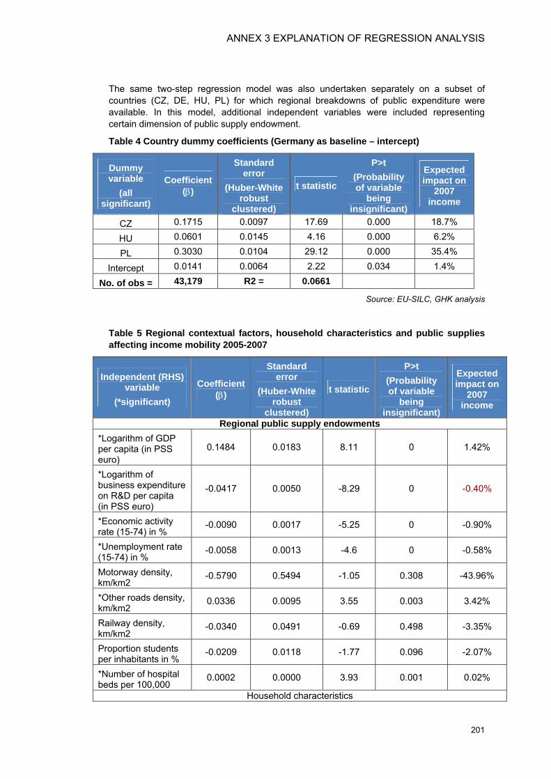
ANNEX 3 EXPLANATION OF REGRESSION ANALYSIS
201
The same two-step regression model was also undertaken separately on a subset of countries (CZ, DE, HU, PL) for which regional breakdowns of public expenditure were available. In this model, additional independent variables were included representing certain dimension of public supply endowment.
Table 4 Country dummy coefficients (Germany as baseline – intercept)
Dummy variable
(all significant)
Coefficient (β)
Standard error
(Huber-White robust
clustered)
t statistic
P>t (Probability of variable
being insignificant)
Expected impact on
2007 income
CZ 0.1715 0.0097 17.69 0.000 18.7%
HU 0.0601 0.0145 4.16 0.000 6.2%
PL 0.3030 0.0104 29.12 0.000 35.4%
Intercept 0.0141 0.0064 2.22 0.034 1.4%
No. of obs = 43,179 R2 = 0.0661
Source: EU-SILC, GHK analysis
Table 5 Regional contextual factors, household characteristics and public supplies affecting income mobility 2005-2007
Independent (RHS) variable
(*significant)
Coefficient (β)
Standard error
(Huber-White robust
clustered)
t statistic
P>t (Probability of variable
being insignificant)
Expected impact on
2007 income
Regional public supply endowments *Logarithm of GDP per capita (in PSS euro)
0.1484 0.0183 8.11 0 1.42%
*Logarithm of business expenditure on R&D per capita (in PSS euro)
-0.0417 0.0050 -8.29 0 -0.40%
*Economic activity rate (15-74) in %
-0.0090 0.0017 -5.25 0 -0.90%
*Unemployment rate (15-74) in %
-0.0058 0.0013 -4.6 0 -0.58%
Motorway density, km/km2
-0.5790 0.5494 -1.05 0.308 -43.96%
*Other roads density, km/km2
0.0336 0.0095 3.55 0.003 3.42%
Railway density, km/km2
-0.0340 0.0491 -0.69 0.498 -3.35%
Proportion students per inhabitants in %
-0.0209 0.0118 -1.77 0.096 -2.07%
*Number of hospital beds per 100,000
0.0002 0.0000 3.93 0.001 0.02%
Household characteristics
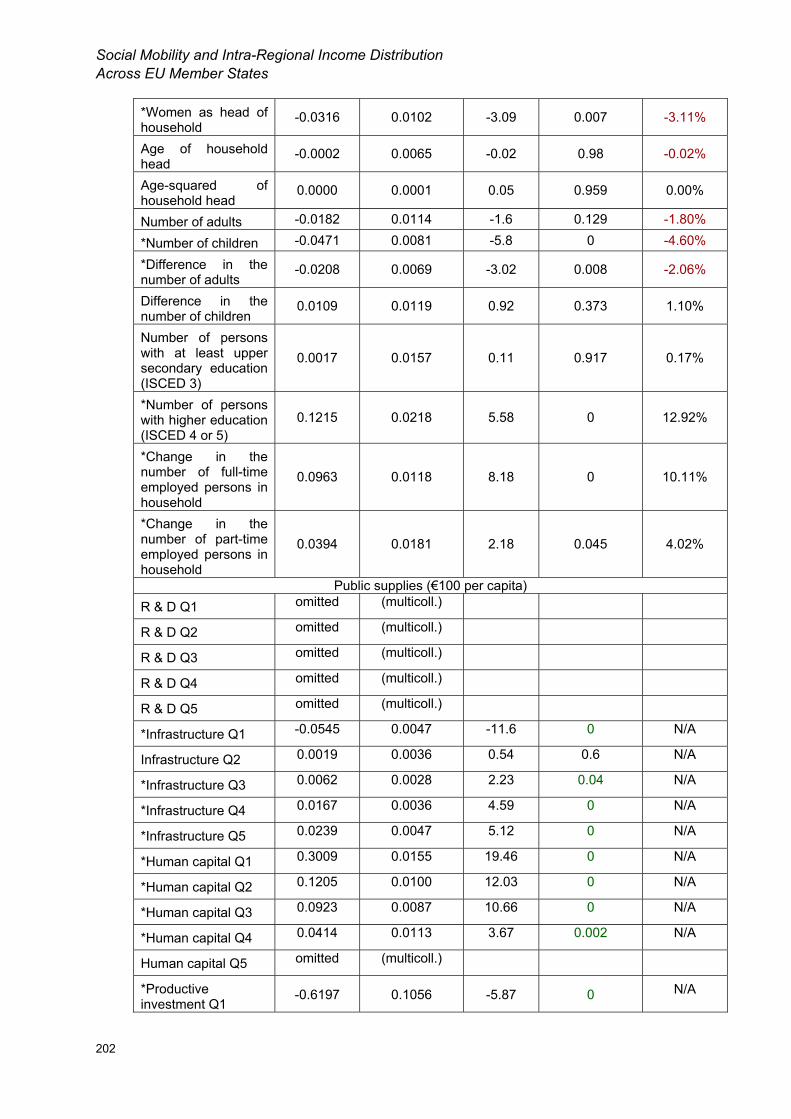
Social Mobility and Intra-Regional Income Distribution Across EU Member States
202
*Women as head of household
-0.0316 0.0102 -3.09 0.007 -3.11%
Age of household head
-0.0002 0.0065 -0.02 0.98 -0.02%
Age-squared of household head
0.0000 0.0001 0.05 0.959 0.00%
Number of adults -0.0182 0.0114 -1.6 0.129 -1.80%
*Number of children -0.0471 0.0081 -5.8 0 -4.60%
*Difference in the number of adults
-0.0208 0.0069 -3.02 0.008 -2.06%
Difference in the number of children
0.0109 0.0119 0.92 0.373 1.10%
Number of persons with at least upper secondary education (ISCED 3)
0.0017 0.0157 0.11 0.917 0.17%
*Number of persons with higher education (ISCED 4 or 5)
0.1215 0.0218 5.58 0 12.92%
*Change in the number of full-time employed persons in household
0.0963 0.0118 8.18 0 10.11%
*Change in the number of part-time employed persons in household
0.0394 0.0181 2.18 0.045 4.02%
Public supplies (€100 per capita) R & D Q1 omitted (multicoll.)
R & D Q2 omitted (multicoll.)
R & D Q3 omitted (multicoll.)
R & D Q4 omitted (multicoll.)
R & D Q5 omitted (multicoll.)
*Infrastructure Q1 -0.0545 0.0047 -11.6 0 N/A
Infrastructure Q2 0.0019 0.0036 0.54 0.6 N/A
*Infrastructure Q3 0.0062 0.0028 2.23 0.04 N/A
*Infrastructure Q4 0.0167 0.0036 4.59 0 N/A
*Infrastructure Q5 0.0239 0.0047 5.12 0 N/A
*Human capital Q1 0.3009 0.0155 19.46 0 N/A
*Human capital Q2 0.1205 0.0100 12.03 0 N/A
*Human capital Q3 0.0923 0.0087 10.66 0 N/A
*Human capital Q4 0.0414 0.0113 3.67 0.002 N/A
Human capital Q5 omitted (multicoll.)
*Productive investment Q1
-0.6197 0.1056 -5.87 0 N/A
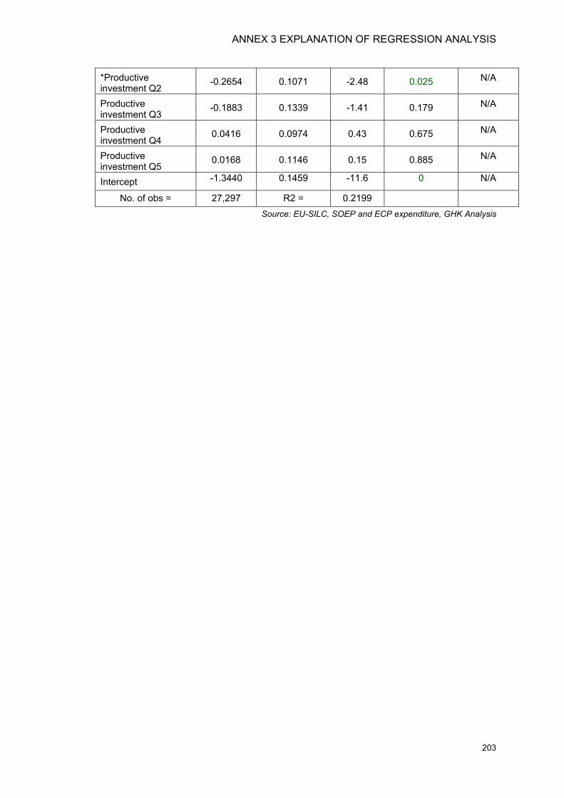
ANNEX 3 EXPLANATION OF REGRESSION ANALYSIS
203
*Productive investment Q2
-0.2654 0.1071 -2.48 0.025 N/A
Productive investment Q3
-0.1883 0.1339 -1.41 0.179 N/A
Productive investment Q4
0.0416 0.0974 0.43 0.675 N/A
Productive investment Q5
0.0168 0.1146 0.15 0.885 N/A
Intercept -1.3440 0.1459 -11.6 0 N/A
No. of obs = 27,297 R2 = 0.2199 Source: EU-SILC, SOEP and ECP expenditure, GHK Analysis

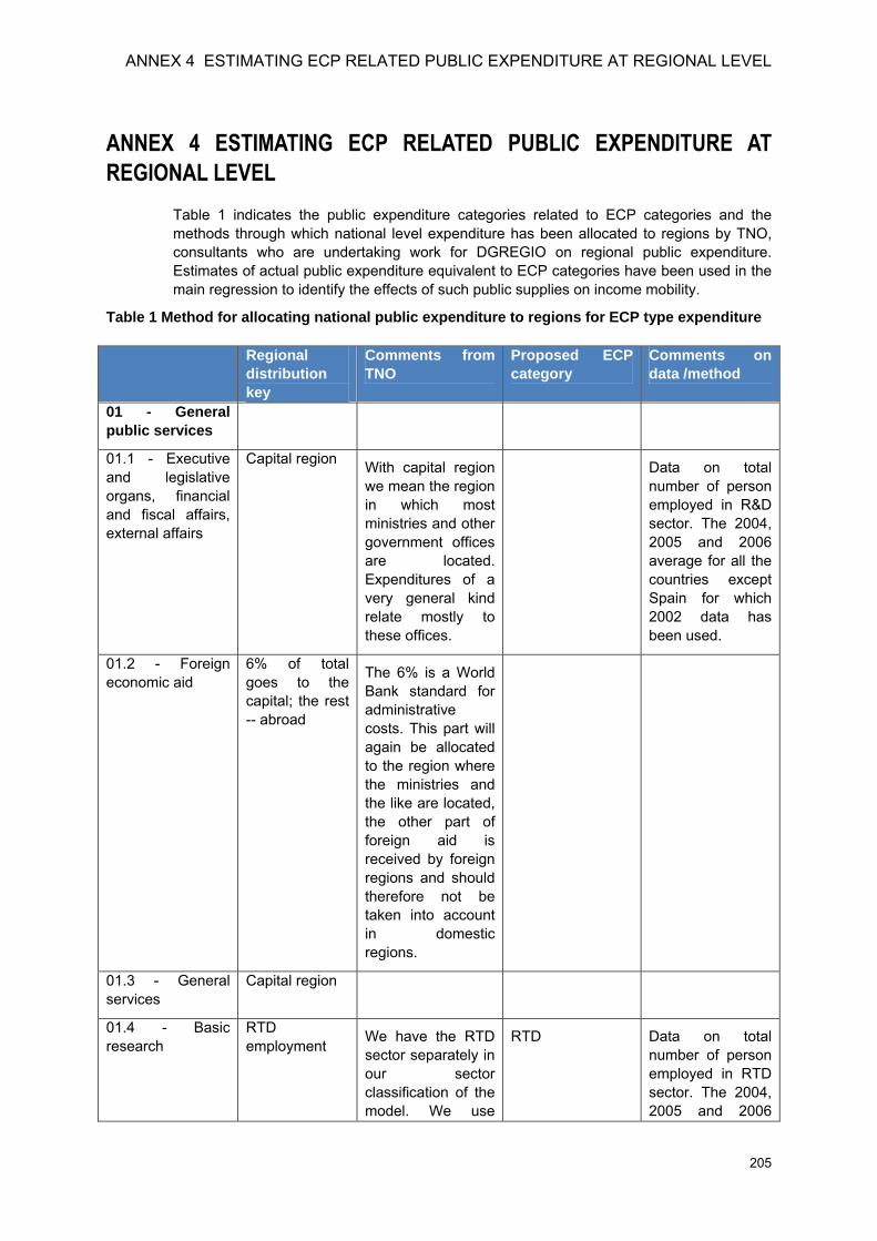
ANNEX 4 ESTIMATING ECP RELATED PUBLIC EXPENDITURE AT REGIONAL LEVEL
205
ANNEX 4 ESTIMATING ECP RELATED PUBLIC EXPENDITURE AT REGIONAL LEVEL
Table 1 indicates the public expenditure categories related to ECP categories and the methods through which national level expenditure has been allocated to regions by TNO, consultants who are undertaking work for DGREGIO on regional public expenditure. Estimates of actual public expenditure equivalent to ECP categories have been used in the main regression to identify the effects of such public supplies on income mobility.
Table 1 Method for allocating national public expenditure to regions for ECP type expenditure Regional
distribution key
Comments from TNO
Proposed ECP category
Comments on data /method
01 - General public services
01.1 - Executive and legislative organs, financial and fiscal affairs, external affairs
Capital region With capital region we mean the region in which most ministries and other government offices are located. Expenditures of a very general kind relate mostly to these offices.
Data on total number of person employed in R&D sector. The 2004, 2005 and 2006 average for all the countries except Spain for which 2002 data has been used.
01.2 - Foreign economic aid
6% of total goes to the capital; the rest -- abroad
The 6% is a World Bank standard for administrative costs. This part will again be allocated to the region where the ministries and the like are located, the other part of foreign aid is received by foreign regions and should therefore not be taken into account in domestic regions.
01.3 - General services
Capital region
01.4 - Basic research
RTD employment We have the RTD
sector separately in our sector classification of the model. We use
RTD Data on total number of person employed in RTD sector. The 2004, 2005 and 2006

Social Mobility and Intra-Regional Income Distribution Across EU Member States
206
Regional distribution key
Comments from TNO
Proposed ECP category
Comments on data /method
employment in this sector as an approximation for all basic research and RTD undertaken in each region.
average for all the countries except Spain for which 2002 data has been used.
01.5 - RTD General public services
RTD employment RTD Data on total
number of person employed in RTD sector. The 2004, 2005 and 2006 average for all the countries except Spain for which 2002 data has been used.
01.6 - General public services n.e.c.
Capital region
01.7 - Public debt transactions
Employment in Financial intermediation (j)
The financial sector is taking care of all transactions with bonds. The regional distribution of employees in the financial sector would therefore be an approximation for the regions in which government bonds are bought.
01.8 - Transfers of a general character between different levels of government
Population Here we assume that the amount of money each regional government receives relates to the total population in each region.
02 - Defence
02.1 - Military defence
Government employment Employment in the
military is part of total government employment. Since we have regional

ANNEX 4 ESTIMATING ECP RELATED PUBLIC EXPENDITURE AT REGIONAL LEVEL
207
Regional distribution key
Comments from TNO
Proposed ECP category
Comments on data /method
data on employment in the government sector, this is the best regional distribution key we have available.
02.2 - Civil defence
Population We assume that Civil defence is related to the amount of people living in each region.
02.3 - Foreign military aid
6% of total goes to the capital; the rest -- abroad
Again the 6% for local administration costs are allocated to the location of ministries. The main part of the expenditure does not relate to domestic regions but flows out of the country.
02.4 - RTD Defence
RTD employment RTD Data on total
number of person employed in R&D sector. The 2004, 2005 and 2006 average for all the countries except Spain for which 2002 data has been used.
02.5 - Defence n.e.c.
Government employment
03 - Public order and safety
03.1 - Police services
Population We assume that the amount of money spent on public order and safety in each region directly correlates to the number of people living in each
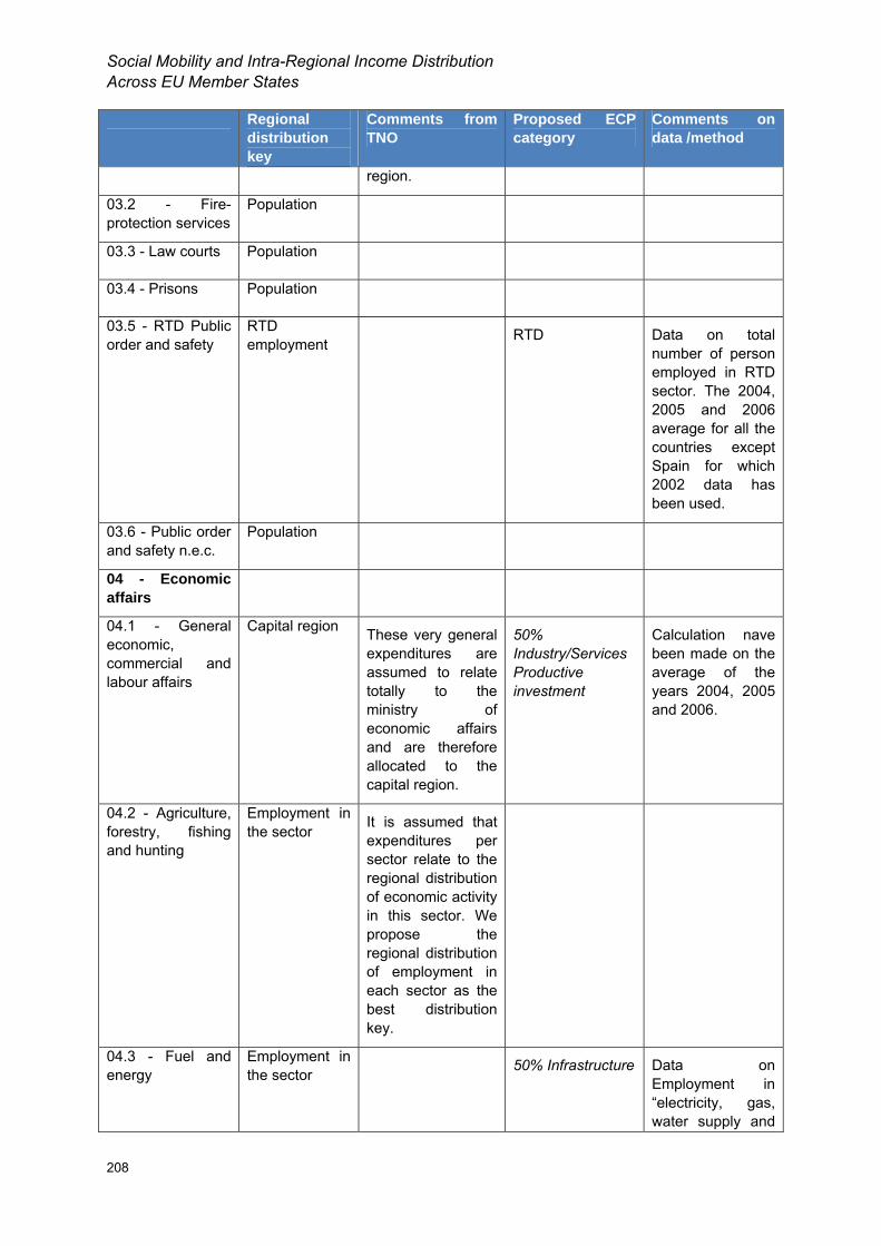
Social Mobility and Intra-Regional Income Distribution Across EU Member States
208
Regional distribution key
Comments from TNO
Proposed ECP category
Comments on data /method
region.
03.2 - Fire-protection services
Population
03.3 - Law courts Population
03.4 - Prisons Population
03.5 - RTD Public order and safety
RTD employment RTD Data on total
number of person employed in RTD sector. The 2004, 2005 and 2006 average for all the countries except Spain for which 2002 data has been used.
03.6 - Public order and safety n.e.c.
Population
04 - Economic affairs
04.1 - General economic, commercial and labour affairs
Capital region These very general expenditures are assumed to relate totally to the ministry of economic affairs and are therefore allocated to the capital region.
50% Industry/Services Productive investment
Calculation nave been made on the average of the years 2004, 2005 and 2006.
04.2 - Agriculture, forestry, fishing and hunting
Employment in the sector It is assumed that
expenditures per sector relate to the regional distribution of economic activity in this sector. We propose the regional distribution of employment in each sector as the best distribution key.
04.3 - Fuel and energy
Employment in the sector 50% Infrastructure Data on
Employment in “electricity, gas, water supply and
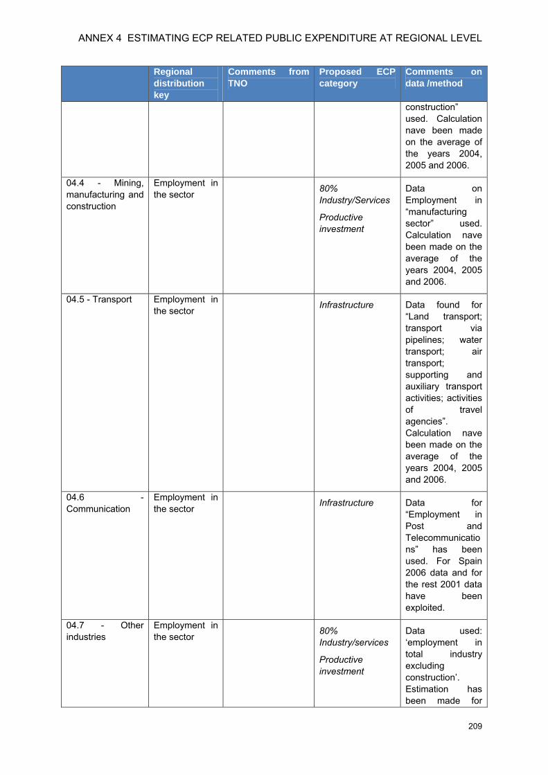
ANNEX 4 ESTIMATING ECP RELATED PUBLIC EXPENDITURE AT REGIONAL LEVEL
209
Regional distribution key
Comments from TNO
Proposed ECP category
Comments on data /method
construction” used. Calculation nave been made on the average of the years 2004, 2005 and 2006.
04.4 - Mining, manufacturing and construction
Employment in the sector 80%
Industry/Services
Productive investment
Data on Employment in “manufacturing sector” used. Calculation nave been made on the average of the years 2004, 2005 and 2006.
04.5 - Transport Employment in the sector Infrastructure Data found for
“Land transport; transport via pipelines; water transport; air transport; supporting and auxiliary transport activities; activities of travel agencies”. Calculation nave been made on the average of the years 2004, 2005 and 2006.
04.6 - Communication
Employment in the sector Infrastructure Data for
“Employment in Post and Telecommunications” has been used. For Spain 2006 data and for the rest 2001 data have been exploited.
04.7 - Other industries
Employment in the sector 80%
Industry/services
Productive investment
Data used: ‘employment in total industry excluding construction’. Estimation has been made for
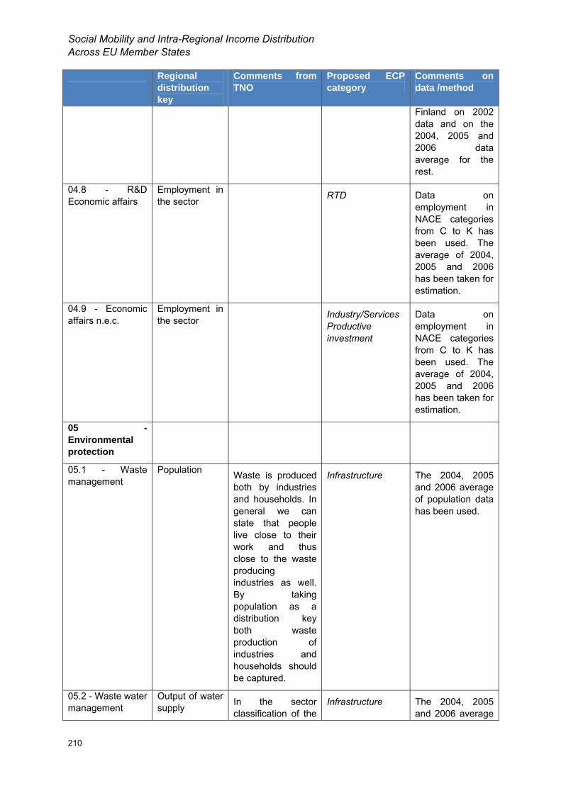
Social Mobility and Intra-Regional Income Distribution Across EU Member States
210
Regional distribution key
Comments from TNO
Proposed ECP category
Comments on data /method
Finland on 2002 data and on the 2004, 2005 and 2006 data average for the rest.
04.8 - R&D Economic affairs
Employment in the sector RTD Data on
employment in NACE categories from C to K has been used. The average of 2004, 2005 and 2006 has been taken for estimation.
04.9 - Economic affairs n.e.c.
Employment in the sector Industry/Services
Productive investment
Data on employment in NACE categories from C to K has been used. The average of 2004, 2005 and 2006 has been taken for estimation.
05 - Environmental protection
05.1 - Waste management
Population Waste is produced both by industries and households. In general we can state that people live close to their work and thus close to the waste producing industries as well. By taking population as a distribution key both waste production of industries and households should be captured.
Infrastructure The 2004, 2005 and 2006 average of population data has been used.
05.2 - Waste water management
Output of water supply In the sector
classification of the Infrastructure The 2004, 2005
and 2006 average
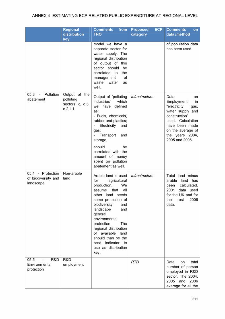
ANNEX 4 ESTIMATING ECP RELATED PUBLIC EXPENDITURE AT REGIONAL LEVEL
211
Regional distribution key
Comments from TNO
Proposed ECP category
Comments on data /method
model we have a separate sector for water supply. The regional distribution of output of this sector should be correlated to the management of waste water as well.
of population data has been used.
05.3 - Pollution abatement
Output of the polluting sectors: c, d.3, e.2, i.1
Output of “polluting industries” which we have defined as: - Fuels, chemicals, rubber and plastics;- Electricity and gas; - Transport and storage,
should be correlated with the amount of money spent on pollution abatement as well.
Infrastructure Data on Employment in “electricity, gas, water supply and construction” used. Calculation nave been made on the average of the years 2004, 2005 and 2006.
05.4 - Protection of biodiversity and landscape
Non-arable land Arable land is used
for agricultural production. We assume that all other land needs some protection of biodiversity and landscape and general environmental protection. The regional distribution of available land should than be the best indicator to use as distribution key.
Infrastructure Total land minus arable land has been calculated. 2001 data used for the UK and for the rest 2006 data.
05.5 - R&D Environmental protection
R&D employment RTD Data on total
number of person employed in R&D sector. The 2004, 2005 and 2006 average for all the
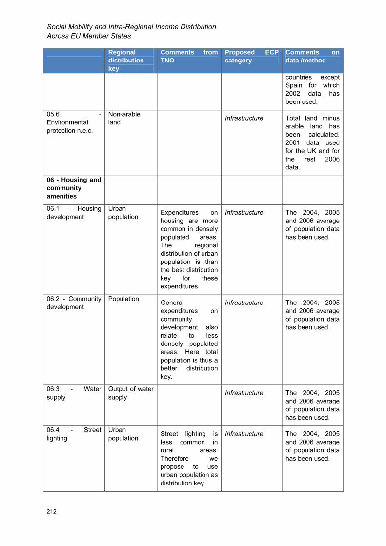
Social Mobility and Intra-Regional Income Distribution Across EU Member States
212
Regional distribution key
Comments from TNO
Proposed ECP category
Comments on data /method
countries except Spain for which 2002 data has been used.
05.6 - Environmental protection n.e.c.
Non-arable land Infrastructure Total land minus
arable land has been calculated. 2001 data used for the UK and for the rest 2006 data.
06 - Housing and community amenities
06.1 - Housing development
Urban population Expenditures on
housing are more common in densely populated areas. The regional distribution of urban population is than the best distribution key for these expenditures.
Infrastructure The 2004, 2005 and 2006 average of population data has been used.
06.2 - Community development
Population General expenditures on community development also relate to less densely populated areas. Here total population is thus a better distribution key.
Infrastructure The 2004, 2005 and 2006 average of population data has been used.
06.3 - Water supply
Output of water supply Infrastructure The 2004, 2005
and 2006 average of population data has been used.
06.4 - Street lighting
Urban population Street lighting is
less common in rural areas. Therefore we propose to use urban population as distribution key.
Infrastructure The 2004, 2005 and 2006 average of population data has been used.
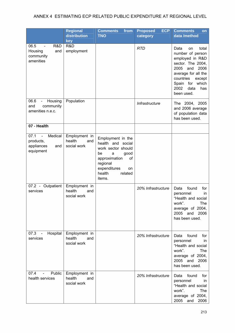
ANNEX 4 ESTIMATING ECP RELATED PUBLIC EXPENDITURE AT REGIONAL LEVEL
213
Regional distribution key
Comments from TNO
Proposed ECP category
Comments on data /method
06.5 - R&D Housing and community amenities
R&D employment RTD Data on total
number of person employed in R&D sector. The 2004, 2005 and 2006 average for all the countries except Spain for which 2002 data has been used.
06.6 - Housing and community amenities n.e.c.
Population Infrastructure The 2004, 2005 and 2006 average of population data has been used.
07 - Health
07.1 - Medical products, appliances and equipment
Employment in health and social work
Employment in the health and social work sector should be a good approximation of regional expenditures on health related items.
07.2 - Outpatient services
Employment in health and social work
20% Infrastructure Data found for personnel in “Health and social work”. The average of 2004, 2005 and 2006 has been used.
07.3 - Hospital services
Employment in health and social work
20% Infrastructure Data found for personnel in “Health and social work”. The average of 2004, 2005 and 2006 has been used.
07.4 - Public health services
Employment in health and social work
20% Infrastructure Data found for personnel in “Health and social work”. The average of 2004, 2005 and 2006
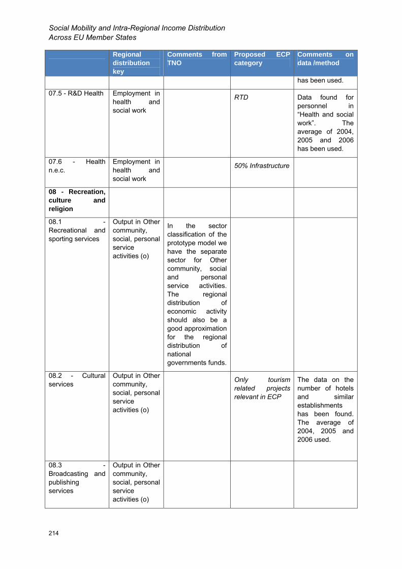
Social Mobility and Intra-Regional Income Distribution Across EU Member States
214
Regional distribution key
Comments from TNO
Proposed ECP category
Comments on data /method
has been used.
07.5 - R&D Health Employment in health and social work
RTD Data found for personnel in “Health and social work”. The average of 2004, 2005 and 2006 has been used.
07.6 - Health n.e.c.
Employment in health and social work
50% Infrastructure
08 - Recreation, culture and religion
08.1 - Recreational and sporting services
Output in Other community, social, personal service activities (o)
In the sector classification of the prototype model we have the separate sector for Other community, social and personal service activities. The regional distribution of economic activity should also be a good approximation for the regional distribution of national governments funds.
08.2 - Cultural services
Output in Other community, social, personal service activities (o)
Only tourism related projects relevant in ECP
The data on the number of hotels and similar establishments has been found. The average of 2004, 2005 and 2006 used.
08.3 - Broadcasting and publishing services
Output in Other community, social, personal service activities (o)
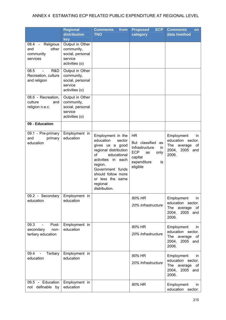
ANNEX 4 ESTIMATING ECP RELATED PUBLIC EXPENDITURE AT REGIONAL LEVEL
215
Regional distribution key
Comments from TNO
Proposed ECP category
Comments on data /method
08.4 - Religious and other community services
Output in Other community, social, personal service activities (o)
08.5 - R&D Recreation, culture and religion
Output in Other community, social, personal service activities (o)
08.6 - Recreation, culture and religion n.e.c.
Output in Other community, social, personal service activities (o)
09 - Education
09.1 - Pre-primary and primary education
Employment in education Employment in the
education sector gives us a good regional distribution of educational activities in each region. Government funds should follow more or less the same regional distribution.
HR
But classified as Infrastructure in ECP as only capital expenditure is eligible
Employment in education sector. The average of 2004, 2005 and 2006.
09.2 - Secondary education
Employment in education 80% HR
20% Infrastructure
Employment in education sector. The average of 2004, 2005 and 2006.
09.3 - Post-secondary non-tertiary education
Employment in education 80% HR
20% Infrastructure
Employment in education sector. The average of 2004, 2005 and 2006.
09.4 - Tertiary education
Employment in education 80% HR
20% Infrastructure
Employment in education sector. The average of 2004, 2005 and 2006.
09.5 - Education not definable by
Employment in education 80% HR Employment in
education sector.
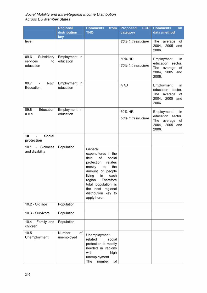
Social Mobility and Intra-Regional Income Distribution Across EU Member States
216
Regional distribution key
Comments from TNO
Proposed ECP category
Comments on data /method
level 20% Infrastructure The average of 2004, 2005 and 2006.
09.6 - Subsidiary services to education
Employment in education 80% HR
20% Infrastructure
Employment in education sector. The average of 2004, 2005 and 2006.
09.7 - R&D Education
Employment in education RTD Employment in
education sector. The average of 2004, 2005 and 2006.
09.8 - Education n.e.c.
Employment in education 50% HR
50% Infrastructure
Employment in education sector. The average of 2004, 2005 and 2006.
10 - Social protection
10.1 - Sickness and disability
Population General expenditures in the field of social protection relates mostly to the amount of people living in each region. Therefore total population is the nest regional distribution key to apply here.
10.2 - Old age Population
10.3 - Survivors Population
10.4 - Family and children
Population
10.5 - Unemployment
Number of unemployed Unemployment
related social protection is mostly needed in regions with high unemployment. The number of
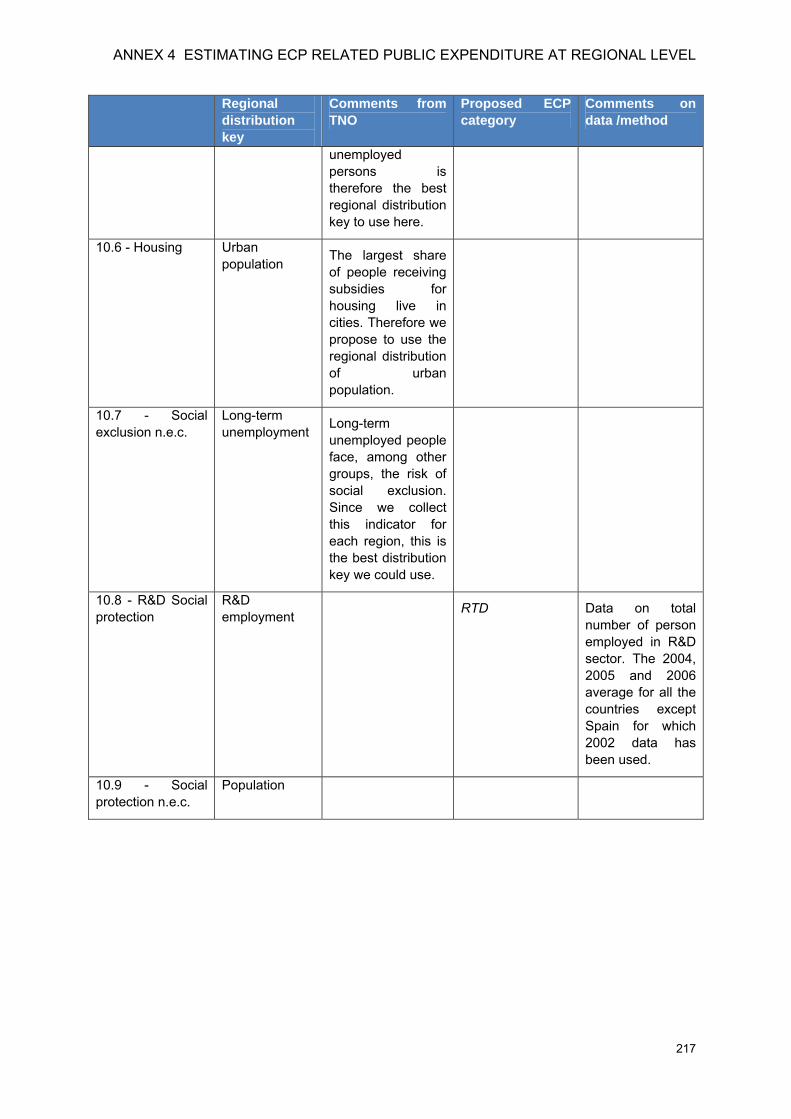
ANNEX 4 ESTIMATING ECP RELATED PUBLIC EXPENDITURE AT REGIONAL LEVEL
217
Regional distribution key
Comments from TNO
Proposed ECP category
Comments on data /method
unemployed persons is therefore the best regional distribution key to use here.
10.6 - Housing Urban population The largest share
of people receiving subsidies for housing live in cities. Therefore we propose to use the regional distribution of urban population.
10.7 - Social exclusion n.e.c.
Long-term unemployment Long-term
unemployed people face, among other groups, the risk of social exclusion. Since we collect this indicator for each region, this is the best distribution key we could use.
10.8 - R&D Social protection
R&D employment RTD Data on total
number of person employed in R&D sector. The 2004, 2005 and 2006 average for all the countries except Spain for which 2002 data has been used.
10.9 - Social protection n.e.c.
Population

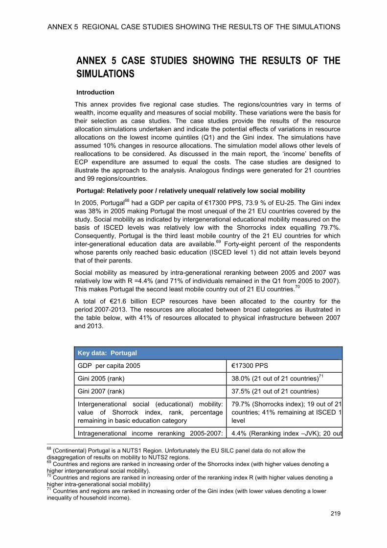
ANNEX 5 REGIONAL CASE STUDIES SHOWING THE RESULTS OF THE SIMULATIONS
219
ANNEX 5 CASE STUDIES SHOWING THE RESULTS OF THE SIMULATIONS Introduction
This annex provides five regional case studies. The regions/countries vary in terms of wealth, income equality and measures of social mobility. These variations were the basis for their selection as case studies. The case studies provide the results of the resource allocation simulations undertaken and indicate the potential effects of variations in resource allocations on the lowest income quintiles (Q1) and the Gini index. The simulations have assumed 10% changes in resource allocations. The simulation model allows other levels of reallocations to be considered. As discussed in the main report, the ‘income’ benefits of ECP expenditure are assumed to equal the costs. The case studies are designed to illustrate the approach to the analysis. Analogous findings were generated for 21 countries and 99 regions/countries.
Portugal: Relatively poor / relatively unequal/ relatively low social mobility
In 2005, Portugal68 had a GDP per capita of €17300 PPS, 73.9 % of EU-25. The Gini index was 38% in 2005 making Portugal the most unequal of the 21 EU countries covered by the study. Social mobility as indicated by intergenerational educational mobility measured on the basis of ISCED levels was relatively low with the Shorrocks index equalling 79.7%. Consequently, Portugal is the third least mobile country of the 21 EU countries for which inter-generational education data are available.69 Forty-eight percent of the respondents whose parents only reached basic education (ISCED level 1) did not attain levels beyond that of their parents.
Social mobility as measured by intra-generational reranking between 2005 and 2007 was relatively low with R =4.4% (and 71% of individuals remained in the Q1 from 2005 to 2007). This makes Portugal the second least mobile country out of 21 EU countries.70
A total of €21.6 billion ECP resources have been allocated to the country for the period 2007-2013. The resources are allocated between broad categories as illustrated in the table below, with 41% of resources allocated to physical infrastructure between 2007 and 2013.
Key data: Portugal
GDP per capita 2005 €17300 PPS
Gini 2005 (rank) 38.0% (21 out of 21 countries)71
Gini 2007 (rank) 37.5% (21 out of 21 countries)
Intergenerational social (educational) mobility: value of Shorrock index, rank, percentage remaining in basic education category
79.7% (Shorrocks index); 19 out of 21 countries; 41% remaining at ISCED 1 level
Intragenerational income reranking 2005-2007: 4.4% (Reranking index –JVK); 20 out 68 (Continental) Portugal is a NUTS1 Region. Unfortunately the EU SILC panel data do not allow the disaggregation of results on mobility to NUTS2 regions. 69 Countries and regions are ranked in increasing order of the Shorrocks index (with higher values denoting a higher intergenerational social mobility). 70 Countries and regions are ranked in increasing order of the reranking index R (with higher values denoting a higher intra-generational social mobility) 71 Countries and regions are ranked in increasing order of the Gini index (with lower values denoting a lower inequality of household income).
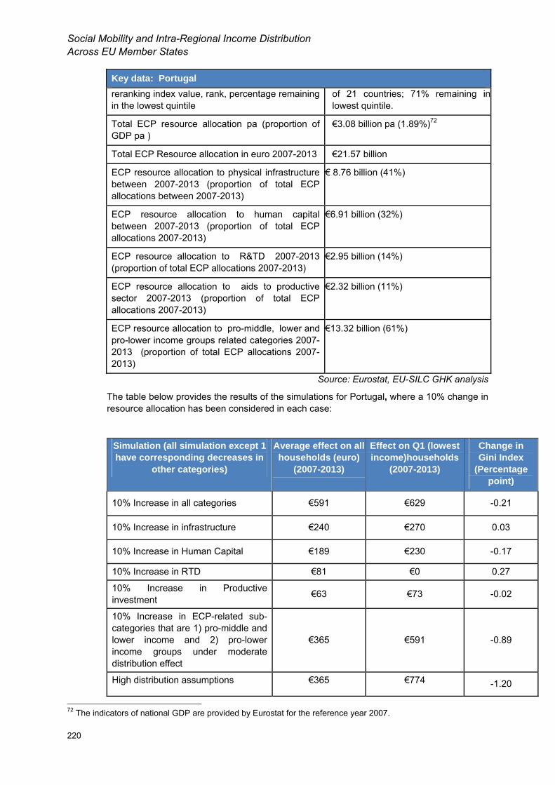
Social Mobility and Intra-Regional Income Distribution Across EU Member States
220
Key data: Portugal reranking index value, rank, percentage remaining in the lowest quintile
of 21 countries; 71% remaining in lowest quintile.
Total ECP resource allocation pa (proportion of GDP pa )
€3.08 billion pa (1.89%)72
Total ECP Resource allocation in euro 2007-2013 €21.57 billion
ECP resource allocation to physical infrastructure between 2007-2013 (proportion of total ECP allocations between 2007-2013)
€ 8.76 billion (41%)
ECP resource allocation to human capital between 2007-2013 (proportion of total ECP allocations 2007-2013)
€6.91 billion (32%)
ECP resource allocation to R&TD 2007-2013 (proportion of total ECP allocations 2007-2013)
€2.95 billion (14%)
ECP resource allocation to aids to productive sector 2007-2013 (proportion of total ECP allocations 2007-2013)
€2.32 billion (11%)
ECP resource allocation to pro-middle, lower and pro-lower income groups related categories 2007-2013 (proportion of total ECP allocations 2007-2013)
€13.32 billion (61%)
Source: Eurostat, EU-SILC GHK analysis
The table below provides the results of the simulations for Portugal, where a 10% change in resource allocation has been considered in each case:
Simulation (all simulation except 1 have corresponding decreases in
other categories)
Average effect on all households (euro)
(2007-2013)
Effect on Q1 (lowest income)households
(2007-2013)
Change in Gini Index
(Percentage point)
10% Increase in all categories €591 €629 -0.21
10% Increase in infrastructure €240 €270 0.03
10% Increase in Human Capital €189 €230 -0.17
10% Increase in RTD €81 €0 0.27
10% Increase in Productive investment €63 €73 -0.02
10% Increase in ECP-related sub-categories that are 1) pro-middle and lower income and 2) pro-lower income groups under moderate distribution effect
€365 €591 -0.89
High distribution assumptions €365 €774 -1.20
72 The indicators of national GDP are provided by Eurostat for the reference year 2007.
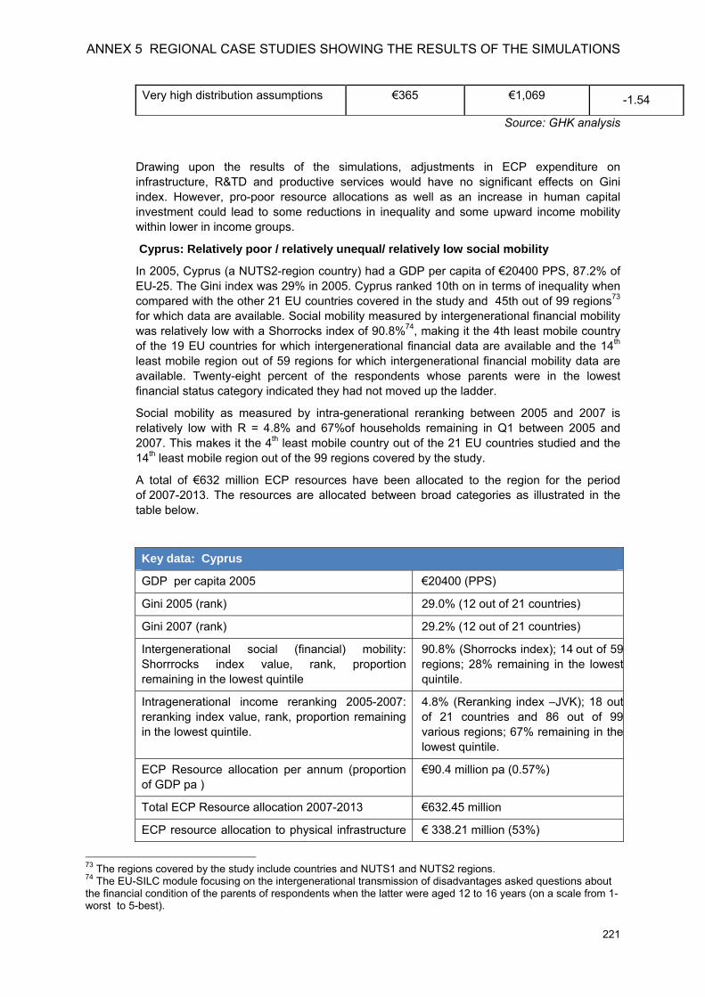
ANNEX 5 REGIONAL CASE STUDIES SHOWING THE RESULTS OF THE SIMULATIONS
221
Very high distribution assumptions €365 €1,069 -1.54
Source: GHK analysis
Drawing upon the results of the simulations, adjustments in ECP expenditure on infrastructure, R&TD and productive services would have no significant effects on Gini index. However, pro-poor resource allocations as well as an increase in human capital investment could lead to some reductions in inequality and some upward income mobility within lower in income groups.
Cyprus: Relatively poor / relatively unequal/ relatively low social mobility
In 2005, Cyprus (a NUTS2-region country) had a GDP per capita of €20400 PPS, 87.2% of EU-25. The Gini index was 29% in 2005. Cyprus ranked 10th on in terms of inequality when compared with the other 21 EU countries covered in the study and 45th out of 99 regions73 for which data are available. Social mobility measured by intergenerational financial mobility was relatively low with a Shorrocks index of 90.8%74, making it the 4th least mobile country of the 19 EU countries for which intergenerational financial data are available and the 14th least mobile region out of 59 regions for which intergenerational financial mobility data are available. Twenty-eight percent of the respondents whose parents were in the lowest financial status category indicated they had not moved up the ladder.
Social mobility as measured by intra-generational reranking between 2005 and 2007 is relatively low with R = 4.8% and 67%of households remaining in Q1 between 2005 and 2007. This makes it the 4th least mobile country out of the 21 EU countries studied and the 14th least mobile region out of the 99 regions covered by the study.
A total of €632 million ECP resources have been allocated to the region for the period of 2007-2013. The resources are allocated between broad categories as illustrated in the table below.
Key data: Cyprus
GDP per capita 2005 €20400 (PPS)
Gini 2005 (rank) 29.0% (12 out of 21 countries)
Gini 2007 (rank) 29.2% (12 out of 21 countries)
Intergenerational social (financial) mobility: Shorrrocks index value, rank, proportion remaining in the lowest quintile
90.8% (Shorrocks index); 14 out of 59 regions; 28% remaining in the lowest quintile.
Intragenerational income reranking 2005-2007: reranking index value, rank, proportion remaining in the lowest quintile.
4.8% (Reranking index –JVK); 18 out of 21 countries and 86 out of 99 various regions; 67% remaining in thelowest quintile.
ECP Resource allocation per annum (proportion of GDP pa )
€90.4 million pa (0.57%)
Total ECP Resource allocation 2007-2013 €632.45 million
ECP resource allocation to physical infrastructure € 338.21 million (53%)
73 The regions covered by the study include countries and NUTS1 and NUTS2 regions. 74 The EU-SILC module focusing on the intergenerational transmission of disadvantages asked questions about the financial condition of the parents of respondents when the latter were aged 12 to 16 years (on a scale from 1-worst to 5-best).
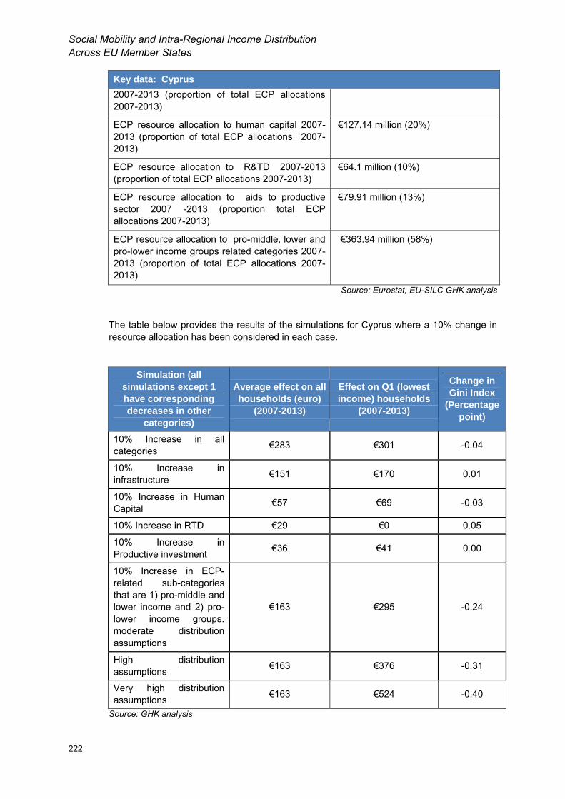
Social Mobility and Intra-Regional Income Distribution Across EU Member States
222
Key data: Cyprus 2007-2013 (proportion of total ECP allocations 2007-2013)
ECP resource allocation to human capital 2007-2013 (proportion of total ECP allocations 2007-2013)
€127.14 million (20%)
ECP resource allocation to R&TD 2007-2013 (proportion of total ECP allocations 2007-2013)
€64.1 million (10%)
ECP resource allocation to aids to productive sector 2007 -2013 (proportion total ECP allocations 2007-2013)
€79.91 million (13%)
ECP resource allocation to pro-middle, lower and pro-lower income groups related categories 2007-2013 (proportion of total ECP allocations 2007-2013)
€363.94 million (58%)
Source: Eurostat, EU-SILC GHK analysis
The table below provides the results of the simulations for Cyprus where a 10% change in resource allocation has been considered in each case.
Simulation (all simulations except 1 have corresponding decreases in other
categories)
Average effect on all households (euro)
(2007-2013)
Effect on Q1 (lowest income) households
(2007-2013)
Change in Gini Index
(Percentage point)
10% Increase in all categories €283 €301 -0.04
10% Increase in infrastructure €151 €170 0.01
10% Increase in Human Capital €57 €69 -0.03
10% Increase in RTD €29 €0 0.05
10% Increase in Productive investment €36 €41 0.00
10% Increase in ECP-related sub-categories that are 1) pro-middle and lower income and 2) pro-lower income groups. moderate distribution assumptions
€163 €295 -0.24
High distribution assumptions €163 €376 -0.31
Very high distribution assumptions €163 €524 -0.40
Source: GHK analysis
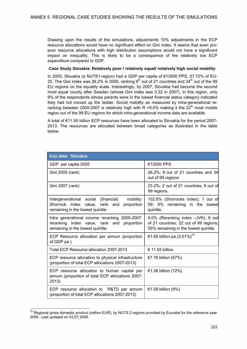
ANNEX 5 REGIONAL CASE STUDIES SHOWING THE RESULTS OF THE SIMULATIONS
223
Drawing upon the results of the simulations, adjustments 10% adjustments in the ECP resource allocations would have no significant effect on Gini index. It seems that even pro-poor resource allocations with high distribution assumptions would not have a significant impact on inequality. This is likely to be a consequence of the relatively low ECP expenditure compared to GDP.
Case Study Slovakia: Relatively poor / relatively equal/ relatively high social mobility
In 2005, Slovakia (a NUTS1-region) had a GDP per capita of €13500 PPS, 57.72% of EU-25. The Gini index was 26.2% in 2005, ranking 8th out of 21 countries and 34th out of the 99 EU regions on the equality scale. Interestingly, by 2007, Slovakia had become the second most equal county after Sweden (whose Gini index was 0.22 in 2007). In this region, only 9% of the respondents whose parents were in the lowest financial status category indicated they had not moved up the ladder. Social mobility as measured by intra-generational re-ranking between 2005-2007 is relatively high with R =9.0% making it the 22th most mobile region out of the 99 EU regions for which intra-generational income data are available.
A total of €11.55 billion ECP resources have been allocated to Slovakia for the period 2007-2013. The resources are allocated between broad categories as illustrated in the table below.
Key data: Slovakia
GDP per capita 2005 €13500 PPS
Gini 2005 (rank) 26.2%; 8 out of 21 countries and 34 out of 99 regions
Gini 2007 (rank) 23.2%; 2 out of 21 countries; 9 out of 99 regions.
Intergenerational social (financial) mobility: Shorrock index value, rank and proportion remaining in the lowest quintile
102.6% (Shorrocks index); 1 out of 59; 9% remaining in the lowest quintile.
Intra generational income reranking 2005-2007: reranking index value, rank and proportion remaining in the lowest quintile.
9.0% (Reranking index –JVK); 6 out of 21 countries; 22 out of 99 regions; 55% remaining in the lowest quintile.
ECP Resource allocation per annum (proportion of GDP pa )
€1.65 billion pa (3.01%)75
Total ECP Resource allocation 2007-2013 € 11.55 billion
ECP resource allocation to physical infrastructure (proportion of total ECP allocations 2007-2013)
€7.76 billion (67%)
ECP resource allocation to human capital per annum (proportion of total ECP allocations 2007-2013)
€1.36 billion (12%)
ECP resource allocation to R&TD per annum (proportion of total ECP allocations 2007-2013)
€1.08 billion (9%)
75 Regional gross domestic product (million EUR), by NUTS 2 regions provided by Eurostat for the reference year 2006. Last updated on 03.07.2009.
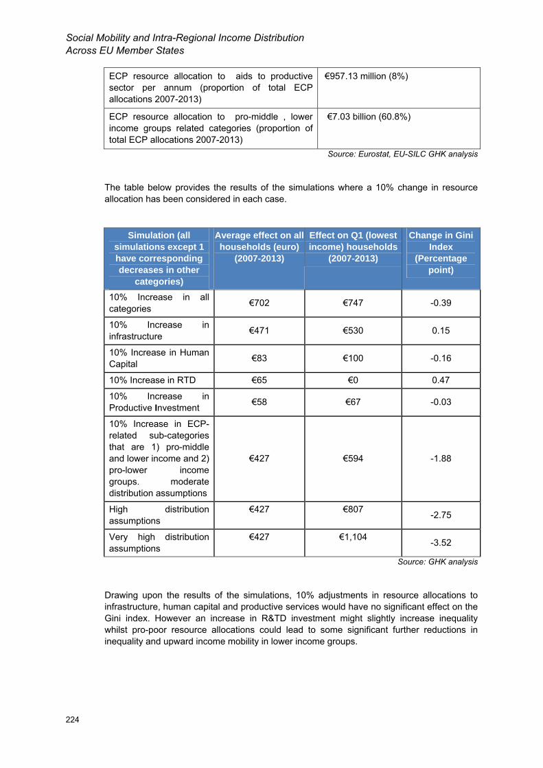
Social Mobility and Intra-Regional Income Distribution Across EU Member States
224
ECP resource allocation to aids to productive sector per annum (proportion of total ECP allocations 2007-2013)
€957.13 million (8%)
ECP resource allocation to pro-middle , lower income groups related categories (proportion of total ECP allocations 2007-2013)
€7.03 billion (60.8%)
Source: Eurostat, EU-SILC GHK analysis
The table below provides the results of the simulations where a 10% change in resource allocation has been considered in each case.
Simulation (all simulations except 1 have corresponding decreases in other
categories)
Average effect on all households (euro)
(2007-2013)
Effect on Q1 (lowest income) households
(2007-2013)
Change in Gini Index
(Percentage point)
10% Increase in all categories €702 €747 -0.39
10% Increase in infrastructure €471 €530 0.15
10% Increase in Human Capital €83 €100 -0.16
10% Increase in RTD €65 €0 0.47
10% Increase in Productive Investment €58 €67 -0.03
10% Increase in ECP-related sub-categories that are 1) pro-middle and lower income and 2) pro-lower income groups. moderate distribution assumptions
€427 €594 -1.88
High distribution assumptions
€427 €807 -2.75
Very high distribution assumptions
€427 €1,104 -3.52
Source: GHK analysis
Drawing upon the results of the simulations, 10% adjustments in resource allocations to infrastructure, human capital and productive services would have no significant effect on the Gini index. However an increase in R&TD investment might slightly increase inequality whilst pro-poor resource allocations could lead to some significant further reductions in inequality and upward income mobility in lower income groups.

ANNEX 5 REGIONAL CASE STUDIES SHOWING THE RESULTS OF THE SIMULATIONS
225
Case Study Italy Centro region: Medium Wealth/ relatively unequal/ relatively low social mobility
In 2005, Italy Centro (a NUTS1-region) had a GDP per capita of €26,400 PPS, 112.8% of EU-25. The Gini index was 31.0% in 2005, the 30th most unequal region out of the 99 EU regions and countries covered by the study. Social mobility as indicated by intergenerational financial mobility was relatively low with Shorrocks index = 90.1% making it the 8th least mobile region out of the 59 regions for which inter-generational financial data are available. Twenty-five percent of the respondents whose parents were in the lowest financial status category indicated they had not moved up the ladder.
Social mobility as measured by intra-generational reranking between 2005 and 2007 is relatively low with R=6.2%. According to the reranking index R, Italy Centro region ranks 35th out of 99 regions covered (where the first is the least mobile region and the 99th marks the most mobile region).
A total of €1.94 billion ECP resources have been allocated to the region for the period 2007-2013. The resources are allocated between broad categories as illustrated in the table below.
Key data: ITE Centro (IT)
GDP per capita 2005 €26400 (PPS)
Gini 2005 (rank) 31.0% (70 out of 99 regions)
Gini 2007 (rank) 30.0% (76 out of 99 regions)
Intergenerational social mobility: Shorrocks index, rank, proportion remaining in the lowest quintile.
90.1% (Shorrocks index); 52 out of 59 regions; 25% remaining in the lowest quintile.
Intra generational income reranking 2005-2007L reranking index, rank, proportion remaining in the lowest quintile.
6.2% (Reranking index –JVK; 65 out of 99; 54% remaining in the lowest quintile.
ECP Resource allocation per annum (proportion of GDP pa )
€ 277 million (0.09%) pa
Total ECP Resource allocation 2007-2013 €1.94 billion
ECP resource allocation to physical infrastructure 2007-2013 (proportion of total ECP allocations 2007-2013)
€ 586.8 million(30%)
ECP resource allocation to human capital per annum (proportion of total ECP allocations 2007-2013)
€ 827.60 million (43%)
ECP resource allocation to R&TD per annum (proportion of total ECP allocations 2007-2013)
€292.71 million (15%)
ECP resource allocation to aids to productive sector per annum (proportion of total ECP allocations 2007-2013)
€165.62 million (9%)
ECP resource allocation to pro-middle and lower income groups related categories (proportion of total ECP allocations 2007-2013)
€1.14 billion (59%)
Source: Eurostat, EU-SILC GHK analysis
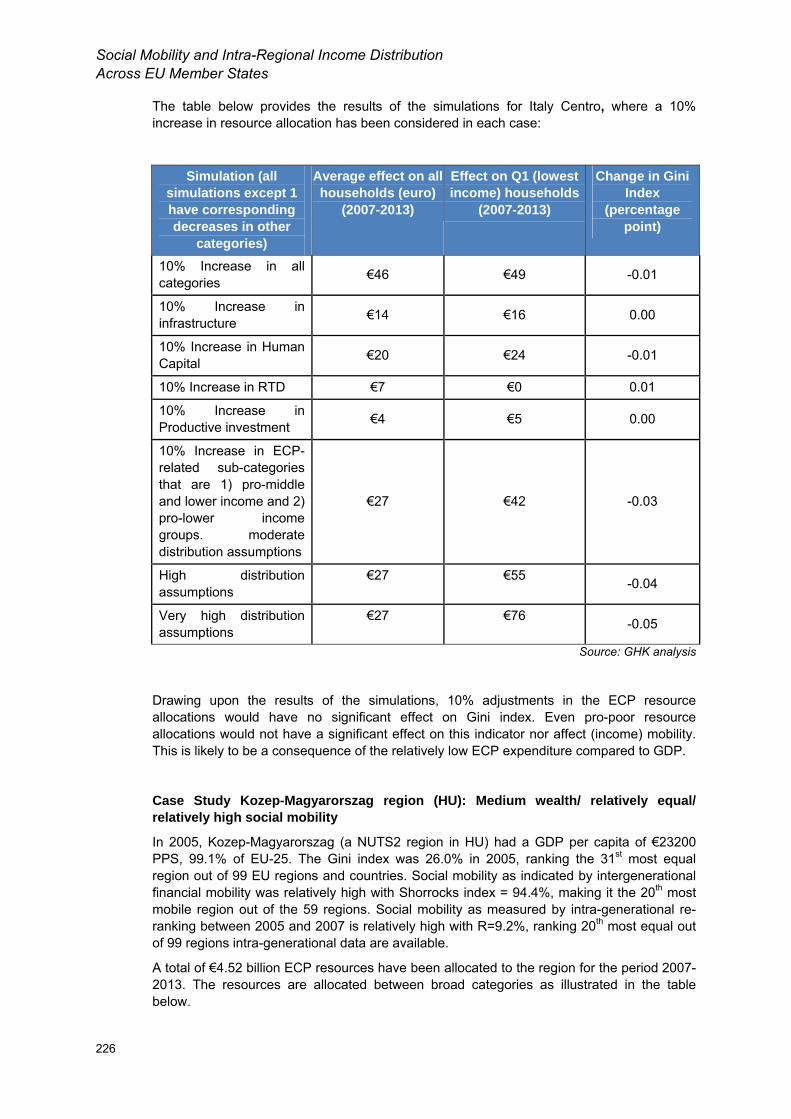
Social Mobility and Intra-Regional Income Distribution Across EU Member States
226
The table below provides the results of the simulations for Italy Centro, where a 10% increase in resource allocation has been considered in each case:
Simulation (all simulations except 1 have corresponding decreases in other
categories)
Average effect on all households (euro)
(2007-2013)
Effect on Q1 (lowest income) households
(2007-2013)
Change in Gini Index
(percentage point)
10% Increase in all categories €46 €49 -0.01
10% Increase in infrastructure €14 €16 0.00
10% Increase in Human Capital €20 €24 -0.01
10% Increase in RTD €7 €0 0.01
10% Increase in Productive investment €4 €5 0.00
10% Increase in ECP-related sub-categories that are 1) pro-middle and lower income and 2) pro-lower income groups. moderate distribution assumptions
€27 €42 -0.03
High distribution assumptions
€27 €55 -0.04
Very high distribution assumptions
€27 €76 -0.05
Source: GHK analysis
Drawing upon the results of the simulations, 10% adjustments in the ECP resource allocations would have no significant effect on Gini index. Even pro-poor resource allocations would not have a significant effect on this indicator nor affect (income) mobility. This is likely to be a consequence of the relatively low ECP expenditure compared to GDP.
Case Study Kozep-Magyarorszag region (HU): Medium wealth/ relatively equal/ relatively high social mobility
In 2005, Kozep-Magyarorszag (a NUTS2 region in HU) had a GDP per capita of €23200 PPS, 99.1% of EU-25. The Gini index was 26.0% in 2005, ranking the 31st most equal region out of 99 EU regions and countries. Social mobility as indicated by intergenerational financial mobility was relatively high with Shorrocks index = 94.4%, making it the 20th most mobile region out of the 59 regions. Social mobility as measured by intra-generational re-ranking between 2005 and 2007 is relatively high with R=9.2%, ranking 20th most equal out of 99 regions intra-generational data are available.
A total of €4.52 billion ECP resources have been allocated to the region for the period 2007-2013. The resources are allocated between broad categories as illustrated in the table below.
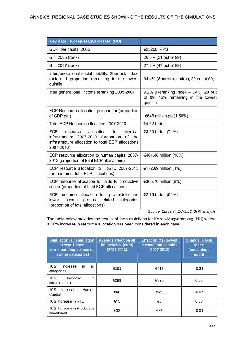
ANNEX 5 REGIONAL CASE STUDIES SHOWING THE RESULTS OF THE SIMULATIONS
227
Key data: Kozep-Magyarorszag (HU)
GDP per capita 2005 €23200 PPS
Gini 2005 (rank) 26.0% (31 out of 99)
Gini 2007 (rank) 27.0% (47 out of 99)
Intergenerational social mobility: Shorrock index; rank and proportion remaining in the lowest quintile
94.4% (Shorrocks index); 20 out of 59;
Intra generational income reranking 2005-2007 9.2% (Reranking index – JVK); 20 out of 99; 45% remaining in the lowest quintile.
ECP Resource allocation per annum (proportion of GDP pa ) €646 million pa (1.58%)
Total ECP Resource allocation 2007-2013 €4.52 billion
ECP resource allocation to physical infrastructure 2007-2013 (proportion of the infrastructure allocation to total ECP allocations 2007-2013)
€3.33 billion (74%)
ECP resource allocation to human capital 2007-2013 (proportion of total ECP allocations)
€461.48 million (10%)
ECP resource allocation to R&TD 2007-2013 (proportion of total ECP allocations)
€172.69 million (4%)
ECP resource allocation to aids to productive sector (proportion of total ECP allocations)
€365.70 million (8%)
ECP resource allocation to pro-middle and lower income groups related categories (proportion of total allocations)
€2.76 billion (61%)
Source: Eurostat, EU-SILC GHK analysis
The table below provides the results of the simulations for Kozep-Magyarorszag (HU) where a 10% increase in resource allocation has been considered in each case:
Simulation (all simulation except 1 have
corresponding decreases in other categories)
Average effect on all households (euro)
(2007-2013)
Effect on Q1 (lowest income) households
(2007-2013)
Change in Gini Index
(percentage point)
10% Increase in all categories €393 €418 -0.21
10% Increase in infrastructure €289 €325 0.08
10% Increase in Human Capital €40 €49 -0.07
10% Increase in RTD €15 €0 0.08
10% Increase in Productive investment €32 €37 -0.01
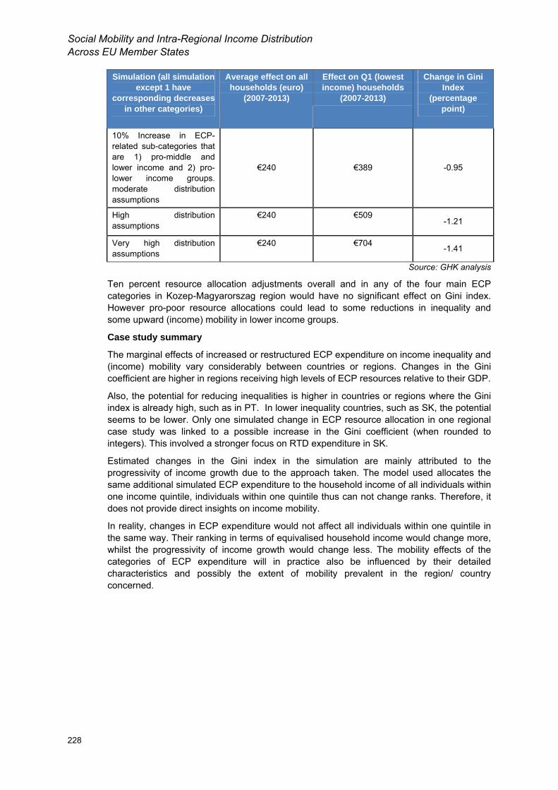
Social Mobility and Intra-Regional Income Distribution Across EU Member States
228
Simulation (all simulation except 1 have
corresponding decreases in other categories)
Average effect on all households (euro)
(2007-2013)
Effect on Q1 (lowest income) households
(2007-2013)
Change in Gini Index
(percentage point)
10% Increase in ECP-related sub-categories that are 1) pro-middle and lower income and 2) pro-lower income groups. moderate distribution assumptions
€240 €389 -0.95
High distribution assumptions
€240 €509 -1.21
Very high distribution assumptions
€240 €704 -1.41
Source: GHK analysis
Ten percent resource allocation adjustments overall and in any of the four main ECP categories in Kozep-Magyarorszag region would have no significant effect on Gini index. However pro-poor resource allocations could lead to some reductions in inequality and some upward (income) mobility in lower income groups.
Case study summary
The marginal effects of increased or restructured ECP expenditure on income inequality and (income) mobility vary considerably between countries or regions. Changes in the Gini coefficient are higher in regions receiving high levels of ECP resources relative to their GDP.
Also, the potential for reducing inequalities is higher in countries or regions where the Gini index is already high, such as in PT. In lower inequality countries, such as SK, the potential seems to be lower. Only one simulated change in ECP resource allocation in one regional case study was linked to a possible increase in the Gini coefficient (when rounded to integers). This involved a stronger focus on RTD expenditure in SK.
Estimated changes in the Gini index in the simulation are mainly attributed to the progressivity of income growth due to the approach taken. The model used allocates the same additional simulated ECP expenditure to the household income of all individuals within one income quintile, individuals within one quintile thus can not change ranks. Therefore, it does not provide direct insights on income mobility.
In reality, changes in ECP expenditure would not affect all individuals within one quintile in the same way. Their ranking in terms of equivalised household income would change more, whilst the progressivity of income growth would change less. The mobility effects of the categories of ECP expenditure will in practice also be influenced by their detailed characteristics and possibly the extent of mobility prevalent in the region/ country concerned.

ANNEX 6 MAPS ILLUSTRATING MAIN FINDINGS FOR COUNTRIES AND REGIONS
229
ANNEX 6 MAPS ILLUSTRATING MAIN FINDINGS FOR COUNTRIES AND REGIONS The maps have been produced by DG REGIO on the basis of data provided by GHK. Table 1 at the end of this Annex gives the input data used to generate the maps.
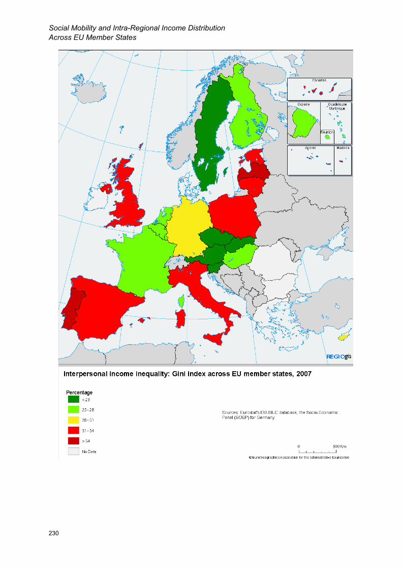
Social Mobility and Intra-Regional Income Distribution Across EU Member States
230
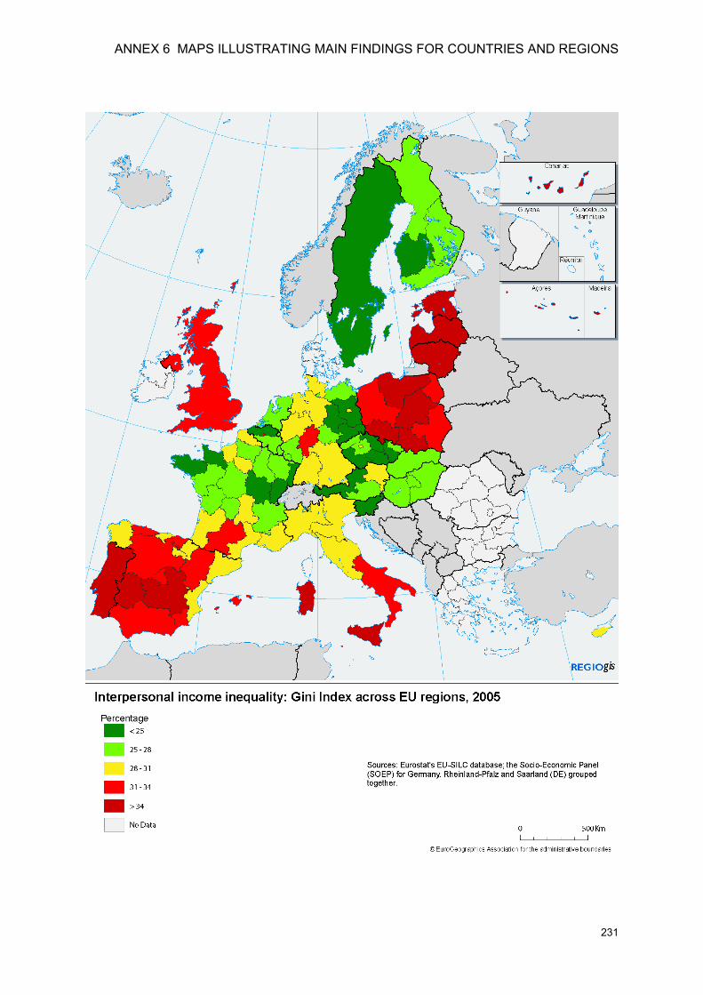
ANNEX 6 MAPS ILLUSTRATING MAIN FINDINGS FOR COUNTRIES AND REGIONS
231
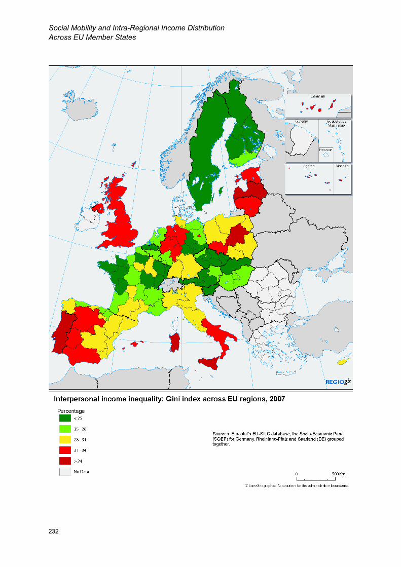
Social Mobility and Intra-Regional Income Distribution Across EU Member States
232
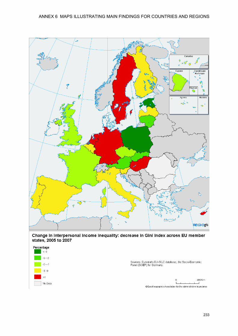
ANNEX 6 MAPS ILLUSTRATING MAIN FINDINGS FOR COUNTRIES AND REGIONS
233
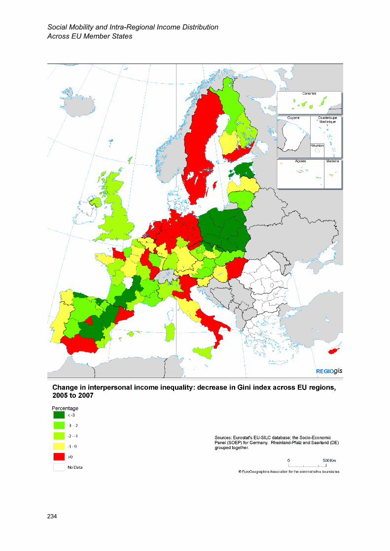
Social Mobility and Intra-Regional Income Distribution Across EU Member States
234
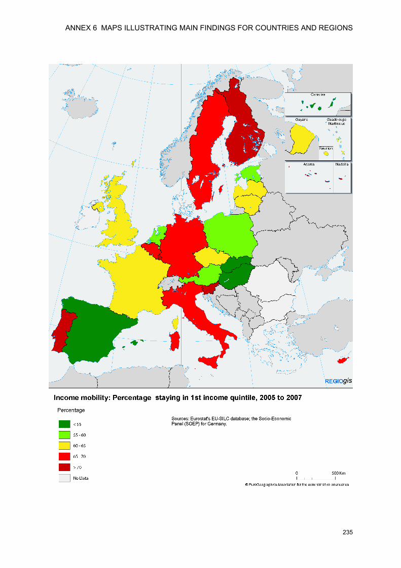
ANNEX 6 MAPS ILLUSTRATING MAIN FINDINGS FOR COUNTRIES AND REGIONS
235
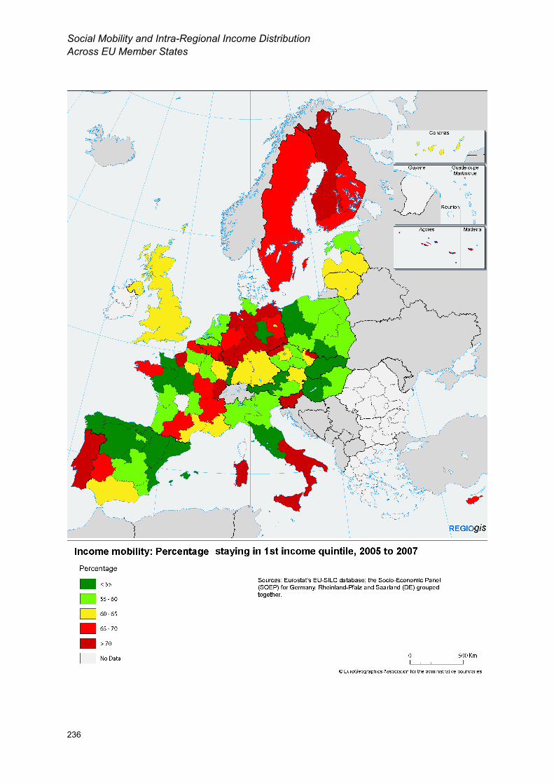
Social Mobility and Intra-Regional Income Distribution Across EU Member States
236
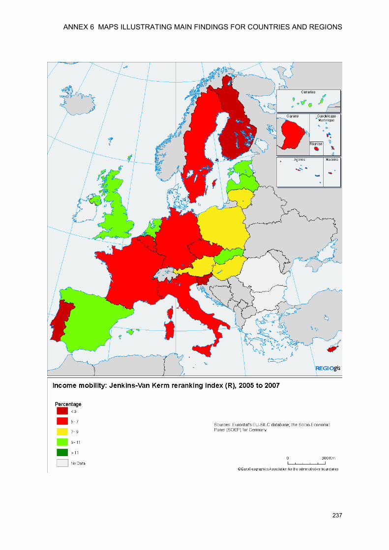
ANNEX 6 MAPS ILLUSTRATING MAIN FINDINGS FOR COUNTRIES AND REGIONS
237
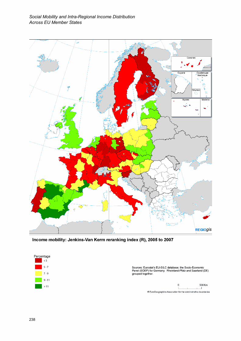
Social Mobility and Intra-Regional Income Distribution Across EU Member States
238
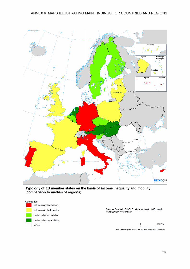
ANNEX 6 MAPS ILLUSTRATING MAIN FINDINGS FOR COUNTRIES AND REGIONS
239
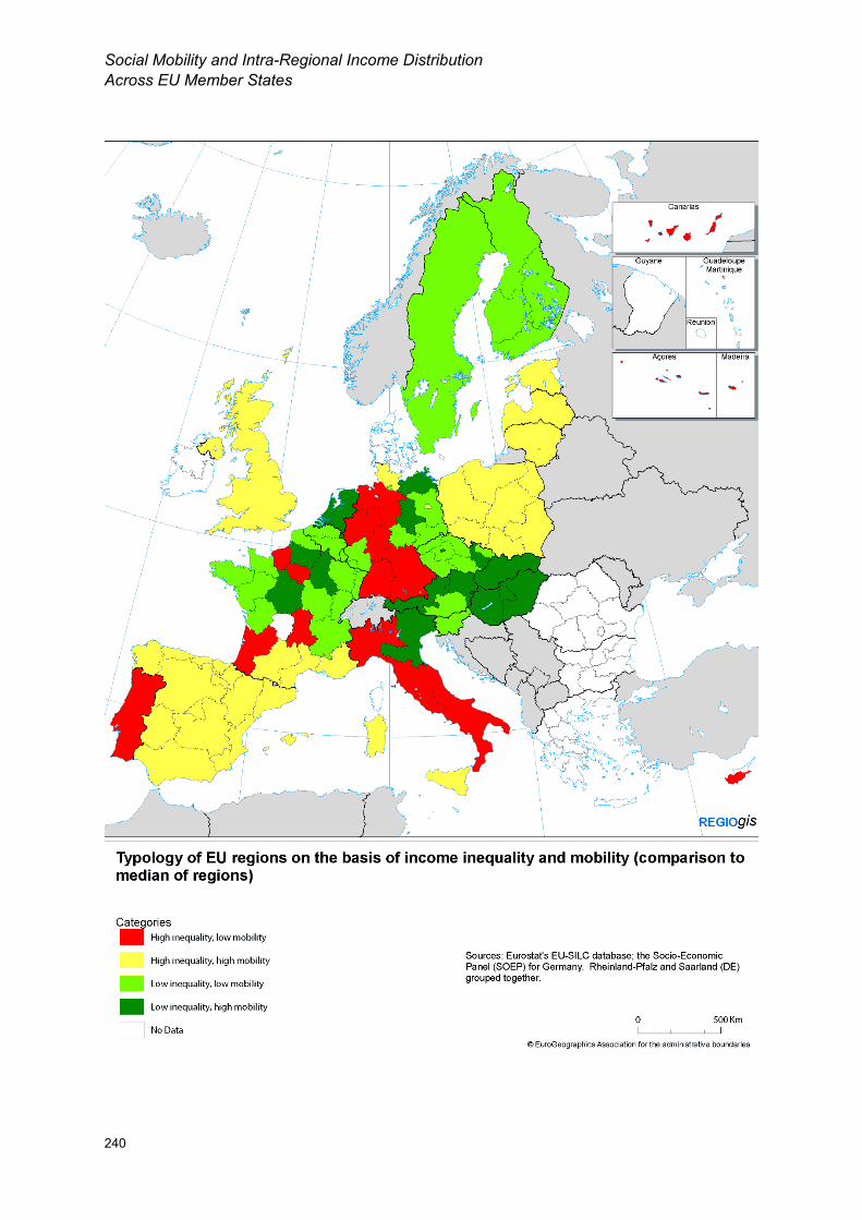
Social Mobility and Intra-Regional Income Distribution Across EU Member States
240
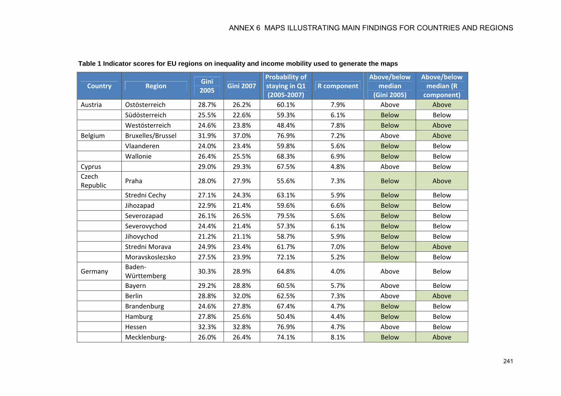
ANNEX 6 MAPS ILLUSTRATING MAIN FINDINGS FOR COUNTRIES AND REGIONS
241
Table 1 Indicator scores for EU regions on inequality and income mobility used to generate the maps
Country Region Gini 2005
Gini 2007 Probability of staying in Q1 (2005-2007)
R component Above/below
median (Gini 2005)
Above/below median (R
component) Austria Ostösterreich 28.7% 26.2% 60.1% 7.9% Above Above Südösterreich 25.5% 22.6% 59.3% 6.1% Below Below Westösterreich 24.6% 23.8% 48.4% 7.8% Below Above Belgium Bruxelles/Brussel 31.9% 37.0% 76.9% 7.2% Above Above Vlaanderen 24.0% 23.4% 59.8% 5.6% Below Below Wallonie 26.4% 25.5% 68.3% 6.9% Below Below Cyprus 29.0% 29.3% 67.5% 4.8% Above Below Czech Republic
Praha 28.0% 27.9% 55.6% 7.3% Below Above
Stredni Cechy 27.1% 24.3% 63.1% 5.9% Below Below Jihozapad 22.9% 21.4% 59.6% 6.6% Below Below Severozapad 26.1% 26.5% 79.5% 5.6% Below Below Severovychod 24.4% 21.4% 57.3% 6.1% Below Below Jihovychod 21.2% 21.1% 58.7% 5.9% Below Below Stredni Morava 24.9% 23.4% 61.7% 7.0% Below Above Moravskoslezsko 27.5% 23.9% 72.1% 5.2% Below Below
Germany Baden-Württemberg
30.3% 28.9% 64.8% 4.0% Above Below
Bayern 29.2% 28.8% 60.5% 5.7% Above Below Berlin 28.8% 32.0% 62.5% 7.3% Above Above Brandenburg 24.6% 27.8% 67.4% 4.7% Below Below Hamburg 27.8% 25.6% 50.4% 4.4% Below Below Hessen 32.3% 32.8% 76.9% 4.7% Above Below Mecklenburg- 26.0% 26.4% 74.1% 8.1% Below Above
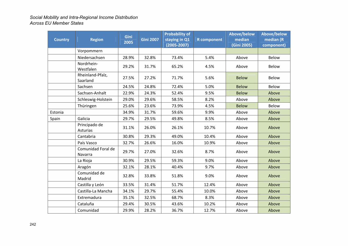
Social Mobility and Intra-Regional Income Distribution Across EU Member States
242
Country Region Gini 2005
Gini 2007 Probability of staying in Q1 (2005-2007)
R component Above/below
median (Gini 2005)
Above/below median (R
component) Vorpommern
Niedersachsen 28.9% 32.8% 73.4% 5.4% Above Below
Nordrhein-Westfalen
29.2% 31.7% 65.2% 4.5% Above Below
Rheinland-Pfalz, Saarland
27.5% 27.2% 71.7% 5.6% Below Below
Sachsen 24.5% 24.8% 72.4% 5.0% Below Below Sachsen-Anhalt 22.9% 24.3% 52.4% 9.5% Below Above Schleswig-Holstein 29.0% 29.6% 58.5% 8.2% Above Above Thüringen 25.6% 23.6% 73.9% 4.5% Below Below Estonia 34.9% 31.7% 59.6% 9.9% Above Above Spain Galicia 29.7% 29.5% 49.8% 8.5% Above Above
Principado de Asturias
31.1% 26.0% 26.1% 10.7% Above Above
Cantabria 30.8% 29.3% 49.0% 10.4% Above Above País Vasco 32.7% 26.6% 16.0% 10.9% Above Above
Comunidad Foral de Navarra
29.7% 27.0% 32.6% 8.7% Above Above
La Rioja 30.9% 29.5% 59.3% 9.0% Above Above Aragón 32.1% 28.1% 40.4% 9.7% Above Above
Comunidad de Madrid
32.8% 33.8% 51.8% 9.0% Above Above
Castilla y León 33.5% 31.4% 51.7% 12.4% Above Above Castilla-La Mancha 34.1% 29.7% 55.4% 10.0% Above Above Extremadura 35.1% 32.5% 68.7% 8.3% Above Above Cataluña 29.4% 30.5% 43.6% 10.2% Above Above Comunidad 29.9% 28.2% 36.7% 12.7% Above Above
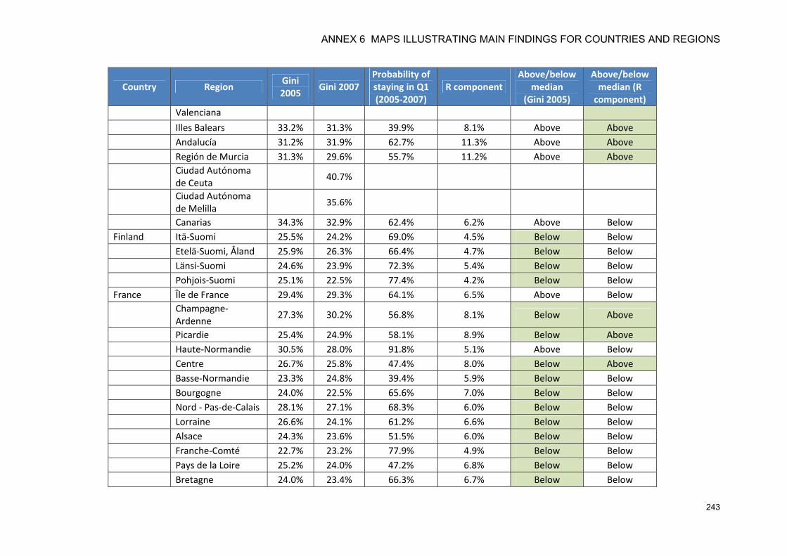
ANNEX 6 MAPS ILLUSTRATING MAIN FINDINGS FOR COUNTRIES AND REGIONS
243
Country Region Gini 2005
Gini 2007 Probability of staying in Q1 (2005-2007)
R component Above/below
median (Gini 2005)
Above/below median (R
component) Valenciana
Illes Balears 33.2% 31.3% 39.9% 8.1% Above Above Andalucía 31.2% 31.9% 62.7% 11.3% Above Above Región de Murcia 31.3% 29.6% 55.7% 11.2% Above Above
Ciudad Autónoma de Ceuta
40.7%
Ciudad Autónoma de Melilla
35.6%
Canarias 34.3% 32.9% 62.4% 6.2% Above Below Finland Itä-Suomi 25.5% 24.2% 69.0% 4.5% Below Below Etelä-Suomi, Åland 25.9% 26.3% 66.4% 4.7% Below Below Länsi-Suomi 24.6% 23.9% 72.3% 5.4% Below Below Pohjois-Suomi 25.1% 22.5% 77.4% 4.2% Below Below France Île de France 29.4% 29.3% 64.1% 6.5% Above Below
Champagne-Ardenne
27.3% 30.2% 56.8% 8.1% Below Above
Picardie 25.4% 24.9% 58.1% 8.9% Below Above Haute-Normandie 30.5% 28.0% 91.8% 5.1% Above Below Centre 26.7% 25.8% 47.4% 8.0% Below Above Basse-Normandie 23.3% 24.8% 39.4% 5.9% Below Below Bourgogne 24.0% 22.5% 65.6% 7.0% Below Below Nord - Pas-de-Calais 28.1% 27.1% 68.3% 6.0% Below Below Lorraine 26.6% 24.1% 61.2% 6.6% Below Below Alsace 24.3% 23.6% 51.5% 6.0% Below Below Franche-Comté 22.7% 23.2% 77.9% 4.9% Below Below Pays de la Loire 25.2% 24.0% 47.2% 6.8% Below Below Bretagne 24.0% 23.4% 66.3% 6.7% Below Below
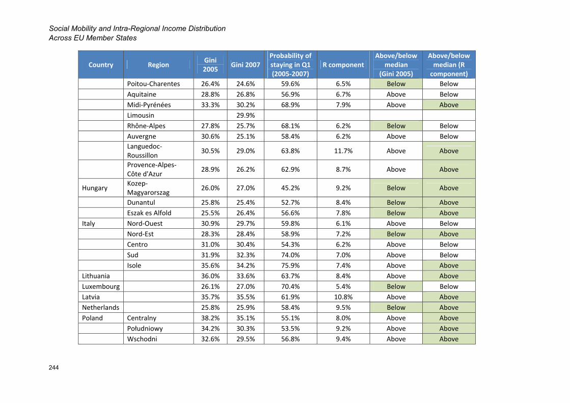
Social Mobility and Intra-Regional Income Distribution Across EU Member States
244
Country Region Gini 2005
Gini 2007 Probability of staying in Q1 (2005-2007)
R component Above/below
median (Gini 2005)
Above/below median (R
component) Poitou-Charentes 26.4% 24.6% 59.6% 6.5% Below Below Aquitaine 28.8% 26.8% 56.9% 6.7% Above Below Midi-Pyrénées 33.3% 30.2% 68.9% 7.9% Above Above Limousin 29.9% Rhône-Alpes 27.8% 25.7% 68.1% 6.2% Below Below Auvergne 30.6% 25.1% 58.4% 6.2% Above Below
Languedoc-Roussillon
30.5% 29.0% 63.8% 11.7% Above Above
Provence-Alpes-Côte d'Azur
28.9% 26.2% 62.9% 8.7% Above Above
Hungary Kozep-Magyarorszag
26.0% 27.0% 45.2% 9.2% Below Above
Dunantul 25.8% 25.4% 52.7% 8.4% Below Above Eszak es Alfold 25.5% 26.4% 56.6% 7.8% Below Above Italy Nord-Ouest 30.9% 29.7% 59.8% 6.1% Above Below Nord-Est 28.3% 28.4% 58.9% 7.2% Below Above Centro 31.0% 30.4% 54.3% 6.2% Above Below Sud 31.9% 32.3% 74.0% 7.0% Above Below Isole 35.6% 34.2% 75.9% 7.4% Above Above Lithuania 36.0% 33.6% 63.7% 8.4% Above Above Luxembourg 26.1% 27.0% 70.4% 5.4% Below Below Latvia 35.7% 35.5% 61.9% 10.8% Above Above Netherlands 25.8% 25.9% 58.4% 9.5% Below Above Poland Centralny 38.2% 35.1% 55.1% 8.0% Above Above Południowy 34.2% 30.3% 53.5% 9.2% Above Above Wschodni 32.6% 29.5% 56.8% 9.4% Above Above
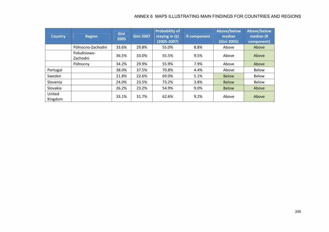
ANNEX 6 MAPS ILLUSTRATING MAIN FINDINGS FOR COUNTRIES AND REGIONS
245
Country Region Gini 2005
Gini 2007 Probability of staying in Q1 (2005-2007)
R component Above/below
median (Gini 2005)
Above/below median (R
component) Północno-Zachodni 33.6% 29.8% 55.0% 8.8% Above Above
Południowo-Zachodni
36.5% 33.0% 55.5% 9.5% Above Above
Północny 34.2% 29.9% 55.9% 7.9% Above Above Portugal 38.0% 37.5% 70.8% 4.4% Above Below Sweden 21.8% 22.6% 69.0% 5.1% Below Below Slovenia 24.0% 23.5% 73.2% 3.8% Below Below Slovakia 26.2% 23.2% 54.9% 9.0% Below Above United Kingdom
33.1% 31.7% 62.6% 9.2% Above Above
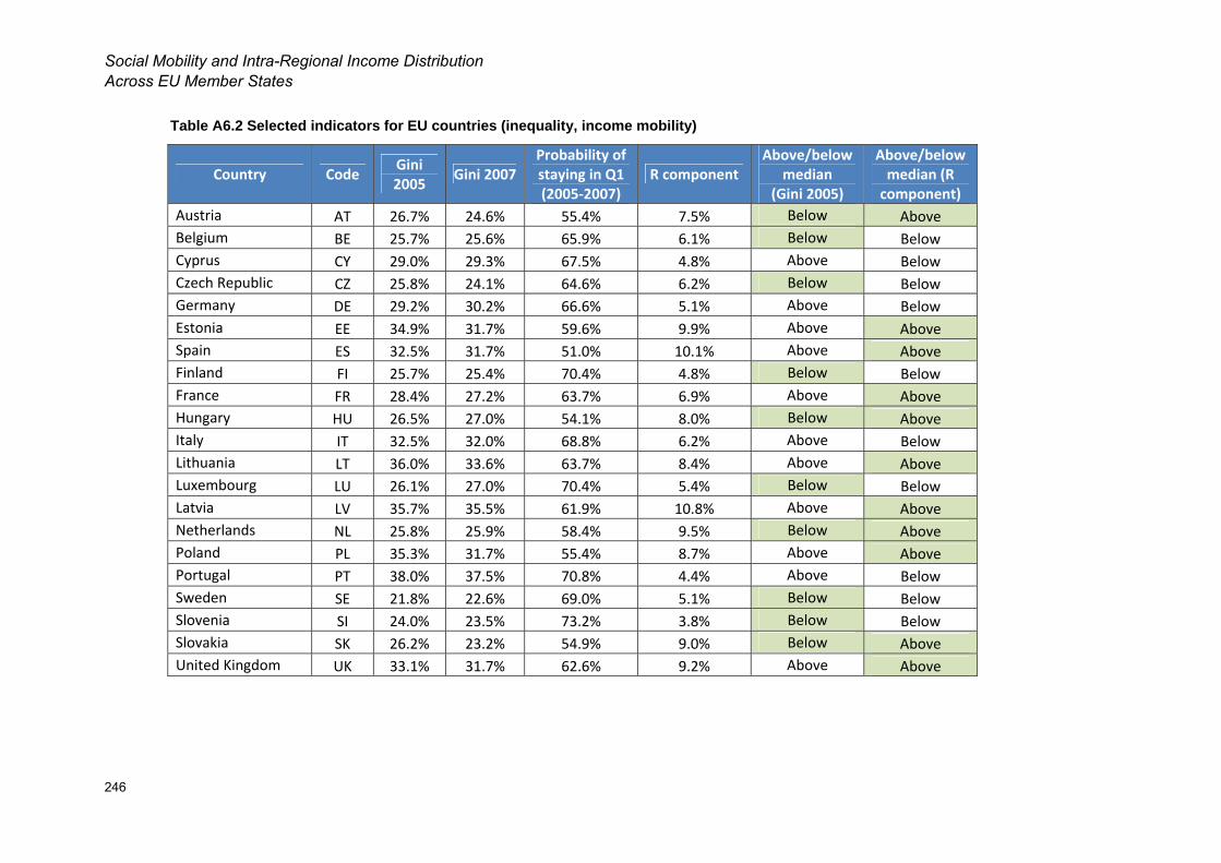
Social Mobility and Intra-Regional Income Distribution Across EU Member States
246
Table A6.2 Selected indicators for EU countries (inequality, income mobility)
Country Code Gini 2005
Gini 2007 Probability of staying in Q1 (2005-2007)
R component Above/below
median (Gini 2005)
Above/below median (R
component) Austria AT 26.7% 24.6% 55.4% 7.5% Below Above Belgium BE 25.7% 25.6% 65.9% 6.1% Below Below Cyprus CY 29.0% 29.3% 67.5% 4.8% Above Below Czech Republic CZ 25.8% 24.1% 64.6% 6.2% Below Below Germany DE 29.2% 30.2% 66.6% 5.1% Above Below Estonia EE 34.9% 31.7% 59.6% 9.9% Above Above Spain ES 32.5% 31.7% 51.0% 10.1% Above Above Finland FI 25.7% 25.4% 70.4% 4.8% Below Below France FR 28.4% 27.2% 63.7% 6.9% Above Above Hungary HU 26.5% 27.0% 54.1% 8.0% Below Above Italy IT 32.5% 32.0% 68.8% 6.2% Above Below Lithuania LT 36.0% 33.6% 63.7% 8.4% Above Above Luxembourg LU 26.1% 27.0% 70.4% 5.4% Below Below Latvia LV 35.7% 35.5% 61.9% 10.8% Above Above Netherlands NL 25.8% 25.9% 58.4% 9.5% Below Above Poland PL 35.3% 31.7% 55.4% 8.7% Above Above Portugal PT 38.0% 37.5% 70.8% 4.4% Above Below Sweden SE 21.8% 22.6% 69.0% 5.1% Below Below Slovenia SI 24.0% 23.5% 73.2% 3.8% Below Below Slovakia SK 26.2% 23.2% 54.9% 9.0% Below Above United Kingdom UK 33.1% 31.7% 62.6% 9.2% Above Above