Social Media Integration of Flood Data: A VineCopula-Based Approach

Lauren Ansell and Luciana Dalla Valle

University of Plymouth

October 7, 2021

Abstract

Floods are the most common and among the most severe natural disastersin many countries around the world. As global warming continues toexacerbate sea level rise and extreme weather, governmental authorities andenvironmental agencies are facing the pressing need of timely and accurateevaluations and predictions of flood risks. Current flood forecasts are generallybased on historical measurements of environmental variables at monitoringstations. In recent years, in addition to traditional data sources, large amountsof information related to floods have been made available via social media.Members of the public are constantly and promptly posting information andupdates on local environmental phenomena on social media platforms. Despitethe growing interest of scholars towards the usage of online data duringnatural disasters, the majority of studies focus exclusively on social mediaas a stand-alone data source, while its joint use with other type of informationis still unexplored. In this paper we propose to fill this gap by integratingtraditional historical information on floods with data extracted by Twitterand Google Trends. Our methodology is based on vine copulas, that allow usto capture the dependence structure among the marginals, which are modelledvia appropriate time series methods, in a very flexible way. We apply ourmethodology to data related to three different coastal locations on the Southcoast of the United Kingdom (UK). The results show that our approach, basedon the integration of social media data, outperforms traditional methods interms of evaluation and prediction of flood events.

Keywords: Climate Change; Dependence Modelling; Floods; NaturalHazards; Social Media Sentiment Analysis; Time Series Modelling; VineCopulas.

1

arX

iv:2

104.

0186

9v2

[st

at.A

P] 6

Oct

202

1

1 Introduction

In recent years, climate change has caused an exacerbation of the frequency andseverity of natural hazard phenomena, such as floods, storms, wildfires and otherextreme weather events (Field et al., 2012; Muller et al., 2015). Around the world, asubstantial part of the population is exposed to flood risk, with more than 2.3 billionpeople residing in locations experiencing inundations during flood events (UN, 2015).In the United Kingdom, intense storms occurred during recent years, bringing severeflooding and causing considerable damage to people, infrastructure and the economy,totalling millions of pounds (Smith et al., 2017). This caused a growing need fortimely and accurate information about the severity of flooding, which is essential forforecasting and nowcasting these phenomena and for effectively managing responseoperations and appropriately allocate resources (Rosser et al., 2017).

Generally, in order to estimate and predict inundations, statistical andmachine learning models are employed, typically using information gathered frommeteorological and climatological instrumentation at monitoring stations. Forexample, Wang and Du (2003) use a combination of meteorological, geographicaland urban data to produce flooding tables and maps published via Internet forpublic consultation. Keef et al. (2013) used data from a set of UK river flowgauges to estimate the probability of widespread floods based on the conditionalexceedance model of Heffernan and Tawn (2004). Grego et al. (2015) collectedhistoric flood frequency data and modelled them via finite mixture models ofstationary distributions using censored data methods. Balogun et al. (2020) utilizedgeographic information system and remote sensing data from Malaysia to generateflood susceptibility maps, applying Fuzzy-Analytic Network Process flood models.Model validation results showed that 59.42% and 36.23% of past flood eventsfall within the very high and high susceptible locations of the susceptibility maprespectively. Moishin et al. (2020) investigated fluvial flood risk in Fiji developinga flood index based on current and antecedent day’s precipitation. Talukdar et al.(2020) gathered historical flood data related to the Teesta River basin in Bangladeshand employed ensemble machine learning algorithms to predict flooding sites andflood susceptible zones. Results showed that an area of more than 800 km2 waspredicted as a very high flood susceptibility zone by all algorithms.

However, information collected at monitoring stations may suffer from datasparsity, time delays and high costs (Muller et al., 2015). In particular, remotelysensed data may take several hours to become available (Mason et al., 2012) andtheir temporal resolution is often limited (Schumann et al., 2009).

On the other hand, an increasing availability of consumer devices, such as

2

smartphones and tablets, is leading to the dissemination and communication offlood events directly by individuals, with information shared in real-time using socialmedia. User-generated content shared online often includes reports on meteorologicalconditions especially in case of extreme or unusual weather (Alam et al., 2018).Recent studies have focused specifically on social media sources, such as Twitter,Facebook and Flickr, to collect real-time information on floods and environmentalevents and their impacts across the globe. For example, Herfort et al. (2014) andDe Albuquerque et al. (2015) identified spatial patterns in the occurrence of flood-related tweets associated with proximity and severity of the River Elbe flood inGermany in June 2013. Saravanou et al. (2015) performed a case study on thefloods that occurred in the UK during January 2014, investigating how these werereflected on Twitter. The authors evaluated their findings against ground truth data,obtained from external independent sources, and were able to identify flood-strickenareas. Twitter data generated during flooding crisis was also used by Spielhoferet al. (2016) to evaluate techniques to be adopted in real-time to provide actionableintelligence to emergency services. Different methods to create flood maps fromTwitter micro-blogging were presented by Brouwer et al. (2017), Smith et al. (2017)and Arthur et al. (2018), who applied their approaches to different locations, suchas the city of York (UK), Newcastle upon Tyne (UK) and the whole England region,respectively. The 2015 South Carolina flood disaster was analysed by Li et al. (2018)to map the flood in real time by leveraging Twitter data in geospatial processes.Results show that the authors’ approach could provide a consistent and comparableestimation of the flood situation in near real time. Spruce et al. (2021) analysedrainfall events occurred across the globe in 2017, comparing outputs from socialsensing against a manually curated database created by the Met Office. The authorsshowed that social sensing successfully identified most high-impact rainfall eventspresent in the manually curated database, with an overall accuracy of 95%.

However, the majority of contributions in the literature analysing onlinegenerated data focus exclusively on social media sources, overlooking any relation orsynergy with other sources of information. One of the few exceptions is the paperby Rosser et al. (2017), who estimated the flood inundation extent in Oxford (UK)in 2014 based on the fusion of remote sensing, social media and topographic datasources, using a simple Weights-of-evidence analysis.

In this paper we propose to leverage the association between social media andenvironmental information via sophisticated statistical modelling based on vinecopulas, to enhance the assessment and prediction of flood phenomena comparedto traditional approaches.

Copulas are multivariate statistical tools, which allow us to model separately the

3

marginal models and their dependence structure (Huang et al., 2017). Copulas wereused in flood risk analysis, for example, by Jane et al. (2016) to predict the waveheight at a given location by exploiting the spatial dependence of the wave heightat nearby locations. The use of copulas in flood risk management was also exploredby Jane et al. (2018), who used a copula to capture dependencies in a 3-dimensionalloading parameter space, estimating the overall failure probability. Copulas havealso been applied in a flood risk context to model the dependence between multipleco-occurring drivers by Ward et al. (2018), among others. Couasnon et al. (2018)use Gaussian pair-copulas in a Bayesian Network to derive boundary conditionsthat account for riverine and coastal interactions for a catchment in southeastTexas. Feng et al. (2020) employed time-varying copulas with nonstationary marginaldistributions to estimate the dependence structure of inundation magnitudes in floodcoincidence risk assessment.

Vine copulas are based on bivariate copulas as building blocks and provide a greatdeal of flexibility, compared to standard copulas and other traditional multivariateapproaches, in modelling complex dependence structures between the variables. Vinecopulas were adopted, for example, by Latif and Mustafa (2020) to model trivariateflood characteristics for the Kelantan River basin in Malaysia. Tosunoglu et al.(2020) applied vine copulas in hydrology for multivariate modelling of peak, volumeand duration of floods in the Euphrates River Basin, Turkey. Vine copulas wereapplied to model compound events by Bevacqua et al. (2017) and by Santos et al.(2021). The former authors adopted this approach to quantify the risk in present-day and future climate, and to measure uncertainty estimates around such risk. Thelatter authors used vines to assess compound flooding from storm surge and multipleriverine discharges in Sabine Lake, Texas.

However, to the best of our knowledge, there are currently no studies exploringthe use of vine copulas to integrate social media data with other types of information.This paper proposes a novel approach, based on vine copulas, that combines datagathered from Twitter and Google Trends with remotely sensed information. Theproposed methodology involves the use of subjective information, more specificallythe feelings of people expressed through social media and quantified by sentimentscores, not merely as stand-alone data sources, used in isolation to predictinundations, but combined with information on the occurrence and magnitude offlood events. The vine copula approach allows us to exploit the associations betweenall the considered data sources, environmental as well as on-line, which all contributeto calculate flood forecasts.

The methodology articulates in the following steps, that will be illustrated indetail in the following sections:

4

1. fit each variable (environmental as well as on-line information) with a suitabletime series model, to remove the temporal effects from the data;

2. construct a vine copula model, which accounts for the dependencies betweenall variables and exploits the associations between environmental and socialmedia information;

3. calculate predictions of the flood variables based on the vine copula model.

The application of our methodology to three different coastal locations in the South ofthe UK shows that our approach performs better than traditional approaches, whichdo not take into account associations between environmental and on-line information,to estimate and predict the occurrence and the magnitude of flood events.

The remainder of the paper is organised as follows. Section 2 describes theenvironmental and social media data used in the analysis; Section 3 illustratesthe vine copula methodology; Section 4 reports the results of the analysis; finally,concluding remarks are presented in Section 5.

2 Study Area and Data Collection

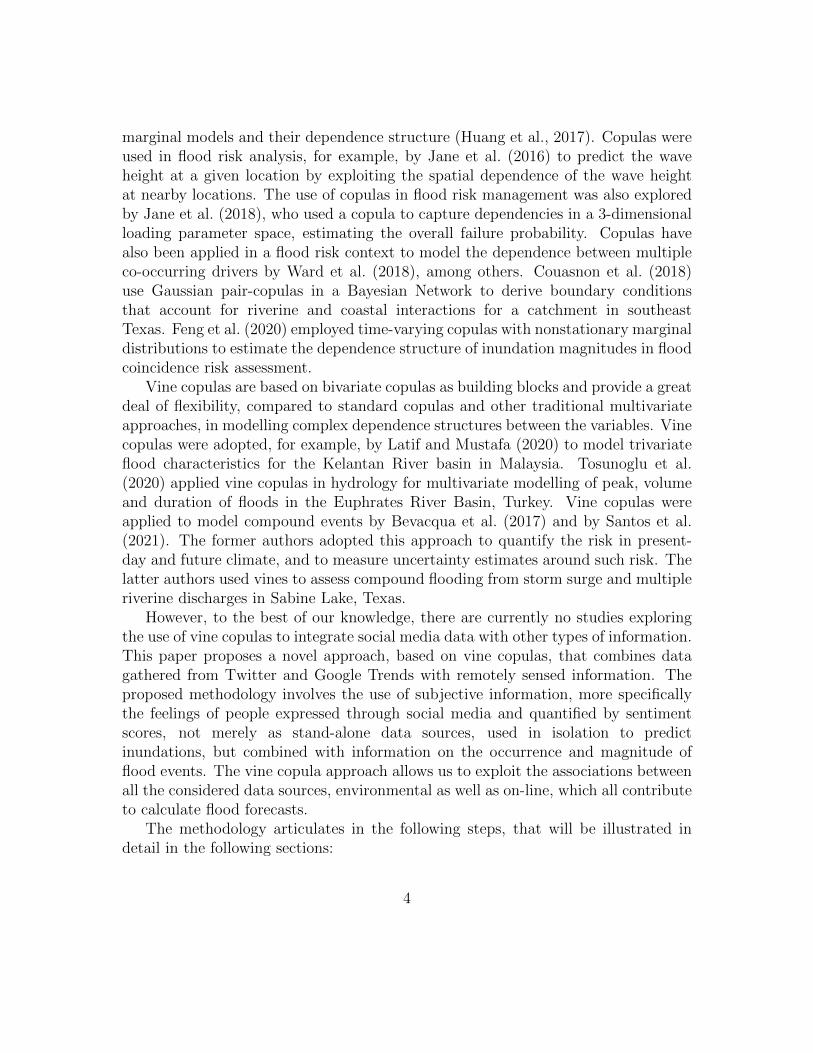
The UK coastline has been subject to terrible floods throughout history. Over thelast few years, storms and floods relentlessly hit the UK coast, triggering intensemedia coverage and public attention. Table 1 lists the major winter storm eventsaffecting the UK between 2012 and 2018.

Table 1: Major winter storm events in the UK between 2012 and 2018. Note thatthe storm naming system was introduced in 2015.

Winter Winter Winter Winter Winter2012/13 2013/14 2015/16 2016/17 2017/18Date Date Storm Date Storm Date Storm Date

Name Name Name11 Oct 28 Oct Abigail 12-13 Nov Angus 20 Nov Aileen 12-13 Sep18 Nov 5-6 Dec Barney 17-18 Nov Barbara 23-24 Dec Brian 21 Oct14 Dec 18-19 Dec Clodagh 29 Nov Conor 25- 26 Dec Caroline 7 Dec19 Dec 23-24 Dec Desmond 5-6 Dec Doris 23 Feb Dylan 30-31 Dec22 Dec 26-27 Dec Eva 24 Dec Ewan 26 Feb Eleanor 2-3 Jan

30-31 Dec Frank 29-30 Dec Fionn 16 Jan3 Jan Gertrude 29 Jan Georgina 24 Jan

25-26 Jan Henry 1-2 Feb31 Jan-1 Feb Imogen 8 Feb

4-5 Feb Jake 2 Mar8-9 Feb Katie 27-28 Mar12 Feb

14-15 Feb

5

In this paper we consider three locations on the South coast of the UK, whichwere severely affected by storm events in recent years: Portsmouth, Plymouthand Dawlish. The inundation episodes of the last few years had a substantialsocioeconomic impact on the local communities of the three locations, which aretotalling a population of almost 500,000. The three areas were affected by most ofthe inundation events listed in Table 1. In particular, devastating overnight stormson February 4, 2014, swept the main rail route at Dawlish, leaving tracks dangling inmid-air. The seawall was breached, a temporary line of shipping containers forming abreakwater was constructed, however huge waves damaged it and punched a new holein the sea wall. Later, a replacement seawall was installed and railway operationsre-commenced on April 4, 2014. The waves on the night of the 4th February wererelatively modest. The breach was more likely a result of a combination of factorsincluding coincidental arrival of swell waves and the highest locally generated windwaves, large storm surge arriving a few days after a spring tide and the sequenceof storm events hitting the South UK coast that winter before the breach loweringbeach level (Sibley et al., 2015).

In order to estimate and predict flood phenomena in the three coastal areas, weapplied the vine copula methodology to data based on historical measurement inconjunction with information gathered online.

For each one of the three locations, we obtained daily hydraulic loading conditiondata as well as social media information for the period between January 2012 andDecember 2016, obtaining 1, 827 daily data points for each variable. We thereforeconstructed a dataset of time series, all of the same length. More precisely, wedownloaded wave height (m) and water level (tidal residual, m) data from the UKEnvironment Agency flood-monitoring API 1. Furthermore, for the aforementionedlocations, we gathered Google Trends information on the number of searches forthe keywords flood, flooding, rain and storm, using the gtrendsR package fromthe R software (Massicotte and Eddelbuettel, 2021; R Core Team, 2020). Inaddition, we collected Twitter messages containing the same keywords used toperform Google Trends searches for the three areas. After removing tweets sent byautomated accounts, which contained factual information about the current weatherin the required location, we obtained 9,781 tweets for Portsmouth, 4,995 tweets forPlymouth and 1,769 tweets for Dawlish. From the Twitter data, we considered thetotal number of tweets as well as the sentiment scores calculated using two differentlexicons: Bing and Afinn (Hu and Liu, 2004), which are available in the R tidytext

package (Silge and Robinson, 2016). The Bing lexicon splits words into positive or

1Available at the website https://environment.data.gov.uk/flood-monitoring/doc/

reference

6

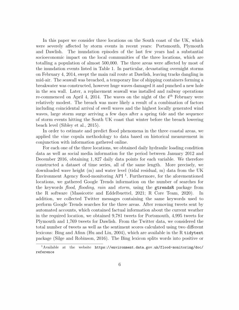
negative. The Bing sentiment score for each tweet is calculated by counting thenumber of positive words used in each tweet and subtracting from this the numberof negative words. The Afinn lexicon scores words between ±5. The Afinn sentimentscore is calculated by multiplying the score of each word by the number of times itappears in the tweet; these scores are then summed to derive the overall sentimentscore. In order to take into account of the different population sizes living in thethree areas 2, we scaled the Bing and Afinn sentiment scores by the relevant numberof residents.

Figure 1: Trace plots of Portsmouth data.

2We considered a total population of 238,137 for Portsmouth; a total population of 234,982 forPlymouth; a total population of 16,298 for Dawlish. Source: 2011 United Nations population figure,available at: https://unstats.un.org/unsd/demographic-social/

7

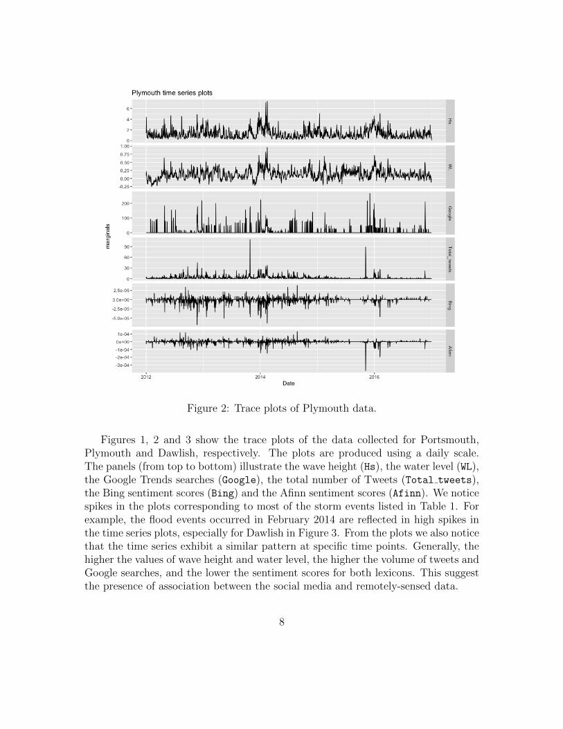
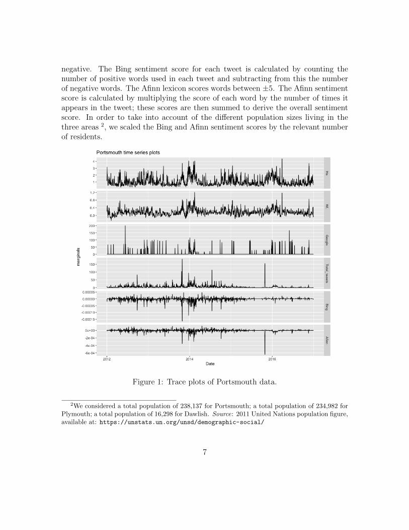
Figure 2: Trace plots of Plymouth data.

Figures 1, 2 and 3 show the trace plots of the data collected for Portsmouth,Plymouth and Dawlish, respectively. The plots are produced using a daily scale.The panels (from top to bottom) illustrate the wave height (Hs), the water level (WL),the Google Trends searches (Google), the total number of Tweets (Total tweets),the Bing sentiment scores (Bing) and the Afinn sentiment scores (Afinn). We noticespikes in the plots corresponding to most of the storm events listed in Table 1. Forexample, the flood events occurred in February 2014 are reflected in high spikes inthe time series plots, especially for Dawlish in Figure 3. From the plots we also noticethat the time series exhibit a similar pattern at specific time points. Generally, thehigher the values of wave height and water level, the higher the volume of tweets andGoogle searches, and the lower the sentiment scores for both lexicons. This suggestthe presence of association between the social media and remotely-sensed data.

8

Figure 3: Trace plots of Dawlish data.

3 Methodology

The copula is a function that allows us to bind together a set of marginals, to modeltheir dependence structure and to obtain the joint multivariate distribution (Joe,1997; Nelsen, 2007). Sklar’s theorem (Sklar, 1959) is the most important result incopula theory. It states that, given a vector of random variables X = (X1, . . . , Xd),with d-dimensional joint cumulative distribution function F (x1, . . . , xd) and marginalcumulative distributions (cdf) Fj(xj), with j = 1, . . . , d, a d-dimensional copula Cexists, such that

F (x1, . . . , xd) = C(F1(x1), . . . , Fd(xd);θ),

9

where Fj(xj) = uj, with uj ∈ [0, 1] are called u-data, and θ denotes the set ofparameters of the copula. The joint density function can be derived as

f(x1, . . . , xd) = c(F1(x1), . . . , Fd(xd);θ) · f1(x1) · · · fd(xd),

where c denotes the d-variate copula density. The copula allows us to determine thejoint multivariate distribution and to describe the dependencies among the marginals,that can potentially be all different and can be modelled using distinct distributions.

In this paper, we adopt the 2-steps inference function for margins (IFM) approach(Joe and Xu, 1996), estimating the marginals in the first step, and then the copula,given the marginals, in the second step.

3.1 Marginal Models

Given the different characteristics of the six marginals, we fitted different models foreach of the six time series for each location. Further, we extracted the residuals εj,with j = 1, . . . , d, from each marginal model and we applied the relevant distributionfunctions to get the u-data Fj(εj) = uj to be plugged into the copula.

3.1.1 Wave height (Hs)

The best fitting model for the log-transformed Hs marginal for all three locations wasthe autoregressive integrated moving average (ARIMA) model (for more informationabout ARIMA models, see, for example Hyndman and Athanasopoulos (2018)).The ARIMA model aims to describe the autocorrelations in the data by combiningautoregressive and moving average models. The model is usually denoted asARIMA(p, d, q), where the values in the brackets indicate the parameters: p, d,q, where p is the order of the autoregressive part, d is the degree of first differencinginvolved and q is the order of the moving average part. The ARIMA model, fort = 1, . . . , T takes the following form:

yt = a+

p∑i=1

φiyt−i +

q∑i=1

θiεt−i + εt (1)

where yt = (1 − B)dxt, xt are the original data values, B is the backshift operator,a is a constant, φi, with i = 1, . . . , p, are the autoregressive parameters, θi, withi = 1, . . . , q, are the moving average parameters and εt ∼ N(0, 1) is the error term.

10

3.1.2 Water level (WL)

We fitted the log-transformed WL marginal for the Plymouth location with an ARIMAmodel, as described in Eq.(1). However, for Portsmouth and Dawlish, the ARIMA-GARCH model with Student’s t innovations appeared to have a better fit. Thismodel combines the features of the ARIMA model with the generalized autoregressiveconditional heteroskedastic (GARCH) model, allowing us to capture time seriesvolatility over time. The GARCH model is typically denoted as GARCH(p, q),with parameters p and q, where p is the number of lag residuals errors and q is thenumber of lag variances. The ARIMA(p, d, q)-GARCH(p, q) model can be expressedas:

yt = a+

p∑i=1

φiyt−i +

q∑i=1

θiεt−i + εt

εt =√σtzt σ2 = ω +

p∑i=1

αiε2t−i +

q∑i=1

βiσ2t−i (2)

where αi, with i = 1, . . . , p, and βi, with i = 1, . . . , q are the parameters of theGARCH part of the model, and εt follows a Student’s t distribution.

3.1.3 Google trends (Google)

Since the Google marginal in all locations includes several values equal to zero, wefitted a zero adjusted gamma distribution (ZAGA) using time as explanatory variable(see Rigby and Stasinopoulos (2005)). This distribution is a mixture of a discretevalue 0 with probability ν, and a gamma distribution on the positive real line (0,∞)with probability (1− ν). The probability density function (pdf) of the ZAGA modelis given by

fX(x|µ, σ, ν) =

{ν if x = 0

(1− ν)fGA(x|µ, σ) if x > 0(3)

for 0 ≤ x < ∞, 0 < ν < 1, where µ > 0 is the scale parameter, σ > 0 is the shapeparameter and fGA(x|µ, σ) is the gamma pdf. We assumed that the parameter µ ofthe ZAGA model is related to time, as explanatory variable, through an appropriatelink function, with coefficient β (for more details, see Rigby et al. (2019)).

3.1.4 Total number of tweets (Total tweets)

The best fitting model for the marginal Total tweets is the zero adjusted inverseGaussian distribution (ZAIG), which is similar to the ZAGA model discussed in

11

Section 3.1.3. The pdf of the ZAIG model is

fX(x|µ, σ, ν) =

{ν if x = 0

(1− ν)fIG(x|µ, σ) if x > 0(4)

for 0 ≤ x < ∞, 0 < ν < 1, where µ > 0 is the location parameter, σ > 0 is thescale parameter and fIG(x|µ, σ) is the inverse Gaussian pdf. Similarly to the ZAGAmodel, for the ZAIG model we assumed that the parameter µ is related to time, asexplanatory variable, through an appropriate link function, with coefficient β (seeRigby and Stasinopoulos (2005); Rigby et al. (2019)).

3.1.5 Bing sentiment score (Bing)

The best model for the Bing marginal for all three locations was the ARIMA-GARCH model with Student’s t innovations, as illustrated in Eq.(2), fitted on thelog-transformed data.

Since the residuals of the Dawlish data still showed some structure, they werefitted using a Generalized t distribution (GT), which depends on four parameterscontrolling location, scale and kurtosis (for more information, see Rigby andStasinopoulos (2005); Rigby et al. (2019)).

3.1.6 Afinn sentiment score (Afinn)

The log-transformed Afinn marginal was fitted with an ARIMA-GARCH model withStudent’s t innovations (see Eq.(2)).

For Portsmouth, since the residuals still presented some structure, they were fittedusing a skew exponential power type 2 distribution (SEP2), which depends on fourparameters: the location, scale, skewness and kurtosis. For the implementation of theSEP2 distribution, we used time as explanatory variable for the location parameter.

For Dawlish, the residuals were fitted using a Normal-exponential-Student-tdistribution (NET), considering time as explanatory variable. The NET distributionis symmetric and depends on four parameters controlling the location, scale andkurtosis (for more details on the SEP2 and NET distributions, see Rigby andStasinopoulos (2005); Rigby et al. (2019)).

3.2 Vine Copula Model

A vine copula (or vine) represents the pattern of dependence of multivariate datavia a cascade of bivariate copulas, allowing us to construct flexible high-dimensional

12

copulas using only bivariate copulas as building blocks. For more details about vinecopulas see Czado (2019).

In order to obtain a vine copula we proceed as follows. First we factorise thejoint distribution f(x1, . . . , xd) of the random vector X = (X1, . . . , Xd) as a productof conditional densities

f(x1, . . . , xd) = fd(xd) · fd−1|d(xd−1|xd) · . . . · f1|2...d(x1|x2, . . . xd). (5)

The factorisation in (5) is unique up to re-labelling of the variables and it can beexpressed in terms of a product of bivariate copulas. In fact, by Sklar’s theorem, theconditional density of Xd−1|Xd can be easily written as

fd−1|d(xd−1|xd) = cd−1,d(Fd−1(xd−1), Fd(xd);θd−1,d) · fd−1(xd−1), (6)

where cd−1,d is a bivariate copula, with parameter vector θd−1,d. Through astraightforward generalisation of Eq.(6), each term in (5) can be decomposed into theappropriate bivariate copula times a conditional marginal density. More precisely,for a generic element Xj of the vector X we obtain

fXj |V(xj|v) = cXJ ,ν`;V−`(FXj |V−`

(xj|v−`), Fν`|V−`(ν`|v−`);θXJ ,ν`;V−`

) ·fXj |V−`(xj|v−`),

(7)where v is the conditioning vector, ν` is a generic component of v, v−` is the vectorv without the component ν`, FXj |v−`

(·|·) is the conditional distribution of Xj givenv−` and cXJ ,ν`;V−`

(·, ·) is the conditional bivariate copula density, which can typicallybelong to any family (e.g. Gaussian, Student’s t, Clayton, Gumbel, Frank, Joe, BB1,BB6, BB7, BB8, etc.; for more information on copula families, see Nelsen (2007)),with parameter θXJ ,ν`;V−`

. The d-dimensional joint multivariate distribution functioncan hence be expressed as a product of bivariate copulas and marginal distributionsby recursively plugging Eq.(7) in Eq.(5).

For example, let us consider a 6-dimensional distribution. Then, Eq.(5) translatesto

f(x1, . . . , x6) = f6(x6) · f5|6(x5|x6) · f4|5,6(x4|x5, x6) · . . . · f1|2...6(x1|x2, . . . x6). (8)

The second factor f5|6(x5|x6) on the right-hand side of (8) can be easily decomposedinto the bivariate copula c5,6(F5(x5), F6(x6)) and marginal density f5(x5):

f5|6(x5|x6) = c5,6(F5(x5), F6(x6);θ5,6) · f5(x5).

On the other hand, the third factor on the right-hand side of (8) can be decomposedusing the (7) as

f4|5,6(x4|x5, x6) = c4,5;6(F4|6(x4|x6), F5|6(x5|x6);θ4,5;6) · f4|6(x4|x6).

13

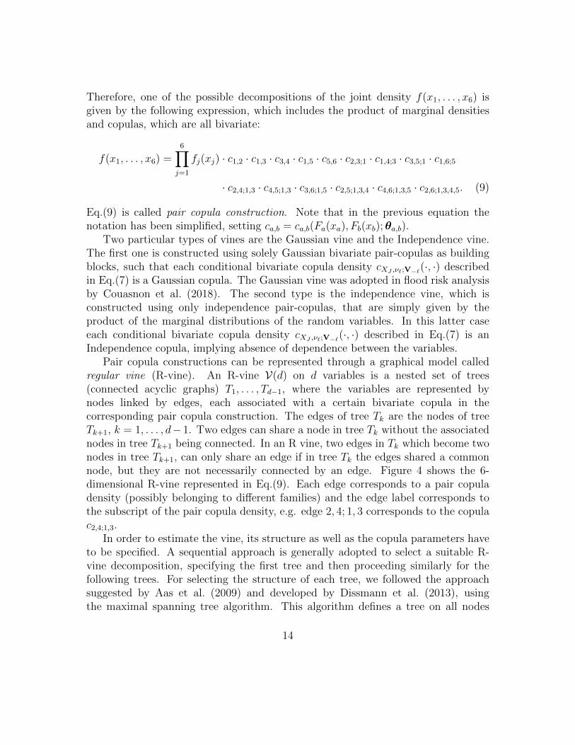
Therefore, one of the possible decompositions of the joint density f(x1, . . . , x6) isgiven by the following expression, which includes the product of marginal densitiesand copulas, which are all bivariate:

f(x1, . . . , x6) =6∏j=1

fj(xj) · c1,2 · c1,3 · c3,4 · c1,5 · c5,6 · c2,3;1 · c1,4;3 · c3,5;1 · c1,6;5

· c2,4;1,3 · c4,5;1,3 · c3,6;1,5 · c2,5;1,3,4 · c4,6;1,3,5 · c2,6;1,3,4,5. (9)

Eq.(9) is called pair copula construction. Note that in the previous equation thenotation has been simplified, setting ca,b = ca,b(Fa(xa), Fb(xb);θa,b).

Two particular types of vines are the Gaussian vine and the Independence vine.The first one is constructed using solely Gaussian bivariate pair-copulas as buildingblocks, such that each conditional bivariate copula density cXJ ,ν`;V−`

(·, ·) describedin Eq.(7) is a Gaussian copula. The Gaussian vine was adopted in flood risk analysisby Couasnon et al. (2018). The second type is the independence vine, which isconstructed using only independence pair-copulas, that are simply given by theproduct of the marginal distributions of the random variables. In this latter caseeach conditional bivariate copula density cXJ ,ν`;V−`

(·, ·) described in Eq.(7) is anIndependence copula, implying absence of dependence between the variables.

Pair copula constructions can be represented through a graphical model calledregular vine (R-vine). An R-vine V(d) on d variables is a nested set of trees(connected acyclic graphs) T1, . . . , Td−1, where the variables are represented bynodes linked by edges, each associated with a certain bivariate copula in thecorresponding pair copula construction. The edges of tree Tk are the nodes of treeTk+1, k = 1, . . . , d− 1. Two edges can share a node in tree Tk without the associatednodes in tree Tk+1 being connected. In an R vine, two edges in Tk which become twonodes in tree Tk+1, can only share an edge if in tree Tk the edges shared a commonnode, but they are not necessarily connected by an edge. Figure 4 shows the 6-dimensional R-vine represented in Eq.(9). Each edge corresponds to a pair copuladensity (possibly belonging to different families) and the edge label corresponds tothe subscript of the pair copula density, e.g. edge 2, 4; 1, 3 corresponds to the copulac2,4;1,3.

In order to estimate the vine, its structure as well as the copula parameters haveto be specified. A sequential approach is generally adopted to select a suitable R-vine decomposition, specifying the first tree and then proceeding similarly for thefollowing trees. For selecting the structure of each tree, we followed the approachsuggested by Aas et al. (2009) and developed by Dissmann et al. (2013), usingthe maximal spanning tree algorithm. This algorithm defines a tree on all nodes

14

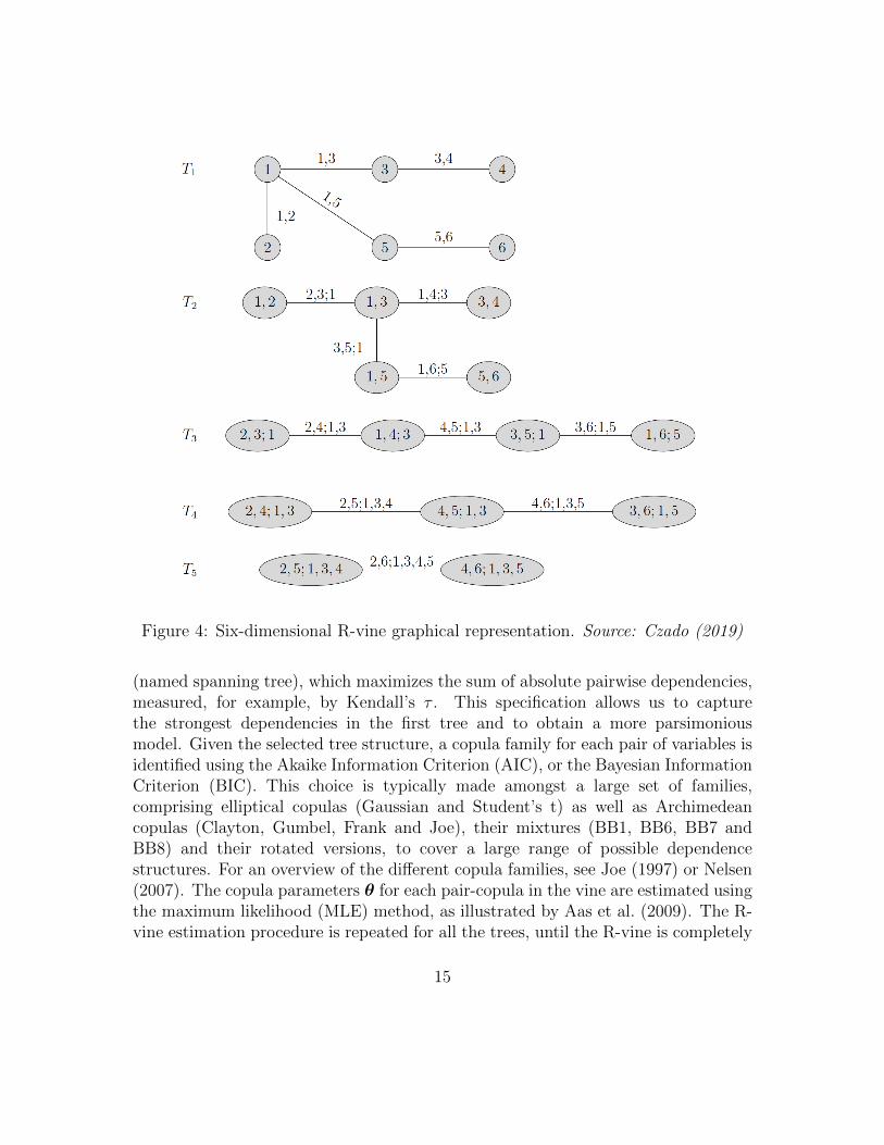
Figure 4: Six-dimensional R-vine graphical representation. Source: Czado (2019)

(named spanning tree), which maximizes the sum of absolute pairwise dependencies,measured, for example, by Kendall’s τ . This specification allows us to capturethe strongest dependencies in the first tree and to obtain a more parsimoniousmodel. Given the selected tree structure, a copula family for each pair of variables isidentified using the Akaike Information Criterion (AIC), or the Bayesian InformationCriterion (BIC). This choice is typically made amongst a large set of families,comprising elliptical copulas (Gaussian and Student’s t) as well as Archimedeancopulas (Clayton, Gumbel, Frank and Joe), their mixtures (BB1, BB6, BB7 andBB8) and their rotated versions, to cover a large range of possible dependencestructures. For an overview of the different copula families, see Joe (1997) or Nelsen(2007). The copula parameters θ for each pair-copula in the vine are estimated usingthe maximum likelihood (MLE) method, as illustrated by Aas et al. (2009). The R-vine estimation procedure is repeated for all the trees, until the R-vine is completely

15

specified.

3.3 Out-of-sample predictions

In order to evaluate the suitability of the proposed vine copula model in relationto other methods, we produced one-day-ahead out-of-sample predictions and wecompared them to the original data. Let X = {Xt; t = 1, . . . , T} be the 6-dimensionaltime series of environmental and social media data. Our aim is to forecast XT+1

based on the information available at time T . In order to do that, we adopted theforecasting method described by Simard and Remillard (2015). Before fitting thevine, we extracted the residuals from the marginals, as explained in Section 3.1, andobtained the u-data. Next, after fitting the vine, we simulated M realizations fromthe vine copula. Hence, we calculated the predicted values for each simulation, usingthe inverse cdf and the relevant fitted marginal models. More precisely, we appliedthe inverse transformation to the M realizations from the vine copula to obtain theresiduals which we then plugged into the marginal models to get the predicted valuesof the environmental variables (wave height and water level). Then, we calculated

the average prediction for all simulations XAvg

T+1 and use it as the forecast XT+1. Theprediction interval of level (1 − α) ∈ (0, 1) for XT+1 was calculated by taking theestimated quantiles of order α/2 and 1−α/2 amongst the simulated data. We denote

by Xl

T+1 and Xu

T+1 the lower and upper values of the prediction intervals.In order to compare and contrast the accuracy of predictions for different models,

we made use of four indicators: the mean squared error (MSE) to evaluate pointforecasts; the mean interval score (MIS), proposed by Gneiting and Raftery (2007), toassess the accuracy of the prediction intervals; the Normalized Nash-Sutcliffe modelefficiency (NNSE) coefficient, proposed by Nash and Sutcliffe (1970) to appraisehydrological models; and the Distance Correlation, proposed by Szekely et al. (2007),to determine the association between observed and predicted data. The MSE for eachvariable j = 1, . . . , d was calculated as follows

MSEj =1

S

T+S∑t=T+1

(xt,j − xt,j)2

where xt,j is the observed value for each variable at each time point t, xt,j is thecorresponding predicted value, T + 1 denotes the first predicted date, while T + Sindicates the last predicted date. The 95% MIS for each variable, at level α = 0.05,

16

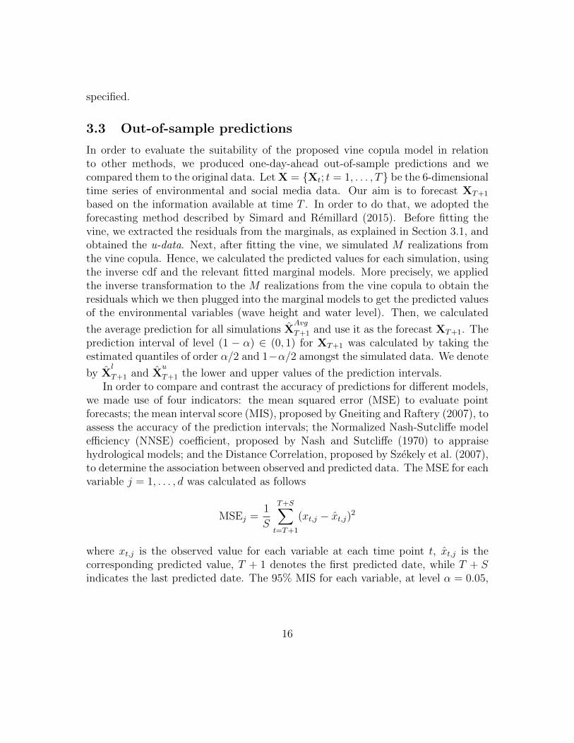
was computed as

MISj =1

S

T+S∑t=T+1

[(xut,j − xlt,j) +

2

α(xlt,j − xt,j)1(xt,j < xlt,j) +

2

α(xt,j − xut,j)1(xt,j > xut,j)

]where xlt,j and xut,j denote, respectively, the lower and upper limits of the predictionintervals for each variable at each time point, and 1(·) is the indicator function. TheNNSE coefficient was calculated as

NNSEj =1

2− NSEj

with

NSEj = 1−∑T+S

t=T+1 (xt,j − xt,j)2∑T+St=T+1 (xt,j − xj)2

where xj is the mean of the observed values for each variable. The NSE is anormalized statistic that determines the relative magnitude of the residual variance(“noise”) compared to the measured data variance (“information”). The DistanceCorrelation takes the form

DCj = dCor(Xj, Xj) =dCov(Xj, Xj)√

dVar(Xj)dVar(Xj)

where Xj is the j-th observed variable, Xj is the corresponding j-th predicted

variable, dCor(Xj, Xj) is the distance covariance and dVar(Xj) and dVar(Xj) arethe distance standard deviations, obtained replacing the signed distances between thevariables with centred Euclidean distances. The DC is a distance-based correlationthat can detect both linear and non-linear relationships between variables.

4 Result Analysis and Discussion

We now present the results of the analysis of the remotely-sensed and online flooddata for the three locations under consideration.

4.1 Twitter Wordclouds

First, we analysed the information gathered on Twitter, cleaning and stemming thetweets and producing wordclouds for each location.

17

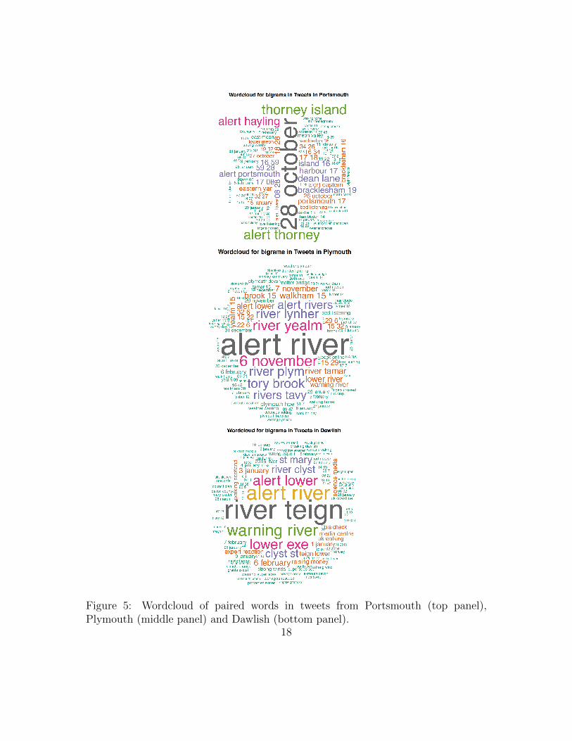
Figure 5: Wordcloud of paired words in tweets from Portsmouth (top panel),Plymouth (middle panel) and Dawlish (bottom panel).

18

Figure 5 displays the wordclouds of paired words obtained by pairing the the mostcommon combinations of words appearing in the collected tweets. The top, middleand bottom panels show the wordclouds of Portsmouth, Plymouth and Dawlishtweets, respectively. The most frequent pairs of words refer to dates indicatingstorm and flood events (e.g. 28 October, 3 January), names of places affected bystorms (e.g. Thorney Island, St Mary) and names of rivers (e.g. river Yealm, riverTeign).

4.2 Marginals Estimation

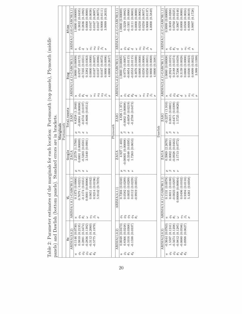
Table 2 lists the parameter estimates, obtained via the MLE method, of the bestfitting models for the marginals, as described in Section 3.1, for Portsmouth (toppanels), Plymouth (middle panels) and Dawlish (bottom panels). Standard errorsare in brackets.3

As an example, Figure 6 shows the fit of the residuals for the Google trendsmarginal for Portsmouth. The other plots for all marginals related to all threelocations exhibit a similar behaviour. The top panel displays the QQ-plot comparingthe Gaussian theoretical quantiles with the sample quantiles, the middle panelillustrates the observations (black line) and in-sample predictions obtained from thefitted ZAGA model (red line), while the bottom panel shows the histogram of theresulting u-data. The plots clearly show an excellent fit of the ZAGA model to themarginal, as demonstrated by the points in the QQ-plot aligning almost perfectly tothe main diagonal, the in-sample predictions overlapping the observed data and theshape of the u-data histogram displaying a uniform pattern.

3Please, note that, due to lack of space, the Table does not include the estimates of the GT,SEP2 and NET models fitted to the residuals of the Bing and Afinn marginals.

19

Tab

le2:

Par

amet

eres

tim

ates

ofth

em

argi

nal

sfo

rea

chlo

cati

on:

Por

tsm

outh

(top

pan

els)

,P

lym

outh

(mid

dle

pan

els)

and

Daw

lish

(bot

tom

pan

els)

.Sta

ndar

der

rors

are

inbra

cket

s.M

argin

als

Portsm

outh

Hs

WL

Google

Totaltweets

Bing

Afinn

ARIM

A(3,0,2)

ARIM

A(1,0,1)-GARCH(1,1)

ZAGA

ZAIG

ARIM

A(1,d,1)-GARCH(3,1)

ARIM

A(1,d,0)-GARCH(3,1)

a-0.1146(0.0730)

a0.1373(0.0066)

µ2.2579(1.5760)

µ8.8258(1.3940)

a1.0000(0.00009)

a1.0000(0.00009)

φ1

0.9810(0.2135)

φ1

0.7679(0.0221)

β0.0001(0.00009)

β-0.0004(0.00008)

φ1

0.8707(0.0172)

φ1

0.3832(0.0435)

φ2

0.2891(0.3474)

θ 1-0.1174(0.0351)

σ-0.5203(0.0581)

σ-0.6741(0.0197)

θ 1-0.7335(0.0351)

d0.2836(0.1092)

φ3

-0.2836(0.1382)

ω0.0001(0.00006)

ν2.5440(0.0901)

ν-0.8606(0.0512)

d0.3382(0.0363)

ω0.0000(0.0000)

θ 1-0.3112(0.2060)

α1

0.0651(0.0162)

ω0.0000(0.0000)

α1

0.0167(0.0038)

θ 2-0.5775(0.1979)

β1

0.9214(0.0196)

α1

0.0167(0.0037)

α2

0.0167(0.0097)

σ5.9142(0.7878)

α2

0.0167(0.0086)

α3

0.0167(0.0075)

α3

0.0167(0.0072)

β1

0.9000(0.0111)

β1

0.9000(0.0096)

σ3.9999(0.2633)

σ4.0000(0.2617)

Plymouth

ARIM

A(1,0,2)

ARIM

A(4,1,1)

ZAGA

ZAIG

ARIM

A(1,d,2)-GARCH(2,1)

ARIM

A(1,d,1)-GARCH(2,1)

a0.0048(0.0473)

φ1

0.7204(0.0240)

µ4.927(1.403)

µ4.826(1.371)

a1.0000(0.00005)

a1.0000(0.00009)

φ1

0.8366(0.0248)

φ2

0.0582(0.0289)

β-0.00005(0.00008)

β-0.0002(0.00008)

φ1

0.9779(0.0007)

φ1

0.3229(0.0882)

θ 1-0.1016(0.0368)

φ3

0.0035(0.0289)

σ-0.3348(0.0395)

σ-0.6058(0.0219)

θ 1-0.8854(0.0115)

θ 1-0.1301(0.0968)

θ 2-0.1598(0.0337)

φ4

0.0112(0.0239)

ν1.7263(0.0653)

ν-0.2788(0.0473)

θ 2-0.0553(0.0115)

d0.3111(0.0683)

θ 1-0.9919(0.0055)

d0.3076(0.0490)

ω0.0000(0.0000)

ω0.0000(0.0000)

α1

0.0250(0.0062)

α1

0.0250(0.0068)

α2

0.0250(0.0057)

α2

0.0250(0.0051)

β1

0.9000(0.0137)

β1

0.9000(0.0069)

σ4.0000(0.5849)

σ4.0000(0.3481)

Dawlish

ARIM

A(2,0,3)

ARIM

A(1,0,1)-GARCH(1,1)

ZAGA

ZAIG

ARIM

A(2,d,1)-GARCH(1,1)

ARIM

A(1,d,1)-GARCH(1,1)

a-0.3644(0.0763)

a0.1131(0.0078)

µ0.3969(2.2670)

µ-0.2273(1.910)

a1.0000(0.00008)

a0.9999(0.00009)

φ1

1.5597(0.1241)

φ1

0.8011(0.0180)

β0.0002(0.0001)

β0.0015(0.0001)

φ1

-0.2924(0.0315)

φ1

0.3049(0.0268)

φ2

-0.5674(0.1208)

θ 1-0.0023(0.0297)

σ-0.0928(0.0463)

σ-0.6471(0.0399)

φ2

0.2188(0.0374)

θ 10.0760(0.0225)

θ 1-0.9812(0.1285)

ω0.00008(0.00004)

ν2.1713(0.0772)

ν1.5725(0.0620)

θ 10.7206(0.0459)

d0.3967(0.0146)

θ 2-0.0680(0.0586)

α1

0.0496(0.0102)

d0.3139(0.0028)

ω0.0000(0.0000)

θ 30.0998(0.0627)

β1

0.9394(0.0116)

ω0.0000(0.0000)

α1

0.0500(0.0024)

σ5.4261(0.6958)

α1

0.0500(0.0023)

β1

0.8999(0.0019)

β1

0.8999(0.0022)

σ3.9997(0.1728)

σ3.999(0.1399)

20

4.3 Vine Estimation

Once the marginals were estimated, we derived the corresponding u-data from theresiduals, as illustrated in Section 3.1. Then, we carried out fitting and modelselection for the vine copula for each location using the R package rvinecopulib

(Nagler and Vatter, 2021).Figure 7 displays the first trees of the vine copulas estimated for Portsmouth

(top panel), Plymouth (middle panel) and Dawlish (bottom panel). The nodesare denoted with blue dots, with the names of the margins reported in boldface4.On each edge, the plots show the name of the selected pair copula family and theestimated copula parameter expressed as Kendall’s τ . In order to estimate the vines,we adopted the Kendall’s τ criterion for tree selection, the AIC for the copula familiesselection and the MLE method for estimating the pair copula parameters. As it isclear from Figure 7, the vines for the three different locations exhibit a very similarstructure, with the environmental variables Hs and WL playing a central role andlinking to the social media variables. The sentiment scores Bing and Afinn aredirectly associated. Likewise, Total tweets and Google are contiguouly related.The symmetric Gaussian copula, which is often employed in traditional multivariatemodelling, was not identified as the best fitting copula for neither of the locations.On the contrary, the selected copula families include the Student’s t copula, which isable to model strong tail dependence, Archimedean copulas such as the Clayton andGumbel, that are able to capture asymmetric dependence, and mixture copulas suchas the BB1 (Clayton-Gumbel) and BB8 (Joe-Frank), that can accommodate variousdependence shapes. Most of the associations between the variables are positive.The strongest associations are between the Bing and Afinn sentiment scores andbetween the environmental variables Hs and WL. Also, Hs and Total tweets aremildly associated.

4.4 Out-of-sample prediction results

In this Section we constructed out-of-sample predictions using the proposed vinemethodology, which integrates environmental and social media variables. We thencompared the predictions obtained with our methodology with those yielded usingtwo traditional approaches. The former is based on vines built exclusively usingGaussian pair copulas, which are the most common in applications, but are restrictedto dependence symmetry and absence of tail dependence. The latter approachassumes independence among the six time series under consideration and therefore

4Please, note that Total tweets is denoted with Tw in the plots.

21

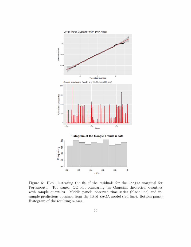
Figure 6: Plot illustrating the fit of the residuals for the Google marginal forPortsmouth. Top panel: QQ-plot comparing the Gaussian theoretical quantileswith sample quantiles. Middle panel: observed time series (black line) and in-sample predictions obtained from the fitted ZAGA model (red line). Bottom panel:Histogram of the resulting u-data.

22

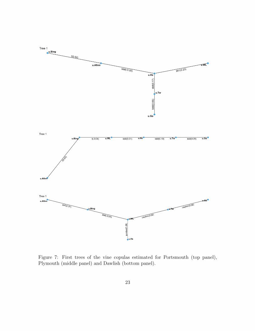
Figure 7: First trees of the vine copulas estimated for Portsmouth (top panel),Plymouth (middle panel) and Dawlish (bottom panel).

23

calculates predictions ignoring any association between environmental and onlineinformation.

Out-of-sample predictions based on the proposed model were constructed asillustrated in Section 3.3, considering the vine copula estimated as explained inSection 4.3 until the 15th February 2016 and using it to predict the period betweenthe 16th February 2016 and the 31st December 2016.

Tables 3 and 4 list the MSE and MIS values calculated for Portsmouth, Plymouthand Dawlish, in the top, middle and bottom panel, respectively, for each variable.The second columns show the results assuming independence among variables, thethird columns show the results assuming all Gaussian pair-copulas, and the fourthcolumns show the vine copula results. The MSEs and MISs of the best performingapproaches for each variable are highlighted in boldface. From Tables 3 and 4, wenotice that the vine copula approach outperforms the other two approaches in themajority of the cases. Comparing the three different locations, in Plymouth thevine copula exceeds the performance of the other two approaches for most of thevariables, whereas the independence approach is never selected. In Portsmouth theGaussian vine method achieves generally the best results, with the independenceapproach only selected in a few cases. In Dawlish, the vine and Gaussian copulamethods are preferred for several variables, although the independence approach isselected in a few cases. This might be due to the lack of social media informationfor Dawlish, compared to the other two locations, as shown in Figure 3, making itdifficult to define associations between online and environmental data and to leveragedata integration for predicting purposes.

The variables Hs and WL are generally better predicted by the vine method,as opposed to the independence approach, which assumes no dependence betweenany of the variables involved in the model. Hence, the independence approachindicates the absence of any association between the environmental and the socialmedia variables, implying the lack of contribution of online-generated informationin predicting the flood variables. On the contrary, the vine approach assumes thepresence of a dependence structure between the variables and, in particular, betweenthe environmental and social media insights. Therefore, the better performanceof the vine compared to the independence model demonstrates usefulness of socialmedia information in forecasting environmental variables.

The prediction of online-generated information also benefits from dataintegration. Google trends are more accurately forecasted by the vine copula method,or by the Gaussian approach in the Portsmouth case, rather than by the independentapproach. The prediction of Total tweets achieves generally better results withthe vine copula method for Plymouth data and with the Gaussian method for

24

Portsmouth data, while the independence approach is typically selected for Dawlishdata, due to the lack of information for this location, as explained above.

Comparing the sentiment scores, we notice that the vine copula approach isgenerally preferred with Afinn, while the Gaussian method is typically selected withBing. This is probably due to the fact that the Afinn lexicon is more sophisticatedthan Bing, since it scores words into several positive and negative categories, andhence provides more information.

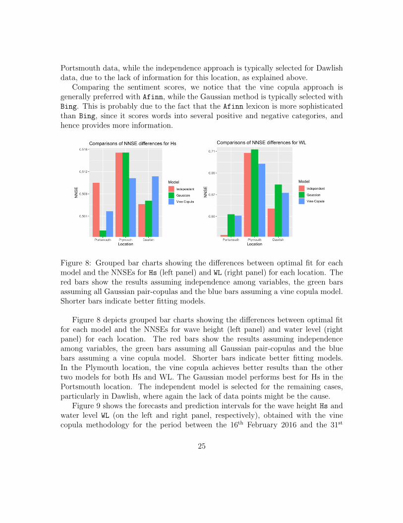
Figure 8: Grouped bar charts showing the differences between optimal fit for eachmodel and the NNSEs for Hs (left panel) and WL (right panel) for each location. Thered bars show the results assuming independence among variables, the green barsassuming all Gaussian pair-copulas and the blue bars assuming a vine copula model.Shorter bars indicate better fitting models.

Figure 8 depicts grouped bar charts showing the differences between optimal fitfor each model and the NNSEs for wave height (left panel) and water level (rightpanel) for each location. The red bars show the results assuming independenceamong variables, the green bars assuming all Gaussian pair-copulas and the bluebars assuming a vine copula model. Shorter bars indicate better fitting models.In the Plymouth location, the vine copula achieves better results than the othertwo models for both Hs and WL. The Gaussian model performs best for Hs in thePortsmouth location. The independent model is selected for the remaining cases,particularly in Dawlish, where again the lack of data points might be the cause.

Figure 9 shows the forecasts and prediction intervals for the wave height Hs andwater level WL (on the left and right panel, respectively), obtained with the vinecopula methodology for the period between the 16th February 2016 and the 31st

25

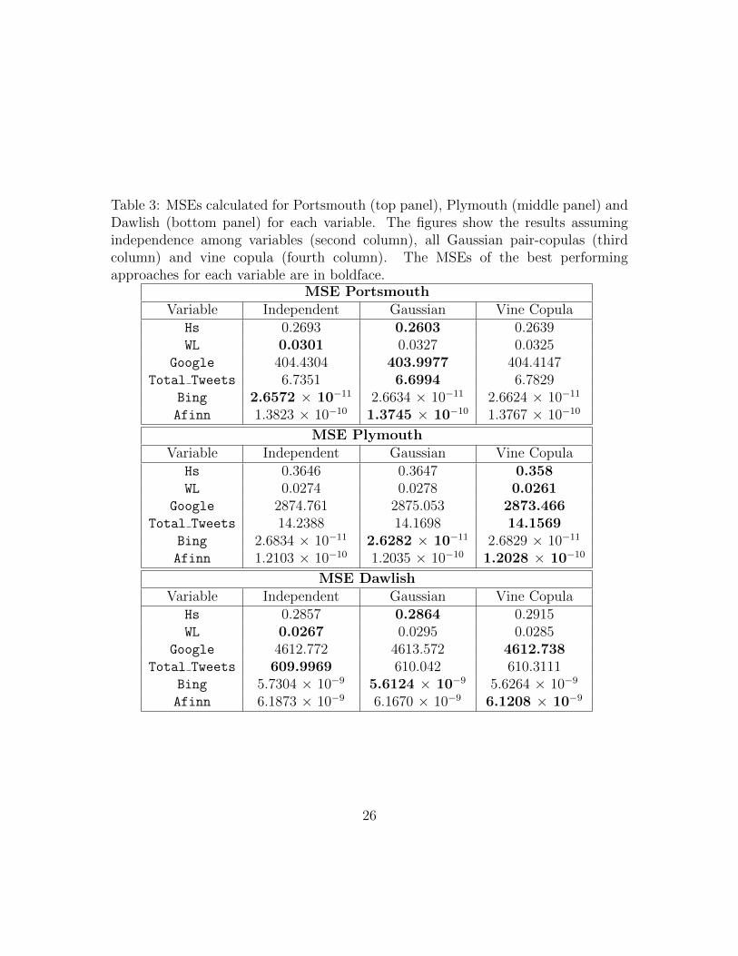
Table 3: MSEs calculated for Portsmouth (top panel), Plymouth (middle panel) andDawlish (bottom panel) for each variable. The figures show the results assumingindependence among variables (second column), all Gaussian pair-copulas (thirdcolumn) and vine copula (fourth column). The MSEs of the best performingapproaches for each variable are in boldface.

MSE PortsmouthVariable Independent Gaussian Vine Copula

Hs 0.2693 0.2603 0.2639WL 0.0301 0.0327 0.0325

Google 404.4304 403.9977 404.4147Total Tweets 6.7351 6.6994 6.7829

Bing 2.6572 × 10−11 2.6634 × 10−11 2.6624 × 10−11

Afinn 1.3823 × 10−10 1.3745 × 10−10 1.3767 × 10−10

MSE PlymouthVariable Independent Gaussian Vine Copula

Hs 0.3646 0.3647 0.358WL 0.0274 0.0278 0.0261

Google 2874.761 2875.053 2873.466Total Tweets 14.2388 14.1698 14.1569

Bing 2.6834 × 10−11 2.6282 × 10−11 2.6829 × 10−11

Afinn 1.2103 × 10−10 1.2035 × 10−10 1.2028 × 10−10

MSE DawlishVariable Independent Gaussian Vine Copula

Hs 0.2857 0.2864 0.2915WL 0.0267 0.0295 0.0285

Google 4612.772 4613.572 4612.738Total Tweets 609.9969 610.042 610.3111

Bing 5.7304 × 10−9 5.6124 × 10−9 5.6264 × 10−9

Afinn 6.1873 × 10−9 6.1670 × 10−9 6.1208 × 10−9

26

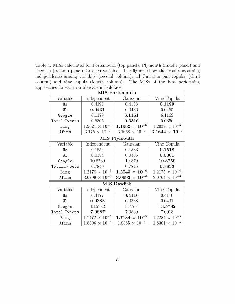
Table 4: MISs calculated for Portsmouth (top panel), Plymouth (middle panel) andDawlish (bottom panel) for each variable. The figures show the results assumingindependence among variables (second column), all Gaussian pair-copulas (thirdcolumn) and vine copula (fourth column). The MISs of the best performingapproaches for each variable are in boldface

MIS PortsmouthVariable Independent Gaussian Vine Copula

Hs 0.4193 0.4158 0.1199WL 0.0431 0.0436 0.0465

Google 6.1179 6.1151 6.1169Total Tweets 0.6366 0.6316 0.6356

Bing 1.2021 × 10−6 1.1982 × 10−6 1.2039 × 10−6

Afinn 3.175 × 10−6 3.1668 × 10−6 3.1644 × 10−6

MIS PlymouthVariable Independent Gaussian Vine Copula

Hs 0.1554 0.1533 0.1518WL 0.0384 0.0365 0.0361

Google 10.8789 10.879 10.8759Total Tweets 0.7849 0.7845 0.7833

Bing 1.2178 × 10−6 1.2043 × 10−6 1.2175 × 10−6

Afinn 3.0799 × 10−6 3.0693 × 10−6 3.0704 × 10−6

MIS DawlishVariable Independent Gaussian Vine Copula

Hs 0.4177 0.4116 0.4116WL 0.0383 0.0388 0.0431

Google 13.5782 13.5794 13.5782Total Tweets 7.0887 7.0889 7.0913

Bing 1.7472 × 10−5 1.7184 × 10−5 1.7284 × 10−5

Afinn 1.8396 × 10−5 1.8385 × 10−5 1.8301 × 10−5

27

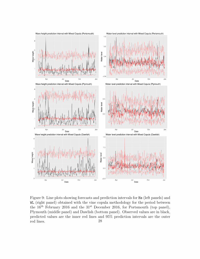
Figure 9: Line plots showing forecasts and prediction intervals for Hs (left panels) andWL (right panel) obtained with the vine copula methodology for the period betweenthe 16th February 2016 and the 31st December 2016, for Portsmouth (top panel),Plymouth (middle panel) and Dawlish (bottom panel). Observed values are in black,predicted values are the inner red lines and 95% prediction intervals are the outerred lines. 28

December 2016. The top panels depict the Portsmouth plots, the middle panelsdepict the Plymouth plots and the bottom panels depict the Dawlish plots. Theblack lines denote the observed values, the inner red lines denote the predicted valuesand the outer red lines denote the 95% prediction intervals. We notice that theforecasted water levels are in line with the observations, and the average dynamics ofwave height is adequately represented by the proposed model. Intervals predicted bythe vine copula method capture most of the dynamic of the environmental variables,indicating that the proposed methodology is able to leverage social media informationfor forecasting flood-related data.

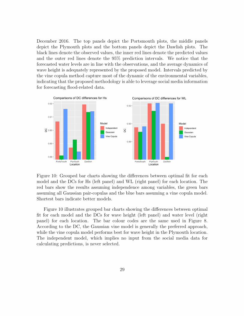
Figure 10: Grouped bar charts showing the differences between optimal fit for eachmodel and the DCs for Hs (left panel) and WL (right panel) for each location. Thered bars show the results assuming independence among variables, the green barsassuming all Gaussian pair-copulas and the blue bars assuming a vine copula model.Shortest bars indicate better models.

Figure 10 illustrates grouped bar charts showing the differences between optimalfit for each model and the DCs for wave height (left panel) and water level (rightpanel) for each location. The bar colour codes are the same used in Figure 8.According to the DC, the Gaussian vine model is generally the preferred approach,while the vine copula model performs best for wave height in the Plymouth location.The independent model, which implies no input from the social media data forcalculating predictions, is never selected.

29

5 Concluding Remarks

In this paper, we propose a new methodology aimed at obtaining more accurateforecasts, compared to traditional approaches, for variables measuring inundationsand floods events. The proposed methodology is based on the integration ofenvironmental variables collected via remote sensing with online generated socialmedia information. We obtained data at three different locations on the Southcoast of the UK, which were affected by severe storm events on several occasionsin the past few years. Together with wave height and water level information,we also gathered Google Trends searches and Twitter microblogging messagesinvolving keywords related to floods and storms. From the tweets, we considered thevolume as well as the sentiment scores, to investigate the feelings of people towardsinundation events. Our methodology is based on vine copulas, which are able tomodel the dependence structure between the marginals, and thus to take advantageof the association between social media and environmental variables. We testedour approach calculating out-of-sample predictions and comparing the vine copulamethod with two traditional approaches: the first based on a vine constructed withall Gaussian copulas, and the second based on independence between variables. Theresults show that the vine copula method outperforms the other two approaches inmost cases, demonstrating that our methodology is able to leverage social mediainformation to obtain more accurate predictions of floods and inundations thanthe other two approaches. In some cases, the Gaussian vine copula method isselected, showing that the vine data integration approach is still achieving thebest performance, although some variables are less affected by asymmetries and taildependence. Since social media information for Dawlish were lacking, they provideda more limited contribution to the prediction of the environmental variables for thislocation. The proposed methodology will support decision-makers enabling them touse knowledge gained from the model results to deepen their understanding of risksassociated to floods and optimise resources in a more effective and efficient way. Atstrategic level, the methodology could be used to validate resource deployments inresponse to threats from floods; while at operational level, the methodology couldassist to improve the effectiveness of civil contingency responses to flood events.

Further investigations involving other locations and including additional socialmedia information will be the object of future work. Also, we will explore the useof the results of the study to validate inundation modes. Another extension willinvolve Bayesian inference, which would allow us to incorporate other information,such as experts’ opinion, in the model. In addition, the use of more sophisticatedmachine learning approaches could be envisaged for deriving the sentiment variables

30

to improve the proposed methodology.

Acknowledgements

The authors are grateful to the anonymous Reviewers for their useful commentswhich significantly improved the quality of the paper. This work was supportedby the European Regional Development Fund project Environmental Futures & BigData Impact Lab, funded by the European Structural and Investment Funds, grantnumber 16R16P01302 .

References

Aas, K., C. Czado, A. Frigessi, and H. Bakken (2009). Pair-copula constructions ofmultiple dependence. Insurance: Mathematics and economics 44 (2), 182–198.

Alam, F., F. Ofli, and M. Imran (2018). Crisismmd: Multimodal twitter datasetsfrom natural disasters. In Proceedings of the International AAAI Conference onWeb and Social Media, Volume 12.

Arthur, R., C. A. Boulton, H. Shotton, and H. T. Williams (2018). Social sensing offloods in the uk. PloS one 13 (1), e0189327.

Balogun, A., S. Quan, B. Pradhan, U. Dano, and S. Yekeen (2020). An improvedflood susceptibility model for assessing the correlation of flood hazard and propertyprices using geospatial technology and fuzzy-anp. Journal of EnvironmentalInformatics .

Bevacqua, E., D. Maraun, I. Hobæk Haff, M. Widmann, and M. Vrac(2017). Multivariate statistical modelling of compound events via pair-copulaconstructions: analysis of floods in ravenna (italy). Hydrology and Earth SystemSciences 21 (6), 2701–2723.

Brouwer, T., D. Eilander, A. v. Loenen, M. J. Booij, K. M. Wijnberg, J. S. Verkade,and J. Wagemaker (2017). Probabilistic flood extent estimates from social mediaflood observations. Natural Hazards and Earth System Sciences 17 (5), 735–747.

Couasnon, A., A. Sebastian, and O. Morales-Napoles (2018). A copula-basedbayesian network for modeling compound flood hazard from riverine and coastalinteractions at the catchment scale: An application to the houston ship channel,texas. Water 10 (9), 1190.

31

Czado, C. (2019). Analyzing dependent data with vine copulas. Lecture Notes inStatistics, Springer .

De Albuquerque, J. P., B. Herfort, A. Brenning, and A. Zipf (2015). A geographicapproach for combining social media and authoritative data towards identifyinguseful information for disaster management. International journal of geographicalinformation science 29 (4), 667–689.

Dissmann, J., E. C. Brechmann, C. Czado, and D. Kurowicka (2013). Selecting andestimating regular vine copulae and application to financial returns. ComputationalStatistics & Data Analysis 59, 52–69.

Feng, Y., P. Shi, S. Qu, S. Mou, C. Chen, and F. Dong (2020). Nonstationaryflood coincidence risk analysis using time-varying copula functions. Scientificreports 10 (1), 1–12.

Field, C. B., V. Barros, T. F. Stocker, and Q. Dahe (2012). Managing the risks ofextreme events and disasters to advance climate change adaptation: special reportof the intergovernmental panel on climate change. Cambridge University Press.

Gneiting, T. and A. E. Raftery (2007). Strictly proper scoring rules, prediction, andestimation. Journal of the American statistical Association 102 (477), 359–378.

Grego, J. M., P. A. Yates, and K. Mai (2015). Standard error estimation for mixedflood distributions with historic maxima. Environmetrics 26 (3), 229–242.

Heffernan, J. E. and J. A. Tawn (2004). A conditional approach for multivariateextreme values (with discussion). Journal of the Royal Statistical Society: SeriesB (Statistical Methodology) 66 (3), 497–546.

Herfort, B., J. P. de Albuquerque, S.-J. Schelhorn, and A. Zipf (2014). Exploringthe geographical relations between social media and flood phenomena to improvesituational awareness. In Connecting a digital Europe through location and place,pp. 55–71. Springer.

Hu, M. and B. Liu (2004). Mining and summarizing customer reviews. In Proceedingsof the tenth ACM SIGKDD international conference on Knowledge discovery anddata mining, pp. 168–177.

Huang, K., L. Dai, M. Yao, Y. Fan, and X. Kong (2017). Modelling dependencebetween traffic noise and traffic flow through an entropy-copula method. Journalof Environmental Informatics 29 (2).

32

Hyndman, R. J. and G. Athanasopoulos (2018). Forecasting: principles and practice.OTexts.

Jane, R., L. Dalla Valle, D. Simmonds, and A. Raby (2016). A copula-based approachfor the estimation of wave height records through spatial correlation. CoastalEngineering 117, 1–18.

Jane, R. A., D. J. Simmonds, B. P. Gouldby, J. D. Simm, L. Dalla Valle, and A. C.Raby (2018). Exploring the potential for multivariate fragility representations toalter flood risk estimates. Risk Analysis 38 (9), 1847–1870.

Joe, H. (1997). Multivariate models and multivariate dependence concepts. CRCPress.

Joe, H. and J. J. Xu (1996). The estimation method of inference functions formargins for multivariate models. Technical Report 166, Department of Statistics,University of British Columbia.

Keef, C., J. A. Tawn, and R. Lamb (2013). Estimating the probability of widespreadflood events. Environmetrics 24 (1), 13–21.

Latif, S. and F. Mustafa (2020). Parametric vine copula construction for floodanalysis for kelantan river basin in malaysia. Civil Engineering Journal 6 (8),1470–1491.

Li, Z., C. Wang, C. T. Emrich, and D. Guo (2018). A novel approach to leveragingsocial media for rapid flood mapping: a case study of the 2015 south carolinafloods. Cartography and Geographic Information Science 45 (2), 97–110.

Mason, D. C., I. J. Davenport, J. C. Neal, G. J.-P. Schumann, and P. D. Bates (2012).Near real-time flood detection in urban and rural areas using high-resolutionsynthetic aperture radar images. IEEE transactions on Geoscience and RemoteSensing 50 (8), 3041–3052.

Massicotte, P. and D. Eddelbuettel (2021). gtrendsR: Perform and Display GoogleTrends Queries. R package version 1.4.8.

Moishin, M., R. C. Deo, R. Prasad, N. Raj, and S. Abdulla (2020). Development offlood monitoring index for daily flood risk evaluation: case studies in fiji. StochasticEnvironmental Research and Risk Assessment , 1–16.

33

Muller, C., L. Chapman, S. Johnston, C. Kidd, S. Illingworth, G. Foody, A. Overeem,and R. Leigh (2015). Crowdsourcing for climate and atmospheric sciences: Currentstatus and future potential. International Journal of Climatology 35 (11), 3185–3203.

Nagler, T. and T. Vatter (2021). rvinecopulib: High Performance Algorithms forVine Copula Modeling. R package version 0.5.5.1.1.

Nash, J. E. and J. V. Sutcliffe (1970). River flow forecasting through conceptualmodels part i—a discussion of principles. Journal of hydrology 10 (3), 282–290.

Nelsen, R. B. (2007). An introduction to copulas. Springer Science & Business Media.

R Core Team (2020). R: A Language and Environment for Statistical Computing.Vienna, Austria: R Foundation for Statistical Computing.

Rigby, R. A. and D. M. Stasinopoulos (2005). Generalized additive models forlocation, scale and shape. Journal of the Royal Statistical Society: Series C(Applied Statistics) 54 (3), 507–554.

Rigby, R. A., M. D. Stasinopoulos, G. Z. Heller, and F. De Bastiani (2019).Distributions for modeling location, scale, and shape: Using GAMLSS in R. CRCpress.

Rosser, J. F., D. Leibovici, and M. Jackson (2017). Rapid flood inundation mappingusing social media, remote sensing and topographic data. Natural Hazards 87 (1),103–120.

Santos, V. M., T. Wahl, R. Jane, S. K. Misra, and K. D. White (2021). Assessingcompound flooding potential with multivariate statistical models in a complexestuarine system under data constraints. Journal of Flood Risk Management ,e12749.

Saravanou, A., G. Valkanas, D. Gunopulos, and G. Andrienko (2015). Twitter floodswhen it rains: a case study of the uk floods in early 2014. In Proceedings of the24th International Conference on World Wide Web, pp. 1233–1238.

Schumann, G., P. D. Bates, M. S. Horritt, P. Matgen, and F. Pappenberger (2009).Progress in integration of remote sensing–derived flood extent and stage data andhydraulic models. Reviews of Geophysics 47 (4).

34

Sibley, A., D. Cox, and H. Titley (2015). Coastal flooding in england and wales fromatlantic and north sea storms during the 2013/2014 winter. Weather 70 (2), 62–70.

Silge, J. and D. Robinson (2016). tidytext: Text mining and analysis using tidy dataprinciples in R. Journal of Statistical Software 1 (3).

Simard, C. and B. Remillard (2015). Forecasting time series with multivariatecopulas. Dependence modeling 3 (1).

Sklar, M. (1959). Fonctions de repartition a n dimensions et leurs marges.Publications de l’Institut de Statistique de l’Universite de Paris 8, 229–231.

Smith, L., Q. Liang, P. James, and W. Lin (2017). Assessing the utility of socialmedia as a data source for flood risk management using a real-time modellingframework. Journal of Flood Risk Management 10 (3), 370–380.

Spielhofer, T., R. Greenlaw, D. Markham, and A. Hahne (2016). Data miningtwitter during the uk floods: Investigating the potential use of social media inemergency management. In 2016 3rd International Conference on Informationand Communication Technologies for Disaster Management (ICT-DM), pp. 1–6.IEEE.

Spruce, M. D., R. Arthur, J. Robbins, and H. T. Williams (2021). Social sensingof high-impact rainfall events worldwide: A benchmark comparison againstmanually curated impact observations. Natural Hazards and Earth System SciencesDiscussions , 1–31.

Szekely, G. J., M. L. Rizzo, and N. K. Bakirov (2007). Measuring and testingdependence by correlation of distances. The annals of statistics 35 (6), 2769–2794.

Talukdar, S., B. Ghose, R. Salam, S. Mahato, Q. B. Pham, N. T. T. Linh,R. Costache, M. Avand, et al. (2020). Flood susceptibility modeling in teestariver basin, bangladesh using novel ensembles of bagging algorithms. StochasticEnvironmental Research and Risk Assessment 34 (12), 2277–2300.

Tosunoglu, F., F. Gurbuz, and M. N. Ispirli (2020). Multivariate modeling of floodcharacteristics using vine copulas. Environmental Earth Sciences 79 (19), 1–21.

UN (2015). The human cost of weather related disasters 1995–2015, United Nations,Geneva, Switzerland, 30 pp.

35

Wang, X. and C. Du (2003). An internet based flood warning system. Journal ofEnvironmental Informatics 2 (1), 48–56.

Ward, P. J., A. Couasnon, D. Eilander, I. D. Haigh, A. Hendry, S. Muis, T. I.Veldkamp, H. C. Winsemius, and T. Wahl (2018). Dependence between high sea-level and high river discharge increases flood hazard in global deltas and estuaries.Environmental Research Letters 13 (8), 084012.

36