NBER WORKING PAPER SERIES

SOCIAL LEARNING AND PEER EFFECTS IN CONSUMPTION:EVIDENCE FROM MOVIE SALES

Enrico Moretti

Working Paper 13832http://www.nber.org/papers/w13832

NATIONAL BUREAU OF ECONOMIC RESEARCH1050 Massachusetts Avenue

Cambridge, MA 02138March 2008

I thank Jerome Adda, David Ahn, Raj Chetty, Roger Gordon, Bryan Graham, David Levine, RobertMcMillan, Stefano Della Vigna and seminar participants at Bank of Italy, Berkeley, Cornell, ChicagoGSB, Nuremberg, LSE, Crest-Paris, Regensburg, San Diego, UCL and Zurich for helpful comments.I am grateful to Stefano Della Vigna, and Phillip Leslie for sharing their box office data. GregorioCaetano, Mariana Carrera, Ashley Langer, David Klein and Erin Metcalf provided excellent researchassistance. The views expressed herein are those of the author(s) and do not necessarily reflect theviews of the National Bureau of Economic Research.

NBER working papers are circulated for discussion and comment purposes. They have not been peer-reviewed or been subject to the review by the NBER Board of Directors that accompanies officialNBER publications.

© 2008 by Enrico Moretti. All rights reserved. Short sections of text, not to exceed two paragraphs,may be quoted without explicit permission provided that full credit, including © notice, is given tothe source.

Social Learning and Peer Effects in Consumption: Evidence from Movie SalesEnrico MorettiNBER Working Paper No. 13832March 2008JEL No. J0,L15

ABSTRACT

Using box-office data for all movies released between 1982 and 2000, I test the implications of a simplemodel of social learning in which the consumption decisions of individuals depend on informationthey receive from their peers. The model predicts different box office sales dynamics depending onwhether opening weekend demand is higher or lower than expected. I use a unique feature of the movieindustry to identify ex-ante demand expectations: the number of screens dedicated to a movie in itsopening weekend reflects the sales expectations held by profit-maximizing theater owners. Severalpieces of evidence are consistent with social learning. First, sales of movies with positive surpriseand negative surprise in opening weekend demand diverge over time. If a movie has better than expectedappeal and therefore experiences larger than expected sales in week 1, consumers in week 2 updateupward their expectations of quality, further increasing week 2 sales. Second, this divergence is smallfor movies for which consumers have strong priors and large for movies for which consumers haveweak priors. Third, the effect of a surprise is stronger for audiences with large social networks. Finally,consumers do not respond to surprises in first week sales that are orthogonal to movie quality, likeweather shocks. Overall, social learning appears to be an important determinant of sales in the movieindustry, accounting for 38% of sales for the typical movie with positive surprise. This implies theexistence of a large "social multiplier'' such that the elasticity of aggregate demand to movie qualityis larger than the elasticity of individual demand to movie quality.

Enrico MorettiUniversity of California, BerkeleyDepartment of Economics549 Evans HallBerkeley, CA 94720-3880and NBERmoretti@econ.berkeley.edu

1 Introduction

The goal of this paper is to test whether the consumption decisions of individuals depend

on information they receive from their peers when product quality is difficult to observe

in advance. I focus on situations where quality is ex-ante uncertain and consumers hold

a prior on quality, which they may update based on information from their peers. This

information may come from direct communication with peers who have already consumed

the good. Alternatively, it may arise from the observation of peers’ purchasing decisions.

If every individual receives an independent signal of the goods quality, then the purchasing

decision of one consumer provides valuable information to other consumers, as individuals

use the information contained in others’ actions to update their own expectations on quality.

This type of social learning is potentially relevant for many experience goods like movies,

books, restaurants, or legal services. Informational cascades are particularly important for

new products. For the first few years of its existence, Google experienced exponential accel-

eration in market share. This acceleration, which displayed hallmarks of contagion dynamics,

was mostly due to word of mouth and occurred without any advertising on the part of Google

(Vise, 2005).

Social learning in consumption has enormous implications for firms. In the presence of

informational cascades, the return to attracting a new customer is different from the direct

effect that the customer has on profits. Attracting a new consumer has a multiplier effect on

profits because it may increase the demand of other consumers. The existence of this “social

multiplier” (Glaeser, Sacerdote and Scheinkman, 2003) implies that, for a given good, the

elasticity of aggregate demand to quality is larger than the elasticity of individual demand

to quality. Furthermore, social learning makes the success of a product more difficult to

predict, as demand depends on (potentially random) initial conditions. Two products of

similar quality may have vastly different demand in the long run, depending on whether the

initial set of potential consumers happens to like the product or not.

Social learning has been extensively studied in theory (Bikhchandani et al., 1992 and

1998; Banerjee, 1992). But despite its tremendous importance for firms, the empirical ev-

idence is limited, because social learning is difficult to identify in practice. The standard

approach in the literature on peer effects and social interactions involves testing whether

an individual decision to purchase a particular good depends on the consumption decisions

and/or the product satisfaction of other individuals that are close, based on some metric.

Such an approach is difficult to implement in most cases. First, data on purchases of specific

goods by individual consumers are difficult to obtain. Second, because preferences are likely

to be correlated among peers, observing that individuals in the same group make similar

consumption decisions may simply reflect shared preferences, not informational spillovers.

In observational data, it is difficult to isolate factors that affect some individuals’ demand

for a good but not the demand of their peers.1

1Randomized experiments may offer a solution. Salganik et al. (2006) set up a web site for music

1

In this paper, I focus on consumption of movies. Since individual-level data are not

available, I use market-level data to test the predictions of a simple model that characterizes

the diffusion of information on movie quality following surprises in quality. In the model,

the quality of a movie is ex-ante uncertain, as consumers do not know for certain whether

they will like the movie or not.2 Consumers have a prior on quality–based on observable

characteristics of the movie such as the genre, actors, director, ratings and budget, etc.–and

they receive an individual-specific, unbiased signal on quality–which reflects how much the

concept of a movie resonates with a specific consumer.

I define social learning as a situation where consumers in week t update their prior based

on feedback from others who have seen the movie in previous weeks. The model predicts

different box office sales dynamics depending on whether a movie’s underlying quality is

better or worse than people’s expectations. Because the signal that each consumer receives

is unbiased, movies that have better than expected underlying quality have stronger than

expected demand in the opening weekend (on average). In the presence of social learning,

they become even more successful over time, as people update upwards their expectations

on quality. On the other hand, movies that have worse than expected quality have weaker

than expected demand in the opening weekend (on average) and become even less successful

over time. In other words, social learning should make successful movies more successful

and unsuccessful movies more unsuccessful. By contrast, without social learning, there is

no updating of individual expectations, and therefore there should be no divergence in sales

over time.

Surprises in the appeal of a movie are key to the empirical identification. I use a unique

feature of the movie industry to identify ex-ante demand expectations: the number of screens

dedicated to a movie in its opening weekend reflects the sales expectations held by the market.

The number of screens is a good summary measure of ex-ante demand expectations because it

is set by forward-looking, profit-maximizing agents–the theater owners–who have an incentive

to correctly predict first week demand. The number of screens should therefore reflect most

of the information that is available to the market before the opening on the expected appeal

of the movie, including actors, director, budget, ratings, advertising, reviews, competitors,

and every other demand shifter that is observed before opening day.3

While on average theaters predict first week demand correctly, there are cases where

they underpredict or overpredict the appeal of a movie. Take, for example, the movie

“Pretty Woman” (1990). Before the opening weekend it was expected to perform well,

since it opened in 1325 screens, more than the average movie. But in the opening weekend it

downloading where users are randomly provided with different amount of information on other users’ ratings.

Cai, Chen and Fang (2007) use a randomized experiment to study learning on menu items in restaurants.2Throughout the paper, the term quality refers to consumers’ utility. It has no reference to artistic value.3Some empirical tests lend credibility to this assumption. For example, in a regression that has opening

weekend sales as dependent variable, the inclusion of very detailed set of movie characteristics–budget,

genre, ratings, date of release, distributor, etc.–add virtually no predictive power once number of screens is

controlled for.

2

significantly exceeded expectations, totalling sales of about $23 million. In this case, demand

was significantly above what the market was expecting, presumably because the concept of

the movie or the look of Julia Roberts appealed to consumers more than one could have

predicted before the opening.

Using data on nation-wide sales by week for all movies released between 1982 and 2000,

I test five empirical implications of the model.

(1) In the presence of social learning, sales trends for positive and negative surprise movies

should diverge over time. Consistent with this hypothesis, I find that the decline over time

of sales for movies with positive surprise is substantially slower than the decline of movies

with negative surprise. This finding is robust to controlling for advertising expenditures and

critic reviews, and to a number of alternative specifications. Moreover, the finding does not

appear to be driven by changes in supply or capacity constraints. For example, results are

not sensitive to using per-screen sales as the dependent variable instead of sales or dropping

movies that sell out in the opening weekend.

(2) The new information contained in peer feedback should be more important when

consumers have more diffuse priors. When a consumer is less certain whether she is going

to like a specific movie, the additional information represented by peer feedback on movie

quality should have more of an effect on her purchasing choices relative to the case where

the consumer is more certain. In practice, to identify movies for which consumers have more

precise priors, I use a dummy for sequels. It is reasonable to expect that consumers have

more precise priors for sequels than non-sequels. Additionally, to generalize this idea, I use

the variance of the first week surprise in box office sales by genre. Genres with large variance

in first week surprise are characterized by more uncertainty and therefore consumers should

have more diffuse priors on their quality. Consistent with social learning, I find that the

impact of a surprise on subsequent sales is significantly smaller for sequels and significantly

larger for genres that have a large variance in first week surprise.

(3) Social learning should be stronger for consumers with a large social network and

weaker for consumers with a small social network. While I do not have a direct measure of

social network, I assume that teenagers have more developed social networks than adults.

Consistent with social learning, I find that the effect of a surprise on subsequent sales is

larger for movies that target teenage audiences.

(4) Under social learning, surprises in opening weekend demand should only matter

insofar as they reflect new information on movie quality. They should not matter when they

reflect factors that are unrelated to movie quality, such as weather shocks. This prediction

is important because it allows one to separate social learning from a leading alternative

explanation of the evidence, the network effects hypothesis. This hypothesis posits that

the utility of watching a movie depends on the number of peers who have seen it or will

see it (for example, because people like discussing movies with friends). This implies that

each consumer’s demand for a good depends directly on the demand of other consumers.

To distinguish between network effects and social learning, I isolate surprises in first week

3

sales that are caused by weather shocks. Under social learning, a negative surprise in first

week demand due to bad weather should have no significant impact on sales in the following

weeks. Weather is unrelated to movie quality and therefore should not induce any updating.

By contrast, under the network effect hypothesis, a negative surprise in first week demand

for any reason, including bad weather, should lower sales in following weeks. Empirically, I

find no significant effect of surprises due to weather on later sales.

(5) Finally, the marginal amount of learning should decline over time, as more information

on quality becomes available. For example, the amount of updating that takes place in week

2 should be larger than the amount of updating that takes place in week 3 given what is

already known in week 2. Consistent with this prediction, I find that sales trends for positive

surprise movies are concave, and sales trends for negative surprise movies are convex.

Overall, the five implications of the model seem remarkably consistent with the data.

Taken individually, each piece of empirical evidence may not be sufficient to establish the

existence of social learning. But taken together, the weight of the evidence supports the

notion of social learning.

My estimates suggest that the amount of sales generated by social learning is substantial.

A movie with stronger than expected demand has $5.8 million in additional sales relative to

the counterfactual where the quality of the movie is the same but consumers don’t learn from

each other. This amounts to 38% of total revenues. From the point of view of the studios,

this implies the existence of a large multiplier. The total effect on profits of attracting an

additional consumer to see a given movie is significantly larger than the direct effect on

profits, because that consumer, if satisfied with the quality of the movie, will increase her

peers’ demand for the same movie.

Besides the substantive findings specific to the movie industry, this paper seeks to make

a broader methodological contribution. It demonstrates that it is possible to identify social

interactions using aggregate data and intuitive comparative statics. In situations where

individual-level, exogenous variation in peer group attributes is not available, this approach

has the potential to provide a credible alternative for the identification of social interactions.

Possible additional applications include studying social learning in the demand for books

(where the size of the first print provides a good measure of expected demand), music,

restaurants, cars or software. This paper is related to the earlier literature on technology

adoption, where diffusion models similar to the one developed here were used to document

the spreading of new technologies based on peer imitation (Griliches, 1957; Bass 1969). A

similar approach has been applied in an interesting recent study of political presidential

primaries (Knight and Schiff, 2007).4

4Knight and Schiff (2007) find that a stronger than expected performance of a candidate in an early voting

state leads voters in other states to update their priors. Examples of existing papers on social learning in

consumption include: Liu (2006), who studies word-of-mouth effects in movies by measuring Internet postings

on a Yahoo Web Site; De Vaney and Cassey (2001), who present an analysis of the dynamics of box office

sales; Grinblatt, Keloharju, and Ikaheimo (2004), who use data on car purchases to estimate the effect of

4

The paper proceeds as follows. In sections 2 and 3 I outline a simple theoretical model

and its empirical implications. In sections 4 and 5 I describe the data and the empirical

identification of surprises. In sections 6 and 7 I describe my empirical findings. Section 8

concludes.

2 A Simple Model of Social Learning

In this section, I outline a simple framework that describes the effect of social learning

on sales. The idea–similar to the one adopted by Bikhchandani et al. (1992) and Banerjee

(1992)–is very simple. Consumers do not know in advance how much they are going to like

a movie. Before the opening weekend, consumers share a prior on the quality of the movie–

based on its observable characteristics–and they receive a private, unbiased signal on quality,

which reflects how much the concept of a movie resonates with a specific consumer. Expected

utility from consumption is a weighted average of the prior and the signal (where the weight

reflects the relative precision of the prior and the signal). Since the consumers’ private signal

is unbiased, high quality movies have on average a stronger appeal and therefore stronger

opening weekend sales, relative to low quality movies.

In week 2, consumers have more information, since they receive feedback from their peers

who have seen the movie in week 1. I define social learning as the process by which individuals

use feedback from their peers to update their own expectations of movie quality. In the

presence of social learning, a consumers expectation of consumption utility is a weighted

average of the prior, the signal and peer feedback, where, as before, the weights reflect

relative precisions. If a movie is better (worse) than expected, consumers in week 2 update

upward (downward) their expectations and therefore even more (less) consumers decide to

see the movie.

This setting generates the prediction that under social learning a movie whose demand

is unexpectedly strong (weak) in the opening weekend should do even better (worse) in the

following weeks. Without social learning, there is no reason for this divergence over time.

The setting also generates four additional comparative statics predictions that have to do

with the precision of the prior, the size of the social network, the functional form of movie

sales and the role of surprises that are orthogonal to quality.5

neighbors’ purchase decisions; and Sorensen (2007), who uses a dataset of university employees to document

social learning in health plan choices. Hendricks and Sorensen (2007) use a clever identification strategy

based on new album releases to analyze the role of information in music purchases. Bertrand, Mullainathan

and Luttmer (2000) and Hong, Kubik and Stein (2005) document social learning in welfare participation

and portfolio choices, respectively.5One difference with Banerjee (1992) and Bikhchandani et al. (1992) is that they focus on the conditions

that generate wrong cascades, where a good of high quality is not purchased because the first consumers

who consider the purchase receive a bad signal, and everybody else after them is affected by their decision.

Wrong equilibria are unlikely to be pervasive in my empirical application, because I use a large sample with

nation-wide data. While it is possible that some groups of friends end up in the wrong equilibrium, this is

5

The focus of the paper is empirical. The purpose of this section is only to formalize a

simple intuition, not to provide a general theoretical treatment of social learning. Therefore,

the model is designed to be simple and to generate transparent and testable predictions to

bring to the data. I follow Bikhchandani et al. (1992) and take the timing of consumption

as exogenous. I purposely do not attempt to model possible generalizations such as strategic

behavior or the value of waiting to obtain more information (option value).

2.1 Sales Dynamics With No Social Learning

The utility that individual i obtains from watching movie j is

Uij = α∗j + νij (1)

where α∗j represents the quality of the movie for the average individual, and νij ∼ N(0, 1

d)

represents how tastes of individual i for movie j differ from the tastes of the average individual.

I assume that α∗j , and νij are unobserved. Given the characteristics of a movie that are ob-

served prior to its release, individuals hold a prior on the quality of the movie. In particular,

I assume that

α∗j ∼ N(X ′

jβ,1

mj) (2)

where X ′jβ represents consumers’ priors on how much they will like movie j. Specifically,

the vector Xj includes the characteristics of movie j that are observable before its release,

including its genre, budget, director, actors, ratings, distribution, date of release, advertising,

etc.; and mj is the precision of the prior, which is allowed to vary across movies. The reason

for differences in the precision of the prior is that the amount of information available to

consumers may vary across movies. For example, if a movie is a sequel, consumers may have

a tighter prior than if a movie is not a sequel.

Before the release of the movie, I assume that each individual also receives a noisy,

idiosyncratic signal of the quality of the movie:

sij = Uij + εij (3)

I interpret this signal as a measure of how much the concept of movie j resonates with

consumer i. I assume that the signal is unbiased within a given movie and is normally

distributed with precision kj:

εij ∼ N(0,1

kj

) (4)

The assumption that the prior and signal are unbiased is important because it ensures that,

while there is uncertainty for any given individual on the true quality of the movie, on

average individuals make the correct decisions regarding each movie. I also assume that νij

unlikely to be true systematically for the entire nation.

6

and εij are i.i.d. and independent of each other and independent of α∗j ; that Xj, β, mj, kj

and d are known to all the consumers; and that consumers do not share their private signal.

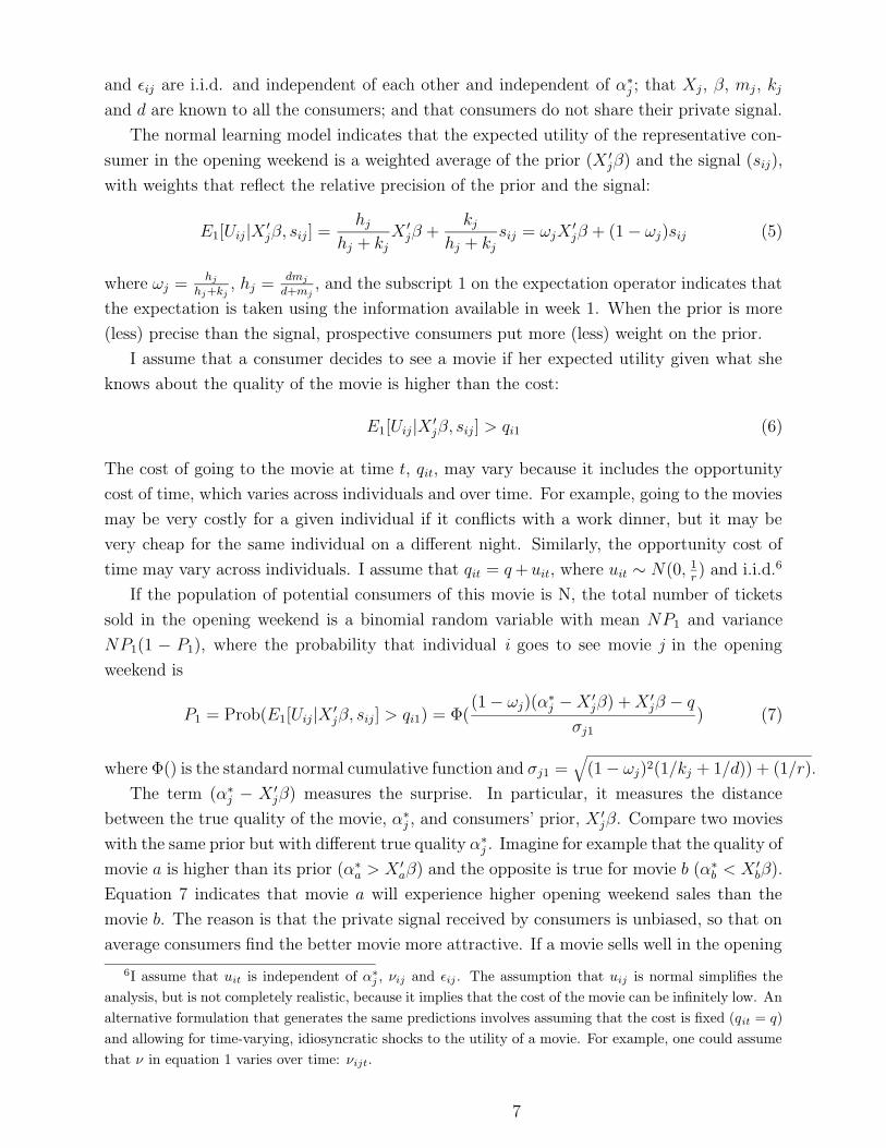
The normal learning model indicates that the expected utility of the representative con-

sumer in the opening weekend is a weighted average of the prior (X ′jβ) and the signal (sij),

with weights that reflect the relative precision of the prior and the signal:

E1[Uij|X ′jβ, sij ] =

hj

hj + kjX ′

jβ +kj

hj + kjsij = ωjX

′jβ + (1 − ωj)sij (5)

where ωj =hj

hj+kj, hj =

dmj

d+mj, and the subscript 1 on the expectation operator indicates that

the expectation is taken using the information available in week 1. When the prior is more

(less) precise than the signal, prospective consumers put more (less) weight on the prior.

I assume that a consumer decides to see a movie if her expected utility given what she

knows about the quality of the movie is higher than the cost:

E1[Uij|X ′jβ, sij] > qi1 (6)

The cost of going to the movie at time t, qit, may vary because it includes the opportunity

cost of time, which varies across individuals and over time. For example, going to the movies

may be very costly for a given individual if it conflicts with a work dinner, but it may be

very cheap for the same individual on a different night. Similarly, the opportunity cost of

time may vary across individuals. I assume that qit = q + uit, where uit ∼ N(0, 1r) and i.i.d.6

If the population of potential consumers of this movie is N, the total number of tickets

sold in the opening weekend is a binomial random variable with mean NP1 and variance

NP1(1 − P1), where the probability that individual i goes to see movie j in the opening

weekend is

P1 = Prob(E1[Uij|X ′jβ, sij] > qi1) = Φ(

(1 − ωj)(α∗j − X ′

jβ) + X ′jβ − q

σj1

) (7)

where Φ() is the standard normal cumulative function and σj1 =√

(1 − ωj)2(1/kj + 1/d)) + (1/r).

The term (α∗j − X ′

jβ) measures the surprise. In particular, it measures the distance

between the true quality of the movie, α∗j , and consumers’ prior, X ′

jβ. Compare two movies

with the same prior but with different true quality α∗j . Imagine for example that the quality of

movie a is higher than its prior (α∗a > X ′

aβ) and the opposite is true for movie b (α∗b < X ′

bβ).

Equation 7 indicates that movie a will experience higher opening weekend sales than the

movie b. The reason is that the private signal received by consumers is unbiased, so that on

average consumers find the better movie more attractive. If a movie sells well in the opening

6I assume that uit is independent of α∗j , νij and εij . The assumption that uij is normal simplifies the

analysis, but is not completely realistic, because it implies that the cost of the movie can be infinitely low. An

alternative formulation that generates the same predictions involves assuming that the cost is fixed (qit = q)

and allowing for time-varying, idiosyncratic shocks to the utility of a movie. For example, one could assume

that ν in equation 1 varies over time: νijt.

7

week it is because the movie is of good quality and therefore many people received a good

signal.

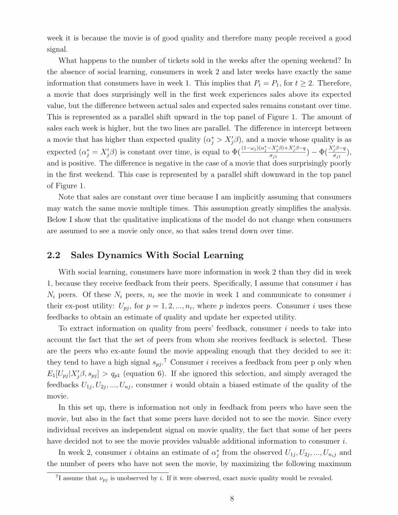
What happens to the number of tickets sold in the weeks after the opening weekend? In

the absence of social learning, consumers in week 2 and later weeks have exactly the same

information that consumers have in week 1. This implies that Pt = P1, for t ≥ 2. Therefore,

a movie that does surprisingly well in the first week experiences sales above its expected

value, but the difference between actual sales and expected sales remains constant over time.

This is represented as a parallel shift upward in the top panel of Figure 1. The amount of

sales each week is higher, but the two lines are parallel. The difference in intercept between

a movie that has higher than expected quality (α∗j > X ′

jβ), and a movie whose quality is as

expected (α∗j = X ′

jβ) is constant over time, is equal to Φ((1−ωj)(α∗

j−X′

jβ)+X′

jβ−q

σj1) − Φ(

X′

jβ−q

σj1),

and is positive. The difference is negative in the case of a movie that does surprisingly poorly

in the first weekend. This case is represented by a parallel shift downward in the top panel

of Figure 1.

Note that sales are constant over time because I am implicitly assuming that consumers

may watch the same movie multiple times. This assumption greatly simplifies the analysis.

Below I show that the qualitative implications of the model do not change when consumers

are assumed to see a movie only once, so that sales trend down over time.

2.2 Sales Dynamics With Social Learning

With social learning, consumers have more information in week 2 than they did in week

1, because they receive feedback from their peers. Specifically, I assume that consumer i has

Ni peers. Of these Ni peers, ni see the movie in week 1 and communicate to consumer i

their ex-post utility: Upj, for p = 1, 2, ..., ni, where p indexes peers. Consumer i uses these

feedbacks to obtain an estimate of quality and update her expected utility.

To extract information on quality from peers’ feedback, consumer i needs to take into

account the fact that the set of peers from whom she receives feedback is selected. These

are the peers who ex-ante found the movie appealing enough that they decided to see it:

they tend to have a high signal spj.7 Consumer i receives a feedback from peer p only when

E1[Upj|X ′jβ, spj ] > qp1 (equation 6). If she ignored this selection, and simply averaged the

feedbacks U1j, U2j, ..., Unj, consumer i would obtain a biased estimate of the quality of the

movie.

In this set up, there is information not only in feedback from peers who have seen the

movie, but also in the fact that some peers have decided not to see the movie. Since every

individual receives an independent signal on movie quality, the fact that some of her peers

have decided not to see the movie provides valuable additional information to consumer i.

In week 2, consumer i obtains an estimate of α∗j from the observed U1j, U2j, ..., Unij and

the number of peers who have not seen the movie, by maximizing the following maximum

7I assume that νpj is unobserved by i. If it were observed, exact movie quality would be revealed.

8

likelihood function:

Lij2 = L[U1j, U2j, . . . , Unij, ni|α∗j ] =

ni∏

p=1

∫ ∞

qf(Upj(α

∗j ), V ) dV

Ni∏

p=ni+1

Pr{Vpj < q} (8)

=ni∏

p=1

√dφ(

√d(Upj−α∗

j ))

(

1 − Φ

(

q − ωjX′jβ − (1 − ωj)Upj

σV |Upj

))

Ni∏

p=ni+1

Φ

(

q − ωjX′jβ − (1 − ωj)α

∗j

σV

)

where f(U, V ) is the joint density of Upj and V ; Vpj is a function of the utility that ex-ante

peer p is expected to gain: Vpj = ωjX′jβ + (1 − ωj)spj − up2; and φ is the standard nor-

mal density.8 The maximum likelihood estimator in week 2 is unbiased and approximately

normal, Sij2 ∼ N(α∗j ,

1bi2

).9 Its precision is the Fisher information:

bi2 ≡ −E[∂2 ln Lij2

∂α∗2j

] = dni + (Ni − ni)φ(c)

Φ(c)

(

c +φ(c)

Φ(c)

)

(

1 − ωj

σV

)2

(9)

The precision of the maximum likelihood estimator varies across individuals, because dif-

ferent individuals have different numbers of peers, Ni, and receive different numbers of

feedbacks, ni.10

In week 2, consumer i’s best guess of how much she will like movie j is a weighted average

of the prior, her private signal, and the information that she obtains from her peers who

have seen that movie, with weights that reflect the relative precision of these three pieces of

information:

E2[Uij|X ′jβ, sij , Sij2] =

hj

hj + kj + zi2X ′

jβ +kj

hj + kj + zi2sij +

zi2

hj + kj + zi2Sij2 (10)

where zi2 = bi2dbi2+d

.11 The key implication is that in week 2 the consumer has more information

relative to the first week, and as a consequence the prior becomes relatively less important.12

In each week after week 2, more peer feedback becomes available. By iterating the normal

8The term σV is equal to

√

(1 − ωj)2(

1d

+ 1kj

)

+ 1r

and σV |Upj=

√

(1 − ωj)2(

1kj

)

+ 1r.

9The maximum likelihood estimate is the value of α∗j that solves α∗

j = 1ni

ni∑

p=1

Upj −

Ni − ni

ni

(1 − ωj)

dσV

φ(q−ωjX′

jβ−(1−ωj)α∗

j

σV)

Φ(

q−ωjX′

jβ−(1−ωj)α∗

j

σV

) . Although this expression cannot be solved analytically, it is clear

that the maximum likelihood estimate is less than the simple average of the utilities Upj reported by peers

who saw the movie. It is dampened by a “selection-correcting” term that increases with the fraction of peers

who did not see the movie.10The term c is equal to (q − ωjX

′jβ − (1 − ωj)α

∗j )/σV . Since E[x|x < c] = φ(c)

Φ(c) for a standard normal

variable x, it is clear that c > φ(c)Φ(c) , bi2 is always positive and the likelihood function is globally concave.

11The reason for having zi2 in this expression (and not bi2) is that the consumer is interested in predicting

Uij , not α∗j . Therefore we need to take into account not just the precision of the ML estimator (bi2), but

also the precision of νij (d).12To see this, compare the weight on the prior in equation 6,

hj

hj+kj, with the weight on the prior in

equation 10,hj

hj+kj+zi. It is clear that

hj

hj+kj>

hj

hj+kj+zi.

9

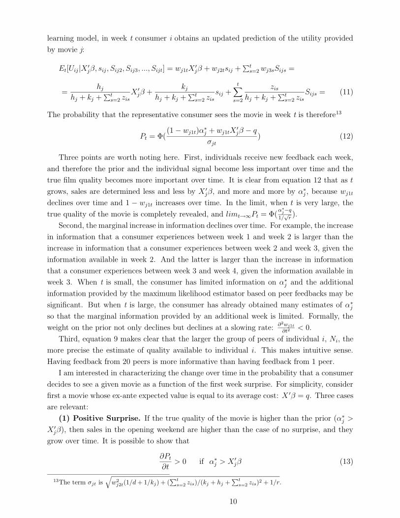
learning model, in week t consumer i obtains an updated prediction of the utility provided

by movie j:

Et[Uij|X ′jβ, sij , Sij2, Sij3, ..., Sijt] = wj1tX

′jβ + wj2tsij +

∑ts=2 wj3sSijs =

=hj

hj + kj +∑t

s=2 zis

X ′jβ +

kj

hj + kj +∑t

s=2 zis

sij +t∑

s=2

zis

hj + kj +∑t

s=2 zis

Sijs = (11)

The probability that the representative consumer sees the movie in week t is therefore13

Pt = Φ((1 − wj1t)α

∗j + wj1tX

′jβ − q

σjt

) (12)

Three points are worth noting here. First, individuals receive new feedback each week,

and therefore the prior and the individual signal become less important over time and the

true film quality becomes more important over time. It is clear from equation 12 that as t

grows, sales are determined less and less by X ′jβ, and more and more by α∗

j , because wj1t

declines over time and 1 − wj1t increases over time. In the limit, when t is very large, the

true quality of the movie is completely revealed, and limt→∞Pt = Φ(α∗

j−q

1/√

r).

Second, the marginal increase in information declines over time. For example, the increase

in information that a consumer experiences between week 1 and week 2 is larger than the

increase in information that a consumer experiences between week 2 and week 3, given the

information available in week 2. And the latter is larger than the increase in information

that a consumer experiences between week 3 and week 4, given the information available in

week 3. When t is small, the consumer has limited information on α∗j and the additional

information provided by the maximum likelihood estimator based on peer feedbacks may be

significant. But when t is large, the consumer has already obtained many estimates of α∗j

so that the marginal information provided by an additional week is limited. Formally, the

weight on the prior not only declines but declines at a slowing rate: ∂2wj1t

∂t2< 0.

Third, equation 9 makes clear that the larger the group of peers of individual i, Ni, the

more precise the estimate of quality available to individual i. This makes intuitive sense.

Having feedback from 20 peers is more informative than having feedback from 1 peer.

I am interested in characterizing the change over time in the probability that a consumer

decides to see a given movie as a function of the first week surprise. For simplicity, consider

first a movie whose ex-ante expected value is equal to its average cost: X ′β = q. Three cases

are relevant:

(1) Positive Surprise. If the true quality of the movie is higher than the prior (α∗j >

X ′jβ), then sales in the opening weekend are higher than the case of no surprise, and they

grow over time. It is possible to show that

∂Pt

∂t> 0 if α∗

j > X ′jβ (13)

13The term σjt is√

w2j2t(1/d + 1/kj) + (

∑t

s=2 zis)/(kj + hj +∑t

s=2 zis)2 + 1/r.

10

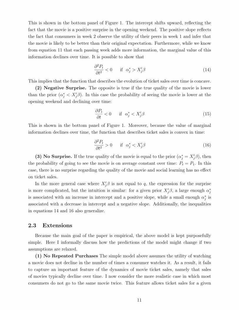
This is shown in the bottom panel of Figure 1. The intercept shifts upward, reflecting the

fact that the movie is a positive surprise in the opening weekend. The positive slope reflects

the fact that consumers in week 2 observe the utility of their peers in week 1 and infer that

the movie is likely to be better than their original expectation. Furthermore, while we know

from equation 11 that each passing week adds more information, the marginal value of this

information declines over time. It is possible to show that

∂2Pt

∂t2< 0 if α∗

j > X ′jβ (14)

This implies that the function that describes the evolution of ticket sales over time is concave.

(2) Negative Surprise. The opposite is true if the true quality of the movie is lower

than the prior (α∗j < X ′

jβ). In this case the probability of seeing the movie is lower at the

opening weekend and declining over time:

∂Pt

∂t< 0 if α∗

j < X ′jβ (15)

This is shown in the bottom panel of Figure 1. Moreover, because the value of marginal

information declines over time, the function that describes ticket sales is convex in time:

∂2Pt

∂t2> 0 if α∗

j < X ′jβ (16)

(3) No Surprise. If the true quality of the movie is equal to the prior (α∗j = X ′

jβ), then

the probability of going to see the movie is on average constant over time: Pt = P1. In this

case, there is no surprise regarding the quality of the movie and social learning has no effect

on ticket sales.

In the more general case where X ′jβ is not equal to q, the expression for the surprise

is more complicated, but the intuition is similar: for a given prior X ′jβ, a large enough α∗

j

is associated with an increase in intercept and a positive slope, while a small enough α∗j is

associated with a decrease in intercept and a negative slope. Additionally, the inequalities

in equations 14 and 16 also generalize.

2.3 Extensions

Because the main goal of the paper is empirical, the above model is kept purposefully

simple. Here I informally discuss how the predictions of the model might change if two

assumptions are relaxed.

(1) No Repeated Purchases The simple model above assumes the utility of watching

a movie does not decline in the number of times a consumer watches it. As a result, it fails

to capture an important feature of the dynamics of movie ticket sales, namely that sales

of movies typically decline over time. I now consider the more realistic case in which most

consumers do not go to the same movie twice. This feature allows ticket sales for a given

11

movie to decline over time. It complicates the analysis, but does not change the fundamental

intuition.

While the probability that the representative consumer sees a movie in week 1 is the

same P1 defined in equation 7, the probability for subsequent weeks changes. Consider first

the case where there is no social learning. The probability that the representative consumer

sees the movie in week 2 is now the joint probability that her expected utility at t = 2

is higher than her cost and her expected utility at t = 1 is lower than her cost: P2 =

Prob(E1[Uij|X ′jβ, sij] < qi1andE2[Uij|X ′

jβ, sij ] > qi2). It is clear that P2 < P1. Intuitively,

many of the consumers who expect to like a given movie watch it during the opening weekend.

Those left are less likely to expect to like the movie, so that attendance in the second week

is weaker than in the first.

The key point here is that, while all movies exhibit a decline in sales over time, this

decline is more pronounced for movies that experience strong sales in the first weekend. In

particular, under these assumptions, it is possible to show that

∂2Pt

∂t∂α∗j

< 0 (17)

A strong performance in week 1 reduces the base of potential customers in week 2. The

effect of this intertemporal substitution is that the decline in sales over time is accelerated

compared to the case of a movie that has an average performance in week 1, although the

total number remains higher because the intercept is higher. The opposite is true if a movie

is worse than expected. Both cases are represented in the top panel of Figure 2.

How do these predictions change with social learning? With social learning,

P2 = Prob(E2[Uij|X ′jβ, sij, Sij2] > qi2 and E1[Uij|X ′

jβ, sij ] < qi1)

= Prob(wj22(νij + εij) + wj32(Sij2 − α∗j ) − ui2) > (q − (1 − wj12)α

∗j − wj12X

′jβ)

and (wj21(νij + εij) + wj31(Sij1 − α∗j ) − ui1) < (q − (1 − wj11)α

∗j − wj11X

′jβ))

The answer depends on the strength of the social learning effect. If social learning is weak,

the dynamics of sales will look qualitatively similar to the ones in the top panel of Figure 2,

although the slope of the movie characterized by a positive (negative) surprise is less (more)

negative. But if social learning is strong enough, the dynamics of sales will look like the

ones in the bottom part of Figure 2, where the slope of the movie characterized by a positive

(negative) surprise is less (more) negative than the slope of the average movie.

(2) Option Value. In my setting I follow Bikhchandani et al. (1992) and model

the timing of purchase as exogenous. This greatly simplifies the model. In each period,

individuals decide whether to see a particular movie by comparing its expected utility to

the opportunity cost of time, qit, assumed to be completely idiosyncratic. This assumption

is not completely unrealistic, because it says that individuals have commitments in their

lives (such as work or family commitments) that are not systematically correlated with the

opening of movies. On the other hand, it ignores the possibility that consumers might want

12

to wait for uncertainty to be resolved before making a decision.

In the case of the latter possibility, consumers would have an expected value of waiting

to decide, as in the Dixit and Pindyck (1994) model of waiting to invest. This would give

rise to an option value associated with waiting. Like in the myopic case described above,

a consumer in this setting decides to see the movie in week 1 only if her private signal on

quality is high enough relative to the opportunity cost of time. However, the signal that

triggers consumption in the option value case is higher than its equivalent in the myopic

case, because waiting generates information and therefore has value. This implies a lower

probability of going to see the movie in week 1.

If εij and qit remain independent of all individual and movie characteristics, and indi-

viduals take their peers’ timing as given, the model generates the same set of implications.

While decisions are more prudent in the strategic case than in the myopic case, the timing

of purchase remains determined by the realization of the signal and of qit, and thus remains

unsystematic. Therefore, information diffusion follows similar dynamics to those described

above.14

3 Empirical Predictions

The model above has several testable predictions that I bring to the data in sections 6

and 7.

1. In the presence of strong enough social learning, sales of movies with stronger than

expected opening weekend demand and sales of movies with weaker than expected

opening weekend demand should diverge over time. This prediction is shown in Figures

1 and 2 and follows from equations 13 and 15. In the absence of social learning, or

with weak social learning, we should see no divergence over time or even convergence.

2. In the presence of social learning, the effect of a surprise should be stronger for movies

with a more diffuse prior and weaker for movies with a more precise prior. Intuitively,

when a consumer has a precise idea of whether she is going to like a specific movie

(strong prior), the additional information provided by her peers should matter less

relative to the case when a consumer has only a vague idea of how much she is going

to like a movie (weak prior). Formally, this is evident from equation 11. A more

precise prior (a larger hj) implies a larger ωj1t, and therefore a smaller ωj3t (everything

else constant). This means that with a more precise prior, the additional information

provided by the peers, Sijs, will receive less weight, while the prior, X ′jβ, will receive

more weight. In the absence of social learning, there is no particular reason for why

14A more complicated scenario arises if timing of purchase strategically depends on peers’ timing. This

could happen, for example, if some individuals wait for their friends to go see the movie in order to have

a more precise estimate of their signal, and their peers wait for the same reason. This scenario might have

different implications and is outside the scope of the paper.

13

the correlation between sales trend and first week surprise should vary systematically

with precision of the prior.

3. In the presence of social learning, the effect of a surprise should be stronger for con-

sumers who have larger social networks. The idea is that receiving feedback from 20

peers is more informative than receiving feedback from 2 peers. Formally, this is clear

from equations 9 and 11. Equation 9 shows that a larger Ni implies a more precise esti-

mate of movie quality based on peer feedback (i.e. a smaller variance of Sijt). In turn,

equation 11 indicates that a smaller variance of Sijt implies a larger ωj3t and smaller

ωj1t and ωj2t. In the absence of social learning, there is no particular reason for why

the correlation between sales trend and first week surprise should vary systematically

with size of the social network.

4. In the presence of social learning, the marginal effect of a surprise on sales should

decline over time. For example, the amount of updating that takes place in week 2

should be larger than the amount of updating that takes place in week 3 given what is

already known in week 2. The implication is that the pattern of sales of movies with a

positive (negative) surprise should be concave (convex) in time. This is evident from

equations 14 and 16. In the absence of social learning, there is no particular reason for

why the curvature of sales over time should vary systematically with the sign of first

week surprise.

5. In the presence of social learning, consumers should only respond to surprises that

reflect new information on movie quality. They should not update their priors based

on surprises that reflect factors other than movie quality. For example, consider the

case of a movie whose opening weekend demand is weaker than expected because of

bad weather. In this case, low demand in first week does not imply that the quality of

the movie is low. Therefore, low demand in the first week should not lead consumers

to update and should have no negative impact on subsequent sales.15 In the absence

of social learning, there is no particular reason for why variation in first week demand

due to surprises in movie quality and variation in first week demand due to factors

unrelated to quality should have different effects on sales trends.

4 Data

I use data on box office sales from the firm ACNielsen-EDI. The sample includes all

movies that opened between 1982 and 2000 for which I have valid sales and screens data.16

15Formally, one can think of weather shocks as part of the cost of going to see the movie, uit. In the case

of bad weather in the opening weekend, ui1 is high for many consumers.16I drop from the sample movies for which sales or number of screens are clearly misreported. In particular,

I drop movies that report positive sales in a week, but zero number of screens, or vice-versa. I am interested

14

Beside total box office sales by movie and week, it reports production costs, detailed genre

classification, ratings and distributor. I have a total of 4,992 movies observed for 8 weeks.

Total sample size is therefore 4, 992 × 8 = 39, 936. This dataset was previously used in

Goettler and Leslie (2005).

I augment box office sales data with data on advertising and critic reviews. Unfortunately,

these data are available only for a limited number of years. Data on TV advertising by movie

and week were purchased from the firm TNS Media Intelligence. They include the totality

of TV advertising expenditures for the years 1995 to 2000. Data on movie reviews were hand

collected for selected years and newspapers by a research assistant. The exact date of the

review and an indicator for whether the review is favorable or unfavorable were recorded.

These data were collected for The New York Times for the movies opening in the years 1983,

1985, 1987, 1989, 1991, 1993, 1995, 1997, 1999; for The Wall Street Journal, USA Today,

The Chicago Sun-Times, The Los Angeles Times, The Atlanta Journal-Constitution and

The Houston Chronicle for the movies opening in the years 1989, 1997 and 1999; and for

The San Francisco Chronicle for the movies opening in the years 1989, 1993, 1995 and 1997

and 1999.

Summary statistics are in Table 1. The average movie has box office sales equal to $1.78

million in the average week. Box office sales are higher in the opening weekend: $3.15 million.

Production costs amount to $4.54 million. All dollar figures are in 2005 dollars. The average

movie is shown on 449 screens on average and on 675 screens in the opening weekend. The

average movie has $6.85 million in cumulative TV advertising expenditures. About half of

the reviews are favorable. The bottom of the table shows the distribution of movies across

genres. Comedy, drama and action are the three most common genres.

The top panel in Figure 3 plots the typical evolution of box office sales over time. The

figure shows a steep decline in the first few weeks and a slowing down in the rate of decline

in the following weeks. The bottom panel in Figure 3 shows the evolution of log sales. The

figure shows that the decline in sales is remarkably log linear. This is convenient, because

the use of log-linear models will simply the empirical analysis.

Not all movies have positive sales for the entire 8 week period. Because the dependent

variable in the econometric models will be in logs, this potentially creates a selection problem.

To make sure that my estimates are not driven by the potentially non-random selection of

poorly performing movies out of the sample, throughout the paper I report estimates where

the dependent variable is the log of sales +$1. The main advantage of this specification is

that it uses a balanced panel: all movies have non-missing values for each of the 8 weeks.

(I have also re-estimated my models using the selected sample that has positive sales and

found generally similar results.)

in movies that are released nationally. Therefore, I drop movies that open only in New York and Los Angeles.

15

5 Identification of Surprise in Opening Week Demand

The first step in testing the predictions of the model is to empirically identify surprise

in opening weekend sales. I define the surprise as the difference between realized box office

sales and predicted box office sales in the opening weekend, and I use the number of screens

in the opening weekend as a sufficient statistic for predicted sales. Specifically, I use the

residual from a regression of first week log sales on log number of screens as my measure of

movie-specific surprise. (In some specifications, I also control for genre, ratings, distribution,

budget and time of release.)

Number of screens is arguably a valid measure of the ex-ante expectations of demand for

a given movie because it is set by profit-maximizing agents (the theater owners), who have

a financial incentive to correctly predict consumer demand for a movie. Number of screens

should therefore summarize the market expectation of how much a movie will sell based on

all information available before opening day: cast, director, budget, advertising before the

opening weekend, the quality of reviews before the opening weekend, the buzz in blogs, the

strength of competitors, and any other demand shifter that is observed by the market before

the opening weekend.

Deviations from this expectation can therefore be considered a surprise. These deviations

reflect surprises in how much the concept of a movie and its cast resonate with the public.

While theaters seem to correctly guess demand for movies on average, there are cases where

the appeal of a movie and therefore its opening weekend demand is higher or lower than

expected. These surprises are the ones used in this paper for identification.17 Formally,

theaters seek to predict P1 in equation 7. It is easy to show that in the case of a positive

surprise in quality–i.e. when a movie true quality is higher than the prior (α∗j > X ′

jβ)–

theaters’ prediction, P̂1 is lower than realized sales: P̂1 < P1. The opposite is true in the

case of a negative surprise–i.e. when a movie true quality is lower than the prior (α∗j < X ′

jβ).

In this latter case, P̂1 > P1.18

Column 1 in Appendix Table A1 shows that the unconditional regression of log sales in

17The data suggests that the number of screens set in the first weekend by theaters is on average exactly

proportional to consumers’ demand. A regression of log screens in the first weekend on log sales in the first

weekend should yield a coefficient close to 1 if the theaters’ prediction is correct on average. Empirically,

this regression yields a coefficient equal to 1.01 (.004). Thus, if the actual demand for movie a in the opening

weekend is 10% higher than the demand for movie b, the number of screens in the opening weekend is on

average 10% higher for movie a than movie b.18To see why, assume that theaters have the same information as consumers and use this information to

predict P1 in equation 7. The terms ωj , X ′jβ, q and σj1 are known, but α∗

j is unknown. Assume that theaters

use the normal learning model to predict α∗j : E1[α

∗j |X ′

jβ, sij ] = wjX′jβ+(1−wj)sij where wj = mj/(aj+mj)

and aj = (dkj)/(d + kj). The weight on the prior used by theaters (wj) is different from the weight on the

prior used by consumers (ωj in equation 5). In particular, it is easy to see that wj > ωj . This implies that

even if consumers and theaters have the same information, theaters put more weight on the prior and less on

their private signal. Intuitively, this is because theaters seek to predict α∗j while consumers seek to predict

Uij .

16

first weekend on log screens in first weekend yields a coefficient equal to .89 (.004), with R2

of .907. This regression is estimated on a sample that includes one observation per movie (N

= 4,992). The R2 indicates that about 90% of the variation in first week sales is predicted by

theater owners. Thus, about 10% of the variation cannot be predicted by theater owners.19

Columns 2 to 7 show what happens to the predictive power of the model as I include

an increasingly rich set of covariates. If my assumption is correct and number of screens is

indeed a good summary measure of all the information that the market has available on the

likely success of a movie, the inclusion of additional covariates should have limited impact

on R2. In column 2, the inclusion of 16 dummies for genre has virtually no impact, as R2

increases from .907 to .908. Similarly, the inclusion of production costs and 8 dummies for

ratings raises R2 only marginally, from .908 to .912. Including 273 dummies for the identity

of the distributor, 12 dummies for months, 56 dummies for week, 6 dummies for weekday

and 18 dummies for year raises R2 to .937. Overall, it is safe to say that the addition of

all available controls has a limited impact on the fit of the model once number of screens is

controlled for.

Appendix Table A2 shows the distribution of surprises in the opening weekend box office

sales, together with some examples of movies. For example, the entry for 75% indicates that

opening weekend sales for the movie at the 75th percentile are 46% higher than expected.

The distribution appears symmetric, and it is centered around 0.02. Since surprise is a

regression residual, its mean is zero by construction.

An example of a movie characterized by large positive surprise is “The Silence of the

Lambs”. Before the opening weekend, it was expected to perform well, since it opened

on 1479 screens, substantially above the average movie. But in the opening weekend, it

significantly exceeded expectations, totalling sales of about $25 million. In this case, sales

were significantly higher than the amount theaters were expecting based on the screens

assigned to it. Other examples of movies that experienced significant positive surprises are

“Ghostbusters,” “Sister Act” and “Breakin.” More typical positive surprises are represented

by movies in the 75th percentile of the surprise distribution, such as “Alive,” “Who Framed

Roger Rabbit” and “House Party.” For many movies, the demand in the first week is close to

market expectations. Examples of movies close to the median include “Highlander 3,” “The

Bonfire of the Vanities,” “The Sting 2,” and “A Midsummer Night’s Dream.” Examples of

19There is ample evidence that the movie industry is focused on opening weekend box office sales. There

are countless newspaper articles and web sites devoted to predictions of opening weekend box office sales,

and at least two web sites that allow betting on opening weekend box office sales. (Unfortunately, betting

sites did not exist during the period for which I have sales data.) This attention to opening weekend box

office sales is consistent with the notion that demand is uncertain, even just days before the opening. During

production, studios do use focus groups to determine which aspects of the story are more likely to resonate

with the public and how to best tailor advertising to different demographic groups. The unpredictable

component of demand that I focus on here is very different in nature, as it takes place just before release.

I am not aware of focus group analysis performed after production and marketing are completed to predict

first weekend sales.

17

negative surprise include “Home Alone 3,” “Pinocchio,” “Lassie,” and “The Phantom of the

Opera.” These four movies opened on a large number of screens (between 1,500 and 1,900),

but had first weekend box office sales lower than one would expect based on the number

of screens. Interestingly, there are two very different versions of Tarzan movies. One is an

example of a strong negative surprise (“Tarzan and the Lost City”), while the second one is

a strong positive surprise (“Tarzan”).

One might wonder whether theaters might find it profitable to set the number of screens

not equal to the expected demand. For example, would it be optimal to systematically

lower the number of screens to artificially boost surprise in first week demand? It seems

unlikely. First, consumers would probably discount systematic underscreening and would

adjust their expectations accordingly. More fundamentally, number of screens is simply a

summary measure that I use to quantify expectations on demand. In my model, consumers’

expected utility is based on movie underlying characteristics (director, actors, genre, etc.)

as well as their private signal. For a given set of movie characteristics and for a given

signal, manipulation of the number of screens would have no impact on consumer demand.

The reason is that consumers in week 2 do not respond causally to surprises in first week

demand. They respond causally only to variation in movie quality. Manipulating surprises

in first week demand without changing actual movie quality is unlikely to generate higher

demand and higher profits.

6 Empirical Evidence

I now present empirical tests of the five implications of the model described in section 3.

I begin in sub-section 6.1 with tests of prediction 1. In subsection 6.2, 6.3 and 6.4, I present

tests of predictions 2, 3 and 4, respectively. Later, in Section 7 I discuss the interpretation

of the evidence and I present a test of prediction 5.

6.1 Prediction 1: Surprises and Sale Dynamics

Graphical Evidence. The main implication of the model is that in the presence of

social learning, movies with a positive surprise in first weekend sales should have a slower

rate of decline in sales than movies with a negative surprise in first weekend sales (prediction

1). In the absence of social learning, movies with a positive and negative surprise should

have the same rate of decline in sales.

Figure 4 shows a graphical test of this prediction based on the raw data. It shows

unconditional average log sales by week and surprise status. The upper line represents the

decline in average sales for movies with a positive surprise, and the bottom line represents

the decline for movies with a negative surprise. The pattern shown in the Figure is striking.

Consistent with Prediction 1, movies with a positive surprise experience a slower decline

in sales than movies with a negative surprise. As a consequence, the distance between

18

the average sales of positive and negative surprise movies is relatively small in the opening

weekend, but increases over time. After 8 weeks the difference is much larger than in week

1.

Baseline Estimates. To test whether the difference in slopes between positive and

negative surprise movies documented in Figure 4 is statistically significant, I estimate models

of the form

ln yjt = β0 + β1t + β2(t × Sj) + dj + ujt (18)

where ln yjt is the log of box office sales in week t; Sj is surprise or an indicator for positive

surprise; and dj is a movie fixed effect. Identification comes from the comparison of the

change over time in sales for movies with a positive and a negative surprise. To account for

the possible serial correlation of the residual within a movie, standard errors are clustered

by movie throughout the paper.

The coefficient of interest is β2. A finding of β2 > 0 is consistent with the social learning

hypothesis, since it indicates that the rate of decline of sales of movies with positive surprise

is slower than the rate of decline of sales of movies with negative surprise, as in Figure 4. A

finding of β2 = 0, on the other hand, is inconsistent with the social learning hypothesis, since

it indicates that the rate of decline of sales of movies with positive and negative surprise is

the same.20

It is important to note that the interpretation of β2 is not causal. The model in section

2 clarifies that, under social learning, a stronger than expected demand in week 1 does not

cause a slower decline in sales in the following weeks. A stronger than expected demand in

week 1 simply indicates (to the econometrician) that the underlying quality of the movie is

better than people had expected. It is the fact that movie quality is better than expected

and the diffusion of information about movie quality that cause the slower decline in sales

in the weeks following a positive surprise in first week demand. A positive surprise in first

week demand is simply a marker for better than expected quality.

Estimates of variants of equation 18 are in Table 2. In column 1, I present the coefficient

from a regression that only includes a time trend. This quantifies the rate of decay of sales for

the average movie, shown graphically in the bottom panel in Figure 3. The entry indicates

that the coefficient on t is -.926. In column 2, the regression includes the time trend×surprise,

with surprise defined as the residual from a regression of log sales on number of screens,

indicators for genre, ratings, production cost, distribution, week, month, year and weekday.

(This definition of surprise is the one used in column 7 of Table A1.) The coefficient β2

from this regression is equal to .46 and is statistically different from zero. Since the variable

“surprise” has by construction mean zero, the coefficient on t is the same in column 1 and 2.

20Because S is estimated, it contains some error. Estimates of β2 are therefore biased toward zero, and

the reported standard errors should in theory be adjusted to reflect this additional source of variability.

Also, because t is predetermined, the following model yields the same estimates of β1 and β2: ln yjt =

β0 + β1t + β2(t × Sj) + β3Sj + ujt.

19

In column 3, Sj is an indicator for whether surprise is positive. The entry for β2 quantifies

the difference in rate of decay between positive and negative surprise movies shown graph-

ically in Figure 4. The entry indicates that the rate of decline for movies with a negative

surprise is -1.25, while the rate of decline for movies with a positive surprise is about half as

big: −1.25 + .619 = −.63. This difference between positive and negative surprise movies is

both statistically and economically significant.

In column 4, I divide the sample into three equally sized groups depending on the mag-

nitude of the surprise, and I allow for the rate of decline to vary across terciles. Compared

to the model in column 3, this specification is less restrictive because it allows the rate of

decline to vary across three groups, instead of two. I find that the rate of decline is a mono-

tonic function of surprise across these three groups. The coefficient for the first tercile (most

negative surprise) is -1.32. The coefficient for the second tercile (zero or small surprise) is

-.98. The coefficient for the third tercile (most positive surprise) is -.47.

To better characterize the variation in the rate of decline of sales, I estimate a more

general model that allows for a movie-specific decline:

ln yjt = β0 + β1jt + dj + ujt (19)

where the rate of decline β1j is now allowed to vary across movies. Table 2 has already

established that the mean rate of decline of positive surprise movies is larger the mean rate

of decline of negative surprise movies. I use estimates of β1j in equation 19 to compare

the entire distribution of movie-specific slopes for positive and negative surprise movies, as

opposed to just the first moment. This specification is therefore more general than the

models in Table 2, because it does not force the rate of decline to be the same with group.

Figure 5 and Table 3 show the distribution of the coefficients β1j separately for positive

and negative surprise movies. It is clear that the distribution of the slope coefficients for

movies with a positive surprise is more to the right than the distribution of the slope co-

efficients for movies with a negative surprise, as predicted by the model. For example, the

25th percentile, the median and the 75th percentile are -.96, -.41 and -.11 for positive surprise

movies, and -1.91, -1.23 and -.60 for negative surprise movies.

Advertising. One might be concerned that the difference in sales trends between pos-

itive and negative surprise movies may be caused by changes in advertising expenditures

induced by the surprise. If studios initially set their optimal advertising budget based on the

expected performance of a movie, then it is plausible that a surprise in actual performance

will change their first order conditions. In particular, if studios adjust their advertising ex-

penditures based on first week surprise, estimates in Table 2 may be biased, although the

sign of the bias is a priori undetermined.21

21The sign of the bias depends on whether the marginal advertising dollar raises revenues more for positive

or negative surprise movies.

20

In practice, endogenous changes in advertising do not appear to be a major factor in

explaining my results. First, most advertising takes place before the release of a movie,

primarily because studios–who are responsible for most advertising—receive a higher share

of profits from earlier weeks than later weeks. In my sample, 94% of TV advertising occurs

before the opening day. Thus, the majority of advertising should already be reflected in the

number of screens and therefore should not enter surprise.

Second, and most importantly, directly controlling for advertising does not significantly

affect estimates. This is shown in the top panel of Table 4. As explained in the data section,

advertising data are not available for all movies. For convenience, columns 1 and 2 report

baseline estimates of equation 18, reproduced from columns 2 and 3 of Table 2. Columns

3 and 4 report estimates of the same models obtained using the sub-sample of movies for

which I have advertising data. The comparison of columns 1 and 2 with columns 3 and 4

suggests that the sub-sample of movies for which I have ad data generates estimates that

are qualitatively similar to the full sample estimates. In columns 5 and 6, I use the sample

used for columns 3 and 4 and include a control for TV advertising. Specifically, I control for

the logarithm of cumulative total expenditures for television advertising until the relevant

week.22

The comparison of columns 5 and 6 with columns 3 and 4 suggests that the inclusion of

controls for TV advertising has limited impact on my estimates. Specifically, the coefficients

on time and time × surprise change from -.940 and .700 (column 3) to -.996 and .661 (column

5), respectively. The coefficients on time and time × an indicator for surprise change from -

1.320 and .777 (column 4) to -1.329 and .730 (column 6), respectively. Increases in advertising

expenditures are associated with sizable increases in box office sales. The coefficient on log

advertising is between .9 and 1.1, indicating that the elasticity of box office sales relative

to cumulative advertising expenditures is close to 1. My data on advertising also identify

specific types of TV ads. For example, the data separately report expenditures for cable,

network, spot, and others. I have re-estimated columns 5 and 6 allowing for separate effects

for each type of ad and found estimates very similar to the ones reported.

I also note that even if advertising could explain the slower decline in sales for positive

surprise movies, it does not explain the comparative statics results on the precision of the

prior and the size of the social network that I describe in sub-sections 6.2 and 6.3 below.

Critic Reviews. Another potentially important omitted variable is represented by critic

reviews. The concern is that movie critics react to a surprise in opening weekend by covering

unexpected successes. This could have the effect of boosting sales for positive surprise movies,

22Cumulative expenditures for advertising for movie j in week t represent the sum of expenditures for all

TV ads broadcasted for movie j until week t. The reason for using cumulative expenditures, as opposed to

current expenditures, is that the demand in week t presumably depends both on ads in week t and ads in

earlier weeks. I have experimented with alternative specifications. For example, in models where advertising

is defined as the sum of ad expenditures in the previous 1, 2, 3 or 4 weeks, results are very similar.

21

thus generating the difference in rate of decline between positive and negative surprise movies

documented above. Like advertising, the majority of reviews take place before the release of

a movie. In my data, 85% of newspaper reviews are published at or before the date of the

opening.

Directly controlling for positive reviews does not affect estimates significantly. This is

shown in the bottom panel of Table 4. As for advertising, data on reviews are available only

for a subset of movies. Columns 1 and 2 report baseline estimates reproduced from Table 2.

In columns 3 and 4 I report estimates of the baseline model obtained using the sub-sample

for which I have data on reviews. In columns 5 and 6, I control for the cumulative share of

reviews that are favorable as a fraction of all the reviews published until the relevant week.

The comparison of columns 5 and 6 with columns 3 and 4 suggests that the inclusion of

controls reviews has limited impact on my estimates. The coefficients on time and time ×surprise change from -.856 and .509 (column 3) to -.927 and .494 (column 5), respectively.

The coefficients on time and time × an indicator for surprise change from -1.163 and .603

(column 4) to -1.227 and .582 (column 6), respectively. The coefficient on favorable reviews

is positive and significantly different from zero, although it can not necessarily be inter-

preted causally. I have also re-estimated the models in columns 5 and 6 separately for each

newspaper and found similar results.23

Like for advertising, I also note that if the only reason for a slow-down in the rate of

decline of positive surprise movies were critic reviews, we would not necessarily see the

comparative statics results on the precision of the prior and size of the social network that

I describe in subsections 6.2 and 6.3 below.

Supply Effects. So far, I have implicitly assumed that all the variation in sales reflects

consumer demand. However, it is possible that changes in the availability of screens affect

sales. Consider the case where there is no social learning, but some theater owners react to

the first week surprise by adjusting the movies they screen. This type of supply effect has the

potential to affect sales, especially in small towns, where the number of screens is limited.

For example, in week 2 a theater owner in a small town may decide to start screening a

movie that had a positive surprise elsewhere, thereby increasing the number of customers

who have access to that movie.

This is important because it implies that the evidence in Table 2 may be explained not

23Specifically, the coefficients on time and time × surprise for USA Today are -.83 (.03) and .60 (.04)

without controls (column 3); and -.83 (.03) and .59 (.04) controlling for favorable reviews (column 5). For

the Wall Street Journal are: -.70 (.05), .46 (.07) without controls and -.72 (.05) and .45 (.07) with controls.

For the New York Times: -.85 (.02) and .50 (.03) without controls; -.86 (.02) and .51 (.02) with controls. For

the Los Angeles Times: -.83 (.03) and .51 (.03) without controls; -.84 (.03) and .51 (.03) with controls. For

the San Francisco Chronicle: -.81 (.03) and .56 (.03) without controls; -.87 (.03) and .54 (.03) with controls.

For the Atlanta Journal Constitution: -.86 (.04) and .60 (.04) without controls; -.91 (.04) and .58 (.04) with

controls. For the Houston Chronicle: -.82 (.03) and .58 (.03) without controls; -.87 (.03) and .56 (.03) with

controls.

22

by learning on the part of consumers, but by learning on the part of theater owners. To test

for this possibility, I have re-estimated my models using sales per screen as the dependent

variable. In this specification, the focus is on changes in the average number of viewers

for a given number of screens. These results are therefore not affected by changes in the

number of theaters screening a given movie. Columns 1 and 3 of Table 5 correspond to a

specification where Sj is the surprise of movie j, while columns 2 and 4 correspond to a

specification where Sj is a dummy for whether the surprise of movie j is positive. Overall,

estimates of the effect of a surprise are qualitatively robust to the change in the definition of

the dependent variable, although the magnitude of the effect declines relative to the baseline.

For example, entries in column 2 indicate that the rate of decline of a positive and negative

surprise movie are -.64 and -1.25, respectively. The corresponding rates of decline in column

4 are -.52 and -.80. In other words, in column 2 the rate of decline of a positive surprise

movie is only half of the rate of decline of a negative surprise movie, while in column 4 the

rate of decline of a positive surprise movie is 65% of the rate of decline of a negative surprise

movie.

Note that the interpretation of this specification requires caution. Number of screens is

an endogenous variable, which presumably adjusts as a function of demand shocks. If there

is social learning, a positive surprise in week 1 will result in an increase in demand in the

following weeks, and, as a consequence, it will also cause an increase in the number of screens

devoted to that particular movie. While the specification in Table 5 is helpful in testing for

the possibility of supply effects, it is not my preferred specification because, by focusing in

sales per screen, it discards useful variation in the dependent variable.

I also note that an increase in number of screens alone would not explain the difference

in the effect of surprise for teen movies and non-teen movies that I document below in

sub-section 6.3.

Sold-out Movies. Another possible interpretation of Table 2 is that the slower decline

in sales for positive surprise movies reflects sold out movies, not social learning. Suppose for

example that demand in week 1 exceeds capacity and that some of this excess demand gets

shifted to later weeks. To test this possibility directly, I re-estimate equation 18 excluding

movies that might have sold out. In particular, I re-estimate my models dropping movies

that are in the top 1%, 3% or 5% of the per-screen attendance distribution. Estimates in

columns 5 and 6 of Table 5–obtained by dropping movies that are in the top 5% of the

per-screen attendance distribution–indicate that results are robust to this specification.

Furthermore, this alternative explanation is not consistent with the comparative statics

on precision of the prior and of the signal documented in sub-sections 6.2 and 6.3 below. If

the only thing driving results is that some positive surprise movies are sold out, we should

not expect to see the effect of surprise vary systematically with the precision of the prior.

Robustness. Here I probe the robustness of estimates in Table 2 using two sets of

23

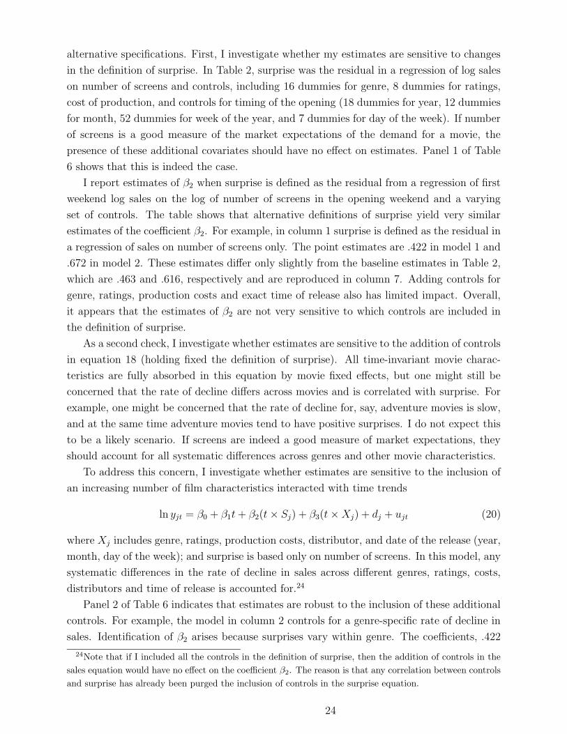
alternative specifications. First, I investigate whether my estimates are sensitive to changes

in the definition of surprise. In Table 2, surprise was the residual in a regression of log sales

on number of screens and controls, including 16 dummies for genre, 8 dummies for ratings,

cost of production, and controls for timing of the opening (18 dummies for year, 12 dummies

for month, 52 dummies for week of the year, and 7 dummies for day of the week). If number

of screens is a good measure of the market expectations of the demand for a movie, the

presence of these additional covariates should have no effect on estimates. Panel 1 of Table

6 shows that this is indeed the case.

I report estimates of β2 when surprise is defined as the residual from a regression of first

weekend log sales on the log of number of screens in the opening weekend and a varying

set of controls. The table shows that alternative definitions of surprise yield very similar

estimates of the coefficient β2. For example, in column 1 surprise is defined as the residual in

a regression of sales on number of screens only. The point estimates are .422 in model 1 and

.672 in model 2. These estimates differ only slightly from the baseline estimates in Table 2,

which are .463 and .616, respectively and are reproduced in column 7. Adding controls for

genre, ratings, production costs and exact time of release also has limited impact. Overall,

it appears that the estimates of β2 are not very sensitive to which controls are included in

the definition of surprise.

As a second check, I investigate whether estimates are sensitive to the addition of controls

in equation 18 (holding fixed the definition of surprise). All time-invariant movie charac-

teristics are fully absorbed in this equation by movie fixed effects, but one might still be

concerned that the rate of decline differs across movies and is correlated with surprise. For

example, one might be concerned that the rate of decline for, say, adventure movies is slow,

and at the same time adventure movies tend to have positive surprises. I do not expect this

to be a likely scenario. If screens are indeed a good measure of market expectations, they

should account for all systematic differences across genres and other movie characteristics.

To address this concern, I investigate whether estimates are sensitive to the inclusion of

an increasing number of film characteristics interacted with time trends

ln yjt = β0 + β1t + β2(t × Sj) + β3(t × Xj) + dj + ujt (20)

where Xj includes genre, ratings, production costs, distributor, and date of the release (year,

month, day of the week); and surprise is based only on number of screens. In this model, any

systematic differences in the rate of decline in sales across different genres, ratings, costs,

distributors and time of release is accounted for.24

Panel 2 of Table 6 indicates that estimates are robust to the inclusion of these additional

controls. For example, the model in column 2 controls for a genre-specific rate of decline in

sales. Identification of β2 arises because surprises vary within genre. The coefficients, .422

24Note that if I included all the controls in the definition of surprise, then the addition of controls in the

sales equation would have no effect on the coefficient β2. The reason is that any correlation between controls

and surprise has already been purged the inclusion of controls in the surprise equation.

24

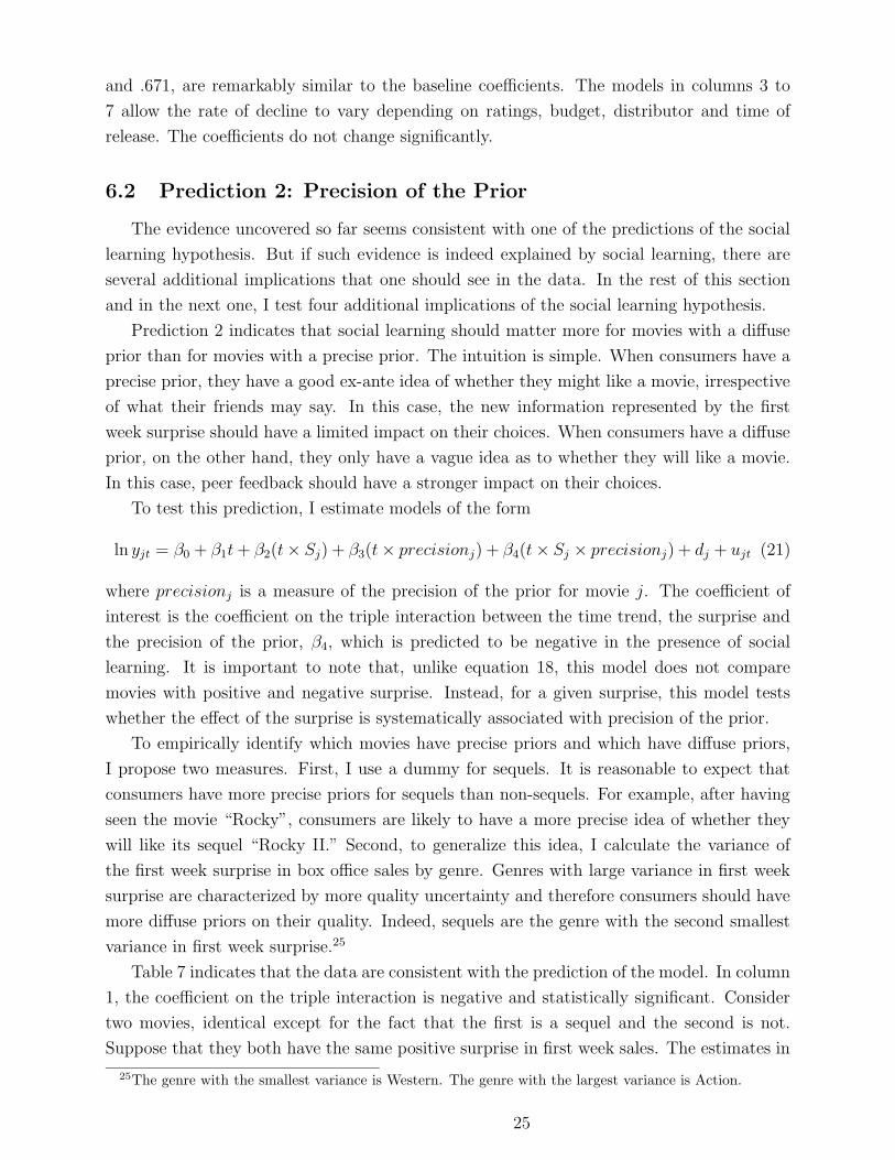
and .671, are remarkably similar to the baseline coefficients. The models in columns 3 to

7 allow the rate of decline to vary depending on ratings, budget, distributor and time of

release. The coefficients do not change significantly.

6.2 Prediction 2: Precision of the Prior

The evidence uncovered so far seems consistent with one of the predictions of the social

learning hypothesis. But if such evidence is indeed explained by social learning, there are

several additional implications that one should see in the data. In the rest of this section

and in the next one, I test four additional implications of the social learning hypothesis.

Prediction 2 indicates that social learning should matter more for movies with a diffuse

prior than for movies with a precise prior. The intuition is simple. When consumers have a

precise prior, they have a good ex-ante idea of whether they might like a movie, irrespective

of what their friends may say. In this case, the new information represented by the first

week surprise should have a limited impact on their choices. When consumers have a diffuse

prior, on the other hand, they only have a vague idea as to whether they will like a movie.

In this case, peer feedback should have a stronger impact on their choices.

To test this prediction, I estimate models of the form

ln yjt = β0 + β1t + β2(t× Sj) + β3(t × precisionj) + β4(t × Sj × precisionj) + dj + ujt (21)

where precisionj is a measure of the precision of the prior for movie j. The coefficient of

interest is the coefficient on the triple interaction between the time trend, the surprise and

the precision of the prior, β4, which is predicted to be negative in the presence of social

learning. It is important to note that, unlike equation 18, this model does not compare

movies with positive and negative surprise. Instead, for a given surprise, this model tests

whether the effect of the surprise is systematically associated with precision of the prior.

To empirically identify which movies have precise priors and which have diffuse priors,

I propose two measures. First, I use a dummy for sequels. It is reasonable to expect that

consumers have more precise priors for sequels than non-sequels. For example, after having

seen the movie “Rocky”, consumers are likely to have a more precise idea of whether they

will like its sequel “Rocky II.” Second, to generalize this idea, I calculate the variance of

the first week surprise in box office sales by genre. Genres with large variance in first week

surprise are characterized by more quality uncertainty and therefore consumers should have

more diffuse priors on their quality. Indeed, sequels are the genre with the second smallest

variance in first week surprise.25

Table 7 indicates that the data are consistent with the prediction of the model. In column

1, the coefficient on the triple interaction is negative and statistically significant. Consider

two movies, identical except for the fact that the first is a sequel and the second is not.

Suppose that they both have the same positive surprise in first week sales. The estimates in

25The genre with the smallest variance is Western. The genre with the largest variance is Action.

25

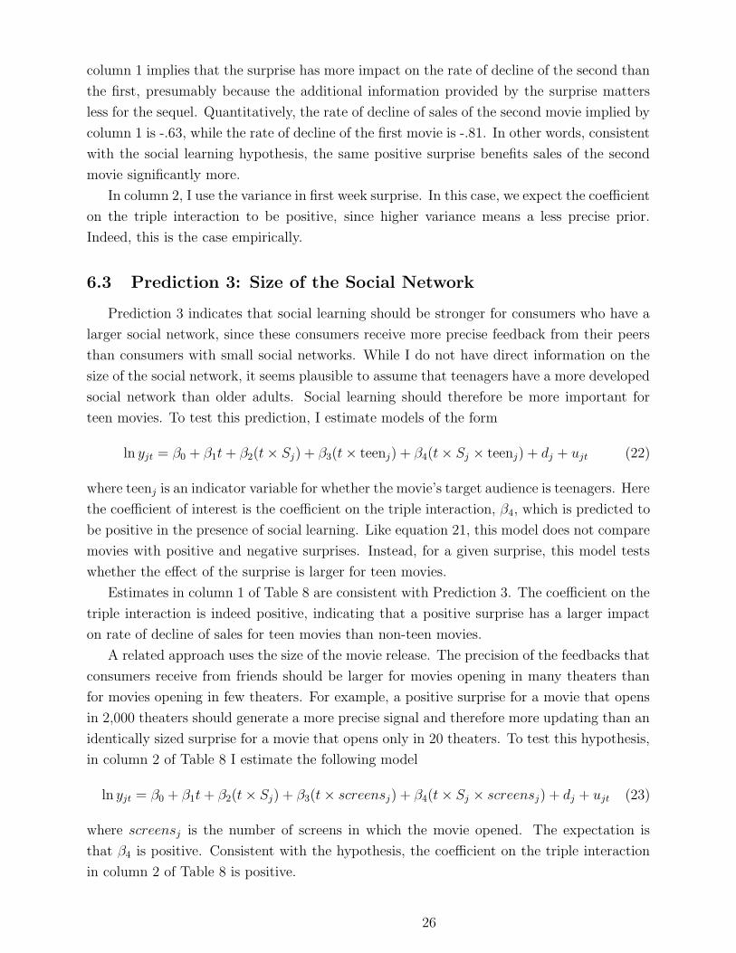
column 1 implies that the surprise has more impact on the rate of decline of the second than

the first, presumably because the additional information provided by the surprise matters

less for the sequel. Quantitatively, the rate of decline of sales of the second movie implied by

column 1 is -.63, while the rate of decline of the first movie is -.81. In other words, consistent

with the social learning hypothesis, the same positive surprise benefits sales of the second

movie significantly more.

In column 2, I use the variance in first week surprise. In this case, we expect the coefficient

on the triple interaction to be positive, since higher variance means a less precise prior.

Indeed, this is the case empirically.

6.3 Prediction 3: Size of the Social Network

Prediction 3 indicates that social learning should be stronger for consumers who have a

larger social network, since these consumers receive more precise feedback from their peers

than consumers with small social networks. While I do not have direct information on the

size of the social network, it seems plausible to assume that teenagers have a more developed

social network than older adults. Social learning should therefore be more important for

teen movies. To test this prediction, I estimate models of the form

ln yjt = β0 + β1t + β2(t × Sj) + β3(t × teenj) + β4(t × Sj × teenj) + dj + ujt (22)

where teenj is an indicator variable for whether the movie’s target audience is teenagers. Here

the coefficient of interest is the coefficient on the triple interaction, β4, which is predicted to

be positive in the presence of social learning. Like equation 21, this model does not compare

movies with positive and negative surprises. Instead, for a given surprise, this model tests

whether the effect of the surprise is larger for teen movies.

Estimates in column 1 of Table 8 are consistent with Prediction 3. The coefficient on the

triple interaction is indeed positive, indicating that a positive surprise has a larger impact

on rate of decline of sales for teen movies than non-teen movies.

A related approach uses the size of the movie release. The precision of the feedbacks that

consumers receive from friends should be larger for movies opening in many theaters than

for movies opening in few theaters. For example, a positive surprise for a movie that opens

in 2,000 theaters should generate a more precise signal and therefore more updating than an

identically sized surprise for a movie that opens only in 20 theaters. To test this hypothesis,

in column 2 of Table 8 I estimate the following model

ln yjt = β0 + β1t + β2(t × Sj) + β3(t × screensj) + β4(t × Sj × screensj) + dj + ujt (23)

where screensj is the number of screens in which the movie opened. The expectation is

that β4 is positive. Consistent with the hypothesis, the coefficient on the triple interaction

in column 2 of Table 8 is positive.

26

6.4 Prediction 4: Does Learning Decline Over Time?

Prediction 4 in section 3 involves the time path of the diffusion of information. It indicates

that in the presence of social learning a positive surprise movie should generate a concave

sales profile, and a negative surprise movie should generate a convex sales profile. To test

this prediction, I estimate the following model:

ln yjt = β0 + β1t + β2t2 + β3(t × 1(Sj > 0)) + β4(t

2 × 1(Sj > 0)) + dj + ujt

where 1(Sj > 0) is a dummy for positive surprise movies. If it is empirically the case

that the sale profile is concave for positive surprise movies, I should find that the second

derivative is negative: 2(β2 + β4) < 0. Similarly, if the profile is convex for negative surprise

movies, I should find that the second derivative is positive: 2β2 > 0.

My estimates are indeed consistent with this prediction. Point estimates and standard

errors are as follows: β1: -1.88 (.051); β2: .089 (.006); β3: 1.38 (.060); β4: -.110 (.007). R2

is .79. Statistical tests confirm that the curvature for positive surprise movies is concave

and the curvature for negative surprise movies is convex. A test of the hypothesis that

2(β2 + β4) < 0 has p-value = 0.0001. A test of the hypothesis that 2β2 > 0 also has p-value

= 0.0001.

7 Alternative Interpretations

Overall, the evidence in the previous section is consistent with the hypothesis that the

diffusion of information through social learning significantly affects consumers’ purchasing

decisions. The rate of decline of sales for movies with positive surprise is much slower than

the rate of decline of movies with negative surprise. This finding does not appear to be driven

only by omitted variables. For example, this finding is not due to endogenous changes in

advertising expenditures or critic reviews in the weeks after the opening. Similarly, this

finding cannot be explained by endogenous changes in the number of screens devoted to a

movie, because it is robust to using per-screen sales as the dependent variable instead of

sales.

Moreover, if this finding were only due to omitted variables, we would not necessarily

observe the comparative static results based on precision of the prior and size of the social

network. The effect of a surprise appears more pronounced when consumers have diffuse

priors on movie quality and less pronounced when consumers have strong priors, as in the

case of sequels. The effect of a surprise is also larger for movies that target audiences with

larger social networks. Moreover, the amount of learning appears to decline over time. This

fact is also consistent with the social learning hypothesis.

In this Section, I discuss three possible alternative explanations of the evidence. First, I

discuss the possibility that the utility of watching a movie depends on the number of peers

who have seen the movie. This type of network effect may occur if, for example, consumers

draw utility from talking about a movie with their friends, and that utility is increasing in

27

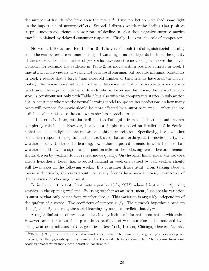
the number of friends who have seen the movie.26 I use prediction 5 to shed some light

on the importance of network effects. Second, I discuss whether the finding that positive

surprise movies experience a slower rate of decline in sales than negative surprise movies

may be explained by delayed consumer responses. Finally, I discuss the role of competitors.

Network Effects and Prediction 5. It is very difficult to distinguish social learning

from the case where a consumer’s utility of watching a movie depends both on the quality

of the movie and on the number of peers who have seen the movie or plan to see the movie.

Consider for example the evidence in Table 2. A movie with a positive surprise in week 1

may attract more viewers in week 2 not because of learning, but because marginal consumers

in week 2 realize that a larger than expected number of their friends have seen the movie,

making the movie more valuable to them. Moreover, if utility of watching a movie is a

function of the expected number of friends who will ever see the movie, the network effects

story is consistent not only with Table 2 but also with the comparative statics in sub-section

6.2. A consumer who uses the normal learning model to update her predictions on how many

peers will ever see the movie should be more affected by a surprise in week 1 when she has

a diffuse prior relative to the case when she has a precise prior.

This alternative interpretation is difficult to distinguish from social learning, and I cannot

completely rule it out. However, I provide a simple test based on Prediction 5 in Section

3 that sheds some light on the relevance of this interpretation. Specifically, I test whether

consumers respond to surprises in first week sales that are orthogonal to movie quality, like

weather shocks. Under social learning, lower than expected demand in week 1 due to bad

weather should have no significant impact on sales in the following weeks, because demand

shocks driven by weather do not reflect movie quality. On the other hand, under the network

effects hypothesis, lower than expected demand in week one caused by bad weather should

still lower sales in the following weeks. If a consumer draws utility from talking about a

movie with friends, she cares about how many friends have seen a movie, irrespective of

their reasons for choosing to see it.

To implement this test, I estimate equation 18 by 2SLS, where I instrument Sj using

weather in the opening weekend. By using weather as an instrument, I isolate the variation

in surprise that only comes from weather shocks. This variation is arguably independent of

the quality of a movie. The coefficient of interest is β2. The network hypothesis predicts

that β2 > 0. By contrast, the social learning hypothesis predicts that β2 = 0.

A major limitation of my data is that it only includes information on nation-wide sales.

However, as it turns out, it is possible to predict first week surprise at the national level

using weather conditions in 7 large cities: New York, Boston, Chicago, Denver, Atlanta,

26Becker (1991) proposes a model of network effects where the demand for a good by a person depends

positively on the aggregate quantity demanded of the good. He hypothesizes that “the pleasure from some

goods is greater when many people want to consume it.”

28

Kansans City and Detroit.27 In general, rain, snow and colder temperatures in these 7 cities

are associated with significantly lower first week demand and significantly lower first week

surprise.

Results are shown in Table 9. The first row corresponds to a specification where Sj is the

surprise of movie j, while the second row corresponds to a specification where Sj is a dummy

for whether the surprise of movie j is positive. Column 1 reports the baseline OLS estimates

for the sample for which I have non-missing temperature data for all 7 cities. These estimates

are very similar to the corresponding estimates for the full sample. Column 2 reports instru-

mental variables estimates where instruments include minimum and maximum temperature

on the opening day and the day before the opening day. It is possible that the effect of

temperature is nonlinear. For example, when it is cold, we expect higher temperatures to

be associated with higher sales, but when it is hot, we expect higher temperatures to lower

sales. For this reason, in column 3 instruments also include the squares of minimum and

maximum temperature on the opening day and the day before. In column 4, instruments

include minimum and maximum temperature as well as precipitation and snowfall on the

opening day and the day before. In column 5, instruments include minimum and maximum

temperature, precipitation, and snowfall, on the opening day and the day before, as well

as these variables squared. Surprise is defined as the deviation of sales from expected sales

based on number of screens. The last row in Table 9 corresponds to a test of whether the

weather variables are jointly significant in the first stage. While only some of the first stage

coefficients are individually significant, taken together they are statistically significant. Tests

for whether the first stage coefficients are jointly equal to 0 have p-values below 0.0001 in

all 4 columns, although the F test statistics are low.

Comparison of columns 1 and 2 indicates that the coefficient on the surprise×t interaction

drops from .413 to -.107, while the coefficient on the positive surprise dummy×t interaction

drops from .643 to -.277. The corresponding coefficients in column 2 are .085 and .123 and

are not statistically significant. Column 3 and 4 display similar results. Not surprisingly,

the IV estimates are considerably less precise than the OLS estimates, most likely because

I can not perform the analysis at the city-level. For this reason it is difficult to draw firm

conclusions. However, the small, insignificant and often wrong-signed point estimates in

columns 2-5 suggest that network effects cannot fully explain the large effects documented

in Table 2.

One concern is that weather might be serially correlated. Because my measure of sales

is for the weekend, this is unlikely to be a serious concern. Indeed, when I measure serial

correlation in temperature, snow or precipitation in my 7 cities, I find that weather is not

correlated with weather 7 days earlier.28

27Dahl and Della Vigna (2007) are the first to document that weather in selected cities shifts aggregate

movie sales.28Positive serial correlation would induce a positive bias into IV estimates, biasing the test in favor of the

network hypothesis.

29

Delayed Consumer Response. It is in theory possible that the patterns in Table 2 are

explained by a slow adjustment of consumers to the innovation represented by the surprise.

Consider for example a positive surprise movie, and assume that there is a fraction of con-

sumers who cannot immediately go when a new movie is released but have already decided

to see the film in later weeks. In this case the positive surprise movie would experience a

slower rate of decline in sales even in the absence of social learning.

However, while this explanation could in theory generate the patterns documented in

Table 2, it is not consistent with the comparative statics on precision of the prior and the

signal documented below in sub-sections 6.2 and 6.3. In the absence of social learning there

is no reason why we should see that the effect of the surprise is systematically associated

with the precision of the prior or the size of the social network.

Competitors. Movies rarely open alone. Often there are 2 or 3 movies opening in the

same weekend. As documented by Einav (2003 and 2007), the competitors a movie faces are

not random, but are determined strategically by the studios. The fact that competitors are

not random does not pose a problem for my estimation. The number of screens allocated

to a given movie should incorporate the best prediction of demand given its competitors.

A movie facing a competitor that is expected to be strong will have a smaller number of

screens than a movie facing a competitor expected to be weak. Thus, while competitors are

not random, the deviation from market expectations is arguably random.

One might still be concerned that a positive surprise competitor might mechanically

induce a negative surprise for a given movie. While this is likely, this mechanism alone

would not generate the increased divergence in sales over time between positive surprise

movies and negative surprise movies documented in section 6. It would simply result in

a parallel shift in sales, without necessarily affecting the rate of decline. Moreover, this

mechanism alone would not generate the comparative statics in sections 6.2 and 6.3.

8 Discussion and Conclusion

This paper makes two contributions. Substantively, I show that social learning is an

important determinant of sales in the movie industry. Social learning makes successful movies

more successful and unsuccessful movies more unsuccessful. Consistent with a simple model

where consumers update their priors based on their peers’ purchasing decisions, the rate of

decline of movies with stronger than expected first week demand is about half the rate of

decline of movies with weaker than expected first week demand.

While I cannot completely rule out alternative explanations, the weight of the evidence

is consistent with the social learning hypothesis. As the model predicts, the effect of a

surprise on subsequent sales is smaller for movies for which consumers have strong priors

and larger for movies for which consumers have more diffuse priors. Additionally, the effect

30

of a surprise is more pronounced for groups of consumers who have more developed social

networks. Finally, consumers do not seem to respond to surprises caused by factors that are

orthogonal to movie quality, like weather shocks.

Quantitatively, social learning appears to have an important effect on profits in the

movie industry. When I use my estimates to quantify the amount of sales generated by

social learning, I find that for the typical movie with positive surprise, social learning raises

box-office sales by $5.8 million–or about 38% of total revenues–relative to the case of a movie

that has similar quality but where consumers do not communicate.29 The existence of this

large “social multiplier” indicates that the elasticity of aggregate movie demand to movie

quality is significantly larger than the elasticity of individual demand to quality.

The second contribution of the paper is methodological. This paper shows that it is pos-

sible to identify social interactions using aggregate data and intuitive comparative statics. In

situations where individual-level data and exogenous variation in peer group attributes are

not available, this approach is a credible alternative methodology for identifying spillovers

and social interactions. For example, this approach can be applied to the study of informa-

tional spillovers in the demand of many other goods or in technology adoption.

29This number is obtained as follows. Equation 18 indicates that over the lifetime of a movie, the effect

of a positive surprise on sales is∑8

t=2 β̂2 S t salest, where the summation does not include the first week

(t=1), as learning begins only after the opening week; β̂2 = .463 is the coefficient in column 2 of Table 2;

salest represents average sales in week t for a movie with no surprise; and S represents the surprise for the

typical positive or negative surprise movie. (For simplicity, in these calculations I ignore the non-linearity

uncovered in subsection 6.4.) For the typical positive surprise movie–that is, the one at the 75th percentile

of the surprise distribution, with sales 46% above expectations–social learning accounts for $5.8 million in

additional sales. For the typical negative surprise movie–that is, the one at the 25th percentile of the surprise

distribution, with sales 41% below expectations–social learning accounts for $5.2 million in lost sales.

31

9 Bibliography

Adda, Gerome ”The Dynamics of Car Sales: A Discrete Choice Approach”, 2007.

Adda Gerome, James Banks and Hans-Martin von Gaudecker ”The Impact of Income

Shocks on Health: Evidence from Cohort Data”, 2006.

Anderson, Lisa R., and Charles A. Holt (1997), Information Cascades in the Laboratory,

American Economic Review, 87:5, 847-862.

Banerjee, Abhijit ”A Simple Model of Herd Behavior”, Quarterly Journal of Economics,

1992.

Bass, Frank (1969). ”A new product growth for model consumer durables”. Management

Science 15 (5): p215-227.

Becker, Gary S, ”A Note on Restaurant Pricing and Other Examples of Social Influences

on Price,” Journal of Political Economy, University of Chicago Press, vol. 99(5), pages

1109-16, October, 1991.

Bertrand, Marianne, Sendhil Mullainathan and Erzo Luttmer Network Effects and Wel-

fare Cultures, The Quarterly Journal of Economics, August 2000.

Besley Tim and Anne Case ”Diffusion as a Learning Process”, 1994.

Bikhchandani Sushil, David Hirshleifer, Ivo Welch ”A Theory of Fads, Fashion, Custom,

and Cultural Change as Informational Cascades”, The Journal of Political Economy, Vol.

100, No. 5 (Oct., 1992), pp. 992-1026

Bikhchandani, Sushil, David Hirshleifer, Ivo Welch ”Learning from the Behavior of Oth-

ers: Conformity, Fads, and Informational Cascades” The Journal of Economic Perspectives,

Vol. 12, No. 3 (Summer, 1998), pp. 151-170

Cai, Hongbin and Yuyu Chen and Hanming Fang, ”Observational Learning: Evidence

from a Randomized Natural Field Experiment”, Duke University (2007).

Dahl, Gordon and Stefano Della Vigna ”Does Movie Violence Increase Violent Crime?”

2007.

De Vany Arthur and Cassey Lee ”Quality Signals in Informational cascades and the

Dynamics of the Distribution of Motion Picture Box Office Revenues”, Journal of Economic

Dynamic and Control, 2001.

Dixit Avinash K. and Robert S. Pindyck, ”Investment under Uncertainty”, Princeton

University Press (1994).

Einav, Liran ”Not All Rivals Look Alike: Estimating an Equilibrium Model of The

Release Date Timing Game” mimeo, Stanford University, 2003.

Einav, Liran ”Seasonality in the U.S. Motion Picture Industry Rand Journal of Eco-

nomics” 38(1), Spring 2007.

Einav, Liran, ”Informational Asymmetries and Observational Learning in Search Journal

of Risk and Uncertainty”, 30(3), June 2005, 241-259.

Ellison Glenn, Drew Fudenberg ”Rules of Thumb for Social Learning” The Journal of

Political Economy, Vol. 101, No. 4 (Aug., 1993), pp. 612-643

32

Foster, D. Andrew and Mark R. Rosenzweig ”Learning by Doing and Learning from

Others: Human Capital and Technical Change in Agriculture”, The Journal of Political

Economy, Vol. 103, No. 6 (Dec., 1995), pp. 1176-1209

Friedman, Milton ”A Theory of the Consumption Function”, (1957)

Glaeser, Edward L., Bruce I. Sacerdote Jose A. Scheinkman The ”Social Multiplier”,

Journal of the European Economic Association, MIT Press, vol. 1(2-3), pages 345-353,

04/05.

Glaeser, Edward L. and Bruce Sacerdote, ”Aggregation Reversals and the Social Forma-

tion Beliefs” (2007)

Glaeser, Edward L., Bruce Sacerdote, Jose A. Scheinkman, ”Crime and Social Interac-

tions” Quarterly Journal of Economics, Vol. 111, no. 2 (May 1996): 507-548.

Goettler Ron and Phillip Leslie ”Cofinancing to Manage Risk in the Motion Picture

Industry,” Journal of Economics and Management Strategy, 14(2), 231-61 (2005)

Goolsbee Austan and Peter J. Klenow ”Evidence on Learning and Network Externalities

in the Diffusion of Home Computers” The Journal of Law and Economics, volume 45 (2002),

pages 317343

Griliches, Zvi ”Hybrid Corn: an Exploration in the Economics of Technical Change”,

Econometrics 25(4), 1957.

Grinblatt Mark, Matti Keloharju, Seppo Ikheimo, ”Interpersonal Effects in Consumption:

Evidence from the Automobile Purchases of Neighbors”, mimeo, 2004.

Hendricks Ken and Alan Sorensen, ”Information and the Skewness of Music Sales”, March

2007.

Hong Harrison, Jeffrey D. Kubik Jeremy C. Stein, ”Thy Neighbor’s Portfolio: Word-of-

Mouth Effects in the Holdings and Trades of Money Managers”, Journal of Finance 2005.

Knight, Brian and Nathan Schiff, ”Momentum and Social Learning in Presidential Pri-

maries” NBER Working Paper No. 13637 (2007).

Liu, Yong ”Word of Mouth for Movies: Its Dynamics and Impact on Box Office Rev-

enues”, Journal of Marketing, 70 (2006).

Luttmer Erzo F.P. ”Neighbors as Negatives: Relative Earnings and Well-Being”, Quar-

terly Journal of Economics, 120(3), pp. 963-1002, August 2005.

Sacerdote, Bruce ”Peer Effects with Random Assignment: Results for Dartmouth Room-

mates”, The Quarterly Journal of Economics, 116 681-704 (2001).

Salganik Matthew J., Peter S. Dodds, and Duncan J. Watts. ”Experimental study of

inequality and unpredictability in an artificial cultural market.” Science, 311:854-856, 2006.

Skinner Jonathan and Douglas Staiger ”Technological Adoption from Hybrid Corn to

Beta Blockers,” with , NBER Working Paper, 2005.

Skinner Jonathan and Douglas Staiger ”Diffusion and Productivity Growth in Health

Care”

Sorensen, Alan ”Bestseller Lists and Product Variety,” forthcoming, Journal of Industrial

Economics.

33

Sorensen, Alan ”Social Learning and Health Plan Choice,” forthcoming, RAND Journal

of Economics.

Vise, David ”The Google Story”, Delacorte Press (2005).

34

Table 1: Summary Statistics

(1)

Weekend Sales (million) 1.78

(4.37)

Weekend Sales in Opening Weekend (million) 4.54

(8.15)

Production Costs (million) 16.88

(.81)

Number of Screens 449.6

(696.9)

Number of Screens in Opening Weekend 675.7

(825.5)

Favorable Review .480

(.499)

Total TV Advertising (million) 6.85

(5.54)

Action .071

Adventure .018

Animated .027

Black Comedy .017

Comedy .191

Documentary .047

Drama .340

Fantasy .011

Film Festival .003

Horror .035

Musical .016

Romantic Comedy .065

Sci-Fiction .018

Sequel .068

Suspense .062

Western 0.005

Number of Movies 4992

Notes: Standard errors are in parentheses. Dollar figures are in 2005 dollars. The sample

includes 4,992 movies that opened between 1982 and 2000. Each of these movies is observed

for 8 weeks. Total sample size is 39936. Sample size for reviews and TV advertising are 5064

and 14840, respectively.

35

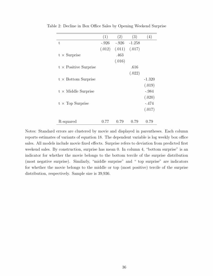
Table 2: Decline in Box Office Sales by Opening Weekend Surprise

(1) (2) (3) (4)

t -.926 -.926 -1.258

(.012) (.011) (.017)

t × Surprise .463

(.016)

t × Positive Surprise .616

(.022)

t × Bottom Surprise -1.320

(.019)

t × Middle Surprise -.984

(.020)

t × Top Surprise -.474

(.017)

R-squared 0.77 0.79 0.79 0.79

Notes: Standard errors are clustered by movie and displayed in parentheses. Each column

reports estimates of variants of equation 18. The dependent variable is log weekly box office

sales. All models include movie fixed effects. Surprise refers to deviation from predicted first

weekend sales. By construction, surprise has mean 0. In column 4, “bottom surprise” is an

indicator for whether the movie belongs to the bottom tercile of the surprise distribution

(most negative surprise). Similarly, “middle surprise” and “ top surprise” are indicators

for whether the movie belongs to the middle or top (most positive) tercile of the surprise

distribution, respectively. Sample size is 39,936.

36

Table 3: Distribution of Movie-Specific Speed of Decline in Box Office Sales over Time, by

Opening Weekend Surprise

Movies with Movies with

Positive Surprise Negative Surprise

(1) (2)

5% -2.30 -2.66

10 % -1.78 -2.47

25 % -.96 -1.91

Median -.41 -1.23

75 % -.11 -.60

90 % .15 -.19

95 % .26 .00

Notes: Entries represent the distribution of the parameter β1j in equation 19 for movies that

experienced a positive first weekend surprise and for movies that experienced a negative

first weekend surprise. There are 4,992 such coefficients, one for each movie. The two

distributions are shown graphically in Figure 5.

37

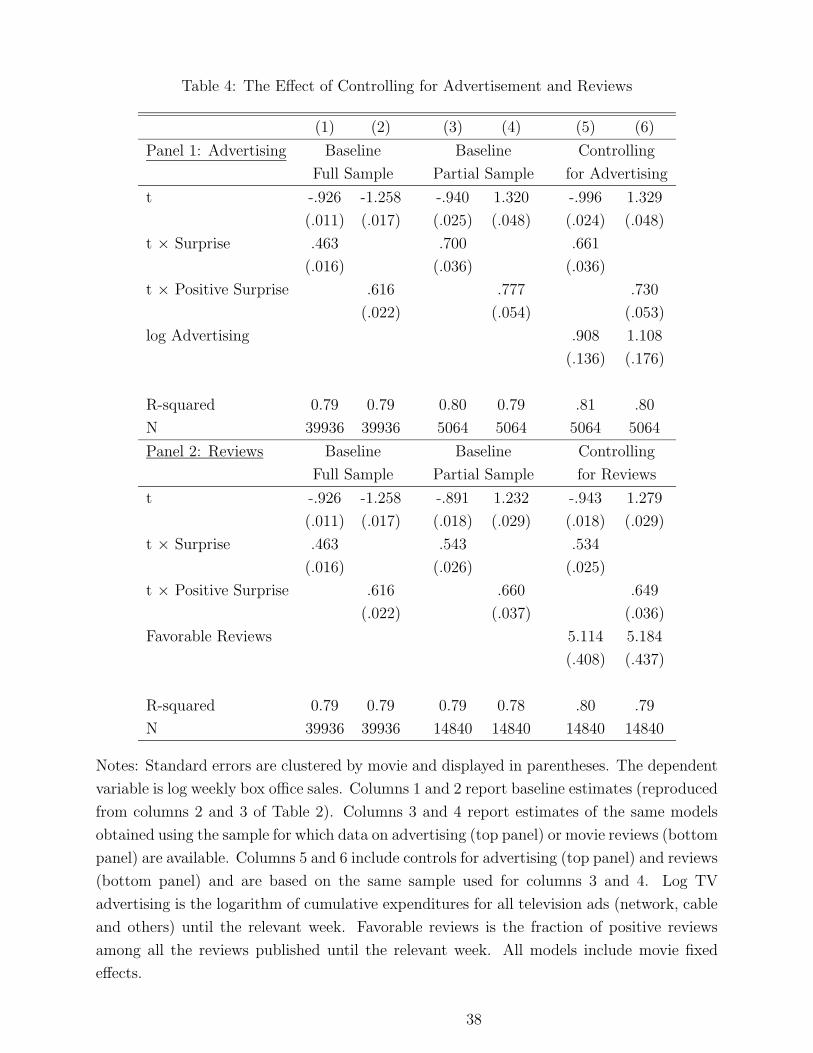
Table 4: The Effect of Controlling for Advertisement and Reviews

(1) (2) (3) (4) (5) (6)

Panel 1: Advertising Baseline Baseline Controlling

Full Sample Partial Sample for Advertising

t -.926 -1.258 -.940 1.320 -.996 1.329

(.011) (.017) (.025) (.048) (.024) (.048)

t × Surprise .463 .700 .661

(.016) (.036) (.036)

t × Positive Surprise .616 .777 .730

(.022) (.054) (.053)

log Advertising .908 1.108

(.136) (.176)

R-squared 0.79 0.79 0.80 0.79 .81 .80

N 39936 39936 5064 5064 5064 5064

Panel 2: Reviews Baseline Baseline Controlling

Full Sample Partial Sample for Reviews

t -.926 -1.258 -.891 1.232 -.943 1.279

(.011) (.017) (.018) (.029) (.018) (.029)

t × Surprise .463 .543 .534

(.016) (.026) (.025)

t × Positive Surprise .616 .660 .649

(.022) (.037) (.036)

Favorable Reviews 5.114 5.184

(.408) (.437)

R-squared 0.79 0.79 0.79 0.78 .80 .79

N 39936 39936 14840 14840 14840 14840

Notes: Standard errors are clustered by movie and displayed in parentheses. The dependent

variable is log weekly box office sales. Columns 1 and 2 report baseline estimates (reproduced

from columns 2 and 3 of Table 2). Columns 3 and 4 report estimates of the same models

obtained using the sample for which data on advertising (top panel) or movie reviews (bottom

panel) are available. Columns 5 and 6 include controls for advertising (top panel) and reviews

(bottom panel) and are based on the same sample used for columns 3 and 4. Log TV

advertising is the logarithm of cumulative expenditures for all television ads (network, cable

and others) until the relevant week. Favorable reviews is the fraction of positive reviews

among all the reviews published until the relevant week. All models include movie fixed

effects.

38

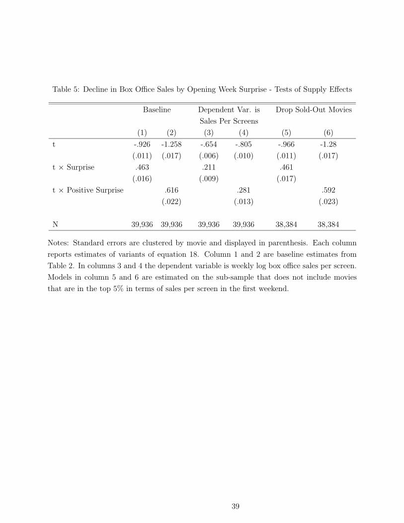
Table 5: Decline in Box Office Sales by Opening Week Surprise - Tests of Supply Effects

Baseline Dependent Var. is Drop Sold-Out Movies

Sales Per Screens

(1) (2) (3) (4) (5) (6)

t -.926 -1.258 -.654 -.805 -.966 -1.28

(.011) (.017) (.006) (.010) (.011) (.017)

t × Surprise .463 .211 .461

(.016) (.009) (.017)

t × Positive Surprise .616 .281 .592

(.022) (.013) (.023)

N 39,936 39,936 39,936 39,936 38,384 38,384

Notes: Standard errors are clustered by movie and displayed in parenthesis. Each column

reports estimates of variants of equation 18. Column 1 and 2 are baseline estimates from

Table 2. In columns 3 and 4 the dependent variable is weekly log box office sales per screen.

Models in column 5 and 6 are estimated on the sub-sample that does not include movies

that are in the top 5% in terms of sales per screen in the first weekend.

39

Table 6: Robustness of the Estimated Effect of Surprise to the Inclusion of Controls

(1) (2) (3) (4) (5) (6) (7)

Panel 1

Model 1

t × Surprise .422 .424 .420 .416 .445 .433 .463

(.012) (.012) (.012) (.012) (.015) (.016) (.016)

Model 2

t × Positive Surprise .672 .666 .659 .646 .585 .561 .616

(.022) (.022) (.022) (.022) (.022) (.022) (.022)

Surprise Equation Controls For:

Genre Y Y Y Y Y Y

Ratings Y Y Y Y Y

Production Cost Y Y Y Y

Distributor Y Y Y

Weekday, Month, Week Y Y

Year Y

Panel 2

Model 3

t × Surprise .422 .422 .425 .427 .444 .433 .473

(.012) (.012) (.012) (.012) (.015) (.015) (.014)

Model 4

t × Positive Surprise .672 .671 .673 .674 .684 .666 .711

(.022) (.022) (.022) (.022) (.022) (.022) (.022)

Sales Equation Controls For:

t × Genre Y Y Y Y Y Y

t × Ratings Y Y Y Y Y

t × Production Cost Y Y Y Y

t × Distributor Y Y Y

t × Weekday, Month Y Y

t × Year Y

Notes: Standard errors are clustered by movie and displayed in parentheses. Each entry is a separate

regression. In panel 1, each entry is an estimate of the parameter β2 in equation 18, where the definition of

surprises varies across columns. Surprise refers to deviation from predicted first week sales, where predicted

first week sales are obtained using the number of screens as a predictor and an increasing number of controls,

as specified at the bottom of the panel. Column 7 reports baseline estimates from the definition of surprise

used in Table 2. Panel 2 reports estimates of equation 20, where an increasing number of controls are added

to the sales equation, as specified at the bottom of the panel. In this panel, surprise is defined using only

the number of screens as predictor. All models include movie fixed effects. Sample size is 39,936.

40

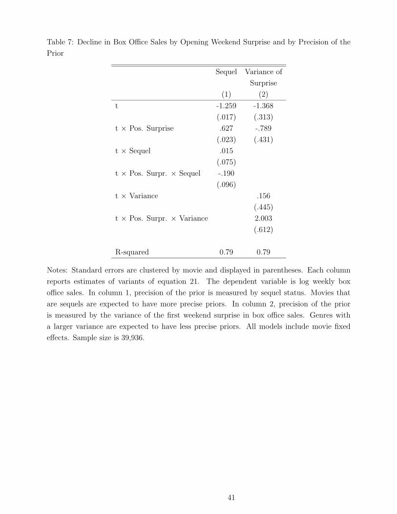
Table 7: Decline in Box Office Sales by Opening Weekend Surprise and by Precision of the

Prior

Sequel Variance of

Surprise

(1) (2)

t -1.259 -1.368

(.017) (.313)

t × Pos. Surprise .627 -.789

(.023) (.431)

t × Sequel .015

(.075)

t × Pos. Surpr. × Sequel -.190

(.096)

t × Variance .156

(.445)

t × Pos. Surpr. × Variance 2.003

(.612)

R-squared 0.79 0.79

Notes: Standard errors are clustered by movie and displayed in parentheses. Each column

reports estimates of variants of equation 21. The dependent variable is log weekly box

office sales. In column 1, precision of the prior is measured by sequel status. Movies that

are sequels are expected to have more precise priors. In column 2, precision of the prior

is measured by the variance of the first weekend surprise in box office sales. Genres with

a larger variance are expected to have less precise priors. All models include movie fixed

effects. Sample size is 39,936.

41

Table 8: Decline in Box Office Sales, by Opening Weekend Surprise and Precision of Peers’

Signal

Movies Size of the

for Teenagers Release

(1) (2)

t -1.163 -1.180

(.022) (.019)

t × Positive Surprise .576 .568

(.029) (.028)

t × Teen Movie -.224

(.034)

t × Positive Surprise × Teen Movie .091

(.046)

t × Screens -.133

(.024)

t × Positive Surprise × Screens .094

(.028)

R-squared 0.79 0.79

Notes: Standard errors are clustered by movie and displayed in parentheses. The dependent

variable is log weekly box office sales. Column 1 reports an estimate of equation 22, where

“Teen Movie” is an indicator equal to one if the intended audience is teenagers, based on

detailed genre. Teenagers are expected to have a larger social network and therefore more

social learning. Column 2 reports an estimate of equation 23, where “Screens” is the number

of screens in the opening weekend. Movies with a larger number of screens are expected to

send a more precise signal. Number of screens is divided by 1,000 to make the reported

coefficients easier to read. All models include movie fixed effects. Sample size is 39,936.

42

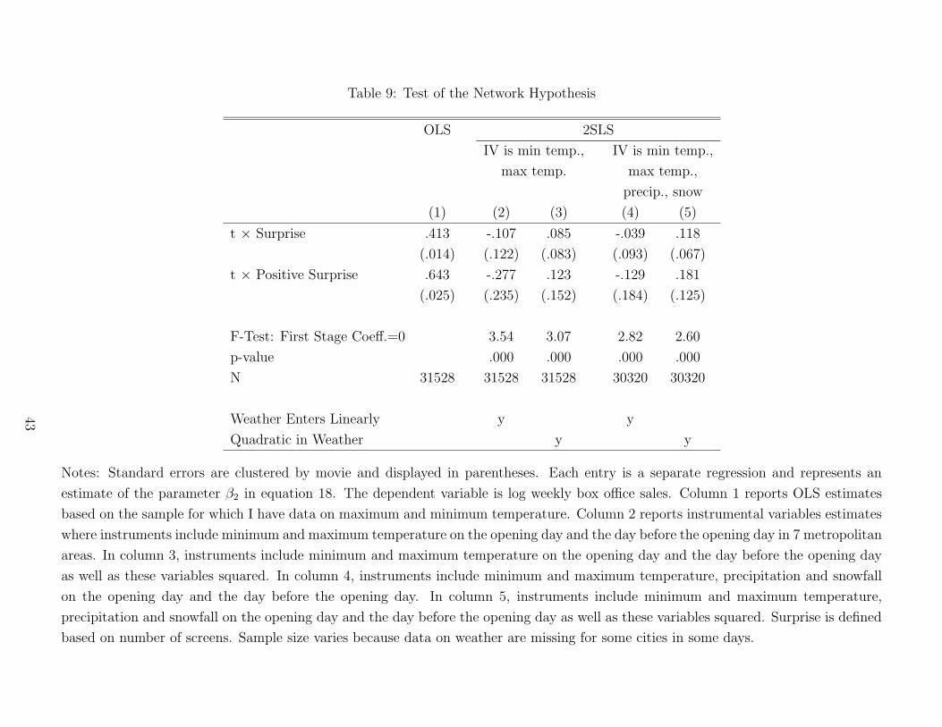
Table 9: Test of the Network Hypothesis

OLS 2SLS

IV is min temp., IV is min temp.,

max temp. max temp.,

precip., snow

(1) (2) (3) (4) (5)

t × Surprise .413 -.107 .085 -.039 .118

(.014) (.122) (.083) (.093) (.067)

t × Positive Surprise .643 -.277 .123 -.129 .181

(.025) (.235) (.152) (.184) (.125)

F-Test: First Stage Coeff.=0 3.54 3.07 2.82 2.60

p-value .000 .000 .000 .000

N 31528 31528 31528 30320 30320

Weather Enters Linearly y y

Quadratic in Weather y y

Notes: Standard errors are clustered by movie and displayed in parentheses. Each entry is a separate regression and represents an

estimate of the parameter β2 in equation 18. The dependent variable is log weekly box office sales. Column 1 reports OLS estimates

based on the sample for which I have data on maximum and minimum temperature. Column 2 reports instrumental variables estimates

where instruments include minimum and maximum temperature on the opening day and the day before the opening day in 7 metropolitan

areas. In column 3, instruments include minimum and maximum temperature on the opening day and the day before the opening day

as well as these variables squared. In column 4, instruments include minimum and maximum temperature, precipitation and snowfall

on the opening day and the day before the opening day. In column 5, instruments include minimum and maximum temperature,

precipitation and snowfall on the opening day and the day before the opening day as well as these variables squared. Surprise is defined

based on number of screens. Sample size varies because data on weather are missing for some cities in some days.

43

Appendix Table A1: Regression of First Weekend Box Office Sales on Number

of Screens and Controls

(1) (2) (3) (4) (5) (6) (7)

Log Screens .892 .895 .882 .870 .802 .806 .813

(.004) (.004) (.005) (.005) (.006) (.006) (.006)

R-squared 0.907 .908 .909 .912 932 .936 .937

Genre Y Y Y Y Y Y

Ratings Y Y Y Y Y

Production Cost Y Y Y Y

Distributor Y Y Y

Weekday, Month, Week Y Y

Year Y

Notes: Standard errors are in parentheses. The dependent variable is the log of opening

weekend box office sales. There are 16 dummies for genre; 8 dummies for ratings; 273

dummies for distributor; 18 dummies for year; 6 dummies for weekday; 11 dummies for

month; 51 dummies for week. Sample size is 4,992.

44

Appendix Table A2: Distribution of Surprises in Opening Weekend Box Office

Sales

Percentile Surprise Examples

(1) (2) (3)

5% -1.21 Tarzan and the Lost City; Big Bully; The Fourth War

10 % -.87 Tom & Jerry ; The Phantom of the Opera; Born to Be Wild

25 % -.41 Home Alone 3; Pinocchio; Miracle on 34th Street

Median .02 Highlander 3; The Bonfire of the Vanities; Fear and Loathing in Las Vegas

75 % .46 Alive; Autumn in New York; House Party

90 % .84 The Muse; Sister Act; Forrest Gump; Tarzan

95 % 1.08 Breakin; Ghostbusters; The Silence of the Lambs

Notes: Entries represent the distribution of surprises (in percent terms) in opening weekend

box office sales. For example, the entry for 75% indicates that opening weekend sales for

the movie at the 75th percentile are 46% higher than expected. Mean surprise is 0 by

construction.

45

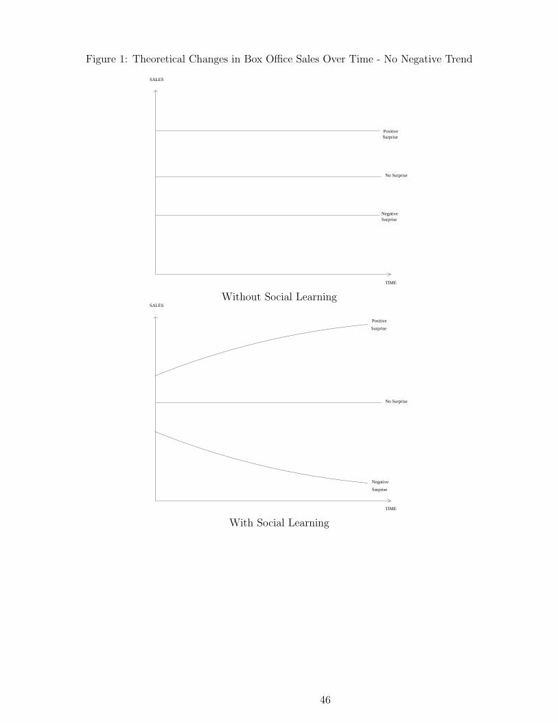
Figure 1: Theoretical Changes in Box Office Sales Over Time - No Negative Trend

TIME

SurpriseNegative

No Surprise

SurprisePositive

SALES

Without Social Learning

Negative

Surprise

Surprise

Positive

TIME

No Surprise

SALES

With Social Learning

46

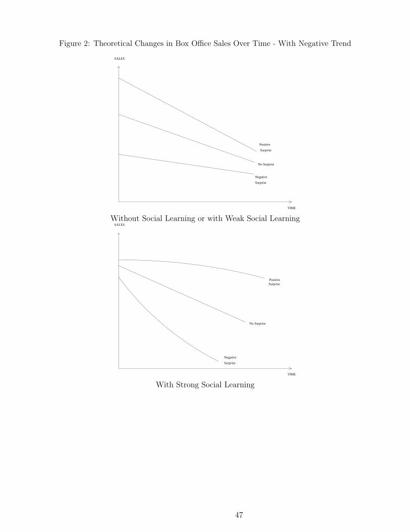
Figure 2: Theoretical Changes in Box Office Sales Over Time - With Negative Trend

Positive

Surprise

Negative

Surprise

No Surprise

TIME

SALES

Without Social Learning or with Weak Social Learning

No Surprise

Surprise

Negative

SurprisePositive

TIME

SALES

With Strong Social Learning

47

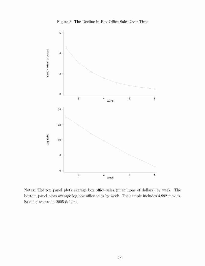
Figure 3: The Decline in Box Office Sales Over Time

Sal

es −

Mill

ion

of D

olla

rs

Week2 4 6 8

0

2

4

6

Log

Sal

es

Week2 4 6 8

6

8

10

12

14

Notes: The top panel plots average box office sales (in millions of dollars) by week. The

bottom panel plots average log box office sales by week. The sample includes 4,992 movies.

Sale figures are in 2005 dollars.

48

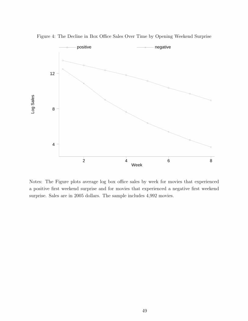
Figure 4: The Decline in Box Office Sales Over Time by Opening Weekend SurpriseLo

g S

ales

Week

positive negative

2 4 6 8

4

8

12

Notes: The Figure plots average log box office sales by week for movies that experienced

a positive first weekend surprise and for movies that experienced a negative first weekend

surprise. Sales are in 2005 dollars. The sample includes 4,992 movies.

49

Figure 5: Distribution of Movie-Specific Speed of Decline in Box Office Sales over Time, by

Opening Weekend Surprise

beta

positive negative

−3 −2 −1 0 1

0

.5

1

Notes: The Figure shows the distribution of the coefficient β1j in equation 19, for movies

that experienced a positive first weekend surprise and for movies that experienced a negative

first weekend surprise. In other words, it shows the distribution of the slope coefficient from

4,992 regressions of log box office sales on a time trend, by surprise. Percentiles of the two

distributions are reported in Table 3.

50