Social Interaction and Stock-Market Participationhh2679/jfsocial.pdfSocial Interaction and Stock-Market Participation 139 In the specific setting of the stock market, there are at

THE JOURNAL OF FINANCE • VOL. LIX, NO. 1 • FEBRUARY 2004

Social Interaction and Stock-MarketParticipation

HARRISON HONG, JEFFREY D. KUBIK, and JEREMY C. STEIN∗

ABSTRACT

We propose that stock-market participation is influenced by social interaction. In ourmodel, any given “social” investor finds the market more attractive when more of hispeers participate. We test this theory using data from the Health and RetirementStudy, and find that social households—those who interact with their neighbors, orattend church—are substantially more likely to invest in the market than non-socialhouseholds, controlling for wealth, race, education, and risk tolerance. Moreover, con-sistent with a peer-effects story, the impact of sociability is stronger in states wherestock-market participation rates are higher.

IN 1998, 48.9 PERCENT OF AMERICAN HOUSEHOLDS owned stock, either directly, orthrough mutual funds or various retirement vehicles such as 401(k) plans orIRAs.1 While this number may appear low in an absolute sense—particularlyin light of the historically high returns to investing in the stock market—itactually represents an all-time peak in the United States, and a dramatic in-crease from prior years. For example, less than a decade earlier, in 1989, theparticipation rate stood at only 31.6 percent; even as late as 1995 it was at just40.4 percent.

What are the underlying determinants of the stock-market participationrate? This question is an important one, for a number of reasons. First, asargued by, for example, Mankiw and Zeldes (1991), Heaton and Lucas (1999),Vissing-Jorgensen (1999), and Brav, Constantinides, and Gezcy (2002), the par-ticipation rate can have a direct effect on the equity premium; thus an under-standing of what drives participation can help shed light on the equity-premiumpuzzle of Mehra and Prescott (1985).

Second, certain policy debates hinge crucially on one’s view of why so manyhouseholds opt not to participate in the stock market. Consider proposals whichwould have the government invest some portion of social security tax proceeds

∗Hong is with the Department of Economics, Princeton University; Kubik is with the Depart-ment of Economics, Syracuse University; and Stein is with the Department of Economics, HarvardUniversity, and NBER. We are grateful to the National Science Foundation for research support,and to Ed Glaeser, Rick Green, Michael Kremer, David Laibson, Jun Liu, Michael Morris, Mark Ru-binstein, Lara Tiedens, Tuomo Vuolteenaho, Ezra Zuckerman, and the referee for their commentsand suggestions. Thanks also to seminar participants at Berkeley, Chicago, Columbia, Illinois,Iowa, Ohio State, Rochester, and Stanford. Any remaining errors are our own.

1 The numbers in this paragraph are from the Survey of Consumer Finances, as reported byBertaut and Starr-McCluer (2000).

137

138 The Journal of Finance

in the stock market. On the one hand, if one takes the perspective of a full-information, frictionless model with optimizing households—in which thosewho sit out do so simply because they find the market’s risk-return profileunattractive—standard arguments suggest that there is nothing to be gainedby having the government invest in the market on their behalf. On the otherhand, if households do not participate because of a lack of information aboutmarket opportunities, or because other frictional costs deter them from do-ing so, the case for these proposals can, at a minimum, begin to make logicalsense.2

A few basic facts about the determinants of household participation in thestock market are already well known.3 First, participation is strongly increas-ing in wealth. This can be understood by thinking of participation as involvingfixed costs; wealthier households have more to invest, and so the fixed cost isless of a deterrent to them. Vissing-Jorgensen (2000) builds a model in whichfixed costs of participation are incurred on a per-period basis, and estimatesthat such costs have to be on the order of $200 per year to explain observedparticipation rates. Of course, such large numbers beg the questions of whatthese black-box fixed costs actually represent, and whether one should thinkof them as being similar across different types of households.

Stock-market participation has also been found to be increasing in house-hold education. One interpretation is that education reduces the fixed costsof participating, by making it easier for would-be investors to understand themarket’s risk–reward trade-offs, to deal with the mechanics of setting up anaccount, and executing trades, etc.4 Finally, there is also a pronounced linkbetween race and participation, with white, non-Hispanic households havingmuch higher participation rates, controlling for wealth and education.

In this paper, we add to this line of work by considering the possibility thatstock-market participation is influenced by social interaction. A priori, thiswould seem to be a promising hypothesis, given the growing body of empiri-cal research that speaks to the importance of peer-group effects in a varietyof other contexts.5 Notably, some of this work finds evidence of peer effects infinancial settings that are suggestively close to the one we have in mind—for example, Madrian and Shea (2000) and Duflo and Saez (2002) demon-strate that an individual’s decision of whether or not to participate in par-ticular employer-sponsored retirement plans is influenced by the choices of hisco-workers.

2 See Abel (2001) and Campbell et al. (1999) for explicit analyses along these lines.3 These facts are documented by, for example, Vissing-Jorgensen (2000) and Bertaut and Starr-

McCluer (2000).4 Bernheim and Garrett (1996) and Bayer, Bernheim, and Scholz (1998) find that financial ed-

ucation in the workplace increases participation in retirement plans.5 Examples include Case and Katz (1991), Glaeser, Sacerdote, and Scheinkman (1996), and

Bertrand, Luttmer, and Mullainathan (2000). Glaeser and Scheinkman (2000) provide a surveywith more references.

Social Interaction and Stock-Market Participation 139

In the specific setting of the stock market, there are at least two broadchannels through which social interaction might influence participation. Thefirst is word-of-mouth or observational learning (Banerjee (1992), Bikchandani,Hirshleifer, and Welch (1992), Ellison and Fudenberg (1993, 1995)).6 For ex-ample, potential investors may learn from one another either about the highreturns that the market has historically offered, or about how to execute trades.Second, in the spirit of Becker (1991), a stock-market participant may get plea-sure from talking about the ups and downs of the market with friends who arealso fellow participants, much as he might enjoy similar conversations aboutrestaurants, books, movies, or local sports teams in which there is a sharedinterest.

We develop a model that captures these ideas in a simple way. Our modelhas two types of investors: (1) “non-socials” and (2) “socials.” The non-socialsare similar to the investors in Vissing-Jorgensen (2000): They each face fixedcosts of participation, but these fixed costs are not influenced by the behaviorof others. In contrast, any given social investor finds it more attractive to investin the market—that is, his fixed costs are lower—when the participation rateamong his peers is higher.

The model’s most basic and unambiguous prediction is that there will behigher participation rates among social investors than among non-socials, allelse being equal. The model also suggests that the participation rate amongsocials can be more sensitive to changes in other exogenous parameters—thatis, there can be “social multiplier” effects. Consider the consequences of a changein technology (e.g., web-based trading) that makes the direct physical costs ofparticipation lower for all investors. In many cases, this technological changewill have a greater impact on the participation of socials than on that of non-socials because of the positive externalities that socials confer on one another.Indeed, when these positive externalities are strong enough, they can generatemultiple equilibria among social investors.

In an effort to test the theory, we draw on data from the Health and Retire-ment Study (HRS). This survey of roughly 7,500 households has a variety ofinformation on wealth, asset holdings, demographics, etc. But most relevantfor our purposes, it also asks respondents several questions which allow usto create empirical analogs to our model’s notion of “non-social” and “social”households. In particular, the survey asks whether households interact withtheir neighbors, or attend church.

We find that more social households—defined as those who answer “yes” tothese questions—are indeed more likely to invest in the stock market, control-ling for other factors like wealth, race, and education. The effects of sociabilityare both strongly statistically significant, as well as economically important.

6 See also Routledge (1999) and DeMarzo, Vayanos, and Zwiebel (2001) for other models of learn-ing in financial markets. Shiller and Pound (1989) present survey data on the diffusion of informa-tion among stock-market investors by word-of-mouth. Kelly and Grada (2000) find evidence that,during banking panics, bad news about banks spreads via word-of-mouth in neighborhoods.


Across the entire sample, households that either know their neighbors or at-tend church have roughly a 4 percent higher probability of participating in thestock market, all else being equal. Among white, educated households withabove-average wealth—those who are typically most likely to be on the cuspof the participation decision—the marginal effect of sociability is substantiallystronger, reaching 8 percent in some specifications.

While the HRS data allow us to address our theory in a straightforward way,they also suffer from an important drawback. The measures of sociability thatwe take from the HRS—whether households know their neighbors or attendchurch—reflect endogenous choices, and hence may capture information notjust about the degree of social interaction per se, but also about other personalitytraits that may be associated with the propensity to invest in the stock market.For example, sociable people may be more bold, and hence less risk-averse whenit comes to investing. Or they may be more optimistic, and hence have higherexpectations for future stock-market returns.

We attempt to address these possibilities in two ways. First, we are fortunatein that the HRS data allow us to construct proxies for other potentially relevantpersonality traits such as risk tolerance and optimism. When entered as addi-tional controls in the stock-market participation regressions, these proxies tendto come in significantly, and with the expected signs—suggesting that they aredoing a good job of measuring what they are supposed to measure—but theyhave little effect on our sociability variables.

Second, we take advantage of the fact that our theory has further implicationsthat are not shared by the alternative hypothesis that sociability is a surrogatefor personality. In particular, if social households invest more because of theirinteractions with other investors, then the marginal effect of sociability oughtto be more pronounced in areas where there is a high density of stock-marketparticipants.7 To take an extreme example, if a social household lives in a statewhere nobody else invests in the stock market (and it does not interact withanybody out-of-state) then according to our theory we should not see any effect ofsociability on participation for this household. In contrast, if our social variablesare simply proxies for, for example, individual risk tolerance, then one mightexpect these variables to attract the same positive coefficients in participationregressions regardless of what kind of state the household lives in.

Consistent with our theory, we document that the impact of household socia-bility is indeed stronger in states where stock-market participation rates arehigher. The cross-state differentials are very substantial. In “high-participation”states (those with average participation rates in the top one-third of the sample)sociability generates an increase in the participation rate that averages roughly7 to 9 percent across all demographic groups; in “low-participation” states thesociability effect is close to zero. Moreover, this cross-state pattern distinguishesour social variables from our measure of risk-tolerance—the risk-tolerance

7 This logic parallels that of Bertrand, Luttmer, and Mullainathan (2000), who find that beingsurrounded by others who speak the same language increases welfare use more for those fromhigh-welfare-using groups.


variable shows no differential effect across states. These results help to al-lay concerns that our proxies for sociability are picking up other personalityattributes that have nothing to do with social interaction.8

The remainder of the paper is organized as follows. We begin in Section Iby discussing a model that illustrates the link between social interaction andstock market participation, and that forms the basis for our subsequent tests. InSection II, we describe our data set, and in Section III we present our empiricalresults. Section IV concludes.

I. The Model

The key implications of our model can be sketched verbally. For a more for-mal treatment, see our NBER working paper (Hong, Kubik, and Stein (2001)).We distinguish between two classes of investors: (1) non-socials and (2) socials.Each non-social investor faces a fixed cost of participating in the market. Thiscost can have both an idiosyncratic component (e.g., the investor has a diffi-cult time understanding financial matters), as well as a common component(e.g., the investor lives in an area where there are few brokerage offices percapita). But importantly, for a non-social investor, the fixed cost is unrelated tothe participation decisions of all other investors. Consequently, each non-socialinvestor makes his participation decision independently, by trading off the ben-efits of participation—which will typically be increasing in wealth—against thefixed cost.9

Social investors differ from non-socials in that their net cost of participatingin the market is influenced by the choices of their peers. Specifically, the cost forany social investor in a given peer group is reduced—relative to the value for anotherwise identical non-social—by an amount that is increasing in the numberof others in the peer group that are participating. Or said differently, any onesocial finds it more attractive to participate in the market when more of hispeers do. In the limiting case where none of a social’s peers are participating,he faces the same fixed cost as an otherwise identical non-social.

As noted earlier, there are several concrete interpretations that can be at-tached to this formulation. And depending on the specific story being told, theactual social interaction may take place either before or after the decision toparticipate in the market is made. For example, in the case of word-of-mouth

8 There is a more subtle version of the endogeneity critique that we cannot address. It maybe, for example, that socials have a higher participation rate not because they have a greaternumber of informative interactions with their peers, but rather because they are better listenersand hence learn more from a given level of interaction. Thus one cannot draw the same kind of causalconclusions that one might from a randomized experiment (as in Sacerdote (2001)). Specifically, itdoes not follow from our results that if a non-social household were somehow forced to spend moretime with its neighbors it would be more likely to participate in the market. We do not think thiscaveat makes our findings less interesting from a positive-economics perspective. But it matterswhen thinking about their normative implications.

9 In our NBER working paper, we show that in a constant-relative-risk-aversion (CRRA) frame-work the benefit to participating in the market is simply a fixed proportion of initial wealth.


learning about the market’s risk/return characteristics, the interaction takesplace before any investment. However, in the case of getting utility from talk-ing with friends about the market, one can imagine that a social would investbased just on the prospect of future interactions.

This set-up leads to the following three implications. First, controlling forwealth, risk tolerance, and measures of participation costs, we should see ahigher participation rate among social investors than among non-socials. Sec-ond, there will be social multiplier effects with respect to changes in exogenousparameters like wealth, risk tolerance, and participation costs. That is, the par-ticipation rate for socials should respond more sensitively to changes in theseparameters than the participation rate for non-socials. And third, our modeladmits the possibility of multiple equilibria among social investors. When thepositive externalities across members of a peer group are strong enough, eithera relatively high or relatively low participation rate can be self-sustaining.

In the empirical work below, much of our focus will be on testing the firstof these three implications—that socials have a higher participation rate thannon-socials—and on ensuring that the results of these tests are not contami-nated by endogeneity biases. Nevertheless, it is worth briefly highlighting howthe model’s implications for social multipliers and multiple equilibria mightmanifest themselves in the data.

The notion of social multipliers may be especially helpful in thinking aboutchanges in aggregate stock-market participation over time. As noted above,the participation rate has increased dramatically over the last decade or so.One candidate explanation for this phenomenon is that the growing promi-nence of mutual funds, along with the introduction of web-based trading, havetogether led to a systematic decline in average costs of participation.10 If so,social-interaction effects may have helped to give this cost shock much morekick than it otherwise would have had. This hypothesis can in principle betested by looking to see if the participation rate of socials has increased morerapidly in recent years than has the participation rate of non-socials. We makean effort in this direction, though data limitations prevent us from going as faras we would like.

To the extent that people tend to interact disproportionately with membersof their own racial/ethnic groups, the multiple-equilibrium feature of the modelcould potentially shed some light on the puzzle of why black and Hispanichouseholds tend to be stuck at much lower participation rates, even when theyare wealthy and highly educated. Loosely speaking, the multiple equilibria sug-gest that an ethnic group’s past history with respect to participation may—byaffecting which equilibrium is chosen—exert an important influence on cur-rent outcomes, above and beyond the effects of any current conditions such aswealth and education.11

10 Choi, Laibson, and Metrick (2002) present direct evidence on the consequences of web-basedtrading.

11 With regard to the role of history, Chiteji, and Stafford (1999) document that young adults aremuch more likely to participate in the stock market if their parents did.


II. Data

Our data come from Health and Retirement Study (HRS) administered bythe Institute for Social Research at the University of Michigan.12 This surveywas first conducted in 1992 (this is referred to as Wave 1 of the survey), andcovers approximately 7,500 households who have a member born during theperiod 1931 through 1941.13 Thus the average age of target respondents atthe time of Wave 1 is roughly 56 years. Follow-up Waves 2, 3, and 4, coveringthe same households, were conducted in 1994, 1996, and 1998, respectively.Our analysis focuses primarily on the data from Wave 1 of the HRS. We havere-run all our tests using the data from the later waves; as might be expected,given that these later waves cover the same households, they contain very littleindependent information, and lead to virtually identical results.14

Beginning in 1998, the HRS also added a new cohort to the survey, composedof households with a member born during the period 1942 through 1947, anddubbed the “war-baby” cohort. The average age of the war babies in 1998 isapproximately 54 years, very similar to that of the original HRS sample in 1992.This 1998 war-baby sample is of obvious interest, for two reasons. First, wewould like some out-of-sample verification of our results from the 1992 survey.And second, it would be interesting to test the model’s intertemporal social-multiplier prediction—to see if, as the overall participation rate has increasedover the 1990s, the differential between socials and non-socials has widened.

Unfortunately, the war-baby sample is much smaller, covering only around1,400 households, which seriously limits our statistical power. Even more prob-lematic, this version of the survey omits several of the questions that are mostcrucial for us, leaving us able to create only one of the three measures of socialinteraction that we use in the original 1992 HRS sample, and forcing us todrop other controls. Thus our analysis of the war-baby sample is restricted tojust a couple of very basic regressions; unless explicitly noted otherwise, every-thing else we discuss from now on refers to the 1992 wave of the original HRSsample.

The HRS includes information on place of residence (by state, along withan urban/rural indicator), age, years of education, race, wealth, income, andmarital status. For age, years of education, and race, we may have two responsesper household—one for the man and one for the woman of the house. We takethe “age” and “education” of a household to be the higher of the two values. Forrace, we classify a household as non-white if either member is.15 With respectto stock-market participation, the survey asks whether households own stocks,

12 The data set, along with all the survey questions and supporting documentation, is availableat: www.umich.edu/∼hrswww/.

13 The HRS is a representative sample within this age group, except that blacks, Hispanics, andFlorida residents are 100 percent oversampled.

14 One reason to focus on the first (1992) wave is that there is some attrition among respondentsin the later follow-up surveys. (The first-wave interviews are done in person, the others by phone.)Moreover, the rate of attrition is correlated with our key variables—there is more attrition amongnon-social households.

15 None of our results is sensitive to how we choose to handle these details.


either directly or through mutual funds. However, it should be noted that thisquestion only pertains to non-retirement-account assets. The data set has verylittle information on assets held in retirement accounts, so these are omittedin our measure of participation. While there is no reason to expect that thisshould bias our inferences about the role of social interactions, it does meanthat the average participation rates that we report are significantly lower thanthose obtained from other data sets (e.g., the Survey of Consumer Finances)that include retirement assets.

To create our measures of social interaction, we focus on three questions inthe survey. A single member of the household, typically the woman, answerseach of these questions.16 The first is: “Of your closest neighbors, how many doyou know?,” to which 92.9 percent of respondents answer either “all,” “most,”or “some.” Our Know Neighbors dummy variable takes on the value one forthese households, and zero for the remainder who answer “none.” The secondquestion is: “How often do you visit with your neighbors?,” to which 63.9 percentof respondents answer either “daily,” “several times a week,” “several times amonth,” or “several times a year.” Our Visit Neighbors dummy is set to one forthese households, and to zero for the remainder who answer “hardly ever.”17

Finally, the third question is: “How often do you attend religious services?,”to which 76.0 percent of respondents answer either “more than once a week,”“once a week,” “two or three times a month,” or “one or more times a year.” OurAttend Church dummy is one for these households, and zero for the remainderwho answer “never.”

A large body of work in sociology supports the premise of using these sortsof variables as measures of the extent to which households have informativeinteractions with one another. Granovetter (1983) surveys much of this work,emphasizing “the strength of weak ties”—that is, the substantial amount ofinformation that people obtain through interactions with neighbors and casualacquaintances. For example, there is a lot of evidence to the effect that peoplelearn about new jobs through such informal connections, rather than throughmore formal channels.18

As mentioned above, we also use the survey questions to create proxies forother personality traits. Risk aversion is the most straightforward, since there isa question designed by Barsky et al. (1997, page 540) to measure this attribute:“. . . you are given the opportunity to take a new and equally good job, with a50-50 chance it will double your (family) income and a 50-50 chance it will cutyour (family) income by a third. Would you take that new job?” In contrast to

16 In our regressions, we include a dummy for the sex of the respondent to the social questions.17 We are bypassing another similar question, “Do you have good friends in your neighborhood?”

because it seems more ambiguous as a measure of social interaction. In particular, we worry that arespondent who interacts regularly with his or her neighbors, but whose best friends live elsewhere,might be inclined to say “no” to this question.

18 The work surveyed in Granovetter (1983) is more directly applicable to the interpretation ofour model in which socials communicate real information about the stock market to one another. Ithas less to say about the interpretation in which socials simply derive utility from investing whentheir friends invest.


the sociability questions, this—like the other “personality-related” questions—is asked separately of each member of a household. Our Risk Tolerant dummy isone for the 32.5 percent of households with at least one member who responds“yes,” and zero for the remainder where both members answer “no.”19

Sociability might also be related to optimism, which could in turn influencestock-market participation. The best we can do on this score is to use the fol-lowing question: “During the past week, I felt depressed. (All or almost all ofthe time, most of the time, some of the time, or none or almost none of thetime?)” Our premise is that there is likely to be a link between depression andpessimism. In any case, our Depressed dummy takes on the value one in the 8.3percent of cases where at least one household member responds “all or almostall of the time;” in the remaining cases the dummy is set to zero.

It is important to stress however, that while we are using this variable inthe hopes that it will control for a purely individual characteristic—namelypessimism—that might be related to participation, it is also plausible that itcontains further independent information about the extent of social interaction,since depressed people may well spend less time interacting with others. Inthis sense, the Depressed dummy differs from the Risk Tolerant dummy, whichseems to be more cleanly interpretable as being strictly about an individualtrait, and not about anything having to do with social interaction.

Finally, one might speculate that sociable people are simply more open-minded and more willing to try new things. The only question that comes closeto allowing us to address this idea is: “How difficult is it for you to use a com-puter or word processor?” Our Low Tech dummy is one for the 30.9 percentof households in which both members answer, “don’t do,” and zero for the re-mainder of households. An obvious problem in interpreting any coefficient onthis Low Tech variable is that unlike risk tolerance or depression, computeruse represents an outcome, not a personality trait. And as with the Depresseddummy, there is also the qualification that even if it contains some informationabout the personality trait of open-mindedness, it may also capture informationabout social interaction, to the extent that there are peer effects in the adoptionof computers.

Tables I and II provide an overview of some basic facts about the data. Panel Aof Table I breaks down participation rates across different demographic groups.Overall, in the whole HRS sample, 26.7 percent of households participate in thestock market. (Recall that this is 1992, and that our measure of participationdoes not include assets held in retirement accounts.) Participation increasessharply with wealth, going from 3.4 percent in the lowest quintile of the wealthdistribution to 55.0 percent in the highest wealth quintile.20 There are also

19 Our results are essentially unchanged if we require both members to respond “yes” in orderto classify a household as risk-tolerant. A similar comment applies to our other personality-traitproxies.

20 We measure wealth as the value of all assets excluding non-retirement stockholdings. Withthis measure, the inter-quintile cutoff values are: $11,000; $55,000; $116,000; and $240,000. Ourprincipal results are unchanged if we include stockholdings in our wealth measure, and they arealso not sensitive to whether or not we include retirement wealth.


Table IStock-Market Participation Rates for Different Categories

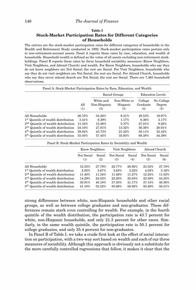
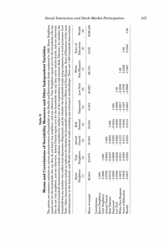
of HouseholdsThe entries are the stock-market participation rates for different categories of households in theHealth and Retirement Study conducted in 1992. Stock-market participation rates pertain onlyto non-retirement-account assets. Panel A reports these rates by race, education, and wealth ofhouseholds. Household wealth is defined as the value of all assets excluding non-retirement stock-holdings. Panel B reports these rates by three household sociability measures (Know Neighbors,Visit Neighbors, and Attend Church) and wealth. For Know Neighbors, households who say theydo not know neighbors are Not Social; the rest are Social. For Visit Neighbors, households whosay they do not visit neighbors are Not Social; the rest are Social. For Attend Church, householdswho say they never attend church are Not Social; the rest are Social. There are 7,465 householdobservations.

Panel A: Stock-Market Participation Rates by Race, Education, and Wealth

Racial Groups Education Levels

White and Non-White or College No CollegeAll Non-Hispanic Hispanic Graduate Degree(1) (2) (3) (4) (5)

All Households 26.70% 34.28% 9.21% 49.53% 19.97%1st Quintile of wealth distribution 3.41% 6.39% 1.17% 6.36% 3.17%2nd Quintile of wealth distribution 11.34% 15.28% 5.37% 27.01% 9.28%3rd Quintile of wealth distribution 24.10% 27.81% 13.32% 36.36% 20.91%4th Quintile of wealth distribution 39.84% 43.73% 21.32% 50.11% 35.42%5th Quintile of wealth distribution 55.03% 57.45% 35.93% 68.38% 44.39%

Panel B: Stock-Market Participation Rates by Sociability and Wealth

Know Neighbors Visit Neighbors Attend Church

Not Social Social Not Social Social Not Social Social(1) (2) (3) (4) (5) (6)

All Households 12.33% 27.79% 22.77% 28.92% 23.52% 27.70%1st Quintile of wealth distribution 2.05% 3.67% 3.63% 3.22% 4.05% 3.16%2nd Quintile of wealth distribution 11.40% 11.34% 11.46% 11.27% 12.24% 11.02%3rd Quintile of wealth distribution 14.29% 24.52% 22.20% 25.05% 23.59% 24.25%4th Quintile of wealth distribution 30.91% 40.18% 37.03% 41.17% 37.14% 40.56%5th Quintile of wealth distribution 41.18% 55.52% 50.86% 56.92% 50.49% 56.21%

strong differences between white, non-Hispanic households and other racialgroups, as well as between college graduates and non-graduates. These dif-ferences remain stark even controlling for wealth. For example, in the fourthquintile of the wealth distribution, the participation rate is 43.7 percent forwhite, non-Hispanic households, and only 21.3 percent for other races. Sim-ilarly, in the same wealth quintile, the participation rate is 50.1 percent forcollege graduates, and only 35.4 percent for non-graduates.

In Panel B of Table I, we take a crude first look at the effect of social interac-tion on participation, with a two-way sort based on wealth and each of our threemeasures of sociability. Although this approach is obviously not a substitute forthe more carefully controlled regressions that follow, it makes it clear that the


Tab

leII

Mea

ns

and

Cor

rela

tion

sof

Soc

iab

ilit

yM

easu

res

and

Oth

erIn

dep

end

ent

Var

iab

les

Th

een

trie

sar

esu

mm

ary

stat

isti

cson

vari

ous

char

acte

rist

ics

ofh

ouse

hol

dsin

the

Hea

lth

and

Ret

irem

ent

Stu

dyco

ndu

cted

in19

92.K

now

Nei

ghbo

rseq

ual

sze

rofo

rth

eh

ouse

hol

dsw

ho

say

they

don

otkn

owan

yn

eigh

bors

,an

don

eot

her

wis

e.V

isit

Nei

ghbo

rseq

ual

sze

rofo

rth

eh

ouse

hol

dsw

ho

say

they

don

otvi

sit

nei

ghbo

rs,a

nd

one

oth

erw

ise.

Att

end

Ch

urc

heq

ual

sze

rofo

rth

eh

ouse

hol

dsw

ho

say

they

nev

erat

ten

dch

urc

h,a

nd

one

oth

erw

ise.

Add

itio

nal

hou

seh

old

char

acte

rist

ics

incl

ude

indi

cato

rva

riab

les

for

wh

eth

eron

eof

the

resp

onde

nts

isri

skto

lera

nt

(Ris

kT

oler

ant)

,for

wh

eth

erth

eh

ouse

hol

dh

ason

em

embe

rw

ho

suff

ers

from

depr

essi

on(D

epre

ssed

),an

dfo

rw

het

her

the

hou

seh

old

avoi

dsu

sin

gco

mpu

ters

orw

ord

proc

esso

rs(L

owT

ech

).O

ther

char

acte

rist

ics

incl

ude

anin

dica

tor

for

wh

eth

erth

eh

ouse

hol

d’s

repo

rted

race

isW

hit

ean

dN

on-H

ispa

nic

,Yea

rsof

Edu

cati

on(o

fth

em

ost

edu

cate

dpe

rson

inth

eh

ouse

hol

d),a

nd

Wea

lth

(hou

seh

old

wea

lth

excl

udi

ng

non

-ret

irem

ent

stoc

khol

din

gs).

Th

ere

are

7,46

5h

ouse

hol

dob

serv

atio

ns.

Kn

owV

isit

Att

end

Ris

kW

hit

eYe

ars

ofN

eigh

bors

Nei

ghbo

rsC

hu

rch

Tol

eran

tD

epre

ssed

Low

Tec

hN

on-H

ispa

nic

Edu

cati

onW

ealt

h(1

)(2

)(3

)(4

)(5

)(6

)(7

)(8

)(9

)

Mea

nof

sam

ple

92.9

4%63

.87%

76.0

2%32

.53%

8.33

%30

.92%

69.7

5%12

.65

$196

,405

Cor

rela

tion

s:K

now

Nei

ghbo

rs1.

000

Vis

itN

eigh

bors

0.36

651.

000

Att

end

Ch

urc

h0.

0792

0.09

421.

000

Ris

kT

oler

ant

−0.0

118

−0.0

213

0.00

351.

000

Dep

ress

ed−0

.068

3−0

.068

9−0

.030

5−0

.003

41.

000

Low

Tec

h−0

.058

9−0

.024

2−0

.022

80.

0505

0.09

201.

00W

hit

eN

on-H

ispa

nic

0.08

720.

0511

−0.1

472

−0.0

016

−0.0

917

−0.2

050

1.00

Year

sof

Edu

cati

on0.

0832

0.05

850.

0171

0.03

45−0

.158

7−0

.378

50.

3226

1.00

Wea

lth

0.05

370.

0352

0.03

100.

0114

−0.0

641

−0.0

900

0.14

810.

1845

1.00


basic patterns emerge in even the simplest tabulations of the data. Using theKnow Neighbors measure of interaction, 12.3 percent of non-social householdsparticipate in the market, while 27.8 percent of social households do. With VisitNeighbors, the corresponding figures are 22.8 percent and 28.9 percent, whilewith Attend Church they are 23.5 percent and 27.7 percent, respectively. Inaddition, when the sample is stratified based on wealth, it appears that thedifferences between social and non-social households become more pronouncedas wealth increases—indeed, virtually all of the action in this respect comesfrom the top three wealth quintiles.

In Table II, we look at the correlations between our three measures of socia-bility, as well as between these measures and the other independent variablesthat will enter our specifications. Not surprisingly, Know Neighbors and VisitNeighbors are highly correlated, with a correlation coefficient of 0.37. On theother hand, both of these measures are more weakly correlated with AttendChurch, with coefficients of only 0.08 and 0.09, respectively. Thus it seems thatAttend Church offers relatively independent information on sociability aboveand beyond that contained in the first two variables.

None of the sociability measures is all that highly correlated with the otherpersonality proxies, though there are some noteworthy differences. On the onehand, Risk Tolerant is essentially uncorrelated with all the social variables.In contrast, both Depressed and Low Tech have statistically significant correla-tions of −0.07 and −0.06, respectively with Know Neighbors. This suggests thatsocial people may indeed be happier (and perhaps more optimistic) as well asmore open to new experiences. It also reinforces the point made above, namelythat unlike the Risk Tolerant variable, Depressed and Low Tech may themselvesbe proxies for the degree of social interaction.

Finally, there are some modest correlations between our sociability measuresand the demographic variables. White, educated, and wealthy households areall somewhat more likely to both know their neighbors and visit them, withpairwise correlation coefficients in the range of 0.04 to 0.09. On the other hand,white households are markedly less churchgoing—the correlation between theindicator for white/non-Hispanic and Attend Church is −0.15.

III. Empirical Results

A. Baseline Effect of Social Interaction on Stock-Market Participation

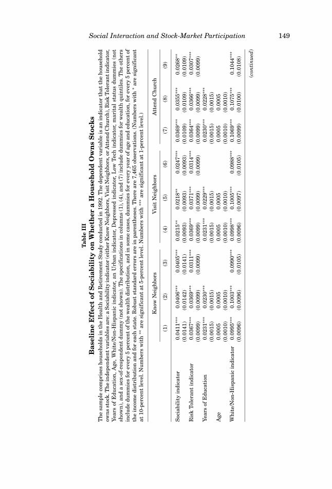
Table III presents our baseline results. All regressions are run by OLS, withthe dependent variable an indicator that takes on the value one when a house-hold owns stock, and zero otherwise.21 There are nine columns, correspondingto three different specifications with each of our three sociability measures—Know Neighbors, Visit Neighbors, and Attend Church. In columns (1), (4), and(7), the social variable enters along with the Risk Tolerant dummy, years of ed-ucation, age, a white/non-Hispanic dummy, an urban dummy, a marital-status

21 Given the dichotomous nature of our left-hand-side variable, we have redone all our tests usingprobit and logit specifications, with very similar results.


Tab

leII

IB

asel

ine

Eff

ect

ofS

ocia

bil

ity

onW

het

her

aH

ouse

hol

dO

wn

sS

tock

sT

he

sam

ple

com

pris

esh

ouse

hol

dsin

the

Hea

lth

and

Ret

irem

ent

Stu

dyco

ndu

cted

in19

92.T

he

depe

nde

nt

vari

able

isan

indi

cato

rth

atth

eh

ouse

hol

dow

ns

stoc

k.T

he

inde

pen

den

tvar

iabl

esar

e:a

Soc

iabi

lity

indi

cato

r(e

ith

erK

now

Nei

ghbo

rs,V

isit

Nei

ghbo

rs,o

rA

tten

dC

hu

rch

),R

isk

Tol

eran

tin

dica

tor,

Year

sof

Edu

cati

on,

Age

,W

hit

e/N

on-H

ispa

nic

indi

cato

r,an

Urb

anin

dica

tor,

Dep

ress

edin

dica

tor,

Low

Tec

hin

dica

tor,

mar

ital

stat

us

dum

mie

s(n

otsh

own

),an

da

sex-

of-r

espo

nde

nt

dum

my

(not

show

n).

Th

esp

ecif

icat

ion

sin

colu

mn

s(1

),(4

),an

d(7

)in

clu

dedu

mm

ies

for

wea

lth

quin

tile

s.T

he

oth

ers

incl

ude

dum

mie

sfo

rev

ery

5pe

rcen

tof

the

wea

lth

dist

ribu

tion

,an

din

som

eca

ses,

dum

mie

sfo

rev

ery

year

ofag

ean

ded

uca

tion

,for

ever

y5

perc

ent

ofth

ein

com

edi

stri

buti

onan

dfo

rea

chst

ate.

Rob

ust

stan

dard

erro

rsar

ein

pare

nth

eses

.Th

ere

are

7,46

5ob

serv

atio

ns.

(Nu

mbe

rsw

ith

∗ar

esi

gnif

ican

tat

10-p

erce

nt

leve

l.N

um

bers

wit

h∗∗

are

sign

ific

ant

at5-

perc

ent

leve

l.N

um

bers

wit

h∗∗

∗ar

esi

gnif

ican

tat

1-pe

rcen

tle

vel.)

Kn

owN

eigh

bors

Vis

itN

eigh

bors

Att

end

Ch

urc

h

(1)

(2)

(3)

(4)

(5)

(6)

(7)

(8)

(9)

Soc

iabi

lity

indi

cato

r0.

0411

∗∗∗

0.04

06∗∗

∗0.

0405

∗∗∗

0.02

15∗∗

0.02

18∗∗

0.02

47∗∗

∗0.

0369

∗∗∗

0.03

55∗∗

∗0.

0268

∗∗(0

.014

1)(0

.014

2)(0

.014

1)(0

.009

3)(0

.009

3)(0

.009

3)(0

.010

9)(0

.010

9)(0

.010

9)R

isk

Tol

eran

tin

dica

tor

0.03

67∗∗

∗0.

0369

∗∗∗

0.03

11∗∗

∗0.

0369

∗∗∗

0.03

71∗∗

∗0.

0314

∗∗∗

0.03

64∗∗

∗0.

0366

∗∗∗

0.03

07∗∗

∗(0

.009

9)(0

.009

9)(0

.009

9)(0

.009

9)(0

.009

9)(0

.009

9)(0

.009

9)(0

.009

9)(0

.009

9)Ye

ars

ofE

duca

tion

0.02

31∗∗

∗0.

0230

∗∗∗

0.02

31∗∗

∗0.

0229

∗∗∗

0.02

30∗∗

∗0.

0228

∗∗∗

(0.0

015)

(0.0

015)

(0.0

015)

(0.0

015)

(0.0

015)

(0.0

015)

Age

0.00

050.

0005

0.00

050.

0005

0.00

050.

0005

(0.0

010)

(0.0

010)

(0.0

010)

(0.0

010)

(0.0

010)

(0.0

010)

Wh

ite/

Non

-His

pan

icin

dica

tor

0.09

95∗∗

∗0.

1003

∗∗∗

0.09

90∗∗

∗0.

0998

∗∗∗

0.10

05∗∗

∗0.

0988

∗∗∗

0.10

69∗∗

∗0.

1075

∗∗∗

0.10

44∗∗

∗(0

.009

6)(0

.009

6)(0

.010

5)(0

.009

6)(0

.009

7)(0

.010

5)(0

.009

9)(0

.010

0)(0

.010

8)

(con

tin

ued

)


Tab

leII

I—C

onti

nu

ed

Kn

owN

eigh

bors

Vis

itN

eigh

bors

Att

end

Ch

urc

h

(1)

(2)

(3)

(4)

(5)

(6)

(7)

(8)

(9)

Urb

anin

dica

tor

0.06

05∗∗

∗0.

0622

∗∗∗

0.04

81∗∗

∗0.

0599

∗∗∗

0.06

16∗∗

∗0.

0477

∗∗∗

0.06

00∗∗

∗0.

0616

∗∗∗

0.04

76∗∗

∗(0

.016

6)(0

.016

6)(0

.016

8)(0

.016

6)(0

.016

6)(0

.016

8)(0

.016

6)(0

.016

6)(0

.016

8)D

epre

ssed

indi

cato

r−0

.030

2∗∗

−0.0

292∗

∗−0

.030

6∗∗

(0.0

126)

(0.0

127)

(0.0

126)

Low

Tec

hin

dica

tor

−0.0

349∗

∗∗−0

.035

2∗∗∗

−0.0

350∗

∗∗(0

.009

8)(0

.009

8)(0

.009

8)2n

dQ

uin

tile

ofw

ealt

hdi

stri

buti

on0.

0281

∗∗∗

0.02

98∗∗

∗0.

0302

∗∗∗

(0.0

099)

(0.0

099)

(0.0

099)

3rdQ

uin

tile

ofw

ealt

hdi

stri

buti

on0.

1156

∗∗∗

0.11

77∗∗

∗0.

1176

∗∗∗

(0.0

130)

(0.0

129)

(0.0

129)

4thQ

uin

tile

ofw

ealt

hdi

stri

buti

on0.

2455

∗∗∗

0.24

76∗∗

∗0.

2462

∗∗∗

(0.0

149)

(0.0

149)

(0.0

149)

5thQ

uin

tile

ofw

ealt

hdi

stri

buti

on0.

3757

∗∗∗

0.37

76∗∗

∗0.

3760

∗∗∗

(0.0

160)

(0.0

159)

(0.0

160)

19W

ealt

hdu

mm

ies

No

Yes

Yes

No

Yes

Yes

No

Yes

Yes

Age

dum

mie

sN

oN

oYe

sN

oN

oYe

sN

oN

oYe

sYe

ars

ofE

duca

tion

dum

mie

sN

oN

oYe

sN

oN

oYe

sN

oN

oYe

s19

Inco

me

dum

mie

sN

oN

oYe

sN

oN

oYe

sN

oN

oYe

sS

tate

dum

mie

sN

oN

oYe

sN

oN

oYe

sN

oN

oYe

s


dummy, a sex-of-respondent dummy, and four dummies corresponding to thesecond, third, fourth, and fifth quintiles of the wealth distribution.

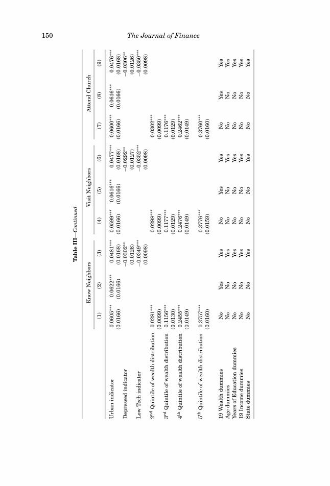
In columns (2), (5), and (8), the only modification is that we use 19, ratherthan four wealth dummies, which means that we have now chopped up thewealth distribution into 5-percent increments. This allows us to get a tighterwealth control, but makes it impractical to display the individual coefficients onall these dummies. Finally, in columns (3), (6), and (9), we add several furthercontrols: 19 income dummies; dummies for each year of age and education(which go in place of the linear age and education terms and represent a moreconservative approach to controlling for these factors); state dummies; and theDepressed and Low Tech variables.

As can be seen, the results paint a consistent picture. Consider first the KnowNeighbors measure of social interaction. The coefficients on this variable arevery close to 0.040 in all three regressions, implying that social households havea 4 percent higher probability of participating in the stock market, all else beingequal. Moreover, in each case the coefficients are statistically significant at the1-percent level. The Visit Neighbors variable looks to be a weaker version ofKnow Neighbors, with coefficients that range between 0.022 and 0.025, but thatare still statistically significant. Finally, the Attend Church variable deliverscoefficients that are comparable to those on Know Neighbors in the first tworegressions—of the order of 0.036—but that tail off a bit, to a value of 0.027,when the full set of controls is added.

The coefficients on some of the other controls are worth a brief mention. To be-gin with, we confirm earlier work by finding very powerful effects of education,race, and wealth on stock-market participation. For example, our estimatessuggest that white, non-Hispanic households have about a 10 percent greaterparticipation rate than other groups, all else being equal. The Risk Tolerantdummy has the expected positive sign, and with a value of around 0.037 acrossmost of the specifications, it appears to be economically as well as strongly sta-tistically significant. The Depressed and Low Tech indicators are both negative,as anticipated, and significantly so.

However, we caution against attaching the same kind of causal interpreta-tion to the Low Tech proxy that one might naturally lend to, for example, theRisk Tolerant variable. As discussed above, with Low Tech, we are in effect run-ning one type of endogenous outcome (stock-market participation) on another(computer use). The goal in this case is not to make a structural inference, butrather to illustrate that, to the best of our ability to control for a personalitytrait like open-mindedness, this control does not seem to affect the coefficientson our key sociability indicators.

The results in Table III speak to the average effects of sociability across all de-mographic groups. In Table IV, we investigate how the marginal effect of socialinteraction varies with race, education, and wealth. Based on our model, thereare two distinct reasons to expect that the coefficients on the social variableswould be higher among white, educated, and wealthy households.22 First, to the

22 Moreover, the simple two-way sorts in Panel B of Table I suggest that the effect of sociabilityis much stronger among wealthier households.


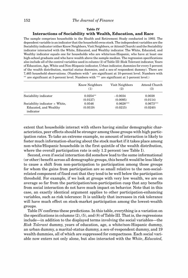
Table IVInteractions of Sociability with Wealth, Education, and Race

The sample comprises households in the Health and Retirement Study conducted in 1992. Thedependent variable is an indicator that the household owns stock. The independent variables are theSociability indicator (either Know Neighbors, Visit Neighbors, or Attend Church) and the Sociabilityindicator interacted with the White, Educated, and Wealthy indicator. The White, Educated, andWealthy indicator equals one for households who are white/non-Hispanic, who have at least onehigh-school graduate and who have wealth above the sample median. The regression specificationsalso include all of the control variables used in column (2) of Table III (Risk Tolerant indicator, Yearsof Education, Age, White and Non-Hispanic indicator, Urban indicator, dummies for every 5 percentof the wealth distribution, marital status dummies, and a sex-of respondent dummy). There are7,465 household observations. (Numbers with ∗ are significant at 10-percent level. Numbers with∗∗ are significant at 5-percent level. Numbers with ∗∗∗ are significant at 1-percent level.)

Know Neighbors Visit Neighbors Attend Church(1) (2) (3)

Sociability indicator 0.0254∗∗ −0.0034 0.0038(0.0127) (0.0095) (0.0114)

Sociability indicator × White,Educated, and Wealthyindicator

0.0546 0.0628∗∗∗ 0.0673∗∗∗(0.0519) (0.0215) (0.0240)

extent that households interact with others having similar demographic char-acteristics, peer effects should be stronger among those groups with high partic-ipation rates. To take an extreme example, no amount of interaction is likely tofoster much information-sharing about the stock market if it takes place amongnon-white/Hispanic households in the first quintile of the wealth distribution,where the overall participation rate is only 1.2 percent (see Table I).

Second, even if social interaction did somehow lead to the same informational(or other) benefit across all demographic groups, this benefit would be less likelyto cause a shift from non-participation to participation among those groupsfor whom the gains from participation are so small relative to the non-social-related component of fixed cost that they tend to be well below the participationthreshold. For example, if we look at groups with very low wealth, we are onaverage so far from the participation/non-participation cusp that any benefitsfrom social interaction do not have much impact on behavior. Note that in thiscase, an exactly identical argument applies to other participation-enhancingvariables, such as risk tolerance: It is unlikely that increases in risk tolerancewill have much effect on stock-market participation among the lowest-wealthgroups.

Table IV confirms these predictions. In this table, everything is a variation onthe specifications in columns (2), (5), and (8) of Table III. That is, the regressionsinclude—in addition to the displayed terms involving the social variables—theRisk Tolerant dummy, years of education, age, a white/non-Hispanic dummy,an urban dummy, a marital-status dummy, a sex-of-respondent dummy, and 19wealth dummies, all of which are suppressed for compactness. Each social vari-able now enters not only alone, but also interacted with the White, Educated,


and Wealthy indicator, which takes on the value 1 for those households whoare white and non-Hispanic, who are at least high-school graduates and whohave wealth above the sample median. These households represent 39.1 per-cent of the total sample, and have an average participation rate of 49.1 percent,as compared to the remaining households, who have an average participationrate of only 12.3 percent.

The interaction terms are large in magnitude, and statistically significant intwo out of three cases. By summing the raw social coefficient with the interac-tion coefficient, one obtains an estimate of the size of the social effect amongwhite, educated, and wealthy households. For the Know Neighbors variable,this number is 0.080, implying that social households in this demographic grouphave an 8 percent greater participation rate than non-social households. Forthe Visit Neighbors and Attend Church variables, the corresponding numbersare 0.059 and 0.071, respectively. In each case, the effect of the social variableamong white, educated, and wealthy households appears to be roughly doublethe size of the unconditional effect across all demographic groups reported inTable III.

Beyond what is displayed in Tables III and IV, we have also experimentedwith a number of variations on our baseline specifications, in order to furthercheck the robustness of our results. First, we have redone everything withalternative definitions of stock-market participation that require a householdto have some minimal level invested in the market (we have tried thresholds of$2,500, $5,000, $10,000, and $25,000) as opposed to just anything over zero, inorder to be counted as a participant.23 This is an effort to address the possibilitythat small stakes in the market may reflect activities like investment clubs,which could be correlated with social interaction in a relatively mechanical anduninteresting way. As it turns out, these alternative definitions of participationlead to results that are very similar to those reported in Tables III and IV. Thusthese results do not appear to be driven by investors with only trivial stakes inthe market.

Second, we have also tried adding several further controls (beyond thoseshown in columns (3), (6), and (9) of Table III) to our specifications. Thesecontrols include: whether or not the household owns its home; whether thehousehold takes regular vacations; employment status; number of people in thehousehold (i.e., how many children there are at home); and various measures ofhealth. Several of these controls can be motivated as attempts to capture howbusy a household is dealing with other things, and hence how little free time ithas to devote to stock-market investing. For example, a household that has fivechildren, two parents with full-time jobs, and that never takes vacations maysimply be too overwhelmed either to interact with its neighbors, or to investin stocks. And we want to be sure that such a lack-of-free-time effect is notinducing a spurious correlation between our sociability measures and stock-market participation. However, we find that none of the additional controls

23 Among those households who participate in the market, the median amount invested is$20,000. The 25th percentile of the distribution is $5,000, and the 75th percentile is $65,000.


has any noticeable impact on the coefficients associated with the sociabilitymeasures.

B. Effect of Social Interaction in High-Participationand Low-Participation States

While the results thus far are consistent with our theory, the worry remainsthat our social variables are not picking up the effect of social interaction per se,but rather an individual personality trait that is correlated with stock-marketparticipation and that is somehow not adequately captured by either our RiskTolerant, Depressed, or Low Tech proxies, or by any of the other controls wehave tried. In an effort to address this concern, we exploit the fact that ourtheory has subsidiary implications that the alternative hypothesis does not.In particular, if social households invest more because of their interactionswith other investors, then the marginal effect of sociability ought to be morepronounced in areas where there is a high density of stock-market participants.

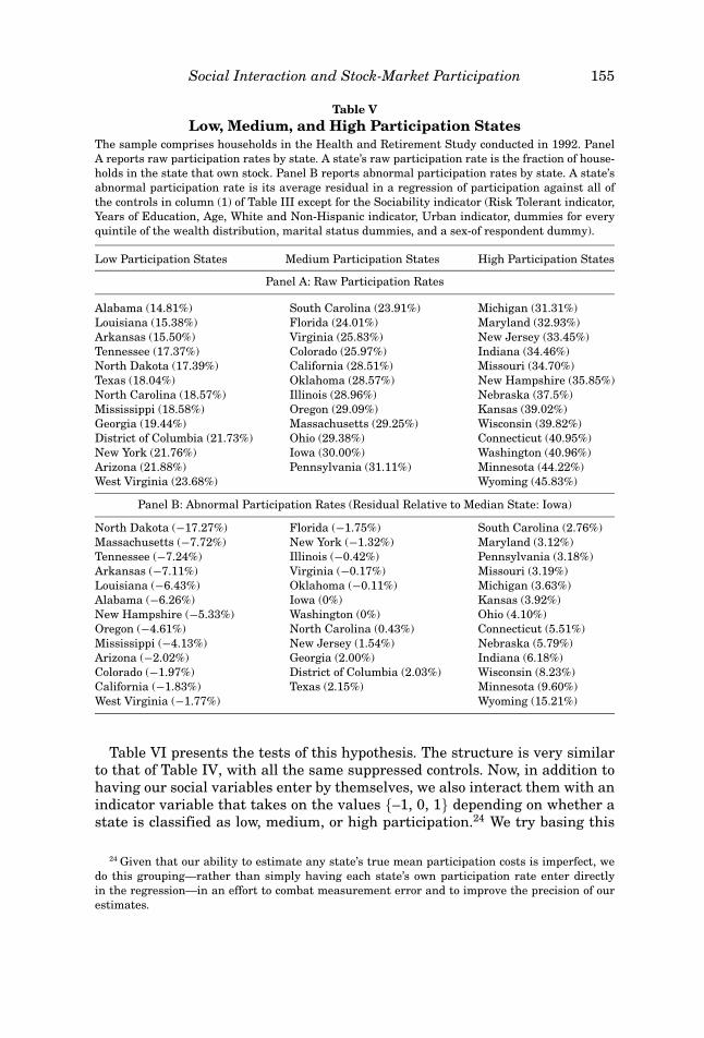
The best we can do to operationalize this idea is to look at the states in whichhouseholds live, since the HRS does not provide more detailed address data.Table V presents some information on stock-market participation at the statelevel. We group states into low, medium, and high participation categories,where a state’s participation level is measured in one of two ways. In Panel A,we look at the raw participation rate, which for any state is simply the fractionof resident households that own stock. In Panel B, we look at the abnormalparticipation rate, which for any state corresponds to the state-average-valueof the residual in a regression of household participation against: the Risk Tol-erant dummy, years of education, age, a white/non-Hispanic dummy, an urbandummy, a marital status dummy, a sex-of-respondent dummy, and four wealthdummies.

As can be seen in Table V, many of the same states show up as outliersaccording to either the raw or abnormal measure. Perhaps most strikingly, sev-eral largely rural southern states—Alabama, Louisiana, Arkansas, Tennessee,Mississippi, and West Virginia—are classified as having low participation rateson either score. In the context of our model, a state’s abnormal participationrate—given that we have taken out the effects of factors like wealth, risk tol-erance, education, and race—is most naturally thought of as a measure of theaverage value of the common participation-cost parameter for its residents. Forexample, a state with a low abnormal participation rate may be one in whichthere are relatively few stockbrokers per capita, so that residents have less helpgetting started in the stock market.

This observation suggests another way to think of our empirical strategy, par-ticularly insofar as we rely on abnormal, rather than raw participation rates.When we look to see if the impact of social interaction is more pronounced ina low-participation-cost (i.e., high-abnormal-participation) state, this is effec-tively a cross-state test of the social multiplier hypothesis. As discussed above,the model suggests that as we move from a high-participation-cost environment(Alabama) to a low-participation-cost environment (Connecticut), participationamong socials should increase by more than participation among non-socials.


Table VLow, Medium, and High Participation States

The sample comprises households in the Health and Retirement Study conducted in 1992. PanelA reports raw participation rates by state. A state’s raw participation rate is the fraction of house-holds in the state that own stock. Panel B reports abnormal participation rates by state. A state’sabnormal participation rate is its average residual in a regression of participation against all ofthe controls in column (1) of Table III except for the Sociability indicator (Risk Tolerant indicator,Years of Education, Age, White and Non-Hispanic indicator, Urban indicator, dummies for everyquintile of the wealth distribution, marital status dummies, and a sex-of respondent dummy).

Low Participation States Medium Participation States High Participation States

Panel A: Raw Participation Rates

Alabama (14.81%) South Carolina (23.91%) Michigan (31.31%)Louisiana (15.38%) Florida (24.01%) Maryland (32.93%)Arkansas (15.50%) Virginia (25.83%) New Jersey (33.45%)Tennessee (17.37%) Colorado (25.97%) Indiana (34.46%)North Dakota (17.39%) California (28.51%) Missouri (34.70%)Texas (18.04%) Oklahoma (28.57%) New Hampshire (35.85%)North Carolina (18.57%) Illinois (28.96%) Nebraska (37.5%)Mississippi (18.58%) Oregon (29.09%) Kansas (39.02%)Georgia (19.44%) Massachusetts (29.25%) Wisconsin (39.82%)District of Columbia (21.73%) Ohio (29.38%) Connecticut (40.95%)New York (21.76%) Iowa (30.00%) Washington (40.96%)Arizona (21.88%) Pennsylvania (31.11%) Minnesota (44.22%)West Virginia (23.68%) Wyoming (45.83%)

Panel B: Abnormal Participation Rates (Residual Relative to Median State: Iowa)

North Dakota (−17.27%) Florida (−1.75%) South Carolina (2.76%)Massachusetts (−7.72%) New York (−1.32%) Maryland (3.12%)Tennessee (−7.24%) Illinois (−0.42%) Pennsylvania (3.18%)Arkansas (−7.11%) Virginia (−0.17%) Missouri (3.19%)Louisiana (−6.43%) Oklahoma (−0.11%) Michigan (3.63%)Alabama (−6.26%) Iowa (0%) Kansas (3.92%)New Hampshire (−5.33%) Washington (0%) Ohio (4.10%)Oregon (−4.61%) North Carolina (0.43%) Connecticut (5.51%)Mississippi (−4.13%) New Jersey (1.54%) Nebraska (5.79%)Arizona (−2.02%) Georgia (2.00%) Indiana (6.18%)Colorado (−1.97%) District of Columbia (2.03%) Wisconsin (8.23%)California (−1.83%) Texas (2.15%) Minnesota (9.60%)West Virginia (−1.77%) Wyoming (15.21%)

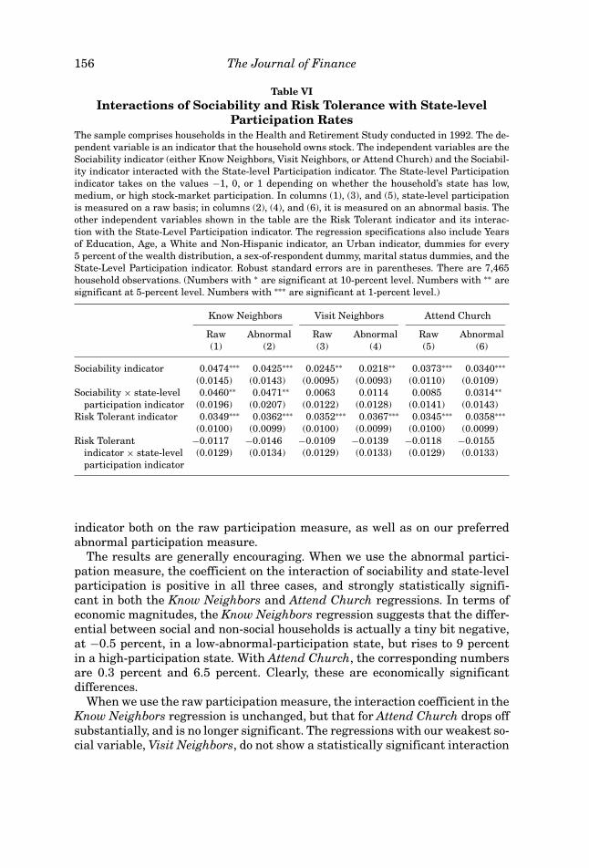
Table VI presents the tests of this hypothesis. The structure is very similarto that of Table IV, with all the same suppressed controls. Now, in addition tohaving our social variables enter by themselves, we also interact them with anindicator variable that takes on the values {–1, 0, 1} depending on whether astate is classified as low, medium, or high participation.24 We try basing this

24 Given that our ability to estimate any state’s true mean participation costs is imperfect, wedo this grouping—rather than simply having each state’s own participation rate enter directlyin the regression—in an effort to combat measurement error and to improve the precision of ourestimates.


Table VIInteractions of Sociability and Risk Tolerance with State-level

Participation RatesThe sample comprises households in the Health and Retirement Study conducted in 1992. The de-pendent variable is an indicator that the household owns stock. The independent variables are theSociability indicator (either Know Neighbors, Visit Neighbors, or Attend Church) and the Sociabil-ity indicator interacted with the State-level Participation indicator. The State-level Participationindicator takes on the values −1, 0, or 1 depending on whether the household’s state has low,medium, or high stock-market participation. In columns (1), (3), and (5), state-level participationis measured on a raw basis; in columns (2), (4), and (6), it is measured on an abnormal basis. Theother independent variables shown in the table are the Risk Tolerant indicator and its interac-tion with the State-Level Participation indicator. The regression specifications also include Yearsof Education, Age, a White and Non-Hispanic indicator, an Urban indicator, dummies for every5 percent of the wealth distribution, a sex-of-respondent dummy, marital status dummies, and theState-Level Participation indicator. Robust standard errors are in parentheses. There are 7,465household observations. (Numbers with ∗ are significant at 10-percent level. Numbers with ∗∗ aresignificant at 5-percent level. Numbers with ∗∗∗ are significant at 1-percent level.)

Know Neighbors Visit Neighbors Attend Church

Raw Abnormal Raw Abnormal Raw Abnormal(1) (2) (3) (4) (5) (6)

Sociability indicator 0.0474∗∗∗ 0.0425∗∗∗ 0.0245∗∗ 0.0218∗∗ 0.0373∗∗∗ 0.0340∗∗∗

(0.0145) (0.0143) (0.0095) (0.0093) (0.0110) (0.0109)Sociability × state-level

participation indicator0.0460∗∗ 0.0471∗∗ 0.0063 0.0114 0.0085 0.0314∗∗

(0.0196) (0.0207) (0.0122) (0.0128) (0.0141) (0.0143)Risk Tolerant indicator 0.0349∗∗∗ 0.0362∗∗∗ 0.0352∗∗∗ 0.0367∗∗∗ 0.0345∗∗∗ 0.0358∗∗∗

(0.0100) (0.0099) (0.0100) (0.0099) (0.0100) (0.0099)Risk Tolerant

indicator × state-levelparticipation indicator

−0.0117 −0.0146 −0.0109 −0.0139 −0.0118 −0.0155(0.0129) (0.0134) (0.0129) (0.0133) (0.0129) (0.0133)

indicator both on the raw participation measure, as well as on our preferredabnormal participation measure.

The results are generally encouraging. When we use the abnormal partici-pation measure, the coefficient on the interaction of sociability and state-levelparticipation is positive in all three cases, and strongly statistically signifi-cant in both the Know Neighbors and Attend Church regressions. In terms ofeconomic magnitudes, the Know Neighbors regression suggests that the differ-ential between social and non-social households is actually a tiny bit negative,at −0.5 percent, in a low-abnormal-participation state, but rises to 9 percentin a high-participation state. With Attend Church, the corresponding numbersare 0.3 percent and 6.5 percent. Clearly, these are economically significantdifferences.

When we use the raw participation measure, the interaction coefficient in theKnow Neighbors regression is unchanged, but that for Attend Church drops offsubstantially, and is no longer significant. The regressions with our weakest so-cial variable, Visit Neighbors, do not show a statistically significant interaction


coefficient in either the raw or abnormal-participation specification, though inboth cases these coefficients have the predicted positive sign.

To further bolster the case that these results are really telling us somethingabout social effects, in all the regressions in Table VI we also interact our RiskTolerant variable with the same state-level participation indicators—that is,we treat Risk Tolerant in a way that is symmetric to our social measures.The premise here is as follows. We are reasonably confident that the RiskTolerant variable is capturing information about a personality trait that is rel-evant for participation but that has nothing to do with social effects. Thus RiskTolerant should have the same coefficient regardless of what state a house-hold lives in. In other words, Risk Tolerant should not show the same inter-action with the state-level participation indicators that our social measuresdo.

And indeed, Table VI confirms this hypothesis. While the Risk Tolerant vari-able continues to attract a highly significant positive coefficient when standingalone, the interaction terms involving Risk Tolerant are small and completelyinsignificant in all six specifications. Thus Risk Tolerant behaves in a funda-mentally different way across states than do our social variables. Again, thislends further weight to the notion that these social variables are not just an-other personality trait in disguise.

It is worth contrasting our approach to using cross-state variation in Table VIto other approaches that are common in the peer-effects literature (see, e.g.,Glaeser and Scheinkman (2000) for a discussion). In particular, by analogyto some of this other work, we can use our data to demonstrate the following.First, if one adds the mean participation rate in a household’s home state to thebaseline regression in column (1) of Table III, it comes in strongly significant,with a coefficient of 0.240 and a t-statistic of 3.48. Thus controlling for its owncharacteristics, a household is substantially more likely to participate in themarket if it lives in a high-participation state. Alternatively, one can add themean education and wealth levels in a state to the same baseline regression,with the same qualitative result—a household is significantly more likely toparticipate in the market if it lives in a state with a wealthier and more educatedpopulation.

These sorts of results are certainly consistent with the existence of socialeffects, and are probably the best that one could do without access to the di-rect measures of sociability that the HRS affords us. But since they do notexploit the interaction of sociability and cross-state variation in participation,they are more subject to alternative interpretations. For example, supposethat brokerage firms endogenously choose to have more branch officesin wealthy states, and that such branch offices facilitate participation. If so,this could explain why either a state’s wealth, or its mean participation rate,matters for individual-household participation, even absent any social effects.By contrast, our Table VI results cannot be explained away in this fashion,so long as one is willing to adopt the identifying assumption that the effectof branch offices on participation is the same for social and non-socialhouseholds.


C. A Look at the 1998 War-Baby Survey

As noted above, in addition to the original 1992 HRS survey, we have a sec-ond independent sample of households—those in the war-baby cohort that weresurveyed in 1998. Unfortunately, this sample is much smaller—roughly 1,400as opposed to 7,500 observations—and it does not include the survey questionsthat allow us to construct either the Know Neighbors or Attend Church vari-ables. The only social variable that remains is the Visit Neighbors variable,which we have found thus far to yield the weakest results of the three.25 Also,this version of the survey does not enable us to construct the Risk Tolerantcontrol.

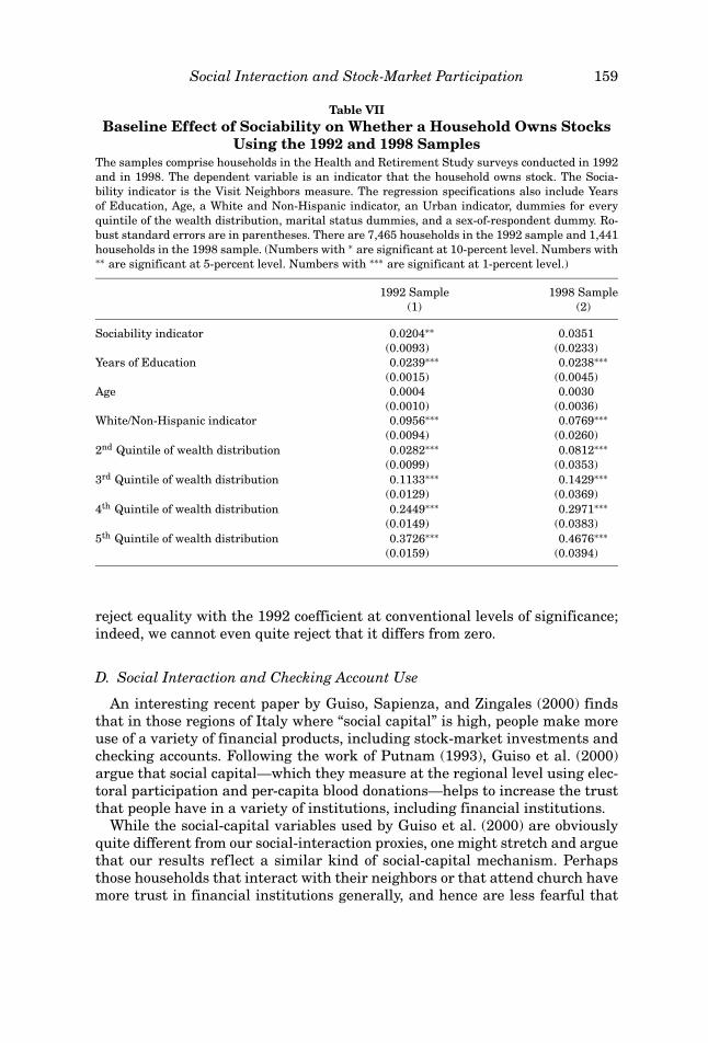
Nevertheless, working with the limited data we do have, we undertake inTable VII a comparison of the two different samples. We run the exact sameregression for each, the specification being the same as that in column (4) ofTable III, except with the Risk Tolerant control dropped. In principle, thereare two things that could potentially be accomplished with such a comparison.First, the 1998 data enable us to perform an obvious out-of-sample robustnesscheck on the results from the 1992 survey.

Second, and more ambitiously, one might hope to test the intertemporalsocial-multiplier aspect of our theory. Mirroring the overall rise in stock-marketparticipation over the 1990s, the average participation rate among the war ba-bies in 1998 is 32.3 percent; this represents a 21 percent increase from the 26.7percent participation rate among the original 1992 HRS cohort.26 If one thinksof this time trend in participation as reflecting an economy-wide decrease incosts of participation, then our model suggests that participation should haveincreased more among socials than among non-socials. Or said differently, theexistence of a social multiplier implies that the 1998 sample should yield alarger coefficient on the social variable than the 1992 sample. Note that thisis essentially just an intertemporal version of the cross-state comparison madein Table VI: In either case the prediction is that there should be a smaller coef-ficient on the social variable in a high-participation-cost regime (Alabama, orthe early 1990s) than in a low-participation-cost regime (Connecticut, or thelate 1990s).

The point estimates in Table VII suggest that our intertemporal social-multiplier hypothesis is on target, but there is not enough power to state thisconclusion with any degree of statistical confidence. In particular, the coeffi-cient on Visit Neighbors goes from 0.020 in the 1992 sample to 0.035 in the1998 sample, a striking increase of 75 percent. Unfortunately, with the muchsmaller sample, the 1998 coefficient is too imprecisely estimated to allow us to

25 Of households, 67.8 percent visit their neighbors in the 1998 sample, very close to the 1992sample value of 63.9 percent, suggesting that this variable is picking up similar information in bothsurveys. Looking over a much broader span of time, Putnam (1995) argues that social interactionamong Americans has declined, but this trend does not show up with our simplistic measure overthe relatively short 1992 to 1998 interval.

26 Moreover, as pointed out above, the war babies are almost exactly the same age in 1998 as theoriginal HRS respondents were in 1992, so this seems to be a clean comparison.


Table VIIBaseline Effect of Sociability on Whether a Household Owns Stocks

Using the 1992 and 1998 SamplesThe samples comprise households in the Health and Retirement Study surveys conducted in 1992and in 1998. The dependent variable is an indicator that the household owns stock. The Socia-bility indicator is the Visit Neighbors measure. The regression specifications also include Yearsof Education, Age, a White and Non-Hispanic indicator, an Urban indicator, dummies for everyquintile of the wealth distribution, marital status dummies, and a sex-of-respondent dummy. Ro-bust standard errors are in parentheses. There are 7,465 households in the 1992 sample and 1,441households in the 1998 sample. (Numbers with ∗ are significant at 10-percent level. Numbers with∗∗ are significant at 5-percent level. Numbers with ∗∗∗ are significant at 1-percent level.)

1992 Sample 1998 Sample(1) (2)

Sociability indicator 0.0204∗∗ 0.0351(0.0093) (0.0233)

Years of Education 0.0239∗∗∗ 0.0238∗∗∗(0.0015) (0.0045)

Age 0.0004 0.0030(0.0010) (0.0036)

White/Non-Hispanic indicator 0.0956∗∗∗ 0.0769∗∗∗(0.0094) (0.0260)

2nd Quintile of wealth distribution 0.0282∗∗∗ 0.0812∗∗∗(0.0099) (0.0353)

3rd Quintile of wealth distribution 0.1133∗∗∗ 0.1429∗∗∗(0.0129) (0.0369)

4th Quintile of wealth distribution 0.2449∗∗∗ 0.2971∗∗∗(0.0149) (0.0383)

5th Quintile of wealth distribution 0.3726∗∗∗ 0.4676∗∗∗(0.0159) (0.0394)

reject equality with the 1992 coefficient at conventional levels of significance;indeed, we cannot even quite reject that it differs from zero.

D. Social Interaction and Checking Account Use

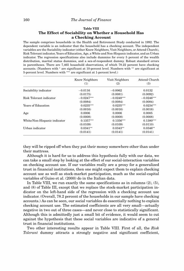
An interesting recent paper by Guiso, Sapienza, and Zingales (2000) findsthat in those regions of Italy where “social capital” is high, people make moreuse of a variety of financial products, including stock-market investments andchecking accounts. Following the work of Putnam (1993), Guiso et al. (2000)argue that social capital—which they measure at the regional level using elec-toral participation and per-capita blood donations—helps to increase the trustthat people have in a variety of institutions, including financial institutions.

While the social-capital variables used by Guiso et al. (2000) are obviouslyquite different from our social-interaction proxies, one might stretch and arguethat our results reflect a similar kind of social-capital mechanism. Perhapsthose households that interact with their neighbors or that attend church havemore trust in financial institutions generally, and hence are less fearful that


Table VIIIThe Effect of Sociability on Whether a Household Has

a Checking AccountThe sample comprises households in the Health and Retirement Study conducted in 1992. Thedependent variable is an indicator that the household has a checking account. The independentvariables are the Sociability indicator (either Know Neighbors, Visit Neighbors, or Attend Church),Risk Tolerant indicator, Years of Education, Age, a White and Non-Hispanic indicator, and an Urbanindicator. The regression specifications also include dummies for every 5 percent of the wealthdistribution, marital status dummies, and a sex-of-respondent dummy. Robust standard errorsin parentheses. There are 7,465 household observations, of which 78.22 percent have checkingaccounts. (Numbers with ∗ are significant at 10-percent level. Numbers with ∗∗ are significant at5-percent level. Numbers with ∗∗∗ are significant at 1-percent level.)

Know Neighbors Visit Neighbors Attend Church(1) (2) (3)

Sociability indicator −0.0116 −0.0062 0.0132(0.0175) (0.0081) (0.0092)

Risk Tolerant indicator −0.0247∗∗∗ −0.0248∗∗∗ −0.0246∗∗∗(0.0084) (0.0084) (0.0084)

Years of Education 0.0235∗∗∗ 0.0235∗∗∗ 0.0234∗∗∗(0.0016) (0.0016) (0.0016)

Age 0.0006 0.0006 0.0005(0.0008) (0.0008) (0.0008)

White/Non-Hispanic indicator 0.1357∗∗∗ 0.1356∗∗∗ 0.1380∗∗∗(0.0109) (0.0109) (0.0110)

Urban indicator 0.0341∗∗ 0.0343∗∗ 0.0346∗∗(0.0141) (0.0141) (0.0141)

they will be ripped off when they put their money somewhere other than undertheir mattress.

Although it is hard for us to address this hypothesis fully with our data, wecan take a small step by looking at the effect of our social-interaction variableson checking account use. If our variables really are a proxy for a generalizedtrust in financial institutions, then one might expect them to explain checkingaccount use as well as stock-market participation, much as the social-capitalvariables of Guiso et al. (2000) do in the Italian data.

In Table VIII, we run exactly the same specifications as in columns (2), (5),and (8) of Table III, except that we replace the stock-market participation in-dicator on the left-hand side of the regression with a checking account useindicator. (Overall, 78.2 percent of the households in our sample have checkingaccounts.) As can be seen, our social variables do essentially nothing to explainchecking account use. The estimated coefficients are all very small—actuallynegative in two out of three cases—and never close to statistically significant.Although this is admittedly just a small bit of evidence, it would seem to cutagainst the hypothesis that these social variables are indicative of a generaltrust in financial institutions.

Two other interesting results appear in Table VIII. First of all, the RiskTolerant dummy attracts a strongly negative and significant coefficient,


suggesting that risk-averse households are, not implausibly, more likely to havechecking accounts. And the coefficient on the race indicator implies that non-white/Hispanic households are almost 14 percent less likely to have checkingaccounts, all else equal. This is an enormous effect, and it suggests that eventhough our social variables may not capture trust, there may be substantiallyless trust of financial institutions among members of some minority groups.

IV. Conclusions

Three significant findings emerge from our analysis of the HRS data. First,social households—those that interact with their neighbors, or that attendchurch—are more likely to invest in the stock market than non-social house-holds, all else equal. Second, the impact of sociability is much stronger in thosestates where stock-market participation rates are higher. Third, and by far mosttentatively, the differential between social and non-social households appearsto have widened over the course of the 1990s, as overall participation rates haveclimbed sharply.

This evidence is broadly consistent with the hypothesis that social interac-tion helps to increase stock-market participation. At the same time, we havebeen somewhat vague as to the exact mechanism by which social interactionpromotes participation. We have discussed two possible stories—one having todo with word-of-mouth information-sharing, the other with the enjoyment thatpeople get from talking about the market together—but have made no effort todiscriminate between them. And it should be noted that this distinction mightbe a significant one, particularly with regard to the more dynamic aspects ofthe theory.

To see why, suppose that the stock market performs poorly over the next sev-eral years, leading some investors to get discouraged and withdraw. To what ex-tent do these departing investors create an externality that affects their peerswho are already in the market?27 Under at least some versions of the word-of-mouth information-sharing story, the externality might be expected to beunimportant, since the presumption is that those who are already in the mar-ket know whatever it is they need to know about how to invest. However, underthe enjoyment-from-talking-about-the-market story, there is an obvious exter-nality, with any individual’s decision to leave the market making it more likelythat others in his peer group will leave too. One objective for future work mightbe to try to distinguish between these two possibilities.

In closing, a final point to highlight is the potentially close connection be-tween the ideas presented here and the growing empirical literature on “lo-cal preference” in the stock market. A series of papers has demonstrated thatinvestors strongly tilt their portfolios not only towards home-country stocks(French and Poterba (1991), Cooper and Kaplanis (1994), Tesar and Werner(1995), Kang and Stulz (1997)), but also towards the stocks of firms that are

27 In any version of our model, there is a clear prediction that departing investors exert a negativeinfluence on the participation decisions of those who have not yet begun to invest in the market.


headquartered nearby, or that are otherwise more familiar (Huberman (2001),Coval and Moskowitz (1999), Grinblatt and Keloharju (2000)). In many of thesepapers, the explicit or implicit story being told is that it is easier for investorsto learn about nearby stocks. In other words, in the language of our model,participation costs are lower for nearby stocks.

If one accepts this interpretation, then our model suggests that social-interaction effects may help to amplify whatever aggregate local preference isinduced by exogenous cross-stock differences in participation costs. Thus evenif the direct, observable costs to a U.S. investor of buying, say, Japanese stocksare only modestly greater than the costs incurred with U.S. stocks, the socialequilibrium may involve a very pronounced home-country bias. In such an equi-librium, many U.S. investors may be deterred from investing in Japan largelybecause they do not know anybody else who does. This hypothesis would seemto provide another natural direction for future research.

REFERENCESAbel, Andrew, 2001, The effects of investing social security funds in the stock market when fixed

costs prevent some households from holding stocks, American Economic Review 91, 128–148.Banerjee, Abhijit, 1992, A simple model of herd behavior, Quarterly Journal of Economics 107,

797–817.Barsky, Robert, Miles S. Kimball, F. Thomas Juster, and Matthew D. Shapiro, 1997, Preference

parameters and behavioral heterogeneity: An experimental approach in the health and retire-ment study, Quarterly Journal of Economics 112, 537–579.

Bayer, Patrick, B. Douglas Bernheim, and Karl Scholz, 1998, The effects of financial education inthe workplace: Evidence from a survey of employers, Working paper, NBER.

Becker, Gary S., 1991, A note on restaurant pricing and other examples of social influences onprice, Journal of Political Economy 99, 1109–1116.

Bernheim, B. Douglas, and Daniel M. Garrett, 1996, The determinants and consequences of fi-nancial education in the workplace: Evidence from a survey of households, Working paper,NBER.

Bertaut, Carol, and Martha Starr-McCluer, 2000, Household portfolios in the U.S., Working paper,Board of Governors of the Federal Reserve.

Bertrand, Marianne, Erzo Luttmer, and Sendhil Mullainathan, 2000, Network effects and welfarecultures, Quarterly Journal of Economics 115, 1019–1055.

Bikchandani, Sushil, David Hirshleifer, and Ivo Welch, 1992, A theory of fads, fashion, custom andcultural change as informational cascades, Journal of Political Economy 100, 992–1026.

Brav, Alon, George Constantinides, and Christopher Gezcy, 2002, Asset pricing with heterogeneousconsumers and limited participation: Empirical evidence, Journal of Political Economy 110,793–824.

Campbell, John Y., Joao F. Cocco, Francisco J. Gomes, and Pascal J. Maenhout, 1999, Investingretirement wealth: A life-cycle model, Working paper, Harvard University.

Case, Anne, and Larry Katz, 1991, The company you keep: The effect of family and neighborhoodon disadvantaged youths, Working paper, NBER.

Chiteji, Ngina S., and Frank P. Stafford, 1999, Portfolio choices of parents and their children asyoung adults: Asset accumulation by African-American families, American Economic ReviewPapers and Proceedings 89, 377–380.

Choi, James J., David Laibson, and Andrew Metrick, 2002, Does the internet increase trading?Evidence from investor behavior in 401(k) plans, Journal of Financial Economics 64, 397–421.

Cooper, Ian, and Evi Kaplanis, 1994, Home bias in equity portfolios, inflation hedging and inter-national capital market equilibrium, Review of Financial Studies 7, 45–60.


Coval, Joshua, and Tobias Moskowitz, 1999, Home bias at home: Local equity preference in domesticportfolios, Journal of Finance 54, 2045–2073.

DeMarzo, Peter, Dimitri Vayanos, and Jeffrey Zwiebel, 2001, Persuasion bias, social influence anduni-dimensional opinions, Working paper, Stanford Business School.

Duflo, Esther, and Emmanuel Saez, 2002, Participation and investment decisions in a retirementplan: The influence of colleagues’ choices, Journal of Public Economics 85, 121–148.

Ellison, Glenn, and Drew Fudenberg, 1993, Rules of thumb for social learning, Journal of PoliticalEconomy 101, 93–126.

Ellison, Glenn, and Drew Fudenberg, 1995, Word of mouth communication and social learning,Quarterly Journal of Economics 110, 93–125.

French, Kenneth, and James Poterba, 1991, Investor diversification and international equity mar-kets, American Economic Review 81, 222–226.

Glaeser, Edward L., Bruce Sacerdote, and Jose Scheinkman, 1996, Crime and social interactions,Quarterly Journal of Economics 111, 502–548.

Glaeser, Edward L., and Jose Scheinkman, 2000, Non-market interactions, Working paper, NBER.Granovetter, Mark, 1983, The strength of weak ties: A network theory revisited, Sociological Theory

1, 201–233.Grinblatt, Mark, and Matti Keloharju, 2000, The investment behavior and performance of various

investor-types: A study of Finland’s unique data set, Journal of Financial Economics 55, 43–67.Guiso, Luis, Paola Sapienza, and Luigi Zingales, 2000, The role of social capital in financial devel-

opment, Working paper, University of Chicago.Heaton, John, and Deborah Lucas, 1999, Stock prices and fundamentals, NBER Macroeconomics

Annual 14, 213–242.Hong, Harrison, Jeffrey D. Kubik, and Jeremy C. Stein, 2001, Social interaction and stock-market

participation, Working paper, NBER.Huberman, Gur, 2001, Familiarity breeds investment, Review of Financial Studies 14, 659–680.Kang, Jun-Koo, and Rene Stulz, 1997, Why is there a home bias? An analysis of foreign portfolio

equity ownership in Japan, Journal of Financial Economics 46, 3–28.Kelly, Morgan, and Cormac O. Grada, 2000, Market contagion: Evidence from the panics of 1854

and 1857, American Economic Review 90, 1110–1124.Madrian, Bridget, and Dennis Shea, 2000, Peer effects and savings behavior in employer-sponsored

savings plans, Working paper, University of Chicago.Mankiw, N. Gregory, and Stephen P. Zeldes, 1991, The consumption of stockholders and non-

stockholders, Journal of Financial Economics 29, 97–112.Mehra, Rajnish, and Edward C. Prescott, 1985, The equity premium: A puzzle, Journal of Monetary

Economics 15, 145–161.Putnam, Robert, 1993, Making Democracy Work: Civic Traditions in Modern Italy (Princeton Uni-

versity Press, Princeton, NJ).Putnam, Robert, 1995, Bowling alone: America’s declining social capital, Journal of Democracy 6,

65–78.Routledge, Bryan R., 1999, Adaptive learning in financial markets, Review of Financial Studies

12, 1165–1202.Sacerdote, Bruce, 2001, Peer effects with random assignment: Results for Dartmouth roommates,

Quarterly Journal of Economics 116, 681–704.Shiller, Robert J., and John Pound, 1989, Survey evidence on diffusion of interest and information

among investors, Journal of Economic Behavior and Organization 12, 47–66.Tesar, Linda, and Ingrid Werner, 1995, Home bias and high turnover, Journal of International

Money and Finance 14, 467–492.Vissing-Jorgensen, Annette, 1999, Limited stock market participation and the equity premium

puzzle, Working paper, University of Chicago.Vissing-Jorgensen, Annette, 2000, Towards an explanation of household portfolio choice hetero-

geneity: Nonfinancial income and participation cost structures, Working paper, University ofChicago.

Documents

Social Interaction and Stock-Market Participationhh2679/jfsocial.pdfSocial Interaction and Stock-Market Participation 139 In the specific setting of the stock market, there are at