Embed Size (px)
Citation preview
SOC 3155
SPSS Review CENTRAL TENDENCY & DISPERSION
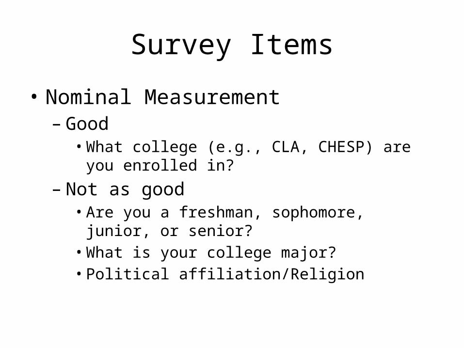
Survey Items
• Nominal Measurement – Good
• What college (e.g., CLA, CHESP) are you enrolled in?
– Not as good• Are you a freshman, sophomore, junior, or senior?• What is your college major? • Political affiliation/Religion
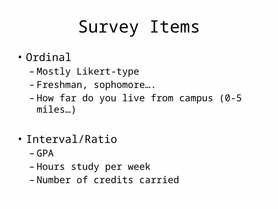
Survey Items
• Ordinal – Mostly Likert-type – Freshman, sophomore….– How far do you live from campus (0-5 miles…)
• Interval/Ratio– GPA– Hours study per week– Number of credits carried
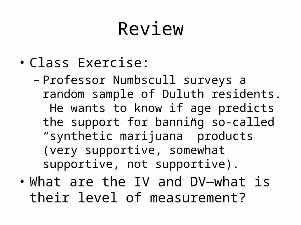
Review
• Class Exercise:– Professor Numbscull surveys a random sample of
Duluth residents. He wants to know if age predicts the support for banning so-called “synthetic marijuana” products (very supportive, somewhat supportive, not supportive).
• What are the IV and DV—what is their level of measurement?
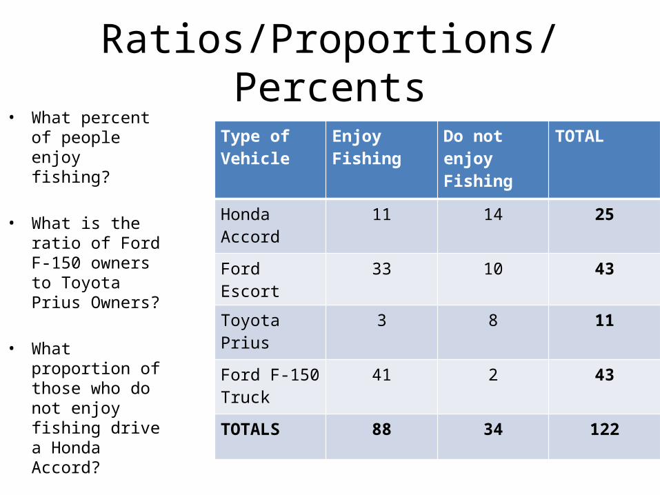
Ratios/Proportions/PercentsType of Vehicle
Enjoy Fishing Do not enjoy Fishing
TOTAL
Honda Accord 11 14 25
Ford Escort 33 10 43
Toyota Prius 3 8 11
Ford F-150 Truck
41 2 43
TOTALS 88 34 122
• What percent of people enjoy fishing?
• What is the ratio of Ford F-150 owners to Toyota Prius Owners?
• What proportion of those who do not enjoy fishing drive a Honda Accord?
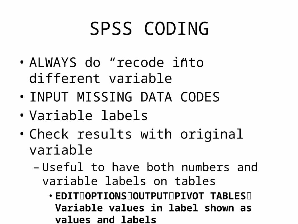
SPSS CODING
• ALWAYS do “recode into different variable”• INPUT MISSING DATA CODES• Variable labels• Check results with original variable
– Useful to have both numbers and variable labels on tables
• EDITOPTIONSOUTPUTPIVOT TABLES Variable values in label shown as values and labels
Class Exercise
• Recode a variable from GSS– Create a variable called “married_r” where:
0 = not married1 = married Be sure to label your new variable!
Run a frequency distribution for the original married variable and “married_r”
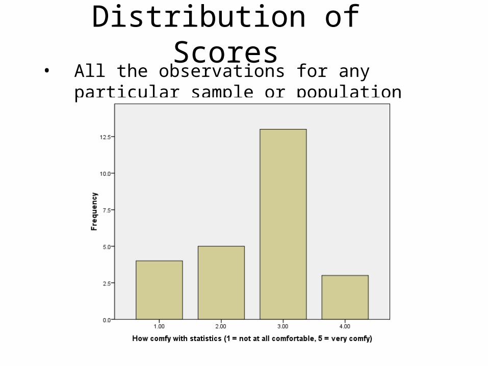
Distribution of Scores• All the observations for any particular sample or
population
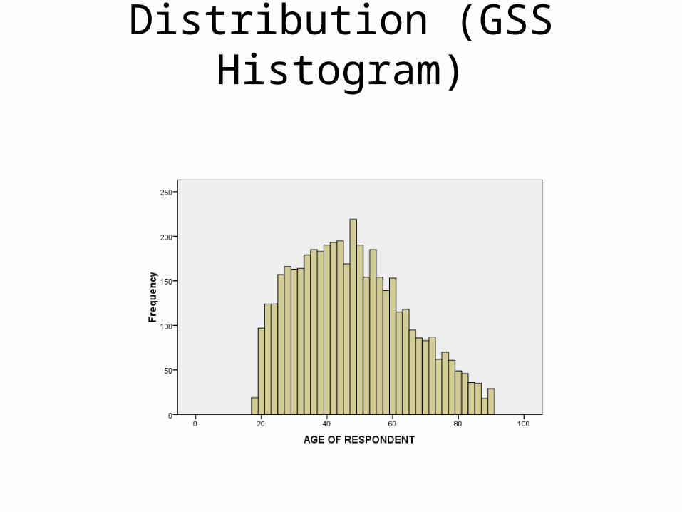
Distribution (GSS Histogram)
Exercise
• Create your own histogram from the GSS data using the variable “TVHOURS”
• Concept of “skew”– Positive vs. negative
• Skew is only possible for ordered data, and typically relevant for interval/ratio data
Measures of Central Tendency
• Purpose is to describe a distribution’s typical case – do not say “average” case
– Mode– Median– Mean (Average)
Measures of Central Tendency
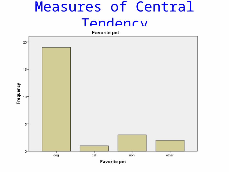
1. Mode • Value of the distribution that occurs most frequently
(i.e., largest category)• Only measure that can be used with nominal-level
variables• Limitations:
– Some distributions don’t have a mode– Most common score doesn’t necessarily mean “typical”– Often better off using proportions or percentages
Measures of Central Tendency
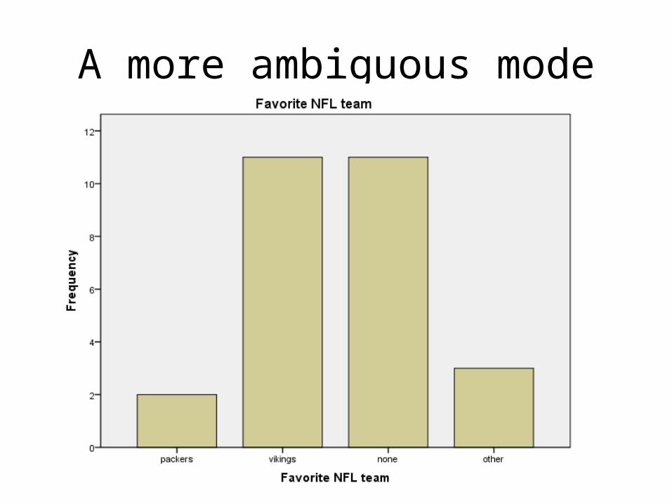
A more ambiguous mode
Measures of Central Tendency
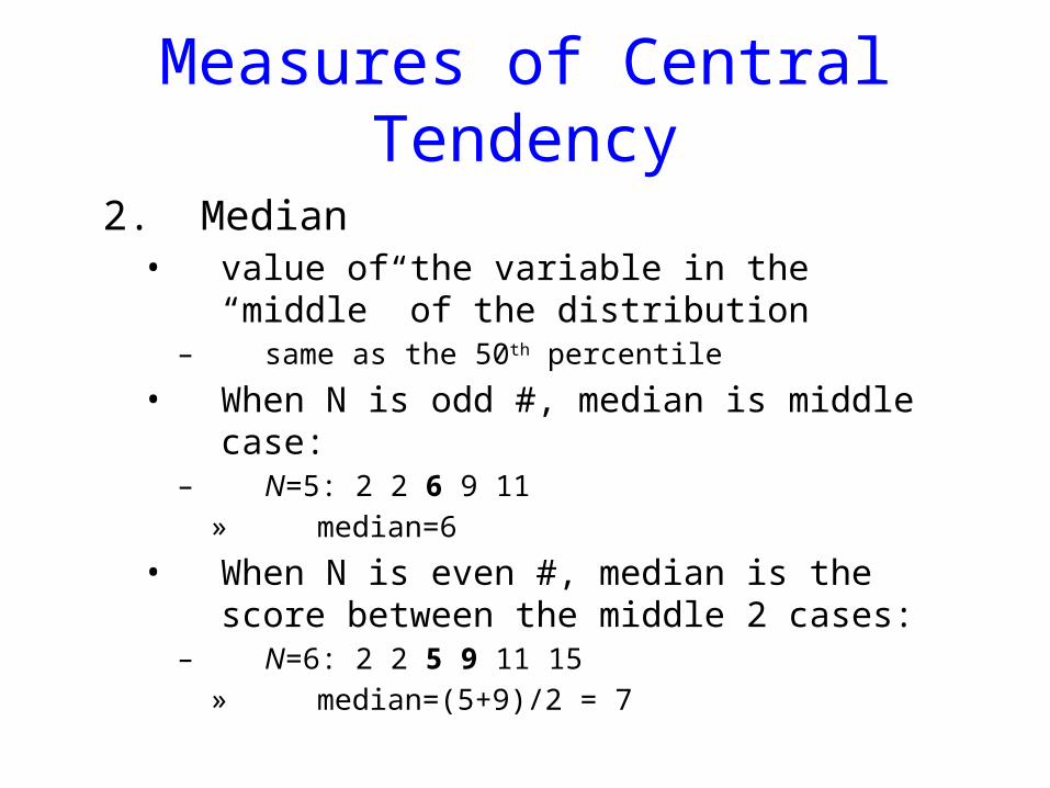
2. Median• value of the variable in the “middle” of the
distribution– same as the 50th percentile
• When N is odd #, median is middle case:– N=5: 2 2 6 9 11
» median=6
• When N is even #, median is the score between the middle 2 cases:
– N=6: 2 2 5 9 11 15 » median=(5+9)/2 = 7
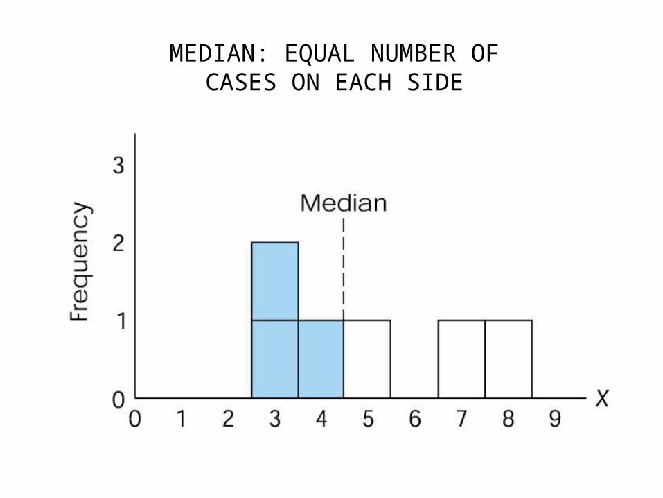
MEDIAN: EQUAL NUMBER OFCASES ON EACH SIDE
Measures of Central Tendency
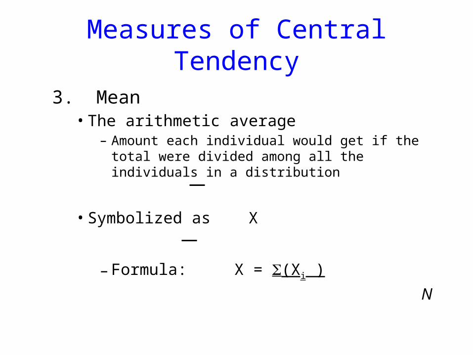
3. Mean• The arithmetic average
– Amount each individual would get if the total were divided among all the individuals in a distribution
• Symbolized as X
– Formula: X = (Xi )
N
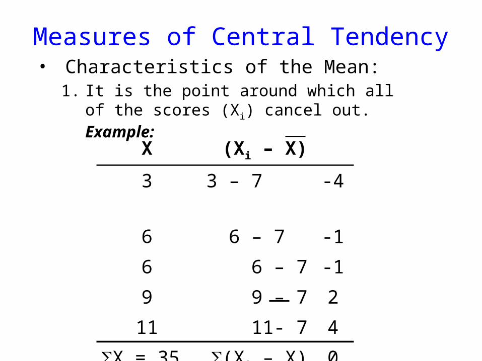
Measures of Central Tendency• Characteristics of the Mean:
1. It is the point around which all of the scores (Xi) cancel out. Example:
X (Xi – X)
3 3 – 7 -46 6 – 7 -16 6 – 7 -19 9 – 7 211 11- 7 4
X = 35 (Xi – X) = 0
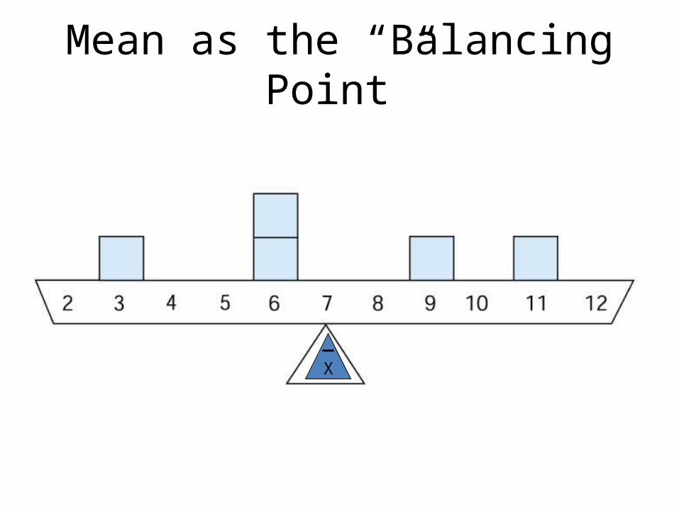
Mean as the “Balancing Point”
X
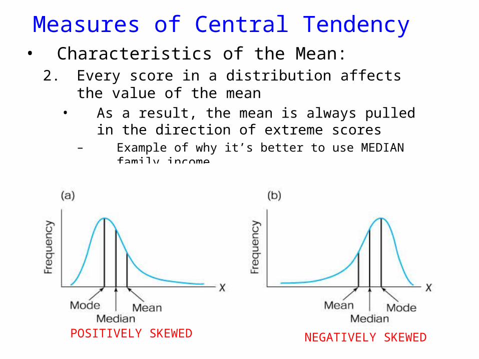
Measures of Central Tendency• Characteristics of the Mean:
2. Every score in a distribution affects the value of the mean• As a result, the mean is always pulled in the direction of
extreme scores– Example of why it’s better to use MEDIAN family income
POSITIVELY SKEWED NEGATIVELY SKEWED
Measures of Central Tendency
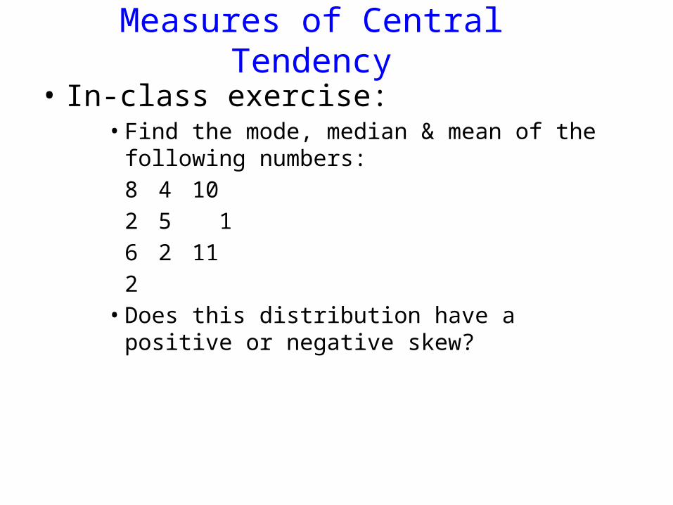
• In-class exercise:• Find the mode, median & mean of the following
numbers:8 4 102 5 1 6 2 11 2
• Does this distribution have a positive or negative skew?
Measures of Central Tendency
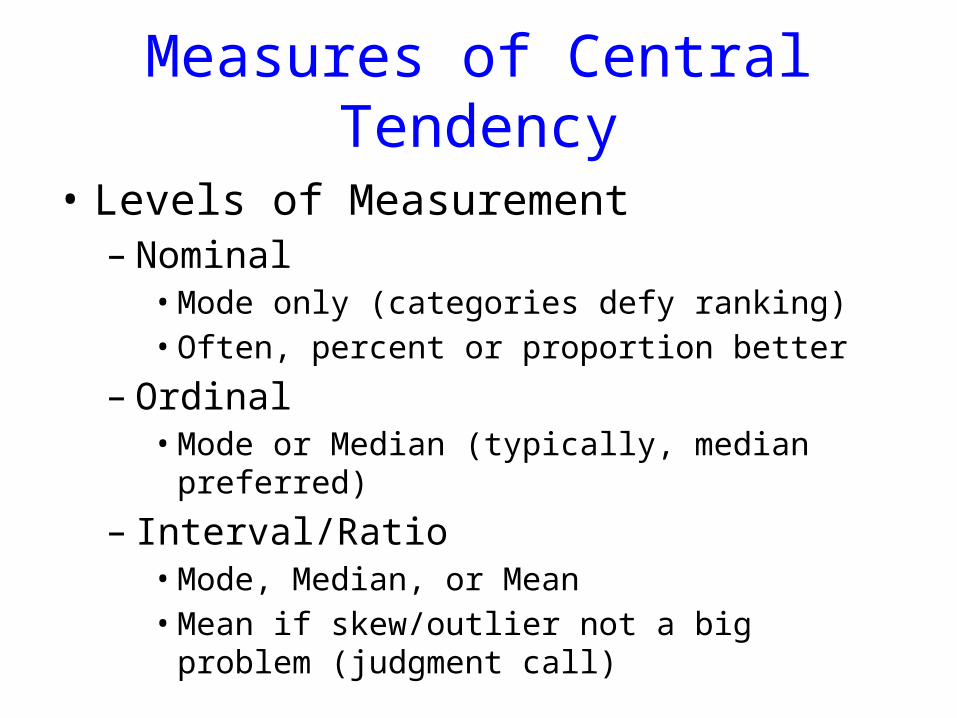
• Levels of Measurement – Nominal
• Mode only (categories defy ranking)• Often, percent or proportion better
– Ordinal• Mode or Median (typically, median preferred)
– Interval/Ratio• Mode, Median, or Mean• Mean if skew/outlier not a big problem (judgment call)
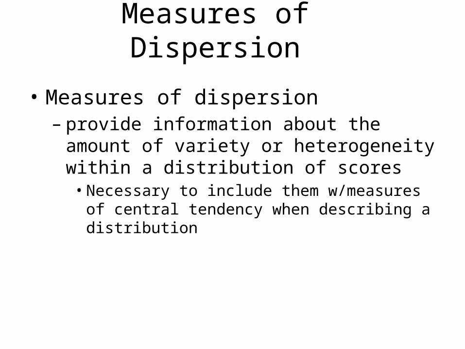
Measures of Dispersion
• Measures of dispersion– provide information about the amount of variety
or heterogeneity within a distribution of scores• Necessary to include them w/measures of central
tendency when describing a distribution
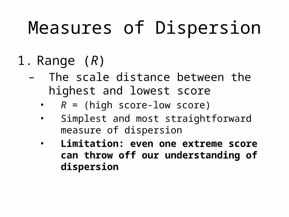
Measures of Dispersion
1. Range (R) – The scale distance between the highest and
lowest score• R = (high score-low score)• Simplest and most straightforward measure of
dispersion• Limitation: even one extreme score can throw off
our understanding of dispersion
Measures of Dispersion
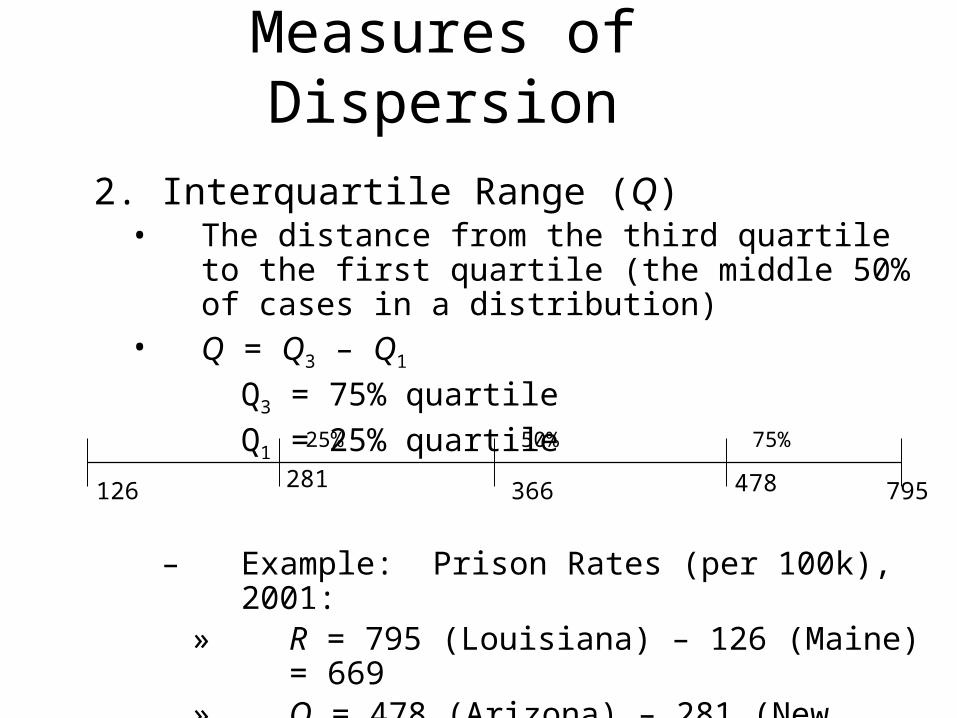
2. Interquartile Range (Q)• The distance from the third quartile to the first quartile
(the middle 50% of cases in a distribution)• Q = Q3 – Q1
Q3 = 75% quartileQ1 = 25% quartile
– Example: Prison Rates (per 100k), 2001:» R = 795 (Louisiana) – 126 (Maine) = 669» Q = 478 (Arizona) – 281 (New Mexico) = 197
126 281 478 795366
25% 50% 75%
MEASURES OF DISPERSION
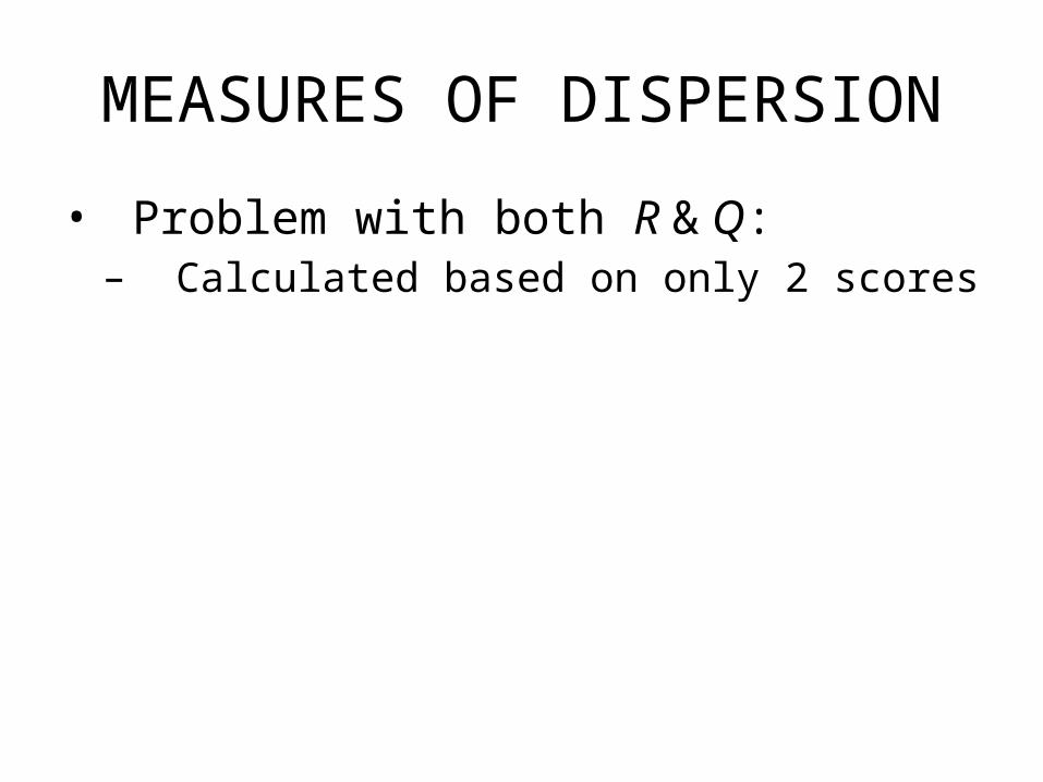
• Problem with both R & Q:– Calculated based on only 2 scores
MEASURES OF DISPERSION
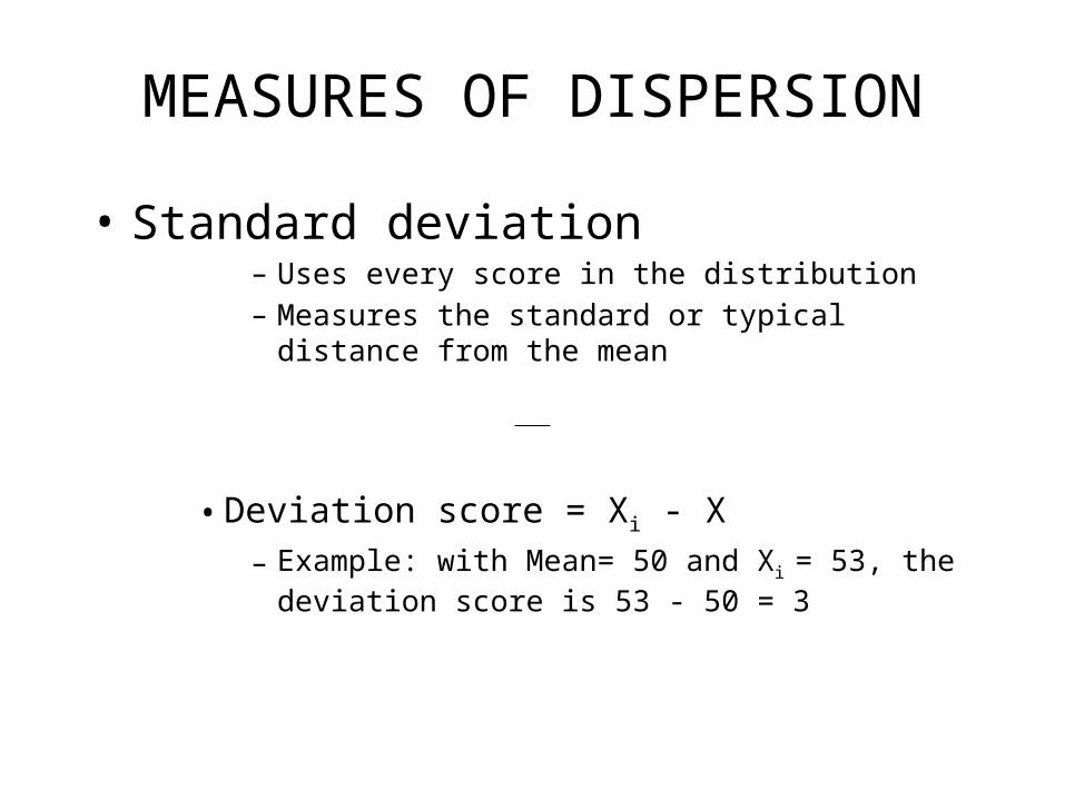
• Standard deviation– Uses every score in the distribution– Measures the standard or typical distance from the mean
• Deviation score = Xi - X– Example: with Mean= 50 and Xi = 53, the deviation score
is 53 - 50 = 3

X Xi - X8 +5 1 -23 00 -312 0
Mean = 3 •Deviation scoresadd up to zero
•Because sum of deviationsis always 0, it can’t be used as a measure of dispersion
The Problem with Summing Deviations From Mean• 2 parts to a deviation score: the sign and the number

Average Deviation (using absolute value of deviations)
– Works OK, but…• AD = |Xi – X|
N X |Xi – X|
8 5 1 23 00 3
12 10
AD = 10 / 4 = 2.5
X = 3
Absolute Value to get rid of negative values (otherwise it
would add to zero)
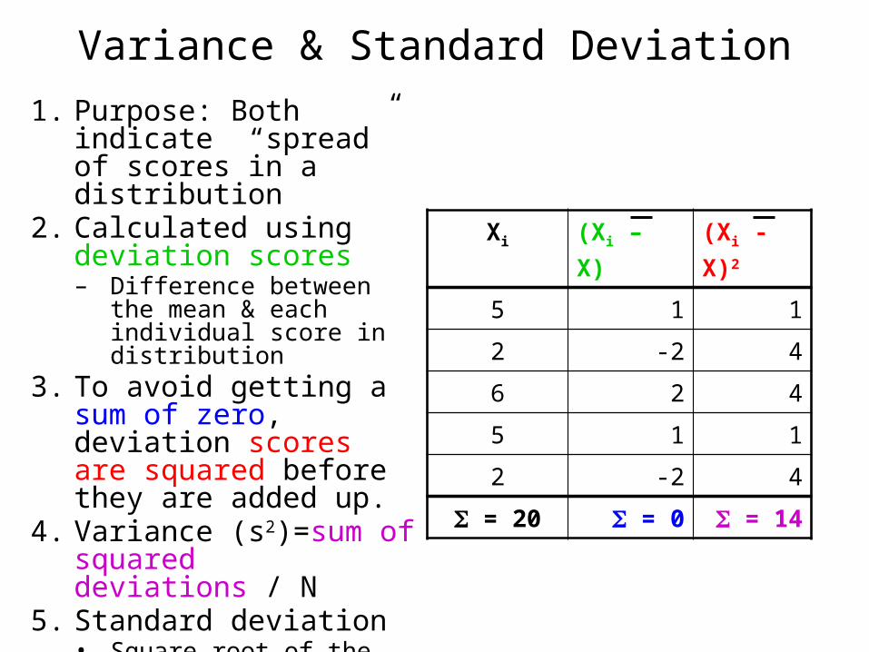
Variance & Standard Deviation1. Purpose: Both indicate
“spread” of scores in a distribution
2. Calculated using deviation scores– Difference between the mean
& each individual score in distribution
3. To avoid getting a sum of zero, deviation scores are squared before they are added up.
4. Variance (s2)=sum of squared deviations / N
5. Standard deviation• Square root of the variance
Xi (Xi – X) (Xi - X)2
5 1 1
2 -2 4
6 2 4
5 1 1
2 -2 4
= 20 = 0 = 14
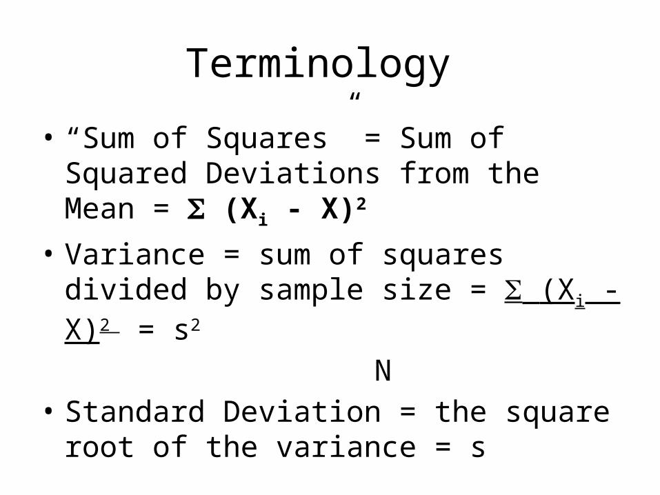
Terminology
• “Sum of Squares” = Sum of Squared Deviations from the Mean = (Xi - X)2
• Variance = sum of squares divided by sample size = (Xi - X)2 = s2
N• Standard Deviation = the square root of the
variance = s
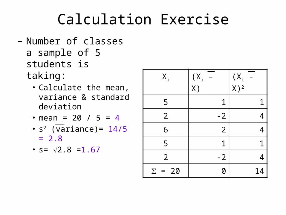
Calculation Exercise– Number of classes a
sample of 5 students is taking:
• Calculate the mean, variance & standard deviation
• mean = 20 / 5 = 4• s2 (variance)= 14/5 = 2.8• s= 2.8 =1.67
Xi (Xi – X) (Xi - X)2
5 1 1
2 -2 4
6 2 4
5 1 1
2 -2 4
= 20 0 14
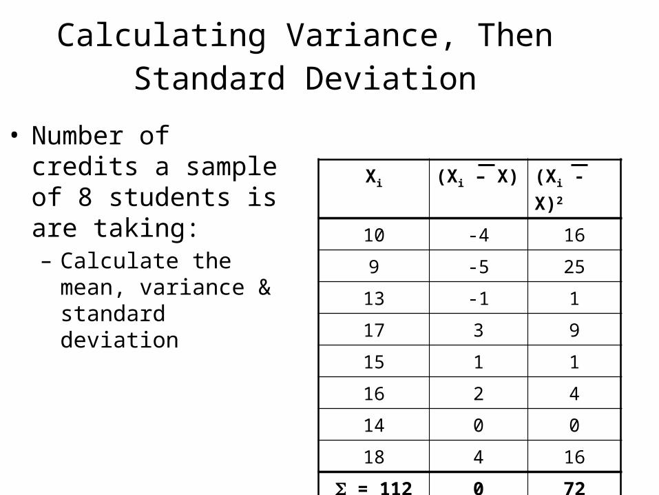
Calculating Variance, Then Standard Deviation
• Number of credits a sample of 8 students is are taking:– Calculate the mean,
variance & standard deviation
Xi (Xi – X) (Xi - X)2
10 -4 16
9 -5 25
13 -1 1
17 3 9
15 1 1
16 2 4
14 0 0
18 4 16
= 112 0 72
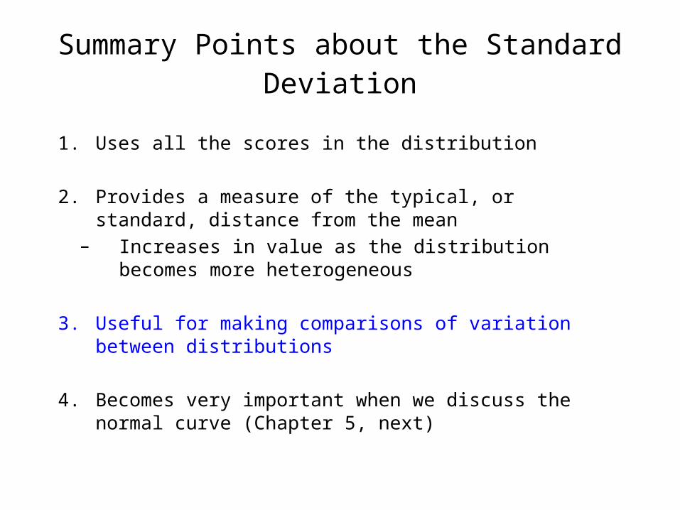
Summary Points about the Standard Deviation
1. Uses all the scores in the distribution
2. Provides a measure of the typical, or standard, distance from the mean
– Increases in value as the distribution becomes more heterogeneous
3. Useful for making comparisons of variation between distributions
4. Becomes very important when we discuss the normal curve (Chapter 5, next)
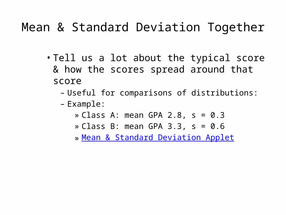
Mean & Standard Deviation Together
• Tell us a lot about the typical score & how the scores spread around that score
– Useful for comparisons of distributions:– Example:
» Class A: mean GPA 2.8, s = 0.3» Class B: mean GPA 3.3, s = 0.6» Mean & Standard Deviation Applet