SO(8) Supergravity and the Magic of Machine Learning

Iulia M. Comsa, Moritz Firsching, Thomas Fischbacher

Google Research

Brandschenkestrasse 110, 8002 Zurich, Switzerland

iuliacomsa,firsching,tfish@google.com

Using de Wit-Nicolai D = 4 N = 8 SO(8) supergravity as an example, we show how modern

Machine Learning software libraries such as Google’s TensorFlow can be employed to greatly simplify

the analysis of high-dimensional scalar sectors of some M-Theory compactifications. We provide

detailed information on the location, symmetries, and particle spectra and charges of 192 critical

points on the scalar manifold of SO(8) supergravity, including one newly discovered N = 1 vacuum

with SO(3) residual symmetry, one new potentially stabilizable non-supersymmetric solution, and

examples for “Galois conjugate pairs” of solutions, i.e. solution-pairs that share the same gauge group

embedding into SO(8) and minimal polynomials for the cosmological constant. Where feasible, we

give analytic expressions for solution coordinates and cosmological constants.

As the authors’ aspiration is to present the discussion in a form that is accessible to both the

Machine Learning and String Theory communities and allows adopting our methods towards the

study of other models, we provide an introductory overview over the relevant Physics as well as

Machine Learning concepts. This includes short pedagogical code examples. In particular, we show

how to formulate a requirement for residual Supersymmetry as a Machine Learning loss function and

effectively guide the numerical search towards supersymmetric critical points. Numerical investigations

suggest that there are no further supersymmetric vacua beyond this newly discovered fifth solution.

1

arX

iv:1

906.

0020

7v4

[he

p-th

] 1

9 Ju

l 201

9

At the moment, the N = 8 Supergravity Theory is the only candidate in sight. There

are likely to be a number of crucial calculations within the next few years that have the

possibility of showing that the theory is no good. If the theory survives these tests, it

will probably be some years more before we develop computational methods that will

enable us to make predictions and before we can account for the initial conditions of

the universe as well as the local physical laws. These will be the outstanding problems

for theoretical physics in the next twenty years or so.

But to end on a slightly alarmist note, they may not have much more time than that.

At present, computers are a useful aid in research, but they have to be directed by

human minds. If one extrapolates their recent rapid rate of development, however, it

would seem quite possible that they will take over altogether in theoretical physics. So,

maybe the end is in sight for theoretical physicists, if not for theoretical physics.

S. Hawking, Conclusion of his 1981 Inaugural lecture[1]

“Is the End in Sight for Theoretical Physics?”

1 Introduction1

Google’s primary open source library for Machine Learning, TensorFlow [2], has many potential uses

beyond Machine Learning. In this article, we want to show how it also is an excellent tool to address

one specific technically challenging M-Theory research problem: Finding static field configurations

of dimensionally reduced models with known but structurally complicated potentials, such as SO(8)

supergravity [3] [4], which we study here, as well as determining their stability properties. The

underlying computational methods can be readily generalized to other models, including for example

maximal five-dimensional supergravity [5].

For the impatient reader, there is an open sourced Google Colab at [6] that runs an efficient search

for vacuum candidates of SO(8) supergravity and can be used interactively from within a web browser,

alongside additional Python code to analyze numerical solutions at [7].

1.1 On M-Theory

“M-Theory”, or “The Theory Formerly Known as Strings” [8] is a so far only partially explored and

understood unifying framework for studying (some) field theoretic models of quantum gravity. The

five known (very likely) consistent ten-dimensional Superstring theories (including compactifications

to lower dimensions), as well as 11-dimensional supergravity are understood to be different limits of

M-Theory dynamics [9]. If supersymmetry [10] is part of the answer why the observed fundamental

laws of physics are the way they are (and it seems to have some good answers to problems that arise

in Planck-scale physics), then, due to the existence of gravity, there is no way to escape the conclusion

that a viable theory must contain supergravity [11], [12] and in particular a supersymmetric partner

to the graviton with spin-3/2, the gravitino. While the question is still not settled whether one can

construct a theory of supergravity that not only works as an effective low energy theory but is well-

behaved at every length scale [13], [14], it is generally thought that problems that arise in simple

models of supergravity [15] are ultimately resolved by the notion of “point particles” in quantum

field theory breaking down at very high energies [16], i.e. superstring theory. Now, if one accepts

1An expanded introduction that provides more context on M-Theory and Machine Learning to interested readers

without a deep background in one of these subjects is available in version 3 of the arXiv preprint of this work at:

https://arxiv.org/abs/1906.00207v3.

2

superstring theory, there is no way to avoid the conclusion that there also needs to be a way to

describe its non-perturbative strong coupling limit, which then inevitably leads us to M-Theory [17].

Despite the remarkable success of the Standard Model (SM) of Elementary Particle Physics [18],

which quantitatively describes the properties and interactions of matter and force particles so well that

the LHC at the time of this writing did not to come up with clear evidence of “new” (beyond-the-SM)

physics, there are a number of unsolved problems, for example non-observation of the particles that

constitute Dark Matter [19], or explaining why the neutron’s electric dipole moment is too small to be

measurable [20]. The most puzzling such problem of theoretical physics currently is perhaps explaining

the observed positive – but from a quantum field theory perspective extremely small – vacuum energy

density [21] of the universe. M-Theory currently struggles to give an answer to how this could arise

naturally. Even if M-Theory ultimately turned out to not be the correct answer to the question how

to quantize gravity, it already by now has made major contributions to uncovering interesting hidden

connections in pure mathematics, of which we here only want to mention the geometric Langlands

correspondence as one example, [22].

1.1.1 Unification

The unification of Quantum Electrodynamics with Quantum Chromodynamics (QCD) and the Weak

Force into the SM is highly successful from a theoretical perspective, with both QCD and Electroweak

theory individually being afflicted by problems that cancel in the SM [23] [24]. A key property is

that in the SM, all forces are described in an uniform way by vector gauge bosons. Since spacetime

symmetries (rotations and boosts) affect all vector gauge bosons in the same way, one can consider

superposition quantum states between them. Indeed, the SM Photon emerges as a specific quantum

superposition of a Weak Force’s particle and another “hidden” force’s particle termed U(1)Y in a way

that is governed by properties of the Brout-Englert-Higgs Boson. This also sets – for example – the

relative strengths of the Electromagnetic and Weak forces. It is quite plausible that at even (much!)

higher energies (but somewhat below the quantum gravity energy scale), the same mechanism also is

at play in the form of “Grand Unification” [25] [26], merging the Strong Force with the Electroweak

Force.

The main new discoveries described in the current article are also about this “Higgs effect” [27] [28],

leading to some particular sets of particles and interactions in “low energy” physics, so in terms of basic

mechanisms this is rather similar to what is now well established SM physics. Our setting, however,

is that of a model that might actually describe Planck-scale physics well, so if this construction ever

turned out to somehow actually be related to the SM (see e.g. [29] [30] [31] for some speculation in

this direction), interesting Physics that is not well understood yet would need to happen in the gap

of ∼ 17 orders of magnitude between the Higgs boson energy scale and the quantum gravity energy

scale. In particular, there is a discrepancy on gauge groups, cosmological constant, and particle

chirality properties.

More likely, this work describes a collection of (stable as well as unstable background-)solutions

to the M-Theory field equations in a very different corner than the one that describes the Standard

Model. Given our still limited understanding of M-Theory, it nevertheless seems useful to get a

better idea about relevant properties, mechanisms, and phenomena by investigating solutions that are

accessible with current technology. In the past, studying solutions to the 4-dimensional field theory

equations and especially their embedding into M-Theory has taught us some very useful lessons about

compactification mechanisms and about 11-dimensional dynamics. One in particular notes that SO(8)

supergravity also describes the physics of a stack of M2-branes [32].

3

1.1.2 Kaluza-Klein Supergravity

While the observation, originally by Kaluza [33] and Klein [34], that four-dimensional physics can

be understood in the context of dynamics in higher dimension was certainly interesting, the question

remained how to find guidance on what higher dimensional dynamics to start from. A major step

forward happened in 1979, when Cremmer, Julia, and Scherk set out to construct the four-dimensional

field theory with the maximum possible amount of boson-fermion symmetry [35] [36] [37]. Due to the

complicated structure of the (Higgs-like) scalar boson interactions, this was achieved by first realizing

that such a theory should be obtainable via compactification of a higher dimensional ancestor theory,

and that there can only be one graviton with helicity ±2 and no interacting massless particles with

higher helicity (due to nonexistence of a suitable source current), and that the highest dimension in

which such a symmetry can exist is eleven (since otherwise dimensional reduction to four dimensions

would give rise to too many supersymmetry generators that require going to helicities beyond +2 that

cannot be consistently coupled). Constructing the 11-dimensional model first in [35], the maximally

symmetric four-dimensional model in which all matter and force particles are unified succeeded in [36]

via Kaluza-Klein reduction on a 7-dimensional torus.

The “auxiliary” 11-dimensional field theory, originally introduced as a mathematical trick, soon

was found to be very interesting in itself. For example, it so turns out that symmetry constraints

completely determine its structure, and there is no way to adjust its parameters or field content. It

almost certainly describes the low energy limit of an as yet unknown 11-dimensional theory of super-

symmetric membranes (and perhaps other dynamical degrees of freedom) which, upon dimensional

reduction on a circle also wrapped by one direction of the membrane, produces 10-dimensional Su-

perstring Theory [9]. This unknown (perhaps) 11-dimensional theory of (likely) supermembranes has

been given the provisional name “M-Theory”.

As explained, a key ingredient in the effort to unify force and matter quantum fields is boson-

fermion symmetry, or “Supersymmetry”, as it is commonly called. This is presently is a somewhat

esoteric topic outside of quantum field theory and some branches of differential topology, plus perhaps

the theory of stochastic dynamical systems [38].

1.1.3 Supergravity in eleven and four dimensions

A supersymmetry transformation changes the helicity of a particle by 1/2 and so – in a theory of

gravity – it must connect the helicity-2 graviton with a helicity-3/2 fermionic particle, the “gravitino”.

It is possible to construct models with more than the minimal amount of supersymmetry that then

fuse more helicity states [39] [40] [41], allowing one to start with a helicity-2 graviton, apply a su-

persymmetry transformation to step down to the helicity-3/2 gravitino, and use another independent

supersymmetry transformation to further step down to a helicity-1 photon-like particle that couples

with gravitational strength (a “graviphoton” [42]). A maximally supersymmetric theory in four di-

mensions, as obtainable through dimensional reduction of 11-dimensional supergravity, has N = 8

independent supersymmetries that connect all quantum states from the helicity +2 graviton down to

the oppositely-polarized helicity −2 graviton, with (according to simple combinatorics)(8k

)particles

of helicity 2 − k/2, so in total one graviton, eight gravitini, 28 photon- or gluon-like force carriers,

56 spin-1/2 fermions, and 70 Higgs-Boson-like scalars. It was the discovery of this N = 8 supergravity,

which manages to unify all particles and interactions starting from only a symmetry principle as input,

that made S. Hawking suggest in his 1981 inaugural lecture [1] that within perhaps 20 years, we would

know the “Theory of Everything”.

4

A peculiar feature of this construction is that it interprets the 70 Higgs fields as parametrizing

a very special 70-dimensional coset manifold. Just as the sphere can be regarded as the manifold

of 3-dimensional rotations (read: orthogonal bases) modulo another rotation (around the outward-

pointing direction), i.e. S2 = SO(3)/SO(2), and the hyperbolic plane2 can be regarded as the coset

space SO(2, 1)/SO(2) = SL(2)/SO(2), the relevant scalar manifold of N = 8 Supergravity is3

E7(7)/SU(8), where SU(8) is the group of complex 8 × 8 matrices with unit determinant and the

maximal compact subgroup of the 133-dimensional non-compact exceptional Lie group E7(7), which

we describe in appendix A.

In Cremmer and Julia’s original construction [36], which compactified 11-dimensional Supergravity

on a 7-dimensional torus, there are 28 photon-like gauge boson particles. Soon after, it was realized

that one can also obtain a four-dimensional theory with the maximal amount of supersymmetry by

dimensionally reducing on the “round” 7-dimensional sphere4 instead [46]. Here, one ends up with the

28 vector gauge bosons belonging to the non-abelian gauge symmetry SO(8), which may superficially

be thought of as some sort of more complicated Quantum Chromodynamics (but with very differently

behaving “quarks” and “gluons”, and perhaps without confinement due to vanishing β-function).

Clearly, given that such nonabelian gauge symmetries do play an important role in the SM, this

looks like a major step in the right direction, but unfortunately, the group SO(8) is too small to

embed the SU(3)QCD × SU(2)Weak × U(1)Y gauge group of the SM into it. Also, the experimentally

observed left-right asymmetry of the SM (“chirality”) cannot be obtained by compactifying non-chiral

11-dimensional supergravity on a manifold [47].

The early literature on this topic contemplated scenarios in which the observed particles would

emerge as composite, being made of more fundamental “preons”, somewhat along the lines of how

QCD at lower energies gives rise to baryon and meson bound states. Given that there are in terms of

energy perhaps 17 orders of magnitude between the quantum gravity scale and the Higgs boson energy

scale, this may not be entirely unplausible. Still, considering in particular the problems associated

e.g. with chiral fermions, it is nowadays generally regarded as more promising to investigate scenarios

in which the SM’s gauge symmetry directly emerges from some large higher-dimensional symmetry.

Going from 11-dimensional M-Theory to Superstring Theory first, and then down to four dimensions,

there are by now multiple options to directly get a large “Grand Unification” gauge symmetry into

which the SM gauge symmetry can be embedded.

The main focus of the current article, however, is not to provide more insights into how experimen-

tal particle physics might be related to M-Theory. Rather, we want to allow deeper investigations into

the structure of M-Theory by both expanding our knowledge on what possible background solutions

to its field equations can look like, and also by providing tools that allow one to come to grips with

some of the technical complications that arise in particular when working with high-dimensional scalar

manifolds. In the past, we have time and again seen the study of models of quantum gravity produce

highly surprising and useful insights even if they were not at all focused on the four-dimensional world

we inhabit. Most notably, there was the realization in 1997 [48] that the partition function (/gener-

ating functional) of a Conformal Field Theory (CFT) can be the same as the partition function of a

supersymmetric theory of gravity with negative cosmological constant (hence in “anti de Sitter (AdS)

2For a game that allows one to develop some intuition about living on a hyperbolic plane, see [43].3Strictly speaking, it is actually E7(7)/(SU(8)/Z2), as the SU(8) group element that maps an 8-vector (or 8-vector)

to minus itself gets represented as the identity operation when acting on the scalar manifold, while this does not happen

for any other element from the center of SU(8), apart from the identity itself.4The 7-sphere is rather special, as there are many (28 in total) different spaces that all are topologically 7-spheres,

but not diffeomorphic to one another [44] [45].

5

space”) in a different spacetime dimension (i.e. with an extra spatial direction), the so-called AdS/CFT

correspondence [49] [50] [48]. One example for a rather surprising further development of this idea

is the insight that Quantum Field Theory may provide a lower bound for the ratio of shear viscosity

to entropy density of any liquid [51]. Another modern development that could not have been antici-

pated is the application of this idea of gauge/gravity duality to study superconductivity [52] [53] [54].

To give another example, “holographic duality” has been employed to map solution-generating sym-

metries of the Einstein equations [55] [56] to solution-generating symmetries for the Navier-Stokes

equation [57] [58].

Concerning specifically AdS4/CFT3 duality, the holographic dual of the SO(8) supergravity stud-

ied here is (the k = 1 case of) three-dimensional ABJM theory [59], which describes the dynamics of

M2-branes. This was used e.g. in [60] to construct new supersymmetric AdS4 black holes and provide

an explanation for their Bekenstein-Hawking entropy, exploiting the relation between mass-deformed

ABJM theory with N = 2 supersymmetry and the AdS4 vacuum with N = 2SU(3)×U(1) symmetry,

which in this work is called solution S0779422.

1.2 On Machine Learning

Artificial Intelligence (AI) is a broad field concerned with crafting algorithms for solving problems

that require some form of human-like intelligence. To avoid any misconceptions, we clarify that the

main concern of AI is not finding ways to allow algorithms to perform introspective reasoning on par

with or exceeding human ability. Indeed, as famously noted by Alan Turing, the question of whether

machines can think is ill-posed [61].

The earliest forms of AI consisted of explicit, manually-crafted rules. Machine Learning (ML)

introduced a new perspective on creating artificially intelligent algorithms. This field was pioneered

by Arthur Samuel, who demonstrated that a computer program can learn to play the game of checkers

better than the person who programmed it [62]. Instead of operating with pre-adjusted rules and fixed

numeric values, the algorithm would instead tune itself in order to solve the problem. In other words,

given a function of an input space that represents the problem data and an output space that represents

the problem solution, the challenge becomes to learn the parameters of this function in such a way that

its results (the output, or the solution of the algorithm) is as close as possible to the correct solution.

Usually, the learned parameters are of numeric form. The field of ML is thus primarily concerned with

the pragmatic problem of finding and efficiently refining functions that usually have a large number

of adjustable (“learnable”) parameters, with the purpose of solving challenging problems that often

involve real-world data. ML methods are suitable whenever facing a problem that is difficult to put

into words or fixed rules.

In a way, Machine Learning (ML) and physics can be regarded as intellectual antipodes: Physics

tries to understand fundamental processes and important mechanisms underlying the functioning of

a system, while ML tries solve a particular problem as well as possible, while eschewing the need to

fully understand it. In fact, the implicit knowledge obtained by an ML algorithm by solving a problem

is often difficult to analyze. Understanding how certain highly-successful ML algorithms manage to

solve highly difficult problems and visualizing various parts of the learned function in order to produce

an intuitive understanding of the problem and the solution space is an active field of research [63].

Example problems that have, sometimes surprisingly so, turned out to be amenable to ML ap-

proaches include text [64] or object [65] [66] recognition in images, mapping pictures to textual de-

scriptions of their content [67], machine translation of natural language [68], scoring possible moves

in the game of Go [69] and Starcraft [70], and many more. Increasingly, we also see ML methods

6

being applied to problems that do not strictly follow this pattern, such as synthesis of realistic-looking

portraits [71].

Concerning direct applications of ML to theoretical physics, it can and indeed has happened

in the past that ML demonstrated an ability to predict a system’s behavior well beyond what our

current thinking would have considered possible, indicating the existence of extra structure that our

current models cannot capture well. For example, [20] demonstrated a clever set-up that allows ML

to accurately predict the behavior of a chaotic system over eight Lyapunov times.

One particularly successful family of ML algorithms is that of Artificial Neural Networks (ANNs).

ANNs are loosely inspired by biological brains, which are made of billions of interconnected neurons

working together to control optimally the behaviour of intelligent organisms. A simple model of a

neuron, called a Perceptron, was proposed by Frank Rosenblatt in 1958 [72], but the idea of networks

composed of multiple layers of Perceptrons only started becoming popular in the ML community in the

1980s [73]. ANNs consist of artificial “neurons”, non-linear circuit elements that are interconnected

through directed artificial “synapses” that transmit signals with different efficacies, which act like

“weights” in directed graphs. The connectivity architecture of such a network is usually layered, the

intuition being that each layer builds up more abstract concepts than the previous. A fully connected

feedforward network includes connections between every node of a layer and every node of the next

layer, but other variations also exist, such as recurrent [74] or convolutional [75] layers.

Such “layered” ANNs are popular as they are known to be universal approximators [76] and have

been found to work well for many problems, but it is by no means true that ML is tied to this

particular class of architectures. As long as there is a way to model a problem in terms of a function

that differentiably depends on many parameters, and parameter-tuning can substantially improve

performance, ML techniques are applicable.

Deep learning, which has recently achieved resounding success in solving difficult real-world prob-

lems like the ones mentioned earlier, refers to ANNs with a large number of stacked layers especially

designed to apply specialized operations on the input. It was not trivial to discover that such deep

networks can work at all – until Hinton’s seminal 2006 article [77], which sparked the deep learning

revolution, common thinking was that networks with more than two layers were essentially impossible

to train, and other ML approaches, such as kernelized support vector machines [78], would generally

perform better than ANNs. Later progress uncovered a number of general misconceptions and useful

tricks on how to train ANNs, for example the superior performance of the “Rectified Linear Un-

bounded” (ReLU) activation function [79] in comparison to the classical sigmoid non-linear activation

function used in earlier research.

What type of problems is ML applicable to? Depending on the amount and type of available data,

there are three main paradigms for training an ML model: supervised, unsupervised and reinforcement

learning. Supervised learning refers to data where the expected result is known in advance for the data

available; for example, given a large set of images of people, the name of the person appearing in each

image is also given. This type of learning is often used with classification (“given m labels, pick the

correct one”) and regression (“predict a value in a continuous domain”), but can often be adapted for

other types of problems, for example in assessing the value of each possible next action in a game [69].

Supervised learning with ANNs is currently the most widely-used and successful approach to ML. In

contrast, unsupervised learning occurs when no labels exist for the given data; in this case, the aim

is to group the data in such a way that items similar to each other belong to the same group, or are

close to each other in the output domain [80]. Examples where this approach is useful are fetching

web pages, songs or videos similar to the one that an internet user might be viewing or listening to

currently. Nonetheless, such problems can also be expressed as a supervised problems [81] Finally,

7

reinforcement learning is applied when no exact labels exist, but there is some knowledge on whether

a proposed output is good or bad. This is applicable in particular to automated game playing, where

the algorithm acts as agent that chooses to perform a sequence of actions with the aim of winning

the game; by playing multiple games, it slowly learns to pick better actions based on whether the

past games resulted in wins or losses. Reinforcement learning can also be combined with supervised

learning: given a very large number of possible actions, a supervised deep ANN can approximate the

value of each possible action [82].

So how does learning in an ML model actually work? A key idea is that learning involves the

minimization of a loss (or error) function. This function is designed such that, when applied to any

given output, it provides a numerical measure of how far off this output is from an expected answer.

In supervised learning, this can be thought of as a distance between the actual output and the target

(desired) output of the algorithm. If the value of the loss function is smaller, the error is smaller, and

the algorithm is closer to the desired output. Thus, instead of deeming an output as either correct or

incorrect, the loss function provides a graded measure of “wrongness”. The output of the network can

thus be often interpreted as a probability. Crucially, if the loss function is differentiable with respect

to the algorithm parameters (for example, in case of an ANN, the network weights), the gradient

of the loss function can be used to point towards the direction of the minimum of this function.

The gradient of the loss function (which usually is estimated on a random selection of examples, see

below) can be used to iteratively tune parameters in order to improve the performance of predictions.

For many problems, there are natural choices of loss functions. For classification problems with n

possible labels (e.g. “which digit does the image show” with n = 10), the predicted probabilities can

be regarded as dual to chemical potentials, represented as (linearly) accumulated evidence Ej for or

against a particular classification label pj , i.e. pj = exp(−Ej)/∑ni=1 exp(−Ei) [83]. However, any

type of loss function can be employed as long as it indicates the correct solution to the given problem,

is differentiable with respect to the learnable parameters, and has a reasonable shape – for example,

not too many ‘bad’ local minima. One of the surprising insights of the Deep Learning revolution was

that a simple non-linear activation function with discontinuous derivative that reduces to the identity

in the activation region and to the null function outside that region, i.e. ReLU (x) := (x + |x|)/2,

allows training deeply nested transformations to extract high-level information such as whether there

is a face in an image. In some situations, finding good loss functions to represent important aspects

of a problem is less straightforward, and may need some experimenting. In this work, for example, we

show how the desire to have unbroken vacuum supersymmetry can be represented concisely through

a ML loss function.

A key idea that made ANN-based learning possible is that, when given a computer program that

computes a Rn → R function f , it is possible to automatically transform this into another program

that computes the n-component gradient ∇f at any given point with relatively small computational

effort that is independent of n [84]. The work on reverse-mode automated differentiation pre-dates

and provides a more general framework than “error backpropagation” for ANNs as it was rediscovered

independently in 1985 in [85]. Interestingly, one can also regard “reverse mode automatic differen-

tiation” as a discretized version of the idea underlying Pontyragin’s maximum principle in Optimal

Control Theory, i.e. the Hamilton-Jacobi-Bellman (HJB) equation [86] from the 50’s, in the sense

that applying reverse-mode AD to the most basic ODE solver algorithm directly produces the HJB

equation.

Given that not all ML applications use a single straightforward layered ANN architecture, it makes

sense for a Machine Learning library like TensorFlow to provide some form of general-purpose reverse-

mode automatic differentiation capabilities. In principle, there are three ways to do this, (1) full

8

program analysis, which for a language as complex as C++ or even only Python is a formidable task

(this has been done for Scheme with R6RS-AD, [87]), (2) implementing some “domain-specific language

(DSL)” for arithmetic graphs, and (3) “Tape-based” AD, where in the forward pass, the sequence of

arithmetic operations gets recorded on a “tape”, which then is replayed in reverse. TensorFlow 1.x

uses approach (2), while TensorFlow 2.x tries to make the tape-based paradigm the default choice. In

this article, we will exclusively use a graph-based TensorFlow 1 approach.

1.3 Tensors in Machine Learning

To give a rough mental picture of what the training process might look like at the level of number-

crunching, we give an example problem where the goal is to predict whether a person appears or not

in a given image. We assume that a labeled dataset on the order of a million images is available for

training. An image could be represented as a 3-index array X[row, col, c], with indices providing row

and column pixel coordinates as well as the color channel c. The label for each image is represented by

the number 1 of there is a person in the image, and the number 0 if not. One would typically start by

grouping example images into sufficiently large (randomized) batches to get reasonable estimates for

loss function gradients with respect to model parameters, perhaps b = 1024 images per batch. A batch

of training images would then be naturally represented as a b-dimensional array of pairs (Xb, Yb). It

has become fashionable to call these higher-rank arrays “tensors” in ML terminology, which indeed

is a useful notion for expressing the ANN operations in terms of tensor products and index-splitting

operations. However, symmetry groups to this date play a rather minor role in ML (with notable

exceptions such as [88]), and if they actually do, one often talks about “equivariant neural networks”

to discriminate these from networks with less structure. For a problem such as recognizing whether

a picture contains a person, which evidently benefits from utilizing symmetry, the common approach

is to factor out translational symmetry by effectively imposing constraints on network parameters

relevant for detecting the target entity, or elements of it, at different locations in the image. This is

usually done by “convolutional layers” that computes convolutions C[b, i, j, k] =∑ξ,ηX[b, i + η, j +

ξ, c]S[k, η, ξ, c] of the example images with a collection S[·, ·, ·, ·] of small stencils represented as an

array of trainable parameters. The stencil parameters then get adjusted in the training phase such

that they are optimally useful for coming up with a good probability prediction for the image to show

a person in any location. Each such stencil will consist of lines that describe typical features associated

with a person in the image, such as noses, eyes or ears. Intuitively, one could imagine one of the stencils

getting tuned by training to have large inner product with “the average shape of all noses”, so getting

specialized to a nose-detector. Each such stencil would, in turn, be made of lower-level stencils, such

as lines with particular orientations, which, in the right combination, form salient shapes. Subsequent

processing layers in the network would then collect and combine different such evidence and in the

end produce a Bayesian prediction roughly along the lines of: “We are highly confident to have seen

a nose in the picture, and we also have moderate confidence to have seen an eye somewhere, so, with

high likelihood, the image shows a person”. Krizhevsky’s seminal paper [65] explains in detail one

such convolutional ANN architecture for image processing. Recent work on feature visualization in

ANNs has spectacularly uncovered collections of shapes and patterns that hidden layers in a network

learn to recognize [63].

The above example illustrates why numerical higher-rank arrays are so prevalent in modern ML.

As hinted earlier in this section, one very common primitive “tensor” operation in such a setting is

batched matrix-multiplication. For example, linear conversion of a set of example images from RGB

color space to some implicit color space that can be trained to be optimally useful for solving the

9

problem codified by the loss function expressed as

X2[b, i, j, d] =∑c

X[b, i, j, c] ∗M [d, c]

with trainable parameters in the matrix M .

2 D = 4 SO(8) supergravity and its scalar sector

Let us briefly review some salient features of supergravity in four and eleven dimensions before we

look into finding equilibrium solutions to the equations of motion.

Four-dimensional supersymmetry can at most unify all particle states from the helicity +2 down

to the helicity -2 graviton. As there are eight helicity-1/2 steps between these helicities, we can have

at most eight times the minimal amount of supersymmetry, and as each of these eight supersymmetry

transformations comes as a real (Majorana) four-dimensional spinor, we are looking at a theory with

8 · 4 = 32 supersymmetry components. The highest spacetime dimension in which we can have a real

32-component spinor is d = 11 (or perhaps d = 12 if we accepted a second direction of time [89]).

A supersymmetric theory of gravity in D = 11 dimensions will have (D − 2)(D − 1)/2 − 1 = 44

transversal graviton polarization states (described by a symmetric traceless 9 × 9 matrix), plus 128

gravitino degrees of freedom. The mismatch in the number of degrees of freedom is compensated by

a gauge field with 84 degrees of freedom, describing a higher-dimensional cousin of the photon whose

polarization is not given by a 1-dimensional vector, but by a 3-dimensional volume(-form) embedded

into 9-dimensional transversal space, AMNP , with associated (4-form) field strength FMNPQ. With

the “polarization” being a 3-dimensional object, this (abelian) gauge field can not be sourced by

charged particles (the 1-dimensional photon polarization couples to the 1-dimensional worldline of an

electron), but by some membrane-like extended object that lives in eleven dimensions. This is now

understood to be the M2-brane [90]. It is amazing to see how starting from one of the three possible

gauge principles, the vector-spinor, in its very own preferred (maximal) dimension, one automatically

obtains a theory that unifies all three of the possible gauge principles, and furthermore turns out to

be completely fixed, i.e. not permit any free parameters.

The Lagrangian of 11-dimensional Supergravity reads [91] [92]

L/e = 14RMN

ABeMAeN

B − i2 ΨMΓMNPDN

(12 (ω + ω)

)ΨP

− 148FMNPQF

MNPQ

+ 2124 ε

MNPQRSTUVWXFMNPQFRSTUAVWX

+ 34·122

(ΨMΓMNWXY ZΨN + 12ΨWΓXY ΨZ

)(FWXY Z + FWXY Z

)where

e := det eMA

DM (ω) := ∂m − 14ωM

ABΓAB ,

ωMAB := 12 (ΩABM − ΩMAB − ΩBMA) +KMAB

KMAB := i4

(−ΨNΓMAB

NPΨP

+2(ΨMΓBΨA − ΨMΓAΨB + ΨBΓMΨA

))ΩMN

A := ∂NeMA − ∂MeNA

ωMAB := ωMAB + i4 ΨNΓMAB

NPΨP

FMNPQ := 4δRSTUMNPQ∂RASTUFMNPQ := FMNPQ − 3δRSTUMNPQΨRΓSTΨU .

(2.1)

10

2.1 Compactification to four dimensions

Freund and Rubin noted [93] that this theory preferentially compactifies to four dimensions due to

the presence of the four-form field strength FABCD. Indeed, a “flux” compactification with FABCD ∼εµνρσ, i.e. flux aligned with the submanifold of four-dimensional spacetime, will look isotropic from

the four dimensional perspective. Kaluza-Klein compactification to four spacetime dimensions on a

7-sphere that is the surface of an 8-ball gives the Lagrangian of the de Wit-Nicolai model [46] [3].

For our investigations, we are mostly concerned with the scalar sector of this “SO(8) super-

gravity”. Naturally, polarized fields in 11 dimensions give rise to different types of fields in four

dimensions, depending on how 11-dimensional polarization is oriented with respect to the split into

a seven-dimensional compact manifold and four-dimensional space-time, just like in original Kaluza-

Klein theory, where the five-dimensional metric gives rise to the four-dimensional metric (gravitons),

vector potential (photons), and scalar field (Higgs boson). Maximal supersymmetry fixes the particle

content completely, and so Cremmer and Julia’s construction of ungauged four-dimensional max-

imal supergravity that compactifies on a 7-torus and drops higher Kaluza-Klein modes must give

rise to the same particle content as compactification on the surface of an 8-ball (and retaining only

massless modes). The rather nontrivial input here is that both constructions actually do lead to

maximally supersymmetric models. In Cremmer and Julia’s construction, one gets 35 Higgs fields

from the 11-dimensional “AMNP -photons” for which the 3-dimensional polarization is parallel to the

direction of the 7-dimensional compactification manifold. Since reversing the handedness of three-

dimensional space can be expressed as an 11-dimensional rotation that also reverses the handedness of

the 7-dimensional compactification manifold, which is experienced by a 3-form field as a sign reversal,

these 7·6·5/3! = 35 scalar fields are pseudo-scalars, i.e. odd under a parity transformation. Correspond-

ingly, we get 7 · 8/2 = 28 scalars from those polarization states of the 11-dimensional graviton gMN

that are parallel to the embedding manifold. However, we also get seven four-dimensional-2-form po-

tentials AµνP for which only one of the three 11-dimensional AMNP polarization directions is parallel

to the compactification manifold. These give rise to four-dimensional 3-form field strengths ∼ Fµνρ,

which can be dualized to 1-form field strengths Gλ ∼ gλσεσµνρFµνρ, which in turn come from scalar

potentials G = ∂AG. So, dualization [94] [95] of these 2-forms produces another seven scalar fields

which, like the 28 from the graviton, are parity-even, so (proper) scalars. One finds that these indeed

combine into one irreducible representation of eight-dimensional rotations, so, in this compactifica-

tion, we have 35 scalars (35+) as well as 35 pseudoscalars (35−) from the (lowest-energy Kaluza-Klein

(“Fourier”) modes of the) 11-dimensional degrees of freedom. One indeed finds that these 35 + 35

scalar fields can be understood at parametrizing the coset space E7(7)/(SU(8)/Z2).

Subtly, despite ungauged maximal supergravity and SO(8) supergravity having equivalent particle

spectra, and the latter also having a smooth limit in which the gauge coupling constant is taken to

zero5., one can not readily identify the 70 scalars of one construction with the 70 scalars of the

other [96]. Rather, when compactifying on a 7-sphere, one has to work out fluctuations around a

compactification background geometry, as explained e.g. in [97], [98], [99], [100]. In the latter case,

there is a straightforward way for the rotational symmetry of the 8-ball to act on these fluctuations, so

all four-dimensional fields should form SO(8) irreducible representations. In the former case, the seven

two-forms which one gets from AMNP clearly do not form an irreducible representation of SO(8), so

the symmetry enlargement is an emergent phenomenon.

In general, determining the low-energy field content of Kaluza-Klein type compactifications of M-

Theory will require carefully analyzing the spectra of generalized Laplace operators which act not on

5This does not hold in general, and in particular not for maximal supergravity in five or seven dimensions, see e.g. [5].

11

scalar but tensor-valued fields (see e.g. [92], esp. chapters 4, 5, 9), whose eigenfunctions can be thought

of as generalized spherical harmonics that live on the compactification manifold rather than the surface

of a 3-dimensional ball (as the spherical harmonics do). On other compactification manifolds, the low

energy particle content of the theory may be rather different, it may even contain more Higgs-like fields

than this SO(8) supergravity, as in the construction discussed in [101], which in total has 67+67 = 134.

The algebra so(8) of eight-dimensional rotations is very special in that it allows an S3 group of outer

algebra automorphisms which permute the roles of the three different real eight-dimensional irreducible

representations, the vectors, spinors, and co-spinors. Due to this phenomenon of “triality”, we have a

choice in how to attach the “vector”, “spinor” and “co-spinor” label to the different eight-dimensional

representations. While it is physically reasonable and common in the literature to associate the 35+

with the symmetric traceless matrices over the so(8) vectors 35v (given that they contain the graviton

polarization states), we deviate from this convention in the present work and instead associate the

scalars with the symmetric traceless matrices over the spinors 35+ ≡ 35s, while associating (now in

alignment with the literature) the pseudoscalars with the symmetric traceless matrices over the co-

spinors, 35− ≡ 35c. The advantage of this approach is that it aligns the defining 8-representation of

the maximal compact subalgebra su(8) of the e7(7) algebra with the so(8) vector representation, as well

as the 35s,c with the self-dual/anti-self-dual four-forms of su(8), i.e. we can use the geometric so(8)-

invariants γijklαβ

, γijklαβ to translate between (anti-)self-dual and symmetric-traceless-matrix language.

We heavily rely on this property to give simple expressions for the locations of all critical points.

While it would be tempting to give the full general N = 8 Lagrangian in the general unifying

form presented in [102] that uses the gauge group embedding tensor framework to also include some

alternative constructions in which the gauge group is a non-compact group6 such as a different real

form of SO(8), i.e. SO(p, 8 − p), or a contraction thereof [104] [103], or a “dyonic” variant [105], it

is more straightforward for this work to instead refer to the “classical” de Wit-Nicolai Lagrangian in

order to explain the physical role of some key objects for which this work provides extensive data.

6While one would be inclined to outright reject the idea of noncompact gauge groups, it turns out that at least the

obvious unitarity problems are avoided in supergravity as the vector kinetic term has a “mass matrix” like factor involving

the scalars that actually fixes the signs for non-compact directions [103], and any concerns about renormalizability of

such theories are not much different from standard supergravity.

12

The Lagrangian of SO(8) supergravity reads [46]:

L/e = − 12 R(e, ω)− 1

2εµνρσ

(ψiµγνDρψσi − ψiµ

←−Dργνψσi

)− 1

12

(χijkγµDµχijk − χijk

←−Dµγ

µχijk

)− 1

96 Aijk`µ Aµijk`

− 18

(F+µν IJ

(2SIJ,KL − δIJKL

)F+µν

KL + h.c.)

− 12

(F+µν IJ

(SIJ,KLO+µν KL

)+ h.c.

)− 1

4

(O+µνIJ(SIJ,KL + uijIJvijKL

)O+µν KL + h.c.

)− 1

24

(χijkγ

νγµψν`

(Aijk`µ +Aijk`µ

)+ h.c.

)− 1

2 δiji′j′ ψ

i′

µψj′

ν ψµi ψ

νj

+√24

(ψiλσ

µνγλχijkψjµψ

kν + h.c.

)+(

1144 ηεijk`mnpqχ

ijkσµνχ`mnψpµψqν+

18 ψ

iλσ

µνγλχik`ψµjγνχjk` + h.c.

)+√2η

6·144

(εijk`mnpqχijkσ

µνχ`mnψrµγνχpqr + h.c.

)+ 1

32 χik`γµχjk`χ

jmnγµχimn− 1

96 χijkγµχijkχ

`mnγµχ`mn+√

2g Aij1 ψµ iσµνψν j + 1

6 g A2ijk`ψµ iγ

µχjk`

+g A3ijk `mnχijkχ`mn + h.c.

+g2(

34 A

ij1 A1 ij − 1

24 A2ijk`A2 i

jk`).

(2.2)

In the above Lagrangian, O±µν KL is a bilinear function of the fermionic fields ψ and χ, SIJ,KL is a

function of the Higgs-fields, uijIJ and vIJKL are pieces of the E7 “vielbein” in the 56× 56 represen-

tation that describes a point on the Higgs scalar manifold, while the Aijk`µ are Higgs-scalar kinetic

velocities. For details cf. [46], [106], [102].

This Lagrangian is a consistent truncation of 11-dimensional supergravity [100], i.e. the Kaluza-

Klein modes retained here do not source higher modes, and so any solution of the four-dimensional field

equations can be uplifted to an exact (non-linear) solution of the equations of motion of 11-dimensional

supergravity. This is a “miraculous” property of the S7 compactification for which the F ∧ F ∧ A-

term in the Lagrangian plays an essential role. The gauge coupling constant g here is proportional

to the inverse radius of the compactification manifold S7 which, in Kaluza-Klein Supergravity, is not

determined.

2.2 The scalar potential

In this work, we are mainly concerned with the ∝ g and ∝ g2 terms in the Lagrangian. At order g1,

we see Yukawa couplings that provide the (naive) gravitino and spin-1/2 fermion mass terms via their

coupling to the Higgs-like scalars, ∼ gA1ψσψ, ∼ gA3χσχ, and ∼ A2ψγχ. Here, the “spin 1/2 fermion

mass matrix” Aijk `mn3 , is given in terms of the gravitino-fermion Yukawa matrix A2 as

Aijk `mn3 =

√2

144εijkpqr`

′m′A2n′pqrδ

`mn`′m′n′ . (2.3)

At order g2, we have the scalar potential

V (φ) := −g2e 1

24A2i

jk`A i2 jk` −

3

4Aij1 A1 ij

. (2.4)

13

Since we are restricting ourselves in this work to the single case of the compact gauge group SO(8)

of the original de Wit-Nicolai model [3], we can ignore a number of subtle aspects of electric/magnetic

duality in four-dimensional supergravity that become relevant when trying to generalize our investi-

gations to other gaugings in four dimensions, for details see [106], [107], [105]. The problem at hand

then consists of finding critical points of the scalar potential V (φ0, . . . , φ69), parametrized by 70 scalar

coefficients of non-compact generators of the e7(7) algebra. In detail, the computation of the potential

looks as follows, using the notational conventions of [108], apart from index-counting always starting

at 0 in this work, in order to make the correspondence between tensor arithmetic and numerical code

published alongside it even more straightforward.

V/g2 = − 34A

ij1

(Aij1

)∗+ 1

24A2ijkl

(A2

ijkl

)∗with:

A1ij = − 4

21Tmijm

A2 `ijk = − 4

3T`i′j′k′δijki′j′k′

T`kij =

(uijIJ + vijIJ

) (u`m

JKukmKI − v`mJKvkmKI)

VAB = exp(∑

n φng(n))A

B

uijIJ = 2VAB δmAδBn δabij δIJcd

for A < 28, B < 28, (a, b) = Z(m), (c, d) = Z(n)

uklKL = 2VAB δmAδBn δklabδcdKLfor A ≥ 28, B ≥ 28, (a, b) = Z(m− 28), (c, d) = Z(n− 28)

vijKL = 2VAB δmAδBn δabij δcdKLfor A < 28, B ≥ 28, (a, b) = Z(m), (c, d) = Z(n− 28)

vklIJ = 2VAB δmAδBn δklabδIJcdfor A ≥ 28, B < 28, (a, b) = Z(m− 28), (c, d) = Z(n)

(2.5)

Here, we are using the auxiliary function Z to translate integer indices for the adjoint represen-

tation of so(8) to ordered pairs of indices in the defining representation, with index-counting starting

at zero,Z(i · 8 + j − (i+ 1)(i+ 2)/2) = (i, j),

i.e. Z(0) = (0, 1), Z(1) = (0, 2), . . . , Z(27) = (6, 7).(2.6)

The “input data” are the 70 φn coefficients of non-compact e7(7) generators g(n). Even as in this

work, we only use the non-compact and so(8) generators of e7(7), we give a complete construction of

the 133 56× 56 generator matrices in appendix A, mostly to ensure that all subsequent investigations

into alternative gaugings can all use the same definitions.

2.2.1 Equilibria of the equations of motion

When looking for viable 11-dimensional field configurations of supergravity that correspond to vacua

of a four-dimensional theory, one is asking for solutions to the dynamical equations of motion in which,

from the four dimensional perspective, all directional quantities are zero (since a “vacuum” should not

have a preferred spatial direction) – so, we can set all four-dimensional gauge boson field strengths to

zero, i.e. we are here not interested in “electrovacuum” [109] type solutions. Also, in this analysis, we

set all fermionic (spin-1/2 matter and spin-3/2 gravitino) fields to zero. We do not consider fermion

condensates here. This leaves us with the need to pick a ground state on the 70-dimensional manifold

parameterized by the Higgs-Boson-like scalars of the theory. Conceptually, one would want to look

for minima of the scalar potential, but the actual story is slightly more involved here [110].

14

2.2.2 Vacuum stability

While the equations of motion for the scalar fields (and fields coupling to them) require the gradient of

the potential to vanish in a vacuum configuration, it so turns out that viable vacuum states correspond

not just to minima, but also some saddle points (and even a maximum at the origin!) in the potential.

This is due to the value of the scalar potential playing the role of a cosmological constant in these

models. So, for a negative cosmological constant, our vacuum will have the geometry of a space of

constant negative curvature – an Anti-de Sitter (AdS) space. When studying stability with respect

to small localized scalar field perturbations of finite total energy, one has to take into account that

the spatial variation of such a perturbation can not be made arbitrarily small in an AdS background

geometry. So, if a localized perturbation of a spatially constant background scalar field at a saddle point

(or maximum) can decrease potential energy, the spatial gradient will lead to an increase in kinetic

energy that cannot be made arbitrarily small. One finds that, overall, one can have (perturbative)

stability even at a non-minimum critical point (i.e. ∇V (φ0) = 0) as long as there is no direction δφ

for which the 2nd derivative of the scalar potential (in a parametrization that gives a “conventionally

normalized” kinetic term Lkin = 12 (δφ)

2) is smaller than a threshold known as the Breitenlohner-

Freedman (BF) bound [111]:

m2L2 = −1

2(d− 1)(d− 2)

V ′′(φ0)

V (φ0)≥ −1

4(d− 1)2, (2.7)

which for d = 4 is −9/4 = −2.25. Here, L is the AdS radius, L2 = m−20 = −3/V (φ0) [100]. Loosely

speaking, “masslessness” does not correspond to zero eigenvalues of the mass matrix in the curved AdS

background. For a representation theoretic perspective and explanation, cf. [107].

In fact, it so turns out that for standard SO(8) supergravity (and many other Kaluza-Klein

models), the potential does not seem to have any minima at all, but there are saddle points that give

rise to AdS backgrounds in which this bound is satisfied. In particular, any background geometry

with some residual supersymmetry will be stable and not violate this bound. To date, there is only a

single known critical point of the scalar potential of SO(8) supergravity that corresponds to a stable

non-supersymmetric AdS background [112] [113] [110]. While even this detailed investigation, which

presents many more critical points, did not manage to reveal any other stable non-supersymmetric

solutions, and there are good reasons to believe that they are indeed rare [114], there are indications

that the method used here to search for solutions tends to (unfortunately) somewhat avoid parameter

space regions that do correspond to stable critical points. This is, after all, how the new N = 1SO(3)

vacuum escaped discovery in earlier investigations. So, the authors consider it possible (but unlikely)

that there still are other such solutions that hide very well.

2.2.3 Finding Solutions

Historically, the most powerful approach to find critical points of supergravity potentials before a

more effective strategy was presented in [115] was to introduce “Euler angle style” coordinate pa-

rameterizations of interesting submanifolds of the scalar manifold that have been selected according

to group-theoretical considerations in such a way that critical points on the submanifold also will be

critical points on the full manifold. While a full coordinate parameterization of E7(7)/(SU(8)/Z2) is

easily seen to be well outside computational reach, it is indeed feasible to consider the subgroup SU(3)

of SO(8) in an SU(3) ⊂ SU(4) ⊂ U(4) ⊂ SO(8) embedding and parameterize the six-dimensional

manifold of SU(3)-invariant scalars. When Taylor expanding the full 70-dimensional potential around

a point that is a critical point on such a subgroup-invariant submanifold, the linear term has to vanish,

15

as the gradient then also decomposes into irreducible representations of the selected subgroup, but

cannot carry any contributions that are not invariant under the chosen subgroup (since each term

in the Taylor expansion is). This strategy was used in [116] to find all7 critical points with residual

symmetry at least SU(3), and led to the general belief that going substantially beyond this analysis

by picking a smaller subgroup of SO(8) would be possible in principle, but technically very much

infeasible, with perhaps only a few possible exceptions. This is due to the combinatorial explosion in

algebraic complexity of explicit forms of coordinate-parametrized potentials as the number of coordi-

nates increases.

Now that we know many critical points that have very little or even no continuous unbroken gauge

symmetry at all, hindsight tells us that insisting on a fully analytic approach to solve a “discovery”-

type problem limited our view. While an analytic approach easily becomes extremely complicated, all

that complexity is eliminated by instead working with numerically evaluated quantities, and focusing

on the use of backpropagation rather than analytic expressions in order to obtain gradients. Once one

has good numerical data, one can start looking for corresponding exact expressions.

Critical points of the scalar potential correspond to (true or false) vacuum solutions, i.e. field

configurations for which all directed quantities vanish, and the scalar fields do not experience any

acceleration. While false vacua are unstable with respect to some small localized fluctuations that

violate the BF bound, and the vast majority of critical points of SO(8) supergravity are indeed

observed to be of this type, they are nevertheless interesting to study. In the past, we have learned

much from such solutions. For example, the study of the SO(7) critical point S0698771 in [117]

revealed the need to generalize the Freund-Rubin ansatz to include a warp factor, while some of the

new solutions from [108] have been useful to identify and resolve subtleties in the uplifting from four

to eleven dimensions in [100]. For some of the new solutions presented here, a deeper investigation

into the nature of accidental (i.e. unrelated to any obvious symmetry) degeneracies in the mass spectra

would seem appropriate.

So, while using the AdS/CFT correspondence to study e.g. condensed matter phenomena is doubt-

ful if the AdS side, when embedded into M-Theory, has unstable modes (which may even be invisible

in the truncation, as is the case for the SU(4) solution), one would nevertheless want to at least come

to a deeper understanding of the 11-dimensional origin(s) of instability(-ies), perhaps even looking for

ways of stabilization, cf. e.g. [118].

The scalars transform as a (reducible, nontrivial) representation of the gauge group SO(8), and

a critical point with nonzero vacuum expectation values for the scalars will hence break the gauge

symmetry to some subgroup of SO(8) via the Higgs effect. As the scalar potential has an overall SO(8)

rotational symmetry, a shift in the scalar fields obtained by applying a small SO(8) rotation that

actually moves the critical point on the scalar manifold, i.e. some generator of the SO(8) symmetry

that is broken by the particular choice of the solution on its SO(8) orbit, corresponds to a flat direction

in the potential. In the particle spectrum, these shifts would hence correspond to massless scalar

(“Goldstone”) particles, which however for a broken local (gauge) symmetry get absorbed (“eaten”)

by the gauge field to form the extra (“longitudinal”) spin-1 polarization state that a massive vector

boson has over a massless helicity-1 vector boson. Likewise, massless fermions get absorbed by the

gravitinos to produce missing gravitino polarization states through the super-Higgs effect.

7There is a second way to embed SU(3) into SO(8), but this does not come with an invariant submanifold of scalars.

16

2.3 TensorFlow to the rescue

While we cannot use the supergravity potential directly as a ML loss function (since we are looking

for saddle points, and not minima), it is possible to derive an expression that conceptually can serve

as the length-squared of the gradient, S := |∇V (φ)|2, which can be used as a loss function and is

reasonably easy to compute, cf. (2.21) in [119]:

S := |Qijkl(+) |2, where

Qijkl(+) = Qijkl + 124ε

ijklmnpqQmnpq, and

Qijkl =(34A2m

ni′j′A2nk′l′m −A1

mi′A2mj′k′l′

)δijkli′j′k′l′ .

(2.8)

The Qijkl+ is the (self-dual) change of the value of the potential under an infinitesimal variation of

the vielbein when multiplying with an infinitesimal E7 element from the left, i.e. we are not consider-

ing δV = V (V(φ + δφ)) − V (V(φ)), which would be the gradient of the potential with respect to the

Higgs fields φ, but use the E7 structure of the potential and rather consider

δV = V ((1 + δV) · V(φ))− V (V(φ)) (2.9)

i.e. the change of the potential with respect to a small E7 rotation applied to the vielbein matrix Vfrom the left. As the 70 parameters of δV transform as self-dual 4-forms under the SU(8) subgroup

of E7(7), the self-dual part of the tensor Qijkl that multiplies this variation to give the change to the

potential has to vanish at a critical point. (This is also the variation one has to perform to get second

derivatives at a critical point that correspond to actual particle masses, i.e. where the normalization

of the kinetic term is the conventional one.) Since we want to compute the tensors A1, A2 anyway

as part of the search procedure, e.g. to add a supersymmetry-encouraging term to the loss function

as discussed later, this is straightforward to implement. A slightly less efficient strategy would be to

ask TensorFlow for the length-squared of the gradient, which would (in “classic” TensorFlow graph-

mode) perform a backpropagating transformation on the computational graph, costing roughly twice

the memory, and six times the computation time.

From the ML perspective, minimizing the “stationarity violation” S of the potential then is a

problem of just tuning 70 “learnable” parameters so that the stationarity condition is satisfied. While

it is indeed possible to use the rotational SO(8) symmetry of the potential to further reduce this 70-

dimensional optimization problem to a 70−28 = 42-dimensional one, performing the search in the full

70 dimensions instead seems to make sense, as it is not very clear what a “good” random distribution

to sample starting points from would be. Furthermore, even if one chooses to use SO(8) symmetry to

(say) diagonalize the 35 pseudo-scalars, it may well happen that a critical point discovered in this way

is more easily understood in a presentation that diagonalizes the 35 scalars. So, one should anyway

always be able to diagonalize any solution for any of these two representations.

Performing numerical optimization in some 70-dimensional space looks like an unusually easy ML

problem. Yet, there are some peculiarities:

• We are not interested in one minimum of the loss function, but (ultimately) want to know all

inequivalent ones.

• The idea of “stochastic gradient descent” does not make sense in this setting: There is a well-

defined gradient, but there are no “examples to perform well on”, and therefore also no human-

provided labels to tune towards.

17

• The loss function takes a highly uncommon form. In particular, its computation involves expo-

nentiating a complex matrix (in a differentiable way).

• We are actually interested in high numerical accuracy in our numerically tuned “training pa-

rameters”.

Our problem, then, is to:

• numerically find solutions to the S = 0 stationarity condition (2.8),

• canonicalize them to a form with few parameters, and obtain highly accurate numerical data,

and

• extract information about physical properties (such as particle charges and masses) as well as

(if possible) analytic expressions for the location of the solution.

Ideally, one would like the last step to at the very least produce sufficiently accurate numerical

data to leave little doubt about the actual existence of a critical point – even if its location and

properties are only approximately known. In the authors’ view, seeing that the stationarity condition

is satisfied numerically to better than 10−100 (as was achievable for most of the new solutions) is rather

convincing.

Of the above steps, the first “discovery” step, when attempted without an efficient computational

framework that can do automated backpropagation, would ask for manually re-writing Ricci-calculus

code. While this is certainly doable by hand (as has been demonstrated with [108] and especially [115],

which was published including hand-backpropagated code), it requires both effort and practice, and

it certainly would be useful if this mechanical transformation were automated – especially when com-

putations involve steps such as matrix exponentiation. Also, debugging hand-written gradient back-

propagation code is often tedious, but at least straightforward, since one can always check the claimed

sensitivitites in the backward pass by ad-hoc injecting an ε change into the associated quantity in the

forward pass and observing the actual sensitivity.

Here, TensorFlow can help in these ways:

• We only need to write code for the computation of the loss function. All code that then computes

the gradient efficiently is generated automatically.

• It becomes almost trivial to do exploration that requires computing gradients for scalar(!) quan-

tities that are themselves defined in terms of gradients.

• Tensor arithmetic be executed on hardware that has been optimized to perform well on such

tasks, such as in particular GPUs.

• Google Colab sandbox notebooks [120] simplify TensorFlow based code sharing and collabora-

tion.

While TensorFlow also allows executing code on specialized Machine Learning hardware, such as

Google’s Tensor Processing Units (TPUs) [121], this is at present not an interesting option for this

research here, since ML applications generally can work with much lower numerical accuracy than

what is needed in this work, and so there is not a strong economic incentive towards high numerical

precision for TPUs. Similarly, while quantum field theoretic problems often involve somewhat sparse

tensors (in particular due to sparsity of Gamma matrices), the general trend in ML seems to be away

18

from designs that rely on sparsely populated tensors, and so trying to exploit sparseness to improve

computational efficiency when solving field theory problems like the ones studied here with TensorFlow

may often not be worthwhile.

The second point above is interesting. As is known from the general theory of reverse-mode

automatic differentiation of algorithms [84], it is always possible to compute the gradient of a scalar

function that is described by an algorithm in a way that needs no more than some small constant k

times the effort for evaluating the original function, independent of the number of components of the

gradient! In practice, k somewhat depends on e.g. cache performance, and one typically finds k ∼ 5,

but never k ≥ 10.

2.3.1 Simplifying basic analysis

For this work, masses of the scalars had to be determined in order to check whether any modes violate

the BF bound (2.7). Still, no code had to be written to implement the mass matrix formula, eq. (2.25)

from [119],

L(Σ2) = − 196 g

µν∂µΣijkl ∂νΣijkl − g2

96

((23 V + 13

72

∣∣A2`ijk∣∣2)Σijkl Σ

ijkl

+(6A2k

mniA2jmn` − 3

2 A2nmijA2

nmk`

)ΣijpqΣ

klpq

− 23 A2

imnpA2q

jk`ΣmnpqΣijkl

).

(2.10)

Rather, scalar masses were computed directly by just left-multiplying the vielbein matrix with an expo-

nentiated e7 generator Taylor-expanded to 2nd order only, and then using TensorFlow’s tf.hessians()

function to obtain the mass matrix. This performs 70 gradient computations each no more than six

times as expensive as one evaluation of the potential starting from the unperturbed vielbein, rather

than ∼ 702 evaluations of the potential. In this sense, this work provides an independent confirmation

for the correctness of (2.10), given that masses match values from the literature for critical points

known earlier.

As the potential is exactly known, our gradients are not noisy estimates (as they usually are

in ML), and it makes sense to employ an optimization method that can utilize this, i.e. conjugate-

gradient optimization or BFGS optimization [122], which both try to use subsequent gradient eval-

uations to estimate the 2nd-order structure of the objective function. One convenient way to use

TensorFlow as a “gradient machine” for various such higher order optimization methods is provided

by the tf.contrib.opt.ScipyOptimizerInterface() helper function. One must be aware, however,

that for degenerate minima of the objective function, these optimization methods are not expected to

always perform well very close to the minimum, and given the rather special structure of the problem

at hand, we may well encounter such degenerate minima.

Starting at randomly chosen locations on the 70-dimensional scalar manifold over and over again

produces different critical points. For this work, the authors solved about 390 000 numerical mini-

mization problems, each producing a critical point, that afterwards were de-duplicated. Two solu-

tions were considered equivalent if both the cosmological constant as well as the eigenvalue spectrum

of the A1IJA1JK tensor were compatible to within the estimated numerical accuracy of a solution

candidate. There are some cases of critical points with very similar cosmological constant, but no

degeneracies arise at the finesse provided by the Snnnnnnn naming scheme that is used in this work

for solutions.

Given location information for a solution-candidate that is good to more than about five decimal

digits, the discovery problem can be considered solved, and one then has to deal with the subsequent

problem of finding a highly accurate – ideally, analytic – form. In some cases, one finds that the

19

geometry of a critical point is rather special, making it hard for a higher order optimizer to produce

an accurate location. In such situations, it typically helps to run basic gradient descent (still with

hardware floating point accuracy) as a post-processing step, which also can be done very efficiently

with TensorFlow.

Using this approach, different critical points of the scalar potential get re-discovered many times

over. One finds that the relative sizes of “basins of attraction” for different solutions are very different.

While details do of course somewhat depend on the probability distribution used to generate starting

points, one observes (for example) that the likelihood to end up at critical point S1400056 is about

100× higher than the likelihood to end up at the S1400000 vacuum. Indeed, some of the solutions

presented here were seen only once8. This makes it rather likely that just increasing the effort by

another factor 10 would produce further solutions. Figuratively speaking, we suffer from some vacua

strongly vacuuming in (pardon the pun) a large region of search space.

2.3.2 Loss function design

Given this situation, one naturally would like to have alternative approaches to investigate the structure

of the scalar manifold. One idea – inspired by Morse Theory9 [123] – is to look not for the minima of

the scalar function that measures stationarity violation, but its saddle points, and then determine how

following the gradient when starting from small perturbations along special unstable directions (such

as the principal axes of the Hessian) carries one into different critical points of the potential. As it is

plausible that a critical point with a small basin of attraction when minimizing stationarity violation

may actually be reachable by walking down from a saddle that has a large basin of attraction in the

search for such saddles, this change of perspective may offer a way to improve the efficiency of the

search for overlooked critical points.

It turns out that implementing this idea in the most naive way is very easy with TensorFlow,

requiring only very little coding while (due to backpropagation) still offering very good numerical

performance. In order to give an impression of how little effort this is indeed, we show example code

in appendix C. One notes that the corresponding calculations involve third derivatives of the potential

(as the stationarity condition is a function of the gradient, and in order to determine its saddle

points, we look at its gradient-squared, as well as the 2nd derivative (Hessian) of the stationarity

condition). Still, as long as these derivatives get combined into intermediate scalar quantities (such

as: length-squared of a gradient), the basic insight of reverse mode automatic differentiation holds,

i.e. an extra derivative only multiplies the computational effort by a factor of about six (but retaining

high numerical accuracy).

While naively following the gradient disrespects the underlying symmetry of our 70-dimensional

space10, this may actually help rather than harm the search, with an eye on the intended purpose, by

breaking up degeneracies in principal axes. With this “naive” saddle point approach, one observes that

minimization is much more likely to run into a saddle than a minimum of the stationarity condition.

Inspection makes it plausible that knowing the height of the saddle as well as the value of the potential

to three digits after the point suffice to (mostly) deduplicate saddles, and with this, one can produce a

“subway map” of how one can cross from one critical point to another via some saddle. Irrespective of

8Specifically: S2503105, S2547536.9One needs to keep in mind that critical points of the (un-adulterated) potential may well be degenerate, and not

of the generic form required by Morse Theory. For example, even when removing the SO(8) degeneracy S0800000 has

extra flat-to-2nd-order directions.10The gradient is an element of the cotangent space, and, with our parametrization of the e7 algebra, already at the

origin, taking a step in the corresponding coordinate-direction is conceptually wrong, as it needs to be mapped back to

an element of tangent space with the inverse scalar product of the non-orthogonal basis used here.

20

whether one uses the “physically correct” geometry on the scalar manifold or not, a (mostly) complete

map is too complex to be fully visualized. Figure 1 provides a glimpse on what a tiny part of the

graph looks like.

Generating 600 (non-unique) near-origin saddle points and then analyzing their 12 000 unstable

principal axes did indeed confirm that some critical points which are hard to find by minimizing

the stationarity condition are easier to obtain by this saddle point method. In particular, the odds

for hitting the non-supersymmetric stable point raise from about 1 : 20 000 to about 1 : 600. This

(limited) analysis did, however, not produce any new critical points in the near-origin region where

the search was performed. In the authors’ opinion, observing that a somewhat independent method

only reproduces the solutions found with a straightforward random search, but fails to discover new

ones, suggests that the list presented here likely is the near-complete answer to the question what the

critical points of SO(8) supergravity are, at least in the near-origin region. That is, the authors expect

the long list to likely still miss a few cases, perhaps even rather interesting ones11, but not to list only

a small selection of critical points that happen to be strongly attractive in a random search.

Likewise, TensorFlow makes it very simple to tweak loss functions in order to search for points

on the scalar manifold with specific desired properties. Clearly, one would like to know whether the

current work now gives a complete list of the supersymmetric vacua of SO(8) supergravity. While the

methods employed here are insufficient to stringently prove this, it is very easy to tune the search to

strongly favor supersymmetric critical points. A straightforward way to do this is to replace the length-

squared-of-the-gradient loss function L0 = |∇V |2 with a loss function that includes another term which

is zero for supersymmetric solutions only. The obvious idea here is that, for a supersymmetric solution,

there needs to be a massless gravitino, i.e. some vector ηK such that

LS :=∣∣∣A1

IJA1IKηK +

V

6g2ηK∣∣∣2 = 0. (2.11)

Due to the SO(8) symmetry of the potential, we do not have to compute an eigenvector in a

differentiable way here, but can simply fix ηK = δK0 without loss of generality. Using not L0 but L0 +

λLs with a BFGS optimizer is indeed observed to be extremely effective for finding supersymmetric

solutions. Taking λ ∼ 10, and starting from a randomly picked 70-dimensional vector (with coordinates

drawn from a normal distribution), with uniform distribution of a length multiplier, one observes that

numerical optimization occasionally does get caught in a new local minimum with L0 > 0 (i.e. not

a critical point), but otherwise manages to find each of the known supersymmetric vacua multiple

times with in less than an hour of computing time on moderately recent hardware. This approach also

unearths one additional supersymmetric vacuum (which also is found many times over) that has N = 1

supersymmetry and breaks SO(8) to SO(3). This is the solution named S1384096, see section 3 and

the appendices for properties. Running this search for a day on a single computer produced 7150

supersymmetric solutions, with each of the now five solutions (SO(8), G2, SU(3)×U(1), U(1)×U(1),

SO(3)) being discovered many times over, the lowest count being 318 for S0600000.

Is it also possible to directly encode BF-stability as a ML loss function, and hence directly search for

stable vacua in a similar way? In principle, this can be implemented e.g. by adding to the stationarity-

violation loss L0 another non-negative contribution LBF that can only be zero if the scalar mass

11Soon after the first release of a preprint of this article, follow-up work [124] as a by-product indeed gave early

evidence for the existence of two further unstable critical points not listed here, S2096313 with SO(3)×U(1) symmetry,

and S2443607 with SO(3) symmetry. These solutions will be discussed in the upcoming article.

21

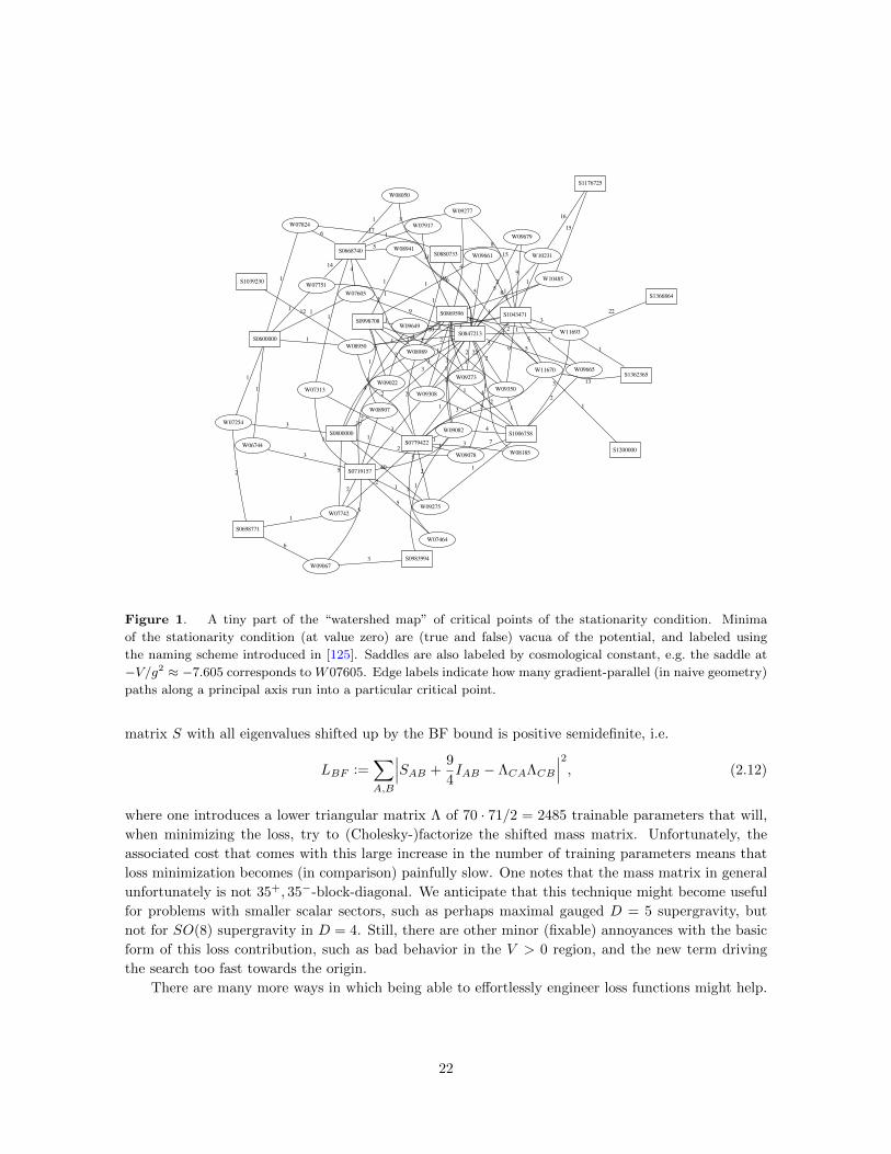
W08050

S0869596

11S0668740

1

W07605

4

S0600000

1

S0847213

9

W09082

1

4

S0719157

5

S0779422 1

S0983994

1

S10067584

W10231

1

S1176725

16

S0880733

8

S1043471

1

W07742

22

S0800000

5

S0698771

1

W07464

5

1

W09661

5

2

S0998708

1

W09273

1

2

12

53

W09679

5

9

W09308

1

3

3

1

222

W11670

1

5

1

5

S1200000

1

S136236513

W09649 14

4

1

W10485

81

15

W116932 1

3

3

1

S1366864

22

W0895031 4

2

S1039230

12

W077511

14

1

W09350

12

3 1

9

W09665

5

2

3

W07313

1

1

2

W07917

1

9

W09078

4

17

2

W08907

3

1

7

1

W07254

1

3

2

W09067

5

3

6

W09277

4

3

15

W078246

1

17

W08185

1

3

W089415

61

W09275

1

2140

W08989

10

2

2

21

1

3

4

1

W09022

1

3

1

7

W06744

1

3

Figure 1. A tiny part of the “watershed map” of critical points of the stationarity condition. Minima

of the stationarity condition (at value zero) are (true and false) vacua of the potential, and labeled using

the naming scheme introduced in [125]. Saddles are also labeled by cosmological constant, e.g. the saddle at

−V/g2 ≈ −7.605 corresponds to W07605. Edge labels indicate how many gradient-parallel (in naive geometry)

paths along a principal axis run into a particular critical point.

matrix S with all eigenvalues shifted up by the BF bound is positive semidefinite, i.e.

LBF :=∑A,B

∣∣∣SAB +9

4IAB − ΛCAΛCB

∣∣∣2, (2.12)

where one introduces a lower triangular matrix Λ of 70 · 71/2 = 2485 trainable parameters that will,

when minimizing the loss, try to (Cholesky-)factorize the shifted mass matrix. Unfortunately, the

associated cost that comes with this large increase in the number of training parameters means that

loss minimization becomes (in comparison) painfully slow. One notes that the mass matrix in general

unfortunately is not 35+, 35−-block-diagonal. We anticipate that this technique might become useful

for problems with smaller scalar sectors, such as perhaps maximal gauged D = 5 supergravity, but

not for SO(8) supergravity in D = 4. Still, there are other minor (fixable) annoyances with the basic

form of this loss contribution, such as bad behavior in the V > 0 region, and the new term driving

the search too fast towards the origin.

There are many more ways in which being able to effortlessly engineer loss functions might help.

22

For example, it might be feasible to multiply the stationarity-violation with an extra factor that

increases as search approaches known strong attractors, effectively reducing the size of their basin of

attraction. One obvious way in which this could be realized would be to add factors of the form

|Qijkl|2 ·

(∑n,p

f(

tr(A1 ijA1

ik)p − cn,p)) (2.13)

where the sum over p runs over (the first few) powers of the gravitino mass matrix that we use to

“fingerprint” solutions, the cn,p is the corresponding known fingerprint-value for the n-th known too-

attractive solution that should be punished in the search, and f is some function with f(x) ≈ 1 away

from 0 and f(x) 1 near 0. Some experimenting will be needed to find an approach that does not

create many new nonzero minima of the loss function.

2.4 Canonicalization

For any critical point obtained by a numerical search, the SO(8) symmetry of the scalar potential

allows us to freely pick an arbitrary point on its SO(8) orbit as an equivalent presentation. Natu-

rally, one would want to use a form that allows describing the solution with a minimal number of

parameters. This is not only desirable for typographic compactness, but also establishes the connec-

tion with simple exact analytic descriptions of these critical points. Setting an additional coordinate

on E7(7)/(SU(8)/Z2 to zero corresponds to imposing an extra algebraic constraint on the solution,

and using sufficiently many such constraints to eliminate all freedom to rotate a solution produces a

56-bein matrix with only algebraic entries, since the defining properties of the 56-bein, i.e. belonging

to E7(7)/(SU(8)/Z2), can also be expressed through algebraic constraints. Specificaly, the 56-bein

respects the symplectic invariant of Sp(56) as well as Cartan’s quartic invariant of E7(7) (e.g. (B.4b)

in [37]),

56 → (28,28) : (xij , ykl)

I4 = xijyjkxkly

li − 14

(xijy

ij)2

+196

(εijklmnpqy

ijyklymnypq + εijklmnpqxijxklxmnxpq).

(2.14)

At the Lie algebra level (i.e. prior to exponentiation), this then means that there are exact analytic

expressions for the coordinate-parameters describing a given solution, typically of the form algebraic number×logalgebraic number. Given that the actual 56-bein entries may well be determined by rather com-

plicated intersections of many algebraic varieties, actually finding algebraic forms may well be com-

putationally out of reach in some cases (i.e. one may well imagine to encounter zeros of irreducible

polynomials of degrees well beyond 1000). Still, for some of the new solutions described here, the

authors were able (with reasonable computational effort) to determine analytic expressions from high-

precision numerics alone. Each such expression is correct with overwhelming likelihood.

This procedure starts with first obtaining high-precision (hundreds to thousands of correct digits)

numerical data for quantities that are known to be algebraic (i.e. vielbein entries and derived quanti-

ties, such as the cosmological constant). Unfortunately for us, as extremely high numerical accuracy

is generally not very relevant for ML, TensorFlow does not support tensor arithmetics with higher

numerical precision than what common hardware can provide, i.e. IEEE-754 double precision floating

point. In that sense, from the perspective of M-Theory research, TensorFlow perhaps is best thought

of as a “discovery machine” and not a “precision machine”, carrying over terminology from accelerator

physics (e.g. [126], [127]).

In principle, it would be doable to run already the “discovery” computation with adjustable

accuracy, computing e.g. the algebraic entries of V to hundreds of decimal digits. This technique has

23

partly been employed in [108], bases on highly performant compiled Common Lisp code in conjunction

with an adapter library that allows a common generic limited-precision numerical optimizer to work in

an high precision setting, but all this generally involves carefully performing the code transformations

needed for sensitivity backpropagation by hand12. This technique that produces algebraic expressions

in a fully automatized way should hence not (yet) be considered as being easy to apply and widely

accessible. It hence makes sense to aim for a clearer separation of the “discovery” and “precision”

steps.

2.5 Parameter-reducing heuristics

An approximate location of a solution obtained by the “discovery” step, once suitably rotated to be

coordinate-aligned to the largest possible extent (using the procedure described further on), gives us an

idea about what coordinates on the scalar manifold can be set to zero, and what others can likely be set

to identical values (or simple rational multiples of one another). One finds that most solutions are very

non-generic and allow very many such simplifying linear identities. In terms of automated processing

of many solution-candidates, this then requires code that tries some basic heuristics (and automatically

abandons them when they turn out to not actually hold at high precision). The basic process is to

go through all coordinates, check if an observed coordinate is close to another one seen earlier (or

a simple rational multiple thereof, or zero) within some tolerance limit τ such as 10−3, 10−4, 10−5,

etc. If so, the observed coincidence is assumed to hold, and codified in a linear model-parameters-to-

solution-coordinates matrix map. If the attempt to improve accuracy based on such a model map runs

into a dead end, the process is restarted with a less permissive tolerance limit τ . This “automated

heuristic modeling” step typically reduces a 70-dimensional optimization problem to a much more

manageable problem in 2–20 or so parameters, for which obtaining high-accuracy data is very often

feasible even without having fast gradient computation available. The most important techniques here

are using a multidimensional Newton solver (as provided by the “mpmath” [128] package), and high-

precision Nelder-Mead optimization, which is feasible for up to about 14 parameters. If both these

techniques fail, it is sometimes useful to use basic fixed-scaling (TensorFlow-based) gradient descent

with hardware numerics to turn a solution that is good to eight digits into one that is good to at

least twelve. One finds that basic gradient descent with some simple heuristic to make learning rates

adaptive indeed seems to work better for this problem than any of the more advanced minimization

methods that are currently popular in ML applications, e.g. Adam, RMSProp, AdaGrad, FTRL. In

some situations, the parameter reducing heuristic produced a problematic canonical form, and one has

to start over with canonicalization after applying a random SO(8) rotation to the solution.

This “distillation” step produces a high degree of evidence for the existence of a particular critical

point (the length of the potential’s gradient having been shown numerically to reach values typically

below 10−20), as well as a first highly accurate location described by only a few numbers, and also

information on whether the solution is sufficiently well-behaved (i.e. non-degenerate) for the multidi-

mensional Newton method to allow quick determination of coordinates and physical properties such

as the cosmological constant to an accuracy of hundreds of digits.

2.6 Coordinate-aligning rotations

As a point on the scalar manifold can be described by giving two symmetric traceless matrices, one

carrying the 35s and one carrying the 35c representation of so(8), and we can always use a SO(8)

12At the time of this writing, trying to combine the “mpmath” [128] and “autograd” [129] Python libraries in order

to achieve this does not work.

24

rotation to diagonalize one of these, the effective dimension of the scalar manifold relevant for finding

critical points is reduced to 70 − 28 = 42. Still, even if one exploited this symmetry from the start

and only looked for critical points for which one of 35s,35c is diagonal, this does not eliminate the

need to numerically canonicalize a solution, as any degeneracy in the entries of the diagonal matrix

would leave some residual rotational symmetry that can be used to reduce the number of non-zero

entries in the other diagonal matrix. For example, if the parameters in 35s can be brought into the

form diag(3A, 3A,−A,−A,−A,−A,−A,−A), this still leaves a residual symmetry of SO(2)× SO(6)

which must be fixed by imposing algebraic constraints on the 35c in order to make the entries of the

56-bein matrix algebraic.

As it hence is difficult, in a numerics-based search, to avoid the need for a “canonicalization” step

that eliminates residual rotational freedom, we may just as well fish for solutions in full 70-dimensional

parameter space. While our particular choice of e7 generators leaves us with a non-diagonal scalar

product on the 70-dimensional manifold of scalars13, we nevertheless start the search with a 70-vector

picked at random from a distribution that is isotropic with respect to the coordinate-basis, not the

restricted e7 Killing form. This choice is apparently “good enough” to find many new solutions.

For elements of a 35-dimensional irreducible representation of SO(8), it is easy to numerically

find a rotation Gd that diagonalizes the corresponding symmetric traceless matrix. The orthonormal

eigenbasis serves this purpose if we multiply the last eigenvector with ±1 in order to ensure a positive

determinant. Knowing how to diagonalize, say, 35s, how do we then find the corresponding action

on the 35c (and vice-versa)? Logarithmizing the group element to obtain the algebra element is

out of the question, but we can employ a higher-dimensional generalization of Davenport chained

rotations [130] [131] to write Gd as a product of a sequence of up to 28 rotations in coordinate-aligned

planes,

Gd = R67(α67) · · ·R57(α57) · · ·R56(α56) · · · ·R02(α02) ·R01(α01), (2.15)

each of which, when moved to the left size, cancels another off-diagonal entry of Gd without destroying

earlier such reductions14. Using this presentation, we can then proceed to logarithmize each factor

Rγδ(αγδ) = exp (rγδ · αγδ) (2.16)

and find the corresponding Lie algebra action on the 8c representation by employing the γαβγδ

invariant.

Lifting this to an action on 35c ⊂ (8c × 8c) and exponentiating, we can readily determine the action

of Gd on 35c. An alternative approach would be to run numerical minimization starting from Lie

algebra elements that get exponentiated to obtain group actions on the 35s and 35c with an objective

function that punishes off-diagonal elements for the matrix carrying the 35s representation.

Once the 35s has been diagonalized by any such method that also gives us the effect of the rotation

which was employed on the 35c, we can proceed to determine the residual subalgebra of so(8) that

keeps the diagonalized 35s unchanged. We can employ this subalgebra to reduce the number of off-

diagonal entries for the matrix carrying the 35c representation, but in general not completely. Also,

this residual symmetry group will typically be rather small – such as SO(3)× SO(2). It hence makes

sense to consider this step as a somewhat low-dimensional numerical optimization problem. In general,

problems that maximize the number of zero entries in a matrix often are hard, but here, a common

sparseness-encouraging ML technique works reasonably well: we use the L1-norm of the off-diagonal

matrix entries as a loss function.

13It is orthonormal up to an overall factor, and the non-orthogonal inner products of the basis vectors that correspond

to the diag(1,−1, 0, . . . , 0), diag(0, 1,−1, 0, . . . , 0) parts of the symmetric traceless matrices.14For better numerical stability, one should re-order processing of row-entries by absolute magnitude.

25

After this sparseness-encouraging rotation, which will in general have put many more than 28 co-

efficients to zero, we proceed by making an automated guess for the form of the symmetric matrices

carrying the 35s and 35c representations as described.

2.7 “Algebraization”

Once an highly-accurate numerical value for a known-to-be-algebraic parameter has been found, one

can use an integer relation algorithm such as PSLQ [132] to find a polynomial of which this is a zero

and that seems plausible, i.e. the total information content of its coefficients is much smaller than the

information content of the known digits of the parameter. This works well for up to a few thousand

decimal digits. More specifically, one scans for a set of integer coefficients cj , j ∈ 0, 1, . . . , N−1, |cj | <10d such that for a number ξ known to D (perhaps D ∼ 300) digits after the point, with D > N ·d+30,

we have |∑j cjξ

j | < 10−(Nd+10). If such a polynomial is found, we can easily determine its actual

zero to D digits after the point, and check if this polynomial correctly predicts many further digits

of ξ that were known but not used to find the cj . Naturally, if there is a single candidate polynomial

that was found by using 300 known good digits of precision manages to predict the next 50 digits, we

would expect this to happen purely by chance to be ∼ 1 : 1050. So, by using a large enough reservoir

of extra precision, we can make the likelihood to accidentally predict an incorrect algebraic expression

fantastically small. While this still does not constitute a strict mathematical proof, it would be rather

unreasonable to disbelieve the result. Of course, it will in many cases then be possible to independently

establish the validity of a claimed exact expression, but this will generally require ingenuity and effort

beyond what can easily be automated to process scores of solutions.

2.8 Tweaks to the basic procedure

In general, it makes sense to use moderately refined numerical data (e.g. known to be good to 14 digits

of accuracy) and then repeat the entire procedure that starts with finding a coordinate-aligning so(8)

rotation from cleaned up numerical data, as limitations on numerical precision of input data from the

ML library data may have caused the (imperfect) heuristic that suggests a low-dimensional model to

miss some reduction opportunities. In particular, starting from an already partially parameter-reduced

model will lead to rather short products of Davenport chained rotations, which are numerically much

better behaved than those seen in the initial reduction step.

Once highly-accurate and nicely coordinate-aligned numerical data are available, inverse symbolic

computation methods can automatically search for exact expressions for physically relevant properties

such as the cosmological constant, coordinates, particle masses and charges (and hence also residual

supersymmetry), and others.

2.9 Extracting the physics

Unbroken continuous gauge symmetries can be determined numerically by mostly straightforward

methods, and Lie group theory then allows an automatic classification. In a first step, one determines

the space h of so(8) generators that leave a given solution invariant and splits it into orthogonal pieces

w.r.t. the Cartan-Killing metric h = [h, h] +h′. This separates off the generators of the U(1)N part of

the residual symmetry. For all new solutions described here, the dimension of the semisimple [h, h] =: h

part is 0, 3, or 6, so the corresponding non-abelian symmetry algebra can only be k ·so(3), k ∈ 0, 1, 2,but perhaps embedded into so(8) in different ways. The authors’ automated analysis handles this case

by looking for a maximal set of p orthogonal and commuting h-elements hc,j , j ∈ 0, . . . , p − 1(which thanks to so(8) being the algebra of a compact Lie group are simultaneously diagonalizable

26

in the adjoint representation), then splitting h into subspaces that are simultaneous eigenspaces for

these p generators, labeled by p-dimensional vectors of eigenvalues. After defining a subspace of

positive roots and identifying simple roots, taking the commutators of raising and lowering operators

associated with simple roots produces a basis for the Cartan subalgebra that is useful for numerically

identifying angular momentum spectra, which for k ·so(3) are straightforward to map to the irreducible

representation content. For U(1)N generators, the N = 2 case will in general require finding a

rotation that coordinate-aligns the charge lattice. In any case, we scale every U(1) generator u such

that exp(2πu) is the identity on all particle states, while no λu with 0 < λ < 1 also has this property.

For solutions whose gauge group has a single U(1), we use superscripts to indicate electric charge

of particle states, while for solutions with U(1) × U(1) abelian gauge symmetry, we use super- and

sub-scripts for the two different types of charges.

Having split the unbroken symmetry in this way, we can proceed to present branching rules for

the 8v,s,c as well as 28, and decompose particle mass-eigenstates for the spin-1/2 fermions, spin-3/2

gravitinos, and spin-0 scalars in terms of irreducible representations of the residual gauge algebra.

For the scalars, we first try to split mass eigenspaces into orthogonal subspaces of the parity oper-

ator P that is +I on 35s and is −I on 35c. However, the analysis presented here only splits off

the pure P = 1 and P = −1 subspaces and subsequently merges their joint orthogonal complement

into one subspace. Mass eigenstates are then determined on these three subspaces, and marked with a

superscript of (s), (c), or (m) for the “mixed” case, respectively. This step is numerically slightly prob-

lematic, as it so turns out that, for some critical points, we find P = 1− ε eigenstates with ε < 10−3.

Hence, auto-identification of some mass eigenstate as a pure scalar or pure pseudoscalar state may

be somewhat unreliable. It is nevertheless reassuring that decomposition of weights into irreducible

representations is observed to always succeed, which it would not if some P -eigenvectors were wrongly

assigned to subspaces. All particle masses are known with an accuracy of more than eight digits,

but it may happen that different particle masses look the same when truncated to three digits af-

ter the point for presentation. This explains why some solutions list the same mass as belonging

to more than one mass-subspace. This happens e.g. for S1039624, which lists scalars with m2/m20

of −2.417m1+++++1−−−− ,−2.417m1 , rather than −2.417m1+++++1−−−−+1 i.e. there is a two-dimensional

subspace of mass eigenstates with electric charges ±4 and another one-dimensional mass eigenstate

with a too-close-to-be-discriminated-at-presentation-accuracy mass. For a solution to be perturba-

tively stable, no scalar mass-eigenstate must have m2/m20 that violates the BF bound of −9/4. Un-

stable mass-eigenstates that violate this bound are marked with an asterisk (∗) in the tables.

As none of the new solutions has a residual gauge group that contains a simple group of rank ≥ 2,

and so apparently all such solutions already have been identified and studied in detail in the 80’s [116],

there is no compelling reason to automate assignment of quantum numbers to such larger symmetry

groups.

Residual supersymmetry can be identified [133] numerically by using Singular Value Decomposi-

tion (SVD) to look for solutions of

ηiA2jkli = 0 . (2.17)

The corresponding gravitino states are marked with an asterisk in the tables.

3 A guide to the new solutions

Detailed data on all the solutions obtained in a large TensorFlow based cluster search are presented

in appendix D.

27

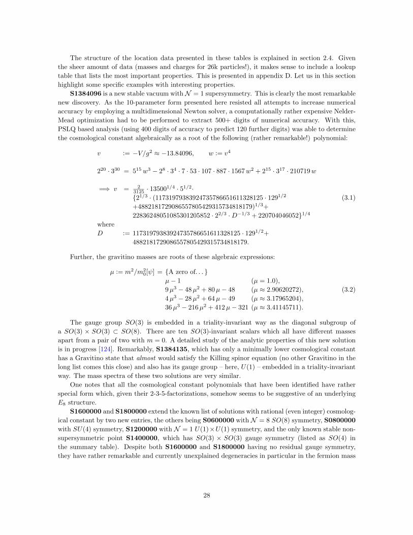
The structure of the location data presented in these tables is explained in section 2.4. Given

the sheer amount of data (masses and charges for 26k particles!), it makes sense to include a lookup

table that lists the most important properties. This is presented in appendix D. Let us in this section

highlight some specific examples with interesting properties.

S1384096 is a new stable vacuum withN = 1 supersymmetry. This is clearly the most remarkable

new discovery. As the 10-parameter form presented here resisted all attempts to increase numerical

accuracy by employing a multidimensional Newton solver, a computationally rather expensive Nelder-

Mead optimization had to be performed to extract 500+ digits of numerical accuracy. With this,

PSLQ based analysis (using 400 digits of accuracy to predict 120 further digits) was able to determine

the cosmological constant algebraically as a root of the following (rather remarkable!) polynomial:

v := −V/g2 ≈ −13.84096, w := v4

220 · 330 = 515 w3 − 28 · 34 · 7 · 53 · 107 · 887 · 1567w2 + 215 · 317 · 210719w

=⇒ v = 23125 · 135001/4 · 51/2·21/3 · (11731979383924735786651611328125 · 1291/2

+4882181729086557805429315734818179)1/3+

22836248051085301205852 · 22/3 ·D−1/3 + 2207040460521/4where

D := 11731979383924735786651611328125 · 1291/2+

4882181729086557805429315734818179.

(3.1)

Further, the gravitino masses are roots of these algebraic expressions:

µ := m2/m20[ψ] = A zero of. . .

µ− 1 (µ = 1.0),

9µ3 − 48µ2 + 80µ− 48 (µ ≈ 2.90620272),

4µ3 − 28µ2 + 64µ− 49 (µ ≈ 3.17965204),

36µ3 − 216µ2 + 412µ− 321 (µ ≈ 3.41145711).

(3.2)

The gauge group SO(3) is embedded in a triality-invariant way as the diagonal subgroup of

a SO(3) × SO(3) ⊂ SO(8). There are ten SO(3)-invariant scalars which all have different masses

apart from a pair of two with m = 0. A detailed study of the analytic properties of this new solution

is in progress [124]. Remarkably, S1384135, which has only a minimally lower cosmological constant

has a Gravitino state that almost would satisfy the Killing spinor equation (no other Gravitino in the

long list comes this close) and also has its gauge group – here, U(1) – embedded in a triality-invariant

way. The mass spectra of these two solutions are very similar.

One notes that all the cosmological constant polynomials that have been identified have rather

special form which, given their 2-3-5-factorizations, somehow seems to be suggestive of an underlying

E8 structure.

S1600000 and S1800000 extend the known list of solutions with rational (even integer) cosmolog-

ical constant by two new entries, the others being S0600000 with N = 8 SO(8) symmetry, S0800000

with SU(4) symmetry, S1200000 with N = 1 U(1)×U(1) symmetry, and the only known stable non-

supersymmetric point S1400000, which has SO(3) × SO(3) gauge symmetry (listed as SO(4) in

the summary table). Despite both S1600000 and S1800000 having no residual gauge symmetry,

they have rather remarkable and currently unexplained degeneracies in particular in the fermion mass

28

spectra. Such “accidental degeneracies” also occur for some other critical points, such as S1046018

or S1176725.

The S0847213 solution is the only “modern” critical point with residual gauge symmetry for

which the 8v,s,c branching does not have any residual triality symmetry. Also, it is the only case with

a 3-component gauge group.

The S1039230 solution has been first described in [134]. In total, there are three known critical

points with residual gauge symmetry SO(4). The gauge group embedding has V ↔ S triality symmetry

for this solution, while it has V ↔ C triality symmetry for the S0880733 solution and S ↔ C

symmetry for the (BF-stable!) S1400000 solution.

S2099419 and S2099422 are a pair of critical points with extremely similar but nevertheless

different particle properties and also cosmological constant. There are a few other examples for

critical points with very small difference in the cosmological constant and similar properties, such as

the pair S2511744-S2512364, or S3254262-S3254576.

For almost every solution, the number of scalar modes with m2/m20 = 0 matches the number of

broken so(8) generators, as it has to according to Goldstone’s theorem. Two solutions have extra

massless (w.r.t. “naive mass”, not AdS-massless) modes that survive being eaten by gauge bosons:

S0800000 (i.e. the SU(4) critical point) and S1200000 (i.e. the N = 1 U(1)× U(1) vacuum).

Solutions S1200000, S2279257 and S2279859 are listed in the summary table with symme-

try U(1)1, since in these cases, the charge of all U(1)-charged particles is the same in magnitude. Still,

these particle-states are listed as having charges 1++ etc. in the tables for typographic reasons, due

to the 8s,c representations branching to 4 × 1+ + 4 × 1−, but the spectrum not having any particles

transforming under these representations.

While this expanded list did not uncover any other stable non-supersymmetric critical points

beyond the known SO(3) × SO(3) solution S1400000, we observe a another instance of the phe-

nomenon that instabilities can become invisible when truncating a solution to the scalar submanifold

that is invariant under the unbroken gauge group. This was first observed and discussed in detail

for S0800000 in [118]. There, the unstable scalars come as a single 20-dimensional irreducible repre-

sentation of SU(4), and the question was raised whether one could project out these unstable modes

with an orbifold construction which would have to use a non-abelian discrete subgroup of SU(4) other

than the Weyl group (since in these cases, the 20’ decomposes with singlets). This phenomenon also

happens for the SO(7) critical points S0668740 and S0698771, where the unstable modes transform

as a 27, as well as for S1424025, where the unstable modes form a single 5 of SO(3). Clearly, the

analysis of all viable discrete subgroups of the gauge group under which this irreducible representation

branches without singlets is greatly simplified by going from SU(4) to SO(3), where there is an obvious

candidate symmetry (namely the icosahedral group) under which 5→ 5.

Remarkably, S2416856 has no residual gauge symmetry, but six unstable scalar modes with

1+2+3 mass-degeneracy. While trying to find a way to stabilize this solution seems hopeless here, it

would be interesting to understand what symmetry is responsible for the accidental mass degeneracies

in the unstable modes.

The solutions S1195898 and S2503105 feature a peculiar SO(3) gauge symmetry which is em-

bedded in a triality-invariant way, with branching 8v,s,c → 3 + 5. In both cases, there are only two

SO(3)-invariant scalars, but unfortunately, one of them is unstable. This is also the only instability

of these solutions. Remarkably, the minimal polynomial for the cosmological constant is identical for

these two solutions, so this seems to be an example of the algebraic equations for a vanishing gradient

allowing a pair of real solutions that are Galois conjugates. It is noteworthy that even in the large

numerical search performed here, S2503105 was a chance hit that only showed up once. Had it been

29

missed, it is conceivable that it ultimately might have been found in a detailed study of S1195898 as

an algebraically equivalent solution. So, looking for Galois conjugates seems to be one new method to

fill possible gaps in the list of solutions.

The same Galois-doubling phenomenon occurs also for the pair S1039624–S1402217, which both

also have identically embedded gauge group. One might speculate that Galois conjugates may well

occur more often, in particular with solutions without residual symmetry and a cosmological constant

that is not known algebraically. Perhaps then, it may be possible to extract algebraic numbers that

are easier to identify from pairs of numerically known cosmological constants of critical points with

identically embedded gauge group.

A rather unique property of the S4168086-solution will be the topic of a short follow-up article.

4 Conclusions and outlook

Some problems in the world are very amenable to ML based approaches, others not so much. As we

are, during the current ML revolution, working on finding out which is which, we sometimes encounter

pleasant surprises. Being able to present an elegant way to address a fundamental need in quantum

gravity research – the need to be able to analyze potentials on complicated high-dimensional scalar

manifolds – certainly is one of these.

More work remains to be done that analyzes other relevant cases using the methods presented here,

in particular the scalar sector of maximal D = 5 gauged supergravity [5], i.e. the AdS side of the best

studied case of the AdS/CFT correspondence, as well as CSO(p, q, r)-gaugings of four-dimensional

maximal supergravity, plus their dyonic variants [105], and other gaugings discussed in [102], as well

as gauged supergravities in three and two dimensions.

Also, while the present article is a major step forward towards a proven-exhaustive classification

of the critical points of SO(8) supergravity, this challenging problem is still out of reach. It is quite

likely that the rather peculiar form of the minimal polynomials of the cosmological constant that could

be obtained for about three dozen critical points (including all solutions that can be described with

up to six parameters) is a very major clue which the authors currently do not know how to utilize.

Nevertheless, having an algebraic expression for the cosmological constant typically means that it is

also feasible to find algebraic expressions for the entries of the 56-bein matrix, and hence quite a bit of

the work required to uplift a critical point to a solution of the equations of motion of 11-dimensional

supergravity can be automated. Not surprisingly, giving exact expressions for coordinates (which

are not algebraic, but typically algebraic · log algebraic) is quite a bit harder (in fact, with the

techniques employed here, this could only be achieved for a few coordinates), but might actually be

unnecessary to answer most questions as long as the vielbein entries are known exactly and one can

show that the vielbein indeed is an element of E7(7). Clearly, it would be very interesting to know in

particular for all the supersymmetric vacua what 11-dimensional geometries these solutions correspond

to – and also what the CFT renormalization group flows on M2-branes between the corresponding

fixed points look line.

For all solutions presented here, numerical data on their location are available in the source package

of the arXiv.org preprint of this article. In many cases, the authors have been able to numerically

reduce the violation of the stationarity condition to much less than 10−1000, and for each claimed

critical point, it would be unreasonable to doubt its existence. Unfortunately, going from machine

accuracy as obtained with TensorFlow to high accuracy is a somewhat messy process as the heuristics

to guess a low-dimensional model as well as the attempt to use a multi-dimensional Newton solver

do occasionally fail (for quite a few independent reasons) and require manual intervention. Due to

30

limited time and a rather large number of cases to analyze, the quality of numerical data is rather

uneven, typically providing 100+ good digits, but sometimes only providing as few as 16. With a bit

of numerical experimenting, it typically is possible to obtain 1000+ good digits for any given solution

within about two days of work.

Quite a few of the solutions feature (occasionally large) accidental degeneracies in the spectrum

that should be understood and may point to exploitable symmetry properties. It may well be that the

accidental U(1) 6⊂ SO(8) “background round S7 diffeomorphism” symmetry of the S1400000 solution

discussed in [113], is a first example of such an extra symmetry. Also, it is interesting to observe that,

out of all the solutions newly discovered by employing numerical methods, there is a single one for

which the residual symmetry group is not embedded in a way that has triality symmetry. Clearly,

triality seems to play a rather important role, and so re-phrasing the problem in octonionic language

might reveal additional structure.

In this work, we have only scratched the surface on cleverly engineering loss functions in order to

extract additional information from the scalar potential. We expect that, with some ingenuity, much

more is possible here, perhaps even allowing an efficient direct scan for BF-stable critical points.

Given that even this long list will still have some gaps, what are the most promising approaches to

fill them? One strategy still is to parametrize and study interesting submanifolds, such as the manifold

of scalars that are invariant under the SO(3) gauge group of the new supersymmetric vacuum. Also,

assuming that there indeed are perfect algebraic “Galois twin” solutions (i.e. not only the cosmological

constant, but also all particle masses are related by root flipping), it may be possible to discover new

solutions by obtaining algebraic expressions for some at present only numerically known solutions and

then check whether root-flipping can produce new real solutions. A very promising further approach

may be to study the extremal structure of the “dyonic” variants described in [105] and study the fate

of critical points when changing the new ω-parameter. In [134], this method found the third SO(4)

critical point S1039230 before it was independently rediscovered here, and it may well reveal further

solutions.

Historically, the potential of SO(8) supergravity was first written down in [3]. About fourty years

later, we now have what is likely the almost-complete list of critical points, and very likely the complete

list of supersymmetric vacua of this theory. Given that some of the ideas that enabled this analysis

were about as old as the original problem but largely unknown in the String Theory community, and

were identified as useful and had to be brought together as part of one of the authors’ personal journey,

it seems likely that other technically hard problems in String Theory also would benefit from more

exchange with other fields of research. We hope that by aiming to keep the introduction in this article

accessible to readers with a technical background who are not experts in field theory, we might attract

the attention of experts who can contribute missing puzzle pieces that we are not even aware of yet,

perhaps even allowing a completeness proof of the list of solutions (perhaps after filling the last gaps).

Acknowledgments

It is a pleasure to thank our managers, first and foremost Jyrki Alakuijala, Rahul Sukthankar, and

Jay Yagnik for support on this rather exotic side project, which turned into a rather unusual Machine

Learning adventure. T.F. would like to thank Hermann Nicolai and the Albert Einstein Institute in

Potsdam for hospitality and useful discussions during the final phase of this project, and also Krzysztof

Pilch, Nikolay Bobev, Adolfo Guarino, and Michael Duff for feedback.

Appendix

31

A E7 Conventions

Spin(8) triality provides some intuitive insights into the question why the exceptional Lie group E7

exists. Let us start from the observation that one can, for example, understand the algebra rotations

in nine spatial dimensions, so(9), as an expansion of the group of rotations in eight spatial dimen-

sions, so(8), by eight extra elements rk8 that, when scaled and exponentiated, rotate each of the

coordinate axes of eight-dimensional space against the ninth axis,

Rk8(α)mn = exp(αrk8)mn= (δkmδkn + δ8mδ8n) cosα+ (δkmδ8n − δ8mδkn) sinα

. (A.1)

and themselves transform under so(8) as eight-dimensional vectors, while giving rise to other so(8)

rotations in their commutator, [r08, r18] = −2r01 so that we get an overall structure of [g, g] ∼ g,

[g, h] ∼ h, [h, h] ∼ g. Likewise, one can obtain the 63-dimensional algebra sl(8) from the 28-dimensional

algebra of so(8) by adding 35 generators that transform as symmetric traceless matrices under so(8).

One easily sees how for the 8-dimensional vector representation of sl(8), the generators can be expressed

in a basis of symmetric and anti-symmetric traceless matrices, where the latter form the subalgebra

of so(8) and the former are the generators that extend this to sl(8). One notes that one also gets a

63-dimensional real algebra (over complex matrices) that closes if one multiplied each of the extra 35

generators with i, so that commutator relations are of the form [g, g] ∼ g, [g, ih] ∼ ih, [ih, ih] ∼ −g.

The extra minus sign here also shows up in the signature of the quadratic invariant that can be formed

from the generators, the Killing form, Gmn := Tr (gmgn). Applying this “Weyl unitarity trick” to sl(8)

produces the Lie algebra of the compact Lie group SU(8), i.e. su(8).

Now, the so(8) (or “spin(8)”) algebra is special in that there is a non-abelian S3 symmetry that acts

on its irreducible representations. This symmetry permutes the roles of the three inequivalent eight-

dimensional irreducible representations, the “vectors”, “spinors”, and “co-spinors”. Let us consider

extending so(8) with an eight-dimensional vector representation v as before in order to get so(9), but

simultaneously with eight-dimensional spinors s and co-spinors c in such a way that we get commutator

relations of the form [g, g] ∼ g, [g, v] ∼ v, [v, v] ∼ g, [v, s] ∼ c plus the corresponding cyclically triality-

rotated forms such as [s, s] ∼ g, [s, c] ∼ v, etc, by employing the invariant tensor γiαβ

of so(8) that

implements a non-degenerate generalized product of eight-dimensional representations. There is a

unique way to work out commutator relations such that the Jacobi identity [a, [b, c]] + cyclic = 0

holds, and this gives the Lie algebra of the 28+3·8 = 52-dimensional exceptional group F4. Performing

a similar construction that extends so(8) in a triality-symmetric way now with the symmetric traceless

matrices over the vectors, spinors and co-spinors produces the 28 + 35v + 35s + 35c = 133-dimensional

Lie algebra of e7. It is possible to choose signs such that one of the 35-dimensional representations

extends so(8) to su(8), while the other two each extend so(8) to sl(8). This then gives the noncompact

real form e7(7) that shows up in four-dimensional N = 8 supergravity. So, in a sense, the e7 algebra can

be thought of as a generalized algebra of rotations with “siamese triplet” structure, three organisms co-

joined at the so(8) heart, but functioning as one whole body. In order to make this work self-contained,

we spell out the conventions underlying our construction of e7(7) in detail. These match [108], apart

from index counting always being 0-based the present article.

We start from the so(8) “Pauli-matrices” γiαβ

in the conventions of Green, Schwarz, and Wit-

ten [135], but with all indices shifted down by 1, as it makes much more sense in a computational

setting to consistently start index counting at zero. The nonzero entries of γiαβ

are all ±1, and we list

them in compact form iαα±, so e.g. 357− translates as γi=3α=5,β=7

= −1, etc.

32

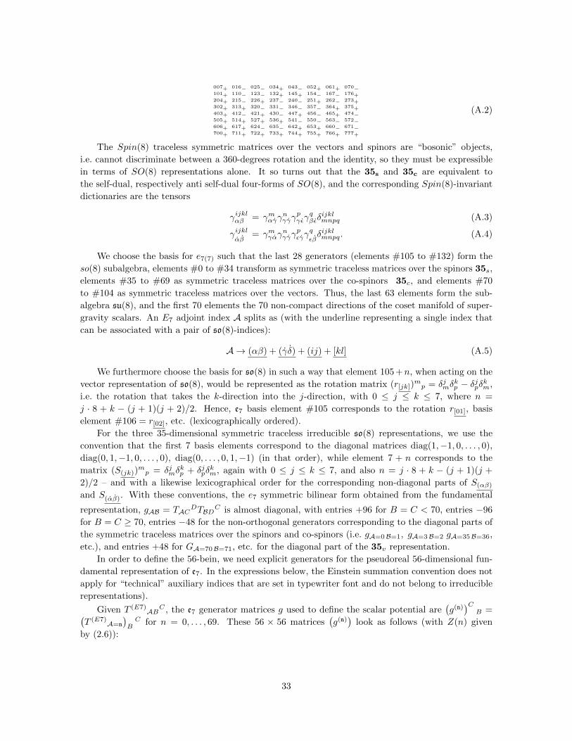
007+ 016− 025− 034+ 043− 052+ 061+ 070−101+ 110− 123− 132+ 145+ 154− 167− 176+204+ 215− 226+ 237− 240− 251+ 262− 273+302+ 313+ 320− 331− 346− 357− 364+ 375+403+ 412− 421+ 430− 447+ 456− 465+ 474−505+ 514+ 527+ 536+ 541− 550− 563− 572−606+ 617+ 624− 635− 642+ 653+ 660− 671−700+ 711+ 722+ 733+ 744+ 755+ 766+ 777+

(A.2)

The Spin(8) traceless symmetric matrices over the vectors and spinors are “bosonic” objects,

i.e. cannot discriminate between a 360-degrees rotation and the identity, so they must be expressible

in terms of SO(8) representations alone. It so turns out that the 35s and 35c are equivalent to

the self-dual, respectively anti self-dual four-forms of SO(8), and the corresponding Spin(8)-invariant

dictionaries are the tensors

γijklαβ = γmαγγnγγγ

pγεγ

qβεδ

ijklmnpq (A.3)

γijklαβ

= γmγαγnγγγ

pεγγ

q

εβδijklmnpq. (A.4)

We choose the basis for e7(7) such that the last 28 generators (elements #105 to #132) form the

so(8) subalgebra, elements #0 to #34 transform as symmetric traceless matrices over the spinors 35s,

elements #35 to #69 as symmetric traceless matrices over the co-spinors 35c, and elements #70

to #104 as symmetric traceless matrices over the vectors. Thus, the last 63 elements form the sub-

algebra su(8), and the first 70 elements the 70 non-compact directions of the coset manifold of super-

gravity scalars. An E7 adjoint index A splits as (with the underline representing a single index that

can be associated with a pair of so(8)-indices):

A → (αβ) + (γδ) + (ij) + [kl] (A.5)

We furthermore choose the basis for so(8) in such a way that element 105 +n, when acting on the

vector representation of so(8), would be represented as the rotation matrix (r[jk])mp = δjmδ

kp − δjpδkm,

i.e. the rotation that takes the k-direction into the j-direction, with 0 ≤ j ≤ k ≤ 7, where n =

j · 8 + k − (j + 1)(j + 2)/2. Hence, e7 basis element #105 corresponds to the rotation r[01], basis

element #106 = r[02], etc. (lexicographically ordered).

For the three 35-dimensional symmetric traceless irreducible so(8) representations, we use the

convention that the first 7 basis elements correspond to the diagonal matrices diag(1,−1, 0, . . . , 0),

diag(0, 1,−1, 0, . . . , 0), diag(0, . . . , 0, 1,−1) (in that order), while element 7 + n corresponds to the

matrix (S(jk))mp = δjmδ

kp + δjpδ

km, again with 0 ≤ j ≤ k ≤ 7, and also n = j · 8 + k − (j + 1)(j +

2)/2 – and with a likewise lexicographical order for the corresponding non-diagonal parts of S(αβ)

and S(αβ). With these conventions, the e7 symmetric bilinear form obtained from the fundamental

representation, gAB = TACDTBD

C is almost diagonal, with entries +96 for B = C < 70, entries −96

for B = C ≥ 70, entries −48 for the non-orthogonal generators corresponding to the diagonal parts of

the symmetric traceless matrices over the spinors and co-spinors (i.e. gA=0B=1, gA=3B=2 gA=35B=36,

etc.), and entries +48 for GA=70B=71, etc. for the diagonal part of the 35v representation.

In order to define the 56-bein, we need explicit generators for the pseudoreal 56-dimensional fun-

damental representation of e7. In the expressions below, the Einstein summation convention does not

apply for “technical” auxiliary indices that are set in typewriter font and do not belong to irreducible

representations).

Given T (E7)AB

C , the e7 generator matrices g used to define the scalar potential are(g(n))C

B =(T (E7)

A=n

)BC for n = 0, . . . , 69. These 56 × 56 matrices

(g(n))

look as follows (with Z(n) given

by (2.6)):

33

T (SU(8))Ajk =

+i for A = j = k < 7

−i for A+ 1 = j = k < 7

+i for 7 ≤ A < 35, (m, n) = Z(A− 7), j = m, k = n

+i for 7 ≤ A < 35, (m, n) = Z(A− 7), j = n, k = m

+1 for 35 ≤ A, (m, n) = Z(A− 35), j = m, k = n

−1 for 35 ≤ A, (m, n) = Z(A− 35), j = n, k = m

S(SO(8))abcd(αβ) =

γabcdαβ (δαm δ

βm − δαn δβn ) for (αβ) = m = n− 1 < 7

γabcdαβ (δαm δβn + δαn δ

βm ) for (αβ) ≥ 7, (m, n) = Z((αβ)− 7)

C(SO(8))abcd(αβ)

=

γabcdαβ

(δαm δβm − δαn δβn ) for (αβ) = m = n− 1 <

γabcdαβ

(δαm δβn + δαn δ

βm ) for (αβ) ≥ 7, (m, n) = Z((αβ)− 7)

T (E7)AB

C =

18S

(SO(8))abcd(αβ)(δ

am δbn − δan δbm)(δcpδdq − δcqδdp ) for

A < 35, (αβ) = A,B ≥ 28, (p, q) = Z(B − 28),

C < 28, (m, n) = Z(C)

18S

(SO(8))cdab(αβ)(δ

cmδdn − δcnδdm )(δap δ

bq − δaq δbp) for

A < 35, (αβ) = A,B < 28, (p, q) = Z(B),

C ≥ 28, (m, n) = Z(C − 28)

i8C

(SO(8))abcd(αβ)

(δam δbn − δan δbm)(δcpδdq − δcqδdp ) for

35 ≤ A < 70, (αβ) = A− 35,

B ≥ 28, (p, q) = Z(B − 28),

C < 28, (m, n) = Z(C)

− i8C

(SO(8))cdab(αβ)

(δcmδdn − δcnδdm )(δap δ

bq − δaq δbp) for

35 ≤ A < 70, (αβ) = A− 35,

B < 28, (p, q) = Z(B),

C ≥ 28, (m, n) = Z(C − 28)

2T (SU(8))Ajk(δqnδjmδ

pk + δ

pmδjnδ

qk − δ

pnδjmδ

qk − δ

qmδjnδ

pk

)for

A ≥ 70, A = A− 70

B < 28, (p, q) = Z(B),

C < 28, (m, n) = Z(C)

2(T (SU(8))

Ajk)∗ (

δqnδjmδpk + δpmδjnδ

qk − δ

pnδjmδ

qk − δ

qmδjnδ

pk

)for

A ≥ 70, A = A− 70

B ≥ 28, (p, q) = Z(B − 28),

C ≥ 28, (m, n) = Z(C − 28)

(A.6)

34

B The Octonions and the spin(8) invariant γiαβ

This section provides a simple and fully self-contained instructive example for using TensorFlow to

numerically solve tensorial algebraic constraints with very little mental effort. The basic techniques

are essentially the same as the ones used for the main part of this work. Also, this section provides

a detailed answer to the question how two common conventions for Octonions and spin(8) gamma

matrices are related.

The Lie group Spin(8) has three inequivalent irreducible eight-dimensional representations, the

vectors 8v, for which we use indices i, j, k, . . ., the spinors 8s, indexed with α, β, . . ., and the co-

spinors 8c, indexed with α, β, . . .. The spin(8) invariant γiαβ

provides a unique way to map spinors

and co-spinors to vectors, φ(·, ·) : 8s×8c → 8v : (s, c)→ v such that (e.g.) for any non-zero element S

of 8s, the map 8c → 8v : c 7→ φ(S, c) is nondegenerate.

This means that we can use γiαβ

to define an invertible 8-dimensional product, that is, an 8-

dimensional real division algebra. Now, using e.g. an explicit form of the (8, 8, 8) tensor γiαβ

such as the

one given in [135], eq. (5.B.3), which has no reason to know about the division algebra interpretation,

some arbitrary choice has been made for the vector space bases of the 8v, 8s, 8c representations.

Without loss of generality, we can identify the chosen basis of 8v with the basis of the “output” vector

space of the octonionic product as it is defined in [136], with the octonionic imaginary units e1 . . . e7satisfying:

ejej = −1, ejek = −ekej (j 6= k), e1 · e2 = e4ei · ej = ek =⇒ ei+1 · ej+1 = ek+1 and e2i · e2j = e2k (mod 7).

(B.1)

Then, as we want to retain orthonormality (but not necessarily handedness), we can try to find

one O(8) element that changes the basis of 8s, and another O(8) element that changes the basis

of 8c in order to precisely align the entries of the (8, 8, 8)-tensor γiαβ

with the (8, 8, 8)-tensor of the

octonionic multiplication table. This objective provides 83 = 512 constraints, while we only have 2 ·28

continuous parameters (two eight-dimensional rotations) to do the alignment. Hence, it is quite a

nontrivial statement that the stated objective can indeed be achieved. (It so turns out that there are

discrete choices for this problem that differ in the way how signs are distributed.) For this instructional

example, we are extra lazy and do not even try to employ a proper parametrization of O(8) elements

(such as e.g. via a Cayley transform M = (I − A)(I + A)−1). Rather, we design our optimization

problem such that we in principle allow arbitrary elements of GL(8), but introduce a term in our

objective function that punishes deviations from orthonormality.

The important point about the piece of code shown below is that, while this solves a numerical

optimization problem in 2 · 64 = 128 parameters both with very good performance and accuracy,

nowhere did the need arise for us to provide any code that computes gradients. This is all handled by

the TensorFlow framework.

import numpy

import t en so r f l ow as t f

def get gamma vsc ( ) :

”””Computes SO(8) gamma−matrices . ”””

# Conventions match Green , Schwarz , Witten ’ s .

e n t r i e s = (

”007+ 016− 025− 034+ 043− 052+ 061+ 070− ”

”101+ 110− 123− 132+ 145+ 154− 167− 176+ ”

”204+ 215− 226+ 237− 240− 251+ 262− 273+ ”

”302+ 313+ 320− 331− 346− 357− 364+ 375+ ”

”403+ 412− 421+ 430− 447+ 456− 465+ 474− ”

35

”505+ 514+ 527+ 536+ 541− 550− 563− 572− ”

”606+ 617+ 624− 635− 642+ 653+ 660− 671− ”

”700+ 711+ 722+ 733+ 744+ 755+ 766+ 777+” )

r e t = numpy . z e ro s ( [ 8 , 8 , 8 ] )

for i j k c in e n t r i e s . s p l i t ( ) :

i j k = tuple (map( int , i j k c [ : −1 ] ) )

r e t [ i j k ] = +1 i f i j k c [−1] == ’+’ else −1return r e t

def g e t o c t on i on mu l t t ab l e ( ) :

”””Computes the octonionic mu l t i p l i c a t i on t a b l e ”””

# Cf . diagram at : h t tp ://math . ucr . edu/home/baez/octonions/

r e t = numpy . z e ro s ( [ 8 , 8 , 8 ] )

f a n o l i n e s = ”124 156 137 235 267 346 457”

for n in range (1 , 8 ) :

r e t [ 0 , n , n ] = −1r e t [ n , n , 0 ] = r e t [ n , 0 , n ] = 1

r e t [ 0 , 0 , 0 ] = 1

for c i j k in f a n o l i n e s . s p l i t ( ) :

i j k = map( int , c i j k )

for p , q , r in ( ( 0 , 1 , 2 ) , (1 , 2 , 0 ) , (2 , 0 , 1 ) ) :

# Note tha t we have to ‘ go agains t the d i r ec t i on of the arrows ’

# to make the correspondence work .

r e t [ i j k [ r ] , i j k [ p ] , i j k [ q ] ] = −1r e t [ i j k [ r ] , i j k [ q ] , i j k [ p ] ] = +1

return r e t

def f i nd t r an s f o rms ( ) :

with t f . Graph ( ) . a s d e f a u l t ( ) :

# Ensure r e p r odu c i b i l i t y by seeding random number generators .

t f . set random seed (0)

t rans forms = t f . g e t v a r i a b l e ( ’ t rans forms ’ , shape=(2 , 8 , 8 ) ,

dtype=t f . f l oa t64 ,

t r a i n ab l e=True ,

i n i t i a l i z e r=t f . r andom no rma l i n i t i a l i z e r ( ) )

id8 = t f . constant (numpy . eye (8 ) , dtype=t f . f l o a t 6 4 )

gamma = t f . constant ( get gamma vsc ( ) , dtype=t f . f l o a t 6 4 )

o tab l e = t f . constant ( g e t o c t on i on mu l t t ab l e ( ) ,

dtype=t f . f l o a t 6 4 )

# Transform gamma matrices step−by−step , s ince t f . einsum () does not

# do SQL−l i k e query planning opt imizat ion .

rotated gamma = t f . einsum (

’vAb ,bB−>vAB ’ , t f . einsum ( ’ vab , aA−>vAb ’ , gamma, t rans forms [ 0 ] ) ,

t rans forms [ 1 ] )

de l ta mul t = rotated gamma − otab l e

d e l t a o r t h o s = t f . einsum ( ’ ab , cb−>ac ’ ,

t rans forms [ 0 ] , t rans forms [ 0 ] ) − id8

d e l t a o r t h o c = t f . einsum ( ’ ab , cb−>ac ’ ,

t rans forms [ 1 ] , t rans forms [ 1 ] ) − id8

# This ’ l o s s ’ funct ion punishes dev ia t ions of the rota ted gamma matrices

# from the octonionic mu l t i p l i c a t i on tab le , and a l so dev ia t ions of the

# spinor and cospinor transformation matrices from or thogona l i t y .

l o s s = ( t f . nn . l 2 l o s s ( de l ta mul t ) +

t f . nn . l 2 l o s s ( d e l t a o r t h o s ) + t f . nn . l 2 l o s s ( d e l t a o r t h o c ) )

opt = t f . c on t r ib . opt . Sc ipyOpt imize r In t e r f a ce (

l o s s , opt ions=dict ( maxiter =1000))

with t f . S e s s i on ( ) as s e s s :

s e s s . run ( t f . g l o b a l v a r i a b l e s i n i t i a l i z e r ( ) )

opt . minimize ( s e s s i o n=s e s s )

return s e s s . run ( [ l o s s , t rans forms ] )

l o s s , t rans forms = f i nd t r an s f o rms ( )

print ( ’ Loss : %.6g , Transforms :\n%r\n ’ % (

l o s s , numpy . round( transforms , dec imals =5)))

36

## Prints :

# Loss : 2.19694e−11, Transforms :

# array ( [ [ [ 0 .5 , −0. , −0. , 0.5 , 0.5 , 0. , 0.5 , 0. ] ,

# [−0.5 , 0. , 0 . , 0 .5 , −0.5 , 0. , 0.5 , 0. ] ,

# [−0. , −0.5 , 0.5 , −0. , −0. , 0.5 , 0. , 0 . 5 ] ,

# [ 0. , 0 .5 , −0.5 , −0. , −0. , 0.5 , −0. , 0 . 5 ] ,

# [−0.5 , 0. , −0. , −0.5 , 0.5 , 0. , 0.5 , 0. ] ,

# [ 0.5 , −0. , 0. , −0.5 , −0.5 , −0. , 0.5 , −0. ] ,

# [ 0. , −0.5 , −0.5 , 0. , 0 . , −0.5 , −0. , 0 . 5 ] ,

# [−0. , 0.5 , 0.5 , 0. , −0. , −0.5 , −0. , 0 . 5 ] ] ,

#

# [[−0. , 0.5 , 0.5 , 0. , 0 . , −0.5 , 0. , 0 . 5 ] ,

# [ 0. , 0 .5 , 0.5 , −0. , −0. , 0.5 , 0. , −0.5] ,

# [ 0.5 , −0. , 0. , 0 .5 , 0.5 , 0. , −0.5 , 0. ] ,

# [ 0.5 , 0. , −0. , −0.5 , 0.5 , 0. , 0.5 , −0. ] ,

# [−0. , −0.5 , 0.5 , −0. , 0. , −0.5 , −0. , −0.5] ,

# [−0. , −0.5 , 0.5 , −0. , 0. , 0 .5 , 0. , 0 . 5 ] ,

# [ 0.5 , 0. , 0. , 0 .5 , −0.5 , −0. , 0.5 , −0. ] ,

# [ 0.5 , −0. , −0. , −0.5 , −0.5 , −0. , −0.5 , −0. ] ] ] )

C TensorFlow code for Watershed Analysis

Finding saddles in the stationarity condition (2.8) as well as their principal axes can in principle

be done symbolically, at the level of tensor equations (requiring substantial effort), or by manually

performing the backpropagation code transformation, and then once again on the backpropagated code

(requiring substantial effort). The code below illustrates how TensorFlow allows one to achieve this

objective with minimal additional coding effort (27 lines of code) if one already has code to compute the

stationarity condition violation. The code shown here sets up a TensorFlow session context (roughly:

an association between a graph describing tensor arithmetic operations and hardware resources) and

then executes a sequence of independent minimization-searches as specified, serializing results to the

filesystem.

def do watershed descent ( s e e d s s c a l e s =[(0 , 0 . 1 ) ] ,

out=’ watershed . p i c k l e ’ ) :

graph = t f . Graph ( )

with graph . a s d e f a u l t ( ) :

t f s c a l a r e v a l u a t o r = s c a l a r s e c t o r . g e t t f s c a l a r e v a l u a t o r ( )

t i npu t = t f . p l a c eho lde r ( t f . f l o a t64 , shape =[70 ] )

t v70 = t f . Var iab le (

i n i t i a l v a l u e=numpy . z e ro s ( [ 7 0 ] ) , t r a i n ab l e=True , dtype=t f . f l o a t 6 4 )

op a s s i gn i npu t = t f . a s s i gn ( t v70 , t i npu t )

s i n f o = t f s c a l a r e v a l u a t o r ( t f . c a s t ( t v70 , t f . complex128 ) )

t p o t e n t i a l = s i n f o . p o t e n t i a l

t s t a t i o n a r i t y = s i n f o . s t a t i o n a r i t y

t g r a d s t a t i o n a r i t y = t f . g r ad i en t s ( t s t a t i o n a r i t y , t v70 ) [ 0 ]

t l o s s = t f . t ensordot ( t g r a d s t a t i o n a r i t y , t g r a d s t a t i o n a r i t y , 1)

t s t a t i o n a r i t y h e s s i a n = t f . h e s s i an s ( [ t s t a t i o n a r i t y ] , [ t v70 ] ) [ 0 ]

opt imize r = t f . c on t r ib . opt . Sc ipyOpt imize r In t e r f a c e ( t l o s s )

with t f . S e s s i on ( ) as s e s s :

s e s s . run ( [ t f . g l o b a l v a r i a b l e s i n i t i a l i z e r ( ) ] )

for n , ( seed , s c a l e ) in enumerate ( s e e d s s c a l e s ) :

rng = numpy . random . RandomState ( seed=seed )

v70 = rng . normal ( s i z e =70, s c a l e=s c a l e )

s e s s . run ( [ op a s s i gn inpu t ] , f e e d d i c t=t i npu t : v70 )opt imize r . minimize ( s e s s )

n i n f o = s e s s . run ( [ t p o t e n t i a l , t s t a t i o n a r i t y , t l o s s ,

t v70 , t s t a t i o n a r i t y h e s s i a n ] )

with open( out . format (n ) , ’w ’ ) as h :

p i c k l e . dump( n in fo , h)

37

D Overview over the solutions

In this table, we list all known critical points of SO(8) supergravity ordered by negative cosmological

constant −V/g2. The table’s columns are:

N Number of the solution

S Tag of the solution, based on the truncated integer part of −V/g2 · 105.

N Number of unbroken supersymmetries. Empty for unstable vacua.

H The residual gauge symmetry Lie group H.

T Triality-invariance of the H ⊆ SO(8) embedding.

M The dimension of the H-invariant submanifold of the scalar manifold.

P Number of parameters of the solution.

D Degree of the cosmological constant’s minimal polynomial.

A Numerical accuracy.

C Citations, major articles that covered this solution.The tag in the S-column uses the truncated, rather than rounded, value of the potential, in

alignment with earlier articles that use this naming scheme – which has become necessary due to the

large number of solutions without any unbroken gauge symmetry. The N -column is empty for (BF-

)unstable critical points, and shows the number of unbroken supersymmetries for stable critical points.

Supersymmetric solutions are automatically stable. The H-columns lists residual gauge symmetry

(ignoring extra discrete factors), where we make an effort here to be specific about the actual group.

So, if a so(3) subalgebra is embedded into so(8) in such a way that some particle state transforms as

a spinor, we call the gauge group “Spin(3)”, otherwise “SO(3)”. For SO(3)×SO(3) ≡ SO(4), we use

the name “SO(4)” if all particle states can be arranged into representations of SO(4) (which would

not hold e.g. for an isolated (3,1) representation), and SO(3) × SO(3) otherwise. For U(1) factors,

we indicate with a subscript the largest observed particle charge once the generator has been re-scaled

to the minimal length that makes all charges integral. So, for example, the gauge group of S0880733

that is associated with the Lie algebra so(3) + so(3) is “SO(4)”, while the gauge group of S1075828

is “Spin(3) × U(1)4”. The T -column indicates what subgroup of the “triality” outer automorphism

group S3 of so(8) the embedding of H is invariant under. Here, “V SC” means full triality invariance,

while “SC” means invariance under a S ↔ C exchange, etc. The M,P,D-columns provide different

rough measures of the complexity of the solution. The M -column shows the dimension of the H-

invariant submanifold of the scalar manifold, if there is some residual gauge symmetry H. If one

wanted to find exact expressions for the location and properties of a solution without resorting to

inverse symbolic computation, one would want to coordinate-parametrize this manifold M . A critical

point of the restricted potential on M is then guaranteed to also be a critical point on the whole scalar

manifold [116]. The P -column lists the number of different numerical parameters used in this work

to describe the solution. It is possible that, in some cases, one can use a SO(8) rotation to find an

alternative form with even fewer parameters, so this value only gives an upper bound on how many

coordinate-parameters are necessary. The D-column shows the degree of the smallest polynomial with

integer coefficients that could be found which has a zero at −V/g2 – if algebraic identification of the

cosmological constant was successful given the number of available digits. An entry a indicates an a-th

order polynomial, while an entry ab indicates an a-th order polynomial in xb. The A-column shows

the decimal logarithm of the residual value of the stationarity condition |Qijkl|2. So, an entry of 100

means that |Qijkl|2 < 10−100 for the numerical location data that have been made available alongside

the preprint of this work. The p column shows the page number on which the solution can be found,

and the C-column lists major articles in which the corresponding critical point is discussed. A “*”

38

indicates a new discovery.

Given the sheer number of almost 200 critical points, and observing that detailed data on each of

these typically fills more than half a page, the total amount of data is too large to be included in full

in a journal publication. Hence, the authors decided to make both raw data and typeset summaries

available as ancillary files to this article’s preprint on arXiv.org. The URL for a typeset PDF document

that describes the properties of critical point Snnnnnnn is:

https://arxiv.org/src/1906.00207v4/anc/extrema/Snnnnnnn/physics.pdf

while the URL for raw position data is:

https://arxiv.org/src/1906.00207v4/anc/extrema/Snnnnnnn/location.py.txt

In online versions of this article, the overview table should have working clickable links to the

corresponding detailed physics summaries and high-accuracy scalar parameters.15.

For each solution, the detailed table shows the location in the form of two symmetric traceless

matrices, Mαβ and Mαβ , which have been rotated to maximize (but in some cases perhaps not globally)

the number of zero entries. The normalization of these matrices is such that the e7 generator G in the

fundamental 56-representation that is parameterized by the matrices Mαβ ,Mαβ satisfies

trG ·G = 48 ·(MαβMαβ +MαβMαβ

). (D.1)

In the literature, locations of critical points are typically given in φijkl four-form language, e.g. (4.7)

in [133] for the solution S1400000,

φijkl = artanh (2/√

5)((δ1234ijkl + δ5678ijkl

)+ i(δ1235ijkl − δ4678ijkl

)). (D.2)

The dictionary to translate between φijkl and Mαβ , Mαβ reads16:

√2 · φijkl = Mαβγ

ijklαβ + i ·Mαβγ

ijkl

αβ(D.3)

The detailed location data on arXiv.org allow checking all claims made here about the existence

of particular critical points to numerical machine precision with the code that has been made avail-

able alongside [137]. For some critical points, the numerical data provided are accurate to beyond

1000 digits, which should in some cases be sufficient to obtain algebraic expressions for the 56-bein

matrix entries via inverse symbolic computation techniques, hence allowing automation(!) of the up-

lifting to 11 dimensions along the lines of the construction presented in [100], [113]. Unfortunately,

for about 40 critical points, the authors were not able to obtain data that in accuracy go substantially

beyond numerical hardware (i.e. IEEE-754 double float) precision.

For the scalars φ, the tables list masses m2/m20[φ] = m2L2 relative to the AdS radius L2 = −3/V

according to eq. (2.7) and (2.10). The “naive” gravitino masses m2/m20[ψ] listed are the eigenvalues

of 2 g2L2A1 ijA1ik, so unbroken supersymmetry shows as a mass-squared eigenvalue of +1. Likewise,

fermion masses m2/m20[χ] are eigenvalues of 2 g2L2 · 16A3 ijk lmnA3

ijk pqr.

The code that was written to automate gauge group representation assignment for the particle

spectra only processes gauge groups whose Lie algebra is of the form so(3)a + u(1)b, which must hold

15 An expanded version of this work with a consolidated table of detailed properties of critical points is available as

a pre-publication preprint of this work on arXiv.org at https://arxiv.org/abs/1906.00207v416For spin(8) with the obvious basis choices for representation spaces, there is no difference between upper and lower

indices.

39

for all new solutions, as all the solutions with symmetry at least su(3) have been classified a long time

ago [116], and there are no critical points with residual symmetry su(3) 6⊇ s ⊆ so(5). So, data on the

spectrum of these points were added by hand, based on [118] and [30].

N S N H T M P D A p C

1 S0600000 8 SO(8) V SC 0 0 1 ∞ 43 [46][110]

2 S0668740 SO(7) V C 1 1 14 2399 43 [116]

3 S0698771 SO(7) V S 1 1 12 2400 43 [138]

4 S0719157 1 G2 V SC 2 2 14 2399 43 [116]

5 S0779422 2 SU(3)×U(1)6 − 4 2 12 2400 43 [116]

6 S0800000 SU(4) V SC 2 1 1 2400 44 [116]

7 S0847213 Spin(3)×U(1)2×U(1)2 − 8 3 2 1978 44 [125]

8 S0869596 SO(3)×U(1)4 V S 4 2 22 2398 45 [125]

9 S0880733 SO(4) V C 6 2 22 2398 45 [125]

10 S0983994 SO(3)×U(1)4 V C 4 3 14 2399 45 [125]

11 S0998708 U(1)4 V SC 14 9 2399 46 [108]

12 S1006758 U(1)2 V SC 26 10 257 46 [125]

13 S1039230 SO(4) V S 6 2 12 2398 47 [134]

14 S1039624 U(1)6 V C 20 6 54 227 47 [125]

15 S1043471 10 2399 48 [108]

16 S1046017 6 219 49 [125]

17 S1067475 U(1)2×U(1)4 V C 12 5 34 2398 49 [108]

18 S1068971 U(1)4×U(1)4 V S 18 7 52 2399 50 [125]

19 S1075828 Spin(3)×U(1)4 V S 10 5 12 256 51 [125]

20 S1165685 U(1)4×U(1)4 V S 18 1 2 2398 51 [108]

21 S1176725 4 44 2399 52 [125]

22 S1195898 SO(3) V SC 2 3 34 2398 52 [125]

23 S1200000 1 U(1)1×U(1)1 SC 14 2 1 2399 53 [108]

24 S1212986 U(1)4 V SC 14 6 257 54 [125]

25 S1271622 Spin(3) V S 20 3 3 2398 54 [125]

26 S1301601 U(1)4×U(1)4 V C 18 4 34 2397 55 [125]

27 S1360892 U(1)6×U(1)2 SC 18 5 32 238 55 [108]

28 S1362365 U(1)2 V SC 26 10 241 56 [125]

29 S1363782 18 230 57 [125]

30 S1366864 9 24 58 [125]

31 S1367611 13 38 58 [108]

32 S1379439 10 2398 59 [125]

33 S1384096 1 SO(3) V SC 10 6 34 522 59 ∗

34 S1384135 U(1)2 V SC 26 11 227 60 [125]

35 S1400000 0 SO(4) SC 4 1 1 2397 61 [110]

36 S1400056 18 149 61 [125]

37 S1402217 U(1)6 V C 20 6 54 245 62 [125]

38 S1424025 SO(3) V SC 10 6 232 63 [125]

39 S1441574 U(1)4 V C 36 11 148 63 [125]

40 S1442018 U(1)4 V C 36 12 228 64 [125]

41 S1443834 U(1)6 V S 20 10 23 64 [125]

42 S1464498 7 42 2398 65 [125]

43 S1465354 19 24 66 [125]

44 S1469693 U(1)2 V SC 26 6 12 2398 67 [125]

45 S1470986 8 2397 67 ∗

46 S1473607 8 74 2398 68 ∗

47 S1474271 11 2398 68 ∗

48 S1477609 6 228 69 ∗

49 S1497038 U(1)2 V SC 26 12 17 70 [108]

50 S1514242 8 226 70 ∗

51 S1571627 U(1)4 V S 36 5 112 2397 71 ∗

52 S1586253 15 237 72 ∗

53 S1588533 12 38 72 ∗

54 S1596185 11 216 73 ∗

55 S1600000 3 1 2398 73 ∗

56 S1603495 10 2398 74 ∗

57 S1609267 16 2397 74 ∗

58 S1611549 U(1)6 V S 20 6 2398 75 ∗

59 S1624005 13 596 76 ∗

60 S1624009 10 204 76 ∗

61 S1627388 13 2398 77 ∗

40

62 S1637792 11 17 78 ∗

63 S1637802 7 257 78 ∗

64 S1641445 18 24 79 [108]

65 S1650530 16 146 79 ∗

66 S1650772 14 256 80 ∗

67 S1652031 18 200 81 ∗

68 S1652212 8 2397 81 ∗

69 S1671973 U(1)4 V S 36 7 2398 82 ∗

70 S1691171 12 216 83 ∗

71 S1775878 10 26 83 ∗

72 S1775885 16 204 84 ∗

73 S1787646 13 26 84 [108]

74 S1800000 4 1 258 85 ∗

75 S1805269 9 26 86 [108]

76 S1810641 U(1)2 V SC 26 8 2396 86 ∗

77 S1880177 U(1)4 V C 36 12 146 87 ∗

78 S1889269 U(1)4 V C 36 10 44 220 87 ∗

79 S2006988 U(1)4 V SC 14 9 2397 88 ∗

80 S2040656 26 21 89 ∗

81 S2043647 23 22 90 ∗

82 S2043965 19 21 90 ∗

83 S2045402 U(1)4 V SC 14 9 2397 91 ∗

84 S2054312 17 257 92 ∗

85 S2054714 U(1)4 V SC 14 6 2397 92 ∗

86 S2074862 13 837 93 ∗

87 S2095412 15 2397 94 ∗

88 S2099077 U(1)2×U(1)4 V S 12 6 256 94 ∗

89 S2099419 16 195 95 ∗

90 S2099421 12 22 96 ∗

91 S2101265 13 21 97 ∗

92 S2118474 16 243 97 ∗

93 S2121742 13 235 98 ∗

94 S2126597 9 74 99 [108]

95 S2135328 26 224 99 ∗

96 S2135978 26 19 100 ∗

97 S2140848 9 24 101 [108]

98 S2144361 27 18 101 ∗

99 S2144749 27 18 102 ∗

100 S2145935 18 149 103 ∗

101 S2147655 18 222 103 ∗

102 S2153574 17 2397 104 ∗

103 S2154972 12 2397 105 ∗

104 S2160231 18 226 105 ∗

105 S2171187 13 236 106 ∗

106 S2178669 11 257 107 ∗

107 S2183495 18 234 107 ∗

108 S2206714 10 2396 108 ∗

109 S2215486 U(1)4 V SC 14 9 2397 109 ∗

110 S2240836 18 21 109 ∗

111 S2241557 11 2397 110 ∗

112 S2262631 13 2397 111 ∗

113 S2279257 U(1)1 SC 30 12 17 111 ∗

114 S2279859 U(1)1 SC 30 7 216 112 ∗

115 S2291945 U(1)6 V S 20 6 241 113 ∗

116 S2308861 18 153 114 ∗

117 S2309630 12 2397 114 ∗

118 S2335620 18 244 115 ∗

119 S2348985 12 28 116 ∗

120 S2389014 U(1)4 V S 36 15 24 116 ∗

121 S2389433 U(1)4 V S 36 9 2396 117 ∗

122 S2395245 13 233 118 ∗

123 S2411233 13 2396 118 ∗

124 S2416856 6 193 119 ∗

125 S2416940 9 226 119 ∗

126 S2420275 17 836 120 ∗

127 S2423138 13 2396 121 ∗

128 S2435197 U(1)4 V SC 14 10 2397 121 ∗

41

129 S2435907 11 207 122 ∗

130 S2440304 16 230 123 ∗

131 S2447241 18 226 123 ∗

132 S2457396 U(1)2 V SC 26 10 225 124 ∗

133 S2476056 26 17 125 ∗

134 S2482062 U(1)2 V SC 26 13 219 126 ∗

135 S2484339 26 18 126 ∗

136 S2488182 17 214 127 ∗

137 S2488241 26 203 128 ∗

138 S2497037 18 17 129 ∗

139 S2502436 18 19 129 ∗

140 S2503105 SO(3) V SC 2 3 34 2397 130 ∗

141 S2503173 18 18 131 ∗

142 S2511744 U(1)4 V S 36 9 2397 131 ∗

143 S2512364 10 17 132 ∗

144 S2514936 18 223 133 [108]

145 S2519962 U(1)2×U(1)4 V S 12 6 238 133 ∗

146 S2522870 U(1)4 V SC 14 9 836 134 ∗

147 S2535465 U(1)4 V C 36 15 17 135 ∗

148 S2535919 17 218 135 ∗

149 S2547536 U(1)2×U(1)4 V S 12 6 256 136 ∗

150 S2550397 16 223 137 ∗

151 S2551136 14 23 138 ∗

152 S2566527 17 20 138 ∗

153 S2584003 13 245 139 ∗

154 S2595657 U(1)4 V C 36 12 2396 140 ∗

155 S2625940 13 245 140 ∗

156 S2644794 17 19 141 ∗

157 S2648510 27 20 142 ∗

158 S2650165 U(1)4 V SC 14 6 2396 142 ∗

159 S2652206 18 225 143 ∗

160 S2652377 26 16 144 ∗

161 S2653753 17 235 145 ∗

162 S2655334 U(1)2 V SC 26 14 76 145 ∗

163 S2655918 U(1)4 V SC 14 9 227 146 ∗

164 S2666807 13 225 147 ∗

165 S2697505 U(1)4 V S 36 11 218 148 ∗

166 S2702580 7 32 2396 148 ∗

167 S2705605 16 116 149 ∗

168 S2707528 U(1)4 V S 36 9 255 149 ∗

169 S2751936 U(1)6 V S 20 10 2396 150 ∗

170 S2803140 8 2396 151 ∗

171 S2849861 18 18 151 ∗

172 S2855585 U(1)4 V S 36 11 2396 152 ∗

173 S2874576 26 226 153 ∗

174 S2952191 U(1)6 V S 20 6 2396 154 ∗

175 S2980210 U(1)4 V S 36 15 75 154 ∗

176 S3108383 U(1)4 V S 36 11 2396 155 ∗

177 S3155402 18 230 156 ∗

178 S3166153 12 2396 156 ∗

179 S3254262 13 17 157 ∗

180 S3254576 15 220 158 ∗

181 S3254929 10 2396 158 ∗

182 S3305153 9 2395 159 ∗

183 S3498681 18 234 159 ∗

184 S3560884 13 241 160 ∗

185 S3640089 U(1)4 V S 36 11 233 161 ∗

186 S3777270 16 226 161 ∗

187 S3908381 18 234 162 ∗

188 S4009882 19 236 163 ∗

189 S4045562 18 232 163 ∗

190 S4145121 18 21 164 ∗

191 S4168086 9 42 227 165 ∗

192 S4599899 12 235 166 ∗

42

E The list of solutions

For convenience, the arXiv.org preprint version of this work also contains the consolidated list of

solutions, which would be too voluminous for journal publication.

S0600000 : so(8)→ so(8),N = 8

V/g2 = −6

m2/m20[ψ] : 1.000∗8

m2/m20[χ] : 0.00056

m2/m20[φ] : −2.0002

35,−2.000c35

Mαβ = 0, Mαβ = 0

S0668740 : so(8)→ so(7)

V/g2 = v ≈ −6.6874030498, v4 − (24 · 53) = 0

8v,c → 8, 8s → 7 + 1, 28→ 21 + 7

m2/m20[ψ] : 1.3508

m2/m20[χ] : 2.7008, 0.07548

m2/m20[φ] : 6.000s1, 0.000s7, −1.200c35, −2.400s∗27

Mαβ = diag (A,A,A,A,A,−7A,A,A) , Mαβ = 0

A = 132

log 5 ≈ 0.0502949348

S0698771 : so(8)→ so(7)

V/g2 = v ≈ −6.9877124297, 26 v2 − 55 = 0

8v,s → 8, 8c → 7 + 1, 28→ 21 + 7

m2/m20[ψ] : 1.3508

m2/m20[χ] : 2.7008, 0.07548

m2/m20[φ] : 6.000c1, 0.000c7, −1.200s35, −2.400c∗27

Mαβ = 0, Mαβ = diag (A,A,A,A,A,A,A,−7A)

A = 18

log(√

5+12

)≈ 0.0601514781

S0719157 : so(8)→ g2,N = 1

V/g2 ≈ −7.1915756261

8v,s,c → 7 + 1, 28→ 14 + 7 + 7

m2/m20[ψ] : 1.5007, 1.000∗1

m2/m20[χ] : 3.0001+7, 0.7507, 0.08327, 0.00014

m2/m20[φ] : 6.449m1 , 1.551m1 , 0.000m7+7, −1.425m27, −2.242m27

Mαβ = diag (A,A,A,A,−7A,A,A,A)

Mαβ = diag (−7B,B,B,B,B,B,B,B)

A ≈ 0.0364336811, B ≈ −0.0534806298

S0779422 : so(8)→ su(3) + u(1),N = 2

V/g2 = v ≈ −7.7942286341, 22 v2 − 35 = 0

8v → 3+ + 3− + 1+++ + 1−−−, 8s → 3−− + 3++ + 1 + 1,

8c → 3+ + 3− + 1+++ + 1−−−,

28→ 8 + 3++++ + 3−− + 3−− + 3−−−− + 3++ + 3++ + 1 + 1

43

m2/m20[ψ] : 1.7783++3− , 1.000∗1++++1−−−

m2/m20[χ] : 3.5563++3− , 3.2811++++1−−− , 1.2191++++1−−− ,

0.8893−−−−−+3++++++3++3− , 0.0563++3−+6−+6+ , 0.0008++++8−−−

m2/m20[φ] : 7.123m1 , 2.000s1+++++++1−−−−−− , 2.000c1, 0.000s3+++++3−−−− ,

0.000c3−−+3++++1, 0.000m3−−+3++ , −1.123m1 , −1.556m3−−+3++ ,

−1.556s6+++6−− , −2.000s8, −2.000c8, −2.222c6−−−−+6++++

Mαβ = diag (−3A,A,A,A,A,A,A,−3A)

Mαβ = diag (B, 0, 0, 0, 0, 0, 0,−B)

A = 116

log 3 ≈ 0.0686632680, B = 14

log(2 +√

3)≈ 0.3292394742

S0800000 : so(8)→ su(4)

V/g2 = −8

8v,s → 4 + 4, 8c → 6 + 1 + 1, 28→ 15 + 6 + 6 + 1

m2/m20[ψ] : 1.68754+4

m2/m20[χ] : 3.3754+4, 2.343754+4, 0.0937520+20

m2/m20[φ] : 6c1+1, 0s15 0c6+6+1, −0.75s

10+10, −3c∗20′

Mαβ = 0, Mαβ = diag (A, 0, 0, 0, 0, 0, 0,−A)

A = 12

log(1 +√

2)≈ 0.4406867935

S0847213 : so(8)→ so(3) + u(1) + u(1)

V/g2 = v ≈ −8.4721359550, v2 + 23 v − 22 = 0

8v → 2× 2 + 1++ + 1++ + 1−− + 1−−, 8s → 2+− + 2−+ + 2× 1+

+ + 2× 1−−,

8c → 2++ + 2−− + 2× 1+

− + 2× 1−+ ,

28 → 3 + 2× 2++ + 2× 2++ + 2× 2−− + 2× 2−− + 1++++ + 1++

−− + 5× 1 + 1−−++ + 1−−−−m2/m2

0[ψ] : 2.1712×2, 1.5711+++1+++1−−+1−−

m2/m20[χ] : 4.3422×2, 3.6461+++1+++1−−+1−− , 3.1421+++1+++1−−+1−− ,

2.2072+++++2−−−−

, 0.5562×2++−−+2×2−−++

, 0.4152×2,

0.2921+++1+++1−−+1−− ,

0.1153+++3+++3−−+3−−+1+++1+++1−−+1−− , 0.0392+++++2−−−−

,

0.0232×2

m2/m20[φ] : 7.296s

1+++++1−−−−

, 7.120m1 , 2.967c1++−−+1−−++

, 0.283c1++−−+1−−++

,

0.000s1+++++1+1−−−−

, 0.000c1++−−+1+1−−++

,

0.000m2×2+++2×2+++2×2−−+2×2−−+1, −0.633c1, −1.267c3+++++3−−−−

,

−1.394m2+++2+++2−−+2−− , −1.416s3, −1.416c3, −1.780s1+++++1−−−−

,

−2.098m2+++2+++2−−+2−− , −2.387m∗1 , −2.400s∗3++−−+3−−++

, −2.833m∗2×1

Mαβ = diag (A,A, 4D, 4D, 4D, 4D,B,B)

Mαβ =

C D 0 0 0 0 0 0

D −C 0 0 0 0 0 0

0 0 0 0 0 0 0 0

0 0 0 0 0 0 0 0

0 0 0 0 0 0 0 0

0 0 0 0 0 0 0 0

0 0 0 0 0 0 E 0

0 0 0 0 0 0 0 −E

A ≈ 0.1100306508, B ≈ −0.3112103899, C ≈ −0.2091138649,

D = 164

log 5 ≈ 0.0251474674, E = 18

log e ≈ 0.2106205204

44

5 e4 − 20 e3 − 34 e2 − 20 e+ 5 = 0, A+ 4D − E = 0, B + 4D + E = 0

S0869596 : so(8)→ so(3) + u(1)

V/g2 = v ≈ −8.6959690792, 52 v4 − (26 · 33) v2 − (212 · 3) = 0

8c → 2× 3 + 1++ + 1−−, 8v,s → 3+ + 3− + 1+ + 1−,

28 → 5 + 2× 3++ + 3× 3 + 2× 3−− + 2× 1m2/m2

0[ψ] : 2.3261++1− , 1.8753++3−

m2/m20[χ] : 4.6521++1− , 3.7503++3− , 3.7363++3− , 2.7241++++1−−− , 0.5155++5− ,

0.3695++5− , 0.2783++3− , 0.1243++++3−−− , 0.0821++1− , 0.0043++3−

m2/m20[φ] : 9.303s1+++1−− , 6.997m1 , 1.965m5 , 0.000s3, 0.000c5+3+++3−−+1,

0.000m3+++3+3−− , −0.296c5, −0.878c1+++++1−−−− , −1.068c1,

−1.285m3+++3−− , −1.319s1+++1−− , −1.718s3, −2.209m3 ,

−2.261s∗5+++5−− , −2.508m∗5 , −3.230m∗1

Mαβ = diag (−3A,A,A,A,A,A,A,−3A)

Mαβ = diag (B,B,B, 0, 0,−B,−B,−B)

A = 116

log(

3 + 2√

7/3)≈ 0.1125557944,

B = 14

log b ≈ 0.1675198696, 5 b4 + 12 b3 − 50 b2 + 12 b+ 5 = 0

S0880733 : so(8)→ so(3) + so(3)

V/g2 = v ≈ −8.8073389501, v4 − (23 · 32) v2 − (24 · 33) = 0

8s → (3,1) + (1,3) + 2× 1, 8v,c → 2× (2,2),

28 → (3,3) + 3× (3,1) + 3× (1,3) + 1m2/m2

0[ψ] : 2.0492×(2,2)

m2/m20[χ] : 4.0982×(2,2), 3.7742×(2,2), 0.3912×(4,2)+2×(2,4), 0.0072×(2,2)

m2/m20[φ] : 10.597s1, 10.098s1, 6.928m1 , 1.464c(3,3), 0.000s(3,1)+(1,3), 0.000c(3,3)+1,

0.000m(3,1)+(1,3), −0.536c(3,3), −1.132s1, −1.902s(3,3), −1.902m(3,1)+(1,3),

−2.536s∗(5,1)+(1,5), −3.464m∗1

Mαβ = diag (A,A,A,−3A,A,−3A,A,A)

Mαβ = diag (B,B,B,B,−B,−B,−B,−B)

A = 116

log(3 + 2

√3)≈ 0.1166415026, B = 1

16log

(5 + 2

√6)≈ 0.1432769793

S0983994 : so(8)→ so(3) + u(1)

V/g2 = v ≈ −9.8399483563, v4 − (3 · 55) = 0

8s → 2× 3 + 1++ + 1−−, 8v,c → 3+ + 3− + 1+ + 1−,

28 → 5 + 2× 3++ + 3× 3 + 2× 3−− + 2× 1m2/m2

0[ψ] : 2.7031++1− , 1.9533++3−

m2/m20[χ] : 5.4061++1− , 3.9623++3− , 3.9063++3− , 2.0391++++1−−− , 1.5495++5− ,

0.2783++3− , 0.1643++++3−−− , 0.1393++3− , 0.1271++1− , 0.0795++5−

m2/m20[φ] : 8.148c1+++1−− , 7.349m1 , 4.717m5 , 0.000s5+3+++3−−+1, 0.000c3,

0.000m3+++3+3−− , −0.993m1 , −1.000m3 , −1.123c1+++1−− ,

−1.387c5+++5−− , −1.405m5 , −1.487m3+++3−− , −1.750s1+++++1−−−− ,

−1.912m5 , −2.400m∗3 , −3.156m∗1

Mαβ = diag (A,A,A,B,B,C,C,C)

Mαβ = diag (−3D,D,D,D,D,D,D,−3D)

A ≈ 0.1500056712, B ≈ 0.1091066023, C ≈ −0.2227434060, D ≈ 0.1276917818

3A+ 2B + 3C = 0

45

S0998708 : so(8)→ u(1)

V/g2 ≈ −9.9870834003

8v,s,c → 1++ + 2× 1+ + 2× 1 + 2× 1− + 1−−,

28 → 2× 1+++ + 3× 1++ + 6× 1+ + 6× 1 + 6× 1− + 3× 1−− + 2× 1−−−

m2/m20[ψ] : 2.7971++1− , 2.1971+++1−− , 2.0811, 1.8901++1− , 1.5981

m2/m20[χ] : 5.5941++1− , 4.3941+++1−− , 4.1621, 4.1161+++1−− , 3.8611++1− ,

3.7811++1− , 3.7701, 3.7451, 3.1961, 2.5641++1− , 2.3011,

1.8961++++1−−− , 1.4541++++1−−− , 1.4001+++1−− , 1.3811++1− ,

1.3751, 0.7951+++1−− , 0.5841, 0.5081++1− , 0.2251, 0.2011++1− ,

0.1551, 0.1531, 0.1311++++1−−− , 0.1241+++1−− , 0.1041+++++1−−−− ,

0.0981++1− , 0.0801+++1−− , 0.0771, 0.0491++1− , 0.0401+++1−− ,

0.0381++++1−−− , 0.0291++1− , 0.0171

m2/m20[φ] : 7.486m1+++1−− , 7.355m1 , 5.576m1+++1−− , 4.884m1++1− , 4.520m1 , 1.732m1 ,

0.000s2×1, 0.000c2×1,

0.000m2×1++++3×1+++6×1++1+6×1−+3×1−−+2×1−−− , −0.662m1+++1−− ,

−1.007m1 , −1.268m1++1− , −1.279m1+++1−− , −1.330m1++++1−−− ,

−1.332m1++1− , −1.349m1 , −1.398m1+++1−− , −1.606m1 ,

−1.764m1++++1−−− , −1.768m1+++++1−−−− , −1.791m1++1− ,

−1.814m1+++1−− , −1.815m1+++++1−−−− , −1.968m1+++1−− , −2.094m1 ,

−2.197m1++1− , −2.433m∗1++1− , −2.476m∗1 , −3.051m∗1

Mαβ = diag (A,A,B,C,C,D,E,E)

Mαβ =

F 0 0 0 0 0 G 0

0 L 0 0 0 0 0 G

0 0 K 0 H 0 0 0

0 0 0 I 0 J 0 0

0 0 H 0 K 0 0 0

0 0 0 J 0 I 0 0

G 0 0 0 0 0 L 0

0 G 0 0 0 0 0 F

A ≈ 0.1520916639, B ≈ 0.1447499883, C ≈ 0.1203780861, D ≈ −0.2136212027,

E ≈ −0.2380341428, F ≈ 0.3642662111, G ≈ 0.0362768680, H ≈ −0.1052192657,

I ≈ −0.0794266565, J ≈ −0.0060655796, K ≈ −0.1907115019, L ≈ −0.09412805272A+B + 2C +D + 2E = 0, F + I +K + L = 0, H + I + J −K = 0

S1006758 : so(8)→ u(1)

V/g2 ≈ −10.0675803596

8v,s,c → 2× 1+ + 4× 1 + 2× 1−, 28 → 1++ + 8× 1+ + 10× 1 + 8× 1− + 1−−

m2/m20[ψ] : 2.9631, 2.4701, 2.2241, 2.2151++1− , 2.0341, 1.7791++1−

m2/m20[χ] : 5.9261, 4.9411, 4.4481, 4.4301++1− , 4.0841, 4.0671, 3.9401,

3.8151++1− , 3.8091++1− , 3.5591++1− , 3.2081, 2.6501++1− , 1.9431,

1.7601, 1.6081++1− , 1.5921, 1.4721+++1−− , 1.0761+++1−− , 0.9831,

0.9461, 0.7151++1− , 0.5961, 0.2221, 0.1891++1− , 0.1791++1− , 0.1501,

0.1471++1− , 0.1021++1− , 0.1001, 0.0941++1− , 0.0931, 0.0871, 0.0841,

0.0471, 0.0441++1− , 0.0351+++1−− , 0.0151+++1−− , 0.0141++1−

46

m2/m20[φ] : 7.701m1 , 7.223m1 , 7.040m1 , 6.046m1++1− , 5.917m1 , 4.005m1+++1−− , 2.247m1 ,

0.804m1++1− , 0.000s1, 0.000c1, 0.000m1+++8×1++7×1+8×1−+1−− ,

−0.898m1 , −1.007m1 , −1.210m1+++1−− , −1.243m1++1− , −1.274m1 ,

−1.358m1 , −1.377m1 , −1.384m1 , −1.424m1++1− , −1.696m1+++1−− ,

−1.720m1 , −1.775m1++1− , −1.794m1 , −1.802m1 , −1.844m1++1− ,

−1.886m1+++1−− , −1.967m1 , −1.988m1++1− , −2.271m∗1++1− , −2.571m∗1 ,

−2.688m∗1+++1−− , −3.120m∗1

Mαβ = diag (A,B,B,C,D,E,E,F)

Mαβ =

G 0 0 0 0 0 0 H

0 I 0 0 0 0 J 0

0 0 K 0 0 L 0 0

0 0 0 G −H 0 0 0

0 0 0 −H G 0 0 0

0 0 L 0 0 K 0 0

0 J 0 0 0 0 I 0

H 0 0 0 0 0 0 G

A ≈ 0.1585642195, B ≈ 0.1466558533, C ≈ 0.1228346997, D ≈ 0.1152981829,

E ≈ −0.2176003717, F ≈ −0.2548080653, G ≈ −0.0843427224,

H ≈ −0.0151742339, I ≈ 0.3669485460, J ≈ −0.0099897556,

K ≈ −0.1982631013, L ≈ −0.1240627573A+ 2B + C +D + 2E + F = 0, 2G+ I +K = 0

S1039230 : so(8)→ so(3) + so(3)

V/g2 = v ≈ −10.3923048454, v2 − (22 · 33) = 0

8c → (3,1) + (1,3) + 2× 1, 8v,s → 2× (2,2),

28 → (3,3) + 3× (3,1) + 3× (1,3) + 1m2/m2

0[ψ] : 2.2502×(2,2)

m2/m20[χ] : 4.5002×(2,2), 4.1252×(2,2), 1.125(4,2)+(2,4), 0.125(4,2)+(2,4)+2×(2,2)

m2/m20[φ] : 11.083c1, 10.500c1, 7.292m1 , 3.236s(3,3), 0.000s(3,3)+1, 0.000c(3,1)+(1,3),

0.000m(3,1)+(1,3), −1.083c1, −1.236s(3,3), −1.500c(3,3), −1.500m(3,1)+(1,3),

−2.000c(5,1)+(1,5), −3.292m∗1

Mαβ = diag (A,−A,A,−A,−A,A,A,−A)

Mαβ = diag (−3B,−3B,B,B,B,B,B,B)

A = 18

log(2 +√

3)≈ 0.1646197371, B = 1

16log

(5− 2

√6)≈ −0.1432769793

S1039624 : so(8)→ u(1)

V/g2 = v ≈ −10.3962460710, 55 v20 − (2 · 54 · 11 · 17 · 673) v16+

(27 · 13 · 223 · 3802759) v12 + (210 · 11 · 13 · 109 · 137 · 809) v8−(213 · 3 · 43 · 131 · 543841) v4 − (221 · 39 · 53 · 83) = 0

8s → 3× 1++ + 2× 1 + 3× 1−−, 8v,c → 1+++ + 3× 1+ + 3× 1− + 1−−−,

28 → 3× 1++++ + 6× 1++ + 10× 1 + 6× 1−− + 3× 1−−−−

m2/m20[ψ] : 2.9571++1− , 2.2901++++1−−− , 2.2311++1− , 1.6571++1−

47

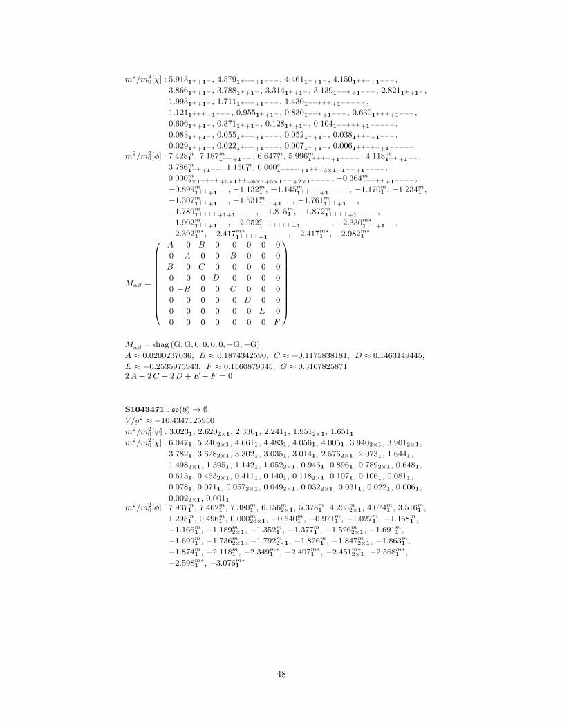
m2/m20[χ] : 5.9131++1− , 4.5791++++1−−− , 4.4611++1− , 4.1501++++1−−− ,

3.8661++1− , 3.7881++1− , 3.3141++1− , 3.1391++++1−−− , 2.8211++1− ,

1.9931++1− , 1.7111++++1−−− , 1.4301++++++1−−−−− ,

1.1211++++1−−− , 0.9551++1− , 0.8301++++1−−− , 0.6301++++1−−− ,

0.6061++1− , 0.3711++1− , 0.1281++1− , 0.1041++++++1−−−−− ,

0.0831++1− , 0.0551++++1−−− , 0.0521++1− , 0.0381++++1−−− ,

0.0291++1− , 0.0221++++1−−− , 0.0071++1− , 0.0061++++++1−−−−−

m2/m20[φ] : 7.428m1 , 7.187m1+++1−− , 6.647m1 , 5.996m1+++++1−−−− , 4.118m1+++1−− ,

3.786m1+++1−− , 1.160m1 , 0.000s1+++++1+++3×1+1−−+1−−−− ,

0.000m2×1+++++5×1+++6×1+5×1−−+2×1−−−− , −0.364m1+++++1−−−− ,

−0.899m1+++1−− , −1.132m1 , −1.145m1+++++1−−−− , −1.170m1 , −1.234m1 ,

−1.307m1+++1−− , −1.531m1+++1−− , −1.761m1+++1−− ,

−1.789m1+++++1+1−−−− , −1.815m1 , −1.872m1+++++1−−−− ,

−1.902m1+++1−− , −2.052c1+++++++1−−−−−− , −2.330m∗1+++1−− ,

−2.392m∗1 , −2.417m∗1+++++1−−−− , −2.417m∗1 , −2.982m∗1

Mαβ =

A 0 B 0 0 0 0 0

0 A 0 0 −B 0 0 0

B 0 C 0 0 0 0 0

0 0 0 D 0 0 0 0

0 −B 0 0 C 0 0 0

0 0 0 0 0 D 0 0

0 0 0 0 0 0 E 0

0 0 0 0 0 0 0 F

Mαβ = diag (G,G, 0, 0, 0, 0,−G,−G)

A ≈ 0.0200237036, B ≈ 0.1874342590, C ≈ −0.1175838181, D ≈ 0.1463149445,

E ≈ −0.2535975943, F ≈ 0.1560879345, G ≈ 0.31678258712A+ 2C + 2D + E + F = 0

S1043471 : so(8)→ ∅V/g2 ≈ −10.4347125950

m2/m20[ψ] : 3.0231, 2.6202×1, 2.3301, 2.2411, 1.9512×1, 1.6511

m2/m20[χ] : 6.0471, 5.2402×1, 4.6611, 4.4831, 4.0561, 4.0051, 3.9402×1, 3.9012×1,

3.7821, 3.6282×1, 3.3021, 3.0351, 3.0141, 2.5762×1, 2.0731, 1.6441,

1.4982×1, 1.3951, 1.1421, 1.0522×1, 0.9461, 0.8961, 0.7892×1, 0.6481,

0.6131, 0.4632×1, 0.4111, 0.1401, 0.1182×1, 0.1071, 0.1061, 0.0811,

0.0781, 0.0711, 0.0572×1, 0.0492×1, 0.0322×1, 0.0311, 0.0221, 0.0061,

0.0022×1, 0.0011

m2/m20[φ] : 7.937m1 , 7.462m1 , 7.380m1 , 6.156m2×1, 5.378m1 , 4.205m2×1, 4.074m1 , 3.516m1 ,

1.295m1 , 0.496m1 , 0.000m28×1, −0.640m1 , −0.971m1 , −1.027m1 , −1.158m1 ,

−1.166m1 , −1.189m2×1, −1.352m1 , −1.377m1 , −1.526m2×1, −1.691m1 ,

−1.699m1 , −1.736m2×1, −1.792m2×1, −1.826m1 , −1.847m2×1, −1.863m1 ,

−1.874m1 , −2.118m1 , −2.349m∗1 , −2.407m∗1 , −2.451m∗2×1, −2.568m∗1 ,

−2.598m∗1 , −3.076m∗1

48

Mαβ =

F 0 0 0 0 A 0 0

0 E 0 B 0 0 0 0

0 0 G 0 0 0 0 C

0 B 0 D 0 0 0 0

0 0 0 0 E 0 B 0

A 0 0 0 0 F 0 0

0 0 0 0 B 0 D 0

0 0 C 0 0 0 0 G

Mαβ = diag (H, I, J,K,−K,−J,−I,−H)

A ≈ 0.1916737277, B ≈ −0.1031587448, C ≈ −0.0007439431,

D ≈ −0.2317730285, E ≈ 0.1171326361, F ≈ −0.0408681192, G ≈ 0.1555085115,

H ≈ 0.3265386604, I ≈ 0.3098791254, J ≈ 0.0149436713, K ≈ 0.0041727212D + E + F +G = 0

S1046017 : so(8)→ ∅V/g2 ≈ −10.4601767468

m2/m20[ψ] : 2.6654×1, 1.9554×1

m2/m20[χ] : 5.3294×1, 3.9104×1, 3.8454×1, 3.7294×1, 2.6514×1, 1.3954×1, 1.0754×1,

0.8064×1, 0.5094×1, 0.1244×1, 0.0924×1, 0.0884×1, 0.0154×1, 0.0104×1

m2/m20[φ] : 8.335m1 , 8.130m1 , 7.322m1 , 5.640m2×1, 4.717m1 , 4.561m2×1, 4.205m1 , 3.192m1 ,

1.510m1 , 0.463m2×1, 0.000s4×1, 0.000c3×1, 0.000m21×1, −0.882m1 , −0.944m1 ,

−1.152m1 , −1.192m2×1, −1.272m2×1, −1.282m1 , −1.461m2×1, −1.533m1 ,

−1.693m1 , −1.714m2×1, −1.765m2×1, −1.771m2×1, −1.824m1 , −1.843m2×1,

−2.135m1 , −2.454m∗1 , −2.531m∗2×1, −2.542m∗2×1, −2.771m∗1 , −3.185m∗1

Mαβ = diag (A,A,B,C,C,D,E,E)

Mαβ =

F 0 0 0 0 0 0 0

0 G 0 0 0 0 0 0

0 0 H 0 I 0 0 0

0 0 0 H 0 I 0 0

0 0 I 0 H 0 0 0

0 0 0 I 0 H 0 0

0 0 0 0 0 0 F 0

0 0 0 0 0 0 0 G

A ≈ 0.1587483894, B ≈ 0.1509917456, C ≈ 0.1432963064, D ≈ −0.2228392936,

E ≈ −0.2661209217, F ≈ −0.0170118689, G ≈ 0.3188399134,

H ≈ −0.1509140222, I ≈ 0.16792589112A+B + 2C +D + 2E = 0, F +H + I = 0, G+H − I = 0

S1067475 : so(8)→ u(1) + u(1)

V/g2 = v ≈ −10.6747541830, 33 v12 − (24 · 21977) v8+

(28 · 3 · 52 · 7 · 101) v4 − (212 · 32 · 11) = 0

8s → 2× 1+ + 1++ + 2× 1 + 1−− + 2× 1−,

8v,c → 1++ + 1+

− + 2× 1+ + 2× 1− + 1−+ + 1−−, 28 →1+++2×1+

+++4×1++2×1+−−+2×1+++6×1+2×1−−+2×1−+++4×1−+2×1−−−+1−−

m2/m20[ψ] : 2.6562×1++2×1− , 2.137

1+++1+

−+1−++1−−

49

m2/m20[χ] : 5.3122×1++2×1− , 4.273

1+++1+

−+1−++1−−, 3.9952×1++2×1− ,

3.6731+++1+

−+1−++1−−, 3.463

1+++1+

−+1−++1−−, 1.3442×1++++2×1−−− ,

1.1951+++ +1++

− +1−−+ +1−−−, 0.8022×1++2×1− , 0.638

1+++1+

−+1−++1−−,

0.1772×1++2×1− , 0.0901+++++1+

−−−+1−++++1−−−−, 0.086

1+++1+

−+1−++1−−,

0.0851+++1+

−+1−++1−−, 0.001

1+++ +1++

− +1−−+ +1−−−

m2/m20[φ] : 9.689m1 , 7.898m1++1− , 7.146m1 , 5.762c1+++1−− , 4.329m1+++1−− ,

3.814c1+++1−− , 2.132c1, 0.987m1++++1+

−−+1−+++1−−−,

0.000s1+++1+++2×1+1−−+1−− , 0.000c1,

0.000m2×1+

+++4×1++2×1+−−+1+++1+1−−+2×1−+++4×1−+2×1−−−

,

−0.040m1++1− , −0.748m1 , −0.780m1 , −1.021m1+++1−− , −1.241m1+++1−− ,

−1.282c1+++1−− , −1.635m1++++1+

−−+1−+++1−−−, −1.696m1++1− ,

−1.924s1+++++1−−−− , −2.086c1+++++1++

−−+1−−+++1−−−−, −2.132m1++1− ,

−2.472m∗1 , −2.638m∗1 , −3.292m∗1+++1−− , −3.367m∗1

Mαβ = diag (A,B,C,C,D,E,A,B)

Mαβ = diag (F,F, 0, 0, 0, 0,−F,−F)

A ≈ 0.1679057457, B ≈ −0.2319756073, C ≈ 0.1299174064, D ≈ 0.1658006759,

E ≈ −0.2974957657, F ≈ 0.32889477392A+ 2B + 2C +D + E = 0

S1068971 : so(8)→ u(1) + u(1)

V/g2 = v ≈ −10.6897177038, 220 v10 − (210 · 13 · 53959) v8+

(13 · 37 · 409 · 769081) v6 − (22 · 32 · 59 · 4089456997) v4−(26 · 34 · 55 · 7 · 11 · 19 · 3709) v2−(24 · 313 · 510) = 0

8c → 1++ + 1++ + 4× 1 + 1−− + 1−−, 8v,s → 2× 1++ + 2× 1+

− + 2× 1−+ + 2× 1−−,

28 → 1++++ + 4× 1++ + 1++

−− + 4× 1++ + 8× 1 + 4× 1−− + 1−−++ + 4× 1−− + 1−−−−m2/m2

0[ψ] : 2.5971+++1+

−+1−++1−−, 2.040

1+++1+

−+1−++1−−

m2/m20[χ] : 5.194

1+++1+

−+1−++1−−, 4.079

1+++1+

−+1−++1−−, 4.026

1+++1+

−+1−++1−−,

3.9091+++1+

−+1−++1−−, 2.485

1+++1+

−+1−++1−−, 1.128

1+++1+

−+1−++1−−,

0.9111++++ +1+++

− +1+++++1+

−−−+1−++++1−−−−+1−−−+ +1−−−−,

0.7871+++1+

−+1−++1−−, 0.108

1+++1+

−+1−++1−−, 0.053

1+++1+

−+1−++1−−,

0.0501+++1+

−+1−++1−−,

0.0451++++ +1+++

− +1+++++1+

−−−+1−++++1−−−−+1−−−+ +1−−−−

m2/m20[φ] : 9.852m1 , 9.527m1 , 7.239m1 , 4.688m1 , 4.120m1+++1+++1−−+1−− ,

2.824m1+++++1++

−−+1−−+++1−−−−, 2.635m1 ,

0.000s1+++++1+++1++

−−+1+++1+1−−+1−−+++1−−+1−−−−,

0.000c2×1+++2×1+++2×1+2×1−−+2×1−− , 0.000m1+++1+++3×1+1−−+1−− ,

−0.410m1 , −1.033m1+++++1++

−−+1−−+++1−−−−, −1.168m1+++1+++1−−+1−− ,

−1.358m2×1, −1.493m1 , −1.604m1+++1+++1−−+1−− , −1.649m1 ,

−1.916m1+++++1++

−−+1−−+++1−−−−, −2.169m1 , −2.184m1+++1+++1−−+1−− ,

−2.725c∗1+++++1+++++1−−−−+1−−−− , −3.109m∗1

Mαβ = diag (A,A,A,A,−A,−A,−A,−A)

50

Mαβ =

B 0 0 0 C D 0 0

0 E 0 0 0 0 0 0

0 0 E 0 0 0 0 0

0 0 0 F 0 0 0 0

C 0 0 0 G H 0 0

D 0 0 0 H I 0 0

0 0 0 0 0 0 E 0

0 0 0 0 0 0 0 F

A ≈ 0.1698981321, B = 1

16log b ≈ −0.2221271162, C ≈ 0.0517654793,

D ≈ −0.1183478207, E = 116

log e ≈ −0.0976740337, F ≈ 0.4174751835,

G ≈ −0.1176605564, H ≈ 0.0456937991, I ≈ −0.2021405935e10 − 69 e9 + 1838 e8 − 7270 e7 + 8289 e6 − 41866 e5 + 8289 e4

−7270 e3 + 1838 e2 − 69 e+ 1 = 0,

b10 + 2 b9 − 1027 b8 − 10504 b7 + 49154 b6 − 189940 b5 + 49154 b4

−10504 b3 − 1027 b2 + 2 b+ 1 = 0, B − F − 2G− 2 I = 0, E + F +G+ I = 0

S1075828 : so(8)→ so(3) + u(1)

V/g2 = v ≈ −10.7582870728, 33 v2 − 55 = 0

8c → 3 + 1++ + 3× 1 + 1−−, 8v,s → 2× 2+ + 2× 2−,

28 → 3++ + 4× 3 + 3−− + 3× 1++ + 4× 1 + 3× 1−−

m2/m20[ψ] : 2.5622++2− , 2.1382++2−

m2/m20[χ] : 5.1242++2− , 4.2762++2− , 3.9882++2− , 3.9832++2− , 2.7872++2− ,

1.1054++4− , 0.8802++2− , 0.6932++++2−−− , 0.1082++2− , 0.1052++2− ,

0.0572++++2−−− , 0.0454++4−

m2/m20[φ] : 10.095m1 , 9.396m1 , 7.146m1 , 5.247s3, 2.990s3+++3−− , 2.946m1 , 0.439m3 ,

0.000c3+2×1+++1+2×1−− , 0.000m3+++2×3+3−−+1+++2×1+1−− ,

−0.800m1+++1−− , −0.990s3+++3−− , −0.996m1 , −1.272m1 , −1.639m3 ,

−1.647s3, −2.000m3+++3−− , −2.400c∗5 , −3.200c∗1+++++1−−−− , −3.314m∗1

Mαβ =

0 0 0 0 0 0 0 A

0 0 0 0 0 0 A 0

0 0 0 0 0 A 0 0

0 0 0 0 −A 0 0 0

0 0 0 −A 0 0 0 0

0 0 A 0 0 0 0 0

0 A 0 0 0 0 0 0

A 0 0 0 0 0 0 0

Mαβ = diag (B,C,D,D,E,E,E,F)

A ≈ −0.1693605251, B ≈ 0.4332764743, C ≈ 0.4074563787, D ≈ −0.0831768605,

E ≈ −0.1031976781, F ≈ −0.3647860976B + C + 2D + 3E + F = 0

S1165685 : so(8)→ u(1) + u(1)

V/g2 = v ≈ −11.6568542495, v2 + (22 · 3) v + 22 = 0

8c → 1++ + 1++ + 4× 1 + 1−− + 1−−, 8v,s → 2× 1++ + 2× 1+

− + 2× 1−+ + 2× 1−−,

28 → 1++++ + 4× 1++ + 1++

−− + 4× 1++ + 8× 1 + 4× 1−− + 1−−++ + 4× 1−− + 1−−−−m2/m2

0[ψ] : 2.5612×1+

++2×1+−+2×1−++2×1−−

51

m2/m20[χ] : 5.121

2×1+++2×1+

−+2×1−++2×1−−, 3.685

2×1+++2×1+

−+2×1−++2×1−−,

3.4642×1+

++2×1+−+2×1−++2×1−−

, 0.8542×1+

++2×1+−+2×1−++2×1−−

,

0.8021++++ +1+++

− +1+++++1+

−−−+1−++++1−−−−+1−−−+ +1−−−−,

0.1182×1+

++2×1+−+2×1−++2×1−−

,

0.0021++++ +1+++

− +1+++++1+

−−−+1−++++1−−−−+1−−−+ +1−−−−

m2/m20[φ] : 8.485s1, 8.485c1, 7.029m1 , 6.364c2×1, 5.652s1+++1+++1−−+1−− , 4.801c1,

3.268s1+++++1++

−−+1−−+++1−−−−, 2.485c1, 0.000s

1+++++1++

−−+2×1+1−−+++1−−−−,

0.000c2×1+++2×1+++2×1+2×1−−+2×1−− ,

0.000m2×1+++2×1+++2×1+2×1−−+2×1−− ,

−0.515m2×1+++2×1+++2×1−−+2×1−− , −0.783s1+++++1++

−−+1−−+++1−−−−,

−1.092m2×1, −1.286c1, −1.409s1+++1+++1−−+1−− ,

−2.121c1+++++1++

−−+1−−+++1−−−−, −2.485s∗1 ,

−3.515c∗1+++++1+++++1−−−−+1−−−− , −3.515m∗1

Mαβ = diag (A,−A,−A,A,−A,A,−A,A)

Mαβ = diag (−2A,−2A, 0, 0, 0, 0, 2A, 2A)

A = − 18

log(

1 +√

2 +√

2 + 2√

2)≈ −0.1910713649

S1176725 : so(8)→ ∅V/g2 = v ≈ −11.7672503174, (212 · 1111) v16−(3 · 23 · 353 · 430873 · 40128577591) v12+

(27 · 38 · 7 · 283 · 7778153 · 590801803) v8−(28 · 315 · 13 · 131 · 1044253583) v4−(213 · 322 · 52 · 1229) = 0

m2/m20[ψ] : 2.8326×1, 2.1552×1

m2/m20[χ] : 5.6636×1, 4.8412×1, 4.3406×1, 4.3102×1, 3.9072×1, 3.0016×1, 0.9602×1,

0.9106×1, 0.8626×1, 0.3262×1, 0.2326×1, 0.1226×1, 0.1092×1, 0.0012×1

m2/m20[φ] : 9.927m2×1, 9.276m3×1, 7.430m1 , 4.279c2×1, 3.788m3×1, 3.003m3×1, 2.353m2×1,

0.000s7×1, 0.000c7×1, 0.000m14×1, −0.512c1, −0.791m3×1, −0.829m2×1,

−1.029m3×1, −1.383m2×1, −1.629m3×1, −1.774m3×1, −2.040m2×1, −2.198m3×1,

−2.353m∗1 , −2.774m∗2×1, −3.364m∗1

Mαβ = diag (A,A,A,B,B,C,C,C)

Mαβ =

D 0 0 0 0 0 0 E

0 −2D 0 0 0 0 0 0

0 0 0 0 0 0 0 0

0 0 0 D E 0 0 0

0 0 0 E −D 0 0 0

0 0 0 0 0 0 0 0

0 0 0 0 0 0 2D 0

E 0 0 0 0 0 0 −D

A ≈ 0.1919781912, B ≈ 0.1644619202, C ≈ −0.3016194713, D ≈ 0.1338549234,

E ≈ −0.23184352823A+ 2B + 3C = 0

S1195898 : so(8)→ so(3)

V/g2 = v ≈ −11.9589830843, (212 · 714) v12−(3 · 73 · 5791 · 238109 · 3799563241) v8+

52

(214 · 317 · 23 · 102701 · 4463153) v4 + (228 · 332) = 0

8v,s,c → 5 + 3, 28 → 2× 7 + 5 + 3× 3

m2/m20[ψ] : 3.0733, 2.5195

m2/m20[χ] : 6.1463, 5.8501, 5.0375, 4.8053, 3.9995, 3.3977, 1.3327, 0.4159, 0.3911,

0.3573, 0.2647, 0.0555

m2/m20[φ] : 9.883m5 , 7.449m1 , 5.591m5 , 0.852m9 , 0.000s7+3, 0.000c7+3, 0.000m5 ,

−0.449m5 , −0.880m5 , −1.981m9 , −2.245m5 , −3.427m∗1

Mαβ =

A 0 0 0 B 0 0 0

0 3A 0 0 0 0 0 0

0 0 −5A 0 0 0 0 0

0 0 0 A 0 0 0 −BB 0 0 0 −3A 0 0 0

0 0 0 0 0 3A 0 0

0 0 0 0 0 0 3A 0

0 0 0 −B 0 0 0 −3A

Mαβ = diag

(− 5

3C,− 5

3C,− 5

3C,C,C,C,C,C

)A ≈ 0.0615899407, B ≈ −0.2133538131, C ≈ −0.1804304168

S1200000 : so(8)→ u(1) + u(1),N = 1

V/g2 = v ≈ −12.0000000000, v + (22 · 3) = 0

8v → 1++ + 1++ + 4× 1 + 1−− + 1−−, 8s,c → 2× 1++ + 2× 1+

− + 2× 1−+ + 2× 1−−,

28 → 1++++ + 4× 1++ + 1++

−− + 4× 1++ + 8× 1 + 4× 1−− + 1−−++ + 4× 1−− + 1−−−−m2/m2

0[ψ] : 4.0001, 3.0002×1, 2.2501+++1+++1−−+1−− , 1.000∗1

m2/m20[χ] : 8.0001, 6.0002×1, 4.7471+++1+++1−−+1−− , 4.5001+++1+++1−−+1−− ,

3.9361+++++1++

−−+1−−+++1−−−−, 3.7321, 2.1661+++1+++1−−+1−− ,

2.0001+++++1++

−−+1+1−−+++1−−−−, 1.5002×1, 1.1251+++1+++1−−+1−− ,

0.5841+++1+++1−−+1−− , 0.5001+++++1++

−−+1−−+++1−−−−, 0.2681,

0.1251+++1+++1−−+1−− , 0.0641+++++1++

−−+1−−+++1−−−−,

0.0031+++1+++1−−+1−− , 0.0004×1

m2/m20[φ] : 8.679m

1+++++1++

−−+1−−+++1−−−−, 8.196m1 , 4.412m1+++1+++1−−+1−− ,

3.067m1+++++1++

−−+1−−+++1−−−−, 2.732m1 , 0.000s

1+++++1++

−−+2×1+1−−+++1−−−−,

0.000c1+++++2×1+++1++

−−+2×1+++2×1+2×1−−+1−−+++2×1−−+1−−−−,

0.000m2×1+++2×1+++2×1+2×1−−+2×1−− , −0.732m1 ,

−1.250m1+++1+++1−−+1−− , −1.517m1+++++1++

−−+1−−+++1−−−−,

−1.912m1+++1+++1−−+1−− , −2.000m4×1, −2.196m1 ,

−2.229m1+++++1++

−−+1−−+++1−−−−, −2.250m1+++1+++1−−+1−−

Mαβ =

0 0 0 0 A 0 0 0

0 0 0 0 0 −A 0 0

0 0 0 0 0 0 A 0

0 0 0 0 0 0 0 −AA 0 0 0 0 0 0 0

0 −A 0 0 0 0 0 0

0 0 A 0 0 0 0 0

0 0 0 −A 0 0 0 0

Mαβ = diag (B,B,C,C,−C,−C,−B,−B)

53

A = 2−7/2 log(5 + 2

√6)≈ 0.2026242474, B ≈ 0.3672439845, C ≈ 0.0380045103

2A−B − C = 0

S1212986 : so(8)→ u(1)

V/g2 ≈ −12.1298657377

8v,s,c → 1++ + 2× 1+ + 2× 1 + 2× 1− + 1−−,

28 → 2× 1+++ + 3× 1++ + 6× 1+ + 6× 1 + 6× 1− + 3× 1−− + 2× 1−−−

m2/m20[ψ] : 3.5361++1− , 2.9211+++1−− , 2.3981++1− , 2.2762×1

m2/m20[χ] : 7.0711++1− , 5.8411+++1−− , 5.3962×1, 5.3381++1− , 4.7961++1− ,

4.5532×1, 4.3401++1− , 4.0691+++1−− , 4.0231++1− , 3.9982×1,

3.8391+++1−− , 2.2501++++1−−− , 1.1411+++1−− , 1.1331++1− ,

1.1251++++1−−− , 1.0612×1, 0.9601++1− , 0.8431+++1−− ,

0.5951++++1−−− , 0.5942×1, 0.4311++1− , 0.3771++1− ,

0.2041+++++1−−−− , 0.1241+++1−− , 0.0512×1, 0.0141++++1−−− ,

0.0061+++1−− , 0.0041++1−

m2/m20[φ] : 12.641m1 , 11.238m1++1− , 8.601m1+++1−− , 7.520m1 , 4.969m1 , 4.648m1++1− ,

4.050m1++1− , 3.994m1 , 3.647m1+++1−− , 3.464m1+++1−− , 0.828m1++++1−−− ,

0.295m1 , 0.000s2×1++2×1+2×1− , 0.000c2×1,

0.000m2×1++++3×1+++4×1++1+4×1−+3×1−−+2×1−−− , −0.873m1+++1−− ,

−0.883m1+++1−− , −1.093m1 , −1.178m1++1− , −1.408m1+++++1−−−− ,

−1.644m1++1− , −1.835m1++++1−−− , −1.921m1+++++1−−−− ,

−1.947m1+++1−− , −1.952m1 , −2.337m∗1++1− , −2.415m∗1 , −2.911m∗1+++1−− ,

−3.375m∗1

Mαβ = diag (A,A,B,B,C,D,D,E)

Mαβ =

F 0 −F 0 0 G 0 G

0 −F 0 F G 0 −G 0

−F 0 F 0 0 G 0 G

0 F 0 −F G 0 −G 0

0 G 0 G 0 0 0 0

G 0 G 0 0 0 0 0

0 −G 0 −G 0 0 0 0

G 0 G 0 0 0 0 0

A ≈ 0.2122724897, B ≈ 0.1711082166, C ≈ 0.1596212853, D ≈ −0.2887351078,

E ≈ −0.3489124823, F ≈ −0.1357468031, G ≈ 0.13636026182A+ 2B + C + 2D + E = 0

S1271622 : so(8)→ so(3)

V/g2 = v ≈ −12.7162248880, 25 v3 + (32 · 5 · 11) v2+

(22 · 33 · 11) v + (25 · 33) = 0

8c → 3 + 5× 1, 8v,s → 4× 2, 28 → 6× 3 + 10× 1

m2/m20[ψ] : 3.5952×2, 2.0132×2

m2/m20[χ] : 7.1902×2, 5.1422×2, 4.6322×2, 4.0262×2, 3.5962×2, 2.7972×2, 1.6772×2,

1.4722×4, 0.3502×2, 0.0642×2, 0.0202×4, 0.0142×2

m2/m20[φ] : 9.374m1 , 8.326m2×1, 8.107m1 , 7.297m3 , 7.248m1 , 6.291m2×3, 2.384m1 , 1.288m3 ,

0.000s3, 0.000c3+6×1, 0.000m3×3+4×1, −1.055m2×3, −1.172m3 , −1.363m2×3,

−1.484m1 , −1.714m1 , −1.865m3 , −1.931m1 , −2.625c∗5 , −3.353m∗1

54

Mαβ =

0 0 0 0 0 A 0 0

0 0 0 A 0 0 0 0

0 0 0 0 0 0 0 A

0 A 0 0 0 0 0 0

0 0 0 0 0 0 A 0

A 0 0 0 0 0 0 0

0 0 0 0 A 0 0 0

0 0 A 0 0 0 0 0

Mαβ = diag (B,C, 0, 0, 0, 0,−C,−B)

A ≈ 0.2088001551, B ≈ 0.4220978340,

C = 14

log c ≈ 0.3721858157, c6 − 3 c5 − 3 c4 − 14 c3 − 3 c2 − 3 c+ 1 = 0

S1301601 : so(8)→ u(1) + u(1)

V/g2 = v ≈ −13.0160180374, 25 v12 − (33 · 33997) v8−(25 · 36 · 11 · 61) v4 − (28 · 313) = 0

8s → 1++ + 1++ + 4× 1 + 1−− + 1−−, 8v,c → 2× 1++ + 2× 1+

− + 2× 1−+ + 2× 1−−,

28 → 1++++ + 4× 1++ + 1++

−− + 4× 1++ + 8× 1 + 4× 1−− + 1−−++ + 4× 1−− + 1−−−−m2/m2

0[ψ] : 3.0062×1+

++2×1+−+2×1−++2×1−−

m2/m20[χ] : 6.011

2×1+++2×1+

−+2×1−++2×1−−, 5.322

2×1+++2×1+

−+2×1−++2×1−−,

4.1272×1+

++2×1+−+2×1−++2×1−−

,

0.8552×1+++

+ +2×1+++− +2×1+

++++2×1+−−−+2×1−++++2×1−−−−+2×1−−−+ +2×1−−−−

,

0.7852×1+

++2×1+−+2×1−++2×1−−

, 0.0962×1+

++2×1+−+2×1−++2×1−−

m2/m20[φ] : 14.519m1 , 12.954m2×1, 11.056m1 , 10.009m1 , 7.459m1 ,

4.469c1+++++1++

−−+1−−+++1−−−−, 3.198c1+++1+++1−−+1−− ,

3.026m1+++++1++

−−+1−−+++1−−−−, 2.913m1+++1+++1−−+1−− ,

0.000s2×1+++2×1+++2×1+2×1−−+2×1−− , 0.000c1+++++1++

−−+1+1−−+++1−−−−,

0.000m2×1+++2×1+++3×1+2×1−−+2×1−− , −0.215c1, −0.515m1 , −0.648m1 ,

−1.083m1+++++1++

−−+1−−+++1−−−−, −1.479m1+++1+++1−−+1−− , −1.717m1 ,

−1.909m1+++1+++1−−+1−− , −2.590s∗1+++++1+++++1−−−−+1−−−− ,

−3.591m∗1 , −3.807m∗1

Mαβ =

A 0 0 0 0 0 0 0

0 B 0 0 C 0 0 0

0 0 D 0 0 0 0 0

0 0 0 D 0 0 0 0

0 C 0 0 B 0 0 0

0 0 0 0 0 A 0 0

0 0 0 0 0 0 D 0

0 0 0 0 0 0 0 D

Mαβ = diag (E,E,E,E,−E,−E,−E,−E)

A 132

log a ≈ −0.3153905442, B 132

log b ≈ −0.0489874112, C ≈ −0.3237262102,

D = 132

log d ≈ 0.1821889777, E ≈ 0.2396913786

1492992 a3 + 608121 a2 + 72458 a− 3 = 0, 884736 b3 − 176389 b2 − 1650 b− 9 = 0,

d3 − 390 d2 + 17541 d− 221184 = 0, A+B + 2D = 0

S1360892 : so(8)→ u(1) + u(1)

55

V/g2 = v ≈ −13.6089263039, 24 v6 − (32 · 5 · 53) v4−(22 · 33 · 977) v2 − (26 · 33 · 132) = 0

8v → 3× 1++ + 1++ + 1−− + 3× 1−−, 8s → 1++++ + 3× 1+

− + 3× 1−+ + 1−−−− ,

8c → 1+++− + 3× 1+

+ + 3× 1−− + 1−−−+ ,

28 → 3× 1++++ + 3× 1++++ + 3× 1++

−− + 10× 1 + 3× 1−−++ + 3× 1−−−− + 3× 1−−−−

m2/m20[ψ] : 4.3701+++1−− , 3.9261+++1−− , 2.1331+++1−− , 1.8261+++1−−

m2/m20[χ] : 8.7411+++1−− , 7.8521+++1−− , 6.1661+++1−− , 6.0391+++1−− ,

5.9671+++1−− , 5.9611+++1−− , 4.2661+++1−− , 3.9691+++1−− ,

3.6521+++1−− , 3.4971+++1−− , 2.9721+++1−− , 2.4901++++++ +1−−−−−−

,

2.2741++++−− +1−−−−++

, 2.1541++++++ +1−−−−−−

, 2.0831+++1−− ,

1.8631+++1−− , 1.8301+++1−− , 1.2281++++−− +1−−−−++

, 0.3001+++1−− ,

0.2791+++1−− , 0.2251+++1−− , 0.1991+++1−− , 0.1251+++1−− ,

0.0621++++++ +1−−−−−−

, 0.0391+++1−− , 0.0351+++1−− ,

0.0191+++++++1−−−−−− , 0.0071++++−− +1−−−−++

m2/m20[φ] : 10.773m

1+++++1−−−−

, 10.282m1+++++1−−−−

, 10.271m1++−−+1−−++

, 9.507m1 ,

9.327m1++−−+1+1−−++

, 7.618m1 , 5.265m1 , 4.137m1++−−+1−−++

,

2.785m1+++++1−−−− , 2.289m1+++++1−−−−

, 1.090m1+++++1−−−−

,

0.000s1+++++1++

−−+2×1+1−−+++1−−−−, 0.000c2×1,

0.000m2×1+++++3×1++

+++2×1++−−+4×1+2×1−−+++3×1−−−−+2×1−−−−

, −0.595m1 ,

−0.609m1 , −0.847m1+++++1−−−− , −0.904m1++−−+1−−++

, −1.251m1++−−+1−−++

,

−1.368m1+++++1−−−−

, −1.402s1++++++++ +1−−−−−−−−

, −1.734m1 ,

−2.091m1+++++1−−−− , −2.132m1 , −2.187m1+++++1−−−−

,

−2.599c∗1++++++−− +1−−−−−−++

, −2.799m∗1 , −3.097m∗1++−−+1−−++

, −3.133m∗1

Mαβ = diag (A,A,B,B,C,C,D,D)

Mαβ =

0 0 0 E 0 F 0 0

0 0 −E 0 −F 0 0 0

0 −E 0 0 0 0 0 0

E 0 0 0 0 0 0 0

0 −F 0 0 0 0 0 0

F 0 0 0 0 0 0 0

0 0 0 0 0 0 0 0

0 0 0 0 0 0 0 0

A ≈ 0.2697328366, B ≈ 0.1492989437, C ≈ −0.1745310997, D ≈ −0.2445006806,

E ≈ 0.2837677652, F ≈ −0.3096941352A+B + C +D = 0

S1362365 : so(8)→ u(1)

V/g2 ≈ −13.6236525917

8v,s,c → 2× 1+ + 4× 1 + 2× 1−, 28 → 1++ + 8× 1+ + 10× 1 + 8× 1− + 1−−

m2/m20[ψ] : 3.4251, 3.3911, 3.3771, 3.0811++1− , 2.3071++1− , 1.4311

m2/m20[χ] : 6.8501, 6.7831, 6.7551, 6.1621++1− , 5.6211, 5.3881, 4.8651++1− ,

4.8621++1− , 4.6141++1− , 4.3671, 4.2711, 4.0461, 3.4031++1− , 2.8621,

2.7561, 2.7541++1− , 2.2841, 2.0041++1− , 1.9371, 1.9011+++1−− ,

1.5531, 1.5051++1− , 1.3501, 1.3461+++1−− , 1.2721, 0.9571++1− ,

0.5401++1− , 0.3051, 0.2421++1− , 0.1721++1− , 0.0881+++1−− , 0.0701,

0.0671++1− , 0.0431++1− , 0.0281+++1−− , 0.0191, 0.0081, 0.0051

56

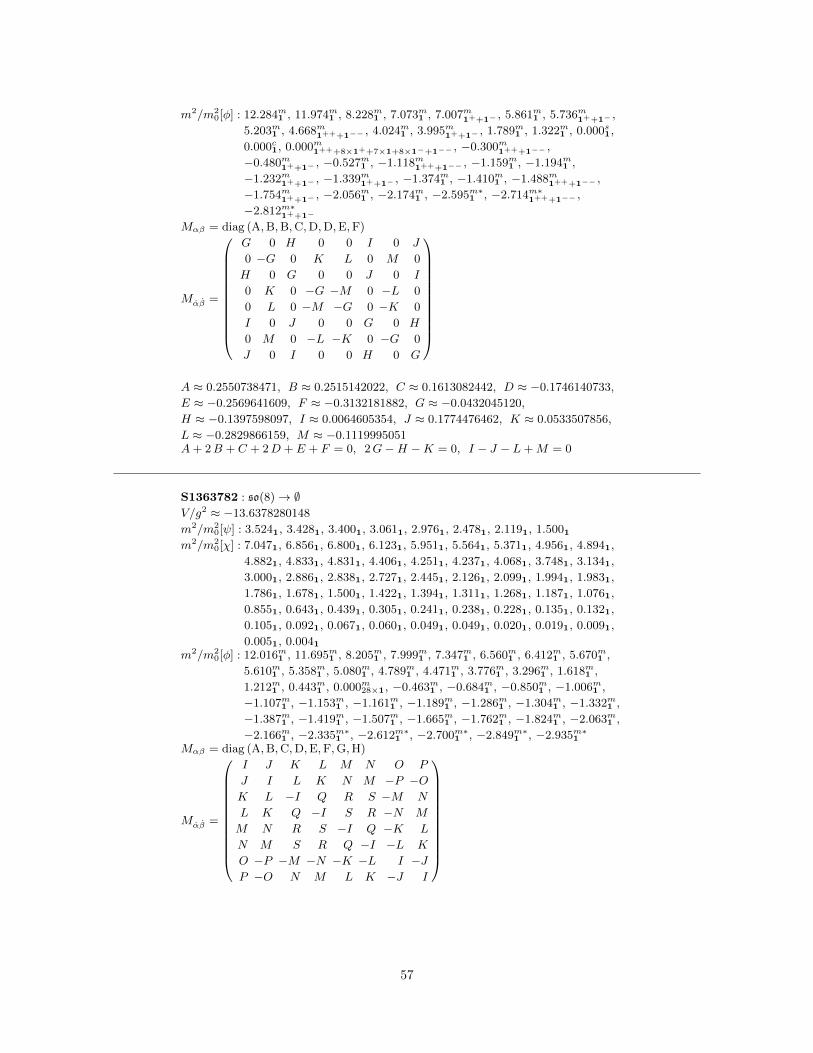
m2/m20[φ] : 12.284m1 , 11.974m1 , 8.228m1 , 7.073m1 , 7.007m1++1− , 5.861m1 , 5.736m1++1− ,

5.203m1 , 4.668m1+++1−− , 4.024m1 , 3.995m1++1− , 1.789m1 , 1.322m1 , 0.000s1,

0.000c1, 0.000m1+++8×1++7×1+8×1−+1−− , −0.300m1+++1−− ,

−0.480m1++1− , −0.527m1 , −1.118m1+++1−− , −1.159m1 , −1.194m1 ,

−1.232m1++1− , −1.339m1++1− , −1.374m1 , −1.410m1 , −1.488m1+++1−− ,

−1.754m1++1− , −2.056m1 , −2.174m1 , −2.595m∗1 , −2.714m∗1+++1−− ,

−2.812m∗1++1−

Mαβ = diag (A,B,B,C,D,D,E,F)

Mαβ =

G 0 H 0 0 I 0 J

0 −G 0 K L 0 M 0

H 0 G 0 0 J 0 I

0 K 0 −G −M 0 −L 0

0 L 0 −M −G 0 −K 0

I 0 J 0 0 G 0 H

0 M 0 −L −K 0 −G 0

J 0 I 0 0 H 0 G

A ≈ 0.2550738471, B ≈ 0.2515142022, C ≈ 0.1613082442, D ≈ −0.1746140733,

E ≈ −0.2569641609, F ≈ −0.3132181882, G ≈ −0.0432045120,

H ≈ −0.1397598097, I ≈ 0.0064605354, J ≈ 0.1774476462, K ≈ 0.0533507856,

L ≈ −0.2829866159, M ≈ −0.1119995051A+ 2B + C + 2D + E + F = 0, 2G−H −K = 0, I − J − L+M = 0

S1363782 : so(8)→ ∅V/g2 ≈ −13.6378280148

m2/m20[ψ] : 3.5241, 3.4281, 3.4001, 3.0611, 2.9761, 2.4781, 2.1191, 1.5001

m2/m20[χ] : 7.0471, 6.8561, 6.8001, 6.1231, 5.9511, 5.5641, 5.3711, 4.9561, 4.8941,

4.8821, 4.8331, 4.8311, 4.4061, 4.2511, 4.2371, 4.0681, 3.7481, 3.1341,

3.0001, 2.8861, 2.8381, 2.7271, 2.4451, 2.1261, 2.0991, 1.9941, 1.9831,

1.7861, 1.6781, 1.5001, 1.4221, 1.3941, 1.3111, 1.2681, 1.1871, 1.0761,

0.8551, 0.6431, 0.4391, 0.3051, 0.2411, 0.2381, 0.2281, 0.1351, 0.1321,

0.1051, 0.0921, 0.0671, 0.0601, 0.0491, 0.0491, 0.0201, 0.0191, 0.0091,

0.0051, 0.0041

m2/m20[φ] : 12.016m1 , 11.695m1 , 8.205m1 , 7.999m1 , 7.347m1 , 6.560m1 , 6.412m1 , 5.670m1 ,

5.610m1 , 5.358m1 , 5.080m1 , 4.789m1 , 4.471m1 , 3.776m1 , 3.296m1 , 1.618m1 ,

1.212m1 , 0.443m1 , 0.000m28×1, −0.463m1 , −0.684m1 , −0.850m1 , −1.006m1 ,

−1.107m1 , −1.153m1 , −1.161m1 , −1.189m1 , −1.286m1 , −1.304m1 , −1.332m1 ,

−1.387m1 , −1.419m1 , −1.507m1 , −1.665m1 , −1.762m1 , −1.824m1 , −2.063m1 ,

−2.166m1 , −2.335m∗1 , −2.612m∗1 , −2.700m∗1 , −2.849m∗1 , −2.935m∗1

Mαβ = diag (A,B,C,D,E,F,G,H)

Mαβ =

I J K L M N O P

J I L K N M −P −OK L −I Q R S −M N

L K Q −I S R −N M

M N R S −I Q −K L

N M S R Q −I −L K

O −P −M −N −K −L I −JP −O N M L K −J I

57

A ≈ 0.2651499941, B ≈ 0.2538119346, C ≈ 0.2323991725, D ≈ 0.1713323966,

E ≈ −0.1511320487, F ≈ −0.2019078999, G ≈ −0.2568361353,

H ≈ −0.3128174138, I ≈ 0.0231160832, J ≈ −0.0332619334, K ≈ −0.0255952778,

L ≈ 0.0959679649, M ≈ 0.1426438834, N ≈ 0.1365120683, O ≈ 0.0436740929,

P ≈ 0.1400602182, Q ≈ −0.0841159158, R ≈ −0.0248832925, S ≈ 0.1451363327A+B + C +D + E + F +G+H = 0

S1366864 : so(8)→ ∅V/g2 ≈ −13.6686490616

m2/m20[ψ] : 3.4572×1, 3.2652×1, 2.7162×1, 1.7742×1

m2/m20[χ] : 6.9132×1, 6.5292×1, 5.4322×1, 5.0802×1, 4.8622×1, 4.7472×1, 4.3922×1,

4.0672×1, 3.5472×1, 3.0572×1, 2.8462×1, 2.3922×1, 1.9712×1, 1.8862×1,

1.5652×1, 1.3542×1, 1.2282×1, 1.1752×1, 0.7412×1, 0.3312×1, 0.2442×1,

0.1972×1, 0.1262×1, 0.0812×1, 0.0722×1, 0.0452×1, 0.0122×1, 0.0012×1

m2/m20[φ] : 11.123m1 , 9.948m2×1, 8.224m1 , 8.216m1 , 6.563m1 , 6.056m1 , 5.830m1 , 5.072m1 ,

5.042m2×1, 4.852m2×1, 3.853m1 , 2.500m1 , 0.851m2×1, 0.649m1 , 0.331m1 ,

0.000c2×1, 0.000m26×1, −0.271m1 , −0.740m1 , −0.963m1 , −1.026m1 ,

−1.121m1 , −1.168m1 , −1.245m2×1, −1.286m2×1, −1.336m1 , −1.443m1 ,

−1.558m2×1, −1.827m1 , −1.887m1 , −2.092m1 , −2.161m1 , −2.309m∗1 ,

−2.686m∗2×1, −3.004m∗1 , −3.009m∗1

Mαβ =

A 0 0 0 0 0 0 B

0 −A 0 C D 0 E 0

0 0 A 0 0 B 0 0

0 C 0 −A −E 0 −D 0

0 D 0 −E −A 0 −C 0

0 0 B 0 0 A 0 0

0 E 0 −D −C 0 −A 0

B 0 0 0 0 0 0 A

Mαβ = diag (F,G,H, I,−I,−H,−G,−F)

A ≈ −0.0176160328, B ≈ 0.2193498190, C ≈ 0.0484193585, D ≈ −0.2459896956,

E ≈ −0.0411175816, F ≈ 0.3916541221, G ≈ 0.3326583756, H ≈ 0.1801069814,

I ≈ 0.0255115572

S1367611 : so(8)→ ∅V/g2 ≈ −13.6761142184

m2/m20[ψ] : 3.6201, 3.3392×1, 3.2201, 2.9741, 2.6121, 1.7972×1

m2/m20[χ] : 7.2391, 6.6782×1, 6.4401, 5.9481, 5.2412×1, 5.2251, 5.1161, 5.0501,

4.7831, 4.6811, 4.4562×1, 4.0612×1, 3.5942×1, 3.0952×1, 2.8981,

2.8501, 2.7801, 2.2021, 2.1891, 2.1062×1, 1.8521, 1.6881, 1.5511,

1.4382×1, 1.2042×1, 1.1421, 1.1291, 0.9271, 0.5821, 0.3102×1, 0.2851,

0.2621, 0.2232×1, 0.1401, 0.0892×1, 0.0841, 0.0811, 0.0581, 0.0352×1,

0.0291, 0.0061, 0.0022×1

m2/m20[φ] : 11.360m1 , 10.188m2×1, 8.531m1 , 8.135m1 , 6.991m1 , 6.109m1 , 5.984m1 ,

5.549m2×1, 5.471m1 , 4.914m2×1, 3.688m1 , 2.339m1 , 1.257m1 , 1.073m2×1,

0.391m1 , 0.000c2×1, 0.000m26×1, −0.102m1 , −0.903m1 , −0.973m1 , −1.071m1 ,

−1.101m1 , −1.216m1 , −1.252m2×1, −1.319m2×1, −1.389m1 , −1.437m1 ,

−1.543m2×1, −1.862m1 , −1.864m1 , −2.068m1 , −2.178m1 , −2.301m∗1 ,

−2.621m∗2×1, −2.998m∗1 , −3.007m∗1

58

Mαβ = diag (A,B,C,C,D,E,E,F)

Mαβ =

G H −G −H I 0 J 0

H −G −H G 0 K 0 L

−G −H G H −J 0 −I 0

−H G H −G 0 L 0 K

I 0 −J 0 M N M −N0 K 0 L N −M N M

J 0 −I 0 M N M −N0 L 0 K −N M −N −M

A ≈ 0.2759551604, B ≈ 0.2563048042, C ≈ 0.1960591984, D ≈ −0.1303508659,

E ≈ −0.2392313079, F ≈ −0.3155648797, G ≈ 0.1056983935,

H ≈ −0.0014558822, I ≈ 0.0015095272, J ≈ 0.1705690591, K ≈ 0.2833665116,

L ≈ 0.1112879254, M ≈ 0.0578560937, N ≈ −0.0007969057A+B + 2C +D + 2E + F = 0

S1379439 : so(8)→ ∅V/g2 ≈ −13.7943987074

m2/m20[ψ] : 4.3681, 3.6262×1, 3.1571, 2.4932×1, 2.3951, 1.5241

m2/m20[χ] : 8.7361, 7.2512×1, 6.3151, 5.3621, 5.3322×1, 5.2721, 5.1311, 4.9852×1,

4.8111, 4.7901, 4.7502×1, 4.4251, 4.0532×1, 3.7251, 3.5961, 3.2342×1,

3.0571, 3.0481, 2.9401, 2.0272×1, 1.7631, 1.6011, 1.4621, 1.3612×1,

1.1741, 1.1372×1, 1.0101, 0.9192×1, 0.8341, 0.4431, 0.3272×1, 0.2751,

0.1651, 0.1001, 0.0841, 0.0792×1, 0.0191, 0.0162×1, 0.0131, 0.0101,

0.0072×1, 0.0061

m2/m20[φ] : 10.687m1 , 10.400m2×1, 10.300m1 , 7.596m1 , 7.256m1 , 6.720m2×1, 6.545m1 ,

5.990m1 , 5.563m2×1, 5.345m1 , 5.111m1 , 3.645m1 , 3.464m2×1, 3.150m1 , 3.037m1 ,

0.000m28×1, −0.297m1 , −0.594m1 , −0.858m1 , −0.865m2×1, −0.906m1 ,

−0.949m1 , −1.132m2×1, −1.178m1 , −1.255m1 , −1.283m1 , −2.133m1 ,

−2.420m∗1 , −2.555m∗1 , −2.687m∗2×1, −2.777m∗1 , −2.852m∗1 , −2.967m∗1 ,

−2.995m∗2×1, −3.045m∗1

Mαβ =

A 0 0 0 0 B 0 C

0 −A 0 D E 0 F 0

0 0 A 0 0 −C 0 B

0 D 0 −A F 0 E 0

0 E 0 F −A 0 D 0

B 0 −C 0 0 A 0 0

0 F 0 E D 0 −A 0

C 0 B 0 0 0 0 A

Mαβ = diag (G,H, I, J,−J,−I,−H,−G)

A ≈ 0.0469049866, B ≈ 0.1988409893, C ≈ 0.0942991254, D ≈ 0.1171146179,

E ≈ 0.1003271047, F ≈ 0.0901572385, G ≈ 0.4446089479, H ≈ 0.4259749432,

I ≈ 0.0274815696, J ≈ 0.0140176426

S1384096 : so(8)→ so(3),N = 1

V/g2 = v ≈ −13.8409638236, 515 v12−(28 · 34 · 7 · 53 · 107 · 887 · 1567) v8+

(215 · 317 · 210719) v4 − (220 · 330) = 0

59

8v,s,c → 2× 3 + 2× 1, 28 → 5 + 7× 3 + 2× 1

m2/m20[ψ] : 3.4113, 3.1801, 2.9063, 1.000∗1

m2/m20[χ] : 7.2301, 7.1561, 6.8233, 6.3591, 5.8123, 5.2873, 5.2043, 3.6891, 2.5353,

2.4783, 1.9275, 1.7063, 1.5901, 1.4533, 1.0145, 0.1645, 0.0905+3,

0.0321, 0.0003

m2/m20[φ] : 16.262m1 , 16.095m1 , 8.657m1 , 8.529m1 , 8.095m1 , 5.322m3 , 5.182m3 , 3.818m5 ,

2.662m1 , 0.000s3, 0.000c3, 0.000m5+4×3+2×1, −0.109m5 , −1.099m5 ,

−1.396m5+3, −1.686m1 , −2.188m1 , −2.244m3 , −2.245m5

Mαβ =

A 0 0 0 0 B 0 0

0 C 0 0 D 0 0 0

0 0 E 0 0 0 0 F

0 0 0 E 0 0 −F 0

0 D 0 0 C 0 0 0

B 0 0 0 0 A 0 0

0 0 0 −F 0 0 E 0

0 0 F 0 0 0 0 E

Mαβ = diag (G,G,G,H,H,H, I, J)

A ≈ −0.1778567542, B ≈ −0.0851652411, C ≈ −0.0053764869,

D ≈ 0.2813012410, E ≈ 0.0916166205, F ≈ 0.1843081336, G ≈ 0.2984524378,

H ≈ 0.0007244824, I ≈ −0.4438492241, J ≈ −0.4536815367A−B −E + F = 0, B −D + 4E = 0, C +D −E − F = 0, 3G+ 3H + I + J = 0

S1384135 : so(8)→ u(1)

V/g2 ≈ −13.8413583020

8v,s,c → 2× 1+ + 4× 1 + 2× 1−, 28 → 1++ + 8× 1+ + 10× 1 + 8× 1− + 1−−

m2/m20[ψ] : 3.4251++1− , 3.3861, 3.1851, 2.9341, 2.8881++1− , 1.0071

m2/m20[χ] : 7.2131, 7.1381, 6.8511++1− , 6.7721, 6.3691, 5.8671, 5.7761++1− ,

5.2981++1− , 5.2391, 5.2071++1− , 5.1761, 3.6921, 2.5381++1− , 2.5361,

2.5321, 2.4671++1− , 2.0161++1− , 2.0131, 1.8671+++1−− , 1.7861,

1.6771++1− , 1.6101, 1.4741, 1.3911++1− , 1.0151++1− , 1.0131+++1−− ,

1.0131, 0.1771, 0.1681++1− , 0.1521+++1−− , 0.1081++1− , 0.1021,

0.1001, 0.0781+++1−− , 0.0751++1− , 0.0301, 0.0021, 0.0011++1−

m2/m20[φ] : 16.209m1 , 16.041m1 , 8.641m1 , 8.509m1 , 8.089m1 , 5.478m1++1− , 5.336m1++1− ,

5.008m1 , 4.916m1 , 4.019m1 , 3.852m1++1− , 3.779m1+++1−− , 2.562m1 , 0.116m1 ,

0.000s1, 0.000c1, 0.000m1+++8×1++7×1+8×1−+1−− , −0.299m1+++1−− ,

−1.085m1+++1−− , −1.111m1++1− , −1.114m1 , −1.281m1++1− , −1.347m1 ,

−1.418m1 , −1.434m1++1− , −1.443m1+++1−− , −1.687m1 , −2.085m1 ,

−2.183m1 , −2.215m1++1− , −2.290m∗1 , −2.299m∗1++1− , −2.306m∗1+++1−−

Mαβ = diag (A,A,B,C,D,D,E,F)

Mαβ =

G H 0 0 I 0 0 0

H J 0 0 K I 0 0

0 0 M 0 0 0 0 L

0 0 0 M 0 0 −L 0

I K 0 0 J H 0 0

0 I 0 0 H G 0 0

0 0 0 −L 0 0 M 0

0 0 L 0 0 0 0 M

60

A ≈ 0.2777293120, B ≈ 0.2718798275, C ≈ −0.0744147376, D ≈ −0.1017683698,

E ≈ −0.2626921799, F ≈ −0.2866947946, G ≈ −0.1665726485,

H ≈ −0.0745972360, I ≈ 0.2914728267, J ≈ −0.1243108661,

K ≈ −0.1651289219, L ≈ −0.1436869006, M ≈ 0.14544175732A+B + C + 2D + E + F = 0, G+ J + 2M = 0

S1400000 : so(8)→ so(3) + so(3)

V/g2 = v ≈ −14.0000000000, v + (2 · 7) = 0

8v → (3,1) + (1,3) + 2× 1, 8s,c → 2× (2,2),

28 → (3,3) + 3× (3,1) + 3× (1,3) + 1m2/m2

0[ψ] : 3.8572×1, 2.143(3,1)+(1,3)

m2/m20[χ] : 7.7142×1, 4.2862×(3,1)+2×(1,3), 2.2442×(3,3), 0.3272×(3,3),

0.000(3,1)+(1,3)

m2/m20[φ] : 8.571m1 , 5.598m(3,3), 2.571c(3,3), 0.000s(3,1)+(1,3), 0.000c(3,1)+(1,3),

0.000m(3,3)+1, −1.312m(3,3), −1.714m2×(3,3)+2×1

Mαβ = diag (A,A,A,A,−A,−A,−A,−A)

Mαβ =

0 0 0 0 0 0 0 −A0 0 0 0 0 −A 0 0

0 0 0 0 0 0 −A 0

0 0 0 0 A 0 0 0

0 0 0 A 0 0 0 0

0 −A 0 0 0 0 0 0

0 0 −A 0 0 0 0 0

−A 0 0 0 0 0 0 0

A = 2−5/2 log

(2 +√

5)≈ 0.2552011085

S1400056 : so(8)→ ∅V/g2 ≈ −14.0005638418

m2/m20[ψ] : 3.9601, 3.6191, 3.4011, 3.3911, 2.8581, 2.7181, 2.6751, 1.3141

m2/m20[χ] : 7.9201, 7.2391, 7.0181, 6.9271, 6.8021, 6.7821, 5.7161, 5.5561, 5.4361,

5.4041, 5.3501, 5.1101, 5.0321, 4.8401, 4.7301, 3.7691, 3.7131, 3.5531,

3.2691, 2.9471, 2.8191, 2.8001, 2.7581, 2.7291, 2.6291, 2.2541, 2.2131,

2.1491, 2.0891, 1.9821, 1.5571, 1.5401, 1.4281, 1.4141, 0.8581, 0.8431,

0.8151, 0.8091, 0.7461, 0.3181, 0.2981, 0.1931, 0.1521, 0.1441, 0.1301,

0.1301, 0.1191, 0.0931, 0.0911, 0.0681, 0.0431, 0.0411, 0.0261, 0.0221,

0.0151, 0.0071

m2/m20[φ] : 14.783m1 , 14.618m1 , 9.280m1 , 9.053m1 , 7.804m1 , 7.790m1 , 7.604m1 , 6.302m1 ,

6.100m1 , 5.980m1 , 5.179m1 , 5.064m1 , 4.764m1 , 4.457m1 , 3.863m1 , 3.642m1 ,

2.039m1 , 1.502m1 , 1.270m1 , 0.546m1 , 0.000m28×1, −0.936m1 , −0.953m1 ,

−0.956m1 , −1.034m1 , −1.046m1 , −1.069m1 , −1.108m1 , −1.171m1 , −1.214m1 ,

−1.658m1 , −1.764m1 , −1.801m1 , −1.943m1 , −2.060m1 , −2.123m1 , −2.147m1 ,

−2.440m∗1 , −2.458m∗1 , −2.467m∗1 , −2.506m∗1 , −2.801m∗1 , −2.870m∗1

61

Mαβ =

A 0 B 0 0 C 0 D

0 E 0 F G 0 H 0

B 0 I 0 0 −D 0 J

0 F 0 L H 0 K 0

0 G 0 H E 0 F 0

C 0 −D 0 0 A 0 −B0 H 0 K F 0 L 0

D 0 J 0 0 −B 0 I

Mαβ = diag (M,N,O,P,Q,R, S,T)

A ≈ −0.1908821818, B ≈ 0.0725951286, C ≈ −0.0530256593, D ≈ 0.0488547269,

E ≈ 0.0181789322, F ≈ −0.0183888904, G ≈ 0.2817201465, H ≈ 0.0550047138,

I ≈ 0.0840728277, J ≈ 0.1323287457, K ≈ −0.1563792750, L ≈ 0.0886304219,

M ≈ 0.3827242899, N ≈ 0.3671045971, O ≈ 0.1584711919, P ≈ 0.0321518206,

Q ≈ −0.0209662732, R ≈ −0.0221617220, S ≈ −0.4423966842,

T ≈ −0.4549272201A+ E + I + L = 0, , M +N +O + P +Q+R+ S + T = 0

S1402217 : so(8)→ u(1)

V/g2 = v ≈ −14.0221724366, 55 v20 − (2 · 54 · 11 · 17 · 673) v16+

(27 · 13 · 223 · 3802759) v12 + (210 · 11 · 13 · 109 · 137 · 809) v8−(213 · 3 · 43 · 131 · 543841) v4 − (221 · 39 · 53 · 83) = 0

8s → 3× 1++ + 2× 1 + 3× 1−−, 8v,c → 1+++ + 3× 1+ + 3× 1− + 1−−−,

28 → 3× 1++++ + 6× 1++ + 10× 1 + 6× 1−− + 3× 1−−−−

m2/m20[ψ] : 4.2871++1− , 3.4781++1− , 2.5541++++1−−− , 1.9391++1−

m2/m20[χ] : 8.5751++1− , 6.9561++1− , 5.8051++++1−−− , 5.6431++++1−−− ,

5.3631++1− , 5.3421++1− , 5.1091++++1−−− , 4.0521++++1−−− ,

3.8781++1− , 3.8261++1− , 3.6021++1− , 3.1331++++1−−− , 3.0161++1− ,

1.7681++++++1−−−−− , 1.7281++++1−−− , 1.7251++1− , 1.6941++1− ,

0.9311++++++1−−−−− , 0.7601++++1−−− , 0.5451++1− , 0.3241++1− ,

0.2721++++1−−− , 0.1411++1− , 0.1051++1− , 0.0201++++1−−− ,

0.0081++++++1−−−−− , 0.0081++1− , 0.0001++++1−−−

m2/m20[φ] : 11.119m1+++1−− , 10.520m1+++1−− , 8.704m1+++++1−−−− , 8.166m1 ,

7.630m1+++++1+1−−−− , 7.433m1 , 4.915m1 , 4.277m1+++1−− ,

3.923m1+++1−− , 3.670m1+++++1−−−− , 2.312m1 , 0.788m1+++1−− ,

0.000s1+++++1+++3×1+1−−+1−−−− , 0.000c2×1,

0.000m2×1+++++5×1+++4×1+5×1−−+2×1−−−− , −0.281m1 , −0.748m1 ,

−0.755m1+++1−− , −0.787m1+++++1−−−− , −0.919m1+++1−− , −1.154m1 ,

−1.187m1+++++1−−−− , −2.294m∗1 , −2.403m∗1+++1−− , −2.767m∗1 ,

−2.804m∗1+++1−− , −3.023m∗1 , −3.035c∗1+++++++1−−−−−− ,

−3.210m∗1+++++1−−−−

Mαβ =

A 0 0 0 0 0 0 0

0 B 0 0 0 0 0 0

0 0 C 0 0 0 0 0

0 0 0 E 0 0 0 D

0 0 0 0 E 0 −D 0

0 0 0 0 0 C 0 0

0 0 0 0 −D 0 F 0

0 0 0 D 0 0 0 F

62

Mαβ = diag (G,G, 0, 0, 0, 0,−G,−G)

A ≈ 0.2107954139, B ≈ −0.0826071995, C ≈ −0.1484636969,

D ≈ −0.2386325809, E ≈ 0.0928203781, F ≈ −0.0084507884, G ≈ 0.4435958698A+B + 2C + 2E + 2F = 0

S1424025 : so(8)→ so(3)

V/g2 ≈ −14.2402599725

8v,s,c → 2× 3 + 2× 1, 28 → 5 + 7× 3 + 2× 1

m2/m20[ψ] : 3.8612×1, 2.3322×3

m2/m20[χ] : 7.7232×1, 4.6642×3, 4.4242×3, 3.9162×1, 3.2622×3, 1.8032×5, 0.9902×1,

0.7022×3, 0.1702×5, 0.0212×3

m2/m20[φ] : 9.856m1 , 8.395m1 , 7.954m3 , 5.443c1, 4.457m5 , 4.020m3 , 2.147m1 , 1.709c5,

0.000s3, 0.000m5+5×3+2×1, −0.386m1 , −0.663m3 , −1.121m5 , −1.251m1 ,

−1.462m3 , −1.740m5 , −1.859m1 , −2.092m1 , −2.865m∗5

Mαβ = diag (A,B,B,B,C,C,C,D)

Mαβ =

0 0 0 0 0 0 0 E

0 0 0 0 0 0 E 0

0 0 0 0 F 0 0 0

0 0 0 0 G −F 0 0

0 0 F G 0 0 0 0

0 0 0 −F 0 0 0 0

0 E 0 0 0 0 0 0

E 0 0 0 0 0 0 0

A ≈ 0.2688248789, B ≈ 0.2480539221, C ≈ −0.2253432180, D ≈ −0.3369569913,

E ≈ 0.2228635886, F ≈ 0.2829151858, G ≈ 0.1362843675A+ 3B + 3C +D = 0

S1441574 : so(8)→ u(1)

V/g2 ≈ −14.4157405138

8s → 1++ + 6× 1 + 1−−, 8v,c → 4× 1+ + 4× 1−, 28 → 6× 1++ + 16× 1 + 6× 1−−

m2/m20[ψ] : 3.9871++1− , 3.7421++1− , 2.8741++1− , 2.3271++1−

m2/m20[χ] : 7.9751++1− , 7.6751++1− , 7.4841++1− , 5.8081++1− , 5.7481++1− ,

5.1251++1− , 4.9111++1− , 4.6551++1− , 4.2871++1− , 3.9871++1− ,

3.6811++1− , 3.5361++1− , 2.9541++++1−−− , 2.9051++1− , 2.8671++1− ,

1.9511++++1−−− , 1.3591++1− , 1.3331++1− , 0.6781++1− , 0.4901++1− ,

0.2041++1− , 0.1891++1− , 0.1801++1− , 0.1621++1− , 0.1111++++1−−− ,

0.1071++++1−−− , 0.0121++1− , 0.0031++1−

m2/m20[φ] : 14.077m1 , 13.724m1 , 12.618m1+++1−− , 10.084m1 , 10.001m1 , 8.425m1 ,

7.540m1+++1−− , 7.482m1 , 7.105m1 , 6.754m1 , 5.282m1 , 4.154m1+++1−− ,

2.801m1+++1−− , 2.726m1 , 1.689m1 , 1.378m1+++1−− , 0.000s3×1,

0.000m6×1+++12×1+6×1−− , −0.222m1 , −0.443m1+++1−− , −0.488m1 ,

−0.841m1 , −0.900m1+++1−− , −1.164m1 , −1.262m1+++1−− ,

−1.344s1+++++1−−−− , −1.494m1+++1−− , −1.924m1 , −1.980m1 ,

−2.152m1+++1−− , −2.353m∗1 , −3.026m∗1 , −3.403m∗1 , −3.683m∗1

63

Mαβ =

A 0 0 0 0 0 0 0

0 A 0 0 0 0 0 0

0 0 B 0 0 0 0 C

0 0 0 D 0 0 E 0

0 0 0 0 F 0 0 0

0 0 0 0 0 G 0 0

0 0 0 E 0 0 H 0

0 0 C 0 0 0 0 I

Mαβ = diag (J, J,K,K,L,L,M,M)

A ≈ 0.1672565908, B ≈ −0.0312347884, C ≈ 0.3092474878, D ≈ −0.2342426738,

E ≈ −0.0304273634, F ≈ 0.2253562631, G ≈ −0.0833739194,

H ≈ −0.2587588032, I ≈ 0.0477407401, J ≈ 0.4452968012, K ≈ 0.0467891851,

L ≈ −0.1002709881, M ≈ −0.39181499832A+B +D + F +G+H + I = 0, J +K + L+M = 0

S1442018 : so(8)→ u(1)

V/g2 ≈ −14.4201873779

8s → 1++ + 6× 1 + 1−−, 8v,c → 4× 1+ + 4× 1−, 28 → 6× 1++ + 16× 1 + 6× 1−−

m2/m20[ψ] : 3.8222×1++2×1− , 2.5962×1++2×1−

m2/m20[χ] : 7.6442×1++2×1− , 6.5022×1++2×1− , 5.1922×1++2×1− , 4.9372×1++2×1− ,

4.0742×1++2×1− , 3.5152×1++2×1− , 3.0672×1++2×1− ,

2.4262×1++++2×1−−− , 1.3182×1++2×1− , 0.5822×1++2×1− ,

0.2072×1++2×1− , 0.1912×1++2×1− , 0.1012×1++++2×1−−− ,

0.0092×1++2×1−

m2/m20[φ] : 12.871m1 , 11.864m1 , 11.058m1 , 10.209m1+++1−− , 10.201m1 , 9.592m1+++1−− ,

9.044m1 , 7.450m1 , 6.756m1 , 6.432m1 , 5.616m1 , 3.573m1+++1−− ,

3.202m1+++1−− , 2.695m1 , 1.825m1 , 1.475m1+++1−− , 0.122m1 , 0.000s3×1,

0.000m6×1+++12×1+6×1−− , −0.431m1+++1−− , −0.478m1 , −0.812m1 ,

−1.053m1+++1−− , −1.158m1 , −1.265m1+++1−− , −1.363s1+++++1−−−− ,

−1.462m1+++1−− , −1.911m1 , −2.011m1 , −2.183m1+++1−− , −2.433m∗1 ,

−3.089m∗1 , −3.464m∗1 , −3.744m∗1

Mαβ =

A 0 0 0 0 0 0 0

0 A 0 0 0 0 0 0

0 0 B C 0 0 D 0

0 0 C E 0 0 F 0

0 0 0 0 G H 0 0

0 0 0 0 H I 0 0

0 0 D F 0 0 J 0

0 0 0 0 0 0 0 K

Mαβ = diag (L,L,M,M,−M,−M,−L,−L)

A ≈ 0.1678343397, B ≈ −0.1280485019, C ≈ 0.1032686475, D ≈ 0.2203461618,

E ≈ −0.1340436080, F ≈ 0.2140430361, G ≈ 0.0607593399, H ≈ 0.1557811701,

I ≈ 0.0791257347, J ≈ 0.0495520689, K ≈ −0.2630137131, L ≈ 0.4211115915,

M ≈ 0.07180678092A+B + E +G+ I + J +K = 0

S1443834 : so(8)→ u(1)

64

V/g2 ≈ −14.4383474481

8c → 3× 1++ + 2× 1 + 3× 1−−, 8v,s → 1+++ + 3× 1+ + 3× 1− + 1−−−,

28 → 3× 1++++ + 6× 1++ + 10× 1 + 6× 1−− + 3× 1−−−−

m2/m20[ψ] : 4.6171++1− , 3.7491++1− , 3.0221++++1−−− , 1.9231++1−

m2/m20[χ] : 9.4421++++1−−− , 9.2341++1− , 7.4981++1− , 6.3091++1− ,

6.0431++++1−−− , 5.7291++1− , 5.0611++++1−−− , 4.9881++1− ,

4.2551++++1−−− , 3.8461++1− , 3.6801++1− , 3.2641++++1−−− ,

3.2431++++++1−−−−− , 2.5181++1− , 2.0041++1− , 1.5991++1− ,

1.5831++++1−−− , 1.1591++++++1−−−−− , 1.0331++++1−−− ,

0.5071++1− , 0.1971++++++1−−−−− , 0.1541++++1−−− , 0.1521++1− ,

0.1061++1− , 0.1001++++1−−− , 0.0401++1− , 0.0381++++1−−− ,

0.0101++1−

m2/m20[φ] : 18.001m1+++1−− , 15.679m1+++++1−−−− , 9.632m1 , 9.451m1 , 8.110m1+++1−− ,

7.723m1 , 5.660m1+++1−− , 5.199m1 , 5.036m1+++++1−−−− ,

4.581m1+++++1−−−− , 3.029m1+++1−− , 2.838m1 , 0.356m1+++1−− , 0.000s2×1,

0.000c3×1, 0.000m3×1+++++6×1+++4×1+6×1−−+3×1−−−− ,

−0.549m1+++++1−−−− , −0.631m1 , −0.911m1+++1−− ,

−1.136m1+++++1−−−− , −1.143m1+++1−− , −1.564s1+++++++1−−−−−− ,

−1.636m1 , −1.688m1+++++1−−−− , −1.841m1+++1−− , −1.877m1 , −2.115m1 ,

−2.655m∗1 , −2.793m∗1+++1−− , −2.894m∗1

Mαβ =

A 0 0 B C 0 0 0

0 A −B 0 0 C 0 0

0 −B D 0 0 E 0 0

B 0 0 D −E 0 0 0

C 0 0 −E F 0 0 0

0 C E 0 0 F 0 0

0 0 0 0 0 0 G 0

0 0 0 0 0 0 0 G

Mαβ = diag (H,H, I, J,K,K,L,L)

A ≈ −0.0660839431, B ≈ 0.1637564671, C ≈ 0.1967459968, D ≈ 0.0356224386,

E ≈ −0.1090091511, F ≈ −0.1658498177, G ≈ 0.1963113221, H ≈ 0.3215895320,

I ≈ 0.2721827887, J ≈ 0.0140927651, K ≈ −0.0064281613, L ≈ −0.4582991476A+D + F +G = 0, 2H + I + J + 2K + 2L = 0

S1464498 : so(8)→ ∅V/g2 = v ≈ −14.6449847504, (24 · 52) v8 − (25 · 5 · 13 · 37) v6−(149 · 12697) v4 − (25 · 32 · 1493) v2 − (26 · 36 · 11) = 0

m2/m20[ψ] : 3.7882×1, 3.1252×1, 2.4402×1, 2.2642×1

m2/m20[χ] : 7.5772×1, 6.2502×1, 4.9282×1, 4.8792×1, 4.7972×1, 4.5282×1, 4.2942×1,

4.2612×1, 4.0912×1, 3.5862×1, 2.9832×1, 2.9732×1, 2.9652×1, 2.3372×1,

1.5452×1, 1.5402×1, 1.1282×1, 1.0662×1, 0.7062×1, 0.5712×1, 0.5562×1,

0.4682×1, 0.2332×1, 0.1202×1, 0.0752×1, 0.0502×1, 0.0372×1, 0.0112×1

m2/m20[φ] : 9.953m1 , 9.518m1 , 8.435m1 , 7.980m1 , 7.646m2×1, 7.518m2×1, 6.547m1 , 5.548c1,

5.168m1 , 4.169m1 , 3.259m2×1, 3.039m1 , 2.677m2×1, 2.510m1 , 2.454m1 , 2.176m1 ,

0.000s2×1, 0.000c4×1, 0.000m22×1, −0.614m1 , −0.844m1 , −0.926m1 ,

−0.946m1 , −1.222m2×1, −1.230m1 , −1.250m2×1, −1.327m1 , −1.419m1 ,

−1.627m2×1, −1.976m2×1, −2.287m∗1 , −2.288m∗1 , −2.382m∗1 , −2.438m∗1 ,

−2.501m∗1 , −2.523m∗1 , −2.544m∗1

65

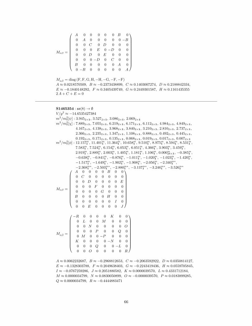
Mαβ =

A 0 0 0 0 0 B 0

0 A 0 0 0 0 0 −B0 0 C 0 D 0 0 0

0 0 0 E 0 −D 0 0

0 0 D 0 E 0 0 0

0 0 0 −D 0 C 0 0

B 0 0 0 0 0 A 0

0 −B 0 0 0 0 0 A

Mαβ = diag (F,F,G,H,−H,−G,−F,−F)

A ≈ 0.0218570509, B ≈ −0.2373438899, C ≈ 0.1403007274, D ≈ 0.2188842334,

E ≈ −0.1840148292, F ≈ 0.3405439749, G ≈ 0.2449301587, H ≈ 0.11614353552A+ C + E = 0

S1465354 : so(8)→ ∅V/g2 ≈ −14.6535427384

m2/m20[ψ] : 3.9452×1, 3.5272×1, 3.0862×1, 2.0692×1

m2/m20[χ] : 7.8892×1, 7.0552×1, 6.2192×1, 6.1712×1, 6.1122×1, 4.9842×1, 4.8492×1,

4.1672×1, 4.1382×1, 3.9682×1, 3.8402×1, 3.2102×1, 2.8102×1, 2.7372×1,

2.3662×1, 2.2352×1, 1.3472×1, 1.1082×1, 0.8882×1, 0.4922×1, 0.4452×1,

0.1922×1, 0.1712×1, 0.1352×1, 0.0682×1, 0.0192×1, 0.0172×1, 0.0072×1

m2/m20[φ] : 12.157m1 , 11.401m1 , 11.364m1 , 10.658m1 , 9.510m1 , 8.975m1 , 8.594m1 , 8.531m1 ,

7.583m1 , 7.524m1 , 6.154m1 , 6.053m1 , 6.051m1 , 4.366m1 , 3.903m1 , 3.459m1 ,

2.919m1 , 2.889m1 , 2.003m1 , 1.405m1 , 1.181m1 , 1.106m1 , 0.000m28×1, −0.385m1 ,

−0.638m1 , −0.841m1 , −0.876m1 , −1.011m1 , −1.020m1 , −1.023m1 , −1.420m1 ,

−1.517m1 , −1.649m1 , −1.902m1 , −1.908m1 , −2.056m1 , −2.340m∗1 ,

−2.368m∗1 , −2.503m∗1 , −2.880m∗1 , −3.137m∗1 , −3.246m∗1 , −3.526m∗1

Mαβ =

A 0 0 0 0 B 0 0

0 C 0 0 0 0 0 0

0 0 D 0 0 0 0 E

0 0 0 F 0 0 0 0

0 0 0 0 G 0 0 0

B 0 0 0 0 H 0 0

0 0 0 0 0 0 I 0

0 0 E 0 0 0 0 J

Mαβ =

−R 0 0 0 0 K 0 0

0 L 0 0 M 0 0 0

0 0 N 0 0 0 0 O

0 0 0 P 0 0 Q 0

0 M 0 0 −P 0 0 0

K 0 0 0 0 −N 0 0

0 0 0 Q 0 0 −L 0

0 0 O 0 0 0 0 R

A ≈ 0.0062232687, B ≈ −0.2968812653, C ≈ −0.2063592922, D ≈ 0.0350814127,

E ≈ −0.1328303788, F ≈ 0.2049638403, G ≈ −0.2243419436, H ≈ 0.0559705845,

I ≈ −0.0767259286, J ≈ 0.2051880582, K ≈ 0.0000039570, L ≈ 0.4331712184,

M ≈ 0.0000034799, N ≈ 0.0830050899, O ≈ −0.0000039570, P ≈ 0.0183899285,

Q ≈ 0.0000034799, R ≈ −0.4444883471

66

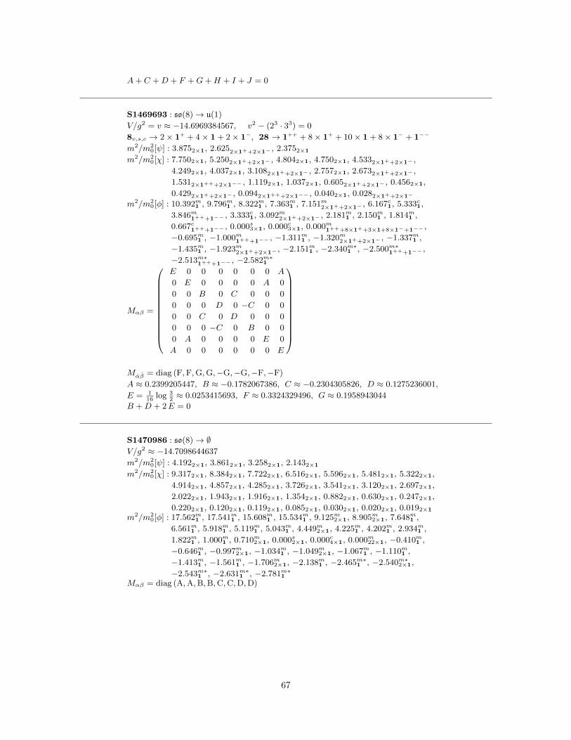
A+ C +D + F +G+H + I + J = 0

S1469693 : so(8)→ u(1)

V/g2 = v ≈ −14.6969384567, v2 − (23 · 33) = 0

8v,s,c → 2× 1+ + 4× 1 + 2× 1−, 28 → 1++ + 8× 1+ + 10× 1 + 8× 1− + 1−−

m2/m20[ψ] : 3.8752×1, 2.6252×1++2×1− , 2.3752×1

m2/m20[χ] : 7.7502×1, 5.2502×1++2×1− , 4.8042×1, 4.7502×1, 4.5332×1++2×1− ,

4.2492×1, 4.0372×1, 3.1082×1++2×1− , 2.7572×1, 2.6732×1++2×1− ,

1.5312×1+++2×1−− , 1.1192×1, 1.0372×1, 0.6052×1++2×1− , 0.4562×1,

0.4292×1++2×1− , 0.0942×1+++2×1−− , 0.0402×1, 0.0282×1++2×1−

m2/m20[φ] : 10.392m1 , 9.796m1 , 8.322m1 , 7.363m1 , 7.151m2×1++2×1− , 6.167c1, 5.333c1,

3.846m1+++1−− , 3.333c1, 3.092m2×1++2×1− , 2.181m1 , 2.150m1 , 1.814m1 ,

0.667c1+++1−− , 0.000s3×1, 0.000c3×1, 0.000m1+++8×1++3×1+8×1−+1−− ,

−0.695m1 , −1.000m1+++1−− , −1.311m1 , −1.320m2×1++2×1− , −1.337m1 ,

−1.435m1 , −1.923m2×1++2×1− , −2.151m1 , −2.340m∗1 , −2.500m∗1+++1−− ,

−2.513m∗1+++1−− , −2.582m∗1

Mαβ =

E 0 0 0 0 0 0 A

0 E 0 0 0 0 A 0

0 0 B 0 C 0 0 0

0 0 0 D 0 −C 0 0

0 0 C 0 D 0 0 0

0 0 0 −C 0 B 0 0

0 A 0 0 0 0 E 0

A 0 0 0 0 0 0 E

Mαβ = diag (F,F,G,G,−G,−G,−F,−F)

A ≈ 0.2399205447, B ≈ −0.1782067386, C ≈ −0.2304305826, D ≈ 0.1275236001,

E = 116

log 32≈ 0.0253415693, F ≈ 0.3324329496, G ≈ 0.1958943044

B +D + 2E = 0

S1470986 : so(8)→ ∅V/g2 ≈ −14.7098644637

m2/m20[ψ] : 4.1922×1, 3.8612×1, 3.2582×1, 2.1432×1

m2/m20[χ] : 9.3172×1, 8.3842×1, 7.7222×1, 6.5162×1, 5.5962×1, 5.4812×1, 5.3222×1,

4.9142×1, 4.8572×1, 4.2852×1, 3.7262×1, 3.5412×1, 3.1202×1, 2.6972×1,

2.0222×1, 1.9432×1, 1.9162×1, 1.3542×1, 0.8822×1, 0.6302×1, 0.2472×1,

0.2202×1, 0.1202×1, 0.1192×1, 0.0852×1, 0.0302×1, 0.0202×1, 0.0192×1

m2/m20[φ] : 17.562m1 , 17.541m1 , 15.608m1 , 15.534m1 , 9.125m2×1, 8.905m2×1, 7.648m1 ,

6.561m1 , 5.918m1 , 5.119m1 , 5.043m1 , 4.449m2×1, 4.225m1 , 4.202m1 , 2.934m1 ,

1.822m1 , 1.000m1 , 0.710m2×1, 0.000s2×1, 0.000c4×1, 0.000m22×1, −0.410m1 ,

−0.646m1 , −0.997m2×1, −1.034m1 , −1.049m2×1, −1.067m1 , −1.110m1 ,

−1.413m1 , −1.561m1 , −1.706m2×1, −2.138m1 , −2.465m∗1 , −2.540m∗2×1,

−2.543m∗1 , −2.631m∗1 , −2.781m∗1

Mαβ = diag (A,A,B,B,C,C,D,D)

67

Mαβ =

E 0 0 0 0 0 0 0

0 F 0 0 0 0 0 0

0 0 G 0 0 0 H 0

0 0 0 I 0 0 0 J

0 0 0 0 E 0 0 0

0 0 0 0 0 F 0 0

0 0 H 0 0 0 G 0

0 0 0 J 0 0 0 I

A ≈ 0.2684289287, B ≈ 0.1907181678, C ≈ −0.1389690318, D ≈ −0.3201780646,

E ≈ 0.0174489198, F ≈ 0.2774132942, G ≈ −0.0444321020, H ≈ −0.4196768832,

I ≈ −0.2504301120, J ≈ 0.2103378488A+B + C +D = 0, E + F +G+ I = 0

S1473607 : so(8)→ ∅V/g2 = v ≈ −14.7360797038, 39 v28 − (24 · 51475093) v24−(28 · 3 · 5 · 1226639507) v20 − (214 · 23 · 59 · 509 · 912103) v16−(224 · 11 · 173 · 62229397) v12 − (226 · 13 · 114415450517) v8+

(238 · 32 · 17 · 23 · 211 · 557) v4 − (256 · 34 · 5 · 13) = 0

m2/m20[ψ] : 3.9532×1, 3.9182×1, 3.2092×1, 2.1682×1

m2/m20[χ] : 8.7662×1, 7.9072×1, 7.8372×1, 6.4172×1, 5.4202×1, 5.4092×1, 5.1392×1,

4.5862×1, 4.4902×1, 4.3372×1, 3.7532×1, 3.6012×1, 3.2822×1, 2.7232×1,

2.4072×1, 2.2562×1, 1.3482×1, 1.2442×1, 0.9292×1, 0.5102×1, 0.2442×1,

0.1912×1, 0.1882×1, 0.1642×1, 0.0682×1, 0.0162×1, 0.0062×1, 0.0052×1

m2/m20[φ] : 16.116m1 , 16.091m1 , 14.856m1 , 14.707m1 , 9.320m1 , 8.827m1 , 7.462m1 ,

7.182m1 , 6.990m1 , 6.661m2×1, 6.572m1 , 6.491m2×1, 4.003m2×1, 2.142m1 ,

1.955m1 , 1.889m1 , 1.565m2×1, 1.282m1 , 0.000s4×1, 0.000c2×1, 0.000m22×1,

−0.206m1 , −0.511m1 , −0.638m1 , −0.768m1 , −0.778m1 , −0.944m1 ,

−0.988m2×1, −1.434m1 , −1.522m2×1, −2.028m1 , −2.081m1 , −2.177m1 ,

−2.257m∗2×1, −2.957m∗2×1, −3.328m∗1 , −3.514m∗1

Mαβ =

A 0 0 0 0 0 0 0

0 B 0 0 0 0 0 0

0 0 C 0 0 0 0 D

0 0 0 E 0 0 F 0

0 0 0 0 A 0 0 0

0 0 0 0 0 B 0 0

0 0 0 F 0 0 E 0

0 0 D 0 0 0 0 C

Mαβ = diag (G,G,H,H, I, I, J, J)

A ≈ −0.0350179646, B ≈ 0.2248119509, C ≈ −0.2147065054,

D ≈ −0.0531175167, E ≈ 0.0249125191, F ≈ 0.3099643056, G ≈ 0.4859198776,

H ≈ 0.0093777193, I ≈ −0.1013012110, J ≈ −0.3939963859A+B + C + E = 0, G+H + I + J = 0

S1474271 : so(8)→ ∅V/g2 ≈ −14.7427134977

m2/m20[ψ] : 4.0001, 3.8882×1, 3.7131, 3.3801, 2.7391, 2.2782×1

68

m2/m20[χ] : 8.0592×1, 8.0001, 7.7762×1, 7.4271, 6.7591, 5.5111, 5.4771, 5.4431,

5.2412×1, 5.0501, 4.9651, 4.5562×1, 4.5341, 4.4231, 4.2161, 4.1461,

3.6682×1, 3.5752×1, 3.4161, 3.2081, 2.8442×1, 2.6481, 2.3802×1,

2.2461, 1.3062×1, 1.3011, 1.1521, 0.9731, 0.7361, 0.5622×1, 0.3361,

0.2812×1, 0.1852×1, 0.1831, 0.1571, 0.1301, 0.0542×1, 0.0331, 0.0111,

0.0052×1, 0.0031, 0.0011

m2/m20[φ] : 14.707m1 , 14.675m1 , 13.558m1 , 13.313m1 , 9.248m1 , 9.164m1 , 7.896m1 ,

7.510m1 , 7.431m1 , 7.162m1 , 6.676m2×1, 5.653m2×1, 4.199m2×1, 2.488m1 ,

2.270m1 , 1.828m1 , 1.667m2×1, 0.916m1 , 0.281m1 , 0.000s2×1, 0.000c2×1,

0.000m24×1, −0.562m1 , −0.669m1 , −0.734m1 , −0.771m1 , −0.980m2×1,

−1.090m1 , −1.526m2×1, −1.659m1 , −1.981m1 , −2.167m1 , −2.275m∗1 ,

−2.337m∗2×1, −3.023m∗2×1, −3.350m∗1 , −3.557m∗1

Mαβ =

G 0 0 0 0 A 0 0

0 B 0 0 −A 0 0 0

0 0 C 0 0 0 0 D

0 0 0 E 0 0 F 0

0 −A 0 0 G 0 0 0

A 0 0 0 0 B 0 0

0 0 0 F 0 0 E 0

0 0 D 0 0 0 0 C

Mαβ = diag (H, I, J, J,K,L,M,M)

A ≈ −0.0356725915, B ≈ 0.2236008836, C ≈ −0.2148902585,

D ≈ −0.0403027676, E ≈ 0.0287525884, F ≈ −0.3064087814,

G ≈ −0.0374632135, H ≈ 0.4169722236, I ≈ 0.3997933008, J ≈ 0.0869223053,

K ≈ −0.0008254174, L ≈ −0.0352547675, M ≈ −0.4772649751B + C + E +G = 0, H + I + 2 J +K + L+ 2M = 0

S1477609 : so(8)→ ∅V/g2 ≈ −14.7760932785

m2/m20[ψ] : 3.8374×1, 2.6524×1

m2/m20[χ] : 7.6734×1, 6.4714×1, 5.3044×1, 4.9344×1, 3.8974×1, 3.8794×1, 3.0754×1,

2.7114×1, 1.2444×1, 0.6724×1, 0.3054×1, 0.2024×1, 0.0284×1, 0.0044×1

m2/m20[φ] : 11.800m1 , 11.655m1 , 10.939m2×1, 10.540m2×1, 10.315m1 , 9.541m1 , 8.411m1 ,

7.363m1 , 5.605m2×1, 5.571m2×1, 4.839m2×1, 2.883m1 , 2.124m1 , 1.915m2×1,

1.757m1 , 0.670m2×1, 0.373m1 , 0.000s4×1, 0.000c3×1, 0.000m21×1, −0.621m1 ,

−0.665m1 , −0.709m1 , −0.960m2×1, −1.208m1 , −1.451m2×1, −2.026m2×1,

−2.157m1 , −2.417m∗1 , −2.464m∗2×1, −3.145m∗2×1, −3.474m∗1 , −3.670m∗1

Mαβ = diag (A,B,B,C,C,D,D,E)

Mαβ =

F 0 0 0 G 0 0 0

0 0 0 0 0 H 0 0

0 0 0 0 0 0 I 0

0 0 0 −F 0 0 0 G

G 0 0 0 F 0 0 0

0 H 0 0 0 0 0 0

0 0 I 0 0 0 0 0

0 0 0 G 0 0 0 −F

69

A ≈ 0.3380833025, B ≈ 0.2272024858, C ≈ −0.0445684005, D ≈ −0.2177569828,

E ≈ −0.2678375076, F ≈ −0.2492391299, G ≈ −0.1997526973,

H ≈ 0.0494864326, I ≈ 0.4489918272A+ 2B + 2C + 2D + E = 0, F −G+H = 0, 2G−H + I = 0

S1497038 : so(8)→ u(1)

V/g2 ≈ −14.9703846700

8v,s,c → 2× 1+ + 4× 1 + 2× 1−, 28 → 1++ + 8× 1+ + 10× 1 + 8× 1− + 1−−

m2/m20[ψ] : 4.0641++1− , 4.0461, 3.9651++1− , 3.6261, 2.2541, 1.5681

m2/m20[χ] : 10.5701, 10.5641, 8.1271++1− , 8.0921, 7.9301++1− , 7.2511,

5.9741++1− , 5.8741++1− , 5.7661, 5.7311, 5.4691, 5.3961, 4.5461++1− ,

4.5071, 4.4581++1− , 3.6611, 3.4221, 3.1361, 2.3741++1− , 2.2991++1− ,

2.0201+++1−− , 2.0171, 1.6021++1− , 1.5941, 1.4681++1− ,

1.2441+++1−− , 0.9831, 0.5781, 0.2061++1− , 0.1371++1− , 0.0821,

0.0721+++1−− , 0.0711++1− , 0.0631++1− , 0.0591+++1−− , 0.0391,

0.0241, 0.0221

m2/m20[φ] : 20.564m1 , 20.534m1 , 17.612m1 , 17.599m1 , 8.683m1 , 8.580m1 , 8.018m1++1− ,

7.746m1++1− , 7.717m1 , 5.533m1 , 4.303m1 , 3.937m1+++1−− , 3.311m1++1− ,

2.892m1++1− , 1.884m1 , 1.063m1 , 0.257m1+++1−− , 0.000s1,

0.000m1+++8×1++8×1+8×1−+1−− , −0.741m1+++1−− , −0.849m1 ,

−0.884m1+++1−− , −0.939m1++1− , −1.006m1 , −1.451m1++1− , −1.795m1 ,

−1.842m1++1− , −1.971m1 , −2.130m1 , −2.430m∗1+++1−− , −2.754m∗1++1− ,

−2.857m∗1

Mαβ =

A 0 B 0 0 C 0 D

0 −A 0 E F 0 G 0

B 0 A 0 0 D 0 C

0 E 0 −A −G 0 −F 0

0 F 0 −G −A 0 −E 0

C 0 D 0 0 A 0 B

0 G 0 −F −E 0 −A 0

D 0 C 0 0 B 0 A

Mαβ = diag (H, I, I, J,K,K,L,M)

A ≈ 0.0432044181, B ≈ 0.0667469537, C ≈ −0.0592944727, D ≈ 0.2268182888,

E ≈ −0.1531557899, F ≈ 0.1421857906, G ≈ 0.0253380255, H ≈ 0.3275164747,

I ≈ 0.2982654585, J ≈ 0.0543793582, K ≈ 0.0076882706, L ≈ −0.4967801751,

M ≈ −0.4970231160H + 2 I + J + 2K + L+M = 0

S1514242 : so(8)→ ∅V/g2 ≈ −15.1424298090

m2/m20[ψ] : 4.2273×1, 3.9883×1, 1.8762×1

m2/m20[χ] : 11.2911, 11.2841, 8.4543×1, 7.9763×1, 5.9423×1, 5.9063×1, 5.3673×1,

5.3393×1, 3.7522×1, 3.5602×1, 2.3853×1, 2.2821, 2.0863×1, 1.7553×1,

1.4741, 1.4123×1, 0.6492×1, 0.1613×1, 0.1301, 0.0893×1, 0.0833×1,

0.0592×1, 0.0553×1, 0.0451

70

m2/m20[φ] : 20.590m2×1, 20.423m2×1, 8.794m3×1, 8.609m3×1, 7.655m1 , 4.958m2×1, 4.421m1 ,

3.694m3×1, 2.065m3×1, 0.991m2×1, 0.849m2×1, 0.000s7×1, 0.000c7×1,

0.000m14×1, −0.867m2×1, −0.892m3×1, −1.361m3×1, −1.812m3×1, −1.937m1 ,

−2.326m∗2×1, −2.743m∗3×1, −2.873m∗1

Mαβ =

A 0 0 0 B 0 0 0

0 F 0 0 0 −B 0 0

0 0 C D 0 0 0 E

0 0 D G 0 0 E −2B

B 0 0 0 F 0 0 0

0 −B 0 0 0 A 0 0

0 0 0 E 0 0 C D

0 0 E −2B 0 0 D G

Mαβ = diag (H,H,H, I, I, I, J, J)

A ≈ 0.2487841341, B ≈ 0.0825928065, C ≈ −0.1379888370, D ≈ −0.0760321465,

E ≈ 0.1946614512, F ≈ −0.0373257404, G ≈ −0.0734695567, H ≈ 0.3083904665,

I ≈ 0.0288923298, J ≈ −0.5059241945A+ C + F +G = 0, 3H + 3 I + 2 J = 0

S1571627 : so(8)→ u(1)

V/g2 = v ≈ −15.7162793558, (27 · 33 · 54) v22−(52 · 11 · 13 · 37 · 11471) v20 + (59 · 2027 · 2063 · 2081) v18−(5 · 7 · 223 · 11902131071) v16 + (23 · 923214452594033) v14−(3 · 73 · 134227 · 1763330467) v12 + (33 · 13 · 1806797 · 4565346281) v10−(22 · 3 · 61 · 283 · 2286301 · 5329931) v8+

(73 · 233 · 4159 · 4673 · 3208463) v6 + (16691 · 322631 · 1644367) v4+

(28 · 327106299439) v2 − (216 · 37 · 54) = 0

8c → 1++ + 6× 1 + 1−−, 8v,s → 4× 1+ + 4× 1−, 28 → 6× 1++ + 16× 1 + 6× 1−−

m2/m20[ψ] : 4.3151++1− , 3.5002×1++2×1− , 1.8731++1−

m2/m20[χ] : 8.6301++1− , 7.0012×1++2×1− , 6.0421++1− , 5.7242×1++2×1− ,

5.3151++1− , 5.0201++1− , 4.4092×1++2×1− , 4.2201++1− , 3.7451++1− ,

3.5841++1− , 1.9632×1++2×1− , 1.5051++1− , 1.4221++++1−−− ,

0.9032×1++2×1− , 0.8371++1− , 0.8312×1++++2×1−−− , 0.4241++1− ,

0.1271++1− , 0.0601++1− , 0.0472×1++2×1− , 0.0131++++1−−−

m2/m20[φ] : 13.735m1 , 12.949m2×1, 12.386m1 , 7.554m1 , 7.131m1 , 7.089s1+++1−− ,

6.235m2×1+++2×1−− , 5.814s1+++1−− , 5.782m1 , 5.550m2×1, 4.859m1 , 4.464s1,

3.759m1+++1−− , 2.202m2×1, 0.452s1+++1−− , 0.000c1+++5×1+1−− ,

0.000m5×1+++10×1+5×1−− , −0.419m1 , −0.727s1+++1−− , −1.062m2×1,

−1.231m1+++1−− , −1.563m1 , −2.474m∗1 , −2.906m∗1 ,

−2.996m∗2×1+++2×1−− , −3.335m∗1 , −3.480m∗1 , −3.498c∗1+++++1−−−−

Mαβ =

A 0 0 0 0 B 0 0

0 −A 0 0 0 0 0 0

0 0 A 0 0 0 0 B

0 0 0 −A 0 0 0 0

0 0 0 0 −A 0 0 0

B 0 0 0 0 A 0 0

0 0 0 0 0 0 −A 0

0 0 B 0 0 0 0 A

71

Mαβ = diag (C,D,E, 0, 0,−E,−D,−C)

A = 116

log a ≈ 0.1104073247, B ≈ −0.2542178232, C ≈ 0.4868747033,

D ≈ 0.4803399628, E ≈ 0.0543732767,

27 a11 − 49 a10 − 581 a9 − 1042 a8 + 3174 a7 + 5554 a6 + 1502 a5

−880 a4 + 351 a3 + 135 a2 + 7 a− 6 = 0

S1586253 : so(8)→ ∅V/g2 ≈ −15.8625354495

m2/m20[ψ] : 4.0042×1, 3.5852×1, 2.8492×1, 2.5742×1

m2/m20[χ] : 8.0092×1, 7.1692×1, 5.6982×1, 5.4342×1, 5.2292×1, 5.1482×1, 5.0382×1,

4.7732×1, 4.6792×1, 4.4842×1, 4.4092×1, 3.4542×1, 3.1292×1, 2.6622×1,

2.5842×1, 2.3282×1, 1.4392×1, 1.3732×1, 1.1672×1, 1.1632×1, 0.5722×1,

0.4062×1, 0.2332×1, 0.2132×1, 0.1422×1, 0.1242×1, 0.0302×1, 0.0192×1

m2/m20[φ] : 10.229m2×1, 10.050m1 , 10.001m1 , 9.553m2×1, 9.280m1 , 7.997m2×1, 7.841m1 ,

7.526m1 , 6.241m1 , 6.007m1 , 5.633m1 , 4.900m2×1, 3.823m1 , 3.767m1 , 2.548m2×1,

0.002m2×1, 0.000s1, 0.000c4×1, 0.000m23×1, −0.060m1 , −0.544m1 , −0.710m1 ,

−0.721m1 , −0.931m2×1, −1.013m1 , −1.027m1 , −1.076m2×1, −1.403m1 ,

−1.403m1 , −1.525m2×1, −1.540m1 , −1.750m1 , −2.513m∗1 , −2.705m∗2×1,

−3.135m∗1

Mαβ = diag (A,A, 2D, 2D,B,B,C,C)

Mαβ =

D E 0 0 0 0 0 0

E −D 0 0 0 0 0 0

0 0 0 0 0 F 0 0

0 0 0 0 G 0 0 0

0 0 0 G 0 0 H 0

0 0 F 0 0 0 0 I

0 0 0 0 H 0 0 0

0 0 0 0 0 I 0 0

A ≈ 0.3078383138, B ≈ −0.2324856722, C ≈ −0.2977659099, D ≈ 0.1112066341,

E ≈ −0.2835547701, F ≈ 0.3796181894, G ≈ 0.1719838393, H ≈ 0.2853355253,

I ≈ 0.0189014847A+B + C + 2D = 0

S1588533 : so(8)→ ∅V/g2 ≈ −15.8853349943

m2/m20[ψ] : 3.9912×1, 3.4392×1, 3.0982×1, 2.5532×1

m2/m20[χ] : 7.9812×1, 6.8772×1, 6.1962×1, 5.5502×1, 5.3782×1, 5.1072×1, 4.7752×1,

4.7642×1, 4.6612×1, 4.5092×1, 4.3402×1, 3.6312×1, 3.1482×1, 2.8722×1,

2.5352×1, 2.4542×1, 1.5642×1, 1.3002×1, 1.2202×1, 1.0542×1, 0.5822×1,

0.3992×1, 0.2852×1, 0.1622×1, 0.1562×1, 0.1222×1, 0.0692×1, 0.0402×1

m2/m20[φ] : 10.360m1 , 10.356m1 , 10.059m1 , 10.010m1 , 9.894m1 , 9.185m1 , 8.827m1 , 8.466m1 ,

8.083m1 , 7.810m1 , 7.762m1 , 6.123m1 , 5.748m1 , 5.650m1 , 5.449m1 , 4.932m1 ,

4.598m1 , 3.199m1 , 2.847m1 , 2.121m1 , 1.528m1 , 0.180m1 , 0.000c4×1, 0.000m24×1,

−0.490m1 , −0.588m1 , −0.672m1 , −0.858m1 , −0.905m1 , −1.003m1 , −1.032m1 ,

−1.036m1 , −1.093m1 , −1.137m1 , −1.361m1 , −1.413m1 , −1.523m1 , −1.706m1 ,

−1.741m1 , −1.787m1 , −2.013m1 , −2.472m∗1 , −2.903m∗1 , −3.189m∗1

72

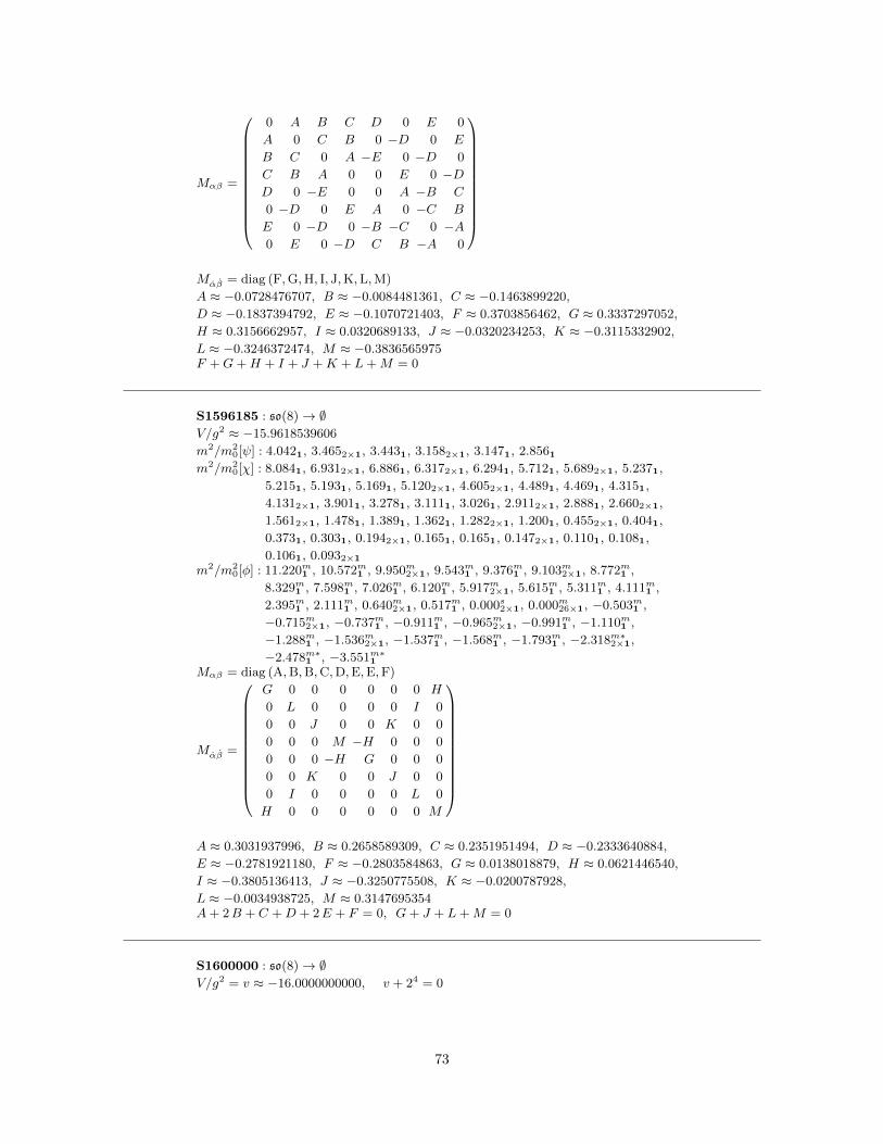
Mαβ =

0 A B C D 0 E 0

A 0 C B 0 −D 0 E

B C 0 A −E 0 −D 0

C B A 0 0 E 0 −DD 0 −E 0 0 A −B C

0 −D 0 E A 0 −C B

E 0 −D 0 −B −C 0 −A0 E 0 −D C B −A 0

Mαβ = diag (F,G,H, I, J,K,L,M)

A ≈ −0.0728476707, B ≈ −0.0084481361, C ≈ −0.1463899220,

D ≈ −0.1837394792, E ≈ −0.1070721403, F ≈ 0.3703856462, G ≈ 0.3337297052,

H ≈ 0.3156662957, I ≈ 0.0320689133, J ≈ −0.0320234253, K ≈ −0.3115332902,

L ≈ −0.3246372474, M ≈ −0.3836565975F +G+H + I + J +K + L+M = 0

S1596185 : so(8)→ ∅V/g2 ≈ −15.9618539606

m2/m20[ψ] : 4.0421, 3.4652×1, 3.4431, 3.1582×1, 3.1471, 2.8561

m2/m20[χ] : 8.0841, 6.9312×1, 6.8861, 6.3172×1, 6.2941, 5.7121, 5.6892×1, 5.2371,

5.2151, 5.1931, 5.1691, 5.1202×1, 4.6052×1, 4.4891, 4.4691, 4.3151,

4.1312×1, 3.9011, 3.2781, 3.1111, 3.0261, 2.9112×1, 2.8881, 2.6602×1,

1.5612×1, 1.4781, 1.3891, 1.3621, 1.2822×1, 1.2001, 0.4552×1, 0.4041,

0.3731, 0.3031, 0.1942×1, 0.1651, 0.1651, 0.1472×1, 0.1101, 0.1081,

0.1061, 0.0932×1

m2/m20[φ] : 11.220m1 , 10.572m1 , 9.950m2×1, 9.543m1 , 9.376m1 , 9.103m2×1, 8.772m1 ,

8.329m1 , 7.598m1 , 7.026m1 , 6.120m1 , 5.917m2×1, 5.615m1 , 5.311m1 , 4.111m1 ,

2.395m1 , 2.111m1 , 0.640m2×1, 0.517m1 , 0.000s2×1, 0.000m26×1, −0.503m1 ,

−0.715m2×1, −0.737m1 , −0.911m1 , −0.965m2×1, −0.991m1 , −1.110m1 ,

−1.288m1 , −1.536m2×1, −1.537m1 , −1.568m1 , −1.793m1 , −2.318m∗2×1,

−2.478m∗1 , −3.551m∗1

Mαβ = diag (A,B,B,C,D,E,E,F)

Mαβ =

G 0 0 0 0 0 0 H

0 L 0 0 0 0 I 0

0 0 J 0 0 K 0 0

0 0 0 M −H 0 0 0

0 0 0 −H G 0 0 0

0 0 K 0 0 J 0 0

0 I 0 0 0 0 L 0

H 0 0 0 0 0 0 M

A ≈ 0.3031937996, B ≈ 0.2658589309, C ≈ 0.2351951494, D ≈ −0.2333640884,

E ≈ −0.2781921180, F ≈ −0.2803584863, G ≈ 0.0138018879, H ≈ 0.0621446540,

I ≈ −0.3805136413, J ≈ −0.3250775508, K ≈ −0.0200787928,

L ≈ −0.0034938725, M ≈ 0.3147695354A+ 2B + C +D + 2E + F = 0, G+ J + L+M = 0

S1600000 : so(8)→ ∅V/g2 = v ≈ −16.0000000000, v + 24 = 0

73

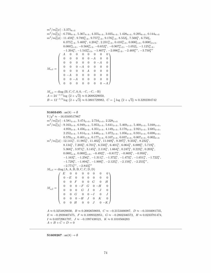
m2/m20[ψ] : 3.3758×1

m2/m20[χ] : 6.7508×1, 5.3678×1, 4.3558×1, 3.0358×1, 1.4288×1, 0.2958×1, 0.1448×1

m2/m20[φ] : 11.459m1 , 9.789m2×1, 9.757m4×1, 9.176m2×1, 8.552c1, 7.500m1 , 6.750c1,

6.375m4×1, 5.469m1 , 4.204m1 , 2.231m2×1, 0.410m4×1, 0.000s3×1, 0.000c12×1,

0.000m13×1, −0.568m2×1, −0.652m1 , −0.907m2×1, −1.052c1, −1.125m2×1,

−1.204m1 , −1.542m4×1, −1.807m1 , −2.096m2×1, −2.469m∗1 , −3.750m∗1

Mαβ =

A 0 0 0 0 0 0 0

0 0 0 0 0 −A 0 0

0 0 0 0 0 0 −A 0

0 0 0 −A 0 0 0 0

0 0 0 0 A 0 0 0

0 −A 0 0 0 0 0 0

0 0 −A 0 0 0 0 0

0 0 0 0 0 0 0 −A

Mαβ = diag (B,C,C, 0, 0,−C,−C,−B)

A = 24−1/2 log(2 +√

3)≈ 0.2688229050,

B = 12−1/2 log(2 +√

3)≈ 0.3801729982, C = 1

4log

(2 +√

3)≈ 0.3292394742

S1603495 : so(8)→ ∅V/g2 ≈ −16.0349517867

m2/m20[ψ] : 4.5812×1, 3.4742×1, 2.7342×1, 2.2282×1

m2/m20[χ] : 9.1632×1, 6.9492×1, 5.9532×1, 5.6412×1, 5.4692×1, 5.4682×1, 5.0482×1,

4.9592×1, 4.4562×1, 4.3512×1, 4.1492×1, 3.1782×1, 2.9212×1, 2.6852×1,

2.2522×1, 1.8142×1, 1.6462×1, 1.0722×1, 1.0562×1, 0.9312×1, 0.6982×1,

0.5702×1, 0.4012×1, 0.1772×1, 0.1072×1, 0.0372×1, 0.0072×1, 0.0022×1

m2/m20[φ] : 12.141m1 , 11.985m1 , 11.402m1 , 11.049m1 , 9.397m1 , 9.333m1 , 8.232m1 ,

8.134m1 , 7.203m1 , 6.701m1 , 6.550m1 , 6.401m1 , 6.064m1 , 6.009m1 , 5.719m1 ,

5.368m1 , 3.971m1 , 3.145m1 , 2.118m1 , 1.664m1 , 0.247m1 , 0.223m1 , 0.203m1 ,

0.000c4×1, 0.000m24×1, −0.492m1 , −0.817m1 , −0.869m1 , −0.950m1 ,

−1.163m1 , −1.256m1 , −1.311m1 , −1.372m1 , −1.473m1 , −1.651m1 , −1.722m1 ,

−1.729m1 , −1.894m1 , −1.909m1 , −2.125m1 , −2.159m1 , −2.253m∗1 ,

−2.771m∗1 , −2.843m∗1

Mαβ = diag (A,A,B,B,C,C,D,D)

Mαβ =

E 0 0 0 0 0 0 0

0 −E 0 0 0 0 0 0

0 0 F 0 0 G 0 H

0 0 0 −F G 0 −H 0

0 0 0 G I 0 J 0

0 0 G 0 0 −I 0 J

0 0 0 −H J 0 K 0

0 0 H 0 0 J 0 −K

A ≈ 0.3254829030, B ≈ 0.2002659693, C ≈ −0.2153406987, D ≈ −0.3104081735,

E ≈ −0.2939407475, F ≈ 0.1099322951, G ≈ −0.2802346572, H ≈ 0.0233781474,

I ≈ 0.0372961797, J ≈ −0.1997438521, K ≈ 0.1010566203A+B + C +D = 0

S1609267 : so(8)→ ∅

74

V/g2 ≈ −16.0926789356

m2/m20[ψ] : 4.1382×1, 3.6042×1, 3.2652×1, 2.1202×1

m2/m20[χ] : 8.2752×1, 7.2092×1, 6.5302×1, 5.6322×1, 5.4122×1, 5.3372×1, 4.9522×1,

4.8792×1, 4.4092×1, 4.2392×1, 4.2042×1, 3.5682×1, 3.0542×1, 2.8742×1,

2.4862×1, 2.0442×1, 1.5342×1, 1.2282×1, 1.0562×1, 1.0222×1, 0.8752×1,

0.4142×1, 0.4032×1, 0.2042×1, 0.1682×1, 0.0762×1, 0.0412×1, 0.0142×1

m2/m20[φ] : 11.867m1 , 11.425m1 , 10.712m1 , 10.182m1 , 10.101m1 , 9.433m1 , 7.949m1 ,

7.478m1 , 7.438m1 , 6.994m1 , 6.915m1 , 6.394m1 , 6.388m1 , 5.858m1 , 4.878m1 ,

4.330m1 , 4.150m1 , 4.083m1 , 4.015m1 , 2.313m1 , 1.410m1 , 0.367m1 , 0.327m1 ,

0.301m1 , 0.000c4×1, 0.000m24×1, −0.419m1 , −0.774m1 , −0.879m1 , −0.940m1 ,

−0.969m1 , −1.035m1 , −1.071m1 , −1.416m1 , −1.664m1 , −1.690m1 , −1.719m1 ,

−1.844m1 , −1.930m1 , −1.951m1 , −2.007m1 , −2.821m∗1 , −3.230m∗1 ,

−3.405m∗1

Mαβ = diag (A,A,B,B,C,C,D,D)

Mαβ =

E F G H 0 0 I J

F −E −H G 0 0 −J I

G −H K 0 0 0 L M

H G 0 −K 0 0 M −L0 0 0 0 N O 0 0

0 0 0 0 O −N 0 0

I −J L M 0 0 P Q

J I M −L 0 0 Q −P

A ≈ 0.3121143003, B ≈ 0.2245291949, C ≈ −0.2322433496, D ≈ −0.3044001455,

E ≈ −0.0459539391, F ≈ −0.0077985222, G ≈ −0.0135745257,

H ≈ −0.1611234224, I ≈ −0.0001155420, J ≈ 0.2960369952,

K ≈ −0.1393769835, L ≈ 0.0514925933, M ≈ 0.0043584525, N ≈ 0.2966839990,

O ≈ 0.0010768247, P ≈ 0.0700300144, Q ≈ 0.0119405514A+B + C +D = 0

S1611549 : so(8)→ u(1)

V/g2 ≈ −16.1154940589

8c → 3× 1++ + 2× 1 + 3× 1−−, 8v,s → 1+++ + 3× 1+ + 3× 1− + 1−−−,

28 → 3× 1++++ + 6× 1++ + 10× 1 + 6× 1−− + 3× 1−−−−

m2/m20[ψ] : 4.1261++1− , 3.7241++1− , 3.1711++++1−−− , 2.1561++1−

m2/m20[χ] : 8.2511++1− , 7.4471++1− , 6.3421++++1−−− , 5.5081++1− , 5.3801++1− ,

5.2971++1− , 5.1381++++1−−− , 5.1331++++1−−− , 4.4081++++1−−− ,

4.3301++1− , 4.3131++1− , 3.3721++1− , 3.0841++1− , 2.8311++++1−−− ,

2.6451++1− , 2.0431++++1−−− , 1.6021++++++1−−−−− ,

1.3201++++++1−−−−− , 1.0251++++1−−− , 0.9851++1− ,

0.7451++++1−−− , 0.4451++1− , 0.3991++1− , 0.2341++++++1−−−−− ,

0.1701++1− , 0.0741++++1−−− , 0.0391++++1−−− , 0.0281++1−

m2/m20[φ] : 11.499m1 , 10.930m1+++1−− , 10.596m1+++1−− , 9.823m1 , 7.956m1 ,

7.509m1+++++1−−−− , 7.184m1 , 6.827m1+++1−− , 6.597m1+++++1−−−− ,

4.616m1+++1−− , 3.845m1 , 3.329m1 , 2.921m1+++1−− , 0.689m1+++1−− ,

0.431m1+++++1−−−− , 0.298m1+++++1−−−− , 0.000s2×1, 0.000c3×1,

0.000m3×1+++++6×1+++4×1+6×1−−+3×1−−−− , −0.855m1+++1−− ,

−0.975m1 , −1.043m1+++1−− , −1.053m1 , −1.628m1+++++1−−−− , −1.652m1 ,

−1.694s1+++++++1−−−−−− , −1.841m1+++++1−−−− , −1.962m1 ,

−2.835m∗1 , −3.465m∗1+++1−−

75

Mαβ =

A 0 0 0 0 0 0 0

0 B C 0 −C 0 0 0

0 C E 0 D 0 0 0

0 0 0 E 0 −D −C 0

0 −C D 0 E 0 0 0

0 0 0 −D 0 E −C 0

0 0 0 −C 0 −C B 0

0 0 0 0 0 0 0 A

Mαβ = diag (F,F,G, 0, 0,−G,−F,−F)

A ≈ −0.2267382900, B ≈ 0.0826151917, C ≈ −0.1720893318, D ≈ 0.2308981599,

E ≈ 0.0720615491, F ≈ 0.3653092284, G ≈ 0.2860767137A+B + 2E = 0

S1624005 : so(8)→ ∅V/g2 ≈ −16.2400530450

m2/m20[ψ] : 3.8822×1, 3.2252×1, 3.2032×1, 3.0102×1

m2/m20[χ] : 7.7642×1, 6.4512×1, 6.4052×1, 6.0192×1, 5.4682×1, 5.4592×1, 5.2232×1,

5.1352×1, 4.4932×1, 4.4012×1, 4.2412×1, 4.1162×1, 3.1292×1, 3.0522×1,

2.9392×1, 2.1752×1, 1.3622×1, 1.3302×1, 1.2962×1, 1.2052×1, 0.7172×1,

0.4212×1, 0.3522×1, 0.3152×1, 0.1372×1, 0.1192×1, 0.0802×1, 0.0712×1

m2/m20[φ] : 12.750m1 , 11.838m1 , 10.682m1 , 10.213m1 , 9.400m1 , 8.439m1 , 8.155m1 , 7.887m1 ,

7.834m1 , 7.707m1 , 7.142m1 , 6.368m1 , 6.187m1 , 5.854m1 , 5.315m1 , 4.889m1 ,

4.652m1 , 3.546m1 , 3.398m1 , 2.266m1 , 2.041m1 , 1.532m1 , 0.871m1 , 0.000m28×1,

−0.020m1 , −0.060m1 , −0.629m1 , −0.718m1 , −0.871m1 , −0.911m1 , −0.979m1 ,

−1.091m1 , −1.321m1 , −1.530m1 , −1.628m1 , −1.655m1 , −1.777m1 , −1.782m1 ,

−2.070m1 , −2.108m1 , −2.477m∗1 , −2.857m∗1 , −3.526m∗1

Mαβ =

J 0 0 0 0 0 0 A

0 B C 0 0 D E 0

0 C F 0 0 G −D 0

0 0 0 I H 0 0 0

0 0 0 H I 0 0 0

0 D G 0 0 F −C 0

0 E −D 0 0 −C B 0

A 0 0 0 0 0 0 J

Mαβ = diag (K,L,M,N,−N,−M,−L,−K)

A ≈ 0.2590103712, B ≈ 0.0017995396, C ≈ −0.2360759194, D ≈ −0.0044988460,

E ≈ 0.0866271237, F ≈ −0.0417626236, G ≈ 0.0979625870, H ≈ 0.3225832822,

I ≈ 0.0011379453, J ≈ 0.0388251388, K ≈ 0.3687609949, L ≈ 0.3268578663,

M ≈ 0.3122761600, N ≈ 0.1042794961B + F + I + J = 0

S1624009 : so(8)→ ∅V/g2 ≈ −16.2400981523

m2/m20[ψ] : 3.8742×1, 3.2292×1, 3.1054×1

m2/m20[χ] : 7.7472×1, 6.4582×1, 6.2104×1, 5.3462×1, 5.2982×1, 5.2814×1, 4.4474×1,

4.1922×1, 4.1882×1, 3.0572×1, 3.0374×1, 2.1742×1, 1.3434×1, 1.2632×1,

1.2362×1, 0.7172×1, 0.4202×1, 0.3344×1, 0.1342×1, 0.1222×1, 0.0774×1

76

m2/m20[φ] : 12.614m1 , 11.227m2×1, 10.233m1 , 9.486m1 , 8.381m1 , 7.976m2×1, 7.887m1 ,

7.740c1, 7.143m1 , 6.192c1, 6.121m2×1, 5.082m2×1, 4.572m1 , 3.537m1 , 3.382m1 ,

2.157m2×1, 1.497m1 , 0.950m1 , 0.010m1 , 0.000s2×1, 0.000c2×1, 0.000m24×1,

−0.058c1, −0.628m1 , −0.815m2×1, −0.871m1 , −0.974m1 , −1.090m1 ,

−1.317m1 , −1.531m1 , −1.644m2×1, −1.777m2×1, −2.079m1 , −2.108m1 ,

−2.474m∗1 , −2.858m∗1 , −3.537m∗1

Mαβ = diag (A,B,C,C,D,E,E,F)

Mαβ =

G 0 G 0 H I H J

0 −G 0 −G K −H L H

G 0 G 0 −H J −H I

0 −G 0 −G −L H −K −HH K −H −L G 0 −G 0

I −H J H 0 −G 0 −GH L −H −K −G 0 G 0

J H I −H 0 −G 0 −G

A ≈ 0.3235643450, B ≈ 0.2980199770, C ≈ 0.2346256560, D ≈ −0.2201457023,

E ≈ −0.2747972526, F ≈ −0.3210954265, G ≈ 0.1489176602, H ≈ 0.1182228253,

I ≈ 0.1252130716, J ≈ −0.0090121054, K ≈ −0.1230553464, L ≈ −0.0068543803A+B + 2C +D + 2E + F = 0, I + J +K − L = 0

S1627388 : so(8)→ ∅V/g2 ≈ −16.2738801391

m2/m20[ψ] : 4.3662×1, 3.5552×1, 3.2012×1, 2.2432×1

m2/m20[χ] : 8.7332×1, 7.1102×1, 6.4022×1, 6.0522×1, 5.8452×1, 5.4552×1, 5.0932×1,

4.9032×1, 4.4862×1, 4.4692×1, 4.2952×1, 4.0482×1, 3.2232×1, 2.3992×1,

2.3512×1, 2.0462×1, 1.5992×1, 1.2042×1, 1.1462×1, 0.9902×1, 0.8292×1,

0.7042×1, 0.4502×1, 0.1752×1, 0.1302×1, 0.1052×1, 0.0232×1, 0.0202×1

m2/m20[φ] : 13.293m1 , 12.909m1 , 11.276m1 , 11.134m1 , 9.110m1 , 8.637m1 , 8.503m1 ,

8.156m1 , 7.921m1 , 7.027m1 , 6.375m1 , 6.322m1 , 6.281m1 , 6.048m1 , 5.715m1 ,

5.113m1 , 5.008m1 , 4.311m1 , 4.283m1 , 2.408m1 , 1.114m1 , 0.615m1 , 0.129m1 ,

0.089m1 , 0.000m28×1, −0.113m1 , −0.524m1 , −0.724m1 , −0.789m1 , −1.076m1 ,

−1.141m1 , −1.355m1 , −1.442m1 , −1.520m1 , −1.658m1 , −1.850m1 , −1.923m1 ,

−2.006m1 , −2.145m1 , −2.599m∗1 , −2.709m∗1 , −2.967m∗1 , −3.015m∗1

Mαβ =

A B 0 0 0 0 C D

B E 0 0 0 0 F C

0 0 G 0 0 H 0 0

0 0 0 I J 0 0 0

0 0 0 J I 0 0 0

0 0 H 0 0 G 0 0

C F 0 0 0 0 E B

D C 0 0 0 0 B A

Mαβ = diag (K,L,M,N,−N,−M,−L,−K)

A ≈ 0.0051702660, B ≈ −0.0874065934, C ≈ −0.1170838477, D ≈ 0.2538109663,

E ≈ −0.2238974361, F ≈ 0.0512610909, G ≈ 0.2057811652, H ≈ −0.0027570340,

I ≈ 0.0129460049, J ≈ 0.3076512588, K ≈ 0.3603659346, L ≈ 0.3330033219,

M ≈ 0.3283238879, N ≈ 0.0909964155A+ E +G+ I = 0

77

S1637792 : so(8)→ ∅V/g2 ≈ −16.3779265774

m2/m20[ψ] : 4.0272×1, 3.7332×1, 3.5712×1, 2.2452×1

m2/m20[χ] : 8.0542×1, 7.4652×1, 7.1412×1, 6.1612×1, 5.9602×1, 5.6142×1, 5.1312×1,

4.9972×1, 4.4902×1, 4.3802×1, 4.2522×1, 4.0612×1, 4.0052×1, 2.3332×1,

2.1992×1, 2.1172×1, 1.5192×1, 1.3352×1, 1.1972×1, 1.1702×1, 0.8732×1,

0.7692×1, 0.4492×1, 0.1562×1, 0.1452×1, 0.0902×1, 0.0702×1, 0.0452×1

m2/m20[φ] : 13.888m1 , 13.299m1 , 11.810m1 , 11.436m1 , 9.164m1 , 8.339m1 , 8.139m1 , 7.809m1 ,

7.487c1, 7.374m1 , 7.120m1 , 6.810m1 , 6.242c1, 6.094m1 , 5.850m1 , 5.826m1 ,

5.449m1 , 5.133m1 , 4.325m1 , 2.628m1 , 0.806m1 , 0.798m1 , 0.756m1 , 0.211m1 ,

0.163m1 , 0.000s1, 0.000m27×1, −0.026m1 , −0.373c1, −0.636m1 , −0.744m1 ,

−1.063m1 , −1.481m1 , −1.530m1 , −1.533m1 , −1.538m1 , −1.700m1 , −1.990m1 ,

−2.059m1 , −2.098m1 , −2.968m∗1 , −2.984m∗1 , −3.010m∗1 , −3.113m∗1

Mαβ =

A 0 0 0 0 0 0 B

0 C 0 0 0 0 D 0

0 0 E 0 0 F 0 0

0 0 0 H G 0 0 0

0 0 0 G H 0 0 0

0 0 F 0 0 E 0 0

0 D 0 0 0 0 C 0

B 0 0 0 0 0 0 A

Mαβ = diag (I, J,K,L,−L,−K,−J,−I)

A ≈ 0.0265288058, B ≈ 0.3012619473, C ≈ 0.2091287823, D ≈ 0.0000493371,

E ≈ −0.2595106171, F ≈ 0.0127642215, G ≈ 0.3119218998, H ≈ 0.0238530290,

I ≈ 0.3583577489, J ≈ 0.3420853045, K ≈ 0.3230697648, L ≈ 0.1090176463A+ C + E +H = 0

S1637802 : so(8)→ ∅V/g2 ≈ −16.3780275534

m2/m20[ψ] : 4.0232×1, 3.6484×1, 2.2462×1

m2/m20[χ] : 8.0472×1, 7.2964×1, 6.0942×1, 5.7604×1, 5.1732×1, 4.9832×1, 4.4932×1,

4.3324×1, 4.0612×1, 4.0062×1, 2.3412×1, 2.1564×1, 1.5142×1, 1.2654×1,

1.1612×1, 0.8214×1, 0.4522×1, 0.1504×1, 0.0892×1, 0.0722×1, 0.0482×1

m2/m20[φ] : 13.626m1 , 12.528m2×1, 11.650m1 , 9.176m1 , 8.228m2×1, 7.805m1 , 7.381c1,

7.343s1, 7.139m1 , 6.433m2×1, 6.329c1, 5.623m1 , 5.582m1 , 5.476m2×1, 4.321m1 ,

2.613m1 , 0.785m2×1, 0.487m2×1, 0.208m1 , 0.014m1 , 0.000s2×1, 0.000c4×1,

0.000m22×1, −0.377c1, −0.633m1 , −0.717m1 , −1.062s1, −1.491m1 , −1.523m1 ,

−1.536m2×1, −1.692m1 , −2.028m2×1, −2.091m1 , −2.991m∗1 , −2.996m∗1 ,

−3.015m∗1 , −3.113m∗1

Mαβ =

A 0 0 0 0 0 0 B

0 C D 0 0 0 0 0

0 D E 0 0 0 0 0

0 0 0 A B 0 0 0

0 0 0 B A 0 0 0

0 0 0 0 0 E D 0

0 0 0 0 0 D C 0

B 0 0 0 0 0 0 A

78

Mαβ = diag (F,G,G,H,−H,−G,−G,−F)

A ≈ 0.0253717974, B ≈ −0.3065580632, C ≈ 0.2092780182, D ≈ 0.0001259073,

E ≈ −0.2600216130, F ≈ 0.3577312944, G ≈ 0.3329948273, H ≈ 0.10909254292A+ C + E = 0

S1641445 : so(8)→ ∅V/g2 ≈ −16.4144563120

m2/m20[ψ] : 4.2591, 4.0831, 4.0201, 3.7291, 3.0771, 3.0421, 2.5881, 2.2891

m2/m20[χ] : 8.5171, 8.1661, 8.0401, 7.4581, 7.4411, 7.3841, 6.1541, 6.0851, 5.9131,

5.7561, 5.3311, 5.2521, 5.1761, 5.0861, 4.9861, 4.8601, 4.8531, 4.5791,

4.4091, 4.3251, 4.1601, 4.0771, 3.6411, 3.2621, 3.1671, 3.1341, 3.0801,

2.8811, 2.7951, 2.7021, 2.2341, 2.1831, 1.9901, 1.8011, 1.6371, 1.2421,

1.0951, 0.8721, 0.8621, 0.8001, 0.6421, 0.6051, 0.5411, 0.5051, 0.4511,

0.3891, 0.3041, 0.2291, 0.2101, 0.2061, 0.1111, 0.0821, 0.0631, 0.0251,

0.0201, 0.0171

m2/m20[φ] : 15.076m1 , 14.959m1 , 11.208m1 , 10.891m1 , 9.762m1 , 9.267m1 , 8.905m1 ,

8.175m1 , 7.985m1 , 7.945m1 , 7.920m1 , 7.583m1 , 6.310m1 , 5.970m1 , 4.454m1 ,

4.174m1 , 2.916m1 , 2.470m1 , 2.446m1 , 2.335m1 , 1.991m1 , 1.439m1 , 0.653m1 ,

0.338m1 , 0.000m28×1, −0.430m1 , −0.793m1 , −0.846m1 , −0.907m1 , −1.119m1 ,

−1.245m1 , −1.267m1 , −1.345m1 , −1.548m1 , −1.550m1 , −1.568m1 , −1.593m1 ,

−1.772m1 , −1.790m1 , −1.807m1 , −2.667m∗1 , −2.730m∗1 , −2.975m∗1

Mαβ =

A 0 B 0 C 0 D 0

0 L 0 E 0 F 0 G

B 0 J 0 H 0 −C 0

0 E 0 K 0 I 0 F

C 0 H 0 J 0 −B 0

0 F 0 I 0 K 0 E

D 0 −C 0 −B 0 A 0

0 G 0 F 0 E 0 L

Mαβ = diag (M,N,O,P,Q,R,S,T)

A ≈ −0.0297469176, B ≈ 0.1086250558, C ≈ 0.1177549358, D ≈ −0.2047871891,

E ≈ −0.0332548588, F ≈ −0.0562438328, G ≈ 0.0089400903, H ≈ 0.1268329526,

I ≈ −0.3219195520, J ≈ −0.1922132517, K ≈ 0.0146983063, L ≈ 0.2072618630,

M ≈ 0.3170185911, N ≈ 0.3034620383, O ≈ 0.2381152676, P ≈ 0.2374315788,

Q ≈ −0.0025365860, R ≈ −0.2942748508, S ≈ −0.3901646447,

T ≈ −0.4090513943A+ L+ J +K = 0, M +N +O + P +Q+R+ S + T = 0

S1650530 : so(8)→ ∅V/g2 ≈ −16.5053058856

m2/m20[ψ] : 4.0322×1, 3.6732×1, 3.2662×1, 2.5032×1

m2/m20[χ] : 8.0642×1, 7.3472×1, 6.5312×1, 6.2602×1, 6.0772×1, 5.2592×1, 5.0062×1,

4.9932×1, 4.3352×1, 4.2252×1, 3.9642×1, 3.8872×1, 3.5952×1, 2.9402×1,

2.7182×1, 2.5982×1, 1.8702×1, 1.5772×1, 0.8352×1, 0.7572×1, 0.6742×1,

0.5362×1, 0.4532×1, 0.2782×1, 0.2402×1, 0.1302×1, 0.0682×1, 0.0472×1

79

m2/m20[φ] : 12.461m1 , 11.670m1 , 11.347m1 , 10.839m1 , 9.461m1 , 9.198m1 , 8.936m1 , 8.768m1 ,

8.743m1 , 8.620m1 , 7.994m1 , 7.841m1 , 7.185m1 , 6.874m1 , 3.853m1 , 3.000m1 ,

2.602m1 , 2.531m1 , 2.437m1 , 2.012m1 , 1.715m1 , 1.384m1 , 1.183m1 , 0.891m1 ,

0.520m1 , 0.000c4×1, 0.000m24×1, −0.326m1 , −0.544m1 , −0.752m1 , −0.985m1 ,

−1.204m1 , −1.223m1 , −1.304m1 , −1.407m1 , −1.501m1 , −1.654m1 , −1.676m1 ,

−1.684m1 , −1.730m1 , −2.068m1 , −2.686m∗1 , −3.026m∗1 , −3.029m∗1

Mαβ = diag (A,A,B,B,C,C,D,D)

Mαβ =

E 0 0 F 0 0 0 G

0 H I 0 0 0 J 0

0 I K 0 0 0 L 0

F 0 0 M 0 0 0 N

0 0 0 0 O 0 0 0

0 0 0 0 0 P 0 0

0 J L 0 0 0 Q 0

G 0 0 N 0 0 0 R

A ≈ 0.3285527682, B ≈ 0.2190110635, C ≈ −0.2518188756, D ≈ −0.2957449561,

E ≈ −0.0259330496, F ≈ −0.2132340531, G ≈ −0.1738652789,

H ≈ −0.0295783527, I ≈ −0.1054042256, J ≈ 0.3232962108, K ≈ 0.2446746021,

L ≈ 0.1138919441, M ≈ −0.1845115637, N ≈ 0.0008449900, O ≈ −0.3459551780,

P ≈ 0.2668714148, Q ≈ −0.0534051357, R ≈ 0.1278372628A+B + C +D = 0, E +H +K +M +O + P +Q+R = 0

S1650772 : so(8)→ ∅V/g2 ≈ −16.5077220330

m2/m20[ψ] : 4.1341, 3.8971, 3.7751, 3.7551, 3.4971, 3.3431, 2.5371, 2.4231

m2/m20[χ] : 8.2671, 7.7931, 7.5501, 7.5111, 7.2161, 7.1551, 6.9941, 6.6861, 5.9031,

5.6451, 5.4121, 5.3761, 5.1541, 5.0731, 4.9441, 4.9281, 4.8451, 4.5541,

4.2631, 4.1491, 4.1271, 4.0781, 3.9651, 3.9011, 3.7171, 3.3591, 2.9101,

2.8631, 2.8321, 2.7731, 2.5321, 2.3531, 2.1631, 1.9291, 1.9281, 1.3331,

0.9991, 0.9201, 0.6961, 0.6671, 0.6491, 0.6441, 0.5831, 0.5791, 0.5101,

0.4081, 0.2641, 0.1921, 0.1851, 0.1751, 0.1741, 0.1261, 0.1101, 0.0811,

0.0501, 0.0441

m2/m20[φ] : 14.343m1 , 14.072m1 , 10.561m1 , 10.124m1 , 9.883m1 , 9.450m1 , 9.450m1 ,

9.132m1 , 8.874m1 , 8.333m1 , 8.101m1 , 7.824m1 , 7.770m1 , 6.753m1 , 4.060m1 ,

3.748m1 , 2.901m1 , 2.539m1 , 2.352m1 , 2.066m1 , 2.051m1 , 1.255m1 , 0.884m1 ,

0.758m1 , 0.634m1 , 0.000m28×1, −0.182m1 , −0.654m1 , −0.698m1 , −0.967m1 ,

−1.187m1 , −1.312m1 , −1.368m1 , −1.548m1 , −1.590m1 , −1.591m1 , −1.604m1 ,

−1.626m1 , −1.827m1 , −2.074m1 , −2.772m∗1 , −2.933m∗1 , −2.950m∗1

Mαβ = diag (A,B,C,D,E,F,G,H)

Mαβ =

I 0 0 J 0 K L 0

0 −I M 0 N 0 0 O

0 M −I 0 O 0 0 N

J 0 0 I 0 −L −K 0

0 N O 0 −I 0 0 M

K 0 0 −L 0 I −J 0

L 0 0 −K 0 −J I 0

0 O N 0 M 0 0 −I

80

A ≈ 0.3451824438, B ≈ 0.3056928611, C ≈ 0.2277969052, D ≈ 0.2074602722,

E ≈ −0.2136834359, F ≈ −0.2696873080, G ≈ −0.2981540269,

H ≈ −0.3046077115, I ≈ −0.1030924656, J ≈ 0.2455554442, K ≈ 0.0555090242,

L ≈ −0.0924642669, M ≈ 0.1740586855, N ≈ 0.1497422628, O ≈ −0.1880447515A+B + C +D + E + F +G+H = 0

S1652031 : so(8)→ ∅V/g2 ≈ −16.5203155076

m2/m20[ψ] : 3.8821, 3.8241, 3.7081, 3.6181, 3.5641, 3.5241, 2.5221, 2.5001

m2/m20[χ] : 7.7641, 7.6471, 7.4151, 7.2371, 7.1291, 7.0471, 6.4911, 6.3621, 6.1931,

6.0111, 5.2481, 5.2091, 5.0431, 5.0001, 4.9481, 4.9031, 4.4451, 4.2621,

4.1601, 4.1201, 4.0941, 4.0621, 4.0411, 4.0401, 3.9961, 3.7261, 2.8531,

2.8341, 2.7881, 2.7041, 2.6201, 2.6061, 1.9801, 1.9361, 1.6981, 1.5501,

0.8431, 0.7931, 0.7401, 0.7071, 0.6451, 0.6281, 0.5951, 0.5871, 0.5371,

0.4581, 0.2541, 0.2401, 0.2051, 0.2031, 0.1731, 0.1521, 0.1111, 0.1001,

0.0741, 0.0631

m2/m20[φ] : 12.940m1 , 12.166m1 , 11.259m1 , 10.676m1 , 9.375m1 , 9.105m1 , 9.081m1 ,

8.657m1 , 8.657m1 , 8.432m1 , 8.326m1 , 7.771m1 , 7.717m1 , 7.596m1 , 3.764m1 ,

2.861m1 , 2.780m1 , 2.630m1 , 2.542m1 , 2.066m1 , 1.770m1 , 1.519m1 , 1.107m1 ,

0.936m1 , 0.330m1 , 0.301m1 , 0.000m28×1, −0.199m1 , −0.680m1 , −0.885m1 ,

−1.178m1 , −1.315m1 , −1.316m1 , −1.351m1 , −1.555m1 , −1.602m1 , −1.631m1 ,

−1.729m1 , −1.778m1 , −2.288m∗1 , −2.726m∗1 , −2.994m∗1 , −3.161m∗1

Mαβ =

A B C D E F G H

B −A I −C J −E −H K

C I −A −B K −H −E J

D −C −B A −H −G −F −EE J K −H −A −B −C I

F −E −H −G −B A −D −CG −H −E −F −C −D A −BH K J −E I −C −B −A

Mαβ = diag (L,M,N,O,P,Q,R, S)

A ≈ −0.0089844160, B ≈ 0.0830877019, C ≈ 0.0218769493, D ≈ 0.2068229497,

E ≈ −0.1066378713, F ≈ 0.0080848253, G ≈ 0.0391585249, H ≈ −0.0165036145,

I ≈ −0.0334317167, J ≈ 0.0098194257, K ≈ −0.2637369914, L ≈ 0.4015839202,

M ≈ 0.3589096245, N ≈ 0.3426367093, O ≈ 0.0142804392, P ≈ −0.2713484765,

Q ≈ −0.2756057093, R ≈ −0.2771433153, S ≈ −0.2933131921L+M +N +O + P +Q+R+ S = 0

S1652212 : so(8)→ ∅V/g2 ≈ −16.5221233128

m2/m20[ψ] : 3.7462×1, 3.7142×1, 3.6012×1, 2.5152×1

m2/m20[χ] : 7.4922×1, 7.4272×1, 7.2012×1, 6.3402×1, 6.1852×1, 5.2132×1, 5.0302×1,

4.9052×1, 4.3462×1, 4.0942×1, 4.0812×1, 4.0752×1, 3.9412×1, 2.8212×1,

2.7352×1, 2.6392×1, 1.9642×1, 1.6272×1, 0.7892×1, 0.7482×1, 0.6282×1,

0.5902×1, 0.5072×1, 0.2402×1, 0.1992×1, 0.1702×1, 0.1172×1, 0.0712×1

81

m2/m20[φ] : 12.875m1 , 11.714m2×1, 10.741m1 , 9.426m1 , 8.980m1 , 8.857m2×1, 8.581m1 ,

8.462m1 , 7.987m2×1, 7.843m1 , 7.761m1 , 3.743m1 , 2.776m1 , 2.658m2×1, 2.650m1 ,

1.939m2×1, 1.561m1 , 1.129m1 , 0.921m1 , 0.197m2×1, 0.175m1 , 0.000s2×1,

0.000c4×1, 0.000m22×1, −0.669m1 , −0.859m1 , −1.172m1 , −1.314m1 ,

−1.327m1 , −1.337m1 , −1.582m1 , −1.600m2×1, −1.762m2×1, −2.328m∗1 ,

−2.729m∗1 , −2.992m∗1 , −3.193m∗1

Mαβ = diag (A,A,B,B,C,C,D,D)

Mαβ =

E 0 0 0 0 0 F 0

0 J 0 0 0 0 0 G

0 0 H 0 0 0 0 0

0 0 0 I 0 0 0 0

0 0 0 0 H 0 0 0

0 0 0 0 0 I 0 0

F 0 0 0 0 0 E 0

0 G 0 0 0 0 0 J

A ≈ 0.3291793752, B ≈ 0.2190651075, C ≈ −0.2629699937, D ≈ −0.2852744890,

E ≈ 0.0635672663, F ≈ −0.3374480574, G ≈ −0.1453581981, H ≈ 0.3508963495,

I ≈ −0.2853106529, J ≈ −0.1291529629A+B + C +D = 0, E +H + I + J = 0

S1671973 : so(8)→ u(1)

V/g2 ≈ −16.7197347809

8c → 1++ + 6× 1 + 1−−, 8v,s → 4× 1+ + 4× 1−, 28 → 6× 1++ + 16× 1 + 6× 1−−

m2/m20[ψ] : 4.2081++1− , 3.9831++1− , 3.2061++1− , 2.2031++1−

m2/m20[χ] : 8.4161++1− , 7.9661++1− , 6.4171++1− , 6.4131++1− , 5.9481++1− ,

5.3461++1− , 5.0351++1− , 4.6001++1− , 4.5171++1− , 4.4061++1− ,

4.2011++1− , 4.0731++1− , 4.0621++1− , 3.1251++++1−−− , 2.3251++1− ,

1.6621++1− , 1.4851++1− , 1.4331++++1−−− , 1.2101++1− , 1.2041++1− ,

0.9421++1− , 0.7051++1− , 0.5911++1− , 0.2471++++1−−− ,

0.0311++++1−−− , 0.0291++1− , 0.0151++1− , 0.0011++1−

m2/m20[φ] : 12.751m1 , 12.317m1 , 11.893m1+++1−− , 10.255m1 , 9.425m1+++1−− , 8.150m1 ,

7.998m1 , 7.179m1 , 6.870m1 , 6.729m1 , 6.123m1+++1−− , 5.674m1 , 5.059m1 ,

4.456m1 , 4.080m1 , 2.923m1+++1−− , 2.866m1 , 0.872m1+++1−− ,

0.843m1+++1−− , 0.000c3×1, 0.000m6×1+++12×1+6×1−− , −0.077m1 ,

−0.657m1+++1−− , −0.810m1 , −1.074m1 , −1.142m1 , −1.299m1+++1−− ,

−1.497m1+++1−− , −1.965c1+++++1−−−− , −1.973m1 , −1.992m1 ,

−2.890m∗1 , −2.956m∗1 , −2.988m∗1+++1−−

Mαβ =

A 0 0 0 0 0 0 0

0 B 0 0 0 0 0 0

0 0 E 0 C 0 0 0

0 0 0 D 0 −C 0 0

0 0 C 0 D 0 0 0

0 0 0 −C 0 E 0 0

0 0 0 0 0 0 B 0

0 0 0 0 0 0 0 A

Mαβ = diag (F,G,H, 0, 0,−H,−G,−F)

A ≈ −0.2181465817, B ≈ 0.2195375679, C ≈ −0.2937737524, D ≈ 0.1449016427,

E ≈ −0.1462926289, F ≈ 0.3844642816, G ≈ 0.3592806043, H ≈ 0.2844634182

82

A+B +D + E = 0

S1691171 : so(8)→ ∅V/g2 ≈ −16.9117102620

m2/m20[ψ] : 4.4212×1, 3.7292×1, 3.1262×1, 2.6802×1

m2/m20[χ] : 8.8432×1, 7.4582×1, 6.7722×1, 6.6492×1, 6.2522×1, 5.4492×1, 5.3592×1,

5.2162×1, 4.5232×1, 4.3672×1, 4.2262×1, 4.1702×1, 3.9552×1, 3.3342×1,

2.8002×1, 2.3692×1, 1.9152×1, 1.6312×1, 0.9872×1, 0.8362×1, 0.7912×1,

0.5502×1, 0.5452×1, 0.3372×1, 0.1382×1, 0.0592×1, 0.0532×1, 0.0212×1

m2/m20[φ] : 13.041m1 , 12.563m1 , 12.351m1 , 11.886m1 , 11.160m1 , 10.592m1 , 10.324m1 ,

10.097m1 , 10.073m1 , 7.943m1 , 7.794m1 , 7.696m1 , 7.616m1 , 7.137m1 , 3.606m1 ,

3.430m1 , 3.333m1 , 2.365m1 , 2.327m1 , 2.321m1 , 2.305m1 , 1.412m1 , 1.405m1 ,

1.160m1 , 1.081m1 , 0.000c4×1, 0.000m24×1, −0.732m1 , −0.782m1 , −0.798m1 ,

−0.836m1 , −0.853m1 , −1.042m1 , −1.050m1 , −1.351m1 , −1.540m1 , −1.582m1 ,

−1.618m1 , −1.680m1 , −1.929m1 , −2.017m1 , −2.592m∗1 , −2.757m∗1 ,

−3.096m∗1

Mαβ = diag (A,A,B,B,C,C,D,D)

Mαβ =

E 0 0 0 0 0 0 F

0 G 0 0 0 0 H 0

0 0 I 0 0 0 0 0

0 0 0 J 0 0 0 0

0 0 0 0 K 0 0 0

0 0 0 0 0 L 0 0

0 H 0 0 0 0 M 0

F 0 0 0 0 0 0 N

A ≈ 0.3150926127, B ≈ 0.2392893198, C ≈ −0.2327365206, D ≈ −0.3216454118,

E ≈ 0.2323106077, F ≈ −0.2339522691, G ≈ −0.0976789219, H ≈ 0.3449655128,

I ≈ 0.2338394425, J ≈ −0.3375300863, K ≈ 0.2321704140, L ≈ 0.0814422813,

M ≈ −0.0463311184, N ≈ −0.2982226190A+B + C +D = 0, E +G+ I + J +K + L+M +N = 0

S1775878 : so(8)→ ∅V/g2 ≈ −17.7587851572

m2/m20[ψ] : 5.1542×1, 4.0792×1, 3.5152×1, 2.5262×1

m2/m20[χ] : 10.3082×1, 9.6272×1, 8.6312×1, 8.1592×1, 7.0312×1, 6.5162×1,

6.0842×1, 5.7622×1, 5.0522×1, 4.7212×1, 4.4682×1, 4.4022×1, 3.3782×1,

3.2872×1, 2.7202×1, 1.9542×1, 1.8292×1, 1.5812×1, 1.4282×1, 1.3752×1,

0.8402×1, 0.7542×1, 0.6912×1, 0.5882×1, 0.1652×1, 0.0952×1, 0.0232×1,

0.0022×1

m2/m20[φ] : 22.600m1 , 22.580m1 , 14.841m1 , 14.696m1 , 10.526m1 , 10.461m1 , 9.986m1 ,

9.349m1 , 9.327m1 , 9.214m1 , 8.227m1 , 7.854m1 , 6.085m1 , 6.026m1 , 5.957m1 ,

5.870m1 , 5.129m1 , 4.993m1 , 4.887m1 , 4.454m1 , 3.001m1 , 2.595m1 , 1.559m1 ,

1.406m1 , 0.868m1 , 0.000c4×1, 0.000m24×1, −0.008m1 , −0.502m1 , −0.654m1 ,

−0.698m1 , −0.699m1 , −1.100m1 , −1.221m1 , −1.249m1 , −1.305m1 , −1.683m1 ,

−1.761m1 , −1.794m1 , −2.234m1 , −2.682m∗1 , −2.955m∗1 , −3.024m∗1 ,

−3.236m∗1

83

Mαβ =

G 0 0 0 A 0 B 0

0 C 0 D 0 0 0 B

0 0 E 0 0 0 0 0

0 D 0 F 0 0 0 A

A 0 0 0 F 0 D 0

0 0 0 0 0 E 0 0

B 0 0 0 D 0 C 0

0 B 0 A 0 0 0 G

Mαβ = diag (H, I, J,K,−K,−J,−I,−H)

A ≈ 0.1284992124, B ≈ 0.2841207183, C ≈ −0.0324990458, D ≈ 0.1915710793,

E ≈ 0.2198977068, F ≈ −0.0403091324, G ≈ −0.1470895286, H ≈ 0.3965165936,

I ≈ 0.3906551601, J ≈ 0.1902623683, K ≈ 0.1718409054C + E + F +G = 0

S1775885 : so(8)→ ∅V/g2 ≈ −17.7588555023

m2/m20[ψ] : 5.1342×1, 4.0612×1, 3.5192×1, 2.5322×1

m2/m20[χ] : 10.2692×1, 9.5622×1, 8.5672×1, 8.1212×1, 7.0372×1, 6.4972×1,

6.0592×1, 5.7462×1, 5.0642×1, 4.7242×1, 4.4672×1, 4.3852×1, 3.4172×1,

3.2712×1, 2.7142×1, 1.9462×1, 1.8202×1, 1.5792×1, 1.4142×1, 1.3872×1,

0.8402×1, 0.7572×1, 0.6932×1, 0.5852×1, 0.1682×1, 0.0972×1, 0.0232×1,

0.0032×1

m2/m20[φ] : 22.435m1 , 22.413m1 , 14.767m1 , 14.619m1 , 10.457m1 , 10.429m1 , 9.883m1 ,

9.358m1 , 9.234m1 , 9.220m1 , 8.233m1 , 7.857m1 , 6.115m1 , 6.011m1 , 5.985m1 ,

5.787m1 , 5.116m1 , 5.060m1 , 4.765m1 , 4.406m1 , 3.016m1 , 2.638m1 , 1.536m1 ,

1.438m1 , 0.918m1 , 0.016m1 , 0.000c4×1, 0.000m24×1, −0.507m1 , −0.670m1 ,

−0.676m1 , −0.702m1 , −1.101m1 , −1.205m1 , −1.274m1 , −1.307m1 , −1.685m1 ,

−1.762m1 , −1.791m1 , −2.236m1 , −2.685m∗1 , −2.959m∗1 , −3.026m∗1 ,

−3.241m∗1

Mαβ = diag (A,A,B,B,C,C,D,D)

Mαβ =

E 0 0 0 0 0 0 0

0 F 0 0 0 0 0 0

0 0 G 0 H 0 I 0

0 0 0 J 0 K 0 L

0 0 H 0 M 0 N 0

0 0 0 K 0 O 0 P

0 0 I 0 N 0 Q 0

0 0 0 L 0 P 0 R

A ≈ 0.3394381773, B ≈ 0.2199683819, C ≈ −0.1784867792, D ≈ −0.3809197799,

E ≈ −0.1827730649, F ≈ 0.1630495752, G ≈ −0.1057007291, H ≈ 0.3257331044,

I ≈ −0.0597124968, J ≈ 0.1347477764, K ≈ −0.3162968719, L ≈ −0.0900693030,

M ≈ 0.0480776535, N ≈ −0.2126941965, O ≈ −0.0454899116,

P ≈ −0.2245675578, Q ≈ −0.1286627365, R ≈ 0.1167514370A+B + C +D = 0, E + F +G+ J +M +O +Q+R = 0

S1787646 : so(8)→ ∅V/g2 ≈ −17.8764610667

84

m2/m20[ψ] : 4.2834×1, 3.0244×1

m2/m20[χ] : 8.5674×1, 7.4894×1, 6.0484×1, 5.9174×1, 4.9524×1, 4.3744×1, 3.6584×1,

2.1064×1, 1.5594×1, 1.3544×1, 0.8154×1, 0.7004×1, 0.1994×1, 0.0294×1

m2/m20[φ] : 18.757m1 , 18.672m1 , 12.311m1 , 11.714m1 , 11.638m1 , 9.845m1 , 8.863m1 ,

8.083m1 , 7.972m1 , 7.932m1 , 7.856m1 , 7.786m1 , 6.430m1 , 5.709m1 , 5.149m1 ,

4.953m1 , 4.913m1 , 4.495m1 , 3.867m1 , 3.551m1 , 3.231m1 , 3.067m1 , 2.508m1 ,

2.492m1 , 1.418m1 , 0.555m1 , 0.040m1 , 0.000s4×1, 0.000m24×1, −0.475m1 ,

−0.665m1 , −0.714m1 , −1.076m1 , −1.088m1 , −1.251m1 , −1.403m1 , −1.641m1 ,

−1.694m1 , −1.827m1 , −2.335m∗1 , −2.739m∗1 , −3.021m∗1 , −3.196m∗1 ,

−3.470m∗1

Mαβ =

A 0 B 0 0 0 0 C

0 D 0 0 0 0 E 0

B 0 F 0 0 0 0 G

0 0 0 H 0 0 0 0

0 0 0 0 I 0 0 0

0 0 0 0 0 J 0 0

0 E 0 0 0 0 K 0

C 0 G 0 0 0 0 L

Mαβ = diag (M,M,N,N,−N,−N,−M,−M)

A ≈ −0.0672060658, B ≈ −0.1858260859, C ≈ 0.2817474117,

D ≈ −0.1391989134, E ≈ −0.3396593931, F ≈ −0.0246601848,

G ≈ −0.1435617895, H ≈ 0.2205214165, I ≈ −0.2207555652, J ≈ 0.2218043610,

K ≈ 0.1202292937, L ≈ −0.1107343420, M ≈ 0.3797810369, N ≈ 0.1992913580A+D + F +H + I + J +K + L = 0

S1800000 : so(8)→ ∅V/g2 = v ≈ −18.0000000000, v + (2 · 32) = 0

m2/m20[ψ] : 4.0004×1, 3.0004×1

m2/m20[χ] : 8.0004×1, 6.0004×1, 5.6734×1, 5.3034×1, 4.9584×1, 4.3734×1, 4.1254×1,

2.1634×1, 1.2934×1, 1.0514×1, 1.0184×1, 0.7564×1, 0.2654×1, 0.0224×1

m2/m20[φ] : 13.959m1 , 13.550s1, 12.014m1 , 10.800m2×1, 10.081m2×1, 8.000m1 , 7.442c1,

7.000c1, 6.862m1 , 6.093m1 , 5.000c2×1, 4.844m1 , 4.667c1, 4.040m2×1, 4.000m1 ,

3.225c1, 2.857m2×1, 2.503m2×1, 1.801m1 , 0.854m1 , 0.633m2×1, 0.000s4×1,

0.000c4×1, 0.000m20×1, −0.440m1 , −0.760m1 , −0.903m1 , −1.217m2×1,

−1.550s1, −1.671m1 , −1.697m2×1, −2.364m∗1 , −2.667m∗1 , −2.913m∗1 ,

−3.422m∗1 , −3.620m∗1

Mαβ =

A 0 0 0 0 0 0 B

0 −A 0 0 0 0 −B 0

0 0 −D 0 0 0 0 0

0 0 0 D 0 0 0 0

0 0 0 0 −D 0 0 0

0 0 0 0 0 D 0 0

0 −B 0 0 0 0 A 0

B 0 0 0 0 0 0 −A

Mαβ = diag (C,C,D,D,−D,−D,−C,−C)

A ≈ −0.0928471735, B ≈ 0.3493476580, C ≈ 0.3614752879,

D = 14

log(1 +√

2)≈ 0.2203433968

85

S1805269 : so(8)→ ∅V/g2 ≈ −18.0526932154

m2/m20[ψ] : 4.3982×1, 3.8112×1, 3.3462×1, 2.3592×1

m2/m20[χ] : 8.7962×1, 7.6232×1, 6.9232×1, 6.9002×1, 6.6922×1, 5.5962×1, 4.8742×1,

4.7192×1, 4.2792×1, 4.2582×1, 4.1762×1, 4.0362×1, 3.4822×1, 3.2002×1,

2.9632×1, 2.3052×1, 2.0102×1, 1.5222×1, 1.0992×1, 1.0672×1, 1.0602×1,

0.9242×1, 0.4402×1, 0.1262×1, 0.0702×1, 0.0432×1, 0.0362×1, 0.0162×1

m2/m20[φ] : 15.892m1 , 15.802m1 , 10.966m1 , 10.677m1 , 8.269m1 , 8.033m2×1, 7.652m1 ,

7.358m2×1, 7.323m1 , 7.209m1 , 6.896m1 , 6.656m1 , 6.342m2×1, 5.563m1 ,

4.270m2×1, 4.228m1 , 2.290m1 , 2.012m2×1, 1.647m1 , 0.000c2×1, 0.000m26×1,

−0.335m2×1, −0.626m1 , −0.686m1 , −0.724m1 , −0.796m1 , −0.945m1 ,

−1.150m2×1, −1.898m1 , −1.994m2×1, −2.274m∗1 , −2.307m∗1 , −2.776m∗1 ,

−2.830m∗1 , −3.291m∗1 , −3.358m∗1

Mαβ =

A 0 0 0 0 0 0 B

0 A 0 0 0 0 B 0

0 0 −A C D E 0 0

0 0 C −A −E −D 0 0

0 0 D −E −A −C 0 0

0 0 E −D −C −A 0 0

0 B 0 0 0 0 A 0

B 0 0 0 0 0 0 A

Mαβ = diag (F,G,H, I,−I,−H,−G,−F)

A ≈ 0.0783403317, B ≈ 0.2266684829, C ≈ 0.1275802481, D ≈ −0.2336675432,

E ≈ 0.1251819165, F ≈ 0.4303766284, G ≈ 0.4119689287, H ≈ 0.2423309108,

I ≈ 0.1173734089

S1810641 : so(8)→ u(1)

V/g2 ≈ −18.1064144355

8v,s,c → 2× 1+ + 4× 1 + 2× 1−, 28 → 1++ + 8× 1+ + 10× 1 + 8× 1− + 1−−

m2/m20[ψ] : 3.9392×1++2×1− , 3.8772×1, 2.3402×1

m2/m20[χ] : 7.8772×1++2×1− , 7.7552×1, 7.3522×1, 7.3352×1, 5.4052×1++2×1− ,

4.6792×1, 4.2622×1, 4.2482×1, 4.0432×1, 3.7592×1++2×1− ,

3.0702×1++2×1− , 2.1602×1, 1.8292×1++2×1− , 1.1372×1++2×1− ,

1.0672×1+++2×1−− , 0.4362×1, 0.0892×1, 0.0512×1+++2×1−− ,

0.0502×1++2×1−

m2/m20[φ] : 17.394m1 , 17.295m1 , 11.272c1, 10.988m1 , 8.188m1 , 7.852m1++1− , 7.745m1 ,

7.662m1 , 7.611m1 , 7.064m1++1− , 6.894m1 , 6.842m1 , 6.276m1++1− ,

5.021m1++1− , 4.756m1 , 3.196c1, 2.212m1++1− , 2.111m1+++1−− ,

0.550c1+++1−− , 0.000s1, 0.000c1, 0.000m1+++8×1++7×1+8×1−+1−− ,

−0.461m1++1− , −0.667m1+++1−− , −0.816m1 , −0.878m1 , −1.126m1++1− ,

−1.958m1 , −2.044m1++1− , −2.371m∗1 , −2.389m∗1 , −2.840m∗1+++1−− ,

−3.343m∗1+++1−−

86

Mαβ =

F 0 0 0 0 0 0 A

0 F 0 0 0 0 A 0

0 0 E 0 0 B 0 0

0 0 0 C D 0 0 0

0 0 0 D C 0 0 0

0 0 B 0 0 E 0 0

0 A 0 0 0 0 F 0

A 0 0 0 0 0 0 F

Mαβ = diag (G,H, I, I,−I,−I,−H,−G)

A ≈ −0.2260019283, B ≈ −0.3635525265, C ≈ −0.2090160791,

D ≈ −0.1182550900, E ≈ 0.0414931428, F ≈ 0.0837614682, G ≈ 0.4310761729,

H ≈ 0.4093413426, I ≈ 0.1877726930C + E + 2F = 0

S1880177 : so(8)→ u(1)

V/g2 ≈ −18.8017734879

8s → 1++ + 6× 1 + 1−−, 8v,c → 4× 1+ + 4× 1−, 28 → 6× 1++ + 16× 1 + 6× 1−−

m2/m20[ψ] : 5.9762×1++2×1− , 2.9822×1++2×1−

m2/m20[χ] : 12.7292×1++2×1− , 11.9512×1++2×1− , 7.8092×1++2×1− ,

6.9762×1++2×1− , 5.9642×1++2×1− , 4.6122×1++2×1− , 3.8712×1++2×1− ,

2.8452×1++++2×1−−− , 2.4952×1++2×1− , 1.8692×1++2×1− ,

0.7022×1++2×1− , 0.5792×1++++2×1−−− , 0.1462×1++2×1− ,

0.0712×1++2×1−

m2/m20[φ] : 31.681m1 , 31.669m1 , 17.392m1 , 17.348m1 , 16.554m1+++1−− ,

16.541m1+++1−− , 10.836m1 , 10.047m1 , 9.702m1 , 8.748m1 , 8.116m1+++1−− ,

7.957m1+++1−− , 7.751m1 , 6.203m1 , 6.190m1 , 6.000m1 , 2.919m1 ,

2.894m1+++1−− , 1.658m1+++1−− , 1.387m1+++1−− , 0.000s3×1,

0.000m6×1+++12×1+6×1−− , −0.363m1 , −0.435m1+++1−− , −0.771m1 ,

−1.096m1+++1−− , −1.102m1 , −1.599m1 , −1.712m1 , −2.110s1+++++1−−−− ,

−2.192m1+++1−− , −2.597m∗1 , −3.484m∗1 , −3.773m∗1

Mαβ =

A 0 0 0 0 0 0 0

0 A 0 0 0 0 0 0

0 0 B 0 0 C D 0

0 0 0 E F 0 0 0

0 0 0 F G 0 0 0

0 0 C 0 0 H I 0

0 0 D 0 0 I J 0

0 0 0 0 0 0 0 K

Mαβ = diag (L,L,M,M,−M,−M,−L,−L)

A ≈ 0.2162868982, B ≈ −0.1601828465, C ≈ 0.3259184543, D ≈ −0.1282659665,

E ≈ −0.2544008740, F ≈ 0.1627055887, G ≈ −0.2041447605, H ≈ 0.0677319111,

I ≈ −0.2049492622, J ≈ −0.1201058513, K ≈ 0.2385286249, L ≈ 0.4342182138,

M ≈ 0.16461477332A+B + E +G+H + J +K = 0

S1889269 : so(8)→ u(1)

V/g2 = v ≈ −18.8926942695, 22 v16 − (32 · 31873) v12−

87

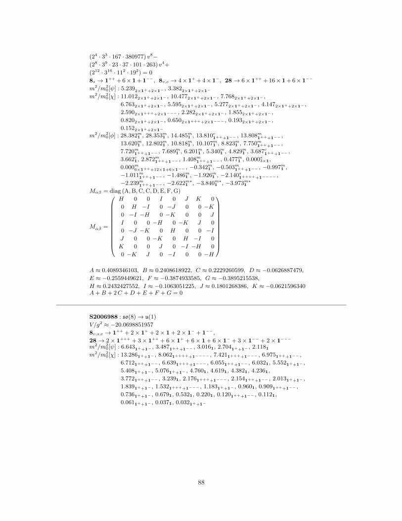
(24 · 33 · 167 · 380977) v8−(28 · 39 · 23 · 37 · 101 · 263) v4+

(212 · 316 · 112 · 192) = 0

8s → 1++ + 6× 1 + 1−−, 8v,c → 4× 1+ + 4× 1−, 28 → 6× 1++ + 16× 1 + 6× 1−−

m2/m20[ψ] : 5.2392×1++2×1− , 3.3822×1++2×1−

m2/m20[χ] : 11.0122×1++2×1− , 10.4772×1++2×1− , 7.7682×1++2×1− ,

6.7632×1++2×1− , 5.5952×1++2×1− , 5.2772×1++2×1− , 4.1472×1++2×1− ,

2.5902×1++++2×1−−− , 2.2822×1++2×1− , 1.8552×1++2×1− ,

0.8202×1++2×1− , 0.6502×1++++2×1−−− , 0.1932×1++2×1− ,

0.1522×1++2×1−

m2/m20[φ] : 28.382m1 , 28.353m1 , 14.485m1 , 13.810c1+++1−− , 13.808m1+++1−− ,

13.620m1 , 12.802m1 , 10.818m1 , 10.107m1 , 8.823m1 , 7.750m1+++1−− ,

7.720m1+++1−− , 7.689m1 , 6.201m1 , 5.340m1 , 4.829m1 , 3.687c1+++1−− ,

3.662c1, 2.872m1+++1−− , 1.408m1+++1−− , 0.477m1 , 0.000s3×1,

0.000m6×1+++12×1+6×1−− , −0.342m1 , −0.503m1+++1−− , −0.997m1 ,

−1.011m1+++1−− , −1.486m1 , −1.926m1 , −2.140s1+++++1−−−− ,

−2.239m1+++1−− , −2.622m∗1 , −3.840m∗1 , −3.973m∗1

Mαβ = diag (A,B,C,C,D,E,F,G)

Mαβ =

H 0 0 I 0 J K 0

0 H −I 0 −J 0 0 −K0 −I −H 0 −K 0 0 J

I 0 0 −H 0 −K J 0

0 −J −K 0 H 0 0 −IJ 0 0 −K 0 H −I 0

K 0 0 J 0 −I −H 0

0 −K J 0 −I 0 0 −H

A ≈ 0.4089346103, B ≈ 0.2408618922, C ≈ 0.2229260599, D ≈ −0.0626887479,

E ≈ −0.2559449621, F ≈ −0.3874933585, G ≈ −0.3895215538,

H ≈ 0.2432427552, I ≈ −0.1063051225, J ≈ 0.1801268386, K ≈ −0.0621596340A+B + 2C +D + E + F +G = 0

S2006988 : so(8)→ u(1)

V/g2 ≈ −20.0698851957

8v,s,c → 1++ + 2× 1+ + 2× 1 + 2× 1− + 1−−,

28 → 2× 1+++ + 3× 1++ + 6× 1+ + 6× 1 + 6× 1− + 3× 1−− + 2× 1−−−

m2/m20[ψ] : 6.6431++1− , 3.4871+++1−− , 3.0161, 2.7041++1− , 2.1181

m2/m20[χ] : 13.2861++1− , 8.0621+++++1−−−− , 7.4211++++1−−− , 6.9751+++1−− ,

6.7121+++1−− , 6.6391++++1−−− , 6.0551+++1−− , 6.0321, 5.5521++1− ,

5.4081++1− , 5.0761++1− , 4.7601, 4.6191, 4.3821, 4.2361,

3.7721+++1−− , 3.2391, 2.1761++++1−−− , 2.1541+++1−− , 2.0131++1− ,

1.8391++1− , 1.5321++++1−−− , 1.1831++1− , 0.9601, 0.9091+++1−− ,

0.7361++1− , 0.6791, 0.5321, 0.2201, 0.1201+++1−− , 0.1121,

0.0611++1− , 0.0371, 0.0321++1−

88

m2/m20[φ] : 15.224m1+++++1−−−− , 13.543m1++++1−−− , 12.331m1+++++1−−−− ,

11.522m1+++1−− , 11.400m1 , 10.940m1++1− , 10.497m1+++1−− , 8.589m1 ,

7.374m1+++1−− , 5.512m1++1− , 2.768m1 , 2.022m1 , 1.862m1++1− ,

1.334m1++++1−−− , 0.088m1+++1−− , 0.000s2×1, 0.000c2×1,

0.000m2×1++++3×1+++6×1++1+6×1−+3×1−−+2×1−−− , −0.532m1 ,

−0.616m1+++1−− , −0.966m1 , −0.996m1++1− , −1.266m1+++1−− ,

−1.775m1++1− , −1.896m1 , −2.064m1++1− , −2.113m1+++1−− , −2.345m∗1 ,

−2.577m∗1

Mαβ = diag (A,A,B,C,D,D,E,E)

Mαβ =

F 0 0 0 0 0 0 0

0 F 0 0 0 0 0 0

0 0 G 0 0 0 0 H

0 0 0 G 0 0 H 0

0 0 0 0 I 0 0 0

0 0 0 0 0 J 0 0

0 0 0 H 0 0 K 0

0 0 H 0 0 0 0 K

A ≈ 0.4223151772, B ≈ 0.1964198291, C ≈ −0.0471835815, D ≈ −0.2325604060,

E ≈ −0.2643728951, F ≈ −0.4486163120, G ≈ 0.2012633161,

H ≈ −0.2476192942, I ≈ −0.1174781685, J ≈ 0.4405972639, K ≈ 0.08579344822A+B + C + 2D + 2E = 0, 2F + 2G+ I + J + 2K = 0

S2040656 : so(8)→ ∅V/g2 ≈ −20.4065672900

m2/m20[ψ] : 6.3041, 6.0451, 4.6571, 4.4831, 3.2901, 3.2661, 2.9621, 2.8801

m2/m20[χ] : 12.6081, 12.0911, 10.5641, 10.5641, 10.0801, 10.0791, 9.3141, 8.9661,

7.3971, 7.3871, 6.5801, 6.5321, 6.4201, 6.4121, 5.9251, 5.8711, 5.8261,

5.7601, 5.1121, 5.0921, 5.0361, 4.9971, 4.7941, 4.6461, 4.5531, 4.4261,

4.4211, 4.3411, 3.9011, 3.8321, 3.5231, 3.3651, 2.8181, 2.5761, 2.0941,

1.8831, 1.8691, 1.8071, 1.6331, 1.5051, 1.0401, 0.9091, 0.7521, 0.7481,

0.6621, 0.6261, 0.5491, 0.3751, 0.2031, 0.1721, 0.1341, 0.1311, 0.0371,

0.0291, 0.0151, 0.0051

m2/m20[φ] : 24.040m1 , 24.040m1 , 16.050m1 , 16.041m1 , 14.516m1 , 14.506m1 , 13.256m1 ,

13.147m1 , 10.815m1 , 10.617m1 , 9.703m1 , 8.160m1 , 8.003m1 , 7.705m1 , 6.841m1 ,

6.781m1 , 6.686m1 , 6.573m1 , 5.676m1 , 4.298m1 , 4.180m1 , 4.152m1 , 4.072m1 ,

3.305m1 , 1.776m1 , 1.772m1 , 0.000m28×1, −0.153m1 , −0.248m1 , −0.458m1 ,

−0.537m1 , −0.600m1 , −0.768m1 , −0.888m1 , −1.117m1 , −1.249m1 , −1.745m1 ,

−1.747m1 , −2.276m∗1 , −2.591m∗1 , −2.711m∗1 , −3.596m∗1 , −3.601m∗1

Mαβ =

A B C D E F G H

B A −D −C F E H G

C −D I J K L M N

D −C J I −L −K −N −ME F K −L R O P Q

F E L −K O R Q P

G H M −N P Q T S

H G N −M Q P S T

Mαβ = diag (U,V,W,X,Y,Z,A′,B′)

89

A ≈ −0.0310155188, B ≈ −0.1044598977, C ≈ −0.0262671760,

D ≈ −0.0120408977, E ≈ 0.1110273146, F ≈ −0.0318532063, G ≈ 0.2756077724,

H ≈ −0.0852883736, I ≈ 0.0513329965, J ≈ 0.1837698278, K ≈ 0.0381187717,

L ≈ −0.0525121403, M ≈ 0.0153608312, N ≈ −0.0255658240, O ≈ 0.1379568192,

P ≈ 0.1254546193, Q ≈ −0.0173057511, R ≈ 0.0961923361, S ≈ −0.0732628828,

T ≈ −0.1165098138, U ≈ 0.4664757019, V ≈ 0.4606093304, W ≈ 0.2640494645,

X ≈ −0.0142676237, Y ≈ −0.0244079083, Z ≈ −0.2057299225,

A′ ≈ −0.4719904991, B′ ≈ −0.4747385433A+ I +R+ T = 0, A′ +B′ + U + V +W +X + Y + Z = 0

S2043647 : so(8)→ ∅V/g2 ≈ −20.4364775879

m2/m20[ψ] : 6.2671, 6.0491, 4.7851, 4.6931, 3.4151, 3.2731, 3.0701, 2.8581

m2/m20[χ] : 12.5341, 12.0981, 11.0201, 11.0201, 10.5311, 10.5311, 9.5691, 9.3851,

7.5931, 7.5921, 6.8301, 6.5461, 6.3731, 6.3671, 6.1401, 5.9071, 5.8771,

5.7161, 5.4131, 5.4041, 5.1791, 4.9691, 4.9501, 4.8891, 4.5171, 4.4931,

4.2921, 4.2801, 3.9281, 3.7211, 3.5761, 3.5541, 2.7731, 2.6031, 2.1701,

1.9661, 1.9451, 1.9181, 1.5681, 1.4931, 1.0131, 0.9151, 0.7911, 0.7241,

0.6001, 0.5871, 0.5391, 0.4611, 0.2181, 0.2091, 0.1661, 0.1581, 0.0331,

0.0211, 0.0101, 0.0071

m2/m20[φ] : 25.390m1 , 25.390m1 , 16.682m1 , 16.662m1 , 14.965m1 , 14.961m1 , 13.281m1 ,

13.176m1 , 11.191m1 , 11.094m1 , 9.801m1 , 8.082m1 , 7.967m1 , 7.923m1 , 7.256m1 ,

7.137m1 , 6.181m1 , 6.171m1 , 5.851m1 , 4.628m1 , 4.535m1 , 3.955m1 , 3.905m1 ,

3.789m1 , 1.761m1 , 1.746m1 , 0.085m1 , 0.000m28×1, −0.128m1 , −0.399m1 ,

−0.413m1 , −0.469m1 , −0.689m1 , −0.734m1 , −1.152m1 , −1.271m1 , −1.695m1 ,

−1.697m1 , −2.225m1 , −2.692m∗1 , −2.852m∗1 , −3.701m∗1 , −3.721m∗1

Mαβ = diag (A,B,C,D,E,F,G,H)

Mαβ =

0 I 0 J 0 K 0 L

I 0 M 0 N 0 O 0

0 M 0 P 0 Q 0 R

J 0 P 0 S 0 T 0

0 N 0 S 0 U 0 V

K 0 Q 0 U 0 W 0

0 O 0 T 0 W 0 X

L 0 R 0 V 0 X 0

A ≈ 0.4754450281, B ≈ 0.2671859448, C ≈ 0.2590808168, D ≈ −0.0115242705,

E ≈ −0.1215163098, F ≈ −0.1457164623, G ≈ −0.3614719886,

H ≈ −0.3614827586, I ≈ −0.0031458899, J ≈ −0.0967722180,

K ≈ 0.2129213804, L ≈ 0.1942522799, M ≈ −0.0786691154, N ≈ −0.2508352877,

O ≈ −0.1521352796, P ≈ −0.0123726646, Q ≈ 0.2496676625, R ≈ 0.2406226960,

S ≈ 0.3082779767, T ≈ 0.1738832518, U ≈ 0.0907728984, V ≈ −0.0015314933,

W ≈ −0.2118153013, X ≈ 0.1297791243A+B + C +D + E + F +G+H = 0

S2043965 : so(8)→ ∅V/g2 ≈ −20.4396582786

m2/m20[ψ] : 6.1832×1, 4.8022×1, 3.2312×1, 3.0662×1

90

m2/m20[χ] : 12.3672×1, 11.1042×1, 10.7302×1, 9.6042×1, 7.6462×1, 6.4632×1,

6.3632×1, 6.1322×1, 6.0072×1, 5.4402×1, 5.0442×1, 4.9292×1, 4.5292×1,

4.2812×1, 3.8502×1, 3.5972×1, 2.7062×1, 2.0632×1, 1.8782×1, 1.6062×1,

0.9412×1, 0.7542×1, 0.5782×1, 0.5132×1, 0.2212×1, 0.1652×1, 0.0252×1,

0.0102×1

m2/m20[φ] : 25.750m1 , 25.750m1 , 16.878m1 , 16.860m1 , 14.831m1 , 14.829m1 , 13.722m1 ,

13.633m1 , 11.305m1 , 11.198m1 , 9.851m1 , 8.090m1 , 7.950m1 , 7.846m1 , 7.344m1 ,

7.260m1 , 6.290m1 , 6.135m1 , 5.743m1 , 4.649m1 , 4.555m1 , 3.880m1 , 3.824m1 ,

3.792m1 , 1.789m1 , 1.767m1 , 0.118m1 , 0.068m1 , 0.000m28×1, −0.376m1 ,

−0.394m1 , −0.460m1 , −0.698m1 , −0.721m1 , −1.149m1 , −1.280m1 , −1.680m1 ,

−1.683m1 , −2.224m1 , −2.722m∗1 , −2.903m∗1 , −3.738m∗1 , −3.753m∗1

Mαβ =

P A B 0 0 C D E

A F G 0 0 H I D

B G O J 0 K −H −C0 0 J L M 0 0 0

0 0 0 M L N 0 0

C H K 0 N O −G −BD I −H 0 0 −G F A

E D −C 0 0 −B A P

Mαβ = diag (Q,R, S,T,−T,−S,−R,−Q)

A ≈ 0.0968882931, B ≈ 0.0737569455, C ≈ −0.0691683110, D ≈ 0.2735081616,

E ≈ 0.0530074705, F ≈ −0.0712078114, G ≈ 0.0797014929, H ≈ −0.0815645322,

I ≈ 0.1427876896, J ≈ 0.0000000000, K ≈ −0.0536857182, L ≈ 0.2580087411,

M ≈ −0.0019954396, N ≈ 0.0000000000, O ≈ −0.0880560317,

P ≈ −0.0987448980, Q ≈ 0.4736210915, R ≈ 0.4733609137, S ≈ 0.2318924219,

T ≈ 0.0022541680F + L+O + P = 0

S2045402 : so(8)→ u(1)

V/g2 ≈ −20.4540245888

8v,s,c → 1++ + 2× 1+ + 2× 1 + 2× 1− + 1−−,

28 → 2× 1+++ + 3× 1++ + 6× 1+ + 6× 1 + 6× 1− + 3× 1−− + 2× 1−−−

m2/m20[ψ] : 5.5851++1− , 4.1771, 3.0841++1− , 2.7691+++1−− , 2.5891

m2/m20[χ] : 11.1701++1− , 8.3551, 6.2211++++1−−− , 6.1801+++1−− , 6.1691++1− ,

6.1621++1− , 5.5371+++1−− , 5.5081, 5.3471, 5.3111+++1−− ,

5.2441+++++1−−−− , 5.1781, 5.0871++1− , 4.9341++++1−−− , 4.8271,

3.3781++1− , 3.3671+++1−− , 2.9311, 2.8111+++1−− , 2.2271++1− ,

1.5811, 1.4801++++1−−− , 1.4701, 1.2871++1− , 0.9251++1− ,

0.7881++++1−−− , 0.5801+++1−− , 0.5611, 0.5361, 0.2851, 0.1101++1− ,

0.0911+++1−− , 0.0531, 0.0161++1−

m2/m20[φ] : 12.290m1 , 12.073m1+++1−− , 11.966m1++++1−−− , 11.360m1++1− ,

9.632m1+++++1−−−− , 8.916m1+++1−− , 8.603m1 , 7.240m1+++++1−−−− ,

6.426m1+++1−− , 6.289m1++1− , 4.712m1 , 4.475m1 , 3.363m1++1− , 1.549m1 ,

0.905m1+++1−− , 0.000s2×1, 0.000c2×1,

0.000m2×1++++3×1+++6×1++1+6×1−+3×1−−+2×1−−− ,

−0.533m1++++1−−− , −0.778m1 , −0.843m1++1− , −0.888m1+++1−− ,

−1.209m1+++1−− , −1.213m1++1− , −1.484m1 , −1.971m1++1− , −2.078m1 ,

−2.409m∗1+++1−− , −2.495m∗1

Mαβ = diag (A,A,B,C,D,D,E,E)

91

Mαβ =

F 0 0 0 0 0 0 G

0 F 0 0 0 0 G 0

0 0 H 0 0 0 0 0

0 0 0 H 0 0 0 0

0 0 0 0 I 0 0 0

0 0 0 0 0 J 0 0

0 G 0 0 0 0 K 0

G 0 0 0 0 0 0 K

A ≈ 0.4061640671, B ≈ 0.2918516810, C ≈ −0.0950849623, D ≈ −0.2519682470,

E ≈ −0.2525791794, F ≈ 0.1421707958, G ≈ −0.2360192861,

H ≈ −0.4104660106, I ≈ 0.4519124396, J ≈ −0.2665304013, K ≈ 0.17560419562A+B + C + 2D + 2E = 0, 2F + 2H + I + J + 2K = 0

S2054312 : so(8)→ ∅V/g2 ≈ −20.5431279537

m2/m20[ψ] : 5.5852×1, 3.8682×1, 3.8342×1, 3.3642×1

m2/m20[χ] : 11.1692×1, 9.5412×1, 9.1202×1, 7.7352×1, 7.6682×1, 7.5862×1,

6.7292×1, 5.5432×1, 5.3242×1, 4.9282×1, 4.8732×1, 4.8282×1, 4.7072×1,

4.6172×1, 4.2572×1, 4.1182×1, 2.4322×1, 1.9152×1, 1.6102×1, 1.2802×1,

1.0272×1, 0.9392×1, 0.8702×1, 0.6062×1, 0.1852×1, 0.1142×1, 0.1012×1,

0.0322×1

m2/m20[φ] : 22.245m2×1, 14.821m1 , 14.820m1 , 13.009m1 , 13.006m1 , 12.483m1 , 12.481m1 ,

11.272m1 , 9.208m1 , 9.207m1 , 8.502m1 , 8.501m1 , 7.909m1 , 6.676m1 , 6.664m1 ,

6.456m1 , 6.196m1 , 5.802m1 , 4.558m1 , 4.384m1 , 4.363m1 , 3.192m1 , 3.191m1 ,

2.928m1 , 2.923m1 , 0.447m1 , 0.421m1 , 0.000s3×1, 0.000c1, 0.000m24×1,

−0.145m1 , −0.223m1 , −0.411m1 , −0.412m1 , −0.652m1 , −1.111m1 , −1.123m1 ,

−1.809m2×1, −2.271m∗1 , −2.775m∗1 , −3.108m∗1 , −3.920m∗1 , −3.922m∗1

Mαβ =

A 0 B C D E 0 F

0 G 0 0 0 0 H 0

B 0 I J K L 0 −EC 0 J N M −K 0 D

D 0 K M N −J 0 C

E 0 L −K −J I 0 −B0 H 0 0 0 0 G 0

F 0 −E D C −B 0 A

Mαβ = diag (O,P,Q,R,−R,−Q,−P,−O)

A ≈ 0.2600820414, B ≈ −0.0337172802, C ≈ −0.0304060482, D ≈ 0.0054500767,

E ≈ −0.0308821730, F ≈ 0.0034015223, G ≈ −0.1437652294,

H ≈ −0.0037501582, I ≈ −0.0579149742, J ≈ −0.1126964527,

K ≈ −0.3013781537, L ≈ −0.1090177478, M ≈ 0.1163265235,

N ≈ −0.0584018378, O ≈ 0.4687054761, P ≈ 0.4685343606, Q ≈ 0.2433680033,

R ≈ 0.0000889081A+G+ I +N = 0

S2054714 : so(8)→ u(1)

V/g2 ≈ −20.5471493057

92

8v,s,c → 1++ + 2× 1+ + 2× 1 + 2× 1− + 1−−,

28 → 2× 1+++ + 3× 1++ + 6× 1+ + 6× 1 + 6× 1− + 3× 1−− + 2× 1−−−

m2/m20[ψ] : 5.5772×1, 3.8861++1− , 3.7831+++1−− , 3.4811++1−

m2/m20[χ] : 11.1532×1, 9.6551++++1−−− , 9.2511++++1−−− , 7.7721++1− ,

7.6471+++1−− , 7.5661+++1−− , 6.9621++1− , 5.5382×1, 5.0672×1,

5.0481++1− , 4.9911+++++1−−−− , 4.8001++1− , 4.6931++1− ,

4.6381+++1−− , 4.5201+++1−− , 4.1171++1− , 2.4322×1, 1.8902×1,

1.5181+++1−− , 1.3461++1− , 1.0121+++1−− , 0.9491++1− ,

0.9201++++1−−− , 0.6041++1− , 0.1902×1, 0.1211++++1−−− ,

0.1031+++1−− , 0.0351++1−

m2/m20[φ] : 22.599m1+++++1−−−− , 15.014m1+++1−− , 12.878m1++1− , 12.695m1+++1−− ,

11.317m1 , 9.397m1++++1−−− , 8.539m1+++1−− , 7.899m1 , 6.695m1++1− ,

6.302m1++1− , 5.819m1 , 4.598m1 , 4.274m1+++1−− , 3.315m1++++1−−− ,

2.959m1+++1−− , 0.418m1++1− , 0.079m1++1− , 0.000s2×1, 0.000c2×1,

0.000m2×1++++3×1+++6×1++1+6×1−+3×1−−+2×1−−− , −0.201m1 ,

−0.398m1+++1−− , −0.636m1 , −1.112m1++1− , −1.792m1+++++1−−−− ,

−2.255m∗1 , −2.814m∗1 , −3.176m∗1 , −3.964m∗1+++1−−

Mαβ =

A 0 0 0 0 0 0 0

0 B 0 0 0 0 0 0

0 0 F 0 C 0 0 0

0 0 0 D 0 E 0 0

0 0 C 0 F 0 0 0

0 0 0 E 0 D 0 0

0 0 0 0 0 0 B 0

0 0 0 0 0 0 0 A

Mαβ = diag (G,G,H, 0, 0,−H,−G,−G)

A ≈ −0.1435704846, B ≈ 0.2644129362, C ≈ 0.1842837925, D ≈ 0.0558383854,

E ≈ −0.4168030149, F ≈ −0.1766808369, G ≈ 0.4699749265, H ≈ 0.2427905463A+B +D + F = 0, C +D + E − F = 0

S2074862 : so(8)→ ∅V/g2 ≈ −20.7486223244

m2/m20[ψ] : 6.5072×1, 6.0662×1, 3.0822×1, 3.0652×1

m2/m20[χ] : 13.0152×1, 12.1952×1, 12.1832×1, 12.1332×1, 8.2252×1, 8.2142×1,

7.3452×1, 7.2682×1, 6.1642×1, 6.1302×1, 5.6182×1, 4.8672×1, 4.4812×1,

4.4002×1, 3.4342×1, 2.7622×1, 2.7342×1, 2.6332×1, 2.2862×1, 2.1412×1,

1.0662×1, 0.9622×1, 0.7992×1, 0.5292×1, 0.4442×1, 0.3682×1, 0.0652×1,

0.0252×1

m2/m20[φ] : 28.904m1 , 28.875m1 , 20.458m1 , 20.354m1 , 16.370m1 , 16.290m1 , 16.281m1 ,

16.280m1 , 13.057m1 , 11.996m1 , 11.246m1 , 10.817m1 , 9.372m1 , 8.654m1 ,

7.833m1 , 7.815m1 , 6.526m1 , 6.412m1 , 6.352m1 , 6.336m1 , 4.883m1 , 4.258m1 ,

3.629m1 , 3.505m1 , 3.505m1 , 2.939m1 , 2.338m1 , 2.255m1 , 0.000m28×1, −0.337m1 ,

−0.427m1 , −0.716m1 , −0.949m1 , −1.043m1 , −1.087m1 , −1.698m1 , −1.917m1 ,

−2.141m1 , −2.301m∗1 , −2.383m∗1 , −3.077m∗1 , −3.393m∗1 , −3.890m∗1

93

Mαβ =

A 0 0 0 0 0 0 B

0 C D 0 0 E F 0

0 D G 0 0 H −E 0

0 0 0 I J 0 0 0

0 0 0 J I 0 0 0

0 E H 0 0 G −D 0

0 F −E 0 0 −D C 0

B 0 0 0 0 0 0 A

Mαβ = diag (K,L,M,N,−N,−M,−L,−K)

A ≈ 0.2470648871, B ≈ −0.0104507828, C ≈ 0.1590211505, D ≈ 0.2227282828,

E ≈ −0.1337655402, F ≈ −0.0987985044, G ≈ −0.1356526935,

H ≈ −0.2236987079, I ≈ −0.2704333441, J ≈ −0.1059508789,

K ≈ 0.4213118035, L ≈ 0.4119154403, M ≈ 0.3317218046, N ≈ 0.0592000361A+ C +G+ I = 0

S2095412 : so(8)→ ∅V/g2 ≈ −20.9541200855

m2/m20[ψ] : 6.8361, 6.4941, 5.7181, 5.5841, 3.6621, 3.3141, 3.0851, 2.4611

m2/m20[χ] : 13.6721, 13.5271, 13.5261, 12.9891, 12.7091, 12.7071, 11.4361, 11.1681,

8.1761, 8.1701, 7.5601, 7.5481, 7.3231, 7.1801, 7.1731, 6.6281, 6.3961,

6.3831, 6.1691, 5.3561, 5.0641, 4.9941, 4.9231, 4.8381, 4.6691, 4.4731,

4.4101, 4.2411, 3.6311, 3.3571, 3.2521, 3.1531, 3.0221, 2.7561, 2.6941,

2.3651, 2.2881, 2.1031, 1.7241, 1.3191, 1.2691, 1.0231, 0.8221, 0.8121,

0.7811, 0.6111, 0.4651, 0.4271, 0.3741, 0.2611, 0.2241, 0.1341, 0.0671,

0.0351, 0.0081, 0.0021

m2/m20[φ] : 32.226m1 , 32.223m1 , 18.797m1 , 18.786m1 , 18.777m1 , 18.766m1 , 14.919m1 ,

14.910m1 , 11.797m1 , 11.532m1 , 9.733m1 , 9.706m1 , 8.073m1 , 7.862m1 , 7.646m1 ,

7.400m1 , 7.238m1 , 7.029m1 , 6.299m1 , 5.652m1 , 5.494m1 , 4.445m1 , 4.153m1 ,

3.004m1 , 1.965m1 , 1.901m1 , 0.912m1 , 0.000m28×1, −0.248m1 , −0.342m1 ,

−0.489m1 , −0.517m1 , −0.620m1 , −0.849m1 , −1.217m1 , −1.278m1 , −1.323m1 ,

−1.392m1 , −2.291m∗1 , −2.515m∗1 , −3.005m∗1 , −3.334m∗1 , −3.669m∗1

Mαβ =

A 0 0 B C 0 0 D

0 E F 0 0 G H 0

0 F I 0 0 J −G 0

B 0 0 L K 0 0 −CC 0 0 K L 0 0 −B0 G J 0 0 I −F 0

0 H −G 0 0 −F E 0

D 0 0 −C −B 0 0 A

Mαβ = diag (M,N,O,P,−P,−O,−N,−M)

A ≈ 0.2387619173, B ≈ −0.0851236169, C ≈ −0.0524166655, D ≈ 0.0165044547,

E ≈ −0.0260527473, F ≈ −0.1334592728, G ≈ −0.1309746199,

H ≈ −0.1154139177, I ≈ −0.0427075134, J ≈ 0.3401000154, K ≈ 0.2103844802,

L ≈ −0.1700016566, M ≈ 0.4755499838, N ≈ 0.4748908426, O ≈ 0.1996313012,

P ≈ 0.1047599753A+ E + I + L = 0

94

S2099077 : so(8)→ u(1) + u(1)

V/g2 ≈ −20.9907719246

8c → 2× 1+ + 1++ + 2× 1 + 1−− + 2× 1−,

8v,s → 1++ + 1+

− + 2× 1+ + 2× 1− + 1−+ + 1−−, 28 →1+++2×1+

+++4×1++2×1+−−+2×1+++6×1+2×1−−+2×1−+++4×1−+2×1−−−+1−−

m2/m20[ψ] : 7.6051++1− , 2.6161++1− , 2.572

1+++1+

−+1−++1−−

m2/m20[χ] : 15.2111++1− , 8.0441++++1−−− , 7.456

1+++++1+

−−−+1−++++1−−−−,

5.2481++1− , 5.2331++1− , 5.1451+++1+

−+1−++1−−, 5.124

1+++1+

−+1−++1−−,

5.1081++1− , 4.8681+++1+

−+1−++1−−, 4.147

1+++ +1++

− +1−−+ +1−−−,

2.3751++++1−−− , 1.1741++1− , 1.0061++1− , 0.9231+++1+

−+1−++1−−,

0.7771++1− , 0.6181+++1+

−+1−++1−−, 0.547

1+++ +1++

− +1−−+ +1−−−,

0.1711+++1+

−+1−++1−−, 0.1251++1−

m2/m20[φ] : 17.648c1+++++1−−−− , 11.047s1+++1−− , 10.072m1 ,

9.972m1++++1+

−−+1−+++1−−−, 9.396m1++1− , 9.282s1+++1−− , 8.668m1 ,

8.409s1+++++1++

−−+1−−+++1−−−−, 7.675m1+++1−− , 0.714m1 , 0.600m1++1− ,

0.307m1 , 0.167m1+++1−− , 0.000s1, 0.000c1+++1+++2×1+1−−+1−− ,

0.000m2×1+

+++4×1++2×1+−−+1+++1+1−−+2×1−+++4×1−+2×1−−−

,

−0.115m1++++1+

−−+1−+++1−−−, −0.611m1 , −1.181s1+++1−− ,

−1.386m1+++1−− , −1.923m1++1− , −2.089m1 , −2.283m∗1+++1−− ,

−2.413m∗1++1− , −2.511m∗1 , −2.612m∗1

Mαβ =

0 0 A 0 B 0 −B 0

0 0 0 A 0 −B 0 −BA 0 0 0 B 0 −B 0

0 A 0 0 0 −B 0 −BB 0 B 0 0 0 −A 0

0 −B 0 −B 0 0 0 A

−B 0 −B 0 −A 0 0 0

0 −B 0 −B 0 A 0 0

Mαβ = diag (C,C,D,D,E,F,F,G)

A ≈ 0.1420111814, B ≈ 0.1744120053, C ≈ 0.5006372444, D ≈ 0.0850397306,

E ≈ 0.0604794054, F ≈ −0.3921708910, G ≈ −0.44749157352C + 2D + E + 2F +G = 0

S2099419 : so(8)→ ∅V/g2 ≈ −20.9941924460

m2/m20[ψ] : 7.6722×1, 2.6662×1, 2.6072×1, 2.5682×1

m2/m20[χ] : 15.3432×1, 8.3062×1, 7.6842×1, 7.6452×1, 5.3322×1, 5.2752×1,

5.2132×1, 5.2032×1, 5.1362×1, 5.1262×1, 5.0922×1, 4.8582×1, 4.8412×1,

4.1352×1, 4.1352×1, 2.5412×1, 1.2252×1, 1.1492×1, 0.9322×1, 0.8942×1,

0.8362×1, 0.7202×1, 0.6272×1, 0.4672×1, 0.4462×1, 0.1692×1, 0.1652×1,

0.1152×1

95

m2/m20[φ] : 18.405m1 , 18.405m1 , 11.387m1 , 11.378m1 , 10.243m1 , 10.234m1 , 10.219m1 ,

10.144m1 , 9.898m1 , 9.463m1 , 9.435m1 , 9.391m1 , 9.214m1 , 8.619m1 , 8.572m1 ,

8.562m1 , 8.512m1 , 8.502m1 , 7.537m1 , 7.533m1 , 0.936m1 , 0.784m1 , 0.606m1 ,

0.538m1 , 0.407m1 , 0.262m1 , 0.000c4×1, 0.000m24×1, −0.012m1 , −0.244m1 ,

−0.660m1 , −1.178m1 , −1.180m1 , −1.411m1 , −1.413m1 , −1.920m1 , −1.949m1 ,

−2.123m1 , −2.315m∗1 , −2.321m∗1 , −2.429m∗1 , −2.458m∗1 , −2.539m∗1 ,

−2.691m∗1

Mαβ =

A 0 B 0 0 C 0 D

0 E 0 F G 0 −D 0

B 0 H 0 0 I 0 G

0 F 0 J I 0 −C 0

0 G 0 I H 0 −B 0

C 0 I 0 0 J 0 F

0 −D 0 −C −B 0 A 0

D 0 G 0 0 F 0 E

Mαβ = diag (K,L,M,N,O,P,Q,R)

A ≈ 0.0353186765, B ≈ 0.1450672974, C ≈ −0.1987794760, D ≈ −0.1710679912,

E ≈ −0.0270338296, F ≈ 0.1323763519, G ≈ −0.1487598607,

H ≈ −0.0218470988, I ≈ −0.1751328036, J ≈ 0.0135622518, K ≈ 0.5060966998,

L ≈ 0.5057305919, M ≈ 0.0825796283, N ≈ 0.0798941267, O ≈ 0.0540222235,

P ≈ −0.3885252986, Q ≈ −0.3920023348, R ≈ −0.4477956369A+ E +H + J = 0, K + L+M +N +O + P +Q+R = 0

S2099421 : so(8)→ ∅V/g2 ≈ −20.9942164355

m2/m20[ψ] : 7.6582×1, 2.6522×1, 2.6052×1, 2.5712×1

m2/m20[χ] : 15.3172×1, 8.2472×1, 7.6602×1, 7.6082×1, 5.3042×1, 5.2582×1,

5.2092×1, 5.1632×1, 5.1432×1, 5.1322×1, 5.0962×1, 4.8762×1, 4.8572×1,

4.1382×1, 4.1382×1, 2.5132×1, 1.2012×1, 1.1442×1, 0.9272×1, 0.8832×1,

0.8502×1, 0.7122×1, 0.6282×1, 0.4722×1, 0.4542×1, 0.1702×1, 0.1662×1,

0.1162×1

m2/m20[φ] : 18.272m1 , 18.271m1 , 11.281m1 , 11.272m1 , 10.206m1 , 10.200m1 , 10.191m1 ,

10.095m1 , 9.902m1 , 9.464m1 , 9.448m1 , 9.399m1 , 9.234m1 , 8.626m1 , 8.552m1 ,

8.540m1 , 8.500m1 , 8.490m1 , 7.557m1 , 7.555m1 , 0.892m1 , 0.779m1 , 0.587m1 ,

0.516m1 , 0.355m1 , 0.207m1 , 0.007m1 , 0.000c4×1, 0.000m24×1, −0.237m1 ,

−0.651m1 , −1.178m1 , −1.180m1 , −1.413m1 , −1.415m1 , −1.920m1 , −1.946m1 ,

−2.122m1 , −2.310m∗1 , −2.315m∗1 , −2.423m∗1 , −2.450m∗1 , −2.528m∗1 ,

−2.684m∗1

Mαβ =

A 0 B 0 0 C 0 D

0 −A 0 B E 0 −D 0

B 0 −A 0 0 D 0 E

0 B 0 A D 0 −C 0

0 E 0 D −A 0 −B 0

C 0 D 0 0 A 0 B

0 −D 0 −C −B 0 A 0

D 0 E 0 0 B 0 −A

Mαβ = diag (F,G,H, I, J,K,L,M)

96

A ≈ 0.0232352194, B ≈ 0.1389591143, C ≈ 0.1979032131, D ≈ 0.1734255889,

E ≈ 0.1501470977, F ≈ 0.5052044951, G ≈ 0.5048563759, H ≈ 0.0833062773,

I ≈ 0.0808195212, J ≈ 0.0547601306, K ≈ −0.3889451502, L ≈ −0.3920321476,

M ≈ −0.4479695023F +G+H + I + J +K + L+M = 0

S2101265 : so(8)→ ∅V/g2 ≈ −21.0126547893

m2/m20[ψ] : 6.3832×1, 6.3012×1, 3.3552×1, 2.9512×1

m2/m20[χ] : 13.7302×1, 13.7292×1, 12.7672×1, 12.6022×1, 8.1522×1, 8.1492×1,

7.0632×1, 7.0532×1, 6.7102×1, 5.9012×1, 5.0102×1, 4.9022×1, 4.6132×1,

4.4582×1, 3.5172×1, 3.4972×1, 2.7342×1, 2.6932×1, 2.4672×1, 1.5242×1,

1.0582×1, 0.7342×1, 0.7232×1, 0.5682×1, 0.3132×1, 0.1832×1, 0.0332×1,

0.0272×1

m2/m20[φ] : 33.862m1 , 33.859m1 , 19.791m1 , 19.780m1 , 18.331m1 , 18.325m1 , 16.961m1 ,

16.927m1 , 12.061m1 , 11.731m1 , 9.905m1 , 9.751m1 , 8.661m1 , 7.849m1 , 7.813m1 ,

7.801m1 , 7.539m1 , 7.531m1 , 6.754m1 , 5.433m1 , 5.132m1 , 3.817m1 , 3.738m1 ,

3.131m1 , 2.321m1 , 1.674m1 , 1.439m1 , 0.298m1 , 0.000m28×1, −0.240m1 ,

−0.272m1 , −0.311m1 , −0.463m1 , −0.778m1 , −1.018m1 , −1.139m1 , −1.285m1 ,

−1.343m1 , −2.323m∗1 , −2.744m∗1 , −3.157m∗1 , −3.498m∗1 , −3.926m∗1

Mαβ =

A 0 0 0 0 0 0 B

0 J C 0 0 D E 0

0 C I 0 0 F −D 0

0 0 0 G H 0 0 0

0 0 0 H G 0 0 0

0 D F 0 0 I −C 0

0 E −D 0 0 −C J 0

B 0 0 0 0 0 0 A

Mαβ = diag (K,L,M,N,−N,−M,−L,−K)

A ≈ 0.2560627010, B ≈ 0.0036274555, C ≈ −0.1356863009, D ≈ −0.1316817261,

E ≈ −0.0903630923, F ≈ 0.3566566499, G ≈ −0.1905878716, H ≈ 0.1970936745,

I ≈ −0.0314700817, J ≈ −0.0340047477, K ≈ 0.4812063411, L ≈ 0.4795849305,

M ≈ 0.1899494485, N ≈ 0.1124970772A+G+ I + J = 0

S2118474 : so(8)→ ∅V/g2 ≈ −21.1847430599

m2/m20[ψ] : 6.5922×1, 5.4592×1, 3.4602×1, 3.1792×1

m2/m20[χ] : 13.5342×1, 13.1842×1, 12.4722×1, 10.9182×1, 8.4072×1, 7.6852×1,

6.9462×1, 6.9192×1, 6.3572×1, 6.3132×1, 5.2722×1, 4.9292×1, 4.5912×1,

4.4182×1, 3.8442×1, 3.5922×1, 2.6462×1, 2.4522×1, 1.9922×1, 1.8702×1,

1.0872×1, 0.8542×1, 0.7012×1, 0.6192×1, 0.2702×1, 0.2182×1, 0.0912×1,

0.0232×1

97

m2/m20[φ] : 32.317m1 , 32.313m1 , 19.820m1 , 19.812m1 , 16.531m1 , 16.474m1 , 15.725m1 ,

15.708m1 , 12.169m1 , 12.010m1 , 9.902m1 , 9.440m1 , 8.856m1 , 7.803m1 , 7.355m1 ,

7.306m1 , 7.237m1 , 6.993m1 , 6.013m1 , 5.572m1 , 5.389m1 , 4.396m1 , 3.621m1 ,

3.121m1 , 2.702m1 , 2.611m1 , 1.535m1 , 0.509m1 , 0.000s4×1, 0.000m24×1,

−0.175m1 , −0.295m1 , −0.338m1 , −0.378m1 , −0.507m1 , −0.766m1 , −1.037m1 ,

−1.184m1 , −1.344m1 , −2.402m∗1 , −2.680m∗1 , −3.247m∗1 , −3.667m∗1 ,

−3.919m∗1

Mαβ =

A 0 B 0 0 C 0 0

0 D 0 E F 0 0 0

B 0 G 0 0 H 0 0

0 E 0 I J 0 0 0

0 F 0 J K 0 0 0

C 0 H 0 0 L 0 0

0 0 0 0 0 0 M 0

0 0 0 0 0 0 0 N

Mαβ = diag (O,O,P,P,Q,Q,R,R)

A ≈ 0.2515325313, B ≈ −0.0948720562, C ≈ −0.0589660410,

D ≈ −0.0004753989, E ≈ 0.1589773711, F ≈ 0.1638511955, G ≈ −0.1990118382,

H ≈ 0.2170462622, I ≈ −0.0608336278, J ≈ 0.3755884160, K ≈ 0.0303150737,

L ≈ −0.1466133643, M ≈ 0.2561929848, N ≈ −0.1311063607, O ≈ 0.4621027750,

P ≈ 0.1716362375, Q ≈ −0.1436921837, R ≈ −0.4900468288A+D +G+ I +K + L+M +N = 0, O + P +Q+R = 0

S2121742 : so(8)→ ∅V/g2 ≈ −21.2174239936

m2/m20[ψ] : 5.8774×1, 3.4484×1

m2/m20[χ] : 12.8114×1, 11.7554×1, 8.0964×1, 6.8974×1, 6.3224×1, 5.1804×1,

4.5884×1, 3.7984×1, 2.5054×1, 1.9574×1, 0.9544×1, 0.7414×1, 0.2634×1,

0.0664×1

m2/m20[φ] : 32.050m1 , 32.044m1 , 18.687m1 , 18.686m1 , 16.742m1 , 16.738m1 , 15.014m1 ,

14.986m1 , 12.564m1 , 12.467m1 , 10.052m1 , 9.533m1 , 9.294m1 , 7.744m1 , 7.442m1 ,

7.437m1 , 7.343m1 , 7.074m1 , 5.967m1 , 5.590m1 , 5.087m1 , 4.148m1 , 3.486m1 ,

3.279m1 , 3.159m1 , 2.252m1 , 2.154m1 , 0.697m1 , 0.225m1 , 0.000s4×1, 0.000m24×1,

−0.137m1 , −0.215m1 , −0.295m1 , −0.462m1 , −0.685m1 , −0.997m1 , −1.049m1 ,

−1.295m1 , −2.366m∗1 , −2.828m∗1 , −3.469m∗1 , −3.766m∗1 , −4.120m∗1

Mαβ =

A 0 0 0 0 0 0 0

0 B 0 C 0 D 0 0

0 0 E 0 F 0 0 0

0 C 0 G 0 H 0 0

0 0 F 0 I 0 0 0

0 D 0 H 0 J 0 0

0 0 0 0 0 0 K 0

0 0 0 0 0 0 0 L

Mαβ = diag (M,M,N,N,−N,−N,−M,−M)

A ≈ 0.2649996965, B ≈ −0.0124955931, C ≈ 0.1442324503, D ≈ −0.1533561318,

E ≈ −0.2130746265, F ≈ 0.2080774017, G ≈ −0.0506314842,

H ≈ −0.3901473182, I ≈ −0.1535564108, J ≈ 0.0491090708, K ≈ 0.2605736865,

L ≈ −0.1449243391, M ≈ 0.4786142905, N ≈ 0.1592876058

98

A+B + E +G+ I + J +K + L = 0

S2126597 : so(8)→ ∅V/g2 ≈ −21.2659762563

m2/m20[ψ] : 5.7852×1, 4.1944×1, 3.6972×1

m2/m20[χ] : 11.5702×1, 9.0012×1, 8.4714×1, 8.3884×1, 7.5542×1, 7.3942×1,

7.0652×1, 6.3522×1, 6.2204×1, 4.5972×1, 4.4074×1, 2.7062×1, 2.4442×1,

1.8534×1, 1.4762×1, 1.3312×1, 1.3034×1, 0.6932×1, 0.5692×1, 0.2934×1,

0.2102×1

m2/m20[φ] : 22.287m1 , 20.926m2×1, 18.868m1 , 14.471m1 , 11.968m2×1, 11.535c1, 11.179m1 ,

11.045m1 , 10.227m2×1, 9.127m1 , 9.034m2×1, 8.240m1 , 7.922m1 , 7.816m1 ,

6.519c1, 4.820m2×1, 4.748m2×1, 4.180c1, 4.092m1 , 3.871m1 , 3.442m1 , 3.114m1 ,

1.286m1 , 0.000s2×1, 0.000c2×1, 0.000m24×1, −0.364m1 , −0.391m1 ,

−0.746m2×1, −1.252m1 , −1.267m1 , −1.804m1 , −1.955m1 , −2.320m∗2×1,

−3.029m∗1 , −3.671m∗1 , −4.227m∗1

Mαβ =

A 0 0 0 0 0 0 B

0 F 0 0 0 0 C 0

0 0 G 0 0 C 0 0

0 0 0 D E 0 0 0

0 0 0 E D 0 0 0

0 0 C 0 0 F 0 0

0 C 0 0 0 0 G 0

B 0 0 0 0 0 0 A

Mαβ = diag (H, I, I, J,−J,−I,−I,−H)

A ≈ 0.2481795995, B ≈ −0.0023500674, C ≈ −0.2559853716,

D ≈ −0.2705070093, E ≈ −0.1056090968, F ≈ 0.2646370219,

G ≈ −0.2423096122, H ≈ 0.4057088466, I ≈ 0.3662921302, J ≈ 0.1318480997A+D + F +G = 0

S2135328 : so(8)→ ∅V/g2 ≈ −21.3532841611

m2/m20[ψ] : 5.9961, 5.0771, 4.4601, 3.6001, 3.5991, 3.1351, 3.0911, 2.4021

m2/m20[χ] : 11.9931, 10.1551, 8.9201, 7.6291, 7.5591, 7.2001, 7.1981, 7.0971,

6.8901, 6.2851, 6.2701, 6.2411, 6.1821, 6.0951, 5.7161, 5.6511, 5.6351,

5.3691, 5.1991, 5.1821, 4.8861, 4.8411, 4.8051, 4.7691, 4.3821, 4.0751,

3.8991, 3.8331, 3.7001, 3.2041, 3.1451, 2.8381, 2.7531, 2.7471, 2.3771,

1.9061, 1.8121, 1.6571, 1.5441, 1.4381, 1.2101, 1.0081, 0.9631, 0.8611,

0.6981, 0.6771, 0.5051, 0.3181, 0.2531, 0.2431, 0.1951, 0.1311, 0.0571,

0.0411, 0.0151, 0.0061

m2/m20[φ] : 14.968m1 , 14.816m1 , 14.074m1 , 13.809m1 , 12.530m1 , 12.439m1 , 11.221m1 ,

10.376m1 , 9.893m1 , 9.149m1 , 8.882m1 , 8.238m1 , 8.071m1 , 7.494m1 , 6.898m1 ,

6.640m1 , 6.538m1 , 5.985m1 , 5.559m1 , 5.315m1 , 4.913m1 , 3.937m1 , 3.496m1 ,

2.537m1 , 2.208m1 , 0.073m1 , 0.000m28×1, −0.305m1 , −0.376m1 , −0.660m1 ,

−0.819m1 , −0.850m1 , −0.987m1 , −1.132m1 , −1.212m1 , −1.505m1 , −1.573m1 ,

−1.679m1 , −1.969m1 , −2.182m1 , −2.472m∗1 , −2.603m∗1 , −2.670m∗1

99

Mαβ =

N A B C D E F G

A M H −B I J K L

B H M −A −L −K −J −IC −B −A N G F E D

D I −L G T O P Q

E J −K F O R S P

F K −J E P S R O

G L −I D Q P O T

Mαβ = diag (U,V,W,X,Y,Z,A′,B′)

A ≈ −0.0023850505, B ≈ −0.0042430152, C ≈ −0.2429414690,

D ≈ 0.0798418980, E ≈ 0.0812606219, F ≈ −0.1409284446, G ≈ −0.1244476471,

H ≈ 0.1481552544, I ≈ 0.0890065363, J ≈ −0.0504081794, K ≈ 0.1796006067,

L ≈ −0.1569058647, M ≈ −0.0554988404, N ≈ 0.0015273866,

O ≈ −0.0404515931, P ≈ 0.0164457948, Q ≈ −0.0850053713, R ≈ 0.1119651285,

S ≈ 0.1207075899, T ≈ −0.0579936746, U ≈ 0.4060778007, V ≈ 0.3989925540,

W ≈ 0.3412312729, X ≈ 0.0713793012, Y ≈ 0.0401109791, Z ≈ −0.3436238837,

A′ ≈ −0.4546562786, B′ ≈ −0.4595117456M +N +R+ T = 0, A′ +B′ + U + V +W +X + Y + Z = 0

S2135978 : so(8)→ ∅V/g2 ≈ −21.3597837620

m2/m20[ψ] : 5.9741, 5.0561, 4.5881, 3.6391, 3.5861, 3.1901, 3.1271, 2.4191

m2/m20[χ] : 11.9481, 10.1111, 9.1761, 7.7001, 7.6461, 7.2781, 7.1711, 7.0871,

6.8941, 6.3791, 6.3341, 6.2731, 6.2541, 6.1071, 5.6851, 5.6761, 5.6391,

5.3841, 5.1921, 5.1241, 5.1131, 4.9821, 4.8381, 4.7631, 4.4041, 4.0831,

3.9781, 3.9461, 3.7381, 3.3051, 3.2641, 2.8571, 2.8541, 2.8071, 2.3781,

1.9701, 1.8361, 1.7621, 1.5801, 1.4541, 1.2041, 1.0321, 0.9711, 0.8411,

0.7441, 0.6711, 0.5651, 0.2691, 0.2671, 0.2271, 0.1891, 0.1251, 0.0671,

0.0371, 0.0141, 0.0031

m2/m20[φ] : 14.917m1 , 14.773m1 , 14.093m1 , 13.810m1 , 12.849m1 , 12.793m1 , 11.148m1 ,

10.269m1 , 10.188m1 , 9.017m1 , 8.900m1 , 8.414m1 , 8.174m1 , 7.747m1 , 7.072m1 ,

6.850m1 , 6.784m1 , 6.052m1 , 5.860m1 , 5.262m1 , 4.883m1 , 4.455m1 , 3.625m1 ,

2.484m1 , 2.210m1 , 0.330m1 , 0.000m28×1, −0.065m1 , −0.422m1 , −0.589m1 ,

−0.773m1 , −0.820m1 , −0.990m1 , −1.042m1 , −1.247m1 , −1.432m1 , −1.525m1 ,

−1.785m1 , −2.134m1 , −2.244m1 , −2.476m∗1 , −2.615m∗1 , −2.715m∗1

Mαβ = diag (A,B,C,D,E,F,G,H)

Mαβ =

V I J K L M N O

I P Q −J R S T U

J Q P −I −U −T −S −RK −J −I V O N M L

L R −U O W X Y Z

M S −T N X A′ B′ Y

N T −S M Y B′ A′ X

O U −R L Z Y X C′

100

A ≈ 0.4207381224, B ≈ 0.4161751774, C ≈ 0.2935710990, D ≈ −0.0941664021,

E ≈ −0.2372032790, F ≈ −0.2594073655, G ≈ −0.2675748203,

H ≈ −0.2721325319, I ≈ −0.1634247283, J ≈ −0.0061521077,

K ≈ −0.2425846631, L ≈ −0.1307384892, M ≈ −0.0180008731,

N ≈ −0.0269370876, O ≈ 0.0184823711, P ≈ 0.1309806374, Q ≈ −0.1358659321,

R ≈ −0.0732016306, S ≈ −0.1353992713, T ≈ −0.1487104304,

U ≈ −0.0158146392, V ≈ 0.1304008286, W ≈ −0.0320392453,

X ≈ −0.0475999937, Y ≈ −0.0401342565, Z ≈ 0.3216644901,

A′ ≈ −0.2293422206, B′ ≈ 0.1839688780, C′ ≈ −0.0320392453A+B + C +D + E + F +G+H = 0, 2A′ + C′ + 2V + 2P +W = 0

S2140848 : so(8)→ ∅V/g2 ≈ −21.4084894288

m2/m20[ψ] : 5.0534×1, 3.9574×1

m2/m20[χ] : 11.2504×1, 10.1074×1, 7.9144×1, 7.8574×1, 5.2514×1, 4.9984×1,

4.9694×1, 4.4594×1, 2.1564×1, 1.5754×1, 1.2724×1, 0.8844×1, 0.2224×1,

0.1804×1

m2/m20[φ] : 28.687m1 , 28.671m1 , 16.749m1 , 16.669c1, 14.464m1 , 14.438c1, 12.538m2×1,

12.377m2×1, 10.614m1 , 10.305m1 , 9.860m1 , 7.719m1 , 6.438m2×1, 6.200m2×1,

5.814m2×1, 4.781m1 , 4.764m1 , 4.279c1, 4.224c1, 3.724m1 , 3.427m1 , 2.258c1,

0.657m2×1, 0.000s4×1, 0.000c2×1, 0.000m22×1, −0.003m1 , −0.093m2×1,

−0.246m1 , −0.468m1 , −0.591m1 , −1.007m2×1, −2.408m∗1 , −2.896m∗1 ,

−3.906m∗1 , −3.918m∗1 , −4.447m∗1

Mαβ = diag (A,B,B,C,D,D,E,F)

Mαβ =

G H −G H 0 I 0 I

H −G −H −G −I 0 −I 0

−G −H G −H 0 I 0 I

H −G −H −G I 0 I 0

0 −I 0 I G −H −G H

I 0 I 0 −H −G H G

0 −I 0 I −G H G −HI 0 I 0 H G −H −G

A ≈ 0.4765271312, B ≈ 0.2699955680, C ≈ 0.0423259168, D ≈ −0.1347932326,

E ≈ −0.3939082578, F ≈ −0.3953494611, G ≈ 0.0380867287, H ≈ 0.0740875024,

I ≈ −0.2377645238A+ 2B + C + 2D + E + F = 0

S2144361 : so(8)→ ∅V/g2 ≈ −21.4436163215

m2/m20[ψ] : 5.7491, 5.2731, 4.4181, 4.1271, 3.6261, 3.4071, 3.1231, 2.7211

m2/m20[χ] : 11.4981, 10.5461, 8.8371, 8.3861, 8.3711, 8.2531, 7.2521, 7.0551,

7.0451, 6.8921, 6.8151, 6.6991, 6.2461, 6.0101, 5.8811, 5.6541, 5.6301,

5.4921, 5.4821, 5.4411, 5.3121, 5.2631, 5.1651, 4.7641, 4.6451, 4.4421,

4.1421, 4.0511, 3.7041, 3.4761, 3.3301, 3.3231, 2.9841, 2.7881, 2.5711,

2.1491, 1.8191, 1.7761, 1.6651, 1.5091, 1.3581, 1.2341, 0.9981, 0.8861,

0.7821, 0.6051, 0.5511, 0.2841, 0.2751, 0.2061, 0.1571, 0.1551, 0.0641,

0.0601, 0.0131, 0.0081

101

m2/m20[φ] : 16.724m1 , 16.680m1 , 15.090m1 , 15.057m1 , 12.510m1 , 12.222m1 , 10.764m1 ,

10.676m1 , 10.145m1 , 10.040m1 , 9.287m1 , 8.982m1 , 8.605m1 , 8.034m1 , 7.713m1 ,

7.606m1 , 7.256m1 , 6.799m1 , 5.688m1 , 5.618m1 , 5.098m1 , 3.817m1 , 3.393m1 ,

3.134m1 , 1.538m1 , 0.946m1 , 0.473m1 , 0.000m28×1, −0.226m1 , −0.271m1 ,

−0.685m1 , −0.751m1 , −0.795m1 , −0.980m1 , −1.038m1 , −1.196m1 , −1.608m1 ,

−1.835m1 , −1.967m1 , −2.008m1 , −2.663m∗1 , −2.716m∗1 , −2.943m∗1

Mαβ =

A B C D E F G H

B T I J K L M G

C I N O P Q −L −FD J O R S −P K E

E K P S R −O J D

F L Q −P −O N −I −CG M −L K J −I T B

H G −F E D −C B U

Mαβ = diag (V,W,X,Y,Z,A′,B′,C′)

A ≈ −0.0134366972, B ≈ 0.1272895215, C ≈ 0.1036995491, D ≈ 0.0161914310,

E ≈ 0.0528275661, F ≈ −0.0382089174, G ≈ 0.1218941499, H ≈ 0.1797555139,

I ≈ 0.1488212503, J ≈ −0.0895372156, K ≈ 0.0365890921, L ≈ 0.0616985161,

M ≈ −0.1233444951, N ≈ −0.0870844688, O ≈ −0.0056629336,

P ≈ 0.1290875428, Q ≈ 0.1341208955, R ≈ 0.0536263566, S ≈ 0.2866485421,

T ≈ 0.0468948094, U ≈ −0.0134366972, V ≈ 0.4686948139, W ≈ 0.4634964130,

X ≈ 0.3279276671, Y ≈ −0.0233226332, Z ≈ −0.0815233623,

A′ ≈ −0.3121044480, B′ ≈ −0.4197488241, C′ ≈ −0.4234196265A+ 2R+ 2N + 2T + U = 0, A′ +B′ + C′ + V +W +X + Y + Z = 0

S2144749 : so(8)→ ∅V/g2 ≈ −21.4474962935

m2/m20[ψ] : 5.2512×1, 4.5142×1, 3.4602×1, 3.0692×1

m2/m20[χ] : 10.5012×1, 9.0282×1, 7.6942×1, 7.6612×1, 6.9202×1, 6.5992×1,

6.1732×1, 6.1382×1, 5.5872×1, 5.4262×1, 5.1082×1, 4.9622×1, 4.5692×1,

4.2612×1, 3.8072×1, 3.3952×1, 2.6442×1, 2.4362×1, 2.0952×1, 1.8022×1,

1.3112×1, 1.0162×1, 0.7732×1, 0.3452×1, 0.1672×1, 0.1282×1, 0.0782×1,

0.0142×1

m2/m20[φ] : 17.019m1 , 16.898m1 , 13.284m1 , 13.208m1 , 12.450m1 , 12.387m1 , 12.131m1 ,

12.013m1 , 9.692m1 , 9.384m1 , 9.065m1 , 8.502m1 , 8.214m1 , 8.052m1 , 7.917m1 ,

7.689m1 , 7.428m1 , 6.820m1 , 6.702m1 , 6.569m1 , 5.956m1 , 4.305m1 , 4.032m1 ,

3.422m1 , 1.608m1 , 1.122m1 , 0.025m1 , 0.000m28×1, −0.281m1 , −0.437m1 ,

−0.459m1 , −0.708m1 , −0.927m1 , −1.111m1 , −1.160m1 , −1.259m1 , −1.338m1 ,

−1.727m1 , −1.744m1 , −2.036m1 , −2.533m∗1 , −2.889m∗1 , −3.070m∗1

Mαβ =

A B C 0 0 D E F

B G H 0 0 I J K

C H L 0 0 M N O

0 0 0 P Q 0 0 0

0 0 0 Q R 0 0 0

D I M 0 0 S T U

E J N 0 0 T V W

F K O 0 0 U W X

Mαβ = diag (Y,Z,A′,B′,−B′,−A′,−Z,−Y)

102

A ≈ 0.0847073791, B ≈ −0.0320725466, C ≈ −0.1965983531, D ≈ 0.0474012377,

E ≈ 0.1611624842, F ≈ −0.1154143315, G ≈ 0.0320906584, H ≈ 0.1252783070,

I ≈ −0.0943794358, J ≈ 0.2277576161, K ≈ −0.0102411434, L ≈ −0.0284778682,

M ≈ −0.1899163022, N ≈ 0.0117869971, O ≈ 0.0056680310, P ≈ −0.0714205603,

Q ≈ −0.3211179085, R ≈ 0.1697750923, S ≈ −0.1208418165, T ≈ −0.0835357811,

U ≈ 0.0325547012, V ≈ 0.0868673656, W ≈ −0.1068778593, X ≈ −0.1527002504,

Y ≈ 0.4482291541, Z ≈ 0.4426400578, A′ ≈ 0.3158263040, B′ ≈ 0.0675477258A+G+ L+ P +R+ S + V +X = 0

S2145935 : so(8)→ ∅V/g2 ≈ −21.4593516969

m2/m20[ψ] : 5.9331, 5.3181, 4.4781, 3.8961, 3.7511, 3.3001, 3.0561, 2.4921

m2/m20[χ] : 11.8661, 10.6361, 8.9561, 8.1571, 8.0681, 7.7921, 7.6001, 7.5021,

7.3631, 7.0401, 6.9651, 6.6011, 6.1871, 6.1121, 5.8611, 5.8531, 5.7801,

5.3881, 5.3011, 5.1441, 5.1361, 5.1101, 4.9841, 4.6711, 4.4451, 4.3031,

4.2941, 4.2271, 3.7361, 3.3121, 3.1401, 3.0311, 2.6831, 2.6641, 2.3371,

2.0301, 1.6311, 1.6211, 1.4931, 1.4621, 1.1431, 1.0801, 1.0711, 0.9141,

0.7311, 0.7201, 0.4491, 0.3601, 0.2931, 0.2521, 0.2051, 0.1631, 0.0671,

0.0451, 0.0341, 0.0111

m2/m20[φ] : 16.418m1 , 16.001m1 , 15.795m1 , 15.207m1 , 13.963m1 , 13.699m1 , 11.094m1 ,

10.044m1 , 9.885m1 , 9.686m1 , 9.286m1 , 8.330m1 , 8.102m1 , 7.852m1 , 7.799m1 ,

6.800m1 , 6.576m1 , 6.130m1 , 6.067m1 , 5.791m1 , 4.986m1 , 3.621m1 , 3.336m1 ,

2.565m1 , 1.084m1 , 0.961m1 , 0.366m1 , 0.000m28×1, −0.567m1 , −0.681m1 ,

−0.779m1 , −0.807m1 , −0.883m1 , −1.107m1 , −1.321m1 , −1.399m1 , −1.424m1 ,

−1.605m1 , −1.733m1 , −1.823m1 , −2.425m∗1 , −2.677m∗1 , −3.074m∗1

Mαβ = diag (A,B,C,D,E,F,G,H)

Mαβ =

I 0 0 0 J 0 0 0

0 K 0 0 0 L 0 0

0 0 M 0 0 0 N 0

0 0 0 O 0 0 0 P

J 0 0 0 Q 0 0 0

0 L 0 0 0 R 0 0

0 0 N 0 0 0 S 0

0 0 0 P 0 0 0 T

A ≈ 0.4357605692, B ≈ 0.4242636830, C ≈ 0.2675883129, D ≈ −0.0953323205,

E ≈ −0.2310256575, F ≈ −0.2560163822, G ≈ −0.2668741013,

H ≈ −0.2783641036, I ≈ 0.3406100242, J ≈ 0.2448488033, K ≈ −0.2718228297,

L ≈ 0.1431277891, M ≈ 0.4437543135, N ≈ −0.1062155026, O ≈ −0.0194268063,

P ≈ −0.0113925961, Q ≈ −0.0055530529, R ≈ 0.3182000827,

S ≈ −0.3954623054, T ≈ −0.4102994261A+B + C +D + E + F +G+H = 0, I +K +M +O +Q+R+ S + T = 0

S2147655 : so(8)→ ∅V/g2 ≈ −21.4765556021

m2/m20[ψ] : 5.9231, 4.6801, 4.2831, 3.4951, 3.3921, 3.3341, 3.0381, 2.4951

103

m2/m20[χ] : 11.8461, 9.3611, 8.5671, 6.9891, 6.8031, 6.7831, 6.7731, 6.6681, 6.6071,

6.3491, 6.2011, 6.0771, 5.8821, 5.7121, 5.5361, 5.3411, 5.3121, 5.2401,

5.1871, 5.0481, 5.0321, 4.9901, 4.4951, 4.3911, 4.2501, 4.1841, 4.1461,

3.8671, 3.6121, 3.3031, 3.0831, 2.7751, 2.4791, 2.3421, 2.1581, 2.1531,

1.9001, 1.8641, 1.8291, 1.5651, 1.1361, 1.1271, 0.8591, 0.8261, 0.7101,

0.6311, 0.4431, 0.4001, 0.3101, 0.2421, 0.1421, 0.1381, 0.0351, 0.0331,

0.0291, 0.0041

m2/m20[φ] : 13.535m1 , 13.512m1 , 11.811m1 , 11.807m1 , 11.638m1 , 11.431m1 , 11.083m1 ,

10.303m1 , 9.928m1 , 9.872m1 , 8.877m1 , 8.428m1 , 8.302m1 , 7.056m1 , 6.919m1 ,

5.715m1 , 5.603m1 , 5.356m1 , 4.975m1 , 4.779m1 , 4.593m1 , 4.529m1 , 4.152m1 ,

2.855m1 , 2.776m1 , 0.380m1 , 0.332m1 , 0.000m28×1, −0.527m1 , −0.779m1 ,

−0.900m1 , −0.932m1 , −0.951m1 , −1.180m1 , −1.184m1 , −1.515m1 , −1.904m1 ,

−1.967m1 , −1.974m1 , −2.018m1 , −2.378m∗1 , −2.482m∗1 , −2.892m∗1

Mαβ =

A B 0 0 0 0 C D

B L 0 0 0 0 −D E

0 0 F G H I 0 0

0 0 G J I K 0 0

0 0 H I F G 0 0

0 0 I K G J 0 0

C −D 0 0 0 0 A −BD E 0 0 0 0 −B L

Mαβ = diag (M,N,O,P,Q,R,S,T)

A ≈ 0.1938720138, B ≈ 0.1296718928, C ≈ 0.2116333269, D ≈ 0.1359053703,

E ≈ 0.1399317702, F ≈ −0.1737921352, G ≈ −0.0884401661, H ≈ 0.0433431920,

I ≈ 0.0502056622, J ≈ 0.0815650718, K ≈ −0.3398014884, L ≈ −0.1016449504,

M ≈ 0.4533863967, N ≈ 0.4507920925, O ≈ 0.3632660151, P ≈ −0.0506147598,

Q ≈ −0.0760024734, R ≈ −0.3692876819, S ≈ −0.3843741477,

T ≈ −0.3871654416A+ F + J + L = 0, M +N +O + P +Q+R+ S + T = 0

S2153574 : so(8)→ ∅V/g2 ≈ −21.5357459358

m2/m20[ψ] : 5.2462×1, 4.7692×1, 3.6552×1, 3.2932×1

m2/m20[χ] : 10.4912×1, 9.5382×1, 8.9392×1, 8.9292×1, 7.3092×1, 6.7642×1,

6.5852×1, 6.5292×1, 5.8172×1, 5.7082×1, 5.1512×1, 5.0042×1, 4.5622×1,

4.3162×1, 3.9282×1, 3.6742×1, 2.7932×1, 2.6162×1, 2.1192×1, 1.6962×1,

1.3752×1, 1.3232×1, 0.5882×1, 0.4072×1, 0.2252×1, 0.1462×1, 0.1082×1,

0.0162×1

m2/m20[φ] : 21.109m1 , 21.067m1 , 14.026m1 , 13.884m1 , 13.566m1 , 13.196m1 , 11.850m1 ,

11.396m1 , 10.200m1 , 10.087m1 , 9.782m1 , 9.724m1 , 8.514m1 , 8.434m1 , 8.370m1 ,

7.739m1 , 7.179m1 , 7.130m1 , 7.043m1 , 6.401m1 , 5.883m1 , 5.391m1 , 4.472m1 ,

4.058m1 , 2.376m1 , 0.438m1 , 0.210m1 , 0.197m1 , 0.000m28×1, −0.201m1 ,

−0.435m1 , −0.607m1 , −0.859m1 , −0.976m1 , −0.993m1 , −1.033m1 , −1.211m1 ,

−1.328m1 , −1.717m1 , −2.302m∗1 , −2.855m∗1 , −2.968m∗1 , −3.311m∗1

104

Mαβ =

A 0 B C D E 0 F

0 G 0 0 0 0 H 0

B 0 N I J K 0 −EC 0 I L M −J 0 D

D 0 J M L −I 0 C

E 0 K −J −I N 0 −B0 H 0 0 0 0 G 0

F 0 −E D C −B 0 A

Mαβ = diag (O,P,Q,R,−R,−Q,−P,−O)

A ≈ −0.1398167146, B ≈ −0.0920919019, C ≈ 0.1063046442, D ≈ 0.0531759062,

E ≈ 0.0028914422, F ≈ 0.1654023628, G ≈ 0.0508160120, H ≈ −0.3730726599,

I ≈ −0.1694570560, J ≈ 0.0379266884, K ≈ 0.1779730882, L ≈ 0.0531706091,

M ≈ 0.1686076263, N ≈ 0.0358300936, O ≈ 0.4593421585, P ≈ 0.4558777516,

Q ≈ 0.2991896044, R ≈ 0.0605695855A+G+ L+N = 0

S2154972 : so(8)→ ∅V/g2 ≈ −21.5497235521

m2/m20[ψ] : 5.0162×1, 4.8172×1, 3.5132×1, 3.1822×1

m2/m20[χ] : 10.0322×1, 9.6342×1, 7.7362×1, 7.7082×1, 7.0252×1, 6.7552×1,

6.4722×1, 6.3632×1, 5.5572×1, 5.5252×1, 5.1012×1, 5.0552×1, 4.7722×1,

4.3842×1, 3.7682×1, 3.5492×1, 2.7302×1, 2.4682×1, 2.2232×1, 2.0622×1,

1.3482×1, 1.0392×1, 0.7882×1, 0.2552×1, 0.1402×1, 0.1322×1, 0.1092×1,

0.0202×1

m2/m20[φ] : 16.204m1 , 15.451m2×1, 14.691m1 , 12.765m1 , 12.710m1 , 12.514m2×1, 9.539m2×1,

8.945m1 , 8.849m1 , 8.772m1 , 7.827m1 , 7.794m1 , 7.786m1 , 7.525m1 , 7.277m1 ,

7.139m2×1, 6.503m1 , 4.610m2×1, 3.376m1 , 0.912m2×1, 0.309m1 , 0.000c2×1,

0.000m26×1, −0.197m1 , −0.283m1 , −0.671m1 , −0.758m2×1, −1.077m1 ,

−1.136m1 , −1.140m1 , −1.504m2×1, −1.599m1 , −1.782m1 , −2.442m∗1 ,

−2.875m∗1 , −3.155m∗1

Mαβ =

A 0 B 0 0 C 0 D

0 E 0 0 0 0 F 0

B 0 A 0 0 D 0 C

0 0 0 E −F 0 0 0

0 0 0 −F G 0 0 0

C 0 D 0 0 H 0 I

0 F 0 0 0 0 G 0

D 0 C 0 0 I 0 H

Mαβ = diag (J,K,L,M,−M,−L,−K,−J)

A ≈ 0.0399235666, B ≈ 0.2441938773, C ≈ 0.0527650760, D ≈ 0.1474127753,

E ≈ −0.0266362022, F ≈ −0.3135794774, G ≈ 0.1550378771,

H ≈ −0.1683252415, I ≈ 0.0047345021, J ≈ 0.4513275960, K ≈ 0.4486914770,

L ≈ 0.3162859590, M ≈ 0.0675896277A+ E +G+H = 0

S2160231 : so(8)→ ∅V/g2 ≈ −21.6023173549

105

m2/m20[ψ] : 5.6311, 5.1441, 4.6191, 4.4301, 3.8501, 3.3051, 3.1851, 3.0281

m2/m20[χ] : 11.2621, 10.2891, 9.2391, 8.8601, 8.3441, 8.3081, 7.7001, 7.4451,

7.4441, 7.3851, 7.0771, 6.6091, 6.3691, 6.1381, 6.1321, 6.0551, 5.9521,

5.7561, 5.6371, 5.5001, 5.4091, 5.2511, 5.1051, 5.0781, 4.6581, 4.4871,

4.3671, 4.3231, 4.0341, 3.6851, 3.4431, 3.2841, 3.0181, 2.9551, 2.4611,

2.1111, 2.0771, 1.9601, 1.8641, 1.8031, 1.3891, 1.3211, 1.1831, 0.9171,

0.7951, 0.6891, 0.4241, 0.2761, 0.1991, 0.1861, 0.1781, 0.0931, 0.0831,

0.0601, 0.0511, 0.0091

m2/m20[φ] : 16.535m1 , 15.914m1 , 15.760m1 , 14.978m1 , 14.833m1 , 14.674m1 , 10.928m1 ,

10.908m1 , 10.395m1 , 9.739m1 , 9.638m1 , 9.177m1 , 8.806m1 , 8.396m1 , 8.144m1 ,

8.048m1 , 7.624m1 , 6.802m1 , 6.344m1 , 5.546m1 , 5.543m1 , 5.534m1 , 3.857m1 ,

2.669m1 , 1.219m1 , 0.564m1 , 0.412m1 , 0.287m1 , 0.000m28×1, −0.390m1 ,

−0.635m1 , −0.638m1 , −0.815m1 , −0.919m1 , −1.097m1 , −1.161m1 , −1.351m1 ,

−1.469m1 , −1.613m1 , −2.012m1 , −2.361m∗1 , −2.953m∗1 , −3.172m∗1

Mαβ = diag (A,B,C,D,E,F,G,H)

Mαβ =

P I J K L M N O

I P −K −J −M −L −O −NJ −K P −I N O L M

K −J −I P O N M L

L −M N O −P Q R S

M −L O N Q −P S R

N −O L M R S −P Q

O −N M L S R Q −P

A ≈ 0.4307398655, B ≈ 0.3795621505, C ≈ 0.3245161216, D ≈ −0.0842642903,

E ≈ −0.2335510263, F ≈ −0.2583566784, G ≈ −0.2732489047,

H ≈ −0.2853972379, I ≈ 0.0691535931, J ≈ 0.2702419549, K ≈ 0.0766501229,

L ≈ 0.0010718406, M ≈ 0.1319842724, N ≈ 0.0138065418, O ≈ 0.0845044137,

P ≈ 0.1239110319, Q ≈ 0.1047464267, R ≈ −0.0771618754, S ≈ −0.2725455768A+B + C +D + E + F +G+H = 0

S2171187 : so(8)→ ∅V/g2 ≈ −21.7118799447

m2/m20[ψ] : 5.2012×1, 4.0552×1, 3.4872×1, 3.1242×1

m2/m20[χ] : 10.4032×1, 8.1092×1, 6.9752×1, 6.9032×1, 6.8682×1, 6.2482×1,

5.9062×1, 5.6802×1, 5.4062×1, 5.0432×1, 5.0362×1, 4.9602×1, 4.5372×1,

4.3662×1, 3.9802×1, 3.0902×1, 2.6712×1, 2.3462×1, 2.1682×1, 2.0692×1,

1.5342×1, 1.2762×1, 0.4602×1, 0.4392×1, 0.1352×1, 0.1292×1, 0.0602×1,

0.0092×1

m2/m20[φ] : 14.634m1 , 14.387m1 , 11.590m1 , 11.537m1 , 10.671m1 , 9.991m1 , 9.957m1 ,

9.955m2×1, 9.813m2×1, 9.456m1 , 9.112m1 , 8.620m2×1, 7.879m1 , 7.650m1 ,

6.969m1 , 6.059m1 , 5.715m2×1, 5.672m1 , 3.763m2×1, 1.214m1 , 0.526m2×1,

0.215m1 , 0.000m28×1, −0.319m1 , −0.389m1 , −0.829m2×1, −0.829m1 ,

−1.107m1 , −1.246m1 , −1.359m1 , −1.817m1 , −2.017m2×1, −2.391m∗1 ,

−2.846m∗1 , −3.495m∗1

Mαβ = diag (A,B,B,C,D,E,F,F)

106

Mαβ =

G 0 H 0 0 I 0 J

0 K 0 L M 0 N 0

H 0 G 0 0 −J 0 −I0 L 0 K N 0 M 0

0 M 0 N O 0 P 0

I 0 −J 0 0 Q 0 R

0 N 0 M P 0 O 0

J 0 −I 0 0 R 0 Q

A ≈ 0.4228966343, B ≈ 0.3710950443, C ≈ −0.1274235065, D ≈ −0.2413776122,

E ≈ −0.2523210558, F ≈ −0.2719822742, G ≈ −0.2736211409,

H ≈ 0.1521491021, I ≈ −0.0077750217, J ≈ −0.0881001272, K ≈ −0.0031012050,

L ≈ −0.3030805859, M ≈ −0.1957460495, N ≈ −0.1154209440,

O ≈ 0.2138269148, P ≈ 0.0923548761, Q ≈ 0.0628954310, R ≈ 0.3628748120A+ 2B + C +D + E + 2F = 0, G− L− P +Q = 0, H + L+O −Q = 0,

I − J +M −N = 0, K + L+O + P = 0, 2L+O + P −Q+R = 0

S2178669 : so(8)→ ∅V/g2 ≈ −21.7866915144

m2/m20[ψ] : 5.0282×1, 4.5512×1, 3.4404×1

m2/m20[χ] : 10.0552×1, 9.1012×1, 7.8864×1, 6.8814×1, 6.1392×1, 6.0752×1,

5.4512×1, 5.1792×1, 5.1044×1, 4.3944×1, 4.3112×1, 3.4032×1, 2.5634×1,

2.3202×1, 2.3052×1, 1.4822×1, 1.4492×1, 0.4054×1, 0.1272×1, 0.1264×1,

0.0162×1

m2/m20[φ] : 17.654m1 , 17.508m1 , 12.703m1 , 12.265c1, 11.772m1 , 11.088m1 , 10.346m1 ,

10.245m2×1, 9.463m2×1, 9.438m1 , 9.295m2×1, 8.981m1 , 8.332c1, 7.703m1 ,

7.625m1 , 6.984m1 , 6.306m2×1, 6.092m1 , 4.127m2×1, 0.848m1 , 0.438m2×1,

0.302m1 , 0.000s2×1, 0.000c2×1, 0.000m24×1, −0.568c1, −0.580m1 , −0.704m2×1,

−0.735m1 , −0.959m1 , −1.131m1 , −1.361m1 , −1.371m1 , −1.687m2×1,

−2.492m∗1 , −2.941m∗1 , −3.624m∗1

Mαβ =

A B 0 0 0 0 C D

B E 0 0 0 0 F −C0 0 G 0 0 H 0 0

0 0 0 I H 0 0 0

0 0 0 H G 0 0 0

0 0 H 0 0 I 0 0

C F 0 0 0 0 E −BD −C 0 0 0 0 −B A

Mαβ = diag (J, J,K,L,−L,−K,−J,−J)

A ≈ −0.1788059125, B ≈ −0.0584926284, C ≈ 0.0557860200, D ≈ 0.0976295767,

E ≈ 0.0695145754, F ≈ −0.3344596197, G ≈ 0.2187157611, H ≈ 0.2591541910,

I ≈ −0.1094244240, J ≈ 0.4491229797, K ≈ 0.3203839999, L ≈ 0.0851299606A+ E +G+ I = 0

S2183495 : so(8)→ ∅V/g2 ≈ −21.8349592681

m2/m20[ψ] : 5.7721, 5.4651, 4.5421, 3.6931, 3.2381, 3.1711, 3.1691, 2.5901

107

m2/m20[χ] : 11.5451, 10.9311, 9.0851, 7.7861, 7.7631, 7.3851, 6.9521, 6.8691,

6.8031, 6.7701, 6.4751, 6.3431, 6.3381, 6.0031, 5.7971, 5.7721, 5.5581,

5.2911, 5.1801, 5.1621, 5.1301, 5.0731, 4.6271, 4.6111, 4.5511, 4.2781,

4.2101, 4.2061, 3.7421, 3.4921, 2.9891, 2.8441, 2.6781, 2.5301, 2.4381,

1.8701, 1.4781, 1.4571, 1.4151, 1.2841, 1.1911, 0.9331, 0.9171, 0.8991,

0.7041, 0.6931, 0.6151, 0.5791, 0.5201, 0.2791, 0.2771, 0.1921, 0.1551,

0.0551, 0.0391, 0.0121

m2/m20[φ] : 16.550m1 , 16.531m1 , 13.466m1 , 13.392m1 , 12.489m1 , 12.228m1 , 11.825m1 ,

11.221m1 , 10.951m1 , 8.470m1 , 7.912m1 , 7.779m1 , 7.344m1 , 7.108m1 , 6.461m1 ,

6.416m1 , 6.140m1 , 5.990m1 , 5.900m1 , 4.920m1 , 4.485m1 , 4.116m1 , 3.547m1 ,

3.077m1 , 2.894m1 , 1.737m1 , 1.369m1 , 1.169m1 , 0.000m28×1, −0.512m1 ,

−0.771m1 , −0.875m1 , −0.959m1 , −1.233m1 , −1.304m1 , −1.697m1 , −1.947m1 ,

−2.054m1 , −2.265m∗1 , −2.478m∗1 , −2.577m∗1 , −2.821m∗1 , −3.023m∗1

Mαβ = diag (A,B,C,D,E,F,G,H)

Mαβ =

I 0 0 0 J 0 0 0

0 K 0 0 0 L 0 0

0 0 M 0 0 0 N 0

0 0 0 O 0 0 0 P

J 0 0 0 Q 0 0 0

0 L 0 0 0 R 0 0

0 0 N 0 0 0 S 0

0 0 0 P 0 0 0 T

A ≈ 0.4572510670, B ≈ 0.4169297548, C ≈ 0.2592037053, D ≈ −0.1293958734,

E ≈ −0.2051935767, F ≈ −0.2223966476, G ≈ −0.2868752596,

H ≈ −0.2895231698, I ≈ 0.0710272122, J ≈ −0.0456781711,

K ≈ −0.4238512816, L ≈ 0.0008602342, M ≈ 0.1149009802, N ≈ 0.3721226857,

O ≈ −0.1999765571, P ≈ −0.2551719032, Q ≈ 0.3827268293, R ≈ 0.3883930725,

S ≈ −0.1579983615, T ≈ −0.1752218940A+B + C +D + E + F +G+H = 0, I +K +M +O +Q+R+ S + T = 0

S2206714 : so(8)→ ∅V/g2 ≈ −22.0671442951

m2/m20[ψ] : 6.6821, 5.2932×1, 4.2291, 3.9291, 3.3412×1, 2.1131

m2/m20[χ] : 13.3641, 10.5862×1, 8.7311, 8.6132×1, 8.4581, 8.2701, 8.1441, 7.8581,

7.4092×1, 6.7501, 6.6812×1, 6.2271, 6.1081, 5.9942×1, 5.3011, 5.2701,

5.1712×1, 4.6131, 4.5632×1, 4.2501, 4.2261, 4.1171, 3.7891, 3.2852×1,

3.1731, 2.4342×1, 2.0862×1, 2.0621, 2.0101, 1.6431, 1.0921, 1.0102×1,

0.9461, 0.8571, 0.8462×1, 0.3712×1, 0.2171, 0.1491, 0.1301, 0.0461,

0.0301, 0.0232×1

m2/m20[φ] : 18.265m1 , 17.600m2×1, 16.221m1 , 15.696m1 , 13.986m2×1, 13.304m1 , 10.219m1 ,

10.201m2×1, 9.188m1 , 8.810m1 , 8.002m1 , 7.996m1 , 7.828m2×1, 7.576m1 ,

5.873m1 , 5.810m2×1, 5.634m1 , 3.871m1 , 3.663m1 , 0.997m1 , 0.897m2×1, 0.869m1 ,

0.000c2×1, 0.000m26×1, −0.303m2×1, −0.544m1 , −0.673m1 , −0.807m1 ,

−1.470m2×1, −1.643m1 , −1.657m1 , −2.023m1 , −2.452m∗1 , −2.466m∗1 ,

−2.855m∗1 , −3.088m∗1

108

Mαβ =

A 0 0 B 0 0 0 C

0 −A D 0 0 E F 0

0 D −A 0 0 −F −E 0

B 0 0 A C 0 0 0

0 0 0 C A 0 0 −B0 E −F 0 0 −A −D 0

0 F −E 0 0 −D −A 0

C 0 0 0 −B 0 0 A

Mαβ = diag (G,H, I, J,−J,−I,−H,−G)

A ≈ 0.0333075820, B ≈ 0.2011650037, C ≈ −0.2189339777, D ≈ −0.1420505716,

E ≈ 0.1390334075, F ≈ 0.2388253064, G ≈ 0.4561100806, H ≈ 0.4534508751,

I ≈ 0.3057683391, J ≈ 0.0653818023

S2215486 : so(8)→ u(1)

V/g2 ≈ −22.1548672930

8v,s,c → 1++ + 2× 1+ + 2× 1 + 2× 1− + 1−−,

28 → 2× 1+++ + 3× 1++ + 6× 1+ + 6× 1 + 6× 1− + 3× 1−− + 2× 1−−−

m2/m20[ψ] : 5.9191, 4.1871++1− , 3.9751, 3.9331+++1−− , 3.1781++1−

m2/m20[χ] : 11.8381, 8.7861++++1−−− , 8.3731++1− , 7.9511, 7.8661+++1−− ,

7.3711+++1−− , 6.3571++1− , 6.2001++1− , 6.1341, 5.6611+++1−− ,

5.5371++1− , 5.4381, 4.7731++++1−−− , 4.7431, 4.3691+++1−− ,

4.2151++1− , 4.0711++1− , 3.7311, 3.7121, 3.6001+++++1−−−− ,

2.4561++1− , 2.3851, 2.1611++++1−−− , 1.8821, 1.5801+++1−− , 1.0651,

0.6951++1− , 0.5891+++1−− , 0.5431, 0.4451++1− , 0.2451++1− ,

0.1011+++1−− , 0.0301++++1−−− , 0.0271

m2/m20[φ] : 17.211m1+++1−− , 14.488m1+++++1−−−− , 12.639m1++1− , 12.238m1 ,

11.634m1++++1−−− , 9.320m1+++1−− , 8.975m1++1− , 8.921m1 , 8.098m1 ,

6.092m1+++1−− , 4.058m1++1− , 4.019m1 , 3.337m1+++1−− , 3.240m1++1− ,

2.842m1 , 1.435m1+++1−− , 0.728m1++++1−−− , 0.000s2×1, 0.000c2×1,

0.000m2×1++++3×1+++6×1++1+6×1−+3×1−−+2×1−−− , −0.650m1 ,

−0.689m1+++1−− , −0.772m1++1− , −0.886m1 , −1.213m1++1− ,

−1.434m1+++++1−−−− , −2.248m1+++1−− , −2.287m∗1 , −3.036m∗1

Mαβ = diag (A,B,B,C,D,D,E,E)

Mαβ =

F 0 G 0 H 0 −H 0

0 I 0 J 0 H 0 −HG 0 F 0 −H 0 H 0

0 J 0 I 0 H 0 −HH 0 −H 0 K 0 L 0

0 H 0 H 0 K 0 L

−H 0 H 0 L 0 K 0

0 −H 0 −H 0 L 0 K

A ≈ 0.4838372668, B ≈ 0.3238477587, C ≈ −0.0888840497, D ≈ −0.2302669551,

E ≈ −0.2910574122, F ≈ 0.0520501273, G ≈ 0.2951895455, H ≈ 0.1519519428,

I ≈ −0.3015172040, J ≈ 0.0583777858, K ≈ 0.1247335383, L ≈ −0.2398209024A+ 2B + C + 2D + 2E = 0, F −G− I − J = 0, G+ 2 I + J + 2K = 0

S2240836 : so(8)→ ∅

109

V/g2 ≈ −22.4083689641

m2/m20[ψ] : 5.4271, 4.7481, 4.6551, 3.9861, 3.9081, 3.6221, 3.5041, 3.2181

m2/m20[χ] : 10.8531, 9.6431, 9.6431, 9.4971, 9.3091, 7.9721, 7.8171, 7.7341, 7.6311,

7.2441, 7.0091, 6.4351, 6.1681, 6.1601, 5.9981, 5.9001, 5.7171, 5.4971,

5.4581, 5.2521, 5.0431, 5.0131, 4.9511, 4.8751, 4.4811, 4.2841, 4.2601,

4.0641, 3.7161, 3.6741, 3.5171, 3.4161, 3.3791, 3.2041, 3.1631, 2.3061,

2.1421, 2.0491, 1.9951, 1.8591, 1.5151, 1.0261, 0.6911, 0.6461, 0.6231,

0.5461, 0.4221, 0.4201, 0.4011, 0.3341, 0.2131, 0.1801, 0.1031, 0.1021,

0.0501, 0.0161

m2/m20[φ] : 18.671m1 , 18.669m1 , 16.344m1 , 16.237m1 , 13.105m1 , 12.901m1 , 12.163m1 ,

12.148m1 , 11.393m1 , 10.275m1 , 9.288m1 , 8.536m1 , 8.079m1 , 7.797m1 , 7.613m1 ,

7.056m1 , 6.674m1 , 4.228m1 , 4.094m1 , 3.942m1 , 3.031m1 , 2.931m1 , 2.555m1 ,

2.255m1 , 2.108m1 , 1.847m1 , 1.766m1 , 1.601m1 , 1.433m1 , 0.000m28×1, −0.275m1 ,

−0.701m1 , −0.739m1 , −0.832m1 , −0.865m1 , −0.943m1 , −1.125m1 , −1.129m1 ,

−1.427m1 , −1.684m1 , −2.242m1 , −2.516m∗1 , −3.303m∗1

Mαβ = diag (A,B,C,D,E,F,G,H)

Mαβ =

I J K L M N O P

J I −L −K −N −M −P −OK −L I −J O P M N

L −K −J I P O N M

M −N O P −I Q R S

N −M P O Q −I S R

O −P M N R S −I Q

P −O N M S R Q −I

A ≈ 0.4561079704, B ≈ 0.3705972745, C ≈ 0.3300852545, D ≈ −0.0992471270,

E ≈ −0.2360954874, F ≈ −0.2473045882, G ≈ −0.2827791593,

H ≈ −0.2913641375, I ≈ −0.1263441934, J ≈ 0.0421135340, K ≈ 0.2840839099,

L ≈ −0.0603480494, M ≈ −0.0032383777, N ≈ 0.1301145260,

O ≈ −0.0318468120, P ≈ −0.1197357570, Q ≈ 0.1617430601,

R ≈ −0.1398469871, S ≈ 0.1724505226A+B + C +D + E + F +G+H = 0

S2241557 : so(8)→ ∅V/g2 ≈ −22.4155713992

m2/m20[ψ] : 5.4401, 4.6721, 4.6561, 3.9972×1, 3.6711, 3.3672×1

m2/m20[χ] : 10.8801, 9.7332×1, 9.3451, 9.3121, 7.9942×1, 7.7811, 7.6811, 7.3431,

6.7342×1, 6.1672×1, 5.9711, 5.8951, 5.8011, 5.5242×1, 5.3101,

5.0162×1, 4.9401, 4.8371, 4.4441, 4.4211, 4.1682×1, 3.8581, 3.5572×1,

3.4991, 3.2952×1, 3.2541, 2.1781, 2.1162×1, 2.0381, 1.7861, 1.5901,

1.0111, 0.6471, 0.6021, 0.5402×1, 0.4832×1, 0.4401, 0.2722×1, 0.1801,

0.1012×1, 0.0511, 0.0191

m2/m20[φ] : 18.791m1 , 18.784m1 , 16.574m1 , 16.483m1 , 12.896m2×1, 12.504m2×1, 11.502m1 ,

10.170m1 , 9.301m1 , 8.163m2×1, 8.069m1 , 7.921m1 , 7.085m1 , 6.651m1 ,

4.012m2×1, 3.921m1 , 2.942m1 , 2.824m1 , 2.275m2×1, 2.129m1 , 1.903m1 ,

1.734m2×1, 1.229m1 , 0.205m1 , 0.000s2×1, 0.000c2×1, 0.000m24×1, −0.690m1 ,

−0.760m1 , −0.812m1 , −0.891m2×1, −1.082m1 , −1.171m1 , −1.463m2×1,

−2.265m∗1 , −2.503m∗1 , −3.318m∗1

110

Mαβ =

A 0 0 0 0 0 B 0

0 C 0 0 0 0 0 B

0 0 D 0 E 0 0 0

0 0 0 F 0 G 0 0

0 0 E 0 D 0 0 0

0 0 0 G 0 F 0 0

B 0 0 0 0 0 C 0

0 B 0 0 0 0 0 A

Mαβ = diag (H,H, I, J,K,L,M,M)

A ≈ −0.1247747340, B ≈ −0.2323684229, C ≈ 0.2321123309,

D ≈ −0.1943257411, E ≈ −0.0988597890, F ≈ 0.0869881441, G ≈ 0.3736919547,

H ≈ 0.4959243857, I ≈ 0.3502672490, J ≈ −0.0601458388, K ≈ −0.2563004861,

L ≈ −0.3273790578, M ≈ −0.3491453188A+ C +D + F = 0, 2H + I + J +K + L+ 2M = 0

S2262631 : so(8)→ ∅V/g2 ≈ −22.6263148818

m2/m20[ψ] : 6.9841, 6.8511, 4.6471, 4.4941, 4.3341, 3.5141, 2.9171, 2.2841

m2/m20[χ] : 13.9681, 13.7031, 11.9671, 11.9671, 10.7581, 10.7571, 9.2941, 8.9881,

8.6681, 7.5031, 7.4641, 7.0281, 7.0251, 6.9921, 6.4431, 6.3551, 5.8931,

5.8351, 5.8311, 5.8131, 5.7621, 5.3761, 5.1781, 4.5681, 4.5521, 4.3131,

4.2751, 4.2381, 4.2151, 4.0091, 3.9711, 3.7431, 3.6251, 2.4991, 2.4181,

2.3691, 1.9851, 1.9411, 1.7391, 1.5071, 1.3071, 1.2491, 1.1231, 1.0551,

0.7811, 0.5821, 0.4401, 0.3681, 0.2951, 0.1301, 0.1201, 0.1051, 0.0671,

0.0511, 0.0201, 0.0011

m2/m20[φ] : 26.056m1 , 26.056m1 , 19.127m1 , 19.124m1 , 17.334m1 , 17.333m1 , 12.837m1 ,

12.725m1 , 11.523m1 , 11.393m1 , 9.180m1 , 8.747m1 , 8.312m1 , 7.961m1 , 7.821m1 ,

7.141m1 , 6.594m1 , 6.513m1 , 6.353m1 , 6.169m1 , 5.534m1 , 4.657m1 , 4.586m1 ,

4.137m1 , 4.072m1 , 2.442m1 , 2.133m1 , 0.249m1 , 0.000c4×1, 0.000m24×1,

−0.408m1 , −0.538m1 , −0.582m1 , −0.691m1 , −0.991m1 , −1.024m1 , −1.048m1 ,

−1.984m1 , −2.261m∗1 , −2.277m∗1 , −2.562m∗1 , −2.725m∗1 , −3.313m∗1 ,

−3.353m∗1

Mαβ =

A 0 B 0 C 0 D 0

0 E 0 F 0 G 0 −DB 0 J 0 H 0 −G 0

0 F 0 I 0 −H 0 −CC 0 H 0 I 0 F 0

0 G 0 −H 0 J 0 B

D 0 −G 0 F 0 E 0

0 −D 0 −C 0 B 0 A

Mαβ = diag (K,L,M,N,−N,−M,−L,−K)

A ≈ 0.1369263584, B ≈ −0.1326656167, C ≈ −0.1509280876,

D ≈ −0.1410488511, E ≈ 0.0088370719, F ≈ 0.1101595332, G ≈ −0.0958419329,

H ≈ 0.2724737916, I ≈ −0.0632965435, J ≈ −0.0824668868, K ≈ 0.5093683532,

L ≈ 0.5090277598, M ≈ 0.2114221391, N ≈ 0.0519409357A+ E + I + J = 0

111

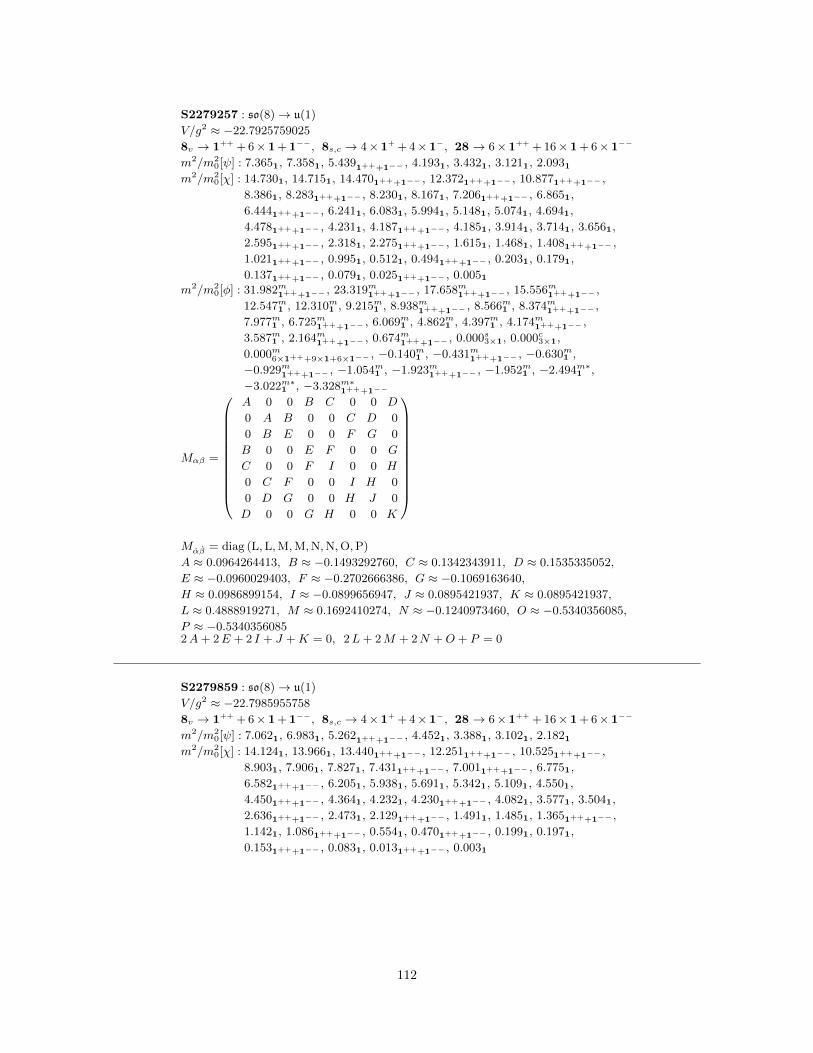
S2279257 : so(8)→ u(1)

V/g2 ≈ −22.7925759025

8v → 1++ + 6× 1 + 1−−, 8s,c → 4× 1+ + 4× 1−, 28 → 6× 1++ + 16× 1 + 6× 1−−

m2/m20[ψ] : 7.3651, 7.3581, 5.4391+++1−− , 4.1931, 3.4321, 3.1211, 2.0931

m2/m20[χ] : 14.7301, 14.7151, 14.4701+++1−− , 12.3721+++1−− , 10.8771+++1−− ,

8.3861, 8.2831+++1−− , 8.2301, 8.1671, 7.2061+++1−− , 6.8651,

6.4441+++1−− , 6.2411, 6.0831, 5.9941, 5.1481, 5.0741, 4.6941,

4.4781+++1−− , 4.2311, 4.1871+++1−− , 4.1851, 3.9141, 3.7141, 3.6561,

2.5951+++1−− , 2.3181, 2.2751+++1−− , 1.6151, 1.4681, 1.4081+++1−− ,

1.0211+++1−− , 0.9951, 0.5121, 0.4941+++1−− , 0.2031, 0.1791,

0.1371+++1−− , 0.0791, 0.0251+++1−− , 0.0051

m2/m20[φ] : 31.982m1+++1−− , 23.319m1+++1−− , 17.658m1+++1−− , 15.556m1+++1−− ,

12.547m1 , 12.310m1 , 9.215m1 , 8.938m1+++1−− , 8.566m1 , 8.374m1+++1−− ,

7.977m1 , 6.725m1+++1−− , 6.069m1 , 4.862m1 , 4.397m1 , 4.174m1+++1−− ,

3.587m1 , 2.164m1+++1−− , 0.674m1+++1−− , 0.000s3×1, 0.000c3×1,

0.000m6×1+++9×1+6×1−− , −0.140m1 , −0.431m1+++1−− , −0.630m1 ,

−0.929m1+++1−− , −1.054m1 , −1.923m1+++1−− , −1.952m1 , −2.494m∗1 ,

−3.022m∗1 , −3.328m∗1+++1−−

Mαβ =

A 0 0 B C 0 0 D

0 A B 0 0 C D 0

0 B E 0 0 F G 0

B 0 0 E F 0 0 G

C 0 0 F I 0 0 H

0 C F 0 0 I H 0

0 D G 0 0 H J 0

D 0 0 G H 0 0 K

Mαβ = diag (L,L,M,M,N,N,O,P)

A ≈ 0.0964264413, B ≈ −0.1493292760, C ≈ 0.1342343911, D ≈ 0.1535335052,

E ≈ −0.0960029403, F ≈ −0.2702666386, G ≈ −0.1069163640,

H ≈ 0.0986899154, I ≈ −0.0899656947, J ≈ 0.0895421937, K ≈ 0.0895421937,

L ≈ 0.4888919271, M ≈ 0.1692410274, N ≈ −0.1240973460, O ≈ −0.5340356085,

P ≈ −0.53403560852A+ 2E + 2 I + J +K = 0, 2L+ 2M + 2N +O + P = 0

S2279859 : so(8)→ u(1)

V/g2 ≈ −22.7985955758

8v → 1++ + 6× 1 + 1−−, 8s,c → 4× 1+ + 4× 1−, 28 → 6× 1++ + 16× 1 + 6× 1−−

m2/m20[ψ] : 7.0621, 6.9831, 5.2621+++1−− , 4.4521, 3.3881, 3.1021, 2.1821

m2/m20[χ] : 14.1241, 13.9661, 13.4401+++1−− , 12.2511+++1−− , 10.5251+++1−− ,

8.9031, 7.9061, 7.8271, 7.4311+++1−− , 7.0011+++1−− , 6.7751,

6.5821+++1−− , 6.2051, 5.9381, 5.6911, 5.3421, 5.1091, 4.5501,

4.4501+++1−− , 4.3641, 4.2321, 4.2301+++1−− , 4.0821, 3.5771, 3.5041,

2.6361+++1−− , 2.4731, 2.1291+++1−− , 1.4911, 1.4851, 1.3651+++1−− ,

1.1421, 1.0861+++1−− , 0.5541, 0.4701+++1−− , 0.1991, 0.1971,

0.1531+++1−− , 0.0831, 0.0131+++1−− , 0.0031

112

m2/m20[φ] : 30.511m1+++1−− , 20.684m1+++1−− , 18.716m1+++1−− , 14.242m1+++1−− ,

12.041m1 , 11.689m1 , 9.342m1 , 9.136m1+++1−− , 8.480m1 , 7.996m1 ,

7.637m1+++1−− , 6.726m1+++1−− , 6.103m1 , 4.673m1 , 4.546m1+++1−− ,

4.246m1 , 3.851m1 , 1.975m1+++1−− , 0.772m1+++1−− , 0.074m1 , 0.000s3×1,

0.000c3×1, 0.000m6×1+++9×1+6×1−− , −0.420m1+++1−− , −0.650m1 ,

−0.955m1+++1−− , −0.989m1 , −1.975m1 , −2.004m1+++1−− , −2.450m∗1 ,

−3.062m∗1 , −3.395m∗1+++1−−

Mαβ = diag (A,A,B,B,C,C,D,D)

Mαβ =

0 0 0 0 0 E 0 F

0 0 0 0 −E 0 −F 0

0 0 0 0 0 G 0 H

0 0 0 0 −G 0 −H 0

0 −E 0 −G 0 0 0 0

E 0 G 0 0 0 0 0

0 −F 0 −H 0 0 0 0

F 0 H 0 0 0 0 0

A ≈ 0.4627041547, B ≈ −0.0321781706, C ≈ −0.0678467269,

D ≈ −0.3626792571, E ≈ 0.3839263486, F ≈ −0.3376757443, G ≈ 0.0960433717,

H ≈ 0.1132550070A+B + C +D = 0

S2291945 : so(8)→ u(1)

V/g2 ≈ −22.9194510184

8c → 3× 1++ + 2× 1 + 3× 1−−, 8v,s → 1+++ + 3× 1+ + 3× 1− + 1−−−,

28 → 3× 1++++ + 6× 1++ + 10× 1 + 6× 1−− + 3× 1−−−−

m2/m20[ψ] : 6.9041++1− , 4.0571++1− , 3.7421++++1−−− , 2.9201++1−

m2/m20[χ] : 13.8081++1− , 10.9671++++++1−−−−− , 9.6261++++++1−−−−− ,

8.1141++1− , 7.4841++++1−−− , 7.4761++++1−−− , 6.2431++1− ,

6.1711++1− , 6.0521++++1−−− , 6.0511++++1−−− , 5.8411++1− ,

4.7711++++1−−− , 4.6071++1− , 4.5071++++++1−−−−− , 4.2821++1− ,

3.6481++++1−−− , 3.1631++1− , 2.1801++++1−−− , 2.1161++1− ,

1.3601++++1−−− , 1.3341++1− , 1.2991++1− , 0.6431++1− ,

0.3911++++1−−− , 0.3161++1− , 0.0771++1− , 0.0651++++1−−− ,

0.0211++1−

m2/m20[φ] : 23.166s1+++++++1−−−−−− , 17.873m1+++++1−−−− , 16.749m1+++++1−−−− ,

12.741m1+++1−− , 10.434m1+++++1−−−− , 9.483m1 , 8.513m1+++1−− , 7.834m1 ,

7.349m1+++++1−−−− , 6.494m1+++1−− , 6.120m1 , 5.826m1+++1−− , 4.471m1 ,

4.250m1 , 3.697m1+++++1−−−− , 2.380m1+++1−− , 1.375m1 , 0.760m1+++1−− ,

0.000s2×1, 0.000c3×1, 0.000m3×1+++++6×1+++4×1+6×1−−+3×1−−−− ,

−0.411m1 , −0.598m1+++1−− , −0.936m1 , −1.142m1+++1−− , −2.258m∗1 ,

−2.404m∗1+++++1−−−− , −2.507m∗1 , −3.022m∗1 , −3.310m∗1+++1−−

Mαβ =

A 0 0 0 0 0 0 0

0 B 0 C 0 −C 0 0

0 0 E 0 D 0 −C 0

0 C 0 E 0 −D 0 0

0 0 D 0 E 0 −C 0

0 −C 0 −D 0 E 0 0

0 0 −C 0 −C 0 B 0

0 0 0 0 0 0 0 A

113

Mαβ = diag (F,F,G, 0, 0,−G,−F,−F)

A ≈ −0.1009265173, B ≈ 0.2071497789, C ≈ −0.1708871490, D ≈ 0.2919626949,

E ≈ −0.0531116308, F ≈ 0.5068828116, G ≈ 0.2279710355A+B + 2E = 0

S2308861 : so(8)→ ∅V/g2 ≈ −23.0886123224

m2/m20[ψ] : 5.7731, 5.4311, 4.9811, 4.2801, 3.8571, 3.8041, 3.5861, 3.0481

m2/m20[χ] : 11.5451, 10.8631, 9.9621, 8.9051, 8.8941, 8.5601, 8.1061, 7.9271,

7.7131, 7.6091, 7.2111, 7.1711, 7.0911, 6.9581, 6.8641, 6.2021, 6.0951,

5.9381, 5.8651, 5.8491, 5.7691, 5.6251, 5.3511, 5.3461, 5.0691, 4.9771,

4.7231, 4.5981, 4.5391, 4.3381, 3.3281, 3.1291, 2.9821, 2.7181, 2.7011,

2.4811, 2.4421, 2.0701, 1.7451, 1.7051, 1.3811, 1.3331, 1.3191, 1.0581,

0.9791, 0.8911, 0.6721, 0.6331, 0.3361, 0.3231, 0.2691, 0.2291, 0.1211,

0.1201, 0.1041, 0.1021

m2/m20[φ] : 19.580m1 , 19.282m1 , 17.057m1 , 16.181m1 , 14.345m1 , 13.480m1 , 11.316m1 ,

11.231m1 , 10.448m1 , 10.129m1 , 9.655m1 , 9.483m1 , 8.773m1 , 8.761m1 , 8.754m1 ,

7.953m1 , 7.471m1 , 6.958m1 , 6.803m1 , 6.791m1 , 6.316m1 , 5.928m1 , 5.816m1 ,

3.228m1 , 2.554m1 , 2.302m1 , 2.127m1 , 1.811m1 , 1.612m1 , 0.000m28×1, −0.260m1 ,

−0.465m1 , −0.632m1 , −0.820m1 , −0.839m1 , −1.191m1 , −1.542m1 , −1.941m1 ,

−1.969m1 , −2.510m∗1 , −2.690m∗1 , −3.093m∗1 , −3.563m∗1

Mαβ = diag (A,B,C,D,E,F,G,H)

Mαβ =

I 0 0 0 J 0 0 0

0 K 0 0 0 L 0 0

0 0 M 0 0 0 N 0

0 0 0 O 0 0 0 P

J 0 0 0 Q 0 0 0

0 L 0 0 0 R 0 0

0 0 N 0 0 0 S 0

0 0 0 P 0 0 0 T

A ≈ 0.4111497551, B ≈ 0.3975580514, C ≈ 0.3644616407, D ≈ −0.0675019851,

E ≈ −0.1854078770, F ≈ −0.2902046795, G ≈ −0.3076408532,

H ≈ −0.3224140524, I ≈ −0.1119387100, J ≈ −0.1717580580,

K ≈ 0.3610424437, L ≈ −0.1891379349, M ≈ −0.1918474986, N ≈ 0.3209577942,

O ≈ 0.3331042804, P ≈ −0.1533814171, Q ≈ −0.3722904062,

R ≈ −0.4012323640, S ≈ 0.1886746776, T ≈ 0.1944875771A+B + C +D + E + F +G+H = 0, I +K +M +O +Q+R+ S + T = 0

S2309630 : so(8)→ ∅V/g2 ≈ −23.0963027021

m2/m20[ψ] : 5.5592×1, 4.5712×1, 3.7732×1, 3.4042×1

m2/m20[χ] : 11.1172×1, 9.1432×1, 8.0702×1, 7.9282×1, 7.5472×1, 7.4092×1,

7.1722×1, 6.8072×1, 5.9882×1, 5.7122×1, 5.6012×1, 5.5582×1, 5.0862×1,

4.6232×1, 4.4902×1, 3.1552×1, 2.8222×1, 2.6022×1, 2.2602×1, 1.6112×1,

1.3942×1, 1.1662×1, 0.9982×1, 0.6592×1, 0.3202×1, 0.2802×1, 0.1262×1,

0.1172×1

114

m2/m20[φ] : 18.925m1 , 17.884m2×1, 16.070m1 , 14.082m1 , 12.151m2×1, 11.266m1 , 10.284m1 ,

10.182m1 , 9.500m2×1, 8.777m1 , 8.176m1 , 7.959m1 , 7.664m2×1, 7.482m1 ,

7.028m1 , 7.021m1 , 6.500m2×1, 5.672m1 , 2.814m2×1, 2.643m1 , 2.080m1 , 1.767m1 ,

1.519m1 , 0.177m1 , 0.000c2×1, 0.000m26×1, −0.460m1 , −0.608m1 , −0.831m2×1,

−1.194m1 , −1.531m1 , −1.963m1 , −1.983m1 , −2.674m∗2×1, −3.166m∗1 ,

−3.619m∗1

Mαβ =

A 0 0 0 0 0 0 B

0 C D 0 0 E F 0

0 D H 0 0 F G 0

0 0 0 I −B 0 0 0

0 0 0 −B A 0 0 0

0 E F 0 0 C D 0

0 F G 0 0 D H 0

B 0 0 0 0 0 0 I

Mαβ = diag (J,K,L,M,−M,−L,−K,−J)

A ≈ 0.2858314530, B ≈ 0.2367208262, C ≈ 0.0832402746, D ≈ 0.1650136180,

E ≈ 0.2472312590, F ≈ 0.0382942934, G ≈ 0.0598504623, H ≈ −0.1633421883,

I ≈ −0.2057295393, J ≈ 0.4439252012, K ≈ 0.4248293983, L ≈ 0.3744302816,

M ≈ 0.0680845443A+ C +H + I = 0

S2335620 : so(8)→ ∅V/g2 ≈ −23.3562003899

m2/m20[ψ] : 8.1051, 7.8281, 7.7191, 7.4081, 3.4701, 3.2161, 3.0321, 2.0291

m2/m20[χ] : 17.7801, 17.7801, 16.2101, 15.6571, 15.4371, 14.8171, 13.7111, 13.7091,

12.0001, 11.9951, 8.5501, 8.5471, 8.5401, 8.5331, 7.4441, 7.4131,

6.9411, 6.5741, 6.5591, 6.4311, 6.0641, 5.8021, 5.7211, 5.1421, 4.9721,

4.9711, 4.9301, 4.4331, 4.1981, 4.0571, 4.0541, 3.7971, 3.5781, 3.5501,

3.3221, 3.0071, 2.8681, 2.1671, 2.1511, 1.8161, 1.5771, 1.3391, 1.2501,

0.8021, 0.7401, 0.6201, 0.5521, 0.3331, 0.2791, 0.1951, 0.1491, 0.0921,

0.0821, 0.0121, 0.0071, 0.0031

m2/m20[φ] : 36.309m1 , 36.309m1 , 31.300m1 , 31.299m1 , 22.830m1 , 22.817m1 , 16.666m1 ,

16.591m1 , 14.892m1 , 14.875m1 , 11.621m1 , 11.590m1 , 11.483m1 , 11.321m1 ,

9.537m1 , 9.372m1 , 8.008m1 , 7.646m1 , 7.031m1 , 7.010m1 , 6.872m1 , 6.009m1 ,

5.561m1 , 5.368m1 , 3.190m1 , 2.685m1 , 1.050m1 , 0.819m1 , 0.000m28×1, −0.204m1 ,

−0.563m1 , −0.670m1 , −0.993m1 , −1.161m1 , −1.237m1 , −1.417m1 , −1.751m1 ,

−2.013m1 , −2.089m1 , −2.271m∗1 , −2.294m∗1 , −2.604m∗1 , −3.503m∗1

Mαβ = diag (A,B,C,D,E,F,G,H)

Mαβ =

I 0 0 J K 0 0 L

0 P M 0 0 N O 0

0 M P 0 0 −O −N 0

J 0 0 I L 0 0 K

K 0 0 L T 0 0 Q

0 N −O 0 0 R S 0

0 O −N 0 0 S R 0

L 0 0 K Q 0 0 T

115

A ≈ 0.4710891271, B ≈ 0.3868019969, C ≈ 0.0944368913, D ≈ 0.0668831950,

E ≈ −0.1733866923, F ≈ −0.1828096356, G ≈ −0.3313498731,

H ≈ −0.3316650094, I ≈ −0.1354057498, J ≈ 0.4401735559, K ≈ 0.0740979279,

L ≈ −0.0003265639, M ≈ 0.3586336577, N ≈ 0.1693983171, O ≈ −0.1158264177,

P ≈ −0.2233797279, Q ≈ 0.2333742217, R ≈ 0.1417084739, S ≈ −0.0726581650,

T ≈ 0.2170770038A+B + C +D + E + F +G+H = 0, I + P +R+ T = 0

S2348985 : so(8)→ ∅V/g2 ≈ −23.4898576606

m2/m20[ψ] : 7.6872×1, 7.1252×1, 3.4122×1, 2.4612×1

m2/m20[χ] : 15.3742×1, 14.6932×1, 14.6922×1, 14.2512×1, 9.4712×1, 9.4432×1,

7.4532×1, 7.4432×1, 6.8242×1, 5.9742×1, 5.8632×1, 5.0182×1, 4.9212×1,

4.6962×1, 4.0162×1, 3.6092×1, 3.5012×1, 3.2652×1, 3.0602×1, 2.6432×1,

1.5822×1, 0.9342×1, 0.5452×1, 0.4192×1, 0.2012×1, 0.1562×1, 0.0992×1,

0.0172×1

m2/m20[φ] : 33.285m1 , 33.285m1 , 22.742m1 , 22.739m1 , 22.172m1 , 22.167m1 , 21.699m1 ,

21.677m1 , 12.921m1 , 11.964m1 , 11.826m1 , 10.300m1 , 9.831m1 , 8.603m1 ,

8.539m1 , 8.490m1 , 8.464m1 , 8.446m1 , 8.416m1 , 8.388m1 , 8.234m1 , 7.670m1 ,

5.545m1 , 5.146m1 , 2.958m1 , 2.642m1 , 1.521m1 , 0.669m1 , 0.146m1 , 0.000m28×1,

−0.369m1 , −0.558m1 , −0.796m1 , −0.937m1 , −1.376m1 , −1.489m1 , −2.168m1 ,

−2.238m1 , −2.272m∗1 , −2.360m∗1 , −2.519m∗1 , −2.642m∗1 , −3.588m∗1

Mαβ =

A 0 B 0 C 0 D 0

0 −A 0 −B 0 −C 0 E

B 0 −A 0 E 0 −C 0

0 −B 0 A 0 −D 0 −CC 0 E 0 −A 0 −B 0

0 −C 0 −D 0 A 0 −BD 0 −C 0 −B 0 A 0

0 E 0 −C 0 −B 0 −A

Mαβ = diag (F,G,H, I, J,K,L,M)

A ≈ −0.0486343144, B ≈ −0.1750236095, C ≈ 0.0751485795,

D ≈ −0.1078302437, E ≈ −0.2808319636, F ≈ 0.4806716467, G ≈ 0.4504401912,

H ≈ 0.3129109970, I ≈ 0.0444819241, J ≈ −0.0084465057, K ≈ −0.1109272540,

L ≈ −0.5837424448, M ≈ −0.5853885547F +G+H + I + J +K + L+M = 0

S2389014 : so(8)→ u(1)

V/g2 ≈ −23.8901476625

8c → 1++ + 6× 1 + 1−−, 8v,s → 4× 1+ + 4× 1−, 28 → 6× 1++ + 16× 1 + 6× 1−−

m2/m20[ψ] : 8.0951++1− , 7.6801++1− , 3.7861++1− , 2.3681++1−

m2/m20[χ] : 16.2781++1− , 16.1891++1− , 15.7981++1− , 15.3591++1− , 10.4221++1− ,

9.9811++1− , 8.0461++1− , 7.9541++1− , 7.5731++1− , 6.9201++1− ,

6.3861++1− , 5.0721++1− , 5.0161++1− , 4.7371++1− , 4.3581++++1−−− ,

3.8991++1− , 3.7461++++1−−− , 3.5231++1− , 3.3411++1− , 2.5581++1− ,

1.6571++1− , 1.1511++1− , 0.4111++1− , 0.3201++1− , 0.3161++++1−−− ,

0.1931++++1−−− , 0.1231++1− , 0.0321++1−

116

m2/m20[φ] : 36.563m1 , 36.561m1 , 26.072m1+++1−− , 24.314m1+++1−− , 22.988m1 ,

22.982m1 , 13.888m1 , 12.925m1 , 12.366m1 , 10.617m1 , 10.358m1 ,

10.236m1+++1−− , 9.506m1+++1−− , 9.366m1 , 9.261m1 , 9.030m1 , 8.903m1 ,

7.694m1 , 5.518m1+++1−− , 3.173m1 , 3.037m1+++1−− , 0.428m1+++1−− ,

0.000c3×1, 0.000m6×1+++12×1+6×1−− , −0.001m1 , −0.466m1+++1−− ,

−0.854m1 , −0.956m1 , −1.197m1+++1−− , −2.154m1 , −2.228m1+++1−− ,

−2.353c∗1+++++1−−−− , −2.985m∗1 , −3.454m∗1

Mαβ =

A 0 B 0 C 0 D 0

0 J 0 E 0 F 0 D

B 0 G 0 H 0 −F 0

0 E 0 I 0 −H 0 C

C 0 H 0 I 0 E 0

0 F 0 −H 0 G 0 −BD 0 −F 0 E 0 J 0

0 D 0 C 0 −B 0 A

Mαβ = diag (K,L,M,N,N,O,P,Q)

A ≈ −0.0764231659, B ≈ 0.0901166727, C ≈ −0.0466379433,

D ≈ −0.2032433828, E ≈ 0.2591302104, F ≈ −0.0371644350,

G ≈ −0.0695227853, H ≈ 0.1933637347, I ≈ 0.0842772023, J ≈ 0.0616687489,

K ≈ 0.5968234492, L ≈ 0.5960863850, M ≈ 0.0681127131, N ≈ 0.0006811279,

O ≈ −0.3172476832, P ≈ −0.4555286177, Q ≈ −0.4896085023A+G+ I + J = 0, K + L+M + 2N +O + P +Q = 0

S2389433 : so(8)→ u(1)

V/g2 ≈ −23.8943375024

8c → 1++ + 6× 1 + 1−−, 8v,s → 4× 1+ + 4× 1−, 28 → 6× 1++ + 16× 1 + 6× 1−−

m2/m20[ψ] : 5.9451++1− , 4.1721++1− , 4.0681++1− , 2.4921++1−

m2/m20[χ] : 11.8901++1− , 8.5851++1− , 8.5571++1− , 8.3451++1− , 8.1361++1− ,

6.8301++++1−−− , 6.0301++1− , 5.9971++1− , 5.3221++1− , 4.9841++1− ,

4.9041++++1−−− , 4.7021++1− , 4.5581++1− , 4.4301++1− , 4.1671++1− ,

3.9481++++1−−− , 3.0301++1− , 2.0761++1− , 1.7701++1− , 1.7271++1− ,

1.1431++1− , 1.0951++++1−−− , 0.8101++1− , 0.3661++1− , 0.2391++1− ,

0.2181++1− , 0.2151++1− , 0.0221++1−

m2/m20[φ] : 19.317m1 , 19.261m1 , 15.521s1+++1−− , 14.511m1+++1−− , 10.507m1 , 9.749m1 ,

8.758m1 , 8.457m1+++1−− , 8.439c1+++++1−−−− , 7.869m1 , 7.821m1 , 7.417m1 ,

6.933s1+++1−− , 6.741m1+++1−− , 4.650m1 , 3.939s1+++1−− , 3.060m1 ,

2.739m1+++1−− , 2.462m1 , 2.055m1 , 0.000c3×1, 0.000m6×1+++12×1+6×1−− ,

−0.165m1 , −0.699m1 , −0.820s1+++1−− , −0.984m1 , −1.004m1 , −1.137m1 ,

−1.693m1+++1−− , −1.827m1+++1−− , −1.998m1 , −2.129m1 , −2.548m∗1 ,

−3.182m∗1

Mαβ =

0 0 0 A B 0 0 C

0 0 A 0 0 B −C 0

0 A 0 0 0 C −B 0

A 0 0 0 C 0 0 B

B 0 0 C 0 0 0 A

0 B C 0 0 0 −A 0

0 −C −B 0 0 −A 0 0

C 0 0 B A 0 0 0

117

Mαβ = diag (D,E,F,G,H, I, J, J)

A ≈ 0.1407733100, B ≈ 0.1294064926, C ≈ 0.2405508145, D ≈ 0.5206803079,

E ≈ 0.4965948264, F ≈ 0.3336264905, G ≈ −0.0267888109, H ≈ −0.1313849282,

I ≈ −0.3343286815, J ≈ −0.4291996021D + E + F +G+H + I + 2 J = 0

S2395245 : so(8)→ ∅V/g2 ≈ −23.9524558813

m2/m20[ψ] : 7.6342×1, 7.2042×1, 3.5322×1, 2.6972×1

m2/m20[χ] : 15.2692×1, 15.1932×1, 15.1922×1, 14.4082×1, 9.0612×1, 9.0332×1,

8.0292×1, 8.0262×1, 7.0642×1, 6.0702×1, 5.9312×1, 5.3932×1, 4.9692×1,

4.7042×1, 4.2362×1, 4.0282×1, 3.8942×1, 3.2352×1, 3.1172×1, 2.3542×1,

1.7712×1, 0.9432×1, 0.7722×1, 0.3952×1, 0.2882×1, 0.1532×1, 0.0602×1,

0.0152×1

m2/m20[φ] : 35.208m1 , 35.207m1 , 23.309m1 , 23.307m1 , 22.631m1 , 22.625m1 , 19.917m1 ,

19.914m1 , 13.253m1 , 13.176m1 , 12.141m1 , 11.849m1 , 10.783m1 , 10.754m1 ,

10.057m1 , 9.088m1 , 8.591m1 , 8.445m1 , 8.370m1 , 8.160m1 , 8.146m1 , 7.874m1 ,

3.922m1 , 2.991m1 , 2.752m1 , 2.486m1 , 2.345m1 , 1.889m1 , 0.000m28×1, −0.099m1 ,

−0.332m1 , −0.714m1 , −0.772m1 , −1.000m1 , −1.032m1 , −1.156m1 , −1.590m1 ,

−1.847m1 , −2.000m1 , −2.228m1 , −2.281m∗1 , −2.549m∗1 , −3.707m∗1

Mαβ = diag (A,B,C,D,E,F,G,H)

Mαβ =

I 0 J 0 K 0 0 0

0 −N 0 L 0 M 0 0

J 0 I 0 0 0 −K 0

0 L 0 −N 0 0 0 M

K 0 0 0 −I 0 −J 0

0 M 0 0 0 N 0 L

0 0 −K 0 −J 0 −I 0

0 0 0 M 0 L 0 N

A ≈ 0.4729017876, B ≈ 0.3618302957, C ≈ 0.2441819466, D ≈ −0.0004494739,

E ≈ −0.1738426254, F ≈ −0.2210770005, G ≈ −0.3410017741,

H ≈ −0.3425431561, I ≈ −0.1245946499, J ≈ 0.3639051016, K ≈ 0.0986278756,

L ≈ −0.2155711099, M ≈ 0.2177802797, N ≈ 0.2184399205A+B + C +D + E + F +G+H = 0

S2411233 : so(8)→ ∅V/g2 ≈ −24.1123340576

m2/m20[ψ] : 7.3392×1, 7.1222×1, 3.7162×1, 2.7532×1

m2/m20[χ] : 15.2222×1, 15.2222×1, 14.6782×1, 14.2432×1, 8.7542×1, 8.7522×1,

8.1052×1, 8.0992×1, 7.4322×1, 5.8662×1, 5.6992×1, 5.5062×1, 5.0052×1,

4.7962×1, 4.4832×1, 4.2312×1, 3.9832×1, 3.0142×1, 2.9202×1, 1.9992×1,

1.5132×1, 1.0592×1, 0.9212×1, 0.4662×1, 0.1902×1, 0.1792×1, 0.0222×1,

0.0112×1

118

m2/m20[φ] : 35.548m1 , 35.548m1 , 23.812m1 , 23.809m1 , 22.648m1 , 22.643m1 , 19.313m1 ,

19.299m1 , 12.759m1 , 12.707m1 , 11.334m1 , 11.245m1 , 10.892m1 , 10.116m1 ,

9.880m1 , 8.926m1 , 8.706m1 , 8.580m1 , 7.913m1 , 7.762m1 , 6.887m1 , 6.763m1 ,

3.917m1 , 3.864m1 , 3.497m1 , 2.960m1 , 1.794m1 , 1.247m1 , 0.570m1 , 0.000m28×1,

−0.070m1 , −0.312m1 , −0.368m1 , −0.592m1 , −0.797m1 , −0.994m1 , −1.745m1 ,

−2.011m1 , −2.184m1 , −2.249m1 , −2.826m∗1 , −2.950m∗1 , −3.800m∗1

Mαβ =

A 0 0 0 0 0 0 B

0 J C 0 0 D E 0

0 C I 0 0 F D 0

0 0 0 G H 0 0 0

0 0 0 H G 0 0 0

0 D F 0 0 I C 0

0 E D 0 0 C J 0

B 0 0 0 0 0 0 A

Mαβ = diag (K,L,M,N,−N,−M,−L,−K)

A ≈ −0.1607266942, B ≈ 0.1920968123, C ≈ 0.1639190992, D ≈ −0.1550182727,

E ≈ −0.2888908796, F ≈ −0.0450471630, G ≈ 0.1013403534, H ≈ 0.2632954838,

I ≈ 0.1221721471, J ≈ −0.0627858063, K ≈ 0.5392180686, L ≈ 0.5358811100,

M ≈ 0.1749514161, N ≈ 0.1138777794A+G+ I + J = 0

S2416856 : so(8)→ ∅V/g2 ≈ −24.1685628157

m2/m20[ψ] : 5.4632×1, 4.2366×1

m2/m20[χ] : 10.9252×1, 8.4726×1, 7.1586×1, 6.9086×1, 6.8572×1, 5.5722×1,

5.2402×1, 4.8686×1, 2.9316×1, 2.9282×1, 1.1166×1, 0.6792×1, 0.6042×1,

0.1256×1

m2/m20[φ] : 16.580m1 , 14.958m3×1, 14.169m2×1, 12.149m3×1, 11.786c2×1, 11.314m3×1,

10.795m2×1, 8.558m3×1, 7.646m1 , 6.897m3×1, 4.272m2×1, 3.123m3×1, 0.000s7×1,

0.000m21×1, −0.044m2×1, −0.273c1, −0.492m3×1, −1.074m2×1, −2.361m∗1 ,

−2.524m∗3×1, −3.278m∗2×1

Mαβ =

A 0 0 0 0 0 0 B

0 C 0 0 0 0 0 0

0 0 D 0 0 E 0 0

0 0 0 F G 0 0 0

0 0 0 G H 0 0 0

0 0 E 0 0 I 0 0

0 0 0 0 0 0 C 0

B 0 0 0 0 0 0 J

Mαβ = diag (K,K,K, 0, 0,−K,−K,−K)

A ≈ 0.3980992991, B ≈ 0.0004883256, C ≈ −0.2401462630, D ≈ −0.0785536156,

E ≈ 0.2756840142, F ≈ −0.0793994204, G ≈ −0.2751956886, H ≈ 0.2394969291,

I ≈ 0.2386511243, J ≈ −0.2380017904, K ≈ 0.4410451252A− F −H + J = 0, B − E −G = 0, C +H + I + J = 0, D − F −H + I = 0,

3F +H − 2 I − 2 J = 0

S2416940 : so(8)→ ∅

119

V/g2 ≈ −24.1694054574

m2/m20[ψ] : 5.4622×1, 4.2722×1, 4.2184×1

m2/m20[χ] : 10.9242×1, 8.5432×1, 8.4364×1, 7.3082×1, 7.1624×1, 6.8862×1,

6.8592×1, 6.8394×1, 5.5902×1, 5.2202×1, 4.8694×1, 4.8652×1, 3.0054×1,

2.9232×1, 2.7712×1, 1.1222×1, 1.1134×1, 0.6812×1, 0.6042×1, 0.1324×1,

0.1152×1

m2/m20[φ] : 16.697m1 , 15.342m2×1, 14.407m1 , 14.214m1 , 13.845m1 , 12.176m2×1, 12.108m1 ,

12.053c1, 11.493c1, 11.368m2×1, 11.164m1 , 10.938m1 , 10.605m1 , 8.754m1 ,

8.435m2×1, 7.648m1 , 6.965m2×1, 6.763m1 , 4.332m1 , 4.204m1 , 3.252m2×1,

2.865m1 , 0.052m1 , 0.000s2×1, 0.000c2×1, 0.000m24×1, −0.113m1 , −0.252c1,

−0.425m1 , −0.517m2×1, −0.927m1 , −1.236m1 , −2.263m∗1 , −2.357m∗1 ,

−2.654m∗2×1, −3.221m∗1 , −3.345m∗1

Mαβ =

A 0 0 0 0 0 0 B

0 C 0 0 0 0 D 0

0 0 F 0 0 E 0 0

0 0 0 G −B 0 0 0

0 0 0 −B A 0 0 0

0 0 E 0 0 F 0 0

0 D 0 0 0 0 C 0

B 0 0 0 0 0 0 G

Mαβ = diag (H, I, I, J,−J,−I,−I,−H)

A ≈ 0.3482168694, B ≈ −0.1725699771, C ≈ 0.0866895502, D ≈ −0.3108177150,

E ≈ 0.0106970764, F ≈ −0.2401590096, G ≈ −0.1947474100, H ≈ 0.4441672651,

I ≈ 0.4392145120, J ≈ 0.0079201454A+ C + F +G = 0

S2420275 : so(8)→ ∅V/g2 ≈ −24.2027521576

m2/m20[ψ] : 6.8152×1, 5.9732×1, 3.6322×1, 2.7562×1

m2/m20[χ] : 13.6292×1, 11.9452×1, 11.4752×1, 11.4662×1, 8.0432×1, 7.9162×1,

7.2642×1, 6.8832×1, 6.7902×1, 5.6732×1, 5.5132×1, 5.4272×1, 5.0942×1,

4.6902×1, 4.3692×1, 3.7912×1, 3.3702×1, 3.1602×1, 2.7772×1, 2.3712×1,

1.9112×1, 1.1782×1, 0.7762×1, 0.4582×1, 0.3662×1, 0.1032×1, 0.0852×1,

0.0552×1

m2/m20[φ] : 25.183m1 , 25.165m1 , 18.232m1 , 18.183m1 , 17.657m1 , 17.574m1 , 15.676m1 ,

15.644m1 , 13.852m1 , 13.709m1 , 11.621m1 , 11.040m1 , 10.788m1 , 10.348m1 ,

10.237m1 , 9.095m1 , 8.720m1 , 7.913m1 , 7.251m1 , 7.247m1 , 6.913m1 , 6.705m1 ,

4.056m1 , 2.567m1 , 2.511m1 , 2.297m1 , 2.165m1 , 1.874m1 , 0.843m1 , 0.000m28×1,

−0.262m1 , −0.681m1 , −0.826m1 , −0.870m1 , −0.963m1 , −1.032m1 , −1.245m1 ,

−1.460m1 , −1.521m1 , −2.020m1 , −2.503m∗1 , −2.934m∗1 , −3.835m∗1

Mαβ =

A B 0 C D 0 E F

B G 0 H I 0 J E

0 0 K 0 0 L 0 0

C H 0 M N 0 −I −DD I 0 N M 0 −H −C0 0 L 0 0 K 0 0

E J 0 −I −H 0 G B

F E 0 −D −C 0 B A

120

Mαβ = diag (O,P,Q,R,−R,−Q,−P,−O)

A ≈ 0.1119856002, B ≈ 0.0283513918, C ≈ 0.1945425226, D ≈ −0.1085760842,

E ≈ −0.1172874577, F ≈ −0.1643961637, G ≈ 0.0765105834, H ≈ 0.0461848091,

I ≈ −0.0252238773, J ≈ 0.3236154198, K ≈ −0.1698958774, L ≈ −0.1235409988,

M ≈ −0.0186003063, N ≈ −0.2541321580, O ≈ 0.4950321172, P ≈ 0.4933756945,

Q ≈ 0.2661242354, R ≈ 0.0897637420A+G+K +M = 0

S2423138 : so(8)→ ∅V/g2 ≈ −24.2313815582

m2/m20[ψ] : 6.6552×1, 5.7242×1, 3.6622×1, 2.8492×1

m2/m20[χ] : 13.3112×1, 11.4472×1, 10.7162×1, 10.7062×1, 7.9702×1, 7.8202×1,

7.3242×1, 6.7712×1, 6.6592×1, 5.6982×1, 5.6692×1, 5.5232×1, 4.9602×1,

4.6972×1, 4.3902×1, 3.8782×1, 3.2652×1, 3.0952×1, 2.7452×1, 2.3722×1,

1.8712×1, 1.2072×1, 0.7892×1, 0.4552×1, 0.4122×1, 0.1182×1, 0.0712×1,

0.0692×1

m2/m20[φ] : 23.094m1 , 23.066m1 , 17.360m1 , 17.271m1 , 16.810m1 , 16.679m1 , 14.907m1 ,

14.854m1 , 14.853m1 , 14.713m1 , 11.154m1 , 11.146m1 , 10.644m1 , 10.456m1 ,

10.310m1 , 9.184m1 , 8.616m1 , 7.887m1 , 7.139m1 , 7.124m1 , 6.448m1 , 6.266m1 ,

4.053m1 , 2.651m1 , 2.433m1 , 2.365m1 , 2.097m1 , 1.968m1 , 0.543m1 , 0.510m1 ,

0.000m28×1, −0.535m1 , −0.643m1 , −0.837m1 , −0.951m1 , −1.061m1 ,

−1.169m1 , −1.444m1 , −1.629m1 , −1.814m1 , −2.621m∗1 , −3.032m∗1 ,

−3.952m∗1

Mαβ =

A 0 0 B C 0 0 D

0 E 0 0 0 0 F 0

0 0 G 0 0 H 0 0

B 0 0 I J 0 0 −CC 0 0 J I 0 0 −B0 0 H 0 0 G 0 0

0 F 0 0 0 0 E 0

D 0 0 −C −B 0 0 A

Mαβ = diag (K,L,M,N,−N,−M,−L,−K)

A ≈ 0.0994475389, B ≈ −0.2028727698, C ≈ −0.0983788381, D ≈ 0.2135515478,

E ≈ 0.0649009503, F ≈ −0.3631285140, G ≈ −0.1668471487, H ≈ 0.1131064798,

I ≈ 0.0024986595, J ≈ 0.2533882346, K ≈ 0.4908385195, L ≈ 0.4891041585,

M ≈ 0.2686316423, N ≈ 0.1018584499A+ E +G+ I = 0

S2435197 : so(8)→ u(1)

V/g2 ≈ −24.3519754626

8v,s,c → 1++ + 2× 1+ + 2× 1 + 2× 1− + 1−−,

28 → 2× 1+++ + 3× 1++ + 6× 1+ + 6× 1 + 6× 1− + 3× 1−− + 2× 1−−−

m2/m20[ψ] : 5.7571, 4.6241++1− , 4.1491, 3.9741++1− , 3.9421+++1−−

121

m2/m20[χ] : 11.5141, 9.2481++1− , 8.4291++++1−−− , 8.2981, 7.9741+++1−− ,

7.9481++1− , 7.8831+++1−− , 7.7901, 7.6951++1− , 6.3861,

5.8581+++1−− , 5.8411++1− , 5.5481, 5.4851, 5.3401++++1−−− ,

4.9441++1− , 4.3241+++++1−−−− , 4.2361+++1−− , 4.1861++1− , 3.6871,

3.4751, 2.3341++1− , 2.1961+++1−− , 2.1241++++1−−− , 1.3331++1− ,

1.0951, 0.8881++1− , 0.7621, 0.6551+++1−− , 0.4831+++1−− , 0.3771,

0.1861++1− , 0.0981, 0.0711++++1−−−

m2/m20[φ] : 16.632m1++1− , 16.612m1 , 16.504m1+++1−− , 15.290m1+++++1−−−− ,

12.329m1 , 11.470m1++1− , 10.312m1++++1−−− , 10.119m1+++1−− , 8.271m1 ,

6.337m1++1− , 5.758m1+++1−− , 4.885m1 , 3.898m1+++1−− , 3.080m1++++1−−− ,

3.002m1++1− , 2.986m1 , 2.924m1+++1−− , 0.000s2×1, 0.000c2×1,

0.000m2×1++++3×1+++6×1++1+6×1−+3×1−−+2×1−−− ,

−0.108m1+++++1−−−− , −0.277m1 , −0.295m1++1− , −0.512m1+++1−− ,

−1.518m1++1− , −1.678m1 , −2.054m1 , −2.349m∗1 , −3.360m∗1+++1−−

Mαβ =

A 0 0 0 0 0 B C

0 A 0 0 0 0 C −B0 0 D 0 0 0 0 0

0 0 0 E 0 0 0 0

0 0 0 0 F 0 0 0

0 0 0 0 0 F 0 0

B C 0 0 0 0 G 0

C −B 0 0 0 0 0 G

Mαβ = diag (H,H, I, J,K,K,L,L)

A ≈ 0.0308767072, B ≈ 0.2999587195, C ≈ −0.0009364452, D ≈ 0.3972388582,

E ≈ −0.1818372170, F ≈ −0.2924269629, G ≈ 0.1538494351, H ≈ 0.4785280956,

I ≈ 0.4682662750, J ≈ −0.1308111656, K ≈ −0.2680297590, L ≈ −0.37922589132A+D + E + 2F + 2G = 0, 2H + I + J + 2K + 2L = 0

S2435907 : so(8)→ ∅V/g2 ≈ −24.3590751033

m2/m20[ψ] : 5.7021, 4.5922×1, 4.3531, 4.1681, 4.0152×1, 3.8541

m2/m20[χ] : 11.4051, 9.1832×1, 8.7061, 8.5312×1, 8.3371, 8.0292×1, 7.9871, 7.9201,

7.7591, 7.7071, 7.6752×1, 6.2671, 6.0431, 5.7312×1, 5.7011, 5.6281,

5.5922×1, 5.4251, 4.9822×1, 4.6611, 4.6101, 4.5281, 4.3972×1, 4.2221,

3.6221, 3.5721, 2.5002×1, 2.4771, 2.0772×1, 1.8811, 1.2852×1, 1.0981,

0.9282×1, 0.7721, 0.7501, 0.7141, 0.6131, 0.3871, 0.3441, 0.1982×1,

0.1001, 0.0772×1

m2/m20[φ] : 16.548m1 , 16.411m1 , 16.364m1 , 16.357m2×1, 15.777m1 , 15.656m1 , 12.591m1 ,

11.921m2×1, 10.922m1 , 10.221m2×1, 9.645m1 , 8.172m1 , 6.506m2×1, 6.317m1 ,

5.959m1 , 4.977m1 , 4.804m1 , 4.045m2×1, 3.568m1 , 3.467m1 , 3.192m1 , 2.663m2×1,

2.433m1 , 0.123m1 , 0.000s2×1, 0.000c2×1, 0.000m24×1, −0.331m1 , −0.336m2×1,

−0.513m1 , −0.526m1 , −1.623m2×1, −1.625m1 , −2.185m1 , −2.505m∗1 ,

−3.304m∗1 , −3.389m∗1

122

Mαβ =

A 0 0 0 0 0 B 0

0 A 0 0 0 0 0 −B0 0 C 0 0 0 0 0

0 0 0 D 0 0 0 0

0 0 0 0 E 0 0 0

0 0 0 0 0 F 0 0

B 0 0 0 0 0 G 0

0 −B 0 0 0 0 0 G

Mαβ = diag (H,H, I, J,K,L,M,M)

A ≈ 0.1676492049, B ≈ −0.2969221731, C ≈ −0.2875375626,

D ≈ −0.2906963603, E ≈ 0.3968438486, F ≈ −0.1874437306, G ≈ 0.0167676976,

H ≈ 0.3855657509, I ≈ 0.3275912940, J ≈ 0.2053691968, K ≈ 0.1180272319,

L ≈ −0.4661073310, M ≈ −0.47800594672A+ C +D + E + F + 2G = 0, 2H + I + J +K + L+ 2M = 0

S2440304 : so(8)→ ∅V/g2 ≈ −24.4030450895

m2/m20[ψ] : 9.3452×1, 7.9512×1, 4.1472×1, 2.5682×1

m2/m20[χ] : 22.3722×1, 18.6892×1, 15.9022×1, 15.6142×1, 13.6862×1, 9.8552×1,

9.8062×1, 9.1512×1, 8.6032×1, 8.2932×1, 7.7072×1, 5.6022×1, 5.1362×1,

4.5862×1, 4.5342×1, 4.1812×1, 3.8252×1, 3.3542×1, 2.5142×1, 1.9062×1,

1.4632×1, 1.3132×1, 1.0562×1, 0.5352×1, 0.2852×1, 0.0992×1, 0.0232×1,

0.0052×1

m2/m20[φ] : 45.243m1 , 45.243m1 , 41.008m1 , 41.007m1 , 25.948m1 , 25.948m1 , 17.937m1 ,

17.902m1 , 17.339m1 , 17.322m1 , 13.922m1 , 13.879m1 , 13.559m1 , 13.516m1 ,

9.221m1 , 8.886m1 , 8.648m1 , 8.558m1 , 7.934m1 , 7.658m1 , 6.865m1 , 5.869m1 ,

5.243m1 , 5.142m1 , 4.165m1 , 3.935m1 , 3.018m1 , 1.656m1 , 1.617m1 , 1.369m1 ,

0.000c4×1, 0.000m24×1, −0.393m1 , −0.404m1 , −0.545m1 , −0.683m1 ,

−0.773m1 , −0.942m1 , −1.312m1 , −2.231m1 , −2.680m∗1 , −3.047m∗1 ,

−3.110m∗1 , −3.140m∗1

Mαβ = diag (A,A,B,B,C,C,D,D)

Mαβ =

E 0 0 F 0 0 0 G

0 H I 0 0 0 J 0

0 I K 0 0 0 L 0

F 0 0 M 0 0 0 N

0 0 0 0 O 0 0 0

0 0 0 0 0 P 0 0

0 J L 0 0 0 Q 0

G 0 0 N 0 0 0 R

A ≈ 0.4377758063, B ≈ 0.0673680823, C ≈ −0.1169335751, D ≈ −0.3882103135,

E ≈ 0.4303790047, F ≈ −0.2906276188, G ≈ 0.0003507433, H ≈ 0.3375100787,

I ≈ −0.3631925843, J ≈ −0.1353698791, K ≈ −0.0628526132, L ≈ 0.2011229348,

M ≈ −0.0083253507, N ≈ −0.3029467502, O ≈ −0.1594355513,

P ≈ 0.0451604713, Q ≈ −0.3844099898, R ≈ −0.1980260497A+B + C +D = 0, E +H +K +M +O + P +Q+R = 0

S2447241 : so(8)→ ∅

123

V/g2 ≈ −24.4724158128

m2/m20[ψ] : 11.4631, 11.3541, 5.6651, 5.5851, 4.3711, 3.8181, 2.9651, 2.8191

m2/m20[χ] : 22.9251, 22.7081, 21.9471, 21.9471, 18.6001, 18.6001, 15.9241, 15.9241,

11.3301, 11.1701, 10.6821, 10.6791, 9.3501, 9.3491, 8.7431, 7.7631,

7.7571, 7.6361, 7.2961, 7.2951, 6.2731, 6.1151, 5.9311, 5.6391, 5.6381,

5.6181, 5.0191, 5.0051, 4.2791, 4.2561, 3.6401, 3.6321, 3.1911, 3.1771,

2.7441, 2.5441, 2.3231, 2.3061, 2.1541, 2.0631, 1.5841, 1.4361, 1.3771,

1.3411, 1.2841, 1.1761, 0.7721, 0.6961, 0.3641, 0.3601, 0.2021, 0.1791,

0.1691, 0.0861, 0.0841, 0.0811

m2/m20[φ] : 54.987m1 , 54.987m1 , 30.221m1 , 30.221m1 , 24.399m1 , 24.398m1 , 20.523m1 ,

20.486m1 , 19.343m1 , 19.327m1 , 15.178m1 , 15.176m1 , 11.652m1 , 11.651m1 ,

10.914m1 , 10.905m1 , 8.444m1 , 8.345m1 , 8.004m1 , 7.819m1 , 7.359m1 , 6.798m1 ,

6.186m1 , 5.726m1 , 5.051m1 , 5.032m1 , 4.280m1 , 0.374m1 , 0.000m28×1, −0.173m1 ,

−0.431m1 , −0.597m1 , −0.996m1 , −1.019m1 , −2.249m1 , −2.352m∗1 ,

−2.410m∗1 , −2.674m∗1 , −2.738m∗1 , −2.764m∗1 , −2.807m∗1 , −2.858m∗1 ,

−3.155m∗1

Mαβ = diag (A,B,C,D,E,F,G,H)

Mαβ =

I J 0 0 K L 0 0

J I 0 0 L K 0 0

0 0 P M 0 0 N O

0 0 M P 0 0 −O −NK L 0 0 Q R 0 0

L K 0 0 R Q 0 0

0 0 N −O 0 0 S T

0 0 O −N 0 0 T S

A ≈ 0.6404352227, B ≈ 0.1858446034, C ≈ −0.0482481217, D ≈ −0.0483576301,

E ≈ −0.1310906221, F ≈ −0.1315915662, G ≈ −0.2334182851,

H ≈ −0.2335736008, I ≈ 0.2177721733, J ≈ 0.0461680934, K ≈ 0.1839370278,

L ≈ 0.0175974223, M ≈ −0.1831323896, N ≈ −0.0317868129,

O ≈ −0.0022022059, P ≈ 0.2075086049, Q ≈ 0.2455185044, R ≈ −0.0360939527,

S ≈ −0.6707992826, T ≈ −0.0002129779A+B + C +D + E + F +G+H = 0, I + P +Q+ S = 0

S2457396 : so(8)→ u(1)

V/g2 ≈ −24.5739699654

8v,s,c → 2× 1+ + 4× 1 + 2× 1−, 28 → 1++ + 8× 1+ + 10× 1 + 8× 1− + 1−−

m2/m20[ψ] : 11.0661, 10.9471, 4.4781++1− , 4.2151, 4.0161++1− , 3.1251

m2/m20[χ] : 22.1321, 21.8951, 19.0871, 19.0871, 17.3841++1− , 17.3841++1− ,

10.2441, 10.2431, 8.9551++1− , 8.4311, 8.0331++1− , 6.5901++1− ,

6.5241++1− , 6.2731, 6.2511, 6.2491, 6.1841, 5.9971, 5.6751++1− ,

5.5931++1− , 5.1451+++1−− , 5.1151+++1−− , 2.8781, 2.5421, 2.4611,

1.9901++1− , 1.8721++1− , 1.5881, 1.5031++1− , 1.4591, 1.3941++1− ,

1.2211+++1−− , 0.9631, 0.7531+++1−− , 0.1831++1− , 0.1691, 0.1181,

0.0971++1−

124

m2/m20[φ] : 52.351m1 , 52.350m1 , 22.915m1 , 22.895m1 , 20.040m1++1− , 20.026m1++1− ,

17.964m1 , 17.918m1 , 16.934m1+++1−− , 16.916m1+++1−− , 8.500m1 , 8.338m1 ,

8.125m1 , 7.707m1 , 7.552m1++1− , 7.355m1++1− , 6.453m1++1− ,

5.099m1+++1−− , 4.200m1 , 1.036m1 , 0.187m1++1− , 0.000s2×1,

0.000m1+++8×1++7×1+8×1−+1−− , −0.059m1 , −0.542m1 , −1.297m1+++1−− ,

−2.346m∗1++1− , −2.753m∗1 , −2.838m∗1++1− , −2.990m∗1+++1−− , −3.064m∗1 ,

−3.287m∗1

Mαβ =

A 0 B 0 0 C 0 D

0 −A 0 E F 0 G 0

B 0 A 0 0 D 0 C

0 E 0 −A −G 0 −F 0

0 F 0 −G −A 0 −E 0

C 0 D 0 0 A 0 B

0 G 0 −F −E 0 −A 0

D 0 C 0 0 B 0 A

Mαβ = diag (H, I, J, J,K,L,L,M)

A ≈ −0.0572996339, B ≈ −0.0505394209, C ≈ 0.0977028842,

D ≈ −0.0985353033, E ≈ −0.1651386887, F ≈ 0.2141529709, G ≈ 0.2133205519,

H ≈ 0.6703016862, I ≈ 0.6699978792, J ≈ −0.0195739365, K ≈ −0.0528282731,

L ≈ −0.3827530702, M ≈ −0.48281727912A+B − E = 0, C +D + F −G = 0, H + I + 2 J +K + 2L+M = 0

S2476056 : so(8)→ ∅V/g2 ≈ −24.7605602545

m2/m20[ψ] : 10.5151, 10.4271, 8.5511, 8.4411, 4.1911, 3.8541, 2.4021, 2.2951

m2/m20[χ] : 24.7501, 24.7501, 21.0301, 20.8551, 17.1021, 16.9781, 16.9771, 16.8831,

15.4701, 15.4691, 10.8531, 10.8521, 10.1571, 10.1561, 10.0181, 10.0141,

9.3971, 9.3951, 8.3811, 8.0041, 8.0031, 7.7071, 5.9311, 5.8081, 5.2681,

5.2011, 4.8041, 4.6461, 4.5891, 4.5011, 3.9771, 3.9631, 3.8641, 3.8571,

3.0691, 3.0151, 2.4771, 2.4611, 2.1491, 1.8511, 1.5951, 1.5461, 1.4131,

1.3631, 1.2021, 1.0951, 0.3361, 0.2891, 0.2281, 0.1861, 0.0801, 0.0381,

0.0331, 0.0281, 0.0081, 0.0081

m2/m20[φ] : 49.784m1 , 49.784m1 , 45.264m1 , 45.264m1 , 29.576m1 , 29.575m1 , 18.865m1 ,

18.836m1 , 17.598m1 , 17.567m1 , 16.856m1 , 16.854m1 , 15.702m1 , 15.686m1 ,

9.193m1 , 9.004m1 , 8.514m1 , 8.496m1 , 8.250m1 , 7.883m1 , 7.557m1 , 5.889m1 ,

5.459m1 , 5.398m1 , 5.202m1 , 2.720m1 , 2.504m1 , 2.136m1 , 1.956m1 , 0.326m1 ,

0.000m28×1, −0.152m1 , −0.570m1 , −0.908m1 , −1.024m1 , −1.424m1 ,

−1.521m1 , −1.528m1 , −2.150m1 , −2.285m∗1 , −2.592m∗1 , −2.842m∗1 ,

−3.249m∗1

Mαβ =

A B C D E F G H

B I J K L M −H N

C J T O P Q −E L

D K O R Q S −F M

E L P Q T O −C J

F M Q S O R −D K

G −H −E −F −C −D A −BH N L M J K −B U

Mαβ = diag (V,W,X,Y,Z,A′,B′,C′)

125

A ≈ 0.2050584788, B ≈ −0.0367592817, C ≈ −0.0889877312,

D ≈ −0.1557128933, E ≈ 0.0030886527, F ≈ 0.1425124437, G ≈ 0.1244922293,

H ≈ −0.0549990498, I ≈ 0.0327774559, J ≈ −0.0455938157, K ≈ 0.0819800674,

L ≈ −0.0432985503, M ≈ −0.0432092942, N ≈ −0.0467099694,

O ≈ 0.0159049152, P ≈ 0.1896074901, Q ≈ −0.0214357193, R ≈ −0.0919661879,

S ≈ −0.2515945228, T ≈ −0.1458697468, U ≈ 0.0327774559, V ≈ 0.4703422876,

W ≈ 0.4574947510, X ≈ 0.3031517077, Y ≈ 0.0665528681, Z ≈ 0.0446060730,

A′ ≈ −0.0617835199, B′ ≈ −0.6400427901, C′ ≈ −0.64032137752A+ I + 2R+ 2T + U = 0, A′ +B′ + C′ + V +W +X + Y + Z = 0

S2482062 : so(8)→ u(1)

V/g2 ≈ −24.8206272291

8v,s,c → 2× 1+ + 4× 1 + 2× 1−, 28 → 1++ + 8× 1+ + 10× 1 + 8× 1− + 1−−

m2/m20[ψ] : 9.6241, 9.6221, 8.3651++1− , 4.0151, 3.9251, 2.5471++1−

m2/m20[χ] : 23.1801++1− , 19.2481, 19.2441, 16.7311++1− , 15.9651+++1−− ,

14.6441, 14.6431, 10.1461++1− , 9.2901, 9.2831, 8.9771++1− ,

8.9181++1− , 8.7651+++1−− , 8.0301, 7.8491, 5.6511, 5.5351,

5.0941++1− , 5.0631++1− , 4.7961, 4.4001, 4.1201++1− , 3.7531++1− ,

3.3061, 2.8251++1− , 2.2931+++1−− , 2.1551, 1.7241, 1.5541++1− ,

1.4301, 0.9371, 0.8391, 0.3261++1− , 0.2361++1− , 0.0611,

0.0521+++1−− , 0.0121, 0.0111++1−

m2/m20[φ] : 45.485m1+++1−− , 43.501m1 , 43.501m1 , 27.240m1++1− , 18.200m1+++1−− ,

17.653m1 , 17.647m1 , 16.163m1++1− , 14.486m1 , 14.373m1 , 9.108m1++1− ,

8.646m1 , 7.995m1 , 7.482m1 , 6.936m1+++1−− , 6.387m1 , 6.126m1++1− , 4.786m1 ,

2.111m1++1− , 1.316m1+++1−− , 0.239m1 , 0.000s2×1, 0.000c1,

0.000m1+++8×1++6×1+8×1−+1−− , −0.061m1++1− , −0.468m1 ,

−0.654m1+++1−− , −0.968m1++1− , −1.051m1 , −1.754m1 , −2.519m∗1++1− ,

−2.724m∗1 , −3.520m∗1

Mαβ = diag (A,B,B,C,D,E,F,F)

Mαβ =

N 0 G 0 H 0 I 0

0 J 0 K 0 L 0 M

G 0 N 0 −I 0 −H 0

0 K 0 J 0 M 0 L

H 0 −I 0 O 0 P 0

0 L 0 M 0 Q 0 R

I 0 −H 0 P 0 O 0

0 M 0 L 0 R 0 Q

A ≈ 0.5587282338, B ≈ 0.1783615918, C ≈ 0.0739338706, D ≈ −0.1040710220,

E ≈ −0.1480661340, F ≈ −0.3686240660, G ≈ 0.3950136640, H ≈ 0.1980851804,

I ≈ 0.0008987200, J ≈ 0.1866053352, K ≈ −0.4057602543, L ≈ 0.1533569260,

M ≈ 0.0456269744, N ≈ 0.1758587449, O ≈ −0.2721455650, P ≈ −0.0581061873,

Q ≈ −0.0903185151, R ≈ −0.2399332371A+ 2B + C +D + E + 2F = 0, G+K − 2N + P − 2Q−R = 0,

H + I − L−M = 0, J +N − P + 2Q+R = 0, O + P −Q−R = 0

S2484339 : so(8)→ ∅V/g2 ≈ −24.8433938062

m2/m20[ψ] : 7.1301, 6.4181, 5.5421, 5.5231, 3.7051, 3.5411, 3.2121, 2.5111

126

m2/m20[χ] : 14.2601, 12.8361, 12.2281, 12.2261, 11.0831, 11.0461, 9.1891, 9.1881,

8.6491, 8.6151, 7.4091, 7.3781, 7.1971, 7.0811, 6.7421, 6.5881, 6.4241,

6.1601, 6.1211, 5.8171, 5.6561, 5.5911, 5.3581, 5.0631, 5.0211, 4.8641,

4.7261, 4.5961, 4.4661, 4.4261, 3.9871, 3.9291, 3.5491, 3.4941, 3.3751,

2.7761, 2.4401, 2.4291, 2.0961, 2.0051, 1.6231, 1.6221, 1.4641, 1.1921,

0.8431, 0.8061, 0.6541, 0.6421, 0.4061, 0.2601, 0.2471, 0.1921, 0.0831,

0.0691, 0.0291, 0.0081

m2/m20[φ] : 24.057m1 , 24.041m1 , 21.057m1 , 21.002m1 , 16.372m1 , 16.258m1 , 13.796m1 ,

13.036m1 , 12.146m1 , 11.673m1 , 11.389m1 , 10.244m1 , 10.022m1 , 9.221m1 ,

8.457m1 , 8.145m1 , 7.965m1 , 7.858m1 , 7.682m1 , 6.432m1 , 5.510m1 , 5.254m1 ,

4.841m1 , 4.465m1 , 3.687m1 , 3.260m1 , 2.378m1 , 1.525m1 , 1.115m1 , 0.754m1 ,

0.000m28×1, −0.180m1 , −0.648m1 , −0.690m1 , −0.935m1 , −1.087m1 ,

−1.181m1 , −1.703m1 , −1.927m1 , −2.171m1 , −2.528m∗1 , −3.229m∗1 ,

−3.240m∗1

Mαβ =

A 0 B 0 C 0 D 0

0 E 0 F 0 G 0 H

B 0 I 0 J 0 K 0

0 F 0 L 0 M 0 N

C 0 J 0 O 0 P 0

0 G 0 M 0 Q 0 R

D 0 K 0 P 0 S 0

0 H 0 N 0 R 0 T

Mαβ = diag (U,V,W,X,Y,Z,A′,B′)

A ≈ 0.1933192915, B ≈ 0.0591442646, C ≈ −0.1388011249, D ≈ −0.2292854103,

E ≈ 0.1192357229, F ≈ 0.0531792277, G ≈ −0.3687744244, H ≈ 0.0423029778,

I ≈ −0.3197978662, J ≈ −0.0085284847, K ≈ −0.0292493283,

L ≈ −0.3145748162, M ≈ −0.0366264349, N ≈ 0.0589633052,

O ≈ −0.1289425513, P ≈ 0.0506324741, Q ≈ 0.1657043109, R ≈ 0.0690943203,

S ≈ −0.0199376540, T ≈ 0.3049935623, U ≈ 0.3973966925, V ≈ 0.3912122676,

W ≈ 0.3435899445, X ≈ 0.1356805290, Y ≈ 0.1125550538, Z ≈ −0.3997637583,

A′ ≈ −0.4889900425, B′ ≈ −0.4916806866A+ E + I + L+O +Q+ S + T = 0, A′ +B′ + U + V +W +X + Y + Z = 0

S2488182 : so(8)→ ∅V/g2 ≈ −24.8818212124

m2/m20[ψ] : 6.2662×1, 5.7752×1, 3.8912×1, 2.8692×1

m2/m20[χ] : 12.5322×1, 11.5502×1, 10.1562×1, 10.1502×1, 7.7832×1, 7.7172×1,

7.5812×1, 6.6792×1, 6.4912×1, 6.0832×1, 5.7382×1, 5.3562×1, 5.0242×1,

4.7882×1, 4.6222×1, 4.2482×1, 3.5712×1, 2.7242×1, 2.5202×1, 2.3832×1,

1.5492×1, 1.3212×1, 0.8822×1, 0.7732×1, 0.4872×1, 0.3662×1, 0.1272×1,

0.0142×1

m2/m20[φ] : 23.143m1 , 23.088m1 , 16.776m1 , 16.603m1 , 15.474m1 , 15.439m1 , 13.336m1 ,

13.327m1 , 13.299m1 , 12.333m1 , 11.521m1 , 10.954m1 , 10.463m1 , 10.242m1 ,

9.767m1 , 8.903m1 , 8.865m1 , 8.211m1 , 7.894m1 , 7.793m1 , 7.058m1 , 6.015m1 ,

5.320m1 , 4.775m1 , 3.767m1 , 3.639m1 , 2.860m1 , 2.418m1 , 2.413m1 , 0.718m1 ,

0.000m28×1, −0.014m1 , −0.381m1 , −0.507m1 , −0.778m1 , −1.100m1 ,

−1.135m1 , −1.977m1 , −2.589m∗1 , −2.692m∗1 , −3.256m∗1 , −3.726m∗1 ,

−3.811m∗1

127

Mαβ =

A 0 0 0 B 0 C 0

0 D 0 E 0 0 0 F

0 0 G 0 0 0 0 0

0 E 0 H 0 0 0 I

B 0 0 0 J 0 K 0

0 0 0 0 0 L 0 0

C 0 0 0 K 0 M 0

0 F 0 I 0 0 0 N

Mαβ = diag (O,P,Q,R,−R,−Q,−P,−O)

A ≈ 0.1737086146, B ≈ −0.3471967231, C ≈ −0.1105705262, D ≈ 0.2131815125,

E ≈ 0.0466642617, F ≈ 0.2660841010, G ≈ −0.3093150049, H ≈ −0.3072801139,

I ≈ 0.0172368511, J ≈ 0.2052982934, K ≈ −0.1188698836, L ≈ −0.1717528905,

M ≈ 0.2145491063, N ≈ −0.0183895174, O ≈ 0.4529894482, P ≈ 0.4485573616,

Q ≈ 0.4070335451, R ≈ 0.0153330652A+D +G+H + J + L+M +N = 0

S2488241 : so(8)→ ∅V/g2 ≈ −24.8824152583

m2/m20[ψ] : 6.4431, 6.1021, 5.8261, 5.7031, 3.9331, 3.8151, 2.9821, 2.7711

m2/m20[χ] : 12.8861, 12.2031, 11.6521, 11.4051, 10.6111, 10.6061, 9.7221, 9.7171,

7.9651, 7.8671, 7.8671, 7.6301, 7.4931, 7.3611, 6.6901, 6.6181, 6.5591,

6.3521, 6.1621, 5.9641, 5.9251, 5.5421, 5.4031, 5.4011, 4.9831, 4.9551,

4.8641, 4.7081, 4.6341, 4.6101, 4.3351, 4.1881, 3.7441, 3.3511, 2.8601,

2.7631, 2.5301, 2.4801, 2.2891, 2.2711, 1.5751, 1.5351, 1.4591, 1.2251,

0.9331, 0.8041, 0.7801, 0.7331, 0.4981, 0.4611, 0.4081, 0.3131, 0.1321,

0.1201, 0.0171, 0.0131

m2/m20[φ] : 23.136m1 , 23.085m1 , 17.374m1 , 17.261m1 , 15.357m1 , 15.252m1 , 13.481m1 ,

13.087m1 , 12.951m1 , 12.391m1 , 11.744m1 , 10.925m1 , 10.586m1 , 9.999m1 ,

9.503m1 , 8.809m1 , 8.717m1 , 7.935m1 , 7.932m1 , 7.783m1 , 6.811m1 , 6.074m1 ,

5.169m1 , 4.782m1 , 3.823m1 , 3.440m1 , 3.142m1 , 2.394m1 , 2.148m1 , 0.702m1 ,

0.024m1 , 0.000m28×1, −0.412m1 , −0.515m1 , −0.785m1 , −1.099m1 , −1.132m1 ,

−1.962m1 , −2.557m∗1 , −2.621m∗1 , −3.208m∗1 , −3.702m∗1 , −3.779m∗1

Mαβ =

A 0 B 0 C 0 D 0

0 E 0 F 0 G 0 H

B 0 I 0 J 0 K 0

0 F 0 L 0 M 0 N

C 0 J 0 O 0 P 0

0 G 0 M 0 Q 0 R

D 0 K 0 P 0 S 0

0 H 0 N 0 R 0 T

Mαβ = diag (U,V,W,X,Y,Z,A′,B′)

128

A ≈ 0.2206304741, B ≈ −0.1177299797, C ≈ 0.0131915270, D ≈ 0.1087312625,

E ≈ −0.0175511526, F ≈ 0.0167495707, G ≈ 0.0176995529, H ≈ −0.2644886017,

I ≈ 0.2036507991, J ≈ 0.0181114784, K ≈ 0.3471689236, L ≈ −0.1684802302,

M ≈ 0.0014101432, N ≈ −0.0345930972, O ≈ −0.3090226989, P ≈ 0.0279567401,

Q ≈ −0.3086526628, R ≈ −0.0469464526, S ≈ 0.1688128347, T ≈ 0.2106126366,

U ≈ 0.4395553940, V ≈ 0.4351835074, W ≈ 0.3943679052, X ≈ 0.0511435892,

Y ≈ 0.0201520220, Z ≈ −0.4147486199, A′ ≈ −0.4606189676,

B′ ≈ −0.4650348304A+ E + I + L+O +Q+ S + T = 0, A′ +B′ + U + V +W +X + Y + Z = 0

S2497037 : so(8)→ ∅V/g2 ≈ −24.9703717627

m2/m20[ψ] : 7.3771, 6.3041, 5.0481, 4.5601, 3.9011, 3.0361, 3.0121, 2.9791

m2/m20[χ] : 14.7541, 12.6091, 11.1651, 11.1611, 10.0951, 9.1211, 8.7151, 8.6851,

7.8011, 7.6981, 7.5711, 6.8211, 6.6401, 6.3821, 6.0721, 6.0231, 5.9581,

5.9491, 5.8851, 5.8391, 5.6991, 5.5151, 5.3961, 5.2711, 5.1301, 5.1131,

4.3841, 4.3721, 4.2301, 4.0601, 4.0071, 3.8731, 3.4671, 3.2151, 3.2101,

3.1841, 2.5311, 2.4151, 2.3741, 2.0531, 1.5551, 1.4911, 1.4381, 1.0701,

1.0011, 0.8031, 0.7881, 0.4881, 0.4471, 0.1391, 0.1341, 0.0731, 0.0331,

0.0261, 0.0171, 0.0031

m2/m20[φ] : 21.228m1 , 21.162m1 , 19.026m1 , 18.997m1 , 15.740m1 , 15.413m1 , 13.082m1 ,

12.213m1 , 11.851m1 , 11.209m1 , 10.788m1 , 10.241m1 , 9.860m1 , 8.992m1 ,

8.419m1 , 8.080m1 , 7.886m1 , 6.983m1 , 6.332m1 , 6.144m1 , 6.098m1 , 5.483m1 ,

4.414m1 , 3.503m1 , 2.351m1 , 2.101m1 , 2.036m1 , 1.921m1 , 1.604m1 , 0.430m1 ,

0.000m28×1, −0.489m1 , −0.706m1 , −0.863m1 , −1.261m1 , −1.270m1 ,

−1.386m1 , −1.477m1 , −1.856m1 , −1.859m1 , −1.912m1 , −2.621m∗1 ,

−2.852m∗1

Mαβ = diag (A,B,C,D,E,F,G,H)

Mαβ =

I J K L M N O P

J I −L −K −N −M −P −OK −L I −J O P M N

L −K −J I P O N M

M −N O P −I Q R S

N −M P O Q −I S R

O −P M N R S −I Q

P −O N M S R Q −I

A ≈ 0.4900257814, B ≈ 0.3849446109, C ≈ 0.3788345584, D ≈ −0.1173468192,

E ≈ −0.2397305851, F ≈ −0.2930804085, G ≈ −0.2942750013,

H ≈ −0.3093721366, I ≈ −0.1459999676, J ≈ −0.0740611085, K ≈ 0.0276820602,

L ≈ 0.3012444090, M ≈ −0.0267738611, N ≈ 0.1830017537, O ≈ 0.0266500159,

P ≈ −0.1364601610, Q ≈ 0.0980614419, R ≈ 0.0576073258, S ≈ −0.0827106418A+B + C +D + E + F +G+H = 0

S2502436 : so(8)→ ∅V/g2 ≈ −25.0243697905

m2/m20[ψ] : 10.3451, 10.2141, 7.5881, 7.2671, 4.1651, 2.9111, 2.8931, 2.7071

129

m2/m20[χ] : 20.9831, 20.9831, 20.6901, 20.4291, 18.4461, 18.4461, 15.1761, 14.5341,

11.5621, 11.5621, 11.1531, 11.1471, 9.8201, 9.8131, 9.7201, 9.7061,

8.3311, 7.8331, 7.7441, 6.5511, 6.4051, 5.9011, 5.8221, 5.7861, 5.7441,

5.4141, 4.7181, 4.6181, 4.3481, 4.3311, 4.0401, 4.0081, 3.8261, 3.7461,

3.3651, 3.2011, 3.1701, 3.1491, 2.9731, 1.8351, 1.6571, 1.6111, 1.4611,

1.1481, 1.0571, 0.8241, 0.6781, 0.6281, 0.1771, 0.1321, 0.1181, 0.0961,

0.0841, 0.0821, 0.0221, 0.0211

m2/m20[φ] : 48.585m1 , 48.585m1 , 31.567m1 , 31.565m1 , 27.889m1 , 27.882m1 , 23.511m1 ,

23.488m1 , 15.972m1 , 15.917m1 , 12.450m1 , 12.318m1 , 12.159m1 , 12.149m1 ,

11.802m1 , 11.462m1 , 9.594m1 , 9.444m1 , 8.685m1 , 8.618m1 , 8.601m1 , 7.750m1 ,

4.755m1 , 3.867m1 , 3.861m1 , 3.431m1 , 2.831m1 , 2.789m1 , 2.565m1 , 0.452m1 ,

0.266m1 , 0.000m28×1, −0.580m1 , −0.952m1 , −1.144m1 , −1.297m1 , −2.313m∗1 ,

−2.473m∗1 , −2.737m∗1 , −2.793m∗1 , −2.901m∗1 , −3.100m∗1 , −3.248m∗1

Mαβ =

A B C D E F G H

B −A I −C J −E −H K

C I −A −B K −H −E J

D −C −B A −H −G −F −EE J K −H −A −B −C I

F −E −H −G −B A −D −CG −H −E −F −C −D A −BH K J −E I −C −B −A

Mαβ = diag (L,M,N,O,P,Q,R,S)

A ≈ 0.0482855235, B ≈ 0.0351677206, C ≈ −0.1397664159, D ≈ 0.1627450929,

E ≈ 0.0343156062, F ≈ −0.1214214317, G ≈ 0.2288273806, H ≈ 0.0374702399,

I ≈ 0.0433129155, J ≈ 0.0234649256, K ≈ 0.1128445691, L ≈ 0.4852859817,

M ≈ 0.4358714628, N ≈ 0.3507632671, O ≈ 0.0362592830, P ≈ 0.0156768975,

Q ≈ −0.0273263312, R ≈ −0.6480999812, S ≈ −0.6484305798L+M +N +O + P +Q+R+ S = 0

S2503105 : so(8)→ so(3)

V/g2 = v ≈ −25.0310538272, (212 · 714) v12−(3 · 73 · 5791 · 238109 · 3799563241) v8+

(214 · 317 · 23 · 102701 · 4463153) v4 + (228 · 332) = 0

8v,s,c → 5 + 3, 28 → 2× 7 + 5 + 3× 3

m2/m20[ψ] : 4.5395, 4.3353

m2/m20[χ] : 9.0785, 8.6703, 8.5937, 6.3921, 6.1315, 5.5893, 4.0779, 2.6057, 0.9483,

0.8145, 0.3631, 0.2467

m2/m20[φ] : 18.489m5 , 12.512m9 , 8.376m1 , 4.563m5 , 3.291m5 , 1.014m9 , 0.000s7+3,

0.000c7+3, 0.000m5 , −0.445m5 , −1.883m5 , −2.407m∗1

Mαβ =

3A 0 0 0 0 0 0 0

0 −5A 0 0 0 0 0 0

0 0 A 0 0 B 0 0

0 0 0 A −B 0 0 0

0 0 0 −B −3A 0 0 0

0 0 B 0 0 −3A 0 0

0 0 0 0 0 0 3A 0

0 0 0 0 0 0 0 3A

Mαβ = diag

(C,C,C,C,C,− 5

3C,− 5

3C,− 5

3C)

130

A ≈ −0.0799146986, B ≈ −0.2768326366, C ≈ 0.2955097493

S2503173 : so(8)→ ∅V/g2 ≈ −25.0317353078

m2/m20[ψ] : 10.2441, 10.2441, 9.2981, 9.2191, 4.2261, 4.1831, 2.6091, 2.2151

m2/m20[χ] : 25.9321, 25.9321, 20.4881, 20.4871, 18.5951, 18.4391, 17.6631, 17.6621,

16.0361, 16.0361, 11.0021, 10.9951, 10.5991, 10.5951, 10.0391, 10.0291,

9.5681, 9.5581, 9.4721, 9.4691, 8.4521, 8.3661, 5.8641, 5.7681, 5.2191,

5.0491, 4.9311, 4.9181, 4.7201, 4.5371, 4.4301, 4.1891, 4.0371, 3.9021,

3.1251, 2.9731, 2.4751, 2.4231, 2.3151, 1.9791, 1.6511, 1.6211, 1.4861,

1.3151, 1.1581, 0.8971, 0.5991, 0.2921, 0.2691, 0.1981, 0.1451, 0.1431,

0.0411, 0.0291, 0.0131, 0.0121

m2/m20[φ] : 51.751m1 , 51.751m1 , 48.226m1 , 48.226m1 , 30.538m1 , 30.537m1 , 19.860m1 ,

19.833m1 , 18.573m1 , 18.570m1 , 17.496m1 , 17.483m1 , 15.887m1 , 15.841m1 ,

9.480m1 , 9.403m1 , 8.717m1 , 8.589m1 , 7.972m1 , 7.649m1 , 6.937m1 , 6.936m1 ,

6.770m1 , 5.894m1 , 4.444m1 , 2.510m1 , 2.410m1 , 2.070m1 , 1.784m1 , 0.740m1 ,

0.551m1 , 0.000m28×1, −0.224m1 , −0.461m1 , −0.699m1 , −0.708m1 , −0.976m1 ,

−1.202m1 , −2.277m∗1 , −2.363m∗1 , −2.764m∗1 , −2.934m∗1 , −3.497m∗1

Mαβ =

L 0 0 A 0 B C 0

0 D E 0 F 0 0 G

0 E H 0 I 0 0 F

A 0 0 J 0 K −B 0

0 F I 0 H 0 0 E

B 0 0 K 0 J −A 0

C 0 0 −B 0 −A L 0

0 G F 0 E 0 0 M

Mαβ = diag (N,O,P,Q,R, S,T,U)

A ≈ −0.1822854375, B ≈ 0.1344273964, C ≈ 0.2732509692, D ≈ −0.1652463603,

E ≈ −0.0701628779, F ≈ −0.0370520836, G ≈ 0.2162729812, H ≈ 0.0129646677,

I ≈ −0.0909889548, J ≈ 0.2592635887, K ≈ −0.0084881956, L ≈ −0.1069818961,

M ≈ −0.1652463603, N ≈ 0.4800337355, O ≈ 0.4642905616, P ≈ 0.2325490923,

Q ≈ 0.1731174768, R ≈ −0.0235418101, S ≈ −0.0721218667, T ≈ −0.6270626845,

U ≈ −0.6272645048D + 2H + 2 J + 2L+M = 0, N +O + P +Q+R+ S + T + U = 0

S2511744 : so(8)→ u(1)

V/g2 ≈ −25.1174430347

8c → 1++ + 6× 1 + 1−−, 8v,s → 4× 1+ + 4× 1−, 28 → 6× 1++ + 16× 1 + 6× 1−−

m2/m20[ψ] : 7.4901++1− , 6.7661++1− , 4.7131++1− , 3.0631++1−

m2/m20[χ] : 16.4361++1− , 15.3961++1− , 14.9801++1− , 13.5321++1− , 9.8731++1− ,

9.4251++1− , 8.5921++++1−−− , 8.2941++1− , 8.0391++1− , 6.6321++1− ,

6.5981++1− , 6.3501++1− , 6.1261++1− , 5.4781++1− , 4.5661++1− ,

4.5521++1− , 4.0041++1− , 3.1221++1− , 3.0001++1− , 2.3471++1− ,

1.3351++++1−−− , 0.9831++1− , 0.9721++1− , 0.8961++++1−−− ,

0.4831++1− , 0.2101++1− , 0.0351++++1−−− , 0.0311++1−

131

m2/m20[φ] : 38.844m1+++1−− , 25.144m1 , 25.098m1 , 24.115m1 , 24.097m1 , 17.888m1 ,

17.829m1 , 14.421m1 , 14.365m1 , 14.164m1+++1−− , 10.433m1 , 10.338m1 ,

9.719m1 , 9.622m1+++1−− , 7.711m1 , 7.009m1+++1−− , 6.664m1+++1−− ,

6.462m1 , 5.160m1 , 5.067m1 , 3.292m1+++1−− , 3.001m1+++1−− , 0.986m1 ,

0.000c3×1, 0.000m6×1+++12×1+6×1−− , −0.158c1+++++1−−−− , −0.276m1 ,

−0.320m1+++1−− , −0.645m1+++1−− , −0.727m1 , −2.290m∗1 , −3.112m∗1 ,

−3.286m∗1 , −3.596m∗1+++1−−

Mαβ =

A 0 B 0 C 0 0 0

0 G 0 0 0 0 0 0

B 0 D 0 E 0 0 0

0 0 0 F 0 −E 0 C

C 0 E 0 F 0 0 0

0 0 0 −E 0 D 0 −B0 0 0 0 0 0 G 0

0 0 0 C 0 −B 0 A

Mαβ = diag (H, I, J, 0, 0,−J,−I,−H)

A ≈ 0.2290530603, B ≈ 0.1964608366, C ≈ −0.1218500384, D ≈ −0.0498819975,

E ≈ −0.3135889819, F ≈ −0.1021547083, G ≈ −0.0770163545,

H ≈ 0.5461361057, I ≈ 0.5422747935, J ≈ 0.1919009352A+D + F +G = 0

S2512364 : so(8)→ ∅V/g2 ≈ −25.1236482711

m2/m20[ψ] : 7.4902×1, 6.7282×1, 4.7112×1, 3.0962×1

m2/m20[χ] : 16.4752×1, 15.4162×1, 14.9812×1, 13.4562×1, 9.8492×1, 9.4222×1,

8.8142×1, 8.1962×1, 7.9652×1, 6.5972×1, 6.5892×1, 6.3362×1, 6.1922×1,

5.4282×1, 4.5812×1, 4.5342×1, 3.9612×1, 3.1082×1, 2.9482×1, 2.3582×1,

1.3672×1, 0.9912×1, 0.9892×1, 0.9112×1, 0.4762×1, 0.2312×1, 0.0332×1,

0.0272×1

m2/m20[φ] : 39.084m1 , 39.084m1 , 25.072m1 , 25.028m1 , 24.030m1 , 24.012m1 , 17.811m1 ,

17.756m1 , 14.375m1 , 14.292m1 , 14.291m1 , 14.230m1 , 10.329m1 , 10.241m1 ,

9.918m1 , 9.590m1 , 9.529m1 , 7.710m1 , 7.103m1 , 6.692m1 , 6.631m1 , 6.549m1 ,

6.385m1 , 5.046m1 , 5.016m1 , 3.418m1 , 3.210m1 , 3.089m1 , 2.889m1 , 0.978m1 ,

0.291m1 , 0.000c4×1, 0.000m24×1, −0.230m1 , −0.270m1 , −0.383m1 , −0.633m1 ,

−0.709m1 , −0.757m1 , −2.307m∗1 , −3.112m∗1 , −3.334m∗1 , −3.535m∗1 ,

−3.695m∗1

Mαβ =

A 0 B 0 0 0 C 0

0 D 0 0 0 E 0 C

B 0 F 0 0 0 −E 0

0 0 0 G 0 0 0 0

0 0 0 0 G 0 0 0

0 E 0 0 0 F 0 −BC 0 −E 0 0 0 D 0

0 C 0 0 0 −B 0 H

Mαβ = diag (I, J,K,L,−L,−K,−J,−I)

132

A ≈ −0.0511506199, B ≈ −0.1950614508, C ≈ −0.3156411187,

D ≈ −0.1018528741, E ≈ −0.1223684577, F ≈ 0.2301774957,

G ≈ −0.0771740018, H ≈ −0.0511506199, I ≈ 0.5448402034, J ≈ 0.5409921042,

K ≈ 0.1868866852, L ≈ 0.0482007857A+ 2D + 2F + 2G+H = 0

S2514936 : so(8)→ ∅V/g2 ≈ −25.1493689791

m2/m20[ψ] : 7.5571, 6.9061, 5.7281, 5.2121, 4.2831, 3.3251, 3.2651, 2.7151

m2/m20[χ] : 15.1141, 13.8131, 13.6361, 13.6311, 11.4551, 10.4241, 9.7301, 9.7281,

9.1691, 9.1631, 8.5661, 7.2001, 7.1061, 7.0101, 6.8881, 6.8661, 6.7611,

6.6501, 6.5301, 6.0161, 6.0151, 5.6091, 5.4321, 5.4301, 5.3791, 5.3111,

5.2681, 5.0581, 4.3981, 4.3791, 4.1061, 3.9621, 3.8691, 3.7611, 3.5441,

3.3671, 2.3651, 2.2261, 2.1811, 2.1631, 1.4371, 1.3331, 1.2321, 1.2211,

0.9521, 0.8441, 0.8161, 0.5801, 0.3761, 0.3151, 0.2371, 0.2191, 0.0531,

0.0211, 0.0021, 0.0011

m2/m20[φ] : 25.669m1 , 25.656m1 , 24.239m1 , 24.203m1 , 19.022m1 , 18.891m1 , 13.863m1 ,

13.048m1 , 12.725m1 , 12.629m1 , 11.837m1 , 10.824m1 , 10.366m1 , 9.836m1 ,

8.210m1 , 8.049m1 , 7.998m1 , 7.969m1 , 7.256m1 , 6.725m1 , 5.930m1 , 4.931m1 ,

3.822m1 , 3.421m1 , 3.382m1 , 3.345m1 , 1.920m1 , 1.759m1 , 1.605m1 , 1.379m1 ,

0.750m1 , 0.000m28×1, −0.489m1 , −0.670m1 , −0.941m1 , −1.268m1 , −1.316m1 ,

−1.481m1 , −1.744m1 , −1.825m1 , −2.166m1 , −2.400m∗1 , −3.089m∗1

Mαβ =

A 0 0 B C 0 0 D

0 E F 0 0 G H 0

0 F I 0 0 H J 0

B 0 0 K −D 0 0 L

C 0 0 −D A 0 0 −B0 G H 0 0 E F 0

0 H J 0 0 F I 0

D 0 0 L −B 0 0 K

Mαβ = diag (M,N,O,P,Q,R,S,T)

A ≈ 0.1587310444, B ≈ −0.0239754197, C ≈ −0.3451833674, D ≈ 0.0888093432,

E ≈ 0.2196060286, F ≈ −0.2533086754, G ≈ −0.0713898023,

H ≈ −0.0722340840, I ≈ −0.1266352575, J ≈ 0.0238924361,

K ≈ −0.2517018155, L ≈ −0.0165121011, M ≈ 0.3651926328, N ≈ 0.3543329017,

O ≈ 0.3477126995, P ≈ 0.1712784899, Q ≈ 0.1648777208, R ≈ −0.3770453149,

S ≈ −0.5120029031, T ≈ −0.5143462268A+ E + I +K = 0, M +N +O + P +Q+R+ S + T = 0

S2519962 : so(8)→ u(1) + u(1)

V/g2 ≈ −25.1996231598

8c → 2× 1+ + 1++ + 2× 1 + 1−− + 2× 1−,

8v,s → 1++ + 1+

− + 2× 1+ + 2× 1− + 1−+ + 1−−, 28 →1+++2×1+

+++4×1++2×1+−−+2×1+++6×1+2×1−−+2×1−+++4×1−+2×1−−−+1−−

m2/m20[ψ] : 5.8631++1− , 3.8021++1− , 3.000

1+++1+

−+1−++1−−

133

m2/m20[χ] : 11.7271++1− , 7.6031++1− , 6.001

1+++1+

−+1−++1−−, 5.922

1+++1+

−+1−++1−−,

5.8361+++ +1++

− +1−−+ +1−−−, 5.178

1+++1+

−+1−++1−−, 5.1781++1− ,

5.1081++1− , 4.4781++++1−−− , 3.9381+++1+

−+1−++1−−,

3.4001+++++1+

−−−+1−++++1−−−−, 2.8131++1− , 1.7011++1− ,

1.3361+++ +1++

− +1−−+ +1−−−, 0.9201++1− , 0.792

1+++1+

−+1−++1−−,

0.4561++++1−−− , 0.1001+++1+

−+1−++1−−, 0.0001++1−

m2/m20[φ] : 14.106m1+++1−− , 11.990m1 , 11.641m1++1− , 9.337s1+++1−− , 8.748m1 ,

7.410m1+++1−− , 7.175s1+++++1++

−−+1−−+++1−−−−, 7.155m

1++++1+

−−+1−+++1−−−,

6.013m1 , 5.957m1 , 5.631m1+++1−− , 5.529s1+++1−− , 3.901c1+++++1−−−− ,

2.660m1++1− , 1.233m1++1− , 0.000s1, 0.000c1+++1+++2×1+1−−+1−− ,

0.000m2×1+

+++4×1++2×1+−−+1+++1+1−−+2×1−+++4×1−+2×1−−−

, −0.494m1 ,

−0.760s1+++1−− , −1.323m1 , −1.583m1++1− , −1.690m1 ,

−2.252m∗1++++1+

−−+1−+++1−−−, −2.782m∗1+++1−− , −3.526m∗1

Mαβ =

A 0 0 0 0 0 B 0

0 −A 0 0 0 0 0 C

0 0 −A 0 C 0 0 0

0 0 0 A 0 −B 0 0

0 0 C 0 −A 0 0 0

0 0 0 −B 0 A 0 0

B 0 0 0 0 0 A 0

0 C 0 0 0 0 0 −A

Mαβ = diag (D,D,E,F,F,G,G,H)

A ≈ −0.1582411053, B ≈ 0.0564969404, C ≈ 0.3729791510, D ≈ 0.4879863647,

E ≈ 0.4001609123, F ≈ −0.0629169145, G ≈ −0.3935234668, H ≈ −0.46325287912A−B + C = 0, 2D + E + 2F + 2G+H = 0

S2522870 : so(8)→ u(1)

V/g2 ≈ −25.2287037926

8v,s,c → 1++ + 2× 1+ + 2× 1 + 2× 1− + 1−−,

28 → 2× 1+++ + 3× 1++ + 6× 1+ + 6× 1 + 6× 1− + 3× 1−− + 2× 1−−−

m2/m20[ψ] : 7.1371, 5.2281++1− , 4.4601, 3.5111++1− , 3.1221+++1−−

m2/m20[χ] : 14.2741, 10.4561++1− , 8.9211, 8.3701, 8.3441++1− , 8.0041+++1−− ,

7.1981, 7.0221++1− , 6.5811++++1−−− , 6.5221++1− , 6.2451+++1−− ,

5.5641+++1−− , 5.5181, 5.3321, 4.8961++1− , 4.7671++++1−−− , 4.7531,

4.5731+++1−− , 4.2931++1− , 3.5011++1− , 3.3541, 3.1041+++1−− ,

2.7321+++++1−−−− , 2.3311++1− , 1.6081++++1−−− , 1.5861, 1.2251,

1.0081++1− , 0.5681, 0.5491+++1−− , 0.1761+++1−− , 0.1271,

0.0391++1− , 0.0111++++1−−−

m2/m20[φ] : 17.783m1 , 16.739m1++1− , 13.748m1+++1−− , 13.124m1 , 12.218m1++1− ,

11.096m1++++1−−− , 10.956m1+++1−− , 10.774m1+++++1−−−− , 9.919m1 ,

8.706m1++1− , 7.927m1 , 6.504m1+++1−− , 5.415m1+++1−− , 3.575m1 ,

3.574m1++1− , 2.338m1++++1−−− , 1.352m1++1− , 1.205m1 , 0.900m1+++1−− ,

0.000s2×1, 0.000c2×1,

0.000m2×1++++3×1+++6×1++1+6×1−+3×1−−+2×1−−− , −0.605m1+++1−− ,

−0.799m1 , −1.377m1++1− , −1.787m1 , −2.135m1+++++1−−−− , −2.273m∗1 ,

−3.301m∗1+++1−−

Mαβ = diag (A,B,B,C,D,D,E,E)

134

Mαβ =

F 0 G 0 H 0 −H 0

0 I 0 J 0 H 0 −HG 0 F 0 −H 0 H 0

0 J 0 I 0 H 0 −HH 0 −H 0 L 0 K 0

0 H 0 H 0 L 0 K

−H 0 H 0 K 0 L 0

0 −H 0 −H 0 K 0 L

A ≈ 0.5042079168, B ≈ 0.3748045268, C ≈ −0.1454018602, D ≈ −0.2484611168,

E ≈ −0.3057464383, F ≈ −0.3239227727, G ≈ −0.1560589596,

H ≈ 0.2005510479, I ≈ 0.0450090077, J ≈ −0.2128728208, K ≈ 0.0442698357,

L ≈ 0.1394568825A+ 2B + C + 2D + 2E = 0, F −G− I − J = 0, G+ 2 I + J + 2L = 0

S2535465 : so(8)→ u(1)

V/g2 ≈ −25.3546543643

8s → 1++ + 6× 1 + 1−−, 8v,c → 4× 1+ + 4× 1−, 28 → 6× 1++ + 16× 1 + 6× 1−−

m2/m20[ψ] : 10.5361++1− , 10.3001++1− , 4.2231++1− , 2.4161++1−

m2/m20[χ] : 27.5601++1− , 21.0711++1− , 20.6001++1− , 19.5611++1− , 16.7941++1− ,

11.8471++1− , 11.3221++1− , 10.6551++1− , 10.3791++1− ,

9.4351++++1−−− , 8.4461++1− , 5.8841++1− , 5.5901++1− , 5.0151++1− ,

4.8941++1− , 4.8321++1− , 4.0391++1− , 3.1581++1− , 2.8091++++1−−− ,

2.5291++1− , 1.6321++1− , 1.2711++1− , 1.0641++++1−−− , 0.3501++1− ,

0.2651++++1−−− , 0.1991++1− , 0.0631++1− , 0.0101++1−

m2/m20[φ] : 56.278m1 , 56.278m1 , 50.209m1+++1−− , 33.199m1 , 33.198m1 ,

22.242m1+++1−− , 19.706m1 , 19.698m1 , 18.682m1+++1−− , 17.174m1 ,

17.122m1 , 10.460m1 , 10.340m1+++1−− , 10.133m1 , 8.574m1 , 7.864m1 , 7.743m1 ,

6.520m1+++1−− , 6.099m1 , 4.321m1 , 3.572m1+++1−− , 1.281m1+++1−− ,

0.658m1+++1−− , 0.000s3×1, 0.000m6×1+++12×1+6×1−− ,

−0.165s1+++++1−−−− , −0.204m1 , −0.459m1+++1−− , −1.022m1 , −1.343m1 ,

−2.265m∗1 , −2.360m∗1+++1−− , −3.124m∗1 , −3.633m∗1

Mαβ =

A 0 0 0 0 0 0 0

0 A 0 0 0 0 0 0

0 0 B 0 0 C 0 D

0 0 0 E F 0 G 0

0 0 0 F H 0 I 0

0 0 C 0 0 J 0 K

0 0 0 G I 0 L 0

0 0 D 0 0 K 0 M

Mαβ = diag (N,N,O,O,P,P,Q,Q)

A ≈ 0.2251134708, B ≈ −0.2024023404, C ≈ −0.2167971537, D ≈ 0.0501659673,

E ≈ −0.1795493525, F ≈ −0.2614872389, G ≈ −0.1493022757,

H ≈ −0.0592896975, I ≈ 0.2750874144, J ≈ −0.1440322437,

K ≈ −0.0935126347, L ≈ 0.2440770738, M ≈ −0.1090303812, N ≈ 0.6255173354,

O ≈ 0.0513622767, P ≈ −0.1949612629, Q ≈ −0.48191834922A+B + E +H + J + L+M = 0, N +O + P +Q = 0

135

S2535919 : so(8)→ ∅V/g2 ≈ −25.3591966707

m2/m20[ψ] : 10.4482×1, 10.3832×1, 4.2572×1, 2.4022×1

m2/m20[χ] : 27.6822×1, 20.8962×1, 20.7672×1, 19.4352×1, 16.9132×1, 11.7552×1,

11.3642×1, 10.5942×1, 10.4262×1, 9.6682×1, 8.5142×1, 5.9042×1,

5.5172×1, 5.0272×1, 4.8712×1, 4.8042×1, 4.0242×1, 3.1162×1, 2.7922×1,

2.4702×1, 1.6282×1, 1.2522×1, 1.1222×1, 0.3512×1, 0.2542×1, 0.1932×1,

0.0632×1, 0.0122×1

m2/m20[φ] : 56.213m1 , 56.213m1 , 50.741m1 , 50.741m1 , 33.222m1 , 33.221m1 , 21.930m1 ,

21.930m1 , 19.631m1 , 19.622m1 , 18.947m1 , 18.946m1 , 17.193m1 , 17.146m1 ,

10.377m1 , 10.103m1 , 10.090m1 , 10.065m1 , 8.470m1 , 7.859m1 , 7.649m1 ,

6.747m1 , 6.724m1 , 5.983m1 , 4.290m1 , 3.800m1 , 3.271m1 , 1.294m1 , 1.142m1 ,

0.836m1 , 0.545m1 , 0.239m1 , 0.000s4×1, 0.000m24×1, −0.273m1 , −0.436m1 ,

−0.505m1 , −1.073m1 , −1.362m1 , −2.279m∗1 , −2.282m∗1 , −2.528m∗1 ,

−3.082m∗1 , −3.622m∗1

Mαβ =

A 0 0 0 0 B C 0

0 D 0 0 E 0 0 F

0 0 G H 0 0 0 0

0 0 H I 0 0 0 0

0 E 0 0 J 0 0 K

B 0 0 0 0 L M 0

C 0 0 0 0 M N 0

0 F 0 0 K 0 0 O

Mαβ = diag (P,P,Q,Q,R,R, S,S)

A ≈ −0.1729416960, B ≈ −0.1521367424, C ≈ −0.2638626193,

D ≈ −0.1969480550, E ≈ 0.0521525706, F ≈ −0.2182701823, G ≈ 0.2290601736,

H ≈ 0.0377553995, I ≈ 0.2047006963, J ≈ −0.1012732912, K ≈ −0.0955707212,

L ≈ 0.2455888285, M ≈ 0.2742833388, N ≈ −0.0620181367, O ≈ −0.1461685194,

P ≈ 0.4802684619, Q ≈ 0.1966709469, R ≈ −0.0489250107, S ≈ −0.6280143981A+D +G+ I + J + L+N +O = 0, P +Q+R+ S = 0

S2547536 : so(8)→ u(1) + u(1)

V/g2 ≈ −25.4753698523

8c → 2× 1+ + 1++ + 2× 1 + 1−− + 2× 1−,

8v,s → 1++ + 1+

− + 2× 1+ + 2× 1− + 1−+ + 1−−, 28 →1+++2×1+

+++4×1++2×1+−−+2×1+++6×1+2×1−−+2×1−+++4×1−+2×1−−−+1−−

m2/m20[ψ] : 6.0841++1− , 4.1491++1− , 2.937

1+++1+

−+1−++1−−

m2/m20[χ] : 12.1681++1− , 8.2981++1− , 6.3391++1− , 6.235

1+++1+

−+1−++1−−,

6.1521++++1−−− , 5.8741+++1+

−+1−++1−−, 5.6441++1− ,

5.1071+++1+

−+1−++1−−, 4.583

1+++ +1++

− +1−−+ +1−−−, 4.1681++1− ,

3.8421+++1+

−+1−++1−−, 3.815

1+++++1+

−−−+1−++++1−−−−, 1.8721++1− ,

1.0651+++1+

−+1−++1−−, 0.7391++++1−−− , 0.6741++1− ,

0.6271+++ +1++

− +1−−+ +1−−−, 0.213

1+++1+

−+1−++1−−, 0.1871++1−

136

m2/m20[φ] : 14.030m1 , 13.013s1+++1−− , 12.912m1++1− , 10.654m1+++1−− ,

9.848m1++++1+

−−+1−+++1−−−, 8.808m1 , 6.521m1 , 6.467c1+++++1−−−− ,

6.174m1+++1−− , 5.756s1+++1−− , 5.451s1+++++1++

−−+1−−+++1−−−−, 4.953m1 ,

4.058m1+++1−− , 2.752m1++1− , 2.131m1++1− , 1.687m1 , 0.000s1,

0.000c1+++1+++2×1+1−−+1−− ,

0.000m2×1+

+++4×1++2×1+−−+1+++1+1−−+2×1−+++4×1−+2×1−−−

,

−0.771s1+++1−− , −0.876m1 , −1.100m1++1− , −1.363m1 , −2.787m∗1+++1−− ,

−2.828m∗1++++1+

−−+1−+++1−−−, −3.151m∗1

Mαβ =

0 0 A 0 B 0 −A 0

0 0 0 −A 0 −B 0 A

A 0 0 0 −A 0 B 0

0 −A 0 0 0 −A 0 B

B 0 −A 0 0 0 A 0

0 −B 0 −A 0 0 0 A

−A 0 B 0 A 0 0 0

0 A 0 B 0 A 0 0

Mαβ = diag (C,D,D,E,E,F,F,G)

A ≈ 0.1829984386, B ≈ −0.1771599902, C ≈ 0.4518572339, D ≈ 0.4124327664,

E ≈ 0.0502182972, F ≈ −0.4491565513, G ≈ −0.4788462584C + 2D + 2E + 2F +G = 0

S2550397 : so(8)→ ∅V/g2 ≈ −25.5039727440

m2/m20[ψ] : 6.7322×1, 5.5562×1, 4.8342×1, 2.7472×1

m2/m20[χ] : 13.4642×1, 11.5592×1, 11.5382×1, 11.1112×1, 9.6672×1, 9.0822×1,

8.0992×1, 6.8552×1, 6.6822×1, 6.0602×1, 5.9132×1, 5.7172×1, 5.4952×1,

5.1392×1, 4.6942×1, 4.4292×1, 4.1992×1, 2.7632×1, 2.6572×1, 2.2522×1,

1.9852×1, 1.5592×1, 0.6682×1, 0.6122×1, 0.3232×1, 0.1612×1, 0.1262×1,

0.0082×1

m2/m20[φ] : 24.930m1 , 24.923m1 , 21.395m1 , 21.090m1 , 21.032m1 , 20.644m1 , 14.802m1 ,

14.516m1 , 14.159m1 , 13.919m1 , 11.688m1 , 11.048m1 , 10.119m1 , 9.425m1 ,

9.405m1 , 9.312m1 , 9.140m1 , 8.025m1 , 8.002m1 , 7.261m1 , 6.922m1 , 6.501m1 ,

5.662m1 , 4.413m1 , 4.336m1 , 3.634m1 , 3.259m1 , 2.048m1 , 0.735m1 , 0.000c4×1,

0.000m24×1, −0.094m1 , −0.151m1 , −0.463m1 , −0.622m1 , −0.766m1 ,

−0.810m1 , −1.244m1 , −1.422m1 , −1.680m1 , −2.121m1 , −2.290m∗1 ,

−2.724m∗1 , −3.637m∗1

Mαβ =

A B C D E 0 F G

B −A D H 0 E I F

C D A B −F G −E 0

D H B −A −I F 0 E

E 0 −F −I −A −B H D

0 E G F −B A −D −CF I −E 0 H −D −A B

G F 0 E D −C B A

Mαβ = diag (J,K,L,M,N,O,P,Q)

137

A ≈ −0.0052098620, B ≈ −0.0806518422, C ≈ −0.1338137667,

D ≈ 0.1126102161, E ≈ −0.0770940715, F ≈ −0.0621315799,

G ≈ −0.2122350513, H ≈ −0.1089463740, I ≈ 0.2500030649, J ≈ 0.5486783475,

K ≈ 0.5409740225, L ≈ 0.2624460836, M ≈ 0.0033129456, N ≈ −0.0734381512,

O ≈ −0.3086216409, P ≈ −0.4860442503, Q ≈ −0.4873073568J +K + L+M +N +O + P +Q = 0

S2551136 : so(8)→ ∅V/g2 ≈ −25.5113699424

m2/m20[ψ] : 6.7812×1, 5.6572×1, 4.8862×1, 2.7722×1

m2/m20[χ] : 13.5612×1, 11.8122×1, 11.7932×1, 11.3152×1, 9.7722×1, 9.2382×1,

8.2592×1, 6.9082×1, 6.7622×1, 6.2002×1, 6.0132×1, 5.8072×1, 5.5432×1,

5.1782×1, 4.8042×1, 4.3812×1, 4.3072×1, 2.7392×1, 2.6672×1, 2.3312×1,

1.8692×1, 1.6982×1, 0.6302×1, 0.6172×1, 0.3542×1, 0.1682×1, 0.1232×1,

0.0102×1

m2/m20[φ] : 25.502m1 , 25.493m1 , 21.928m1 , 21.600m1 , 21.554m1 , 21.156m1 , 15.079m1 ,

14.745m1 , 14.530m1 , 14.288m1 , 11.687m1 , 10.671m1 , 10.181m1 , 10.123m1 ,

9.602m1 , 9.596m1 , 9.259m1 , 7.939m1 , 7.840m1 , 7.419m1 , 7.336m1 , 6.609m1 ,

5.785m1 , 4.496m1 , 4.225m1 , 3.662m1 , 3.271m1 , 2.132m1 , 0.305m1 , 0.080m1 ,

0.000c4×1, 0.000m24×1, −0.031m1 , −0.152m1 , −0.595m1 , −0.705m1 ,

−0.797m1 , −1.211m1 , −1.371m1 , −1.705m1 , −2.161m1 , −2.265m∗1 ,

−2.745m∗1 , −3.673m∗1

Mαβ =

0 −D A B E 0 0 C

−D 0 −B −A 0 −E −C 0

A −B 0 D 0 C E 0

B −A D 0 C 0 0 E

E 0 0 C 0 −D −A B

0 −E C 0 −D 0 B −A0 −C E 0 −A B 0 −DC 0 0 E B −A −D 0

Mαβ = diag (F,G,H, I, J,K,L,M)

A ≈ −0.1227863235, B ≈ −0.1132537988, C ≈ −0.2395660697,

D ≈ 0.0789725783, E ≈ 0.0772611600, F ≈ 0.4890559020, G ≈ 0.4873504071,

H ≈ 0.3112952924, I ≈ 0.0744946722, J ≈ −0.0143148946, K ≈ −0.2537176641,

L ≈ −0.5434181565, M ≈ −0.5507455586F +G+H + I + J +K + L+M = 0

S2566527 : so(8)→ ∅V/g2 ≈ −25.6652747418

m2/m20[ψ] : 8.1412×1, 7.2252×1, 4.1122×1, 3.3682×1

m2/m20[χ] : 17.1622×1, 16.8752×1, 16.2812×1, 14.4512×1, 10.1092×1, 9.1182×1,

8.9482×1, 8.5092×1, 8.2252×1, 7.0342×1, 6.7372×1, 6.6912×1, 5.9322×1,

5.8172×1, 4.7772×1, 4.5882×1, 4.2812×1, 3.4632×1, 3.1632×1, 2.6252×1,

1.4962×1, 1.0172×1, 0.7082×1, 0.6492×1, 0.5842×1, 0.2912×1, 0.0902×1,

0.0022×1

138

m2/m20[φ] : 40.798m1 , 40.798m1 , 26.724m1 , 26.712m1 , 25.923m1 , 25.920m1 , 20.413m1 ,

20.394m1 , 15.739m1 , 15.718m1 , 13.576m1 , 13.467m1 , 11.600m1 , 11.413m1 ,

10.390m1 , 9.297m1 , 8.966m1 , 8.619m1 , 8.327m1 , 7.820m1 , 7.734m1 , 7.471m1 ,

5.384m1 , 5.124m1 , 4.949m1 , 4.470m1 , 2.571m1 , 2.290m1 , 2.280m1 , 1.307m1 ,

0.982m1 , 0.000m28×1, −0.253m1 , −0.340m1 , −0.460m1 , −0.758m1 , −0.921m1 ,

−0.965m1 , −2.444m∗1 , −2.856m∗1 , −3.181m∗1 , −3.421m∗1 , −3.875m∗1

Mαβ =

N 0 A B C D 0 E

0 F 0 0 0 0 G 0

A 0 H I J K 0 −DB 0 I L M −J 0 C

C 0 J M L −I 0 B

D 0 K −J −I H 0 −A0 G 0 0 0 0 F 0

E 0 −D C B −A 0 N

Mαβ = diag (O,P,Q,R,−R,−Q,−P,−O)

A ≈ 0.1637722597, B ≈ 0.0652237115, C ≈ −0.0909098156, D ≈ 0.0931220491,

E ≈ 0.0575158084, F ≈ −0.0620301845, G ≈ −0.0787222044,

H ≈ −0.0688799684, I ≈ 0.0402397070, J ≈ −0.2764809868, K ≈ 0.1125690031,

L ≈ −0.1167591779, M ≈ 0.0232442105, N ≈ 0.2476693307, O ≈ 0.5614640888,

P ≈ 0.5592302589, Q ≈ 0.1916715480, R ≈ 0.0259763932F +H + L+N = 0

S2584003 : so(8)→ ∅V/g2 ≈ −25.8400304919

m2/m20[ψ] : 7.9072×1, 7.4972×1, 4.0192×1, 3.6352×1

m2/m20[χ] : 17.4232×1, 17.4222×1, 15.8152×1, 14.9942×1, 9.8262×1, 9.8152×1,

8.8682×1, 8.8532×1, 8.0382×1, 7.2702×1, 6.7502×1, 6.7432×1, 5.9082×1,

5.8962×1, 4.7862×1, 4.5862×1, 4.1802×1, 3.3652×1, 3.0162×1, 2.7402×1,

1.6022×1, 0.9972×1, 0.8822×1, 0.7142×1, 0.5922×1, 0.3472×1, 0.0862×1,

0.0092×1

m2/m20[φ] : 42.515m1 , 42.515m1 , 26.784m1 , 26.772m1 , 26.010m1 , 26.005m1 , 20.594m1 ,

20.590m1 , 15.470m1 , 15.392m1 , 14.508m1 , 14.276m1 , 11.698m1 , 11.012m1 ,

10.269m1 , 9.953m1 , 9.264m1 , 8.339m1 , 7.809m1 , 7.733m1 , 7.341m1 , 7.120m1 ,

5.012m1 , 4.789m1 , 4.722m1 , 4.356m1 , 2.937m1 , 2.406m1 , 2.386m1 , 1.800m1 ,

1.226m1 , 0.427m1 , 0.000m28×1, −0.148m1 , −0.192m1 , −0.434m1 , −0.579m1 ,

−0.810m1 , −2.549m∗1 , −2.882m∗1 , −3.255m∗1 , −3.418m∗1 , −4.133m∗1

Mαβ = diag (A,B,C,D,E,F,G,H)

Mαβ =

I 0 0 J K 0 0 L

0 M N 0 0 K L 0

0 N M 0 0 −L −K 0

J 0 0 I L 0 0 K

K 0 0 L −M 0 0 N

0 K −L 0 0 −I −J 0

0 L −K 0 0 −J −I 0

L 0 0 K N 0 0 −M

139

A ≈ 0.5421345405, B ≈ 0.3253411239, C ≈ 0.1016557721, D ≈ 0.0121725324,

E ≈ −0.0636006558, F ≈ −0.1382813277, G ≈ −0.3894923940,

H ≈ −0.3899295915, I ≈ −0.2730542482, J ≈ 0.2477849173, K ≈ −0.1744776988,

L ≈ −0.0567917248, M ≈ −0.1335585191, N ≈ 0.3310345452A+B + C +D + E + F +G+H = 0

S2595657 : so(8)→ u(1)

V/g2 ≈ −25.9565730844

8s → 1++ + 6× 1 + 1−−, 8v,c → 4× 1+ + 4× 1−, 28 → 6× 1++ + 16× 1 + 6× 1−−

m2/m20[ψ] : 8.8992×1++2×1− , 3.6712×1++2×1−

m2/m20[χ] : 20.3552×1++2×1− , 17.7982×1++2×1− , 11.2102×1++2×1− ,

10.2802×1++2×1− , 7.5852×1++2×1− , 7.3422×1++2×1− ,

5.2102×1++++2×1−−− , 5.1992×1++2×1− , 4.1182×1++2×1− ,

3.5762×1++2×1− , 1.3672×1++2×1− , 0.6042×1++++2×1−−− ,

0.4422×1++2×1− , 0.0462×1++2×1−

m2/m20[φ] : 50.068m1 , 50.068m1 , 29.991m1+++1−− , 29.990m1+++1−− , 25.312m1 ,

25.289m1 , 18.552m1 , 18.386m1 , 13.850m1+++1−− , 13.605m1+++1−− ,

12.338m1 , 11.820m1 , 11.482m1 , 10.023m1 , 9.211m1 , 9.154m1 , 8.453m1 ,

7.757m1 , 4.179m1 , 4.103m1+++1−− , 3.818m1+++1−− , 1.936m1+++1−− ,

1.602m1+++1−− , 1.055m1 , 0.000s3×1, 0.000m6×1+++12×1+6×1−− , −0.175m1 ,

−0.395m1+++1−− , −0.943s1+++++1−−−− , −1.042m1 , −2.210m1 ,

−2.603m∗1+++1−− , −3.835m∗1 , −3.873m∗1

Mαβ =

A 0 B 0 0 C 0 0

0 D 0 0 0 0 0 0

B 0 E 0 0 F 0 0

0 0 0 G H 0 0 0

0 0 0 H I 0 0 0

C 0 F 0 0 J 0 0

0 0 0 0 0 0 K 0

0 0 0 0 0 0 0 K

Mαβ = diag (L,L,M,M,−M,−M,−L,−L)

A ≈ 0.2103799081, B ≈ −0.2746379481, C ≈ 0.1346452449, D ≈ −0.1920773071,

E ≈ 0.0207193512, F ≈ −0.2829830013, G ≈ −0.0999745932,

H ≈ −0.2262169016, I ≈ −0.2246099675, J ≈ −0.1988539400,

K ≈ 0.2422082742, L ≈ 0.5591979435, M ≈ 0.1348816918A+D + E +G+ I + J + 2K = 0

S2625940 : so(8)→ ∅V/g2 ≈ −26.2594048885

m2/m20[ψ] : 8.3024×1, 3.8584×1

m2/m20[χ] : 19.0894×1, 16.6044×1, 10.6804×1, 9.5354×1, 7.7164×1, 7.2644×1,

5.8844×1, 4.8674×1, 4.0114×1, 3.2334×1, 1.3094×1, 0.7414×1, 0.4754×1,

0.0324×1

140

m2/m20[φ] : 46.909m1 , 46.908m1 , 29.031m1 , 29.030m1 , 28.223m1 , 28.223m1 , 22.930m1 ,

22.908m1 , 17.382m1 , 17.232m1 , 14.742m1 , 14.460m1 , 12.458m1 , 12.084m1 ,

11.640m1 , 11.136m1 , 10.444m1 , 8.979m1 , 8.322m1 , 7.873m1 , 7.700m1 , 7.647m1 ,

4.994m1 , 4.826m1 , 4.751m1 , 4.167m1 , 2.962m1 , 2.669m1 , 2.083m1 , 1.480m1 ,

1.084m1 , 1.016m1 , 0.650m1 , 0.000s4×1, 0.000m24×1, −0.196m1 , −0.302m1 ,

−0.334m1 , −0.949m1 , −2.324m∗1 , −2.769m∗1 , −3.567m∗1 , −3.669m∗1 ,

−3.880m∗1

Mαβ =

A 0 0 0 0 0 0 B

0 C D 0 0 0 E 0

0 D F 0 0 0 G 0

0 0 0 H 0 0 0 0

0 0 0 0 I 0 0 0

0 0 0 0 0 J 0 0

0 E G 0 0 0 K 0

B 0 0 0 0 0 0 L

Mαβ = diag (M,M,N,N,−N,−N,−M,−M)

A ≈ −0.1125553260, B ≈ 0.2472253803, C ≈ 0.0132083087, D ≈ 0.2598720104,

E ≈ −0.3219860301, F ≈ 0.2188597868, G ≈ −0.1555405748,

H ≈ −0.1498182779, I ≈ 0.2958594134, J ≈ 0.0553829703, K ≈ −0.1386075261,

L ≈ −0.1823293493, M ≈ 0.5656674207, N ≈ 0.1340526489A+ C + F +H + I + J +K + L = 0

S2644794 : so(8)→ ∅V/g2 ≈ −26.4479496274

m2/m20[ψ] : 6.5012×1, 5.5912×1, 3.7052×1, 2.9282×1

m2/m20[χ] : 13.0022×1, 11.1822×1, 10.2012×1, 10.1692×1, 7.4092×1, 7.1942×1,

6.8012×1, 6.6442×1, 6.6212×1, 5.9792×1, 5.8562×1, 5.8412×1, 4.9712×1,

4.7732×1, 4.3052×1, 4.1292×1, 3.6902×1, 3.3982×1, 2.8512×1, 2.3692×1,

1.5572×1, 1.2132×1, 1.0422×1, 0.8352×1, 0.2702×1, 0.2002×1, 0.0142×1,

0.0082×1

m2/m20[φ] : 21.670m1 , 21.630m1 , 17.814m1 , 17.687m1 , 17.505m1 , 17.408m1 , 12.905m1 ,

12.899m1 , 12.387m1 , 12.289m1 , 10.862m1 , 10.808m1 , 9.954m1 , 9.369m1 ,

8.437m1 , 8.234m1 , 8.151m1 , 7.958m1 , 7.503m1 , 7.469m1 , 7.102m1 , 6.408m1 ,

5.311m1 , 4.303m1 , 4.238m1 , 4.226m1 , 3.480m1 , 2.083m1 , 1.553m1 , 0.000m28×1,

−0.326m1 , −0.389m1 , −0.521m1 , −0.615m1 , −0.859m1 , −0.914m1 , −1.270m1 ,

−1.585m1 , −1.766m1 , −1.843m1 , −2.460m∗1 , −2.845m∗1 , −3.955m∗1

Mαβ =

A 0 B C D E 0 F

0 G 0 0 0 0 H 0

B 0 I J K L 0 −EC 0 J M N −K 0 D

D 0 K N M −J 0 C

E 0 L −K −J I 0 −B0 H 0 0 0 0 G 0

F 0 −E D C −B 0 O

Mαβ = diag (P,Q,R, S,−S,−R,−Q,−P)

141

A ≈ 0.0637457559, B ≈ −0.0440665968, C ≈ 0.1571023934, D ≈ −0.1223147463,

E ≈ 0.0155857003, F ≈ −0.3129243975, G ≈ −0.1479911689, H ≈ 0.1197549114,

I ≈ 0.0810570522, J ≈ −0.0872853715, K ≈ −0.1782140942, L ≈ −0.2851493992,

M ≈ 0.0031883608, N ≈ −0.1457195990, O ≈ 0.0637457560, P ≈ 0.5160419298,

Q ≈ 0.5029350030, R ≈ 0.3166042945, S ≈ 0.0452572824A+ 2G+ 2 I + 2M +O = 0

S2648510 : so(8)→ ∅V/g2 ≈ −26.4851038637

m2/m20[ψ] : 6.5452×1, 5.6632×1, 3.7772×1, 3.1412×1

m2/m20[χ] : 13.0912×1, 11.3262×1, 10.6222×1, 10.5942×1, 7.5912×1, 7.5542×1,

7.2102×1, 6.6802×1, 6.5922×1, 6.2822×1, 6.0752×1, 5.9072×1, 5.1082×1,

4.8272×1, 4.4362×1, 4.3552×1, 3.8622×1, 3.5822×1, 2.7972×1, 2.2732×1,

1.7162×1, 1.2862×1, 1.0882×1, 0.7692×1, 0.2752×1, 0.1972×1, 0.0282×1,

0.0132×1

m2/m20[φ] : 22.873m1 , 22.841m1 , 18.528m1 , 18.355m1 , 18.266m1 , 18.112m1 , 13.775m1 ,

13.697m1 , 12.643m1 , 12.313m1 , 11.166m1 , 11.008m1 , 10.185m1 , 9.853m1 ,

8.980m1 , 8.971m1 , 8.355m1 , 8.051m1 , 7.840m1 , 7.735m1 , 6.542m1 , 5.867m1 ,

5.077m1 , 4.820m1 , 4.735m1 , 4.331m1 , 3.376m1 , 2.085m1 , 1.268m1 , 0.431m1 ,

0.000m28×1, −0.228m1 , −0.274m1 , −0.651m1 , −0.771m1 , −0.881m1 ,

−1.381m1 , −1.531m1 , −1.652m1 , −1.837m1 , −2.384m∗1 , −2.929m∗1 ,

−4.020m∗1

Mαβ =

A 0 0 0 0 0 0 B

0 C D E F G H 0

0 D I J K L M 0

0 E J N O P Q 0

0 F K O R S T 0

0 G L P S U V 0

0 H M Q T V W 0

B 0 0 0 0 0 0 X

Mαβ = diag (Y,Z,A′,B′,−B′,−A′,−Z,−Y)

A ≈ −0.1114286877, B ≈ −0.1296467150, C ≈ 0.1121482379, D ≈ 0.0713778747,

E ≈ −0.0847523765, F ≈ 0.0385890198, G ≈ −0.1755919556, H ≈ 0.3113927434,

I ≈ −0.0826781359, J ≈ −0.0871565428, K ≈ 0.1748654289, L ≈ −0.1282865382,

M ≈ 0.0413783880, N ≈ 0.0851355690, O ≈ −0.2935536024, P ≈ −0.1427203526,

Q ≈ −0.0144114347, R ≈ 0.0912169549, S ≈ 0.0591299023, T ≈ −0.0198805018,

U ≈ 0.0830002260, V ≈ −0.1937251676, W ≈ 0.0000510005, X ≈ −0.1774451646,

Y ≈ 0.5221677184, Z ≈ 0.5099230460, A′ ≈ 0.3056738317, B′ ≈ 0.0535333305A+ C + I +N +R+ U +W +X = 0

S2650165 : so(8)→ u(1)

V/g2 ≈ −26.5016561480

8v,s,c → 1++ + 2× 1+ + 2× 1 + 2× 1− + 1−−,

28 → 2× 1+++ + 3× 1++ + 6× 1+ + 6× 1 + 6× 1− + 3× 1−− + 2× 1−−−

m2/m20[ψ] : 6.7912×1, 6.4301++1− , 3.5931+++1−− , 2.9881++1−

142

m2/m20[χ] : 13.5812×1, 12.8591++1− , 9.4862×1, 9.4181++1− , 9.1091++1− ,

8.3191+++1−− , 8.2431+++1−− , 7.1871+++1−− , 6.8552×1, 6.3301++1− ,

6.2571++++1−−− , 5.9771++1− , 5.7211++++1−−− , 5.4801++1− ,

4.7191+++1−− , 4.1122×1, 4.1031++1− , 2.6952×1, 2.6521+++1−− ,

2.6371++1− , 1.8971+++++1−−−− , 1.2371+++1−− , 1.1941++++1−−− ,

1.1711++1− , 0.4222×1, 0.3331++1− , 0.1881+++1−− , 0.0351++++1−−−

m2/m20[φ] : 20.912m1 , 19.835m1++1− , 17.376m1+++1−− , 15.682m1 , 14.544m1++1− ,

14.457m1 , 14.187m1++++1−−− , 13.119m1++1− , 11.676m1+++1−− ,

9.519m1+++++1−−−− , 9.218m1+++1−− , 8.186m1 , 7.507m1 , 6.930m1++1− ,

4.061m1 , 3.642m1++1− , 3.595m1+++1−− , 2.522m1+++1−− , 0.867m1++++1−−− ,

0.000s2×1, 0.000c2×1,

0.000m2×1++++3×1+++6×1++1+6×1−+3×1−−+2×1−−− , −0.157m1 ,

−0.332m1+++1−− , −0.815m1 , −1.886m1++1− , −3.034m∗1 ,

−3.455m∗1+++++1−−−− , −3.528m∗1+++1−−

Mαβ = diag (A,B,B,C,D,D,E,E)

Mαβ =

F 0 F 0 G 0 −G 0

0 −F 0 F 0 G 0 −GF 0 F 0 −G 0 G 0

0 F 0 −F 0 G 0 −GG 0 −G 0 0 0 0 0

0 G 0 G 0 0 0 0

−G 0 G 0 0 0 0 0

0 −G 0 −G 0 0 0 0

A ≈ 0.6255238053, B ≈ 0.2964278756, C ≈ −0.2252043144, D ≈ −0.2455791723,

E ≈ −0.2510084488, F ≈ 0.2326609965, G ≈ 0.2221706207A+ 2B + C + 2D + 2E = 0

S2652206 : so(8)→ ∅V/g2 ≈ −26.5220618783

m2/m20[ψ] : 7.7441, 7.4221, 6.6311, 6.5911, 4.0711, 3.7471, 2.8451, 2.7621

m2/m20[χ] : 15.4891, 15.2721, 15.2721, 14.8441, 13.2621, 13.1811, 12.7171, 12.7151,

9.6261, 9.6261, 8.1861, 8.1831, 8.1431, 7.6651, 7.6261, 7.4931, 7.3711,

7.3691, 6.3261, 6.2371, 6.0321, 5.7501, 5.6891, 5.5241, 5.0191, 4.8721,

4.8611, 4.7651, 4.6771, 4.4671, 4.4191, 4.3021, 4.2221, 3.8341, 3.7191,

3.5881, 3.5761, 3.0811, 2.2301, 2.2281, 1.9201, 1.8841, 1.5051, 1.3131,

1.1891, 0.9281, 0.6441, 0.5051, 0.2121, 0.2031, 0.2011, 0.1551, 0.0651,

0.0621, 0.0561, 0.0201

m2/m20[φ] : 31.524m1 , 31.523m1 , 25.079m1 , 25.078m1 , 22.172m1 , 22.172m1 , 17.520m1 ,

17.510m1 , 12.543m1 , 12.169m1 , 11.866m1 , 11.739m1 , 10.948m1 , 10.817m1 ,

9.137m1 , 8.784m1 , 8.265m1 , 8.216m1 , 7.932m1 , 7.755m1 , 7.149m1 , 5.578m1 ,

5.521m1 , 3.704m1 , 3.615m1 , 3.372m1 , 2.465m1 , 2.254m1 , 1.909m1 , 1.576m1 ,

0.565m1 , 0.000m28×1, −0.141m1 , −0.669m1 , −0.691m1 , −0.882m1 , −0.965m1 ,

−1.773m1 , −1.906m1 , −2.067m1 , −2.108m1 , −2.654m∗1 , −3.220m∗1

Mαβ = diag (A,B,C,D,E,F,G,H)

143

Mαβ =

I 0 J 0 K 0 L 0

0 P 0 M 0 N 0 O

J 0 I 0 −L 0 −K 0

0 M 0 P 0 O 0 N

K 0 −L 0 Q 0 R 0

0 N 0 O 0 T 0 S

L 0 −K 0 R 0 Q 0

0 O 0 N 0 S 0 T

A ≈ 0.5377928666, B ≈ 0.3982878150, C ≈ 0.1816613418, D ≈ 0.0024940574,

E ≈ −0.2300018198, F ≈ −0.2583944178, G ≈ −0.3153728365,

H ≈ −0.3164670067, I ≈ 0.0350432919, J ≈ 0.2683682706, K ≈ −0.1097855785,

L ≈ 0.0559943985, M ≈ 0.0648572729, N ≈ −0.2000466164, O ≈ 0.0039082539,

P ≈ 0.3294314045, Q ≈ −0.1806227530, R ≈ −0.3821507512,

S ≈ −0.3498356075, T ≈ −0.1838519434A+B + C +D + E + F +G+H = 0, I + P +Q+ T = 0

S2652377 : so(8)→ ∅V/g2 ≈ −26.5237726509

m2/m20[ψ] : 6.9861, 6.6941, 5.9601, 5.5901, 3.7701, 3.7641, 3.1841, 3.1011

m2/m20[χ] : 13.9721, 13.3881, 11.9191, 11.6241, 11.6151, 11.1801, 11.0091, 10.9981,

7.9081, 7.8391, 7.5401, 7.5291, 7.3351, 7.2361, 7.0161, 6.9311, 6.8401,

6.6741, 6.3671, 6.3291, 6.2021, 6.1761, 6.0621, 5.7911, 5.1661, 5.0941,

4.9471, 4.8271, 4.5261, 4.4521, 4.3261, 4.2251, 4.1481, 3.9991, 3.7811,

3.4761, 2.8511, 2.7871, 2.3431, 2.1181, 1.8361, 1.7211, 1.4431, 1.2691,

0.9801, 0.9541, 0.8291, 0.6851, 0.3261, 0.2741, 0.2271, 0.2231, 0.0521,

0.0371, 0.0171, 0.0091

m2/m20[φ] : 24.850m1 , 24.828m1 , 20.220m1 , 20.192m1 , 18.046m1 , 18.046m1 , 13.800m1 ,

13.644m1 , 13.421m1 , 12.937m1 , 11.633m1 , 11.458m1 , 10.306m1 , 9.919m1 ,

9.651m1 , 9.228m1 , 8.300m1 , 8.100m1 , 8.050m1 , 7.863m1 , 6.182m1 , 5.625m1 ,

5.106m1 , 4.689m1 , 4.639m1 , 4.342m1 , 3.913m1 , 2.299m1 , 1.169m1 , 0.485m1 ,

0.187m1 , 0.000m28×1, −0.267m1 , −0.698m1 , −0.811m1 , −0.877m1 , −1.331m1 ,

−1.571m1 , −1.757m1 , −1.860m1 , −2.511m∗1 , −2.836m∗1 , −3.936m∗1

Mαβ = diag (A,B,C,D,E,F,G,H)

Mαβ =

I J K L M N O P

J I −L −K N M P O

K −L Q R S T U V

L −K R Q −T −S −V −UM N S −T W X Y Z

N M T −S X W Z Y

O P U −V Y Z A′ B′

P O V −U Z Y B′ C′

144

A ≈ 0.5600786695, B ≈ 0.4580689042, C ≈ 0.0354496168, D ≈ −0.0002214186,

E ≈ −0.2328611131, F ≈ −0.2482714897, G ≈ −0.2831577865,

H ≈ −0.2890853827, I ≈ 0.3681427667, J ≈ 0.0071274809, K ≈ 0.2497129959,

L ≈ −0.0128681379, M ≈ 0.1053545856, N ≈ 0.0051030315, O ≈ 0.0230812405,

P ≈ −0.0361777194, Q ≈ 0.0254036517, R ≈ 0.1518231075, S ≈ 0.0288385862,

T ≈ 0.0679510358, U ≈ −0.1149912676, V ≈ −0.0228363146,

W ≈ −0.3640323274, X ≈ −0.0122890074, Y ≈ −0.2405086954,

Z ≈ 0.0396779508, A′ ≈ −0.0295140910, B′ ≈ −0.1798936516,

C′ ≈ −0.0295140910A+B + C +D + E + F +G+H = 0, A′ + C′ + 2 I + 2Q+ 2W = 0

S2653753 : so(8)→ ∅V/g2 ≈ −26.5375362796

m2/m20[ψ] : 6.9392×1, 5.9792×1, 3.8162×1, 3.2442×1

m2/m20[χ] : 13.8782×1, 12.0032×1, 11.9852×1, 11.9582×1, 7.9772×1, 7.6312×1,

7.6042×1, 7.0782×1, 6.8792×1, 6.4902×1, 6.4882×1, 6.2692×1, 5.2322×1,

4.9022×1, 4.5342×1, 4.2912×1, 4.2582×1, 3.6892×1, 2.8502×1, 2.2392×1,

1.8492×1, 1.4032×1, 0.9572×1, 0.7422×1, 0.3122×1, 0.2392×1, 0.0482×1,

0.0142×1

m2/m20[φ] : 26.836m1 , 26.819m1 , 20.200m1 , 20.068m1 , 19.902m1 , 19.797m1 , 14.363m1 ,

14.228m1 , 13.643m1 , 12.973m1 , 11.947m1 , 11.575m1 , 10.947m1 , 10.475m1 ,

9.893m1 , 9.560m1 , 8.402m1 , 8.313m1 , 8.196m1 , 7.987m1 , 6.216m1 , 5.552m1 ,

5.287m1 , 4.932m1 , 4.499m1 , 4.476m1 , 3.997m1 , 2.207m1 , 1.121m1 , 0.348m1 ,

0.309m1 , 0.300m1 , 0.000m28×1, −0.676m1 , −0.770m1 , −0.859m1 , −1.362m1 ,

−1.429m1 , −1.597m1 , −1.917m1 , −2.533m∗1 , −2.875m∗1 , −3.979m∗1

Mαβ = diag (A,B,C,D,E,F,G,H)

Mαβ =

−R I J K L 0 M N

I −R −K −J 0 L N M

J −K Q O M −N P 0

K −J O Q N −M 0 −PL 0 M N R I −J −K0 L −N −M I R −K −JM N P 0 −J −K −Q −ON M 0 −P −K −J −O −Q

A ≈ 0.5587200270, B ≈ 0.4471341861, C ≈ 0.0432786942, D ≈ 0.0117682643,

E ≈ −0.2240528078, F ≈ −0.2425912187, G ≈ −0.2943717728,

H ≈ −0.2998853723, I ≈ −0.1513534916, J ≈ 0.2536546842, K ≈ −0.0348387404,

L ≈ 0.1140843779, M ≈ −0.0279337998, N ≈ −0.0514427462, O ≈ 0.0157106711,

P ≈ −0.1183526681, Q ≈ 0.3613813209, R ≈ −0.0286179310A+B + C +D + E + F +G+H = 0

S2655334 : so(8)→ u(1)

V/g2 ≈ −26.5533442913

8v,s,c → 2× 1+ + 4× 1 + 2× 1−, 28 → 1++ + 8× 1+ + 10× 1 + 8× 1− + 1−−

m2/m20[ψ] : 8.2361, 8.1021, 7.3151++1− , 3.8491, 3.2671++1− , 2.8001

145

m2/m20[χ] : 17.1931++1− , 16.4711, 16.2041, 14.6301++1− , 13.6291, 13.6261,

11.1601+++1−− , 8.9141++1− , 8.1261, 8.0881, 7.6991, 7.6251++1− ,

7.0541++1− , 6.5341++1− , 6.1461, 5.9841, 5.5991, 5.2121+++1−− ,

5.0511++1− , 4.9871, 4.7961, 4.7211, 4.4641++1− , 3.8101++1− , 3.7301,

3.6301, 2.7331++1− , 2.1471++1− , 1.8741, 1.3891+++1−− , 1.3301,

1.0001, 0.5441++1− , 0.1581, 0.1511++1− , 0.1401, 0.0641+++1−− ,

0.0331++1−

m2/m20[φ] : 34.451m1 , 34.450m1 , 29.577m1+++1−− , 24.538m1++1− , 18.425m1 , 18.403m1 ,

13.218m1++1− , 13.159m1 , 12.858m1 , 12.823m1+++1−− , 9.770m1 , 8.902m1++1− ,

8.227m1 , 8.068m1 , 7.866m1 , 7.146m1 , 6.012m1++1− , 3.619m1++1− , 2.981m1 ,

2.475m1+++1−− , 1.753m1++1− , 1.147m1 , 0.138m1+++1−− , 0.000s2×1, 0.000c1,

0.000m1+++8×1++6×1+8×1−+1−− , −0.658m1 , −0.757m1++1− , −1.024m1 ,

−1.892m1+++1−− , −2.266m∗1++1− , −2.314m∗1 , −3.130m∗1

Mαβ = diag (A,B,B,C,D,E,F,F)

Mαβ =

G 0 H 0 I 0 J 0

0 K 0 L 0 M 0 N

H 0 G 0 −J 0 −I 0

0 L 0 K 0 N 0 M

I 0 −J 0 O 0 P 0

0 M 0 N 0 R 0 Q

J 0 −I 0 P 0 O 0

0 N 0 M 0 Q 0 R

A ≈ 0.5433209206, B ≈ 0.2894969938, C ≈ 0.0091429439, D ≈ −0.2196131959,

E ≈ −0.2555254692, F ≈ −0.3281595935, G ≈ −0.3317308972,

H ≈ 0.0658044175, I ≈ −0.1981777542, J ≈ −0.0051308673,

K ≈ −0.0284567627, L ≈ 0.2374697170, M ≈ −0.1295689868, N ≈ 0.0634779001,

O ≈ 0.1728699028, P ≈ 0.3697087786, Q ≈ 0.3841566329, R ≈ 0.1873177571A+ 2B + C +D + E + 2F = 0, G+H −K + L = 0,

H − 2K + L− P +Q− 2R = 0, I − J −M +N = 0, O − P +Q−R = 0

S2655918 : so(8)→ u(1)

V/g2 ≈ −26.5591814200

8v,s,c → 1++ + 2× 1+ + 2× 1 + 2× 1− + 1−−,

28 → 2× 1+++ + 3× 1++ + 6× 1+ + 6× 1 + 6× 1− + 3× 1−− + 2× 1−−−

m2/m20[ψ] : 6.9961, 6.2941++1− , 6.2711, 3.6251+++1−− , 3.1831++1−

m2/m20[χ] : 13.9931, 12.5881++1− , 12.5421, 10.4821, 10.2221++1− , 9.1141+++1−− ,

8.1701, 7.9781++1− , 7.2921, 7.2501+++1−− , 7.1641+++1−− ,

6.7151++++1−−− , 6.4891++1− , 6.3671++1− , 6.0661, 5.2231++++1−−− ,

5.1611++1− , 4.8991, 4.8661, 4.8511+++1−− , 4.4471++1− ,

2.9361+++1−− , 2.5991++1− , 2.1461, 2.0291+++++1−−−− , 1.9441,

1.2821++++1−−− , 1.0221+++1−− , 0.9431++1− , 0.4901, 0.3831++1− ,

0.3631, 0.2101+++1−− , 0.0221++++1−−−

146

m2/m20[φ] : 20.299m1 , 19.273m1++1− , 18.933m1 , 17.652m1++1− , 17.002m1+++1−− ,

13.992m1++++1−−− , 13.840m1+++1−− , 11.472m1 , 10.166m1++1− ,

9.536m1+++++1−−−− , 8.030m1 , 7.300m1 , 7.019m1+++1−− , 6.428m1++1− ,

4.506m1+++1−− , 3.633m1++1− , 3.393m1 , 1.797m1+++1−− , 1.058m1++++1−−− ,

0.282m1 , 0.000s2×1,

0.000m2×1++++3×1+++6×1++3×1+6×1−+3×1−−+2×1−−− ,

−0.364m1+++1−− , −0.843m1 , −1.698m1++1− , −2.861m∗1 ,

−3.149m∗1+++++1−−−− , −3.393m∗1+++1−−

Mαβ =

G 0 0 0 A 0 0 0

0 B 0 0 0 C 0 0

0 0 D 0 0 0 −C 0

0 0 0 E 0 0 0 F

A 0 0 0 G 0 0 0

0 C 0 0 0 D 0 0

0 0 −C 0 0 0 B 0

0 0 0 F 0 0 0 E

Mαβ = diag (H, I, I, J, J,K,K,L)

A ≈ −0.0142334628, B ≈ 0.3121645033, C ≈ 0.0040450691, D ≈ −0.2475594215,

E ≈ 0.1755391535, F ≈ −0.4299168518, G ≈ −0.2401442354, H ≈ 0.4981983252,

I ≈ 0.4697911610, J ≈ −0.1042142097, K ≈ −0.4060613175, L ≈ −0.4172295925A− E − F +G = 0, B +D + E +G = 0, H + 2 I + 2 J + 2K + L = 0

S2666807 : so(8)→ ∅V/g2 ≈ −26.6680769775

m2/m20[ψ] : 5.8572×1, 5.7052×1, 3.6872×1, 3.5552×1

m2/m20[χ] : 11.7132×1, 11.4102×1, 9.3242×1, 9.3202×1, 7.8532×1, 7.8522×1,

7.3732×1, 7.1102×1, 6.3062×1, 6.3012×1, 5.8032×1, 5.6692×1, 5.2472×1,

4.8942×1, 4.6692×1, 4.5362×1, 3.7432×1, 3.2842×1, 2.7712×1, 2.6372×1,

1.3812×1, 1.2902×1, 1.1762×1, 1.1302×1, 0.1982×1, 0.1962×1, 0.0272×1,

0.0192×1

m2/m20[φ] : 18.857m1 , 18.678m1 , 18.328m1 , 18.264m1 , 17.253m1 , 17.218m1 , 15.696m1 ,

15.602m1 , 10.705m1 , 10.683m1 , 10.312m1 , 10.070m1 , 9.855m1 , 9.748m1 ,

9.349m1 , 8.744m1 , 8.475m1 , 8.202m1 , 7.822m1 , 7.752m1 , 7.623m1 , 6.403m1 ,

5.528m1 , 5.256m1 , 5.148m1 , 4.458m1 , 2.400m1 , 1.902m1 , 1.656m1 , 0.579m1 ,

0.179m1 , 0.000m28×1, −0.476m1 , −0.627m1 , −0.819m1 , −0.913m1 , −1.029m1 ,

−1.355m1 , −1.433m1 , −1.892m1 , −2.310m∗1 , −3.060m∗1 , −4.334m∗1

Mαβ = diag (A,B,C,D,E,F,G,H)

Mαβ =

I J K L 0 0 0 0

J I −L −K 0 0 0 0

K −L M N 0 0 0 0

L −K N M 0 0 0 0

0 0 0 0 −M N K −L0 0 0 0 N −M −L K

0 0 0 0 K −L −I −J0 0 0 0 −L K −J −I

147

A ≈ 0.5546719591, B ≈ 0.4972537172, C ≈ 0.0081388807, D ≈ −0.0244890948,

E ≈ −0.2277529484, F ≈ −0.2503180179, G ≈ −0.2724206859,

H ≈ −0.2850838100, I ≈ −0.0769559107, J ≈ 0.0935171027, K ≈ 0.2794087302,

L ≈ −0.1097328088, M ≈ −0.3270831623, N ≈ −0.1145252029A+B + C +D + E + F +G+H = 0

S2697505 : so(8)→ u(1)

V/g2 ≈ −26.9750589990

8c → 1++ + 6× 1 + 1−−, 8v,s → 4× 1+ + 4× 1−, 28 → 6× 1++ + 16× 1 + 6× 1−−

m2/m20[ψ] : 5.5791++1− , 5.4821++1− , 4.6011++1− , 3.0731++1−

m2/m20[χ] : 11.5531++1− , 11.5511++1− , 11.1581++1− , 10.9631++1− , 9.2031++1− ,

7.2101++1− , 7.1551++1− , 6.1971++1− , 6.1461++1− , 6.0551++1− ,

5.7561++1− , 5.4251++1− , 4.5621++1− , 4.5391++1− , 4.2731++++1−−− ,

3.9551++1− , 3.5751++++1−−− , 3.3531++1− , 2.2191++1− ,

2.1701++++1−−− , 1.7591++1− , 1.4381++1− , 1.0141++1− , 0.8371++1− ,

0.2501++++1−−− , 0.2271++1− , 0.0461++1− , 0.0261++1−

m2/m20[φ] : 27.453m1 , 27.447m1 , 16.845m1 , 16.829m1 , 16.591m1+++1−− ,

16.480m1+++1−− , 12.796m1 , 12.476m1 , 9.414m1 , 8.171m1+++1−− , 8.170m1 ,

7.428m1+++1−− , 6.341m1 , 5.411m1 , 5.411m1 , 5.382m1+++1−− , 5.141m1 ,

5.086m1 , 4.274m1 , 3.977m1+++1−− , 3.156m1+++1−− , 0.899c1+++++1−−−− ,

0.708m1+++1−− , 0.000c3×1, 0.000m6×1+++12×1+6×1−− , −0.440m1 ,

−0.522m1 , −0.550m1+++1−− , −0.676m1 , −0.925m1 , −1.330m1 ,

−2.035m1+++1−− , −2.964m∗1 , −4.079m∗1

Mαβ = diag (A,A,B,B,C,C,D,D)

Mαβ =

E 0 0 0 0 0 0 0

0 E 0 0 0 0 0 0

0 0 F 0 G 0 0 0

0 0 0 H 0 I 0 0

0 0 G 0 J 0 0 0

0 0 0 I 0 K 0 0

0 0 0 0 0 0 L 0

0 0 0 0 0 0 0 M

A ≈ 0.5156890953, B ≈ 0.0213032864, C ≈ −0.2611960304, D ≈ −0.2757963513,

E ≈ 0.3488882116, F ≈ 0.3833335359, G ≈ 0.1386107857, H ≈ −0.3185963155,

I ≈ 0.0099412251, J ≈ 0.0737125211, K ≈ −0.5567042121, L ≈ −0.5670663083,

M ≈ 0.2875443556A+B + C +D = 0, 2E + F +H + J +K + L+M = 0

S2702580 : so(8)→ ∅V/g2 = v ≈ −27.0258092851, v6 − (2 · 5 · 73) v4 − (25 · 32) v2 − 25 = 0

m2/m20[ψ] : 5.0214×1, 4.3844×1

m2/m20[χ] : 10.0414×1, 8.7674×1, 8.4244×1, 8.3984×1, 5.7604×1, 5.3384×1,

5.3344×1, 5.2024×1, 3.8474×1, 2.5774×1, 1.3764×1, 1.3534×1, 0.1204×1,

0.0994×1

148

m2/m20[φ] : 18.282m1 , 17.664m2×1, 17.054s1, 16.524c1, 16.427m1 , 16.259m2×1, 11.555s1,

10.176m2×1, 9.914m1 , 9.686m2×1, 8.658m2×1, 8.649s1, 8.394c1, 7.740m1 , 7.702s1,

7.685m1 , 6.333m1 , 6.022s1, 6.007m2×1, 5.804m1 , 1.630m2×1, 1.382s1, 0.625m2×1,

0.000c4×1, 0.000m24×1, −0.013c1, −0.455m2×1, −0.503m1 , −0.521s1,

−0.608s1, −1.365m1 , −1.614m1 , −2.369m∗1 , −3.605m∗1 , −4.727m∗1

Mαβ = diag (A,A,B,B,C,C,D,D)

Mαβ = diag (E,F,G,H,−F,−E,−H,−G)

A ≈ 0.5169497082, B ≈ 0.0118964546, C ≈ −0.2542491871, D ≈ −0.2745969758,

E ≈ −0.5092642947, F ≈ −0.1051665778, G ≈ −0.5324814480, H ≈ 0.3042259234A+B + C +D = 0

S2705605 : so(8)→ ∅V/g2 ≈ −27.0560577753

m2/m20[ψ] : 5.2292×1, 4.7852×1, 4.5322×1, 3.7522×1

m2/m20[χ] : 10.4592×1, 10.1462×1, 10.1432×1, 9.5702×1, 9.0642×1, 7.5042×1,

6.9762×1, 6.9372×1, 6.0542×1, 5.6812×1, 5.3412×1, 5.1002×1, 4.9962×1,

4.6722×1, 4.6562×1, 4.3122×1, 3.6452×1, 2.8472×1, 2.7252×1, 1.8782×1,

1.6762×1, 1.4722×1, 1.3782×1, 1.0362×1, 0.1732×1, 0.1522×1, 0.0542×1,

0.0382×1

m2/m20[φ] : 24.188m1 , 24.169m1 , 15.894m1 , 15.784m1 , 15.276m1 , 15.108m1 , 13.438m1 ,

13.335m1 , 12.353m1 , 12.296m1 , 10.670m1 , 8.310m1 , 8.204m1 , 7.492m1 ,

6.943m1 , 6.918m1 , 6.875m1 , 6.698m1 , 6.571m1 , 6.334m1 , 6.170m1 , 5.673m1 ,

5.386m1 , 5.310m1 , 5.225m1 , 4.253m1 , 3.264m1 , 2.704m1 , 1.213m1 , 0.548m1 ,

0.226m1 , 0.000c4×1, 0.000m24×1, −0.241m1 , −0.476m1 , −0.567m1 , −0.589m1 ,

−0.748m1 , −0.891m1 , −1.277m1 , −1.902m1 , −2.190m1 , −3.164m∗1 ,

−4.436m∗1

Mαβ = diag (A,A,B,B,C,C,D,D)

Mαβ =

E F 0 0 0 0 0 0

F G 0 0 0 0 0 0

0 0 H I J K 0 0

0 0 I L M N 0 0

0 0 J M O 0 0 0

0 0 K N 0 P 0 0

0 0 0 0 0 0 Q 0

0 0 0 0 0 0 0 R

A ≈ 0.5184891561, B ≈ 0.0047428290, C ≈ −0.2524766389, D ≈ −0.2707553462,

E ≈ 0.5476191623, F ≈ 0.0009975559, G ≈ −0.0122970045, H ≈ 0.5589254663,

I ≈ 0.0018566767, J ≈ −0.0000855041, K ≈ −0.0503514603, L ≈ −0.2770504988,

M ≈ 0.0384987489, N ≈ −0.0001118285, O ≈ −0.2724075909,

P ≈ −0.4028895038, Q ≈ 0.3323278607, R ≈ −0.4742278914A+B + C +D = 0, E +G+H + L+O + P +Q+R = 0

S2707528 : so(8)→ u(1)

V/g2 ≈ −27.0752851668

8c → 1++ + 6× 1 + 1−−, 8v,s → 4× 1+ + 4× 1−, 28 → 6× 1++ + 16× 1 + 6× 1−−

m2/m20[ψ] : 5.0671++1− , 4.7641++1− , 4.7261++1− , 3.6391++1−

149

m2/m20[χ] : 10.3661++1− , 10.3651++1− , 10.1341++1− , 9.5281++1− , 9.4511++1− ,

7.2781++1− , 7.1161++1− , 7.0571++1− , 6.0791++1− , 5.6681++1− ,

4.9121++1− , 4.9061++1− , 4.7401++1− , 4.6051++1− , 4.4851++1− ,

4.2161++1− , 3.8441++++1−−− , 2.7361++++1−−− , 2.4791++++1−−− ,

1.6811++1− , 1.6781++1− , 1.5191++1− , 1.5091++1− , 0.9911++1− ,

0.1651++1− , 0.1641++++1−−− , 0.0531++1− , 0.0331++1−

m2/m20[φ] : 25.082m1 , 25.065m1 , 15.695m1 , 15.600m1 , 14.292s1+++1−− ,

14.098m1+++1−− , 13.150m1 , 12.910m1 , 10.857m1 , 8.302m1 , 7.617m1+++1−− ,

6.659m1 , 6.364m1+++1−− , 5.965s1+++1−− , 5.192m1 , 5.163m1 , 5.069m1 ,

4.714s1+++1−− , 4.713m1 , 4.228m1+++1−− , 3.875m1 , 0.526m1+++1−− ,

0.337m1 , 0.126c1+++++1−−−− , 0.000c3×1, 0.000m6×1+++12×1+6×1−− ,

−0.518s1+++1−− , −0.555m1 , −0.638m1 , −1.169m1 , −1.219m1 ,

−1.989m1+++1−− , −3.078m∗1 , −4.386m∗1

Mαβ =

0 A 0 0 0 0 B C

A 0 0 0 0 0 C B

0 0 0 A −B C 0 0

0 0 A 0 −C B 0 0

0 0 −B −C 0 −A 0 0

0 0 C B −A 0 0 0

B C 0 0 0 0 0 A

C B 0 0 0 0 A 0

Mαβ = diag (D,E,E,F,G,H, I, J)

A ≈ −0.1336999131, B ≈ 0.2612081389, C ≈ −0.1243875873, D ≈ 0.4620708515,

E ≈ 0.3408309931, F ≈ 0.2825317645, G ≈ 0.0267955843, H ≈ −0.3376986060,

I ≈ −0.5509611158, J ≈ −0.5644004648D + 2E + F +G+H + I + J = 0

S2751936 : so(8)→ u(1)

V/g2 ≈ −27.5193619991

8c → 3× 1++ + 2× 1 + 3× 1−−, 8v,s → 1+++ + 3× 1+ + 3× 1− + 1−−−,

28 → 3× 1++++ + 6× 1++ + 10× 1 + 6× 1−− + 3× 1−−−−

m2/m20[ψ] : 6.4831++1− , 4.8221++1− , 3.7331++1− , 3.2761++++1−−−

m2/m20[χ] : 12.9651++1− , 10.4751++++1−−− , 9.6441++1− , 8.3021++++++1−−−−− ,

7.7891++1− , 7.4661++1− , 6.5521++++1−−− , 6.4551++1− , 6.1231++1− ,

5.8821++++1−−− , 5.5641++1− , 5.5161++++1−−− , 4.9741++++1−−− ,

4.7651++1− , 4.3621++1− , 4.0151++++++1−−−−− , 3.7771++++1−−− ,

3.5161++++1−−− , 2.9641++1− , 2.2041++1− , 1.6651++++++1−−−−− ,

1.2581++++1−−− , 1.1471++1− , 0.8351++1− , 0.3051++1− ,

0.1831++++1−−− , 0.1061++1− , 0.0121++++1−−−

m2/m20[φ] : 21.958m1+++++1−−−− , 16.900m1+++1−− , 14.587m1+++++1−−−− ,

12.156m1+++1−− , 11.977m1 , 10.489m1 , 9.771m1 , 9.738s1+++++++1−−−−−− ,

8.706m1+++1−− , 8.652m1 , 7.718m1 , 7.299m1+++1−− , 6.895m1+++++1−−−− ,

5.650m1+++1−− , 5.398m1 , 4.223m1+++1−− , 2.441m1 , 1.616m1+++++1−−−− ,

1.492m1+++1−− , 0.164m1+++++1−−−− , 0.000s2×1, 0.000c3×1,

0.000m3×1+++++6×1+++4×1+6×1−−+3×1−−−− , −0.530m1 ,

−0.678m1+++1−− , −0.908m1 , −1.851m1+++1−− , −2.625m∗1 ,

−2.640m∗1+++++1−−−− , −4.037m∗1

150

Mαβ =

A 0 B 0 C 0 D 0

0 J 0 E 0 C 0 F

B 0 G 0 −F 0 H 0

0 E 0 I 0 D 0 −HC 0 −F 0 J 0 E 0

0 C 0 D 0 A 0 −BD 0 H 0 E 0 I 0

0 F 0 −H 0 −B 0 G

Mαβ = diag (K,L,L,M,M,N,O,O)

A ≈ −0.0850161771, B ≈ 0.0761312789, C ≈ −0.0631540407,

D ≈ −0.3037700206, E ≈ 0.0613590056, F ≈ −0.0936761940,

G ≈ −0.0524741075, H ≈ −0.1794818556, I ≈ 0.2951100038, J ≈ −0.1576197192,

K ≈ 0.4848689073, L ≈ 0.4111129231, M ≈ 0.0495886579, N ≈ −0.3226780507,

O ≈ −0.5417970094A− C −H + J = 0, B + C + E +G+H − J = 0, C +G+H + I = 0,

D − F −G− J = 0, K + 2L+ 2M +N + 2O = 0

S2803140 : so(8)→ ∅V/g2 ≈ −28.0314057643

m2/m20[ψ] : 6.6782×1, 4.9894×1, 4.1942×1

m2/m20[χ] : 13.3552×1, 10.4552×1, 10.2504×1, 10.1002×1, 9.9784×1, 8.3892×1,

6.5672×1, 6.5472×1, 6.5034×1, 5.9142×1, 5.2944×1, 5.1302×1, 4.7632×1,

3.8354×1, 2.5342×1, 1.4684×1, 1.1992×1, 0.9732×1, 0.3604×1, 0.3372×1,

0.0072×1

m2/m20[φ] : 21.503m1 , 21.259m2×1, 21.150m1 , 20.983m1 , 20.728m2×1, 20.601m1 , 13.283m1 ,

13.050m2×1, 12.942s1, 11.263m2×1, 10.923m1 , 10.913m1 , 10.692m1 , 8.521m1 ,

7.755m1 , 7.344m2×1, 6.840m1 , 5.757m1 , 5.206s1, 5.105m1 , 4.589m1 , 3.766m2×1,

2.907m1 , 1.395m2×1, 0.838m1 , 0.000c4×1, 0.000m24×1, −0.484m1 , −0.523m1 ,

−0.525m1 , −0.564m1 , −0.981m2×1, −1.603m1 , −2.294m∗1 , −3.707m∗1 ,

−4.658m∗1

Mαβ =

A 0 B 0 0 0 0 C

0 −A 0 0 0 0 D 0

B 0 A 0 0 C 0 0

0 0 0 −A −D 0 0 0

0 0 0 −D −A 0 0 0

0 0 C 0 0 A 0 −B0 D 0 0 0 0 −A 0

C 0 0 0 0 −B 0 A

Mαβ = diag (E,F,G,H,−H,−G,−F,−E)

A ≈ 0.1114865470, B ≈ 0.1689635353, C ≈ 0.3459801092, D ≈ −0.1745166631,

E ≈ 0.5522515009, F ≈ 0.5407773125, G ≈ 0.2722728865, H ≈ 0.0907112360

S2849861 : so(8)→ ∅V/g2 ≈ −28.4986176357

m2/m20[ψ] : 7.5291, 7.4341, 7.1751, 6.7281, 4.5851, 4.3501, 2.8291, 2.0901

151

m2/m20[χ] : 15.5151, 15.5151, 15.0571, 14.8681, 14.3551, 14.3531, 14.3501, 13.4561,

9.1691, 9.1201, 9.1151, 8.7001, 8.5941, 8.5851, 8.2371, 8.1761, 7.6391,

7.5991, 6.1151, 6.0901, 6.0881, 6.0021, 5.6591, 5.5961, 5.4981, 5.4541,

5.4011, 4.6661, 4.5301, 4.4911, 4.1801, 3.8321, 3.7071, 3.4051, 3.2311,

3.1031, 3.0821, 2.8311, 2.5951, 2.3351, 2.1461, 1.9101, 1.7671, 1.5891,

0.9741, 0.7881, 0.7561, 0.7291, 0.5521, 0.3711, 0.1781, 0.1601, 0.1481,

0.0481, 0.0331, 0.0321

m2/m20[φ] : 34.378m1 , 34.375m1 , 24.480m1 , 24.469m1 , 23.467m1 , 23.458m1 , 19.469m1 ,

19.455m1 , 13.582m1 , 13.343m1 , 11.048m1 , 10.641m1 , 10.352m1 , 9.543m1 ,

9.505m1 , 8.860m1 , 8.590m1 , 7.649m1 , 7.081m1 , 7.040m1 , 7.010m1 , 6.151m1 ,

6.038m1 , 4.147m1 , 3.937m1 , 3.418m1 , 3.173m1 , 2.473m1 , 2.207m1 , 2.060m1 ,

0.966m1 , 0.000m28×1, −0.214m1 , −0.618m1 , −0.646m1 , −0.728m1 , −0.847m1 ,

−0.995m1 , −1.939m1 , −2.259m∗1 , −2.378m∗1 , −2.683m∗1 , −2.984m∗1

Mαβ =

A B C D E F G H

B A D C F E −H −GC D −A I G −H J K

D C I −A −H G −K −JE F G −H A B C −DF E −H G B A D −CG −H J −K C D −A −IH −G K −J −D −C −I −A

Mαβ = diag (L,M,N,O,P,Q,R, S)

A ≈ 0.2108771790, B ≈ 0.0536572488, C ≈ 0.1434586350, D ≈ −0.0242472654,

E ≈ 0.1909067192, F ≈ 0.0846663057, G ≈ 0.0616719172, H ≈ 0.1345376217,

I ≈ −0.0234442716, J ≈ 0.0271746742, K ≈ 0.0587860795, L ≈ 0.5744282825,

M ≈ 0.5736366088, N ≈ 0.3237794059, O ≈ −0.1262262947, P ≈ −0.2113659822,

Q ≈ −0.3632013607, R ≈ −0.3839367310, S ≈ −0.3871139285L+M +N +O + P +Q+R+ S = 0 a

S2855585 : so(8)→ u(1)

V/g2 ≈ −28.5558543658

8c → 1++ + 6× 1 + 1−−, 8v,s → 4× 1+ + 4× 1−, 28 → 6× 1++ + 16× 1 + 6× 1−−

m2/m20[ψ] : 7.1481++1− , 6.6621++1− , 4.5341++1− , 2.4361++1−

m2/m20[χ] : 14.2961++1− , 14.2951++1− , 14.2941++1− , 13.3251++1− , 9.0681++1− ,

8.3301++1− , 8.2991++1− , 7.4931++1− , 7.4771++1− , 6.1971++1− ,

6.0801++1− , 5.3131++++1−−− , 5.2571++++1−−− , 4.8711++1− ,

4.5371++1− , 4.1361++1− , 3.2421++1− , 3.1671++1− , 2.9091++1− ,

2.5741++1− , 2.0761++++1−−− , 1.6641++1− , 0.7521++1− ,

0.5271++++1−−− , 0.3691++1− , 0.2801++1− , 0.1691++1− , 0.0251++1−

m2/m20[φ] : 32.968m1 , 32.965m1 , 22.319m1+++1−− , 22.295m1+++1−− , 18.972m1 ,

18.972m1 , 13.820m1 , 13.337m1 , 10.410m1+++1−− , 9.937m1 , 9.216m1+++1−− ,

8.529m1 , 8.004m1 , 7.148m1 , 6.833m1+++1−− , 6.284m1 , 6.271m1 , 5.994m1 ,

3.320m1 , 2.783c1+++++1−−−− , 2.682m1+++1−− , 2.193m1+++1−− , 1.108m1 ,

0.247m1+++1−− , 0.000c3×1, 0.000m6×1+++12×1+6×1−− , −0.711m1+++1−− ,

−0.786m1 , −0.812m1 , −1.393m1 , −1.997m1 , −2.021m1+++1−− , −2.299m∗1 ,

−2.989m∗1

Mαβ = diag (A,A,B,B,C,C,D,D)

152

Mαβ =

E 0 0 0 0 0 0 0

0 F 0 0 0 0 0 0

0 0 G 0 H 0 0 0

0 0 0 I 0 J 0 0

0 0 H 0 K 0 0 0

0 0 0 J 0 L 0 0

0 0 0 0 0 0 M 0

0 0 0 0 0 0 0 M

A ≈ 0.5265005062, B ≈ 0.0646901625, C ≈ −0.2930639585, D ≈ −0.2981267102,

E ≈ 0.5728913867, F ≈ −0.2643508850, G ≈ −0.1474516113, H ≈ 0.3165113128,

I ≈ 0.5723545858, J ≈ 0.0312353073, K ≈ 0.1324773766, L ≈ −0.1527873379,

M ≈ −0.3565667575A+B + C +D = 0, E + F +G+ I +K + L+ 2M = 0

S2874576 : so(8)→ ∅V/g2 ≈ −28.7457611570

m2/m20[ψ] : 9.1521, 9.0331, 7.6601, 7.3291, 4.4391, 4.1801, 3.0291, 2.2831

m2/m20[χ] : 19.1801, 19.1801, 18.3041, 18.0651, 15.3211, 14.9871, 14.9871, 14.6581,

12.4681, 12.4651, 9.5061, 9.4981, 9.4191, 9.4041, 8.8771, 8.3611,

8.3021, 8.2941, 7.8311, 7.8151, 6.8061, 6.7911, 6.0571, 5.7751, 5.6811,

5.3061, 5.2681, 5.0861, 5.0781, 4.5661, 4.4211, 4.4191, 4.2021, 4.0141,

3.8101, 3.2621, 3.2461, 2.8761, 2.5961, 2.5271, 2.2901, 1.8661, 1.7241,

1.6791, 1.2321, 1.2001, 0.8941, 0.7961, 0.5231, 0.4201, 0.2571, 0.2101,

0.0521, 0.0451, 0.0381, 0.0001

m2/m20[φ] : 39.018m1 , 39.017m1 , 34.391m1 , 34.390m1 , 25.672m1 , 25.668m1 , 20.164m1 ,

20.105m1 , 15.243m1 , 15.203m1 , 14.355m1 , 14.302m1 , 12.732m1 , 12.686m1 ,

9.770m1 , 9.557m1 , 9.235m1 , 8.397m1 , 8.218m1 , 7.719m1 , 6.953m1 , 6.698m1 ,

6.384m1 , 6.197m1 , 5.377m1 , 3.900m1 , 3.506m1 , 3.027m1 , 2.606m1 , 2.085m1 ,

0.889m1 , 0.604m1 , 0.000m28×1, −0.281m1 , −0.494m1 , −0.701m1 , −0.886m1 ,

−1.098m1 , −1.704m1 , −2.050m1 , −2.645m∗1 , −3.259m∗1 , −3.486m∗1

Mαβ =

A B C D E F G H

B A D C F E −H −GC D I J K L M N

D C J I L K −N −ME F K L R O P Q

F E L K O R −Q −PG −H M −N P −Q S T

H −G N −M Q −P T S

Mαβ = diag (U,V,W,X,Y,Z,A′,B′)

A ≈ 0.2592914349, B ≈ −0.0283116023, C ≈ −0.1058499850, D ≈ 0.0104057062,

E ≈ 0.1175482417, F ≈ −0.1153372339, G ≈ −0.1094509798, H ≈ 0.1893196439,

I ≈ −0.3019768646, J ≈ −0.0030170189, K ≈ −0.0248793043,

L ≈ −0.0576439475, M ≈ 0.0202730487, N ≈ −0.0252113881,

O ≈ −0.1112013269, P ≈ −0.1992448089, Q ≈ −0.0581878292,

R ≈ 0.1041608784, S ≈ −0.0614754487, T ≈ 0.0042985788, U ≈ 0.5795208895,

V ≈ 0.5790607292, W ≈ 0.2944197370, X ≈ −0.0900638341, Y ≈ −0.1572584366,

Z ≈ −0.3561098280, A′ ≈ −0.4217294143, B′ ≈ −0.4278398426A+ I +R+ S = 0, A′ +B′ + U + V +W +X + Y + Z = 0

153

S2952191 : so(8)→ u(1)

V/g2 ≈ −29.5219153587

8c → 3× 1++ + 2× 1 + 3× 1−−, 8v,s → 1+++ + 3× 1+ + 3× 1− + 1−−−,

28 → 3× 1++++ + 6× 1++ + 10× 1 + 6× 1−− + 3× 1−−−−

m2/m20[ψ] : 6.6781++1− , 5.6631++1− , 4.4081++1− , 2.3441++++1−−−

m2/m20[χ] : 13.3561++1− , 11.3261++1− , 8.8161++1− , 8.6051++1− ,

8.6031++++1−−− , 8.5711++1− , 8.5471++++1−−− , 6.6391++1− ,

6.1781++1− , 5.4761++1− , 5.3731++1− , 5.2691++++1−−− , 4.7591++1− ,

4.6891++++1−−− , 4.5681++++1−−− , 4.4791++++++1−−−−− ,

4.3431++++1−−− , 4.1561++1− , 3.0681++++++1−−−−− ,

2.5661++++1−−− , 2.1491++++1−−− , 1.4011++1− ,

0.9551++++++1−−−−− , 0.8051++1− , 0.6261++++1−−− ,

0.2301++++1−−− , 0.2191++1− , 0.0711++1−

m2/m20[φ] : 17.348m1 , 16.889m1 , 15.840m1+++1−− , 15.801m1+++1−− ,

14.085m1+++++1−−−− , 13.570m1+++++1−−−− , 11.978m1 , 11.893m1+++1−− ,

11.397m1+++1−− , 10.455m1 , 8.183m1 , 8.004m1+++++1−−−− ,

7.702m1+++++1−−−− , 6.727m1+++1−− , 5.055m1+++1−− , 4.626m1 ,

3.363s1+++++++1−−−−−− , 2.801m1 , 2.303m1 , 2.013m1+++1−− , 0.000s2×1,

0.000c3×1, 0.000m3×1+++++6×1+++4×1+6×1−−+3×1−−−− ,

−0.718m1+++1−− , −0.802m1 , −1.171m1+++1−− , −1.548m1 ,

−2.696m∗1+++++1−−−− , −3.578m∗1+++++1−−−− , −4.181m∗1

Mαβ =

E 0 A 0 B 0 0 0

0 C 0 0 0 0 0 0

A 0 D 0 −A 0 0 0

0 0 0 E 0 −A 0 B

B 0 −A 0 E 0 0 0

0 0 0 −A 0 D 0 A

0 0 0 0 0 0 C 0

0 0 0 B 0 A 0 E

Mαβ = diag (F,G,G, 0, 0,−G,−G,−F)

A ≈ 0.2540048342, B ≈ −0.2689248232, C ≈ −0.2135231210, D ≈ 0.0332106931,

E ≈ 0.0901562140, F ≈ 0.4709971838, G ≈ 0.4659155833C +D + 2E = 0

S2980210 : so(8)→ u(1)

V/g2 ≈ −29.8021007938

8c → 1++ + 6× 1 + 1−−, 8v,s → 4× 1+ + 4× 1−, 28 → 6× 1++ + 16× 1 + 6× 1−−

m2/m20[ψ] : 8.8181++1− , 7.9121++1− , 4.6561++1− , 2.5761++1−

m2/m20[χ] : 20.9771++1− , 17.6361++1− , 15.8231++1− , 15.2301++1− , 12.5391++1− ,

9.6211++1− , 9.3131++1− , 8.9731++1− , 8.6671++1− , 8.4101++1− ,

8.1921++++1−−− , 5.8231++1− , 5.2541++1− , 5.1511++1− , 5.0421++1− ,

4.0501++1− , 3.7581++1− , 3.1821++1− , 2.8661++++1−−− , 2.7891++1− ,

1.8321++++1−−− , 1.8001++1− , 1.3871++1− , 0.6991++1− , 0.2701++1− ,

0.2441++++1−−− , 0.1241++1− , 0.0011++1−

154

m2/m20[φ] : 42.136m1 , 42.136m1 , 37.843m1+++1−− , 26.446m1 , 26.446m1 ,

18.553m1+++1−− , 16.642m1 , 16.559m1 , 15.320m1+++1−− , 12.404m1 ,

12.173m1 , 9.121m1 , 8.282m1 , 8.220m1 , 8.082m1+++1−− , 7.782m1 ,

6.225m1+++1−− , 5.681m1 , 3.825m1 , 3.734m1+++1−− , 3.342m1 ,

2.587m1+++1−− , 2.316m1 , 1.154c1+++++1−−−− , 1.148m1+++1−− , 0.000c3×1,

0.000m6×1+++12×1+6×1−− , −0.457m1 , −0.527m1+++1−− , −0.938m1 ,

−1.652m1 , −2.043m1+++1−− , −2.436m∗1 , −3.256m∗1

Mαβ = diag (A,A,B,B,C,C,D,D)

Mαβ =

E 0 0 F 0 G 0 0

0 H I 0 J 0 0 0

0 I K 0 L 0 0 0

F 0 0 M 0 N 0 0

0 J L 0 O 0 0 0

G 0 0 N 0 P 0 0

0 0 0 0 0 0 Q 0

0 0 0 0 0 0 0 Q

A ≈ 0.5177054537, B ≈ 0.0818897443, C ≈ −0.2429549474, D ≈ −0.3566402506,

E ≈ −0.0610359996, F ≈ −0.4146136710, G ≈ 0.1277575886,

H ≈ −0.0691799054, I ≈ −0.3914140394, J ≈ −0.2271745697,

K ≈ −0.3109513752, L ≈ 0.1488972032, M ≈ −0.2790009341,

N ≈ −0.0338906050, O ≈ −0.1858020484, P ≈ 0.2787102736, Q ≈ 0.3136299946A+B + C +D = 0, E +H +K +M +O + P + 2Q = 0

S3108383 : so(8)→ u(1)

V/g2 ≈ −31.0838307967

8c → 1++ + 6× 1 + 1−−, 8v,s → 4× 1+ + 4× 1−, 28 → 6× 1++ + 16× 1 + 6× 1−−

m2/m20[ψ] : 7.8821++1− , 7.6441++1− , 4.0991++1− , 3.4831++1−

m2/m20[χ] : 16.8471++1− , 16.8471++1− , 15.7641++1− , 15.2881++1− , 9.3511++1− ,

9.3511++1− , 8.8801++1− , 8.8751++1− , 8.1971++1− , 6.9651++1− ,

6.8871++1− , 6.8491++1− , 5.9101++1− , 5.7751++1− , 4.8571++1− ,

4.2271++1− , 4.0651++++1−−− , 3.9101++++1−−− , 3.5961++1− ,

3.0561++1− , 1.5231++1− , 1.4591++++1−−− , 1.4121++1− , 1.2631++1− ,

0.3031++1− , 0.2011++1− , 0.1781++1− , 0.1291++++1−−−

m2/m20[φ] : 40.093m1 , 40.092m1 , 26.228m1 , 26.227m1 , 24.194m1+++1−− ,

24.183m1+++1−− , 16.167m1 , 15.944m1 , 10.559m1 , 10.188m1+++1−− ,

10.152m1+++1−− , 9.949m1 , 9.646m1 , 9.206m1 , 8.051m1 , 8.024m1 , 7.650m1 ,

7.068m1+++1−− , 5.442m1 , 4.286m1 , 4.015m1+++1−− , 2.895m1+++1−− ,

2.624m1 , 1.456m1 , 1.310m1+++1−− , 0.000c3×1, 0.000m6×1+++12×1+6×1−− ,

−0.432m1+++1−− , −0.686m1 , −0.744m1 , −0.919m1+++1−− ,

−1.990c1+++++1−−−− , −2.433m∗1 , −4.105m∗1

Mαβ = diag (A,A,B,B,C,C,D,D)

Mαβ =

E 0 0 0 0 F 0 0

0 G 0 0 H 0 0 0

0 0 I 0 0 0 0 0

0 0 0 J 0 0 0 0

0 H 0 0 K 0 0 0

F 0 0 0 0 L 0 0

0 0 0 0 0 0 M 0

0 0 0 0 0 0 0 M

155

A ≈ 0.5192106471, B ≈ 0.0932832661, C ≈ −0.3040428276, D ≈ −0.3084510856,

E ≈ −0.6063710699, F ≈ −0.0768236289, G ≈ 0.1537166036, H ≈ 0.2905308737,

I ≈ −0.6104003259, J ≈ 0.2371964536, K ≈ −0.1593768958, L ≈ 0.4421806586,

M ≈ 0.2715272879A+B + C +D = 0, E +G+ I + J +K + L+ 2M = 0

S3155402 : so(8)→ ∅V/g2 ≈ −31.5540207699

m2/m20[ψ] : 8.8041, 8.7281, 8.6051, 8.5701, 4.4451, 4.3541, 3.7821, 2.9541

m2/m20[χ] : 20.7071, 20.7071, 17.6081, 17.4981, 17.4971, 17.4561, 17.2101, 17.1391,

11.6881, 11.6881, 10.1681, 10.1651, 9.9381, 9.9371, 9.5481, 9.5351,

8.8901, 8.7091, 8.0061, 7.9651, 7.6811, 7.6541, 7.5631, 6.7061, 6.6731,

6.4901, 6.2481, 5.9091, 5.1771, 5.1741, 4.7071, 4.5121, 4.4471, 3.8941,

3.8671, 3.8251, 3.5361, 3.4941, 3.4601, 2.8791, 2.0401, 1.8671, 1.7121,

1.7081, 1.3961, 1.2461, 1.0751, 1.0441, 0.5251, 0.4931, 0.4431, 0.3221,

0.1881, 0.0741, 0.0601, 0.0281

m2/m20[φ] : 45.103m1 , 45.102m1 , 34.515m1 , 34.514m1 , 28.892m1 , 28.892m1 , 23.660m1 ,

23.636m1 , 17.155m1 , 17.142m1 , 14.022m1 , 13.860m1 , 11.305m1 , 11.067m1 ,

10.804m1 , 10.786m1 , 9.771m1 , 9.654m1 , 8.816m1 , 8.474m1 , 8.110m1 , 7.872m1 ,

6.980m1 , 5.586m1 , 5.365m1 , 4.865m1 , 3.813m1 , 3.425m1 , 2.967m1 , 2.603m1 ,

2.267m1 , 1.777m1 , 1.566m1 , 1.242m1 , 0.000c1, 0.000m27×1, −0.340m1 ,

−0.371m1 , −0.721m1 , −0.763m1 , −2.161m1 , −2.786m∗1 , −3.037m∗1 ,

−4.044m∗1

Mαβ =

A 0 B 0 0 C 0 D

0 E 0 F G 0 H 0

B 0 A 0 0 D 0 C

0 F 0 E −H 0 −G 0

0 G 0 −H I 0 J 0

C 0 D 0 0 K 0 L

0 H 0 −G J 0 I 0

D 0 C 0 0 L 0 K

Mαβ = diag (M,N,O,P,Q,R, S,T)

A ≈ −0.2071505686, B ≈ 0.1098549305, C ≈ −0.0422135917,

D ≈ −0.1550579930, E ≈ −0.0235368933, F ≈ −0.2708470552,

G ≈ 0.0985025509, H ≈ 0.2960457949, I ≈ 0.2211587304, J ≈ −0.1849591697,

K ≈ 0.0095287315, L ≈ −0.0839640144, M ≈ 0.4581376218, N ≈ 0.3868393032,

O ≈ 0.3329168800, P ≈ 0.2069103207, Q ≈ 0.1689915268, R ≈ −0.3082837502,

S ≈ −0.6222402574, T ≈ −0.6232716449A+ E + I +K = 0, M +N +O + P +Q+R+ S + T = 0

S3166153 : so(8)→ ∅V/g2 ≈ −31.6615397068

m2/m20[ψ] : 6.7212×1, 5.9842×1, 4.4982×1, 3.6042×1

156

m2/m20[χ] : 13.4412×1, 11.9682×1, 9.6782×1, 9.5262×1, 9.3452×1, 9.1842×1,

8.9962×1, 7.3262×1, 7.2082×1, 7.1912×1, 7.0492×1, 6.9382×1, 5.7472×1,

5.6202×1, 4.8512×1, 4.3442×1, 4.2232×1, 3.8122×1, 3.1162×1, 2.6132×1,

2.1542×1, 2.0692×1, 1.5152×1, 1.4102×1, 0.8852×1, 0.5052×1, 0.4732×1,

0.0732×1

m2/m20[φ] : 22.936m1 , 22.319m2×1, 21.730m1 , 16.004m1 , 15.844m2×1, 15.822m1 , 12.626m1 ,

12.619m2×1, 12.614m1 , 12.011m1 , 10.677m2×1, 9.910m1 , 9.387m1 , 9.342m1 ,

8.127m1 , 7.973m1 , 7.640m2×1, 7.444m1 , 6.571m1 , 5.846m2×1, 5.640m1 , 4.792m1 ,

4.381m2×1, 4.297m1 , 0.957m1 , 0.000c2×1, 0.000m26×1, −0.582m1 , −0.592m1 ,

−0.839m1 , −1.161m1 , −1.475m2×1, −1.607m1 , −1.867m1 , −2.910m∗1 ,

−3.747m∗1

Mαβ =

H 0 0 0 0 0 0 A

0 B 0 C D 0 E 0

0 0 F 0 0 −A 0 0

0 C 0 I E 0 G 0

0 D 0 E B 0 C 0

0 0 −A 0 0 H 0 0

0 E 0 G C 0 I 0

A 0 0 0 0 0 0 F

Mαβ = diag (J,K,L,M,−M,−L,−K,−J)

A ≈ 0.2288997924, B ≈ −0.1926567039, C ≈ 0.1398675163, D ≈ −0.0772854731,

E ≈ −0.2705463850, F ≈ 0.3528354239, G ≈ −0.2139688370,

H ≈ −0.2564148966, I ≈ 0.0962361766, J ≈ 0.4559943820, K ≈ 0.4503909946,

L ≈ 0.3497002282, M ≈ 0.2103315507B + F +H + I = 0

S3254262 : so(8)→ ∅V/g2 ≈ −32.5426234736

m2/m20[ψ] : 6.6932×1, 5.3552×1, 4.6692×1, 3.4652×1

m2/m20[χ] : 13.3862×1, 10.7112×1, 9.3372×1, 8.8212×1, 8.7002×1, 7.8362×1,

7.3662×1, 7.2332×1, 6.9312×1, 6.6402×1, 6.5982×1, 6.4142×1, 5.6522×1,

5.3492×1, 5.2882×1, 5.1612×1, 4.6022×1, 4.0242×1, 3.6582×1, 2.5512×1,

2.0152×1, 1.9022×1, 1.6892×1, 1.5722×1, 0.8122×1, 0.7442×1, 0.5782×1,

0.0712×1

m2/m20[φ] : 20.723m1 , 20.067m1 , 18.321m1 , 17.344m1 , 14.616m1 , 13.271m1 , 12.957m1 ,

12.828m1 , 12.199m1 , 11.801m1 , 11.550m1 , 11.286m1 , 11.184m1 , 10.729m1 ,

10.514m1 , 9.777m1 , 9.749m1 , 9.622m1 , 9.418m1 , 8.800m1 , 8.284m1 , 8.168m1 ,

7.955m1 , 7.699m1 , 6.793m1 , 6.241m1 , 5.961m1 , 5.454m1 , 4.882m1 , 4.633m1 ,

3.618m1 , 1.813m1 , 0.201m1 , 0.000m28×1, −0.077m1 , −0.526m1 , −0.645m1 ,

−1.324m1 , −1.604m1 , −1.658m1 , −2.038m1 , −3.378m∗1 , −4.111m∗1

Mαβ =

A 0 0 0 0 0 0 B

0 C 0 D E 0 F 0

0 0 G 0 0 H 0 0

0 D 0 I J 0 −E 0

0 E 0 J I 0 −D 0

0 0 H 0 0 G 0 0

0 F 0 −E −D 0 C 0

B 0 0 0 0 0 0 A

157

Mαβ = diag (K,L,M,N,−N,−M,−L,−K)

A ≈ 0.1090517790, B ≈ 0.4705953331, C ≈ 0.1380822932, D ≈ 0.2845960673,

E ≈ −0.0664169305, F ≈ −0.2014555864, G ≈ −0.2328255812,

H ≈ −0.1384078296, I ≈ −0.0143084909, J ≈ −0.2471816187,

K ≈ 0.4301654416, L ≈ 0.4262012146, M ≈ 0.4109549970, N ≈ 0.2036785066A+ C +G+ I = 0

S3254576 : so(8)→ ∅V/g2 ≈ −32.5457632988

m2/m20[ψ] : 6.7092×1, 5.3042×1, 4.7042×1, 3.4782×1

m2/m20[χ] : 13.4182×1, 10.6072×1, 9.4092×1, 9.0052×1, 8.9292×1, 7.8632×1,

7.6692×1, 6.9572×1, 6.8882×1, 6.5782×1, 6.3552×1, 6.3442×1, 5.6392×1,

5.3372×1, 5.2772×1, 5.2532×1, 4.5952×1, 3.8992×1, 3.8222×1, 2.5562×1,

1.9362×1, 1.7412×1, 1.7362×1, 1.7232×1, 0.8012×1, 0.7572×1, 0.6022×1,

0.0632×1

m2/m20[φ] : 21.895m1 , 21.602m1 , 17.049m1 , 16.344m1 , 14.396m1 , 13.064m1 , 12.987m1 ,

12.749m1 , 12.433m1 , 11.776m1 , 11.304c1, 11.108m1 , 10.988m1 , 10.675m1 ,

10.470m1 , 9.717m1 , 9.681m1 , 9.570m1 , 9.531c1, 9.307m1 , 9.011m1 , 8.529m1 ,

7.996m1 , 7.578m1 , 6.815c1, 6.571m1 , 5.640m1 , 5.467m1 , 4.893m1 , 4.089m1 ,

3.426m1 , 1.621m1 , 0.119m1 , 0.000m28×1, −0.121m1 , −0.474m1 , −0.669m1 ,

−1.385m1 , −1.513m1 , −1.576m1 , −1.756m1 , −3.364m∗1 , −4.077m∗1

Mαβ =

A 0 0 0 0 0 0 B

0 C 0 0 0 0 D 0

0 0 E 0 0 F 0 0

0 0 0 G H 0 0 0

0 0 0 H I 0 0 0

0 0 F 0 0 J 0 0

0 D 0 0 0 0 K 0

B 0 0 0 0 0 0 L

Mαβ = diag (M,N,O,P,−P,−O,−N,−M)

A ≈ 0.0593637784, B ≈ 0.4670999324, C ≈ −0.2148184643, D ≈ −0.2589245371,

E ≈ −0.2108345763, F ≈ −0.1371428815, G ≈ 0.3562442125,

H ≈ −0.2209617672, I ≈ −0.2507476898, J ≈ −0.2524488972,

K ≈ 0.3545077646, L ≈ 0.1587338722, M ≈ 0.4270323399, N ≈ 0.4246872219,

O ≈ 0.4073448885, P ≈ 0.2120773818A+ C + E +G+ I + J +K + L = 0

S3254929 : so(8)→ ∅V/g2 ≈ −32.5492923323

m2/m20[ψ] : 6.6852×1, 4.9874×1, 3.4642×1

m2/m20[χ] : 13.3702×1, 9.9734×1, 8.5502×1, 8.1874×1, 7.5352×1, 7.1792×1,

6.9292×1, 6.6242×1, 6.4374×1, 5.6362×1, 5.3352×1, 5.2544×1, 4.6132×1,

3.8634×1, 2.5462×1, 1.8454×1, 1.7392×1, 1.6752×1, 0.8462×1, 0.6724×1,

0.0652×1

158

m2/m20[φ] : 20.384m1 , 19.055m2×1, 17.346m1 , 14.413m1 , 12.929m1 , 12.798m1 , 12.600m2×1,

11.361m2×1, 10.984c1, 10.736m1 , 10.733m1 , 9.977m2×1, 9.797m1 , 9.560c1,

9.406m1 , 8.537m1 , 8.524m1 , 8.442m2×1, 7.960m1 , 6.956c1, 6.154m2×1, 5.339m1 ,

4.810m2×1, 3.399m1 , 1.691m1 , 0.066m1 , 0.053m1 , 0.000s2×1, 0.000c2×1,

0.000m24×1, −0.495m1 , −0.634m1 , −1.483m2×1, −1.619m1 , −1.757m1 ,

−3.408m∗1 , −4.091m∗1

Mαβ =

A 0 0 0 0 0 0 B

0 C D 0 0 0 E 0

0 D F 0 0 E 0 0

0 0 0 G H 0 0 0

0 0 0 H G 0 0 0

0 0 E 0 0 C −D 0

0 E 0 0 0 −D F 0

B 0 0 0 0 0 0 A

Mαβ = diag (I, J, J,K,−K,−J,−J,−I)

A ≈ 0.1097391459, B ≈ 0.4715517977, C ≈ 0.3560441498, D ≈ 0.0000386865,

E ≈ −0.2381202200, F ≈ −0.2327933825, G ≈ −0.2329899132,

H ≈ −0.1379352822, I ≈ 0.4228136273, J ≈ 0.4184514321, K ≈ 0.2113616448A+ C + F +G = 0

S3305153 : so(8)→ ∅V/g2 ≈ −33.0515375556

m2/m20[ψ] : 7.7072×1, 7.4682×1, 4.9092×1, 4.2082×1

m2/m20[χ] : 15.4142×1, 14.9372×1, 13.3902×1, 13.3692×1, 12.4602×1, 12.4112×1,

9.8192×1, 8.9232×1, 8.8922×1, 8.4162×1, 7.2092×1, 7.1482×1, 6.4392×1,

6.3922×1, 6.1672×1, 6.0252×1, 4.9992×1, 4.8892×1, 3.7922×1, 3.1522×1,

2.2992×1, 1.8922×1, 1.7872×1, 1.7122×1, 0.2882×1, 0.1942×1, 0.1442×1,

0.0762×1

m2/m20[φ] : 29.714m1 , 29.262m2×1, 28.752m1 , 25.502m1 , 25.374m2×1, 25.333m1 , 14.644m1 ,

14.023m2×1, 13.888m1 , 13.716m1 , 13.612m2×1, 13.597m1 , 11.669m2×1,

11.623m1 , 9.362m1 , 9.359m1 , 7.939m1 , 7.321m1 , 7.040m1 , 6.902m1 , 6.364m2×1,

6.158m1 , 4.256m2×1, 3.120m1 , 1.469m1 , 0.819m1 , 0.000c2×1, 0.000m26×1,

−0.344m1 , −1.477m2×1, −1.584m1 , −1.678m1 , −1.872m1 , −1.984m1 ,

−2.246m1 , −4.512m∗1

Mαβ =

A 0 B 0 0 C 0 D

0 −A 0 0 0 0 E 0

B 0 A 0 0 D 0 C

0 0 0 −A −E 0 0 0

0 0 0 −E −A 0 0 0

C 0 D 0 0 A 0 B

0 E 0 0 0 0 −A 0

D 0 C 0 0 B 0 A

Mαβ = diag (F,G,H, I,−I,−H,−G,−F)

A ≈ 0.0808033935, B ≈ 0.1669144955, C ≈ 0.1672056490, D ≈ 0.3355466425,

E ≈ −0.1801782593, F ≈ 0.6082808822, G ≈ 0.6062579924, H ≈ 0.2720144437,

I ≈ 0.0567547348

159

S3498681 : so(8)→ ∅V/g2 ≈ −34.9868129905

m2/m20[ψ] : 7.6861, 7.3641, 6.3871, 5.0411, 4.1461, 3.8661, 3.5331, 3.2431

m2/m20[χ] : 15.3721, 14.7281, 12.7751, 10.1051, 10.0821, 10.0301, 9.4951, 9.3891,

8.2921, 8.1131, 7.8861, 7.7891, 7.7311, 7.5661, 7.0651, 7.0611, 7.0071,

6.9081, 6.8811, 6.6851, 6.6811, 6.5651, 6.4861, 6.1801, 5.9421, 5.8841,

5.8711, 5.6711, 5.3831, 5.0631, 4.9661, 4.7741, 4.7561, 4.5581, 4.5271,

4.2591, 4.2201, 3.9751, 3.3411, 2.9321, 2.2261, 2.0601, 1.8371, 1.7971,

1.5971, 1.5401, 1.2791, 1.0931, 0.7471, 0.6541, 0.6091, 0.5921, 0.1311,

0.1171, 0.0971, 0.0171

m2/m20[φ] : 20.557m1 , 19.665m1 , 18.991m1 , 17.602m1 , 17.226m1 , 16.669m1 , 15.442m1 ,

15.295m1 , 14.207m1 , 13.232m1 , 12.938m1 , 11.866m1 , 11.621m1 , 10.886m1 ,

10.334m1 , 9.905m1 , 9.543m1 , 9.030m1 , 8.699m1 , 8.669m1 , 8.601m1 , 8.160m1 ,

7.724m1 , 7.638m1 , 6.235m1 , 6.224m1 , 5.970m1 , 5.254m1 , 4.905m1 , 3.507m1 ,

2.990m1 , 2.528m1 , 2.442m1 , 0.000m28×1, −0.518m1 , −0.620m1 , −0.887m1 ,

−1.151m1 , −1.722m1 , −3.109m∗1 , −3.325m∗1 , −3.709m∗1 , −3.799m∗1

Mαβ =

A B C D E F G H

B A D C F E −H −GC D −A I J K −E F

D C I −A K J −F E

E F J K −A I −C D

F E K J I −A −D C

G −H −E −F −C −D A −BH −G F E D C −B A

Mαβ = diag (L,M,N,O,P,Q,R, S)

A ≈ 0.1357396091, B ≈ −0.0302021076, C ≈ −0.0926276637,

D ≈ −0.1258470606, E ≈ 0.0873440773, F ≈ 0.1339370950, G ≈ 0.3019422458,

H ≈ 0.1004669857, I ≈ 0.0753435521, J ≈ −0.0666562309, K ≈ −0.1308253391,

L ≈ 0.5308975055, M ≈ 0.5216964098, N ≈ 0.4986498746, O ≈ −0.0294796161,

P ≈ −0.1926069812, Q ≈ −0.3963941278, R ≈ −0.4518488145,

S ≈ −0.4809142504L+M +N +O + P +Q+R+ S = 0

S3560884 : so(8)→ ∅V/g2 ≈ −35.6088437027

m2/m20[ψ] : 6.8722×1, 6.5292×1, 3.8802×1, 3.5842×1

m2/m20[χ] : 13.7432×1, 13.0582×1, 9.2922×1, 9.2102×1, 8.0872×1, 7.9372×1,

7.7602×1, 7.2382×1, 7.1682×1, 6.8652×1, 6.7662×1, 6.3332×1, 6.1612×1,

6.1072×1, 5.1862×1, 4.9462×1, 4.8312×1, 4.7922×1, 4.1562×1, 2.8862×1,

2.2372×1, 2.1842×1, 1.6522×1, 1.5142×1, 0.7422×1, 0.7092×1, 0.1592×1,

0.0622×1

m2/m20[φ] : 20.601m1 , 20.318m1 , 16.996m1 , 16.461m1 , 15.848m1 , 15.685m1 , 14.652m1 ,

14.583m1 , 14.019m1 , 13.772m1 , 12.924m1 , 12.670m1 , 12.024m1 , 11.407m1 ,

11.338m1 , 10.662m1 , 10.148m1 , 10.001m1 , 9.816m1 , 9.568m1 , 8.789m1 , 8.079m1 ,

7.704m1 , 7.630m1 , 7.262m1 , 6.919m1 , 6.715m1 , 5.873m1 , 5.306m1 , 4.402m1 ,

3.233m1 , 2.569m1 , 1.471m1 , 1.385m1 , 0.000m28×1, −0.617m1 , −0.627m1 ,

−0.897m1 , −1.505m1 , −3.153m∗1 , −3.831m∗1 , −3.961m∗1 , −4.024m∗1

Mαβ = diag (A,B,C,D,E,F,G,H)

160

Mαβ =

−N 0 I 0 J 0 0 0

0 M 0 K 0 L 0 0

I 0 −N 0 0 0 −J 0

0 K 0 M 0 0 0 L

J 0 0 0 N 0 −I 0

0 L 0 0 0 −M 0 K

0 0 −J 0 −I 0 N 0

0 0 0 L 0 K 0 −M

A ≈ 0.6682225285, B ≈ 0.5731584202, C ≈ −0.0287073048, D ≈ −0.1169346690,

E ≈ −0.2197942404, F ≈ −0.2711926893, G ≈ −0.2901885090,

H ≈ −0.3145635363, I ≈ 0.0312800236, J ≈ −0.3704874668, K ≈ −0.2950624999,

L ≈ −0.1560446921, M ≈ −0.1269533480, N ≈ 0.3048358736A+B + C +D + E + F +G+H = 0

S3640089 : so(8)→ u(1)

V/g2 ≈ −36.4008979141

8c → 1++ + 6× 1 + 1−−, 8v,s → 4× 1+ + 4× 1−, 28 → 6× 1++ + 16× 1 + 6× 1−−

m2/m20[ψ] : 8.6571++1− , 5.2871++1− , 4.7671++1− , 3.8281++1−

m2/m20[χ] : 17.3141++1− , 14.1081++1− , 11.5811++1− , 10.5731++1− , 9.5341++1− ,

8.6281++1− , 8.0411++1− , 7.6641++1− , 7.6561++1− , 7.5351++++1−−− ,

7.3821++1− , 6.9701++1− , 6.2961++1− , 5.8601++++1−−− , 5.8341++1− ,

5.7551++1− , 5.0451++1− , 4.8801++1− , 4.3541++1− , 4.2781++1− ,

2.1021++1− , 1.4271++1− , 1.2151++1− , 1.0661++++1−−− , 1.0031++1− ,

0.5031++++1−−− , 0.1591++1− , 0.0811++1−

m2/m20[φ] : 27.867m1 , 27.746m1 , 24.190m1+++1−− , 20.461m1+++1−− , 19.598m1 ,

17.708m1 , 16.163m1 , 14.899m1+++1−− , 13.798m1 , 13.639m1 , 11.075m1 ,

10.661m1 , 10.533m1 , 10.483m1 , 8.392m1 , 8.194m1+++1−− , 7.943m1+++1−− ,

7.670m1 , 5.835m1 , 5.445m1+++1−− , 5.157m1+++1−− , 4.368m1 ,

3.696c1+++++1−−−− , 2.651m1+++1−− , 2.123m1 , 1.969m1 , 0.000c3×1,

0.000m6×1+++12×1+6×1−− , −0.634m1+++1−− , −0.646m1 , −1.196m1 ,

−2.562m∗1 , −3.380m∗1+++1−− , −3.396m∗1

Mαβ =

A 0 0 B C 0 0 D

0 A B 0 0 −C D 0

0 B −A 0 0 D E 0

B 0 0 −A −D 0 0 E

C 0 0 −D A 0 0 −B0 −C D 0 0 A B 0

0 D E 0 0 B −A 0

D 0 0 E −B 0 0 −A

Mαβ = diag (F,G,H, I, J, J,K,L)

A ≈ −0.1713431741, B ≈ −0.1533838810, C ≈ 0.0416367322, D ≈ 0.1354714570,

E ≈ −0.3624038734, F ≈ 0.5605223006, G ≈ 0.5379156410, H ≈ 0.5177679225,

I ≈ −0.0726245236, J ≈ −0.3258227610, K ≈ −0.4431750976, L ≈ −0.4487607208F +G+H + I + 2 J +K + L = 0

S3777270 : so(8)→ ∅V/g2 ≈ −37.7727003912

161

m2/m20[ψ] : 13.8432×1, 8.2812×1, 4.4682×1, 4.0962×1

m2/m20[χ] : 27.6862×1, 25.1292×1, 21.1862×1, 16.5632×1, 16.3722×1, 13.9612×1,

12.6872×1, 11.5702×1, 10.7592×1, 8.9362×1, 8.3512×1, 8.1932×1,

8.1542×1, 7.6882×1, 6.9592×1, 6.7162×1, 5.3062×1, 5.1742×1, 4.5372×1,

4.2072×1, 2.7412×1, 2.3222×1, 2.0472×1, 1.4272×1, 0.5642×1, 0.4772×1,

0.2782×1, 0.2072×1

m2/m20[φ] : 51.563m1 , 51.563m1 , 45.136m1 , 45.136m1 , 40.181m1 , 40.180m1 , 31.160m1 ,

31.160m1 , 21.912m1 , 21.899m1 , 18.855m1 , 18.402m1 , 16.759m1 , 15.922m1 ,

15.893m1 , 15.863m1 , 14.044m1 , 13.754m1 , 11.454m1 , 10.436m1 , 10.399m1 ,

9.378m1 , 8.969m1 , 7.978m1 , 7.968m1 , 7.907m1 , 7.436m1 , 7.079m1 , 6.242m1 ,

5.806m1 , 4.088m1 , 3.021m1 , 1.496m1 , 0.962m1 , 0.000c4×1, 0.000m24×1,

−0.507m1 , −0.520m1 , −0.654m1 , −0.880m1 , −1.705m1 , −2.491m∗1 ,

−2.774m∗1 , −3.189m∗1

Mαβ =

J 0 A 0 B 0 C 0

0 D 0 E 0 B 0 F

A 0 G 0 −F 0 H 0

0 E 0 I 0 C 0 −HB 0 −F 0 D 0 E 0

0 B 0 C 0 J 0 −AC 0 H 0 E 0 I 0

0 F 0 −H 0 −A 0 G

Mαβ = diag (K,L,M,N,O,P,Q,R)

A ≈ 0.1759036371, B ≈ −0.0526107032, C ≈ 0.2208753735, D ≈ −0.2428259203,

E ≈ −0.1098807223, F ≈ 0.2517918089, G ≈ 0.3357690813, H ≈ 0.1561220971,

I ≈ 0.1334590394, J ≈ −0.2264022004, K ≈ 0.5101715657, L ≈ 0.4837307275,

M ≈ 0.3551493451, N ≈ 0.2256712465, O ≈ −0.1605178486, P ≈ −0.1836886948,

Q ≈ −0.6151685307, R ≈ −0.6153478106D +G+ I + J = 0, K + L+M +N +O + P +Q+R = 0

S3908381 : so(8)→ ∅V/g2 ≈ −39.0838158278

m2/m20[ψ] : 20.5901, 20.5731, 11.5711, 11.5431, 5.0201, 4.4701, 4.4121, 3.4121

m2/m20[χ] : 41.1801, 41.1461, 39.8622×1, 36.7681, 36.7681, 23.1421, 23.0871,

23.0511, 23.0511, 21.4491, 21.4481, 19.4221, 19.4221, 15.9621, 15.9621,

13.2751, 13.2701, 12.4681, 12.4571, 10.4621, 10.4411, 10.0401, 9.7761,

9.7751, 8.9401, 8.8251, 7.9591, 7.9281, 6.9171, 6.8901, 6.8231, 6.1501,

6.0751, 5.8681, 5.8041, 5.2771, 5.2481, 4.9371, 4.8441, 3.2861, 2.4961,

2.3101, 2.1861, 1.9151, 1.9041, 1.5481, 1.2271, 1.2081, 0.8871, 0.4711,

0.3651, 0.2161, 0.1711, 0.0601, 0.0411

m2/m20[φ] : 95.188m2×1, 62.071m1 , 62.071m1 , 57.392m1 , 57.392m1 , 51.383m1 , 51.383m1 ,

33.030m1 , 33.028m1 , 27.499m1 , 27.495m1 , 23.609m1 , 23.573m1 , 20.083m1 ,

20.063m1 , 17.689m1 , 17.657m1 , 12.565m1 , 12.284m1 , 12.042m1 , 11.979m1 ,

11.218m1 , 10.636m1 , 9.954m1 , 9.769m1 , 8.115m1 , 7.023m1 , 5.952m1 , 4.595m1 ,

4.331m1 , 4.207m1 , 2.533m1 , 1.551m1 , 0.000s1, 0.000m27×1, −0.380m1 ,

−1.143m1 , −1.380m1 , −1.425m1 , −1.892m1 , −2.021m1 , −2.457m∗1 ,

−3.570m∗1

Mαβ = diag (A,B,C,D,E,F,G,H)

162

Mαβ =

I J 0 0 0 0 K L

J I 0 0 0 0 L K

0 0 M N O P 0 0

0 0 N M −P −O 0 0

0 0 O −P R Q 0 0

0 0 P −O Q R 0 0

K L 0 0 0 0 S T

L K 0 0 0 0 T S

A ≈ 0.7322083526, B ≈ 0.3900874951, C ≈ 0.0821296385, D ≈ 0.0741096876,

E ≈ −0.2743226459, F ≈ −0.2762590640, G ≈ −0.3638635125,

H ≈ −0.3640899513, I ≈ 0.2708273334, J ≈ −0.2348963676,

K ≈ −0.0065948467, L ≈ 0.0029325901, M ≈ 0.2114452917, N ≈ −0.2168313229,

O ≈ −0.1530306251, P ≈ 0.0791921009, Q ≈ 0.0276803985, R ≈ 0.2366510209,

S ≈ −0.7189236460, T ≈ −0.0000241959A+B + C +D + E + F +G+H = 0, I +M +R+ S = 0

S4009882 : so(8)→ ∅V/g2 ≈ −40.0988285306

m2/m20[ψ] : 8.7052×1, 8.4802×1, 5.3472×1, 4.8382×1

m2/m20[χ] : 17.4102×1, 16.9612×1, 16.5282×1, 16.5282×1, 12.5002×1, 12.4952×1,

10.6942×1, 10.0282×1, 10.0202×1, 9.6772×1, 8.6772×1, 8.6352×1,

8.0832×1, 8.0342×1, 6.1642×1, 6.1372×1, 5.5612×1, 5.3802×1, 4.6552×1,

4.5542×1, 3.3892×1, 2.4852×1, 1.7002×1, 1.2642×1, 1.1142×1, 0.9992×1,

0.3412×1, 0.3232×1

m2/m20[φ] : 39.080m1 , 39.078m1 , 28.159m1 , 28.153m1 , 28.121m1 , 28.108m1 , 27.686m1 ,

27.668m1 , 21.459m1 , 21.411m1 , 19.496m1 , 19.433m1 , 16.891m1 , 16.501m1 ,

12.333m1 , 12.264m1 , 11.945m1 , 11.939m1 , 11.584m1 , 11.158m1 , 10.260m1 ,

9.496m1 , 8.817m1 , 7.930m1 , 7.312m1 , 6.789m1 , 6.547m1 , 6.238m1 , 5.696m1 ,

5.606m1 , 5.481m1 , 5.429m1 , 4.325m1 , 3.578m1 , 1.459m1 , 0.000m28×1, −0.337m1 ,

−0.492m1 , −0.997m1 , −1.142m1 , −2.622m∗1 , −3.672m∗1 , −3.795m∗1

Mαβ =

A 0 0 B C 0 0 D

0 E 0 0 0 0 F 0

0 0 G 0 0 H 0 0

B 0 0 I J 0 0 K

C 0 0 J L 0 0 M

0 0 H 0 0 N 0 0

0 F 0 0 0 0 O 0

D 0 0 K M 0 0 P

Mαβ = diag (Q,R, S,T,−T,−S,−R,−Q)

A ≈ −0.2696566638, B ≈ −0.0567257566, C ≈ 0.0353147367, D ≈ 0.2300490889,

E ≈ −0.2857394632, F ≈ −0.1556889302, G ≈ 0.4389226021,

H ≈ −0.2865823801, I ≈ 0.1999632526, J ≈ −0.2791961585,

K ≈ −0.1893239430, L ≈ −0.2231316171, M ≈ 0.1607102914,

N ≈ −0.2599879057, O ≈ 0.0234561441, P ≈ 0.3761736510, Q ≈ 0.5598767002,

R ≈ 0.5595363440, S ≈ 0.3051588465, T ≈ 0.1827372455A+ E +G+ I + L+N +O + P = 0

163

S4045562 : so(8)→ ∅V/g2 ≈ −40.4556260565

m2/m20[ψ] : 14.9771, 14.9191, 8.4361, 8.3321, 6.0371, 5.8451, 4.6611, 4.0141

m2/m20[χ] : 29.9541, 29.8381, 28.8571, 28.8571, 27.1781, 27.1781, 17.8541, 17.8531,

16.8711, 16.6641, 14.4311, 14.4291, 13.2861, 13.2781, 12.7511, 12.7481,

12.0741, 11.6891, 11.5441, 11.5441, 11.5331, 11.5301, 9.3221, 8.5961,

8.5151, 8.1781, 8.1001, 8.0281, 7.0271, 6.9741, 6.8091, 6.7771, 5.7681,

5.7061, 5.7041, 5.6141, 4.4711, 4.4311, 4.3831, 4.2431, 3.9451, 2.8971,

2.7931, 2.2471, 2.2021, 2.0841, 1.4941, 1.3331, 1.0611, 0.8911, 0.5601,

0.3811, 0.3361, 0.1061, 0.0301, 0.0251

m2/m20[φ] : 69.709m1 , 69.709m1 , 44.664m1 , 44.663m1 , 43.393m1 , 43.392m1 , 36.766m1 ,

36.764m1 , 23.779m1 , 23.742m1 , 23.341m1 , 23.310m1 , 17.403m1 , 17.362m1 ,

15.461m1 , 15.326m1 , 14.479m1 , 14.123m1 , 11.914m1 , 11.833m1 , 10.881m1 ,

10.666m1 , 10.192m1 , 9.394m1 , 8.803m1 , 8.004m1 , 7.157m1 , 6.362m1 , 6.328m1 ,

5.402m1 , 4.070m1 , 4.055m1 , 3.691m1 , 3.059m1 , 1.684m1 , 0.000s1, 0.000m27×1,

−0.355m1 , −0.366m1 , −1.111m1 , −1.657m1 , −1.994m1 , −2.277m∗1 ,

−4.049m∗1

Mαβ = diag (A,B,C,D,E,F,G,H)

Mαβ =

I J 0 0 0 0 K L

J I 0 0 0 0 L K

0 0 M N O P 0 0

0 0 N M −P −O 0 0

0 0 O −P Q R 0 0

0 0 P −O R Q 0 0

K L 0 0 0 0 T S

L K 0 0 0 0 S T

A ≈ 0.7803692477, B ≈ 0.2840689575, C ≈ 0.1106272564, D ≈ 0.0958260630,

E ≈ −0.3086216936, F ≈ −0.3115211640, G ≈ −0.3242875443,

H ≈ −0.3264611227, I ≈ 0.3103436852, J ≈ −0.2096125624,

K ≈ −0.0088267521, L ≈ −0.0002155816, M ≈ 0.1909215833,

N ≈ −0.3255616578, O ≈ −0.1341578252, P ≈ 0.1120793414, Q ≈ 0.1925378477,

R ≈ 0.0309195133, S ≈ 0.0000633802, T ≈ −0.6938031162A+B + C +D + E + F +G+H = 0, I +M +Q+ T = 0

S4145121 : so(8)→ ∅V/g2 ≈ −41.4512104765

m2/m20[ψ] : 15.8911, 15.8671, 9.9461, 9.7011, 5.9101, 5.6671, 5.1191, 3.6321

m2/m20[χ] : 32.4061, 32.4061, 31.7831, 31.7351, 28.1151, 28.1151, 19.8921, 19.4011,

18.4161, 18.4161, 17.3341, 17.3291, 14.9031, 14.8931, 13.4181, 13.4051,

12.6271, 12.5791, 11.8201, 11.7701, 11.7121, 11.3341, 10.2371, 9.2281,

9.1721, 8.8581, 8.8221, 7.8371, 7.7731, 7.7491, 7.6871, 7.2641, 5.7561,

5.7271, 5.7091, 5.7041, 5.0981, 4.9551, 4.8361, 4.5261, 4.0281, 2.8311,

2.5841, 2.1551, 2.0061, 1.8101, 1.7231, 1.5891, 1.3461, 1.3201, 0.4401,

0.3881, 0.3541, 0.1291, 0.1021, 0.0491

164

m2/m20[φ] : 74.108m2×1, 52.793m1 , 52.793m1 , 47.831m1 , 47.830m1 , 38.069m1 , 38.068m1 ,

27.472m1 , 27.465m1 , 22.006m1 , 21.978m1 , 19.995m1 , 19.871m1 , 17.323m1 ,

16.947m1 , 16.452m1 , 15.590m1 , 13.506m1 , 13.223m1 , 10.234m1 , 10.075m1 ,

9.999m1 , 9.784m1 , 9.120m1 , 8.799m1 , 8.446m1 , 7.574m1 , 7.469m1 , 6.963m1 ,

4.768m1 , 3.680m1 , 3.666m1 , 3.321m1 , 1.529m1 , 0.636m1 , 0.000s1, 0.000m27×1,

−0.378m1 , −0.733m1 , −1.838m1 , −2.282m∗1 , −2.596m∗1 , −3.402m∗1

Mαβ = diag (A,B,C,D,E,F,G,H)

Mαβ =

I 0 0 0 0 0 J 0

0 K 0 0 0 0 0 L

0 0 M 0 N 0 0 0

0 0 0 O 0 P 0 0

0 0 N 0 Q 0 0 0

0 0 0 P 0 R 0 0

J 0 0 0 0 0 S 0

0 L 0 0 0 0 0 T

A ≈ 0.7764681348, B ≈ 0.3151565813, C ≈ 0.1096986763, D ≈ 0.0933448169,

E ≈ −0.3028117653, F ≈ −0.3062459502, G ≈ −0.3428212151,

H ≈ −0.3427892787, I ≈ 0.1702406588, J ≈ 0.2057627045, K ≈ 0.2433691284,

L ≈ 0.0438110713, M ≈ −0.6957076485, N ≈ 0.0216315446, O ≈ −0.6960516125,

P ≈ −0.0011636253, Q ≈ 0.5398783944, R ≈ −0.2003022171, S ≈ 0.1225038276,

T ≈ 0.5160694688A+B + C +D + E + F +G+H = 0, I +K +M +O +Q+R+ S + T = 0

S4168086 : so(8)→ ∅V/g2 = v ≈ −41.6808620362, v8 − (11 · 157) v6 + (23 · 6121) v4−(24 · 34 · 5 · 131 · 137) v2 + (213 · 38 · 5) = 0

m2/m20[ψ] : 6.8684×1, 6.6494×1

m2/m20[χ] : 13.8364×1, 13.8344×1, 13.7354×1, 13.2984×1, 9.2324×1, 9.2114×1,

6.7994×1, 6.7284×1, 5.7414×1, 5.3894×1, 2.2064×1, 2.1134×1, 0.9754×1,

0.5524×1

m2/m20[φ] : 32.212m1 , 32.160m2×1, 32.135m1 , 26.933m1 , 26.888m2×1, 26.856c1, 19.269m2×1,

19.254m1 , 19.251m1 , 13.146m1 , 12.952m1 , 12.858m1 , 12.856m2×1, 12.664m2×1,

12.626m1 , 10.881m1 , 9.307c1, 9.219m1 , 8.003m1 , 7.366m2×1, 7.322m2×1,

5.957m1 , 5.678m1 , 5.496c1, 5.423m1 , 5.337m1 , 4.630m1 , 1.097m2×1, 0.000c4×1,

0.000m24×1, −0.230m1 , −0.432m1 , −0.465m1 , −2.874m∗1 , −4.064m∗1 ,

−4.404m∗1

Mαβ = diag (A,A,B,B,C,C,D,D)

Mαβ =

E 0 0 0 0 0 0 0

0 F 0 0 0 0 0 0

0 0 G 0 0 0 0 H

0 0 0 I 0 0 J 0

0 0 0 0 −F 0 0 0

0 0 0 0 0 −E 0 0

0 0 0 J 0 0 −I 0

0 0 H 0 0 0 0 −G

A ≈ 0.5764600163, B ≈ 0.1445880007, C ≈ −0.3559441237, D ≈ −0.3651038934,

E ≈ 0.1737604223, F ≈ −0.5730907361, G ≈ 0.0135292641, H ≈ 0.3157118058,

I ≈ −0.5641605819, J ≈ 0.1137489040

165

A+B + C +D = 0

S4599899 : so(8)→ ∅V/g2 ≈ −45.9989984703

m2/m20[ψ] : 9.8602×1, 9.5182×1, 6.7592×1, 6.1332×1

m2/m20[χ] : 19.7202×1, 19.0362×1, 18.6402×1, 18.6372×1, 18.0652×1, 18.0622×1,

13.5182×1, 12.2652×1, 10.9312×1, 10.9192×1, 10.4442×1, 10.4242×1,

9.7722×1, 9.7542×1, 8.2102×1, 8.2042×1, 6.3442×1, 6.3082×1, 5.8772×1,

5.6612×1, 4.0102×1, 2.6682×1, 2.6372×1, 1.4762×1, 1.2442×1, 1.0622×1,

0.3532×1, 0.1862×1

m2/m20[φ] : 41.468m1 , 41.393m2×1, 41.316m1 , 38.124m1 , 38.104m2×1, 38.092m1 , 24.736m1 ,

24.113m2×1, 23.125m1 , 19.501m1 , 18.123m2×1, 16.900m1 , 15.086m1 ,

14.587m2×1, 14.544m1 , 10.606m1 , 10.533m1 , 10.359m2×1, 9.529m1 , 8.224m1 ,

7.849m1 , 6.867m2×1, 5.913m1 , 5.841m1 , 5.627m1 , 4.706m2×1, 3.805m1 , 3.092m1 ,

1.884m1 , 0.000c2×1, 0.000m26×1, −0.339m1 , −0.498m1 , −2.397m∗1 ,

−3.675m∗1 , −3.841m∗1

Mαβ =

A 0 0 0 0 0 0 B

0 H 0 C D 0 E 0

0 0 F 0 0 −B 0 0

0 C 0 I E 0 G 0

0 D 0 E H 0 C 0

0 0 −B 0 0 A 0 0

0 E 0 G C 0 I 0

B 0 0 0 0 0 0 F

Mαβ = diag (J,K,L,M,−M,−L,−K,−J)

A ≈ −0.2828996160, B ≈ 0.1827016582, C ≈ −0.1019063389, D ≈ 0.0309756249,

E ≈ −0.2658236540, F ≈ 0.1279636775, G ≈ 0.2519867377, H ≈ −0.2563004571,

I ≈ 0.4112363956, J ≈ 0.6293902172, K ≈ 0.6283123501, L ≈ 0.2843188556,

M ≈ 0.1660015990A+ F +H + I = 0

References

[1] S. W. Hawking, Is the End in Sight for Theoretical Physics?, Physics Bulletin 32 (1981) 15.

[2] M. Abadi, P. Barham, J. Chen, Z. Chen, A. Davis, J. Dean et al., TensorFlow: A system for

large-scale machine learning, in 12th USENIX Symposium on Operating Systems Design and

Implementation (OSDI 16), pp. 265–283, 2016,

https://www.usenix.org/system/files/conference/osdi16/osdi16-abadi.pdf.

[3] B. de Wit and H. Nicolai, N = 8 supergravity with local SO(8) × SU(8) invariance, Physics Letters B

108 (1982) 285.

[4] B. de Wit and H. Nicolai, Local SO (8) × SU (8) Invariance in N = 8 Supergravity and its

Implication for Superunification, tech. rep., CM-P00062104, Erice, Italy, 1981.

[5] M. Gunaydin, L. Romans and N. Warner, Gauged N = 8 supergravity in five dimensions, Physics

Letters B 154 (1985) 268.

[6] “so8 supergravity.ipynb. https://colab.sandbox.google.com/github/google-

research/google-research/blob/master/m theory/dim4/

so8 supergravity extrema/colab/so8 supergravity.ipynb.”

166

[7] “M-theory branch of https://github.com/google-research/google-research/tree/master/m theory.”

[8] M. J. Duff, The theory formerly known as strings, Scientific American 278 (1998) 64 [9608117].

[9] E. Witten, String theory dynamics in various dimensions, Nuclear Physics B 443 (1995) 85.

[10] J. Wess and B. Zumino, Supergauge transformations in four dimensions, Nuclear Physics B 70 (1974)

39.

[11] D. Z. Freedman, P. van Nieuwenhuizen and S. Ferrara, Progress Toward a Theory of Supergravity,

Phys. Rev. D13 (1976) 3214.

[12] S. Deser and B. Zumino, Consistent supergravity, Physics Letters B 62 (1976) 335.

[13] Z. Bern, J. J. M. Carrasco, L. J. Dixon, H. Johansson and R. Roiban, Ultraviolet behavior of N = 8

supergravity at four loops, Physical Review Letters 103 (2009) 81301.

[14] Z. Bern, Ultraviolet Surprises in Gravity, in Bay Area Particle Theory Seminar (BAPTS), 2015.

[15] S. Deser, J. H. Kay and K. S. Stelle, Renormalizability Properties of Supergravity, Physical Review

Letters 38 (1977) 527.

[16] E. Witten, What every physicist should know about string theory, in Foundations of Mathematics and

Physics One Century After Hilbert, pp. 197–210, Springer, (2018), DOI.

[17] S. Weinberg, The quantum theory of fields. Vol. 3: Supersymmetry. Cambridge University Press, 2013.

[18] M. Tanabashi, K. Hagiwara, K. Hikasa, K. Nakamura, Y. Sumino, F. Takahashi et al., Review of

Particle Physics, Physical Review D 98 (2018) 030001.

[19] G. Bertone, D. Hooper and J. Silk, Particle dark matter: evidence, candidates and constraints, Physics

Reports 405 (2005) 279.

[20] R. D. Peccei, The Strong CP Problem and Axions, in Axions, (Berlin, Heidelberg), pp. 3–17, Springer

Berlin Heidelberg, (2008), DOI.

[21] S. M. Carroll, The Cosmological Constant, Living Reviews in Relativity 4 (2001) 1.

[22] E. Witten, Geometric Langlands From Six Dimensions, 0905.2720.

[23] S. L. Adler, Axial-Vector Vertex in Spinor Electrodynamics, Physical Review 177 (1969) 2426.

[24] A. Bilal, Lectures on Anomalies, arXiv preprint arXiv:0802.0634 (2008) [0802.0634].

[25] H. Georgi and S. L. Glashow, Unity of All Elementary-Particle Forces, Physical Review Letters 32

(1974) 438.

[26] J. C. Pati and A. Salam, Lepton number as the fourth ”color”, Physical Review D 10 (1974) 275.

[27] F. Englert, Nobel Lecture: The BEH mechanism and its scalar boson, Reviews of Modern Physics 86

(2014) 843.

[28] P. W. Higgs, Nobel Lecture: Evading the Goldstone theorem, Reviews of Modern Physics 86 (2014) 851.

[29] H. Nicolai and N. Warner, The SU(3) × U(1) invariant breaking of gauged N = 8 supergravity,

Nuclear Physics B 259 (1985) 412.

[30] K. A. Meissner and H. Nicolai, Standard model fermions and N = 8 supergravity, Physical Review D

91 (2015) 65029.

[31] A. Kleinschmidt and H. Nicolai, Standard model fermions and K(E10), Physics Letters B 747 (2015)

251.

[32] N. Bobev, N. Halmagyi, K. Pilch and N. P. Warner, Holographic, N = 1 supersymmetric RG flows on

M2 branes, Journal of High Energy Physics 2009 (2009) 043 [0901.2736].

167

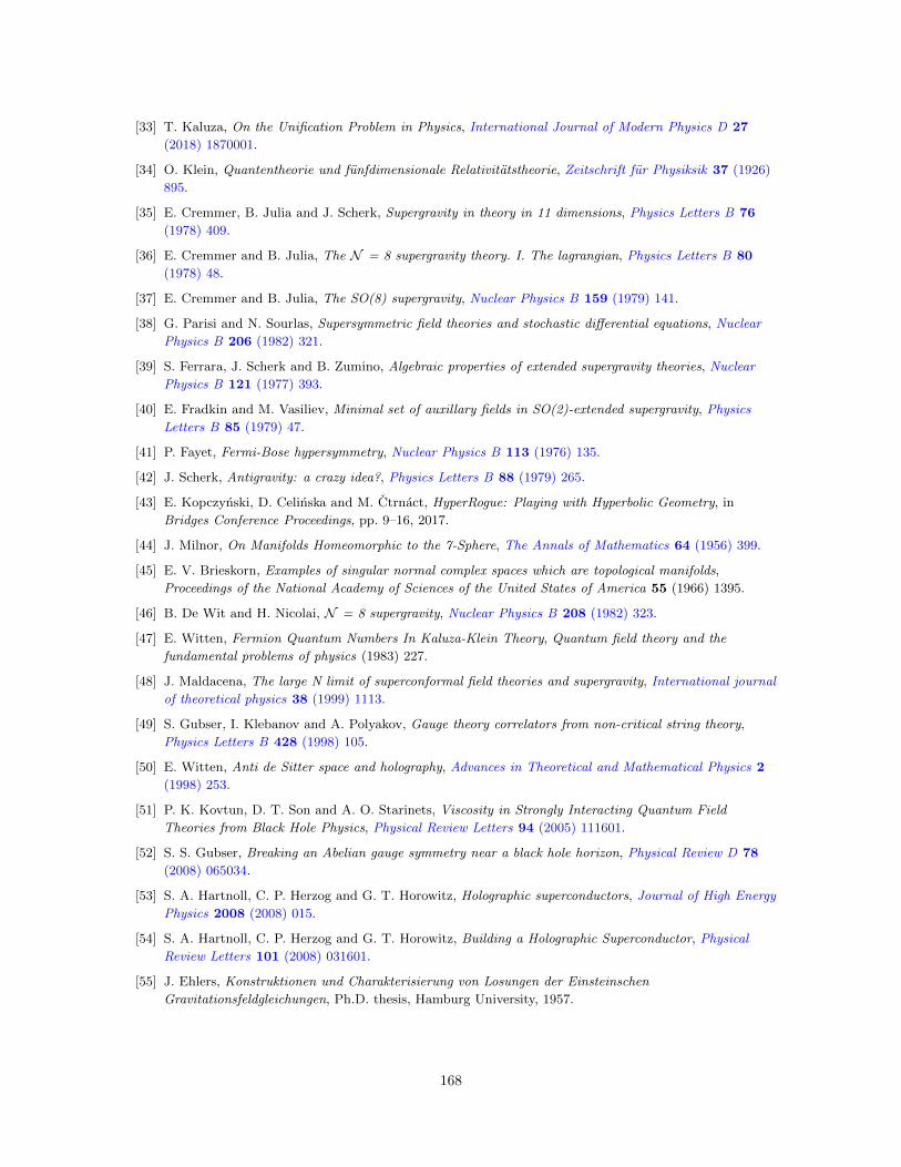
[33] T. Kaluza, On the Unification Problem in Physics, International Journal of Modern Physics D 27

(2018) 1870001.

[34] O. Klein, Quantentheorie und funfdimensionale Relativitatstheorie, Zeitschrift fur Physiksik 37 (1926)

895.

[35] E. Cremmer, B. Julia and J. Scherk, Supergravity in theory in 11 dimensions, Physics Letters B 76

(1978) 409.

[36] E. Cremmer and B. Julia, The N = 8 supergravity theory. I. The lagrangian, Physics Letters B 80

(1978) 48.

[37] E. Cremmer and B. Julia, The SO(8) supergravity, Nuclear Physics B 159 (1979) 141.

[38] G. Parisi and N. Sourlas, Supersymmetric field theories and stochastic differential equations, Nuclear

Physics B 206 (1982) 321.

[39] S. Ferrara, J. Scherk and B. Zumino, Algebraic properties of extended supergravity theories, Nuclear

Physics B 121 (1977) 393.

[40] E. Fradkin and M. Vasiliev, Minimal set of auxillary fields in SO(2)-extended supergravity, Physics

Letters B 85 (1979) 47.

[41] P. Fayet, Fermi-Bose hypersymmetry, Nuclear Physics B 113 (1976) 135.

[42] J. Scherk, Antigravity: a crazy idea?, Physics Letters B 88 (1979) 265.

[43] E. Kopczynski, D. Celinska and M. Ctrnact, HyperRogue: Playing with Hyperbolic Geometry, in

Bridges Conference Proceedings, pp. 9–16, 2017.

[44] J. Milnor, On Manifolds Homeomorphic to the 7-Sphere, The Annals of Mathematics 64 (1956) 399.

[45] E. V. Brieskorn, Examples of singular normal complex spaces which are topological manifolds,

Proceedings of the National Academy of Sciences of the United States of America 55 (1966) 1395.

[46] B. De Wit and H. Nicolai, N = 8 supergravity, Nuclear Physics B 208 (1982) 323.

[47] E. Witten, Fermion Quantum Numbers In Kaluza-Klein Theory, Quantum field theory and the

fundamental problems of physics (1983) 227.

[48] J. Maldacena, The large N limit of superconformal field theories and supergravity, International journal

of theoretical physics 38 (1999) 1113.

[49] S. Gubser, I. Klebanov and A. Polyakov, Gauge theory correlators from non-critical string theory,

Physics Letters B 428 (1998) 105.

[50] E. Witten, Anti de Sitter space and holography, Advances in Theoretical and Mathematical Physics 2

(1998) 253.

[51] P. K. Kovtun, D. T. Son and A. O. Starinets, Viscosity in Strongly Interacting Quantum Field

Theories from Black Hole Physics, Physical Review Letters 94 (2005) 111601.

[52] S. S. Gubser, Breaking an Abelian gauge symmetry near a black hole horizon, Physical Review D 78

(2008) 065034.

[53] S. A. Hartnoll, C. P. Herzog and G. T. Horowitz, Holographic superconductors, Journal of High Energy

Physics 2008 (2008) 015.

[54] S. A. Hartnoll, C. P. Herzog and G. T. Horowitz, Building a Holographic Superconductor, Physical

Review Letters 101 (2008) 031601.

[55] J. Ehlers, Konstruktionen und Charakterisierung von Losungen der Einsteinschen

Gravitationsfeldgleichungen, Ph.D. thesis, Hamburg University, 1957.

168

[56] R. Geroch, A Method for Generating Solutions of Einstein’s Equations, Journal of Mathematical

Physics 12 (1971) 918.

[57] J. Berkeley and D. S. Berman, The Navier–Stokes equation and solution generating symmetries from

holography, Journal of High Energy Physics 2013 (2013) 92.

[58] S. Bhattacharyya, S. Minwalla, V. E. Hubeny and M. Rangamani, Nonlinear fluid dynamics from

gravity, Journal of High Energy Physics 2008 (2008) 045.

[59] O. Aharony, O. Bergman, D. L. Jafferis and J. Maldacena, N = 6 superconformal

Chern-Simons-matter theories, M2-branes and their gravity duals, Journal of High Energy Physics

2008 (2008) 091.

[60] N. Bobev, V. S. Min and K. Pilch, Mass-deformed ABJM and black holes in AdS4, Journal of High

Energy Physics 2018 (2018) 50.

[61] A. M. Turing, Computing machinery and intelligence, Mind 49 (1950) 433.

[62] A. L. Samuel, Some Studies in Machine Learning Using the Game of Checkers, IBM Journal of

Research and Development 3 (1959) 210.

[63] C. Olah, A. Mordvintsev and L. Schubert, Feature visualization, Distill 2 (2017) e7.

[64] D. Genzel and A. Popat, Paper to Digital in 200+ languages, 2015.

[65] A. Krizhevsky, I. Sutskever and G. E. Hinton, ImageNet Classification with Deep Convolutional Neural

Networks, in Advances in Neural Information Processing Systems 25, F. Pereira, C. J. C. Burges,

L. Bottou and K. Q. Weinberger, eds., pp. 1097–1105, Curran Associates, Inc., (2012),

http://papers.nips.cc/paper/4824-imagenet-classification-with-deep-convolutional-neural-networks.pdf.

[66] C. Szegedy, Wei Liu, Yangqing Jia, P. Sermanet, S. Reed, D. Anguelov et al., Going deeper with

convolutions, in 2015 IEEE Conference on Computer Vision and Pattern Recognition (CVPR),

pp. 1–9, IEEE, jun, 2015, 1409.4842, DOI.

[67] P. Sharma, N. Ding, S. Goodman and R. Soricut, Conceptual Captions: A Cleaned, Hypernymed,

Image Alt-text Dataset For Automatic Image Captioning, in Proceedings of the 56th Annual Meeting of

the Association for Computational Linguistics (Volume 1: Long Papers), (Melbourne, Australia),

pp. 2556–2565, Association for Computational Linguistics, jul, 2018,

https://www.aclweb.org/anthology/P18-1238.

[68] A. Vaswani, N. Shazeer, N. Parmar, J. Uszkoreit, L. Jones, A. N. Gomez et al., Attention is All you

Need, in Advances in Neural Information Processing Systems 30, I. Guyon, U. V. Luxburg, S. Bengio,

H. Wallach, R. Fergus, S. Vishwanathan et al., eds., pp. 5998–6008, Curran Associates, Inc., (2017),

http://papers.nips.cc/paper/7181-attention-is-all-you-need.pdf.

[69] D. Silver, A. Huang, C. J. Maddison, A. Guez, L. Sifre, G. van den Driessche et al., Mastering the

game of Go with deep neural networks and tree search, Nature 529 (2016) 484.

[70] O. Vinyals, I. Babuschkin, J. Chung, M. Mathieu, M. Jaderberg, W. M. Czarnecki et al., “AlphaStar:

Mastering the Real-Time Strategy Game StarCraft II.”

https://deepmind.com/blog/alphastar-mastering-real-time-strategy-game-starcraft-ii, 2019.

[71] T. Karras, S. Laine and T. Aila, A Style-Based Generator Architecture for Generative Adversarial

Networks, arXiv preprint arXiv:1812.04948 (2018) [1812.04948].

[72] F. Rosenblatt, The perceptron: A probabilistic model for information storage and organization in the

brain., Psychological Review 65 (1958) 386.

[73] D. D. E. Rumelhart, G. E. Hinton, J. L. McClelland and Others, A general framework for parallel

169

distributed processing, Parallel distributed processing: Explorations in the microstructure of cognition 1

(1986) 26.

[74] S. Hochreiter and J. Schmidhuber, Long Short-Term Memory, Neural Computation 9 (1997) 1735.

[75] Y. Lecun, L. Bottou, Y. Bengio and P. Haffner, Gradient-based learning applied to document

recognition, Proceedings of the IEEE 86 (1998) 2278.

[76] E. J. Hartman, J. D. Keeler and J. M. Kowalski, Layered Neural Networks with Gaussian Hidden Units

as Universal Approximations, Neural Computation 2 (1990) 210.

[77] G. E. Hinton, S. Osindero and Y.-W. Teh, A Fast Learning Algorithm for Deep Belief Nets, Neural

Computation 18 (2006) 1527 [1111.6189v1].

[78] C. Cortes and V. Vapnik, Support-vector networks, Machine Learning 20 (1995) 273.

[79] X. Glorot, A. Bordes and Y. Bengio, Deep Sparse Rectifier Neural Networks, in Proceedings of the

Fourteenth International Conference on Artificial Intelligence and Statistics, G. Gordon, D. Dunson

and M. Dudık, eds., vol. 15 of Proceedings of Machine Learning Research, (Fort Lauderdale, FL, USA),

pp. 315–323, PMLR, 2011, http://proceedings.mlr.press/v15/glorot11a.html.

[80] T. Kohonen, Self-organized formation of topologically correct feature maps, Biological Cybernetics 43

(1982) 59.

[81] P. Covington, J. Adams and E. Sargin, Deep Neural Networks for YouTube Recommendations, in

Proceedings of the 10th ACM Conference on Recommender Systems - RecSys ’16, (New York, New

York, USA), pp. 191–198, ACM Press, 2016, DOI.

[82] V. Mnih, K. Kavukcuoglu, D. Silver, A. A. Rusu, J. Veness, M. G. Bellemare et al., Human-level

control through deep reinforcement learning, Nature 518 (2015) 529.

[83] R. Dunne and N. Campbell, On the pairing of the Softmax activation and cross-entropy penalty

functions and the derivation of the Softmax activation function, Proc. 8th Aust. Conf. on the Neural

Networks (1997) 1.

[84] B. Speelpenning, Compiling Fast Partial Derivatives of Functions Given by Algorithms, Ph.D. thesis,

University of Illinois Urbana-Champaign, Champaign, IL, USA, 1980.

[85] D. E. Rumelhart, G. E. Hinton and R. J. Williams, Learning Internal Representations by Error

Propagation, tech. rep., US Dept of the Navy, Cambridge, MA, sep, 1985. 10.21236/ADA164453.

[86] R. Bellman, Dynamic Programming and a New Formalism in the Calculus of Variations, Proceedings

of the National Academy of Sciences 40 (1954) 231.

[87] “R6RS-AD. http://web.archive.org/web/20180611012500/https:// github.com/qobi/R6RS-AD.”

[88] R. Kondor, H. T. Son, H. Pan, B. Anderson and S. Trivedi, Covariant compositional networks for

learning graphs, arXiv preprint arXiv:1801.02144 (2018) .

[89] I. Bars, Supersymmetry, p-brane duality, and hidden spacetime dimensions, Physical Review D 54

(1996) 5203 [hep-th/9604139].

[90] E. Bergshoeff, E. Sezgin and P. Townsend, Supermembranes and eleven-dimensional supergravity,

Physics Letters B 189 (1987) 75.

[91] E. Cremmer, B. Julia and J. Scherk, Supergravity theory in 11 dimensions, in Supergravities in Diverse

Dimensions, pp. 139–142, World Scientific Publishing Company, (jun, 1989), DOI.

[92] M. J. Duff, B. E. W. Nilsson and C. N. Pope, Kaluza-Klein Supergravity, Phys. Rept. 130 (1986) 1.

[93] P. G. Freund and M. A. Rubin, Dynamics of dimensional reduction, Physics Letters B 97 (1980) 233.

170

[94] E. Cremmer, B. Julia, H. Lu and C. Pope, Dualisation of dualities, Nuclear Physics B 523 (1998) 73

[hep-th/9710119].

[95] E. Cremmer, B. Julia, H. Lu and C. Pope, Dualisation of dualities II: twisted self-duality of doubled

fields and superdualities, Nuclear Physics B 535 (1998) 242 [hep-th/9806106].

[96] M. J. Duff, Ultraviolet divergences in extended supergravity, in First School on Supergravity Trieste,

Italy, April 22-May 6, 1981, 1982, 1201.0386.

[97] B. Biran, F. Englert, B. de Wit and H. Nicolai, Gauged N = 8 Supergravity and Its Breaking From

Spontaneous Compactification, Phys. Lett. 124B (1983) 45.

[98] M. J. Duff and C. N. Pope, KALUZA-KLEIN SUPERGRAVITY AND THE SEVEN SPHERE, in

September School on Supergravity and Supersymmetry Trieste, Italy, September 6-18, 1982,

pp. 183–228, 1983.

[99] B. de Wit and H. Nicolai, The Consistency of the S**7 Truncation in D=11 Supergravity, Nucl. Phys.

B281 (1987) 211.

[100] H. Nicolai and K. Pilch, Consistent truncation of d = 11 supergravity on AdS4 × S7, Journal of High

Energy Physics 2012 (2012) 99.

[101] M. J. Duff, B. E. W. Nilsson and C. N. Pope, Compactification of d = 11 Supergravity on K(3) X

U(3), Phys. Lett. B129 (1983) 39.

[102] B. de Wit, H. Samtleben and M. Trigiante, The maximal D = 4 supergravities, Journal of High Energy

Physics 2007 (2007) 049.

[103] C. Hull and N. Warner, The structure of the gauged N = 8 supergravity theories, Nuclear Physics B

253 (1985) 650.

[104] C. M. Hull, Non-compact gaugings of N = 8 supergravity, in Supergravities in Diverse Dimensions:

Commentary and Reprints (In 2 Volumes), pp. 693–695, World Scientific, (1989), DOI.

[105] G. Dall’Agata, G. Inverso and M. Trigiante, Evidence for a Family of SO(8) Gauged Supergravity

Theories, Physical Review Letters 109 (2012) 201301.

[106] B. de Wit, H. Samtleben and M. Trigiante, On Lagrangians and gaugings of maximal supergravities,

Nuclear Physics B 655 (2003) 93 [hep-th/0212239].

[107] B. de Wit, Supergravity, in Unity from duality: Gravity, gauge theory and strings. Proceedings, NATO

Advanced Study Institute, Euro Summer School, 76th session, Les Houches, France, July 30-August 31,

2001, pp. 1–135, dec, 2002, 0212245, http://arxiv.org/abs/hep-th/0212245.

[108] T. Fischbacher, Fourteen new stationary points in the scalar potential of SO(8)-gauged N = 8, D = 4

supergravity, Journal of High Energy Physics 2010 (2010) 68.

[109] G. Y. Rainich, Electrodynamics in the General Relativity Theory, Proceedings of the National Academy

of Sciences 10 (1924) 124.

[110] N. Warner, Some properties of the scalar potential in gauged supergravity theories, Nuclear Physics B

231 (1984) 250.

[111] P. Breitenlohner and D. Z. Freedman, Stability in gauged extended supergravity, Annals of Physics 144

(1982) 249.

[112] T. Fischbacher, K. Pilch and N. P. Warner, New Supersymmetric and Stable, Non-Supersymmetric

Phases in Supergravity and Holographic Field Theory, arXiv preprint arXiv:1010.4910 (2010)

[1010.4910].

171

[113] H. Godazgar, M. Godazgar, O. Kruger, H. Nicolai and K. Pilch, An SO(3)× SO(3) invariant solution

of D = 11 supergravity, Journal of High Energy Physics 2015 (2015) 56.

[114] A. Borghese, R. Linares and D. Roest, Minimal stability in maximal supergravity, Journal of High

Energy Physics 2012 (2012) 34.

[115] T. Fischbacher, The many vacua of gauged extended supergravities, General Relativity and Gravitation

41 (2009) 315.

[116] N. Warner, Some new extrema of the scalar potential of gauged N = 8 supergravity, Physics Letters B

128 (1983) 169.

[117] B. de Wit and H. Nicolai, A new SO(7) invariant solution of d = 11 supergravity, Physics Letters B

148 (1984) 60.

[118] N. Bobev, N. Halmagyi, K. Pilch and N. P. Warner, Supergravity instabilities of non-supersymmetric

quantum critical points, Classical and Quantum Gravity 27 (2010) 235013.

[119] B. De Wit and H. Nicolai, The parallelizing S7 torsion in gauged N = 8 supergravity, Nuclear Physics

B 231 (1984) 506.

[120] “Google colaboratory. https://colab.sandbox.google.com.”

[121] N. P. Jouppi, A. Borchers, R. Boyle, P.-l. Cantin, C. Chao, C. Clark et al., In-Datacenter Performance

Analysis of a Tensor Processing Unit, in Proceedings of the 44th Annual International Symposium on

Computer Architecture - ISCA ’17, (New York, New York, USA), pp. 1–12, IEEE, ACM Press, 2017,

1704.04760, DOI.

[122] J. Nocedal and S. Wright, Numerical Optimization, Springer Series in Operations Research and

Financial Engineering. Springer New York, 2nd ed., 2006, 10.1007/978-0-387-40065-5.

[123] M. Morse, The calculus of variations in the large, Monatshefte fur Mathematik und Physik 47 (1939)

A10.

[124] N. Bobev, T. Fischbacher and K. Pilch, “A new N = 1 AdS4 Vacuum of Maximal Supergravity (Work

in progress).”

[125] T. Fischbacher, The Encyclopedic Reference of Critical Points for SO(8)-Gauged N = 8 Supergravity

Part 1: Cosmological Constants in the Range -Λ/g2 ∈ [6; 14.7), arXiv preprint arXiv:1109.1424 (2011)

[1109.1424].

[126] S. Dittmaier, Precision Standard Model Physics, LoopFest V, SLAC (2006) .

[127] G. P. Collins, The Large Hadron Collider: The Discovery Machine, Scientific American (2008) 39.

[128] F. Johansson and Others, mpmath: a Python library for arbitrary-precision floating-point arithmetic

(version 0.18), dec, 2013.

[129] D. Maclaurin, Modeling, inference and optimization with composable differentiable procedures, Ph.D.

thesis, Harvard University, 2016.

[130] P. B. Davenport, Rotations about nonorthogonal axes., AIAA Journal 11 (1973) 853.

[131] J. Wittenburg and L. Lilov, Decomposition of a finite rotation into three rotations about given axes,

Multibody System Dynamics 9 (2003) 353.

[132] D. H. Bailey and J. M. Borwein, PSLQ: An Algorithm to Discover Integer Relations, apr, 2009.

10.2172/963658.

[133] B. de Wit and H. Nicolai, Properties Of N = 8 Supergravity, in 19th Winter School and Workshop on

Theoretical Physics: Supersymmetry and Supergravity Karpacz, Poland, February 14-26, 1983, 1983.

172

[134] A. Borghese, A. Guarino and D. Roest, Triality, Periodicity and Stability of SO(8) Gauged

Supergravity, JHEP 05 (2013) 107 [1302.6057].

[135] M. B. Green, J. H. Schwarz and E. Witten, Superstring Theory, Cambridge Monographs on

Mathematical Physics 150 (2012) .

[136] J. C. Baez, The octonions, Bulletin of the American Mathematical Society 39 (2001) 145

[math/0105155].

[137] T. Fischbacher, Numerical tools to validate stationary points of SO(8)-gauged N = 8 D = 4

supergravity, Computer Physics Communications 183 (2012) 780 [1007.0600].

[138] F. Englert, Spontaneous compactification of eleven-dimensional supergravity, Physics Letters B 119

(1982) 339.

173