Snowmelt Hydrology of a Sierra Nevada StreamIn exposed areas wind is an important element in the convection process; in heavily forested areas wind becomes a minor factor. It has been

Snowmelt Hydrology of a Sierra Nevada Stream

GEOLOGICAL SURVEY WATER-SUPPLY PAPER 1779-R

Prepared in cooperation with California Department of W^ater Resources

Snowmelt Hydrology of a Sierra Nevada StreamBy S. E. RANTZ

CONTRIBUTIONS TO THE HYDROLOGY OF THE UNITED STATES

GEOLOGICAL SURVEY WATER-SUPPLY PAPER 1779-R

Prepared in cooperation with California Department of Water Resources

UNITED STATES GOVERNMENT PRINTING OFFICE, WASHINGTON : 1964

UNITED STATES DEPARTMENT OF THE INTERIOR

STEWART L. UDALL, Secretary

GEOLOGICAL SURVEY

Thomas B. Nolan, Director

For sale by the Superintendent of Documents, U.S. Government Printing Office Washington, D.C. 21)402

CONTENTS

Pag«Abstract______________________________________________________ RlIntroduction.____________________________________________________ 1

Purpose and scope_____-_____________________ ________________ 1Acknowledgments.________________________________________ __ 3

Theory of snowmelt______________________________________________ 4Snowmelt at a point-___________-______________________________ 4Basin snowmelt-___-_____-__--__________________-_____________ 7Generalized basin snowmelt equations__________________________ 11

Hydrologic characteristics of the North Yuba River basin._____________ 12Analysis of snowmelt runoff_______________________________________ 15

Synthesis of hydrometeorological elements._______________________ 15Computation of daily snowmelt-____________________________ 19Computation of daily runoff.__________________________________ 22

Evaluation of computed daily snowmelt runoff-_______________________ 32Degree-day method of computing snowmelt runoff-____________________ 35Summary_____________________________________ 36References_________________^__ ___________________»___. 36

ILLUSTRATIONS

P&St FIGURE 1. Location map showing report area-_____-______-___________ R3

2. Maximum daily solar radiation at latitude of North Yuba Riverbasin_________________________________________ 5

3. Sketch map of North Yuba River basin upstream from Good- years Bar_________________________________ 13

4. Area-altitude distribution for the North Yuba River basin____ 145. Relation of water equivalent of snowpack to altitude, at start

of melt season_____________________________________ 166. Relation between cloud cover and percent of maximum daily

insolation at Davis, Calif., for period April 1 through June 30- 187. Variation of snow-surface albedo with time during the snow-

melt season. __________________________________________ 198. Base-flow recession curve for North Yuba River below Good-

years Bar___________________________________________ 279. Relation of base flow to volume of "live" ground-water storage. 27

10. Daily distribution graph for North Yuba River below Good- years Bar_________________________________________ 32

11. Synthesized and observed daily runoff during the snowmeltseasons, North Yuba River below Goodyears Bar __________ 33

m

IV CONTENTS

TABLES

Page TABLE 1. Hydrologic characteristics of the North Yuba River basin____ R 15

2. Snow-course data for the North Yuba River basin____________ 153. Daily distribution of snowraelt and rainfall, North Yuba River

basin, 1956, 1958, 1959______________.__________ 234. Daily infiltration and evapotranspiration loss for various condi

tions of snow cover____---___-------------_--.--_-------- 265. Synthesized and observed daily runoff, North Yuba River below

Goodyears Bar, 1956, 1958, 1959________________ 296. Degree-day indices of runoff at snow laboratory basins._______ 35

CONTRIBUTIONS TO THE HYDROLOGY OF THE UNITED STATES

SNOWMELT HYDROLOGY OF A SIERRA NEVADA STREAM

By S. E. RANTZ

ABSTRACT

This report demonstrates a rational method of computing snowmelt runoff. The area utilized for this study was the North Yuba River basin upstream from the gaging station below Goodyears Bar, in the Sierra Nevada in California. The snowmelt formulas that were used had been previously arrived at during a Federal interagency snow investigation, conducted in small mountain study areas in western United States. These formulas are based on physical laws of heat ex change, and in them are incorporated constants that reflect the effect of such environmental influences as forest cover and basin exposure. The formulas were used to compute the daily magnitude of the various components of snowmelt; namely, shortwave and longwave radiation melt, convection melt, condensation melt, and rain melt. These melt components were then totaled and routed to the gaging station.

Three years were selected for study; the years 1956 and 1958 when the heaviest snowpack of the last decade occurred, and the year 1959 when one of the lightest snowpacks of recent years occurred. The snow-survey data collected in late March or early April of each of these years, and daily meteorological observations by the U.S. Weather Bureau during the ensuing 3-month snowmelt seasons, were used to compute synthetic records of daily discharge of the North Yuba River below Goodyears Bar. The computed hydrographs of snowmelt discharge for these 3 years showed satisfactory agreement with the recorded hydrographs, thereby attesting to the soundness of the method used.

Because few of the hydrometeorological elements needed for computing snowmelt are observed within the North Yuba River basin, it had been necessary in this study to transfer observations from nearby weather stations and to synthe size daily values of other required elements. Closer agreement between computed and observed hydrographs would undoubtedly have been attained had there been a more comprehensive network of hydrometeorological stations within the basin.

INTRODUCTION

PURPOSE AND SCOPE

Until recent years the problem of estimating snowmelt runoff from mountainous river basins was dealt with by using simple empirical relations, primarily because of a lack of adequate basic knowledge of the physical processes involved. The formulation of a rational

Rl

R2 CONTRIBUTIONS TO THE HYDROLOGY OF THE UNITED STATES

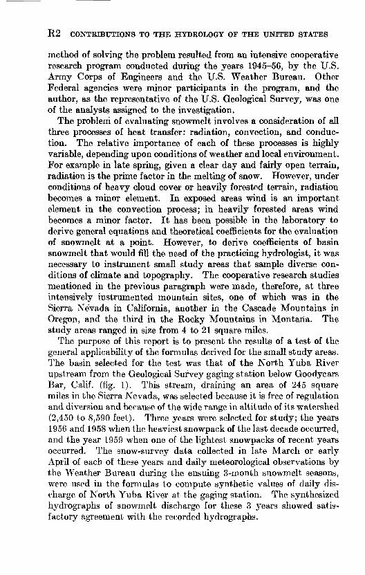
method of solving the problem resulted from an intensive cooperative research program conducted during the years 1945-56, by the U.S. Army Corps of Engineers and the U.S. Weather Bureau. Other Federal agencies were minor participants in the program, and the author, as the representative of the U.S. Geological Survey, was one of the analysts assigned to the investigation.

The problem of evaluating snowmelt involves a consideration of all three processes of heat transfer: radiation, convection, and conduc tion. The relative importance of each of these processes is highly variable, depending upon conditions of weather and local environment. For example in late spring, given a clear day and fairly open terrain, radiation is the prime factor in the melting of snow. However, under conditions of heavy cloud cover or heavily forested terrain, radiation becomes a minor element. In exposed areas wind is an important element in the convection process; in heavily forested areas wind becomes a minor factor. It has been possible in the laboratory to derive general equations and theoretical coefficients for the evaluation of snowmelt at a point. However, to derive coefficients of basin snowmelt that would fill the need of the practicing hydrologist, it was necessary to instrument small study areas that sample diverse con ditions of climate and topography. The cooperative research studies mentioned in the previous paragraph were made, therefore, at three intensively instrumented mountain sites, one of which was in the Sierra Nevada in California, another in the Cascade Mountains in Oregon, and the third in the Rocky Mountains in Montana. The study areas ranged in size from 4 to 21 square miles.

The purpose of this report is to present the results of a test of the general applicability of the formulas derived for the small study areas. The basin selected for the test was that of the North Yuba River upstream from the Geological Survey gaging station below Goodyears Bar, Calif, (fig. 1). This stream, draining an area of 245 square miles in the Sierra Nevada, was selected because it is free of regulation and diversion and because of the wide range in altitude of its watershed (2,450 to 8,590 feet). Three years were selected for study; the years 1956 and 1958 when the heaviest snowpack of the last decade occurred, and the year 1959 when one of the lightest snowpacks of recent years occurred. The snow-survey data collected in late March or early April of each of these years and daily meteorological observations by the Weather Bureau during the ensuing 3-month snowmelt seasons, were used in the formulas to compute synthetic values of daily dis charge of North Yuba River at the gaging station. The synthesized hydrographs of snowmelt discharge for these 3 years showed satis factory agreement with the recorded hydrographs.

SNOWMELT HYDROLOGY OF A SIERRA NEVADA STREAM R3

Ji^/^drovme"<tr

$0ubBlue Canyon

$

Davis 1 Sacramento

AREA OF MAP

EXPLANATION

Report area

20I

30 MILES

INDEX MAP OF CALIFORNIA

FIGURE 1. Location map showing report area.

ACKNOWLEDGMENTS

The study described in this report was authorized by a cooperative agreement between the U.S. Geological Survey and the California Department of Water Resources. The report was prepared under the supervision of Walter Hofmann, district engineer of the Surface Water Branch of the Geological Survey.


The cooperation of the U.S. Weather Bureau in furnishing unpub lished meteorological data for the station at Blue Canyon, Calif., is gratefully acknowledged.

THEORY OF SNOWMELT

SNOWMELT AT A POINT

This paper does not contain a detailed treatise on the theory of point and basin snowmelt. An excellent treatment of the subject is found in a summary report of the cooperative snow investigations by the U.S. Army Corps of Engineers (1956) and in a condensed version of that report by the same agency (1960). The paragraphs that follow have been largely abstracted from these publications to provide the modicum of theoretical background material that is needed for an understanding of the computational procedures used in this study of the North Yuba River basin.

Sources of heat. The sources of heat involved in the melting of snow are:1. Absorbed solar radiation, HTS .2. Net longwave (terrestrial) radiation, HT i.3. Convection heat transfer from the air, Hc .4. Latent heat of vaporation by condensation from the air, He.5. Conduction of heat from the ground, Hg .6. Heat content of rainwater, Hf.The summation of the net exchange from all sources of heat represents the amount of energy available for melting the snowpack, and the resulting melt may be expressed by the general formula

whereM= snowmelt in inches of water

= algebraic sum of all heat components, in calories per square centimeter

B= thermal quality (see below)

203= number of calories per square centimeter required to melt 1 inch of water equivalent of ice at 0°C (80 cal per gin X 2.54 cm per in).

Thermal quality. A melting snowpack consists of a mixture of ice and a small quantity of free water. The term "thermal quality" denotes the ratio, by weight, of ice to the total snow mixture. For a melting mountain snowpack, after free drainage of water by gravity, the thermal quality normally ranges from 0.95 to 0.97, corresponding


to a retention of 3 to 5 percent liquid water. In equation 1 above, a value of 0.97 is usually used for B, the thermal quality.

Solar radiation. The amount of heat transferred to the snowpack by solar (shortwave) radiation varies with latitude, season, time of day, atmospheric conditions, forest cover, and albedo (reflectivity) of the snow. Figure 2 shows the daily solar radiation on cloudless

- 650

550

I T I I

5 10 15 20 25 30 5 10 15 20 25 31April May June

FIGURE 2. Maximum daily solar radiation at latitude of North Yuba River basin. Curve interpolated from Hamon and others (1954, fig. 5).

days that is incident upon a horizontal surface at the latitude (39° 35') of the North Yuba River basin, during the 3-month snowmelt period, April through June.

Albedo. The albedo, or reflectivity, of the snowpack varies over a considerable range, and greatly affects the amount of solar radiation absorbed by the pack. Albedo is expressed as the ratio of reflected shortwave radiation to that incident on the snow surface. Values range from more than 0.80 for new-fallen snow to as little as 0.40 for melting late-season snow. The melt equivalent from shortwave radiation, MTS, in inches per day is

(2)

where

a= albedo

/i=daily incident solar radiation in langleys

B thermal quality, assumed to be 0.97.

713-991 64 2


Longwave radiation. Snow is very nearly a black body with respect to longwave (terrestrial) radiation, absorbing almost all such radiation incident upon it, and emitting almost the maximum possible radiation corresponding to its temperature. A melting snowpack has a surface temperature of 0°C, and, according to Stefan's law, loses energy at a rate of 0.459 langleys per minute. Opposed to this loss is the back radiation from the atmosphere or forest. For clear skies, the heat gain from back radiation is generally less than the heat loss, so that there is a net heat loss from the snowpack by longwave radiation. With cloudy skies or beneath a forest canopy, however, the back radiation may be greater or less than the loss from the snowpack, depending principally upon the ambient air temperature. Precise computation of back radiation from the atmosphere with clear skies is complex and far too cumbersome for practical use in snow hydrology. By applying some simplifying assumptions, however, the following simple equations are obtained for the melt equivalent from longwave radiation, Mrt, in inches per day. In the open with clear skies

MrJ =0.0212 (Tfl -32)-0.84 (3)

under forest canopy(Tfl -32). (4)

In equations 3 and 4

Ta =ihe air temperature over the snow surface at the 10-foot level in degrees Fahrenheit.

Energy exchange from the atmosphere. Turbulent heat exchange from the atmosphere involves the transfer of sensible heat from warm ah* advected over the snowfield (convection), and also the heat of condensation of atmospheric water vapor that is condensed on the snow surfaces (condensation). The principal elements affecting con- vective heat exchange are the temperature gradient of the atmosphere measured above the snow surface, and the corresponding wind speed. A secondary factor is the density of the atmosphere, which may be expressed as a function of air pressure. The prime factors affecting condensation melt are the vapor pressure gradient and the wind speed. The computation of heat exchange from the atmosphere is complex from a theoretical standpoint, and exchange coefficients are derived empirically from controlled experiments. By making some simplifying assumptions concerning air density ratios and the relation of dewpoint temperatures to vapor pressures, simple equations are obtained for MC1 the daily melt equivalent from convection, and Me , the daily melt equivalent from condensation. Because similar terms appear in both equations, these equations may be combined into a


single equation for the melt equivalent from convection and conden sation, Mce, in inches per day.

Mce =0.0084 » [0.22(T.-32)+0.78(2^-32)] (5) where

Ta =mean air temperature at the 10-foot level in degrees Fahren heit

Td =mean dewpoint temperature at the 10-foot level in degrees Fahrenheit

v =mean wind speed at the 50-foot level in miles per hour.

Conduction oj heat from the ground. The heat conducted from the ground is almost negligible, and the complex observations required for its determination are therefore not warranted. The snowmelt from ground heat may be assumed to be 0.02 inch per day.

Heat content oj rainwater. Snowmelt resulting from the transfer of heat from rainwater is relatively small, and may be expressed simply in terms of amount of rainfall and dewpoint temperature. Dewpoint temperature is used because numerous investigators have demonstrated that this temperature closely approximates that of the raindrops. The melt equivalent from rainwater, Mp, in inches per day is

MP = 0.007 Pr(Td- 32) (6)

wherePr=the daily rainfall in inchesTd =mean dewpoint temperature at the 10-foot level in

degrees Fahrenheit.

BASIN SNOWMELT

The snowmelt equations in the preceding section dealt with the evaluation of snowmelt at a point. To apply these equations to a mountainous basin, however, it is necessary to use coefficients for the effect of such local environmental features as forest cover and basin exposure. The density of the forest canopy is particularly important because it influences all the principal melt processes. For the purpose of deriving appropriate basin snowmelt coefficients for forested regions, the average forest density, F, in a basin was classified as shown below,

Forest density, P (in percent)

1. Open___._.__.__.._.________. <102. Partly forested J......________ 10-803. Heavily forested____________ >80

1 The report of the U.S. Army Corps of Engineers (1960) subdivides this classification into forested and partly forested classes. For the purpose of this study, the single classification partly tforested was preferred.


The second environmental feature, basin exposure, influences the amount of solar radiation the basin receives. Basins whose exposure is predominantly south-facing receive more insolation than do those that face the north. In recognition of this effect a basin shortwave radiation melt coefficient, k', was introduced. The value of k' is 1.0 for a basin that is largely horizontal or whose north and south slopes are equal in area. During the spring snowmelt season, the value of k' falls to 0.9 for a basin that is predominantly north-facing, and to 1.1 for a basin that is predominantly south-facing.

As for the effects of weather conditions on basin snowmelt, they are more easily discussed if rain periods are treated separately from rain- free periods.

Basin snowmelt during periods of rainfall. The evaluation of basin snowmelt during periods of rainfall presents a special condition for which certain simplifying assumptions can be made in the snowmelt equations. During rainstorms, solar radiation melt is relatively small, and snowmelt resulting from longwave radiation is easily evaluated from theoretical considerations. Heat transfer by con vection and condensation represents the major source of energy for snowmelt, but the equation for this transfer must be modified for the effect of the forest density of the basin. Evaluation of the various sources of heat transfer to the snowpack during periods of rainfall involves the basic considerations that follow.1. Shortwave radiation is relatively unimportant. It can be ex

pressed by the equation

Mr.= (l-F) (0.07) (7) where

MrS solar radiation melt in inches per dayF = forest density expressed as a decimal ratio0.07=the assumed daily radiation melt in the open.

2. Longwave radiation exchange between forest or low clouds and the snowpack may be computed as a linear function of air tem perature.

Mrl =0.029 (T«-32) (8) where

Mri =longwave radiation melt in inches per day Ta =the mean air temperature at the 10-foot level, in

degrees Fahrenheit.

3. Air is assumed to be saturated, so that an air temperature-wind speed expression may be used in evaluating both convection and


condensation melt. This is done by assuming a linear rela tion between vapor pressure and dewpoint. For computing convection-condensation melt on basins, it is necessary to intro duce a basin constant, k, which represents the effect of forest density on the wind speed. The value of k may be computed from the strictly empirical equation

fc=l 0.7 F (9) where

F= forest density expressed as a decimal ratio.

For open or partly forested areas, convection-condensation melt may be computed from the equation

Mce=k (0.0084 ») (TV-32) (10)

For heavily forested areas, an average wind condition is as sumed, thereby eliminating the wind variable, and the equation used is

Mce=0.045 (r«-32) (11)

In equations 10 and 11

Mce=convection-condensation melt in inches per dayk =the basin constant described abovev =mean wind speed at the 50 foot-level in miles per

hour Ta =mean temperature of saturated air at the 10-foot

level in degrees Fahrenheit.4. Rain melt (snowmelt from transfer of heat from rainwater) is

expressed as a function of daily rainfall and dewpoint tempera ture. Under the assumption, however, of saturated air, the mean dewpoint temperature and mean air temperature will be identical. The equation for rain melt is

Mp =0.007 Pr (TV-32) (12)

where

Mp =rain melt in inches per day Pr=daily rainfall in inchesT0=mean temperature of saturated air at the 10-foot level,

in degrees Fahrenheit.

RIO CONTRIBUTIONS TO THE HYDROLOGY OF THE UNITED STATES

5. Ground melt (snowmelt from ground heat) is assumed to be con stant at 0.02 inch per day.

Basin snowmelt during rain-free periods. Rational determination of basin snowmelt during rain-free periods requires formulas that are more complex than those needed for periods of rainfall. Solar and terrestrial radiation both become important variables in the balance of heat exchange to the snowpack, and require direct evaluation for the given conditions of forest cover. Convection and condensation are generally less important heat sources than radiation. To arrive at generalized and simplified basin snowmelt equations for rain-free periods, the rational analysis of snowmelt at a point has been combined with statistically derived weightings of the air and dewpoint tempera tures for varying conditions of forest environment.

Basic forms of the snowmelt equations, for the three classifications of forest density, involve the following considerations:1. Open area (less than 10 percent cover)

a. Shortwave radiation is almost always the most important melt factor. Evaluation of this factor requires estimates of inci dent solar radiation, snow surface albedo, and the basin shortwave radiation melt coefficient.

b. Heat exchange by longwave radiation during cloud-free periods may be evaluated on the basis of surface air temperatures. Net longwave radiation exchange during periods of cloud cover may be estimated on the basis of cloud temperature and degree of cloud cover.

c. Convection and condensation snowmelt during clear weather is usually of minor importance. It may be evaluated with an air temperature, dewpoint temperature, and wind function, as previously discussed.

2. Partly forested area (10-80 percent cover)a. Shortwave radiation melt is evaluated for the unforested parts

of the basin, considering incident solar radiation, snow sur face albedo, and the basin shortwave radiation melt coefficient.

b. Longwave radiation melt for the forested part of the basin may be evaluated linearly as an air temperature function. For the unforested part, heat loss by longwave radiation may be accounted for indirectly by reducing the shortwave radia tion melt coefficient, thereby allowing longwave loss to be a function of net shortwave radiation.

c. A wind variable is specified for evaluation of convection- condensation melt, together with a basin convection- condensation melt coefficient.

3. Heavily forested area (more than 80 percent cover) a. Shortwave radiation melt is a very minor element.

SNOWMELT HYDROLOGY OF A SIERRA NEVADA STREAM Rll

b. Longwave radiation and convection melt may be combined intoa single linear function of air temperature.

c. Wind is unimportant in evaluating convection and condensationmelt.

d. Condensation melt may be evaluated as a linear function ofdewpoint temperature.

GENERALIZED BASIN SNOWMELT EQUATIONS

Generalized basin snowmelt equations for direct use in solving problems in snow hydrology have been developed on the basis of the theoretical considerations and assumptions discussed in the preceding section, "Basin Snowmelt." These equations, which combine all components of melt, are applicable only for a snowpack that is isothermal at 32 °F and contains 3 percent of free water.

General equations for basin melt during periods of rainfall

1. For open or partly forested areasM=(0.029+0.0084&y+0.007 Pr) (T'a ) (13)

+ (l-F) (0.07) + 0.02

2. For heavily forested areasM= (0.074 +0.007 Pr} (T'J + (l-F) (0.07)+0.02 (14)

General equations for basin melt during rain-free periods

1. For open areasM=fc' (0.00508 I\) (l-a) + (l-N) (0.0212 2^-0.84) (15)

+N (0.029 T'c)+k (0.0084*?) (0.22 T'a +Q.78 3^) +0.02

2. For partly forested areas

M=k' (l-F) (0.0040 7<) (l-a)+k (0.00840)' (0.22 T'a +0.7S Tj (16) +F (0.029 T;)+0.02

3. For heavily forested areas

M-0.074 (0.53 r;+0.47 3T£)+0.06 (17)

In equations 13-17F=the forest-canopy cover of the basin, effective in shading the

area from solar radiation, expressed as a decimal ratio. 7'4 =the incident solar radiation in langleys per day M=the snowmelt rate in inches per day AT=the cloud cover, expressed as a decimal ratio Pr=the daily rainfall in inches

Ill2 CONTRIBUTIONS TO THE HYDROLOGY OF THE UNITED STATES

T'a =ihe difference between the mean air temperature at the 10- foot level and the snow-surface temperature (32 °F) in degrees Fahrenheit

Trf=the difference between the mean dewpoint temperature at the 10-foot level and the snow-surface temperature (32°F) in degrees Fahrenheit

T^=the difference between the cloud-base temperature and snow-surface temperature (32°F) in degrees Fahrenheit. Cloud-base temperature is estimated from upper air temperatures or by lapse rates from a surface station, which preferably is on a snow-free site

a=the average snow-surface albedo k=ihe basin convection-condensation melt factor (see equation

9) k' = the basin shortwave radiation melt factor (ranges from 0.9

to 1.1) y=mean wind speed at the 50-foot level, in miles per hour.

HYDROLOGIC CHARACTERISTICS OF THE NORTH YUBARIVER BASIN

Before using the general snowmelt formulas for computing snowmelt runoff of the North Yuba River basin, it was first necessary to evaluate pertinent basin characteristics. The study area, which is located in the Sierra Nevada, is 245 square miles in area and is drained by the headwaters of the North Yuba River and its principal tributary, Downie River (fig. 3). Altitudes in the watershed range from 2,450 feet at the gaging station below Goodyears Bar to 8,590 feet at Look out Peak, 2 miles north of Sierra City. Figure 4 is a hypsometric curve for the North Yuba River basin showing the area-altitude dis tribution. The area lying within various altitude zones and the forest density for these zones were determined from the latest Geological Survey maps and are listed in table 1. The forest density figures, though crudely derived, compare favorably with those obtained by the U.S. Forest Service in an inventory of forests and large brushfields in the Sierra Nevada (Anderson and Richards, 1961, p. 145). The Forest Service report shows a cover of 61 percent for all the Yuba River basin above 5,000 feet; table 1 indicates a forest density of 65 percent for that part of the North Yuba River basin above 5,000 feet.

The altitude of the snowline at the beginning of the snowmelt season (approx. Apr. 1) varies annually and averages about 4,500 feet. Average annual precipitation over the entire basin is approxi mately 60 inches; the annual average water equivalent of the basin snowpack on April 1, over the 80 percent of the basin that is normally snow covered on that date, is about 24 inches. Table 2 presents


EXPLANATION

Boundary of basin

Stream-gaging station below Goodyears Bar

Weather Bureau station (precipita tion and temperature)

82D

Snow course

FIGUEE 3. Sketch map of North Yuba River basin upstream from Goodyears Bar.

data for the eignt snow courses shown on figure 3, for the 3 years (1956, 1958, and 1959) that were used in this study. Measurements of water equivalent of the snowpack are normally made as close as possible to April 1 each year. In 1958, however, only two snow courses were observed in early April because of unseasonably heavy storms that occurred during the period March 29 to April 3. Data from table 2 were plotted in figure 5 to show the relation of water equivalent of snowpack to altitude. Snowpack data pertinent to this study were then extracted from figure 5 and entered in table 1.

713-991-


9000

8000

7000

6000

5000

4000

3000

8590 -

2450

2000

0 20 40 60 80 100

PERCENT OF AREA BELOW INDICATED ALTITUDE

FioimE 4. Area-altitude distribution for the North Yuba River basin.

A preceding section of this report discussed the influence of basin exposure on the amount of solar radiation received, and introduced a basin shortwave radiation melt coefficient, kr . Because the North Yuba River watershed is predominantly south-facing, the value of kr was assumed to be 1.1.


TABLE 1. Hydrologic characteristics of the North Yuba River basin

Altitude zone (range in altitude,

in feet)

2,460-i,000_._________

4,000-4,500...........

4,500-6,000. _____

6,000-6,000 ______

6,000-7,000 ______

7,000-8,590 ______

Area

Percent of total

10.5

9.5

10

24

28

18

Square miles

25.7

23.3

24.5

58.8

68.6

44.1

Forest density ( F) (percent)

100

96

96

70

57

70

Water equivalent of snowpack when melt starts (inches)

Year

1966 1968 1959 1956 1958 1959 1956 1968 1969 1966 1958 1959 1966 1958 1969 1956 1958 1959

At lowest altitude of

zone

(>)

(0

0 14.5 0

14.5 26.5

0 33.5 45.1 12.0 49.1 60.9 20.0

At highest altitude of

zone

(')

f 0 \ 14.51 o

14.5 26.5

0 33.5 45.1 12.0 49.1 60.9 20.0 74.1 86.0 32.5

At median altitude of

zone

(»)

0 7.5 0 8.0

20.5 0

25.0 36.5 6.6

41.0 53.0 16.3 54.0 65.5 22.8

i No snow.

TABLE 2. Snow-course data for the North Yuba River basin

Data on water equivalence for indicated snow course

Altitude.-.-.-.-feet.. 30-year average water

equivalent on April 1 _____ inches..

1956: Date.. __ Water equiva

lent inches.. 1958:

Water equiva lent- -..inches..

1959:

Water equiva lent inches

64

7,800

42.0

Mar. 26

64.2

lApr. 22

70.1

Mar. 31

26.2

74

6,700

31.8

Mar. 29

48.2

»Mar. 31

44.5

Mar. 30

16.7

75

6,700

30.4

Mar. 30

42.8

Apr. 3

66.3

Mar. 31

20.0

78

6,500

27.6

Mar. 28

39.5

lApr. 23

50.0

Apr. 1

13.8

79

6,300

29.1

Mar. 28

42.0

>Apr. 23

50.8

Apr. 1

18.3

82

5,700

18.0

Apr. 2

20.4

Apr. 7

40.7

Mar. 31

9.6

83

5,660

19.9

Mar. 28

28.1

lApr. 23

42.0

Apr. 1

9.1

89

6,800

30.9

Mar. 26

46.0

'Apr. 22

48.4

Mar. 31

18.7

i After snowmelt had progressed. * Prior to heavy storm of early April.

ANALYSIS OF SNOWMELT RUNOFF

SYNTHESIS OF HYDRO METEOROLOGICAL ELEMENTS

Few basins can be found where all the hydrometeorological elements required for computing snowmelt are observed. The North Yuba River basin is not such a basin. The only meteorological stations there are at Sierra City (alt 4,182 ft) and Downieville Ranger Station (alt 2,895 ft), and at these stations only precipitation and temperature are observed (fig. 3). It was therefore necessary to derive synthetic daily values of the many elements required in the generalized basin snowmelt equations.


9000

8000

7000

6000

5000

4000

3000

EXPLANATION

x

Mean of snow-course observations

1958 snow-course observations

1959 snow-course observations

10 80 9020 30 40 50 60 70

WATER EQUIVALENT OF SNOW PACK, IN INCHES

FIGURE 5. Relation of water equivalent of snowpack to altitude, at start of melt season.

Weather records for Sierra City were incomplete for the period studied; consequently, the observations recorded at Downieville Ranger Station were used to derive figures of air temperature and precipitation for each of the altitude zones listed in table 1. The daily mean temperature at the station was computed by the accepted method of averaging the maximum and minimum temperatures recorded each day. To obtain the daily mean temperatures for each altitude zone, a lapse rate of 3°F per 1,000 feet of altitude was


applied to the Downieville temperatures. This lapse rate, computed from temperature records at nearby stations, is in agreement with the figure commonly used in studies in the Sierra Nevada.

The precipitation that occurred in each altitude zone during the snowmelt season was assumed to be equivalent to that recorded at Downieville Kanger Station. This assumption does not lead to serious error because the mean annual precipitation at the meteoro logical station agrees very closely with the mean annual basinwide precipitation. When air temperatures were close to 32°F, there was some question as to whether the precipitation was in the form of rain or snow. This was resolved by the use, at such times, of the snowfall record for the meteorological station at Blue Canyon (fig. 1) at altitude 5,280 feet.

The daily mean dewpoint temperature for each altitude zone was based on the record of observed dewpoints at Blue Canyon. During fair weather, a dewpoint lapse rate of 1°F per 1,000 feet of altitude was assumed; during periods of precipitation the pseudoadiabatic lapse rate of 3°F per 1,000 feet of altitude was used. It was found that during periods of precipitation a difference of a few degrees generally existed between the air temperature and the dewpoint temperature. For those occasions, equations 13 and 14 were modified

j by substituting v g T^ *' for T'a . Because none of the altitude

zones in the basin was classed as open terrain, equation 15 was not used in this study, and accordingly there was no need to estimate T'c , the difference between cloud-base temperature and snow-surface temperature.

In synthesizing a daily record of incident solar radiation for the North Yuba River basin, it was necessary to use the records of daily insolation and cloud cover for Davis (fig. 1), together with the obser vations of cloud cover at Blue Canyon. As a first step, the solar radiation observed each day at Davis was expressed as a percentage of the maximum daily radiation that could be received on that date at the latitude of Davis (38°32'). This percentage was plotted on figure 6 against the corresponding cloud cover at Davis. The rela tion curve obtained was assumed to be as valid for the Sierra Nevada as it was for the Sacramento Valley, where Davis is located. The values of cloud cover observed at Blue Canyon were then used with the curve in figure 6 to obtain the percent of maximum daily insolation in the North Yuba River basin. These daily percentages were finally applied to the maximum solar radiation data for the North Yuba River basin, shown on figure 2, to give daily values of incident solar radiation in the study area. These daily figures of incident insolation were applicable to all altitude zones in the basin, . ,


100

80

60 -

u. 40 o

20

20 40 60

PERCENT OF CLOUD COVER

80 100

FIGUKE 6. Relation between cloud cover and percent of maximum daily insolation at Davis, Calif., forperiod April 1 through June 30.

The relation shown in figure 6 is approximate. The individual points that defined the relation were widely scattered and are not shown in the figure. This scatter is understandable in view of the fact that the solar radiation incident at the ground surface is affected not only by the percentage of cloud cover, but also by thickness of the clouds and their location in the sky relative to the position of the sun. It would have been much more desirable to use duration of sunshine as an index of incident radiation (Hamon and others, 1954) rather than cloud cover, but, unfortunately, this element is not observed at any nearby Sierra Nevada meteorological stations.

Because only part of the incident solar radiation is absorbed by the snowpack, a daily record of the albedo of the snow surface was needed. Nowhere is this element regularly observed, but it may be estimated from relations that were derived at the mountain laboratory basins. At best such estimates must be considered only approximations, but


limiting conditions during the snowmelt season are fairly well known. Figure 7 shows a typical variation of snow-surface albedo with tune during the snowmelt season, and this relation was used for all altitude zones. An albedo of 0.65 was assumed at the start of each snowmelt season and immediately following any snowfall during the season; the lower limit of the albedo was assumed to be 0.40. A value of 0.40 was used on days when rain fell during the melt season.

0.65

2 0.55

= 0.45

0.354 8 12 16 20 24

AGE OF SNOW SURFACE, IN DAYS

FIGURE 7. Variation of snow-surface albedo with time during the snowmelt season.

The remaining meteorological element to be deduced was wind speed. The daily average wind speed observed at Blue Canyon was used directly for all altitude zones in the North Yuba River basin. Because wind speed is affected greatly by the local environment, it was not considered practicable to attempt any adjustments in trans ferring observed wind speeds from Blue Canyon to the study area.

COMPUTATION OF DAILY SNOWMELT

With a record, either synthetic or observed, of all the necessary hydrometeorological elements, the snowmelt in each altitude zone can be computed. The formulas in the preceding sections of this report are applicable only for a snowpack that is ready to produce runoff (one that is isothermal at 32 °F and contains 3 percent free water). Some criterion was therefore required to identify the date when the snowpack reached that condition. This date was arbi trarily assumed to be the first day, after the snow survey of late March or early April, when the recorded stage hydrograph for the river showed the easily identifiable diurnal fluctuation that is char acteristic of snowmelt runoff. The closing date for the study in any year was the day when streamflow had receded to the discharge


recorded on the opening date of the study and had entered the base- flow recession phase of the runoff cycle. For the years that were investigated, the study dates were as follows:

1956 ____ . __ April 6-June 30 1958 ________ April 8-June 30 1959_. __________ April 1-May 16

Snowmelt does not start simultaneously in all altitude zones. A certain amount of heat is required to ready the snowpack for runoff, and the colder upper altitude zones will lag behind the lower altitude zones in receiving the necessary heat. It was arbitrarily assumed that at the start of the snowmelt season each year, the snowpack in the altitude zone between 6,000 and 7,000 feet would have an average temperature of 2°C, and in the altitude zone between 7,000 and 8,590 feet, an average temperature of 4°C. (The centigrade scale was used in these assumptions to simplify the com putations.) Consequently, no melt was assumed to occur in these upper altitude zones until sufficient heat had been transmitted to the snowpack to raise its temperature to 0°C and then melt 3 percent (by weight) of the pack. This heat deficit, Ma, expressed in equiv alent inches of melt water, is computed from the formula

whereW0 = initial average water equivalent of the snowpack, in inchesT~ average snowpack temperature in °C below zero

160=latent heat of fusion of ice (80 cal per gin) divided byspecific heat of ice (0.5 cal per gm per °C)

0.03=3 percent of free water.The liquid water needed to overcome the heat deficit may be supplied by either snowmelt or rain.

If rain falls on a melting snowpack, the rainwater is transmitted without loss through the pack and is subject to only minor detention lag (U.S. Army Corps of Engineers, 1956, p. 304-308). Should snow be the form of precipitation, however, it is assumed that the only water made available for runoff will be that due to ground melt, 0.02 inch per day.

With these additional assumptions established, equations 9, 13, 14, 16, 17, and 18 were applied and the daily snowmelt component of runoff for each altitude zone was computed. However, as snowmelt pro gresses the snowline recedes, and the snow-covered part of the zone diminishes in area. Consequently it was necessary to establish a procedure for determining the effective area of snowmelt. In any


zone, the entire area was assumed to be contributing snowmelt until the day when the accumulated melt exceeded the water equivalent at the lowest altitude of the zone. For example, consider the altitude zone between 5,000 and 6,000 feet in 1956. Table 1 shows that the water equivalent of the pack on April 1 of that year was 14.5 inches at altitude 5,000 feet and 33.5 inches at altitude 6,000 feet. By May 7, the melt in this zone totaled 14.5 inches, and by May 30 it totaled 33.5 inches. Consequently, it was assumed that: (1) until May 8 the entire zone was contributing melt, (2) after May 30 the entire zone was bare of snow, and (3) between May 9 and May 30 a steadily decreasing percentage of the area in the zone was snow covered.

The percentage of area that was snow covered, or effective, on any given date in mid-May was computed by the following procedure. Between May 8 and May 30 the snowmelt amounted to 19 inches (33.5 in. minus 14.5 in.). On May 8 the daily snowmelt was 0.45 inch. It was assumed therefore that on May 8 the snow-covered area shrank by a percentage equal to 0.45/19.00X100, or 2.4 percent. Consequently, on May 9, only 97.6 percent of the area in the zone was effective in contributing snowmelt. To compute effective area on some other date, May 20 for example, the melt between the inclusive dates of May 8 and May 19 was added. The sum equaled 7.40 inches and the assumption was made that on May 19 the snow-covered area had shrunk by a percentage equal to 7.40/19.00X100, or 39 percent. Therefore the effective area on May 20 was 61 percent of the total in the zone.

Finally, to obtain the water produced on each day in each zone, the computed snowmelt for the day was multiplied by the percentage of zonal area that was effective on that date, and to this product was added the rainfall, if any. It is of interest that the maximum snowmelt computed for any day during this study was 2 inches. The only large quantity of runoff that was produced by rain on the snowpack occurred on May 4, 1956, when the daily discharge was 3,400 cfs (cubic feet per second). Eighty-five percent of the water available for run off at that time was contributed by rainfall.

Having computed the daily increment of water, in inches, produced in each zone, and knowing the percentage of the total basin area occupied by each zone (table 1), it was simple to compute the daily equivalent depth of water produced over the entire basin. The weighting method of determining this equivalent depth is illustrated in the computation shown below for May 22, 1958. Figures in the last column are obtained by multiplying those in the two preceding columns.


Altitude zone (feet)

2,450-4,000.. __________________________________4,000-5,000 . ___ _________ __ __ _ _________5,000-6,000. __ _____ _ ____ _______ _________6,000-7,000_. __ _ ____.___._ ____ __. __ .. ....7,000-8,590 ___ __._ ___ ___ ____ ... __ ______

Percent of total area

10.5 19.5 24.0 28.0 18.0

Depth of water (inches)

Zone

1 0. 550 >. 550

2 1. 331 2 1. 546 2 1. 345

Basin equivalent

0 058 107 319 433 242

1. 159

i Rain only.* Snowmelt and rain.

Daily figures of equivalent depth of water produced over the basin are listed in table 3 under the heading "Available Supply."

COMPUTATION OF DAILY RUNOFF

Daily runoff during the snowmelt season was computed by routing the melt and rainwater for each day to the gaging station below Goodyears Bar. There are many complicating factors, however. Lag time increases as the season progresses because ablation of the snowpack increases the distance between the gaging station and the snowfield. Because the intensity of snowmelt generation is low, a large part of the melt infiltrates and reaches the ground-water body, and much of the surface runoff proceeds to the various watercourses as interflow. The basinwide value of infiltration itself is reduced during the season as snowpack area diminishes, but the reduction is not directly proportional to the change in snowpack area; some of the surface runoff traversing the areas from which all snow has been melted, undoubtedly infiltrates and reaches the ground-water body. Moisture content of soil probably decreases during the course of the season as a result of evaportranspiration, although interflow tends to maintain the content at high levels. Meanwhile, the rate of evapotranspiration loss increases as the melt season progresses and tem peratures rise, but this increase in rate is offset, to a large degree, by the reduced availability of water as the snow-covered area shrinks.

Various assumptions concerning infiltration and evapotranspiration loss, that are consistent with the statements in the preceding para graph, were tested. The criteria finally adopted for these two elements are listed in table 4.

The appropriate values of infiltration and evapotranspiration loss from table 4 were entered in table 3. In the latter table the surface- runoff increment is the difference between available supply and infil tration. On those days when infiltration exceeds available supply, the surface runoff is zero and the increment to ground water is the

TAB

LE 3

. D

aily

dis

trib

utio

n, i

n i

nche

s, o

f sn

owm

elt

and

rain

fall

, N

orth

Yub

a R

iver

bas

in,

1956

, 19

58,

1959

Day

Apr

il

Ava

il

able

su

pply

Infi

ltra

ti

on

Eva

po-

tran

s-

pira

tion

lo

ss

Incr

e

men

t to

gr

ound

w

ater

Surf

ace

runo

fl

incr

e

men

t

May

Ava

il

able

su

pply

Infi

ltra

ti

on

Eva

po-

tran

s-

pira

tion

lo

ss

Incr

e

men

t to

gr

ound

w

ater

Surf

ace

runo

ff

incr

e

men

t

June

Ava

il

able

su

pply

' Inf

iltr

a

tion

Eva

po-

tran

s-

pira

tion

lo

ss

Incr

e

men

t to

gr

ound

w

ater

Surf

ace

runo

ff

incr

e

men

t5 a o SJ o F

O

O

H

1956

1..

....

_ . _

_ .

2..

. . .....

.... ...

3., . .

4... ...

. ...

5... .

...........

.6

_..

_

_ .....

7 ...

...

...

....

8... .

....

. .

9................

10..... .

....

....

.11

. ...... ..

....

. .

12... .

.......... .

13

-..- -

..

14.

15..

....

__

_ ...

.1

6. .

17

18

19

20

.. . ...........

.21

22

23

. ...

...

24

25

26

. ..

....

.27

28

29

..

..

....

. .

30

...

....

31

. ....

0.17

3.0

99.1

56.4

26.2

05.1

25.0

73.0

57.0

69.1

35.3

66.1

86.4

92.5

02.8

25.6

49.7

11.7

11.6

43.3

42.2

54.2

30.3

53.4

63.6

53

0.20

0.2

00.2

00

.320

.450

0.06

0.0

60.0

60

.080

' .100

0.11

3.0

39.0

96.2

40.1

25.0

450 0 0 .0

55.2

40.1

06.2

40.3

50.3

50.3

50.3

50.3

50.3

50.2

42

.130

.253

.350

.350

0 0 0 .106

0 0 0 0 0 0 .046

0

07 c

1QQ

.261

.261

.193

0 0 0 0 .013

.203

0.54

2.3

981.

236

.277

.292

.093

.147

.087

.201

.063

.281

.037

.423 <i89

.650

.634

QA

Q

.908 oo

n.9

691.

063

.984

.708

.780 os

o«

47

.613

.596

.767

.623

0.45

0

.350

0.10

0

0.35

0.2

98.3

50.1

77.1

92.

0fU

71Q

S

0.1

01

0.1

810 .3

23.3

50.3

50 iw .350

.350

OE

fl

.350

.350

.350

.350

.350

OE

fl

1*fi

.350

.350

.350

.250

0.09

20 .7

860 0 0 0 0 0 0 0 0 0 0 .1

32.2

00 18

4

.398

.458 KA

{\

.519

.613

.534 OK

ft

.330

.530 19

7

.146

.317

.273

0.52

7.4

93.7

14.3

04.2

49.2

98Q

*M

.312

.368

.377

OK

A

.245

.220 99

1

180

191

OQ

1

97

9io

n9fU

.238

.304 998

.234 29

49Q

7

.258

.205

0.35

0

.250

0.10

0

0.25

0.2

50.2

50.2

04.1

49.1

98.2

31 91

9

.250

.250

.145

.120

.054

.080

.150

.150

AQ

fl

IfU

.138

.150 19

ft1*

14.

.150 i^n

iftf>

.105

0.17

7.1

43.3

640 0 0 0 .0

18.0

270 0 0 0 0 0 0 .0

220 0 0 .0

540 0

(\A

A

fl<17

AA

Q

0

to CO

to

TAB

LE 3

. D

aily

dis

trib

utio

n, i

n in

ches

, of

sno

wm

elt

and

rain

fall

, N

orth

Yub

a R

iver

bas

in,

1956

, 19

58,

19

59

Con

tinu

ed

a 3 o » o f o

Day

Apr

il

Ava

il

able

su

pply

Infi

ltra

ti

on

Eva

po-

tran

s-

pira

tion

lo

ss

Incr

e

men

t to

gr

ound

w

ater

Surf

ace

runo

ff

incr

e

men

t

May

Ava

il

able

su

pply

Infi

ltra

ti

on

Eva

po-

tran

s-

pira

tion

lo

ss

Incr

e

men

t to

gr

ound

w

ater

Surf

ace

runo

fi

incr

e

men

t

June

Ava

il

able

su

pply

Infi

ltra

ti

on

Eva

po-

tran

s-

pira

tion

lo

ss

Incr

e

men

t to

gr

ound

w

ater

Surf

ace

runo

ff

incr

e

men

t

1958

1. _

_ _

. ..

....

.2 _

___ ..

.. .....

3 ..

.4.. ...

....

....

...

5 6..

. ...

... ..

. ...

-7

.

8 9 ..

..1

0..

_ ..

.......

11 12-.

... -.

13 - -

14. .

15

16

17

18

..1

9

ao...

_. ..

........

21 22

23

24

25.

26

27.

28

29. .

30.

01

0.09

8.1

61.1

86.1

28.1

68.4

19.4

38.3

28.3

56.4

04.4

89.3

01.4

13.7

49.2

03.0

71.0

34.2

62.5

24.1

22.2

88.6

55.3

61

0.20

0

.320

i .4

50

0.06

0

0.03

8.1

01.1

26.0

68.1

08.2

40.2

40.2

40.2

40.2

40.2

40.2

01.3

13.3

50.1

030 0 .1

62.3

50.0

22.1

88.3

50.2

61

0 0 0 0 0 .099

.118

.008

.036

.084

.169

0 0 .299

0 0 0 0 .074

0 0 .205

0

0.64

1.7

24.7

46.9

151.

021

.663

.636

.826

.964

.455

.768

.266

.508

.705

.723

.995

1.05

31.

091

.960

.798

.700

1.15

9.8

85.6

07.9

23.8

32.7

57.6

48.5

20.6

56.5

78

0.45

00.

100

0.35

0

.166

.350

0.19

1.2

74.2

96.4

65.5

71.2

13.1

86.3

76.5

14.0

05.3

180 .0

58.2

55.2

73.5

45.6

03.6

41.5

10.3

48.2

50.7

09.4

35.1

57.4

73.3

82.3

07.1

98.0

70.2

06.1

28

0.48

3.6

71.2

15.4

10.4

16.4

34.2

13.2

53.1

70.2

94.2

37.5

28.2

05.3

99.3

83.2

98.3

27.2

90.2

64.2

21.2

73.2

50.3

07.2

49.2

61.3

07.1

62.2

00.2

00.1

87

0.45

0.4

50.4

50

.350

> .

.GU

V

0.10

0

0.35

0.3

50.1

15.2

50.2

50.2

50.1

13.1

53.0

70.1

94.1

37.2

50.1

05.2

50.2

50.1

98.2

27.1

90.1

50.1

21.1

50.1

50.1

50.1

49.1

50.1

50.0

62.1

00.1

00.0

87

0.03

3.2

210 .0

60.0

66.0

840 0 0 0 .1

780 .0

49.0

330 0 0 .0

140 .0

230 .0

570 .0

11.0

570 0 0 0

a 00


OOOOOOOOOOOO *OOo

ooooo

O t~r-4 <N ,_< <N 05 TO rt -* <O i-*O O T-H t

o 'o ' 'ooooo 'oooooooooooo 'ooooo

§ IO »O


difference between available supply and evapotranspiration loss. On days when surface runoff occurs, the increment to ground water is the difference between infiltration and loss.

TABLE 4. Daily infiltration and evapotranspiration loss for various conditions ofsnow cover

[Altitude zones: A, snow-covered area below 5,000 ft; B, between 5,000 and 6,000 ft; C, between 6,000 and 7,000 ft; D, between 7,000 and 8,590 ft]

Altitude zones contributing snowmelt

A, BIBI

A, B, C'B, C2

A, B, C, DB, C, D

C, DD

Infiltration (inches per day)

0 2020323245453525

Evapotranspiration loss (inches per day)

0 0606080810101010

J In early April when heat deficit exists in Tones C and D. 2 In early April when heat deficit exists in zone D.

The daily increment of supply that reaches the ground-water body affects the base flow of the North Yuba River in the same manner that inflow affects the outflow of a surface-water detention reservoir. When this increment of supply is greater than the base flow, both the base flow and the amount of ground water in storage are increased. Conversely, when the daily increment to ground water is less than the base flow, both the base flow and the ground-water storage are reduced. In accordance with the principle of conservation of mass, the daily change in storage, in each instance, is equal to the difference between the daily increment to ground water and the daily volume of bass flow. A prerequisite then for routing the increment of supply through ground-water storage is the establishment of the relation between volume of ground-water storage and base flow.

To obtain this relation it was first necessary to derive the base-flow recession curve for the river at the Goodyears Bar gage site. This curve, shown in figure 8, averages the discharge recessions recorded at the gaging station during the past several years. The area under the curve was computed using the base-flow discharge of 210 cfs as an arbitrary lower limit (area=0 when base flow=210 cfs). The area bounded by (1) the curve, (2) the number of days corresponding to the lower limit of 210 cfs, and (3) the number of days corresponding to some greater value of base flow, X cfs, represents the volume of live ground-water storage (above the arbitrary lower limit) when the base flow is X cfs. A curve relating base flow to the corresponding volume of live ground-water storage is found in figure 9. This rela tion curve was used in a reservoir-type routing procedure to obtain


10 20 30 40 50 60

TIME, IN DAYS

FIGURE 8. Base-flow recession curve for North Yuba River below Goodyears Bar.

2000

1500

- 1000

Note: Storage indicated is that in excess of the storage corresponding to a base flow of 210 cfs

10 20 30 40 50

"LIVE" GROUND-WATER STORAGE, IN THOUSANDS OF CFS-DAYS

FIGURE 9. Relation of base flow to volume of "live" ground-water storage.


the base flow resulting from each daily increment of supply that reaches the ground-water body. This type of routing is familiar to practicing hydrologists; for details the reader may consult any stand ard hydrology text.

The two preceding paragraphs refer throughout to the daily incre ment of supply that reaches the ground-water body. A time lag exists between the infiltration of snowmelt or rain and the arrival of this infiltrated water into the ground-water reservoir. By trial-and- error it was found that a time lag of 5 days gave best results, and this figure was accordingly used in the routing procedure. For example, table 3 shows that on May 1 of the increment to ground water was 0.350 inch; in the routing procedure this increment was used on May 6. The use of a 5-day lag makes it impossible, however, to compute base flow for the first 5 days of each snowmelt season. For each of these days base flow was assumed to equal the discharge immediately prior to the start of the melt season. The error introduced by this assumption is probably negligible, in view of the many other uncer tainties of the procedure. The computed daily values of base flow for each of the three snowmelt seasons are listed in table 5.

The next step was to route the surface-water increment of supply to the Goodyears Bar gaging station. For this purpose the unit- hydrograph principle, or more specifically, the distribution-graph method was used. The distribution graph, a variation of the unit- hydrograph, is a flow histogram showing the percentages of the total surface runoff that occur in successive increments of time. Because the incremental average percentages define the hydrograph less ex plicitly than instantaneous flows, the distribution graph is more easily derived than the unit hydrograph. By using time increments of 1 day, the effect of the change in traveltime as the snowfield recedes is minimized. The use of distribution graphs in computing snowmelt is justified because peak rates of discharge are relatively low and estimates of flow volume are usually more important than detailed rates of flow, as, for example, in analyzing the inflow to a reservoir.

Figure 10 is the 24-hour distribution graph that was derived for this study. The value of runoff on the first calendar day (9 percent) is low owing to the fact that very little of the day's snowmelt reaches the snow-ground interface before noon. In deriving the distribution graph no attempt was made to differentiate between snowmelt and rain. The method of applying the graph is similar to that which would be used in a unit-hydrograph procedure; the daily increments of surface runoff are multiplied by the daily ordinates of the distribution graph (percent), and the appropriate products are added. The

TAB

LE 5

. Sy

nthe

size

d an

d ob

serv

ed d

aily

run

off,

in c

ubic

feet

per

sec

ond,

Nor

th Y

uba

Riv

er b

elow

Goo

dyea

rs B

ar,

1956

, 19

58,

1959

Day

Apr

il

Synt

hesi

zed

runo

ff

Bas

e fl

owSu

rfac

e ru

noff

Tot

al

runo

ff

Obs

erve

d ru

noff

May

Synt

hesi

zed

runo

ff

Bas

e fl

owSu

rfac

e ru

noff

Tot

al

runo

ff

Obs

erve

d ru

noff

June

Synt

hesi

zed

runo

ff

Bas

e flo

wSu

rfac

e ru

noff

Tot

al

runo

ff

Obs

erve

d ru

noff

1956

1 ..

..2 3

.

4 5 6 -

-

7 ....

9

10.

11

. -

.12

_. ...

....

....

... ..

....

.13 14.-

.---

----

-.-.

- --

...

15

.

16... ...

17

...

18.

19..

21

.

22 23.

.

24

25. .

26.

27.

28

....

29

..

30.-

31 -

- .-

1 on

nI

nnn

1,00

01,

000

1,00

0

959

945

972

966

938

899

862

826

807

839

833

864

924

982

1,03

71,

090

1,14

11,

190

1,20

7

0 0 0 63 266

203

126 42 0 0 27 115

190

517

699

1,36

01,

500

1,65

51,

651

1,37

178

233

2 76 815

3

1,00

01,

000

1,00

01,

060

1.27

01,

190

1,08

098

797

296

696

51,

010

1,05

01,

340

1,51

02,

200

2,33

02,

520

2,58

02,

350

1,82

01,

420

1,22

01,

200

1,36

0

1,04

01,

140

1,20

01,

280

1,45

01,

350

1,25

01,

140

1,08

01,

020

1,00

01,

060

1,09

01,

200

1,42

01,

640

1,74

01,

980

2,10

02,

080

2,06

01,

750

1,55

01,

450

1,49

0

1,19

91,

185

1,20

51,

251

1,29

51,

339

1,36

61,

407

1,39

71,

391

1,33

11,

287

1,28

81,

234

1,21

01,

160

1,16

11,

113

1,15

51,

203

1,24

91,

293

1,33

71,

379

1,41

91,

457

1,49

41,

529

1,56

31,

595

1,62

6

588

633

888

2,15

71,

538

932

311 0 0 0 0 0 0 0 78 450

862

1,23

61,

910

2,52

53,

080

3,39

63,

666

3,49

22,

794

2,50

82,

592

2,09

71,

630

1,30

91,

506

1,79

01,

820

2,09

03,

410

2,83

02,

270

1,68

01,

410

1,40

01,

390

1,33

01,

290

1,29

01,

230

1,29

01,

610

2,02

02,

350

3,06

03,

730

4,33

04,

690

5,00

04,

870

4,21

03,

960

4,09

03,

630

3,19

02,

900

3,13

0

1,59

01,

750

1,93

03,

400

2,66

02,

580

2,44

02,

180

2,04

01,

920

1,92

01,

750

1,62

01,

560

1,63

01,

910

2,20

02,

300

2.53

02,

990

3,31

03,

710

3,88

03,

610

3,33

03,

180

3,07

02,

960

2,69

02,

740

2,69

0

1,65

61,

684

1,71

11,

737

1,73

31,

729

1,72

61,

723

1,70

71,

675

1,65

91,

653

1,64

21,

642

1,64

21,

615

1,58

61,

551

1,51

81,

467

1,42

61,

390

1,37

31,

356

1,32

31,

295

1,27

91,

267

1,24

31,

226

1,53

21,

484

1,36

11,

503

936

489

144 0 11 61 103 73 39 11 0 0 0 18 91 114 79 38 41 135

103 64 47 138

207

162

3,19

03,

170

3,07

03,

240

2,67

02,

220

1,87

01,

720

1,72

01,

740

1,76

01,

730

1,68

01,

650

1,64

01,

620

1,59

01,

570

1,61

01,

580

1,50

01,

430

1,41

01,

490

1,43

01,

360

1,33

01,

400

1,45

01,

390

W O

2, 5

40

F2,

510

O2,

680

O

2, 5

50

^2,

160

1, 9

80

O1,

920

^

1, 9

50

.2,

010

>

2,06

0

2, 0

70

»1,

930

H1,

840

W

1, 7

80

W1,

660

>

1,

550

1, 4

60

fej

1, 4

80

H1,

540

<

j1,

450

>

1, 3

50

O1,

310

>

1,31

01,

300

21

1,22

0 2

1,18

0 2

1,19

0 £

1,18

0 &

1,15

0 P>

1,06

0

br to

TAB

LE 5

. Sy

nthe

size

d an

d ob

serv

ed d

aily

run

off,

in c

ubic

feet

per

sec

ond,

Nor

th Y

uba

Riv

er b

elow

Goo

dyea

rs B

ar,

1956

, 19

58,

1959

C

on.

Day

Apr

il

Synt

hesi

zed

runo

ff

Bas

e fl

owSu

rfac

e ru

noff

Tot

al

runo

ff

Obs

erve

d ru

noff

May

Synt

hesi

zed

runo

ff

Bas

e flo

wSu

rfac

e ru

noff

Tot

al

runo

ff

Obs

erve

d ru

noff

June

Synt

hesi

zed

runo

ff

Bas

e fl

owSu

rfac

e ru

noff

Tot

al

runo

ff

Obs

erve

d ru

noff

# co o

1958

1 2

4.

6.

7 9

10 11

13.-

14

15

16 17-

18

19

20

21

22

23

.

24.

25

26

27. . .

28

29

. -

- -

30.

31

1,00

01,

000

1,00

01,

000

1,00

096

995

695

1

921

949

976

1,00

11,

025

1,04

81,

070

1,08

11,

122

1,17

11,

150

1,10

21,

056

1,05

6

0 0 0 0 0 59 318

490

384

334

437

630

437

411

816

571

355

118 44 185

142

210

542

1,00

01,

000

1,00

01,

000

1,00

01,

030

1,27

01,

440

1,31

01,

260

1,39

01,

610

1,44

01,

440

1,86

01,

640

1,44

01,

240

1,22

01,

340

1,24

01,

270

1,60

0

1,00

01,

000

1,10

01,

290

1,47

01,

610

1,86

02,

060

2,05

02,

190

2,25

02,

280

2,38

02,

640

2,77

02,

300

1,98

01,

820

1,80

01,

810

1,86

01,

940

2,06

0

1,10

81,

068

1,07

51,

126

1,15

11,

199

1,24

51,

289

1,33

31,

375

1,41

51,

454

1,49

11,

526

1,56

01,

592

1,57

01,

602

1,63

31,

662

1,69

01,

717

1,74

31,

767

1,79

01,

812

1,83

41,

855

1,87

51,

894

1,91

2

505

884

1,30

81,

768

2,47

02,

904

2,46

41,

957

2,08

22,

314

1,70

41,

565

851

675

1,03

71,

563

2,57

03,

357

3,81

43,

639

2,99

22,

569

3,12

52,

972

2,44

52,

507

2,40

02,

239

1,76

41,

190

1,08

2

1,61

01,

950

2,38

02,

890

3,62

04,

100

3,71

03,

250

3,42

03,

690

3,12

03,

020

2,34

02,

200

2,60

03,

160

4,14

04,

960

5,45

05,

300

4,68

04,

290

4,87

04,

740

4,24

04,

320

4,23

04,

090

3,64

03,

080

2,99

0

2,20

02,

450

2,64

02,

900

3,33

03,

450

3,31

03,

700

3,82

03,

870

3,29

02,

900

9 so

n3,

140

3,99

04,

360

4,47

04,

260

4,22

04,

140

4,56

04,

400

4,12

03,

980

3,70

03,

420

3,18

03,

070

3,00

0

1Q

9O

1,94

51,

961

1,97

61

QQ

A

2C

\f\A

2,01

71,

962

1,94

81

935

1,92

31

879

1,83

41,

774

1,75

21,

715

1,71

21,

668

1,66

71,

666

1,65

01,

643

1,62

61,

598

1,56

31,

538

1,51

41,

491

1,46

91,

448

896

730

849

497

464

417

408

126 33 0

106

446

369

354

121 58 91 35 41 76 84 170

194

19

O107

122 72 23

9

S9rt

2,68

09

Kin

2,47

02,

450

24

OA

2,22

02,

070

1,97

01

o9n

1Q

OA

2,28

02,

140

2,11

0I

Qfl

fi1

fi3H

1,73

01,

690

1,70

01,

690

1,72

01,

710

1,77

01,

690

1,67

01,

700

1,61

0

1,47

0

2 S

I A

*"

3

3,13

0 °

2 95

0 f-J

2!5

40

M2,

520

52,

470

2,27

0 H

2,14

0 2

2A

1A

*2T

21

ftft

u

2, 1

70

O9

ion

A2,

230

KJ2,

320

2qn

n

1 n

an

ff

l1,

930

ra1

89

fl

1,66

0 H

1,48

0 3

1,40

0 S

1,30

0 g

1,17

0 S

1,10

0 W

1, 0

10

O> S H

CO

1959

I-. .

...-

..

.-

2. _

_

3 ..

....

....

....

....

....

4 --

6 7 . -

9 ...

....

. .. ..- ...

.10

.

11

12

13.

14

15.

16.

17.

18

19

20

,

21

.

22

23

.

24

.-..

25.-

_ _____ - _ . ....

26

27

28

29

30

31

800

800

800

800

800

798

831

871

931

988

1,02

9 98

6 94

5 92

3 92

8 98

5 1,

027

995

985

1,01

5 1,

029

1,01

4 98

2 98

7 99

5 1,

025

1,07

4 1,

077

1,12

8 1,

134

0 12

50

155

535

462

293

115 12 0 7 30

23

14 5 0 0 0 0 0 0 0 0 84

353

269

167 56

0 15

800

812

850

955

1,34

0 1,

260

1,12

0 98

6 94

3 98

8 1,

040

1,02

0 96

8 93

7 93

3 98

5 1,

030

995

985

1,02

0 1,

030

1,01

0 98

2 1,

070

1,35

0 1,

290

1,24

0 1,

130

1,13

0 1,

150

870

980

1,06

0 1,

160

1,28

0 1,

310

1,22

0 1,

070

1,02

0 1,

020

1,06

0 1,

100

1,09

0 1,

050

1,01

0 93

5 92

5 87

9 84

7 84

7 86

5 90

1 92

5 95

5 1,

100

1,18

0 98

0 97

0 1,

000

1,05

0

1,11

1 1,

082

1,07

8 1,

100

1,12

3 1,

130

1,08

3 1,

038

995

954

927

916

920

918

905

907

65

50

31

10 0 0 0 0 0 0 0 0 33

138

105 65

End o

f sn

ov

1,18

0 1,

130

1,11

0 1,

110

1,12

0 1,

130

1,08

0 1,

040

995

954

927

916

953

1,06

0 1,

010

972

iTne

lt ru

no

ff

1,06

0 96

5 85

2 80

0 78

0 75

2 79

2 82

5 86

5 88

3 91

5 99

5 1,

060

975

879

804

1 I


40

30

20

012345

TIME, IN DAYS

FIGURE 10. Daily distribution graph for North Yuba River below Goodyears Bar.

computed daily values of surface runoff for the three snowmelt seasons have been listed in table 5, where they have also been added to the base flow to give the synthesized total runoff for each day. Also shown in these tables is the observed mean discharge for each day. The synthesized and observed daily runoff may be compared in the graphs in figure 11.

EVALUATION OF COMPUTED DAILY SNOWMELT RUNOFF

The graphs of figure 11 indicate satisfactory agreement between the synthesized and observed daily runoff of the North Yuba River, thereby attesting to the soundness of the method used. A factor that undoubtedly limited the accuracy of the computed hydrograph was the paucity of hydrometeorological data. For example, although eight snow courses were used at the start of the snowmelt seasons for determining the areal distribution of water equivalent in the approxi mately 200-square-mile snowfield, only two of these courses were actually within the study area. This lack of comprehensive snowpack data is especially critical in computing daily runoff when the melting snowpack is very light. At those times the snowfield is

6000

4000

o O

2000

2000

1000

I I

I I

AS

yn

the

siz

ed

^/

^

Obs

erve

d J__I

I I

1959

5 10

15

20

25

30

5

10

15

20

25

31

5 10

15

20

25

April

May

June

6000

4000

2000

FIG

URE

11.

Syn

thes

ized

and

obs

erve

d da

ily ru

noff

dur

ing

the

snow

mel

t sea

sons

, Nor

th Y

uba

Riv

er b

elow

Qoo

dyea

rs B

ar.

a CO

G

O


invariably patchy, and the use of only a few snow courses at well- sheltered sites usually leads to an overestimate of daily discharge. Figure 11 shows that this situation prevailed at the end of each snowmelt season, and particularly during the snow-deficient year, 1959, when observed daily mean discharge ranged from a low of 750 cfs to a high of only 1,300 cfs.

Another very serious deficiency hi the basic data was the lack of solar radiation observations in the Sierra Nevada. The method used in this study to synthesize a record of incident radiation for the North Yuba River basin is of limited reliability, and it is quite possible that much of the difference between observed and computed discharge results from inaccurate estimates of this important component of the heat supply. The use of Geological Survey quandrangle maps for estimating forest cover may also introduce considerable error into the computation of snowmelt. The coloring on these maps generally does not delineate forest and brush-covered areas with the precision required.

It is obvious, too, that there may be error in the numerous assump tions that were made in separating snowmelt into its component parts for routing to the gaging station. This type of error is inherrent, however, hi any basin-routing procedure that involves the separation of runoff components and is generally not serious. As for routing procedures, it is not to be inferred that the methods used here are specifically recommended for all snowmelt studies of this type. The selection of a simple reservoir-type routing procedure for base flow and a distribution-graph lagging procedure for surface runoff, was influenced by the fact that the accuracy of the estimates of daily snowmelt did not warrant the use of more refined routing techniques. It is a matter of interest that in the wet years, 1956 and 1958, the ratio of computed base flow to computed surface runoff was about 1.7; in the extremely dry year, 1959, this ratio was 14.2.

Also of interest is the fact that at the close of each snowmelt season, when the river entered the base-flow recession phase of the runoff cycle, the computations showed some snow remaining in the upper most altitude zone. This is consistent with fact. Remnants of the snowpack invariably exist after the snowmelt runoff season. The melt that subsequently occurs contributes little to riverflow and is eventually dissipated by evapotranspiration.

Getting back to the reliability of the method demonstrated in this report, it is concluded that very good results can be expected from its use in an adequately instrumented basin. Aerial photographs to delineate the areal extent of the snowpack and forest cover would be a most helpful adjunct to the observational program.

SNOWMELT HYDROLOGY OF A SIERKA NEVADA STREAM R35

DEGREE-DAY METHOD OF COMPUTING SNOWMELTRUNOFF

No discussion of the computation of snowmelt runoff would be complete without reference to the empirical degree-day method that has been so widely used in the past. The apparent simplicity of the method is attractive. The average air temperature during a period of melt is considered an index of the integrated effect of radiation and sensible heat exchange. It is further assumed that negligible melting will occur when the air temperature is below some base value, usually 32 °F. The difference, therefore, between the mean air temperature for any given date and the base temperature is the degree-days for that date. For example, using a base of 32°F, a day with a mean tempera ture of 49 °F has 17 degree-days. Degree-days are then correlated with observed snowmelt runoff to provide a temperature index of melt runoff.

A weakness of the method lies in the fact that temperature is generally unsatisfactory as a basin index of the effect of such meteoro logical elements as wind, humidity, and radiation. Also, the method gives no consideration to the albedo of the snow surface, which may vary considerably with time, particularly as a result of early spring snowfalls. Because the degree-day index is correlated with basin runoff, its evaluation becomes complicated by such hydrologic factors as basin storage and lag, evapotranspiration losses, and the varying areal extent of the snowpack which shrinks as the melt season pro gresses. It is not surprising, therefore, that the degree-day index for a given basin invariably shows wide variation with time, both within the snowmelt season and between snowmelt seasons. Table 6 lists

TABLE 6. Degree-day indices of runoff at snow laboratory basins

[Data are in Inches of runoff per degree-day from the snow-covered area. Index based on daily mean airtemp above 32° F]

Laboratory basin

Upper Columbia. __ _ __

Month

fApril___.___\May ___f April __ _

Degree-day index of runoff

1947

0. 037 .078 . 113 . 107

1948

0.019 .068 .048 . 082

1949

0. 050 . 067 .088 . 105

1950

0. 042 .077 .084 .099

values of the degree-day index of runoff at two snow laboratory basins where the hydrologic water budget was studied in detail. (Data for the third laboratory basin were unavailable.) Even in these two basins, where the snow-covered areas were mapped and where con-


ditions were relatively favorable for its determination, the degree-day index varied widely. No figures were computed for June because of the nonuniformity of the depleted snowpack. It is apparent from this discussion that a more rational approach to the snowmelt problem is needed; the method described in this report should fill that need.

SUMMARY

This report demonstrates a rational approach to the problem of computing snowmelt runoff. The formulas used in the computation of daily melt have a sound theoretical basis, and the accuracy of the results obtained will depend primarily on the adequacy of the hydrometeorological network in providing the data required in the formulas. After the daily snowmelt quantities have been determined, any of the standard routing procedures, such as the unit hydrograph method, may be used to derive the streamflow hydrograph.

The adequacy of the above methodology was tested, using the hydrometeorological data collected in and about a typical Sierra Nevada watershed, that of the upper North Yuba River. The synthesized and observed hydrographs of daily snowmelt discharge agreed satisfactorily.

REFERENCES

Anderson, H. W., and Richards, L. G., 1961, Fourth Progress Report, 1960-61, California cooperative snow management research: Pacific Southwest Forest and Range Experiment Station, U.S. Forest Service, 110 p.

Hamon, R. W., Weiss, L. L., and Wilson, W. T., 1954, Insolation as an empirical function of daily sunshine duration: Monthly Weather Rev., v. 82, p. 141-146.

U.S. Army Corps of Engineers, 1956, Snow hydrology, Summary report of the snow investigations: North Pacific Division, Portland, Oreg., 437 p.

U.S. Army Corps of Engineers, 1960, Runoff from snowmelt: Eng. Manual 1110-2-1406, 59 p.

o