Snowball Earth: Ice thickness on the tropical oceansgw/PAPERS/2002_Snowball.pdf · The same climate model applied to Snowball Earth con-ditions at 750 and 550 Myr ago similarly indicates

Snowball Earth: Ice thickness on the tropical ocean

Stephen G. Warren,1 Richard E. Brandt,1 Thomas C. Grenfell,1

and Christopher P. McKay2

Received 29 August 2001; revised 11 June 2002; accepted 12 June 2002; published 23 October 2002.

[1] On the tropical oceans of a neo-Proterozoic Snowball Earth, snow-free ice would haveexisted in regions of net sublimation. Photosynthesis could have continued beneath thisbare ice if it was sufficiently thin and sufficiently clear. The steady state ice thickness isdetermined by the necessity to balance the upward conduction of heat with three subsurfaceheating rates: the heat flux from the ocean to the ice base, the latent heat of freezing to theice base, and the solar energy absorbed within the ice. A preliminary study, using abroadband model for solar radiation and assuming a large freezing rate, had indicated thattropical ice might be only a few meters thick. Here we show that the vertical throughputof ice by surface sublimation and basal freezing would be too slow to keep the ice thin andthat the broadband model had exaggerated the absorption depth of sunlight. We use aspectral model for solar absorption, computing radiative transfer at 60 wavelengths,considering absorption by the ice, and scattering by bubbles. With the spectral model, thecomputed ice thickness is much greater. For a solar flux of 320 W m�2 at the equatorialsurface and expected albedo of 0.5 for bare sea ice, we find that surface temperatures below�12�C generate ice layers too thick for photosynthesis (>100 m). If the albedo were as lowas 0.4, thick ice would occur only for surface temperatures below �25�C, but such lowtemperatures would be difficult to maintain with such low albedo. For surface temperatureswarmer than these limits, the ice becomes thin (<1 m) and is unlikely to represent a coherentice layer. However, glacial deformation of thick floating ice from nearby oceanicregions may preclude the existence of thin or ice-free patches. INDEX TERMS: 1863

Hydrology: Snow and ice (1827); 4215 Oceanography: General: Climate and interannual variability (3309);

4540 Oceanography: Physical: Ice mechanics and air/sea/ice exchange processes; 4853 Oceanography:

Biological and Chemical: Photosynthesis; 0370 Atmospheric Composition and Structure: Volcanic effects

(8409); 0360 Atmospheric Composition and Structure: Transmission and scattering of radiation; KEYWORDS:

Snowball Earth, sea ice, marine ice, solar radiation, albedo, ice shelf

Citation: Warren, S. G., R. E. Brandt, T. C. Grenfell, and C. P. McKay, Snowball Earth: Ice thickness on the tropical ocean,

J. Geophys. Res., 107(C10), 3167, doi:10.1029/2001JC001123, 2002.

1. Introduction

[2] Geological evidence of glaciers extending to sea levelat low latitude in the neo-Proterozoic period about 700million years (Myr) ago was first presented by Harland[1964] and recently reviewed by Evans [2000]. Energy-balance climate modeling of the snow albedo feedback[Budyko, 1969; Sellers, 1969] indicated that if sea icereaches 30� latitude it will proceed catastrophically to theequator. Kirschvink [1992] drew the connection betweengeological evidence and climate modeling to propose thatthe Earth had indeed been entirely ice covered on at leasttwo occasions during the neo-Proterozoic. That hypothesiswas greatly strengthened by carbon-isotopic evidence from

carbonate sedimentary rocks [Hoffman et al., 1998]. Cli-mate models of the greenhouse effect from volcanic CO2

[Caldeira and Kasting, 1992], and geological evidencefrom thickness of the carbonate layers [Hoffman et al.,1998; Hoffman and Schrag, 2000], both suggest that theice-covered state persisted for 4–30 Myr. The suggestedcause of the snowball events was a reduction of theatmospheric greenhouse effect resulting from disturbanceto the global carbon cycle that affected levels of both CO2

and CH4 [Schrag et al., 2002].[3] Photosynthetic eukaryotic algae appear to have been

present both before and after the times of the hypothe-sized snowball events [Knoll, 1985]. They could havesurvived either in isolated pools of liquid water at thesurface at geothermal hot spots such as in Iceland today[Hoffman and Schrag, 2000], or as a widespread com-munity under thin snow-free sea ice in a tropical oceanicbelt of net sublimation [McKay, 2000]. Survival only atisolated hot spot refugia could have promoted the evolu-tion of diversity and might help to explain the ‘‘CambrianExplosion’’ (the simultaneous appearance of many animal

JOURNAL OF GEOPHYSICAL RESEARCH, VOL. 107, NO. C10, 3167, doi:10.1029/2001JC001123, 2002

1Department of Atmospheric Sciences, University of Washington,Seattle, Washington, USA.

2Space Science Division, NASA Ames Research Center, Moffett Field,California, USA.

Copyright 2002 by the American Geophysical Union.0148-0227/02/2001JC001123$09.00

31 - 1

phyla) 575–525 Myr ago that followed the snowballevents.[4] Here we examine the second possibility, that sun-

light adequate for photosynthesis could be transmittedthrough the sea ice. Where the ice was snow covered,its equilibrium thickness (after the ocean had lost itsreservoir of heat) would have been at least several hundredmeters, and probably over a kilometer; here we investigatewhether the ice might have been thin in snow-free regions.According to the GENESIS general circulation model[Pollard and Kasting, 2001] (D. Pollard, personal commu-nication, 2001), in nearly half the modern ocean, mostly insubtropical bands centered at 20�N and 20�S, evaporation(E) exceeds precipitation (P), typically by 1–5 mm day�1.The same climate model applied to Snowball Earth con-ditions at 750 and 550 Myr ago similarly indicates thatabout half the world ocean had negative P � E, but in asingle belt centered on the Equator rather than in twosubtropical belts, and with net sublimation rates of only1–10 mm yr�1. These are conditions for ‘‘full snowball,’’the coldest part of the snowball era before CO2 had risensubstantially.[5] The snowball hypothesis, i.e., that the ocean surface

completely froze, is not universally accepted [Kennedy etal., 2001; Williams and Schmidt, 2000]. Here we examineconsequences of the hypothesis, which may prove useful intesting its validity. In this paper we assume that the snow-ball events did occur, and we compute the ice thicknessesthat would have resulted, given a range of boundary con-ditions. We assume that the surface temperatures werebelow 0�C over the entire Earth in all seasons. An initialinvestigation of the thickness of tropical sea ice was madeby McKay [2000]; in this paper we obtain improvedestimates.

2. Heat Conduction Model for Ice Thickness

[6] Thermodynamic models of equilibrium sea ice thick-ness [e.g., Maykut and Untersteiner, 1971] typically consistof (1) a surface energy budget to determine the surfacetemperature Ts, (2) a bottom energy budget to determine thefreezing rate and associated latent heat release FL, and (3) anequation for heat conduction through the ice. McKay [2000]reduced the problem to a single equation (the heat con-duction equation), by specifying Ts and FL:

kdT

dz¼ S zð Þ þ FL þ Fg; ð1Þ

where k is the thermal conductivity of ice, T is the meanannual temperature at depth z below the ice surface, S(z) isthe solar radiation flux absorbed below level z, and Fg is thegeothermal heat flux supplied to the base of the ice. Thethree terms on the right-hand side are the three sources ofheat that must be balanced by the heat conducted upwardacross level z. During a transient period following the initialfreezing of the tropical ocean surface, the heat supplied bythe ocean water to the base of the ice would have exceededFg; equation (1) applies to the equilibrium situation thatbecomes established after the ocean has lost its reservoir ofheat. (The transient period would be short. Even if the entiredepth of the ocean has to cool by 10 K at the rate of only

1 W m�2, the transient period would be only 5000 years.Maximum modern heat fluxes from ocean to atmosphere areover the Gulf Stream in autumn, 400 W m�2 [Sellers, 1965,Figure 32]. A flux of 1 W m�2 can be conducted through70 m of ice with Ts = �30�C.)[7] For snow-covered ice, essentially all the absorbed

sunlight is absorbed in the top few centimeters [Brandt andWarren, 1993], resulting in very thick ice. This is whylakes under the snow-covered East Antarctic ice sheetoccur only under thick ice. The existence of Lake Vostok(and the nonexistence of lakes under thin parts of the icesheet) is consistent with equation (1) if S(z) is set to zeroand FL is small. For Fg = 0.035 W m�2, FL = 0, k = 2.5 Wm�1 K�1, Ts = �55�C, and ice thickness Z = 3700 m[Kapitsa et al., 1996], equation (1) gives bottom temper-ature To = �3.4�C, the freezing point of water under 340bars pressure.[8] By contrast, the ice cover of Lake Hoare, in the

McMurdo Dry Valleys at the same latitude as Lake Vostok(78�S), is thinner by three orders of magnitude (Z = 5m).Higher Ts (�20�C) and greater Fg (0.08 W m�2) togetheraccount for only a factor of 6 difference in ice thickness; themajor heat fluxes responsible for the thinness of the lake iceare latent heat released by freezing of lake water to thebottom of the ice, and penetration of solar radiation into theice, as explained by McKay et al. [1985].[9] McKay [2000] used Lake Hoare as a surrogate for sea

ice on the snowball ocean, with FL = 3.4 W m�2 (corre-sponding to a freezing rate of 35 cm yr�1). Strong dry windscause 35 cm yr�1 of sublimation from the surface of LakeHoare; the ice thickness is maintained in a steady state byfreezing of lake water to the base at the same rate. Thiswater is supplied by meltwater from a nearby glacier; thewater flows under the ice when a moat forms at the edge ofthe lake in summer. Recent climate modeling results forSnowball Earth, however, show that Lake Hoare is aninappropriate surrogate as regards latent heat release.[10] The climate model estimates of P � E from the

works of Pollard and Kasting [2001] and Pollard (personalcommunication, 2001), cited above, imply a freezing rate atthe base of tropical sea ice of 1–10 mm yr�1, correspondingto a latent heat release at the base of only 0.01–0.10 Wm�2, i.e., the same order of magnitude as Fg. Furthermore,even this small amount of latent heat of fusion that isreleased at the base of the ice need not be conductedupward through the ice; it may instead be transferredhorizontally via the ‘‘ice pump’’ mechanism that occursunder ice shelves, making use of the pressure dependence offreezing temperature [Lewis and Perkin, 1986; Kipfstuhl etal., 1992]. For example, seawater freezes to the base of theAmery Ice Shelf in East Antarctica at a rate of 20 cm yr�1

[Morgan, 1972; Budd et al., 1982], implying FL = 2 W m�2,but the ice is 400 m thick so only 0.1 W m�2 can beconducted upward through the ice. Most of the latent heatreleased is used to warm supercooled seawater up to thelocal freezing temperature, effectively resulting in a hori-zontal transfer of heat to deeper parts of the ice shelf base.The relevance of the ice pump to Snowball Earth isuncertain, because the slope of the ice bottom would havebeen much less than on modern ice shelves.[11] In any case, the geothermal heat flux and the latent

heat flux would both be of small magnitude in the snowball

31 - 2 WARREN ET AL.: SNOWBALL EARTH: ICE THICKNESS ON THE TROPICAL OCEAN

ocean, of order 0.01–0.1 W m�2. Their exact values dobecome important in determining the ice thickness if it is inthe range 300–3000 m, but they cannot cause the ice to bethin. On the other hand, the incident solar radiation S0 at theequatorial sea surface is on the order of 300 W m�2

(averaged over day and night), so if even a small part ofthis energy can be absorbed at depth in the ice it completelyoverwhelms FL and Fg in determining ice thickness, andoffers the possibility of thin ice even with low surfacetemperatures. We therefore now take particular care tocompute the vertical distribution of absorbed sunlight accu-rately.

3. Model of Solar Radiation Absorption

[12] Integration of (1) yields

k�T ¼ Z Fg þ FL

� �þZ Z

0

S zð Þdz; ð2Þ

where �T � To � Ts, the temperature difference frombottom to top, and Z is the total ice thickness to be solvedfor. Here we assume k = 2.4 W m�1 K�1 independent ofdepth. The thermal conductivity of ice varies from 2.2 at0�C to 2.7 at �40�C, and McKay [2000] accounted for thistemperature dependence; here we use a constant value of kfor simplicity. The error in Z caused by this approximationis small compared to uncertainty in Z caused by lack ofknowledge of surface temperature and ice transparency.[13] McKay [2000] expressed S(z) as a single exponential

function:

S zð Þ ¼ S0 1� að Þexp �z=hð Þ; ð3Þ

where S0 is the solar flux incident on the top surface, a isthe albedo, and h is the attenuation length for absorption, h =0.8 m. In reality, both a and (more importantly) h depend onwavelength; we now show that the assumption of constant h(i.e., the ‘‘broadband’’ approximation) deposits the absorbedsolar energy too deeply in the ice. In reality the wavelengthsthat are absorbed by ice (near-infrared (IR)) are absorbednear the surface, and the wavelengths that do penetrate(visible) are mostly not absorbed; they are turned around byscattering off air bubbles, vapor bubbles, and brineinclusions, and reemerge to contribute to the albedo.[14] We use n = 50 vertical layers and l = 60 wavelength

intervals to compute radiative transfer in the ice. For level jat depth zj, instead of (3) we use:

S zj� �

¼Xni¼j

fi þ fnþ1; ð4Þ

where fi is the solar flux absorbed in layer i within the ice(each fi is a sum over 60 wavelength intervals) and fn + 1 isthe solar flux absorbed in the water below the ice. Then,equation (2) becomes

k�T ¼ Z Fg þ FL þ fnþ1

� �þXni¼1

ifi �zi: ð5Þ

The factor i appears in the summation in (5) because S(z) in(2) is itself an integral (equation (4)); the energy of solar

absorption at all levels below level i must be conductedupward across level i.

3.1. Absorption Spectrum of Ice

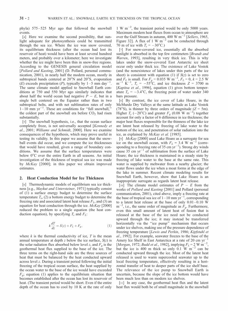
[15] Figure 1 shows that the spectral absorption coeffi-cient of ice (the reciprocal of the attenuation length) variesby 6 orders of magnitude across the solar spectrum, andcompares it to the single value of h�1 used in the earlierwork. Ice absorbs most weakly in the blue and near-ultra-violet (UV) parts of the spectrum. The solid line in Figure 2comes mostly from Warren’s [1984] compilation of labo-ratory measurements; for the visible and near-visible wave-lengths (0.3–1.4 mm) the absorption was determined bymeasuring attenuation of a beam passing through clearbubble-free ice [Grenfell and Perovich, 1981; Perovichand Govoni, 1991]. If a small amount of undetectablescattering was present, the reported absorption coefficientkabs would be too large. Recently, measurements of photontravel time distributions in ice by the Antarctic Muon andNeutrino Detector Array (AMANDA) have been used toinfer both scattering and absorption coefficients [Price andBergstrom, 1997; Askebjer et al., 1997a, 1997b] (K. Wosch-nagg, personal communication, 2002). The AMANDAabsorption coefficients agree with the laboratory measure-ments at wavelengths l > 0.6 mm, but at shorter wave-lengths AMANDA infers a smaller kabs than obtained in thelaboratory, suggesting that the laboratory ice did indeedexhibit a small amount of scattering; this scattering domi-nated the absorption at blue wavelengths because theabsorption is so weak there.[16] The absorption by ice is so weak in the visible and

UV that kabs in Antarctic ice is dominated by the smallamount of dust naturally present in the ice. The kabs is higherin ice that fell as snow during the last glacial maximum,when the atmosphere was dustier [He and Price, 1998]. Ourcalculations in this paper use kabs for the cleanest ice at theSouth Pole (dashed line in Figure 1). The ice in the snowballtropics is likely to have contained more dust than thiscleanest ice, because it would have collected windblowndust from unglaciated continental deserts. The equilibriumice thickness Z given by (5) is smaller if kabs is smaller,because sunlight penetrates more deeply, so by using thedashed line in Figure 1 we are biasing our results toward thinice. We can therefore be confident in the conclusion of ourmodel if it predicts thick ice.

3.2. Incident Solar Radiation Spectrum

[17] To obtain the incident solar spectrum at sea level, wehave taken the subarctic summer (SAS) standard atmos-phere of McClatchey et al. [1972] and multiplied thetemperatures at all levels by the factor 0.812, so as to obtaina surface air temperature Ts = �40�C. We used the SASatmosphere as a starting point, rather than the subarcticwinter (SAW) because the SAW contains a surface-basedtemperature inversion that we think is unlikely to have beenpresent under the intense sunlight at low latitudes. For thewater vapor content of the modified SAS atmosphere weassumed saturation with respect to ice up to 10 km; dryabove. We then used an atmospheric radiation model,‘‘ATRAD’’ [Wiscombe et al., 1984], to compute the spectraldownward flux at the sea surface under clear sky (Figure 2).In comparison to the spectrum for the unmodified SAS

WARREN ET AL.: SNOWBALL EARTH: ICE THICKNESS ON THE TROPICAL OCEAN 31 - 3

atmosphere (dashed line in Figure 2), the cold atmosphereabsorbs much less radiation in the water vapor bands.[18] The reason we assumed saturation with respect to

ice was that this is what is commonly found in the tropo-sphere over the Antarctic Plateau, where the surface tem-perature is similar to that of the snowball tropics. Thisassumption of saturation probably exaggerates the relativehumidity of the tropical troposphere. However, the watervapor content of an atmosphere at �40�C with 100%relative humidity is the same as that of an atmosphere at�30�C with 34% relative humidity, so the solar spectrumwe are using should be appropriate for the standard casebelow, where Ts = �30�C.

3.3. Radiative Transfer in Ice

[19] The ice in this model has a clean top surface; it is freeof any deposits of snow, salt, or dust. The ice is assumed tobe homogeneous and contains a uniform distribution ofspherical air bubbles of radius 0.1 mm of specified numberdensity neff. The single-scattering phase function of thebubbles is given by Mullen and Warren [1988]. Bubblesare used to represent all scatterers in the ice; brine inclusions

are not explicitly modeled. In the marine ice discussedbelow, the scattering is by cracks rather than bubbles, butbubbles can adequately represent their effect on radiativetransfer [cf. Bohren, 1983], because both bubbles and cracksare nonspectrally selective scatterers. The fact that thespectral absorption coefficient of water is very similar tothat of ice allows scattering by brine inclusions also to berepresented adequately by an effective bubble density in themodel. The flat upper surface of the ice reflects specularlyboth up and down.[20] We use a multilayer discrete ordinates radiative

transfer model with a specularly reflecting upper surface,developed by Grenfell [1983]. Radiation fluxes are com-puted at 50 unequally spaced vertical levels (with finerspacing near the upper surface) to determine the totalabsorbed radiation within each layer. The model was runfor twelve bubble densities, two solar zenith angles, and forice thickness Z ranging from 0.1 to 30 m at 0.1 m incre-ments and from 30 to 200 m at 1 m increments, for a total of11,280 cases. For the thinnest cases the spacing of verticallevels increased from 0.5 mm at the top to 2.5 mm at thebottom. For Z = 200 m the layer spacing increased from

Figure 1. Spectral absorption coefficient of pure ice from laboratory measurements [Grenfell andPerovich, 1981; Perovich and Govoni, 1991; Warren, 1984] and as inferred from field measurements bythe AMANDA project [Askebjer et al., 1997a, Figure 4] (K. Woschnagg, personal communication, 2002).Also shown is the broadband absorption coefficient used for sea ice on Snowball Earth byMcKay [2000].


0.5 mm at the top to 25 m at the bottom. (For Z > 200 mthere is no need for vertical resolution below 200 m becauseno sunlight penetrates that deeply.) For each of thesecases the sum �ifi �zi and the flux fn+1 to be used inequation (5) were computed and stored in a lookup table forcomputation of equilibrium ice thickness. We also ran theradiative transfer model at finer and coarser vertical reso-lution to ensure that the sum used for equation (5) hadconverged at all ice thicknesses. With specified surfacetemperature, bottom fluxes, ice bubble density, and solarzenith angle, the equilibrium ice thickness can be computedby iterating equation (5) to solve for Z using the followingmethod. From the lookup table, �ifi �zi and fn+1 for 0.1 mice is used to calculate Z. If the calculated Z exceeds 0.1 m,the next entry in the table is used, and so on, until theminimum difference between the thickness in the table entryand Z is found. If Z exceeds 200 m, the ice is optically thick

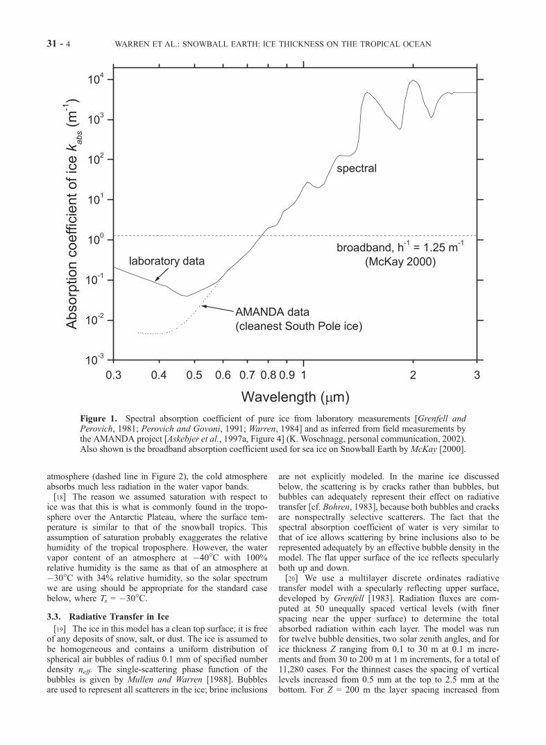
even for low bubble densities so �ifi �zi is the same as itwould be for 200 m thick ice (because all the solar flux isabsorbed in the top 200 m) and fn+1 = 0 (no solar flux exitsthe bottom of the ice), so equation (5) is now explicit andcan be solved directly for Z.[21] Figure 3 shows the absorption of solar radiation as a

function of depth in the top meter of the ice for a bubbledensity neff = 10 mm�3, corresponding to an albedo of 0.6.The broadband model, also shown in Figure 3, has thesame albedo, and hence the same total absorbed energy, butthe absorbed energy is distributed with depth quite differ-ently in the two models. The near-IR part of the solarspectrum is responsible for the high near-surface absorptionrate in the spectral model. Figure 4 is an expanded view ofthe uppermost 1 mm of Figure 3, for two ice types: pure icewith no bubbles, and ice with high bubble density (neff =200 mm�3), both computed using the spectral model. The

Figure 2. Downward solar spectrum, with solar constant reduced by 6% from its present value, atzenith angle 60�. The spectrum is plotted for the top of the atmosphere [Labs and Neckel, 1970;Neckel and Labs, 1984] and at a sea level surface either under the SAS standard atmosphere[McClatchey et al., 1972] or under an atmospheric temperature and humidity profile suggested for lowlatitude in daytime on Snowball Earth: temperatures reduced proportionately from SAS at all levels togive a surface temperature of �40�C and assuming water vapor saturation with respect to ice throughoutthe troposphere (up to 10 km). The spectrally integrated fluxes (in W m�2) are 644 at the top of theatmosphere, 509 at the surface under the SAS atmosphere, and 566 at the surface under the coldatmosphere.


broadband model’s absorption in the top millimeter is soclose to zero on this scale that it cannot be distinguishedfrom the left vertical axis. Figures 3 and 4 confirm theexpectation expressed above, that the broadband modeldeposits the solar radiation too deeply in the ice.[22] Figure 5 shows the spectrally averaged (‘‘allwave’’)

albedo, a, for 2 and 200 m thick ice as a function of bubbledensity for direct beam incidence at solar zenith angle q0 =0� or q0 = 60�. The albedo at very low bubble content is justthe Fresnel reflectivity of the surface, which depends onincidence angle. In subsequent figures we often use albedoof 200 m thick ice as a convenient surrogate for bubbledensity.[23] Figure 6 shows the fraction of the absorbed solar flux

that is absorbed in the topmost layers of ice, as a function ofbubble density (bottom scale) or albedo (top scale). Foralbedos 0.3–0.5, 50–85% of the absorption occurs in thetopmost 10 cm and is therefore quickly conducted up tothe top surface. In the broadband model only 12% of theabsorption is deposited into the topmost 10 cm; the remain-der penetrates more deeply and its energy must then be

conducted up, resulting in an equilibrium ice thickness thatis too small, as shown in Figure 7, which we discuss next.

3.4. Equilibrium Ice Thickness: Spectral VersusBroadband Model

[24] Figure 7 compares the equilibrium ice thickness, Z,computed by the spectral model to that computed by thebroadband model, for conditions expected to be representa-tive of the equatorial ocean on Snowball Earth. In bothcases Z is plotted as a function of albedo (a surrogate forneff, which is also shown on the top horizontal axis). This‘‘albedo’’ is the asymptotic albedo for 200 m thick ice,which is indistinguishable from the albedo of kilometer-thick ice.[25] Both models use Fg = 0.08 W m�2, a typical value

for geothermal heat flux from the ocean floor [Lillie, 1999].As discussed above, FL is at most 0.1 W m�2, and at thisvalue it would reduce the thickness of thick ice by a factorof 2 but would not change the location of the steeptransition to thin ice in Figure 7. Whatever value we choosefor FL in the range 0.0–0.1 W m�2 will not affect our

Figure 3. Solar energy absorbed per unit volume (i.e., heating rate) as a function of depth within the topmeter of the ice, comparing the broadband model with the spectral model. Number density of bubbles isneff = 10 mm�3, chosen to give albedo 0.60. The incident solar flux of 320 W m�2 is thought to representannual average conditions at the equator of Snowball Earth.


conclusions about the possible existence of thin ice. It iseven possible that FL is negative in the tropics and the icethicker than we calculate here (J. Goodman and R. T.Pierrehumbert, Glacial flow of floating marine ice in‘‘Snowball Earth,’’ submitted to Journal of GeophysicalResearch, 2002, hereinafter referred to Goodman and Pier-rehumbert, submitted manuscript, 2002). We therefore setFL = 0 for simplicity.[26] For the surface temperature Ts we refer to the results

of the GENESIS model [Pollard and Kasting, 2001] (D.Pollard, personal communication, 2001), which gives Ts =�30 to �35�C for the equatorial ocean in all seasons in the‘‘full snowball’’ state. In Figure 7 we set Ts = �30�C. Thetemperature at the bottom of the ice is �2�C, the freezingpoint of seawater.[27] The solar irradiance incident at the surface, S0 = 320

W m�2, is an estimate of the mean annual equatorial valuefor 700 Myr ago, as follows. The annual average solar flux,S0, incident at the surface at latitude f, is given by

S0 fð Þ ¼ 0:94Q0

4

� �s fð Þt; ð6Þ

where Q0 is the present value of the solar constant, Q0 =1370 W m�2, s(f) is the normalized latitudinal distributionof insolation, and t is the annual average atmospherictransmittance (average of clear and cloudy skies). The factor0.94 accounts for the 6% reduction in solar constantexpected for 700 Myr ago. For an orbital obliquity of 23.5�,the equatorial value of s(0) is 1.224 [Chylek and Coakley,1975, Table 1]. The atmospheric transmittance t given byATRAD for the cold atmosphere (Figure 2) is t = 0.88 forthe global average solar zenith angle q0 = 60�, and t = 0.92for overhead Sun, q0 = 0�. These values of t assume theatmosphere is devoid of clouds and ice crystals, which inreality would be present at times. To account for clouds andice crystals, we use t = 0.81 and obtain S0 = 320 W m�2.(However, in Figure 11 below, we will show results for allvalues of S0 in the range 0–400 W m�2.)[28] Figure 7 shows that as neff increases, there is a

sharp transition in ice thickness from less than 1 m toseveral hundred meters. This transition occurs when theice becomes sufficiently opaque that essentially no sun-light reaches the lower parts of the ice; then the icethickness jumps to a large value limited only by thegeothermal heat flux.

Figure 4. Solar energy absorbed per unit volume as a function of depth in the top millimeter of the ice,for the spectral model, both for pure bubble-free ice and for ice with a high bubble density.


[29] With the more accurate spectral model it is mucheasier to get thick ice. For any albedo in the range 0.4–0.7the spectral model gives Z > 200 m but the broadbandmodel gives Z < 2 m. In the earlier work [McKay, 2000], thebroadband model indicated that even for albedo as high as0.7 the tropical ice could be thin enough to permit photo-synthesis below. The spectral model shows that this isimpossible. We will argue in section 4 below that bare icewould have albedo greater than 0.4 and would therefore bethick.[30] The lower (thin-ice) branch of the curve, below the

inflection point, is probably not relevant to the real Earth. Itindicates, for example, that ice with an albedo of 0.3 couldhave an equilibrium thickness of 0.6 m. But this result isobtained only because we have specified Ts = �30�C. Inreality an ocean albedo less than 0.4 under a tropical Sun isprobably inconsistent with Ts < 0�C. When a = 0.4 isspecified for the tropical ocean in a general circulationmodel of Snowball Earth (D. Pollard, personal communi-cation, 2001), the surface temperature rises to the meltingpoint and the ice melts. We therefore have drawn a dashedline in Figure 7 to show our expectation of how the

equilibrium ice thickness would likely drop to zero forlow albedo in a coupled sea ice/climate model.[31] Low-albedo ice does exist on the modern Earth in the

Dry Valley lakes, because of the low regional air temper-ature. Thin ice of low albedo could possibly occur ontropical lakes on Snowball Earth, if they were sufficientlysmall in area that their low albedo did not affect the regionalclimate, so that the low regional air temperature could keepthem frozen. They would have to be landlocked, becauseany small thin-ice regions on the sea would be invaded byglacial flow of nearby thicker ice.

3.5. The Dry Valley Lakes Revisited

[32] Since the broadband model leads to large errors inthe computed ice thickness for the tropical ocean, we mustask why it was able to give the correct thickness for lake icein the McMurdo Dry Valleys, 3–6 m. Using the annualaverage solar incidence (S0 = 104 W m�2) and a latent heatflux of 3.4 W m�2, corresponding to the observed freezingrate of 35 cm yr�1,McKay et al. [1985] computed Z = 3.4 mfor an allwave albedo a = 0.6. When we put the bubbledensity corresponding to this albedo into the spectral model,

Figure 5. Spectrally averaged (‘‘allwave’’) albedo as a function of bubble density, for ice thickness Z =200 or 2 m, and solar zenith angle q0 = 0� or 60�.


we compute Z = 13 m. It appears that the reason for thebroadband model’s correct prediction of thickness was theuse of an unrealistically high albedo. The albedo of 0.6 usedby McKay et al. [1985] was based on a single cursorymeasurement (‘‘slightly more than 0.50’’) on Lake Vanda[Ragotzkie and Likens, 1964]. However, when McKay et al.[1994, Figures 11 and 13] measured the albedo accuratelyand repeatedly on Lake Hoare, it averaged to about 0.3.With this observed albedo, it is the spectral model that givesa reasonable ice thickness, Z = 4 m; the broadband modelmakes it too thin (Z = 1 m).[33] The simple analytical model can still be applied to

the ice covers of the Dry Valley lakes if one considers it as atwo-band model: a visible band that penetrates the ice coverand a near-IR band that does not. About half the solarradiation is in the visible band. Using the measured visiblealbedo for Lake Hoare (0.3) and computing h = 1.2 m fromthe measured transmissivity of the lake ice in the visible

[McKay et al., 1994] the model correctly predicts the icethickness (4 m for a mean annual temperature of �20�C)when the solar flux is reduced by a factor of 2.

4. Modern Surrogates for Ice on theTropical Ocean

[34] In steady state, ice in the snow-free regions of thetropical ocean will experience a slow loss of a fewmillimeters per year by sublimation at the upper surface,balanced by freezing of seawater at the lower surface andinflow from higher latitudes where the ice is thicker. Thekilometer-thick snow-covered ice sheets covering midlati-tude and polar oceans would flow like modern ice shelves,but we prefer to call them ‘‘sea glaciers’’ because theirexistence is independent of any continental glaciation.Near the poleward limit of the net sublimation regionthe bare ice will therefore be freshwater ice (resembling

Figure 6. Percent of the absorbed solar flux that is absorbed in the topmost 1 mm, 1 cm, or 10 cm of theice, for two different zenith angles, as a function of bubble density (lower scale) or the correspondingalbedo for thick ice (top scale). In the broadband model, only 12% of the absorbed sunlight is absorbed inthe top 10 cm.


glacier ice), originally formed by compression of snow,that has flowed equatorward as sea glaciers (Goodman andPierrehumbert, submitted manuscript, 2002). Closer to theequator, if the net sublimation rate exceeds the rate of net

ice inflow, the ice exposed at the surface will consist offrozen seawater. There are therefore several modern icetypes that should be considered as possible surrogates forice on the tropical ocean, all of which are more appropriate

Table 1. Potential Modern Surrogates for Equatorial Sea Ice With No Surface Deposits

Albedo (q0 = 60�) Albedo (q0 = 0�)

Cold blue glacier ice [Warren et al., 1993a] 0.63Cold blue glacier ice [Bintanja, 1999, Figure 14] 0.6 0.57a

Nonmelting snow-free sea ice, Ts = �5�C [Brandt et al., 1999] 0.49b (0.47a) 0.44a

Subeutectic bare sea ice, Ts = �37�C [Perovich and Grenfell, 1981] 0.75b (0.71a) 0.69a

Marine ice [Warren et al., 1997] 0.27b (0.25a) 0.21a

Melting multiyear Arctic sea ice with granular surface layer[Grenfell and Perovich, 1984; Perovich et al., 2002]

0.63 ± 0.05

aAlbedos for solar spectrum expected under colder atmosphere (Figure 2).bAlbedos under ambient environmental conditions during the measurement.

Figure 7. Equilibrium ice thickness predicted by both spectral and broadband models as a function ofbubble density (top scale) or the corresponding thick ice albedo (lower scale). All input variables are thesame in both models, at values thought appropriate for the equator of Snowball Earth. The only differencebetween the models is that the penetration depth h and the albedo have constant values for allwavelengths in the broadband model but vary with wavelength in the spectral model. The lower (thin ice)branch of the curve is artificial, because Ts is fixed at �30�C. For a < 0.4 in a coupled sea ice/climatemodel, Ts would most likely rise and the ice would melt (dashed line).


than the lake ice of the Dry Valleys. They are summarizedin Table 1.

4.1. Glacier Ice

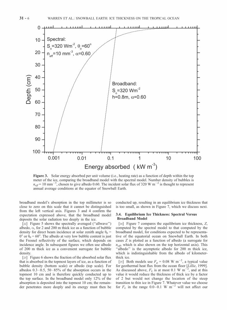
[35] In some mountainous regions in Antarctica, strongwinds blow away the fallen snow, exposing areas of glacierice, which are further ablated by sublimation. The spectralalbedo of this ice was measured at one site by Warren et al.[1993a] and is shown in Figure 8; the allwave albedo atseveral sites has been reported by Bintanja [1999], averag-ing 0.6. The exposed surface is often called ‘‘blue ice,’’ butits appearance might better be described as ‘‘blue-white,’’because the ice contains numerous bubbles, since the originof this ice was compression of snow.

4.2. Frozen Seawater

[36] On regions of the snowball ocean where net sub-limation exceeds inflow of sea glaciers, seawater will freezeto the base. The density of bubbles (and brine inclusions)

incorporated into this ice will depend on the rate of freezingand also on the depth at which freezing occurs, i.e., on howthick the ice is. These bubbles and brine inclusions will thenbe carried slowly upward as the top surface sublimates.Both bubbles and brine inclusions migrate toward the warmend of a temperature gradient [Wettlaufer, 1998], but thesublimation rate probably exceeds the migration rate (S. G.Warren et al., Ocean surfaces on Snowball Earth, in prep-aration, 2002). This process can lead to accumulation of saltcrystals at the top surface, as discussed below, but for nowwe ignore the possibility of a salt crust.[37] Three modern examples of frozen seawater can serve

as surrogates. The first is sea ice freezing at the oceansurface. Such ice that has grown through an entire winter isnormally snow covered, but near the coast of Antarcticastrong winds blow the snow away. The spectral albedo ofbare cold sea ice, 1.4 m thick, measured by Brandt et al.[1999], is shown in Figure 8. Its allwave albedo was 0.49under the ambient conditions, but it would be lower, about

Figure 8. Spectral albedos of possible modern surrogates for ocean surfaces on Snowball Earth. Theblue glacier ice was measured in the Trans-Antarctic Mountains by Warren et al. [1993a]. Sea ice andicebergs were measured near the coast of Antarctica at 68�S, 77�E [Warren et al., 1997]. The sea ice was1.4 m thick and windswept, so it was mostly bare, but there were patches of thin snow cover, coveringareas large enough for their albedo to be measured as well (upper curve). The blue marine ice wasmeasured on a capsized iceberg; the ice had originally frozen to the base of an ice shelf. The subeutecticsea ice was measured in a laboratory by Perovich and Grenfell [1981].


0.47, under the colder atmosphere of Snowball Earth,because the near-IR solar radiation, for which ice has lowalbedo, would not be filtered out as effectively by atmos-pheric water vapor (Table 1). Figure 8 also shows thedramatic effect of a thin layer of snow, which was foundin patches on this same region of coastal ice. Just 5–10 mmof snow raised the albedo from 0.49 to 0.81.[38] That ice was measured at a temperature of �5�C. If it

had been much colder, below the eutectic temperature ofNaCl in seawater, �23�C [Pounder, 1965], salt crystalsforming in the brine inclusions would have raised thealbedo. Such subeutectic ice has been studied only in thelaboratory, by Perovich and Grenfell [1981], who measuredspectral albedo from 400 to 1000 nm. This wavelengthrange covers about 80% of the solar energy spectrum. Weextrapolate the measured spectral albedo further into thenear-IR using spectral shapes of albedo that are typical ofsea ice (a procedure used previously by Allison et al.[1993]) and obtain an estimated allwave albedo a = 0.75under the SAS atmosphere, and 0.71 under the cold atmos-phere (Figure 8 and Table 1). The albedo of bare ice on theequator of Snowball Earth will reach this level only if Ts <�23�C and the salt content of the ice is similar to that ofmodern first-year sea ice.[39] Frozen seawater also accretes to the base of Antarctic

ice shelves [Morgan, 1972; Lange and MacAyeal, 1986], bymeans of the ‘‘ice pump’’ mentioned above. It is called‘‘marine ice’’ to distinguish it from ‘‘sea ice’’ forming at theocean surface; these two forms of frozen seawater differsubstantially in their composition and structure. Marine iceforms at a depth of 400 m or so, where the solubility of airin water is greater than at the sea surface, so the ice does notincorporate bubbles. Nor does it contain brine inclusions; itssalinity is typically one-thousandth that of seawater [Warrenet al., 1993b, Table 1], in contrast to sea ice whose salinityis initially about one-third that of seawater. Reasons for thedesalination of marine ice were investigated theoretically byTabraham [1997].[40] Marine ice at the base of the Amery Ice Shelf attains

a thickness of 190 m in places [Fricker et al., 2001], i.e.,about 40% of the total ice thickness. Icebergs originatingfrom such ice shelves may capsize, and then the marine icebecomes exposed to view. Its color may be green or blue,depending on the concentration of dissolved organic matterin the ice. Although the ice is bubble free, it contains alattice of cracks perpendicular to the surface with a typicalspacing of 0.5 m. Their mechanism of formation has notbeen studied; presumably they result from thermal and/ormechanical stresses. These cracks are responsible for thealbedo of marine ice shown in Figure 8. The allwave albedounder the ambient clear sky was 0.27, but with the coldatmosphere solar spectrum of Figure 2 it would be 0.25(Table 1).[41] If the ice on the snowball ocean is hundreds of

meters thick, the lower part of the ice sheet may thereforeresemble marine ice rather than sea ice. The accreted icewould slowly move upward as the surface is ablated bysublimation and the marine ice might then be exposed at thesurface. The development of thermal and mechanicalstresses would be much slower than in a capsizing icebergand the stresses might be released by recrystallization, sothe density of cracks might be less.

[42] We adjust the effective bubble density neff in ourradiative transfer model to match the spectral albedos inFigure 8 as closely as possible; the best fit for sea ice is neff= 2 mm�3. In the case of marine ice these bubbles in themodel, neff = 0.1 mm�3, are just a proxy for the crackswhich actually cause the scattering.[43] On the snowball ocean, the rate of freezing to the

base of the ice would be at most equal to the sublimationrate, i.e., only 1–10 mm yr�1, much slower than for modernsea ice or marine ice. At slow freezing rates the bubbledensity would be less than at rapid freezing rates, accordingto the laboratory experiments of Carte [1961] and Bari andHallett [1974]. Those experiments were performed onfreshwater ice and obtained bubble densities orders ofmagnitude smaller than are found in natural sea ice at thesame growth rate, so we cannot apply their results quanti-tatively. However, it does seem possible that even sea iceonly a few meters thick could be as clear as marine ice if itcould grow sufficiently slowly in a calm (wave-free) envi-ronment.[44] However, there are two reasons to think that marine

ice is unlikely to be exposed at the surface of the snowballocean. First, the flow of sea glaciers is sufficiently fast thatGoodman and Pierrehumbert (submitted manuscript, 2002)predict glacier ice to be exposed even at the equator.Second, if frozen seawater does sublimate at the equator,a salt crust would likely develop on the surface (Warren etal., in preparation, 2002).

4.3. Melting Sea Ice

[45] In the Arctic Ocean, bare multiyear sea ice isexposed in summer after the snow cover has melted anddrained. This ice has a high albedo of 0.63 because it isactively melting and develops a granular surface layer thatis similar in appearance to coarse-grained snow. Thismechanism would be absent if the air temperatures arebelow freezing throughout the year, but could becomeimportant in summer as the climate warms toward the endof a snowball event.

5. Equilibrium Ice Thickness

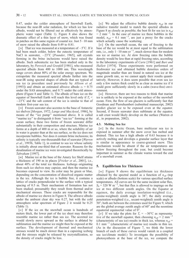
[46] Figure 9 shows the equilibrium ice thicknessobtained by the spectral model as a function of neff (topscale) or albedo (bottom scale) for various specified surfacetemperatures. All curves are for the same incident solar flux,S0 = 320 W m�2, but that flux is allowed to impinge on theice at two different zenith angles. On the Equator atequinox, the daily average insolation-weighted (i.e.,cosine-weighted) zenith angle is 38�; the daily averagepenetration-weighted (i.e., secant-weighted) zenith angle is50�; both are between the extremes used for Figure 9, whichare the global average zenith angle of 60� and the noontimeequatorial equinoctial value of 0�.[47] If we take the plots for Ts = �30�C as representa-

tive of the snowball equator, then choosing neff = 2 mm�3

(characteristic of sea ice) results in thick ice, whereas neff =0.1 mm�3 (characteristic of marine ice) results in thin ice.(As in the discussion of Figure 7, we think the lowerbranch of each of these curves would vanish in a coupledsea ice/climate model.) To investigate the possibility ofphotosynthesis at the base of the ice, we compute the


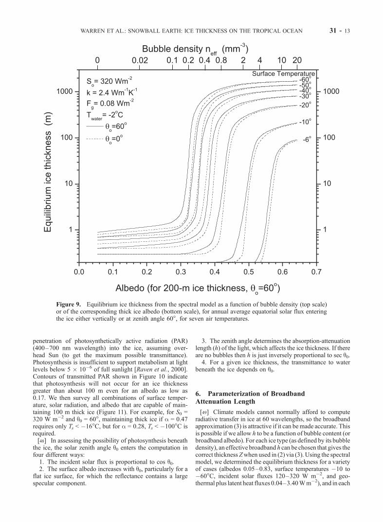
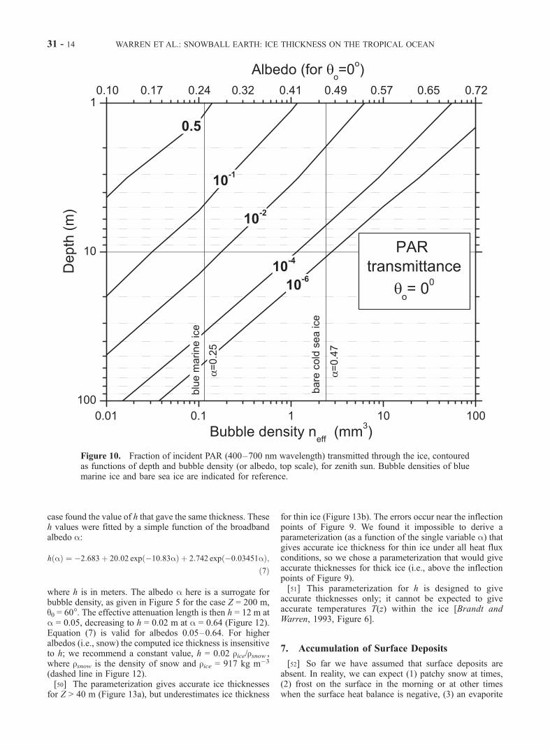
penetration of photosynthetically active radiation (PAR)(400–700 nm wavelength) into the ice, assuming over-head Sun (to get the maximum possible transmittance).Photosynthesis is insufficient to support metabolism at lightlevels below 5 � 10�6 of full sunlight [Raven et al., 2000].Contours of transmitted PAR shown in Figure 10 indicatethat photosynthesis will not occur for an ice thicknessgreater than about 100 m even for an albedo as low as0.17. We then survey all combinations of surface temper-ature, solar radiation, and albedo that are capable of main-taining 100 m thick ice (Figure 11). For example, for S0 =320 W m�2 and q0 = 60�, maintaining thick ice if a = 0.47requires only Ts < �16�C, but for a = 0.28, Ts < �100�C isrequired.[48] In assessing the possibility of photosynthesis beneath

the ice, the solar zenith angle q0 enters the computation infour different ways:1. The incident solar flux is proportional to cos q0.2. The surface albedo increases with q0, particularly for a

flat ice surface, for which the reflectance contains a largespecular component.

3. The zenith angle determines the absorption-attenuationlength (h) of the light, which affects the ice thickness. If thereare no bubbles then h is just inversely proportional to sec q0.4. For a given ice thickness, the transmittance to water

beneath the ice depends on q0.

6. Parameterization of BroadbandAttenuation Length

[49] Climate models cannot normally afford to computeradiative transfer in ice at 60 wavelengths, so the broadbandapproximation (3) is attractive if it can bemade accurate. Thisis possible if we allow h to be a function of bubble content (orbroadband albedo). For each ice type (as defined by its bubbledensity), an effective broadband h can be chosen that gives thecorrect thicknessZwhen used in (2) via (3). Using the spectralmodel, we determined the equilibrium thickness for a varietyof cases (albedos 0.05–0.83, surface temperatures �10 to�60�C, incident solar fluxes 120–320 W m�2, and geo-thermal plus latent heat fluxes 0.04–3.40Wm�2), and in each

Figure 9. Equilibrium ice thickness from the spectral model as a function of bubble density (top scale)or of the corresponding thick ice albedo (bottom scale), for annual average equatorial solar flux enteringthe ice either vertically or at zenith angle 60�, for seven air temperatures.


case found the value of h that gave the same thickness. Theseh values were fitted by a simple function of the broadbandalbedo a:

h að Þ ¼ �2:683þ 20:02 exp �10:83að Þ þ 2:742 exp �0:03451að Þ;ð7Þ

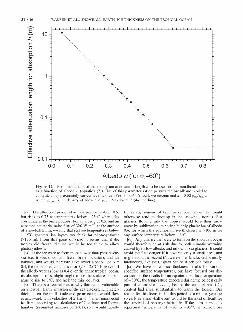
where h is in meters. The albedo a here is a surrogate forbubble density, as given in Figure 5 for the case Z = 200 m,q0 = 60�. The effective attenuation length is then h = 12 m ata = 0.05, decreasing to h = 0.02 m at a = 0.64 (Figure 12).Equation (7) is valid for albedos 0.05–0.64. For higheralbedos (i.e., snow) the computed ice thickness is insensitiveto h; we recommend a constant value, h = 0.02 rice/rsnow ,where rsnow is the density of snow and rice = 917 kg m�3

(dashed line in Figure 12).[50] The parameterization gives accurate ice thicknesses

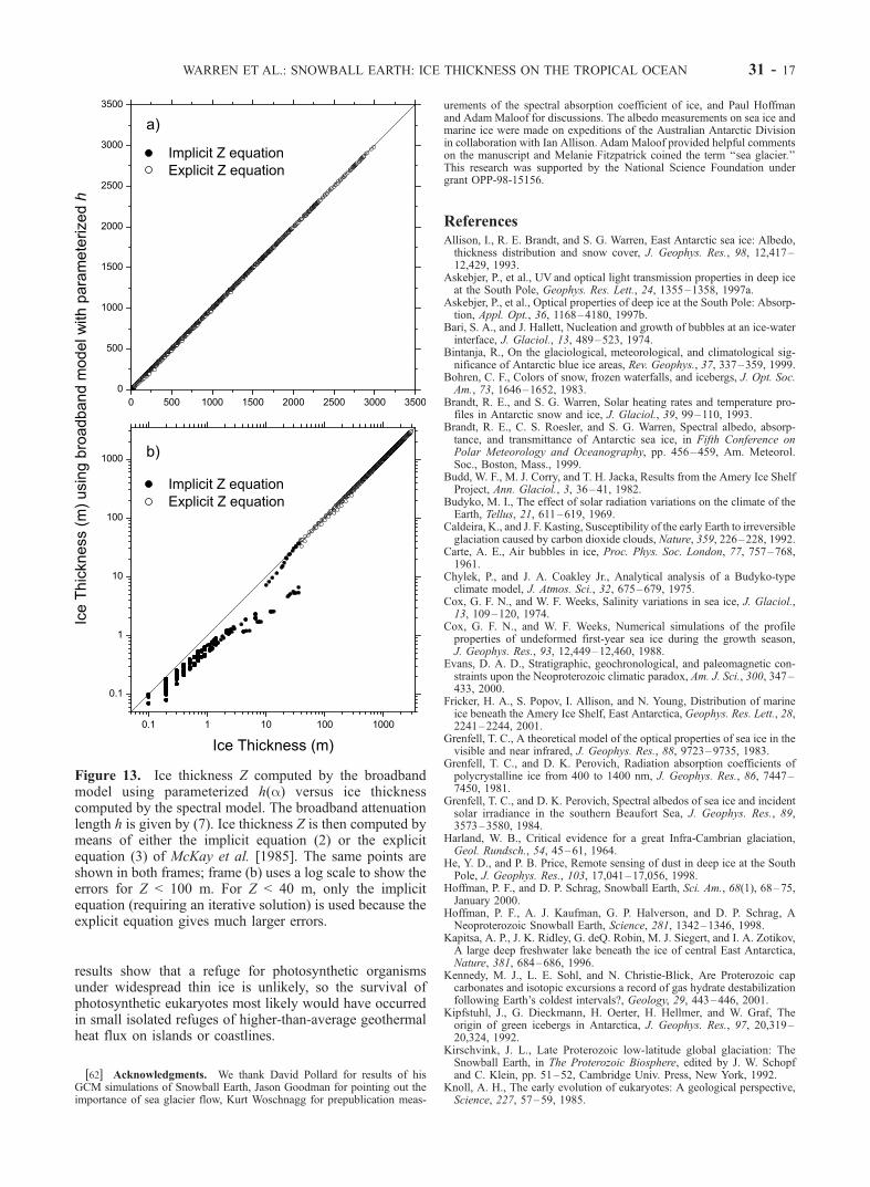
for Z > 40 m (Figure 13a), but underestimates ice thickness

for thin ice (Figure 13b). The errors occur near the inflectionpoints of Figure 9. We found it impossible to derive aparameterization (as a function of the single variable a) thatgives accurate ice thickness for thin ice under all heat fluxconditions, so we chose a parameterization that would giveaccurate thicknesses for thick ice (i.e., above the inflectionpoints of Figure 9).[51] This parameterization for h is designed to give

accurate thicknesses only; it cannot be expected to giveaccurate temperatures T(z) within the ice [Brandt andWarren, 1993, Figure 6].

7. Accumulation of Surface Deposits

[52] So far we have assumed that surface deposits areabsent. In reality, we can expect (1) patchy snow at times,(2) frost on the surface in the morning or at other timeswhen the surface heat balance is negative, (3) an evaporite

Figure 10. Fraction of incident PAR (400–700 nm wavelength) transmitted through the ice, contouredas functions of depth and bubble density (or albedo, top scale), for zenith sun. Bubble densities of bluemarine ice and bare sea ice are indicated for reference.


accumulation of salt, (4) wind-blown dust from unglaciatedcontinental deserts, and perhaps (5) an evaporite accumu-lation of freeze-dried algae incorporated into the ice baseand carried upward as sublimation proceeds, if photosyn-thetic life does exist below the ice.[53] Probably the most important surface deposits are

patchy snow and frost; they can dramatically raise thealbedo (Figure 8). Another possibly important process isaccumulation of salt. The first ice to form on the tropicalocean would probably form quickly, so it should resemblemodern sea ice forming in winter. First-year sea ice at theend of winter contains about 0.4% salt [Cox and Weeks,1974, 1988], so about 1 cm of salt would accumulate at thesurface if the top 2.5 m of ice sublimates. If the salt issomehow removed, for example by wind, and desalinatedmarine ice reaches the surface, salt will continue to accu-mulate, because marine ice does still contain 20 ppm of salt.The consequences of salt accumulation are investigatedfurther by Warren et al. (in preparation, 2002).[54] The accumulation of freeze-dried algae at the sur-

face, blocking the sunlight so as to suppress photosynthesisbelow the ice, is also an interesting possibility. It would be

an example of life altering its environment in a way thatmakes it unsuitable for life, i.e., the opposite of Gaia.

8. Discussion and Conclusion

[55] The solution for ice thickness is strikingly bimodal.Low surface temperature Ts, small basal freezing rate FL,and high albedo a result in equilibrium ice thickness on theorder of 1 km. As any of these variables changes in thedirection favoring thinner ice, a sharp transition is experi-enced to equilibrium thicknesses of a meter or less.[56] Thin ice (�1 m) is common on today’s high-latitude

oceans because warmer ocean water flowing below the icesupplies a heat flux of several watts per square meter. Thissource of heat ultimately comes from absorption of sunlightat the sea surface at lower latitudes; it would be absent onthe Snowball Earth after completion of a transient period ofa few thousand years during which the ocean would lose itsreservoir of heat. The existence of widespread thin ice onthe modern oceans is therefore not a reason to expect thinice on a snowball ocean.

Figure 11. Surface temperature required to obtain ice thickness of 100 m, contoured as functions ofincident solar flux and albedo (a surrogate for bubble density), for two different angles of incidence of thesunlight.


[57] The albedo of present-day bare sea ice is about 0.5,but rises to 0.75 at temperatures below �23�C when saltscrystallize in the brine pockets. For an albedo of 0.5, and anexpected equatorial solar flux of 320 W m�2 at the surfaceof Snowball Earth, we find that surface temperatures below�12�C generate ice layers too thick for photosynthesis(>100 m). From this point of view, it seems that if thetropics did freeze, the ice would be too thick to allowphotosynthesis.[58] If the ice were to form more slowly than present-day

sea ice, it would contain fewer brine inclusions and airbubbles, and would therefore have lower albedo. For a =0.4, the model predicts thin ice for Ts > �25�C. However, ifthe albedo were as low as 0.4 over the entire tropical ocean,its absorption of sunlight might cause the surface temper-ature to rise to 0�C, and melt the thin ice layer.[59] There is a second reason why thin ice is vulnerable

on Snowball Earth: invasion of the sea glaciers. Kilometer-thick ice on the midlatitude and polar oceans would flowequatorward, with velocities of 2 km yr�1 at an unimpededice front, according to calculations of Goodman and Pierre-humbert (submitted manuscript, 2002), so it would rapidly

fill in any regions of thin ice or open water that mightotherwise tend to develop in the snowball tropics. Seaglaciers flowing into the tropics would lose their snowcover by sublimation, exposing bubbly glacier ice of albedo0.6, for which the equilibrium ice thickness is >100 m forany surface temperature below �8�C.[60] Any thin ice that were to form on the snowball ocean

would therefore be at risk due to both climatic warmingcaused by its low albedo, and inflow of sea glaciers. It couldavoid the first danger if it covered only a small area, andmight avoid the second if it were either landlocked or nearlylandlocked, like the Caspian Sea or Black Sea today.[61] We have shown ice thickness results for various

specified surface temperatures, but have focused our dis-cussion on the results for an equatorial surface temperatureof �30�C, the temperature expected during the coldest earlypart of a snowball event, before the atmospheric CO2

content had risen substantially to warm the tropics. Ourreason for this focus is that this period of a million years orso early in a snowball event would be the most difficult forthe survival of photosynthetic life. If the climate model’sequatorial temperature of �30 to �35�C is correct, our

Figure 12. Parameterization of the absorption-attenuation length h to be used in the broadband modelas a function of albedo a (equation (7)). Use of this parameterization permits the broadband model tocompute an approximately correct ice thickness. For a > 0.64 (snow), we recommend h = 0.02 rice/rsnow,where rsnow is the density of snow and rice = 917 kg m�3 (dashed line).


results show that a refuge for photosynthetic organismsunder widespread thin ice is unlikely, so the survival ofphotosynthetic eukaryotes most likely would have occurredin small isolated refuges of higher-than-average geothermalheat flux on islands or coastlines.

[62] Acknowledgments. We thank David Pollard for results of hisGCM simulations of Snowball Earth, Jason Goodman for pointing out theimportance of sea glacier flow, Kurt Woschnagg for prepublication meas-

urements of the spectral absorption coefficient of ice, and Paul Hoffmanand Adam Maloof for discussions. The albedo measurements on sea ice andmarine ice were made on expeditions of the Australian Antarctic Divisionin collaboration with Ian Allison. Adam Maloof provided helpful commentson the manuscript and Melanie Fitzpatrick coined the term ‘‘sea glacier.’’This research was supported by the National Science Foundation undergrant OPP-98-15156.

ReferencesAllison, I., R. E. Brandt, and S. G. Warren, East Antarctic sea ice: Albedo,thickness distribution and snow cover, J. Geophys. Res., 98, 12,417–12,429, 1993.

Askebjer, P., et al., UV and optical light transmission properties in deep iceat the South Pole, Geophys. Res. Lett., 24, 1355–1358, 1997a.

Askebjer, P., et al., Optical properties of deep ice at the South Pole: Absorp-tion, Appl. Opt., 36, 1168–4180, 1997b.

Bari, S. A., and J. Hallett, Nucleation and growth of bubbles at an ice-waterinterface, J. Glaciol., 13, 489–523, 1974.

Bintanja, R., On the glaciological, meteorological, and climatological sig-nificance of Antarctic blue ice areas, Rev. Geophys., 37, 337–359, 1999.

Bohren, C. F., Colors of snow, frozen waterfalls, and icebergs, J. Opt. Soc.Am., 73, 1646–1652, 1983.

Brandt, R. E., and S. G. Warren, Solar heating rates and temperature pro-files in Antarctic snow and ice, J. Glaciol., 39, 99–110, 1993.

Brandt, R. E., C. S. Roesler, and S. G. Warren, Spectral albedo, absorp-tance, and transmittance of Antarctic sea ice, in Fifth Conference onPolar Meteorology and Oceanography, pp. 456–459, Am. Meteorol.Soc., Boston, Mass., 1999.

Budd, W. F., M. J. Corry, and T. H. Jacka, Results from the Amery Ice ShelfProject, Ann. Glaciol., 3, 36–41, 1982.

Budyko, M. I., The effect of solar radiation variations on the climate of theEarth, Tellus, 21, 611–619, 1969.

Caldeira, K., and J. F. Kasting, Susceptibility of the early Earth to irreversibleglaciation caused by carbon dioxide clouds, Nature, 359, 226–228, 1992.

Carte, A. E., Air bubbles in ice, Proc. Phys. Soc. London, 77, 757–768,1961.

Chylek, P., and J. A. Coakley Jr., Analytical analysis of a Budyko-typeclimate model, J. Atmos. Sci., 32, 675–679, 1975.

Cox, G. F. N., and W. F. Weeks, Salinity variations in sea ice, J. Glaciol.,13, 109–120, 1974.

Cox, G. F. N., and W. F. Weeks, Numerical simulations of the profileproperties of undeformed first-year sea ice during the growth season,J. Geophys. Res., 93, 12,449–12,460, 1988.

Evans, D. A. D., Stratigraphic, geochronological, and paleomagnetic con-straints upon the Neoproterozoic climatic paradox, Am. J. Sci., 300, 347–433, 2000.

Fricker, H. A., S. Popov, I. Allison, and N. Young, Distribution of marineice beneath the Amery Ice Shelf, East Antarctica, Geophys. Res. Lett., 28,2241–2244, 2001.

Grenfell, T. C., A theoretical model of the optical properties of sea ice in thevisible and near infrared, J. Geophys. Res., 88, 9723–9735, 1983.

Grenfell, T. C., and D. K. Perovich, Radiation absorption coefficients ofpolycrystalline ice from 400 to 1400 nm, J. Geophys. Res., 86, 7447–7450, 1981.

Grenfell, T. C., and D. K. Perovich, Spectral albedos of sea ice and incidentsolar irradiance in the southern Beaufort Sea, J. Geophys. Res., 89,3573–3580, 1984.

Harland, W. B., Critical evidence for a great Infra-Cambrian glaciation,Geol. Rundsch., 54, 45–61, 1964.

He, Y. D., and P. B. Price, Remote sensing of dust in deep ice at the SouthPole, J. Geophys. Res., 103, 17,041–17,056, 1998.

Hoffman, P. F., and D. P. Schrag, Snowball Earth, Sci. Am., 68(1), 68–75,January 2000.

Hoffman, P. F., A. J. Kaufman, G. P. Halverson, and D. P. Schrag, ANeoproterozoic Snowball Earth, Science, 281, 1342–1346, 1998.

Kapitsa, A. P., J. K. Ridley, G. deQ. Robin, M. J. Siegert, and I. A. Zotikov,A large deep freshwater lake beneath the ice of central East Antarctica,Nature, 381, 684–686, 1996.

Kennedy, M. J., L. E. Sohl, and N. Christie-Blick, Are Proterozoic capcarbonates and isotopic excursions a record of gas hydrate destabilizationfollowing Earth’s coldest intervals?, Geology, 29, 443–446, 2001.

Kipfstuhl, J., G. Dieckmann, H. Oerter, H. Hellmer, and W. Graf, Theorigin of green icebergs in Antarctica, J. Geophys. Res., 97, 20,319–20,324, 1992.

Kirschvink, J. L., Late Proterozoic low-latitude global glaciation: TheSnowball Earth, in The Proterozoic Biosphere, edited by J. W. Schopfand C. Klein, pp. 51–52, Cambridge Univ. Press, New York, 1992.

Knoll, A. H., The early evolution of eukaryotes: A geological perspective,Science, 227, 57–59, 1985.

Figure 13. Ice thickness Z computed by the broadbandmodel using parameterized h(a) versus ice thicknesscomputed by the spectral model. The broadband attenuationlength h is given by (7). Ice thickness Z is then computed bymeans of either the implicit equation (2) or the explicitequation (3) of McKay et al. [1985]. The same points areshown in both frames; frame (b) uses a log scale to show theerrors for Z < 100 m. For Z < 40 m, only the implicitequation (requiring an iterative solution) is used because theexplicit equation gives much larger errors.


Labs, D., and H. Neckel, Transformation of the absolute solar radiation datainto the International Practical Temperature Scale of 1968, Sol. Phys., 15,79–87, 1970.

Lange, M. A., and D. R. MacAyeal, Numerical models of the Filchner–Ronne Ice Shelf: An assessment of reinterpreted ice thickness distribu-tion, J. Geophys. Res., 91, 10,457–10,462, 1986.

Lewis, E. L., and R. G. Perkin, Ice pumps and their rates, J. Geophys. Res.,91, 11,756–11,762, 1986.

Lillie, R. J., Whole Earth Geophysics, p. 326, Prentice-Hall, Old Tappan,N. J., 1999.

Maykut, G. A., and N. Untersteiner, Some results from a time-dependentthermodynamic model of sea ice, J. Geophys. Res., 76, 1550–1575,1971.

McClatchey, R. A., R. W. Fenn, J. E. A. Selby, F. E. Volz, and J. S. Garing,Optical Properties of the Atmosphere (Third Edition), 108 pp., ReportAFCRL-72-0497, Air Force Cambridge Res. Lab., Hanscom Air ForceBase, Bedford, Mass., 1972.

McKay, C. P., Thickness of tropical ice and photosynthesis on a snowballEarth, Geophys. Res. Lett., 27, 2153–2156, 2000.

McKay, C. P., G. D. Clow, R. A. Wharton Jr., and S. W. Squyres, Thicknessof ice on perennially frozen lakes, Nature, 313, 561–562, 1985.

McKay, C. P., G. D. Clow, D. T. Andersen, and R. A. Wharton Jr., Lighttransmission and reflection in perennially ice-covered Lake Hoare, Ant-arctica, J. Geophys. Res., 99, 20,427–20,444, 1994.

Morgan, V. I., Oxygen isotope evidence for bottom freezing on the AmeryIce Shelf, Nature, 238, 393–394, 1972.

Mullen, P. C., and S. G. Warren, Theory of the optical properties of lake ice,J. Geophys. Res., 93, 8403–8414, 1988.

Neckel, H., and D. Labs, The solar radiation between 3300 and 12,500Angstroms, Sol. Phys., 90, 205–258, 1984.

Perovich, D. K., and J. W. Govoni, Absorption coefficients of ice from 250to 400 nm, Geophys. Res. Lett., 18, 1233–1235, 1991.

Perovich, D. K., and T. C. Grenfell, Laboratory studies of the opticalproperties of young sea ice, J. Glaciol., 27, 331–346, 1981.

Perovich, D. K., T. C. Grenfell, B. Light, and P. V. Hobbs, Seasonal evolu-tion of the albedo of multiyear Arctic Sea ice, J. Geophys. Res., 107,10.1029/2000JC000438, 2002.

Pollard, D., and J. F. Kasting, Coupled GCM-Ice sheet simulations ofSturtian (750–720 Ma) glaciation: When in the Snowball-Earth cyclecan tropical glaciation occur?, Eos Trans. AGU, 82, S8, 2001.

Pounder, E. R., The Physics of Ice, 151 pp., Pergamon, New York, 1965.Price, P. B., and L. Bergstrom, Optical properties of deep ice at the SouthPole: Scattering, Appl. Opt., 36, 4181–4194, 1997.

Ragotzkie, R. A., and G. E. Likens, The heat balance of two Antarcticlakes, Limnol. Oceanogr., 9, 412–425, 1964.

Raven, J. A., J. E. Kubler, and J. Beardall, Put out the light, and then put outthe light, J. Mar. Biol. Assoc. U. K., 80, 1–25, 2000.

Schrag, D. P., R. A. Berner, P. F. Hoffman, and G. P. Halverson, On theinitiation of a snowball Earth, Geochem. Geophys. Geosyst., 3, 1036,doi:10.1029/2001GC000219, 2002.

Sellers, W. D., Physical Climatology, 272 pp., Univ. of Chicago Press,Chicago, Ill., 1965.

Sellers, W. D., A global climatic model based on the energy balance of theEarth–atmosphere system, J. Appl. Meteorol., 8, 392–400, 1969.

Tabraham, J., The desalination of marine ice, Ph.D. Thesis, 177 pp., Cam-bridge Univ. Press, New York, 1997.

Warren, S. G., Optical constants of ice from the ultraviolet to the micro-wave, Appl. Opt., 23, 1206–1225, 1984.

Warren, S. G., R. E. Brandt, and R. D. Boime, Blue ice and green ice,Antarct. J. U. S., 28, 255–256, 1993a.

Warren, S. G., C. S. Roesler, V. I. Morgan, R. E. Brandt, I. D. Goodwin, andI. Allison, Green icebergs formed by freezing of organic-rich seawater tothe base of Antarctic ice shelves, J. Geophys. Res., 98, 6921–6928 and18,309, 1993b.

Warren, S. G., C. S. Roesler, and R. E. Brandt, Solar radiation processes inthe East Antarctic sea ice zone, Antarct. J. U. S., 32, 185–187, 1997.

Wettlaufer, J. S., Introduction to crystallization phenomena in sea ice, inPhysics of Ice-Covered Seas, edited by M. Lepparanta, pp. 105–194,Univ. of Helsinki Press, Helsinki, 1998.

Williams, G. and P. Schmidt, Proterozoic equatorial glaciation: Has ‘‘snow-ball earth’’ a snowball’s chance?, Aust. Geol.117, pp. 21–25, 2000 [Re-ply by P. F. Hoffman (http://www.eps.harvard.edu/people/faculty/hoffman/TAG.html)].

Wiscombe, W. J., R. M. Welch, and W. D. Hall, The effects of very largedrops on cloud absorption, part I, Parcel models, J. Atmos. Sci., 41,1336–1355, 1984.

��R. E. Brandt, T. C. Grenfell, and S. G. Warren, Department of

Atmospheric Sciences, Box 351640, University of Washington, Seattle,WA 98196-1640, USA. ([email protected]; [email protected]; [email protected])C. P. McKay, Space Science Division, NASA Ames Research Center,

Mail Stop 245-3, Moffett Field, CA 94035, USA. ([email protected])


Documents

Snowball Earth: Ice thickness on the tropical oceansgw/PAPERS/2002_Snowball.pdf · The same climate model applied to Snowball Earth con-ditions at 750 and 550 Myr ago similarly indicates