U.S. DEPARTMENT OF THE INTERIOR U.S. GEOLOGICAL SURVEY

SMSIM Fortran Programs for Simulating Ground Motions from Earthquakes: Version 1.0

by

David M. Boore

Open-File Report 96-80-A

This report is preliminary and has not been reviewed for conformity with U.S. Geological Survey editorial standards or with the North American Stratigraphic Code. Any use of trade, product, or firm names is for descriptive purposes only and does not imply endorsement by the U.S. Government.

Although this program has been used by the U.S. Geological Survey, no warranty, expressed

or implied, is made by the USGS as to the accuracy and functioning of the program and

related program material, nor shall the fact of distribution constitute any such warranty, and no responsibility is assumed by the USGS in connection therewith.

. Geological Survey, MS 977, 345 Middlefield Rd., Menlo Park, CA 94025

SMSIM Fortran Programs for Simulating Ground Motions from Earthquakes

TABLE OF CONTENTS

INTRODUCTION ............................. 4METHOD ................................. 5THE PROGRAMS

PROGRAM OVERVIEW ........................ 7ANNOTATED LIST OF PROGRAMS .................. 8

Random-Vibration Programs ..................... 8Time-Domain Programs ....................... 9Fourier-Amplitude Programs ..................... 11Subroutine Modules ......................... 11Site-Amplification Programs ..................... 13

COMPILATION AND MODIFICATION ................. 14INPUT AND OUTPUT OF SMSIM PROGRAMS ............. 15

Input From Screen ......................... 15Input From File .......................... 16Output of SMSIM and FAS Programs ................. 21

INPUT AND OUTPUT OF SITE-AMPLIFICATION PROGRAMS ...... 22Input From Screen ......................... 22Input From File .......................... 23Output of Site-Amplification Programs ................ 24

ACKNOWLEDGMENTS .......................... 25REFERENCES ............................... 25FIGURES:

1. Motions computed using various rms-to-peak relations ............ 282. Sample input file for the SMSIM programs ................. 293. The specification of Q .......................... 304. The specification of path duration ..................... 315. The specification of site amplification ................... 326. Parameters used to define the exponential window ............. 337. Dependence on type of window: M 4, r 10 ................ 348. Dependence on type of window: M 4, r = 200 ............... 359. Dependence on type of window: M 7, r = 10 ................ 36

10. Dependence on type of window: M 7, r = 200 ............... 3711. Dependence on number of runs: M 4, r = 10 ................ 3812. Dependence on number of runs: M 7, r = 10 ................ 39

13. Output summary file: RV-DRVR program ................. 4014. Output column file: RV-DRVR program .................. 41

15. Output time series file: TD.DRVR program ................ 4216. Time series produced by TD.DRVR program ................ 43

17. Sample input file for the SITE-AMP program ............... 4418. Output file for the SITE-AMP program .................. 45

APPENDICES: SOURCE LISTINGS AND INPUT-PARAMETER FILESA. Random-Vibration Programs ....................... 47B. Time-Domain Programs ......................... 52C. Fourier-Amplitude Programs ....................... 58D. Subroutine Modules ........................... 61E. Site-Amplification Programs ....................... 68F. Atkinson & Boore (1995) Input-Parameter File ............... 72G. Coastal California Input-Parameter File .................. 73

SMSIM Fortran Programs for Simulating Ground Motions from Earthquakes

by

David M. Boore

INTRODUCTION

This Open-File Report is in response to requests for my programs for simulating ground motions from earthquakes. The programs are based on modifications I have made to the stochastic model first introduced by Hanks and McGuire (1981). The report contains source codes, written in Fortran, and executables that can be used on a PC. Programs are included both for time-domain and for random-vibration simulations. In addition, programs are included to produce Fourier amplitude spectra for the models used in the simulations and to convert shear velocity vs. depth into frequency-dependent amplification. The report contains an improvement in the implementation of the random- vibration method not published before.

The programs do not include extended-fault models, nor do they account for path and site effects by direct computations of wave propagation in layered media (but such path and site effects can be captured in the program by piecewise-continuous frequency- or distance-dependent functions specified by the user). Furthermore, the random-vibration calculations do not make use of the many advancements in random-vibration theory subsequent to the early work of Cartwright and Longuet-Higgins (1956).

The programs are a recent major revision of my earlier programs and therefore almost certainly contain uneradicated bugs. Although they are distributed on an "as is" basis, with no warranty of support from me, I would appreciate hearing about bugs and improvements to the codes. Please note that I have made little effort to optimize the coding of the programs or to include a user-friendly interface. Speed of execution has been sacrificed in favor of a code that is intended to be easy to understand. I will be pleased if users incorporate portions of my programs in their own applications.

Other stochastic-model codes are available and in common use. In particular, the reader is directed to the programs in Volume VIII of Herrmann (1996) and RASCAL by Silva and Lee (1987). I have not made a detailed comparison of my codes to these other codes and therefore cannot make any statements about the relative strengths and weaknesses of the various codes.

The programs can be obtained via anonymous ftp on samoa.wr.usgs.gov in directory get. The source code, executables, sample input and sample output have been compressed into a single self-extracting binary file with the name SMSIM10.EXE. After copying this file to the user's PC, the files can be extracted by typing the name SMSIM10. The portion of the file name with the version number ("10" in this case) will change if the program is modified.

METHOD

A description of the method is given in Boore (1983), Boore and Joyner (1984), Boore (1986), and Joyner and Boore (1988), and will not be repeated here, other than to say that the radiation from a fault is assumed to be distributed randomly over a time interval whose duration is related to the source size and possibly the distance from the source to the site. The detailed parameters used to characterize the source, path, and site effects are described later in this report.

The ground motion can be obtained via time-domain (TD ) simulation, from which peak parameters such as peak acceleration and response spectra can be obtained (mean values of the parameters require a Monte Carlo simulation with many realizations for given input parameters). The peak parameters also can be obtained directly using random- vibration (RV) theory'. This is a much quicker way of obtaining the peak parameters, but it is not useful if time series are needed in the analysis. In addition, there are assumptions in the random-vibration theory that are not present in the time-domain simulations. For this reason, the time-domain simulations can be considered "truth" in the simulations; many simulations are needed (on the order of 50 or more), however, in order for the square-root-of-n reduction of noise to provide accurate estimates of the peak parameters. In general, I have found the random-vibration simulations to be good estimates of the ground motions in almost all cases, at greatly reduced computer time.

This report contains an improvement in my implementation of random-vibration theory. That an improvement was needed is shown in Figure 1, which compares the response spectrum computed using RV and TD simulations. The heavy line is the TD simulation, and the dashed line is the result from what used to be the preferred RV method. The results from the two methods track one another very well, except for certain period ranges where the RV results show discontinuous changes in value. I first noticed

'Some would prefer the term "random-process theory"; I have used "random-vibration theory" because many of the applications are to the vibrations of harmonic oscillators and because the term is more familiar to engineers.

these changes several years ago, but I had no explanation for them. I now understand why they occur, and I have found a way to prevent them (the improved results are given

by the circles). The explanation has to do with how I treated the following integral from Cartwright and Longuet-Higgins (1956; their equation (6.8)):

1 r L /

2 Jov 2

where e is computed from the spectral moments and is a measure of the bandwidth of the spectrum, and N is the number of extrema, proportional to the square root of

the ratio of the fourth and second spectral moments. This integral is the ratio of the peak and rms motions, which for our purposes is the fundamental piece of information provided by random-vibration theory. (Cartwright and Longuet-Higgins' equation (6.8) is an approximation to their equation (6.4); the code for computing equation (6.8) is simpler than that for equation (6.4), and judging from the comparisons with time-domain calculations in this report and other comparisons that I have made, it is an excellent approximation for the ranges of magnitudes, distances, and oscillator periods of interest

in earthquake engineering. Using equation (6.4) would also require redoing the analysis of Boore and Joyner (1984) for determining the duration used to compute the rms the

Boore and Joyner results are based on equation (6.8) ). As described in my first paper on the stochastic model (Boore, 1983), I expanded the term in square brackets using the binomial series and integrated term-by-term. This gave equation (21) in Boore (1983).

The expansion assumes that N is an integer, but N is computed from spectral moments and in general is not an integer. In the calculations shown by the dashed line in Figure 1, however, the real number N was converted to an integer to determine how many terms

of the series to include in the sum (equation (21) in Boore, 1983). For small N (e.g., for long-period oscillator response for short-duration earthquakes), changes by one integer

lead to the discontinuous offsets seen in Figure 1. The solution to this is simple: calculate the integral in equation (1) numerically. The integral has an integrable singularity that is easily removed by the variable transformation

and the integrand is very well behaved, having a simple shape and decaying rapidly with increasing z. Using routines from Press et al. (1992), the integration is very rapid. Doing the integration numerically has another advantage: before, I devised an ad hoc scheme for switching from what I called the "exact" solution (the summation given by equation (21) in Boore, 1983, yielding the dashed line in Figure 1) to the asymptotic expansion of the integral. This scheme is discussed on p. 82 of Joyner and Boore (1988). Now there is no

need to switch from one approximation of the integral to another one simply computes

6

the integral numerically at all times. Speaking of the asymptotic expansion (which is Commonly used in applications of random-vibration theory), the two-term approximation is shown by the light line in Figure 1; it is clearly inadequate at long periods.

One of the most important messages from the comparisons shown in Figure 1 is how well the RV method works, even for excitations much shorter than the oscillator period

(the M = 4.0 source, with a stress parameter of 200 bars, has a duration of 0.24 sec). Further comparisons are shown in Figures 7, 8, 9, and 10, referred to in the discussion of

input parameters.

THE PROGRAMS

PROGRAM OVERVIEW:

The set of programs are collectively called SMSIM (Stochastic Model Simulation or Strong Motion Simulation, take your pick). Separate programs are included for the RV and the TD simulations, but an effort has been made to make the input and output parameter files the same for both applications. The programs include application-

specific drivers (RV.DRVR and TD.DRVR) that call modules of subroutines (SMSIM.RV

and SMSIM-TD}; these modules in turn call two additional modules of subroutines (RVTDSUBS and RECIPES). RVTDSUBS contains routines that are common to both

applications, and RECIPES contains programs from Numerical Recipes (Press et a/., 1992). A few of the RECIPES subroutines are minor modifications of the routines in Press et al. ; the modifications are noted in the annotated list of programs.

The drivers provided in this report produce peak acceleration, peak velocity, and response spectra for a range of oscillator periods, all for a given distance and magnitude. The modules were designed so that the drivers can be easily modified to produce

the ground-motion parameters for other combinations of magnitude, distance, or input parameters. (For example, recently I needed a table of response spectral values at many magnitudes and distances for a set of oscillator periods one file per period; it was easy to generate this by modifying RV.DRVR.)

Programs are also given to compute Fourier spectral amplitudes corresponding to the model specified by the input-parameter file (FAS.DRVR) and for computing a first-

order approximation to site amplification given depth-dependent velocity and density(SITE-AMP).

The purpose of each program and subroutine is noted in the following annotated list. Following this description are some notes about compiling and modifying the programs

and descriptions of parameter input and program output.

ANNOTATED LIST OF PROGRAMS:

A short description is given of the purpose of each program; for details, see the program listings in Appendices A through E. The user may find that some of these programs are

useful in other applications.

Random Vibration Programs:

RV-DRVR: The front-end program for the random-vibration calculations. Interac­

tively obtains input and output file names, whether or not response spectra are to be computed, and information needed to set the damping and periods for the response spectra. The periods can be either individual periods or a set of periods between specified limits. The program obtains input parameters from a file, and passes these parameters to the subsequent subroutine modules through common blocks (dimension statements, variable declarations, and common statements are contained in SMSIM.FI

and are inserted into RV-DRVR at compile time by the use of the Fortran INCLUDE statement.) The input parameters can, of course, be overridden in customizations of the driver program. This would occur if, for example, the motion is required for many values of the stress parameter rather than the one value included in the input

parameter file. The program also obtains interactively the magnitude and distance for the simulation. The program computes peak velocity, peak acceleration, and, if specified, response-spectral amplitudes, with separate calls to the main subroutine (SMSIM-RV). After writing the results to an output file in columnar format, the

program loops back for another magnitude and distance, if desired.

SMSIM-RV: The main subroutine module for the random-vibration calculations, called separately for peak velocity, peak acceleration, and response-spectral output.

The routine calls subroutines to set some frequency-independent spectral parameters and calls GET-MOTION, which does the actual simulations. The various subroutines included in the module are:

GET-MOTION: Computes the necessary spectral moments and uses these moments in the numerical integration that provides the simulated amplitudes. The routine also computes the values based on the one- and two-term asymptotic expansions, in case the user wants to compare them to the results from the direct

integration of equation (1). These estimates, pk.cLl and pk.cL2 (standing for r>eak motion from Cartwright and Longuet-Higgins formulation using i- and 2- term asymptotic expansions), are available through a common block included in SMSIM.FI.

CL68-NUMRCLJNT: Calls routines to compute the integral in equation (1) (equation (6.8) of Cartwright and Longuet-Higgins, thus "CL68').

CL68-INTEGRAND: A function defining the integrand in equation (1).

AMOM-RV: A function that returns a spectral moment, computed by adaptive integration. Unlike the straightforward integration of equation (1), I recommend adaptive integration (whose step sizes vary according to the requirements of the integrand) for the spectral moments; the spectral moments can have spike-like integrands, particularly for lightly-damped oscillators. The problem of fixed- increment integration is particularly critical for long-period oscillators, for which care must be taken that the frequency increment is not too coarse to approximate adequately the spectral moment.

DERIVS: Subroutine needed in the adaptive-integration routine ODEINT de­ scribed in the RECIPES section.

Time-Domain Programs:

TD-DRVR: The front-end program for the time-domain calculations. Interactively obtains input and output file names, whether or not response spectra are to be computed, and information needed to set the damping and periods for the response spectra. The periods can be either individual periods or a set of periods between specified limits. The program also asks if sample time series are to be saved in a file. The program obtains input parameters from a file. The program also obtains interactively the magnitude and distance for the simulation. The program determines peak velocity, peak acceleration, and, if specified, response-spectral amplitudes, with one call to the main subroutine (SMSIM.TD). This differs from RV-DRVR, which made separate calls to SMSIM.RV in order to obtain the three main types of ground motion (the reason for the difference is that I decided that most applications would require simulations for a number of oscillator periods, which are most efficiently computed by passing a simulated time series to a subroutine that computes response spectra). After writing the results to an output file, the program loops back for another magnitude and distance, if desired.

9

SMSIM-TD: The main subroutine module for the time-domain calculations. For each realization, it calls a routine that returns the acceleration time series, and then computes peak acceleration, peak velocity, and response spectral amplitudes for this time series. After the loop over realizations, the program computes the arithmetic average (NOT the log average) of the motions. The various subroutines included in

the module are:

GET-ACC: The main computations for computing a time series are contained

in this routine, which passes the time series through its argument list. The amplitudes are scaled such that the average of the squared spectral amplitudes

of the random number sample, before frequency-domain filtering, is unity. This scaling differs somewhat from that of G. M. Atkinson, which was used in Atkinson

and Boore (1995). In her implementation, the scaling was in terms of the average

spectral amplitude rather than the average of the squared spectral amplitude. The difference between scaling leads to a systematic difference in the results, such that the motions in the tables in the Appendix of Atkinson and Boore (1995) would be reduced by about a factor of 0.89 if my scaling is used.

GET-VEL: Returns a times series that is the integral of an input time series,

after detrending the input.

DCDT: A routine written by C. S. Mueller that detrends a time series.

MNMAX: Returns the minimum and maximum of an array.

MEAN: Computes the mean of an array.

AVGSQ-REALFT: Returns the average of the squared spectral amplitudes computed by REALFT, not including the values at zero frequency and the

Nyquist frequency.

WIND-BOX: Returns values of a window using a raised cosine-taper at each end.

WIND-EXP: Returns values of an exponential window (see Boore, 1983, for the equation).

RD-CALC: Computes the relative displacement of the response of an oscillator to a specified motion; see the program listing for authorship.

10

Fourier-Amplitude Programs:

FAS-DRVR: The front-end program for the calculation of Fourier amplitude spectra. The program closely follows the other drivers in obtaining input and output file names. After writing the results to an output file, the program loops back for another magnitude and distance, if desired. The program will compute Fourier amplitude

spectra of ground displacement, velocity, and acceleration; it will also compute the Fourier amplitude spectra of the response of up to 10 oscillators.

SMSIMFAS: The main routine for computing the Fourier acceleration spectra.

Subroutine Modules:

Many of the subroutines are common to the RV , TD , and FAS programs, and they have been collected into two modules, as listed below. In addition, a file with declaration

and common statements is used by all of the programs.

SMSIM.FI: This is the file with the declaration, dimension, and common statements.

RVTDSUBS: This includes the following routines:

GET.PARAMS: Reads the input parameters from a file and computes the upper limit of integration for RV calculations and the number of points for the FFT calculation in TD simulations.

WRITE.PARAMS: Writes the input parameters to a file.

SPECT.AMP: A frequency-dependent function that computes the Fourier spec­ tral amplitudes.

CONST.AMO.GSPRD: Computes the frequency-independent part of the Fourier spectrum, including the geometrical spreading factor.

GSPRD: A function that computes the geometrical spreading factor.

BUTTRLCF: A function that returns the response of a bidirectional high-pass Butterworth filter.

SPECT^SHAPE: A frequency-dependent function that computes the displace­ ment spectrum, normalized to unity at zero frequency. Several spectral shapes

11

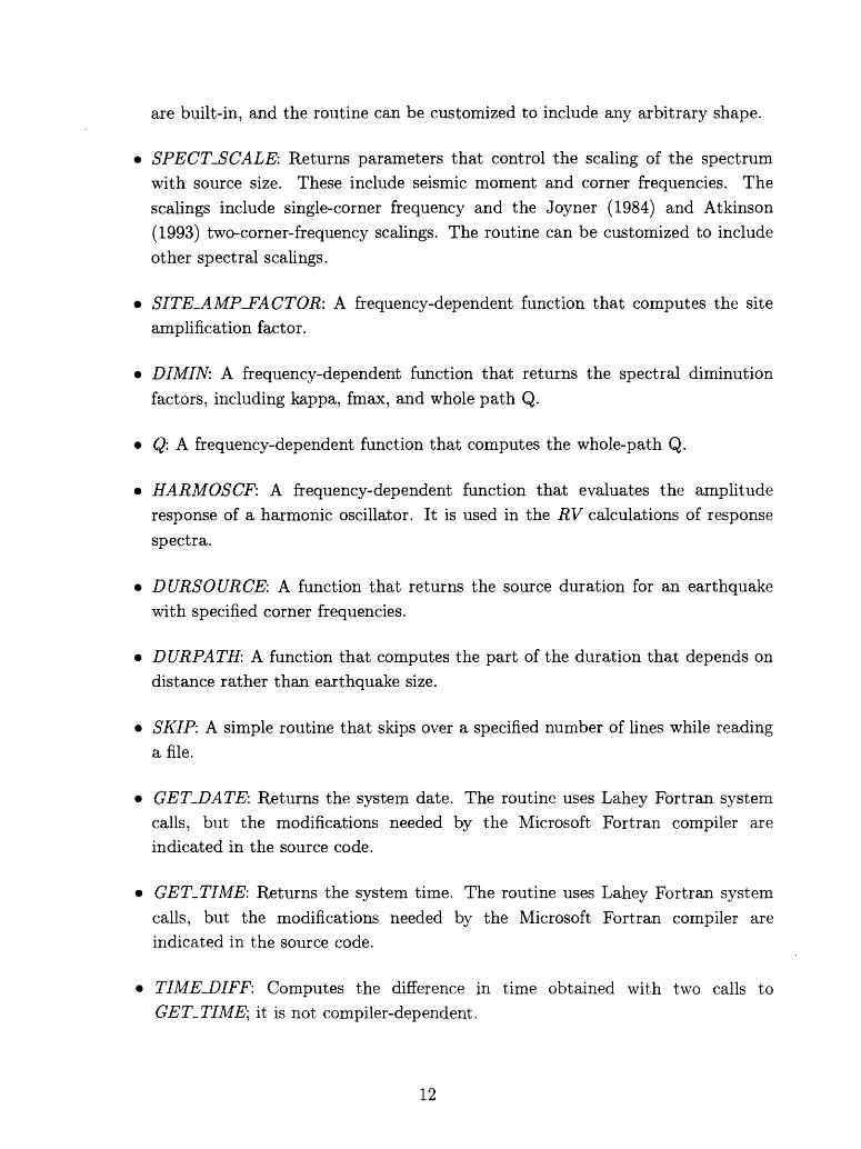
are built-in, and the routine can be customized to include any arbitrary shape.

SPECT-SCALE: Returns parameters that control the scaling of the spectrum with source size. These include seismic moment and corner frequencies. The

scalings include single-corner frequency and the Joyner (1984) and Atkinson (1993) two-corner-frequency scalings. The routine can be customized to include

other spectral scalings.

SITE-AMP-FACTOR: A frequency-dependent function that computes the site amplification factor.

DIMIN: A frequency-dependent function that returns the spectral diminution

factors, including kappa, fmax, and whole path Q.

Q\ A frequency-dependent function that computes the whole-path Q.

HARMOSCF: A frequency-dependent function that evaluates the amplitude response of a harmonic oscillator. It is used in the RV calculations of response

spectra.

DURSOURCE: A function that returns the source duration for an earthquake

with specified corner frequencies.

DURPATH: A function that computes the part of the duration that depends on

distance rather than earthquake size.

SKIP: A simple routine that skips over a specified number of lines while reading a file.

GET-DATE: Returns the system date. The routine uses Lahey Fortran system calls, but the modifications needed by the Microsoft Fortran compiler are indicated in the source code.

GET-TIME: Returns the system time. The routine uses Lahey Fortran system

calls, but the modifications needed by the Microsoft Fortran compiler are indicated in the source code.

TIME-DIFF: Computes the difference in time obtained with two calls to GET-TIME; it is not compiler-dependent.

12

RECIPES: Except for a few minor modifications indicated in the annotated list, the routines in this module are taken directly from the second edition of Numerical Recipes

(Press et a/., 1992). I was not able to obtain permission to distribute the source code, either via hard-copy or via diskette, without paying a license fee. The routines have been linked into RV.DRVR.EXE and TD.DRVR.EXE, and I do have permission to

use them in this way. Users of anything but these executables must obtain their own

Numerical Recipes routines, which is excellent advice in any case. The book and

the diskette that can be purchased from Cambridge University Press (address: Order Department, 110 Midland Avenue, Port Chester, New York 10573; phone: 1-800-431- 1580). The module includes the following routines; annotation is given only when a modification of the original routine has been used:

QMIDPNT: This is Numerical Recipes routine QTRAP, renamed and with the word "midpnt" substituted for "trapzd".

MIDPNT:

LOCATE:

ODEINT: The program must be modified by removing the word "rkqs" from the

parameter list and from the external statement.

RKQS:

RKCK:

GASDEV:

RANI:

REALFT:

FOUR1:

Site-Amplification Programs:

Included here are other programs that may be useful to the user.

SITE-AMP: This program converts a velocity and density model into a frequency- dependent site amplification, using the square root of the ratio of seismic impedances

13

at the source and near the surface. The surface seismic impedance is based on the shear velocity and density averaged over a depth equivalent to a quarter of a wavelength (this is how frequency enters into the computation).

F4RATTLE: This program reads a file made by SITE-AMP and writes a file in the proper format for use by RATTLE, C. Mueller's program for computing the response of a stack of layers to SH waves.

COMPILATION AND MODIFICATION:

I used the F77L-EM/32 Fortran 77 Version 5.20 compiler from Lahey Computer Systems for all but the site-amplification programs, for which I used the Microsoft Fortran compiler, Version 5.1. The Lahey compiler was used in order to handle the large arrays in the time-domain programs. The commands to compile and link the program are as follows:

f7713 rv.drvr

f7713 smsim_rv

3861ink rv.drvr smsim_rv -maxdata 0 -stub runb -exe rv_drvr.exe

The time-domain code is assembled by substituting "td" for "rv".

The -stub switch binds a run-time DOS-extender into the executable file, so that the Lahey programs are not needed to run the program. As a result of the extra code, the executable file is larger than if, for example, the Microsoft Fortran version 5.1 compiler had been used (I have assembled the random-vibration code using both; although a larger file size, the execution time is shorter with the Lahey compiler).

The compilers are fast enough that I have used the Fortran INCLUDE statement at the end of SMSIM.RV.FOR and SMSIM.TD.FOR to bring in the subroutine modules RVTDSUBS.FOR and RECIPES.FOR at compile time. It would be more efficient, of course, to produce a library module and link this module with the application-specific programs.

Modifications are easy to make in the routines. As indicated above, changes in source shape and source scaling can be included by modifying the appropriate routines in RVTDSUBS.FOR] allowance has been made for an input parameter to choose any added source shaping or scaling without changing the original meanings of the input parameter. A more likely modification would be to write new drivers to produce ground motion for

14

other combinations of magnitude, distance, stress parameter, or oscillator periods. In this case, only the drivers RV.DRVR.FOR and TD.DRVR.FOR need be changed.

The emphasis in the output is on various peak measures of ground shaking. The time- domain simulation program does have the option of storing an acceleration and velocity time series in a file, but modifications are required if the user needs to store a suite of time series. This can be done easily by modifying the "if (isim .eq. nacc.save)" loop in subprogram SMSIM.TD.

INPUT AND OUTPUT OF SMSIM AND FAS PROGRAMS:

A sample input file is given in Figure 2. The parameters in this file do not represent any particular model that I have used in applications to either western North America (e.g., Boore, 1983, 1986; Boore et a/., 1992) or eastern North America (e.g., Boore and Atkinson, 1987; Boore and Joyner, 1991; Atkinson and Boore, 1995). The parameters have been chosen to illustrate the input parameters needed by the programs. The parameters are not to be used for a particular application. I am reluctant to give input files with the parameters used in some of my papers because my ideas concerning the appropriate parameters are evolving. For the convenience of the reader, however, I have included the input-parameter files for the Atkinson and Boore (1995) model and my current coastal California model in Appendices F and G. (I use the term "coastal California" to reflect more accurately the source of the data used in determining the parameters than the commonly used phrases "western United States" or "western North America"; this parameter file must not be used for distances beyond 100 km.) To emphasize the evolving nature of the coastal California model, I have used the date of the latest modification of the file as part of the file name.

The input-parameter file is made up of lines of text and lines containing the input parameters. The lines of text are for the convenience of the user; the programs skip over them. It is very important that the number of text lines remain the same, however, for otherwise the program will attempt to read a text line as a parameter line. In other words, only change the parameter lines! In addition, list-directed input is used. This means that all parameters must be included, even if some are not used.

The program FASJDRVR does not need the parameters in the last several lines of input file, but these lines should be included nevertheless.

Input From Screen:

The programs ask questions of the user regarding input file name, file name for

15

summary listing, and file name of file containing results in columnar form, suitable for import into graphics programs. In addition, the user is asked to provide information regarding whether or not response spectra are to be computed and the damping and the periods for which the spectra will be computed. The periods can be entered

individually or can be computed by the program for a specified range and number of periods

(logarithmically spaced) . Alternatively, the spectra can be computed at the standard set of 91 periods used by the USGS and CSMIP in their routine processing of strong-motion data. In addition, the time-domain program asks if a sample of the acceleration and velocity time series should be saved, and if so, which sample. After the results are written to various

output files, the program asks if computations are to be made for another distance and magnitude, and if so, asks for the name of the file to which the output will be written in

columnar format.

The numbers entered in response to a program query need not contain decimal points. For example, a period of 2.0 sees can be entered as "2.0" or "2". In addition, if the user forgets to enter the parameter on one line, the program will expect the input on the next line.

Input From File:

1. rho, beta, prtitn, radpat, fs: These parameters are the density (in gm/cc) and shear-

wave velocity (in km/s) in the vicinity of the source, the partition factor (to partition

the S wave energy into two horizontal components, usually given by l/\/2; it should be consistent with the next parameter), the radiation pattern, averaged over some portion of the focal sphere (this should refer to the radiation factor of the total S-

wave radiation if the partition factor is taken to be l/\/2; see Boore and Boatwright, 1984, for tables of values), and the free surface factor (usually equal to 2). Note that

rho, beta were 2.7, 3.2 and 2.8, 3.8 in the applications of Boore (1983) and Atkinson and Boore (1995), respectively. I now suggest 2.8, 3.5 for WNA and 2.8, 3.6 for ENA.

2. source number, pf, pd: These parameters control the shape of the spectrum. As explained in the text lines in the input-parameter file, the source number specifies

whether the spectral shape is a single-corner spectrum (source number = 1), one of two possible double-corner spectra (source number = 2 for Joyner (1984), as modified

in Boore and Joyner (1991); source number = 3 for Atkinson (1993)), or a different spectral shape resulting from a modification of the program (source number = 4). The parameters pf and pd are used if source number = 1 and control the spectral shape given in the following equation:

+ (f/fc ) pfrd , (2)16

where fc is the corner frequency. For the usual single-corner model, pf = 2 and pd = I. A sharper corner, preferred by some, is given by pf = 4 and pd = 0.5. In all cases, an omega-square model requires that pf x pd = 2.

3. stressc, dlsdm, fbdfa, amagc: These parameters control the scaling of the spectral amplitudes with source size, primarily by specifying the dependence of the corner frequencies on magnitude. The parameters are not used if source number = 3, but in this case dummy parameters must be included in the input-parameter file. The parameters fbdfa and amagc are used if source number = 2, in which case fbdfa is the corner frequency fb divided by fa and amagc is the critical moment magnitude beyond which the scaling is no longer self-similar. If source number = 1, then the stress parameter is given by:

A<7 = streSSC X lQdlsdmx(M-amagc) ^

The usual case of magnitude-independent stress is given by setting dlsdm, = 0.0 (note that "dlsdm" stands for derivative of log sigma with respect to magnitude), stressc has units of bars.

4. nsegs, (rlow(i), slope(i), i = 1, nsegs): These parameters control the geometrical spreading, as represented by nsegs segments, each starting at rlow with a distance- dependence of rslope beyond rlow (in all cases, specify rlow(l) = 1.0). In the sample input-parameter file, the geometrical spreading is r~ l from 1.0 (actually, any distance less than 70 km) to 70 km, r° from 70 to 130 km, and r~°- 5 beyond 130 km (this is the dependence used by Atkinson and Boore, 1995).

5. frl, Qrl, si, ftl, ft2, fr2, Qr2, s2: The whole-path attenuation is given by

exp(-7r/r/e(/)/J), (4)

in which the function Q(f) is described by the parameters in this entry of the input- parameter file. As shown in Figure 3, Q(f) is given by a piece wise continuous set of three straight lines in log Q and log/ space. The first and third lines have slopes of si and s2 and values of Qrl and Qr2 at reference frequencies frl and /r2, respectively. The first and third lines apply for / < ftl and / > /t2, respectively, with a straight line in log Q, log/ space connecting the values of Q at the transition frequencies ftl and ftl (in other words, Q(f) = Qrl(f/frl) sl for / < ftl and Q(f) = Qrl(f/frl) sl for / > /£2, with a connecting line between these two). I decided on this representation after much experimentation; it is the simplest way of representing a complicated Q(f) function with terms that are familiar to most users. The values in the sample input- parameter file have been chosen to represent closely the Q(f) function given in Boore

17

(1984) and in my WNA applications. (As in all of the input parameters for specific applications, this function should be confirmed or modified based on special studies; in particular, intermediate- and long-period motions at large distances can be sensitive to the location of the low-frequency branch of the Q(f) function, which is not well determined from data). Note that because the decision of which line segment to use depends solely on the transition frequencies, the relative size of the reference frequencies does not matter (i.e., frl could be less than frl). Two special cases should be mentioned: Q = QQ (a constant) and Q = Qr (f/fr ) s - The constant-Q case is given by specifying si = 0, s2 = 0, Qrl = QQ, Qrl = Q0 , and any non-zero values for frl, fr2, ftl, and ftl. The special case of a single power-law dependence is specified by Qrl = Qr , Qrl = Qr , frl = fr , and frl = fr , and any non-zero values for ftl and ftl. All frequencies should have units of Hz.

6. W-fa, W-fb: The source duration used in the calculations is given by

dursource = w.fa/fa + w-fb/fb, (5)

where fa and fb are the source corner frequencies. For the single corner-frequency model (source number = I), fa fb, so any combination of weights w-fa and w.fb can be used, as long as they add up to the desired weight. In my WNA applications, I used w-fa = 1.0 and W-fb = 0.0. In Atkinson and Boore (1995), w-fa = 0.5 and w.fb = 0.0.

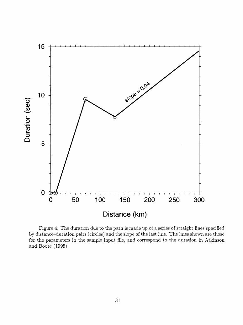
7. nknots, (rdur(i), dur(i), i = 1, nknots), slope of last segment: These parameters are used in the specification of the path duration by a series of straight-line segments with parameters nknots, rdur, dur, slope of last segment, where nknots is the number of intersections between line segments. The meaning of these parameters is indicated in Figure 4. The values given in the figure correspond to those in the input-parameter file, which in turn were chosen to represent the duration used by Atkinson and Boore (1995). For my WNA applications I used one segment with a slope of 0.05 (i.e., nknots = 1, rdur 0.0, dur 0.0, slope = 0.05), but this was assumed without any special studies as was done for the Atkinson and Boore (1995) application. Atkinson (1995) finds a very different relation for western Canada; a comparable study should be done for other regions.

8. namps, (famp(i), amp(i), i = 1, namps): The site amplification is approximated by a series of straight-line segments in log amplification, log frequency space, connecting the values famp, amp. The amplification for / < famp(l) and / > famp(namps] is given by amp(l) and amp(namps), respectively. This is shown in Figure 5 (which uses the parameters in the input-parameter file). The numbers in the data file were

18

invented for the sake of illustration. Suggested values for WNA, based on my recent work (Boore and Joyner, 1996), are given in Appendix G. For no amplification, set namps 1, amp = 1.0, and famp equal to any number.

9. fm, kappa: The diminution function is controlled by the parameters fm and kappa.

They are used in the following filter:

exp (-TT x kappa x f)/\/l + (f/fm)8 . (6)

In many applications only one or the other of the two parameters are desired; this is easy to implement with appropriate choices of the parameters. For example, to use only /ra, specify kappa = 0.0; to use only kappa, specify a large number for fm,. The

units of fm, kappa should be consistent with that of / Hz and I/Hz.

10. fcut, norder: In some cases it may be desired to include a low-cut filter in the simulations. This might be the case, for example, for simulations of processed strong-

motion data. The parameters fcut and norder control the low-cut filter and are used in BUTTRLCF. The filter is given by the following function:

1.0/(1.0 + (fcut/f) 2 - 0xnorder ) (7)

(this is the response of a bidirectional filter made up of two Butterworth filters, each

of order norder). Set fcut = 0.0 for no filter.

11. zup, eps.int, amp.cutoff: The first parameter specifies the upper limit in the integral of equation (1). I have found that 5 seems to be a good number for this limit, and

there is probably no reason to change the value from that in the sample file (zup = 10). The second parameter specifies the error in the adaptive integration routine ODEINT,

and the third is used as the basis for computing the upper frequency limit (fup) used in the random-vibration calculations (this is computed in subroutine GET.PARAMS

and also in RV.DRVR). fup is determined such that the exponential in the equation above has a value of amp.cutoff. I have found the values in the sample input-parameter file to give good results, but the user should experiment to make sure that they are

appropriate values. I have included these three parameters for generality, even though I do not anticipate that they will be changed.

12. indxwind, taper, twdtmotion, eps.wind, eta.wind: These parameters control the shape of the window applied to the random number time series in the time-domain simulations. Either a box (indxwind = 0) or an exponential window (indxwind = 1)

can be used (see Boore (1983) for more discussion of the latter), taper is used only

19

in the box window; it is the fraction of the duration of motion for which a raised- cosine taper will be applied to the front and to the back of the box window (i.e., , the extent of the taper will be taper x (dursource -f durpath) in both the front and the back of the window), taper is not used for the exponential window. The parameters twdtmotion, eps.wind, and etajwind are only used for the exponential window. The meaning of the parameters is best seen by referring to Figure 6. Sample output for the box and exponential windows is given in Figures 7 through 10 for M = 4 and

7, and R = 10 and 200 km. The results in the figures indicate that, in general, the response spectral amplitudes from the exponential window are closer to the random vibration results than are those from the box window. This is not surprising, because the correction factor for oscillator response proposed by Boore and Joyner (1984) and used in the SMSIM programs was derived empirically from calculations made using

the exponential window.

13. tsimdur, dt, tshift, seed, nruns: These parameters deal with time-domain details.

tsimdur is a minimum duration for which the motion will be computed and dt is the

time spacing. The program chooses the number of time points npts to be a power

of 2 such that the duration of the time series equals or exceeds tsimdur (the arrays are dimensioned such that npts must be less than or equal to 16,384; it is up to the user to make sure that this condition is satisfied). The program will display an

error message and stop if the calculated duration (including contributions from the initial delay, the source, the path, and the window) exceeds the duration npts x dt.

The parameter tshift produces a time shift in the start of time series; this can be useful to accommodate pre-arrival tails due to the noncausal filters used in the analysis, seed and nruns are the initial seed of the random-number generator and the number of time-domain simulations, respectively. If peak motions are desired, nruns should be large enough to reduce the uncertainty in the computed means of

the peak motions determined from each realization. Examples of results computed for several nruns are given in Figures 11 and 12. In general, the uncertainty in the mean

decreases as l/^/nruns. Note in these figures that the time-domain and random-

vibration results show some systematic disagreements for the larger earthquake. This difference is a maximum of a factor of about 1.12, and is probably related to the

assumption in the random-vibration theory that the amplitudes of successive peaks are independent of one another. This is certainly not true for a long-period oscillator response. Corrections schemes for "clumping" might yield a better comparison. I tried one such scheme (due to Toro, 1985), but the comparison was not improved. In view of the aleatory uncertainty in ground-motion data and the epistemic uncertainty in the input parameters, I am willing to live with uncertainties that in general are

less than 10 percent in order to take advantage of the greatly increased speed of the

20

random-vibration calculations compared to the time-domain calculations.

14. remove dc from random series?: This parameter was included in the development of the program. If not equal to 0.0, then the mean of the random number sample will

be removed before windowing and transforming into the frequency domain. I suggest

that the parameter be set to 0.0.

Output of SMSIM and FAS Programs:

Two or three files are produced by the SMSIM program, the first containing a summary of the input and the results, and the second a file with columns containing the oscillator

period and frequency and response spectra amplitudes (both pseudo relative velocity, PRV,

and pseudo absolute acceleration, PA A; note that the "RV" in PRV should not be confused

with the use of "RV to stand for "Random Vibration"). This latter file is in a convenient format to be imported into the graphics program that I use (CoPlot, published by CoHort Software, 1-800-728-9878). A third file is produced if it is desired to save a sample acceleration and velocity time series computed by the time-domain simulation. Sample

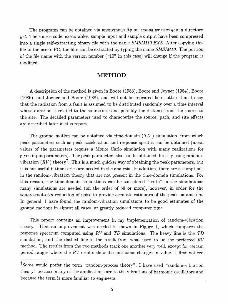
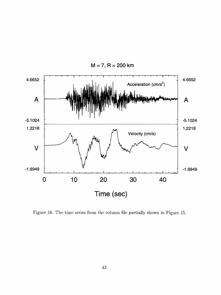
output files are given in Figures 13, 14, and 15; a sample of the time series is given in Figure 16. The output files from RV.DRVR includes estimates of dominant frequency, as measured

from the frequency of zero crossings (equation 27 in Boore, 1983). In addition, the output includes the parameter eps that measures the bandwidth of the motion (eps = ^/l £2 ,

where £ is given by equation (22) in Boore, 1983; see Cartwright and Longuet-Higgins, 1956, p. 216-217, for more discussion). Finally, the random-vibration output also includes estimates of the number of extrema (nx) and the number of zero crossings (nz). The bandwidth parameter £ and nx and nz are related by f = nz/nx.

The response of a single-degree-of-freedom oscillator with gain of V and specified

natural period (T0 ) and damping (77) can be obtained by multiplying the PRV output for the specified natural period and damping by the factor VT^/I-K. This scheme can be used

to simulate the response of a Wood-Anderson instrument and thereby to obtain estimates of local magnitude ML corresponding to the ground motion. According to Uhrhammer and

Collins (1990), for a Wood-Anderson instrument V = 2080, T0 = 0.8s, and rj = 0.69. Time series corresponding to the oscillator output are not returned by the programs, although they can be produced by a simple modification to the subprogram RD-CALC'm the module SMSIM.TD; the modification is indicated by a comment in RD.CALC.

The FAS program creates a summary file and a file with columns of frequency, period,

and Fourier spectral amplitude for the ground displacement, velocity, acceleration, and oscillator response. The output is similar to that in Figures 13 and 14.

21

With the units as given in the discussion of input, the output ground motion will be

in cgs units.

INPUT AND OUTPUT OF SITE-AMPLIFICATION PROGRAMS:

As in the previous programs, input comes from the screen and from a parameter file.

Input From Screen:

SITE-AMP: The program first asks the user for the names of the input and output files. It then asks if the default coefficients of a linear relation between density and velocity will be used, in which case the program asks for the values specifying the end points of the line (the densities are given by the end-point values for velocities outside of the specified

range). As explained below, the program looks at the parameter file and queries the user about whether the velocities are a piecewise continuous function of depth or represent a

layered model. Finally, the program asks for the velocity and the density in the source

region.

I have found that it is very convenient to produce the input-parameter file using a spreadsheet and printing the necessary columns to a file. With a spreadsheet it is easy to subdivide a thick const ant-velocity layer into pseudo-layers. This may be necessary to

obtain amplifications at closely-spaced frequencies, since the program computes frequencies only for depths included in the input file (a future version will interpolate between input

depth points to produce amplification at a specified set of frequencies). Using a spreadsheet also makes it easy to include velocity models of varying complexity (I often use power laws fit to two end points, as well as linear velocity gradients).

Regarding units: velocity and depth units can by anything as long as they are consistent with one another (i.e., depth in meters should be matched with velocity in meters per second). Note that if the densities are to be computed from the default end points, the velocity units must be kilometers per second. The density units do not have to be consistent with those of depth and velocity. I strongly advise that the density units be given in grams per cubic centimeters.

F4RATTLE: The program asks for the name of input and output files (with a default of Rattle.In for the output file, which is what the program RATTLE expects). The program

then asks for a series of input parameters:

1. zdepth: The depth at which the response is to be computed (usually 0.0 for the ground

22

surface).

2. theta: The angle of incidence, in degrees, of the incident wave (0.0 for vertical).

3. Q: The program asks for the attenuation parameter Q to be assigned to the layers. It

assumes the same value for all layers.

4. sps, mx\ The final two parameters control the frequency spacing through the equation

ddf=sps/2mx.

They are used rather than a simple specification of the frequency spacing because the

original intent of the program RA TTLE was to provide a table of response values that could be used with a Fourier transform to yield a time series of the response (in this context, sps is the number of samples per second in the time series and the number of samples is 2mx ). The number of frequencies for which the response is calculated is

given by

The program RATTLE is currently being modified by C. Mueller, and as a result, it may be necessary to modify F4RATTLE to allow a different specification of the

frequency spacing and number of frequency points.

Input From File:

SITE-AMP: A sample input file is given in Figure 17. The parameters in this file have

been made up to illustrate the input; they do not represent a real application.

1. The first column is labeled "Depth", but it could also contain layer thickness. The units can be anything. If the first entry is "0.0", the program assumes that the

entries will be depths and that the velocities and densities are the values for the specified depth; it asks the user to confirm this. If the first column is depth, then the program simply assumes straight- line connections between the entries. In this way a mix of linearly increasing, constant, and step changes can be included in the model. A constant parameter (velocity or density) over a depth range is entered by the depths that bound the layer, but with the same velocity or density for the two consecutive entries (e.g., as between depths 0.040 - 0.100 and 0.300-8.000 for

the velocity parameter in the sample input file, with intermediate layers for better frequency resolution); similarly, a layered model can be included easily by entering

the velocities and densities on either side of the interface, but with the same depth

23

for the two consecutive entries (e.g., at depths of 0.040 and 0.300 in the sample input file).

2. The second column contains the velocities, in any units that match the depth units.

3. The third column contains the densities. An entry of "0.0" will flag the program to use the DENSITY function. To compute a density from the velocity, using the relation specified interactively or the default relation built into the program (with end points of 2.5 gm/cm? at 0.3 km/s and 2.8 gm/cm3 at 3.5 fcra/s, values that I have assumed for generic rock in WNA (see Boore and Joyner, 1996)). A nonzero entry will override the value that would have been computed by the DENSITY function (as has been done for a few depths in the sample input file, although it should be noted that the specified values for density of 3.0 and 4.0 gm/cc are very unrealistic).

F4RATTLE: This program uses a file made by SITE.AMP as input.

Output of Site-Amplification Programs:

SITE-AMP: One output file is created with columns containing the input model, the average velocities and densities, and the frequency and amplification for each input depth. A sample is given in Figure 18. The first three columns repeat the input parameters. Column 4 contains the depths at which the velocities have been specified, without the repeated depths needed for layers of constant velocity (if the input depth column corresponds to depth rather than thickness); this is why nout ^ ndepths. Column 5 is the travel time to the indicated depth; it is the basis for the rest of the results. Columns 6 through 8 contain a constant-velocity approximation to the input velocity model (it is constructed to give the same travel times for each depth as the continuous model) and are included as a convenience in case the approximate amplifications are to be checked using a wave-propagation program that requires a stack of const ant-velocity layers. Columns 9 and 10 are the velocities and densities averaged from the surface to the specified depth. Columns 11 and 12 are the computed frequency and amplification. Note that for identification purposes, the stem of the input file name has been used to label columns 11 and 12.

One way in which I use the program SITE.AMP is to import the output file into my graphics program and plot the amplification vs. frequency (using log-log axes). I then pick off a set of amplifications and frequencies that will be used as input to the SMSIM programs.

F4RATTLE: The output is a file in the format required by RATTLE.

24

ACKNOWLEDGMENTS

I thank Bill Joyner for advice and encouragement over the years and Bob Herrmann for cross-checking of output from our programs and for reminding me that Cartwright and Longuet-Higgins' equation (6.8) is an approximation to their equation (6.4). In addition, I am grateful to Gail Atkinson for her version of my original time-domain simulation program, to Walt Silva for helpful discussions, and to Basil Margaris for provoking me into writing this report. Bill and Basil reviewed the manuscript. I also thank Stavros Anagnostopoulos and Jose Roesset for permission to use their program for computing response spectra and Chuck Mueller for permission to distribute his programs.

This work was partially supported by the Nuclear Regulatory Commission.

REFERENCES

Atkinson, G. M. (1993). Earthquake source spectra in eastern North America, Bull. Seism. Soc. Am. 83, 1778-1798.

Atkinson, G.M. (1995). Attenuation and source parameters of earthquakes in the Cascadia region, 85, 1327-1342.

Atkinson, G. M. and D. M. Boore (1995). Ground motion relations for eastern North America, Bull. Seism. Soc. Am. 85, 17-30.

Boore, D. M. (1983). Stochastic simulation of high-frequency ground motions based on seismological models of the radiated spectra, Bull. Seism. Soc. Am. 73, 1865-1894.

Boore, D. M. (1984). Use of seismoscope records to determine ML and peak velocities, Bull. Seism. Soc. Am. 74, 315-324.

Boore, D. M. (1986). Short-period P- and 5-wave radiation from large earthquakes: implications for spectral scaling relations, Bull. Seism. Soc. Am. 76, 43-64.

Boore, D. M. and G. M. Atkinson (1987). Stochastic prediction of ground motion and spectral response parameters at hard-rock sites in eastern North America, Bull. Seism,. Soc. Am. 77, 440-467.

Boore, D. M. and J. Boatwright (1984). Average body-wave radiation coefficients, Bull. Seism,. Soc. Am. 74, 1615-1621.

25

Boore, D. M. and W. B. Joyner (1984). A note on the use of random vibration theory to predict peak amplitudes of transient signals, Bull. Seism. Soc. Am. 74, 2035-2039.

Boore, D. M. and W. B. Joyner (1991). Estimation of ground motion at deep-soil sites in eastern North America, Bull. Seism. Soc. Am. 81, 2167-2185.

Boore, D.M. and W.B. Joyner (1996). Site-amplifications for generic rock sites, Bull. Seism. Soc. Am. 86, (submitted)

Boore, D. M., W. B. Joyner, and L. Wennerberg (1992). Fitting the Stochastic cj~ 2 Source Model to Observed Response Spectra in Western North America: Trade-offs Between ACT and K, Bulletin of the Seismological Society of America, Vol. 82, p. 1956-1963.

Cartwright, D. E. and M. S. Longuet-Higgins (1956). The statistical distribution of the maxima of a random function, Proc. R. Soc. London 237, 212-232.

Hanks, T. C. and R. K. McGuire (1981). The character of high-frequency strong ground motion, Bull. Seism. Soc. Am. 71, 2071-2095.

Herrmann, R.B. (1996). Computer Programs in Seismology, Dept. of Earth and Atmospheric Sciences, St. Louis University, St. Louis, Missouri.

Joyner, W. B. (1984). A scaling law for the spectra of large earthquakes, Bull. Seism. Soc. Am. 74, 1167-1188.

Joyner, W. B. and D. M. Boore (1988). Measurement, characterization, and prediction of strong ground motion, in Earthquake Engineering and Soil Dynamics II, Proc. Am. Soc. Civil Eng. Geotech. Eng. Div. Specialty Conf., June 27-30, 1988, Park City, Utah, 43-102.

Press, W.H., S.A. Teukolsky, W.T. Vetterling, and B.P. Flannery (1992). Numerical Recipes in FORTRAN: The Art of Scientific Computing, Cambridge University Press, Cambridge, England, 963 pp.

Silva, W.J. and Lee, K. (1987). WES RASCAL code for synthesizing earthquake ground motions, State-of-the-Art for Assessing Earthquake Hazards in the United States, Report 24, U.S. Army Engineers Waterways Experiment Station, Misc. Paper S-73-1.

Toro, G.R. (1985). Stochastic model estimates of strong ground motion, Section 3 of Seismic Hazard Methodology for Nuclear Facilities in the Eastern United States,

26

Report Prepared for EPRI, Project Number P101-29.

Uhrhammer, R.A. and E.R. Collins (1990). Synthesis of Wood-Anderson seismograms from broadband digital records, Bull. Seism. Soc. Am. 80, 702-716.

27

CO C/> Q.

10-1

M = 4.0, R = 10km

K = 0.02, Aa = 200 bars

TD

o RV (using numerical integration) RV (series expansion)

RV (2-term asymptotic)

10-2 10'1

Period (sec)

Figure 1. Response spectra computed with time-domain simulations and random- vibration simulations with various relations between the peak and rms values. The series expansion uses equation (21) in Boore (1983), and for the model parameters in this figure produces response spectra that are a discontinuous function of period. The function does not appear discontinuous in the plot because the period values are spaced too widely. The 2-term asymptotic expansion uses equation (24) in Boore (1983), and the random-vibration results computed with numerical integration use equation (1) in this report.

28

to CO

Sample d

ata

file

***

* NOT

FOR

A PARTICULAR A

PPLI

CATI

ON **

rho, be

ta,

prtitn,

radpat,

fs:

2.8

3.6

0.71 0.

55 2.

0 sp

ectr

al shape: source n

umber

(1=Single

Corner;2=Joyner;3=A93;4=custom),

pf,

pd (1

-cor

ner

spectrum =

1/

(1+(

f/fc

)**p

f)**

pd;

0.0

othe

rwis

e)

(usual model: pf=2.0,pd=1.0; Butterworth: pf=4.0,pd=0.5)

(Note: po

wer

of hi

gh freq d

ecay

-->

pf*p

d)

1 2.

0 1.0

spec

tral

sc

alin

g: stressc, dl

sdm,

fb

dfa,

am

agc

(str

ess=

stre

ssc*

10.0

**(d

lsdm

*(am

ag-a

magc

))

(fbdfa,

amag

c for

Joyner m

odel

, us

uall

y 4.0, 7.

0)

(not u

sed

for

source 3

, but

plac

ehol

ders still

need

ed)

80.0 0.

0 4.

0 7.

0 gs

prd:

ns

egs,

(r

low(

i),

slop

ed')

) (S

et rl

ow(1

) =

1.0)

1.0

-1.0

70.0

0.0

130.0

-0.5

q: fr

1, Qr

1, s1,

ft1, ft2, fr

2, qr

2, s2

0.1

275

-2.0

0.2

0.6

1.0

88.0 0.

9 so

urce

dur

atio

n: we

ight

s of 1/fa,

1/fb

1.0

0.0

path

dur

atio

n: nknots,

(rdur(i),

dur(

i)),

sl

ope

of last se

gmen

t

0.0

0.0

10.0

0.0

70

.0 9

.6

130.0

7.8

0.04

si

te a

mpli

fica

tion

: na

mps, (famp(i),

amp(

i))

0.1

1.0

1.0

1.5

2.0

2.0

5.0

2.5

10.0

3.

0 si

te d

iminution

parameters:

fm,

akappa

25.0

0.03

low-

cut

filt

er parameters:

fcut

, norder

0.0

2 rv

integration

para

ms:

zup,

ep

s in

t (integration a

ccur

acy)

, amp

cutoff (f

or fup)

10.0

0.00001

0.00

1 window p

arams: in

dxwi

nd(0

=box

,1=e

xp),

ta

per(

<1),

tw

dtmo

tion

, ep

s wind,

eta

wind

1 0.

05 1.0

0.2

0.05

ti

ming

stuf

f: ts

imdu

r, dt

, tshift,

seed

, nruns

50.0

0.

005

7.0

640.0

640

remo

ve d

c from random s

eries

before transforming to

fr

eq.

doma

in (0

=no;

1=ye

s)?

0

Fig

ure

2.

Sam

ple

inpu

t fil

e fo

r th

e SM

SIM

pr

ogra

ms.

T

he

file

h

as

bee

n

con

stru

cted

fo

r il

lust

rati

ve

pu

rpos

es

and

d

oes

not

co

rres

pon

d

to

a re

al

app

lica

tion

.

10'

1 fl­

10'

10-2

(fr1,Qr1)

10-1

Freq

10'

Figure 3. Illustration of the specification of Q(f): it is made up of three lines in log-log space. The lines shown are those for the parameters in the sample input file, which is an approximation of the Q(f) function in Boore (1984).

30

15

10 -o o u^c oV-»

2DQ 5 -

050 100 150 200 250 300

Distance (km)

Figure 4. The duration due to the path is made up of a series of straight lines specified by distance-duration pairs (circles) and the slope of the last line. The lines shown are those for the parameters in the sample input file, and correspond to the duration in Atkinson and Boore (1995).

31

c,0" * COo

Q.

<

3 -

2 -

1 -

10-1 10C

Frequency (Hz)

Figure 5. The site-amplification is specified by a series of straight lines in log frequency, log amplification space. The lines shown are those for the parameters in the sample input file, and are made up; they do not correspond to any of my published applications.

32

o

.55 0.5 -c 0 c oQ. x

LLJ

0

twdtmotion = 0.7 eps_wind = 0.3 eta wind = 0.4

0.5

time/tmotion

Figure 6. The exponential window is specified by parameters whose meaning is shown here. Note that the abscissa has been normalized by a quantity proportional to the duration of the motion (tmotion). (In the program, tmotion is given by doubling the source plus path durations). The parameters have been chosen to illustrate their meaning and are not those in the input file.

33

2-

1 -

CO

E

COCL

0.2

0.1

0.02 H

0.01

= 4.0, R = 10km

Random Vibration ° Time Domain: exponential window x Time Domain: box window

10-1 10°

Period (sec)Figure 7. Comparison of simulations using box and exponential windows, with the

random-vibration calculations for magnitude 4 at 10 km, using the parameters in the input-parameter file (except for the time-domain simulations, where indxwind = 0 for the box window).

34

0.02-

0.01 -

0.002 -

0.001

2e-4-

1e-4

M = 4.0, R = 200 km

Random Vibrationo Time Domain: exponential windowx Time Domain: box window

10-1 10°

Period (sec)

Figure 8. Comparison of simulations using box and exponential windows, with the random-vibration calculations for magnitude 4 at 200 km, using the parameters in the input-parameter file (except for the time-domain simulations, where indxwind = 0 for the box window).

35

100

CO

CO Q.

30-

20-

10-

M = 7.0, R = 10km

Random Vibration ° Time Domain: exponential window x Time Domain: box window

10-1 10°

Period (sec)

Figure 9. Comparison of simulations using box and exponential windows, with the random-vibration calculations for magnitude 7 at 10 km, using the parameters in the input-parameter file (except for the time-domain simulations, where indxwind = 0 for the box window).

36

2-

1 -

.CO

^

(/) Q.

0.2-

0.1

M = 7.0, R = 200 km

Random Vibration° Time Domain: exponential windowx Time Domain: box window

10-1 10'

Period (sec)

Figure 10. Comparison of simulations using box and exponential windows, with the random-vibration calculations for magnitude 7 at 200 km, using the parameters in the input-parameter file (except for the time-domain simulations, where indxwind = 0 for the box window and tsimdur = 50.0 for the exponential window).

37

.CO

^o,

(/}Q.

2-

1 -

0.2

0.1

0.02-

0.01

Random Vibration ° Time Domain: 10 runs

Time Domain: 40 runs ° Time Domain: 160 runs v Time Domain: 640 runs

10-1

= 4.0, R = 10km

10'

Period (sec)Figure 11. Comparison of simulations using the time-domain calculations with various

values for nruns, with seed = nruns for each suite of realizations. The random-vibration results are shown for comparison. The calculations are for magnitude 4 at 10 km, using the parameters in the input-parameter file.

38

100

.en

COCL

30-

20-

10-

= 7.0, R=10km

Random Vibration° Time Domain: 10 runsx Time Domain: 40 runs° Time Domain: 160 runs* Time Domain: 640 runs

10-1 10°

Period (sec)

Figure 12. Comparison of simulations using the time-domain calculations with various values for nruns, with seed = nruns for each suite of realizations. The random-vibration results are shown for comparison. The calculations are for magnitude 7 at 10 km, using the parameters in the input-parameter file.

39

outp

ut fi

le:

sample.sum

***

Resu

lts

computed u

sing

RV_DRVR

***

Date

: 04/12/96

Time

: 18:11:54.63

file

wit

h pa

rame

ters

: of

r.da

tTi

tle: Sa

mple d

ata

file

***

* NO

T FOR

A PARTICULAR A

PPLICATION *

* rh

o, beta,

prti

tn,

rtp,

fs:

2.80

000

3.60000

0.710000

0.55

0000

2.

0000

0 sp

ectr

al shape: source n

umber

(1=Single

Corner;2=Joyner;3=A93;4=custom)

pf,

pd (1

-cor

ner

spec

trum =

1/(1+(f/fc)**pf)**pd;

0.0

othe

rwis

e)

(usu

al mo

del:

pf

=2.0

,pd=

1.0;

Butterworth: pf

=4.0

,pd=

0.5)

(Not

e: po

wer

of hi

gh freq d

ecay -->

pf*p

d)1

2.00

000

1.00000

spectral scaling: st

ress

c, dl

sdm,

fbdfa, am

agc

(stress=stressc*10.0**

(dls

dm*(

amag

-ama

gc))

(f

bdfa

, am

agc

for

Joyner m

odel

, us

uall

y 4.0, 7.

0)

(not

us

ed f

or sr

ce 3

, but

placeholders st

ill

need

ed)

80.0

000

' --

----

--

gspr

d: nsegs,

»C J, UUL

0.00

0000

4.00000

7.00

000

(rlow(i),

slope(i))

(Set rl

ow(1

) =

1.0)

31.

0000

0 70.0000

130.

000

q: fr

1, Qr1, s1,

0.10

0000

1.

0000

0 source d

urat

ion:

1.00000

-1.0

0000

0.00

0000

-0

.500

000

ft1,

ft

2, fr2, qr2, s2

275.

000

-2.0

0000

88.0000

0.900000

weig

hts

of 1/fa,

1/fb

0.000000

0.200000

0.60

0000

path

du

rati

on:

nknots,

(rdu

r(i)

, du

r(i)

, sl

ope

of last se

gmen

t

0.000000

0.000000

9.60000

7.80

000

(fam

p(i)

, amp(i))

0.000000

10.0000

70.0

000

130.000

0.400000E-01

site a

mpli

fica

tion

: na

mps

0.1000

00

1.00

000

1.00000

1.50

000

2.00

000

2.00

000

5.00

000

2.50

000

10.0000

3.00000

site d

imin

utio

n parameters:

fm,

akap

pa25

.000

0 0.300000E-01

low-

cut

filt

er parameters:

fcut

, norder

0.000000

2 parameters fo

r rv

integration: zu

p, eps

int, amp

cutoff

10.0000

0.10

0000E-04

0.100000~E-02

calc

ulat

ed f

up =

7.

329E

+01

fup

calculated in d

river

= 7.

329E

+01

Frac

tion

al oscillator d

amping =

0.

050

per(

s)

freq p

rv(cm/

s) paa(cm/s2)

domfreq

eps

0.10

0 10

.000

2.

08E-

01

1.30

E+01

8.91 0.4418

10.0

00

0.100

2.89E+

00

1.82

E+00

0.

10 0.7139

Time S

top: 18

:13:

08.1

2 Elapsed

time

(sec):

0.2

nx395.25

5.94

nz pk

rms

354.58

3.57

4.16

1.

96

Fig

ure

13.

Sam

ple

sum

mar

y fil

e fr

om t

he r

ando

m-v

ibra

tion

pro

gram

. T

he t

ime-

do

mai

n su

mm

ary

ou

tpu

t is

sim

ilar

, ex

cept

that

it

does

not

inc

lude

est

imat

es o

f do

min

ant

freq

uenc

y.

****

****

***

****

****

**NE

W R

AND

M r, am

ag =

2.00

0E+0

2 7.000E+00

Time

Start: 18:13:07.95

Column f

ile:

sample.col

cons

t=

4.757E-24

amag,

stress,

fa,

fb,

durex=

7.00

0 8.

00E+

01 1.

075E

-01

1.075E-01

1.99E+01

amO,

am

Ob_m

Ofa=

3.

548E

+26

O.OO

OE+0

0pg

a(cm

/s2)

do

mfre

q5.

75E+

00

6.12

pgv(cm/s)

domf

req

1.96E+00

0.33

eps

nx0.8914

537.

62eps

nx0.9985

243.

73

nz pk

rms

243.67

3.47

nz pk

rms

13.23

2.47

Figure 13

. Sample o

utput

sunmary file -

- File SAM

PLE.

SUM,

Page 1

of

1

per

freq

prv

:sam

ple

paa:

samp

le

dom.

freq

.1.

000E

-01

1.000E+01

2.076E-UT

1.30

4E+U

T 8.

908E

+00

1.00

0E+0

1 1.000E-01

2.89

2E+0

0 1.

817E

+00

1.04

5E-0

1

Fig

ure

14.

Sam

ple

colu

mn

file

fro

m t

he r

ando

m-v

ibra

tion

pro

gram

, fo

r M

= 7

and

R

= 2

00km

. T

he t

ime-

dom

ain

sum

mar

y ou

tput

is

sim

ilar

, ex

cept

that

it

does

not

inc

lude

es

tim

ates

of

dom

inan

t fr

eque

ncy.

.*<

g 3

rra

oooooooooooooooooooo

r>j^~-»~-»~-»ooooo*o<o<o<o<oooooooa>poooco-^:

rnrnrnrnrnrnrnrnrnrnrnrnrnrnrnrnrnrnrn

rn rn rn rn rn rn rn rn rn rn rn rn rn rn rn rn rn rni m m rn rn m m rn m m m ITI m m m rn m m m rn m m m)0000000000

M = 7, R = 200 km

4.6652

-5.1024

1.2218

V

-1.6949

Acceleration (cm/s )

Velocity (cm/s)

4.6652

-5.1024

1.2218

V

-1.6949

0 10 20 30

Time (sec)

40

Figure 16. The time series from the column file partially shown in Figure 15.

43

Dept

h 00.

001

0.00

5 0.

010

0.01

5 0.020

0.030

0.040

0.040

0.060

0.080

0.100

0.15

0 0.200

0.300

0.300

1.000

8.00

0

SVel

0.30

00.300

0.500

0.60

00.

700

0.80

00.900

000

500

500

500

500

1.60

01.800

2.000

3.500

3.500

3.50

0

Dens

2.0

2.0

0.0

0.0

0.0

0.0

0.0

0.0

0.0

0.0

0.0

3.0

0.0

0.0

0.0

0.0

4.0

4.0

Fig

ure

17.

Sam

ple

inpu

t-pa

ram

eter

file

for

the

SIT

E.A

MP

pro

gram

. T

he

file

has

b

een

co

nst

ruct

ed f

or i

llu

stra

tive

pu

rpos

es a

nd

doe

s n

ot c

orre

spon

d t

o a

rea

l ap

pli

cati

on.

Not

e th

at t

he v

eloc

ity

mod

el i

s m

ade

up o

f a

com

bina

tion

of

cons

tant

- ve

loci

ty l

ayer

s an

d ve

loci

ty g

radi

ents

. F

or t

he s

ake

of i

llus

trat

ion,

the

den

sity

has

bee

n as

sign

ed s

peci

fic

(and

unr

eali

stic

, in

som

e ca

ses)

val

ues

for

cert

ain

dept

hs;

thes

e va

lues

ov

erri

de t

he

dens

itie

s as

sign

ed w

ithi

n th

e pr

ogra

m w

hen

the

input

file

con

tain

s 0.

0 fo

r th

e de

nsit

y.

If t

he v

eloc

ity

mod

el i

s a

stac

k of

con

st an

t-ve

loci

ty l

ayer

s, t

hen

laye

r th

ickn

ess

rath

er t

han

dep

th c

ould

hav

e be

en u

sed,

in

whi

ch c

ase

the

dept

hs w

ould

not

be

repe

ated

(i

.e.,

ther

e w

ould

be

one

entr

y pe

r la

yer)

. A

con

tinu

ous

velo

city

fun

ctio

n sh

ould

sta

rt w

ith

a de

pth

of 0

.0,

as i

n th

e in

put-

para

met

er f

ile.

Q.O OOOOOOOOOOOOOr- EO OOOOOOOOOOOOOO

i MJMJMJMJMJMJMJMJ MI in in 111 111 in ^

coo^ocol^in^*-)l->*r*.rOCMCMCMCMCMfM«-«-«-«-«-CO"o

ov- «-«-oooooooooo«-«-C-OOOOOOOOOOOOOOO

I III III III III III III III III III III III III III III IIIQ.O in i*.« co o« r ~ ~~ -._-. -E o - -

t_ W «- «- CO >O in >* 1*1 CM CM «- «- «- -O «- H-o

MOOOOOOOOOOOOOOOcooooooooooooooo9)+ + + + + + + + + + + + + + +

T3 'H II I II I II I li I |JJ |JJ MJ MJ MJ MJ II I II I II I li I

>Ot>CMCOO>*>OC>«-in«-«-CMOCMcoo«-roro>*s3-s3->*inin>o>o>ooco

CMCMfMCMCMCMCMCMCMCMCMCMCMrOrOoin uooooooooooooooo?*". D)LU 111 111 111 111 111 111 111 111 111 111 111 111 111111

O O 'O >* O> !« ) «- S- CM CM O «- (

co ro i>o >*>* in <o >o co o«-«-«-«-CM i>oCM t-OOOOOOOOOOOOOOO

>-0 OOOOOOOOOOOOOO

O * 111 111 111 111 111 111 111 111 111 111 111 111 111 111 111 O |O O> CO t^ l>^ 'O >O CM CM O CM «- O> O Oi>n wo»-cMi>n>*in'>o«-«-ocM>*inoo

T3(MCMCMCMCMCMCMCMCMI>OCMCMCM>*>*

O i_«-»-^«-«-«-«-OOOOOOOO O (UOOOOOOOOOOOOOOOin >»iiiiiii+ + + + + + + + co ii 1111 ii i ii i iii iii iii ii i iii ii i ii i ii i ii i ii i ii iCM om mN-oo«-o oo oco cooo

(O^OOOOOOOOOOO^ChCNOO"oJ II >lj: c. ro ro ro ro ro CM CM CM CM CM CM CM T-<-o

r- [n i 111 111 111 111 111 111 111 111 111 111 111 111 111 111 UOOOOOOOOOOOOOOO

- UOOOOOOOOOOOOOOO

o *j«->* m in in «-«- CM CM CM in in«-1^ !> -tUI>nCMCMCMCMCMCMCMCMCM»-»-«-«-O EOOOOOOOOOOOOOOO

O 4-^ LLJ LLJ LLJ LLJ LLJ LLJ LLJ LLJ LLJ LLJ LLJ LLJ LLJ LLJ LLJ

*JrOI>OCMCMCMCMCMCMCM«-«-«-«-OO DOOOOOOOOOOOOOOOOIIIIIIIIIIIII+ +

III I III III III III III III III III III III III III III III UOOOOOOOOOOOOOOO MoooinooooooinooooQ. ..............oj «- in «- «- CM i>n >* »o co «- «- CM i>n «- co~O

MCM CM CM CM CM CM CM CM CM CM CM rO CM CM CM CM >* s»o

II -M Co c< we -<

C CO) ^ -^"LU in in in in 111 111 iii lit iii iii iii iii iii lit iii iii iii

V O O O O O O O O O O O O O O O O O O>oooooooooooooooooo oS a. oooooooomininin>ocooininin

8.

I>O I>O in vO N-CO O «

> X.C COMhOCMfMCMCMfMfMfMCM'

CM ro ro ro oo

a> a. i+ i i i i i i i i i i i i i i i + +O W <L> f lit lit 111 111 lit 111 111 111 111 111 111 111 111 111 111 111 iii iii

OO OJ ..................tn T3 o «-in«-«-r\j ro s» >* >o co«-«-CM ro i>o«-co

I 03 ^ ^ O>*^~ bjo -e

.-ts g TJ z £cc h a) O£ -*C CC f-i OO CO 3 *& £31U:R- I"-

c o

CC

+33

cc CX

o6,.a 8^

c^ ^o _^^1; IH

a^ " a a ^ ° >. o o

CC -t-3 -M ^H

P o ^ a-2^ -e

^3 u^-^ CM

^ 13a>

^H ^

S 4^bJO

> a> o coI Jfl fX C

3 >> ^ g O

fe ^ I te wa; C ^S o

45

APPENDICES: SOURCE LISTINGS AND INPUT-PARAMETER FILES

A. Random-Vibration Programs ....................... 47B. Time-Domain Programs ......................... 52C. Fourier-Amplitude Programs ....................... 58D. Subroutine Modules ........................... 61E. Site-Amplification Programs ....................... 68F. Atkinson & Boore (1995) Input-Parameter File ............... 72G. Coastal California Input-Parameter File .................. 73

46

Program

RV_D

rvr

RVDRVR

* Ob

tains

input

para

meters a

nd c

alls random v

ibration

simulation

Dates: 06

/01/

95

- Writ

ten

by D

.M.

Boor

e; Modified f

rom

TD_DRVR

06/0

9/95

- Bell

s and

whistles s

till

being

added

08/1

1/95

- Add

freq

uenc

y column t

o output

08/11/95

- Ch

ange

d places w

here p

aram

eter

-fil

e an

d co

lumn

-fil

e names

are

requ

este

d08

/18/

95

- Added

call to

Write_Params

10/1

7/95

- Added

a fl

ag to

Get

Params

and Wr

ite_

Para

ms to t

ell

if u

sing

time

domain

or r

andom vibration

proc

edur

e 11/14/95

- Co

mbined s

msim

.fi

and

rv.fi

11/16/95

- Mi

nor

chan

ges

to i/o; mo

ved

calcul

ation

of fu

p to g

et_params

12/06/95

- Adde

d "p

atie

nce"

mes

sage

on

screen

. 12/08/95

- Ad

ded

switch fo

r 91 standard p

erio

ds.

12/14/95

- Pr

int

out

freq

uenc

y and

duration o

f excitation

12/1

4/95

- Repeated c

ompu

tati

on o

f fu

p in t

his

driv

er.

12/17/95

- Ch

ange

d location o

f asking f

or c

ol fi

le a

nd r

eord

ered

some

output

12/31/95

- Mo

difi

ed s

ome

of the

*.sum

output

01

/03/

96 -

Ad

ded

pk r

ms_c

l eq68 t

o *.sum

outp

ut

01/05/96 -

Ad

ded

column fi

le s

tem

name

to

colu

mn h

eadings

02/06/96 -

Mino

r fo

rmat

ting

im

prov

emen

ts

04/1

2/96

- chan

ged

name

s psv, ps

a to

prv,

paa

character

fnam

e_params*80, fn

ame_

out*

80,

buf*80

character

colp

rv_head*12,

colpaa_head*12

character

prvc

alc*1, in

dvid

per*

1, f_col*80,

mess

age*80,

: st

anda

rd^p

erio

ds*1

, :

date

beg

Tn*1

0, time_begin*11, time_start*11, time_stop*11

logical

tdflag,

fparam_exist

REAL PE

R(91

)DATA PE

R/0.

040,

0.04

2,0.

044,

0.04

6,0.

048,

* 0.050,0.055,0.06

0,0.

065,

0.07

0,*

0.075,0.080,0.085,

0.09

0,0.

095,

0.10

,0.1

1,0.

12,0

.13,0.14,

* 0.15,0.16,0.17,0.1

8,0.

19,0

.20,

0.22

,0.2

4,0.

26,0

.28,

* 0.

30,0

.32,

0.34

,0.3

6,0.

38,0

.40,

0.42

,0.4

4,0.

46,0

.48,

* 0.

50,0

.55,

0.60

,0.6

5,0.

70,0

.75,

0.80

,0.8

5,0.

90,0

.95,

* 1.0,1.1,1.2,1.3,

1.4,

1.5,

1.6,

1.7,

1.8,

1.9,

* 2.

0,2.2,2.4,2.6,2.

8,3.

0,3.

2,3.

4,3.

6,3.

8,* 4.

0,4.2,4.4,4.6,4.8,5.0,5.5,6.0,6.5,7.0,

* 7.

5,8.0,8.5,9.0,9.5,10.0,11.0,12.0,13.0,14.0,

* 15.O

/

include

'smsim.fi

1

pi =

4.0

* atan(I.O)

twop

i =

2.0

* pi

333

write(*,

: ' Enter

a message,

if d

esired:

' me

ssage

= '

' read(*,

'(a)

') m

essa

ge

cont i nue

fnam

e_pa

rams

=

' '

write(*, '(a\)')

: ' Enter

name o

f fi

le w

ith

parameters (cr

to q

uit):

' read(*,

'(a)

1) fn

ame_params

if (f

name

jaar

ams(

1:4) .eq.

' ') st

op

i nqui re(fTle=fnam

ejparams,

ex i s

t=fp

aram

_ex

i st)

if (.not. fparam_e

xist

) then

write(*,'(a)')

' _ ***

****

FIJ.EJDOES N

OT E

XIST *

****

** '____________

Appe

ndix A

: Ra

ndom

-Vib

rati

on Programs

-- Fi

le R

V_DRVR.FOR,

Page

1 of

3

go t

o 333

end

if

fnam

e_ou

t =

write(*.

: ' En

ter

name

of

summ

ary

file

: '

read(*,

'(a)') fn

ame_ou

tno

ut =

10

open

(uni

t=no

ut,f

i I e=fna

me_o

ut,s

tatu

s=' un

know

n1 )

write(nout,

'(a)') m

essage

write(nout,

'(2a

)')

' ou

tput

fi

le:

',

: fname_out(1:20)

writ

e(no

ut,

'(a)')

: ' ***

Resu

lts

comput

ed u

sing R

V_DRVR *

**'

call ge

t_da

te(d

ate_

begin)

writ

e(no

ut,

'(2a

)')

' Date:

', date_begin

call ge

t_ti

me(t

ime_

begi

n)wr

ite(

nout

, '(2a)')

' Time:

', time_begin

writ

e(no

ut,

'(2a

)')

' fi

le w

ith

para

mete

rs:

',

: fn

ame_

para

ms(1

:20)

write(*, '(a\)')

' Comp

ute

prv

(y/n

):

'prvcalc

= 'n

1read(*,

'(a)

1) p

rvcalc

if (p

rvca

lc .e

q.

'y'

.or.

prvcalc

.eq.

'Y

') th

enwrite(*, '(a\)')

: ' En

ter

individual periods(y/n)?:

' in

dvid

per

= '

' read(*,

'(a)') in

dvid

per

if (indvidper .e

q.

'y1

.or.

in

dvid

per

.eq.

'Y') th

enwr

ite(

*, '(a\)')

: ' En

ter

fraction

al da

mpin

g, np

erio

ds:

' re

ad(*

, *) d

amp,

nper

do

i =

1 , np

erwr

ite(

*, '(a\)')

' En

ter

oscillator p

erio

d:

' read(*,*)

per(i)

end do

el

se writ

e(*,

'(a\)')

' Us

e st

anda

rd s

et o

f 91 pe

riod

s (y/n)?

' st

anda

rd_p

erio

ds =

'

' re

ad(*

, '(a)') standard_periods

nper

= 9

1if

(s

tand

ard

period

s .eq. 'y

1 .o

r.

: st

anda

rdja

eriods

.eq. 'Y') th

en

nper

= 9

1write(*, '(a\)')

' Enter

frac

tion

al d

ampi

ng:

' re

ad(*

, *) d

amp

else wr

ite(*, '(a\)')

: ' En

ter

fraction

al da

mpin

g, pe

r lo

w, pe

rhig

h, np

er:

' read(*,*)

damp,

perl

ow,

perh

igh,

np

er

do i

=

1, np

erper(i) =

: pe

rlow

* (per

high

/per

low)

**(f

loa

t(i-

1 )/f loat(nper-l))

end do

en

d if

en

d if

el

se nper

= 0

en

d if

tdfl

ag =

.f

alse

. ! cont

rols

ext

ent

of in

put

file

rea

d an

d wr

itte

n call get_params(

fname_

para

ms,

tdfl

ag

)

call wr

ite_

para

ms(

nout

, tdflag)

* compute

fup

(thi

s is al

so d

one

in rvtdsubs,

but

if the

driver is changed

* su

ch th

at th

ere

is a

loop

ove

r fm

or

akappa,

then f

up s

hould

be recomputed

* wi

thin

the

loop;

I ha

ve repeated t

he c

alculation h

ere

as a

remi

nder

* in c

ase

the

driver is

cha

nged

):

if(

akap

pa .eq. 0.

0) th

enfu

p =

fm/a

mp_c

utof

f**0

.25

else

fu

p =

-alo

g(am

p_cu

toff

)/(pi*akappa))

oo

amin1(fm/amp_c

utof

f**0

.25

l en

d if

writ

eCno

ut,

'(a,1pe10.3)')

' fu

p calculated in d

river

=fup

100

cont

inue

buf

= '

'write(*, '(a\)')

' di

st (c

r to

qui

t):

read

(*f

'(a)') bu

fif

(buf (1:

4) .eq.

' ')

go

to

999

read(buf,

'(flO.O)

1) r

amag:

writ

e(*,

read(*,

*) am

ag

newmr

= .true.

.eq

'y1

.or. prvcalc

.eq. 'Y') th

enif

(p

rvca

lcwr

ite(

*f

' :

' En

ter

name

of

column fi

le fo

r prv

results:

'f_

col

= '

're

ad(

*, '(a)

1) f_

col

ncol

=

50op

en(u

nit=

ncol

, fi

le=f

_col

, status=' unk

nown

1)co

lprv

_hea

d =

'prv: _____ '

colp

rv_h

ead(

5: ind

ex(f

_col

, ' .

' )+

3) =

f_co

l(1 :index(f_col,

' . '

)-colpaa_head

= 'paa: _____ '

colp

aa_h

ead(

5: index(f col, '

. ' )+3

) =

f_co

l(1:

inde

x(f_

col,

' . '

)-

write(ncol,

'(t8,a,

tT7,

a, t2

2,a,

t35,a, t48,

a)')

:

'per

1, 'f

req

1, colprv_head, co

lpaa

_hea

d, 'd

om.f

req.

1

end

if

call get_time(time_start)

iaor

ins

= 1

idva

=

1 wr

ite(

*,'(

a)')

: '

Patience!

Computing

peak v

eloc

ity

1 call smsim_rv(pgvsim)

freq

20pg

v =

freq20

ane_pgv

= an

e an

z_pg

v =

anz

eps_

pgv

= eps_rv

pk_rms_pgv =

pk

_rms

_c I_e

q68

idva =

2 wr

ite(

*,'(

a)')

: '

Patience!

Comp

utin

g peak a

ccel

erat

ion

1 call sm

sim_

rv(p

gasi

m)

freq

20pg

a =

freq

20

ane_pga

= an

e an

z_pga

= an

z ep

s_pg

a =

eps_rv

pk_rms_pga =

pk_rms_cl_eq68

writ

e(no

ut,*

)write(nout,

'(a)

1)

' ***********

NEW

R AN

D M

**********

wr

ite(

nout

, '(a, 1p

2(1x

,e10

.3))

')

p, am

ag =

',

r, amag

writ

e(no

ut,

'(2x,2a)')

' Time S

tart:

', time_start

writ

e(no

ut,

'(2x,2a)')

' Column f

ile:

', f_

col(

1:30

) wr

ite(

nout

, '(2x,a,1x,1pe10.3)')

' const=

', co

nst

writ

e(no

ut,

I(2x,a

/f6.

3/1pe9.2,2e10.3

/e9.2)

1)

1 am

ag,

stress,

fa,

fb,

durex=

',am

ag,

stress,

fa,

fb,

durex

write(nout,

'(2x

,a,1

p2(1

x,e1

0.3)

)')

' am

O, am

Ob m

Ofa=

',amO, amObjnO

writ

e(no

ut,'

( t31,a, t43,a, t55,a,

t63,a, t71,a, t74,a)')

'pga(cm/s2)',

'dom

freq

1, 'eps

1, 'n

x1,

'nz

1, 'pk_rms'

writ

e(no

ut,

'( 1p,

t31,

e10.

2, Op

, t43,f7.2,

t51,f6.4,

t58,

f7.2

,t66,f7.2,

t74,

f6.2

)')

pgas

im,

freq

20pg

a, ep

s_pg

a, ane_pga, an

z_pg

a, pk

_rms

_pga

write(nout,'(

2x,

t21,a, t43,a, t54,a,

t63,a, t71,a, t74,a)')

lpgv(cm/s)

1,'d

omfr

eq1,

'eps

1, 'nx',

'nz'

, 'pk_rms'

write(nout,

'( 1p

, t2

1,e9

.2,

Op,

t43,f7.2,

t51,f6.4,

t58,

f7.2

,t6

6,f7

.2,

t74,

f6.2

)')

pgvs

im,

freq

20pgv,

eps_pgv, an

e_pg

v, an

z_pg

v, pk

_rms

_pgv

writ

e(*,

*)

if (p

rvca

lc .eq.

'y'

.or. pr

vcal

c .eq. 'Y

') then

write(nout,'(2x,a,f6.3)')

: ' Fr

acti

onal

os

cill

ator

dam

ping

=

', damp

write(nout,'(

t5,a,

t16,a, t21,a, t31,a, t4

3,a,

t54,a,

: t63,a, t71,a, t74,a)')

: 'p

er(s

)',

'fre

q',

'piM

cm/s

)1,

'paa(cm/s2)',

: 'domfreq', 'e

ps',

'n

x',

'nz',

'pk_rms'

iaorins

= 2

do

i =

1, np

erwrite(*,'(a,i3,a,i3,a)')

: '+ Patience!

Computing

resp

onse

spectra n

umber

',

: i,

' ou

t of

', np

er,

' periods.'

perosc =

per(

i)call smsim_rv(prvsim)

freq20prv

= freq20

ane_

prv

= an

eanz_prv

= anz

eps_prv

= eps_rv

pk_rms_prv =

pk

_rms

_cl_

eq68

writ

e(no

ut,

'( t4

,f7.

3, t1

3,f7

.3,

1p,

t21,e9.2,

t31,e10.2,

Op,

t43,

f7.2

, t51,f6.4,

t58,

f7.2

, t66,f7.2,

t74,f6

.2)'

)pe

rosc

, 1.

0/pe

rosc

, pr

vsim

, (twopi/perosc)*prvsim,

freq

20pr

v,

eps_prv, an

e_pr

v, an

z_pr

v, pk

_rms

_prv

writ

e(nc

ol,'

(1p2

e10.

3,2e

13.3

,e10

.3)'

) pe

rosc

, 1.

0/pe

rosc

, prvsim,

(twopi/perosc)*prvsim,

freq20prv

end

doclose(unit=ncol)

end

ifAppendix A

: Ra

ndom

-Vib

rati

on Pro

gram

s -- File RV_DRVR.FOR,

Page

2 o

f 3

999

CO

call

ge

t_ti

me(t

ime_

stop

)wr

ite(

nout

, '(

ZXjZ

a)1)

' Time S

top:

', time_stop

call

ti

me_d

iff(

time

sta

rt,

time

_sto

p, time_elapsed)

writ

e(no

ut,

'(2x

,a,T

x,f6

.1)'

) :

' Elapsed

time

(s

ec):

', time_elapsed

write(*,*)

writ

e(*,

'(

a\)'

):

' Co

mput

e re

sult

s for

anot

her

r an

d M

(y/n

;cr=

quit

)?

' re

ad(*

, '(a)') buf

if (buf(1:4)

.eq.

' ')

go

to

999

if (buf(1:1)

.eq. 'n

1 .or. buf(1:1) .eq. 'N') go

to

999

goto 100

cont

i nu

e close(unit=nout)

stop

en

d .--..-......_. END

RV D

RVR

...........................

Appe

ndix

A:

Rand

om- Vi

brat

ion Programs -- File R

V_DRVR.FOR,

of 3

....

....

._..

....

. BE

GIN

SMSIM_RV -----------------------------

subroutine sm

sim

rv(g

msim

) Da

tes:

06/07/95

- Written

by D

.M.

Boore

06/0

8/95

- Pa

ss a

mag,

r

through

common b

lock

in smsim.fi

11/14/95

- Co

mbined s

msim

.fi

and

rv.f

i12

/14/

95

- Pa

ss freq20,

durex

thro

ugh

common b

lock in s

msim.fi

Uses ra

ndom

-vib

rati

on s

tochastic

mode

l to

compute g

round

motion

(SMS

IM =

Stoc

hast

ic M

odel Si

mula

tion

)

* Da

tes:

05/10/95

- Wr

itte

n by D

. M. Boore, based

on R

VIB

include

'sms

im.f

i'

pi = 4.0*atan(1.0)

twop

i =

2.0

* pi

* Set

spec

tral

pa

rame

ters

:call sp

ect_

scal

e()

! Be

sure

to c

all

Get_

Para

ms in d

river

* Ge

t frequency-independent

fact

or:

ca11

const_amO_gsprd()

* Se

t pa

rame

ters

related

to ty

pe o

f ou

tput

: fo

sc =

1.0

if (iaorins .eq. 2)

th

en

fosc

=

1.0/perosc

end

if

lfc......................

....

....

....

....

* As

sume

that in

stru

ment

re

spon

se is re

lati

ve t

o ground

* displacement.

In th

is case id

va =

0, an

d to m

ake

sure

* th

at th

is is so,

I in

clud

e the

following

stat

emen

t:

if (i

aori

ns .gt. 1) id

va =

0

Or O

call ge

t_mo

tion

(gms

im)

retu

rn

end

END

SMSI

M RV

-------------

BEGI

N GET_MOTION

subroutine g

et_motion(gmsim)

Date

s: 06

/06/

95

-

06/0

7/95

-

06/0

8/95

-

06/08/95

-

06/09/95

-

10/17/95

-

12/14/95

12/1

9/95

12/25/95

written

by D

.M.

Boore, ad

apte

d from m

ain.for, wh

ich

see

for

code for

printing out

much

more in

fo.

Changed

to two

term a

symp

toti

c expression for

outp

ut.

The

'exa

ct1 causes p

robl

ems.

Chan

ged

anz

to h

ave

a mi

nimu

m value

of 1.33 (as mentioned

by T

oro

in s

ecti

on 3

, vol. 3,

appendices B

& C

, Se

ismi

cHazard M

ethodology f

or N

ucle

ar Facilities in th

e Eastern

Unit

ed S

tate

s, EP

RI,

Apri

l 30

, 1985,

eq.

B-35,

p. B-

80.)

Chan

ged

name

s of

variables

such

as 'anclee' to m

ore

mean

ingf

ul names, an

d also put

the

sqrt

2

into

the

prop

erplace

rath

er th

an c

arrying

it ar

ound

wit

h rms

(in

'afa

ct'

in s

ubro

utin

e ma

in o

n th

e VA

X).

Chan

ged

meth

od o

f co

mput

ing

'exa

ct'

solu

tion

to a

nu

meri

cal

integration.

Eliminated e

xact

series e

valuation, as

well as the

swit

chfrom a

symp

toti

c to "exact";

I also e

limi

nate

d th

e co

mmen

ted

statements th

at in

clud

ed T

oro's

"clumping" correction...

the

source c

ode

for

that

ha

s be

en retained in s

msmc

lmp.

for.

Pass

fr

eq20

, du

rex

through

common b

lock in s

msim.fi

Added

zup

to e

xactjiumrcl

(as

of 1/

3/96

, cl68_numrcl_int)

Add He

rman

n's

integration

of C&

L-H

eq.

6.4

12/2

6/95

- Pa

ss e

ps_r

v an

d ane

thro

ugh

smsim.fi common ra

ther

th

anth

roug

h th

e parameter

list

12

/28/

95

- Changed

vari

able

nam

es to in

dica

te that equation 6

.8 o

fCartwright an

d Longuet-Higgins

is b

eing

use

d.

12/3

0/95

- Remove Herrmann's in

tegr

atio

n of C&L-H

eq.

6.4

incl

ude

'sms

im.f

i'

character

e_or_a*1

real amomO,amom1,amom2,

amom

4,an

z,an

e

c c compute

moments

and

frequencies, bandwidth

fact

ors,

rm

s.c C

amomO=amom_rv(0)

amoml=amom_rv(1)

amom2=amom_rv(2)

amom4=amom r

v(4)

see

MAIN,

used in V

-M o

r T&U

calc

s

arg=1.0-amoml*amom1/amomO/amom2

if(a

bs(a

rg).

lt.1

.0e-

20)

arg=

1.0e

-20

deltay=sqrt(arg)

xi =

amom2/sqrt(amomO*a

mom4

)ar

g=(1

.-xi

*xi)

if(abs(arg).lt.1.0e-20

) arg=1.0e-20

eps_rv=sqrt(arg)

freq20=sqrt(amom2/amomO)/(2.0*pi)

freq42=sqrt(amom4/amom2)/(2.0*pi)

c c be

caus

e the

acceleration is a

tran

sien

t, th

e durations

for

c computing

rms

and

for

dete

rmin

ing

n ma

y be

different,

c du

rex

Duration o

f excitation)

is u

sed

for

comp

utin

g N.

c Th

e rms

is c

ompu

ted

usin

g c

trms,

whic

h is d

etermined

as d

urex f

orc

regu

lar

time

series

and

durex

+ to

sc *

(

rf/(rf+avib)

) fo

r th

e c

oscillator output,

where

tosc

is th

e ti

me fo

r an

osc

illa

tor

c to d

ecay t

o 1/e

and

rf =

(fosc

* du

rex)

**3.

av

ib is an a

djus

tabl

e c

para

mete

r, cu

rren

tly

set

to 1/

3. The

reason f

or u

sing

th

e os

cill

ator

c duration is that th

e ra

ndom

vibration theory g

ives th

e ra

tio

c of

peak to rm

s.

If th

e spec

tral

energy is spread o

ver

a number of

c cycles as in a

n oscillator,

the

"loc

al"

rms

is smaller

than

c

if contained

just within d

urex

. c

In e

ffec

t, we

are

forced

to a

pply

a fixup

in a

n c

atte

mpt

to g

et around t

his

basic

limi

tati

on.

cavib =

1./3.

c de

term

ine

duration o

f ex

cita

tion

.durex

= du

rsou

rce(

w_fa

, fa,

w_fb,

fb)+

:

durpath(r, nk

nots

, rdur,

dur, sl

ast)

c de

term

ine

dura

tion

of

rms

trms

= d

urex

if (i

aori

ns .eq. 2

.or.

iaorins

.eq. 3

) th

en

rf =

(fosc

* durex)**3

tosc

=

1.O/(twopi*damp*fosc)

trms

= tr

ms +

tosc *

(

rf/(rf+avib)

)en

d if

rms=

sqrt

(amo

mO/t

rms)

ane

= 2.0*freq42 *

durex

anz

= 2.0*freq20 *

durex

if (a

ne .le. 1.0) ane

= 1.002

if (a

nz .le. 1.

33)

anz

= 1.

33

c fa

ctor

of

2.

0 because

cons

ider

pos

itiv

e ma

xima

c

and

negative m

inima.

Appe

ndix

A:

Random-Vibration Pro

gram

s -- File S

MSIMJIV.FOR, Pa

ge 1 of

2

c an

e is

an

est

imat

e of th

e to

tal

numb

er o

f ex

trem

a.c

anz

( also=ane*sqrt(

1.0-

eps_

rv*e

ps_r

v)

) is

an

estimate

of the

c number of

positive a

nd n

egative

zero c

ross

ings

.c c c

compute

Cart

wrig

ht an

d Longuet-Higgins

estimates

of pe

ak/r

ms:

pk_r

ms_c

l_1

= sq

rt(2

.0*a

log(

anz»

!

'cl

1 =

Cart

. &

L-H

pk_r

ms_c

l_2

= pk

_rms

cl_1+0.5772/pk_rms_cl_1

pk_rms_cl_eq68 =

cl65_numrcl_int(

ane, xi,

zup)

e or

a

= 'e

1might

be used in a

pr

int

statement

pk_cl_eq68 =

rms

* pk

_rms

_cl_

eq68

pk_cl_1

= rms

* pk_rms_cl_1

pk_c

l_2

= rms

* pk

_rms

_cl_

2

gmsim

= pk_cl_eq68

! eq

. 6.8

of C&

L-H

! 1 term a

symptotic

! 2

term a

symptotic

c th

at is

al

l c

retu

rnend

END

GET

MOTION

....

.............

BEGI

N CL68_NUMRCL_INT

----

----

----

----

----

----

----

-fu

ncti

on c

l68_numrcl_int(

an_i

n, xi

_in,

zu

p)Nu

meri

cal

integration

of eq

. 6.8

in C

artwright

and

Longuet-Higgins

Date

s: 06

/09/

95

- Written

by D

.M.

Boor

e, an

d tested u

sing

CHK INT.

I also p

lott

ed t

he integrand

for

typi

cal

values

of an

, xi

, and

found

that

it d

ecays

strongly t

o ze

ro

by a

va

lue

of 5

for

the

vari

able

. I us

e 10

as

an u

pper

limit, wh

ich

should b

e mu

ch more th

an e

nough.

The

integration

rout

ines

ar

e su

ch,

howe

ver,

th

at

I could

probably u

se a

much la

rger

m=n

umbe

r wi

th li

ttle

ex

tra

time.

12/1

9/95

- Added

zup

to e

xact_numrcl

12/2

8/95

- Na

me c

hanged from e

xact_numrcl

to c

l68_numrcl

01/0

3/96

- Na

me ch

ange

d from c

l68_numrcl to c

l68_numrcl_int

external cl68_integrand

common /di

nt/

xi,

an

an =

an_

inxi

=

xi in

zlow

= 5

.0calI qmidpnt(cl68_integrand,zlow,zup,result)

cl68_numrcl_int

= result/sqrt(2.0)

retu

rn

end

*...

....

....

....

.. EN

D CL6

8 NUMRCL INT

CL6

8JN

TE

GR

AN

D -----------------------------

func

tion

cl6

8_in

tegr

and(

z)

Date

s: 06/09/95

- Wr

itte

n by

D.M

. Bo

ore.

See

7/11/82

note

s for

stochastic m

odel

, wi

th 6/9/95 ad

diti

on th

at us

es

a va

riab

le tr

ansf

orma

tion

to

re

move

the

sqrt

si

ngul

arit

y at th

e or

igin

. 01/03/95

- Name c

hanged from c

l_in

t to

cl6

8_in

tegr

and

common /

clint/ xi

, an

cl68

_int

egra

nd =

2.0*(1.0-(1.0-xi*exp(-z**2))**an)

return

____ ____

_______ ____ __________

Appendix A

: Ra

ndom

-Vib

rati

on P

rogrs

end

END

CL68 IN

TEGR

AND

*...

....

....

....

.. BE

GIN

AMOM

_RV

----

----

----

----

----

----

----

-fu

ncti

on a

mom_

rv(i

) c

Date

s: 06

/06/

95

- Wr

itte

n by

D.M

. Bo

ore,

patterned

afte

r AM

OMI,

wh

ich

* se

e fo

r mo

re d

etailed

hist

ory.

* 11

/14/

95

- Ob

tain

eps_int from g

et_p

aram

s an

d pass th

roug

h common

exte

rnal

derivs

include

'sms

im.f

i'

hi =

0.1

hmin =

0.0

imom

=

i ! keep p

aram

i

in p

arameter list rather th

an im

om;

! im

om is pa

ssed

thr

ough

th

e rv c

ommo

n block

resu

lt =

0.0

call od

eint

(res

ult,

1, 0.

0, fup, ep

s_in

t, hi,

hmin,

: nok, nb

ad,

derivs)

amom r

v =

2.0

* re

sult

return

end

END

AMOM RV

*...

.---

--.-

-._.

.. BEGIN

DERI

VS ----------

* Da

tes:

06/07/95

- Wr

itte

n by

D.M

. Bo

ore

subroutine d

erivs(freq,

y, dy

df)

include

'smsim.fi'

f =

freq

if (f

req

.eq. 0.

0) f

= 0.

001

w =

twop

i *

f

a =

spect_amp(f)

if(i

mom

.eq. 0) then

dydf=a*a

else dy

df=a

*a*w

**im

om

end

if

retu

rn

end

END

DERI

VS

include

'rvtdsubs.for'

include

'recipes.for'

Fi

le S

MSIM

_RV.

FOR,

Pa

ge 2

of

2

TDDRVR

Program

TD_D

rvr

Obtains

inpu

t pa

rame

ters

and c

alls time d

omai

n si

mula

tion

Dates:

06

/01/

95

06/0

9/95

06/12/95

08/1

1/95

08

/11/

95

08/1

8/95

10/17/95

11/1

4/95

-

12/0

8/95

-

12/14/95

-12

/17/

95

-

12/28/95

-

12/3

1/95

-

01/05/96

-01

/22/

96

-02/06/96

-04

/12/

96

-

333

- Written

by D

. M. Boore;

Renamed

and

slightly m

odified

PSV_

DRVR

- Pa

ss r,

am

ag through

common ra

ther

th

an p

arameter lists

- Ad

ded

optional writing

of ace, vel

time

series

to a

file

- Ad

ded

freq

uenc

y column to p

sv o

utput

- Changed

places where

para

mete

r-fi

le a

nd c

olumn-file n

ames

are

requ

este

d- Ad

ded

call to W

rite_Params

- Ad

ded

flag

to g

et_p

aram

s an

d write^params th

at te

lls

whether

are

deal

ing

with

ti

me d

omai

n or rv.

- Mo

difi

ed o

utpu

t sl

ight

ly- Added

swit

ch to us

e 91 standard p

eriods

- Pr

int

out

frequency

and

dura

tion

of

excitation

- Changed

loca

tion

of

asking fo

r col

file n

ame

and

reor

der

some o

utpu

tUs

ed n

ewjnr

to co

rrec

t bu

g re

lated

to u

se o

f lo

op o

ver

amag,r

Modified s

ome

of th

e *.sum

output

Adde

d column file s

tem

name to column h

eadings

Adde

d total

dura

tion

, np

ts to output

Minor

formatting improvements

changed

names

psv, psa

to prv, paa; changed

form

at of

ti

me in

acc

vel

file to

fi

xed

format.

character

colp

rv_h

ead*

12,

colpaa_head*12

char

acte

r fn

ame_params*80, fname_out*80,

buf*80

char

acte

r fn

ame

accv

el*8

0, save a

v*1

char

acte

r pr

vcaT

c*!,

in

dvid

per*

!, f_

col*

80,

message*80,

£3

: st

anda

rdJ3

erio

ds*1

,:

date b

egTn*10, ti

me_b

egin

*11,

ti

me_s

tart

*11,

time_stop*11

logi

cal

tdflag,

fparam_exist

real prvsim(IOO),

: ac

c_sa

ve(1

6400

), ve

l_sa

ve(1

6400

)

REAL PE

R(91

)DA

TA PER/0.040,

0.042,0.044,0.046,0.048,

0.05

0,0.

055,

0.06

0,0.

065,

0.07

0,0.075,0.080,0.085,0.090,0.095,0.10,0.11,0.12,0.13,0.14,

0.15,0.16,0.17,0.18,0.19,0.20,0.22,0.24,0.26,0.28,

0.30,0.32,0.34,0.36,0.38,0.40,0.42,0.44,0.46,0.48,

0.50,0.55,0.60,0.65,0.70,0.75,0.80,0.85,0.90,0.95,

1.0,

1.1,

1.2,

1.3,

1.4,

1.5,

1.6,

1.7,

1.8,

1.9,

2.

0,2.

2,2.

4,2.

6,2.

8,3.

0,3.

2,3.

4,3.

6,3.

8,

4.0,4.2,4.4,4.6,4.8,5.0,5.5,6.0,6.5,7.0,

7.5,8.0,8.5,9.0,9.5,10.0,11.0,12.0,13.0,14.0,

15.0

/

include

'sms

im.fi

1

pi = 4.0

* at

anp.

O)

twop

i =

2.0

* pi

writ

e(*,

: ' En

ter

a message,

if desired:

' message

= '

' read(*,

'(a)

1) me

ssag

e

continue

fname_params =

' '

writeC*,

: ' Enter

name o

f file w

ith

para

mete

rs (cr

to q

uit)

: '

read(*,

'(a)

1) fname_params

if (f

name

par

ams(

1:4)

.eq.

' ') stop

inquire(fTle=fname_p

aram

s, ex

ist=

fpar

am_e

xist

) if

(.not. fparam e

xist

) th

enwr

ite(

*,'(

a)')

' **

****

* FI

LE DO

ES NO

T EXIST

****

***

'go

to

33

3 en

d if

fnam

e_ou

t =

' '

write(*, '(a\)')

: ' En

ter

name o

f summary

file:

'read(*,

'(a)

1) fn

ame_

out

nout

=

10op

en(u

nit=

nout

,fil

e=fn

ame

out,

stat

us=l

unkn

own'

)wr

ite(

nout

, '(a)

1) message

writ

e(no

ut,

'(2a)')

' summary

file:

',

: fn

ame_

out(

1:20

)

writ

e(no

ut,

'(a)

1)

: ' ***

Resu

lts

computed us

ing

TD_D

RVR

***'

call get_date(date_begin)

writ

e(no

ut,

'(2a)')

' Date:

', date_begin

call

ge

t_ti

me(t

ime_

begi

n)write(nout,

'(2a)')

' Ti

me:

', time_begin

writ

e(no

ut,

'(2a)')

' fi

le w

ith

parameters:

',

: fname_params(1:20)

writ

e(*,

'(a\)')

' Compute

prv

(y/n):

'pr

vcal

c =

'n1

read(*,

'(a)

1) pr

vcal

cif

(p

rvca

lc .eq.

'y1

.or. pr

vcal

c .eq. 'Y

') th

enwr

ite(

*, '(a\)')

: ' Enter

indi

vidu

al pe

riod

s(y/

n)?:

'

indv

idpe

r =

' '

read(*,

'(a)

1) in

dvid

per

if (i

ndvi

dper

.eq.

'y1

.or. in

dvid

per

.eq. 'Y

') th

enwrite(*, '(a\)')

: ' En

ter

frac

tion

al da

mpin

g, np

erio

ds:

' re

ad(*

, *)

damp,

nper

do

i =

1, nper

writ

e(*,

'(a\)')

' Enter

osci

llat

or period:

' re

ad(*

,*)

per(

i)

end

do

else wr

ite(

*, '(a\)')

' Use

stan

dard

set of

91 pe

riod

s (y

/n)?

'

standard_periods

=

' '

read

(*,

'(a)

1) st

anda

rd_p

erio

ds

nper

=

91if

(standard_periods

.eq.

'y1

.or.

: standard_per

iods

.eq. 'Y

') th

en

nper =

91wr

ite(

*, '(a\)')

' En

ter

fractional damping:

' re

ad(*

, *) da

mp

else wr

ite(

*, '(a\)')

: ' En

ter

fractional da

mpin

g, pe

r lo

w, perhigh, nper:

' re

ad(*

,*)

damp,

per low, pe

rhig

h, nper

do

i =

1, nper

per(

i) =

: perlow *

(perhigh/perlow)**(float(i-1)/float(nper-D)

end

do

end

if

end

ifAppendix B

: Time-Domain Pr

ogra

ms -- File T

D_DRVR.FOR,

Page

1 of

2

else np

er =

0 en

d if

tdfl

ag =

.true.

! controls ex

tent

of the

input

file re

ad a

nd w

ritten

call ge

t_pa

rams

( fname_params,

tdfl

ag

) call write_params(nout, tdflag)

writ

e(no

ut,

*)wr

ite(

nout

, '(

a,i6

, f8

.5,

f6.1

)')

: ' np

ts,

dt,

tota

l duration =

', np

ts,

dt,

npts

*dt

writ

e(no

ut,

*)

100

continue

buf

= '

'write(*, '(a\)')

' di

st (cr

to q

uit)

: '

read(*,

'(a)

1) bu

fif (b

uf(1

:4)

.eq.

' ')

go

to 99

9read(buf,

'(fl

O.O)

') r

amag

:wr

ite(

*,

read

(*,

*) am

ag

new

mr =

.true.

if (prvcalc .eq.

'y1

.or.

prvcalc

.eq. 'Y

') then

write(*, '(a\)')

: ' En

ter

name o

f column f

ile

to c

ontain re

spon

se s

pect

ra:

'f_

col

= '

'read(

*, '(

a)')

f_

col

ncol =

50op

en(u

nit=

ncol

, fi

le=f

_col

, status='unknown')

colprv_head

= 'prv:

'co

lprv

_hea

d(5:

i ndex(f_col,'.')+3) =

f_co

l(1:index(f_col,'.')-

colp

aa_h

ead

= 'p

aa:

'co

lpaa

_hea

d(5:

inde

x(f

col,

'.')

+3)

= f_

col(

1:in

dex(

f_co

l,'.

' )-

writ

e(nc

ol,

'(t8,a,

tT7,

a, t2

2,a,

t35,a)')

:

'per

', 'freq',

colprv_head, colpaa_head

end

if

write(*, '(

a\)'

) ' Save a

ce &

vel

time

ser

ies?

(y/n):

'save_av

= 'n

'read(*,

'(a)') sa

ve_a

vif (save

av .eq.

'y1

.or.

sa

ve_a

v .eq. 'Y

') then

writ

e(*,

'(

a\)'

) :

' Sa

ve w

hich

simulation (g

ive

sim

number)?

'

read

(*f

*) nacc_save

writ

e(*,

'(a\)')

: '

Ente

r fi

le n

ame

for

time

series

(cr=accvel.col):

'fn

ame

accv

el =

' '

read

(*,

'(a)') fname_accvel

if (fname_accvel(1:3) .eq.

' ')

then

fname_accvel =

'acc

vel.

col'

end

if

else na

cc_s

ave

= 0

end

if

call get_time(t

ime_

star

t)

call sm

sim_

td(p

er,

nper

, :

prvs

im,

pgasim,

pgvsim,

prvc

alc,

:

nacc

_sav

e, ac

c_sa

ve,

vel_

save

)

if (s

ave_

av .eq.

'y'

.or. save_av

.eq. 'Y

') then

nuac

c =

1 1open(unit=nuacc,f

i le=fname_accvel,status='unknown'

)write(nuacc, '(

t12,

a, t24,a,t36,a)' )

'T', 'A', 'V

do

i =

1, np

tswrite(nuacc, '(1x,f 11.6, 1p2(1x,e1 1.4

))')

:

f lo

at(i

-1)*

dt,

acc_save(i), vel_save(i)

end

doclose(unit=nuacc)

end

if

writ

e(no

ut,

*)wr

ite(

nout

, '(a)')

' ***********

NEW

R AN

D M

************

writ

e(no

ut,

'(a, 1p2(1x,e10.3))')

: '

r, am

ag =

',

r, am

agwr

ite(

nout

, '(

2x,2

a)')

' Time S

tart

: ', time_start

writ

e(no

ut,

'(2x

,2a)

')

' Column f

ile:

', f_

col(

1:30

)wr

ite(

nout

, '(

2x,a

,1x,

1pe1

0.3)

' )

' const= T

, co

nst

writ

e(no

ut,

'(2x,a,f6.3,1pe9.2,2e10.3,e9.2)' )

:

' am

ag,

stress,

fa,

fb,

dure

x=

',

: amag,

stre

ss,

fa,

fb,

dure

xwr

ite(

nout

, '(

2x,a

,1p2

(1x,

e10.

3))'

)

' amO, am

Ob mOfa=

',

: am

O, am

Ob_m

O"wr

ite(

nout

, '( t2

1,a,

t3

1,a)

') 'p

gv(c

m/s)

', 'p

ga(c

m/s2

)'write(nout,'(1p,t21,e9.2,

t31,e10.2)') pgvsim,

pgas

im

writ

e(*,

*)

if (p

rvca

lc .eq.

'y'

.or. pr

vcal

c .eq. 'Y

') then

write(nout,'(2x,a,f6.3)')

: ' Fractional os

cill

ator

damping =

',

da

mpwrite(nout,'(

t5,a,

t16,a, t21,a, t3

1,a)

')

: 'per(s)',

'fre

q',

'prv

(cm/

s)',

'p

aa(c

m/s2

)'

do

i =

1, np

erwr

ite(

nout

,:

'( t4

,f7.

3, t1

3,f7

.3,

1p,

t21,

e9.2

, t31,e10.2)')

: per(i),

1.0/

per(

i)

prvs

im(i

), (t

wopi

/per

(i))

*prv

sim(

i)wr

ite(

ncol

,'(1

p2e1

0.3,

2e13

.3,e

10.3

)')

: pe

r(i)

, 1.

0/pe

r(i)

, prvsim(i), (t

wopi

/per

(i))

*prv

sim(

i)

end

doclose(unit=ncol)

end

if

call ge

t_ti

me(t

ime_

stop

)wr

ite(

nout

, '(

2x,2

a)')

' Ti

me St

op:

', ti

me_s

top

call ti

me_d

iff(

time

sta

rt,

time

_sto

p, ti

me_e

laps

ed)

writ

e(no

ut,

'(2x

,a,T

x,f6

.1)'

)

: ' Elapsed

time (sec):

', time_elapsed

writ

e(*,

*)

write(*, '(a\)')

: ' Compute

resu

lts

for

anot

her

r an

d M

(y/n;cr=quit)?

' read(*,

'(a)') buf

) go

to 9

99if

(buf(1:4)

.eq.

if (buf(1:1)

.eq.

goto 10

0

999

cont

inue

clos

e(un

it=n

out)

stop

end

* ---------------

END

TD DRVR

.or. buf (1:1)

.eq. 'N

') go

to

999

Appe

ndix

B:

Time

-Dom

ain Programs -

- Fi

le T

D_DR

VR.F

OR,

Page

2 o

f 2

.----.-----------

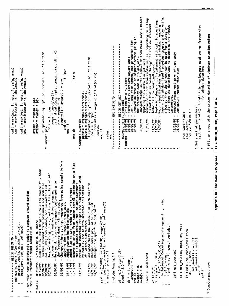
BEGIN

SMSI

MJTD

--

----

----

----

----

----

----

-su

brou

tine

smsim t

d(per, np

er,

: prvsim,

pgasTm,

pgvs

im,

prvcalc,

: nacc_save, ac

c_sa

ve,

vel_save)

Uses

ti

me-d

omai

n st

ocha

stic

mod

el to c

ompute ground m

otio

n (S

MSIM

=

Stoc

hast

ic M

odel Simulation)

Date

s:

05/10/95

- 05/30/95

- 06/02/95

- 06/09/95

- 06

/12/

95

-

08/08/95

-

08/08/95

-

08/18/95

- 10

/17/

95

- 10

/17/

95

-

11/1

4/95

-

12/1

4/95

04/12/96

04/1

5/96

01

Written

by D

. M.

Bo

ore

Modified b

y Basil

Marg

aris

to

allow c

hoice

of window

Furt

her

rena

med

(fro

m psvsimnu)

and

modi

fied

.Ge

t r,

am

ag fr

om c

ommon, no

t parameter

list

Remo

ved

writ

ing

of ace, vel

to a

file;

this should

be d

one

in the

front-end

driver pr

ogra

m.Removed

dc from n

oise segment

before g

oing

to

the

frequency

domain (in

get_acc)

.Changed

thin

gs so

th

at remove d

c from n

oise

sample

before

appl

ying

the

window (in

get_

acc)

.Ad

ded

subr

outi

ne W

rite_Params

Added

flag

to G

et Params and

Write_Params

Remove d

c or

no

t Trom r

andom

series,

depending

on a

fl

agth

at is

passed th

roug

h th

e in

clud

e st

atem

ent

Brok

e ou

t nu

meri

cal

reci

pes

and

subroutines

used

by b

oth

rv a

nd t

d in

to separate co

llec

tion

sof

Fortran

subroutines

Assigned d

urex

the

source p

lus

path

dur

atio

nChanged

name

s ps

v, sd

to

prv

, rd

Changed

"rd_spect" to "r

d_ca

lc"

real

ac

c(16

400)

, ye

l(16

400)

, avgprv(120),

: pe

r(*)

, pr

vsim

(*),

acc_save(*), ve

l_sa

ve(*

) character

prvcalc*!

include

'sms

im.f

i'

pi =

4.0

* atanp-

0)

twop

i =

2.0

* pi

do

i =

1, np

erav

gprv

(i)

= 0.

en

d do

avgpga =

0.

avgpgv =

0.

iseed

= -abs(seed)

writ

e(*,

*)do

is

im =

1,

nr

uns

write(*,'(3(a,

i3),

a)')

' + Patience!

Comp

utin

g ac

cele

rogr

am #

', is

im,

1 of

', nruns,

1 an

d rs at

',

np

er,

1 periods.

1

call

get_acc(acc)

call

get_vel(acc, np

ts,

dt,

vel)

if (isim

.eq. na

cc_s

ave)

th

en

do

i =

1, np

tsacc_save(i)

= ac

c(i)

vel_save(i)

= ve

l(i)

end

do

end

if

Comp

ute

pga, pg

v:

call mnrnax(acc,

1, npts,

1, am

in,

amax)

pga

= amax1(abs(amin

), abs(amax))

call

mn

max(

vel,

1,

npts,

1, vm

in,

vmax

) pgv

= amaxKabs(vmin),

abs(vmax))

avgpga =

avgpga +

pg

a avgpgv =

avg

pgv

+ pgv

if (p

rvca

lc .eq.

'y1

.or. prvcalc

.eq. 'Y

') th

en

Compute

prv: do

i =

1, nper

omega

= twopi/per(i)

call rd

_cal

c(ac

c, np

ts,

omeg

a, damp,

dt,

rd)

prv

= omega

* rd

avgprv(i)

= av

gprv

(i)

+ prv

end

do

! iper

end

if

end

do!

isim

* Compute

averages

pgas

im =

av

gpga

/flo

at(n

runs

) pg

vsim

= av

gpgv

/flo

at(n

runs

)if

(prvcalc .eq.

'y1

.or. prvcalc

.eq. 'Y

') th

en

do

i =

1, np

erprvsim(i)

= avgprv(i)/float(nruns)

end

do

end

if

return

end

END

SMSIM

TO

Appendix B

: Time-Domain

Progr.

....

....

....

....

. BEGIN

QET_

ACC

-----------------------------

subr

outi

ne g

et_acc(acc)

Date

s:

06/0

7/95

- Wr

itte

n by

D.M

. Bo

ore

06/0

8/95

- No

rmal

ize

by s

qrt(avg

square am

p)06

/09/

95

- Ge

t r,

am

ag fr

om c

ommon, not

para

mete

r list

08/0

8/95

- Removed

dc from n

oise

seg

ment

before g

oing

to

the

freq

uenc

y do

main

(in

get_

acc)

. 08

/08/

95

- Changed

thin

gs so

th

at remove d

c from n

oise

sample

before

appl

ying

th

e window (in

get_

acc)

. 10

/17/

95

- Remove d

c or no

t fr

om r

andom

seri

es,

depending

on a

fla

g(irmvdc) th

at is

passed th

roug

h the

incl

ude

stat

emen

t 11

/14/

95

- Added

call to c

onst

_amO

_gsp

rd11

/16/

95

- Replaced

'shape =

...' st

atem

ent

with

call to s

pect_amp

12/0

6/95

- Major

simp

lifi

cati

on in

exp

onen

tial

wi

ndow

, re

movi

ngtapers (t

he w

indow

itself pr

ovid

es tapers)

and

correcting

a bu

g so

th

at the

window c

an b

e used f

or a du

rati

onother

than

the

dura

tion

used

to d

etermine the

window

para

mete

rs.

12/2

2/95

- Removed

rmea

n real pa

rt of

work o

nly

01/22/96

- Use

REALFT ra

ther

than FO

RK

real

wo

rk(1

6400

) real ac

c(*)

in

clud

e 'smsim.fi'

* Set

spec

tral

parameters:

call sp

ect_

scal

e()

! call th

is no

w because

need c

orner

freq

uenc

ies

* for

window d

urat

ions

* Fi

ll an

array w

ith

the

proper d

urat

ion

of wi

ndow

ed G

auss

ian

noise:

c _________________

__

__

__

__

_T

ile

SH

SIH

_jb7

FOR

/ P

age

1 o

f ^

Or

Or

do

i =1, np

tsac

c(i)

=0.

work(i)

= 0.

end

do

* Mo

difi

cati

ons

in o

rder

to us

e an

othe

r wi

ndow

5/30/1995

ifd'ndxwind

.eq. 0) th

en

! BO

X WI

NDOW

* Fi

gure

out

in

dice

s fo

r a

noise

sample o

f th

e proper d

urat

ion:

ns

tart

=

tshi

ft/d

tdu

rex

= dursource(w_fa,

fa,

w_fb

, fb

)+

: du

rpat

h(r,

nk

nots

, rdur,

dur,

sl

ast)

nm

otio

n =

dure

x/dt

* In

crea

se d

urat

ion

of motion b

y ta

pers

(figure

1/2

fron

t an

d back):

ntap

er =

ifix

(tap

er*n

moti

on)

! ta

per

is fractional,

not

perc

ent

nmotion

= nmotion

+ ntaper

nstop

= nstart +

nmo

tion

if

(nstop .gt. np

ts)

then

write(*,'(2x,a,i5,a,i5,a)')

1 ***

FATA

L ER

ROR:

NSTOP

(',

nsto

p,

') >

NPTS ('

,np

ts,

');

QUITTING!

1 stop

end

if

* Generate G

aussian

whit

e noise

with

ze

ro m

ean, un

it va

rian

ce:

do

i =

nsta

rt,

nstop

work(i)

= ga

sdev

(ise

ed)

end

do

if (irmvdc

.eq. 0) then

rmea

n =

0.0

else ca

ll mean(work, nstart,

nsto

p, rm

ean}

en

d if

do

i =

nsta

rt,

nsto

pwo

rk(i

) =

wind_box(i,

nsta

rt,

nsto

p, ntap

er)

* (work(i)

- rm

ean)

end

do

else

EXPONENTIAL WINDOW

* Fi

gure

out

in

dice

s for

a no

ise

sample o

f th

e proper d

urat

ion:

ns

tart

=

tshift/dt

dure

x = dursource(w_fa,

fa,

w fb

, fb

)+

: durpath(r, nknots,

rdur,

dur,

sl

ast)

nmot

ion

= 2.

0 * durex/dt

! do

uble

d fo

llow

ing

Boor

e (1983, p.

1869)

tmot

ion

= nmotion

* dt

nstop

= nstart +

nmotion

if (nstop .gt. npts)

then

write(*

f'(2x,

a,i5,a,i5,a)')

: ' **

* FA

TAL

ERRO

R: NS

TOP

(',

: ns

top,

:

') >

NPTS ('

, :

npts,

');

QUIT

TING

!'

stop

end

if

* Ge

nera

te G

auss

ian

whit

e no

ise

with

ze

ro m

ean,

un

it v

aria

nce:

tw =

tm

otio

n *

twdtmotion

do

i =

nsta

rt,

nsto

p

work

(i)

= ga

sdev

(ise

ed)

end

do

if (irmvdc

.eq. 0)

then

rmea

n =0.0

else ca

ll me

an(w

ork,

nstart,

nstop, rm

ean)

end

if

do

i =

nsta

rt,

nsto

pt

= fl

oat(

i-ns

tart

) *

dtwo

rk(i

) =

wind

_exp

( t, tw,

eps_

wind

, et

a_wi

nd,

newjnr)

: *

(wor

k(i)

-

rmea

n)

end

do

end

if

* Tr

ansf

orm

to f

requ

ency

dom

ain:

call re

alft

(wor

k,np

ts,+

1)

* Fi

nd s

qrt

of sq

uare

d sp

ectr

al amplitude

for

norm

aliz

atio

n:

calI

avgsq_reaIft(work,npts,avgsqamp)

sqrt

_avg

sqam

p =

sqrt(avgsqamp)

* Ge

t fr

eque

ncy

inde

pend

ent

parameter:

call

const_amO_gsprd()

! returns

freq_indep_factor

thro

ugh

comm

on

iaorins

= 1

idva

= 2

! ground m

otio

n ! ac

cele

rati

on

df =

1.0/(float(npts)

*dt)

do

i =

2,npts/2

f =

(i-1)

* df

sfac

t =

spec

t_am

p(f)

/ sq

rt avgsqamp

work(2*i-1)

= sf

act

* wo

rk("

2*i-

1)work(2*i)

= sf

act

* wo

rk(2

*i)

end

do

work

(1)

= 0.0

! OK f

or ac

cele

rati

on s

pect

rum,

but

not

for

! di

spla

ceme

nt sp

ectr

um

fnyq =

1.0/(2.0*dt)

work

(2)

= sp

ect_

amp(

fnyq

) *

work

(2)/

sq

rt_a

vgsq

amp

* Tr

ansf

orm

back to ti

me d

omai

n:

call

realft(work,npts,-

1)

* Apply

FFT

norm

aliz

atio

n:

afac

t =

2 *

df

do

i =

1, npts

acc(

i) =

afac

t *

work

(i)

end

do

return

end

END

GET

ACC

*...

....

....

....

.. BE

GIN

GET

VEL

.............................

* Da

tes:

06/07/95

- Wr

itte

n By D

.M.

Boor

e*

02/02/96

- Modified to u

se d

oubl

e precision

for

* th

e accumulator, fo

llow

ing

Conv

erse

's B

AP routine.

subroutine g

et_vel(acc,

npts

, dt

, ve

l)

real ve

l(*)

, ac

c(*)

do

uble

precision c

um,

hdt

* remove trend

firs

tAp

pendix B

: Time-Domain Programs -

- Fi

le S

MSIM T

D.FOR, Pa

ge 2

of

4

call dcdt(acc,

dt,

npts

, 1,

np

ts,

.fal

se.,

.true.)

* comput

e velocity (a

ssum

e ve

l =

0 for

first

poin

t)

hdt

= db

le(d

t) * db

le(O

.S)

cum =0.0

vel(

1) =

sngl

(cum

)do

j=2,npts

cum

= cum

+ db

le(a

cc(j

) + acc(j-D) *

hdt

vel(

j) =

sngl

(cum)

end

do

* hi

gh pa

ss fi

lter

th

e velocity (m

ay w

ant

to a

llow th

is in a

fu

ture

ver

sion

;*

as it

is

, th

e ac

cele

ration t

ime

seri

es can

be fi

lter

ed,

so th

ere

is n

o need

* to

do

it ag

ain)

.

retu

rn

end

END

GET

VEL

c+ c C c c c c-

....

....

....

....

. BE

GIN

DCDT .

....

....

....

....

....

....

....

Date

s:

- Wr

itte

n by

C.S.

Muel

ler

SUBROUTINE DCDT (Y,DT,NPTS,INDX1,INDX2,LDC,LOT)

DCDT

-

Fits

DC

or tr

end

between

indi

ces

INDX1

and

INDX2.

Then re

move

s DC

or

detrends

whole

trac

e.

Y is real,

DT = delta

t.

If re

move

DC,

LD

C =

.TRUE.

IF detrend, LOT

= .TRUE.

c c...

100

200

C C...

300

360

C C...

400

450

real

Y(

1)

logical

LDC,

LOT

Fit

DC an

d tr

end

betw

een

indi

ces

INDX1

and

INDX2.

NSUM

= INDX2-INDX1+1

SUMX

= 0.

0 SU

MX2 =0.0

SUMY

=0.0

SUMX

Y =0.0

DO 2

00 I=

INDX

1,IN

DX2

XSUB

I =

(I-1)*DT

SUMXY

= SUMXY+

XSUBI*Y(I)

SUMX =

SUMX+XSU

BISU

MX2

= SUMX2+XSUBI*XSUBI

SUMY

=

SUMY

+Y(I

)

Remo

ve D

C.

IF (LDC)

THEN

AVY

= SUMY/NSUM

DO 3

60 1=1,NPTS

Y(I)

= Y(

I)-A

VY

RETURN

END

IF

Detrend. Se

e Draper and

Smith, p. 10

. IF (L

OT)

THEN

BXY

= (S

UMXY

-SUM

X*SU

MY/N

SUM)

/(SU

MX2-

SUMX

*SUM

X/NS

UM)

AXY

= (SUMY-BXY*

SUMX

)/NS

UM

QXY

= DT

*BXY

DO 4

50 1=1,NPTS

Y(I) = Y(I)-(

AXY+

(I-1

)*QX

Y)

RETU

RN

END

IF

STOP

END

END

DCDT

HP.................

BEGI

N MN

MAX

....

....

....

....

....

..su

brou

tine

mnm

ax(a

,nst

rt,n

stop

,nin

c,am

in,a

max)

c c

author:

D. M. Boore

c la

st change:

9/7/84

cdi

mens

ion

a(1)

amax =

a(

nstrt)

amin

=ama

xdo

10 i=nstrt,nstop,ni

neif

(a(i

)-am

ax)

15,1

5,20

amax

=a(i

)go

to 10

if(a

(i)-

amin

) 25,10,10

amin

=a(i

)continue

return

end

............ END

MNMAX

........................

*...

....

....

....

.. BE

GIN

MEAN

....................

subr

outi

ne m

ean(

work

, nstart,

nstop, rm

ean)

* Da

tes:

01/22/96

- Wr

itte

n by D

. Bo

ore

real wo

rk(*

)*

find

mea

n of

th

e ar

ray:

su

m =

0.0

do

i =

nstart,

nsto

p sum

= sum

+ wo

rk(i

) end

dorm

ean

= sum/float(nstop-nstart+1)

return

end

*...

.._.

....

....

.. END

MEAN

..

....

....

....

....

....

*...

....

....

....

....

BEGIN

AVGS

Q_RE

ALFT

-------------------------------

* Da

tes:

01/22/96

- Wr

itte

n by D

.M.

Boore

subr

outi

ne av

gsq_

real

ft(

s, npts,

avgs

qamp

)real s(

*)su

m=0.

do

j =

2, npts/2

Idon't include

the

dc or Ny

quis

t values

sum=sum

+ s(

2*j-

1)**

2 +

s(2*j)**2

! odd, even =

real,

imag

sp

ect

end

doavgsqamp =

su

m/fl

oat(

npts

/2

- 1)

return

end

* ..

....

....

....

....

. END

AVGSQ

REAL

FT --

----

----

----

----

----

----

----

-

* ...................

BEGIN

func

tion

win

d_bo

x(

i, ns

tart

, ns

top,

nt

aper

) c c

appl

ies

cosine tapered

wind

ow,

c un

it amplitude

assumed

c c written

by D

. M. Boore

c c latest re

visi

on:

9/26/95

real wi

nd_b

oxwindjpox =0.0

if

( i

.It. nstart .or.

i. gt

. ns

top)

return

wind_box =

1.0

if

( i

.ge. ns

tart

+nta

per

.and

. i

.le. ns

top-

ntap

er

) return

cpi

= 4.0

* atan(LO)

Appe

ndix

B:

Time-Domain

Programs -- File S

MSIM

_TD.

FOR

f Pa

ge 3 o

f 4

duml =

(nstop+nstart)/2.0

dum2

=

(nstop-nst

art-

ntap

er)/

2.0

wind

_box

= 0.

5 *

(1.0

-

sin( pi

* "

( ab

s(fl

oat(

i)-d

um1)

- du

m2

) /f

loat

(nta

per)

retu

rnen

d ..

....

....

....

...

END

WIN

D BOX

----

----

----

----

func

tion

WIND

_EXP

-----------------------

wind

_exp

( t,

tw,

eps_

wind

, eta_wind,

new_mr)

appl

y Sa

rgon

i an

d Ha

rt (1

974)

window,

with

pa

rameters

tw,

eps

(fra

ctio

n of

tw to

re

ach

peak

), an

d eta

( fr

acti

on o

f peak a

mpl.

at

tw

).

See

Boor

e (BSSA,

p. 1869).

Note

th

at t can

be la

rger

th

an tw.

1983,

Date

s:

at

05/30/95

- In

itia

lly

writ

ten

by D

ave

Boore, based

on a

ro

utin

e by

G.

Atkinson b

ut wi

th si

gnif

ican

t st

ruct

ural

ch

anges

and

the

taper

to b

e a

raised c

osine

tape

r12/06/95

- Re

move

d th

e taper

and

simp

lifi

ed th

e parameters in th

e ca

lling

list.

Also a

dded

a sw

itch

so

th

at th

e window

shap

e co

effi

cien

ts ar

e only c

omputed

once

. Th

is assumes

that

th

e sh

ape

coefficients w

ill

be th

e same f

or

any

run

of th

e pr

ogra

m...

a

good a

ssumption.

12/28/95

- Us

ed n

ewjnr, set

from d

rive

r, to

con

trol

computation

of b,

c,a;

before

I used "

firs

tcal

l",

set

in th

is

subp

rogr

am,

but

this

gave

an e

rror if

the

driver

loop

ed o

ver

mult

iple

values

of m

and r.

real

wi

nd_e

xp

logical

newjnr

save

a,

b, c

if (newjnr) th

enb

= -eps_wind

* alog(eta_wind)/

: (1.

+ ep

s_wi

nd*(

alog

(eps

_win

d)-1

.))

c =

b/(e

ps_w

ind*

tw)

a =

(exp

(1.0

)/(e

ps_w

ind*

tw))

**b

new

mr =

.fal

se,

end

i?

wind

_exp

= 0.

if(

t .It. 0.

0) re

turn

Apply

Sarg

oni

and

Hart

wi

ndow

.

wind

_exp

= a*t**b *

exp(-c*t)

retu

rn

end

END

WIND

EX

P

RD_C

ALC

----

----

----

----

------

----

---

subroutine rd

calc(acc,na,omega,damp,dt,rd)

This

is a

mo

difi

e3 v

ersi

on o

f "Quake.For", or

igin

ally

writte

n by J

.M.

Roesse

t in

19

71 an

d modified b

ySt

avro

s A. Anagnostopoulos, Oc

t. 1986.

The

formulation

is th

at of

Nigam

and

Jennings (B

SSA,

v. 59

, 90

9-92

2, 1969).

This

modification

eliminates th

e co

mput

atio

n of the

relative v

elocit

y and

abso

lute

acce

lera

tion

; it returns

only th

e relative d

ispl

acem

ent.

Date

s: 05/06/95

- Modified b

y David

M. Bo

ore

04/1

5/96

- Changed

name

to R

D_CALC an

d ad

ded

comm

ent

line

sin

dica

ting

ch

ange

d for

storing

the

oscillator ti

me s

eries

and

computing

the

relative v

elocity

and

absolute

accele

rati

on

ace

= ac

cele

rati

on time s

erie

s na

= length of ti

me s

eries

omega

= 2*

pi/p

erda

mp =

fr

acti

onal

da

mpin

g (e.g., 0.

05)

dt =

time

spacing o

f input

rd =

re

lati

ve d

isplacement

of os

cill

ator

dime

nsio

n ac

c(*)

omt=omega*dt

d2=1

-dam

p*da

mp

d2=sqrt(d2)

bom=damp*omega

d3 =

2.

*bom

! for

aa

omd=omega*d2

om2=omega*omega

omdt=omd*dt

c1=1./om2

c2=2.*damp/(om2*omt)

c3=c

1+c2

c4=1./(omega*omt)

ss=sin(omdt)

cc=cos(omdt)

bomt

=dam

p*om

t ee

=exp

(-bo

mt)

ss=ss*ee

cc=cc*ee

s1=ss/omd

s2=s1*bom

s3=s2+cc

a11=s3

a12=

s1

a21=-om2*s1

a22=cc-s2

s4=c

4*(1

.-s3

) s5=s1*c4+c2

b11=s3*c3-s5

b12=-c2*s3+s5-d

b21=

-s1+

s4

b22=-s4

rd=0.

rv =

0.

!

for

rv

aa =

0.

!

for

aa

n1=na-1

y=0.

ydot=0.

do i=1,n1

y1=a

11*y

+a12

*ydo

t+b1

1*ac

c(i)

+b12

*acc

(i+1

)yd

ot=a

21*y

+a22

*ydo

t+b2

1*ac

c(i)

+b22

*acc

(i+1

)y=y1

! y

is the

oscillator ou

tput

at ti

me c

orre

spon

ding

to

index

iz=

abs(

y)if

(z

.gt.

rd)

rd=z

zl =

abs(ydot)

! fo

r rv

if (z

1.gt

.rv)

rv =

z1

! fo

r rv

ra =

-d3*ydot -om2*y1

! fo

r aa

z2 =

abs(

ra)

! for

aaif

(z

2.gt

.aa)

aa

= z2

!

for

aaen

d do

re

turn

en

dEND

RD CALC

incl

ude

incl

ude

Appe

ndix

B:

Time

-Dom

ain

Progrs

1rvtdsubs.for'

______

'rec

ipes

.for

'__

File

SMSIM_TD.FOR, Pa

ge 4 o

f 4

-...

....

..--

.-..

. BE

GIN

FAS_DRVR --

----

----

----

------

----

---

Prog

ram

FAS_

Drvr

Obtains

inpu

t pa

rame

ters

, ca

lls

FAS

routine, and

writes o

utput.

Write

out

Fourier

displacement,

velocity,

and

acceleration s

pect

ra,

and

Four

ier

spec

tra

of th

e os

cill

ator

re

spon

se,

if used (m

ax o

f 10 p

erio

ds).

Date

s: 12

/16/

95

- Written

by D

.M.

Boore; Modified from R

V_DRVR

01/0

3/96

- Added

oscillator response

04/1

2/96

- Ch

ange

d name p

sv t

o prv

character

prvc

alc*

!, in

dvid

per*

1, bi

gbuf

*150

character

fnam

e pa

rams

*80,

fn

ame_

out*

80,

buf*80

character

jndv

idf req*1,

f col*80,

message*80,

: date be

gin*

10,

time

_beg

Tn*1

1, ti

me_s

tart

*11,

time_stop*11

logi

cal

fparam_exist,

tdfl

ag

real

freq(1000),

fds(

1000

) re

al pe

r(10

), pr

v(10

00,

10)

integer

irec

ord_ length

include

'sms

im.f

i '

pi =

4.0

* at

an(1

.0)

twop

i =

2.0

* pi

333

Ol

OO

write(*,

: ' En

ter

a message, if

des

ired

: '

mess

age

= '

' re

ad( *

, ' (

a )

' ) me

ssag

e

cont

inue

fname_params =

' '

writ

e(*,

'(a\)')

: ' En

ter

name

of

file

wit

h pa

rame

ters

(cr

to q

uit)

: read(*,

'(a)

1) fname_params

if (f

name

jDar

ams(

1:4)

.eq.

' ')

stop

inqui re(fTle=fnam

e_params,

exis

t=fp

aram

_exi

st)

if (.not. fp

aram

_exi

st)

then

writ

e(*,

'(a)

')

' **

****

* FILE DOES NOT

EXIS

T *******

go to 3

33

end

if

fnam

e_ou

t =

' '

write(*

f '(a\)')

: ' En

ter

name

of

summary

file:

're

adC *

, ' (

a )

' ) f name_out

nout

=

10op

en(u

nit=

nout

,f i le

=fna

me_o

ut,s

tatu

s='u

nkno

wn'

)wr

ite(

nout

, '(a)

1) message

writ

e(no

ut,

'(2a

)')

' ou

tput

file:

',

: fn

ame_

out(

1:20

)

writ

e(no

ut,

'(a)

1)

: ' **

* Re

sult

s computed u

sing

FA

S_DR

VR ***'

call ge

t_da

te(d

ate_

begi

n)write(nout,

'(2a)')

' Date:

', da

te_b

egin

call

ge

t_ti

me(t

ime_

begi

n)write(nout,

'(2a)')

' Ti

me:

', ti

me_b

egin

write(nout,

'(2a)')

' fi

le w

ith

parameters:

',

: fname_params(1

:20

)

write(*,

: ' En

ter

indi

vidu

al

f requencies(y/n)?:

indv

idfr

eq =

'

'read(*,

'(a)

1) indvidfreq

if (i

ndvi

dfre

q .eq. 'y

1 .or. indvidfreq .eq. 'Y') th

enwrite(*, '(a\)')

: ' En

ter

nfre

qs:

' read(*,

*> nfreq

do

i =

1, nfreq

writ

e(*,

'(

a\)'

) '

Ente

r fr

eque

ncy

for

FAS:

'

read

(*,*

) fr

eq(i

) end

do

else wr

ite(

*, '(a\)')

: ' En

ter

freqlow, freqhigh,

nfre

q (f

req

.ne. 0!):

' re

ad(*

,*)

freqlow, fr

eqhi

gh,

nfre

q if

(freqlow .eq. 0.

0 .or. fr

eqhi

gh .eq. 0.

0) th

enwrite(*, '(

a)1)

.

**

****

* FR

EQ =

o NO

T AL

LOWE

D; AB

ORTI

NG!!

**

****

*'go

to 9

99

end

if

do

i =1, nfreq

freq(i)

= :

freq

low

* (freqhigh/freqlow)**(float(i-1)/float(nfreq-D)

end

do

end

if

writ

e(*,

'(a\)')

' Compute

prv

(y/n):

'prvcalc

= 'n

1read(*,

'(a)

1) pr

vcal

cif

(p

rvca

lc .eq. 'y

1 .or. pr

vcal

c .eq. 'Y

') th

enwr

ite(

*, '(a\)')

: ' Enter

individual pe

riod

s(y/

n)?:

'

indv

idpe

r =

' '

read(*,

'(a)

1) indvidper

if (i

ndvi

dper

.eq. 'y

1 .or. in

dvid

per

.eq. 'Y

') th

enwr

ite(

*, '(a\)')

: ' En

ter

frac

tion

al da

mpin

g, np

erio

ds (m

ax o

f 10

):

' read(*,

*) damp,

nper

do

i

= 1,

np

erwr

ite(

*, '(

a\)')

' Enter

osci

llat

or p

erio

d:

' re

ad(*

,*)

per(

i)

end

do

else wr

ite(

*, '(2a\)')

: ' En

ter

frac

tion

al da

mpin

g, perlow,

perh

igh,

1,

: ' np

er (m

ax o

f 10

):

're

ad(*

,*)

damp,

perl

ow,

perh

igh,

np

er

do

i =

1, np

erpe

r(i)

=

: perlow *

(perhigh/perlow)**(float(i-1)/float(nper-D)

end

do

end

if

if (nper

.gt. 10

) th

enwr

ite(

*, '(

a,i4

,a)'

) ' **

* ER

ROR

****** nper =

',

: np

er,

' >

10;

QUITTING?!!!

1 ! should c

heck th

is when o

btai

n! np

er and

forc

e th

e user to e

nter

! a valid

numb

er.

Perhaps

this

! will be

don

e in

a future v

ersi

on.

close(unit=nout)

stop

end

if

else np

er =

0 end

if

tdflag =

.false.

call ge

t_pa

rams

( fn

ame_

para

ms,

tdflag

)Appendix C

: Fo

urie

r Amplitude-Spectra

Programs -

- Fi

le F

AS_D

RVR.

FOR,

Pa

ge 1

of 2

call wr

ite_

para

ms(

nout

, td

flag

)

100

continue

buf

= '

'write(*, '(

a\)'

) ' dist (cr

to q

uit)

:read(*,

'(a)') bu

fif (buf (1:

4) .eq.

' ')

go

to

999

read(buf,

'(fl

O.O)

1) r

amag

: '

write(*,

read

(*,

*) am

ag

Cn CO

writ

e(*,

: ' En

ter

name o

f column fi

le f

or FA

S results:

' f_col

= '

' read(

*,

'(a)

1) f_

col

* Figure o

ut re

cord

le

ngth

and

open t

he f

ile:

i rec

ord

leng

th =

10*(

nper

+5)

ncol

= 50

open

(uni

t=nc

ol,

file

=f_c

ol,

: re

el =

irecord_length,

status=' unk

nown

1)

* Write

the

head

er:

bigb

uf =

' '

bigbuf(3:10) =

'freq(Hz)

1 bigbuf(15:20)

= 'per(s)'

bigb

uf (22:30) =

'fds

(cm-

s)1

bigb

uf (34:40) =

'fvs

(cm)

1 bi

gbuf

(42

:50)

=

'fas

(cm/

s)'

if (nper

.gt. 0) then

do iper =

1,

np

er

iseg

= 10*(iper +4)

writ

e(bi

gbuf

(ise

g+3:

iseg

+10)

,'(a

,f6.

3)1)

:

'!=',

per(iper)

end

do

end

if

writ

e(nc

ol,

'(a)

1) bi

gbuf

(1:

irec

ord_

len

gth)

call ge

t_ti

me(t

ime_

star

t)

iaor

ins

= 1

idva =

0

writ

e(*,

'(a)

'):

' Pa

tien

ce!

Computing

displacement sp

ectr

um1

call

smsimfas(fds,

freq

, nf

req)

if (p

rvca

lc .eq.

'y1

.or. pr

vcal

c .eq. 'Y

') then

iaorins

= 2

idva

= 0

writ

e(*,

*)

do ip

er =

1,

np

erwrite(*,'<a,i3,a,i3,a)')

: '+ Pa

tien

ce!

Computing

response s

pect

ra number

',

: iper,

' ou

t of

', np

er,

' periods.

1 perosc =

per (i

per)

fo

sc =

1.0/perosc

call sm

simf

as(p

rv(1

,ipe

r),

freq,

nfre

q)

end

do

end

if

writ

e(no

ut,*

)wr

ite(

nout

, '(a)

1)

' ***********

NEW

R AN

D M

****

****

***'

wr

ite(

nout

, '(a, 1p2(1x,e10.3)) ')

: '

r, am

ag =

' ,

r,

amag

wrjt

e(no

ut,

'(2x,2a)')

' Ti

me S

tart

: ', time_start

writ

e( nout,

'(2x,a,1x,1pe10.3)')

' const=

', co

nst

writ

e( nout,

'(2x,a,1p4(1x,e10.3))')

: ' amag,

stre

ss,

fa,

fb=

', am

ag,

stre

ss,

fa,

fbwr

ite(

nout,

'(2x,a,1p2(1x,e10.3))')

' amO, am

Ob_m

Ofa=

:

amO, amObjnO

writ

e(*,

*)

do

i =

1, nf req

per4

freq

= 1.

0e10

if (freq(i) .ne. 0.

0) pe

r4fr

eq =

1.

0/fr

eq(i

)fvs

= (2

.0*p

i*fr

eq(i

)) *

fds(

i)fas

= (2

.0*p

i*fr

eq(i

)) *

fvs

bigbuf =

' '

writ

e(bi

gbuf

(1:5

0),

'(1p

5(e1

0.3)

)')

: freq(i), pe

r4fr

eq,

fds(

i),

fvs, fas

if (nper

.gt. 0)

th

en

do iper =

1,

nper

iseg =

10

*(ip

er +

4)

writ

e(bi

gbuf

(ise

g+1:

iseg

+10)

,'(1

pe10

.3)'

) :

prv(

i,ip

er)

end

do

end

if

writ

e(nc

ol,

'(a)

1) bigbuf(1:irecord_length)

end do

close(unit=ncol)

call

ge

t_ti

me(t

ime_

stop

)write(nout,

'(2x

,2a)

')

' Ti

me S

top:

', ti

me_s

top

call

ti

me_d

iff(

time

start,

time

_sto

p, ti

me_e

laps

ed)

write(nout,

'(2x,a,Tx,f6.1)')

: ' Elapsed

time

(sec):

', ti

me_e

laps

ed

writ

e(*,

*)

writ

e(*,

'(a\)')

: ' Compute

resu

lts

for

anot

her

r and

M (y/n;cr=quit)?

' re

ad(*

f '(a)

1) buf

if (b

uf(1

:4)

if (b

uf(1

:1)

goto 100

.eq.

.eq.

') go

to

999

.or. bu

f(1:

1) .eq.

N1)

go

to

999

999

cont

inue

clos

e(un

i t=nout)

stop

end

* -----------------

END

FAS

DRVR

Appendix C

: Fourier Amplitude-Spectra

Prog

rams

--

File

FAS

_DRV

R.FO

R, Pa

ge 2 o

f 2

*__.

._..

....

....

.. B£

GIN

SMSIMFAS ---------------------------

subroutine s

msimfas(fas, fr

eq,

nfreq)

* Da

tes:

12

/16/

95

- Written

by D

.M.

Boor

e, based

on S

MSIM_RV

real

fas(*>,

freq

(*>

include

'sms

im.f

i'

pi =

4.0*

atan

(1.0

) tw

opi

= 2.0

* pi

* Set

spectral pa

rame

ters

: call sp

ect_

scal

e()

Be su

re to

ca

ll Get

Para

ms in

driver

* Get

freq

uenc

y-in

depe

nden

t fa

ctor

: call const_amO_gsprd()

do

i =

1, nfreq

fas(

i) = sp

ect_

amp(

freq

(i»

end

do

return

end

END

SMSI

MFAS

include

'rvt

dsub

s.fo

r'

include

'recipes.for

1

Appe

ndix

C:

Fourier Am

plit

ude-

Spec

tra

Programs --

File S

MSIM

FAS.

FOR,

Pa

ge 1

of

1

* st

art

of smsim.fi (inserted

into

code

via

'include sm

sim.

fi1)

re

al rho, beta,

prti

tn,

rtp,

fs

, co

nst,

fbdfa, amagc

real

w

fa,

w fb,

pi,

twopi

real

f?1, qrT, si,

ftl,

ft

2, fr

2, qr

2, s2

, sl

ast

real rl

ow(1

0),

slop

e(IO

) re

al rd

ur(I

O),

dur(

10),

fa

mp(2

0),

amp(

20)

real

ts

imdu

r, dt

, tshift,

tape

r, seed

inte

ger

nknots,

nums

ourc

e, nsprd_segs,

namps, nruns, np

ts

inte

ger

indxwind

char

acte

r ti

tle*

70

logi

cal

new_

mr

common /

titl

e/ ti

tle

common /

magdist/ r,

am

agcommon /

const_params/

rho,

be

ta,

prtitn,

rtp,

fs,

pi,

twopi,

: co

nst,

iaorins, idva,

freq

_ind

ep_f

acto

rcommon /

source_shape_params/ nu

msou

rce,

pf

, pd

common /

source_scale_params/ st

ress

c, dl

sdm,

amagc,

: st

ress

, fa,

fb,

amO, am

Objn

O, fb

dfa

common /

gsprd_params/

nsprd_segs,

rlow

, slope

common /

q_params/

fr1,

qr1, s1

, ft

1, ft

2, fr2, qr2, s2

common /

source d

ur_p

aram

s/ w_

fa,

w fb

common /

path_dur_params/ n

knots, r3ur,

dur, slast

common /

site

_amp

par

ams/

nam

ps,

famp

, amp

common /

site

_dim

Tn_p

aram

s/ fm,

akappa

common /

rs/

pero

sc,

fosc

, da

mpcommon /

rv/

fup,

im

om,

zup,

eps_int, amp_cu

toff

, :

eps_

rv,

ane,

anz,

: pk

_rms

_cl

1, pk_rms_cl_2,

: pk

cl

eqoH

, pk

rms

cl eq

68,

: pklcp, pk

_cl~

2 ~

~common /

lowcut_fiTter

params/

fcut

, norder

common /

wind

_par

ams/

in3x

wind

,tap

er,t

wdtm

otio

n,ep

s_wi

nd,e

ta_w

ind

common /

tdsi

m_pa

rams

/tsi

mdur

,dt,

tshi

ft,s

eed,

:

nruns, np

ts,

iseed, ir

mvdc

common /

misc/freq20, durex, ne

w_mr

save

/ti

tle/

, /const_params/

save

/source_shape_params/,

/sou

rce_

scal

e_pa

rams

/sa

ve /

gsprd_params/, /q

_par

ams/

save

/source_dur_params/,

/pat

h dur_params/

save

/si

te_a

mp_p

aram

s/,

/sit

e_dT

min_

para

ms/

save

/rs/

save

/rv

/sa

ve /

process_params/

save /

wind

_par

ams/

, /tdsim_params/

save

/misc/

* en

d of smsim.fi (inserted

into

code

via

"inc

lude

sm

sim.

fi"

Appe

ndix

D:

Subroutine Nodules -- Fi

le S

MSIM

.FI,

Pa

ge 1

of

1

05 to

....

..._

.__.

____

. BE

GIN

GET

subroutine g

et_p

aram

s(Tn

ame_

para

ms,

tdfl

ag)

Date

s: 06

/07/

95

- Wr

itte

n by

D.M.

Boore

10/1

7/95

- Ad

ded

tdfl

ag to

control if mo

re d

ata

need b

e re

ad for

the

time

ser

ies

proc

essi

ng;

also a

dded

irmvdc as an

input

para

mete

r11

/14/

95

- Read e

ps^int from d

ata

file

11

/15/

95

- chan

ged

Inpu

t of sp

ectr

al parameters

11/16/95

- Read a

mp c

utof

f fr

om data

file a

nd d

etermine fu

p 11

/27/

95

- changed

Inpu

t of

spectral pa

rame

ters ag

ain

12/0

6/95

-

Get

low-cut

filt

er p

aram

eter

s before rv a

nd t

d params

12/0

7/95

-

Get

taper

with

window p

aram

eter

s 12

/19/

95

- Adde

d zu

p to

input

parameters

char

acte

r fn

ame_

para

ms*(

*>

logi

cal

tdflag

incl

ude

'smsim.fi

1

pi =

4.0

* at

an(1.0)

nin

= 98

open

(uni

t=ni

n, fi

le=f

name

_par

ams,

st

atus

='un

know

n')

* ti

tle: re

ad(n

in,

'(a)

1) ti

tle

* rho, be

ta,

prti

tn,

fs:

call sk

ip(n

in,

1)

read(nin,

*) rh

o, be

ta,

prti

tn,

rtp,

fs

c Define c

onst

ant,

fo

r r=

1 km

cons

t=pr

titn

*rtp

*fs*

(1.e

-20)

/(4.

*pi*

rho*

beta

**3)

* source sh

ape:

call skip(nin,

4)re

ad(n

in,

*) nu

msou

rce,

pf,

pd

* source s

cali

ng:

(not

e: stress is

no

w re

ad in h

ere; to w

rite

a d

river

* th

at lo

ops

over

st

ress

, just assign t

he d

esir

ed v

alues

of stress

* after

calling

get_

para

ms)

call skip(nin,

4)

read(nin,

*) st

ress

c, dl

sdm,

fb

dfa,

am

agc

* gs

prd: ca

ll skip(nin,

1)

read(nin,

*) nspr

d_se

gs

do

i =

1, ns

prd_

segs

read(nin,

*) rl

ow(i

), sloped")

end

do*

assume th

at rlowd) =

1, for

proper scaling

when c

onst

ruct

gsprd.

* Ch

eck

this

an

d quit pr

ogra

m if it isn't:

if

( rlowd) .ne. 1.0) then

writ

e(*,

'(a, e10.3, a)

')

: 'MM! rlowd) =

', rl

owd)

, ', .ne. 1.

0; qu

itti

ng!!

!!!'

stop

end

if

* Q:

call

sk

ip(n

in,

1)read(nin,

*) fr

l, qrl, si,

ft1,

ft

2, fr

2, qr2, s2

* source d

urat

ion:

call sk

ip(n

in,

1)

read

(nin

, *) w_fa,

w_fb

* pa

th d

uration:

call sk

ip(n

in,

1)

read

(nin

, *) nk

nots

do

i

= 1,

nknots

read

(nin

, *) rd

ur(i

), du

r(i)

en

d do

read(nin,

*) slast

* site a

mps:

call sk

ip(n

in,

1)

read(nin,

*) na

mps

do

i =

1, na

mps

read

(nin

, *) famp(i), am

p(i)

en

d do

* site d

imin

utio

n:call sk

ip(n

in,

1)

read(nin,

*) fm

, ak

appa

* lo

w-cu

t filter p

arameters:

call sk

ip(n

in,

1)

read

(nin

, *) fc

ut,

norder

* parameters for

rv in

tegr

atio

n:

call sk

ip(n

in,

1)re

ad(n

in,

*) zu

p, ep

s_in

t, amp_cutoff

if(

akappa .eq. 0.0) th

enfup

= fm

/amp

cutoff**0.25

else fu

p =

: amin1(fm/amp_cutoff*

*0.2

5, -a

log(

amp_

cuto

ff)/

(pi*

akap

pa))

en

d if

* Read m

ore

if time d

omain

method:

if (.not. tdflag)

goto 9

99

window

aram

eter

s:call sk

ip(n

in,

1)

read

(nin

, *) indxwind,

taper, twdtmotion,

eps_wind,

eta_

wind

* timing st

uff:

call sk

ip(n

in,

1)read(nin,

*) tsimdur, dt,

tshift,

seed

, nr

uns

* Fl

ag c

ontrolling th

e removal

of the

dc fr

om t

he random s

eries:

call sk

ip(n

in,

1)

read(nin,

*) irmvdc

* compute

smal

lest

po

wer

of two

for

whic

h the

resu

ltin

g du

rati

on is g

reat

er*

than o

r equal

to t

simdur:

npts

=

2.0**ifix(alog

10(t

simd

ur/d

t +

1.0)/alog10(2.0))

if

( (n

pts-

1)*d

t .It. ts

imdu

r) npts =

2 *

npts

999

cont

i nue

close(unit=nin)

return

end

END

GET

PARAMS

----

----

----

- BEGIN

WRITE_PARAMS ------

subroutine w

rite

_par

ams(

nout

, tdflag)

Appendix D

: Subroutine Nodules -- Fi

le R

VTDS

UBS.

FOR,

Pa

ge 1

of

5

Oi co

Dates: 08

/18/

95

- Wr

itte

n by

D.

Boor

e10/17/95

- Ad

ded

tdfl

ag t

o control

if m

ore

data n

eed

be r

ead

for

the

time

ser

ies

processing;

also a

dded

irmvdc

as a

n in

put

parameter

11/1

4/95

- Wr

ite

eps_int

11/16/95

- Wr

ite

amp_

cuto

ff,

fup

12/0

6/95

- Wr

ite

low-

cut

filter p

aram

s before r

v an

d td

par

ams

12/07/95

- Wr

ite

tape

r with w

indo

w pa

rame

ters

12/19/95

- Ad

ded

zup

to input

parameters

logi

cal

tdfl

ag

include

'sms

im.f

i1

write( nout,

'(a)

1)

' Title:

1 write( no

ut,

'(4x,a)')

titl

e

write( nout,

'(a)

1)

' rho, be

ta,

prtitn,

rtp, fs:

1 write( no

ut,

* )

rho, be

ta,

prtitn,

rtp, fs

write( nout,

'(2a/2a/a/a)')

1 sp

ectr

al shape: so

urce

num

ber

(1=Single

Corner;2=Joyner;',

'3=A

93;4

=cus

tom)

',1 pf,

pd (

1-corn

er s

pectrum

= ',

'1/(

1+(f

/fc)

**pf

)**p

d; 0.0

otherwise)

1,1 (u

sual

model:

pf=2.0,pd=1.0; Bu

tter

wort

h: pf=4.0,pd=0.5)',

1 (N

ote:

power

of h

igh

freq

decay -

-> p

f*pd

)'

write( no

ut,

*) n

umso

urce

, pf,

pd

write( nout,

'(a/a/a/a)

1):

' sp

ectr

al scaling: stressc, dlsdm, fb

dfa,

am

agc

1,

: ' (stress=stressc*10.0**(dlsdm*(amag-amagc))',

: '

(fbd

fa,

amag

c for

Joyn

er m

odel,

usua

lly

4.0, 7.0)',

: '

(not u

sed

for

srce

3,

but

plac

ehol

ders

still

needed)

1write( no

ut,

*) st

ress

c, dlsdm, fbdfa, am

agc

write( no

ut,

"(2a)')

' gsprd: nsegs, (rlow(i),

slope(i))

1,

: '

(Set

rl

ow(1

) =

1.0)'

write( no

ut,

*) n

sprd

_seg

s do i

=

1, ns

prd

segs

write( no

ut,

T) rlow(i), sl

oped

")

end

do

write( no

ut,

write( no

ut.

'(a)')

' q: fr

1, Qr1, s1,

ft1, ft

2, fr

2, qr2, s2'

*) fr1, qr1, s1,

ft1,

ft2, fr

2, qr

2, s2

write( no

ut,

'(a)

1)

' so

urce

dur

atio

n: we

ight

s of

1/

fa,

1/fb

1 write( no

ut,

*) w_

fa,

w_fb

write( nout,

'(2a

)')

' pa

th d

urat

ion:

nk

nots

, (r

dur(

i),

dur(

i),

1,

: ' sl

ope

of la

st s

egment

1 write( no

ut,

*) nknots

do i

=

1, nknots

write( no

ut,

*) rdur(i), du

r(i)

en

d do

write( no

ut,

*) sl

ast

write( no

ut,

'(2a)')

' si

te a

mplification:

namps, (f

amp(

i),

',

: 'a

mp(i

))'

write( no

ut,

*) n

amps

do

i

= 1,

namps

write( nout,

*) famp(i), amp(i)

end

do

writ

e( n

out,

'(a)

1)

' si

te d

iminution

para

mete

rs:

fm,

akappa

1 write( no

ut,

*) fm,

akap

pa

write( no

ut,

'(a)

1)

' low-cut

filt

er p

arameters: fc

ut,

nord

er1

write( no

ut,

*) fcut,

nord

er

if (.

not.

tdflag)

then

writ

e( no

ut,

'(a)

1):

' parameters f

or rv

integration:

zup,

eps_int, am

p_cu

toff

' wr

ite(

no

ut,

*) zu

p, epsint,

amp_cutoff

writ

e(no

ut,

'(a,1pe1

0.3)

')

' calculated f

up =

',

fu

p en

d if

* Wr

ite

more

if

time

domain

meth

od:

if (.not. tdflag)

goto

999

writ

e( no

ut,

: ' window p

arams: in

dxwi

nd(0

=box

,1=e

xp),

',

: ' taper, twdtmotion

, eps_wind,

eta_

wind

'write( no

ut,

*) indxwind,

taper, tw

dtmo

tion

, eps_wind,

eta_

wind

write( no

ut,

'(a)

1):

' timing s

tuff:

tsimdur, dt

, tshift,

seed

, nruns

1 write( no

ut,

*) ts

imdur, dt

, ts

hift

, se

ed,

nruns

write( no

ut,

'(2a/2a)')

: ' pa

rame

ter

to c

ontrol whether

dc is

1,:

' re

move

d fr

om r

ando

m se

ries

before

1,:

' transforma

tion t

o frequency domain

1,:

' (0=no, 1=yes)'

write( no

ut,

*) irmvdc

999

cont

inue

retu

rnen

dEND

WRIT

E PARAMS

*................. BE

GIN

SPEC

T_AM

P -----------------------------

* Da

tes:

06/07/95

- Wr

itte

n by

D.M.

Boore

func

tion

spect_amp(f)

incl

ude

'smsim.fi

1

temp

f =

1.0

if

( id

va .ne. 0

) tempf

= (t

wopi

*f)*

*flo

at(i

dva)

spect_amp

= fr

eq i

ndep

_fac

tor

* (

temp

f )

*:

butt

rlcf

(f,

fcut

, no

rder

) *

: sp

ect_

shap

e(f,

fa,

fb,

pf,

pd,

amOb

jnO,

numsource) *

: si

te_a

mp_f

acto

r(f,

namps, famp,

amp) *

: di

min(

f)! Co

uld

save

some

multiplications

! by r

emov

ing

freq

_ind

ep_f

acto

r ou

tsid

e th

e ! function,

but

at t

he c

ost

of p

ossi

ble

! co

nfus

ion.

go t

o ( 301, 30

2, 30

3 ), ia

orin

s c

no i

nstrument

resp

onse

.301

h=1

go t

o 30

0 c

prv

302

v =

twop

i *

fosc

h =

v *

harm

oscf

( f,

fosc,

damp

, id

va

) go t

o 30

0*

for

customized r

esponse

(net

work

in

stru

ment

s, etc)

303

h=1

go t

o 30

0 30

0 co

nt i n

uesp

ect_

amp

= h

* spect_amp

! sp

ect_

amp

cont

ains

the

spectral

ampl

itud

e.Appe

ndix

D:

Subroutine Nodules -- File RVT

DSUB

S.FO

R, Page 2 o

f 5

retu

rn

end

END

SPEC

T AM

P

CONST_AMO_GSPRD

----

----

----

----

----

----

----

-*

Date

s: 11/14/95

- Written

by D

.M.

Boore

subroutine c

onst_amO_gsprd()

include

'sms

im.f

i'

freq_indep_factor

= const*amO*gsprd(r, ns

prd_

segs

, rlow,

slop

e)*

(con

st fr

om G

et_Params, amO

from S

pect_Scale)

retu

rn

end

END

CONST

AMO

GSPRD

0}

*-..

....

...-

.---

-_ BE

GIN

GSPRD

-----------------------------

* Da

tes:

06

/07/

95

- Wr

itte

n by

D.M.

Boore

func

tion

gsp

rd(r

, ns

prd_

segs

, rlow,

slop

e)

real

rl

ow(*

), sl

ope(

*)f geff(IO)

geff

(1)

= 1.0/rlowCD

! assume rl

ow(l

) =

1.0

do

i =

2, ns

prd

segs

geff

(i)

= gefT(i-1)*(rlow(i)/rlow(i-1))**slope(i-1)

end

do

if (r .le. rl

ow(D

) th

enj

= 1

else if (r

.ge. rlow(nsprd_segs))

then

j =

nsprd_segs

else ca

ll lo

cate

(rlo

w, ns

prd_

segs

, r,

j)

end

if

gsprd

= (geff(j))

* (r

/rlo

w(j)

)**s

lope

(j)

return

end

END

GSPRD

BUTT

RLCF

--

----

----

----

---

* Da

tes:

06

/07/

95

- Written

by D

.M.

Boore

func

tion

but

trlc

fC f,

fc

ut,

norder)

c c Co

mput

es th

e response o

f an

nor

der,

bi

dire

ctio

nal

* hi

gh-p

ass

Butt

erwo

rth

filter.

This

is th

e filter

* used b

y th

e AGRAM

processing (t

he e

quat

ion

was

* provided b

y April

Conv

erse

).

* Mo

difi

cati

on:

3/27/89

- created

by m

odifying HiPass

F

real buttrlcf

butt

rlcf

=

1.0

if

( fc

ut.e

q.0.

0 )

retu

rn

buttrlcf =

0.0

if

( f

.eq. 0.

0) re

turn

buttrlcf =

1.0/

(1

.0+(

fcut

/f)*

*(2.

0*no

rder

))

return

end

END

BUTT

RLCF

*--..-..--.------. BEGI

N SPECT_SHAPE

----

-*

Date

s: 06/07/95

- Written

by D

.M.

Boore

* 11/15/95

- ch

anged

source ty

pes

function s

pect_shape(f,

fa,

fb,

pf,

pd,

amObjnO, numsource)

real spect_shape

goto (1,

2, 3,

4)

, numsource

writ

e(*,

'(a, i5

, a)

1)

' MM!! numsource

= ',

: nu

msou

rce,

', .ne. le

gal

valu

e; qu

itti

ng MM!!

1 stop

* Single c

orner

freq

uenc

y:1

sb =

1.0

sa =

1.0/

( 1.0

+ (f

/fa)

**pf

)**pd

go t

o 900

* Jo

yner

mod

el2

sb =

1.

0/

( 1.0

+ (f

/fb)

**2

)**0.25

sa =

1.

0/

( 1.0

+ (f

/fa)

**2

)**0.75

go to 9

00

* Atkinson 19

93 m

odel

3 sb =

1.0

sa =

(1.0

- amOb m

O)/(

1.0

+ (f

/fa)

**2

) :

+ (a

mUb_

mO)/

( 1.0

+ (f/fb)**2

) go

to 9

00

* For

cust

omiz

ed relation:

4 sb =

1.0

sa =

1.0

go to 9

00

900

continue

spect_shape

= sa*sb

return

end

END

SPEC

T SH

APE

Appe

ndix

D:

Subroutine Nodules --

*...

....

....

....

.. BEGIN

SPEC

T_SC

ALE

---------------------------

* Da

tes:

06

/07/

95

- Written

by D

.M.

Boor

e subroutine spect_scale()

incl

ude

'smsim.fi

1

amO

= 10.**(1.5*amag +

16.05)

amObjnO =0.0

goto (1,

2, 3,

4)

, numsource

writ

e(*,

'(a, i5

, a)

')

' MM!! nu

msou

rce

= ',

: nu

msou

rce,

',

.ne. legal

valu

e; quitting !!

!!!!

' stop

* Single c

orner

frequency:

1 stress =

stre

ssc*

10.0

**(d

lsdm

*(am

ag-a

magc

))fa =

(4.9

06e+

06)

* be

ta *

(stress/amO)**(1.0/3.0)

fb =

fa

return

* Joyner sc

alin

g:2

amOc

=

10.0

**

(

1.5*

amag

c +

16.0

5 )

stress =

stre

ssc*

10.0

**(d

lsdm

*(am

ag-a

magc

))

rat

= stress/amO

dum

= 4.906e+06

if

( am

O .gt. am

Oc

) ra

t =

stress/amOc

fb =

( dum*beta

) *

( fbdfa

)**(3./4.) *

( rat

)**(

1./3

.)

_____fa =

( dum*beta

) *

(stress)**<J_./3.) *

(amOc)**(1./6.)

?Ue R

VTDS

UBS.

FOR,

Pa

ge 3 o

f 5

* *

( fbdfa

)**(-0.25) *

( amO

)**(

-0.5

) if

( am

O .It. am

Oc

) fa

= fb

/ fbdfa

retu

rn

* At

kins

on 9

3 sc

alin

g:3

fa =

10.0

**(2

.41

- 0.

533

* amag)

fb =

10

.0**

(1.4

3 - 0.188

* amag)

amObjnO

= 10.0**(2.52

- 0.

637

* amag)

retu

rn

* Fo

r customized s

cali

ng:

4 fa =

0.

0 fb

= 0

.0

retu

rn

end

END

SPEC

T SCALE

Cn

*.......-...-.-... BEGI

N SI

TE_A

MP_F

ACTO

R -----------------

* Da

tes:

06/07/95

- Written

by D

.M.

Boore

func

tion

sit

e_am

p_fa

ctor

(f,

namps, famp,

amp)

re

al fa

mp(*

)f am

p(*)

, site_amp_factor

if

( f

.le. fampCD

) th

en

site

amp

fact

or =

amp(

1)

else iT

( 7

.ge. fa

mp(n

amps

) ) th

ensi

te_a

mp_f

acto

r =

amp(

namp

s)

else ca

ll lo

cate

( fa

mp,

namp

s, f, j)

site_amp_factor

= am

p(j)

*10.

0**(

alog

10(f

/fam

p< j))

:

*alog10(amp(j+1)/amp(j))

: /alo

g10(

famp

(j+1

)/fa

mp(j

)))

end

if

retu

rn

end

END

SITE AM

P FA

CTOR

*.........--...... BEGIN

DIMI

N -----------------

* Da

tes:

06/07/95

- Written

by D

.M.

Boore

func

tion

dim

in(f

) re

al dimin

include

'sms

im.f

i'

akappaq

= r/(beta*q(f))

dimin

= exp( -pi*(akappa

+ akappaq) *

f)/

: sqrt(

1. +

(f/fm)**8.0

)

retu

rn

end

END

DIMI

N

Q*

Date

s: 06

/07/

95

- Written

by D

.M.

Boor

e*

12/1

4/95

- Adde

d ch

eck

for

equa

l transition

fr

eque

ncie

s function q

(f)

logical

firstcall

/ .true. /

save q

t1 ,

qt2, st

in

clud

e 's

msim

.fi'

q =

99

99

.0

%if

(f

.eq.

0.0

) re

turn

if (firstcall)

then

qt1

= qr

1*(f

t1/f

r1)*

*s1

qt2

= qr2*(ft2/fr2

)**s

2 st =

0.0

if (f

t1 .ne. ft

2) th

enst

=

alog10(qt2/qt1)/alog10(ft2/ft1)

end

iffi

rstc

all

= .false

, end

if

if

( f

.le. ft

1) th

enq

= gr1*<f/fr1)**s

1 else if

(

f .ge. ft2)

th

enq

= qr

2*(f

/fr2

)**s

2 else q

= qt1*(f/ft1)**st

end

if

retu

rn

end

END

Q

*...

....

....

....

.. BEGIN

HARM

OSCF

--

----

----

----

----

----

----

-fu

ncti

on h

armoscf( f, fosc,

damp

, id

va)

c ha

rmon

ic o

scil

lato

r response to g

round

c di

spla

ceme

nt.

* idva =

0 fo

r response to d

isplacement

* idva =

2 fo

r response to a

ccel

erat

ion

* idva =

1

retu

rns

0 fo

r th

e response

* Th

e re

spon

se is normalized t

o be

uni

ty in

the fl

at portion.

* Written

by D

. Bo

ore,

12

/01/

83

c latest mo

difi

cati

on:

3/25/89

if (i

dva

.ne. 0

.and

. idva .ne. 2)

du

n =

0.0

if (i

dva

.eq. 0)

du

m =

f**2

if (i

dva

.eq. 2) du

m =

fosc

**2

harm

oscf

= du

m /

sqrt

( ( fo

sc*f

osc

- f*f

)**2

*

+ ( 2.

0*f*

fosc

*dam

p )**2

) return

end

*................. END

HARM

OSCF

-----------------------------

.................

BEGI

N DURSOURCE

----

----

--Da

tes:

06/07/95

- Wr

itte

n by D

.M.

Boor

efu

ncti

on d

urso

urce

(w_f

a, fa

, w_

fb,

fb)

real du

rsou

rce

dursource

= w_fa/fa

+ w_fb/fb

return

end

.................

END

DURS

OURC

E --

----

----

--

*_..

....

....

....

._ BEGIN

DURPATH

----------------------.

* Da

tes:

06

/07/

95

- Wr

itte

n by

D.M.

Boore

function d

urpath(r,

nkno

ts,

rdur,

dur,

slast)

real

rdur(*), du

r(*)

, du

rpat

h

if

( r

.ge. rdur(nknots)

) th

en

durpath

= (r -rdur(nknots))*slast +

dur(nknots)

else ca

ll locate(rdur, nk

nots

, r,

j)

durpath

= (r

- rd

ur(j

))*(

dur(j+1)-dur(j))

: /(rdur(j+1)-rdur(j)) +

dur(j)

end

if

retu

rnAp

pend

ix D

: Subroutine Modules File R

VTDS

UBS.

FOR,

Pa

ge 4 o

f 5

end

END

DURP

ATH

.---

--..

....

. BEGI

N SKIP --

----

-subroutine SK

IP(l

unit

, nlines)

do

i =

1, nl

ines

re

ad(l

unit

, *)

end

do

retu

rn

end

.............

END

SKIP

--

----

---

GET_DATE

subroutine g

et_date(date_c)

char

acte

r date_c*(*)

inte

ger*

2 iyr, im

on,

iday

* Mi

cros

oft

comp

iler

ver

sion

:*

call GE

TDAT

(iyr,

imon,

iday)

date_c =

' '

date

_c(3

:3)

= '/

' date c

(6:6

) =

'/'

char

acte

r date c

*10

write(date_c(1:2

),'(

i2.2

)')

imon

write(date_c(4:5),'(i2.2)')

iday

write(date_c(7:10),'(i4.4)') iyr

Lahey

compiler v

ersi

on:

call DATE(date_c)

! ch

arac

ter

date_c*8,

but

*10

is O

KO5

05

retu

rn

end

END

GET

DATE

*..._........._...._.. BEGIN

GET_

TIME

--

----

subr

outi

ne g

et_t

ime(

time

_c)

char

acte

r time_c*(*)

inte

ger*

2 ihr, im

in,

isec

, i100th

* Mi

cros

oft

compiler ve

rsio

n:*

call

GETTIM (ihr,

imin

, isec,

ilOO

th)

time

_c =

' '

time

_c(3

:3)

= ':

time

_c(6

:6)

= ':

time

c(9

:9)

= '.

! character

time

_c*1

1 for

both

compilers

writ

e(ti

me_c

(1:2

),'(

i2.2

)')

ihr

write(time_c(4:5),'(i2.2)')

imin

wr

ite(

time

_c(7

:8),'(i2.2)')

isec

writ

e(ti

me_c

(10:

11),

'(i2

.2)'

) ilOOth

Lahe

y compiler v

ersi

on:

call TIME(time

c)

retu

rn

end

END

GET

TIME

TIME

DIF

F ----.--.

* Da

tes:

06/07/95

- Written By

D.M.

Boor

e

subr

outi

ne ti

me_d

iff(ti

me_s

tart

, ti

me s

top,

ti

me_e

laps

ed)

character

time

_sta

rt*(

*),

time

sto

p*(T

)read(time_start(1:11),'(i2,1x,T2,1x,i2,1x,i2)

1)

: ihb, im

b, isb, ih

sbread(time_stop(1:11),'

(i2,

1x,i

2,1x

,i2,

1x,i

2)')

:

ihe, ime, is

e, ih

setbegin =

360

0.0*

ihb

+ 60.0*imb +

isb

+ float(ihsb)/100.0

tend

= 3600.0*ihe +

60.

0*im

e +

ise

+ float(ihse)/100.0

time_elapsed =

te

nd

- tbegin

retu

rnend

.-----------.

END

TIME

DIF

F ..

....

....

....

....

....

....

....

..

Appe

ndix

D:

Subr

outi

ne Nodules -- Fi

le R

VTDS

UBS.

FOR,

Pa

ge 5

of

5

QMID

PNT

----

----

----

----

----

----

----

-SU

BROU

TINE

qmidpnt(func,a

fb,s

)*

Date

s: 06

/09/

95

- qt

rap,

wi

th midpnt substitu

ted

for

trapzd.

* Th

e us

er m

ust

obtain a

copy o

f th

e Numerical

Recipes

Programs

* fr

om t

he p

ublisher (s

ee t

he t

ext

for

ordering

in

form

atio

n)*................. EN

D QM

IDPN

T --

----

----

----

----

----

----

---

*...

....

....

....

.- BEGIN

MIDPNT --

----

----

----

----

----

----

---

SUBR

OUTI

NE m

idpn

t(fu

nc,a

,b,s

,n)

* Th

e us

er m

ust

obtain a

copy o

f th

e Nu

meri

cal

Recipes

Prog

rams

* fr

om t

he p

ublisher (s

ee t

he t

ext

for

ordering

in

form

atio

n)*................. EN

D MIDPNT --

----

----

----

----

----

----

---

*-------.__-_----- BEGIN

LOCA

TE --

----

----

----

----

----

----

---

SUBROUTINE lo

cate

(xx,

n,x,

j)*

The

user

mus

t obtain a

copy o

f the

Nume

rica

l Recipes

Programs

* fr

om th

e publisher

(see

the

text fo

r or

deri

ng in

form

atio

n)*_..__...____..... EN

D LO

CATE

--

----

----

----

----

----

----

---

* ..

....

....

....

. BEGIN

ODEI

NT ---------------------------------

SUBR

OUTI

NE odeint(ystart,nvar,x1,x2,eps,h1,hmin,nok,nbad,derivs)

* 6/

01/9

5 -

D. Boore

remo

ved

rkqs

from t

he li

st of

ca

llin

g arguments

* an

d fr

om t

he e

xternal

stat

emen

t.

* The

user

mus

t obtain a

copy

of th

e Numerical

Recipes

Programs

* fr

om t

he p

ublisher (s

ee t

he t

ext

for

orde

ring

in

form

atio

n)*

...............

END

ODEI

NT ---------------------------------

* ..

....

....

....

. BE

GIN

RKQS ---------------------------------

SUBR

OUTI

NE rkqs(y,dydx,n,x,htry,eps,yscal,hdid,hnext,derivs)

Oi

* The

user

mus

t obtain a

copy o

f th

e Numerical

Recipes

Prog

rams

-<l

* fr

om t

he p

ublisher (s

ee t

he t

ext

for

ordering

information)

* ..

....

....

....

. END

RKQS ---------------------------------

* ...............

BEGI

N RK

CK ---------------------------------

SUBROUTINE rk

ck(y

,dyd

x,n,

x,h,

yout

,yer

r,de

rivs

)*

The

user

mus

t obtain a

copy o

f th

e Numerical

Recipes

Prog

rams

* fr

om th

e publisher

(see

the

tex

t fo

r ordering information)

* ...............

END

RKCK

---------------------------------

* ...................

BEGI

N GASDEV --

----

----

----

----

----

----

FUNCTION gasdev(idum)

* Th

e us

er m

ust

obtain a

copy o

f th

e Nu

meri

cal

Recipes

Prog

rams

* fr

om t

he p

ublisher (s

ee t

he te

xt fo

r ordering

in

form

atio

n)*

....

....

....

....

...

END

GASDEV --

----

----

----

----

----

----

* --.---.........--.-

BEGI

N RANI --

----

----

----

----

----

----

FUNC

TION

ra

nKid

um)

* Th

e us

er m

ust

obtain a

copy o

f th

e Numerical

Recipes

Prog

rams

* fr

om th

e publisher

(see

the

tex

t for

ordering

information)

* ..

....

....

....

....

. END

RAN1 --------------------------

* ..

....

....

....

....

. BE

GIN

REALFT --------------------------

FUNC

TION

re

alft

(dat

a,n,

isig

n)*

The

user

mu

st obtain a

copy o

f the

Nume

rica

l Recipes

Prog

rams

* fr

om th

e pu

blis

her

(see

the

tex

t for

ordering

information)

* ...................

END

REAL

FT --------------------------

* ..

....

....

.---

.---

. BE

GIN

FOUR

1 --

----

----

----

----

----

----

FUNC

TION

fo

ur1(

data

,n,i

sign

)*

The

user

mus

t obtain a

copy o

f the

Numerical

Recipes

Programs

* fr

om th

e pu

blis

her

(see

th

e te

xt for

ordering in

form

atio

n)*

....

....

....

....

...

END

FQUR1

-----.-..--.--------------

App

endi

x D

: S

ub

rou

tin

e M

odul

es --

F

ile R

ECIP

ES.F

OR

, P

age

1 o

f 1

O5

OO

Program

Site

_Amp

Convert

a ve

loci

ty a

nd d

ensity m

odel in

to s

ite

ampl

ific

atio

ns,

usin

g th

e square-root

of the

impedance.

NOTE

: if wa

nt pr

ogra

m to a

ssign

density, en

ter

0.0

in th

ird

column;

in t

his

case

als

o no

te th

at velocities m

ust

be in k

m/s.

If

wa

nt to u

se s

ome

other

unit

s, th

e densities

must

al

l be

ass

igne

d.

For

a future v

ersion:

calc

ulat

e am

plif

icat

ion

at s

pecified f

requ

enci

es

Date

s:

10/3

0/95

- Written

by D

.M.

Boore

11/2

1/95

- Changed

column labels to

help

identify r

esul

tswh

en m

aking

plot

of

several

amplifications an

d removed

debu

g wr

ite

stat

emen

ts.

12/0

5/95

- Adde

d new density

routine

12/08/95

- Adde

d po

ssib

ilit

y of

obtaining

coefficients for

an e

quat

ion

relating d

ensity a

nd v

eloc

ity.

12

/12/

95

- Modified o

utpu

t fo

rmat

12/1

8/95

-

Included tt

and c

onstant

velocities in o

utpu

t 04

/15/

96

- Adde

d Inquire

to a

sking

for

inpu

t fi

le

real de

pth(

600)

, vel(600),

dens

(600

),

: slope(600),

tt(600), d2

b(0:

600)

, av

gden

s(60

0),

: co

lumn

!(60

0),

colu

mn2(

600)

, co

lumn

3(60

0)

real vel_layer(600),

dens_layer(600), th

ick_

laye

r(60

0)

real

de

pth_

out(

0:60

0),

tt_o

ut(0

:600

), avgvel_out(600),

: avgdens_put(600),

freq

_out

(600

), ampli_out(600)

char

acte

r f_

in*8

0, f_out*80,

constant ve

l*1,

dtbot*1,

: an

swer

*1,

outb

uf*1

40,

col7

*T2,

co

l8*1

2, tempbuf*8

logi

cal

spec

ify_

dens

_coe

ff,

f_in

_exi

st

666

cont

i nu

e

* Ge

t na

me o

f input

file

and o

pen

the

file

:

write(*,*)

f in e

xist

=

.fal

se.

do w

Rile

(.not. f_in_exist)

f_in

=

' '

writ

e(*,

'(

a\)')

: ' Enter

name o

f in

put

file

(cr

to q

uit)

: '

read(*,

'(a)

1) f_

inif (f_in(1:4) .eq.

' ')

stop

inquire(file=f_in, ex

ist=

f_in

_exi

st)

if (.

not.

f_

in_e

xist

) th

en

write(*,'(a)')

' *******

FILE

DOES NOT

EXIS

T *******

'en

d if

end

do

nu_in

= 10

open

(uni

t=nu

_in,

fi

le=f

_in,

status='unknown')

* Get

name o

f output fi

le a

nd o

pen

the

file

:

write(*, '(a\)')

' En

ter

name o

f output fi

le (cr=end):'

f_out

= '

'read(*,

'(a)

1) f_out

if(f_out(1:3)

.eq.

' ') goto 9

99

nu_out =50

open(unit=nu_out,

file

=f_o

ut,

stat

us='

unknown

1)

Find

out if

wa

nt to in

put

dens

ity

coef

fici

ents

:

write(*,

: ' Do y

ou w

ant

to specify

dens

ity

coefficients (y

,n)?

'

tempbuf

= '

' read(*,

'(a)

1) tempbuf

specify_dens coeff

= .false.

if

( tem

pbuf

(T:1) .eg. 'y

1 .or. te

mpbu

f (1:1)

.eq. 'Y

') then

specify_dens_coeff =

.true.

write(*, '(a\)')

' En

ter

dens

_low

, ve

l_lo

w:

'read(*,

*) de

ns_l

ow,

vel_

low

writ

e(*,

'(a\)')

' En

ter

dens

jiig

h, ve

l_hi

gh:

'read(*,

*) dens high,

vel

high

en

d if

* Skip c

olumn

headers:

read

(nu_

in,*

)

nent

ries

=

0 100

cont

inue

nent

ries

=

nent

ries

+

1 re

ad(n

u_in

, *, end=200)

: columnl (n

entr

ies)

, column2(nentries), column3(nentries)

if(column2(nentries) .e

q. 0.

0) then

! ch

eck

for

the

last layer

goto 2

00

else go

to 100

end if

200

continue

nentries =

nentries

- 1

close(unit=nu_in)

* Fi

nd o

ut something

abou

t th

e ty

pe o

f velocity m

odel

: constant_vel =

'y1

if (columnl (1)

.eq. 0.

0) then

writ

e(*,

'(a/a\)')

: '

The

model

appears

to b

e pi

ecew

ise

cont

inuo

us;

1,

: '

if so,

press

ENTE

R; if

not, pr

ess

n:

' answer =

' '

read(*, '(

a)1 )

answer

if (a

nswe

r .eq.

' ')

co

nsta

nt v

el =

'n1

end

ifif

(constant_vel

.eq.

'y1

.or. constant vel

.eq. 'Y

') th

en

dtbo

t =

'y1

do

i =

2, ne

ntri

esif

(c

olum

nKi)

.le. co

lumn

Ki-1

)) then

write(*, '(

a/a\

)')

: '

The

firs

t column a

ppears to

be

layer

thic

knes

s;1,

:

' if

so

, pr

ess

ENTE

R; if

not, pr

ess

n:

' answer =

' '

read

(*,'

(a)'

) answer

if (a

nswe

r .eq.

' ')

dtbot

= 'n

1 goto 4

44

endi

f en

d do

writ

e(*,

'(a/a\)')

: '

The

first

column a

ppears to be

dep

th -to

- bo

ttom

; ',

: '

if s

o, press

ENTE

R; if

not, press

n:

' answer =

' '

read(*, '(a)

1) answer

if (a

nswe

r .eq. 'n

1 .or. answer .e

q. 'N') dt

bot

= 'n

1Appendix

E:

Site

-Amp

lifi

cati

on P

rograms

-- Fi

le S

ITE_AHP.FOR, Pa

ge 1

of 3

444

cont

inue

en

d if

05

CO

* If cons

tant

ve

loci

ty layers,

conv

ert

into

a velocity-depth function (with

* repeated

depths

at in

terf

aces

) so

th

at it is

in

the

same

form

at as a

* pi

ecew

ise

continuous fu

ncti

on.

if (c

onst

ant_

vel

.eq. 'y

1 .or. constant_vel .eq. 'Y

') th

en

nlayers

= nentries

idepth =

0 d2

b(0)

=

0.0

do il

ayer

=

1, nl

ayer

s*

first

fill in d

epth

-to-

bott

om a

rray

:if (d

tbot

.eq. 'y

1 .or. dt

bot

.eq.

'Y1)

then

d2b(

ilay

er)

= column!(ilayer)

else d2b(

ilay

er)

= d2

b(il

ayer

-1)

+ co

lumn

!(il

ayer

) en

d if

* no

w assign a

rray v

alues

for

the

inte

rfac

es ab

ove

and

below

each

layer:

* first

above:

idep

th =

idep

th +

1 de

pth(

idep

th)

= d2

b(il

ayer

-1)

vel(

idep

th)

= column2(ilayer)

dens(idepth) =

column3(ilayer)

* no

w be

low:

idep

th =

idep

th +

1

dept

h(id

epth

) = d2b(ilayer)

vel(

idep

th)

= column2(ilayer)

dens(idepth) =

column3(ilayer)

end do

ndep

ths

= id

epth

el

se ndepths

= nentries

do id

epth

=

1, ndepths

dept

h(id

epth

) =

coIu

mn1(

idep

th)

vel(

idep

th)

= coIumn2(idepth)

dens

(ide

pth)

=

column3(idepth)

Fill

in density f

rom velocity-density re

lati

on if de

nsit

y =

0.0

if (dens(idepth)

.eq. 0.

0) th

en

dens

(ide

pth)

= density(vel(idepth),

specify_dens coeff,

dens

_low

, veT

low,

dens

_hig

h, veT_high)

end

if

end

do

end

if

Now

the

info

rmat

ion

is in

the

same

form

at and

we c

an treat

it in

the

same

way

.

tt(1

) =

0.0

slop

ed)

= 0.

0 av

gden

s(1)

= de

ns(1

) do id

epth

=

2, ndepths

if (vel(idepth) .eq. vel(idepth-D)

then

! constant velocity

slop

e(id

epth

) =

0.0

tt( id

epth

) =

ttd'depth-1) +

: (d

epth

(ide

pth)

-dep

th(i

dept

h-1)

)/ve

l(id

epth

) el

se if(d

epth

(ide

pth)

.eq. depth(idepth-D)

then

! step c

hange

slop

e(id

epth

) =

1.0e

10

tt(i

dept

h) =

tt(idepth-l)

else sI

ope(

idep

th)

=:

(vel(idepth)-vel(idepth-1))/(depth(idepth)-depth(idepth-1))

tt(i

dept

h) =

tt(idepth-1) +

: (1.0/slope(ide

pth)

)*al

og(v

el(i

dept

h)/v

el(i

dept

h-1)

)end

if

end

ifav

gden

s(id

epth

) =

(1.0

/tt(

idep

th))

* :

(tt(

idep

th-1

)*av

gden

s(id

epth

-1)+

: (tt(idepth)-tt(idepth-1))*(dens(idepth)+dens(idepth-1))/2.0)

end

do

write(*,'(a)

1) '$

Ent

er source v

eloc

ity

and

density:

' read(*,

*) ve

lsou

rce,

de

nsso

urce

INSERT CO

DE TO

INTERPOLAT

E HE

RE..

. BU

T DON'T

WANT

EQ

UAL

INCR

EMEN

TS FO

R ALL

DEPT

HS..

. BETTER TO WORK WI

TH AP

PROX

IMAT

E FR

EQUE

NCY

SPAC

ING

AND

DIVIDE

DEPT

HS AS

NE

EDED

.

write(nu_out,

I(a,

1p2(

1x,e

10.3

))1)

1 source v

el & dens

=

',

vels

ourc

e, de

nsso

urce

if

(specify_dens_coeff) th

en

write(nu o

ut,

'(a, 4(

1x,f

6.3)

)')

1 De

nsit

y coefficients sp

ecif

ied;

dens,

vel, low, hi

gh =

',

dens

_low

, ve

l_lo

w, de

ns_h

igh,

vel_high

else wr

ite(

nuj3

ut,

'(2a

, 4(

1x,f

6.3)

)')

1 De

nsTt

y coeffs not

specified;

',

'ass

umed

den

s, vel, low, hi

gh =

',

dens

_low

, ve

l_lo

w, de

ns_h

igh,

ve

l_hi

gh

end

if

* Se

t up o

utpu

t ar

rays

...

only n

eed

this

because w

ant

to o

utput

both

th

e input

* mo

del

and

the

resu

lts

in the

same f

ile, si

de b

y si

de,

and

don't

want

* th

e output re

peat

ed w

hen

two depths ar

e th

e same

nout

=

0depth_out(0) =0.0

tt_o

ut(0

) =

0.0

do id

epth

=

2, ndepths

if (d

epth

(ide

pth)

.eq. de

pth(

idep

th-1

)) goto 7

77

! sk

ip r

epeated

dept

hsno

ut =

nout

+

1depth_out(nout)

= de

pth(

idep

th)

tt ou

t(no

ut)

= tt

(ide

pth)

thTc

k_la

yer(

nout

) = depth_out(nout)

- depth_out(nout-1)

vel_layer(nout)

= th

ick

layer(nout)/

: (tt

out(

nout

) - tt_out(nout-1))

dens

layer(nout)

= (d

ens(

idep

th)+

dens

(ide

pth)

)/2.

0av

gvel

_out

(nou

t) = de

pth(

idep

th)/

tt(i

dept

h)avgdens_out(nout)

= av

gden

s(id

epth

)fr

eqja

ut(

nout)

=

1.0

/(4

.0*t

t(id

ep

th))

ampli

out(nout)

= sq

rt(

(denssource*velsource) /

: (a

vg3e

ns_o

ut(n

out)

*avg

vel_

out(

nout

))

) 777

cont

inue

en

d do

write(nu_out,

'(t4,a,t

14,i

4,t2

0,a,

t27,

i4)'

) :

'nde

pths

=

', ndepths, 'nout

= ',

no

ut

tempbuf

= '

'tempbuf(1:8) =

f in(1:index(f in,'.')-!)

col7 =

'

'co

l7(9

-len

_tri

m(te

mpbu

f):8

) =

temp

buf(

1:Ie

n_tr

im(t

empb

uf))

col7

(9:1

2) =

'-frq'

col8 =

'

'co

l8(9

-len

_tri

m(te

mpbu

f):8

) =

temp

buf(

1:le

n tr

im(t

empb

uf))

col8

(9:1

2) =

'-amp'

writ

e(nu

_out

, 30

9) co

l7,

col8

309

form

at(

t2,'

dept

h_in

', t1

4,'v

el_i

n',

t23,

'den

s_in

',Ap

pend

ix E

: Si

te-A

mpli

fica

tion

Programs

-- File S

ITE_

AMP.

FOR,

Pa

ge 2

of 3

t33,'depth ou

t1,

t43,'travltime',

t53,'thck_Tyr',

t62,

'vel

_lay

er',

t7

2,'d

ens_

layr

',

t85,

'avg

vel'

, t94,'avgdens', t1

02,a

, t115,a)

* As

sume

no

ut .le. nd

epth

s...

perhaps

this

sh

ould

be

checked

do

i =

1, nout

outbuf =

' '

write(outbuf,

'(1x,1pe8.2,2(1x,e9.3),3x,1x,e8.2,

1x,e9.3,1x,e8.

2,

4(1x,e9.3),2(4x,e9.3))')

depth(i),

veld

"),

dens

(i),

depth_out(i),

tt_out(i),

thick

layer(i),

vel_layer(i),

dens

_lay

er(i

),

avgv

eT_o

ut(i

), avgdens_out(i),

freq

_out

(i),

ampli_out(i)

writ

e(nu

_out

, '(a)') outbuf

end

dodo

i =

nout

+1,

ndepths

outbuf =

' '

write(outbuf,

: '(1x,1pe8.2,2(1x,e9.3),t41,a,t51,a,t60,a,t70,a,t80,a,

: t90,a,t100,a,t

113,a,t126,a)')

: de

pth(

i),

vel(

i),

dens

(i),

'.',

'.'

,'.'

,'.' ,'

.'

,

write(nu_out,

'(a)') outbuf

end

do

close(unit=nu_out)

writ

e(*.

'(a)')

' FI

NISH

ED ---

Loop

back

for

another

case'

goto 6

66

999

cont

i nue

, stop

i en

d

.......................

BEGI

N DE

NSIT

Y ----------------------------

func

tion

den

sity

(vel

s,specify_dens co

eff,

de

ns_l

ow,

veT

low,

dens

_hig

h, veT_high)

* Assigns

a de

nsit

y based

on s

hear

ve

loci

ty.

If sp

ecify_dens_coeff =

.true.,

then

a st

raig

ht line is fi

t between

the

coef

fici

ents (a

nd d

ensity =

de

ns_l

ow

for

vels

< vel_low

and

dens

ity

= de

ns_h

igh

for

vels

>

vel_

high

).

If specify

dens_coeff =

.false,

then t

he coefficients ar

e set

internally

to th

e fo

llow

ing

valu

es:

dens

velo

city

2.5

0.30

(clo

se to n

ear-surface

velocity f

or U

NA g

ener

ic ro

ck site

2.8

3.50

Another

relation to c

onsider

dens

ity

= 1.

73 +

0.2

9* v

els

(Fro

m fi

ttin

g da

ta in

a m

odel

pr

ovid

ed b

y H. Magistrate,

prob

ably

bas

edon

a Nafe &

Drake re

lati

on).

Date

s: 12

/05/

95

- Written

by D

.M.

Boore

12/08/95

- Adde

d specify_dens_coeff an

d th

e coefficients

04/1

6/96

- Changed

vel_low

from 0

.291

to

0.3

logi

cal

spec

ify_

dens

_coe

ff,

firstcall/.true./

save fi

rstc

all

if (firstcall)

then

fi

rstc

all

= .fal

se,

if (.not. specif

y_de

ns_c

oeff

) th

en

dens low

= 2.

5

vel_

low

= 0.

3dens hi

gh =

2.8

vel

High =

3.5

end

iTsl

ope

= (densjiigh

- de

ns_l

ow)/

(vel

_hig

h - vel_low)

end

if

if (v

els

.It. vel

low)

then

dens

ity

= de

ns_T

ow

else if

(v

els

.gt. vel_high)

then

dens

ity

= dens_high

else de

nsit

y =

dens low

+ (vels

- vel

low)

*slo

pe

end

if

return

end

END

DENSITY

Appe

ndix

E:

Site

-Amp

lifi

cati

on P

rograms

-- File S

ITE_

AMP.

FOR,

Pa

ge 3 o

f 3

Program

F4Ra

ttle

* Re

ads

in a

n ou

tput

fi

le fr

om S

ite_Amp

and

makes

a fi

le for

use

* as input

to R

attle

* Da

tes:

12/17/95

- Written

by D

.M.

Boor

e*

12/2

1/95

- mo

difi

ed I/O

char

acte

r f_

in*8

0, f_out*80

logi

cal

f_in

_exi

st

f_in

exist =

.fal

se.

do w

Hile (.not. f_in_exist)

f_in

=

' '

write(*

f '(

a\)'

) :

' En

ter

name

of

inpu

t file (c

r to

qui

t):

'read(*,

'(a)

1) f_

inif (f

_in(

1:4)

.eq.

' ')

stop

inquire(fi le=f_in,

exist=f_in_exist)

if (.

not.

f_in_exist)

then

write(*,'(a)

1)

' *******

FILE DOES NOT

EXIS

T *******

'end

if

end

do

nu_in

= 10

open

(uni

t=nu_in, fi

le=f

_in,

status=

' unk

nown

')

f_out

= '

' write(*, '(a\)')

: ' Enter

name o

f output file (cr=rattle.in):

' re

ad(*

, '(

a)1)

f_out

if (f

_out

(1:4

) .eq.

' ')

f_out

= 'r

attle. in

1 nu

_out

=

20

open(unit=nu_out,

file

=f_o

ut,

status

=l unknown

1)

read

(nuj

n, '(t23,e10.3, t34,e10.3)') velsource, denssource

call

sk

Tp(n

u_in

, 1 )

read(nu

in, '(

127,

14)'

) no

utcall sk

Tp(n

u_in

,1)

writ

e(*,

: ' En

ter

zdep

th (usually 0

.0):

'

read(*,

*) zd

epth

write(*,

: ' En

ter

theta

(angle o

f incidence

from v

ertical):

read

(*,

*) theta

writ

e(*,

: ' En

ter

Q of

layers:

read(*,

*) q

write(*

f:

' Enter

sps,

mx

(s

ee t

ext):

' read(*,

*) sp

s, mx

write(nu_out,

'(2a

)')

' Fi

le fr

om S

ite_

Amp:

',

f_in

writ

e(nu

_out

, '(

1x,i

4, 1p4(1x,e11 .4),1x,0pi4)' )

: no

ut,

sps, theta, ve

lsou

rce,

:

denssource,

mx

do

i =

1 , no

utre

ad(n

u_in

,l(t53,e8.2,t62,e9.3,t72,e9.3)

1)

: di

, vel, dens

writ

e(nu

_out

, *) i, di,

vel, q,

dens

end

do

write(nu_out,

*) zd

epth

close(unjt=nu_

in)

clos

e(un

i t=

nu_o

ut)

stop

end

subroutine S

KIP(lunit, nl

ines

)do

i

= 1,

nl

ines

re

addu

nit,

*)

end

doreturn

end

Appe

ndix E

: Si

te-A

mpli

fica

tion

Programs

-- Fi

le F

4RAT

TLE.

FOR,

Pa

ge 1

of 1

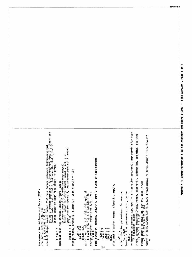
Para

mete

rs fo

r At

kins

on a

nd B

oore

(1

995)

rh

o, be

ta,

prti

tn,

rtp,

fs

: 2.

8 3.8

0.70

7 0.

55 2.

0 sp

ectr

al shape: source n

umbe

r (1=Single

Corn

er;2

=Joy

ner;

3=A9

3;4=

cust

om),

pf,

pd (1-corner

spec

trum

= 1/

(1+(

f/fc

)**p

f)**

pd;

0.0

othe

rwis

e)

(usu

al model: pf

=2.0

,pd=

1.0;

Butterworth: pf=4.0,pd=0.5)

(Note: po

wer

of hi

gh fr

eq d

ecay -->

pf*p

d)

3 2.

0 1.0

spec

tral

sc

alin

g: st

ress

c, dl

sdm,

fbdfa, am

agc

(str

ess=

stre

ssc*

10.0

**(d

lsdm

*(am

ag-a

magc

))

(fbdfa,

amagc

for

Joyn

er m

odel

, usually

4.0, 7.

0)

(not us

ed fo

r source 3

, but

plac

ehol

ders still

needed)

100.0

0.0

4.0

7.0

gspr

d: ns

egs,

(rlow(i),

slop

ed")

) (S

et rlow(1)

= 1.0)

1.0

-1.0

70

.0

0.0

130.0

-0.5

q:

fr

1, Qr1, s1

, ft

1, ft

2, fr

2, qr

2, s2

1.0

680

0.36 1.

0 1.0

1.0

680

0.36

source d

urat

ion:

weight

s of 1/

fa,

1/fb

0.5

0.0

path

du

rati

on:

nkno

ts,

(rdur(i),

dur(

i),

slope

of la

st se

gmen

t

0.0

0.0

5 10

.0 0

.070

.0 9

.6130.0

7.8

0.04

si

te a

mpli

fica

tion

: namp

s, (f

amp(

i),

amp(i))

1 1.0

1.0

site

diminution

parameters:

fm,

akappa

50.0

0.

0 lo

w-cu

t fi

lter

parameters: fcut,

norder

0.0

2 rv

integration

params:

zup,

ep

s in

t (integration a

ccur

acy)

, amp

cuto

ff (f

or fup)

10.0

0.00001

0.001

wind

ow p

aram

s: in

dxwi

nd(0

=box

,1=e

xp),

taper(<1), tw

dtmo

tion

, eps

wind,

eta

wind

1 0.

05 1.0

0.2

0.05

ti

ming

st

uff:

tsimdur, dt

, ts

hift

, se

ed,

nruns

40.0

0.00

5 5.

0 12

3.0

100

remo

ve d

c from r

andom

series before transforming to

freq.

doma

in (0

=no;

1=ye

s)?

0

Appe

ndix

F:

Input-Parameter

File

for

Atk

inso

n an

d Boore

(199

5) -- Fi

le AB95.DAT, Pa

ge 1

of

1

Coastal

California mo

del

(SUB

JECT

TO

CHA

NGE!

DO

N'T

USE

BEYOND 100

KM)

rho, beta

, prtitn,

radp

at,

fs:

2.8

3.5

0.707

0.55 2

.0

spectral

shape: so

urce

number

(1=Single

Corner;2=Joyner;3=A93;4=custom),

pf,

pd (

1-co

rner

spe

ctru

m =

1/(1+(f/fc

)**p

f )**pd; 0.

0 otherwise)

(usual mo

del:

pf=2.0,pd=1 .0;

Butt

erworth: pf

=4.0

,pd=

0.5)

(Note: power

of h

igh

freq

decay -

-> p

f*pd)

1 2.

0 1.

0 spectral

scaling: stress

c, dl

sdm,

fb

dfa,

amagc

(stres

s=stressc*10.0**(dlsdm*(amag-a

magc))

(fbd

fa,

amag

c fo

r Joyner m

odel

, us

uall

y 4.0, 7.0)

(not us

ed f

or s

ource

3, bu

t placeholde

rs s

till

ne

eded

) 70.0 0.

0 4.0

7.0

gspr

d: ns

egs,

(rlow(i),

slop

ed" ))

(Set rlow(1)

= 1.

0)

1.0

-1.0

q: fr1, Qr1, s1

, ft1, ft

2, fr2, qr

2, s2

0.1

275

-2.0

0.2

0.6

1.0

88.0 0

.9

source d

uration: we

ight

s of 1/

fa,

1/fb

1.

0 0.

0nknots,

(rdur(i),

dur(i),

co

path d

uration:

1 0.0

0.0

0.05

site a

mpli

fica

tion

: namp

s,

1.00

1.10

1.18

1.42

1.58

slope

of last s

egme

nt)

(famp(i),

amp(i))

0.01

0.09

0.16

0.51

0.84

1.25

1.74

2.26

2.06

3.17

2.25

6.05

2.58

16.6

3.13

61.2

4.00

site d

iminution

paramete

rs:

fm,

akappa

100.

0 0.035

low-cut

filter p

aram

eter

s: fc

ut,

norder

0.0

2 rv integr

atio

n params:

zup,

ep

s in

t (integration a

ccur

acy)

, am

p_cu

toff

(for fup)

10.0 0

.00001

0.001

window p

arams: indxwind

(0=b

ox,1

=exp

), ta

per(

<1),

tw

dtmo

tion

, eps

wind,

eta

wind

1 0.05 1.

0 0.

2 0.05

timing s

tuff

: tsimdur, dt,

tshi

ft,

seed,

nruns

40.0

0.005

7.0

123.

0 100

remo

ve d

c fr

om r

ando

m se

ries b

efore

tran

sfor

ming

to

fre

q. do

main

(0=no;1=yes)?

0

Appe

ndix

G:

Input-Parameter

File

for

Coa

stal

California -- File WR0

3249

6.DA

T, Pa

ge 1

of

1