Embed Size (px)
Citation preview
NIST Technical Note 1762
Smoke Component Yields from Bench-scale Fire Tests 3 ISO 5660-1 ASTM
E 1354 with Enclosure and Variable Oxygen Concentration
Nathan D Marsh Richard G Gann
httpdxdoiorg106028NISTTN1762
NIST Technical Note 1762
Smoke Component Yields from Bench-scale Fire Tests 3 ISO 5660-1 ASTM
E 1354 with Enclosure and Variable Oxygen Concentration
Nathan D Marsh Richard G Gann
Fire Research Division Engineering Laboratory
httpdxdoiorg106028NISTTN 1762
December 2013
US Department of Commerce Penny Pritzker Secretary
National Institute of Standards and Technology Patrick D Gallagher Under Secretary of Commerce for Standards and Technology and Director
Certain commercial entities equipment or materials may be identified in this document in order to describe an experimental procedure or concept adequately
Such identification is not intended to imply recommendation or endorsement by the National Institute of Standards and Technology nor is it intended to imply that the entities materials or equipment are necessarily the best available for the purpose
National Institute of Standards and Technology Technical Note 1762 Natl Inst Stand Technol Tech Note 1762 43 pages (December 2013)
httpdxdoiorg106028NISTTN 1762 CODEN NTNOEF
ABSTRACT
A standard procedure is needed for obtaining smoke toxic potency data for use in fire hazard and risk analyses Room fire testing of finished products is impractical directing attention to the use of apparatus that can obtain the needed data quickly and at affordable cost This report presents examination of the fourth of a series bench-scale fire tests to produce data on the yields of toxic products in both pre-flashover and post-flashover flaming fires The apparatus is the ISO 5660-1 ASTM E 1354 cone calorimeter modified to have an enclosure and a gas delivery system allowing variable oxygen concentration The test specimens was cut from finished products that were also burned in room-scale tests a sofa made of upholstered cushions on a steel frame particleboard bookcases with a laminated finish and household electric cable Initially the standard test procedure was followed Subsequent variation in the procedure included reducing the supplied oxygen volume fraction to 018 016 and 014 reducing the incident heat flux to 25 kWm2 and reducing the gas flow rate by half
The yields of CO2 CO HCl and HCN were determined The yields of other toxicants (NO NO2 formaldehyde and acrolein) were below the detection limits but volume fractions at the detection limits were shown to be of limited toxicological importance relative to the detected toxicants In general performing the tests at the reduced oxygen volume fraction led to small increases on the toxic gas yields The exceptions were an increase in the CO yield for the bookcase at 014 oxygen volume fraction Reducing the incident heat flux had little effect on the toxic gas yields other than increasing variability Reducing the gas flow rate reduced the limits of detection by half but also resulted in reduced gas yields at lower oxygen volume fractions In none of the procedure variations did the CO yield approach the value of 02 found in real-scale postflashover fire tests
Keywords fire fire research smoke room fire tests fire toxicity smoke toxicity
iii
This page intentionally left blank
iv
TABLE OF CONTENTS
LIST OF FIGURES VI LIST OF TABLES VI
I INTRODUCTION 1
A CONTEXT OF THE RESEARCH 1 B OBTAINING INPUT DATA 2 C PRIOR ROOM‐SCALE TESTS 3
1 Test Configuration 3 2 Combustibles 3
D PHYSICAL FIRE MODELS5
II EXPERIMENTAL INFORMATION 7
A SUMMARY OF ISO 5660‐1 ASTM E 1354 APPARATUS 7 1 Hardware 7 2 Gas Sampling and Analysis Systems8
B OPERATING PROCEDURES 11 1 Standard Testing 11 2 Test Specimens 12 3 Test Procedure Variation 12
C DATA COLLECTION 13
III CALCULATION METHODS15
A MASS LOSS RATE 15 B NOTIONAL GAS YIELDS 15 C CALCULATED GAS YIELDS 15
1 CO and CO2 15 2 HCl and HCN 16 3 Other Gases 17
IV RESULTS19
A TESTS PERFORMED 19 B CALCULATIONS OF TOXIC GAS YIELDS WITH UNCERTAINTIES26
V DISCUSSION 29
A OVERALL TEST VALUES29 B SPECIMEN PERFORMANCE AND TEST REPEATABILITY 29
1 CO2 and CO 29 2 HCl and HCN 31
C MEASURED VS NOTIONAL VALUES 34 D SPECIES SAMPLING AND MEASUREMENT 35
1 Species Measurement Using FTIR Spectroscopy 35 E IMPORTANCE OF UNDETECTED GASES 35
VI CONCLUSIONS39
VII ACKNOWLEDGEMENTS 40
REFERENCES 41
v
LIST OF FIGURES
FIGURE 1 MODIFIED CONE CALORIMETER 8 FIGURE 2 FTIR SPECTRUM OF COMBUSTION PRODUCTS FROM A CABLE SPECIMEN 10 FIGURE 3 COMPARISON OF FTIR AND NDIR MEASUREMENTS OF CO VOLUME FRACTION 16 FIGURE 4 EFFECT OF OXYGEN CONCENTRATION ON CO YIELDS BOOKCASE (DASHED LINE = REDUCED FLOW) ERROR BARS ARE plusmn THE
STANDARD DEVIATION OF YIELDS FROM MULTIPLE RUNS 30 FIGURE 5 EFFECT OF OXYGEN CONCENTRATION ON CO YIELDS SOFA (DASHED LINE = REDUCED FLOW) ERROR BARS ARE plusmn THE
STANDARD DEVIATION OF YIELDS FROM MULTIPLE RUNS 30 FIGURE 6 EFFECT OF OXYGEN CONCENTRATION ON CO YIELDS CABLE (DASHED LINE = REDUCED FLOW) ERROR BARS ARE plusmn THE
STANDARD DEVIATION OF YIELDS FROM MULTIPLE RUNS 31 FIGURE 7 HCN VOLUME FRACTIONS SOFA 50 KWM2 125 LS 16 O2 BY VOLUME UNCERTAINTY IS 10 OF THE REPORTED HCN
VOLUME FRACTION 32 FIGURE 8 EFFECT OF OXYGEN CONCENTRATION ON HCN YIELDS SOFA ERROR BARS ARE plusmn THE STANDARD DEVIATION OF YIELDS FROM
MULTIPLE RUNS 32 FIGURE 9 HCL VOLUME FRACTIONS CABLE 50 KWM2 125 LS 16 O2 BY VOLUME UNCERTAINTY IS 10 OF THE REPORTED
VOLUME FRACTION 33 FIGURE 10 EFFECT OF OXYGEN CONCENTRATION ON YIELDS OF HCL CABLES ERROR BARS ARE plusmn THE STANDARD DEVIATION OF YIELDS
FROM MULTIPLE RUNS 34
LIST OF TABLES
TABLE 1 ELEMENTAL ANALYSIS OF FUEL COMPONENTS 4 TABLE 2 SPECIES AND FREQUENCY WINDOWS FOR FTIR ANALYSIS11 TABLE 3 CALCULATED NOTIONAL YIELDS OF TOXIC PRODUCTS FROM THE TEST SPECIMENS 15 TABLE 4 DATA FROM BOOKCASE MATERIAL TESTS 20 TABLE 5 DATA FROM SOFA MATERIAL TESTS 21 TABLE 6 DATA FROM CABLE MATERIAL TESTS 22 TABLE 7 GAS YIELDS FROM BOOKCASE MATERIAL TESTS 23 TABLE 8 GAS YIELDS FROM SOFA MATERIAL TESTS24 TABLE 9 GAS YIELDS FROM CABLE MATERIAL TESTS 25 TABLE 10 YIELDS OF COMBUSTION PRODUCTS FROM CONE CALORIMETER TESTS26 TABLE 11 FRACTIONS OF NOTIONAL YIELDS 28 TABLE 12 LIMITS OF IMPORTANCE OF UNDETECTED TOXINS 36 TABLE 13 LIMITS OF IMPORTANCE OF UNDETECTED TOXICANTS37
vi
I INTRODUCTION
A CONTEXT OF THE RESEARCH
Estimation of the times that building occupants will have to escape find a place of refuge or survive in place in the event of a fire is a principal component in the fire hazard or risk assessment of a facility An accurate assessment enables public officials and facility owners to provide a selected or mandated degree of fire safety with confidence Without this confidence regulators andor designers tend to apply large safety factors to lengthen the tenable time This can increase the cost in the form of additional fire protection measures and can eliminate the consideration of otherwise desirable facility designs and construction products Error in the other direction is also risky in that if the time estimates are incorrectly long the consequences of a fire could be unexpectedly high
Such fire safety assessments now rely on some form of computation that takes into account multiple diverse factors including the facility design the capabilities of the occupants the potential growth rate of a design fire the spread rates of the heat and smoke and the impact of the fire effluent (toxic gases aerosols and heat) on people who are in or moving through the fire vicinity1 The toolkit for these assessments while still evolving has achieved some degree of maturity and quality The kit includes such tools as
Computer models of the movement and distribution of fire effluent throughout a facility
o Zone models such as CFAST2 have been in use for over two decades This model takes little computational time a benefit achieved by simplifying the air space in each room into two zones A number of laboratory programs validation studies3 and reconstructions of actual fires have given credence to the predictions4
o Computational fluid dynamics (CFD) models such as the Fire Dynamics Simulator (FDS)5 have seen increased use over the past decade FDS is more computationally intense than CFAST in order to provide three-dimensional temperature and species concentration profiles There has been extensive verification and validation of FDS predictions5
These models calculate the temperatures and combustion product concentrations as the fire develops These profiles can be used for estimating when a person would die or be incapacitated ie is no longer able to effect hisher own escape
Devices such as the cone calorimeter6 and larger scale apparatus7 which are routinely used to generate information on the rate of heat release as a commercial product burns
A number of standards from ISO TC92 SC3 that provide support for the generation and use of fire effluent information in fire hazard and risk analyses8 Of particular importance is ISO 13571 which provides consensus equations for estimating the human incapacitating exposures to the narcotic gases irritant gases heat and smoke generated in fires9
More problematic are the sources of data for the production of the harmful products of combustion Different materials can generate fire effluent with a wide range of toxic potencies Most furnishing and interior finish products are composed of multiple materials assembled in a variety of geometries and there is as of yet no methodology for predicting the evolved products
1
from these complex assemblies Furthermore the generation of carbon monoxide (CO) the most common toxicant can vary by orders of magnitudes depending on the fire conditions10
An analysis of the US fire fatality data11 showed that post-flashover fires comprise the leading scenarios for life loss from smoke inhalation Thus it is most important to obtain data regarding the generation of harmful species under post-flashover (or otherwise underventilated) combustion conditions Data for pre-flashover (well-ventilated) conditions have value for ascertaining the importance of prolonged exposure to ordinary fire effluent and to short exposures to effluent of high potency
B OBTAINING INPUT DATA
The universal metric for the generation of a toxic species from a burning specimen is the yield of that gas defined as the mass of the species generated divided by the consumed mass of the specimen12 If both the mass of the test specimen and the mass of the evolved species are measured continuously during a test then it is possible to obtain the yields of the evolved species as the burning process and any chemical change within the specimen proceeds If continuous measurements are not possible there is still value in obtaining a yield for each species integrated over the burning history of the test specimen
The concentrations of the gases (resulting from the yields and the prevalent dilution air) are combined using the equations in ISO 13571 for a base set of the most prevalent toxic species Additional species may be needed to account for the toxic potency of the fire-generated environment
To obtain an indicator of whether the base list of toxic species needs to be enhanced living organisms should also be exposed to the fire effluent The effluent exposure that generates an effect on the organisms is compared to the effect of exposure to mixtures of the principal toxic gases Disagreement between the effluent exposure and the mixed gas exposure is an indicator of effluent components not included in the mixed gas data or the existence of synergisms or antagonisms among the effluent components This procedure has been standardized based on data developed using laboratory rats1314 However it is recognized that animal testing is not always possible In these cases it is important to identify from the material degradation chemistry a reasonable list of the degradation and combustion products that might be harmful to people
Typically the overall effluent from a harmful fire is determined by the large combustibles such as a bed or a row of auditorium seats The ideal fire test specimen for obtaining the yields of effluent components is the complete combustible item with the test being conducted in an enclosure of appropriate size Unfortunately reliance on real-scale testing of commercial products is impractical both for its expense per test and for the vast number of commercial products used in buildings Such testing is practical for forensic investigations in which there is knowledge of the specific items that combusted
A more feasible approach for obtaining toxic gas yields for facility design involves the use of a physical fire model ndash a small-scale combustor that captures the essence of the combustible and of the burning environment of interest The test specimen is an appropriate cutting from the full combustible To have confidence in the accuracy of the effluent yields from this physical fire model it must be demonstrated
2
How to obtain from the full combustible a representative cutting that can be accommodated and burned in the physical fire model
That the combustion conditions in the combustor (with the test specimen in place) are related to the combustion conditions in the fire of interest generally pre-flashover flaming (well ventilated or underventilated) post-flashover flaming pyrolysis or smoldering
How well for a diverse set of combustible items the yields from the small-scale combustor relate to the yields from real-scale burning of the full combustible items and
How sensitive the effluent yields are to the combustor conditions and to the manner in which the test specimen was obtained from the actual combustible item
At some point there will be sufficient data to imbue confidence that testing of further combustibles in a particular physical fire model will generate yields of effluent components with a consistent degree of accuracy
The National Institute of Standards and Technology (NIST) has completed a project to establish a technically sound protocol for assessing the accuracy of bench-scale device(s) for use in generating fire effluent yield data for fire hazard and risk evaluation In this protocol the yields of harmful effluent components are determined for the real-scale burning of complete finished products during both pre-flashover and post-flashover conditions Specimens cut from these products are then burned in various types of bench-scale combustors using their standard test protocols The test protocols are then varied within the range of the combustion conditions related to these fire stages to determine the sensitivity of the test results to the test conditions and to provide a basis for improving the degree of agreement with the yields from the room-scale tests
This report continues with a brief description of the previously conducted room fire tests The full details can be found in Reference 15 Following this recap are the details of the tests using the fourth of four bench-scale apparatus to be examined
C PRIOR ROOM-SCALE TESTS
1 Test Configuration
With additional support from the Fire Protection Research Foundation NIST staff conducted a series of room-fire tests of three complex products The burn room was 244 m wide 244 m high and 366 m long (8 ft x 8 ft x 12 ft) The attached corridor was a 975 m (32 ft) long extension of the burn room A doorway 076 m (30 in) wide and 20 m (80 in) high was centered in the common wall The downstream end of the corridor was fully open
2 Combustibles
Three fuels were selected for diversity of physical form combustion behavior and the nature and yields of toxicants produced Supplies of each of the test fuels were stored for future use in bench-scale test method assessment
ldquoSofasrdquo made of up to 14 upholstered cushions supported by a steel frame The cushions consisted of a zippered cotton-polyester fabric over a block of a flexible polyurethane (FPU) foam The fire retardant in the cushion padding contains chlorine atoms Thus
3
this fuel would be a source of CO2 CO HCN HCl and partially combusted organics The ignition source was the California TB133 propane ignition burner16 faced downward centered over the center of the row of seat cushions In all but two of the tests the sofa was centered along the rear wall of the burn room facing the doorway In the other two tests the sofa was placed in the middle of the room facing away from the doorway to compare the burning behavior under different air flow conditions Two of the first group of sofa tests were conducted in a closed room to examine the effect of vitiation on fire effluent generation In these an electric ldquomatchrdquo was used to initiate the fires
Particleboard (ground wood with a urea formaldehyde binder) bookcases with a laminated polyvinylchloride (PVC) finish This fuel would be a source of CO2 CO partially combusted organics HCN and HCl To sustain burning two bookcases were placed in a ldquoVrdquo formation with the TB133 burner facing upward under the lower shelves
Household wiring cable consisting of two 14 gauge copper conductors insulated with a nylon and a polyvinyl chloride (PVC) an uninsulated ground conductor two paper filler strips and an outer jacket of a plasticized PVC This fuel would be a source of CO2 CO HCl and partially combusted organics Two cable racks containing 3 trays each supported approximately 30 kg of cable in each of the bottom two trays and approximately 17 kg in each of the middle and top trays The cable trays were placed parallel to the rear of the burn room Twin propane ignition burners were centered under the bottom tray of each rack
The elemental chemistry of each combustible was determined by an independent testing laboratory More details regarding the elemental analysis can be found in NIST TN 176017 The elemental composition of the component materials in the fuels is shown in Table 1
Table 1 Elemental Analysis of Fuel Components Sample C H N Cl P O
Bookcase 0481 06 0062 08 0029 13 00030 4 NA 0426 1
Sofa 0545 1 0080 1 0100 1 00068 16 00015 17 0267 4
Cable 0576 05 0080 15 0021 6 0323 04 NA NA
The uncertainties are the standard deviation of three elemental analysis tests combined with the uncertainty of the mass fraction of individual material components ie fabric vs foam for the sofa
4
D PHYSICAL FIRE MODELS
Historically there have been numerous bench-scale devices that were intended for measuring the components of the combustion effluent1819 The combustion conditions and test specimen configuration in the devices vary widely and some devices have flexibility in setting those conditions Currently ISO TC92 SC3 (Fire Threat to People and the Environment) is proceeding toward standardization of one of these devices a tube furnace (ISOTS 1970020) and is considering standardization of another the cone calorimeter (ISO 5660-121) with a controlled combustion environment There are concurrent efforts in Europe and ISO to upgrade the chemical analytical capability for a closed box test (ISO 5659-222) Thus before too long there may well be diverse (and perhaps conflicting) data on fire effluent component yields available for any given product This situation does not support either assured fire safety or marketplace stability
In related work we report toxic gas measurements in the NFPA 269 toxicity test method17 the ISOTS 19700 tube furnace23 and the smoke density chamber24
The modification of the cone calorimeter to measure gas yields in vitiated environments was first introduced in the early 1990s25mdash27 and has recently received renewed interest28 mdash30 The more recent work has focused on the effect of secondary oxidation on the heat release rate measurement and progress on measuring chemical species is just beginning
5
This page intentionally left blank
6
II EXPERIMENTAL INFORMATION
A SUMMARY OF ISO 5660-1 ASTM E 1354 APPARATUS
1 Hardware
The standard apparatus consists of a load cell specimen holder truncated cone electrical resistance heater spark igniter canopy hood and exhaust ductwork The electrical heater is calibrated using a Schmidt-Boelter heat flux gauge which itself is calibrated using a standardized source linked to a primary calibration standard Exhaust flow in the duct is normally controlled by a variable-speed fan of the ldquosquirrel cagerdquo design and measured by measuring the pressure drop across an orifice plate installed downstream from the fan along with the temperature at that location
Under standard operation the heat release rate is measured via oxygen consumption calorimetry thus the oxygen concentration in the exhaust must be measured See the following section for more detail
For this work the apparatus was modified to include 1) an enclosure measuring 430 mm by 500 mm by 570 mm high constructed of aluminum framing and polycarbonate walls (insulated in the locations of highest heat flux with aluminum foil) which seals against the underside of the canopy hood and 2) a gas delivery system capable of delivering at 25 Ls a mixture of air and nitrogen This consisted of a self-pressurizing 180 L liquid nitrogen dewar and a 120 psi supply of filtered ldquohouserdquo air A standard CGA 580 regulator on gas outlet of the dewar maintained pressure at 80 psi and was connected to a control manifold by 13 mm diameter copper tubing Valves on the manifold allowed individual control of both the nitrogen gas and the compressed air which were metered by 3 high-capacity rotameters (2 in parallel for air and one for nitrogen) The rotameters were then connected to a gas mixing chamber constructed out of 400 mm by 60 mm tube with 2 air and 2 nitrogen inlets on one end and 4 mixed gas outlets on the other These outlets were then each connected by more 13 mm tubing to each side of the enclosure at the base frame The interior edges of this (hollow) aluminum frame were perforated on each side by 5 equally spaced holes 64 mm diameter providing an even supply of gas around the perimeter at the base of the enclosure Some features of this setup can be seen in Figure 1
One face of the enclosure includes a latchable door (20 cm square) for loading and unloading the test specimen In order to allow time for the desired gas mixture to expel air introduced during specimen loading a shutter composed of ceramic board supported by a metal frame and slide mechanism was placed between the specimen and the cone heater Attached to the shutter was a rod extending through a bulkhead fitting in the enclosure wall so that the shutter could be withdrawn to commence a test During operation balancing of the gas supply and the exhaust was accomplished by observing a small perforation in the enclosure provided with soap film while monitoring the recorded volumetric flow rate calculated from the pressure differential across the orifice plate in the exhaust duct
7
Figure 1 Modified Cone Calorimeter
Although not discussed here the heat release rate measurement was calibrated daily using a 5 kW methane burner itself calibrated by measuring the gas flow using a piston-type primary standard calibrator accurate to 1 of the reading
2 Gas Sampling and Analysis Systems
In the room-scale tests (Section IC) measurements were made of 12 gases Water and methane were included because of their potential interference with the quantification of the toxic gases Two of the toxic gases HBr and HF were not found in the combustion products because there was no fluorine or bromine in the test specimens The remaining eight toxic gases were acrolein (C3H4O) Carbon monoxide (CO) carbon dioxide (CO2) formaldehyde (CH2O) hydrogen chloride (HCl) hydrogen cyanide (HCN) nitric oxide (NO) and nitrogen dioxide (NO2) Some of these turned out to be generated at levels that would not have contributed significantly to the incapacitation of exposed people Thus it was deemed unlikely that animal tests would have added much tenability information As a result the same gases were monitored in the bench-scale tests and no animals were exposed The basis for comparison between tests of the same combustibles at the two scales is the yields of the chemically diverse set of toxicants
CO and CO2 were quantified using a nondispersive infrared (NDIR) gas analyzer oxygen was quantified by a paramagnetic analyzer in the same instrument The precisions of the analyzers as provided by the manufacturer were
CO 10 microLL
CO2 002 LL
O2 005 LL
Sampling for this instrument was pulled from the exhaust duct upstream from the exhaust fan using a perforated ring sampling probe The flow passed through a large volume cartridge filter
8
through two parallel membrane HEPA filters through an electrical chiller maintained at -2 ordmC to -5 ordmC and finally through a fixed bed of calcium sulfate desiccant The stream sent to the O2
analyzer also passed through a fixed bed of sodium hydroxide-coated silica particles The flows were maintained at 3 Lmin The analyzer itself was calibrated daily with zero and span gases (a mixture of 2800 microLL CO and 0028 LL of CO2 in nitrogen and ambient air (02095 LL oxygen on a dry basis)) The span gas is certified to be accurate to within 2 of the value
The concentrations of CO and the additional six toxic gases were measured using a Bruker Fourier transform infrared (FTIR) spectrometer equipped with an electroless nickel plated aluminum flow cell (2 mm thick KBr windows and a 1 m optical pathlength) with an internal volume of 02 L maintained at (170 plusmn 5) degC Samples were drawn through a heated 635 mm (frac14 in) stainless steel tube from inside the exhaust duct upstream of the exhaust with its tip at approximately the centerline The sample was pulled through the sampling line and flow cell by a small pump located downstream from the flow cell There were no traps or filters in this sampling line The pump flow was measured at 4 Lmin maximum but was at times lower due to fouling of the sampling lines with smoke deposits
Although this instrument has a longer path length and is therefore more sensitive than the one used in our previous studies the ldquobatchrdquo nature of a cone calorimeter experiment along with the continuous flow of the exhaust requires instantaneous data collection in this case at 017 Hz that did not allow for data averaging to improve the signal-to-noise Therefore the limits of detection are essentially unchanged from the previous studies The implications of this will be discussed in Section V
An example of a spectrum measured by FTIR spectroscopy during one such test is displayed in Figure 2 The series of peaks extending from about 3050 cm-1 to 2600 cm-1 are due to HCl In this case it is possible to resolve the individual frequencies corresponding to changes in the population of rotational states as the H-Cl bonds vibrate This is usually only possible for small gas phase molecules There are three spectral features due to CO2 that are evident in this spectrum The most intense centered at 2350 cm-1 corresponds to asymmetric stretching of the two C=O bonds The symmetric stretch is not observed because there is no change in dipole moment when both O atoms move in phase The second feature seen as two distinct peaks centered at about 3650 cm-1 is an overtone band that derives from the simultaneous excitation of these bond-stretching modes The third peak at about 650 cm-1 is due to the out of plane bending of the molecule There are bands due to the CequivO stretching vibrations in carbon monoxide centered at about 2150 cm-1 The remaining peaks in this spectrum are due to H2O
Certain commercial equipment products or materials are identified in this document in order to describe a procedure or concept adequately or to trace the history of the procedures and practices used Such identification is not intended to imply recommendation endorsement or implication that the products materials or equipment are necessarily the best available for the purpose
9
50010001500200025003000350040004500 Wavenumber (cm‐1)
H2O H2O
CO
CO2 CO2
HCl
CO2
Figure 2 FTIR Spectrum of Combustion Products from a Cable Specimen
Using these spectra gas concentrations were quantified using the Autoquant software This is a software package for performing real time and off-line quantitative analyses of target compounds and is based on the Classical Least Squares (CLS) algorithm as described by Haaland et al31 In this method the measured spectra are fit to linear combinations of reference spectra corresponding to the target compounds
Calibration spectra were obtained from a quantitative spectral library assembled by Midac32 and from a collection of spectra provided the Federal Aviation Administration who performed bench-scale fire tests on similar materials33 In this analysis the least squares fits were restricted to characteristic frequency regions or windows for each compound that were selected in such a way as to maximize the discrimination of the compounds of interest from other components present in fire gases All reference spectra were recorded at 170 degC and ambient pressure
The identities of the target compounds (as well as other compounds that absorb at the same frequencies and must therefore be included in the analyses) their corresponding concentrations (expressed in units of microLL for a mixture of the calibration gas and N2 in a 1 meter cell) and the characteristic spectral windows used in the quantitative analyses are listed in Table 2
Also listed in this Table are minimum detection limits (MDLs) for each of the target compounds These values which represent the lowest concentrations that can be measured with the instrumentation employed in these tests were estimated as follows The calibration spectra were added to test spectra (which when possible were selected in such a way that only the compound of interest was not present) with varying coefficients until the characteristic peaks of the target compounds were just discernible above the baseline noise The MDL values reported in Table 2
10
were obtained by multiplying these coefficients by the known concentrations of the target compound in the calibration mixtures
Water methane and acetylene are included in the quantitative analyses because they have spectral features that interfere with the target compounds The nitrogen oxides absorb in the middle of the water band that extends from about 1200 cm-1 to 2050 cm-1 Consequently the real limits of detection for these two compounds are an order of magnitude higher than for any of the other target compounds Thus it is not surprising that their presence was not detected in any of the tests
Table 2 Species and Frequency Windows for FTIR Analysis
Compound
Reference Volume Fraction
(microLL) Frequency
Window (cm-1)
Minimum Detection Limit
(microLL)
CH4 483 2800 to 3215 20
C3H4O 2250 850 to 1200 20 CH2O 11300 2725 to 3000 40 CO2 47850 660 to 725 2230 to 2300 800a
CO 2410 2050 to 2225 20 H2O 100000 1225 to 2050 3400 to 4000 130a
HCl 9870 2600 to 3100 20
HCN 507 710 to 722 3200 to 3310 35 NO 512 1870 to 1950 70 NO2 70 1550 to 1620 40
a Present in the background
Delay times for gas flows from the sampling locations within the test structure to the gas analyzers were small compared to the duration of the specimen burning The burn durations were near 20 min for the bookcase specimens 1 to 3 min for the sofa specimens and 2 to 4 min for the cable specimens Combining the gas sample pumping rate and the volumes of the sampling lines the delay time to the oxygen analyzer was about 5 s about 1 s to the CO and CO2
analyzers and 1 s to the FTIR analyzer These delay times are long enough to allow for a small degree of axial diffusion However since our analysis integrates the data over time this did not adversely affect the quantification of total gas evolved
B OPERATING PROCEDURES
1 Standard Testing
The intent was to test specimens of each of the three types under normal and reduced-oxygen conditions two incident heat fluxes and two gas flow rates The steps in the procedure are
Calibrate the heat flux to the specimen surface and calibrate the gas analyzers (each performed daily)
Establish the desired gas flow rates and oxygen concentration with an empty specimen holder in place
11
Turn on the gas sampling data collection and establish background data for the combustion product concentrations
Open the chamber door
Replace the empty specimen holder with one containing the specimen
Close the chamber door
Wait for the oxygen concentration to return to its established value
Withdraw the shutter and insert the spark igniter
Turn on the spark igniter
Record the time of ignition turn off and withdraw the spark igniter
Collect concentration data until a steady state of pyrolysis is reached
Open the chamber door remove the specimen close the chamber door
Record a post-test background to account for any drift
Weigh any specimen residue
As in the previous work the bookcase material underwent considerable pyrolyzing after the flames disappeared However as the cone calorimeter is a continuous-flow apparatus no physical steps were necessary to isolate the pyrolysis results from the flaming results and the transition between the two is clearly visible in the data eg the differential of the mass loss data
2 Test Specimens
The specimens were intended to approximate the full item Specimen size was mostly limited by the size of the specimen holder although in the case of the cables it was not necessary to completely fill the pan or use multiple layers Instead the number of cables was chosen to produce similar gas concentrations and heat release rates compared to the other two types of specimens The bookcase specimens were single 10 cm x 10 cm pieces of the particle board with the vinyl surface facing up The sofa specimens were each a single piece of foam 10 cm by 10 cm by 1 cm thick covered with a single piece of the polyestercotton cover fabric 105 cm x 105 cm on the upper (exposed) surface (the fabric being slightly oversized so that it could be ldquotuckedrdquo in around the edges of the foam) The cable specimens were five 10 cm lengths of cable cut from the spool and placed side-by-side All specimens were wrapped on the bottom and sides with aluminum foil which was cut to be flush with the top surface of the specimen The specimen holder was lined with a refractory aluminosilicate blanket adjusted in thickness so that each specimen was the same distance from the upper surface to the cone heater assembly (28 mm) Note that with the exception of area dimensions these specimens were prepared almost identically to those in Ref 17 and are therefore not reproduced here Also in our prior work we found little to no impact from ldquodicingrdquo the specimens ie cutting them into small pieces and therefore did not investigate that effect here
3 Test Procedure Variation
One of the purposes of this program was to obtain effluent composition data in tests with variants on the standard operating procedure This would enable examination of the potential for an
12
improved relationship with the yield data from the room-scale tests as well as an indication of the sensitivity of the gas yields to the specified operating conditions
Variation in incident heat flux between 20 kWm2 and 50 kWm2 to determine the significance on evolved gases
Variation of the available oxygen volume fraction from 21 to 14 to more closely approach the post-flashover conditions that occurred in the room-scale tests During pre-flashover burning the air entrained by a fire has an oxygen volume fraction of nominally 021 This fraction is lower for post-flashover fires As part of this work it was determined that combustion was barely sustainable at an oxygen volume fraction of 014
Variation of overall gas flow rate from 25 Ls to 125 Ls in order to increase sensitivity in gas measurements and to allow the reduction of oxygen volume fraction to 014 which was difficult in our system at the higher flow A known drawback to reducing the flow is that the sensitivity of the flow measurement via the pressure drop across the orifice plate is reduced (This can be ameliorated by installing a smaller orifice so that the pressure drop in brought back up to the optimal range of the pressure sensor)
C DATA COLLECTION
The signals from the load cell temperature and pressure needed for ISO 5660-1 and from the fixed gas analyzer were recorded on a personal computer using a custom-made data acquisition system based on National Instruments data acquisition hardware Values were recorded at 1 s intervals The FTIR spectra were recorded using the software package provided by the manufacturer Spectra were recorded every 6 s
13
This page intentionally left blank
14
III CALCULATION METHODS
A MASS LOSS RATE
The specimen mass loss during a test was determined from the initial reading from the load cell and from a point where the specimen transitioned from burning to pyrolyzing which was characterized by a sudden drop in the mass loss rate (derivative of the mass loss calculated over 16 data points seconds) The uncertainty in the mass loss derived from the uncertainties in these two measurements was 01 g
B NOTIONAL GAS YIELDS
The notional or maximum possible gas yields (Table 3) were calculated as follows
CO2 Assume all the carbon in the test specimen is converted to CO2 Multiply the mass fraction of C in the test specimen (Table 1) by the ratio of the molecular mass of CO2 to the atomic mass of carbon
CO Assume all the carbon in the test specimen is converted to CO Multiply the mass fraction of C by the ratio of the molecular mass of CO to the atomic mass of carbon
HCN Assume all the nitrogen in the test specimen is converted to HCN Multiply the mass fraction of N by the ratio of the molecular mass of HCN to the atomic mass of nitrogen
HCl Assume all the chlorine in the test specimen is converted to HCl Multiply the mass fraction of Cl by the ratio of the molecular mass of HCl to the atomic mass of chlorine
The notional yields from the bookcase and cable specimens were assumed to be the same as the yields from the intact combustibles15 The sofa specimen had a mass ratio of fabric to foam that differed modestly from the intact sofas
Table 3 Calculated Notional Yields of Toxic Products from the Test Specimens Notional Yields
Gas Bookcase Cable Sofa CO2 172 plusmn 1 211 plusmn 1 195 plusmn 4 CO 109 plusmn 1 133 plusmn 1 124 plusmn 4 HCN 0057 plusmn 13 0040 plusmn 6 0193 plusmn 4 HCl 00026 plusmn 4 0332 plusmn 1 00069 plusmn 19
The uncertainty in the notional yield values is determined by the uncertainty in the prevalence of the central element (in the bullets just above) in the combustible For the cuttings from the sofas the uncertainty in the notional yields was increased by the small variability (estimated at 3 percent) in the relative masses of the fabric and padding materials in the test specimens
C CALCULATED GAS YIELDS
1 CO and CO2
Yields of CO and CO2 were calculated using the measured gas concentrations from the NDIR instrument the measured flows in the exhaust the exhaust temperature (accounting for the
15
background concentrations in room air) the consumed mass of the fuel and the ideal gas law Concentrations were converted to mass flow then integrated numerically (rectangular) over the time of flaming combustion
As we observed previously17 the CO2 absorption band in the FTIR is saturated at normal volume fractions and is therefore highly non-linear As both the FTIR and NDIR measurements were taken from the same location it was not necessary to measure the CO2 concentration by FTIR
Figure 3 shows a comparison of the maximum CO volume fractions measured by the two instruments The FTIR consistently found a lower volume fraction than the NDIR above 300 microLL This is likely due to the non-linearity inherent in IR spectra at higher absorption Since the spectrometer used in this study had a path length that was 10 times that used in the previous work172324 it is not unreasonable that these data fall more in the non-linear range Therefore the data reported here for CO are taken from the NDIR results
0
100
200
300
400
500
600
700
800
0 200 400 600 800
CO
Volume Fraction
(LL) ‐FTIR
CO Volume Fraction (LL) ‐NDIR
Figure 3 Comparison of FTIR and NDIR Measurements of CO Volume Fraction
2 HCl and HCN
The only calculable HCN yields were from the sofa specimens The only calculable HCl yields were from the cable specimens FTIR spectra from these experiments were analyzed as described in section IIA2 This analysis normally includes an uncertainty of 10 of the reported value Volume fractions were converted into mass flows using the flow and temperature data then numerically integrated over the period of flaming combustion Because
16
these data are more sparse than those from the NDIR (017 Hz vs 10 Hz) a trapezoidal integration was used We considered the possibility that these results suffered from the same non-linear relation between absorption and concentration that occurred with the CO measurements However since the HCN concentrations were quite low and the HCl yields were reasonably close to their notional yields (see Table 11) and similar to the previous work using a different instrument with a shorter path length172324 we determined that non-linear effects were not significant Furthermore because the lower heat flux did not by any other indication have a significant impact on gas yields other than increased variability the quantification of FTIR data from these runs was omitted
3 Other Gases
The volume fractions of the other toxic gases were always below the detection limit Thus the upper limits of the yields of these gases were estimated using their limits of detection
17
This page intentionally left blank
18
IV RESULTS
A TESTS PERFORMED
The following is the test numbering key with format F(2)-q-[O2]-N where
F Fuel [S = sofas B = bookcases C = cable]
(2) present for the 125 Ls flow rate absent for the 25 Ls flow rate
q heat flux per unit area (kWm2)
[O2] Approximate initial oxygen volume percent in the supply gas
N Replicate test number for that set of combustible and conditions
Table 4 through Table 9 present the test data and the calculated yields for the bookcase sofa and cable specimens respectively In these tables Δt is the observed duration of flaming combustion and Δm is the measured mass lost during the flaming combustion Volume fractions represent the maximum value in the test usually soon after ignition A yield number in red indicates a potential outlier that if discarded could improve the repeatability under those conditions
The horizontal shaded bands highlight groups of replicate tests
19
Table 4 Data from Bookcase Material Tests
NDIR
Code Specimen
Mass (g)
Δm
(g)
Δt (s)
Flaming
FCO2
(LL)
FCO
(LL)
FO2
(LL)
b‐50‐21‐1 1498 1060 1068 00065 120 02037
b‐50‐21‐2 1356 1052 1090 00067 140 02033
b‐50‐21‐3 1384 1037 1043 00072 150 02028
b‐50‐18‐1 1360 1038 1110 00070 160 01731
b‐50‐18‐2 1374 1015 1060 00070 160 01730
b‐50‐18‐3 1381 1021 1110 00064 160 01748
b‐50‐16‐1 1192 984 993 00066 140 01559
b‐50‐16‐2 1366 1017 1115 00062 170 01545
b‐50‐16‐3 1206 916 940 00062 150 01548
b2‐50‐21‐1 1315 996 1110 00121 240 01974
b2‐50‐21‐2 1302 973 1010 00123 230 01972
b2‐50‐21‐3 1274 969 1040 00124 230 01970
b2‐50‐16‐1 1316 997 1140 00106 250 01504
b2‐50‐16‐2 1282 973 1050 00103 230 01495
b2‐50‐16‐3 1238 938 1070 00103 230 01499
b2‐50‐14‐1 1297 957 1170 00099 850 01285
b2‐50‐14‐2 1322 981 1160 00100 450 01297
b2‐50‐14‐3 1316 982 1200 00101 460 01298
b‐25‐21‐1 1246 933 1295 00053 180 02051
b‐25‐21‐3 1286 1030 1590 00057 200 02046
b‐25‐21‐4 1388 1025 1590 00058 190 02045
b‐25‐18‐1 1266 346 590 00045 220 01675
b‐25‐18‐2 1274 303 540 00043 280 01773
b‐25‐18‐3 1309 545 620 00042 200 01593
b‐25‐18‐4 1225 322 550 00041 190 01769
b‐25‐16‐1 1284 269 620 00037 210 01578
b‐25‐16‐2 1296 219 450 00037 230 01594
b‐25‐16‐3 1286 258 520 00032 220 01590
20
Table 5 Data from Sofa Material Tests
NDIR FTIR
Code Specimen
Mass (g)
Δm
(g)
Δt (s)
Flaming
FCO2
(LL)
FCO
(LL)
FO2
(LL)
FCO
(LL)
FHCN
(LL)
s‐50‐21‐1 120 85 62 00071 290 02012 260 80 s‐50‐21‐2 118 85 65 00074 310 02007 310 90 s‐50‐21‐3 117 87 66 00076 310 02007 300 90 s‐50‐18‐1 124 86 82 00067 370 01727 290 150 s‐50‐18‐2 118 85 125 00064 330 01730 270 130 s‐50‐18‐3 119 86 105 00066 380 01727 300 170 s‐50‐16‐1 122 87 115 00068 470 01522 380 270 s‐50‐16‐2 121 84 110 00067 420 01524 370 250 s‐50‐16‐3 123 90 120 00071 430 01527 340 230 s2‐50‐21‐1 115 85 85 00149 520 01903 390 210 s2‐50‐21‐2 118 87 100 00120 480 01944 400 180 s2‐50‐21‐3 118 87 90 00138 510 01919 390 170 s2‐50‐16‐1 106 77 100 00119 500 01445 360 330 s2‐50‐16‐2 117 86 130 00102 640 01485 460 380 s2‐50‐16‐3 117 86 120 00106 770 01481 570 460 s2‐50‐14‐1 112 80 120 00105 440 01265 370 110 s2‐50‐14‐2 117 85 120 00104 510 01266 380 180 s2‐50‐14‐3 119 85 120 00115 670 01252 470 250 s‐25‐21‐1 124 85 150 00059 170 02041 s‐25‐21‐2 121 64 115 00054 160 02045 s‐25‐21‐3 122 81 170 00055 170 02044 s‐25‐18‐1 122 53 165 00043 130 01758 s‐25‐18‐2 122 55 150 00045 130 01756 s‐25‐18‐3 123 50 110 00049 180 01755 s‐25‐18‐4 122 91 170 00044 140 01748 s‐25‐18‐5 122 56 120 00047 170 01751 s‐25‐16‐1 122 35 135 00007 50 01601 s‐25‐16‐3 123 51 105 00039 110 01593 s‐25‐16‐4 122 35 180 00008 50 01361
21
Table 6 Data from Cable Material Tests
NDIR FTIR
Code Specimen
Mass (g)
Δm
(g)
Δt (s)
Flaming
FCO2
(LL)
FCO
(LL)
FO2
(LL)
FCO
(LL)
FHCl
(LL)
c‐50‐21‐1 569 138 175 00041 340 02051 310 900 c‐50‐21‐2 382 95 169 00033 220 02051 220 810 c‐50‐21‐3 377 91 145 00033 240 02062 230 800 c‐50‐18‐1 357 87 180 00029 210 01779 210 750 c‐50‐18‐2 356 87 190 00028 220 01769 220 730 c‐50‐18‐3 360 89 175 00032 280 01764 250 820 c‐50‐16‐1 362 87 160 00029 230 01597 230 750 c‐50‐16‐2 350 78 135 00033 340 01562 300 880 c‐50‐16‐3 352 81 158 00030 230 01564 240 850 c2‐50‐21‐1 365 81 140 00048 330 02044 330 1220 c2‐50‐21‐2 373 82 140 00050 340 02042 320 1180 c2‐50‐21‐3 372 84 135 00052 370 02039 350 1190 c2‐50‐16‐1 372 88 180 00046 410 01554 350 1080 c2‐50‐16‐2 380 89 190 00044 350 01554 310 1100 c2‐50‐16‐3 375 87 175 00047 410 01546 340 1160 c2‐50‐14‐2 368 84 185 00041 380 01361 320 1370 c2‐50‐14‐3 387 96 240 00036 290 01335 290 1210 c2‐50‐14‐4 369 81 175 00039 360 01366 310 1240 c‐25‐21‐1 380 85 220 00028 160 02072 c‐25‐21‐2 374 83 230 00027 140 02075 c‐25‐21‐3 372 81 230 00026 130 02072 c‐25‐18‐1 360 72 230 00020 120 01789 c‐25‐18‐2 354 67 260 00020 120 01786 c‐25‐18‐3 357 68 250 00019 110 01775 c‐25‐16‐1 357 48 265 00014 80 01584 c‐25‐16‐2 364 42 260 00014 80 01586 c‐25‐16‐3 358 44 245 00015 80 01604
22
Table 7 Gas Yields from Bookcase Material Tests Code Specimen
Mass (g)
Δm
(g)
yCO2
(gg)
yCO
(gg)
yHCN
(gg)
yHCl
(gg)
yNO
(gg)
yNO2
(gg)
yacrolein
(gg)
yform
(gg)
b‐50‐21‐1 1498 1060 110 0010 lt 00084 lt 00065 lt 0019 lt 0016 lt 0010 lt 0011 b‐50‐21‐2 1356 1052 111 0010 lt 00086 lt 00066 lt 0019 lt 0017 lt 0010 lt 0011 b‐50‐21‐3 1384 1037 113 0009 lt 00083 lt 00064 lt 0018 lt 0016 lt 0010 lt 0011 b‐50‐18‐1 1360 1038 109 0013 lt 00087 lt 00067 lt 0019 lt 0017 lt 0010 lt 0011 b‐50‐18‐2 1374 1015 110 0012 lt 00084 lt 00065 lt 0019 lt 0016 lt 0010 lt 0011 b‐50‐18‐3 1381 1021 110 0013 lt 00087 lt 00067 lt 0019 lt 0017 lt 0010 lt 0011 b‐50‐16‐1 1192 984 102 0020 lt 00079 lt 00061 lt 0018 lt 0015 lt 0009 lt 0010 b‐50‐16‐2 1366 1017 105 0020 lt 00086 lt 00066 lt 0019 lt 0017 lt 0010 lt 0011 b‐50‐16‐3 1206 916 110 0018 lt 00080 lt 00062 lt 0018 lt 0016 lt 0010 lt 0010 b2‐50‐21‐1 1315 996 102 0006 lt 00045 lt 00035 lt 0010 lt 0009 lt 0005 lt 0006 b2‐50‐21‐2 1302 973 101 0006 lt 00042 lt 00032 lt 0009 lt 0008 lt 0005 lt 0005 b2‐50‐21‐3 1274 969 103 0006 lt 00043 lt 00033 lt 0010 lt 0008 lt 0005 lt 0005 b2‐50‐16‐1 1316 997 103 0010 lt 00048 lt 00037 lt 0011 lt 0009 lt 0006 lt 0006 b2‐50‐16‐2 1282 973 102 0008 lt 00045 lt 00035 lt 0010 lt 0009 lt 0005 lt 0006 b2‐50‐16‐3 1238 938 103 0009 lt 00048 lt 00037 lt 0011 lt 0009 lt 0006 lt 0006 b2‐50‐14‐1 1297 957 069 0058 lt 00051 lt 00039 lt 0011 lt 0010 lt 0006 lt 0006 b2‐50‐14‐2 1322 981 093 0032 lt 00048 lt 00037 lt 0011 lt 0009 lt 0006 lt 0006 b2‐50‐14‐3 1316 982 093 0032 lt 00049 lt 00038 lt 0011 lt 0010 lt 0006 lt 0006 b‐25‐21‐1 1246 933 115 0015 b‐25‐21‐3 1286 1030 112 0020 b‐25‐21‐4 1388 1025 114 0022 b‐25‐18‐1 1266 346 085 0028 b‐25‐18‐2 1274 303 092 0023 b‐25‐18‐3 1309 545 055 0018 b‐25‐18‐4 1225 322 092 0022 b‐25‐16‐1 1284 269 061 0037 b‐25‐16‐2 1296 219 084 0027 b‐25‐16‐3 1286 258 086 0027
23
Table 8 Gas Yields from Sofa Material Tests Code Specimen
Mass (g)
Δm
(g)
yCO2
(gg)
yCO
(gg)
yHCN
(gg)
yHCl
(gg)
yNO
(gg)
yNO2
(gg)
yacrolein
(gg)
yform
(gg)
s‐50‐21‐1 120 85 139 0026 00033 lt 00055 lt 0016 lt 0014 lt 00085 lt 00091 s‐50‐21‐2 118 85 139 0027 00045 lt 00051 lt 0015 lt 0013 lt 00078 lt 00084 s‐50‐21‐3 117 87 145 0027 00032 lt 00054 lt 0016 lt 0014 lt 00083 lt 00089 s‐50‐18‐1 124 86 143 0034 00071 lt 00058 lt 0017 lt 0015 lt 00089 lt 00096 s‐50‐18‐2 118 85 148 0036 00071 lt 00054 lt 0016 lt 0014 lt 00083 lt 00089 s‐50‐18‐3 119 86 145 0036 00088 lt 00054 lt 0016 lt 0014 lt 00083 lt 00089 s‐50‐16‐1 122 87 138 0045 00124 lt 00056 lt 0016 lt 0014 lt 00086 lt 00092 s‐50‐16‐2 121 84 144 0044 00120 lt 00059 lt 0017 lt 0015 lt 00091 lt 00097 s‐50‐16‐3 123 90 141 0044 00132 lt 00060 lt 0017 lt 0015 lt 00092 lt 00099 s2‐50‐21‐1 115 85 134 0024 00035 lt 00025 lt 0007 lt 0006 lt 00038 lt 00041 s2‐50‐21‐2 118 87 140 0024 00036 lt 00029 lt 0008 lt 0007 lt 00045 lt 00048 s2‐50‐21‐3 118 87 134 0025 00038 lt 00027 lt 0008 lt 0007 lt 00042 lt 00044 s2‐50‐16‐1 106 77 131 0032 00059 lt 00033 lt 0010 lt 0008 lt 00051 lt 00054 s2‐50‐16‐2 117 86 142 0036 00114 lt 00032 lt 0009 lt 0008 lt 00049 lt 00053 s2‐50‐16‐3 117 86 140 0037 00114 lt 00030 lt 0009 lt 0008 lt 00046 lt 00049 s2‐50‐14‐1 112 80 138 0033 00022 lt 00036 lt 0010 lt 0009 lt 00055 lt 00059 s2‐50‐14‐2 117 85 141 0032 00041 lt 00030 lt 0009 lt 0008 lt 00046 lt 00049 s2‐50‐14‐3 119 85 138 0034 00054 lt 00032 lt 0009 lt 0008 lt 00049 lt 00053 s‐25‐21‐1 124 85 156 0024 s‐25‐21‐2 121 64 145 0024 s‐25‐21‐3 122 81 163 0024 s‐25‐18‐1 122 53 091 0030 s‐25‐18‐2 122 55 106 0028 s‐25‐18‐3 123 50 132 0028 s‐25‐18‐4 122 91 142 0024 s‐25‐18‐5 122 56 194 0037 s‐25‐16‐1 122 35 015 0022 s‐25‐16‐3 123 51 136 0029 s‐25‐16‐4 122 35 016 0030
24
Table 9 Gas Yields from Cable Material Tests Code Specimen
Mass (g)
Δm
(g)
yCO2
(gg)
yCO
(gg)
yHCN
(gg)
yHCl
(gg)
yNO
(gg)
yNO2
(gg)
yacrolein
(gg)
yform
(gg)
c‐50‐21‐1 569 138 094 0056 lt 0011 023 lt 0024 lt 0021 lt 0013 lt 0014 c‐50‐21‐2 382 95 112 0051 lt 0016 022 lt 0036 lt 0031 lt 0019 lt 0020 c‐50‐21‐3 377 91 106 0055 lt 0014 024 lt 0031 lt 0027 lt 0017 lt 0018 c‐50‐18‐1 357 87 116 0066 lt 0016 026 lt 0036 lt 0031 lt 0019 lt 0020 c‐50‐18‐2 356 87 121 0065 lt 0017 026 lt 0038 lt 0033 lt 0020 lt 0022 c‐50‐18‐3 360 89 114 0071 lt 0016 025 lt 0036 lt 0031 lt 0019 lt 0020 c‐50‐16‐1 362 87 102 0063 lt 0017 029 lt 0038 lt 0033 lt 0020 lt 0022 c‐50‐16‐2 350 78 115 0078 lt 0015 030 lt 0033 lt 0029 lt 0018 lt 0019 c‐50‐16‐3 352 81 116 0073 lt 0020 032 lt 0044 lt 0039 lt 0024 lt 0025 c2‐50‐21‐1 365 81 103 0049 lt 0007 022 lt 0016 lt 0014 lt 0008 lt 0009 c2‐50‐21‐2 373 82 104 0049 lt 0007 023 lt 0016 lt 0014 lt 0008 lt 0009 c2‐50‐21‐3 372 84 099 0051 lt 0007 021 lt 0016 lt 0014 lt 0008 lt 0009 c2‐50‐16‐1 372 88 099 0062 lt 0008 023 lt 0018 lt 0016 lt 0009 lt 0010 c2‐50‐16‐2 380 89 103 0059 lt 0009 024 lt 0020 lt 0018 lt 0011 lt 0011 c2‐50‐16‐3 375 87 104 0061 lt 0008 023 lt 0018 lt 0016 lt 0009 lt 0010 c2‐50‐14‐4 368 84 091 0057 lt 0009 028 lt 0020 lt 0018 lt 0011 lt 0011 c2‐50‐14‐2 387 96 082 0048 lt 0009 028 lt 0020 lt 0018 lt 0011 lt 0011 c2‐50‐14‐3 369 81 091 0057 lt 0009 029 lt 0020 lt 0018 lt 0011 lt 0011 c‐25‐21‐1 380 85 108 0050 c‐25‐21‐2 374 83 109 0050 c‐25‐21‐3 372 81 121 0051 c‐25‐18‐1 360 72 125 0059 c‐25‐18‐2 354 67 133 0068 c‐25‐18‐3 357 68 125 0062 c‐25‐16‐1 357 48 065 0039 c‐25‐16‐2 364 42 066 0043 c‐25‐16‐3 358 44 072 0043
25
B CALCULATIONS OF TOXIC GAS YIELDS WITH UNCERTAINTIES
Table 10 contains the yields of the combustion products calculated using the data from Table 7 Table 8 and Table 9 The estimated uncertainties reflect the repeatability of the volume fractions in replicate tests uncertainties in the other terms in the yields calculations and degree of proximity of the measured values to the background levels
Table 10 Yields of Combustion Products from Cone Calorimeter Tests
Gas Heat Flux (kWm2)
Flow Rate (Ls)
Initial O2 Bookcase Sofa Cable
CO2
50 25 21 18 16
111 plusmn 15 110 plusmn 01 106 plusmn 35
141 plusmn146 plusmn 141 plusmn
22 18 23
104 plusmn 85 117 plusmn 30 111 plusmn 68
50 125 21 16 14
102 plusmn 11 103 plusmn 05 093 plusmn 03
136 plusmn138 plusmn 139 plusmn
26 44 13
102 plusmn 25 102 plusmn 26 088 plusmn 59
25 25 21 18 16
114 plusmn 12 089 plusmn 44 085 plusmn 14
155 plusmn133 plusmn 136 plusmn
61 30 51
113 plusmn 64 128 plusmn 37 068 plusmn 57
CO
50 25 21 18 16
0010 plusmn 77 0013 plusmn 29 0019 plusmn 74
0027 plusmn 0035 plusmn 0044 plusmn
19 42 14
0054 plusmn 48 0067 plusmn 43 0071 plusmn 11
50 125 21 16 14
0006 plusmn 26 0009 plusmn 91 0032 plusmn 08
0024 plusmn 0035 plusmn 0033 plusmn
09 73 36
0050 plusmn 26 0061 plusmn 30 0054 plusmn 99
25 25 21 18 16
0019 plusmn 20 0023 plusmn 17 0027 plusmn 09
0024 plusmn 0029 plusmn 0029 plusmn
05 16 15
0051 plusmn 12 0063 plusmn 70 0042 plusmn 62
HCN
50 25 21 18 16
lt 00084 lt 00086 lt 00082
00037 plusmn 00077 plusmn 00125 plusmn
29 23 15
lt 0014 lt 0016 lt 0017
50 125 21 16 14
lt 00043 lt 00047 lt 00049
00036 plusmn 00096 plusmn 00039 plusmn
15 43 50
lt 00070 lt 00083 lt 00090
HCl
50 25 21 18 16
lt 00065 lt 00066 lt 00063
lt lt lt
00053 00055 00058
023 plusmn 14 026 plusmn 12 030 plusmn 15
50 125 21 16 14
lt 00033 lt 00036 lt 00038
lt lt lt
00027 00032 00033
022 plusmn 15 023 plusmn 14 028 plusmn 12
NO
50 25 21 18 16
lt 0019 lt 0019 lt 0018
lt lt lt
0015 0016 0017
lt 0030 lt 0036 lt 0038
50 125 21 16 14
lt 0010 lt 0010 lt 0011
lt lt lt
00078 00091 00094
lt 0016 lt 0019 lt 0020
26
Gas Heat Flux (kWm2)
Flow Rate (Ls)
Initial O2 Bookcase Sofa Cable
NO2
50 25 21 18 16
lt 0016 lt 0017 lt 0016
lt 0013 lt 0014 lt 0015
lt 0027 lt 0032 lt 0034
50 125 21 16 14
lt 00084 lt 00092 lt 0010
lt 00068 lt 00080 lt 00082
lt 0014 lt 0016 lt 0018
Acrolein
50 25 21 18 16
lt 0010 lt 0010 lt 0010
lt 00082 lt 00085 lt 00090
lt 0016 lt 0019 lt 0021
50 125 21 16 14
lt 00051 lt 00056 lt 00058
lt 00042 lt 00049 lt 00050
lt 00083 lt 0010 lt 0011
Formaldehyd e
50 25 21 18
16
lt 0011 lt 0011
lt 0010
lt 00088 lt 00091
lt 0010
lt 0017 lt 0021
lt 0022
50 125 21 16 14
lt 00055 lt 00060 lt 00063
lt 00044 lt 00052 lt 00054
lt 00089 lt 0011 lt 0011
27
The values in Table 11 are the values from Table 10 divided by the notional yields from Table 3 Thus the uncertainties are the combined uncertainties from those two tables
Table 11 Fractions of Notional Yields
Gas
Heat Flux
(kWm2)
Flow Rate
(Ls)
Initial
O2 Bookcase Sofa Cable
CO2
50 25 21 18 16
065 plusmn 25 064 plusmn 11 062 plusmn 45
072075072
plusmn plusmn plusmn
32 28 33
049 plusmn 95 055 plusmn 40 053 plusmn 78
50 125 21 16 14
059 plusmn 19 060 plusmn 08 054 plusmn 05
070071071
plusmn plusmn plusmn
36 54 23
048 plusmn 35 048 plusmn 36 042 plusmn 69
25 25 21 18 16
066 plusmn 21 052 plusmn 75 050 plusmn 24
079068070
plusmn plusmn plusmn
71 31 52
053 plusmn 74 061 plusmn 47 032 plusmn 67
CO
50 25 21 18 16
0009 plusmn 87 0012 plusmn 87 0018 plusmn 87
0022 0028 0036
plusmn plusmn plusmn
59 82 54
0041 plusmn 58 0051 plusmn 53 0054 plusmn 12
50 125 21 16 14
0006 plusmn 87 0008 plusmn 87 0029 plusmn 87
0020 0028 0027
plusmn plusmn plusmn
49 11 76
0037 plusmn 36 0046 plusmn 40 0040 plusmn 11
25 25 21 18 16
0017 plusmn 87 0021 plusmn 87 0025 plusmn 87
0020 0023 0024
plusmn plusmn plusmn
45 20 19
0038 plusmn 22 0047 plusmn 80 0031 plusmn 72
HCN
50 25 21 18 16
lt 015 lt 015 lt 014
00190040 0065
plusmnplusmn plusmn
33 27 19
lt 034 lt 041 lt 043
50 125 21 16 14
lt 0076 lt 0082 lt 0087
0019 0050 0020
plusmn plusmn plusmn
19 47 54
lt 018 lt 021 lt 023
HCl
50 25 21 18 16
lt 25 lt 26 lt 24
lt lt lt
077 080 085
069 plusmn 14 078 plusmn 13 091 plusmn 16
50 125 21 16 14
lt 13 lt 14 lt 15
lt lt lt
039 046 047
067 plusmn 15 071 plusmn 14 086 plusmn 12
28
V DISCUSSION
A OVERALL TEST VALUES
The principal outcome of this series of tests is a well-documented set of combustion product yields This includes the numerical values themselves the apparatus conditions under which they were obtained the uncertainty in their calculated values and the repeatability of the tests
Next most important is a determination of the extent to which the toxic gas yields are affected by variations in the test protocol that are reasonable in light of possible variations in combustion conditions in fires involving the intact products
Third it is important to evaluate the quality of the derived knowledge in the context of its intended use The yield information would be used with a computational fire model (zone or CFD) to generate the time-dependent environment generated by a fire Equations such as those in ISO 135719 would then be used to assess whether the combination of occupancy design contained combustibles and occupantresponder characteristics lead to the desired level of life safety
The documentation of the yields has been provided in the earlier sections The following examines the context and quality of the results
B SPECIMEN PERFORMANCE AND TEST REPEATABILITY
1 CO2 and CO
Changing the oxygen concentration had little effect on CO2 yields In some cases at the lowest oxygen concentrations there was a measurable reduction In the case of the sofa materials at the lower heat flux reducing the oxygen concentration increased the variability in the CO2 yield considerably This was the result of the combined effect of low heat flux and low oxygen failing to sustain combustion of the specimen resulting in some degree of non-flaming pyrolysis in which the specimen mass failed to oxidize to either CO or CO2 but instead escaped as unreacted hydrocarbon (which we did not measure)
On the other hand CO yields at 50 kWm2 and 25 Ls were affected by altering the available oxygen As can be seen in Figure 4 to Figure 6 decreasing the available oxygen to 16 increased the CO yieldsmdashabout a twofold increase for the bookcase a 60 increase for the sofa and a 30 increase for the cable When the oxygen volume percent was lower than 16 this resulted in a very large increase in the CO yield a factor of 4 for the bookcase or a slight decrease (less than 10 ) from the maximum yield at 16 oxygen for the sofa and cable
It can also be seen in these figures that reducing the air flow to 125 Ls resulted in consistently lower CO yields There are several possible explanations for example the lower flow may have increased the effluent residence time near the hot cone allowing more time to oxidize or the slower flow may have allowed more steady combustion whereas a more fluctuating flow at the higher flow has the potential to choke off and quench pockets that have not fully oxidized
29
0
0005
001
0015
002
0025
003
0035
CO
Yield
(g g)
10 12 14 16 18 20 22
O2 by Volume
Figure 4 Effect of Oxygen Concentration on CO Yields Bookcase (dashed line = reduced flow) Error bars are plusmn the standard deviation of yields from multiple runs
005
004
CO
Yield
(g g)
10 12 14 16 18 20 22
003
002
001
0
O2 by Volume
Figure 5 Effect of Oxygen Concentration on CO Yields Sofa (dashed line = reduced flow) Error bars are plusmn the standard deviation of yields from multiple runs
30
0
001
002
003
004
005
006
007
008
009
CO
Yield
(g g)
10 12 14 16 18 20 22
O2 by Volume
Figure 6 Effect of Oxygen Concentration on CO Yields Cable (dashed line = reduced flow) Error bars are plusmn the standard deviation of yields from multiple runs
2 HCl and HCN
HCN was detected via FTIR and was only observed in the sofa material tests Figure 7 shows the calculated volume fraction from the FTIR spectra for each of 3 experiments all conducted at 50 kWm2 125 Ls flow and 16 oxygen by volume The three superimposed plots have been time shifted so that the time of ignition is normalized One of the runs (circles) ultimately resulted in a calculated yield roughly half of the other two resulting in a large variability of 33 (see Table 10) If this run is discarded then the reported yield of HCN at this condition should be 00114 with an uncertainty of 02
It is also worth noting that the total time for combustion extended to about 120 s on the scale in Figure 7 Other combustion products continue to be observed in this time period In other words the bulk of the HCN is produced early in the combustion process
Figure 8 shows the results as yields for the generation of HCN at different oxygen volume fractions As with the CO there is linear increase in HCN yields as the oxygen volume fraction decreases from 021 to 016 but at the lowest oxygen volume fraction the yield of HCN is quite low Another important consideration for Figure 8 is that if the outlier run is excluded then the results from the 125 Ls experiments are much closer to the 25 Ls ones although still slightly lower The outlier was included because we feel it is representative of the variability of this measurement
31
0
50
100
150
200
250
300
350
400
450
500
30 50 70 90 110 130 150
HCN
Volume Fraction
(LL)
Test Time (sec)
Figure 7 HCN Volume Fractions Sofa 50 kWm2 125 Ls 16 O2 by Volume Uncertainty is 10 of the Reported HCN Volume Fraction
0014
0012
HCN
Yield
(gg) 0010
0008
0006
0004
0002
0000
O2 by Volume
10 12 14 16 18 20 22
Figure 8 Effect of Oxygen Concentration on HCN Yields Sofa Error bars are plusmn the standard deviation of yields from multiple runs
32
HCl was detected via FTIR and was only observed in the cable tests Figure 9 shows the calculated volume fraction from the FTIR spectra for each of 3 experiments all conducted at 50 kWm2 125 Ls flow and 16 oxygen by volume The three superimposed plots have been time shifted so that the time of ignition is normalized The 3 runs are quite consistent and numerically have a variability in yield of 38 This is despite the fact that there is some variability in the timing of the release of HCl lasting approximately 20 s longer for one of the experiments (diamonds in the figure) In other words the measured volume fraction at any one time is more variable than the integrated quantity
0
200
400
600
800
1000
1200
1400
30 80 130 180 230 280
HCl Volume Fraction
(LL)
Test Time (sec)
Figure 9 HCl Volume Fractions Cable 50 kWm2 125 Ls 16 O2 by Volume Uncertainty is 10 of the Reported Volume Fraction
Figure 10 shows the effect of oxygen concentration on the yields of HCl from the cable materials The yields are somewhat higher at lower oxygen concentrations but this may be accounted for by a slightly lower total mass lostmdashif disproportionately more of the carbon remains in the char At the lowest oxygen volume fraction 014 the yield of HCl increases by about 20
33
000
005
010
015
020
025
030
035
10 12 14 16 18 20 22
HCl Yield
(g g)
O2 by Volume
Figure 10 Effect of Oxygen Concentration on Yields of HCl Cables Error bars are plusmn the standard deviation of yields from multiple runs
C MEASURED VS NOTIONAL VALUES
During sustained and complete combustion the yield of CO2 should approach its notional values since CO2 is a marker for combusted carbon In these experiments the sofa material came out best achieving over 70 of the notional yield The bookcase fared slightly worse achieving only 65 of the notional yield for CO2 and the cable had the lowest at around half The relatively lower yields of CO2 from the cables is an expected result of flame inhibition due to the chlorine These trends are consistent with our qualitative observation of for example the thickness of the smoke produced
The yields of CO from all the specimens ranged from about 001 to 006 which corresponds to 1 to 5 of the notional values These values are consistent with relatively fuel-lean combustion34 and are an order of magnitude lower than the CO yields expected of postflashover fires14
The yields of HCl from the cable specimens approach their notional values The deficit may reflect scavenging by the calcium carbonate filler in the cable jacket or wall loss in the duct or sampling line
The detection limited yields of HCl from the sofa specimens was 80 of the notional yield at the higher flow rate and 40 of the notional yield at the lower flow rate The detection limited yield of HCl from the bookcase was 25 and 15 times the notional yield for the high and low flows respectively Chlorine is present at well under one percent by mass in these two products Such small quantities are not capable of producing toxicologically significant yields of HCl suggesting that they can be either ruled out by elemental analysis as unimportant or that limits of detection are not a barrier to measuring significant quantities of HCl in this apparatus
34
Yields of HCN from the sofa are between 2 and 6 of their notional values The highest relative yield is found at 16 oxygen by volume Despite the lower oxygen these flames appear relatively fuel-lean and the nitrogen may appear as molecular nitrogen or nitrogen dioxides
D SPECIES SAMPLING AND MEASUREMENT
1 Species Measurement Using FTIR Spectroscopy
FTIR spectroscopic analysis of combustion products has become fairly common in fire research laboratories However that does not mean that its use is straightforward The data from a recent round robin involving FTIR measurement of toxic combustion products from a standardized apparatus showed interlaboratory variations of up to an order of magnitude There are documents under development in ISO TC92 SC1 and SC3 to standardize the implementation
We were able to obtain usable information using this technique There are a number of lessons emerging from this test series that can provide useful input to these efforts such as the following
The application of FTIR spectroscopy to fire testing requires the constant attention of an experienced professional at a level well beyond the demands of the more traditional fire test instrumentation
In this work we used a longer path length cell than in previous work However the increased sensitivity was offset by the instantaneous nature of the measurements (as opposed to averaging over dozens of data points) and the fact that the gases did not accumulate as they do in the closed chamber tests such as NFPA 269 and NFPA 270 (toxicity test method and smoke density chamber respectively) The CO concentrations measured here are approximately one-tenth of those measured in the closed-chamber apparatus However non-linear effects resulted in a 25 deficit compared to the NDIR measurements of CO at the highest concentrations
The cell volume remained small and provided good time resolution For example the measured HCl concentrations go from zero to the maximum in two data intervals (see Figure 9)
The lack of a filter did not adversely affect the measurements Compared to previous work with other apparatus the smoke measured here was relatively dilute The cell only required cleaning a few times over the course of all of the experiments reported here The internal mirrors were easily cleaned with ethanol and deionized water The KBr windows were replaced once
A heated sample line (as recommended in the SAFIR report35 and ISO 1970236) enabled near-quantitative collection of HCl a compound that is generally regarded as difficult to determine
E IMPORTANCE OF UNDETECTED GASES
The equations in ISO 13571 include provision for additional gases to be included in estimating the time available for escape or refuge from a fire HBr HF SO2 NO2 acrolein (C3H4O) and formaldehyde (H2CO) There was no Br F or S in any of the products examined in this project
35
so the first three of these gases were not expected The presence of the latter three was not detected thus establishing the upper limits of their presence at the volume fractions listed in Table 2
To put the potential contributions of the sensory irritant gases (HCl NO2 acrolein and formaldehyde) in context we use the equations in ISO 13571 for calculating the Fractional Effective Dose (FED) for the narcotic gases CO2 and CO and the Fractional Effective Concentration (FEC) for the four sensory irritant gases
The FED equation is
CO2exp 5t 2 t 2 236
CO HCNFED t 6 t
t1 35000 t1 12 10 where Δt is the exposure interval in minutes
The FEC of the four irritant gases were estimated from their volume fractions and the incapacitating levels in ISO 13571 (FHCl etc) The results are compiled in Table 12
The FEC equation in ISO 13571 is
HCl HBr HF SO2 NO 2 acrolein formaldehyde irritant FEC = F F F F F F F FHCl HBr HF SO NO acrolein formaldehyde Ci2 2
Table 12 Limits of importance of undetected toxins
Volume fraction (μLL) FEC Contribution
HCl NO2 C3H4O H2CO HCl NO2 C3H4O H2CO Incapacitating Level 1000 250 30 250 Bookcase lt 20 lt 40 lt 20 lt 40 lt 002 lt 016 lt 066 lt 016 Sofa lt 20 lt 40 lt 20 lt 40 lt 002 lt 016 lt 066 lt 016
Cable 1370 lt 40 lt 20 lt 40 058 lt 007 lt 028 lt 007 to 730 lt 40 lt 20 lt 40 043 lt 009 lt 039 lt 009
It stands out that the FEC contribution from acrolein is as much as two-thirds of an incapacitating level This is because (a) the limit of detection is close to the listed incapacitating level and (b) the incapacitating level is very low While there is agreement among experts that this value of 30 μLL is reasonable there are data that suggest strongly that this is unnecessarily conservative Kaplan and co-workers exposed individual baboons to various concentrations of acrolein in air37 At the end of 5 min each baboon was given a signal and could perform an action that led to escape from the test chamber The baboons exposed at up to 500 μLL escaped and survived Those exposed to higher levels escaped but died later These data suggest that people should be able to accommodate a nearly instantaneous exposure to eg at least 300 μLL without becoming incapacitated If we increase the incapacitating level of acrolein to 250 μLL the relative contribution to FEC become those in Table 13 In this case the relative importance of acrolein falls below 01 when other irritants are detected
36
Table 13 Limits of Importance of Undetected Toxicants Volume fraction (μLL) FEC Contribution
HCl NO2 C3H4O H2CO HCl NO2 C3H4O H2CO Incapacitating Level 1000 250 250 250 Bookcase lt 20 lt 40 lt 20 lt 40 lt 005 lt 038 lt 019 lt 038 Sofa lt 20 lt 40 lt 20 lt 40 lt 005 lt 038 lt 019 lt 038 Cable 1370 lt 40 lt 20 lt 40 077 lt 009 lt 005 lt 009
to 730 lt 40 lt 20 lt 40 065 lt 014 lt 007 lt 014
Where specimens like the bookcase and sofa produce narcotic gases CO and HCN and irritants are below the limits of detection the narcotic gases are the primary contributors to incapacitation Assuming that the irritant gases are present in just under the limits of detection in order for them to reach an incapacitating concentration the relative concentration of CO would be incapacitating in a few minutes the relative concentration of HCN would be incapacitating in under a minute
37
This page intentionally left blank
38
VI CONCLUSIONS
This paper reports toxic gas yield data for specimens cut from three complex combustibles a bookcase a sofa and residential electrical power cable The physical fire model used was the cone calorimeter from ISO 5660-1 ASTM E 1354 This apparatus allows the use of a test specimen that approximates the geometry and radiant exposure that might be experienced by the intact combustible in a well-ventilated flaming fire In addition to performing the tests as prescribed in the standards this work added an enclosure and a gas supply capable of reduced oxygen in order to better approximate conditions in an underventilated fire
For the standard test procedure
The CO2 yields were very repeatable and represented between half and 80 of the carbon in the specimens All specimens left a black residue that continued to pyrolyze after the flaming halted These residues were presumably carbon-enriched accounting for the yields being below the notional yields
The CO yields were also very repeatable with the exception of the bookcase at low heat flux and the higher oxygen concentrations
The HCN yields were below the limit of detection for the bookcase and cable specimens The HCN yields from the sofa were 3 to 10 times the limit of detection and had a variation in repeatability between 5 and 40 of the reported yield depending on the test conditions
The HCl yields were below the limit of detection for the bookcase and sofa specimens For the cables they were well above the limit of detection and accounted for 70 of the Cl in the specimens
None of the other irritant gases appeared in concentrations above their limits of detection
Regarding the variation in test conditions we conclude
An incident heat flux of 25 kWm2 does not provide any information beyond that which is found at 50 kWm2 In fact it leads to increased variability from test to test because of slow ignition or early extinction
The trend of toxic gas yields increasing with decreasing initial oxygen concentration holds uniformly across gases and specimen types over the oxygen volume fraction range of 021 to 016 When the oxygen volume fraction is 014 the results are unpredictable for both gases and items burned Therefore we donrsquot recommend testing at this level With the exception of CO from the bookcase the majority of the CO yields were lower at 014 than at 016
Reducing the total flow to 125 Ls reduces the limit of detection of the gases by a factor of two and allows the achievement of lower oxygen concentrations However yields measured at the lower flow were consistently lower than at the higher flow
Calculation of the contributions of the gases to incapacitation of people who might be exposed to these environments showed
Incapacitation from the bookcase material effluent would be primarily from CO
39
Incapacitation from the sofa material effluent would be from a combination of CO and HCN
Incapacitation from the cable effluent would be initially from HCl the related yield of CO would become incapacitating after approximately15 minutes
If the CO yield were at the expected postflashover value of 02
Incapacitation from the bookcase material effluent would be primarily from CO
Incapacitation from the sofa material effluent would be primarily from CO
Incapacitation from the cable material effluent would be initially from HCl a 02 yield of CO would become incapacitating after a few minutes
VII ACKNOWLEDGEMENTS
The authors express their appreciation to Randy Shields for his assistance in performing the tests
40
References
1 Phillips WGB Beller DK and Fahy RF ldquoComputer Simulation for Fire Protection Engineeringrdquo Chapter 5-9 in SFPE Handbook of Fire Protection Engineering 4th Edition PJ DiNenno et al eds NFPA International Quincy MA 2008
2 httpwwwnistgovelfire_researchcfastcfm
3 Peacock RD Jones WW and Reneke PA ldquoCFASTmdashConsolidated Model of Fire Growth and Smoke Transport (Version 6) Software Development and Evaluation Guiderdquo NIST Special Publication 1086 National Institute of Standards and Technology Gaithersburg MD 187 pages (2008)
4 Peacock RD Jones WW and Bukowski RW ldquoVerification of a Model of Fire and Smoke Transportrdquo Fire Safety Journal 21 89-129 (1993)
5 httpfirenistgovfds
6 ldquoStandard Test Method for Heat and Visible Smoke Release Rates for Materials and Products Using an Oxygen Consumption Calorimeterrdquo ASTM E1354-04a ASTM International West Conshohocken PA 2004
7 See eg ldquoStandard for the Flammability (Open Flame) of Mattress Setsrdquo 16 CFR Part 1633 Federal Register 70 (50) 13471-13523 2006
8httpwwwisoorgisoiso_cataloguecatalogue_tccatalogue_tc_browsehtmcommid=50540amp published=onampdevelopment=on
9 ldquoLife-threatening Components of Fire ndash Guidelines for the Estimation of Time to Compromised Tenability in Firesrdquo ISO 13571 International Standards Organization Geneva 2012
10 Guidelines for Assessing the Fire Threat to People ISO 19706 International Standards Organization Geneva 2011
11 Gann RG Babrauskas V Peacock RD and Hall Jr JR Fire Conditions for Smoke Toxicity Measurement Fire and Materials 18 193-199 (1994)
12 Guidance for Comparison of Toxic Gas Data between Different Physical Fire Models and Scales ISO 29903 International Standards Organization Geneva 2012
13 ldquoStandard Test Method for Developing Toxic Potency Data for Use in Fire Hazard Modelingrdquo NFPA 269 NFPA International Quincy MA 2012
14 ldquoStandard Test Method for Measuring Smoke Toxicity for Use in Fire Hazard Analysisrdquo ASTM E1678-10 ASTM International West Conshohocken PA 2010
15 (a) Gann RG Averill JD Nyden MR Johnsson EL and Peacock RD ldquoSmoke Component Yields from Room-scale Fire Testsrdquo NIST Technical Note 1453 National Institute of Standards and Technology Gaithersburg MD 159 pages (2003)
(b) Gann RG Averill JD Nyden MR Johnsson EL and Peacock RD ldquoFire Effluent Component Yields from Room-scale Fire Testsrdquo Fire and Materials 34 285-314 (2010) DOI 101002fam1024
41
16 Ohlemiller TJ and Villa K ldquoFurniture Flammability An Investigation of the California Bulletin 133 Test Part II Characterization of the Ignition Source and a Comparable Gas Burnerrdquo NISTIR 4348 National Institute of Standards and Technology Gaithersburg MD 1990
17 Gann RG Marsh ND Averill JA and Nyden MR ldquoSmoke Component Yields from Bench-scale Fire Tests 1 NFPA 269ASTM E 1678rdquo NIST Technical Note 1760 National Institute of Standards and Technology Gaithersburg MD 57 pages (2013)
18 Kaplan HL Grand AF and Hartzell GE Combustion Toxicology Principles and Test Methods Technology Publishing Co Lancaster PA 1983
19 Guidance for Evaluating the Validity of Physical Fire Models for Obtaining Fire Effluent Toxicity Data for Use in Fire Hazard and Risk Assessment ndash Part 2 Evaluation of Individual Physical Fire Models ISOTR 16312-2 International Standards Organization Geneva 2007
20 Controlled Equivalence Ratio Method for the Determination of the Hazardous Components of Fire Effluent ISOTS 19700 International Standards Organization 2010
21 Reaction-to-fire Tests ndash Heat Release Smoke Production and Mass Loss Rates ndash Part 1 Heat Release (Cone Calorimeter Method) ISO 5660-1 International Standards Organization Geneva 2002
22 Plastics mdash Smoke Generation mdash Part 2 Determination of Optical Density by a Single-chamber Test ISO 5659-2 International standards Organization Geneva 1994
23 Marsh ND Gann RG and Nyden MR ldquoSmoke Component Yields from Bench-scale Fire Tests 2 ISO 19700 Controlled Equivalence Ratio Tube Furnacerdquo NIST Technical Note 1761 National Institute of Standards and Technology Gaithersburg MD 45 pages (2013)
24 Marsh ND Gann RG and Nyden MR ldquoObservations on the Generation of Toxic Products in the NFPAISO Smoke Density Chamberrdquo Proceedings of the 12th International Conference on Fire Science amp Engineering (Interflam 2010) Nottingham UK (2010)
25 Mulholland G Janssens M Yusa S Twilley W and Babrauskas VrdquoThe effect of oxygen concentration on CO and Smoke Produced by Flamesrdquo Proceedings of the Third International Symposium on Fire Safety Science Edinburgh UK pp 585-594 (1991) doi103801IAFSSFSS3-585
26 Babrauskas V Twilley WH Janssens M and Yusa S ldquoA cone calorimeter for controlled-atmosphere studiesrdquo Fire and Materials 16 37-43 (1992)
27 Hshieh FY Motto SE Hirsch DB and Beeson HD ldquoFlammability Testing Using a Controlled-atmosphere Cone Calorimeterrdquo Proceedings of the 18th International Conference on Fire Safety Science Millbrae CA p 999 (1993)
28 Gomez C Janssens M and Zalkin A ldquoUsing the Cone Calorimeter for Quantifying Toxic Potencyrdquo Proceedings of the 12th International Fire Science amp Engineering Conference (Interflam 10) Nottingham UK (2010)
42
29 Gomez C Janssens M and Zalkin A ldquoMeasuring the Yields of Toxic Gases from Materials during Different Stages of Fire Developmentrdquo In Fire and Materials 12 international conference San Francisco CA (2011)
30 Guillaume E Marquis DM and Chivas-Joly C ldquoUsage of Controlled-atmosphere Cone Calorimeter to Provide Input Data for Toxicity Modelingrdquo in Fire and Materials 12 International Conference San Francisco CA (2011)
31 Haaland DM Easterling RG and Vopicka DA ldquoMultivariate Least-Squares Methods Applied to the Quantitative Spectral Analysis of Multicomponent Samplesrdquo Applied Spectroscopy 39 73-84 (1985) doi1013660003702854249376
32 Gas Phase Infrared Spectral Standards Revision B Midac Corp Irvine CA (1999)
33 Speitel LC ldquoFourier Transform Infrared Analysis of Combustion Gasesrdquo Federal Aviation Administration Report DOTFAAAR-0188 2001
34 Pitts WM The Global Equivalence Ratio Concept and the Formations Mechanisms of Carbon Monoxide in Fires Progress in Energy and Combustion Science 21 197-237 (1995)
35 Smoke Gas Analysis by Fourier Transform Infrared Analysis The SAFIR Project VTT Research Note Technical Research Centre of Finland 81 Pages 1999
36 ldquoToxicity testing of fire effluents -- Guidance for analysis of gases and vapours in fire effluents using FTIR gas analysisrdquo ISO 19702 International Standards Organization Geneva 2006
37 Kaplan HL Grand AF Switzer WG Mitchell DS Rogers WR and Hartzell GE Effects of Combustion Gases on Escape Performance of the Baboon and the Rat Journal of Fire Sciences 3 228-244 (1985)
43
This page intentionally left blank
iv
TABLE OF CONTENTS
LIST OF FIGURES VI LIST OF TABLES VI
I INTRODUCTION 1
A CONTEXT OF THE RESEARCH 1 B OBTAINING INPUT DATA 2 C PRIOR ROOM‐SCALE TESTS 3
1 Test Configuration 3 2 Combustibles 3
D PHYSICAL FIRE MODELS5
II EXPERIMENTAL INFORMATION 7
A SUMMARY OF ISO 5660‐1 ASTM E 1354 APPARATUS 7 1 Hardware 7 2 Gas Sampling and Analysis Systems8
B OPERATING PROCEDURES 11 1 Standard Testing 11 2 Test Specimens 12 3 Test Procedure Variation 12
C DATA COLLECTION 13
III CALCULATION METHODS15
A MASS LOSS RATE 15 B NOTIONAL GAS YIELDS 15 C CALCULATED GAS YIELDS 15
1 CO and CO2 15 2 HCl and HCN 16 3 Other Gases 17
IV RESULTS19
A TESTS PERFORMED 19 B CALCULATIONS OF TOXIC GAS YIELDS WITH UNCERTAINTIES26
V DISCUSSION 29
A OVERALL TEST VALUES29 B SPECIMEN PERFORMANCE AND TEST REPEATABILITY 29
1 CO2 and CO 29 2 HCl and HCN 31
C MEASURED VS NOTIONAL VALUES 34 D SPECIES SAMPLING AND MEASUREMENT 35
1 Species Measurement Using FTIR Spectroscopy 35 E IMPORTANCE OF UNDETECTED GASES 35
VI CONCLUSIONS39
VII ACKNOWLEDGEMENTS 40
REFERENCES 41
v
LIST OF FIGURES
FIGURE 1 MODIFIED CONE CALORIMETER 8 FIGURE 2 FTIR SPECTRUM OF COMBUSTION PRODUCTS FROM A CABLE SPECIMEN 10 FIGURE 3 COMPARISON OF FTIR AND NDIR MEASUREMENTS OF CO VOLUME FRACTION 16 FIGURE 4 EFFECT OF OXYGEN CONCENTRATION ON CO YIELDS BOOKCASE (DASHED LINE = REDUCED FLOW) ERROR BARS ARE plusmn THE
STANDARD DEVIATION OF YIELDS FROM MULTIPLE RUNS 30 FIGURE 5 EFFECT OF OXYGEN CONCENTRATION ON CO YIELDS SOFA (DASHED LINE = REDUCED FLOW) ERROR BARS ARE plusmn THE
STANDARD DEVIATION OF YIELDS FROM MULTIPLE RUNS 30 FIGURE 6 EFFECT OF OXYGEN CONCENTRATION ON CO YIELDS CABLE (DASHED LINE = REDUCED FLOW) ERROR BARS ARE plusmn THE
STANDARD DEVIATION OF YIELDS FROM MULTIPLE RUNS 31 FIGURE 7 HCN VOLUME FRACTIONS SOFA 50 KWM2 125 LS 16 O2 BY VOLUME UNCERTAINTY IS 10 OF THE REPORTED HCN
VOLUME FRACTION 32 FIGURE 8 EFFECT OF OXYGEN CONCENTRATION ON HCN YIELDS SOFA ERROR BARS ARE plusmn THE STANDARD DEVIATION OF YIELDS FROM
MULTIPLE RUNS 32 FIGURE 9 HCL VOLUME FRACTIONS CABLE 50 KWM2 125 LS 16 O2 BY VOLUME UNCERTAINTY IS 10 OF THE REPORTED
VOLUME FRACTION 33 FIGURE 10 EFFECT OF OXYGEN CONCENTRATION ON YIELDS OF HCL CABLES ERROR BARS ARE plusmn THE STANDARD DEVIATION OF YIELDS
FROM MULTIPLE RUNS 34
LIST OF TABLES
TABLE 1 ELEMENTAL ANALYSIS OF FUEL COMPONENTS 4 TABLE 2 SPECIES AND FREQUENCY WINDOWS FOR FTIR ANALYSIS11 TABLE 3 CALCULATED NOTIONAL YIELDS OF TOXIC PRODUCTS FROM THE TEST SPECIMENS 15 TABLE 4 DATA FROM BOOKCASE MATERIAL TESTS 20 TABLE 5 DATA FROM SOFA MATERIAL TESTS 21 TABLE 6 DATA FROM CABLE MATERIAL TESTS 22 TABLE 7 GAS YIELDS FROM BOOKCASE MATERIAL TESTS 23 TABLE 8 GAS YIELDS FROM SOFA MATERIAL TESTS24 TABLE 9 GAS YIELDS FROM CABLE MATERIAL TESTS 25 TABLE 10 YIELDS OF COMBUSTION PRODUCTS FROM CONE CALORIMETER TESTS26 TABLE 11 FRACTIONS OF NOTIONAL YIELDS 28 TABLE 12 LIMITS OF IMPORTANCE OF UNDETECTED TOXINS 36 TABLE 13 LIMITS OF IMPORTANCE OF UNDETECTED TOXICANTS37
vi
I INTRODUCTION
A CONTEXT OF THE RESEARCH
Estimation of the times that building occupants will have to escape find a place of refuge or survive in place in the event of a fire is a principal component in the fire hazard or risk assessment of a facility An accurate assessment enables public officials and facility owners to provide a selected or mandated degree of fire safety with confidence Without this confidence regulators andor designers tend to apply large safety factors to lengthen the tenable time This can increase the cost in the form of additional fire protection measures and can eliminate the consideration of otherwise desirable facility designs and construction products Error in the other direction is also risky in that if the time estimates are incorrectly long the consequences of a fire could be unexpectedly high
Such fire safety assessments now rely on some form of computation that takes into account multiple diverse factors including the facility design the capabilities of the occupants the potential growth rate of a design fire the spread rates of the heat and smoke and the impact of the fire effluent (toxic gases aerosols and heat) on people who are in or moving through the fire vicinity1 The toolkit for these assessments while still evolving has achieved some degree of maturity and quality The kit includes such tools as
Computer models of the movement and distribution of fire effluent throughout a facility
o Zone models such as CFAST2 have been in use for over two decades This model takes little computational time a benefit achieved by simplifying the air space in each room into two zones A number of laboratory programs validation studies3 and reconstructions of actual fires have given credence to the predictions4
o Computational fluid dynamics (CFD) models such as the Fire Dynamics Simulator (FDS)5 have seen increased use over the past decade FDS is more computationally intense than CFAST in order to provide three-dimensional temperature and species concentration profiles There has been extensive verification and validation of FDS predictions5
These models calculate the temperatures and combustion product concentrations as the fire develops These profiles can be used for estimating when a person would die or be incapacitated ie is no longer able to effect hisher own escape
Devices such as the cone calorimeter6 and larger scale apparatus7 which are routinely used to generate information on the rate of heat release as a commercial product burns
A number of standards from ISO TC92 SC3 that provide support for the generation and use of fire effluent information in fire hazard and risk analyses8 Of particular importance is ISO 13571 which provides consensus equations for estimating the human incapacitating exposures to the narcotic gases irritant gases heat and smoke generated in fires9
More problematic are the sources of data for the production of the harmful products of combustion Different materials can generate fire effluent with a wide range of toxic potencies Most furnishing and interior finish products are composed of multiple materials assembled in a variety of geometries and there is as of yet no methodology for predicting the evolved products
1
from these complex assemblies Furthermore the generation of carbon monoxide (CO) the most common toxicant can vary by orders of magnitudes depending on the fire conditions10
An analysis of the US fire fatality data11 showed that post-flashover fires comprise the leading scenarios for life loss from smoke inhalation Thus it is most important to obtain data regarding the generation of harmful species under post-flashover (or otherwise underventilated) combustion conditions Data for pre-flashover (well-ventilated) conditions have value for ascertaining the importance of prolonged exposure to ordinary fire effluent and to short exposures to effluent of high potency
B OBTAINING INPUT DATA
The universal metric for the generation of a toxic species from a burning specimen is the yield of that gas defined as the mass of the species generated divided by the consumed mass of the specimen12 If both the mass of the test specimen and the mass of the evolved species are measured continuously during a test then it is possible to obtain the yields of the evolved species as the burning process and any chemical change within the specimen proceeds If continuous measurements are not possible there is still value in obtaining a yield for each species integrated over the burning history of the test specimen
The concentrations of the gases (resulting from the yields and the prevalent dilution air) are combined using the equations in ISO 13571 for a base set of the most prevalent toxic species Additional species may be needed to account for the toxic potency of the fire-generated environment
To obtain an indicator of whether the base list of toxic species needs to be enhanced living organisms should also be exposed to the fire effluent The effluent exposure that generates an effect on the organisms is compared to the effect of exposure to mixtures of the principal toxic gases Disagreement between the effluent exposure and the mixed gas exposure is an indicator of effluent components not included in the mixed gas data or the existence of synergisms or antagonisms among the effluent components This procedure has been standardized based on data developed using laboratory rats1314 However it is recognized that animal testing is not always possible In these cases it is important to identify from the material degradation chemistry a reasonable list of the degradation and combustion products that might be harmful to people
Typically the overall effluent from a harmful fire is determined by the large combustibles such as a bed or a row of auditorium seats The ideal fire test specimen for obtaining the yields of effluent components is the complete combustible item with the test being conducted in an enclosure of appropriate size Unfortunately reliance on real-scale testing of commercial products is impractical both for its expense per test and for the vast number of commercial products used in buildings Such testing is practical for forensic investigations in which there is knowledge of the specific items that combusted
A more feasible approach for obtaining toxic gas yields for facility design involves the use of a physical fire model ndash a small-scale combustor that captures the essence of the combustible and of the burning environment of interest The test specimen is an appropriate cutting from the full combustible To have confidence in the accuracy of the effluent yields from this physical fire model it must be demonstrated
2
How to obtain from the full combustible a representative cutting that can be accommodated and burned in the physical fire model
That the combustion conditions in the combustor (with the test specimen in place) are related to the combustion conditions in the fire of interest generally pre-flashover flaming (well ventilated or underventilated) post-flashover flaming pyrolysis or smoldering
How well for a diverse set of combustible items the yields from the small-scale combustor relate to the yields from real-scale burning of the full combustible items and
How sensitive the effluent yields are to the combustor conditions and to the manner in which the test specimen was obtained from the actual combustible item
At some point there will be sufficient data to imbue confidence that testing of further combustibles in a particular physical fire model will generate yields of effluent components with a consistent degree of accuracy
The National Institute of Standards and Technology (NIST) has completed a project to establish a technically sound protocol for assessing the accuracy of bench-scale device(s) for use in generating fire effluent yield data for fire hazard and risk evaluation In this protocol the yields of harmful effluent components are determined for the real-scale burning of complete finished products during both pre-flashover and post-flashover conditions Specimens cut from these products are then burned in various types of bench-scale combustors using their standard test protocols The test protocols are then varied within the range of the combustion conditions related to these fire stages to determine the sensitivity of the test results to the test conditions and to provide a basis for improving the degree of agreement with the yields from the room-scale tests
This report continues with a brief description of the previously conducted room fire tests The full details can be found in Reference 15 Following this recap are the details of the tests using the fourth of four bench-scale apparatus to be examined
C PRIOR ROOM-SCALE TESTS
1 Test Configuration
With additional support from the Fire Protection Research Foundation NIST staff conducted a series of room-fire tests of three complex products The burn room was 244 m wide 244 m high and 366 m long (8 ft x 8 ft x 12 ft) The attached corridor was a 975 m (32 ft) long extension of the burn room A doorway 076 m (30 in) wide and 20 m (80 in) high was centered in the common wall The downstream end of the corridor was fully open
2 Combustibles
Three fuels were selected for diversity of physical form combustion behavior and the nature and yields of toxicants produced Supplies of each of the test fuels were stored for future use in bench-scale test method assessment
ldquoSofasrdquo made of up to 14 upholstered cushions supported by a steel frame The cushions consisted of a zippered cotton-polyester fabric over a block of a flexible polyurethane (FPU) foam The fire retardant in the cushion padding contains chlorine atoms Thus
3
this fuel would be a source of CO2 CO HCN HCl and partially combusted organics The ignition source was the California TB133 propane ignition burner16 faced downward centered over the center of the row of seat cushions In all but two of the tests the sofa was centered along the rear wall of the burn room facing the doorway In the other two tests the sofa was placed in the middle of the room facing away from the doorway to compare the burning behavior under different air flow conditions Two of the first group of sofa tests were conducted in a closed room to examine the effect of vitiation on fire effluent generation In these an electric ldquomatchrdquo was used to initiate the fires
Particleboard (ground wood with a urea formaldehyde binder) bookcases with a laminated polyvinylchloride (PVC) finish This fuel would be a source of CO2 CO partially combusted organics HCN and HCl To sustain burning two bookcases were placed in a ldquoVrdquo formation with the TB133 burner facing upward under the lower shelves
Household wiring cable consisting of two 14 gauge copper conductors insulated with a nylon and a polyvinyl chloride (PVC) an uninsulated ground conductor two paper filler strips and an outer jacket of a plasticized PVC This fuel would be a source of CO2 CO HCl and partially combusted organics Two cable racks containing 3 trays each supported approximately 30 kg of cable in each of the bottom two trays and approximately 17 kg in each of the middle and top trays The cable trays were placed parallel to the rear of the burn room Twin propane ignition burners were centered under the bottom tray of each rack
The elemental chemistry of each combustible was determined by an independent testing laboratory More details regarding the elemental analysis can be found in NIST TN 176017 The elemental composition of the component materials in the fuels is shown in Table 1
Table 1 Elemental Analysis of Fuel Components Sample C H N Cl P O
Bookcase 0481 06 0062 08 0029 13 00030 4 NA 0426 1
Sofa 0545 1 0080 1 0100 1 00068 16 00015 17 0267 4
Cable 0576 05 0080 15 0021 6 0323 04 NA NA
The uncertainties are the standard deviation of three elemental analysis tests combined with the uncertainty of the mass fraction of individual material components ie fabric vs foam for the sofa
4
D PHYSICAL FIRE MODELS
Historically there have been numerous bench-scale devices that were intended for measuring the components of the combustion effluent1819 The combustion conditions and test specimen configuration in the devices vary widely and some devices have flexibility in setting those conditions Currently ISO TC92 SC3 (Fire Threat to People and the Environment) is proceeding toward standardization of one of these devices a tube furnace (ISOTS 1970020) and is considering standardization of another the cone calorimeter (ISO 5660-121) with a controlled combustion environment There are concurrent efforts in Europe and ISO to upgrade the chemical analytical capability for a closed box test (ISO 5659-222) Thus before too long there may well be diverse (and perhaps conflicting) data on fire effluent component yields available for any given product This situation does not support either assured fire safety or marketplace stability
In related work we report toxic gas measurements in the NFPA 269 toxicity test method17 the ISOTS 19700 tube furnace23 and the smoke density chamber24
The modification of the cone calorimeter to measure gas yields in vitiated environments was first introduced in the early 1990s25mdash27 and has recently received renewed interest28 mdash30 The more recent work has focused on the effect of secondary oxidation on the heat release rate measurement and progress on measuring chemical species is just beginning
5
This page intentionally left blank
6
II EXPERIMENTAL INFORMATION
A SUMMARY OF ISO 5660-1 ASTM E 1354 APPARATUS
1 Hardware
The standard apparatus consists of a load cell specimen holder truncated cone electrical resistance heater spark igniter canopy hood and exhaust ductwork The electrical heater is calibrated using a Schmidt-Boelter heat flux gauge which itself is calibrated using a standardized source linked to a primary calibration standard Exhaust flow in the duct is normally controlled by a variable-speed fan of the ldquosquirrel cagerdquo design and measured by measuring the pressure drop across an orifice plate installed downstream from the fan along with the temperature at that location
Under standard operation the heat release rate is measured via oxygen consumption calorimetry thus the oxygen concentration in the exhaust must be measured See the following section for more detail
For this work the apparatus was modified to include 1) an enclosure measuring 430 mm by 500 mm by 570 mm high constructed of aluminum framing and polycarbonate walls (insulated in the locations of highest heat flux with aluminum foil) which seals against the underside of the canopy hood and 2) a gas delivery system capable of delivering at 25 Ls a mixture of air and nitrogen This consisted of a self-pressurizing 180 L liquid nitrogen dewar and a 120 psi supply of filtered ldquohouserdquo air A standard CGA 580 regulator on gas outlet of the dewar maintained pressure at 80 psi and was connected to a control manifold by 13 mm diameter copper tubing Valves on the manifold allowed individual control of both the nitrogen gas and the compressed air which were metered by 3 high-capacity rotameters (2 in parallel for air and one for nitrogen) The rotameters were then connected to a gas mixing chamber constructed out of 400 mm by 60 mm tube with 2 air and 2 nitrogen inlets on one end and 4 mixed gas outlets on the other These outlets were then each connected by more 13 mm tubing to each side of the enclosure at the base frame The interior edges of this (hollow) aluminum frame were perforated on each side by 5 equally spaced holes 64 mm diameter providing an even supply of gas around the perimeter at the base of the enclosure Some features of this setup can be seen in Figure 1
One face of the enclosure includes a latchable door (20 cm square) for loading and unloading the test specimen In order to allow time for the desired gas mixture to expel air introduced during specimen loading a shutter composed of ceramic board supported by a metal frame and slide mechanism was placed between the specimen and the cone heater Attached to the shutter was a rod extending through a bulkhead fitting in the enclosure wall so that the shutter could be withdrawn to commence a test During operation balancing of the gas supply and the exhaust was accomplished by observing a small perforation in the enclosure provided with soap film while monitoring the recorded volumetric flow rate calculated from the pressure differential across the orifice plate in the exhaust duct
7
Figure 1 Modified Cone Calorimeter
Although not discussed here the heat release rate measurement was calibrated daily using a 5 kW methane burner itself calibrated by measuring the gas flow using a piston-type primary standard calibrator accurate to 1 of the reading
2 Gas Sampling and Analysis Systems
In the room-scale tests (Section IC) measurements were made of 12 gases Water and methane were included because of their potential interference with the quantification of the toxic gases Two of the toxic gases HBr and HF were not found in the combustion products because there was no fluorine or bromine in the test specimens The remaining eight toxic gases were acrolein (C3H4O) Carbon monoxide (CO) carbon dioxide (CO2) formaldehyde (CH2O) hydrogen chloride (HCl) hydrogen cyanide (HCN) nitric oxide (NO) and nitrogen dioxide (NO2) Some of these turned out to be generated at levels that would not have contributed significantly to the incapacitation of exposed people Thus it was deemed unlikely that animal tests would have added much tenability information As a result the same gases were monitored in the bench-scale tests and no animals were exposed The basis for comparison between tests of the same combustibles at the two scales is the yields of the chemically diverse set of toxicants
CO and CO2 were quantified using a nondispersive infrared (NDIR) gas analyzer oxygen was quantified by a paramagnetic analyzer in the same instrument The precisions of the analyzers as provided by the manufacturer were
CO 10 microLL
CO2 002 LL
O2 005 LL
Sampling for this instrument was pulled from the exhaust duct upstream from the exhaust fan using a perforated ring sampling probe The flow passed through a large volume cartridge filter
8
through two parallel membrane HEPA filters through an electrical chiller maintained at -2 ordmC to -5 ordmC and finally through a fixed bed of calcium sulfate desiccant The stream sent to the O2
analyzer also passed through a fixed bed of sodium hydroxide-coated silica particles The flows were maintained at 3 Lmin The analyzer itself was calibrated daily with zero and span gases (a mixture of 2800 microLL CO and 0028 LL of CO2 in nitrogen and ambient air (02095 LL oxygen on a dry basis)) The span gas is certified to be accurate to within 2 of the value
The concentrations of CO and the additional six toxic gases were measured using a Bruker Fourier transform infrared (FTIR) spectrometer equipped with an electroless nickel plated aluminum flow cell (2 mm thick KBr windows and a 1 m optical pathlength) with an internal volume of 02 L maintained at (170 plusmn 5) degC Samples were drawn through a heated 635 mm (frac14 in) stainless steel tube from inside the exhaust duct upstream of the exhaust with its tip at approximately the centerline The sample was pulled through the sampling line and flow cell by a small pump located downstream from the flow cell There were no traps or filters in this sampling line The pump flow was measured at 4 Lmin maximum but was at times lower due to fouling of the sampling lines with smoke deposits
Although this instrument has a longer path length and is therefore more sensitive than the one used in our previous studies the ldquobatchrdquo nature of a cone calorimeter experiment along with the continuous flow of the exhaust requires instantaneous data collection in this case at 017 Hz that did not allow for data averaging to improve the signal-to-noise Therefore the limits of detection are essentially unchanged from the previous studies The implications of this will be discussed in Section V
An example of a spectrum measured by FTIR spectroscopy during one such test is displayed in Figure 2 The series of peaks extending from about 3050 cm-1 to 2600 cm-1 are due to HCl In this case it is possible to resolve the individual frequencies corresponding to changes in the population of rotational states as the H-Cl bonds vibrate This is usually only possible for small gas phase molecules There are three spectral features due to CO2 that are evident in this spectrum The most intense centered at 2350 cm-1 corresponds to asymmetric stretching of the two C=O bonds The symmetric stretch is not observed because there is no change in dipole moment when both O atoms move in phase The second feature seen as two distinct peaks centered at about 3650 cm-1 is an overtone band that derives from the simultaneous excitation of these bond-stretching modes The third peak at about 650 cm-1 is due to the out of plane bending of the molecule There are bands due to the CequivO stretching vibrations in carbon monoxide centered at about 2150 cm-1 The remaining peaks in this spectrum are due to H2O
Certain commercial equipment products or materials are identified in this document in order to describe a procedure or concept adequately or to trace the history of the procedures and practices used Such identification is not intended to imply recommendation endorsement or implication that the products materials or equipment are necessarily the best available for the purpose
9
50010001500200025003000350040004500 Wavenumber (cm‐1)
H2O H2O
CO
CO2 CO2
HCl
CO2
Figure 2 FTIR Spectrum of Combustion Products from a Cable Specimen
Using these spectra gas concentrations were quantified using the Autoquant software This is a software package for performing real time and off-line quantitative analyses of target compounds and is based on the Classical Least Squares (CLS) algorithm as described by Haaland et al31 In this method the measured spectra are fit to linear combinations of reference spectra corresponding to the target compounds
Calibration spectra were obtained from a quantitative spectral library assembled by Midac32 and from a collection of spectra provided the Federal Aviation Administration who performed bench-scale fire tests on similar materials33 In this analysis the least squares fits were restricted to characteristic frequency regions or windows for each compound that were selected in such a way as to maximize the discrimination of the compounds of interest from other components present in fire gases All reference spectra were recorded at 170 degC and ambient pressure
The identities of the target compounds (as well as other compounds that absorb at the same frequencies and must therefore be included in the analyses) their corresponding concentrations (expressed in units of microLL for a mixture of the calibration gas and N2 in a 1 meter cell) and the characteristic spectral windows used in the quantitative analyses are listed in Table 2
Also listed in this Table are minimum detection limits (MDLs) for each of the target compounds These values which represent the lowest concentrations that can be measured with the instrumentation employed in these tests were estimated as follows The calibration spectra were added to test spectra (which when possible were selected in such a way that only the compound of interest was not present) with varying coefficients until the characteristic peaks of the target compounds were just discernible above the baseline noise The MDL values reported in Table 2
10
were obtained by multiplying these coefficients by the known concentrations of the target compound in the calibration mixtures
Water methane and acetylene are included in the quantitative analyses because they have spectral features that interfere with the target compounds The nitrogen oxides absorb in the middle of the water band that extends from about 1200 cm-1 to 2050 cm-1 Consequently the real limits of detection for these two compounds are an order of magnitude higher than for any of the other target compounds Thus it is not surprising that their presence was not detected in any of the tests
Table 2 Species and Frequency Windows for FTIR Analysis
Compound
Reference Volume Fraction
(microLL) Frequency
Window (cm-1)
Minimum Detection Limit
(microLL)
CH4 483 2800 to 3215 20
C3H4O 2250 850 to 1200 20 CH2O 11300 2725 to 3000 40 CO2 47850 660 to 725 2230 to 2300 800a
CO 2410 2050 to 2225 20 H2O 100000 1225 to 2050 3400 to 4000 130a
HCl 9870 2600 to 3100 20
HCN 507 710 to 722 3200 to 3310 35 NO 512 1870 to 1950 70 NO2 70 1550 to 1620 40
a Present in the background
Delay times for gas flows from the sampling locations within the test structure to the gas analyzers were small compared to the duration of the specimen burning The burn durations were near 20 min for the bookcase specimens 1 to 3 min for the sofa specimens and 2 to 4 min for the cable specimens Combining the gas sample pumping rate and the volumes of the sampling lines the delay time to the oxygen analyzer was about 5 s about 1 s to the CO and CO2
analyzers and 1 s to the FTIR analyzer These delay times are long enough to allow for a small degree of axial diffusion However since our analysis integrates the data over time this did not adversely affect the quantification of total gas evolved
B OPERATING PROCEDURES
1 Standard Testing
The intent was to test specimens of each of the three types under normal and reduced-oxygen conditions two incident heat fluxes and two gas flow rates The steps in the procedure are
Calibrate the heat flux to the specimen surface and calibrate the gas analyzers (each performed daily)
Establish the desired gas flow rates and oxygen concentration with an empty specimen holder in place
11
Turn on the gas sampling data collection and establish background data for the combustion product concentrations
Open the chamber door
Replace the empty specimen holder with one containing the specimen
Close the chamber door
Wait for the oxygen concentration to return to its established value
Withdraw the shutter and insert the spark igniter
Turn on the spark igniter
Record the time of ignition turn off and withdraw the spark igniter
Collect concentration data until a steady state of pyrolysis is reached
Open the chamber door remove the specimen close the chamber door
Record a post-test background to account for any drift
Weigh any specimen residue
As in the previous work the bookcase material underwent considerable pyrolyzing after the flames disappeared However as the cone calorimeter is a continuous-flow apparatus no physical steps were necessary to isolate the pyrolysis results from the flaming results and the transition between the two is clearly visible in the data eg the differential of the mass loss data
2 Test Specimens
The specimens were intended to approximate the full item Specimen size was mostly limited by the size of the specimen holder although in the case of the cables it was not necessary to completely fill the pan or use multiple layers Instead the number of cables was chosen to produce similar gas concentrations and heat release rates compared to the other two types of specimens The bookcase specimens were single 10 cm x 10 cm pieces of the particle board with the vinyl surface facing up The sofa specimens were each a single piece of foam 10 cm by 10 cm by 1 cm thick covered with a single piece of the polyestercotton cover fabric 105 cm x 105 cm on the upper (exposed) surface (the fabric being slightly oversized so that it could be ldquotuckedrdquo in around the edges of the foam) The cable specimens were five 10 cm lengths of cable cut from the spool and placed side-by-side All specimens were wrapped on the bottom and sides with aluminum foil which was cut to be flush with the top surface of the specimen The specimen holder was lined with a refractory aluminosilicate blanket adjusted in thickness so that each specimen was the same distance from the upper surface to the cone heater assembly (28 mm) Note that with the exception of area dimensions these specimens were prepared almost identically to those in Ref 17 and are therefore not reproduced here Also in our prior work we found little to no impact from ldquodicingrdquo the specimens ie cutting them into small pieces and therefore did not investigate that effect here
3 Test Procedure Variation
One of the purposes of this program was to obtain effluent composition data in tests with variants on the standard operating procedure This would enable examination of the potential for an
12
improved relationship with the yield data from the room-scale tests as well as an indication of the sensitivity of the gas yields to the specified operating conditions
Variation in incident heat flux between 20 kWm2 and 50 kWm2 to determine the significance on evolved gases
Variation of the available oxygen volume fraction from 21 to 14 to more closely approach the post-flashover conditions that occurred in the room-scale tests During pre-flashover burning the air entrained by a fire has an oxygen volume fraction of nominally 021 This fraction is lower for post-flashover fires As part of this work it was determined that combustion was barely sustainable at an oxygen volume fraction of 014
Variation of overall gas flow rate from 25 Ls to 125 Ls in order to increase sensitivity in gas measurements and to allow the reduction of oxygen volume fraction to 014 which was difficult in our system at the higher flow A known drawback to reducing the flow is that the sensitivity of the flow measurement via the pressure drop across the orifice plate is reduced (This can be ameliorated by installing a smaller orifice so that the pressure drop in brought back up to the optimal range of the pressure sensor)
C DATA COLLECTION
The signals from the load cell temperature and pressure needed for ISO 5660-1 and from the fixed gas analyzer were recorded on a personal computer using a custom-made data acquisition system based on National Instruments data acquisition hardware Values were recorded at 1 s intervals The FTIR spectra were recorded using the software package provided by the manufacturer Spectra were recorded every 6 s
13
This page intentionally left blank
14
III CALCULATION METHODS
A MASS LOSS RATE
The specimen mass loss during a test was determined from the initial reading from the load cell and from a point where the specimen transitioned from burning to pyrolyzing which was characterized by a sudden drop in the mass loss rate (derivative of the mass loss calculated over 16 data points seconds) The uncertainty in the mass loss derived from the uncertainties in these two measurements was 01 g
B NOTIONAL GAS YIELDS
The notional or maximum possible gas yields (Table 3) were calculated as follows
CO2 Assume all the carbon in the test specimen is converted to CO2 Multiply the mass fraction of C in the test specimen (Table 1) by the ratio of the molecular mass of CO2 to the atomic mass of carbon
CO Assume all the carbon in the test specimen is converted to CO Multiply the mass fraction of C by the ratio of the molecular mass of CO to the atomic mass of carbon
HCN Assume all the nitrogen in the test specimen is converted to HCN Multiply the mass fraction of N by the ratio of the molecular mass of HCN to the atomic mass of nitrogen
HCl Assume all the chlorine in the test specimen is converted to HCl Multiply the mass fraction of Cl by the ratio of the molecular mass of HCl to the atomic mass of chlorine
The notional yields from the bookcase and cable specimens were assumed to be the same as the yields from the intact combustibles15 The sofa specimen had a mass ratio of fabric to foam that differed modestly from the intact sofas
Table 3 Calculated Notional Yields of Toxic Products from the Test Specimens Notional Yields
Gas Bookcase Cable Sofa CO2 172 plusmn 1 211 plusmn 1 195 plusmn 4 CO 109 plusmn 1 133 plusmn 1 124 plusmn 4 HCN 0057 plusmn 13 0040 plusmn 6 0193 plusmn 4 HCl 00026 plusmn 4 0332 plusmn 1 00069 plusmn 19
The uncertainty in the notional yield values is determined by the uncertainty in the prevalence of the central element (in the bullets just above) in the combustible For the cuttings from the sofas the uncertainty in the notional yields was increased by the small variability (estimated at 3 percent) in the relative masses of the fabric and padding materials in the test specimens
C CALCULATED GAS YIELDS
1 CO and CO2
Yields of CO and CO2 were calculated using the measured gas concentrations from the NDIR instrument the measured flows in the exhaust the exhaust temperature (accounting for the
15
background concentrations in room air) the consumed mass of the fuel and the ideal gas law Concentrations were converted to mass flow then integrated numerically (rectangular) over the time of flaming combustion
As we observed previously17 the CO2 absorption band in the FTIR is saturated at normal volume fractions and is therefore highly non-linear As both the FTIR and NDIR measurements were taken from the same location it was not necessary to measure the CO2 concentration by FTIR
Figure 3 shows a comparison of the maximum CO volume fractions measured by the two instruments The FTIR consistently found a lower volume fraction than the NDIR above 300 microLL This is likely due to the non-linearity inherent in IR spectra at higher absorption Since the spectrometer used in this study had a path length that was 10 times that used in the previous work172324 it is not unreasonable that these data fall more in the non-linear range Therefore the data reported here for CO are taken from the NDIR results
0
100
200
300
400
500
600
700
800
0 200 400 600 800
CO
Volume Fraction
(LL) ‐FTIR
CO Volume Fraction (LL) ‐NDIR
Figure 3 Comparison of FTIR and NDIR Measurements of CO Volume Fraction
2 HCl and HCN
The only calculable HCN yields were from the sofa specimens The only calculable HCl yields were from the cable specimens FTIR spectra from these experiments were analyzed as described in section IIA2 This analysis normally includes an uncertainty of 10 of the reported value Volume fractions were converted into mass flows using the flow and temperature data then numerically integrated over the period of flaming combustion Because
16
these data are more sparse than those from the NDIR (017 Hz vs 10 Hz) a trapezoidal integration was used We considered the possibility that these results suffered from the same non-linear relation between absorption and concentration that occurred with the CO measurements However since the HCN concentrations were quite low and the HCl yields were reasonably close to their notional yields (see Table 11) and similar to the previous work using a different instrument with a shorter path length172324 we determined that non-linear effects were not significant Furthermore because the lower heat flux did not by any other indication have a significant impact on gas yields other than increased variability the quantification of FTIR data from these runs was omitted
3 Other Gases
The volume fractions of the other toxic gases were always below the detection limit Thus the upper limits of the yields of these gases were estimated using their limits of detection
17
This page intentionally left blank
18
IV RESULTS
A TESTS PERFORMED
The following is the test numbering key with format F(2)-q-[O2]-N where
F Fuel [S = sofas B = bookcases C = cable]
(2) present for the 125 Ls flow rate absent for the 25 Ls flow rate
q heat flux per unit area (kWm2)
[O2] Approximate initial oxygen volume percent in the supply gas
N Replicate test number for that set of combustible and conditions
Table 4 through Table 9 present the test data and the calculated yields for the bookcase sofa and cable specimens respectively In these tables Δt is the observed duration of flaming combustion and Δm is the measured mass lost during the flaming combustion Volume fractions represent the maximum value in the test usually soon after ignition A yield number in red indicates a potential outlier that if discarded could improve the repeatability under those conditions
The horizontal shaded bands highlight groups of replicate tests
19
Table 4 Data from Bookcase Material Tests
NDIR
Code Specimen
Mass (g)
Δm
(g)
Δt (s)
Flaming
FCO2
(LL)
FCO
(LL)
FO2
(LL)
b‐50‐21‐1 1498 1060 1068 00065 120 02037
b‐50‐21‐2 1356 1052 1090 00067 140 02033
b‐50‐21‐3 1384 1037 1043 00072 150 02028
b‐50‐18‐1 1360 1038 1110 00070 160 01731
b‐50‐18‐2 1374 1015 1060 00070 160 01730
b‐50‐18‐3 1381 1021 1110 00064 160 01748
b‐50‐16‐1 1192 984 993 00066 140 01559
b‐50‐16‐2 1366 1017 1115 00062 170 01545
b‐50‐16‐3 1206 916 940 00062 150 01548
b2‐50‐21‐1 1315 996 1110 00121 240 01974
b2‐50‐21‐2 1302 973 1010 00123 230 01972
b2‐50‐21‐3 1274 969 1040 00124 230 01970
b2‐50‐16‐1 1316 997 1140 00106 250 01504
b2‐50‐16‐2 1282 973 1050 00103 230 01495
b2‐50‐16‐3 1238 938 1070 00103 230 01499
b2‐50‐14‐1 1297 957 1170 00099 850 01285
b2‐50‐14‐2 1322 981 1160 00100 450 01297
b2‐50‐14‐3 1316 982 1200 00101 460 01298
b‐25‐21‐1 1246 933 1295 00053 180 02051
b‐25‐21‐3 1286 1030 1590 00057 200 02046
b‐25‐21‐4 1388 1025 1590 00058 190 02045
b‐25‐18‐1 1266 346 590 00045 220 01675
b‐25‐18‐2 1274 303 540 00043 280 01773
b‐25‐18‐3 1309 545 620 00042 200 01593
b‐25‐18‐4 1225 322 550 00041 190 01769
b‐25‐16‐1 1284 269 620 00037 210 01578
b‐25‐16‐2 1296 219 450 00037 230 01594
b‐25‐16‐3 1286 258 520 00032 220 01590
20
Table 5 Data from Sofa Material Tests
NDIR FTIR
Code Specimen
Mass (g)
Δm
(g)
Δt (s)
Flaming
FCO2
(LL)
FCO
(LL)
FO2
(LL)
FCO
(LL)
FHCN
(LL)
s‐50‐21‐1 120 85 62 00071 290 02012 260 80 s‐50‐21‐2 118 85 65 00074 310 02007 310 90 s‐50‐21‐3 117 87 66 00076 310 02007 300 90 s‐50‐18‐1 124 86 82 00067 370 01727 290 150 s‐50‐18‐2 118 85 125 00064 330 01730 270 130 s‐50‐18‐3 119 86 105 00066 380 01727 300 170 s‐50‐16‐1 122 87 115 00068 470 01522 380 270 s‐50‐16‐2 121 84 110 00067 420 01524 370 250 s‐50‐16‐3 123 90 120 00071 430 01527 340 230 s2‐50‐21‐1 115 85 85 00149 520 01903 390 210 s2‐50‐21‐2 118 87 100 00120 480 01944 400 180 s2‐50‐21‐3 118 87 90 00138 510 01919 390 170 s2‐50‐16‐1 106 77 100 00119 500 01445 360 330 s2‐50‐16‐2 117 86 130 00102 640 01485 460 380 s2‐50‐16‐3 117 86 120 00106 770 01481 570 460 s2‐50‐14‐1 112 80 120 00105 440 01265 370 110 s2‐50‐14‐2 117 85 120 00104 510 01266 380 180 s2‐50‐14‐3 119 85 120 00115 670 01252 470 250 s‐25‐21‐1 124 85 150 00059 170 02041 s‐25‐21‐2 121 64 115 00054 160 02045 s‐25‐21‐3 122 81 170 00055 170 02044 s‐25‐18‐1 122 53 165 00043 130 01758 s‐25‐18‐2 122 55 150 00045 130 01756 s‐25‐18‐3 123 50 110 00049 180 01755 s‐25‐18‐4 122 91 170 00044 140 01748 s‐25‐18‐5 122 56 120 00047 170 01751 s‐25‐16‐1 122 35 135 00007 50 01601 s‐25‐16‐3 123 51 105 00039 110 01593 s‐25‐16‐4 122 35 180 00008 50 01361
21
Table 6 Data from Cable Material Tests
NDIR FTIR
Code Specimen
Mass (g)
Δm
(g)
Δt (s)
Flaming
FCO2
(LL)
FCO
(LL)
FO2
(LL)
FCO
(LL)
FHCl
(LL)
c‐50‐21‐1 569 138 175 00041 340 02051 310 900 c‐50‐21‐2 382 95 169 00033 220 02051 220 810 c‐50‐21‐3 377 91 145 00033 240 02062 230 800 c‐50‐18‐1 357 87 180 00029 210 01779 210 750 c‐50‐18‐2 356 87 190 00028 220 01769 220 730 c‐50‐18‐3 360 89 175 00032 280 01764 250 820 c‐50‐16‐1 362 87 160 00029 230 01597 230 750 c‐50‐16‐2 350 78 135 00033 340 01562 300 880 c‐50‐16‐3 352 81 158 00030 230 01564 240 850 c2‐50‐21‐1 365 81 140 00048 330 02044 330 1220 c2‐50‐21‐2 373 82 140 00050 340 02042 320 1180 c2‐50‐21‐3 372 84 135 00052 370 02039 350 1190 c2‐50‐16‐1 372 88 180 00046 410 01554 350 1080 c2‐50‐16‐2 380 89 190 00044 350 01554 310 1100 c2‐50‐16‐3 375 87 175 00047 410 01546 340 1160 c2‐50‐14‐2 368 84 185 00041 380 01361 320 1370 c2‐50‐14‐3 387 96 240 00036 290 01335 290 1210 c2‐50‐14‐4 369 81 175 00039 360 01366 310 1240 c‐25‐21‐1 380 85 220 00028 160 02072 c‐25‐21‐2 374 83 230 00027 140 02075 c‐25‐21‐3 372 81 230 00026 130 02072 c‐25‐18‐1 360 72 230 00020 120 01789 c‐25‐18‐2 354 67 260 00020 120 01786 c‐25‐18‐3 357 68 250 00019 110 01775 c‐25‐16‐1 357 48 265 00014 80 01584 c‐25‐16‐2 364 42 260 00014 80 01586 c‐25‐16‐3 358 44 245 00015 80 01604
22
Table 7 Gas Yields from Bookcase Material Tests Code Specimen
Mass (g)
Δm
(g)
yCO2
(gg)
yCO
(gg)
yHCN
(gg)
yHCl
(gg)
yNO
(gg)
yNO2
(gg)
yacrolein
(gg)
yform
(gg)
b‐50‐21‐1 1498 1060 110 0010 lt 00084 lt 00065 lt 0019 lt 0016 lt 0010 lt 0011 b‐50‐21‐2 1356 1052 111 0010 lt 00086 lt 00066 lt 0019 lt 0017 lt 0010 lt 0011 b‐50‐21‐3 1384 1037 113 0009 lt 00083 lt 00064 lt 0018 lt 0016 lt 0010 lt 0011 b‐50‐18‐1 1360 1038 109 0013 lt 00087 lt 00067 lt 0019 lt 0017 lt 0010 lt 0011 b‐50‐18‐2 1374 1015 110 0012 lt 00084 lt 00065 lt 0019 lt 0016 lt 0010 lt 0011 b‐50‐18‐3 1381 1021 110 0013 lt 00087 lt 00067 lt 0019 lt 0017 lt 0010 lt 0011 b‐50‐16‐1 1192 984 102 0020 lt 00079 lt 00061 lt 0018 lt 0015 lt 0009 lt 0010 b‐50‐16‐2 1366 1017 105 0020 lt 00086 lt 00066 lt 0019 lt 0017 lt 0010 lt 0011 b‐50‐16‐3 1206 916 110 0018 lt 00080 lt 00062 lt 0018 lt 0016 lt 0010 lt 0010 b2‐50‐21‐1 1315 996 102 0006 lt 00045 lt 00035 lt 0010 lt 0009 lt 0005 lt 0006 b2‐50‐21‐2 1302 973 101 0006 lt 00042 lt 00032 lt 0009 lt 0008 lt 0005 lt 0005 b2‐50‐21‐3 1274 969 103 0006 lt 00043 lt 00033 lt 0010 lt 0008 lt 0005 lt 0005 b2‐50‐16‐1 1316 997 103 0010 lt 00048 lt 00037 lt 0011 lt 0009 lt 0006 lt 0006 b2‐50‐16‐2 1282 973 102 0008 lt 00045 lt 00035 lt 0010 lt 0009 lt 0005 lt 0006 b2‐50‐16‐3 1238 938 103 0009 lt 00048 lt 00037 lt 0011 lt 0009 lt 0006 lt 0006 b2‐50‐14‐1 1297 957 069 0058 lt 00051 lt 00039 lt 0011 lt 0010 lt 0006 lt 0006 b2‐50‐14‐2 1322 981 093 0032 lt 00048 lt 00037 lt 0011 lt 0009 lt 0006 lt 0006 b2‐50‐14‐3 1316 982 093 0032 lt 00049 lt 00038 lt 0011 lt 0010 lt 0006 lt 0006 b‐25‐21‐1 1246 933 115 0015 b‐25‐21‐3 1286 1030 112 0020 b‐25‐21‐4 1388 1025 114 0022 b‐25‐18‐1 1266 346 085 0028 b‐25‐18‐2 1274 303 092 0023 b‐25‐18‐3 1309 545 055 0018 b‐25‐18‐4 1225 322 092 0022 b‐25‐16‐1 1284 269 061 0037 b‐25‐16‐2 1296 219 084 0027 b‐25‐16‐3 1286 258 086 0027
23
Table 8 Gas Yields from Sofa Material Tests Code Specimen
Mass (g)
Δm
(g)
yCO2
(gg)
yCO
(gg)
yHCN
(gg)
yHCl
(gg)
yNO
(gg)
yNO2
(gg)
yacrolein
(gg)
yform
(gg)
s‐50‐21‐1 120 85 139 0026 00033 lt 00055 lt 0016 lt 0014 lt 00085 lt 00091 s‐50‐21‐2 118 85 139 0027 00045 lt 00051 lt 0015 lt 0013 lt 00078 lt 00084 s‐50‐21‐3 117 87 145 0027 00032 lt 00054 lt 0016 lt 0014 lt 00083 lt 00089 s‐50‐18‐1 124 86 143 0034 00071 lt 00058 lt 0017 lt 0015 lt 00089 lt 00096 s‐50‐18‐2 118 85 148 0036 00071 lt 00054 lt 0016 lt 0014 lt 00083 lt 00089 s‐50‐18‐3 119 86 145 0036 00088 lt 00054 lt 0016 lt 0014 lt 00083 lt 00089 s‐50‐16‐1 122 87 138 0045 00124 lt 00056 lt 0016 lt 0014 lt 00086 lt 00092 s‐50‐16‐2 121 84 144 0044 00120 lt 00059 lt 0017 lt 0015 lt 00091 lt 00097 s‐50‐16‐3 123 90 141 0044 00132 lt 00060 lt 0017 lt 0015 lt 00092 lt 00099 s2‐50‐21‐1 115 85 134 0024 00035 lt 00025 lt 0007 lt 0006 lt 00038 lt 00041 s2‐50‐21‐2 118 87 140 0024 00036 lt 00029 lt 0008 lt 0007 lt 00045 lt 00048 s2‐50‐21‐3 118 87 134 0025 00038 lt 00027 lt 0008 lt 0007 lt 00042 lt 00044 s2‐50‐16‐1 106 77 131 0032 00059 lt 00033 lt 0010 lt 0008 lt 00051 lt 00054 s2‐50‐16‐2 117 86 142 0036 00114 lt 00032 lt 0009 lt 0008 lt 00049 lt 00053 s2‐50‐16‐3 117 86 140 0037 00114 lt 00030 lt 0009 lt 0008 lt 00046 lt 00049 s2‐50‐14‐1 112 80 138 0033 00022 lt 00036 lt 0010 lt 0009 lt 00055 lt 00059 s2‐50‐14‐2 117 85 141 0032 00041 lt 00030 lt 0009 lt 0008 lt 00046 lt 00049 s2‐50‐14‐3 119 85 138 0034 00054 lt 00032 lt 0009 lt 0008 lt 00049 lt 00053 s‐25‐21‐1 124 85 156 0024 s‐25‐21‐2 121 64 145 0024 s‐25‐21‐3 122 81 163 0024 s‐25‐18‐1 122 53 091 0030 s‐25‐18‐2 122 55 106 0028 s‐25‐18‐3 123 50 132 0028 s‐25‐18‐4 122 91 142 0024 s‐25‐18‐5 122 56 194 0037 s‐25‐16‐1 122 35 015 0022 s‐25‐16‐3 123 51 136 0029 s‐25‐16‐4 122 35 016 0030
24
Table 9 Gas Yields from Cable Material Tests Code Specimen
Mass (g)
Δm
(g)
yCO2
(gg)
yCO
(gg)
yHCN
(gg)
yHCl
(gg)
yNO
(gg)
yNO2
(gg)
yacrolein
(gg)
yform
(gg)
c‐50‐21‐1 569 138 094 0056 lt 0011 023 lt 0024 lt 0021 lt 0013 lt 0014 c‐50‐21‐2 382 95 112 0051 lt 0016 022 lt 0036 lt 0031 lt 0019 lt 0020 c‐50‐21‐3 377 91 106 0055 lt 0014 024 lt 0031 lt 0027 lt 0017 lt 0018 c‐50‐18‐1 357 87 116 0066 lt 0016 026 lt 0036 lt 0031 lt 0019 lt 0020 c‐50‐18‐2 356 87 121 0065 lt 0017 026 lt 0038 lt 0033 lt 0020 lt 0022 c‐50‐18‐3 360 89 114 0071 lt 0016 025 lt 0036 lt 0031 lt 0019 lt 0020 c‐50‐16‐1 362 87 102 0063 lt 0017 029 lt 0038 lt 0033 lt 0020 lt 0022 c‐50‐16‐2 350 78 115 0078 lt 0015 030 lt 0033 lt 0029 lt 0018 lt 0019 c‐50‐16‐3 352 81 116 0073 lt 0020 032 lt 0044 lt 0039 lt 0024 lt 0025 c2‐50‐21‐1 365 81 103 0049 lt 0007 022 lt 0016 lt 0014 lt 0008 lt 0009 c2‐50‐21‐2 373 82 104 0049 lt 0007 023 lt 0016 lt 0014 lt 0008 lt 0009 c2‐50‐21‐3 372 84 099 0051 lt 0007 021 lt 0016 lt 0014 lt 0008 lt 0009 c2‐50‐16‐1 372 88 099 0062 lt 0008 023 lt 0018 lt 0016 lt 0009 lt 0010 c2‐50‐16‐2 380 89 103 0059 lt 0009 024 lt 0020 lt 0018 lt 0011 lt 0011 c2‐50‐16‐3 375 87 104 0061 lt 0008 023 lt 0018 lt 0016 lt 0009 lt 0010 c2‐50‐14‐4 368 84 091 0057 lt 0009 028 lt 0020 lt 0018 lt 0011 lt 0011 c2‐50‐14‐2 387 96 082 0048 lt 0009 028 lt 0020 lt 0018 lt 0011 lt 0011 c2‐50‐14‐3 369 81 091 0057 lt 0009 029 lt 0020 lt 0018 lt 0011 lt 0011 c‐25‐21‐1 380 85 108 0050 c‐25‐21‐2 374 83 109 0050 c‐25‐21‐3 372 81 121 0051 c‐25‐18‐1 360 72 125 0059 c‐25‐18‐2 354 67 133 0068 c‐25‐18‐3 357 68 125 0062 c‐25‐16‐1 357 48 065 0039 c‐25‐16‐2 364 42 066 0043 c‐25‐16‐3 358 44 072 0043
25
B CALCULATIONS OF TOXIC GAS YIELDS WITH UNCERTAINTIES
Table 10 contains the yields of the combustion products calculated using the data from Table 7 Table 8 and Table 9 The estimated uncertainties reflect the repeatability of the volume fractions in replicate tests uncertainties in the other terms in the yields calculations and degree of proximity of the measured values to the background levels
Table 10 Yields of Combustion Products from Cone Calorimeter Tests
Gas Heat Flux (kWm2)
Flow Rate (Ls)
Initial O2 Bookcase Sofa Cable
CO2
50 25 21 18 16
111 plusmn 15 110 plusmn 01 106 plusmn 35
141 plusmn146 plusmn 141 plusmn
22 18 23
104 plusmn 85 117 plusmn 30 111 plusmn 68
50 125 21 16 14
102 plusmn 11 103 plusmn 05 093 plusmn 03
136 plusmn138 plusmn 139 plusmn
26 44 13
102 plusmn 25 102 plusmn 26 088 plusmn 59
25 25 21 18 16
114 plusmn 12 089 plusmn 44 085 plusmn 14
155 plusmn133 plusmn 136 plusmn
61 30 51
113 plusmn 64 128 plusmn 37 068 plusmn 57
CO
50 25 21 18 16
0010 plusmn 77 0013 plusmn 29 0019 plusmn 74
0027 plusmn 0035 plusmn 0044 plusmn
19 42 14
0054 plusmn 48 0067 plusmn 43 0071 plusmn 11
50 125 21 16 14
0006 plusmn 26 0009 plusmn 91 0032 plusmn 08
0024 plusmn 0035 plusmn 0033 plusmn
09 73 36
0050 plusmn 26 0061 plusmn 30 0054 plusmn 99
25 25 21 18 16
0019 plusmn 20 0023 plusmn 17 0027 plusmn 09
0024 plusmn 0029 plusmn 0029 plusmn
05 16 15
0051 plusmn 12 0063 plusmn 70 0042 plusmn 62
HCN
50 25 21 18 16
lt 00084 lt 00086 lt 00082
00037 plusmn 00077 plusmn 00125 plusmn
29 23 15
lt 0014 lt 0016 lt 0017
50 125 21 16 14
lt 00043 lt 00047 lt 00049
00036 plusmn 00096 plusmn 00039 plusmn
15 43 50
lt 00070 lt 00083 lt 00090
HCl
50 25 21 18 16
lt 00065 lt 00066 lt 00063
lt lt lt
00053 00055 00058
023 plusmn 14 026 plusmn 12 030 plusmn 15
50 125 21 16 14
lt 00033 lt 00036 lt 00038
lt lt lt
00027 00032 00033
022 plusmn 15 023 plusmn 14 028 plusmn 12
NO
50 25 21 18 16
lt 0019 lt 0019 lt 0018
lt lt lt
0015 0016 0017
lt 0030 lt 0036 lt 0038
50 125 21 16 14
lt 0010 lt 0010 lt 0011
lt lt lt
00078 00091 00094
lt 0016 lt 0019 lt 0020
26
Gas Heat Flux (kWm2)
Flow Rate (Ls)
Initial O2 Bookcase Sofa Cable
NO2
50 25 21 18 16
lt 0016 lt 0017 lt 0016
lt 0013 lt 0014 lt 0015
lt 0027 lt 0032 lt 0034
50 125 21 16 14
lt 00084 lt 00092 lt 0010
lt 00068 lt 00080 lt 00082
lt 0014 lt 0016 lt 0018
Acrolein
50 25 21 18 16
lt 0010 lt 0010 lt 0010
lt 00082 lt 00085 lt 00090
lt 0016 lt 0019 lt 0021
50 125 21 16 14
lt 00051 lt 00056 lt 00058
lt 00042 lt 00049 lt 00050
lt 00083 lt 0010 lt 0011
Formaldehyd e
50 25 21 18
16
lt 0011 lt 0011
lt 0010
lt 00088 lt 00091
lt 0010
lt 0017 lt 0021
lt 0022
50 125 21 16 14
lt 00055 lt 00060 lt 00063
lt 00044 lt 00052 lt 00054
lt 00089 lt 0011 lt 0011
27
The values in Table 11 are the values from Table 10 divided by the notional yields from Table 3 Thus the uncertainties are the combined uncertainties from those two tables
Table 11 Fractions of Notional Yields
Gas
Heat Flux
(kWm2)
Flow Rate
(Ls)
Initial
O2 Bookcase Sofa Cable
CO2
50 25 21 18 16
065 plusmn 25 064 plusmn 11 062 plusmn 45
072075072
plusmn plusmn plusmn
32 28 33
049 plusmn 95 055 plusmn 40 053 plusmn 78
50 125 21 16 14
059 plusmn 19 060 plusmn 08 054 plusmn 05
070071071
plusmn plusmn plusmn
36 54 23
048 plusmn 35 048 plusmn 36 042 plusmn 69
25 25 21 18 16
066 plusmn 21 052 plusmn 75 050 plusmn 24
079068070
plusmn plusmn plusmn
71 31 52
053 plusmn 74 061 plusmn 47 032 plusmn 67
CO
50 25 21 18 16
0009 plusmn 87 0012 plusmn 87 0018 plusmn 87
0022 0028 0036
plusmn plusmn plusmn
59 82 54
0041 plusmn 58 0051 plusmn 53 0054 plusmn 12
50 125 21 16 14
0006 plusmn 87 0008 plusmn 87 0029 plusmn 87
0020 0028 0027
plusmn plusmn plusmn
49 11 76
0037 plusmn 36 0046 plusmn 40 0040 plusmn 11
25 25 21 18 16
0017 plusmn 87 0021 plusmn 87 0025 plusmn 87
0020 0023 0024
plusmn plusmn plusmn
45 20 19
0038 plusmn 22 0047 plusmn 80 0031 plusmn 72
HCN
50 25 21 18 16
lt 015 lt 015 lt 014
00190040 0065
plusmnplusmn plusmn
33 27 19
lt 034 lt 041 lt 043
50 125 21 16 14
lt 0076 lt 0082 lt 0087
0019 0050 0020
plusmn plusmn plusmn
19 47 54
lt 018 lt 021 lt 023
HCl
50 25 21 18 16
lt 25 lt 26 lt 24
lt lt lt
077 080 085
069 plusmn 14 078 plusmn 13 091 plusmn 16
50 125 21 16 14
lt 13 lt 14 lt 15
lt lt lt
039 046 047
067 plusmn 15 071 plusmn 14 086 plusmn 12
28
V DISCUSSION
A OVERALL TEST VALUES
The principal outcome of this series of tests is a well-documented set of combustion product yields This includes the numerical values themselves the apparatus conditions under which they were obtained the uncertainty in their calculated values and the repeatability of the tests
Next most important is a determination of the extent to which the toxic gas yields are affected by variations in the test protocol that are reasonable in light of possible variations in combustion conditions in fires involving the intact products
Third it is important to evaluate the quality of the derived knowledge in the context of its intended use The yield information would be used with a computational fire model (zone or CFD) to generate the time-dependent environment generated by a fire Equations such as those in ISO 135719 would then be used to assess whether the combination of occupancy design contained combustibles and occupantresponder characteristics lead to the desired level of life safety
The documentation of the yields has been provided in the earlier sections The following examines the context and quality of the results
B SPECIMEN PERFORMANCE AND TEST REPEATABILITY
1 CO2 and CO
Changing the oxygen concentration had little effect on CO2 yields In some cases at the lowest oxygen concentrations there was a measurable reduction In the case of the sofa materials at the lower heat flux reducing the oxygen concentration increased the variability in the CO2 yield considerably This was the result of the combined effect of low heat flux and low oxygen failing to sustain combustion of the specimen resulting in some degree of non-flaming pyrolysis in which the specimen mass failed to oxidize to either CO or CO2 but instead escaped as unreacted hydrocarbon (which we did not measure)
On the other hand CO yields at 50 kWm2 and 25 Ls were affected by altering the available oxygen As can be seen in Figure 4 to Figure 6 decreasing the available oxygen to 16 increased the CO yieldsmdashabout a twofold increase for the bookcase a 60 increase for the sofa and a 30 increase for the cable When the oxygen volume percent was lower than 16 this resulted in a very large increase in the CO yield a factor of 4 for the bookcase or a slight decrease (less than 10 ) from the maximum yield at 16 oxygen for the sofa and cable
It can also be seen in these figures that reducing the air flow to 125 Ls resulted in consistently lower CO yields There are several possible explanations for example the lower flow may have increased the effluent residence time near the hot cone allowing more time to oxidize or the slower flow may have allowed more steady combustion whereas a more fluctuating flow at the higher flow has the potential to choke off and quench pockets that have not fully oxidized
29
0
0005
001
0015
002
0025
003
0035
CO
Yield
(g g)
10 12 14 16 18 20 22
O2 by Volume
Figure 4 Effect of Oxygen Concentration on CO Yields Bookcase (dashed line = reduced flow) Error bars are plusmn the standard deviation of yields from multiple runs
005
004
CO
Yield
(g g)
10 12 14 16 18 20 22
003
002
001
0
O2 by Volume
Figure 5 Effect of Oxygen Concentration on CO Yields Sofa (dashed line = reduced flow) Error bars are plusmn the standard deviation of yields from multiple runs
30
0
001
002
003
004
005
006
007
008
009
CO
Yield
(g g)
10 12 14 16 18 20 22
O2 by Volume
Figure 6 Effect of Oxygen Concentration on CO Yields Cable (dashed line = reduced flow) Error bars are plusmn the standard deviation of yields from multiple runs
2 HCl and HCN
HCN was detected via FTIR and was only observed in the sofa material tests Figure 7 shows the calculated volume fraction from the FTIR spectra for each of 3 experiments all conducted at 50 kWm2 125 Ls flow and 16 oxygen by volume The three superimposed plots have been time shifted so that the time of ignition is normalized One of the runs (circles) ultimately resulted in a calculated yield roughly half of the other two resulting in a large variability of 33 (see Table 10) If this run is discarded then the reported yield of HCN at this condition should be 00114 with an uncertainty of 02
It is also worth noting that the total time for combustion extended to about 120 s on the scale in Figure 7 Other combustion products continue to be observed in this time period In other words the bulk of the HCN is produced early in the combustion process
Figure 8 shows the results as yields for the generation of HCN at different oxygen volume fractions As with the CO there is linear increase in HCN yields as the oxygen volume fraction decreases from 021 to 016 but at the lowest oxygen volume fraction the yield of HCN is quite low Another important consideration for Figure 8 is that if the outlier run is excluded then the results from the 125 Ls experiments are much closer to the 25 Ls ones although still slightly lower The outlier was included because we feel it is representative of the variability of this measurement
31
0
50
100
150
200
250
300
350
400
450
500
30 50 70 90 110 130 150
HCN
Volume Fraction
(LL)
Test Time (sec)
Figure 7 HCN Volume Fractions Sofa 50 kWm2 125 Ls 16 O2 by Volume Uncertainty is 10 of the Reported HCN Volume Fraction
0014
0012
HCN
Yield
(gg) 0010
0008
0006
0004
0002
0000
O2 by Volume
10 12 14 16 18 20 22
Figure 8 Effect of Oxygen Concentration on HCN Yields Sofa Error bars are plusmn the standard deviation of yields from multiple runs
32
HCl was detected via FTIR and was only observed in the cable tests Figure 9 shows the calculated volume fraction from the FTIR spectra for each of 3 experiments all conducted at 50 kWm2 125 Ls flow and 16 oxygen by volume The three superimposed plots have been time shifted so that the time of ignition is normalized The 3 runs are quite consistent and numerically have a variability in yield of 38 This is despite the fact that there is some variability in the timing of the release of HCl lasting approximately 20 s longer for one of the experiments (diamonds in the figure) In other words the measured volume fraction at any one time is more variable than the integrated quantity
0
200
400
600
800
1000
1200
1400
30 80 130 180 230 280
HCl Volume Fraction
(LL)
Test Time (sec)
Figure 9 HCl Volume Fractions Cable 50 kWm2 125 Ls 16 O2 by Volume Uncertainty is 10 of the Reported Volume Fraction
Figure 10 shows the effect of oxygen concentration on the yields of HCl from the cable materials The yields are somewhat higher at lower oxygen concentrations but this may be accounted for by a slightly lower total mass lostmdashif disproportionately more of the carbon remains in the char At the lowest oxygen volume fraction 014 the yield of HCl increases by about 20
33
000
005
010
015
020
025
030
035
10 12 14 16 18 20 22
HCl Yield
(g g)
O2 by Volume
Figure 10 Effect of Oxygen Concentration on Yields of HCl Cables Error bars are plusmn the standard deviation of yields from multiple runs
C MEASURED VS NOTIONAL VALUES
During sustained and complete combustion the yield of CO2 should approach its notional values since CO2 is a marker for combusted carbon In these experiments the sofa material came out best achieving over 70 of the notional yield The bookcase fared slightly worse achieving only 65 of the notional yield for CO2 and the cable had the lowest at around half The relatively lower yields of CO2 from the cables is an expected result of flame inhibition due to the chlorine These trends are consistent with our qualitative observation of for example the thickness of the smoke produced
The yields of CO from all the specimens ranged from about 001 to 006 which corresponds to 1 to 5 of the notional values These values are consistent with relatively fuel-lean combustion34 and are an order of magnitude lower than the CO yields expected of postflashover fires14
The yields of HCl from the cable specimens approach their notional values The deficit may reflect scavenging by the calcium carbonate filler in the cable jacket or wall loss in the duct or sampling line
The detection limited yields of HCl from the sofa specimens was 80 of the notional yield at the higher flow rate and 40 of the notional yield at the lower flow rate The detection limited yield of HCl from the bookcase was 25 and 15 times the notional yield for the high and low flows respectively Chlorine is present at well under one percent by mass in these two products Such small quantities are not capable of producing toxicologically significant yields of HCl suggesting that they can be either ruled out by elemental analysis as unimportant or that limits of detection are not a barrier to measuring significant quantities of HCl in this apparatus
34
Yields of HCN from the sofa are between 2 and 6 of their notional values The highest relative yield is found at 16 oxygen by volume Despite the lower oxygen these flames appear relatively fuel-lean and the nitrogen may appear as molecular nitrogen or nitrogen dioxides
D SPECIES SAMPLING AND MEASUREMENT
1 Species Measurement Using FTIR Spectroscopy
FTIR spectroscopic analysis of combustion products has become fairly common in fire research laboratories However that does not mean that its use is straightforward The data from a recent round robin involving FTIR measurement of toxic combustion products from a standardized apparatus showed interlaboratory variations of up to an order of magnitude There are documents under development in ISO TC92 SC1 and SC3 to standardize the implementation
We were able to obtain usable information using this technique There are a number of lessons emerging from this test series that can provide useful input to these efforts such as the following
The application of FTIR spectroscopy to fire testing requires the constant attention of an experienced professional at a level well beyond the demands of the more traditional fire test instrumentation
In this work we used a longer path length cell than in previous work However the increased sensitivity was offset by the instantaneous nature of the measurements (as opposed to averaging over dozens of data points) and the fact that the gases did not accumulate as they do in the closed chamber tests such as NFPA 269 and NFPA 270 (toxicity test method and smoke density chamber respectively) The CO concentrations measured here are approximately one-tenth of those measured in the closed-chamber apparatus However non-linear effects resulted in a 25 deficit compared to the NDIR measurements of CO at the highest concentrations
The cell volume remained small and provided good time resolution For example the measured HCl concentrations go from zero to the maximum in two data intervals (see Figure 9)
The lack of a filter did not adversely affect the measurements Compared to previous work with other apparatus the smoke measured here was relatively dilute The cell only required cleaning a few times over the course of all of the experiments reported here The internal mirrors were easily cleaned with ethanol and deionized water The KBr windows were replaced once
A heated sample line (as recommended in the SAFIR report35 and ISO 1970236) enabled near-quantitative collection of HCl a compound that is generally regarded as difficult to determine
E IMPORTANCE OF UNDETECTED GASES
The equations in ISO 13571 include provision for additional gases to be included in estimating the time available for escape or refuge from a fire HBr HF SO2 NO2 acrolein (C3H4O) and formaldehyde (H2CO) There was no Br F or S in any of the products examined in this project
35
so the first three of these gases were not expected The presence of the latter three was not detected thus establishing the upper limits of their presence at the volume fractions listed in Table 2
To put the potential contributions of the sensory irritant gases (HCl NO2 acrolein and formaldehyde) in context we use the equations in ISO 13571 for calculating the Fractional Effective Dose (FED) for the narcotic gases CO2 and CO and the Fractional Effective Concentration (FEC) for the four sensory irritant gases
The FED equation is
CO2exp 5t 2 t 2 236
CO HCNFED t 6 t
t1 35000 t1 12 10 where Δt is the exposure interval in minutes
The FEC of the four irritant gases were estimated from their volume fractions and the incapacitating levels in ISO 13571 (FHCl etc) The results are compiled in Table 12
The FEC equation in ISO 13571 is
HCl HBr HF SO2 NO 2 acrolein formaldehyde irritant FEC = F F F F F F F FHCl HBr HF SO NO acrolein formaldehyde Ci2 2
Table 12 Limits of importance of undetected toxins
Volume fraction (μLL) FEC Contribution
HCl NO2 C3H4O H2CO HCl NO2 C3H4O H2CO Incapacitating Level 1000 250 30 250 Bookcase lt 20 lt 40 lt 20 lt 40 lt 002 lt 016 lt 066 lt 016 Sofa lt 20 lt 40 lt 20 lt 40 lt 002 lt 016 lt 066 lt 016
Cable 1370 lt 40 lt 20 lt 40 058 lt 007 lt 028 lt 007 to 730 lt 40 lt 20 lt 40 043 lt 009 lt 039 lt 009
It stands out that the FEC contribution from acrolein is as much as two-thirds of an incapacitating level This is because (a) the limit of detection is close to the listed incapacitating level and (b) the incapacitating level is very low While there is agreement among experts that this value of 30 μLL is reasonable there are data that suggest strongly that this is unnecessarily conservative Kaplan and co-workers exposed individual baboons to various concentrations of acrolein in air37 At the end of 5 min each baboon was given a signal and could perform an action that led to escape from the test chamber The baboons exposed at up to 500 μLL escaped and survived Those exposed to higher levels escaped but died later These data suggest that people should be able to accommodate a nearly instantaneous exposure to eg at least 300 μLL without becoming incapacitated If we increase the incapacitating level of acrolein to 250 μLL the relative contribution to FEC become those in Table 13 In this case the relative importance of acrolein falls below 01 when other irritants are detected
36
Table 13 Limits of Importance of Undetected Toxicants Volume fraction (μLL) FEC Contribution
HCl NO2 C3H4O H2CO HCl NO2 C3H4O H2CO Incapacitating Level 1000 250 250 250 Bookcase lt 20 lt 40 lt 20 lt 40 lt 005 lt 038 lt 019 lt 038 Sofa lt 20 lt 40 lt 20 lt 40 lt 005 lt 038 lt 019 lt 038 Cable 1370 lt 40 lt 20 lt 40 077 lt 009 lt 005 lt 009
to 730 lt 40 lt 20 lt 40 065 lt 014 lt 007 lt 014
Where specimens like the bookcase and sofa produce narcotic gases CO and HCN and irritants are below the limits of detection the narcotic gases are the primary contributors to incapacitation Assuming that the irritant gases are present in just under the limits of detection in order for them to reach an incapacitating concentration the relative concentration of CO would be incapacitating in a few minutes the relative concentration of HCN would be incapacitating in under a minute
37
This page intentionally left blank
38
VI CONCLUSIONS
This paper reports toxic gas yield data for specimens cut from three complex combustibles a bookcase a sofa and residential electrical power cable The physical fire model used was the cone calorimeter from ISO 5660-1 ASTM E 1354 This apparatus allows the use of a test specimen that approximates the geometry and radiant exposure that might be experienced by the intact combustible in a well-ventilated flaming fire In addition to performing the tests as prescribed in the standards this work added an enclosure and a gas supply capable of reduced oxygen in order to better approximate conditions in an underventilated fire
For the standard test procedure
The CO2 yields were very repeatable and represented between half and 80 of the carbon in the specimens All specimens left a black residue that continued to pyrolyze after the flaming halted These residues were presumably carbon-enriched accounting for the yields being below the notional yields
The CO yields were also very repeatable with the exception of the bookcase at low heat flux and the higher oxygen concentrations
The HCN yields were below the limit of detection for the bookcase and cable specimens The HCN yields from the sofa were 3 to 10 times the limit of detection and had a variation in repeatability between 5 and 40 of the reported yield depending on the test conditions
The HCl yields were below the limit of detection for the bookcase and sofa specimens For the cables they were well above the limit of detection and accounted for 70 of the Cl in the specimens
None of the other irritant gases appeared in concentrations above their limits of detection
Regarding the variation in test conditions we conclude
An incident heat flux of 25 kWm2 does not provide any information beyond that which is found at 50 kWm2 In fact it leads to increased variability from test to test because of slow ignition or early extinction
The trend of toxic gas yields increasing with decreasing initial oxygen concentration holds uniformly across gases and specimen types over the oxygen volume fraction range of 021 to 016 When the oxygen volume fraction is 014 the results are unpredictable for both gases and items burned Therefore we donrsquot recommend testing at this level With the exception of CO from the bookcase the majority of the CO yields were lower at 014 than at 016
Reducing the total flow to 125 Ls reduces the limit of detection of the gases by a factor of two and allows the achievement of lower oxygen concentrations However yields measured at the lower flow were consistently lower than at the higher flow
Calculation of the contributions of the gases to incapacitation of people who might be exposed to these environments showed
Incapacitation from the bookcase material effluent would be primarily from CO
39
Incapacitation from the sofa material effluent would be from a combination of CO and HCN
Incapacitation from the cable effluent would be initially from HCl the related yield of CO would become incapacitating after approximately15 minutes
If the CO yield were at the expected postflashover value of 02
Incapacitation from the bookcase material effluent would be primarily from CO
Incapacitation from the sofa material effluent would be primarily from CO
Incapacitation from the cable material effluent would be initially from HCl a 02 yield of CO would become incapacitating after a few minutes
VII ACKNOWLEDGEMENTS
The authors express their appreciation to Randy Shields for his assistance in performing the tests
40
References
1 Phillips WGB Beller DK and Fahy RF ldquoComputer Simulation for Fire Protection Engineeringrdquo Chapter 5-9 in SFPE Handbook of Fire Protection Engineering 4th Edition PJ DiNenno et al eds NFPA International Quincy MA 2008
2 httpwwwnistgovelfire_researchcfastcfm
3 Peacock RD Jones WW and Reneke PA ldquoCFASTmdashConsolidated Model of Fire Growth and Smoke Transport (Version 6) Software Development and Evaluation Guiderdquo NIST Special Publication 1086 National Institute of Standards and Technology Gaithersburg MD 187 pages (2008)
4 Peacock RD Jones WW and Bukowski RW ldquoVerification of a Model of Fire and Smoke Transportrdquo Fire Safety Journal 21 89-129 (1993)
5 httpfirenistgovfds
6 ldquoStandard Test Method for Heat and Visible Smoke Release Rates for Materials and Products Using an Oxygen Consumption Calorimeterrdquo ASTM E1354-04a ASTM International West Conshohocken PA 2004
7 See eg ldquoStandard for the Flammability (Open Flame) of Mattress Setsrdquo 16 CFR Part 1633 Federal Register 70 (50) 13471-13523 2006
8httpwwwisoorgisoiso_cataloguecatalogue_tccatalogue_tc_browsehtmcommid=50540amp published=onampdevelopment=on
9 ldquoLife-threatening Components of Fire ndash Guidelines for the Estimation of Time to Compromised Tenability in Firesrdquo ISO 13571 International Standards Organization Geneva 2012
10 Guidelines for Assessing the Fire Threat to People ISO 19706 International Standards Organization Geneva 2011
11 Gann RG Babrauskas V Peacock RD and Hall Jr JR Fire Conditions for Smoke Toxicity Measurement Fire and Materials 18 193-199 (1994)
12 Guidance for Comparison of Toxic Gas Data between Different Physical Fire Models and Scales ISO 29903 International Standards Organization Geneva 2012
13 ldquoStandard Test Method for Developing Toxic Potency Data for Use in Fire Hazard Modelingrdquo NFPA 269 NFPA International Quincy MA 2012
14 ldquoStandard Test Method for Measuring Smoke Toxicity for Use in Fire Hazard Analysisrdquo ASTM E1678-10 ASTM International West Conshohocken PA 2010
15 (a) Gann RG Averill JD Nyden MR Johnsson EL and Peacock RD ldquoSmoke Component Yields from Room-scale Fire Testsrdquo NIST Technical Note 1453 National Institute of Standards and Technology Gaithersburg MD 159 pages (2003)
(b) Gann RG Averill JD Nyden MR Johnsson EL and Peacock RD ldquoFire Effluent Component Yields from Room-scale Fire Testsrdquo Fire and Materials 34 285-314 (2010) DOI 101002fam1024
41
16 Ohlemiller TJ and Villa K ldquoFurniture Flammability An Investigation of the California Bulletin 133 Test Part II Characterization of the Ignition Source and a Comparable Gas Burnerrdquo NISTIR 4348 National Institute of Standards and Technology Gaithersburg MD 1990
17 Gann RG Marsh ND Averill JA and Nyden MR ldquoSmoke Component Yields from Bench-scale Fire Tests 1 NFPA 269ASTM E 1678rdquo NIST Technical Note 1760 National Institute of Standards and Technology Gaithersburg MD 57 pages (2013)
18 Kaplan HL Grand AF and Hartzell GE Combustion Toxicology Principles and Test Methods Technology Publishing Co Lancaster PA 1983
19 Guidance for Evaluating the Validity of Physical Fire Models for Obtaining Fire Effluent Toxicity Data for Use in Fire Hazard and Risk Assessment ndash Part 2 Evaluation of Individual Physical Fire Models ISOTR 16312-2 International Standards Organization Geneva 2007
20 Controlled Equivalence Ratio Method for the Determination of the Hazardous Components of Fire Effluent ISOTS 19700 International Standards Organization 2010
21 Reaction-to-fire Tests ndash Heat Release Smoke Production and Mass Loss Rates ndash Part 1 Heat Release (Cone Calorimeter Method) ISO 5660-1 International Standards Organization Geneva 2002
22 Plastics mdash Smoke Generation mdash Part 2 Determination of Optical Density by a Single-chamber Test ISO 5659-2 International standards Organization Geneva 1994
23 Marsh ND Gann RG and Nyden MR ldquoSmoke Component Yields from Bench-scale Fire Tests 2 ISO 19700 Controlled Equivalence Ratio Tube Furnacerdquo NIST Technical Note 1761 National Institute of Standards and Technology Gaithersburg MD 45 pages (2013)
24 Marsh ND Gann RG and Nyden MR ldquoObservations on the Generation of Toxic Products in the NFPAISO Smoke Density Chamberrdquo Proceedings of the 12th International Conference on Fire Science amp Engineering (Interflam 2010) Nottingham UK (2010)
25 Mulholland G Janssens M Yusa S Twilley W and Babrauskas VrdquoThe effect of oxygen concentration on CO and Smoke Produced by Flamesrdquo Proceedings of the Third International Symposium on Fire Safety Science Edinburgh UK pp 585-594 (1991) doi103801IAFSSFSS3-585
26 Babrauskas V Twilley WH Janssens M and Yusa S ldquoA cone calorimeter for controlled-atmosphere studiesrdquo Fire and Materials 16 37-43 (1992)
27 Hshieh FY Motto SE Hirsch DB and Beeson HD ldquoFlammability Testing Using a Controlled-atmosphere Cone Calorimeterrdquo Proceedings of the 18th International Conference on Fire Safety Science Millbrae CA p 999 (1993)
28 Gomez C Janssens M and Zalkin A ldquoUsing the Cone Calorimeter for Quantifying Toxic Potencyrdquo Proceedings of the 12th International Fire Science amp Engineering Conference (Interflam 10) Nottingham UK (2010)
42
29 Gomez C Janssens M and Zalkin A ldquoMeasuring the Yields of Toxic Gases from Materials during Different Stages of Fire Developmentrdquo In Fire and Materials 12 international conference San Francisco CA (2011)
30 Guillaume E Marquis DM and Chivas-Joly C ldquoUsage of Controlled-atmosphere Cone Calorimeter to Provide Input Data for Toxicity Modelingrdquo in Fire and Materials 12 International Conference San Francisco CA (2011)
31 Haaland DM Easterling RG and Vopicka DA ldquoMultivariate Least-Squares Methods Applied to the Quantitative Spectral Analysis of Multicomponent Samplesrdquo Applied Spectroscopy 39 73-84 (1985) doi1013660003702854249376
32 Gas Phase Infrared Spectral Standards Revision B Midac Corp Irvine CA (1999)
33 Speitel LC ldquoFourier Transform Infrared Analysis of Combustion Gasesrdquo Federal Aviation Administration Report DOTFAAAR-0188 2001
34 Pitts WM The Global Equivalence Ratio Concept and the Formations Mechanisms of Carbon Monoxide in Fires Progress in Energy and Combustion Science 21 197-237 (1995)
35 Smoke Gas Analysis by Fourier Transform Infrared Analysis The SAFIR Project VTT Research Note Technical Research Centre of Finland 81 Pages 1999
36 ldquoToxicity testing of fire effluents -- Guidance for analysis of gases and vapours in fire effluents using FTIR gas analysisrdquo ISO 19702 International Standards Organization Geneva 2006
37 Kaplan HL Grand AF Switzer WG Mitchell DS Rogers WR and Hartzell GE Effects of Combustion Gases on Escape Performance of the Baboon and the Rat Journal of Fire Sciences 3 228-244 (1985)
43
This page intentionally left blank
6
II EXPERIMENTAL INFORMATION
A SUMMARY OF ISO 5660-1 ASTM E 1354 APPARATUS
1 Hardware
The standard apparatus consists of a load cell specimen holder truncated cone electrical resistance heater spark igniter canopy hood and exhaust ductwork The electrical heater is calibrated using a Schmidt-Boelter heat flux gauge which itself is calibrated using a standardized source linked to a primary calibration standard Exhaust flow in the duct is normally controlled by a variable-speed fan of the ldquosquirrel cagerdquo design and measured by measuring the pressure drop across an orifice plate installed downstream from the fan along with the temperature at that location
Under standard operation the heat release rate is measured via oxygen consumption calorimetry thus the oxygen concentration in the exhaust must be measured See the following section for more detail
For this work the apparatus was modified to include 1) an enclosure measuring 430 mm by 500 mm by 570 mm high constructed of aluminum framing and polycarbonate walls (insulated in the locations of highest heat flux with aluminum foil) which seals against the underside of the canopy hood and 2) a gas delivery system capable of delivering at 25 Ls a mixture of air and nitrogen This consisted of a self-pressurizing 180 L liquid nitrogen dewar and a 120 psi supply of filtered ldquohouserdquo air A standard CGA 580 regulator on gas outlet of the dewar maintained pressure at 80 psi and was connected to a control manifold by 13 mm diameter copper tubing Valves on the manifold allowed individual control of both the nitrogen gas and the compressed air which were metered by 3 high-capacity rotameters (2 in parallel for air and one for nitrogen) The rotameters were then connected to a gas mixing chamber constructed out of 400 mm by 60 mm tube with 2 air and 2 nitrogen inlets on one end and 4 mixed gas outlets on the other These outlets were then each connected by more 13 mm tubing to each side of the enclosure at the base frame The interior edges of this (hollow) aluminum frame were perforated on each side by 5 equally spaced holes 64 mm diameter providing an even supply of gas around the perimeter at the base of the enclosure Some features of this setup can be seen in Figure 1
One face of the enclosure includes a latchable door (20 cm square) for loading and unloading the test specimen In order to allow time for the desired gas mixture to expel air introduced during specimen loading a shutter composed of ceramic board supported by a metal frame and slide mechanism was placed between the specimen and the cone heater Attached to the shutter was a rod extending through a bulkhead fitting in the enclosure wall so that the shutter could be withdrawn to commence a test During operation balancing of the gas supply and the exhaust was accomplished by observing a small perforation in the enclosure provided with soap film while monitoring the recorded volumetric flow rate calculated from the pressure differential across the orifice plate in the exhaust duct
7
Figure 1 Modified Cone Calorimeter
Although not discussed here the heat release rate measurement was calibrated daily using a 5 kW methane burner itself calibrated by measuring the gas flow using a piston-type primary standard calibrator accurate to 1 of the reading
2 Gas Sampling and Analysis Systems
In the room-scale tests (Section IC) measurements were made of 12 gases Water and methane were included because of their potential interference with the quantification of the toxic gases Two of the toxic gases HBr and HF were not found in the combustion products because there was no fluorine or bromine in the test specimens The remaining eight toxic gases were acrolein (C3H4O) Carbon monoxide (CO) carbon dioxide (CO2) formaldehyde (CH2O) hydrogen chloride (HCl) hydrogen cyanide (HCN) nitric oxide (NO) and nitrogen dioxide (NO2) Some of these turned out to be generated at levels that would not have contributed significantly to the incapacitation of exposed people Thus it was deemed unlikely that animal tests would have added much tenability information As a result the same gases were monitored in the bench-scale tests and no animals were exposed The basis for comparison between tests of the same combustibles at the two scales is the yields of the chemically diverse set of toxicants
CO and CO2 were quantified using a nondispersive infrared (NDIR) gas analyzer oxygen was quantified by a paramagnetic analyzer in the same instrument The precisions of the analyzers as provided by the manufacturer were
CO 10 microLL
CO2 002 LL
O2 005 LL
Sampling for this instrument was pulled from the exhaust duct upstream from the exhaust fan using a perforated ring sampling probe The flow passed through a large volume cartridge filter
8
through two parallel membrane HEPA filters through an electrical chiller maintained at -2 ordmC to -5 ordmC and finally through a fixed bed of calcium sulfate desiccant The stream sent to the O2
analyzer also passed through a fixed bed of sodium hydroxide-coated silica particles The flows were maintained at 3 Lmin The analyzer itself was calibrated daily with zero and span gases (a mixture of 2800 microLL CO and 0028 LL of CO2 in nitrogen and ambient air (02095 LL oxygen on a dry basis)) The span gas is certified to be accurate to within 2 of the value
The concentrations of CO and the additional six toxic gases were measured using a Bruker Fourier transform infrared (FTIR) spectrometer equipped with an electroless nickel plated aluminum flow cell (2 mm thick KBr windows and a 1 m optical pathlength) with an internal volume of 02 L maintained at (170 plusmn 5) degC Samples were drawn through a heated 635 mm (frac14 in) stainless steel tube from inside the exhaust duct upstream of the exhaust with its tip at approximately the centerline The sample was pulled through the sampling line and flow cell by a small pump located downstream from the flow cell There were no traps or filters in this sampling line The pump flow was measured at 4 Lmin maximum but was at times lower due to fouling of the sampling lines with smoke deposits
Although this instrument has a longer path length and is therefore more sensitive than the one used in our previous studies the ldquobatchrdquo nature of a cone calorimeter experiment along with the continuous flow of the exhaust requires instantaneous data collection in this case at 017 Hz that did not allow for data averaging to improve the signal-to-noise Therefore the limits of detection are essentially unchanged from the previous studies The implications of this will be discussed in Section V
An example of a spectrum measured by FTIR spectroscopy during one such test is displayed in Figure 2 The series of peaks extending from about 3050 cm-1 to 2600 cm-1 are due to HCl In this case it is possible to resolve the individual frequencies corresponding to changes in the population of rotational states as the H-Cl bonds vibrate This is usually only possible for small gas phase molecules There are three spectral features due to CO2 that are evident in this spectrum The most intense centered at 2350 cm-1 corresponds to asymmetric stretching of the two C=O bonds The symmetric stretch is not observed because there is no change in dipole moment when both O atoms move in phase The second feature seen as two distinct peaks centered at about 3650 cm-1 is an overtone band that derives from the simultaneous excitation of these bond-stretching modes The third peak at about 650 cm-1 is due to the out of plane bending of the molecule There are bands due to the CequivO stretching vibrations in carbon monoxide centered at about 2150 cm-1 The remaining peaks in this spectrum are due to H2O
Certain commercial equipment products or materials are identified in this document in order to describe a procedure or concept adequately or to trace the history of the procedures and practices used Such identification is not intended to imply recommendation endorsement or implication that the products materials or equipment are necessarily the best available for the purpose
9
50010001500200025003000350040004500 Wavenumber (cm‐1)
H2O H2O
CO
CO2 CO2
HCl
CO2
Figure 2 FTIR Spectrum of Combustion Products from a Cable Specimen
Using these spectra gas concentrations were quantified using the Autoquant software This is a software package for performing real time and off-line quantitative analyses of target compounds and is based on the Classical Least Squares (CLS) algorithm as described by Haaland et al31 In this method the measured spectra are fit to linear combinations of reference spectra corresponding to the target compounds
Calibration spectra were obtained from a quantitative spectral library assembled by Midac32 and from a collection of spectra provided the Federal Aviation Administration who performed bench-scale fire tests on similar materials33 In this analysis the least squares fits were restricted to characteristic frequency regions or windows for each compound that were selected in such a way as to maximize the discrimination of the compounds of interest from other components present in fire gases All reference spectra were recorded at 170 degC and ambient pressure
The identities of the target compounds (as well as other compounds that absorb at the same frequencies and must therefore be included in the analyses) their corresponding concentrations (expressed in units of microLL for a mixture of the calibration gas and N2 in a 1 meter cell) and the characteristic spectral windows used in the quantitative analyses are listed in Table 2
Also listed in this Table are minimum detection limits (MDLs) for each of the target compounds These values which represent the lowest concentrations that can be measured with the instrumentation employed in these tests were estimated as follows The calibration spectra were added to test spectra (which when possible were selected in such a way that only the compound of interest was not present) with varying coefficients until the characteristic peaks of the target compounds were just discernible above the baseline noise The MDL values reported in Table 2
10
were obtained by multiplying these coefficients by the known concentrations of the target compound in the calibration mixtures
Water methane and acetylene are included in the quantitative analyses because they have spectral features that interfere with the target compounds The nitrogen oxides absorb in the middle of the water band that extends from about 1200 cm-1 to 2050 cm-1 Consequently the real limits of detection for these two compounds are an order of magnitude higher than for any of the other target compounds Thus it is not surprising that their presence was not detected in any of the tests
Table 2 Species and Frequency Windows for FTIR Analysis
Compound
Reference Volume Fraction
(microLL) Frequency
Window (cm-1)
Minimum Detection Limit
(microLL)
CH4 483 2800 to 3215 20
C3H4O 2250 850 to 1200 20 CH2O 11300 2725 to 3000 40 CO2 47850 660 to 725 2230 to 2300 800a
CO 2410 2050 to 2225 20 H2O 100000 1225 to 2050 3400 to 4000 130a
HCl 9870 2600 to 3100 20
HCN 507 710 to 722 3200 to 3310 35 NO 512 1870 to 1950 70 NO2 70 1550 to 1620 40
a Present in the background
Delay times for gas flows from the sampling locations within the test structure to the gas analyzers were small compared to the duration of the specimen burning The burn durations were near 20 min for the bookcase specimens 1 to 3 min for the sofa specimens and 2 to 4 min for the cable specimens Combining the gas sample pumping rate and the volumes of the sampling lines the delay time to the oxygen analyzer was about 5 s about 1 s to the CO and CO2
analyzers and 1 s to the FTIR analyzer These delay times are long enough to allow for a small degree of axial diffusion However since our analysis integrates the data over time this did not adversely affect the quantification of total gas evolved
B OPERATING PROCEDURES
1 Standard Testing
The intent was to test specimens of each of the three types under normal and reduced-oxygen conditions two incident heat fluxes and two gas flow rates The steps in the procedure are
Calibrate the heat flux to the specimen surface and calibrate the gas analyzers (each performed daily)
Establish the desired gas flow rates and oxygen concentration with an empty specimen holder in place
11
Turn on the gas sampling data collection and establish background data for the combustion product concentrations
Open the chamber door
Replace the empty specimen holder with one containing the specimen
Close the chamber door
Wait for the oxygen concentration to return to its established value
Withdraw the shutter and insert the spark igniter
Turn on the spark igniter
Record the time of ignition turn off and withdraw the spark igniter
Collect concentration data until a steady state of pyrolysis is reached
Open the chamber door remove the specimen close the chamber door
Record a post-test background to account for any drift
Weigh any specimen residue
As in the previous work the bookcase material underwent considerable pyrolyzing after the flames disappeared However as the cone calorimeter is a continuous-flow apparatus no physical steps were necessary to isolate the pyrolysis results from the flaming results and the transition between the two is clearly visible in the data eg the differential of the mass loss data
2 Test Specimens
The specimens were intended to approximate the full item Specimen size was mostly limited by the size of the specimen holder although in the case of the cables it was not necessary to completely fill the pan or use multiple layers Instead the number of cables was chosen to produce similar gas concentrations and heat release rates compared to the other two types of specimens The bookcase specimens were single 10 cm x 10 cm pieces of the particle board with the vinyl surface facing up The sofa specimens were each a single piece of foam 10 cm by 10 cm by 1 cm thick covered with a single piece of the polyestercotton cover fabric 105 cm x 105 cm on the upper (exposed) surface (the fabric being slightly oversized so that it could be ldquotuckedrdquo in around the edges of the foam) The cable specimens were five 10 cm lengths of cable cut from the spool and placed side-by-side All specimens were wrapped on the bottom and sides with aluminum foil which was cut to be flush with the top surface of the specimen The specimen holder was lined with a refractory aluminosilicate blanket adjusted in thickness so that each specimen was the same distance from the upper surface to the cone heater assembly (28 mm) Note that with the exception of area dimensions these specimens were prepared almost identically to those in Ref 17 and are therefore not reproduced here Also in our prior work we found little to no impact from ldquodicingrdquo the specimens ie cutting them into small pieces and therefore did not investigate that effect here
3 Test Procedure Variation
One of the purposes of this program was to obtain effluent composition data in tests with variants on the standard operating procedure This would enable examination of the potential for an
12
improved relationship with the yield data from the room-scale tests as well as an indication of the sensitivity of the gas yields to the specified operating conditions
Variation in incident heat flux between 20 kWm2 and 50 kWm2 to determine the significance on evolved gases
Variation of the available oxygen volume fraction from 21 to 14 to more closely approach the post-flashover conditions that occurred in the room-scale tests During pre-flashover burning the air entrained by a fire has an oxygen volume fraction of nominally 021 This fraction is lower for post-flashover fires As part of this work it was determined that combustion was barely sustainable at an oxygen volume fraction of 014
Variation of overall gas flow rate from 25 Ls to 125 Ls in order to increase sensitivity in gas measurements and to allow the reduction of oxygen volume fraction to 014 which was difficult in our system at the higher flow A known drawback to reducing the flow is that the sensitivity of the flow measurement via the pressure drop across the orifice plate is reduced (This can be ameliorated by installing a smaller orifice so that the pressure drop in brought back up to the optimal range of the pressure sensor)
C DATA COLLECTION
The signals from the load cell temperature and pressure needed for ISO 5660-1 and from the fixed gas analyzer were recorded on a personal computer using a custom-made data acquisition system based on National Instruments data acquisition hardware Values were recorded at 1 s intervals The FTIR spectra were recorded using the software package provided by the manufacturer Spectra were recorded every 6 s
13
This page intentionally left blank
14
III CALCULATION METHODS
A MASS LOSS RATE
The specimen mass loss during a test was determined from the initial reading from the load cell and from a point where the specimen transitioned from burning to pyrolyzing which was characterized by a sudden drop in the mass loss rate (derivative of the mass loss calculated over 16 data points seconds) The uncertainty in the mass loss derived from the uncertainties in these two measurements was 01 g
B NOTIONAL GAS YIELDS
The notional or maximum possible gas yields (Table 3) were calculated as follows
CO2 Assume all the carbon in the test specimen is converted to CO2 Multiply the mass fraction of C in the test specimen (Table 1) by the ratio of the molecular mass of CO2 to the atomic mass of carbon
CO Assume all the carbon in the test specimen is converted to CO Multiply the mass fraction of C by the ratio of the molecular mass of CO to the atomic mass of carbon
HCN Assume all the nitrogen in the test specimen is converted to HCN Multiply the mass fraction of N by the ratio of the molecular mass of HCN to the atomic mass of nitrogen
HCl Assume all the chlorine in the test specimen is converted to HCl Multiply the mass fraction of Cl by the ratio of the molecular mass of HCl to the atomic mass of chlorine
The notional yields from the bookcase and cable specimens were assumed to be the same as the yields from the intact combustibles15 The sofa specimen had a mass ratio of fabric to foam that differed modestly from the intact sofas
Table 3 Calculated Notional Yields of Toxic Products from the Test Specimens Notional Yields
Gas Bookcase Cable Sofa CO2 172 plusmn 1 211 plusmn 1 195 plusmn 4 CO 109 plusmn 1 133 plusmn 1 124 plusmn 4 HCN 0057 plusmn 13 0040 plusmn 6 0193 plusmn 4 HCl 00026 plusmn 4 0332 plusmn 1 00069 plusmn 19
The uncertainty in the notional yield values is determined by the uncertainty in the prevalence of the central element (in the bullets just above) in the combustible For the cuttings from the sofas the uncertainty in the notional yields was increased by the small variability (estimated at 3 percent) in the relative masses of the fabric and padding materials in the test specimens
C CALCULATED GAS YIELDS
1 CO and CO2
Yields of CO and CO2 were calculated using the measured gas concentrations from the NDIR instrument the measured flows in the exhaust the exhaust temperature (accounting for the
15
background concentrations in room air) the consumed mass of the fuel and the ideal gas law Concentrations were converted to mass flow then integrated numerically (rectangular) over the time of flaming combustion
As we observed previously17 the CO2 absorption band in the FTIR is saturated at normal volume fractions and is therefore highly non-linear As both the FTIR and NDIR measurements were taken from the same location it was not necessary to measure the CO2 concentration by FTIR
Figure 3 shows a comparison of the maximum CO volume fractions measured by the two instruments The FTIR consistently found a lower volume fraction than the NDIR above 300 microLL This is likely due to the non-linearity inherent in IR spectra at higher absorption Since the spectrometer used in this study had a path length that was 10 times that used in the previous work172324 it is not unreasonable that these data fall more in the non-linear range Therefore the data reported here for CO are taken from the NDIR results
0
100
200
300
400
500
600
700
800
0 200 400 600 800
CO
Volume Fraction
(LL) ‐FTIR
CO Volume Fraction (LL) ‐NDIR
Figure 3 Comparison of FTIR and NDIR Measurements of CO Volume Fraction
2 HCl and HCN
The only calculable HCN yields were from the sofa specimens The only calculable HCl yields were from the cable specimens FTIR spectra from these experiments were analyzed as described in section IIA2 This analysis normally includes an uncertainty of 10 of the reported value Volume fractions were converted into mass flows using the flow and temperature data then numerically integrated over the period of flaming combustion Because
16
these data are more sparse than those from the NDIR (017 Hz vs 10 Hz) a trapezoidal integration was used We considered the possibility that these results suffered from the same non-linear relation between absorption and concentration that occurred with the CO measurements However since the HCN concentrations were quite low and the HCl yields were reasonably close to their notional yields (see Table 11) and similar to the previous work using a different instrument with a shorter path length172324 we determined that non-linear effects were not significant Furthermore because the lower heat flux did not by any other indication have a significant impact on gas yields other than increased variability the quantification of FTIR data from these runs was omitted
3 Other Gases
The volume fractions of the other toxic gases were always below the detection limit Thus the upper limits of the yields of these gases were estimated using their limits of detection
17
This page intentionally left blank
18
IV RESULTS
A TESTS PERFORMED
The following is the test numbering key with format F(2)-q-[O2]-N where
F Fuel [S = sofas B = bookcases C = cable]
(2) present for the 125 Ls flow rate absent for the 25 Ls flow rate
q heat flux per unit area (kWm2)
[O2] Approximate initial oxygen volume percent in the supply gas
N Replicate test number for that set of combustible and conditions
Table 4 through Table 9 present the test data and the calculated yields for the bookcase sofa and cable specimens respectively In these tables Δt is the observed duration of flaming combustion and Δm is the measured mass lost during the flaming combustion Volume fractions represent the maximum value in the test usually soon after ignition A yield number in red indicates a potential outlier that if discarded could improve the repeatability under those conditions
The horizontal shaded bands highlight groups of replicate tests
19
Table 4 Data from Bookcase Material Tests
NDIR
Code Specimen
Mass (g)
Δm
(g)
Δt (s)
Flaming
FCO2
(LL)
FCO
(LL)
FO2
(LL)
b‐50‐21‐1 1498 1060 1068 00065 120 02037
b‐50‐21‐2 1356 1052 1090 00067 140 02033
b‐50‐21‐3 1384 1037 1043 00072 150 02028
b‐50‐18‐1 1360 1038 1110 00070 160 01731
b‐50‐18‐2 1374 1015 1060 00070 160 01730
b‐50‐18‐3 1381 1021 1110 00064 160 01748
b‐50‐16‐1 1192 984 993 00066 140 01559
b‐50‐16‐2 1366 1017 1115 00062 170 01545
b‐50‐16‐3 1206 916 940 00062 150 01548
b2‐50‐21‐1 1315 996 1110 00121 240 01974
b2‐50‐21‐2 1302 973 1010 00123 230 01972
b2‐50‐21‐3 1274 969 1040 00124 230 01970
b2‐50‐16‐1 1316 997 1140 00106 250 01504
b2‐50‐16‐2 1282 973 1050 00103 230 01495
b2‐50‐16‐3 1238 938 1070 00103 230 01499
b2‐50‐14‐1 1297 957 1170 00099 850 01285
b2‐50‐14‐2 1322 981 1160 00100 450 01297
b2‐50‐14‐3 1316 982 1200 00101 460 01298
b‐25‐21‐1 1246 933 1295 00053 180 02051
b‐25‐21‐3 1286 1030 1590 00057 200 02046
b‐25‐21‐4 1388 1025 1590 00058 190 02045
b‐25‐18‐1 1266 346 590 00045 220 01675
b‐25‐18‐2 1274 303 540 00043 280 01773
b‐25‐18‐3 1309 545 620 00042 200 01593
b‐25‐18‐4 1225 322 550 00041 190 01769
b‐25‐16‐1 1284 269 620 00037 210 01578
b‐25‐16‐2 1296 219 450 00037 230 01594
b‐25‐16‐3 1286 258 520 00032 220 01590
20
Table 5 Data from Sofa Material Tests
NDIR FTIR
Code Specimen
Mass (g)
Δm
(g)
Δt (s)
Flaming
FCO2
(LL)
FCO
(LL)
FO2
(LL)
FCO
(LL)
FHCN
(LL)
s‐50‐21‐1 120 85 62 00071 290 02012 260 80 s‐50‐21‐2 118 85 65 00074 310 02007 310 90 s‐50‐21‐3 117 87 66 00076 310 02007 300 90 s‐50‐18‐1 124 86 82 00067 370 01727 290 150 s‐50‐18‐2 118 85 125 00064 330 01730 270 130 s‐50‐18‐3 119 86 105 00066 380 01727 300 170 s‐50‐16‐1 122 87 115 00068 470 01522 380 270 s‐50‐16‐2 121 84 110 00067 420 01524 370 250 s‐50‐16‐3 123 90 120 00071 430 01527 340 230 s2‐50‐21‐1 115 85 85 00149 520 01903 390 210 s2‐50‐21‐2 118 87 100 00120 480 01944 400 180 s2‐50‐21‐3 118 87 90 00138 510 01919 390 170 s2‐50‐16‐1 106 77 100 00119 500 01445 360 330 s2‐50‐16‐2 117 86 130 00102 640 01485 460 380 s2‐50‐16‐3 117 86 120 00106 770 01481 570 460 s2‐50‐14‐1 112 80 120 00105 440 01265 370 110 s2‐50‐14‐2 117 85 120 00104 510 01266 380 180 s2‐50‐14‐3 119 85 120 00115 670 01252 470 250 s‐25‐21‐1 124 85 150 00059 170 02041 s‐25‐21‐2 121 64 115 00054 160 02045 s‐25‐21‐3 122 81 170 00055 170 02044 s‐25‐18‐1 122 53 165 00043 130 01758 s‐25‐18‐2 122 55 150 00045 130 01756 s‐25‐18‐3 123 50 110 00049 180 01755 s‐25‐18‐4 122 91 170 00044 140 01748 s‐25‐18‐5 122 56 120 00047 170 01751 s‐25‐16‐1 122 35 135 00007 50 01601 s‐25‐16‐3 123 51 105 00039 110 01593 s‐25‐16‐4 122 35 180 00008 50 01361
21
Table 6 Data from Cable Material Tests
NDIR FTIR
Code Specimen
Mass (g)
Δm
(g)
Δt (s)
Flaming
FCO2
(LL)
FCO
(LL)
FO2
(LL)
FCO
(LL)
FHCl
(LL)
c‐50‐21‐1 569 138 175 00041 340 02051 310 900 c‐50‐21‐2 382 95 169 00033 220 02051 220 810 c‐50‐21‐3 377 91 145 00033 240 02062 230 800 c‐50‐18‐1 357 87 180 00029 210 01779 210 750 c‐50‐18‐2 356 87 190 00028 220 01769 220 730 c‐50‐18‐3 360 89 175 00032 280 01764 250 820 c‐50‐16‐1 362 87 160 00029 230 01597 230 750 c‐50‐16‐2 350 78 135 00033 340 01562 300 880 c‐50‐16‐3 352 81 158 00030 230 01564 240 850 c2‐50‐21‐1 365 81 140 00048 330 02044 330 1220 c2‐50‐21‐2 373 82 140 00050 340 02042 320 1180 c2‐50‐21‐3 372 84 135 00052 370 02039 350 1190 c2‐50‐16‐1 372 88 180 00046 410 01554 350 1080 c2‐50‐16‐2 380 89 190 00044 350 01554 310 1100 c2‐50‐16‐3 375 87 175 00047 410 01546 340 1160 c2‐50‐14‐2 368 84 185 00041 380 01361 320 1370 c2‐50‐14‐3 387 96 240 00036 290 01335 290 1210 c2‐50‐14‐4 369 81 175 00039 360 01366 310 1240 c‐25‐21‐1 380 85 220 00028 160 02072 c‐25‐21‐2 374 83 230 00027 140 02075 c‐25‐21‐3 372 81 230 00026 130 02072 c‐25‐18‐1 360 72 230 00020 120 01789 c‐25‐18‐2 354 67 260 00020 120 01786 c‐25‐18‐3 357 68 250 00019 110 01775 c‐25‐16‐1 357 48 265 00014 80 01584 c‐25‐16‐2 364 42 260 00014 80 01586 c‐25‐16‐3 358 44 245 00015 80 01604
22
Table 7 Gas Yields from Bookcase Material Tests Code Specimen
Mass (g)
Δm
(g)
yCO2
(gg)
yCO
(gg)
yHCN
(gg)
yHCl
(gg)
yNO
(gg)
yNO2
(gg)
yacrolein
(gg)
yform
(gg)
b‐50‐21‐1 1498 1060 110 0010 lt 00084 lt 00065 lt 0019 lt 0016 lt 0010 lt 0011 b‐50‐21‐2 1356 1052 111 0010 lt 00086 lt 00066 lt 0019 lt 0017 lt 0010 lt 0011 b‐50‐21‐3 1384 1037 113 0009 lt 00083 lt 00064 lt 0018 lt 0016 lt 0010 lt 0011 b‐50‐18‐1 1360 1038 109 0013 lt 00087 lt 00067 lt 0019 lt 0017 lt 0010 lt 0011 b‐50‐18‐2 1374 1015 110 0012 lt 00084 lt 00065 lt 0019 lt 0016 lt 0010 lt 0011 b‐50‐18‐3 1381 1021 110 0013 lt 00087 lt 00067 lt 0019 lt 0017 lt 0010 lt 0011 b‐50‐16‐1 1192 984 102 0020 lt 00079 lt 00061 lt 0018 lt 0015 lt 0009 lt 0010 b‐50‐16‐2 1366 1017 105 0020 lt 00086 lt 00066 lt 0019 lt 0017 lt 0010 lt 0011 b‐50‐16‐3 1206 916 110 0018 lt 00080 lt 00062 lt 0018 lt 0016 lt 0010 lt 0010 b2‐50‐21‐1 1315 996 102 0006 lt 00045 lt 00035 lt 0010 lt 0009 lt 0005 lt 0006 b2‐50‐21‐2 1302 973 101 0006 lt 00042 lt 00032 lt 0009 lt 0008 lt 0005 lt 0005 b2‐50‐21‐3 1274 969 103 0006 lt 00043 lt 00033 lt 0010 lt 0008 lt 0005 lt 0005 b2‐50‐16‐1 1316 997 103 0010 lt 00048 lt 00037 lt 0011 lt 0009 lt 0006 lt 0006 b2‐50‐16‐2 1282 973 102 0008 lt 00045 lt 00035 lt 0010 lt 0009 lt 0005 lt 0006 b2‐50‐16‐3 1238 938 103 0009 lt 00048 lt 00037 lt 0011 lt 0009 lt 0006 lt 0006 b2‐50‐14‐1 1297 957 069 0058 lt 00051 lt 00039 lt 0011 lt 0010 lt 0006 lt 0006 b2‐50‐14‐2 1322 981 093 0032 lt 00048 lt 00037 lt 0011 lt 0009 lt 0006 lt 0006 b2‐50‐14‐3 1316 982 093 0032 lt 00049 lt 00038 lt 0011 lt 0010 lt 0006 lt 0006 b‐25‐21‐1 1246 933 115 0015 b‐25‐21‐3 1286 1030 112 0020 b‐25‐21‐4 1388 1025 114 0022 b‐25‐18‐1 1266 346 085 0028 b‐25‐18‐2 1274 303 092 0023 b‐25‐18‐3 1309 545 055 0018 b‐25‐18‐4 1225 322 092 0022 b‐25‐16‐1 1284 269 061 0037 b‐25‐16‐2 1296 219 084 0027 b‐25‐16‐3 1286 258 086 0027
23
Table 8 Gas Yields from Sofa Material Tests Code Specimen
Mass (g)
Δm
(g)
yCO2
(gg)
yCO
(gg)
yHCN
(gg)
yHCl
(gg)
yNO
(gg)
yNO2
(gg)
yacrolein
(gg)
yform
(gg)
s‐50‐21‐1 120 85 139 0026 00033 lt 00055 lt 0016 lt 0014 lt 00085 lt 00091 s‐50‐21‐2 118 85 139 0027 00045 lt 00051 lt 0015 lt 0013 lt 00078 lt 00084 s‐50‐21‐3 117 87 145 0027 00032 lt 00054 lt 0016 lt 0014 lt 00083 lt 00089 s‐50‐18‐1 124 86 143 0034 00071 lt 00058 lt 0017 lt 0015 lt 00089 lt 00096 s‐50‐18‐2 118 85 148 0036 00071 lt 00054 lt 0016 lt 0014 lt 00083 lt 00089 s‐50‐18‐3 119 86 145 0036 00088 lt 00054 lt 0016 lt 0014 lt 00083 lt 00089 s‐50‐16‐1 122 87 138 0045 00124 lt 00056 lt 0016 lt 0014 lt 00086 lt 00092 s‐50‐16‐2 121 84 144 0044 00120 lt 00059 lt 0017 lt 0015 lt 00091 lt 00097 s‐50‐16‐3 123 90 141 0044 00132 lt 00060 lt 0017 lt 0015 lt 00092 lt 00099 s2‐50‐21‐1 115 85 134 0024 00035 lt 00025 lt 0007 lt 0006 lt 00038 lt 00041 s2‐50‐21‐2 118 87 140 0024 00036 lt 00029 lt 0008 lt 0007 lt 00045 lt 00048 s2‐50‐21‐3 118 87 134 0025 00038 lt 00027 lt 0008 lt 0007 lt 00042 lt 00044 s2‐50‐16‐1 106 77 131 0032 00059 lt 00033 lt 0010 lt 0008 lt 00051 lt 00054 s2‐50‐16‐2 117 86 142 0036 00114 lt 00032 lt 0009 lt 0008 lt 00049 lt 00053 s2‐50‐16‐3 117 86 140 0037 00114 lt 00030 lt 0009 lt 0008 lt 00046 lt 00049 s2‐50‐14‐1 112 80 138 0033 00022 lt 00036 lt 0010 lt 0009 lt 00055 lt 00059 s2‐50‐14‐2 117 85 141 0032 00041 lt 00030 lt 0009 lt 0008 lt 00046 lt 00049 s2‐50‐14‐3 119 85 138 0034 00054 lt 00032 lt 0009 lt 0008 lt 00049 lt 00053 s‐25‐21‐1 124 85 156 0024 s‐25‐21‐2 121 64 145 0024 s‐25‐21‐3 122 81 163 0024 s‐25‐18‐1 122 53 091 0030 s‐25‐18‐2 122 55 106 0028 s‐25‐18‐3 123 50 132 0028 s‐25‐18‐4 122 91 142 0024 s‐25‐18‐5 122 56 194 0037 s‐25‐16‐1 122 35 015 0022 s‐25‐16‐3 123 51 136 0029 s‐25‐16‐4 122 35 016 0030
24
Table 9 Gas Yields from Cable Material Tests Code Specimen
Mass (g)
Δm
(g)
yCO2
(gg)
yCO
(gg)
yHCN
(gg)
yHCl
(gg)
yNO
(gg)
yNO2
(gg)
yacrolein
(gg)
yform
(gg)
c‐50‐21‐1 569 138 094 0056 lt 0011 023 lt 0024 lt 0021 lt 0013 lt 0014 c‐50‐21‐2 382 95 112 0051 lt 0016 022 lt 0036 lt 0031 lt 0019 lt 0020 c‐50‐21‐3 377 91 106 0055 lt 0014 024 lt 0031 lt 0027 lt 0017 lt 0018 c‐50‐18‐1 357 87 116 0066 lt 0016 026 lt 0036 lt 0031 lt 0019 lt 0020 c‐50‐18‐2 356 87 121 0065 lt 0017 026 lt 0038 lt 0033 lt 0020 lt 0022 c‐50‐18‐3 360 89 114 0071 lt 0016 025 lt 0036 lt 0031 lt 0019 lt 0020 c‐50‐16‐1 362 87 102 0063 lt 0017 029 lt 0038 lt 0033 lt 0020 lt 0022 c‐50‐16‐2 350 78 115 0078 lt 0015 030 lt 0033 lt 0029 lt 0018 lt 0019 c‐50‐16‐3 352 81 116 0073 lt 0020 032 lt 0044 lt 0039 lt 0024 lt 0025 c2‐50‐21‐1 365 81 103 0049 lt 0007 022 lt 0016 lt 0014 lt 0008 lt 0009 c2‐50‐21‐2 373 82 104 0049 lt 0007 023 lt 0016 lt 0014 lt 0008 lt 0009 c2‐50‐21‐3 372 84 099 0051 lt 0007 021 lt 0016 lt 0014 lt 0008 lt 0009 c2‐50‐16‐1 372 88 099 0062 lt 0008 023 lt 0018 lt 0016 lt 0009 lt 0010 c2‐50‐16‐2 380 89 103 0059 lt 0009 024 lt 0020 lt 0018 lt 0011 lt 0011 c2‐50‐16‐3 375 87 104 0061 lt 0008 023 lt 0018 lt 0016 lt 0009 lt 0010 c2‐50‐14‐4 368 84 091 0057 lt 0009 028 lt 0020 lt 0018 lt 0011 lt 0011 c2‐50‐14‐2 387 96 082 0048 lt 0009 028 lt 0020 lt 0018 lt 0011 lt 0011 c2‐50‐14‐3 369 81 091 0057 lt 0009 029 lt 0020 lt 0018 lt 0011 lt 0011 c‐25‐21‐1 380 85 108 0050 c‐25‐21‐2 374 83 109 0050 c‐25‐21‐3 372 81 121 0051 c‐25‐18‐1 360 72 125 0059 c‐25‐18‐2 354 67 133 0068 c‐25‐18‐3 357 68 125 0062 c‐25‐16‐1 357 48 065 0039 c‐25‐16‐2 364 42 066 0043 c‐25‐16‐3 358 44 072 0043
25
B CALCULATIONS OF TOXIC GAS YIELDS WITH UNCERTAINTIES
Table 10 contains the yields of the combustion products calculated using the data from Table 7 Table 8 and Table 9 The estimated uncertainties reflect the repeatability of the volume fractions in replicate tests uncertainties in the other terms in the yields calculations and degree of proximity of the measured values to the background levels
Table 10 Yields of Combustion Products from Cone Calorimeter Tests
Gas Heat Flux (kWm2)
Flow Rate (Ls)
Initial O2 Bookcase Sofa Cable
CO2
50 25 21 18 16
111 plusmn 15 110 plusmn 01 106 plusmn 35
141 plusmn146 plusmn 141 plusmn
22 18 23
104 plusmn 85 117 plusmn 30 111 plusmn 68
50 125 21 16 14
102 plusmn 11 103 plusmn 05 093 plusmn 03
136 plusmn138 plusmn 139 plusmn
26 44 13
102 plusmn 25 102 plusmn 26 088 plusmn 59
25 25 21 18 16
114 plusmn 12 089 plusmn 44 085 plusmn 14
155 plusmn133 plusmn 136 plusmn
61 30 51
113 plusmn 64 128 plusmn 37 068 plusmn 57
CO
50 25 21 18 16
0010 plusmn 77 0013 plusmn 29 0019 plusmn 74
0027 plusmn 0035 plusmn 0044 plusmn
19 42 14
0054 plusmn 48 0067 plusmn 43 0071 plusmn 11
50 125 21 16 14
0006 plusmn 26 0009 plusmn 91 0032 plusmn 08
0024 plusmn 0035 plusmn 0033 plusmn
09 73 36
0050 plusmn 26 0061 plusmn 30 0054 plusmn 99
25 25 21 18 16
0019 plusmn 20 0023 plusmn 17 0027 plusmn 09
0024 plusmn 0029 plusmn 0029 plusmn
05 16 15
0051 plusmn 12 0063 plusmn 70 0042 plusmn 62
HCN
50 25 21 18 16
lt 00084 lt 00086 lt 00082
00037 plusmn 00077 plusmn 00125 plusmn
29 23 15
lt 0014 lt 0016 lt 0017
50 125 21 16 14
lt 00043 lt 00047 lt 00049
00036 plusmn 00096 plusmn 00039 plusmn
15 43 50
lt 00070 lt 00083 lt 00090
HCl
50 25 21 18 16
lt 00065 lt 00066 lt 00063
lt lt lt
00053 00055 00058
023 plusmn 14 026 plusmn 12 030 plusmn 15
50 125 21 16 14
lt 00033 lt 00036 lt 00038
lt lt lt
00027 00032 00033
022 plusmn 15 023 plusmn 14 028 plusmn 12
NO
50 25 21 18 16
lt 0019 lt 0019 lt 0018
lt lt lt
0015 0016 0017
lt 0030 lt 0036 lt 0038
50 125 21 16 14
lt 0010 lt 0010 lt 0011
lt lt lt
00078 00091 00094
lt 0016 lt 0019 lt 0020
26
Gas Heat Flux (kWm2)
Flow Rate (Ls)
Initial O2 Bookcase Sofa Cable
NO2
50 25 21 18 16
lt 0016 lt 0017 lt 0016
lt 0013 lt 0014 lt 0015
lt 0027 lt 0032 lt 0034
50 125 21 16 14
lt 00084 lt 00092 lt 0010
lt 00068 lt 00080 lt 00082
lt 0014 lt 0016 lt 0018
Acrolein
50 25 21 18 16
lt 0010 lt 0010 lt 0010
lt 00082 lt 00085 lt 00090
lt 0016 lt 0019 lt 0021
50 125 21 16 14
lt 00051 lt 00056 lt 00058
lt 00042 lt 00049 lt 00050
lt 00083 lt 0010 lt 0011
Formaldehyd e
50 25 21 18
16
lt 0011 lt 0011
lt 0010
lt 00088 lt 00091
lt 0010
lt 0017 lt 0021
lt 0022
50 125 21 16 14
lt 00055 lt 00060 lt 00063
lt 00044 lt 00052 lt 00054
lt 00089 lt 0011 lt 0011
27
The values in Table 11 are the values from Table 10 divided by the notional yields from Table 3 Thus the uncertainties are the combined uncertainties from those two tables
Table 11 Fractions of Notional Yields
Gas
Heat Flux
(kWm2)
Flow Rate
(Ls)
Initial
O2 Bookcase Sofa Cable
CO2
50 25 21 18 16
065 plusmn 25 064 plusmn 11 062 plusmn 45
072075072
plusmn plusmn plusmn
32 28 33
049 plusmn 95 055 plusmn 40 053 plusmn 78
50 125 21 16 14
059 plusmn 19 060 plusmn 08 054 plusmn 05
070071071
plusmn plusmn plusmn
36 54 23
048 plusmn 35 048 plusmn 36 042 plusmn 69
25 25 21 18 16
066 plusmn 21 052 plusmn 75 050 plusmn 24
079068070
plusmn plusmn plusmn
71 31 52
053 plusmn 74 061 plusmn 47 032 plusmn 67
CO
50 25 21 18 16
0009 plusmn 87 0012 plusmn 87 0018 plusmn 87
0022 0028 0036
plusmn plusmn plusmn
59 82 54
0041 plusmn 58 0051 plusmn 53 0054 plusmn 12
50 125 21 16 14
0006 plusmn 87 0008 plusmn 87 0029 plusmn 87
0020 0028 0027
plusmn plusmn plusmn
49 11 76
0037 plusmn 36 0046 plusmn 40 0040 plusmn 11
25 25 21 18 16
0017 plusmn 87 0021 plusmn 87 0025 plusmn 87
0020 0023 0024
plusmn plusmn plusmn
45 20 19
0038 plusmn 22 0047 plusmn 80 0031 plusmn 72
HCN
50 25 21 18 16
lt 015 lt 015 lt 014
00190040 0065
plusmnplusmn plusmn
33 27 19
lt 034 lt 041 lt 043
50 125 21 16 14
lt 0076 lt 0082 lt 0087
0019 0050 0020
plusmn plusmn plusmn
19 47 54
lt 018 lt 021 lt 023
HCl
50 25 21 18 16
lt 25 lt 26 lt 24
lt lt lt
077 080 085
069 plusmn 14 078 plusmn 13 091 plusmn 16
50 125 21 16 14
lt 13 lt 14 lt 15
lt lt lt
039 046 047
067 plusmn 15 071 plusmn 14 086 plusmn 12
28
V DISCUSSION
A OVERALL TEST VALUES
The principal outcome of this series of tests is a well-documented set of combustion product yields This includes the numerical values themselves the apparatus conditions under which they were obtained the uncertainty in their calculated values and the repeatability of the tests
Next most important is a determination of the extent to which the toxic gas yields are affected by variations in the test protocol that are reasonable in light of possible variations in combustion conditions in fires involving the intact products
Third it is important to evaluate the quality of the derived knowledge in the context of its intended use The yield information would be used with a computational fire model (zone or CFD) to generate the time-dependent environment generated by a fire Equations such as those in ISO 135719 would then be used to assess whether the combination of occupancy design contained combustibles and occupantresponder characteristics lead to the desired level of life safety
The documentation of the yields has been provided in the earlier sections The following examines the context and quality of the results
B SPECIMEN PERFORMANCE AND TEST REPEATABILITY
1 CO2 and CO
Changing the oxygen concentration had little effect on CO2 yields In some cases at the lowest oxygen concentrations there was a measurable reduction In the case of the sofa materials at the lower heat flux reducing the oxygen concentration increased the variability in the CO2 yield considerably This was the result of the combined effect of low heat flux and low oxygen failing to sustain combustion of the specimen resulting in some degree of non-flaming pyrolysis in which the specimen mass failed to oxidize to either CO or CO2 but instead escaped as unreacted hydrocarbon (which we did not measure)
On the other hand CO yields at 50 kWm2 and 25 Ls were affected by altering the available oxygen As can be seen in Figure 4 to Figure 6 decreasing the available oxygen to 16 increased the CO yieldsmdashabout a twofold increase for the bookcase a 60 increase for the sofa and a 30 increase for the cable When the oxygen volume percent was lower than 16 this resulted in a very large increase in the CO yield a factor of 4 for the bookcase or a slight decrease (less than 10 ) from the maximum yield at 16 oxygen for the sofa and cable
It can also be seen in these figures that reducing the air flow to 125 Ls resulted in consistently lower CO yields There are several possible explanations for example the lower flow may have increased the effluent residence time near the hot cone allowing more time to oxidize or the slower flow may have allowed more steady combustion whereas a more fluctuating flow at the higher flow has the potential to choke off and quench pockets that have not fully oxidized
29
0
0005
001
0015
002
0025
003
0035
CO
Yield
(g g)
10 12 14 16 18 20 22
O2 by Volume
Figure 4 Effect of Oxygen Concentration on CO Yields Bookcase (dashed line = reduced flow) Error bars are plusmn the standard deviation of yields from multiple runs
005
004
CO
Yield
(g g)
10 12 14 16 18 20 22
003
002
001
0
O2 by Volume
Figure 5 Effect of Oxygen Concentration on CO Yields Sofa (dashed line = reduced flow) Error bars are plusmn the standard deviation of yields from multiple runs
30
0
001
002
003
004
005
006
007
008
009
CO
Yield
(g g)
10 12 14 16 18 20 22
O2 by Volume
Figure 6 Effect of Oxygen Concentration on CO Yields Cable (dashed line = reduced flow) Error bars are plusmn the standard deviation of yields from multiple runs
2 HCl and HCN
HCN was detected via FTIR and was only observed in the sofa material tests Figure 7 shows the calculated volume fraction from the FTIR spectra for each of 3 experiments all conducted at 50 kWm2 125 Ls flow and 16 oxygen by volume The three superimposed plots have been time shifted so that the time of ignition is normalized One of the runs (circles) ultimately resulted in a calculated yield roughly half of the other two resulting in a large variability of 33 (see Table 10) If this run is discarded then the reported yield of HCN at this condition should be 00114 with an uncertainty of 02
It is also worth noting that the total time for combustion extended to about 120 s on the scale in Figure 7 Other combustion products continue to be observed in this time period In other words the bulk of the HCN is produced early in the combustion process
Figure 8 shows the results as yields for the generation of HCN at different oxygen volume fractions As with the CO there is linear increase in HCN yields as the oxygen volume fraction decreases from 021 to 016 but at the lowest oxygen volume fraction the yield of HCN is quite low Another important consideration for Figure 8 is that if the outlier run is excluded then the results from the 125 Ls experiments are much closer to the 25 Ls ones although still slightly lower The outlier was included because we feel it is representative of the variability of this measurement
31
0
50
100
150
200
250
300
350
400
450
500
30 50 70 90 110 130 150
HCN
Volume Fraction
(LL)
Test Time (sec)
Figure 7 HCN Volume Fractions Sofa 50 kWm2 125 Ls 16 O2 by Volume Uncertainty is 10 of the Reported HCN Volume Fraction
0014
0012
HCN
Yield
(gg) 0010
0008
0006
0004
0002
0000
O2 by Volume
10 12 14 16 18 20 22
Figure 8 Effect of Oxygen Concentration on HCN Yields Sofa Error bars are plusmn the standard deviation of yields from multiple runs
32
HCl was detected via FTIR and was only observed in the cable tests Figure 9 shows the calculated volume fraction from the FTIR spectra for each of 3 experiments all conducted at 50 kWm2 125 Ls flow and 16 oxygen by volume The three superimposed plots have been time shifted so that the time of ignition is normalized The 3 runs are quite consistent and numerically have a variability in yield of 38 This is despite the fact that there is some variability in the timing of the release of HCl lasting approximately 20 s longer for one of the experiments (diamonds in the figure) In other words the measured volume fraction at any one time is more variable than the integrated quantity
0
200
400
600
800
1000
1200
1400
30 80 130 180 230 280
HCl Volume Fraction
(LL)
Test Time (sec)
Figure 9 HCl Volume Fractions Cable 50 kWm2 125 Ls 16 O2 by Volume Uncertainty is 10 of the Reported Volume Fraction
Figure 10 shows the effect of oxygen concentration on the yields of HCl from the cable materials The yields are somewhat higher at lower oxygen concentrations but this may be accounted for by a slightly lower total mass lostmdashif disproportionately more of the carbon remains in the char At the lowest oxygen volume fraction 014 the yield of HCl increases by about 20
33
000
005
010
015
020
025
030
035
10 12 14 16 18 20 22
HCl Yield
(g g)
O2 by Volume
Figure 10 Effect of Oxygen Concentration on Yields of HCl Cables Error bars are plusmn the standard deviation of yields from multiple runs
C MEASURED VS NOTIONAL VALUES
During sustained and complete combustion the yield of CO2 should approach its notional values since CO2 is a marker for combusted carbon In these experiments the sofa material came out best achieving over 70 of the notional yield The bookcase fared slightly worse achieving only 65 of the notional yield for CO2 and the cable had the lowest at around half The relatively lower yields of CO2 from the cables is an expected result of flame inhibition due to the chlorine These trends are consistent with our qualitative observation of for example the thickness of the smoke produced
The yields of CO from all the specimens ranged from about 001 to 006 which corresponds to 1 to 5 of the notional values These values are consistent with relatively fuel-lean combustion34 and are an order of magnitude lower than the CO yields expected of postflashover fires14
The yields of HCl from the cable specimens approach their notional values The deficit may reflect scavenging by the calcium carbonate filler in the cable jacket or wall loss in the duct or sampling line
The detection limited yields of HCl from the sofa specimens was 80 of the notional yield at the higher flow rate and 40 of the notional yield at the lower flow rate The detection limited yield of HCl from the bookcase was 25 and 15 times the notional yield for the high and low flows respectively Chlorine is present at well under one percent by mass in these two products Such small quantities are not capable of producing toxicologically significant yields of HCl suggesting that they can be either ruled out by elemental analysis as unimportant or that limits of detection are not a barrier to measuring significant quantities of HCl in this apparatus
34
Yields of HCN from the sofa are between 2 and 6 of their notional values The highest relative yield is found at 16 oxygen by volume Despite the lower oxygen these flames appear relatively fuel-lean and the nitrogen may appear as molecular nitrogen or nitrogen dioxides
D SPECIES SAMPLING AND MEASUREMENT
1 Species Measurement Using FTIR Spectroscopy
FTIR spectroscopic analysis of combustion products has become fairly common in fire research laboratories However that does not mean that its use is straightforward The data from a recent round robin involving FTIR measurement of toxic combustion products from a standardized apparatus showed interlaboratory variations of up to an order of magnitude There are documents under development in ISO TC92 SC1 and SC3 to standardize the implementation
We were able to obtain usable information using this technique There are a number of lessons emerging from this test series that can provide useful input to these efforts such as the following
The application of FTIR spectroscopy to fire testing requires the constant attention of an experienced professional at a level well beyond the demands of the more traditional fire test instrumentation
In this work we used a longer path length cell than in previous work However the increased sensitivity was offset by the instantaneous nature of the measurements (as opposed to averaging over dozens of data points) and the fact that the gases did not accumulate as they do in the closed chamber tests such as NFPA 269 and NFPA 270 (toxicity test method and smoke density chamber respectively) The CO concentrations measured here are approximately one-tenth of those measured in the closed-chamber apparatus However non-linear effects resulted in a 25 deficit compared to the NDIR measurements of CO at the highest concentrations
The cell volume remained small and provided good time resolution For example the measured HCl concentrations go from zero to the maximum in two data intervals (see Figure 9)
The lack of a filter did not adversely affect the measurements Compared to previous work with other apparatus the smoke measured here was relatively dilute The cell only required cleaning a few times over the course of all of the experiments reported here The internal mirrors were easily cleaned with ethanol and deionized water The KBr windows were replaced once
A heated sample line (as recommended in the SAFIR report35 and ISO 1970236) enabled near-quantitative collection of HCl a compound that is generally regarded as difficult to determine
E IMPORTANCE OF UNDETECTED GASES
The equations in ISO 13571 include provision for additional gases to be included in estimating the time available for escape or refuge from a fire HBr HF SO2 NO2 acrolein (C3H4O) and formaldehyde (H2CO) There was no Br F or S in any of the products examined in this project
35
so the first three of these gases were not expected The presence of the latter three was not detected thus establishing the upper limits of their presence at the volume fractions listed in Table 2
To put the potential contributions of the sensory irritant gases (HCl NO2 acrolein and formaldehyde) in context we use the equations in ISO 13571 for calculating the Fractional Effective Dose (FED) for the narcotic gases CO2 and CO and the Fractional Effective Concentration (FEC) for the four sensory irritant gases
The FED equation is
CO2exp 5t 2 t 2 236
CO HCNFED t 6 t
t1 35000 t1 12 10 where Δt is the exposure interval in minutes
The FEC of the four irritant gases were estimated from their volume fractions and the incapacitating levels in ISO 13571 (FHCl etc) The results are compiled in Table 12
The FEC equation in ISO 13571 is
HCl HBr HF SO2 NO 2 acrolein formaldehyde irritant FEC = F F F F F F F FHCl HBr HF SO NO acrolein formaldehyde Ci2 2
Table 12 Limits of importance of undetected toxins
Volume fraction (μLL) FEC Contribution
HCl NO2 C3H4O H2CO HCl NO2 C3H4O H2CO Incapacitating Level 1000 250 30 250 Bookcase lt 20 lt 40 lt 20 lt 40 lt 002 lt 016 lt 066 lt 016 Sofa lt 20 lt 40 lt 20 lt 40 lt 002 lt 016 lt 066 lt 016
Cable 1370 lt 40 lt 20 lt 40 058 lt 007 lt 028 lt 007 to 730 lt 40 lt 20 lt 40 043 lt 009 lt 039 lt 009
It stands out that the FEC contribution from acrolein is as much as two-thirds of an incapacitating level This is because (a) the limit of detection is close to the listed incapacitating level and (b) the incapacitating level is very low While there is agreement among experts that this value of 30 μLL is reasonable there are data that suggest strongly that this is unnecessarily conservative Kaplan and co-workers exposed individual baboons to various concentrations of acrolein in air37 At the end of 5 min each baboon was given a signal and could perform an action that led to escape from the test chamber The baboons exposed at up to 500 μLL escaped and survived Those exposed to higher levels escaped but died later These data suggest that people should be able to accommodate a nearly instantaneous exposure to eg at least 300 μLL without becoming incapacitated If we increase the incapacitating level of acrolein to 250 μLL the relative contribution to FEC become those in Table 13 In this case the relative importance of acrolein falls below 01 when other irritants are detected
36
Table 13 Limits of Importance of Undetected Toxicants Volume fraction (μLL) FEC Contribution
HCl NO2 C3H4O H2CO HCl NO2 C3H4O H2CO Incapacitating Level 1000 250 250 250 Bookcase lt 20 lt 40 lt 20 lt 40 lt 005 lt 038 lt 019 lt 038 Sofa lt 20 lt 40 lt 20 lt 40 lt 005 lt 038 lt 019 lt 038 Cable 1370 lt 40 lt 20 lt 40 077 lt 009 lt 005 lt 009
to 730 lt 40 lt 20 lt 40 065 lt 014 lt 007 lt 014
Where specimens like the bookcase and sofa produce narcotic gases CO and HCN and irritants are below the limits of detection the narcotic gases are the primary contributors to incapacitation Assuming that the irritant gases are present in just under the limits of detection in order for them to reach an incapacitating concentration the relative concentration of CO would be incapacitating in a few minutes the relative concentration of HCN would be incapacitating in under a minute
37
This page intentionally left blank
38
VI CONCLUSIONS
This paper reports toxic gas yield data for specimens cut from three complex combustibles a bookcase a sofa and residential electrical power cable The physical fire model used was the cone calorimeter from ISO 5660-1 ASTM E 1354 This apparatus allows the use of a test specimen that approximates the geometry and radiant exposure that might be experienced by the intact combustible in a well-ventilated flaming fire In addition to performing the tests as prescribed in the standards this work added an enclosure and a gas supply capable of reduced oxygen in order to better approximate conditions in an underventilated fire
For the standard test procedure
The CO2 yields were very repeatable and represented between half and 80 of the carbon in the specimens All specimens left a black residue that continued to pyrolyze after the flaming halted These residues were presumably carbon-enriched accounting for the yields being below the notional yields
The CO yields were also very repeatable with the exception of the bookcase at low heat flux and the higher oxygen concentrations
The HCN yields were below the limit of detection for the bookcase and cable specimens The HCN yields from the sofa were 3 to 10 times the limit of detection and had a variation in repeatability between 5 and 40 of the reported yield depending on the test conditions
The HCl yields were below the limit of detection for the bookcase and sofa specimens For the cables they were well above the limit of detection and accounted for 70 of the Cl in the specimens
None of the other irritant gases appeared in concentrations above their limits of detection
Regarding the variation in test conditions we conclude
An incident heat flux of 25 kWm2 does not provide any information beyond that which is found at 50 kWm2 In fact it leads to increased variability from test to test because of slow ignition or early extinction
The trend of toxic gas yields increasing with decreasing initial oxygen concentration holds uniformly across gases and specimen types over the oxygen volume fraction range of 021 to 016 When the oxygen volume fraction is 014 the results are unpredictable for both gases and items burned Therefore we donrsquot recommend testing at this level With the exception of CO from the bookcase the majority of the CO yields were lower at 014 than at 016
Reducing the total flow to 125 Ls reduces the limit of detection of the gases by a factor of two and allows the achievement of lower oxygen concentrations However yields measured at the lower flow were consistently lower than at the higher flow
Calculation of the contributions of the gases to incapacitation of people who might be exposed to these environments showed
Incapacitation from the bookcase material effluent would be primarily from CO
39
Incapacitation from the sofa material effluent would be from a combination of CO and HCN
Incapacitation from the cable effluent would be initially from HCl the related yield of CO would become incapacitating after approximately15 minutes
If the CO yield were at the expected postflashover value of 02
Incapacitation from the bookcase material effluent would be primarily from CO
Incapacitation from the sofa material effluent would be primarily from CO
Incapacitation from the cable material effluent would be initially from HCl a 02 yield of CO would become incapacitating after a few minutes
VII ACKNOWLEDGEMENTS
The authors express their appreciation to Randy Shields for his assistance in performing the tests
40
References
1 Phillips WGB Beller DK and Fahy RF ldquoComputer Simulation for Fire Protection Engineeringrdquo Chapter 5-9 in SFPE Handbook of Fire Protection Engineering 4th Edition PJ DiNenno et al eds NFPA International Quincy MA 2008
2 httpwwwnistgovelfire_researchcfastcfm
3 Peacock RD Jones WW and Reneke PA ldquoCFASTmdashConsolidated Model of Fire Growth and Smoke Transport (Version 6) Software Development and Evaluation Guiderdquo NIST Special Publication 1086 National Institute of Standards and Technology Gaithersburg MD 187 pages (2008)
4 Peacock RD Jones WW and Bukowski RW ldquoVerification of a Model of Fire and Smoke Transportrdquo Fire Safety Journal 21 89-129 (1993)
5 httpfirenistgovfds
6 ldquoStandard Test Method for Heat and Visible Smoke Release Rates for Materials and Products Using an Oxygen Consumption Calorimeterrdquo ASTM E1354-04a ASTM International West Conshohocken PA 2004
7 See eg ldquoStandard for the Flammability (Open Flame) of Mattress Setsrdquo 16 CFR Part 1633 Federal Register 70 (50) 13471-13523 2006
8httpwwwisoorgisoiso_cataloguecatalogue_tccatalogue_tc_browsehtmcommid=50540amp published=onampdevelopment=on
9 ldquoLife-threatening Components of Fire ndash Guidelines for the Estimation of Time to Compromised Tenability in Firesrdquo ISO 13571 International Standards Organization Geneva 2012
10 Guidelines for Assessing the Fire Threat to People ISO 19706 International Standards Organization Geneva 2011
11 Gann RG Babrauskas V Peacock RD and Hall Jr JR Fire Conditions for Smoke Toxicity Measurement Fire and Materials 18 193-199 (1994)
12 Guidance for Comparison of Toxic Gas Data between Different Physical Fire Models and Scales ISO 29903 International Standards Organization Geneva 2012
13 ldquoStandard Test Method for Developing Toxic Potency Data for Use in Fire Hazard Modelingrdquo NFPA 269 NFPA International Quincy MA 2012
14 ldquoStandard Test Method for Measuring Smoke Toxicity for Use in Fire Hazard Analysisrdquo ASTM E1678-10 ASTM International West Conshohocken PA 2010
15 (a) Gann RG Averill JD Nyden MR Johnsson EL and Peacock RD ldquoSmoke Component Yields from Room-scale Fire Testsrdquo NIST Technical Note 1453 National Institute of Standards and Technology Gaithersburg MD 159 pages (2003)
(b) Gann RG Averill JD Nyden MR Johnsson EL and Peacock RD ldquoFire Effluent Component Yields from Room-scale Fire Testsrdquo Fire and Materials 34 285-314 (2010) DOI 101002fam1024
41
16 Ohlemiller TJ and Villa K ldquoFurniture Flammability An Investigation of the California Bulletin 133 Test Part II Characterization of the Ignition Source and a Comparable Gas Burnerrdquo NISTIR 4348 National Institute of Standards and Technology Gaithersburg MD 1990
17 Gann RG Marsh ND Averill JA and Nyden MR ldquoSmoke Component Yields from Bench-scale Fire Tests 1 NFPA 269ASTM E 1678rdquo NIST Technical Note 1760 National Institute of Standards and Technology Gaithersburg MD 57 pages (2013)
18 Kaplan HL Grand AF and Hartzell GE Combustion Toxicology Principles and Test Methods Technology Publishing Co Lancaster PA 1983
19 Guidance for Evaluating the Validity of Physical Fire Models for Obtaining Fire Effluent Toxicity Data for Use in Fire Hazard and Risk Assessment ndash Part 2 Evaluation of Individual Physical Fire Models ISOTR 16312-2 International Standards Organization Geneva 2007
20 Controlled Equivalence Ratio Method for the Determination of the Hazardous Components of Fire Effluent ISOTS 19700 International Standards Organization 2010
21 Reaction-to-fire Tests ndash Heat Release Smoke Production and Mass Loss Rates ndash Part 1 Heat Release (Cone Calorimeter Method) ISO 5660-1 International Standards Organization Geneva 2002
22 Plastics mdash Smoke Generation mdash Part 2 Determination of Optical Density by a Single-chamber Test ISO 5659-2 International standards Organization Geneva 1994
23 Marsh ND Gann RG and Nyden MR ldquoSmoke Component Yields from Bench-scale Fire Tests 2 ISO 19700 Controlled Equivalence Ratio Tube Furnacerdquo NIST Technical Note 1761 National Institute of Standards and Technology Gaithersburg MD 45 pages (2013)
24 Marsh ND Gann RG and Nyden MR ldquoObservations on the Generation of Toxic Products in the NFPAISO Smoke Density Chamberrdquo Proceedings of the 12th International Conference on Fire Science amp Engineering (Interflam 2010) Nottingham UK (2010)
25 Mulholland G Janssens M Yusa S Twilley W and Babrauskas VrdquoThe effect of oxygen concentration on CO and Smoke Produced by Flamesrdquo Proceedings of the Third International Symposium on Fire Safety Science Edinburgh UK pp 585-594 (1991) doi103801IAFSSFSS3-585
26 Babrauskas V Twilley WH Janssens M and Yusa S ldquoA cone calorimeter for controlled-atmosphere studiesrdquo Fire and Materials 16 37-43 (1992)
27 Hshieh FY Motto SE Hirsch DB and Beeson HD ldquoFlammability Testing Using a Controlled-atmosphere Cone Calorimeterrdquo Proceedings of the 18th International Conference on Fire Safety Science Millbrae CA p 999 (1993)
28 Gomez C Janssens M and Zalkin A ldquoUsing the Cone Calorimeter for Quantifying Toxic Potencyrdquo Proceedings of the 12th International Fire Science amp Engineering Conference (Interflam 10) Nottingham UK (2010)
42
29 Gomez C Janssens M and Zalkin A ldquoMeasuring the Yields of Toxic Gases from Materials during Different Stages of Fire Developmentrdquo In Fire and Materials 12 international conference San Francisco CA (2011)
30 Guillaume E Marquis DM and Chivas-Joly C ldquoUsage of Controlled-atmosphere Cone Calorimeter to Provide Input Data for Toxicity Modelingrdquo in Fire and Materials 12 International Conference San Francisco CA (2011)
31 Haaland DM Easterling RG and Vopicka DA ldquoMultivariate Least-Squares Methods Applied to the Quantitative Spectral Analysis of Multicomponent Samplesrdquo Applied Spectroscopy 39 73-84 (1985) doi1013660003702854249376
32 Gas Phase Infrared Spectral Standards Revision B Midac Corp Irvine CA (1999)
33 Speitel LC ldquoFourier Transform Infrared Analysis of Combustion Gasesrdquo Federal Aviation Administration Report DOTFAAAR-0188 2001
34 Pitts WM The Global Equivalence Ratio Concept and the Formations Mechanisms of Carbon Monoxide in Fires Progress in Energy and Combustion Science 21 197-237 (1995)
35 Smoke Gas Analysis by Fourier Transform Infrared Analysis The SAFIR Project VTT Research Note Technical Research Centre of Finland 81 Pages 1999
36 ldquoToxicity testing of fire effluents -- Guidance for analysis of gases and vapours in fire effluents using FTIR gas analysisrdquo ISO 19702 International Standards Organization Geneva 2006
37 Kaplan HL Grand AF Switzer WG Mitchell DS Rogers WR and Hartzell GE Effects of Combustion Gases on Escape Performance of the Baboon and the Rat Journal of Fire Sciences 3 228-244 (1985)
43
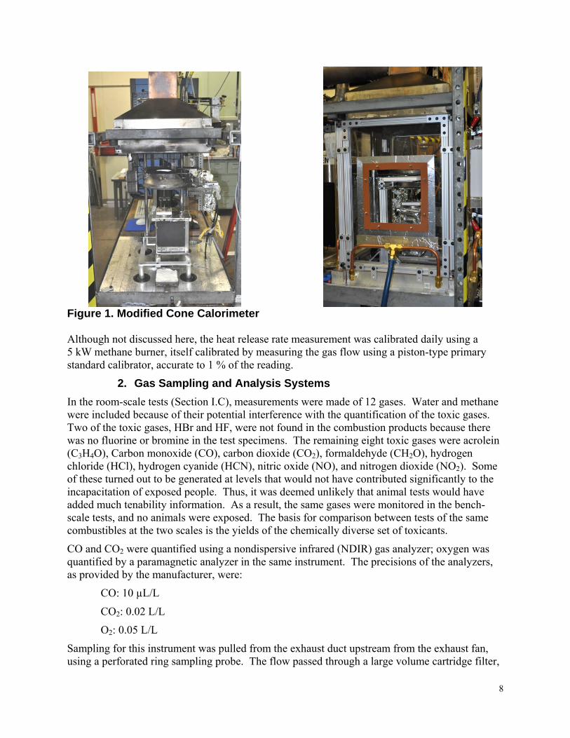
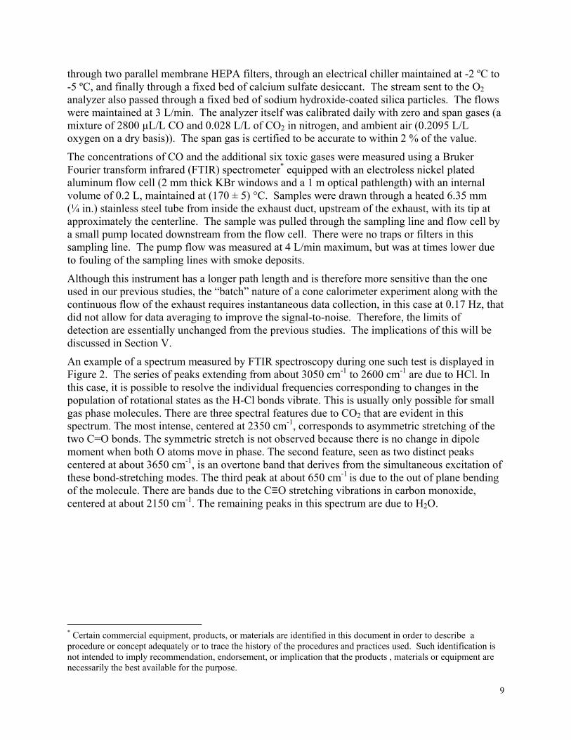
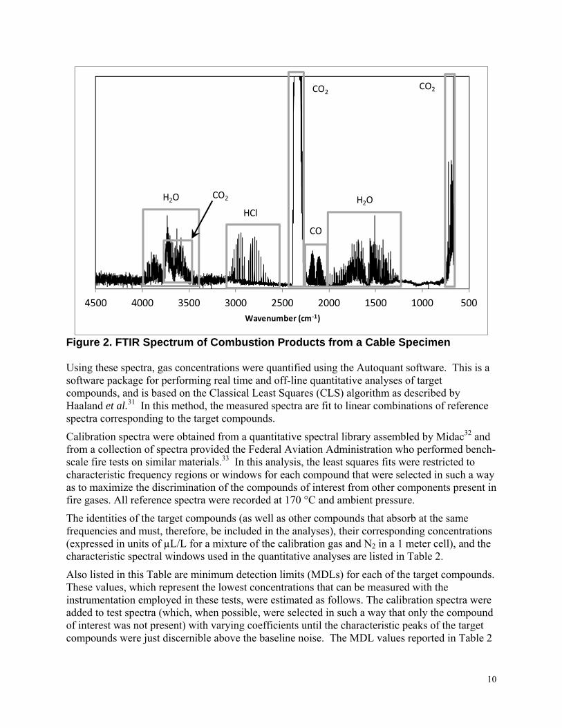

This page intentionally left blank
14
III CALCULATION METHODS
A MASS LOSS RATE
The specimen mass loss during a test was determined from the initial reading from the load cell and from a point where the specimen transitioned from burning to pyrolyzing which was characterized by a sudden drop in the mass loss rate (derivative of the mass loss calculated over 16 data points seconds) The uncertainty in the mass loss derived from the uncertainties in these two measurements was 01 g
B NOTIONAL GAS YIELDS
The notional or maximum possible gas yields (Table 3) were calculated as follows
CO2 Assume all the carbon in the test specimen is converted to CO2 Multiply the mass fraction of C in the test specimen (Table 1) by the ratio of the molecular mass of CO2 to the atomic mass of carbon
CO Assume all the carbon in the test specimen is converted to CO Multiply the mass fraction of C by the ratio of the molecular mass of CO to the atomic mass of carbon
HCN Assume all the nitrogen in the test specimen is converted to HCN Multiply the mass fraction of N by the ratio of the molecular mass of HCN to the atomic mass of nitrogen
HCl Assume all the chlorine in the test specimen is converted to HCl Multiply the mass fraction of Cl by the ratio of the molecular mass of HCl to the atomic mass of chlorine
The notional yields from the bookcase and cable specimens were assumed to be the same as the yields from the intact combustibles15 The sofa specimen had a mass ratio of fabric to foam that differed modestly from the intact sofas
Table 3 Calculated Notional Yields of Toxic Products from the Test Specimens Notional Yields
Gas Bookcase Cable Sofa CO2 172 plusmn 1 211 plusmn 1 195 plusmn 4 CO 109 plusmn 1 133 plusmn 1 124 plusmn 4 HCN 0057 plusmn 13 0040 plusmn 6 0193 plusmn 4 HCl 00026 plusmn 4 0332 plusmn 1 00069 plusmn 19
The uncertainty in the notional yield values is determined by the uncertainty in the prevalence of the central element (in the bullets just above) in the combustible For the cuttings from the sofas the uncertainty in the notional yields was increased by the small variability (estimated at 3 percent) in the relative masses of the fabric and padding materials in the test specimens
C CALCULATED GAS YIELDS
1 CO and CO2
Yields of CO and CO2 were calculated using the measured gas concentrations from the NDIR instrument the measured flows in the exhaust the exhaust temperature (accounting for the
15
background concentrations in room air) the consumed mass of the fuel and the ideal gas law Concentrations were converted to mass flow then integrated numerically (rectangular) over the time of flaming combustion
As we observed previously17 the CO2 absorption band in the FTIR is saturated at normal volume fractions and is therefore highly non-linear As both the FTIR and NDIR measurements were taken from the same location it was not necessary to measure the CO2 concentration by FTIR
Figure 3 shows a comparison of the maximum CO volume fractions measured by the two instruments The FTIR consistently found a lower volume fraction than the NDIR above 300 microLL This is likely due to the non-linearity inherent in IR spectra at higher absorption Since the spectrometer used in this study had a path length that was 10 times that used in the previous work172324 it is not unreasonable that these data fall more in the non-linear range Therefore the data reported here for CO are taken from the NDIR results
0
100
200
300
400
500
600
700
800
0 200 400 600 800
CO
Volume Fraction
(LL) ‐FTIR
CO Volume Fraction (LL) ‐NDIR
Figure 3 Comparison of FTIR and NDIR Measurements of CO Volume Fraction
2 HCl and HCN
The only calculable HCN yields were from the sofa specimens The only calculable HCl yields were from the cable specimens FTIR spectra from these experiments were analyzed as described in section IIA2 This analysis normally includes an uncertainty of 10 of the reported value Volume fractions were converted into mass flows using the flow and temperature data then numerically integrated over the period of flaming combustion Because
16
these data are more sparse than those from the NDIR (017 Hz vs 10 Hz) a trapezoidal integration was used We considered the possibility that these results suffered from the same non-linear relation between absorption and concentration that occurred with the CO measurements However since the HCN concentrations were quite low and the HCl yields were reasonably close to their notional yields (see Table 11) and similar to the previous work using a different instrument with a shorter path length172324 we determined that non-linear effects were not significant Furthermore because the lower heat flux did not by any other indication have a significant impact on gas yields other than increased variability the quantification of FTIR data from these runs was omitted
3 Other Gases
The volume fractions of the other toxic gases were always below the detection limit Thus the upper limits of the yields of these gases were estimated using their limits of detection
17
This page intentionally left blank
18
IV RESULTS
A TESTS PERFORMED
The following is the test numbering key with format F(2)-q-[O2]-N where
F Fuel [S = sofas B = bookcases C = cable]
(2) present for the 125 Ls flow rate absent for the 25 Ls flow rate
q heat flux per unit area (kWm2)
[O2] Approximate initial oxygen volume percent in the supply gas
N Replicate test number for that set of combustible and conditions
Table 4 through Table 9 present the test data and the calculated yields for the bookcase sofa and cable specimens respectively In these tables Δt is the observed duration of flaming combustion and Δm is the measured mass lost during the flaming combustion Volume fractions represent the maximum value in the test usually soon after ignition A yield number in red indicates a potential outlier that if discarded could improve the repeatability under those conditions
The horizontal shaded bands highlight groups of replicate tests
19
Table 4 Data from Bookcase Material Tests
NDIR
Code Specimen
Mass (g)
Δm
(g)
Δt (s)
Flaming
FCO2
(LL)
FCO
(LL)
FO2
(LL)
b‐50‐21‐1 1498 1060 1068 00065 120 02037
b‐50‐21‐2 1356 1052 1090 00067 140 02033
b‐50‐21‐3 1384 1037 1043 00072 150 02028
b‐50‐18‐1 1360 1038 1110 00070 160 01731
b‐50‐18‐2 1374 1015 1060 00070 160 01730
b‐50‐18‐3 1381 1021 1110 00064 160 01748
b‐50‐16‐1 1192 984 993 00066 140 01559
b‐50‐16‐2 1366 1017 1115 00062 170 01545
b‐50‐16‐3 1206 916 940 00062 150 01548
b2‐50‐21‐1 1315 996 1110 00121 240 01974
b2‐50‐21‐2 1302 973 1010 00123 230 01972
b2‐50‐21‐3 1274 969 1040 00124 230 01970
b2‐50‐16‐1 1316 997 1140 00106 250 01504
b2‐50‐16‐2 1282 973 1050 00103 230 01495
b2‐50‐16‐3 1238 938 1070 00103 230 01499
b2‐50‐14‐1 1297 957 1170 00099 850 01285
b2‐50‐14‐2 1322 981 1160 00100 450 01297
b2‐50‐14‐3 1316 982 1200 00101 460 01298
b‐25‐21‐1 1246 933 1295 00053 180 02051
b‐25‐21‐3 1286 1030 1590 00057 200 02046
b‐25‐21‐4 1388 1025 1590 00058 190 02045
b‐25‐18‐1 1266 346 590 00045 220 01675
b‐25‐18‐2 1274 303 540 00043 280 01773
b‐25‐18‐3 1309 545 620 00042 200 01593
b‐25‐18‐4 1225 322 550 00041 190 01769
b‐25‐16‐1 1284 269 620 00037 210 01578
b‐25‐16‐2 1296 219 450 00037 230 01594
b‐25‐16‐3 1286 258 520 00032 220 01590
20
Table 5 Data from Sofa Material Tests
NDIR FTIR
Code Specimen
Mass (g)
Δm
(g)
Δt (s)
Flaming
FCO2
(LL)
FCO
(LL)
FO2
(LL)
FCO
(LL)
FHCN
(LL)
s‐50‐21‐1 120 85 62 00071 290 02012 260 80 s‐50‐21‐2 118 85 65 00074 310 02007 310 90 s‐50‐21‐3 117 87 66 00076 310 02007 300 90 s‐50‐18‐1 124 86 82 00067 370 01727 290 150 s‐50‐18‐2 118 85 125 00064 330 01730 270 130 s‐50‐18‐3 119 86 105 00066 380 01727 300 170 s‐50‐16‐1 122 87 115 00068 470 01522 380 270 s‐50‐16‐2 121 84 110 00067 420 01524 370 250 s‐50‐16‐3 123 90 120 00071 430 01527 340 230 s2‐50‐21‐1 115 85 85 00149 520 01903 390 210 s2‐50‐21‐2 118 87 100 00120 480 01944 400 180 s2‐50‐21‐3 118 87 90 00138 510 01919 390 170 s2‐50‐16‐1 106 77 100 00119 500 01445 360 330 s2‐50‐16‐2 117 86 130 00102 640 01485 460 380 s2‐50‐16‐3 117 86 120 00106 770 01481 570 460 s2‐50‐14‐1 112 80 120 00105 440 01265 370 110 s2‐50‐14‐2 117 85 120 00104 510 01266 380 180 s2‐50‐14‐3 119 85 120 00115 670 01252 470 250 s‐25‐21‐1 124 85 150 00059 170 02041 s‐25‐21‐2 121 64 115 00054 160 02045 s‐25‐21‐3 122 81 170 00055 170 02044 s‐25‐18‐1 122 53 165 00043 130 01758 s‐25‐18‐2 122 55 150 00045 130 01756 s‐25‐18‐3 123 50 110 00049 180 01755 s‐25‐18‐4 122 91 170 00044 140 01748 s‐25‐18‐5 122 56 120 00047 170 01751 s‐25‐16‐1 122 35 135 00007 50 01601 s‐25‐16‐3 123 51 105 00039 110 01593 s‐25‐16‐4 122 35 180 00008 50 01361
21
Table 6 Data from Cable Material Tests
NDIR FTIR
Code Specimen
Mass (g)
Δm
(g)
Δt (s)
Flaming
FCO2
(LL)
FCO
(LL)
FO2
(LL)
FCO
(LL)
FHCl
(LL)
c‐50‐21‐1 569 138 175 00041 340 02051 310 900 c‐50‐21‐2 382 95 169 00033 220 02051 220 810 c‐50‐21‐3 377 91 145 00033 240 02062 230 800 c‐50‐18‐1 357 87 180 00029 210 01779 210 750 c‐50‐18‐2 356 87 190 00028 220 01769 220 730 c‐50‐18‐3 360 89 175 00032 280 01764 250 820 c‐50‐16‐1 362 87 160 00029 230 01597 230 750 c‐50‐16‐2 350 78 135 00033 340 01562 300 880 c‐50‐16‐3 352 81 158 00030 230 01564 240 850 c2‐50‐21‐1 365 81 140 00048 330 02044 330 1220 c2‐50‐21‐2 373 82 140 00050 340 02042 320 1180 c2‐50‐21‐3 372 84 135 00052 370 02039 350 1190 c2‐50‐16‐1 372 88 180 00046 410 01554 350 1080 c2‐50‐16‐2 380 89 190 00044 350 01554 310 1100 c2‐50‐16‐3 375 87 175 00047 410 01546 340 1160 c2‐50‐14‐2 368 84 185 00041 380 01361 320 1370 c2‐50‐14‐3 387 96 240 00036 290 01335 290 1210 c2‐50‐14‐4 369 81 175 00039 360 01366 310 1240 c‐25‐21‐1 380 85 220 00028 160 02072 c‐25‐21‐2 374 83 230 00027 140 02075 c‐25‐21‐3 372 81 230 00026 130 02072 c‐25‐18‐1 360 72 230 00020 120 01789 c‐25‐18‐2 354 67 260 00020 120 01786 c‐25‐18‐3 357 68 250 00019 110 01775 c‐25‐16‐1 357 48 265 00014 80 01584 c‐25‐16‐2 364 42 260 00014 80 01586 c‐25‐16‐3 358 44 245 00015 80 01604
22
Table 7 Gas Yields from Bookcase Material Tests Code Specimen
Mass (g)
Δm
(g)
yCO2
(gg)
yCO
(gg)
yHCN
(gg)
yHCl
(gg)
yNO
(gg)
yNO2
(gg)
yacrolein
(gg)
yform
(gg)
b‐50‐21‐1 1498 1060 110 0010 lt 00084 lt 00065 lt 0019 lt 0016 lt 0010 lt 0011 b‐50‐21‐2 1356 1052 111 0010 lt 00086 lt 00066 lt 0019 lt 0017 lt 0010 lt 0011 b‐50‐21‐3 1384 1037 113 0009 lt 00083 lt 00064 lt 0018 lt 0016 lt 0010 lt 0011 b‐50‐18‐1 1360 1038 109 0013 lt 00087 lt 00067 lt 0019 lt 0017 lt 0010 lt 0011 b‐50‐18‐2 1374 1015 110 0012 lt 00084 lt 00065 lt 0019 lt 0016 lt 0010 lt 0011 b‐50‐18‐3 1381 1021 110 0013 lt 00087 lt 00067 lt 0019 lt 0017 lt 0010 lt 0011 b‐50‐16‐1 1192 984 102 0020 lt 00079 lt 00061 lt 0018 lt 0015 lt 0009 lt 0010 b‐50‐16‐2 1366 1017 105 0020 lt 00086 lt 00066 lt 0019 lt 0017 lt 0010 lt 0011 b‐50‐16‐3 1206 916 110 0018 lt 00080 lt 00062 lt 0018 lt 0016 lt 0010 lt 0010 b2‐50‐21‐1 1315 996 102 0006 lt 00045 lt 00035 lt 0010 lt 0009 lt 0005 lt 0006 b2‐50‐21‐2 1302 973 101 0006 lt 00042 lt 00032 lt 0009 lt 0008 lt 0005 lt 0005 b2‐50‐21‐3 1274 969 103 0006 lt 00043 lt 00033 lt 0010 lt 0008 lt 0005 lt 0005 b2‐50‐16‐1 1316 997 103 0010 lt 00048 lt 00037 lt 0011 lt 0009 lt 0006 lt 0006 b2‐50‐16‐2 1282 973 102 0008 lt 00045 lt 00035 lt 0010 lt 0009 lt 0005 lt 0006 b2‐50‐16‐3 1238 938 103 0009 lt 00048 lt 00037 lt 0011 lt 0009 lt 0006 lt 0006 b2‐50‐14‐1 1297 957 069 0058 lt 00051 lt 00039 lt 0011 lt 0010 lt 0006 lt 0006 b2‐50‐14‐2 1322 981 093 0032 lt 00048 lt 00037 lt 0011 lt 0009 lt 0006 lt 0006 b2‐50‐14‐3 1316 982 093 0032 lt 00049 lt 00038 lt 0011 lt 0010 lt 0006 lt 0006 b‐25‐21‐1 1246 933 115 0015 b‐25‐21‐3 1286 1030 112 0020 b‐25‐21‐4 1388 1025 114 0022 b‐25‐18‐1 1266 346 085 0028 b‐25‐18‐2 1274 303 092 0023 b‐25‐18‐3 1309 545 055 0018 b‐25‐18‐4 1225 322 092 0022 b‐25‐16‐1 1284 269 061 0037 b‐25‐16‐2 1296 219 084 0027 b‐25‐16‐3 1286 258 086 0027
23
Table 8 Gas Yields from Sofa Material Tests Code Specimen
Mass (g)
Δm
(g)
yCO2
(gg)
yCO
(gg)
yHCN
(gg)
yHCl
(gg)
yNO
(gg)
yNO2
(gg)
yacrolein
(gg)
yform
(gg)
s‐50‐21‐1 120 85 139 0026 00033 lt 00055 lt 0016 lt 0014 lt 00085 lt 00091 s‐50‐21‐2 118 85 139 0027 00045 lt 00051 lt 0015 lt 0013 lt 00078 lt 00084 s‐50‐21‐3 117 87 145 0027 00032 lt 00054 lt 0016 lt 0014 lt 00083 lt 00089 s‐50‐18‐1 124 86 143 0034 00071 lt 00058 lt 0017 lt 0015 lt 00089 lt 00096 s‐50‐18‐2 118 85 148 0036 00071 lt 00054 lt 0016 lt 0014 lt 00083 lt 00089 s‐50‐18‐3 119 86 145 0036 00088 lt 00054 lt 0016 lt 0014 lt 00083 lt 00089 s‐50‐16‐1 122 87 138 0045 00124 lt 00056 lt 0016 lt 0014 lt 00086 lt 00092 s‐50‐16‐2 121 84 144 0044 00120 lt 00059 lt 0017 lt 0015 lt 00091 lt 00097 s‐50‐16‐3 123 90 141 0044 00132 lt 00060 lt 0017 lt 0015 lt 00092 lt 00099 s2‐50‐21‐1 115 85 134 0024 00035 lt 00025 lt 0007 lt 0006 lt 00038 lt 00041 s2‐50‐21‐2 118 87 140 0024 00036 lt 00029 lt 0008 lt 0007 lt 00045 lt 00048 s2‐50‐21‐3 118 87 134 0025 00038 lt 00027 lt 0008 lt 0007 lt 00042 lt 00044 s2‐50‐16‐1 106 77 131 0032 00059 lt 00033 lt 0010 lt 0008 lt 00051 lt 00054 s2‐50‐16‐2 117 86 142 0036 00114 lt 00032 lt 0009 lt 0008 lt 00049 lt 00053 s2‐50‐16‐3 117 86 140 0037 00114 lt 00030 lt 0009 lt 0008 lt 00046 lt 00049 s2‐50‐14‐1 112 80 138 0033 00022 lt 00036 lt 0010 lt 0009 lt 00055 lt 00059 s2‐50‐14‐2 117 85 141 0032 00041 lt 00030 lt 0009 lt 0008 lt 00046 lt 00049 s2‐50‐14‐3 119 85 138 0034 00054 lt 00032 lt 0009 lt 0008 lt 00049 lt 00053 s‐25‐21‐1 124 85 156 0024 s‐25‐21‐2 121 64 145 0024 s‐25‐21‐3 122 81 163 0024 s‐25‐18‐1 122 53 091 0030 s‐25‐18‐2 122 55 106 0028 s‐25‐18‐3 123 50 132 0028 s‐25‐18‐4 122 91 142 0024 s‐25‐18‐5 122 56 194 0037 s‐25‐16‐1 122 35 015 0022 s‐25‐16‐3 123 51 136 0029 s‐25‐16‐4 122 35 016 0030
24
Table 9 Gas Yields from Cable Material Tests Code Specimen
Mass (g)
Δm
(g)
yCO2
(gg)
yCO
(gg)
yHCN
(gg)
yHCl
(gg)
yNO
(gg)
yNO2
(gg)
yacrolein
(gg)
yform
(gg)
c‐50‐21‐1 569 138 094 0056 lt 0011 023 lt 0024 lt 0021 lt 0013 lt 0014 c‐50‐21‐2 382 95 112 0051 lt 0016 022 lt 0036 lt 0031 lt 0019 lt 0020 c‐50‐21‐3 377 91 106 0055 lt 0014 024 lt 0031 lt 0027 lt 0017 lt 0018 c‐50‐18‐1 357 87 116 0066 lt 0016 026 lt 0036 lt 0031 lt 0019 lt 0020 c‐50‐18‐2 356 87 121 0065 lt 0017 026 lt 0038 lt 0033 lt 0020 lt 0022 c‐50‐18‐3 360 89 114 0071 lt 0016 025 lt 0036 lt 0031 lt 0019 lt 0020 c‐50‐16‐1 362 87 102 0063 lt 0017 029 lt 0038 lt 0033 lt 0020 lt 0022 c‐50‐16‐2 350 78 115 0078 lt 0015 030 lt 0033 lt 0029 lt 0018 lt 0019 c‐50‐16‐3 352 81 116 0073 lt 0020 032 lt 0044 lt 0039 lt 0024 lt 0025 c2‐50‐21‐1 365 81 103 0049 lt 0007 022 lt 0016 lt 0014 lt 0008 lt 0009 c2‐50‐21‐2 373 82 104 0049 lt 0007 023 lt 0016 lt 0014 lt 0008 lt 0009 c2‐50‐21‐3 372 84 099 0051 lt 0007 021 lt 0016 lt 0014 lt 0008 lt 0009 c2‐50‐16‐1 372 88 099 0062 lt 0008 023 lt 0018 lt 0016 lt 0009 lt 0010 c2‐50‐16‐2 380 89 103 0059 lt 0009 024 lt 0020 lt 0018 lt 0011 lt 0011 c2‐50‐16‐3 375 87 104 0061 lt 0008 023 lt 0018 lt 0016 lt 0009 lt 0010 c2‐50‐14‐4 368 84 091 0057 lt 0009 028 lt 0020 lt 0018 lt 0011 lt 0011 c2‐50‐14‐2 387 96 082 0048 lt 0009 028 lt 0020 lt 0018 lt 0011 lt 0011 c2‐50‐14‐3 369 81 091 0057 lt 0009 029 lt 0020 lt 0018 lt 0011 lt 0011 c‐25‐21‐1 380 85 108 0050 c‐25‐21‐2 374 83 109 0050 c‐25‐21‐3 372 81 121 0051 c‐25‐18‐1 360 72 125 0059 c‐25‐18‐2 354 67 133 0068 c‐25‐18‐3 357 68 125 0062 c‐25‐16‐1 357 48 065 0039 c‐25‐16‐2 364 42 066 0043 c‐25‐16‐3 358 44 072 0043
25
B CALCULATIONS OF TOXIC GAS YIELDS WITH UNCERTAINTIES
Table 10 contains the yields of the combustion products calculated using the data from Table 7 Table 8 and Table 9 The estimated uncertainties reflect the repeatability of the volume fractions in replicate tests uncertainties in the other terms in the yields calculations and degree of proximity of the measured values to the background levels
Table 10 Yields of Combustion Products from Cone Calorimeter Tests
Gas Heat Flux (kWm2)
Flow Rate (Ls)
Initial O2 Bookcase Sofa Cable
CO2
50 25 21 18 16
111 plusmn 15 110 plusmn 01 106 plusmn 35
141 plusmn146 plusmn 141 plusmn
22 18 23
104 plusmn 85 117 plusmn 30 111 plusmn 68
50 125 21 16 14
102 plusmn 11 103 plusmn 05 093 plusmn 03
136 plusmn138 plusmn 139 plusmn
26 44 13
102 plusmn 25 102 plusmn 26 088 plusmn 59
25 25 21 18 16
114 plusmn 12 089 plusmn 44 085 plusmn 14
155 plusmn133 plusmn 136 plusmn
61 30 51
113 plusmn 64 128 plusmn 37 068 plusmn 57
CO
50 25 21 18 16
0010 plusmn 77 0013 plusmn 29 0019 plusmn 74
0027 plusmn 0035 plusmn 0044 plusmn
19 42 14
0054 plusmn 48 0067 plusmn 43 0071 plusmn 11
50 125 21 16 14
0006 plusmn 26 0009 plusmn 91 0032 plusmn 08
0024 plusmn 0035 plusmn 0033 plusmn
09 73 36
0050 plusmn 26 0061 plusmn 30 0054 plusmn 99
25 25 21 18 16
0019 plusmn 20 0023 plusmn 17 0027 plusmn 09
0024 plusmn 0029 plusmn 0029 plusmn
05 16 15
0051 plusmn 12 0063 plusmn 70 0042 plusmn 62
HCN
50 25 21 18 16
lt 00084 lt 00086 lt 00082
00037 plusmn 00077 plusmn 00125 plusmn
29 23 15
lt 0014 lt 0016 lt 0017
50 125 21 16 14
lt 00043 lt 00047 lt 00049
00036 plusmn 00096 plusmn 00039 plusmn
15 43 50
lt 00070 lt 00083 lt 00090
HCl
50 25 21 18 16
lt 00065 lt 00066 lt 00063
lt lt lt
00053 00055 00058
023 plusmn 14 026 plusmn 12 030 plusmn 15
50 125 21 16 14
lt 00033 lt 00036 lt 00038
lt lt lt
00027 00032 00033
022 plusmn 15 023 plusmn 14 028 plusmn 12
NO
50 25 21 18 16
lt 0019 lt 0019 lt 0018
lt lt lt
0015 0016 0017
lt 0030 lt 0036 lt 0038
50 125 21 16 14
lt 0010 lt 0010 lt 0011
lt lt lt
00078 00091 00094
lt 0016 lt 0019 lt 0020
26
Gas Heat Flux (kWm2)
Flow Rate (Ls)
Initial O2 Bookcase Sofa Cable
NO2
50 25 21 18 16
lt 0016 lt 0017 lt 0016
lt 0013 lt 0014 lt 0015
lt 0027 lt 0032 lt 0034
50 125 21 16 14
lt 00084 lt 00092 lt 0010
lt 00068 lt 00080 lt 00082
lt 0014 lt 0016 lt 0018
Acrolein
50 25 21 18 16
lt 0010 lt 0010 lt 0010
lt 00082 lt 00085 lt 00090
lt 0016 lt 0019 lt 0021
50 125 21 16 14
lt 00051 lt 00056 lt 00058
lt 00042 lt 00049 lt 00050
lt 00083 lt 0010 lt 0011
Formaldehyd e
50 25 21 18
16
lt 0011 lt 0011
lt 0010
lt 00088 lt 00091
lt 0010
lt 0017 lt 0021
lt 0022
50 125 21 16 14
lt 00055 lt 00060 lt 00063
lt 00044 lt 00052 lt 00054
lt 00089 lt 0011 lt 0011
27
The values in Table 11 are the values from Table 10 divided by the notional yields from Table 3 Thus the uncertainties are the combined uncertainties from those two tables
Table 11 Fractions of Notional Yields
Gas
Heat Flux
(kWm2)
Flow Rate
(Ls)
Initial
O2 Bookcase Sofa Cable
CO2
50 25 21 18 16
065 plusmn 25 064 plusmn 11 062 plusmn 45
072075072
plusmn plusmn plusmn
32 28 33
049 plusmn 95 055 plusmn 40 053 plusmn 78
50 125 21 16 14
059 plusmn 19 060 plusmn 08 054 plusmn 05
070071071
plusmn plusmn plusmn
36 54 23
048 plusmn 35 048 plusmn 36 042 plusmn 69
25 25 21 18 16
066 plusmn 21 052 plusmn 75 050 plusmn 24
079068070
plusmn plusmn plusmn
71 31 52
053 plusmn 74 061 plusmn 47 032 plusmn 67
CO
50 25 21 18 16
0009 plusmn 87 0012 plusmn 87 0018 plusmn 87
0022 0028 0036
plusmn plusmn plusmn
59 82 54
0041 plusmn 58 0051 plusmn 53 0054 plusmn 12
50 125 21 16 14
0006 plusmn 87 0008 plusmn 87 0029 plusmn 87
0020 0028 0027
plusmn plusmn plusmn
49 11 76
0037 plusmn 36 0046 plusmn 40 0040 plusmn 11
25 25 21 18 16
0017 plusmn 87 0021 plusmn 87 0025 plusmn 87
0020 0023 0024
plusmn plusmn plusmn
45 20 19
0038 plusmn 22 0047 plusmn 80 0031 plusmn 72
HCN
50 25 21 18 16
lt 015 lt 015 lt 014
00190040 0065
plusmnplusmn plusmn
33 27 19
lt 034 lt 041 lt 043
50 125 21 16 14
lt 0076 lt 0082 lt 0087
0019 0050 0020
plusmn plusmn plusmn
19 47 54
lt 018 lt 021 lt 023
HCl
50 25 21 18 16
lt 25 lt 26 lt 24
lt lt lt
077 080 085
069 plusmn 14 078 plusmn 13 091 plusmn 16
50 125 21 16 14
lt 13 lt 14 lt 15
lt lt lt
039 046 047
067 plusmn 15 071 plusmn 14 086 plusmn 12
28
V DISCUSSION
A OVERALL TEST VALUES
The principal outcome of this series of tests is a well-documented set of combustion product yields This includes the numerical values themselves the apparatus conditions under which they were obtained the uncertainty in their calculated values and the repeatability of the tests
Next most important is a determination of the extent to which the toxic gas yields are affected by variations in the test protocol that are reasonable in light of possible variations in combustion conditions in fires involving the intact products
Third it is important to evaluate the quality of the derived knowledge in the context of its intended use The yield information would be used with a computational fire model (zone or CFD) to generate the time-dependent environment generated by a fire Equations such as those in ISO 135719 would then be used to assess whether the combination of occupancy design contained combustibles and occupantresponder characteristics lead to the desired level of life safety
The documentation of the yields has been provided in the earlier sections The following examines the context and quality of the results
B SPECIMEN PERFORMANCE AND TEST REPEATABILITY
1 CO2 and CO
Changing the oxygen concentration had little effect on CO2 yields In some cases at the lowest oxygen concentrations there was a measurable reduction In the case of the sofa materials at the lower heat flux reducing the oxygen concentration increased the variability in the CO2 yield considerably This was the result of the combined effect of low heat flux and low oxygen failing to sustain combustion of the specimen resulting in some degree of non-flaming pyrolysis in which the specimen mass failed to oxidize to either CO or CO2 but instead escaped as unreacted hydrocarbon (which we did not measure)
On the other hand CO yields at 50 kWm2 and 25 Ls were affected by altering the available oxygen As can be seen in Figure 4 to Figure 6 decreasing the available oxygen to 16 increased the CO yieldsmdashabout a twofold increase for the bookcase a 60 increase for the sofa and a 30 increase for the cable When the oxygen volume percent was lower than 16 this resulted in a very large increase in the CO yield a factor of 4 for the bookcase or a slight decrease (less than 10 ) from the maximum yield at 16 oxygen for the sofa and cable
It can also be seen in these figures that reducing the air flow to 125 Ls resulted in consistently lower CO yields There are several possible explanations for example the lower flow may have increased the effluent residence time near the hot cone allowing more time to oxidize or the slower flow may have allowed more steady combustion whereas a more fluctuating flow at the higher flow has the potential to choke off and quench pockets that have not fully oxidized
29
0
0005
001
0015
002
0025
003
0035
CO
Yield
(g g)
10 12 14 16 18 20 22
O2 by Volume
Figure 4 Effect of Oxygen Concentration on CO Yields Bookcase (dashed line = reduced flow) Error bars are plusmn the standard deviation of yields from multiple runs
005
004
CO
Yield
(g g)
10 12 14 16 18 20 22
003
002
001
0
O2 by Volume
Figure 5 Effect of Oxygen Concentration on CO Yields Sofa (dashed line = reduced flow) Error bars are plusmn the standard deviation of yields from multiple runs
30
0
001
002
003
004
005
006
007
008
009
CO
Yield
(g g)
10 12 14 16 18 20 22
O2 by Volume
Figure 6 Effect of Oxygen Concentration on CO Yields Cable (dashed line = reduced flow) Error bars are plusmn the standard deviation of yields from multiple runs
2 HCl and HCN
HCN was detected via FTIR and was only observed in the sofa material tests Figure 7 shows the calculated volume fraction from the FTIR spectra for each of 3 experiments all conducted at 50 kWm2 125 Ls flow and 16 oxygen by volume The three superimposed plots have been time shifted so that the time of ignition is normalized One of the runs (circles) ultimately resulted in a calculated yield roughly half of the other two resulting in a large variability of 33 (see Table 10) If this run is discarded then the reported yield of HCN at this condition should be 00114 with an uncertainty of 02
It is also worth noting that the total time for combustion extended to about 120 s on the scale in Figure 7 Other combustion products continue to be observed in this time period In other words the bulk of the HCN is produced early in the combustion process
Figure 8 shows the results as yields for the generation of HCN at different oxygen volume fractions As with the CO there is linear increase in HCN yields as the oxygen volume fraction decreases from 021 to 016 but at the lowest oxygen volume fraction the yield of HCN is quite low Another important consideration for Figure 8 is that if the outlier run is excluded then the results from the 125 Ls experiments are much closer to the 25 Ls ones although still slightly lower The outlier was included because we feel it is representative of the variability of this measurement
31
0
50
100
150
200
250
300
350
400
450
500
30 50 70 90 110 130 150
HCN
Volume Fraction
(LL)
Test Time (sec)
Figure 7 HCN Volume Fractions Sofa 50 kWm2 125 Ls 16 O2 by Volume Uncertainty is 10 of the Reported HCN Volume Fraction
0014
0012
HCN
Yield
(gg) 0010
0008
0006
0004
0002
0000
O2 by Volume
10 12 14 16 18 20 22
Figure 8 Effect of Oxygen Concentration on HCN Yields Sofa Error bars are plusmn the standard deviation of yields from multiple runs
32
HCl was detected via FTIR and was only observed in the cable tests Figure 9 shows the calculated volume fraction from the FTIR spectra for each of 3 experiments all conducted at 50 kWm2 125 Ls flow and 16 oxygen by volume The three superimposed plots have been time shifted so that the time of ignition is normalized The 3 runs are quite consistent and numerically have a variability in yield of 38 This is despite the fact that there is some variability in the timing of the release of HCl lasting approximately 20 s longer for one of the experiments (diamonds in the figure) In other words the measured volume fraction at any one time is more variable than the integrated quantity
0
200
400
600
800
1000
1200
1400
30 80 130 180 230 280
HCl Volume Fraction
(LL)
Test Time (sec)
Figure 9 HCl Volume Fractions Cable 50 kWm2 125 Ls 16 O2 by Volume Uncertainty is 10 of the Reported Volume Fraction
Figure 10 shows the effect of oxygen concentration on the yields of HCl from the cable materials The yields are somewhat higher at lower oxygen concentrations but this may be accounted for by a slightly lower total mass lostmdashif disproportionately more of the carbon remains in the char At the lowest oxygen volume fraction 014 the yield of HCl increases by about 20
33
000
005
010
015
020
025
030
035
10 12 14 16 18 20 22
HCl Yield
(g g)
O2 by Volume
Figure 10 Effect of Oxygen Concentration on Yields of HCl Cables Error bars are plusmn the standard deviation of yields from multiple runs
C MEASURED VS NOTIONAL VALUES
During sustained and complete combustion the yield of CO2 should approach its notional values since CO2 is a marker for combusted carbon In these experiments the sofa material came out best achieving over 70 of the notional yield The bookcase fared slightly worse achieving only 65 of the notional yield for CO2 and the cable had the lowest at around half The relatively lower yields of CO2 from the cables is an expected result of flame inhibition due to the chlorine These trends are consistent with our qualitative observation of for example the thickness of the smoke produced
The yields of CO from all the specimens ranged from about 001 to 006 which corresponds to 1 to 5 of the notional values These values are consistent with relatively fuel-lean combustion34 and are an order of magnitude lower than the CO yields expected of postflashover fires14
The yields of HCl from the cable specimens approach their notional values The deficit may reflect scavenging by the calcium carbonate filler in the cable jacket or wall loss in the duct or sampling line
The detection limited yields of HCl from the sofa specimens was 80 of the notional yield at the higher flow rate and 40 of the notional yield at the lower flow rate The detection limited yield of HCl from the bookcase was 25 and 15 times the notional yield for the high and low flows respectively Chlorine is present at well under one percent by mass in these two products Such small quantities are not capable of producing toxicologically significant yields of HCl suggesting that they can be either ruled out by elemental analysis as unimportant or that limits of detection are not a barrier to measuring significant quantities of HCl in this apparatus
34
Yields of HCN from the sofa are between 2 and 6 of their notional values The highest relative yield is found at 16 oxygen by volume Despite the lower oxygen these flames appear relatively fuel-lean and the nitrogen may appear as molecular nitrogen or nitrogen dioxides
D SPECIES SAMPLING AND MEASUREMENT
1 Species Measurement Using FTIR Spectroscopy
FTIR spectroscopic analysis of combustion products has become fairly common in fire research laboratories However that does not mean that its use is straightforward The data from a recent round robin involving FTIR measurement of toxic combustion products from a standardized apparatus showed interlaboratory variations of up to an order of magnitude There are documents under development in ISO TC92 SC1 and SC3 to standardize the implementation
We were able to obtain usable information using this technique There are a number of lessons emerging from this test series that can provide useful input to these efforts such as the following
The application of FTIR spectroscopy to fire testing requires the constant attention of an experienced professional at a level well beyond the demands of the more traditional fire test instrumentation
In this work we used a longer path length cell than in previous work However the increased sensitivity was offset by the instantaneous nature of the measurements (as opposed to averaging over dozens of data points) and the fact that the gases did not accumulate as they do in the closed chamber tests such as NFPA 269 and NFPA 270 (toxicity test method and smoke density chamber respectively) The CO concentrations measured here are approximately one-tenth of those measured in the closed-chamber apparatus However non-linear effects resulted in a 25 deficit compared to the NDIR measurements of CO at the highest concentrations
The cell volume remained small and provided good time resolution For example the measured HCl concentrations go from zero to the maximum in two data intervals (see Figure 9)
The lack of a filter did not adversely affect the measurements Compared to previous work with other apparatus the smoke measured here was relatively dilute The cell only required cleaning a few times over the course of all of the experiments reported here The internal mirrors were easily cleaned with ethanol and deionized water The KBr windows were replaced once
A heated sample line (as recommended in the SAFIR report35 and ISO 1970236) enabled near-quantitative collection of HCl a compound that is generally regarded as difficult to determine
E IMPORTANCE OF UNDETECTED GASES
The equations in ISO 13571 include provision for additional gases to be included in estimating the time available for escape or refuge from a fire HBr HF SO2 NO2 acrolein (C3H4O) and formaldehyde (H2CO) There was no Br F or S in any of the products examined in this project
35
so the first three of these gases were not expected The presence of the latter three was not detected thus establishing the upper limits of their presence at the volume fractions listed in Table 2
To put the potential contributions of the sensory irritant gases (HCl NO2 acrolein and formaldehyde) in context we use the equations in ISO 13571 for calculating the Fractional Effective Dose (FED) for the narcotic gases CO2 and CO and the Fractional Effective Concentration (FEC) for the four sensory irritant gases
The FED equation is
CO2exp 5t 2 t 2 236
CO HCNFED t 6 t
t1 35000 t1 12 10 where Δt is the exposure interval in minutes
The FEC of the four irritant gases were estimated from their volume fractions and the incapacitating levels in ISO 13571 (FHCl etc) The results are compiled in Table 12
The FEC equation in ISO 13571 is
HCl HBr HF SO2 NO 2 acrolein formaldehyde irritant FEC = F F F F F F F FHCl HBr HF SO NO acrolein formaldehyde Ci2 2
Table 12 Limits of importance of undetected toxins
Volume fraction (μLL) FEC Contribution
HCl NO2 C3H4O H2CO HCl NO2 C3H4O H2CO Incapacitating Level 1000 250 30 250 Bookcase lt 20 lt 40 lt 20 lt 40 lt 002 lt 016 lt 066 lt 016 Sofa lt 20 lt 40 lt 20 lt 40 lt 002 lt 016 lt 066 lt 016
Cable 1370 lt 40 lt 20 lt 40 058 lt 007 lt 028 lt 007 to 730 lt 40 lt 20 lt 40 043 lt 009 lt 039 lt 009
It stands out that the FEC contribution from acrolein is as much as two-thirds of an incapacitating level This is because (a) the limit of detection is close to the listed incapacitating level and (b) the incapacitating level is very low While there is agreement among experts that this value of 30 μLL is reasonable there are data that suggest strongly that this is unnecessarily conservative Kaplan and co-workers exposed individual baboons to various concentrations of acrolein in air37 At the end of 5 min each baboon was given a signal and could perform an action that led to escape from the test chamber The baboons exposed at up to 500 μLL escaped and survived Those exposed to higher levels escaped but died later These data suggest that people should be able to accommodate a nearly instantaneous exposure to eg at least 300 μLL without becoming incapacitated If we increase the incapacitating level of acrolein to 250 μLL the relative contribution to FEC become those in Table 13 In this case the relative importance of acrolein falls below 01 when other irritants are detected
36
Table 13 Limits of Importance of Undetected Toxicants Volume fraction (μLL) FEC Contribution
HCl NO2 C3H4O H2CO HCl NO2 C3H4O H2CO Incapacitating Level 1000 250 250 250 Bookcase lt 20 lt 40 lt 20 lt 40 lt 005 lt 038 lt 019 lt 038 Sofa lt 20 lt 40 lt 20 lt 40 lt 005 lt 038 lt 019 lt 038 Cable 1370 lt 40 lt 20 lt 40 077 lt 009 lt 005 lt 009
to 730 lt 40 lt 20 lt 40 065 lt 014 lt 007 lt 014
Where specimens like the bookcase and sofa produce narcotic gases CO and HCN and irritants are below the limits of detection the narcotic gases are the primary contributors to incapacitation Assuming that the irritant gases are present in just under the limits of detection in order for them to reach an incapacitating concentration the relative concentration of CO would be incapacitating in a few minutes the relative concentration of HCN would be incapacitating in under a minute
37
This page intentionally left blank
38
VI CONCLUSIONS
This paper reports toxic gas yield data for specimens cut from three complex combustibles a bookcase a sofa and residential electrical power cable The physical fire model used was the cone calorimeter from ISO 5660-1 ASTM E 1354 This apparatus allows the use of a test specimen that approximates the geometry and radiant exposure that might be experienced by the intact combustible in a well-ventilated flaming fire In addition to performing the tests as prescribed in the standards this work added an enclosure and a gas supply capable of reduced oxygen in order to better approximate conditions in an underventilated fire
For the standard test procedure
The CO2 yields were very repeatable and represented between half and 80 of the carbon in the specimens All specimens left a black residue that continued to pyrolyze after the flaming halted These residues were presumably carbon-enriched accounting for the yields being below the notional yields
The CO yields were also very repeatable with the exception of the bookcase at low heat flux and the higher oxygen concentrations
The HCN yields were below the limit of detection for the bookcase and cable specimens The HCN yields from the sofa were 3 to 10 times the limit of detection and had a variation in repeatability between 5 and 40 of the reported yield depending on the test conditions
The HCl yields were below the limit of detection for the bookcase and sofa specimens For the cables they were well above the limit of detection and accounted for 70 of the Cl in the specimens
None of the other irritant gases appeared in concentrations above their limits of detection
Regarding the variation in test conditions we conclude
An incident heat flux of 25 kWm2 does not provide any information beyond that which is found at 50 kWm2 In fact it leads to increased variability from test to test because of slow ignition or early extinction
The trend of toxic gas yields increasing with decreasing initial oxygen concentration holds uniformly across gases and specimen types over the oxygen volume fraction range of 021 to 016 When the oxygen volume fraction is 014 the results are unpredictable for both gases and items burned Therefore we donrsquot recommend testing at this level With the exception of CO from the bookcase the majority of the CO yields were lower at 014 than at 016
Reducing the total flow to 125 Ls reduces the limit of detection of the gases by a factor of two and allows the achievement of lower oxygen concentrations However yields measured at the lower flow were consistently lower than at the higher flow
Calculation of the contributions of the gases to incapacitation of people who might be exposed to these environments showed
Incapacitation from the bookcase material effluent would be primarily from CO
39
Incapacitation from the sofa material effluent would be from a combination of CO and HCN
Incapacitation from the cable effluent would be initially from HCl the related yield of CO would become incapacitating after approximately15 minutes
If the CO yield were at the expected postflashover value of 02
Incapacitation from the bookcase material effluent would be primarily from CO
Incapacitation from the sofa material effluent would be primarily from CO
Incapacitation from the cable material effluent would be initially from HCl a 02 yield of CO would become incapacitating after a few minutes
VII ACKNOWLEDGEMENTS
The authors express their appreciation to Randy Shields for his assistance in performing the tests
40
References
1 Phillips WGB Beller DK and Fahy RF ldquoComputer Simulation for Fire Protection Engineeringrdquo Chapter 5-9 in SFPE Handbook of Fire Protection Engineering 4th Edition PJ DiNenno et al eds NFPA International Quincy MA 2008
2 httpwwwnistgovelfire_researchcfastcfm
3 Peacock RD Jones WW and Reneke PA ldquoCFASTmdashConsolidated Model of Fire Growth and Smoke Transport (Version 6) Software Development and Evaluation Guiderdquo NIST Special Publication 1086 National Institute of Standards and Technology Gaithersburg MD 187 pages (2008)
4 Peacock RD Jones WW and Bukowski RW ldquoVerification of a Model of Fire and Smoke Transportrdquo Fire Safety Journal 21 89-129 (1993)
5 httpfirenistgovfds
6 ldquoStandard Test Method for Heat and Visible Smoke Release Rates for Materials and Products Using an Oxygen Consumption Calorimeterrdquo ASTM E1354-04a ASTM International West Conshohocken PA 2004
7 See eg ldquoStandard for the Flammability (Open Flame) of Mattress Setsrdquo 16 CFR Part 1633 Federal Register 70 (50) 13471-13523 2006
8httpwwwisoorgisoiso_cataloguecatalogue_tccatalogue_tc_browsehtmcommid=50540amp published=onampdevelopment=on
9 ldquoLife-threatening Components of Fire ndash Guidelines for the Estimation of Time to Compromised Tenability in Firesrdquo ISO 13571 International Standards Organization Geneva 2012
10 Guidelines for Assessing the Fire Threat to People ISO 19706 International Standards Organization Geneva 2011
11 Gann RG Babrauskas V Peacock RD and Hall Jr JR Fire Conditions for Smoke Toxicity Measurement Fire and Materials 18 193-199 (1994)
12 Guidance for Comparison of Toxic Gas Data between Different Physical Fire Models and Scales ISO 29903 International Standards Organization Geneva 2012
13 ldquoStandard Test Method for Developing Toxic Potency Data for Use in Fire Hazard Modelingrdquo NFPA 269 NFPA International Quincy MA 2012
14 ldquoStandard Test Method for Measuring Smoke Toxicity for Use in Fire Hazard Analysisrdquo ASTM E1678-10 ASTM International West Conshohocken PA 2010
15 (a) Gann RG Averill JD Nyden MR Johnsson EL and Peacock RD ldquoSmoke Component Yields from Room-scale Fire Testsrdquo NIST Technical Note 1453 National Institute of Standards and Technology Gaithersburg MD 159 pages (2003)
(b) Gann RG Averill JD Nyden MR Johnsson EL and Peacock RD ldquoFire Effluent Component Yields from Room-scale Fire Testsrdquo Fire and Materials 34 285-314 (2010) DOI 101002fam1024
41
16 Ohlemiller TJ and Villa K ldquoFurniture Flammability An Investigation of the California Bulletin 133 Test Part II Characterization of the Ignition Source and a Comparable Gas Burnerrdquo NISTIR 4348 National Institute of Standards and Technology Gaithersburg MD 1990
17 Gann RG Marsh ND Averill JA and Nyden MR ldquoSmoke Component Yields from Bench-scale Fire Tests 1 NFPA 269ASTM E 1678rdquo NIST Technical Note 1760 National Institute of Standards and Technology Gaithersburg MD 57 pages (2013)
18 Kaplan HL Grand AF and Hartzell GE Combustion Toxicology Principles and Test Methods Technology Publishing Co Lancaster PA 1983
19 Guidance for Evaluating the Validity of Physical Fire Models for Obtaining Fire Effluent Toxicity Data for Use in Fire Hazard and Risk Assessment ndash Part 2 Evaluation of Individual Physical Fire Models ISOTR 16312-2 International Standards Organization Geneva 2007
20 Controlled Equivalence Ratio Method for the Determination of the Hazardous Components of Fire Effluent ISOTS 19700 International Standards Organization 2010
21 Reaction-to-fire Tests ndash Heat Release Smoke Production and Mass Loss Rates ndash Part 1 Heat Release (Cone Calorimeter Method) ISO 5660-1 International Standards Organization Geneva 2002
22 Plastics mdash Smoke Generation mdash Part 2 Determination of Optical Density by a Single-chamber Test ISO 5659-2 International standards Organization Geneva 1994
23 Marsh ND Gann RG and Nyden MR ldquoSmoke Component Yields from Bench-scale Fire Tests 2 ISO 19700 Controlled Equivalence Ratio Tube Furnacerdquo NIST Technical Note 1761 National Institute of Standards and Technology Gaithersburg MD 45 pages (2013)
24 Marsh ND Gann RG and Nyden MR ldquoObservations on the Generation of Toxic Products in the NFPAISO Smoke Density Chamberrdquo Proceedings of the 12th International Conference on Fire Science amp Engineering (Interflam 2010) Nottingham UK (2010)
25 Mulholland G Janssens M Yusa S Twilley W and Babrauskas VrdquoThe effect of oxygen concentration on CO and Smoke Produced by Flamesrdquo Proceedings of the Third International Symposium on Fire Safety Science Edinburgh UK pp 585-594 (1991) doi103801IAFSSFSS3-585
26 Babrauskas V Twilley WH Janssens M and Yusa S ldquoA cone calorimeter for controlled-atmosphere studiesrdquo Fire and Materials 16 37-43 (1992)
27 Hshieh FY Motto SE Hirsch DB and Beeson HD ldquoFlammability Testing Using a Controlled-atmosphere Cone Calorimeterrdquo Proceedings of the 18th International Conference on Fire Safety Science Millbrae CA p 999 (1993)
28 Gomez C Janssens M and Zalkin A ldquoUsing the Cone Calorimeter for Quantifying Toxic Potencyrdquo Proceedings of the 12th International Fire Science amp Engineering Conference (Interflam 10) Nottingham UK (2010)
42
29 Gomez C Janssens M and Zalkin A ldquoMeasuring the Yields of Toxic Gases from Materials during Different Stages of Fire Developmentrdquo In Fire and Materials 12 international conference San Francisco CA (2011)
30 Guillaume E Marquis DM and Chivas-Joly C ldquoUsage of Controlled-atmosphere Cone Calorimeter to Provide Input Data for Toxicity Modelingrdquo in Fire and Materials 12 International Conference San Francisco CA (2011)
31 Haaland DM Easterling RG and Vopicka DA ldquoMultivariate Least-Squares Methods Applied to the Quantitative Spectral Analysis of Multicomponent Samplesrdquo Applied Spectroscopy 39 73-84 (1985) doi1013660003702854249376
32 Gas Phase Infrared Spectral Standards Revision B Midac Corp Irvine CA (1999)
33 Speitel LC ldquoFourier Transform Infrared Analysis of Combustion Gasesrdquo Federal Aviation Administration Report DOTFAAAR-0188 2001
34 Pitts WM The Global Equivalence Ratio Concept and the Formations Mechanisms of Carbon Monoxide in Fires Progress in Energy and Combustion Science 21 197-237 (1995)
35 Smoke Gas Analysis by Fourier Transform Infrared Analysis The SAFIR Project VTT Research Note Technical Research Centre of Finland 81 Pages 1999
36 ldquoToxicity testing of fire effluents -- Guidance for analysis of gases and vapours in fire effluents using FTIR gas analysisrdquo ISO 19702 International Standards Organization Geneva 2006
37 Kaplan HL Grand AF Switzer WG Mitchell DS Rogers WR and Hartzell GE Effects of Combustion Gases on Escape Performance of the Baboon and the Rat Journal of Fire Sciences 3 228-244 (1985)
43
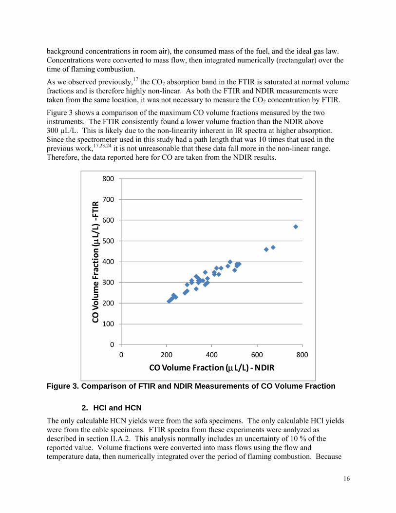
This page intentionally left blank
18
IV RESULTS
A TESTS PERFORMED
The following is the test numbering key with format F(2)-q-[O2]-N where
F Fuel [S = sofas B = bookcases C = cable]
(2) present for the 125 Ls flow rate absent for the 25 Ls flow rate
q heat flux per unit area (kWm2)
[O2] Approximate initial oxygen volume percent in the supply gas
N Replicate test number for that set of combustible and conditions
Table 4 through Table 9 present the test data and the calculated yields for the bookcase sofa and cable specimens respectively In these tables Δt is the observed duration of flaming combustion and Δm is the measured mass lost during the flaming combustion Volume fractions represent the maximum value in the test usually soon after ignition A yield number in red indicates a potential outlier that if discarded could improve the repeatability under those conditions
The horizontal shaded bands highlight groups of replicate tests
19
Table 4 Data from Bookcase Material Tests
NDIR
Code Specimen
Mass (g)
Δm
(g)
Δt (s)
Flaming
FCO2
(LL)
FCO
(LL)
FO2
(LL)
b‐50‐21‐1 1498 1060 1068 00065 120 02037
b‐50‐21‐2 1356 1052 1090 00067 140 02033
b‐50‐21‐3 1384 1037 1043 00072 150 02028
b‐50‐18‐1 1360 1038 1110 00070 160 01731
b‐50‐18‐2 1374 1015 1060 00070 160 01730
b‐50‐18‐3 1381 1021 1110 00064 160 01748
b‐50‐16‐1 1192 984 993 00066 140 01559
b‐50‐16‐2 1366 1017 1115 00062 170 01545
b‐50‐16‐3 1206 916 940 00062 150 01548
b2‐50‐21‐1 1315 996 1110 00121 240 01974
b2‐50‐21‐2 1302 973 1010 00123 230 01972
b2‐50‐21‐3 1274 969 1040 00124 230 01970
b2‐50‐16‐1 1316 997 1140 00106 250 01504
b2‐50‐16‐2 1282 973 1050 00103 230 01495
b2‐50‐16‐3 1238 938 1070 00103 230 01499
b2‐50‐14‐1 1297 957 1170 00099 850 01285
b2‐50‐14‐2 1322 981 1160 00100 450 01297
b2‐50‐14‐3 1316 982 1200 00101 460 01298
b‐25‐21‐1 1246 933 1295 00053 180 02051
b‐25‐21‐3 1286 1030 1590 00057 200 02046
b‐25‐21‐4 1388 1025 1590 00058 190 02045
b‐25‐18‐1 1266 346 590 00045 220 01675
b‐25‐18‐2 1274 303 540 00043 280 01773
b‐25‐18‐3 1309 545 620 00042 200 01593
b‐25‐18‐4 1225 322 550 00041 190 01769
b‐25‐16‐1 1284 269 620 00037 210 01578
b‐25‐16‐2 1296 219 450 00037 230 01594
b‐25‐16‐3 1286 258 520 00032 220 01590
20
Table 5 Data from Sofa Material Tests
NDIR FTIR
Code Specimen
Mass (g)
Δm
(g)
Δt (s)
Flaming
FCO2
(LL)
FCO
(LL)
FO2
(LL)
FCO
(LL)
FHCN
(LL)
s‐50‐21‐1 120 85 62 00071 290 02012 260 80 s‐50‐21‐2 118 85 65 00074 310 02007 310 90 s‐50‐21‐3 117 87 66 00076 310 02007 300 90 s‐50‐18‐1 124 86 82 00067 370 01727 290 150 s‐50‐18‐2 118 85 125 00064 330 01730 270 130 s‐50‐18‐3 119 86 105 00066 380 01727 300 170 s‐50‐16‐1 122 87 115 00068 470 01522 380 270 s‐50‐16‐2 121 84 110 00067 420 01524 370 250 s‐50‐16‐3 123 90 120 00071 430 01527 340 230 s2‐50‐21‐1 115 85 85 00149 520 01903 390 210 s2‐50‐21‐2 118 87 100 00120 480 01944 400 180 s2‐50‐21‐3 118 87 90 00138 510 01919 390 170 s2‐50‐16‐1 106 77 100 00119 500 01445 360 330 s2‐50‐16‐2 117 86 130 00102 640 01485 460 380 s2‐50‐16‐3 117 86 120 00106 770 01481 570 460 s2‐50‐14‐1 112 80 120 00105 440 01265 370 110 s2‐50‐14‐2 117 85 120 00104 510 01266 380 180 s2‐50‐14‐3 119 85 120 00115 670 01252 470 250 s‐25‐21‐1 124 85 150 00059 170 02041 s‐25‐21‐2 121 64 115 00054 160 02045 s‐25‐21‐3 122 81 170 00055 170 02044 s‐25‐18‐1 122 53 165 00043 130 01758 s‐25‐18‐2 122 55 150 00045 130 01756 s‐25‐18‐3 123 50 110 00049 180 01755 s‐25‐18‐4 122 91 170 00044 140 01748 s‐25‐18‐5 122 56 120 00047 170 01751 s‐25‐16‐1 122 35 135 00007 50 01601 s‐25‐16‐3 123 51 105 00039 110 01593 s‐25‐16‐4 122 35 180 00008 50 01361
21
Table 6 Data from Cable Material Tests
NDIR FTIR
Code Specimen
Mass (g)
Δm
(g)
Δt (s)
Flaming
FCO2
(LL)
FCO
(LL)
FO2
(LL)
FCO
(LL)
FHCl
(LL)
c‐50‐21‐1 569 138 175 00041 340 02051 310 900 c‐50‐21‐2 382 95 169 00033 220 02051 220 810 c‐50‐21‐3 377 91 145 00033 240 02062 230 800 c‐50‐18‐1 357 87 180 00029 210 01779 210 750 c‐50‐18‐2 356 87 190 00028 220 01769 220 730 c‐50‐18‐3 360 89 175 00032 280 01764 250 820 c‐50‐16‐1 362 87 160 00029 230 01597 230 750 c‐50‐16‐2 350 78 135 00033 340 01562 300 880 c‐50‐16‐3 352 81 158 00030 230 01564 240 850 c2‐50‐21‐1 365 81 140 00048 330 02044 330 1220 c2‐50‐21‐2 373 82 140 00050 340 02042 320 1180 c2‐50‐21‐3 372 84 135 00052 370 02039 350 1190 c2‐50‐16‐1 372 88 180 00046 410 01554 350 1080 c2‐50‐16‐2 380 89 190 00044 350 01554 310 1100 c2‐50‐16‐3 375 87 175 00047 410 01546 340 1160 c2‐50‐14‐2 368 84 185 00041 380 01361 320 1370 c2‐50‐14‐3 387 96 240 00036 290 01335 290 1210 c2‐50‐14‐4 369 81 175 00039 360 01366 310 1240 c‐25‐21‐1 380 85 220 00028 160 02072 c‐25‐21‐2 374 83 230 00027 140 02075 c‐25‐21‐3 372 81 230 00026 130 02072 c‐25‐18‐1 360 72 230 00020 120 01789 c‐25‐18‐2 354 67 260 00020 120 01786 c‐25‐18‐3 357 68 250 00019 110 01775 c‐25‐16‐1 357 48 265 00014 80 01584 c‐25‐16‐2 364 42 260 00014 80 01586 c‐25‐16‐3 358 44 245 00015 80 01604
22
Table 7 Gas Yields from Bookcase Material Tests Code Specimen
Mass (g)
Δm
(g)
yCO2
(gg)
yCO
(gg)
yHCN
(gg)
yHCl
(gg)
yNO
(gg)
yNO2
(gg)
yacrolein
(gg)
yform
(gg)
b‐50‐21‐1 1498 1060 110 0010 lt 00084 lt 00065 lt 0019 lt 0016 lt 0010 lt 0011 b‐50‐21‐2 1356 1052 111 0010 lt 00086 lt 00066 lt 0019 lt 0017 lt 0010 lt 0011 b‐50‐21‐3 1384 1037 113 0009 lt 00083 lt 00064 lt 0018 lt 0016 lt 0010 lt 0011 b‐50‐18‐1 1360 1038 109 0013 lt 00087 lt 00067 lt 0019 lt 0017 lt 0010 lt 0011 b‐50‐18‐2 1374 1015 110 0012 lt 00084 lt 00065 lt 0019 lt 0016 lt 0010 lt 0011 b‐50‐18‐3 1381 1021 110 0013 lt 00087 lt 00067 lt 0019 lt 0017 lt 0010 lt 0011 b‐50‐16‐1 1192 984 102 0020 lt 00079 lt 00061 lt 0018 lt 0015 lt 0009 lt 0010 b‐50‐16‐2 1366 1017 105 0020 lt 00086 lt 00066 lt 0019 lt 0017 lt 0010 lt 0011 b‐50‐16‐3 1206 916 110 0018 lt 00080 lt 00062 lt 0018 lt 0016 lt 0010 lt 0010 b2‐50‐21‐1 1315 996 102 0006 lt 00045 lt 00035 lt 0010 lt 0009 lt 0005 lt 0006 b2‐50‐21‐2 1302 973 101 0006 lt 00042 lt 00032 lt 0009 lt 0008 lt 0005 lt 0005 b2‐50‐21‐3 1274 969 103 0006 lt 00043 lt 00033 lt 0010 lt 0008 lt 0005 lt 0005 b2‐50‐16‐1 1316 997 103 0010 lt 00048 lt 00037 lt 0011 lt 0009 lt 0006 lt 0006 b2‐50‐16‐2 1282 973 102 0008 lt 00045 lt 00035 lt 0010 lt 0009 lt 0005 lt 0006 b2‐50‐16‐3 1238 938 103 0009 lt 00048 lt 00037 lt 0011 lt 0009 lt 0006 lt 0006 b2‐50‐14‐1 1297 957 069 0058 lt 00051 lt 00039 lt 0011 lt 0010 lt 0006 lt 0006 b2‐50‐14‐2 1322 981 093 0032 lt 00048 lt 00037 lt 0011 lt 0009 lt 0006 lt 0006 b2‐50‐14‐3 1316 982 093 0032 lt 00049 lt 00038 lt 0011 lt 0010 lt 0006 lt 0006 b‐25‐21‐1 1246 933 115 0015 b‐25‐21‐3 1286 1030 112 0020 b‐25‐21‐4 1388 1025 114 0022 b‐25‐18‐1 1266 346 085 0028 b‐25‐18‐2 1274 303 092 0023 b‐25‐18‐3 1309 545 055 0018 b‐25‐18‐4 1225 322 092 0022 b‐25‐16‐1 1284 269 061 0037 b‐25‐16‐2 1296 219 084 0027 b‐25‐16‐3 1286 258 086 0027
23
Table 8 Gas Yields from Sofa Material Tests Code Specimen
Mass (g)
Δm
(g)
yCO2
(gg)
yCO
(gg)
yHCN
(gg)
yHCl
(gg)
yNO
(gg)
yNO2
(gg)
yacrolein
(gg)
yform
(gg)
s‐50‐21‐1 120 85 139 0026 00033 lt 00055 lt 0016 lt 0014 lt 00085 lt 00091 s‐50‐21‐2 118 85 139 0027 00045 lt 00051 lt 0015 lt 0013 lt 00078 lt 00084 s‐50‐21‐3 117 87 145 0027 00032 lt 00054 lt 0016 lt 0014 lt 00083 lt 00089 s‐50‐18‐1 124 86 143 0034 00071 lt 00058 lt 0017 lt 0015 lt 00089 lt 00096 s‐50‐18‐2 118 85 148 0036 00071 lt 00054 lt 0016 lt 0014 lt 00083 lt 00089 s‐50‐18‐3 119 86 145 0036 00088 lt 00054 lt 0016 lt 0014 lt 00083 lt 00089 s‐50‐16‐1 122 87 138 0045 00124 lt 00056 lt 0016 lt 0014 lt 00086 lt 00092 s‐50‐16‐2 121 84 144 0044 00120 lt 00059 lt 0017 lt 0015 lt 00091 lt 00097 s‐50‐16‐3 123 90 141 0044 00132 lt 00060 lt 0017 lt 0015 lt 00092 lt 00099 s2‐50‐21‐1 115 85 134 0024 00035 lt 00025 lt 0007 lt 0006 lt 00038 lt 00041 s2‐50‐21‐2 118 87 140 0024 00036 lt 00029 lt 0008 lt 0007 lt 00045 lt 00048 s2‐50‐21‐3 118 87 134 0025 00038 lt 00027 lt 0008 lt 0007 lt 00042 lt 00044 s2‐50‐16‐1 106 77 131 0032 00059 lt 00033 lt 0010 lt 0008 lt 00051 lt 00054 s2‐50‐16‐2 117 86 142 0036 00114 lt 00032 lt 0009 lt 0008 lt 00049 lt 00053 s2‐50‐16‐3 117 86 140 0037 00114 lt 00030 lt 0009 lt 0008 lt 00046 lt 00049 s2‐50‐14‐1 112 80 138 0033 00022 lt 00036 lt 0010 lt 0009 lt 00055 lt 00059 s2‐50‐14‐2 117 85 141 0032 00041 lt 00030 lt 0009 lt 0008 lt 00046 lt 00049 s2‐50‐14‐3 119 85 138 0034 00054 lt 00032 lt 0009 lt 0008 lt 00049 lt 00053 s‐25‐21‐1 124 85 156 0024 s‐25‐21‐2 121 64 145 0024 s‐25‐21‐3 122 81 163 0024 s‐25‐18‐1 122 53 091 0030 s‐25‐18‐2 122 55 106 0028 s‐25‐18‐3 123 50 132 0028 s‐25‐18‐4 122 91 142 0024 s‐25‐18‐5 122 56 194 0037 s‐25‐16‐1 122 35 015 0022 s‐25‐16‐3 123 51 136 0029 s‐25‐16‐4 122 35 016 0030
24
Table 9 Gas Yields from Cable Material Tests Code Specimen
Mass (g)
Δm
(g)
yCO2
(gg)
yCO
(gg)
yHCN
(gg)
yHCl
(gg)
yNO
(gg)
yNO2
(gg)
yacrolein
(gg)
yform
(gg)
c‐50‐21‐1 569 138 094 0056 lt 0011 023 lt 0024 lt 0021 lt 0013 lt 0014 c‐50‐21‐2 382 95 112 0051 lt 0016 022 lt 0036 lt 0031 lt 0019 lt 0020 c‐50‐21‐3 377 91 106 0055 lt 0014 024 lt 0031 lt 0027 lt 0017 lt 0018 c‐50‐18‐1 357 87 116 0066 lt 0016 026 lt 0036 lt 0031 lt 0019 lt 0020 c‐50‐18‐2 356 87 121 0065 lt 0017 026 lt 0038 lt 0033 lt 0020 lt 0022 c‐50‐18‐3 360 89 114 0071 lt 0016 025 lt 0036 lt 0031 lt 0019 lt 0020 c‐50‐16‐1 362 87 102 0063 lt 0017 029 lt 0038 lt 0033 lt 0020 lt 0022 c‐50‐16‐2 350 78 115 0078 lt 0015 030 lt 0033 lt 0029 lt 0018 lt 0019 c‐50‐16‐3 352 81 116 0073 lt 0020 032 lt 0044 lt 0039 lt 0024 lt 0025 c2‐50‐21‐1 365 81 103 0049 lt 0007 022 lt 0016 lt 0014 lt 0008 lt 0009 c2‐50‐21‐2 373 82 104 0049 lt 0007 023 lt 0016 lt 0014 lt 0008 lt 0009 c2‐50‐21‐3 372 84 099 0051 lt 0007 021 lt 0016 lt 0014 lt 0008 lt 0009 c2‐50‐16‐1 372 88 099 0062 lt 0008 023 lt 0018 lt 0016 lt 0009 lt 0010 c2‐50‐16‐2 380 89 103 0059 lt 0009 024 lt 0020 lt 0018 lt 0011 lt 0011 c2‐50‐16‐3 375 87 104 0061 lt 0008 023 lt 0018 lt 0016 lt 0009 lt 0010 c2‐50‐14‐4 368 84 091 0057 lt 0009 028 lt 0020 lt 0018 lt 0011 lt 0011 c2‐50‐14‐2 387 96 082 0048 lt 0009 028 lt 0020 lt 0018 lt 0011 lt 0011 c2‐50‐14‐3 369 81 091 0057 lt 0009 029 lt 0020 lt 0018 lt 0011 lt 0011 c‐25‐21‐1 380 85 108 0050 c‐25‐21‐2 374 83 109 0050 c‐25‐21‐3 372 81 121 0051 c‐25‐18‐1 360 72 125 0059 c‐25‐18‐2 354 67 133 0068 c‐25‐18‐3 357 68 125 0062 c‐25‐16‐1 357 48 065 0039 c‐25‐16‐2 364 42 066 0043 c‐25‐16‐3 358 44 072 0043
25
B CALCULATIONS OF TOXIC GAS YIELDS WITH UNCERTAINTIES
Table 10 contains the yields of the combustion products calculated using the data from Table 7 Table 8 and Table 9 The estimated uncertainties reflect the repeatability of the volume fractions in replicate tests uncertainties in the other terms in the yields calculations and degree of proximity of the measured values to the background levels
Table 10 Yields of Combustion Products from Cone Calorimeter Tests
Gas Heat Flux (kWm2)
Flow Rate (Ls)
Initial O2 Bookcase Sofa Cable
CO2
50 25 21 18 16
111 plusmn 15 110 plusmn 01 106 plusmn 35
141 plusmn146 plusmn 141 plusmn
22 18 23
104 plusmn 85 117 plusmn 30 111 plusmn 68
50 125 21 16 14
102 plusmn 11 103 plusmn 05 093 plusmn 03
136 plusmn138 plusmn 139 plusmn
26 44 13
102 plusmn 25 102 plusmn 26 088 plusmn 59
25 25 21 18 16
114 plusmn 12 089 plusmn 44 085 plusmn 14
155 plusmn133 plusmn 136 plusmn
61 30 51
113 plusmn 64 128 plusmn 37 068 plusmn 57
CO
50 25 21 18 16
0010 plusmn 77 0013 plusmn 29 0019 plusmn 74
0027 plusmn 0035 plusmn 0044 plusmn
19 42 14
0054 plusmn 48 0067 plusmn 43 0071 plusmn 11
50 125 21 16 14
0006 plusmn 26 0009 plusmn 91 0032 plusmn 08
0024 plusmn 0035 plusmn 0033 plusmn
09 73 36
0050 plusmn 26 0061 plusmn 30 0054 plusmn 99
25 25 21 18 16
0019 plusmn 20 0023 plusmn 17 0027 plusmn 09
0024 plusmn 0029 plusmn 0029 plusmn
05 16 15
0051 plusmn 12 0063 plusmn 70 0042 plusmn 62
HCN
50 25 21 18 16
lt 00084 lt 00086 lt 00082
00037 plusmn 00077 plusmn 00125 plusmn
29 23 15
lt 0014 lt 0016 lt 0017
50 125 21 16 14
lt 00043 lt 00047 lt 00049
00036 plusmn 00096 plusmn 00039 plusmn
15 43 50
lt 00070 lt 00083 lt 00090
HCl
50 25 21 18 16
lt 00065 lt 00066 lt 00063
lt lt lt
00053 00055 00058
023 plusmn 14 026 plusmn 12 030 plusmn 15
50 125 21 16 14
lt 00033 lt 00036 lt 00038
lt lt lt
00027 00032 00033
022 plusmn 15 023 plusmn 14 028 plusmn 12
NO
50 25 21 18 16
lt 0019 lt 0019 lt 0018
lt lt lt
0015 0016 0017
lt 0030 lt 0036 lt 0038
50 125 21 16 14
lt 0010 lt 0010 lt 0011
lt lt lt
00078 00091 00094
lt 0016 lt 0019 lt 0020
26
Gas Heat Flux (kWm2)
Flow Rate (Ls)
Initial O2 Bookcase Sofa Cable
NO2
50 25 21 18 16
lt 0016 lt 0017 lt 0016
lt 0013 lt 0014 lt 0015
lt 0027 lt 0032 lt 0034
50 125 21 16 14
lt 00084 lt 00092 lt 0010
lt 00068 lt 00080 lt 00082
lt 0014 lt 0016 lt 0018
Acrolein
50 25 21 18 16
lt 0010 lt 0010 lt 0010
lt 00082 lt 00085 lt 00090
lt 0016 lt 0019 lt 0021
50 125 21 16 14
lt 00051 lt 00056 lt 00058
lt 00042 lt 00049 lt 00050
lt 00083 lt 0010 lt 0011
Formaldehyd e
50 25 21 18
16
lt 0011 lt 0011
lt 0010
lt 00088 lt 00091
lt 0010
lt 0017 lt 0021
lt 0022
50 125 21 16 14
lt 00055 lt 00060 lt 00063
lt 00044 lt 00052 lt 00054
lt 00089 lt 0011 lt 0011
27
The values in Table 11 are the values from Table 10 divided by the notional yields from Table 3 Thus the uncertainties are the combined uncertainties from those two tables
Table 11 Fractions of Notional Yields
Gas
Heat Flux
(kWm2)
Flow Rate
(Ls)
Initial
O2 Bookcase Sofa Cable
CO2
50 25 21 18 16
065 plusmn 25 064 plusmn 11 062 plusmn 45
072075072
plusmn plusmn plusmn
32 28 33
049 plusmn 95 055 plusmn 40 053 plusmn 78
50 125 21 16 14
059 plusmn 19 060 plusmn 08 054 plusmn 05
070071071
plusmn plusmn plusmn
36 54 23
048 plusmn 35 048 plusmn 36 042 plusmn 69
25 25 21 18 16
066 plusmn 21 052 plusmn 75 050 plusmn 24
079068070
plusmn plusmn plusmn
71 31 52
053 plusmn 74 061 plusmn 47 032 plusmn 67
CO
50 25 21 18 16
0009 plusmn 87 0012 plusmn 87 0018 plusmn 87
0022 0028 0036
plusmn plusmn plusmn
59 82 54
0041 plusmn 58 0051 plusmn 53 0054 plusmn 12
50 125 21 16 14
0006 plusmn 87 0008 plusmn 87 0029 plusmn 87
0020 0028 0027
plusmn plusmn plusmn
49 11 76
0037 plusmn 36 0046 plusmn 40 0040 plusmn 11
25 25 21 18 16
0017 plusmn 87 0021 plusmn 87 0025 plusmn 87
0020 0023 0024
plusmn plusmn plusmn
45 20 19
0038 plusmn 22 0047 plusmn 80 0031 plusmn 72
HCN
50 25 21 18 16
lt 015 lt 015 lt 014
00190040 0065
plusmnplusmn plusmn
33 27 19
lt 034 lt 041 lt 043
50 125 21 16 14
lt 0076 lt 0082 lt 0087
0019 0050 0020
plusmn plusmn plusmn
19 47 54
lt 018 lt 021 lt 023
HCl
50 25 21 18 16
lt 25 lt 26 lt 24
lt lt lt
077 080 085
069 plusmn 14 078 plusmn 13 091 plusmn 16
50 125 21 16 14
lt 13 lt 14 lt 15
lt lt lt
039 046 047
067 plusmn 15 071 plusmn 14 086 plusmn 12
28
V DISCUSSION
A OVERALL TEST VALUES
The principal outcome of this series of tests is a well-documented set of combustion product yields This includes the numerical values themselves the apparatus conditions under which they were obtained the uncertainty in their calculated values and the repeatability of the tests
Next most important is a determination of the extent to which the toxic gas yields are affected by variations in the test protocol that are reasonable in light of possible variations in combustion conditions in fires involving the intact products
Third it is important to evaluate the quality of the derived knowledge in the context of its intended use The yield information would be used with a computational fire model (zone or CFD) to generate the time-dependent environment generated by a fire Equations such as those in ISO 135719 would then be used to assess whether the combination of occupancy design contained combustibles and occupantresponder characteristics lead to the desired level of life safety
The documentation of the yields has been provided in the earlier sections The following examines the context and quality of the results
B SPECIMEN PERFORMANCE AND TEST REPEATABILITY
1 CO2 and CO
Changing the oxygen concentration had little effect on CO2 yields In some cases at the lowest oxygen concentrations there was a measurable reduction In the case of the sofa materials at the lower heat flux reducing the oxygen concentration increased the variability in the CO2 yield considerably This was the result of the combined effect of low heat flux and low oxygen failing to sustain combustion of the specimen resulting in some degree of non-flaming pyrolysis in which the specimen mass failed to oxidize to either CO or CO2 but instead escaped as unreacted hydrocarbon (which we did not measure)
On the other hand CO yields at 50 kWm2 and 25 Ls were affected by altering the available oxygen As can be seen in Figure 4 to Figure 6 decreasing the available oxygen to 16 increased the CO yieldsmdashabout a twofold increase for the bookcase a 60 increase for the sofa and a 30 increase for the cable When the oxygen volume percent was lower than 16 this resulted in a very large increase in the CO yield a factor of 4 for the bookcase or a slight decrease (less than 10 ) from the maximum yield at 16 oxygen for the sofa and cable
It can also be seen in these figures that reducing the air flow to 125 Ls resulted in consistently lower CO yields There are several possible explanations for example the lower flow may have increased the effluent residence time near the hot cone allowing more time to oxidize or the slower flow may have allowed more steady combustion whereas a more fluctuating flow at the higher flow has the potential to choke off and quench pockets that have not fully oxidized
29
0
0005
001
0015
002
0025
003
0035
CO
Yield
(g g)
10 12 14 16 18 20 22
O2 by Volume
Figure 4 Effect of Oxygen Concentration on CO Yields Bookcase (dashed line = reduced flow) Error bars are plusmn the standard deviation of yields from multiple runs
005
004
CO
Yield
(g g)
10 12 14 16 18 20 22
003
002
001
0
O2 by Volume
Figure 5 Effect of Oxygen Concentration on CO Yields Sofa (dashed line = reduced flow) Error bars are plusmn the standard deviation of yields from multiple runs
30
0
001
002
003
004
005
006
007
008
009
CO
Yield
(g g)
10 12 14 16 18 20 22
O2 by Volume
Figure 6 Effect of Oxygen Concentration on CO Yields Cable (dashed line = reduced flow) Error bars are plusmn the standard deviation of yields from multiple runs
2 HCl and HCN
HCN was detected via FTIR and was only observed in the sofa material tests Figure 7 shows the calculated volume fraction from the FTIR spectra for each of 3 experiments all conducted at 50 kWm2 125 Ls flow and 16 oxygen by volume The three superimposed plots have been time shifted so that the time of ignition is normalized One of the runs (circles) ultimately resulted in a calculated yield roughly half of the other two resulting in a large variability of 33 (see Table 10) If this run is discarded then the reported yield of HCN at this condition should be 00114 with an uncertainty of 02
It is also worth noting that the total time for combustion extended to about 120 s on the scale in Figure 7 Other combustion products continue to be observed in this time period In other words the bulk of the HCN is produced early in the combustion process
Figure 8 shows the results as yields for the generation of HCN at different oxygen volume fractions As with the CO there is linear increase in HCN yields as the oxygen volume fraction decreases from 021 to 016 but at the lowest oxygen volume fraction the yield of HCN is quite low Another important consideration for Figure 8 is that if the outlier run is excluded then the results from the 125 Ls experiments are much closer to the 25 Ls ones although still slightly lower The outlier was included because we feel it is representative of the variability of this measurement
31
0
50
100
150
200
250
300
350
400
450
500
30 50 70 90 110 130 150
HCN
Volume Fraction
(LL)
Test Time (sec)
Figure 7 HCN Volume Fractions Sofa 50 kWm2 125 Ls 16 O2 by Volume Uncertainty is 10 of the Reported HCN Volume Fraction
0014
0012
HCN
Yield
(gg) 0010
0008
0006
0004
0002
0000
O2 by Volume
10 12 14 16 18 20 22
Figure 8 Effect of Oxygen Concentration on HCN Yields Sofa Error bars are plusmn the standard deviation of yields from multiple runs
32
HCl was detected via FTIR and was only observed in the cable tests Figure 9 shows the calculated volume fraction from the FTIR spectra for each of 3 experiments all conducted at 50 kWm2 125 Ls flow and 16 oxygen by volume The three superimposed plots have been time shifted so that the time of ignition is normalized The 3 runs are quite consistent and numerically have a variability in yield of 38 This is despite the fact that there is some variability in the timing of the release of HCl lasting approximately 20 s longer for one of the experiments (diamonds in the figure) In other words the measured volume fraction at any one time is more variable than the integrated quantity
0
200
400
600
800
1000
1200
1400
30 80 130 180 230 280
HCl Volume Fraction
(LL)
Test Time (sec)
Figure 9 HCl Volume Fractions Cable 50 kWm2 125 Ls 16 O2 by Volume Uncertainty is 10 of the Reported Volume Fraction
Figure 10 shows the effect of oxygen concentration on the yields of HCl from the cable materials The yields are somewhat higher at lower oxygen concentrations but this may be accounted for by a slightly lower total mass lostmdashif disproportionately more of the carbon remains in the char At the lowest oxygen volume fraction 014 the yield of HCl increases by about 20
33
000
005
010
015
020
025
030
035
10 12 14 16 18 20 22
HCl Yield
(g g)
O2 by Volume
Figure 10 Effect of Oxygen Concentration on Yields of HCl Cables Error bars are plusmn the standard deviation of yields from multiple runs
C MEASURED VS NOTIONAL VALUES
During sustained and complete combustion the yield of CO2 should approach its notional values since CO2 is a marker for combusted carbon In these experiments the sofa material came out best achieving over 70 of the notional yield The bookcase fared slightly worse achieving only 65 of the notional yield for CO2 and the cable had the lowest at around half The relatively lower yields of CO2 from the cables is an expected result of flame inhibition due to the chlorine These trends are consistent with our qualitative observation of for example the thickness of the smoke produced
The yields of CO from all the specimens ranged from about 001 to 006 which corresponds to 1 to 5 of the notional values These values are consistent with relatively fuel-lean combustion34 and are an order of magnitude lower than the CO yields expected of postflashover fires14
The yields of HCl from the cable specimens approach their notional values The deficit may reflect scavenging by the calcium carbonate filler in the cable jacket or wall loss in the duct or sampling line
The detection limited yields of HCl from the sofa specimens was 80 of the notional yield at the higher flow rate and 40 of the notional yield at the lower flow rate The detection limited yield of HCl from the bookcase was 25 and 15 times the notional yield for the high and low flows respectively Chlorine is present at well under one percent by mass in these two products Such small quantities are not capable of producing toxicologically significant yields of HCl suggesting that they can be either ruled out by elemental analysis as unimportant or that limits of detection are not a barrier to measuring significant quantities of HCl in this apparatus
34
Yields of HCN from the sofa are between 2 and 6 of their notional values The highest relative yield is found at 16 oxygen by volume Despite the lower oxygen these flames appear relatively fuel-lean and the nitrogen may appear as molecular nitrogen or nitrogen dioxides
D SPECIES SAMPLING AND MEASUREMENT
1 Species Measurement Using FTIR Spectroscopy
FTIR spectroscopic analysis of combustion products has become fairly common in fire research laboratories However that does not mean that its use is straightforward The data from a recent round robin involving FTIR measurement of toxic combustion products from a standardized apparatus showed interlaboratory variations of up to an order of magnitude There are documents under development in ISO TC92 SC1 and SC3 to standardize the implementation
We were able to obtain usable information using this technique There are a number of lessons emerging from this test series that can provide useful input to these efforts such as the following
The application of FTIR spectroscopy to fire testing requires the constant attention of an experienced professional at a level well beyond the demands of the more traditional fire test instrumentation
In this work we used a longer path length cell than in previous work However the increased sensitivity was offset by the instantaneous nature of the measurements (as opposed to averaging over dozens of data points) and the fact that the gases did not accumulate as they do in the closed chamber tests such as NFPA 269 and NFPA 270 (toxicity test method and smoke density chamber respectively) The CO concentrations measured here are approximately one-tenth of those measured in the closed-chamber apparatus However non-linear effects resulted in a 25 deficit compared to the NDIR measurements of CO at the highest concentrations
The cell volume remained small and provided good time resolution For example the measured HCl concentrations go from zero to the maximum in two data intervals (see Figure 9)
The lack of a filter did not adversely affect the measurements Compared to previous work with other apparatus the smoke measured here was relatively dilute The cell only required cleaning a few times over the course of all of the experiments reported here The internal mirrors were easily cleaned with ethanol and deionized water The KBr windows were replaced once
A heated sample line (as recommended in the SAFIR report35 and ISO 1970236) enabled near-quantitative collection of HCl a compound that is generally regarded as difficult to determine
E IMPORTANCE OF UNDETECTED GASES
The equations in ISO 13571 include provision for additional gases to be included in estimating the time available for escape or refuge from a fire HBr HF SO2 NO2 acrolein (C3H4O) and formaldehyde (H2CO) There was no Br F or S in any of the products examined in this project
35
so the first three of these gases were not expected The presence of the latter three was not detected thus establishing the upper limits of their presence at the volume fractions listed in Table 2
To put the potential contributions of the sensory irritant gases (HCl NO2 acrolein and formaldehyde) in context we use the equations in ISO 13571 for calculating the Fractional Effective Dose (FED) for the narcotic gases CO2 and CO and the Fractional Effective Concentration (FEC) for the four sensory irritant gases
The FED equation is
CO2exp 5t 2 t 2 236
CO HCNFED t 6 t
t1 35000 t1 12 10 where Δt is the exposure interval in minutes
The FEC of the four irritant gases were estimated from their volume fractions and the incapacitating levels in ISO 13571 (FHCl etc) The results are compiled in Table 12
The FEC equation in ISO 13571 is
HCl HBr HF SO2 NO 2 acrolein formaldehyde irritant FEC = F F F F F F F FHCl HBr HF SO NO acrolein formaldehyde Ci2 2
Table 12 Limits of importance of undetected toxins
Volume fraction (μLL) FEC Contribution
HCl NO2 C3H4O H2CO HCl NO2 C3H4O H2CO Incapacitating Level 1000 250 30 250 Bookcase lt 20 lt 40 lt 20 lt 40 lt 002 lt 016 lt 066 lt 016 Sofa lt 20 lt 40 lt 20 lt 40 lt 002 lt 016 lt 066 lt 016
Cable 1370 lt 40 lt 20 lt 40 058 lt 007 lt 028 lt 007 to 730 lt 40 lt 20 lt 40 043 lt 009 lt 039 lt 009
It stands out that the FEC contribution from acrolein is as much as two-thirds of an incapacitating level This is because (a) the limit of detection is close to the listed incapacitating level and (b) the incapacitating level is very low While there is agreement among experts that this value of 30 μLL is reasonable there are data that suggest strongly that this is unnecessarily conservative Kaplan and co-workers exposed individual baboons to various concentrations of acrolein in air37 At the end of 5 min each baboon was given a signal and could perform an action that led to escape from the test chamber The baboons exposed at up to 500 μLL escaped and survived Those exposed to higher levels escaped but died later These data suggest that people should be able to accommodate a nearly instantaneous exposure to eg at least 300 μLL without becoming incapacitated If we increase the incapacitating level of acrolein to 250 μLL the relative contribution to FEC become those in Table 13 In this case the relative importance of acrolein falls below 01 when other irritants are detected
36
Table 13 Limits of Importance of Undetected Toxicants Volume fraction (μLL) FEC Contribution
HCl NO2 C3H4O H2CO HCl NO2 C3H4O H2CO Incapacitating Level 1000 250 250 250 Bookcase lt 20 lt 40 lt 20 lt 40 lt 005 lt 038 lt 019 lt 038 Sofa lt 20 lt 40 lt 20 lt 40 lt 005 lt 038 lt 019 lt 038 Cable 1370 lt 40 lt 20 lt 40 077 lt 009 lt 005 lt 009
to 730 lt 40 lt 20 lt 40 065 lt 014 lt 007 lt 014
Where specimens like the bookcase and sofa produce narcotic gases CO and HCN and irritants are below the limits of detection the narcotic gases are the primary contributors to incapacitation Assuming that the irritant gases are present in just under the limits of detection in order for them to reach an incapacitating concentration the relative concentration of CO would be incapacitating in a few minutes the relative concentration of HCN would be incapacitating in under a minute
37
This page intentionally left blank
38
VI CONCLUSIONS
This paper reports toxic gas yield data for specimens cut from three complex combustibles a bookcase a sofa and residential electrical power cable The physical fire model used was the cone calorimeter from ISO 5660-1 ASTM E 1354 This apparatus allows the use of a test specimen that approximates the geometry and radiant exposure that might be experienced by the intact combustible in a well-ventilated flaming fire In addition to performing the tests as prescribed in the standards this work added an enclosure and a gas supply capable of reduced oxygen in order to better approximate conditions in an underventilated fire
For the standard test procedure
The CO2 yields were very repeatable and represented between half and 80 of the carbon in the specimens All specimens left a black residue that continued to pyrolyze after the flaming halted These residues were presumably carbon-enriched accounting for the yields being below the notional yields
The CO yields were also very repeatable with the exception of the bookcase at low heat flux and the higher oxygen concentrations
The HCN yields were below the limit of detection for the bookcase and cable specimens The HCN yields from the sofa were 3 to 10 times the limit of detection and had a variation in repeatability between 5 and 40 of the reported yield depending on the test conditions
The HCl yields were below the limit of detection for the bookcase and sofa specimens For the cables they were well above the limit of detection and accounted for 70 of the Cl in the specimens
None of the other irritant gases appeared in concentrations above their limits of detection
Regarding the variation in test conditions we conclude
An incident heat flux of 25 kWm2 does not provide any information beyond that which is found at 50 kWm2 In fact it leads to increased variability from test to test because of slow ignition or early extinction
The trend of toxic gas yields increasing with decreasing initial oxygen concentration holds uniformly across gases and specimen types over the oxygen volume fraction range of 021 to 016 When the oxygen volume fraction is 014 the results are unpredictable for both gases and items burned Therefore we donrsquot recommend testing at this level With the exception of CO from the bookcase the majority of the CO yields were lower at 014 than at 016
Reducing the total flow to 125 Ls reduces the limit of detection of the gases by a factor of two and allows the achievement of lower oxygen concentrations However yields measured at the lower flow were consistently lower than at the higher flow
Calculation of the contributions of the gases to incapacitation of people who might be exposed to these environments showed
Incapacitation from the bookcase material effluent would be primarily from CO
39
Incapacitation from the sofa material effluent would be from a combination of CO and HCN
Incapacitation from the cable effluent would be initially from HCl the related yield of CO would become incapacitating after approximately15 minutes
If the CO yield were at the expected postflashover value of 02
Incapacitation from the bookcase material effluent would be primarily from CO
Incapacitation from the sofa material effluent would be primarily from CO
Incapacitation from the cable material effluent would be initially from HCl a 02 yield of CO would become incapacitating after a few minutes
VII ACKNOWLEDGEMENTS
The authors express their appreciation to Randy Shields for his assistance in performing the tests
40
References
1 Phillips WGB Beller DK and Fahy RF ldquoComputer Simulation for Fire Protection Engineeringrdquo Chapter 5-9 in SFPE Handbook of Fire Protection Engineering 4th Edition PJ DiNenno et al eds NFPA International Quincy MA 2008
2 httpwwwnistgovelfire_researchcfastcfm
3 Peacock RD Jones WW and Reneke PA ldquoCFASTmdashConsolidated Model of Fire Growth and Smoke Transport (Version 6) Software Development and Evaluation Guiderdquo NIST Special Publication 1086 National Institute of Standards and Technology Gaithersburg MD 187 pages (2008)
4 Peacock RD Jones WW and Bukowski RW ldquoVerification of a Model of Fire and Smoke Transportrdquo Fire Safety Journal 21 89-129 (1993)
5 httpfirenistgovfds
6 ldquoStandard Test Method for Heat and Visible Smoke Release Rates for Materials and Products Using an Oxygen Consumption Calorimeterrdquo ASTM E1354-04a ASTM International West Conshohocken PA 2004
7 See eg ldquoStandard for the Flammability (Open Flame) of Mattress Setsrdquo 16 CFR Part 1633 Federal Register 70 (50) 13471-13523 2006
8httpwwwisoorgisoiso_cataloguecatalogue_tccatalogue_tc_browsehtmcommid=50540amp published=onampdevelopment=on
9 ldquoLife-threatening Components of Fire ndash Guidelines for the Estimation of Time to Compromised Tenability in Firesrdquo ISO 13571 International Standards Organization Geneva 2012
10 Guidelines for Assessing the Fire Threat to People ISO 19706 International Standards Organization Geneva 2011
11 Gann RG Babrauskas V Peacock RD and Hall Jr JR Fire Conditions for Smoke Toxicity Measurement Fire and Materials 18 193-199 (1994)
12 Guidance for Comparison of Toxic Gas Data between Different Physical Fire Models and Scales ISO 29903 International Standards Organization Geneva 2012
13 ldquoStandard Test Method for Developing Toxic Potency Data for Use in Fire Hazard Modelingrdquo NFPA 269 NFPA International Quincy MA 2012
14 ldquoStandard Test Method for Measuring Smoke Toxicity for Use in Fire Hazard Analysisrdquo ASTM E1678-10 ASTM International West Conshohocken PA 2010
15 (a) Gann RG Averill JD Nyden MR Johnsson EL and Peacock RD ldquoSmoke Component Yields from Room-scale Fire Testsrdquo NIST Technical Note 1453 National Institute of Standards and Technology Gaithersburg MD 159 pages (2003)
(b) Gann RG Averill JD Nyden MR Johnsson EL and Peacock RD ldquoFire Effluent Component Yields from Room-scale Fire Testsrdquo Fire and Materials 34 285-314 (2010) DOI 101002fam1024
41
16 Ohlemiller TJ and Villa K ldquoFurniture Flammability An Investigation of the California Bulletin 133 Test Part II Characterization of the Ignition Source and a Comparable Gas Burnerrdquo NISTIR 4348 National Institute of Standards and Technology Gaithersburg MD 1990
17 Gann RG Marsh ND Averill JA and Nyden MR ldquoSmoke Component Yields from Bench-scale Fire Tests 1 NFPA 269ASTM E 1678rdquo NIST Technical Note 1760 National Institute of Standards and Technology Gaithersburg MD 57 pages (2013)
18 Kaplan HL Grand AF and Hartzell GE Combustion Toxicology Principles and Test Methods Technology Publishing Co Lancaster PA 1983
19 Guidance for Evaluating the Validity of Physical Fire Models for Obtaining Fire Effluent Toxicity Data for Use in Fire Hazard and Risk Assessment ndash Part 2 Evaluation of Individual Physical Fire Models ISOTR 16312-2 International Standards Organization Geneva 2007
20 Controlled Equivalence Ratio Method for the Determination of the Hazardous Components of Fire Effluent ISOTS 19700 International Standards Organization 2010
21 Reaction-to-fire Tests ndash Heat Release Smoke Production and Mass Loss Rates ndash Part 1 Heat Release (Cone Calorimeter Method) ISO 5660-1 International Standards Organization Geneva 2002
22 Plastics mdash Smoke Generation mdash Part 2 Determination of Optical Density by a Single-chamber Test ISO 5659-2 International standards Organization Geneva 1994
23 Marsh ND Gann RG and Nyden MR ldquoSmoke Component Yields from Bench-scale Fire Tests 2 ISO 19700 Controlled Equivalence Ratio Tube Furnacerdquo NIST Technical Note 1761 National Institute of Standards and Technology Gaithersburg MD 45 pages (2013)
24 Marsh ND Gann RG and Nyden MR ldquoObservations on the Generation of Toxic Products in the NFPAISO Smoke Density Chamberrdquo Proceedings of the 12th International Conference on Fire Science amp Engineering (Interflam 2010) Nottingham UK (2010)
25 Mulholland G Janssens M Yusa S Twilley W and Babrauskas VrdquoThe effect of oxygen concentration on CO and Smoke Produced by Flamesrdquo Proceedings of the Third International Symposium on Fire Safety Science Edinburgh UK pp 585-594 (1991) doi103801IAFSSFSS3-585
26 Babrauskas V Twilley WH Janssens M and Yusa S ldquoA cone calorimeter for controlled-atmosphere studiesrdquo Fire and Materials 16 37-43 (1992)
27 Hshieh FY Motto SE Hirsch DB and Beeson HD ldquoFlammability Testing Using a Controlled-atmosphere Cone Calorimeterrdquo Proceedings of the 18th International Conference on Fire Safety Science Millbrae CA p 999 (1993)
28 Gomez C Janssens M and Zalkin A ldquoUsing the Cone Calorimeter for Quantifying Toxic Potencyrdquo Proceedings of the 12th International Fire Science amp Engineering Conference (Interflam 10) Nottingham UK (2010)
42
29 Gomez C Janssens M and Zalkin A ldquoMeasuring the Yields of Toxic Gases from Materials during Different Stages of Fire Developmentrdquo In Fire and Materials 12 international conference San Francisco CA (2011)
30 Guillaume E Marquis DM and Chivas-Joly C ldquoUsage of Controlled-atmosphere Cone Calorimeter to Provide Input Data for Toxicity Modelingrdquo in Fire and Materials 12 International Conference San Francisco CA (2011)
31 Haaland DM Easterling RG and Vopicka DA ldquoMultivariate Least-Squares Methods Applied to the Quantitative Spectral Analysis of Multicomponent Samplesrdquo Applied Spectroscopy 39 73-84 (1985) doi1013660003702854249376
32 Gas Phase Infrared Spectral Standards Revision B Midac Corp Irvine CA (1999)
33 Speitel LC ldquoFourier Transform Infrared Analysis of Combustion Gasesrdquo Federal Aviation Administration Report DOTFAAAR-0188 2001
34 Pitts WM The Global Equivalence Ratio Concept and the Formations Mechanisms of Carbon Monoxide in Fires Progress in Energy and Combustion Science 21 197-237 (1995)
35 Smoke Gas Analysis by Fourier Transform Infrared Analysis The SAFIR Project VTT Research Note Technical Research Centre of Finland 81 Pages 1999
36 ldquoToxicity testing of fire effluents -- Guidance for analysis of gases and vapours in fire effluents using FTIR gas analysisrdquo ISO 19702 International Standards Organization Geneva 2006
37 Kaplan HL Grand AF Switzer WG Mitchell DS Rogers WR and Hartzell GE Effects of Combustion Gases on Escape Performance of the Baboon and the Rat Journal of Fire Sciences 3 228-244 (1985)
43
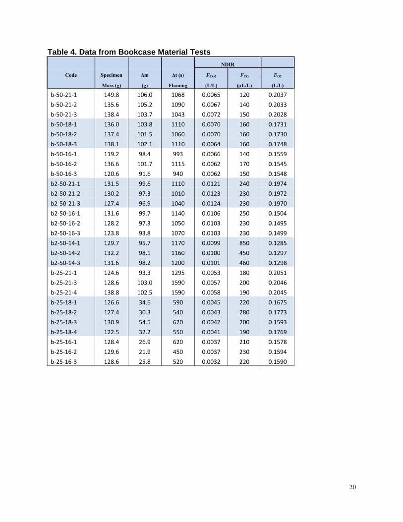
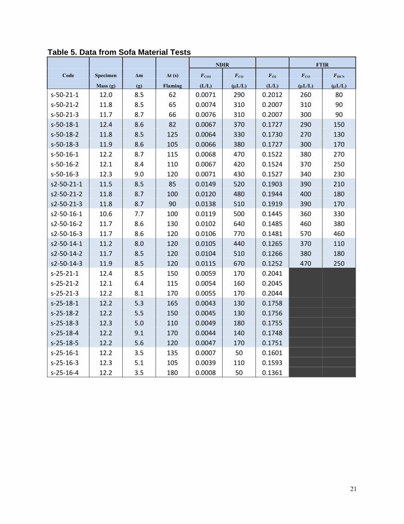
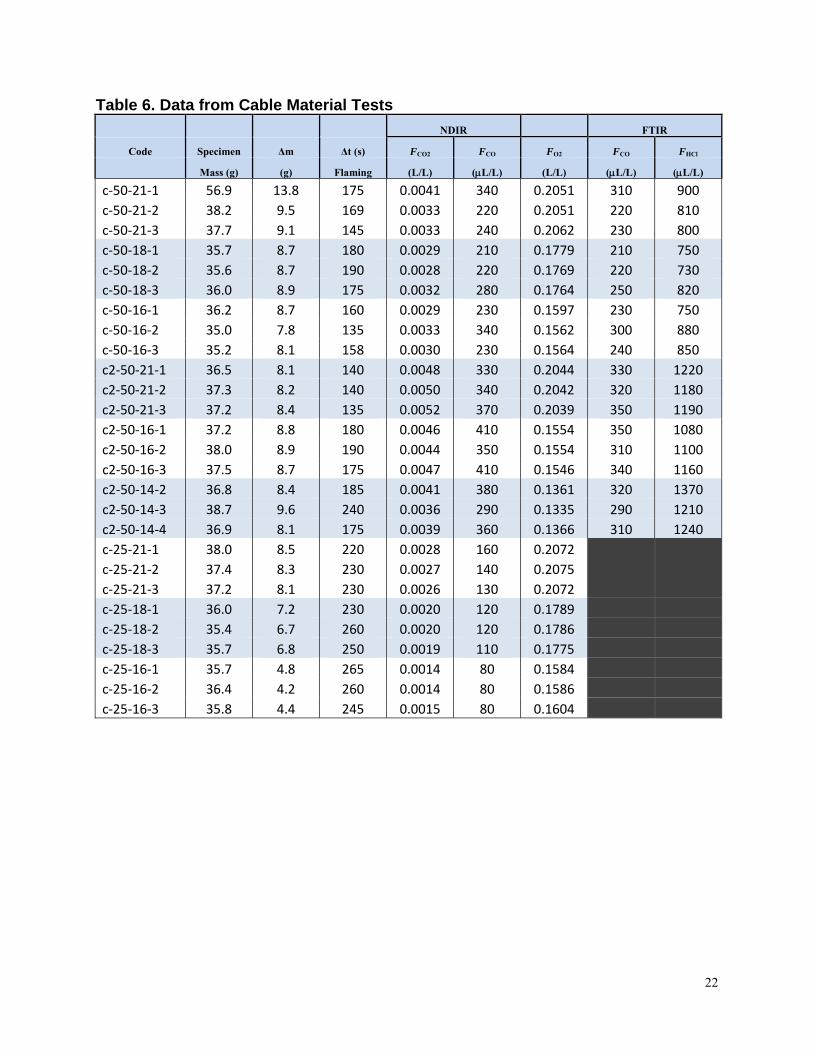
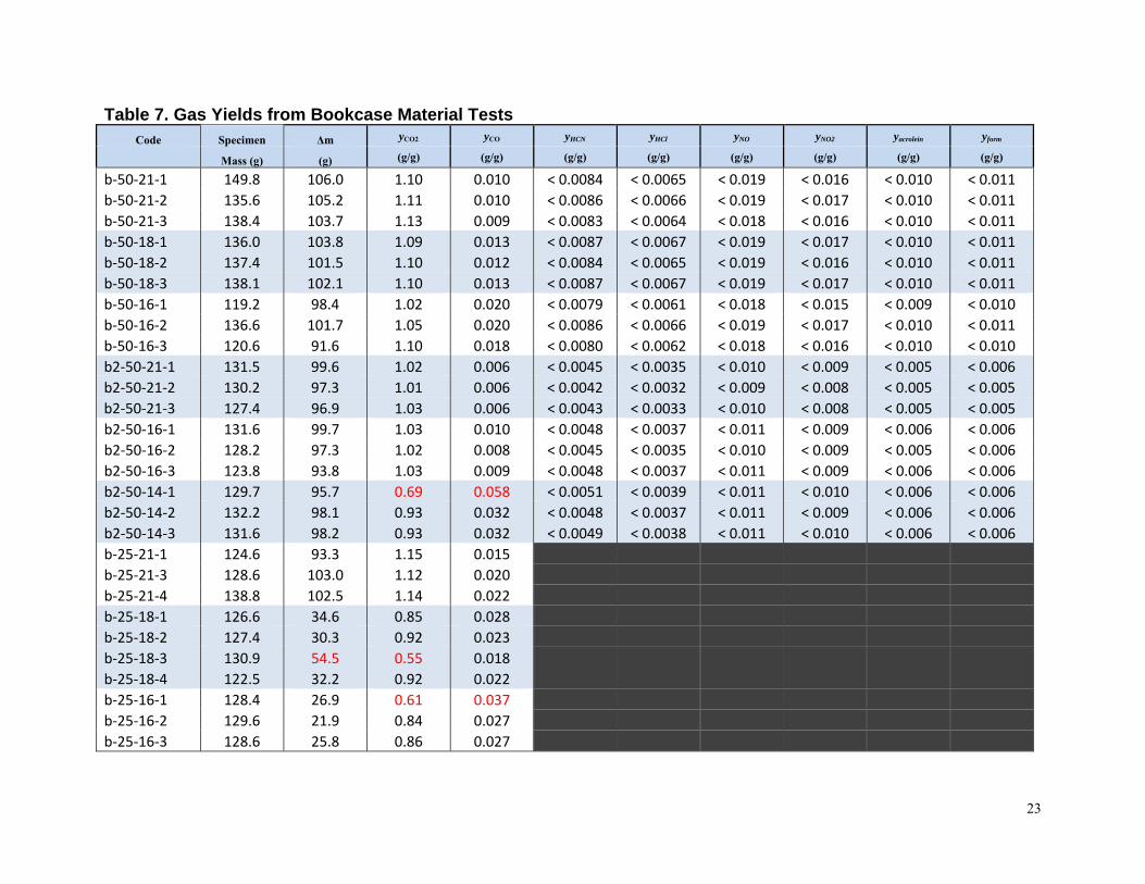
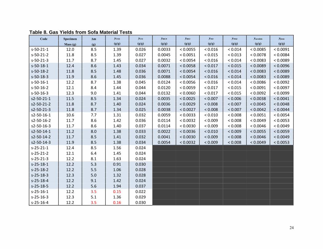
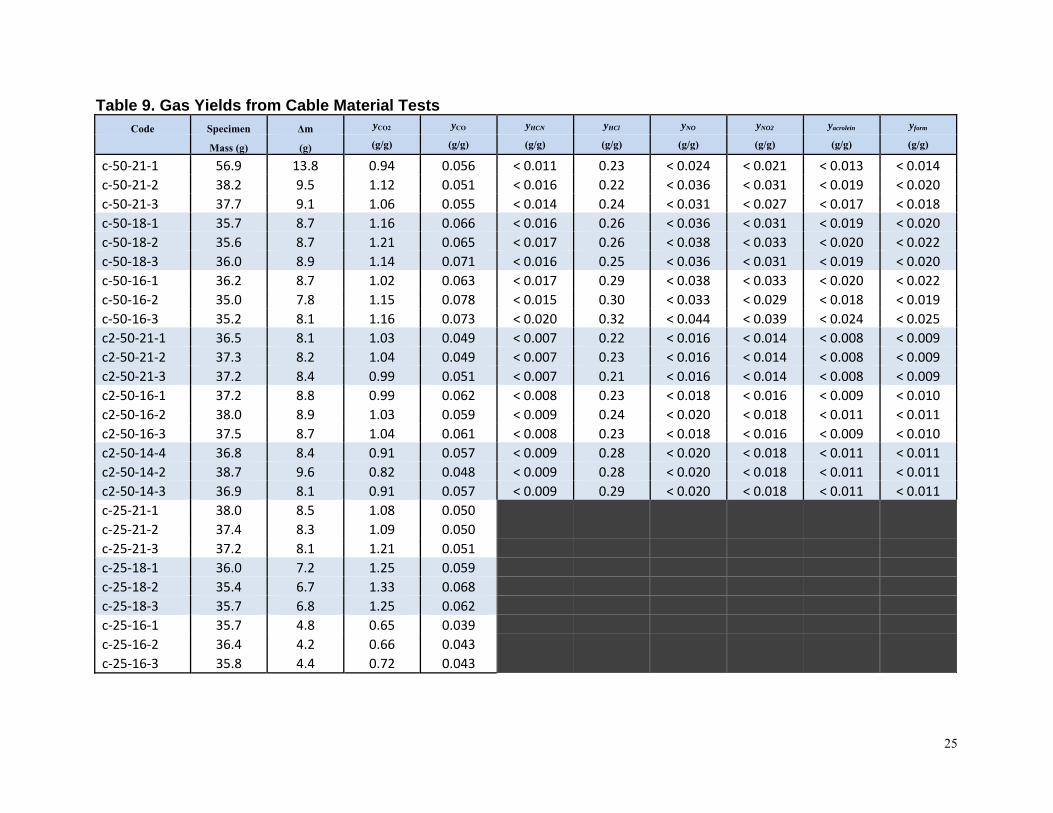
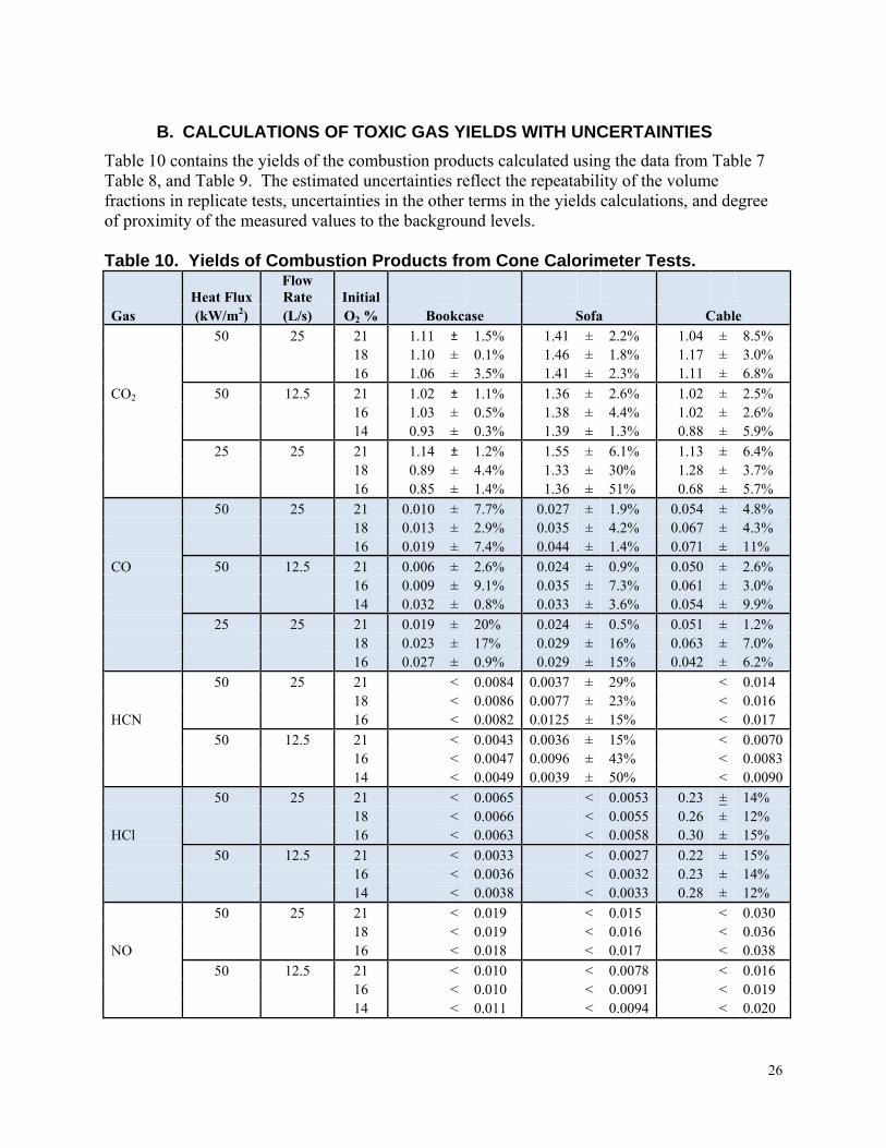
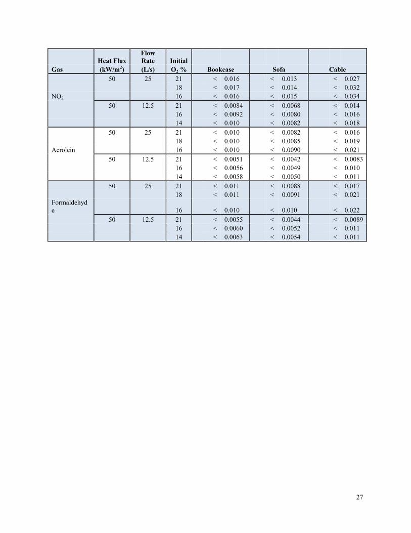
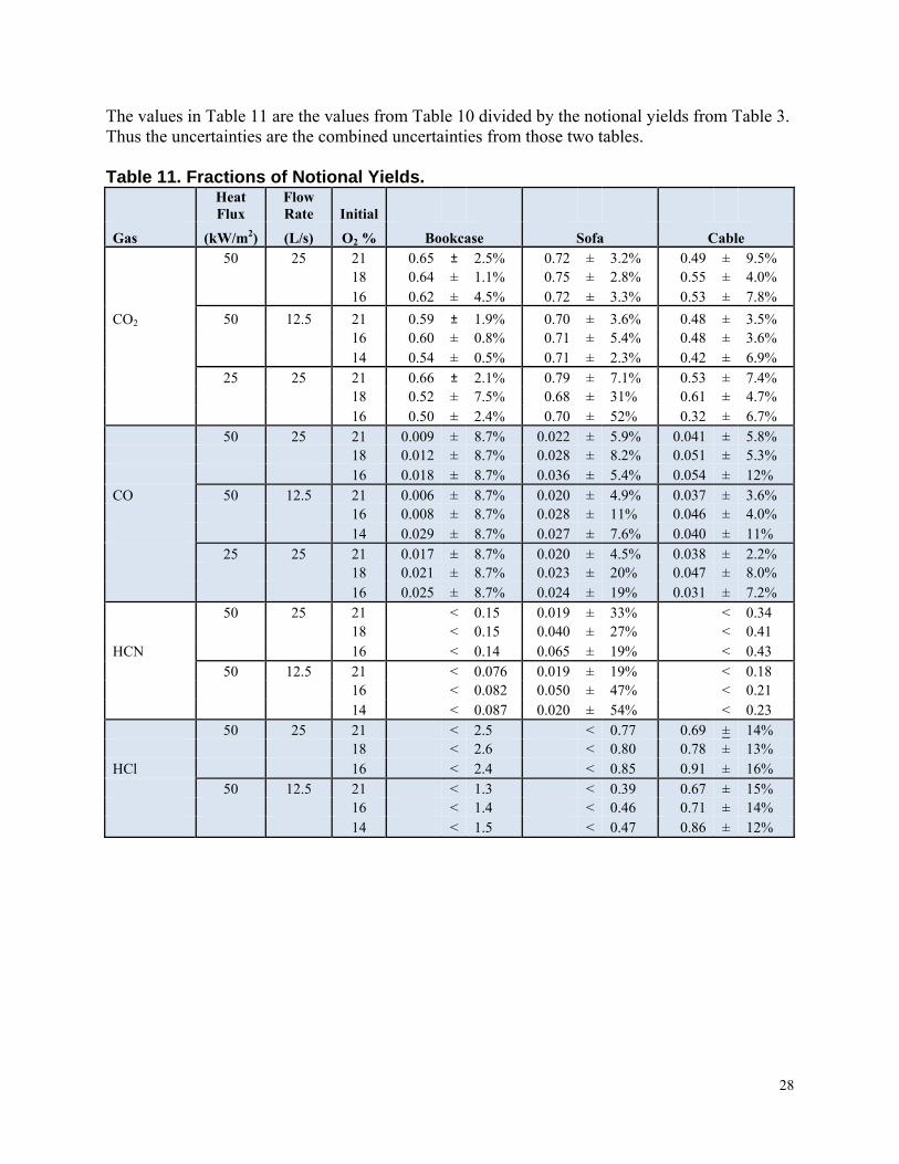
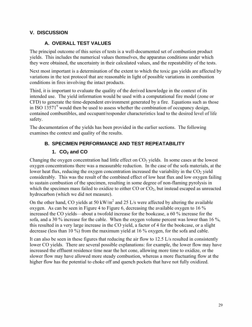
0
0005
001
0015
002
0025
003
0035
CO
Yield
(g g)
10 12 14 16 18 20 22
O2 by Volume
Figure 4 Effect of Oxygen Concentration on CO Yields Bookcase (dashed line = reduced flow) Error bars are plusmn the standard deviation of yields from multiple runs
005
004
CO
Yield
(g g)
10 12 14 16 18 20 22
003
002
001
0
O2 by Volume
Figure 5 Effect of Oxygen Concentration on CO Yields Sofa (dashed line = reduced flow) Error bars are plusmn the standard deviation of yields from multiple runs
30
0
001
002
003
004
005
006
007
008
009
CO
Yield
(g g)
10 12 14 16 18 20 22
O2 by Volume
Figure 6 Effect of Oxygen Concentration on CO Yields Cable (dashed line = reduced flow) Error bars are plusmn the standard deviation of yields from multiple runs
2 HCl and HCN
HCN was detected via FTIR and was only observed in the sofa material tests Figure 7 shows the calculated volume fraction from the FTIR spectra for each of 3 experiments all conducted at 50 kWm2 125 Ls flow and 16 oxygen by volume The three superimposed plots have been time shifted so that the time of ignition is normalized One of the runs (circles) ultimately resulted in a calculated yield roughly half of the other two resulting in a large variability of 33 (see Table 10) If this run is discarded then the reported yield of HCN at this condition should be 00114 with an uncertainty of 02
It is also worth noting that the total time for combustion extended to about 120 s on the scale in Figure 7 Other combustion products continue to be observed in this time period In other words the bulk of the HCN is produced early in the combustion process
Figure 8 shows the results as yields for the generation of HCN at different oxygen volume fractions As with the CO there is linear increase in HCN yields as the oxygen volume fraction decreases from 021 to 016 but at the lowest oxygen volume fraction the yield of HCN is quite low Another important consideration for Figure 8 is that if the outlier run is excluded then the results from the 125 Ls experiments are much closer to the 25 Ls ones although still slightly lower The outlier was included because we feel it is representative of the variability of this measurement
31
0
50
100
150
200
250
300
350
400
450
500
30 50 70 90 110 130 150
HCN
Volume Fraction
(LL)
Test Time (sec)
Figure 7 HCN Volume Fractions Sofa 50 kWm2 125 Ls 16 O2 by Volume Uncertainty is 10 of the Reported HCN Volume Fraction
0014
0012
HCN
Yield
(gg) 0010
0008
0006
0004
0002
0000
O2 by Volume
10 12 14 16 18 20 22
Figure 8 Effect of Oxygen Concentration on HCN Yields Sofa Error bars are plusmn the standard deviation of yields from multiple runs
32
HCl was detected via FTIR and was only observed in the cable tests Figure 9 shows the calculated volume fraction from the FTIR spectra for each of 3 experiments all conducted at 50 kWm2 125 Ls flow and 16 oxygen by volume The three superimposed plots have been time shifted so that the time of ignition is normalized The 3 runs are quite consistent and numerically have a variability in yield of 38 This is despite the fact that there is some variability in the timing of the release of HCl lasting approximately 20 s longer for one of the experiments (diamonds in the figure) In other words the measured volume fraction at any one time is more variable than the integrated quantity
0
200
400
600
800
1000
1200
1400
30 80 130 180 230 280
HCl Volume Fraction
(LL)
Test Time (sec)
Figure 9 HCl Volume Fractions Cable 50 kWm2 125 Ls 16 O2 by Volume Uncertainty is 10 of the Reported Volume Fraction
Figure 10 shows the effect of oxygen concentration on the yields of HCl from the cable materials The yields are somewhat higher at lower oxygen concentrations but this may be accounted for by a slightly lower total mass lostmdashif disproportionately more of the carbon remains in the char At the lowest oxygen volume fraction 014 the yield of HCl increases by about 20
33
000
005
010
015
020
025
030
035
10 12 14 16 18 20 22
HCl Yield
(g g)
O2 by Volume
Figure 10 Effect of Oxygen Concentration on Yields of HCl Cables Error bars are plusmn the standard deviation of yields from multiple runs
C MEASURED VS NOTIONAL VALUES
During sustained and complete combustion the yield of CO2 should approach its notional values since CO2 is a marker for combusted carbon In these experiments the sofa material came out best achieving over 70 of the notional yield The bookcase fared slightly worse achieving only 65 of the notional yield for CO2 and the cable had the lowest at around half The relatively lower yields of CO2 from the cables is an expected result of flame inhibition due to the chlorine These trends are consistent with our qualitative observation of for example the thickness of the smoke produced
The yields of CO from all the specimens ranged from about 001 to 006 which corresponds to 1 to 5 of the notional values These values are consistent with relatively fuel-lean combustion34 and are an order of magnitude lower than the CO yields expected of postflashover fires14
The yields of HCl from the cable specimens approach their notional values The deficit may reflect scavenging by the calcium carbonate filler in the cable jacket or wall loss in the duct or sampling line
The detection limited yields of HCl from the sofa specimens was 80 of the notional yield at the higher flow rate and 40 of the notional yield at the lower flow rate The detection limited yield of HCl from the bookcase was 25 and 15 times the notional yield for the high and low flows respectively Chlorine is present at well under one percent by mass in these two products Such small quantities are not capable of producing toxicologically significant yields of HCl suggesting that they can be either ruled out by elemental analysis as unimportant or that limits of detection are not a barrier to measuring significant quantities of HCl in this apparatus
34
Yields of HCN from the sofa are between 2 and 6 of their notional values The highest relative yield is found at 16 oxygen by volume Despite the lower oxygen these flames appear relatively fuel-lean and the nitrogen may appear as molecular nitrogen or nitrogen dioxides
D SPECIES SAMPLING AND MEASUREMENT
1 Species Measurement Using FTIR Spectroscopy
FTIR spectroscopic analysis of combustion products has become fairly common in fire research laboratories However that does not mean that its use is straightforward The data from a recent round robin involving FTIR measurement of toxic combustion products from a standardized apparatus showed interlaboratory variations of up to an order of magnitude There are documents under development in ISO TC92 SC1 and SC3 to standardize the implementation
We were able to obtain usable information using this technique There are a number of lessons emerging from this test series that can provide useful input to these efforts such as the following
The application of FTIR spectroscopy to fire testing requires the constant attention of an experienced professional at a level well beyond the demands of the more traditional fire test instrumentation
In this work we used a longer path length cell than in previous work However the increased sensitivity was offset by the instantaneous nature of the measurements (as opposed to averaging over dozens of data points) and the fact that the gases did not accumulate as they do in the closed chamber tests such as NFPA 269 and NFPA 270 (toxicity test method and smoke density chamber respectively) The CO concentrations measured here are approximately one-tenth of those measured in the closed-chamber apparatus However non-linear effects resulted in a 25 deficit compared to the NDIR measurements of CO at the highest concentrations
The cell volume remained small and provided good time resolution For example the measured HCl concentrations go from zero to the maximum in two data intervals (see Figure 9)
The lack of a filter did not adversely affect the measurements Compared to previous work with other apparatus the smoke measured here was relatively dilute The cell only required cleaning a few times over the course of all of the experiments reported here The internal mirrors were easily cleaned with ethanol and deionized water The KBr windows were replaced once
A heated sample line (as recommended in the SAFIR report35 and ISO 1970236) enabled near-quantitative collection of HCl a compound that is generally regarded as difficult to determine
E IMPORTANCE OF UNDETECTED GASES
The equations in ISO 13571 include provision for additional gases to be included in estimating the time available for escape or refuge from a fire HBr HF SO2 NO2 acrolein (C3H4O) and formaldehyde (H2CO) There was no Br F or S in any of the products examined in this project
35
so the first three of these gases were not expected The presence of the latter three was not detected thus establishing the upper limits of their presence at the volume fractions listed in Table 2
To put the potential contributions of the sensory irritant gases (HCl NO2 acrolein and formaldehyde) in context we use the equations in ISO 13571 for calculating the Fractional Effective Dose (FED) for the narcotic gases CO2 and CO and the Fractional Effective Concentration (FEC) for the four sensory irritant gases
The FED equation is
CO2exp 5t 2 t 2 236
CO HCNFED t 6 t
t1 35000 t1 12 10 where Δt is the exposure interval in minutes
The FEC of the four irritant gases were estimated from their volume fractions and the incapacitating levels in ISO 13571 (FHCl etc) The results are compiled in Table 12
The FEC equation in ISO 13571 is
HCl HBr HF SO2 NO 2 acrolein formaldehyde irritant FEC = F F F F F F F FHCl HBr HF SO NO acrolein formaldehyde Ci2 2
Table 12 Limits of importance of undetected toxins
Volume fraction (μLL) FEC Contribution
HCl NO2 C3H4O H2CO HCl NO2 C3H4O H2CO Incapacitating Level 1000 250 30 250 Bookcase lt 20 lt 40 lt 20 lt 40 lt 002 lt 016 lt 066 lt 016 Sofa lt 20 lt 40 lt 20 lt 40 lt 002 lt 016 lt 066 lt 016
Cable 1370 lt 40 lt 20 lt 40 058 lt 007 lt 028 lt 007 to 730 lt 40 lt 20 lt 40 043 lt 009 lt 039 lt 009
It stands out that the FEC contribution from acrolein is as much as two-thirds of an incapacitating level This is because (a) the limit of detection is close to the listed incapacitating level and (b) the incapacitating level is very low While there is agreement among experts that this value of 30 μLL is reasonable there are data that suggest strongly that this is unnecessarily conservative Kaplan and co-workers exposed individual baboons to various concentrations of acrolein in air37 At the end of 5 min each baboon was given a signal and could perform an action that led to escape from the test chamber The baboons exposed at up to 500 μLL escaped and survived Those exposed to higher levels escaped but died later These data suggest that people should be able to accommodate a nearly instantaneous exposure to eg at least 300 μLL without becoming incapacitated If we increase the incapacitating level of acrolein to 250 μLL the relative contribution to FEC become those in Table 13 In this case the relative importance of acrolein falls below 01 when other irritants are detected
36
Table 13 Limits of Importance of Undetected Toxicants Volume fraction (μLL) FEC Contribution
HCl NO2 C3H4O H2CO HCl NO2 C3H4O H2CO Incapacitating Level 1000 250 250 250 Bookcase lt 20 lt 40 lt 20 lt 40 lt 005 lt 038 lt 019 lt 038 Sofa lt 20 lt 40 lt 20 lt 40 lt 005 lt 038 lt 019 lt 038 Cable 1370 lt 40 lt 20 lt 40 077 lt 009 lt 005 lt 009
to 730 lt 40 lt 20 lt 40 065 lt 014 lt 007 lt 014
Where specimens like the bookcase and sofa produce narcotic gases CO and HCN and irritants are below the limits of detection the narcotic gases are the primary contributors to incapacitation Assuming that the irritant gases are present in just under the limits of detection in order for them to reach an incapacitating concentration the relative concentration of CO would be incapacitating in a few minutes the relative concentration of HCN would be incapacitating in under a minute
37
This page intentionally left blank
38
VI CONCLUSIONS
This paper reports toxic gas yield data for specimens cut from three complex combustibles a bookcase a sofa and residential electrical power cable The physical fire model used was the cone calorimeter from ISO 5660-1 ASTM E 1354 This apparatus allows the use of a test specimen that approximates the geometry and radiant exposure that might be experienced by the intact combustible in a well-ventilated flaming fire In addition to performing the tests as prescribed in the standards this work added an enclosure and a gas supply capable of reduced oxygen in order to better approximate conditions in an underventilated fire
For the standard test procedure
The CO2 yields were very repeatable and represented between half and 80 of the carbon in the specimens All specimens left a black residue that continued to pyrolyze after the flaming halted These residues were presumably carbon-enriched accounting for the yields being below the notional yields
The CO yields were also very repeatable with the exception of the bookcase at low heat flux and the higher oxygen concentrations
The HCN yields were below the limit of detection for the bookcase and cable specimens The HCN yields from the sofa were 3 to 10 times the limit of detection and had a variation in repeatability between 5 and 40 of the reported yield depending on the test conditions
The HCl yields were below the limit of detection for the bookcase and sofa specimens For the cables they were well above the limit of detection and accounted for 70 of the Cl in the specimens
None of the other irritant gases appeared in concentrations above their limits of detection
Regarding the variation in test conditions we conclude
An incident heat flux of 25 kWm2 does not provide any information beyond that which is found at 50 kWm2 In fact it leads to increased variability from test to test because of slow ignition or early extinction
The trend of toxic gas yields increasing with decreasing initial oxygen concentration holds uniformly across gases and specimen types over the oxygen volume fraction range of 021 to 016 When the oxygen volume fraction is 014 the results are unpredictable for both gases and items burned Therefore we donrsquot recommend testing at this level With the exception of CO from the bookcase the majority of the CO yields were lower at 014 than at 016
Reducing the total flow to 125 Ls reduces the limit of detection of the gases by a factor of two and allows the achievement of lower oxygen concentrations However yields measured at the lower flow were consistently lower than at the higher flow
Calculation of the contributions of the gases to incapacitation of people who might be exposed to these environments showed
Incapacitation from the bookcase material effluent would be primarily from CO
39
Incapacitation from the sofa material effluent would be from a combination of CO and HCN
Incapacitation from the cable effluent would be initially from HCl the related yield of CO would become incapacitating after approximately15 minutes
If the CO yield were at the expected postflashover value of 02
Incapacitation from the bookcase material effluent would be primarily from CO
Incapacitation from the sofa material effluent would be primarily from CO
Incapacitation from the cable material effluent would be initially from HCl a 02 yield of CO would become incapacitating after a few minutes
VII ACKNOWLEDGEMENTS
The authors express their appreciation to Randy Shields for his assistance in performing the tests
40
References
1 Phillips WGB Beller DK and Fahy RF ldquoComputer Simulation for Fire Protection Engineeringrdquo Chapter 5-9 in SFPE Handbook of Fire Protection Engineering 4th Edition PJ DiNenno et al eds NFPA International Quincy MA 2008
2 httpwwwnistgovelfire_researchcfastcfm
3 Peacock RD Jones WW and Reneke PA ldquoCFASTmdashConsolidated Model of Fire Growth and Smoke Transport (Version 6) Software Development and Evaluation Guiderdquo NIST Special Publication 1086 National Institute of Standards and Technology Gaithersburg MD 187 pages (2008)
4 Peacock RD Jones WW and Bukowski RW ldquoVerification of a Model of Fire and Smoke Transportrdquo Fire Safety Journal 21 89-129 (1993)
5 httpfirenistgovfds
6 ldquoStandard Test Method for Heat and Visible Smoke Release Rates for Materials and Products Using an Oxygen Consumption Calorimeterrdquo ASTM E1354-04a ASTM International West Conshohocken PA 2004
7 See eg ldquoStandard for the Flammability (Open Flame) of Mattress Setsrdquo 16 CFR Part 1633 Federal Register 70 (50) 13471-13523 2006
8httpwwwisoorgisoiso_cataloguecatalogue_tccatalogue_tc_browsehtmcommid=50540amp published=onampdevelopment=on
9 ldquoLife-threatening Components of Fire ndash Guidelines for the Estimation of Time to Compromised Tenability in Firesrdquo ISO 13571 International Standards Organization Geneva 2012
10 Guidelines for Assessing the Fire Threat to People ISO 19706 International Standards Organization Geneva 2011
11 Gann RG Babrauskas V Peacock RD and Hall Jr JR Fire Conditions for Smoke Toxicity Measurement Fire and Materials 18 193-199 (1994)
12 Guidance for Comparison of Toxic Gas Data between Different Physical Fire Models and Scales ISO 29903 International Standards Organization Geneva 2012
13 ldquoStandard Test Method for Developing Toxic Potency Data for Use in Fire Hazard Modelingrdquo NFPA 269 NFPA International Quincy MA 2012
14 ldquoStandard Test Method for Measuring Smoke Toxicity for Use in Fire Hazard Analysisrdquo ASTM E1678-10 ASTM International West Conshohocken PA 2010
15 (a) Gann RG Averill JD Nyden MR Johnsson EL and Peacock RD ldquoSmoke Component Yields from Room-scale Fire Testsrdquo NIST Technical Note 1453 National Institute of Standards and Technology Gaithersburg MD 159 pages (2003)
(b) Gann RG Averill JD Nyden MR Johnsson EL and Peacock RD ldquoFire Effluent Component Yields from Room-scale Fire Testsrdquo Fire and Materials 34 285-314 (2010) DOI 101002fam1024
41
16 Ohlemiller TJ and Villa K ldquoFurniture Flammability An Investigation of the California Bulletin 133 Test Part II Characterization of the Ignition Source and a Comparable Gas Burnerrdquo NISTIR 4348 National Institute of Standards and Technology Gaithersburg MD 1990
17 Gann RG Marsh ND Averill JA and Nyden MR ldquoSmoke Component Yields from Bench-scale Fire Tests 1 NFPA 269ASTM E 1678rdquo NIST Technical Note 1760 National Institute of Standards and Technology Gaithersburg MD 57 pages (2013)
18 Kaplan HL Grand AF and Hartzell GE Combustion Toxicology Principles and Test Methods Technology Publishing Co Lancaster PA 1983
19 Guidance for Evaluating the Validity of Physical Fire Models for Obtaining Fire Effluent Toxicity Data for Use in Fire Hazard and Risk Assessment ndash Part 2 Evaluation of Individual Physical Fire Models ISOTR 16312-2 International Standards Organization Geneva 2007
20 Controlled Equivalence Ratio Method for the Determination of the Hazardous Components of Fire Effluent ISOTS 19700 International Standards Organization 2010
21 Reaction-to-fire Tests ndash Heat Release Smoke Production and Mass Loss Rates ndash Part 1 Heat Release (Cone Calorimeter Method) ISO 5660-1 International Standards Organization Geneva 2002
22 Plastics mdash Smoke Generation mdash Part 2 Determination of Optical Density by a Single-chamber Test ISO 5659-2 International standards Organization Geneva 1994
23 Marsh ND Gann RG and Nyden MR ldquoSmoke Component Yields from Bench-scale Fire Tests 2 ISO 19700 Controlled Equivalence Ratio Tube Furnacerdquo NIST Technical Note 1761 National Institute of Standards and Technology Gaithersburg MD 45 pages (2013)
24 Marsh ND Gann RG and Nyden MR ldquoObservations on the Generation of Toxic Products in the NFPAISO Smoke Density Chamberrdquo Proceedings of the 12th International Conference on Fire Science amp Engineering (Interflam 2010) Nottingham UK (2010)
25 Mulholland G Janssens M Yusa S Twilley W and Babrauskas VrdquoThe effect of oxygen concentration on CO and Smoke Produced by Flamesrdquo Proceedings of the Third International Symposium on Fire Safety Science Edinburgh UK pp 585-594 (1991) doi103801IAFSSFSS3-585
26 Babrauskas V Twilley WH Janssens M and Yusa S ldquoA cone calorimeter for controlled-atmosphere studiesrdquo Fire and Materials 16 37-43 (1992)
27 Hshieh FY Motto SE Hirsch DB and Beeson HD ldquoFlammability Testing Using a Controlled-atmosphere Cone Calorimeterrdquo Proceedings of the 18th International Conference on Fire Safety Science Millbrae CA p 999 (1993)
28 Gomez C Janssens M and Zalkin A ldquoUsing the Cone Calorimeter for Quantifying Toxic Potencyrdquo Proceedings of the 12th International Fire Science amp Engineering Conference (Interflam 10) Nottingham UK (2010)
42
29 Gomez C Janssens M and Zalkin A ldquoMeasuring the Yields of Toxic Gases from Materials during Different Stages of Fire Developmentrdquo In Fire and Materials 12 international conference San Francisco CA (2011)
30 Guillaume E Marquis DM and Chivas-Joly C ldquoUsage of Controlled-atmosphere Cone Calorimeter to Provide Input Data for Toxicity Modelingrdquo in Fire and Materials 12 International Conference San Francisco CA (2011)
31 Haaland DM Easterling RG and Vopicka DA ldquoMultivariate Least-Squares Methods Applied to the Quantitative Spectral Analysis of Multicomponent Samplesrdquo Applied Spectroscopy 39 73-84 (1985) doi1013660003702854249376
32 Gas Phase Infrared Spectral Standards Revision B Midac Corp Irvine CA (1999)
33 Speitel LC ldquoFourier Transform Infrared Analysis of Combustion Gasesrdquo Federal Aviation Administration Report DOTFAAAR-0188 2001
34 Pitts WM The Global Equivalence Ratio Concept and the Formations Mechanisms of Carbon Monoxide in Fires Progress in Energy and Combustion Science 21 197-237 (1995)
35 Smoke Gas Analysis by Fourier Transform Infrared Analysis The SAFIR Project VTT Research Note Technical Research Centre of Finland 81 Pages 1999
36 ldquoToxicity testing of fire effluents -- Guidance for analysis of gases and vapours in fire effluents using FTIR gas analysisrdquo ISO 19702 International Standards Organization Geneva 2006
37 Kaplan HL Grand AF Switzer WG Mitchell DS Rogers WR and Hartzell GE Effects of Combustion Gases on Escape Performance of the Baboon and the Rat Journal of Fire Sciences 3 228-244 (1985)
43
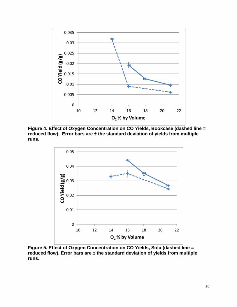
0
001
002
003
004
005
006
007
008
009
CO
Yield
(g g)
10 12 14 16 18 20 22
O2 by Volume
Figure 6 Effect of Oxygen Concentration on CO Yields Cable (dashed line = reduced flow) Error bars are plusmn the standard deviation of yields from multiple runs
2 HCl and HCN
HCN was detected via FTIR and was only observed in the sofa material tests Figure 7 shows the calculated volume fraction from the FTIR spectra for each of 3 experiments all conducted at 50 kWm2 125 Ls flow and 16 oxygen by volume The three superimposed plots have been time shifted so that the time of ignition is normalized One of the runs (circles) ultimately resulted in a calculated yield roughly half of the other two resulting in a large variability of 33 (see Table 10) If this run is discarded then the reported yield of HCN at this condition should be 00114 with an uncertainty of 02
It is also worth noting that the total time for combustion extended to about 120 s on the scale in Figure 7 Other combustion products continue to be observed in this time period In other words the bulk of the HCN is produced early in the combustion process
Figure 8 shows the results as yields for the generation of HCN at different oxygen volume fractions As with the CO there is linear increase in HCN yields as the oxygen volume fraction decreases from 021 to 016 but at the lowest oxygen volume fraction the yield of HCN is quite low Another important consideration for Figure 8 is that if the outlier run is excluded then the results from the 125 Ls experiments are much closer to the 25 Ls ones although still slightly lower The outlier was included because we feel it is representative of the variability of this measurement
31
0
50
100
150
200
250
300
350
400
450
500
30 50 70 90 110 130 150
HCN
Volume Fraction
(LL)
Test Time (sec)
Figure 7 HCN Volume Fractions Sofa 50 kWm2 125 Ls 16 O2 by Volume Uncertainty is 10 of the Reported HCN Volume Fraction
0014
0012
HCN
Yield
(gg) 0010
0008
0006
0004
0002
0000
O2 by Volume
10 12 14 16 18 20 22
Figure 8 Effect of Oxygen Concentration on HCN Yields Sofa Error bars are plusmn the standard deviation of yields from multiple runs
32
HCl was detected via FTIR and was only observed in the cable tests Figure 9 shows the calculated volume fraction from the FTIR spectra for each of 3 experiments all conducted at 50 kWm2 125 Ls flow and 16 oxygen by volume The three superimposed plots have been time shifted so that the time of ignition is normalized The 3 runs are quite consistent and numerically have a variability in yield of 38 This is despite the fact that there is some variability in the timing of the release of HCl lasting approximately 20 s longer for one of the experiments (diamonds in the figure) In other words the measured volume fraction at any one time is more variable than the integrated quantity
0
200
400
600
800
1000
1200
1400
30 80 130 180 230 280
HCl Volume Fraction
(LL)
Test Time (sec)
Figure 9 HCl Volume Fractions Cable 50 kWm2 125 Ls 16 O2 by Volume Uncertainty is 10 of the Reported Volume Fraction
Figure 10 shows the effect of oxygen concentration on the yields of HCl from the cable materials The yields are somewhat higher at lower oxygen concentrations but this may be accounted for by a slightly lower total mass lostmdashif disproportionately more of the carbon remains in the char At the lowest oxygen volume fraction 014 the yield of HCl increases by about 20
33
000
005
010
015
020
025
030
035
10 12 14 16 18 20 22
HCl Yield
(g g)
O2 by Volume
Figure 10 Effect of Oxygen Concentration on Yields of HCl Cables Error bars are plusmn the standard deviation of yields from multiple runs
C MEASURED VS NOTIONAL VALUES
During sustained and complete combustion the yield of CO2 should approach its notional values since CO2 is a marker for combusted carbon In these experiments the sofa material came out best achieving over 70 of the notional yield The bookcase fared slightly worse achieving only 65 of the notional yield for CO2 and the cable had the lowest at around half The relatively lower yields of CO2 from the cables is an expected result of flame inhibition due to the chlorine These trends are consistent with our qualitative observation of for example the thickness of the smoke produced
The yields of CO from all the specimens ranged from about 001 to 006 which corresponds to 1 to 5 of the notional values These values are consistent with relatively fuel-lean combustion34 and are an order of magnitude lower than the CO yields expected of postflashover fires14
The yields of HCl from the cable specimens approach their notional values The deficit may reflect scavenging by the calcium carbonate filler in the cable jacket or wall loss in the duct or sampling line
The detection limited yields of HCl from the sofa specimens was 80 of the notional yield at the higher flow rate and 40 of the notional yield at the lower flow rate The detection limited yield of HCl from the bookcase was 25 and 15 times the notional yield for the high and low flows respectively Chlorine is present at well under one percent by mass in these two products Such small quantities are not capable of producing toxicologically significant yields of HCl suggesting that they can be either ruled out by elemental analysis as unimportant or that limits of detection are not a barrier to measuring significant quantities of HCl in this apparatus
34
Yields of HCN from the sofa are between 2 and 6 of their notional values The highest relative yield is found at 16 oxygen by volume Despite the lower oxygen these flames appear relatively fuel-lean and the nitrogen may appear as molecular nitrogen or nitrogen dioxides
D SPECIES SAMPLING AND MEASUREMENT
1 Species Measurement Using FTIR Spectroscopy
FTIR spectroscopic analysis of combustion products has become fairly common in fire research laboratories However that does not mean that its use is straightforward The data from a recent round robin involving FTIR measurement of toxic combustion products from a standardized apparatus showed interlaboratory variations of up to an order of magnitude There are documents under development in ISO TC92 SC1 and SC3 to standardize the implementation
We were able to obtain usable information using this technique There are a number of lessons emerging from this test series that can provide useful input to these efforts such as the following
The application of FTIR spectroscopy to fire testing requires the constant attention of an experienced professional at a level well beyond the demands of the more traditional fire test instrumentation
In this work we used a longer path length cell than in previous work However the increased sensitivity was offset by the instantaneous nature of the measurements (as opposed to averaging over dozens of data points) and the fact that the gases did not accumulate as they do in the closed chamber tests such as NFPA 269 and NFPA 270 (toxicity test method and smoke density chamber respectively) The CO concentrations measured here are approximately one-tenth of those measured in the closed-chamber apparatus However non-linear effects resulted in a 25 deficit compared to the NDIR measurements of CO at the highest concentrations
The cell volume remained small and provided good time resolution For example the measured HCl concentrations go from zero to the maximum in two data intervals (see Figure 9)
The lack of a filter did not adversely affect the measurements Compared to previous work with other apparatus the smoke measured here was relatively dilute The cell only required cleaning a few times over the course of all of the experiments reported here The internal mirrors were easily cleaned with ethanol and deionized water The KBr windows were replaced once
A heated sample line (as recommended in the SAFIR report35 and ISO 1970236) enabled near-quantitative collection of HCl a compound that is generally regarded as difficult to determine
E IMPORTANCE OF UNDETECTED GASES
The equations in ISO 13571 include provision for additional gases to be included in estimating the time available for escape or refuge from a fire HBr HF SO2 NO2 acrolein (C3H4O) and formaldehyde (H2CO) There was no Br F or S in any of the products examined in this project
35
so the first three of these gases were not expected The presence of the latter three was not detected thus establishing the upper limits of their presence at the volume fractions listed in Table 2
To put the potential contributions of the sensory irritant gases (HCl NO2 acrolein and formaldehyde) in context we use the equations in ISO 13571 for calculating the Fractional Effective Dose (FED) for the narcotic gases CO2 and CO and the Fractional Effective Concentration (FEC) for the four sensory irritant gases
The FED equation is
CO2exp 5t 2 t 2 236
CO HCNFED t 6 t
t1 35000 t1 12 10 where Δt is the exposure interval in minutes
The FEC of the four irritant gases were estimated from their volume fractions and the incapacitating levels in ISO 13571 (FHCl etc) The results are compiled in Table 12
The FEC equation in ISO 13571 is
HCl HBr HF SO2 NO 2 acrolein formaldehyde irritant FEC = F F F F F F F FHCl HBr HF SO NO acrolein formaldehyde Ci2 2
Table 12 Limits of importance of undetected toxins
Volume fraction (μLL) FEC Contribution
HCl NO2 C3H4O H2CO HCl NO2 C3H4O H2CO Incapacitating Level 1000 250 30 250 Bookcase lt 20 lt 40 lt 20 lt 40 lt 002 lt 016 lt 066 lt 016 Sofa lt 20 lt 40 lt 20 lt 40 lt 002 lt 016 lt 066 lt 016
Cable 1370 lt 40 lt 20 lt 40 058 lt 007 lt 028 lt 007 to 730 lt 40 lt 20 lt 40 043 lt 009 lt 039 lt 009
It stands out that the FEC contribution from acrolein is as much as two-thirds of an incapacitating level This is because (a) the limit of detection is close to the listed incapacitating level and (b) the incapacitating level is very low While there is agreement among experts that this value of 30 μLL is reasonable there are data that suggest strongly that this is unnecessarily conservative Kaplan and co-workers exposed individual baboons to various concentrations of acrolein in air37 At the end of 5 min each baboon was given a signal and could perform an action that led to escape from the test chamber The baboons exposed at up to 500 μLL escaped and survived Those exposed to higher levels escaped but died later These data suggest that people should be able to accommodate a nearly instantaneous exposure to eg at least 300 μLL without becoming incapacitated If we increase the incapacitating level of acrolein to 250 μLL the relative contribution to FEC become those in Table 13 In this case the relative importance of acrolein falls below 01 when other irritants are detected
36
Table 13 Limits of Importance of Undetected Toxicants Volume fraction (μLL) FEC Contribution
HCl NO2 C3H4O H2CO HCl NO2 C3H4O H2CO Incapacitating Level 1000 250 250 250 Bookcase lt 20 lt 40 lt 20 lt 40 lt 005 lt 038 lt 019 lt 038 Sofa lt 20 lt 40 lt 20 lt 40 lt 005 lt 038 lt 019 lt 038 Cable 1370 lt 40 lt 20 lt 40 077 lt 009 lt 005 lt 009
to 730 lt 40 lt 20 lt 40 065 lt 014 lt 007 lt 014
Where specimens like the bookcase and sofa produce narcotic gases CO and HCN and irritants are below the limits of detection the narcotic gases are the primary contributors to incapacitation Assuming that the irritant gases are present in just under the limits of detection in order for them to reach an incapacitating concentration the relative concentration of CO would be incapacitating in a few minutes the relative concentration of HCN would be incapacitating in under a minute
37
This page intentionally left blank
38
VI CONCLUSIONS
This paper reports toxic gas yield data for specimens cut from three complex combustibles a bookcase a sofa and residential electrical power cable The physical fire model used was the cone calorimeter from ISO 5660-1 ASTM E 1354 This apparatus allows the use of a test specimen that approximates the geometry and radiant exposure that might be experienced by the intact combustible in a well-ventilated flaming fire In addition to performing the tests as prescribed in the standards this work added an enclosure and a gas supply capable of reduced oxygen in order to better approximate conditions in an underventilated fire
For the standard test procedure
The CO2 yields were very repeatable and represented between half and 80 of the carbon in the specimens All specimens left a black residue that continued to pyrolyze after the flaming halted These residues were presumably carbon-enriched accounting for the yields being below the notional yields
The CO yields were also very repeatable with the exception of the bookcase at low heat flux and the higher oxygen concentrations
The HCN yields were below the limit of detection for the bookcase and cable specimens The HCN yields from the sofa were 3 to 10 times the limit of detection and had a variation in repeatability between 5 and 40 of the reported yield depending on the test conditions
The HCl yields were below the limit of detection for the bookcase and sofa specimens For the cables they were well above the limit of detection and accounted for 70 of the Cl in the specimens
None of the other irritant gases appeared in concentrations above their limits of detection
Regarding the variation in test conditions we conclude
An incident heat flux of 25 kWm2 does not provide any information beyond that which is found at 50 kWm2 In fact it leads to increased variability from test to test because of slow ignition or early extinction
The trend of toxic gas yields increasing with decreasing initial oxygen concentration holds uniformly across gases and specimen types over the oxygen volume fraction range of 021 to 016 When the oxygen volume fraction is 014 the results are unpredictable for both gases and items burned Therefore we donrsquot recommend testing at this level With the exception of CO from the bookcase the majority of the CO yields were lower at 014 than at 016
Reducing the total flow to 125 Ls reduces the limit of detection of the gases by a factor of two and allows the achievement of lower oxygen concentrations However yields measured at the lower flow were consistently lower than at the higher flow
Calculation of the contributions of the gases to incapacitation of people who might be exposed to these environments showed
Incapacitation from the bookcase material effluent would be primarily from CO
39
Incapacitation from the sofa material effluent would be from a combination of CO and HCN
Incapacitation from the cable effluent would be initially from HCl the related yield of CO would become incapacitating after approximately15 minutes
If the CO yield were at the expected postflashover value of 02
Incapacitation from the bookcase material effluent would be primarily from CO
Incapacitation from the sofa material effluent would be primarily from CO
Incapacitation from the cable material effluent would be initially from HCl a 02 yield of CO would become incapacitating after a few minutes
VII ACKNOWLEDGEMENTS
The authors express their appreciation to Randy Shields for his assistance in performing the tests
40
References
1 Phillips WGB Beller DK and Fahy RF ldquoComputer Simulation for Fire Protection Engineeringrdquo Chapter 5-9 in SFPE Handbook of Fire Protection Engineering 4th Edition PJ DiNenno et al eds NFPA International Quincy MA 2008
2 httpwwwnistgovelfire_researchcfastcfm
3 Peacock RD Jones WW and Reneke PA ldquoCFASTmdashConsolidated Model of Fire Growth and Smoke Transport (Version 6) Software Development and Evaluation Guiderdquo NIST Special Publication 1086 National Institute of Standards and Technology Gaithersburg MD 187 pages (2008)
4 Peacock RD Jones WW and Bukowski RW ldquoVerification of a Model of Fire and Smoke Transportrdquo Fire Safety Journal 21 89-129 (1993)
5 httpfirenistgovfds
6 ldquoStandard Test Method for Heat and Visible Smoke Release Rates for Materials and Products Using an Oxygen Consumption Calorimeterrdquo ASTM E1354-04a ASTM International West Conshohocken PA 2004
7 See eg ldquoStandard for the Flammability (Open Flame) of Mattress Setsrdquo 16 CFR Part 1633 Federal Register 70 (50) 13471-13523 2006
8httpwwwisoorgisoiso_cataloguecatalogue_tccatalogue_tc_browsehtmcommid=50540amp published=onampdevelopment=on
9 ldquoLife-threatening Components of Fire ndash Guidelines for the Estimation of Time to Compromised Tenability in Firesrdquo ISO 13571 International Standards Organization Geneva 2012
10 Guidelines for Assessing the Fire Threat to People ISO 19706 International Standards Organization Geneva 2011
11 Gann RG Babrauskas V Peacock RD and Hall Jr JR Fire Conditions for Smoke Toxicity Measurement Fire and Materials 18 193-199 (1994)
12 Guidance for Comparison of Toxic Gas Data between Different Physical Fire Models and Scales ISO 29903 International Standards Organization Geneva 2012
13 ldquoStandard Test Method for Developing Toxic Potency Data for Use in Fire Hazard Modelingrdquo NFPA 269 NFPA International Quincy MA 2012
14 ldquoStandard Test Method for Measuring Smoke Toxicity for Use in Fire Hazard Analysisrdquo ASTM E1678-10 ASTM International West Conshohocken PA 2010
15 (a) Gann RG Averill JD Nyden MR Johnsson EL and Peacock RD ldquoSmoke Component Yields from Room-scale Fire Testsrdquo NIST Technical Note 1453 National Institute of Standards and Technology Gaithersburg MD 159 pages (2003)
(b) Gann RG Averill JD Nyden MR Johnsson EL and Peacock RD ldquoFire Effluent Component Yields from Room-scale Fire Testsrdquo Fire and Materials 34 285-314 (2010) DOI 101002fam1024
41
16 Ohlemiller TJ and Villa K ldquoFurniture Flammability An Investigation of the California Bulletin 133 Test Part II Characterization of the Ignition Source and a Comparable Gas Burnerrdquo NISTIR 4348 National Institute of Standards and Technology Gaithersburg MD 1990
17 Gann RG Marsh ND Averill JA and Nyden MR ldquoSmoke Component Yields from Bench-scale Fire Tests 1 NFPA 269ASTM E 1678rdquo NIST Technical Note 1760 National Institute of Standards and Technology Gaithersburg MD 57 pages (2013)
18 Kaplan HL Grand AF and Hartzell GE Combustion Toxicology Principles and Test Methods Technology Publishing Co Lancaster PA 1983
19 Guidance for Evaluating the Validity of Physical Fire Models for Obtaining Fire Effluent Toxicity Data for Use in Fire Hazard and Risk Assessment ndash Part 2 Evaluation of Individual Physical Fire Models ISOTR 16312-2 International Standards Organization Geneva 2007
20 Controlled Equivalence Ratio Method for the Determination of the Hazardous Components of Fire Effluent ISOTS 19700 International Standards Organization 2010
21 Reaction-to-fire Tests ndash Heat Release Smoke Production and Mass Loss Rates ndash Part 1 Heat Release (Cone Calorimeter Method) ISO 5660-1 International Standards Organization Geneva 2002
22 Plastics mdash Smoke Generation mdash Part 2 Determination of Optical Density by a Single-chamber Test ISO 5659-2 International standards Organization Geneva 1994
23 Marsh ND Gann RG and Nyden MR ldquoSmoke Component Yields from Bench-scale Fire Tests 2 ISO 19700 Controlled Equivalence Ratio Tube Furnacerdquo NIST Technical Note 1761 National Institute of Standards and Technology Gaithersburg MD 45 pages (2013)
24 Marsh ND Gann RG and Nyden MR ldquoObservations on the Generation of Toxic Products in the NFPAISO Smoke Density Chamberrdquo Proceedings of the 12th International Conference on Fire Science amp Engineering (Interflam 2010) Nottingham UK (2010)
25 Mulholland G Janssens M Yusa S Twilley W and Babrauskas VrdquoThe effect of oxygen concentration on CO and Smoke Produced by Flamesrdquo Proceedings of the Third International Symposium on Fire Safety Science Edinburgh UK pp 585-594 (1991) doi103801IAFSSFSS3-585
26 Babrauskas V Twilley WH Janssens M and Yusa S ldquoA cone calorimeter for controlled-atmosphere studiesrdquo Fire and Materials 16 37-43 (1992)
27 Hshieh FY Motto SE Hirsch DB and Beeson HD ldquoFlammability Testing Using a Controlled-atmosphere Cone Calorimeterrdquo Proceedings of the 18th International Conference on Fire Safety Science Millbrae CA p 999 (1993)
28 Gomez C Janssens M and Zalkin A ldquoUsing the Cone Calorimeter for Quantifying Toxic Potencyrdquo Proceedings of the 12th International Fire Science amp Engineering Conference (Interflam 10) Nottingham UK (2010)
42
29 Gomez C Janssens M and Zalkin A ldquoMeasuring the Yields of Toxic Gases from Materials during Different Stages of Fire Developmentrdquo In Fire and Materials 12 international conference San Francisco CA (2011)
30 Guillaume E Marquis DM and Chivas-Joly C ldquoUsage of Controlled-atmosphere Cone Calorimeter to Provide Input Data for Toxicity Modelingrdquo in Fire and Materials 12 International Conference San Francisco CA (2011)
31 Haaland DM Easterling RG and Vopicka DA ldquoMultivariate Least-Squares Methods Applied to the Quantitative Spectral Analysis of Multicomponent Samplesrdquo Applied Spectroscopy 39 73-84 (1985) doi1013660003702854249376
32 Gas Phase Infrared Spectral Standards Revision B Midac Corp Irvine CA (1999)
33 Speitel LC ldquoFourier Transform Infrared Analysis of Combustion Gasesrdquo Federal Aviation Administration Report DOTFAAAR-0188 2001
34 Pitts WM The Global Equivalence Ratio Concept and the Formations Mechanisms of Carbon Monoxide in Fires Progress in Energy and Combustion Science 21 197-237 (1995)
35 Smoke Gas Analysis by Fourier Transform Infrared Analysis The SAFIR Project VTT Research Note Technical Research Centre of Finland 81 Pages 1999
36 ldquoToxicity testing of fire effluents -- Guidance for analysis of gases and vapours in fire effluents using FTIR gas analysisrdquo ISO 19702 International Standards Organization Geneva 2006
37 Kaplan HL Grand AF Switzer WG Mitchell DS Rogers WR and Hartzell GE Effects of Combustion Gases on Escape Performance of the Baboon and the Rat Journal of Fire Sciences 3 228-244 (1985)
43
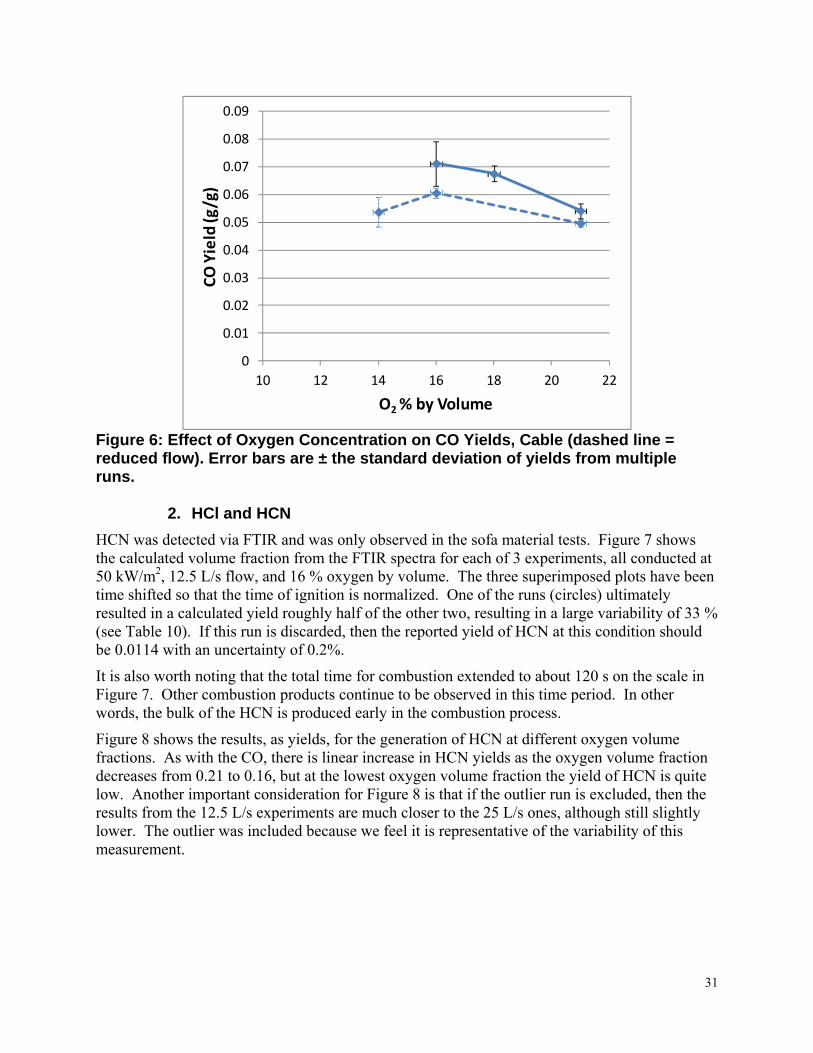
0
50
100
150
200
250
300
350
400
450
500
30 50 70 90 110 130 150
HCN
Volume Fraction
(LL)
Test Time (sec)
Figure 7 HCN Volume Fractions Sofa 50 kWm2 125 Ls 16 O2 by Volume Uncertainty is 10 of the Reported HCN Volume Fraction
0014
0012
HCN
Yield
(gg) 0010
0008
0006
0004
0002
0000
O2 by Volume
10 12 14 16 18 20 22
Figure 8 Effect of Oxygen Concentration on HCN Yields Sofa Error bars are plusmn the standard deviation of yields from multiple runs
32
HCl was detected via FTIR and was only observed in the cable tests Figure 9 shows the calculated volume fraction from the FTIR spectra for each of 3 experiments all conducted at 50 kWm2 125 Ls flow and 16 oxygen by volume The three superimposed plots have been time shifted so that the time of ignition is normalized The 3 runs are quite consistent and numerically have a variability in yield of 38 This is despite the fact that there is some variability in the timing of the release of HCl lasting approximately 20 s longer for one of the experiments (diamonds in the figure) In other words the measured volume fraction at any one time is more variable than the integrated quantity
0
200
400
600
800
1000
1200
1400
30 80 130 180 230 280
HCl Volume Fraction
(LL)
Test Time (sec)
Figure 9 HCl Volume Fractions Cable 50 kWm2 125 Ls 16 O2 by Volume Uncertainty is 10 of the Reported Volume Fraction
Figure 10 shows the effect of oxygen concentration on the yields of HCl from the cable materials The yields are somewhat higher at lower oxygen concentrations but this may be accounted for by a slightly lower total mass lostmdashif disproportionately more of the carbon remains in the char At the lowest oxygen volume fraction 014 the yield of HCl increases by about 20
33
000
005
010
015
020
025
030
035
10 12 14 16 18 20 22
HCl Yield
(g g)
O2 by Volume
Figure 10 Effect of Oxygen Concentration on Yields of HCl Cables Error bars are plusmn the standard deviation of yields from multiple runs
C MEASURED VS NOTIONAL VALUES
During sustained and complete combustion the yield of CO2 should approach its notional values since CO2 is a marker for combusted carbon In these experiments the sofa material came out best achieving over 70 of the notional yield The bookcase fared slightly worse achieving only 65 of the notional yield for CO2 and the cable had the lowest at around half The relatively lower yields of CO2 from the cables is an expected result of flame inhibition due to the chlorine These trends are consistent with our qualitative observation of for example the thickness of the smoke produced
The yields of CO from all the specimens ranged from about 001 to 006 which corresponds to 1 to 5 of the notional values These values are consistent with relatively fuel-lean combustion34 and are an order of magnitude lower than the CO yields expected of postflashover fires14
The yields of HCl from the cable specimens approach their notional values The deficit may reflect scavenging by the calcium carbonate filler in the cable jacket or wall loss in the duct or sampling line
The detection limited yields of HCl from the sofa specimens was 80 of the notional yield at the higher flow rate and 40 of the notional yield at the lower flow rate The detection limited yield of HCl from the bookcase was 25 and 15 times the notional yield for the high and low flows respectively Chlorine is present at well under one percent by mass in these two products Such small quantities are not capable of producing toxicologically significant yields of HCl suggesting that they can be either ruled out by elemental analysis as unimportant or that limits of detection are not a barrier to measuring significant quantities of HCl in this apparatus
34
Yields of HCN from the sofa are between 2 and 6 of their notional values The highest relative yield is found at 16 oxygen by volume Despite the lower oxygen these flames appear relatively fuel-lean and the nitrogen may appear as molecular nitrogen or nitrogen dioxides
D SPECIES SAMPLING AND MEASUREMENT
1 Species Measurement Using FTIR Spectroscopy
FTIR spectroscopic analysis of combustion products has become fairly common in fire research laboratories However that does not mean that its use is straightforward The data from a recent round robin involving FTIR measurement of toxic combustion products from a standardized apparatus showed interlaboratory variations of up to an order of magnitude There are documents under development in ISO TC92 SC1 and SC3 to standardize the implementation
We were able to obtain usable information using this technique There are a number of lessons emerging from this test series that can provide useful input to these efforts such as the following
The application of FTIR spectroscopy to fire testing requires the constant attention of an experienced professional at a level well beyond the demands of the more traditional fire test instrumentation
In this work we used a longer path length cell than in previous work However the increased sensitivity was offset by the instantaneous nature of the measurements (as opposed to averaging over dozens of data points) and the fact that the gases did not accumulate as they do in the closed chamber tests such as NFPA 269 and NFPA 270 (toxicity test method and smoke density chamber respectively) The CO concentrations measured here are approximately one-tenth of those measured in the closed-chamber apparatus However non-linear effects resulted in a 25 deficit compared to the NDIR measurements of CO at the highest concentrations
The cell volume remained small and provided good time resolution For example the measured HCl concentrations go from zero to the maximum in two data intervals (see Figure 9)
The lack of a filter did not adversely affect the measurements Compared to previous work with other apparatus the smoke measured here was relatively dilute The cell only required cleaning a few times over the course of all of the experiments reported here The internal mirrors were easily cleaned with ethanol and deionized water The KBr windows were replaced once
A heated sample line (as recommended in the SAFIR report35 and ISO 1970236) enabled near-quantitative collection of HCl a compound that is generally regarded as difficult to determine
E IMPORTANCE OF UNDETECTED GASES
The equations in ISO 13571 include provision for additional gases to be included in estimating the time available for escape or refuge from a fire HBr HF SO2 NO2 acrolein (C3H4O) and formaldehyde (H2CO) There was no Br F or S in any of the products examined in this project
35
so the first three of these gases were not expected The presence of the latter three was not detected thus establishing the upper limits of their presence at the volume fractions listed in Table 2
To put the potential contributions of the sensory irritant gases (HCl NO2 acrolein and formaldehyde) in context we use the equations in ISO 13571 for calculating the Fractional Effective Dose (FED) for the narcotic gases CO2 and CO and the Fractional Effective Concentration (FEC) for the four sensory irritant gases
The FED equation is
CO2exp 5t 2 t 2 236
CO HCNFED t 6 t
t1 35000 t1 12 10 where Δt is the exposure interval in minutes
The FEC of the four irritant gases were estimated from their volume fractions and the incapacitating levels in ISO 13571 (FHCl etc) The results are compiled in Table 12
The FEC equation in ISO 13571 is
HCl HBr HF SO2 NO 2 acrolein formaldehyde irritant FEC = F F F F F F F FHCl HBr HF SO NO acrolein formaldehyde Ci2 2
Table 12 Limits of importance of undetected toxins
Volume fraction (μLL) FEC Contribution
HCl NO2 C3H4O H2CO HCl NO2 C3H4O H2CO Incapacitating Level 1000 250 30 250 Bookcase lt 20 lt 40 lt 20 lt 40 lt 002 lt 016 lt 066 lt 016 Sofa lt 20 lt 40 lt 20 lt 40 lt 002 lt 016 lt 066 lt 016
Cable 1370 lt 40 lt 20 lt 40 058 lt 007 lt 028 lt 007 to 730 lt 40 lt 20 lt 40 043 lt 009 lt 039 lt 009
It stands out that the FEC contribution from acrolein is as much as two-thirds of an incapacitating level This is because (a) the limit of detection is close to the listed incapacitating level and (b) the incapacitating level is very low While there is agreement among experts that this value of 30 μLL is reasonable there are data that suggest strongly that this is unnecessarily conservative Kaplan and co-workers exposed individual baboons to various concentrations of acrolein in air37 At the end of 5 min each baboon was given a signal and could perform an action that led to escape from the test chamber The baboons exposed at up to 500 μLL escaped and survived Those exposed to higher levels escaped but died later These data suggest that people should be able to accommodate a nearly instantaneous exposure to eg at least 300 μLL without becoming incapacitated If we increase the incapacitating level of acrolein to 250 μLL the relative contribution to FEC become those in Table 13 In this case the relative importance of acrolein falls below 01 when other irritants are detected
36
Table 13 Limits of Importance of Undetected Toxicants Volume fraction (μLL) FEC Contribution
HCl NO2 C3H4O H2CO HCl NO2 C3H4O H2CO Incapacitating Level 1000 250 250 250 Bookcase lt 20 lt 40 lt 20 lt 40 lt 005 lt 038 lt 019 lt 038 Sofa lt 20 lt 40 lt 20 lt 40 lt 005 lt 038 lt 019 lt 038 Cable 1370 lt 40 lt 20 lt 40 077 lt 009 lt 005 lt 009
to 730 lt 40 lt 20 lt 40 065 lt 014 lt 007 lt 014
Where specimens like the bookcase and sofa produce narcotic gases CO and HCN and irritants are below the limits of detection the narcotic gases are the primary contributors to incapacitation Assuming that the irritant gases are present in just under the limits of detection in order for them to reach an incapacitating concentration the relative concentration of CO would be incapacitating in a few minutes the relative concentration of HCN would be incapacitating in under a minute
37
This page intentionally left blank
38
VI CONCLUSIONS
This paper reports toxic gas yield data for specimens cut from three complex combustibles a bookcase a sofa and residential electrical power cable The physical fire model used was the cone calorimeter from ISO 5660-1 ASTM E 1354 This apparatus allows the use of a test specimen that approximates the geometry and radiant exposure that might be experienced by the intact combustible in a well-ventilated flaming fire In addition to performing the tests as prescribed in the standards this work added an enclosure and a gas supply capable of reduced oxygen in order to better approximate conditions in an underventilated fire
For the standard test procedure
The CO2 yields were very repeatable and represented between half and 80 of the carbon in the specimens All specimens left a black residue that continued to pyrolyze after the flaming halted These residues were presumably carbon-enriched accounting for the yields being below the notional yields
The CO yields were also very repeatable with the exception of the bookcase at low heat flux and the higher oxygen concentrations
The HCN yields were below the limit of detection for the bookcase and cable specimens The HCN yields from the sofa were 3 to 10 times the limit of detection and had a variation in repeatability between 5 and 40 of the reported yield depending on the test conditions
The HCl yields were below the limit of detection for the bookcase and sofa specimens For the cables they were well above the limit of detection and accounted for 70 of the Cl in the specimens
None of the other irritant gases appeared in concentrations above their limits of detection
Regarding the variation in test conditions we conclude
An incident heat flux of 25 kWm2 does not provide any information beyond that which is found at 50 kWm2 In fact it leads to increased variability from test to test because of slow ignition or early extinction
The trend of toxic gas yields increasing with decreasing initial oxygen concentration holds uniformly across gases and specimen types over the oxygen volume fraction range of 021 to 016 When the oxygen volume fraction is 014 the results are unpredictable for both gases and items burned Therefore we donrsquot recommend testing at this level With the exception of CO from the bookcase the majority of the CO yields were lower at 014 than at 016
Reducing the total flow to 125 Ls reduces the limit of detection of the gases by a factor of two and allows the achievement of lower oxygen concentrations However yields measured at the lower flow were consistently lower than at the higher flow
Calculation of the contributions of the gases to incapacitation of people who might be exposed to these environments showed
Incapacitation from the bookcase material effluent would be primarily from CO
39
Incapacitation from the sofa material effluent would be from a combination of CO and HCN
Incapacitation from the cable effluent would be initially from HCl the related yield of CO would become incapacitating after approximately15 minutes
If the CO yield were at the expected postflashover value of 02
Incapacitation from the bookcase material effluent would be primarily from CO
Incapacitation from the sofa material effluent would be primarily from CO
Incapacitation from the cable material effluent would be initially from HCl a 02 yield of CO would become incapacitating after a few minutes
VII ACKNOWLEDGEMENTS
The authors express their appreciation to Randy Shields for his assistance in performing the tests
40
References
1 Phillips WGB Beller DK and Fahy RF ldquoComputer Simulation for Fire Protection Engineeringrdquo Chapter 5-9 in SFPE Handbook of Fire Protection Engineering 4th Edition PJ DiNenno et al eds NFPA International Quincy MA 2008
2 httpwwwnistgovelfire_researchcfastcfm
3 Peacock RD Jones WW and Reneke PA ldquoCFASTmdashConsolidated Model of Fire Growth and Smoke Transport (Version 6) Software Development and Evaluation Guiderdquo NIST Special Publication 1086 National Institute of Standards and Technology Gaithersburg MD 187 pages (2008)
4 Peacock RD Jones WW and Bukowski RW ldquoVerification of a Model of Fire and Smoke Transportrdquo Fire Safety Journal 21 89-129 (1993)
5 httpfirenistgovfds
6 ldquoStandard Test Method for Heat and Visible Smoke Release Rates for Materials and Products Using an Oxygen Consumption Calorimeterrdquo ASTM E1354-04a ASTM International West Conshohocken PA 2004
7 See eg ldquoStandard for the Flammability (Open Flame) of Mattress Setsrdquo 16 CFR Part 1633 Federal Register 70 (50) 13471-13523 2006
8httpwwwisoorgisoiso_cataloguecatalogue_tccatalogue_tc_browsehtmcommid=50540amp published=onampdevelopment=on
9 ldquoLife-threatening Components of Fire ndash Guidelines for the Estimation of Time to Compromised Tenability in Firesrdquo ISO 13571 International Standards Organization Geneva 2012
10 Guidelines for Assessing the Fire Threat to People ISO 19706 International Standards Organization Geneva 2011
11 Gann RG Babrauskas V Peacock RD and Hall Jr JR Fire Conditions for Smoke Toxicity Measurement Fire and Materials 18 193-199 (1994)
12 Guidance for Comparison of Toxic Gas Data between Different Physical Fire Models and Scales ISO 29903 International Standards Organization Geneva 2012
13 ldquoStandard Test Method for Developing Toxic Potency Data for Use in Fire Hazard Modelingrdquo NFPA 269 NFPA International Quincy MA 2012
14 ldquoStandard Test Method for Measuring Smoke Toxicity for Use in Fire Hazard Analysisrdquo ASTM E1678-10 ASTM International West Conshohocken PA 2010
15 (a) Gann RG Averill JD Nyden MR Johnsson EL and Peacock RD ldquoSmoke Component Yields from Room-scale Fire Testsrdquo NIST Technical Note 1453 National Institute of Standards and Technology Gaithersburg MD 159 pages (2003)
(b) Gann RG Averill JD Nyden MR Johnsson EL and Peacock RD ldquoFire Effluent Component Yields from Room-scale Fire Testsrdquo Fire and Materials 34 285-314 (2010) DOI 101002fam1024
41
16 Ohlemiller TJ and Villa K ldquoFurniture Flammability An Investigation of the California Bulletin 133 Test Part II Characterization of the Ignition Source and a Comparable Gas Burnerrdquo NISTIR 4348 National Institute of Standards and Technology Gaithersburg MD 1990
17 Gann RG Marsh ND Averill JA and Nyden MR ldquoSmoke Component Yields from Bench-scale Fire Tests 1 NFPA 269ASTM E 1678rdquo NIST Technical Note 1760 National Institute of Standards and Technology Gaithersburg MD 57 pages (2013)
18 Kaplan HL Grand AF and Hartzell GE Combustion Toxicology Principles and Test Methods Technology Publishing Co Lancaster PA 1983
19 Guidance for Evaluating the Validity of Physical Fire Models for Obtaining Fire Effluent Toxicity Data for Use in Fire Hazard and Risk Assessment ndash Part 2 Evaluation of Individual Physical Fire Models ISOTR 16312-2 International Standards Organization Geneva 2007
20 Controlled Equivalence Ratio Method for the Determination of the Hazardous Components of Fire Effluent ISOTS 19700 International Standards Organization 2010
21 Reaction-to-fire Tests ndash Heat Release Smoke Production and Mass Loss Rates ndash Part 1 Heat Release (Cone Calorimeter Method) ISO 5660-1 International Standards Organization Geneva 2002
22 Plastics mdash Smoke Generation mdash Part 2 Determination of Optical Density by a Single-chamber Test ISO 5659-2 International standards Organization Geneva 1994
23 Marsh ND Gann RG and Nyden MR ldquoSmoke Component Yields from Bench-scale Fire Tests 2 ISO 19700 Controlled Equivalence Ratio Tube Furnacerdquo NIST Technical Note 1761 National Institute of Standards and Technology Gaithersburg MD 45 pages (2013)
24 Marsh ND Gann RG and Nyden MR ldquoObservations on the Generation of Toxic Products in the NFPAISO Smoke Density Chamberrdquo Proceedings of the 12th International Conference on Fire Science amp Engineering (Interflam 2010) Nottingham UK (2010)
25 Mulholland G Janssens M Yusa S Twilley W and Babrauskas VrdquoThe effect of oxygen concentration on CO and Smoke Produced by Flamesrdquo Proceedings of the Third International Symposium on Fire Safety Science Edinburgh UK pp 585-594 (1991) doi103801IAFSSFSS3-585
26 Babrauskas V Twilley WH Janssens M and Yusa S ldquoA cone calorimeter for controlled-atmosphere studiesrdquo Fire and Materials 16 37-43 (1992)
27 Hshieh FY Motto SE Hirsch DB and Beeson HD ldquoFlammability Testing Using a Controlled-atmosphere Cone Calorimeterrdquo Proceedings of the 18th International Conference on Fire Safety Science Millbrae CA p 999 (1993)
28 Gomez C Janssens M and Zalkin A ldquoUsing the Cone Calorimeter for Quantifying Toxic Potencyrdquo Proceedings of the 12th International Fire Science amp Engineering Conference (Interflam 10) Nottingham UK (2010)
42
29 Gomez C Janssens M and Zalkin A ldquoMeasuring the Yields of Toxic Gases from Materials during Different Stages of Fire Developmentrdquo In Fire and Materials 12 international conference San Francisco CA (2011)
30 Guillaume E Marquis DM and Chivas-Joly C ldquoUsage of Controlled-atmosphere Cone Calorimeter to Provide Input Data for Toxicity Modelingrdquo in Fire and Materials 12 International Conference San Francisco CA (2011)
31 Haaland DM Easterling RG and Vopicka DA ldquoMultivariate Least-Squares Methods Applied to the Quantitative Spectral Analysis of Multicomponent Samplesrdquo Applied Spectroscopy 39 73-84 (1985) doi1013660003702854249376
32 Gas Phase Infrared Spectral Standards Revision B Midac Corp Irvine CA (1999)
33 Speitel LC ldquoFourier Transform Infrared Analysis of Combustion Gasesrdquo Federal Aviation Administration Report DOTFAAAR-0188 2001
34 Pitts WM The Global Equivalence Ratio Concept and the Formations Mechanisms of Carbon Monoxide in Fires Progress in Energy and Combustion Science 21 197-237 (1995)
35 Smoke Gas Analysis by Fourier Transform Infrared Analysis The SAFIR Project VTT Research Note Technical Research Centre of Finland 81 Pages 1999
36 ldquoToxicity testing of fire effluents -- Guidance for analysis of gases and vapours in fire effluents using FTIR gas analysisrdquo ISO 19702 International Standards Organization Geneva 2006
37 Kaplan HL Grand AF Switzer WG Mitchell DS Rogers WR and Hartzell GE Effects of Combustion Gases on Escape Performance of the Baboon and the Rat Journal of Fire Sciences 3 228-244 (1985)
43
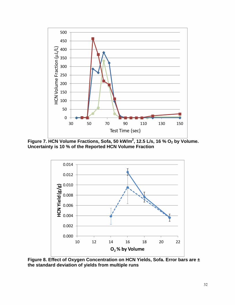
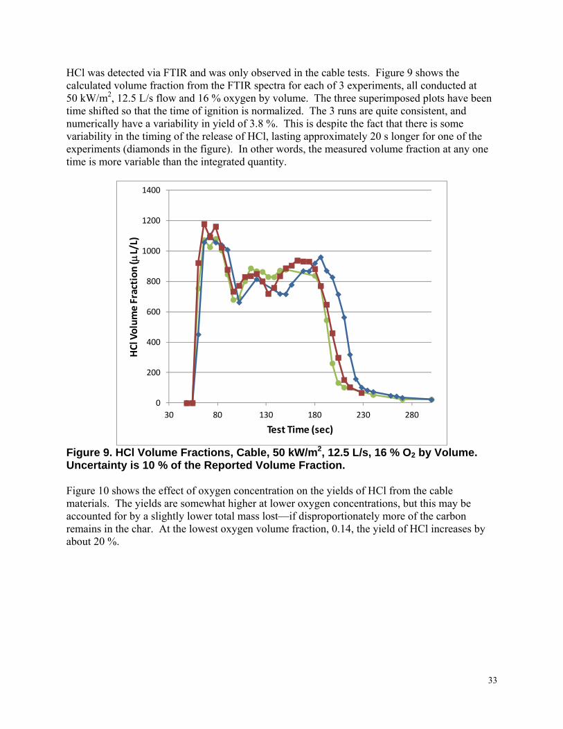
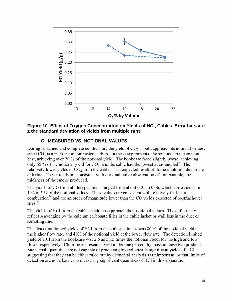
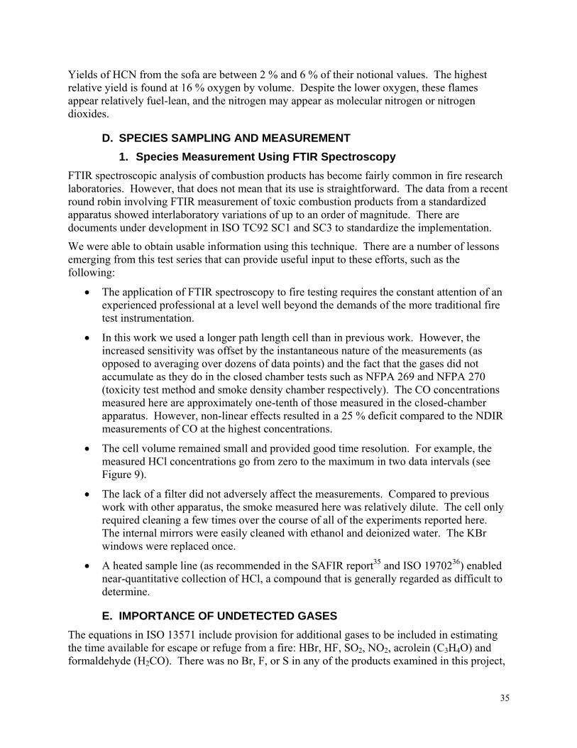
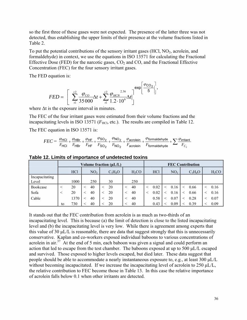
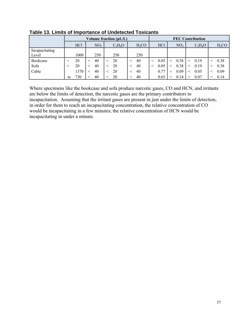