Embed Size (px)
Citation preview
Smog Check II EvaluationPart II: Overview of Vehicle
Emissions. . . . . . . . . . . .
Prepared by
Joel SchwartzExecutive Officer
California Inspection andMaintenance Review Committee
TABLE OF CONTENTS
1. Introduction ______________________________________________ 1
2. Emissions Concepts Used in Later Sections ____________________ 1
3. Older Vehicles Have Higher Emissions on Average _____________ 3
4. The Vehicle Fleet Is Dominated by Newer Vehicles______________ 8
5. More Recent Vehicle Models Start Cleaner and Stay CleanerLonger___________________________________________________ 9
6. Emissions Vary Substantially for the Fleet as a Whole andwithin each Model Year ___________________________________ 12
7. Emissions of Individual Vehicles Vary from Test to Test ________ 15
8. Total Emissions Are Dominated by a Small Number of HighEmitters ________________________________________________ 18
9. Most Potential Smog Check Emissions Reductions Comefrom a Small Percentage of Vehicles _________________________ 20
10. Current Failure Cut Points Capture Most Potential Benefits ____ 25
11. Failure Cut Points Used for SIP Emissions Reduction TargetsWould Fail Many Marginally Emitting Cars __________________ 30
12. Appropriate Cut Points for Initial Failure and Post-RepairCertification Might Be Different ____________________________ 31
II-1
1. Introduction
This chapter provides a summary of (1) information on the nature and distribution ofvehicle emissions in the on-road vehicle fleet, and (2) analysis of vehicle emissions issuesthat have relevance for Smog Check policy.
2. Emissions Concepts Used in Later Sections
2.1. “Excess,” “Reducible,” and “Repairable” Emissions
Regulators and emissions researchers generally classify vehicle emissions intocategories that reflect the extent to which they can potentially be reduced by repair. Carsthat fail an emissions test are generally expected to have the potential for emissionsreductions due to repair. Vehicles fail an emissions test if their emissions are above pre-determined levels known as “cut points” or “failure standards.” Emissions above the cutpoints are generally referred to as excess, repairable, or reducible emissions. Note,however, that many vehicles’ emissions are intrinsically variable from test to test(emissions variability is discussed in more detail in Section 7).
2.2. Fuel-Based vs. Travel-Based Emissions Tests
Emissions tests can be divided into those that measure emissions in grams per gallonof fuel consumed (fuel-based tests) and in grams per mile traveled (travel-based tests).The IM240, used in many centralized I/M programs, and the Federal Test Procedure(FTP), which is used to certify that new vehicles meet federal and California emissionsstandards, are travel-based emissions tests. Emissions from these tests are generallyreported in grams per mile (g/mile). The ASM emissions test used in California’s SmogCheck program, and remote sensing devices are fuel-based tests. Emissions from thesetests are generally reported in concentration units (parts per million (ppm) or percent (%)where 1% = 10,000 ppm) or in grams of emissions per gallon of fuel consumed (g/gal).
2.2.1. Converting between fuel-based and travel-based measurements
Emissions regulations are based on travel-based tests, so it is useful to be able toconvert between the two types of measurements. There are two ways to estimate travel-based emissions from fuel-based emissions. First, if the fuel economy of a vehicle isknown, one can directly convert from fuel-based emissions to travel-based emissions bymultiplying emissions in grams per gallon times the fuel economy in gallons per mile.However, the exact fuel economy of any particular vehicle at a particular moment in timeis uncertain, because it is dependent on the type of vehicle, the condition it is in, and theload its engine is under when tested. Nonetheless, one can use the reported fuel economyof the vehicle on the FTP, or the fleet-weighted average fuel economy, for vehicles in agiven model year as an estimate for this calculation.
Second, if data for a large group of randomly selected cars that has been tested on twodifferent tests, say the ASM and the FTP, one can use a statistical technique calledregression analysis to develop a set of equations relating ASM emissions to FTPemissions. Under a contract with BAR, the Eastern Research Group (ERG) has developed
II-2
such a set of equations. The ERG model uses vehicle-specific factors, such as age,weight, whether it has a carburetor or is fuel injected, and whether it is a passenger car ora truck, to predict FTP emissions from ASM measurements. Although the conversion isnot exact, this method is useful for estimating average FTP emissions of large samples ofvehicles. However, ERG stresses that it is not suitable for accurately predicting FTPemissions of a single vehicle.
2.3. Tailpipe vs. Non-Tailpipe Emissions
NOx and CO emissions are produced only during fuel combustion and thereforegenerally are emitted only from the tailpipe of a vehicle. HC emissions also come out ofthe tailpipe when they are incompletely burned in the engine and not destroyed by thecatalytic converter. However, the hydrocarbons of which gasoline is composed can alsoleak or evaporate from the fuel storage and delivery systems of cars. These emissions aregenerally referred to as non-tailpipe, or evaporative, emissions.
There is a great deal of uncertainty about what portion of vehicle HC emissionscomes from non-tailpipe sources. A recent peer-reviewed study concluded that the non-tailpipe fraction could range from as low as 15 percent to more than 50 percent and thatcurrent data are insufficient to resolve the issue.1
California’s Smog Check program currently has the potential to affect non-tailpipeemissions mainly through the gas cap pressure test. However, other sources of non-tailpipe emissions, such as liquid leaks and problems with automobile evaporativeemissions-control systems are likely much larger sources of non-tailpipe HC. The IMRCevaluation does not include non-tailpipe HC emissions in its Smog Check evaluation dueto lack of appropriate data. However, the IMRC plans to examine this issue further in thecoming months. This report focuses only on tailpipe emissions.
2.4. Dealing with Uncertainty
The following sections of this report present data on many aspects of vehicleemissions, including the number of vehicles on the road, average emissions for eachmodel year, and the distribution of emissions among vehicles. These results are estimatesof what is going on in the real world, and they are subject to uncertainties. Theseuncertainties may be small in some cases and large in others. Several factors createuncertainty in estimates of real-world vehicle emissions:
• Sample Bias. Millions of vehicles are on the road in California. Researchersestimate their emissions characteristics by sampling a small portion of them. Butsampling always entails the possibility that the sample might not be representativeof the whole population. For example, high-emitting vehicles might beunderrepresented in a sample of vehicles relative to their presence in the vehiclefleet as a whole.
1 Pierson, W. R., D. E. Schorran, et al. (1999) “Assessment of Nontailpipe Hydrocarbon Emissions
from Motor Vehicles”, Journal of the Air and Waste Management Association, vol. 49, pp. 498-519, May1999.
II-3
• Artificial Test Conditions. In I/M programs, vehicle emissions are measuredusing specific emissions tests such as the ASM or the IM240. These tests includecarefully controlled driving conditions. However, the driving conditions on thetest will not represent the way many cars are actually driven. For example, theASM test includes only a steady cruise and the IM240 test does not include veryhigh accelerations. Emissions change with driving conditions, so variationbetween test conditions and real driving can cause errors in fleet emissionsestimates.2
• Fleet Turnover. The vehicle fleet is constantly changing, with older cars beingtotaled or scrapped, new cars entering the fleet, and people moving in and out ofan area. The fleet measured today differs from the way the fleet will look nextweek or next month.
Despite these uncertainties, some estimates have a relatively high level of reliability.For example, the IMRC’s data show that a small number of cars account for mostpollution. This result is seen over and over again in vehicle emissions studies. But thesegeneral observations are qualitative rather than offering numerical precision. It is moredifficult to say with certainty exactly what percentage of cars accounts for whatpercentage of total emissions.
For example, whether the dirtiest 10 percent of vehicles account for 40 percent of HCemissions or 50 percent (numbers in this range have been seen around the country) willchange from time to time and place to place. The emission distribution will changebecause the makeup of the vehicle fleet changes with location and time and also becauseof the uncertainties in the methods used to measure the fleet. Thus, one may be quitecertain of a qualitative result, but less certain of exact numerical values.
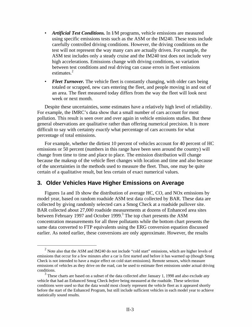
3. Older Vehicles Have Higher Emissions on Average
Figures 1a and 1b show the distribution of average HC, CO, and NOx emissions bymodel year, based on random roadside ASM test data collected by BAR. These data arecollected by giving randomly selected cars a Smog Check at a roadside pullover site.BAR collected about 27,000 roadside measurements at dozens of Enhanced area sitesbetween February 1997 and October 1999.3 The top chart presents the ASMconcentration measurements for all three pollutants while the bottom chart presents thesame data converted to FTP equivalents using the ERG conversion equation discussedearlier. As noted earlier, these conversions are only approximate. However, the results
2 Note also that the ASM and IM240 do not include “cold start” emissions, which are higher levels of
emissions that occur for a few minutes after a car is first started and before it has warmed up (though SmogCheck is not intended to have a major effect on cold start emissions). Remote sensors, which measureemissions of vehicles as they drive on the road, can be used to estimate fleet emissions under actual drivingconditions.
3 These charts are based on a subset of the data collected after January 1, 1998 and also exclude anyvehicle that had an Enhanced Smog Check before being measured at the roadside. These selectionconditions were used so that the data would most closely represent the vehicle fleet as it appeared shortlybefore the start of the Enhanced Program, but still include sufficient vehicles in each model year to achievestatistically sound results.
II-4
displayed here follow the same pattern seen in all emissions measurements of a broadrange of vehicles. Note also that:
• CO emissions should be read from the right axis scale rather than the left. Theseparate scale for CO is necessary because CO emissions span a much largerrange than HC and NOx emissions.
• On the ASM test, HC and NOx emissions are reported in parts per million (ppm),while CO emissions are reported in percent (1% = 10,000 ppm).
• FTP emissions of all pollutants are reported in grams per mile (g/mile).
Note the following in these graphs:
• Average emissions are much higher for older vehicles for all three pollutants.
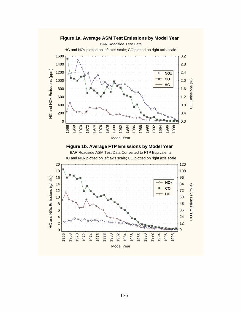
• Mass emissions of HC and CO are much higher than NOx for older vehicles.However, emissions of all three pollutants are starting to converge for newervehicles. Figure 1c zooms in on FTP emissions of newer vehicles. As the graphshows, average HC emissions are lower than average NOx emissions for newervehicles. Note that all three pollutants are plotted against the left axis scale in thisgraph.
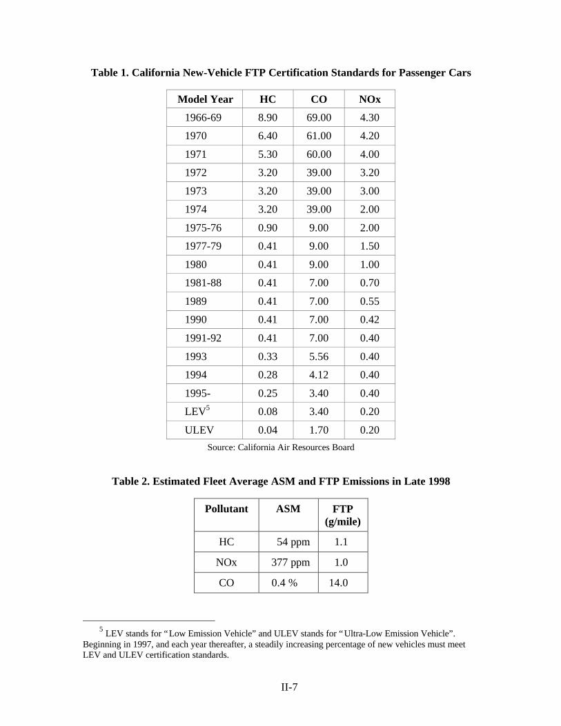
For comparison, Table 1 displays California’s new-vehicle FTP certificationstandards for passenger cars for selected model years. These standards have becomemuch more stringent for more recent model years. Table 2 displays average ASM andFTP emissions for the fleet as a whole. Based on the time period in which the roadsidedata were collected, these values roughly represent average fleet emissions in late 1998.These values were estimated by calculating average emissions by model year from theroadside data and then weighting these data by the estimated travel fraction of thevehicles in each model year. The travel fraction is the percentage of total miles traveledaccounted for by a given model year of vehicles. For each model year, total milestraveled is estimated by taking the product of the estimated number of vehicles on theroad from a given model year, and the estimated average miles per year traveled byvehicles in that model year.
II-5
Figure 1a. Average ASM Test Emissions by Model YearBAR Roadside Test Data
HC and NOx plotted on left axis scale; CO plotted on right axis scale
Model Year
HC
and
NO
x E
mis
sion
s (p
pm)
CO
Em
issi
ons
(%)
0.0
0.4
0.8
1.2
1.6
2.0
2.4
2.8
3.2
0
200
400
600
800
1000
1200
1400
1600
1966
1968
1970
1972
1974
1976
1978
1980
1982
1984
1986
1988
1990
1992
1994
1996
1998
NOxCOHC
Figure 1b. Average FTP Emissions by Model YearBAR Roadside ASM Test Data Converted to FTP Equivalents
HC and NOx plotted on left axis scale; CO plotted on right axis scale
Model Year
HC
and
NO
x E
mis
sion
s (g
/mile
)
CO
Em
issi
ons
(g/m
ile)
0
12
24
36
48
60
72
84
96
108
120
0
2
4
6
8
10
12
14
16
18
20
1966
1968
1970
1972
1974
1976
1978
1980
1982
1984
1986
1988
1990
1992
1994
1996
1998
NOxCOHC
II-6
Figure 1c. Blowup of Average FTP Emissions by Model Year for Newer Vehicles
Model Year
Em
issi
ons
(g/m
ile)
01
2
3
4
5
6
7
89
10
1986
1987
1988
1989
1990
1991
1992
1993
1994
1995
1996
1997
1998
1999
NOxCOHC
The travel fraction of each model year changes with time for two reasons. First, thenumber of vehicles from a given model year decreases with time as vehicles are retired.Second, older vehicles travel fewer miles, on average, than newer ones. Thus, it isimportant to apply a travel fraction appropriate to the time period in which emissions areestimated. Calculations for this report use a travel fraction calculator (TFC) developed bySonoma Technology under contract with BAR.4
4 The data for the travel fraction calculator (TFC) come from three sources: vehicle registration data,
changes in vehicle odometer readings between Smog Checks, and new vehicle sales data. The IMRC hasnot evaluated the data or methodology that go into the TFC. However, it is important to note that estimatesof the number of vehicles on the road and the number of miles they travel each year are subject touncertainties for several reasons. Some vehicles are unregistered and some are scrapped or totaled withoutnotification to DMV. Estimates of miles traveled are based on odometer readings taken at Smog Checkstations. These are subject to potential data entry errors – the data may be entered haphazardly or not at allby some stations. In addition, a change in economic conditions can affect the rate at which motoristsreplace their vehicles.
II-7
Table 1. California New-Vehicle FTP Certification Standards for Passenger Cars
Model Year HC CO NOx
1966-69 8.90 69.00 4.30
1970 6.40 61.00 4.20
1971 5.30 60.00 4.00
1972 3.20 39.00 3.20
1973 3.20 39.00 3.00
1974 3.20 39.00 2.00
1975-76 0.90 9.00 2.00
1977-79 0.41 9.00 1.50
1980 0.41 9.00 1.00
1981-88 0.41 7.00 0.70
1989 0.41 7.00 0.55
1990 0.41 7.00 0.42
1991-92 0.41 7.00 0.40
1993 0.33 5.56 0.40
1994 0.28 4.12 0.40
1995- 0.25 3.40 0.40
LEV5 0.08 3.40 0.20
ULEV 0.04 1.70 0.20Source: California Air Resources Board
Table 2. Estimated Fleet Average ASM and FTP Emissions in Late 1998
Pollutant ASM FTP(g/mile)
HC 54 ppm 1.1
NOx 377 ppm 1.0
CO 0.4 % 14.0
5 LEV stands for “Low Emission Vehicle” and ULEV stands for “Ultra-Low Emission Vehicle”.
Beginning in 1997, and each year thereafter, a steadily increasing percentage of new vehicles must meetLEV and ULEV certification standards.
II-8
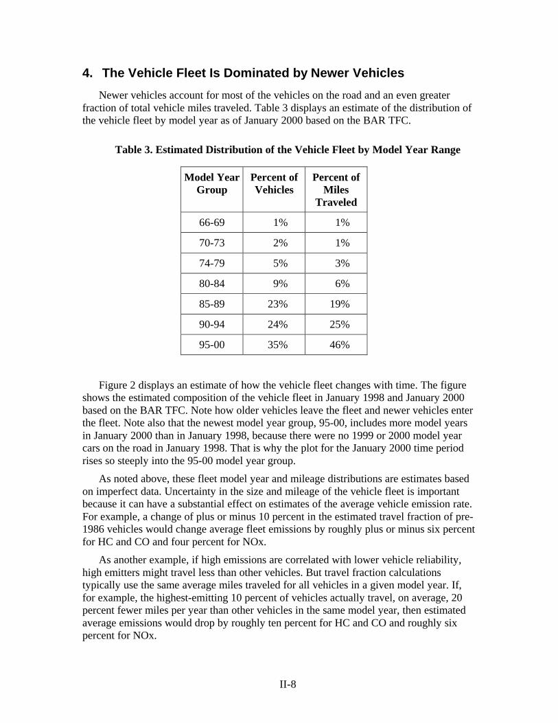
4. The Vehicle Fleet Is Dominated by Newer Vehicles
Newer vehicles account for most of the vehicles on the road and an even greaterfraction of total vehicle miles traveled. Table 3 displays an estimate of the distribution ofthe vehicle fleet by model year as of January 2000 based on the BAR TFC.
Table 3. Estimated Distribution of the Vehicle Fleet by Model Year Range
Model YearGroup
Percent ofVehicles
Percent ofMiles
Traveled
66-69 1% 1%
70-73 2% 1%
74-79 5% 3%
80-84 9% 6%
85-89 23% 19%
90-94 24% 25%
95-00 35% 46%
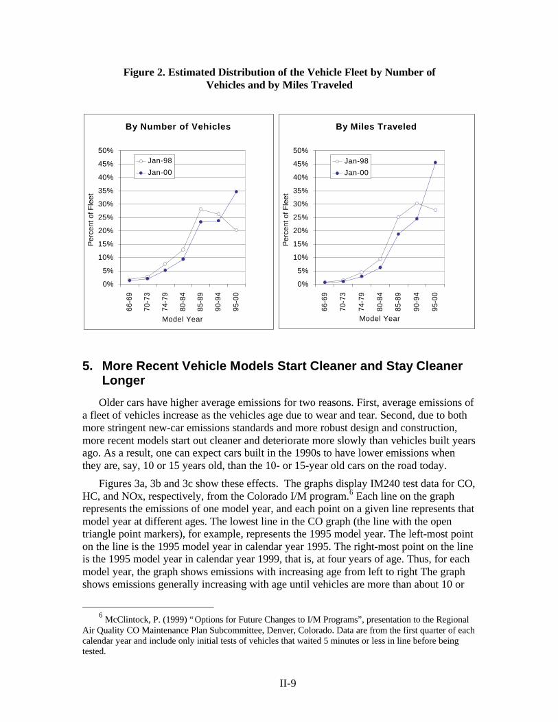
Figure 2 displays an estimate of how the vehicle fleet changes with time. The figureshows the estimated composition of the vehicle fleet in January 1998 and January 2000based on the BAR TFC. Note how older vehicles leave the fleet and newer vehicles enterthe fleet. Note also that the newest model year group, 95-00, includes more model yearsin January 2000 than in January 1998, because there were no 1999 or 2000 model yearcars on the road in January 1998. That is why the plot for the January 2000 time periodrises so steeply into the 95-00 model year group.
As noted above, these fleet model year and mileage distributions are estimates basedon imperfect data. Uncertainty in the size and mileage of the vehicle fleet is importantbecause it can have a substantial effect on estimates of the average vehicle emission rate.For example, a change of plus or minus 10 percent in the estimated travel fraction of pre-1986 vehicles would change average fleet emissions by roughly plus or minus six percentfor HC and CO and four percent for NOx.
As another example, if high emissions are correlated with lower vehicle reliability,high emitters might travel less than other vehicles. But travel fraction calculationstypically use the same average miles traveled for all vehicles in a given model year. If,for example, the highest-emitting 10 percent of vehicles actually travel, on average, 20percent fewer miles per year than other vehicles in the same model year, then estimatedaverage emissions would drop by roughly ten percent for HC and CO and roughly sixpercent for NOx.
II-9
Figure 2. Estimated Distribution of the Vehicle Fleet by Number ofVehicles and by Miles Traveled
By Number of Vehicles
0%
5%
10%
15%
20%
25%
30%
35%
40%
45%
50%
66-6
9
70-7
3
74-7
9
80-8
4
85-8
9
90-9
4
95-0
0
Model Year
Per
cent
of F
leet
Jan-98
Jan-00
By Miles Traveled
0%
5%
10%
15%
20%
25%
30%
35%
40%
45%
50%
66-6
9
70-7
3
74-7
9
80-8
4
85-8
9
90-9
4
95-0
0
Model Year
Per
cent
of F
leet
Jan-98Jan-00
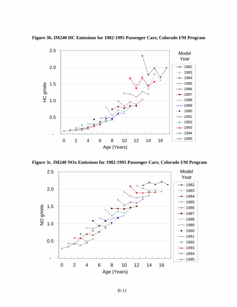
5. More Recent Vehicle Models Start Cleaner and Stay CleanerLonger
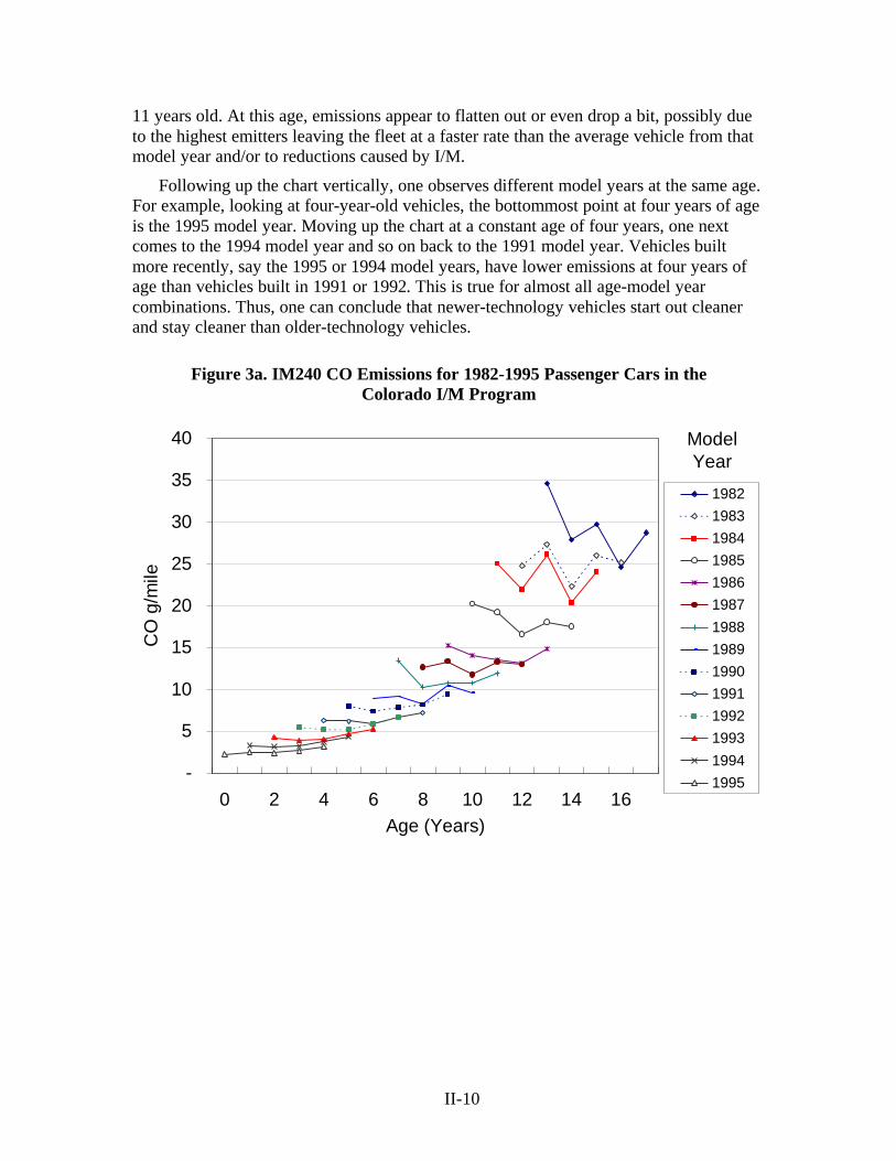
Older cars have higher average emissions for two reasons. First, average emissions ofa fleet of vehicles increase as the vehicles age due to wear and tear. Second, due to bothmore stringent new-car emissions standards and more robust design and construction,more recent models start out cleaner and deteriorate more slowly than vehicles built yearsago. As a result, one can expect cars built in the 1990s to have lower emissions whenthey are, say, 10 or 15 years old, than the 10- or 15-year old cars on the road today.
Figures 3a, 3b and 3c show these effects. The graphs display IM240 test data for CO,HC, and NOx, respectively, from the Colorado I/M program.6 Each line on the graphrepresents the emissions of one model year, and each point on a given line represents thatmodel year at different ages. The lowest line in the CO graph (the line with the opentriangle point markers), for example, represents the 1995 model year. The left-most pointon the line is the 1995 model year in calendar year 1995. The right-most point on the lineis the 1995 model year in calendar year 1999, that is, at four years of age. Thus, for eachmodel year, the graph shows emissions with increasing age from left to right The graphshows emissions generally increasing with age until vehicles are more than about 10 or
6 McClintock, P. (1999) “Options for Future Changes to I/M Programs”, presentation to the Regional
Air Quality CO Maintenance Plan Subcommittee, Denver, Colorado. Data are from the first quarter of eachcalendar year and include only initial tests of vehicles that waited 5 minutes or less in line before beingtested.
II-10
11 years old. At this age, emissions appear to flatten out or even drop a bit, possibly dueto the highest emitters leaving the fleet at a faster rate than the average vehicle from thatmodel year and/or to reductions caused by I/M.
Following up the chart vertically, one observes different model years at the same age.For example, looking at four-year-old vehicles, the bottommost point at four years of ageis the 1995 model year. Moving up the chart at a constant age of four years, one nextcomes to the 1994 model year and so on back to the 1991 model year. Vehicles builtmore recently, say the 1995 or 1994 model years, have lower emissions at four years ofage than vehicles built in 1991 or 1992. This is true for almost all age-model yearcombinations. Thus, one can conclude that newer-technology vehicles start out cleanerand stay cleaner than older-technology vehicles.
Figure 3a. IM240 CO Emissions for 1982-1995 Passenger Cars in theColorado I/M Program
-
5
10
15
20
25
30
35
40
0 2 4 6 8 10 12 14 16Age (Years)
CO
g/m
ile
19821983198419851986198719881989199019911992199319941995
Model Year
II-11
Figure 3b. IM240 HC Emissions for 1982-1995 Passenger Cars; Colorado I/M Program
-
0.5
1.0
1.5
2.0
2.5
0 2 4 6 8 10 12 14 16Age (Years)
HC
g/m
ile
19821983198419851986198719881989199019911992199319941995
Model Year
Figure 3c. IM240 NOx Emissions for 1982-1995 Passenger Cars; Colorado I/M Program
-
0.5
1.0
1.5
2.0
2.5
0 2 4 6 8 10 12 14 16Age (Years)
NO
g/m
ile
19821983198419851986198719881989199019911992199319941995
Model Year
II-12
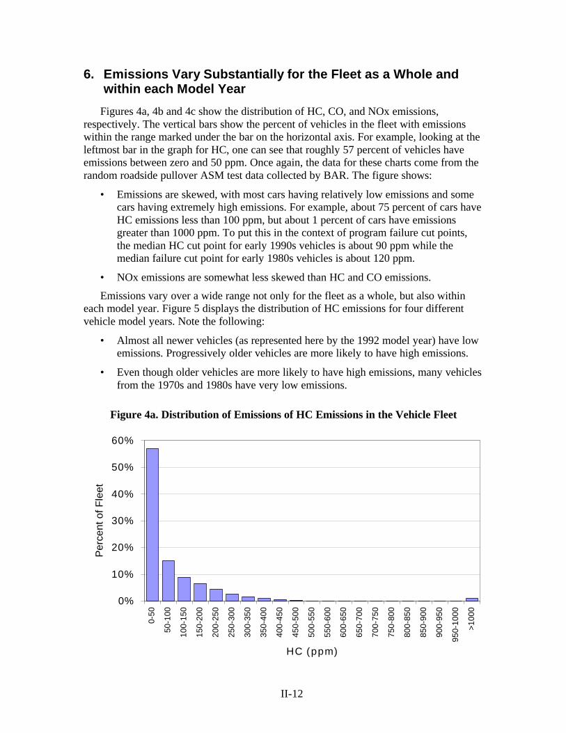
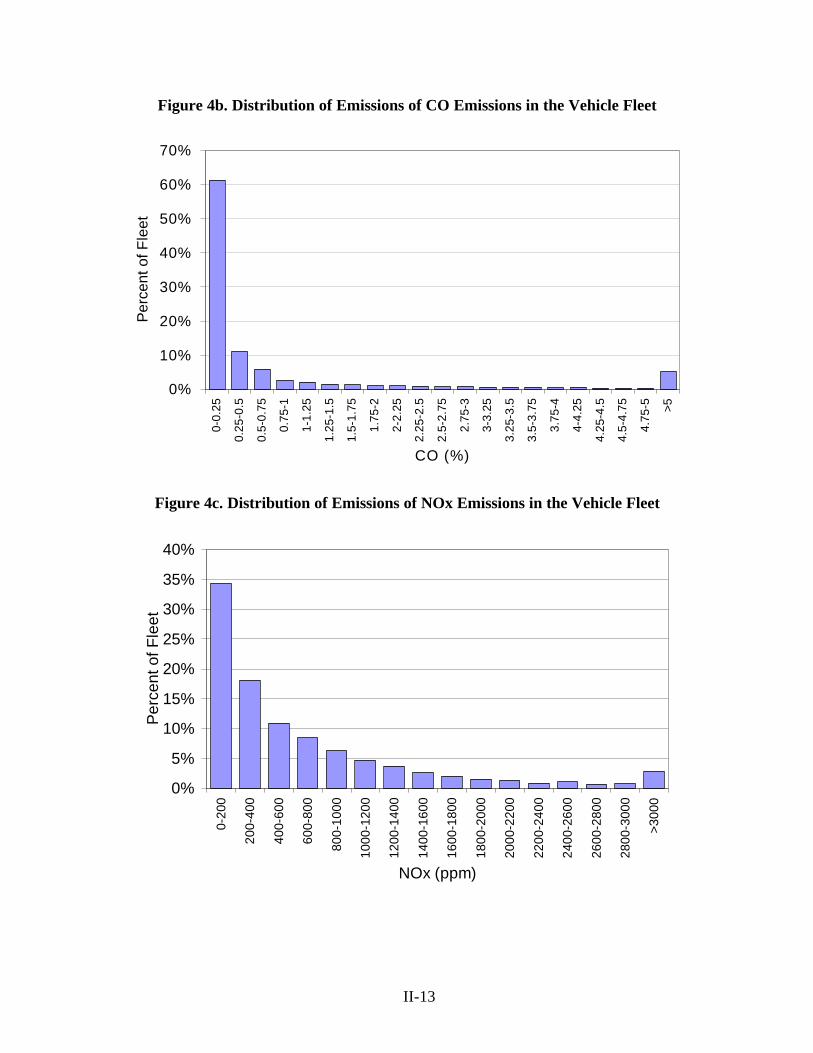
6. Emissions Vary Substantially for the Fleet as a Whole andwithin each Model Year
Figures 4a, 4b and 4c show the distribution of HC, CO, and NOx emissions,respectively. The vertical bars show the percent of vehicles in the fleet with emissionswithin the range marked under the bar on the horizontal axis. For example, looking at theleftmost bar in the graph for HC, one can see that roughly 57 percent of vehicles haveemissions between zero and 50 ppm. Once again, the data for these charts come from therandom roadside pullover ASM test data collected by BAR. The figure shows:
• Emissions are skewed, with most cars having relatively low emissions and somecars having extremely high emissions. For example, about 75 percent of cars haveHC emissions less than 100 ppm, but about 1 percent of cars have emissionsgreater than 1000 ppm. To put this in the context of program failure cut points,the median HC cut point for early 1990s vehicles is about 90 ppm while themedian failure cut point for early 1980s vehicles is about 120 ppm.
• NOx emissions are somewhat less skewed than HC and CO emissions.
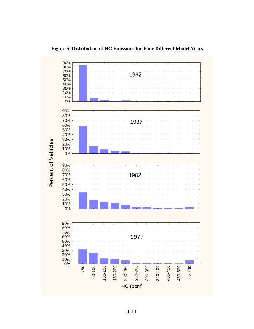
Emissions vary over a wide range not only for the fleet as a whole, but also withineach model year. Figure 5 displays the distribution of HC emissions for four differentvehicle model years. Note the following:
• Almost all newer vehicles (as represented here by the 1992 model year) have lowemissions. Progressively older vehicles are more likely to have high emissions.
• Even though older vehicles are more likely to have high emissions, many vehiclesfrom the 1970s and 1980s have very low emissions.
Figure 4a. Distribution of Emissions of HC Emissions in the Vehicle Fleet
0%
10%
20%
30%
40%
50%
60%
0-50
50-1
00
100-
150
150-
200
200-
250
250-
300
300-
350
350-
400
400-
450
450-
500
500-
550
550-
600
600-
650
650-
700
700-
750
750-
800
800-
850
850-
900
900-
950
950-
1000
>100
0
HC (ppm)
Per
cent
of F
leet
II-13
Figure 4b. Distribution of Emissions of CO Emissions in the Vehicle Fleet
0%
10%
20%
30%
40%
50%
60%
70%
0-0.
25
0.25
-0.5
0.5-
0.75
0.75
-1
1-1.
25
1.25
-1.5
1.5-
1.75
1.75
-2
2-2.
25
2.25
-2.5
2.5-
2.75
2.75
-3
3-3.
25
3.25
-3.5
3.5-
3.75
3.75
-4
4-4.
25
4.25
-4.5
4.5-
4.75
4.75
-5 >5
CO (%)
Per
cent
of F
leet
Figure 4c. Distribution of Emissions of NOx Emissions in the Vehicle Fleet
0%
5%
10%
15%
20%
25%
30%
35%
40%
0-20
0
200-
400
400-
600
600-
800
800-
1000
1000
-120
0
1200
-140
0
1400
-160
0
1600
-180
0
1800
-200
0
2000
-220
0
2200
-240
0
2400
-260
0
2600
-280
0
2800
-300
0
>300
0
NOx (ppm)
Per
cent
of F
leet
II-14
Figure 5. Distribution of HC Emissions for Four Different Model Years
0%
10%20%30%40%50%60%70%80%90%
1992
0%
10%20%30%40%50%60%70%80%90%
1987
0%
10%20%30%40%50%60%70%80%90%
1982
HC (ppm)
0%10%20%30%40%50%60%70%80%90%
<50
50-1
00
100-
150
150-
200
200-
250
250-
300
300-
350
350-
400
400-
450
450-
500
> 50
0
1977
Per
cent
of V
ehic
les
II-15
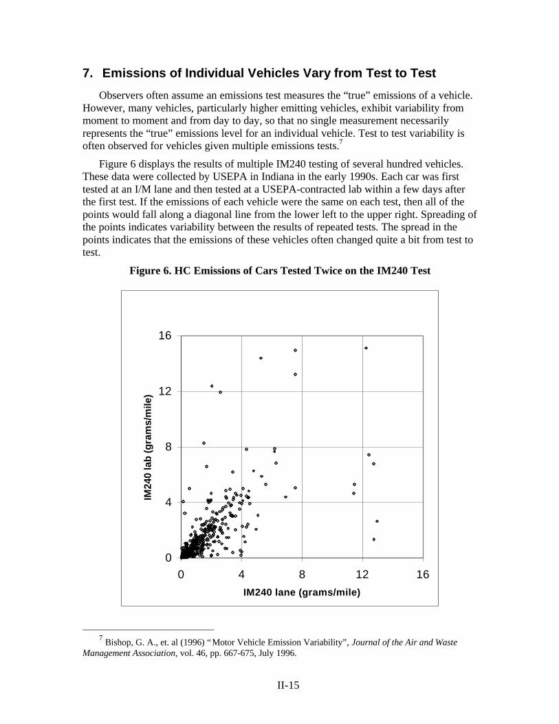
7. Emissions of Individual Vehicles Vary from Test to Test
Observers often assume an emissions test measures the “true” emissions of a vehicle.However, many vehicles, particularly higher emitting vehicles, exhibit variability frommoment to moment and from day to day, so that no single measurement necessarilyrepresents the “true” emissions level for an individual vehicle. Test to test variability isoften observed for vehicles given multiple emissions tests.7
Figure 6 displays the results of multiple IM240 testing of several hundred vehicles.These data were collected by USEPA in Indiana in the early 1990s. Each car was firsttested at an I/M lane and then tested at a USEPA-contracted lab within a few days afterthe first test. If the emissions of each vehicle were the same on each test, then all of thepoints would fall along a diagonal line from the lower left to the upper right. Spreading ofthe points indicates variability between the results of repeated tests. The spread in thepoints indicates that the emissions of these vehicles often changed quite a bit from test totest.
Figure 6. HC Emissions of Cars Tested Twice on the IM240 Test
0
4
8
12
16
0 4 8 12 16IM240 lane (grams/mile)
IM24
0 la
b (g
ram
s/m
ile)
7 Bishop, G. A., et. al (1996) “Motor Vehicle Emission Variability”, Journal of the Air and Waste
Management Association, vol. 46, pp. 667-675, July 1996.
II-16
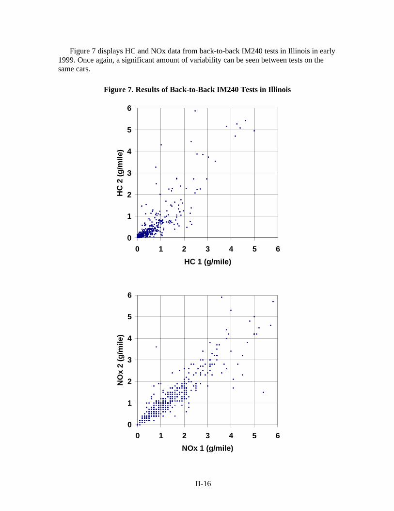
Figure 7 displays HC and NOx data from back-to-back IM240 tests in Illinois in early1999. Once again, a significant amount of variability can be seen between tests on thesame cars.
Figure 7. Results of Back-to-Back IM240 Tests in Illinois
0
1
2
3
4
5
6
0 1 2 3 4 5 6
HC 1 (g/mile)
HC
2 (g
/mile
)
0
1
2
3
4
5
6
0 1 2 3 4 5 6
NOx 1 (g/mile)
NO
x 2
(g/m
ile)
II-17
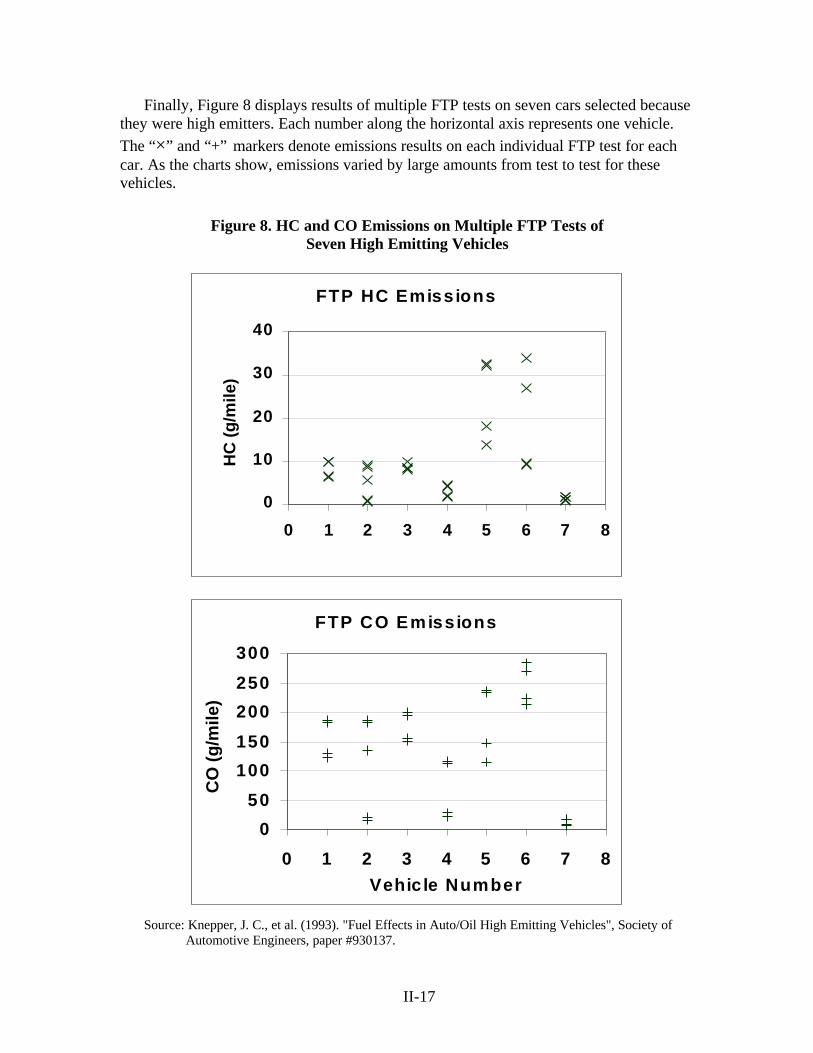
Finally, Figure 8 displays results of multiple FTP tests on seven cars selected becausethey were high emitters. Each number along the horizontal axis represents one vehicle.The “×” and “+” markers denote emissions results on each individual FTP test for eachcar. As the charts show, emissions varied by large amounts from test to test for thesevehicles.
Figure 8. HC and CO Emissions on Multiple FTP Tests ofSeven High Emitting Vehicles
FTP HC Emiss ions
0
10
20
30
40
0 1 2 3 4 5 6 7 8
HC
(g/m
ile)
FTP CO Emiss ions
0
50
100
150
200
250
300
0 1 2 3 4 5 6 7 8Vehic le Number
CO
(g/m
ile)
Source: Knepper, J. C., et al. (1993). "Fuel Effects in Auto/Oil High Emitting Vehicles", Society ofAutomotive Engineers, paper #930137.
II-18
The FTP tests vehicles on a dynamometer over a range of speeds and accelerations.Test conditions are carefully controlled in order to minimize factors that could causeemissions variability. In the regulatory community, the FTP is considered the “goldstandard” for measurement of vehicle emissions. Nevertheless, vehicles can displaysignificant variability on the FTP.
Vehicles that are low emitters on average have low emissions almost all of the timeand average high emitters have high emissions almost all of the time. Nevertheless, thesethree data sets show that many vehicles exhibit a great deal of random variation from testto test.
This variability can have a significant effect on pass/fail decisions when applying I/Mcut points. In the Illinois data above, if one applies USEPA’s phase-in cut points for theIM240 test and treats the second test as a check on the first, one would find that 20percent of cars that failed the first test, passed the second test. On the other hand, 26percent of cars that should have failed the first test actually passed. These jumps betweenpassing and failing are more likely to happen to cars with average emissions that arerelatively close to the failure cut points because emissions variations of just a few percentfrom test to test can change the pass/fail determination. Pass/fail changes can also occurbetween tests for high emitting vehicles that have intermittent malfunctions.
8. Total Emissions Are Dominated by a Small Number of HighEmitters
As noted earlier, most cars have relatively low emissions, and a few cars have veryhigh emissions. Because of this skewed emissions distribution, a small number of high-emitting vehicles account for most of the emissions from the fleet. This result can be seenby ranking cars from dirtiest to cleanest and then determining what percentage of totalemissions comes from a given percentage of the fleet.
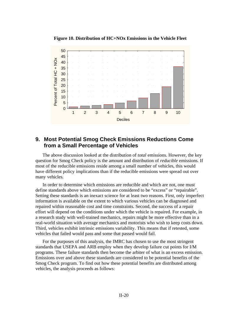
Figure 9 was created by ranking cars from dirtiest to cleanest and then dividing theminto ten groups or “deciles”, with the first decile representing the cleanest 10 percent ofcars and the tenth decile representing the dirtiest 10 percent of cars. Figure 9 shows thatthe dirtiest 10 percent of cars for a given pollutant account for anywhere from 30 percentto almost 50 percent of total emissions of that pollutant. The cleanest 50 percent of carsaccount for about 10 to 15 percent of total emissions.8
The dirtiest ten percent of cars on one pollutant might not be the same cars that arethe dirtiest for another pollutant, though there will be some overlap. To see this result,one can first add together the pollutants and then rank them. Figure 10 shows the resultsfor HC and NOx. For this chart, HC and NOx emissions of each vehicle were addedtogether and then the vehicles were ranked from dirtiest to cleanest, just as before. As thegraph shows, the dirtiest 10 percent account for about 37 percent of total HC+NOx. Soeven when combining pollutants, one observes a skewed emissions distribution.
8 Once again Roadside ASM data were converted to FTP equivalents and then emissions were
weighted by the estimated travel fraction for each model year.

II-19
Figure 9. Distribution of HC, NOx and CO Emissions in the Vehicle Fleet(separate ranking for each pollutant)
Per
cent
of T
otal
HC
0
10
20
30
40
50
Per
cent
of T
otal
NO
x
0
10
20
30
40
50
Deciles
Per
cent
of T
otal
CO
0
10
20
30
40
50
1 2 3 4 5 6 7 8 9 10
II-20
Figure 10. Distribution of HC+NOx Emissions in the Vehicle Fleet
Deciles
Per
cent
of T
otal
HC
+ N
Ox
05
101520253035404550
1 2 3 4 5 6 7 8 9 10
9. Most Potential Smog Check Emissions Reductions Comefrom a Small Percentage of Vehicles
The above discussion looked at the distribution of total emissions. However, the keyquestion for Smog Check policy is the amount and distribution of reducible emissions. Ifmost of the reducible emissions reside among a small number of vehicles, this wouldhave different policy implications than if the reducible emissions were spread out overmany vehicles.
In order to determine which emissions are reducible and which are not, one mustdefine standards above which emissions are considered to be “excess” or “repairable”.Setting these standards is an inexact science for at least two reasons. First, only imperfectinformation is available on the extent to which various vehicles can be diagnosed andrepaired within reasonable cost and time constraints. Second, the success of a repaireffort will depend on the conditions under which the vehicle is repaired. For example, ina research study with well-trained mechanics, repairs might be more effective than in areal-world situation with average mechanics and motorists who wish to keep costs down.Third, vehicles exhibit intrinsic emissions variability. This means that if retested, somevehicles that failed would pass and some that passed would fail.
For the purposes of this analysis, the IMRC has chosen to use the most stringentstandards that USEPA and ARB employ when they develop failure cut points for I/Mprograms. These failure standards then become the arbiter of what is an excess emission.Emissions over and above these standards are considered to be potential benefits of theSmog Check program. To find out how these potential benefits are distributed amongvehicles, the analysis proceeds as follows:
II-21
• Using the random roadside ASM data, convert emissions to FTP equivalentsusing the ERG equation. The IMRC used the Roadside ASM data collectedbetween February 1997 and June 1998 in this case.
• Calculate excess emissions based on FTP failure cut points.9
• Weight emissions by the percent of the vehicle fleet in each model year and theaverage annual miles traveled by each model year.10
• Rank cars from dirtiest to cleanest based on the sum of their excess HC and NOxemissions and divide them into ten deciles from dirtiest 10 percent to cleanest 10percent.
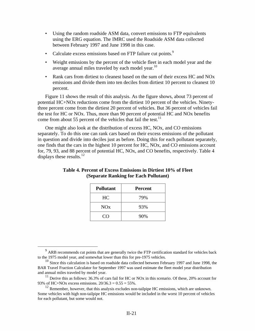
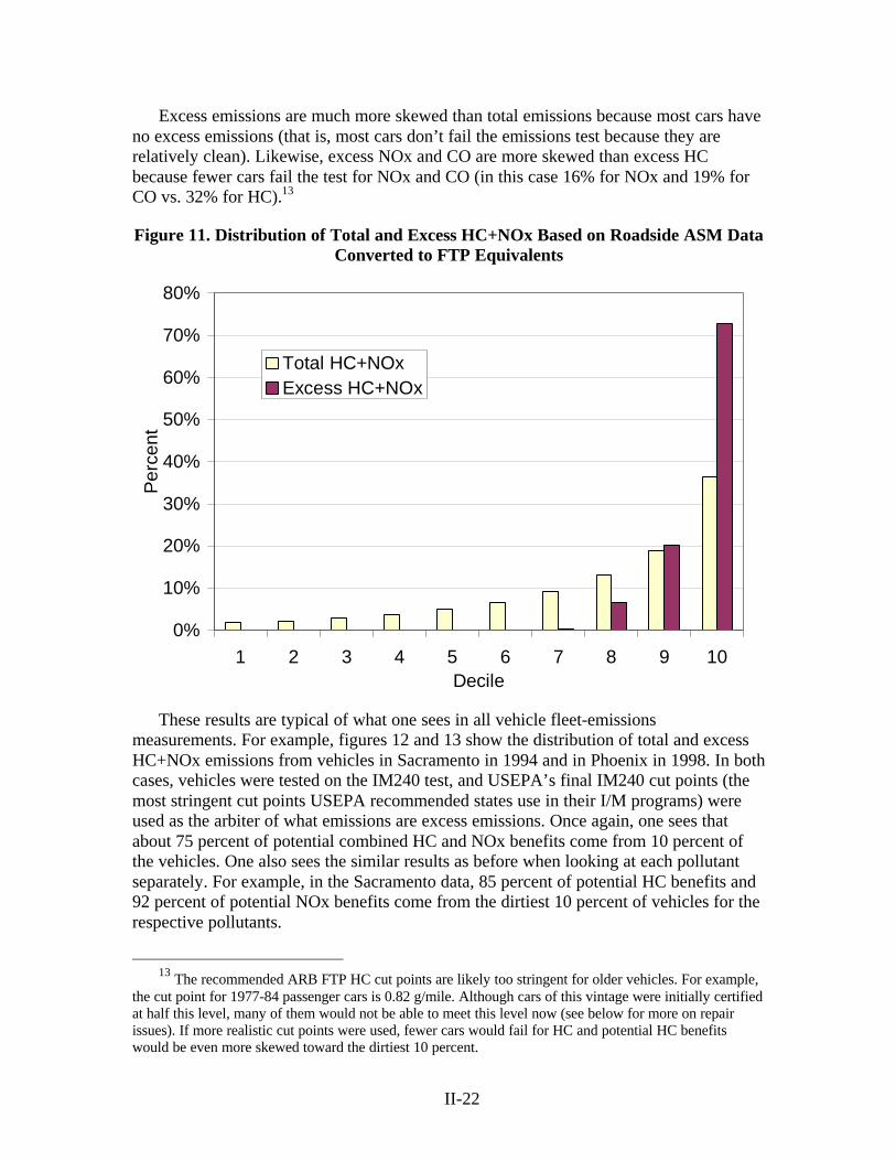
Figure 11 shows the result of this analysis. As the figure shows, about 73 percent ofpotential HC+NOx reductions come from the dirtiest 10 percent of the vehicles. Ninety-three percent come from the dirtiest 20 percent of vehicles. But 36 percent of vehicles failthe test for HC or NOx. Thus, more than 90 percent of potential HC and NOx benefitscome from about 55 percent of the vehicles that fail the test.11
One might also look at the distribution of excess HC, NOx, and CO emissionsseparately. To do this one can rank cars based on their excess emissions of the pollutantin question and divide into deciles just as before. Doing this for each pollutant separately,one finds that the cars in the highest 10 percent for HC, NOx, and CO emissions accountfor, 79, 93, and 88 percent of potential HC, NOx, and CO benefits, respectively. Table 4displays these results.12
Table 4. Percent of Excess Emissions in Dirtiest 10% of Fleet(Separate Ranking for Each Pollutant)
Pollutant Percent
HC 79%
NOx 93%
CO 90%
9 ARB recommends cut points that are generally twice the FTP certification standard for vehicles back
to the 1975 model year, and somewhat lower than this for pre-1975 vehicles.10 Since this calculation is based on roadside data collected between February 1997 and June 1998, the
BAR Travel Fraction Calculator for September 1997 was used estimate the fleet model year distributionand annual miles traveled by model year.
11 Derive this as follows: 36.3% of cars fail for HC or NOx in this scenario. Of these, 20% account for93% of HC+NOx excess emissions. 20/36.3 = 0.55 = 55%.
12 Remember, however, that this analysis excludes non-tailpipe HC emissions, which are unknown.Some vehicles with high non-tailpipe HC emissions would be included in the worst 10 percent of vehiclesfor each pollutant, but some would not.
II-22
Excess emissions are much more skewed than total emissions because most cars haveno excess emissions (that is, most cars don’t fail the emissions test because they arerelatively clean). Likewise, excess NOx and CO are more skewed than excess HCbecause fewer cars fail the test for NOx and CO (in this case 16% for NOx and 19% forCO vs. 32% for HC).13
Figure 11. Distribution of Total and Excess HC+NOx Based on Roadside ASM DataConverted to FTP Equivalents
0%
10%
20%
30%
40%
50%
60%
70%
80%
1 2 3 4 5 6 7 8 9 10Decile
Per
cent
Total HC+NOxExcess HC+NOx
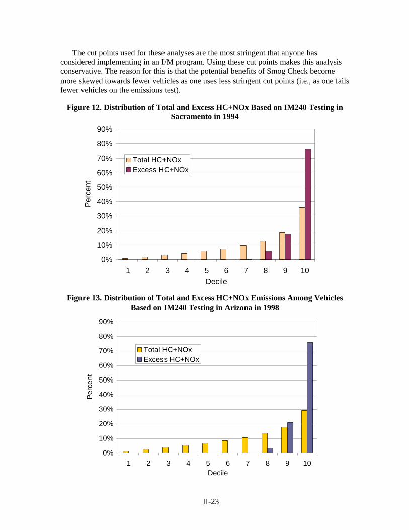
These results are typical of what one sees in all vehicle fleet-emissionsmeasurements. For example, figures 12 and 13 show the distribution of total and excessHC+NOx emissions from vehicles in Sacramento in 1994 and in Phoenix in 1998. In bothcases, vehicles were tested on the IM240 test, and USEPA’s final IM240 cut points (themost stringent cut points USEPA recommended states use in their I/M programs) wereused as the arbiter of what emissions are excess emissions. Once again, one sees thatabout 75 percent of potential combined HC and NOx benefits come from 10 percent ofthe vehicles. One also sees the similar results as before when looking at each pollutantseparately. For example, in the Sacramento data, 85 percent of potential HC benefits and92 percent of potential NOx benefits come from the dirtiest 10 percent of vehicles for therespective pollutants.
13 The recommended ARB FTP HC cut points are likely too stringent for older vehicles. For example,
the cut point for 1977-84 passenger cars is 0.82 g/mile. Although cars of this vintage were initially certifiedat half this level, many of them would not be able to meet this level now (see below for more on repairissues). If more realistic cut points were used, fewer cars would fail for HC and potential HC benefitswould be even more skewed toward the dirtiest 10 percent.
II-23
The cut points used for these analyses are the most stringent that anyone hasconsidered implementing in an I/M program. Using these cut points makes this analysisconservative. The reason for this is that the potential benefits of Smog Check becomemore skewed towards fewer vehicles as one uses less stringent cut points (i.e., as one failsfewer vehicles on the emissions test).
Figure 12. Distribution of Total and Excess HC+NOx Based on IM240 Testing inSacramento in 1994
0%
10%
20%
30%
40%
50%
60%
70%
80%
90%
1 2 3 4 5 6 7 8 9 10Decile
Per
cent
Total HC+NOxExcess HC+NOx
Figure 13. Distribution of Total and Excess HC+NOx Emissions Among VehiclesBased on IM240 Testing in Arizona in 1998
0%
10%
20%
30%
40%
50%
60%
70%
80%
90%
1 2 3 4 5 6 7 8 9 10Decile
Per
cent
Total HC+NOxExcess HC+NOx
II-24
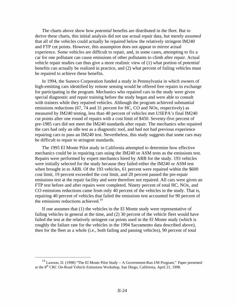
The charts above show how potential benefits are distributed in the fleet. But toderive these charts, this initial analysis did not use actual repair data, but merely assumedthat all of the vehicles could actually be repaired below the relatively stringent IM240and FTP cut points. However, this assumption does not appear to mirror actualexperience. Some vehicles are difficult to repair, and, in some cases, attempting to fix acar for one pollutant can cause emissions of other pollutants to climb after repair. Actualvehicle repair studies can thus give a more realistic view of (1) what portion of potentialbenefits can actually be realized in practice, and (2) what percent of failing vehicles mustbe repaired to achieve these benefits.
In 1994, the Sunoco Corporation funded a study in Pennsylvania in which owners ofhigh-emitting cars identified by remote sensing would be offered free repairs in exchangefor participating in the program. Mechanics who repaired cars in the study were givenspecial diagnostic and repair training before the study began and were able to consultwith trainers while they repaired vehicles. Although the program achieved substantialemissions reductions (67, 74 and 31 percent for HC, CO and NOx, respectively) asmeasured by IM240 testing, less than 40 percent of vehicles met USEPA’s final IM240cut points after one round of repairs with a cost limit of $450. Seventy-five percent ofpre-1985 cars did not meet the IM240 standards after repair. The mechanics who repairedthe cars had only an idle test as a diagnostic tool, and had not had previous experiencerepairing cars to pass an IM240 test. Nevertheless, this study suggests that some cars maybe difficult to repair to stringent standards.
The 1995 El Monte Pilot study in California attempted to determine how effectivemechanics could be in repairing cars using the IM240 or ASM tests as the emissions test.Repairs were performed by expert mechanics hired by ARB for the study. 193 vehicleswere initially selected for the study because they failed either the IM240 or ASM testwhen brought in to ARB. Of the 193 vehicles, 61 percent were repaired within the $600cost limit, 19 percent exceeded the cost limit, and 20 percent passed the pre-repairemissions test at the repair facility and were therefore not repaired. All cars were given anFTP test before and after repairs were completed. Ninety percent of total HC, NOx, andCO emissions reductions came from only 40 percent of the vehicles in the study. That is,repairing 40 percent of vehicles that failed the emissions test accounted for 90 percent ofthe emissions reductions achieved.14
If one assumes that (1) the vehicles in the El Monte study were representative offailing vehicles in general at the time, and (2) 30 percent of the vehicle fleet would havefailed the test at the relatively stringent cut points used in the El Monte study (which isroughly the failure rate for the vehicles in the 1994 Sacramento data described above),then for the fleet as a whole (i.e., both failing and passing vehicles), 90 percent of total
14 Lawson, D. (1998) “The El Monte Pilot Study – A Government-Run I/M Program,” Paper presented
at the 8th CRC On-Road Vehicle Emissions Workshop, San Diego, California, April 21, 1998.
II-25
repair benefits came from 12 percent of the entire vehicle fleet.15 Other repair studies alsoshow that a minority of failing vehicles accounts for the vast majority of repair benefits.16
Not only does attempting to repair cars with marginally high emissions create fewemissions benefits, it can also be counterproductive. For example, in the El Monte study,some cars with relatively low initial FTP emissions had higher FTP emissions for at leastone pollutant after repair. Twelve percent of repaired cars had higher FTP emissionsoverall after repair.17 Other repair studies have also found few emissions benefits fromrepairing marginally failing cars.18
The El Monte study also highlights the issue of emissions variability, which wasdiscussed in Section 7. Twenty percent of the vehicles that were selected for the programbecause they failed the emissions test when brought to ARB, passed a second test at therepair facility. Furthermore, when these vehicles were brought back to ARB and retested,56 percent failed for at least one different pollutant than they had failed for in their firsttest at ARB.19 These vehicles had average emissions 50 to 70 percent lower (dependingon the pollutant) than the vehicles that were repaired. That is, the vehicles that jumpedbetween failing and passing status from one test to the next, had emissions much closer tothe failure cut points than vehicles that continued to fail on successive tests (prior torepair).
10. Current Failure Cut Points Capture Most Potential Benefits
Current Smog Check failure cut points are less stringent than the failure cut pointsARB used to derive California’s SIP emissions reduction targets. For example, based onthe roadside data, 23 percent of all model year 1974 to 1999 vehicles on the road wouldfail Smog Check at current cut points, but 37 percent would fail at the ARB SIP cutpoints.20 Section 9 demonstrated that when applying the most stringent cut points ARBand USEPA have considered using in an I/M program, the dirtiest 10 percent of vehicles
15 Note that the second assumption is conservative. At a lower failure rate, 90 percent of the benefits
would reside in a smaller percent of the vehicle fleet.16 Slott, R. (1993) “Economic Incentives and Inspection and Maintenance Programs,” Proceedings of
the AWMA Specialty Conference New Partnerships: Economic Incentives for EnvironmentalManagement, November 3, 1993.
17 With benefits calculated as HC+CO/7+NOx for each car.18 Slott, R. (1993), ibid19 Lawson, D. (1996) “Analysis of the 1995 El Monte I/M Pilot Study Data Set”, paper Presented at
the 6th CRC On-Road Emissions Workshop, March 18-20, 1996.20 The on-road failure rate at current cut points is 23% for all 1974-1999 vehicles. (This rate rises to
29% when only change-of-ownership testing is assumed for vehicles four-years-old and newer, becauseincluding fewer new vehicles increases the average failure rate for the remaining vehicles. At the ARB SIPcut points, the on-road failure rate rises from 38% to 46% when only change-of-ownership testing isassumed for the four newest model years). However, the failure rate at Smog Check stations is only about14%. The discrepancy between the roadside data and the official Smog Check results is likely due to acombination of factors, including (1) deterioration of vehicles’ emissions systems since their last SmogCheck, (2) vehicles that passed their last Smog Check, but should not have, (3) unregistered vehicles thatnever received a Smog Check and are probably more likely than the average car to be a high emitter, and(4) cars that received repairs or maintenance shortly before their initial Smog Check or official pretest. PartIII of this report provides estimates for some of these factors.
II-26
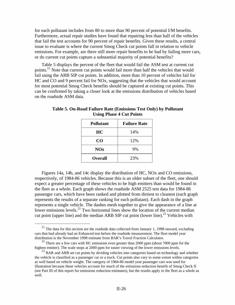
for each pollutant includes from 80 to more than 90 percent of potential I/M benefits.Furthermore, actual repair studies have found that repairing less than half of the vehiclesthat fail the test accounts for 90 percent of repair benefits. Given these results, a centralissue to evaluate is where the current Smog Check cut points fall in relation to vehicleemissions. For example, are there still more repair benefits to be had by failing more cars,or do current cut points capture a substantial majority of potential benefits?
Table 5 displays the percent of the fleet that would fail the ASM test at current cutpoints.21 Note that current cut points would fail more than half the vehicles that wouldfail using the ARB SIP cut points. In addition, more than 10 percent of vehicles fail forHC and CO and 9 percent fail for NOx, suggesting that the vehicles that would accountfor most potential Smog Check benefits should be captured at existing cut points. Thiscan be confirmed by taking a closer look at the emissions distribution of vehicles basedon the roadside ASM data.
Table 5. On-Road Failure Rate (Emissions Test Only) by PollutantUsing Phase 4 Cut Points
Pollutant Failure Rate
HC 14%
CO 12%
NOx 9%
Overall 23%
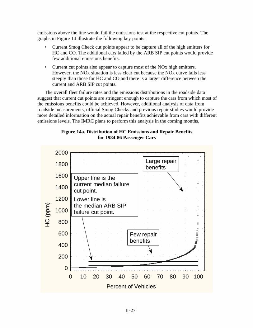
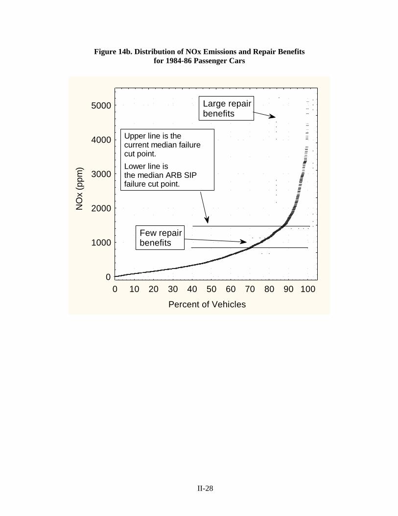
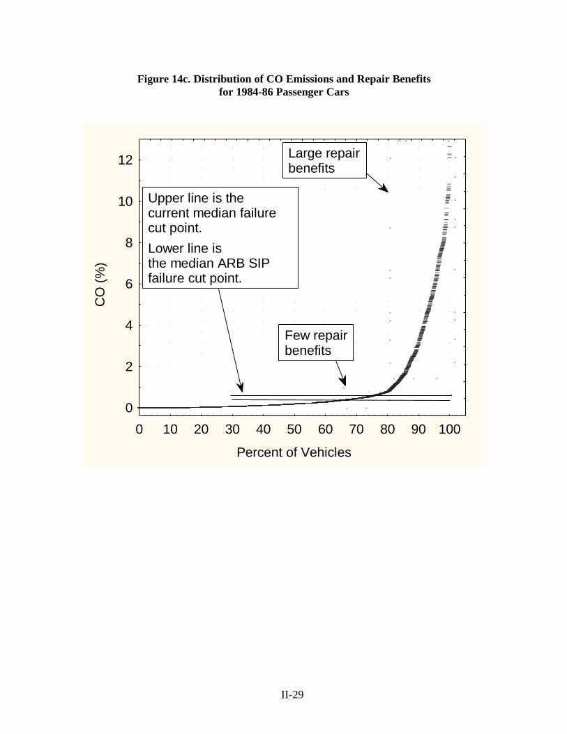
Figures 14a, 14b, and 14c display the distribution of HC, NOx and CO emissions,respectively, of 1984-86 vehicles. Because this is an older subset of the fleet, one shouldexpect a greater percentage of these vehicles to be high emitters than would be found inthe fleet as a whole. Each graph shows the roadside ASM 2525 test data for 1984-86passenger cars, which have been ranked and plotted from dirtiest to cleanest (each graphrepresents the results of a separate ranking for each pollutant). Each dash in the graphrepresents a single vehicle. The dashes mesh together to give the appearance of a line atlower emissions levels.22 Two horizontal lines show the location of the current mediancut point (upper line) and the median ARB SIP cut point (lower line).23 Vehicles with
21 The data for this section are the roadside data collected from January 1, 1998 onward, excluding
cars that had already had an Enhanced test before the roadside measurement. The fleet model yeardistribution is the November 1998 estimate from BAR’s Travel Fraction Calculator.
22 There are a few cars with HC emissions even greater than 2000 ppm (about 7000 ppm for thehighest emitter). The scale stops at 2000 ppm for easier viewing of the lower emissions levels.
23 BAR and ARB set cut points by dividing vehicles into categories based on technology and whetherthe vehicle is classified as a passenger car or a truck. Cut points also vary to some extent within categoriesas well based on vehicle weight. The category of 1984-86 model year passenger cars was used forillustration because these vehicles account for much of the emissions reduction benefit of Smog Check II(see Part III of this report for emissions reduction estimates), but the results apply to the fleet as a whole aswell.
II-27
emissions above the line would fail the emissions test at the respective cut points. Thegraphs in Figure 14 illustrate the following key points:
• Current Smog Check cut points appear to be capture all of the high emitters forHC and CO. The additional cars failed by the ARB SIP cut points would providefew additional emissions benefits.
• Current cut points also appear to capture most of the NOx high emitters.However, the NOx situation is less clear cut because the NOx curve falls lesssteeply than those for HC and CO and there is a larger difference between thecurrent and ARB SIP cut points.
The overall fleet failure rates and the emissions distributions in the roadside datasuggest that current cut points are stringent enough to capture the cars from which most ofthe emissions benefits could be achieved. However, additional analysis of data fromroadside measurements, official Smog Checks and previous repair studies would providemore detailed information on the actual repair benefits achievable from cars with differentemissions levels. The IMRC plans to perform this analysis in the coming months.
Figure 14a. Distribution of HC Emissions and Repair Benefitsfor 1984-86 Passenger Cars
Percent of Vehicles
HC
(ppm
)
0
200
400
600
800
1000
1200
1400
1600
1800
2000
0 10 20 30 40 50 60 70 80 90 100
Large repairbenefits
Few repairbenefits
Upper line is the current median failure cut point.Lower line is the median ARB SIP failure cut point.
II-28
Figure 14b. Distribution of NOx Emissions and Repair Benefitsfor 1984-86 Passenger Cars
Percent of Vehicles
NO
x (p
pm)
0
1000
2000
3000
4000
5000
0 10 20 30 40 50 60 70 80 90 100
Large repairbenefits
Few repairbenefits
Upper line is the current median failure cut point.Lower line is the median ARB SIP failure cut point.
II-29
Figure 14c. Distribution of CO Emissions and Repair Benefitsfor 1984-86 Passenger Cars
Percent of Vehicles
CO
(%)
0
2
4
6
8
10
12
0 10 20 30 40 50 60 70 80 90 100
Upper line is the current median failure cut point.Lower line is the median ARB SIP failure cut point.
Large repairbenefits
Few repairbenefits
II-30
11. Failure Cut Points Used for SIP Emissions Reduction TargetsWould Fail Many Cars with Only Marginally High Emissions
The graphs in Figure 14 show that the cars that fail at current cut points wouldprovide significantly more emissions reductions than the additional cars that fail at theARB SIP cut points. For example, if cars that fail at the current cut points are repaireddown to the ARB SIP cut points, they would achieve average emission reductions ofabout 220 ppm for HC, 3.3 percent for CO and 890 ppm for NOx.24 The correspondingemissions reductions for cars falling between the two sets of cut points are about 12 ppmfor HC, 0.15 percent for CO, and 280 ppm for NOx. Thus, when compared with theadditional cars failed by the ARB SIP cut points, the cars that fail under current cut pointswould achieve emissions reductions 18 times greater for HC, 22 times greater for CO andthree times greater for NOx. In addition, based on results of previous repair studies, theactual emissions benefit for these lower-emitting cars might be less than this becausesome of these cars would likely be difficult to repair or might even have increases in oneor more pollutants after repair (see Section 9, above).
The three graphs in Figure 14 illustrate an additional potential problem with verystringent cut points that is related to emissions variability. Section 7 showed that manyvehicles have intrinsically variable emissions and change to some extent from test to test.This means that some cars that fail a test will pass if tested again without any repairshaving been made, and vice versa. This “false failure” and “false pass” problem willlikely be more pronounced if there are more vehicles with emissions relatively close tothe cut points. To the extent that the cut points are set so that they cross the emissionscurve when its slope is steep (the right side of the graphs where the high emitters are),there will be fewer cars with emissions close to the cut point. On the other hand, to theextent that the cut points cross the emissions curve where its slope is shallow (both sets ofcut points for HC exhibit this characteristic, for example), many more cars will haveemissions near the cut points.
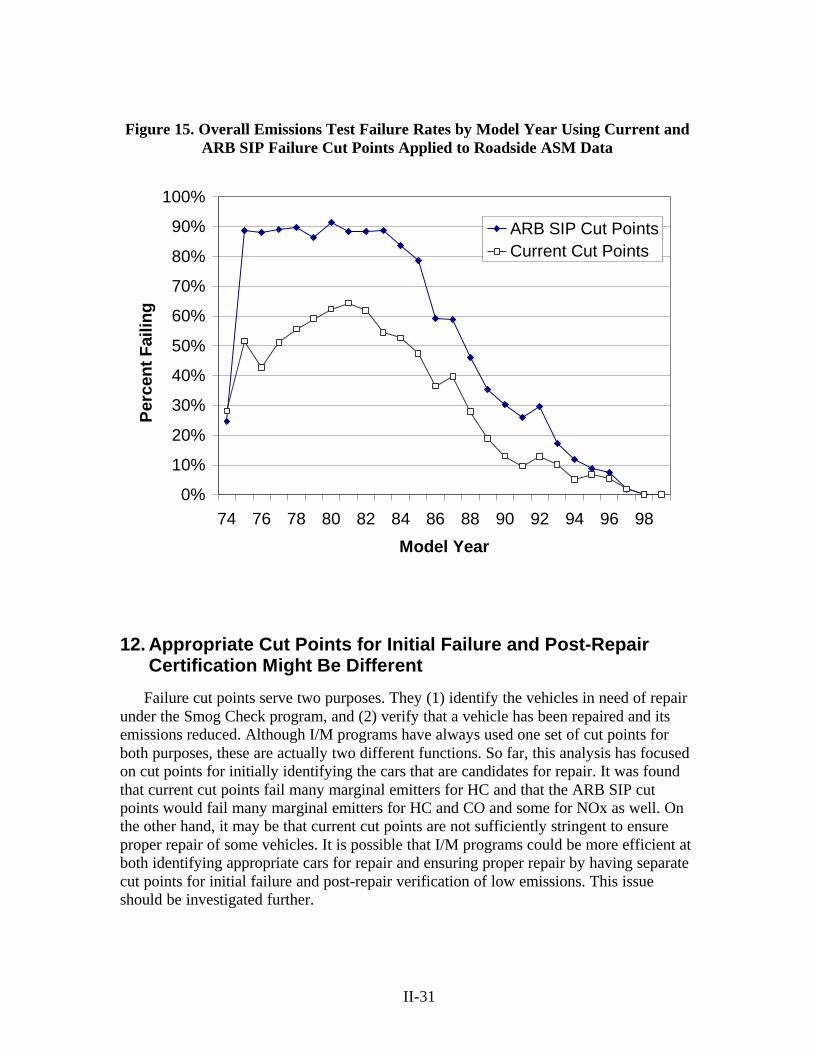
In addition to limitations on their potential to create additional Smog Check benefits,the ARB SIP cut points would fail a very high percentage of older vehicles. Figure 15displays the average emissions test failure rates (i.e., total failure rate including all threepollutants and both the ASM 2525 and ASM 5015 tests) by model year of vehiclesmeasured by Roadside ASM using current and ARB SIP cut points. Roughly 90 percentof pre-1984 vehicles would fail the test at the SIP standards, and 38 percent of all 1974 to1999 model year vehicles would fail.25
24 One might argue that at current cut points, cars would not be repaired down to the ARB SIP cut
points. However, analysis of the VID data indicates that, on average, final emissions of fail-pass vehiclesare well below the current cut points. In addition, as discussed below, cut points for initial failure and post-repair verification need not be the same.
25 If only change-of-ownership testing is assumed for vehicles four years old and newer, the failurerate for the remaining vehicles rises to 46 percent (see footnote #20).
II-31
Figure 15. Overall Emissions Test Failure Rates by Model Year Using Current andARB SIP Failure Cut Points Applied to Roadside ASM Data
0%
10%
20%
30%
40%
50%
60%
70%
80%
90%
100%
74 76 78 80 82 84 86 88 90 92 94 96 98
Model Year
Per
cent
Fai
ling
x
ARB SIP Cut PointsCurrent Cut Points
12. Appropriate Cut Points for Initial Failure and Post-RepairCertification Might Be Different
Failure cut points serve two purposes. They (1) identify the vehicles in need of repairunder the Smog Check program, and (2) verify that a vehicle has been repaired and itsemissions reduced. Although I/M programs have always used one set of cut points forboth purposes, these are actually two different functions. So far, this analysis has focusedon cut points for initially identifying the cars that are candidates for repair. It was foundthat current cut points fail many marginal emitters for HC and that the ARB SIP cutpoints would fail many marginal emitters for HC and CO and some for NOx as well. Onthe other hand, it may be that current cut points are not sufficiently stringent to ensureproper repair of some vehicles. It is possible that I/M programs could be more efficient atboth identifying appropriate cars for repair and ensuring proper repair by having separatecut points for initial failure and post-repair verification of low emissions. This issueshould be investigated further.