Smilen Dimitrov · forces, which cause atoms to bind in molecules. Therefore, the number and distribution of the electrons in the shell – especially the outer shell of the atom,

Aalborg University Copenhagen Medialogy MED4 2007

Sensors Technology Electronics – particle level: structure of matter Smilen Dimitrov

Electronics – particle level: structure of matter 1

Contents 1 Introduction ............................................................................................................... 3 2 Structure of matter .................................................................................................... 4 3 Historical timeline of the atomic model.................................................................... 8

3.1 Democritus ...........................................................................................................8 3.2 Billiard Ball Model................................................................................................9 3.3 Thomson - Plumb Pudding Model .......................................................................9 3.4 Einstein – photoelectric effect ........................................................................... 10 3.5 Rutherford - Solar System (planetary) Model ................................................... 13 3.6 Bohr (Semi-Classical) Model.............................................................................. 13 3.7 Electron Cloud (Quantum Mechanical) Model.................................................. 14

4 Basic atomic properties ............................................................................................16 5 Hydrogen – single electron system ..........................................................................18

5.1 Bohr (semi-classical) model ............................................................................... 18 5.2 QM model ...........................................................................................................23

5.2.1 Long exposition photography analogy .......................................................24 5.2.2 From Bohr orbit to QM orbital ................................................................... 27

5.3 Electron orbitals of the hydrogen atom .............................................................29 5.4 Photoelectric effect – effect of field on the shell ................................................ 31 5.5 Hydrogen transition ........................................................................................... 33

6 Free electron ............................................................................................................ 34 7 Multi-electron atoms ............................................................................................... 39

7.1 Bohr model perspective......................................................................................39 7.2 QM model perspective........................................................................................ 41

8 Bonding – molecules and crystals ........................................................................... 43 8.1 Bonding in H2 – covalent bonding ....................................................................44 8.2 Bonding in H2O – covalent bonding ................................................................. 45

9 Metallic bonding and conductivity .......................................................................... 48 10 PE Questions.............................................................................................................55


1 Introduction We have previously introduced the model that conceptualizes the focus we have in ST:

In these parts of the lectures, we focus on the hardware – electronics part of our sensor-based interaction input system:

The understanding of this part of the process requires in essence two things: understanding of the conversion from a given physical parameter into an electric parameter – which is the sensing process: process of electric measurement that the sensor performs; and understanding concepts in electrical circuits which are used to perform signal conditioning. Both of these require understanding of electrical properties of matter. In this part of the lectures, we start looking at the structure of matter, mostly through visualization, in order to gain a basic understanding of the electrical and sensing processes on the atomic level.


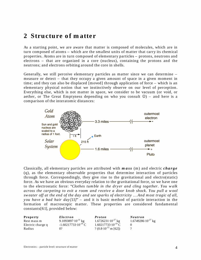
2 Structure of matter As a starting point, we are aware that matter is composed of molecules, which are in turn composed of atoms – which are the smallest units of matter that carry its chemical properties. Atoms are in turn composed of elementary particles – protons, neutrons and electrons – that are organized in a core (nucleus), containing the protons and the neutrons; and electrons orbiting around the core in shells. Generally, we still perceive elementary particles as matter since we can determine – measure or detect – that they occupy a given amount of space in a given moment in time; and they can also be displaced [moved] through application of force – which is an elementary physical notion that we instinctively observe on our level of perception. Everything else, which is not matter in space, we consider to be vacuum (or void, or aether, or The Great Emptyness depending on who you consult ☺) – and here is a comparison of the interatomic distances:

Classically, all elementary particles are attributed with mass (m) and electric charge (q), as the elementary observable properties that determine interaction of particles through force. Correspondingly, they give rise to the gravitational and electro(static) force. As we have an obvious everyday relation to the gravitational force, so we have one to the electrostatic force: “Clothes tumble in the dryer and cling together. You walk across the carpeting to exit a room and receive a door knob shock. You pull a wool sweater off at the end of the day and see sparks of electricity … And most tragic of all, you have a bad hair day[11]” – and it is basic method of particle interaction in the formation of macroscopic matter. These properties are considered fundamental constants[61], provided below: Property Electron Proton Neutron Rest mass m 9.1093897·10-31 kg 1.6726231·10-27 kg 1.6749286·10-27 kg Electric charge q -1.60217733·10-19 C 1.60217733·10-19 C 0 Radius 0? ? (0.8·10-15 m [62]) ?


So, masses of the proton and neutron are approximately equal, and about 1800 times larger than the mass of the electron:

enp mmm ⋅≈≈ 1836 ; ep mm >> And, the charges of the proton and the electron are equal in quantity, but opposite in sign:

eqeq pe =−= ,

where is the elementary electric charge – the smallest unit of electric charge in nature. There is a question mark for the radii of these elementary particles – due to the quantum uncertainty in positioning of elementary particles that we will discuss further, when we compare the Bohr and QM model of the atom (although there is a constant known as classical electron radius, according to which “it can be calculated that the number of electrons that would fit in the observable universe is on the order of 10

C ·101.60217733 -19=e

130. Of course, this number is even less meaningful than the classical electron radius itself [64]” - for more discussion about particle radii, see [63], [26]). However, experimental data seems to point out that the radius of the electron particle, may indeed be zero: “The electron (and all truly 'fundamental' particles) are considered to be true mathematical points in the sense that they have no classical spatial extent. This is known, for example in the case of the electron, by performing scattering experiments: the way particles scatter off one another is quite different if the target is represented as a point as opposed to having some finite size. All of the electron scattering experiments done so far are consistent with the hypothesis that the electron is truly a 'point particle.'[26]” In the text further on, we will therefore distinguish between two concepts of a point particle – a physical (classical) point particle – which has mass, charge and some very small radius which we don’t know, but which is however finite and measurable; and a mathematical point particle, which too has charge and mass – however with a radius of 0 (immeasurably small radius, or no radius at all). Classically, forces on this level are mediated by fields, which fill out the vacuum space around a particle - we will take a closer look at the classical theory of electrostatic field and force in a future module. For now, we are aware that a given force between particles is determined by the value of the corresponding properties of the particles - gravitational force is strictly attractive (and the mass property is correspondingly always positive) – yet on atomic level it is inferior to the electrostatic force, due to the negligibly small mass of the electron. The electrostatic force is attractive for unlike charges, and repulsive for like charges – and correspondingly the proton is attributed with positive charge, the electron with negative and the neutron with charge 0. Thus, the attractive electrostatic force between the protons in the core and electrons in the shell is what binds the atom - keeps the atom together. The number of positive and negative charge in a stable atom tends to pair and cancel out; so as we go along the elements in the periodic table, the number of protons in the atom core of the elements increases, and so does the number of electrons -


making the atoms as units to tend to be electrically neutral. However, here there also appear repulsive electrostatic forces between the electrons themselves, which causes grouping of the electrons into orbitals (shells) - and the slight disbalances of charge, determined by the distribution and number of electrons in the shell, cause interatomic forces, which cause atoms to bind in molecules. Therefore, the number and distribution of the electrons in the shell – especially the outer shell of the atom, which is known as the valence shell – determine the chemical properties of atoms. It is through the electrons in the valence shell, that the atoms interact between each other, forming molecules, and eventually macroscopic material structures – manifesting themselves in several aggregate states: in gaseous, fluid or solid form (plasma should be mentioned as well). Although atoms tend to be electrically neutral, under certain interactions they may lose or gain electrons, thereby losing the electrical neutrality and gaining a net charge – which effectively turns the atoms into ions. This eventually shows, that an electron need not be bound to an atom always – given a favorable energetic situation, it can leave the attractive forces of the nucleus and become a free electron. As the electrons are primary actors in interaction of atoms, they are essential in forming matter as we know it. Thus, as an elementary building block in nature they are in focus both in physics, chemistry and other physical sciences – and obviously in electronics. Whereas chemistry, for instance, is concerned with the chemical reactions involved in formation of molecules and compounds, and hence always keeps a focus on the electrons as part of the atom – in electronics we deal mostly with the notion of free electrons, the possibility to move them at will in a controlled manner, and the application of this possibility in electrical circuits. In electronics, at least on a basic level, we can deal with a simplified model of an atom. However, in certain applications of electronics, most notably high frequency circuits – which are related both to wireless radio transmission and hardware computing power – certain effects come into play, which stem from the complex nature of matter on the atomic level; and then more complex models need to be taken into account. Here we are aware that an accelerating electron, changes the distribution of the electrostatic field in space, and such a change spreads through space as a wave – which is the notion of the electromagnetic wave, which as a phenomenon covers both light and radio waves. Needless to say, both light and radio have huge application in electronics. It is thus obvious that a model of the atom needs to be discussed, in order to discuss the electron and the issues in electronics. As noted before, we can discuss quite a basic model of the atom in order to introduce basic concepts in electronics. On the other hand, the recent developments of technology, have brought about computer simulations as a tool to visualize matter on the atomic level and test theories – and the development of scanning-tunneling microscopy (STM) and attosecond laser imaging allows direct peak into matter on the level of atoms, and verification of theories. This then supports the further development of applications of technical processes on this level of matter, chiefly through the recent development of nanotechnology. As the this development continues, new knowledge is acquired and the models of matter on the atomic level are


constantly updated. As matter on this level begins to behave contradictory to our daily experience, although still bound by physical laws – this is traditionally an area whose understanding demands a significant use of theory and serious mathematical effort. Of course, the scope of this course makes it impossible that all the theories, necessary for understanding matter on this level, are introduced on the level as they are studied in electronic engineering. Yet, we can take advantage of the recent research in visualization and imaging, and the availability of material of the Internet, to discuss the atom on a more detailed level – without going into the complex mathematical details which otherwise follow. This approach will serve both as a basis for understanding electric sensing processes from a wider perspective; and as a basis for understanding to what level we approximate things when we discuss basic electric circuits – hopefully without going too deep and risking the loss of connection of the overall perspective that we have in ST, which is again application of sensing in user interaction. Providing a visual overview of the atomic effects of interest should also keep us alert on new developments in technology, which sooner or later will influence the applications in media communication and interaction too. It is important that historically, the technical development around understanding matter on the atomic level goes but a couple of centuries back – and the discussion of these matters has been mostly on a mathematical level, to set a theoretical framework for experimental results. This influenced a historical change of the general model of the atom, which even today is being updated with new theoretical and experimental findings. That is why we begin the discussion of a model of the atom by providing a short historical overview of the general models of the atom.


3 Historical timeline of the atomic model There are plenty of historical timelines of the atomic model on the Internet, consider any of [1]-[11], offering visual resources as well. In short, we can see an overview on these slides:

[11] [60]

Here we will mostly borrow the short timeline from [9]:

3.1 Democritus a fifth century B.C. Greek philosopher proposed that all matter was composed of indivisible particles called atoms (Greek for uncuttable). [9]


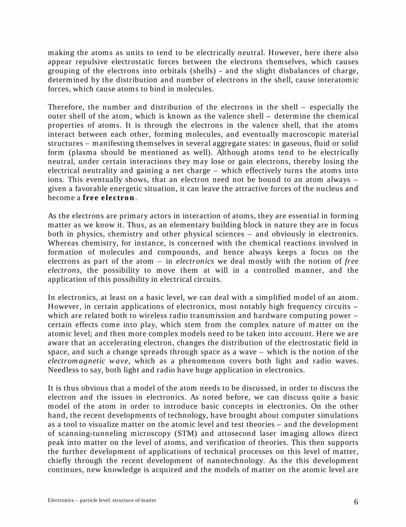
3.2 Billiard Ball Model (1803) - John Dalton viewed the atom as a small solid sphere. • Each element was composed of the same kind of atoms. • Each element was composed of different kinds of atoms. • Compounds are composed of atoms in specific ratios. • Chemical reactions are rearrangements of atoms (mass is conserved). [9]

[6] [7] [5]

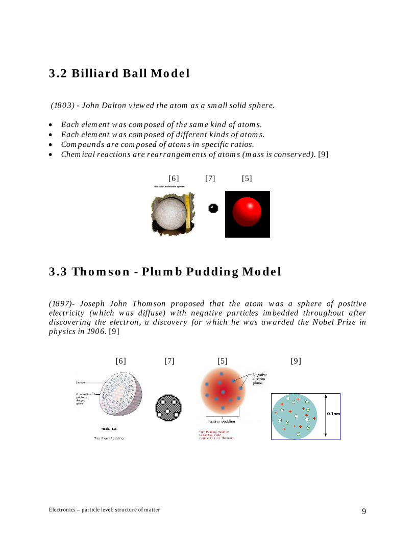
3.3 Thomson - Plumb Pudding Model (1897)- Joseph John Thomson proposed that the atom was a sphere of positive electricity (which was diffuse) with negative particles imbedded throughout after discovering the electron, a discovery for which he was awarded the Nobel Prize in physics in 1906. [9]

[6] [7] [5] [9]


3.4 Einstein – photoelectric effect Although not an atomic model, Einstein’s explanation of the photoelectric effect (1905), which matched experimental results, raised the issue of interaction between light and matter – and at the same time, the issue of wave-particle duality. As such, this issue is of central focus in Bohr and QM models – and needless to say, it represents the basic light sensing process through electrical means. Notice that at this time in history, there is no model of the atom as we know it yet. Let’s use Wikipedia’s entry to introduce the photoelectric effect: ”

Upon exposing a metallic surface to electromagnetic radiation that is above the threshold frequency (which is particular to each type of surface and material), the photons are absorbed and current is produced. No electrons are emitted for radiation with a frequency below that of the threshold, as the electrons are unable to gain sufficient energy to overcome the electrostatic barrier presented by the termination of the crystalline surface (the material's work function). By conservation of energy, energy of the photon is absorbed by the electron and, if energetic enough, can escape from the material with a

finite kinetic energy. One photon can only remove one electron. The electrons that are emitted are often termed photoelectrons.

[60]

Albert Einstein's mathematical description in 1905 of how it was caused by absorption of what were later called photons, or quanta of light, in the interaction of light with the electrons in the substance, was contained in the paper named "On a Heuristic Viewpoint Concerning the Production and Transformation of Light". This paper proposed the simple description of "light quanta" (later called "photons") and showed how they could be used to explain such phenomena as the photoelectric effect. The simple explanation by Einstein in terms of absorption of single quanta of light explained the features of the phenomenon and helped explain the characteristic frequency. Einstein's explanation of the photoelectric effect won him the Nobel Prize of 1921. The photoelectric effect helped propel the then-emerging concept of the dual nature of light, that light exhibits characteristics of waves and particles at different times. The effect was impossible to understand in terms of the classical wave description of light, as the energy of the emitted electrons did not depend on the intensity of the incident radiation. Classical theory predicted that the electrons could 'gather up' energy over a period of time, and then be emitted. … These ideas were abandoned.


The photons of the light beam have a characteristic energy given by the wavelength of the light. In the photoemission process, if an electron absorbs the energy of one photon and has more energy than the work function, it is ejected from the material. If the photon energy is too low, however, the electron is unable to escape the surface of the material. Increasing the intensity of the light beam does not change the energy of the constituent photons, only their number, and thus the

energy of the emitted electrons does not depend on the intensity of the incoming light. Electrons can absorb energy from photons when irradiated, but they follow an "all or nothing" principle. All of the energy from one photon must be absorbed and used to liberate one electron from atomic binding, or the energy is re-emitted. If the photon is absorbed, some of the energy is used to liberate it from the atom, and the rest contributes to the electron's kinetic (moving) energy as a free particle. [16]“ The way this explanation of the photoelectric effect influenced the wave-particle duality can be seen on this figure

[17]

From here, we can note that although most of the observable effects of light indicate that it is a wave phenomenon, the fact that it can knock material particles (electrons) out, points out a particle nature. Also, the possibility to discretize a light quantum – photon – indicates that light would be divisible in a smaller ‘particle’. And hence, the relation of energy of light to frequency (color), relates the intensity of light to “the number of photon particles” that are emitted, instead of an intensity of a wave.


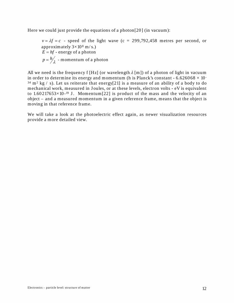
Here we could just provide the equations of a photon[20] (in vacuum):

cfv == λ - speed of the light wave (c = 299,792,458 metres per second, or approximately 3×108 m/s.)

hfE = - energy of a photon

λhp = - momentum of a photon

All we need is the frequency f [Hz] (or wavelength λ [m]) of a photon of light in vacuum in order to determine its energy and momentum (h is Planck’s constant - 6.626068 × 10-

34 m2 kg / s). Let us reiterate that energy[21] is a measure of an ability of a body to do mechanical work, measured in Joules, or at these levels, electron volts - eV is equivalent to 1.60217653×10-19 J. Momentum[22] is product of the mass and the velocity of an object – and a measured momentum in a given reference frame, means that the object is moving in that reference frame. We will take a look at the photoelectric effect again, as newer visualization resources provide a more detailed view.


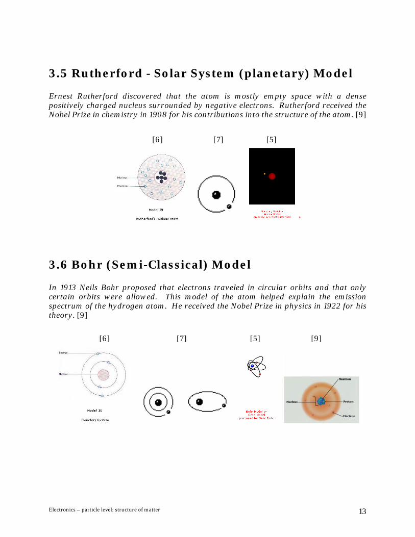
3.5 Rutherford - Solar System (planetary) Model Ernest Rutherford discovered that the atom is mostly empty space with a dense positively charged nucleus surrounded by negative electrons. Rutherford received the Nobel Prize in chemistry in 1908 for his contributions into the structure of the atom. [9]

[6] [7] [5]

3.6 Bohr (Semi-Classical) Model In 1913 Neils Bohr proposed that electrons traveled in circular orbits and that only certain orbits were allowed. This model of the atom helped explain the emission spectrum of the hydrogen atom. He received the Nobel Prize in physics in 1922 for his theory. [9]

[6] [7] [5] [9]


3.7 Electron Cloud (Quantum Mechanical) Model (1920's) - an atom consists of a dense nucleus composed of protons and neutrons surrounded by electrons that exist in different clouds at the various energy levels. Erwin Schrodinger and Werner Heisenburg developed probability functions to determine the regions or clouds in which electrons would most likely be found. [9]

[6] [7] [5] [9]

These models developed over history, as new discoveries tested theories and required their adjustment. Today, the quantum mechanical model is integrated with new findings and is known as the Standard Model of particle physics, displayed on the figure on the right. It is important to take note of this about this model: “Developed between 1970 and 1973, it is a quantum field theory, and consistent with both quantum mechanics and special relativity. To date, almost all experimental tests of the three forces described by the Standard Model have agreed with its predictions. However, the Standard Model is not a complete theory of fundamental interactions, primarily because it does not describe the gravitational force[12]”.

[12]


As the Standard model also discusses subparticles that constitute the proton and neutron (quarks) it provides a level of detail that we do not need to discuss basic electronic concepts (for a simple applet that includes this perspective, see Atom Builder [14]). However it does spawn some interesting conclusions, as the two primary types of interactions in the universe manifested through fermions and bosons, displayed on the image on the left – and motivates theorists to continue towards a possible theory that will unify all physical phenomena (the so-called Grand Unified Theory [23]).

[4]

Instead, here we will focus on the atomic structure on the level of nucleus (protons and neutrons) and electron shells. First we discuss a single electron system through the simplest atom, the hydrogen atom – which can serve as a basis to discuss both the Bohr and QM models, and can help us understand the transition from one to the other. Then we briefly discuss multielectron systems, followed by atomic and molecular binding – so we can eventually arrive at a brief description of metals and electric conductivity.


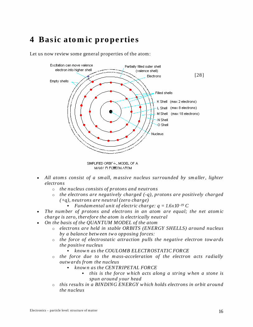
4 Basic atomic properties Let us now review some general properties of the atom:

[28]

• All atoms consist of a small, massive nucleus surrounded by smaller, lighter electrons

o the nucleus consists of protons and neutrons o the electrons are negatively charged (-q), protons are positively charged

(+q), neutrons are neutral (zero charge) Fundamental unit of electric charge: q = 1.6x10-19 C

• The number of protons and electrons in an atom are equal; the net atomic charge is zero, therefore the atom is electrically neutral

• On the basis of the QUANTUM MODEL of the atom o electrons are held in stable ORBITS (ENERGY SHELLS) around nucleus

by a balance between two opposing forces: o the force of electrostatic attraction pulls the negative electron towards

the positive nucleus known as the COULOMB ELECTROSTATIC FORCE

o the force due to the mass-acceleration of the electron acts radially outwards from the nucleus

known as the CENTRIPETAL FORCE this is the force which acts along a string when a stone is

spun around your head o this results in a BINDING ENERGY which holds electrons in orbit around

the nucleus


• The bound electrons do not possess any value of energy, but can only possess specific discrete energies according to the allowed orbits

o the energy is said to be QUANTISED and the permitted values of energy are known as energy levels

o the further the electron is from the nucleus the less tightly bound it will be to the nucleus.

• Each atom has an infinity of possible orbits (energy shells) o the electrons are confined to orbit in these discrete shells o not all shells will contain an electron o the number of electrons in a given shell is restricted to specific values

• The outermost occupied shell is known as the VALENCE SHELL o the valence electrons are very important

they determine material properties o the maximum number of valence electrons is 8

an atom with a valence of 8 is a stable atom (inert or unreactive) an atom with a valence of 1 is highly reactive [28]


5 Hydrogen – single electron system

5.1 Bohr (semi-classical) model

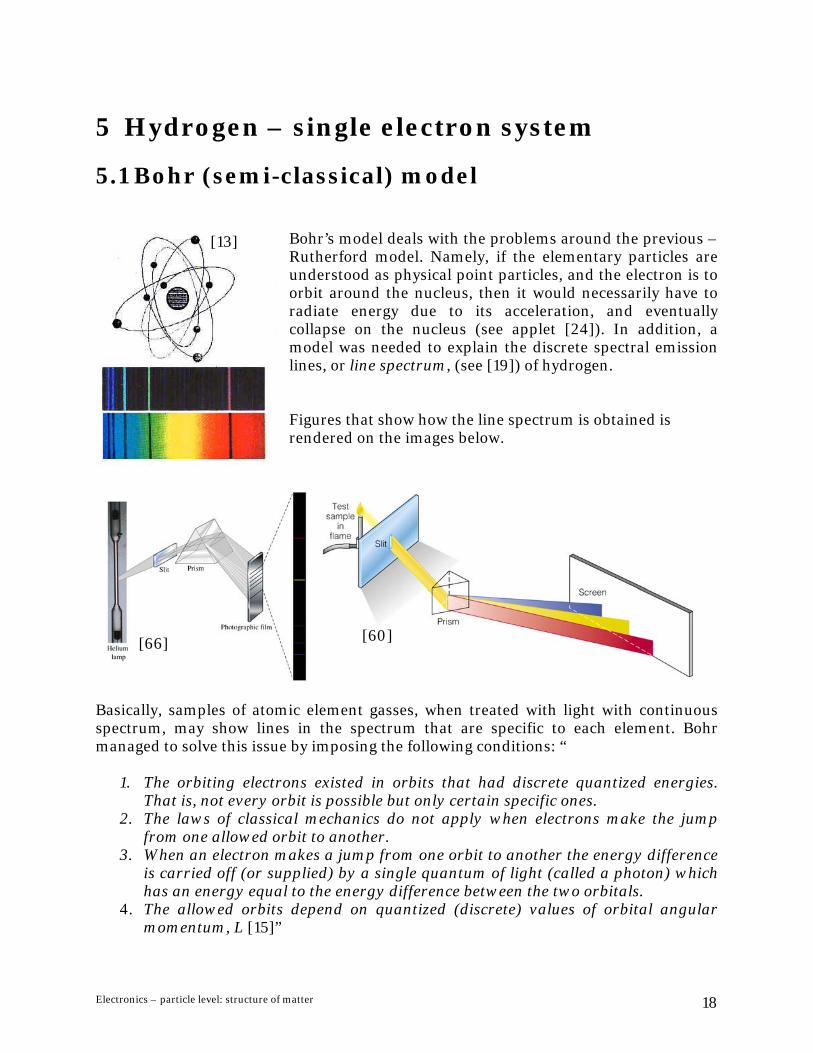
Bohr’s model deals with the problems around the previous – Rutherford model. Namely, if the elementary particles are understood as physical point particles, and the electron is to orbit around the nucleus, then it would necessarily have to radiate energy due to its acceleration, and eventually collapse on the nucleus (see applet [24]). In addition, a model was needed to explain the discrete spectral emission lines, or line spectrum, (see [19]) of hydrogen.

[13]

Figures that show how the line spectrum is obtained is rendered on the images below.

[60] [66]

Basically, samples of atomic element gasses, when treated with light with continuous spectrum, may show lines in the spectrum that are specific to each element. Bohr managed to solve this issue by imposing the following conditions: “

1. The orbiting electrons existed in orbits that had discrete quantized energies. That is, not every orbit is possible but only certain specific ones.

2. The laws of classical mechanics do not apply when electrons make the jump from one allowed orbit to another.

3. When an electron makes a jump from one orbit to another the energy difference is carried off (or supplied) by a single quantum of light (called a photon) which has an energy equal to the energy difference between the two orbitals.

4. The allowed orbits depend on quantized (discrete) values of orbital angular momentum, L [15]”


In essence, Bohr says: “constrain the angular momentum to be an integer times Planck's constant over 2π. This prevents the electron from losing energy continuously; instead it must lose (or gain) energy in jumps (quanta). By imposing this condition on the electron, Bohr has not solved the problem, for we now have an inconsistent model: an accelerating charged particle which cannot lose angular momentum (or energy) continuously. The solution is actually to abandon the ‘classical’ concept of a point particle with a well-defined orbit. But Bohr's model leads to a decent agreement with experimental data[25]” By setting these restrains, Bohr obtains strictly defined orbits in space – similar to the orbits of planets around the solar system - related to the energy of the electron, where the electron may orbit around the nucleus. The electron may gain energy through light – in which case it would make a jump from a low energy to a higher energy orbit. The electron could also transit from a high energy orbit to a low energy orbit – radiating the difference in energy between the levels as light with a specific frequency – which accounts for the discrete spectral lines for the elements (see applet [18]). The key is that the energy of a quantum of light is related only to frequency; hence, since the energy levels are quantised, so are their differences – and so will be the frequency of the emitted light, during a transition from higher to lower energy level. Let us though remember that “The Bohr model is accurate only for one-electron systems such as the hydrogen atom or singly-ionized helium. The Bohr model does make accurate predictions that fit well with experimental data, using, at its core, only a simple set of assumptions. However, it is not a complete picture, just an aid to understanding. Atoms are not really little solar systems. [15]”

However, that idea of the solar system relation is still the starting point of discussion of atoms; the famous Bohr basic diagrams of the hydrogen atom - the simplest of all atoms, having only one proton and electron – still constitute the basic introduction to atomic structure.


Using Bohr’s model, the energy and radius ([67]) of a bound electron in the hydrogen atom is calculated as

2

][ 6.13n

eVEn −= 22

02

nem

hr

e ⋅⋅⋅

=π

ε

where n=1,2,3 (an integer quantisation parameter) is the principal quantum number, or the orbital number – which simply tells us what orbit does the electron sit in. “Thus, the lowest energy level of hydrogen (n = 1) is about -13.6 eV. The next energy level (n = 2) is -3.4 eV. The third (n = 3) is -1.51 eV, and so on. Note that these energies are less than zero, meaning that the electron is in a bound state with the proton. Positive energy states correspond to the ionized atom where the electron is no longer bound, but is in a scattering state. [15]” At this point, we recognize the electron as a physical point particle – with a defined mass, charge and size, which circles around the nucleus in well-defined orbits. Which orbit the electron will assume – meaning with what radius will the electron orbit around the nucleus – depends on the energy of the electron. The electron needs least energy to assume the lowest energy level – to orbit with the smallest radius. If the electron receives additional enough energy, it can transit to the next higher level and orbit there – if it loses some energy it will descend to a lower orbit. The interesting thing is that the energies and the corresponding orbits / radii are quantized – meaning that an electron having energies different than the given ones, will not orbit in a radius between two defined levels – it will stay on one or the other (compare this to analog to digital conversion – if a digital signal has a defined quantisation step of 1, then it can represent either 2 or 3, as values but not 2,5). The energy levels an electron can have, when bound in an atom, are correspondingly quantised. Often, diagrams like these on the right, are used to display the energy levels in a hydrogen atom – where we can visualize the quantised energy levels – but we can also realize that as the energy is increased, the quantisation step gets smaller, resulting in an ‘energy continuum’ for positive electron energies - above zero.

[27]

Finally, the photoelectric effect, as a form of interaction between electromagnetic field and the electron particle, is a major mechanism for energy exchange with the bound electron, and here, the discrete frequency of the light quanta (photons) are related to the particular transition from orbit to orbit.


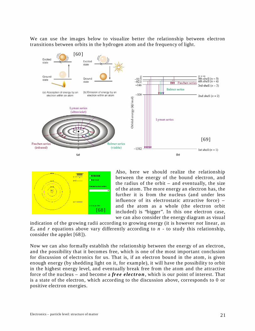
We can use the images below to visualize better the relationship between electron transitions between orbits in the hydrogen atom and the frequency of light.

[69]

[60]

Also, here we should realize the relationship between the energy of the bound electron, and the radius of the orbit – and eventually, the size of the atom. The more energy an electron has, the further it is from the nucleus (and under less influence of its electrostatic attractive force) – and the atom as a whole (the electron orbit included) is “bigger”. In this one electron case, we can also consider the energy diagram as visual

indication of the growing radii according to growing energy (it is however not linear, as En and r equations above vary differently according to n - to study this relationship, consider the applet [68]).

[68]

Now we can also formally establish the relationship between the energy of an electron, and the possibility that it becomes free, which is one of the most important conclusion for discussion of electronics for us. That is, if an electron bound in the atom, is given enough energy (by shedding light on it, for example), it will have the possibility to orbit in the highest energy level, and eventually break free from the atom and the attractive force of the nucleus – and become a free electron, which is our point of interest. That is a state of the electron, which according to the discussion above, corresponds to 0 or positive electron energies.


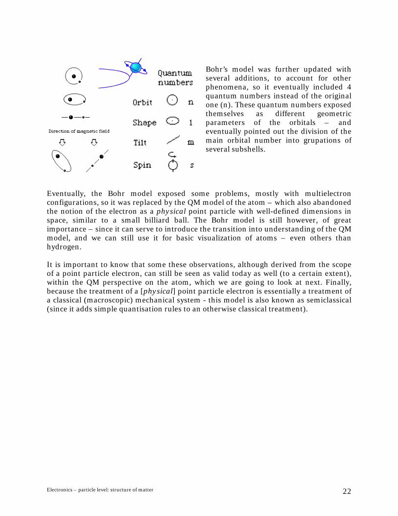
Bohr’s model was further updated with several additions, to account for other phenomena, so it eventually included 4 quantum numbers instead of the original one (n). These quantum numbers exposed themselves as different geometric parameters of the orbitals – and eventually pointed out the division of the main orbital number into grupations of several subshells.

Eventually, the Bohr model exposed some problems, mostly with multielectron configurations, so it was replaced by the QM model of the atom – which also abandoned the notion of the electron as a physical point particle with well-defined dimensions in space, similar to a small billiard ball. The Bohr model is still however, of great importance – since it can serve to introduce the transition into understanding of the QM model, and we can still use it for basic visualization of atoms – even others than hydrogen. It is important to know that some these observations, although derived from the scope of a point particle electron, can still be seen as valid today as well (to a certain extent), within the QM perspective on the atom, which we are going to look at next. Finally, because the treatment of a [physical] point particle electron is essentially a treatment of a classical (macroscopic) mechanical system - this model is also known as semiclassical (since it adds simple quantisation rules to an otherwise classical treatment).


5.2 QM model The QM model, in essence, revolves around the improvement of the Bohr model (which is mostly seen as 2D model): “Werner Heisenberg developed the full quantum mechanical theory in 1925 at the young age of 23. Following his mentor, Niels Bohr, Werner Heisenberg began to work out a theory for the quantum behavior of electron orbitals. Because electron orbits could not be observed, Heisenberg went about creating a mathematical description of quantum mechanics built on what could be observed, that is, the light emitted from atoms in their atomic spectrum … By this time it was known that the electron orbital was three-dimensional, but trying to work out the mathematics for a three-dimensional atom proved too complicated, so he imagined the electron orbital flattened out to one dimension[29]” In this research, a principle was discovered that seems to guide behavior of particles at the atomic level: “In 1927, Heisenberg made a new discovery on the basis of his quantum theory that had further practical consequences of this new way of looking at matter and energy on the atomic scale ... This had the consequence of being able to describe the electron as a point particle in the center of one cycle of a wave so that its position would have a standard deviation ... In three-dimensions a standard deviation is a displacement in any direction. What this means is that when a moving particle is viewed as a wave it is less certain where the particle is. In fact, the more certain the position of a particle is known, the less certain the momentum is known. This conclusion came to be called ‘Heisenberg's Indeterminacy Principle,’ or Heisenberg's Uncertainty Principle [29]” Heisenberg developed matrix mechanics, as “the first complete definition of quantum mechanics, its laws, and properties that described fully the behavior of the electron[29]”. The other important definition of quantum mechanics comes from Schrödinger, who “analyzed what an electron would look like as a wave around the nucleus of the atom. Using this model, he formulated his equation for particle waves. Rather than explaining the atom by analogy to satellites in planetary orbits, he treated everything as waves whereby each electron has its own unique wavefunction[29]”

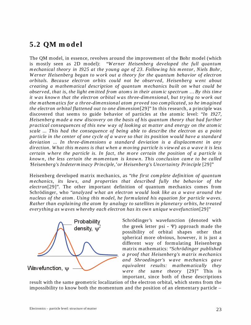
Schrödinger’s wavefunction (denoted with the greek letter psi - Ψ) approach made the possibility of orbital shapes other that spherical more obvious, however, it is just a different way of formulating Heisenbergs matrix mathematics: “Schrödinger published a proof that Heisenberg's matrix mechanics and Shroedinger's wave mechanics gave equivalent results: mathematically they were the same theory [29]” This is important, since both of these descriptions

result with the same geometric localization of the electron orbital, which stems from the impossibility to know both the momentum and the position of an elementary particle –


which spreads our perception of the particle out in a wave: “This is because a wave is naturally a widespread disturbance and not a point particle. Therefore, Schroedinger's wave equation has the same predictions made by the uncertainty principle because uncertainty of location is built into the definition of a widespread disturbance like a wave. Uncertainty only needed to be defined from Heisenberg's matrix mechanics because the treatment was from the particle-like aspects of the electron. Schrödinger's wave equation shows that the electron is in the probability cloud at all times in its probability distribution as a wave that is spread out. Max Born discovered in 1928 that when you compute the square of Schrödinger's wavefunction (psi-squared), you get the electron's location as a probability distribution. Therefore, if a measurement of the position of an electron is made as an exact location in space instead of as a probability distribution, it ceases to have wave-like properties. Without wave-like properties, none of Schrödinger's definitions of the electron being wave-like make sense anymore. The measurement of the position of the particle nullifies the wave-like properties and Schrödinger's equation then fails[29]” The wave particle duality present at this level, coupled with Heisenbergs uncertainty principle, makes the understanding of the effects quite difficult – although there are two forms of a mathematical apparatus in place one could apply: Schrödinger's wavefunction, or Heisenberg’s matrix mathematics. However, we can apply a rather simplified understanding here, which can be related to image processing – without going into the tricky mathematical issues.

5.2.1 Long exposition photography analogy The analogy we can apply is an effect known in photography, namely that the clarity of the photography depends on how long the paper has been exposed – or how quickly the camera shutter mechanism opens and closes. While the shutter mechanism stays open, light keeps falling on the paper, reflecting the changes of scene as time goes by; and we eventually obtain an ‘blurred’ image, that would represent a sum of the individual ‘clear’ images that would otherwise be obtained with a shorter exposition time. Here we can look at several examples:


In the end, the obtained image is unlike what we know the object to be – like this long exposition photograph of a ceiling fan on the left shows. That effect can also be obtained through computer software, by running a video file through an integration process.

The discussion we had about point particles so far makes it interesting to see how the observation of a moving localized object, like a ping-pong ball, which would correspond to the notion of a localized point particle, would behave under these conditions.


The image on the left represents a frame from the original video file (top left) and the effects of three different integration algorithms running on the video file. If we focus on the motion of the ping-pong ball, it is maybe mostly obvious from the bottom left image, that given a sufficiently long exposition time, we will always obtain a blurry cloud that would represent all the past positions where the ball has been. In that sense, the blurry, spread out image would represent the ‘wavefunction’ of the ping-pong ball – since the distribution of the ping-pong pixels on the image tells us the percentage of the time that the ping-pong ball has spent there.

In essence, what we try to do here is to relax the strict scientific approach in the quantum mechanic theories – which needs to stay valid in prediction. In a strict approach, one operates with statistical terms – the values of the wavefunction are understood as probability (percentage) that an electron would be found in a given point of space [at all times - in the past and in the future]. Assuming the long exposition analogy, we simply can understand the wavefunction as an effect of the imperfection of the devices we use to “photograph” the atom, and the extremely long time the ‘shutter’ stays open in relation to the time it would take a hypothetical point particle to orbit around the nucleus – thereby obtaining a blurry image, whose values we would interpret as percentage of the time that the electron has spent at a given point in space [in the past]. That is – even if the electron in fact was a point particle, all we can see from our level of perception is a smeared ‘long shutter’ cloud of past positions – this cloud can then be seen to manifest wave properties. We will look at this again when we discuss the free particle. This approach is actually quite similar to the relatively new application of attosecond lasers to image electron transitions in real-time. The following introduction is taken from a webpage dedicated to this research: “An electron that completes a transition deep inside an atom now started its motion some tens to thousands of attoseconds before. This motion can therefore be most conveniently measured in units of attoseconds just as macroscopic phenomena are naturally clocked in seconds. In the microscopic world of electrons (attoworld for short) motion is speeded up so immensely that the respective time unit makes the period of a heart beat (~1018 attoseconds) appear to be stretched beyond the age of the universe (~5x1017 seconds). This is evident from the accompanying time scale, on which a step represents a thousandfold time expansion (upwards) or shortening (downwards) [30]”

Electronics – particle level: structure of matter 26[30]

5.2.2 From Bohr orbit to QM orbital In any case, this analogy allows us to establish a direct relationship between Bohr’s model of hydrogen atom, and what we observe as a wavefunction; we simply let our camera shutter stay open, and we observe the motion of a moving point particle – as on these frames taken from a Lorentz attractor demo in Matlab:

Obviously, the image represents an integral of the previous point positions (blue traces) – as if we recorded the motion on a long exposition photograph. We could apply the same approach to the rotating orbital motion of a point particle electron in the ground state of the hydrogen atom, allowing at the same time rotation of the orbital plane itself:

[31]

As the radius of the rotation of the electron around the nucleus is fixed, this example would result in a spherical cloudlike surface. As this example corresponds to a hydrogen atom, the radius of the spherical surface cloud would still correspond to Bohr’s radius for the ground state orbit. Afterwards, we allow that subtle changes in the environment, like background fields or changes of temperature, would cause slight changes of the orbiting radius of the point electron. This means we would extend the spherical surface into a cloudlike ball-like volume – with however the strongest intensity around the Bohr radius. We have thus obtained a 3D shape of the electron orbital (it is interesting that the 3D shape of the atomic orbitals in QM follow the shapes of spherical harmonics [75])


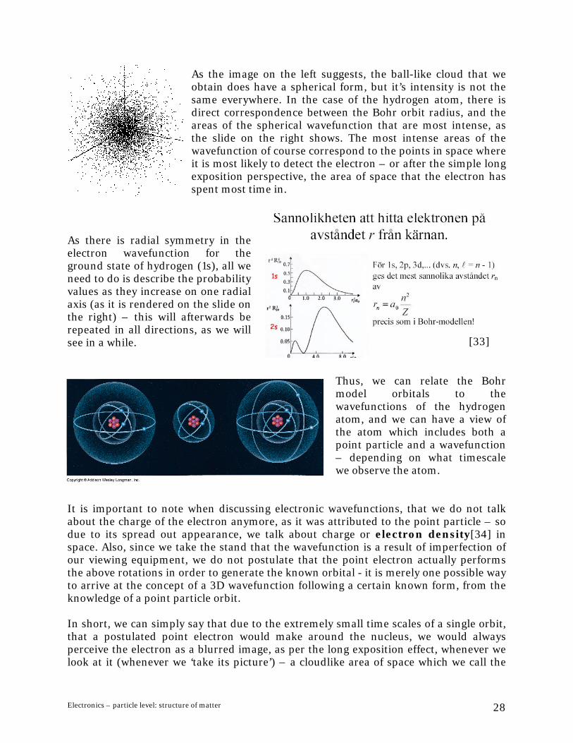
As the image on the left suggests, the ball-like cloud that we obtain does have a spherical form, but it’s intensity is not the same everywhere. In the case of the hydrogen atom, there is direct correspondence between the Bohr orbit radius, and the areas of the spherical wavefunction that are most intense, as the slide on the right shows. The most intense areas of the wavefunction of course correspond to the points in space where it is most likely to detect the electron – or after the simple long exposition perspective, the area of space that the electron has spent most time in.

As there is radial symmetry in the electron wavefunction for the ground state of hydrogen (1s), all we need to do is describe the probability values as they increase on one radial axis (as it is rendered on the slide on the right) – this will afterwards be repeated in all directions, as we will see in a while. [33]

Thus, we can relate the Bohr model orbitals to the wavefunctions of the hydrogen atom, and we can have a view of the atom which includes both a point particle and a wavefunction – depending on what timescale we observe the atom.

It is important to note when discussing electronic wavefunctions, that we do not talk about the charge of the electron anymore, as it was attributed to the point particle – so due to its spread out appearance, we talk about charge or electron density[34] in space. Also, since we take the stand that the wavefunction is a result of imperfection of our viewing equipment, we do not postulate that the point electron actually performs the above rotations in order to generate the known orbital - it is merely one possible way to arrive at the concept of a 3D wavefunction following a certain known form, from the knowledge of a point particle orbit. In short, we can simply say that due to the extremely small time scales of a single orbit, that a postulated point electron would make around the nucleus, we would always perceive the electron as a blurred image, as per the long exposition effect, whenever we look at it (whenever we ‘take its picture’) – a cloudlike area of space which we call the


electron wavefunction. The interesting thing about this is that the wavefunction actually does have all the properties of a wave – even though we may have arrived at it starting from the concept of a point particle electron. However, please note that the previous analogy is NOT a statement of a scientific theory - it is simply a possible way to simplify the visual interpretations of the notions exhibited in the QM model (this is particularly true since one obvious visual correspondence - the Bohr radius as the most likely region where the electron in a ground state hydrogen atom can be found - is actually only one perspective on the problem; in fact, the squared probability density has a maximum at r=0, which implies that the electron should be localised at the nucleus, as seen on this image;

[35]

for more see [93]). With this in mind, we can now note down several of the electron bound state orbitals of the hydrogen atom, from a QM model perspective – as wavefunctions, whose value in each point in space represents the probability of finding the electron there (or from our long exposition perspective – the percentage of time the electron has spent in that point in space).

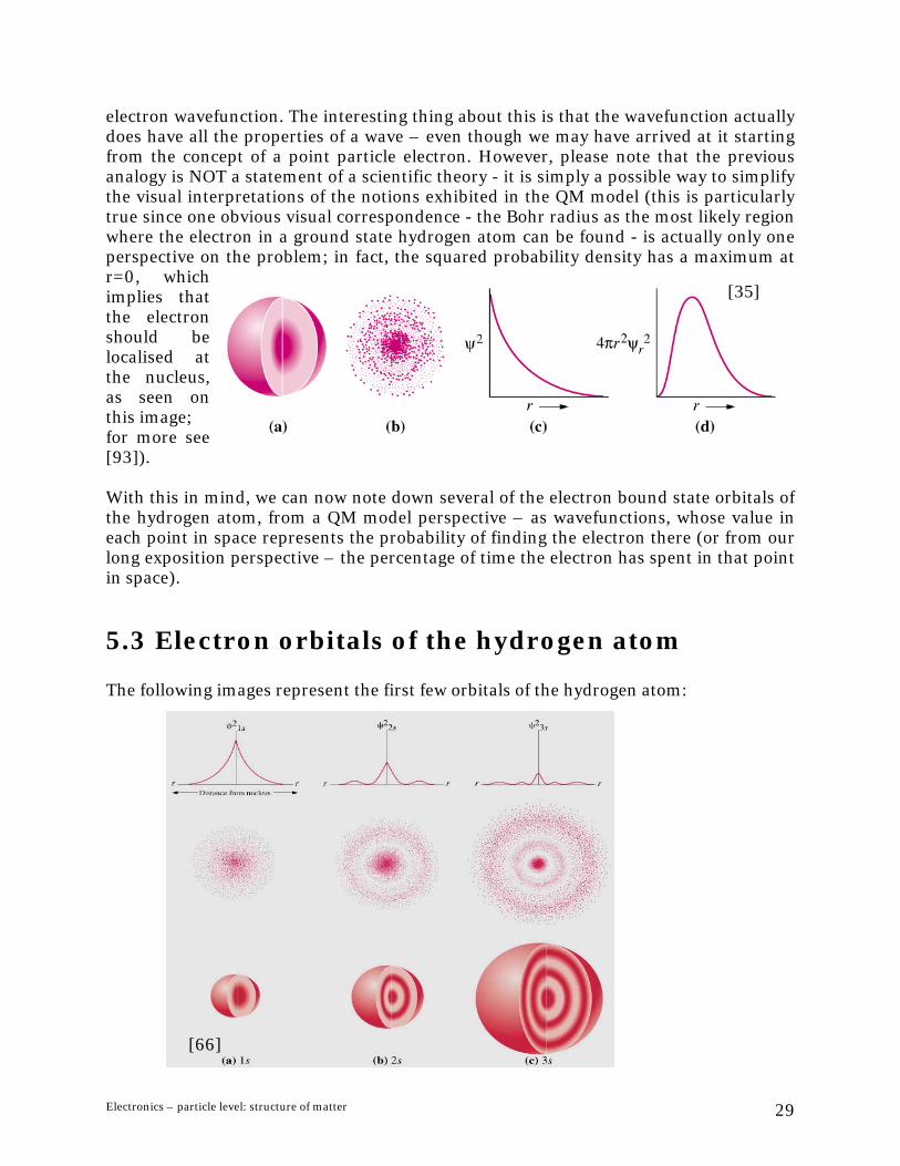
5.3 Electron orbitals of the hydrogen atom The following images represent the first few orbitals of the hydrogen atom:

[66]


[35]

We remember from Bohr’s model that the energy of the electron in the hydrogen atom, although discretized, still can reach many possible levels as n increases. Whereas in the Bohr model, an increase of the energy of the electron resulted with a larger orbit radius, in the QM model, as we can see, it results with different shapes too. As the energy of the electron in the hydrogen atom increases beyond the first quantum energy levels, its wavefunction can eventually reach many complex shapes – some of which are visualized here: a) superposition of 4p, -d and -f states with magnetic quantum number 0 [38]; b) state with n=10, l=8, m=3 [38]; c) highly excited hydrogen atom [45]: [38] [38] [45] Although complex, these shapes still follow the physical laws and the rules of wave mechanics. However, even now we can see, that if a single electron system can result with such complex possibilities, calculating multi-electron systems would certainly be correspondingly complex.


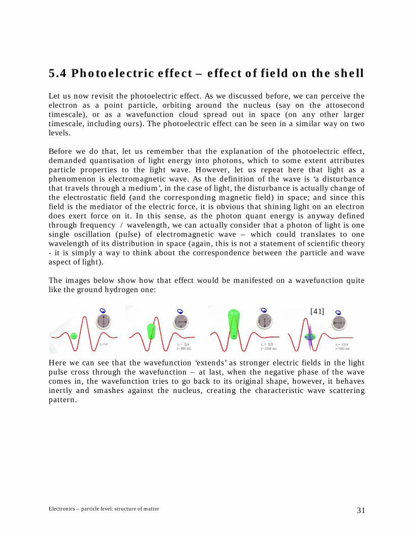
5.4 Photoelectric effect – effect of field on the shell Let us now revisit the photoelectric effect. As we discussed before, we can perceive the electron as a point particle, orbiting around the nucleus (say on the attosecond timescale), or as a wavefunction cloud spread out in space (on any other larger timescale, including ours). The photoelectric effect can be seen in a similar way on two levels. Before we do that, let us remember that the explanation of the photoelectric effect, demanded quantisation of light energy into photons, which to some extent attributes particle properties to the light wave. However, let us repeat here that light as a phenomenon is electromagnetic wave. As the definition of the wave is ‘a disturbance that travels through a medium’, in the case of light, the disturbance is actually change of the electrostatic field (and the corresponding magnetic field) in space; and since this field is the mediator of the electric force, it is obvious that shining light on an electron does exert force on it. In this sense, as the photon quant energy is anyway defined through frequency / wavelength, we can actually consider that a photon of light is one single oscillation (pulse) of electromagnetic wave – which could translates to one wavelength of its distribution in space (again, this is not a statement of scientific theory - it is simply a way to think about the correspondence between the particle and wave aspect of light). The images below show how that effect would be manifested on a wavefunction quite like the ground hydrogen one:

[41]

Here we can see that the wavefunction ‘extends’ as stronger electric fields in the light pulse cross through the wavefunction – at last, when the negative phase of the wave comes in, the wavefunction tries to go back to its original shape, however, it behaves inertly and smashes against the nucleus, creating the characteristic wave scattering pattern.


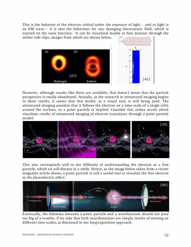
This is the behavior of the electron orbital under the exposure of light – and as light is an EM wave – it is also the behaviour for any changing electrostatic field, which is exerted on the wave function. It can be visualized maybe in best manner through the online vide clips, images from which are shown below.

[42]

[43]

However, although results like these are available, that doesn’t mean that the particle perspective is totally abandoned. Actually, as the research in attosecond imaging begins to show results, it seems that this model, as a visual tool, is still being used. The attosecond imaging assumes that it follows the electron on a time scale of a single orbit around the nucleus, so a point particle is implied. Consider this online movie which visualizes results of attosecond imaging of electron transitions through a point particle model:

[39]

This also corresponds well to the difficulty of understanding the electron as a free particle, which we will discuss in a while. Hence, as the image below taken from a recent magazine article shows, a point particle is still a useful tool to visualize the free electron in the photoelectric effect:

[40]

Eventually, the dilemma between a point particle and a wavefunction should not pose too big of a trouble, if we take that both manifestations are simply results of viewing on different time scales, as discussed in our long exposition approach.


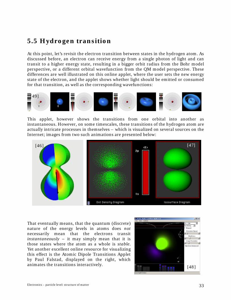
5.5 Hydrogen transition At this point, let’s revisit the electron transition between states in the hydrogen atom. As discussed before, an electron can receive energy from a single photon of light and can transit to a higher energy state, resulting in a bigger orbit radius from the Bohr model perspective, or a different orbital wavefunction from the QM model perspective. These differences are well illustrated on this online applet, where the user sets the new energy state of the electron, and the applet shows whether light should be emitted or consumed for that transition, as well as the corresponding wavefunctions:

[49]

This applet, however shows the transitions from one orbital into another as instantaneous. However, on some timescales, these transitions of the hydrogen atom are actually intricate processes in themselves – which is visualized on several sources on the Internet; images from two such animations are presented below:

[46] [47]

That eventually means, that the quantum (discrete) nature of the energy levels in atoms does not necessarily mean that the electrons transit instantaneously – it may simply mean that it is those states where the atom as a whole is stable. Yet another excellent online resource for visualizing this effect is the Atomic Dipole Transitions Applet by Paul Falstad, displayed on the right, which animates the transitions interactively. [48]


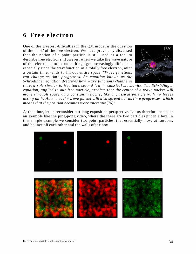
6 Free electron One of the greatest difficulties in the QM model is the question of the ‘look’ of the free electron. We have previously discussed that the notion of a point particle is still used as a tool to describe free electrons. However, when we take the wave nature of the electron into account things get increasingly difficult – especially since the wavefunction of a totally free electron, after a certain time, tends to fill out entire space: “Wave functions can change as time progresses. An equation known as the Schrödinger equation describes how wave functions change in time, a role similar to Newton's second law in classical mechanics. The Schrödinger equation, applied to our free particle, predicts that the center of a wave packet will move through space at a constant velocity, like a classical particle with no forces acting on it. However, the wave packet will also spread out as time progresses, which means that the position becomes more uncertain[76]”

[39]

At this time, let us reconsider our long exposition perspective. Let us therefore consider an example like the ping-pong video, where the there are two particles put in a box. In this simple example we consider two point particles, that essentially move at random, and bounce off each other and the walls of the box.


The long exposition effect provides us with a cloud with past positions that we can interpret as a probability cloud – with darker and brighter areas of the cloud corresponding to the percentage of time the particle has spent at a given point. If we observe both particles as wavefunction (here by coloring them in different colors) – we will observe that their corresponding wavefunctions on the long expositions photographs have merged – that is, occupy the same area of space. That points to the essential difference we attribute to matter and waves – matter exclusively occupies space, so when (hard) matter interacts, it bounces off (like the point particles do) – waves, when they interact, they do not necessarily occupy their space, but they will interfere (merge, as the probability clouds – the square of the wavefunction, do); and it is the same difference between the fermions and bosons in the Standard model. The idea is, if we focus on the development of the probability cloud on some larger timescale, than where we would perceive a theoretical point particle:

then, taken all electrostatic and quantum interactions of the particle, we should observe the development of a wave. (we do not observe it in the above images since again, essentially the particles are moving at random). This is the common problem of particle in a box (see [78]), which can also be found animated on the internet – such as the one displayed on the left, where the 2D cloud values are represented as height. In it, the electron starts of as a localized wave – a wave packet – which then bounces of the edges of the box, and also slowly delocalises.

[77]

These wave aspects and spreading make the visualization of the free electron difficult: “we can measure just the position alone of a moving free particle creating an eigenstate of position with a wavefunction that is very large at a particular position x, and zero everywhere else. If we perform a position measurement on such a wavefunction, we will obtain the result x with 100% probability. In other words, we will know the position of the free particle. This is called an eigenstate of position. If the particle is in an eigenstate of position then its momentum is completely unknown. An


eigenstate of momentum, on the other hand, has the form of a plane wave. It can be shown that the wavelength is equal to h/p, where h is Planck's constant and p is the momentum of the eigenstate. If the particle is in an eigenstate of momentum then its position is completely blurred out[76]” The illustration from [53] is an illustration of a plane wave – and as such it’s difficult to geometrically relate it to anything we’ve discussed so far.

[53]

[52]

On the other hand, images like from [52] reveal a probability cloud for a free electron that is localized, and that indeed seems to have the most probable locations ‘flattened’. Although a long exposition approach looks fine in the explanation of the transition from orbits to orbitals, it gets harder to give it a physical meaning in the context of a free particle – at best, we can say that when we observe a free electron moving through space as a wave packet cloud, the hypothetical point particle that would have created it, would have to move back and forth, as it progresses forward. That also leads to trouble with the physical understanding of some more obscure notions that stem from the wave nature – like the electron tunneling, where a wave crosses a barrier – which according to this understanding, would mean that within the time when the picture is taken, the assumed point has jumped [teleported] from a location to a location instantaneously (see movies from [37]):

[37]


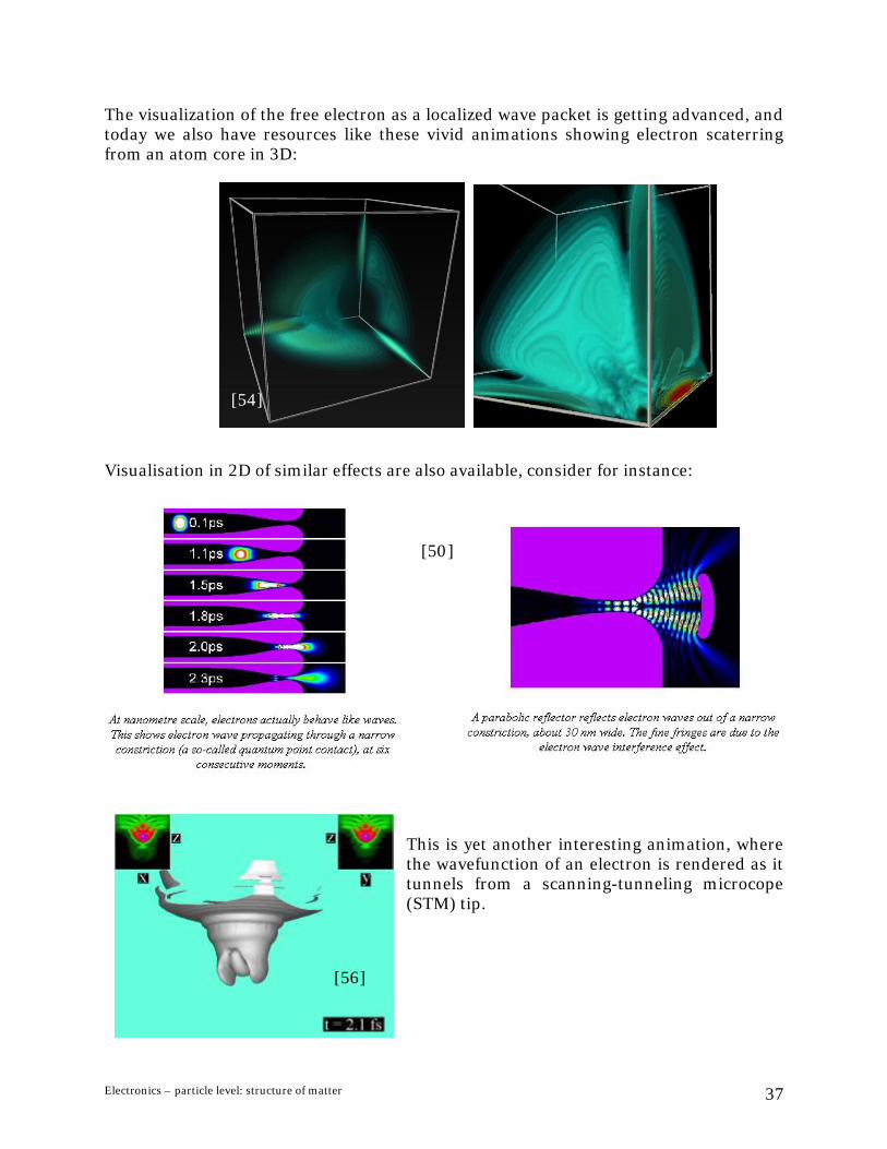
The visualization of the free electron as a localized wave packet is getting advanced, and today we also have resources like these vivid animations showing electron scaterring from an atom core in 3D:

[39]

[54]

Visualisation in 2D of similar effects are also available, consider for instance:

[50]

[56]

This is yet another interesting animation, where the wavefunction of an electron is rendered as it tunnels from a scanning-tunneling microcope (STM) tip.


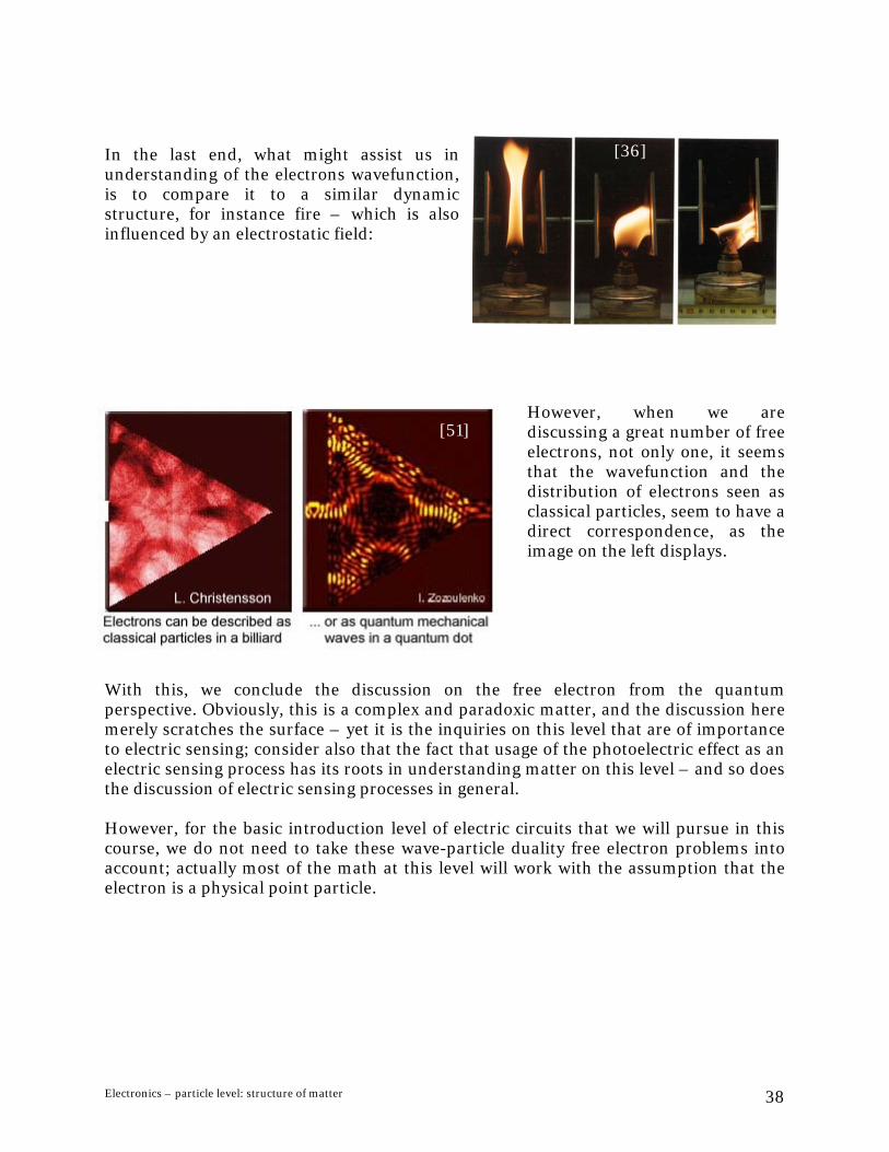
In the last end, what might assist us in understanding of the electrons wavefunction, is to compare it to a similar dynamic structure, for instance fire – which is also influenced by an electrostatic field:

[36]

However, when we are discussing a great number of free electrons, not only one, it seems that the wavefunction and the distribution of electrons seen as classical particles, seem to have a direct correspondence, as the image on the left displays.

[51]

With this, we conclude the discussion on the free electron from the quantum perspective. Obviously, this is a complex and paradoxic matter, and the discussion here merely scratches the surface – yet it is the inquiries on this level that are of importance to electric sensing; consider also that the fact that usage of the photoelectric effect as an electric sensing process has its roots in understanding matter on this level – and so does the discussion of electric sensing processes in general. However, for the basic introduction level of electric circuits that we will pursue in this course, we do not need to take these wave-particle duality free electron problems into account; actually most of the math at this level will work with the assumption that the electron is a physical point particle.


7 Multi-electron atoms As we discussed so far, a single electron can be bound to a proton in a hydrogen atom in several orbits, depending on the quantised energy of the electron. Once a single electron system is discussed, the question is how would that apply to all the other atomic elements of the periodic table, which involve multiple electrons, and how would that relate to molecular binding. Generally, we are aware that instead of one quantisation parameter (n) that placed the electron in a given orbit in the original Bohr model, we have four quantum numbers that determine the placement of an electron in a given orbit. As we go along the periodic system, and the number of protons and electrons of elementary atoms increase, there are several rules that apply as to which particular orbits get occupied first. These rules are known as the electron shell filling rules (see [71]). Those that are occupied later are under less influence by the core, and can therefore more easily participate in the interaction with other atoms. The outermost electron shell of an atom is known as the valence shell, and it is of crucial importance to determining the chemical properties of elements.

7.1 Bohr model perspective Although we discussed that the Bohr model applies (strictly speaking) mostly to one-electron systems, the type of visualization inherited from it is still used today as a valuable tool – consider for example the Bohr diagrams rendered below:

[60]


It is interesting to look at the historical perspective that brought about the filling rules, which originates with Bohr: “From 1920 to 1923, Bohr applied his ideas to explain features of the periodic table; Bohr's work in this vein was corrected and extended by Pauli in 1924 (with an assist from Stoner). Suppose we treat the states in the term scheme for hydrogen as slots to hold electrons. Let us hypothesize that each slot can hold at most two electrons. We start with hydrogen, and keep adding electrons, adding new electrons always to the lowest slot that has a vacancy. (Bohr christened this the Aufbauprincip, the building-up principle.) The energy levels of the slots may shift somewhat as a result of interactions between the electrons. This simple model (extremely naive from the modern viewpoint) serves to explain a remarkable number of chemical regularities. For example, energy level n can hold 2n2 electrons. We therefore get completely filled energy levels for 2 electrons, 2+8 electrons, 2+8+18 electrons, etc.-- which correspond exactly to the noble gases. Bohr was able to explain some properties of the rare earth elements using his version of this model; he even predicted correctly that element 72 (not yet discovered) would not be a rare earth, but instead would resemble zirconium (contrary to what some chemists expected). Students of Bohr then discovered element 72 in zirconium ore samples, and element 72 was named hafnium in honor of the Latin name for Copenhagen. Why two electrons per slot? Pauli proposed adding a new quantum number to the triple (n, l, m); nowadays we use s for this number, and recognize that it stands for the spin of the electron. So s is restricted to the values ±½, and each state (or slot) in the term scheme above is really two states … Pauli also proposed his famous exclusion principle: a state can hold at most one electron. A historical note: Bohr made no detailed orbit calculations for multi-electron atoms. He did use some general intuitive principles stemming from a classical picture, e.g., a electron in a state of large n will be far away from the nucleus, and electrons with smaller n will partly ‘screen’ the charge of the nucleus from the far-off electron. Nevertheless, the Bohr-Sommerfeld hydrogen model had a comforting, semi-classical feel to it: we compute the classical orbits, then decree that only some are permitted. For multi-electron atoms, Bohr dropped this connection. The term scheme becomes almost a combinatorial device. Physicists (such as Born and Heisenberg) who did perform detailed orbit calculations found utter disagreement between theory and experiment-- even for helium, a mere two electrons. No surprise, since the classical picture leaves out spin, the exclusion principle, and other purely quantum interactions between the electrons. Bohr intuited just how far to push the classical picture; he picked those approximation schemes that survive (reinterpreted) in quantum mechanics. [70]”


We are not going to focus on the electron filling process in detail, we can just mention that here we can recognize three principles: Exclusion principle, Build-up principle and Hund’s rule (see [71]). The Pauli exclusion principle will be important when discussing conductivity, so let’s note it here briefly: “No more than one electron can have all four quantum numbers the same. What this translates to in terms of our pictures of orbitals is that each orbital can only hold two electrons, one ‘spin up’ and one ‘spin down’[71] ” For an easy introduction, you may want to consider the online video file “Electron Configurations” from [66]:

[66]

[66]

7.2 QM model perspective We can introduce the QM perspective on the electron orbital filling with this excerpt: “ When an atom or ion receives electrons into its orbitals, the orbitals and shells fill up in a particular manner. The equations (like the Legendre polynomials that describe spherical harmonics, and thus the shapes of orbitals) of quantum mechanics are distinguished by four types of numbers. The first of these quantum numbers is referred to as the principal quantum number, and is indicated by n. This merely represents which shell electrons occupy, and shows up in the periodic chart as the rows of the periodic chart. It has integral values, n=1,2,3 . . . . The highest energy electrons of the atoms in the first row all have n=1. Those in the atoms in the second row all have n=2. As one gets into n=3, Hund's rule mixes it up a little bit, but when one gets to the end of the third row, at least, the electrons with the highest energy have n=3. The next quantum number is indicated by the letter m and indicates how many different types of shells an atom can have. Those elements in the first row can have just one, the s orbital. The elements in the second row can have two, the s and the p orbitals. The elements in the third row can have three, the s, p, and d orbitals. And so on. It may be funny to think of s, p and d as "numbers", but these are used as an historical and geometrical convenience.


The third kind of quantum number ml specifies, for those kinds of orbitals that can have different shapes, which of the possible shapes one is referring to. So, for example, a 2pz orbital indicates three quantum numbers, represented respectively by the 2, the p and the z. Finally, the fourth quantum number is the spin of the electron. It has only two possible values, +1/2 or -1/2. Pretty much only computational chemists have to treat quantum numbers as numbers per se in equations. But it helps to know that the wide variety of elements of the periodic table and the different shapes and other properties of electron orbitals have a unifying principle--the proliferation of different shapes is not completely arbitrary, but is instead bounded by very specific rules.[71]” The complexity of shapes that can occur, is obvious from the sequence of images shown below, taken from an online lecture [44], which shows the different orbital shapes in 3D for each distinct orbital for the krypton atom – as they are being filled in, from lowest to highest energy orbitals. Obviously, this results with a multitude of complex shapes, superimposed upon one another.

[44]

It should be mentioned, that recently, attempts are being made to use atomic force microscopy (AFM) in order to ‘see’ the orbitals. Although these results are still disputed, mathematical simulations say that it is not impossible – below are images of one such study, mathematical simulation (left) of what the microscope tip ‘would’ see, and an actual image of one silicon atom, apparently showing its orbitals (see [72]).

[72]

[73]


8 Bonding – molecules and crystals Chemical bonding is the process where atoms interact through their electron shells, and join to form bigger structures like molecules or crystals. There are in general three types of bonds: “ Ionic bonds form between positive and negative ions (atoms). In an ionic solid, the ions arrange themselves into a rigid crystal lattice. NaCl (common salt) is an example of an ionic substance. Covalent bonds are formed when atoms share electrons with each other. This gives rise to two structures: molecules and covalent network solids. Methane (CH4) is a covalent molecule and glass is a covalent network solid. Metallic bonds occur between metal atoms. In a metallically bonded substance, the atoms' outer electrons are able to freely move around - they are delocalised. Iron is a metallically bonded substance. [79]” We are especially interested in the metallic bonds, since they are crucial in understanding electric conductivity. We should also mention that recent advances in AFM microscopy, open possibilities to peek directly in the electron orbital configuration of atoms bound in molecules / crystals, like the image below shows:

AFM-image with 77 pm resolution. Subatomic structures are visible within single tungsten atoms. The simultaneously recorded STM image shows the atomic positions. Image size 500 × 500 pm2.

[73]


8.1 Bonding in H2 – covalent bonding [57] Here we can just briefly mention that as the maximum number of electrons that the first orbital can hold is 2, two hydrogen atoms can share their electrons to create a common molecular orbital. It thus represents a covalent bond. Considering the perception of electronic wavefunctions, that would simply imply that the two wavefunctions will merge into a single one, covering both nuclei - which is shown in this online animation:

[58]

Lets remember that although the wavefunction is merged, the Pauli exclusion principle states that they still need to have the four quantum numbers different – which implies they will have slightly different energies, or in other words – a single wavefunction is only our perception; the electrons need to retain their distinct character and have own molecular orbital that simply overlaps in space: “When a covalent molecule is formed, the electron orbitals are modified. Orbitals from each atom mix together in such a way that the electrons from those orbitals are shared between the two (or more) atoms involved in the bond and, since two atomic orbitals are involved (one from each atom), two 'molecular' orbitals are formed. The energies of these new molecular orbitals are slightly different from the energies of the atomic orbitals, one being slightly higher in energy than either atomic orbital and one being slightly lower in energy than either atomic orbital. Each orbital can accept two electrons with opposite spins.[81]”

[74]


8.2 Bonding in H2O – covalent bonding


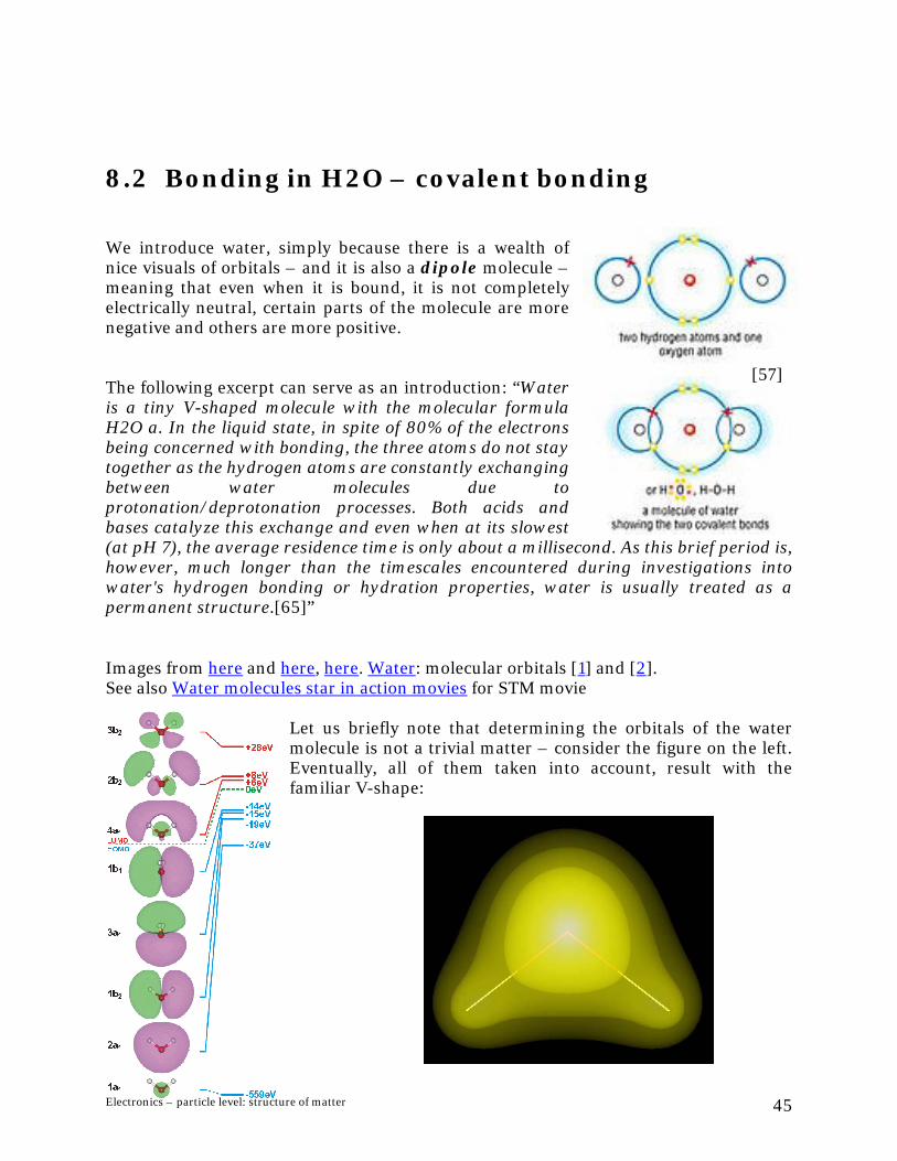
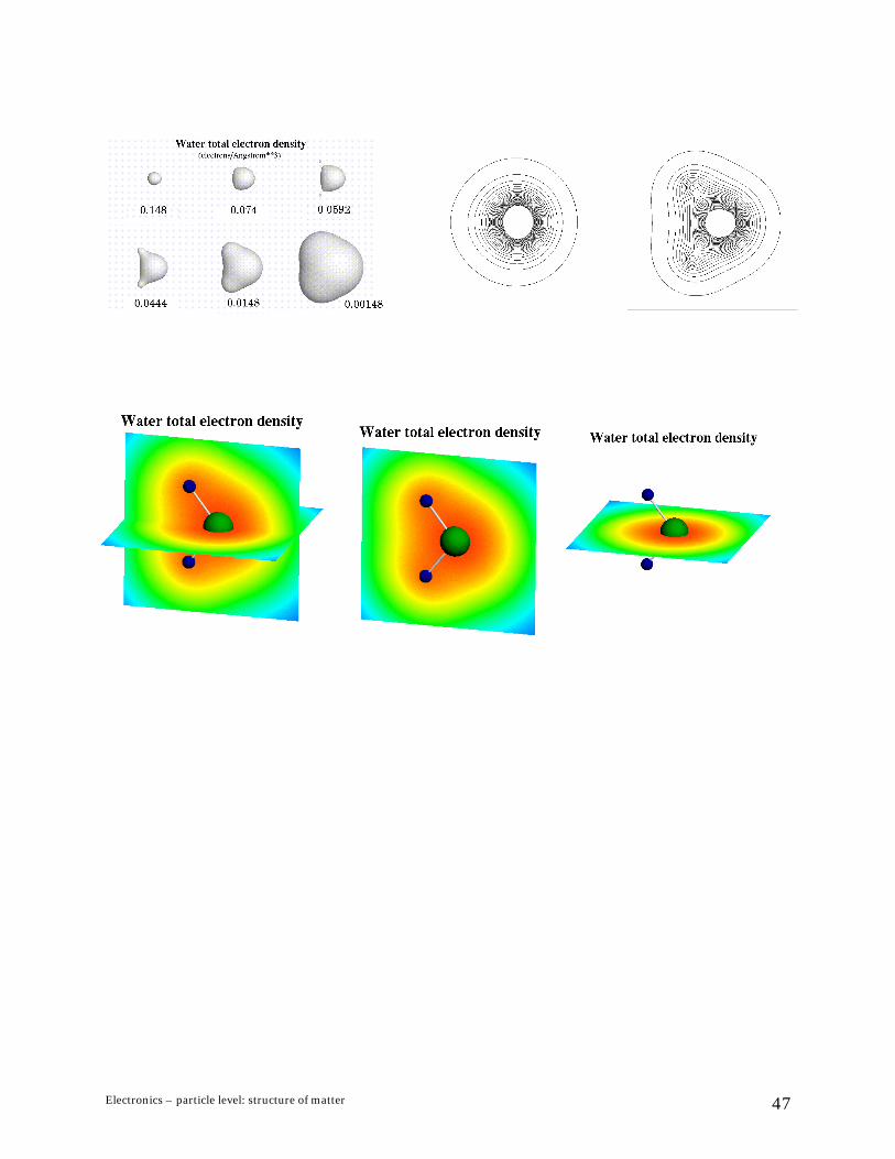
We introduce water, simply because there is a wealth of nice visuals of orbitals – and it is also a dipole molecule – meaning that even when it is bound, it is not completely electrically neutral, certain parts of the molecule are more negative and others are more positive. The following excerpt can serve as an introduction: “Water is a tiny V-shaped molecule with the molecular formula H2O a. In the liquid state, in spite of 80% of the electrons being concerned with bonding, the three atoms do not stay together as the hydrogen atoms are constantly exchanging between water molecules due to protonation/deprotonation processes. Both acids and bases catalyze this exchange and even when at its slowest (at pH 7), the average residence time is only about a millisecond. As this brief period is, however, much longer than the timescales encountered during investigations into water's hydrogen bonding or hydration properties, water is usually treated as a permanent structure.[65]”

[57]

Images from here and here, here. Water: molecular orbitals [1] and [2]. See also Water molecules star in action movies for STM movie

Let us briefly note that determining the orbitals of the water molecule is not a trivial matter – consider the figure on the left. Eventually, all of them taken into account, result with the familiar V-shape:

http://www.ccl.net/cca/documents/dyoung/water/lp3.shtml

http://www.uam.es/departamentos/ciencias/qfa/DAM/chemicalforces.html

http://www.dit.ie/DIT/science/chemistry/rsccomp/competition01/chemweb5/w_shp.html

http://www.lsbu.ac.uk/water/

http://www.lsbu.ac.uk/water/h2oorb.html

http://www.chm.bris.ac.uk/pt/harvey/elstruct/lcao_mo.html

http://www.lbl.gov/Science-Articles/Archive/MSD-action-movies-Salmeron.html

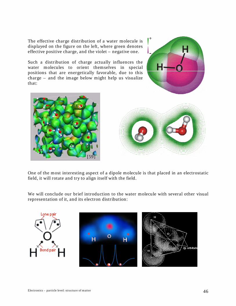
The effective charge distribution of a water molecule is displayed on the figure on the left, where green denotes effective positive charge, and the violet – negative one. Such a distribution of charge actually influences the water molecules to orient themselves in special positions that are energetically favorable, due to this charge – and the image below might help us visualize that:

[59]

One of the most interesting aspect of a dipole molecule is that placed in an electrostatic field, it will rotate and try to align itself with the field. We will conclude our brief introduction to the water molecule with several other visual representation of it, and its electron distribution:



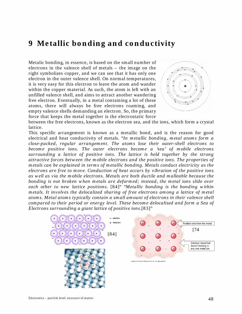
9 Metallic bonding and conductivity Metalic bonding, in essence, is based on the small number of electrons in the valence shell of metals – the image on the right symbolizes copper, and we can see that it has only one electron in the outer valence shell. On normal temperatures, it is very easy for this electron to leave the atom and wander within the copper material. As such, the atom is left with an unfilled valence shell, and aims to attract another wandering free electron. Eventually, in a metal containing a lot of these atoms, there will always be free electrons roaming, and empty valence shells demanding an electron. So, the primary force that keeps the metal together is the electrostatic force between the free electrons, known as the electron sea, and the ions, which form a crystal lattice. This specific arrangement is known as a metallic bond, and is the reason for good electrical and heat conductivity of metals. “In metallic bonding, metal atoms form a close-packed, regular arrangement. The atoms lose their outer-shell electrons to become positive ions. The outer electrons become a ‘sea’ of mobile electrons surrounding a lattice of positive ions. The lattice is held together by the strong attractive forces between the mobile electrons and the positive ions. The properties of metals can be explained in terms of metallic bonding. Metals conduct electricity as the electrons are free to move. Conduction of heat occurs by vibration of the positive ions as well as via the mobile electrons. Metals are both ductile and malleable because the bonding is not broken when metals are deformed; instead, the metal ions slide over each other to new lattice positions. [84]“ “Metallic bonding is the bonding within metals. It involves the delocalized sharing of free electrons among a lattice of metal atoms. Metal atoms typically contain a small amount of electrons in their valence shell compared to their period or energy level. These become delocalised and form a Sea of Electrons surrounding a giant lattice of positive ions.[83]”

[74[84]


Applying quantum mechanics to the problem of conductivity is a difficult problem, dealt with in solid-state physics [85]. It is based on the repeatability of the crystal structure of metals – the ordered arrangement of the metal ions in a lattice: The calculations of the electric properties via wavefunctions are difficult, involving transformation of the lattice structure in 3D space into so-called k-space (which corresponds to some extent to Fourier transformation of time into frequency domain). Without going into those details, we should mention that most of the electrical characteristics of solids are covered by the band theory of solids. In general, whereas in a single atom we observe discrete energy levels for the electron, in systems involving a lot of atoms, those levels turn into bands of possible energy values. The arrangement of these bands for a given material determines the electric properties. Let’s include some excerpts which will help us understand these concepts better: “The electrons of a single free-standing atom occupy atomic orbitals, which form a discrete set of energy levels. If several atoms are brought together into a molecule, their atomic orbitals split, producing a number of molecular orbitals proportional to the number of atoms. When a large number of atoms (of order 1020 or more) are brought together to form a solid, the number of orbitals becomes exceedingly large, and the difference in energy between them becomes very small. However, some intervals of energy contain no orbitals, no matter how many atoms are aggregated. These energy levels are so numerous as to be indistinct. First, the separation between energy levels in a solid is comparable with the energy that electrons constantly exchange with phonons (atomic vibrations). Second, it is comparable with the energy uncertainty due to the Heisenberg uncertainty principle, for reasonably long intervals of time.[82]” “A lump of metal is essentially one big molecule. There are so many atomic orbitals involved in the individual bonds that the molecular orbital spreads out over the entire lump of metal, meaning that an electron put into one end of the lump (or wire) can be taken out at the other end because the molecular orbital allows it to be anywhere in the wire. There are as many molecular orbitals as there are electrons in the wire and they each have slightly different energies. In metals, semiconductors, and insulators these


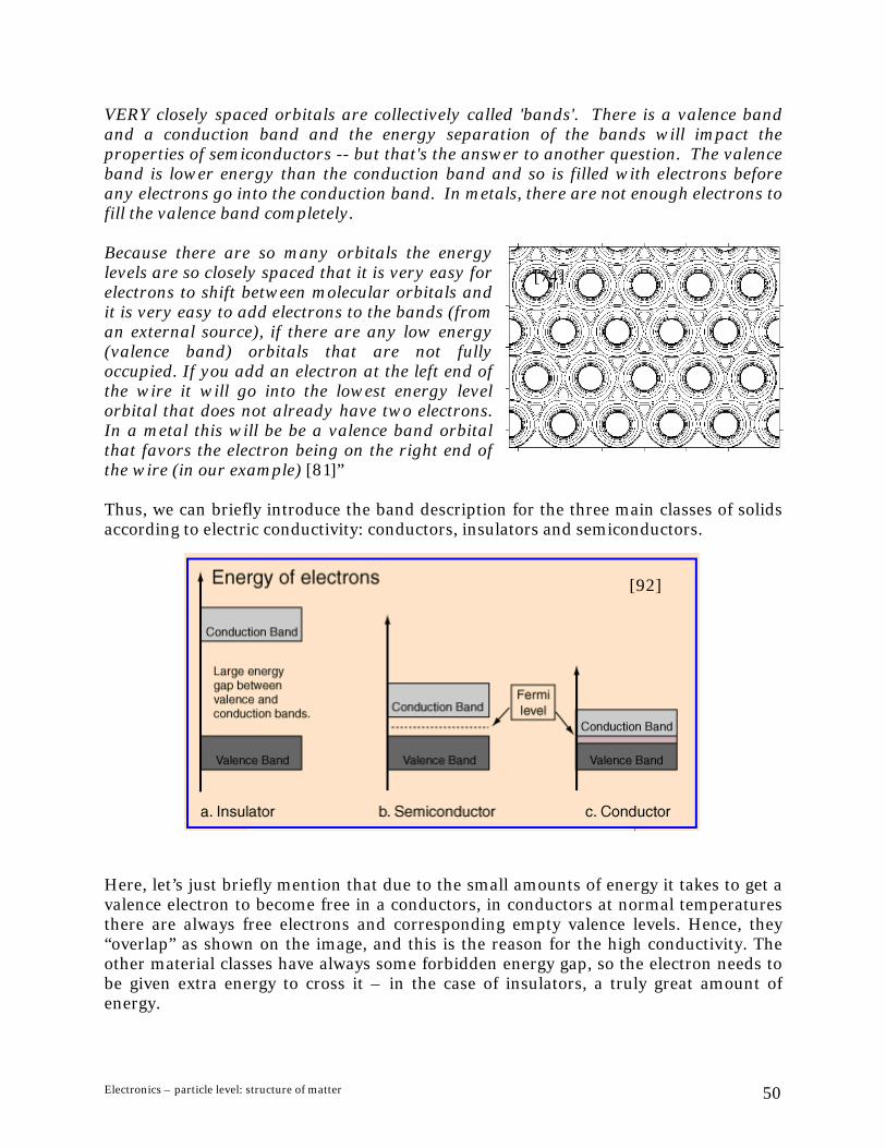
VERY closely spaced orbitals are collectively called 'bands'. There is a valence band and a conduction band and the energy separation of the bands will impact the properties of semiconductors -- but that's the answer to another question. The valence band is lower energy than the conduction band and so is filled with electrons before any electrons go into the conduction band. In metals, there are not enough electrons to fill the valence band completely. Because there are so many orbitals the energy levels are so closely spaced that it is very easy for electrons to shift between molecular orbitals and it is very easy to add electrons to the bands (from an external source), if there are any low energy (valence band) orbitals that are not fully occupied. If you add an electron at the left end of the wire it will go into the lowest energy level orbital that does not already have two electrons. In a metal this will be be a valence band orbital that favors the electron being on the right end of the wire (in our example) [81]”

[74]

Thus, we can briefly introduce the band description for the three main classes of solids according to electric conductivity: conductors, insulators and semiconductors.

[92] Here, let’s just briefly mention that due to the small amounts of energy it takes to get a valence electron to become free in a conductors, in conductors at normal temperatures there are always free electrons and corresponding empty valence levels. Hence, they “overlap” as shown on the image, and this is the reason for the high conductivity. The other material classes have always some forbidden energy gap, so the electron needs to be given extra energy to cross it – in the case of insulators, a truly great amount of energy.


If we try to imagine the effect of this, maybe we could use the following image, which shows the bound orbitals of copper atoms in cuprite (a conductive copper oxide) – as well as the free electrons as cloudlike areas that however are distributed only at certain places in the lattice. We can crudely say, that this cloudlike area is a molecular orbital corresponding to the conduction band energy levels; the more dense it is, the more likely, and therefore more easier for an electron to get through there. The areas where the cloud is ‘thin’ are areas of low probability, where the electrons do not go. Eventually, this cloudlike area can be seen as continuous throughout the metal, the it would provide a path for all the free electrons, so they can easily move through the conductor.

[86]

This can also be seen on the following image – the blue areas represent areas of low likelihood of finding an electron; so the material is not very conductive. As pressure is increased, atoms come closer together, and so do the electronic wavefunctions, which increases the probability of finding an electron there (green). Again, let’s not forget that also availability of valence states is important too – since that determines

whether an external electron can readily enter the conductor material.

[87]


Recently, visualization of the surface conditions of a material are becoming more interesting, since STM and AFM microscopy also allow imaging of s ch surfaces, so theoretical data can be compared with experimental. The images elow, although discussing semiconductor structures, can help us see that the quantumbe visible on the surface of the material. In any case, we can easily imcontinuous wavefunction on the surface of the conductor.

[89]

[89]

Electronics – particle level: structure of matter

ub
effects will also agine a similar
52

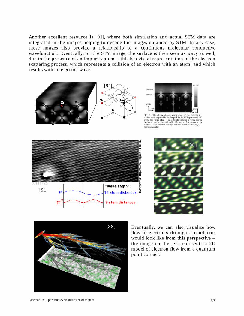
Another excellent resource is [91], where both simulation and actual STM data are integrated in the images helping to decode the images obtained by STM. In any case, these images also provide a relationship to a continuous molecular conductive wavefunction. Eventually, on the STM image, the surface is then seen as wavy as well, due to the presence of an impurity atom – this is a visual representation of the electron scattering process, which represents a collision of an electron with an atom, and which results with an electron wave.

[91]

[91]

[90]

[91]

[88] Eventually, we can also visualize how

flow of electrons through a conductor would look like from this perspective – the image on the left represents a 2D model of electron flow from a quantum point contact.


Finally, let’s note that although we should be aware of the issues on this level of matter, especially since they will probably influence the future development of technology – we do not need such a detailed and complex model in order to discuss basic electronics. Actually, in the discussions further on, we will take the classical approach, and we will treat the electron like a physical point particle. The metal will then be assumed as a lattice of ‘hard’ ions that form the crystal lattice, and as free particle electrons that roam through it – and the effect of interaction of a free electron with an in the crystal lattice, (which we have previously seen as scaterring) will be a simple billiard-ball like hit; which is in essence the Drude model of conduction – the simplest model of conduction.


10 PE Questions • Discuss briefly the atomic structure of matter, and the concept of free electron. • Discuss briefly the photoelectric effect. • Discuss briefly the bonding in, and the properties of, metals.


Resources and references [1]. Atomic Structure Timeline, http://www.watertown.k12.wi.us/HS/Staff/Buescher/atomtime.asp [2]. Atomic Structure Timeline, http://www.cartage.org.lb/en/themes/Sciences/Physics/Atomicphysics/Atomicstructure/AtomicTimeline/AtomicTimeline.htm [3]. History of Science: Aligned Entries http://cse.edc.org/products/historyscience/alignedchart.asp [4]. Evolution of our understanding of matter, http://www.hyperhistory.com/online_n2/people_n2/science_n2/atomic_theory.html [5]. Atomic models, http://mhsweb.ci.manchester.ct.us/Library/webquests/atomicmodels.htm [6]. Atom timeline, http://hi.fi.tripod.com/timeline/timeline.htm [7]. History of atoms, http://www.nobeliefs.com/atom.htm [8]. Teaching Standard Model at high school - Timeline, http://teachers.web.cern.ch/teachers/archiv/HST2003/publish/standard%20model/History/layer1.htm [9]. Atom Model History http://www.csmate.colostate.edu/cltw/cohortpages/viney/atomhistory.html [10]. Timeline of quantum mechanics, molecular physics, atomic physics, nuclear physics, and particle physics, http://en.wikipedia.org/wiki/Timeline_of_quantum_mechanics%2C_molecular_physics%2C_atomic_physics%2C_nuclear_physics%2C_and_particle_physics [11]. Charge and Charge Interactions: The Structure of Matter http://www.glenbrook.k12.il.us/gbssci/phys/Class/estatics/u8l1a.html [12]. Standard model, http://en.wikipedia.org/wiki/Standard_model [13]. Bohrs pusselbitar, http://kurslab.fysik.lth.se/E1Fysik/Del2/OH/Bohr-tot.jpg [14]. Atom Builder, http://www.pbs.org/wgbh/aso/tryit/atom/ [15]. Bohr model, http://en.wikipedia.org/wiki/Bohr_model [16]. Photoelectric effect, http://en.wikipedia.org/wiki/Photoelectric_effect [17]. Wave-particle duality, http://hyperphysics.phy-astr.gsu.edu/hbase/mod1.html [18]. Atomic Spectra applet, http://www.colorado.edu/physics/2000/quantumzone/lines2.html [19]. Atomic Emission Spectra - Origin of Spectral Lines http://www.avogadro.co.uk/light/bohr/spectra.htm [20]. Photon, http://en.wikipedia.org/wiki/Photon [21]. Energy, http://en.wikipedia.org/wiki/Energy [22]. Momentum, http://en.wikipedia.org/wiki/Momentum [23]. Grand Unified Theory, http://en.wikipedia.org/wiki/Grand_Unified_Theory [24]. The Electric Force applet, http://www.colorado.edu/physics/2000/waves_particles/wavpart2.html [25]. Bohr Model of the Atom, http://www.rwc.uc.edu/koehler/biophys/6a.html [26]. Why isn't the electron considered a black hole?, http://www.physlink.com/Education/AskExperts/ae191.cfm


http://www.watertown.k12.wi.us/HS/Staff/Buescher/atomtime.asp

http://www.cartage.org.lb/en/themes/Sciences/Physics/Atomicphysics/Atomicstructure/AtomicTimeline/AtomicTimeline.htm

http://www.cartage.org.lb/en/themes/Sciences/Physics/Atomicphysics/Atomicstructure/AtomicTimeline/AtomicTimeline.htm

http://cse.edc.org/products/historyscience/alignedchart.asp

http://www.hyperhistory.com/online_n2/people_n2/science_n2/atomic_theory.html

http://mhsweb.ci.manchester.ct.us/Library/webquests/atomicmodels.htm

http://hi.fi.tripod.com/timeline/timeline.htm

http://www.nobeliefs.com/atom.htm

http://teachers.web.cern.ch/teachers/archiv/HST2003/publish/standard model/History/layer1.htm

http://teachers.web.cern.ch/teachers/archiv/HST2003/publish/standard model/History/layer1.htm

http://www.csmate.colostate.edu/cltw/cohortpages/viney/atomhistory.html

http://en.wikipedia.org/wiki/Timeline_of_quantum_mechanics%2C_molecular_physics%2C_atomic_physics%2C_nuclear_physics%2C_and_particle_physics

http://en.wikipedia.org/wiki/Timeline_of_quantum_mechanics%2C_molecular_physics%2C_atomic_physics%2C_nuclear_physics%2C_and_particle_physics

http://www.glenbrook.k12.il.us/gbssci/phys/Class/estatics/u8l1a.html

http://en.wikipedia.org/wiki/Standard_model

http://kurslab.fysik.lth.se/E1Fysik/Del2/OH/Bohr-tot.jpg

http://www.pbs.org/wgbh/aso/tryit/atom/

http://en.wikipedia.org/wiki/Bohr_model

http://en.wikipedia.org/wiki/Photoelectric_effect

http://hyperphysics.phy-astr.gsu.edu/hbase/mod1.html

http://www.colorado.edu/physics/2000/quantumzone/lines2.html

http://www.avogadro.co.uk/light/bohr/spectra.htm

http://en.wikipedia.org/wiki/Photon

http://en.wikipedia.org/wiki/Energy

http://en.wikipedia.org/wiki/Momentum

http://en.wikipedia.org/wiki/Grand_Unified_Theory

http://www.colorado.edu/physics/2000/waves_particles/wavpart2.html

http://www.rwc.uc.edu/koehler/biophys/6a.html

http://www.physlink.com/Education/AskExperts/ae191.cfm

[27]. Hydrogen atom, quantisation energy - http://www.chemistry.mcmaster.ca/esam/Chapter_3/section_1.html [28]. Atomic Structure, http://www.cartage.org.lb/en/themes/Sciences/Physics/Atomicphysics/Atomicstructure/Atomicstructure/Atomicstructure.htm [29]. Basics of quantum mechanics, http://en.wikipedia.org/wiki/Basics_of_quantum_mechanics [30]. Attoworld web, http://www.attoworld.de/attoworld.html [31]. “The inside of atoms.....what the scientists discovered ”, Chemistry School website, http://www.chemistry-school.info/inside_of_atoms.htm [32]. http://www.chemistry.uvic.ca/chem222/Notes/lect2v1.htm [33]. Elektrondensiteter i väte (pdf) http://kurslab.fysik.lth.se/E1Fysik/Del2/OH/Radial-Distrib.pdf [34]. What is electron density? http://academic.reed.edu/chemistry/roco/Density/cloud.html [35]. Atomic Structure, http://cwx.prenhall.com/bookbind/pubbooks/hillchem3/medialib/media_portfolio/07.html [36]. http://www.eng.tau.ac.il/~gadip/work/flm_plat.jpg [37]. When Particles Behave Like Waves (in 2-D), http://www.gmi.edu/~drussell/Demos/schrodinger/schrodinger.html [38]. Visual Bohmian mechanics, Institute for Theoretical Physics, University of Innsbruck, http://bohm-c705.uibk.ac.at/index.htm?refbody=visu_seiten/dreid.htm&refmenuleiste=visu_seiten/visu_leiste.htm [39]. http://www.attoworld.de/animations/ElectrSlowM2.swf [40]. Superlaser slår alle fartrekorder, Illustreret Videnskab, http://www.illvid.dk/Crosslink.jsp?d=103&a=147&id=9287 [41]. http://www.attoworld.de/attoworld/attosecpulses.html# [42]. Multiphoton Processes and Electron Collisions Consortium, "Laser-driven H2+ Animations of the Probability Density", http://www.am.qub.ac.uk/mecpc/multi1_results.html [43]. West, J. A. et al., "Visualization of the core-scattering dynamics of Rydberg wave packets", University of Rochester, http://www.optics.rochester.edu:8080/users/stroud/publications/west971.html [44]. The Nature and Structure of Energy http://www1.fccj.edu/sjlukacs/chm_lectures/energy.htm [45]. Quantum Leaps - A curious branch of physics holds the key to understanding our world, http://technolog.it.umn.edu/technolog/spring2003/quantum_leaps.html [46]. HydrogenLab, http://www.hydrogenlab.de/ [47]. Henderson, Giles et al., "How a Photon Is Created or Absorbed", Journal of Chemical Education Software, http://jchemed.chem.wisc.edu/JCESoft/Issues/Series_C/5C2/prog1-5C2.html [48]. Falstad, Paul, Math, Physics, and Engineering Applets, http://falstad.com/mathphysics.html [49]. Schrödinger's Atom, applet, University of Colorado at Boulder, http://www.colorado.edu/physics/2000/quantumzone/schroedinger.html


http://www.chemistry.mcmaster.ca/esam/Chapter_3/section_1.html

http://www.cartage.org.lb/en/themes/Sciences/Physics/Atomicphysics/Atomicstructure/Atomicstructure/Atomicstructure.htm

http://www.cartage.org.lb/en/themes/Sciences/Physics/Atomicphysics/Atomicstructure/Atomicstructure/Atomicstructure.htm

http://en.wikipedia.org/wiki/Basics_of_quantum_mechanics

http://www.attoworld.de/attoworld.html

http://www.chemistry-school.info/inside_of_atoms.htm

http://www.chemistry.uvic.ca/chem222/Notes/lect2v1.htm

http://kurslab.fysik.lth.se/E1Fysik/Del2/OH/Radial-Distrib.pdf

http://academic.reed.edu/chemistry/roco/Density/cloud.html

http://cwx.prenhall.com/bookbind/pubbooks/hillchem3/medialib/media_portfolio/07.html

http://cwx.prenhall.com/bookbind/pubbooks/hillchem3/medialib/media_portfolio/07.html

http://www.eng.tau.ac.il/~gadip/work/flm_plat.jpg

http://www.gmi.edu/~drussell/Demos/schrodinger/schrodinger.html

http://bohm-c705.uibk.ac.at/index.htm?refbody=visu_seiten/dreid.htm&refmenuleiste=visu_seiten/visu_leiste.htm



http://www.attoworld.de/animations/ElectrSlowM2.swf

http://www.illvid.dk/Crosslink.jsp?d=103&a=147&id=9287

http://www.attoworld.de/attoworld/attosecpulses.html

http://www.am.qub.ac.uk/mecpc/multi1_results.html

http://www.optics.rochester.edu:8080/users/stroud/publications/west971.html

http://www1.fccj.edu/sjlukacs/chm_lectures/energy.htm

http://technolog.it.umn.edu/technolog/spring2003/quantum_leaps.html

http://www.hydrogenlab.de/

http://jchemed.chem.wisc.edu/JCESoft/Issues/Series_C/5C2/prog1-5C2.html

http://falstad.com/mathphysics.html

http://www.colorado.edu/physics/2000/quantumzone/schroedinger.html

[50]. Nanometre-Scale Technology and Devices, http://www.ee.umist.ac.uk/mmd/research/nano_research.htm [51]. Electron Wave Billiards, http://www.phys.unsw.edu.au/STAFF/RESEARCH/linke.html [52]. 3D visualisation of the photoelectron cloud, http://conference.kek.jp/two-stream/Lanfa.pdf [53]. http://newton.umsl.edu/~philf/electron.html [54]. LBNL/NERSC Visualization Group Vignettes page - http://www-vis.lbl.gov/Vignettes/ [55]. Michielsen, K. et al. "Motion in a potential", Quantum Mechanics presentation web page, Computational Physics, University of Groningen, http://rugth30.phys.rug.nl/quantummechanics/potential.htm [56]. Géza, I. Márk, et al. "3D calculation of wave packet tunneling through a supported carbon nanotube", Nanostructures Laboratory, KFKI MFA Budapest, http://www.mfa.kfki.hu/int/nano/online/kirchberg2001/index.html [57]. Bond (chemistry) http://www.tiscali.co.uk/reference/encyclopaedia/hutchinson/m0006555.html [58]. The Orbitron: a gallery of atomic orbitals and molecular orbitals on the WWW, University of Sheffield, http://winter.group.shef.ac.uk/orbitron/MOs/H2/1s1s-sigma/index.html [59]. Bulk water, http://www.theochem.ruhr-uni-bochum.de/~axel.kohlmeyer/cpmd-tutor/part5.html [60]. Burns et al. ”Fundamentals of chemistry”, online media, http://wps.prenhall.com/wps/media/objects/439/449969/Media_Portfolio/ch05.html [61]. Fundamental physical constants, http://www.chemie.fu-berlin.de/chemistry/general/constants_en.html [62]. Proton, Eric Weisstein’s World of Physics, http://scienceworld.wolfram.com/physics/Proton.html [63]. Proton radius, http://www.newton.dep.anl.gov/askasci/phy00/phy00306.htm [64]. Electron, Wikipedia, http://en.wikipedia.org/wiki/Electron [65]. Water molecule structure, http://www.lsbu.ac.uk/water/molecule.html [66]. Petrucci et al. “General chemistry”, online media, http://cwx.prenhall.com/petrucci/medialib/media_portfolio/09.html [67]. Bohr's Model of the Hydrogen Atom, Mathematical Appendix, http://www.walter-fendt.de/ph11e/bohrmath_e.htm [68]. Bohr theory of the hydrogen atom applet, http://www.walter-fendt.de/ph11e/bohrh.htm [69]. McMurry et al. ”Chemistry”, online media, http://wps.prenhall.com/wps/media/objects/602/616516/Chapter_05.html [70]. The Periodic Table, http://math.ucr.edu/home/baez/spin/node7.html [71]. Filling electron shells, From Wikibooks, http://en.wikibooks.org/wiki/Filling_electron_shells [72]. Observing the ‘Wings’ of Atoms - Study Indicates It Is Possible to See Electrons’ Orbital Paths Around Atoms, http://www.utah.edu/unews/releases/03/jun/orbitals.html [73]. Scanning Probes, http://www.physik.uni-augsburg.de/exp6/research/sxm/sxm_e.shtml


http://www.ee.umist.ac.uk/mmd/research/nano_research.htm

http://www.phys.unsw.edu.au/STAFF/RESEARCH/linke.html

http://conference.kek.jp/two-stream/Lanfa.pdf

http://conference.kek.jp/two-stream/Lanfa.pdf

http://newton.umsl.edu/~philf/electron.html

http://www-vis.lbl.gov/Vignettes/

http://www-vis.lbl.gov/Vignettes/

http://rugth30.phys.rug.nl/quantummechanics/potential.htm

http://www.mfa.kfki.hu/int/nano/online/kirchberg2001/index.html

http://www.tiscali.co.uk/reference/encyclopaedia/hutchinson/m0006555.html

http://www.shef.ac.uk/chemistry/orbitron/

http://www.shef.ac.uk/chemistry/orbitron/

http://www.theochem.ruhr-uni-bochum.de/~axel.kohlmeyer/cpmd-tutor/part5.html

http://www.theochem.ruhr-uni-bochum.de/~axel.kohlmeyer/cpmd-tutor/part5.html

http://wps.prenhall.com/wps/media/objects/439/449969/Media_Portfolio/ch05.html

http://www.chemie.fu-berlin.de/chemistry/general/constants_en.html

http://www.chemie.fu-berlin.de/chemistry/general/constants_en.html

http://scienceworld.wolfram.com/physics/Proton.html

http://www.newton.dep.anl.gov/askasci/phy00/phy00306.htm

http://en.wikipedia.org/wiki/Electron

http://www.lsbu.ac.uk/water/molecule.html

http://cwx.prenhall.com/petrucci/medialib/media_portfolio/09.html

http://www.walter-fendt.de/ph11e/bohrmath_e.htm

http://www.walter-fendt.de/ph11e/bohrh.htm

http://www.walter-fendt.de/ph11e/bohrh.htm

http://wps.prenhall.com/wps/media/objects/602/616516/Chapter_05.html

http://math.ucr.edu/home/baez/spin/node7.html

http://en.wikibooks.org/wiki/Filling_electron_shells

http://www.utah.edu/unews/releases/03/jun/orbitals.html

http://www.physik.uni-augsburg.de/exp6/research/sxm/sxm_e.shtml

http://www.physik.uni-augsburg.de/exp6/research/sxm/sxm_e.shtml

[74]. Electronic origins of bonding, http://www.geo.arizona.edu/xtal/geos306/fall05-3.htm [75]. Spherical harmonics, http://en.wikipedia.org/wiki/Spherical_harmonics [76]. Quantum Mechanics, http://en.wikipedia.org/wiki/Quantum_mechanics [77]. http://rugth30.phys.rug.nl/quantummechanics/movies/box2.mpg [78]. Particle in a box, http://hyperphysics.phy-astr.gsu.edu/hbase/quantum/schr.html#c3 [79]. Overview of bonding, General chemistry, http://en.wikibooks.org/wiki/Overview_of_bonding_%28General_Chemistry%29 [80]. http://www.accelrys.com/reference/gallery/catalysis.html [81]. Metal conductivity, http://www.newton.dep.anl.gov/askasci/chem99/chem99447.htm [82]. Electronic band structure, http://en.wikipedia.org/wiki/Electronic_band_structure [83]. Metallic bond, http://en.wikipedia.org/wiki/Metallic_bond [84]. Metallic bond, http://www.tiscali.co.uk/reference/encyclopaedia/hutchinson/m0030538.html [85]. Quick and dirty preview of solid state physics, http://www.pha.jhu.edu/~jeffwass/2ndYrSem/slide1.html [86]. http://cbed.mse.uiuc.edu/pictbond.htm [87]. Materials under extreme conditions, http://www.msm.cam.ac.uk/Teaching/matmin1a/courseG/images/iodine_e_density.jpg [88]. Electron Flow in a High Mobility Two Dimensional Electron Gas. http://www.mrsec.harvard.edu/research/nugget_25.html [89]. Electronic structure of a InAs/GaAs self-assembled quantum dot as deduced from the 3D resolution of the Schrödinger equation written in a 8 band k.p formalism. http://pages.ief.u-psud.fr/QDgroup/ [90]. Physicists play the nanopipe, Nature, (electron waves in carbon nanotubes) http://www.nature.com/news/2001/010809/images/nano_160.jpg [91]. Electron Waves and Orbitals - Interference Phenomena of Surface and Bulk States, http://www.iap.tuwien.ac.at/www/surface/STM_Gallery/electronwaves.html [92]. Band Theory of Solids, http://hyperphysics.phy-astr.gsu.edu/hbase/solids/band.html [93]. “wavefunction vs. radial distribution - Advanced Physics Forums.” http://www.advancedphysics.org/forum/showthread.php?t=6935


http://www.geo.arizona.edu/xtal/geos306/fall05-3.htm

http://www.geo.arizona.edu/xtal/geos306/fall05-3.htm

http://en.wikipedia.org/wiki/Spherical_harmonics

http://en.wikipedia.org/wiki/Quantum_mechanics

http://rugth30.phys.rug.nl/quantummechanics/movies/box2.mpg

http://en.wikibooks.org/wiki/Overview_of_bonding_%28General_Chemistry%29

http://www.accelrys.com/reference/gallery/catalysis.html

http://www.newton.dep.anl.gov/askasci/chem99/chem99447.htm

http://en.wikipedia.org/wiki/Electronic_band_structure

http://en.wikipedia.org/wiki/Metallic_bond

http://www.tiscali.co.uk/reference/encyclopaedia/hutchinson/m0030538.html

http://www.pha.jhu.edu/~jeffwass/2ndYrSem/slide1.html

http://cbed.mse.uiuc.edu/pictbond.htm

http://www.msm.cam.ac.uk/Teaching/matmin1a/courseG/images/iodine_e_density.jpg

http://www.msm.cam.ac.uk/Teaching/matmin1a/courseG/images/iodine_e_density.jpg

http://www.mrsec.harvard.edu/research/nugget_25.html

http://pages.ief.u-psud.fr/QDgroup/

http://www.nature.com/news/2001/010809/images/nano_160.jpg

http://www.iap.tuwien.ac.at/www/surface/STM_Gallery/electronwaves.html

http://hyperphysics.phy-astr.gsu.edu/hbase/solids/band.html

http://hyperphysics.phy-astr.gsu.edu/hbase/solids/band.html

http://www.advancedphysics.org/forum/showthread.php?t=6935

Documents

Smilen Dimitrov · forces, which cause atoms to bind in molecules. Therefore, the number and distribution of the electrons in the shell – especially the outer shell of the atom,