SMILE: A Data Sharing Platformfor Mobile Apps in the Cloud

Jagan SankaranarayananHakan Hacıgümüs

NEC Labs America, Cupertino, CA{jagan,hakan}@nec-labs.com

Haopeng Zhang∗

University of Massachusetts Amhersthaopeng@cs.umass.edu

Mohamed Sarwat∗

University of Minnesotasarwat@cs.umn.edu

ABSTRACTWe identify an opportunity to share data among mobile apps hostedin the cloud, thus helping users improve their mobile experience,while resulting in cost savings for the cloud provider. In this work,we propose a platform for sharing data among mobile apps hostedin the cloud. A “sharing” is specified by a triple consisting of: (a)a set of data sources to be shared, (b) a set of specified transforma-tions on the shared data, and (c) a staleness (freshness) requirementon the shared data. The platform addresses the following two mainchallenges: What sharings to admit into the system under a set ofspecified constraints, how to implement a sharing at a low cost whilemaintaining the desired level of staleness. We show that reductionsin costs are achievable by exploiting the commonalities between thedifferent sharings in the platform. Experimental evaluation is per-formed with a cloud platform containing 25 sharings among mo-bile apps with realistic datasets containing user, social, location andcheckin data. Our platform is able to maintain the sharings with veryfew violations, even under a very high update rate. Our results showthat our method results in a cost savings of over 35% for the cloudprovider, while enabling an improved mobile experience for users.

1. INTRODUCTIONMobile applications (apps) compete in an increasingly crowded

marketplace, with possibly thousand of apps performing similar oridentical functions. In this crowded marketplace, developers can dif-ferentiate their apps by offering features that make the user’s mobileexperience more personalized. For instance, apps like SpotiSquareconnect with Foursquare venues to determine the current location(venue) of the user, and then choose a music playlist depending onusers’ current context (e.g., eating dinner, exercising, driving etc.).To create such an experience requires that the app has access to ad-ditional information (i.e., datasets) about its user. The followingexample shows possible interactions among three apps, showcasingthe benefits of sharing user information.

EXAMPLE 1. Consider the three apps — Opentable (restaurantreservation), Plango (calendar) and Sonar (friends location monitor-ing). Appointments of users requiring dinner reservations are sharedby Plango with Opentable, which can then suggest restaurant optionsto users. Sonar can suggest a nearby restaurant as a meeting placeby sharing their location information with Opentable. Mobile users

∗Work done while at NEC Labs

(c) 2014, Copyright is with the authors. Published in Proc. of EDBT onOpenProceedings.org. Distribution of this paper is permitted under theterms of the Creative Commons license CC-by-nc-nd 4.0

get a seamless experience as the three apps now behave as a singleentity.

Interestingly, with the increasing use of cloud-based resources,many of these apps may be hosted in the same cloud infrastructure(e.g., Amazon EC2). To enable such rich interactions, mobile appsshould make their datasets available for sharing, as a way of encour-aging other apps to build complementary features. At the same time,apps can consume several datasets from other apps in the cloud in-frastructure. We identify two key considerations in sharing data thatis important to mobile app developers.

• App developers want reliable access to datasets and do notwant to deal with the complexity of creating and maintainingmechanisms (e.g., APIs [1, 4] or web services [2]) for sharingdata. Furthermore, they desire a service that is flexible enoughto meet their needs while providing guarantees on the qualityof the service.

• App developers want timely access to datasets. Mobility ofusers imposes limits on how much staleness app developerscan tolerate on the datasets. This is because many types ofuser-related data get progressively less valuable with time. Forinstance, the location of a mobile user that is 50 seconds stalemay be of limited use to a navigation app; however, 10 sec-onds stale data may be suitable.

In this paper, we propose a data sharing service in the cloud calledSMILE (Sharing MIddLEware). The service provider, who managesthe cloud infrastructure, offers data sharing as service and like anycommercial business makes money by delivering services accordingto agreed upon quality of service levels. Data sharing is achievedby a mobile app developer (henceforth referred to as a consumer)specifying a sharing. A sharing must identify datasets of interest,the desired transformations on the data, and a staleness requirement.The consumer and the provider enter into a Service Level Agreement(SLA). The SLA is a contract specifying that the provider will en-sure reliable access to the consumer on the shared data at the risk ofpaying a penalty if it is not maintained at the agreed upon staleness.

To successfully achieve data sharing on a large scale, two practicalproblems need to be solved by the provider. First, it is important todetermine if a new sharing can be admitted (i.e., accepted) into thesystem and maintained at the appropriate staleness. This may notalways be possible, especially if the datasets are updated at a highrate and the sharing needs to be maintained at a low staleness. If asharing is incorrectly admitted, it will result in significant losses forthe provider since the SLA may specify penalties for the provider incase the sharing misses the staleness requirement. Second, imple-menting the sharings is not free in the sense that the provider has to

688 10.5441/002/edbt.2014.75

pay for the resources (i.e., CPU, Disk, Network) consumed in thecloud. Reducing provider cost is another important consideration.

The two practical problems we outlined above pose significanttechnical challenges that we address in this paper.

1. Maintaining the shared datasets at required staleness: Theshared datasets are maintained as materialized views (MVs)and are always kept under the staleness specified in the SLAs.This is challenging because the sharings involve multipledatasets with varying staleness requirements. Note that thereare many other ways (e.g., APIs, web services) of enablingsharing in the cloud; a discussion on the various methods andthe pros-and-cons of each is given in [25].

2. Testing for admissibility: As noted above, there is a needfor an effective method to decide whether to accept or de-cline a sharing agreement under multiple constraints, such asthe given staleness, SLA penalty and platform cost considera-tions.

3. Cost reduction for the provider: To reduce cost, the plat-form provider needs to identify commonalities across multi-ple sharings with different staleness requirements, in order tosave computational effort.

These three problems may not be specific to data sharing for mobileapps only, but also applicable to other areas. However, we observethat mobility makes these problems challenging and the solutionsmuch more relevant in real world settings.

Some of these problems have been previously considered in thecontext of MV maintainance [5, 16, 23, 24] and multi-query opti-mization [11, 26]. However, prior work either considers the me-chanics of MV maintainance [24] and refresh rates [16], or cost sav-ings by removing commonalities [23, 26], but not staleness and costrequirements simultaneously. While important, the feasibility andeconomic value of sharing as well as infrastructure and privacy con-siderations are considered by [9, 13, 25], thus it is not the focus inthis work.

In this work, we focus on the practical and technical challengesof enabling data sharing for mobile apps in the cloud. Mobility pro-vides a perfect use-case scenario as it aligns with the three elementsof our problem setup: it is cloud-based, requires reliable access torich information, and has strict staleness requirements on datasets.To our knowledge, this work represents the first systematic, cloud-based platform for enabling data sharing with staleness guarantees.We make the following contributions in this paper.

1. A declarative sharing platform, which is fully implemented asa part of industrial system, with staleness guarantees on thesharings (Section 3).

2. A method of determining the admissibility of sharings ensuresthat the system only admits those sharings that it can maintain(Section 6).

3. A method for reducing the cost of maintaining the sharings byamortizing work across multiple sharings, where each sharinghas its own constraints (Section 7).

4. Experimental evaluation is performed on a cloud platformwith 25 sharings posed on realistic user, location, social, andcheckin datasets. Our results show that the SMILE platformcan maintain a large number of sharings with very low SLAviolations, even under a high rate of updates. By amortizingwork across multiple sharings, SMILE is able to achieve a costsavings of over 35% for the provider (Section 9).

2. RELATED WORKWhile there has been some work on sharing in a mobile environ-

ment, they consider sharing either in an adhoc setting, such as be-tween two mobile users [19], or among a group of mobile users [22].A middleware for connecting mobile users and devices has been pro-posed [27] for providing various mobile services, such as manage-ment, security, and context awareness, but not for sharing.

Sharing using MVs adds interesting dimensions to a well stud-ied problem domain. An MV maintenance process traditionally isbroken into a propagation step, where updates to the MV are com-puted and an apply step, where updates are applied to the MV. Firstof all, the autonomy of the tenants means that synchronous prop-agation algorithms [10], where all sources are always at a consis-tent snapshot, are unsuitable for our purposes. Furthermore, to dealwith the autonomy of the tenants, one has to resort to a compen-sation algorithm [28], where the propagation is computed on asyn-chronous source relations [5, 24, 29]. In particular, MVs over dis-tributed asynchronous sources have been studied in the context ofa single data warehouse [5, 29] to which all updates are sent. Thekey optimization studied in [5, 29] is in terms of reducing the num-ber of queries needed to bring the MVs to a consistent state in theface of continuous updates on the source relations. [24] shows hown-way asynchronous propagation queries can be computed in smallasynchronous steps, which are rolled together to bring the MVs toany consistent state between last refresh and present. Reducing thecost of maintenance plans of a set of materialized view S is exploredin [20], where common subexpressions [23] are created that are mostbeneficial to S. Their optimization is to decide what set of commonsubexpressions to create and whether to maintain views in an incre-mental or recomputation fashion. Staleness of MVs in a data ware-house setup is discussed in [16], where a coarse model to determineperiodicity of refresh operation is developed.

As we will see later in the paper, our setup is different from [5,29]in the sense that multiple MVs are maintained on multiple machinesin our multitenant cloud database. Moreover, different update mech-anisms with different costs and staleness properties can be generatedbased on where the updates are shipped as well as where the inter-mediate relations are placed, making the problem harder than [5,29].Next, [24] assumes that all the source relations are locally avail-able on the same machine, which makes the application of their ap-proach to our problem infeasible without an expensive distributedquery. We combine propagation queries from [24] with join order-ing [11, 18], such that propagation queries involving n source rela-tions are computed in a sequence involving two relations at a time,requiring no distributed queries. In particular, we first ensure thatthe update mechanisms can provide SLA guarantees, after whichcommon expressions among the various sharing arrangements aremerged to reduce cost for the provider, which is similar in spiritto [20, 23]. Our work adds several additional dimensions to [20, 23]in terms of placement of relations, capacity of machines, SLA guar-antee, and cost.

In contrast to [16], which determines the periodicity of the re-fresh operation of MVs maintained in a warehouse, our work is dis-tinguished in the following way. Our work develops refresh cyclesfor multiple MVs from distributed sources with different stalenessrequirements while simultaneously reducing the total maintenancecost. This is significantly more complicated than the simple setupin [16] where they develop a simple model for determining a singlerefresh periodicity between a RDBMS and data warehouse withoutconsidering cost.

Our work is related to traditional view selection problems [6] inthe sense that the set of sharing arrangements could have been ob-tained via the application of a view selection algorithm taking the

689

consumer workload as input. Our problem shares common aspectswith the cache investment problem [14] in terms of placement (whatand where to be cached) of intermediate results and the goodness(another notion of staleness) of cache. Cache refresh in [14] piggybanks on queries, whereas we establish a dedicated mechanism tokeep the MVs at the desired staleness. Our work shares commonelements with [15] in the sense that merging data flow paths withcommon tuple lineage is similar to the way we perform plumbingoperations on a sharing plan.

A related data sharing effort in the cloud is the FLEXSCHEME [8],where multiple versions of shared schema are maintained in thecloud, with the focus on enabling evolution of shared schema usedby multiple tenants. Data markets [9] for pricing data in the cloudlooks at the problem from tenant and consumer perspectives, but welook at the problem from the provider’s perspective. A similar butnot identical problem is reducing the cost for the consumers (i.e., fairpricing of common queries) [9] and sharing work across concurrentrunning queries [26]. Although we only concern ourselves with thestaleness of the data as the only quality measure of the data beingshared, other considerations such as data completeness, accuracy arealso applicable here [7]. In our problem, the challenge is to maintainthe sharing arrangements always maintained on agreed upon terms(i.e., SLAs), while keeping down the infrastructure costs. Satisfyingthese dual goals makes the sharing problem challenging from theprovider’s perspective.

3. PRELIMINARIESThe provider has to consider a set S of sharings {S1, S2 · · ·Sm},

for inclusion in the sharing platform. Here, we consider the casewhere there are no existing sharings in the system, yet the solutionwe develop is equally applicable to the case when the platform al-ready has several prior sharings. Our solution that we later developwill identify which of the sharings in S should be admitted intothe sharing framework, while at the same time minimizing providercost and meeting SLA requirements. Each Si specifies the applica-ble datasets, transformations, staleness requirements and penaltiesas described next.

To specify a sharing Si, a consumer starts by identifying datasets(i.e., base relations) of interest, or subsets of datasets. Next, the con-sumer must determine a way to combine these datasets by specifyingtransformations on the data. In this work, we restrict the transforma-tions on the base relations to include the following three operators.

1. Choose a subset of tuples using a selection predicate

2. Choose a subset of the attributes

3. Combine base relations using a common key

In other words, the transformation can be specified using a Select-Project-Join (SPJ) query that is applied on the base relations. Theconsumer next specifies a staleness requirement t expressed in timeunits (e.g., 20 seconds) on the shared data as well as any applica-ble penalty pens. A sharing in SMILE is enabled by the creationof a materialized view (MV), which describes the transformationsover the base relations. For each sharing Si, the system creates aMV which is always maintained within a staleness of t time units asspecified by Si. This means even though the base relations are inde-pendently updated, the state of the MV is always consistent with thestate of the base relations within t seconds.

As an illustration of defining a sharing, we revisit Example 1 andprovide a more concrete example of a sharing that the Opentable(i.e., restaurant) app may define using the SMILE platform.

EXAMPLE 2. Plango (i.e., Calendar app) makes the base re-lation of User_Events of events extracted from users’ calendaravailable for sharing. Opentable has its own relation User_Acctsof users that use the app. It specifies a sharing, “I want to knowabout dinner events for the users who use my app within 10 secondsof a new event being recorded so that I could offer recommenda-tions to them.” The base relations are User_Events and User_-Accts, and the transformations are specified as the following SPJquery: EventType=“dinner" from a join of User_Eventsand User_Accts. The staleness t is specified as 10 seconds andthe penalty pens is $.001 per late delivery of a tuple.

After the sharing Si is defined as per the above example, it isgiven to the provider for deciding admissibility and implementationin the platform, which is described in Section 6.

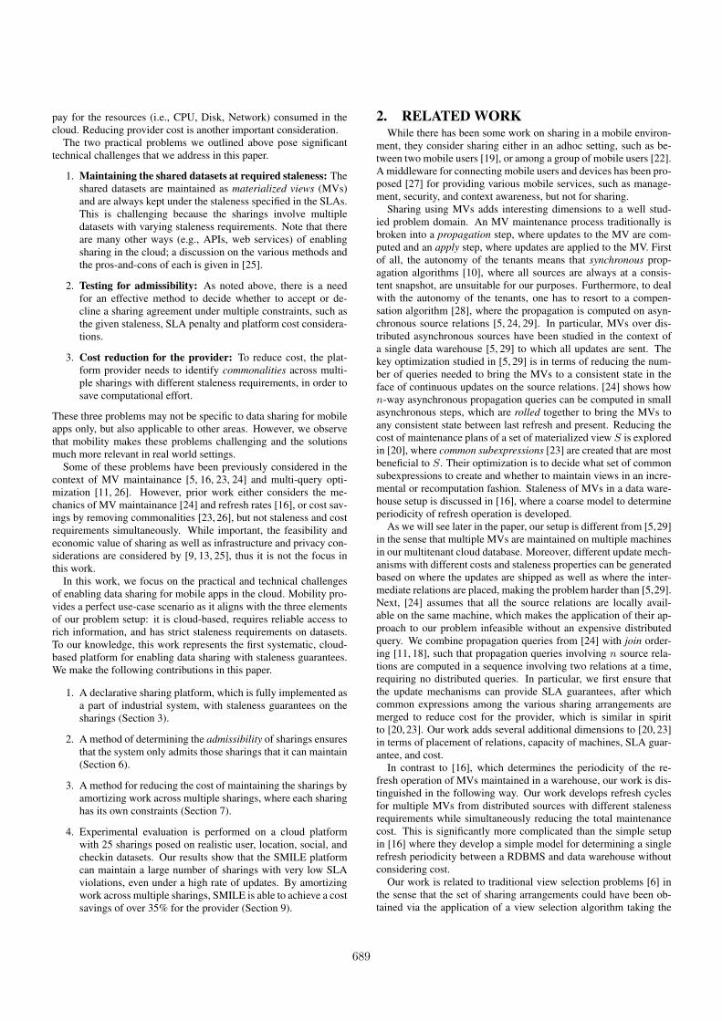
4. SMILE ARCHITECTUREFigure 1 shows the architecture of the system. There is a set of

machines available to implement the sharings. Each machine runs asingle database instance (Postgresql in our case). The SMILE plat-form consists of three main components — (a) delta capture, (b)sharing optimizer, and (c) sharing executor — that perform the fol-lowing functions, respectively: (a) capture changes (i.e., delta) onthe base relations as updates are applied on them; (b) generates planfor moving these updates from the base relations to the MVs; and(c) schedules the movement of these updates by taking system fluc-tuations into account. We briefly describe the three main systemcomponents below.

Machine

Pos

tgre

sql

Machine P

ostg

resq

l

Dat

abas

e

R

DELTA CAPTURE

¢R

Sharing Plan

Push

Agent

Heartbeat

Agent

Gat

eway

Wor

kloa

d

MV

Machine Machine

Agent Agent

Data Sharing Framework

Sharing Optimizer

Input Sharings S

Sharing Executor

Pub/Sub

Infrastructure

Figure 1: Architecture of the sharing platform

4.0.1 Delta Capture and TimestampsAs the base relations are updated, a delta capturing mechanism

(i.e., tuple creation, deletion or updates) records the modified tu-ples. Our mechanism uses the Streaming Replication facility [3] inPostgresql to capture the deltas. This module in Postgres allowsthe Write Ahead Log (WAL) to be streamed on to another Post-gresql instance in recovery mode so that a nearly identical replicaof a database can be maintained. Our module fakes itself as a Post-gresql instance and obtains a WAL stream. The modified tuples areextracted from the stream, unpacked and written to the disk.

Every base relation R is associated with a delta relation, denotedby ∆R that records the modified tuples as update queries are appliedon R. The tuples in ∆R are populated by the delta capturing mod-ule. The MVs in the system also contain corresponding delta tables.If R is a MV then ∆R contains both prior updates as well as thosethat have not yet been applied to R. The tuples in ∆R of a MV ispopulated, moved and applied by the sharing executor.

690

Every relation, delta of a relation or MV in our platform recordsits last modification timestamp. The timestamps are generated usinga distributed clock [17] that is periodically synchronized. Each tuplein the delta also records an associated timestamp. Maintaining thesharings at their appropriate level of staleness is achieved by keep-ing track of the last modification timestamps of the base relationsand comparing them to the timestamp of the MV. The SMILE sys-tem maintains an up-to-date timestamp information on each sharing,hence is aware of the current staleness of all the sharings. Updatesare moved from the base relations to the MV in a way that ensuresthat the sharings do not miss their SLAs.

4.0.2 Sharing OptimizerGiven a set S of new sharings, the sharing optimizer generates an

update mechanism for each sharing in S using a three step proceduredescribed below.

a. A sharing Si in S can be admitted if the system can maintainSi at the desired level of staleness. This determination is nec-essary to prevent the system from entering into SLAs that itcannot satisfy (Section 6).

b. If Si is admissible, we generate its sharing plan such that itcan move updates from the base relations to the MV withinthe time specified in the staleness SLA. Moreover, the sharingplan is also cost effective in terms of its infrastructure resourceconsumption (Section 6).

c. Once the individual sharing plans of all the sharings in S aredetermined, commonalities across sharings are identified andremoved to produce a single global sharing planD that imple-ments all the sharings (Section 7).

4.0.3 Sharing ExecutorThe sharing executor is the execution engine of the system which

maintains the sharings at or below the required staleness level. Thesharing executor is an implementation of an asynchronous viewmaintenance algorithm [24].

The sharing executor computes the current staleness of a sharingby taking the difference between the maximum of the timestamps ofall the base relations to that of the MV. The executor keeps track ofwhich of the sharings will soon miss their staleness SLA. It sched-ules the updates to be applied on the MV so that its staleness isreduced. Each machine in the infrastructure runs an agent that com-municates with the sharing executor via a pub/sub system (e.g., Ac-tiveMQ). The agents send periodic messages to the sharing executorwith the last modification timestamps of the base relations and theMVs.

Our implementation of the executor is lazy by design in the sensethat it does not refresh unless it is absolutely necessary or the sharingwill miss its SLA. This way, the executor bunches as much work aspossible thereby reducing redundant effort. The refresh is neither tooearly nor too late, but finishes just before a sharing is about to missits staleness SLA. We provide more details on the sharing executorin Section 8.

5. SHARING PLANThe update mechanism of a sharing is implemented as a sharing

plan, which is analogous to a query execution plan in databases. Wewill henceforth refer to it simply as a plan in the rest of the pa-per. The plan is expressed in terms of four operators that form thetransformational path for the updates from the base relations to theMV. This is represented using a Directed Acyclic Graph (DAG) such

that the vertices are relations or deltas of relations tied to a partic-ular machine, and the edges apply transformational operators. Theplan is expressed using the following four edge operators, that 1)apply updates (DeltaToRel) , 2) copy updates between machines(CopyDelta) , 3) join updates (Join), and 4) union (i.e., merge) up-dates (Union).

As the plan operates on base relations that are asynchronouslyupdated, the input vertices to an operator may have different times-tamps. An operator takes any mismatch in the timestamps intoaccount by rolling back all the input vertices to the minimum ofthe timestamps among its inputs. This is referred to as compensa-tions [28]. Rolling back the timestamp of a relation or a MV ispossible due to the delta relations associated it. The operators forapplying, copying and merging updates are based on their standardinterpretations, except that they additionally apply compensations tothe inputs as the first step. Our join operator performs a compensa-tion which is an implementation of the algorithm from [28].

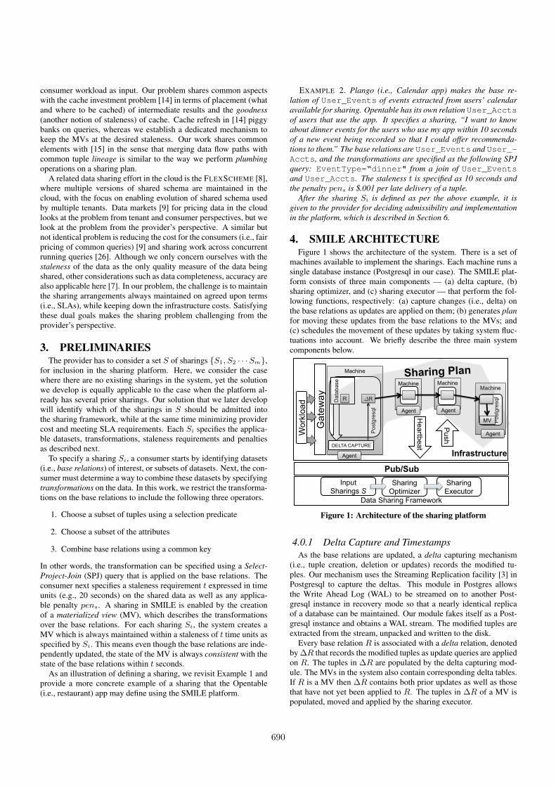
We will not provide the implementational details of the operatorsbut instead show an example of a plan that performs a relational joinon two asynchronous base relations A and B on different machines.The plan is referred to as “in-place” as it does not involve makingthe copies of the base relations. The vertices and the edge operatorsin the plan periodically move the updates from the base relations tothe MV to keep it maintained incrementally.

DELTA CAPTURE DELTA CAPTURE

COPY UPDATES

Machine m1 Machine m2

ΔA

ΔA A ΔB B ΔB

Δ(A⋈ΔB)

Δ(ΔA⋈B)

Δ(ΔA⋈B)

Δ(A⋈B)

A⋈B

JOIN JOIN

APPLY UPDATES

COPY UPDATES

Machine m3

Δ(A⋈ΔB)

COPY UPDATES

UNION UPDATES

Figure 2: One possible plan involving an in-place join of a baserelation A on machine m1 and B on machine m2 such that theresulting MV A 1 B is placed on machine m3

EXAMPLE 3. Figure 2 shows the plan of a sharing Si that per-forms a transformation A 1 B on two base relations, A and B.The plan is a DAG consisting of 12 vertices and 10 edges. The ver-tices are either base relations (e.g., A, B or its copies), MVs (e.g.,A 1 B) or delta relations (e.g., ∆(∆A 1 B)). The edges cor-responds to operators that either apply, copy, merge, join updates,to complete the transformation path from the base relations to theMV. Note that select and project predicates can be specified in Si’stransformation. All the four edge types can apply select and projectpredicates to their inputs if one is specified in addition to their usualfunctionalities. We handle these predicates by using the pushdownheuristic [11].

Given a sharing that specifies a set of transformations on the baserelations, the plan generation algorithm enumerates all the plans thatimplement the sharing. However, not all of the plans satisfy theconstraints we develop in the reminder of this section. In particular,we concern ourselves with two key properties of a plan, namely itscritical time path and dollar costs, which are described below.

691

5.1 Critical Time PathThe critical time path of the plan is the longest path in terms of

seconds that represents the most time consuming data transforma-tion path in the plan. Note that the plan is admissible only if thelength of its critical time path is less than the required staleness ofthe sharing, or else the system cannot maintain it.

The sharing optimizer estimates the critical time path of a planusing a time cost model for each operator. The model estimates thetime taken for each operator given the size of the updates. Note thatfinding the longest path between two vertices on a general graphis an NP-hard problem, but the plans are DAGs, on which longestpath calculation is tractable. The system implements the procedureCP(p) that takes a sharing plan p and outputs its critical time pathin seconds. For example, in the plan p shown in Figure 2, CP(p)computes the time taken along the longest transformation path fromA or B to the MV A 1 B. Section 9 provides additional details onhow we developed the time cost model for the four operators.

5.2 Cost ModelThe cost of the plan, expressed in dollars per second, is com-

puted by the amount of CPU, network, and disk capacity consumedto setup the sharing and maintain it at the required staleness. Theprovider periodically moves the updates to the MVs and buys CPU,disk and network capacities from the Infrastructure as a Service(IaaS). This cost can be further divided into two categories: resourceusage (i.e., CPU, disk capacity, network capacity) and penalty dueto possible SLA violations.

Resource Usage. There are existing analytical models that esti-mate the usage of various resources for maintaining a MV, based onupdate rate, join selectivity, data location, etc. (e.g., [21]). Thisanalytical model is implemented as a resCost function that com-putes the cost of the resources consumed by a plan. Furthermore,the resource usage should also vary with the staleness SLA of thesharing. When the required staleness is much longer than the criti-cal time path, e.g., the critical time path is 1 second and the stalenessrequirement is 30 seconds, the sharing executor has much flexibil-ity in deciding when to update the MV. Specifically, given a newtuple to the base relations, the service provider can push it to theMV immediately, or wait for as long as 29 second before pushing it.On the other hand, when the staleness becomes close to the criticaltime path, there is much less flexibility since other sharings in theinfrastructure may compete for resources.

In order to reduce the negative interaction at low staleness values,the resources allocated to the plan are over-provisioned by a factorthat is inversely proportional to the required staleness. This simplestrategy ensures that the negative interactions are mostly avoided atlow staleness values.

SLA Penalty. At low staleness values the natural fluctuations inthe update rates may cause a plan to miss the SLA. This is becausethe plan estimates the critical time path using the average arrival rate,but in practice this is an over simplification as the updates frequentlyvary. So, we have to estimate how much of penalty may be incurredgiven the required staleness, which also has to be factored into thecost. We estimate this by assuming a Possion arrival of updates, andmodeling the plan as a M/M/1 queuing system. Given the arrival rateof each base relations, we can estimate the arrival rate of tuples inthe MV based on the selectivity of joins. The average service time ofthe M/M/1 queue corresponds to the most time consuming operatorin the plan.

For an M/M/1 queue with arrival rate λ and service rate µ, thepercentage of items with sojourn time t larger than the staleness SLAs is P (t > s) = e(λ−µ)·s. Thus the dynamic cost of a plan p withstaleness s is calculated as:

COST(p) = resCost(p) · (1 +CP (p)

s) + e(λ−µ)·s · pens (1)

resCost(p) is the cost of resource usage. As discussed be-fore, to avoid SLA violation due to multiple sharings compet-ing for resource, we over-provision the resource by a factor ofCP (p)/s where CP (p) is the length of the critical time path ofp. e(λ·a−µ)·s ·pens is the estimated penalty of missing the stalenessSLA due to higher-than-expected tuple arrival rate, where pens isthe penalty of missing the staleness SLA for a single tuple.

6. SHARING OPTIMIZERThe goal of the sharing optimizer is to produce a low-cost admis-

sible plan. Satisfying the dual constraints of finding an admissibleplan that is provably cheapest amongst all plans is a hard problem.

A sharing Si specifies SPJ transformations on a set of base rela-tions. As the base relations are hosted on different machines, thereare several ways of combining them as well as where to place theintermediate results. This results in plans with varying dollar costand critical time paths. For instance, performing many operationsin parallel on different machines may produce a plan with a smallcritical time path. But such a plan may have a high dollar cost due tohigh infrastructure costs involved in using many machines. On theother hand, operations can also be performed sequentially to reducethe dollar cost but at the expense of a high critical time path.

Among the generated plans those that have a critical time pathgreater than the SLA of Si cannot be maintained by the system at thedesired staleness level, and hence are not admissible. The admissi-bility of plans forms the hard constraint of our problem in the sensethat the system should not admit a sharing that cannot be handledby the system. At the same time, it also should not deny admittingsharings that otherwise should have been admissible.

The sharing optimizer is based on the polynomial time heuristicsolution developed for System-R [11] and its analogous distributedvariant R∗ [18]. Our approach relies on generating, using a dynamicprogramming approach, the cheapest possible plan in terms of dollarcosts, regardless of its critical time path and another plan with thesmallest critical time path, regardless of its dollar costs. We refer tothese plans as Dynamic Programming Dollar (DPD) and DynamicProgramming Time (DPT), respectively. The DPD and DPT planshave the following properties:

1. DPT is a plan with a low critical time path that is not optimizedon the operating dollar cost. If DPT is not admissible, then thesharing can be safely rejected by the provider as there cannotbe a plan with a lower critical time path.

2. DPD is a plan with a low operating dollar cost that is not op-timized on the critical time path. If DPD is admissible, then itis also of the cheapest cost.

We provide a dynamic programming formulation to produce DPTand DPD in Section 6.1, and provide a plan generation algorithm inSection 6.2.

6.1 Dynamic Programming FormulationWe cast the problem of generating a plan as a bottom-up dynamic

programming formulation given by JOINCOST in Algorithm 1. Con-sider a sharing that specifies a join sequence on the base relations.For example, Figure 2 shows a join sequence of length two using thetwo base relations, A and B.

Let Si be a sharing in S such that SRC(Si) is the set of sourcevertices of Si and MV(Si) is the vertex corresponding to the MV

692

COPYDELTA COPYDELTA

m1

JOIN

UNION

COPY DELTA

ΔA

ΔA A ΔB B ΔB

Δ(A⋈ΔB)

Δ(ΔA⋈B)

Δ(ΔA⋈B)

Δ(A⋈B)

A⋈B

Δ(A⋈ΔB)

COPYDELTA JOIN JOIN

UNION

DELTATOREL

COPY DELTA

COPYDELTA

ΔA A ΔB B ΔB

Δ(A⋈ΔB)

Δ(ΔA⋈B)

Δ(ΔA⋈B)

Δ(A⋈B)

A⋈B

Δ(A⋈ΔB)

B

m2

m3

(a) (b)

m2

m3

m1

COPY DELTA

DELTA TOREL

JOIN

Δ(A⋈ΔB)

Δ(A⋈B)

A⋈B

ΔA A

Δ(ΔA⋈B)

ΔB B ΔA

Δ(ΔA⋈B)

Δ(A⋈ΔB)

A ΔA A ΔB B

Δ(A⋈ΔB)

Δ(A⋈B)

A⋈B

Δ(ΔA⋈B)

ΔA A B ΔB

(c) (d)

m1

m2

m3

m3

m1 m2

UNION DELTATOREL

JOIN JOIN

COPYDELTA COPYDELTA

UNION

DELTATOREL

JOIN

JOIN

COPY DELTA DELTA

TOREL DELTATOREL CO

PY

DE

LTA

COPY DELTA

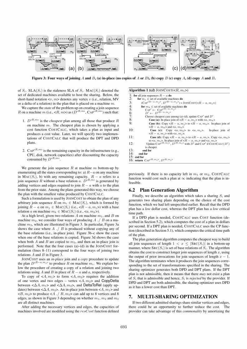
Figure 3: Four ways of joining A and B, (a) in-place (no copies of A or B), (b) copy B (c) copy A, (d) copy A and B.

of Si. SLA(Si) is the staleness SLA of Si. MAC(Si) denoted theset of dedicated machines available to host the sharing. Below, theshort-hand notation <v,m> denotes any vertex v (i.e., relation, MVor a delta of a relation) in the plan that is placed on a machine m.

We capture the state of the problem up on creating a join sequenceR on a machinem (i.e., <R,m>) as (D<R,m>, CAP<R,m>) such that:

1. D<R,m> is the cheapest plan among all those that produce Ron machine m. The cheapest plan is chosen by applying acost function COSTCALC, which takes a plan as input andproduces a cost value. Later, we will specify two implemen-tations of COSTCALC that will produce the DPT and DPDplans.

2. CAP<R,m> is the remaining capacity in the infrastructure (e.g.,CPU, disk, network capacities) after discounting the capacityconsumed by D<R,m>.

We generate the join sequence R at machine m bottom-up byenumerating all the states corresponding to: a)R−a on any machinein MAC(Si), b) with any remaining capacity. R − a refers to ajoin sequence R without a base relation a. D<R,m> is generated byadding vertices and edges required to join R − a with a to the planfrom the prior state. Among the plans generated this way, we choosethe plan with the smallest value produced by COSTCALC.

Such a formulation is used by JOINCOST to obtain the plan of anyarbitrary join sequence R on mi ∈ MAC(Si), which is formed byjoining R − a on mj ∈ MAC(Si) (i.e., <R− a,mj>) with a baserelation a on machine mk ∈ MAC(Si) (i.e., <a,mk>).

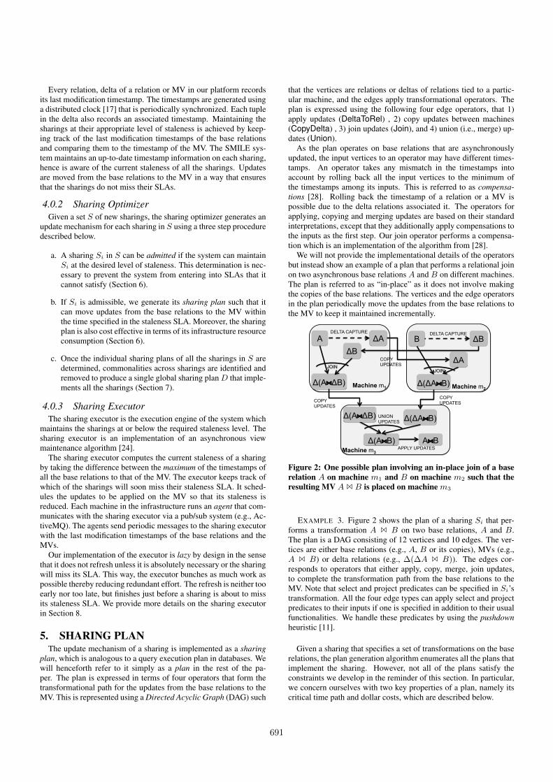
At a high level, given two relations A on machine m1, and B onmachine m2, we consider four ways of producing A ./ B on a ma-chine m3, which are illustrated in Figure 3. In particular, Figure 3ashows the case where A ./ B is produced without copying any ofthe base relations (i.e., in-place join). Figure 3b–c show the caseswhen one of the base relations is copied. Figure 3d shows the casewhen both A and B are copied to m3, and then an in-place join isperformed. Note that the four cases (a)–(d) in the JOINCOST for-mulation (lines 8–11) correspond to the four ways of joining tworelations A and B in Figure 3.

JOINCOST uses an in-place join and a copy procedure to updatethe plan D<R−a,mj> to produce R on machine mi. We explain be-low the procedure of creating a copy of a relation and joining tworelations using A and B in place of R− a and a, respectively.

To copy of <A,m1> to form <A,m2> requires the additionof one vertex and two edges – vertex <A,m2> and CopyDeltabetween <∆A,m1> and <∆A,m2>, and DeltaToRel (apply up-dates) between <∆A,m2>. An in-place join between <A,m1> and<B,m2> to produce <A ./ B,m3> can add up to 8 vertices and 8edges, as shown in Figure 3 depending on whether m1, m2 and m3

are all distinct machines.After adding the necessary vertices and edges, the capacities of

machines involved are modified using the resCost function defined

Algorithm 1 sub JOINCOST(<R,mi>)1: for all join sequences R− a do2: for mj ∈ set of available machines do3: (CAP<R−a,mj>, D<R−a,mj>) = JOINCOST(<R− a,mj>)4: for mk ∈ set of available machines do5: CAP′← CAP<R−a,mj>

6: D′← D<R−a,mj>

7: Choose cheapest case among (a)–(d), update CAP′ and D′

8: Case (a): In-place join of <R− a,mj> with <a,mk>9: Case (b): Copy <R− a,mj> to <R− a,mk>. In-place join of

<R− a,mk> and <a,mk>10: Case (c): Copy <a,mk> to <a,mj>. In-place join of

<R− a,mj> with <a,mj>.11: Case (d): Copy <R− a,mj> to <R− a,mi>. Copy <a,mk>

to <a,mi>. In-place join of <R− a,mi> and <a,mi>12: Update CAP<R,mi>, D<R,mi> with D′ and CAP′ if COSTCALC(D′)

is cheaper.13: end for14: end for15: end for16: return CAP<R,mi>, D<R,mi>

previously. If there is no capacity left in m1 or m2, COSTCALCfunction would cost such a plan at∞ indicating that the plan is in-feasible.

6.2 Plan Generation AlgorithmFinally, we describe an algorithm which takes a sharing Si and

generates two sharing plans depending on the choice of the costfunction, which we had left unspecified earlier. Recall that the DPDplan has a low dollar cost, whereas the DPT plan has a low criticaltime path.

If a DPD plan is needed, COSTCALC uses COST function (de-scribed in Section 5.2), which computes the cost of a plan in dollarsper second. If a DPT plan is needed, COSTCALC uses the CP func-tion (described in Section 5.1), which computes the critical time pathof the plan.

The plan generation algorithm computes the cheapest way to buildall join sequences of length 1 < x ≤ |SRC(Si)| in a bottom-upmanner, where SRC(Si) is set of base relations of Si. The algorithmobtains the cost to construct longer join sequences of length x, usingthe output of prior invocations for join sequences of length x − 1.The algorithm terminates when it produces the join sequences corre-sponding to the set of transformations specified in the sharing. Thesharing optimizer generates both DPD and DPT plans. If the DPTplan is not admissible, then it means that there may not exist a planof Si that is admissible and hence, Si is rejected by the provider. IfDPD and DPT are both admissible, the sharing optimizer uses DPDas it has a lower cost than DPT.

7. MULTI-SHARING OPTIMIZATIONIf two different admitted sharings share similar vertices and edges,

there could be an opportunity to further reduce the cost. Theprovider can take advantage of this commonality by amortizing the

693

operating costs across several sharings. The commonality here isreplacing two disjoint sets of vertices and edges belonging to differ-ent sharings that perform identical or similar transformation with acommon set for multiple sharings.

Although our idea of merging commonalities in plans is similar asmerging common subexpressions in concurrent running query exe-cution plans [26], there are two main differences. First, our infras-tructure contains multiple servers and the cost of moving the dataacross the servers has to be considered. Second, as we show below,unlike [26] we do not restrict to only merging identical subexpres-sions across plans.D is a global plan obtained by merging the plan of sharings in

S and then discarding duplicate edges and vertices. Note that Dneed not be a single connected component. Each vertex (or edge)v ∈ D records the identity of all the sharings that it serves, such thatSHR(v) records the sharings to which v belongs. Given a vertex (ora set of vertices) v, let ANC(v) be the set of vertices and edges thatare ancestors of v in D.

Commonalities inD are reduced by applying a plumbing operatorrepeatedly until the D does not perform any redundant work. Aplumbing operator takes two sets of vertices v1 and v2 belonging toplans as inputs. Then, vertices and edges that supply the vertices inv2 (or v1) are retained but those supplying v1 (or v2) are discarded.We now discuss the mechanics of a plumbing operator as well as analgorithm to apply them.

7.1 Plumbing OperationsA plumbing operation p is defined between a set of source ver-

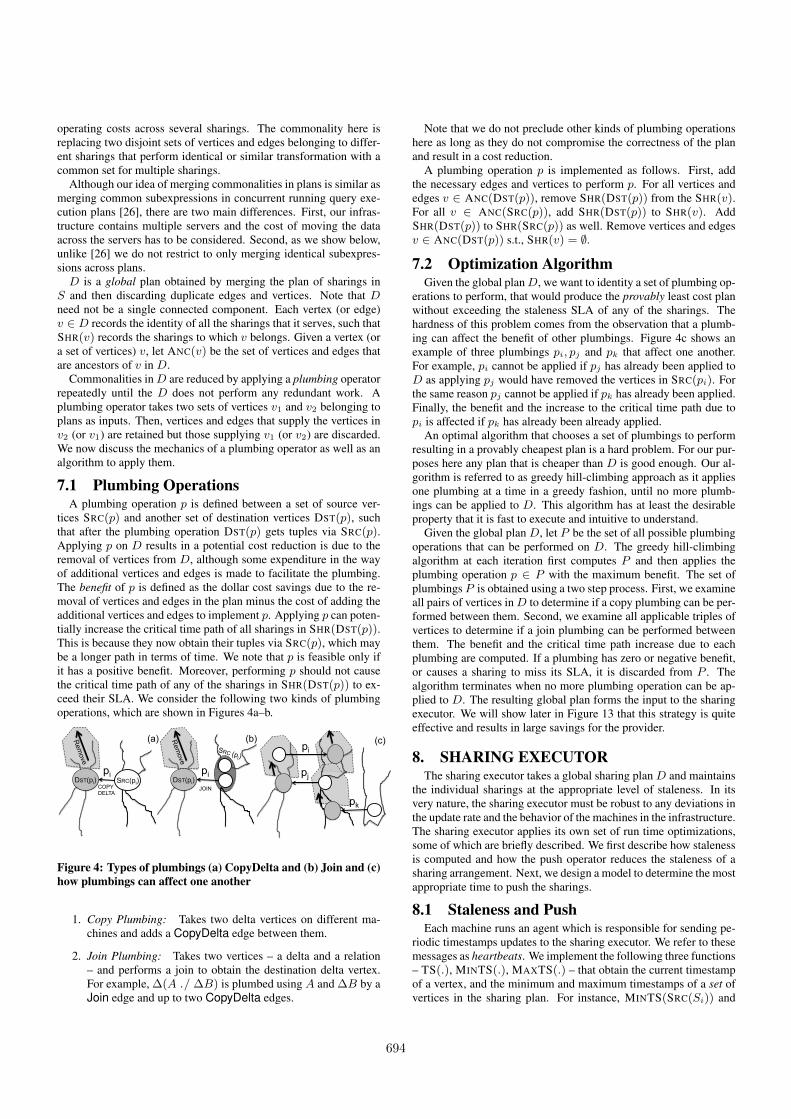
tices SRC(p) and another set of destination vertices DST(p), suchthat after the plumbing operation DST(p) gets tuples via SRC(p).Applying p on D results in a potential cost reduction is due to theremoval of vertices from D, although some expenditure in the wayof additional vertices and edges is made to facilitate the plumbing.The benefit of p is defined as the dollar cost savings due to the re-moval of vertices and edges in the plan minus the cost of adding theadditional vertices and edges to implement p. Applying p can poten-tially increase the critical time path of all sharings in SHR(DST(p)).This is because they now obtain their tuples via SRC(p), which maybe a longer path in terms of time. We note that p is feasible only ifit has a positive benefit. Moreover, performing p should not causethe critical time path of any of the sharings in SHR(DST(p)) to ex-ceed their SLA. We consider the following two kinds of plumbingoperations, which are shown in Figures 4a–b.

COPY DELTA

SRC(pi) DST(pi) pi

Rem

ove

(a)

JOIN DST(pi)

pi

Rem

ove

(b) SRC (pi)

pj

(c)

pk

pi

Figure 4: Types of plumbings (a) CopyDelta and (b) Join and (c)how plumbings can affect one another

1. Copy Plumbing: Takes two delta vertices on different ma-chines and adds a CopyDelta edge between them.

2. Join Plumbing: Takes two vertices – a delta and a relation– and performs a join to obtain the destination delta vertex.For example, ∆(A ./ ∆B) is plumbed using A and ∆B by aJoin edge and up to two CopyDelta edges.

Note that we do not preclude other kinds of plumbing operationshere as long as they do not compromise the correctness of the planand result in a cost reduction.

A plumbing operation p is implemented as follows. First, addthe necessary edges and vertices to perform p. For all vertices andedges v ∈ ANC(DST(p)), remove SHR(DST(p)) from the SHR(v).For all v ∈ ANC(SRC(p)), add SHR(DST(p)) to SHR(v). AddSHR(DST(p)) to SHR(SRC(p)) as well. Remove vertices and edgesv ∈ ANC(DST(p)) s.t., SHR(v) = ∅.

7.2 Optimization AlgorithmGiven the global planD, we want to identity a set of plumbing op-

erations to perform, that would produce the provably least cost planwithout exceeding the staleness SLA of any of the sharings. Thehardness of this problem comes from the observation that a plumb-ing can affect the benefit of other plumbings. Figure 4c shows anexample of three plumbings pi, pj and pk that affect one another.For example, pi cannot be applied if pj has already been applied toD as applying pj would have removed the vertices in SRC(pi). Forthe same reason pj cannot be applied if pk has already been applied.Finally, the benefit and the increase to the critical time path due topi is affected if pk has already been already applied.

An optimal algorithm that chooses a set of plumbings to performresulting in a provably cheapest plan is a hard problem. For our pur-poses here any plan that is cheaper than D is good enough. Our al-gorithm is referred to as greedy hill-climbing approach as it appliesone plumbing at a time in a greedy fashion, until no more plumb-ings can be applied to D. This algorithm has at least the desirableproperty that it is fast to execute and intuitive to understand.

Given the global plan D, let P be the set of all possible plumbingoperations that can be performed on D. The greedy hill-climbingalgorithm at each iteration first computes P and then applies theplumbing operation p ∈ P with the maximum benefit. The set ofplumbings P is obtained using a two step process. First, we examineall pairs of vertices inD to determine if a copy plumbing can be per-formed between them. Second, we examine all applicable triples ofvertices to determine if a join plumbing can be performed betweenthem. The benefit and the critical time path increase due to eachplumbing are computed. If a plumbing has zero or negative benefit,or causes a sharing to miss its SLA, it is discarded from P . Thealgorithm terminates when no more plumbing operation can be ap-plied to D. The resulting global plan forms the input to the sharingexecutor. We will show later in Figure 13 that this strategy is quiteeffective and results in large savings for the provider.

8. SHARING EXECUTORThe sharing executor takes a global sharing plan D and maintains

the individual sharings at the appropriate level of staleness. In itsvery nature, the sharing executor must be robust to any deviations inthe update rate and the behavior of the machines in the infrastructure.The sharing executor applies its own set of run time optimizations,some of which are briefly described. We first describe how stalenessis computed and how the push operator reduces the staleness of asharing arrangement. Next, we design a model to determine the mostappropriate time to push the sharings.

8.1 Staleness and PushEach machine runs an agent which is responsible for sending pe-

riodic timestamps updates to the sharing executor. We refer to thesemessages as heartbeats. We implement the following three functions– TS(.), MINTS(.), MAXTS(.) – that obtain the current timestampof a vertex, and the minimum and maximum timestamps of a set ofvertices in the sharing plan. For instance, MINTS(SRC(Si)) and

694

MAXTS(SRC(Si)) are the minimum and maximum timestamps ofthe sources of Si.

The current staleness of a sharing is defined as the difference be-tween the maximum of the timestamps of the base relations of Si tothat of the MV of Si. Note that the staleness should always be main-tained to be less than SLA(Si). This is captured by the followinginequality.

MAXTS(SRC(Si))− TS(MV(Si)) ≤ SLA(Si).

To reduce the staleness of a sharing Si, the executor schedules asequence of PUSH commands in a topological order starting withSRC(Si), until the timestamp of the MV has a more up-to-datetimestamp. A PUSH command instructs the agent to advance thetimestamp of a vertex in the sharing plan by applying an operatordenoted by its incoming edge. The incoming edge belongs to one ofthe four edge types we described in Section 5.

Suppose an agent receives a PUSH command to advance a vertexv to timestamp t. Suppose that e is an incoming edge of v. Theagent first obtains a write lock on v. It then compares the currenttimestamp t′ of v with that of t. If t′ ≥ t then there is no need toperform any work. If t′ < t, then the agent performs the operationcorresponding to e’s type so that the timestamp of v can be advancedto t. Once the operation has been performed the agent respondswith a PUSHDONE command, and piggybacks useful statistics suchas time taken to perform the operation and current timestamps. Theexecutor up on receiving the PUSHDONE proceeds with the outgoingedges of v.

When it comes to maintaining multiple sharings, the design of asharing executor is simplified due to the observation that any shar-ing in S can be pushed independently of the others in S even thoughthey may have common edges and vertices. Suppose a vertex is ata timestamp t and there are two concurrent PUSH commands to ad-vance it to t1 and t2, t ≤ t1 ≤ t2, respectively. Regardless of theorder in which the two commands are executed, the amount of workdone by e is equal to the work done to advance the timestamp tot2. This is why the sharing executor does not have to coordinatePUSH commands between the various sharings that it maintains.This makes for a simple design of the sharing executor, especiallysince the sharings may have different staleness SLAs and may haveto be pushed at different rates.

8.2 DesignOur sharing executor uses a simple model to determine two key

questions: a) Is it time to push Si? b) By how much to advancethe timestamp of MV of Si? To determine these two questions, wedevelop a model to determine the most appropriate time to schedulethe push and the timestamp to push the MV to such that the sharingwill not miss its SLA.

A simpler design of a sharing executor pushes all the sharingsin S every second so that they do not violate their SLA. Given theproperty that the critical time path of an admissible sharing is lessthan its staleness SLA, the push will finish before the SLA is vio-lated. However, our sharing executor does not push every secondbut rather bunches up sufficient work so that the push is issued aslate as possible. Yet, it is scheduled such that the push would becompleted before Si becomes stale.

To develop the model, we modify the critical time path functionCP(Di, x) to take an additional parameter x, which corresponds tothe amount of timestamp to advance the MV of Si. In Section 5.1when we described how we compute the critical time path of a shar-ing plan, xwas defaulted to be one but now can take up any arbitraryvalue greater than or equal to one. We also added a feedback loopto the CP function so that it constantly recomputes the time model

to take into account recent system fluctuations. We record the actualtime to perform each of the operators, compare it against estimatedtime and periodically recompute the time model. This feedback loopallows our system to be reasonably robust to data and machine fluc-tuations.

An appropriate timestamp t to advance the MV of Si should begreater than the current timestamp of MV but should be less thanor equal to the minimum of the timestamp of the sources of Si. Inparticular,

TS(MV(Si)) < t ≤ MINTS(SRC(Si)).

When the push finishes, the MV would be at the timestamp t, whilethe timestamp of the sources may all be advanced by CP(Di, t −TS(MV(Si))). So, the staleness of the sharing at the time the pushfinishes would be: MAXTS(SRC(Si)) + CP(Di, t−TS(MV(Si))).We stipulate that the staleness when the push finishes should be lessthan the staleness SLA using the following inequality:

MAXTS(SRC(Si)) + CP(Di, t− TS(MV(Si)))− t ≤ SLA(Si).

On the other hand, the sharing executor does not want to push tooearly as well. In other words, the sharing executor is early if thepush command could have waited a bit longer and still could havecompleted before Si became stale. This can be stipulated by addingthe additional constraint that:

l ∗ SLA(Si) ≤ MAXTS(SRC(Si))+ ≤ SLA(Si),

CP(Di, t− TS(MV(Si)))− t

where l > 0 (0.8 in our case) is chosen to account for run-timedeviations, such as a queuing delay if the PUSH waits for the ca-pacity on a machine to be available. An appropriate value of t isobtained by performing a binary search between TS(MV(Si)) andMINTS(SRC(Si)) that satisfies the above constraint.

9. EXPERIMENTSIn this section, we present an experimental study to validate the

SMILE sharing platform. We first describe the experimental setupin Section 9.1. We then evaluate the performance of our system forvarying rate of updates on the base relation in Section 9.2 and vary-ing SLA in Section 9.3. We examine the effect of varying the num-ber of machines and the sharings in the infrastructure in Section 9.4.Next, the efficacy of the hill-climbing algorithm applied to DPT andDPD is shown in Section 9.5. Finally, we highlight the robustnessof the sharing executor in Section 9.6 by varying the update rates onthe base relations and varying read workload on the MV.

9.1 SetupOur experimental setup creates a mobile cloud ecosystem con-

taining 25 apps where sharings are specified using user, social net-work, location, checkin, and user-content datasets; the datasets andthe sharings are representative of those one may find in a mobilecloud. We collected Twitter tweets from a gardenhose stream, whichis a 10% sampling of all the tweets in Twitter, for a six monthperiod starting from September 2010. The tweets were unpackedinto nine base relations corresponding to the information about theuser (i.e., users relation), tweets (i.e., tweets relation), socialnetwork (socnet relation), checkins (foursq), and user-content(i.e., urls, hashtags, curloc, photos relations) associatedwith the tweets and the location of the user (i.e., loc relation).This creates our realistic datasets that capture rich information aboutusers, locations, social contacts, checkins and the various contentsthe users are interest in.

695

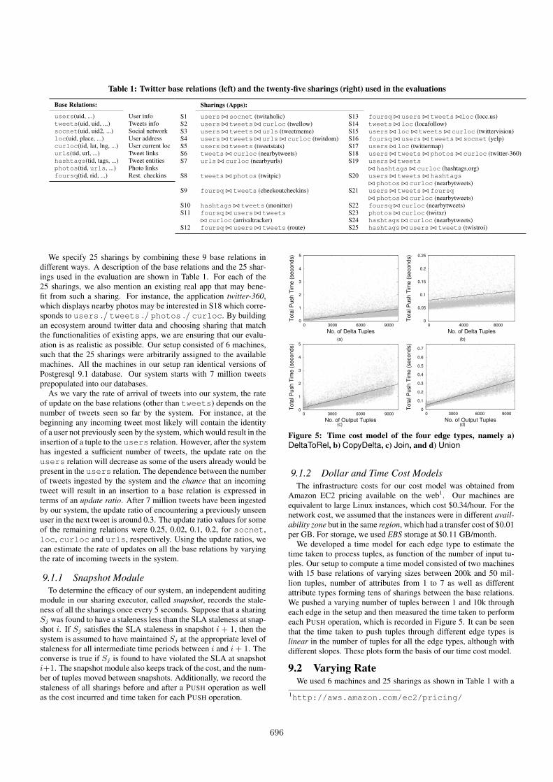
Table 1: Twitter base relations (left) and the twenty-five sharings (right) used in the evaluations

Base Relations:

users(uid, ...) User infotweets(uid, uid, ...) Tweets infosocnet(uid, uid2, ...) Social networkloc(uid, place, ...) User addresscurloc(tid, lat, lng, ...) User current locurls(tid, url, ...) Tweet linkshashtags(tid, tags, ...) Tweet entitiesphotos(tid, urls, ...) Photo linksfoursq(tid, rid, ...) Rest. checkins

Sharings (Apps):

S1 users ./ socnet (twitaholic) S13 foursq ./ users ./ tweets ./loc (locc.us)S2 users ./ tweets ./ curloc (twellow) S14 tweets ./ loc (locafollow)S3 users ./ tweets ./ urls (tweetmeme) S15 users ./ loc ./ tweets ./ curloc (twittervision)S4 users ./ tweets ./ urls ./ curloc (twitdom) S16 foursq ./ users ./ tweets ./ socnet (yelp)S5 users ./ tweets (tweetstats) S17 users ./ loc (twittermap)S6 tweets ./ curloc (nearbytweets) S18 users ./ tweets ./ photos ./ curloc (twitter-360)S7 urls ./ curloc (nearbyurls) S19 users ./ tweets

./ hashtags ./ curloc (hashtags.org)S8 tweets ./ photos (twitpic) S20 users ./ tweets ./ hashtags

./ photos ./ curloc (nearbytweets)S9 foursq ./ tweets (checkoutcheckins) S21 users ./ tweets ./ foursq

./ photos ./ curloc (nearbytweets)S10 hashtags ./ tweets (monitter) S22 foursq ./ curloc (nearbytweets)S11 foursq ./ users ./ tweets S23 photos ./ curloc (twitxr)

./ curloc (arrivaltracker) S24 hashtags ./ curloc (nearbytweets)S12 foursq ./ users ./ tweets (route) S25 hashtags ./ users ./ tweets (twistroi)

We specify 25 sharings by combining these 9 base relations indifferent ways. A description of the base relations and the 25 shar-ings used in the evaluation are shown in Table 1. For each of the25 sharings, we also mention an existing real app that may bene-fit from such a sharing. For instance, the application twitter-360,which displays nearby photos may be interested in S18 which corre-sponds to users ./ tweets ./ photos ./ curloc. By buildingan ecosystem around twitter data and choosing sharing that matchthe functionalities of existing apps, we are ensuring that our evalu-ation is as realistic as possible. Our setup consisted of 6 machines,such that the 25 sharings were arbitrarily assigned to the availablemachines. All the machines in our setup ran identical versions ofPostgresql 9.1 database. Our system starts with 7 million tweetsprepopulated into our databases.

As we vary the rate of arrival of tweets into our system, the rateof update on the base relations (other than tweets) depends on thenumber of tweets seen so far by the system. For instance, at thebeginning any incoming tweet most likely will contain the identityof a user not previously seen by the system, which would result in theinsertion of a tuple to the users relation. However, after the systemhas ingested a sufficient number of tweets, the update rate on theusers relation will decrease as some of the users already would bepresent in the users relation. The dependence between the numberof tweets ingested by the system and the chance that an incomingtweet will result in an insertion to a base relation is expressed interms of an update ratio. After 7 million tweets have been ingestedby our system, the update ratio of encountering a previously unseenuser in the next tweet is around 0.3. The update ratio values for someof the remaining relations were 0.25, 0.02, 0.1, 0.2, for socnet,loc, curloc and urls, respectively. Using the update ratios, wecan estimate the rate of updates on all the base relations by varyingthe rate of incoming tweets in the system.

9.1.1 Snapshot ModuleTo determine the efficacy of our system, an independent auditing

module in our sharing executor, called snapshot, records the stale-ness of all the sharings once every 5 seconds. Suppose that a sharingSj was found to have a staleness less than the SLA staleness at snap-shot i. If Sj satisfies the SLA staleness in snapshot i + 1, then thesystem is assumed to have maintained Sj at the appropriate level ofstaleness for all intermediate time periods between i and i+ 1. Theconverse is true if Sj is found to have violated the SLA at snapshoti+1. The snapshot module also keeps track of the cost, and the num-ber of tuples moved between snapshots. Additionally, we record thestaleness of all sharings before and after a PUSH operation as wellas the cost incurred and time taken for each PUSH operation.

0

1

2

3

4

5

0 3000 6000 9000

To

tal P

ush

Tim

e (

se

co

nd

s)

No. of Delta Tuples

0

0.05

0.1

0.15

0.2

0.25

0 4000 8000

To

tal P

ush

Tim

e (

se

co

nd

s)

No. of Delta Tuples

(a) (b)

0

1

2

3

4

5

0 3000 6000 9000

To

tal P

ush

Tim

e (

se

co

nd

s)

No. of Output Tuples

0

0.1

0.2

0.3

0.4

0.5

0.6

0.7

0 3000 6000 9000

To

tal P

ush

Tim

e (

se

co

nd

s)

No. of Output Tuples(c) (d)

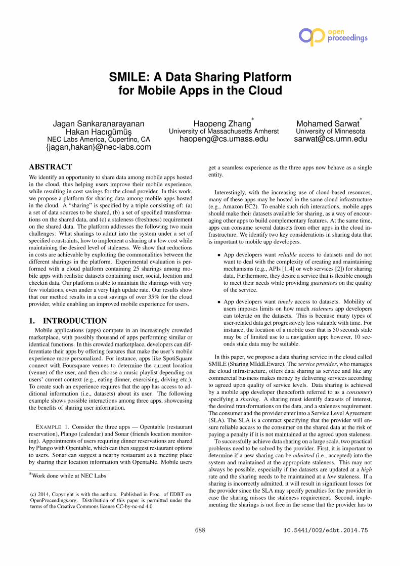
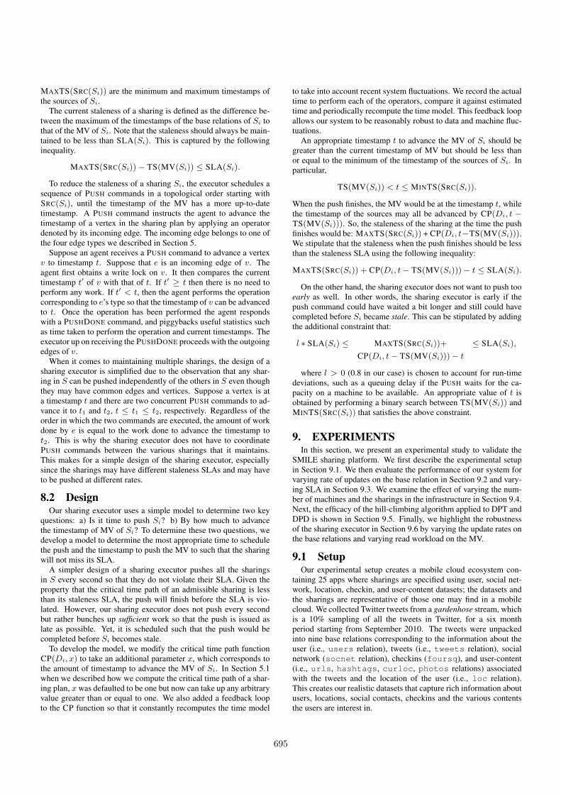
Figure 5: Time cost model of the four edge types, namely a)DeltaToRel, b) CopyDelta, c) Join, and d) Union

9.1.2 Dollar and Time Cost ModelsThe infrastructure costs for our cost model was obtained from

Amazon EC2 pricing available on the web1. Our machines areequivalent to large Linux instances, which cost $0.34/hour. For thenetwork cost, we assumed that the instances were in different avail-ability zone but in the same region, which had a transfer cost of $0.01per GB. For storage, we used EBS storage at $0.11 GB/month.

We developed a time model for each edge type to estimate thetime taken to process tuples, as function of the number of input tu-ples. Our setup to compute a time model consisted of two machineswith 15 base relations of varying sizes between 200k and 50 mil-lion tuples, number of attributes from 1 to 7 as well as differentattribute types forming tens of sharings between the base relations.We pushed a varying number of tuples between 1 and 10k througheach edge in the setup and then measured the time taken to performeach PUSH operation, which is recorded in Figure 5. It can be seenthat the time taken to push tuples through different edge types islinear in the number of tuples for all the edge types, although withdifferent slopes. These plots form the basis of our time cost model.

9.2 Varying RateWe used 6 machines and 25 sharings as shown in Table 1 with a

1http://aws.amazon.com/ec2/pricing/

696

0

10

20

30

40

50

60

0 100 200 300

Sta

len

ess (

se

co

nd

s)

Snapshot

(S1), SLA=45s

0 10 20 30 40 50 60

0 100 200 300Sta

leness (

seconds)

Snapshot

(S2)

0 10 20 30 40 50 60

0 100 200 300Sta

leness (

seconds)

Snapshot

(S3)

0 10 20 30 40 50 60

0 100 200 300Sta

leness (

seconds)

Snapshot

(S4)

0 10 20 30 40 50 60

0 100 200 300Sta

leness (

seconds)

Snapshot

(S5)

0 10 20 30 40 50 60

0 100 200 300Sta

leness (

seconds)

Snapshot

(S6)

0 10 20 30 40 50 60

0 100 200 300Sta

leness (

seconds)

Snapshot

(S7)

0 10 20 30 40 50 60

0 100 200 300Sta

leness (

seconds)

Snapshot

(S8)

0 10 20 30 40 50 60

0 100 200 300Sta

leness (

seconds)

Snapshot

(S9)

0 10 20 30 40 50 60

0 100 200 300Sta

leness (

seconds)

Snapshot

(S10)

0 10 20 30 40 50 60

0 100 200 300Sta

leness (

seconds)

Snapshot

(S11)

0 10 20 30 40 50 60

0 100 200 300Sta

leness (

seconds)

Snapshot

(S12)

0 10 20 30 40 50 60

0 100 200 300Sta

leness (

seconds)

Snapshot

(S13)

0 10 20 30 40 50 60

0 100 200 300Sta

leness (

seconds)

Snapshot

(S14)

0 10 20 30 40 50 60

0 100 200 300Sta

leness (

seconds)

Snapshot

(S15)

0 10 20 30 40 50 60

0 100 200 300Sta

leness (

seconds)

Snapshot

(S16)

0 10 20 30 40 50 60

0 100 200 300Sta

leness (

seconds)

Snapshot

(S17)

0 10 20 30 40 50 60

0 100 200 300Sta

leness (

seconds)

Snapshot

(S18)

0 10 20 30 40 50 60

0 100 200 300Sta

leness (

seconds)

Snapshot

(S19)

0 10 20 30 40 50 60

0 100 200 300Sta

leness (

seconds)

Snapshot

(S20)

0 10 20 30 40 50 60

0 100 200 300Sta

leness (

seconds)

Snapshot

(S21)

0 10 20 30 40 50 60

0 100 200 300Sta

leness (

seconds)

Snapshot

(S22)

0 10 20 30 40 50 60

0 100 200 300Sta

leness (

seconds)

Snapshot

(S23)

0 10 20 30 40 50 60

0 100 200 300Sta

leness (

seconds)

Snapshot

(S24)

0 10 20 30 40 50 60

0 100 200 300Sta

leness (

seconds)

Snapshot

(S25)

0

100000

200000

300000

400000

500000

600000

700000

800000

900000

1e+06

1.1e+06

1.2e+06

0 100 200 300 400

No

. T

up

les M

ove

d

Snapshot

ALL, SLA=45s

0

100000

200000

300000

0 200 400

No. T

uple

s M

oved

Snapshot

S1

0

100000

200000

300000

0 200 400

No. T

uple

s M

oved

Snapshot

S3

0

100000

200000

300000

0 200 400

No. T

uple

s M

oved

Snapshot

S11

0

100000

200000

0 200 400

No. T

uple

s M

oved

Snapshot

S16

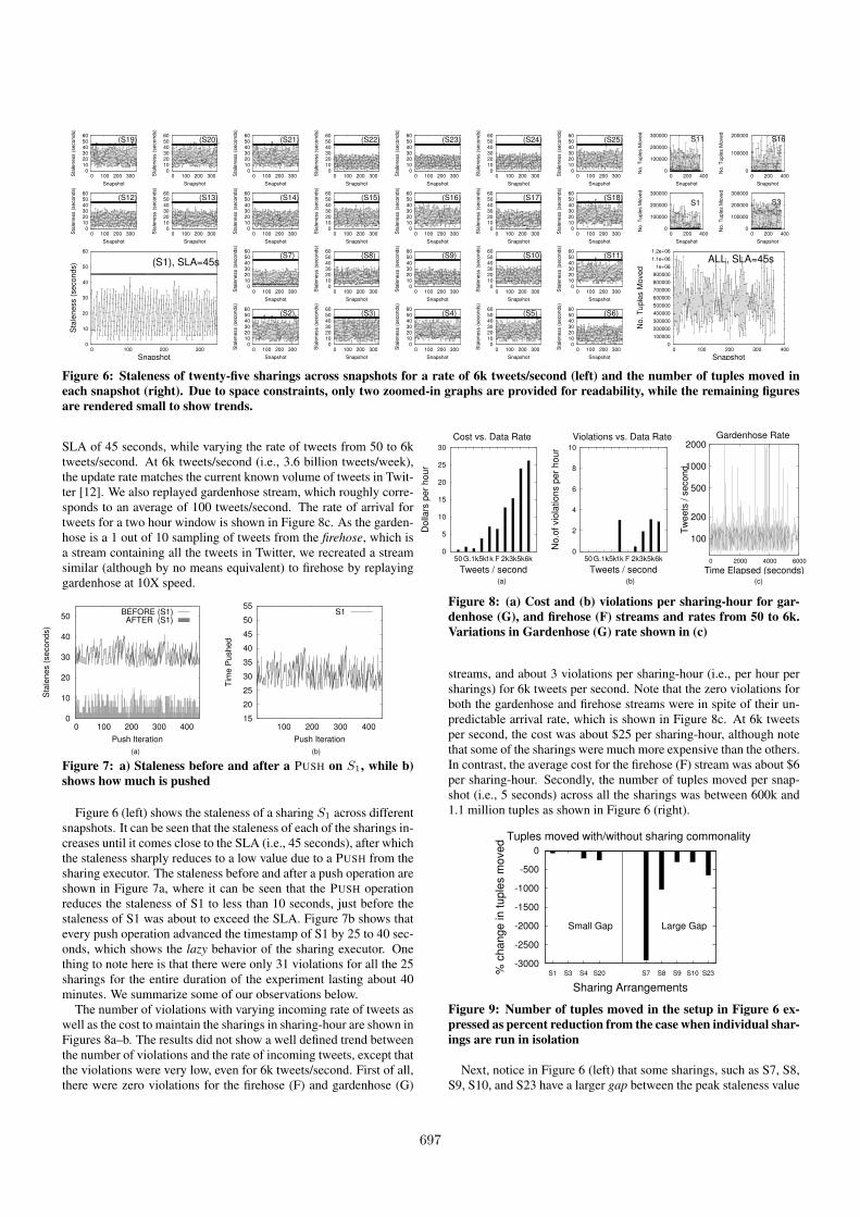
Figure 6: Staleness of twenty-five sharings across snapshots for a rate of 6k tweets/second (left) and the number of tuples moved ineach snapshot (right). Due to space constraints, only two zoomed-in graphs are provided for readability, while the remaining figuresare rendered small to show trends.

SLA of 45 seconds, while varying the rate of tweets from 50 to 6ktweets/second. At 6k tweets/second (i.e., 3.6 billion tweets/week),the update rate matches the current known volume of tweets in Twit-ter [12]. We also replayed gardenhose stream, which roughly corre-sponds to an average of 100 tweets/second. The rate of arrival fortweets for a two hour window is shown in Figure 8c. As the garden-hose is a 1 out of 10 sampling of tweets from the firehose, which isa stream containing all the tweets in Twitter, we recreated a streamsimilar (although by no means equivalent) to firehose by replayinggardenhose at 10X speed.

0

10

20

30

40

50

0 100 200 300 400

Sta

lenes (

seconds)

Push Iteration

BEFORE (S1)AFTER (S1)

15

20

25

30

35

40

45

50

55

100 200 300 400

Tim

e P

ushed

Push Iteration

S1

(a) (b)

Figure 7: a) Staleness before and after a PUSH on S1, while b)shows how much is pushed

Figure 6 (left) shows the staleness of a sharing S1 across differentsnapshots. It can be seen that the staleness of each of the sharings in-creases until it comes close to the SLA (i.e., 45 seconds), after whichthe staleness sharply reduces to a low value due to a PUSH from thesharing executor. The staleness before and after a push operation areshown in Figure 7a, where it can be seen that the PUSH operationreduces the staleness of S1 to less than 10 seconds, just before thestaleness of S1 was about to exceed the SLA. Figure 7b shows thatevery push operation advanced the timestamp of S1 by 25 to 40 sec-onds, which shows the lazy behavior of the sharing executor. Onething to note here is that there were only 31 violations for all the 25sharings for the entire duration of the experiment lasting about 40minutes. We summarize some of our observations below.

The number of violations with varying incoming rate of tweets aswell as the cost to maintain the sharings in sharing-hour are shown inFigures 8a–b. The results did not show a well defined trend betweenthe number of violations and the rate of incoming tweets, except thatthe violations were very low, even for 6k tweets/second. First of all,there were zero violations for the firehose (F) and gardenhose (G)

0

5

10

15

20

25

30

50G.1k.5k1k F 2k3k5k6k

Do

llars

pe

r h

ou

r

Tweets / second

Cost vs. Data Rate

0

2

4

6

8

10

50G.1k.5k1k F 2k3k5k6kN

o.o

f vio

latio

ns p

er

ho

ur

Tweets / second

Violations vs. Data Rate

100

200

500

1000

2000

0 2000 4000 6000

Tw

ee

ts /

se

co

nd

Time Elapsed (seconds)

Gardenhose Rate

(a) (b) (c)

Figure 8: (a) Cost and (b) violations per sharing-hour for gar-denhose (G), and firehose (F) streams and rates from 50 to 6k.Variations in Gardenhose (G) rate shown in (c)

streams, and about 3 violations per sharing-hour (i.e., per hour persharings) for 6k tweets per second. Note that the zero violations forboth the gardenhose and firehose streams were in spite of their un-predictable arrival rate, which is shown in Figure 8c. At 6k tweetsper second, the cost was about $25 per sharing-hour, although notethat some of the sharings were much more expensive than the others.In contrast, the average cost for the firehose (F) stream was about $6per sharing-hour. Secondly, the number of tuples moved per snap-shot (i.e., 5 seconds) across all the sharings was between 600k and1.1 million tuples as shown in Figure 6 (right).

-3000

-2500

-2000

-1500

-1000

-500

0

S1 S3 S4 S20 S7 S8 S9 S10 S23% c

hange in tuple

s m

oved

Sharing Arrangements

Tuples moved with/without sharing commonality

Small Gap Large Gap

Figure 9: Number of tuples moved in the setup in Figure 6 ex-pressed as percent reduction from the case when individual shar-ings are run in isolation

Next, notice in Figure 6 (left) that some sharings, such as S7, S8,S9, S10, and S23 have a larger gap between the peak staleness value

697

and the SLA, whereas others such as S1, S3, S4, and S20 have rel-atively smaller gaps. The reason for this is that those sharings withlarger gaps benefit from the commonality with other sharings but notso for those with smaller gaps. To test this hypothesis, we comparedthe number of tuples moved for each sharing in the above experi-mental setup with the number of tuples moved when the sharingsare run in isolation. The number of tuples moved in the former caseis shown as a percentage reduction from the latter case in Figure 9.It can be seen that sharings with small gaps only benefit modestlyfrom the presence of other sharings, whereas those with larger gapsbenefit immensely from the presence of other sharings.

9.3 Varying SLATable 2: Number of violations per sharing-hour (rounded-up)for varying SLA between 10 and 60 secs

Staleness SLA 10 20 30 40 50 60 MixViolations 4 1 2 1 0 0 0

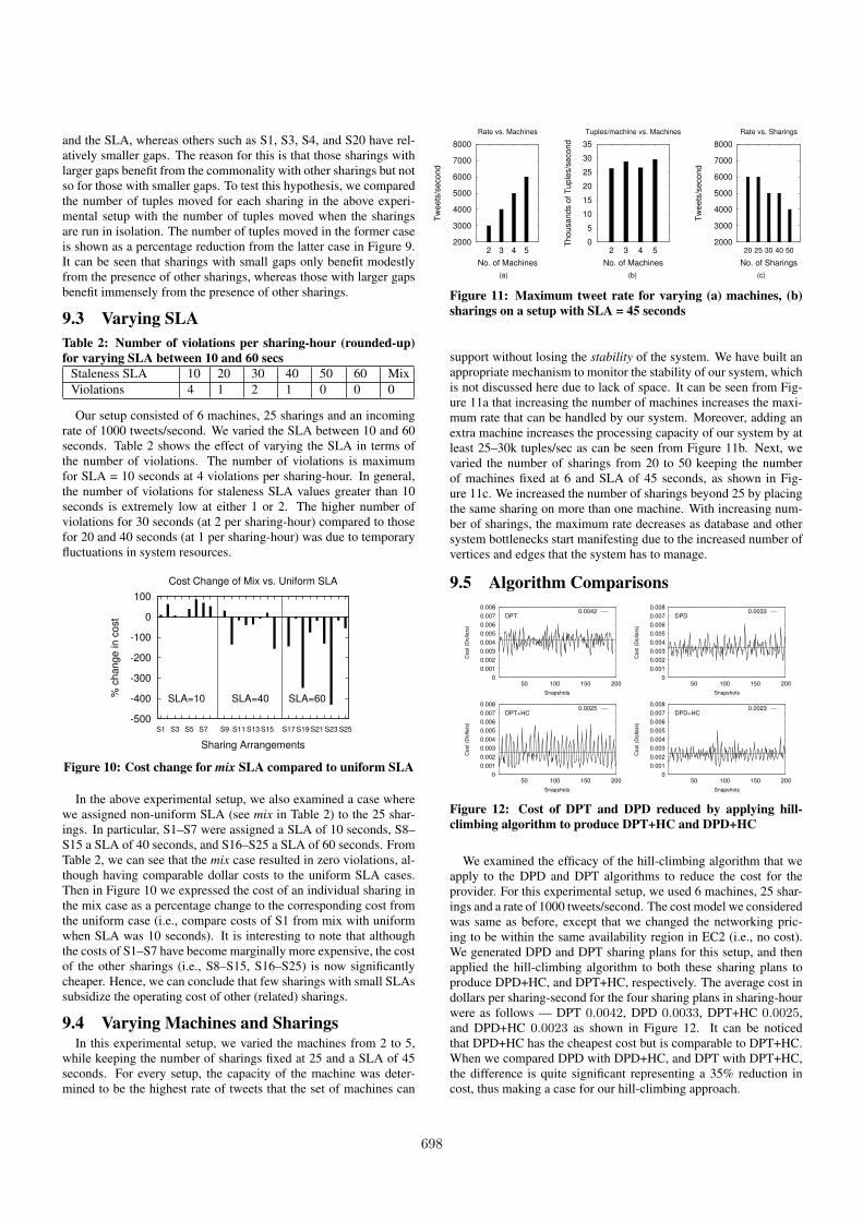
Our setup consisted of 6 machines, 25 sharings and an incomingrate of 1000 tweets/second. We varied the SLA between 10 and 60seconds. Table 2 shows the effect of varying the SLA in terms ofthe number of violations. The number of violations is maximumfor SLA = 10 seconds at 4 violations per sharing-hour. In general,the number of violations for staleness SLA values greater than 10seconds is extremely low at either 1 or 2. The higher number ofviolations for 30 seconds (at 2 per sharing-hour) compared to thosefor 20 and 40 seconds (at 1 per sharing-hour) was due to temporaryfluctuations in system resources.

-500

-400

-300

-200

-100

0

100

S1 S3 S5 S7 S9 S11 S13 S15 S17 S19 S21 S23 S25

% c

hange in c

ost

Sharing Arrangements

Cost Change of Mix vs. Uniform SLA

SLA=10 SLA=40 SLA=60

Figure 10: Cost change for mix SLA compared to uniform SLA

In the above experimental setup, we also examined a case wherewe assigned non-uniform SLA (see mix in Table 2) to the 25 shar-ings. In particular, S1–S7 were assigned a SLA of 10 seconds, S8–S15 a SLA of 40 seconds, and S16–S25 a SLA of 60 seconds. FromTable 2, we can see that the mix case resulted in zero violations, al-though having comparable dollar costs to the uniform SLA cases.Then in Figure 10 we expressed the cost of an individual sharing inthe mix case as a percentage change to the corresponding cost fromthe uniform case (i.e., compare costs of S1 from mix with uniformwhen SLA was 10 seconds). It is interesting to note that althoughthe costs of S1–S7 have become marginally more expensive, the costof the other sharings (i.e., S8–S15, S16–S25) is now significantlycheaper. Hence, we can conclude that few sharings with small SLAssubsidize the operating cost of other (related) sharings.

9.4 Varying Machines and SharingsIn this experimental setup, we varied the machines from 2 to 5,

while keeping the number of sharings fixed at 25 and a SLA of 45seconds. For every setup, the capacity of the machine was deter-mined to be the highest rate of tweets that the set of machines can

2000

3000

4000

5000

6000

7000

8000

2 3 4 5

Tw

ee

ts/s

eco

nd

No. of Machines

Rate vs. Machines

0

5

10

15

20

25

30

35

2 3 4 5

Th

ou

sa

nd

s o

f T

up

les/s

eco

nd

No. of Machines

Tuples/machine vs. Machines

2000

3000

4000

5000

6000

7000

8000

20 25 30 40 50

Tw

ee

ts/s

eco

nd

No. of Sharings

Rate vs. Sharings

(a) (b) (c)

Figure 11: Maximum tweet rate for varying (a) machines, (b)sharings on a setup with SLA = 45 seconds

support without losing the stability of the system. We have built anappropriate mechanism to monitor the stability of our system, whichis not discussed here due to lack of space. It can be seen from Fig-ure 11a that increasing the number of machines increases the maxi-mum rate that can be handled by our system. Moreover, adding anextra machine increases the processing capacity of our system by atleast 25–30k tuples/sec as can be seen from Figure 11b. Next, wevaried the number of sharings from 20 to 50 keeping the numberof machines fixed at 6 and SLA of 45 seconds, as shown in Fig-ure 11c. We increased the number of sharings beyond 25 by placingthe same sharing on more than one machine. With increasing num-ber of sharings, the maximum rate decreases as database and othersystem bottlenecks start manifesting due to the increased number ofvertices and edges that the system has to manage.

9.5 Algorithm Comparisons

0

0.001

0.002

0.003

0.004

0.005

0.006

0.007

0.008

50 100 150 200

Co

st

(Do

llars

)

Snapshots

DPT+HC0.0025

0

0.001

0.002

0.003

0.004

0.005

0.006

0.007

0.008

50 100 150 200

Co

st

(Do

llars

)

Snapshots

DPD+HC0.0023

0

0.001

0.002

0.003

0.004

0.005

0.006

0.007

0.008

50 100 150 200

Co

st

(Do

llars

)

Snapshots

DPT0.0042

0

0.001

0.002

0.003

0.004

0.005

0.006

0.007

0.008

50 100 150 200

Co

st

(Do

llars

)

Snapshots

DPD0.0033

Figure 12: Cost of DPT and DPD reduced by applying hill-climbing algorithm to produce DPT+HC and DPD+HC

We examined the efficacy of the hill-climbing algorithm that weapply to the DPD and DPT algorithms to reduce the cost for theprovider. For this experimental setup, we used 6 machines, 25 shar-ings and a rate of 1000 tweets/second. The cost model we consideredwas same as before, except that we changed the networking pric-ing to be within the same availability region in EC2 (i.e., no cost).We generated DPD and DPT sharing plans for this setup, and thenapplied the hill-climbing algorithm to both these sharing plans toproduce DPD+HC, and DPT+HC, respectively. The average cost indollars per sharing-second for the four sharing plans in sharing-hourwere as follows — DPT 0.0042, DPD 0.0033, DPT+HC 0.0025,and DPD+HC 0.0023 as shown in Figure 12. It can be noticedthat DPD+HC has the cheapest cost but is comparable to DPT+HC.When we compared DPD with DPD+HC, and DPT with DPT+HC,the difference is quite significant representing a 35% reduction incost, thus making a case for our hill-climbing approach.

698

160

180

200

220

240

260

280

0 2 4 6 8 10 12 14 0 2 4 6 8 10 12 14 16

Nu

mbe

r of

Ve

rtic

es/E

dg

es

Iterations

DPT

DP

T+

HC

DPD

DP

D+

HC

EdgeVertex

Figure 13: Reduction in vertices and edges as plumbing opera-tions are sequentially applied to DPD and DPT

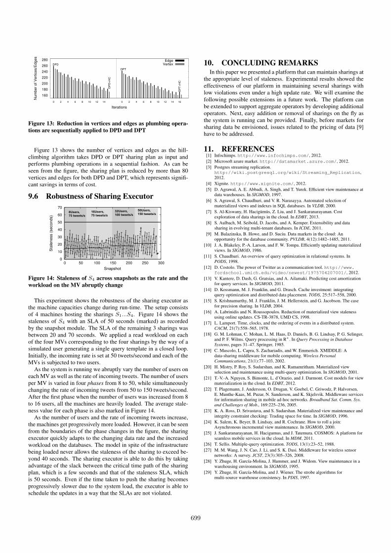
Figure 13 shows the number of vertices and edges as the hill-climbing algorithm takes DPD or DPT sharing plan as input andperforms plumbing operations in a sequential fashion. As can beseen from the figure, the sharing plan is reduced by more than 80vertices and edges for both DPD and DPT, which represents signifi-cant savings in terms of cost.

9.6 Robustness of Sharing Executor

8Users, 75 tweets/s

16Users, 75 tweets/s

32Users, 100 tweets/s

50Users, 150 tweets/s

0

10

20

30

40

50

60

70

0 50 100 150 200 250 300

Sta

len

ess

(se

con

ds)

Snapshot

Figure 14: Staleness of S4 across snapshots as the rate and theworkload on the MV abruptly change

This experiment shows the robustness of the sharing executor asthe machine capacities change during run-time. The setup consistsof 4 machines hosting the sharings S1...S4. Figure 14 shows thestaleness of S4 with an SLA of 50 seconds (marked) as recordedby the snapshot module. The SLA of the remaining 3 sharings wasbetween 20 and 70 seconds. We applied a read workload on eachof the four MVs corresponding to the four sharings by the way of asimulated user generating a single query template in a closed loop.Initially, the incoming rate is set at 50 tweets/second and each of theMVs is subjected to two users.

As the system is running we abruptly vary the number of users oneach MV as well as the rate of incoming tweets. The number of usersper MV is varied in four phases from 8 to 50, while simultaneouslychanging the rate of incoming tweets from 50 to 150 tweets/second.After the first phase when the number of users was increased from 8to 16 users, all the machines are heavily loaded. The average stale-ness value for each phase is also marked in Figure 14.

As the number of users and the rate of incoming tweets increase,the machines get progressively more loaded. However, it can be seenfrom the boundaries of the phase changes in the figure, the sharingexecutor quickly adapts to the changing data rate and the increasedworkload on the databases. The model in spite of the infrastructurebeing loaded never allows the staleness of the sharing to exceed be-yond 40 seconds. The sharing executor is able to do this by takingadvantage of the slack between the critical time path of the sharingplan, which is a few seconds and that of the staleness SLA, whichis 50 seconds. Even if the time taken to push the sharing becomesprogressively slower due to the system load, the executor is able toschedule the updates in a way that the SLAs are not violated.

10. CONCLUDING REMARKSIn this paper we presented a platform that can maintain sharings at

the appropriate level of staleness. Experimental results showed theeffectiveness of our platform in maintaining several sharings withlow violations even under a high update rate. We will examine thefollowing possible extensions in a future work. The platform canbe extended to support aggregate operators by developing additionaloperators. Next, easy addition or removal of sharings on the fly asthe system is running can be provided. Finally, before markets forsharing data be envisioned, issues related to the pricing of data [9]have to be addressed.

11. REFERENCES[1] Infochimps. http://www.infochimps.com/, 2012.[2] Microsoft azure market. http://datamarket.azure.com/, 2012.[3] Postgres streaming replication.

http://wiki.postgresql.org/wiki/Streaming_Replication,2012.

[4] Xignite. http://www.xignite.com/, 2012.[5] D. Agrawal, A. E. Abbadi, A. Singh, and T. Yurek. Efficient view maintenance at

data warehouses. In SIGMOD, 1997.[6] S. Agrawal, S. Chaudhuri, and V. R. Narasayya. Automated selection of

materialized views and indexes in SQL databases. In VLDB, 2000.[7] S. Al-Kiswany, H. Hacigümüs, Z. Liu, and J. Sankaranarayanan. Cost

exploration of data sharings in the cloud. In EDBT, 2013.[8] S. Aulbach, M. Seibold, D. Jacobs, and A. Kemper. Extensibility and data

sharing in evolving multi-tenant databases. In ICDE, 2011.[9] M. Balazinska, B. Howe, and D. Suciu. Data markets in the cloud: An

opportunity for the database community. PVLDB, 4(12):1482–1485, 2011.[10] J. A. Blakeley, P.-A. Larson, and F. W. Tompa. Efficiently updating materialized

views. In SIGMOD, 1986.[11] S. Chaudhuri. An overview of query optimization in relational systems. In

PODS, 1998.[12] D. Costolo. The power of Twitter as a communication tool. http://www.

fordschool.umich.edu/video/newest/1975704207001/, 2012.[13] V. Kantere, D. Dash, G. Gratsias, and A. Ailamaki. Predicting cost amortization

for query services. In SIGMOD, 2011.[14] D. Kossmann, M. J. Franklin, and G. Drasch. Cache investment: integrating

query optimization and distributed data placement. TODS, 25:517–558, 2000.[15] S. Krishnamurthy, M. J. Franklin, J. M. Hellerstein, and G. Jacobson. The case

for precision sharing. In VLDB, 2004.[16] A. Labrinidis and N. Roussopoulos. Reduction of materialized view staleness

using online updates. CS-TR-3878, UMD CS, 1998.[17] L. Lamport. Time, clocks, and the ordering of events in a distributed system.

CACM, 21(7):558–565, 1978.[18] G. M. Lohman, C. Mohan, L. M. Haas, D. Daniels, B. G. Lindsay, P. G. Selinger,

and P. F. Wilms. Query processing in R∗. In Query Processing in DatabaseSystems, pages 31–47. Springer, 1985.

[19] C. Mascolo, L. Capra, S. Zachariadis, and W. Emmerich. XMIDDLE: Adata-sharing middleware for mobile computing. Wireless PersonalCommunications, 21(1):77–103, 2002.

[20] H. Mistry, P. Roy, S. Sudarshan, and K. Ramamritham. Materialized viewselection and maintenance using multi-query optimization. In SIGMOD, 2001.

[21] T.-V.-A. Nguyen, S. Bimonte, L. d’Orazio, and J. Darmont. Cost models for viewmaterialization in the cloud. In EDBT, 2012.

[22] T. Plagemann, J. Andersson, O. Drugan, V. Goebel, C. Griwodz, P. Halvorsen,E. Munthe-Kaas, M. Puzar, N. Sanderson, and K. Skjelsvik. Middleware servicesfor information sharing in mobile ad-hoc networks. Broadband Sat. Comm. Sys.and Challenges of Mob., 169:225–236, 2005.

[23] K. A. Ross, D. Srivastava, and S. Sudarshan. Materialized view maintenance andintegrity constraint checking: Trading space for time. In SIGMOD, 1996.

[24] K. Salem, K. Beyer, B. Lindsay, and R. Cochrane. How to roll a join:Asynchronous incremental view maintenance. In SIGMOD, 2000.

[25] J. Sankaranarayanan, H. Hacigumus, and J. Tatemura. COSMOS: A platform forseamless mobile services in the cloud. In MDM, 2011.

[26] T. Sellis. Multiple-query optimization. TODS, 13(1):23–52, 1988.[27] M. M. Wang, J. N. Cao, J. Li, and S. K. Dasi. Middleware for wireless sensor

networks: A survey. JCST, 23(3):305–326, 2008.[28] Y. Zhuge, H. García-Molina, J. Hammer, and J. Widom. View maintenance in a

warehousing environment. In SIGMOD, 1995.[29] Y. Zhuge, H. García-Molina, and J. Wiener. The strobe algorithms for

multi-source warehouse consistency. In PDIS, 1997.

699