SMIF Notes Part 2 201011

Lecture notes for STAT3006 / STATG017

Stochastic Methods in Finance

Part 2

Julian Herbert

Department of Statistical Science, UCL

2010-2011

Contents

4 Arbitrage and the pricing of forward contracts 29

4.1 Arbitrage . . . . . . . . . . . . . . . . . . . . . . . . . . . . . . . . . . 29

4.2 Example - Arbitrage opportunities in a forward contract . . . . . . . . 30

4.3 Pricing forward contracts for securities that provides no income . . . . 31

4.4 Value of a forward contract . . . . . . . . . . . . . . . . . . . . . . . . 32

5 Pricing Options under the Binomial Model 34

5.1 Modelling the uncertainty of the underlying asset price . . . . . . . . . 34

5.2 A simple example . . . . . . . . . . . . . . . . . . . . . . . . . . . . . . 34

5.2.1 Arbitrage opportunity . . . . . . . . . . . . . . . . . . . . . . . 36

5.2.2 No-arbitrage pricing . . . . . . . . . . . . . . . . . . . . . . . . 37

5.3 One-step binomial tree . . . . . . . . . . . . . . . . . . . . . . . . . . . 38

5.4 A replicating portfolio . . . . . . . . . . . . . . . . . . . . . . . . . . . 39

5.5 Risk-neutral valuation . . . . . . . . . . . . . . . . . . . . . . . . . . . 40

5.6 Appendix: A riskless portfolio . . . . . . . . . . . . . . . . . . . . . . . 41

5.6.1 Example revisited . . . . . . . . . . . . . . . . . . . . . . . . . . 41

5.6.2 No-arbitrage pricing . . . . . . . . . . . . . . . . . . . . . . . . 42

5.6.3 Riskless portfolio - general result . . . . . . . . . . . . . . . . . 43

5.7 Further reading . . . . . . . . . . . . . . . . . . . . . . . . . . . . . . . 44

6 Applications of the Binomial Model 45

6.1 The value of a forward contract . . . . . . . . . . . . . . . . . . . . . . 45

6.1.1 A replicating strategy . . . . . . . . . . . . . . . . . . . . . . . 45

6.1.2 Risk-neutral valuation . . . . . . . . . . . . . . . . . . . . . . . 46

6.2 A European put option . . . . . . . . . . . . . . . . . . . . . . . . . . . 48

6.3 Two-step binomial trees . . . . . . . . . . . . . . . . . . . . . . . . . . 49

6.4 General method for n-step trees . . . . . . . . . . . . . . . . . . . . . . 50

6.5 Pricing of American options . . . . . . . . . . . . . . . . . . . . . . . . 51

i

Chapter 4

Arbitrage and the pricing of

forward contracts

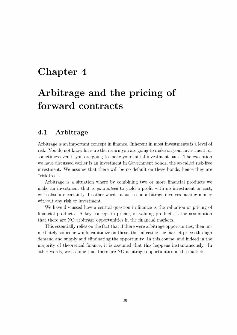
4.1 Arbitrage

Arbitrage is an important concept in finance. Inherent in most investments is a level of

risk. You do not know for sure the return you are going to make on your investment, or

sometimes even if you are going to make your initial investment back. The exception

we have discussed earlier is an investment in Government bonds, the so-called risk-free

investment. We assume that there will be no default on these bonds, hence they are

“risk free”.

Arbitrage is a situation where by combining two or more financial products we

make an investment that is guaranteed to yield a profit with no investment or cost,

with absolute certainty. In other words, a successful arbitrage involves making money

without any risk or investment.

We have discussed how a central question in finance is the valuation or pricing of

financial products. A key concept in pricing or valuing products is the assumption

that there are NO arbitrage opportunities in the financial markets.

This essentially relies on the fact that if there were arbitrage opportunities, then im-

mediately someone would capitalize on these, thus affecting the market prices through

demand and supply and eliminating the opportunity. In this course, and indeed in the

majority of theoretical finance, it is assumed that this happens instantaneously. In

other words, we assume that there are NO arbitrage opportunities in the markets.

29


4.2 Example - Arbitrage opportunities in a forward

contract

Assume that a forward contract on a non-dividend paying stock matures in 3 months.

i.e. the contract involves delivery of the stock in 3 months time. The stock price is

£100 now, the three-month risk-free interest is 12% p.a. Suppose the forward contract

price is £105, i.e. the stock will be delivered for payment of £105 in 3 months time.

Questions to consider:

• Is this the correct price for the forward contract today?

• What do we mean by “correct price?”

• Can I make money without any risk?

Consider the following trading strategy:

• Time 0:

– Borrow £100 at 12%

– Buy a share at £100

– Sell a forward at £105

• 3 months:

– Get £105 for the share

– Pay back £103 (including £3 interest payment at the risk free rate of 12%)

– ⇒ profit £2

This has yielded a riskless profit of £2 with no initial investment. In other words,

an arbitrage opportunity.

What about the case where the forward price is £102? Consider an investor who

has a portfolio with one share of the stock. Can he make money without any risk?

• Time 0:

– Sell the share at £100

– Invest the £100 at 12%

– Buy a forward at £102

• 3 months:

30 J Herbert UCL 2010-11


– Get £103

– Pay £102 for the share

– ⇒ profit £1

This has yielded a riskless profit of £1 with no initial investment, so that an arbitrage

opportunity exists if £102 is the forward price. Clearly neither of the two forward prices

considered, £105 or £102, are sustainable in a market without arbitrage opportunities.

They cannot be the correct price for the forward contract in such a market.

In fact, whenever the forward price in this example is higher or lower that £103

there is an arbitrage opportunity.

What happens in the market? The first strategy is profitable when the forward

price is greater than £103. This will lead to an increased demand for short forward

contracts, and therefore the three-month forward price of the stock will fall. On the

other hand, the second strategy is profitable when the price is smaller than £103,

therefore we will see an increase in the demand for long forward contracts and in turn

an increase in the three-month forward price of the stock. These activities of traders

will cause the three-month forward price to be exactly £103.

Therefore, from now on the basic assumption in derivative pricing is that

there are no arbitrage opportunities in the financial markets

Question: How did we calculate the figure £103 in this example?

4.3 Pricing forward contracts for securities that pro-

vides no income

The principal in the above example can be extended to price forward contracts in

general.

Assumptions: 1) No transaction costs 2) The market participants can borrow or

lend money at the same continously compounded risk-free rate r.

We also further assume that the underlying provide no income. Extensions to the

argument are needed if the underlying provides an income, such as a share yielding

dividends. We do not consider this here.

The example in the previous section indicates that the delivery price of a forward

contract should be the Future Value (FV) of the underlying security price. If S is the

spot price and F is the forward price, then

F = SerT

where T is the time to maturity and r is the corresponding risk-free interest rate. If

F < SerT or F > SerT , then there are arbitrage opportunities. See exercises for a



proof of this.

Example. If the stock price is £40 with no dividends, and the interest rate is 5%,

then a forward contract after 3 months should have delivery price equal to

F = 40e0.05×0.25 = 40.50

This is the correct price so that the initial value of the contract is zero, and the contract

is therefore a fair one.

4.4 Value of a forward contract

As we have seen, the no-arbitrage principle requires that the value of a forward contract

at the time it is first entered into is zero, i.e. the delivery price equals the forward

price. The value of the contract, however, can change afterwards and become positive

or negative, because the “fair” forward price, if recalculated, can change as the price

of the underlying changes over time (while the delivery price of the contract remains

the same).

At any time between the beginning of the contract and the delivery date, the value

f of a long forward contract with delivery price K can be found by considering the

following two portfolios:

• Port. A: One long forward contract + cash Ke−rT

• Port. B: One security

Here T now denotes the remaining time until delivery, and r the associated risk-free

interest rate. We consider only non-wasting securities, which can be kept indefinitely

with no storage costs. Thus the argument is not directly applicable to e.g . commodity

futures.

After time T , Ke−rT will become K and I will use this money to buy one unit of the

security. Therefore at time T the two portfolios have the same value (independent of

the security price), which means that they must have the same value today (otherwise

there is arbitrage).

• The value of portfolio A today is: f +Ke−rT , where f is the value of the forward

contract.

• The value of portfolio B today is S.

Therefore, since the value of the two portfolios is the same we have f +Ke−rT = S,

and so the value of the contract is:

f = S −Ke−rT



This value is zero if and only if K = SerT .

Notice that S = Fe−rT , where F is the current forward price, i.e. the delivery price

that would apply if the contract were entered in today. Therefore, we can rewrite the

above as f = (F − K)e−rT . This equation shows that we can value a long forward

contract on an asset by assuming that the cash value of the asset at the maturity of the

forward contract is the forward price F . In fact, under this assumption, the contract

will give a payoff of F −K, which is worth (F −K)e−rT today.

Example. Let us consider a six-month forward contract on a one-year T-bill with

principal of $1,000. The delivery price is $950, and the six-month interest rate is 6%

(with continuous compounding). The current bond price is $930. Then the value of

the contract is:

f = S −Ke−rT = 930− 950 e−0.06× 612 = 8.08

Example. Consider now a forward contract on a non-dividend paying stock that

matures in six months. The spot price is £1 and the risk-free interest rate is 10%.

Therefore the forward price is F = SerT = 1 · e0.1× 612 = 1.05127, and the value f is

zero.

After three months the spot price is £1.05, and the interest rate remains the same.

What is the value of the contract now? We obtain f = 1.05 − 1.05127e−0.1× 312 =

0.02469.


Chapter 5

Pricing Options under the Binomial

Model

We have seen in the last lecture that there is a fair contract price for forward contracts

that does not allow arbitrage. Any other price will allow arbitrage. We now look at

how we can determine this price in for other more general derivatives.

5.1 Modelling the uncertainty of the underlying as-

set price

In order to model the value of a variable that changes over time we will develop models

based on stochastic processes.

We can use discrete time, where the variable changes only at certain fixed points

in time, or we can use continuous time, where the variable changes at any time.

Also, the variable can be continuous (can take any value within a range), or it can

be discrete (takes only certain values).

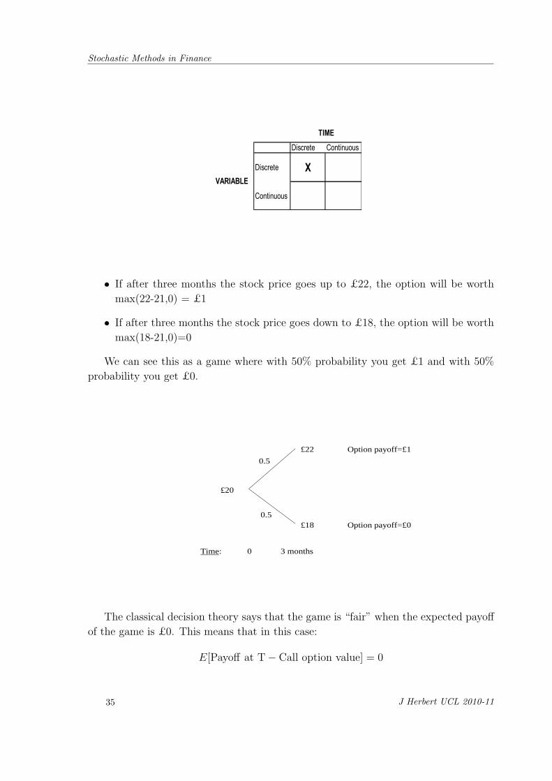
We will start now with discrete time and discrete variables.

In order to introduce the basic logic behind option pricing we start from an ex-

tremely simple model, the one-step binomial tree.

5.2 A simple example

Assume that the price of a stock is currently £20, and after three months it will, with

equal probabilities, either be £22 or £18 (discrete time, discrete variable). We want

to find the value of a European call option with strike price £21.

The payoff of the call option will be as follows:

34


Discrete Continuous

Discrete X

Continuous

TIME

VARIABLE

• If after three months the stock price goes up to £22, the option will be worth

max(22-21,0) = £1

• If after three months the stock price goes down to £18, the option will be worth

max(18-21,0)=0

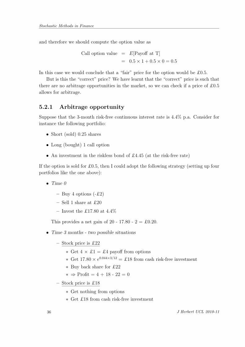
We can see this as a game where with 50% probability you get £1 and with 50%

probability you get £0.

0.5

0.5

Time: 0 3 months

£18

£22 Option payoff=£1

Option payoff=£0

£20

The classical decision theory says that the game is “fair” when the expected payoff

of the game is £0. This means that in this case:

E[Payoff at T− Call option value] = 0



and therefore we should compute the option value as

Call option value = E[Payoff at T]

= 0.5× 1 + 0.5× 0 = 0.5

In this case we would conclude that a “fair” price for the option would be £0.5.

But is this the “correct” price? We have learnt that the “correct” price is such that

there are no arbitrage opportunities in the market, so we can check if a price of £0.5

allows for arbitrage.

5.2.1 Arbitrage opportunity

Suppose that the 3-month risk-free continuous interest rate is 4.4% p.a. Consider for

instance the following portfolio:

• Short (sold) 0.25 shares

• Long (bought) 1 call option

• An investment in the riskless bond of £4.45 (at the risk-free rate)

If the option is sold for £0.5, then I could adopt the following strategy (setting up four

portfolios like the one above):

• Time 0

– Buy 4 options (-£2)

– Sell 1 share at £20

– Invest the £17.80 at 4.4%

This provides a net gain of 20 - 17.80 - 2 = £0.20.

• Time 3 months - two possible situations

– Stock price is £22

∗ Get 4 × £1 = £4 payoff from options

∗ Get 17.80× e0.044×3/12 = £18 from cash risk-free investment

∗ Buy back share for £22

∗ ⇒ Profit = 4 + 18 - 22 = 0


∗ Get nothing from options

∗ Get £18 from cash risk-free investment




∗ ⇒ Profit = 18 - 18 = 0

Notice that, regardless of what happens in the future (whether the stock goes up

or down), my position after 3 months is neutral, and I cannot lose any money.

The initial profit of £0.20 at time zero means that regardless of the stock price

in the future, I can make this profit of £0.20 today, with no chance of a loss

in the future. This is an arbitrage opportunity. Hence we conclude that £0.50

cannot be the “correct” price for the option.

5.2.2 No-arbitrage pricing

So how can we obtain a price for the option such that no arbitrage opportunities can

arise? Let us consider again the riskless and share assets in the portfolio we just

introduced, but taking the reverse positions (i.e. long the stock and short the riskless

asset); the value of the risk-free investment combined with the stock position, after

three months, will be:

• If the stock price goes up to £22: 0.25× 22− 4.45e0.044×3/12 = 1

• If the stock price goes down to £18: 0.25× 18− 4.45e0.044×3/12 = 0

Compare this with the payoff of the option in each case. We can see that the value of the

portfolio always equals the value of the call option: it is therefore called a replicating

portfolio - it replicates the value of the option in all future states of the world (which

in the case of the binomial model, is the the two possible stock movements, up and

down). In order to avoid arbitrage, the value of this portfolio must equal the value of

the derivative at all times (prove this to yourself).

The value of this portfolio at time zero is

PV = −4.45 + 20 · 0.25 = 0.55

and so the no-arbitrage price for the option at time zero must also be £0.55.

Note that, unlike the earlier argument, this approach does not depend on the

probabilities of the different possible outcomes; instead it depends on the risk-free

interest rate.

We have found that if we can find a replicating strategy for a derivative, we are

then able to price it. However the replicating portfolio we set up was no co-incidence.

The amounts of stock and riskless bond were deliberately chosen to make the portfolio

replicating. We now turn to the question of how we can determine what the amounts

should be for a general derivative pricing problem.



5.3 One-step binomial tree

To look now at a general framework for the pricing of options we need to introduce

some notation.

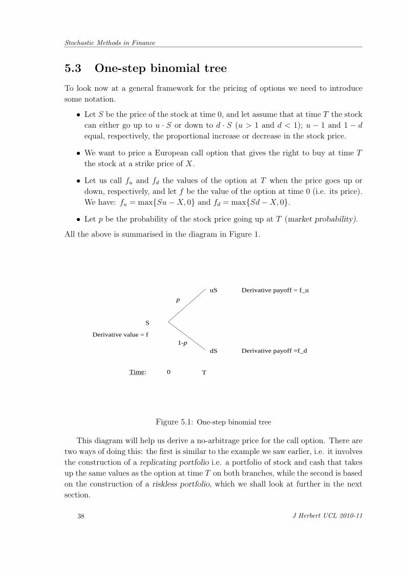
• Let S be the price of the stock at time 0, and let assume that at time T the stock

can either go up to u · S or down to d · S (u > 1 and d < 1); u − 1 and 1 − d

equal, respectively, the proportional increase or decrease in the stock price.

• We want to price a European call option that gives the right to buy at time T

the stock at a strike price of X.

• Let us call fu and fd the values of the option at T when the price goes up or

down, respectively, and let f be the value of the option at time 0 (i.e. its price).

We have: fu = max{Su−X, 0} and fd = max{Sd−X, 0}.

• Let p be the probability of the stock price going up at T (market probability).

All the above is summarised in the diagram in Figure 1.

1-p

p

Time: 0 T

dS

uS Derivative payoff = f_u

Derivative payoff =f_d

S

Derivative value = f

Figure 5.1: One-step binomial tree

This diagram will help us derive a no-arbitrage price for the call option. There are

two ways of doing this: the first is similar to the example we saw earlier, i.e. it involves

the construction of a replicating portfolio i.e. a portfolio of stock and cash that takes

up the same values as the option at time T on both branches, while the second is based

on the construction of a riskless portfolio, which we shall look at further in the next

section.



5.4 A replicating portfolio

Let us consider a portfolio of x worth of riskless zero-coupon bonds and y stocks.

A replicating portfolio has the property that its value tracks the target value (in

this case the derivative value) exactly over time. It is constructed to have the same

terminal value as the derivative. By no-arbitrage, it therefore has the same value as

the derivative at all times prior to maturity, including time 0.

According to our notation, f is the value of the option at time 0, while fu and fdare the option values at T if the stock price has gone up or down, respectively (see the

diagram above). How can we construct our replicating portfolio? Let us look at the

value of the portfolio:

• At 0: Π0 = x+ yS

• At T:

ΠT =

{Πu = xerT + ySu ifST = Su

Πd = xerT + ySd ifST = Sd

For the portfolio to be replicating, we must have Πu = fu and Πd = fd, i.e. choose x

and y such that

xerT + ySu = fu

xerT + ySd = fd

The solution is given by

x =ufd − dfuu− d

e−rT y =fu − fdSu− Sd

With this choice, the portfolio has the same value at T as the option. By no-arbitrage,

the values at time zero must be the same, and we obtain:

f = x+ yS =ufd − dfuu− d

e−rT +fu − fdSu− Sd

S

as the price of the derivative today. This can be rearranged as follows:

f = e−rT

{erT − d

u− dfu +

u− erT

u− dfd

}= e−rT {pfu + (1− p)fd}

where we have written

p :=erT − d

u− d

Notice that d < erT < u, otherwise there would be arbitrage opportunities, and

therefore p is a probability, since the above implies 0 < p < 1.



5.5 Risk-neutral valuation

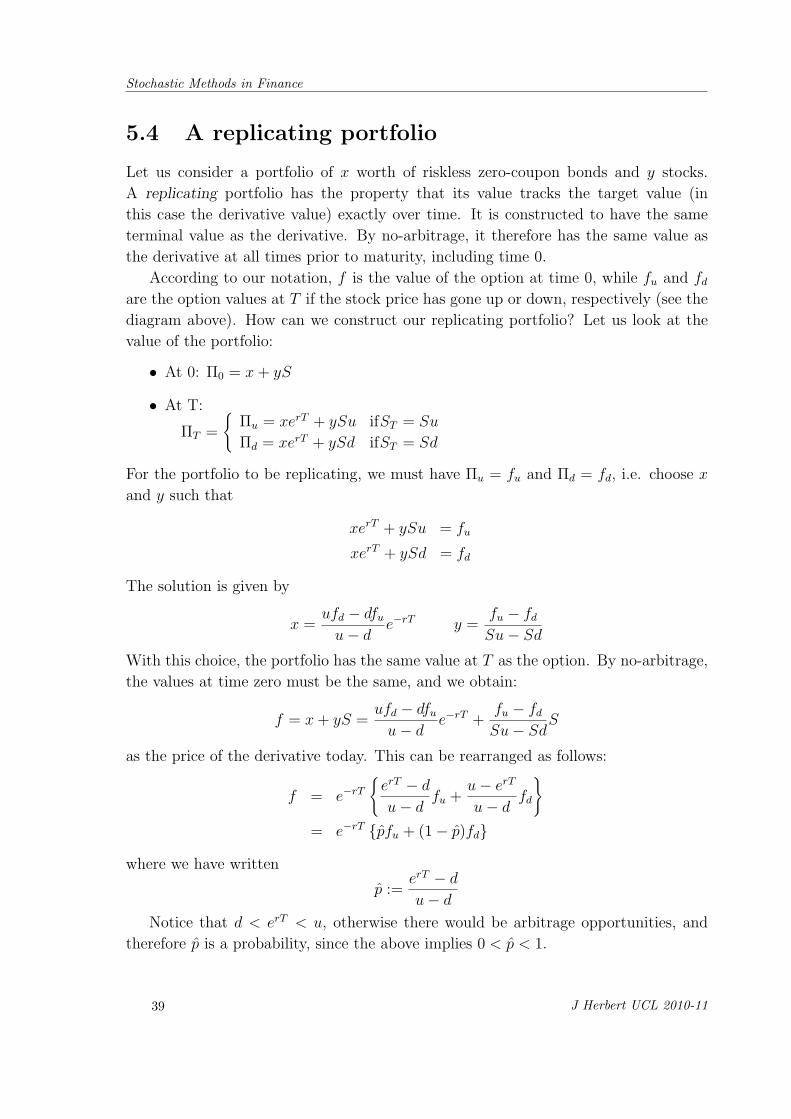
Notice that the formula for f has a very nice interpretation: if we consider the following

diagram:

1-p^

p^

Time: 0 T

dS

uS Derivative payoff = f_u

Derivative payoff =f_d

S


we see that f = e−rT E[fT ], where

fT =

{fu ifST = Su

fd ifST = Sd

and E denotes the expectation with respect to p, i.e. E[fT ] = pfu+(1−p)fd. Therefore

f is the discounted, expected payoff under the probability p, which does not depend

on the market probability p.

What is the interpretation of p? If we calculate the expected stock price at time T

with respect to this probability we obtain

E[ST ] = pSu+ (1− p)Sd

= pS(u− d) + Sd

=erT − d

u− d· S(u− d) + Sd = erTS

Therefore

E[ST ] = erTS

which is the forward price.

In a risk-neutral world, all individuals are indifferent to risk and require no com-

pensation for risk, and the expected return on all securities is the same (the risk-free

rate). The result above implies that setting the probability of the stock price going



up to Su equal to p is equivalent to assuming that the return on the stock equals the

risk-free rate. Therefore, p is the probability of an “up”-step in a risk-neutral world,

and the option value is the discounted expected payoff in that risk-neutral world. This

method of deriving option value is called risk-neutral valuation.

Example. Let us apply this to our numerical example: as before, r = 0.044, S = 20,

u = 1.1, d = 0.9 and T = 0.25. We computed earlier p = 0.5553.

The expected payoff form the option is then 0.5553× 1+ 0.4447× 0 = 0.5553, and

if we discount back to time 0 we obtain the call option value: 0.5553e−0.044×0.25 = 0.55

as before.

Risk-neutral valuation is also related to what is sometimes called the change in

measure approach to option valuation. This refers to the fact that a probability is a

measure. When we use p to calculate our discounted expected payoffs rather than the

actual market probabilities p, we are “changing the probability measure”.

We will explore this technique further in a continuous time framework later in the

course.

5.6 Appendix: A riskless portfolio

5.6.1 Example revisited

Consider again the example outlined in section 5.2 above.

We will now look at the pricing problem in a slightly different way. Consider the

following portfolio:

• Long (bought) 0.25 shares

• Short (sold) 1 call option

If the option is sold for £0.5 (which we already know is a price that offers arbitrage

opportunities), then I could adopt the following strategy (selling four portfolios like

the one above):

• Time 0

– Buy 4 options (-£2)

– Sell 1 share at £20

– Invest the £18 at 4.4%



• Time 3 months Note that this time this portfolio costs nothing to set up and

gains nothing. After three months:


∗ Get £4 from options

∗ Get £18.20 from investment


∗ ⇒ Profit = 4 + 18.20 - 22 = 0.20


∗ Get nothing from options

∗ Get £18.5482 from investment


∗ ⇒ Profit = 18.20 - 18 =0.20

Regardless of the stock price I make a profit of £0.20 - so we have again shown

(using a slightly different approach) that a price of £0.50 for the option allows

an arbitrage opportunity.

Notice that this differs from the replicating portfolio approach in that it costs

nothing to set up, but guarantees a profit in the future, The replicating portfolio

made a profit at set-up at time 0, but was guaranteed to produce a neutral

position in the future.

5.6.2 No-arbitrage pricing

As with the replicating approach above, we can use this construction to find a price

for the option such that no arbitrage opportunities can arise. Let us consider again

the portfolio we just introduced; its value after three months will be:

• If the stock price is £22: 0.25× 22− 1 = 4.5

• If the stock price is £18: 0.25× 18− 0 = 4.5

We can see that the value of the portfolio does not change with the value of the stock:

it is therefore called a riskless portfolio. In order to avoid arbitrage, its value at time 0

should be simply the present value of £4.5 computed using the risk-free discount rate

(4.4%), since it is a riskless portfolio. Hence:

PV = 4.5 · e−0.044× 312 = 4.45



We know that the value of the portfolio at time 0 is 0.25 times the value of the share at

time 0 minus the value of the call option f (I am in a short position), and this equals

the PV above. Therefore:

0.25× 20− f = 4.45

and so we obtain:

f = 5− 4.45 = 0.55

the no-arbitrage price for the option is £0.55 as we found previously. We know need

to look at how to establish a riskless portfolio in a general derivative pricing situation.

5.6.3 Riskless portfolio - general result

Consider the notation introduced in section 5.3. In order to construct a riskless port-

folio we can start with ∆ shares long and 1 call option short. We will then find what

∆ needs to be. The value of this portfolio is as follows:

• At 0: Π0 = ∆S − f

• At T:

ΠT =

{∆Su− fu ifST = Su

∆Sd− fd ifST = Sd

The portfolio is riskless iff the value at T is independent of the price of the stock, i.e.

iff ∆Su− fu = ∆Sd− fd, which gives:

∆ =fu − fdSu− Sd

With this ∆ the portfolio is riskless and its value at T equals ∆Su− fu.

In order to avoid arbitrage, the value of the portfolio at time 0 must equal the value

at T discounted at the risk-free rate r:

Π0 = ΠT e−rT

This is equivalent to:

∆S − f = [∆Su− fu]e−rT

which gives the following expression for the value of the option at time 0:

f = e−rT [pfu + (1− p)fd]

where

p =erT − d

u− d

(Check!)

This is exactly the same result as before under the replicating portfolio pricing

approach.



5.7 Further reading

Martin Baxter & Andrew Rennie, Financial Calculus. – Chapter 1 and 2

Marek Capinski & Tomasz Zastawniak, Mathematics for Finance: An Introduction to

Financial Engineering (Springer) – Chapter 1, 8.1-8.2.

John C. Hull, Options Futures and Other Derivative Securities – Section 9.1 (in the

5th edition)


Chapter 6

Applications of the Binomial Model

We are going to look now at some applications of the binomial model for the pricing of

derivatives. We will show that the model can be used not only for option pricing, but

also for other derivatives, giving the example of a forward contract. We then examine

the case of a European put option.

We will then move on to the application of the binomial model for the evaluation of

two-step and three-step trees, and look at the pricing of American options, addressing

the issue of optimal early exercise.

6.1 The value of a forward contract

The binomial model can be used to compute the value of any derivative (not only

options), provided that we can express its features using a binomial tree. In this

section we look at an example considering a forward contract, but a similar analysis

can be undertaken for other derivatives.

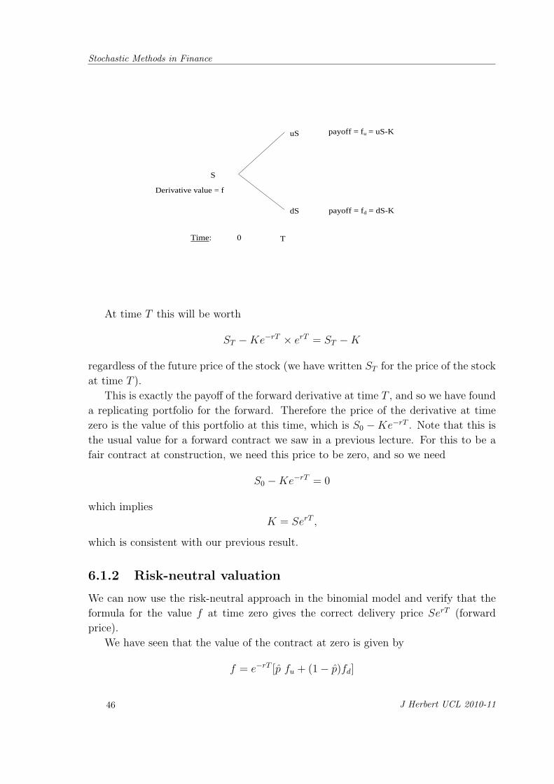
A forward contract with delivery price K is pictured in the diagram, and can be

thought of as the payoff fT given by

fT =

{fu = Su−K

fd = Sd−K

6.1.1 A replicating strategy

We can now determine the no-arbitrage price for the forward in the binomial model

by replicating the forward contract using an amount of stock and an amount of the

riskless investment (investment in risk-free bonds). Consider the portfolio that consists

of long one unit of stock, and short Ke−rT units of the riskless investment (i.e. you

have sold the riskless, zero-coupon government bonds to “borrow” money, and so will

have to pay the risk-free rate of interest).

45


Time: 0 T

dS

uS

payoff = fd = dS-K

S

payoff = fu = uS-K


At time T this will be worth

ST −Ke−rT × erT = ST −K

regardless of the future price of the stock (we have written ST for the price of the stock

at time T ).

This is exactly the payoff of the forward derivative at time T , and so we have found

a replicating portfolio for the forward. Therefore the price of the derivative at time

zero is the value of this portfolio at this time, which is S0 −Ke−rT . Note that this is

the usual value for a forward contract we saw in a previous lecture. For this to be a

fair contract at construction, we need this price to be zero, and so we need

S0 −Ke−rT = 0

which implies

K = SerT ,

which is consistent with our previous result.

6.1.2 Risk-neutral valuation

We can now use the risk-neutral approach in the binomial model and verify that the

formula for the value f at time zero gives the correct delivery price SerT (forward

price).

We have seen that the value of the contract at zero is given by

f = e−rT [p fu + (1− p)fd]



This, in our case, gives the following expression once we substitute in the appropriate

values for fu and fd:

f = e−rT [p (Su−K) + (1− p)(Sd−K)]

which simplifies to

f = e−rT [p Su+ (1− p)Sd−K]

Replace now the formula for the risk-neutral probability p

p =erT − d

u− d

and obtain

f = e−rT

[erT − d

u− d× Su+

u− erT

u− d× Sd−K

]

= e−rT

[erTSu− Sud+ Sud− erTSd

u− d−K

]

= e−rT

[erTS(u− d)

u− d−K

]= S −Ke−rT

Again this is the usual value for a forward contract, and therefore we see that the

binomial model gives consistent results also for other derivatives (not only options).

Once again, we see that the only delivery price which gives zero initial value to the

forward contract is K = SerT .



6.2 A European put option

We consider again the example presented in the last lecture, but this time we look at

a put option. Once computed the price of the put option, we will compare it with

the call price obtained previously, and check whether a result called put-call parity is

satisfied.

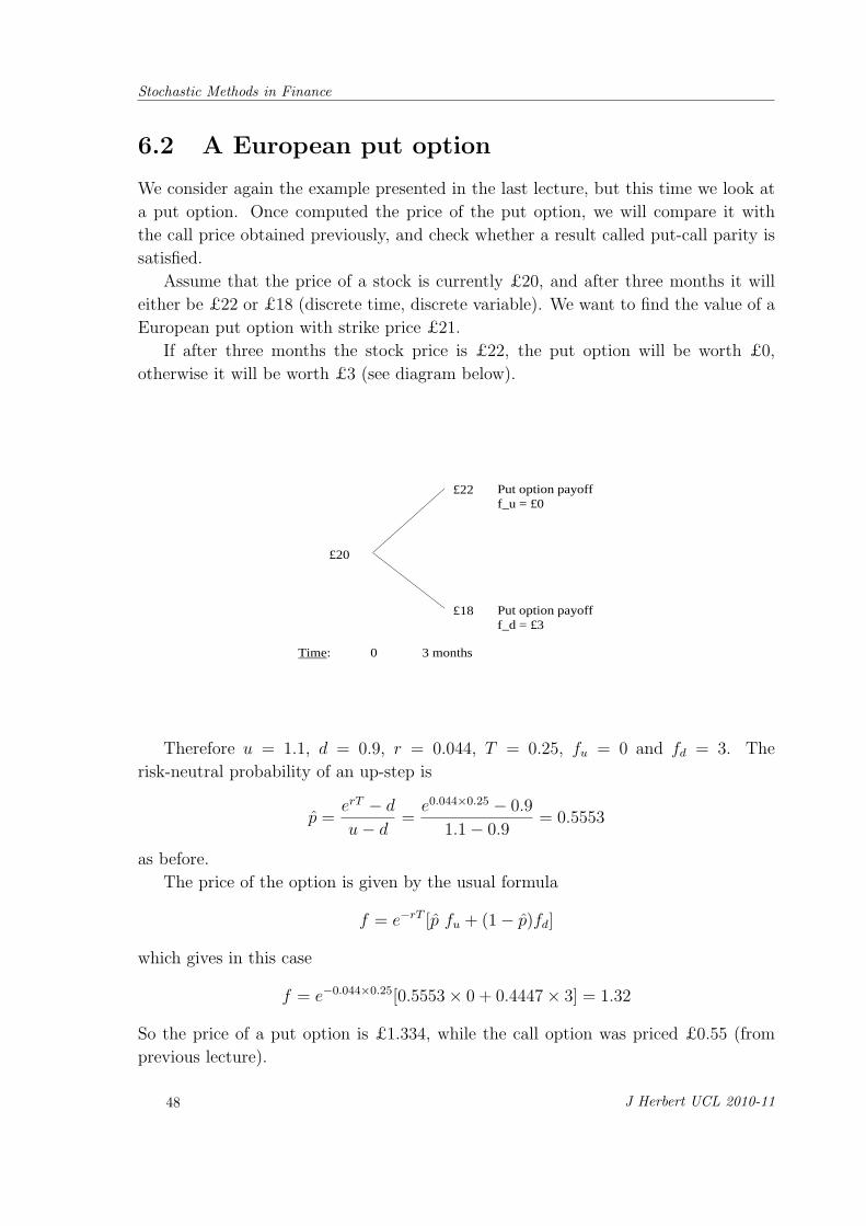
Assume that the price of a stock is currently £20, and after three months it will

either be £22 or £18 (discrete time, discrete variable). We want to find the value of a

European put option with strike price £21.

If after three months the stock price is £22, the put option will be worth £0,

otherwise it will be worth £3 (see diagram below).

Time: 0 3 months

£18

£22 Put option payoff f_u = £0

Put option payoff f_d = £3

£20

Therefore u = 1.1, d = 0.9, r = 0.044, T = 0.25, fu = 0 and fd = 3. The

risk-neutral probability of an up-step is

p =erT − d

u− d=

e0.044×0.25 − 0.9

1.1− 0.9= 0.5553

as before.

The price of the option is given by the usual formula

f = e−rT [p fu + (1− p)fd]

which gives in this case

f = e−0.044×0.25[0.5553× 0 + 0.4447× 3] = 1.32

So the price of a put option is £1.334, while the call option was priced £0.55 (from

previous lecture).



We can know look at the put-call parity relationship for the price of put and call

options, given by the following:

Call− Put = S −Ke−rT

with the usual notation (K is the strike price). In our case, S = 20, K = 21 and r and

T are the same as above. It follows that

S −Ke−rT = 20− 21e−0.044×0.25 = −0.77

This equals the difference between the call and put price that we found, since 0.55−1.32 = −0.77, and therefore the put-call parity result is satisfied.

6.3 Two-step binomial trees

We can now extend the discussion to two-step binomial trees where the asset price will

change twice before maturity.

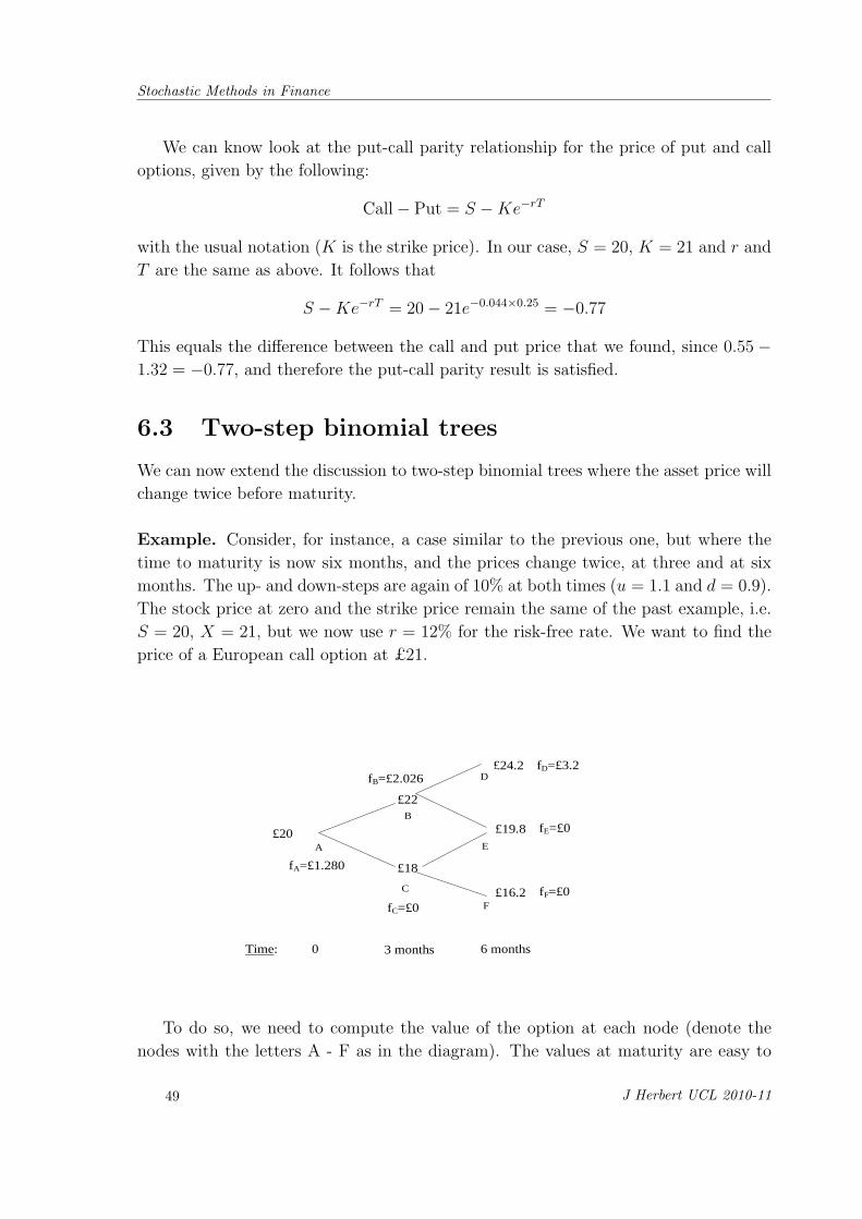
Example. Consider, for instance, a case similar to the previous one, but where the

time to maturity is now six months, and the prices change twice, at three and at six

months. The up- and down-steps are again of 10% at both times (u = 1.1 and d = 0.9).

The stock price at zero and the strike price remain the same of the past example, i.e.

S = 20, X = 21, but we now use r = 12% for the risk-free rate. We want to find the

price of a European call option at £21.

C

A

fC=£0

fB=£2.026 fD=£3.2

£20

£18

£22

£24.2

£19.8

£16.2

B

D

E

F

fE=£0

fF=£0

fA=£1.280

3 months 6 months 0 Time:

To do so, we need to compute the value of the option at each node (denote the

nodes with the letters A - F as in the diagram). The values at maturity are easy to



compute at each of the final nodes. To obtain the values at three months we need

to compute the risk-neutral probability p and then apply the one-step formula. From

there we can then obtain the initial value applying again the one-step formula with

the three-months values just obtained. Notice that the risk-neutral probability is the

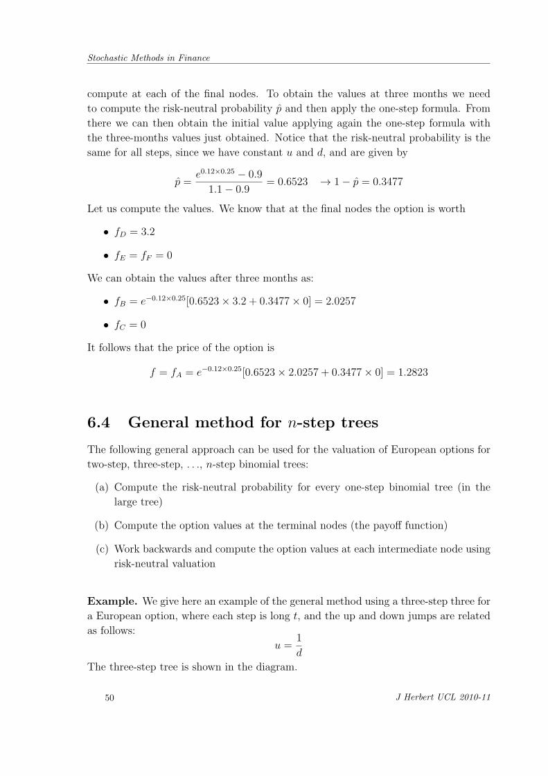
same for all steps, since we have constant u and d, and are given by

p =e0.12×0.25 − 0.9

1.1− 0.9= 0.6523 → 1− p = 0.3477

Let us compute the values. We know that at the final nodes the option is worth

• fD = 3.2

• fE = fF = 0

We can obtain the values after three months as:

• fB = e−0.12×0.25[0.6523× 3.2 + 0.3477× 0] = 2.0257

• fC = 0

It follows that the price of the option is

f = fA = e−0.12×0.25[0.6523× 2.0257 + 0.3477× 0] = 1.2823

6.4 General method for n-step trees

The following general approach can be used for the valuation of European options for

two-step, three-step, . . ., n-step binomial trees:

(a) Compute the risk-neutral probability for every one-step binomial tree (in the

large tree)

(b) Compute the option values at the terminal nodes (the payoff function)

(c) Work backwards and compute the option values at each intermediate node using

risk-neutral valuation

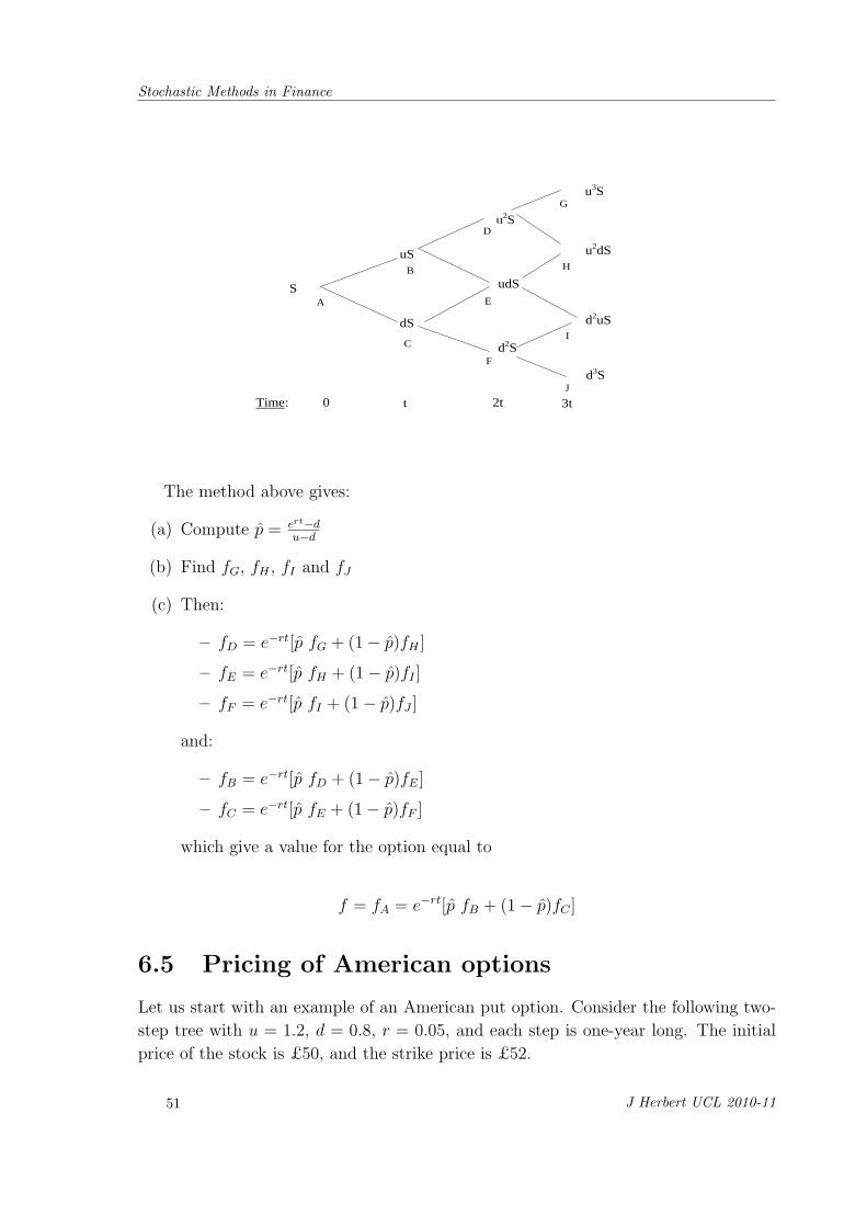
Example. We give here an example of the general method using a three-step three for

a European option, where each step is long t, and the up and down jumps are related

as follows:

u =1

d

The three-step tree is shown in the diagram.



C

A S

dS

uS

u2S

udS

d2S

B

D

E

F

t 2t 0 Time:

G

H

I

J

u3S

u2dS

d2uS

d3S

3t

The method above gives:

(a) Compute p = ert−du−d

(b) Find fG, fH , fI and fJ

(c) Then:

– fD = e−rt[p fG + (1− p)fH ]

– fE = e−rt[p fH + (1− p)fI ]

– fF = e−rt[p fI + (1− p)fJ ]

and:

– fB = e−rt[p fD + (1− p)fE]

– fC = e−rt[p fE + (1− p)fF ]

which give a value for the option equal to

f = fA = e−rt[p fB + (1− p)fC ]

6.5 Pricing of American options

Let us start with an example of an American put option. Consider the following two-

step tree with u = 1.2, d = 0.8, r = 0.05, and each step is one-year long. The initial

price of the stock is £50, and the strike price is £52.



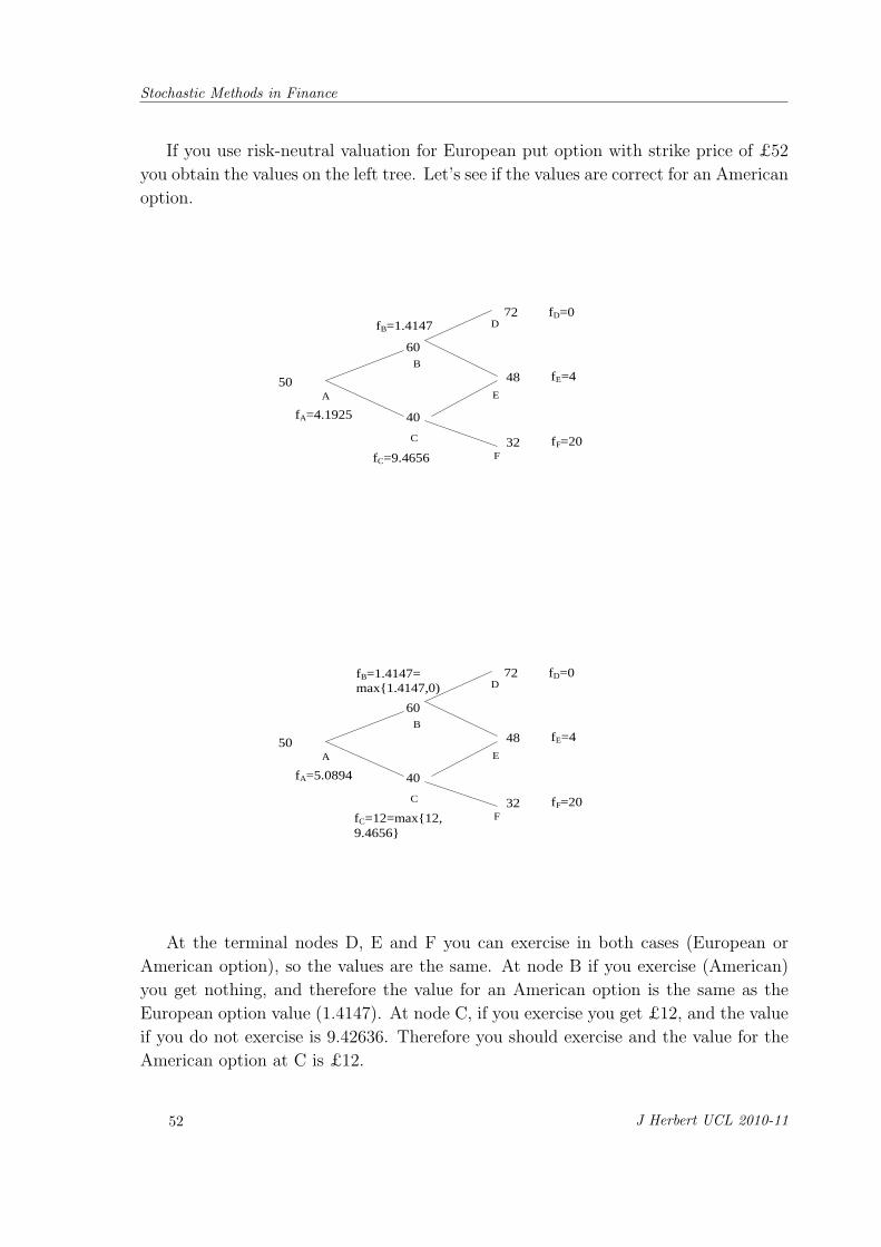
If you use risk-neutral valuation for European put option with strike price of £52

you obtain the values on the left tree. Let’s see if the values are correct for an American

option.

C

A

fC=9.4656

fB=1.4147 fD=0

50

40

60

72

48

32

B

D

E

F

fE=4

fF=20

fA=4.1925

C

A

fC=12=max{12,9.4656}

fB=1.4147= max{1.4147,0)

fD=0

50

40

60

72

48

32

B

D

E

F

fE=4

fF=20

fA=5.0894

At the terminal nodes D, E and F you can exercise in both cases (European or

American option), so the values are the same. At node B if you exercise (American)

you get nothing, and therefore the value for an American option is the same as the

European option value (1.4147). At node C, if you exercise you get £12, and the value

if you do not exercise is 9.42636. Therefore you should exercise and the value for the

American option at C is £12.



Now in order to find the value at A you use risk-neutral valuation

f = fA = e−0.05×1[p 1.4147 + (1− p)12] = 5.0894

So the general valuation method for an American option is

(a) Compute the risk-neutral probability for every one-step binomial tree (in the

large tree)

(b) Compute the option values at the terminal nodes using the payoff function

(c) Work backwards and compute the option values at each intermediate node us-

ing risk-neutral valuation. Test if early exercise at each node is optimal. If it

is, replace the value from the risk-neutral valuation with the payoff from early

exercise.

(d) Continue with the nodes one step earlier


Documents

SMIF Notes Part 2 201011