Embed Size (px)
Citation preview

HAL Id: hal-03100989https://hal.archives-ouvertes.fr/hal-03100989
Submitted on 6 Jan 2021
HAL is a multi-disciplinary open accessarchive for the deposit and dissemination of sci-entific research documents, whether they are pub-lished or not. The documents may come fromteaching and research institutions in France orabroad, or from public or private research centers.
L’archive ouverte pluridisciplinaire HAL, estdestinée au dépôt et à la diffusion de documentsscientifiques de niveau recherche, publiés ou non,émanant des établissements d’enseignement et derecherche français ou étrangers, des laboratoirespublics ou privés.
Smart Responsive Polymers: Fundamentals and DesignPrinciples
Debashish Mukherji, Carlos Marques, Kurt Kremer
To cite this version:Debashish Mukherji, Carlos Marques, Kurt Kremer. Smart Responsive Polymers: Fundamentalsand Design Principles. Annual Review of Condensed Matter Physics, Annual Reviews 2020, 11 (1),pp.271-299. �10.1146/annurev-conmatphys-031119-050618�. �hal-03100989�

Smart responsive polymers:
Fundamentals and design
principles
Debashish Mukherji,1,2 Carlos M. Marques,3
and Kurt Kremer2
1Stewart Blusson Quantum Matter Institute, University of British Columbia,
Vancouver BC V6T 1Z4, Canada:
[email protected];[email protected] Institut fur Polymerforschung, Ackermannweg 10, 55128 Mainz
Germany: [email protected] Charles Sadron, Universite de Strasbourg, CNRS, Strasbourg, France:
Xxxx. Xxx. Xxx. Xxx. YYYY. AA:1–29
https://doi.org/10.1146/((please add
article doi))
Copyright c© YYYY by Annual Reviews.
All rights reserved
Keywords
Soft matter, Smart polymers, Multi-responsive systems, Solvation
thermodynamics
Abstract
In this review we summarize recent theoretical and computational de-
velopments in the field of smart responsive materials, together with
complementary experimental data. A material is referred to as smart
responsive when a slight change in external stimulus can drastically
alter its structure, function, or stability. Because of this smart respon-
siveness, these systems are used for the design of advanced functional
materials. The most characteristic properties of smart polymers will
be discussed, especially polymer properties in solvent mixtures. We
will show how a multi-scale simulation approach can shed light on the
intriguing experimental observations. Special emphasis will be given to
two symmetric phenomena: co-non-solvency and co-solvency. The first
phenomenon is associated with the collapse of polymers in two miscible
good solvents, while the later is associated with the swelling of polymers
in poor solvent mixtures. Furthermore, we will discuss when the stan-
dard Flory-Huggins type mean-field polymer theory can (or can not) be
applied to understand these complex solution properties. We will also
point towards future directions− how smart polymer properties can be
used for the design principles of advanced functional materials.
1

Contents
1. INTRODUCTION .. . . . . . . . . . . . . . . . . . . . . . . . . . . . . . . . . . . . . . . . . . . . . . . . . . . . . . . . . . . . . . . . . . . . . . . . . . . . . . . . . . . . . . . . . . . 2
2. THERMORESPONSIVE SMART POLYMERS . . . . . . . . . . . . . . . . . . . . . . . . . . . . . . . . . . . . . . . . . . . . . . . . . . . . . . . . . . . . . 3
2.1. Effect of copolymer sequence . . . . . . . . . . . . . . . . . . . . . . . . . . . . . . . . . . . . . . . . . . . . . . . . . . . . . . . . . . . . . . . . . . . . . . . . . . . 4
3. CO-NON-SOLVENCY: POLYMER COLLAPSE IN MISCIBLE GOOD SOLVENTS . . . . . . . . . . . . . . . . . . . . . . . 8
3.1. Multiscale simulations complex mixtures and polymer in mixed solvents. . . . . . . . . . . . . . . . . . . . . . . . . . . . . . 10
3.2. Analytical theory . . . . . . . . . . . . . . . . . . . . . . . . . . . . . . . . . . . . . . . . . . . . . . . . . . . . . . . . . . . . . . . . . . . . . . . . . . . . . . . . . . . . . . . . 13
3.3. UCST-like swelling of LCST polymer . . . . . . . . . . . . . . . . . . . . . . . . . . . . . . . . . . . . . . . . . . . . . . . . . . . . . . . . . . . . . . . . . . . 19
4. CO-SOLVENCY: POLYMER SWELLING IN MISCIBLE POOR SOLVENTS . . . . . . . . . . . . . . . . . . . . . . . . . . . . . . 20
4.1. Flory-Huggins mean-field theory . . . . . . . . . . . . . . . . . . . . . . . . . . . . . . . . . . . . . . . . . . . . . . . . . . . . . . . . . . . . . . . . . . . . . . . . 22
5. SMART POLYMERS FOR MATERIALS DESIGN . . . . . . . . . . . . . . . . . . . . . . . . . . . . . . . . . . . . . . . . . . . . . . . . . . . . . . . . . . 23
5.1. Design of multi-responsive copolymer architectures . . . . . . . . . . . . . . . . . . . . . . . . . . . . . . . . . . . . . . . . . . . . . . . . . . . . 23
5.2. Polymers with improved thermal properties . . . . . . . . . . . . . . . . . . . . . . . . . . . . . . . . . . . . . . . . . . . . . . . . . . . . . . . . . . . . 24
6. SUMMARY.. . . . . . . . . . . . . . . . . . . . . . . . . . . . . . . . . . . . . . . . . . . . . . . . . . . . . . . . . . . . . . . . . . . . . . . . . . . . . . . . . . . . . . . . . . . . . . . . . . 25
1. INTRODUCTION
Soft, smart and small are three keywords that are essential in designing multi-responsive
materials for advanced functional applications (1, 2, 3, 4, 5, 6). A material is referred to as
smart responsive when a slight change in external stimulus can drastically alter its structure,
function or stability. These stimuli can be temperature (7, 8, 9, 10, 11, 12, 13, 14), ionic
strength (13, 15, 16, 17), cosolvent composition (18, 19, 20, 21, 22, 23, 24, 25, 26, 27, 28,
29, 30, 31, 32, 33, 34, 35, 36, 37), light (37, 38, 39, 40, 41, 42, 43), and mechanical stress
(44, 45, 46), to name a few. Furthermore, when relevant energy scale in systems is of the
order of the thermal energy kBT , the materials are classified as soft matter and thus are
dictated by large conformational and compositional fluctuations. Because of this strong
fluctuations, entropy (generic physical concepts and scaling laws) becomes as important as
energy (molecular level chemical details). Therefore, establishing a delicate balance between
entropy and energy is at the heart of understanding soft matter properties.
Polymers are one class of soft materials that are of high importance as they provide suit-
able platform to tune materials properties, while still having rather simple materials pro-
cessing. For example, establishing the microscopic understanding of the solvation behavior
of smart polymeric materials, such as hydrogels, microgels, and/or composite networks in
single or multi-component solvents, are of tremendous technological interests. This ranges
from organic semiconductors (47), photonic band gap materials (48, 49, 50, 51), self healing
networks (52, 53, 54), tuning of thermal conductivity of thermoplastic materials (55, 56),
and bio-medical applications (57, 58, 59, 60, 61, 62, 63), to name a few.
In this review, we highlight recent developments in the field of smart responsive polymers
and their connections to the design of smart materials. We will discuss recent experimental
findings and show how complementary molecular simulation data, together with theoretical
arguments, can shed light to better understand smart polymer behavior in aqueous and
aqueous-cosolvent mixtures. In this context, it is important to note that polymer properties
are inherently multi-scale in nature, where delicate local interaction details play a key role in
describing the large scale conformational properties. We will, therefore, emphasize the need
of the multi-scale modeling to arrive at a comprehensive view of the existing experimental
findings. We will also discuss open questions in this field.
2 Mukherji et al.

2. THERMORESPONSIVE SMART POLYMERS
Most commonly known smart polymers are those that swiftly change their conformation
upon varying temperature T , thus also known as thermoresponsive smart polymers. Here,
T responsiveness can either be classified as lower critical solution (LCST) or upper critical
solution (UCST) behavior. In the case of LCST, monomer-solvent interactions confer an
expanded polymer structure at low T values. When T is increased above a certain crit-
ical value Tc, monomer-solvent interaction becomes significantly weaker and thus solvent
molecules get expelled from near the polymer backbone. In this process, the energy-entropy
balance is such that the translational entropy of the released solvent molecules wins, i.e.,
solvent translational entropy becomes larger than the polymer conformational entropy loss
upon collapse. Therefore, a chain collapses in solution. Because a chain collapses upon
increasing T , LCST transition is an entropy driven process as already proposed by Flory
(64, 65, 66). In this case, Tc is refereed to as Tℓ, the lower critical solution temperature
of a polymer in a particular solvent. For microgels, Tc = TVPTT with TVPTT is referred to
as volume phase transition temperature (67, 68, 69). Typical examples of LCST systems
are those that are mostly governed by hydrogen bonding between monomer and solvent
molecules, where solvent (or one of the solvents) is usually water. On the other hand, an
UCST polymer undergoes coil-to-globule transition upon decreasing T , making UCST an
energy driven process.
Figure 1
Left panel shows gyration radius Rg of a poly(N-isopropylcrylamide) chain in water. Thetransition temperature is around 32◦ C (or 305 K). A hysteresis is observed between the heatingand cooling cycles around this transition temperature (8). Right panel shows turbidity
measurement of a semidilute solution of a poly(ethyleneoxide) based system. The transitiontemperature is around 32◦ C (or 305 K) (13), with no hysteresis is observed around transitiontemperature. Figures are taken from American Chemical Society.
In a standard LCST collapse, starting from a good solvent condition (for T < Tℓ) in-
creasing effective attraction between monomers first brings a polymer into a Θ−condition.
Further increase of of monomer-monomer attraction collapses a polymer into a compact
globule. This globular conformation is dictated by balancing the second virial osmotic con-
tributions with attractive coefficient −|V| and three body repulsions, were V is the monomer
excluded volume. Furthermoremore, the Θ−collapse is a second-order phase behavior, with
the critical point (or the Θ−point) characterized by large diverging fluctuations. Moreover,
in some cases a hysteresis is also observed near Tℓ, indicating a first-order like transition and
www.annualreviews.org • Smart responsive polymers 3
thus is represented by a bimodal distribution in the interaction energy (70, 71). It should
also be mentioned that a hysteresis is usually visible for polymers with short side groups,
such as the poly(N-isopropylacrylamide) (PNIPAm) (7, 8) and poly(N-n-propylacrylamide)
(PNNIPAm) (72, 73). On the other hand, linear chains (such as PEO or PEO based sys-
tems) do not shown any hysteresis, see the right panel of Figure 1 for more details (13).
Therefore, the specific correlation between the monomer-level structural packing and first-
or a second-order like transitions for LCST systems is still not entirely understood.
For a given chemical structure of monomer species in a homopolymer chain, Tℓ is rather
well defined. In this context, an atactic PNIPAm chain has a Tℓ ∼ 305 K (7), which
can, however, be tuned by slight change in monomer level chemistry. For example, by
a slight increase in hydrophobicity, as seen by changing isopropyl group to n-propyl, in-
creases hydrophobicity leading to a reduced Tℓ ∼ 297 K (72, 73). On the other hand,
adding an extra methyl group to the backbone alkane chain of PNIPAm, as in the case of
poly(N-isopropylmethacrylamide) (PNIPMAm) (74), Tℓ increases to ∼ 313 K even when
an additional methyl group is expected to increase hydrophobicity. This indicates that a
slight change in the monomeric structures can unexpectedly change the polymer properties
and thus lead to noticeably different Tℓ.
Tℓ can also be tuned by changing the tacticity of a homopolymer chain. For example,
going from a chain with 100% meso diads (isotactic chain) to 0% meso diads or 100% racemo
diads (syndiotactic chain), Tℓ follows the trend T isotacticℓ < T atactic
ℓ < T syndiotactic
ℓ with 50-
50 combination of meso and racemo diads approximately corresponding to an atactic chain
(75, 76, 77). Here, the stiffness of a chain, as measured in terms of the Kuhn length ℓk,
follows the trend ℓisotactick < ℓatactick < ℓsyndiotactick (77). In this context, it should also be
noted that following simple entropic arguments, the stiffer the chain the lesser its solubility.
This will then corresponds to decreasing LCST with increasing ℓk. Here, however, we
observe an opposite trend that is attributed to the different solvation structure around the
side groups and are more exposed when a chain has syndiotactic tacticity (or altering side
groups). Another possible route to tune Tℓ is by copolymerization. This is discussed in the
following section.
2.1. Effect of copolymer sequence
A more flexible tuning of Tℓ can be achieved by introducing hydrophilic (or hydrophobic)
monomers along the native polymer backbone, where the more hydrophilic (or hydrophobic)
is described in comparison to the native homopolymer chain. More specifically, introducing
hydrophilic units usually increases Tℓ, while hydrophobic units decrease Tℓ. An example
includes copolymer sequence poly(NIPAm-co-Am) consisting of two monomers: acrylamide
(Am) and N-isopropylcrylamide (NIPAm) (78, 79). It should be noted that Am is more
hydrophilic than NIPAm, where no Tℓ is reported within the range of 273-350 K in pure
water. Therefore, as expected, increasing mole fraction of Am xa along a PNIPAm backbone
also increases Tℓ, see a comparative simulation and experimental plot in Figure 2 (77, 78, 79).
Moreover, it can be seen that the increase in Tℓ is difficult to predict and nonlinear with
increasing xa. Therefore, it is desirable to have a more predictive and tunable polymer
sequence. In this context, copolymer sequences consisting of hydrophobic (methylene) and
hydrophilic (ethylene-oxide) monomer units (see Figure 3(a)) was recently synthesized (13),
which show highly predictive thermal responsivess. Added advantage of these systems
is that they are acetal linked, making them pH degradable (13). In this context note
4 Mukherji et al.

Figure 2
Lower critical solution temperature Tℓ of a random copolymer of poly(N-isopropylacrylamide) andpoly(N-isopropylacrylamide) as a function of acrylamide mole fraction xa (77). Figure is takenfrom American Institute of Physics.
that carbon-carbon bond strength is of the order of 80 kBT and, therefore, these bonds
live for ever under unperturbed circumstances, leading to severe environmental problems.
Acetal linkage made these copolymers biodegradable and highly suitable bio-compatible
polymers. Polyacetal, as termed in Ref. (13), increasing the fractions of hydrophobic
(represented by ni) or hydrophilic (represented by mi) units (see Figure 3(a)), linearly
changes Tℓ of a copolymer chain. Because of this linear behavior, which was also observed
in a generic molecular simulation study (80), these copolymer sequences provide a rather
flexible molecular toolbox for desired applications. Moreover, these systems also show severe
Figure 3
Parts (a) and (b) show chemical structure and simulation snapshot of a polyacetal chain (81).
Here the hydrophobic methylene units (represented by n1 and n2) and hydrophilic ethylene oxideunits (represented by m1 and m2) are tuned to obtain different amphiphilic sequences. Part (c)presents a Fox-Flory relationship showing transition temperature with inverse of the molecular
weight Mn for a given copolymer sequence(13). The parts (a) and (b) is reproduced fromAmerican Institute of Physics and part (c) is taken from American Chemical Society.
chain length effects. As shown in Figure 3(c), a molecular weight Mn of above 104 g/mol is
required to obtain a well converged cloud point temperature T∞cp . Moreover, depending of
www.annualreviews.org • Smart responsive polymers 5

hydrophilic (-OH) or hydrophobic (vinyl ester -VE) termination, Tcp shows different slopes
with Mn, with both following Flory-Fox relationship (64, 65, 66),
Tcp = T∞
cp −const.
Mn. 1.
Furthermore, as indicated by Figure 3(c) specific chemical details matter for rather short
chain lengths (or oligomeric units) because of their end termination, this indicates that
the global polymer behavior in the asymptotic limit is independent of the end termination.
Therefore, while the copolymer structure is given by the statistical distribution of polymer
segments, the global polymer conformation is well described by scaling laws.
2.1.1. Systematic structural coarse-grained model. While polyacetal based systems are
highly important for smart materials design, to further increase their usefulness will re-
quire a rather large set of polymer architectures with predictable behavior. This, however,
in experiments is not trivial at all. Therefore, coarse-grained (CG) simulation models have
been also developed to study these systems (81). In this context, a linear dependence of
Tcp with polymer sequences, as seen from the experiments (13), indicates that the effect
of one monomer type is independent of the effects induced by the other monomer type.
Therefore, a systematic CG model was developed at the segment (or monomer) level. A
simple mapping scheme is shown in Figure 4(a), with two corresponding copolymer se-
quences in Figures 4(b) and (c). For the derivation of CG model a combination of two
O OO
OO
O
Figure 4
Parts (a-c) show a mapping scheme of methylene and ethylene oxide monomers and two differentcopolymer sequences, namely n1 = 4, m1 = 0, n2 = 2, and m2 = 3 and n1 = 2, m1 = 1, n2 = 1,
and m2 = 2, respectively (81). Part (d) shows the pairwise coarse-grained potentials. Figure istaken from American Institute of Physics.
structure-based techniques for solutions were used (82, 83): namely the iterative Boltz-
mann inversion (IBI) (84) and the cumulative iterative Boltzmann inversion (C−IBI) (85).
In a nutshell, the IBI procedure starts from an initial guess of the interaction potential of
the CG model V0(r) = −kBT ln[
gtargetij (r)]
. Here gtargetij (r) is the pair distribution func-
tion between different solvent components obtained from the reference all atom simulation.
Then the potentials are updated over several iterations n using the protocol, VIBIn (r) =
VIBIn−1(r) + kBT ln
[
gn−1ij (r)/gtargetij (r)
]
. Moreover, in the IBI protocol, solution component
fluctuations that are related to the tail of gij(r) sometimes need fine tuning, especially when
6 Mukherji et al.
dealing with multi-component systems. For this purpose, the C−IBI might serve as a possi-
ble candidate. In C−IBI, the initial guess of potential is taken from IBI, i.e., VIBIn (r), which
is then updated with a protocol, VC−IBIn+1 (r) = VC−IBI
n (r) + kBT ln[
Cnij(r)/C
targetij (r)
]
, with
cumulative integral Cnij(r) = 4π
∫ r
0gnij(r
′)r′2dr′. by this a single set of CG potentials (see
Figure 4(d)), obtained from the monomer level simulations of individual monomer species,
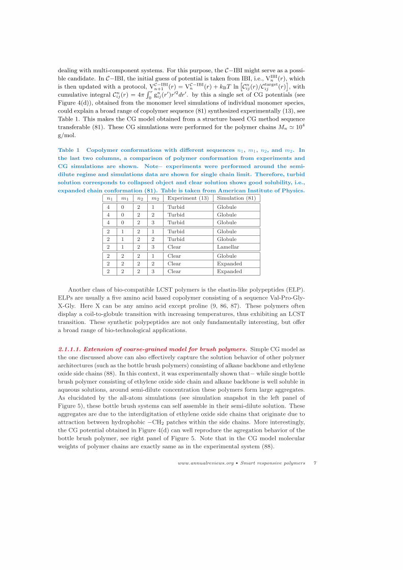
could explain a broad range of copolymer sequence (81) synthesized experimentally (13), see
Table 1. This makes the CG model obtained from a structure based CG method sequence
transferable (81). These CG simulations were performed for the polymer chains Mn ≃ 104
g/mol.
Table 1 Copolymer conformations with different sequences n1, m1, n2, and m2. In
the last two columns, a comparison of polymer conformation from experiments and
CG simulations are shown. Note− experiments were performed around the semi-
dilute regime and simulations data are shown for single chain limit. Therefore, turbid
solution corresponds to collapsed object and clear solution shows good solubility, i.e.,
expanded chain conformation (81). Table is taken from American Institute of Physics.
n1 m1 n2 m2 Experiment (13) Simulation (81)
4 0 2 1 Turbid Globule
4 0 2 2 Turbid Globule
4 0 2 3 Turbid Globule
2 1 2 1 Turbid Globule
2 1 2 2 Turbid Globule
2 1 2 3 Clear Lamellar
2 2 2 1 Clear Globule
2 2 2 2 Clear Expanded
2 2 2 3 Clear Expanded
Another class of bio-compatible LCST polymers is the elastin-like polypeptides (ELP).
ELPs are usually a five amino acid based copolymer consisting of a sequence Val-Pro-Gly-
X-Gly. Here X can be any amino acid except proline (9, 86, 87). These polymers often
display a coil-to-globule transition with increasing temperatures, thus exhibiting an LCST
transition. These synthetic polypeptides are not only fundamentally interesting, but offer
a broad range of bio-technological applications.
2.1.1.1. Extension of coarse-grained model for brush polymers. Simple CG model as
the one discussed above can also effectively capture the solution behavior of other polymer
architectures (such as the bottle brush polymers) consisting of alkane backbone and ethylene
oxide side chains (88). In this context, it was experimentally shown that− while single bottle
brush polymer consisting of ethylene oxide side chain and alkane backbone is well soluble in
aqueous solutions, around semi-dilute concentration these polymers form large aggregates.
As elucidated by the all-atom simulations (see simulation snapshot in the left panel of
Figure 5), these bottle brush systems can self assemble in their semi-dilute solution. These
aggregates are due to the interdigitation of ethylene oxide side chains that originate due to
attraction between hydrophobic −CH2 patches within the side chains. More interestingly,
the CG potential obtained in Figure 4(d) can well reproduce the agregation behavior of the
bottle brush polymer, see right panel of Figure 5. Note that in the CG model molecular
weights of polymer chains are exactly same as in the experimental system (88).
www.annualreviews.org • Smart responsive polymers 7

Figure 5
Simulation snapshot showing aggregation of bottle brush polymer consisting of alkane backboneand ethylene oxide side chains (88). A comparison of all-atom and coarse-grained simulations
results are shown. Note− the molecular weight Mn for all-atom simulations were half the Mn
from experimental synthesis. For CG simulation, Mn is same as experimental polymers.
2.1.1.2. Temperature transferability of coarse-grained model. The CG model de-
scribed above is transferable with changing sequences, they are not transferable with chang-
ing T . For example, structure based CG methods are dependent on pair-wise structure that
inherently depends on temperature, thus making structure-based CG models state point de-
pendent. In this context, however, CG model for a PNIPAm chain in bundled water (four
water molecules clustered into one CG bead) was developed (89) based on the CG force field
(90, 91). This work presents results for two different temperatures, where two different sets
of pair-wise CG potentials were used to account for the temperature effect. Furthermore,
when a polymer goes from coil-to-globule transition, it is dictated by a delicate balance
between entropy and energy near the transition point that originate from the three-body
effect. It should still be mentioned that the collapsed transition itself does not need three
body effects. Moreover, three-body effects guarantees a finite density in the collapsed state.
In general CG energies are free energies when compared to the all-atom systems. Thus are
linked to a thermodynamic state point and one can not expect temperature transferability.
However, if a CG model can properly account for this delicate entropy-energy balance, as
in the case of azobenzene (92), it is also expected that the underlying CG model may also
be able to give temperature transferability.
3. CO-NON-SOLVENCY: POLYMER COLLAPSE IN MISCIBLE GOOD
SOLVENTS
So far we have discussed polymer properties in single component solvents and their coil-to-
globule transition with change in temperature. However, the conformational behavior of a
polymer also can be greatly influenced by the presence of small cosolvent molecules within
the solvation volume of a polymer in solution, because of the competitive interaction of
solvent and cosolvent with polymer. This is because cosolvents can often drastically alter the
solvation structure and thus the solvation free energy of a polymer (18, 19, 20, 24, 26). For
example, starting from an expanded chain of PNIPAm in pure water below its Tℓ, addition of
cosolvent (especially small alcohols and other organic solvents) first decreases Tℓ and then Tℓ
eventually sharply increases when alcohol content increases beyond a certain concentration
(18, 19). In Figure 6 a representative phase diagram of PNIPAm in aqueous methanol
8 Mukherji et al.
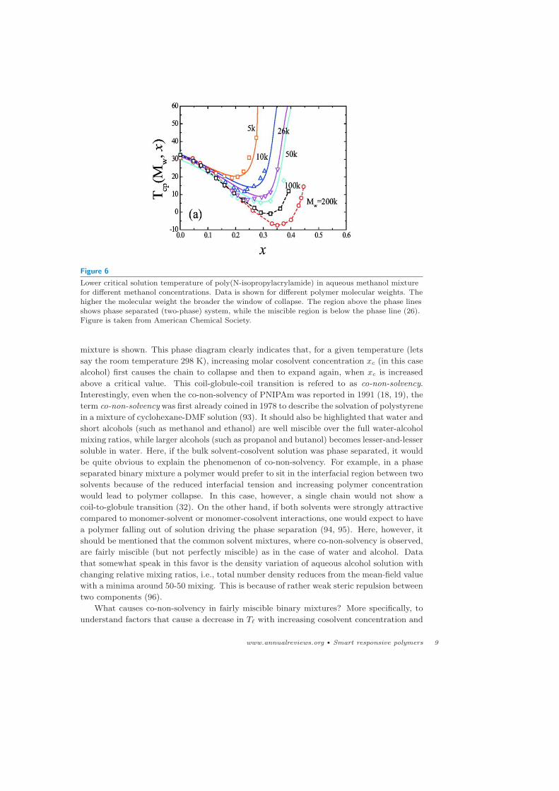
Figure 6
Lower critical solution temperature of poly(N-isopropylacrylamide) in aqueous methanol mixturefor different methanol concentrations. Data is shown for different polymer molecular weights. Thehigher the molecular weight the broader the window of collapse. The region above the phase lines
shows phase separated (two-phase) system, while the miscible region is below the phase line (26).Figure is taken from American Chemical Society.
mixture is shown. This phase diagram clearly indicates that, for a given temperature (lets
say the room temperature 298 K), increasing molar cosolvent concentration xc (in this case
alcohol) first causes the chain to collapse and then to expand again, when xc is increased
above a critical value. This coil-globule-coil transition is refered to as co-non-solvency.
Interestingly, even when the co-non-solvency of PNIPAm was reported in 1991 (18, 19), the
term co-non-solvency was first already coined in 1978 to describe the solvation of polystyrene
in a mixture of cyclohexane-DMF solution (93). It should also be highlighted that water and
short alcohols (such as methanol and ethanol) are well miscible over the full water-alcohol
mixing ratios, while larger alcohols (such as propanol and butanol) becomes lesser-and-lesser
soluble in water. Here, if the bulk solvent-cosolvent solution was phase separated, it would
be quite obvious to explain the phenomenon of co-non-solvency. For example, in a phase
separated binary mixture a polymer would prefer to sit in the interfacial region between two
solvents because of the reduced interfacial tension and increasing polymer concentration
would lead to polymer collapse. In this case, however, a single chain would not show a
coil-to-globule transition (32). On the other hand, if both solvents were strongly attractive
compared to monomer-solvent or monomer-cosolvent interactions, one would expect to have
a polymer falling out of solution driving the phase separation (94, 95). Here, however, it
should be mentioned that the common solvent mixtures, where co-non-solvency is observed,
are fairly miscible (but not perfectly miscible) as in the case of water and alcohol. Data
that somewhat speak in this favor is the density variation of aqueous alcohol solution with
changing relative mixing ratios, i.e., total number density reduces from the mean-field value
with a minima around 50-50 mixing. This is because of rather weak steric repulsion between
two components (96).
What causes co-non-solvency in fairly miscible binary mixtures? More specifically, to
understand factors that cause a decrease in Tℓ with increasing cosolvent concentration and
www.annualreviews.org • Smart responsive polymers 9

not that the original T driven of collapse of a chain in water is entropy driven. In this con-
text, to reveal the microscopic origin of this puzzling behavior, extensive studies have been
performed using experiments, theory and computer simulations. In view of these studies,
three main pictures were proposed to understand the microscopic origin of co-non-solvency:
based on solvent-cosolvent interactions (18, 32, 94, 95), cooperative polymer-solvent and
polymer-cosolvent hydrogen bonding (24, 26), and preferential polymer-cosolvent binding
(28, 29, 30). Therefore, we proceed here with highlighting results from the molecular sim-
ulations.
3.1. Multiscale simulations complex mixtures and polymer in mixed solvents
As mentioned earlier, polymer properties are governed by a rather delicate energy (details
of the chemical structure) and entropy (generic, universal scaling laws, critical phenomena)
interplay. This connection is at heart of the understanding of many biological as well as syn-
thetic materials and processes. At the same time it is very difficult to address the questions
to understand details within conventional experimental and mid sized canonical (NVT) or
isobaric (NpT) simulation setups, where N is the number of particles in the simulation box,
V is volume of the system, T is the temperature and p is the pressure. Therefore, there is
a need to address these problems within multiscale simulation approaches, where local mi-
croscopic interaction details (where local is referred to the range of correlation length that
is typically less than 2.0 nm in these water soluble systems) are coupled in equilibrium with
a large solvent bath allowing for global conformational fluctuations. For example, polymer
properties in mixed solvents typically are dictated by large conformational and (co-)solvent
compositional fluctuations. Computer simulations in canonical ensemble usually, however,
suffer from system size effects (97, 98). This is partially due to the fact that the local
agregation of one of the solvent components at one place of simulation box leads to the
depletion of the same species at other region within the simulation box. This disturbs the
solvent equilibrium and thus leads to wrong fluctuations.
A quantity that gives the direct measure of the fluctuation within the simulation domain
is,
Gij = 4π
∫
∞
0
[
gµVTij (r)− 1
]
r2dr = V
[
〈NiNj〉 − 〈Ni〉 〈Nj〉
〈Ni〉 〈Nj〉−
δij〈Nj〉
]
, 2.
where thermal averages are denoted by brackets 〈·〉. V is the volume, Ni is the number of
particles of species i, δij is the Kronecker delta, gµVTij (r) is the radial distribution function
in the µVT ensemble (30, 98, 99, 100, 101, 102). Here, Gij is refereed differently in different
communities. In bio-physical community Gij is known as the Kirkwood-Buff integrals (KBI)
(99) and in statistical physics Gij/4π is known as the Mayer’s function. −Gij/2 also gives
direct measure of the second virial coefficient β2 (or the excluded volume V), a highly useful
quantity to describe polymer conformation (6, 29). Furthermore, Gij is a local quantity that
can be used as a measure of the affinity between solution components i and j. A positive
(or negative) value of Gij refers to excess (or depletion) of component j around component
i. Gij can also be used to calculate solvation thermodynamics of multi-component complex
fluids.
Following Eq. 2 Gij should be calculated in a grand canonical ensemble, while in a
closed boundary setup Gij can only be estimated at r → ∞ (99). A typical cumulative
Gij is shown in Figure 7(a). It can be seen that for a small system size (consisting of
6× 10³ molecules) Gij(r) suffers from severe system size effects and it is impossible to get
10 Mukherji et al.
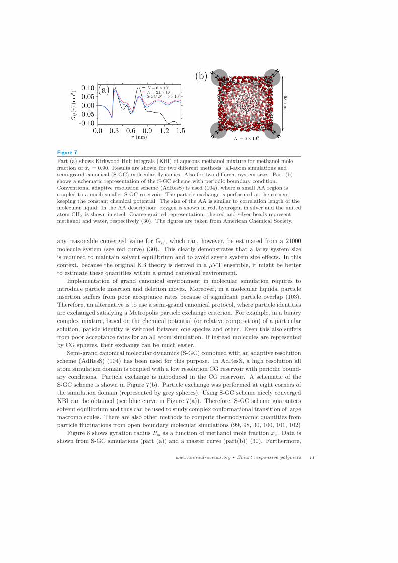
Figure 7
Part (a) shows Kirkwood-Buff integrals (KBI) of aqueous methanol mixture for methanol mole
fraction of xc = 0.90. Results are shown for two different methods: all-atom simulations andsemi-grand canonical (S-GC) molecular dynamics. Also for two different system sizes. Part (b)shows a schematic representation of the S-GC scheme with periodic boundary condition.Conventional adaptive resolution scheme (AdResS) is used (104), where a small AA region is
coupled to a much smaller S-GC reservoir. The particle exchange is performed at the cornerskeeping the constant chemical potential. The size of the AA is similar to correlation length of themolecular liquid. In the AA description: oxygen is shown in red, hydrogen in silver and the united
atom CH3 is shown in steel. Coarse-grained representation: the red and silver beads representmethanol and water, respectively (30). The figures are taken from American Chemical Society.
any reasonable converged value for Gij , which can, however, be estimated from a 21000
molecule system (see red curve) (30). This clearly demonstrates that a large system size
is required to maintain solvent equilibrium and to avoid severe system size effects. In this
context, because the original KB theory is derived in a µVT ensemble, it might be better
to estimate these quantities within a grand canonical environment.
Implementation of grand canonical environment in molecular simulation requires to
introduce particle insertion and deletion moves. Moreover, in a molecular liquids, particle
insertion suffers from poor acceptance rates because of significant particle overlap (103).
Therefore, an alternative is to use a semi-grand canonical protocol, where particle identities
are exchanged satisfying a Metropolis particle exchange criterion. For example, in a binary
complex mixture, based on the chemical potential (or relative composition) of a particular
solution, paticle identity is switched between one species and other. Even this also suffers
from poor acceptance rates for an all atom simulation. If instead molecules are represented
by CG spheres, their exchange can be much easier.
Semi-grand canonical molecular dynamics (S-GC) combined with an adaptive resolution
scheme (AdResS) (104) has been used for this purpose. In AdResS, a high resolution all
atom simulation domain is coupled with a low resolution CG reservoir with periodic bound-
ary conditions. Particle exchange is introduced in the CG reservoir. A schematic of the
S-GC scheme is shown in Figure 7(b). Particle exchange was performed at eight corners of
the simulation domain (represented by grey spheres). Using S-GC scheme nicely converged
KBI can be obtained (see blue curve in Figure 7(a)). Therefore, S-GC scheme guarantees
solvent equilibrium and thus can be used to study complex conformational transition of large
macromolecules. There are also other methods to compute thermodynamic quantities from
particle fluctuations from open boundary molecular simulations (99, 98, 30, 100, 101, 102)
Figure 8 shows gyration radius Rg as a function of methanol mole fraction xc. Data is
shown from S-GC simulations (part (a)) and a master curve (part(b)) (30). Furthermore,
www.annualreviews.org • Smart responsive polymers 11
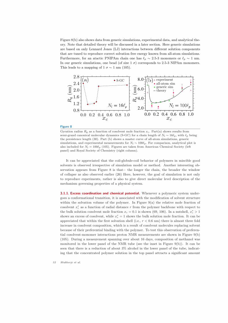
Figure 8(b) also shows data from generic simulations, experimental data, and analytical the-
ory. Note that detailed theory will be discussed in a later section. Here generic simulations
are based on only Lennard Jones (LJ) interactions between different solution components
that are tuned to reproduce correct solvation free energy known from all-atom simulations.
Furthermore, for an atactic PNIPAm chain one has ℓp ∼ 2.5-3 monomers or ℓp ∼ 1 nm.
In our generic simulations, one bead (of size 1 σ) corresponds to 2.5-3 NIPAm monomers.
This leads to a mapping of 1 σ ∼ 1 nm (105).
2.0
4.0
6.0
8.0
0.0 0.2 0.4 0.6 0.8 1.0
Figure 8
Gyration radius Rg as a function of cosolvent mole fraction xc. Part(a) shows results fromsemi-grand canonical molecular dynamics (S-GC) for a chain length of Nl ∼ 16ℓp, with ℓp beingthe persistence length (30). Part (b) shows a master curve of all-atom simulations, generic
simulations, and experimental measurements for Nl ∼ 100ℓp. For comparison, analytical plot isalso included for Nl = 100ℓp (105). Figures are taken from American Chemical Society (leftpanel) and Royal Society of Chemistry (right column).
It can be appreciated that the coil-globule-coil behavior of polymers in miscible good
solvents is observed irrespective of simulation model or method. Another interesting ob-
servation appears from Figure 8 is that− the longer the chain, the broader the window
of collapse as also observed earlier (26) Here, however, the goal of simulation is not only
to reproduce experiments, rather is also to give direct molecular level description of the
mechanism governing properties of a physical system.
3.1.1. Excess coordination and chemical potential. Whenever a polymeric system under-
goes a conformational transition, it is associated with the modification of solvent structure
within the solvation volume of the polymer. In Figure 9(a) the relative mole fraction of
cosolvent x∗c as a function of radial distance r from the polymer backbone with respect to
the bulk solution cosolvent mole fraction xc = 0.1 is shown (69, 106). In a nutshell, x∗c > 1
shows an excess of cosolvent, while x∗c = 1 shows the bulk solution mole fraction. It can be
appreciated that within the first solvation shell (i.e., r < 0.6 nm) there is almost three fold
increase in cosolvent composition, which is a result of cosolvent molecules replacing solvent
because of their preferential binding with the polymer. To test this observation of preferen-
tial cosolvent-monomer interactions proton NMR measurements are shown in Figure 9(b)
(105). During a measurement spanning over about 16 days, composition of methanol was
monitored in the lower panel of the NMR tube (see the inset in Figure 9(b)). It can be
seen that there is a reduction of about 3% alcohol in the lower panel of the tube, indicat-
ing that the concentrated polymer solution in the top panel attracts a significant amount
12 Mukherji et al.
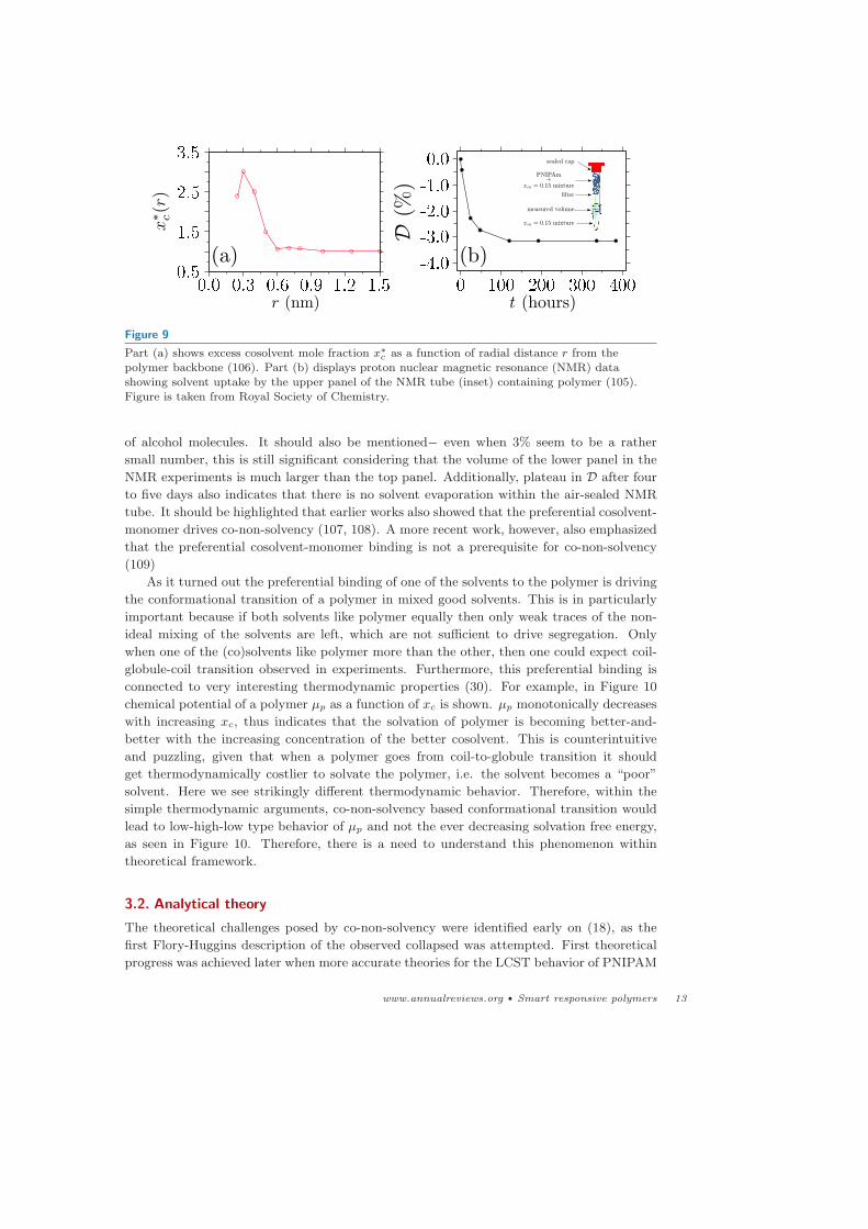
Figure 9
Part (a) shows excess cosolvent mole fraction x∗c as a function of radial distance r from the
polymer backbone (106). Part (b) displays proton nuclear magnetic resonance (NMR) datashowing solvent uptake by the upper panel of the NMR tube (inset) containing polymer (105).Figure is taken from Royal Society of Chemistry.
of alcohol molecules. It should also be mentioned− even when 3% seem to be a rather
small number, this is still significant considering that the volume of the lower panel in the
NMR experiments is much larger than the top panel. Additionally, plateau in D after four
to five days also indicates that there is no solvent evaporation within the air-sealed NMR
tube. It should be highlighted that earlier works also showed that the preferential cosolvent-
monomer drives co-non-solvency (107, 108). A more recent work, however, also emphasized
that the preferential cosolvent-monomer binding is not a prerequisite for co-non-solvency
(109)
As it turned out the preferential binding of one of the solvents to the polymer is driving
the conformational transition of a polymer in mixed good solvents. This is in particularly
important because if both solvents like polymer equally then only weak traces of the non-
ideal mixing of the solvents are left, which are not sufficient to drive segregation. Only
when one of the (co)solvents like polymer more than the other, then one could expect coil-
globule-coil transition observed in experiments. Furthermore, this preferential binding is
connected to very interesting thermodynamic properties (30). For example, in Figure 10
chemical potential of a polymer µp as a function of xc is shown. µp monotonically decreases
with increasing xc, thus indicates that the solvation of polymer is becoming better-and-
better with the increasing concentration of the better cosolvent. This is counterintuitive
and puzzling, given that when a polymer goes from coil-to-globule transition it should
get thermodynamically costlier to solvate the polymer, i.e. the solvent becomes a “poor”
solvent. Here we see strikingly different thermodynamic behavior. Therefore, within the
simple thermodynamic arguments, co-non-solvency based conformational transition would
lead to low-high-low type behavior of µp and not the ever decreasing solvation free energy,
as seen in Figure 10. Therefore, there is a need to understand this phenomenon within
theoretical framework.
3.2. Analytical theory
The theoretical challenges posed by co-non-solvency were identified early on (18), as the
first Flory-Huggins description of the observed collapsed was attempted. First theoretical
progress was achieved later when more accurate theories for the LCST behavior of PNIPAM
www.annualreviews.org • Smart responsive polymers 13

Figure 10
A master curve showing the shift in chemical potential µp per monomer as a function of cosolventmole fraction (30). The data was obtained for a temperature of 298 K, where kBT = 2.5 kJ/mol.
Figure is taken from American Chemical Society.
became available (24, 26). However, not until recently was the generic character of this
phenomena recognized and explained by a combination of analytical theory and numerical
simulations (3, 110).
3.2.1. Flory-Huggins mean-field theory. A standard thermodynamic theory to describe
polymer conformation is the mean-field theory of Flory-Huggins. In this theory, when
a polymer p with chain length Nl at volume fraction φp is dissolved in a binary mixture of
solvent s and cosolvent c, the Flory-Huggins free energy FFH of polymer solutions is written
as (64, 65, 66),
FFH
κBT=
φp
Nllnφp + xc (1− φp) ln [xc (1− φp)] + (1− xc) (1− φp) ln [(1− xc) (1− φp)]
+ χpsφp (1− xc) (1− φp) + χpcφpxc (1− φp) + χscxc (1− xc) (1− φp)2 . 3.
Here, the first three terms represent the entropy of mixing and the last three terms deal
with interactions between different components i and j through χij parameters. The second
order expansion of Eq. 3 gives a direct measure of the excluded volume V of the polymer,
V = 1− 2 (1− xc)χps − 2xcχpc + 2xc (1− xc)χsc, 4.
In a nutshell, under a good solvent condition for a polymer V > 0 with the scaling law
for gyration radius and single chain static structure factor S(q) following Rg ∼ N3/5l and
S(q) ∼ q−5/3, respectively. Increasing monomer-monomer attraction first brings a polymer
into the Θ−condition where long range energetic attraction gets exactly cancelled by the
short range entropic repulsion. At the Θ−condition V = 0, Rg ∼ N1/2l and S(q) ∼ q−2.
When the monomer-monomer attractions is even further increased, a polymer collapses into
a compact globule where V < 0, Rg ∼ N1/3l and S(q) ∼ q−4 (64, 65, 66).
When both solvent and cosolvent are good solvents for a polymer, χps < 1/2 and
χpc < 1/2 (18). If the bulk binary solution is perfectly miscible (i.e. χsc = 0) the first two
14 Mukherji et al.

Figure 11
Parts (a) and (b) show schematic representations of the polymer excluded volume V and chemical
potential of polymer µp as a function of cosolvent mole fraction xc. The horizontal line (dashedblack) in part (a) shows Θ−point when V = 0. Figures are taken from American Institute ofPhysics.
terms of Eq. 4 give a linear variation of V with xc, see the blue line in Figure 11(a). Only
when χsc < 0 can V become negative, opening the possibility for the coil-to-globule-to-coil
conformation changes typical of co-non-solvency, see the red line in Figure 11(a).
Furthermore, within the mean-field picture in Eq. 3, the shift in chemical potential of
polymer µp under infinite dilution φp → 0 can be written as,
µp (φp → 0) =∂FFH
∂φp
∣
∣
∣
∣
φp→0
= const− xc lnxc − (1− xc) ln (1− xc) + (1− xc)χps + xcχpc − 2xc (1− xc)χsc.5.
In Figure 11(b) a schematic representation of µp is shown as obtained from Eq. 5, see the
red line in Figure 11(b). Note that µp(xc = 1) < µp(xc = 0) because cosolvent is the better
of the two (co)solvents. Furthermore the behavior of V presented in Figure 11 is consistent
with the µp for χsc < 0 shown by a hump for the intermediate mixing ratios, thus the
solvent quality goes from good-to-poor-to-good again. It should also be noted that the
trend in Figure 10 is qualitatively different from what is expected from the Flory-Huggins
theory. In the mean-field picture, however, when χsc >> 0 similar trend as in Figure 10 be
expected, see the black curve in Figure 11(b). Moreover, this will imply that the trend in µp
is obtained at the non-realistic cost of driving the system towards solvent phase separation.
In this context, it was already noticed early (18) that for common solvent mixtures where
co-non-solvency effects are observed, such as water-alcohol mixtures, χsc ≥ 0.
3.2.2. Co-non-solvency as a result of cooperativity effects. A theoretical approach for de-
scribing the LCST behavior of PNIPAm was developed earlier (111), based on two central
ideas: i) water molecules bind to the PNIPAm backbone through hydrogen bonds, in a
cooperative manner: the formation of bonds between one water molecule and the monomer
facilitates the formation of the next bonds, and ii) the sections of the backbone without
bound water molecules are naturally in a collapsed state while the sections with bound
water molecules are naturally in good solvent conditions. An extension of this model for
co-non-solvency was then considered (24) where both water and cosolvent were treated in
the same manner, albeit with possible different values for the parameters measuring affini-
ties and cooperativity. Model parameters can be found that fit well experimental results
on the variation of PNIPAm radius of gyration in water-methanol mixtures (24).
www.annualreviews.org • Smart responsive polymers 15
3.2.3. Competitive displacement of solvent by cosolvent. The approach in Ref. (24) suc-
cessfully displays the non-monotonic collapse behavior of a polymer under con-non-solvency,
it can lead to the conclusion that co-non-solvency can only be generated by the the compe-
tition between two solvents that cooperatively bind to the chain backbone in a poor solvent.
More recently it was shown that the co-non-solvency can be a generic phenomena emerging
in much less restrictive conditions.
As demonstrated by the simulations (see Figure 9) the polymer has preferential inter-
actions with the cosolvent molecules. Because of this preferential interaction, when a small
amount of cosolvents are added into the solution it tries to minimize the polymer-cosolvent
binding free energy by attaching to more than one monomer at a time. Furthermore, the
molecular flexibility of a polymer can help in this cause by forming segmental loops when
cosolvent molecules form contact between two monomers far along the polymer backbone.
Note− within the simplified generic model, one cosolvent sphere does not necessarily cor-
respond to one alcohol molecule, rather a collections of several alcohol molecules.
The general picture of cosolvent molecules forming bridging interactions between two
monomers topologically far along the polymer backbone has also been proposed for polymer
collapse in a broad range of aqueous cosolvent mixtures. For example, the collapse of
a PNIPAm in aqueous urea mixtures was shown to be driven by bridging-like hydrogen
bonding of urea with two NIPAm monomers (15, 35). Furthermore, there are also other
works showing that bridging interactions are responsible for a polymer collapse in a mixtures
of two cosolvents (36, 37), while another work highlighted that the preferential binding may
not be prerequisite for co-non-solvency (109).
In view of this, a non Flory-Huggins mean-field description of polymer solution can be
formulated that is based on the Langmuir like adsorption isotherm of competitive displace-
ment (112). Within this theory a polymer is considered as an adsorbing substrate, where
N sites are exposed to the bulk solution, of which ns sites are occupied by s (solvent)
molecules, nc sites by non-bridging c (co-solvent) molecules and 2ncB sites by bridging c
(co-solvent) molecules, with N = ns + nc + 2ncB . The observed sequence of collapse and
re-swelling of the polymer corresponds to a fast growth of ncB as xc increases, followed by
a displacement of ncB by nc for larger xc values. Such a sequence is typical for competitive
displacement in adsorption phenomena (112).
The results from numerical simulations for ncB and nc, or alternatively for the fractions
φB = ncB/N and φ = nc/N , are very well described by a competitive adsorption model with
the following associated free energy density of adsorption for non-bridges and bridges (3),
Ψ
κBT= φ ln (φ) + ζφB ln (2φB)
+ (1− φ− 2φB) ln (1− φ− 2φB)
− Eφ− EBφB −µ
κBT(φ+ φB) , 6.
with µ = κBT ln(xc) being the chemical potential of the cosolvent in the bulk solvent
mixture and the adsorption energies E and EB measure the excess affinities of individual
non-bridging and bridging cosolvent molecules to the chain monomers. The first three
terms in Eq. 6 express entropic contributions of the adsorbed bridges and non-bridges to
the energy densities, while the two following terms measures contact energies between the
cosolvents bridges and non-bridges with the polymer backbone. The unusual pre-factor ζ
is a consequence of assuming a logarithmic form for the dependence of the energy required
to make a bridge on the average density of existing bridges. This is the case for instance
16 Mukherji et al.

(3), if one assumes that in order to make a new bridge at density φB, the chain needs to
make a loop of length ℓ = 1/φB, with associated penalty ∼ log ℓ ∼ log(1/φB).
Minimization of Eq. 6 with respect to φB and φ leads to the implicit equation for the
bridge density φB(xc),
16φBζxc = x∗
c
{(
x∗c
x∗∗c
)1/2
(1− 2φB)
±
√
(
x∗c
x∗∗c
)
(1− 2φB)2 − 16φB
ζ
}2
. 7.
with x∗c = exp(−E) and x∗∗
c = exp(−EB + 2 ln 2e− ζ) are the characteristic concentrations
related to the adsorption energies E and EB for non-bridges and bridges. In Fig. 12(a) we
show φB, the fraction of backbone sites participating in bridge formation, as a function
of xc. Note that φ and φB are cosolvent molecules that are directly in contact with the
monomers at a distance 21/6σpc ∼ 0.84σ. As the figure shows expression Eq. 7 describes
very well our experimental results, with ζ = 0.05.
0.0 0.3 0.6 0.90.00
0.03
0.06
0.09
0.12
0.0 0.3 0.6 0.9
-8
-6
-4
-2
0
Figure 12
A comparative plot of molecular dynamics simulation (symbols) and theoretical plot (solid line)
(3). Part (a) shows bridging fraction of cosolvents φB as a function of cosolvent mole fraction xc.Theoretical prediction is represented by Eq. 7. Part (b) shows chemical potential shift µp with xc.Figure is taken from Nature Publishing Group.
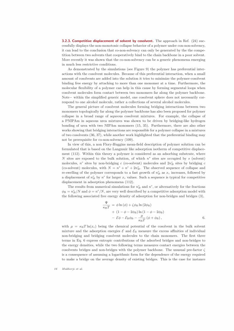
Eq. (7) can equivalently be derived by considering the two pseudo chemical reactions
cosolvent + empty site ⇀↽ non− bridge 8.
cosolvent + 2 empty site ⇀↽ ζ bridge, 9.
sketched in Figure 13. When the solvent and cosolvent interactions with the polymer
backbone empty sites are described as pseudo reactions, a cosolvent molecule reacts with
one empty adsorption site to form one adsorbed non-bridge, while it reacts with two empty
sites to make ζ bridges. The associated equilibrium mass-action laws can thus be written
as
xc
x∗c
=φ
1− φ− 2φB
10.
xc
4x∗∗c
=φζB
(1− φ− 2φB)2, 11.
www.annualreviews.org • Smart responsive polymers 17
+ =
+ =
(a)
(b)
(c)
Figure 13
A schematic representation of the chemical reaction described in Eq. 11. Part (a) shows a polymer
conformation decorated by non-bridging and bridging cosolvents. Part (b) shows a polymersegment and a cosolvent forming a single non-bridging cosolvent, while part (b) represents twosegments making a cosolvent bridge (110). Figure is taken from American Institute of Physics.
with equilibrium reaction constants 1/x∗c and 1/x∗∗
c , where the reaction equilibrium con-
centration x∗∗c has been, for mathematical convenience, defined up to a factor four. Solving
the mass-action laws for φB gives Eq. (7). In this pseudo-chemical language, the factor ζ
describing the effective number of bridges formed by the interaction between one cosolvent
molecule and the two empty sites of the backbone appears as a consequence of assuming a
power-law dependence for the equilibrium constant of the pseudo-chemical reaction. Note
that the actual shape of Eq. 7 is quite sensitive to the value of ζ. In particular, the choice
ζ = 1, corresponding to a standard chemical reaction between free species in solution, leads
to a prediction that can not describe our data.
In a previous work (3), it was argued that a value of ζ = 0.05 can be understood by
considering loop contributions to the cost of making a bridge. When a pure configurational
cost for distributing the bridges amongst the possible occupation sites is combined with the
entropic cost of loop formation, one can write ζ = 2−m. Here the critical exponent m can
be estimated within a simple scaling argument. In this context, one can characterize the
loop formation by a partition function of vanishing end-to-end distance Re → 0 (66),
ZNl(Re → 0) ∝ qNlNl
α−2, 12.
and the partition function at finite Re is given by,
ZNl(Re) ∝ qNlNl
γ−1. 13.
Here 1/q is the critical fugacity and the universal exponent α ∼= 0.2 (66). From these
two cases one can estimate the free energy barrier to form a loop of length ℓ as △F(ℓ) =
mκBT ln(ℓ), with m = γ − α + 1 being the critical exponent (66). Although this gives
18 Mukherji et al.

m = 1.95 for loop formation in self-avoiding walks, in excellent agreement with our findings,
it is worth pointing to the fact that our simple analytical description does not address other
possible contributions to bridge formation, such as cooperative or other non-trivial entropic
effects that might be determinant in the dense chain globule.
This selective adsorption model provides also for an analytical prediction of the shift in
the chemical potential µp as a function of xc,
µp
κBT= const+ (2− ζ)φB
− ln
{
1 + φB1−ζ/2
(
xc
x∗∗c
)1/2
+(
xc
x∗c
)
}
. 14.
Fig. 12(b) shows a comparison between predictions from Eq. 14 and the values of the
chemical potential obtained from Eq. 14. A very good agreement is obtained by simply
inserting into Eq. 14 the values for ζ and concentrations obtained from the fit of the bridging
fraction, further confirming the consistency and validity of our approach.
Note that while standard Flory-Huggins type mean field theory does not describe co-
non-solvency, mean-field descriptions with higher order corrections may be more applicable.
In this context, a recent extension of the competitive displacement concept (3, 110) led to
the introduction of sticky sites within a mean-field picture to describe co-non-solvency of
polymer brushes (113, 114).
3.3. UCST-like swelling of LCST polymer
It is commonly known that a PNIPAm chain collapses in water upon increase of T , thus
showing a LCST like temperature effect. Moreover, in aqueous alcohol mixtures, especially
for larger alcohol (such as ethanol or propanol), PNIPAm also shows UCST-like swelling
with increasing T (69, 31, 115). As shown in Figure 14 both simulation and experiments
Figure 14
Part (a) shows hydrodynamic radius Rh obtained from dynamics light scattering of PNIPAmmicrogel and part (b) for all-atom molecular dynamics simulations of single PNIPAm chain,
respectively. Data is shown fro three different ethanol volume fractions and with varyingtemperature T (69). Figure is taken from American Chemical Society.
show that the UCST-like re-swelling is more prominent for ethanol volume fraction φe >
50% (69). This can be attributed to the fact that for T > 305 K pure water is always a poor
solvent for PNIPAm, while no such LCST behavior is known for pure alcohol. Therefore,
for φe > 50%, alcohol acts as addition of good solvent in poor solvent, thus results in
re-swelling. There are of-course other mechanism proposed for such UCST-reswelling via
kosmotropic effects (31) and cooperative hydrogen bonded effects (115).
www.annualreviews.org • Smart responsive polymers 19

4. CO-SOLVENCY: POLYMER SWELLING IN MISCIBLE POOR SOLVENTS
In the previous section we reviewed the phenomenon of co-non-solvency that describes
polymer collapse in a mixtures of two competing, (fairly) miscible good solvents, while the
same polymer remains expanded in these two solvents individually. An opposite effect is
the swelling of a polymer in mixtures of two fairly miscible poor solvents. In this context,
it has been commonly observed that a polymer may remain collapsed in two different
poor solvents, whereas it is somewhat “better” soluble in their mixtures (116, 117, 118,
119). This phenomenon known as co-solvency will be discussed in this section. Typical
systems include− poly(methyl methacrylate) (PMMA) (116, 117, 118, 119, 120), poly(N-(6-
acetamidopyridin-2-yl)acrylamide) (PNAPAAm) (121), and corn starch in solvent mixtures
(122). For example, both water and alcohol are poor solvents for PMMA, it swells within
the intermediate mixing ratios of water-alcohol mixtures (such as the aqueous methanol,
ethanol and propanol, respectively). Attaining a maximum degree of swelling around 60-
70% alcohol mole fraction, see Figure 15.
0.0 0.2 0.4 0.6 0.8 1.0
1.0
1.1
1.2
1.3
1.4
1.5
1.6
1.7
Figure 15
Normalized squared radius of gyration R2
g =⟨
R2g
⟩
/⟨
Rg(xc = 0)2⟩
as a function of cosolventmolar concentration xc. Results are shown for the generic simulations and for three different
cases. Here⟨
Rg(xc = 0)2⟩
= 2.6± 0.4σ2 and R2
Θ = 2.13 with RΘ = RΘ/Rg(xc = 0) is thenormalized Θ−point gyration radius. Here case 2 closely mimics the conformational behavior ofPMMA in aqueous methanol mixture (6). Figure is taken from Nature Publishing Group.
When a polymer collapses in a poor solvent, this collapsed structure is described by
balancing negative second virial osmotic contributions −|V| and three body repulsions.
Under such a poor solvent condition, the effective attraction between the monomers of a
polymer can be viewed as a depletion induced attraction, a phenomenon well described for
colloidal suspensions (123, 124, 125, 126, 127) of purely repulsive particles. More specif-
ically, monomer-monomer attraction will occur when monomer-solvent excluded volume
interactions become larger than the monomer-monomer excluded volume interactions. The
resulting isolated polymer conformation can be well described by the Porod scaling law of
the single chain static structure factor S(q) ∝ q−4 presenting a compact spherical globule,
see Figure 16(a). This argument holds in pure water and in pure alcohol for PMMA. Fur-
thermore, the extent of depletion induced attraction between two particles is dictated by
the number density ρ of depletants, in this case solvent particles consisting of water and
alcohol, within the solvation volume (6). Data that support this view is given by the total
number density ρtotal of bulk solution as a function of mixing ratio of two solvents (6). In
Figure 17 it is shown that for aqueous alcohol mixtures ρtotal reduces from its mean-field
20 Mukherji et al.

10-1
100
101
10-1
100
101
102
10-1
100
101
Figure 16
Single chain static structure factor S(q) for: xc = 0.0 in part (a) and xc = 0.7 in part (b). In part(a) analytical expression for sphere scattering is included. In part (b) red and green lines arepower law fits to the data at different length scales. The black line represents the Guiner regionfor q → 0. The vertical arrow indicates the effective Θ−like blob size at q = qΘ (6). Figure is
taken from Nature Publishing Group.
0.0 0.2 0.4 0.6 0.8 1.0
10
15
20
25
30
35
Figure 17
Total number density ρtotal of the bulk solution as a function of mole fraction xc of aqueous
methanol and aqueous ethanol solutions, respectively. Solid lines are linear interpolation betweenthe data points of xc = 0.0 and xc = 1.0 (128). Figure is taken from Institute of Physics.
value (linear extrapolation between pure solvent xc = 0.0 and pure cosolvent xc = 1.0) with
a maximum deviation observed for the 50-50 mixing ratio (96, 128). The larger the alcohol
the larger the deviation from the linear density of interpolation. This deviation is a key
factor that reduces the number of depletants within the solvation volume and thus reduces
the depletion induced attractive forces, reducing the magnitude of the negative excluded
volume V. Therefore, the polymer swelling in a mixture of two poor solvents can be viewed
as a second order effect. For example, the solvent molecules deplete monomers giving rise
to the poor solvent condition for a polymer. However, when cosolvent molecules are added
into the system, cosolvents not only deplete monomers but also solvent molecules leading
to a second order depletion effect.
As a consequence the mixed solvent remains a poor solvent, while the effective depletion,
which drives the polymer collapse is reduced. Thus the observed swelling of about 30-70%
in R2g (or 10-30% swelling in Rg), as observed in Figure 15, does not mean that a polymer
is fully swollen into a self avoiding random walk. As seen from Figure 16(b), S(q) shows a
www.annualreviews.org • Smart responsive polymers 21
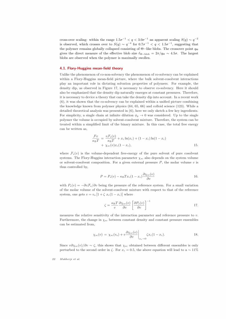
cross-over scaling: within the range 1.5σ−1 < q < 3.0σ−1 an apparent scaling S(q) ∼ q−2
is observed, which crosses over to S(q) ∼ q−4 for 0.7σ−1 < q < 1.5σ−1, suggesting that
the polymer remains globally collapsed consisting of Θ−like blobs. The crossover point qΘgives the direct measure of the effective blob size ℓΘ−blob = 2π/qΘ ∼ 4.5σ. The largest
blobs are observed when the polymer is maximally swollen.
4.1. Flory-Huggins mean-field theory
Unlike the phenomenon of co-non-solvency the phenomenon of co-solvency can be explained
within a Flory-Huggins mean-field picture, where the bulk solvent-cosolvent interactions
play an important role in dictating solvation properties of polymers. For example, the
density dip, as observed in Figure 17, is necessary to observe co-solvency. Here it should
also be emphasized that the density dip naturally emerges at constant pressures. Therefore,
it is necessary to device a theory that can take the density dip into account. In a recent work
(6), it was shown that the co-solvency can be explained within a unified picture combining
the knowledge known from polymer physics (64, 65, 66) and colloid science (123). While a
detailed theoretical analysis was presented in (6), here we only sketch a few key ingredients.
For simplicity, a single chain at infinite dilution φp → 0 was considered. Up to the single
polymer the volume is occupied by solvent-cosolvent mixture. Therefore, the system can be
treated within a simplified limit of the binary mixture. In this case, the total free energy
can be written as,
Fv
κBT=
vFs(v)
κBT+ xc ln(xc) + (1− xc) ln(1− xc)
+ χsc(v)xc(1− xc), 15.
where Fs(v) is the volume-dependent free-energy of the pure solvent of pure cosolvent
systems. The Flory-Huggins interaction parameter χsc also depends on the system volume
or solvent-cosolvent composition. For a given external pressure P , the molar volume v is
thus controlled by,
P = Ps(v)− κBTxc(1− xc)∂χsc(v)
∂v16.
with Ps(v) = −∂vFs/∂v being the pressure of the reference system. For a small variation
of the molar volume of the solvent-cosolvent mixture with respect to that of the reference
system, one gets v = vo [1 + ζ xc(1− xc)] where
ζ =κBT
v
∂χsc(v)
∂v
[
∂Ps(v)
∂v
]−1
17.
measures the relative sensitivity of the interaction parameter and reference pressure to v.
Furthermore, the change in χsc between constant density and constant pressure ensembles
can be estimated from,
χsc(v) = χsc(vo) + v∂χsc(v)
∂v
∣
∣
∣
∣
xc→0
ζxc(1− xc). 18.
Since v∂χsc(v)/∂v ∼ ζ, this shows that χsc obtained between different ensembles is only
perturbed to the second order in ζ. For xc = 0.5, the above equation will lead to a ∼ 11%
22 Mukherji et al.

variation in χsc values with respect to the standard values calculated when ρtotal is kept
constant (6). Even though 11% may sound like a small number, this is enough to induce
polymer swelling in poor solvent mixtures. Note that in this case swelling does not mean
a polymer undergoes a globule-to-coil transition, but experience a rather slight swelling as
seen in Figure 16.
5. SMART POLYMERS FOR MATERIALS DESIGN
Polymers are everywhere in our every day life, finding uses ranging from physics to materials
science and chemistry to biology (1, 4, 5). In this context, so far we have emphasized the
need to develop fundamental understanding of smart polymer properties in single and/or
multi-component solvents. Moreover, discussions presented above also aim at the future
directions for operational understanding and functional design principles of smart materials.
For this purpose, molecular simulations are of particular importance in interpreting and
guiding experiments to new directions. Therefore, we aim to finish this review sketching a
few examples where the knowledge discussed so far can be used to propose a design principle
of polymeric materials.
5.1. Design of multi-responsive copolymer architectures
In section 2.1.1 a discussion is presented related to a sequence transferable CG model for
polyacetal based copolymer architectures (13, 81). While varying parameter space with
Figure 18
A representative phase diagram of the amphiphilic copolymers with different sequences, see
Figure 3. Every symbol in these figures represent one configuration with the color code consistentwith the configurations presented in the right column. The data is shown for (a) m1 = 0, (b) m1
= 1, (c) m1 = 2, and (d) m1 = 3 with n2 = 2 and varying m2 and n1. Ethylene oxide beads arerendered in silver and methylene units are represented by red spheres. Figure is taken from
American Institute of Physics.
different sequences is rather non trivial in experiments, the CG model can be used to
predict a much broader range of polymer architectures. In Figure 18 a representative phase
diagram for 192 polymer sequences are shown. Several interesting structures are observed
reminiscent of the poly-soap collapse (129, 130, 131).
While conformations presented in Figure 18 are shown for statistical copolymers, there
are also studies showing nice thermal switching of micellar structures in pure water based
on di- (or tri-)block copolymer architectures (11, 132, 133). Moreover, sometimes thermal
switching requires a temperature change much above normal human body temperature.
This often restricts broader applications of proposed polymer architectures for biomedi-
www.annualreviews.org • Smart responsive polymers 23

cal encapsulations. An alternative may, therefore, be to use (co-)solvents as a switchable
stimulus at a fixed T , preferably around ambient temperatures. Here the phenomenon of
co-non-solvency (see Section 3) can serve as an ideal platform to tune polymer conformation
for desired application. More specifically, if di-block copolymer architectures are designed
such that different monomer units of a chain show distinct responsiveness in the same
solvent-cosolvent mixtures (68, 134, 135), one can expect to see interesting structures. One
possible example may be a di-block consisting of PNIPAm and PMPC. The specific choice
of these monomer structures are because both PNIPAm and PMPC shows co-non-solvency
in aqueous alcohol mixtures, while PNIPAm collapses between 10-40% and PMPC between
50-90% alcohol mixing ratios, respectively. A comparative figure showing conformation of
a p(NIPAm-co-MPC) in aqueous ethanol mixtures is shown in Figure 19.
Figure 19
Main panel shows the normalized gyration radius Rg = Rg/R◦g as a function of cosolvent mole
fraction xc obtained from generic molecular simulations cite us. Two minima around xc = 0.1and 0.9 are because of the collapse of one block, as shown by the simulation snapshots. Inset alsoshows cryo-TEM images indicating the presence of micellar objects (135). Arrows in thecryo-TEM images indicate at the region of maximum contrast.
The generic molecular simulations predict a bimodal conformational transition (see the
main panel in Figure 19), while cryo-TEM also suggests micellar structures for xc = 0.1
and 0.9 (see the insets in Figure 19). These interesting conformations show that solvent-
cosolvent composition can induce switchable micellization.
5.2. Polymers with improved thermal properties
Another interesting application of hydrogen bonded polymers is their possible use for the
improved (tunable) thermal properties of polymeric materials (55, 56, 136, 137). In this
context, while polymers are versatile and widely used, one drawback that often limits
their usefulness under high temperature conditions is their poor thermal conductivity κ.
Most commonly known polymers, namely polystyrene, polypropylene, poly-carbonate and
PMMA to name a few, show κ values that are below 0.2 W/K−m (136). This is because
the dominant interactions in these systems is of the order of kBT . One standard protocol
to improve κ of polymers is to blend them with high κ materials, such as the carbon based
materials that show κ exceeding above normal metals. Moreover, significant improvement
24 Mukherji et al.

in κ often requires blending concentrations exceeding their percolation threshold. A more
attractive protocol, therefore, is to use monomer chemistry that show stronger interac-
tion between monomer segments. Here water soluble polymers are of particular important,
where dominant interaction is hydrogen bonding and the strength of whose ranges from 4-8
kBT depending on temperatures and dielectric constants of the medium.
Figure 20
Thermal transport coefficient κ of poly(acrylic acid) (PAA) and poly(N-acryloyl piperidine)(PAP) blend as a function of PAP monomer mole fractions φPAP (55). Figure is taken fromNature Publishing Groups.
There are recent interests to study thermal properties of water soluble polymers in their
dry states (55, 56). This reaches from the homopolymer to copolymers and to polymer
blends. For example, hydrogen bonded homopolymer systems shows κ ∼ 0.4 W/K−m
(56). In particular, when two hydrogen bonded polymers are blended in, κ could be tuned
with their typical values exceeding 1.5 W/K−m (55). One of the experimentally relevant
systems is asymmetric blend of a long poly(acrylic acid) (PAA) and short poly(N-acryloyl
piperidine) (PAP), see Figure 20. In a separate study, however, no such enhancement was
observed for the PAA-PAP blend, while the the system phase separate over almost full
concentration range of φPAP (56, 138)
6. SUMMARY
Over the last three decades the field of smart polymer research has grown enormously,
and there is now an exciting body of literature about this class of polymers. In this short
overview we have reviewed a facet of smart polymer research related to the solvation ther-
modynamics of hydrogen bonded polymers in mostly aqueous mixtures. In particular, we
have discussed two symmetric, yet distinct, phenomena of polymers in miscible solvent
mixtures: co-non-solvency and co-solvency. We have put these phenomena into perspective
by a combination of multi-scale modeling with complimentary experiments and analytical
theories. It is discussed how the changes in solution behavior or morphology of polymer
systems emerge as a function of external driving forces, such as the changes in temperature,
concentration or additives and subject to (small) chemical variations. We highlighted here
www.annualreviews.org • Smart responsive polymers 25

the more recent unified frameworks that allow researchers to combine different concepts in
order to arrive at tailor made properties.
DISCLOSURE STATEMENT
The authors are not aware of any affiliations, memberships, funding, or financial holdings
that might be perceived as affecting the objectivity of this review.
ACKNOWLEDGMENTS
We have reviewed several results that were obtained within fruitful collaborations with many
colleagues, especially− Torsten Stuhn, Paulo Netz, Tiago Oliveira, Manfred Wagner, Mark
Watson, Marc Schmutz, Svenja Morsbach, Takahiro Ohkuma, Chathuranga De Silva, Po-
rakrit Leophairatana, Jeffrey Koberstein, Sebastian Backes, Regine von Klitzing, David Ng,
Tanja Weil, Daniel Bruns and Jorg Rottler− which we take this opportunity to gratefully
acknowledge. Furthermore, this work has greatly benefited from stimulating discussions
with Burkhard Dunweg, Martin Muser, Kostas Ch. Daoulas, Robinson Cortes-Huerto,
Christine Rosenauer, and Robert Graf. K.K. acknowledges the support by the European
Research Council under the European Union’s Seventh Framework Programme (FP7/2007-
2013)/ERC Grant Agreement No. 340906-MOLPROCOMP. We further thank Robinson
Cortes-Huerto and Tapan Chandra Adhyapak for the critical reading of this manuscript.
LITERATURE CITED
1. Cohen-Stuart MA, Huck WTS, Genzer J, Muller M, Ober C, Stamm M, Sukhorukov GB,
Szleiferi I, Tsukruk VV, Urban M, Winnik F, Zauscher S, Luzinov I, Minko S. 2010. Nature
Materials 9:101.
2. de Beer S, Kutnyanszky E, Schon PM, Vancso GJ, Muser MH. 2014. Nat. Commun. 5:3781.
3. Mukherji D, Marques CM, Kremer K. 2014. Nat. Commun. 5:4882.
4. Halperin A, Kroger M, Winnik FM. 2015 Angew. Chem. Int. Ed. 54:15342.
5. Zhang Q, Hoogenboom R. 2015. Prog. Polym. Science 48:122.
6. Mukherji D, Marques CM, Stuhn, Kremer K. 2017. Nat. Commun. 8:1374.
7. Wu C, Wang X. 1998. Phys. Rev. Lett. 80:4092.
8. Wang X, Qui X, Wu C. 1998. Macromolecules 31:2972.
9. Meyer DE, Chilkoti A. 1999. Nat. Biotechnol. 17:1112.
10. Li C, Buurma NJ, Haq I, Turner C, Armes SP, Castelletto V, Hamley IW, Lewis AL. 2005.
Langmuir 21:11026.
11. Lutz JF, Akbemir O, Hoth A. 2006. J. Am. Chem. Soc. 128:13046.
12. Cui S, Pang X, Zhang S, Yu Y, Ma H, Zhang X. 2012. Langmuir 28:5151.
13. Samanta S, Bogdanowicz DR, Lu HH, Koberstein JT. 2016. Macromolecules 49:1858.
14. Zhang M, Jia Y-G, Liu L, Li J, Zhu XX. 2018. ACS Omega 3:10172.
15. Zhang Y, Furyk S, Bergbreiter DE, Cremer PS. 2005. J. Amer. Chem. Soc. 127:14505.
16. Sakota K, Tabata D, Sekiya H. 2015. J. Phys. Chem. B 119:10334.
17. Okur HI, Hladilkova J, Rembert KB, Cho Y, Heyda J, Dzubiella J, Cremer PS, Jungwirth P.
2017. J. Phys. Chem. B 121:1997.
18. Schild HG, Muthukumar M, Tirrell DA. 1991. Macromolecules 24:948.
19. Winnik FM, Ringsdorf H, Venzmer J. 1990. Macromolecules 23:2415.
20. Zhang G, Wu C. 2001. Phys. Rev. Lett. 86:822.
21. Hiroki, A, Maekawa Y, Yoshida M, Kubota K, Katakai R. 2001. Polymer 42:1863.
26 Mukherji et al.

22. Kiritoshi Y, Ishihara K. 2002. J. Biomater. Sci., Polym. Ed. 13:213.
23. Kiritoshi Y, Ishihara K. 2003. Sci. Technol. Adv. Mater. 4:93.
24. Tanaka F, Koga T, Winnik FM. 2008. Phys. Rev. Lett. 101:028302.
25. Sagle LB, Zhang Y, Litosh VA, Chen X, Cho Y, Cremer PS. 2010. J. Amer. Chem. Soc.
131:9304.
26. Tanaka F, Koga T, Kojima H, Xue N, Winnik FM. 2011. Macromolecules 44:2978.
27. Kojima H, Tanaka F, Scherzinger C, Richtering W. 2012. J. Polym. Sci. B 51:1100.
28. Walter J, Sehrt J, Vrabec J, Hasse H. 2012. J. Phys. Chem. B 116:5251.
29. Heyda J, Muzdalo A, Dzubiella J. 2013. Macromolecules 46:1231.
30. Mukherji D, Kremer K. 2013. Macromolecules 46:9158.
31. Bischofberger I, Calzolari DCE, Trappe V. 2014. Soft Matter 10:8288.
32. Dudowicz J, Freed KF, Douglas JF. 2015. J. Chem. Phys. 143:131101.
33. Rodriguez-Ropero F, Hajari T, van der Vegt NFA. 2015. J. Phys. Chem. B 119:15780.
34. Kyriakos K, Philipp M, Lin C-H, Dyakonova M, Vishnevetskaya N, Grillo I, Zaccone A, Mias-
nikova A, Laschewsky A, Muller-Buschbaum P, Papadakis CM. 2016. Macromol. Rapid Com-
mun. 37:420.
35. Micciulla S, Michalowsky J, Schroer MA, Holm C, von Klitzinga R, Smiatek J. 2016. Phys.
Chem. Chem. Phys. 18:5324.
36. Zhu P-W, Chen L. 2019. Phys. Rev. E 99:022501.
37. Perez-Ramirez HA, Haro-Prez C, Vzquez-Contreras E, Klapp J, Bautista-Carbajald G, Odrio-
zola G. 2019. Phys. Chem. Chem. Phys. 21:5106.
38. Bedard MF, De Geest BG, Skirtach AG, Mohwald H, Sukhorukov GB. 2010. Adv. Coll. Int.
Sci. 158:2.
39. Ishii N, Obeid R, Qiu XP, Mamiya J, Ikeda T, Winnik FM. 2010. Mol. Cryst. Liq. Cryst.
527:60.
40. Ishii N, Mamiya J, Ikedaa T, Winnik FM. 2011. Chem. Comm. 47:1267.
41. Esser-Kahn AP, Odom SA, Sottos NR, White SR, Moore JS. 2011. Macromolecules 44:5539.
42. 2012. Macromolecules 45:3647.
43. Kitayama Y, Yoshikawa K, Takeuchi T. 2016. Langmuir 32:9245.
44. Lowe C, Weber C. 2002. Adv. Mat. 14:1625.
45. Caruso MM, Davis DA, Shen Q, Odom SA, Sottos NR, White SR, Moore JS. 2009. Chem. Rev.
109:5755.
46. Bruns N, Pustelny K, Bergeron LM, Whitehead TA, Clark DS. 2009. Angewandte Chem.
48:5666.
47. HernandezSosa G, Bornemann N, Ringle I, Agari M, Dorsam E, Mechau N, Lemmer U. 2013.
Adv. Func. Mat. 23:3164.
48. Yablonovitch E. 1987. Phys. Rev. Lett. 58:2059
49. John S. 1987. Phys. Rev. Lett. 58:2486.
50. Fudouzi H, Xia Y. 2003. Langmuir 19:9653.
51. Yin SN, W CF, Liu SS, Chen S. 2013. J. Mat. Chem. C 1:4685.
52. Montarnal D, Capelot M, Tournilhac F, Leibler L. 2011. Science 334:965.
53. Brutman JP, Delgado PA, Hillmyer MA. 2014. ACS Macro Letters 3:607.
54. Rottger M, Domenech T, van der Weegen R, Breuillac A, Nicolay R, Leibler L. 2017. Science
356:62.
55. Kim G, Lee D, Shanker A, Shao L, Kwon MS, Gidley D, Kim J, Pipe KP. 2015. Nat. Mat.
14:295.
56. Xie X, Li D, Tsai T, Liu J, Braun PV, Cahill DG. 2016. Macromolecules 49:972.
57. Adams ML, Lavasanifar A, Kwon GS. 2003. J. Pharma. Sci. 92:1343.
58. Chang DP, Dolbow JE, Zauscher S. 2007. Langmuir 23:250.
59. Lee H, Lee BP, Messersmith PB. 2007. Nature 448:338.
60. Batrakova EV, Kabanov AV. 2008. J. Cont. Rel. 130:98.
www.annualreviews.org • Smart responsive polymers 27

61. Schmidt S, Zeiser M, Hellweg T, Duschl C, Fery A, Mohwald, H. 2010. Adv. Funct. Mater.
20:3235.
62. Vogel MJ, Steen PH. 2010. Proc. Natl. Acad. Sci. U.S.A. 107:3377.
63. Meddahi-Pelle A, Legrand A, Marcellan A, Louedec L, Letourneur D, Leibler L. 2014. Angew.
Chem., Int. Ed. 53:6369.
64. de Gennes PG. 1979. Scaling Concepts in Polymer Physics Cornell University Press.
65. Doi M, Edwards SF. 1986. The Theory of Polymer Dynamics Oxford University Press.
66. Des Cloizeaux J, Jannink G. 1990. Polymers in Solution: Their Modelling and Structure Claren-
don Press.
67. Kratz K, Hellweg T, Eimer W. 2000. Coll. Surf. A: Phys. Eng. Aspects 170:137.
68. Scherzinger C, Lindner P, Keerl M, Richtering W, 2010. Macromolecules 43:6829.
69. Backes S, Krause P, Tabaka W, Witt MU, Mukherji D, Kremer K, von Klitzing R. 2017. ACS
Macro Lett. 6:1042.
70. Landau LD, Lifshitz EM. 2003. Statistical Physics 3rd Edition Elsevier Butterworth-
Heinemann.
71. Jeppesen C, Kremer K. 1996. Europhys. Lett. 34:563.
72. Kawasaki H, Nakamura T, Miyamoto K, Tokita M, Komai T. 1995. J. Chem. Phys 103:6241.
73. de Oliveira TE, Marques CM, Netz PA. 2018. Phys. Chem. Chem. Phys. 20:10100.
74. Gernandt J, Frenning G, Richtering W, Hansson P. 2011. Soft Matter 7:10327.
75. Ray B, Okamoto Y, Kamigaito M, Sawamoto M, Seno K, Kanaoka S, Aoshima S. 2005. Polym.
J 37:234.
76. Hirano T, Okumura Y, Kitajima H, Seno M, Sato T. 2006. J. Polym. Sc. A: Polym. Chem.
44:4450.
77. de Oliveira TE, Mukherji D, Kremer K, Netz PA. 2017. J. Chem. Phys. 146:034904.
78. Hoffman AS et al. 2000. J. Biomed. Mater. Res. 52:577.
79. Shen Z, Terao K, Maki Y, Dobashi T, Ma G, Yamamoto T. 2006. Colloid Polym. Sci. 284:1001.
80. Schulz B, Chudoba R, Heyda J, Dzubiella J. 2015. J. Chem. Phys. 143:243119.
81. De Silva CC, Leophairatana P, Ohkuma T, Koberstein JT, Kremer K, Mukherji D. 2017. J.
Chem. Phys. 147:064904.
82. Tschop W, Kremer K, Batoulis J, Burger T, Hahn O. 1998. Acta. Polym. 49:61.
83. Tschop W, Kremer K, Batoulis J, Burger T, Hahn O. 1998. Acta. Polym. 49:75.
84. Reith D, Putz M, Muller-Plathe F. 2003. J. Comput. Chem 24:1624.
85. de Oliveira TE, Netz PA, Kremer K, Junghans C, Mukherji D. 2016. J. Chem. Phys. 144:174106.
86. Wu Y, Ng DYW, Kuan SL, Weil T. 2014. Biomater. Sci. 3:214.
87. Weinberger A, Walter V, MacEwan, SR, Schmatko T, Muller P, Schroder AP, Chilkoti A,
Marques CM. 2017. Sci. Rep. 7:43963.
88. Riegger A, Chen C, Zirafi O, Daiss N, Mukherji D, Walter K, Tokura Y, Stoeckle B, Kremer
K, Kirchhoff F, Ng DYW, Hermann PC, Munch J, Weil T. 2017. ACS Macro Lett. 6:241.
89. Abbott LJ, Stevens MJ. 2015. J. Chem. Phys. 143:244901.
90. Shinoda W, DeVane R, Klein ML. 2007. Mol. Simul. 33:27.
91. Marrink SJ, Tieleman DP. 2013. Chem. Soc. Rev. 42:6801.
92. Mukherjee B, Delle Site L, Kremer K, Peter C. 2012. J. Phys. Chem. B 116:8474.
93. Wolf BA, Willms MM. 1978. Makromol. Chem. 179:2265.
94. Di J, Zuo T, Sarah R, Cheng H, Hammouda B, Han CC. 2016. Macromolecules 49:5152.
95. Di J, Murugappan M, Cheng H, Han CC, Hammouda B. 2017. Macromolecules 50:7291.
96. Perera A, Sokolic F, Almasy L, Koga Y. 2006. J. Chem. Phys. 124:124515.
97. Mukherji D, van der Vegt NFA, Kremer K, Delle Site L. 2012. J. Chem. Theor. Comp. 8:375.
98. Kruger P, Schnell SK, Bedeaux D, Kjelstrup S, Vlugt TJH, Simon JM. 2012. J. Phys. Chem.
Lett. 4:235.
99. Ben-Naim A. 2006. Molecular Theory of Solutions Oxford University Press.
100. Cortes-Huerto R, Kremer K, Potestio R. 2016. J. Chem. Phys. 145:141103.
28 Mukherji et al.
101. Heidari M, Kremer K, Cortes-Huerto R, Potestio R. 2018. J. Chem. Theor. Comp. 14:3409.
102. Panagiotis PC, Stefanos AD, Panagiotis-Nikolaos T, Theodorou DN. 2019. J. Phys. Chem. B
123:247.
103. Frenkel D, Smit B. 2002. Understanding Molecular Simulations 2nd Edition Academic Press:
New York.
104. Praprotnik M, Delle Site L, Kremer K. 2005. J. Chem. Phys. 123:224106.
105. Mukherji D, Wagner M, Watson MD, Winzen S, de Oliveir TE, Marques CM, Kremer K. 2016.
Soft Matter 12:7995.
106. Mukherji D, Kremer K. 2017. Polym. Sc. Ser. C 59:119.
107. Magda JJ, Fredrickson GH, Larson RG, Helfand E. 1988. Macromolecules 21:726.
108. Winnik FM, Ottaviani MF, Bossmann SH, Garcia-Garibay M, Turro NJ. 1992.Macromolecules
25:6007.
109. Wang J, Wang N, Liu B, Bai J, Gong P, Rua G, Feng J. 2017. Phys. Chem. Chem. Phys.
19:30097.
110. Mukherji D, Marques CM, Stuehn T, Kremer K. 2015. J. Chem. Phys. 142:114903.
111. Okada Y, Tanaka F. 2005. Macromolecules 38:4465.
112. Hill TL. 1986. An introduction to statistical thermodynamics Courier Corporation.
113. Sommer JU. 2017. Macromolecules 50:2219.
114. Sommer JU. 2018. Macromolecules 51:3066.
115. Toshiki F, Shinyashiki N, Yagihara S, Kita R, Tanaka F. 2018. Langmuir 34:3003.
116. Masegosa RM, Prolongo MG, Hernandez-Feures I, Horta A. 1984. Macromolecules 17:1181.
117. Hoogenboom R, Remzi BC, Guerrero-Sanchez C, Hoeppener S, Schubert US. 2010. Aust. J.
Chem. 63:1173.
118. Lee SM, Bae YC. 2014. Polymer 55:4684.
119. Yu Y, Kieviet BD, Kutnyanszky E, Vancso GJ, de Beer S. 2015. ACS Macro Lett. 4:75.
120. Wolf BA, Blaum GJ. 1975. J. Polym. Sci. Polym. Phys. Ed. 13:1115.
121. Asadujjaman A, Ahmadi V, Yalcin M, ten Brummelhuis N, Bertin A. 2017. Polym. Chem.
8:3140.
122. Galvez LO, de Beer S, van der Meer D, Pons A. 2017. Phys. Rev. E 95:030602.
123. Lekkerkerker HNW, Tuinier R. 1990. Colloids and the Depletion Interaction Clarendon Press,
Oxford.
124. Mao Y, Cates ME, Lekkerkerker HNW. 1995. Phys. Rev. Lett. 75:4548.
125. Mao Y, Cates ME, Lekkerkerker HNW. 1995. Physica A 222:10.
126. Crocker JC, Matteo JA, Dinsmore AD, Yodh AG. 1999. Phys. Rev. Lett. 82:4352.
127. Phillips R. et al. 2012. Physical Biology of the Cell 2nd Edition Garland Science.
128. Mukherji D, Marques CM, Kremer K. 2018. J. Phys. Cond. Mat. 30:024002.
129. Borisov OV, Halperin A. 1995. Langmuir 11:2911.
130. Lashewki A. 1995. Adv. Polym. Sci. 124:1.
131. Lee NK, Abrams CF. 2004. J. Chem. Phys. 121:7484.
132. Chengming L, Buurma NJ, Haq I, Turner C, Armes SP, Castelletto V, Hamley IW, Lewis AL.
2005. Langmuir 21:11026.
133. Sezonenko T, Qiu XP, Winnik FM, Sato T. 2019. Macromolecules 52:935.
134. Kelley EG, Smart TP, Jackson AJ, Sullivana MO, Epps III TH. 2011. Soft Matter 7:7094.
135. Mukherji D, Watson MD, Morsbach S, Schmutz M, Wagner M, Marques CM, Kremer K. 2019.
submitted.
136. Choy CL. 1977. Polymer 18:984.
137. Shen S, Henry A, Tong J, Zheng R, Chen G. 2010. Nat. Nanotech. 5:251.
138. Bruns D, de Oliveira TE, Rottler J, Mukherji D. 2019. submitted.
www.annualreviews.org • Smart responsive polymers 29


![Responsive Design Fundamentals [Read-Only] - … Design Fundame… · Responsive Design Fundamentals Carolyn Yon, PMI-ACP Development Manager ... Responsive Design • web design](https://img.pdfslide.us/doc/110x75/5b7c060b7f8b9adb4c8df8c4/responsive-design-fundamentals-read-only-design-fundame-responsive-design.jpg)