Smart-Meter Enabled Estimationand Prediction of Outdoor

Residential Water Consumption

by

Valerie Platsko

A thesispresented to the University of Waterloo

in fulfillment of thethesis requirement for the degree of

Master of Mathematicsin

Computer Science

Waterloo, Ontario, Canada, 2018

c© Valerie Platsko 2018

I hereby declare that I am the sole author of this thesis. This is a true copy of thethesis, including any required final revisions, as accepted by my examiners.

I understand that my thesis may be made electronically available to the public.

ii

Abstract

Smart meter technology allows frequent measurements of water consumption at ahousehold level. This greater availability of data allows improved analysis of patternsof residential water consumption, which is important for demand management andtargeting conservation efforts. The dataset in this thesis includes 8,000 single fam-ily residences in Abbotsford, British Columbia from 2012–2013, and contains hourlymeasurements of water consumption recorded by smart meters installed in 2010. Thiswork focuses on identifying outdoor consumption due to its contribution to peak de-mand during the summer, which is important because of concerns about strain oninfrastructure in Abbotsford. This research shows that outdoor water consumptioncan be robustly identified from hourly measurement of total water consumption bydetermining an upper threshold on plausible indoor usage, and that this estimatedoutdoor water consumption is consistent with seasonal patterns of water consumptionidentified in previous work, with the timing of restrictions on outdoor watering, andwith household size. The research also includes regression tree-based models for pre-dicting next-hour water consumption, however the predictability of this consumptionis limited. In contrast to previous work, there is little correlation between outdoorconsumption and demographic factors such as income. Outdoor consumption showsa large amount of individual variability, with 8.6% of households accounting for 50%of the total outdoor usage. This limits the predictability of outdoor consumption,but also highlights the importance of identifying this consumption for each householdto allow for targeted conservation efforts.

iii

Acknowledgements

First, I’m grateful to my advisor, Professor Peter van Beek, for his advice, pa-tience, and encouragement. Thanks also to my labmates Steven Wang and IrishMedina. In particular, I’d like to thank Steven for his considerable work prepro-cessing and cleaning the water consumption and weather data, and for providinginformation about the datasets. Finally, I’d like to thank Professors Kate Larson andJesse Hoey, for reading and providing helpful feedback on this thesis.

iv

Table of Contents

List of Tables viii

List of Figures ix

1 Introduction 1

1.1 Residential Water Demand and Outdoor Water Consumption . . . . 1

1.2 Organization and Overview . . . . . . . . . . . . . . . . . . . . . . . 2

2 Background 3

2.1 Residential Water Consumption and Forecasting . . . . . . . . . . . . 3

2.2 Summer Water Demand in Abbotsford . . . . . . . . . . . . . . . . . 4

2.3 Smart Meters . . . . . . . . . . . . . . . . . . . . . . . . . . . . . . . 5

2.4 Times Series Forecasting as Supervised Learning . . . . . . . . . . . . 5

2.5 Regression Trees . . . . . . . . . . . . . . . . . . . . . . . . . . . . . 7

2.6 Ensembles of Regression Trees . . . . . . . . . . . . . . . . . . . . . . 8

2.7 Problem Description . . . . . . . . . . . . . . . . . . . . . . . . . . . 9

2.8 Summary . . . . . . . . . . . . . . . . . . . . . . . . . . . . . . . . . 10

3 Related Work 11

3.1 Disaggregating Household Water Consumption . . . . . . . . . . . . . 11

3.1.1 Identifying Seasonal Water Consumption . . . . . . . . . . . . 12

3.2 Forecasting Water Consumption . . . . . . . . . . . . . . . . . . . . . 12

3.3 Explaining Outdoor Residential Water Consumption . . . . . . . . . 15

3.3.1 Weather . . . . . . . . . . . . . . . . . . . . . . . . . . . . . . 15

3.3.2 Income . . . . . . . . . . . . . . . . . . . . . . . . . . . . . . . 15

3.3.3 Property and Building Factors . . . . . . . . . . . . . . . . . . 16

3.4 Summary . . . . . . . . . . . . . . . . . . . . . . . . . . . . . . . . . 16

v

4 Data and Preprocessing 18

4.1 Smart Meter Water Consumption Data . . . . . . . . . . . . . . . . . 18

4.2 Weather . . . . . . . . . . . . . . . . . . . . . . . . . . . . . . . . . . 19

4.3 National Household Survey . . . . . . . . . . . . . . . . . . . . . . . . 19

4.4 Property Assesment Data . . . . . . . . . . . . . . . . . . . . . . . . 20

4.5 Combining Datasets . . . . . . . . . . . . . . . . . . . . . . . . . . . 21

4.6 Summary . . . . . . . . . . . . . . . . . . . . . . . . . . . . . . . . . 21

5 Identifying Outdoor Water Consumption 22

5.1 Cyclical Patterns in Water Consumption . . . . . . . . . . . . . . . . 23

5.2 Approach . . . . . . . . . . . . . . . . . . . . . . . . . . . . . . . . . 24

5.3 Hourly Consumption Volumes . . . . . . . . . . . . . . . . . . . . . . 26

5.4 Seasonal Patterns and Developing a Threshold . . . . . . . . . . . . . 27

5.5 Sensitivity of the Threshold . . . . . . . . . . . . . . . . . . . . . . . 28

5.6 Peak and Average Consumption . . . . . . . . . . . . . . . . . . . . . 33

5.7 Summary . . . . . . . . . . . . . . . . . . . . . . . . . . . . . . . . . 33

6 Predicting Outdoor Water Consumption 37

6.1 Problem Definition and Model Structure . . . . . . . . . . . . . . . . 37

6.2 Model Training and Evaluation . . . . . . . . . . . . . . . . . . . . . 39

6.3 Parameter Selection . . . . . . . . . . . . . . . . . . . . . . . . . . . . 40

6.4 Results . . . . . . . . . . . . . . . . . . . . . . . . . . . . . . . . . . . 40

6.5 Interpretability . . . . . . . . . . . . . . . . . . . . . . . . . . . . . . 42

6.6 Discussion . . . . . . . . . . . . . . . . . . . . . . . . . . . . . . . . . 44

6.7 Summary . . . . . . . . . . . . . . . . . . . . . . . . . . . . . . . . . 46

7 Explaining Outdoor Water Consumption 50

7.1 Statistical Methods . . . . . . . . . . . . . . . . . . . . . . . . . . . . 50

7.2 Temperature and Rainfall . . . . . . . . . . . . . . . . . . . . . . . . 51

7.3 Variability Between Households . . . . . . . . . . . . . . . . . . . . . 52

7.4 Explanatory Factors at the Dissemination Area Level . . . . . . . . . 55

7.5 Explanatory Factors at the Household Level . . . . . . . . . . . . . . 56

7.6 Summary . . . . . . . . . . . . . . . . . . . . . . . . . . . . . . . . . 58

vi

8 Conclusion and Future Work 60

8.1 Future Work . . . . . . . . . . . . . . . . . . . . . . . . . . . . . . . . 61

References 62

vii

List of Tables

3.1 Previous work on forecasting total water consumption . . . . . . . . . 14

4.1 Maintenance periods . . . . . . . . . . . . . . . . . . . . . . . . . . . 19

4.2 Temperature and rainfall in Abbotsford 2012–2013 . . . . . . . . . . 20

4.3 Variables from National Household Survey data . . . . . . . . . . . . 20

4.4 Variables from property assesment data . . . . . . . . . . . . . . . . . 20

5.1 Consumption volumes for indoor end uses (1999) . . . . . . . . . . . 27

5.2 Consumption volumes for indoor end uses (2016) . . . . . . . . . . . 27

6.1 Features for predictive model . . . . . . . . . . . . . . . . . . . . . . 38

6.2 Absolute errors for Outdoor1 . . . . . . . . . . . . . . . . . . . . . . . 42

6.3 Absolute errors for Outdoor2 . . . . . . . . . . . . . . . . . . . . . . . 43

6.4 Absolute errors for Total . . . . . . . . . . . . . . . . . . . . . . . . . 43

viii

List of Figures

2.1 Example of partitioning for regression trees . . . . . . . . . . . . . . . 7

4.1 Map of summer water consumption by dissemination area . . . . . . 21

5.1 City-wide water consumption, monthly . . . . . . . . . . . . . . . . . 23

5.2 Daily water consumption, December and January . . . . . . . . . . . 24

5.3 Daily water consumption, July and August . . . . . . . . . . . . . . . 25

5.4 Average water consumption, hourly . . . . . . . . . . . . . . . . . . . 26

5.5 Percentage of consumption by hourly volume . . . . . . . . . . . . . . 28

5.6 Percentage of consumption by hourly volume, large ranges . . . . . . 29

5.7 Percentage of consumption by hourly volume, summer and winter . . 30

5.8 Estimated outdoor consumption by month . . . . . . . . . . . . . . . 30

5.9 Estimated indoor consumption by month . . . . . . . . . . . . . . . . 30

5.10 Odd-numbered houses, 200 L threshold . . . . . . . . . . . . . . . . . 31

5.11 Odd-numbered houses, 300 L threshold . . . . . . . . . . . . . . . . . 31

5.12 Odd-numbered houses, 400 L threshold . . . . . . . . . . . . . . . . . 31

5.13 Even-numbered houses, 200 L threshold . . . . . . . . . . . . . . . . . 32

5.14 Even-numbered houses, 300 L threshold . . . . . . . . . . . . . . . . . 32

5.15 Even-numbered houses, 400 L threshold . . . . . . . . . . . . . . . . . 32

5.16 Outdoor consumption, 1 and 2 bedroom houses . . . . . . . . . . . . 34

5.17 Outdoor consumption, 3 bedroom houses . . . . . . . . . . . . . . . . 34

5.18 Outdoor consumption, 4-plus bedroom houses . . . . . . . . . . . . . 34

5.19 Indoor consumption, 1 and 2 bedroom houses . . . . . . . . . . . . . 35

5.20 Indoor consumption, 3 bedroom houses . . . . . . . . . . . . . . . . . 35

5.21 Indoor consumption, 4-plus bedroom houses . . . . . . . . . . . . . . 35

5.22 Peak and average hour consumption . . . . . . . . . . . . . . . . . . . 36

ix

5.23 Peak and average day consumption . . . . . . . . . . . . . . . . . . . 36

6.1 MSE and model parameters . . . . . . . . . . . . . . . . . . . . . . . 40

6.2 Performance of outdoor consumption model . . . . . . . . . . . . . . 41

6.3 Performance of total consumption model . . . . . . . . . . . . . . . . 42

6.4 Accuracy by hour of day, Outdoor1 . . . . . . . . . . . . . . . . . . . 44

6.5 Accuracy by hour of day, Total . . . . . . . . . . . . . . . . . . . . . 45

6.6 Accuracy by hour of day, Outdoorweekday . . . . . . . . . . . . . . . . . 46

6.7 Accuracy by hour of day, Outdoorweekend . . . . . . . . . . . . . . . . 47

6.8 Variable importance for Outdoor1 . . . . . . . . . . . . . . . . . . . . 47

6.9 Variable importance for Outdoorweekday . . . . . . . . . . . . . . . . . 48

6.10 Variable importance for Outdoorweekday . . . . . . . . . . . . . . . . . 48

6.11 Variable importance for Total . . . . . . . . . . . . . . . . . . . . . . 49

7.1 Rainfall and outdoor water consumption . . . . . . . . . . . . . . . . 51

7.2 Temperature and water consumption . . . . . . . . . . . . . . . . . . 52

7.3 Correlation between rainfall and daily consumption . . . . . . . . . . 53

7.4 Histogram of outdoor water consumption . . . . . . . . . . . . . . . . 53

7.5 Histogram of indoor water consumption . . . . . . . . . . . . . . . . . 53

7.6 Cumulative water consumption of highest-consumption households . . 54

7.7 Income and outdoor water consumption . . . . . . . . . . . . . . . . . 55

7.8 Lot size and outdoor water consumption . . . . . . . . . . . . . . . . 56

7.9 Pool ownership and outdoor water consumption . . . . . . . . . . . . 57

7.10 Pool ownership and outdoor water consumption, by household . . . . 58

7.11 Lot size and outdoor water consumption, by household . . . . . . . . 59

x

Chapter 1

Introduction

In this chapter, I informally introduce the problems in my thesis related to identi-fying and predicting outdoor residential water consumption. I also summarize thecontributions of the thesis and the organization of the thesis.

1.1 Residential Water Demand and Outdoor Wa-

ter Consumption

Accurate knowledge about water demand is important for a variety of reasons includ-ing short-term operating decisions for water utilities, long-term planning on the partof municipalities, decisions about when to enact watering restrictions, and for tar-geting conservation messages. In particular, it is beneficial to have information bothabout the amount of water consumed and about how that water is consumed [1].The amount of water consumed and the timing of that consumption determines thestrain on infrastructure, while the end-uses of that consumption can be used to targetconservation efforts and to make estimates about what amount of reduction might berealistic [2].

This thesis focuses on residential water consumption in Abbotsford, British Columbia.The main dataset is one year of water consumption measurements for each household,recorded from September 2012 to August 2013. The dataset includes hourly waterconsumption measurements for each customer, recorded by the smart meters installedby the municipality in 2010. The increased frequency of water measurements allowedby smart water meters (see Chapter 2) allows more detailed methods of analysisthan water meter readings collected at a monthly or bimonthly frequency for billing.Abbotsford is most concerned about high levels of water consumption during the sum-mer, because increased demand occurring at the same time contributes to strain oninfrastructure. This thesis focuses on identifying, predicting, and explaining outdoorwater consumption (such as water used for irrigation) during the summer months.Understanding this consumption is important because of its contribution to periodsof high total water demand.

1

1.2 Organization and Overview

In Chapter 2, I discuss general background related to water consumption and to themachine learning models used for prediction. I also outline the problems coveredin this thesis in more detail. In Chapter 3, I discuss related work in identifyingindividual uses of water from a single measurement of total consumption, forecastingwater consumption, and the determinants of both total and outdoor consumption.Chapter 4 discusses the datasets used in the rest of the work.

The next three chapters discuss the main contributions of my thesis:

• Chapter 5 discusses an approach to estimating hourly water consumption, adaptedfrom previous work [2]. This approach takes advantage of the fact that outdooruses of water such as irrigation are high-volume compared to indoor use, andinvolves identifying an upper threshold indoor water consumption, such that anhourly consumption measurement past the threshold indicates probable outdoorconsumption. In contrast to the previous work, potential alternative thresholdsare evaluated using qualitative and quantitative evidence to determine the idealthreshold.

• Chapter 6 discusses models for predicting next-hour outdoor water consump-tion (estimated using the method above). The models are based on ensemblesof regression trees to allow some interpretability, and are the first models forpredicting outdoor water consumption at a fine temporal scale (hourly) and afine spatial scale (small neighbourhoods).

• Chapter 7 includes an analysis of the factors affecting outdoor water consump-tion over the whole summer. In contrast to previous work, demographic factorssuch as income are not strongly correlated with outdoor water consumption. Ialso find significant individual variability in outdoor water consumption, witha small number of households consuming most of the water used for outdoorpurposes. Previous work [3, 4] that focused on analysing outdoor water con-sumption required specially installed high-resolution water meters that limitthe viable sample sizes. The approach to separating outdoor water consump-tion described previously allows this analysis using only existing water meters,and therefore it can be performed on a larger number of households.

Finally, Chapter 8 contains some concluding remarks and discussion of futurework.

2

Chapter 2

Background

In this chapter, I briefly review the necessary background in residential water con-sumption generally, the concerns about water consumption in Abbotsford, smart wa-ter meters, time series forecasting as supervised learning, and ensembles of regressiontrees.

2.1 Residential Water Consumption and Forecast-

ing

This thesis focuses on explaining and predicting single-family outdoor residential wa-ter consumption. This section covers relevant facts about residential water consump-tion, and about how forecasts are developed and for what purposes they are used.For technical details about various types of forecasting, see Chapter 3.

Managing residential water demand is important because of strain on infrastruc-ture, growing populations, and concerns about water pressure [1]. Additionally, res-idential water is a significant part of the treated water supplied by municipal waterutilities [5]. In particular, it is important to manage peak demand, which is the largestamount of water required in a fixed period of time (such as a day) [6] in situationswhere the concern is not the total amount of water used, but potential strain on thewater-delivery infrastructure’s ability to deliver the required amount of water at onetime.

Cole and Stewart [2] note that improved water demand forecasting will requireaccurate knowledge of the timing, location, and purposes of water use. When water isused depends primarily on three cycles of different frequencies [7]. Residential waterconsumption has a daily pattern in which consumption peaks in the morning andin the evening, which can be attributed to activities such as bathing and cooking,before and after work. There is relatively little consumption overnight. There is aalso weekly cycle, with different patterns of consumption on weekends and weekdays.Additionally, in many climates there is a seasonal pattern, with larger amounts of

3

water consumption during the summer months [8]. These patterns are particularlyimportant for managing peak demand because the timing of water consumption,rather than only the total amount, is relevant in that case.

How and where water is consumed are also relevant for demand management andmaking predictions or inferences about future water consumption. Outdoor uses ofwater such as irrigation have typically been considered discretionary [4], and can bemore easily reduced in response to water shortages than necessary indoor end usessuch as toilet flushing. In comparison, indoor consumption is largely used for basicneeds and primarily determined by household size [8], although there are indoor end-uses such as showering which are also behaviourally-influenced [4]. Where there areconcerns about water demand, it is also important to know the purposes (end-uses)of that consumption, in order to target conservation efforts and estimate the amountthat water consumption could be reasonably reduced [2].

In addition to understanding water consumption, it is often useful to be able toestimate the total amount of future consumption. Forecasts may be developed forvarious purposes such as day-to-day management of water systems or for longer termplanning and the ideal forecasting method depends on the purpose of the forecast,its required accuracy, and the resources (including data) which are available [6]. Inpractice, very simple forecasting methods such as multiplying per-capita consump-tion by projected population growth are common [9]. Forecasts may be of differentperiodicities (for example, daily, monthly, or annual predictions) and have differenttime horizons (for example, a monthly forecast of the next 12 months). Donkor etal.’s [9] survey on forecasting methods describes three basic categories of forecasts de-pending on the time horizon: operational forecasts for management of water systems(which typically have hourly, daily, monthly, or annual periodicity), tactical forecastsfor revenue estimation and investment planning (monthly or annual periodicity), andstrategic forecasts for planning major infrastructure expansion (annual periodicityand multi-year time horizon). The accuracy of the forecasts required for any of thesepurposes depends on many factors such as the likely strain on infrastructure, theamount of water available, and the costs of infrastructure expansion [6].

See [8] for an overview of patterns in residential water use in North America,and [6] for an overview of the forecasting methods typically used by water utilities andthe trade-offs involved. Also see [10] for an overview of how urban water consumptionis modelled.

2.2 Summer Water Demand in Abbotsford

The water consumption data in this thesis is from Abbotsford, British Columbia.During the data collection period (September 2012 to August 2013) the city hadongoing conservation measures to reduce peak day water demand. The peak day waterdemand in Abbotsford typically occurs in July or August due to increased outdoorwater consumption, and conservation measures include rebate programs, sprinkling

4

restrictions, seasonal water rates, and education about efficient irrigation [11]. Themotivation for reducing peak day consumption is to avoid requiring infrastructureexpansion which has both financial and environmental costs [12].

During July and August 2013, the city of Abbotsford enacted watering restrictions,as they have in most years since 1995, in order to reduce the peak day demand [12].Lawn irrigation was permitted on two days per week per household from 6:00 am to8:00 am, determined by the street address. Even-numbered houses were permittedto water their lawns on Wednesdays and Saturdays, and odd-numbered houses werepermitted to water their lawns on Thursdays and Sundays. These restrictions onlyapplied to using sprinklers for automatic irrigation. Manual watering of gardens andtrees with a spring-loaded hose and filling pools were permitted at any time.

2.3 Smart Meters

Smart water meters were installed in Abbotsford beginning in 2010, with the goalsof detecting leaks, reducing meter reading costs, and collecting data for targetingconservation initiatives [13]. Smart meters are water meters that allowing the logging,storage, and transmission of water consumption measurements [14]. Typically smartmeters record household water consumption at a higher frequency than the monthlyor bi-monthly frequencies required for billing, and measurements every 15 minutes orevery hour are common [14]. This increased temporal resolution allows better demandmanagement by showing when water is consumed, which is important for managingpeak demand [15]. Smart meters are useful for both providing real-time feedbackabout water consumption habits to consumers in order to encourage conservation, aswell as useful to water utilities for water consumption purposes [16].

The water consumption measurements recorded by smart water meters can beprocessed and analysed in the same way as any other signal [17]. This is useful forshort-term demand forecasting as well as giving better insight into the end-uses ofwater than allowed by measurements of water consumption at the frequency requiredfor billing [15]. (See Chapter 3 for methods of identifying the end-uses of water fromhousehold-level measurements of total water consumption.)

See [14] for a basic description of how smart meters function and [15] and [16] fora summary of the ways smart meters are used to encourage water conservation andfor management of water systems.

2.4 Times Series Forecasting as Supervised Learn-

ing

The water consumption data collected from Smart Meters can be thought of as atime series: a series of measurements of a quantity at regular points in time. Themeasurement of the variable y at time t is denoted yt:

5

y1, y2, ...yt−2, yt−1, yt.

Often, the goal is to predict future values of the time series. Predicted values ofthe time series are written as yt. Predictions for a time series may also take intoaccount other variables, x1, ..., xn. In the time series literature, previous values of theseries yt−k are referred to as lagged values and x1, ..., xn are referred to as exogenousvariables.

Time series prediction can be formulated as a supervised learning problem [18].Supervised learning takes a set of features and fits a model which maps the features tooutputs. The rest of this thesis uses the terminology common in the machine learningliterature, referring to both lagged values of y and exogenous variables as features.Given the past k values of y, the relationship of the output to the features can bewritten as:

yt = f(yt−1...yt−n, x1, ..., xn).

Where f is a function that maps the features to the output yt. The formalizationabove is given for simplicity, but the model may use non-consecutive previous valuesof y. Once the task is modelled as a supervised learning problem, yt can be predictedusing standard machine learning techniques. The goal of supervised learning is tofind a function f which approximates f such that the differences between the truevalues yt and the predicted values yt are minimized:

yt = f(yt−1...yt−n, x1, ..., xn).

The vector of all of the features, yt−1...yt−n, x1, ..., xn, is referred to as an observa-tion and is subsequently denoted as X for simplicity:

y = f(X).

It is possible to choose f such that it closely predicts correct outputs for the dataused to fit the model, but does not generalize well to unseen data. To avoid over-fitting to the data used to fit the model, the observations are typically divided intoat least two sets. The training set is used to fit the model, and the testing set is usedto evaluate its performance. When a limited number of observations are available,cross-validation is typically used to evaluate the model, which involves partitioningthe dataset into several folds, and using one fold as test data and the rest as trainingdata on each iteration.

See [18] for more background on supervised learning for time series prediction, [19]for background on supervised learning generally, and [20] for background on evaluatingmachine learning algorithms.

6

2.5 Regression Trees

Regression trees are an interpretable machine learning method that involves parti-tioning the feature space into rectangular regions and predicting a simple function foreach region. The description given here is of regression trees built using the CARTalgorithm [21], and the explanation is adapted from [19], which can be referred to formore detail.

When building a regression tree, the feature space is divided into regions by cre-ating recursive binary partitions over a single variable at a time. See Figure 2.1for an example of this partitioning. The value in each region Rm is predicted as aconstant cm. Consider the case with two continuous-valued features, x1 and x2 asa simple example of this partitioning. Figure 2.1 shows a potential partition of thefeature space and its associated tree. Each time the input is partitioned, it is splitinto two halves, with one half containing the observations {X|xj < si} and the othercontaining {X|xj ≥ si}.

R1

R2

R3 R4

x1

x2

s1

s2

s3x1<s2

x2<s2

c1 x1<s3

c3 c4

c2

Figure 2.1: Example of input space partitioning for regression trees

The predicted value for an observation X is simply a constant associated with theregion that contains it:

f(X) =M∑

m=1

cmI(X ∈ Rm).

Where I(X ∈ Rm) has value 1 when X is contained in Rm and value 0 otherwise.Using the sum of squares error for the predictions in a single region,

∑i∈{i|Xi∈Rm}(yi−

cm)2, the optimal value for cm is the mean value of the observations that fall in theregion,

cm = mean(yi | Xi ∈ Rm).

7

The regions are partitioned using a greedy algorithm, splitting based on a singlefeature at a time. Each time a region is partitioned, the variable xj and the thresholdvalue s at which to split are chosen to minimize the sum of errors in the new regions,

minj,s

∑i∈{i|xij<s}

(yi − cj,s)2 +∑

i∈{i|xij≥s}

(yi − cj,s)2 .

Regions are partitioned recursively until some stopping condition is met. Stop-ping criteria can include a maximum depth for the tree or a minimum number ofobservations per region.

While regression trees are visually interpretable, it is also possible to quantifythe influence that each feature has on reducing the error of the prediction. For eachinternal node of the tree, t, the reduction in the error by splitting the initial region R1

into new regions R2 and R3 (compared to the error if R1 had not been partitioned)can be calculated as:

i2j =∑

i∈{i|Xi∈R1}

(yi − c1)2 −∑

i∈{i|Xi∈R2}

(yi − c2)2 −∑

i∈{i|Xi∈R3}

(yi − c3)2.

This value is averaged over all internal nodes t ∈ J in a tree T that split on afeature xj to give the variable importance for xj,

I 2j (T ) =

∑t∈J

i2t .

2.6 Ensembles of Regression Trees

A single regression tree is easy to interpret visually, but using multiple trees to makea prediction can improve the prediction accuracy. In this section I describe boostedregression trees using the LSBoost algorithm [22], which involves fitting subsequenttrees to the errors of the trees already in the model in order to iteratively improveperformance. As in the previous section, the description is adapted from [19].

In the LSBoost algorithm applied to regression trees, at each step, a regressiontree is fit to the residuals, ri = yi − yi of the model at the previous step. The basicalgorithm for fitting an ensemble model with B regression trees is as follows:

1. Set f(x) = 0 and ri = yi for all i

2. For b=1 to B:

Fit a tree f b to the observations, using ri as the output variable

Update f(X) = f(X) + f b(X)

8

Update the residuals ri = ri − f b(Xi)

3. The final model is f(X) =∑B

b=1 fb(X)

While ensembles of regression trees are less easily visually interpreted than indi-vidual regression trees, the variable importances for the ensemble can be calculatedby averaging the variable importances for each tree Tb in the ensemble:

I2j =1

B

B∑b=1

I2j(Tb)

2.7 Problem Description

As discussed previously, outdoor water consumption is a major component of peakusage. Additionally, reducing outdoor consumption is an important part of reducingpeak demand because water consumption for irrigation is more discretionary thanmost indoor end-uses of water. Because Abbotsford is concerned with strain oninfrastructure, and because water demand is highest in July and August, I focusprimarily on analysing outdoor water consumption in these months. The main datasetin this thesis is hourly water consumption data for 2012 and 2013 (see Chapter 4)which was recorded by the smart water meters installed in Abbotsford beginning in2010. There are three problems considered: identifying outdoor water consumption,predicting next-hour outdoor water consumption, and explaining the determinants ofthis consumption over the entire summer.

The first problem is identifying outdoor water consumption. Although variousmethods of separating the end-uses of water exist (see Chapter 3) the hourly resolu-tion of the water consumption measurements in the dataset prevent the use of morecomplicated methods of disaggregation. I adapt Cole and Stewart’s [2] work on iden-tifying outdoor water consumption from hourly measurements. This method involvesfinding a threshold for hourly usage past which it is implausible that all of the usage isfor indoor purposes. I validate this threshold based primarily on the cyclical patternsof water consumption discussed in this chapter, and on water consumption patternsin relation to Abbotsford’s watering restrictions.

After the outdoor consumption is identified, it can be treated as time series dataand used for developing a forecast of future outdoor water consumption. I developmodels to predict the next-hour outdoor water consumption for small neighbourhoods,based on previous water consumption and on demographic data. Hourly forecasts areprimarily useful for operational management of water systems. The models are basedon ensembles of regression trees, in order to allow them to be interpreted.

Lastly, although the predictive models can allow some insight into the determi-nants of water consumption at the hourly level, these determinants may vary at differ-ent time scales. I also analyse the relationships between outdoor water consumption

9

over the whole summer and demographic and household variables (such as income,lot size, and the presence of a swimming pool), as well as discuss the variability ofwater consumption between consumers.

2.8 Summary

In this chapter, I described the necessary background related to residential waterconsumption and supervised learning. I also described the problems covered in therest of this thesis in more detail.

In the next chapter, I present related work on the three problems described in thischapter: identifying outdoor water consumption, forecasting future water consump-tion, and explaining this outdoor water consumption.

10

Chapter 3

Related Work

In this chapter I discuss the previous work related to the problems in this thesis:identifying, predicting, and explaining outdoor water consumption. Because not allof the prediction and explanatory work is focused exclusively on outdoor prediction,I also discuss prediction and explanation of total water consumption where relevant.

3.1 Disaggregating Household Water Consumption

Non-intrusive methods of recording water consumption, such as smart water metersor traditional metering, produce a single measurement per time period per meter.This has the drawback that, while total consumption is known, it is not known whichuses contribute to that total or when those uses occur. The obvious solution for thisis to install separate meters for each water-consuming appliance, but this is costly,time-consuming, and less acceptable to consumers [1]. A second approach, typicallycalled non-intrusive disaggregation, is to take a single (or a smaller number) of meters,typically outside the house, and from the patterns of consumption, separate differentend-uses or fixture categories from each other algorithmically. The approaches pos-sible vary by the recording frequency of the meter used. High frequency recordings(such as multiple measurements per minute) allow much more complex approachesthan is possible with data typically collected by smart meters in practice. Fifteenminute or hourly frequency of measurements is more common, in order to reducestorage and transmission costs [14].

Various methods of disaggregation have been developed, depending on the type ofmeter used for recording. The most common type of meters used to collect data fordisaggregation are flow meters [23], which measure the volume of water consumption.Typically flow meters require measurements at 5 second intervals and categorize end-uses by classifying distinct flow patterns from different end-use events [1]. There arevarious tools available for this kind of disaggregation such as TraceWizard [24], andIdentiflow [25]. While flow meters are the most common because they may be installedoutside of the house, other methods of sensing exist. These include acoustic [26] and

11

pressure sensing [27, 28], but these both require higher-frequency sampling than doflow meters, and therefore have higher storage and processing cost. In addition,combined approaches exist [29, 30].

3.1.1 Identifying Seasonal Water Consumption

All of the above systems require relatively high-resolution data, and, other than flowmeters, additional equipment beyond what is already installed by water utilities forbilling purposes. However, for less detailed disaggregation, simpler approaches maybe sufficient. In particular, it is possible to estimate outdoor water consumption moreeasily because it is high-volume in comparison to indoor uses [1]. Although this two-category disaggregation is less detailed than an appliance-level disaggregation, it canstill give important insights into how water is being used and how it can be conserved.Outdoor consumption is a good target for conservation efforts because, unlike manycategories of indoor use where consumption depends on appliance efficiency, such asclothes washing and toilet flushing, the amount of water used outdoors can be moreeasily reduced by consumer choices.

Many previous methods of identifying outdoor water consumption have used themonthly or bi-monthly data typically used for billing. They involve subtracting baseuse, defined as monthly usage during the winter, from consumption measurementsduring the summer in order to estimate outdoor consumption [31–34]. This requiresthe assumption that indoor use has no seasonal pattern, which is not true for all enduses, such as shower water consumption [35]. Gato et al. [36] introduce a variationon this approach, which uses temperature and rainfall thresholds to identify base useas weather-insensitive use.

Related methods involve using linear regression models to find the sensitivityof consumption to temperature variation, with the assumption that temperature-sensitive use is likely to be primarily outdoor consumption [37, 38]. This gives anestimate of how outdoor consumption is distributed spatially, but does not provide areal disaggregation of consumption.

Castledine et al. [39] produce an estimated disaggregation of outdoor water con-sumption based on clustering daily water usage and taking into account the presenceof watering restrictions. Cole and Stewart [2] estimate outdoor consumption by estab-lishing an hourly threshold past which consumption could not reasonably be primarilyfor indoor uses. This is the only previous method of disaggregation I am aware ofwhich produces an hourly estimate at the household level. The approach I take issimilar, although I establish and test the threshold differently (see Chapter 5).

3.2 Forecasting Water Consumption

Forecasting water consumption is important for various purposes. Short-term fore-casts are used primarily for operation and management, while longer-term forecasts

12

are used for planning and infrastructure design [40]. House-Peters et al. [10] suggestthat it is important to develop reliable demand forecast models, especially for peakdemand. Some previous work focuses on predicting peak consumption at the weeklylevel [40,41]. However, despite outdoor consumption being an important determinantof the variability in peak demand, few studies have predicted it directly. Taylor etal. [42] predict outdoor water consumption at a monthly timescale for various citiesin Australia, but no other previous work that I am aware of predicts outdoor waterconsumption at a finer temporal or spatial scale.

I discuss relatively short-term (monthly and sub-monthly) prediction methodsfor total water consumption below, with an emphasis on the size of the area forwhich forecasting is being performed, the temporal scale of the forecast, the modellingmethod, and the features used. Table 3.1 shows a non-exhaustive comparison forprevious work along these axes. See [9] for a more complete review of forecastingapproaches.

The majority of previous work produces forecasts for an entire city. It is thereforenot directly comparable to this work because larger areas tend to have more pre-dictable water consumption [43]. However, some previous work forecasts at somewhatsmaller spatial scales. Herrera et al. [44] predict consumption for a hydraulic sectorcontaining approximately 5000 consumers. Adamowski and Karapataki [41] predictover neighbourhoods of unspecified size, and Jain et al. [45] predict consumption fora university campus with approximately 6,500 students. The most similar work inscale to this work is by Walker et al. [46], which predicts hourly water consumptionat the individual household level.

Initial work on forecasting water consumption used time series or regression mod-els. More recent work has used a variety of machine learning models, including arti-ficial neural networks (ANN), support vector regression (SVR), and random forests.Herrera et al. [44] find that random forest models produce comparable results toother methods such as SVR and multivariate adaptive regression splines (MARS),and superior results to the ANN models evaluated.

In summary, there is no work on explicitly predicting outdoor consumption whichuses a fine temporal scale (such as hourly) or produces forecasts for a small area.While previous work on predicting total water consumption includes forecast modelsat a wide variety of temporal scales, the majority of this work uses large spatial scales(such as an entire city or large neighbourhood). The previous work on predictingshort-term water consumption at a smaller spatial scale (household level) has limitedaccuracy. The models I discuss in Chapter 6 predict outdoor consumption at both amuch finer temporal scale (hourly) and a finer spatial scale (small neighbourhoods)than previous work on predicting outdoor consumption.

13

Tab

le3.

1:P

revio

us

wor

kon

fore

cast

ing

tota

lw

ater

consu

mpti

on

Paper

SpatialScale

Tempora

lScale

ModelType

ModelVariables

Nas

seri

etal

.[4

7]

city

leve

lm

onth

lyge

net

icp

rogr

amm

ing

and

ex-

ten

ded

Kah

lman

filt

ers

pre

vio

us

con

sum

pti

onva

lues

Wal

ker

etal.

[46]

hou

seh

old

hou

rly

AN

Np

revio

us

con

sum

pti

onva

lues

,av

erag

esof

pre

vio

us

con

sum

p-

tion

valu

es,

hou

rof

day

Cu

tore

etal.

[48]

larg

en

eigh

-b

ou

rhood

(pop

ula

tion

50,0

00)

dai

lyS

CE

M-U

AA

NN

pre

vio

us

con

sum

pti

onva

lues

,d

ayof

the

wee

k

Her

rera

etal

.[4

4]

hyd

rau

lic

sect

orh

ourl

yA

NN

,p

roje

ctio

np

urs

uit

regr

essi

on,

mu

ltiv

aria

tead

ap-

tive

regr

essi

onsp

lin

es,

SV

R,

ran

dom

fore

sts,

wei

ghte

dp

atte

rn-b

ased

mod

el

pre

vio

us

con

sum

pti

onva

lues

,d

ayof

wee

k,cl

imat

icva

riab

les

Jain

etal

.[4

5]

un

iver

sity

cam

-p

us

wee

kly

AN

N,

lin

ear

regr

essi

on,

tim

ese

ries

mod

els

pre

vio

us

con

sum

pti

onva

lues

,ra

infa

ll,

air

tem

per

atu

re

Zh

ou

etal.

[49]

wate

rsu

pp

lyzo

ne

dai

lyan

dh

ourl

yti

me

seri

esm

od

els,

dis

aggr

e-ga

tion

pre

vio

us

con

sum

pti

onva

lues

,ra

infa

ll,

air

tem

per

atu

re

Bou

gad

iset

al.

[40]

sub

urb

wee

kly

pea

kli

nea

rre

gres

sion

,m

ult

iple

re-

gres

sion

,ti

me

seri

es,

AN

Np

revio

us

con

sum

pti

onva

lues

,ra

infa

ll,

air

tem

per

atu

re

Caia

do

[50]

cou

ntr

yd

aily

(mu

ltis

tep

)ti

me

seri

esm

od

els

pre

vio

us

con

sum

pti

onva

lues

Maid

men

tan

dP

arze

n[5

1]

city

mon

thly

casc

aded

tim

ese

ries

mod

els

pre

vio

us

con

sum

pti

onva

lues

,cl

imat

e,p

opu

lati

on

Pra

skie

vic

zan

dC

han

g[5

2]

city

leve

lm

onth

lyti

me

seri

esp

revio

us

con

sum

pti

onva

lues

,cl

imat

e

Won

get

al.

[53]

city

leve

ld

aily

stat

isti

cal

mod

elp

revio

us

con

sum

pti

onva

lues

,cl

imat

e,ca

len

dar

vari

able

s

Mia

ou

[54]

city

leve

lm

onth

lyn

onli

nea

rre

gres

sion

mod

els

pre

vio

us

con

sum

pti

onva

lues

,cl

imat

icva

riab

les

Ad

am

owsk

ian

dK

ara

p-

ata

ki

[41]

nei

ghb

ourh

ood

wee

kly

(pea

k)

regr

essi

onm

od

els,

AN

Ns

pre

vio

us

con

sum

pti

onva

lues

,cl

imat

icva

riab

les

14

3.3 Explaining Outdoor Residential Water Con-

sumption

Identifying the determinants of outdoor water consumption is important for demandmanagement purposes [2]. In this section I describe the previous work on explain-ing the determinants of outdoor water consumption. Some previous work has focusedexplicitly on outdoor consumption, and other work has used the sensitivity to temper-ature as an indicator of likely outdoor consumption, and then determined the factorsthat contribute to this sensitivity. I also include some work on the determinants oftotal water consumption where relevant.

The influence of various factors may depend on the timescale studied. Miaou [54]finds that weather is the primarily determinant of short-term variation in water con-sumption, while demographic characteristics are important at longer timescales.

3.3.1 Weather

Previous work has shown that water consumption is dependent on weather. Althoughgenerally this work analyses total consumption, outdoor use is thought to be theprimary driver of this consumption. Results on the influence of weather have variedby location. For example, Mayer et al. [8] found greater per-capita water consumptionin locations with hotter climates.

In addition, the influence of weather is not likely to be constant across the year.For example, Akuoku et al. [55] find that total water consumption is only dependanton temperature past a threshold value. Similar findings were reported by Gato etal. [36] and Maidment and Miaou [43].

The impact of weather on water consumption also appears to vary by location andthe particular water usage patterns in the city studies. Balling et al. [56] find thatresidential water consumption in Pheonix is not as variable as expected in response toweather conditions, which they hypothesize is because of appliances such as automaticsprinklers which are not adjusted in response to changing weather conditions.

3.3.2 Income

Previous work has generally shown outdoor water consumption to be positively cor-related with higher income (although this was not true in the Abbotsford dataset;see Chapter 7). Loh et al.’s [3] end-use study in Australia finds that income is highlycorrelated with outdoor consumption but not with indoor consumption. Additionally,Syme et al. [34] similarly find that outdoor consumption is correlated with income.However, Willis et al. [4] show that within middle-to-upper income houses, no signif-icant differences in outdoor water consumption are detected, so this may vary basedon the range of incomes studied. This previous work on explaining outdoor con-sumption used specially installed higher-frequency smart meters [3, 4], which limits

15

the sample sizes that can be used, or produced a rough estimate of summer outdoorwater demand from billing data by subtracting winter consumption [34]. Addition-ally, Corbella et al. [57] suggest that the dependence on income may not be directsensitivity to price, but rather vary based on lifestyle factors such as the ownership ofwater-using appliances and pools. Similarly, Harlan et al. [58] find that the influenceof income on total water consumption was not significant once other factors such asirrigable outdoor space and house size were considered. Mayer et al. [8] show that forvarious North American cities, the end-use of water most correlated with income isirrigation.

Some additional work has studied the demographic factors that related to thesensitivity of total water consumption to changes in temperature and precipitation.This sensitivity to temperature is used as a measure of outdoor consumption. Ballinget al. [37] find that in Phoenix census tracts with a large percentage of high-incomehouseholds are most sensitive to changes in weather conditions. Polebitski et al. [59]also show that for their study in Seattle, the ratio of summer to winter consumption,as well as total summer consumption are significantly influenced by income.

3.3.3 Property and Building Factors

In addition to demographic factors, previous work has shown that water consumptionis related to property factors such as lot size, the amount of irrigable outdoor space,and the type of vegetation. In contrast to most of the previous work, there is not astrong relationship between lot size and outdoor water consumption in this research(see Chapter 3).

Breyer et al. [38] compare the temperature sensitivity of water consumption inPortland to that in Phoenix and find that water consumption is most sensitive tooutdoor space in Portland, and most sensitive to vegetation type in Phoenix. Williset al. [4] find that irrigation increases with lot size. In contrast, Loh and Coghlan’send use study in Western Australia found no correlation between irrigable outdoorspace and outdoor water consumption [3]. They hypothesize this is due to inefficientirrigation practices. Syme et al. [34] show that at the household level larger lot sizesincrease water consumption. Polebitski et al. [59] find that lot size is an importantexplanatory factor for seasonal water demand.

3.4 Summary

In this chapter, I described the previous work on identifying, predicting, and explain-ing outdoor water consumption. Most previous work on identifying outdoor waterconsumption either requires high-frequency water consumption data or assumes thatall winter consumption is for indoor use and all increases in summer consumption arerelated to outdoor water consumption. Additionally, little previous work focuses onpredicting disaggregated outdoor consumption.

16

In the next chapter, I present a method of estimating outdoor water consumptionfrom hourly smart meter data, based on Cole and Stewart’s approach [2].

17

Chapter 4

Data and Preprocessing

In this section I discuss the datasets used in the rest of the thesis (see Chapters 5, 6,and 7) and the preprocessing done on the data. The main dataset consists of hourlysmart meter recordings of water consumption from Abbotsford, British Columbia.Secondary datasets are weather information, the National Household Survey resultsfor Abbotsford, and per-household property assessment information from BCAssess-ment. I describe all of them below, followed by a brief description of how they werecombined.

4.1 Smart Meter Water Consumption Data

The primary dataset used is hourly water consumption measurements from the cityof Abbotsford, British Columbia. It also contains billing information with an addressfor each customer. The water consumption data was preprocessed by Steven Wang(see Acknowledgements) and I briefly describe the preprocessing here.

The initial dataset contained water consumption data for more than 20,000 cus-tomers. First, the dataset was limited to single-family residential units. Of the singlefamily residential units, records for 873 customers were removed due to network issuesthat caused periods of no recorded consumption, followed by a very high measure-ment representing the aggregate value for the previous hours. There were 8229 single-family residential households remaining. The water consumption measurements spanthe time period from September 1, 2012 to August 31, 2013. The dataset was notrecorded in local (Pacific) time, and therefore was adjusted by 7 hours to match thelocal time.

Additionally, there are two problems with missing or duplicated data. First, thereare 96 hours total missing for each consumer, due to maintenance. Second, there ismissing and duplicate data related to Daylight Savings Time. For each customer,there are duplicate records at 1:00am on November 4th 2012, and a missing record at1:00am on March 10, 2013. The duplicate records were averaged to produce a singlenew value, which was used as the water consumption for that hour.

18

In total, there are missing records for 97 hours: 1 hour associated with daylightsavings time, and 4 days which are missing due to hardware maintenance. Table 4.1shows the exact hours missing due to maintenance. Note that the maintenance periodbeginning on March 9th is also 24 hours long, but there is an additional missing recordassociated with the time change.

Table 4.1: Time periods of data missing due to maintenance

Start End2013/Feb/16 17:00 2013/Feb/17 16:002013/Mar/9 17:00 2013/Mar/10 17:002013/Mar/30 17:00 2013/Mar/31 17:002013/Jul/27 18:00 2013/Jul/28 17:00

The missing data were estimated using regression tree models. A model wastrained for each customer on the non-missing data. The features for the model werethe water consumption measurements for 1 hour previous, 2 hours previous, and thehour exactly a week previous. The trained model was used to estimate and fill in themissing values, using previously predicted values as input in cases where there werecontiguous missing values.

4.2 Weather

Seasonal water consumption is weather sensitive [8,36,59,60]. This secondary datasetincludes daily measurements of temperature and rainfall for the same period as thewater consumption data, September 1, 2012 to August 31, 2013. Abbotsford has atemperate climate, with generally heavy rainfall but less during summer. Table 4.2shows the temperature and rainfall by month. Note that average winter temperaturesare above freezing.

4.3 National Household Survey

The National Household Survey1 (NHS) includes demographic information collectedin an optional addition to the 2011 Census, distributed to a subset of households.It contains demographic information such as income information and average familysize. The variables used are shown in Table 4.3.

The NHS data is only publicly available at the census dissemination area level.A dissemination area is a contiguous geographic area consisting of multiple censusblocks, typically containing 400 to 700 people. See Section 4.5 for a description ofhow this was combined with the other data available at the household level.

1http://www12.statcan.gc.ca/nhs-enm/2011/dp-pd/prof/index.cfm

19

Table 4.2: Monthly average temperature and total rainfall in Abbotsford, September2012–August 2013

Month Mean Temperature Total RainfallSeptember 2012 15.5 ◦C 5.5 mmOctober 2012 10.5 ◦C 306.3 mmNovember 2012 6.6 ◦C 240.2 mmDecember 2012 3.3 ◦C 184.2 mmJanuary 2013 2.5 ◦C 152.2 mmFebruary 2013 5.0 ◦C 103.4 mmMarch 2013 7.1 ◦C 206.4 mmApril 2013 9.1 ◦C 157.6 mmMay 2013 13.7 ◦C 101.4 mmJune 2013 16.2 ◦C 85.0 mmJuly 2013 19.4 ◦C 1.6 mmAugust 2013 19.1 ◦C 57.0 mm

Table 4.3: Variables from National Household Survey data

Variable Descriptionincome median household total income in dissemination area ($)family size average family size in dissemination area

4.4 Property Assesment Data

Information about property values and household characteristics was provided byBCAssesment2. The data provided was from 2012. This information is availableat the household level with addresses, and contains property values, lot sizes, andbuilding characteristics such as number of bedrooms, and whether the household hasa pool. Table 4.4 shows the variables used from this dataset.

Table 4.4: Variables from property assessment data

Variable Descriptionlot size lot size (acres)bedrooms number of bedroomsvalue assessed value of house ($)pool code true if pool is present

2https://www.bcassessment.ca/

20

4.5 Combining Datasets

Water consumption data was retained both at the individual household level foridentifying outdoor consumption and aggregated into small neighbourhoods for pre-diction. The household-level water consumption data was combined by address withthe property assessment data only.

The water consumption data for prediction was also aggregated by census dissem-ination areas, both to allow it to be linked with the NHS data, and because individualwater consumption at the hourly and daily levels is extremely variable [46]. For eachcustomer, the address was converted to a latitude and longitude, which was used incombination with the boundary file for census dissemination areas provided by Statis-tics Canada to map each household to a dissemination area. After this mapping wasobtained, the water consumption data for each dissemination area was averaged overits households, to allow a comparison between differently-sized dissemination areas.Figure 4.1 shows the average summer water consumption by dissemination area.

The water consumption data spans 158 dissemination areas, each containing from1 to 178 consumers. Because small neighbourhoods retain much of the unpredictabil-ity associated with individual consumption, for the prediction task only, I removedall dissemination areas with fewer than 50 single-family households. The resultingset is 77 dissemination areas containing 6789 households.

0

1

2

Mea

n Da

ily C

onsu

mpt

ion

(kL)

Figure 4.1: Summer water consumption by dissemination area

4.6 Summary

In this chapter, I described the datasets used in the rest of this thesis, and the datacleaning and preprocessing that was performed. In the next chapter, I discuss amethod of estimating outdoor water consumption from the hourly household-leveldata available.

21

Chapter 5

Identifying Outdoor WaterConsumption

As discussed in Chapter 2, identifying outdoor consumption is important for planningand demand management because it consists of high volumes of consumption duringrelatively short periods, is more easily reducible than indoor consumption, is morevariable between households, and contributes proportionally more to peak usage thanto average usage. The City of Abbotsford is particularly concerned with identifyingand explaining outdoor consumption because of strain on infrastructure during thesummer. In this chapter, I describe a method of estimating the amount of water con-sumption used by a household for outdoor purposes, based on hourly measurementsof total water consumption.

Many previous methods of identifying outdoor consumption are not well-suitedto disaggregating the data collected from smart meters in practice, which is oftenrecorded at a lower frequency than allowed by the smart meter hardware itself, inorder to reduce storage and transmission costs [14]. Although there are disaggrega-tion methods that can accurately identifying individual end uses, they rely on muchhigher frequency data such as recording consumption every 5s [1], and are thereforeless useful when data was not collected specifically for these purposes. On the otherhand, older methods that estimate outdoor consumption by subtracting winter use(see Chapter 3) typically use monthly or bimonthly measurements and cannot be usedto determine exactly when within a week or at which times of day outdoor water con-sumption occurs. Additionally, these older methods make the assumption that allseasonal differences in water consumption are due to increased outdoor consumptionduring the summer. The method of estimating outdoor water consumption describedin this section is similar to Cole and Stewart’s approach [2], which identifies outdoorconsumption from hourly data by setting a maximum plausible threshold for indooruse. This approach relies on the fact that outdoor consumption, such as that usedfor irrigation and pool filling, is typically high-volume compared to water used forindoor purposes such as bathing, cooking and toilet flushing, and therefore complexdisaggregation techniques are less necessary [1]. Additionally, this indoor consump-tion follows different temporal patterns [8], which can be used to establish a rough

22

threshold.

5.1 Cyclical Patterns in Water Consumption

Water consumption follows three cyclical patterns: seasonal, weekly and daily [7].The seasonal cycle is associated largely with differences in outdoor water consumptionduring the summer. I briefly describe these cycles here, because they are used in thenext section to contrast the patterns of indoor and outdoor consumption.

The seasonal pattern is associated with greater total water consumption during thesummer months, but this pattern may not hold for some end uses, such as showering[35]. Water consumption in the Abbotsford dataset is highest in July and August(see Figure 5.1), despite restrictions on irrigation during these months. This seasonalpattern is likely to be caused by a combination of outdoor consumption and increasedindoor consumption due to additional occupancy after the end of the school year.

Sept

201

2

Oct 2

012

Nov

2012

Dec

2012

Jan

2013

Feb

2013

Mar

201

3

Apr 2

013

May

201

3

June

201

3

July

201

3

Aug

2013

140000

160000

180000

200000

220000

240000

Cons

umpt

ion

(kL)

Figure 5.1: Total water consumption for single-family residences by month

There is also a weekly cycle, associated with different consumption patterns onweekends and weekdays. This pattern is much more stable in the winter than in thesummer. Figure 5.2 shows a clear weekly pattern with the exception of the weekof Christmas (December 25). In contrast, there is no clear weekly pattern in thesummer consumption (see Figure 5.3). This is an additional reason why it is useful toanalyze outdoor consumption in summer: to determine the reasons for this variability,including whether it is due to outdoor consumption or additional indoor consumption.

Finally, there is a daily cycle, with peaks in the morning and afternoon caused byrepeated water consumption habits, such as bathing and toilet flushing [61]. Thesepeaks occur in Abbotsford at 8:00am and 7:00pm (see Figure 5.4).

23

Dec

1

Dec

31

Janu

ary

31

5000

5200

5400

5600

5800

6000

6200

Cons

umpt

ion

(kL)

Figure 5.2: Total water consumption for single-family residences in December andJanuary

5.2 Approach

The majority of outdoor water consumption is for two purposes: irrigation and poolfilling. Because both of these are very high-volume uses, it is less necessary to usecomplicated disaggregation techniques requiring high frequency data [1]. Given thatoutdoor uses require considerably more water in short periods, there should be anhourly consumption threshold that indicates that consumption is unlikely to consistsolely of indoor end-uses such as running faucets and flushing toilets. For example, anhourly consumption value in the range of 600 L (litres), more than twice the typicaldaily per-capita indoor consumption of 262 L [8], is almost certainly used at leastpartially for outdoor purposes. Therefore, I estimate that all consumption below aparticular threshold is used for indoor purposes, and consumption above this rangeis for outdoor purposes. Formally, after finding a threshold t, I estimate the indoorand outdoor consumption, per-hour and per-household, as:

youtdoor = max (ytotal − t, 0), (5.1)

yindoor = min (ytotal, t). (5.2)

This threshold is established by finding a plausible upper limit on hourly indoorconsumption across all households, and analysing when water is used. I validatethis by comparing with household characteristics. For example, outdoor consump-tion should not be as significantly correlated with number of occupants as is indoorconsumption.

24

July

1

Aug

1

Aug

30

5500

6000

6500

7000

7500

8000

8500

9000

Cons

umpt

ion

(kL)

Figure 5.3: Total daily water consumption for single-family residences in July andAugust

The existence of such a threshold rests on two primary assumptions:

1. Outdoor water consumption is higher-volume than typical indoor usage.

2. Outdoor consumption followings different temporal patterns than indoor use,for example occurring more frequently in the summer.

This method is adapted from Cole and Stewart’s [2] approach. Their method alsoinvolves selecting a threshold, but if hourly consumption exceeds some threshold thenall consumption in that hour is counted as outdoor consumption, under the assump-tion that a significant amount of that consumption is for outdoor purposes. Thisis sufficient for drawing conclusions about outdoor water consumption on average,but also produces sharp jumps in outdoor consumption around the threshold. (Forexample, with a 300 L threshold, an hour with 290 L total consumption would con-tribute nothing to outdoor usage, and an hour with 310 L total consumption wouldbe counted as entirely outdoor usage.) This produces an estimate that does not makesense at the household level, and also would make prediction difficult, which is whyI used the approach described previously.

I validate this threshold in large part based on the seasonal patterns of waterconsumption. At the correct threshold, there should be little outdoor usage for thewinter months, although because Abbotsford’s climate is temperate, there may stillbe small amounts of outdoor consumption over the winter. I begin to develop athreshold by looking at plausible indoor uses. I also validate this threshold by showingits relationship to the times when irrigation is allowed in Abbotsford during July andAugust and how indoor consumption estimated in this way relates to household size.

25

0 5 10 15 20Hour (0 = 12:00am)

50

100

150

200

250

300

350

400

Cons

umpt

ion

(kL)

Figure 5.4: Average water consumption per hour over the entire year, summed overall households

5.3 Hourly Consumption Volumes

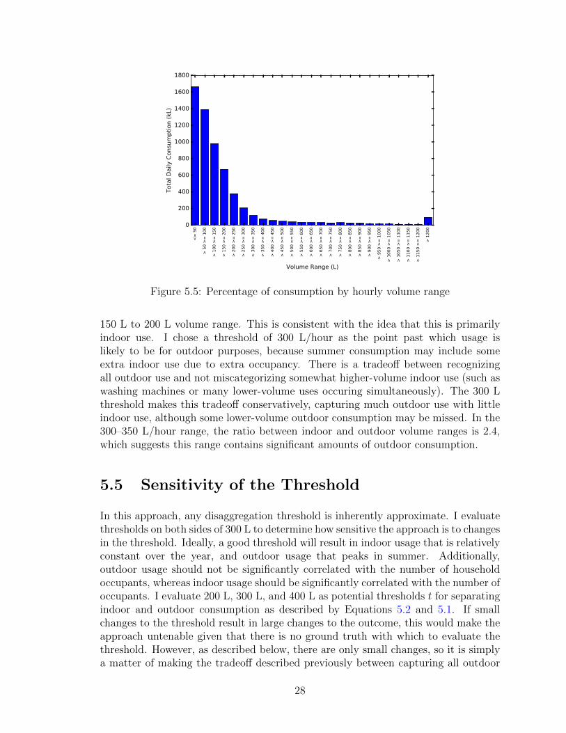
Total water consumption in the study dataset is 731 L/household/day for single-family units, or about 240 L/person/day. Typical indoor water consumption is 261L/person/day in North America [8]. Therefore, consumption significantly past thisrange in a single hour indicates this water is probably used at least partially forhigh-volume outdoor purposes.

Individual indoor end uses typically require smaller volumes of water than outdooruses such as irrigation, but they may be combined, especially during the morning andafternoon peaks in consumption. Tables 5.1 and 5.2 show volumes of water usedfor typical indoor uses, adapted from two versions of the Residential End Uses ofWater study in 1999 [8] and 2016 [62]. The shower water consumption includes bothtypical flow rate and typical duration of a shower. Faucet consumption is given asa flow rate because the volume per use varies by activity. Typical faucet usage was8.1 minutes/day in both versions of the study. Note that water consumption fordishwashers and clothes washers has significantly decreased between 1999 and 2016;data from both years are included for reference because rates of ownership of moreefficient appliances in Abbotsford are unknown.

Figure 5.5 shows the hourly consumption in each range. Consumption is concen-trated in the lower ranges: most consumption is the result of many households usingsmall amounts of water per hour, rather than more infrequent but higher-volumeconsumption. This indicates that, taken over the whole year, most consumption isfor (low-volume) indoor purposes which is consistent with Abbotsford’s temperateclimate.

26

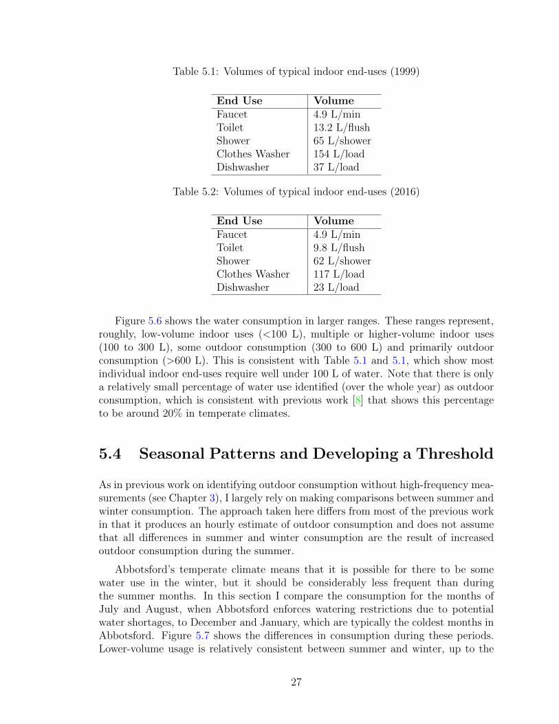
Table 5.1: Volumes of typical indoor end-uses (1999)

End Use VolumeFaucet 4.9 L/minToilet 13.2 L/flushShower 65 L/showerClothes Washer 154 L/loadDishwasher 37 L/load

Table 5.2: Volumes of typical indoor end-uses (2016)

End Use VolumeFaucet 4.9 L/minToilet 9.8 L/flushShower 62 L/showerClothes Washer 117 L/loadDishwasher 23 L/load

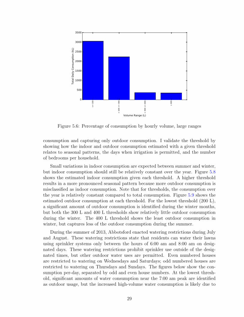
Figure 5.6 shows the water consumption in larger ranges. These ranges represent,roughly, low-volume indoor uses (<100 L), multiple or higher-volume indoor uses(100 to 300 L), some outdoor consumption (300 to 600 L) and primarily outdoorconsumption (>600 L). This is consistent with Table 5.1 and 5.1, which show mostindividual indoor end-uses require well under 100 L of water. Note that there is onlya relatively small percentage of water use identified (over the whole year) as outdoorconsumption, which is consistent with previous work [8] that shows this percentageto be around 20% in temperate climates.

5.4 Seasonal Patterns and Developing a Threshold

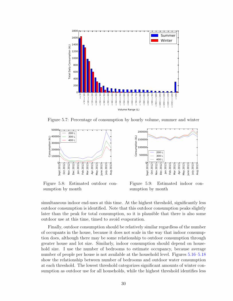
As in previous work on identifying outdoor consumption without high-frequency mea-surements (see Chapter 3), I largely rely on making comparisons between summer andwinter consumption. The approach taken here differs from most of the previous workin that it produces an hourly estimate of outdoor consumption and does not assumethat all differences in summer and winter consumption are the result of increasedoutdoor consumption during the summer.

Abbotsford’s temperate climate means that it is possible for there to be somewater use in the winter, but it should be considerably less frequent than duringthe summer months. In this section I compare the consumption for the months ofJuly and August, when Abbotsford enforces watering restrictions due to potentialwater shortages, to December and January, which are typically the coldest months inAbbotsford. Figure 5.7 shows the differences in consumption during these periods.Lower-volume usage is relatively consistent between summer and winter, up to the

27

<= 5

0

> 50

>=

100

> 10

0 >=

150

> 15

0 >=

200

> 20

0 >=

250

> 25

0 >=

300

> 30

0 >=

350

> 35

0 >=

400

> 40

0 >=

450

> 45

0 >=

500

> 50

0 >=

550

> 55

0 >=

600

> 60

0 >=

650

> 65

0 >=

700

> 70

0 >=

750

> 75

0 >=

800

> 80

0 >=

850

> 85

0 >=

900

> 90

0 >=

950

> 95

0 >=

100

0

> 10

00 >

= 10

50

> 10

50 >

= 11

00

> 11

00 >

= 11

50

> 11

50 >

= 12

00

> 12

00

Volume Range (L)

0

200

400

600

800

1000

1200

1400

1600

1800

Tota

l Dai

ly C

onsu

mpt

ion

(kL)

Figure 5.5: Percentage of consumption by hourly volume range

150 L to 200 L volume range. This is consistent with the idea that this is primarilyindoor use. I chose a threshold of 300 L/hour as the point past which usage islikely to be for outdoor purposes, because summer consumption may include someextra indoor use due to extra occupancy. There is a tradeoff between recognizingall outdoor use and not miscategorizing somewhat higher-volume indoor use (such aswashing machines or many lower-volume uses occuring simultaneously). The 300 Lthreshold makes this tradeoff conservatively, capturing much outdoor use with littleindoor use, although some lower-volume outdoor consumption may be missed. In the300–350 L/hour range, the ratio between indoor and outdoor volume ranges is 2.4,which suggests this range contains significant amounts of outdoor consumption.

5.5 Sensitivity of the Threshold

In this approach, any disaggregation threshold is inherently approximate. I evaluatethresholds on both sides of 300 L to determine how sensitive the approach is to changesin the threshold. Ideally, a good threshold will result in indoor usage that is relativelyconstant over the year, and outdoor usage that peaks in summer. Additionally,outdoor usage should not be significantly correlated with the number of householdoccupants, whereas indoor usage should be significantly correlated with the number ofoccupants. I evaluate 200 L, 300 L, and 400 L as potential thresholds t for separatingindoor and outdoor consumption as described by Equations 5.2 and 5.1. If smallchanges to the threshold result in large changes to the outcome, this would make theapproach untenable given that there is no ground truth with which to evaluate thethreshold. However, as described below, there are only small changes, so it is simplya matter of making the tradeoff described previously between capturing all outdoor

28

<= 1

00

> 10

0 >=

300

> 30

0 >=

600

> 60

0

Volume Range (L)

0

500

1000

1500

2000

2500

3000

3500

Tota

l Dai

ly C

onsu

mpt

ion

(kL)

Figure 5.6: Percentage of consumption by hourly volume, large ranges

consumption and capturing only outdoor consumption. I validate the threshold byshowing how the indoor and outdoor consumption estimated with a given thresholdrelates to seasonal patterns, the days when irrigation is permitted, and the numberof bedrooms per household.

Small variations in indoor consumption are expected between summer and winter,but indoor consumption should still be relatively constant over the year. Figure 5.8shows the estimated indoor consumption given each threshold. A higher thresholdresults in a more pronounced seasonal pattern because more outdoor consumption ismisclassified as indoor consumption. Note that for thresholds, the consumption overthe year is relatively constant compared to total consumption. Figure 5.9 shows theestimated outdoor consumption at each threshold. For the lowest threshold (200 L),a significant amount of outdoor consumption is identified during the winter months,but both the 300 L and 400 L thresholds show relatively little outdoor consumptionduring the winter. The 400 L threshold shows the least outdoor consumption inwinter, but captures less of the outdoor consumption during the summer.

During the summer of 2013, Abbotsford enacted watering restrictions during Julyand August. These watering restrictions state that residents can water their lawnsusing sprinkler systems only between the hours of 6:00 am and 8:00 am on desig-nated days. These watering restrictions prohibit sprinkler use outside of the desig-nated times, but other outdoor water uses are permitted. Even numbered housesare restricted to watering on Wednesdays and Saturdays; odd numbered houses arerestricted to watering on Thursdays and Sundays. The figures below show the con-sumption per-day, separated by odd and even house numbers. At the lowest thresh-old, significant amounts of water consumption near the 7:00 am peak are identifiedas outdoor usage, but the increased high-volume water consumption is likely due to

29

<= 5

0

> 50

>=

100

> 10

0 >=

150

> 15

0 >=

200

> 20

0 >=

250

> 25

0 >=

300

> 30

0 >=

350

> 35

0 >=

400

> 40

0 >=

450

> 45

0 >=

500

> 50

0 >=

550

> 55

0 >=

600

> 60

0 >=

650

> 65

0 >=

700

> 70

0 >=

750

> 75

0 >=

800

> 80

0 >=

850

> 85

0 >=

900

> 90

0 >=

950

> 95

0 >=

100

0

> 10

00 >

= 10

50

> 10

50 >

= 11

00

> 11

00 >

= 11

50

> 11

50 >

= 12

00

> 12

00

Volume Range (L)

0

200

400

600

800

1000

1200

1400

1600

1800

Tota

l Dai

ly C

onsu

mpt

ion

(kL)

SummerWinter

Figure 5.7: Percentage of consumption by hourly volume, summer and winter

Sept

201

2Oc

t 201

2No

v 20

12De

c 20

12Ja

n 20

13Fe

b 20

13M

ar 2

013

Apr 2

013

May

201

3Ju

ne 2

013

July

201

3Au

g 20

13

0

10000

20000

30000

40000

50000

Cons

umpt

ion

(kL)

200 L300 L400 L

Figure 5.8: Estimated outdoor con-sumption by month

Sept

201

2Oc

t 201

2No

v 20

12De

c 20

12Ja

n 20

13Fe

b 20

13M

ar 2

013

Apr 2

013

May

201

3Ju

ne 2

013

July

201

3Au

g 20

13

0

50000

100000

150000

200000Co

nsum

ptio

n (k

L)

200 L300 L400 L

Figure 5.9: Estimated indoor con-sumption by month

simultaneous indoor end-uses at this time. At the highest threshold, significantly lessoutdoor consumption is identified. Note that this outdoor consumption peaks slightlylater than the peak for total consumption, so it is plausible that there is also someoutdoor use at this time, timed to avoid evaporation.

Finally, outdoor consumption should be relatively similar regardless of the numberof occupants in the house, because it does not scale in the way that indoor consump-tion does, although there may be some relationship to outdoor consumption throughgreater house and lot size. Similarly, indoor consumption should depend on house-hold size. I use the number of bedrooms to estimate occupancy, because averagenumber of people per house is not available at the household level. Figures 5.16–5.18show the relationship between number of bedrooms and outdoor water consumptionat each threshold. The lowest threshold categorizes significant amounts of winter con-sumption as outdoor use for all households, while the highest threshold identifies less

30

0 5 10 15 20Hour

0

200

400

600

800

1000

1200

Cons

umpt

ion

(kL)

MondayTuesdayWednesdayThursdayFridaySaturdaySunday

Figure 5.10: Odd-numbered houses, 200 Lthreshold

0 5 10 15 20Hour

0

200

400

600

800

1000

1200

Cons

umpt

ion

(kL)

MondayTuesdayWednesdayThursdayFridaySaturdaySunday

Figure 5.11: Odd-numbered houses, 300 Lthreshold

0 5 10 15 20Hour

0

200

400

600

800

1000

1200

Cons

umpt

ion

(kL)

MondayTuesdayWednesdayThursdayFridaySaturdaySunday

Figure 5.12: Odd-numbered houses, 400 Lthreshold

31

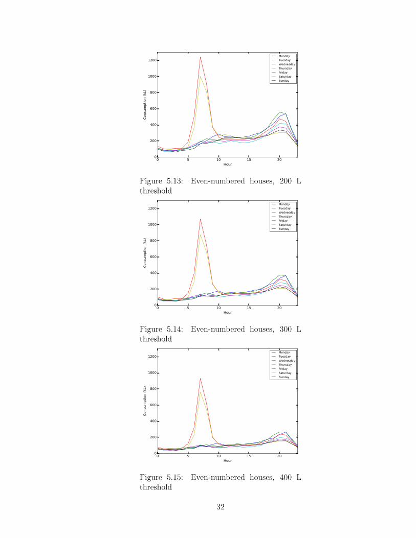
0 5 10 15 20Hour

0

200

400

600

800

1000

1200

Cons

umpt

ion

(kL)

MondayTuesdayWednesdayThursdayFridaySaturdaySunday

Figure 5.13: Even-numbered houses, 200 Lthreshold

0 5 10 15 20Hour

0

200

400

600

800

1000

1200

Cons

umpt

ion

(kL)

MondayTuesdayWednesdayThursdayFridaySaturdaySunday

Figure 5.14: Even-numbered houses, 300 Lthreshold

0 5 10 15 20Hour

0

200

400

600

800

1000

1200

Cons

umpt

ion

(kL)

MondayTuesdayWednesdayThursdayFridaySaturdaySunday

Figure 5.15: Even-numbered houses, 400 Lthreshold

32

outdoor consumption in the summer without significantly decreasing the amount ofoutdoor consumption identified in the winter. At the middle threshold, the outdoorconsumption is relatively constant for all numbers of bedrooms, which is consistentwith the idea that outdoor consumption should vary less by household size than indoorconsumption. Figures 5.19–5.21 show the relationship between number of bedroomsand indoor consumption, which for all household sizes is more consistent over the yearthan outdoor consumption. Note that on average, households with more bedroomshave higher indoor water consumption.

The previous discussion shows that while the threshold is relatively robust tochanges, raising or lowering the threshold from 300 L means potentially miscategoriz-ing more indoor use or not identifying significant amounts of outdoor use. Therefore,I use a 300 L threshold for identifying outdoor water consumption in the rest of thethesis. Based on Equation 5.1, the outdoor consumption at each hour (in litres) isnow defined as:

youtdoor = max (ytotal − 300, 0). (5.3)

5.6 Peak and Average Consumption

While the total amount of outdoor consumption identified is relatively low, this es-timation of outdoor water consumption is still useful because outdoor consumptioncontributes proportionally more to peak consumption than to average consumption.Figure 5.22 shows the indoor and outdoor consumption at the peak hour and onaverage. Note that indoor consumption is also greater at the peak hour becausethe average hour includes overnight consumption, which is low in all volume ranges.Figure 5.23 shows the consumption on the peak day. While outdoor consumption isrelatively low, even on the peak day, the greater variability in outdoor consumptionbetween the average and peak days means that it is useful to be able to estimate thisconsumption.

5.7 Summary

In this chapter, I described a method of estimating outdoor water consumption fromhourly data by setting an upper threshold on plausible indoor consumption. I showedthat this threshold is relatively robust to changes, and chose 300 L/hour as a thresholdfor the remaining work. I also showed that the contribution of outdoor consumptionto total consumption is relatively greater for peak periods of use than it is for average-use periods.

In the next chapter, I take the estimate of outdoor consumption produced usingthis method and create a model to predict hourly outdoor water consumption.

33

Sept

201

2

Oct 2

012

Nov

2012

Dec

2012

Jan

2013

Feb

2013

Mar

201

3

Apr 2

013

May

201

3

June

201

3

July

201

3

Aug

2013

0

1

2

3

4

5

6

Cons

umpt

ion

Per H

ouse

hold

(kL)

200.0 L300.0 L400.0 L

Figure 5.16: Outdoor consumption, 1 and 2bedroom houses

Sept

201

2

Oct 2

012

Nov

2012

Dec

2012

Jan

2013

Feb

2013

Mar

201

3

Apr 2

013

May

201

3

June

201

3

July

201

3

Aug

2013

0

1

2

3

4

5

6

Cons

umpt

ion

Per H

ouse

hold

(kL)

200.0 L300.0 L400.0 L

Figure 5.17: Outdoor consumption, 3 bedroomhouses

Sept

201

2

Oct 2

012

Nov

2012

Dec

2012

Jan

2013

Feb

2013

Mar

201

3

Apr 2

013

May

201

3

June

201

3

July

201

3

Aug

2013

0

1

2

3

4

5

6

Cons

umpt

ion

Per H

ouse

hold

(kL)

200.0 L300.0 L400.0 L

Figure 5.18: Outdoor consumption, 4-plus bed-room houses

34

Sept

201

2

Oct 2

012

Nov

2012

Dec

2012

Jan

2013

Feb

2013

Mar

201

3

Apr 2

013

May

201

3

June

201

3

July

201

3

Aug

2013

0

5

10

15

20

Cons

umpt

ion

Per H

ouse

hold

(kL)

200.0 L300.0 L400.0 L

Figure 5.19: Indoor consumption, 1 and 2 bed-room houses

Sept

201

2

Oct 2

012

Nov

2012

Dec

2012

Jan

2013

Feb

2013

Mar

201

3

Apr 2

013

May

201

3

June

201

3

July

201

3

Aug

2013

0

5

10

15

20

Cons

umpt

ion

Per H

ouse

hold

(kL)

200.0 L300.0 L400.0 L

Figure 5.20: Indoor consumption, 3 bedroomhouses

Sept

201

2

Oct 2

012

Nov

2012

Dec

2012

Jan

2013

Feb

2013

Mar

201

3

Apr 2

013

May

201

3

June

201

3

July

201

3

Aug

2013

0

5

10

15

20

25

Cons

umpt

ion

Per H

ouse

hold

(kL)

200.0 L300.0 L400.0 L

Figure 5.21: Indoor consumption, 4-plus bed-room houses

35

Peak Hour Average Hour0

100

200

300

400

500

600

Cons

umpt

ion

(kL)

IndoorOutdoor

Figure 5.22: Peak and average hour consumption

Peak Day Average Day0

1000

2000

3000

4000

5000

6000

7000

8000

Cons

umpt

ion

(kL)

IndoorOutdoor

Figure 5.23: Peak and average day consumption

36

Chapter 6

Predicting Outdoor WaterConsumption

In this chapter, I present a model for predicting outdoor hourly water consump-tion, and discuss the challenges of this prediction task by comparing to a modelfor prediction of total outdoor consumption. The prediction task described in thischapter differs from previous work in that it attempts to predict disaggregated out-door rather than total consumption, and additionally predicts over a smaller spatialscale than does most previous work. Previous work has found similar difficulties withpredictability for single-household consumption [46].

Accurate prediction of outdoor water consumption would be useful for short-termmanagement in that it could be used to better estimate the effects of variationsin weather and of restrictions on short-term water consumption. I focus on hourlyprediction because, although daily prediction would be more useful for managingwater restrictions, daily consumption appears to be more unpredictable. I use a modelbased on ensembles of regression trees in order to maintain some interpretability ofthe models because knowing the determinants of hourly water consumption would beuseful for planning. Previous work has found good results with ensembles of trees forpredicting total water consumption [44].

6.1 Problem Definition and Model Structure

The prediction task is essentially time series prediction and can be formulated as a su-pervised learning task (see Chapter 2). Previous measurements of water consumptionand additional features are used to predict the next hour’s water consumption.

I develop models for predicting outdoor hourly water consumption for individualdissemination areas. The water consumption is normalized by dividing by the numberof households in the dissemination area so that the models will not have to take intoaccount the varying sizes of disseminations areas, and only the 77 dissemination areaswith greater than 50 single-family residences are included. Only summer consumption

37

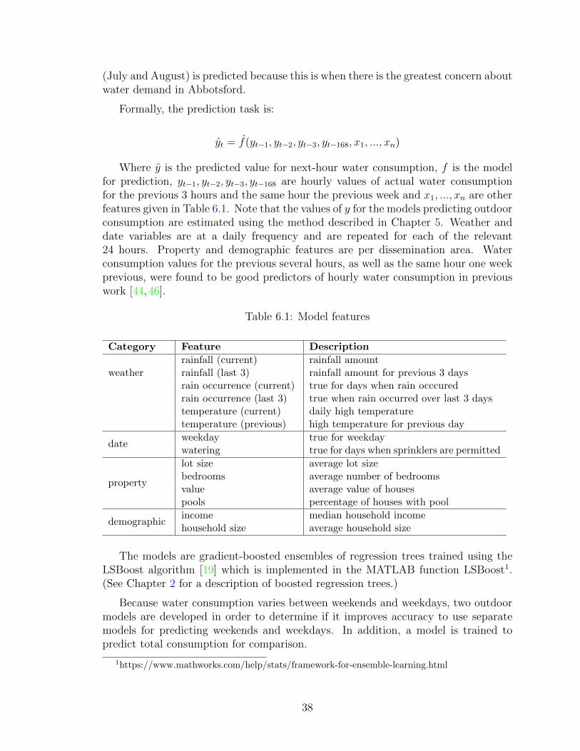
(July and August) is predicted because this is when there is the greatest concern aboutwater demand in Abbotsford.

Formally, the prediction task is:

yt = f(yt−1, yt−2, yt−3, yt−168, x1, ..., xn)

Where y is the predicted value for next-hour water consumption, f is the modelfor prediction, yt−1, yt−2, yt−3, yt−168 are hourly values of actual water consumptionfor the previous 3 hours and the same hour the previous week and x1, ..., xn are otherfeatures given in Table 6.1. Note that the values of y for the models predicting outdoorconsumption are estimated using the method described in Chapter 5. Weather anddate variables are at a daily frequency and are repeated for each of the relevant24 hours. Property and demographic features are per dissemination area. Waterconsumption values for the previous several hours, as well as the same hour one weekprevious, were found to be good predictors of hourly water consumption in previouswork [44,46].

Table 6.1: Model features

Category Feature Description

weatherrainfall (current) rainfall amountrainfall (last 3) rainfall amount for previous 3 daysrain occurrence (current) true for days when rain occcuredrain occurrence (last 3) true when rain occurred over last 3 daystemperature (current) daily high temperaturetemperature (previous) high temperature for previous day

dateweekday true for weekdaywatering true for days when sprinklers are permitted

property

lot size average lot sizebedrooms average number of bedroomsvalue average value of housespools percentage of houses with pool

demographicincome median household incomehousehold size average household size

The models are gradient-boosted ensembles of regression trees trained using theLSBoost algorithm [19] which is implemented in the MATLAB function LSBoost1.(See Chapter 2 for a description of boosted regression trees.)

Because water consumption varies between weekends and weekdays, two outdoormodels are developed in order to determine if it improves accuracy to use separatemodels for predicting weekends and weekdays. In addition, a model is trained topredict total consumption for comparison.

1https://www.mathworks.com/help/stats/framework-for-ensemble-learning.html

38

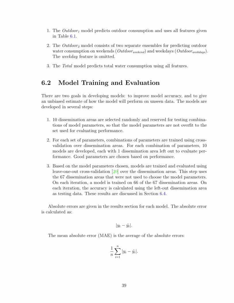
1. The Outdoor1 model predicts outdoor consumption and uses all features givenin Table 6.1.

2. The Outdoor2 model consists of two separate ensembles for predicting outdoorwater consumption on weekends (Outdoorweekend) and weekdays (Outdoorweekdays).The weekday feature is omitted.

3. The Total model predicts total water consumption using all features.

6.2 Model Training and Evaluation

There are two goals in developing models: to improve model accuracy, and to givean unbiased estimate of how the model will perform on unseen data. The models aredeveloped in several steps:

1. 10 dissemination areas are selected randomly and reserved for testing combina-tions of model parameters, so that the model parameters are not overfit to theset used for evaluating performance.

2. For each set of parameters, combinations of parameters are trained using cross-validation over dissemination areas. For each combination of parameters, 10models are developed, each with 1 dissemination area left out to evaluate per-formance. Good parameters are chosen based on performance.

3. Based on the model parameters chosen, models are trained and evaluated usingleave-one-out cross-validation [20] over the dissemination areas. This step usesthe 67 dissemination areas that were not used to choose the model parameters.On each iteration, a model is trained on 66 of the 67 dissemination areas. Oneach iteration, the accuracy is calculated using the left-out dissemination areaas testing data. These results are discussed in Section 6.4.

Absolute errors are given in the results section for each model. The absolute erroris calculated as:

|yt − yt|.

The mean absolute error (MAE) is the average of the absolute errors:

1

n

n∑i=1

|yi − yi|.

39

6.3 Parameter Selection

Based on the reserved set of 10 dissemination areas discussed previously, I chose valuesfor two parameters that are likely to produce good performance on the remainingdissemination areas. I optimized over two parameters: maximum number of splitsper tree, and the number of trees per ensemble. The maximum number of splitsis the total number of non-leaf nodes in the tree. Figure 6.1 shows the accuracyover these parameters, for the Outdoor1 model. While the strictly optimal valuefor the maximum number of splits is 2, the accuracy is relatively sensitive to thenumber of trees in the ensemble. I instead chose 1 split and 80 trees per ensemblebecause the performance is not significantly affected by the ensemble size past thatpoint, suggesting those parameters will result in more stable performance for the finalmodels. While it would have been ideal to perform parameter selection within themain cross-validation step and choose the optimal value on each iteration, it wasprohibitively slow.

I chose the same parameters for all models. The maximum number of splits is alsonot strictly optimal for the other models, however it was similarly close-to-optimaland chosen because the accuracy was less sensitive to variation in the ensemble sizeand therefore likely to transfer better to the remaining data.

Number of Trees10 20 30 40 50 60 70 80 90 100

MS

E

#10 -5

2.2

2.3

2.4

2.5

2.6

2.7

2.8

2.9

3

3.1

3.212345

Max Splits

Figure 6.1: MSE for number of trees and maximum number of splits used as modelparameters

6.4 Results

In this section I compare results for all models, and although the predictive accuracyis not high, the comparison with total consumption gives insights into why this is the

40

case.

While the outdoor models show a general ability to predict the direction of con-sumption, they do not perform well at predicting the magnitude of consumption,especially for high values. Previous work with predicting individual consumption hadsimilar difficulties with predicting the magnitude of peaks [46]. Figure 6.2 shows thepredicted outdoor consumption for the largest dissemination area. Note that the pre-diction of peaks is often one sample late, because as discussed in the next section, themodel predicts largely based on the previous hour’s consumption. Figure 6.3 showsthe predicted total consumption for the same dissemination area. Although overallperformance is better for total consumption, the model still fails to predict the mag-nitude of the morning and afternoon consumption peaks accurately, and sharp peaksin consumption are typically not predicted accurately.

Hour10 20 30 40 50 60 70

Con

sum

ptio

n P

er H

ouse

hold

(kL

)

0

0.005

0.01

0.015

0.02

0.025

0.03

0.035

0.04

Figure 6.2: Prediction of Outdoor1 compared to actual value for the largest dissemi-nation area in the first 3 days of July. The orange line is the predicted consumptionvalue and the blue line is the actual value.

Tables 6.2–6.4 show the errors in kilolitres for each model type. The tables shouldbe interpreted in the light of the fact that the model predicts mean water consump-tion per household in a dissemination area. Although the model errors are small inabsolute terms, they become more significant in terms of the average hourly valuesof 0.0045 kL (4.5 L) for outdoor water consumption and 0.0353 kL (35.3 L) for totalwater consumption. Note that for both types of consumption, the average errors aresignificantly higher than the median, suggesting that the poor performance is in largepart due to large errors rather than many small errors.

The overall error for both the Outdoor1 and Outdoor2 models are similar, de-spite performance being significantly worse on the weekends. A potential reason thatseparate models are not useful is discussed in the next section.

41

Hour10 20 30 40 50 60 70

Con

sum

ptio

n P

er H

ouse

hold

(kL

)

0

0.01

0.02

0.03

0.04

0.05

0.06

0.07

0.08

Figure 6.3: Prediction of Total compared to actual value for the largest disseminationarea in the first 3 days of July. The orange line is the predicted consumption valueand the blue line is the actual value.

Weekends and watering days when sprinkling is permitted have high errors for allmodels. This suggests that this variability is hard to predict.

Table 6.2: Absolute errors for Outdoor1 (kL)

average median 75th percentile 90th percentileoverall 5.054× 10−3 2.819× 10−3 6.453× 10−3 1.212× 10−2

weekdays 4.877× 10−3 2.752× 10−3 6.281× 10−3 1.178× 10−2

weekends 5.558× 10−3 3.027× 10−3 7.010× 10−3 1.330× 10−2

watering 5.407× 10−3 3.040× 10−3 6.890× 10−3 1.281× 10−2

no watering 4.612× 10−3 2.572× 10−3 5.938× 10−3 1.134× 10−2

The prediction accuracy varies significantly by hour. Figures 6.4–6.7 show theMAE by hour. Note that in all cases the error is highest at the morning peak,which probably is related to more variability in consumption during these times. Inaddition, even predicting total water consumption for the summer is more difficultthan it would be for winter consumption due to higher variability, which explains therelatively low accuracy.

6.5 Interpretability

Ensembles of regression trees were selected as a model because of their relative in-terpretability compared to, for example, neural network models. However, ensembles

42

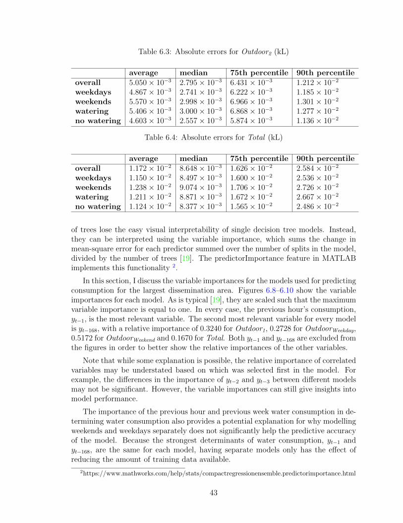
Table 6.3: Absolute errors for Outdoor2 (kL)

average median 75th percentile 90th percentileoverall 5.050× 10−3 2.795× 10−3 6.431× 10−3 1.212× 10−2

weekdays 4.867× 10−3 2.741× 10−3 6.222× 10−3 1.185× 10−2

weekends 5.570× 10−3 2.998× 10−3 6.966× 10−3 1.301× 10−2

watering 5.406× 10−3 3.000× 10−3 6.868× 10−3 1.277× 10−2

no watering 4.603× 10−3 2.557× 10−3 5.874× 10−3 1.136× 10−2

Table 6.4: Absolute errors for Total (kL)

average median 75th percentile 90th percentileoverall 1.172× 10−2 8.648× 10−3 1.626× 10−2 2.584× 10−2

weekdays 1.150× 10−2 8.497× 10−3 1.600× 10−2 2.536× 10−2

weekends 1.238× 10−2 9.074× 10−3 1.706× 10−2 2.726× 10−2

watering 1.211× 10−2 8.871× 10−3 1.672× 10−2 2.667× 10−2

no watering 1.124× 10−2 8.377× 10−3 1.565× 10−2 2.486× 10−2

of trees lose the easy visual interpretability of single decision tree models. Instead,they can be interpreted using the variable importance, which sums the change inmean-square error for each predictor summed over the number of splits in the model,divided by the number of trees [19]. The predictorImportance feature in MATLABimplements this functionality 2.

In this section, I discuss the variable importances for the models used for predictingconsumption for the largest dissemination area. Figures 6.8–6.10 show the variableimportances for each model. As is typical [19], they are scaled such that the maximumvariable importance is equal to one. In every case, the previous hour’s consumption,yt−1, is the most relevant variable. The second most relevant variable for every modelis yt−168, with a relative importance of 0.3240 for Outdoor1, 0.2728 for OutdoorWeekday,0.5172 for OutdoorWeekend and 0.1670 for Total. Both yt−1 and yt−168 are excluded fromthe figures in order to better show the relative importances of the other variables.

Note that while some explanation is possible, the relative importance of correlatedvariables may be understated based on which was selected first in the model. Forexample, the differences in the importance of yt−2 and yt−3 between different modelsmay not be significant. However, the variable importances can still give insights intomodel performance.

The importance of the previous hour and previous week water consumption in de-termining water consumption also provides a potential explanation for why modellingweekends and weekdays separately does not significantly help the predictive accuracyof the model. Because the strongest determinants of water consumption, yt−1 andyt−168, are the same for each model, having separate models only has the effect ofreducing the amount of training data available.

2https://www.mathworks.com/help/stats/compactregressionensemble.predictorimportance.html

43

hour (0 = 12:00 am)0 5 10 15 20

MA

E

0

0.002

0.004

0.006

0.008

0.01

0.012

Figure 6.4: MAE per hour for Outdoor1

While the importance of other variables is very small compared to the previousvalues of water consumption, some variables show up consistently for all models.Weather-related features appear in all models, and although their importance is veryminor compared to yt−1 and yt−168, an influence from both temperature and rainfallis consistent with previous work on total water consumption [8, 36, 59, 60]. Housevalue appears in the explanatory variables for all models, and median income ap-pears for OutdoorWeekend and OutdoorWeekday. Although previous work has focusedon the influence of income on both total water consumption [63] and seasonal waterconsumption [59], the inclusion of house value in all models is consistent with theidea that income has only an indirect influence through factors such as larger housesizes and greater ownership of water-using appliances and pools [57]. Household sizeor number of bedrooms also appear as slightly important in all models, althoughprevious work has found household size is only strongly correlated with indoor waterconsumption [8].

6.6 Discussion

It is not clear that the accuracy of the models presented are sufficiently high to beuseful in practice for day-to-day management of water systems, or that the models aresufficiently accurate to justify collecting the amount of additional data required be-yond previous water consumption values. The models discussed require demographicdata and property data, as well as previous temperature and rainfall information andweather forecasts. While the model does provide some ability to forecast next-houroutdoor consumption, the accuracy of any method has to be balanced against theresources required to create a forecast, including collecting the required data [6], and

44

hour (0 = 12:00 am)0 5 10 15 20

MA

E

0

0.002

0.004

0.006

0.008

0.01

0.012

0.014

0.016

0.018

Figure 6.5: MAE per hour for Total

particularly for short-term forecasts used for operational purposes, the additionaldata required creates practical difficulties [9]. The regression tree models were chosenin order to allow interpretability, but the only features that are highly importantin reducing model error are previous values of water consumption. It may be thecase that accuracy could be improved by adding additional features or by choosinga different machine learning method, but to be practically useful the benefits of themodelling method would need to be balanced against the resources required for theforecast.

Additionally, it would be more useful to be able to predict outdoor water con-sumption further in advance, such as 24 hours ahead, or to be able to predict dailyconsumption (ideally several days ahead). This would be useful for making changesto watering restrictions [2]. I found in preliminary work that daily consumption isvery difficult to predict as compared to hourly consumption, and this seems to berelated to the fact that previous-day and current-day consumption are less correlatedthan previous-hour and current-hour consumption.

If more data were available, it would also be informative to further aggregatethe data in order to determine how large neighbourhoods must be for outdoor waterconsumption to be accurately predicted. However, given the number of single-familyresidences in the study and the single-year timespan for the water consumption mea-surements, significant aggregation would not leave enough data for training a model.There also appears to be significant individual variability in outdoor water consump-tion (see Chapter 7), which likely constrains predictability except for very large neigh-bourhoods because the average outdoor water consumption for a dissemination areacan be significantly affected by a small number of consumers. Previous work hasfound that even for entire cities, population size influences the accuracy of predic-

45

hour (0 = 12:00 am)0 5 10 15 20

MA

E

0

0.001

0.002

0.003

0.004

0.005

0.006

0.007

0.008

0.009

Figure 6.6: MAE per hour for Outdoorweekday

tion for total water consumption [43], and the difficulty of predicting outdoor waterconsumption for small neighbourhoods is consistent with that observation.

6.7 Summary

In this chapter, I presented a model for predicting outdoor water consumption, how-ever it is not clear if the model’s accuracy is sufficiently high to be useful for day-to-daymanagement of water systems. I also discussed some of the predictive factors in themodels developed.

In the next section, I discuss the explanatory factors for outdoor water consump-tion over the entire summer.

46

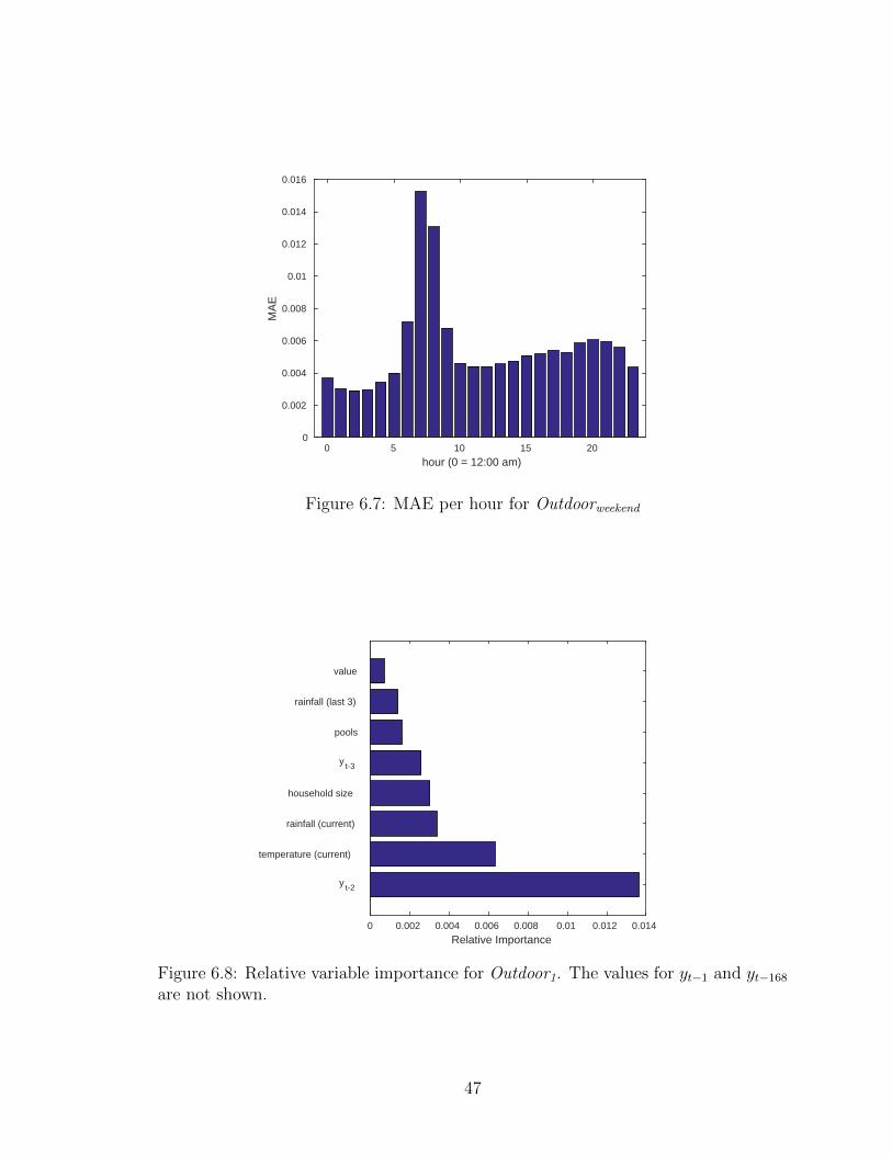
hour (0 = 12:00 am)0 5 10 15 20

MA

E

0

0.002

0.004

0.006

0.008

0.01

0.012

0.014

0.016

Figure 6.7: MAE per hour for Outdoorweekend

Relative Importance0 0.002 0.004 0.006 0.008 0.01 0.012 0.014

y t-2

temperature (current)

rainfall (current)

household size

y t-3

pools

rainfall (last 3)

value

Figure 6.8: Relative variable importance for Outdoor1. The values for yt−1 and yt−168are not shown.

47

Relative Importance0 0.002 0.004 0.006 0.008 0.01

y t-2

temperature (current)

rainfall (current)

household size

rain occurrence (current)

y t-3

pools

temperature (prev)

value

rainfall (last 3)

median income

rain occurrence (last 3)

watering

bedrooms

Figure 6.9: Relative variable importance for Outdoorweekday. The values for yt−1 andyt−168 are not shown.

Relative Importance0 0.005 0.01 0.015 0.02 0.025 0.03 0.035

y t-2

temperature (current)

y t-3

household size

temperature (prev)

rainfall (last 3)

pools

value

bedrooms

rainfall (current)

lot size

median income

Figure 6.10: Relative variable importance for Outdoorweekend. The values for yt−1 andyt−168 are not shown.

48

Relative Importance0 0.005 0.01 0.015

y t-3

temperature (current)

y t-2

temperature (prev)

rain occurrence (current)

bedrooms

household size

rain occurrence (last 3)

value

Figure 6.11: Relative variable importance for Total. The values for yt−1 and yt−168are not shown.

49

Chapter 7

Explaining Outdoor WaterConsumption

The City of Abbotsford is particularly interested in the determinants of outdoor waterconsumption. Explainable variation in outdoor water consumption between house-holds or between neighbourhoods can be used for demand management and planningwatering restrictions [2]. In this chapter, I explain how outdoor water consumption(estimated as described in Chapter 5) during the study period in Abbotsford is relatedto weather, household income, lot size, and pool ownership. I also show that there isa large amount of variability between households, with a relatively small percentageof households consuming the majority of water used outdoors.

7.1 Statistical Methods

In the following analysis, linear regression is used to model the relationship betweenoutdoor water consumption and demographic and property variables. The correlationcoefficient (r) shows the strength of the linear relationship between variables. Inter-preting the correlation coefficient requires several assumptions about the underlyingdata: the residuals (model errors) should have zero mean and constant variance, andbe normally distributed and independent [64]. It was determined by visual observa-tion of the data that these assumptions do not hold for all of the data in this chapter;the correlation coefficients from linear regression are given regardless for comparisonwith previous work, and it is noted where they may not be reliable. To strengthen theresults, Spearman’s rank correlation coefficient (ρ) is also used to show the strengthof a monotonic (rather than linear) relationship between two variables and does notrequire the same assumptions.

50

7.2 Temperature and Rainfall

Previous work has shown that water consumption depends on temperature and rain-fall (see Chapter 3), and that the sensitivity of water consumption to variation inweather is not consistent across the year but is highest during the summer [36,59,60].The analysis in this section is restricted to the summer because only a single year ofdata is available, so it is hard to otherwise separate the effects of changes in weatherfrom unrelated seasonal effects over the year. Further, I only consider the highest-usage months (July and August) because the watering restrictions in these monthsmake it difficult to directly compare the effects of temperature and rainfall relativeto the other summer months.

July

1

Aug

1

Aug

300

5

10

15

20

25

Rain

fall

(mm

)

0

500

1000

1500

2000

Cons

umpt

ion

(kL)

Figure 7.1: Rainfall and outdoor water consumption for all households in July andAugust 2013

Because a major source of outdoor water demand is irrigation, it is expected thatoutdoor water consumption will decrease with rainfall. There are clear decreases inoutdoor consumption when rainfall occurs, as shown in Figure 7.1. Despite similaraverage temperatures (19.4 ◦C and 19.1 ◦C), the total outdoor consumption for July2013 was 1037 kL. compared to 698 kL a day in August 2013. This can be explainedby the significantly higher and more frequent rainfall in August (57 mm over 9 days) ascompared to in July (1.6 mm on a single day). Although total rainfall in both monthsis relatively low, the drop in outdoor consumption during August is consistent withprevious work that suggests the occurence of rainfall (at a weekly timescale) has moreeffect on water consumption than the amount of rainfall [41].

There is a weak positive correlation (ρ = 0.401, r = 0.409) between tempera-ture and outdoor water consumption during July and August. Figure 7.2 shows thetemperature and total water consumption for July and August 2013, and Figure 7.3

51

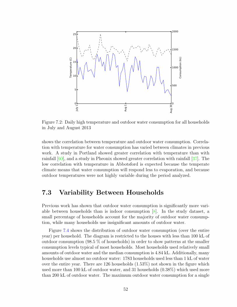
July

1

Aug

1

Aug

30

0

5

10

15

20

25

Tem

pera

ture

(C)

0

500

1000

1500

2000

Cons

umpt

ion

(kL)

Figure 7.2: Daily high temperature and outdoor water consumption for all householdsin July and August 2013

shows the correlation between temperature and outdoor water consumption. Correla-tion with temperature for water consumption has varied between climates in previouswork. A study in Portland showed greater correlation with temperature than withrainfall [60], and a study in Pheonix showed greater correlation with rainfall [37]. Thelow correlation with temperature in Abbotsford is expected because the temperateclimate means that water consumption will respond less to evaporation, and becauseoutdoor temperatures were not highly variable during the period analyzed.

7.3 Variability Between Households

Previous work has shown that outdoor water consumption is significantly more vari-able between households than is indoor consumption [8]. In the study dataset, asmall percentage of households account for the majority of outdoor water consump-tion, while many households use insignificant amounts of outdoor water.

Figure 7.4 shows the distribution of outdoor water consumption (over the entireyear) per household. The diagram is restricted to the houses with less than 100 kL ofoutdoor consumption (98.5 % of households) in order to show patterns at the smallerconsumption levels typical of most households. Most households used relatively smallamounts of outdoor water and the median consumption is 4.84 kL. Additionally, manyhouseholds use almost no outdoor water: 1783 households used less than 1 kL of waterover the entire year. There are 126 households (1.53%) not shown in the figure whichused more than 100 kL of outdoor water, and 31 households (0.38%) which used morethan 200 kL of outdoor water. The maximum outdoor water consumption for a single

52

14 16 18 20 22 24 26Temperature (C)

0

200

400

600

800

1000

1200

1400

1600

Cons

umpt

ion

(kL)

r^2 = 0.1671

Figure 7.3: Correlation between temperature and daily outdoor water consumptionin July and August 2013

household is 1024 kL, about 210 times the median consumption.

In comparison, indoor water consumption is much less variable between house-holds. Figure 7.5 shows the indoor consumption for all single-family households.The maximum indoor consumption for a household is only 7.9 times the median con-sumption. Similarly, the ratio between the median and the 95th percentile value is 2.4compared to 10.9 for outdoor consumption. The relatively low variability of indoorconsumption is consistent with the idea that indoor usage is primarily determinedby the number of people in the household. Even with some additional variation inindoor usage, such as due to water-conserving behaviours or appliance stock, lessbetween-household variation is expected than with outdoor consumption [8].

By ordering the households by their total consumption, it is possible to show how

0 20 40 60 80 100Outdoor Water Consumption (kL)

0500

1000150020002500300035004000

Hous

ehol

ds

Figure 7.4: Histogram of outdoor wa-ter consumption

400 800 1200 1600Indoor Water Consumption (kL)

0

500

1000

1500

2000

2500

Hous

ehol

ds

Figure 7.5: Histogram of indoor waterconsumption

53

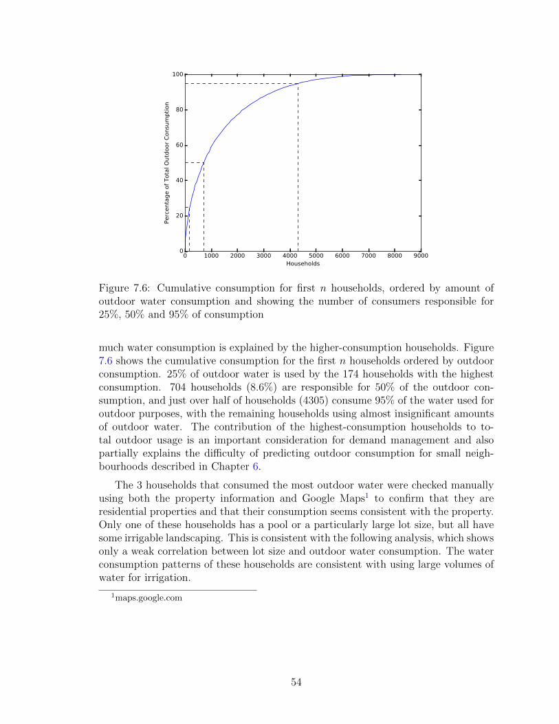
0 1000 2000 3000 4000 5000 6000 7000 8000 9000Households

0

20

40

60

80

100

Perc

enta

ge o

f Tot

al O

utdo

or C

onsu

mpt

ion

Figure 7.6: Cumulative consumption for first n households, ordered by amount ofoutdoor water consumption and showing the number of consumers responsible for25%, 50% and 95% of consumption

much water consumption is explained by the higher-consumption households. Figure7.6 shows the cumulative consumption for the first n households ordered by outdoorconsumption. 25% of outdoor water is used by the 174 households with the highestconsumption. 704 households (8.6%) are responsible for 50% of the outdoor con-sumption, and just over half of households (4305) consume 95% of the water used foroutdoor purposes, with the remaining households using almost insignificant amountsof outdoor water. The contribution of the highest-consumption households to to-tal outdoor usage is an important consideration for demand management and alsopartially explains the difficulty of predicting outdoor consumption for small neigh-bourhoods described in Chapter 6.

The 3 households that consumed the most outdoor water were checked manuallyusing both the property information and Google Maps1 to confirm that they areresidential properties and that their consumption seems consistent with the property.Only one of these households has a pool or a particularly large lot size, but all havesome irrigable landscaping. This is consistent with the following analysis, which showsonly a weak correlation between lot size and outdoor water consumption. The waterconsumption patterns of these households are consistent with using large volumes ofwater for irrigation.

1maps.google.com

54

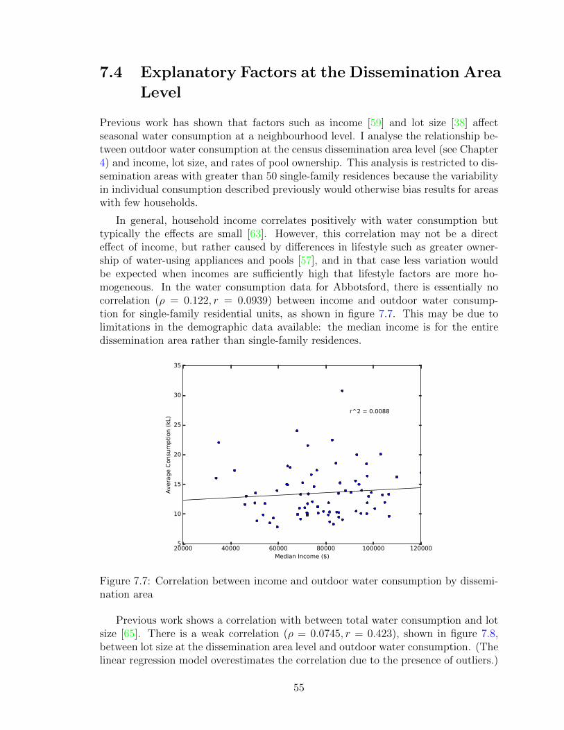
7.4 Explanatory Factors at the Dissemination Area

Level

Previous work has shown that factors such as income [59] and lot size [38] affectseasonal water consumption at a neighbourhood level. I analyse the relationship be-tween outdoor water consumption at the census dissemination area level (see Chapter4) and income, lot size, and rates of pool ownership. This analysis is restricted to dis-semination areas with greater than 50 single-family residences because the variabilityin individual consumption described previously would otherwise bias results for areaswith few households.

In general, household income correlates positively with water consumption buttypically the effects are small [63]. However, this correlation may not be a directeffect of income, but rather caused by differences in lifestyle such as greater owner-ship of water-using appliances and pools [57], and in that case less variation wouldbe expected when incomes are sufficiently high that lifestyle factors are more ho-mogeneous. In the water consumption data for Abbotsford, there is essentially nocorrelation (ρ = 0.122, r = 0.0939) between income and outdoor water consump-tion for single-family residential units, as shown in figure 7.7. This may be due tolimitations in the demographic data available: the median income is for the entiredissemination area rather than single-family residences.

20000 40000 60000 80000 100000 120000Median Income ($)

5

10

15

20

25

30

35

Aver

age

Cons

umpt

ion

(kL)

r^2 = 0.0088

Figure 7.7: Correlation between income and outdoor water consumption by dissemi-nation area

Previous work shows a correlation with between total water consumption and lotsize [65]. There is a weak correlation (ρ = 0.0745, r = 0.423), shown in figure 7.8,between lot size at the dissemination area level and outdoor water consumption. (Thelinear regression model overestimates the correlation due to the presence of outliers.)

55

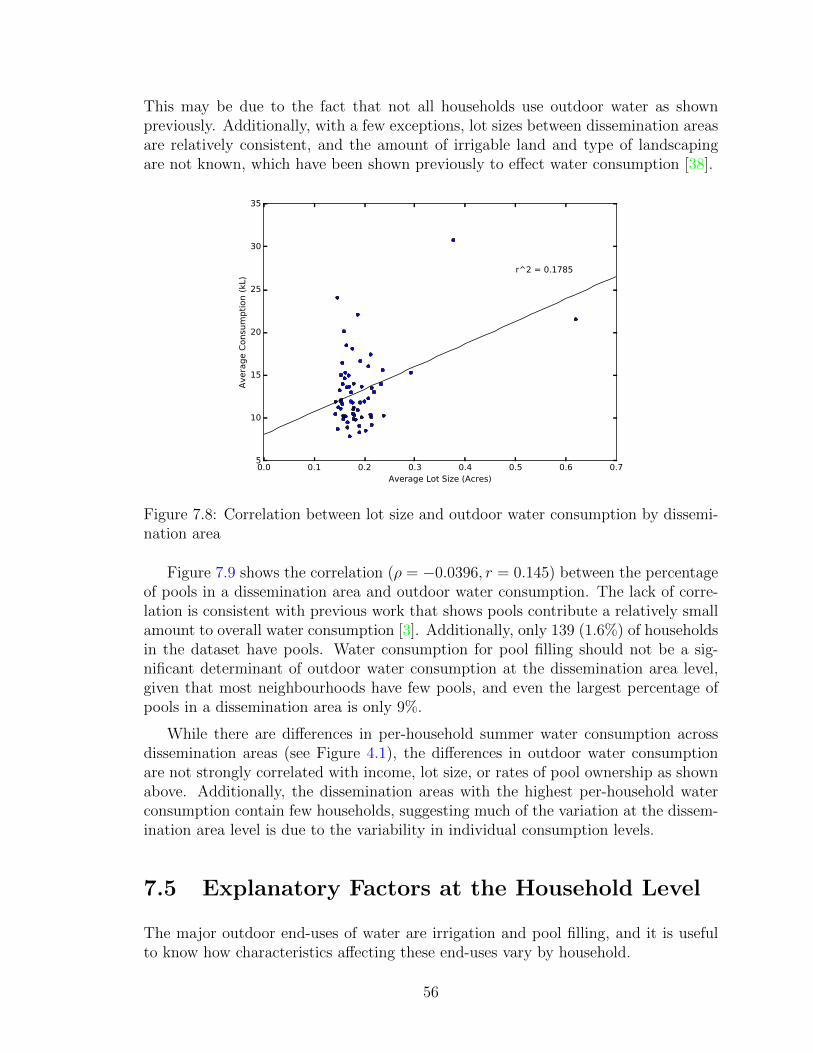
This may be due to the fact that not all households use outdoor water as shownpreviously. Additionally, with a few exceptions, lot sizes between dissemination areasare relatively consistent, and the amount of irrigable land and type of landscapingare not known, which have been shown previously to effect water consumption [38].

0.0 0.1 0.2 0.3 0.4 0.5 0.6 0.7Average Lot Size (Acres)

5

10

15

20

25

30

35

Aver

age

Cons

umpt

ion

(kL)

r^2 = 0.1785

Figure 7.8: Correlation between lot size and outdoor water consumption by dissemi-nation area

Figure 7.9 shows the correlation (ρ = −0.0396, r = 0.145) between the percentageof pools in a dissemination area and outdoor water consumption. The lack of corre-lation is consistent with previous work that shows pools contribute a relatively smallamount to overall water consumption [3]. Additionally, only 139 (1.6%) of householdsin the dataset have pools. Water consumption for pool filling should not be a sig-nificant determinant of outdoor water consumption at the dissemination area level,given that most neighbourhoods have few pools, and even the largest percentage ofpools in a dissemination area is only 9%.

While there are differences in per-household summer water consumption acrossdissemination areas (see Figure 4.1), the differences in outdoor water consumptionare not strongly correlated with income, lot size, or rates of pool ownership as shownabove. Additionally, the dissemination areas with the highest per-household waterconsumption contain few households, suggesting much of the variation at the dissem-ination area level is due to the variability in individual consumption levels.

7.5 Explanatory Factors at the Household Level

The major outdoor end-uses of water are irrigation and pool filling, and it is usefulto know how characteristics affecting these end-uses vary by household.

56

0 1 2 3 4 5 6 7 8 9Percentage of Households With Pools

5

10

15

20

25

30

35

Aver

age

Cons

umpt

ion

(kL)

r^2 = 0.0211

Figure 7.9: Correlation between pool ownership and outdoor water consumption bydissemination area

While rates of pool ownership do not significantly affect outdoor water consump-tion at the dissemination area level, there are significant differences in water con-sumption between individual households with and without pools. As shown in Figure7.10, typical water consumption is much higher for households that have pools. Themedian consumption is 24.7 kL for households with pools and 4.7 kL for householdswithout pools. Additionally, there is greater variability in water consumption forthese households. These differences are obscured at the household level because ofthe relatively low rates of pool ownership in Abbotsford.

Assuming households used water for irrigation proportionally to lawn size, thereshould be some correlation between outdoor water consumption and lot size. How-ever, there is essentially no correlation (at the household level) in the dataset. Becausemany households do not use significant amounts of outdoor water, the analysis is re-stricted to the 703 highest-consumption households which account for 50% of outdoorwater consumption. Figure 7.11 shows almost no correlation (ρ = 0.0817, r = 0.144)between lot size and outdoor water consumption even for the households that use largeamounts of outdoor water, where it might be expected that lot size would be a goodmeasurement of irrigation needs. The lack of correlation may be because lot size isrelatively consistent between households, with almost all households having relativelysmall lots. Additionally, no information about ground cover or type of landscaping isavailable, which has been shown to affect water consumption for irrigation [38].

57

Pool No Pool0

20

40

60

80

100

Cons

umpt

ion

(kL)

Figure 7.10: Variability of outdoor water consumptions for households with and with-out pools, showing the 5th, 25th, 50th, 75th, and 95th percentiles of consumption

7.6 Summary

In this section I showed some of the determinants of outdoor water consumption inAbbotsford, British Columbia. As in previous work, water consumption was shownto be sensitive to the occurrence of rainfall, and to vary somewhat based on tem-perature. Additionally, outdoor water consumption is extremely variable betweenhouseholds, but is not strongly related to demographic or property variables (besidesthe presence of a pool at the household level). This individual variability is an im-portant consideration for demand management, and for the predictability of outdoorwater consumption. In the next section I summarize the contributions of my thesisand discuss related work.

58

0.0 0.2 0.4 0.6 0.8 1.0 1.2 1.4Lot Size (Acres)

0

100

200

300

400

500

600

700

800

900

Cons

umpt

ion

(kL)

r^2 = 0.0208

Figure 7.11: Correlation between lot size and outdoor water consumption by house-hold, for households that use in the top 50 % of outdoor water consumption

59

Chapter 8

Conclusion and Future Work

This work has shown that outdoor water consumption can be identified using a sim-ple upper threshold on probable indoor water consumption. Identifying outdoor con-sumption is important for demand management and reducing peak demand. Outdoorconsumption estimated using this method contributes significantly to peak day de-mand, when compared to the contribution of outdoor use to average day consumption.I also showed that this threshold is relatively robust, and produces a reasonable es-timate of outdoor consumption even if it is slightly modified, allowing for choosinga trade-off between identifying more outdoor water consumption and not miscate-gorizing indoor consumption. This method is useful because it uses data alreadycollected by smart meters, and does not require additional equipment or higher-frequency recording.

The models developed for predicting outdoor consumption show some ability toforecast next-hour water consumption, but the accuracy leaves room for improvement.Short-term prediction of outdoor water consumption appears to be a difficult problem,because of its variability compared to total consumption. Additionally, outdoor waterconsumption varies significantly between households. This also contributes to thedifficulty in predicting consumption for small neighbourhoods, because the average issignificantly affected by individual behaviour.

Finally, the variability of outdoor water consumption between households and thelack of correlation between outdoor water consumption and demographic variables areimportant considerations for targeting conservation efforts. Because a small numberof households consume very large amounts of outdoor water, significant reductions indemand could be achieved by targeting these households directly. In contrast, effortstargeted by demographic factors or by neighbourhood would likely be less useful. Theability to estimate outdoor consumption per household can therefore be an importanttool for managing peak demand.

60

8.1 Future Work

While outdoor water consumption in Abbotsford is not affected by the demographicfactors evaluated in this work, it is not clear if there are other factors which contributeto household-level variability in outdoor water consumption. Future work could focuson evaluating more variables such as the amount of irrigable area for each house, andfactors such as attitudes to conservation.

The main limitations of this work involve the accuracy of the predictive models.While short-term predictions of outdoor water consumption appear to be a difficultproblem, such predictions would be useful for day-to-day management and planningwatering restrictions. Future work could involve more spatial aggregation to deter-mine how large neighbourhoods must be to allow accurate prediction. In particular,daily prediction of water consumption would be more useful for planning wateringrestrictions, and this is an important problem for future research.

61

References

[1] D. Carboni, A. Gluhak, J. A. McCann, and T. H. Beach, “Contextualising wateruse in residential settings: A survey of non-intrusive techniques and approaches,”Sensors, vol. 16, no. 5, p. 738, 2016.

[2] G. Cole and R. Stewart, “Smart meter enabled disaggregation of urban peak wa-ter demand: Precursor to effective urban water planning,” Urban Water Journal,vol. 10, no. 3, pp. 174–194, 2013.

[3] M. Loh and P. Coghlan, Domestic water use study in Perth, Western Australia,1998-2001. Water Corporation Perth, 2003.

[4] R. M. Willis, R. A. Stewart, K. Panuwatwanich, P. R. Williams, and A. L.Hollingsworth, “Quantifying the influence of environmental and water conserva-tion attitudes on household end use water consumption,” Journal of Environ-mental Management, vol. 92, no. 8, pp. 1996–2009, 2011.

[5] Environment Canada, “2011 municipal water use report : Municipal water use2009 statistics,” 2011.

[6] R. B. Billings and C. V. Jones, Forecasting Urban Water Demand. AmericanWater Works Association, 2011.

[7] A. MacDonald, “Water needs: The demand for water,” Report of the RoyalSociety of Chemistry. University of Leeds, 2007.

[8] P. W. Mayer, W. B. DeOreo, E. M. Opitz, J. C. Kiefer, W. Y. Davis,B. Dziegielewski, and J. O. Nelson, “Residential end uses of water,” 1999.

[9] E. Donkor, T. Mazzuchi, R. Soyer, and J. Roberson, “Urban water demand fore-casting: Review of methods and models,” Journal of Water Resources Planningand Management, vol. 140, no. 2, pp. 146–159, 2012.

[10] L. House-Peters and H. Chang, “Urban water demand modeling: Review of con-cepts, methods, and organizing principles,” Water Resources Research, vol. 47,no. 5, 2011.

[11] A. Wakeford, “2011 water conservation summary,” Tech. Rep. WSC 1-2012,Abbotsford/Misson Water & Sewer Commission, 2012.

62

[12] K. Filiatrault, “2013 sprinkling restrictions,” Tech. Rep. WSC 21-2013, Abbots-ford/Misson Water & Sewer Commission, 2013.

[13] K. Filiatrault and T. Kyle, “Smart meter update,” Tech. Rep. ENG 45-2011,Abbotsford/Misson Water & Sewer Commission, 2013.

[14] G. Hauber-Davidson and E. Idris, “Smart water metering,” Water, vol. 33, no. 3,pp. 38–41, 2006.

[15] T. Boyle, D. Giurco, P. Mukheibir, A. Liu, C. Moy, S. White, and R. Stewart,“Intelligent metering for urban water: A review,” Water, vol. 5, no. 3, pp. 1052–1081, 2013.

[16] R. A. Stewart, R. Willis, D. Giurco, K. Panuwatwanich, and G. Capati, “Web-based knowledge management system: linking smart metering to the future ofurban water planning,” Australian Planner, vol. 47, no. 2, pp. 66–74, 2010.

[17] T. Britton, G. Cole, R. Stewart, and D. Wiskar, “Remote diagnosis of leakage inresidential households,” Journal of Australian Water Association, vol. 35, no. 6,pp. 89–93, 2008.

[18] G. Bontempi, S. Taieb, and Y. Le Borgne, “Machine learning strategies for timeseries forecasting,” in Business Intelligence, pp. 62–77, Springer, 2013.

[19] J. Friedman, T. Hastie, and R. Tibshirani, The Elements of Statistical Learning,vol. 1. Springer series in statistics New York, 2001.

[20] N. Japkowicz and M. Shah, Evaluating Learning Algorithms: A ClassificationPerspective. Cambridge University Press, 2011.

[21] L. Breiman, J. Friedman, C. J. Stone, and R. A. Olshen, Classification andRegression Trees. CRC press, 1984.

[22] J. H. Friedman, “Greedy function approximation: A gradient boosting machine,”Annals of statistics, pp. 1189–1232, 2001.

[23] W. B. DeOreo, J. P. Heaney, and P. W. Mayer, “Flow trace analysis to assesswater use,” American Water Works Association. Journal, vol. 88, no. 1, p. 79,1996.

[24] P. Mayer, W. DeOreo, and M. Alexander, “Trace wizard water uses analysissoftware,” Aquacraft, 1999.

[25] “Identiflow for microcomponent analysis,” Water Research Centre, 2014.

[26] J. Fogarty, C. Au, and S. E. Hudson, “Sensing from the basement: A feasibilitystudy of unobtrusive and low-cost home activity recognition,” in Proceedings ofthe 19th Annual ACM Symposium on User Interface Software and Technology,pp. 91–100, ACM, 2006.

63

[27] J. Froehlich, E. Larson, E. Saba, T. Campbell, L. Atlas, J. Fogarty, and S. Patel,“A longitudinal study of pressure sensing to infer real-world water usage eventsin the home,” in International Conference on Pervasive Computing, pp. 50–69,Springer, 2011.

[28] E. Larson, J. Froehlich, T. Campbell, C. Haggerty, L. Atlas, J. Fogarty, andS. N. Patel, “Disaggregated water sensing from a single, pressure-based sensor:An extended analysis of hydrosense using staged experiments,” Pervasive andMobile Computing, vol. 8, no. 1, pp. 82–102, 2012.

[29] Y. Kim, T. Schmid, Z. M. Charbiwala, J. Friedman, and M. B. Srivastava,“Nawms: Nonintrusive autonomous water monitoring system,” in Proceedings ofthe 6th ACM Conference on Embedded Network Sensor Systems, pp. 309–322,ACM, 2008.

[30] V. Srinivasan, J. Stankovic, and K. Whitehouse, “Watersense: Water flow disag-gregation using motion sensors,” in Proceedings of the Third ACM Workshop onEmbedded Sensing Systems for Energy-Efficiency in Buildings, pp. 19–24, ACM,2011.

[31] D. R. Maidment, S.-P. Miaou, and M. M. Crawford, “Transfer function modelsof daily urban water use,” Water Resources Research, vol. 21, no. 4, pp. 425–432,1985.

[32] S. L. Zhou, T. A. McMahon, A. Walton, and J. Lewis, “Forecasting daily urbanwater demand: A case study of Melbourne,” Journal of Hydrology, vol. 236,no. 3-4, pp. 153–164, 2000.

[33] L. House-Peters, B. Pratt, and H. Chang, “Effects of urban spatial structure,sociodemographics, and climate on residential water consumption in Hillsboro,Oregon,” JAWRA Journal of the American Water Resources Association, vol. 46,no. 3, pp. 461–472, 2010.

[34] G. J. Syme, Q. Shao, M. Po, and E. Campbell, “Predicting and understandinghome garden water use,” Landscape and Urban Planning, vol. 68, no. 1, pp. 121–128, 2004.

[35] A. A. Makki, R. A. Stewart, K. Panuwatwanich, and C. Beal, “Revealing thedeterminants of shower water end use consumption: Enabling better targetedurban water conservation strategies,” Journal of Cleaner Production, vol. 60,pp. 129–146, 2013.

[36] S. Gato, N. Jayasuriya, and P. Roberts, “Temperature and rainfall thresholds forbase use urban water demand modelling,” Journal of Hydrology, vol. 337, no. 3,pp. 364–376, 2007.

[37] R. C. Balling, P. Gober, and N. Jones, “Sensitivity of residential water con-sumption to variations in climate: An intraurban analysis of Phoenix, Arizona,”Water Resources Research, vol. 44, no. 10, 2008.

64

[38] B. Breyer, H. Chang, and G. Parandvash, “Land-use, temperature, and single-family residential water use patterns in Portland, Oregon and Phoenix, Arizona,”Applied Geography, vol. 35, no. 1, pp. 142–151, 2012.

[39] A. Castledine, K. Moeltner, M. K. Price, and S. Stoddard, “Free to choose:Promoting conservation by relaxing outdoor watering restrictions,” Journal ofEconomic Behavior & Organization, vol. 107, pp. 324–343, 2014.

[40] J. Bougadis, K. Adamowski, and R. Diduch, “Short-term municipal water de-mand forecasting,” Hydrological Processes, vol. 19, no. 1, pp. 137–148, 2005.

[41] J. Adamowski and C. Karapataki, “Comparison of multivariate regression and ar-tificial neural networks for peak urban water-demand forecasting: Evaluation ofdifferent ANN learning algorithms,” Journal of Hydrologic Engineering, vol. 15,no. 10, pp. 729–743, 2010.

[42] B. Taylor, “Predicting normalised monthly patterns of domestic external waterdemand using rainfall and temperature data,” Water Science and Technology:Water Supply, vol. 12, no. 2, pp. 168–178, 2012.

[43] D. R. Maidment and S.-P. Miaou, “Daily water use in nine cities,” Water Re-sources Research, vol. 22, no. 6, pp. 845–851, 1986.

[44] M. Herrera, L. Torgo, J. Izquierdo, and R. Perez-Garcıa, “Predictive models forforecasting hourly urban water demand,” Journal of Hydrology, vol. 387, no. 1,pp. 141–150, 2010.

[45] A. Jain, A. K. Varshney, and U. C. Joshi, “Short-term water demand fore-cast modelling at IIT Kanpur using artificial neural networks,” Water ResourcesManagement, vol. 15, no. 5, pp. 299–321, 2001.

[46] D. Walker, E. Creaco, L. Vamvakeridou-Lyroudia, R. Farmani, Z. Kapelan, andD. Savic, “Forecasting domestic water consumption from smart meter readingsusing statistical methods and artificial neural networks,” Procedia Engineering,vol. 119, pp. 1419–1428, 2015.

[47] M. Nasseri, A. Moeini, and M. Tabesh, “Forecasting monthly urban water de-mand using extended Kalman filter and genetic programming,” Expert Systemswith Applications, vol. 38, no. 6, pp. 7387–7395, 2011.

[48] P. Cutore, A. Campisano, Z. Kapelan, C. Modica, and D. Savic, “Probabilisticprediction of urban water consumption using the SCEM-UA algorithm,” UrbanWater Journal, vol. 5, no. 2, pp. 125–132, 2008.

[49] S. Zhou, T. McMahon, A. Walton, and J. Lewis, “Forecasting operational de-mand for an urban water supply zone,” Journal of Hydrology, vol. 259, no. 1,pp. 189–202, 2002.

65

[50] J. Caiado, “Performance of combined double seasonal univariate time series mod-els for forecasting water demand,” Journal of Hydrologic Engineering, vol. 15,no. 3, pp. 215–222, 2009.

[51] D. R. Maidment and E. Parzen, “Cascade model of monthly municipal wateruse,” Water Resources Research, vol. 20, no. 1, pp. 15–23, 1984.

[52] S. Praskievicz and H. Chang, “Identifying the relationships between urban waterconsumption and weather variables in Seoul, Korea,” Physical Geography, vol. 30,no. 4, pp. 324–337, 2009.

[53] J. S. Wong, Q. Zhang, and Y. D. Chen, “Statistical modeling of daily urbanwater consumption in hong kong: Trend, changing patterns, and forecast,” WaterResources Research, vol. 46, no. 3, 2010.

[54] S.-P. Miaou, “A class of time series urban water demand models with nonlinearclimatic effects,” Water Resources Research, vol. 26, no. 2, pp. 169–178, 1990.

[55] A. Akuoko-Asibey, L. Nkemdirim, and D. Draper, “The impacts of climaticvariables on seasonal water consumption in calgary, alberta,” Canadian WaterResources Journal, vol. 18, no. 2, pp. 107–116, 1993.

[56] R. C. Balling Jr and P. Gober, “Climate variability and residential water use inthe city of phoenix, arizona,” Journal of Applied Meteorology and Climatology,vol. 46, no. 7, pp. 1130–1137, 2007.

[57] H. M. Corbella and D. S. Pujol, “What lies behind domestic water use? a reviewessay on the drivers of domestic water consumption,” Boletın de la Asociacionde Geografos Espanoles, vol. 50, pp. 297–314, 2009.

[58] S. L. Harlan, S. T. Yabiku, L. Larsen, and A. J. Brazel, “Household waterconsumption in an arid city: Affluence, affordance, and attitudes,” Society andNatural Resources, vol. 22, no. 8, pp. 691–709, 2009.

[59] A. Polebitski and R. Palmer, “Seasonal residential water demand forecasting forcensus tracts,” Journal of Water Resources Planning and Management, vol. 136,no. 1, pp. 27–36, 2009.

[60] H. Chang, S. Praskievicz, and H. Parandvash, “Sensitivity of urban water con-sumption to weather and climate variability at multiple temporal scales: Thecase of Portland, Oregon,” International Journal of Geospatial and Environmen-tal Research, vol. 1, no. 1, 2014.

[61] K. Kappel and T. Grechenig, “Show-me: Water consumption at a glance to pro-mote water conservation in the shower,” in Proceedings of the 4th InternationalConference on Persuasive Technology, p. 26, ACM, 2009.

[62] W. B. DeOreo, P. W. Mayer, B. Dziegielewski, and J. Kiefer, “Residential enduses of water, version 2,” 2016.

66

[63] A. C. Worthington and M. Hoffman, “An empirical survey of residential waterdemand modelling,” Journal of Economic Surveys, vol. 22, no. 5, pp. 842–871,2008.

[64] I. Pardoe, Applied Regression Modelling. New York: Wiley & Sons, 2012.

[65] E. A. Wentz and P. Gober, “Determinants of small-area water consumption forthe city of Phoenix, Arizona,” Water Resources Management, vol. 21, no. 11,pp. 1849–1863, 2007.

67