Embed Size (px)
Citation preview

Faculdade de Engenharia da Universidade do Porto
Smart Hydraulics Controller
Simão Pedro Rocha Ribeiro
V0.1
Dissertation prepared under the Master in Electrical and Computers Engineering
Major Automation
Supervisor: Prof. Dr. António Pina Martins Co-supervisor: Eng.º Nuno André Silva
June 2014

ii
© Simão Pedro Ribeiro, 2014

iii

iv
v
Resumo
Um problema atual dos sistemas de aquecimento instantâneo de águas sanitárias, por
esquentador, é a dificuldade de se obter uma temperatura estável à saída do equipamento.
Entende-se por temperatura estável conseguir que ao longo do tempo a temperatura não
varie substancialmente e que também, nos momentos de iniciação e pós interrupção, não
haja variações de temperatura abruptos que possam ser bastante incómodos e até mesmo
prejudiciais para o utilizador.
Deste modo, foram estudados os vários conceitos físicos presentes no sistema para assim
se compreender melhor quais os possíveis métodos para controlar o esquentador, por modo a
conseguir suprimir temperaturas indesejadas e assim aumentar o conforto do utilizador.
No presente documento, são demonstrados os procedimentos realizados no
desenvolvimento de soluções possíveis, por modo a se conseguir atingir o objetivo principal.
Foi realizado um modelo geral de um aparelho em plataforma Matlab/Simulink e, através
do mesmo, em simulação computacional, projetaram-se várias possibilidades de controlar o
sistema.
No final deste documento são apresentados resultados experimentais relativamente ao
método de variação de parâmetros de PID e resultados simulados quanto ao método de
Bypass.

vi

vii
Abstract
One of the actual problems regarding to instantaneous water systems, in particular gas
water heaters, is the difficulty to obtain a stable temperature in the output of the heater.
It is understood by stable, a heater capable of providing a response over time without
substantial variations in temperature and, in the start and after a brief interruption, there
are no abrupt overshoots and undershoots which can be very uncomfortable and also harmful
to the user.
Thus, in this document are studied with some detail the physics involved and reviewed a
few possible methods for the control architecture of the gas water heaters in order to
suppress unwanted temperatures and this way, improve the comfort to the user.
In this thesis are demonstrated the procedures made in the development of a possible
solution which can achieve the main goal with respect to the European standard EN13203.
A model of the whole system was implemented in computational environment,
Matlab/Simulink. This way, was possible to develop and test different control methodologies.
At the end of this document are presented the experimental results from the PID Gain
Scheduling and model implementation of the bypass control.

viii

ix
Acknowledgments
Foremost, I would like to express my sincere gratitude to my supervisors Prof. Dr. António
de Pina Martins and Eng. Nuno André Silva for the continuous share of knowledge and support
provided for the fulfillment of this dissertation.
To all my teammates of the development department of Bosch Termotecnologia SA for
providing such a good environment giving me all the help needed, especially to Carlos
Ferreira, João Felgueiras, Fernando Dias, Helena Sousa, Tiago Almeida, Ricardo Vieira, André
Ribeiro, Catarina Santiago, Luís Monteiro, Joel Pereira and David Guilherme.
To my parents and family for the unconditional help, for supporting my studies through
these years and for all the teachings.
I also want to thank my dear girlfriend Sara Mendonça Tavares for all the love and for
being there all the time giving me the strength to finish my studies.
To my friends and comrades for all the great moments through these years, supporting
me in my studies and as being part of my life, a very special thank to João Teles, José
Oliveira, Eduardo Barbosa, Fábio Silva, João Vieira, João Bastos, Miguel Gomes, André
Santiago and André Simões.
Finally, to FEUP and Bosch Termotecnologia SA for giving me the opportunity to develop
my dissertation in such a good environment of research and development.

x

xi
Contents
Resumo ............................................................................................. v
Abstract ............................................................................................ vii
Acknowledgments ............................................................................... ix
Contents ........................................................................................... xi
List of Figures ................................................................................... xiii
List of Tables ..................................................................................... xv
Abbreviations and Symbols .................................................................. xvii
Chapter 1 ........................................................................................... 1
Introduction ....................................................................................................... 1 1.1. Motivation .............................................................................................. 1 1.2. The Company ........................................................................................... 2 1.3. Objectives .............................................................................................. 2 1.4. Document Structure .................................................................................. 3
Chapter 2 ........................................................................................... 5
State of Art ....................................................................................................... 5 2.1. Gas Water Heater ..................................................................................... 5
2.1.1. Working principle .......................................................................... 6 2.2. Thermodynamics and Fluids ......................................................................... 7
2.2.1. Thermodynamics ........................................................................... 8 2.2.2. Combustion ............................................................................... 10 2.2.3. Heat Transfer ............................................................................ 12 2.2.4. Fluids ...................................................................................... 15
2.3. Control Methodology ................................................................................ 15 2.3.1. MPC ........................................................................................ 16 2.3.2. PID.......................................................................................... 16 2.3.3. Feedforward and Model Following .................................................... 19 2.3.4. Automatic Tuning and Adaptation .................................................... 21 2.3.5. Fuzzy ....................................................................................... 23
2.4. Regulations ........................................................................................... 27 2.4.1. EN13203-1................................................................................. 27 2.4.2. EN13203-2................................................................................. 29
Chapter 3 .......................................................................................... 31
System Modeling ............................................................................................... 31
xii
3.1. Blower .................................................................................................. 33 3.2. Gas Valve .............................................................................................. 37 3.3. Water Valve ........................................................................................... 41 3.4. Burner .................................................................................................. 43 3.5. Model validation ..................................................................................... 47 3.6. Control Architecture ................................................................................ 48
3.6.1. Gain Scheduling .......................................................................... 49 3.6.2. Bypass ...................................................................................... 50
3.7. Resume ................................................................................................ 51
Chapter 4 ......................................................................................... 53
Implementation and Results .................................................................................. 53 4.1. Simplifications Issues ................................................................................ 53
4.1.1. Temperature Sensor ..................................................................... 53 4.1.2. Water Flow Sensor ....................................................................... 54
4.2. Implementation on the Model ..................................................................... 54 4.2.1. Gain Scheduling .......................................................................... 54 4.2.2. Bypass ...................................................................................... 55
4.3. Implementation on the Appliance ................................................................ 57 4.3.1. Discretization ............................................................................. 57 4.3.2. Gain Scheduling .......................................................................... 58 4.3.3. Results ..................................................................................... 58
4.4. Resume ................................................................................................ 60
Chapter 5 ......................................................................................... 61
Conclusions ...................................................................................................... 61 5.1. Simulation ............................................................................................. 61 5.2. Overshoots ............................................................................................ 61 5.3. Undershoots ........................................................................................... 62 5.4. Future works .......................................................................................... 62
References ........................................................................................ 63
Bibliography ...................................................................................... 65
xiii
List of Figures
Figure 2.1 – Gas water heater physic configuration .................................................... 6
Figure 2.2 – Three ways of heat transfer: Conduction, Convection and Radiation ............... 13
Figure 2.3 – Example of heat conduction ................................................................ 13
Figure 2.4 – Example of heat convection ................................................................ 14
Figure 2.5 – Step response of a first order lag element ............................................... 18
Figure 2.6 – Block diagram of a system with feedforward control from a measurable disturbance ............................................................................................. 20
Figure 2.7 – Block diagram of a system based on model following.................................. 20
Figure 2.8 – Block diagram of a system that combines model following and feedforward from the command signal ............................................................................ 21
Figure 2.9 – Block diagram of an indirect adaptive controller ....................................... 22
Figure 2.10 – Block diagram of a system with gain scheduling ...................................... 22
Figure 2.11 – Fuzzy architecture diagram blocks ....................................................... 23
Figure 2.12 – Membership function examples [4] ...................................................... 25
Figure 2.13 – Fuzzy gain scheduling control diagram blocks ......................................... 26
Figure 3.1 – System overview diagram ................................................................... 32
Figure 3.2 – Pressure rise versus air flow graphic ...................................................... 34
Figure 3.3 – Step response of a PT1 element ............................................................ 35
Figure 3.4 – Fan Speed on the blower step response time ........................................... 36
Figure 3.5 – First layer blower block ..................................................................... 36
Figure 3.6 – Second layer block diagram of the blower ............................................... 36
Figure 3.7 – Third layer block diagram of the blower ................................................. 37
Figure 3.8 – Gas valve output nozzle model ............................................................ 38

xiv
Figure 3.9 – Model of gas delivery to the burner ...................................................... 39
Figure 3.10 – Burner plate configuration ................................................................ 40
Figure 3.11 – First layer of the gas valve ................................................................ 40
Figure 3.12 – Second layer of the gas valve; type of gas and section/segment selection ...... 40
Figure 3.13 – Third layer of the gas valve; time delays and gas flow estimator for G20 ....... 41
Figure 3.14 – Example of a water valve ................................................................. 41
Figure 3.15 – Characteristic curve of valve opening .................................................. 42
Figure 3.16 – First layer block of water valve .......................................................... 42
Figure 3.17 – Second layer block of water valve ....................................................... 43
Figure 3.18 – Heat transfer from the flame to the burner ........................................... 43
Figure 3.19 – Heat exchanger representation .......................................................... 44
Figure 3.20 – Step response of heat exchange for maximum power of the appliance for different water flows ................................................................................ 45
Figure 3.21 – First layer of the combustion chamber block .......................................... 45
Figure 3.22 – Second layer of the combustion chamber .............................................. 46
Figure 3.23 – Inside of the combustion heat block .................................................... 47
Figure 3.24 – Model validation graphic with real temperature compared to modeled .......... 48
Figure 3.25 – Appliance response temperature ........................................................ 49
Figure 3.26 – Possible diagram of fuzzy gain scheduler .............................................. 50
Figure 3.27 – Diagram of bypass configuration for the appliance ................................... 50
Figure 3.28 – Overall overview of the gas water heater model ..................................... 51
Figure 4.1 – Diagram blocks for the gain scheduling control ........................................ 54
Figure 4.2 – Diagram blocks of the T-junction and Bypass ratio calculator D .................... 55
Figure 4.3 – Physic diagram implementation of bypass control ..................................... 55
Figure 4.4 – Bypass control response graphic ........................................................... 56
Figure 4.5 – PID implementation block .................................................................. 58
Figure 4.6 – Test performed from the appliance with original controller ......................... 59
Figure 4.7 – Test performed form the appliance with the gain scheduling controller .......... 60

xv
List of Tables
Table 1.1 - Document Structure............................................................................ 3 Table 2.1 - Flammable limits and Auto ignition values of fuels ..................................... 10
Table 2.2 - Air composition ................................................................................ 10
Table 2.3 - Mixture richness ............................................................................... 11
Table 2.4 – Cohen-Coon Tuning Gains .................................................................... 19
Table 2.5 – Ziegler-Nichols Tuning Gains ................................................................ 19
Table 2.6 – Particular performance and weighting criteria [EN13203-1] .......................... 28
Table 2.7 – Classification according to factor F ........................................................ 29
Table 2.8 – Tapping types with energy and flow rates defined ...................................... 29
Table 4.1 – Water delay time in the appliance pipes .................................................. 56

xvi
xvii
Abbreviations and Symbols
Abbreviations (alphabetical order)
AFR Air-Fuel Ratio
AG Aktiengesellschaft
CEN European Committee for Standardization
CENELEC European Committee for Electrotechnical Standardization
DEEC Departamento de Engenharia Eletrotécnica e de Computadores
DFT Discrete Fourier Transform
ECU Electronic Control Unit
EU European Union
EN European Standard
ETSI European Telecommunications Standards Institute
FEUP Faculdade de Engenharia da Universidade do Porto
GmbH Gesellschaft mit beschränkter Haftung (Company with limited liability)
HHV Higher Heating Value
HMI Human Machine Interface
I&D Innovation and Development
LFL Lower Flammable Limit
LHV Lower Heating Value
MIMO Multivariable Input and Multivariable Output
MPC Model predictive control
MV Manipulated variable
PID Proportional Integrative Derivative
PT1 First order lag element
PWM Pulse with modulation
RPM Revolutions per minute
SA Sociedade Anónima
TS Takagi-Sugeno
UFL Upper Flammable Limit

xviii
Symbols
A Area
Fan law flow coefficient
Fan law pressure coefficient
Fan law power coefficient
Specific heat capacity at constant pressure
Bypass ratio
Control error
Kinetic Energy
Potential Energy
Gravitational acceleration
Mass
Mass flow
Molar mass
Amount of substance
Fan speed
L Length
Pressure
Heat
Heat Power
Ideal gas constant
Temperature
Integral time
Derivative time
Internal Energy
Volume
Volume Flow
Electric Power
h Heat transfer coefficient
Sample time
k Thermal conductivity
Controller gain
Derivative gain
Integrative gain
Proportional gain
λ Air-Fuel Equivalence Ratio

xix
Surface emissivity
Mass density
Stefan-Boltzmann constant

xx

Chapter 1
Introduction
This dissertation is prepared to develop a smart hydraulics controller for a new
generation of gas water heaters, providing a comfort optimization for the user. This will be
done by means of controlling a set of actuators within the hydraulic system.
In this chapter is presented the specific objectives, motivation regarded by this new
generation product and the structure of the whole document.
1.1. Motivation
The energy consumption is seen today in a more relevant way than a few decades ago
therefore all new equipments have a common factor, energy efficiency allied with maximum
comfort.
The gas water heater is one of the most used equipment in domestic dwellings for
instantaneous water heating. The principle of operation of the heater is based on fuel fossil.
It is not totally right to think that the water heater is a non-eco-friendly equipment
compared to other heating systems, however, it should be kept in mind that it consumes
directly fuel fossil, which in some cases can be used in a power plant for production of
electrical energy that powers other water heating systems, thus lowering the overall
efficiency of them.
It is therefore important to achieve the greatest possible comfort for the consumer,
which will be the focus of this work, without compromising the efficiency.
The possibility to develop this work in Bosch Termotecnologia SA, is very attractive
because it allows to work in a professional environment of innovation and research.

2 Introduction
1.2. The Company
Bosch Group
On November 15, 1886, Robert Bosch (1868-1942) received official approval to open a
“Workshop for precision Mechanics and Electrical Engineering” in Stuttgart. This how the
company as we know it started, Robert Bosch GmbH (known only for Bosch).
On November 4, 1932, Robert Bosch AG acquired Junkers & Co. GmbH, which
manufactured gas-fired heating and hot water systems in Dessau. The acquisition marked the
beginning of today’s thermo technology division.
All over the years the company spread over the world, opening offices and manufacturing
plants. Today, presents itself as one of the largest private industrial corporations in the
world. As a result, Bosch Portugal is one of the subsidiaries of the group actuating in several
areas as: automotive technology; industrial technology and consumer equipments
technologies (as a part of it, Bosch Termotecnologia SA).
Bosch Termotecnologia SA
On March 17, 1977, Vulcano Termodomésticos SA started is activities, producing gas water
heaters under a license agreement with Robert Bosch GmbH.
On 1983, the Bosch Group acquired Vulcano and two years later, in 1985, Vulcano
established itself as Portuguese market leader in gas water heaters.
On 1992, Vulcano Termodomésticos SA reaches European leadership of gas water heaters.
Nowadays as Bosch Termotecnologia SA, the company produces not only gas water
heaters but wall mounted boilers, solar heating and heat pumps. This is due to a R&D
department in charge of the design and development of new products.
1.3. Objectives
The existence of temperature overshoots, undershoots and adverse transient responses in
the hot water flow provided by instantaneous gas water heaters is presented as a major
problem in providing a stable temperature for final consumer. This fact is due to the inertia
presented in the whole system, constituted by the water heater itself and the water
distribution system to the point of consumption.

Document Structure 3
In order to provide a solution to this problem the focus of this dissertation will be the
development of a controller suitable for instantaneous gas water heaters that minimizes the
variations of non-wanted temperatures.
In other words we can say the main objective is the improvement of the user comfort.
1.4. Document Structure
Here is presented how the document is divided and explained the content of each
division, table 1.1 demonstrates those divisions. The subdivisions are not discussed here.
This first chapter seeks to introduce the main goal of the dissertation and all the parts
involved.
Chapter 2 introduces and explores the technologies referred to the system in study.
Chapter 3 details the models and simulations made in order to provide a base for the
control architecture.
Chapter 4 demonstrates and explains the control implemented and its results.
Chapter 5 presents the whole project work, final conclusions and suggestions for possible
future developments.
Table 1.1 - Document Structure
Chapter Title
1 Introduction
2 State of Art
3 System Modeling
4 Implementation and Results
5 Conclusions


Chapter 2
State of Art
This chapter introduces and explores the technologies referred to the system in study. For
that, a theoretical background must be comprehended also with the understanding of the
overall matters. The different matters are divided in this chapter by four stages.
The first section refers to the gas water heaters. An explanation about how it works and
the processes related.
In the second section the thermodynamics and fluids of the gas water heaters are
explored, this section is particularly important for understanding the dynamics that are
presented in the system.
The third refers to the control method that will be considered for the application. In this
case Fuzzy logic will be the base on the controller algorithm.
The fourth and last introduces some regulations regarded to the EU and some safety
requirements.
2.1. Gas Water Heater
In the past there wasn’t hot water for everyone, only the wealthy ones were capable to
afford it. Hot water might be relevant for some people to bath regularly, as a consequence,
there was an improve in hygiene. To surpass that problem, people start to heat water in
many different ways. One of the most common ways was heating water to a storage tank but
that was a time-consuming ordeal. Through ages the development of equipment with more
comfort and efficiency was a need for society. With time and engineering work the
instantaneous gas water heaters finally appeared.
The basic idea of a gas water heater is the energy transformation of a gas fuel fossil into
heat to the water, considering this transfer of heat instantaneous.
6 State of Art
2.1.1. Working principle
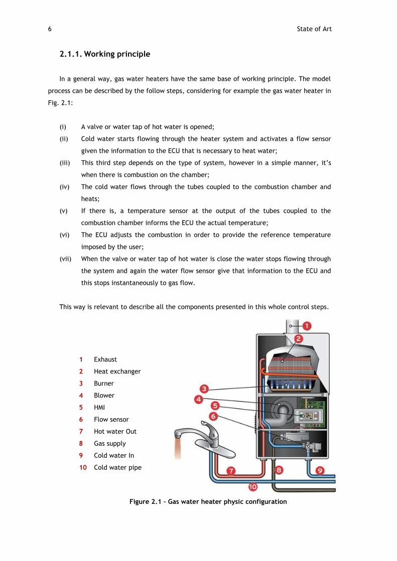
In a general way, gas water heaters have the same base of working principle. The model
process can be described by the follow steps, considering for example the gas water heater in
Fig. 2.1:
(i) A valve or water tap of hot water is opened;
(ii) Cold water starts flowing through the heater system and activates a flow sensor
given the information to the ECU that is necessary to heat water;
(iii) This third step depends on the type of system, however in a simple manner, it’s
when there is combustion on the chamber;
(iv) The cold water flows through the tubes coupled to the combustion chamber and
heats;
(v) If there is, a temperature sensor at the output of the tubes coupled to the
combustion chamber informs the ECU the actual temperature;
(vi) The ECU adjusts the combustion in order to provide the reference temperature
imposed by the user;
(vii) When the valve or water tap of hot water is close the water stops flowing through
the system and again the water flow sensor give that information to the ECU and
this stops instantaneously to gas flow.
This way is relevant to describe all the components presented in this whole control steps.
1 Exhaust
2 Heat exchanger
3 Burner
4 Blower
5 HMI
6 Flow sensor
7 Hot water Out
8 Gas supply
9 Cold water In
10 Cold water pipe
Figure 2.1 – Gas water heater physic configuration

Thermodynamics and Fluids 7
(1) Exhaust - This component is responsible for the exhaust of gases resulting from the
combustion. Some heaters have different architecture of exhaust in consequence of
the chimney structure.
(2) Heat Exchanger - Being this the core of heater is there where the energy provided by
the gas fuel transforms in heat to the water. This process depends on several aspects
that will be taken into account for the control system processed in the ECU. The
efficiency of the heater also depends on the capability of heat transfer of this part.
(3) Burner - It’s in the burner where the gas fuel is expelled to the heat exchanger by a
controlled way. Provides a stable and homogeneous flame.
(4) Blower - The blower is responsible for the inlet air to the combustion chamber. With
the capability of controlling the RPM it’s possible to control the air flux and static
pressure that is provided.
(5) HMI - Human machine interface permits the user to easily configure the machine to
its defined values of working, like hot water temperature in this case.
(6) Flow Sensor – Provides to the ECU water flow requested by the user, very important
for the control, and also indicates when is necessary to start the heater. Also here,
there is a possibility to have a controlled flux restrainer.
(7) Hot water out – The hot water output is the most important in the perspective of
final control. Is there were the goal will be present, so in the hot water output,
depending where we consider it is (in the output of the heat exchanger or elsewhere)
its needed to have temperature sensors to give the right feedback to the ECU.
(8) Gas supply – It’s from the gas supply that the heater gets its energy in the shape of
fuel gas fossil, usually natural gas, propane or butane.
(9) Cold water in – This is the fundamental resource of working, without it would be
useless. It’s also important for control that the cold water temperature is acquired by
temperature sensors.
(10) Cold water pipe – Not relevant if the user sets the right temperature in the HMI but
relevant if the user wants a lower temperature.
2.2. Thermodynamics and Fluids
To comprehend the energy process in the gas water heater is important to have a general
study base in thermodynamics and fluids. As being a gas heater its source of energy is fuel, so
there will be combustion. This way is relevant to understand well the principal components
that will affect the combustion in a way that will be possible to control them by the ECU to
get the right heat from the combustion. With this process is possible to transfer the energy to
water and then accomplish the ultimate goal, a stable and precise hot water temperature.
8 State of Art
2.2.1. Thermodynamics
J. P. Joule carried out some precise experiments on the nature of heat and work. The
results of his experiments are very important for understanding the first law of
thermodynamics and the concept of energy. He found out that an amount of work per unit
mass, done in an insulated recipe with water by a stirrer, raised the temperature of the
water. Then the initial temperature could be restored by the transfer of heat through a
contact with a cooler object. Thus Joule was able to conclusively shown the relation between
work and heat, and therefore, that heat was a form of energy. What happened to the energy
transferred by work to the water was the transformation to internal energy. The addition of
heat to a substance increases the molecular activity and thus causes an increase in its
internal energy.
“Although energy assumes many forms, the total quantity of energy is constant, and
when energy disappears in one form it appears simultaneously in other forms” [1]. This
recognition of heat as an internal energy suggested to the formulation of the first law of
thermodynamics, as the law of conservation of mechanical energy. It’s conclusive to say that
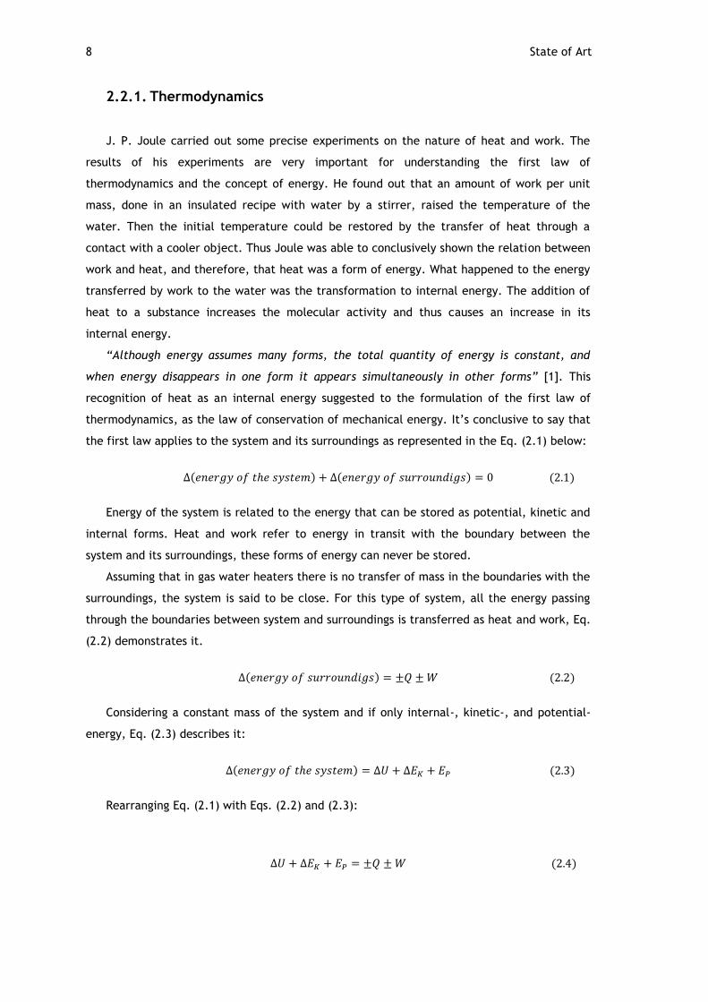
the first law applies to the system and its surroundings as represented in the Eq. (2.1) below:
( ) ( ) (2.1)
Energy of the system is related to the energy that can be stored as potential, kinetic and
internal forms. Heat and work refer to energy in transit with the boundary between the
system and its surroundings, these forms of energy can never be stored.
Assuming that in gas water heaters there is no transfer of mass in the boundaries with the
surroundings, the system is said to be close. For this type of system, all the energy passing
through the boundaries between system and surroundings is transferred as heat and work, Eq.
(2.2) demonstrates it.
( ) (2.2)
Considering a constant mass of the system and if only internal-, kinetic-, and potential-
energy, Eq. (2.3) describes it:
( ) (2.3)
Rearranging Eq. (2.1) with Eqs. (2.2) and (2.3):
(2.4)
Thermodynamics and Fluids 9
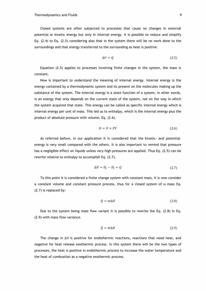
Closed systems are often subjected to processes that cause no changes in external
potential or kinetic energy but only in internal energy. It is possible to reduce and simplify
Eq. (2.4) to Eq. (2.5) considering also that in the system there will be no work done to the
surroundings and that energy transferred to the surrounding as heat is positive.
(2.5)
Equation (2.5) applies to processes involving finite changes in the system, the mass is
constant.
Now is important to understand the meaning of internal energy. Internal energy is the
energy contained by a thermodynamic system and its present on the molecules making up the
substance of the system. The internal energy is a state function of a system, in other words,
is an energy that only depends on the current state of the system, not on the way in which
the system acquired that state. This energy can be called as specific internal energy which is
internal energy per unit of mass. This led us to enthalpy, which is the internal energy plus the
product of absolute pressure with volume, Eq. (2.6).
(2.6)
As referred before, in our application it is considered that the kinetic- and potential-
energy is very small compared with the others. It is also important to remind that pressure
has a negligible effect on liquids unless very high pressures are applied. Thus Eq. (2.5) can be
rewrite relative to enthalpy to accomplish Eq. (2.7).
(2.7)
To this point it is considered a finite change system with constant mass, it is now consider
a constant volume and constant pressure process, thus for a closed system of mass Eq.
(2.7) is replaced by:
(2.8)
Due to the system being mass flow variant it is possible to rewrite the Eq. (2.8) in Eq.
(2.9) with mass flow variance.
(2.9)
The change in is positive for endothermic reactions, reactions that need heat, and
negative for heat release exothermic process. In this system there will be the two types of
processes, the heat is positive in endothermic process to increase the water temperature and
the heat of combustion as a negative exothermic process.
10 State of Art
2.2.2. Combustion
As known, the energy need to raise the water temperature comes from gas fuel. Thus, is
very important understand correctly the process occurred during combustion and the heat
produced. In this work it will be consider three types of fuel gas: methane (G20), butane
(G30) and propane (G31). It’s considered methane as being the principal gas present in
natural gas to simplify equations.
Combustion is a chemical process that we usually call burning in which a substance reacts
rapidly with oxygen and gives off heat. The substance is called the fuel, and the source of
oxygen is called the oxidizer, in this case, air. To start the combustion some source of heat
with a minimum energy of ignition is needed and it depends on the mixture of fuel/air. In
addition, for the flame to spread there must be two limits in the mixture, the lower
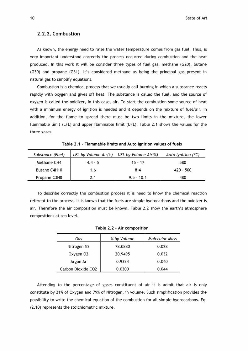
flammable limit (LFL) and upper flammable limit (UFL). Table 2.1 shows the values for the
three gases.
Table 2.1 - Flammable limits and Auto ignition values of fuels
Substance (Fuel) LFL by Volume Air(%) UFL by Volume Air(%) Auto ignition (ºC)
Methane CH4 4.4 - 5 15 - 17 580
Butane C4H10 1.6 8.4 420 – 500
Propane C3H8 2.1 9.5 – 10.1 480
To describe correctly the combustion process it is need to know the chemical reaction
referent to the process. It is known that the fuels are simple hydrocarbons and the oxidizer is
air. Therefore the air composition must be known. Table 2.2 show the earth’s atmosphere
compositions at sea level.
Table 2.2 - Air composition
Gas % by Volume Molecular Mass
Nitrogen N2 78.0880 0.028
Oxygen O2 20.9495 0.032
Argon Ar 0.9324 0.040
Carbon Dioxide CO2 0.0300 0.044
Attending to the percentage of gases constituent of air it is admit that air is only
constitute by 21% of Oxygen and 79% of Nitrogen, in volume. Such simplification provides the
possibility to write the chemical equation of the combustion for all simple hydrocarbons. Eq.
(2.10) represents the stoichiometric mixture.

Thermodynamics and Fluids 11
(
) ( )
→
(
) (2.10)
In practice is known that when the stoichiometric quantity of air is supplied for the
combustion the combustion will not be complete. Due to this behavior it is important to
define richness is combustion. Richness is related to the air-fuel ratio AFR that is the ratio
between the mass of air and the mass of fuel in the mixture. More useful, is the air-fuel
equivalence ratio, λ, that is the ratio of actual AFR and stoichiometric AFR, this gives the
richness of combustion, Table 2.3. Eqs. (2.11) and (2.12) demonstrate the AFR and λ
calculation.
(2.11)
(2.12)
Table 2.3 - Mixture richness
Mixture λ
Stoichiometric 1
Rich <1
Lean >1
Rich mixtures are usually used for internal combustion engines and are not the aim for
the gas water heaters. Rich mixtures also have ambient problems with products of
combustion due to the generation of hydrogen and carbon monoxide, being this last one a
serious atmospheric pollutant. Ideally lean mixtures produce the products present on Eq.
(2.10) plus oxygen. For a lean mixture Eq. (2.10) can be rewrite as shown in Eq. (2.13).
(
) (
) ( )
→
(
) (
) (
) (
)
(2.13)
Defined the chemical reaction, it is of great interest know the heat produce during the
reaction for each type of fuel and AFR. Heat of combustion of a fuel it’s the absolute value of
heat released during a complete combustion at standard conditions. This value is often
presented in J/Kg, J/mol or J/m3 of fuel and has two values for the same fuel, the higher
heating value and the lower heating value. This distinction comes from the physical state of
water in the products of combustion. For gas fuels it is normally used the lower heating
value.

12 State of Art
Considering the gases involved in the process as ideal and the combustion at constant
temperature and pressure is then possible to write the equation for the combustion heat. In
Eq. (2.14) represent the temperature of the fuel, the temperature of the air, the
temperature of exhaust gases and .
∑ ( )
∑ ( )
(2.14)
In gas water heaters the main objective is to release and transfer the maximum energy
from the fuel to the water, thus is important to understand the efficiency of the combustion
that can be calculated by Eq. (2.15).
| |
(2.15)
Usually the combustion efficiency is calculated with the absolute heat transferred to the
fluid. This way is more relevant to know the heat exchanger efficiency that considers also the
heat provided form the exhaust gases and products.
2.2.3. Heat Transfer
It is known from experience and by the zeroth law of thermodynamics that a hot object in
contact with a cold one becomes cooler, while the cold object becomes warmer. Heat flows
from a higher temperature object to a lower one, this leads to the conceptual idea that
temperature acts as driving force for the transfer of energy as heat. More precisely, the rate
of heat transfers from one body to another is proportional to the temperature difference
between the two bodies. This is presented in equation (2.16).
(2.16)
In heat transfer there are three ways of transfer, as demonstrate on Fig. 2.2: conduction,
convection and radiation.
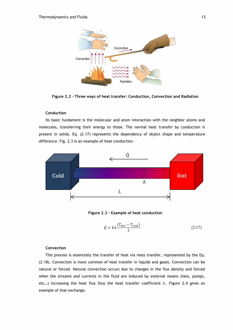
Thermodynamics and Fluids 13
Figure 2.2 – Three ways of heat transfer: Conduction, Convection and Radiation
Conduction
Its basic fundament is the molecular and atom interaction with the neighbor atoms and
molecules, transferring their energy to those. The normal heat transfer by conduction is
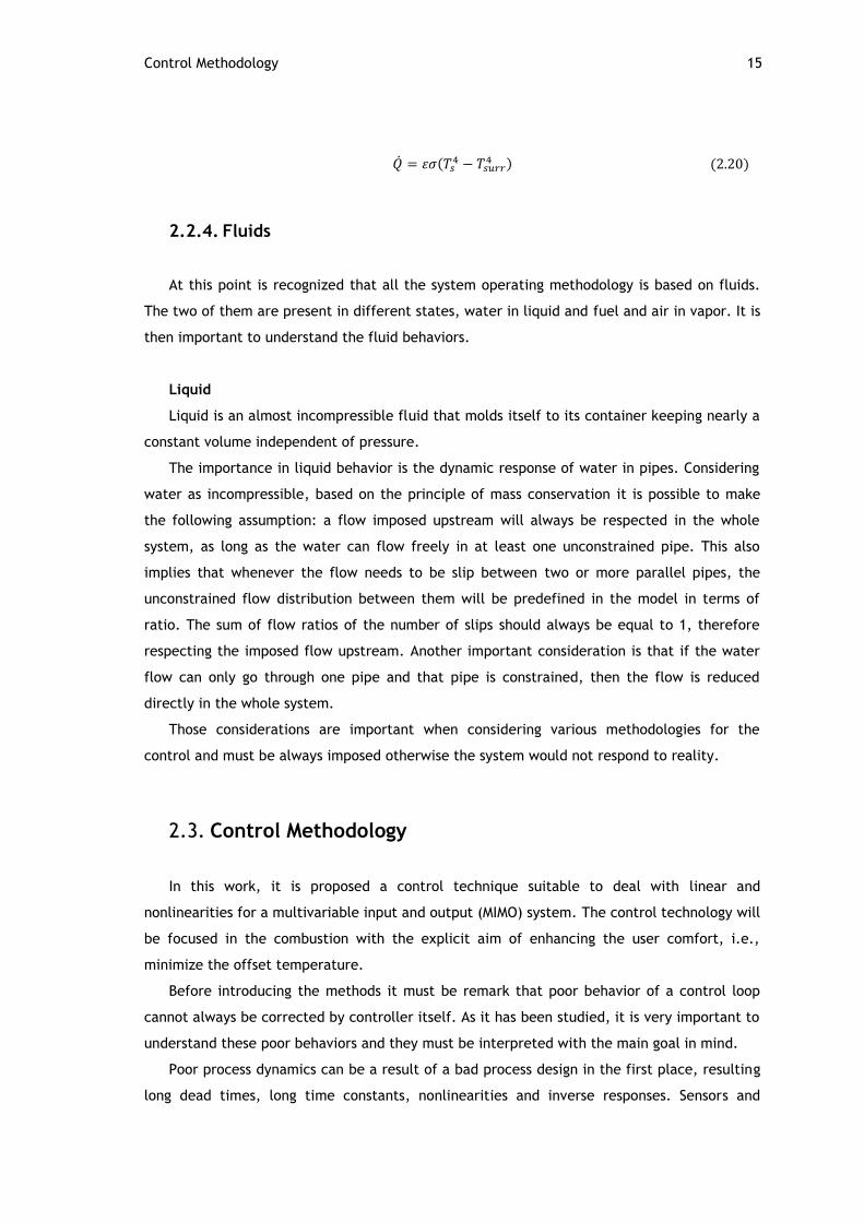
present in solids. Eq. (2.17) represents the dependency of object shape and temperature
difference. Fig. 2.3 is an example of heat conduction.
Figure 2.3 – Example of heat conduction
( )
(2.17)
Convection
This process is essentially the transfer of heat via mass transfer, represented by the Eq.
(2.18). Convection is more common of heat transfer in liquids and gases. Convection can be
natural or forced. Natural convection occurs due to changes in the flux density and forced
when the streams and currents in the fluid are induced by external means (fans, pumps,
etc…) increasing the heat flux thus the heat transfer coefficient . Figure 2.4 gives an
example of that exchange.

14 State of Art
Figure 2.4 – Example of heat convection
(2.18)
An essential consideration in convection problem is to determine whether the boundary
layer is laminar or turbulent. Surface friction and the convection transfer rates depend
strongly on which of these conditions are present. For laminar boundary layer the fluid
motion is very ordered and is characterized by the velocity which is normal to the surface. In
turbulent boundary layer the fluid is in contrast very irregular and is characterized by
velocity fluctuations. These fluctuations improve the heat transfer rates with the surface.
These effects vary the convection coefficient h, increasing for turbulent fluid flow and
decreasing for laminar fluid flow.
Radiation
Thermal radiation is heat transferred by electromagnetic waves, this is the method
humans receive heat from the sun, so it propagates without the presence of matter. Since
there is an eye of sight between objects there will be transport of heat by radiation.
The energy emitted by real surfaces is then expressed in Eq. (2.19) where
⁄ is the Stefan-Boltzmann constant, is the surface emissivity in the range of
and is the surface temperature. This equation provides a measure of how
efficiently a surface emits energy relative to a blackbody.
(2.19)
The equation for heat flux radiation is then presented in Eq. (2.20) and also depends on
the temperature of the surface of the surroundings, .
Control Methodology 15
(
) (2.20)
2.2.4. Fluids
At this point is recognized that all the system operating methodology is based on fluids.
The two of them are present in different states, water in liquid and fuel and air in vapor. It is
then important to understand the fluid behaviors.
Liquid
Liquid is an almost incompressible fluid that molds itself to its container keeping nearly a
constant volume independent of pressure.
The importance in liquid behavior is the dynamic response of water in pipes. Considering
water as incompressible, based on the principle of mass conservation it is possible to make
the following assumption: a flow imposed upstream will always be respected in the whole
system, as long as the water can flow freely in at least one unconstrained pipe. This also
implies that whenever the flow needs to be slip between two or more parallel pipes, the
unconstrained flow distribution between them will be predefined in the model in terms of
ratio. The sum of flow ratios of the number of slips should always be equal to 1, therefore
respecting the imposed flow upstream. Another important consideration is that if the water
flow can only go through one pipe and that pipe is constrained, then the flow is reduced
directly in the whole system.
Those considerations are important when considering various methodologies for the
control and must be always imposed otherwise the system would not respond to reality.
2.3. Control Methodology
In this work, it is proposed a control technique suitable to deal with linear and
nonlinearities for a multivariable input and output (MIMO) system. The control technology will
be focused in the combustion with the explicit aim of enhancing the user comfort, i.e.,
minimize the offset temperature.
Before introducing the methods it must be remark that poor behavior of a control loop
cannot always be corrected by controller itself. As it has been studied, it is very important to
understand these poor behaviors and they must be interpreted with the main goal in mind.
Poor process dynamics can be a result of a bad process design in the first place, resulting
long dead times, long time constants, nonlinearities and inverse responses. Sensors and

16 State of Art
actuators have a key weight in the control. There are several reasons that may lead to a
weak control loop like defective placing, badly mounted, bad dynamics, lack or too wide in
resolution, imperfect accuracy, and so on.
“If a control loop is behaving unsatisfactorily, it is essential that we first determine the
reason for this before tuning is attempted” [2].
2.3.1. MPC
Regarding to control methodology, model predictive control (MPC) has been successfully
applied to a wide variety of industrial processes [3]. Model predictive control has been widely
used for process control in chemical plants in which the controllers rely mostly on dynamic
models of the process, often linear empirical models obtained by system identification. As
study previously, a dynamic mathematical model combined with system experimental data
will be implemented in Matlab/Simulink.
2.3.2. PID
The proportional integral derivative control is the most popular feedback controller used
over the years in process industries. Its implementation is widely used in control
architectures and has been successfully used for over fifty years. This is due its robust and
easily understood algorithm that can provide excellent error cancelation despite the varied
dynamic characteristics of process plants.
As the name suggests, the PID controller algorithm involves three different and separate
constant parameters with its own time behavior: the proportional (P) depends on the present
error, the integrative (I) on the accumulation of past errors and the derivative (D) is based on
rate of change, thus predicting future errors.
There are many ways to configure different type of PID controllers as: P, I, PI, PD, PID,
etc… More frequently used are the P, PI and PID controllers.
Proportional Controller
This is the simplest construction and tuning controller. It adjusts the output signal in
direct proportion of the error, introducing then a steady state error. It is recommended to
use in process having transfer functions with a pole at the origin or for transfer functions
having a single dominating pole. The mathematical representation is shown in Eq. (2.21).
( ) ( ) (2.21)

Control Methodology 17
For a larger the controller output will change proportionally. In the first term of the
equation ( ) represents the error compensation output, the second term when the error
( ) is zero the compensation assumes the steady state operating point that should be
calibrated to be in the setpoint when there is no error. Thus, if error is present change
proportionally the error compensation.
Proportional controller reduces error but does not eliminate it, then, an offset value will
normally exist.
Proportional Integrative Controller
The addition of the integrative part corrects offset that may occur between the desired
value and the process output. Although integrative alone does not exhibit steady state error,
the PI provides a much faster steady state error cancelation.
PI controllers are widely used in process industries for slow variables like flow, pressure,
level, etc… The mathematical representation is shown in Eq. (2.22).
( ) [ ( )
∫ ( ) ] (2.22)
The adjustable parameter apart from is the integral time .
Proportional Integrative Derivative Controller
This is the most well-known controller due to its universal applicability. It can be used in
any type of SISO systems and, even in MIMO systems they are separate into several SISO.
What is new form the last controller introduced is the derivative part which action is to
anticipate how the error will progress looking at the time rate of change of the controlled
variables. The mathematical representation is shown in Eq. (2.23).
( ) [ ( )
∫ ( )
( )
] (2.23)
The derivative action is characterized by the time constant. Although in theory the
derivative part should improve the dynamic response, if noisy signals are present in the
control variable, noise will take control over the derivative part which will affect the steady
state error. This way proper tuning of the PID controller is difficult and must be well done
otherwise the system will fall into instability.
Equation (2.23) can be written in a simple sum of parts in which ,
⁄ and . Eq. (2.24) is the parallel form of the PID controller.
( ) ( ) ∫ ( ) ( )
(2.24)

18 State of Art
PID Controller Tuning
As mentioned before, PID controllers must be tuned correctly otherwise they will make
the system unstable. There are several methods to tune the PID gains as: manual tuning,
Ziegler-Nichols, Software tools, Cohen-Coon, Tyreus-Luyben, etc... it will be presented the
Ziegler-Nichols and Cohen-Coon methods.
Cohen-Coon
This method depends on experimental data and is suitable for first order lag systems. This
method is not suitable for zero or virtually no time delay as we will see.
To compute the right gains, the Cohen-Coon provides a three step scheme. First it is
needed to perform a step test to obtain the parameters of a PT1 model. Is necessary to
ensure that the element is at an initial steady state and after the step imposition the
element settles at a new steady state. After that, a curve similar with Fig. 2.5 must be
obtained.
Figure 2.5 – Step response of a first order lag element
The second step is solely parameters calculations as shown in the equations below.
( )
(2.25)
(2.26)
(2.27)
(2.28)
(2.29)

Control Methodology 19
The final step consists in use the parameters calculated in the second step and apply
them accordingly with table 2.4.
Table 2.4 – Cohen-Coon Tuning Gains
KP KP/KI KD/KP
P
(
)
PI
(
)
PID
(
)
Ziegler-Nichols
This method is also heuristic. The gains calculated by this method are suitable for the
parallel form of the PID controller. The process is also simple to achieve the results. First the
integral and derivative gains are set to zero, then the proportional gain is increased until the
output start to oscillate by itself. In the right moment when it starts to oscillate the
proportional gain, that will be called the ultimate gain , and wave signal period have
to be recorded to allow the final gains calculations.
Table 2.5 shows the gains calculation according to Ziegler-Nichols method.
Table 2.5 – Ziegler-Nichols Tuning Gains
KP KP/KI KD/KP
P
PI
PID
Although PID controllers are suitable for many applications given the user a satisfactory
error control, they lack is some applications. This lack is due to its constant parameters.
When process changes in some way the controller don’t have the capability to understand
and adapt to those changes. Thus PID alone doesn’t allow the optimum control performance
for process that requires some knowledge. Therefore the PID control should be used for error
control.
2.3.3. Feedforward and Model Following
20 State of Art
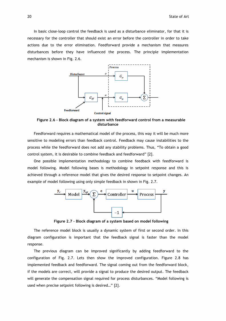
In basic close-loop control the feedback is used as a disturbance eliminator, for that it is
necessary for the controller that should exist an error before the controller in order to take
actions due to the error elimination. Feedforward provide a mechanism that measures
disturbances before they have influenced the process. The principle implementation
mechanism is shown in Fig. 2.6.
Figure 2.6 – Block diagram of a system with feedforward control from a measurable
disturbance
Feedforward requires a mathematical model of the process, this way it will be much more
sensitive to modeling errors than feedback control. Feedback may cause instabilities to the
process while the feedforward does not add any stability problems. Thus, “To obtain a good
control system, it is desirable to combine feedback and feedforward” [2].
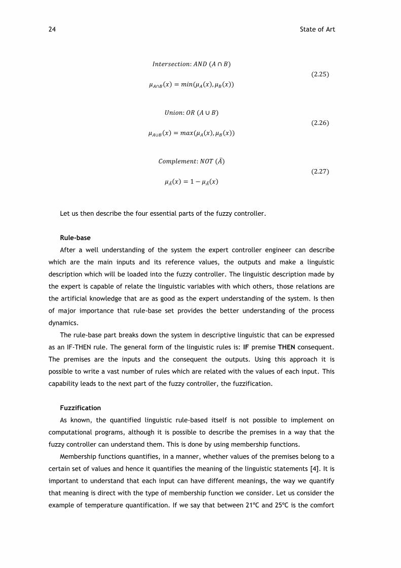
One possible implementation methodology to combine feedback with feedforward is
model following. Model following bases is methodology in setpoint response and this is
achieved through a reference model that gives the desired response to setpoint changes. An
example of model following using only simple feedback in shown in Fig. 2.7.
Figure 2.7 – Block diagram of a system based on model following
The reference model block is usually a dynamic system of first or second order. In this
diagram configuration is important that the feedback signal is faster than the model
response.
The previous diagram can be improved significantly by adding feedforward to the
configuration of Fig. 2.7. Lets then show the improved configuration. Figure 2.8 has
implemented feedback and feedforward. The signal coming out from the feedforward block,
if the models are correct, will provide a signal to produce the desired output. The feedback
will generate the compensation signal required for process disturbances. “Model following is
used when precise setpoint following is desired…” [2].

Control Methodology 21
Figure 2.8 – Block diagram of a system that combines model following and feedforward
from the command signal
2.3.4. Automatic Tuning and Adaptation
Combining the dynamics studies of the process with the methods for computing the PID
parameters it is possible to obtain a method for automatic tuning [2]. Automatic tuning refers
to methods that can change PID parameters depending on the system demand. For
implementation of auto-tuning methodology it is first need to study correctly the process,
after that the expert can understand which the system disturbances are, who generates them
and how they will affect the system response.
“Industrial experience has clearly indicated that automatic tuning is a highly desirable
and useful feature” [2]. Nowadays it’s possible to implement this methodology even if it is
computationally weight. The auto-tuning methodology is based on two different approaches:
the model-based, in which the tuning is based on developed system model and the rule-based
approach in which the tuning is based on rules similar to a manually control overview.
Adaptive Control
Adaptive control is a methodology wherein the controller parameters are continuously
adjusted in order to settle changes in process dynamics and disturbances. Adaptive control
can be applied both in feedback and feedforward control, and particularly more
advantageous for feedforward. There are two different ways to implement adaptive
controllers: direct and indirect methods. The direct method is based on data acquired from
the control loop and the indirect is based on recursive estimation of parameters from a model
base of the process. Figure 2.9 shows indirect adaptive control in which its represented all
the blocks necessary for the parameters computation.

22 State of Art
Figure 2.9 – Block diagram of an indirect adaptive controller
Automatic Tuning
As stated before, automatic tuning is tuned by demand from a user. Auto-tuning can be
built inside the controller and can also be performed with external devices which can
drastically simplify the use of the controllers. The main subject for this type of tuning is PID
controllers which are widely used and are the most used type of controllers.
Gain Scheduling
This technique is fairly wide; it can deal with nonlinear processes, processes with time
variations or situations where the operating conditions require such control change. For this
method it is necessary to define the variables that will schedule the gains. This method is
very effective for system whose dynamics change with the operating conditions.
Gain scheduling is a good alternative instead of adaptive methods. If the scheduling is
based on a good knowledge of the process dynamics this method is advantageous and it can
follow rapid changes. The key element for this technique is to find the suitable scheduling
variables and this can take a substantial engineering effort. Figure 2.10 represents a block
diagram of a system with scheduling gain and has it can be seen it has two loops in which the
scheduling variable comes from the process but it can be chose as the control expert decides.
Figure 2.10 – Block diagram of a system with gain scheduling

Control Methodology 23
2.3.5. Fuzzy
As mentioned before in subchapter 2.3.2., the lack in PID controllers referred to the
knowledge and capability to adapt to different situations was one of the reasons that fuzzy
control is presented in this dissertation. It’s of great importance to understand the
capabilities of real implementations of the fuzzy logic control.
The principal needs for fuzzy control implementation is due to the difficult task of
modeling and simulate complex real world systems [4]. Even if a good model of the system
could be implemented it is difficult to take into account all the complex responses that might
appear. For that, fuzzy logic provides a formal methodology for representing, manipulating
and implementing a human heuristic knowledge to the control system.
The fuzzy control architecture, Fig. 2.11, is the combination of four main components:
the rule-base, that have the intelligence in the form of a set rules; the inference mechanism,
evaluates which rules are more relevant for a given input; the fuzzification interface, is the
component that understands the input and modifies it in order to the be interpreted and
compared to the rules in the rule base and finally the defuzzification interface which
converts the conclusions made by the inference mechanism and converts that conclusions to
inputs to the process. We can say that a fuzzy logic controller is an artificial smart decision
maker for real time closed loop systems. That smart component of the controller is as good
as the rule base set. For that, the control engineer must gather as much and good
information about the system.
Figure 2.11 – Fuzzy architecture diagram blocks
Before the introduction of the essential parts it also important to understand the fuzzy
sets and fuzzy set operations. A fuzzy set is a set in which the elements have degrees of
membership, they in confront with classical set theory do not have a binary assessment. As
in binary computation the set operations have the same operators as it can be seen in Eq.
(2.25), (2.26) and (2.27) among other possible definitions.
24 State of Art
( )
( ) ( ( ) ( ))
(2.25)
( )
( ) ( ( ) ( ))
(2.26)
( )
( ) ( )
(2.27)
Let us then describe the four essential parts of the fuzzy controller.
Rule-base
After a well understanding of the system the expert controller engineer can describe
which are the main inputs and its reference values, the outputs and make a linguistic
description which will be loaded into the fuzzy controller. The linguistic description made by
the expert is capable of relate the linguistic variables with which others, those relations are
the artificial knowledge that are as good as the expert understanding of the system. Is then
of major importance that rule-base set provides the better understanding of the process
dynamics.
The rule-base part breaks down the system in descriptive linguistic that can be expressed
as an IF-THEN rule. The general form of the linguistic rules is: IF premise THEN consequent.
The premises are the inputs and the consequent the outputs. Using this approach it is
possible to write a vast number of rules which are related with the values of each input. This
capability leads to the next part of the fuzzy controller, the fuzzification.
Fuzzification
As known, the quantified linguistic rule-based itself is not possible to implement on
computational programs, although it is possible to describe the premises in a way that the
fuzzy controller can understand them. This is done by using membership functions.
Membership functions quantifies, in a manner, whether values of the premises belong to a
certain set of values and hence it quantifies the meaning of the linguistic statements [4]. It is
important to understand that each input can have different meanings, the way we quantify
that meaning is direct with the type of membership function we consider. Let us consider the
example of temperature quantification. If we say that between 21ºC and 25ºC is the comfort

Control Methodology 25
temperature of air and near that is more-or-less comfort the way to characterize this
understanding is via the trapezoid membership function. If it is applied the sharp peak
membership function it might be said something like: the comfortable air temperature is the
almost exact 23ºC otherwise at the slightest difference it will not be comfortable. As these
two examples there are more different ways to characterize the premises, this application
depends on the control expert choice. Figure 2.12 shows some examples of membership
functions for a different application case.
Figure 2.12 – Membership function examples [4]
Inference systems
The inference process generally involves two steps: first the premises of all the rules are
compared to the system inputs to decide which rules have to be applied and in second the
consequent is computed. For this mechanism two methods can be considered: Mamdani and
Takagi-Sugeno.
Mamdani
In Mamdani models, the premises and the consequents are both fuzzy propositions. A
Mamdani fuzzy model of a system is represented as shown in Eq. (2.28) in which is input,
is a linguistic term associated with a membership, is a output, is also a linguistic term
associated with a membership and is the number of rules.
(2.28)

26 State of Art
Takagi-Sugeno
In TS models, the premises and the consequents are crisp functions of the premises
variables. A TS model of a system with rules is represented with Eq. (2.29).
( ) (2.29)
Defuzzification
The fuzzy inference mechanism results to a fuzzy output, this output does not indicate
the exact value of the process overall output. This task of providing an exact value is
accomplished by the defuzzifier which performs a fuzzy value to a crisp value conversion.
This process is called defuzzification and there are a number of different strategies to
implement this process.
For the TS inference system the defuzzification can be represented by the Eq. (2.30).
∑
∑
(2.30)
In the case of Mamdani models, the aggregation and defuzzification processes are more
distinct from the TS models. The more common defuzzification calculations methods are the
center of gravity, first-of-maxima and mean of maxima.
Gain Scheduling with Fuzzy
One of the possibilities of fuzzy control is to provide a gain scheduler for the PID
controller. Figure 2.13 demonstrates a block configuration tor this methodology. There are
other possibilities of gain scheduling as reviewed before then is important to understand why
to use fuzzy for this accomplishment. Fuzzy logic unlike the other methodologies has
weighted and continuous gains. This method has the advantage of being more stable and a
smother gain transient response.
Figure 2.13 – Fuzzy gain scheduling control diagram blocks

Regulations 27
2.4. Regulations
Standards are present in daily routine even people don’t realize them. Standards have
been around for at least as long as science exists, without them people wouldn’t understand
correctly and a great and unnecessary effort would be done to synchronize different people’s
work. A simple example of these standards is the paper sizes, for example this document in
size A4.
As this dissertation is done in the EU is of great importance to follow some European
standards (ENs). There are three European standardization organizations, CEN, CENELEC and
ETSI that are officially recognized in the area of voluntary technical standardization. An EN is
a document that sets some technical specification that must be achieved. ENs provide the
improvement of market trade, reduction of costs also for the companies as for the consumers
and enhances the performance and safety.
There are several types of standards. In this work it will be approach some for
requirements and others for recommendations.
2.4.1. EN13203-1
This standard, the first of two parts of EN 13203, has been prepared by CEN and approved
on 18 May 2006 and is applicable to gas-fired appliances for producing domestic hot water
both for instantaneous and storage appliances with heat input not exceeding 70 kW and, if it
have storage tank, it should not exceed 300 liters of storage capacity. In this work it is
considered that there won’t be a heat input above the maximum stipulated and even if the
storage tank approach might be studied it won’t be above the 300 liters.
This first part of this EN is of major importance for the main goal of this dissertation
because is a standard for assessment of performance of hot water deliveries.
In this EN are presented the reference conditions, measurement uncertainties and test
conditions that are well described in the papers for further information if needed.
More relevant is the characterization of the gas water heater. In general, domestic hot
water appliances are characterized in two different ways: the specific hot water rate deliver
under tapping test and to the quality of the domestic hot water produced.
Characterization according to the domestic hot water rates
The specific rate of a gas water heater appliance is calculated by the hot output
temperature minus the cold inlet temperature and that difference should not be less than 30

28 State of Art
Kelvin for the maximum water rate. The requirements and test need to characterize the
appliance are described in [EN13203-1] chapter 5.2.
Characterization according to the quality of the domestic hot water produced
This classification is the most relevant for this dissertation. It represents the overall
performance of the appliance measured by a given set of criterions with a specific weight for
a final ranking calculation. These criterions are: waiting time, variation of the temperature
according to the water rate, temperature fluctuation during delivery at a constant water
rate, temperature stabilization time in case of variation of the water rate, minimum nominal
water rate and temperature fluctuation under tapping.
According to those criterions presented, EN13203-1 presents table 2.6 where the
performance factors and the weighting factors corresponding to each criteria are presented,
thus by Eq. (2.27) it’s possible to quantify the overall performance factor F, which can be
interpreted as the comfort of the appliance.
∑
(2.27)
Depending on the value obtained in Eq. (2.27) table 2.7 classifies the appliance.
Table 2.6 – Particular performance and weighting criteria [EN13203-1]
Particular performance
criterion
Particular performance factor fi Weighting
coefficient
ai
0 1 2 3
Waiting time > 60 s ≤ 60 s ≤ 35 s ≤ 5 s 4
Temperature variation
according to water rate
> 10 K ≤ 10 K ≤ 5 K ≤ 2 K 3
Temperature fluctuation
at constant water rate
> 5 K ≤ 5 K ≤ 3 K ≤ 2 K 3
Temperature stabilization
time
≥ 60 s < 60 s < 30 s < 10 s 2
Minimum nominal water
rate
> 6 l/min ≤ 6 l/min ≤ 4 l/min ≤ 2 l/min 1
Temperature fluctuation
under tapping
> 20 K ≤ 20 K ≤ 10 K ≤ 5 K 1
Regulations 29
Table 2.7 – Classification according to factor F
Label Value of the factor F
_ _ _ < 14 points
* _ _ 14 to 27 points
* * _ 28 to 39 points
* * * ≥ 40 points with all particular factors ≥ 2
The test for classification according to performance are presented in [EN13203-1] in
section 5.3.2.
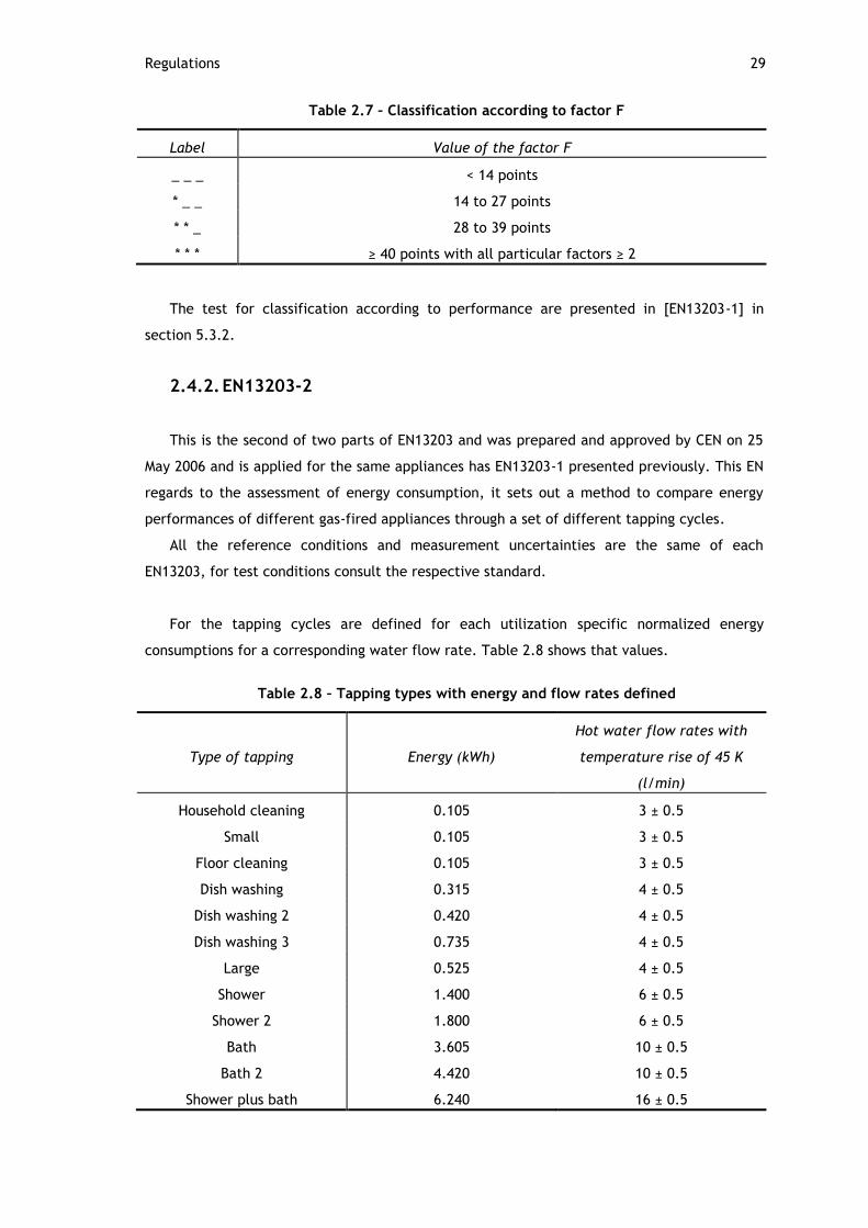
2.4.2. EN13203-2
This is the second of two parts of EN13203 and was prepared and approved by CEN on 25
May 2006 and is applied for the same appliances has EN13203-1 presented previously. This EN
regards to the assessment of energy consumption, it sets out a method to compare energy
performances of different gas-fired appliances through a set of different tapping cycles.
All the reference conditions and measurement uncertainties are the same of each
EN13203, for test conditions consult the respective standard.
For the tapping cycles are defined for each utilization specific normalized energy
consumptions for a corresponding water flow rate. Table 2.8 shows that values.
Table 2.8 – Tapping types with energy and flow rates defined
Type of tapping Energy (kWh)
Hot water flow rates with
temperature rise of 45 K
(l/min)
Household cleaning 0.105 3 ± 0.5
Small 0.105 3 ± 0.5
Floor cleaning 0.105 3 ± 0.5
Dish washing 0.315 4 ± 0.5
Dish washing 2 0.420 4 ± 0.5
Dish washing 3 0.735 4 ± 0.5
Large 0.525 4 ± 0.5
Shower 1.400 6 ± 0.5
Shower 2 1.800 6 ± 0.5
Bath 3.605 10 ± 0.5
Bath 2 4.420 10 ± 0.5
Shower plus bath 6.240 16 ± 0.5

30 State of Art
The tapping cycles shown in table 2.8 are from [EN13203-2] on chapter 5. One of the goal
of this standard is to determinate the daily energy consumption, for that, subsection 5.2.2 of
[EN13203-2] presents the formulas to calculate the useful energy recovered by the water, the
gas consumption, the electric energy if needed as auxiliary, water waste and energy
consumption in stand-by mode.

Chapter 3
System Modeling
To understand the overall dynamic of the system a detailed and modulate approach needs
to be done. Thus, a dynamic model of the entire gas water heater system will be
implemented in the Matlab/Simulink environment. This model has the purpose to simulate
various operation conditions giving us the possibility to develop the control method in a more
precise way, being then easier to calibrate when implemented in real systems.
For the model let us consider the basic configuration presented before in Fig. 2.1 and
then detach all the parts. As this document in more focused in the control method, some
assumptions and simplifications are made in order to simplify the model. Nevertheless is
always important to describe the physical structure of the system in order to have a more
reliable model and thus a more realistic control.
In this chapter it is assumed that the sensors are all ideal for a simplified model.
System Overall
The general configuration of a basic gas water heater is already known, thus the dynamic
subsystems with great importance are: the blower, gas valve, burner and water valves.
The flow components like the intake box and flue gas pipe are not considered in the
modeled system.
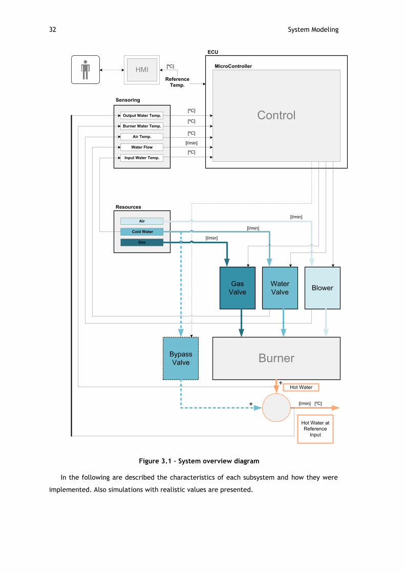
Fig. 3.1 presents an overview about the modeled system with a new component named
bypass valve that will be explained further and is also a water valve.
32 System Modeling
ECU
Control
HMIMicroController
Sensoring
Burner Water Temp.
Air Temp.
Water Flow
Input Water Temp.
Reference
Temp.
Air
Cold Water
Gas
Resources
Gas
Valve
Water
ValveBlower
BurnerBypass
Valve
+
+
Hot Water at
Reference
Input
Hot Water
Output Water Temp.
[ºC]
[ºC]
[ºC]
[ºC]
[ºC]
[l/min]
[l/min]
[l/min]
[l/min]
[l/min] [ºC]
Figure 3.1 – System overview diagram
In the following are described the characteristics of each subsystem and how they were
implemented. Also simulations with realistic values are presented.

Blower 33
3.1. Blower
As heat demand differs, different air flow is necessary to provide in order to have the
right amount of oxygen for combustion. The most important characteristic of the blower is
the relation of pressure rise with air flow at different fan speeds. Usually fan suppliers
provide the fan curves for a limited fan speeds. It is then necessary to know the right
pressure rise and air flow for a specific fan speed. This can be achieved using the fan laws.
Fan laws are useful for geometrically similar fans using dimensionless constants which can
be calculated. Thus let describe these fan laws. Eqs. (3.1), (3.2) and (3.3) represent flow rate
law, pressure rise law and power law respectively [10].
(3.1)
(3.2)
(3.3)
Assuming the air incompressible and no change in the fan diameter, , it’s possible to
rewrite the Eqs. (3.1), (3.2) and (3.3) in a way that given one fan curve by the supplier it’s
possible to know the pressure rise versus air flow for any given fan speed. Equations (3.4),
(3.5) and (3.6) makes it possible to trace the graph of Fig. 3.2 and then know the specific
curve of the blower.
( ) (3.4)
( )
(3.5)
( )
(3.6)
The intersection of the specific curve with the pressure rise curve defines the operating
point. When the system resistance changes the operating point also change. Thus is important
to know one point for a specific fan speed to trace the specific curve.

34 System Modeling
Figure 3.2 – Pressure rise versus air flow graphic
Another important factor for air flow calculation is the inlet air density. This value can be
estimated assuming the air as an ideal gas. Combining the ideal gases equation (3.7) with the
density equation (3.8) and molar mass equation (3.9) it is possible to get Eq. (3.10) and it’s
visible that the most relevant factors are temperature and pressure which change in time.
Considering that the system will operate at constant ambient pressure the only influence
factor is temperature.
(3.7)
(3.8)
(3.9)
(3.10)
Now that the inlet air density change with temperature is possible to compute, applying
Bernoulli’s equation for fluids it’s possible to compute the air flow variation with inlet air
temperature variation.
Considering that the air density used to calculate the specific curve is known we can
apply Eq. (3.11).
(3.11)

Blower 35
Let us consider and knowing that , with constant area Eq. (3.11) can be
written as Eq. (3.12).
(3.12)
Dynamic Response
Real blowers have specific response curves. This is due to mass inertia and friction losses.
Is then of major importance to know how the blower accelerates to its reference speed. With
the help of characteristic transfer function it’s possible to model the time variance of the
system [7]. Experimental data show that the start-up response of the blower is very similar to
a first order lag element (PT1) show in Fig. 3.3. Thus is possible to describe the blower by the
general step response function of Eq. (3.13).
Figure 3.3 – Step response of a PT1 element
( ) ( ⁄ ) ( ) (3.13)
The corresponding transfer function in frequency domain is written as Eq. (3.14).
( )
(3.14)
To estimate the time constant of the blower transfer function, a step signal input from
zero speed to a fixed value speed must be measured in order to visualize the time that the
response signal needed to reach approximately 63% of its final value Fig.3.3.
With all this methods it’s possible to implement the blower behavior in Matlab/Simulink.
Implementation
In order to estimate the rise time, measures where made as shown in Fig. 3.4. With those
values it was made an initial estimation. During simulations various values for times where
tried to approximate to reality.

36 System Modeling
Figure 3.4 – Fan Speed on the blower step response time
The Matlab/Simulink implementation of the blower is here represented in Fig. 3.5, 3.6
and 3.7.
Figure 3.5 – First layer blower block
Above is presented the simplified block of the blower. Figure 3.6 is a second layer in
which is presented the response delay and the block “Blower” which has the specific curve of
the blower.
Figure 3.6 – Second layer block diagram of the blower
0
10
20
30
40
50
60
0 20 40 60 80 100
Fan
Sp
ee
d [
RP
M/1
00
]
Time [s]
Fan Speed
Fan Speed

Gas Valve 37
Figure 3.7 – Third layer block diagram of the blower
As stated previously, the air temperature changes the air flow. Figure 3.7 has
implemented these variable behaviors with the “Air Density” block. Also altitude could be
considered, but in this model it was considered sea level simulation. The lookup tables have
the specific behaviors for a particular product. The supplier gives a lower and upper
performance values this is why there are two lookup tables for each variable.
3.2. Gas Valve
The gas valve is one of the most important actuators present in the system. It’s from it
that energy in form of fuel is delivered to the burner in a controlled way. Thus is very
important to provide the exact gas flow to the burner.
Gas valves can be electromagnetically or step-motor driven which provides them different
quality in terms of accuracy, reliability, longevity, security, etc. Suppliers provide the
pressure rise exactly at the output of the valve related with the command signal given to the
valve actuator. This relation can be also acquired by experimental procedures with different
valve configuration and different drive signal commands [8].

38 System Modeling
Pulse with modulation (PWM) is the more common way to drive these valves but to
simplify the modeled valve behavior pretended is a current command signal vs. gas flow. In
order to find the relation of pressure rise in the valve vs. gas flow to the output we will
consider the model of Fig. 3.8.
Figure 3.8 – Gas valve output nozzle model
The Bernoulli equation describes the variation in flow through the gas valve. In Eq. (3.15)
it is considered the (1) as the direct output of the valve actuators and (2) as output space
where the gas flow will be injected.
(3.15)
Eq. (3.15) can be simplified if it is assumed a horizontal flow and a constant fluid
density . We also consider that the speed of the gas in (1) is much slower than in
(2), then , so it is feasible to obtain Eq. (3.16) from which we can calculate
indirectly the output flow.
(3.16)
For the present nozzle shown above in Fig. 3.8, it is now possible to estimate the gas flow
as a function of pressure gradient with a specific and constant cross-section
nozzle area. As the system is suitable for different types of fuel gas, Eq. (3.17) is also fuel gas
density dependent.
(
)
(3.17)
√
(3.18)
Dynamic Response
Since the fuel is not injected directly in the burner it will need to cover a distance from
the nozzle to the direct output into the burner. Thus, there will be a delay in the delivery of
the gas that can be calculated according to the model in Fig. 3.9.

Gas Valve 39
Figure 3.9 – Model of gas delivery to the burner
Assuming this configuration, a cylindrical tube with a length and cross-section , to
calculate the delay as a function of the fuel gas flow it is used Eq. (3.19).
(3.19)
At this point the need to go further in the understanding of the gas valve operation is
important. Let’s consider Fig. 3.9 as a single fuel supplier to the burner, then consider it as
many as wanted and divide them by sections. Fig. 3.10 shows a possible implementation of a
burner plate. The burner plane is divided in three sections, A, B and C. These represent the
three configurations possible of fuel gas deliver. The possibility inherent with this
configuration is to provide a wide minimum to maximum range of combustion. For this
possibility, the gas valve has two on-off actuators which can provide the three operation
conditions.
The change between on and off for each section has a time delay inherent and some
particular considerations. These will be studied further.
Implementation
This part of the simulation was considered a key element for the right performance of the
model. As stated before, the burner is divided by section/segments. Fig. 3.10 shows a
possible configuration of it. The important understanding is the minimum and maximum
power that each section/segment can deliver and the time delay that takes to ignite and turn
off the flame.
The configuration also have the particularity that only section A has the ignition spark,
this means that all the other sections need that previously one of the other was already
burning, in order to propagate the flame. This is what influence the time delays explained
before.

40 System Modeling
Figure 3.10 – Burner plate configuration
In Matlab/Simulink the gas valve block layers were the following shown in Fig. 3.11, 3.12
and 3.13.
Figure 3.11 – First layer of the gas valve
This first layer shown above is the simplest block for the gas valve. It has the possibility
to configure the type of gas that is being used with input “Gas Type”. The section selection
represents the dynamic explained before regarding the segmentation process.
Figure 3.12 – Second layer of the gas valve; type of gas and section/segment selection

Water Valve 41
Due to the size of “Segment Delay” block it will not be shown in this document the inside
layer but it follows specific time delays.
Figure 3.13 – Third layer of the gas valve; time delays and gas flow estimator for G20
It is inside of “Gas Flow Calculation” block in Fig. 3.13 that the equations regarding gas
flow estimation are implemented. There are also functions implemented for the delay time
of the gas propagation. This can be used also as a tuning block for unpredicted time delays in
the gas valve.
3.3. Water Valve
Water valves aim is to suppress or regulate water flow in the system with a consequent
change in pressure. Bernoulli’s equation demonstrates that relation as shown in Eq. (3.15).
The importance of the water valve model will be further explained in the implementation
chapter. In Fig. 3.14 is shown an example of a water valve.
Figure 3.14 – Example of a water valve

42 System Modeling
The principal characteristic of valves is fluid flow vs. valve opening. Fig. 3.15 illustrates
three possible response curves. In then important to know in which of those responses our
valve is operating.
For this work it will not be consider the drive signal, assuming that there is already a
command signal processor for those valves.
Figure 3.15 – Characteristic curve of valve opening
Implementation
For the water valves no time delay is considered. It is then a simpler model than the
other ones. The block of this actuator is important to be totally independent to enable the
use of the same in totally different situations. Figure 3.16 and 3.17 shows the
implementation blocks.
Figure 3.16 – First layer block of water valve
The “Water Valve” block has inside a lookup table with the characteristic curve of the
valve opening or closing, depending on the valve configuration. In this model it is considered
a specific closing curve; this means that in standby the valve is fully open. To perform the
flow restriction it is used a saturation block with variable saturation values. No change in
pressure is calculated.

Burner 43
Figure 3.17 – Second layer block of water valve
3.4. Burner
It is in the burner/combustion chamber that the fuel mixes with air and where the
combustion takes place. As the source of energy comes from the combustion, in order to
calculate the heat transferred to the water it is important to model the right dynamic and
make some assumptions.
As study in chapter two, the principal heat transfer present in the burner is convection.
Conduction and radiation are considered not so relevant for the model, providing then a
simpler model of the heat exchanger. Conduction is the heat transfer between the heat
provided by convection and heat transferred to the water. Figure 3.18 shows that action.
Those considerations in fact are related to: and the high . Being
then the copper mass of the heat exchanger low, thus a low is obtained.
The heat exchanger is a physical device similar to a radiator, but in the reverse
operation. Therefore is highly important to understand its dynamics and its performance. Due
Figure 3.18 – Heat transfer from the flame to the burner

44 System Modeling
to the high complexity of heat transfer calculation and modulation. Experimental data will be
gathered in order to make a mathematical approximation for its dynamics and performance.
The burner can be divided into the following sections: the air ventilation with gas
injection into the combustion chamber providing the , the combustion chamber
and the heat exchanger that transfers the heat form the flame to the water. Figure 3.19
simplifies all those parts in one single representation. In terms of heat transfer by the
equation of conservation of energy Eq. (3.20) simplifies the whole physics processes of the
device.
Figure 3.19 – Heat exchanger representation
∑
∑
(3.20)
For equations simplifications it is considered the transfer of heat between the flame and
water without losses, then it’s possible to compute Eq. (3.20) as Eq. (3.21).
( ) (3.21)
Implementation
For this part of the appliance experimental data was acquired and interpreted. As can be
seen in Fig. 3.20, the time response of the heat exchanger is similar to a PT1 element.
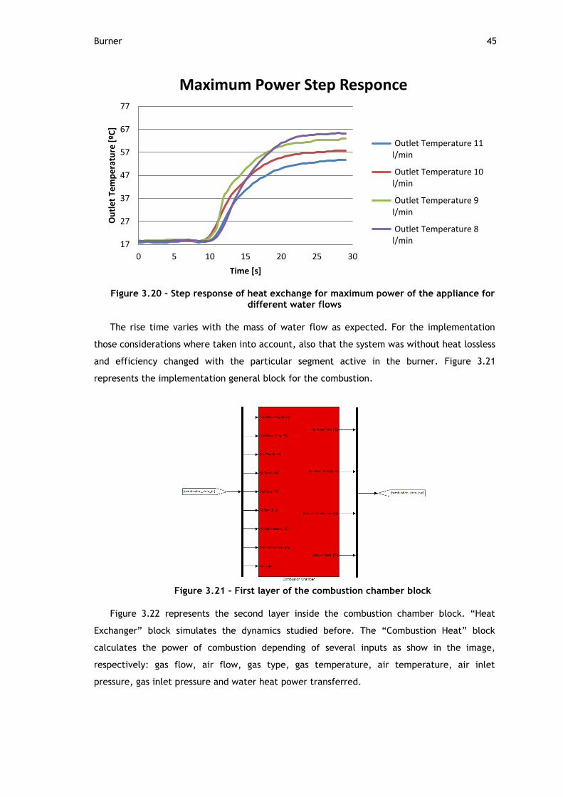
Burner 45
Figure 3.20 – Step response of heat exchange for maximum power of the appliance for
different water flows
The rise time varies with the mass of water flow as expected. For the implementation
those considerations where taken into account, also that the system was without heat lossless
and efficiency changed with the particular segment active in the burner. Figure 3.21
represents the implementation general block for the combustion.
Figure 3.21 – First layer of the combustion chamber block
Figure 3.22 represents the second layer inside the combustion chamber block. “Heat
Exchanger” block simulates the dynamics studied before. The “Combustion Heat” block
calculates the power of combustion depending of several inputs as show in the image,
respectively: gas flow, air flow, gas type, gas temperature, air temperature, air inlet
pressure, gas inlet pressure and water heat power transferred.
17
27
37
47
57
67
77
0 5 10 15 20 25 30
Ou
tle
t Te
mp
era
ture
[ºC
]
Time [s]
Maximum Power Step Responce
Outlet Temperature 11l/min
Outlet Temperature 10l/min
Outlet Temperature 9l/min
Outlet Temperature 8l/min
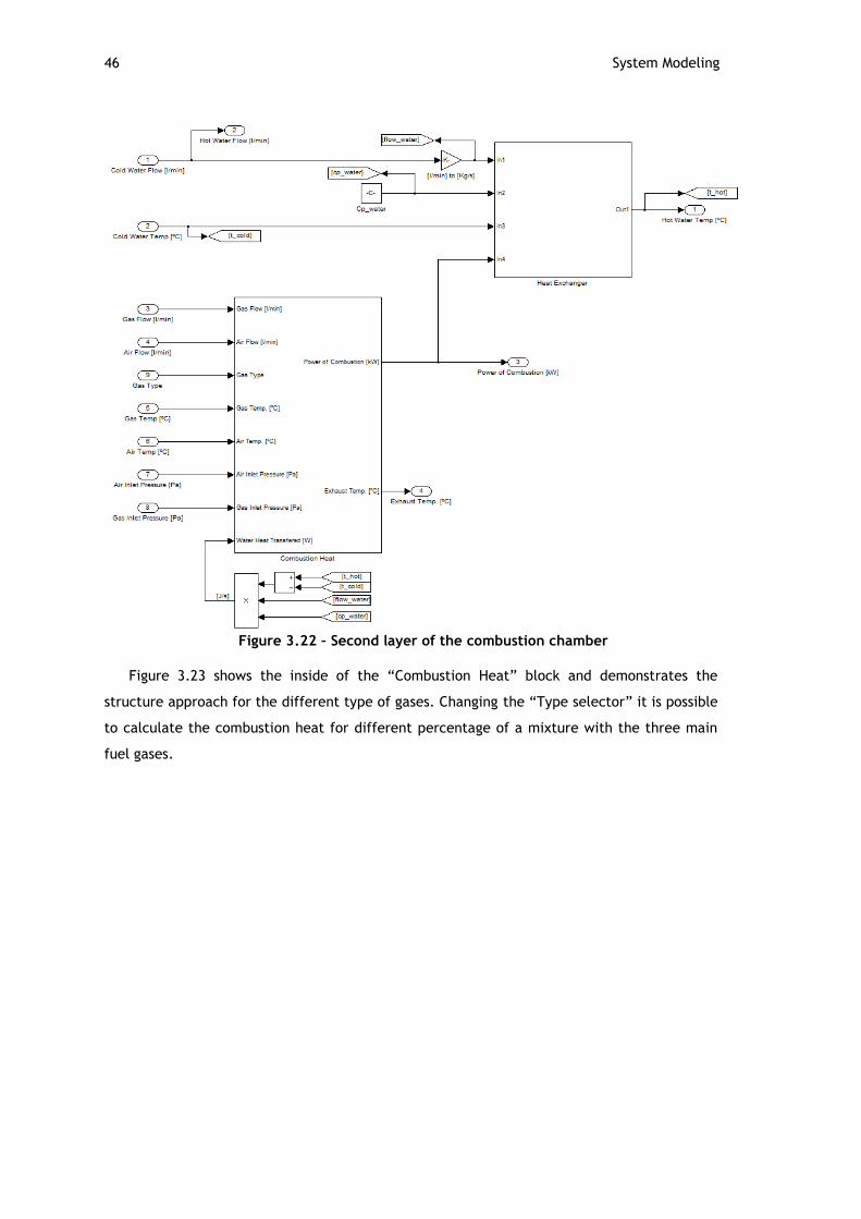
46 System Modeling
Figure 3.22 – Second layer of the combustion chamber
Figure 3.23 shows the inside of the “Combustion Heat” block and demonstrates the
structure approach for the different type of gases. Changing the “Type selector” it is possible
to calculate the combustion heat for different percentage of a mixture with the three main
fuel gases.

Model validation 47
Figure 3.23 – Inside of the combustion heat block
3.5. Model validation
To ensure control algorithms with accurate dynamic response it is important to verify if
the modeled system had the same dynamic response has the real appliance. Thus, after
assembling all the separately parts modeled, an all in one system was constructed and a
comparison between experimental data acquired directly from the appliance and the
modeled system was made. Figure 3.24 shows the data log variables recorded during the
experimental tests with the simulations results. The main variables used to validate the
model were water inlet temperature, water outlet temperature, setpoint temperature and
water flow.

48 System Modeling
Figure 3.24 – Model validation graphic with real temperature compared to modeled
In the test made, the appliance had specific control architecture with well-defined
control values. Because of that, a study of the control code implemented in the appliance
was made and then implemented in the simulation model. This way it is guaranteed a more
accurate assessment.
From the result of these tests it can be concluded that the simulation model is close to
the real appliance. The forward in time is due to the hot water sensor position in the
appliance compared to the position on the model. Also, the peak amplitudes have a
significant deviation but not enough to compromise the simulated validation. Those
deviations from reality came from the simplifications made before in each part of the system.
It is important to underline the real application of this model that is simulate a real
appliance to perform a comfort optimization, this way even if the temperature peaks are
with different values they represent a real dynamic response that it will be possible to work
on.
3.6. Control Architecture
Taking into account the main goal, from experimental data it is possible to understand
which dynamic behaviors must be eliminated. Figure 3.25 is a good example of some dynamic
behaviors that must be eliminated or if not possible, reduced as much as possible. As it can
be seen, the red line represents the output temperature of the appliance with a set point
temperature of 55 ºC.
4042,5
4547,5
5052,5
5557,5
6062,5
6567,5
70
0 1 2 3 4 5 6
Tem
pe
ratu
re [°C
]
Time [min]
Model validation
Real Temperature [ºC] Model Temperature [ºC]

Control Architecture 49
Figure 3.25 – Appliance response temperature
In the instant before 3 min, the water flow change to a lower flow rate, due to dynamic
restrictions and the control present in the appliance, the water outlet temperature increases
significantly passing above set point temperature, which is very uncomfortable and can harm
the user. Also in the instant before 2 min the water flow increases quickly, then again for the
same reasons the appliance can’t compensate properly this dynamic and a decrease in
temperature is obtained. This test was performed near full power of the appliance. The
parameters were the defined by [EN13203] for appliance tests.
3.6.1. Gain Scheduling
Studies on PID parameter varying and possible implementations of fuzzy with the PID are
made on [9-11]. Those methods are important for a robust and effective control action over
the process. On [10] there is concluded that the dynamic behavior of a fuzzy-PID controller
using minimum inference engine and center average defuzzification behaves approximately
like a parameter varying PID controller, thus a fuzzy gain scheduling controller. The generic
diagram for this controller for the simulation environment can be represented as in Fig. 3.26.
0
10
20
30
40
50
60
0 1 2 3 4 5 6 7
Tem
pe
ratu
re [°
C]
/ W
ate
r Fl
ow
[l/
min
]
Time [min]
Appliance Response
Appliance Temp [ºC] Water Flow [l/min]

50 System Modeling
Figure 3.26 – Possible diagram of fuzzy gain scheduler
The implementation of the controller is described next in the implementation chapter.
3.6.2. Bypass
Before introducing the control scheme is important to understand the physics behind the
control. As studied before in chapter two, for the water pipe system is considered the mass
conservation principle. This consideration is a base principle for all the assumption made
further. Let us consider the physical configuration demonstrate in Fig. 3.27.
Figure 3.27 – Diagram of bypass configuration for the appliance

Resume 51
Being defined the configuration and variables it is then possible to describe the system
into equations.
( ) (3.22)
( ) (3.23)
(3.24)
In the point of view of the system variables, is the setpoint temperature desired, is
the temperature measured in the outlet of the heat exchanger and is the inlet
temperature. With Eq. (3.24) it is possible to calculate the ratio to control the bypass
configuration water valves. Another consideration that must be taken into account is that the
range in must be saturated between zero and one.
3.7. Resume
With all the actuators modeled it is then possible to assemble the parts and construct an
overall system. Figure 3.28 demonstrates as the model can be used without a deeper
knowledge of the layers inside.
Figure 3.28 – Overall overview of the gas water heater model
The system is also capable of being detached in several parts to make different
configurations with the work already done. This provides the ability to upgrade the blocks
made without spend too much time on it.
52 System Modeling
This model also favors the implementation of control schemes. It is easy to see the
variables that are being used, this is very intuitive for understand what to control and the
range of the variables.

Chapter 4
Implementation and Results
In the previous chapter ideal situations were considered in order to simplify the
construction of a solid and not too much complex model. Despite of some simplifications here
are discussed some of them and understand its real weight in the dynamic response.
As an appliance for domestic dwellings it must be understood the hot water needs that
will be present. This way, there must be considered use cases. After this analysis it will be a
more approachable to tune the control structure.
Also a computer controller is implemented. Thus a description of the discretization
process and considerations taken in account are presented.
In the end, the results from the simulation control model are compared with the same
control in the real appliance.
4.1. Simplifications Issues
As said before, in chapter three, for the simulation model some simplifications were
made in order to simplify the system. Although when simulation results were compared to
real appliance it was clear that some important aspects might be neglected when they
shouldn’t. Here we discuss the simplification problem that might be arising from the sensors
of water temperature and water flow. It is important to understand these two type of sensors
because they are the principal variables of the control.
4.1.1. Temperature Sensor
Water temperature sensors are very important in the control. In specific, the water outlet
temperature sensor is the one that will generate the error signal and the water inlet
temperature sensor provides one of the variables to compute de amount of heat required to
heat the water.

54 Implementation and Results
Taking into account the overall time constant of the system, the response delay time of
the temperature sensors and its resolution are suitable for the application, otherwise, in the
simulation model there would be needed to make specific blocks that would describe the
behavior of the temperature sensors.
4.1.2. Water Flow Sensor
Water flow sensor is a key component in the control system, is from it that sudden
changes in water flow can be interpreted by the control. If the values read are wrong or have
a huge delay, wrong heat computations will be made.
These hypotheses have to be analyzed and understand carefully. Considering the time
delay that the sensor senses changes in the flow is very important, this capability can
compromise the overall performance of the appliance. If the flow is sensed by the control too
late or it is reading wrong values there will be great offsets in temperature that can cause
harm to the user and even for the appliance itself.
4.2. Implementation on the Model
Before implementing the control methodologies in real appliance we proceed with the
implementation on the modeled system.
4.2.1. Gain Scheduling
Figure 4.1 demonstrates de black box of the gain scheduling implementation. Inside there
are specific appliance control schemes. Those are similar to the one mentioned before in
chapter three.
Figure 4.1 – Diagram blocks for the gain scheduling control
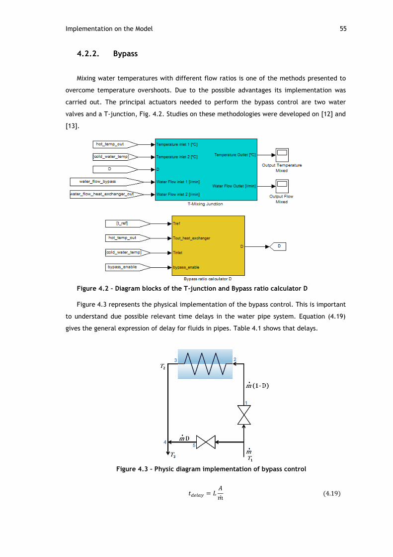
Implementation on the Model 55
4.2.2. Bypass
Mixing water temperatures with different flow ratios is one of the methods presented to
overcome temperature overshoots. Due to the possible advantages its implementation was
carried out. The principal actuators needed to perform the bypass control are two water
valves and a T-junction, Fig. 4.2. Studies on these methodologies were developed on [12] and
[13].
Figure 4.2 – Diagram blocks of the T-junction and Bypass ratio calculator D
Figure 4.3 represents the physical implementation of the bypass control. This is important
to understand due possible relevant time delays in the water pipe system. Equation (4.19)
gives the general expression of delay for fluids in pipes. Table 4.1 shows that delays.
Figure 4.3 – Physic diagram implementation of bypass control
(4.19)

56 Implementation and Results
Table 4.1 – Water delay time in the appliance pipes
Water pipe length Water Flow Delay
Time
( )
( )
Results
As can be seen in Fig. 4.4 the bypass control method is efficient for the main goal. There
are no overshoots present in the dynamic response in the output of the T-junction due to the
turbulent mixing [13] and energy conservation principle [12].
For the implementation of this methodology the time delay present in the system due to
water flow in the pipes were neglected. Without this simplification the factor would need
to be adjusted with the times calculated in Table 4.1.
Figure 4.4 – Bypass control response graphic
0
10
20
30
40
50
60
70
80
90
0 1 2 3 4 5 6 7
Tem
pe
ratu
re [°
C]
/ W
ate
r Fl
ow
[l/
min
]
Time [min]
Bypass Control
Heat Exchanger Temp [°C] Bypass Temp [°C]
Without Bypass Temp [°C] Water Flow [l/min]

Implementation on the Appliance 57
It is important to evidence what occurs during a fall in water flow. For example in time
6,5 min occurs a high fall in water flow, then the bypass ratio calculator gives the signal to
suppress the water flow for the heat exchanger and opens the cold water flow. This situation
leads to high temperature in the heat exchanger that can damage the appliance or activate
the safe mode then shutting down the gas water heater. It is then important to take into
account this behavior.
4.3. Implementation on the Appliance
4.3.1. Discretization
The process of discretization concerns to transform a continuous model to equations into
discrete parts. This process is needed in order to implement mathematical equations into
digital processors.
Discrete-Time Integrator
The integrator is present in almost all equations present in this system. The time delays
are present in the actuators, mass inertias, etc, and those are calculated with time
integrators. Also for control they are very important to understand and compute the correct
amount of error accumulated. Thus, is quite important to discretize correctly the integrator.
Some approaches are possible. Matlab/Simulink provides the follow methods: Forward Euler,
Backward Euler and Trapezoidal. The method chosen was the Forward Euler due its simple
implementation and low cost computation. If the sample time is smaller than the time
constant of a system this method adds small global error. The expression for the discrete-
time integrator is then shown below in Eq. (4.4) [2] in which is the sample time, integral
time and the control error.
( )
∫ ( )
(4.1)
(4.2)
( ) ( )
( ) (4.3)
( ) ( ) ( ) (4.4)

58 Implementation and Results
In microprocessor code it is possible to define the initial conditions of each integrator
used, define the upper and lower limits to prevent windup and to reset the integrator value.
Discrete-Time Differentiator
As the integrator the differentiator is also very important to describe differential
equations. For the controller is necessary to compute de error change. Using the Euler
backward method as the integrator, the discrete differentiator is described by Eq. (4.7) [2] in
which is the derivative gain limitation, derivative time and the derivative component.
The approximation in Eq. (4.5), instead of , acts as a derivative for low-frequency
signal components, avoiding then measurement of noise.
(4.5)
( ) ( )
( )
( ) ( )
(4.6)
( )
( )
( ( ) ( )) (4.7)
The advantage by using a backward difference is that the parameter ( )⁄ is in a
range of 0 to 1 for all values of the parameters guarantee then that the difference equation
is always stable.
4.3.2. Gain Scheduling
The control architecture implemented in the ECU is represented by the block of Fig. 4.5.
In the “PID” block are implemented in C code the Eq. (4.4) and (4.7). The inputs in “PID”
block are connected with the gain scheduling. With different temperature error the gains are
changed in order to perform a better dynamic response.
Figure 4.5 – PID implementation block
4.3.3. Results

Implementation on the Appliance 59
To perform a comparison between the appliance controller and the new scheduling
controller a set of different water flow requests were made all with the same setpoint
temperature of 50 ºC. The water flow requests were made by hand with a tap, this way the
tests performed aren’t exactly the same but very similar.
Figure 4.6 – Test performed from the appliance with original controller
From the test made we can see in Fig. 4.6 that near instant 2 min and 3,5 min the
appliance might enter in a safe mode due to high increase in the combustion power. Also the
setpoint temperature is followed with some offset.
For the new gain schedule controller implemented the same conditions were performed
as equal as possible as previously in Fig. 4.6. The setpoint temperature, as it can be seen in
Fig. 4.7, is the same as performed in the appliance controller. From Fig. 4.7 we can see that
the output temperature follows the setpoint temperature in a more precise way than in the
appliance controller.
0
10
20
30
40
50
60
70
0 1 2 3 4 5 6 7 8 9
Tem
pe
ratu
re [
°C]
/ W
ate
r Fl
ow
[l/
min
]
Time [min]
Appliance Controller
Outlet Temperature [°C] Water Flow [l/min]

60 Implementation and Results
Figure 4.7 – Test performed form the appliance with the gain scheduling controller
In Fig. 4.7 it is observed that steady state error is smaller than in Fig. 4.6, this behavior is
due to an increase in the integral action of the controller and decrease in derivative. The
derivative action as a term that allows prediction of the future error if is to high will sense
the small changes in water flow that can be considered as noise, then, for steady state
condition the term must be small.
4.4. Resume
Through these results it can be conclude that the appliance has physical limitations that
don’t allow a great improvement in dynamic response with its own actuators.
Even though, with the gain scheduling controller it is possible to achieve a better steady
state error and thus follow the setpoint temperature more precisely.
With the upgrade of the bypass methodology, using two water valves and a T-junction, by
simulation it is possible to achieve a total cancelation of the overshoots.
0
10
20
30
40
50
60
70
0 1 2 3 4 5 6 7 8 9
Tem
pe
ratu
re [
°C]
/ W
ate
r Fl
ow
[l/
min
]
Time [min]
Gain Scheduling Controller
Outlet Temperature [°C] Water Flow [l/min]
Chapter 5
Conclusions
In this chapter are presented the conclusions upon the simulations and implementation
made and discuss the possibilities to overcome unwanted dynamics from the system.
5.1. Simulation
The ability to represent real systems into a set of equations capable of perform a good
representation of reality is a time consuming and difficult task to accomplish. In this work an
overall model was implemented with success regarding the main objective of this
dissertation.
As the main goal of this work was not to develop an exact model of a gas water heater
but instead improve its comfort some aspects in the model were simplified or even
neglected.
Those neglected aspects were made on the gas valve, blower, ratio control (λ – control),
pipe lengths and sensors position. The most relevant might have been the pressure along the
system from inlet air to flue gas exhaust. Despite it has been neglected those aspects, in the
overall the model was performing as needed.
5.2. Overshoots
These dynamics were always the most unwanted from all possibilities. From the point of
view of comfort it is extreme important to suppress those responses. Here we discuss why
those peaks are present and how to eliminate them.
62 Conclusions
As we studied before, these dynamics appear during quick negative changes in water
flow. The question that can be made is ‘why they appear?’ and this can be answered based
on the knowledge gained during the working principle studies.
Water temperature overshoot appears due to slow response of the system components,
respectively the air fan and gas valve. As the water flow fall quickly, the combustion process
can’t be stopped instantaneously to establish the heat necessary for that change. We
conclude that the minimum time of overshoot was already implemented previously. To
overcome that problem extra actuators must had been implemented is the system.
Bypass Valve
This possibility is the most suitable for the system as shown in the implementation
chapter. It provides a good response without compromising the overall performance, in
particular the waiting time imposed in the [EN13203-1] that is the factor whit most weight in
the total performance calculation. Table 2.6 in chapter 2 shows that importance.
5.3. Undershoots
Undershoots are also a dynamic problem present in the system. Similarly as the
overshoots, the undershoots appear when sudden increase in water flow is present and due to
the same problem as for overshoots, the system can’t respond quickly enough.
In order to prevent this dynamic response an improvement in the actuators delay time
or the solution of a water tank working as an inertia accumulator must be taken in account.
These two solutions have their problems, the first requires an associated investment and the
second compromises the performance quantification of the appliance.
The undershoots affect the comfort as well known but, taking into account that they
don’t injure the user, unlike the overshoots, thus the undershoots are below in priority than
overshoots.
5.4. Future works
As future works several aspects could be done in two different aspects. First in the model
point of view, as mentioned above on the simulation conclusions. The second respecting to
implementation on the appliance, it would be of great value to implement the bypass
controller.
References
[1] H. C. Van Ness, J. M. Smith. “Introduction to Chemical Engineering
Thermodynamics”. McGraw-Hill, Fourth edition, 1987.
[2] K. Åström, T. Hägglund. “PID Controllers: Theory, Design, and Tuning”. ISA, second
edition, 1995.
[3] D. Bhope, P. Padole, 2004. “Experimental and theoretical analysis of stresses, noise
and flow in centrifugal fan impeller”. Mechanism and Machine Theory, 39:1257-1271.
[4] K. Passino, S. Yurkovich. “Fuzzy control”. Addison-Wesley, edition of 1998.
[5] European Standard EN13203-2. “Gas-fired domestic appliances producing hot water –
Appliances not exceeding 70 kW heat input and 300 l water storage capacity - Part 1:
Assessment of performance of hot water deliveries”. CEN, July 2006.
[6] European Standard EN13203-2. “Gas-fired domestic appliances producing hot water –
Appliances not exceeding 70 kW heat input and 300 l water storage capacity - Part 2:
Assessment of energy consumption”. CEN, June 2006.
[7] J. Jeng, W. Tseng, M. Chiu, 2013. “A one-step tuning method for PID controllers with
robustness specification using plant step-response data”. Chemical Engineering Research and
Design, 92:545-558.
[8] R. Champagne, S. Boyle, 1996. “Optimizing valve actuator parameters to enhance
control valve performance”. ISA Transactions, 35:217-223.
[9] M. Miccio, B. Cosenza, 2014. “Control of distillation column by type-2 and type-1
fuzzy logic PID controllers”. Journal of Process Control, 24:475-484.
[10] T. Huang, H. Chung, J. Lin, 1999. “A fuzzy PID controller being like parameter varying
PID”. IEEE International Fuzzy Systems Conference Proceeding, Seoul, Korea, 1:269-276.
[11] A. El-Nagar, M. El-Bardini, 2014. “Practical implementation for the interval type-2
fuzzy PID controller using a low cost microcontroller”. Ain Shams Engineering Journal, 5:475-
487.
[12] R. Stevenson, Z. Yang, V. Jairazbhoy, 2008. “Transient Bernoulli flow in multi-port
fluid devices with arbitrary geometry”. Applied Mathematical Modelling, 32:123-140.

[13] M. Gritskevich, A. Garbaruk, T. Frank, F. Menter, 2014. “Investigation of the thermal
mixing in a T-junction flow with different SRS approaches”. Nuclear Engineering and Design,
only accepted.
Bibliography
M. Rajhi, R. Ben-Mansour, M. Habib, M. Nemitallah, 2014. “Evaluation of gas radiation models
in CFD modeling of oxy-combustion”. Energy Conversion and Management, 81:83-97.
T. Kamada, H. Nakamura, T. Tezuka, S. Hasegawa, K. Maruta, 2013. “Study on combustion
and ignition characteristics of natural gas components in a micro flow reactor with a
controlled temperature profile”. Combustion and Flame, 161:37-48.
Z. Zhang, H. Zhang, T. Wang, M. Jia, 2013. “Effects of tumble combined with EGR (exhaust
gas recirculation) on the combustion and emissions in a spark ignition engine at part loads”.
Energy, 65:18-24.
H. Zhen, Y. Choy, C. Leung, C. Cheung, 2011. “Effects of nozzle length on flame and emission
behaviors of a multi-fuel-jet inverse diffusion flame burner”. Applied Energy, 88:2917-2924.
A. Sobiesiak, J. Wenzell, 2005. “Characteristics and structure of inverse flames of natural
gas”. Proceedings of the Combustion Institute, 30:743-749.
L. Jia, X. Peng, Y. Yan, J. Sun, X. Li, 2001. “Effects of water vapor condensation on the
convection heat transfer of wet flue gas in a vertical tube”. International Journal of Heat and
Mass Transfer, 44:4257-4265.
R. Rihani, A. Bensmaili, J. Legrand, 2009. “Fuzzy logic modelling tracer response in milli
torus reactor under aerated and non-aerated conditions”. Chemical Engineering Journal,
152:566-574.
J. Mendes, R. Araújo, F. Souza, 2013. “Adaptive fuzzy identification and predictive control
for industrial processes”. Expert Systems with Applications, 40:6964-6975.
Z. Li, Z. Qin, Z. Wu, S. Li, Y. Zhang, M. Dong, W. Fan, J. Wang, 2014. “Fuzzy logic control of
a reverse flow reactor for catalytic oxidation of ventilation air methane”. Control Engineering
Practice, 25:112-122.
G. Liu, M. Liu, 2011. “Development of simplified in-situ fan curve measurement method using
the manufacturers fan curve”. Building and Environment, 48:77-83.
C. Long, J. Guan, 2011. “A method for determining valve coefficient and resistance
coefficient for predicting gas flowrate”. Experimental Thermal and Fluid Science, 35:1162-
1168.
A. Heinsbroek, 1997. “Fluid-structure interaction in a non-rigid pipeline systems”. Nuclear
Engineering and Design, 172:123-135.
S. Baek, J. Nam, H. Hong, C. Kim, 2011. “Effect of brine flow rate on the performance of a
spiral-jacketed thermal storage tank used for SDHW systems: A computational fluid dynamics
study”. Applied Thermal Engineering, 31:2716-2725.
O. Ibrahim, F. Fardoun, R. Younes, H. Louahlia-Gualous, 2013. “Review of water-heating
systems: General selection approach based on energy and environmental aspects”. Building
and Environment, 72:259-286.
A. Arce, N. Dowell, N. Shah, L. Vega, 2012. “Flexible operation of solvent regeneration
systems for CO2 capture processes using advanced control techniques: Towards operational
cost minimization”. International Journal of Greenhouse Gas Control, 11:236-250.
P. Balaguer, V. Alfaro, O. Arrieta, 2010. “Second order inverse response process
identification from transient step response”. ISA Transactions, 50:231-238.
F. Incropera, D. DeWitt. “Fundamentals of Heat and Mass Transfer”. John Wiley & Sons, Fifth
edition, 2002.
K. Åström, B. Wittenmark. “Computer-Controlled Systems: Theory and Design”. Prentice Hall
Information and System Sciences Series, Third edition, 1997.