Embed Size (px)
Citation preview
SMART BULK MODULUS SENSOR
By
KARTHIK BALASUBRAMANIAN
A THESIS PRESENTED TO THE GRADUATE SCHOOL OF THE UNIVERSITY OF FLORIDA IN PARTIAL FULFILLMENT
OF THE REQUIREMENTS FOR THE DEGREE OF MASTER OF SCIENCE
UNIVERSITY OF FLORIDA
2003

Copyright 2003
by
Karthik Balasubramanian

I would like to dedicate this work to my parents for whom my education meant everything.
ACKNOWLEDGMENTS
I would like to express my gratitude to my advisor, Dr. Christopher Niezrecki, for
assisting and guiding me in my research. This experience with him has been enriching
and delightful, to say the least. I would like to express my sincere thanks to Dr. John
Schueller for his invaluable suggestions and insight. I would also like to thank Dr. Carl
D. Crane for serving on my supervisory committee.
My thanks go out to Mr. Howard Purdy for his effort and assistance in performing
all the machining operations associated with this work. Finally, I would like to thank my
family and friends for being there during all those tough times.
iv
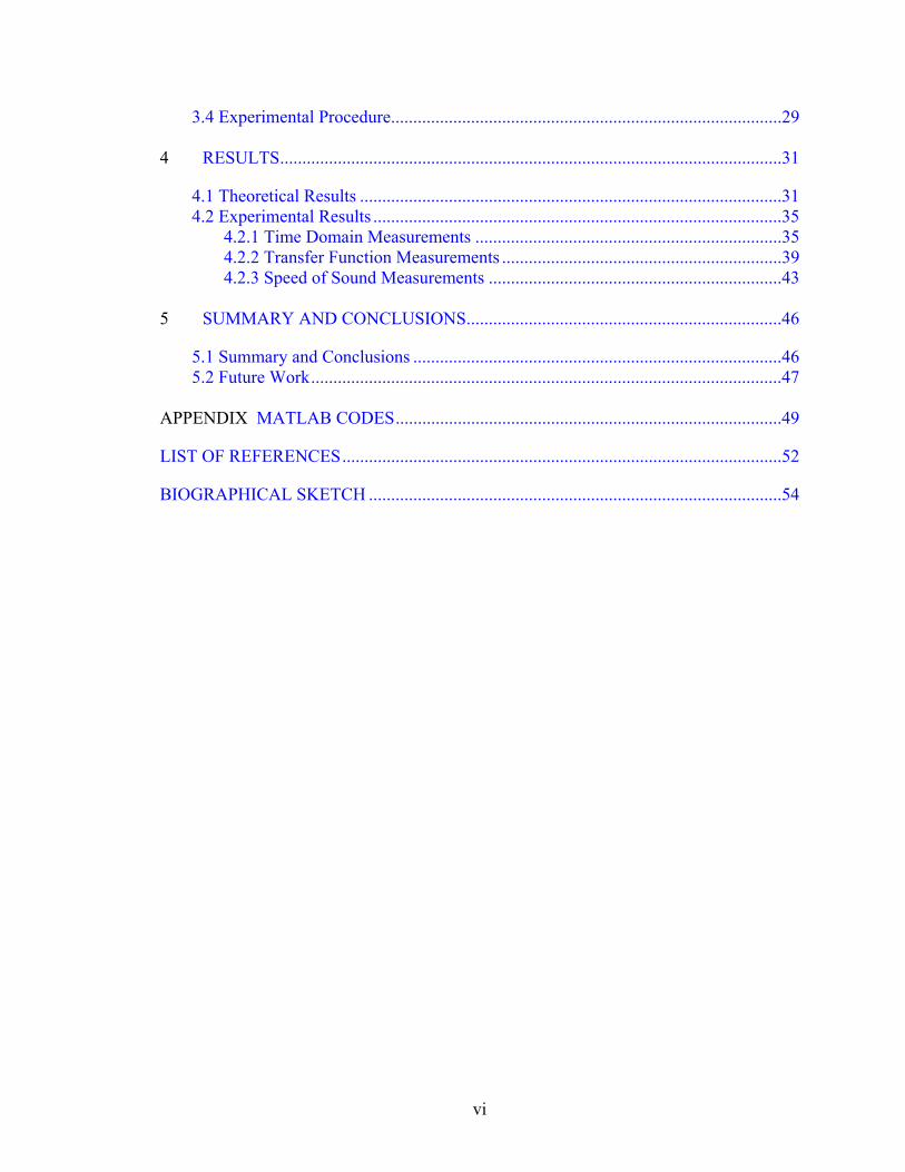
TABLE OF CONTENTS page ACKNOWLEDGMENTS ................................................................................................. iv
LIST OF TABLES............................................................................................................ vii
LIST OF FIGURES ......................................................................................................... viii
ABSTRACT.........................................................................................................................x
CHAPTER 1 INTRODUCTION......................................................................................................1
1.1 The Importance of Bulk Modulus...........................................................................1 1.2 Current Bulk Modulus Measurements....................................................................5
1.2.1 Vibration Tester............................................................................................6 1.2.2 Acoustic Coupler ..........................................................................................6 1.2.3 Holographic Interferometer ..........................................................................6 1.2.4 Electronic Speckle Pattern Interferometer....................................................7 1.2.5 Doppler Interferometer .................................................................................7 1.2.6 Normal Impedance and Flow Ripple Apparatus ..........................................8 1.2.7 Acoustic Methods.........................................................................................9 1.2.8 Other Methods ............................................................................................10
1.3 Motivation and Approach .....................................................................................11 2 THEORETICAL DEVELOPMENT........................................................................14
2.1 Piezoelectric Material ...........................................................................................14 2.2 Constitutive Equations..........................................................................................16 2.3 Speed of Sound and Transfer Function Measurements ........................................17 2.4 Piezoelectric Based Sensor ...................................................................................18
3 EXPERIMENTAL SETUP ......................................................................................23
3.1 Test Equipment .....................................................................................................23 3.1.1 Aluminum Block ........................................................................................24 3.1.2 Transducers, Plunger and Modal Hammer.................................................24 3.1.3 Signal Conditioner and Signal Analyzer ....................................................26
3.2 Experimental Setup...............................................................................................26 3.3 Pre-experimental Procedure..................................................................................28
v
3.4 Experimental Procedure........................................................................................29 4 RESULTS.................................................................................................................31
4.1 Theoretical Results ...............................................................................................31 4.2 Experimental Results ............................................................................................35
4.2.1 Time Domain Measurements .....................................................................35 4.2.2 Transfer Function Measurements ...............................................................39 4.2.3 Speed of Sound Measurements ..................................................................43
5 SUMMARY AND CONCLUSIONS.......................................................................46
5.1 Summary and Conclusions ...................................................................................46 5.2 Future Work..........................................................................................................47
APPENDIX MATLAB CODES.......................................................................................49
LIST OF REFERENCES...................................................................................................52
BIOGRAPHICAL SKETCH .............................................................................................54
vi
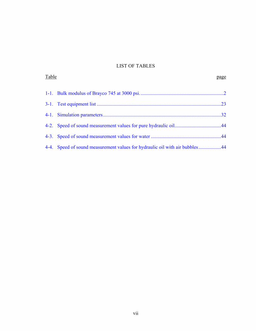
LIST OF TABLES
Table page
1-1. Bulk modulus of Brayco 745 at 3000 psi. ..................................................................2
3-1. Test equipment list ...................................................................................................23
4-1. Simulation parameters..............................................................................................32
4-2. Speed of sound measurement values for pure hydraulic oil.....................................44
4-3. Speed of sound measurement values for water ........................................................44
4-4. Speed of sound measurement values for hydraulic oil with air bubbles ..................44
vii
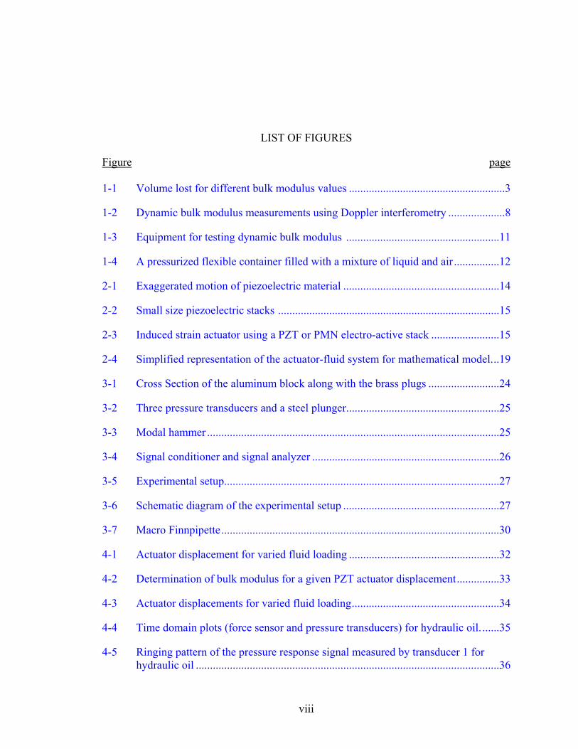
LIST OF FIGURES
Figure page 1-1 Volume lost for different bulk modulus values .......................................................3
1-2 Dynamic bulk modulus measurements using Doppler interferometry ....................8
1-3 Equipment for testing dynamic bulk modulus ......................................................11
1-4 A pressurized flexible container filled with a mixture of liquid and air ................12
2-1 Exaggerated motion of piezoelectric material .......................................................14
2-2 Small size piezoelectric stacks ..............................................................................15
2-3 Induced strain actuator using a PZT or PMN electro-active stack ........................15
2-4 Simplified representation of the actuator-fluid system for mathematical model...19
3-1 Cross Section of the aluminum block along with the brass plugs .........................24
3-2 Three pressure transducers and a steel plunger......................................................25
3-3 Modal hammer .......................................................................................................25
3-4 Signal conditioner and signal analyzer ..................................................................26
3-5 Experimental setup.................................................................................................27
3-6 Schematic diagram of the experimental setup .......................................................27
3-7 Macro Finnpipette..................................................................................................30
4-1 Actuator displacement for varied fluid loading .....................................................32
4-2 Determination of bulk modulus for a given PZT actuator displacement...............33
4-3 Actuator displacements for varied fluid loading....................................................34
4-4 Time domain plots (force sensor and pressure transducers) for hydraulic oil. ......35
4-5 Ringing pattern of the pressure response signal measured by transducer 1 for hydraulic oil ...........................................................................................................36
viii
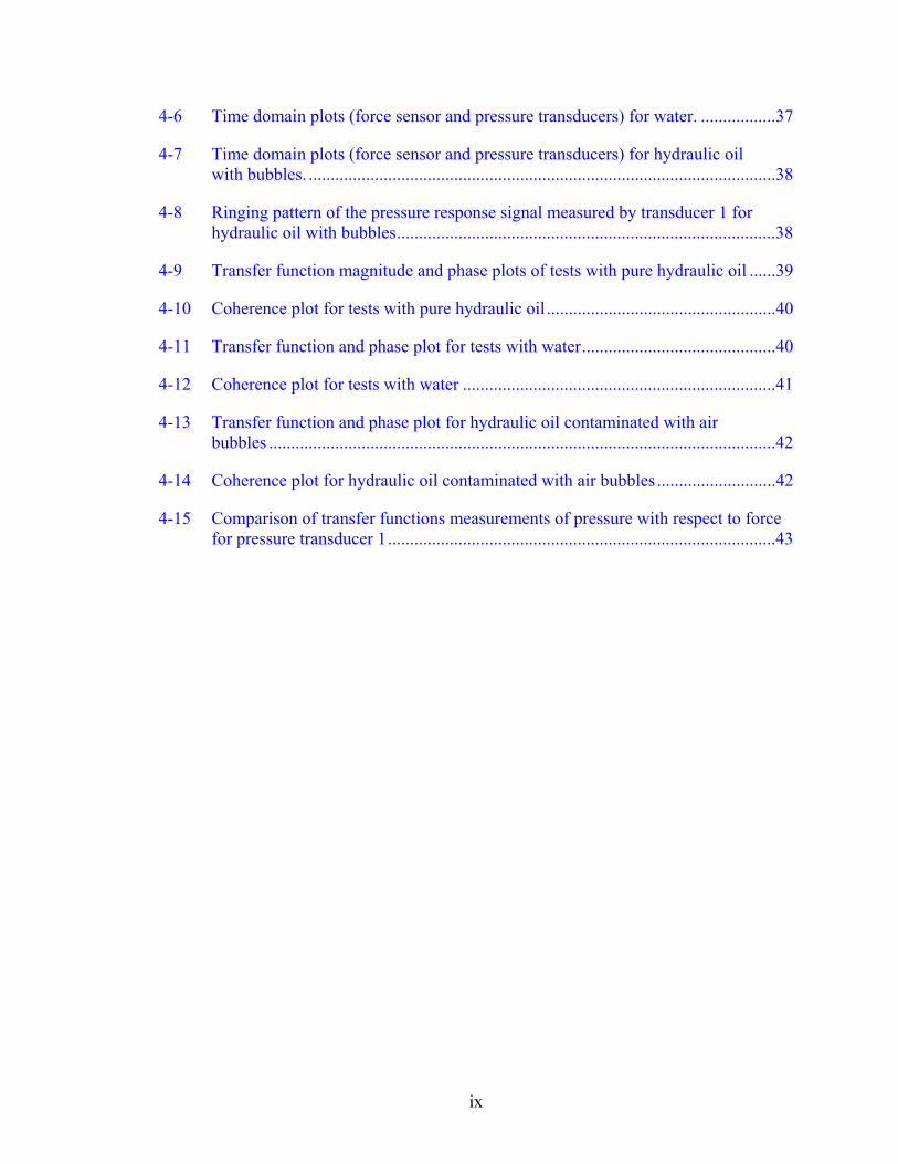
4-6 Time domain plots (force sensor and pressure transducers) for water. .................37
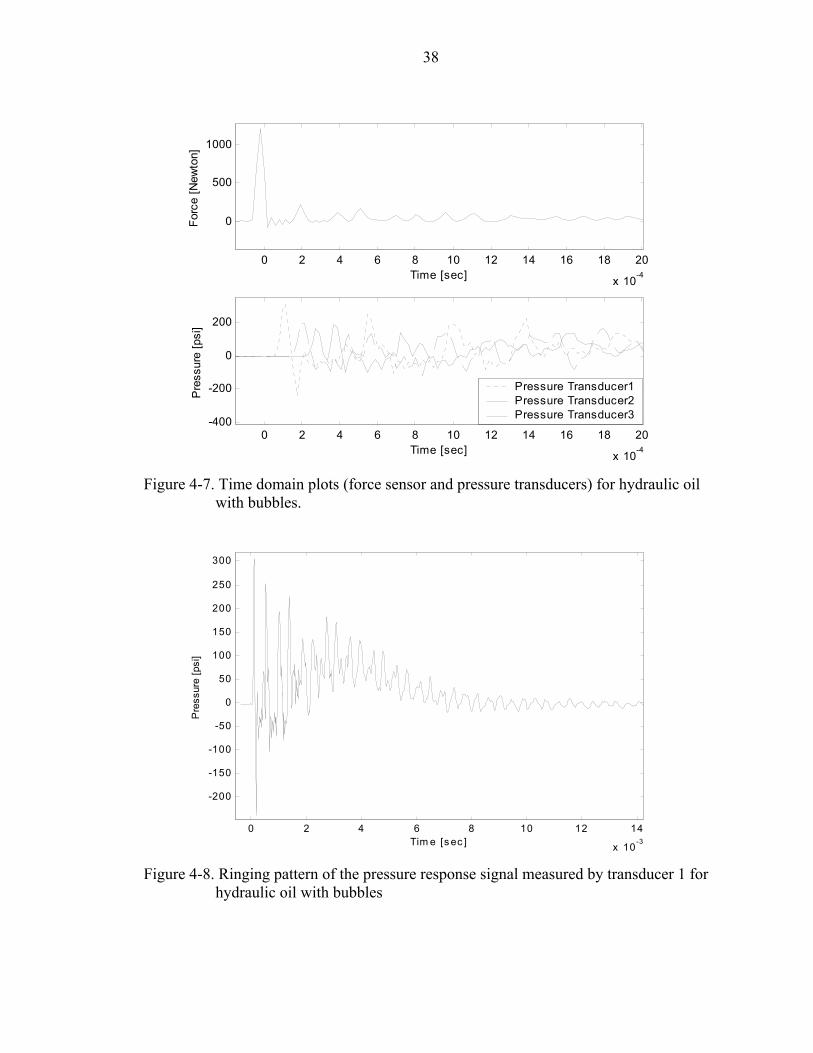
4-7 Time domain plots (force sensor and pressure transducers) for hydraulic oil with bubbles. ..........................................................................................................38
4-8 Ringing pattern of the pressure response signal measured by transducer 1 for hydraulic oil with bubbles......................................................................................38
4-9 Transfer function magnitude and phase plots of tests with pure hydraulic oil ......39
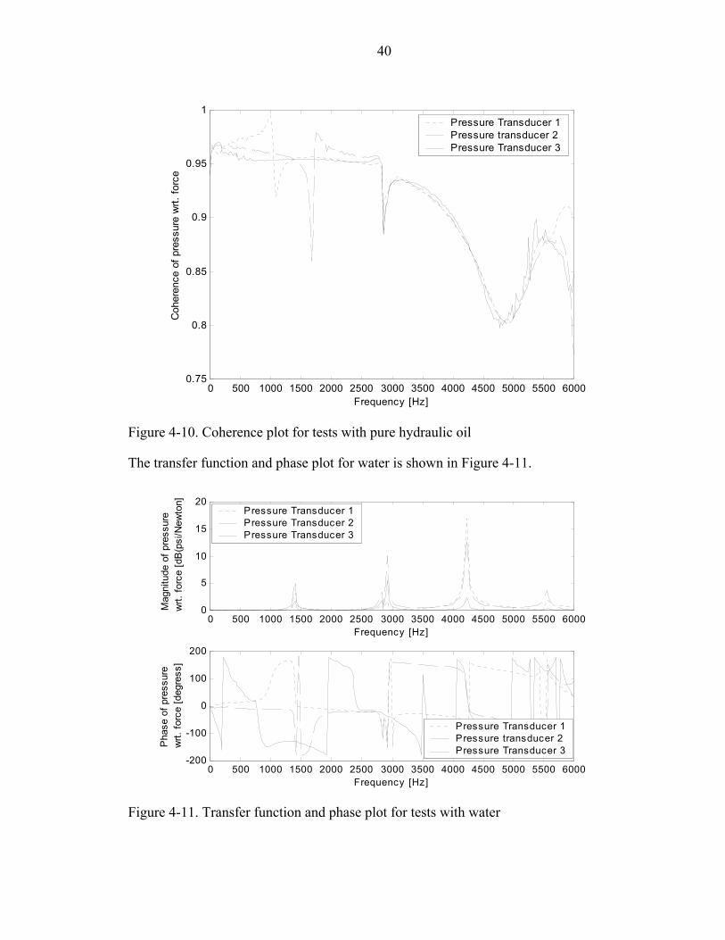
4-10 Coherence plot for tests with pure hydraulic oil ....................................................40
4-11 Transfer function and phase plot for tests with water............................................40
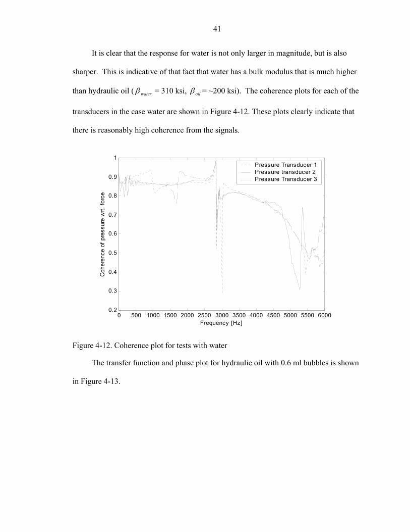
4-12 Coherence plot for tests with water .......................................................................41
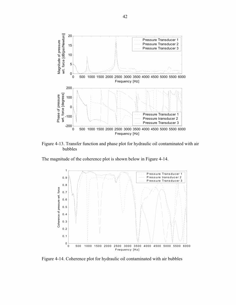
4-13 Transfer function and phase plot for hydraulic oil contaminated with air bubbles ...................................................................................................................42
4-14 Coherence plot for hydraulic oil contaminated with air bubbles...........................42
4-15 Comparison of transfer functions measurements of pressure with respect to force for pressure transducer 1........................................................................................43
ix
Abstract of Thesis Presented to the Graduate School
of the University of Florida in Partial Fulfillment of the Requirements for the Degree of Master of Science
SMART BULK MODULUS SENSOR
By
Balasubramanian Karthik
December 2003
Chair: Christopher Niezrecki Major Department: Mechanical and Aerospace Engineering
One application that smart materials may have a significant impact in is the
measurement of bulk modulus. Accurately knowing the bulk modulus of a fluid is very
important in many hydraulic applications. The absolute bulk modulus has a major effect
on the position, power delivery, response time, and stability of virtually all hydraulic
systems. The focus of this research is to develop a novel sensor to measure bulk modulus
of a fluid in real time. The work investigated three different strategies to determine the
bulk modulus of a fluid within a system. The first approach is to develop a theoretical
model to extract the bulk modulus of the fluid system by knowing the excitation voltage
and measuring the strain. The results indicate that matching the stiffness of the actuator
to the stiffness of the fluidic system is critical in obtaining a high sensitivity to the bulk
modulus measurement.
The second approach determines the frequency response functions by performing
transfer function measurements using an impulse response test. In this test, the transfer
x
function of the pressure response with respect to the applied force is measured. By doing
so it is possible to extract information about the properties of a fluid. The tests are
performed on three different fluids: water, hydraulic oil and hydraulic oil with bubbles.
The results indicate that magnitudes of the peaks (at 1400 Hz) were larger and sharper for
water compared to oil. Also, the magnitude of the peaks (at 1400 Hz) in the case of
hydraulic oil with bubbles was not only reduced but also occurred at a lower frequency
compared to the other two fluids.
The third approach uses speed of sound measurements to determine the bulk
modulus of the fluid in real time. The results indicate the theoretical values are
reasonably close to the actual bulk modulus values. Also, the hydraulic oil contaminated
with bubbles has a lower bulk modulus value compared with the pure hydraulic oil.
xi
CHAPTER 1 INTRODUCTION
The motivation for developing an in situ bulk modulus sensor is described in this
chapter. The importance of the bulk modulus in hydraulic applications, followed by a
general review of the current methods of measuring bulk modulus, is also presented.
Lastly, the approach adopted for determining the bulk modulus of a fluid in real time is
discussed.
1.1 The Importance of Bulk Modulus
The US market for pumps, cylinders, motors, valves and other fluid power
components alone is $12 billion annually, exceeding the value of other well-known
industries such as machine tools and robotics. The largest consumers are the aerospace,
construction equipment, heavy truck, agricultural equipment, machine tool and material
handling industries that take these components and integrate them in equipment worth
many billions of dollars. Yet despite the industry’s importance, and the fact that fluid
power imports grew at an average annual growth rate of 30% during much of the 1990’s,
little support has been given to the industry by the engineering research community
(National Fluid Power, 2002). The bulk modulus of a fluid (or solid) is a measure of its
compressibility and is given by
VPVOe ∆
∆−=β (1.1)
where
eβ - effective bulk modulus of the fluid
1
2
OV - unpressurized fluid volume,
P - fluid pressure and
V - instantaneous fluid volume.
The negative sign indicates a decrease in volume with a corresponding increase in
pressure. The parameters that primarily affect the bulk modulus of a fluid are
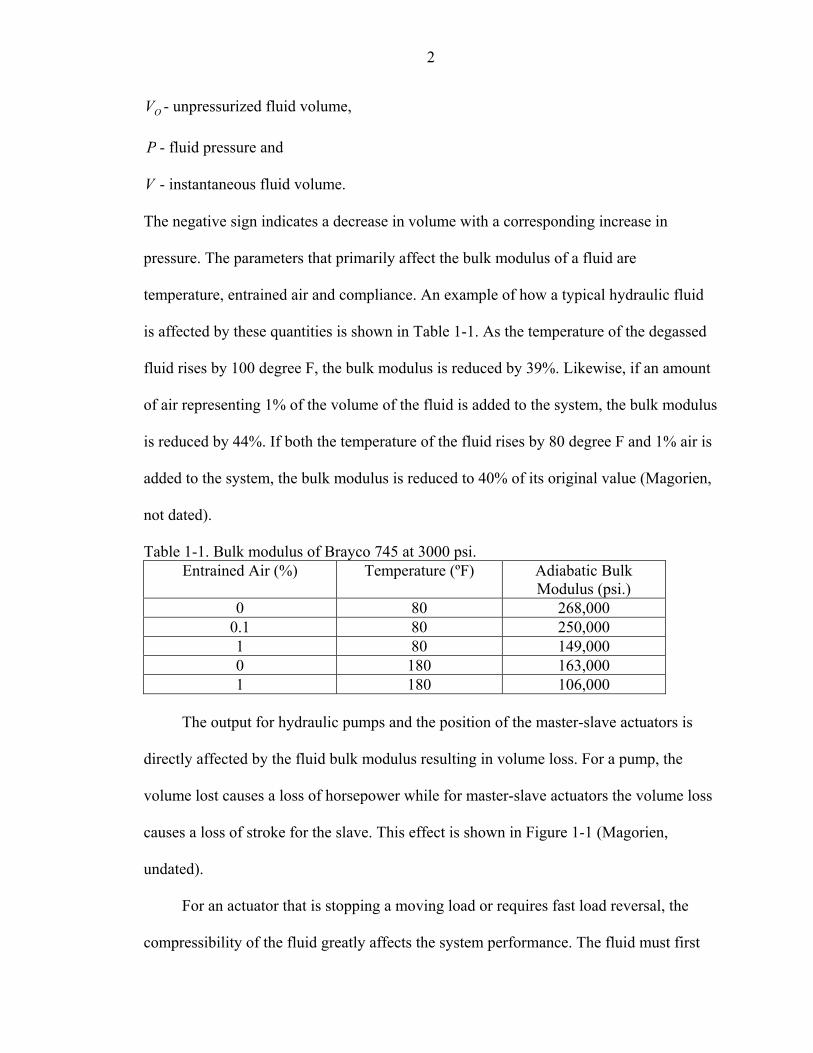
temperature, entrained air and compliance. An example of how a typical hydraulic fluid
is affected by these quantities is shown in Table 1-1. As the temperature of the degassed
fluid rises by 100 degree F, the bulk modulus is reduced by 39%. Likewise, if an amount
of air representing 1% of the volume of the fluid is added to the system, the bulk modulus
is reduced by 44%. If both the temperature of the fluid rises by 80 degree F and 1% air is
added to the system, the bulk modulus is reduced to 40% of its original value (Magorien,
not dated).
Table 1-1. Bulk modulus of Brayco 745 at 3000 psi. Entrained Air (%) Temperature (ºF) Adiabatic Bulk
Modulus (psi.) 0 80 268,000
0.1 80 250,000 1 80 149,000 0 180 163,000 1 180 106,000
The output for hydraulic pumps and the position of the master-slave actuators is
directly affected by the fluid bulk modulus resulting in volume loss. For a pump, the
volume lost causes a loss of horsepower while for master-slave actuators the volume loss
causes a loss of stroke for the slave. This effect is shown in Figure 1-1 (Magorien,
undated).
For an actuator that is stopping a moving load or requires fast load reversal, the
compressibility of the fluid greatly affects the system performance. The fluid must first

3
be compressed before the cylinder and piston can move the load to perform any useful
work. The power lost generally increases as the actuator size increases and the response
time decreases. If the bulk modulus of the hydraulic fluid is low, then energy is wasted in
compressing the fluid.
Vol
ume
Lost
[%]
Pressure [psi]
Figure 1-1. Volume lost for different bulk modulus values
Apart from the reasons previously discussed, one other reason that motivates the
need to determine the exact values of the bulk modulus of a fluid is its enormous
variability. Although it was published long ago in 1967, Hydraulic Control Systems by
Hebert E. Merritt is still the “bible” of dynamic hydraulic system design. It remains the
most-cited item in hydraulic research papers and is usually the basis for most dynamic
hydraulic modeling. Merritt says that:
4
“Interaction of the spring effect of a liquid and the mass of mechanical parts gives a
resonance in nearly all hydraulic components. In most cases this resonance is the chief
limitation to dynamic performance. The fluid spring is characterized by the value for the
bulk modulus” (Merritt, 1967, pg. 14).
Since the mass is commonly known in most practical systems, or can be
determined by the instrumentation such as load cells or strain gages, the bulk modulus of
the hydraulic fluid determines the dynamic performance capability of many hydraulic
systems. If the bulk modulus of a fluid is reduced by 50% due to the introduction of a 1%
volume of air, the system’s natural frequency will be reduced by 30%. This greatly
reduces the stability of the system. However, the bulk modulus is usually unknown.
Merritt again says:
In the absence of entrapped air, the effective bulk modulus would be 210,000 psi. In any practical case, it is difficult to determine the effective bulk modulus other than by direct measurement. Estimates of entrapped air in hydraulic systems run as high as 20% when the fluid is at atmospheric pressure. As pressure is increased, much of the air dissolves into the liquid and does not affect the bulk modulus. Blind use of the bulk modulus of the liquid alone without regard for entrapped air and structured elasticity can lead to gross errors in calculated resonances. Calculated resonances in hydraulic systems at best are approximate. (Merritt, 1967, pg.18)
Perhaps the second most cited text is John Watton’s is Fluid Power Systems. He says
succinctly:
Bulk modulus is a measure of the compressibility of a fluid and is inevitably required to calculate hydraulic natural frequencies in a system. It is perhaps one fluid parameter that causes most concern in its numerical evaluation due to other effects which modify it. (Watton, 1989, pg.28)
As hydraulics engineering matures, the levels of sophistication and detail are
greatly increasing. Yet, close examination of much hydraulics research indicates that a
value of the effective bulk modulus is just roughly assumed with no high degree of
5
accuracy. These assumed values vary widely, often despite similar oils and components.
For example, in recent issues of the Journal of Dynamics Systems, Measurement and
Control, the values ranged from 150 kPa (Abbott et al., 2001) to 784 MPa (Hayase et al.,
2000), which is equivalent to 22 to 114,000 psi. Hence, the values of bulk modulus do
vary in practice and are usually unknown. Bulk modulus assumptions commonly range
from 60,000 psi to 150,000 psi for common hydraulic systems (Habibi, 1999).
Consequently, achievable hydraulic system performance suffers. Typically,
designer’s primary goal when creating hydraulic control systems is to achieve a trajectory
with small error. The second goal is to design the system such that it is robust to
variations in the hydraulic fluid bulk modulus (Eryilmaz and Wilson, 2001). They say,
“Other control laws often employ hydraulic fluid bulk modulus- a difficult to characterize
quantity- as a parameter.” Knowing the bulk modulus of a fluid in real time will improve
the performance of a wide variety of controllers. To date, there is no convenient method
to measure the bulk modulus of fluid in a hydraulic system.
1.2 Current Bulk Modulus Measurements
In order to measure the bulk modulus of a fluid, a sample of the fluid is typically
placed in a chamber having a piston that can vary the volume of the fluid. As the fluid is
loaded its compressibility is determined. However this method requires a fairly
sophisticated testing apparatus. Some special techniques to determine the dynamic bulk
modulus of fluids, elastomers have also been created. One such method is holographic
interferometry (Holownia, 1986). Other researchers have investigated measuring bulk
modulus of fluids and solids through acoustic methods (Marvin et al., 1954). This Section
discusses some of these measuring techniques.

6
1.2.1 Vibration Tester
Philipoff and Brodynan found the bulk compressibility of plastics using harmonic
vibrations at very low frequencies (10-5 Hz – 10 Hz). The apparatus consists of a
hardened steel pressure chamber, a steel plunger that rests on a jack together with a
vibrating testing machine. A strain gauge is used to pre-stress the system to a desired
value after which the jack is locked in its place. The instrument is calibrated using
mercury and water to determine a correction factor. The compressibility of the plastic is
calculated after knowing the area of the plunger, the volume of the plastic, the mercury
volume, the volume of the pressure chamber and the correction factor. They concluded
that the compressibility is a complex quantity but could not determine the exact phase
angle for plastics (Philippoff and Brodnyan, 1955).
1.2.2 Acoustic Coupler
McKinney et al. improvised on the prior setup to determine the dynamic bulk
modulus of materials over the frequency range of 50 Hz to 10,000 Hz using an acoustic
coupler. In this method, the sample is placed within the cavity of a rigid pressure vessel
that is equipped with two sets of pressure transducers. The cavity is filled with light oil,
which is used as a transmitting medium. One set of piezoelectric transducers is used as an
actuator to compress the fluid. The second set is used as a receiver whose output voltage
measures the resulting pressure changes. The ratio of the output to input voltages is then
used to determine the compliance of the coupler and its content, in particular, the
compliance of the sample (McKinney et al., 1956).
1.2.3 Holographic Interferometer
Holographic interferometry is a technique that is used to measure the static and
dynamic bulk modulus of elastomers. Experimentally, this is realized by subjecting a

7
sample placed in a pressure cell to a hydrostatic pressure of up to 20 atmospheres. The
sample is then exposed to a single laser beam that captured its contraction onto a
holographic plate resulting in fringe pattern from which the bulk modulus is calculated.
The pressure cell is provided with static and dynamic pressure supply lines. The peak-to-
peak dynamic pressure is on the order of 1 to 5 atmospheres. Glycerine and transformer
oil are the two fluids that are used in the pressure cell. The frequency range that is
covered is from 1 to 1000 Hz (Holownia, 1986).
1.2.4 Electronic Speckle Pattern Interferometer
Howlonia and Rowland measured the volume changes of a rubber sample in
glycerine by applying sinusoidal pressures using electronic speckle pattern interferometry
(ESPI). The system comprises of three control areas: the electro-optical system, the
hydraulic system and the electrical system. The electro-optical system provides a He-Ne
laser that is used for illuminating the rubber sample. A photodiode is used to analyze the
beam modulation. The hydraulic system supplies the sinusoidal pressures to be applied
on the sample through an oil-glycerine interface. A piezoelectric transducer measures the
applied pressure. The electrical system monitors the signal from the photodiode and the
transducer on a cathode-ray tube, where the pressure and phase angles are measured by
observing the fringes. The advantage of this technique over holography is that the fringes
obtained can be seen “live” as the sample deflects. The range of frequency covered is 50-
1000 Hz (Holownia and Rowland, 1986).
1.2.5 Doppler Interferometer
Guillot and Jarzynski used the laser Doppler interferometer to detect the strain
resulting from the compression of a sample to determine the bulk modulus. In this
method, the sample is placed at one end of a tube and a loud speaker is attached at the
8
other end as shown in Figure 1-2. The loudspeaker is driven with a transient signal and
the pressure inside the tube is recorded using a sound level meter. A pair of photodiodes
detected the displacement signals from each side of the sample. A phase-locked loop
circuit processes the output of each photodiode. After integration and calibration, the
displacements on either side of the sample were determined. These displacement values
are then used to calculate the bulk modulus. The frequency range for this method is from
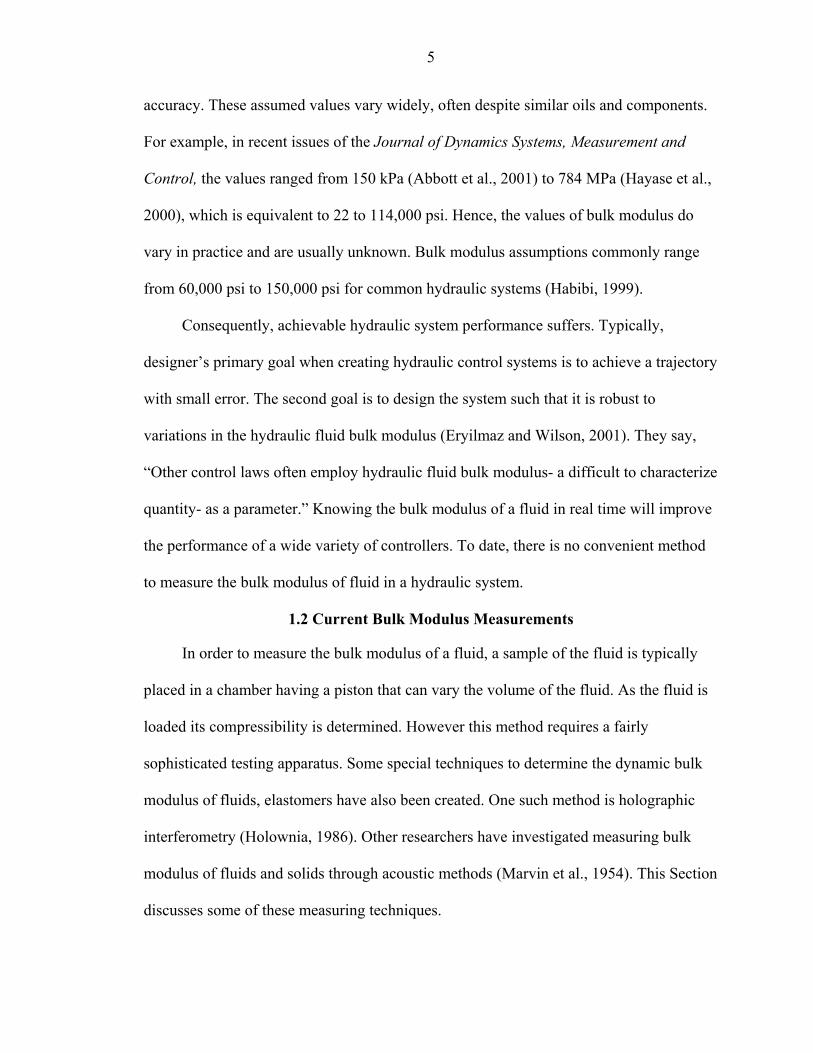
200 Hz to 2 kHz (Guillot and Jarzynski, 2000).
Figure 1-2. Dynamic bulk modulus measurements using Doppler interferometry (Guillot
and Jarzynski, 2000).
1.2.6 Normal Impedance and Flow Ripple Apparatus
Fluid bulk modulus is measured by using a normal impedance and flow ripple
apparatus in accordance with the International Standards Organization (ISO 1067-1). The
test rig contains two reservoirs in order to switch between fluids, if needed. One variable
speed motor is used to drive the pump while another variable speed secondary motor is
used to develop pressure pulses along the fluid line. Three pressure transducers
assembled at the outlet of the pump are connected to the data acquisition system. An
iterative method is used for calculating the speed of sound and the bulk modulus wherein
the starting value for the effective bulk modulus is assumed and the speed of sound
calculated based on this assumption. Then a correction to the speed of sound is made and

9
the revised speed of sound is calculated. This revised speed of sound is then used for
calculating the effective bulk modulus (Qatu and Dougherty, 1998).
1.2.7 Acoustic Methods
The dynamic bulk modulus of polyisobutylene is calculated from the longitudinal-
wave and shear moduli. For a purely elastic material the longitudinal wave modulus (M)
is related to the bulk modulus ( eβ ) and shear modulus (G ) by
3)4( G
M e +=β
(1.2)
In a viscoelastic medium the same relation is applicable, except that both eβ and
become complex functions rather than constants. In this method, a signal is transmitted
from one piezoelectric transducer to a sample and from the sample to another transducer
that acts as a receiver. The medium used for transmitting the plane wave is ethylene
glycol. The velocity is determined by measuring the phase shift introduced in the
received signal on inserting the sample. The frequency of interest is from 0.9 to 7
megacycles per second (Marvin et al., 1954).
G
Burns et al. discuss two experimental methods for measuring the dynamic bulk
modulus in elastomers. In the impedance tube method the speed of a longitudinal plane
wave in the material is measured. The longitudinal wave modulus is calculated from the
sound speed and the density of the solid. The bulk modulus is then calculated from the
shear modulus and the wave modulus using Equation 1.2. This method is most useful at
relatively high frequencies, above 10 kHz. The second method involves using an acoustic
coupler at low frequencies. This technique is similar to the one developed by McKinney,
et al. Both the methods were used by the authors but the coupler gave them more accurate
results (Burns et al., 1990).
10
Koda et al. determined the longitudinal, shear and bulk moduli of polymeric
materials by measuring the longitudinal and transverse sound velocities. Experimentally,
the sound velocity is obtained from the measurement of time required for transmission
through a specimen of thickness. The transmit time is determined by using the TAC
(time-to-amplitude converter) method in a double transducer system. Lead zirconate
titanate (PZT) and quartz are used as transducers for the transverse and longitudinal
sound waves, respectively. The sound waves propagate through an aluminum buffer
before reaching the specimen. The TAC system starts when the transducer detects the
sound wave reflected from the interface between the buffer and the specimen and stops
when another transducer receives the transmitted sound wave. From the sound velocity,
the longitudinal and shear moduli are obtained. The relation between the longitudinal
wave modulus, shear modulus and the bulk modulus are then used to calculate the bulk
modulus (Koda et al., 1993).
1.2.8 Other Methods
Holownia and James used hydraulic pressure change rather than volume change to
compress an elastomeric specimen to measure dynamic bulk modulus from 100 Hz up to
1200 Hz. In this method, two identical chambers are filled with liquid and a rubber
sample placed in one of them as shown in Figure 1-3. A stepped piston, attached to a
vibrator, is then used to pressurize both the chambers. The resulting pressure, which will
depend on the volume and compressibility of the rubber sample, is then measured using
piezoelectric transducers (Holownia and James, 1993).
11
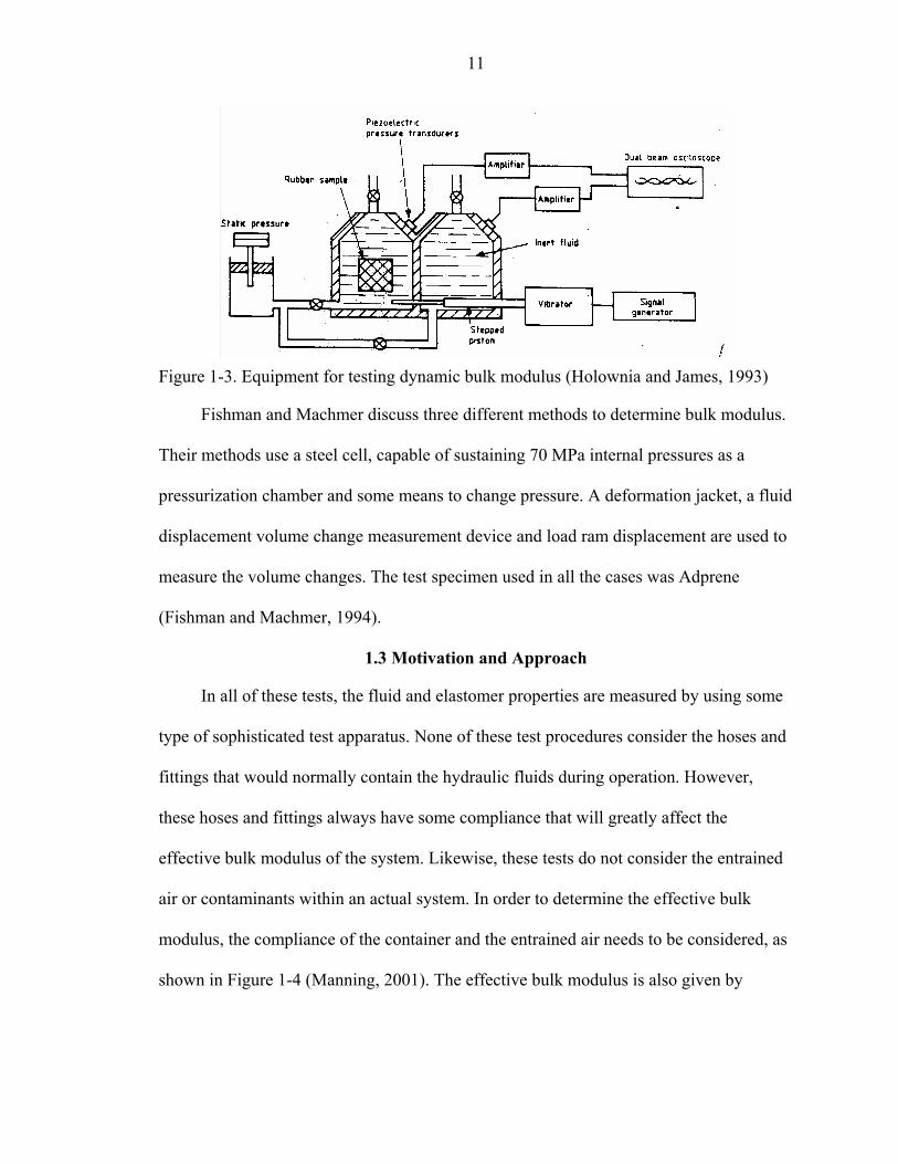
Figure 1-3. Equipment for testing dynamic bulk modulus (Holownia and James, 1993)
Fishman and Machmer discuss three different methods to determine bulk modulus.
Their methods use a steel cell, capable of sustaining 70 MPa internal pressures as a
pressurization chamber and some means to change pressure. A deformation jacket, a fluid
displacement volume change measurement device and load ram displacement are used to
measure the volume changes. The test specimen used in all the cases was Adprene
(Fishman and Machmer, 1994).
1.3 Motivation and Approach
In all of these tests, the fluid and elastomer properties are measured by using some
type of sophisticated test apparatus. None of these test procedures consider the hoses and
fittings that would normally contain the hydraulic fluids during operation. However,
these hoses and fittings always have some compliance that will greatly affect the
effective bulk modulus of the system. Likewise, these tests do not consider the entrained
air or contaminants within an actual system. In order to determine the effective bulk
modulus, the compliance of the container and the entrained air needs to be considered, as
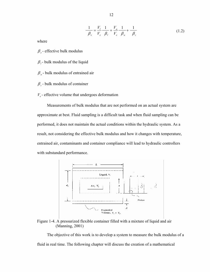
shown in Figure 1-4 (Manning, 2001). The effective bulk modulus is also given by
12
cae
a
le
l
e VV
VV
ββββ1111
++= (1.2)
where
eβ - effective bulk modulus
lβ - bulk modulus of the liquid
aβ - bulk modulus of entrained air
cβ - bulk modulus of container
eV - effective volume that undergoes deformation
Measurements of bulk modulus that are not performed on an actual system are
approximate at best. Fluid sampling is a difficult task and when fluid sampling can be
performed, it does not maintain the actual conditions within the hydraulic system. As a
result, not considering the effective bulk modulus and how it changes with temperature,
entrained air, contaminants and container compliance will lead to hydraulic controllers
with substandard performance.
Figure 1-4. A pressurized flexible container filled with a mixture of liquid and air
(Manning, 2001)
The objective of this work is to develop a system to measure the bulk modulus of a
fluid in real time. The following chapter will discuss the creation of a mathematical
13
model of a fluidic system response to a quasi-static excitation that incorporates the
constitutive Equations of a piezoelectric actuator. The specific test apparatus used to
measure the effective bulk modulus and its variation with entrained air, two approaches
(speed of sound measurements and frequency response functions using a modal hammer
test) to compute bulk modulus, and an analysis of the results using these two methods are
also presented. Conclusions will be drawn and future work will be discussed.
CHAPTER 2 THEORETICAL DEVELOPMENT
Within this chapter a brief review of piezoelectric actuation and its constitutive
Equations is presented. The piezoelectric actuator is the heart of the bulk modulus sensor
being investigated. Additionally bulk modulus variability on speed of sound is described
along with transfer function measurements. Finally a mathematical formulation to extract
the bulk modulus of a fluid using piezoelectric actuator is derived.
2.1 Piezoelectric Material
Piezoelectric material comes in variety of forms, ranging from rectangular patches,
thin discs and tubes, to very complex shapes fabricated using solid freeform fabrication
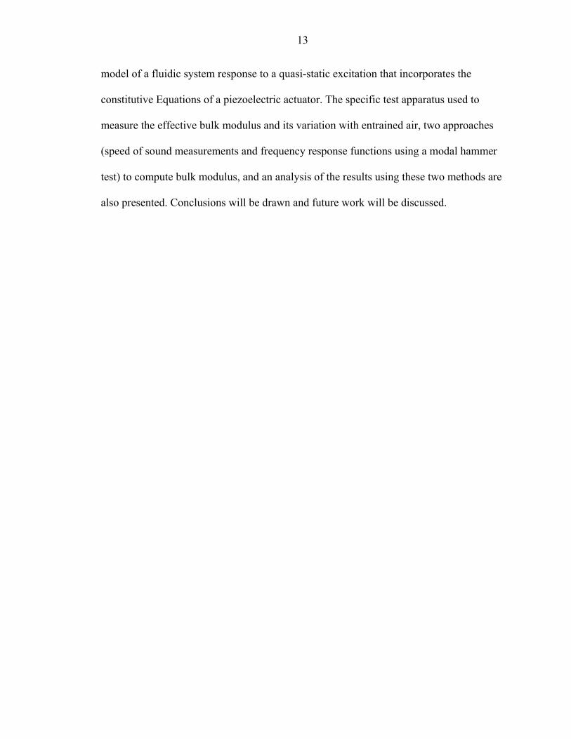
or injection molding. Due to its crystalline nature, a piezoelectric material expands and
contracts when an electric field is applied as shown in Figure 2-1. Typical free strains
induced in these elements are on the order of 0.1% to 0.2%. Because of the free strain or
displacement (in plane: d31, out of plane: d33) of these piezoceramics is so small, they
typically cannot be used as actuators in their raw form; rather, amplification is required.
As a result numerous, novel and ingenious mechanisms to amplify the actuator motion
have been developed. One such development is the use of piezoelectric stacks.
Figure 2-1. Exaggerated motion of piezoelectric material (Niezrecki et al., 2001)
14
15
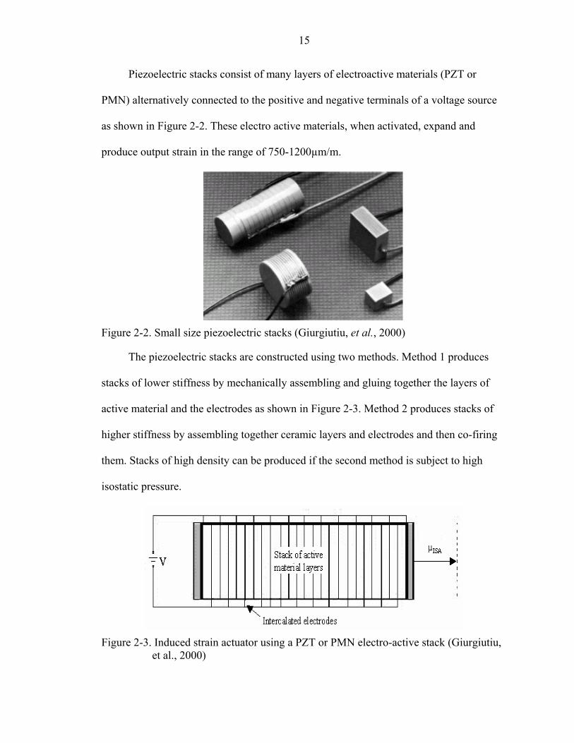
Piezoelectric stacks consist of many layers of electroactive materials (PZT or
PMN) alternatively connected to the positive and negative terminals of a voltage source
as shown in Figure 2-2. These electro active materials, when activated, expand and
produce output strain in the range of 750-1200µm/m.
Figure 2-2. Small size piezoelectric stacks (Giurgiutiu, et al., 2000)
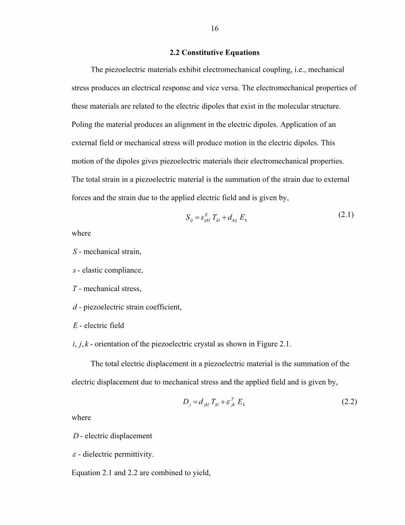
The piezoelectric stacks are constructed using two methods. Method 1 produces
stacks of lower stiffness by mechanically assembling and gluing together the layers of
active material and the electrodes as shown in Figure 2-3. Method 2 produces stacks of
higher stiffness by assembling together ceramic layers and electrodes and then co-firing
them. Stacks of high density can be produced if the second method is subject to high
isostatic pressure.
Figure 2-3. Induced strain actuator using a PZT or PMN electro-active stack (Giurgiutiu,
et al., 2000)
16
2.2 Constitutive Equations
The piezoelectric materials exhibit electromechanical coupling, i.e., mechanical
stress produces an electrical response and vice versa. The electromechanical properties of
these materials are related to the electric dipoles that exist in the molecular structure.
Poling the material produces an alignment in the electric dipoles. Application of an
external field or mechanical stress will produce motion in the electric dipoles. This
motion of the dipoles gives piezoelectric materials their electromechanical properties.
The total strain in a piezoelectric material is the summation of the strain due to external
forces and the strain due to the applied electric field and is given by,
kkijklEijklij EdTsS += (2.1)
where
S - mechanical strain,
s - elastic compliance,
T - mechanical stress,
d - piezoelectric strain coefficient,
E - electric field
kji ,, - orientation of the piezoelectric crystal as shown in Figure 2.1.
The total electric displacement in a piezoelectric material is the summation of the
electric displacement due to mechanical stress and the applied field and is given by,
(2.2) kTjkkljklj ETdD ε+=
where
D - electric displacement
ε - dielectric permittivity.
Equation 2.1 and 2.2 are combined to yield,
17
=
ET
dds
DS
ε (2.3)
Equation 2.3 clearly indicates that the mechanical and electrical domains are
coupled through the piezoelectric strain coefficient, For piezoelectric stacked
actuators, the three-dimensional tensor Equation can be reduced to a one-dimensional
Equation in which the induced deformation of the actuator is dependent on the electric
field (or voltage) and the mechanical loading applied on the actuator. The reduced
constitutive relation is then given by:
.d
(2.4) 3333333 TsEdS E+=
Equation 2.4 can be rewritten in terms of the piezoelectric strain, pε , the applied
voltage, v , the thickness of the piezoelectric stack, t , the Young’s modulus of the
piezoelectric material, , and the piezoelectric stress,pE pσ . The above Equation then
becomes,
pε = ppEt
vd σ133 + (2.5)
The first term in Equation 2.5 is the induced strain under stress free conditions.
This Equation is used in the development of the theoretical model that will be discussed
later in this Section.
2.3 Speed of Sound and Transfer Function Measurements
Apart from the model presented is Section 2.4, the speed of sound and transfer
function measurements may also be used to determine the bulk modulus of the fluid in
real time. As a signal is applied to a piezoelectric actuator, the deflection of the actuator
will generate a propagating acoustic wave that will travel from the actuator through the
fluid and will reach a pressure sensor. Because the pressure sensor is located some

18
distance from the actuator, there will be a time delay between the induced actuator pulse
and the measured pressure sensor response. From the measured time delay and known
distance, the wave speed and fluid bulk modulus can be determined. The speed of sound
of a wave traveling in a fluid is given by (Streeter and Wylie, 1975):
ρβ ec= (2.6)
where
c - wave speed
ρ - fluid mass density
Another approach that will be investigated involves performing transfer function
measurements. Transfer function measurements are routinely used in structural dynamic
analysis to characterize the mechanical properties (natural frequency, damping, stiffness,
etc.) of structures. These same experimental techniques can be applied to hydraulic fluids
to determine their properties by knowing the frequency response functions (FRFs). The
frequency response functions for a fluid can be obtained by using an impulse response
test. In this test, the transfer function of the pressure response with respect to the applied
force is measured. By doing so it is possible to extract information about the properties
(stiffness, bulk modulus, etc.) of a fluid.
2.4 Piezoelectric Based Sensor
Within this Section an expression relating a piezoelectric (PZT) actuator input
voltage to its displacement for a given fluidic system (containing entrained air and
mechanical compliance) is derived. The model can be used to extract the bulk modulus of
the fluid in real time.
19
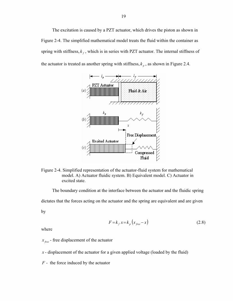
The excitation is caused by a PZT actuator, which drives the piston as shown in
Figure 2-4. The simplified mathematical model treats the fluid within the container as
spring with stiffness, , which is in series with PZT actuator. The internal stiffness of
the actuator is treated as another spring with stiffness, , as shown in Figure 2.4.
fk
pk
Figure 2-4. Simplified representation of the actuator-fluid system for mathematical
model. A) Actuator fluidic system. B) Equivalent model. C) Actuator in excited state.
The boundary condition at the interface between the actuator and the fluidic spring
dictates that the forces acting on the actuator and the spring are equivalent and are given
by
( )xxkxkF freepf −== (2.8) where
freex - free displacement of the actuator
x - displacement of the actuator for a given applied voltage (loaded by the fluid)
F - the force induced by the actuator
20
During expansion, the active material works to compress the fluid and to expand
the internal stiffness of the piezoelectric material. Rearranging Equation 2.8 and solving
for the actuator displacement yields:
(2.9)
pf
freep
kkxk
x+
=
Equation 1.1 can also be arranged in terms of the change in pressure ( ): P∆
O
e VVP ∆
−=∆ β (2.10)
The change in volume , is related to the area of the fluid, , and change in
actuator displacement, . Likewise, the induced force is equivalent to the product of
induced pressure and the area of the actuator. Using the relationship in Equation 2.10
yields:
V∆ fA
x∆
( )
o
fe
p VxA
AF ∆−
−=∆ β
(2.11)
Rearranging Equation 2.11 and expressing it in terms of the applied force induced
by the actuator, F∆ ,
o
fe
VxA
F∆
=∆2β
(2.12)
The stiffness of the fluid can be expressed in terms of the bulk modulus by
rearranging Equation 2.12
f
fe
ff
fef
O
fe
lA
lAA
kV
AxF βββ
====∆∆ 22
(2.13)
where l is the length of the fluid as described in Figure 2.4. The axial stiffness of the
PZT actuator can be expressed as:
f
21
p
ppp l
EA=k (2.14)
where
pE - modulus of elasticity of the piezoelectric material,
pl - length of the actuator and
PA - cross-Sectional area of the actuator.
The displacement of the actuator can be expressed in terms of the bulk modulus of
the fluid by substituting the expressions for k and (Equation 2.13 and 2.14) into
Equation 2.9.The expression can then be solved for the actuator displacement and is
given by:
f pk
( )pppffep
freepp
lEAlAlxEA
x+
=β
(2.15)
The free displacement of a piezoelectric actuator is directly related to the dielectric
coefficient, , the applied electric field and the length of the actuator. The free
displacement for a stress free state is the product of the stress free strain and the length of
the piezoelectric actuator. From Equation 2.5 the induced strain is
33d
tvd33 and hence the
free displacement is given by:
pfree ltvdx 33= (2.16)
where
v - applied voltage and
t - thickness of the actuator.
22
Substituting the expression for the free displacement (Equation 2.16) into Equation
2.15 produces a solution for the actuator displacement in terms of the effective bulk
modulus and other known quantities, and is given by:
( )pppffe
pp
lEAlAtvdEA
x+
=β
33 (2.17)
Equation 2.17 can be rearranged to obtain an expression for the effective bulk
modulus of the fluid, and is given by:
−=pf
fppe ltx
vdA
lEA 133β ; freexx ≤ (2.18)
The expression derived in Equation 2.18 assumes that the displacement of the
actuator is a known quantity. In order to utilize this result, the displacement of the
actuator needs to be measured. This can be accomplished placing a strain sensor on the
PZT actuator to measure the displacement. Assuming the geometry, physical properties
of the actuator, applied voltage, and the displacement are known, Equation 2.18 can be
used to extract the effective bulk modulus of the fluid in real time.

CHAPTER 3 EXPERIMENTAL SETUP
One objective of this experiment is to determine the transfer function of the
pressure response with respect to applied force. By obtaining these frequency response
functions (FRFs), it may be possible to correlate this data to the stiffness (or bulk
modulus) of the fluid. Another objective is to compute the bulk modulus of the fluid in
real time using speed of sound measurements. This chapter will describe how the
experiments are setup and run, to achieve these objectives.
3.1 Test Equipment
The primary test equipment consists of an aluminum block with a cavity, a plunger,
three pressure transducers and a modal hammer. A comprehensive list of all the test
equipment and their quantities is shown in Table 3-1. This is followed by a brief
description of the essential components.
Table 3-1. Test equipment list Equipment Quantity
Aluminum block (highly rigid) with a cavity
1
Pressure transducers 3
Aluminum plunger 1
Modal hammer 1
Brass plugs 2
Signal conditioner 1
DSP siglab 1
BNC cables 3
23
24
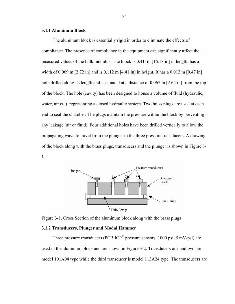
3.1.1 Aluminum Block
The aluminum block is essentially rigid in order to eliminate the effects of
compliance. The presence of compliance in the equipment can significantly affect the
measured values of the bulk modulus. The block is 0.411m [16.18 in] in length, has a
width of 0.069 m [2.72 in] and is 0.112 m [4.41 in] in height. It has a 0.012 m [0.47 in]
hole drilled along its length and is situated at a distance of 0.067 m [2.64 in] from the top
of the block. The hole (cavity) has been designed to house a volume of fluid (hydraulic,
water, air etc), representing a closed hydraulic system. Two brass plugs are used at each
end to seal the chamber. The plugs maintain the pressure within the block by preventing
any leakage (air or fluid). Four additional holes have been drilled vertically to allow the
propagating wave to travel from the plunger to the three pressure transducers. A drawing
of the block along with the brass plugs, transducers and the plunger is shown in Figure 3-
1.
Figure 3-1. Cross Section of the aluminum block along with the brass plugs
3.1.2 Transducers, Plunger and Modal Hammer
Three pressure transducers (PCB ICP® pressure sensors, 1000 psi, 5 mV/psi) are
used in the aluminum block and are shown in Figure 3-2. Transducers one and two are
model 101A04 type while the third transducer is model 113A24 type. The transducers are

25
taped with Teflon before they are fit into the block in order to prevent any leaks and to
ensure a tight fit.
The aluminum or steel plunger is fit at one end of the block and the stem of the
plunger has two grooves that accommodate two o-rings (see Figure 3.2). The purpose of
the o-rings is to prevent any leakage. The plunger acts as a piston and is used to generate
a pressure pulse within the fluid. Grease is applied to the stem to facilitate easy
movement of the plunger.
Figure 3-2. Three pressure transducers and a steel plunger
The type of modal hammer used for the experiment is the 086BO4 PCB modal
hammer as shown in Figure 3-3. The hammer used has a range from 0 to 1000 lbs and a
sensitivity of 943 N/V. The purpose of the hammer is to provide the impact to the plunger
in order to generate a pressure wave in the fluidic cavity.
Figure 3-3. Modal hammer
26
3.1.3 Signal Conditioner and Signal Analyzer
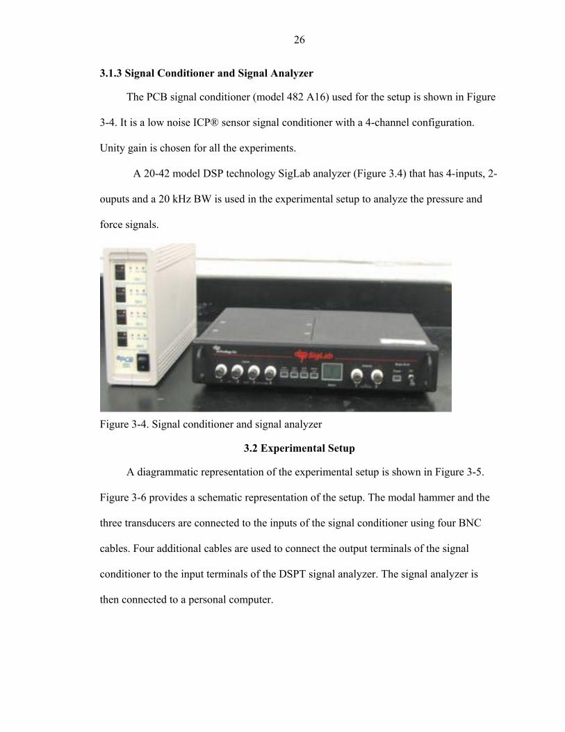
The PCB signal conditioner (model 482 A16) used for the setup is shown in Figure
3-4. It is a low noise ICP® sensor signal conditioner with a 4-channel configuration.
Unity gain is chosen for all the experiments.
A 20-42 model DSP technology SigLab analyzer (Figure 3.4) that has 4-inputs, 2-
ouputs and a 20 kHz BW is used in the experimental setup to analyze the pressure and
force signals.
Figure 3-4. Signal conditioner and signal analyzer
3.2 Experimental Setup
A diagrammatic representation of the experimental setup is shown in Figure 3-5.
Figure 3-6 provides a schematic representation of the setup. The modal hammer and the
three transducers are connected to the inputs of the signal conditioner using four BNC
cables. Four additional cables are used to connect the output terminals of the signal
conditioner to the input terminals of the DSPT signal analyzer. The signal analyzer is
then connected to a personal computer.

27
Figure 3-5. Experimental setup
Ch 1 In
Ch 2 In
Ch 3 In
Ch 4 In
DSPT Siglab
Ch 1 out Ch 1 In
Ch 2 out Ch 2 In
Ch 3 out Ch 3 In
Ch 4 out Ch 4 In
PC
Signal Conditioner
Modal Hammer
Transducer 1
Transducer 2
Transducer 3
Figure 3-6. Schematic diagram of the experimental setup

28
The modal hammer is used to provide an impact force on the plunger that acts like a
piston. This causes a pressure pulse to travel through the cavity. The transducers then
measure the pressure pulse. The delivery of the pressure pulse can be ultimately provided
by a piezoelectric actuator. Once the force and pressure are known, the transfer function
is determined between the pressure and applied force. By knowing this it is possible to
extract information about the properties (stiffness, bulk modulus, etc.) of a fluid.
In order to measure the speed of sound in the fluid, the same experimental setup is
used as shown in Figure 3.6. The wave speed is determined by measuring a time delay
between induced actuator pulse (provided by the modal hammer) and the measured
pressure sensor response. From the measured time delay and known distance between the
bottom of the plunger and each of the pressure sensors through the fluid (0.17 m, 0.29 m
and 0.41 m), the wave speed and fluid bulk modulus can be determined using the formula
stated in Section 2.3.
3.3 Pre-experimental Procedure
All the measurements are conducted using three different fluids within the cavity:
water, Mystik AW/AL (anti-wear/anti-leak) ISO 32 hydraulic oil and oil contaminated
with a specified quantity of air. Before performing the measurements for a given fluid the
following procedure is meticulously performed to ensure that the system is free of air
bubbles:
1. The cavity is cleaned using a solution of water and liquid detergent (when using oil). The surface of the block is then cleaned using a dry cloth. The block is oven dried at temperature of 200°C to remove any water particles. It is then allowed to cool to room temperature.
2. The cavity at one end of the aluminum block is fitted with a brass plug. The three transducers and the plunger are then fitted into their respective holes. Teflon tape is used while fitting the transducers and the brass plugs to ensure a tight fit. Grease is also applied on the plunger to facilitate easy movement.
29
3. The block is then kept in the upright position such that the other end of the cavity is at the top. Water or hydraulic oil is slowly filled into the cavity using a test tube. Now, the block is rested against a wall in a 45-degree position and maintained in that position for one whole day. This is to ensure that the air bubbles rise up and the cavity is filled only with the fluid.
4. The cavity is repeatedly checked to see if it is filled with the fluid to its brim during the course of the day. If not, more fluid is poured into the cavity. Once the cavity is completely filled with fluid (or devoid of bubbles), the other brass plug is fit into the cavity. To further ensure that there are no air bubbles, the plunger is pressed down by providing some force. If the system is full of water (without any bubbles) then the plunger will provide firm resistance (upward) to the downward force that is applied.
3.4 Experimental Procedure
The experimental procedure consists of performing tests on three different fluids:
water, hydraulic oil and hydraulic oil with known quantity of air bubbles. The
experimental setup shown in Figure 3.6 is used for all the three tests. The pre-
experimental procedure (from step 1 to step 4) is performed before switching to a
different fluid. The transfer function measurements and speed of sound measurements for
water and hydraulic oil follow the same procedure described in Section 2.3.
In the case of hydraulic oil with air bubbles a slight modification is involved. In
order to determine a known quantity of air bubbles an instrument called Finnpipette
(macro) is used as shown in Figure 3-7. It has range of 0.5-5ml with a capability to
increase every 0.01 ml for accurate measurement. The aluminum block is filled with
water up to its brim and then the Finnpipette is preset to the quantity needed to pipette.
The white tip is inserted into the water and the red top is pressed down partially to pipette
the required quantity of fluid into the instrument. The red top is then pressed completely
to eject the fluid. For the experiments that used oil as a fluid and an air bubble, the bubble
volume was estimated to be approximately 0.6 ml. The plug is then screwed onto the

30
block. The presence of an air bubble allowed the plunger to have a softer response as
compared to when the cavity was filled completely with fluid.
Tip
e p
Figure 3-7. Macro Finnpipette
Preset scal
TiRed top
CHAPTER 4 RESULTS
This chapter presents the results obtained from analyzing the theoretical model that
can be used to extract the bulk modulus of a fluid in real time. It also discusses the
experimental results obtained from the transfer function and speed of sound
measurements using the three fluids: water, hydraulic oil and hydraulic oil with bubbles.
4.1 Theoretical Results
Within this Section a test case for a fluidic system is simulated using the
expressions found in Equations 2.17 and 2.18 (which have been restated below as
Equations 4.1 and 4.2).
( )pppffe
pp
lEAlAtvdEA
x+
=β
33 (4.1)
−=pf
fppe ltx
vdA
lEA 133β ; freexx ≤ (4.2)
The simulation parameters chosen are shown in Table 4-1. It is assumed that the
piezoelectric actuator is cylindrical along with the cavity containing the fluid. The
piezoelectric actuator material chosen for this simulation is a piezoelectric material
manufactured by Piezo Systems, Inc. (PSI-5H-S4-ENH). The thickness of the actuator is
chosen such that at 250 V, the electric field applied at its maximum level (3.0 x 10⁵ V/m)
31
32
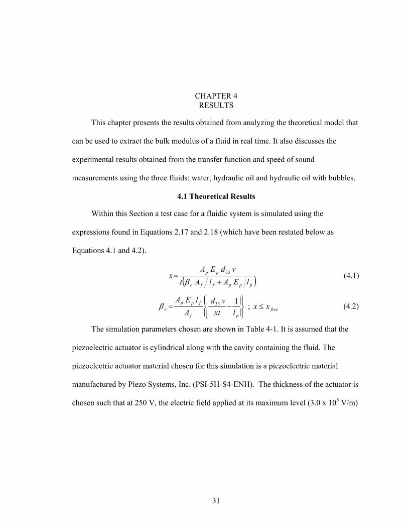
Table 4-1. Simulation parameters Variable Value
pl 0.1 m
fl 0.5 m
pA 7.85e-7 m2 (Diameter = 0.001 m)
fA 7.85e-5 m2 (Diameter = 0.01 m)
pE 5GPa
t 8.33e-4 meters
33d (PZT-5H) 650e-12 m/V
Given a known applied voltage and an effective bulk modulus, Equation 4.1 can be
used to calculate the displacement of the actuator. The appendix contains the code used
for calculating and plotting the results. When the effective bulk modulus is zero, this
represents the free expansion of the piezoelectric actuator. As the bulk modulus increases,
the displacement of the actuator decreases as shown in Figure 4-1.
Figure 4-1: Actuator displacement for varied fluid loading
33
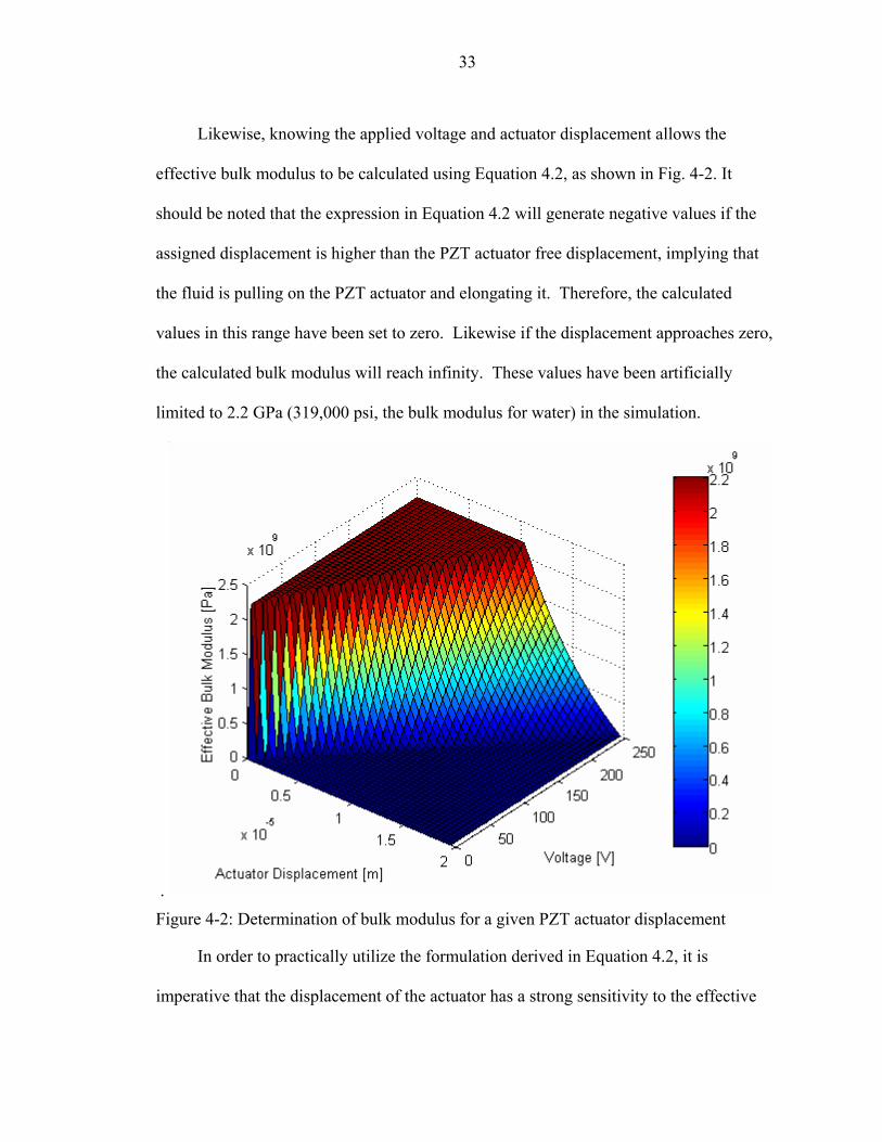
Likewise, knowing the applied voltage and actuator displacement allows the
effective bulk modulus to be calculated using Equation 4.2, as shown in Fig. 4-2. It
should be noted that the expression in Equation 4.2 will generate negative values if the
assigned displacement is higher than the PZT actuator free displacement, implying that
the fluid is pulling on the PZT actuator and elongating it. Therefore, the calculated
values in this range have been set to zero. Likewise if the displacement approaches zero,
the calculated bulk modulus will reach infinity. These values have been artificially
limited to 2.2 GPa (319,000 psi, the bulk modulus for water) in the simulation.
.
Figure 4-2: Determination of bulk modulus for a given PZT actuator displacement
In order to practically utilize the formulation derived in Equation 4.2, it is
imperative that the displacement of the actuator has a strong sensitivity to the effective
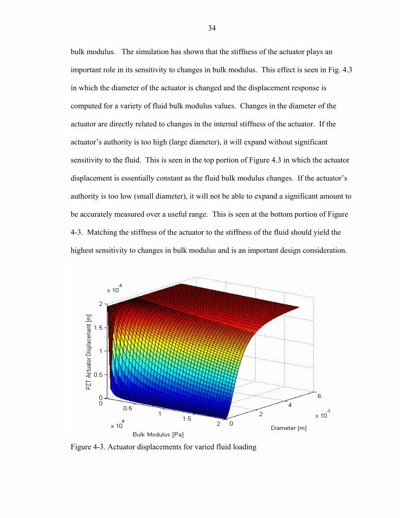
34
bulk modulus. The simulation has shown that the stiffness of the actuator plays an
important role in its sensitivity to changes in bulk modulus. This effect is seen in Fig. 4.3
in which the diameter of the actuator is changed and the displacement response is
computed for a variety of fluid bulk modulus values. Changes in the diameter of the
actuator are directly related to changes in the internal stiffness of the actuator. If the
actuator’s authority is too high (large diameter), it will expand without significant
sensitivity to the fluid. This is seen in the top portion of Figure 4.3 in which the actuator
displacement is essentially constant as the fluid bulk modulus changes. If the actuator’s
authority is too low (small diameter), it will not be able to expand a significant amount to
be accurately measured over a useful range. This is seen at the bottom portion of Figure
4-3. Matching the stiffness of the actuator to the stiffness of the fluid should yield the
highest sensitivity to changes in bulk modulus and is an important design consideration.
Figure 4-3. Actuator displacements for varied fluid loading

35
4.2 Experimental Results
Within this Section the time domain and frequency response for three fluids
(hydraulic oil, water and hydraulic oil with bubbles) is analyzed and compared. This is
followed by speed of sound measurement calculations for the three fluids.
4.2.1 Time Domain Measurements
The time domain plot for hydraulic oil is shown in Figure 4-4.
0 2 4 6 8 10 12 14 16 18 20
x 10-4
0
500
1000
1500
Time [sec]
Forc
e [N
ewto
n]
0 2 4 6 8 10 12 14 16 18 20
x 10-4
-100
0
100
Time [sec]
Pre
ssur
e [p
si]
Pressure Transducer1Pressure Transducer2Pressure Transducer3
Figure 4-4. Time domain plots (force sensor and pressure transducers) for hydraulic oil.
The single hit of the modal hammer on the plunger is characterized by the
dominant peak force of 1756 Newtons at approximately 0 sec in the force signal plot. The
plunger then generates a pressure wave within the fluid. The pressure pulse is detected by
each of the three transducers and is shown in Figure 4-4. The pressure wave reaches
transducer 1, 0.00012 seconds after impact, transducer 2, 0.00022 seconds after impact,
and reaches transducer 3, 0.00030 seconds after impact. The pressure signals have a
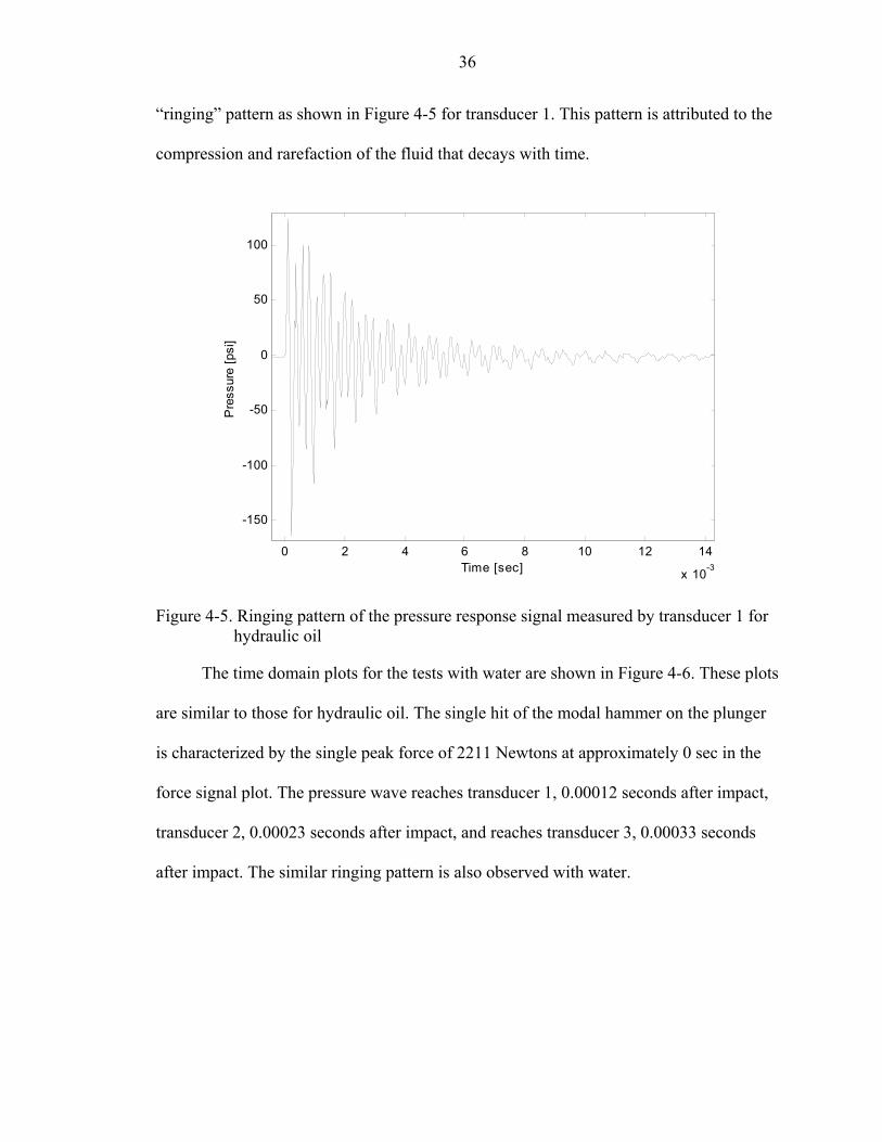
36
“ringing” pattern as shown in Figure 4-5 for transducer 1. This pattern is attributed to the
compression and rarefaction of the fluid that decays with time.
0 2 4 6 8 10 12 14
x 10-3
-150
-100
-50
0
50
100
Time [sec]
Pre
ssur
e [p
si]
Figure 4-5. Ringing pattern of the pressure response signal measured by transducer 1 for hydraulic oil
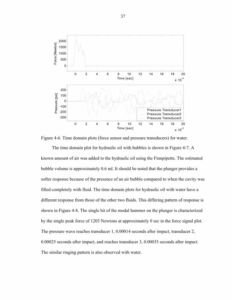
The time domain plots for the tests with water are shown in Figure 4-6. These plots
are similar to those for hydraulic oil. The single hit of the modal hammer on the plunger
is characterized by the single peak force of 2211 Newtons at approximately 0 sec in the
force signal plot. The pressure wave reaches transducer 1, 0.00012 seconds after impact,
transducer 2, 0.00023 seconds after impact, and reaches transducer 3, 0.00033 seconds
after impact. The similar ringing pattern is also observed with water.
37
0 2 4 6 8 10 12 14 16 18 20
x 10-4
0
500
1000
1500
2000
Time [sec]
Forc
e [N
ewto
n]
0 2 4 6 8 10 12 14 16 18 20
x 10-4
-300
-200-100
0
100
200
Time [sec]
Pre
ssur
e [p
si]
Pressure Transducer1Pressure Transducer2Pressure Transducer3
Figure 4-6. Time domain plots (force sensor and pressure transducers) for water.
The time domain plot for hydraulic oil with bubbles is shown in Figure 4-7. A
known amount of air was added to the hydraulic oil using the Finnpipette. The estimated
bubble volume is approximately 0.6 ml. It should be noted that the plunger provides a
softer response because of the presence of an air bubble compared to when the cavity was
filled completely with fluid. The time domain plots for hydraulic oil with water have a
different response from those of the other two fluids. This differing pattern of response is
shown in Figure 4-8. The single hit of the modal hammer on the plunger is characterized
by the single peak force of 1203 Newtons at approximately 0 sec in the force signal plot.
The pressure wave reaches transducer 1, 0.00014 seconds after impact, transducer 2,
0.00025 seconds after impact, and reaches transducer 3, 0.00035 seconds after impact.
The similar ringing pattern is also observed with water.
38
0 2 4 6 8 10 12 14 16 18 20
x 10-4
0
500
1000
Time [sec]
Forc
e [N
ewto
n]
0 2 4 6 8 10 12 14 16 18 20
x 10-4
-400
-200
0
200
Time [sec]
Pre
ssur
e [p
si]
Pressure Transducer1Pressure Transducer2Pressure Transducer3
Figure 4-7. Time domain plots (force sensor and pressure transducers) for hydraulic oil
with bubbles.
0 2 4 6 8 10 12 14
x 10-3
-200
-150
-100
-50
0
50
100
150
200
250
300
Tim e [s ec ]
Pre
ssur
e [p
si]
Figure 4-8. Ringing pattern of the pressure response signal measured by transducer 1 for
hydraulic oil with bubbles

39
4.2.2 Transfer Function Measurements
The transfer function and phase plots of pressure with respect to force for hydraulic oil is shown in Figure 4-9.
0 500 1000 1500 2000 2500 3000 3500 4000 4500 5000 5500 60000
5
10
15
Frequency [Hz]
Mag
nitu
de o
f pre
ssur
e
w
rt. fo
rce
[dB
(psi
/New
ton)
]Pressure Transducer 1Pressure Transducer 2Pressure Transducer 3
0 500 1000 1500 2000 2500 3000 3500 4000 4500 5000 5500 6000-200
-100
0
100
200
Frequency [Hz]
Pha
se o
f pre
ssur
e w
rt. fo
rce
[deg
rees
]
Pressure Transducer 1Pressure transducer 2Pressure Transducer 3
Figure 4-9. Transfer function magnitude and phase plots of tests with pure hydraulic oil
The coherence plot for pure hydraulic oil is given in Figure 4-10. These plots clearly
indicate that there is reasonably high coherence from the signals.
40
0 500 1000 1500 2000 2500 3000 3500 4000 4500 5000 5500 60000.75
0.8
0.85
0.9
0.95
1
Frequency [Hz]
Coh
eren
ce o
f pre
ssur
e w
rt. fo
rce
Pressure Transducer 1Pressure transducer 2Pressure Transducer 3
Figure 4-10. Coherence plot for tests with pure hydraulic oil
The transfer function and phase plot for water is shown in Figure 4-11.
0 500 1000 1500 2000 2500 3000 3500 4000 4500 5000 5500 60000
5
10
15
20
Frequency [Hz]
Mag
nitu
de o
f pre
ssur
e
wrt.
forc
e [d
B(p
si/N
ewto
n]
P ressure Transducer 1Pressure Transducer 2Pressure Transducer 3
0 500 1000 1500 2000 2500 3000 3500 4000 4500 5000 5500 6000-200
-100
0
100
200
Frequency [Hz]
Pha
se o
f pre
ssur
e w
rt. fo
rce
[deg
ress
]
P ressure Transducer 1Pressure transducer 2Pressure Transducer 3
Figure 4-11. Transfer function and phase plot for tests with water
41
It is clear that the response for water is not only larger in magnitude, but is also
sharper. This is indicative of that fact that water has a bulk modulus that is much higher
than hydraulic oil ( waterβ = 310 ksi, oilβ = ~200 ksi). The coherence plots for each of the
transducers in the case water are shown in Figure 4-12. These plots clearly indicate that
there is reasonably high coherence from the signals.
0 500 1000 1500 2000 2500 3000 3500 4000 4500 5000 5500 60000.2
0.3
0.4
0.5
0.6
0.7
0.8
0.9
1
Frequency [Hz]
Coh
eren
ce o
f pre
ssur
e w
rt. fo
rce
Pressure Transducer 1Pressure transducer 2Pressure Transducer 3
Figure 4-12. Coherence plot for tests with water
The transfer function and phase plot for hydraulic oil with 0.6 ml bubbles is shown
in Figure 4-13.
42
0 500 1000 1500 2000 2500 3000 3500 4000 4500 5000 5500 60000
5
10
15
20
Frequency [Hz]
Mag
nitu
de o
f pre
ssur
e
w
rt. fo
rce
[dB
(psi
/New
ton)
]
Pressure Transducer 1Pressure Transducer 2Pressure Transducer 3
0 500 1000 1500 2000 2500 3000 3500 4000 4500 5000 5500 6000-200
-100
0
100
200
Frequency [Hz]
Pha
se o
f pre
ssur
e w
rt. fo
rce
[deg
ress
]
Pressure Transducer 1Pressure transducer 2Pressure Transducer 3
Figure 4-13. Transfer function and phase plot for hydraulic oil contaminated with air
bubbles
The magnitude of the coherence plot is shown below in Figure 4-14.
0 500 1000 1500 2000 2500 3000 3500 4000 4500 5000 5500 60000
0 .1
0 .2
0 .3
0 .4
0 .5
0 .6
0 .7
0 .8
0 .9
1
F requenc y [H z ]
Coh
eren
ce o
f pre
ssur
e w
rt. fo
rce
P res s u re Trans duc er 1P res s u re t rans duc e r 2P res s u re Trans duc er 3
Figure 4-14. Coherence plot for hydraulic oil contaminated with air bubbles
43
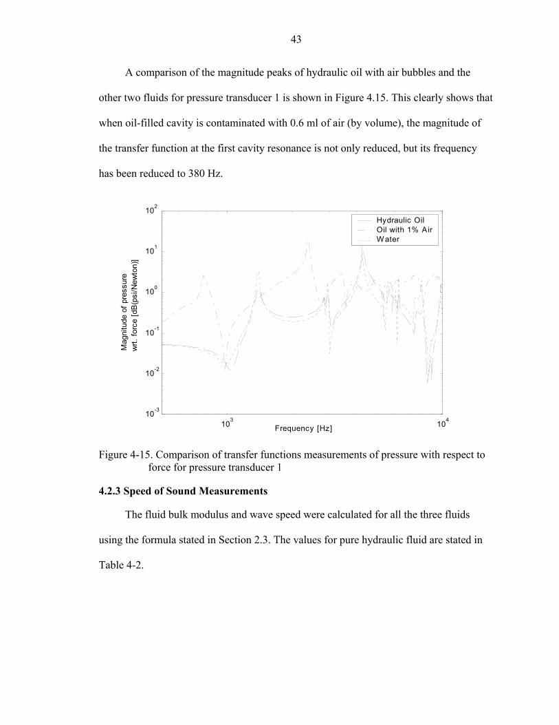
A comparison of the magnitude peaks of hydraulic oil with air bubbles and the
other two fluids for pressure transducer 1 is shown in Figure 4.15. This clearly shows that
when oil-filled cavity is contaminated with 0.6 ml of air (by volume), the magnitude of
the transfer function at the first cavity resonance is not only reduced, but its frequency
has been reduced to 380 Hz.
103
104
10-3
10-2
10-1
100
101
102
Frequency [Hz]
Mag
nitu
de o
f pre
ssur
e
wrt.
forc
e [d
B(p
si/N
ewto
n)]
Hydraulic Oil Oil with 1% AirW ater
Figure 4-15. Comparison of transfer functions measurements of pressure with respect to
force for pressure transducer 1
4.2.3 Speed of Sound Measurements
The fluid bulk modulus and wave speed were calculated for all the three fluids
using the formula stated in Section 2.3. The values for pure hydraulic fluid are stated in
Table 4-2.
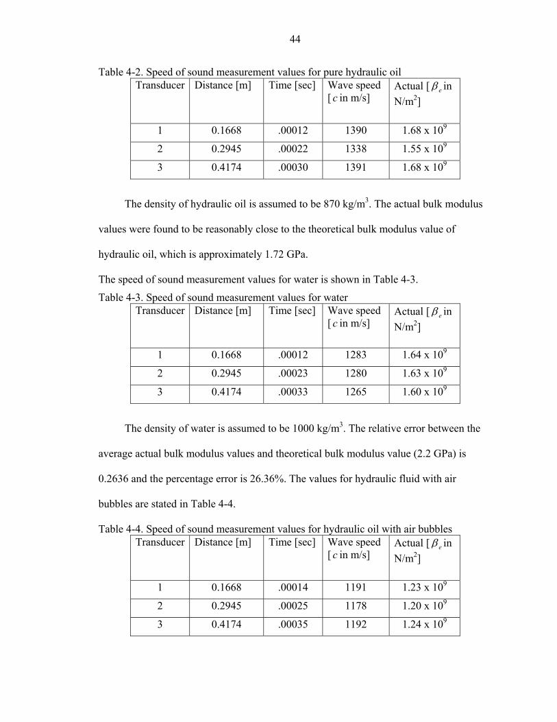
44
Table 4-2. Speed of sound measurement values for pure hydraulic oil Transducer Distance [m] Time [sec] Wave speed
[ in m/s] cActual [ eβ in N/m2]
1 0.1668 .00012 1390 1.68 x 10⁹
2 0.2945 .00022 1338 1.55 x 10⁹
3 0.4174 .00030 1391 1.68 x 10⁹
The density of hydraulic oil is assumed to be 870 kg/m3. The actual bulk modulus
values were found to be reasonably close to the theoretical bulk modulus value of
hydraulic oil, which is approximately 1.72 GPa.
The speed of sound measurement values for water is shown in Table 4-3.
Table 4-3. Speed of sound measurement values for water Transducer Distance [m] Time [sec] Wave speed
[ in m/s] cActual [ eβ in N/m2]
1 0.1668 .00012 1283 1.64 x 10⁹
2 0.2945 .00023 1280 1.63 x 10⁹
3 0.4174 .00033 1265 1.60 x 10⁹
The density of water is assumed to be 1000 kg/m3. The relative error between the
average actual bulk modulus values and theoretical bulk modulus value (2.2 GPa) is
0.2636 and the percentage error is 26.36%. The values for hydraulic fluid with air
bubbles are stated in Table 4-4.
Table 4-4. Speed of sound measurement values for hydraulic oil with air bubbles Transducer Distance [m] Time [sec] Wave speed
[ in m/s] cActual [ eβ in N/m2]
1 0.1668 .00014 1191 1.23 x 10⁹
2 0.2945 .00025 1178 1.20 x 10⁹
3 0.4174 .00035 1192 1.24 x 10⁹
45
The presence of entrained air has clearly resulted in decreasing the bulk modulus
values. Thus, the speed of sound measurement test can be used to calculate the bulk
modulus of hydraulic fluids in real time with reasonable accuracy. Precise results can be
achieved if the possible sources of error (26.36%) are identified and removed. Some
possible sources of error for this experiment include the following:
Mass of the plunger:
Ideally, all the force that is provided by the impact hammer on the plunger should
be transmitted to the fluid. However, some of this force is spent in accelerating the
plunger. The resulting transfer functions are likely distorted due to the force signal being
affected by the inertia of the plunger. Different results may be obtained if the mass of the
plunger is reduced.
Friction of the plunger:
Some of the impact force from the modal hammer is also spent in overcoming the
friction that exists between the surface of the plunger and the aluminum block. Grease
reduces the force spent in overcoming the friction but does not eliminate it. This could
provide another source of error.
Bubble removing technique:
The method adopted to ensure that the system contains pure fluid (water or
hydraulic oil) is not foolproof. The approach does not provide a definite way to ensure
that the system is free of all the bubbles and hence could result in causing errors in the
bulk modulus value.
CHAPTER 5 SUMMARY AND CONCLUSIONS
This work presents a novel sensing technique to determine the bulk modulus of a fluid
or hydraulic system. Within this Section, a summary of the work and the conclusions
drawn from it are presented. Improvements and modifications to the existing experiment
are suggested.
5.1 Summary and Conclusions
The work investigated three different strategies to determine the bulk modulus of a
fluid within a system. The first approach was to develop a theoretical model to extract
the bulk modulus of the fluid system by knowing the excitation voltage and measuring
the strain. The results indicate that matching the stiffness of the actuator to the stiffness
of the fluidic system is critical in obtaining a high sensitivity to the bulk modulus
measurement.
The second approach determines the frequency response functions by performing
transfer function measurements using an impulse response test. In this test, the transfer
function of the pressure response with respect to the applied force is measured. By doing
so it is possible to extract information about the property (i.e. bulk modulus) of a fluid.
The tests were performed on three different fluids: water, hydraulic oil and hydraulic oil
with bubbles. The results indicate that magnitudes of the peaks (at 1400 Hz) were larger
and sharper for water compared to oil. Also, the magnitude of the peaks (at 1400 Hz) in
the case of hydraulic oil with bubbles was not only reduced but they also occurred at a
lower frequency compared to the other two fluids.
46
47
The third approach uses speed of sound measurements to determine the bulk
modulus of the fluid in real time. The results indicate the theoretical values are
reasonably close to the actual bulk modulus values. Also, the hydraulic oil with bubbles
has a lower bulk modulus value compared with the pure hydraulic oil.
5.2 Future Work
One improvement to the present system would be to implement a new design for
the test apparatus to remove air from the chamber prior to filling the block with fluid.
This would ensure the system is perfectly free of air bubbles except when it is chosen to
artificially introduce bubbles for testing. Also, the new design could make use of valves
and pipes as would be found in a typical hydraulic system.
Another improvement would be to replace the plunger with an actual
actuator/sensor. The deformation of the actuator in response to the applied voltage can be
measured by attaching a fiber-optic strain sensor to the piezoelectric stack. The resulting
volume change of the system can therefore be determined. The pressure change can be
measured by pressure transducers.
For the experiment performed, there are several potential sources of error. The
mass of the plunger used to transmit pressure to the fluid moves during the impact. The
impact provided by the modal hammer is measured by the force transducer. The force
signal is affected by the inertial force that the plunger provides to the force transducer
and the frictional force that the O-rings induce on the plunger. These factors can
influence the force measurement and the resulting transfer functions. One possible way to
reduce these effects is to reduce the mass and friction of the plunger. Another possible
source of error is the imperfect removal of bubbles in cavity. It should be possible to

48
eliminate any remaining gas by evacuating the cavity prior to testing. Modifications to
the test apparatus should improve the result.
APPENDIX MATLAB CODES
clear clc % Program that computes the displacement of the actuator for the ISA-Fluid model %Variables for ISA (Induced Strain Actuator) Lp = 0.1; % Length of the PZT, m Dp = 0.001; % Diameter of the PZT, m Ap = (pi * Dp^2)/4; % Cross-Sectional area of ISA, m2 Df = 0.01; % Diameter of the Fluid, m Af = (pi * Df^2)/4; % Cross-Sectional area of fluid, m2 Lf = 0.5; % Length of the fluid, m %Physical properties for PSI-5H-S4-ENH from Piezo Systems Inc. % http://www.piezo.com/en-us/dept_10.html Ep = 5e10; % Modulus of Elasticity of the PZT, Pa d33 = 650e-12; % Dielectric coefficient m/v = C/N Depoling Field = 3e5; % V/m t = 250/DepolingField; % Thickness of the PZT, m Voltage = 0:10:250; % V %Variables for the fluid Efluid= 0:0.1e9:2e9; %Program begins for i = 1:length (Voltage); for j = 1:length (Efluid); x(i,j) = (Ap*Ep*d33*Voltage(1,i)/t)/(Efluid(1,j)*Af/Lf + Ap*Ep/Lp); end end Figure (1) Surf (Efluid, Voltage, x) xlabel ('Effective Bulk Modulus [Pa]') ylabel ('Voltage [V]') zlabel ('PZT Actuator Displacement [m]') view ([14,32])
49
50
clear clc % Program that computes bulk modulus for the ISA-fluid model % Variables for ISA Lp = 0.1; % Length of the PZT, m Dp = 0.001; % Diameter of the PZT, m Ap = (pi * Dp^2)/4; % Cross-Sectional area of ISA, m2 Df = 0.01; % Diameter of the Fluid, m Af = (pi * Df^2)/4; % Cross-Sectional area of fluid, m2 Lf = 0.5; % Length of the fluid, m %Physical properties for PSI-5H-S4-ENH from Piezo Systems Inc. % http://www.piezo.com/en-us/dept_10.html Ep = 5e10; %Modulus of Elasticity of the PZT, Pa d33 = 650e-12; %Dielectric coefficient m/v = C/N VoltageMax= 250; % V depolingField = 3e5; %V/m t = VoltageMax/depolingField; %Thickness of the PZT, m Voltage = 0: 5: VoltageMax; steps = 40; Bmax = 2.2e9; xf = d33*VoltageMax*Lp/t xs = xf/200; deltaLISA = xs:(xf-xs)/steps:xf; %Program begins for i = 1:length(Voltage); for j = 1:length(deltaLISA); B2(i,j)=(Lf*Ap*Ep/Af)*( d33*Voltage(1,i)/(deltaLISA(1,j)*t) - 1/Lp ); % Make the bulk modulus values equal to zero if they are negative. if B2(i,j)<0 B2(i,j)=0; elseif B2(i,j)>Bmax B2(i,j)=Bmax; end end end Figure (2) surf (deltaLISA,Voltage,B2) ylabel ('Voltage [V]') xlabel ('Actuator Displacement [m]') zlabel ('Effective Bulk Modulus [Pa]') colorbar
51
clear clc % Program that computes the displacement response of a PZT actuator % Fluid loading for a variety of diameters. Diam = 1e-3*[0.05:.05:2 2:.2:5]; % Diameter of the actuator, m Df = 0.01; % Diameter of the fluid, m Af = pi*Df^2/4; % Cross-Sectional area, m2
Ap = pi*Dp^2/4; %Cross-Sectional Area Lp = 0.1; % Length of the PZT, m Lf = 0.5; % Length of the fluid, m %Physical properties for PSI-5H-S4-ENH from Piezo Systems Inc. % http://www.piezo.com/en-us/dept_10.html Ep = 5e10; %Modulus of Elasticity of the PZT, Pa d33 = 650e-12; %Dielectric coefficient m/v = C/N Voltage= 250; %V depolingField = 3e5; %V/m t = Voltage/depolingField; %Thickness of the PZT B= 0:.05e9:2e9; %N/m2 for ii=1:1:length(Diam) Dp=Diam(ii); num=Ap*Ep*d33*Voltage; for j= 1:length(B); x(j,ii)=num/(t*(B(j)*Af/Lf + Ap*Ep/Lp)); end end Figure(3) surf(B,Diam,x) ylabel ('Diameter [m]') xlabel ('Bulk Modulus [Pa]') zlabel ('PZT Actuator Displacement [m]') view([37,20])

LIST OF REFERENCES
Abbott, R. D., McLain, T. W., and Beard, R. W., 2001, “Application of an Optimal Control Synthesis Strategy to an Electro-Hydraulic Positioning System,” Journal of Dynamic Systems, Measurement and Control, Vol. 123, No. 3, pp. 377-384. Burns, J., Dubbleday, P.S. and Ting, R. Y., 1990, “Dynamic Bulk Modulus of Various Elastomers,” Journal of Polymer Science: Part B Polymer Physics, Vol. 28, pp. 1187-1205. Eryilmaz, B. and Wilson, B. H., 2001, “Improved Tracking Control of Hydraulic Systems,” Journal of Dynamic Systems, Measurement and Control, Vol. 123, No. 3, pp. 457-462. Fishman, K. L. and Machmer, D., 1994, “Testing Techniques for the Measurement of Bulk Modulus,” Journal of Testing and Evaluation, Vol. 22, No. 2, pp. 161-167. Guillot, F.M. and Jarzynski, J., 2000, “A New Method for Measuring the Bulk Modulus of Compliant Acoustic Materials,” Journal of Sound and Vibration, Vol. 233, No. 5, pp. 929-934. Giurgiutiu, V., Chaudhry, Z., and Rogers, C.A., 1995, “Energy-Based Comparison of Solid-State Actuators,” Center for Intelligent Material systems and Structures, Virginia Polytechnic Institute and State University, Report No. CIMSS 95-101. Habibi, S. R., 1999, “Sliding Mode Control of a Hydraulic Industrial Robot,” Journal of Dynamic Systems, Measurement and Control, Vol. 121, No. 2, pp. 312-317. Hayase, T., Hayashi, S., Kojima, K., and Iimura, I., 2000, “Suppression of Micro Stick- Slip Vibrations in Hydraulic Servo-System,” Journal of Dynamic Systems, Measurement and Control, Vol. 122, No. 2, pp. 249-256. Holownia, B.P., 1986, “Experimental Measurement of Dynamic Bulk Modulus Using Holography,” Rubber Chemistry and Technology, Vol. 58, No.2, pp. 258-268. Holownia, B.P. and James, E. H., 1993, “Determination of Dynamic Bulk Modulus of Elastomers Using Pressure Measurement,” Rubber Chemistry and Technology, Vol. 66, No. 5, pp. 749-753.
52
53
Holownia, B.P. and Rowland, A.C., 1986, “Measurement of Dynamic Bulk Modulus and Phase Angle Using ESPI,” Rubber Chemistry and Technology, Vol. 59, No.2, pp. 223-232. Koda, S., Yamashita, K., Matsumoto, K., and Nomura, H., 1993, “Characterization of Polyvinylchloride by Means of Sound Velocity and Longitudinal Modulus Measurements,” Japanese Journal of Applied Physics, Vol. 32, No.5B, pp. 2234-2237. Magorien, V.G., n.d, What is Bulk Modulus and When is it Important? Seaton- Wilson, Inc. Burbank, California. Manring, N.D., “Estimating the Fluid Bulk Modulus within Hydraulic Systems,” http://web.missouri.edu/~maringn/Overview_files/slide0004.htm, April 20, 2001. Marvin, R.S., Aldrich, R., and Sack, H.S., 1954, “The Dynamic Bulk Viscosity of Polyisobutylene,” Journal of Applied Physics, Vol. 25, No.10, pp. 1213-1218. Merritt, Herbert E. 1967, Hydraulic Control Systems, John Wiley & Sons, New York, pp. 14 and 18. McKinney, J. F., Edelman, S., and Marvin, R. S., 1956, “Apparatus for the Direct Determination of the Dynamic Bulk Modulus,” Journal of Applied Physics, Vol. 27, No. 5, pp. 425-430. National Fluid Power Association, “Industry Numbers: Segments, Size, Growth, Imports and Exports,” http://www.nfpa.com/default.asp?pid=14, January 28, 2002. Niezrecki, C., Brei, D., Balakrishnan, S., Moskalik, A., 2001, “Piezoelectric Actuation: The State of the Art,” Shock and Vibration Digest, Vol. 33, No. 4, pp. 269-280. Philippoff, W., and Brodnyan, J., 1955, “Preliminary Results in Measuring Dynamic Compressibilities,” Journal of Applied Physics, Vol. 26, No. 7, pp. 113-123. Qatu, M. S. and Dougherty, M. L. Sr., 1998, “Measurement of Fluid Bulk Modulus Using Impedance of Hydraulic Circuits,” Society of Automotive Engineers, Paper 99PC-380, pp. 1-4. Streeter, Victor L., and Wylie, Benjamin E., 1976, Fluid Mechanics, McGraw-Hill Book Company, New York, pp. 342. Watton, J., 1989, Fluid Power Systems Modeling, Simulation, Analog and Microcomputer Control, Prentice Hall, New York, pp. 28.
BIOGRAPHICAL SKETCH
The author was born in 1979 in Bangalore, India. He graduated with a Bachelor of
Science in mechanical engineering degree in May 2000 from the University of Madras,
Chennai, India. He then obtained Master of Science degrees in mechanical engineering
and management in December 2003 from the University of Florida.
54