Embed Size (px)
Citation preview
Smart Beta Strategies: the Social Responsibility of InvestmentUniverses Does Matter
Philippe Bertrand1, Vincent Lapointe2 ∗
April 2013
1 CERGAM, IAE Aix-en-Provence and Euromed Management2 Aix-Marseille University, Aix-Marseille School of Economics
Abstract
In this article we extend the research on smart beta strategies by exploring how using an SRIuniverse impacts the properties of smart beta portfolios. We focus on four smart beta strategies:the Equally Weighted (EW), the Most Diversified Portfolio (MDP), the Minimum Variance (MV)and the Equal Risk Contribution (ERC). Using different estimators of the matrix of covariances,we apply these strategies to the EuroStoxx universe of stocks, the ASPI and the complement of theASPI in the EuroStoxx universe from March 15, 2002 to May 1, 2012. We show that smart betastrategies, built on the entire universe, concentrate their solution on non-SRI stocks. Consequently,the portfolios built on the ASPI are more diversified and, tend to have higher turnover. In addition,their tracking error against EuroStoxx, is smaller than those of their respective counterparts builton the two other universes, and their distribution of returns has positive skewness, while those ofportfolios built on the two other universes have negative skewness. Consistent with the empiricalliterature, all the smart beta portfolios built on the ASPI universe in our sample outperform theCW portfolio.
JEL Classification:G11, C58, C60, G32, M14Keywords:Socially responsible investment, alternative andsmart beta strategies, performance, diversifica-tion, turnover, robust covariances matrix
Contact:Vincent Lapointe,Aix Marseille University2, rue de la Charité13236 Marseille cedex [email protected]@iae-aix.com
∗Corresponding author: [email protected]. We thank Thierry Roncalli and Raul Leote de Carvalhofor their valuable comments. We are grateful to Vigeo for granting us access to their data. We thank Fouad Benseddikand Antoine Begasse from Vigeo for their support in understanding the methodology of these data. An early version ofthis work was presented in a working paper entitled "Smart Beta Strategies: the Socially Responsible Investment case".
1
P. Bertrand, V. Lapointe Working Paper
1 Smart beta strategies and SociallyResponsible Investment: Introduc-tion
Against a background of market disappointments,such as poor performance of market capitalizationweighted indices and active portfolios, risk-basedstrategies stand out as financial vehicles for sophis-ticated institutional investors. Risk-based strate-gies are heuristic and quantitative asset allocationstrategies that are special cases of the risk budget-ing allocation approach; the approach itself is onetype of alternative weighting approach to asset allo-cation, the other being the fundamental allocation(Arnott, Hsu, and Moore [2005]). The differentalternative weighting strategies are also known assmart beta strategies1. These smart beta strategiesdefine the weights of assets in portfolios as func-tions of individual and common asset risks. Thestrategies are heuristic because they do not rely onany formal equilibrium model of expected return.The adoption of smart beta strategies is commonlyjustified by three principal arguments (Maillard,Roncalli, and Teiletche [2010], Demey, Maillard,and Roncalli [2010]). First, while they implicitlyuse estimations of expected returns, smart betastrategies do not require any stock return forecasts,which eliminates the challenge of estimating them.This is an advantage compared to Mean-Varianceapproaches. Second, smart beta strategies aim toimprove the risk/return ratio by improving risk di-versification. This is an advantage compared tothe capitalization-weighted (CW) strategy, whichis usually not mean-variance efficient in practice.Third, when back-tested, smart beta strategies out-perform the traditional CW investment strategy.However, smart beta strategies have two draw-backs. Not only there is a lack of theoreticalbackground proving their historical efficiency, butthese strategies also involve issues of stability (i.e.turnover) and concentration in terms of weightingof the components of portfolios. To overcome thesedrawbacks, asset managers follow different imple-mentation approaches. The consequence is thatfor a given smart beta strategy, institutional in-vestors are faced with the costs involved in choosingfrom a wide range of implementation approaches2,
which will have major implications for the subse-quent characteristics of their portfolios.In parallel with the rise of smart beta strategies andfuelled by the increasing public concern for sustain-able development (Brundtland et al. [1987]), a typeof investment generally called socially responsibleinvestment (SRI), is rapidly gaining favour with in-stitutional investors. Briefly, SRI incorporates non-financial criteria into the construction of financialportfolios. These criteria include respecting simplesubjective rules (e.g. no investment in gambling ortobacco businesses), or meeting a minimum level ofextra-financial performance (e.g. investment in is-suers that have low carbon emissions or low rate offatalities compared to industry competitors). Thelatter criterion is evaluated by extra-financial rat-ing agencies such as VIGEO.The popularity of SRI is partly explained by a largeliterature showing that corporate social perfor-mance (CSP) can lead to superior economic and/orfinancial performance through different mecha-nisms (Renneboog, Horst, and Zhang [2008], Kitz-mueller and Shimshack [2012]). However, a re-view of these mechanisms is outside the scope ofthis paper and is covered in a companion paperthat focuses on the question of the performance ofSRI. The principle of SRI is to incorporate extra-financial criteria into portfolio construction so as tocapture these characteristics and yield higher risk-adjusted returns in the long-run3.In the light of these two parallel trends, smart betastrategies and SRI, a key question arises for insti-tutional investors. If firms that demonstrate a highlevel of CSP are different from low CSP firms, arethe characteristics of smart beta portfolios modi-fied by an SRI universe? A positive answer wouldimply that institutional investors should run a newselection process, to decide which implementationapproach for a smart beta strategy is in their bestinterests for the SRI universe. A negative answerwould imply that institutional investors could keeptheir current smart beta portfolio managers andjust switch to an SRI universe.Here, we seek to extend the research on smart betaallocation by examining the impact of using an SRIuniverse on certain characteristics of smart betaportfolios. We look at four smart beta strategies,the Equally Weighted (EW), the Most Diversified
2
P. Bertrand, V. Lapointe Working Paper
Portfolio (MDP), which is equivalent to the modi-fied Maximum Sharpe Ratio (MSR) portfolio, theMinimum Variance (MV) and the Equal Risk Con-tribution (ERC). Using different estimators of thematrix of covariances, we apply these strategies tothe EuroStoxx universe of stocks, the ASPI andthe complement of the ASPI in the EuroStoxx uni-verse4.Six types of impact of using the ASPI universe ofstocks emerge from our study. First, smart betastrategies applied on the EuroStoxx favour stocksthat do not belong to the ASPI universe. Second,there is increased diversification of the weight andrisk measure distributions. Third, smart beta port-folios built on the ASPI universe tend to presenthigher weight and component turnovers. Fourth,the distributions of returns of portfolios built onthe ASPI universe have positive skewness, whilewith the two other universes, portfolios have distri-butions of returns with negative skewness. Fifth,the volatility of tracking error against EuroStoxxof smart beta strategies built on the ASPI universeis lower than that of their respective counterpartsbuilt on the two other universes. Finally, on theASPI universe, all the smart beta strategies domi-nate the CW strategy, which is similar to findingson the two other universes and consistent with theempirical literature.Thus we are able to conclude that combining thesmart beta strategies with the SRI approach doesmodify some properties of smart beta portfolios.This means that the adoption of SRI is not neu-tral, and needs particular attention from the insti-tutional investors.In the rest of the paper we first present the foursmart beta strategies examined. Section 2 givesthe data and methodology for our back-tests andin section 3 we analyze portfolios characteristics.The two last sections review the robustness of ourresults regarding risk models and conclude.
2 Smart beta strategies: calculationof weights
According to Demey, Maillard, and Roncalli [2010]there are four common types of smart beta strate-gies yielding four types of smart beta portfolios.
In this section we review these four strategies andtheir particular risk contribution properties.The first type is the EW portfolio. The EW portfo-lio depends solely on the number n of componentsand its weights wi are given by:
∀i, wi = 1n
(1)
This portfolio is straightforward and presents goodout-of-sample performance compared to optimalportfolios (DeMiguel, Garlappi, and Uppal [2009]).It is perfectly diversified in weights, by construc-tion.The second type is the MV portfolio. The vector ofweights w of the MV portfolio, with the variance-covariance matrix Σ, is given by the following op-timisation program:
w = arg min(w′Σw)
s.t.n∑i
wi = 1
∀i, 0 ≤ wi ≤ 1
(2)
This portfolio is straightforward to understand: ithas the lowest ex ante volatility, does not relyon expected return input and offers good relativeperformance (Clarke, Silva, and Thorley [2006],Scherer [2011]). In addition, marginal risks (MR)are equal for all the components with a weight dif-ferent from zero.
∀i, j, (wi 6= 0 ∧ wj 6= 0⇒ δσ(w)δwi
= δσ(w)δwj
) (3)
The third type of portfolio, the MDP (Choueifatyand Coignard [2008]) or modified MSR (Martellini[2008]), is more complicated. To obtain the vec-tor of weights w of this portfolio, Choueifaty andCoignard [2008] introduce a diversification measurethat is maximized:
w = arg max( w′σ√w′Σw
)
s.t.n∑i
wi = 1
∀i, 0 ≤ wi ≤ 1
(4)
This portfolio does not explicitly rely on expected
3
P. Bertrand, V. Lapointe Working Paper
return input (see the introduction of Martellini[2008]); it is more diversified and less sensitive tosmall modifications in inputs than the MV port-folio. In addition, relative marginal risk (RMR) isequal for all the components with a weight differentfrom zero.
∀i, j, (wi 6= 0 ∧ wj 6= 0
⇒ 1σi
δσ(w)δwi
= 1σj
δσ(w)δwj
)(5)
The last type is the ERC portfolio (Maillard, Ron-calli, and Teiletche [2010]), also rather complicated,where the risk contribution (RC) of each asset isthe same.
∀i, j, (wiδσ(w)δwi
= wjδσ(w)δwj
) (6)
The composition of this portfolio is given by thefollowing program:
w = arg min(n∑i=1
n∑j=1
(wi(Σw)i − wj(Σw)j)2)
s.t.n∑i
wi = 1
∀i, 0 ≤ wi ≤ 1
(7)
This portfolio does not explicitly rely on expectedreturn input, by construction it is well diversifiedin terms of weights5 and risk, and it is less sensi-tive to slight modifications in inputs than the MVor MDP portfolios (Demey, Maillard, and Roncalli[2010]).
Table 1: Smart beta strategies: a comparisonThe table lists the conditions (columns) on stocks necessary for each strategy (lines) to be equivalent either to
one other strategy or to the tangent portfolio.
Conditions on stocksStrategies Same Same expec- Same cor- Same Sharpe Equivalent
volatility ted return relation ratio toEW X X X TangentMV X Tangent
MDP/mMSR X MVMDP/mMSR X Tangent
ERC X X TangentERC X MDP/mMSRERC X (ρ = −1
N−1 ) MVERC X X EW
Table 1, based on the literature, summarizes howthe different smart beta strategies stand in relationto each other, and to the tangent portfolio. Notethat depending on the statistical properties of thestocks included in the portfolios, different strate-gies can yield the same allocation and the latter canbe the tangent portfolio. In particular, the ERCand the MDP portfolios are to be identical whenpairwise correlation is uniform. Since we use theconstant correlation matrix of covariances in ouranalyses, it is important to control for this case.Finally these different approaches, apart from theEW portfolio, rely on the matrix of variances andcovariances Σ. In the next section we present thedifferent risk models we use to estimate our fourportfolios.
3 Data and methodology of the study
We run our back-tests using daily returns (adjustedprice and arithmetic returns) for three differentuniverses of stocks: the EuroStoxx, the ASPI andthe complement of the ASPI in the EuroStoxx uni-verse. We use data from March 15, 2002 to May 1,2012. Our data sources are, Datastream for pricesand composition of the EuroStoxx, and IEM6 forcomposition of the ASPI index. We check the relia-bility of our in-house-built universes by calculatingthe volatility of the tracking error (TEV) of theCW portfolios with the respective indices. We ob-tain a TEV of 26.9 bps for the replication of ASPIand a TEV of 11.6 bps for the replication of Eu-roStoxx, which are common levels of TEV (table 2).
4
P. Bertrand, V. Lapointe Working Paper
Because the ASPI is a best-in-class index, we canverify that the industrial composition of the differ-ent universes are similar (table 3). Finally, we usearithmetic returns and calculate all returns in Eu-ros7 and, following the indices calculation method-
ology, we rebalance the portfolios at closing on thethird Friday of March, June, September and De-cember. The portfolios weights are allowed to driftbetween rebalancing dates.
Table 2: Performance of real and replication of CW indicesPerformance of real and replication of CW indices from March 15, 2002 to May 1, 2012. The two replicated CWportfolios are benchmarked against their respective real counterparts (i.e. real EuroStoxx and ASPI). We alsoreport statistics on performances and crossed benchmark for the two real indices. Sharpe ratio is calculatedagainst a zero risk free rate. Annualized realized performance is annual rate equivalent to total performance.
EuroStoxx EuroStoxx ASPI ASPIReplication Real Replication Real
Historical performanceTotal realized perf. (%) -26,58 -26,37 -29,74 -29,67
Annualized perf. (%) -2,99 -2,97 -3,41 -3,40Volatility (%) 23,14 23,49 24,20 24,52Sharpe ratio -0,13 -0,13 -0,14 -0,14
Max. draw down (%) -61,79 -61,75 -60,30 -60,10Performance of tracking
Daily TE (%) -0,0004 0,0008 -0,0003 -0,0008TEV (%) 0,1160 0,2623 0,2699 0,2623
Information ratio -0,0037 0,0030 -0,0012 -0,0030Correlation 0,9999 0,9984 0,9999 0,9984
Table 3: Industrial average compositionColumn A is Consumer Discretionary, B is Consumer Staples, C is Energy, D is Financials, E is Health Care, F is
Industrials, G is Information Technology, H is Materials, I is Telecommunication Services, J is Utilities.
Nb A B C D E F G H I J NA TOTALEuroStoxx 41,4 23,2 11,0 63,9 14,1 48,8 14,3 26,1 11,5 18,4 32,8 305,4Comp 22,9 12,2 7,0 41,3 10,3 30,7 6,0 16,6 6,2 12,5 22,1 187,9Aspi 18,5 11,0 4,4 23,4 3,6 18,0 9,2 9,5 5,3 5,9 11,0 119,9% A B C D E F G H I J NA TOTAL
EuroStoxx 13,6% 7,6% 3,6% 20,9% 4,6% 16,0% 4,7% 8,5% 3,8% 6,0% 10,8% 100%Comp 12,2% 6,5% 3,7% 22,0% 5,5% 16,3% 3,2% 8,8% 3,3% 6,7% 11,8% 100%Aspi 15,4% 9,2% 3,7% 19,5% 3,0% 15,0% 7,7% 7,9% 4,4% 4,9% 9,2% 100%
For the EuroStoxx and the complement universesof stocks, the weights of CW portfolios are calcu-lated using free float market capitalization basedon Datastream information. The EW portfoliosweights are given by the number of components,which is around 300 for EuroStoxx and around 180for the complement of ASPI in the EuroStoxx uni-verse8. For MV, MDP, ERC portfolios, we esti-mate weights by optimizing the respective objec-tive functions introduced in the previous section.For the three optimization programs, constraintsare no short-sells and no cash holdings. For theASPI universe of stocks, the weights of CW portfo-lios are calculated using information given by IEM.The EW portfolio weights are given by N=120, thenumber of components of ASPI9. For MV, MDP,ERC portfolios, we estimate weights by optimiz-
ing the respective objective functions introduced inthe previous section. For EuroStoxx and the com-plement universe, optimization constraints are noshort-sells and no cash holdings.Note that the solutions of the MV, MDP and ERCoptimization programs depends on the matrix ofvariances and covariances (the VCV matrix) ofstock returns. The estimation of the VCV ma-trix is challenging, and consequently the solutionsgiven by the optimizations are not stable, leadingto high turnover. To improve the stability of solu-tions given by MV, MDP and ERC optimizations,different estimators of the VCV matrix have beenproposed in the literature, a reminder of the diver-sity of implementation that investors may face. Tocontrol for the possible impact of the VCV matri-
5
P. Bertrand, V. Lapointe Working Paper
ces, we use four estimators: the empirical, the con-stant correlation, the shrinkage estimator with theconstant correlation VCV matrix, and the shrink-age estimator with the one-factor model VCV ma-trix (Ledoit and Wolf [2004]). At the outset and ateach rebalancing, we update the VCV matrix froma 260-day rolling window of the most recent histor-ical data10. Another problem in MV and MDP op-timizations is the high concentration of solutions.As examined and proposed by Maillard, Roncalli,and Teiletche [2010], we run MV and MDP opti-mization programs with upper-bound constraints(5� or 10� ) for weights.As for our method of analysis, we first describe theportfolios that we obtain in terms of number ofcomponents, number of differences between portfo-lios yielded by the same strategy on different uni-verses and, differences in weights for identical com-ponents in portfolios yielded by the same strategyapplied to different universes. This enables us tocompare portfolios. Second we focus on diversifica-tion, by reporting for each portfolio and universe,the relative mean difference coefficients for weights,risk budget11, marginal risk, relative marginal riskand risk contribution. The use of relative meandifference will be explained later. Third we focuson turnover, by reporting for each portfolio anduniverse, turnover of components and turnover ofweights. Regressions are performed for all threesteps to analyze the correlation of particular char-acteristics of portfolios with the strategy and theuniverse used. These regressions give us the eco-nomic and statistical significance of the relations ofinterest while controlling for particular parameters.Finally, we focus on performance. For each port-folio and universe we report descriptive statisticsregarding the statistical properties of the distribu-tion of returns of the different portfolios. We re-port annualized historical performance, annualizedhistorical volatility, annual Sharpe ratio, historicalmaximum draw down, correlation with benchmark(i.e. the replications of ASPI or EuroStoxx), meanof daily return, its standard error, their two annu-
alized values, mean daily tracking error12, volatilityof daily tracking error and daily information ratio.Our default case is the empirical VCV matrix.To develop analyses that are not dependent onthe VCV matrix, we also run the regressions ondatasets that pool the back tests obtained withthe four VCV matrices. We discuss the impact ofchanging the risk model in section 6.
4 Analysis of portfolios characteris-tics
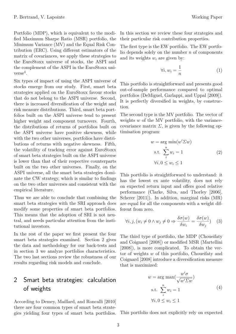
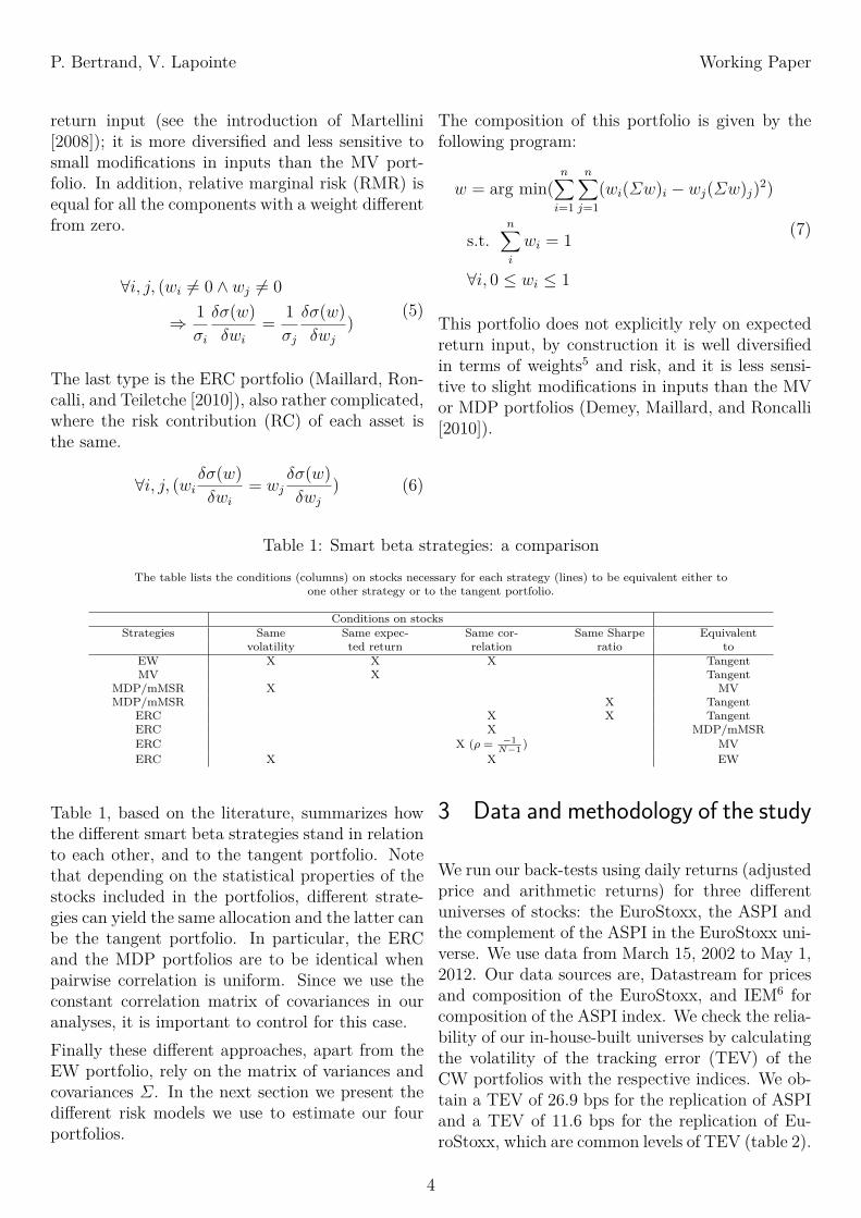
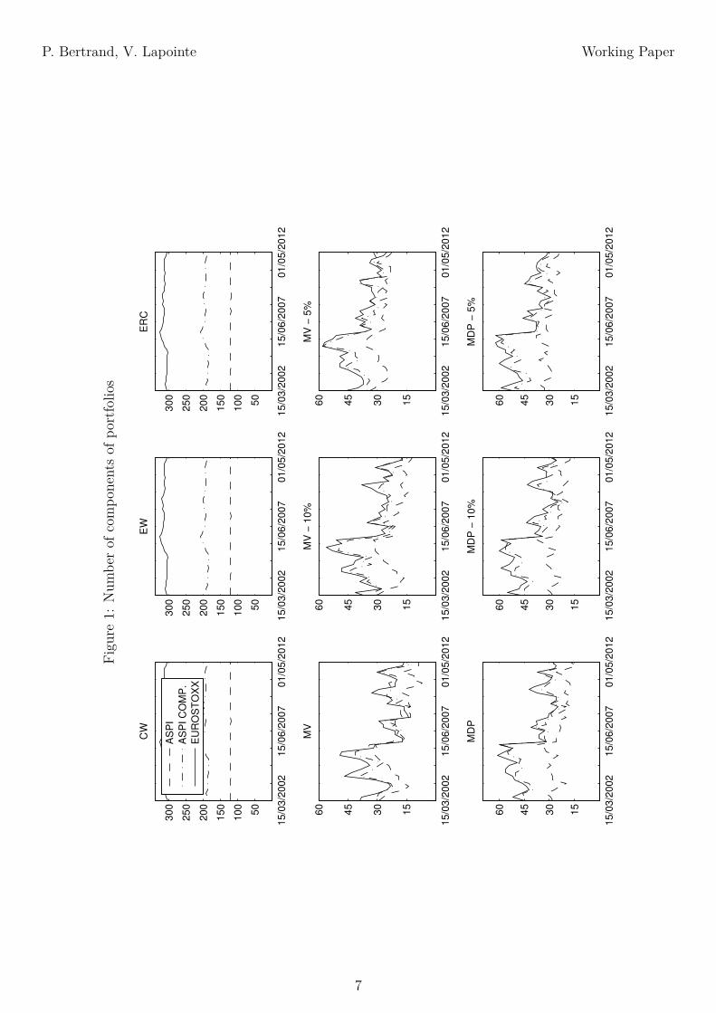
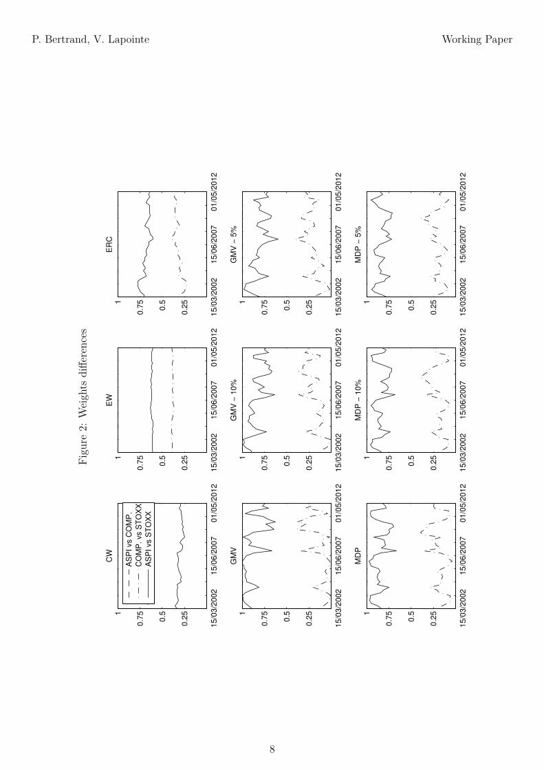
Composition and differences in compositionof portfoliosWe first report and analyze the composition anddifferences in composition of portfolios (Figures 1,2), so as to describe the portfolios obtained andto measure degrees of similarity between portfoliosyielded by the same strategy applied to the differ-ent universes.First, we analyzed portfolio composition. By sim-ply counting the number of components (Figure1), we distinguished two types of strategy: strate-gies that invest in the entire available universe (i.e.CW, EW, ERC) and strategies that pick somestocks from the available universe (i.e. MV, MDPand their bounded versions). Although this typol-ogy is obtained with the empirical VCV matrix, itis stable when we switch to other types of VCV.Only the MDP strategy with a constant VCV ma-trix is modified (cf. Table 1).Second, we calculated differences in portfolio usingtwo measures of difference. Measure D1 is the ab-solute difference in weights wi between the compo-nents of portfolios A and B. With n as overlappingcomponents, this measure is given by the followingformula13:
D1(A,B) = 1−n∑i
min(wAi, wBi) (8)
6
P. Bertrand, V. Lapointe Working Paper
Figu
re1:
Num
berof
compo
nentsof
portfolio
s
15/0
3/2
002
15/0
6/2
007
01/0
5/2
012
50
100
150
200
250
300
CW
AS
PI
AS
PI C
OM
P.
EU
RO
ST
OX
X
15/0
3/2
002
15/0
6/2
007
01/0
5/2
012
50
100
150
200
250
300
EW
15/0
3/2
002
15/0
6/2
007
01/0
5/2
012
15
30
45
60
MD
P
15/0
3/2
002
15/0
6/2
007
01/0
5/2
012
15
30
45
60
MV
15/0
3/2
002
15/0
6/2
007
01/0
5/2
012
50
100
150
200
250
300
ER
C
15/0
3/2
002
15/0
6/2
007
01/0
5/2
012
15
30
45
60
MD
P −
5%
15/0
3/2
002
15/0
6/2
007
01/0
5/2
012
15
30
45
60
MD
P −
10%
15/0
3/2
002
15/0
6/2
007
01/0
5/2
012
15
30
45
60
MV
− 5
%
15/0
3/2
002
15/0
6/2
007
01/0
5/2
012
15
30
45
60
MV
− 1
0%
7
P. Bertrand, V. Lapointe Working Paper
Figu
re2:
Weigh
tsdiffe
rences
15/0
3/2
002
15/0
6/2
007
01/0
5/2
012
0.2
5
0.5
0.7
51
CW
AS
PI vs C
OM
P.
CO
MP
. vs S
TO
XX
AS
PI vs S
TO
XX
15/0
3/2
002
15/0
6/2
007
01/0
5/2
012
0.2
5
0.5
0.7
51
EW
15/0
3/2
002
15/0
6/2
007
01/0
5/2
012
0.2
5
0.5
0.7
51
ER
C
15/0
3/2
002
15/0
6/2
007
01/0
5/2
012
0.2
5
0.5
0.7
51
GM
V
15/0
3/2
002
15/0
6/2
007
01/0
5/2
012
0.2
5
0.5
0.7
51
MD
P
15/0
3/2
002
15/0
6/2
007
01/0
5/2
012
0.2
5
0.5
0.7
51
MD
P −
5%
15/0
3/2
002
15/0
6/2
007
01/0
5/2
012
0.2
5
0.5
0.7
51
MD
P −
10%
15/0
3/2
002
15/0
6/2
007
01/0
5/2
012
0.2
5
0.5
0.7
51
GM
V −
5%
15/0
3/2
002
15/0
6/2
007
01/0
5/2
012
0.2
5
0.5
0.7
51
GM
V −
10%
8
P. Bertrand, V. Lapointe Working Paper
Figu
re3:
Turnover
ofwe
ights
15/0
3/2
002
15/0
6/2
007
01/0
5/2
012
0.2
5
0.5
0.7
51
1.2
5
1.5
1.7
52
CW
AS
PI
AS
PI C
OM
P.
ST
OX
X
15/0
3/2
002
15/0
6/2
007
01/0
5/2
012
0.2
5
0.5
0.7
51
1.2
5
1.5
1.7
52
EW
15/0
3/2
002
15/0
6/2
007
01/0
5/2
012
0.2
5
0.5
0.7
51
1.2
5
1.5
1.7
52
MD
P
15/0
3/2
002
15/0
6/2
007
01/0
5/2
012
0.2
5
0.5
0.7
51
1.2
5
1.5
1.7
52
MV
15/0
3/2
002
15/0
6/2
007
01/0
5/2
012
0.2
5
0.5
0.7
51
1.2
5
1.5
1.7
52
ER
C
15/0
3/2
002
15/0
6/2
007
01/0
5/2
012
0.2
5
0.5
0.7
51
1.2
5
1.5
1.7
52
MD
P −
5%
15/0
3/2
002
15/0
6/2
007
01/0
5/2
012
0.2
5
0.5
0.7
51
1.2
5
1.5
1.7
52
MD
P −
10%
15/0
3/2
002
15/0
6/2
007
01/0
5/2
012
0.2
5
0.5
0.7
51
1.2
5
1.5
1.7
52
MV
− 5
%
15/0
3/2
002
15/0
6/2
007
01/0
5/2
012
0.2
5
0.5
0.7
51
1.2
5
1.5
1.7
52
MV
− 1
0%
9
P. Bertrand, V. Lapointe Working Paper
Figu
re4:
Turnover
ofcompo
nents
15/0
3/2
002
15/0
6/2
007
01/0
5/2
012
0.2
5
0.5
0.7
51
1.2
5
1.5
1.7
52
CW
AS
PI
AS
PI C
OM
P.
ST
OX
X
15/0
3/2
002
15/0
6/2
007
01/0
5/2
012
0.2
5
0.5
0.7
51
1.2
5
1.5
1.7
52
EW
15/0
3/2
002
15/0
6/2
007
01/0
5/2
012
0.2
5
0.5
0.7
51
1.2
5
1.5
1.7
52
MD
P
15/0
3/2
002
15/0
6/2
007
01/0
5/2
012
0.2
5
0.5
0.7
51
1.2
5
1.5
1.7
52
MV
15/0
3/2
002
15/0
6/2
007
01/0
5/2
012
0.2
5
0.5
0.7
51
1.2
5
1.5
1.7
52
ER
C
15/0
3/2
002
15/0
6/2
007
01/0
5/2
012
0.2
5
0.5
0.7
51
1.2
5
1.5
1.7
52
MD
P −
5%
15/0
3/2
002
15/0
6/2
007
01/0
5/2
012
0.2
5
0.5
0.7
51
1.2
5
1.5
1.7
52
MD
P −
10%
15/0
3/2
002
15/0
6/2
007
01/0
5/2
012
0.2
5
0.5
0.7
51
1.2
5
1.5
1.7
52
MV
− 5
%
15/0
3/2
002
15/0
6/2
007
01/0
5/2
012
0.2
5
0.5
0.7
51
1.2
5
1.5
1.7
52
MV
− 1
0%
10
P. Bertrand, V. Lapointe Working Paper
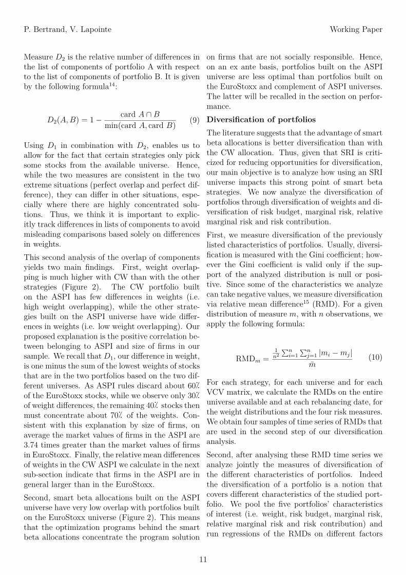
Measure D2 is the relative number of differences inthe list of components of portfolio A with respectto the list of components of portfolio B. It is givenby the following formula14:
D2(A,B) = 1− card A ∩Bmin(card A, card B) (9)
Using D1 in combination with D2, enables us toallow for the fact that certain strategies only picksome stocks from the available universe. Hence,while the two measures are consistent in the twoextreme situations (perfect overlap and perfect dif-ference), they can differ in other situations, espe-cially where there are highly concentrated solu-tions. Thus, we think it is important to explic-itly track differences in lists of components to avoidmisleading comparisons based solely on differencesin weights.This second analysis of the overlap of componentsyields two main findings. First, weight overlap-ping is much higher with CW than with the otherstrategies (Figure 2). The CW portfolio builton the ASPI has few differences in weights (i.e.high weight overlapping), while the other strate-gies built on the ASPI universe have wide differ-ences in weights (i.e. low weight overlapping). Ourproposed explanation is the positive correlation be-tween belonging to ASPI and size of firms in oursample. We recall thatD1, our difference in weight,is one minus the sum of the lowest weights of stocksthat are in the two portfolios based on the two dif-ferent universes. As ASPI rules discard about 60�of the EuroStoxx stocks, while we observe only 30�of weight differences, the remaining 40� stocks thenmust concentrate about 70� of the weights. Con-sistent with this explanation by size of firms, onaverage the market values of firms in the ASPI are3.74 times greater than the market values of firmsin EuroStoxx. Finally, the relative mean differencesof weights in the CW ASPI we calculate in the nextsub-section indicate that firms in the ASPI are ingeneral larger than in the EuroStoxx.Second, smart beta allocations built on the ASPIuniverse have very low overlap with portfolios builton the EuroStoxx universe (Figure 2). This meansthat the optimization programs behind the smartbeta allocations concentrate the program solution
on firms that are not socially responsible. Hence,on an ex ante basis, portfolios built on the ASPIuniverse are less optimal than portfolios built onthe EuroStoxx and complement of ASPI universes.The latter will be recalled in the section on perfor-mance.Diversification of portfoliosThe literature suggests that the advantage of smartbeta allocations is better diversification than withthe CW allocation. Thus, given that SRI is criti-cized for reducing opportunities for diversification,our main objective is to analyze how using an SRIuniverse impacts this strong point of smart betastrategies. We now analyze the diversification ofportfolios through diversification of weights and di-versification of risk budget, marginal risk, relativemarginal risk and risk contribution.First, we measure diversification of the previouslylisted characteristics of portfolios. Usually, diversi-fication is measured with the Gini coefficient; how-ever the Gini coefficient is valid only if the sup-port of the analyzed distribution is null or posi-tive. Since some of the characteristics we analyzecan take negative values, we measure diversificationvia relative mean difference15 (RMD). For a givendistribution of measure m, with n observations, weapply the following formula:
RMDm =1n2
∑ni=1
∑nj=1 |mi −mj|m̄
(10)
For each strategy, for each universe and for eachVCV matrix, we calculate the RMDs on the entireuniverse available and at each rebalancing date, forthe weight distributions and the four risk measures.We obtain four samples of time series of RMDs thatare used in the second step of our diversificationanalysis.Second, after analysing these RMD time series weanalyze jointly the measures of diversification ofthe different characteristics of portfolios. Indeedthe diversification of a portfolio is a notion thatcovers different characteristics of the studied port-folio. We pool the five portfolios’ characteristicsof interest (i.e. weight, risk budget, marginal risk,relative marginal risk and risk contribution) andrun regressions of the RMDs on different factors
11
P. Bertrand, V. Lapointe Working Paper
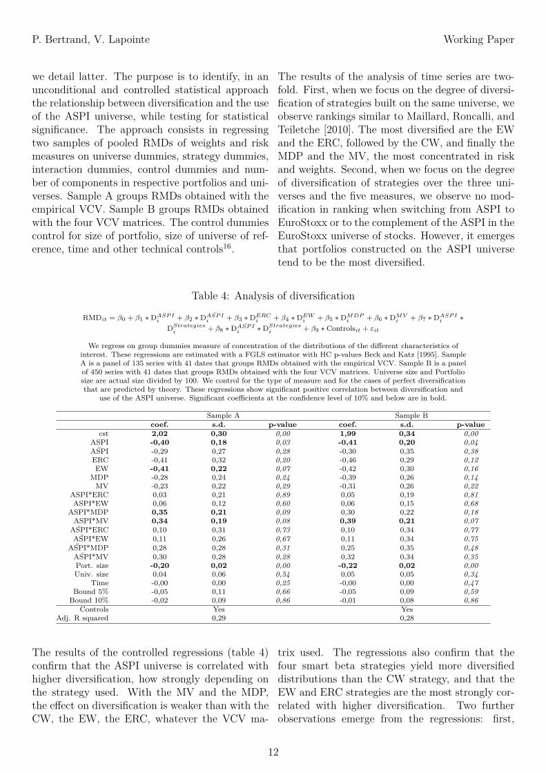
we detail latter. The purpose is to identify, in anunconditional and controlled statistical approachthe relationship between diversification and the useof the ASPI universe, while testing for statisticalsignificance. The approach consists in regressingtwo samples of pooled RMDs of weights and riskmeasures on universe dummies, strategy dummies,interaction dummies, control dummies and num-ber of components in respective portfolios and uni-verses. Sample A groups RMDs obtained with theempirical VCV. Sample B groups RMDs obtainedwith the four VCV matrices. The control dummiescontrol for size of portfolio, size of universe of ref-erence, time and other technical controls16.
The results of the analysis of time series are two-fold. First, when we focus on the degree of diversi-fication of strategies built on the same universe, weobserve rankings similar to Maillard, Roncalli, andTeiletche [2010]. The most diversified are the EWand the ERC, followed by the CW, and finally theMDP and the MV, the most concentrated in riskand weights. Second, when we focus on the degreeof diversification of strategies over the three uni-verses and the five measures, we observe no mod-ification in ranking when switching from ASPI toEuroStoxx or to the complement of the ASPI in theEuroStoxx universe of stocks. However, it emergesthat portfolios constructed on the ASPI universetend to be the most diversified.
Table 4: Analysis of diversification
RMDit = β0 + β1 ∗DASP Ii + β2 ∗D
¯ASP Ii + β3 ∗DERC
i + β4 ∗DEWi + β5 ∗DMDP
i + β6 ∗DMVi + β7 ∗DASP I
i ∗DStrategies
i + β8 ∗D¯ASP I
i ∗DStrategiesi + β9 ∗ Controlsit + εit
We regress on group dummies measure of concentration of the distributions of the different characteristics ofinterest. These regressions are estimated with a FGLS estimator with HC p-values Beck and Katz [1995]. SampleA is a panel of 135 series with 41 dates that groups RMDs obtained with the empirical VCV. Sample B is a panelof 450 series with 41 dates that groups RMDs obtained with the four VCV matrices. Universe size and Portfoliosize are actual size divided by 100. We control for the type of measure and for the cases of perfect diversificationthat are predicted by theory. These regressions show significant positive correlation between diversification and
use of the ASPI universe. Significant coefficients at the confidence level of 10% and below are in bold.
Sample A Sample Bcoef. s.d. p-value coef. s.d. p-value
cst 2,02 0,30 0,00 1,99 0,34 0,00ASPI -0,40 0,18 0,03 -0,41 0,20 0,04
¯ASPI -0,29 0,27 0,28 -0,30 0,35 0,38ERC -0,41 0,32 0,20 -0,46 0,29 0,12EW -0,41 0,22 0,07 -0,42 0,30 0,16
MDP -0,28 0,24 0,24 -0,39 0,26 0,14MV -0,23 0,22 0,29 -0,31 0,26 0,22
ASPI*ERC 0,03 0,21 0,89 0,05 0,19 0,81ASPI*EW 0,06 0,12 0,60 0,06 0,15 0,68
ASPI*MDP 0,35 0,21 0,09 0,30 0,22 0,18ASPI*MV 0,34 0,19 0,08 0,39 0,21 0,07¯ASPI*ERC 0,10 0,31 0,73 0,10 0,34 0,77¯ASPI*EW 0,11 0,26 0,67 0,11 0,34 0,75
¯ASPI*MDP 0,28 0,28 0,31 0,25 0,35 0,48¯ASPI*MV 0,30 0,28 0,28 0,32 0,34 0,35
Port. size -0,20 0,02 0,00 -0,22 0,02 0,00Univ. size 0,04 0,06 0,54 0,05 0,05 0,34
Time -0,00 0,00 0,25 -0,00 0,00 0,47Bound 5% -0,05 0,11 0,66 -0,05 0,09 0,59Bound 10% -0,02 0,09 0,86 -0,01 0,08 0,86
Controls Yes YesAdj. R squared 0,29 0,28
The results of the controlled regressions (table 4)confirm that the ASPI universe is correlated withhigher diversification, how strongly depending onthe strategy used. With the MV and the MDP,the effect on diversification is weaker than with theCW, the EW, the ERC, whatever the VCV ma-
trix used. The regressions also confirm that thefour smart beta strategies yield more diversifieddistributions than the CW strategy, and that theEW and ERC strategies are the most strongly cor-related with higher diversification. Two furtherobservations emerge from the regressions: first,
12
P. Bertrand, V. Lapointe Working Paper
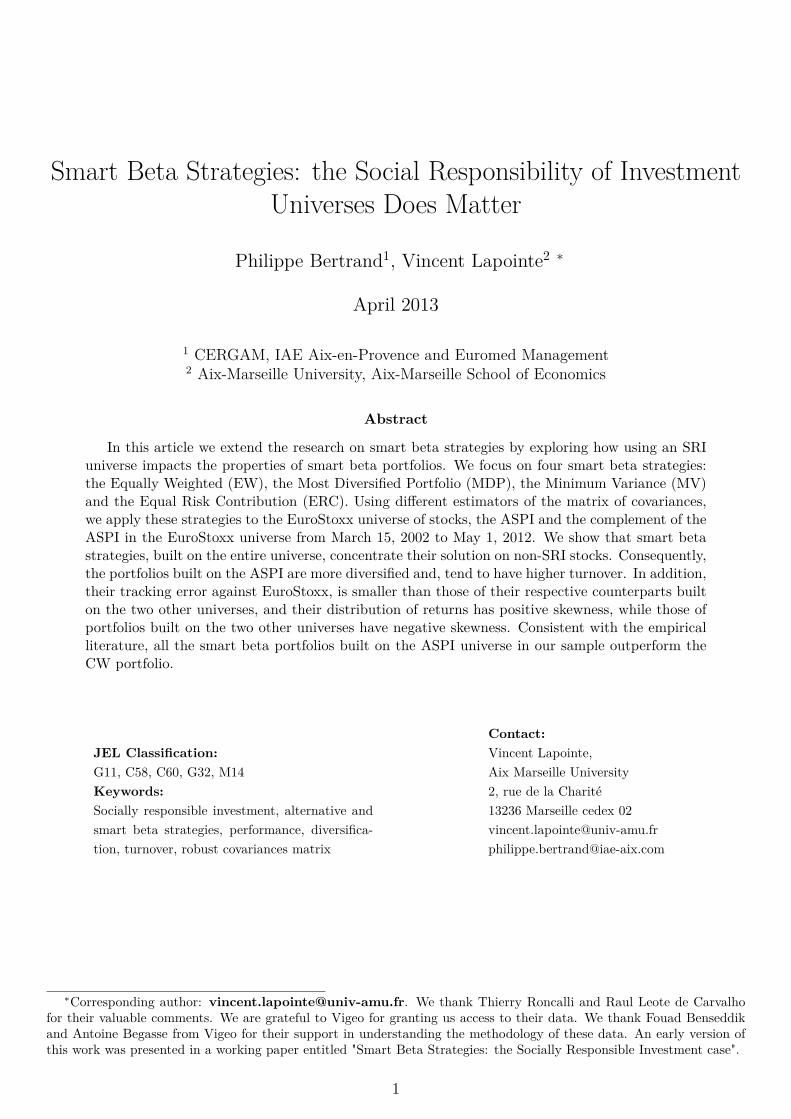
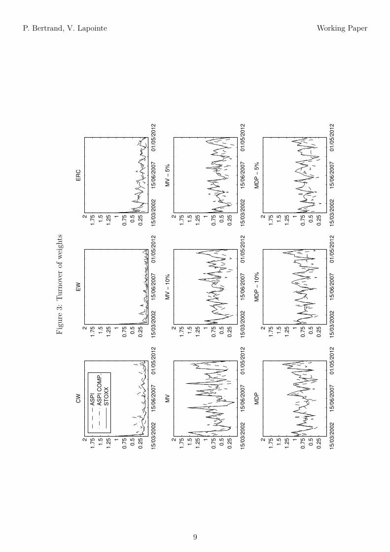
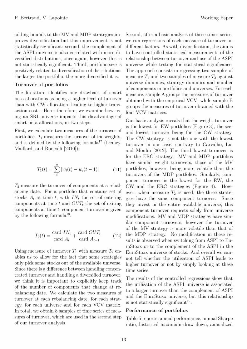
adding bounds to the MV and MDP strategies im-proves diversification but this improvement is notstatistically significant; second, the complement ofthe ASPI universe is also correlated with more di-versified distributions; once again, however this isnot statistically significant. Third, portfolio size ispositively related to diversification of distributions:the larger the portfolio, the more diversified it is.Turnover of portfoliosThe literature identifies one drawback of smartbeta allocations as being a higher level of turnoverthan with CW allocation, leading to higher trans-action costs. Here, therefore, we examine how us-ing an SRI universe impacts this disadvantage ofsmart beta allocations, in two steps.First, we calculate two measures of the turnover ofportfolios. T1 measures the turnover of the weights,and is defined by the following formula17 (Demey,Maillard, and Roncalli [2010]):
T1(t) =n∑i
|wi(t)− wi(t− 1)| (11)
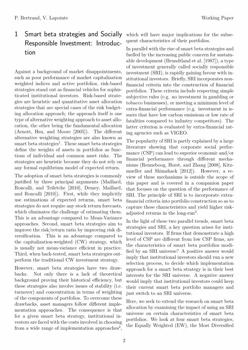
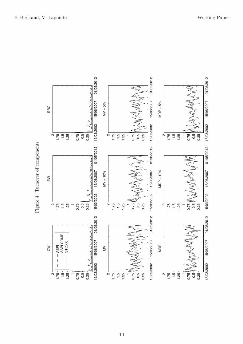
T2 measure the turnover of components at a rebal-ancing date. For a portfolio that contains set ofstocks At at time t, with INt the set of enteringcomponents at time t and OUTt the set of exitingcomponents at time t, component turnover is givenby the following formula18:
T2(t) = card INt
card At+ card OUTt
card At−1(12)
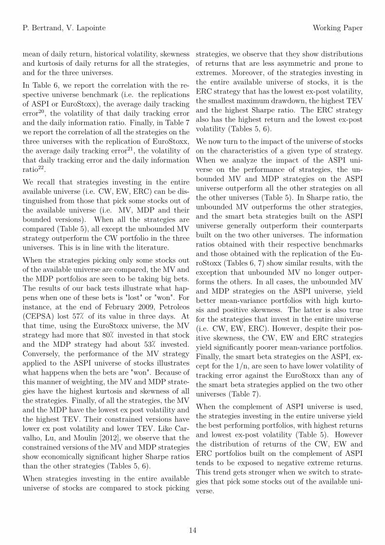
Using measure of turnover T1 with measure T2 en-ables us to allow for the fact that some strategiesonly pick some stocks out of the available universe.Since there is a difference between handling concen-trated turnover and handling a diversified turnover,we think it is important to explicitly keep trackof the number of components that change at re-balancing date. We calculate the two measures ofturnover at each rebalancing date, for each strat-egy, for each universe and for each VCV matrix.In total, we obtain 8 samples of time series of mea-sures of turnover, which are used in the second stepof our turnover analysis.
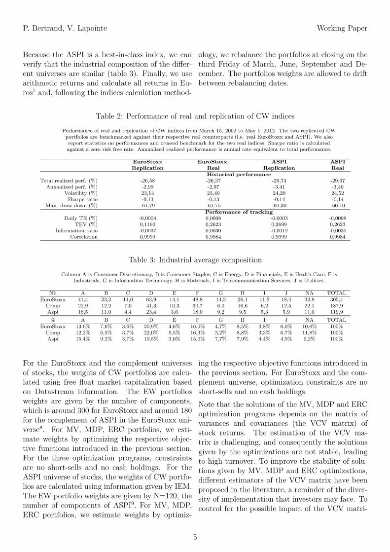
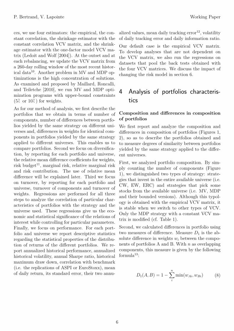
Second, after a basic analysis of these times series,we run regressions of each measure of turnover ondifferent factors. As with diversification, the aim isto have controlled statistical measurements of therelationship between turnover and use of the ASPIuniverse while testing for statistical significance.The approach consists in regressing two samples ofmeasure T1 and two samples of measure T2 againstuniverse dummies, strategy dummies and numberof components in portfolios and universes. For eachmeasure, sample A groups the measures of turnoverobtained with the empirical VCV, while sample Bgroups the measures of turnover obtained with thefour VCV matrices.Our basic analysis reveals that the weight turnoveris the lowest for EW portfolios (Figure 3), the sec-ond lowest turnover being for the CW strategy.The CW strategy is not the one with the lowestturnover in our case, contrary to Carvalho, Lu,and Moulin [2012]. The third lowest turnover isfor the ERC strategy. MV and MDP portfolioshave similar weight turnovers, those of the MVportfolios, however, being more volatile than theturnovers of the MDP portfolios. Similarly, com-ponent turnover is the lowest for the EW, theCW and the ERC strategies (Figure 4). How-ever, when measure T2 is used, the three strate-gies have the same component turnover. Sincethey invest in the entire available universe, thiscomponent turnover requests solely from universemodifications. MV and MDP strategies have sim-ilar component turnovers; however the turnoverof the MV strategy is more volatile than that ofthe MDP strategy. No modification in these re-sults is observed when switching from ASPI to Eu-roStoxx or to the complement of the ASPI in theEuroStoxx universe of stocks. And overall we can-not tell whether the utilisation of ASPI leads tohigher turnover or not by simply looking at thesetime series.The results of the controlled regressions show thatthe utilization of the ASPI universe is associatedto a larger turnover than the complement of ASPIand the EuroStoxx universe, but this relationshipis not statistically significant19.Performance of portfoliosTable 5 reports annual performance, annual Sharperatio, historical maximum draw down, annualized
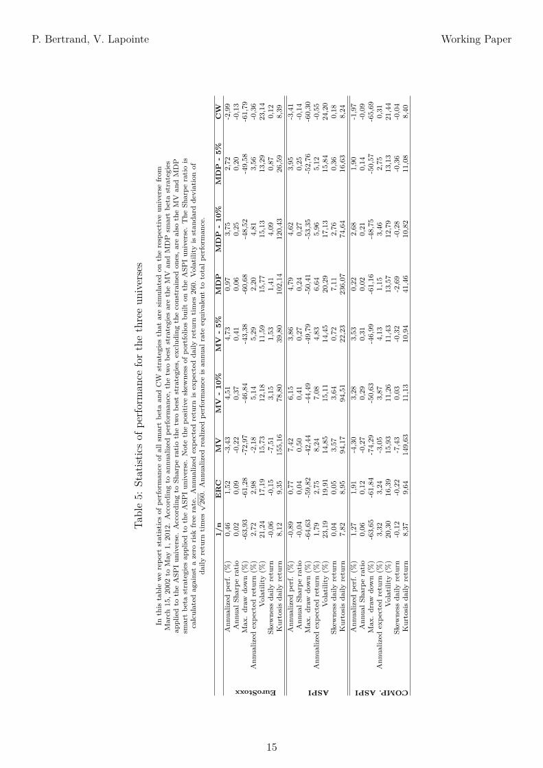
13
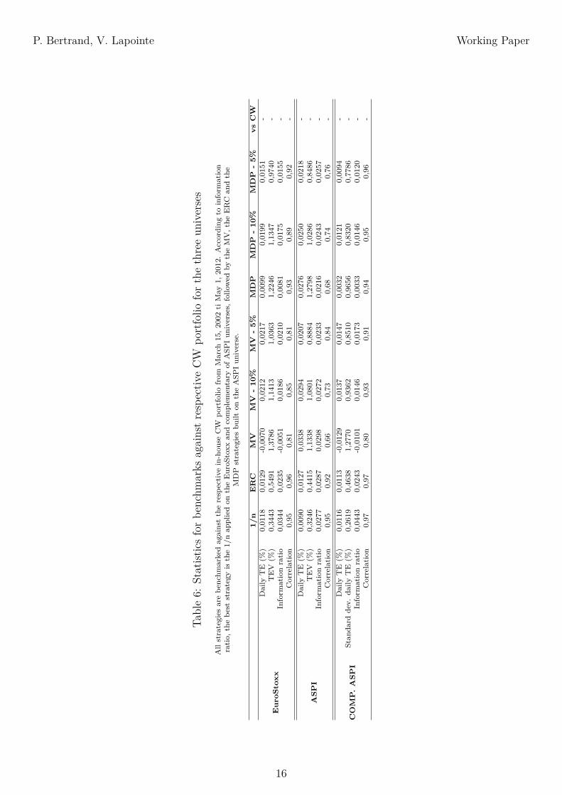
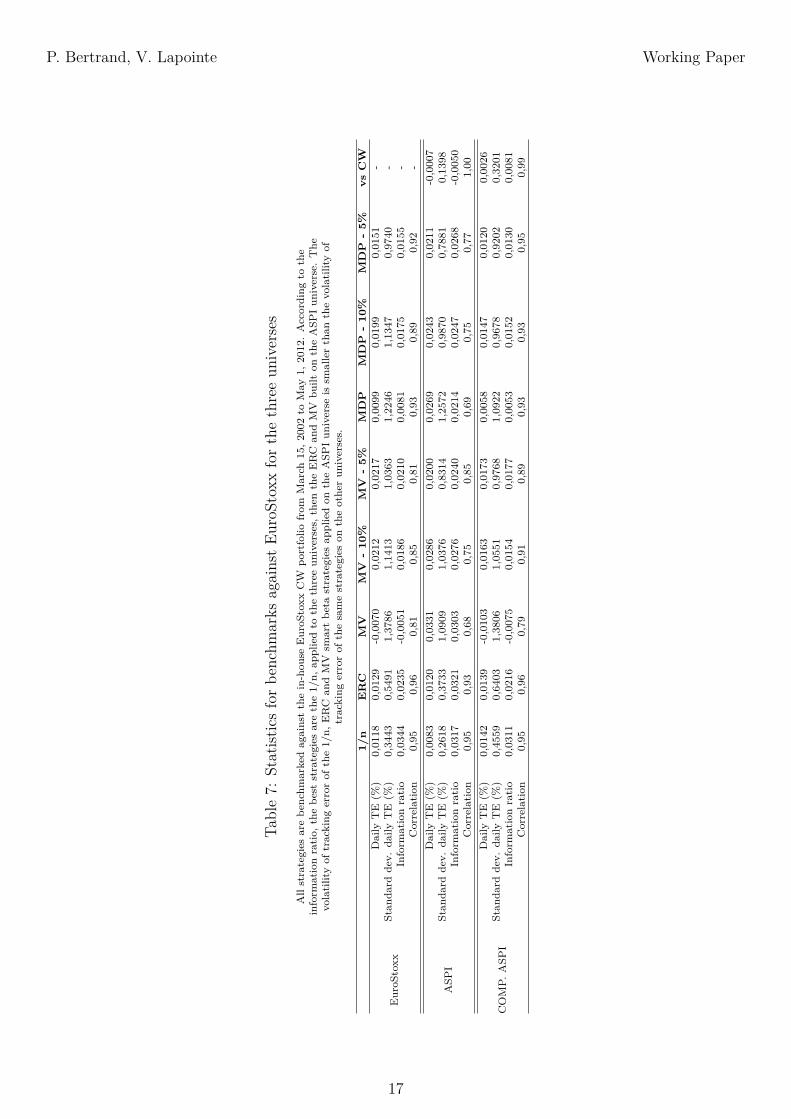
P. Bertrand, V. Lapointe Working Paper
mean of daily return, historical volatility, skewnessand kurtosis of daily returns for all the strategies,and for the three universes.In Table 6, we report the correlation with the re-spective universe benchmark (i.e. the replicationsof ASPI or EuroStoxx), the average daily trackingerror20, the volatility of that daily tracking errorand the daily information ratio. Finally, in Table 7we report the correlation of all the strategies on thethree universes with the replication of EuroStoxx,the average daily tracking error21, the volatility ofthat daily tracking error and the daily informationratio22.We recall that strategies investing in the entireavailable universe (i.e. CW, EW, ERC) can be dis-tinguished from those that pick some stocks out ofthe available universe (i.e. MV, MDP and theirbounded versions). When all the strategies arecompared (Table 5), all except the unbounded MVstrategy outperform the CW portfolio in the threeuniverses. This is in line with the literature.When the strategies picking only some stocks outof the available universe are compared, the MV andthe MDP portfolios are seen to be taking big bets.The results of our back tests illustrate what hap-pens when one of these bets is "lost" or "won". Forinstance, at the end of February 2009, Petroleos(CEPSA) lost 57� of its value in three days. Atthat time, using the EuroStoxx universe, the MVstrategy had more that 80� invested in that stockand the MDP strategy had about 53� invested.Conversely, the performance of the MV strategyapplied to the ASPI universe of stocks illustrateswhat happens when the bets are "won". Because ofthis manner of weighting, the MV and MDP strate-gies have the highest kurtosis and skewness of allthe strategies. Finally, of all the strategies, the MVand the MDP have the lowest ex post volatility andthe highest TEV. Their constrained versions havelower ex post volatility and lower TEV. Like Car-valho, Lu, and Moulin [2012], we observe that theconstrained versions of the MV and MDP strategiesshow economically significant higher Sharpe ratiosthan the other strategies (Tables 5, 6).When strategies investing in the entire availableuniverse of stocks are compared to stock picking
strategies, we observe that they show distributionsof returns that are less asymmetric and prone toextremes. Moreover, of the strategies investing inthe entire available universe of stocks, it is theERC strategy that has the lowest ex-post volatility,the smallest maximum drawdown, the highest TEVand the highest Sharpe ratio. The ERC strategyalso has the highest return and the lowest ex-postvolatility (Tables 5, 6).We now turn to the impact of the universe of stockson the characteristics of a given type of strategy.When we analyze the impact of the ASPI uni-verse on the performance of strategies, the un-bounded MV and MDP strategies on the ASPIuniverse outperform all the other strategies on allthe other universes (Table 5). In Sharpe ratio, theunbounded MV outperforms the other strategies,and the smart beta strategies built on the ASPIuniverse generally outperform their counterpartsbuilt on the two other universes. The informationratios obtained with their respective benchmarksand those obtained with the replication of the Eu-roStoxx (Tables 6, 7) show similar results, with theexception that unbounded MV no longer outper-forms the others. In all cases, the unbounded MVand MDP strategies on the ASPI universe, yieldbetter mean-variance portfolios with high kurto-sis and positive skewness. The latter is also truefor the strategies that invest in the entire universe(i.e. CW, EW, ERC). However, despite their pos-itive skewness, the CW, EW and ERC strategiesyield significantly poorer mean-variance portfolios.Finally, the smart beta strategies on the ASPI, ex-cept for the 1/n, are seen to have lower volatility oftracking error against the EuroStoxx than any ofthe smart beta strategies applied on the two otheruniverses (Table 7).When the complement of ASPI universe is used,the strategies investing in the entire universe yieldthe best performing portfolios, with highest returnsand lowest ex-post volatility (Table 5). Howeverthe distribution of returns of the CW, EW andERC portfolios built on the complement of ASPItends to be exposed to negative extreme returns.This trend gets stronger when we switch to strate-gies that pick some stocks out of the available uni-verse.
14
P. Bertrand, V. Lapointe Working Paper
Table5:
Statist
icsof
perfo
rman
ceforthethreeun
iverses
Inthis
tablewerepo
rtstatistics
ofpe
rforman
ceof
alls
martbe
taan
dCW
strategies
that
aresimulated
ontherespective
universe
from
March
15,2
002to
May
1,2012.According
toan
nualized
performan
ce,the
twobe
ststrategies
aretheMV
andMDP
smartbe
tastrategies
appliedto
theASP
Iun
iverse.According
toSh
arpe
ratiothetw
obe
ststrategies,e
xcluding
theconstrainedon
es,a
realso
theMV
andMDP
smartbe
tastrategies
appliedto
theASP
Iun
iverse.Notethepo
sitive
skew
ness
ofpo
rtfolio
sbu
ilton
theASP
Iun
iverse.The
Sharpe
ratiois
calculated
againstazero
risk
free
rate.Ann
ualized
expe
cted
return
isexpe
cted
daily
return
times
260.
Volatility
isstan
dard
deviationof
daily
return
times√
260.
Ann
ualized
realized
performan
ceis
annu
alrate
equivalent
tototalp
erform
ance.
1/n
ER
CM
VM
V-
10%
MV
-5%
MD
PM
DP
-10
%M
DP
-5%
CW
EuroStoxx
Ann
ualized
perf.(%
)0,46
1,52
-3,43
4,51
4,73
0,97
3,75
2,72
-2,99
Ann
ualS
harperatio
0,02
0,09
-0,22
0,37
0,41
0,06
0,25
0,20
-0,13
Max
.draw
down(%
)-63,93
-61,28
-72,97
-46,84
-43,38
-60,68
-48,52
-49,58
-61,79
Ann
ualiz
edexpe
cted
return
(%)
2,72
2,98
-2,18
5,14
5,29
2,20
4,81
3,56
-0,36
Volatility
(%)
21,24
17,19
15,73
12,18
11,59
15,77
15,13
13,29
23,14
Skew
ness
daily
return
-0,06
-0,15
-7,51
3,15
1,53
1,41
4,09
0,87
0,12
Kurtosisda
ilyreturn
8,12
9,35
155,16
78,80
39,80
102,14
120,43
26,59
8,39
ASPI
Ann
ualized
perf.(%
)-0,89
0,77
7,42
6,15
3,86
4,79
4,62
3,95
-3,41
Ann
ualS
harperatio
-0,04
0,04
0,50
0,41
0,27
0,24
0,27
0,25
-0,14
Max
.draw
down(%
)-64,63
-59,82
-42,44
-44,49
-49,79
-50,41
-53,35
-52,76
-60,30
Ann
ualiz
edexpe
cted
return
(%)
1,79
2,75
8,24
7,08
4,83
6,64
5,96
5,12
-0,55
Volatility
(%)
23,19
19,91
14,85
15,11
14,45
20,29
17,13
15,84
24,20
Skew
ness
daily
return
0,04
0,05
3,57
3,64
0,72
7,11
2,76
0,36
0,18
Kurtosisda
ilyreturn
7,82
8,95
94,17
94,51
22,23
236,07
74,64
16,63
8,24
COMP.ASPI
Ann
ualized
perf.(%
)1,27
1,91
-4,30
3,28
3,53
0,22
2,68
1,90
-1,97
Ann
ualS
harperatio
0,06
0,12
-0,27
0,29
0,31
0,02
0,21
0,14
-0,09
Max
.draw
down(%
)-63,65
-61,84
-74,29
-50,63
-46,99
-61,16
-48,75
-50,57
-65,69
Ann
ualiz
edexpe
cted
return
(%)
3,32
3,24
-3,05
3,87
4,13
1,15
3,46
2,75
0,31
Volatility
(%)
20,30
16,39
15,93
11,26
11,43
13,57
12,79
13,13
21,44
Skew
ness
daily
return
-0,12
-0,22
-7,43
0,03
-0,32
-2,69
-0,28
-0,36
-0,04
Kurtosisda
ilyreturn
8,37
9,64
149,63
11,13
10,94
41,46
10,82
11,08
8,40
15
P. Bertrand, V. Lapointe Working Paper
Table6:
Statist
icsforbe
nchm
arks
againstrespectiv
eCW
portfolio
forthethreeun
iverses
Allstrategies
arebe
nchm
arkedagainsttherespective
in-hou
seCW
portfolio
from
March
15,2
002tiMay
1,2012.According
toinform
ation
ratio,
thebe
ststrategy
isthe1/nap
pliedon
theEuroS
toxx
andcomplem
entary
ofASP
Iun
iverses,
follo
wed
bytheMV,the
ERC
andthe
MDP
strategies
built
ontheASP
Iun
iverse.
1/n
ER
CM
VM
V-
10%
MV
-5%
MD
PM
DP
-10
%M
DP
-5%
vsC
W
Eur
oSto
xx
Daily
TE
(%)
0,0118
0,0129
-0,0070
0,0212
0,0217
0,0099
0,0199
0,0151
-TEV
(%)
0,3443
0,5491
1,3786
1,1413
1,0363
1,2246
1,1347
0,9740
-Inform
ationratio
0,0344
0,0235
-0,0051
0,0186
0,0210
0,0081
0,0175
0,0155
-Correlation
0,95
0,96
0,81
0,85
0,81
0,93
0,89
0,92
-
ASP
I
Daily
TE
(%)
0,0090
0,0127
0,0338
0,0294
0,0207
0,0276
0,0250
0,0218
-TEV
(%)
0,3246
0,4415
1,1338
1,0801
0,8884
1,2798
1,0286
0,8486
-Inform
ationratio
0,0277
0,0287
0,0298
0,0272
0,0233
0,0216
0,0243
0,0257
-Correlation
0,95
0,92
0,66
0,73
0,84
0,68
0,74
0,76
-
CO
MP
.A
SPI
Daily
TE
(%)
0,0116
0,0113
-0,0129
0,0137
0,0147
0,0032
0,0121
0,0094
-Stan
dard
dev.
daily
TE
(%)
0,2619
0,4638
1,2770
0,9362
0,8510
0,9656
0,8320
0,7786
-Inform
ationratio
0,0443
0,0243
-0,0101
0,0146
0,0173
0,0033
0,0146
0,0120
-Correlation
0,97
0,97
0,80
0,93
0,91
0,94
0,95
0,96
-
16
P. Bertrand, V. Lapointe Working Paper
Table7:
Statist
icsforbe
nchm
arks
againstEu
roStox
xforthethreeun
iverses
Allstrategies
arebe
nchm
arkedagainstthein-hou
seEuroS
toxx
CW
portfolio
from
March
15,2
002to
May
1,2012.According
tothe
inform
ationratio,
thebe
ststrategies
arethe1/n,
appliedto
thethreeun
iverses,
then
theERC
andMV
built
ontheASP
Iun
iverse.The
volatilityof
tracking
errorof
the1/n,
ERC
andMV
smartbe
tastrategies
appliedon
theASP
Iun
iverse
issm
allerthan
thevolatilityof
tracking
errorof
thesamestrategies
ontheotherun
iverses.
1/n
ER
CM
VM
V-
10%
MV
-5%
MD
PM
DP
-10
%M
DP
-5%
vsC
W
EuroS
toxx
Daily
TE
(%)
0,0118
0,0129
-0,0070
0,0212
0,0217
0,0099
0,0199
0,0151
-Stan
dard
dev.
daily
TE
(%)
0,3443
0,5491
1,3786
1,1413
1,0363
1,2246
1,1347
0,9740
-Inform
ationratio
0,0344
0,0235
-0,0051
0,0186
0,0210
0,0081
0,0175
0,0155
-Correlation
0,95
0,96
0,81
0,85
0,81
0,93
0,89
0,92
-
ASP
I
Daily
TE
(%)
0,0083
0,0120
0,0331
0,0286
0,0200
0,0269
0,0243
0,0211
-0,0007
Stan
dard
dev.
daily
TE
(%)
0,2618
0,3733
1,0909
1,0376
0,8314
1,2572
0,9870
0,7881
0,1398
Inform
ationratio
0,0317
0,0321
0,0303
0,0276
0,0240
0,0214
0,0247
0,0268
-0,0050
Correlation
0,95
0,93
0,68
0,75
0,85
0,69
0,75
0,77
1,00
COMP.
ASP
I
Daily
TE
(%)
0,0142
0,0139
-0,0103
0,0163
0,0173
0,0058
0,0147
0,0120
0,0026
Stan
dard
dev.
daily
TE
(%)
0,4559
0,6403
1,3806
1,0551
0,9768
1,0922
0,9678
0,9202
0,3201
Inform
ationratio
0,0311
0,0216
-0,0075
0,0154
0,0177
0,0053
0,0152
0,0130
0,0081
Correlation
0,95
0,96
0,79
0,91
0,89
0,93
0,93
0,95
0,99
17
P. Bertrand, V. Lapointe Working Paper
Hence, the distribution of returns of the MV andMDP portfolios built on the complement of ASPIhave high kurtosis and negative skewness. This isconsistent with the observation that investors per-ceive a correlation between extreme specific riskand weak social performance (Waddock and Graves[1997], Hong and Kacperczyk [2009]), and withempirical findings (Boutin-Dufresne and Savaria[2004]).When the EuroStoxx universe is used, we obtainstatistics that are similar to these obtained with thecomplement of ASPI. This is consistent with thehigh level of overlapping previously revealed. TheMV portfolios built on the EuroStoxx and comple-ment of ASPI universes also have ex-post volatili-ties higher than the volatility of the ASPI MV port-folio. This observation, together with that on theoptimality of smart beta solutions (cf. page 11), il-lustrates the gap between ex ante optimisation andex post realisation. It may also illustrate the lowerquality of the statistical inputs obtained with theEuroStoxx and complement of ASPI universes.
5 Robustness
As previously introduced, to treat the issue of sta-bility of solutions given by MV, MDP and ERCoptimizations we used four different estimations ofthe VCV matrix: the empirical, the constant corre-lation and two shrinkage estimators23 (Ledoit andWolf [2004]). The different analysis we report inthis paper are done with the empirical VCV ma-trix sample, and with the sample pooling the fourdifferent VCV matrices.Whatever the estimator, using an SRI universe isseen to impact the characteristics (i.e. diversifica-tion) of smart beta portfolios to the same degree.However, we find some differences in the degree towhich use of smart beta strategies affects the per-formance of SRI portfolios. For example, using theSharpe ratio, non-reported regression shows thatthe constant VCV matrix yields portfolios with sig-nificantly poorer performance. We observe lowerreturns and higher variance of returns than forportfolios built with other VCV matrices. In addi-tion, the shrinkage estimators of the VCV matrixyield portfolios with better performance than port-
folios built with empirical estimators of the VCVmatrix; but this latter observation is not statisti-cally significant.However, the use of more sophisticated estimatorsof the VCV matrix leads to other significant advan-tages. Non-reported regressions show that more so-phisticated VCVmatrices significantly decrease theturnover of weights and components. The smallestimprovement is obtained with the shrinkage towardthe constant VCV matrix. The shrinkage towardthe one-factor model and the constant VCV matrixare equivalent.
6 Conclusion
Our intention here was to further explore smartbeta allocation by examining how using an SRIuniverse impacts the characteristics of smart betaportfolios. We studied four smart beta strategies,the EW, the MDP, the MV and the ERC, usingthree universes of stocks, the EuroStoxx, the ASPIand the complement of ASPI universe. We workedwith four different estimators of the VCV matrix:the empirical, the constant, the matrices shrunktowards a constant and towards a one-actor model.Six types of impact of using the ASPI universe ofstocks emerge from our study. First, smart betastrategies applied on the EuroStoxx favour stocksthat do not belong to the ASPI universe. In fact,the lists of components and the weights of over-lapping components in EuroStoxx and ASPI differwidely. Second, there is increased diversification ofthe weight and risk measure distributions. Diversi-fication also increases when we use the complementof the ASPI universe; however the correlation is notstatistically significant and is lower than the oneobtained with the ASPI universe. These observa-tions do not depend on type of VCV. Third, smartbeta portfolios built on the ASPI universe tend topresent higher weight and component turnovers.Again, these observations do not depend on type ofVCV. Fourth, the distributions of returns of portfo-lios built on the ASPI universe have positive skew-ness, while with the two other universes, portfolioshave distributions of returns with negative skew-ness. Fifth, the volatility of tracking error againstEuroStoxx of smart beta strategies built on the
18
P. Bertrand, V. Lapointe Working Paper
ASPI universe is lower than that of their respec-tive counterparts built on the two other universes.Moreover, on the ASPI universe, all the smart betastrategies dominate the CW strategy, which is sim-ilar to findings on the two other universes and con-sistent with the empirical literature.Hence, while recalling the usual limitations of back-testing, we conclude that using smart beta strate-gies in combination with the SRI approach some-what modifies the properties of smart beta portfo-lios. Adopting SRI thus cannot be considered neu-tral and warrants careful attention from the insti-tutional investor. A valuable extension of this workwould be to check the robustness of our resultsusing a different SRI universe with different rat-ing methodology and covering different geographi-cal zones.
Notes
1Though we are interested in risk-based alternativeweighting, we will stick to the term "smart beta" in the restof the article.
2Some of the implementation choices will be discussed inthis paper, in the section on data and methodology.
3The second justification for adoption of SRI ressemblesthe intuition justifying alternative weighting schemes. Ac-tually, SRI can be considered a smart beta approach, be-tween fundamental and risk based allocations, where assetsthat do not match extra-financial criteria are given a weightequal to zero. Fundamental allocations define the weightsas a function of issuers’ fundamental statistics. See Arnott,Hsu, and Moore [2005].
4The EuroStoxx is a subset of the EuroStoxx 600 thatcontains a variable number of stocks, roughly 300, traded inEurozone countries. The ASPI is a subset of EuroStoxx thatcontains the 120 best rated stocks. This social performancerating is given by VIGEO. The complement of the ASPI inthe EuroStoxx universe is the universe of about 180 stocksthat are in the EuroStoxx but not in the ASPI.
5There is no weight equal to zero in the original theory,but in practice see the numerical approach of Carvalho, Lu,and Moulin [2012], and the analytical work of Clarke, Silva,and Thorley [2012] that shows why stocks with particularnegative values of the beta with an ERC portfolio can beexcluded from the ERC.
6IEM is the firm in charge of calculation methodologyfor the ASPI. VIGEO is a provider of social performanceratings and sponsor of the ASPI.
7By construction EuroStoxx is a Euro Zone universe.
8As previously stated, the EuroStoxx is a subset of theEuroStoxx 600 that contains a variable number of stocks,roughly 300.
9For 2 rebalancing dates ASPI is defined by N=118 andN=119.
10For some stocks historical series are shorter than theVCV estimation window. For the ASPI universe, this con-cerns two stocks out of 238, the smallest window is 100 days.For EuroStoxx and complement of ASPI universe, this con-cerns 53 stocks out of 536, the smallest windows is 12 days.
11Risk budget is defined as the product of the weight ofcomponent i combined with its volatility.
12The benchmarks used are our replications of ASPI andEuroStoxx CW indices.
13When D1 equals 1, it means that the two portfolios donot overlap. The portfolios have different lists of compo-nents. When D1 equals 0, it means that the two portfolioare identical.
14When D2 equals 1, it means that the two lists of com-ponents do not intersect. When D2 equals 0 it means thatone list is equal to, or included in, the other.
15The RMD is closely related to the Gini coefficient. Thecloser the relative mean difference gets to zero the less con-centrated the distribution is.
16We control for the case of perfect diversification for thedifferent VCV matrices. That is, the EW and weights, theMDP, ERC and the risk contribution. We control for thedifferent types of characteristics analyzed.
17By definition T1 is between 0 and 2 for one rebalancingand, for the first rebalancing, the turnover equals 1.
18By definition T2 is between 0 and 2 for one rebalancingand, for the first rebalancing, the turnover equals 1.
19We do not report the results because of space con-straints. They are available from the authors upon request
20The benchmarks used are our replications of ASPI andEuroStoxx CW indices.
21The benchmarks used are our replications EuroStoxxCW indices.
22The results in these three tables are obtained with em-pirical covariance matrices, using daily returns for three dif-ferent universes of stocks, the EuroStoxx, the ASPI and thecomplement of the ASPI in the EuroStoxx universe.
23Shrinkage targets are the constant correlation and theone-factor market model VCV matrices.
References
Arnott, Robert, Jason Hsu, and Philip Moore(2005). “Fundamental Indexation”. In: Finan-cial Analysts Journal 61, pp. 83–99.
19
P. Bertrand, V. Lapointe Working Paper
Beck, Nathaniel and Jonathan N. Katz (1995).“What to do (and not to do) with Time-SeriesCross-Section Data”. In: The American Politi-cal Science Review 89, pp. 643–647.
Boutin-Dufresne, François and Patrick Savaria(2004). “Corporate Social Responsibility andFinancial Risk”. In: Journal of Investing 13,pp. 57–66.
Brundtland, H. et al. (1987). Report of the WorldCommission on Environment and Develop-ment: Our Common Future. Tech. rep. UnitedNation.
Carvalho, Raul Leote de, Xiao Lu, andPierre Moulin (2012). “Demystifying EquityRisk–Based Strategies: A Simple Alpha plusBeta Description”. In: Journal of PortfolioManagement 38, pp. 56–70.
Choueifaty, Yves and Yves Coignard (2008). “To-wards maximum diversification”. In: Journal ofPortfolio Management 34, pp. 40–51.
Clarke, Roger, Harindra de Silva, and Steven Thor-ley (2006). “Minimum-Variance Portfolios inthe U.S. Equity Market”. In: Journal of Port-folio Management 33, pp. 10–24.
— (2012). Risk Parity, Maximum Diversification,and Minimum Variance: An Analytic Perspec-tive. Tech. rep. BYU & Analytic Investor, LLC.
Demey, Paul, Sébastien Maillard, and Thierry Ron-calli (2010). Risk-Based Indexation. Tech. rep.Lyxor.
DeMiguel, Victor, Lorenzo Garlappi, and RamanUppal (2009). “Optimal Versus Naive Diver-sification: How Inefficient is the 1/N Portfolio
Strategy?” In: Review of Financial Studies 22,pp. 1915–1953.
Hong, H. and M. Kacperczyk (2009). “The price ofsin: the effects of social norms on markets”. In:Journal of Financial Economics 93, pp. 15–36.
Kitzmueller, Markus and Jay Shimshack (2012).“Economic Perspectives on Corporate SocialResponsibility”. In: Journal of Economic Lit-erature 50, pp. 51–84.
Ledoit, Olivier and Michael Wolf (2004). “Honey,I Shrunk the Sample Covariance Matrix”. In:Journal of Portfolio Management 30, pp. 110–119.
Maillard, Sébastien, Thierry Roncalli, and JérômeTeiletche (2010). “On the properties of equally-weighted risk contributions portfolios”. In:Journal of Portfolio Management 36, pp. 60–70.
Martellini, Lionel (2008). “Toward the design ofbetter equity benchmarks”. In: Journal of Port-folio Management 34, pp. 1–8.
Renneboog, Luc, Jenke Ter Horst, and ChendiZhang (2008). “Socially responsible invest-ments: Institutional aspects, performance, andinvestor behavior”. In: Journal of Banking andFinance 32, pp. 1723–1742.
Scherer, Bernd (2011). “A note on the returns fromminimum variance investing”. In: Journal ofEmpirical Finance 18, pp. 652–660.
Waddock, Sandra A. and Samuel B. Graves (1997).“The Corporate Social Performance-FinancialPerformance Link”. In: Strategic ManagementJournal 18, pp. 303–319.
20