Smallholder Heterogeneity and Maize Market Participation in

MSU Agricultural Economics Web Site: http://www.aec.msu.edu MSU Food Security Group Web Site: http://www.aec.msu.edu/fs2/index.htm

MSU is an affirmative-action, equal-opportunity employer

MSU International Development

Working Paper 113 October, 2011

Smallholder Heterogeneity and Maize Market Participation in Southern and Eastern Africa: Implications for Investment Strategies to Increase Marketed Food Staple Supply by David Mather, Duncan Boughton, and T.S. Jayne

Department of Agricultural, Food, and Resource Economics Department of Economics

MICHIGAN STATE UNIVERSITY East Lansing, Michigan 48824

MSU International Development

Working Paper

http://www.aec.msu.edu

http://www.aec.msu.edu/fs2/index.htm

MSU INTERNATIONAL DEVELOPMENT PAPERS The Michigan State University (MSU) International Development Paper series is designed to further the comparative analysis of international development activities in Africa, Latin America, Asia, and the Near East. The papers report research findings on historical, as well as contemporary, international development problems. The series includes papers on a wide range of topics, such as alternative rural development strategies; nonfarm employment and small scale industry; housing and construction; farming and marketing systems; food and nutrition policy analysis; economics of rice production in West Africa; technological change, employment, and income distribution; computer techniques for farm and marketing surveys; farming systems and food security research. The papers are aimed at teachers, researchers, policy makers, donor agencies, and international development practitioners. Selected papers will be translated into French, Spanish, or other languages. Copies of all MSU International Development Papers, Working Papers, and Policy Syntheses are freely downloadable in pdf format from the following Web sites: MSU International Development Papers http://www.aec.msu.edu/fs2/papers/idp.htm http://ideas.repec.org/s/ags/mididp.html MSU International Development Working Papers http://www.aec.msu.edu/fs2/papers/idwp.htm http://ideas.repec.org/s/ags/midiwp.html MSU International Development Policy Syntheses http://www.aec.msu.edu/fs2/psynindx.htm http://ideas.repec.org/s/ags/midips.html Copies of all MSU International Development publications are also submitted to the USAID Development Experience Clearing House (DEC) at: http://dec.usaid.gov/

http://www.aec.msu.edu/fs2/papers/idp.htm

http://ideas.repec.org/s/ags/mididp.html

http://www.aec.msu.edu/fs2/papers/idwp.htm

http://ideas.repec.org/s/ags/midiwp.html

http://www.aec.msu.edu/fs2/psynindx.htm

http://ideas.repec.org/s/ags/midips.html

http://dec.usaid.gov/

Smallholder Heterogeneity and Maize Market Participation in Southern and Eastern Africa: Implications for Investment Strategies to Increase

Marketed Food Staple Supply

by

David Mather, Duncan Boughton, and T.S. Jayne

October 2011

Mather is assistant professor, and Boughton is associate professor, and Jayne is professor, International Development, all are with the Department of Agricultural, Food, and Resource Economics, Michigan State University.

ii

ISSN 0731-3483 © All rights reserved by Michigan State University, 2011. Michigan State University agrees to and does hereby grant to the United States Government a royalty-free, non-exclusive and irrevocable license throughout the world to use, duplicate, disclose, or dispose of this publication in any manner and for any purposes and to permit others to do so. Published by the Department of Agricultural, Food, and Resource Economics and the Department of Economics, Michigan State University, East Lansing, Michigan 48824-1039, U.S.A.

iii

ACKNOWLEDGMENTS

This research was supported by United States Agency for International Development (USAID) Bureau for Africa and the Bureau for Food Security through the Food Security III Cooperative Agreement. This report would not be possible without the data collection efforts of colleagues at Tegemeo Institute (Kenya), Ministry of Agriculture and Rural Development (Mozambique) and the Ministry of Agriculture and Cooperatives and the Central Statistical Office, (CSO Zambia). The authors acknowledge the invaluable contributions that Professor Jeffrey Wooldridge of the Department of Economics at MSU made to the econometrics methods employed in this paper. The authors also wish to acknowledge the time and information provided by the rural families who have participated in household surveys in each country, without which this research would not be possible, and Patricia Johannes for her editing and formatting assistance.

v

EXECUTIVE SUMMARY

In many African countries, as well as in other parts of the world where a significant part of the rural population is poor and food insecure, policymakers face what is called the food price dilemma. On the one hand, they need to provide farmers with incentives to increase the quantity of marketed food staples to feed a growing population, especially in rapidly growing urban centers where unrest can be politically destabilizing. On the other hand, because staple foods account for a large portion of total household expenditures for both urban and rural households, policymakers also are drawn to policies that lower the retail price of staple foods for consumers. Achieving both objectives – increasing marketed supplies of food staples while maintaining low retail prices – are also key to continued poverty reduction, as smallholder incomes increase when they receive higher prices for their surplus marketed output, while lower retail food prices decrease the cost of living for both rural and urban households. Hence, these objectives figure prominently in Comprehensive Africa Agriculture Development Programme (CAADP) investment plans and the United States (U.S.) Feed The Future initiative. The food price dilemma has become more acute in recent years because of the international commodity market food price shocks in 2008 and 2011, aggravated by slower economic growth because of the global financial crisis. A number of African countries have recently sought to respond to the food price dilemma through large-scale fertilizer subsidy programs to increase food crop production, often coupled with purchases of a large part of the marketed surplus by state-run marketing boards to both avoid price collapses and to support farmgate maize prices in general. However, there is growing evidence that such programs are not sustainable from a fiscal perspective, and have little enduring benefit for either urban consumers or rural smallholders. A key challenge for the architects of country and regional investment plans in Africa, and initiatives like Feed The Future that seek to support them, is to identify investment programs that can achieve sustainable increases in both marketed food production and poverty reduction. In this paper, we use descriptive and econometric analysis of nationally-representative smallholder panel data sets from Kenya, Mozambique, and Zambia to examine the question of how to achieve increases in marketed surplus of maize, the most widely marketed cereal food staple of eastern and southern Africa (ESA). Our findings suggest that there are alternative ways to invest public resources that will lead to sustainable outcomes in the long term, recognizing that, in the short term, safety nets will be needed to protect the household assets of poor urban consumers and food insecure rural households, alleviate suffering, and safeguard political stability until such longer-term investments bear fruit (an area addressed by CAADP’s Pillar 3). Across our three case countries, there is a wide range of market access conditions, as conventionally measured by distance to a tarmac or feeder road or to an input dealer. For example, a Kenyan smallholder farmer need travel just 3 km on average to purchase from a fertilizer retailer, compared to 37 km in Zambia and almost 70 km in Mozambique. Across and within these three countries there is also wide variation in household assets and agro-ecological potential. This diversity allows us to analyze the extent to which smallholder production and marketing patterns vary by household asset levels and agro-ecological zone, using panel regression techniques to determine how marginal changes in smallholders’ access to assets, technologies, and markets affect their decisions about whether and how much maize to sell.

vi

Among our three study countries, Kenya has both the highest level of smallholder commercialization and the lowest rural poverty rate. For example, the median Kenyan smallholder sells 46% of the value of their crop production, while the median smallholders in Zambia and Mozambique sell only 14% and 8% of the value of their crop production, respectively. Even though the share of total household income from crops and livestock in Kenya is only slightly lower (at 62%) than either Zambia or Mozambique (64% and 69% respectively), median household income per adult equivalent in Kenya is almost six times that of Mozambique and almost four times that of Zambia. Kenya thus demonstrates that smallholder agriculture can provide a pathway out of poverty when households have the necessary assets and access to improved agricultural technologies that enable them to take advantage of investments in market development. In all three countries, maize sales are concentrated in a minority of the population. For example, in Kenya, approximately a quarter of the smallholders sell more than a 100kg bag per adult equivalent1, in Zambia between 10 and 20% depending on the year, and in Mozambique only 3%. In all three countries, smallholders selling more than a 100kg bag have production levels per adult equivalent five times that of their counterparts who have negligible or no sales. To answer the question of what kinds of CAADP investment will shift more of the smallholder distribution into the category with significant maize surpluses to sell on a sustainable basis, we turn to multivariate regression analysis of the determinants of smallholder maize sales. Our econometric analysis yields seven principal findings. First, previous research on household food grain sales behavior in developing countries has tended to focus on the role of market access and price-related factors to explain why many rural households do not sell staple crops such as maize. The conclusions of this line of research have been to promote market liberalization and road construction so as to provide smallholders with ‘access’ to markets, lower transaction costs, and thus more favorable input and output prices. While such policies and investments are vital to improving the input and output prices facing smallholders, we present evidence that suggests that many smallholders in these countries already enjoy reasonable market access. For example, our descriptive analysis of rural household data from Mozambique, Zambia, and Kenya shows that in general there is little difference between large and small net maize sellers in any of the three countries in regard to market access, as measured by distance to the nearest road and access to market information. In addition, the majority of maize sellers in each country make their sales within their village. This is consistent with our econometric analysis of household maize sales, which finds that typical market access proxies (distance to physical infrastructure or towns) are not significant, or of small magnitude in most zones of our case countries. These findings are also consistent with recent rapid appraisal work in each country, which found that trader presence even in ‘remote’ villages has greatly improved within the past decade, perhaps a result of increased investments in road construction as well as the recent proliferation of cell phones in rural areas. Thus, while there still may be significant transport costs to the nearest relevant market for farmers in ‘remote’ villages (which would cause traders to adjust their maize buying prices lower), even these farmers now face considerably lower search costs for price information and access to traders than they did a decade ago. The implication of these results is not that additional infrastructure improvements in ESA countries are no longer needed, but that there are household-specific factors – such as low household asset endowments and poor access to improved inputs – which appear to constrain the ability of

1 Adult equivalent is a measure that adjusts the size of a household to reflect its caloric consumption needs based on the age and gender or each individual in the household (WHO 1985).

vii

many smallholders to produce a surplus and hence be able to take advantage of public goods that reduce the cost of market access. Second, another potential factor affecting transaction costs is access to market price information, which would be expected to improve maize market participation. In Mozambique, we find that household receipt of market price information results in large increases in the probability of smallholder maize sale and sale quantities. In Kenya and Zambia, we use radio and cell phone ownership as a proxy for household access to market price information, and find significant positive effects of such assets on quantities sold. These findings suggest that funding to increase the spatial coverage and frequency of radio broadcasts in these countries could potentially lead to large increases in both quantities of maize sold as well as the numbers of households selling maize. Third, in each country, we find that village or district-level measures of either rainfall or drought stress have significant and large effects on smallholders’ probability of selling maize and/or amounts sold, while controlling for household assets, maize price, and market access. These results highlight the sensitivity of marketed maize surplus to weather shocks, and thus the potential value of investment in climate change adaptation measures. Such investments include the development and dissemination of drought-tolerant maize varieties, as well as widespread promotion of smallholder access to low-cost methods of irrigation and/or conservation farming techniques to reduce the impact of drought. Fourth, our results from Kenya and Zambia show that use of divisible improved technologies such as hybrid seed and chemical fertilizer can significantly increase the number of households selling maize as well as quantities sold. In addition, the large effects of these inputs on smallholder maize sales are significant among farmers of various landholding sizes and from various agro-ecological zones. While the question of how best to increase smallholder access to such inputs is currently the focus of much debate, it is clear that improvements in access to input markets and extension to enable smallholders to deploy profitable technology packages are at least as important as access to output markets, especially in countries like Mozambique and Zambia where the majority of farmers have negligible amounts of surplus food staples to sell. An alternative to direct fertilizer subsidies is to strengthen farmers’ effective demand for fertilizer through investments in public/collective goods that make fertilizer use more profitable, and by building durable input markets and output markets that can absorb the increased output without gluts that depress producer prices. Such investments would include rural road infrastructure and port facilities to reduce the costs of distribution; agricultural research to develop and adapt varieties that respond more efficiently to fertilizer; the development and dissemination of fertilizer use recommendations that are appropriate for different agro-ecological zones; and the development of rural financial systems and market information systems. The specific mix of such investments would clearly vary across and within our three countries given the dramatically different stage of development of the private input markets in each country, and variation in the profitability of input use across agro-ecologies. Nevertheless, returns to these investments require durable input and output markets, which depend upon a supportive policy environment that attracts local and foreign direct investment. The case of Kenya demonstrates that a stable policy environment – with respect to fertilizer, land, and maize markets – can induce an impressive private sector response over time that has helped to make fertilizer and improved maize seed varieties accessible to most small farmers.

viii

Fifth, we find that marginal increases in landholding in Mozambique and Zambia have significant and relatively large effects on the quantities of maize sold by both current sellers and all households (whether currently selling maize or not). Given that Zambia and Mozambique both contain large tracts of uncultivated land, there are clear opportunities in these countries to address the extremely low levels of landholding among the bottom half of the land distribution, though this will require investment in public goods, such as investments to eradicate disease constraints to animal traction use in Mozambique, and infrastructure investments in unsettled areas to promote migration in Zambia. In the short run, expanding access to improved seed and fertilizer is a powerful way to overcome smallholder land constraints, while expanded access to animal traction and/or re-settlement in more land abundant areas can further increase labor productivity and incomes in the medium to longer term. Sixth, while we find that the responsiveness of smallholder maize sales to changes in expected farmgate maize prices is significant and positive in most areas of Kenya, in higher potential zones in Zambia, and among current sellers in Mozambique, we also find insignificant or negative household responsiveness to maize prices in lower potential zones of Zambia and Mozambique. The heterogeneity of maize price responsiveness in Zambia and Mozambique indicates that while improved infrastructure may elicit a positive sales response in some regions, policymakers aiming to increase marketed maize surplus from smallholders need to also consider non-price factors such as the distribution and level of key production assets such as landholding, as well as factors which affect the return to those productive assets, such as technology use and agro-ecological potential (which affects the technology needs for a given region). In the case of Mozambique, until productive assets such as landholding and animal traction use are increased, and returns to existing assets are improved via adoption of technologies such as fertilizer and improved seed, it is questionable whether improved prices alone (through improvements in infrastructure) will elicit a positive supply response from maize producers who currently do not sell maize (i.e., 80% of maize growers). Seventh, our findings with respect to gender of the household head differ considerably across countries. In Kenya, households headed by a single female are just as likely as male-headed households to sell maize. By contrast, households headed by a single female in Zambia are less likely to sell maize, while those in both Zambia and Mozambique sell lower quantities of maize. Descriptive analysis suggests that the reason for this is not related to land access, because these households actually have higher average total landholding and area planted to maize, relative to male-headed households. However, households headed by a single female have significantly lower maize production per adult equivalent on average relative to other households. In Mozambique, low maize productivity in households headed by a single female appears to be due to the relatively high percentage of these households located in areas of low agro-ecological potential, while in Zambia female-headed households are less likely to use either hybrid maize seed or to apply fertilizer to maize relative to other households, and likely have lower levels of unobserved factors such as soil quality, length of fallows, and knowledge of crop management practices. A key implication of our gender findings is that there is unlikely to be a unique strategy to improve the food security and welfare of female-headed households. Rather, programs designed to address the needs of female-headed households must be based on an understanding of the specific constraints they face in each country. A key implication of the foregoing for CAADP and Feed The Future is that investment strategies at country level can achieve increases in both marketed surpluses of food staples and smallholder incomes, but to do so requires very effective spatial coordination between

ix

investments under Pillars 1, 2 and 4 to ensure that farmers have sufficient access to land and technology with which they can take advantage of investments in improved market access. Likewise, investment plans will need to target different investment bundles to different groups of smallholders, adapted to the agro-ecology where they farm. For example, technology packages need to be well-adapted to agro-ecological conditions, and integrate conservation agriculture methods to counter weather shocks. In the case of maize, for example, high-yielding longer duration hybrids will be more appropriate for commercial smallholders in mid-elevation areas whereas a combination of medium and short-duration drought tolerant varieties would be more appropriate for vulnerable smallholders and/or low elevation zones. While the private sector has a vital role to play in developing seed and fertilizer markets, there are strong public good aspects to both the development of technology packages which are adapted to varying agro-ecological conditions – especially for farmers in zones with poorer agro-ecological potential – as well as extension services to farmers, which address smallholder constraints related to both crop and livestock production and marketing. Although CAADP and recent donor statements include agricultural research and development as a key to improved food security in Sub-Saharan Africa, the reality is that government and donor funding for National Agricultural Research Systems and the Consultative Group on International Agricultural Research (CGIAR) system has declined significantly over the past few decades. These declines in funding for agricultural research and development (R&D) must be reversed, with the recognition that many Sub-Saharan African countries may be too small to undertake crop research programs for every food crop, thus necessitating regional research cooperation. In summary, many African governments have pledged through the CAADP process to correct the decades-long underinvestment in agriculture in Africa, and many international donors have indicated their support for this goal. This paper highlights various investments in public/collective goods that African governments and donors can make through the CAADP process to increase both domestic quantities of marketed maize and smallholder incomes. Yet, increased funding for such public goods depends upon governments successfully managing the challenge posed by political economy factors which have recently led many of them to funnel increased spending in the agricultural sector into subsidizing private goods (fertilizer) and grain parastatal activities – which provide economic and thus political benefits in the short-term – rather than investment in public goods such as agricultural research and development, extension and improved road infrastructure, whose benefits are only realized in the longer-term.

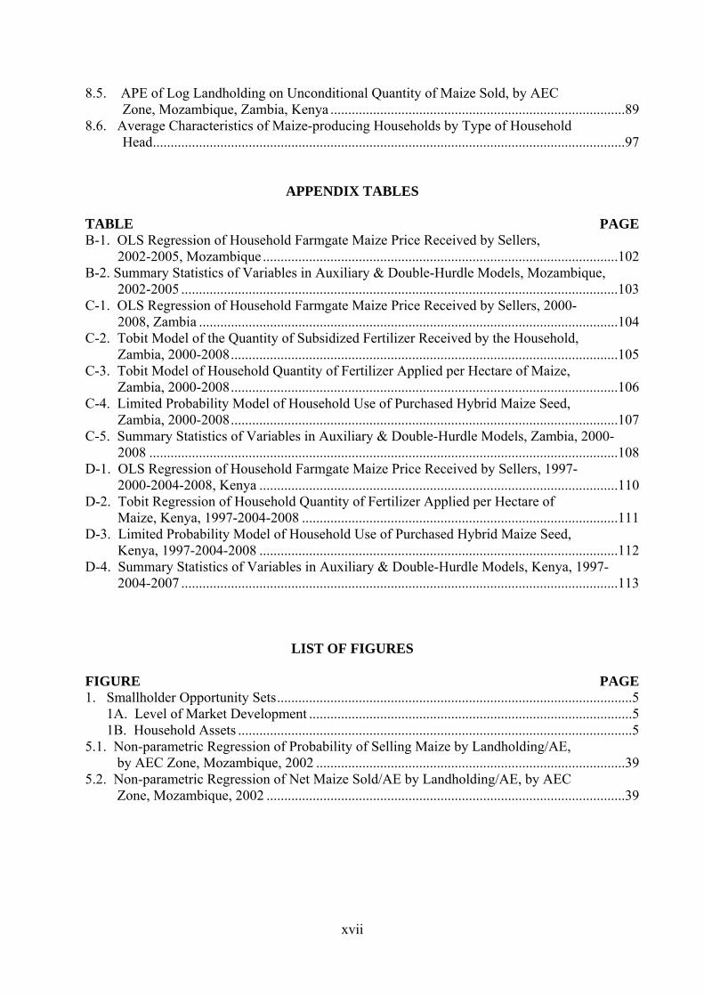
CONTENTS ACKNOWLEDGMENTS ............................................................................................................. iii EXECUTIVE SUMMARY .............................................................................................................v LIST OF TABLES ....................................................................................................................... xiii APPENDIX TABLES AND LIST OF FIGURES ...................................................................... xvii ACRONYMS ............................................................................................................................. xviii 1. INTRODUCTION ......................................................................................................................1 2. CAADP INVESTMENTS AND FOOD STAPLE PROFITABILITY FOR

SMALLHOLDER FARMERS: A CONCEPTUAL FRAMEWORK .......................................3 3. DESCRIPTIVE RESULTS .........................................................................................................8 3.1. Data Sources ......................................................................................................................8 3.2. Household Asset and Market Access Indicators in Kenya, Mozambique and

Zambia ..............................................................................................................................9 3.3. Extent of Household Integration into Markets and Diversification away from Farm

Activities .........................................................................................................................11 3.4. Role of Maize Production and Maize Sales in Rural Incomes ........................................13 3.5. Rural Household Position in Maize Markets ...................................................................17 4. ECONOMETRIC MODELING FRAMEWORK FOR HOUSEHOLD CEREAL

MARKET PARTICIPATION DECISIONS............................................................................21

4.1. Previous Approaches to Modeling Market Participation and Sales .................................21 4.2. Modeling Maize Market Participation and Sales Using a Double-hurdle Model ............23

4.2.1. The Cragg Double-hurdle Model ..........................................................................23 4.2.2. Estimation .............................................................................................................24 4.2.3. Model Variables ....................................................................................................26 4.2.4. Modeling Farmgate Maize Price Expectations .....................................................30

5. ECONOMETRIC ANALYSIS: MOZAMBIQUE ...................................................................32

5.1. Explanatory Variables ......................................................................................................32 5.2. Econometric Results ........................................................................................................33

5.2.1. Agro-ecological Potential......................................................................................33 5.2.2. Weather and Other Covariate Shocks ...................................................................33 5.2.3. Household Productive Assets ................................................................................36 5.2.4. Technology Use ....................................................................................................40 5.2.5. Market Access and Market Information ...............................................................40 5.2.6. Maize Price ...........................................................................................................42 5.2.7. Gender and Household Demographics..................................................................43

5.3. Conclusions ......................................................................................................................44

xii

6. ECONOMETRIC ANALYSIS: ZAMBIA ...............................................................................47 6.1. Explanatory Variables ......................................................................................................47 6.2. Econometric Results: Zambia ..........................................................................................50

6.2.1. Agro-ecological Potential.....................................................................................50 6.2.2. Rainfall and Drought Shocks ................................................................................53 6.2.3. Household Productive Assets ................................................................................53 6.2.4. Technology Use ....................................................................................................54 6.2.5. Market Access .......................................................................................................57 6.2.6. Farmgate Maize Price ...........................................................................................63 6.2.7. Gender and Household Demographics..................................................................64

6.3. Conclusions ......................................................................................................................65 7. ECONOMETRIC ANALYSIS: KENYA .................................................................................69

7.1. Introduction ......................................................................................................................69 7.1.1. Explanatory Variables ...........................................................................................69 7.1.2. Testing/controlling for Endogeneity of Regressors .............................................70

7.2. Econometric Results ........................................................................................................71 7.2.1. Agro-ecological Potential.....................................................................................71 7.2.2. Drought Shocks .....................................................................................................72 7.2.3. Household Productive Assets ................................................................................72 7.2.4. Technology Use ....................................................................................................75 7.2.5. Market Access .......................................................................................................79 7.2.6. Farmgate Maize Price ...........................................................................................83 7.2.7. Gender and Household Demographics..................................................................84

7.3. Conclusions ......................................................................................................................85 8. CROSS-COUNTRY SYNTHESIS OF ECONOMETRIC RESULTS ....................................87

8.1. Agroecological Potential and Weather Shocks ................................................................87 8.2. Total Household Landholding .........................................................................................87 8.3. Technology ......................................................................................................................90

8.3.1. Hybrid Maize Seed ................................................................................................90 8.3.2. Chemical Fertilizer ................................................................................................90 8.3.3. Animal Traction ....................................................................................................92

8.4. Market Access ..................................................................................................................92 8.4.1. Distance to Road Infrastructure and/or Town .........................................................92

8.4.2. Household Ownership of Transportation Assets...................................................93 8.4.3. Market Price Information ......................................................................................93 8.4.4. Grain Marketing Parastatal Activities ...................................................................94

8.5. Farmgate Maize Price ......................................................................................................94 8.6. Gender and Household Demographics ............................................................................95

9. CONCLUSIONS.......................................................................................................................98 APPENDIX A-1...........................................................................................................................100 REFERENCES ............................................................................................................................115

xiii

LIST OF TABLES TABLE PAGE 3.1. Market Access and Household Asset Indicators in Kenya, Mozambique, and Zambia ........10 3.2a. Percent Shares of Farm Income in Smallholder Household Income by Quintile of

Income per Adult Equivalent (AE) in Mozambique, Zambia, and Kenya ...........................11 3.2b. Percent Shares of Farm Income in Smallholder Household Income by Landholding

Quintile in Mozambique, Zambia, and Kenya ......................................................................12 3.3a. Percent Shares of Retained Crop Income in Smallholder Household Income by Income Quintile in Mozambique, Zambia, and Kenya ........................................................12 3.3b. Percent Shares of Retained Crop Income in Smallholder Household Income by Landholding Quintile in Mozambique, Zambia, and Kenya ...............................................12 3.4. Percent Shares of Maize and Other Food Staples in Farm Income in Mozambique, Zambia, and Kenya ..............................................................................................................14 3.5a. Percent Shares of Maize and Other Food Staples Retained and Sold by Quintile of Household Income in Mozambique, Zambia, and Kenya ...................................................15 3.5b. Percent Shares of Maize and Other Food Staples Retained and Sold by Quintile of

Household Landholding in Mozambique, Zambia, and Kenya ...........................................16 3.6. Household Net Maize Market Position in Kenya, Mozambique, and Zambia ....................17 3.7. Size Distribution of Households Participating in Maize Markets in Kenya,

Mozambique, and Zambia ....................................................................................................18 3.8. Maize Production and Sales per AE by Household Market Position in Kenya,

Mozambique, and Zambia ....................................................................................................19 3.9. Household Assets and Demographics by Household Market Position in Kenya,

Mozambique, and Zambia ....................................................................................................20 4.1. Attrition Bias Test Results: Mozambique, Zambia, and Kenya ...........................................26 5.1. Average Partial Effects of Agro-ecological Potential on the Probability of Maize Sale and Quantities Sold, Mozambique, 2002-2005 .............................................................34 5.2. Cragg Model of Maize Market Sales Participation and Level of Maize Sold,

Mozambique, 2002-05 ..........................................................................................................35 5.3a. APE of District-Level Days of Drought on Probability of Maize Sale, by AEC Zone and by Landholding Quartile, Mozambique ................................................................36 5.3b. APE of District-Level Days of Drought on Log Quantity of Maize Sold (Conditional), by AEC Zone and by Landholding Quartile, Mozambique ..........................36 5.3c. APE of District-Level Days of Drought on Log Quantity of Maize Sold

(Unconditional), by AEC Zone and by Landholding Quartile, Mozambique ......................36 5.4a. APE of % of Village Households with Maize Yield Shock to Maize on Probability of Maize Sale, by AEC Zone and by Landholding Quartile, Mozambique ..........................37 5.4b. APE of % of Village Households with Maize Yield Shock on Log Quantity of Maize Sold (Conditional), by AEC Zone, and by Landholding Quartile, Mozambique ......37 5.4c. APE of % of Village Households with Maize Yield Shock on Log Quantity of Maize Sold (Unconditional), by AEC Zone and by Landholding Quartile, Mozambique ...37 5.5a. APE of Animal Traction Ownership on Probability of Maize Sale, by AEC Zone and by Landholding Quartile, Mozambique .........................................................................41 5.5b. APE of Animal Traction Ownership on Log Quantity of Maize Sold (Conditional), by AEC Zone, and by Landholding Quartile, Mozambique .................................................41

xiv

5.5c. APE of Animal Traction Ownership on Log Quantity of Maize Sold (Unconditional), by AEC Zone and by Landholding Quartile, Mozambique ......................41 5.6a. APE of Receipt of Market Price Information on Probability of Maize Sale, by AEC Zone and by Landholding Quartile, Mozambique .......................................................42 5.6b. APE of Receipt of Market Price Information on Log Quantity of Maize Sold

(Conditional), by AEC Zone, and by Landholding Quartile, Mozambique .........................42 5.6c. APE of Receipt of Market Price Information on Log Quantity of Maize Sold

(Unconditional), by AEC Zone and by Landholding Quartile, Mozambique ......................42 5.7a. APE of Log Expected Farmgate Maize Price on Probability of Maize Sale, by AEC Zone and by Landholding Quartile, Mozambique .......................................................43 5.7b. APE of Log Expected Farmgate Maize Price on Log Quantity of Maize Sold

(Conditional), by AEC Zone and by Landholding Quartile, Mozambique ..........................43 5.7c. APE of Log Expected Farmgate Maize Price on Log Quantity of Maize Sold

(Unconditional), by AEC Zone and by Landholding Quartile, Mozambique ......................43 6.1. Average Partial Effects of Agro-Ecological Potential on the Probability of Maize Sale and Quantities Sold, Zambia, 2000-2008......................................................................51 6.2. Cragg Model of Household Probability of Maize Sale and Quantities of Maize Sold, Zambia, 2000-2008 ......................................................................................................52 6.3a. APE of Log Landholding on Probability of Maize Sale, by AEC Zone and by

Landholding Quartile, Zambia ..............................................................................................54 6.3b. APE of Log Landholding on Log Quantity of Maize Sold (Conditional), by AEC Zone, and by Landholding Quartile, Zambia ...............................................................54 6.3c. APE of Log Landholding on Log Quantity of Maize Sold (Unconditional), by AEC Zone, and by Landholding Quartile, Zambia ...............................................................54 6.4a. APE of Log Fertilizer Applied To Maize on Probability of Maize Sale, by AEC Zone and by Landholding Quartile, Zambia .........................................................................55 6.4b. APE of Log Fertilizer Applied To Maize on Log Quantity of Maize Sold (Conditional), by AEC Zone and by Landholding Quartile, Zambia ...................................55 6.4c. APE of Log Fertilizer Applied To Maize on Log Quantity of Maize Sold

(Unconditional), by AEC Zone and by Landholding Quartile, Zambia ...............................55 6.5a. APE of Hybrid Seed Use on Probability of Maize Sale, by AEC Zone and by

Landholding Quartile, Zambia ..............................................................................................56 6.5b. APE of Hybrid Seed Use on Log Quantity of Maize Sold (Conditional), by AEC Zone, and by Landholding Quartile, Zambia ........................................................................56 6.5c. APE of Hybrid Seed Use on Log Quantity of Maize Sold (Unconditional), by AEC Zone and by Landholding Quartile, Zambia ................................................................56 6.6a. APE of Distance to Feeder Road (2000) on Probability of Maize Sale, by AEC Zone and by Landholding Quartile, Zambia .........................................................................57 6.6b. APE of Distance to Feeder Road (2000) on Log Quantity of Maize Sold (Conditional), by AEC Zone, and by Landholding Quartile, Zambia ..................................57 6.6c. APE of Distance to Feeder Road (2000) on Log Quantity of Maize Sold

(Unconditional), by AEC Zone and by Landholding Quartile, Zambia ...............................57 6.7a. APE of Distance to Main Road (2000) on Probability of Maize Sale, by AEC Zone and by Landholding Quartile, Zambia .........................................................................58 6.7b. APE of Distance to Main Road (2000) on Log Quantity of Maize Sold (Conditional), by AEC Zone, and by Landholding Quartile, Zambia ..................................58 6.7c. APE of Distance to Main Road (2000) on Log Quantity of Maize Sold (Unconditional), by AEC Zone and by Landholding Quartile, Zambia ...............................58 6.8a. APE of Bike Ownership on Probability of Maize Sale, by AEC Zone and by

Landholding Quartile, Zambia ..............................................................................................60

xv

6.8b. APE of Bike Ownership on Log Quantity of Maize Sold (Conditional), by AEC Zone, and by Landholding Quartile, Zambia ...............................................................60 6.8c. APE of Bike Ownership on Log Quantity of Maize Sold (Unconditional), by AEC Zone and by Landholding Quartile, Zambia ................................................................60 6.9a. APE of Radio Ownership on Probability of Maize Sale, by AEC Zone and by

Landholding Quartile, Zambia ..............................................................................................61 6.9b. APE of Radio Ownership on Log Quantity of Maize Sold (Conditional), by AEC Zone, and by Landholding Quartile, Zambia ........................................................................61 6.9c. APE of Radio Ownership on Log Quantity of Maize Sold (Unconditional), by AEC Zone and by Landholding Quartile, Zambia ................................................................61 6.10a APE of Cell Phone Ownership on Probability of Maize Sale, by AEC Zone and by Landholding Quartile, Zambia .........................................................................................62 6.10b. APE of Cell Phone Ownership on Log Quantity of Maize Sold (Conditional), by AEC Zone, and by Landholding Quartile, Zambia ...............................................................62 6.10c. APE of Cell Phone Ownership on Log Quantity of Maize Sold (Unconditional), by AEC Zone and by Landholding Quartile, Zambia ...........................................................62 6.11a. APE of Log of District FRA Purchase per Maize Hectares on Probability of Maize Sale, by AEC Zone and by Landholding Quartile, Zambia ..................................................63 6.11b. APE of Log of District FRA Purchase per Maize Hectares on Log Quantity of Maize Sold (Conditional), by AEC Zone, and by Landholding Quartile, Zambia ...............63 6.11c. APE of Log of District FRA Purchase per Maize Hectares on Log Quantity of Maize Sold (Unconditional), by AEC Zone and by Landholding Quartile, Zambia ............63 6.12a. APE of Log Expected Farmgate Maize Price on Probability of Maize Sale, by AEC Zone and by Landholding Quartile, Zambia ................................................................64 6.12b. APE of Log Expected Farmgate Maize Price on Log Quantity of Maize Sold (Conditional), by AEC Zone and by Landholding Quartile, Zambia ...................................64 6.12c. APE of Log Expected Farmgate Maize Price on Log Quantity of Maize Sold (Unconditional), by AEC Zone and by Landholding Quartile, Zambia ...............................64 6.13a. APE of Binary Indicator that Household Is Headed by a Single Female on Probability of Maize Sale, by AEC Zone and by Landholding Quartile, Zambia ................65 6.13b. APE of Binary Indicator that Household Is Headed by a Single Female on Log

Quantity of Maize Sold (Conditional), by AEC Zone and by Landholding Quartile, Zambia ..................................................................................................................................65 6.13c. APE of Binary Indicator that Household Is Headed by a Single Female on Log Quantity of Maize Sold (Unconditional), by AEC Zone and by Landholding Quartile, Zambia ..................................................................................................................................65 7.1 Average Partial Effects of Agro-Ecological Potential on the Probability of Maize Sale and Quantities Sold, Kenya, 1997-2004-2007 ..............................................................73 7.2. Cragg Model of Maize Market Sales Participation and Level of Maize Sold, Kenya,

1997-2004-2007 ....................................................................................................................74 7.3a. APE of Log of Landholding on Probability of Maize Sale, by AEC Zone and by

Landholding Quartile, Kenya................................................................................................75 7.3b. APE of Log of Landholding on Log Quantity of Maize Sold (Conditional), by AEC Zone, and by Landholding Quartile, Kenya .................................................................75 7.3c. APE of Log of Landholding on Log Quantity of Maize Sold (Unconditional), by AEC Zone and by Landholding Quartile, Kenya ..................................................................75 7.4a. APE of Irrigation Equipment Ownership on Probability of Maize Sale, by AEC Zone and by Landholding Quartile, Kenya ...........................................................................76 7.4b. APE of Irrigation Equipment Ownership on Log Quantity of Maize Sold (Conditional), by AEC Zone, and by Landholding Quartile, Kenya ....................................76

xvi

7.4c. APE of Irrigation Equipment Ownership on Log Quantity of Maize Sold (Unconditional), by AEC Zone and by Landholding Quartile, Kenya .................................76

7.5a. APE of Hybrid Maize Use on Probability of Maize Sale, by AEC Zone and by Landholding Quartile, Kenya................................................................................................77

7.5b. APE of Hybrid Maize Use on Log Quantity of Maize Sold (Conditional), by AEC Zone and by Landholding Quartile, Kenya ................................................................77 7.5c. APE of Hybrid Maize Use on Log Quantity of Maize Sold (Unconditional), by AEC Zone and by Landholding Quartile, Kenya ................................................................77 7.6a. APE of Log of Fertilizer per Hectare of Maize on Probability of Maize Sale, by AEC Zone and by Landholding Quartile, Kenya ................................................................78 7.6b. APE of Log of Fertilizer per Hectare of Maize on Log Quantity of Maize Sold

(Conditional), by AEC Zone, and by Landholding Quartile, Kenya ..................................78 7.6c. APE of Log of Fertilizer per Hectare of Maize on Log Quantity of Maize Sold

(Unconditional), by AEC Zone and by Landholding Quartile, Kenya ...............................78 7.7a. APE of Animal Traction Ownership on Probability of Maize Sale, by AEC Zone and by Landholding Quartile, Kenya ..................................................................................79 7.7b. APE of Animal Traction Ownership on Log Quantity of Maize Sold (Conditional), by AEC Zone, and by Landholding Quartile, Kenya ..........................................................79 7.7c. APE of Animal Traction Ownership on Log Quantity of Maize Sold (Unconditional), by AEC Zone and by Landholding Quartile, Kenya ...............................79 7.8a. APE of Distance from Motorable Road on Probability of Maize Sale, by AEC Zone and by Landholding Quartile, Kenya .........................................................................80 7.8b. APE of Distance from Motorable Road on Log Quantity of Maize Sold (Conditional), by AEC Zone, and by Landholding Quartile, Kenya ..................................80 7.8c. APE of Distance from Motorable Road on Log Quantity of Maize Sold

(Unconditional), by AEC Zone and by Landholding Quartile, Kenya ...............................80 7.9. APE of Distance to Nearest Motorable Road on Probability of Maize Sale, by AEC Zone and by Year, Kenya, 1997, 2004, 2007 .......................................................................81 7.10a. APE of Radio Ownership on Probability of Maize Sale, by AEC Zone and by

Landholding Quartile, Kenya ..............................................................................................82 7.10b. APE of Radio Ownership on Log Quantity of Maize Sold (Conditional), by AEC

Zone, and by Landholding Quartile, Kenya ........................................................................82 7.10c. APE of Radio Ownership on Log Quantity of Maize Sold (Unconditional), by AEC Zone and by Landholding Quartile, Kenya ................................................................82 7.11a. APE of Phone Ownership on Probability of Maize Sale, by AEC Zone and by

Landholding Quartile, Kenya, 2004-2007 ...........................................................................83 7.12a. APE of Log of Expected Farmgate Maize Price on Probability of Maize Sale, by AEC Zone and by Landholding Quartile, Kenya ...........................................................84 7.12b. APE of Log Expected Farmgate Maize Price on Log Quantity of Maize Sold

(Conditional), by AEC Zone and by Landholding Quartile, Kenya ...................................84 7.12c. APE of Log Expected Farmgate Maize Price on Log Quantity of Maize Sold

(Unconditional), by AEC Zone and by Landholding Quartile, Kenya ...............................84 8.1. Average Partial Effect of an Increase in Landholding on the Probability of Household Maize Sale and Quantities Sold in Mozambique, Zambia, and Kenya .............87 8.2. APE of Log Landholding on Probability of Maize Sale, by Landholding Quartile,

Mozambique, Zambia, Kenya .............................................................................................88 8.3. Average Total Landholding by Quartile of Landholding among Small and Medium-holders in Mozambique, Zambia, Kenya .............................................................89 8.4. APE of Log Landholding on Unconditional Quantity of Maize Sold, by Land- holding Quartile, Mozambique, Zambia, Kenya .................................................................89

xvii

8.5. APE of Log Landholding on Unconditional Quantity of Maize Sold, by AEC Zone, Mozambique, Zambia, Kenya ...................................................................................89 8.6. Average Characteristics of Maize-producing Households by Type of Household Head .....................................................................................................................................97

APPENDIX TABLES TABLE PAGE B-1. OLS Regression of Household Farmgate Maize Price Received by Sellers, 2002-2005, Mozambique ....................................................................................................102 B-2. Summary Statistics of Variables in Auxiliary & Double-Hurdle Models, Mozambique,

2002-2005 ...........................................................................................................................103 C-1. OLS Regression of Household Farmgate Maize Price Received by Sellers, 2000- 2008, Zambia ......................................................................................................................104 C-2. Tobit Model of the Quantity of Subsidized Fertilizer Received by the Household,

Zambia, 2000-2008 .............................................................................................................105 C-3. Tobit Model of Household Quantity of Fertilizer Applied per Hectare of Maize,

Zambia, 2000-2008 .............................................................................................................106 C-4. Limited Probability Model of Household Use of Purchased Hybrid Maize Seed,

Zambia, 2000-2008 .............................................................................................................107 C-5. Summary Statistics of Variables in Auxiliary & Double-Hurdle Models, Zambia, 2000-

2008 ....................................................................................................................................108 D-1. OLS Regression of Household Farmgate Maize Price Received by Sellers, 1997- 2000-2004-2008, Kenya .....................................................................................................110 D-2. Tobit Regression of Household Quantity of Fertilizer Applied per Hectare of Maize, Kenya, 1997-2004-2008 .........................................................................................111 D-3. Limited Probability Model of Household Use of Purchased Hybrid Maize Seed, Kenya, 1997-2004-2008 .....................................................................................................112 D-4. Summary Statistics of Variables in Auxiliary & Double-Hurdle Models, Kenya, 1997-

2004-2007 ...........................................................................................................................113

LIST OF FIGURES

FIGURE PAGE 1. Smallholder Opportunity Sets ....................................................................................................5 1A. Level of Market Development ...........................................................................................5 1B. Household Assets ...............................................................................................................5 5.1. Non-parametric Regression of Probability of Selling Maize by Landholding/AE, by AEC Zone, Mozambique, 2002 .......................................................................................39 5.2. Non-parametric Regression of Net Maize Sold/AE by Landholding/AE, by AEC Zone, Mozambique, 2002 .....................................................................................................39

xviii

ACRONYMS AE Adult Equivalent APE average partial effects AU/NEPAD African Union/New Partnership for Africa’s Development CAADP Comprehensive Africa Agriculture Development Programme CF Control Function CGIAR Consultative Group on International Agricultural Research CRE correlated random effects CSA Census Supervisory Areas CSO Central Statistical Office DAP Diammonium Phosphate ESA Eastern and Southern Africa FE Fixed Effects FRA Food Reserve Agency GDP Gross Domestic Product GPS Global Positioning System GRZ Republic of Zambia INE National Institute of Statistics IPW Inverse Probability Weighting LPM limited probability model MADER Mozambican Ministry of Agriculture and Rural Development MMD Movement for Multi-Party Democracy MSU Michigan State University NCPB National Cereals and Produce Board OLS ordinary least squares PHS Central Statistical Office’s Post Harvest Survey ReSAKSS Regional Strategic Analysis and Knowledge Support System for Southern Africa R&D Research and Development SEA Standard Enumeration Areas SS Supplementary Surveys TIA Trabalho de Inquérito Agrícola (Agricultural Household Surveys) U.S. United States USAID United States Agency for International Development WHO World Health Organization

1

1. INTRODUCTION

The African Union/New Partnership for Africa’s Development’s (AU/NEPAD) Comprehensive African Agricultural Development Program (CAADP) represents African leaders’ rallying cry to correct underinvestment in agriculture. The CAADP identifies two key targets to strengthen agriculture’s contribution to achieving the Millennium Development Goals of poverty and hunger reduction: investment of a 10% share of public expenditure in the agricultural sector and achieving a 6% annual sector growth rate. The challenge facing those designing country and regional CAADP investment programs, termed compacts, is to determine what kinds of investment will have the highest payoff, where and for whom? Four investment areas, termed pillars, have been identified: (i) extending the area under sustainable land management and reliable water control systems; (ii) improving rural infrastructure and trade-related capacities for improved market access; (iii) increasing food supply, reducing hunger and improved emergency food response; and (iv) agricultural research, technology dissemination and adoption. The allocation of investments across and within pillars to achieve optimum growth and poverty reduction will depend in part on regional and country-level policy priorities, constraints, opportunities and trade-offs. A particular concern of CAADP’s Pillar 3 is to increase the marketed supply of food staples and at the same time increase broad-based opportunities for the poor to benefit from rural economic growth (African Union/NEPAD 2009). Increasing the marketed supply of food staples is crucial because of rapid urbanization, which is a result of population growth and migration. Since many of these new urban consumers will have low incomes, there is inevitably strong political pressure to keep food staple prices low. However, the objective of low urban food staple prices is likely to conflict with the objective of offering remunerative food prices to smallholder producers – the classic food price dilemma. In view of the urgency of this dilemma in the presence of sharply rising international food staple prices, some African countries have resorted to large scale fertilizer and marketing subsidies whose costs exceed the 10% CAADP public sector expenditure target. A key issue for CAADP Pillar 3 investment strategies is to what extent the two objectives of increased marketed supply of food staples at affordable prices and broad-based rural economic growth are competing or complementary. In other words, will a common set of investments and enabling policies enable both objectives to be achieved or will it require different investment packages targeted to different groups of farmers (e.g., large-scale commercial versus smallholder, or commercial smallholders versus semi-subsistence smallholders with off-farm income)? During the 1990s, it was a widely held view that market-friendly policies, combined with investments in collective goods2 to increase farm productivity and reduce marketing costs, would be sufficient to overcome barriers to specialization and trade by rural smallholders. In practice, however, levels of investment in 2 The economics literature typically defines public goods as goods that are profitable for society as a whole but which no private individual has an incentive to produce since it is impossible to exclude people from using the good without paying for it. A classic example is national defence. Such goods are often provided by the public sector and financed through taxation. In agricultural development, typical public goods include market information, grades and standards, and research on open-pollinated crop varieties. Research has shown, however, that such goods sometimes can be provided by groups of actors working collectively through means other than the state. For example, club goods refer to goods that are of value to a group of actors (but not necessarily to all of society) and that are provided by the group as a whole, such as through a professional organization. Thus, in this paper, we refer to collective goods, whether they are provided or financed by the public sector or through some other form of collective action. In the context of tightly constrained government budgets, one of the challenges facing food-insecure countries is to examine a whole range of alternatives for providing such collective goods.

2

important collective goods such as national agricultural research and extension systems were woefully inadequate in the 1990s and are only beginning to increase after two decades of neglect.3 Furthermore, some of the recent literature has questioned whether heterogeneity in household resource endowments might also constrain an important number of poor households from taking advantage of lower market access costs.4 In other words, increases in collective good-type investments to improve market access may be a necessary but not sufficient condition to enable a significant number of households to escape poverty and become food secure. The purpose of this paper is to use empirical evidence on smallholder maize production and marketing patterns in three countries in Southern and Eastern Africa to inform the design of investment packages that will enable smallholders to increase their marketed food staple surpluses in a financially sustainable manner. Specifically, we aim to quantify how investments in collective/public goods to improve market access, the use of improved production technologies, and household resource and agro-climatic endowments affect smallholder maize market participation. The results indicate that household land endowments, access to improved seed and fertilizer, access to price information, and weather shocks all affect farmers’ maize marketing decisions. Three sets of conclusions of relevance to CAADP investment plans flow from the empirical findings. First, there will be trade-offs between the objective of increasing marketed maize surpluses and broad-based rural poverty reduction since smallholders differ in their ability to increase their income through maize market participation. Second, investments that raise farm-level productivity are an essential complement to investments that improve market access (reduce marketing costs). Third, the mix of investments will need to vary according investment program objectives and smallholder target group circumstances. The next section of this paper provides a conceptual framework for understanding how we might expect heterogeneity in smallholder circumstances to affect food staple production and marketing. A conceptual framework is useful for identifying which types of CAADP investments are relevant to increase marketed food supply and overcome poverty under different circumstances. We then turn to empirical evidence, with section 3 providing a brief background to the data sources used for the descriptive analysis presented in section 4 and the econometric analysis presented in section 5. Section 6 concludes with implications of these empirical analyses for the design of CAADP investments to increase marketed food staple surpluses and achieved broad-based reductions in rural poverty taking account of a wide range of smallholder circumstances.

3 Ironically, the dramatic increases in the level of public expenditures on fertilizer and marketing subsidies in some African countries in response to high food staple prices threaten to continue to starve research and extension of funding even in an era of increased attention to agriculture. 4 Examples of recent papers include Boughton et al. 2007; Barrett 2008; and Jayne et al. 2009.

3

2. CAADP INVESTMENTS AND FOOD STAPLE PROFITABILITY FOR SMALLHOLDER FARMERS: A CONCEPTUAL FRAMEWORK

The fact that smallholder agriculture exhibits tremendous heterogeneity in developing countries is well documented (Timmer 1997; Barrett et al. 2005; Jayne et al. 2009). The purpose of this section is to identify the significance of smallholder heterogeneity for different kinds of CAADP investments; how investments in different CAADP pillars might affect smallholder incentives and how different smallholder circumstances might affect the payoff to those investments. These expectations are then compared to actual empirical patterns observed in three countries in section 4, while section 5 estimates marketed maize response to different kinds of investment for different groups of farmers. The focus of our study is marketed maize surplus by smallholder farmers. What determines whether and how much maize smallholder farmers sell depends on how profitable they perceive this activity to be compared to other uses of their assets (land, labor, and financial resources). The more profitable they perceive the maize activity to be relative to other farm and non-farm enterprises the more assets they will allocate to it. Although we cannot observe farmers’ perceptions directly we know that profitability depends on productivity (physical output per unit of resource engaged), output price, input costs, and the costs of getting output to the point of sale. Productivity in turn depends, in the case of maize, on agro-ecological potential, crop management (including use of improved seed and fertilizer), and weather (rainfall amount and distribution). Farmers’ perceptions of profitability will be influenced by their risk attitudes and the availability of price information. Variation in any of these factors gives rise to variations in farmers’ perceptions of profitability of maize compared to other opportunities, and hence their decisions to produce and sell maize. Variation in farmer circumstances, which we refer to as smallholder heterogeneity, can be grouped into three key dimensions: 1) their household assets (including land, labor, equipment, livestock and human capital), 2) how agro-ecological conditions affect the potential productivity of household assets, and 3) how the costs of exchange in agricultural output and input markets affect the financial returns to those assets. The costs of exchange are important because they have a large impact on farmers’ incentives to specialize in production activities where they have a potential comparative advantage in production, and hence induce a process of structural transformation whereby an increasing share of household production and consumption is exchanged through markets over time. 5 The costs of exchange in turn depend on physical infrastructure (e.g., all weather roads, communications), institutions (e.g., property rights and contract enforcement, financial markets, risk markets, information systems), and the behavior of market actors, including governments. Marketing costs incurred in transferring produce from production to consumption locations are lower with higher levels of investment in physical and institutional market infrastructure, thereby encouraging higher levels of specialization and exchange, which in turn lead to higher levels of agricultural productivity as the use of improved inputs increases, and commodities are increasingly grown by the most efficient producers. As household incomes increase, consumers spend increasing amounts of additional income on

5 We assume that households choose a mix of economic activities that allow them to maximize their welfare (commonly measured as expenditure or income), subject to the household’s resource endowments, agro-ecological conditions, and market opportunity set, as well as to its subsistence requirements and household-specific risk preferences.

4

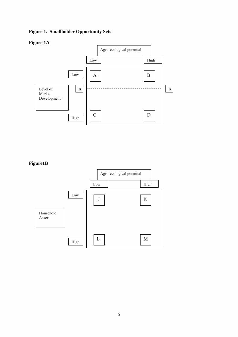
non-food goods and services. Within food-related expenditures, which account for a smaller and smaller share of household budgets as incomes grow, the pattern shifts to higher value foods. Thus, historically, we observe that as economic development proceeds, the share of agriculture in overall economic activity falls over time, even as agricultural gross domestic product (GDP) continues to grow in absolute magnitude (Johnston and Kilby 1975). To visualize how the opportunity sets facing smallholder farmers expand (or shrink) along each of these dimensions, consider Figure 1. The top half of the figure (Figure 1 A) shows the dimensions of agro-ecological potential and level of investment in market institutions and infrastructure (termed market collective goods), while Figure 1 B shows the dimensions of agro-ecological potential and resource endowment for a given level of market assets (e.g., for the transect XX in Figure 1 A). Since in reality the different combinations of resource endowments, agro-ecological potential, and market assets can lead to a myriad of opportunity sets for smallholder farmers, we develop a simple, stylized model of how different types of investment contemplated by the CAADP will interact with smallholder heterogeneity to guide the empirical analysis in subsequent sections. We look first at the market asset dimension, then agro-ecological potential and finally household resource endowments. How do smallholders’ opportunity sets change with investment in collective goods that facilitate market development? The higher the level of market development, the greater we expect the potential for specialization and exchange via the market to be. Higher levels of market development (the vertical axis in Figure 1A) induce specialization and structural transformation of the rural economy, strengthening growth linkages with the rural non-farm sectors of the economy. This increasingly provides many smallholder families with opportunities for off-farm employment at small businesses such as trading or value-added processing of farm and natural resource products. (Haggblade, Hazell, and Reardon (2009). For the farm component of the rural household economy, there could be a wider choice of technologies through access to inputs such as improved seed and fertilizer, a wider choice of crops through linkages with agro-industrial companies (cotton, tobacco, oilseeds, sugarcane), and more options in terms of how much own-production of different crops or livestock to consume and how much to sell. Enabling government policies act as a positive multiplier to the incentive effects of market development investments whereas inappropriate policies act as a negative multiplier. In terms of food security objectives, households have more options along the continuum from self-provisioning of food to market-reliance for food both in regard to availability (market supply) and access (off-farm income to enable effective demand). The kinds of investments that have the highest payoff under CAADP Pillar 2 will depend very much on the level of market collective goods and stage of structural transformation of the rural economy of a given country. For example, a highly subsistence-oriented and remote rural economy would likely generate most economic growth and poverty reduction from broad-based improvements in staple food crop productivity and roads. By contrast, a country or region with higher food crop productivity and well-functioning food crop markets might benefit more from investments that improve access of smallholders to higher-value crop production technologies and real-time market information.

5

Figure 1. Smallholder Opportunity Sets Figure 1A

Figure1B

Agro-ecological potential

Low High

Low

High

Household Assets

J

L

K

M

Agro-ecological potential

Low High

A

C

B

D

Low

High

Level of Market Development

X X

6

How are smallholder opportunity sets affected by agro-ecological zone? At first glance, this is perhaps the most familiar dimension for many who work with and study the agricultural sector. The kinds of crops that can be grown and the types of technology that are most appropriate clearly vary with soil, rainfall, altitude, and sunlight. Improved technologies seek to mitigate the biotic and abiotic stresses that characterize low potential agro-ecologies (e.g., through disease or drought tolerant varieties, or conservation farming to improve moisture utilization) or seek to exploit the potential of better agro-ecologies (e.g., through hybrids and inorganic fertilizer). While the productivity of crop technology depends on agro-ecological potential, the profitability of a specific technology and agro-ecology will also depend on the costs of exchange and farmers’ ability to use crop technology effectively.6 A smallholder’s agro-ecological opportunity set can also be changed to an extent by investments in water control and/or fertilizer, or by re-locating farm families to agro-ecological areas that are more favorable. This is the investment domain of CAADP Pillar 1. Disease control (and drought tolerance) can also expand the agro-ecological opportunity set (e.g., tsetse fly control to permit the use of animal traction), and it is important that this kind of innovation not be overlooked. How do smallholders’ opportunity sets change with household assets? While market access costs may be similar to households in a given area, market opportunity sets are often household-specific due to household-specific credit constraints, minimum scale requirements for certain types of crop production, ownership of transportation assets, and differences in farmers’ marketing knowledge and negotiation skills. The relationship between household assets and market participation has come into prominence with an increasing realization that many smallholders, often the majority of them, are net buyers who may be chronically poor and/or vulnerable (Weber et al. 1988; Jayne, Zulu, and Nijhoff 2006). Thus, inclusive poverty reduction strategies need to be based on an understanding of how farmers’ assets (the vertical access in Figure 1 B) condition their ability to use particular technologies and/or utilize farm and non-farm market opportunities. Where available land for cultivation is an absolutely binding constraint, investment strategies to re-locate families to more land abundant locations may be an option under CAADP Pillar 1. If energy for land preparation and weeding is the binding constraint, Pillar 4 investments in animal traction or minimum tillage diffusion may be more appropriate. We can use the conceptual framework presented above to anticipate or formulate hypotheses about the food security status and market participation behavior of smallholder households in the different situations represented in Figure 1. Households in low agro-ecological potential zones with low investment in market development (quadrant A of Figure 1) are likely to be vulnerable. If they also have limited resource endowments (quadrant J), they are likely to be more dependent on direct food aid distributions to resolve short-run crises, and on out-migration as a pathway out of poverty. Households in quadrant C face similar food production constraints, but have much better market access. Households in quadrant C can purchase food from the market if they have sufficient endowments (quadrant L); while poor households (quadrant J) may need some form of transfer to enable them to achieve food security (Magen et al. 2009). Households in high agro-ecological zones with low investment in market development (quadrant B) may be able to achieve a high degree of food security, but lack of access to markets prevents them from specializing in production for the market as a means to increase income and escape from poverty. Pillar 2 investments in roads, market

6 CAADP Pillar 4 investments need to take account of all three dimensions in developing profitable (and hence sustainable) technology transfer strategies.

7

information, and grower marketing associations will help move households from quadrant B to quadrant D (where they will have greater incentives to generate surpluses to sell). A key issue that the quantitative analysis in sections 4 and 5 will address is how differences in household assets (quadrant M versus quadrant K for example) affect market participation response to investments in market development. We now turn to an empirical investigation of household cereal marketing in our three study countries, beginning with a descriptive analysis of crop production and marketing patterns, and then an econometric analysis to assess the response of cereal market participation to different factors.

8

3. DESCRIPTIVE RESULTS

After providing a thumbnail sketch of market development and household asset indicators for each country, our review of empirical patterns of maize market participation begins with a broad lens and progressively focuses down on the characteristics of smallholder maize market participation in four steps.7 We first examine the shares of farm and retained crop income in total smallholder income as indicators of the overall degree of smallholder integration with and diversification of the market economy in each country. By retained crop income, we mean the value of the share of total crop production that is not sold. Second, we look at the share of maize and other food staples in farm income, and the shares of retained versus sold maize as indicators of the role of maize in the rural economy of each country, and of the role of maize sales in farm income (i.e., the extent of maize market participation). For the first two stages of analysis, we stratify farmers by their level of relative income (welfare outcome) and relative landholding (resource base), to see if there are associations between income, landholding, and activity choices. Third, we look at household positions in the maize market, and thus the proportions of households which engage the maize market (as buyers, sellers, or both) or not (autarkic). Recognizing that not all maize sellers are necessarily surplus producers (they may buy back more than they sell over the course of a year), we next define household position by net maize sales. Finally, we look at how the household assets and access to collective goods vary according to household net maize marketing position. This descriptive sequence provides an empirical baseline for the econometric analysis in the next chapter that will address the question of how maize marketed surpluses can be expected to change in response to investment in collective goods to improve market access.

3.1. Data Sources Kenya: The Tegemeo Institute of Egerton University and Michigan State University designed and implemented smallholder farm surveys in eight agro-ecological zones where crop cultivation predominates. The sampling frame for the survey was prepared in consultation with the Central Bureau of Statistics. Households and divisions were selected randomly within purposively chosen districts in the eight agro-ecological zones. Sampling details are provided in Argwings-Kodhek et al. (1998); attrition bias issues are examined and discussed in Burke and Jayne (2008). A total of 1,578 small-scale farming households were surveyed in 1997. Of these, we drop 48 households because either they were found to be mainly pastoral farmers or their landholding size exceeded 20 hectares. The 1997 survey therefore constituted 1,530 sedentary households farming under 20 hectares. Subsequent panel waves were conducted in 2000, 2004, and 2007. The 2007 sample contains 1,342 households of the original 1,578 sampled, a re-interview rate of 85%. The nationwide survey includes 106 villages in 24 districts in the nation’s eight agriculturally-oriented provinces. Mozambique: In 2002, the Mozambican Ministry of Agriculture and Rural Development (MADER) in collaboration with the National Institute of Statistics (INE) conducted a national agricultural and rural household income survey called the Trabalho do Inquerito Agrìcola (TIA) survey. The sampling frame was derived from the Census of Agriculture and Livestock 2000, used a stratified, clustered sample design that is representative of small- and medium-scale farm households at the provincial and national levels. The sample was stratified by 7 With at least four to five agro-ecological zones in each country, a detailed breakdown by agro-ecological zone and income/resource endowment strata in each country would be very cumbersome and detract from the logical flow. We therefore limit ourselves to qualitative observations on how agro-ecology modifies the patterns observed at national level without presenting a detailed empirical exposition.

9

province (10 provinces) and agro-ecological zones, and included eighty of the country's 128 districts. A total of 4,908 small and medium-sized farms were interviewed in 559 communities (clusters). A subsequent panel wave was conducted in 2005, with a re-interview rate of 82.7%, and replacement of attrited households to retain a representative sample of the population. Attrition bias is examined in Mather and Donovan (2007). Zambia: Data is drawn from the Central Statistical Office’s Post Harvest Survey (PHS) of 1999/2000, and the linked 2001, 2004, and 2008 Supplementary Surveys (SS) designed and conducted jointly by the government’s Central Statistical Office and Michigan State University. A 3-wave panel data set is available for the three agricultural production seasons, 1999/2000, 2002/2003, and 2007/08. The PHS is a nationally representative survey using a stratified three-stage sampling design. Census Supervisory Areas (CSA) were first selected within each district, next Standard Enumeration Areas (SEA) were sampled from each selected CSA, and in the last stage a sample of households was randomly selected from a listing of households within each sample SEA. The SEA is the most disaggregated geographic unit in the data, which typically includes 2-4 villages of several hundred households. The 2000, 2004, and 2008 surveys are based on a sample frame of about 7,400 small-scale (0.1 to 5 hectares) and medium-scale farm households, defined as those cultivating areas between 5 to 20 hectares. Survey method details and attrition bias are examined in Chapoto and Jayne (2008). Because this descriptive and panel work is focused on small and medium-scale farmers, we include households with 20 or fewer hectares of total cultivated in Mozambique (in 2002) and Zambia (in 2000), and households with 20 or fewer hectares owned in Kenya (in 1997). For the descriptive tables in this paper, we use all households interviewed in a given year. For the panel econometric work, we only use households that were interviewed in each panel year.

3.2. Household Asset and Market Access Indicators in Kenya, Mozambique and Zambia The three countries in our study provide a wide range of levels of market development and household asset levels. Table 3.1. provides a set of indicators for each country. Kenya has the highest share of rural dwellers among the total population (almost 80%) and the lowest rural poverty rate (just under half). Rural population density is highest in Kenya at 5.6 people per hectare of arable land, compared to 3.0 and 3.4 people per hectare in Mozambique and Zambia respectively. Although land is relatively scarce in Kenya, household asset and market access indicators are much higher than either Zambia or Mozambique. Most strikingly, a Kenyan smallholder can obtain fertilizer at a distance of just 3km from their farm; a Zambian farmer has to travel more than ten times, and a Mozambican farmer more than twenty times, that distance. The proportion of smallholder farmers using fertilizer and improved seed on their maize fields is inversely correlated with these average distances to a fertilizer seller: 70% in Kenya, compared to half that share in Zambia and negligible numbers in Mozambique (4%).8 In addition to the advantage of physical proximity of input sellers, access for smallholder farmers in Kenya is facilitated by credit: just over half of Kenyan smallholder farmers use credit compared to less than 10% in Zambia and just 3% in Mozambique. Despite smaller

8 The higher average level of fertilizer use per hectare in Zambia is due to the Government’s subsidy program.

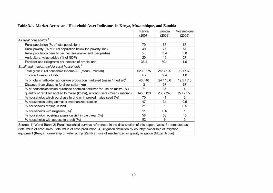
10

Table 3.1. Market Access and Household Asset Indicators in Kenya, Mozambique, and Zambia Kenya (2007)

Zambia (2008)

Mozambique (2005)

All rural households 1

Rural population (% of total population) 79 65 66Rural poverty (% of rural population below the poverty line) 49 77 57Rural population density per hectare arable land (people/ha) 5.6 3.4 3.0Agriculture, value added (% of GDP) 20 19 27Fertilizer use (kilograms per hectare of arable land) 36.4 50.1 1.6

Small and medium-holder rural households 2

Total gross rural household income/AE (mean / median) 620 / 375 218 / 102 121 / 63Tropical Livestock Units 4.2 2.4 1.0% of total smallholder agriculture production marketed (mean / median)3 46 / 46 24 / 13.6 19.5 / 7.6Distance from village to fertilizer seller (km) 3 37 67% of households which purchase chemical fertilizer for use on maize (%) 71 37 4quantity of fertilizer applied to maize (kg/ha), among users (mean / median) 145 / 123 286 / 246 277 / 153% households which purchase hybrid or improved maize seed (%) 70 41 2% households using animal or mechanized traction 47 34 9.5% households renting in land 21 1 0.5% households with irrigation (%)4 11 0.6 1% households receiving extension visit in past year (%) 58 53 15% households with access to credit (%) 52 9 3

Source: 1) World Bank; 2) Rural household surveys referenced in the data section of this paper. Notes: 3) computed as (total value of crop sales / total value of crop production) 4) irrigation definition by country: ownership of irrigation equipment (Kenya); ownership of water pump (Zambia); use of mechanized or gravity irrigation (Mozambique)

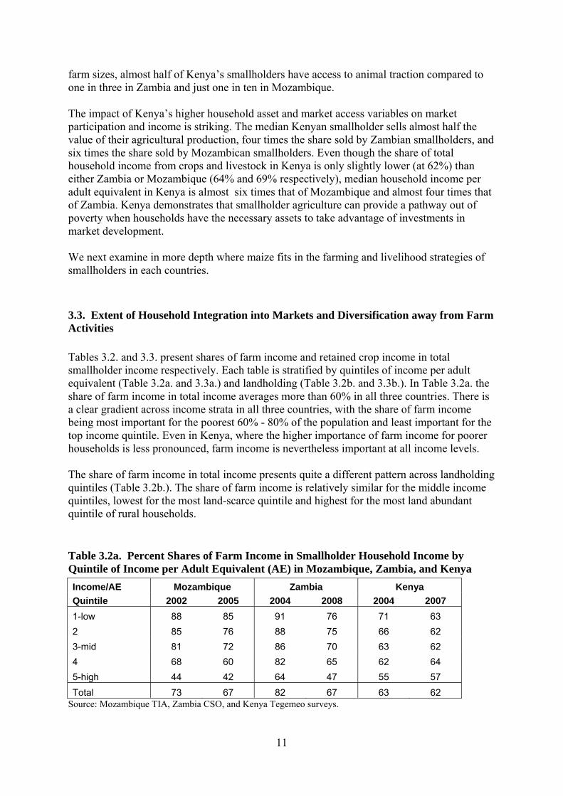
11

farm sizes, almost half of Kenya’s smallholders have access to animal traction compared to one in three in Zambia and just one in ten in Mozambique. The impact of Kenya’s higher household asset and market access variables on market participation and income is striking. The median Kenyan smallholder sells almost half the value of their agricultural production, four times the share sold by Zambian smallholders, and six times the share sold by Mozambican smallholders. Even though the share of total household income from crops and livestock in Kenya is only slightly lower (at 62%) than either Zambia or Mozambique (64% and 69% respectively), median household income per adult equivalent in Kenya is almost six times that of Mozambique and almost four times that of Zambia. Kenya demonstrates that smallholder agriculture can provide a pathway out of poverty when households have the necessary assets to take advantage of investments in market development. We next examine in more depth where maize fits in the farming and livelihood strategies of smallholders in each countries. 3.3. Extent of Household Integration into Markets and Diversification away from Farm Activities Tables 3.2. and 3.3. present shares of farm income and retained crop income in total smallholder income respectively. Each table is stratified by quintiles of income per adult equivalent (Table 3.2a. and 3.3a.) and landholding (Table 3.2b. and 3.3b.). In Table 3.2a. the share of farm income in total income averages more than 60% in all three countries. There is a clear gradient across income strata in all three countries, with the share of farm income being most important for the poorest 60% - 80% of the population and least important for the top income quintile. Even in Kenya, where the higher importance of farm income for poorer households is less pronounced, farm income is nevertheless important at all income levels. The share of farm income in total income presents quite a different pattern across landholding quintiles (Table 3.2b.). The share of farm income is relatively similar for the middle income quintiles, lowest for the most land-scarce quintile and highest for the most land abundant quintile of rural households. Table 3.2a. Percent Shares of Farm Income in Smallholder Household Income by Quintile of Income per Adult Equivalent (AE) in Mozambique, Zambia, and Kenya Income/AE Mozambique Zambia Kenya Quintile 2002 2005 2004 2008 2004 2007 1-low 88 85 91 76 71 63 2 85 76 88 75 66 62 3-mid 81 72 86 70 63 62 4 68 60 82 65 62 64 5-high 44 42 64 47 55 57 Total 73 67 82 67 63 62

Source: Mozambique TIA, Zambia CSO, and Kenya Tegemeo surveys.

12

Table 3.2b. Percent Shares of Farm Income in Smallholder Household Income by Landholding Quintile in Mozambique, Zambia, and Kenya Landholding Mozambique Zambia Kenya Quintile 2002 2005 2004 2008 2004 2007 1-low 65 37 77 50 61 57 2 76 42 82 65 61 61 3-mid 75 49 83 70 63 61 4 75 52 84 71 63 63 5-high 74 84 85 76 69 67 Total 73 67 82 67 63 62

Source: Mozambique TIA, Zambia CSO, and Kenya Tegemeo surveys. Table 3.3a. Percent Shares of Retained Crop Income in Smallholder Household Income by Income Quintile in Mozambique, Zambia, and Kenya Income/AE Mozambique Zambia Kenya Quintile 2002 2005 2004 2008 2004 2007 1-low 75 67 78 59 43 37 2 70 55 70 52 30 27 3-mid 63 51 65 44 22 20 4 48 41 55 36 18 15 5-high 29 28 35 22 12 10

Total 57 49 61 43 25 22 Source: Mozambique TIA, Zambia CSO, and Kenya Tegemeo surveys. Table 3.3b. Percent Shares of Retained Crop Income in Smallholder Household Income by Landholding Quintile in Mozambique, Zambia, and Kenya

Landholding Mozambique Zambia Kenya

Quintile 2002 2005 2004 2008 2004 2007

1-low 54 48 63 31 29 26

2 63 49 64 48 30 24

3-mid 60 48 62 49 24 21

4 55 49 60 45 21 22

5-high 53 48 54 41 21 16

Total 57 49 61 43 25 22 Source: Mozambique TIA, Zambia CSO, and Kenya Tegemeo surveys. Retained crop income accounts for a large share of total smallholder income on average, but with a greater dispersion across countries and income strata compared to total farm income (Table 3.3a.). Whereas retained crop income accounts for about half of all smallholder income on average in Zambia and Mozambique, it represents only a little more than one fifth of total smallholder income in Kenya. As would be expected, the share of retained crop income shows an even steeper gradient across income quintiles than farm income share, with the poorest households retaining most value of crop production on the farm and the wealthiest least.

13

Across land quintiles, households in the middle of the distribution tend to have a higher share of retained crop income than either of the tails in Mozambique and Zambia, whereas in Kenya the share of retained crop income consistently declines the higher the landholding quintile (Table 3.3b.). The high average shares of retained crop income in Zambia and Mozambique indicate that the majority of households remain semi-subsistence, and that the process of structural transformation of the rural economy is still at a relatively early stage compared to Kenya. The fact that the poorest households have the highest share of retained crop income indicates a lack of opportunity to diversify into off-farm or cash crop production, and hence a high degree of vulnerability to variation in crop income due to weather or pests.9 As we will see in subsequent analysis, Kenyan smallholders sell a much higher proportion of their value of crop production relative to Zambia and Mozambique across all landholding quintiles. We next turn to the place of maize, as the most widely commercialized food staple, in smallholder crop and farm incomes. 3.4. Role of Maize Production and Maize Sales in Rural Incomes Table 3.4. shows the contribution of maize and other food staples to farm income in each country. In Mozambique food staples account for almost two thirds of all farm income, and maize one third of the food staple share. Although maize is the most heavily commercialized food staple in Mozambique, still only about 10% of the crop is sold. In Zambia, food staples account for about half of total farm income, but the share of maize in food staples is considerably higher than Mozambique, accounting for between half and two thirds of food staple value depending on the year. Around one fifth of maize is sold in Zambia, roughly double the proportion sold in Mozambique. Farm income sources are much more diversified in Kenya, with high value crops, cash crops and livestock products all playing a significantly greater role than in Mozambique or Zambia. Food staples account for only about one third of farm income in Kenya, but maize accounts for about three quarters of the value of all food staples in Kenya. Kenya also has the highest proportion of maize sold, between one sixth and one third depending on the year. In general terms Table 3.4. suggests that, for our three study countries, crop diversification increases with the degree of structural transformation of the economy, but that the share of maize sold may increase even as the overall importance of food staples in smallholder farm income portfolios declines. Table 3.5a. shows how the shares of farm income for maize and other food staples retained and sold varies across income quintiles within countries. In Mozambique, the shares of maize and other food staples are relatively stable across income quintiles. In Zambia, the share of maize retained decreases while the share sold increases rapidly from negligible amounts for the poorest quintiles to half for the highest income quintile; the share of other food staples is relatively stable across income quintiles. In Kenya, the share of maize in crop income is inversely related to income quintile as households in higher income quintiles diversify into traditional cash crops instead of food staples. 9 Cunguara (2008), for example, analyzed panel household rural income data in Mozambique in 2002 and 2005 and found that the main characteristic of households that were poorer in the deeper and more widespread drought of 2005 were households that could not compensate through off-farm diversification of income.

14

Table 3.4. Percent Shares of Maize and Other Food Staples in Farm Income in Mozambique, Zambia, and Kenya

Maize Other Staple Food

Crops High-value Food

Crops Traditional Cash Crops

Livestock Products

Ag Wage Labor Retained Sold Retained Sold Retained Sold

Country Year Mean shares of component in total gross farm income (%) Mozambique 2002 22 3 40 1 18 7 3 4 3 Mozambique 2005 20 2 36 1 19 9 4 4 5 Zambia 2004 26 5 22 3 26 6 5 4 2 Zambia 2008 35 8 18 3 11 6 4 8 5 Kenya 2004 19 7 7 4 20 12 12 19 2 Kenya 2007 24 3 7 3 24 15 3 21 1

Source: Mozambique TIA, Zambia CSO, and Kenya Tegemeo surveys. Notes: Other Staple Food Crops = cassava, sweet potato, millet, sorghum, rice High-value Food Crops = groundnuts, beans, soybeans, cashew, coconut, sunflower, sesame; sales of fruit & vegetables Traditional Cash Crops = cotton, tobacco, tea, coffee, sugarcane Livestock Products = sales of live animals, meat, dairy products, and eggs; value of fodder crops sold (napier grass, clover, alfalfa) Retained' in this table refers to 'retained value'. Thus, Retained maize share of total income = HH value of retained maize production / HH total farm income

15

Table 3.5a. Percent Shares of Maize and Other Food Staples Retained and Sold by Quintile of Household Income in Mozambique, Zambia, and Kenya

Mozambique 2005


Crops Income/AE Mean Farm

Income ($US) Retained Sold Retained Sold

Quintile mean shares in total gross farm income (%) 1-low 49 21 2 28 1 2 97 19 2 36 1 3-mid 163 20 3 37 1 4 242 19 3 38 1 5-high 466 20 3 38 2 Total 204 20 2 36 1

Zambia 2008




Quintile mean shares in total gross farm income (%) 1-low 100 43 2 20 3 2 221 39 5 19 3 3-mid 356 34 8 20 4 4 507 31 9 18 3 5-high 1,102 30 16 14 3 Total 457 35 8 18 3

Kenya 2007




Quintile mean shares in total gross farm income (%) 1-low 374 32 2 10 4 2 512 29 2 8 2 3-mid 781 23 2 6 3 4 1029 20 4 5 3 5-high 1677 17 5 4 3 Total 876 24 3 7 3

Source: Mozambique TIA, Zambia CSO, and Kenya Tegemeo surveys. Table 3.5b. shows how the shares of farm income for maize and other food staples retained and sold varies across landholding quintiles within countries. In Mozambique, the share of maize retained increases with landholding while that of other food staples decreases; this may reflect the higher risk of maize production relative to other food staples for land-scarce households.

16

Table 3.5b. Percent Shares of Maize and Other Food Staples Retained and Sold by Quintile of Household Landholding in Mozambique, Zambia, and Kenya

Mozambique 2005

Maize Other Staple Food Crops

Landholding Mean Farm Income ($US)

Retained Sold Retained Sold Quintile Mean shares in total gross farm income (%) 1-low 112 15 1 41 2 2 138 18 1 39 1 3-mid 171 21 2 35 2 4 214 22 3 34 1 5-high 382 24 5 28 2 Total 204 20 2 36 1

Zambia 2008



Retained Sold Retained Sold Quintile Mean shares in total gross farm income (%) 1-low 198 35 3 17 1 2 250 39 6 23 3 3-mid 304 35 7 21 4 4 485 33 9 18 4 5-high 1,049 34 15 12 3 Total 457 35 8 18 3

Kenya 2007



Retained Sold Retained Sold Quintile Mean shares in total gross farm income (%) 1-low 672 22 3 6 2 2 950 20 5 6 3 3-mid 1259 18 5 5 3 4 1465 19 8 4 3 5-high 2711 15 13 3 7 Total 1408 19 7 5 4


17

The proportion of maize sold also increases with landholding, but is only one fifth of the crop even for the highest landholding quintile. In Zambia, by contrast, the amount of maize retained is stable across landholding quintiles but the share sold is much higher for the top quintile, indicating some degree of specialization in maize production for the market.10 In Kenya the share of maize (retained and sold) in farm income is relatively constant across quintiles of landholding, but the share retained decreases and the share sold increases consistently at higher landholding quintiles. Comparing the disaggregated results of Table 3.5b. with the earlier Table 3.1. allows us to formulate some preliminary hypotheses about the interaction between maize market participation, household assets, and market development. In Mozambique, smallholder farming appears to have barely evolved from a subsistence mode with little crop diversification out of maize and even land abundant households selling only a small proportion of the crop. In Zambia, the proportion of maize sold increases much more rapidly with landholding size than in Mozambique, and there may be specialization in maize production for the market for the highest landholdings. In Kenya, the combination of market development and land constraints result in a high degree of commercialization of maize but with a higher level of diversification into other commercial crops (and livestock) as well.

3.5. Rural Household Position in Maize Markets The fact that a household sells maize does not necessarily mean that it produces more maize than it consumes in a given year. We therefore consider smallholders’ net position in the maize market. Households can be divided into three categories based on their marketing position in a given year: net sellers (sell only or sales greater than purchases), net buyers (buy only or purchases greater than sales), and households that neither buy nor sell more than trivial amounts (autarkic). Table 3.6. presents the distribution of households among these categories for each country. Clearly, these are snapshots from particular production and marketing years, and hence are presented for illustrative rather than inferential purposes. Table 3.6. Household Net Maize Market Position in Kenya, Mozambique, and Zambia

Maize market position Mozambique Zambia Kenya

2002 2005 2004 2008 2004 2007 Autarkic (no buy or sell) 23.4 28.9 37.4 22.9 10.7 14 Buy only 55.5 52.3 34.4 47.2 45.2 39.9 Buy and Sell (net buyer) 5.5 4.3 2.7 3.0 5.7 2.9 Sell only 10.5 11.1 20.3 17.7 23.5 27.3 Sell and Buy (net seller) 5.1 3.4 5.2 9.2 14.9 15.9 TOTAL 100 100 100 100 100 100


10 Inter-annual differences make it difficult to infer specialization in maize production for the market simply on the basis of crops income shares and share retained/sold. For example, the share of maize in crop income for the highest landholding quintile in Zambia was considerably higher in 2008 than 2004. This may reflect a combination of factors, including high maize prices and subsidized fertilizer distribution which favors larger smallholders.

18

Kenya has the lowest proportion of autarkic households, and the highest proportion of net sellers: approximately one Kenyan rural household is a net maize buyer for every household that is a net seller. Mozambique has the highest proportion of net buyer households (3 out of every 5), outnumbering net sellers by 4 to 1. Even allowing for geographical specialization in crop production, the fact that Mozambique has such a high proportion of net buyers suggests that low productivity rather than market access may be the binding constraint on increased smallholder maize sales. In Zambia, approximately 1 in 4 households is a net seller, half are net buyers, and 1 out of 4 is autarkic. As expected with a drought sensitive crop like maize, households’ net market status varies greatly across agro-ecologies and between years, with a much higher proportion of net buyers in dryer years and/or less favorable agro-climatic zones (low rainfall and/or sandy soils). In Kenya, for example, 70% of households in the high-potential maize zone of the country are net sellers. To take account of the concern to increase marketed food staple surpluses to feed growing urban populations and chronically food deficit areas, Table 3.7. further disaggregates net seller households into three groups: 1) large net sellers, 2) small net sellers, and 3) negligible net sellers. Large net sellers are defined as those households selling more than 100 kg of maize per adult equivalent (roughly one bag), adequate to meet the food staple calorie needs of an adult for about 6 months. Small net sellers are those selling less than 100 kg but more than 25 kg per adult equivalent (AE), while negligible net sellers have net sales of maize between 25 kg/AE and -25 kg/AE. Autarkic households are included in the negligible sales category as they have net sales of 0 kg/AE. Deficit households have net maize purchases greater than 25 kg/AE. In Mozambique, not only is the share of large and small net sellers very small (less than 10%), but small net sellers outnumber large net sellers by 2 to 1. Only three households out of every hundred in Mozambique sell more than a 100 kg bag of maize per adult equivalent.11 In Zambia and Kenya by contrast, not only is the proportion of large and small net sellers much higher overall, but large net sellers predominate. The proportion of households in each maize market position category provides only limited information about the quantities marketed by net sellers. Table 3.8. presents the quantity produced and sold per adult equivalent, and the share of sales in total production, for each household category by country. Two observations immediately leap out. First, as might be expected, large net sellers have much higher maize production per adult equivalent than small net sellers do. Second, the ratio of maize sold to maize produced per adult equivalent is also much higher for large net sellers that small net sellers.

Table 3.7. Size Distribution of Households Participating in Maize Markets in Kenya, Mozambique, and Zambia

Maize market position Mozambique Zambia Kenya

2002 2005 2004 2008 2004 2007 Deficit 27 32 22 30 36 24 Negligible sales 64 60 57 42 29 37 Small net sales 6 6 9 8 9 12 Large net sales 3 3 12 19 26 27 TOTAL 100 100 100 100 100 100

Source: Mozambique TIA, Zambia CSO, and Kenya Tegemeo surveys. 11 Adult equivalent is a measure that adjusts the size of a household to reflect its caloric consumption needs based on the age and gender or each individual in the household (WHO 1985).

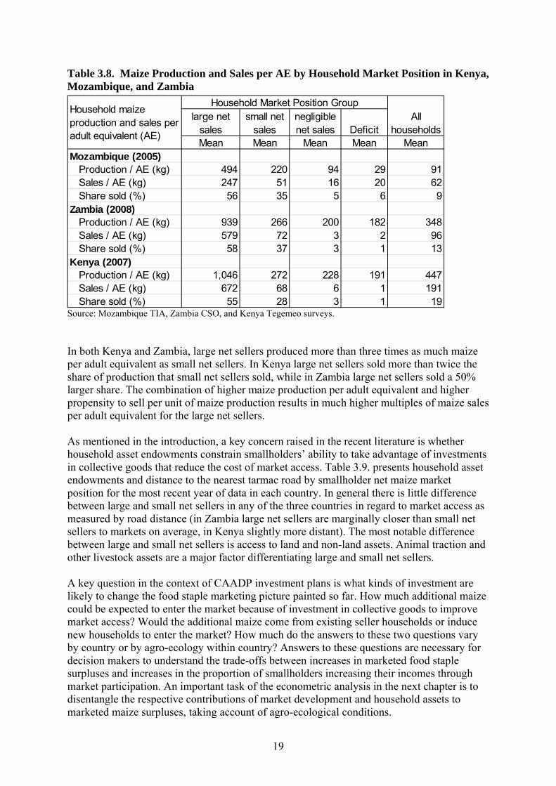
19

Table 3.8. Maize Production and Sales per AE by Household Market Position in Kenya, Mozambique, and Zambia

large net sales

small net sales

negligible net sales Deficit

Mean Mean Mean Mean MeanMozambique (2005)

Production / AE (kg) 494 220 94 29 91Sales / AE (kg) 247 51 16 20 62Share sold (%) 56 35 5 6 9

Zambia (2008)Production / AE (kg) 939 266 200 182 348Sales / AE (kg) 579 72 3 2 96Share sold (%) 58 37 3 1 13

Kenya (2007)Production / AE (kg) 1,046 272 228 191 447Sales / AE (kg) 672 68 6 1 191Share sold (%) 55 28 3 1 19

All households

Household Market Position GroupHousehold maize production and sales per adult equivalent (AE)

Source: Mozambique TIA, Zambia CSO, and Kenya Tegemeo surveys. In both Kenya and Zambia, large net sellers produced more than three times as much maize per adult equivalent as small net sellers. In Kenya large net sellers sold more than twice the share of production that small net sellers sold, while in Zambia large net sellers sold a 50% larger share. The combination of higher maize production per adult equivalent and higher propensity to sell per unit of maize production results in much higher multiples of maize sales per adult equivalent for the large net sellers. As mentioned in the introduction, a key concern raised in the recent literature is whether household asset endowments constrain smallholders’ ability to take advantage of investments in collective goods that reduce the cost of market access. Table 3.9. presents household asset endowments and distance to the nearest tarmac road by smallholder net maize market position for the most recent year of data in each country. In general there is little difference between large and small net sellers in any of the three countries in regard to market access as measured by road distance (in Zambia large net sellers are marginally closer than small net sellers to markets on average, in Kenya slightly more distant). The most notable difference between large and small net sellers is access to land and non-land assets. Animal traction and other livestock assets are a major factor differentiating large and small net sellers. A key question in the context of CAADP investment plans is what kinds of investment are likely to change the food staple marketing picture painted so far. How much additional maize could be expected to enter the market because of investment in collective goods to improve market access? Would the additional maize come from existing seller households or induce new households to enter the market? How much do the answers to these two questions vary by country or by agro-ecology within country? Answers to these questions are necessary for decision makers to understand the trade-offs between increases in marketed food staple surpluses and increases in the proportion of smallholders increasing their incomes through market participation. An important task of the econometric analysis in the next chapter is to disentangle the respective contributions of market development and household assets to marketed maize surpluses, taking account of agro-ecological conditions.

20

Table 3.9. Household Assets and Demographics by Household Market Position in Kenya, Mozambique, and Zambia

large net sales

small net sales

negligible net sales Deficit

Mean Mean Mean Mean Mean Mozambique

Total HH landholding (ha) 3.31 2.74 1.81 1.85 1.92No. of prime-age adults (age 15-59) 2.2 2.6 2.4 2.8 2.5Max years education male 3.6 3.6 3.1 3.6 3.3Max years education female 1.6 1.9 1.7 2.2 1.9Tropical livestock units (TLU) 1.7 1.2 0.9 1.2 1.0Own animal traction (%) 4.4 3.9 3.0 4.4 3.5Value of farm equipment ($) 107 58 31 35 36Own bicycle (%) 56.7 50.4 29.4 28.5 31.1Distance to tarmac road (km) 67.1 67.8 58.7 54.0 58.0

ZambiaTotal HH landholding (ha) 3.1 2.1 1.5 1.3 1.7No. of prime-age adults (age 15-59) 3 3 3 3 3Max years education male 8 7 7 7 7Max years education female 7 6 5 6 6Tropical livestock units (TLU) 5.4 2.4 1.8 1.9 2.4Own animal traction (%) 26 15 9 9 12Value of farm equipment ($) 105 34 24 21 36Own bicycle (%) 76 68 50 49 55Distance to tarmac road (km) 22.7 25.6 26.2 24.8 25.1

KenyaTotal HH landholding (ha) 3.7 1.9 1.8 1.4 2.2No. of prime-age adults (age 15-59) 4 4 4 3 4Max years education male 11 10 10 9 10Max years education female 10 9 9 8 9Tropical livestock units (TLU) 6.6 3.1 3.5 2.9 4.2Own animal traction (%) 15 9 11 9 11Value of farm equipment ($) 4,032 2,491 2,912 2,094 2,966Own bicycle (%) 55 51 48 41 49Distance to tarmac road (km) 7.0 6.5 7.8 8.4 7.6

Household Asset Type

Household Market Position GroupAll

households

Source: Mozambique TIA, Zambia CSO, and Kenya Tegemeo surveys Notes: TLU = cattle + 0.6*donkeys + 0.4*pigs + 0.2*(goats + sheep) + 0.02*chickens + 0.06*ducks/geese/turkeys + 0.04*rabbits. (FAO)

21

4. ECONOMETRIC MODELING FRAMEWORK FOR HOUSEHOLD CEREAL MARKET PARTICIPATION DECISIONS

4.1. Previous Approaches to Modeling Market Participation and Sales The conceptual framework for many of the existing empirical papers on marketed food staples is based on seminal theoretical work by de Janvry, Fafchamps, and Sadoulet (1991), who used a household model to demonstrate that costs associated with market transactions can explain why some households avoid engaging in food and cash crop markets. Their results derive from the premise that the typical rural household in a developing country faces a wedge between the sales price of a given commodity and its purchase price. This wedge may be due to a combination of factors related to marketing, production, or consumption. Market-related factors include transport costs between the farm household’s village and the relevant market, non-competitive behavior among local traders, poor access to price information, and shallow local markets. Production-related factors include lack of credit to finance key inputs and low food crop productivity, while consumption-related factors include lack of insurance (credit) against household risks of excessive variation in food market prices and availability. The larger the wedge between sales and purchase prices, the greater the width of the price band (wedge) in which the costs of selling exceed a household’s willingness to sell (i.e., utility gained by selling), and the costs of purchasing the commodity are greater than a household’s willingness to pay (i.e., utility gained by buying the commodity). A household whose internal or shadow price for the commodity falls within this price band or wedge will thus chose to not participate in the market, as either a seller or buyer. This condition is sometimes referred to as a missing market or as a market failure. In this context, non-existence of a market is an extreme case of market failure. More commonly, a missing or failed market refers to a situation where a market may exist for some households (who participate as buyers or sellers); yet other households do not participate, as their gains from participation are less than the costs, once transaction costs are included. Therefore, in this context, market failure is household- and not commodity-specific. The principal strand of empirical literature on smallholder participation in staple food markets has built upon these theoretical results, yet has focused primarily on the role of transaction costs in discouraging market participation (Goetz 1992; Key, Sadoulet, and de Janvry 2000; Renkow, Hallstrom, and Karanja 2004). In general, these studies find that transportation and search costs (usually proxied by distance from the village to the nearest road or town) are negatively associated with market participation, while household ownership of transportation assets such as bicycles, pack animals, carts, and motorized vehicles (which would tend to reduce search costs) have a positive association with market participation. Based on these results, they argue that the effects of price policy are muted for a majority of rural households due to insufficient investment in institutional and physical marketing-related infrastructure. However, de Janvry’s theoretical model does not explain the missing market outcome on the basis of transaction costs alone. For example, while transaction costs define the width of the price band, the location of the household’s individual shadow price for the commodity is of course influenced by its supply curve (i.e., household-specific costs of production), which is determined by household asset levels (landholding, farm equipment), input choices (including technology choice), local agro-ecological potential, etc. While Alene et al.’s (2007) recent empirical study focuses on the role of transaction costs in impeding market participation, they

22

are one of the few papers in this area which also highlight the role of non-price factors such as household assets (landholding) and technology choice in improving the probability of maize sale and/or quantities sold. Literature that is more recent has questioned whether the lack of smallholder response to market reforms is due to heterogeneity in household resource endowments, which prevents a large number of poorer households from taking advantage of lower market access costs (Boughton et al. 2007; Barrett 2008). The conceptual framework underlying these papers comes from the theory of asset poverty traps (Carter and Barrett 2006), which argues that lack of assets may preclude many smallholders from being able to produce a surplus necessary for participating in markets as sellers, and which give rise to the existence of minimum asset thresholds which must be overcome for a household to escape from poverty. A few recent papers on market participation have used this conceptual framework, which find evidence that there are strong associations between household market participation and household asset holdings, including private assets such as land, and geographic factors such as market access and agro-ecological potential. This evidence suggests that increases in public good-type investments to improve market access may be a necessary but not sufficient condition to enable a significant number of households to escape poverty and become food secure. Thus, increased public good-type investments in improving the productivity of existing household assets (e.g., crop science, farmer know-how) may be an important compliment to investments to promote market development. A secondary strand of literature has demonstrated the importance of using the household model framework of Singh, Squire, and Strauss (1986) to study the marketed surplus of semi-subsistence rural households, given that such households are both producers and consumers of food crops. Strauss’ theoretical work (1984) explicitly recognizes the importance of wealth effects on home consumption of a food crop, which may result from the impact of price changes on farm profits. This work has important implications for estimation of the responsiveness of marketed surplus to price changes, as his results demonstrate that these wealth effects tend to dampen supply response, and in some cases may be large enough to induce negative marketed surplus response. Renkow (1990) builds on Strauss’ work by considering how post-harvest stocks influence household wealth and thus the marketing decision. He demonstrates that incorporating post-harvest stocks into the wealth effect further dampens long-run supply response, and may result in negative supply response in the short-run. Further details are provided in Appendix A-1. In our case countries, we might expect to see low or even negative supply response where we observe an asset-poor grower in a poor agro-ecological environment (i.e., low supply elasticity), for whom maize constitutes a large portion of his household income (i.e., high income elasticity) and who has a low substitution effect between food and other goods. For such a grower, a price increase theoretically would lead to a relatively small increase in maize production, an increase of income due principally to the increased value of their maize crop, and a strong increase in maize consumption – the net effect being a negative response of marketed surplus to price (Sadoulet and de Janvry 1995.) Such a scenario has been has been observed empirically in a few cases (Bardhan 1970; de Janvry and Kumar 1981). Scandizzo and Bruce’s (1980) survey of supply response elasticities for major staples in 103 developing countries also finds that supply response to higher prices is quite limited in many cases;12 they found that 62% of the supply elasticities were less than 0.50 and 27% were negative. 12 It is important to note that most ‘supply response’ literature estimates the responsiveness of crop production to changes in prices, whereas a much smaller literature (which includes our paper) estimates the responsiveness of marketed quantities of food crops to price changes.

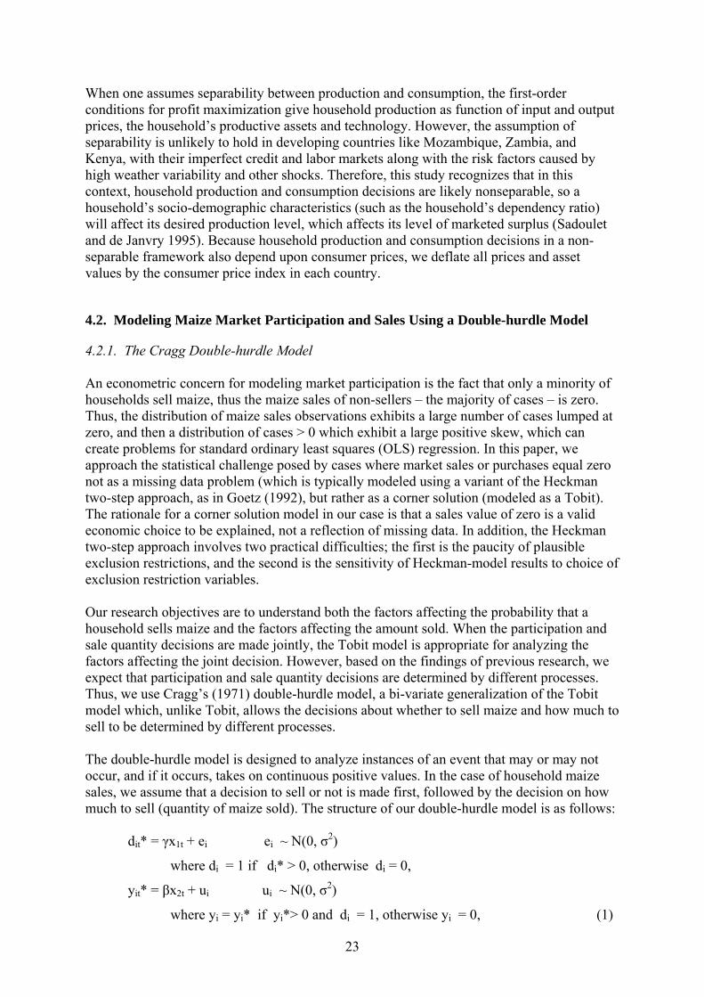
23

When one assumes separability between production and consumption, the first-order conditions for profit maximization give household production as function of input and output prices, the household’s productive assets and technology. However, the assumption of separability is unlikely to hold in developing countries like Mozambique, Zambia, and Kenya, with their imperfect credit and labor markets along with the risk factors caused by high weather variability and other shocks. Therefore, this study recognizes that in this context, household production and consumption decisions are likely nonseparable, so a household’s socio-demographic characteristics (such as the household’s dependency ratio) will affect its desired production level, which affects its level of marketed surplus (Sadoulet and de Janvry 1995). Because household production and consumption decisions in a non-separable framework also depend upon consumer prices, we deflate all prices and asset values by the consumer price index in each country.

4.2. Modeling Maize Market Participation and Sales Using a Double-hurdle Model

4.2.1. The Cragg Double-hurdle Model An econometric concern for modeling market participation is the fact that only a minority of households sell maize, thus the maize sales of non-sellers – the majority of cases – is zero. Thus, the distribution of maize sales observations exhibits a large number of cases lumped at zero, and then a distribution of cases > 0 which exhibit a large positive skew, which can create problems for standard ordinary least squares (OLS) regression. In this paper, we approach the statistical challenge posed by cases where market sales or purchases equal zero not as a missing data problem (which is typically modeled using a variant of the Heckman two-step approach, as in Goetz (1992), but rather as a corner solution (modeled as a Tobit). The rationale for a corner solution model in our case is that a sales value of zero is a valid economic choice to be explained, not a reflection of missing data. In addition, the Heckman two-step approach involves two practical difficulties; the first is the paucity of plausible exclusion restrictions, and the second is the sensitivity of Heckman-model results to choice of exclusion restriction variables. Our research objectives are to understand both the factors affecting the probability that a household sells maize and the factors affecting the amount sold. When the participation and sale quantity decisions are made jointly, the Tobit model is appropriate for analyzing the factors affecting the joint decision. However, based on the findings of previous research, we expect that participation and sale quantity decisions are determined by different processes. Thus, we use Cragg’s (1971) double-hurdle model, a bi-variate generalization of the Tobit model which, unlike Tobit, allows the decisions about whether to sell maize and how much to sell to be determined by different processes. The double-hurdle model is designed to analyze instances of an event that may or may not occur, and if it occurs, takes on continuous positive values. In the case of household maize sales, we assume that a decision to sell or not is made first, followed by the decision on how much to sell (quantity of maize sold). The structure of our double-hurdle model is as follows:

dit* = γx1t + ei ei ~ N(0, σ2)

where di = 1 if di* > 0, otherwise di = 0,

yit* = βx2t + ui ui ~ N(0, σ2)

where yi = yi* if yi*> 0 and di = 1, otherwise yi = 0, (1)

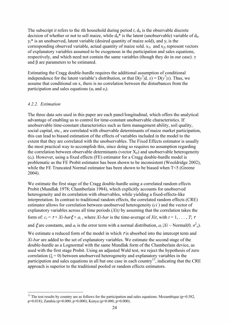
24

The subscript it refers to the ith household during period t, dit is the observable discrete decision of whether or not to sell maize, while dit* is the latent (unobservable) variable of dit. yi* is an unobserved, latent variable (desired quantity of maize sold), and yi is the corresponding observed variable, actual quantity of maize sold. x1t and x2t represent vectors of explanatory variables assumed to be exogenous in the participation and sales equations, respectively, and which need not contain the same variables (though they do in our case). γ and β are parameters to be estimated.

Estimating the Cragg double-hurdle requires the additional assumption of conditional independence for the latent variable’s distribution, or that D(y*|d, x) = D(y*|x). Thus, we assume that conditional on x, there is no correlation between the disturbances from the participation and sales equations (ui and ei).

4.2.2. Estimation The three data sets used in this paper are each panel/longitudinal, which offers the analytical advantage of enabling us to control for time-constant unobservable characteristics. If unobservable time-constant characteristics such as farm management ability, soil quality, social capital, etc., are correlated with observable determinants of maize market participation, this can lead to biased estimation of the effects of variables included in the model to the extent that they are correlated with the unobservables. The Fixed Effects estimator is usually the most practical way to accomplish this, since doing so requires no assumption regarding the correlation between observable determinants (vector Xit) and unobservable heterogeneity (ci). However, using a fixed effects (FE) estimator for a Cragg double-hurdle model is problematic as the FE Probit estimator has been shown to be inconsistent (Wooldridge 2002), while the FE Truncated Normal estimator has been shown to be biased when T<5 (Greene 2004). We estimate the first stage of the Cragg double-hurdle using a correlated random effects Probit (Mundlak 1978; Chamberlain 1984), which explicitly accounts for unobserved heterogeneity and its correlation with observables, while yielding a fixed-effects-like interpretation. In contrast to traditional random effects, the correlated random effects (CRE) estimator allows for correlation between unobserved heterogeneity (ci ) and the vector of explanatory variables across all time periods (Xit) by assuming that the correlation takes the form of: ci = τ + Xi-barξ + ai , where Xi-bar is the time-average of Xit, with t = 1, . . . , T; τ and ξ are constants, and ai is the error term with a normal distribution, ai |Xi ~ Normal(0, σ2

a).

We estimate a reduced form of the model in which τ is absorbed into the intercept term and Xi-bar are added to the set of explanatory variables. We estimate the second stage of the double-hurdle as a Lognormal with the same Mundlak form of the Chamberlain device, as used with the first stage Probit. Using an adjusted Wald test, we reject the hypothesis of zero correlation (ξ = 0) between unobserved heterogeneity and explanatory variables in the participation and sales equations in all but one case in each country13, indicating that the CRE approach is superior to the traditional pooled or random effects estimators.

13 The test results by country are as follows for the participation and sales equations: Mozambique (p=0.582, p=0.018); Zambia (p=0.000; p=0.000); Kenya (p=0.000, p=0.000).

25

To facilitate interpretation of the results, we compute average partial effects14 (APE) for each regressor, along with bootstrapped standard errors.15 Although the vast majority of rural households in the three case countries grow maize, we focus our analysis on those which we consider to be consistent maize growers.16 In Kenya and Mozambique, there are in fact few households that grew maize in one panel year but not the other. Therefore, we only include households that grew maize in each of the panel years. However, because the proportion of rural households in Zambia growing maize has increased dramatically between 2000 and 2008 (due to an increase in maize parastatal purchasing from farmers, and from a widespread fertilizer subsidy program which began around 2004), our analysis includes households which grew maize in either both years or at least one of the two panel years.17 As outlined in the conceptual section, we hypothesize that marginal changes in household assets or public goods will have larger effects on the probability of sale and of sale quantities among higher potential AEC zones and for households with larger land endowments. In each country, we therefore run Chow-like tests to check our assumption that regression results differ significantly across AEC zones and across quartiles of total landholding. These tests consistently support our hypothesis, thus we run regressions and present results at the national level, by AEC zone, and by landholding quartile. For the panel econometric work, we use only households that were re-interviewed in each of the subsequent panel surveys. Given that over time, some households move away from a village and others dissolve as part of a typical household life-cycle, panel household surveys typically have to contend with at least some sample attrition over time. If households that are not re-interviewed are a non-random sub-sample of the population, then using the re-interviewed households to estimate the means or partial effects of variables during one of the later panel time periods may result in biased estimates. To test for attrition bias, we follow the approach described in Wooldridge (2002, p. 585) and define a selection indicator variable, reinterviewi,t + 1, equal to one if the household was re-interviewed in the next wave of the panel survey, and equal to zero if the household was not interviewed. The binary variable reinterviewi,t + 1 is then included as an additional explanatory variable in each equation of interest. If the coefficient on reinterviewi,t + 1 is statistically different from zero, this indicates the presence of attrition bias. Given n=K number of waves of panel data in each country, only the first K-1 waves are used in this test.

14 Because the effect of an explanatory variable in a nonlinear equation depends on the level of all explanatory variables, not just its own coefficient, analysts typically compute the marginal effects for a given variable using the mean of all regressors. By contrast, we compute the partial effect for each household, and then take the average partial effect across the entire sample (or subsample), and compute bootstrapped standard errors for inference (Wooldridge 2002). We use survey sampling weights in the Mozambique regressions in accordance with the complex survey design of TIA. 15 Our bootstrapping routine is replicated 500 times, accounts for sampling weights used in the regressions, and selects each bootstrap sample by replicating the complex survey design used to collect the Mozambique data (i.e., stratification and clustering). 16 We exclude households considered to be non-consistent maize growers in part because our interest is in traditional maize-growing households, and in part because the panel nature of our analysis implies that households which change from zero (or very little) area owned in the first year of a panel to some positive number in a later year (or vice versa) automatically creates a potential outlying case (because of an extremely large change in landholding). 17 As noted below in more detail, our Zambia results which include new growers are robust to analysis which uses a sample of only consistent growers over time.

26

Table 4.1. Attrition Bias Test Results: Mozambique, Zambia, and Kenya

Estimator

p-value for test of H0: β reinterviewi,t + 1 = 0

vs H1: β reinterviewi,t + 1= 1

Mozambique (using 2002 data)Auxilary regressions

Quantity of maize sold (kg) Tobit 0.963Farmgate maize sale price (LC/kg) OLS 0.003

Maize market participation regressions1=HH sold maize Probit 0.993ln(Quantity of maize sold (kg)) Log Normal 0.949

Zambia (using 2000 data)Auxilary regressions

Quantity of maize sold (kg) Tobit 0.170Farmgate maize sale price (LC/kg) OLS 0.228Quantity of subsidized fertilizer received (kg) Tobit 0.240Quantity of fertilizer used on maize (kg/ha) Tobit 0.2001=HH used improved variety Probit 0.006

Maize market participation regressions1=HH sold maize Probit 0.018ln(Quantity of maize sold (kg)) Log Normal 0.046

Kenya (using 1997, 2000, 2004 data)Auxilary regressions

Quantity of maize sold (kg) Pooled Tobit CRE 0.153Farmgate maize sale price (LC/kg) Pooled OLS CRE 0.220Quantity of fertilizer used on maize (kg/ha) Pooled Tobit CRE 0.0791=HH used improved variety Pooled Probit CRE 0.162

Maize market participation regressions1=HH sold maize Pooled Probit CRE 0.540ln(Quantity of maize sold (kg)) Pooled Log Normal CRE 0.630

Dependent variable

Notes: LC = local currency Attrition bias test results are reported in Table 4.1. For regressions that are affected by attrition bias, we use sampling weights that are adjusted for panel attrition bias using the Inverse Probability Weighting (IPW) method (Wooldridge 2002).18

4.2.3. Model Variables Dependent Variable: In the existing literature, explanatory variables typically used to explain food market sales behavior can be divided into three major categories: agro-ecological conditions, market characteristics (e.g., prices and market access), and household characteristics. For purposes of cross-country comparison, we use as many variables in common as possible. Those which are common to each country are described below, while those which differ somewhat are described separately in each country chapter. Agro-ecological Potential and Rainfall: To control for spatial variation in agro-ecological potential in a national sample, we include dummies for either agro-ecological zones or

18 The attrition-correction factors for Mozambique was computed and described by Mather and Donovan (2007), those for Zambia was computed by the authors, and those for Kenya by Bill Burke, as described in Burke and Jayne (2008). The Kenya survey does not use population sampling weights as it was not developed to be a nationally-representative sample.

27

provinces. Using rainfall data from each country, we are able to measure the effect of drought stress on marketed surplus during each season. In Kenya, we also include 3 soil-type dummies created using village-level information on soil type, depth and percentage of sand and clay (Sheahan forthcoming). In Zambia, we use a binary variable that equals one if soil characteristics in the village are suitable for low input fertilizer use, and equals zero otherwise. Market Characteristics: Market characteristic variables include those that measure transaction costs and maize prices. In Kenya and Zambia, we use distance to the nearest feeder road to proxy for transport cost to the nearest market. For Mozambique, we use a variable, travel time to nearest city of 10,000 residents or more, as described in more detail in the Mozambique chapter. While the distance to road measure of market access does not account for the costs of transport from the road to the relevant market itself, the majority of the transport cost to market is often from the village to the nearest good road. Household marketing assets are assumed to reduce search costs, thus we include binary variables for ownership of a bicycle, ownership of a cart and ownership of a vehicle (motorcycle, truck). Household receipt of market price information is recorded in the Mozambique data and should serve to reduce information costs dramatically for rural households. To avoid potential endogeneity issues (from simultaneity bias or reverse causation), we only use cases in which the household which received price information also owns a radio, which accounts for roughly 75% of all households which report receipt of market price information (which is broadcast via radio in many rural areas of the country). We use radio ownership as a proxy of market information receipt in Kenya, and cell phone ownership as a proxy in Zambia. Household membership in a farmer association may also reduce the costs of obtaining market information (or market access), though this is only observed in Mozambique. To measure the farmgate price of maize facing rural households at planting, we use the log of the expected farmgate maize price. We explain the construction of this variable in more detail below. Household Production and Consumption Characteristics: Household characteristic variables are included to control for variation in productive assets, technology use, and consumption requirements. Household productive assets include physical assets such as the log of total landholding size19 and landholding size squared, and the log of total farm assets. Because landholding has been shown to be highly correlated with household wealth and income in southern and eastern Africa (Jayne et al. 2003), estimates of the effect of landholding on participation in income activities may well be correlated with other important factors such as credit access, farmer management skills, soil quality, etc. Thus, if high initial landholding is correlated with various unobservables, then this correlation would bias estimates of landholding on participation. We address this concern through inclusion of household-time-average landholding as an additional regressor (as part of the CRE approach described above), and we have assumed that unobservable factors are correlated with the time-averages of the household-level variables in the model. 19 Landholding is defined as land for which the household has title or use-rights, excluding land which is rented in. Thus, total landholding is the sum of household land area which is cultivated to annual or perennial crops (excluding land rented in), in fallow, gardens, and virgin.

28

To proxy for the availability of family labor for agricultural activities, we use the number of prime-age adults and its square. In Kenya and Zambia, we are able to adjust the number of adults by how their actual months of residence (over the 12-month recall period), while in Mozambique we use the number of prime-age adults who claim agriculture as a primary or secondary occupation. We include head’s years of education as a measure of human capital (in Kenya, we use maximum education among adults due to data limitations in the first panel year). Head’s age and age squared is included as a proxy for lifecycle and taste effects, and because it’s time-average may be correlated with unobservable characteristics for which we hope to control. In the interest of testing for gender disparities in maize marketing, we include a binary variable which equals one if the household is headed by a single female (and zero otherwise), and a separate binary variable which equals one if the head is a female with a resident spouse (and zero otherwise). Because the binary variable for single female-headed households may pick up negative effects of adult mortality (in the event that she was recently widowed), we also include a binary variable which equals one if the household suffered a death of an adult age 15-59 within the past 3 years. Thus, if the average partial effect of having a single female head is statistically significant, this should represent gender disparities in the ability to produce and market maize, free of any adverse effects due to recent adult mortality. Input Use and Improved Technologies: In each country, we include a binary variable which equals one if the household owns animal traction (a suitable animal and equipment) – and zero otherwise – which may increase crop productivity due to more timely planting and improved soil aeration and weed control. In Kenya and Zambia, we include a binary variable that equals one if the household used a purchased hybrid maize seed variety that season, as well as the log of the quantity of chemical fertilizer applied per hectare of maize planted. We chose not to include such variables for Mozambique because we only have information on purchased improved maize seed in the second year of the Mozambique panel, and because information on fertilizer (total cost) is at the farm (not crop) level. In each country, we also include a measure of access to credit, which due to endogeneity concerns is proxied by the percentage of village households that received credit for purchase of farm inputs that season. Handling the Potential Endogeneity of Household Use of Fertilizer and Hybrid Maize Seed: We include two variables which measure household use of technology, fertilizer applied per hectare of maize and use of hybrid maize seed. Household choices regarding input use are typically considered endogenous due to either omitted variable bias or the simultaneity of input decisions and realized outputs. For example, because input use is likely to be correlated with unobserved time-constant household characteristics such as farm management skill, soil quality, social contacts, etc., failure to control for these unobserved factors can lead to omitted variable bias on the coefficients of variables measuring input use. Assuming that the time-constant unobserved characteristics are correlated with time-averages of assets, other household characteristics, and use of the input in question (i.e., our Correlated Random Effect terms in the double-hurdle model), we can control for such unobserved factors via the CRE specification. However, simultaneity of input use and an outcome such as yield, crop income, or sales decision may occur if input use if correlated with unobserved time-varying factors such as the rainfall or pest pressure at different points during the growing season, which is also likely correlated with the dependent variable. We partially control for such time-varying factors by using drought stress variables in each season.

29

In Kenya and Zambia, we address the remaining potential for endogeneity bias of fertilizer use by using an adapted Control Function (CF) approach developed by Rivers and Vuong (1988) to control for a continuous endogenous explanatory variable, and by Vella (1993) to control for an endogenous variable that is also a corner solution.20 We use village-level median fertilizer price for Diammonium Phosphate (DAP) and the median distance to fertilizer seller as the instruments. Because we also are testing for the potential endogeneity of household use of hybrid maize seed, we also include the instrument for that variable (distance to hybrid seed seller). The CF approach involves two steps. First, we run a reduced form Tobit regression of the quantity of fertilizer used per hectare of maize planted (kg/ha) as a function of all the variables in our structural regression plus the instruments for both fertilizer use and hybrid seed use. Second, we include the residual from the Tobit regression of fertilizer use as a regressor in the structural equations of the Cragg double-hurdle model, along with the endogenous variable, household fertilizer use (kg/ha). The fertilizer variable is deemed endogenous if the partial effect of the Tobit reduced form residual is significant in either of the stages of the double-hurdle. Validity of our instruments for fertilizer use depends upon two assumptions, one of which cannot be tested. First, we must test whether or not these instruments have a significant effect on the endogenous variable (log of fertilizer applied per hectare of maize) in the reduced form regression. Second, we must assume that our instruments are not correlated with the outcome of interest (probability of sale or quantities sold), conditional on the other observable factors (an assumption that cannot be tested). While fertilizer price is clearly exogenous in the structural model, distance to fertilizer seller may be correlated with agro-ecological potential. Thus, the exogeneity of distance to fertilizer seller in the structural equation depends upon whether or not we have adequate observable measures of agro-ecological potential. We assume that we do, given that the reduced form regression for each country includes variables such as: dummies for district or village-level information on soil types known to be more responsive to chemical fertilizers; provincial and time dummies; the long-term average of seasonal rainfall and rainfall shocks at the district or village level (and their time-averages); as well as the household-specific time-average of fertilizer use on maize and hybrid seed use. Another potentially endogenous variable used in Kenya and Zambia is household use of purchased hybrid maize seed that year (which equals one if they used it, and zero otherwise). Because the time-average of this variable should control for time-constant unobserved factors, and as this decision is made at planting, it is not likely to suffer from simultaneity bias to the same extent we might expect from an input such as fertilizer, pesticide or labor for weeding, etc. Nevertheless, we also use the CF approach to test for the potential endogeneity of this dichotomous variable, employing a limited probability model (LPM)21 for the reduced form regression of hybrid seed use. We include the binary variable for household use of purchased hybrid maize seed in the structural regression (the double-hurdle model) along with the residual from the LPM of hybrid seed use, where a t-test on the residual term provides a test of the exogeneity of hybrid seed use (Wooldridge 2002). We assume that the instruments for hybrid maize seed use are exogenous in the structural model because of our existing controls for agro-ecological potential and the CRE time-average terms (as described above for the fertilizer instruments).

20 See Ricker-Gilbert, Jayne, and Chirwa (2011) for a recent application of this adapted control function approach. 21 LPM is equivalent to an OLS regression on a dichotomous dependent variable.

30

4.2.4. Modeling Farmgate Maize Price Expectations Farmgate Maize Price Prediction Model: With one exception (Renkow 1990), empirical research to date on food grain market participation in developing countries has used farmgate or wholesale food grain prices which are contemporaneous to the marketing decision. The reason for this has either been a lack of available data at both points in time, or use of a theoretical model that assumes simultaneity of production and consumption decisions (and thus, use of a single, annual average maize price). However, the use of post-harvest prices alone could be especially problematic in the case of thin markets in areas of low food crop productivity.22 In reality, and as noted by Renkow (1990), a farmer’s maize marketing decision is likely to be a function of maize prices at two different points in time: first, the farmer’s expectation concerning the maize price at or after the harvest month (which is based upon information available to the farmer at or before the planting month) influences the area he plants to maize and the amount of fertilizer or other inputs that he decides to apply; second, once the farmer harvests his maize, his decision of whether to sell or not (from one week to the next in the post-harvest period) will depend in part on prevailing maize prices at that point in time. Following recent work by Mather and Jayne (forthcoming) and Muyanga (forthcoming), we model expected farmgate prices as a function of variables observed at planting, such as lagged wholesale market prices of maize from the nearest regional market, lagged effective parastatal prices (in Kenya and Zambia), and household and village characteristics which might affect the maize sale price received by a given household. Thus, we use expected maize prices at planting in our model, rather than post-harvest prices. We leave for future research an empirical investigation of the responsiveness of household maize sales to farmgate maize prices which accounts for the both the effect of expected maize prices on maize production and that of post-harvest sales prices on maize consumption. In each country, our farmgate price data consists of observations of farmgate sales prices of maize in the panel surveys. Wholesale market prices of maize include the price in the planting month from the nearest regional wholesale, as well as 11 months of lagged wholesale prices. In Mozambique, our lagged wholesale prices are quarterly average prices. In Kenya, we also include a variable distance to regional market to control for variation across villages in transport costs between the village and the regional market.

Household characteristics that might influence the price received by a farmer include age of the household head, a proxy for market experience, and education level of the head, a proxy for negotiation skill. We also use measures of the household value of storage assets, total value of farm assets, and dummies for truck and bicycle ownership as proxies for negotiation leverage enjoyed by a given farmer. Distance to the nearest motorable road serves as a proxy for transport costs to the relevant market. Because weather conditions may influence market prices, we include variables to measure expected rainfall levels and expected rainfall shocks. These variables are described in more detail in each country chapter. Finally, we also include the long-term average of each time-varying variable in the model, used to control for unobserved time-constant household heterogeneity using the correlated random effects (CRE) approach.

22 Under such conditions, we would expect to observe that following a good production season, maize prices at harvest will likely be low, yet the probability of maize sale would be higher than average. Following a poor production season (due to drought), we would expect to observe relatively high farmgate maize prices, yet a lower than average probability of maize sale. These scenarios could result in a negative correlation between maize sale prices and the probability of maize sale.

31

Testing for Potential Sample Selection Bias in Observable Maize Prices: Before we estimate a regression to predict farmgate maize prices in each country, we note that such price data is only observed for a subsample of the population which actually sells maize (in the case of Kenya, n=537 households sold maize in 2007). If this subsample has non-random characteristics, it is possible that using OLS on the observed maize sale prices could produce biased results due to incidental truncation of the observable maize price distribution. We therefore test for the presence of sample selection bias using a Tobit selection equation and a method outlined by Wooldridge (2002, p. 572). The first step in testing for potential sample selection bias is to run a Tobit regression of ‘quantity of maize sold >=0’ by maize growers (i.e., almost the entire household sample). The second step is to take the residual from this Tobit, and to include it as a regressor in the farmgate maize price regression. If the coefficient on the residual term in the price regression is significant, this indicates the presence of sample selection bias. Variables in the Tobit regression include factors related to agro-ecological potential and shocks, household assets related to maize production, assets related to marketing, household consumption requirements, and the price of maize. Note that instead of using expected maize prices, we use the log of the district median of household maize sale prices. Because maize sales are made in Kenya at harvest as well as months afterward, this price is essentially the median annual district-level post-harvest farmgate maize sales price. We also include the long-term average of each time-varying variable in the model, which are collectively used to control for unobserved time-constant household heterogeneity under the correlated random effects (CRE) approach.

32

5. ECONOMETRIC ANALYSIS: MOZAMBIQUE

5.1. Explanatory Variables This section describes explanatory variables used in the Mozambique analysis that were not already described in the section 4.2.3. The binary dependent variable in the Probit stage of the double-hurdle =1 if the household sold maize, or =0 otherwise. The dependent variable in the lognormal stage is the natural log of maize quantity sold (kgs). To control for spatial variation in agro-ecological potential, we include agro-ecological zone dummies (we create dummies for 7 out of the 10 agro-ecological zones). Given that nearly all maize production in Mozambique is rainfed, we include two variables to capture the effect of drought or other shocks to local maize production. The first is an estimate of the ‘days of drought’ during the primary agricultural season (November/December – March/April, depending on the district), to control for rainfall variation across districts.23 The second is the percentage of village households that report maize yield loss (due to weather, pest, or disease shocks). Based on information from community-level surveys (implemented along with the household TIA survey) on flood, drought, and disease shocks experienced in each village that year, it is clear that the principal cause of maize yield losses in the majority of villages in 2002 and 2005 was drought. Expected post-harvest farmgate maize prices are computed for each household using the regression method described in 4.2.4. and the model presented in Appendix Table B-1. Because the only distance to road variable which is available for use with the Mozambique household survey data is distance to nearest paved road – which in many districts appears to be much further than the nearest motorable road or city – we instead use a measure of market access which is the travel time (hours) from the village to the nearest town of 10,000 residents or more. This variable was computed using a travel time model and GIS information on the nearest road (of any type), towns/cities as well as topographical information on the land terrain between the village and the nearest road.24 While the travel time variable was created with road maps which date to the first year of the Mozambique panel (2002), it does not drop out of the model because we do not compute between-effect terms for them (i.e., the time-average term), under the assumption that such variables are at least partially uncorrelated with the unobservable household heterogeneity, conditional on the other variables in the model (Wooldridge 2002). Unlike the Zambia and Kenya cases, we do not have panel information on household use of improve maize varieties. While the Mozambique survey did record total fertilizer costs, we do not use a fertilizer use variable because we do not know if it was applied to maize or not, because only 3.5% of farmers at the national level used fertilizer in 2002 (though was as high as 19% in Niassa and 14% in Tete), and most fertilizer use is applied by growers of tobacco, cotton, and horticultural crops. Although very few Mozambican households use fertilizer on maize, we use the log of the distance to the nearest fertilizer seller as a proxy for input costs. Summary statistics of all variables used in the auxiliary and double-hurdle models for Mozambique are presented in Appendix Table B-2.

23 We compute days of drought at the district level, using district-level dekadal rainfall estimates from FEWS, which we feed into a water balance model. Further details are provided in Mather, Cunguara, and Boughton. (2008). 24 The authors thank Jordan Chamberlain and Jenny Cairns (who are Ph.D. and M.Sc. graduate students, respectively, in the Department of Agricultural Food and Resource Economics at MSU) for constructing the travel time variable for Mozambique and sharing this with us.

33

Anticipating that average partial effects for some variables may differ by agro-ecological zone, we aggregate agro-ecological zones into four zones that represent maize-production potential: Low potential, Low-Medium, Medium, and High. We run the equivalent of a Chow test on the sales equation, which shows that the model coefficients are (jointly) significantly different enough by region to warrant the use of either separate zonal regressions or zonal interaction terms (we run separate zonal regressions). We find the same result when testing for differences among coefficients by quartiles of total landholding (computed for each zone). Thus, we report results from a national regression, and separate regressions for each zone, and for each landholding quartile.

5.2. Econometric Results

5.2.1. Agro-ecological Potential Given that nearly all maize production in Mozambique is rain fed and that use of improved maize seed and fertilizer on maize is quite rare, we would expect that agro-ecological potential would play an important role in maize market participation. To measure the role of agro-ecological factors on household maize market participation – controlling for household-level factors and prices – we run the Probit and Lognormal stages of the Cragg double-hurdle model described above using all the household and village-level variables, though we drop our district and village-level drought shock variables. The results from several zones show that, even after controlling for household assets, prices, and market access, agro-ecological potential has significant and large effects on both the probability of selling and amounts sold, conditional on selling (Table 5.1.). For example, relative to the base category (the low potential zone 1 and 2, which corresponds to parts of rural Maputo Province, coastal Gaza, and Inhambane), households in other zones are 29 to 45% more likely to sell maize than households in the base zones, and sell between 90% to 130% more maize on average (conditional on selling). In the results that follow, we use several variables to control for agro-ecological potential and actual weather conditions: agro-ecological zone dummies and district and village-level weather shock variables.

5.2.2. Weather and Other Covariate Shocks We find that an additional day of drought (a district-level variable) does not have a significant effect on probability of sale or quantities sold at the national level (Table 5.2.), though it does reduce probability of sale by 0.3 points in the low potential zone (Table 5.3b.). Given that only 11% of households in the low potential zone sell maize, this means that the percentage decrease in probability of sale due to an extra day of drought is about 2.7% in the low potential zones. The other shock variable, percentage of village households reporting maize yield shock, has a significant negative effect on quantities sold by current sellers (the conditional effect); a 20% increase in the percentage of village households reporting maize yield loss results in a 6.5% decrease in a household’s probability of selling maize (Table 5.2.).25 A 20% increase in village yield shock also causes a significant 10% loss in quantities sold by any randomly selected household, whether a current seller or not (i.e., unconditional quantity) (Table 5.2.). 25 Because the range of the variable (% of village households who report yield shock) is from 0 to 1, a one-unit increase in this variable represents the entire range of the variable. Thus, a standard way to interpret the marginal change in a fractional variable is to multiply the standard deviation of the variable by the standard deviation of the variable by the partial effect, or by a value such as 0.20, which we use here.

34

Table 5.1. Average Partial Effects of Agro-ecological Potential on the Probability of Maize Sale and Quantities Sold, Mozambique, 2002-2005

Independent variablesAPE BS se p-value APE BS se p-value APE BS se p-value

Agroecological zone 3 (low) 0.026 0.042 0.545 0.833 0.635 0.189 1.023 0.935 0.274Agroecological zone 6 (low) 0.296 0.045 0.000 1.418 0.731 0.052 5.828 3.479 0.094Agroecological zone 5 (low-medium) 0.355 0.051 0.000 0.446 0.436 0.306 3.765 2.125 0.076Agroecological zone 8 (low-medium) 0.294 0.049 0.000 0.425 0.428 0.321 2.972 2.067 0.150Agroecological zone 4 (medium) 0.446 0.036 0.000 1.364 0.617 0.027 9.183 4.462 0.040Agroecological zone 7 (medium) 0.377 0.043 0.000 0.895 0.448 0.046 6.087 3.289 0.064Agroecological zone 10 (high) 0.312 0.046 0.000 1.328 0.617 0.031 5.858 2.949 0.047Year = 2005 (time dummy) -0.037 0.048 0.436 -0.553 0.204 0.007 -0.779 0.357 0.029

cases 6353 1468 6353

Notes: Agroecological zone 1-2 (low potential) is the base. APE= average partial effect, BS se = bootstrapped standard error. Other variables include all those in Table 5.2 except for weather shock variables.

Probit Lognormal

APE of Xj on P(y>0)APE (Conditional) of Xj on lny,

given y>0APE (Unconditional) effect of Xj

on lny

Dept variable = 1 if hh sold maize, 0 otherwise Dept variable = ln(kgs of maize sold)

35

Table 5.2. Cragg Model of Maize Market Sales Participation and Level of Maize Sold, Mozambique, 2002-05


# of days of drought (district-level) 0.000 0.001 0.809 0.006 0.005 0.200 0.005 0.006 0.393% village hhs which report maize yield loss -0.066 0.052 0.203 -0.394 0.169 0.020 -0.709 0.313 0.023ln(total area) 0.039 0.016 0.018 0.314 0.067 0.000 0.470 0.096 0.000ln(total assets) 0.010 0.005 0.040 0.025 0.025 0.319 0.072 0.038 0.058# prime-age adults working in ag -0.007 0.012 0.544 0.078 0.070 0.269 0.044 0.078 0.5711=HH owns animal traction -0.108 0.040 0.008 0.353 0.457 0.440 -0.290 0.348 0.405% village hhs received extension visit 0.054 0.059 0.362 0.343 0.268 0.201 0.603 0.328 0.066head's age 0.000 0.002 0.890 0.007 0.011 0.520 0.000 0.013 0.988head's education level -0.001 0.005 0.871 -0.036 0.025 0.145 -0.041 0.036 0.253ln(distance to fertilizer seller) 0.012 0.006 0.044 0.000 0.037 0.995 0.059 0.053 0.272travel time to nearest 10k town (hours) -0.002 0.001 0.254 -0.002 0.006 0.711 -0.010 0.008 0.2401=HH owns bike 0.023 0.021 0.266 0.083 0.082 0.308 0.201 0.157 0.2021=HH owns cart 0.130 0.101 0.198 -0.101 0.512 0.844 0.522 0.663 0.4311=HH received market price info 0.035 0.022 0.101 0.211 0.096 0.028 0.412 0.156 0.0081=HH belongs to farm association 0.001 0.032 0.982 -0.018 0.200 0.927 -0.015 0.272 0.956ln(expected farmgate maize price) 0.005 0.161 0.974 1.179 0.673 0.080 1.205 1.014 0.235dependency ratio 0.007 0.014 0.611 0.072 0.069 0.298 0.106 0.085 0.2141=HH headed by single female -0.005 0.045 0.919 -0.333 0.201 0.098 -0.358 0.277 0.1951=HH headed by female with spouse -0.021 0.045 0.640 -0.190 0.233 0.416 -0.275 0.259 0.2881=HH had prime-age death in past 3 years -0.027 0.027 0.312 -0.269 0.154 0.081 -0.368 0.174 0.035

cases 6352 1468 6352

Model includes dummies for agroecology (7) and year. Also included are X-bar terms for each of the time-varying regressors. APE= average partial effect, BS se = bootstrapped standard error

Probit Lognormal



on lny

Dept variable = 1 if HH sold maize, 0 otherwise Dept variable = ln(kgs of maize sold)

36

AEC zone APE BSE p-valueLandholding

quartile APE BSE p-value1- low -0.003 0.002 0.060 1- low -0.006 0.005 0.218

2 low-medium 0.004 0.004 0.363 2 -0.003 0.002 0.2163 medium -0.001 0.004 0.761 3 -0.004 -1.140 0.997

4 - high -0.015 0.018 0.401 4 - high 0.001 0.002 0.661National 0.000 0.001 0.809 National 0.000 0.001 0.809

AEC zone APEAdjusted

APE p-valueLandholding

quartile APEAdjusted

APE p-value1- low -0.003 -0.003 0.871 1- low 0.046 0.047 0.302

2 low-medium -0.005 -0.005 0.854 2 -0.005 -0.005 0.7653 medium 0.013 0.013 0.457 3 -0.010 -0.010 0.401

4 - high 0.076 0.079 0.670 4 - high 0.009 0.009 0.257National 0.006 0.006 0.200 National 0.006 0.006 0.200




APE p-value1- low -0.042 -0.041 0.186 1- low 0.007 0.007 0.856

2 low-medium 0.013 0.013 0.689 2 -0.019 -0.019 0.2303 medium 0.009 0.009 0.628 3 -0.029 -0.028 0.197


APE= Average Partial Effect; BSE = Boostrapped standard error -- both computed from subgroup regressions

Table 5.3a. APE of district-level days of drought on probability of maize sale, by AEC zone and by landholding quartile, Mozambique

Table 5.3c. APE of district-level days of drought on log quantity of maize sold (unconditional), by AEC zone and by landholding quartile, Mozambique

Table 5.3b. APE of district-level days of drought on log quantity of maize sold (conditional), by AEC zone and by landholding quartile, Mozambique

APE= Average Partial Effect; BSE = Boostrapped standard error. APEs and BSEs are from subgroup regressions

As these results demonstrate, weather-related shocks can lower aggregate quantities of maize sold both by lowering the quantity of maize sold by current sellers and by lowering the probability that a given household sells maize in the first place (i.e., lowering the number of sellers). The unconditional partial effect of the village shock describes the expected change in maize quantity sold by a randomly selected household (i.e., actual sellers or non-sellers) given a change in the village shock. This effect contains a participation component, which represents the change in sales quantities due to the amount sold by a new seller, and a sales quantity component, which represents the change in sales quantities due to a change in the amount sold by a current seller.

5.2.3. Household Productive Assets Total household landholding has a significant though small effect on the probability of selling maize, as a 1% increase in landholding increases the probability of selling maize by 0.04 points on the probability scale from 0 to 1 (Table 5.4a.). Thus, a 10% increase in landholding would increase the probability of selling maize by only 0.4 points, on average. Given that only 19% of households sell maize, this means that a 10% increase in landholding would increase the probability of selling maize by about 2%.

37


quartile APE BSE p-value1- low 0.034 0.015 0.028 1- low -0.016 0.043 0.712

2 low-medium 0.025 0.040 0.531 2 0.032 0.032 0.3123 medium 0.070 0.028 0.012 3 0.117 0.037 0.001





APE p-value1- low 0.161 0.174 0.323 1- low 0.241 0.273 0.511









APE= Average Partial Effect; BSE = Boostrapped standard error -- both computed from subgroup regressions

Table 5.4a. APE of log landholding on probability of maize sale, by AEC zone and by landholding quartile, Mozambique

Table 5.4c. APE of log landholding on log quantity of maize sold (unconditional), by AEC zone and by landholding quartile, Mozambique

Table 5.4b. APE of log landholding on log quantity of maize sold (conditional), by AEC zone and by landholding quartile, Mozambique


Landholding has a significant and larger partial effect on sales quantities (both conditional and unconditional), as a 1% increase in landholding increases maize sold by current sellers (conditional effect) by 0.37% (Table 5.4b.), while it increases maize sold by any given household (from current sellers or non-sellers – the unconditional effect) by 0.6% (Table 5.4c.).26 With a few exceptions (Boughton et al. 2007; Barrett 2008), the extant literature on food staple marketing in Sub-Saharan Africa gives scant attention to the role of household productive assets in explaining food market participation, focusing instead on the role of transaction costs. This evidence demonstrates that while landholding has a rather small effect on probability of sale, it has rather large effects on quantities sold, both by current and potential sellers. Given the extremely low levels of improved input use in Mozambique – in 2005, only 9% of Mozambican farmers used animal traction, 4% bought improved maize

26 Results for conditional and unconditional effects on the log of sales quantities report the actual change in the natural log of the dependent variable, not the percentage change in the first column (APE); note that the actual percentage change in the dependent variable needs to be adjusted since the logarithmic transformation approximates small changes well (those under 20%) but larger changes less well (Wooldridge 2002). The necessary adjustment is as follows: % change in y = [exp(B) – 1], which is done for the APEs in the column denoted ‘Adjusted APE’.

38

seed, and 4% used fertilizer on maize – it should perhaps not be surprising that expanding landholdings would have such a large effect on maize quantities sold. We next run separate regressions on the AEC zone subsamples to see whether or not the partial effect of landholding is greater in higher potential zones, and find this while the APE is higher in the medium zone relative to the low potential zone (Table 5.4a.), it is not significantly higher (p=0.26). Although the APEs of landholding on conditional quantities are larger in magnitude for the medium and low-medium zones relative to the low zone, the difference is not significant. To test our hypothesis that marginal returns to principal assets such as landholding increase in landholding, we also run separate regressions by quartiles of landholding (where the quartiles are computed separately for each AEC zone). We find that the APEs of landholding on the probability of maize sale are significantly higher for households in the top three quartiles, relative to those in the lowest landholding quartile (Table 5.4a.). We do not find a statistically significant pattern among the APEs of landholding on conditional or unconditional quantities sold. The first and most obvious implication of these results is that marginal increases in landholding elicit larger participation and quantity effects from households in higher landholding quartiles. What is perhaps less obvious is that the effect of increasing landholding among households in the lowest land quartile is highly insignificant, suggesting that there is a threshold level of landholding necessary for maize market participation. Evidence of such a landholding threshold is also seen in non-parametric regressions of probability of sale on landholding/AE (Figure 5.1.), where the probability of sale in each AEC zone tends to increase slowly as landholding/AE increases from zero to 1 hectare/AE, and then increases at a higher rate after about 1 to 1.5 ha/AE, depending on the zone. We also see non-parametric regression evidence of landholding threshold effects on net sales/AE, as results show that net sales/AE increases gradually in landholding/AE up to about 1 to 1.5 ha/AE, and then the rate of increase in net sales/AE jumps upward as landholding/AE continues to increase (Figure 5.2.). Household total farm assets (a proxy for wealth) also have a significant positive effect on participation, though these are quite small: a 1% increase in assets increases the probability of selling maize by 0.01%. The APE of farm assets on unconditional quantity sold is also significant though also of low magnitude, as a 1% increase in assets increases unconditional sale quantity by 0.07%. This positive correlation between commodity sales and household wealth is consistent with findings elsewhere in Sub-Saharan Africa (Barrett 2008). One explanation of the wealth effect could be that it fosters higher productivity through better access to improved inputs (and/or the credit necessary for their financing). Note that our asset result does not simply proxy for use of animal traction, as we control for that separately. Another explanation of this wealth effect is related to the household’s consumption needs. For example, recalling the context of the transaction cost literature, wealthier households tend to have narrower price bands due to lower risk aversion, and would therefore be less likely to fall within the autarkic price region. In other words, households with higher wealth are less concerned with food market risk, and thus are not as worried as poorer households are about having to buy back maize in the lean season.

39

Figure 5.1. Non-parametric Regression of Probability of Selling Maize by Landholding/AE, by AEC Zone, Mozambique, 2002

.1.2

.3.4

.5P

roba

bilit

y of

sel

ling

0 .5 1 1.5 2Total area/AE (ha)

aec1 aec2aec3 aec4

* computed among maize growers; Nadaraya-Watson regression with bandwidth=1.0 and an Epanechikov kernel. Aec1 = low AEC potential, Aec2=low-medium, Aec3=medium-high, Aec4 = high AEC potential Figure 5.2. Non-parametric Regression of Net Maize Sold/AE by Landholding/AE, by AEC Zone, Mozambique, 2002

050

100

150

200

250

Net

mai

ze s

old/

AE

0 .5 1 1.5 2Total area/AE (ha)

aec1 aec2aec3 aec4

40

Given that Mozambican agriculture relies heavily upon manual labor, it is perhaps surprising that the APE of available family adult labor on probability of maize sale and on sale quantities is insignificant (and negative in the probability case). This suggests that our use of family adults working primarily or secondarily in agriculture may not be a good proxy for actual labor application.

5.2.4. Technology Use We find that ownership of animal traction has a surprisingly negative (and significant) effect on the probability of sale at the national level (Table 5.2.), reducing probability of sale by 10%. This negative effect might be due to the fact that all of Mozambique’s animal traction is found in southern and central provinces of Mozambique which were hardest-hit by drought in both 2002 and 2005. Nevertheless, animal traction has been found to have rather large effects on crop income in other studies using the same data (Mather 2009).

5.2.5. Market Access and Market Information Travel Time to Nearest Town: We find that our measure of market access is the travel time to the nearest town of 10,000 residents or more has the expected negative effect on probability of sale and quantities sold, though the effect is not significant at the national level (Tables 5.5a, b, c.). Given that 53% maize sellers in 2002 lived in a village in which at least one household sold to a private sector agent (i.e., not including sales to other households), the national-level result suggests that a majority of rural households live in villages have reasonable market access. However, we do find that in the medium potential zone, a one-hour decrease in travel time increases conditional quantity sold by 2% and unconditional quantity by 3% (Tables 5.5b, c.). Household Ownership of Transportation Assets: There is also some evidence of the existence of marketing-related transaction costs as seen by the positive and significant effects on probability of sale of owning a bicycle (9% increase in probability of sale in the low potential zone) or a cart (43% in the medium zone and 42% in the high zone). It perhaps is not a coincidence that the country with the lowest road density (Mozambique) in our study is where we find significant effects of household transportation assets on the probability of maize sale. Market Price Information: Household receipt of market price information has a significant effect on participation, increasing the probability of selling by 3.5 points. Taken as a percentage of the proportion of households selling maize, this represents an 18% increase in the probability of sale (Table 5.6a.). It also has a considerably large and significant effect on conditional and unconditional sales, increasing quantity sold by 21% and 41%, respectively (Table 5.3.). However, these large quantity effects appear to be driven by those in the higher landholding quartiles, suggesting that there may be a land threshold below which market information will not increase quantities sold perhaps because those in the lower land quartiles produce such small quantities of maize that the advantage given by receipt of price information by itself is not sufficient to increase sold quantities.

41


quartile APE BSE p-value1- low 0.000 0.001 0.890 1- low -0.001 0.004 0.851

2 low-medium 0.001 0.004 0.899 2 0.002 0.002 0.2693 medium -0.003 0.002 0.179 3 0.001 0.002 0.532

4 - high 0.005 0.006 0.411 4 - high 0.000 0.002 0.899National -0.002 0.001 0.254 National -0.002 0.001 0.254




APE p-value1- low 0.013 0.013 0.319 1- low -0.009 -0.009 0.662

2 low-medium -0.012 -0.012 0.671 2 -0.030 -0.030 0.0013 medium -0.020 -0.020 0.066 3 -0.010 -0.010 0.245

4 - high -0.040 -0.039 0.231 4 - high 0.001 0.001 0.941National -0.002 -0.002 0.711 National -0.002 -0.002 0.711





2 low-medium -0.010 -0.010 0.747 2 -0.019 -0.019 0.1933 medium -0.031 -0.030 0.046 3 -0.004 -0.004 0.788

4 - high -0.017 -0.016 0.757 4 - high 0.000 0.000 0.988National -0.010 -0.010 0.240 National -0.010 -0.010 0.240

APE=Average partial effect; BSE=Boostrapped standard error. APEs and BSEs are from subgroup regressio

Table 5.5a. APE of travel time (hours) to the nearest town of 10,000 residents or more on probability of sale, by AEC zone and by landholding quartile, Mozambique

Table 5.5c. APE of travel time (hours) to the nearest town of 10,000 residents or more on log quantity of maize sold (unconditional), by AEC zone and by landholding quartile, Mozambique

Table 5.5b. APE of travel time (hours) to the nearest town of 10,000 residents or more on log quantity of maize sold (conditional), by AEC zone and by landholding quartile, Mozambique

Farmer Association Membership: We find that membership in a farmer association does not have a significant effect on either probability of sale or quantities sold (Table 5.2.). One explanation for the lack of an effect is simply that such associations do not have a positive effect on maize marketing, once we are able to control for a household’s time-average asset levels. It is also possible that because we do not have information on the types of farmer associations, we cannot distinguish between those whose activities improve food grain productivity or marketing versus other types of associations.

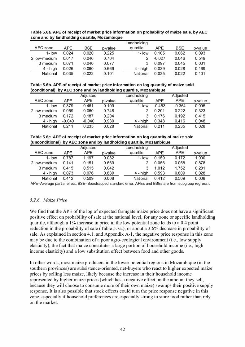
42


quartile APE BSE p-value1- low 0.024 0.020 0.225 1- low 0.105 0.062 0.093

2 low-medium 0.017 0.046 0.704 2 -0.027 0.046 0.5493 medium 0.071 0.040 0.077 3 0.097 0.045 0.031







4 - high -0.040 -0.040 0.930 4 - high 0.348 0.416 0.048National 0.211 0.235 0.028 National 0.211 0.235 0.028








Table 5.6a. APE of receipt of market price information on probability of maize sale, by AEC zone and by landholding quartile, Mozambique

Table 5.6c. APE of receipt of market price information on log quantity of maize sold (unconditional), by AEC zone and by landholding quartile, Mozambique

Table 5.6b. APE of receipt of market price information on log quantity of maize sold (conditional), by AEC zone and by landholding quartile, Mozambique

5.2.6. Maize Price We find that the APE of the log of expected farmgate maize price does not have a significant positive effect on probability of sale at the national level, for any zone or specific landholding quartile, although a 1% increase in price in the low potential zone leads to a 0.4 point reduction in the probability of sale (Table 5.7a.), or about a 3.6% decrease in probability of sale. As explained in section 4.1. and Appendix A-1, the negative price response in this zone may be due to the combination of a poor agro-ecological environment (i.e., low supply elasticity), the fact that maize constitutes a large portion of household income (i.e., high income elasticity) and a low substitution effect between food and other goods. In other words, most maize producers in the lower potential regions in Mozambique (in the southern provinces) are subsistence-oriented, net-buyers who react to higher expected maize prices by selling less maize, likely because the increase in their household income represented by higher maize prices (which has a negative effect on the amount they sell, because they will choose to consume more of their own maize) swamps their positive supply response. It is also possible that stock effects could turn the price response negative in this zone, especially if household preferences are especially strong to store food rather than rely on the market.

43


quartile APE BSE p-value1- low -0.421 0.249 0.091 1- low 1.154 1.072 0.282

2 low-medium -0.059 0.643 0.927 2 -0.910 0.664 0.1703 medium 0.822 0.811 0.311 3 0.660 0.757 0.383






2 low-medium 6.064 429.1 0.092 2 5.801 329.8 0.2173 medium -1.518 -0.781 0.550 3 5.284 196.2 0.024





APE p-value1- low -1.411 -0.756 0.577 1- low -6.587 -0.999 0.566




Table 5.7a. APE of log expected farmgate maize price on probability of maize sale, by AEC zone and by landholding quartile, Mozambique

Table 5.7c. APE of log expected farmgate maize price on log quantity of maize sold (unconditional), by AEC zone and by landholding quartile, Mozambique

Table 5.7b. APE of log expected farmgate maize price on log quantity of maize sold (conditional), by AEC zone and by landholding quartile, Mozambique

The near-zero partial effect of maize prices on probability of sale at the national level is due to a combination of positive (though insignificant) effects in the medium and high potential zones, and negative effects in the lower potential zones (significant in the lowest potential zone). Nevertheless, this suggests that even in higher potential zones, non-sellers are unlikely to respond to higher maize prices by selling some maize. Among current maize sellers, we find a very strong positive price response on conditional sale quantities, at the national level, where a 1% increase in the expected maize price leads to a 2.2% increase in the conditional quantity sold. The conditional effect result demonstrates that current sellers are highly price responsive, though the descriptive analysis above demonstrated that only about 20% of rural households sell maize, and most of these are smallholders with considerably landholding and assets. It is not surprising that the unconditional quantity effect is not significant, given that maize prices do not appear to affect the probability of selling.

5.2.7. Gender and Household Demographics Head’s age and education level do not have a significant effect on probability of sale or sale quantities at the national level. These results are consistent with Boughton et al.’s (2007) finding that education is significant factor explaining market participation for commodities which require more precise crop and post-harvest management (such as cotton and tobacco),

44

but not for maize. This is not to say that education is irrelevant to food crop production and marketing, as education has been found in other countries to be an important factor explaining the adoption of improved technologies. The lack of an education effect on marketed maize is likely related to the very low use of improved technology among the vast majority of maize producers.27 We find that while households headed by a single female are as likely to sell maize as other male-headed households, those who do, sell about 33% less (Table 5.2.). We also find that households headed by a single female that are in the lowest landholding quartile are 34% more likely to sell maize than male-headed households in the same landholding quartile are. Given that women in Mozambique are less likely to have access to cash crops and higher-wage non-farm employment or activities, this suggests that single female-headed households have a limited number of cash-generating activities – especially those with limited landholding – and that selling maize appears to be one of them.

5.3. Conclusions There are six primary findings from our econometric analysis of maize market participation by households in rural Mozambique. First, given that all maize production in Mozambique is rainfed, we would expect that agro-ecological potential and weather-related shocks would play an important role in the probability of maize sale and quantities sold. Our results show that even after controlling for household productive assets, prices, and market access, farmers in areas of higher agro-ecological potential have a significantly higher probability of selling maize (and quantities sold) relative to farmers in areas of lower potential. In addition, we find that a 20% increase in the percentage of village households reporting maize yield loss results in an 6.5% decline in quantity sold among current sellers (conditional quantity), and a 10% decline among all growers (unconditional quantity). These results suggest an important role for agricultural research and extension with respect to the development and dissemination of drought-resistant maize varieties as well as widespread promotion of smallholder access to low-cost methods of irrigation and/or conservation farming techniques. Second, given that we find large effects of additional landholding on conditional and unconditional quantities of maize sold, it would appear that increasing household landholding sizes among smallholders in Mozambique could play an important role in increasing quantities of marketed maize. An obvious constraint to landholding in the north of the country (home to over 50% of the rural population) is the almost complete lack of animal traction, due to trypanosomiasis carried by the tsetse fly. The following investments to promote animal traction use in Mozambique would therefore appear to have much potential to increase maize marketed surplus: a) address disease constraints to animal traction in the north via vaccination services; b) address household financial constraints to traction rental throughout the country via rural financial services; c) livestock transfer programs; and d) increase livestock extension efforts to promote oxen ownership or rental in areas with little experience in oxen husbandry. Another constraint to land access is the near absence of a land rental market, which would require establishment of formal titling. Third, we find that household receipt of market price information leads to an 18% increase in the probability of sale as well as increases in the quantity sold by current sellers (21%) and by all households (41%). However, these large quantity effects appear to be driven by those in 27 Regression analysis by Mather (2009) found no significant effects of head’s or maximum education levels on household crop income.

45

the higher landholding quartiles, suggesting that there may be a land threshold below which market information will not increase quantities sold. Nevertheless, these results suggest that funding to increase the spatial coverage and frequency of radio broadcasts in rural Mozambique could potentially lead to large increases in quantities of maize sold, primarily by increasing the number of households selling maize. Fourth, we do not find significant positive effects of higher expected maize prices on probability of sale at the national or zonal levels. In fact, we find that households in the lowest potential region react to higher expected maize prices by reducing their probability of selling maize. Yet, we do find that current sellers respond to higher expected maize prices by selling more maize. Given that non-maize sellers appear to not respond to higher expected maize prices by selling at least some maize, this suggests that while investments such as road infrastructure would tend to increase farmgate prices (by reducing marketing margins), this by itself will probably only increase quantities of maize sold by current sellers (only 20% of smallholders), and thus such investments are unlikely – by themselves – to expand the number of smallholders selling maize, which would undoubtedly limit the potential increase in quantities marketed. Another clear policy implication is that existing maize price policies, such as the current VAT on maize grain imports – which is defended by claims that it provides incentives for maize producers – will actually drive many potential domestic sellers in lower potential zone away from the market, at least in the short-run, and will only increase quantities sold by existing sellers. Fifth, we find that reducing the travel time to the nearest town of 10,000 residents or more suggest does not by itself improve the probability of sale at the national or zonal level. While we do find that a one-hour decrease in travel time increases conditional quantity sold by 2% and unconditional quantity by 3% in the medium-potential zone, effects of improved market access on quantity sold are not significant in other areas. As with the price results, the market access results suggest that improvements in road infrastructure – by themselves – will not likely result in larger numbers of maize sellers. Finally, while the available data from Mozambique do not allow us to estimate the effect of sale of fertilizer or improved maize varieties on maize sales, results from our analysis in Kenya and Zambia find that these technologies can result in large increases in probability of maize sale and quantities sold. In addition, because these technologies are divisible, we find them to be scale-neutral with respect to farm size, thus a wide range of smallholders can employ them. However, moving beyond the current situation of a near absence of fertilizer and hybrid seed use in Mozambique is a large challenge that will require policymakers to address constraints to private sector development of seed and fertilizer markets, as well as effective linking of agro-dealer network development with improved extension services. In conclusion, the lack of clear significant and positive response of smallholders to increases in expected maize prices, the significant negative price response in the low potential region, and the lack of response of improved market access on probability of sale, together suggest that non-price factors are vital for increasing maize marketed surplus in Mozambique, at this stage of the country’s development. For example, until productive assets such as landholding and animal traction are increased, and returns to existing assets are improved via adoption of inorganic fertilizer and improved maize varieties, it is questionable whether improved prices alone (through better infrastructure) will elicit a supply response from maize producers who currently do not sell maize (i.e., 80% of growers). While road infrastructure may help foster the private sector development of seed and fertilizer markets, there is an important role for the government in developing and disseminating improved maize varieties tailored to the

46

constraints faced in the different agro-ecological zones, as well as in developing recommendations for fertilizer use and low-cost soil management techniques for each agro-ecological zone. Therefore, in order to increase the volumes of marketed maize via increased numbers of smallholders who sell maize, the Government of Mozambique needs an approach which spatially integrates investments in the four CAADP pillars; investments to improve market access (road infrastructure) need to be made together with investments and policies to increase the adoption of improved technologies such as fertilizer and improved maize varieties, to improve landholding sizes of smallholders through adoption of animal traction, and to expand the spatial coverage of the agricultural market information system.

47

6. ECONOMETRIC ANALYSIS: ZAMBIA

6.1. Explanatory Variables This section describes explanatory variables used in the Zambia econometric analysis that were not already described in section 4.3.2. The binary dependent variable in the Probit stage of the double-hurdle =1 if the household sold maize, or =0 otherwise. The dependent variable in the lognormal stage is the natural log of maize quantity sold (kgs). Unless otherwise indicated, the analysis below uses data from the 2000 and 2008 supplemental surveys (but not 2004), because the 2004 survey did not collect information on household land owned, a key variable in our analysis. Given that most maize production in Zambia is rainfed, we include two variables to capture the effect of local long-term rainfall levels and variability on household maize marketing decisions. The first is the log of rainfall during the main growing season. The second is an indicator of drought stress, which is measured as the number of back-to-back 10-day periods with <40 mm rainfall. We also include a binary variable that equals one for villages (SEA) with soils that are suitable for low input fertilizer, and zero otherwise. To control for spatial variation in agro-ecological potential, we use binary variables for each province rather than for each agro-ecological zone given that the AEC zone classification we are using divides the country into only four zones, two of which are considerably larger than the others (in terms of population and thus sample size). Expected post-harvest farmgate maize prices are computed for each household using the regression method described in 4.2.4. (Farmgate Maize Price Prediction Model and Testing for Potential Sample Selection Bias in Observable Maize Prices) and the model presented in Appendix Table C-1. Proxies for market access include distance to the nearest feeder road, distance to the nearest main/paved road, and distance to the nearest boma (administrative town), all of these were observed in 2000. We include the distance to nearest boma assuming that this is the closest relevant market for maize and anticipating that this may improve the ability of the distance to road variables to serve as proxies of market access. The correlation between distances to feeder and main/paved road are quite low. While these measures of market access do not account for the costs of transport from the road to the relevant market itself, the majority of the transport cost to market is often from the village to the nearest good road. As the Zambia survey instruments for 2000 and 2008 did not ask households if they received market price information that year, we use household radio ownership as a proxy for receipt of market price information, given that according to the 2008 survey, 35% of households that receive price information get it from radio, and 25% from other farmers. We also use cell phone ownership as a proxy for receipt of market price information. Another factor, which may affect the market access of smallholders in Zambia, is farmers’ expectations regarding future maize purchases in their district by the Food Reserve Agency (FRA), a government parastatal. After nearly a of negligible purchasing activity, the FRA purchased 23,000 MT of maize in 2002, and increased their aggregate purchase volume to 105,000 MT by 2004, as well as the spatial distribution of their purchases. Large volume purchasing by the FRA should tend to put upward pressure on prices, which would theoretically induce an increase in maize area planted, maize production, and marketed maize.

48

To measure the potential influence of the activities of the FRA on household maize marketing decisions, we include a variable that measures the log of FRA’s district-level maize purchase quantity in the marketing year that occurs just prior to the planting for the 2000 and 2008 supplemental surveys. For example, most of FRA’s purchases are made from June to August (from the harvest of the prior season), and main season planting occurs later in the year. This lagged FRA district-level variable should therefore be exogenous to the performance of the 1999/00 and 2006/07 agricultural seasons. We also assume that a farmer’s expectations of FRA purchasing in his/her district is perhaps best modeled as a simple naïve forecast (i.e., farmers expect FRA purchase volumes this year in their district to be some fraction of last year’s purchase volume). There are two aspects of household fertilizer use in Zambia that may be endogenous to their maize sales decisions. First, household choices regarding input use are typically considered endogenous due to either omitted variable bias or the simultaneity of input decisions and realized outputs. We can control for the former via our long-term average CRE terms, as described in Section 4.2.3. (Handling the Potential Endogeneity of Household Use of Fertilizer and Hybrid Maize Seed). We control for potential simultaneity bias via inclusion of time-varying shocks such as main season rainfall and drought shocks, as well as use of the Control Function approach (CF) to endogenous regressors, which are binary or non-linear as described in section 4.2.3. (Input Use and Improved Technologies). The CF approach in this case entails running a reduced form Tobit regression of quantity of household fertilizer used per hectare of maize as a function of all the variables in the double-hurdle model, plus the quantity of subsidized fertilizer received by the household, and the instrumental variables distance from village median commercial fertilizer price, median distance from village to fertilizer seller, and a binary variable which equals one for villages in districts which had no commercial fertilizer purchases (and zero otherwise). Second, during the agricultural seasons covered by the 2000 and 2008 Supplemental Surveys, there were one to three programs (depending on the year) implemented by the Government of the Republic of Zambia (GRZ) which either made fertilizer available to some farmers at subsidized loan rates or via subsidized vouchers. Because receipt of subsidized fertilizer by households was not likely random, we need to test and control for the potential endogeneity of the quantity of subsidized fertilizer received by the household in our Tobit regression of household fertilizer applied per hectare of maize. We therefore use the CF approach and run a Tobit reduced form regression of quantity of subsidized fertilizer received by the household, as a function of all the variables in the double-hurdle model, plus the village median commercial fertilizer price, and two instrumental variables related to constituency-level electoral results from the presidential elections held prior to each survey round. These IVs were created and used by Mason (2011a) in her study of the effect of fertilizer subsidies on household demand for commercial fertilizer in Zambia. Banful (2011) used similar instrumental variables to explain the allocation of subsidized fertilizer in Ghana. The first IV is a binary variable equal to one if the household’s constituency was won by the ruling party (the Movement for Multi-Party Democracy, MMD) during the last presidential election, and equal to zero otherwise. Presidential and parliamentary elections in Zambia take place every five years and the MMD candidate has won every presidential election since 1991. The second IV is the percentage point spread between the MMD and the lead opposition party in the household’s constituency in the last presidential election. Beginning with the Tobit reduced form regression of the quantity of subsidized fertilizer received by the household, we find that the first IV (a binary variable indicating that MMD won the household’s constituency in the previous election) is significant (p=0.00) in our

49

Tobit reduced form regression of the quantity of subsidized fertilizer received by the household (Appendix Table C-2). We then include the quantity of subsidized fertilizer received by the household in our Tobit reduced form regression of household fertilizer quantity applied per hectare of maize (Appendix Table C-3). Because the APE of the residual from the Tobit of subsidized fertilizer quantity is significant (p=0.04), we conclude that quantity of subsidized fertilizer received by the household is endogenous to household fertilizer use and we leave this residual in the Tobit of household fertilizer quantity applied per hectare of maize. Next, we find that the IV distance to nearest fertilizer seller is significant (p=0.001) in the reduced form regression of household quantity of fertilizer applied to maize (Appendix Table C-3). We then include the variable household fertilizer quantity applied per hectare of maize in the double-hurdle model of maize sales – along with the residual from the Tobit reduced form regression of household fertilizer quantity applied per hectare of maize. While this residual is not significant in the Probit stage of the double-hurdle model of household maize sales (p=0.76), it is significant in the Lognormal stage (p=0.00). We therefore leave this residual in the double-hurdle model and conclude that household fertilizer quantity applied per hectare of maize is endogenous in the double-hurdle model of household maize sales. We also use the CF approach to test for the potential endogeneity of household use of purchased hybrid maize seed. Because this is a binary variable (which equals one if the household used purchased hybrid maize seed that season, and zero otherwise), we use a Linear Probability Model (LPM, i.e., OLS on a binary variable) for its reduced form regression as demonstrated by Rivers and Vuong (1988) and outlined by Wooldridge (2002). Because we are including two endogenous variables in our double-hurdle model, we need to use the instruments for both in each reduced form regression (and we need at least as many instruments as endogenous variables). Thus, our instruments for hybrid maize seed use include the village median fertilizer price, distance to fertilizer seller, and a binary variable that which equals one for districts with no fertilizer sales and zero otherwise. Because one of the GRZ’s fertilizer subsidy programs also made hybrid seed available to farmers, we include in our LPM regression the variable quantity of subsidized fertilizer received by the household along with the residual from its Tobit reduced form (as discussed above). Distance to fertilizer seller is significant (p=0.024) in the LPM regression of the binary variable household use of purchased hybrid maize seed, and is of the expected sign (negative), supporting its validity as an instrument (Appendix C-4). Because the LPM reduced form residual is insignificant in both stages of the double-hurdle model of household maize sales (p=0.68 in Probit, 0.85 in Lognormal), we conclude that household use of hybrid maize seed is exogenous. Summary statistics of all variables used in the auxiliary and double-hurdle models for Zambia are presented in Appendix Table C-5. Anticipating that average partial effects for some variables may differ by agro-ecological zone, we aggregate households into four zones which represent maize-production potential: Low rainfall (low); two zones with medium rainfall (medium-1 and medium-2); high rainfall (high).28 We run the equivalent of a Chow test on the participation equation, which shows that the model coefficients are (jointly) significantly different enough by region to warrant separate zonal regressions. We find the same result when testing for differences among coefficients by quartiles of total landholding (computed

28 The low zone includes parts of the Southern, Western, Eastern, and Lusaka provinces; the Medium-1 potential zone includes Central, Eastern, Lusaka, and Southern provinces; the Medium-2 zone includes parts of Western province; and the high potential zone includes parts of Central, Copperbelt, Northern, Northwestern, Luapula provinces.

50

for each zone). Thus, we report results from a national regression, and regressions by zone and by landholding quartile. 6.2. Econometric Results: Zambia

6.2.1. Agro-ecological Potential Given that most maize production in Zambia is rainfed, we would expect agro-ecological potential to play an important role in maize market participation. Multivariate regression enables us to measure the effect of agro-ecological potential on the probability of selling and quantities sold, controlling for household asset levels and market access (road infrastructure). To isolate the effect of agro-ecological potential on probability of selling maize and quantities sold, we run the Cragg double-hurdle model described in the Methods section (and shown in Table 6.2.), though we drop the rainfall variables, the soil dummy, and provincial dummies. Using the medium-1 potential zone as the base category, the results show that – controlling for household assets, prices, and market access – agro-ecological potential has significant effects on the probability of selling maize only in the high potential zone (Table 6.1.). For example, relative to the base category (the Medium-1 potential zone), households in the high potential zone were 9 points more likely than households in the base zone in 2000 & 2008 (Table 6.1.). Given that about 31% of households in the base zone sell maize, this means that households in the high potential zone are about 29% more likely to sell maize. However, households in the higher potential zone apparently do not sell larger quantities of maize than those in the Medium-1 zone. While we would expect that households in the lower potential zone would have a lower probability of selling maize (and lower quantities sold), this is not the case. However, residence in the lower potential zone leads to negative (though insignificant) effects on quantities sold by current sellers (conditional effect), and a significant negative effect on quantities sold by the average household (unconditional effect – encompassing both current sellers and non-sellers). For example, relative to households in the base zone (Medium-1), households in the lower potential zone sell approximately 10% less maize (Table 6.1.). We note that it is strange to find that the year=2008 dummy has a negative effect on probability of sale (indicating that probability of sale is lower in 2008 relative to 2000), which contradicts the fact that fewer households sold maize in 2000 (28%) relative to 2008 (35%). This curious result appears to be due to the fact that the levels of several other factors that have strong positive effects on probability of sale – namely use of fertilizer and hybrid seed – increased dramatically from 2000 to 2008. Thus, when we run a Probit regression which excludes household variables, we find that the year=2008 dummy has a positive and significant effect on probability of sale.

51

Table 6.1. Average Partial Effects of Agro-Ecological Potential on the Probability of Maize Sale and Quantities Sold, Zambia, 2000-2008

Independent variables

APE BSE p-value APEAdjusted

APE p-value APEAdjusted

APE p-value1= Low potential zone 0.017 0.050 0.732 -0.166 0.206 0.422 -0.106 0.050 0.0361= Medium-2 potential zone -0.011 0.074 0.881 -0.260 0.266 0.329 -0.300 0.478 0.5301= High potential zone 0.090 0.048 0.061 -0.150 0.136 0.269 0.209 0.320 0.5151= Year=2008 -0.408 0.130 0.002 1.035 9.195 0.910 -0.756 15.764 0.962

cases 7402 2552 7402

Base zone is the medium-1 potential zone. Computed from a Cragg double-hurdle model shown in Table 6.2, although the model for this table does not include provincial dummies, rainfall or soil variables. Also included are X-bar terms for each of the time-varying regressors. APE= average partial effect, BS se = bootstrapped standard error

Probit Lognormal



on lny


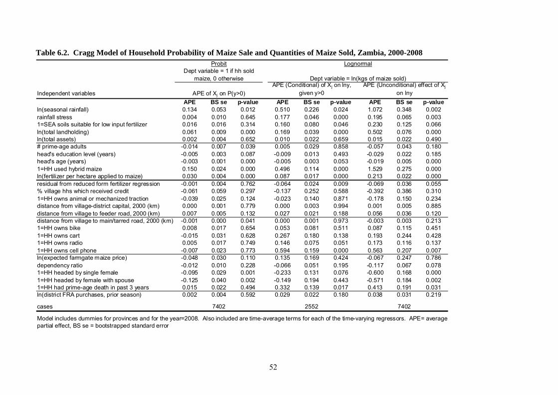
52

Table 6.2. Cragg Model of Household Probability of Maize Sale and Quantities of Maize Sold, Zambia, 2000-2008


ln(seasonal rainfall) 0.134 0.053 0.012 0.510 0.226 0.024 1.072 0.348 0.002rainfall stress 0.004 0.010 0.645 0.177 0.046 0.000 0.195 0.065 0.0031=SEA soils suitable for low input fertilizer 0.016 0.016 0.314 0.160 0.080 0.046 0.230 0.125 0.066ln(total landholding) 0.061 0.009 0.000 0.169 0.039 0.000 0.502 0.076 0.000ln(total assets) 0.002 0.004 0.652 0.010 0.022 0.659 0.015 0.022 0.490# prime-age adults -0.014 0.007 0.039 0.005 0.029 0.858 -0.057 0.043 0.180head's education level (years) -0.005 0.003 0.087 -0.009 0.013 0.493 -0.029 0.022 0.185head's age (years) -0.003 0.001 0.000 -0.005 0.003 0.053 -0.019 0.005 0.0001=HH used hybrid maize 0.150 0.024 0.000 0.496 0.114 0.000 1.529 0.275 0.000ln(fertilizer per hectare applied to maize) 0.030 0.004 0.000 0.087 0.017 0.000 0.213 0.022 0.000residual from reduced form fertilizer regression -0.001 0.004 0.762 -0.064 0.024 0.009 -0.069 0.036 0.055% village hhs which received credit -0.061 0.059 0.297 -0.137 0.252 0.588 -0.392 0.386 0.3101=HH owns animal or mechanized traction -0.039 0.025 0.124 -0.023 0.140 0.871 -0.178 0.150 0.234distance from village-district capital, 2000 (km) 0.000 0.001 0.779 0.000 0.003 0.994 0.001 0.005 0.885distance from village to feeder road, 2000 (km) 0.007 0.005 0.132 0.027 0.021 0.188 0.056 0.036 0.120distance from village to main/tarred road, 2000 (km) -0.001 0.000 0.041 0.000 0.001 0.973 -0.003 0.003 0.2131=HH owns bike 0.008 0.017 0.654 0.053 0.081 0.511 0.087 0.115 0.4511=HH owns cart -0.015 0.031 0.628 0.267 0.180 0.138 0.193 0.244 0.4281=HH owns radio 0.005 0.017 0.749 0.146 0.075 0.051 0.173 0.116 0.1371=HH owns cell phone -0.007 0.023 0.773 0.594 0.159 0.000 0.563 0.207 0.007ln(expected farmgate maize price) -0.048 0.030 0.110 0.135 0.169 0.424 -0.067 0.247 0.786dependency ratio -0.012 0.010 0.228 -0.066 0.051 0.195 -0.117 0.067 0.0781=HH headed by single female -0.095 0.029 0.001 -0.233 0.131 0.076 -0.600 0.168 0.0001=HH headed by female with spouse -0.125 0.040 0.002 -0.149 0.194 0.443 -0.571 0.184 0.0021=HH had prime-age death in past 3 years 0.015 0.022 0.494 0.332 0.139 0.017 0.413 0.191 0.031ln(district FRA purchases, prior season) 0.002 0.004 0.592 0.029 0.022 0.180 0.038 0.031 0.219

cases 7402 2552 7402

Model includes dummies for provinces and for the year=2008. Also included are time-average terms for each of the time-varying regressors. APE= average partial effect, BS se = bootstrapped standard error

Probit Lognormal



on lny


53

6.2.2. Rainfall and Drought Shocks At the national level, seasonal rainfall has a significant though relatively small effect on probability of maize sale, as a 1% increase in rainfall leads to a 0.1 point increase in probability of sale; thus a 10% increase in rainfall leads to a 1 point increase (Table 6.2.). Given that approximately 31% of rural households sold maize across the panel years, a 10% increase in rainfall would improve probability of sale by 3.2%. Seasonal rainfall has significant and larger effects on quantities sold, as a 1% increase in rainfall leads to a 0.5% increase quantity sold by current sellers (conditional quantity) and a 1.0% increase in quantities sold by the average household (sellers and non-sellers). The effects of drought stress on maize sales are contrary to expectation, as we find a significant positive effect of drought stress on both conditional and unconditional quantities sold, at the national level (Table 6.2.). When we analyze the APE of drought stress by AEC zone (using separate zonal regressions), we also fail to find the expected negative and significant effect of this factor on the probability of maize sale or sale quantities. One explanation for not finding a negative effect of drought stress on maize sales could be that the rainfall and drought stress variables have a relatively high correlation (-0.57), though even if we drop the rainfall variables, drought stress still does not have a significant negative effect on sales. Given that rainfall has such a strong positive effect on maize sales, this suggests that our stress variable is somehow not a good measure of drought stress. Another explanation could be that in areas which receive drought shocks, higher post-harvest prices lead net buyer and small net seller households to hold on to their maize rather than selling some, in anticipation of higher retail prices in the future.

6.2.3. Household Productive Assets At the national level, total household landholding has a significant though relatively small effect on the probability of selling maize in Zambia, as a 1% increase in landholding increases the probability of selling maize by 0.06 points (Table 6.3a.). This means that a 10% increase in landholding would increase the probability of selling by 0.6 points, which amounts to approximately a 1.9% increase in probability of sale.

Marginal changes in landholding also have significant and large effects on sales quantities (both conditional and unconditional), as a 1% increase in landholding increases maize sold by current sellers (conditional effect) by 0.16%, and maize sold by any household (unconditional effect) by 0.5% (Tables 6.3a, b.). These results demonstrate the importance of landholding in explaining maize sales behavior in the case of Zambia. As in Mozambique, the importance of landholding in agricultural production in Zambia is magnified by the fact that very few Zambian households rent or borrow land (in 2008, 1.4% rented land and 2% borrowed), and improved input use is relatively low (in 2008, 33% of households use fertilizer on maize, 27% use hybrid maize seed, and 36% used animal or mechanized traction). We next run separate regressions by each agro-ecological (AEC) zone, hypothesizing that the marginal effects of landholding are larger in higher potential zones. Contrary to this expectation, we find the magnitude of effects of marginal changes in landholding on probability of sale are similar across the zones (Table 6.3a.), as are effects on conditional and unconditional quantities (Tables 6.3b. and c). It’s possible that the lack of significant partial effects of landholding in these zones is due to their relatively small sample sizes.

54


quartile APE BSE p-valueLow 0.052 0.038 0.178 1- low 0.093 0.028 0.001

Medium-1 0.056 0.018 0.002 2 0.031 0.027 0.247Medium-2 0.051 0.027 0.057 3 0.073 0.020 0.000

High 0.051 0.017 0.003 4 - high 0.026 0.017 0.114National 0.061 0.009 0.000 National 0.061 0.009 0.000




APE p-valueLow 0.218 0.244 0.453 1- low 0.140 0.150 0.433

Medium-1 0.271 0.311 0.000 2 0.376 0.457 0.004Medium-2 -0.007 -0.007 0.987 3 0.133 0.142 0.183






Medium-1 0.519 0.681 0.000 2 0.669 0.951 0.001Medium-2 0.636 0.889 0.230 3 0.487 0.628 0.000



Table 6.3a. APE of log landholding on probability of maize sale, by AEC zone and by landholding quartile, Zambia

Table 6.3c. APE of log landholding on log quantity of maize sold (unconditional), by AEC zone and by landholding quartile, Zambia

Table 6.3b. APE of log landholding on log quantity of maize sold (conditional), by AEC zone and by landholding quartile, Zambia

When we run separate regressions on subsamples of landholding quartiles, we find that there is no evidence of increasing returns to landholding with respect to probability of sale or conditional and unconditional quantities sold (Table 6.3a, b, c.). In fact, the results suggest the opposite, as the APE of landholding on probability of sale for the lowest landholding quartile is significantly larger than that of the APE for the highest quartile (p=0.04). This finding is consistent with the fact that households in the lowest landholding quartile are about one-half as likely to use fertilizer on maize relative to household in the highest quartile, and one-third as likely to use hybrid seed – thus extensification is their most likely means for increasing maize production and thus probability of maize sale.

6.2.4. Technology Use Fertilizer: At the national level, a 1% increase in fertilizer use on maize leads to a small though significant increase in probability of sale of 0.03 points (Table 6.4a.). Given that 31% of households currently sell maize, a 10% increase in fertilizer would increase probability of sale by approximately 0.9%. A 1% increase in fertilizer use also leads to significant 0.08% increase in quantity sold by current sellers (conditional) and a 0.2% increase by any given household (unconditional) (Tables 6.4a, c.). Thus, a 10% increase in fertilizer use on maize would increase conditional sale quantity by 0.8% and unconditional quantities by 2%. The fact that the quantity effect among all households (both current sellers and non-sellers – the unconditional effect) is considerably larger than the effect among current sellers (conditional effect) suggests that much of the unconditional quantity effect is due to increased

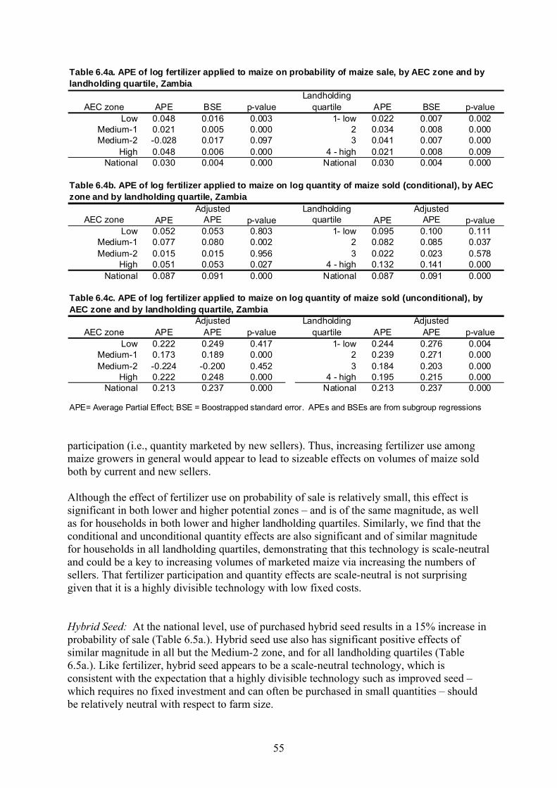
55



Medium-1 0.021 0.005 0.000 2 0.034 0.008 0.000Medium-2 -0.028 0.017 0.097 3 0.041 0.007 0.000






Medium-1 0.077 0.080 0.002 2 0.082 0.085 0.037Medium-2 0.015 0.015 0.956 3 0.022 0.023 0.578






Medium-1 0.173 0.189 0.000 2 0.239 0.271 0.000Medium-2 -0.224 -0.200 0.452 3 0.184 0.203 0.000



Table 6.4a. APE of log fertilizer applied to maize on probability of maize sale, by AEC zone and by landholding quartile, Zambia

Table 6.4c. APE of log fertilizer applied to maize on log quantity of maize sold (unconditional), by AEC zone and by landholding quartile, Zambia

Table 6.4b. APE of log fertilizer applied to maize on log quantity of maize sold (conditional), by AEC zone and by landholding quartile, Zambia

participation (i.e., quantity marketed by new sellers). Thus, increasing fertilizer use among maize growers in general would appear to lead to sizeable effects on volumes of maize sold both by current and new sellers. Although the effect of fertilizer use on probability of sale is relatively small, this effect is significant in both lower and higher potential zones – and is of the same magnitude, as well as for households in both lower and higher landholding quartiles. Similarly, we find that the conditional and unconditional quantity effects are also significant and of similar magnitude for households in all landholding quartiles, demonstrating that this technology is scale-neutral and could be a key to increasing volumes of marketed maize via increasing the numbers of sellers. That fertilizer participation and quantity effects are scale-neutral is not surprising given that it is a highly divisible technology with low fixed costs. Hybrid Seed: At the national level, use of purchased hybrid seed results in a 15% increase in probability of sale (Table 6.5a.). Hybrid seed use also has significant positive effects of similar magnitude in all but the Medium-2 zone, and for all landholding quartiles (Table 6.5a.). Like fertilizer, hybrid seed appears to be a scale-neutral technology, which is consistent with the expectation that a highly divisible technology such as improved seed – which requires no fixed investment and can often be purchased in small quantities – should be relatively neutral with respect to farm size.

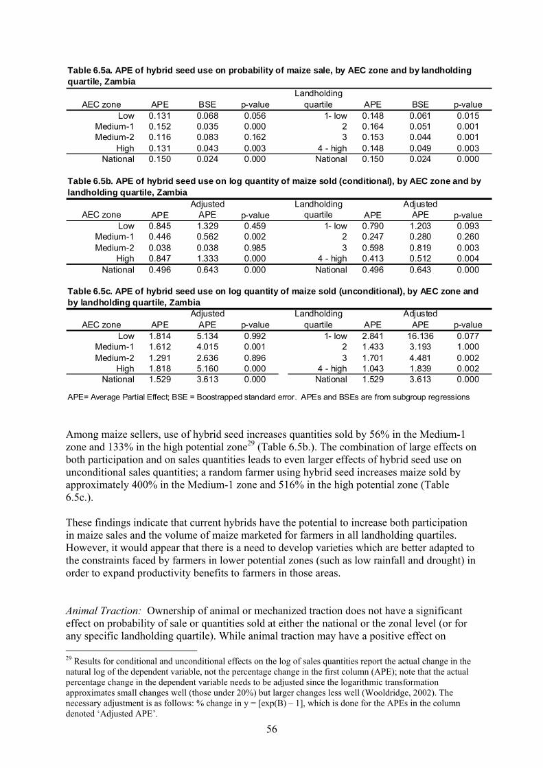
56



Medium-1 0.152 0.035 0.000 2 0.164 0.051 0.001Medium-2 0.116 0.083 0.162 3 0.153 0.044 0.001






Medium-1 0.446 0.562 0.002 2 0.247 0.280 0.260Medium-2 0.038 0.038 0.985 3 0.598 0.819 0.003






Medium-1 1.612 4.015 0.001 2 1.433 3.193 1.000Medium-2 1.291 2.636 0.896 3 1.701 4.481 0.002



Table 6.5a. APE of hybrid seed use on probability of maize sale, by AEC zone and by landholding quartile, Zambia

Table 6.5c. APE of hybrid seed use on log quantity of maize sold (unconditional), by AEC zone and by landholding quartile, Zambia

Table 6.5b. APE of hybrid seed use on log quantity of maize sold (conditional), by AEC zone and by landholding quartile, Zambia

Among maize sellers, use of hybrid seed increases quantities sold by 56% in the Medium-1 zone and 133% in the high potential zone29 (Table 6.5b.). The combination of large effects on both participation and on sales quantities leads to even larger effects of hybrid seed use on unconditional sales quantities; a random farmer using hybrid seed increases maize sold by approximately 400% in the Medium-1 zone and 516% in the high potential zone (Table 6.5c.). These findings indicate that current hybrids have the potential to increase both participation in maize sales and the volume of maize marketed for farmers in all landholding quartiles. However, it would appear that there is a need to develop varieties which are better adapted to the constraints faced by farmers in lower potential zones (such as low rainfall and drought) in order to expand productivity benefits to farmers in those areas. Animal Traction: Ownership of animal or mechanized traction does not have a significant effect on probability of sale or quantities sold at either the national or the zonal level (or for any specific landholding quartile). While animal traction may have a positive effect on 29 Results for conditional and unconditional effects on the log of sales quantities report the actual change in the natural log of the dependent variable, not the percentage change in the first column (APE); note that the actual percentage change in the dependent variable needs to be adjusted since the logarithmic transformation approximates small changes well (those under 20%) but larger changes less well (Wooldridge, 2002). The necessary adjustment is as follows: % change in y = [exp(B) – 1], which is done for the APEs in the column denoted ‘Adjusted APE’.

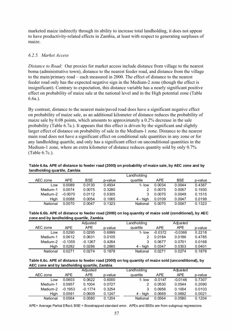
57

marketed maize indirectly through its ability to increase total landholding, it does not appear to have productivity-related effects in Zambia, at least with respect to generating surpluses of maize. 6.2.5. Market Access Distance to Road: Our proxies for market access include distance from village to the nearest boma (administrative town), distance to the nearest feeder road, and distance from the village to the main/primary road – each measured in 2000. The effect of distance to the nearest feeder road only has the expected negative sign in the Medium-2 zone (though the effect is insignificant). Contrary to expectation, this distance variable has a nearly significant positive effect on probability of maize sale at the national level and in the High potential zone (Table 6.6a.). By contrast, distance to the nearest main/paved road does have a significant negative effect on probability of maize sale, as an additional kilometer of distance reduces the probability of maize sale by 0.08 points, which amounts to approximately a 0.2% decrease in the sale probability (Table 6.7a.). It appears that this effect is driven by the significant and slightly larger effect of distance on probability of sale in the Medium-1 zone. Distance to the nearest main road does not have a significant effect on conditional sale quantities in any zone or for any landholding quartile, and only has a significant effect on unconditional quantities in the Medium-1 zone, where an extra kilometer of distance reduces quantity sold by only 0.7% (Table 6.7c.).



Medium-1 0.0074 0.0075 0.3280 2 0.0075 0.0057 0.1930Medium-2 -0.0070 0.0112 0.5305 3 0.0070 0.0049 0.1515





APE p-valueLow 0.0290 0.0295 0.6999 1- low -0.0372 -0.0366 0.2218

Medium-1 0.0612 0.0631 0.0105 2 0.0184 0.0186 0.4785Medium-2 -0.1355 -0.1267 0.4264 3 0.0677 0.0701 0.0168






Medium-1 0.0957 0.1004 0.0727 2 0.0530 0.0544 0.2090Medium-2 -0.1953 -0.1774 0.3254 3 0.0956 0.1004 0.0103



Table 6.6a. APE of distance to feeder road (2000) on probability of maize sale, by AEC zone and by landholding quartile, Zambia

Table 6.6c. APE of distance to feeder road (2000) on log quantity of maize sold (unconditional), by AEC zone and by landholding quartile, Zambia

Table 6.6b. APE of distance to feeder road (2000) on log quantity of maize sold (conditional), by AEC zone and by landholding quartile, Zambia

58


quartile APE BSE p-valueLow 0.0001 0.0066 0.9820 1- low -0.0003 0.0005 0.5705

Medium-1 -0.0014 0.0004 0.0016 2 -0.0014 0.0005 0.0031Medium-2 -0.0021 0.0031 0.4868 3 -0.0013 0.0004 0.0011

High 0.0002 0.0005 0.6842 4 - high -0.0005 0.0004 0.2706National -0.0008 0.0004 0.0406 National -0.0008 0.0004 0.0406




APE p-valueLow -0.0005 -0.0005 0.9900 1- low 0.0027 0.0027 0.4325

Medium-1 -0.0009 -0.0009 0.6469 2 0.0032 0.0032 0.1381Medium-2 0.0185 0.0187 0.6580 3 -0.0031 -0.0031 0.1102

High -0.0004 -0.0004 0.8740 4 - high 0.0012 0.0012 0.4858National 0.0000 0.0000 0.9725 National 0.0000 0.0000 0.9725





Medium-1 -0.0074 -0.0074 0.0350 2 -0.0033 -0.0033 0.3433Medium-2 0.0004 0.0004 0.9943 3 -0.0084 -0.0083 0.0020

High 0.0004 0.0004 0.9134 4 - high -0.0002 -0.0002 0.9387National -0.0035 -0.0035 0.2134 National -0.0035 -0.0035 0.2134


Table 6.7a. APE of distance to main road (2000) on probability of maize sale, by AEC zone and by landholding quartile, Zambia

Table 6.7c. APE of distance to main road (2000) on log quantity of maize sold (unconditional), by AEC zone and by landholding quartile, Zambia

Table 6.7b. APE of distance to main road (2000) on log quantity of maize sold (conditional), by AEC zone and by landholding quartile, Zambia

To date, studies of marketed surplus of maize or food grains in Sub-Saharan Africa which have included proxy variables for transaction costs (two from Kenya, one from Senegal) have found distance to the nearest road or town to have a significant and negative effect on probability of sale (Goetz 1992; Renkow, Hallstrom, and Karanja 2004; Alene et al. 2007), even when local farmgate sales prices are also included in the model. However, recent field work from Zambia suggests two reasons why the results for our market access proxy variables from the Zambia data for 2000-2008 are insignificant or of negligible magnitude.30 First, in nearly all the villages interviewed, maize sellers reported that 20 or more traders had visited the village during the post-harvest period. This suggests that, while significant transport costs to market may still exist, farmers likely face lower search costs for price information, as compared with the situation 5-10 years earlier. Thus, while a variable such as distance to road, market, or public transport may have served well as a proxy for the transaction costs of market access (i.e., access to multiple traders) in previous years, we suspect that the apparent increase in trader access in many villages explains why this transaction cost proxy is no longer significant in our probit of maize sale in Zambia.

30 This field work was implemented by the Food Security Group of the Department of Agricultural, Food, and Resource Economics of Michigan State University as part of a maize value chain study in Zambia for the Guiding Investments for Sustainable Agricultural Markets in Africa project, funded by the Bill & Melinda Gates Foundation.

59

Note that because district-median farmgate sales price is also included in our model, transport costs should be included in this observed price.31 Second, according to maize traders interviewed in recent focus group research, the proliferation of cell phones in rural Zambia since approximately 2004 has dramatically reduced the risk involved in assembly of small amounts of maize from remote villages, because cell phones substantially reduce the search costs involved in locating bags of maize. This is consistent with Overå’s (2006) research from Ghana, which found that mobile phones are lowering the transaction costs of interactions over dispersed areas: discovery and exchange of information, negotiation, and monitoring. For example, instead of having to drive from village to village to search for bags of maize, larger traders simply wait for a cell phone call from small traders at the village level, who call these larger traders only after they have already gathered a certain number of bags of maize. If roads to a given remote village are poor, there is no way to avoid higher transport costs to and from that village, but knowing ahead of time of that a certain quantity of maize is ready and available for pick-up dramatically lowers the risk of sourcing maize from that village. It would appear that lower trading risk has subsequently lowered the barriers to entry for trading in both small and large quantities, which would help to explain why maize farmers interviewed in focus groups note a large increase in the number of traders visiting their village in recent years. Bicycle and Cart Ownership: Ownership of a bicycle only has a significant effect on probability of maize sale in the relatively small Medium-2 zone, where a bicycle improves probability of sale by 14% (Table 6.8a.). We also find that bicycle ownership improves probability of sale by 6% for those in the top landholding quartile (Table 6.8a.). Given that we found fertilizer and hybrid use to be scale-neutral with respect to the effect of these technologies on probability of maize sale, it is difficult to explain the insignificance and very low magnitude of the effects of bicycle ownership on probability of sale for households in lower landholding quartiles, as even 34% of households in the lowest quartile own a bike. Bicycle ownership does not have a significant effect on either conditional or unconditional quantities at the national or zonal level, or for any specific landholding quartile. Cart ownership does not have a significant positive effect on either probability of sale or quantities sold at the national or zonal level, or for any landholding quartile. Combined with the lack of significant results from bicycle ownership, this suggests that the transaction costs related with searching for and locating a buyer for a household’s maize do not appear to be very high in Zambia. This is consistent with the recent rapid appraisal work in Zambia (cited above) which found most villages to have received visits from a large number of traders during the post-harvest period. That is, ownership of transportation assets does not significantly improve a farmer’s probability of selling maize if trader presence in villages is strong. This is not to say that transportation costs between markets and more remote villages are relatively higher than those for more accessible villages – but because 68% of Zambian farmers sold their maize in the village in 2004, our expected price variable already captures the transport costs between most villages and their relevant markets.

31 Our price variable, district-median farmgate sales price, likely captures the transport costs between most villages and their relevant markets given 68% of farmers sold in the village in 2004, and over 90% of rural households live in a village where there was at least one seller. Nevertheless, there were 50 of 387 villages which had no observed maize seller, thus our district price may not reflect transport costs to those villages (which one would assume might be relatively remote).

60



Medium-1 -0.023 0.027 0.395 2 0.002 0.031 0.941Medium-2 0.142 0.083 0.087 3 0.024 0.036 0.501






Medium-1 0.085 0.088 0.467 2 0.112 0.119 0.474Medium-2 -0.199 -0.180 0.896 3 0.110 0.116 0.484

High -0.113 -0.107 0.468 4 - high -0.104 -0.099 0.495National 0.053 0.055 0.511 National 0.053 0.055 0.511





Medium-1 -0.021 -0.021 0.912 2 0.124 0.132 0.640Medium-2 1.120 2.065 0.915 3 0.210 0.233 0.374



Table 6.8a. APE of bike ownership on probability of maize sale, by AEC zone and by landholding quartile, Zambia

Table 6.8c. APE of bike ownership on log quantity of maize sold (unconditional), by AEC zone and by landholding quartile, Zambia

Table 6.8b. APE of bike ownership on log quantity of maize sold (conditional), by AEC zone and by landholding quartile, Zambia

Access to Market Price Information: Another type of transaction cost, which may reduce market participation, is the cost of searching for market price information. We would expect that access to low-cost market price information, such as that provided via radio broadcast in rural Zambia, would improve farmer’s bargaining power with intermediaries, improve farmgate price offers for maize, and therefore increase both the probability of sale and sales quantities. Using radio ownership as a proxy for access to market price information, we find that radio ownership does not have a significant effect on probability of maize sale at the national or regional level, or for any specific landholding quartile (Table 6.9a.). However, radio ownership does have a significant effect on conditional sales, increasing quantity sold by current sellers by 15% (Table 6.9b.).

61



Medium-1 -0.025 0.026 0.345 2 0.025 0.034 0.466Medium-2 -0.002 0.046 0.974 3 0.026 0.034 0.443

High 0.020 0.032 0.530 4 - high -0.014 0.035 0.693National 0.005 0.017 0.749 National 0.005 0.017 0.749





Medium-1 -0.044 -0.043 0.720 2 0.176 0.193 0.253Medium-2 0.231 0.260 0.794 3 0.026 0.026 0.840






Medium-1 -0.160 -0.148 0.415 2 0.303 0.354 0.295Medium-2 0.222 0.249 0.971 3 0.131 0.139 0.499



Table 6.9a. APE of radio ownership on probability of maize sale, by AEC zone and by landholding quartile, Zambia

Table 6.9c. APE of radio ownership on log quantity of maize sold (unconditional), by AEC zone and by landholding quartile, Zambia

Table 6.9b. APE of radio ownership on log quantity of maize sold (conditional), by AEC zone and by landholding quartile, Zambia

We also use household cell phone ownership as a proxy for receipt of market price information, and find that it does not have a significant effect on probability of maize sale (Table 6.10a.). However, cell ownership has a significant and large effect on conditional and unconditional sale quantities, increasing conditional sales by 81% and unconditional sales by 76% (Tables 6.10b, c.). We also find that effects of cell ownership on conditional quantity sold are only significant for households in the top two landholding quartiles, which suggests that only sellers with relatively more land produce enough maize to be able to take advantage of access to market price information.

62



Medium-1 0.001 0.034 0.972 2 -0.037 0.049 0.449Medium-2 0.155 0.123 0.207 3 -0.021 0.044 0.633






Medium-1 0.708 1.029 0.004 2 0.223 0.250 0.394Medium-2 -0.654 -0.480 0.993 3 1.140 2.126 0.007






Medium-1 0.739 1.093 0.055 2 0.026 0.027 0.949Medium-2 0.139 0.149 1.000 3 1.001 1.722 0.055



Table 6.10a. APE of cell phone ownership on probability of maize sale, by AEC zone and by landholding quartile, Zambia

Table 6.10c. APE of cell phone ownership on log quantity of maize sold (unconditional), by AEC zone and by landholding quartile, Zambia

Table 6.10b. APE of cell phone ownership on log quantity of maize sold (conditional), by AEC zone and by landholding quartile, Zambia

Maize Purchases by the Food Reserve Agency: Our results show that farmer expectations of the district-level FRA volume of maize purchase do not have a significant effect on probability of maize sale at the national or zonal level, or for any specific landholding quartile (Table 6.11a.). While the effect of expected FRA purchases on probability of sale is nearly significant (p=0.11) for the top landholding quartile, the magnitude of this effect is quite small; a 10% increase in expected purchase volume increases probability of sale by 0.12 points, which amounts to only a 0.2% increase in probability of sale. Expected FRA purchase volume does not have a significant effect on conditional or unconditional sale quantities at the national or zonal levels. The only significant quantity effect is found among households in the lowest quartile, where a 10% increase in expected FRA purchase volume leads to a 1% increase in quantity sold among sellers. The lack of significant effects of expected FRA purchase volumes on either probability of sale or quantity sold – as well as the negligible effects which are found to be significant (or nearly so) – may be due to the fact that expected FRA purchases are already included as a regressor in our household farmgate price expectation model, in which it has a significant positive effect (though quite small, as a 1% increase in expected FRA purchase volume only increases the expected farmgate maize price by 0.02%). Another explanation for the lack of an effect of expected FRA purchases on maize sales could be that our relatively simple price expectation model is not as theoretically or empirically appropriate as the rather complicated one developed by Mason (2011b).

63


quartile APE BSE p-valueLow -0.015 0.070 0.832 1- low -0.003 0.006 0.570

Medium-1 0.031 0.020 0.126 2 0.010 0.008 0.234Medium-2 -0.035 0.040 0.390 3 -0.007 0.009 0.392

High -0.015 0.010 0.136 4 - high 0.012 0.007 0.115National 0.002 0.004 0.592 National 0.002 0.004 0.592





Medium-1 0.011 0.011 0.875 2 0.031 0.032 0.447Medium-2 -0.075 -0.073 0.870 3 0.032 0.032 0.367






Medium-1 0.155 0.168 0.318 2 0.076 0.079 0.190Medium-2 -0.368 -0.308 0.609 3 0.003 0.003 0.957



Table 6.11a. APE of log of district FRA purchase per maize hectares on probability of maize sale, by AEC zone and by landholding quartile, Zambia

Table 6.11c. APE of log of district FRA purchase per maize hectares on log quantity of maize sold (unconditional), by AEC zone and by landholding quartile, Zambia

Table 6.11b. APE of log of district FRA purchase per maize hectares on log quantity of maize sold (conditional), by AEC zone and by landholding quartile, Zambia

6.2.6. Farmgate Maize Price Our findings on the APE of the log of expected farmgate maize sales price on probability of sale appear at first glance to be contradictory (Table 6.12a.). For example, while we find that the expected maize price has a nearly significant (p=0.11) negative effect on probability of sale at the national level, the signs of the price effect from each AEC zone regression are all positive – and even significant in the large Medium-1 zone. In addition, the price effects on sale probability for each landholding quartile are negative. Another puzzling result is that we find negative price response both for households in the second landholding quartile (which is not unexpected, as per the discussion in Section 4.1.) and for those in the top quartile (which is unexpected). However, there is an important element of consistency across these results in that the regression samples which include households from across the country (those at the national level and for each of the landholding quartiles) all show a negative price effect, while those at the regional level (AEC zones) are all positive. Why this is the case is not clear, as the negative response at the national level is robust to various alternative specifications such as dropping provincial dummies and rain variables, interacting provincial dummies with the time dummy, etc. Secondly, there is clear evidence of significant positive responsiveness of the quantities sold by households to higher expected maize prices in the largest two AEC zones.

64



Medium-1 0.107 0.065 0.100 2 -0.115 0.048 0.017Medium-2 0.345 0.463 0.456 3 -0.002 0.055 0.975






Medium-1 0.317 0.374 0.231 2 -0.078 -0.075 0.751Medium-2 -0.990 -0.628 0.851 3 0.113 0.120 0.700






Medium-1 0.818 1.266 0.086 2 -0.608 -0.456 0.072Medium-2 1.934 5.914 0.796 3 0.106 0.112 0.771

High 2.187 7.904 0.005 4 - high 0.042 0.042 0.903National -0.067 -0.065 0.786 National -0.067 -0.065 0.786


Table 6.12a. APE of log expected farmgate maize price on probability of maize sale, by AEC zone and by landholding quartile, Zambia

Table 6.12c. APE of log expected farmgate maize price on log quantity of maize sold (unconditional), by AEC zone and by landholding quartile, Zambia

Table 6.12b. APE of log expected farmgate maize price on log quantity of maize sold (conditional), by AEC zone and by landholding quartile, Zambia

For example, households in the High potential zone respond to a 1% increase in the expected maize price by increasing the conditional (unconditional) quantity sold by 4.2% (7.9%), while those in the Medium-1 zone increase unconditional quantity sold by 1.2% (Tables 6.12b, c.). What seems clear from these results is that there is considerably heterogeneity of household responsiveness to expected maize prices across rural Zambia. On the one hand, households in the Medium-1 and High potential zones behave as we would expect more commercially-oriented farmers to behave, as they appear to increase their probability of maize sale and/or quantities sold in response to higher expected maize prices. On the other hand, many households in the Low and Medium-2 potential region appear to have a combination of low (positive) supply response and a strong preference for stock-holding to minimize food market risk (i.e., a negative response to price), which combine to result in little to no positive household responsiveness to higher expected maize prices.

6.2.7. Gender and Household Demographics There is no evidence that households with better-educated heads are more likely to sell maize or to sell larger quantities. However, we do find that, relative to male-headed households, households headed by a single female are 9.5% less likely to sell maize, and have lower conditional and unconditional sale quantities (20% and 45% less, respectively) (Tables 6.13a, b, c.).

65


quartile APE BSE p-valueLow -0.056 0.070 0.423 1- low -0.063 0.050 0.210

Medium-1 -0.125 0.039 0.001 2 -0.071 0.062 0.250Medium-2 -0.025 0.091 0.785 3 -0.091 0.050 0.070

High -0.056 0.062 0.365 4 - high -0.186 0.069 0.007National -0.095 0.029 0.001 National -0.095 0.029 0.001





Medium-1 -0.363 -0.304 0.029 2 -0.487 -0.386 0.049Medium-2 0.041 0.042 1.000 3 -0.269 -0.236 0.199

High -0.391 -0.324 0.031 4 - high -0.284 -0.247 0.228National -0.233 -0.208 0.076 National -0.233 -0.208 0.076




APE p-valueLow -0.564 -0.431 1.000 1- low -0.257 -0.226 0.639

Medium-1 -0.912 -0.598 0.001 2 -0.782 -0.542 0.052Medium-2 -0.170 -0.157 1.000 3 -0.574 -0.437 0.037

High -0.569 -0.434 0.056 4 - high -0.741 -0.523 0.002National -0.600 -0.451 0.000 National -0.600 -0.451 0.000


Table 6.13a. APE of binary indicator that household is headed by a single female on probability of maize sale, by AEC zone and by landholding quartile, Zambia

Table 6.13c. APE of binary indicator that household is headed by a single female on log quantity of maize sold (unconditional), by AEC zone and by landholding quartile, Zambia

Table 6.13b. APE of binary indicator that household is headed by a single female on log quantity of maize sold (conditional), by AEC zone and by landholding quartile, Zambia

We also find that households headed by a female with a resident spouse are 12% less likely to sell maize and have lower unconditional sale quantities (43% less). Descriptive results in section 8.6 show that while households headed by a single female in Zambia have similar landholding and maize area planted, they are less likely to use fertilizer and hybrids and produce considerably less maize per AE than male-headed households. Given that we are already separately controlling for both time-variant and time-average landholding, head’s education level, input use, dependency ratio, etc., this suggests that households headed by a single female have less technical knowledge of maize production relative to male-headed households or that these households farm fields with lower quality soils and/or fewer fallows. Further research using this household survey data or perhaps qualitative methods would be required to investigate why these households produce less maize/AE and are less likely to sell maize.

6.3. Conclusions There are eight primary findings from our econometric analysis of maize market participation by households in rural Zambia. First, given that nearly all maize production in Zambia is rainfed, it is not surprising that we find that households in zones of higher agro-ecological potential are more likely to sell maize, even after controlling for household landholding, input use, etc. In addition, we find that a 1% increase in seasonal rainfall leads to 0.5% increase in quantity sold by current sellers and a 1.0% increase in quantities sold by the average household (sellers and non-sellers). These results suggest an important role for agricultural

66

research and extension with respect to the development and dissemination of drought-resistant maize varieties, as well as widespread promotion of smallholder access to low-cost methods of irrigation and/or conservation farming techniques. Second, marginal increases in total household landholding have significant though relatively small effects on probability of sale, as a 10% increase in landholding would elicit a 1.9% increase in probability of sale. Marginal increases in landholding also lead to significant and relatively large increases in conditional and unconditional quantities sold, as a 1% increase in landholding would elicit a 0.2% increase in quantities sold by current sellers and a 0.65% increase in quantities sold by any given household. These partial effects are significant for households from both lower and higher landholding quartiles, which suggest that increasing household landholding in Zambia could play an important role in increasing quantities of marketed maize, given that Zambia has large uncultivated tracts of land that could be settled by smallholders. However, migration and settlement of uncultivated areas would require not only a legal mechanism to transfer land rights from current owners (state and other) to migrants, but also complementary public goods such as social services (schools, health clinics) and road infrastructure which could link such areas to markets (Jayne et al. 2008). Third, we find that marginal increases in fertilizer applied to maize have relatively small effects on the probability of sale and quantities sold by current sellers, as a 10% increase in fertilizer applied to maize would increase probability of sale by about 0.9% and quantity sold by 0.8%. Fertilizer has larger effects on unconditional quantities sold, as a 10% increase in fertilizer use increases quantity sold by any given household by 2%. Although these quantity effects are only significant in medium and higher-potential zones, we find that fertilizer use is scale-neutral as it has a significant positive effect on probability of sale and quantities sold for households in every landholding quartile. Fourth, household use of purchased hybrid maize seed has large and significant effects on probability of sale in low, medium and high potential zones, increasing sale probability by 15% at the national level. Hybrid seed use also increases conditional (unconditional) quantities sold by 56% (400%) in the Medium-1 zone and by 130% (516%) in the High potential zone. Like fertilizer, we also find that hybrid seed is scale-neutral as it has significant effects on both probability of sale and quantities sold for households in lower and higher landholding quartiles. That fertilizer and hybrid seed are scale-neutral is not surprising as they are highly divisible technologies with very low fixed costs. Fifth, we find minimal evidence that improvements in market access are a key constraint to increasing marketed maize volumes. For example, distance to the nearest feeder road does not have the significant negative effect on probability of sale or quantities sold that we would expect, and its effect in the Medium-1 zone is actually positive (that is, the more inaccessible the village, the higher the probability of maize sale and the larger the quantities sold). By contrast, we find that distance to the nearest main/paved road does have a significant negative effect on probability of maize sale at the national level, though this effect is very small, as a decrease in distance by one kilometer only increases the probability of maize sale by only 0.2%. These inconsistent and/or negligible effects of market access on maize market participation are consistent with recent rapid appraisal work in Zambia (cited above) which found most villages to have received visits from a large number of traders during the post-harvest period. Thus, given increasing small trader presence across rural Zambia in recent years, using traditional measures of access to physical infrastructure to proxy for market access may no longer be useful in defining which villages are remote with respect to access to markets (Chamberlain and Jayne 2011). We also find that there are no significant effects of

67

bicycle ownership or cart ownership on probability of maize sale or quantities sold, which is consistent with the rapid appraisal finding of strong trader presence even in ‘remote’ villages. Sixth, using radio ownership and cell phone ownership as proxies of household access to market price information, we find that neither has a significant effect on probability of maize sale, though radio ownership increases quantity sold by current sellers by 15%, while cell phone ownership increases conditional sale quantities by 81% and unconditional sales by 76%. While more research is warranted to document the link between radio and cell phone ownership and household access to market price information, these results nevertheless suggest that funding to increase the spatial coverage and frequency of radio broadcasts in rural Zambia could potentially lead to large increases in quantities of maize sold. Seventh, we find that farmer expectations of the district-level FRA volume of maize purchase do not have a significant effect on probability of maize sale, and have insignificant or negligible effects on quantities sold. The lack of significant effects of expected FRA purchase volumes may be due to the fact that the effect of expected FRA purchases already operates indirectly through our model of household expectations of farmgate maize prices (though we find that expected FRA purchases have a very small effect on expected farmgate prices). Our lack of large FRA purchase effects on expected prices may also have to do with the simple specification of our expected price model, as Mason (2011b) found relatively larger effects of expected FRA purchase volumes on households’ expected maize prices using a more complex specification. Eighth, we find that there is considerably spatial heterogeneity in household responsiveness of maize market participation to expected farmgate maize prices across rural Zambia. Households in the Medium-1 and High potential zones behave as we would expect more commercially-oriented farmers to behave, as there is some evidence that they increase their probability of maize sale and/or quantities sold in response to higher expected maize prices. By contrast, many households in the Low and Medium-2 potential region appear to have little to no positive household responsiveness of maize market participation to higher expected maize prices. In conclusion, our finding of negligible and/or insignificant responses of household maize market participation to improved market access combined with the lack of significant positive response of smallholders in both lower and medium potential zones, together suggest that non-price factors are vital for increasing maize marketed surplus in Zambia, at this stage of the country’s development. For example, without investments to increase household asset levels (by improving landholding access for the land-poor) and returns to existing assets (by fostering increased adoption rates of inorganic fertilizer and improved maize varieties), it is questionable whether improved input and output prices alone (through additional investment in road infrastructure) will elicit much of a supply response from maize producers who currently do not sell maize (i.e., 69% of maize growers). While road infrastructure may help foster the private sector development of seed and fertilizer markets, there is an important role for the government in developing and disseminating improved maize varieties tailored to the constraints faced in the different agro-ecological zones, as well as in developing recommendations for fertilizer use and low-cost soil management techniques for each agro-ecological zone. Therefore, in order to increase the volumes of marketed maize while also increasing the number of smallholders who sell maize, the Government of Zambia needs an approach which spatially integrates investments in the four CAADP pillars; investments to improve market access (road infrastructure) need to be made together with investments and policies to increase the adoption of improved technologies such as fertilizer and improved

68

maize varieties, to improve landholding sizes of smallholders through public investments necessary to settle currently uncultivated tracts of land, and to expand household access to reports from the agricultural market information system.

69

7. ECONOMETRIC ANALYSIS: KENYA

7.1. Introduction

7.1.1. Explanatory Variables This section describes explanatory variables used in the Kenya econometric analysis that were not already described in the section 4.3.2. The binary dependent variable in the Probit stage of the double-hurdle =1 if the household sold maize, or =0 otherwise. 32 The dependent variable in the lognormal stage is the natural log of maize quantity sold (kgs). To control for spatial variation in agro-ecological potential, we include agro-ecological zone dummies (7 zones, 6 dummies) as well as dummies to indicate the latter two panel survey years (2004 and 2007). Given that most maize production in Kenya is rainfed, we include a village-level measure of drought shock during the main growing season,33 which is the percentage of 20 day periods during the main season with <40mm rain. Using information on soil classification, soil depth, and percentage of sand and clay, we also include three separate dummies for three of the six principal soil types in rural Kenya, categorized by Sheahan (forthcoming) as volcanic soils, humic soils, and rankers with high sand content. Household technology use is measured by various binary variables such as the household owns irrigation equipment, the household purchased maize hybrid seed that season, and the household owned animal or mechanized traction for land preparation. As detailed in section 4.2.3. (Input Use and Improved Technologies), we use the Control Function approach to test for the potential endogeneity of household fertilizer used on maize and use of purchased hybrid maize seed (results below). Distance from the village to the nearest extension agent serves as a proxy for household access to agricultural extension, and the percentage of village households that received credit as a proxy for household credit access. Due to the lack of mortality information in the 1997 Kenya/Tegemeo (first) survey, we set the binary variable for adult mortality to zero for all households in this year. While this will obviously affect the reliability of the partial effect on the mortality dummy, we are including this variable in order to estimate the effect of having a single female head, which is free of any adverse effects due to recent adult mortality. Expected post-harvest farmgate maize prices are computed for each household using the regression method described in 4.2.4. (Farmgate Maize Price Prediction Model and Testing for Potential Sample Selection Bias in Observable Maize Prices) and the model presented in Appendix Table D-1. (and discussed in more detail in Mather and Jayne forthcoming). Throughout the time period covered by the Tegemeo household survey data, the Government of Kenya’s National Cereals and Produce Board (NCPB) has procured and sold maize at administratively determined prices, and stored maize as a contingency against future shortages. During this time, a private sector marketing channel has competed with the NCPB. Because fewer than 1% of smallholders in Kenya sell directly to the NCPB, for the purposes of this paper, our treatment of NCPB activities only involves inclusion of expected NCPB 32 Each country’s survey instrument asks respondents about actual sales as of the date of the survey interview as well as expected sales. As expected sales were not asked in 2007, we define sales for Kenya as actual sales. 33 This rainfall variables are derived from rainfall estimates based on data from satellites (such as on cloud cover and cloud top temperatures) and rain stations, which are combined to interpolate estimates of decadal (10-day period) rainfall, which can be matched to sample households/villages using global positioning system (GPS) coordinates. Rainfall estimates were matched to 1360 households using GPS coordinates, and to the village for the remaining households.

70

purchase volumes as a regressor in our model of farmer price expectations (Appendix Table D-1.). Research on the effects of NCPB maize purchasing activities on household crop production and input use is beyond the scope of this paper and is presented elsewhere (Mather and Jayne forthcoming). Household marketing assets include binary variables for ownership of a bicycle, ownership of a cart, ownership of a vehicle (motorcycle, truck), and ownership of radio (proxy for receipt of market price information). Distance to the nearest motorable road serves as a proxy for transport costs to the relevant market, which declines considerably in many villages between 1997 and 2007. While a limitation of this measure of market access is that it does not account for the costs of transport from the road to the relevant market itself, the majority of the total transport cost to market is likely the segment from the village to the nearest road. Anticipating that average partial effects for some variables may differ by agro-ecological zone, we aggregate agro-ecological zones into three zones, which represent maize-production potential: East and West Lowlands (Low potential), West Transitional, West and Central Highlands (Medium), and the High Potential Maize zone (High). We run the equivalent of a Chow test on the sales equation, which shows that the model coefficients are (jointly) significantly different enough by region to warrant the use of either separate zonal regressions or zonal interaction terms (we run separate zonal regressions). We find the same result when testing for differences among coefficients by quartiles of total landholding (computed for each zone). Thus, we report results from a national regression (not including Coastal cases, which are dropped from the ensuing analyses), and separate regressions for each zone, and for each landholding quartile.

7.1.2. Testing/controlling for Endogeneity of Regressors To test for the potential endogeneity of household quantity of fertilizer applied per hectare of maize, we use the Control Function (CF) approach of Rivers and Vuong (1988), as explained in section 4.2.3. (Handling the Potential Endogeneity of Household Use of Fertilizer and Hybrid Maize Seed). We first estimate a reduced form regression (Tobit) of the household’s quantity of fertilizer applied per hectare of maize. Because we have two potentially endogenous variables in our double-hurdle model of maize sales (hybrid use and fertilizer use on maize), the reduced form regression for each variable includes the instrumental variables for both of them: village median fertilizer price, distance to fertilizer seller, and distance to hybrid seed seller. In the reduced form Tobit regression of fertilizer quantity (Appendix Table D-2.), we find that while fertilizer price does not have a significant effect (p=0.54) on the quantity of fertilizer used, distance to fertilizer has a significant effect (p=0.004) (though is surprisingly positive), and distance to seed seller has a significant negative effect (p=0.001). Following the CF approach, we include both the potentially endogenous variable – quantity of fertilizer used on maize – and the reduced form residual (from the Tobit) in the double-hurdle model of maize sales. Because the coefficient on the reduced form residual is insignificant in both stages of the double-hurdle (p=0.97; p=0.85), we conclude that household fertilizer use on maize is exogenous, and we leave the reduced form Tobit residual out of the double-hurdle model at the national level. However, we do find use of fertilizer on maize is endogenous in the high potential zone and for the 1st and 4th landholding quartiles, thus for these subgroup regressions we control for the endogeneity of this variable by including the Tobit reduced form residual in each regression.

71

We also use the CF approach to test for the potential endogeneity of household use of purchased hybrid maize seed. We first estimate a reduced form regression (Limited Probability Model, i.e., OLS) of a binary variable which =1 if the household used purchased hybrid maize seed that season, =0 otherwise. Because we have two potentially endogenous variables in our double-hurdle model of maize sales (hybrid use and fertilizer use on maize), the reduced form regression for each variable includes the instrumental variables for both of them: village median fertilizer price, distance to fertilizer seller, and distance to hybrid seed seller. In the reduced form LPM regression (Appendix Table D-3.), we find that fertilizer price has a significant effect (p=0.04) on the probability of using purchased hybrid maize seed (though it is surprisingly positive), distance to fertilizer seller has a significant negative effect (p=0.05), and distance to seed seller has a negative effect which is nearly significant (p=0.105). Following the CF approach, we include both the potentially endogenous variable – the binary variable for ‘1=household used purchased hybrid maize seed’ – and the reduced form residual (from the LPM) in the double-hurdle model of maize sales. Because the coefficient on the reduced form residual is insignificant in both stages of the double-hurdle (p=0.71; p=0.70), we conclude that the binary variable for hybrid use is exogenous, and we do not need to leave the reduced form LPM residual out of the double-hurdle model at the national level.34 Summary statistics of all variables used in the auxiliary and double-hurdle models for Kenya are presented in Appendix Table D-4.

7.2. Econometric Results

7.2.1. Agro-ecological Potential Given that most maize production in Kenya is rainfed, and that maize is a staple food crop throughout the country, we would expect that agro-ecological potential would play an important role in maize market participation. To isolate the effect of agro-ecological potential on the probability of maize sale and sale quantities, we run the double-hurdle model described above, dropping the drought shock variable. The results from several zones show that, after controlling for household assets, prices, and market access, agro-ecological potential has significant and large effects on both the probability of selling and amounts sold, conditional on selling (Table 7.1.). For example, relative to the base category (the lower potential zone representing Western Transitional, Western Lowlands and Marginal Rain Shadow), households in the Western Highlands are 13% more likely to sell maize. Effects of agro-ecological potential on probability of sale (relative to the low potential zones) are close to significant for other medium-potential zones such as Western Transitional and Central Highlands. Households in the High Potential Maize Zone are 18% more likely to sell maize, and current sellers (conditional effect) sell 200% more maize, on average. In the results that follow, we include agro-ecological zone dummies as well as village drought shock variables to control for variation in agro-ecological potential.

34 As per Wooldridge (2002), the LPM residual can be used to test for endogeneity in a probit in the CF framework, though if this test finds the variable to be endogenous, the correction entails more than simply leaving the LPM residual in the model.

72

7.2.2. Drought Shocks We would expect to find that external production-related shocks such as drought significantly reduce the probability of selling maize (participation) and the quantities sold (sales). We find that a 20% increase in the percentage of 20-day periods during the main season with less than 40 mm rain leads a significant reduction of 8.8% in probability of sale and a 12.6% reduction in unconditional quantity sold at the national level (Table 7.2.). The effect of the same increase in drought shock on current sellers is nearly significant and suggests a loss of 6.7% in quantity sold. As these results demonstrate, weather-related shocks can reduce the aggregate quantities of maize sold both by lowering the quantity of maize sold by current sellers, and by lowering the probability that any given household (seller or non-seller) sells maize in the first place (i.e., reducing the number of sellers). The unconditional average partial effect of an additional 20-day period of drought stress describes the expected change in maize quantity sold by any given household (i.e., actual sellers or non-sellers) given a change in drought stress frequency during the main season. This effect contains a participation component, which represents the change in sales quantities due to the amount sold by a new seller, and a sales quantity component, which represents the change in sales quantities due to a change in the amount sold by a current seller. Thus, the average effect of increased drought stress frequency on reducing the maize quantity sold by any given household is due both to lowering the probability that the given household sells any maize at all, and to reducing quantities sold, conditional on making a sale.

7.2.3. Household Productive Assets We find that a marginal increase in total household landholding does not have a significant effect (p=0.15) on the probability of selling maize at the national level (Table 3.4a.). Marginal increases in landholding have a significant though small effect on probability of sale in the medium potential zone, as a 1% increase in landholding raises the probability of sale by 0.04 points (Table 7.3a.). Given that about 35% of households in the medium zone sell maize, a 10% increase in landholding raises the probability of sale by 0.4 points, which translates to roughly a 1.1% increase in probability of sale. Marginal changes in landholding have a considerably larger effect on quantities sold, as a 1% increase in landholding increases conditional sales by 0.21% and unconditional sales by 0.27% at the national level (Tables 7.3b, c.). Contrary to what we might expect, these sale quantity effects are considerably larger in the low and medium potential zones relative to the high potential zone. An explanation for this could be that because farmers in the lowest potential zone are less likely to use improved inputs such as hybrid seed and fertilizer, extensification may offer the sole or primary means for increasing production quantities of maize for some of these farmers. However, this would not explain why the conditional APEs from the medium-term zones are at least double those of the high potential zone, because input use rates are somewhat similar between the two zones.

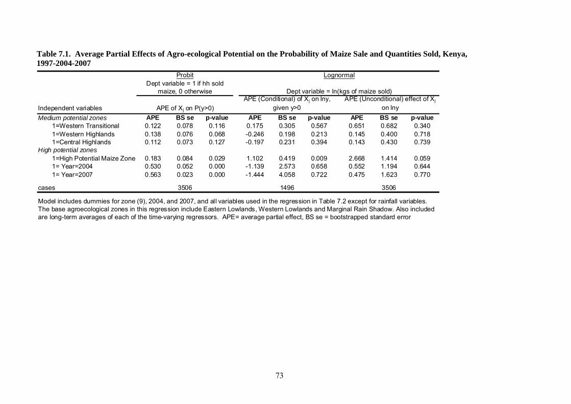
73

Table 7.1. Average Partial Effects of Agro-ecological Potential on the Probability of Maize Sale and Quantities Sold, Kenya, 1997-2004-2007

Independent variablesMedium potential zones APE BS se p-value APE BS se p-value APE BS se p-value

1=Western Transitional 0.122 0.078 0.116 0.175 0.305 0.567 0.651 0.682 0.3401=Western Highlands 0.138 0.076 0.068 -0.246 0.198 0.213 0.145 0.400 0.7181=Central Highlands 0.112 0.073 0.127 -0.197 0.231 0.394 0.143 0.430 0.739

High potential zones1=High Potential Maize Zone 0.183 0.084 0.029 1.102 0.419 0.009 2.668 1.414 0.0591= Year=2004 0.530 0.052 0.000 -1.139 2.573 0.658 0.552 1.194 0.6441= Year=2007 0.563 0.023 0.000 -1.444 4.058 0.722 0.475 1.623 0.770

cases 3506 1496 3506

Model includes dummies for zone (9), 2004, and 2007, and all variables used in the regression in Table 7.2 except for rainfall variables. The base agroecological zones in this regression include Eastern Lowlands, Western Lowlands and Marginal Rain Shadow. Also included are long-term averages of each of the time-varying regressors. APE= average partial effect, BS se = bootstrapped standard error

Probit Lognormal



on lny


74

Table 7.2. Cragg Model of Maize Market Sales Participation and Level of Maize Sold, Kenya, 1997-2004-2007


main season drought shocks -0.185 0.079 0.019 -0.409 0.256 0.109 -1.013 0.351 0.004ln(total area) 0.022 0.015 0.151 0.216 0.069 0.002 0.273 0.086 0.002ln(total assets) -0.006 0.017 0.725 -0.081 0.069 0.238 -0.090 0.070 0.201# prime-age adults -0.009 0.007 0.209 -0.002 0.030 0.959 -0.034 0.040 0.4051=HH owns irrigation equipment 0.065 0.041 0.116 0.261 0.221 0.237 0.528 0.368 0.1511=HH used hybrid maize 0.031 0.020 0.122 0.161 0.092 0.080 0.267 0.108 0.013ln(fertilizer applied to maize) (kg/ha) 0.016 0.007 0.027 0.118 0.027 0.000 0.171 0.035 0.000ln(village agricultural wage) 0.141 0.087 0.104 -0.095 0.200 0.635 0.367 0.351 0.295% village hhs which received credit -0.089 0.074 0.231 -0.389 0.269 0.148 -0.679 0.419 0.1051=HH owns animal or mechanized traction 0.016 0.039 0.686 0.072 0.133 0.587 0.128 0.228 0.575distance from village to nearest extension 0.004 0.007 0.575 -0.007 0.021 0.732 0.005 0.034 0.880head's age (years) 0.004 0.002 0.045 0.001 0.002 0.715 0.014 0.008 0.078maximum adult education (years) 0.000 0.003 0.900 0.004 0.003 0.215 0.012 0.013 0.346distance from village to motorable road (km) -0.003 0.021 0.882 0.063 0.058 0.280 0.053 0.090 0.5571=HH owns bike 0.032 0.025 0.202 -0.065 0.085 0.444 0.040 0.113 0.7221=HH owns vehicle 0.134 0.080 0.093 -0.066 0.172 0.699 0.380 0.395 0.3361=HH owns cart -0.073 0.052 0.160 0.498 0.231 0.031 0.161 0.276 0.5601=HH owns radio 0.005 0.023 0.836 0.209 0.103 0.043 0.225 0.118 0.057ln(expected farmgate maize price) 0.453 0.126 0.000 -0.268 0.261 0.305 1.215 0.542 0.025dependency ratio -0.013 0.014 0.370 0.069 0.069 0.315 0.028 0.082 0.7321=HH headed by single female 0.060 0.037 0.105 0.033 0.121 0.787 0.240 0.184 0.1921=HH headed by female with spouse 0.060 0.060 0.317 -0.178 0.202 0.377 -0.009 0.299 0.9771=HH had prime-age death in past 3 years -0.021 0.048 0.657 0.479 0.249 0.054 0.380 0.324 0.241

cases 3506 1496 3506

Probit Lognormal



on lny


Model includes dummies for agroecological zone (7 zones, 6 dummies), 2004, and 2007. Also included are long-term averages of each of the time-varying regressors. APE= average partial effect, BS se = bootstrapped standard error

75


quartile APE BSE p-valueE-W Lowlands 0.035 0.029 0.232 1- low 0.053 0.027 0.050

WT, W.Hi, C.Hi 0.043 0.023 0.067 2 0.079 0.039 0.042High Potential 0.008 0.031 0.800 3 0.030 0.033 0.360

National 0.022 0.015 0.151 4 - high -0.005 0.030 0.862National 0.022 0.015 0.151




APE p-valueE-W Lowlands 0.396 0.486 0.004 1- low 0.208 0.231 0.271


National 0.216 0.242 0.002 4 - high 0.260 0.297 0.008National 0.216 0.242 0.002







Table 7.3a. APE of log of landholding on probability of maize sale, by AEC zone and by landholding quartile, Kenya

Table 7.3b. APE of log of landholding on log quantity of maize sold (conditional), by AEC zone and by landholding quartile, Kenya

Table 7.3c. APE of log of landholding on log quantity of maize sold (unconditional), by AEC zone and by landholding quartile, Kenya

APE= Average Partial Effect; BSE = Boostrapped standard error. APEs and BSEs are from subgroup regressions. East and West (E-W) Lowlands is low potential; WT = Western Transitional, W.Hi = Western Highlands, and C.Hi = Central Highlands are medium potential. When we run separate regressions by quartiles of landholding, we do not find evidence of larger APEs for households with larger landholding on probability of sale or sale quantities (Tables 7.3a, b, c.). Although the quantity APEs for the 2nd quartile appear to be double those of the 1st quartile, they are not statistically different. We would expect wealthier households to be more likely to sell maize given that their financial position likely enables them to sell maize after harvest with less concern for retail maize price variability during the lean season. However, we find that the APEs of total household assets on probability of sale and on sale quantities are insignificant, and the sign of the quantity effects is surprisingly negative (Table 7.2.).

7.2.4. Technology Use Irrigation Equipment: Ownership of irrigation equipment has a nearly significant effect on probability of sale at the national level (p=0.11), increasing probability of sale by 6.5 points (which translates to a 16% increase in probability of sale (Table 7.4a.). Irrigation equipment ownership does not have significant effects on quantities sold at the national level, by agro-ecological zone, or by landholding quartile (Tables 7.4b, c.). There is also no apparent pattern to the landholding quartile, which is perhaps not surprising because although only

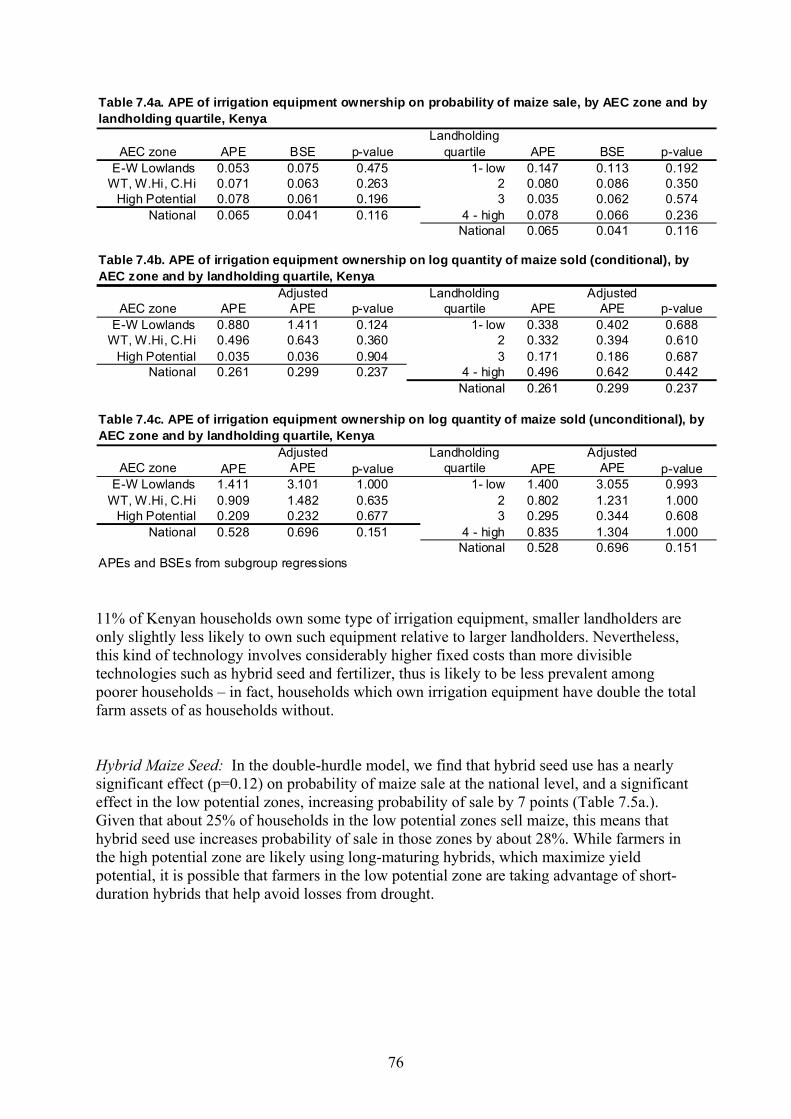
76

















APEs and BSEs from subgroup regressions

Table 7.4b. APE of irrigation equipment ownership on log quantity of maize sold (conditional), by AEC zone and by landholding quartile, Kenya

Table 7.4c. APE of irrigation equipment ownership on log quantity of maize sold (unconditional), by AEC zone and by landholding quartile, Kenya

Table 7.4a. APE of irrigation equipment ownership on probability of maize sale, by AEC zone and by landholding quartile, Kenya

11% of Kenyan households own some type of irrigation equipment, smaller landholders are only slightly less likely to own such equipment relative to larger landholders. Nevertheless, this kind of technology involves considerably higher fixed costs than more divisible technologies such as hybrid seed and fertilizer, thus is likely to be less prevalent among poorer households – in fact, households which own irrigation equipment have double the total farm assets of as households without. Hybrid Maize Seed: In the double-hurdle model, we find that hybrid seed use has a nearly significant effect (p=0.12) on probability of maize sale at the national level, and a significant effect in the low potential zones, increasing probability of sale by 7 points (Table 7.5a.). Given that about 25% of households in the low potential zones sell maize, this means that hybrid seed use increases probability of sale in those zones by about 28%. While farmers in the high potential zone are likely using long-maturing hybrids, which maximize yield potential, it is possible that farmers in the low potential zone are taking advantage of short-duration hybrids that help avoid losses from drought.

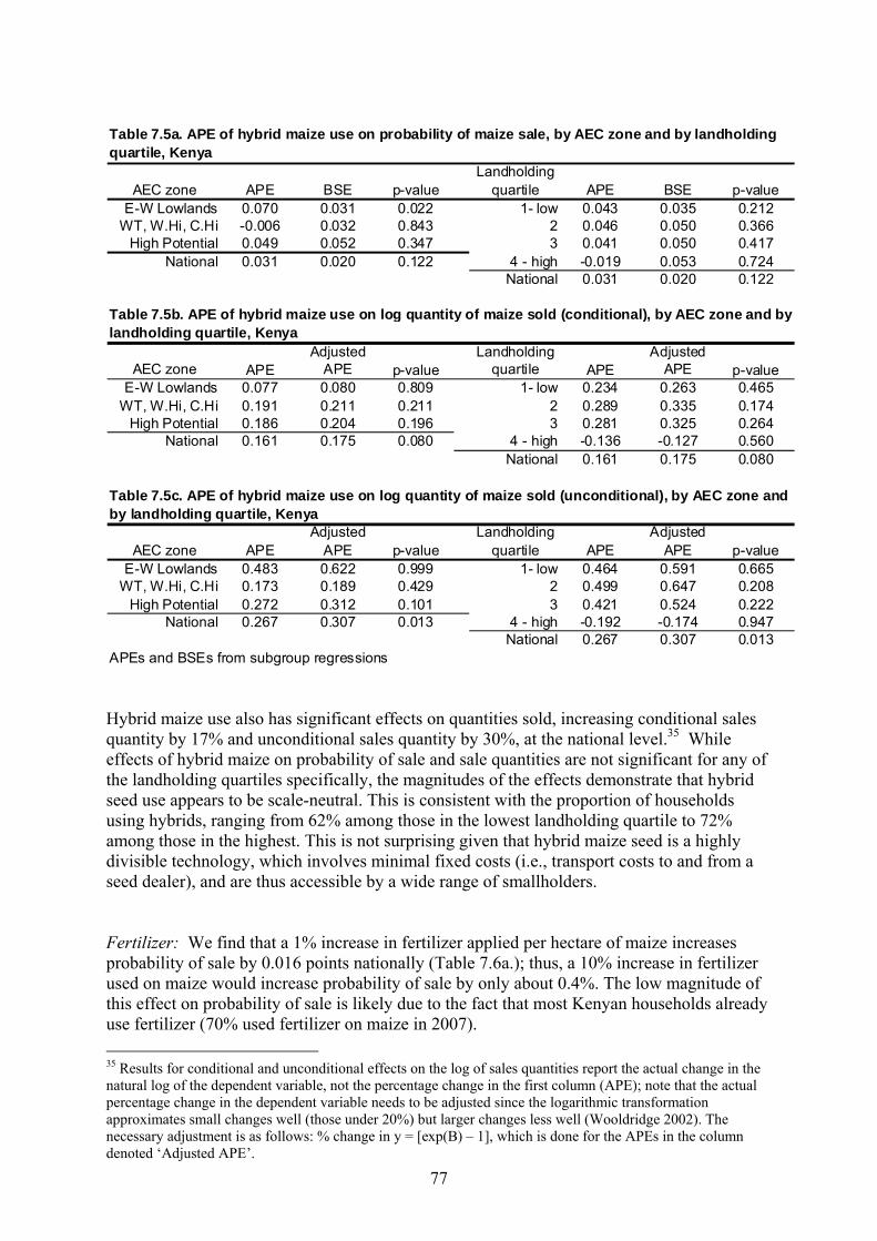
77



WT, W.Hi, C.Hi -0.006 0.032 0.843 2 0.046 0.050 0.366High Potential 0.049 0.052 0.347 3 0.041 0.050 0.417







National 0.161 0.175 0.080 4 - high -0.136 -0.127 0.560National 0.161 0.175 0.080








Table 7.5a. APE of hybrid maize use on probability of maize sale, by AEC zone and by landholding quartile, Kenya

Table 7.5b. APE of hybrid maize use on log quantity of maize sold (conditional), by AEC zone and by landholding quartile, Kenya

Table 7.5c. APE of hybrid maize use on log quantity of maize sold (unconditional), by AEC zone and by landholding quartile, Kenya

Hybrid maize use also has significant effects on quantities sold, increasing conditional sales quantity by 17% and unconditional sales quantity by 30%, at the national level.35 While effects of hybrid maize on probability of sale and sale quantities are not significant for any of the landholding quartiles specifically, the magnitudes of the effects demonstrate that hybrid seed use appears to be scale-neutral. This is consistent with the proportion of households using hybrids, ranging from 62% among those in the lowest landholding quartile to 72% among those in the highest. This is not surprising given that hybrid maize seed is a highly divisible technology, which involves minimal fixed costs (i.e., transport costs to and from a seed dealer), and are thus accessible by a wide range of smallholders. Fertilizer: We find that a 1% increase in fertilizer applied per hectare of maize increases probability of sale by 0.016 points nationally (Table 7.6a.); thus, a 10% increase in fertilizer used on maize would increase probability of sale by only about 0.4%. The low magnitude of this effect on probability of sale is likely due to the fact that most Kenyan households already use fertilizer (70% used fertilizer on maize in 2007). 35 Results for conditional and unconditional effects on the log of sales quantities report the actual change in the natural log of the dependent variable, not the percentage change in the first column (APE); note that the actual percentage change in the dependent variable needs to be adjusted since the logarithmic transformation approximates small changes well (those under 20%) but larger changes less well (Wooldridge 2002). The necessary adjustment is as follows: % change in y = [exp(B) – 1], which is done for the APEs in the column denoted ‘Adjusted APE’.

78


quartile APE BSE p-valueE-W Lowlands -0.001 0.014 0.922 1- low 0.038 0.016 0.017
















Table 7.6b. APE of log of fertilizer per hectare of maize on log quantity of maize sold (conditional), by AEC zone and by landholding quartile, Kenya

Table 7.6c. APE of log of fertilizer per hectare of maize on log quantity of maize sold (unconditional), by AEC zone and by landholding quartile, Kenya

Table 7.6a. APE of log of fertilizer per hectare of maize on probability of maize sale, by AEC zone and by landholding quartile, Kenya

Effects of fertilizer use are somewhat larger on sale quantities, where a 1% increase in fertilizer use increases conditional sale quantity by 0.11% and unconditional quantities by 0.17% at the national level (Tables 7.6a, b, c.). Conditional and unconditional quantity effects are significant in all AEC zones, highlighting the widespread applicability and importance of this improved input, and are largest in the lowest potential zones. When we consider effects of fertilizer use by landholding quartile, there is considerable evidence that fertilizer use is scale-neutral, which is not surprising as fertilizer (like hybrid seed) is a highly divisible technology with very low fixed costs. For example, we find that it has a significant positive effect on probability of sale even for the lowest quartile (Table 7.6a.). We also find that conditional quantity effects are significant for households in the 2nd quartile and nearly significant (p=0.13) for the lowest quartile, and of similar magnitude to effects in the 3rd quartile (Table 7.6b.). Unconditional quantity effects are significant for all quartiles, and those in the lowest two quartiles are nearly double in magnitude relative to higher quartiles (Table 7.6c.). An explanation for this could be that because households in lower quartiles have a somewhat lower average level of fertilizer use, a 1% increase in fertilizer use represents a larger relative and absolute effect on probability of sale and sale quantities. Animal Traction: Ownership of animal or mechanized traction does not appear to have any significant effects on probability of sale, at any level (national or by AEC zone) or for any

79








APE p-valueE-W Lowlands -0.229 -0.205 0.406 1- low 0.300 0.350 0.981

WT, W.Hi, C.Hi -0.322 -0.276 0.205 2 -0.075 -0.072 0.898High Potential 0.303 0.354 0.157 3 0.411 0.508 0.225






WT, W.Hi, C.Hi -0.517 -0.403 0.049 2 0.719 1.052 1.000High Potential 0.512 0.668 0.098 3 0.476 0.609 0.474



Table 7.7b. APE of animal traction ownership on log quantity of maize sold (conditional), by AEC zone and by landholding quartile, Kenya

Table 7.7c. APE of animal traction ownership on log quantity of maize sold (unconditional), by AEC zone and by landholding quartile, Kenya

Table 7.7a. APE of animal traction ownership on probability of maize sale, by AEC zone and by landholding quartile, Kenya

specific landholding quartile (Table 7.7a.). While there are no effects of traction ownership on conditional sale quantities, it has rather contradictory effects on unconditional quantities; it reduces quantity sold by about 40% in the medium potential zone and increases quantity sold by 67% in the high potential zone. While smallholders with more land are considerably more likely to own traction equipment (and a suitable animal or tractor) – about 16% of household in the top quartile own traction compared with about 4% in the lowest quartile – there are no significant effects of traction ownership on sale quantities by landholding quartile. Our lack of significant effects of traction ownership on probability of sale or conditional quantities sold is consistent with a synthesis of productivity studies that found that the main effect of animal traction in cases from various regions of Africa has been to reduce field labor inputs and facilitate area expansion, rather than to increase yields (Reardon et al. 1996). Thus, since we control for total landholding separately, any effect of traction ownership would be due to increased maize yields (which do not appear to be significant). 7.2.5. Market Access Distance to Road: Our proxy for market access in Kenya is distance from the village to the nearest motorable road (km). The mean of this variable declined slightly from 1997 to 2004 (1.10 to 1.05 km), then by one-half between 2004 and 2007 (1.05 to 0.52 km). While we find the expected negative sign on this variable with respect to participation at the national level, it

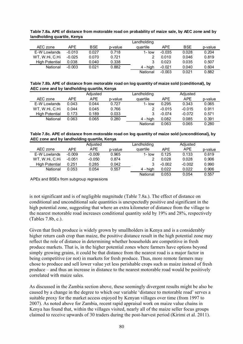
80


quartile APE BSE p-valueE-W Lowlands -0.010 0.027 0.718 1- low -0.035 0.028 0.204


National -0.003 0.021 0.882 4 - high -0.021 0.040 0.604National -0.003 0.021 0.882





WT, W.Hi, C.Hi 0.044 0.045 0.766 2 -0.015 -0.015 0.911High Potential 0.173 0.189 0.033 3 -0.074 -0.072 0.571






WT, W.Hi, C.Hi -0.051 -0.050 0.874 2 0.028 0.028 0.906High Potential 0.251 0.285 0.042 3 -0.002 -0.002 0.990



Table 7.8a. APE of distance from motorable road on probability of maize sale, by AEC zone and by landholding quartile, Kenya

Table 7.8b. APE of distance from motorable road on log quantity of maize sold (conditional), by AEC zone and by landholding quartile, Kenya

Table 7.8c. APE of distance from motorable road on log quantity of maize sold (unconditional), by AEC zone and by landholding quartile, Kenya

is not significant and is of negligible magnitude (Table 7.8a.). The effect of distance on conditional and unconditional sale quantities is unexpectedly positive and significant in the high potential zone, suggesting that where an extra kilometer of distance from the village to the nearest motorable road increases conditional quantity sold by 19% and 28%, respectively (Tables 7.8b, c.). Given that fresh produce is widely grown by smallholders in Kenya and is a considerably higher return cash crop than maize, the positive distance result in the high potential zone may reflect the role of distance in determining whether households are competitive in fresh produce markets. That is, in the higher potential zones where farmers have options beyond simply growing grains, it could be that distance from the nearest road is a major factor in being competitive (or not) in markets for fresh produce. Thus, more remote farmers may chose to produce and sell lower value yet less perishable crops such as maize instead of fresh produce – and thus an increase in distance to the nearest motorable road would be positively correlated with maize sales. As discussed in the Zambia section above, these seemingly divergent results might be also be caused by a change in the degree to which our variable ‘distance to motorable road’ serves a suitable proxy for the market access enjoyed by Kenyan villages over time (from 1997 to 2007). As noted above for Zambia, recent rapid appraisal work on maize value chains in Kenya has found that, within the villages visited, nearly all of the maize seller focus groups claimed to receive upwards of 30 traders during the post-harvest period (Kirimi et al. 2011).

81

According to MSU’s long-term experience in Kenya, this was certainly not the case 10 years ago, at which point farmers indicated that the number of traders visiting villages was considerably smaller. Such an increase in trader presence over time in remote villages is also consistent with changes in the average distance from the village to nearest motorable road, as reported above. An explanation for why trader presence has increased was discussed earlier in section 6.2.5. (Distance to Road); recent rapid appraisal interviews with maize traders suggests that the recent proliferation of cell phones in rural areas of Kenya has dramatically reduced the risks involved in maize trading, which has subsequently lowered barriers to entry. The implication of these rapid appraisal findings is that if the number and frequency of private traders visiting villages has increased over time, then the ability of ‘distance to road’ to explain market participation could diminish over time as search costs decline with increased trader presence in villages, and as the price variable better reflects transportation costs to market. Given the results from our regression using data from 1997-2004-2007 above, and the anecdotal evidence of an increase in private trader visits to villages, we test whether the magnitude and/or sign of the APE of the distance variable changes over time, by computing this APE separately for the three panel survey years.36 The results suggest that there was no effect of distance on probability of sale in 1997, a significant negative effect in 2004, and a significant positive effect in 2007 (Table 7.9.). Given that the only region with a significant distance response in 2004 was the drought-prone East and Western Lowlands, it is possible that this effect is picking up a response of remote villages to drought shock in that zone. These results are difficult to interpret, given that distance to road declined considerably (on average) between 1997 and 2004, yet the change in sign of the variable occurs between 2004 and 2007. However, the positive APEs of this market access variable in the medium and higher potential zones in 2004 and 2007 suggest that remoteness has not been a serious constraint to selling maize in Kenya since 1997 or before. Access to Market Price Information: Another potential factor affecting transaction costs of search for price information is access to market price information, which would be expected to improve market participation. Access to such information might also be expected to improve farmer’s bargaining power with intermediaries, which could improve both participation and sales quantities. As we do not have information on whether or not households received market price information, we use radio ownership as a proxy.

AEC zone APE SE p-value APE SE p-value APE SE p-valueE-W Lowlands 0.000 0.006 0.942 -0.168 0.049 0.001 0.067 0.090 0.460

WT, W.Hi, C.Hi -0.022 0.012 0.062 0.058 0.076 0.445 0.313 0.136 0.021High Potential -0.027 0.075 0.718 0.008 0.106 0.939 0.204 0.077 0.008

National -0.026 0.026 0.302 -0.132 0.033 0.000 0.078 0.040 0.055

Table 7.9. APE of distance to nearest motorable road on probability of maize sale, by AEC zone and by year, Kenya, 1997, 2004, 2007

2004 20071997

36 We do this by running separate regressions for 1997, 2004 and for 2007, including the time-average terms in each.

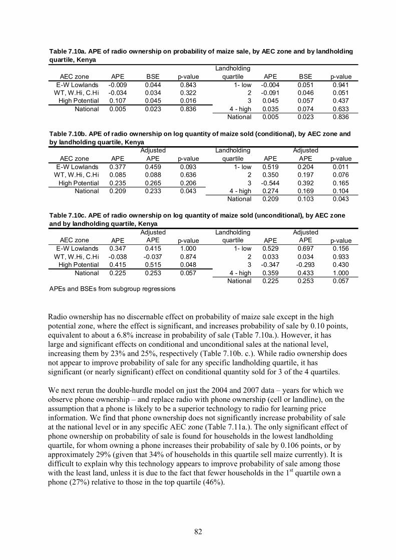
82


quartile APE BSE p-valueE-W Lowlands -0.009 0.044 0.843 1- low -0.004 0.051 0.941

WT, W.Hi, C.Hi -0.034 0.034 0.322 2 -0.091 0.046 0.051High Potential 0.107 0.045 0.016 3 0.045 0.057 0.437






WT, W.Hi, C.Hi 0.085 0.088 0.636 2 0.350 0.197 0.076High Potential 0.235 0.265 0.206 3 -0.544 0.392 0.165






WT, W.Hi, C.Hi -0.038 -0.037 0.874 2 0.033 0.034 0.933High Potential 0.415 0.515 0.048 3 -0.347 -0.293 0.430



Table 7.10a. APE of radio ownership on probability of maize sale, by AEC zone and by landholding quartile, Kenya

Table 7.10b. APE of radio ownership on log quantity of maize sold (conditional), by AEC zone and by landholding quartile, Kenya

Table 7.10c. APE of radio ownership on log quantity of maize sold (unconditional), by AEC zone and by landholding quartile, Kenya

Radio ownership has no discernable effect on probability of maize sale except in the high potential zone, where the effect is significant, and increases probability of sale by 0.10 points, equivalent to about a 6.8% increase in probability of sale (Table 7.10a.). However, it has large and significant effects on conditional and unconditional sales at the national level, increasing them by 23% and 25%, respectively (Table 7.10b. c.). While radio ownership does not appear to improve probability of sale for any specific landholding quartile, it has significant (or nearly significant) effect on conditional quantity sold for 3 of the 4 quartiles. We next rerun the double-hurdle model on just the 2004 and 2007 data – years for which we observe phone ownership – and replace radio with phone ownership (cell or landline), on the assumption that a phone is likely to be a superior technology to radio for learning price information. We find that phone ownership does not significantly increase probability of sale at the national level or in any specific AEC zone (Table 7.11a.). The only significant effect of phone ownership on probability of sale is found for households in the lowest landholding quartile, for whom owning a phone increases their probability of sale by 0.106 points, or by approximately 29% (given that 34% of households in this quartile sell maize currently). It is difficult to explain why this technology appears to improve probability of sale among those with the least land, unless it is due to the fact that fewer households in the 1st quartile own a phone (27%) relative to those in the top quartile (46%).

83

AEC zone APE SE p-valueLandholding

quartile APE SE p-valueE-W Lowlands -0.011 0.055 0.838 1- low 0.106 0.054 0.052

WT, W.Hi, C.Hi 0.051 0.046 0.264 2 0.018 0.058 0.751High Potential -0.066 0.047 0.161 3 0.000 0.059 0.999


APEs and SE's computed from subgroup regressions; SE's computed using the delta method

Table 7.11a. APE of phone ownership on probability of maize sale, by AEC zone and by landholding quartile, Kenya, 2004-2007

Household Transportation Assets: Although our limited market access variables suggest that distance from market is not a significant constraint on selling maize, this does not imply that households will necessarily decide to sell maize, as prices offered by traders who come to the village may be too low for some farmers. We would expect transportation assets to more likely improve probability of sale rather than quantity sold, given that such assets can reduce search costs for a sale opportunity, which are fixed costs. We find that ownership of a vehicle improves probability of sale by 13% at the national level, while ownership of a cart improves quantity sold among sellers by 63% (Table 7.2.). Effects from bicycle ownership are likely not significant because 48% of households own a bike, compared with only 5% who own a vehicle (or 4% a cart). Thus, it appears that the majority of smallholders have reasonably good access to sale opportunities, such that it takes ownership of something like a vehicle to improve a household’s probability of sale, on average.

7.2.6. Farmgate Maize Price We find that the log of expected farmgate maize price has a significant and large effect on probability of sale, as a 1% increase in expected maize prices increases probability of sale by 0.0045 points, which is equivalent to approximately a 1.1% increase in probability of sale (Table 7.12a.). This effect is significant in each AEC zone, and for all but the lowest landholding quartile (Table 7.12a.). These results show that unlike Mozambique and Zambia, the majority of smallholders in Kenya respond to higher expected maize prices by increasing the probability that they sell some maize. The expected maize price does not have a significant effect on conditional sale quantities at the national level due to a large negative and significant effect in the low potential zone, combined with a strong significant positive effect in the high potential zone (Table 7.12b.). The negative effect in the low potential zone is likely due to stock effects and the more semi-subsistence orientation of producers in these lower potential zones, as explained earlier in the Mozambique chapter. The positive response in the high potential zone is quite strong, as a 1% increase in the expected maize price increases quantity sold among current sellers by 2.2% (Table 7.12b.). The large and significant unconditional quantity effects in the medium and high potential zones (Table 7.12c.) demonstrate that higher expected maize prices result in considerably larger volumes of maize marketed due to a combination of increases in participation (the number of households selling maize) and quantities sold by current sellers (the conditional effect).

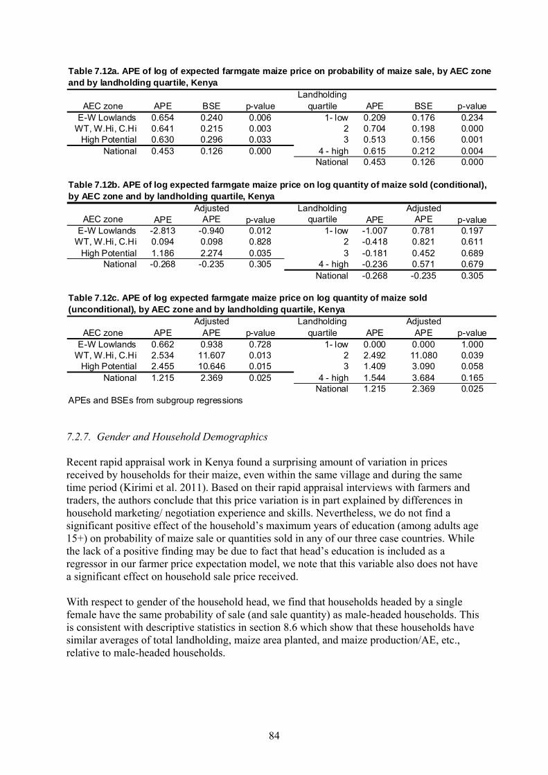
84








APE p-valueE-W Lowlands -2.813 -0.940 0.012 1- low -1.007 0.781 0.197

WT, W.Hi, C.Hi 0.094 0.098 0.828 2 -0.418 0.821 0.611High Potential 1.186 2.274 0.035 3 -0.181 0.452 0.689

National -0.268 -0.235 0.305 4 - high -0.236 0.571 0.679National -0.268 -0.235 0.305








Table 7.12b. APE of log expected farmgate maize price on log quantity of maize sold (conditional), by AEC zone and by landholding quartile, Kenya

Table 7.12c. APE of log expected farmgate maize price on log quantity of maize sold (unconditional), by AEC zone and by landholding quartile, Kenya

Table 7.12a. APE of log of expected farmgate maize price on probability of maize sale, by AEC zone and by landholding quartile, Kenya

7.2.7. Gender and Household Demographics Recent rapid appraisal work in Kenya found a surprising amount of variation in prices received by households for their maize, even within the same village and during the same time period (Kirimi et al. 2011). Based on their rapid appraisal interviews with farmers and traders, the authors conclude that this price variation is in part explained by differences in household marketing/ negotiation experience and skills. Nevertheless, we do not find a significant positive effect of the household’s maximum years of education (among adults age 15+) on probability of maize sale or quantities sold in any of our three case countries. While the lack of a positive finding may be due to fact that head’s education is included as a regressor in our farmer price expectation model, we note that this variable also does not have a significant effect on household sale price received. With respect to gender of the household head, we find that households headed by a single female have the same probability of sale (and sale quantity) as male-headed households. This is consistent with descriptive statistics in section 8.6 which show that these households have similar averages of total landholding, maize area planted, and maize production/AE, etc., relative to male-headed households.

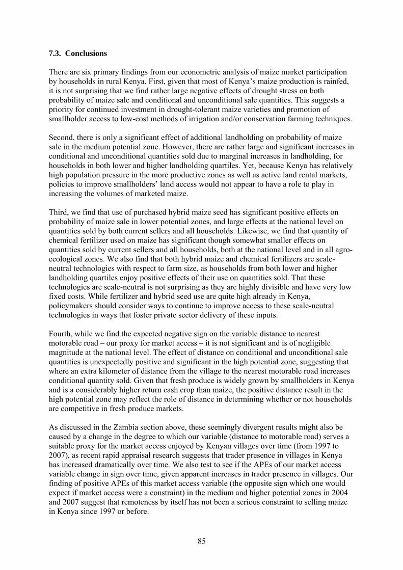
85

7.3. Conclusions There are six primary findings from our econometric analysis of maize market participation by households in rural Kenya. First, given that most of Kenya’s maize production is rainfed, it is not surprising that we find rather large negative effects of drought stress on both probability of maize sale and conditional and unconditional sale quantities. This suggests a priority for continued investment in drought-tolerant maize varieties and promotion of smallholder access to low-cost methods of irrigation and/or conservation farming techniques. Second, there is only a significant effect of additional landholding on probability of maize sale in the medium potential zone. However, there are rather large and significant increases in conditional and unconditional quantities sold due to marginal increases in landholding, for households in both lower and higher landholding quartiles. Yet, because Kenya has relatively high population pressure in the more productive zones as well as active land rental markets, policies to improve smallholders’ land access would not appear to have a role to play in increasing the volumes of marketed maize. Third, we find that use of purchased hybrid maize seed has significant positive effects on probability of maize sale in lower potential zones, and large effects at the national level on quantities sold by both current sellers and all households. Likewise, we find that quantity of chemical fertilizer used on maize has significant though somewhat smaller effects on quantities sold by current sellers and all households, both at the national level and in all agro-ecological zones. We also find that both hybrid maize and chemical fertilizers are scale-neutral technologies with respect to farm size, as households from both lower and higher landholding quartiles enjoy positive effects of their use on quantities sold. That these technologies are scale-neutral is not surprising as they are highly divisible and have very low fixed costs. While fertilizer and hybrid seed use are quite high already in Kenya, policymakers should consider ways to continue to improve access to these scale-neutral technologies in ways that foster private sector delivery of these inputs. Fourth, while we find the expected negative sign on the variable distance to nearest motorable road – our proxy for market access – it is not significant and is of negligible magnitude at the national level. The effect of distance on conditional and unconditional sale quantities is unexpectedly positive and significant in the high potential zone, suggesting that where an extra kilometer of distance from the village to the nearest motorable road increases conditional quantity sold. Given that fresh produce is widely grown by smallholders in Kenya and is a considerably higher return cash crop than maize, the positive distance result in the high potential zone may reflect the role of distance in determining whether or not households are competitive in fresh produce markets. As discussed in the Zambia section above, these seemingly divergent results might also be caused by a change in the degree to which our variable (distance to motorable road) serves a suitable proxy for the market access enjoyed by Kenyan villages over time (from 1997 to 2007), as recent rapid appraisal research suggests that trader presence in villages in Kenya has increased dramatically over time. We also test to see if the APEs of our market access variable change in sign over time, given apparent increases in trader presence in villages. Our finding of positive APEs of this market access variable (the opposite sign which one would expect if market access were a constraint) in the medium and higher potential zones in 2004 and 2007 suggest that remoteness by itself has not been a serious constraint to selling maize in Kenya since 1997 or before.

86

Fifth, we find that radio ownership (our proxy for household access to market information) has no discernable effect on probability of maize sale except in the high potential zone, though it has large and significant effects on conditional and unconditional sales at the national level, increasing them by 23% and 25%, respectively. While further research is warranted to discern the extent to which radio ownership serves as a reasonable proxy for access to market information, these results suggest that public investment to improve smallholders’ access to market price information might yield high returns in terms of volumes of maize marketed. Sixth, we find that the log of expected farmgate maize price has significant and large effect on probability of sale, as a 1% increase in expected maize prices increases probability of sale by 1.1%. This effect is significant in each AEC zone, and for all but the lowest landholding quartile. These results show that unlike Mozambique and Zambia, the majority of smallholders in Kenya respond to higher expected maize prices by increasing the probability that they sell some maize. The reason for this is likely related to the widespread use of fertilizer and hybrid maize by both smaller and larger smallholders in Kenya (as well as enjoying a larger percentage of arable land in areas of medium and higher-potential, relative to say, Mozambique), which enable smallholders to increase their maize yields in response to higher expected output prices. We also find strong positive maize price responsiveness of conditional quantities sold in the high potential zone, as a 1% increase in the expected maize price increases quantity sold among current sellers by 2.2%. In addition, we find strong maize price responsiveness for unconditional quantities in the medium and higher potential zones. However, as in Mozambique, we find significant negative effects of expected maize prices on sale quantities of current sellers in the low potential zone, which are likely due to stock effects and the more semi-subsistence orientation of producers in these lower potential zones. Policymakers should be wary of employing market and trade policies which raise average retail maize prices as a means to incentivize farmers to increase the volume of maize marketed, because higher domestic maize prices tend to benefit only the 40% of rural households which are net sellers, at the expense of lower welfare for the majority of rural as well as urban households. An alternative means of increasing farmgate maize prices could be increased via improved road infrastructure, which can lower marketing costs and thereby increase prices paid to farmers without increasing retail-level prices. Improved road infrastructure and/or support for input marketing coops could theoretically also lower farmer prices for fertilizer and hybrid maize seed, which are found to have strong effects on maize quantities sold.

87

8. CROSS-COUNTRY SYNTHESIS OF ECONOMETRIC RESULTS

8.1. Agroecological Potential and Weather Shocks Given that nearly all maize production in these countries is rainfed, and that maize is a principal staple food crop in most areas, we would expect that agro-ecological potential and weather-related shocks would play an important role in the probability of maize sale and quantities sold. The results from each country demonstrate that even after controlling for household assets, prices, and market access, farmers in areas of higher agro-ecological potential have a significantly higher probability of selling maize (and quantities sold) relative to farmers in areas of lower potential. In each country, we also use data on rainfall during the principal growing season to create indicators of drought stress for our econometric analysis, and in Mozambique, we also have household measures of maize yield loss, which we aggregate to the village level. These stress variables have significant and large effects on the probability of selling and/or amounts sold, while controlling for household assets, maize price, and market access. These results highlight the sensitivity of marketed maize surplus to weather shocks, and thus the potential value of: a) investment in development and dissemination of drought-tolerant maize varieties; and b) widespread promotion of smallholder access to low-cost methods of irrigation and/or conservation farming techniques to reduce the impact of drought – in contrast to the recent emphasis of heavy investment in formal perimeter irrigation schemes, which tend to benefit only a small proportion of the smallholder population.

8.2. Total Household Landholding We have three principal findings across our three case countries with respect to the relationship between landholding and maize market participation. First, we find that marginal increases in landholding have significant effects on the probability of maize sale in Mozambique and Zambia, though the effects are relatively small. For example, controlling separately for a household’s long-term average landholding size, a 10% increase in landholding would improve probability of sale by 2% in Mozambique, by 1.9% in Zambia and by 1.17% in the medium potential zones of Kenya (Table 8.1.). Table 8.1. Average Partial Effect of an Increase in Landholding on the Probability of Household Maize Sale and Quantities Sold in Mozambique, Zambia, and Kenya

Probability of maize sale

Quantity sold, conditional on

selling (existing sellers)

Quantity sold, unconditional

(sellers or non-sellers)

Mozambique 2.0 3.6 6.0

Zambia 1.9 1.8 6.5

Kenya 1.1a 2.4 3.1

Notes: a) effect significant only in the medium potential zones.

Average Partial Effect of 10% increase in landholding on:

---------- % change ------------

88

Second, marginal increases in landholding also have relatively small (though significant) effects on sale quantities by existing sellers (conditional effect), though considerably larger effects on sales of all growers (unconditional effect) in Mozambique and Zambia (Table 8.1.). For example, a 10% increase in landholding increases unconditional quantity sold by 6% in Mozambique and by 6.5% in Zambia. The fact that unconditional quantity effects are larger than conditional effects in these two countries demonstrates that a considerable amount of the increase in quantity sold by a random household would be due to a rise in the number of households selling at least some maize, in addition to increased quantities from current sellers. Third, only in Mozambique does the average partial effect (APE) of landholding appear to increase in land endowment (Table 8.2.), as hypothesized in Chapter 2. Given the considerable heterogeneity in landholdings among smallholders in southern and eastern Africa (e.g., Jayne et al. 2003), we rank all households in each of our country samples from largest to smallest in terms of landholding, divide them into four quartiles, and compute the means of landholding by quartile (Table 8.3.), as well as the APE of landholding on maize market participation in each country. In Mozambique, the APE of landholding for the top two landholding quartiles are significantly larger than those for the lower two quartiles (Table 8.2.), though there is a significant difference in APEs of landholding by quartile on unconditional quantities sold (Table 8.4.). The insignificant and small marginal effects found at the lowest initial landholding quartiles in Mozambique likely reflects the need for a minimum threshold of landholding to meet a critical proportion of the household’s maize consumption requirements, combined with the almost complete absence of fertilizer and improved maize seed -- less than 4% of Mozambican households use fertilizer on maize and less than 2% use improved maize varieties. Together, these two factors imply that Mozambican households must rely on extensification to increase their maize production and thus probability of maize sale. By contrast, in Zambia and Kenya, there is no evidence that the APE of landholding on probability of sale or sale quantities is larger for households with larger land endowments. The lack of threshold effects in Zambia and Kenya is likely due to the fact that fertilizer and hybrid use are much more common in these countries than in Mozambique, even for households in the lower landholding quartiles. Table 8.2. APE of Log Landholding on Probability of Maize Sale, by Landholding Quartile, Mozambique, Zambia, Kenya

APE p-value APE p-value APE p-value1- low -0.016 0.712 0.093 0.001 0.053 0.050

2 0.032 0.312 0.031 0.247 0.079 0.0423 0.117 0.001 0.073 0.000 0.030 0.360

4 - high 0.092 0.014 0.026 0.114 -0.005 0.862National 0.039 0.018 0.061 0.000 0.022 0.151

Mozambique Zambia KenyaLandholding quartile

89

Table 8.3. Average Total Landholding by Quartile of Landholding among Small and Medium-holders in Mozambique, Zambia, Kenya

Mozambique Zambia Kenya2005 2008 2007

1- low 0.94 0.86 0.612 1.59 1.54 1.163 2.33 2.46 2.18

4 - high 4.10 6.05 4.77National 2.24 2.79 2.15

---- household average total landholding (ha) ----

Landholding quartile

Table 8.4. APE of Log Landholding on Unconditional Quantity of Maize Sold, by Landholding Quartile, Mozambique, Zambia, Kenya

Adj. APE p-value Adj. APE p-value Adj. APE p-value1- low 0.088 0.862 1.028 0.006 0.455 0.089

2 1.071 0.021 0.951 0.001 1.326 0.0053 1.322 0.011 0.628 0.000 0.164 0.328

4 - high 1.160 0.001 0.257 0.002 0.252 0.117National 0.601 0.000 0.652 0.000 0.313 0.002

Mozambique Zambia Kenya

Notes: Adj. APE = Average Partial Effects adjusted for logarithmic transformation of the dependent variable

Landholding quartile

However, when we compute APEs separately by AEC zone in each country, we do find significant and large effects of additional landholding on unconditional quantities sold in low, medium, and higher potential zones (Table 8.5.). Given that our findings show significant effects of additional landholding on both probability of sale and unconditional quantities sold in various AEC zones in Mozambique and Zambia, this suggests that policies and investments to improve land access of smallholders in these countries could play an important role in increasing both the quantities of marketed maize and the number of households participating as maize sellers. Because Kenya already has relatively high population pressure in the more productive zones, rapidly decreasing farm sizes, and active land rental markets, it would appear that improving smallholders’ access to land is neither viable nor appropriate. Rather, policies or investments to increase volumes of marketed maize would more appropriately focused on fostering continued uptake of land-saving inputs such as fertilizer and improved maize varieties, as well as low-cost irrigation technologies and/or conservation farming techniques. Table 8.5. APE of Log Landholding on Unconditional Quantity of Maize Sold, by AEC Zone, Mozambique, Zambia, Kenya

Adj. APE p-value Adj. APE p-value Adj. APE p-value1- low 0.632 0.073 0.622 0.228 0.697 0.034

2-medium 0.706 0.033 0.681 0.0003-medium 0.706 0.000 0.889 0.230 0.654 0.005

4 - high 0.094 0.873 0.618 0.000 0.128 0.325National 0.601 0.000 0.652 0.000 0.313 0.002

AEC zoneMozambique Zambia Kenya

90

Both Mozambique and Zambia have large uncultivated tracts of land that could be settled by smallholders. In the case of Zambia, migration and settlement of uncultivated areas would require not only a legal mechanism to transfer land rights from current owners (state and other) to migrants, but also complementary public goods such as social services (schools, health clinics) and road infrastructure which could link such areas to markets (Jayne et al. 2008). In Mozambique, a serious constraint to expansion of land area is the negligible use of animal traction in northern Mozambique, home to over half of the rural population. Public investment could potentially increase adoption of animal traction in the north by alleviating disease constraints to animal traction via medicinal subsidies and/or eradication of the tsetse fly. In addition, because oxen ownership represents a high investment cost, support for rural financial services might help to address household financial constraints to financing traction rental. Given the lack of tradition of maintaining oxen in these areas, livestock extension could also play a valuable role in promoting oxen ownership or rental.

8.3. Technology

8.3.1. Hybrid Maize Seed In Zambia, we find that household use of purchased hybrid maize seed has large and significant effects on probability of sale in low, medium, and high potential zones, increasing sale probability by 15% at the national level. Hybrid seed use also increases conditional (unconditional) quantities sold by 56% (400%) in the Medium-1 zone and by 130% (516%) in the High potential zone. In Kenya, household use of purchased hybrid maize seed has large and significant effects on quantities sold at the national level, increasing conditional quantity sold by 17% and unconditional quantity sold by 30%. We also find that hybrid seed is scale-neutral in each country with respect to farm size, as households from both lower and higher landholding quartiles enjoy significant positive effects of hybrid use on both quantities sold (in both countries) and the probability of maize sale (in Zambia). While maize hybrids are typically developed for use with fertilizer and adequate water, the results from the rainfall variables in each country suggest that increased investment in the development and dissemination of drought-resistant maize varieties could improve maize production and marketed surpluses in lower potential zones.

8.3.2. Chemical Fertilizer In both Zambia and Kenya, we find that marginal increases in fertilizer applied to maize have relatively small effects on the probability of sale and quantities sold by current sellers, though larger effects on unconditional quantities sold, as a 10% increase in fertilizer use increases quantity sold by any given household by 1.8% in Kenya and 2.3% in Zambia. These quantity effects of fertilizer use are significant in all AEC zones in Kenya and in medium to high potential zones in Zambia. Like hybrid maize seed, we also find that fertilizer use is scale-neutral with respect to farm size as it has a significant positive effect on probability of sale and/or quantities sold for households in every landholding quartile. That hybrid maize seed and fertilizer are scale-neutral is not surprising as they are highly divisible inputs with very low fixed costs. Our three case countries present very different cases with respect to the current status of private sector fertilizer and seed markets. In Mozambique, less than 4% of households use fertilizer on maize and fewer than 2% use improved maize varieties. At the other end of the spectrum is Kenya, where 71% of rural households use fertilizer on maize and 70% use

91

hybrids. Zambia represents an intermediate case as a sizeable minority of growers use fertilizer and hybrid seed (37% and 41%, respectively).. While it is clear that increased use of fertilizer would increase both the numbers of households selling maize and quantities sold in Mozambique and Zambia, the question of how best to promote fertilizer use has been the subject of much debate in recent years. While targeted fertilizer subsidies are growing in popularity in Sub-Saharan Africa, Morris et al. (2007) argue, “The weight of empirical evidence now show(s) that fertilizer subsidies are likely to be inefficient, costly, and fiscally unsustainable.” The efficiency of these programs depends on the extent to which subsidized fertilizer ‘crowds in’ (augments) or ‘crowds out’ (displaces) commercial fertilizer demand. For example, in Malawi, where a government fertilizer subsidy program reached as many as 57% of rural households in some years, a study found that for every kilogram of subsidized fertilizer received, households reduced their demand for commercial fertilizer by 0.22 kilograms on average (Ricker-Gilbert, Jayne, and Chirwa 2011). Another recent example is found in Zambia, where since 2004 the government has invested a large proportion of its agricultural sector budget on a fertilizer subsidy program that reached as many as 12% of rural Zambian households in 2007. A recent study of the effects of this program on smallholder commercial fertilizer purchases finds that each kilogram of subsidized fertilizer provided displaced between 0.08 and 0.28 kilograms of commercial fertilizer demand (Mason 2011a). Both of these studies highlight that the efficiency of such programs depend on the extent to which they are able to target households which otherwise would not have purchased commercial fertilizer (or who would have purchased much smaller quantities). An alternative to direct fertilizer subsidies is to strengthen farmers’ effective demand for fertilizer through investments in collective goods, which make fertilizer use more profitable, and by building durable input markets and output markets that can absorb the increased output without gluts that depress producer prices (Minde et al. 2008). Such investments would include: rural road infrastructure and port facilities to reduce the costs of distribution; agricultural research to develop and adapt varieties that respond to fertilizer; the development and dissemination of fertilizer use recommendations that are appropriate for different areas (as opposed to applying one blanket recommendation for an entire country); and the development of rural financial systems and market information systems (ibid 2008). Returns to these investments require durable input and output markets, which depend upon a supportive policy environment that attracts local and foreign direct investment. The case of Kenya demonstrates that a stable policy environment – with respect to fertilizer, land, and maize markets – can induce an impressive private sector response over time that has helped to make fertilizer accessible to most small farmers (ibid 2008). For example, in the medium and high potential zones of Kenya, 88% and 92% of growers used fertilizer on maize in 2007, respectively. By contrast, only 27% of growers in the Zambian high potential zone (31% in the medium-1) used fertilizer on maize, despite the fact that 42% of fertilizer users in the high zone (and 30% in the medium-1 zone) obtained subsidized fertilizer in 2007. In Mozambique, moving beyond the current situation of a near absence of fertilizer and hybrid seed use is a large challenge, which will require policymakers to address constraints to private sector development of seed and fertilizer markets, and effectively linking agro-dealer network development with improved extension services.

92

8.3.3. Animal Traction Animal traction ownership does not have a significant effect on probability of maize sale or quantities sold in our case countries. These results are consistent with a synthesis of productivity studies that found that the main effect of animal traction in cases from various regions of Africa has been to reduce field labor inputs and facilitate area expansion, rather than to increase yields (Reardon et al. 1996).

8.4. Market Access 8.4.1. Distance to Road Infrastructure and/or Town Conventional wisdom on agricultural marketing in Sub-Saharan Africa (SSA) has long held that poor road infrastructure results in remote African villages having poor market access, meaning that these villages receive few (if any) traders. Farmers in villages that receive few trader visits likely face oligopolistic pricing (i.e., low price offers for their agricultural goods due to lack of competition among traders). However farmers in villages which receive no traders at all incur not only substantial transport costs to their point of sale (i.e., the nearest road, nearest small town, etc.), but also search costs for a market and for price information. Thus, the conventional explanation for observing a low percentage of rural households in SSA that sell food grains is that it is caused by poor market access (which results in high transaction costs for farmers – costs both of search and for transportation) and/or oligopolistic trader behavior. Previous studies of food marketing behavior in rural areas of developing countries have used variables such as distance to the nearest road (or town) as a proxy for households’ market access, and have consistently found such variables to have a significant and negative relationship with the probability of selling food grains. By contrast, while our study uses similar proxies for market access, we find that such variables do not have a significant negative effect on probability of sale or quantity sold in most zones of our case countries. In the few cases where a significant negative effect is found, it is of very small magnitude. Recent rapid appraisal work on maize value chains in our three case countries explains the discrepancy between our results and those from other studies. Contrary to the conventional depiction of poor to negligible market access in rural Sub-Saharan Africa, recent rapid appraisal work in Zambia, Kenya, and Mozambique found that maize sellers in both remote and non-remote villages claimed that upwards of 30 traders had visited their village during the most recent post-harvest period (in 2009) (Kirimi et al. 2011). This suggests that, while there still may be significant transport costs to the nearest relevant market for farmers in remote villages (which would cause traders to adjust their maize buying prices lower), even these farmers now face considerably lower search costs for price information and access to traders than they did a decade ago. For example, the percentage of rural households which live in a village in which at least one grower sold maize on their farm or within the village to a private-sector trader (i.e., not including sales to other households) is 53% for Mozambique (2002), 67% for Zambia (2004), and 82% for Kenya (2007). Thus, while variables measuring access to physical infrastructure such as distance to road/market/public transport may have served as a reasonable proxy for market access (i.e., reasonable access to traders) in previous years, it is possible that the lack of significant results for such variables in our study is due to increased presence of traders in rural areas in these

93

countries – a finding consistent with recent empirical study of market access measures in Kenya (Chamberlain and Jayne 2011). Trader presence has likely increased in recent years due to increased investments in road construction in some countries (Kenya, Zambia) as well as the recent proliferation of cell phones in rural areas, which has dramatically reduced the risks involved in maize trading and thus lowered barriers to entry. Note that because expected farmgate maize sales price is included in our model, and that the location for the majority of sales observed in these countries is the village, then transport costs for most sales should be reflected included in the farmgate sales prices that we observe. Thus, while prices may still be too low to induce some farmers to sell (because of low maize productivity and/or high transport costs to relevant markets), our results suggest that lack of access to traders is not a principal constraint to maize marketing in most areas of these three countries. The implication of this finding is not that further investment in road infrastructure is unnecessary – because better road infrastructure should lead to lower input prices for farmers, and higher output prices – but rather that road investments alone are not likely to be sufficient to elicit broad-based increases in maize market participation.

8.4.2. Household Ownership of Transportation Assets There is some evidence from Mozambique of the existence of marketing-related transaction costs – apart from those already captured by expected farmgate prices – as seen by the positive and significant effects on probability of sale of owning a bicycle (9% increase in probability of sale in the low potential zone) and cart (43% in medium zone and 42% in the high zone). In Zambia, ownership of a bicycle only has a significant effect on probability of maize sale in the relatively small Medium-2 potential zone, and cart ownership does not have a significant positive effect on either probability of sale or quantities sold. In Kenya, we find that ownership of a vehicle improves probability of sale by 13%, while ownership of a cart improves quantity sold among sellers by 63%. Thus, it appears that because the majority of smallholders in Kenya have reasonably good access to sale opportunities, it takes ownership of something like a vehicle to improve a household’s probability of maize sale, on average. It perhaps is not a coincidence that the country with the lowest road density in our study (Mozambique) is where we find the most evidence of significant effects of household transportation assets on the probability of maize sale.

8.4.3. Market Price Information Another potential factor affecting transaction costs of search for price information is access to market price information, which would be expected to improve maize market participation. Access to such information might also be expected to improve farmer’s bargaining power with intermediaries, which could improve both participation and sales quantities. In Mozambique, we find that household receipt of market price information leads to an 18% increase in the probability of sale as well as increases in the quantity sold by current sellers (21%) and by all households (41%). In Zambia and Kenya, we use radio ownership and cell/landline phone ownership as proxies of household access to market price information. While in each country we find that neither proxy has a significant effect on probability of maize sale, in Zambia, radio ownership increases conditional sale quantity by 15%, while cell phone ownership increases conditional sale quantities by 81% and unconditional sales by 76%. In Kenya, radio ownership has increases conditional and unconditional sales by 23% and 25%, respectively. While more research is warranted to document the link between radio

94

and cell phone ownership and household access to market price information, these results nevertheless suggest that funding to increase the spatial coverage and frequency of radio broadcasts in rural Mozambique, Zambia, and Kenya could potentially lead to large increases in quantities of maize sold.

8.4.4. Grain Marketing Parastatal Activities The implementation of food market policy reforms in the early 1990s in eastern and southern Africa has been associated with a partial withdrawal of the state from operations in food markets. However, in recent years, grain marketing boards in Zambia and Kenya have re-emerged as significant actors in maize markets. In Zambia, the Food Reserve Agency (FRA) has reportedly purchased approximately 75% of the maize marketed by smallholder farmers in recent years, while in Kenya, the NCPB has increased its maize purchase volumes in recent years, particularly in the high potential zone. In both countries, the objectives of marketing board operations have been to raise maize production incentives, thereby increasing planted area and smallholders’ uptake of fertilizer and other inputs in order to increase total maize production, and stabilize the maize markets. Research on the effects of FRA and NCPB maize purchase activities on household crop production and input use is beyond the scope of this paper and is presented elsewhere (Mason 2011a; Mather and Jayne forthcoming). Because less than 1% of smallholders in Kenya sell directly to the NCPB, for the purposes of this paper, our treatment of NCPB activities only involves inclusion of expected NCPB purchase volumes as a regressor in our model of farmer price expectations. However, in Zambia, we do measure the effect of expected district-level volumes of FRA maize purchases on household maize market participation, and find they do not have a significant effect on probability of maize sale, and have insignificant or negligible effects on quantities sold (depending on the AEC zone). The lack of significant effects of expected FRA purchase volumes may be due to the fact that the effect of expected FRA purchases already operates indirectly through our model of household farmgate maize price expectations (though we find that expected FRA purchases have a very small effect on expected farmgate prices). Our lack of large FRA purchase effects on expected prices may also have to do with the simple specification of our expected price model, as Mason (2011b) found relatively larger effects of expected FRA purchase volumes on households’ expected maize prices using a more complex specification.

8.5. Farmgate Maize Price In contrast to previous studies that have used average annual or post-harvest farmgate prices, we compute expected farmgate maize prices in order to study the responsiveness of household maize sales to changes in farmgate prices. Further empirical work is needed to estimate the responsiveness of household maize sales to both expected farmgate prices and realized post-harvest prices. In Mozambique, while we do not find significant positive effects of higher expected maize prices on probability of sale at the national or zonal levels, we do find that current sellers respond to higher expected maize prices by selling more maize (as a 1% increase in the expected maize price leads to a 2.2% increase in quantity sold). However, we also find that households in the lowest potential region react to higher expected maize prices by reducing

95

their probability of selling maize. The negative price response in this zone may be due to the combination of a poor agro-ecological environment (i.e., low supply elasticity), the fact that maize constitutes a large portion of household income (i.e., high income elasticity), and the possibility that stock effects could turn the price response negative in this zone, especially if household preferences are especially strong to store food rather than rely on the market and a low substitution effect between food and other goods. In Zambia, we also find that there is considerably spatial heterogeneity in the responsiveness of household maize sales to changes in expected farmgate maize prices. For example, households in the Medium-1 and High potential zones behave as we would expect more commercially-oriented farmers to behave, as there is some evidence that they increase their probability of maize sale and/or quantities sold in response to higher expected maize prices. By contrast, many households in the Low and Medium-2 potential region appear to have little to no positive household responsiveness of maize market participation to higher expected maize prices In contrast to Mozambique and Zambia, the majority of smallholders in Kenya respond to higher expected maize prices by increasing the probability that they sell some maize (as a 1% increase in expected maize prices increases probability of sale by 1.1%). The reason for this is likely related to the widespread use of fertilizer and hybrid maize by both smaller and larger smallholders in Kenya (as well as enjoying a larger percentage of arable land in areas of medium and higher-potential, relative to say, Mozambique), which enable smallholders to increase their maize yields in response to higher expected output prices. The heterogeneity found in the responsiveness of household maize sales to changes in expected farmgate maize prices in Zambia and Mozambique indicates that while improved infrastructure may elicit a positive sales response in some regions, non-price factors are vital for increasing maize production and sales in other regions. For example, in the lower potential zones of Mozambique, until productive assets such as landholding and animal traction are increased, and returns to existing assets are improved via adoption of inorganic fertilizer and improved maize varieties, it is questionable whether improved prices alone (through better infrastructure) will elicit a positive supply response from maize producers who currently do not sell maize (i.e., 80% of maize growers).

8.6. Gender and Household Demographics Recent rapid appraisal work in Kenya found a surprising amount of variation in prices received by households for their maize, even within the same village and during the same period (Kirimi et al. 2011). The authors conclude from rapid appraisal interviews with farmers and traders that this price variation is in part explained by differences in household marketing/ negotiation experience and skills. Nevertheless, we do not find a significant positive effect of head’s years of education on probability of maize sale or quantities sold in any country. While the lack of a positive finding may be due to fact that head’s education is included as a regressor in our farmer price expectation models, head’s education only has a significant effect on sale price received in Mozambique, and the magnitude of the effect is quite small. Alternatively, this may indicate that head’s education level is not the most appropriate proxy for a household’s marketing/negotiation skills, or that some other variable(s) in our price expectation models is picking up the effect of household marketing experience/skill.

96

Given the potentially large negative welfare effects of adult mortality on rural households in our case countries, we also look to see if households headed by a single female are less likely to sell maize (while separately controlling for recent adult mortality shocks). Our findings with respect to gender of the household head are mixed. For example, in Kenya, we find that households headed by a single female are just as likely to sell maize as male-headed households are. By contrast, in Zambia, we find households headed by a single female are 9.5% less likely to sell maize relative to male-headed households, and have lower sale quantities. In Mozambique, we find that households headed by a single female are just as likely to sell maize as male-headed households are, though among sellers, they sell about 33% less. To gain more insight into these results, we consider bivariate statistics of household maize sales by gender of the household head. While households headed by a single female in Mozambique and Zambia are less likely to own marketing-related assets such as a bicycle or radio, the reason why these households are less likely to sell maize (in Zambia) or sell lower quantities of maize (Zambia and Mozambique) appears to be due to the fact they have significantly lower maize production per AE (Table 8.6.). The relatively low maize productivity of these households is not due to differences in land access, as households headed by a single female have more total landholding and area planted to maize than male-headed households (on average) in each of the three countries (Table 8.6.) In Mozambique, low maize productivity by households headed by a single female appears to be due to the higher percentage of these households that live in areas of low agro-ecological potential, while in Zambia, these households are less likely to use either hybrid maize seed or to apply fertilizer to maize (Table 8.6.). However, we note that once we control for factors such as input use in multivariate regression analysis, households headed by a single female are still less likely to sell maize in Zambia. This suggests that their lower maize productivity and probability of maize sale may also be due to unobserved factors such as poorer quality soils, fields with shorter fallows, and/or less knowledge of crop management practices in maize production.

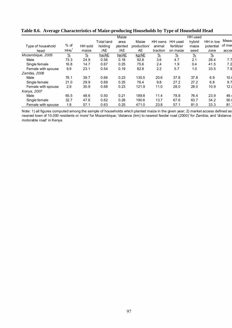
97

Table 8.6. Average Characteristics of Maize-producing Households by Type of Household Head

% of HHs1

HH sold maize

Total land-holding

/AE

Maize area

planted /AE

Maize production/

AE

HH owns animal traction

HH used fertilizer

on maize

HH used hybrid maize seed

HH in low potential

zone

Measuof maracces

Mozambique, 2005 % % ha/AE ha/AE kg/AE % % % %Male 73.3 24.9 0.56 0.18 92.8 3.6 4.7 2.1 28.4 7.7Single female 16.8 14.7 0.67 0.25 75.6 2.4 1.9 0.4 41.5 7.2Female with spouse 9.9 23.1 0.54 0.19 82.8 2.2 5.7 1.0 33.5 7.9

Zambia, 2008Male 76.1 39.7 0.66 0.23 130.5 20.6 37.8 37.8 6.9 10.6Single female 21.0 29.9 0.69 0.25 76.4 9.8 27.2 27.2 6.8 9.7Female with spouse 2.9 30.9 0.68 0.23 121.9 11.0 28.0 28.0 10.9 12.8

Kenya, 2007Male 65.5 48.6 0.50 0.21 189.8 11.4 78.8 76.4 23.9 49.4Single female 32.7 47.6 0.62 0.28 190.6 13.7 67.6 63.7 34.2 50.0Female with spouse 1.8 57.1 0.63 0.25 471.0 23.8 57.1 81.0 33.3 81.7

Type of household head

Note: 1) all figures computed among the sample of households which planted maize in the given year; 2) market access defined as nearest town of 10,000 residents or more' for Mozambique; 'distance (km) to nearest feeder road (2000)' for Zambia; and 'distance motorable road' in Kenya.

98

9. CONCLUSIONS

Previous research on household food grain sales behavior in developing countries has tended to focus on the role of market access and price-related factors to explain why many rural households do not sell staple crops such as maize. The conclusions of this line of research have been to promote market liberalization and road construction to provide producers with lower transaction costs and more favorable input and output prices. However, a key concern raised in recent literature is that low household asset endowments may constrain the ability of many smallholders to take advantage of public goods that reduce the cost of market access. While a combination of market liberalization and improved road infrastructure would tend to improve input and output prices facing smallholders, we present evidence that suggests that many smallholders in these countries already enjoy reasonable market access. Our descriptive analysis of rural household data from Mozambique, Zambia, and Kenya shows that in general there is little difference between large and small net sellers in any of the three countries in regard to market access as measured by distance to the nearest road, and access to market information, and that the majority of maize sellers in each country make their sales within their village. This is consistent with our finding from econometric analysis of household maize sales that typical market access proxies (distance to physical infrastructure or towns) are not significant or of small magnitude in most zones in our case countries. These findings are also consistent with recent rapid appraisal work in each country which found that trader presence even in ‘remote’ villages has greatly improved compared with the situation a decade ago, perhaps a result of increased investments in road construction as well as the recent proliferation of cell phones in rural areas. Thus, while there still may be significant transport costs to the nearest relevant market for farmers in ‘remote’ villages (which would cause traders to adjust their maize buying prices lower), even these farmers now face considerably lower search costs for price information and access to traders than they did a decade ago. Another potential factor affecting transaction costs of search for price information is access to market price information, which would be expected to improve maize market participation. In Mozambique, we find that household receipt of market price information results in large increases in the probability of maize sale and sale quantities. In Kenya and Zambia, we use radio and cell phone ownership as a proxy for household access to market price information; we also find significant positive effects of such assets on quantities sold. These findings suggest that funding to increase the spatial coverage and frequency of radio broadcasts in these countries could potentially lead to large increases in both quantities of maize sold as well as the numbers of households selling maize. While we also find that responsiveness of household maize sales to changes in expected farmgate maize prices are significant and positive in most areas of Kenya, in higher potential zones in Zambia, and among current sellers in Mozambique, we find insignificant or negative household responsiveness to maize prices in lower potential zones of Zambia and Mozambique. The heterogeneity of maize price responsiveness in Zambia and Mozambique indicates that while improved infrastructure may elicit a positive sales response in some regions, policymakers aiming to increase marketed maize surplus from smallholders need to also consider several non-price factors. These include the distribution and level of key production assets such as landholding, as well as factors that affect the return to those productive assets, such as technology use and agro-ecological potential (which affects the technology needs for a given region). In the case of Mozambique, until productive assets such as landholding and animal traction use are increased, and returns to existing assets are improved via adoption of technologies such as fertilizer and improved seed, it is questionable

99

whether improved prices alone (through better infrastructure) will elicit a positive supply response from maize producers who currently do not sell maize (i.e., 80% of maize growers). There are clear opportunities in Zambia and Mozambique to address the extremely low levels of landholding among the bottom half of the land distribution, though this will require investment in public goods, such as investments to eradicate disease-constraints to animal traction in Mozambique, and infrastructure investments in unsettled areas to promote migration in Zambia. Our results from Kenya and Zambia also show that use of divisible inputs such as hybrid seed and fertilizer can significantly increase the number of households selling maize as well as quantities sold, among farmers of various landholding sizes and from various agro-ecological zones. However, policy prescriptions for increasing smallholder access to fertilizer and hybrid maize seed varies considerably across our three countries given the dramatically different state of the private input markets in each country. In each country, we find that measures of either rainfall or drought stress have significant and large effects on the probability of selling and/or amounts sold, while controlling for household assets, maize price, and market access. These results highlight the sensitivity of marketed maize surplus to weather shocks, and thus the potential value of: a) investment in development and dissemination of drought-tolerant maize varieties; and b) widespread promotion of smallholder access to low-cost methods of irrigation and/or conservation farming techniques to reduce the impact of drought. A key implication of the foregoing for CAADP investment strategies at country level is that there needs to be very effective spatial coordination between investments under Pillars 1, 2, and 4 to ensure that farmers have sufficient access to land and technology with which they can take advantage of investments in improved market access. While CAADP and recent donor statements include agricultural research and development as a key to improved food security in Sub-Saharan Africa, the fact is that agricultural R&D has faced declining host government and donor funding for several decades; a trend that will have to be reversed if SSA countries are going to improve food crop productivity. A further challenge facing countries in southern and eastern Africa is that political economy factors have recently led several governments in the region to funnel increased spending in the agricultural sector into subsidizing private goods (fertilizer) and grain parastatal activities rather than investment in public goods such as agricultural R&D and improved road infrastructure, whose benefits are realized in the longer-term.

100

APPENDIX A-1

A critical assumption of the argument for improving road infrastructure and market access in rural SSA is that if such investment lowers transportation and search costs for farmers, they would respond to higher effective farmgate prices for food crops by producing and selling more. This assumption is based on neoclassical economic theory of the firm (farmer, producer, etc.), which predicts that producers will increase quantity produced as output price increases, holding other factors constant. However, the vast majority of small and medium-holder farmers in SSA are semi-subsistence producers, which both produce and consume food crops. For example, the value of retained food crops accounts for about two-thirds or more of total household income for the poorest 60% of households in Mozambique and Zambia (Table 4.2a). With respect to maize, we find that only 20% of maize growers are net maize sellers in Mozambique (25% in Zambia, and 41% in Kenya) (Table 4.5.). Recognition that semi-subsistence maize growers are both producers and consumers of maize leads to a household modeling approach to analysis of household response of marketed surplus to price changes (Sadoulet and de Janvry 1995). This is typically done by starting from the identity for marketed surplus: Mt = Qt – Ct (1) where: Mt = marketed surplus, Qt = production, and Ct = consumption Renkow (1990) adds inventory (stocks) to this identity, which are used by households for two main reasons. First, households might want to minimize their reliance on local markets to satisfy consumption requirements, holding stocks of food as a contingency against unanticipated price rises or quantity disruptions. Second, households might store grain in pursuit of arbitrage opportunities (i.e., hold onto grain in the event that prices rise faster than storage and interest costs). Adding stocks to the identity yields the following: Mt = Qt + It – Ct – It+1 (2) where: It = holdover stocks (carry-in) and It+1 = future stock (carry-out) As there are very few households in these countries which carry stocks from the previous season at the end of the lean season, we assume that It=0. We then differentiate (2) with respect to Pt. dMt/dPt = dQt/dPt – dCt/Pt|u=0 - (Qt – Ct)dCt/dYt – dIt+1 /dPt (3) dMt/dPt = supply -- (substitution effect) – (Qt – Ct)(income effect) -- (future stocks) (4) ( +) -- (--) -- (--/+ )(+) -- (+) The first term on the left in (3) is the producer supply response, which is positive. The second term is the consumer’s substitution effect, which is negative. The third term is the income or profit effect, which is positive for a normal good; that is, as the price of the good rises, household income increases (since the value of maize production represents a significant portion of crop income) and the household chooses to consume more of that good. The fourth

101

term is a stock effect, which is an additional wealth effect (Renkow 1990), and which represents the effect on marketed surplus of the household’s demand for stocks in the following period, given an increase in price during the current time period. The income effect can be relatively large if the good constitutes a large share of household income, which appears to be the case with maize for poor farmers in these countries. This positive income effect is multiplied by the household’s net position, which is negative for net buyers and positive for net sellers. While the supply and substitution effects generally are large enough to ensure that price response is positive, it is possible that a positive income effect for a poor net seller could be large enough to turn the total response negative, especially in a situation where substitution effects and supply response are low (i.e., low agro-ecological potential and low input use). However, even among net buyers (for whom the income effect term ends up positive), it is possible that stock effects could turn the price response negative, especially in a situation where household preference to store food rather than rely on the market is strong, because the stored crop represents a large proportion of consumption of that good and a relatively large proportion of total household wealth. The response of marketed surplus to changes in price has been found to be positive in most studies (Strauss 1984; Renkow 1990; Goetz 1992; Key, Sadoulet, and de Janvry 2000; Renkow, Hallstrom, and Karanja 2004; Alene et al. 2007), though a few have found a negative response (de Janvry and Kumar 1981; Bardhan 1970). Renkow (1990) also finds a negative price response, though this is in the short-term; he finds a positive response in the long-term. Further work is required to understand whether the discrepancy posed by these studies finding insignificant own-price supply response can be explained by methodological differences.

102

Appendix Table B-1. OLS Regression of Household Farmgate Maize Price Received by Sellers, 2002-2005, Mozambique

Independent variables Coefficient SE p-value1=year 2002 0.374 0.247 0.130distance from village to district capital, 2002 (km) 0.000 0.025 0.998distance from village to public transport, 2002 (km) -0.031 0.023 0.169travel time from village to nearest town of 10k residents 0.005 0.004 0.134education level of the HH head (years) 0.014 0.018 0.423age of the HH head (years) -0.004 0.006 0.548total landholding (ha) 0.000 0.015 0.9871=HH owns bicycle 0.034 0.054 0.5301=HH owns cart 0.416 0.343 0.2261=HH received market price info -0.015 0.056 0.797average regional wholesale price in Oct-Dec (planting) 0.095 0.068 0.164average regional wholesale price in Jul-Sep (t-1 quarter) -0.187 0.226 0.407average regional wholesale price April-June (t-2 quarter) 0.273 0.291 0.349average regional wholesale price Jan-Marc (t-3 quarter) -0.093 0.083 0.262Constant -15.871 1.582 0.000

District dummies included yesCorrelated Random Effect time-average terms included yesObservations 1,462R-squared 0.195

F-testsH0: District dummies=0 17.9 (0.000)H0: Lagged regional prices=0 40.0 (0.000)Overall F(97, 1177) 3.44 (0.000)

Dept Variable = ln(farmgate maize sales price)

103

Appendix Table B-2. Summary Statistics of Variables in Auxiliary & Double-Hurdle Models, Mozambique, 2002-2005

Obs. Mean SE Mean SEDependent variables

maize sale price ('000 meticais/kg) 1,462 2.487 0.065 3.586 0.108ln(maize sale price) 1,462 0.773 0.020 1.104 0.0271=HH sold maize 6,352 0.276 0.010 0.238 0.009quantity of maize sold (kg) 6,352 61.926 4.416 59.673 4.651ln(quantity of maize sold) 6,352 1.284 0.046 1.134 0.045

Independent variables# of days of drought (district-level) 6,352 32.737 0.738 48.088 0.625% village hhs which report maize yield loss 6,352 0.628 0.006 0.820 0.004total landholding 6,352 2.099 0.038 2.238 0.032ln(total landholding) 6,352 0.475 0.016 0.572 0.014ln(total assets) 6,352 6.168 0.052 6.137 0.055# prime-age adults working in ag 6,352 2.407 0.026 2.496 0.0291=HH owns animal traction 6,352 0.026 0.003 0.035 0.003% village hhs received extension visit 6,352 0.150 0.003 0.172 0.004head's age 6,352 42.917 0.313 45.414 0.312head's education level 6,352 2.221 0.049 1.985 0.054ln(distance to fertilizer seller) 6,352 3.565 0.029 3.566 0.029travel time to nearest 10k town (hours) 6,352 7.602 0.131 7.601 0.1311=HH owns bike 6,352 0.271 0.009 0.346 0.0101=HH owns cart 6,352 0.012 0.002 0.016 0.0021=HH received market price info 6,352 0.229 0.009 0.266 0.0091=HH belongs to farm association 6,352 0.043 0.004 0.079 0.006ln(expected farmgate maize price) 6,352 0.802 0.006 1.179 0.007dependency ratio 6,352 0.525 0.012 1.269 0.0211=HH headed by single female 6,352 0.154 0.007 0.158 0.0081=HH headed by female with spouse 6,352 0.074 0.006 0.100 0.0061=HH had prime-age death in past 3 years 6,352 0.036 0.004 0.059 0.005ln(distance to main district town) 6,352 2.513 0.022 2.513 0.022ln(distance to public transport) 6,352 2.921 0.024 2.921 0.024average regional wholesale price in Oct-Dec (planting) 6,352 3.978 0.012 3.432 0.009average regional wholesale price in Jul-Sep (t-1 quarter) 6,352 2.532 0.008 3.137 0.008average regional wholesale price April-June (t-2 quarter) 6,352 1.514 0.008 3.071 0.012average regional wholesale price Jan-Marc (t-3 quarter) 6,352 1.729 0.007 4.416 0.013

2004/052001/02

104

Appendix Table C-1. OLS Regression of Household Farmgate Maize Price Received by Sellers, 2000-2008, Zambia

Independent variables Coefficient SE p-value1=year 2008 (omitted)ln(6-year moving average seasonal rainfall) -0.344 0.137 0.0126-year moving average seasonal drought stress -0.001 0.005 0.868distance from village to district capital, 2000 (km) 0.000 0.000 0.283distance from village to feeder road, 2000 (km) 0.004 0.002 0.108distance from village to main/tarred road, 2000 (km) -0.001 0.000 0.023Education level of the HH head (years) 0.003 0.004 0.400Age of the HH head (years) 0.000 0.001 0.956ln(total landholding) 0.029 0.012 0.019ln(total value of farm assets) 0.004 0.002 0.0371=HH owns bicycle 0.030 0.020 0.1401=HH owns cart 0.058 0.032 0.0671=HH owns radio -0.009 0.019 0.6161=HH owns cell phone 0.013 0.026 0.628Last season's district median farmgate maize sales price 0.000 0.000 0.034ln(FRA district-level purchases, last year) 0.020 0.006 0.001residual from Tobit of household quantity of maize sold 0.000 0.000 0.000regional wholesale price in planting month 0.001 0.000 0.001regional wholesale price in planting month, t-1 (months) 0.002 0.001 0.001regional wholesale price in planting month, t-2 0.000 0.000 0.363regional wholesale price in planting month, t-3 0.000 0.000 0.920regional wholesale price in planting month, t-4 0.001 0.000 0.041regional wholesale price in planting month, t-5 -0.001 0.000 0.000regional wholesale price in planting month, t-6 0.000 0.000 0.552regional wholesale price in planting month, t-7 -0.001 0.000 0.000regional wholesale price in planting month, t-8 0.000 0.000 0.912regional wholesale price in planting month, t-9 (omitted)regional wholesale price in planting month, t-10 -0.001 0.000 0.024regional wholesale price in planting month, t-11 0.002 0.000 0.000Constant 1.482 1.233 0.229

Province dummies included yesCorrelated Random Effect time-average terms included yesObservations 2,586R-squared 0.80

F-testsH0: Lagged regional prices=0 24.6 (0.000)Overall F(44, 1965) 237 (0.000)


105

Appendix Table C-2. Tobit Model of the Quantity of Subsidized Fertilizer Received by the Household, Zambia, 2000-2008

Independent variablesAPE SE p-value

1= year 2008 -1361.740 511.511 0.008ln(6-year moving average seasonal rainfall) 63.103 37.264 0.0906-year moving average seasonal drought stress -1.065 1.237 0.3891=SEA suitable for low input fertilizer -7.307 5.253 0.164ln(total landholding) 6.691 3.042 0.028ln(total assets) 0.355 1.696 0.834# prime-age adults -0.358 1.509 0.813head's education level (years) 0.663 0.717 0.355head's age (years) -0.160 0.166 0.334% village hhs which received credit 47.536 17.340 0.0061=HH owns animal traction or tractor 16.704 9.630 0.083distance from village-district capital, 2000 (km) -0.330 0.162 0.041distance from village to feeder road, 2000 (km) -0.999 0.096 0.000distance from village-main/tarred road, 2000 (km) -0.162 1.260 0.8981=HH owns bike 11.497 5.853 0.0491=HH owns cart 17.612 10.272 0.0861=HH owns radio -4.560 5.228 0.3831=HH owns cell phone -0.522 6.683 0.938ln(expected farmgate maize price) -39.921 9.156 0.000dependency ratio 0.562 2.874 0.8451=HH headed by single female -7.247 8.519 0.3951=HH headed by female with spouse -6.290 9.322 0.5001=HH had prime-age death in past 3 years 1.535 6.302 0.808ln(district FRA purchases, prior season) -0.726 1.761 0.680ln(district median farmgate fertilizer price) 9.497 27.340 0.7281=HH's constituency won by MMD in last presidential election 16.324 5.872 0.005% point gap in last election between MMD and nearest challenger 0.023 0.092 0.798

cases 7402

Model includes dummies for province and year=2008. Also included are time-average terms for each of the time-varying regressors. BS se = bootstrapped standard error. Standard errors are bootstrapped to account for the fact that the expected farmgate maize price variable is a generated regressor.

Tobit

Average Partial Effect of dE[ y | x ] / dxj (unconditional)

Dept variable = kg of subsidized fertilizer received by HH)

106

Appendix Table C-3. Tobit Model of Household Quantity of Fertilizer Applied per Hectare of Maize, Zambia, 2000-2008

Independent variablesAPE SE p-value

1= year 2008 -8.645 4.802 0.072ln(6-year moving average seasonal rainfall) 0.041 0.100 0.6816-year moving average seasonal drought stress -0.476 0.752 0.5271=SEA suitable for low input fertilizer -0.021 0.024 0.381ln(total landholding) -0.010 0.065 0.879ln(total assets) 0.128 0.029 0.000# prime-age adults 0.028 0.031 0.359head's education level (years) 0.044 0.014 0.002head's age (years) 0.003 0.003 0.381% village hhs which received credit -0.266 0.562 0.6361=HH owns animal or mechanized traction -0.250 0.158 0.113distance from village-district capital, 2000 (km) -0.005 0.003 0.149distance from village to feeder road, 2000 (km) -0.028 0.002 0.000distance from village-main/tarred road, 2000 (km) 0.003 0.024 0.9141=HH owns bike -0.041 0.124 0.7421=HH owns cart -0.183 0.183 0.3171=HH owns radio 0.177 0.104 0.0891=HH owns cell phone -0.010 0.132 0.940ln(expected farmgate maize price) -0.589 0.338 0.081dependency ratio 0.087 0.057 0.1291=HH headed by single female 0.165 0.175 0.3471=HH headed by female with spouse -0.089 0.251 0.7221=HH had prime-age death in past 3 years 0.033 0.114 0.770ln(district FRA purchases, prior season) 0.085 0.031 0.006quantity of subsidized fertlilizer received by HH (kg) 0.001 0.001 0.021residual from reduced form regression of subsidized fertilizer -0.001 0.001 0.044ln(district median farmgate fertilizer price) -0.018 0.556 0.975distance from village to nearest fertilizer seller -0.004 0.001 0.0031=district reported no fertilizer sales -0.004 0.001 0.003

cases 7402

Model includes dummies for province and year=2008. Also included are time-average terms for each of the time-varying regressors. BS se = bootstrapped standard error. Standard errors are bootstrapped to account for the fact that the variables expected farmgate maize price and quantity of subsidized fertilizer received by the HH are generated regressors.

Tobit

Average Partial Effect of dE[ y | x ] / dxj (unconditional)

Dept variable = ln(kg of fertilizer applied per hectare of maize)

107

Appendix Table C-4. Limited Probability Model of Household Use of Purchased Hybrid Maize Seed, Zambia, 2000-2008

Independent variablesCoefficient SE p-value

1= year 2008 5.628 2.125 0.008ln(6-year moving average seasonal rainfall) -0.845 0.079 0.0006-year moving average seasonal drought stress 0.012 0.572 0.9841=SEA suitable for low input fertilizer 0.129 0.022 0.000ln(total landholding) -0.058 0.071 0.416ln(total landholding), squared -0.015 0.026 0.580ln(total assets) -0.002 0.030 0.939ln(total assets), squared 0.000 0.002 0.961# prime-age adults 0.043 0.049 0.384# prime-age adults, squared -0.004 0.005 0.370head's education level (years) -0.011 0.012 0.362head's age (years) -0.007 0.013 0.580head's age (years), squared 0.000 0.000 0.404% village hhs which received credit -1.035 0.373 0.0061=HH owns animal traction or tractor -0.225 0.146 0.124distance from village-district capital, 2000 0.006 0.003 0.056distance from village to feeder road, 2000 (km) 0.017 0.002 0.000distance from village-main/tarred road, 2000 0.002 0.020 0.9041=HH owns bike -0.201 0.098 0.0411=HH owns cart -0.227 0.133 0.0871=HH owns radio 0.085 0.080 0.2921=HH owns cell phone 0.009 0.119 0.938ln(expected farmgate maize price) 0.661 0.223 0.003dependency ratio 0.018 0.049 0.7181=HH headed by single female 0.071 0.165 0.6691=HH headed by female with spouse 0.037 0.189 0.8451=HH had prime-age death in past 3 years 0.001 0.103 0.991ln(district FRA purchases, prior season) 0.021 0.030 0.483kg of subsidized fertlilizer received by HH 0.000 0.000 0.190residual from tobit reduced form of kg of subsidized fert. -0.001 0.000 0.000ln(district median farmgate fertilizer price) 0.090 0.478 0.851distance from village to nearest fertilizer seller -0.0004 0.0002 0.0241=district reported no fertilizer sales -0.007 0.018 0.703

cases 7402

Model includes dummies for province and year=2008. Also included are time-average terms for each of the time-varying regressors. BS se = bootstrapped standard error. Standard errors are bootstrapped to account for the fact that the variables expected farmgate maize price and quantity of subsidized fertilizer received by the HH are generated regressors.

LPM

PE of xj on P(y>0)

Dept variable = 1 if household used purchased hybrid maize

seed, =0 otherwise

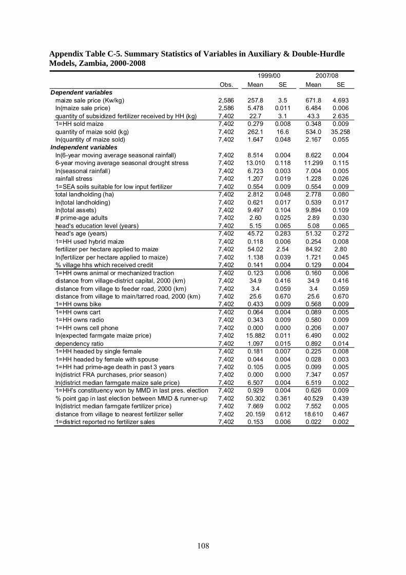
108

Appendix Table C-5. Summary Statistics of Variables in Auxiliary & Double-Hurdle Models, Zambia, 2000-2008

Obs. Mean SE Mean SEDependent variables

maize sale price (Kw/kg) 2,586 257.8 3.5 671.8 4.693ln(maize sale price) 2,586 5.478 0.011 6.484 0.006quantity of subsidized fertilizer received by HH (kg) 7,402 22.7 3.1 43.3 2.6351=HH sold maize 7,402 0.279 0.008 0.348 0.009quantity of maize sold (kg) 7,402 262.1 16.6 534.0 35.258ln(quantity of maize sold) 7,402 1.647 0.048 2.167 0.055

Independent variablesln(6-year moving average seasonal rainfall) 7,402 8.514 0.004 8.622 0.0046-year moving average seasonal drought stress 7,402 13.010 0.118 11.299 0.115ln(seasonal rainfall) 7,402 6.723 0.003 7.004 0.005rainfall stress 7,402 1.207 0.019 1.228 0.0261=SEA soils suitable for low input fertilizer 7,402 0.554 0.009 0.554 0.009total landholding (ha) 7,402 2.812 0.048 2.778 0.080ln(total landholding) 7,402 0.621 0.017 0.539 0.017ln(total assets) 7,402 9.497 0.104 9.894 0.109# prime-age adults 7,402 2.60 0.025 2.89 0.030head's education level (years) 7,402 5.15 0.065 5.08 0.065head's age (years) 7,402 45.72 0.283 51.32 0.2721=HH used hybrid maize 7,402 0.118 0.006 0.254 0.008fertilizer per hectare applied to maize 7,402 54.02 2.54 84.92 2.80ln(fertilizer per hectare applied to maize) 7,402 1.138 0.039 1.721 0.045% village hhs which received credit 7,402 0.141 0.004 0.129 0.0041=HH owns animal or mechanized traction 7,402 0.123 0.006 0.160 0.006distance from village-district capital, 2000 (km) 7,402 34.9 0.416 34.9 0.416distance from village to feeder road, 2000 (km) 7,402 3.4 0.059 3.4 0.059distance from village to main/tarred road, 2000 (km) 7,402 25.6 0.670 25.6 0.6701=HH owns bike 7,402 0.433 0.009 0.568 0.0091=HH owns cart 7,402 0.064 0.004 0.089 0.0051=HH owns radio 7,402 0.343 0.009 0.580 0.0091=HH owns cell phone 7,402 0.000 0.000 0.206 0.007ln(expected farmgate maize price) 7,402 15.882 0.011 6.490 0.002dependency ratio 7,402 1.097 0.015 0.892 0.0141=HH headed by single female 7,402 0.181 0.007 0.225 0.0081=HH headed by female with spouse 7,402 0.044 0.004 0.028 0.0031=HH had prime-age death in past 3 years 7,402 0.105 0.005 0.099 0.005ln(district FRA purchases, prior season) 7,402 0.000 0.000 7.347 0.057ln(district median farmgate maize sale price) 7,402 6.507 0.004 6.519 0.0021=HH's constituency won by MMD in last pres. election 7,402 0.929 0.004 0.626 0.009% point gap in last election between MMD & runner-up 7,402 50.302 0.361 40.529 0.439ln(district median farmgate fertilizer price) 7,402 7.669 0.002 7.552 0.005distance from village to nearest fertilizer seller 7,402 20.159 0.612 18.610 0.4671=district reported no fertilizer sales 7,402 0.153 0.006 0.022 0.002

2007/081999/00

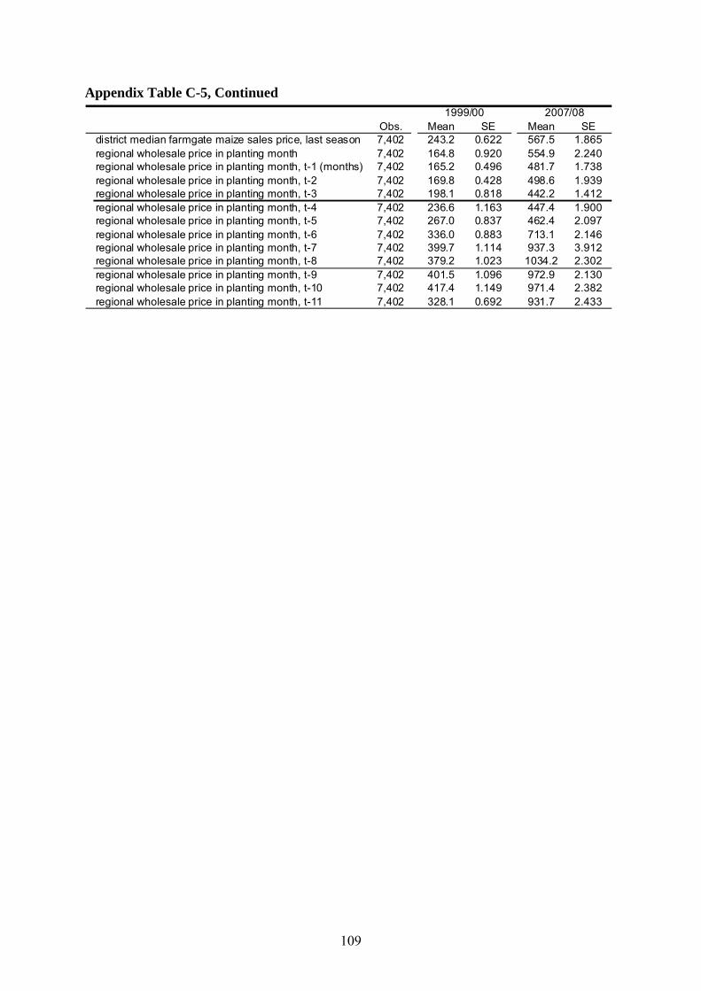
109

Appendix Table C-5, Continued

Obs. Mean SE Mean SEdistrict median farmgate maize sales price, last season 7,402 243.2 0.622 567.5 1.865regional wholesale price in planting month 7,402 164.8 0.920 554.9 2.240regional wholesale price in planting month, t-1 (months) 7,402 165.2 0.496 481.7 1.738regional wholesale price in planting month, t-2 7,402 169.8 0.428 498.6 1.939regional wholesale price in planting month, t-3 7,402 198.1 0.818 442.2 1.412regional wholesale price in planting month, t-4 7,402 236.6 1.163 447.4 1.900regional wholesale price in planting month, t-5 7,402 267.0 0.837 462.4 2.097regional wholesale price in planting month, t-6 7,402 336.0 0.883 713.1 2.146regional wholesale price in planting month, t-7 7,402 399.7 1.114 937.3 3.912regional wholesale price in planting month, t-8 7,402 379.2 1.023 1034.2 2.302regional wholesale price in planting month, t-9 7,402 401.5 1.096 972.9 2.130regional wholesale price in planting month, t-10 7,402 417.4 1.149 971.4 2.382regional wholesale price in planting month, t-11 7,402 328.1 0.692 931.7 2.433

1999/00 2007/08

110

Appendix Table D-1. OLS Regression of Household Farmgate Maize Price Received by Sellers, 1997-2000-2004-2008, Kenya

Independent variables Coefficient SE p-value1=year 2000 -0.050 0.144 0.7271=year 2004 0.008 0.115 0.9421=year 2008 -0.240 0.174 0.1686-year moving average of seasonal rainfall 0.000 0.000 0.0416-year moving average of seasonal drought shock 0.145 0.184 0.4311=sale quarter is Apr-June 0.017 0.018 0.3231=sale quarter is July-Sept -0.021 0.021 0.3331=sale quarter is Oct-Dec -0.029 0.016 0.063distance to regional wholesale market (km) 0.000 0.000 0.230distance to nearest motorable road (km) 0.004 0.005 0.4271=HH buyer type: NCPB 0.053 0.043 0.2151=HH buyer type: processor/miller 0.079 0.029 0.0061=HH buyer type: other 0.138 0.126 0.2751=HH buyer type: other household 0.054 0.018 0.0021=HH owns truck 0.037 0.039 0.3401=HH owns bicycle -0.021 0.018 0.236ln(value of storage assets) 0.003 0.002 0.211ln(total landholding) 0.012 0.009 0.216ln(total value of farm assets) 0.018 0.005 0.000Age of the HH head (years) -0.002 0.001 0.122Education level of the HH head (years) -0.003 0.002 0.2291=HH suffered a prime-age death in previous 3 years 0.025 0.036 0.4871=HH headed by female with resident husband 0.033 0.025 0.1841=HH headed by female with no resident husband 0.023 0.035 0.505village-level effective NCPB purchase price at planting 0.012 0.006 0.070ln(NCPB distric t-level purchases, las t year) 0.007 0.010 0.482ln(NCPB distric t-level purchases, las t year)2 -0.001 0.001 0.354residual from Tobit of household maize sale volume 0.000 0.000 0.004regional wholesale price in planting month -0.666 0.600 0.267regional wholesale price in planting month, t-1 (months) 0.873 0.491 0.075regional wholesale price in planting month, t-2 -0.156 0.222 0.481regional wholesale price in planting month, t-3 -0.392 0.108 0.000regional wholesale price in planting month, t-4 0.718 0.338 0.034regional wholesale price in planting month, t-5 -0.557 0.397 0.161regional wholesale price in planting month, t-6 0.682 0.603 0.258regional wholesale price in planting month, t-7 -0.061 0.343 0.858regional wholesale price in planting month, t-8 -0.401 0.411 0.329regional wholesale price in planting month, t-9 -0.071 0.361 0.844regional wholesale price in planting month, t-10 0.514 0.281 0.068regional wholesale price in planting month, t-11 -0.225 0.336 0.502Constant -1.199 2.379 0.614


Province dummies included yesCorrelated Random Effect time-average terms included yesObservations 1,658R-squared 0.27

F-tes tsH 0: Province dummies=0 10.84 (0.000)H 0: Lagged regional prices=0 2.80 (0.000)H 0: Buyer types=0 3.91 (0.000)Overall F(68, 729) 9.82 (0.000)

111

Appendix Table D-2. Tobit Regression of Household Quantity of Fertilizer Applied per Hectare of Maize, Kenya, 1997-2004-2008

Independent variablesAPE BS se p-value

1=year 2004 4.555 0.830 0.0001=year 2007 6.025 1.102 0.0001=volcanic soils in village -0.214 0.340 0.5291=humic soils in village 0.153 0.388 0.6941=Rankers soils with high sand in village 0.388 0.398 0.3306-year moving average seasonal rainfall -0.001 0.001 0.0526-year moving average seasonal drought shock 1.355 0.838 0.106ln(total area) -0.058 0.046 0.208ln(total assets) 0.070 0.064 0.274# prime-age adults 0.030 0.026 0.2451=HH owns irrigation equipment 0.176 0.160 0.269ln(village agricultural wage) 0.326 0.254 0.199% village hhs which received credit 0.024 0.243 0.9201=HH owns animal or mechanized traction 0.307 0.168 0.067distance from village to nearest extension 0.000 0.021 0.986head's age (years) -0.003 0.619 0.996maximum adult education (years) 0.007 0.010 0.502distance from village to motorable road (km) 0.004 0.074 0.9551=HH owns bike 0.240 0.091 0.0081=HH owns vehicle -0.231 0.188 0.2181=HH owns cart 0.020 0.171 0.9071=HH owns radio 0.074 0.097 0.446ln(expected farmgate maize price) 1.565 0.367 0.000dependency ratio 0.031 0.057 0.5821=HH headed by single female 0.033 0.130 0.8001=HH headed by female with spouse -0.388 0.331 0.2411=HH had prime-age death in past 3 years -0.220 0.177 0.214ln(district median farmgate fertilizer price) -0.375 0.619 0.544village median distance to fertilizer seller 0.052 0.018 0.004village median distance to hybrid seed seller -0.087 0.026 0.001

cases 3506

Model includes dummies for agroecological zone. Also included are time-average terms for each of the time-varying regressors. APE= average partial effect, BS se = bootstrapped standard error. Standard errors are bootstrapped to account for the fact that the expected farmgate maize price variable is a generated regressor.

Tobit

Average Partial Effect of dE[ y | x] / dxj (unconditional)

Dept variable = ln(kg of fertilizer applied to maize, per hectare)

112

Appendix Table D-3. Limited Probability Model of Household Use of Purchased Hybrid Maize Seed, Kenya, 1997-2004-2008

Independent variablesCoefficient SE p-value

1=year 2004 0.139 0.155 0.3681=year 2007 0.298 0.218 0.1701=volcanic soils in village 0.075 0.076 0.3281=humic soils in village 0.069 0.078 0.3741=Rankers soils with high sand in village 0.044 0.082 0.5926-year moving average seasonal rainfall 0.000 0.000 0.2436-year moving average seasonal drought shock 0.322 0.190 0.090ln(total area) 0.023 0.011 0.039ln(total area), squared -0.005 0.005 0.331ln(total assets) -0.020 0.018 0.258ln(total assets), squared 0.001 0.001 0.228# prime-age adults 0.006 0.012 0.627# prime-age adults, squared -0.001 0.002 0.3601=HH owns irrigation equipment -0.012 0.041 0.774ln(village agricultural wage) -0.037 0.060 0.535% village hhs which received credit 0.160 0.046 0.0011=HH owns animal or mechanized traction 0.067 0.027 0.014distance from village to nearest extension -0.007 0.005 0.155head's age (years) 0.002 0.005 0.731head's age, squared (years) 0.000 0.000 0.860maximum adult education (years) 0.002 0.002 0.247distance from village to motorable road (km) -0.010 0.015 0.4911=HH owns bike 0.053 0.021 0.0121=HH owns vehicle 0.019 0.036 0.5951=HH owns cart -0.002 0.034 0.9521=HH owns radio 0.043 0.021 0.039ln(expected farmgate maize price) 0.120 0.068 0.080dependency ratio -0.026 0.012 0.0301=HH headed by single female -0.002 0.028 0.9521=HH headed by female with spouse -0.052 0.057 0.3561=HH had prime-age death in past 3 years 0.021 0.033 0.532ln(district median farmgate fertilizer price) 0.212 0.116 0.067village median distance to fertilizer seller 0.004 0.004 0.310village median distance to hybrid seed seller -0.006 0.005 0.188

cases 3506

Model includes dummies for agroecological zone. Also included are time-average terms for each of the time-varying regressors. BS se = bootstrapped standard error. Standard errors are bootstrapped to account for the fact that expected farmgate maize price is a generated regressor.

LPM

PE of xj on P(y>0)

Dept variable = 1 if household used purchased hybrid maize

seed; =0 otherwise

113

Appendix Table D-4. Summary Statistics of Variables in Auxiliary and Double-Hurdle Models, Kenya, 1997-2004-2007

Obs. Mean SE Mean SE Mean SEDependent variables

maize sale price (Ksh/kg) 1,658 11.481 0.169 13.186 0.139 12.332 0.119ln(maize sale price) 1,658 2.407 0.014 2.554 0.010 2.491 0.0101=HH sold maize 3,506 0.321 0.014 0.473 0.015 0.486 0.015quantity of maize sold (kg) 3,506 481.636 55.329 737.824 53.408 805.838 63.318ln(quantity of maize sold) 3,506 2.016 0.089 3.054 0.099 3.160 0.099

Independent variables6-year moving average seasonal rainfall 3,506 558.977 5.840 573.765 4.314 512.744 5.4226-year moving average seasonal drought shock 3,506 0.318 0.006 0.284 0.006 0.338 0.007main season drought shocks 3,506 0.234 0.007 0.237 0.007 0.294 0.006total landholding 3,506 2.155 0.077 2.303 0.087 2.152 0.078ln(total landholding) 3,506 0.162 0.034 0.347 0.029 0.287 0.028ln(total assets) 3,506 10.878 0.064 10.268 0.065 10.590 0.045# prime-age adults 3,506 3.456 0.054 3.107 0.051 3.113 0.0551=HH owns irrigation equipment 3,506 0.126 0.010 0.110 0.009 0.112 0.0091=HH used hybrid maize 3,506 0.683 0.014 0.634 0.014 0.723 0.013ln(fertilizer applied to maize) (kg/ha) 3,506 2.267 0.057 3.225 0.066 3.428 0.064ln(village agricultural wage) 3,506 4.876 0.008 4.587 0.010 4.400 0.009% village hhs which received credit 3,506 0.401 0.009 0.346 0.010 0.526 0.0081=HH owns animal or mechanized traction 3,506 0.118 0.009 0.081 0.008 0.110 0.009distance from village to nearest extension 3,506 5.036 0.078 4.731 0.082 4.398 0.082head's age (years) 3,506 50.321 0.388 56.520 0.387 58.814 0.384maximum adult education (years) 3,506 3.999 0.042 12.185 0.162 11.510 0.114distance from village to motorable road (km) 3,506 1.091 0.034 1.017 0.025 0.501 0.0141=HH owns bike 3,506 0.413 0.014 0.469 0.015 0.499 0.0151=HH owns vehicle 3,506 0.032 0.005 0.049 0.006 0.051 0.0061=HH owns cart 3,506 0.034 0.005 0.045 0.006 0.039 0.0061=HH owns radio 3,506 0.758 0.013 0.886 0.009 0.907 0.008ln(expected farmgate maize price) 3,506 5.282 0.007 3.463 0.004 2.500 0.003dependency ratio 3,506 0.837 0.024 0.566 0.018 0.499 0.0161=HH headed by single female 3,506 0.121 0.010 0.190 0.011 0.328 0.0141=HH headed by female with spouse 3,506 0.003 0.001 0.014 0.003 0.018 0.004

2003/041996/97 2006/07

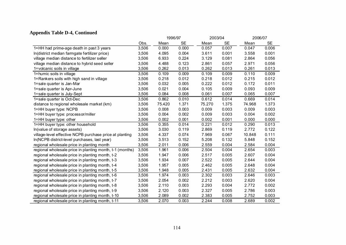
114

Appendix Table D-4, Continued

Obs. Mean SE Mean SE Mean SE1=HH had prime-age death in past 3 years 3,506 0.000 0.000 0.057 0.007 0.047 0.006ln(district median farmgate fertilizer price) 3,506 4.095 0.004 3.611 0.001 3.558 0.001village median distance to fertilizer seller 3,506 6.933 0.224 3.129 0.081 2.864 0.056village median distance to hybrid seed seller 3,506 4.488 0.123 2.861 0.057 2.971 0.0561=volcanic soils in village 3,506 0.262 0.013 0.262 0.013 0.261 0.0131=humic soils in village 3,506 0.109 0.009 0.109 0.009 0.110 0.0091=Rankers soils with high sand in village 3,506 0.218 0.012 0.218 0.012 0.215 0.0121=sale quarter is Jan-Mar 3,506 0.032 0.005 0.222 0.012 0.172 0.0111=sale quarter is Apr-June 3,506 0.021 0.004 0.105 0.009 0.093 0.0091=sale quarter is July-Sept 3,506 0.084 0.008 0.061 0.007 0.065 0.0071=sale quarter is Oct-Dec 3,506 0.862 0.010 0.612 0.014 0.669 0.014distance to regional wholesale market (km) 3,506 75.420 1.371 75.270 1.375 74.968 1.3731=HH buyer type: NCPB 3,506 0.008 0.003 0.009 0.003 0.009 0.0031=HH buyer type: processor/miller 3,506 0.004 0.002 0.009 0.003 0.004 0.0021=HH buyer type: other 3,506 0.002 0.001 0.002 0.001 0.000 0.0001=HH buyer type: other household 3,506 0.355 0.014 0.221 0.012 0.290 0.013ln(value of storage assets) 3,506 3.030 0.119 2.869 0.119 2.772 0.122village-level effective NCPB purchase price at planting 3,506 4.337 0.074 7.969 0.067 10.848 0.111ln(NCPB district-level purchases, last year) 3,506 3.513 0.152 5.208 0.132 5.848 0.152regional wholesale price in planting month 3,506 2.011 0.006 2.559 0.004 2.584 0.004regional wholesale price in planting month, t-1 (months) 3,506 1.961 0.006 2.504 0.004 2.654 0.003regional wholesale price in planting month, t-2 3,506 1.947 0.006 2.517 0.005 2.607 0.004regional wholesale price in planting month, t-3 3,506 1.934 0.007 2.522 0.005 2.644 0.004regional wholesale price in planting month, t-4 3,506 1.957 0.005 2.462 0.005 2.648 0.004regional wholesale price in planting month, t-5 3,506 1.948 0.005 2.431 0.005 2.632 0.004regional wholesale price in planting month, t-6 3,506 1.974 0.003 2.302 0.003 2.646 0.003regional wholesale price in planting month, t-7 3,506 2.054 0.002 2.212 0.003 2.620 0.004regional wholesale price in planting month, t-8 3,506 2.110 0.003 2.293 0.004 2.772 0.002regional wholesale price in planting month, t-9 3,506 2.120 0.003 2.327 0.005 2.786 0.003regional wholesale price in planting month, t-10 3,506 2.089 0.002 2.383 0.005 2.752 0.003regional wholesale price in planting month, t-11 3,506 2.070 0.003 2.244 0.008 2.689 0.002

1996/97 2003/04 2006/07

115

REFERENCES African Union/NEPAD. 2009. CAADP Framework for African Food Security. Midrand,

South Africa: NEPAD. Alene, A.D., V.M. Manyong, G. Omanya, H.D. Mignouna, M. Bokanga, and G. Odhiambo.

2007. Smallholder Market Participation under Transactions Costs: Maize Supply and Fertilizer Demand in Kenya. Food Policy 33: 318-328.

Argwings-Kodhek, G., T. Jayne, G. Nyambane, T. Awuor, and T. Yamano. 1998. How Can Micro-level Household Survey Data Make a Difference for Agricultural Policy Making? Nairobi: Egerton University/Tegemeo Institute of Agricultural Policy and Development. Available at: http://www.tegemeo.org/viewdocument.asp?ID=28 Banful, Afua Branoah. 2011. Old Problems in the New Solutions? Politically Motivated

Allocation of Program Benefits and the “New” Fertilizer Subsidies. World Development 39:7: 1166–176.

Bardhan, K. 1970. Price and Output Response of Marketed Surplus of Foodgrains: A Cross-

Sectional Study of Some North Indian Villages. American Journal of Agricultural Economics 52: 51-61.

Barrett, C.B. 2008. Smallholder Market Participation: Concepts and Evidence from Eastern

and Southern Africa. Food Policy 33.4: 299-317. Barrett, C.B, M. Bezuneh, D.C. Clay and T. Reardon. 2005. Heterogeneous Constraints,

Incentives and Income Diversification Strategies in Rural Africa. Quarterly Journal of International Agriculture 44.1: 37-60.

Boughton, D., D. Mather, C. B. Barrett, R. Benfica, D. Abdula, D. Tschirley, and B.

Cunguara. 2007. Market Participation by Rural Households in a Low-Income Country: An Asset-Based Approach Applied to Mozambique. Faith and Economics 50: 64-101.

Burke, W.J. and T.S. Jayne. 2008. Spatial Disadvantages or Spatial Poverty Traps:

Household Evidence from Rural Kenya. MSU International Development Working Paper No. 93. East Lansing: Michigan State University.

Carter. M.R. and C. B. Barrett. 2006. The Economics of Poverty Traps and Persistent

Poverty: An Assets-Based Approach. Journal of Development Studies 42.2: 178-99. Chamberlain, G. 1984. Panel Data. In Handbook of Econometrics, Vol. 2, ed. Z. Grilliches,

and M.D. Intriligator. Amsterdam, North Holland: Elsevier. Chamberlain, J. and T.S. Jayne. 2011. Unpacking the Meaning of Market Access.

Unpublished manuscript. Chapoto, A. and T.S. Jayne. 2008. Impact of AIDS-Related Mortality on Farm Households

Welfare in Zambia. Economic Development and Cultural Change 56.2: 327-74. Cragg, J.G. 1971. Some Statistical Models for Limited Dependent Variables with Application

to the Demand for Durable Goods. Econometrica 39.5: 829‐44.

http://www.tegemeo.org/viewdocument.asp?ID=28

116

CSO/FSRP. Various dates. Post Harvest Survey 1999/2000 and Supplemental Surveys 2001, 2004, and 2008. Lusaka: FSRP.

Cunguara, B. 2008. Pathways Out of Poverty in Rural Mozambique. M.Sc. thesis, Michigan

State University. de Janvry, A., M. Fafchamps, and E. Sadoulet. 1991. Peasant Household Behaviour with

Missing Markets: Some Paradoxes Explained. The Economic Journal 101.409: 1400-1417.

de Janvry, A. and P. Kumar. 1981. The Transmission of Cost Inflation in Agriculture with

Subsistence Production: A Case Study in Northern India. Indian Journal of Agricultural Economics 36: 1-14.

Goetz, S.J. 1992. A Selectivity Model of Household Food Marketing Behavior in Sub-

Saharan Africa. American Journal of Agricultural Economics 74.2: 444-52. Greene, W. 2004. Fixed Effects and Bias due to the Incidental Parameters Problem in the

Tobit Model. Econometric Reviews 23.2: 125-47. Haggblade, S., P. Hazell, and T. Reardon. 2009. Transforming the Rural Nonfarm Economy:

Opportunities and Threats in the Developing World. International Food Policy Research Institute (IFPRI) Issue Brief No. 58. Washington, D.C.: IFPRI.

Jayne, T.S., N. Mason, R. Myers, J. Ferris, D. Mather, M. Beaver, N. Lenski, A. Chapoto,

and D. Boughton. 2009. Patterns and Trends in Food Staples Markets in Eastern and Southern Africa: Toward the Identification of Priority Investments and Strategies for Developing Markets and Promoting Smallholder Productivity Growth. MSU International Development Paper No. 104. East Lansing, MI: Michigan State University.

Jayne, T.S., T. Yamano, M. Weber, D. Tschirley, R. Benfica, A. Chapoto, and B. Zulu. 2003.

Smallholder Income and Land Distribution in Africa: Implications for Poverty Reduction Strategies. Food Policy 28.3: 253-75.

Jayne, T.S., B. Zulu, G. Kajoba, and M. Weber. 2008. Access to Land, Agricultural Growth,

and Poverty Reduction in rural Zambia: Connecting the Policy Issues. FSRP Working Paper No. 34. Lusaka, Zambia: Food Security Research Project.

Available at: http://aec.msu.edu/fs2/zambia/wp_34.pdf Jayne, T.S., B. Zulu, and J.J. Nijhoff. 2006. Stabilizing Food Markets in Eastern and

Southern Africa. Food Policy 31.4: 328-41. Johnston, B. F. and P. Kilby. 1975. Agriculture and Structural Transformation: Economic

Strategies in Late Developing Countries. New York: Oxford University Press. Key, N., E. Sadoulet, and A. de Janvry. 2000. Transactions Costs and Agricultural Household

Supply Response. American Journal of Agricultural Economics 82: 245-59. Kirimi, L., N. Sitko, T.S. Jayne, F. Karin, M. Muyanga, M. Sheahan, J. Flock, and G. Bor.

2011. A Farmgate-to-Consumer Value Chain Analysis of Kenya’s Maize Marketing

http://aec.msu.edu/fs2/zambia/wp_34.pdf

117

System. MSU International Development Working Paper No. 111. East Lansing, Michigan: Michigan State University.

Magen, B., Cynthia Donovan, and Valerie Kelly. 2009. Can Cash Transfers Promote Food

Security in the Context of Volatile Commodity Prices? A Review of Empirical Evidence. MSU International Development Working Paper No. 96. East Lansing, Michigan: Michigan State University.

Mason, N. 2011a. Fertilizer Subsidies and Displacement of Farmers’ Commercial Fertilizer

Purchases – the Case of Zambia, Revisited. Essays on Marketing Boards, Fertilizer Subsidies, Prices, and Smallholder Behavior: Modeling and Policy Implications for Zambia. Ph.D. dissertation, Michigan State University. http://www.aec.msu.edu/theses/fulltext/mason_phd.pdf

Mason, N. 2011b. The Effects of the Zambian Food Reserve Agency and Government

Fertilizer Programs on Smallholder Farm Household Fertilizer Use and Crop Production. Essays on Marketing Boards, Fertilizer Subsidies, Prices, and Smallholder Behavior: Modeling and Policy Implications for Zambia. Ph.D. dissertation, Michigan State University. http://www.aec.msu.edu/theses/fulltext/mason_phd.pdf

Mather, D. 2009. Measuring the Impact of Public and Private Assets on Household Crop

Income in Rural Mozambique, 2002-2005. MINAG Directorate of Economics Research Paper No. 67. Maputo, Mozambique: MINAG.

Mather, D., B. Cunguara, and D. Boughton. 2008. Household Income and Assets in Rural

Mozambique, 2002-2005: Can Pro-poor Growth Be Sustained? MINAG Directorate of Economics Research Paper No. 66. Maputo, Mozambique: MINAG.

Mather, D. and C. Donovan. 2007. The Impacts of Prime-age Adult Mortality on Rural

Household Income, Assets, and Poverty in Mozambique. Directorate of Economics Research Paper 65E. Maputo, Mozambique: Directorate of Economics.

Mather, D. and T.S. Jayne. Forthcoming. The Impact of State Marketing Board Operations

on Smallholder Maize Price Expectations, Crop Production, and Fertilizer Use: The Case of Kenya.

Minde, I., T.S. Jayne, E. Crawford, J. Ariga, and J. Govereh. 2008. Promoting Fertilizer Use

in Africa: Current Issues and Empirical Evidence from Malawi, Zambia, and Kenya. Regional Strategic Analysis and Knowledge Support System for Southern Africa. (ReSAKSS) Working Paper No. 13. Pretoria, South Africa: ReSAKSS.

Morris, M., V. Kelly, R. Kopicki, and D. Byerlee. 2007. Fertilizer Use in African

Agriculture: Lessons Learned and Good Practice Guidelines. Washington, D.C.: The World Bank, Department of Agriculture and Rural Development,.

Mozambican Ministry of Agriculture (MINAG). 2002 and 2005. Trabalho do Inquerito

Agrìcola (TIA) Survey. Maputo: MINAG. Mundlak, Y. 1978. On the Pooling of Time Series and Cross Section Data. Econometrica 46: 69-85.

http://www.aec.msu.edu/theses/fulltext/mason_phd.pdf

http://www.aec.msu.edu/theses/fulltext/mason_phd.pdf

118

Muyanga, M. Forthcoming. Ph.D. dissertation essay on Marketing Margins for Maize in Kenya.

Overå, R. 2006. Networks, Distance, and Trust: Telecommunications Development and

Changing Trading Practices in Ghana. World Development 34.7: 1301-1315. Reardon, T., V. Kelley, E. Crawford, T.S. Jayne, K. Savadogo, and D. Clay. 1996.

Determinants of Farm Productivity in Africa: A Synthesis of Four Case Studies. MSU International Development Paper No. 22. East Lansing, Michigan: Michigan State University.

Renkow, M. 1990. Household Inventories and Marketed Surplus in Semi Subsistence

Agriculture. American Journal of Agricultural Economics 72: 664-75. Renkow, M., D.G. Hallstrom, and D. Karanja. 2004. Rural Infrastructure, Transactions Costs

and Market Participation in Kenya. Journal of Development Economics 85.5: 1140-1146.

Ricker-Gilbert, J., T.S. Jayne, and E. Chirwa. 2011. Subsidies and Crowding out: A Double-

hurdle Model of Fertilizer Demand in Malawi. American Journal of Agricultural Economics 93.1: 26–42.

Rivers, D. and Q.H. Vuong. 1988. Limited Information Estimators and Exogeneity Tests for Simultaneous Probit Models. Journal of Econometrics 39: 347-366. Sadoulet, E. and A. de Janvry. 1995. Quantitative Development Policy Analysis. Baltimore:

The Johns Hopkins University Press. Scandizzo, P. and C. Bruce. 1980. Methodologies for Measuring Agricultural Price

Intervention Effects. World Bank Staff Working Paper No. 394. Washington, D.C.: The World Bank.

Sheahan, M. Forthcoming. M.Sc. thesis. Analysis of Fertilizer Profitability and Use in Kenya.

Michigan State University. Singh, I, L. Squire, and J. Strauss. 1986. Agricultural Household Models. Baltimore: Johns

Hopkins University Press. Strauss, J. 1984. Marketed Surpluses of Agricultural Households in Sierra Leone. American

Journal of Agricultural Economics 66: 321-331. Tegemeo Institute of Egerton University. Various years. Smallholder Farm Surveys. Nairobi:

Tegemeo Institute. Timmer, C.P. 1997. Farmers and Markets: The Political Economy of New Paradigms. American Journal of Agricultural Economics 79: 621-27. Vella, F. 1993. A Simple Estimator for Simultaneous Models with Censored Endogenous Regressors. International Economic Review 34.2: 441-57.

119

Weber, M., J.M. Staatz, J.S. Holtzman, E.W. Crawford, and R.H. Bernsten. 1988. Informing Food Security Decisions in Africa: Empirical Analysis and Policy Dialogue. American Journal of Agricultural Economics 70.5: 1044-1052.

Wooldridge, J.M. 2002. Econometric Analysis of Cross Section and Panel Data. Cambridge,

MA: MIT Press. World Health Organization (WHO). 1985. WHO Technical Report Series No. 724. Geneva:

WHO.

Documents

Smallholder Heterogeneity and Maize Market Participation in