Small vessel detection in high qualityoptical satellite imagery- using component tree image representation and random forest classification

Patrik Johansson881129-5917, patrijoh@student.chalmers.se

AbstractMaritime vessel detection is an important part of maritime safety and at its heart liesdetection of vessels in satellite imagery. Current developments have made the detectionof small vessels particularly important as pronounced by the International MaritimeOrganization. The growing availability of high-quality (sub-meter resolution) imageshas made feasible the detection of small vessels that previously seemed impossible. Asthe amount of data increases so does the need for efficient methods of processing suchdata.

The work here presented introduces a new method for detection of small vessels inhigh resolution optical satellite images. The isolation of vessel candidates is performedby filtering applied to a component tree representation of the satellite image. Theclassification of the extracted vessel candidates is performed by a feature based randomforest classifier.

Performance of the vessel detection introduced in this work ranges from 85-99%depending on the tolerance for the amount of false detections. The method presentedperforms well compared to other work in the are and gives confidence in the possibilitiesof a method based on the approach presented in this work.

Course: TMS016, Statistical Image AnalysisExaminer: Mats Rudemo

Chalmers University of TechnologyGothenburg, May 31, 2011

Contents1 Introduction 1

2 Detection method 22.1 Overview . . . . . . . . . . . . . . . . . . . . . . . . . . . . . . . . . . . . . . 22.2 Component tree . . . . . . . . . . . . . . . . . . . . . . . . . . . . . . . . . . . 32.3 Building the component tree . . . . . . . . . . . . . . . . . . . . . . . . . . . 42.4 Filtering . . . . . . . . . . . . . . . . . . . . . . . . . . . . . . . . . . . . . . . 42.5 Classification . . . . . . . . . . . . . . . . . . . . . . . . . . . . . . . . . . . . 5

3 Experimental results 73.1 Vessel detection performance . . . . . . . . . . . . . . . . . . . . . . . . . . . 83.2 Prediction confidence . . . . . . . . . . . . . . . . . . . . . . . . . . . . . . . . 103.3 Feature selection . . . . . . . . . . . . . . . . . . . . . . . . . . . . . . . . . . 11

4 Discussion 12

5 Conclusion 13

6 Acknowledgments 13

ii

1 IntroductionMaritime vessel detection has recently received much attention as a consequence of the surgein piracy off the coast of Somalia. In a recent speech [1] by the Secretary-General of the In-ternational Maritime Organization the problem of piracy off the coast of Somalia was clearlyhighlighted and proposed as the theme for the World Maritime Day for 2011. Many authori-ties on maritime surveillance have highlighted the importance of satellite surveillance as onecomponent in prevention of unlawful maritime activities, among them the European Mar-itime Safety Agency [2, 3]. The detection of small vessels is of particular interest since onlylarger vessels are regulated to be monitored by systems such as AIS (automatic identificationsystem).

There are two main sources of satellite imagery used for vessel detection, SAR (SyntheticAperture Radar) and optical sensors. Theses two methods both have their advantages butalso their respective drawbacks. The choice of image acquisition method is central to anyvessel detection platform. Since SAR images are captured by radar sensors they are relativelyinsensitive to weather conditions such as cloud cover. Optical images have the advantage ofbeing very detailed but on the other hand are more sensitive to weather conditions.

In 2007 the Joint Research Centre (JRC) of the European Commission concluded a projectabbreviated DECLIMS (Detection, Classification and Identification of Marine Traffic fromSpace). The goal of this project was “to understand in detail the vessel detection and classi-fication on commercial satellite imagery of both types radar and optical”. In the final report[4] of this project a clear picture of the relative advantages and drawbacks of SAR and op-tical images is given. It is concluded that SAR images have been extensively studied dueto their ready availability and relative indifference to weather conditions. Typical detectionperformance for methods based on SAR images is >97% under favorable conditions and85-95% under normal conditions. Examples of complicating factors are extreme wind con-ditions, image artifacts and land-masking errors. Regarding optical imagery it is concludedthat although these images contain more information, detection systems are less developed.The proposed reason for this is the smaller image sizes, higher cost and higher sensitivity toweather conditions as compared to SAR images.

The field of vessel detection is well explored and lots of work have been done. Older workis manly focused on thresholding methods for component detection and classification usingstandard methods such as discriminant analysis. More recent work has shown a shift towardsmore advanced detection methods and more recent developments in the field of classification.Examples include an image component tree approach and wavelet analysis by Najman andCouprie [5]. Another interesting approach is using feature based neural networks as proposedby Corbane et al. [6]. Najman and Couprie report a detection rate around 60% to 90% undervarying weather conditions. The false detection rates varies between 30% and 130% in thisapplication. Corbane et al. report detection rates around 80% with no false detection ingood weather conditions and 60% detection rate with 5700% false detection rate under badweather conditions. Both use optical images with 5 meters per pixel resolution

The work here presented focuses on detection of small vessels in high quality opticalimagery (sub-meter resolution). This is intended to anticipate the shift of the field towardsmore data intensive methods as availability of high quality optical imagery increases. Themethod for component isolation is based on the image component tree approach described byNajman and Couprie [7]. For classification of isolated components a random forest classifieris proposed and evaluated. The data used for performance evaluation is high quality opticalimagery from the coast of the horn of Africa.

1

2 Detection method

2.1 OverviewThe vessel detection problem essentially reduces to two distinct problems. One regarding theisolation of components in an image and the other regarding the classification of the isolatedcomponents as being “vessel” or “other”.

Many component isolation methods are available among which the most used is threshold-ing. The idea is to split an image in to parts according to wether each pixel value is above orbelow a selected threshold value. Many methods for selecting a threshold value are available(e.g. histogram-based, local, spatial) but it is common knowledge that most commonly usedthresholding methods perform poorly on maritime vessel detection problems [5].

The component isolation method used in this work is based on the image componenttree algorithm introduced by Najman and Couprie [7]. This method will be discussed belowunder the heading “filtering”.

Once the components of interest have been satisfactorily isolated some decision rule forwether we regard a certain component as a boat or not is needed. Of course there are manymethods available, the one chosen in this work is a random forest classifier implemented inJava using the WEKA [8] API.

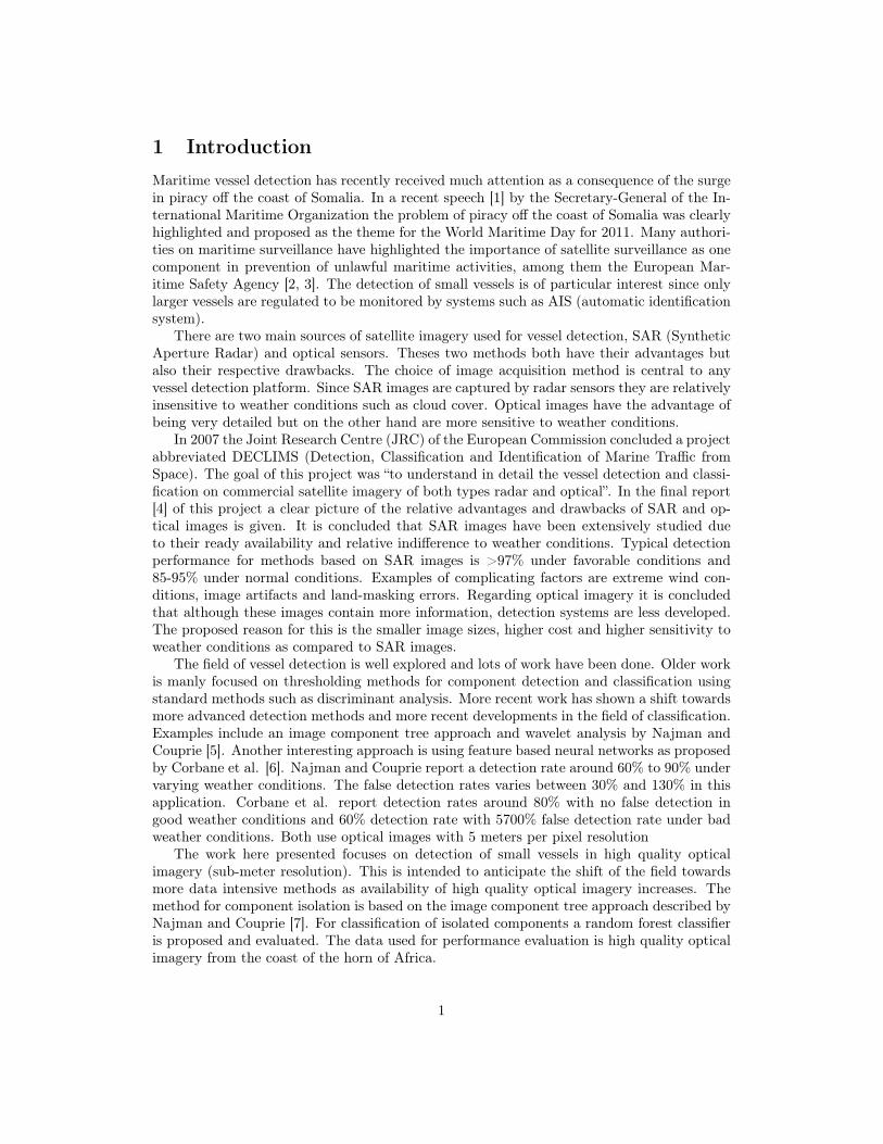
The classifier needs to be constructed based on some training data in order to be ableto predict data not yet seen. This means that a human must identify a number of vesseltargets to be used as training data. The workflow using training data, component isolationand classification is shown schematically in figure 1.

pre-processing andcomponent isolation

vesseldetection by

operator

featuresfor training

classifier

classificationrule

vesselcandidatefeatures

componentprediction

trainingimages

Figure 1: Schematic representation of detection workflow. Images are processedand then vessels in the training data are identified by a human operator. A classifieris built and used as basis for predicting future data.

2

2.2 Component treeA two-dimensional raster image can be described as a m × n matrix F containing values(fij , i = 1, ...,m, j = 1, ..., n) where ∀fij ∈ G and G is the set of all possible pixel values.Typical pixel values are G = {0, 1} (binary image), G = {0, ..., 255} (grayscale image) andG = {0, ..., 255}3 (RGB image). In this way a pixel is completely described by its position inthe image (i, j) and the value or level of the pixel fij .

An equivalent way of representing a raster image is with a vertex-weighted graph. Thuslywe denote a vertex-weighted graph by the triplet (V,E, F ) where V is a finite set of verticesand E is a subset of the cartesian product V × V . E are called edges. P(V ) denotes theset of all possible subsets of V . As such we can define the neighborhood of a vertex x asΓ(x) = {y ∈ V ‖(x, y) ∈ E}. If y ∈ Γ(x) we say that x and y are adjacent. For a vertex xwe define the level as F (x). A connected component of a graph is a set of vertices such thatthere exists a path (in the sense of a series of edges) between all vertices of the component.A (cross-)section of F is defined by Fk = {x ∈ V ‖F (x) ≥ k} where k is a level of F . Aconnected component of a section Fk is called a (level k) compnent. For stricter and moreextensive definitions, consult Najman and Couprie [7].

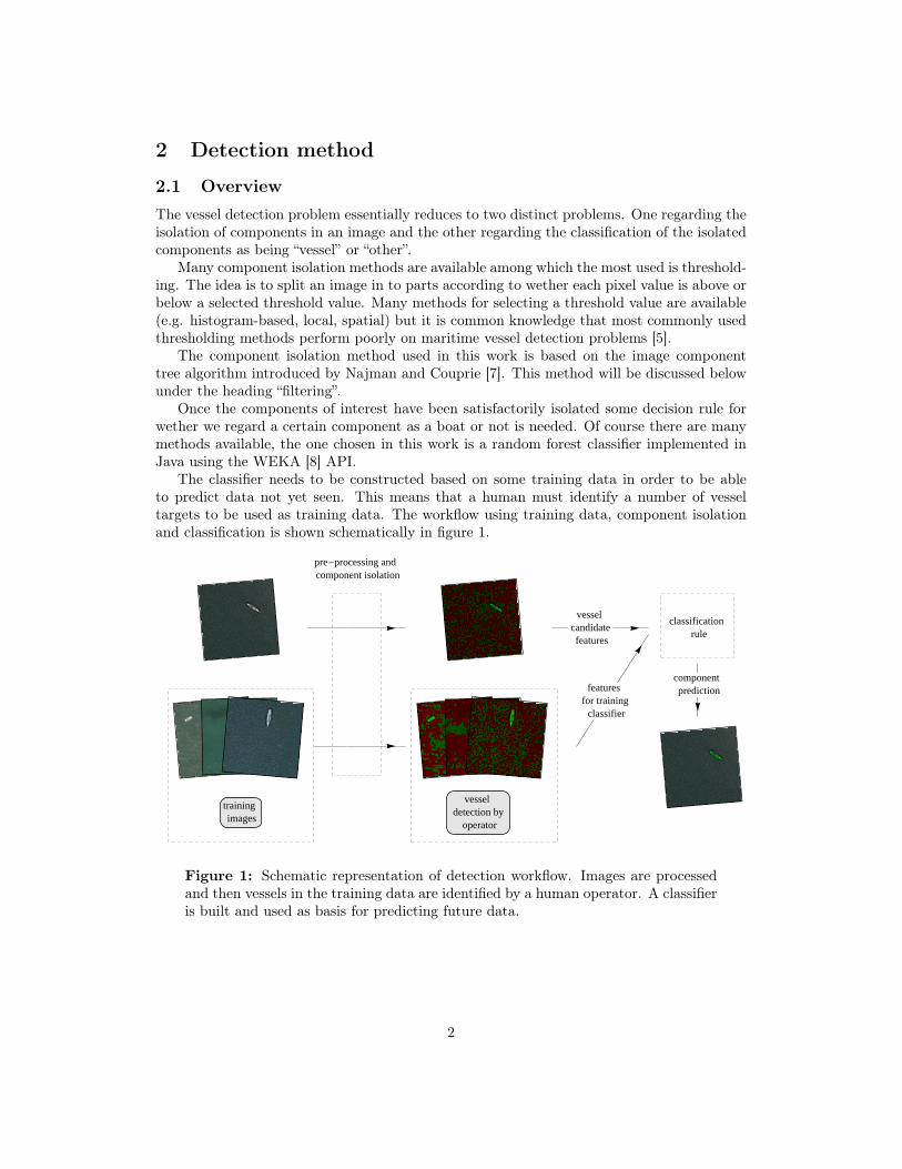
The definition of a vertex-weighted graph suggests a simple way of representing an imageas a tree. We define a tree as a set of nodes with another set of nodes being their children.This is most intuitively explained by figure 2. In this figure we see how the inclusion relationdefines a successive ordering of the connected components of different cross sections and thusthe components of the image. This tree is called the component tree.

(a) A weighted graph F and its cross-sections at levels 1,2,3 and 4.

(b) The component tree of the weighted graph F and the mapping between eachpoint and the component to which it belongs.

Figure 2: Figure used with permission from Najman and Couprie [7].

3

2.3 Building the component treeBy implementing the “Quasi-linear algorithm for the component tree” proposed by Najmanand Couprie [7] in Java the component tree is obtained efficiently for any grayscale image.The description of the algorithm will not be presented here since it would mostly labour thereader unnecessarily.

As an extension to the algorithm by Najman and Couprie a version for RGB images hasbeen implemented. The original algorithm merges two adjacent components if they havethe same level. In the extended algorithm the notion of grayscale level is still used but themerging of components is based on the Euclidean distance of the vertices in RGB space. Inthis way components are merged if the distance is less than some value, called α. α is in thecurrent implementation selected based on experience.

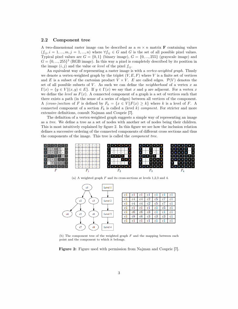
The complexity of the algorithm is quasi-linear [7], provided one sorts the data in lineartime complexity. Figure 3 shows the relative performance of the component tree algorithmnot regarding the sorting step. This was done by randomly generating grayscale images ofsuccessively larger dimensions. We conclude that the component tree algorithm performs asexpected for general input. The implementation in Java allows the algorithm to process a500x500 pixel image in a few second on a modern desktop computer (2.4GHz Intel Core 2Duo, 4GB 1067 MHz DDR3).

200 000 400 000 600 000 800 000 1 ´ 106n

0

5

10

15

20

25THnL

Figure 3: The relative computational time T (n) as a function of the number ofpixels n for randomly generated grayscale images. The dots represent empiricaldata and the line is the best linear description of the data.

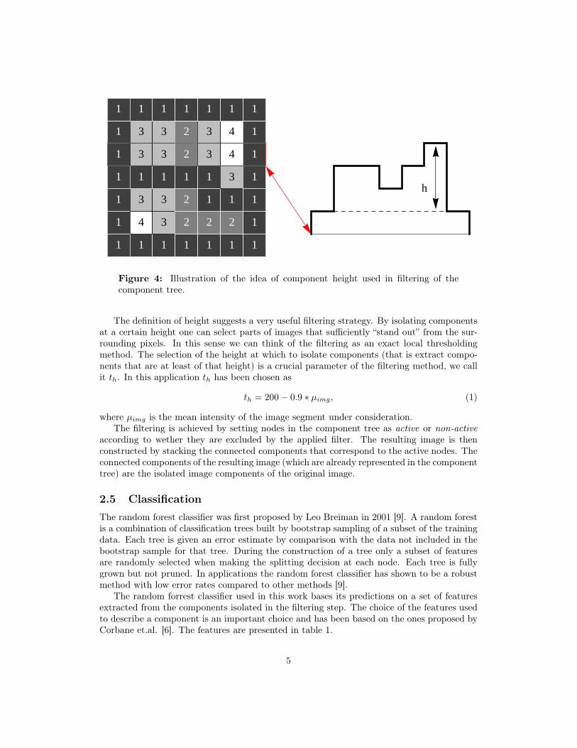
2.4 FilteringThe component tree is a useful representation of an image because it represents the connectedcomponents obtained by thresholding at all possible grey-level values. During the construc-tion of the component tree some useful properties of each component can be calculated withvirtually no additional cost. One such property is the height of each component, i.e. themaximum level ascribed to that component. The idea of component height is illustrated infigure 4.

4

1

1

1

1

1

1

1

1

4

3

1

3

3

1

1

3

3

1

3

3

1

1

2

2

1

2

2

1

1

2

1

1

3

3

1

1

2

1

3

4

4

1

1

1

1

1

1

1

1

h

Figure 4: Illustration of the idea of component height used in filtering of thecomponent tree.

The definition of height suggests a very useful filtering strategy. By isolating componentsat a certain height one can select parts of images that sufficiently “stand out” from the sur-rounding pixels. In this sense we can think of the filtering as an exact local thresholdingmethod. The selection of the height at which to isolate components (that is extract compo-nents that are at least of that height) is a crucial parameter of the filtering method, we callit th. In this application th has been chosen as

th = 200− 0.9 ∗ µimg, (1)

where µimg is the mean intensity of the image segment under consideration.The filtering is achieved by setting nodes in the component tree as active or non-active

according to wether they are excluded by the applied filter. The resulting image is thenconstructed by stacking the connected components that correspond to the active nodes. Theconnected components of the resulting image (which are already represented in the componenttree) are the isolated image components of the original image.

2.5 ClassificationThe random forest classifier was first proposed by Leo Breiman in 2001 [9]. A random forestis a combination of classification trees built by bootstrap sampling of a subset of the trainingdata. Each tree is given an error estimate by comparison with the data not included in thebootstrap sample for that tree. During the construction of a tree only a subset of featuresare randomly selected when making the splitting decision at each node. Each tree is fullygrown but not pruned. In applications the random forest classifier has shown to be a robustmethod with low error rates compared to other methods [9].

The random forrest classifier used in this work bases its predictions on a set of featuresextracted from the components isolated in the filtering step. The choice of the features usedto describe a component is an important choice and has been based on the ones proposed byCorbane et.al. [6]. The features are presented in table 1.

5

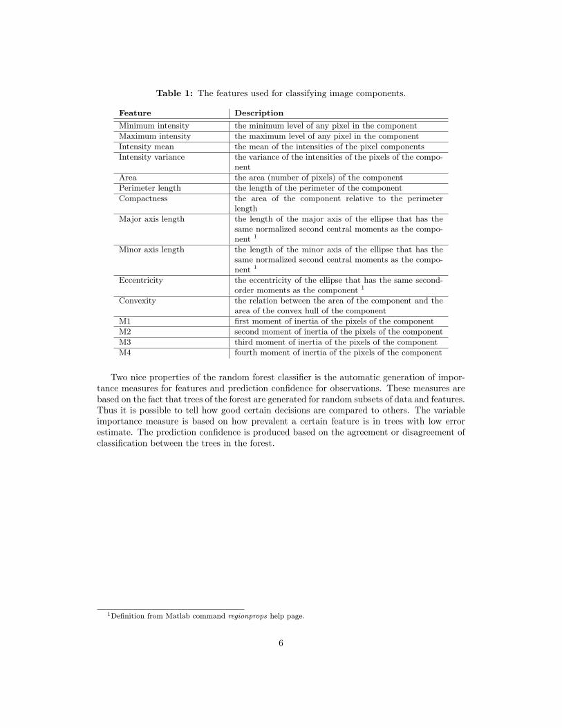
Table 1: The features used for classifying image components.

Feature DescriptionMinimum intensity the minimum level of any pixel in the componentMaximum intensity the maximum level of any pixel in the componentIntensity mean the mean of the intensities of the pixel componentsIntensity variance the variance of the intensities of the pixels of the compo-

nentArea the area (number of pixels) of the componentPerimeter length the length of the perimeter of the componentCompactness the area of the component relative to the perimeter

lengthMajor axis length the length of the major axis of the ellipse that has the

same normalized second central moments as the compo-nent 1

Minor axis length the length of the minor axis of the ellipse that has thesame normalized second central moments as the compo-nent 1

Eccentricity the eccentricity of the ellipse that has the same second-order moments as the component 1

Convexity the relation between the area of the component and thearea of the convex hull of the component

M1 first moment of inertia of the pixels of the componentM2 second moment of inertia of the pixels of the componentM3 third moment of inertia of the pixels of the componentM4 fourth moment of inertia of the pixels of the component

Two nice properties of the random forest classifier is the automatic generation of impor-tance measures for features and prediction confidence for observations. These measures arebased on the fact that trees of the forest are generated for random subsets of data and features.Thus it is possible to tell how good certain decisions are compared to others. The variableimportance measure is based on how prevalent a certain feature is in trees with low errorestimate. The prediction confidence is produced based on the agreement or disagreement ofclassification between the trees in the forest.

1Definition from Matlab command regionprops help page.

6

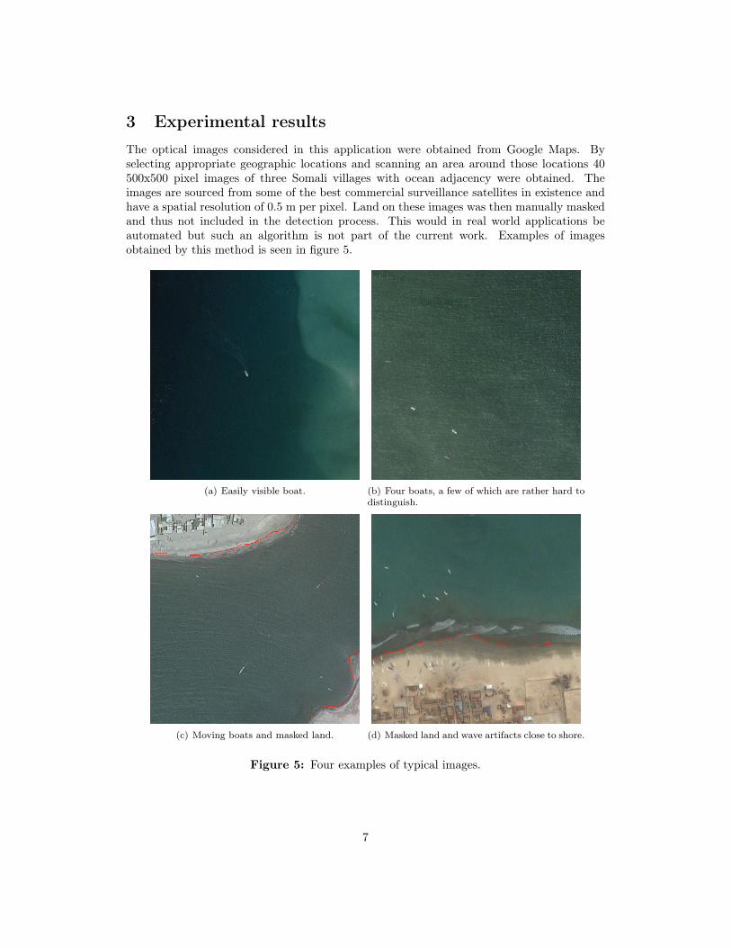
3 Experimental resultsThe optical images considered in this application were obtained from Google Maps. Byselecting appropriate geographic locations and scanning an area around those locations 40500x500 pixel images of three Somali villages with ocean adjacency were obtained. Theimages are sourced from some of the best commercial surveillance satellites in existence andhave a spatial resolution of 0.5 m per pixel. Land on these images was then manually maskedand thus not included in the detection process. This would in real world applications beautomated but such an algorithm is not part of the current work. Examples of imagesobtained by this method is seen in figure 5.

(a) Easily visible boat. (b) Four boats, a few of which are rather hard todistinguish.

(c) Moving boats and masked land. (d) Masked land and wave artifacts close to shore.

Figure 5: Four examples of typical images.

7

3.1 Vessel detection performanceTo evaluate the performance of the method described in section 2, cross-validation applied toa dataset with ground truth identified by a human operator has been performed. This givesa good measure of how well the method will perform on future data given that such datais similar to the data used for cross-validation. To this end the 40 images described in theprevious section were subjected to the component isolation and filtering algorithm and truevessel targets were manually identified. The total number of vessels identified by the humanoperator was 155. The height filtering parameter was chosen as described in equation 1 andthe filtering parameter α was set to 5. The features in table 1 were then calculated for eachisolated component found in the filtering step. 10-fold cross-validation of the random forestclassifier was then performed on the component data.

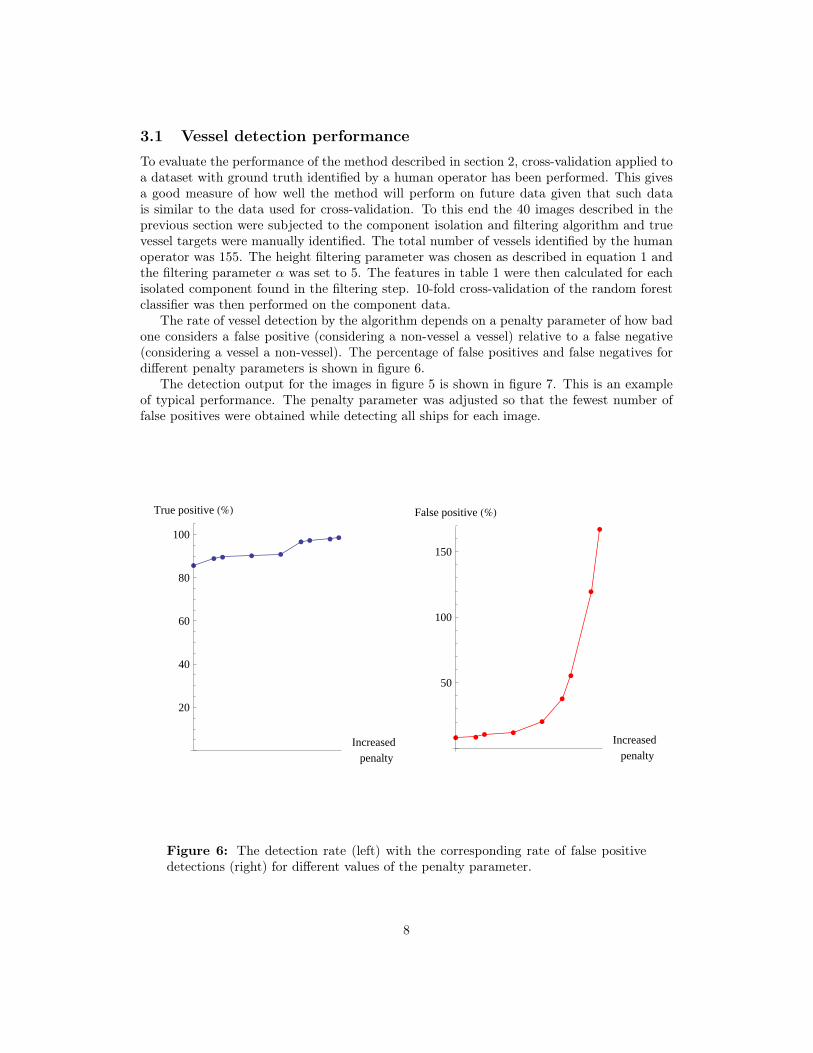
The rate of vessel detection by the algorithm depends on a penalty parameter of how badone considers a false positive (considering a non-vessel a vessel) relative to a false negative(considering a vessel a non-vessel). The percentage of false positives and false negatives fordifferent penalty parameters is shown in figure 6.

The detection output for the images in figure 5 is shown in figure 7. This is an exampleof typical performance. The penalty parameter was adjusted so that the fewest number offalse positives were obtained while detecting all ships for each image.

æ

æ æ æ æ

æ æ æ æ

Increasedpenalty

20

40

60

80

100

True positive H%L

æ ææ æ

æ

æ

æ

æ

æ

Increasedpenalty

50

100

150

False positive H%L

Figure 6: The detection rate (left) with the corresponding rate of false positivedetections (right) for different values of the penalty parameter.

8

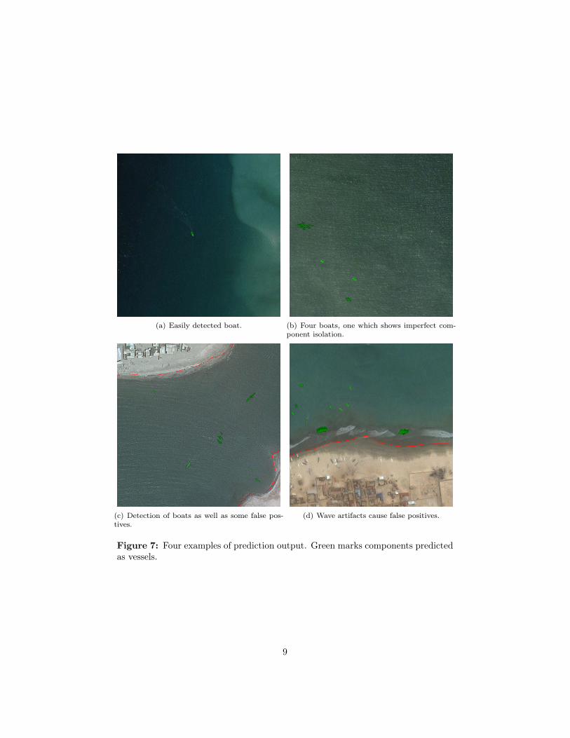
(a) Easily detected boat. (b) Four boats, one which shows imperfect com-ponent isolation.

(c) Detection of boats as well as some false pos-tives.

(d) Wave artifacts cause false positives.

Figure 7: Four examples of prediction output. Green marks components predictedas vessels.

9

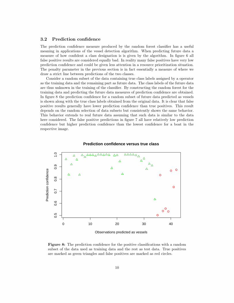
3.2 Prediction confidenceThe prediction confidence measure produced by the random forest classifier has a usefulmeaning in applications of the vessel detection algorithm. When predicting future data ameasure of how confident a class designation is is given by the algorithm. In figure 6 allfalse positive results are considered equally bad. In reality many false positives have very lowprediction confidence and could be given less attention in a resource prioritization situation.The penalty parameter in the previous section is in fact essentially a measure of where wedraw a strict line between predictions of the two classes.

Consider a random subset of the data containing true class labels assigned by a operatoras the training data and the remaining part as future data. The class labels of the future dataare thus unknown in the training of the classifier. By constructing the random forest for thetraining data and predicting the future data measures of prediction confidence are obtained.In figure 8 the prediction confidence for a random subset of future data predicted as vesselsis shown along with the true class labels obtained from the original data. It is clear that falsepositive results generally have lower prediction confidence than true positives. This resultdepends on the random selection of data subsets but consistently shows the same behavior.This behavior extends to real future data assuming that such data is similar to the datahere considered. The false positive predictions in figure 7 all have relatively low predictionconfidence but higher prediction confidence than the lowest confidence for a boat in therespective image.

●

●

●●

●

●

●

●

0 10 20 30 40

0.5

0.6

0.7

0.8

0.9

1.0

Prediction confidence versus true class

Observations predicted as vessels

Pre

dict

ion

conf

iden

ce

Figure 8: The prediction confidence for the positive classifications with a randomsubset of the data used as training data and the rest as test data. True positivesare marked as green triangles and false positives are marked as red circles.

10

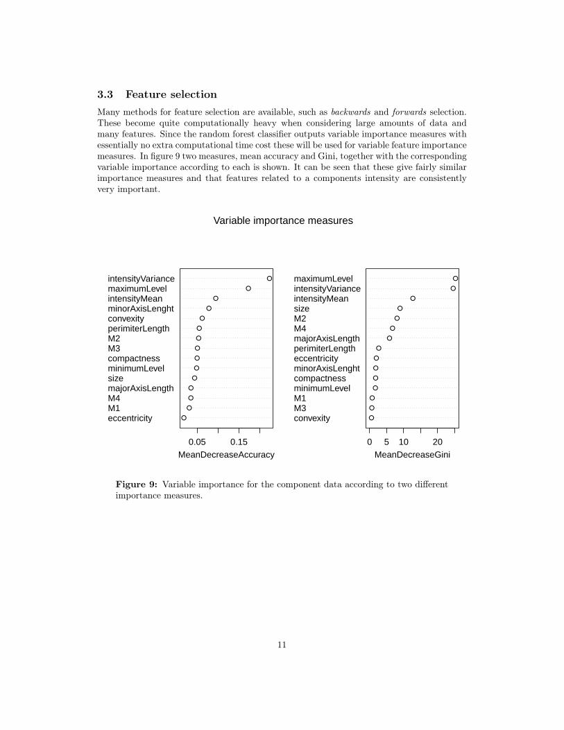
3.3 Feature selectionMany methods for feature selection are available, such as backwards and forwards selection.These become quite computationally heavy when considering large amounts of data andmany features. Since the random forest classifier outputs variable importance measures withessentially no extra computational time cost these will be used for variable feature importancemeasures. In figure 9 two measures, mean accuracy and Gini, together with the correspondingvariable importance according to each is shown. It can be seen that these give fairly similarimportance measures and that features related to a components intensity are consistentlyvery important.

eccentricityM1M4majorAxisLengthsizeminimumLevelcompactnessM3M2perimiterLengthconvexityminorAxisLenghtintensityMeanmaximumLevelintensityVariance

●

●

●

●

●

●

●

●

●

●

●

●

●

●

●

0.05 0.15MeanDecreaseAccuracy

convexityM3M1minimumLevelcompactnessminorAxisLenghteccentricityperimiterLengthmajorAxisLengthM4M2sizeintensityMeanintensityVariancemaximumLevel

●

●

●

●

●

●

●

●

●

●

●

●

●

●

●

0 5 10 20MeanDecreaseGini

Variable importance measures

Figure 9: Variable importance for the component data according to two differentimportance measures.

11

4 DiscussionThe result presented in section 3.1 compares favorably to performance reported in otherwork [4, 5, 6]. This is however greatly dependent on image sources and weather conditionsbut is nevertheless reason for confidence in the method described in the current work. Itshould be noted that the data used here can be considered to have favorable cloud conditionsand normal sea conditions. Still the method described performs comparatively well. Belowfollows a brief discussion of perceived pros, cons and important further work to evaluate theusefulness of the method in greater detail.

Due to the high image resolution of the images very small vessels are detected with greatsuccess. This result is unrivaled by other image sources, e.g. SAR or lower resolution opticalimagery. The algorithm should however be extended to handle ships of varying size. Thecurrent setup is designed to consider ships somewhere in the range of a few meters up to afew tens of meters. It will not perform well on vessels larger than around 50 meters. Thedetection of vessels of different sizes is entirely dependent on the parameter th.

In the filtering stage the parameters th and α have been chosen by a visual performanceevaluation. To enhance performance these parameters should be selected based on objectiveperformance measures. A proposed extension is to develop an iterative process consisting ofparameter selection, performance evaluation compared to operator vessel identification andconsequent parameter adjustment.

The image data used to evaluate method performance in section 3.1 is limited and shouldbe extended to include a larger sample and subsequent analysis of performance dependenceon weather conditions. This was not feasible in the scope of this work but is an importantdirection of further evaluation.

The detection method has a clear absence of image processing methods commonly usedin image analysis. A more developed algorithm should include a processing step before thecurrent filtering strategy as well as before the classification step. Smart usage of imageenhancement techniques and morphological operations would surely increase performance.The focus of this work however has been on the image component tree implementation andthe random forest classifier. Although introducing more processing steps would improveperformance it would also make the relative performance of each step less clear.

It was shown in section 3.3 that features dependent on component intensity are importantfor classification. This does not however show, as one might be inclined to think, thatthresholding is a suitable component isolation method. The strength of the component treealgorithm lies in the extremely local character of the achieved thresholding. That intensityis important for distinguishing vessels does not entail that we need not be sensitive to smallintensity changes when isolating components.

The result of the variable importance analysis in section 3.3 does not clearly state whichfeatures should be disregarded if one were in need of a faster algorithm. For example con-vexity is an rather important feature according to one measure but unimportant accordingto the other. Further investigation of feature importance should include a wider range offeatures as well as an analysis of how features depend on each other. It is clear that somefeatures are highly correlated and that even a forwards feature selection might not give themost efficient feature selection. The proposed next step would be to gather a large amountof conceivably important features and analyze the correlation between them and the datavariability associated with each of them.

It has been shown that the random forest classifier is a strong candidate for classifyingdata in the vessel detection problem. Other classifiers might also perform well and a thor-

12

ough comparison between different classifiers should be performed before settling on a finalimplementation.

Other extensions include the classification of different vessel types as well as wake detec-tion for heading and speed analysis. This was however not feasible considering the scope ofthis work.

The image component tree algorithm is very complex compared to many other compo-nent isolation methods. A standard thresholding and union find algorithm is very efficientand takes virtually no time to execute on a modern desktop computer for 500x500 pixelimages. The component tree algorithm on the other hand executes in a few seconds for a500x500 pixel image. The performance has been shown bot theoretically and practicality tobe essentially linear (section 2.3) but performance is still an issue for large amounts of data.This is a clear drawback of using such high resolution data together with a costly detectionalgorithm. In order to feasibly monitor large stretches of ocean with the proposed methodspeed improvements would be necessary.

5 ConclusionThis work has demonstrated a unique approach to the vessel detection problem in high qualityoptical image data. The filtering step takes advantage of the growing capability of moderncomputers to perform component isolation with high precision. The random forest classifieris a novel introduction to the field (at least as known to the author) and has shown verygood performance. Performance of the detection method compares well to other approachesand indicates the usefulness of the methods described in this work.

Further work is needed to fully explore the capability of the approach under a widerrange of data and weather conditions. In the current form the result is a good basis forfurther development of methods that might be useful in real world applications of maritimesurveillance.

6 AcknowledgmentsThis work would not have been as good without the previous work done by others in the field.Especially Najman and Couprie are thanked for their work on the component tree algorithmand their image usage permission in relation with the description of that algorithm.

13

References[1] International Maritime Organization Speech by Efthimios E. Mitropoulos,

Secretary-General. “Piracy: Orchestrating the Response”. http://www.imo.org/MediaCentre/SecretaryGeneral/SpeechesByTheSecretaryGeneral/Pages/piracyactionplanlaunch.aspx, 2011. (2011-05-09).

[2] Maritime Affairs European Comission. Integrated maritime surveillance, policy doc-uments. http://ec.europa.eu/maritimeaffairs/surveillance_en.html. (2011-05-09).

[3] Maritime Affairs European Comission. Hr geo user consultation workshop. http://due.esrin.esa.int/files/GeoHR_9.pdf, 2010. (2011-05-09).

[4] H. Greidanus. Final report, DECLIMS: Detection, classification and identification ofmarine traffic from space. 2007. http://maritimeaffairs.jrc.ec.europa.eu/c/document_library/get_file?p_l_id=1782&folderId=2482&name=DLFE-189.pdf.

[5] Christina Corbane, Laurent Najman, Emilien Pecoul, Laurent Demagistri, and MichelPetit. A complete processing chain for ship detection using optical satellite imagery.International Journal of Remote Sensing, 31(22):5837–5854, 2010. http://www.esiee.fr/~najmanl/papers/TRES-SIP-2009-0133_FINAL.pdf.

[6] Christina Corbane, Fabrice Marre, and Michel Petit. Using spot-5 hrg data in panchro-matic mode for operational detection of small ships in tropical area. Sensors, 8(5):2959–2973, 2008. http://www.mdpi.org/sensors/papers/s8052959.pdf.

[7] L. Najman and M. Couprie. Quasi-linear algorithm for the component tree. SPIE VisionGeometry XII, 5300:98–107, 2004. http://www.esiee.fr/~info/a2si/Ps/nc04.pdf.

[8] Machine Learning Group at University of Waikato. Weka 3: Data Mining Software inJava. http://www.cs.waikato.ac.nz/ml/weka/. (2011-05-09).

[9] Leo Breiman. Random forests. Mach. Learn., 45:5–32, October 2001.

14