Embed Size (px)
Citation preview

Small universal Turing machines
Turlough Neary
A thesis submitted for thedegree of Doctor of Philosophy
Department of Computer ScienceNational University of Ireland, Maynooth
Supervisors: Dr. Damien Woods and Dr. J. Paul GibsonExternal Examiner: Prof. Maurice Margenstern
Internal Examiner: Dr. James PowerDepartment Head: Dr. Adam Winstanley
October 2008

Acknowledgements
My supervisor Damien Woods deserves a special thank you. His help andguidance went far beyond the role of supervisor. He was always enthusiastic,and generous with his time. This work would not have happened withouthim. I would also like to thank my supervisor Paul Gibson for his adviceand support.
Thanks to the staff and postgraduates in the computer science depart-ment at NUI Maynooth for their support and friendship over the last fewyears. In particular, I would like to mention Niall Murphy he has alwaysbeen ready to help whenever he could and would often lighten the mood indark times with some rousing Gilbert and Sullivan.
I thank the following people for their interesting discussions and/or ad-vice: Maurice Margenstern, Yurii Rogozhin, Manfred Kudlek, MatthewCook, Liesbeth De Mol, Fred Lunnon, Ronan Reilly, James Power, andTom Naughton. I would also like to thank Tony Seda for his support andallowing me the time to complete my work.
I would like to thank my parents Ann and Donal, my brother Fiachra,and my sisters Sarah and Rebecca for their help and support over the years.Finally, I would like to dedicate this work to the three most important peoplein my life Astrid, Lelah, and Benjamin.
ii

Abstract
Numerous results for simple computationally universal systems are pre-sented, with a particular focus on small universal Turing machines. Theseresults are towards finding the simplest universal systems. We add a new as-pect to this area by examining trade-offs between the simplicity of universalsystems and their time/space computational complexity.
Improving on the earliest results we give the smallest known universalTuring machines that simulate Turing machines in O(t2) time. They are alsothe smallest known machines where direct simulation of Turing machines isthe technique used to establish their universality. This result gives a newalgorithm for small universal Turing machines.
We show that the problem of predicting t steps of the 1D cellular automa-ton Rule 110 is P-complete. As a corollary we find that the small weaklyuniversal Turing machines of Cook and others run in polynomial time, an ex-ponential improvement on their previously known simulation time overhead.These results are achieved by improving the cyclic tag system simulationtime of Turing machines from exponential to polynomial.
A new form of tag system which we call a bi-tag system is introduced.We prove that bi-tag systems are universal by showing they efficiently sim-ulate Turing machines. We also show that 2-tag systems efficiently simulateTuring machines in polynomial time. As a corollary we find that the smalluniversal Turing machines of Rogozhin, Minsky and others simulate Turingmachines in polynomial time. This is an exponential improvement on thepreviously known simulation time overhead and improves on a forty-year oldresult.
We present new small polynomial time universal Turing machines withstate-symbol pairs of (5, 5), (6, 4), (9, 3) and (15, 2). These machines simu-late bi-tag systems and are the smallest known universal Turing machineswith 5, 4, 3 and 2-symbols, respectively. The 5-symbol machine uses thesame number of instructions (22) as the current smallest known universalTuring machine (Rogozhin’s 6-symbol machine).
We give the smallest known weakly universal Turing machines. Thesemachines have state-symbol pairs of (6, 2), (3, 3) and (2, 4). The 3-stateand 2-state machines are very close to the minimum possible size for weaklyuniversal machines with 3 and 2 states, respectively.
iii

Contents
Acknowledgements ii
Abstract iii
1 Introduction 11.1 History of simple universal models . . . . . . . . . . . . . . . 21.2 Decidability and lower bounds . . . . . . . . . . . . . . . . . . 91.3 Thesis outline . . . . . . . . . . . . . . . . . . . . . . . . . . . 12
2 Preliminaries 152.1 Definitions . . . . . . . . . . . . . . . . . . . . . . . . . . . . . 152.2 Notes on universal Turing machines . . . . . . . . . . . . . . 172.3 Notational conventions . . . . . . . . . . . . . . . . . . . . . . 192.4 Complexity analysis of previous simulations . . . . . . . . . . 20
3 O(t2) time universal machines 223.1 Introduction . . . . . . . . . . . . . . . . . . . . . . . . . . . . 223.2 Preliminaries . . . . . . . . . . . . . . . . . . . . . . . . . . . 233.3 Construction of U3,11 . . . . . . . . . . . . . . . . . . . . . . . 283.4 Proof of correctness of U3,11 . . . . . . . . . . . . . . . . . . . 373.5 Polynomial time Curve . . . . . . . . . . . . . . . . . . . . . . 443.6 Conclusion and future work . . . . . . . . . . . . . . . . . . . 60
4 P-completeness of Rule 110 624.1 Introduction . . . . . . . . . . . . . . . . . . . . . . . . . . . 624.2 Cyclic tag systems . . . . . . . . . . . . . . . . . . . . . . . . 644.3 Time efficiency of cyclic tag systems . . . . . . . . . . . . . . 654.4 P-completeness of Rule 110 . . . . . . . . . . . . . . . . . . . 764.5 Discusion . . . . . . . . . . . . . . . . . . . . . . . . . . . . . 77
5 Tag systems 785.1 Introduction . . . . . . . . . . . . . . . . . . . . . . . . . . . 785.2 Bi-tag systems simulate Turing machines . . . . . . . . . . . 805.3 Time complexity of 2-tag systems . . . . . . . . . . . . . . . 85
iv

5.4 Discussion . . . . . . . . . . . . . . . . . . . . . . . . . . . . 89
6 Four small universal machines 906.1 Introduction . . . . . . . . . . . . . . . . . . . . . . . . . . . 906.2 Universal Turing machines . . . . . . . . . . . . . . . . . . . 926.3 Discussion . . . . . . . . . . . . . . . . . . . . . . . . . . . . 105
7 Small weakly universal machines 1087.1 Introduction . . . . . . . . . . . . . . . . . . . . . . . . . . . 1087.2 Rule 110 . . . . . . . . . . . . . . . . . . . . . . . . . . . . . 1097.3 Three small weakly universal machines . . . . . . . . . . . . 1107.4 Discussion . . . . . . . . . . . . . . . . . . . . . . . . . . . . 117
8 Conclusion 1198.1 Future work . . . . . . . . . . . . . . . . . . . . . . . . . . . 120
Notation 123
Bibliography 124
v

List of Figures
1.1.1 State-symbol plot of small universal Turing machines, exclud-ing the work presented in this thesis . . . . . . . . . . . . . . 4
1.3.1 State-symbol plot of small universal Turing machines, includ-ing the work presented in this thesis . . . . . . . . . . . . . . 13
3.1.1 State-symbol plot of small universal Turing machines, featur-ing new O(t2) time machines . . . . . . . . . . . . . . . . . . 23
3.2.1 Universal Turing machine indexing an encoded transition rule 263.2.2 Universal Turing machine printing an encoded transition rule 273.2.3 Universal Turing machine simulating right and left moving
transition rules . . . . . . . . . . . . . . . . . . . . . . . . . . 283.4.1 Universal Turing machine simulating a right moving transi-
tion rule (special case) . . . . . . . . . . . . . . . . . . . . . . 38
4.3.1 Cyclic tag system simulating a transition rule . . . . . . . . . 684.3.2 Cyclic tag system simulating a transition rule that increases
tape length . . . . . . . . . . . . . . . . . . . . . . . . . . . . 73
5.1.1 State-symbol plot of small universal Turing machines, featur-ing new polynomial time curve . . . . . . . . . . . . . . . . . 79
5.2.1 Clockwise Turing machine encoding of a Turing machine con-figuration . . . . . . . . . . . . . . . . . . . . . . . . . . . . . 81
5.2.2 Bi-tag system simulating a clockwise transition rule . . . . . 84
6.1.1 State-symbol plot of small universal Turing machines, featur-ing new bi-tag simulators . . . . . . . . . . . . . . . . . . . . 91
6.2.1 Universal Turing machine indexing an encoded production . . 936.2.2 Universal Turing machine indexing an encoded production . . 94
7.1.1 State-symbol plot of small universal Turing machines, featur-ing new weakly universal machines . . . . . . . . . . . . . . . 110
7.2.1 Seven consecutive timesteps of Rule 110 . . . . . . . . . . . . 111
vi

1
Introduction
Since the advent of the Church-Turing thesis there has been much work tosimplify computationally universal systems. Now, seventy years on, the sizeof the simplest universal systems is quite amazing. In this thesis we examinesome of the most intuitively simple universal models of computation includ-ing Turing machines [Tur37, Min67, HU79], tag systems [Pos43, Min67] andcellular automata [vN66]. We improve the state of the art in many of thesesimple models by giving even simpler models. Furthermore, moving in a newdirection we examine possible trade-offs between the simplicity of a modeland its time/space resource efficiency.
The problem of finding simple universal systems is in itself an interest-ing one and also has a number of applications. Perhaps the most obviousis in finding boundaries between universality and non-universality. Anotherapplication is that giving increasingly simple computationally universal sys-tems in many cases simplifies the problem of emulating universal systems.This simplifies proving universality results for other computational systems.It also simplifies the problem of proving various questions about the be-haviour of a dynamical system are undecidable. For example a dynamicalsystem emulates a universal system then that dynamical system must havesome undecidable properties.
Giving universal systems that are time efficient1 also has important ap-plications. For instance simulating an existing efficient universal system inpolynomial time is one way to prove that another computational model is ef-ficient. Another application would be determining whether a computationalmodel may be predicted exponentially faster (in parallel) than explicit step-by-step simulation. If a computational model simulates Turing machinesin polynomial time then such exponentially fast prediction is not possibleunless P = NC.
1

1 Introduction 2
1.1 History of simple universal models
In Turing’s paper [Tur37] he defines the machine model that is now knownas the Turing machine. It has become widely accepted that the Turing ma-chine model captures the notion of algorithm. In his paper, Turing alsogives an instance of his model, a universal Turing machine, that simulatesthe behaviour of any Turing machine when given a description (suitableencoding) of the machine and its input. This reduces the problem of simu-lating all Turing machines to the problem of simulating any universal Turingmachine.
Independently of Turing, Emil Post [Pos36] gave a machine similarto that of Turing. The basic operations employed by these two types ofmachines are essentially the same. In [Pos36], Post gives no details of howhis machines would solve specific problems or encode them as input to hismachines. Despite this, Post hypothesised that his machine would be provedequivalent to Church’s λ-calculus and thus, by inference, Turing machines.Unlike Turing’s machines, Post’s machines2 used only 2 symbols and so, inthe wake of the Church-Turing thesis, Post’s hypothesis could be construedas an early conjecture that 2-symbol Turing machines are universal.
Years later, Moore [Moo52] noted that 2-symbol machines were univer-sal as any Turing machine could be converted into a 2-symbol machine byencoding the symbols in binary. In the same paper Moore used this ob-servation to give a universal 3-tape machine with 2 symbols and 15 states.Moore’s machine uses only 57 instructions, each instruction being a sextuplethat either moves one of its tape heads or prints a single symbol to one ofits tapes. This result has been largely ignored in the literature despite beingthe first small universal Turing machine.
In the seminal paper on small universal Turing machines, it was provedby Shannon [Sha56] that both 2-state and 2-symbol universal Turing ma-chines existed. Shannon’s paper ends with the sentence: “An interestingunsolved problem is to find the minimum state-symbol product for a univer-sal Turing machine.” This sparked a vigorous competition between Minskyand Watanabe to see who could come up with the smallest universal Turingmachine [Min60a, Wat60, Wat61, Min62a, Min67, Wat72]. The game wasnow afoot!
1Here we say a system is time efficient if it simulates Turing machines in polynomialtime.
2In later papers when authors [Fis65, AF67] refer to Post machines they mean a (Tur-ing) machine whose instructions are defined by quadruples instead of quintuples and anyfinite tape alphabet. This follows from a later paper by Post [Pos47] where he adoptsquadruples in his “formulation of a Turing machine.” Davis [Dav58] also adopts thisquadruples formalism but does not refer to such machines as Post machines.
1 Introduction 3
states symbols state-symbol author
product
m 2 2m Shannon [Sha56]
2 n 2n Shannon [Sha56]
12 6 72 Takahashi [Tak58] (mentioned in [Wat61])
10 6 60 Ikeno [Ike58] (also appears in [Min60a])
17 3 51 Watanabe [Wat60] (mentioned in [Wat61])
8 6 48 Watanabe [Wat60] (mentioned in [Min62a])
25 2 50 Minsky [Min62b]
7 6 42 Minsky [Min60a]
8 5 40 Watanabe [Wat61]
9 4 36 Alan Tritter (mentioned in [Min62a])
6 5 30 Watanabe [Wat61]†
25 2 50 Minsky [Min62b]
6 6 36 Minsky [Min62a]
7 4 28 Minsky [Min62a, Min62b]
9 3 27 Goto (mentioned in [Wat72])
7 3 21 Watanabe (mentioned in [Wat72, Noz69])†
5 4 20 Watanabe [Wat72]†
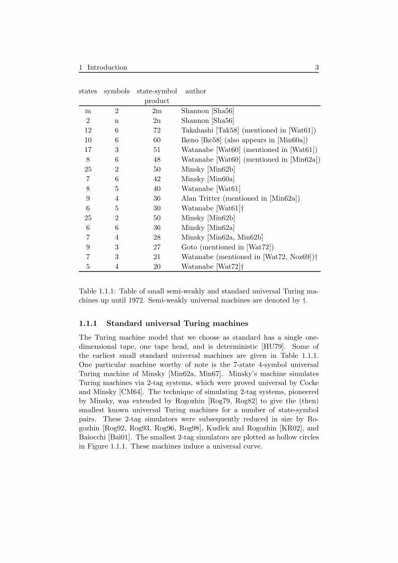
Table 1.1.1: Table of small semi-weakly and standard universal Turing ma-chines up until 1972. Semi-weakly universal machines are denoted by †.
1.1.1 Standard universal Turing machines
The Turing machine model that we choose as standard has a single one-dimensional tape, one tape head, and is deterministic [HU79]. Some ofthe earliest small standard universal machines are given in Table 1.1.1.One particular machine worthy of note is the 7-state 4-symbol universalTuring machine of Minsky [Min62a, Min67]. Minsky’s machine simulatesTuring machines via 2-tag systems, which were proved universal by Cockeand Minsky [CM64]. The technique of simulating 2-tag systems, pioneeredby Minsky, was extended by Rogozhin [Rog79, Rog82] to give the (then)smallest known universal Turing machines for a number of state-symbolpairs. These 2-tag simulators were subsequently reduced in size by Ro-gozhin [Rog92, Rog93, Rog96, Rog98], Kudlek and Rogozhin [KR02], andBaiocchi [Bai01]. The smallest 2-tag simulators are plotted as hollow circlesin Figure 1.1.1. These machines induce a universal curve.

1 Introduction 4
bc : universal, 2-tag simulation, O(t222t)
ld : semi-weakly universal, direct simulation, O(t2)
l : semi-weakly universal, cyclic tag simulation, O(t222t)
rs : weakly universal, Rule 110 simulation, O(t222t)
: universal curve
: weakly universal curve
: decidable halting problem
0 1 2 3 4 5 6 7 8 9 10 11 12 13 14 15 16 17 18 19
0
1
2
3
4
5
6
7
8
9
10
11
12
13
14
15
16
17
18
states
symbols
bc
bc
bc
bc
bc
bc
bc
ld
ld
l
l
l
rs
rs
rs
rs
Figure 1.1.1: State-symbol plot of small universal Turing machines, exclud-ing the work presented in this thesis. The simulation technique is givenfor each group of machines. Also, we give the simulation time overheads interms of simulating any single tape, deterministic Turing machine that runsin time t.
1.1.2 Weakly and semi-weakly universal Turing machines
Over the years, small universal machines were given for a number of vari-ants on the standard Turing machine model. By generalising the model weoften find smaller universal programs. One variation on the standard Turingmachine is to allow an infinitely repeated word to one side of its input, andon the other side a (standard) infinitely repeated blank symbol. We callsuch a machine semi-weak. In 1961 Watanabe [Wat61] gave a semi-weaklyuniversal Turing machine with 6 states and 5 symbols. Watanabe improvedon his earlier machine to give 5-state, 4-symbol and 7-state, 3-symbol semi-weakly universal machines [Wat72]. These semi-weak machines are plottedas hollow diamonds in Figure 1.1.1.
Recently, Woods and Neary [WN07b, WNb] have given semi-weaklyuniversal machines with state-symbol pairs of (2, 14), (3, 7), and (4, 5) that

1 Introduction 5
states symbols tape tapes author
dimension
15 2 1 3 Moore [Moo52]
1 2 1 4 Hooper [Hoo63, Hoo69]†
2 3 1 2 Hooper [Hoo63, Hoo69]
8 4 2 1 Wagner [Wag73]
2 7 2 1 Ottmann [Ott75a]†
10 2 2 1 Ottmann [Ott75b, KBO77]†
6 3 2 1 Ottmann [Ott75b, KBO77]†
4 4 2 1 Ottmann [Ott75b, KBO77]†
2 6 2 1 Kleine-Buning & Ottmann [KBO77]†
1 7 3 1 Kleine-Buning & Ottmann [KBO77]†
2 5 2 1 Kleine-Buning & Ottmann [KBO77]†
2 3 2 1 Kleine-Buning & Ottmann [KBO77]†
4 5 2 1 Kleine-Buning & Ottmann [KBO77]
3 6 2 1 Kleine-Buning & Ottmann [KBO77]
10 2 2 1 Kleine-Buning [KB77]
2 5 2 1 Kleine-Buning [KB77]
2 4 2 1 Priese [Pri79]
2 2 2 2 Priese [Pri79]
4 7 1 1 Pavlotskaya [Pav96]‡
2 5 1 1 Margenstern & Pavlotskaya [MP95b]‡
2 3 1 1 Margenstern & Pavlotskaya [MP03]‡
Table 1.1.2: Table of small non-standard universal Turing machines, ex-cluding semi-weak machines. Weakly universal machines are denoted by †.Turing machines that are universal when coupled with a finite automatonare denoted by ‡.
simulate cyclic tag systems. These semi-weak machines are plotted as soliddiamonds in Figure 1.1.1.
A further generalisation on the standard model is to allow the blankportion of the Turing machine’s tape to have an infinitely repeated word tothe left, and another to the right. We refer to such universal machines asweakly universal Turing machines. Cook and Eppstein [Coo04], and Wol-fram [Wol02] recently gave weakly universal Turing machines, smaller thanWatanabe’s semi-weak machines, that simulate the universal cellular au-tomaton Rule 110. These machines have state-symbol pairs of (7, 2), (4, 3),(3, 4), and (2, 5) and are plotted as hollow squares in Figure 1.1.1. (Notethat David Eppstein constructed the (7, 2) machine to be found in [Coo04].)
1 Introduction 6
1.1.3 Other non-standard universal Turing machines
Weakness has not been the only generalisation on the standard model inthe search for small universal Turing machines. We give some notable ex-amples here, others are to be found in Table 1.1.2. Hooper [Hoo63, Hoo69]gave a universal machine with 2 states, 3 symbols, and 2 tapes, and an-other with 1 state, 2 symbols and 4 tapes. One of the tapes in Hooper’s4-tape machine is circular and contains the simulated program. His ma-chine would also operate correctly if this circular tape is replaced with asemi-weak tape. Thus Hooper’s 4-tape machine could be considered semi-weak. Priese [Pri79] gave a 2-state, 4-symbol machine with a 2-dimensionaltape, and a 2-state, 2-symbol machine with a pair of 2-dimensional tapes.Margenstern and Pavlotskaya [MP95b, MP03] gave a 2-state, 3-symbol Tur-ing machine that uses only 5 instructions and is universal when coupled witha finite automaton.
1.1.4 Universal Turing machines with restrictions
If we restrict the standard Turing machine model the problem of finding ma-chines with small state-symbol products becomes more difficult. Non-erasingTuring machines are a restriction of Turing machines that are permittedto overwrite blank symbols only. Moore [Moo52] mentions that Shannonhad proved that non-erasing Turing machines simulate Turing machines,however this result was never published. Shortly after, Shannon proved2-symbol Turing machines universal, Wang [Wan57] proved 2-symbol non-erasing Turing machines universal. Later, Minsky [Min61] proved the sameresult as Wang using a different technique. Minsky proved 2-tape non-writing Turing machines were universal and showed 2-symbol non-erasingTuring machines simulate these non-writing machines. More recently, Mar-genstern [Mar92, Mar93, Mar94, Mar95a, Mar95b, Mar01] has constructeda number of small non-erasing universal machines with further restrictions.
Fischer [Fis65] gives universality results for Turing machines that userestricted forms of transition rules. Fischer gives results for variations onthe quadruple formulation (see Footnote 1.1). In one result he proves 3-statePost machines universal.
1.1.5 Universal tag systems
Post [Pos43] proved that a restriction of his canonical systems, called normalsystems, are universal. Post also wondered if tag systems, a restriction ofnormal systems, had an unsolvable prediction problem. Minsky [Min60b,Min61] settled this problem when he proved that tag systems with dele-tion number 6 (called 6-tag systems) simulate Turing machines and hence

1 Introduction 7
are universal. Later, Cocke and Minsky [Min62b, CM63, CM64] provedthat 2-tag systems are universal by showing that they simulate Turing ma-chines. Their technique used productions (appendants) of length 4 or less.Wang [Wan63] further improved on this result by showing that 2-tag sys-tems with productions of length 3 or less also simulate Turing machines.Wang also proved the universality of lag systems, a variation of tag systems.Recently, cyclic tag systems were proved universal [Coo04, Wol02]. Kudlekand Rogozhin [KR01b, KR01a] introduced another tag like system called acircular Post machine. The operation of a circular Post machine is also sim-ilar to that of a Turing machine with a circular tape and a tape head thatonly moves one direction. Small universal circular Post machines have beengiven by Kudlek, Rogozhin and Alhazov [KR01b, KR01a, KR03, AKR02].
1.1.6 Simple universal cellular automata
Since cellular automata [vN66] were first proved universal there have beena number of incremental steps towards giving simpler universal cellular au-tomata. Here we consider a cellular automata to be universal if it is Tur-ing universal. Below we give results only for the most common types ofcellular automata, those with one-dimensional nearest neighbour and two-dimensional von Neumann (5 neighbours) and Moore neighbourhoods (8neighbours).
Codd [Cod68] gave a universal cellular automaton with von Neumannneighbourhood and 8 states on a blank background. Banks [Ban70] re-duced the number of states needed for universality to 3 for a blank back-ground and 2 for a periodic background. Conway [BCG82] proved thatwith a Moore neighbourhood it is possible to have universality with only2 states on a blank background. Smith [Smi71], gave a one-dimensionalnearest neighbour cellular automaton with 18 states that is universal on ablank background. Albert and Culik [AC87] reduced the number of statessufficient for universality, on a blank background, to 14. Lindgren and Nor-dahl [LN90] further reduced the number of states needed for universalityto 9 on a blank background and 7 on a periodic background. Recently,Cook [Coo04] proved that Rule 110, a one-dimensional nearest neighbourcellular automaton with 2 states, is universal on a periodic background (asketch of Cook’s proof also appears in [Wol02]). There have been many otherforms of simple cellular automata given. Both Albert and Culik [AC87], andLindgren and Nordahl [LN90], have given one-dimensional universal cellularautomata with neighbourhoods greater than three. Some other examples ofsimple universal cellular automata have been given for reversible cellular au-tomata [Tof77, MH89, MF05], majority voting cellular automata [Moo97a],and cellular automata in the hyperbolic plane [HM03, IIM07, Mar06].
In the literature the stronger notion of intrinsic universality [Oll02] is
1 Introduction 8
also used. An intrinsically universal cellular automaton simulates other cel-lular automata in linear time using a constant number of cells to encode asingle cell. Ollinger [Oll02] gave a one dimensional nearest neighbour cel-lular automaton that is intrinsically universal and has only 6 states. LaterRichard [Ric06] improved this result by giving a 4-state intrinsically univer-sal cellular automaton.
1.1.7 Other simple universal systems
Many biologically inspired computational models have also been simplifiedto give simple universal models. Some examples of these are neural net-works [MP43, Sie98], H systems [Hea87, PRS98] (also called splicing sys-tems), P systems [Pau00, Pau02] (also called membrane systems), and spik-ing neural P systems [IPY06]. Neural networks have been around since the1940s and more recently a number of different authors have given increas-ingly simple universal neural networks [Ind95, KCG94, KS96, Pol87, SM99,SS91, SS95]. In 1987, Head systems were born. Some results from the area ofsimple universal Head systems are to be found in [FMKY00, HM05, MR02].Membrane computing has received much attention since Paun introducedthis model of computation. Some results relating to small universal mem-brane systems can be found in [AFR06, AR06, CVMVV07, FO06, NPRP06,RV06]. Spiking neural P systems [IPY06] are a very new model inspiredby a fusion of spiking neural networks and P systems. These systems havealready given rise to a number of number of small spiking neural P sys-tems [PP07, ZZP, Nea08a, Nea08b].
Minsky [Min67] proved that register machines with only 2 registers areuniversal. Later focusing on a different parameter, Korec [Kor96] provedthat between 14 and 32 instructions are sufficient for universality depend-ing on the type of instructions allowed. Morita [Mor96] has proved that re-versible registers machines with 2 registers are universal. Benett [Ben73] hasshown that 3-tape reversible Turing machines are universal. Morita [MSG89]improved on this result proving that reversible Turing machines with 1 tapeand 2 symbols are universal. More recently Morita and Yamaguchi [MY07]gave a universal reversible Turing machine with 1 tape, 17 states, and 5symbols.
The very earliest proofs of universality, the negative solution to theEntscheidungsproblem, and the first problems proved undecidable are to befound in Davis’s [Dav65] book. Minsky’s [Min67] book contains a numberof early results on simple computationally universal models. More recentlyMargenstern [Mar00] gave a survey on the subject that catalogues manyinteresting results. Also, Delvenne et al. [DKB04, ?] gives universality resultsfor dynamical systems. There are a multitude of other simple universalmodels to be found in the literature but we will stop here.
1 Introduction 9
1.2 Decidability and lower bounds
The pursuit to find the simplest universal models must also involve thesearch for lower bounds. To simplify our point we will take the example ofShannon’s problem of finding the minimal state-symbol product for a uni-versal Turing machine. For Shannon’s problem, lower bounds involve findingthe largest state-symbol product which, in some sense, is non-universal. Oneapproach is to settle the decidability of the halting problem. However, wewill see that this approach is not suitable for all models. We give an overviewof decidability results for some of the models from Section 1.1.
Shannon [Sha56] claimed that 1-state Turing machines are non-universal.Fischer [Fis65] and Nozaki [Noz69] both note that Shannon’s definition ofuniversal Turing machine is too strict and so his proof is not sufficientlygeneral. On page 281 of his book, Minsky [Min67] mentions that he andBobrow proved that the halting problem is decidable for Turing machineswith 2 states and 2 symbols “by a tedious reduction to thirty-odd cases (un-publishable).” It is currently known that the halting problem is decidable formachines with the following state-symbol pairs (2, 2) [DK89, Kud96, Pav73],(3, 2) [Pav78], (2, 3) (claimed by Pavlotskaya [Pav73]), (1, n) [Her66a, Her66b,Her68c, Noz69, Fis65] and (n, 1) (trivial), where n > 1. These results inducethe decidable halting problem curve in Figure 1.1.1. Also, these decidabilityresults imply that a universal Turing machine, that simulates any Turingmachine M and halts if and only if M halts, is not possible for these state-symbol pairs. Hence these results give lower bounds on the size of universalmachines of this type. While it is trivial to prove that the halting problemis decidable for weak machines with a halting state and state-symbol pairsof the form (n, 1), it is not known whether the other decidability resultsgiven above generalise to weak Turing machines that have a halting state.More recently, Pavlotskaya [Pav02] has shown that the halting problem isdecidable for machines with less than 5 instructions.
Nozaki [Noz69] claims the non-universality of Turing machines withstate-symbol pairs of (2, 2) and (3, 2). Kryukov [Kry71] claimed that thestate-symbol pair (1, n) is non-universal and used a computer to solve the(3, 2) case. However, in the English translation versions of these papersinsufficient details are given to reconstruct these proofs. More details of thetechnique used by Kryukov is available in [Kry67].
Herman [Her66a, Her68a, Her68c] proved the halting problem decid-able for a number of Turing machine variants with 1-state, including Turingmachines with a single 2-dimensional tape. Wagner [Wag73] generalisedKryukov’s [Kry67] non-universality result for 2-state, 2-symbol machines toTuring machines with n-dimensional tapes. Aandrea and Fischer [AF67]

1 Introduction 10
proved the decidability of the halting problem for 2-state Post machines(see footnote 1.1). Fischer [Fis65] gives universality results for Turing ma-chines that use restricted forms of transition rules. Fischer gives non-universality [Fis65] results for variations on the quadruple formulation (seeFootnote 1.1).
Margenstern [Mar95a, Mar97b, Mar97a] introduced a useful notion, thatof decidability criterion, which we now define. Let f be a positive integer-valued function defined on a set of Turing machines M1 such that, thereis an integer d where for all machines with f < d, the halting problem isdecidable and for each f > d a universal machine exists. We say that f hasfrontier value of d for M1. Also, d may be described as a boundary betweenuniversality and non-universality in the following sense. A decidability cri-terion f implies that a universal Turing machine, that simulates any Turingmachine M and halts if and only if M halts, is not possible in M1 for f < d.
Recall from Section 1.1.3 that Margenstern and Pavlotskaya gave a uni-versal (Turing machine, finite automaton) pair where the Turing machineuses only 5 instructions. Margenstern and Pavlotskaya [MP03] also showthat the halting problem is decidable for all such pairs if the Turing ma-chine has 4 instructions. Their results give a frontier value of 5 instructionsfor the Turing machine in such pairs. Hence they have given the smallestpossible Turing machine that is universal in this sense. Note that here weare considering the notion of non-universality given in the final sentence ofthe previous paragraph.
The following decidability results of Margenstern and Pavlotskaya arefor 2-symbol Turing machines. One decidability criterion they use is thenumber of colours. The number of colours of a machine is the number ofdistinct triples (σ,D, δ), where some transition rule in the machine has readsymbol σ, move direction D, and write symbol δ. Pavlotskaya [Pav73, Pav75]established a frontier value of 3 colours for Turing machines. Margen-stern [Mar93] established a frontier value of 5 colours for non-erasing Turingmachines. Let l be the number of left instructions and r be the number ofright instructions in a machine. The minimum of l and r is called the later-ality number of a machine. Margenstern and Pavlotskaya [Pav73, MP95a]established a frontier value of 2 for the laterality number of Turing machines.Margenstern [Mar95a, Mar97b] established a frontier value of 3 for the lat-erality number of non-erasing Turing machines. The above results involvedthe construction of a number of different universal Turing machines. Mar-genstern gives a 125-state, 2-symbol non-erasing machine that uses only 5colours [Mar93], a 218-state, 2-symbol non-erasing machine that uses only3 left-move instructions [Mar95a], a 59-state, 2-symbol standard machinethat uses only 6 left-move instructions [Mar01], and a 190-state, 2-symbolmachine that uses only 3 left-move instructions [Mar01].
There are also decidability results given for other models. Wang [Wan63]showed that the reachability problem, and hence the halting problem, is de-

1 Introduction 11
cidable for 1-tag systems. Stephen Cook [Coo66] proved that the reachabilityproblem, and hence the halting problem, is decidable for non-deterministic1-tag systems. Post [Pos65] mentioned that he solved the reachability prob-lem for 2-tag systems with productions of length strictly less than 3; how-ever he did not publish this result. Recently, De Mol [De Mol07] proved thereachability problem decidable for this class of tag systems.
A number of small Turing machines have been given for other inter-esting problems. Many of these machines lie between the current univer-sality curve, and the current decidable halting problem curve. Margen-stern [Mar98, Mar00] gives machines that simulate iterations of the Col-latz function (3x + 1 problem) with state-symbol pairs of (11, 2), (5, 3),(4, 4), (3, 6) and (2, 10). Later, Baiocchi [Bai98] reduced the size of some ofthese machines to give Turing machines with state-symbol pairs of (10, 2),(5, 3), (4, 4), (3, 5) and (2, 8). Michel [Mic04, Mic93] has shown that thereare Turing machines that simulate iterations of Collatz-like functions withstate-symbol pairs of (2, 4), (3, 3), and (5, 2). Kudlek [Kud96] has given a4-state, 4-symbol machine that accepts a context-sensitive language. Thesemachines would seem to suggest that it will be difficult to improve on thecurrent decidable halting problem curve in Figure 1.1.1.
An interesting problem, introduced by Tibor Rado [Rad62], is the BusyBeaver problem. The problem is as follows. Let Tx,2 be the set of all binaryTuring machines with x states. For a given x determine the maximumnumber of non-blank symbols on the tape of any machine in Tx,2 when ithalts, having started on a blank tape (sometimes the maximum time beforehalting is also considered). To date the problem has been solved for thefollowing values Rado [Rad62] x = 2, Lin and Rado [LR65] x = 3 andBrady [Bra83] x = 4. The best results known for x = 5 and x = 6 aregiven by Marxen3 and Buntrock [MB90] and halt in 47,176,870 timestepsand 3 × 101730 timesteps, respectively. Michel [Mic93, Mic04] gives resultsfor a generalisation of the problem by allowing more than 2 tape symbols.He has given results for the following state-symbols pairs (2, 3), (3, 3) and(2, 4). Lafitte and Papazian [LP07] proved that the 2-state, 3-symbol resultgiven by Michel’s machine solves the problem for this class of machines.They also gave an analysis of some other classes.
There are many other decidability results many of which are to be foundin Margenstern’s [Mar00] survey. Also, Delvenne [?] gives decidability resultsfor dynamical systems.

1 Introduction 12
1.3 Thesis outline
The results presented in this thesis are concerned with simple universalmodels of computation with a particular focus on small universal Turingmachines. Many of our results may be thought of as a continuation ofthe work mentioned in the previous sections. However, a new aspect isadded to the study of simple universal systems as we also focus on theresource usage, such as the time and space complexity [Pap95], of suchmodels. The efficiency of many existing simple universal systems is improvedand new efficient systems are given. Many of our results are to be found inFigure 1.3.1. Improvements in the simulation time of previously constructedmachines may seen by comparing Figures 1.1.1 and 1.3.1.
Chapter 2 gives time/space complexity analysis of previous simple uni-versal models. It also contains important definitions and discussions, as wellas technical information regarding the notation used in the thesis.
Notice from Figure 1.1.1 that when work began on this thesis all ofthe smallest universal Turing machines were exponentially slow. The resultsin Chapter 3 were aimed at giving small polynomial time universal Turingmachines. Let t be the running time of any deterministic single tape Turingmachine M . Then, the main result in Chapter 3 states that there existsdeterministic O(t2) polynomial time universal Turing machines with state-symbol pairs of (3, 11), (5, 7), (6, 6), (7, 5) and (8, 4). To date, these are thesmallest known standard machines that simulate Turing machines in O(t2)time. They are also the smallest known standard machines where directsimulation of Turing machines is the technique used to establish their uni-versality. Each of these machines is plotted as a solid circle in Figure 1.3.1.This result established a polynomial time universal curve and gave a newsimulation algorithm for universal Turing machines.
Our search to find simple models led us to cyclic tag systems andRule 110. Cook [Coo04] proved that Rule 110 is universal. In Chapter 4we prove that Rule 110 is an efficient simulator of Turing machines, an ex-ponential improvement on the previous time overhead. Rule 110 simulatesTuring machines via cyclic tag systems. We improve the cyclic tag systemsimulation time of Turing machines from exponential to polynomial. As acorollary, we find that the prediction problem for Rule 110 is P-complete.This is the simplest cellular automaton proved to be P-complete. As an-other corollary, all of the small weak and semi-weak Turing machines inFigure 1.3.1 now simulate in polynomial time, an exponential improvement.
In Chapter 5 our attention turns to tag systems. 2-tag systems are atype of Post system that were originally proved to simulate Turing machines,by Cocke and Minsky. Their simulation is exponentially slow. Here we give aproof that 2-tag systems simulate Turing machines efficiently in polynomial
3See webpage: http://www.drb.insel.de/ heiner/BB/

1 Introduction 13
b : universal, direct simulation, O(t2)
bc : universal, 2-tag simulation, O(t4 log2 t)
u : universal, bi-tag simulation, O(t6)
ld : semi-weakly universal, direct simulation, O(t2)
l : semi-weakly universal, cyclic tag simulation, O(t4 log2 t)
rs : weakly universal, Rule 110 simulation, O(t4 log2 t)
r : weakly universal, Rule 110 simulation, O(t4 log2 t)
: universal curve
: weakly universal curve
: decidable halting problem
0 1 2 3 4 5 6 7 8 9 10 11 12 13 14 15 16 17 18 19
0
1
2
3
4
5
6
7
8
9
10
11
12
13
14
15
16
17
18
states
symbols
b
b
b
b
bu
u
u
u
r
r
r
bc
bc
bc
bc
bc
bc
bc
l
l
l
ld
ld
rs
rs
rs
rs
Figure 1.3.1: State-symbol plot of small universal Turing machines, includ-ing the work presented in this thesis. The (improved) simulation time andsimulation technique is given for each group of machines. Each of our newuniversal Turing machines is represented by a solid shape.
time. As an immediate corollary, all of the small universal Turing machinesthat simulate 2-tag systems (see Figure 1.3.1) now simulate in polynomialtime, an exponential improvement. This result also improves the efficiencyof a number of other models that simulate 2-tag systems. In addition, wegive a new variant on tag systems called bi-tag systems, and prove that theyare efficient simulators of Turing machines.
In Chapter 6 we present small polynomial time universal Turing ma-chines with state-symbol pairs of (5, 5), (6, 4), (9, 3) and (15, 2). These ma-chines simulate bi-tag systems and are plotted as triangles in Figure 1.3.1.They are the smallest known standard universal Turing machines with 5, 4,3, and 2 symbols, respectively. Our 5-symbol machine uses the same num-ber of instructions (22) as the smallest known universal Turing machine byRogozhin.
In Chapter 7 we give small weakly universal machines with state-symbolpairs of (6, 2), (3, 3) and (2, 4). These machines improve on the size of

1 Introduction 14
the Rule 110 simulators given by Cook and Eppstein [Coo04], and Wol-fram [Wol02]. The machines we present here also simulate Rule 110 and arethe smallest known weakly universal Turing machines. Our machines areplotted as solid squares in Figure 1.3.1.
Finally, in Chapter 8 we discuss our results and possible future work.Much of the work that we present and survey here has previously beenpublished, and may be found in [Nea06, NW06c, NW06a, NW, NW07a,WN06c, WN06a, WN07a, WNa].
2
Preliminaries
We begin by giving definitions that are used throughout the thesis. We thendiscuss definitions of universal Turing machine and simulation that are givenby a number of different authors. Next we establish notational conventionsused in the thesis. Finally, we give a brief time/space complexity analysisof previous small universal Turing machines.
2.1 Definitions
The Turing machine model we choose has a single one-dimensional tape, onetape head, and is deterministic [HU79]. We choose this particular modelas standard because it is common throughout the small Turing machineliterature.
Definition 2.1.1 (Turing machine) A Turing machine is a tuple M =(Q,Σ, b, f, q1,H). Here Q and Σ are the finite sets of states and tape symbolsrespectively. The blank symbol is b ∈ Σ, q1 ∈ Q is the start state, and H ⊆ Qis the set of halt states. The transition function f : Q×Σ→ Σ×{L,R}×Qis defined for all q ∈ Q−H. If q ∈ H then the function f is undefined onat least one element of q ×Σ.
We write f as a list of transition rules. Each transition rule is a quintuplet = (qi, σ1, σ2,D, qj), with initial state qi, read symbol σ1, write symbol σ2,move direction D and next state qj. The Turing machine definition we usehere is standard in the literature. However, it is often common to have a setof input symbols (not including the blank symbol) that is a proper subsetof the tape alphabet. This would not be suitable for our purposes.
Definition 2.1.2 (Weak Turing machine) A weak Turing machine is atuple M = (Q,Σ, r, l, f, q1,H). Here r ∈ Σ∗ and l ∈ Σ∗ are fixed constantlength words called the right blank word and the left blank word, respectively.Definition 2.1.1 defines the remaining elements of the tuple M .
Another related model is the semi-weak Turing machine. A semi-weakTuring machine has an infinitely repeated word to one side of its input, andon the other side a (standard) infinitely repeated blank symbol. Semi-weak
15
2 Preliminaries 16
machines are a generalisation on the standard model and a restriction of theweak model.
Definition 2.1.3 (Turing machine configuration) A configuration of aTuring machine consists of the current state qi, the read symbol σ0 and itstape contents . . . σ−3 σ−2 σ−1 σ0 σ1 σ2 σ3 . . ..
Example 2.1.1 (Turing machine configuration) In the thesis we rep-resent Turing machine configurations as follows:
qiqiqi, . . . σ−3 σ−2 σ−1 σ0 σ1 σ2 σ3 . . .
where qi is the current state, . . . σ−3 σ−2 σ−1 σ0 σ1 σ2 σ3 . . . is the tape con-tents and the tape head location given by an underline is under the readsymbol σ0.
Definition 2.1.4 (Turing machine computation step) If the currentstate is qi and the read symbol is σ1 then the transition rule (qi, σ1, σ2,D, qj)is applied to the configuration in the following way. The symbol under thetape head σ1 is replaced with σ2, qj becomes the new current state, and ifD = L the tape head moves one cell to the left and if D = R the tape headmoves one cell to the right.
A computation step is deterministic. In the sequel we write c1 ⊢ c2 if aconfiguration c2 is obtained from c1 via a single computation step.
Example 2.1.2 (Turing machine computation step) We show the ex-ecution of the transition rule (qi, σ0, σx, R, qj).
qiqiqi, . . . σ−3 σ−2 σ−1 σ0 σ1 σ2 σ3 . . .
⊢ qjqjqj, . . . σ−3 σ−2 σ−1 σx σ1 σ2 σ3 . . .
Definition 2.1.5 (Turing machine computation) A computation is afinite sequence of configurations c1, c2, . . . , ct of a Turing machine M thatends in a terminal configuration ct where ∀i, ci ⊢ ci+1. Also, we writeM(c1) = ct.
Definition 2.1.6 (Turing machine halting configuration) A haltingconfiguration is a terminal configuration where no transition rule is definedfor the current state q ∈ H and the read symbol.
2 Preliminaries 17
Definition 2.1.7 (Universal Turing machine) A Turing machine U isuniversal if there exists recursive functions h and f such that
M(c) = h(U(f(g(M, c)))) (2.1.1)
where M is any Turing machine, c is a configuration of M , g(M, c) is theGodel number of the ordered pair (M, c), f maps g(M, c) to a configurationof U , and h maps a terminal configuration of U to a terminal configurationof M .
The function f is injective and the function h is total and surjective. Also,the encoding function f and decoding function h are both recursive. Thelatter requirement, which is standard in the literature, ensures that theuniversality lies in the machine that we claim is universal and not in theencoding or decoding functions.
With the exception of some minor details, Definition 2.1.7 is equivalent toPriese’s [Pri79] definition of universal Turing machine. It is also equivalentto Davis’s [Dav57] definition if the terminal configuration is always assumedto be a halting configuration. Throughout the thesis it is assumed thatthe terminal configuration is a halting configuration unless explicitly statedotherwise.
In the definition of universal Turing machine it is also standard in the lit-erature [Dav57, Noz69, Pri79] to use a Godel numbering of Turing machinesand Turing machine configurations as the domain of the encoding function.This ensures that: (1) there is a standard representation of (Turing ma-chine, Turing machine configuration) pairs, and (2) the domain of f is theset of all (Turing machine, Turing machine configuration) pairs. In practicewhen constructing a universal Turing machine the domain of the encodingfunction is usually the table of behaviour (e.g. the set of transition rules) ofa Turing machine and a Turing machine configuration. It is sufficient thatthe set of (Turing machines, Turing machine configuration) pairs that definethe domain of our encoding function admit a Godel numbering of all suchpairs.
2.2 Some notes on universal Turing machines
We discuss definitions of universal Turing machine and then take a brief lookat some previous definitions of universal Turing machine. Following this weconsider the problem of defining the notion of simulation.
2.2.1 Previous definitions of universal Turing machine
Davis [Dav56] gave the following definition of universal Turing machine. ATuring machine is universal if the set of configurations which lead to a halt-ing configuration is recursively enumerable complete. A set C is recursively
2 Preliminaries 18
enumerable complete if it is recursively enumerable and for every recur-sively enumerable set R there is a recursive function f such that if x ∈ R,f(x) ∈ C. Later, Davis [Dav57] gave a more restricted definition which alsorequired that the output of the machine being simulated be retrievable fromthe halting configuration of the universal machine via a recursive function.Davis’s earlier definition requires only that the universal machine halts ifand only if the simulated machine halts. Davis also proves that machineswhich obey his later definition also obey his earlier definition and that theconverse of this is false.
Priese [Pri79] gives a definition of universal Turing machine that differsfrom Davis’s definition in the following respect. Priese does not requirethe universal machine to halt. Priese’s universal machine computes until aconfiguration at time t containing the encoded output is reached, such thata recursive function may be applied to any configuration after time t − 1to retrieve the output. Note that many different configurations may encodethe same output.
Nozaki [Noz69] discusses the notion of universal Turing machine andgives a definition of universal Turing machine. Like Priese, Nozaki’s defi-nition does not require his universal machine to halt when the machine itsimulates halts. Also, Nozaki’s definition involves emulating the sequenceof configurations of the machine being simulated. The definitions of Davisand Priese do not have this restriction. We discuss some of the implicationsof this restriction in the next section.
Finally, we note that to date all of the small universal Turing machinesconstructed are Nozaki-universal and Priese-universal. However, some ofthese machines are not Davis-universal as they do not halt.
2.2.2 The simulation of one abstract machine by another
The problem of defining simulation of one abstract machine by another hasbeen discussed by a number of different authors [Fis65, Her68b, vEB90].To quote van Emde Boas [vEB90]: “it is hard to define simulation as amathematical object and still remain sufficiently general.”
Fischer [Fis65] gives a definition of “simulation of one machine by an-other.” where the following property holds. If machine M ′ simulates machineM then for each computation in M defined by the sequence of configurationsc1, c2, c3 . . . there is a computation f(c′g(1)), . . . , f(c′g(2)), . . . , f(c′g(3)), . . . in
M ′ such that the computation of M ′ halts if and only if the computationof M halts. Note ∀i, g(i) > g(i + 1). We are interested in the fact thatevery configuration ci of the machine M being simulated is encoded by aunique configuration c′g(i) in M ′. This requirement may exclude some sim-ulations which may be considered reasonable. Take the example given byHerman [Her68b] where more than one computation step of M is simu-lated by a single computation step of M ′. If this is the case then there
2 Preliminaries 19
exists configurations in the computation of M that are not uniquely en-coded in the computation of M ′. In her definition of universal Turing ma-chine, Nozaki [Noz69] uses a notion of simulation that is similar to Fischer’sand so has the same problem of excluding reasonable simulations from herdefinition.
Herman accepted Fischer’s invitation to improve his definition. Her-man’s definition is concerned only with the input-output relationship of thesimulated machine. If machine M ′ simulates machine M then M(c1) =h(M ′(f(c1))) where f and h are the encoding and decoding functions re-spectively. The definitions of universal Turing machine given by Davis andPriese use this notion of simulation and so they avoid the problem of re-stricting the simulation technique in the manner of Fischer and Nozaki.
We have seen that the problem of defining the term simulation is sim-plified if we consider only the input-output relationship of the simulatedmachine. However, it is useful in our analysis to consider the sequence ofcomputation steps taken by the simulator and the machine being simulated.While the notion of simulation in Definition 2.1.7 is not concerned withthese steps we often talk about simulations in these terms. For instancein the sequel we often speak of the simulator simulating a transition ruleof the machine being simulated. In our explanations we also use the termssimulated tape head, simulated read symbol, simulated current state ,etc. ofthe Turing machine being simulated. While in Definition 2.1.7 these objectsare not defined; they are always well-defined in any of the proofs we give.
Another idea that is useful in our analysis of simulators is that of simu-lation technique. For instance model A is proved universal through simula-tion of Turing machines and model B is proved universal through simulationof model A. We say that model A simulates Turing machines directly andmodel B simulates Turing machines via model A. In terms of Definition 2.1.7the notions of “simulates directly” and “simulate via model A” are redun-dant. However, we permit this abuse of the term “simulate” as we viewthe “simulation technique” as being important in our analysis of universalTuring machines.
2.3 Notational conventions
Throughout the thesis we adopt the following notational conventions. M de-notes a deterministic Turing Machine with a single bi-infinite tape and asingle tape head [HU79]. We let t denote the running time of M . U denotesa universal Turing machine and Um,n denotes some specific universal Turingmachine with m states and n symbols. The encoding of M as a word isdenoted 〈M〉. Analogously the encodings of state q and tape symbol σ aredenoted 〈q〉 and 〈σ〉, respectively. For convenience we often call the word〈q〉 a state of 〈M〉.
2 Preliminaries 20
In the sequel we write c1 ⊢ c2 if a configuration c2 is obtained fromc1 via a single computation step. We let c1 ⊢
s c2 denote a sequence of scomputation steps and let c1 ⊢
∗ c2 denote 0 or more computation steps.In regular expressions ∪, ∗, ǫ and parentheses have their usual mean-
ings [HU79]. Let Σ = {σ1, σ2, . . . , σn}, then Σ∗ is the set of all wordsof length > 0 over the alphabet {σ1, σ2, . . . , σn}. The length of the wordw ∈ Σ∗ is denoted by |w|.
We use big-Oh notation in the analysis of time and space resource us-age [Pap95]. Let f : N 7→ N and g : N 7→ N we write g(n) = O(f(n)) whenthere exists b, n0 ∈ N such that for all n > n0, g(n) 6 bf(n).
2.4 Complexity analysis of previous simulations
We give some terminology that we use in our analysis of the time/spacecomplexity of simulators. Let M be any Turing machine and let t be therunning time of M . B is a polynomial time simulator of Turing machines if(1) ∃k ∈ N such that ∀M : tB = O(tk) where tB is the running time of Band (2) its encoding and decoding functions are logspace computable. Wesay that B simulates M in polynomial time O(tk). The terms exponentialtime simulator and linear time simulator may be defined analogously usingappropriate encoding and decoding functions. Definitions of time and spacesimulation overheads are to be found in Boas [vEB90].
With the exception of Watanabe’s Turing machines, the results given inthis thesis give improvements on simulation times of all the simple modelsgiven in this section.
We give a time/space complexity analysis of Cocke and Minsky’s [CM64]simulation of a single tape deterministic Turing machine M by a 2-tag sys-tem TM . The tape contents of M has a maximum length of O(t). This isencoded as a 2-tag system dataword of length O(2t). Thus O(2t) space issufficient to simulate M . Each simulated timestep of M takes time O(2t).Hence O(t2t) time is sufficient to simulate the computation of M .
The universal machines of Minsky and Rogozhin et al. [Min62a, Rog96,KR02, Bai01] in Figure 1.1.1 simulate 2-tag systems with a quadratic poly-nomial overhead in time. Hence O(t222t) time is sufficient to simulate thecomputation of M .
Cyclic tag systems simulate 2-tag systems in linear time [Coo04, Wol02].Hence O(t2t) time is sufficient for cyclic tag systems to simulate the com-putation of M . Rule 110 simulates cyclic tag system in linear time [Coo04].Hence O(t2t) time is sufficient for Rule 110 to simulate the computation ofM . The weakly universal Turing machines of Cook and Eppstein [Coo04],and Wolfram [Wol02] in Figure 1.1.1 simulate Rule 110 with a quadraticincrease in time. Hence O(t222t) time is sufficient for these machines tosimulate the computation of M .

2 Preliminaries 21
The semi-weakly universal Turing machines of Woods and Neary [WN07b,WNb] in Figure 1.1.1 simulate cyclic tag system with a quadratic polynomialincrease in time. Hence O(t222t) time is sufficient to simulate the computa-tion of M , via the above simulations.
The semi-weakly universal Turing machines of Watanabe simulate Tur-ing machines directly with a quadratic polynomial increase in time. HenceO(t2) time is sufficient to simulate the computation of M .
The results we give in the thesis are for deterministic single tape Turingmachines. The multitape Turing machine model is more usually used in com-plexity analysis. Some of our results also assume that the simulated machinehas a binary tape alphabet. The simulation times we give do not changegreatly when we consider deterministic multitape machines with larger al-phabets. For example, let M ′ be a deterministic multitape Turing machinewith more than two symbols. M ′ is converted to a two symbol, single tapeTuring machine M . The number of states in M is only a constant timesgreater than the number of states and symbols of M ′, also M is at worstO(t2) polynomially slower than M ′ [Pap95].

3
Small O(t2) time universal Turing
machines
3.1 Introduction
In this chapter we present deterministic O(t2) polynomial time universalTuring machines with state-symbol pairs of (3, 11), (5, 7), (6, 6), (7, 5) and(8, 4). These are the smallest known machines that simulate Turing ma-chines in O(t2) time. Each of the machines is plotted as a solid circle inFigure 3.1.1. The O(t2) polynomial time curve that is induced by thesemachines is also given in Figure 3.1.1.
Initially small universal Turing machines were constructed that directlysimulated Turing machines [Ike58, Wat61]. Subsequently, the technique ofindirect simulation via 2-tag systems was applied by Minsky [Min62a]. Dueto their unary encoding of Turing machine tape contents, 2-tag systems wereexponentially slow simulators of Turing machines [CM64]. Hence the smalluniversal Turing machines of Minsky, Rogozhin, Kudlek and Baiocchi allsuffered from a O(t222t) exponential time overhead [Min62a, Rog96, KR02,Bai01]. In Chapter 5 we show that 2-tag systems simulate Turing machinesefficiently in polynomial time. From this result it follows that the univer-sal Turing machines of Minsky and Rogozhin et al. simulate in O(t4 log2 t)time. The smallest of these 2-tag simulators are plotted as hollow circles inFigure 3.1.1. The O(t4 log2 t) time curve induced by these machines is alsoplotted in Figure 3.1.1.
The small universal Turing machines presented in Chapter 6 are plottedas solid triangles in Figure 3.1.1. These machines simulate Turing machinesvia bi-tag systems in O(t6) time. Here we are particularly interested in thecomparison between our O(t2) machines and other standard small univer-sal machines. Thus only standard machines (see Section 1.1.1) appear inFigure 3.1.1.
Prior to the work in this chapter the smallest known polynomial timeuniversal Turing machine was constructed by Watanabe [Wat61] in 1961and has 8 states and 5 symbols. Our machines are significantly smaller andrepresent a new algorithm for small universal Turing machines. It should alsobe noted that they are the smallest known machines where direct simulation
22

3 O(t2) time universal machines 23
b : universal, direct simulation, O(t2)
bc : universal, 2-tag simulation, O(t4 log2 t)
u : universal, bi-tag simulation, O(t6)
: universal O(t2) curve
: universal curve
0 1 2 3 4 5 6 7 8 9 10 11 12 13 14 15 16 17 18 19
0
1
2
3
4
5
6
7
8
9
10
11
12
13
14
15
16
17
18
states
symbols
b
b
b
b
bu
u
u
u
bc
bc
bc
bc
bc
bc
bc
Figure 3.1.1: State-symbol plot of small universal Turing machines. Eachnew O(t2) machine is plotted as a solid circle.
of Turing machines is the technique used to establish their universality.In Section 3.2 we give some definitions used to encode input to our
universal Turing machines and an overview of the simulation algorithm. InSection 3.3 we give a 3-state, 11-symbol machine. We explain its inputencoding and computation in some detail. Section 3.4 contains a proofof correctness which proves that this universal Turing machine simulatesTuring machines in O(t2) polynomial time. In Section 3.5 our algorithm isextended to universal Turing machines with a number of other state-symbolpairs and finally a conclusion is given.
The results we present in this chapter we previously given in [NW05b,NW06c].
3.2 Preliminaries
At the beginning of this section we establish some formal conventions. Wethen introduce some general encodings that each of our five machines adhere

3 O(t2) time universal machines 24
to. We also give an overview of our simulation algorithm. Each universalTuring machine uses a variation on this algorithm. The Turing machines weconsider in this chapter have a single one-way infinite tape but otherwiseadhere to Definition 2.1.1.
3.2.1 Input encodings for universal Turing machines
Without loss of generality, any simulated Turing machine M has the fol-lowing restrictions: (i) M ’s tape alphabet is Σ = {0, 1} and 0 is the blanksymbol, (ii) for all qi ∈ Q, i satisfies 1 6 i 6 |Q|, (iii) f is always defined, (iv)M ’s start state is q1, (v) M has exactly one halt state q|Q| and its transitionrules are of the form (q|Q|, 0, 0, L, q|Q|) and (q|Q|, 1, 1, L, q|Q|). Point (v) is awell-known halting technique that places the tape head at the beginning ofthe output. The following definitions encode M .
Definition 3.2.1 (Encoding of M ’s tape symbols) The binary tape
symbols 0 and 1 of M are encoded as the words 〈0〉 =←−a←−a and 〈1〉 =←−b←−a .
Each of our five universal Turing machines has the symbols ←−a ,←−b and λ
as part of its tape alphabet. The symbols ←−a and←−b are typically used to
encode M ’s tape contents while λ is usually used as a marker symbol.
Definition 3.2.2 (Encoding of M ’s initial configuration) The encod-ing of an initial configuration of M is of the form
〈M〉〈q1〉〈w〉←−a ω
where 〈q1〉 is the start state of 〈M〉, 〈w〉 ∈ {←−a←−a ,←−b←−a }∗ is the encoding of
the input w to M that is given by Definition 3.2.1, ←−a ω = ←−a←−a←−a . . ., and〈M〉 is the encoding of M :
〈M〉 = λP(f, q|Q|)λP(f, q|Q|−1)λ . . . λP(f, q2)λP(f, q1)λE (3.2.1)
where the function P is defined below in Equation (3.2.2), and the word
E ∈ {ǫ, e,←−a , λ←−b λ←−a ,
←−b←−b←−b λ←−a } specifies the ending.
The initial position of U ’s tape head is at the leftmost symbol of 〈q1〉.
In the previous definition the encoding of M is placed to the left of itsencoded input. The initial position of M ’s simulated tape head is indicatedby the word 〈q1〉 and is immediately to the left of the leftmost encodedinput symbol. The remainder of the infinite tape of U contains the blanksymbol ←−a . The ending E varies over the five universal Turing machinesthat we present.
The encoding of M ’s transition rules is defined using the function P thatspecifies the relative positions of encoded transition rules for a given state qi.
P(f, qi) = E(ti,1)λE(ti,0)λE(ti,0)λE(ti,1)λE′(f, ti,0) (3.2.2)
3 O(t2) time universal machines 25
In Equation 3.2.2 ti,1 and ti,0 denote the unique transition rules for thestate-symbol pairs (qi, 1) and (qi, 0), respectively. This notation is used fortransition rules throughout this chapter. The encoding functions E and E ′
map transition rules to words called ETRs (encoded transition rules). Thereis a unique pair of E and E ′ functions for each of our five universal Turingmachines. Given what we have so far, we need only to give E , E ′ and 〈q1〉to completely define the input to our universal Turing machines. Thesefunctions are given before each universal Turing machine.
3.2.2 Universal Turing machine algorithm overview
In order to distinguish the current state qx of a simulated Turing machine M ,the earliest small universal Turing machines [Ike58, Wat61] maintained a listof all states with a marker at qx. A change in M ’s current state is simulatedby moving the marker to another location in the list of states. The most sig-nificant difference between these earlier universal Turing machines and ouralgorithm is that we store the encoded current state of M on M ’s simulatedtape at the location of M ’s tape head. Thus the encoded current state alsorecords the current location of M ’s tape head during the simulation. Thispoint is illustrated in Figure 3.2.3.
The problem of constructing a universal Turing machine can be dividedinto the following basic steps. The universal Turing machine (1) reads theencoded current state and (2) reads the encoded read symbol. Next theuniversal Turing machine (3) prints the encoded write symbol, (4) movesthe simulated tape head and (5) establishes the new encoded current state.Due to the location of the encoded current state and the encodings that weuse for our universal Turing machines, the sets {(1), (2)} and {(3), (4), (5)}each become a single process. Steps (1) and (2) are combined such that asingle set of transition rules read both the encoded current state and theencoded read symbol. Steps (3), (4) and (5) have been similarly combined.Combining these steps has reduced the number of transition rules neededby our universal Turing machines.
Here we give a brief description of the simulation algorithm. The en-coded current state of M is positioned at the simulated tape head locationof M . Using a unary indexing method, our universal Turing machine U lo-cates the next ETR (encoded transition rule) to execute (see Figure 3.2.1).
The next ETR is indexed (pointed to) by the number of←−b symbols con-
tained in the encoded current state and read symbol. If the number of←−b
symbols in the encoded current state and encoded read symbol is i thenthe number of λ markers between the encoded current state and the nextETR to be executed is i− 1. To locate the next ETR, U simply neutralises
the rightmost λ (i.e. replaces λ with some other symbol) for each←−b in the
encoded current state and read symbol, until there is only one←−b remaining.

3 O(t2) time universal machines 26
Encoding of Turing machine M -� Simulated tape of M� -
encodedcurrent state
encodedread symbol
λ · · · λ ETR λ ETR λ ETR λ ETR λ ←−b←−b←−b←−b ←−a
λ · · · λ ETR λ ETR λ ETR λ ETR λ ←−b←−b←−b←−b ←−a
x� tape head of U
λ · · · λ ETR λ ETR λ ETR λ ETR λ←−b/←−b←−b←−b ←−a
x
λ · · · λ ETR λ ETR λ ETR λ ETR λ←−b/←−b←−b←−b ←−a
x
λ · · · λ ETR λ ETR λ ETR λ ETR λ/ ←−b/←−b/←−b←−b ←−a
x
λ · · · λ ETR λ ETR λ ETR λ ETR λ/ ←−b/←−b/←−b←−b ←−a
x
λ · · · λ ETR λ ETR λ ETR λ/ ETR λ/ ←−b/←−b/←−b/←−b ←−ax
λ · · · λ ETR λ ETR λ ETR λ/ ETR λ/ ←−b/←−b/←−b/←−b ←−a
x
(a) λ · · · λ ETR λ ETRλ/ ETR λ/ ETR λ/ ←−b/←−b/←−b/←−b/ ←−a
xindexed ETR
Figure 3.2.1: Indexing of an encoded transition rule (ETR) during simula-tion of a transition rule of M . The ETR to be executed is indexed by readingthe encoded current state and read symbol, and marking off λ symbols inthe encoding of M .
This indexed ETR is printed over the encoded current state and read sym-bol (see Figure 3.2.2). This printing completes the execution of the ETRand establishes the new encoded current state, encoded write symbol andsimulated tape head move. Figure 3.2.3(b) represents the tape contents of Uafter an ETR of 〈M〉 is indexed. Figures 3.2.3(cR) and 3.2.3(cL) representthe two possibilities for U ’s tape contents after an ETR is printed. To givemore details we present the algorithm as four cycles.
Cycle 1 (Index next ETR)
In this cycle U reads the encoded current state and encoded read symboland neutralises markers to index the next ETR (see Figure 3.2.1). Initially
U ’s tape head scans to the right until it reads a←−b . This
←−b is replaced with
some other symbol. U ’s tape head then scans left to neutralise a λ marker.
This process is repeated until U reads the subword←−b←−a while scanning

3 O(t2) time universal machines 27
Encoding of Turing machine M -� Simulated tape of M� -
(a) λ · · · λ ETR λ←−b←−a←−b←−b←−b λ/ ETR λ/ ETR λ/
←−b/←−b/←−b/←−b/ ←−a
x
λ · · · λ ETR λ←−b←−a←−b←−b←−b λ/ ETR λ/ ETR λ/
←−b/←−b/←−b/←−b/ γ
x
λ · · · λ ETR λ←−b←−a←−b←−b←−b/ λ/ ETR λ/ ETR λ/
←−b/←−b/←−b/←−b/ γ
x
λ · · · λ ETR λ←−b←−a←−b←−b←−b/ λ/ ETR λ/ ETR λ/
←−b/←−b/←−b/ γ ←−b
x
λ · · · λ ETR λ←−b←−a←−b←−b/←−b/ λ/ ETR λ/ ETR λ/
←−b/←−b/←−b/ γ ←−b
x
λ · · · λ ETR λ←−b←−a←−b←−b/←−b/ λ/ ETR λ/ ETR λ/
←−b/←−b/ γ ←−b
←−b
x
λ · · · λ ETR λ←−b←−a←−b/←−b/←−b/ λ/ ETR λ/ ETR λ/
←−b/←−b/ γ ←−b
←−b
x
λ · · · λ ETR λ←−b←−a←−b/←−b/←−b/ λ/ ETR λ/ ETR λ/
←−b/ γ ←−
b←−b←−b
x
λ · · · λ ETR λ←−b←−a/←−b/←−b/←−b/ λ/ ETR λ/ ETR λ/
←−b/ γ ←−
b←−b←−b
x
λ · · · λ ETR λ←−b←−a/←−b/←−b/←−b/ λ/ ETR λ/ ETR λ/ γ ←−a
←−b←−b←−b
x
λ · · · λ ETR λ←−b/←−a/←−b/←−b/←−b/ λ/ ETR λ/ ETR λ/ γ ←−a
←−b←−b←−b
x
(b) λ · · · λ ETR λ←−b/←−a/←−b/←−b/←−b/ λ/ ETR λ/ ETR λ/ γ ←−
b ←−a←−b←−b←−b
x
(c) λ · · · λ ETR λ←−b←−a←−b←−b←−b λ ETR λ ETR λ
←−b ←−a
←−b←−b←−b
x encodedcurrent state
encodedwrite symbol
Figure 3.2.2: Printing of an encoded transition rule (ETR) during simula-tion of a transition rule of M . The ETR indexed in configuration (a) ofFigure 3.2.1 is printed over the previous encoded current state and readsymbol to complete the transition rule simulation.
right. This signals that the encoded current state and encoded read symbolhave been read. Cycle 1 is now complete and Cycle 2 begins.
Cycle 2 (Print ETR)
Cycle 2 copies an ETR to M ’s simulated tape head location (see Fig-ure 3.2.2). U scans left and records the next symbol of the ETR to beprinted. U then scans right and prints the next symbol of the ETR at alocation specified by a marker. The location of this marker is initially setat the end of Cycle 1 and its location is updated after the printing of eachsymbol of the ETR. This process is repeated until the end of the ETR is

3 O(t2) time universal machines 28
(a)
(b)
(cR) (cL)
encoded current state encoded read symbol
encoded write symbol
Figure 3.2.3: Right and left moving transition rule simulations. The en-coded current state marks the location of M ’s simulated tape head. (a)Encoded configurations before beginning each transition rule simulation.(b) Intermediate configurations immediately after the encoded read symboland encoded current state have been read. (cR) Configuration immediatelyafter the simulated right move. (cL) Configuration immediately after thesimulated left move.
detected causing U to enter Cycle 3. The end of the ETR is detected by Uencountering the marker or neutralised marker that separates ETRs.
Cycle 3 (Restore tape)
Cycle 3 restores M ’s encoded table of behaviour after an ETR has beenindexed and printed (see configurations (b) and (c) in Figure 3.2.2). U scansright restoring 〈M〉 to its initial value. This Cycle ends when U encountersthe marker which was used in Cycle 2 to specify the position of the nextsymbol of the ETR to be printed. U then enters Cycle 4.
Cycle 4 (Choose read or write symbol)
This cycle either (i) begins the indexing of an ETR or (ii) completes theexecution of an ETR. More precisely: (i) if U is immediately after simulatinga left move then this cycle reads the encoded read symbol to the left of theencoded current state, (ii) if U is simulating a right move then this cycleprints the encoded write symbol to the left of the encoded current state. Oncompletion of either case Cycle 1 is entered.
3.3 Construction of U3,11
Our first machine has 3 states and 11 symbols and is denoted U3,11. Asusual we let M be a Turing machine that is simulated by U3,11.

3 O(t2) time universal machines 29
Definition 3.3.1 (Encoding of start state of 〈M〉 for U3,11) The start
state of 〈M〉 is 〈q1〉 =←−a 5|Q|←−b 2.
Recall that 〈M〉 is the encoding of M and is defined via the functions Eand E ′. These encoding functions map to words over the alphabet of U3,11,as defined in Equations (3.3.1) and (3.3.2). We denote the words defined byE and E ′ with the acronyms ETR and ETR′, respectively.
Recall that ti,σ1 denotes the unique transition rule qi, σ1, σ2,D, qy in Mwith initial state qi and read symbol σ1. Also, tR,i = (qx, σ1, σ2, R, qi) andtL,i = (qx, σ1, σ2, L, qi); we write ∃tR,i to mean that there exists a transitionrule which moves right and has qi as its next state (there are zero or moresuch transition rules).
Let t = (qx, σ1, σ2,D, qy) be a fixed transition rule in M , then t is en-coded via Equation (3.2.2) using the function E on its own, or in conjunctionwith E ′, where
E(t) =
ea(t)hb(t) if D = R,σ2 = 0
hea(t)hb(t) if D = R,σ2 = 1
ea(t)−1hb(t)eee if D = L, σ2 = 0
ea(t)−1hb(t)ehe if D = L, σ2 = 1
(3.3.1)
and
E ′(f, t) =
ea(tR,x)−3hb(tR,x)+2 if ∃tR,x, qx 6= q1
ǫ if ∄tR,x, qx 6= q1
e5|Q|−3h4 if qx = q1
(3.3.2)
where as before tR,x is any right moving transition rule such that tR,x ⊢ t,the functions a(·) and b(·) are defined by Equations (3.3.3) and (3.3.4), e andh are tape symbols, and ǫ is the empty word.
a(t) = 5|Q|+ 2− b(t) (3.3.3)
b(t) = 2 +
y∑
j=1
g(t, j) (3.3.4)
where g(·) is given by
g(t, j) =
5 if j < y
3 if D = L, j = y
0 if D = R, j = y
(3.3.5)
Definition 3.3.2 (Encoding of M ’s current state for U3,11) The en-
coding of M ’s current state is of the form ←−a ∗←−b 2←−b ∗{←−a ∪ ǫ} and is of length
5|Q|+ 2.

3 O(t2) time universal machines 30
ETR transition rule tR,x for E ′ b(t) a(t) E ′ or E
E ′(f, t1,0) q1, 0, 1, R, q2 q1, 1, 0, R, q1 2 + 0 = 2 15 e12h4
E(t1,0) q1, 0, 1, R, q2 2 + 5 + 0 = 7 10 he10h7
E(t1,1) q1, 1, 0, R, q1 2 + 0 = 2 15 e15h2
E ′(f, t2,0) q2, 0, 0, L, q2 q1, 0, 1, R, q2 2 + 5 + 0 = 7 10 e7h9
E(t2,0) q2, 0, 0, L, q2 2 + 5 + 3 = 10 7 e6h10eee
E(t2,1) q2, 1, 1, L, q3 2 + 5 + 5 + 3 = 15 2 eh15ehe
E ′(f, t3,0) q3, 0, 0, L, q3 null null null ǫ
E(t3,0) q3, 0, 0, L, q3 2 + 5 + 5 + 3 = 15 2 eh15eee
E(t3,1) q3, 1, 1, L, q3 2 + 5 + 5 + 3 = 15 2 eh15ehe
Table 3.3.1: Values for the a(·) and b(·) functions, and for each ETR of 〈M1〉in Example 3.3.1 .
The value of the ending E, from Equation (3.2.1), for U3,11 is E = e.
Example 3.3.1 (Encoding of M1 for U3,11) Let Turing machine M1 =({q1, q2, q3}, {0, 1}, 0, f, q1 , {q3}) where f = {(q1, 0, 1, R, q2), (q1, 1, 0, R, q1),(q2, 0, 0, L, q2), (q2, 1, 1, L, q3), (q3, 0, 0, L, q3), (q3, 1, 1, L, q3)}. Using Equa-tion (3.2.1), M1 is encoded as:
〈M1〉 = λP(f, q3)λP(f, q2)λP(f, q1)λe
From Definition 3.3.1 the start state of 〈M1〉 is ←−a 15←−b 2. Substituting theappropriate values from Equation (3.2.2) gives
〈M1〉 =λE(t3,1)λE(t3,0)λE(t3,0)λE(t3,1)λE′(f, t3,0)
λE(t2,1)λE(t2,0)λE(t2,0)λE(t2,1)λE′(f, t2,0)
λE(t1,1)λE(t1,0)λE(t1,0)λE(t1,1)λE′(f, t1,0)λe
Rewriting 〈M1〉 using Equations (3.3.1) and (3.3.2) and the values given inTable 3.3.1 gives the word
〈M1〉 =λeh15eheλeh15eeeλeh15eeeλeh15eheλǫλeh15eheλe6h10eeeλ
e6h10eeeλeh15eheλe7h9λe15h2λhe10h7λhe10h7λe15h2λe12h4λe(3.3.6)
To aid understanding, note that a key property of P from Equation (3.2.2)is that it creates five ETRs in 〈M〉 for each state in M . Hence five ETRsencode two transition rules. This apparent redundancy is due to the algo-rithm used by our universal Turing machines. When executing an ETR, thealgorithm makes use of the direction of the previous tape head movementof M . The leftmost ETR given by Equation (3.2.2) simulates execution oftransition rule ti,1 following a simulated left move. The second ETR from
3 O(t2) time universal machines 31
the left simulates execution of transition rule ti,0 following a simulated leftmove. The rightmost ETR and the centre ETR are both used to simulateexecution of transition rule ti,0 following a simulated right move. Finallythe second ETR from the right simulates execution of transition rule ti,1following a simulated right move.
In our simulation, the number of←−b symbols in the encoded current
state is used as a unary index to locate the next ETR to be executed. Thefunction b(·) defined by Equation (3.3.4) gives the number of h symbols inan ETR. The number of h symbols in the ETR being executed defines the
number of←−b symbols in the next encoded current state 〈qy〉. The word
P(f, qy) gives the ETRs that encode the transition rules for state qy. Hencethe next ETR to be indexed is a subword of P(f, qy) and b(·) is a summationdependant on all encoded states 〈qj〉 such that j 6 y. The function g definedby Equation (3.3.5) is used by b(·) to calculate the number of ETRs in each〈qj〉. The first case of g corresponds exactly to the number of ETRs given inP (Equation (3.2.2)). The final two cases of g define whether the encodedcurrent state points to the rightmost ETR (g = 0) in the list of ETRs for astate, or to the fourth from the right (g = 3).
It is important to note that the input and output encodings for ouruniversal Turing machines are efficiently (logspace) computable. This is animportant requirement for universal Turing machines that simulate Turingmachines in polynomial time. Recall that a logspace transducer [Sip97] is aTuring machine that has a read-only input tape, a work tape, and a write-only output tape, where only the space used by the work tape is considered.Definition 3.2.2 gives the encoding of an initial configuration of M . Thetransducer that computes this input encoding to U3,11 takes M and w asinput, where M is explicitly given as a word in some straightforward manner.
Lemma 3.3.1 Given Turing machine M as a word, and its input w, thenthere exists a logspace transducer that computes the input 〈M〉〈q1〉〈w〉 toU3,11.
Proof. The input to U3,11 is given by Definition 3.2.2. Space of O(log |M |) issufficient to compute 〈M〉 and 〈q1〉 via Equations (3.2.1) to (3.3.5). Constantspace is sufficient to compute 〈w〉 via Definition 3.2.1. �
We state the lemma for U3,11. However all five universal Turing machinesin this chapter have logspace computable input encodings. The decodingof the output from U3,11, and our four other universal Turing machines, iscomputed by a linear time, constant space transducer via Definition 3.2.1.

3 O(t2) time universal machines 32
3.3.1 U3,11 and its computation
Definition 3.3.3 (U3,11) Let Turing machine U3,11 = ({u1, u2, u3}, {←−a ,←−b ,
e, h,−→e ,−→h ,←−e ,
←−h , λ, δ, γ},←−a , f, u1, {u3}) where f is given by Table 3.3.2.
u1 u2 u3←−a ←−e ,R, u1 γ, L, u2
←−a ,L, u3←−b ←−e ,R, u2
←−b , L, u1 e,R, u1
e −→e , L, u1←−e ,R, u1 e,R, u1
h−→h ,L, u1
←−h ,R, u3
←−a ,L, u1−→e ←−e ,R, u1 e,R, u2
←−e ,R, u3−→h←−h ,R, u1 h,R, u2
←−h ,R, u3
←−e −→e , L, u1−→e , L, u2 γ, L, u2
←−h−→h ,L, u1
−→h ,L, u2
←−a ,L, u3
λ δ,R, u1 λ,R, u2 δ,R, u3
δ λ, L, u1 λ,L, u2
γ ←−a ,L, u3←−h ,R, u3
←−b , L, u3
Table 3.3.2: Table of behaviour for U3,11.
We give an example of U3,11 simulating a transition rule of M1 fromExample 3.3.1. This simulation is of the first step in M1’s computationfor a specific input. The example is presented as the 4 cycles given inSection 3.2.2. In the below configurations the current state of U3,11 is high-lighted in bold font, to the left of U3,11’s tape contents. M1’s encoded readand write symbols are also highlighted in bold font. The position of U3,11’stape head is given by an underline. In the sequel we use the term overlinedregion.
Definition 3.3.4 (Overlined region) The overlined region exactly spansthe encoded current state (has length 5|Q| + 2), except on completion ofreading an encoded read symbol (has length 5|Q|+ 4) until the next encodedcurrent state is established.
Example 3.3.2 (U3,11’s simulation of the right moving transitionrule t1,1 = (q1, 1, 0, R, q1) from Turing machine M1) The start state ofU3,11 is u1 and tape head of U3,11 is over the leftmost symbol of 〈q1〉 (as inDefinition 3.2.2). In this example M1’s input is 101 (encoded via 〈0〉 =←−a←−a
and 〈1〉 =←−b←−a ). 〈M1〉 is in start state 〈q1〉 with encoded read symbol 〈1〉.
Thus the initial configuration of U is:
u1u1u1, (λEλEλEλEλE′)3λe←−a←−a 14
←−b←−b←−b←−a←−b←−a←−b←−a←−a←−a
←−b←−a←−a ω
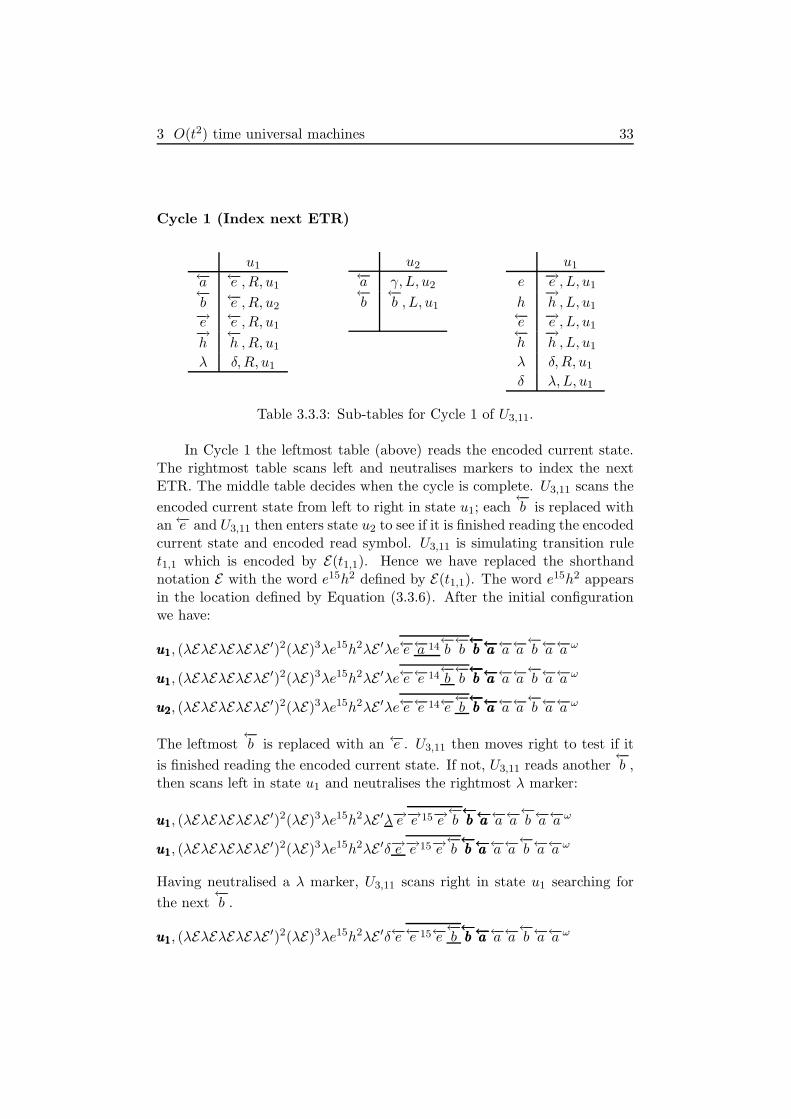
3 O(t2) time universal machines 33
Cycle 1 (Index next ETR)
u1←−a ←−e ,R, u1←−b ←−e ,R, u2−→e ←−e ,R, u1−→h←−h ,R, u1
λ δ,R, u1
u2←−a γ,L, u2←−b←−b , L, u1
u1
e −→e , L, u1
h−→h ,L, u1
←−e −→e , L, u1←−h−→h ,L, u1
λ δ,R, u1
δ λ, L, u1
Table 3.3.3: Sub-tables for Cycle 1 of U3,11.
In Cycle 1 the leftmost table (above) reads the encoded current state.The rightmost table scans left and neutralises markers to index the nextETR. The middle table decides when the cycle is complete. U3,11 scans the
encoded current state from left to right in state u1; each←−b is replaced with
an←−e and U3,11 then enters state u2 to see if it is finished reading the encodedcurrent state and encoded read symbol. U3,11 is simulating transition rulet1,1 which is encoded by E(t1,1). Hence we have replaced the shorthandnotation E with the word e15h2 defined by E(t1,1). The word e15h2 appearsin the location defined by Equation (3.3.6). After the initial configurationwe have:
u1u1u1, (λEλEλEλEλE′)2(λE)3λe15h2λE ′λe←−e←−a 14
←−b←−b←−b←−a←−b←−a←−b←−a←−a←−a
←−b←−a←−a ω
u1u1u1, (λEλEλEλEλE′)2(λE)3λe15h2λE ′λe←−e←−e 14
←−b←−b←−b←−a←−b←−a←−b←−a←−a←−a
←−b←−a←−a ω
u2u2u2, (λEλEλEλEλE′)2(λE)3λe15h2λE ′λe←−e←−e 14←−e
←−b←−b←−a←−b←−a←−b←−a←−a←−a
←−b←−a←−a ω
The leftmost←−b is replaced with an ←−e . U3,11 then moves right to test if it
is finished reading the encoded current state. If not, U3,11 reads another←−b ,
then scans left in state u1 and neutralises the rightmost λ marker:
u1u1u1, (λEλEλEλEλE′)2(λE)3λe15h2λE ′λ−→e −→e 15−→e
←−b←−b←−a←−b←−a←−b←−a←−a←−a
←−b←−a←−a ω
u1u1u1, (λEλEλEλEλE′)2(λE)3λe15h2λE ′δ−→e −→e 15−→e
←−b←−b←−a←−b←−a←−b←−a←−a←−a
←−b←−a←−a ω
Having neutralised a λ marker, U3,11 scans right in state u1 searching for
the next←−b .
u1u1u1, (λEλEλEλEλE′)2(λE)3λe15h2λE ′δ←−e←−e 15←−e
←−b←−b←−a←−b←−a←−b←−a←−a←−a
←−b←−a←−a ω

3 O(t2) time universal machines 34
The neutralisation process is repeated until the end of this cycle. Thus the
number of←−b symbols index the next ETR to be executed. U3,11 is finished
reading the encoded current state and read symbol when U3,11 reads a←−b
in state u1, moves right to test for the end of the encoded current state andencoded read symbol, and reads an ←−a in state u2. In the configurationsbelow when all the e and h symbols in an E ′ or an E are replaced with ←−e
and←−h symbols the resulting word is denoted
←−E ′ or
←−E respectively. Similarly
when all the e and h symbols in an E ′ or an E are replaced with −→e and−→h
symbols the resulting word is denoted−→E ′ or
−→E respectively.
u1u1u1, (λEλEλEλEλE′)2(λE)3λe15h2δ
←−E ′δ←−e←−e 15←−e←−e
←−b←−b←−b←−a←−a←−a←−a←−a
←−b←−a←−a ω
u2u2u2, (λEλEλEλEλE′)2(λE)3λe15h2δ
←−E ′δ←−e←−e 15←−e←−e←−e←−e←−e←−a←−a←−a←−a←−a
←−b←−a←−a ω
u2u2u2, (λEλEλEλEλE′)2(λE)3λe15h2δ
←−E ′δ←−e←−e 15←−e←−e←−e γ←−a←−a
←−b←−a←−a ω (I)
In configuration (I) above U3,11 has entered Cycle 2. Also, the overlinedregion is now extended to include the encoded read symbol as this has beenread and thus recorded in the same manner as the encoded current state.
Cycle 2 (Print ETR)
u2←−a γ,L, u2
e ←−e ,R, u1
h←−h ,R, u3
←−e −→e , L, u2←−h−→h ,L, u2
λ λ,R, u2
δ λ, L, u2
u1−→e ←−e ,R, u1−→h←−h ,R, u1
λ δ,R, u1
γ ←−a ,L, u3
u3−→e ←−e ,R, u3−→h←−h ,R, u3
←−e γ, L, u2
λ δ,R, u3
γ←−b , L, u3
Table 3.3.4: Sub-tables for Cycle 2 of U3,11.
This cycle copies an ETR to 〈M〉’s tape head position. The leftmosttable scans left and records the next symbol of the ETR to be printed.The two right tables scan right and print the appropriate symbol. In theconfigurations below, U3,11 scans left until a h is read. Then U3,11 movesright and records this h by entering u3.
u2u2u2, (λEλEλEλEλE′)2(λE)3λe15hhδ
←−E ′δ←−e←−e 17←−e γ←−a←−a
←−b←−a←−a ω
u2u2u2, (λEλEλEλEλE′)2(λE)3λe15hhλ
−→E ′λ−→e −→e 17−→e γ←−a←−a
←−b←−a←−a ω
u3u3u3, (λEλEλEλEλE′)2(λE)3λe15h
←−h λ−→E ′λ−→e −→e 17−→e γ←−a←−a
←−b←−a←−a ω

3 O(t2) time universal machines 35
U3,11 now scans right until it reads a γ and prints the recorded symbol.
u3u3u3, (λEλEλEλEλE′)2(λE)3λe15h
←−h δ←−E ′δ←−e←−e 17←−e γ←−a←−a
←−b←−a←−a ω
u3u3u3, (λEλEλEλEλE′)2(λE)3λe15h
←−h δ←−E ′δ←−e←−e 17←−e
←−b←−a←−a
←−b←−a←−a ω
u2u2u2,(λEλEλEλEλE′)2(λE)3λe15h
←−h δ←−E ′δ←−e←−e 17γ
←−b←−a←−a
←−b←−a←−a ω
This printing process is iterated until U3,11 is finished printing the ETR.The completion of this process occurs on reading a λ in state u2.
u2u2u2, (λEλEλEλEλE′)2(λE)3λ−→e 15−→h 2λ
−→E ′λ−→e −→e γ←−a 15
←−b 2←−a←−a
←−b←−a←−a ω
u2u2u2, (λEλEλEλEλE′)2(λE)3λ−→e
15−→h 2λ−→E ′λ−→e −→e γ←−a 15
←−b 2←−a←−a
←−b←−a←−a ω
Cycle 3 (Restore tape)
u2−→e e,R, u2−→h h,R, u2
λ λ,R, u2
γ←−h ,R, u3
Table 3.3.5: Cycle 3 of U3,11.
This table restores M ’s simulated tape and encoded table of behaviour.This cycle is entered from Cycle 2 (Print ETR). In Cycle 3, U3,11 moves
right restoring each −→e to e and each−→h to h. This continues until U3,11
reads γ, sending U3,11’s control to u3. Thus the configuration:
u2u2u2, (λEλEλEλEλE′)2(λE)3λe15h2λE ′λeeγ←−a←−a 14
←−b 2←−a←−a
←−b←−a←−a ω
becomes:
u3u3u3, (λEλEλEλEλE′)2(λE)3λe15h2λE ′λee
←−h←−a←−a 14
←−b 2←−a←−a
←−b←−a←−a ω
Cycle 4 (Choose read or write symbol)
This cycle either (i) begins the indexing of an ETR or (ii) completes theexecution of an ETR. More precisely: (i) if U3,11 is immediately after sim-ulating a left move then this cycle reads the encoded read symbol to the
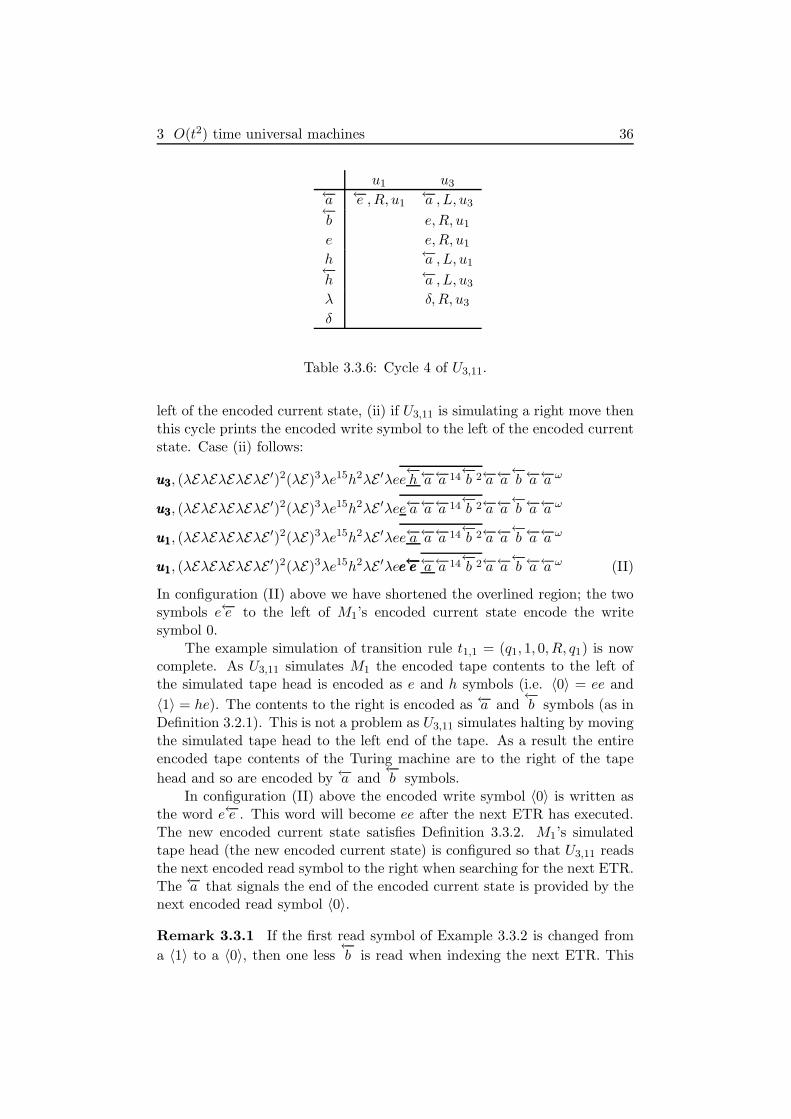
3 O(t2) time universal machines 36
u1 u3←−a ←−e ,R, u1
←−a ,L, u3←−b e,R, u1
e e,R, u1
h ←−a ,L, u1←−h ←−a ,L, u3
λ δ,R, u3
δ
Table 3.3.6: Cycle 4 of U3,11.
left of the encoded current state, (ii) if U3,11 is simulating a right move thenthis cycle prints the encoded write symbol to the left of the encoded currentstate. Case (ii) follows:
u3u3u3, (λEλEλEλEλE′)2(λE)3λe15h2λE ′λee
←−h←−a←−a 14
←−b 2←−a←−a
←−b←−a←−a ω
u3u3u3, (λEλEλEλEλE′)2(λE)3λe15h2λE ′λee←−a←−a←−a 14
←−b 2←−a←−a
←−b←−a←−a ω
u1u1u1, (λEλEλEλEλE′)2(λE)3λe15h2λE ′λee←−a←−a←−a 14
←−b 2←−a←−a
←−b←−a←−a ω
u1u1u1, (λEλEλEλEλE′)2(λE)3λe15h2λE ′λee←−ee←−ee←−e←−a←−a 14
←−b 2←−a←−a
←−b←−a←−a ω (II)
In configuration (II) above we have shortened the overlined region; the twosymbols e←−e to the left of M1’s encoded current state encode the writesymbol 0.
The example simulation of transition rule t1,1 = (q1, 1, 0, R, q1) is nowcomplete. As U3,11 simulates M1 the encoded tape contents to the left ofthe simulated tape head is encoded as e and h symbols (i.e. 〈0〉 = ee and
〈1〉 = he). The contents to the right is encoded as ←−a and←−b symbols (as in
Definition 3.2.1). This is not a problem as U3,11 simulates halting by movingthe simulated tape head to the left end of the tape. As a result the entireencoded tape contents of the Turing machine are to the right of the tape
head and so are encoded by ←−a and←−b symbols.
In configuration (II) above the encoded write symbol 〈0〉 is written asthe word e←−e . This word will become ee after the next ETR has executed.The new encoded current state satisfies Definition 3.3.2. M1’s simulatedtape head (the new encoded current state) is configured so that U3,11 readsthe next encoded read symbol to the right when searching for the next ETR.The ←−a that signals the end of the encoded current state is provided by thenext encoded read symbol 〈0〉.
Remark 3.3.1 If the first read symbol of Example 3.3.2 is changed from
a 〈1〉 to a 〈0〉, then one less←−b is read when indexing the next ETR. This

3 O(t2) time universal machines 37
indexes the rightmost (rather than the second from the right) ETR.
3.4 Proof of correctness of U3,11
In this section we prove that U3,11 correctly simulates a number of the pos-sible types of transition rules. We then extend these cases to all cases thusproving the correctness of U3,11’s computation.
Lemma 3.4.1 Given a valid initial configuration of U3,11, the encodedstart state indexes the ETR defined by E(t1,1) if M ’s read symbol is 1 andE ′(f, t1,0) if M ’s read symbol is 0.
Proof. The encoded start state contains exactly two←−b symbols. From
Example 3.3.2 when U3,11 reads a 〈1〉 in state 〈q1〉 it neutralises two λ mark-ers thus locating the second ETR from the right. By Definition 3.2.2 andEquation (3.2.2) this ETR is defined by E(t1,1). From Remark 3.3.1 andExample 3.3.2 when U3,11 reads a 〈0〉 in state 〈q1〉 it neutralises one λ, thusindexing the rightmost ETR defined by E ′(f, t1,0). �
Example 3.4.1 (U3,11’s simulation of the right moving transitionrule t1,0 = (q1, 0, 1, R, q2) from M1) In this example U3,11 is reading a〈0〉 after a right move. The right move was given by the simulation oft1,1 = (q1, 1, 0, R, q1) in Example 3.3.2. This unique case involves two steps,executing an ETR′ and then an ETR. The execution of an ETR′ is repre-sented by parts (a) and (b) of Figure 3.4.1 and the execution of the subse-quent ETR is represented by parts (c) and (d) of Figure 3.4.1.
We take the last configuration of Example 3.3.2, with the encoded readsymbol 〈0〉 = ←−a←−a to the right of the encoded current state. Substitutingthe appropriate ETR′ e12h4 from Equation (3.3.6) gives:
u1u1u1, (λEλEλEλEλE′)2(λE)4λe12h4λee←−e←−a 15
←−b←−b←−a←−a←−a←−a←−a←−a
←−b←−a←−a ω
u2u2u2, (λEλEλEλEλE′)2(λE)4λe12h4δ←−e←−e←−e←−e 15←−e←−e γ←−a←−a←−a
←−b←−a←−a ω
In the configuration immediately above we have reached the end of Cycle 1(Index next ETR). One λ has been replaced with one δ, thus indexing the
ETR′ e12h4. The←−b←−a that signaled the end of Cycle 1 was provided by the
rightmost←−b of the encoded current state and the leftmost←−a of the encoded
read symbol. Thus, only the leftmost ←−a of 〈0〉 = ←−a←−a←−a←−a←−a←−a was read and this
is sufficient to distinguish 〈0〉 from 〈1〉 =←−b←−a . However, the overlined
region does not cover the entire encoded read symbol which is why an ETR′

3 O(t2) time universal machines 38
(a)
(b)
(c)
(d)
encoded current stateencoded read symbol
encoded write symbol
Figure 3.4.1: Right move simulation (special case). The encoded currentstate marks the location of M ’s simulated tape head. The configurationsgiven in (a), (b) and (c) represent the reading of the encoded current stateand an encoded 0 following a right move. (a) Encoded configuration beforebeginning the transition rule simulation. (b) Intermediate configuration af-ter the encoded current state and first symbol of the encoded read symbolhave been read. (c) Intermediate configuration immediately after the en-coded read symbol has been read. (d) Configuration immediately after thesimulated right move.
executes before an ETR in this unique case. Skipping to the end of Cycle 2(Print ETR) gives:
u2u2u2, (λEλEλEλEλE′)2(λE)4λ−→e 12−→h 4λ−→e −→e −→e −→e γ←−a←−a 11
←−b 4←−a←−a←−a
←−b←−a←−a ω
u2u2u2, (λEλEλEλEλE′)2(λE)4λe12h4λeeeeγ←−a←−a 11
←−b 4←−a←−a←−a
←−b←−a←−a ω
u3u3u3, (λEλEλEλEλE′)2(λE)4λe12h4λeeee
←−h←−a←−a 11
←−b 4←−a←−a←−a
←−b←−a←−a ω
u3u3u3, (λEλEλEλEλE′)2(λE)4λe12h4λeeee
←−h←−a←−a 11
←−b 4←−a←−a←−a
←−b←−a←−a ω
u3u3u3, (λEλEλEλEλE′)2(λE)4λe12h4λeeee←−a←−a←−a 11
←−b 4←−a←−a←−a
←−b←−a←−a ω
u1u1u1, (λEλEλEλEλE′)2(λE)4λe12h4λeeee←−a←−a←−a 11
←−b 4←−a←−a←−a
←−b←−a←−a ω
At this point U3,11 has executed the ETR′. U3,11 now executes the ETR thatrepresents the second step of the simulation of transition rule t1,0. This ETRis defined by E(t1,0). Substituting the ETR he10h7 from Equation (3.3.6)into the configuration immediately above gives:
u1u1u1, (λEλEλEλEλE′)2(λE)2λhe10h7λEλE ′λeeee←−a←−a←−a 11
←−b 4←−a←−a←−a
←−b←−a←−a ω
We now skip to the end of Cycle 1 (Index next ETR) giving:
u2u2u2, (λEλEλEλEλE′)2(λE)2λhe10h7δ
←−E δ←−E ′δ←−e←−e←−e←−e 18←−a←−a←−a
←−b←−a←−a ω
u2u2u2, (λEλEλEλEλE′)2(λE)2λhe10h7δ
←−E δ←−E ′δ←−e←−e←−e←−e
18γ←−b←−a←−a ω (III)

3 O(t2) time universal machines 39
The ETR is indexed by neutralising three λ markers. The second part of the〈0〉 is read during this process. We now skip to the end of Cycle 3 (Restoretape) and illustrate a 〈1〉 being written to the left of the encoded currentstate:
u2u2u2, (λEλEλEλEλE′)2(λE)2λ
−→h−→e 10−→h 7λ
−→E λ−→E ′λ−→e −→e −→e γ
←−b←−a 10
←−b 7←−b←−a←−a ω
u2u2u2, (λEλEλEλEλE′)2(λE)2λhe10h7λEλE ′λeeeγ
←−b←−a 10
←−b 7←−b←−a←−a ω
u3u3u3, (λEλEλEλEλE′)2(λE)2λhe10h7λEλE ′λeee
←−h←−b←−a 10
←−b 7←−b←−a←−a ω
u1u1u1, (λEλEλEλEλE′)2(λE)2λhe10h7λEλE ′λeee
←−h e←−h e←−h e←−a
10←−b 7←−b←−a←−a ω
In the configuration immediately above the write symbol is positioned to theleft of the new encoded current state. Recall that to the left of the simulatedtape head the symbol 1 is encoded as he. The
←−h becomes h after execution
of the next ETR. The new encoded current state satisfies Definition 3.3.2and the simulation of transition rule t1,0 = (q1, 0, 1, R, q2) is complete.
Lemma 3.4.2 Given a valid configuration of U3,11, the encoded currentstate 〈qx〉 and encoded read symbol 〈σ1〉 index the ETR E(tx,σ1).
Proof. 〈M〉 is a list of ETRs, five ETRs for each state (pair of transition
rules) in M . The number of←−b symbols in the encoded current state 〈qx〉
and encoded read symbol, is used to index the next ETR to be executed. If
the number of←−b symbols is l then the l−1th ETR from the right is indexed.
In the encoding, the function b(·) determines the number of←−b symbols in
the next encoded current state. The function b(·) is defined as a summationover g(·) in Equation (3.3.4) for j, where 1 6 j 6 x.
From Equation (3.3.5), for each j < x, the function g(·) always has value
5, hence there are at least 5(x−1) juxtaposed←−b symbols in 〈qx〉. The state
qx is encoded using five ETRs. When j = x, then g = 0 or g = 3; giving a
total number of←−b symbols that point to the 1st or 4th of these five ETRs
respectively.Any encoded current state 〈qx〉, was established by execution of an ETR
r. The ETR r encodes move direction Dr and next state qx. The location ofthe ETR that is indexed by 〈qx〉 is dependent on the move direction Dr of r.When Dr = L and j = x then g(·) = 3; when this 3 is added to 5(x−1) thisindexes the 4th ETR (from the right) of the ETRs for qx. Using this valueof 5(x − 1) + 3 we get Cases A and B below. For clarity at this point notethat Dr is the move direction of the ETR r that established 〈qx〉 and 〈σ1〉is the read symbol that is read with 〈qx〉 to index the next ETR E(tx,σ1).
Case A: (Dr = L, σ1 = 0). 〈0〉 = ←−a←−a adds no extra←−b symbols to the
number of←−b symbols provided by 〈qx〉, thus the number of
←−b symbols is
given by g(·) alone and indexes the 4th ETR (from the right). By Equa-tion (3.2.2) this is E(tx,0).
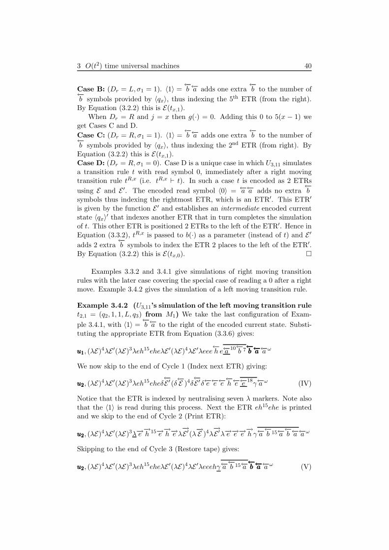
3 O(t2) time universal machines 40
Case B: (Dr = L, σ1 = 1). 〈1〉 =←−b←−a adds one extra
←−b to the number of
←−b symbols provided by 〈qx〉, thus indexing the 5th ETR (from the right).By Equation (3.2.2) this is E(tx,1).
When Dr = R and j = x then g(·) = 0. Adding this 0 to 5(x − 1) weget Cases C and D.
Case C: (Dr = R,σ1 = 1). 〈1〉 =←−b←−a adds one extra
←−b to the number of
←−b symbols provided by 〈qx〉, thus indexing the 2nd ETR (from right). ByEquation (3.2.2) this is E(tx,1).Case D: (Dr = R,σ1 = 0). Case D is a unique case in which U3,11 simulatesa transition rule t with read symbol 0, immediately after a right movingtransition rule tR,x (i.e. tR,x ⊢ t). In such a case t is encoded as 2 ETRs
using E and E ′. The encoded read symbol 〈0〉 = ←−a←−a adds no extra←−b
symbols thus indexing the rightmost ETR, which is an ETR′. This ETR′
is given by the function E ′ and establishes an intermediate encoded currentstate 〈qx〉
′ that indexes another ETR that in turn completes the simulationof t. This other ETR is positioned 2 ETRs to the left of the ETR′. Hence inEquation (3.3.2), tR,x is passed to b(·) as a parameter (instead of t) and E ′
adds 2 extra←−b symbols to index the ETR 2 places to the left of the ETR′.
By Equation (3.2.2) this is E(tx,0). �
Examples 3.3.2 and 3.4.1 give simulations of right moving transitionrules with the later case covering the special case of reading a 0 after a rightmove. Example 3.4.2 gives the simulation of a left moving transition rule.
Example 3.4.2 (U3,11’s simulation of the left moving transition rulet2,1 = (q2, 1, 1, L, q3) from M1) We take the last configuration of Exam-
ple 3.4.1, with 〈1〉 =←−b←−a to the right of the encoded current state. Substi-
tuting the appropriate ETR from Equation (3.3.6) gives:
u1u1u1, (λE)4λE ′(λE)3λeh15eheλE ′(λE)4λE ′λeee
←−h e←−a
10←−b 7←−b←−a←−b←−a←−b←−a←−a ω
We now skip to the end of Cycle 1 (Index next ETR) giving:
u2u2u2, (λE)4λE ′(λE)3λeh15eheδ
←−E ′ (δ←−E )4δ
←−E ′δ←−e←−e←−e
←−h←−e←−e
18γ←−a ω (IV)
Notice that the ETR is indexed by neutralising seven λ markers. Note alsothat the 〈1〉 is read during this process. Next the ETR eh15ehe is printedand we skip to the end of Cycle 2 (Print ETR):
u2u2u2, (λE)4λE ′(λE)3λ−→e
−→h 15−→e
−→h−→e λ
−→E ′(λ−→E )4λ
−→E ′λ−→e −→e −→e
−→h γ←−a
←−b 15←−a
←−b←−a←−a ω
Skipping to the end of Cycle 3 (Restore tape) gives:
u2u2u2, (λE)4λE ′(λE)3λeh15eheλE ′(λE)4λE ′λeeehγ←−a
←−b 15←−a
←−b←−a←−b←−a←−b←−a←−a ω (V)
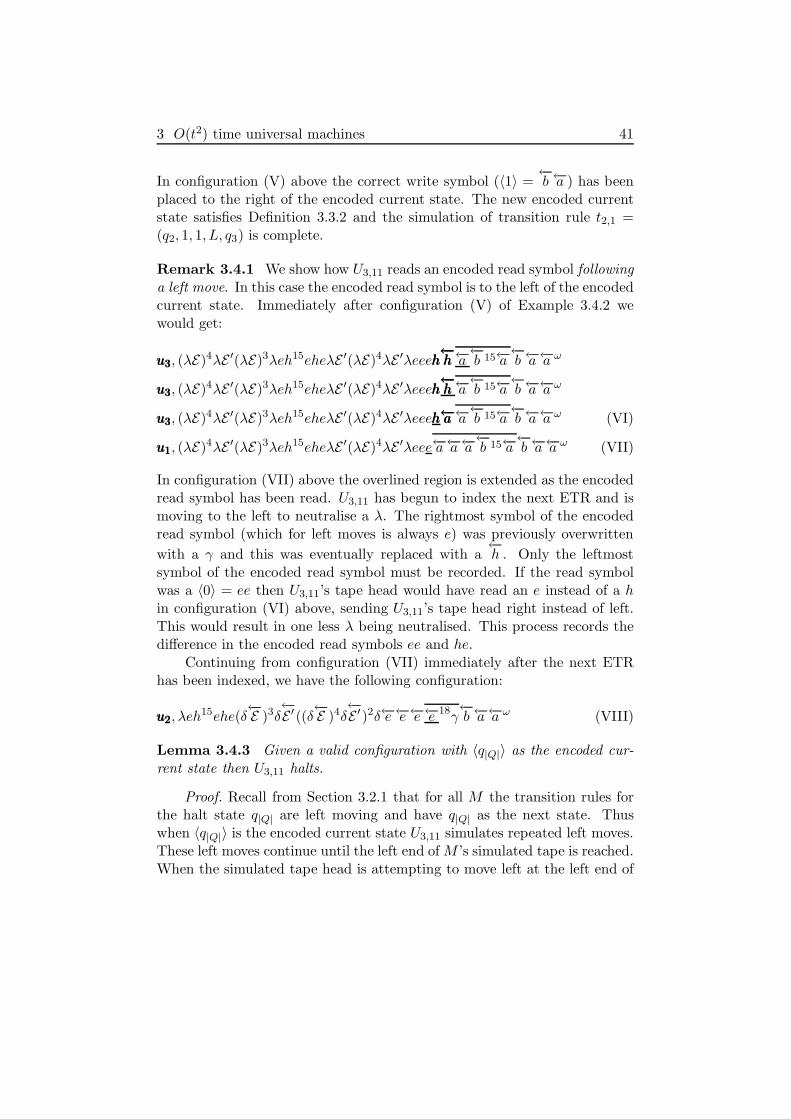
3 O(t2) time universal machines 41
In configuration (V) above the correct write symbol (〈1〉 =←−b←−a ) has been
placed to the right of the encoded current state. The new encoded currentstate satisfies Definition 3.3.2 and the simulation of transition rule t2,1 =(q2, 1, 1, L, q3) is complete.
Remark 3.4.1 We show how U3,11 reads an encoded read symbol followinga left move. In this case the encoded read symbol is to the left of the encodedcurrent state. Immediately after configuration (V) of Example 3.4.2 wewould get:
u3u3u3, (λE)4λE ′(λE)3λeh15eheλE ′(λE)4λE ′λeeeh
←−hh←−hh←−h←−a←−b 15←−a
←−b←−a←−a ω
u3u3u3, (λE)4λE ′(λE)3λeh15eheλE ′(λE)4λE ′λeeehhh
←−h←−h←−h←−a←−b 15←−a
←−b←−a←−a ω
u3u3u3, (λE)4λE ′(λE)3λeh15eheλE ′(λE)4λE ′λeeehhh←−a←−a←−a←−a
←−b 15←−a
←−b←−a←−a ω (VI)
u1u1u1, (λE)4λE ′(λE)3λeh15eheλE ′(λE)4λE ′λeee←−a←−a←−a
←−b 15←−a
←−b←−a←−a ω (VII)
In configuration (VII) above the overlined region is extended as the encodedread symbol has been read. U3,11 has begun to index the next ETR and ismoving to the left to neutralise a λ. The rightmost symbol of the encodedread symbol (which for left moves is always e) was previously overwritten
with a γ and this was eventually replaced with a←−h . Only the leftmost
symbol of the encoded read symbol must be recorded. If the read symbolwas a 〈0〉 = ee then U3,11’s tape head would have read an e instead of a hin configuration (VI) above, sending U3,11’s tape head right instead of left.This would result in one less λ being neutralised. This process records thedifference in the encoded read symbols ee and he.
Continuing from configuration (VII) immediately after the next ETRhas been indexed, we have the following configuration:
u2u2u2, λeh15ehe(δ←−E )3δ
←−E ′ ((δ
←−E )4δ
←−E ′ )2δ←−e←−e←−e←−e
18γ←−b←−a←−a ω (VIII)
Lemma 3.4.3 Given a valid configuration with 〈q|Q|〉 as the encoded cur-rent state then U3,11 halts.
Proof. Recall from Section 3.2.1 that for all M the transition rules forthe halt state q|Q| are left moving and have q|Q| as the next state. Thuswhen 〈q|Q|〉 is the encoded current state U3,11 simulates repeated left moves.These left moves continue until the left end of M ’s simulated tape is reached.When the simulated tape head is attempting to move left at the left end of

3 O(t2) time universal machines 42
the simulated tape then immediately after Cycle 3 the following computationoccurs:
u2u2u2, (λEλEλEλEλE′)∗λγ←−a←−a ∗
←−b 2←−b ∗←−a (
←−b←−a ∪←−a←−a )∗←−a ω
u3u3u3, (λEλEλEλEλE′)∗λ←−h←−a←−a ∗
←−b 2←−b ∗←−a (
←−b←−a ∪←−a←−a )∗←−a ω
u3u3u3, (λEλEλEλEλE′)∗λ←−h←−a←−a ∗
←−b 2←−b ∗←−a (
←−b←−a ∪←−a←−a )∗←−a ω
u3u3u3, (λEλEλEλEλE′)∗λ←−a←−a←−a ∗
←−b 2←−b ∗←−a (
←−b←−a ∪←−a←−a )∗←−a ω
u3u3u3, (λEλEλEλEλE′)∗δ←−a←−a←−a ∗
←−b 2←−b ∗←−a (
←−b←−a ∪←−a←−a )∗←−a ω
u3u3u3, (λEλEλEλEλE′)∗δ←−a←−a←−a ∗
←−b 2←−b ∗←−a (
←−b←−a ∪←−a←−a )∗←−a ω
There is no transition rule for the state-symbol pair (u3, δ) in U3,11 so thesimulation halts. �
Lemma 3.4.4 Given a valid initial configuration of U3,11, then immedi-ately after the first ETR of a computation is indexed, the overlined regionis of the form ←−e 5|Q|+3γ.
Proof. From Definition 3.3.1 the encoded start state 〈q1〉 in an initial
configuration is of the form←−a 5|Q|←−b 2. Example 3.3.2 gives the case of readinga 〈1〉 in the encoded start state 〈q1〉. In this case 〈q1〉 and 〈1〉 have both
been read, that is the←−b and ←−a symbols of 〈q1〉 and 〈1〉 have been replaced
with ←−e symbols and the rightmost ←−a is replaced with a γ. This gives anoverlined region of ←−e 5|Q|+3γ.
The other case is reading a 〈0〉 in state 〈q1〉. By Definition 3.2.2 the 〈0〉is located immediately to the right of 〈q1〉. When reading a 〈0〉 on the rightthere are two steps; executing an ETR′ and then an ETR. From Lemma 3.4.1we know that the ETR′ E ′(f, t1,0) is indexed. Example 3.4.1 executes anETR′ and indexes the subsequent ETR, while in encoded state 〈q1〉. At
this point the entire 〈0〉 has been read. Thus the←−b and ←−a symbols of 〈q1〉
and 〈0〉 have been replaced with←−e symbols and the rightmost←−a is replacedwith a γ. This gives an overlined region of ←−e 5|Q|+3γ. �
Lemma 3.4.5 U3,11 simulates any transition rule of any deterministic Tur-ing machine M .
Proof. The proof is by induction on the form of the overlined region.The base case is given by Lemma 3.4.4; after the first ETR is indexed thenthe overlined region is ←−e 5|Q|+3γ.
We will show that immediately after any ETR is indexed, the overlinedregion is ←−e 5|Q|+3γ.

3 O(t2) time universal machines 43
Assume that the overlined region is←−e 5|Q|+3γ immediately after indexingan ETR ξ1 in the simulation of timestep i of M ’s computation. Let ξ2 bethe ETR that is executed immediately after ξ1. We now show that theoverlined region is←−e 5|Q|+3γ immediately after indexing ξ2 in the simulationof timestep i + 1.
The four cases of ETRs are defined by Equation (3.3.1). In Exam-ples 3.3.2, 3.4.1 and 3.4.2, three of these cases are shown to execute cor-rectly on an overlined region of the form ←−e 5|Q|+3γ. We use Example 3.4.2to verify the remaining case (left move, write 0) by substitution of the ETRdefined by Case 4 of Equation (3.3.1) with the ETR defined by Case 3 ofEquation (3.3.1). The examples generalise to arbitrary transition rules.
Case 1 of Equation (3.3.1): Examples 3.3.2 and 3.4.1 verify Case1. In configuration (I) (in simulation of timestep i) the overlined region is←−e 5|Q|+3γ and the ETR ξ1 that is indexed is defined by Case 1 of Equa-tion (3.3.1). In configuration (III) (in simulation of timestep i + 1) the nextETR ξ2 has been indexed and the overlined region is ←−e 5|Q|+3γ.
Case 2 of Equation (3.3.1): Examples 3.4.1 and 3.4.2 verify Case 2.In configuration (III) (in simulation of timestep i) the overlined region is←−e 5|Q|+3γ and the ETR ξ1 that is indexed is defined by Case 2 of Equa-tion (3.3.1). In configuration (IV) (in simulation of timestep i + 1) the nextETR ξ2 has been indexed and the overlined region is ←−e 5|Q|+3γ.
Case 4 of Equation (3.3.1): Example 3.4.2 and configuration (VIII)verify Case 4. In configuration (IV) (in simulation of timestep i) the over-lined region is←−e 5|Q|+3γ and the ETR ξ1 that is indexed is defined by Case 4of Equation (3.3.1). In configuration (VIII) (in simulation of timestep i+1)the next ETR ξ2 has been indexed and the overlined region is ←−e 5|Q|+3γ.
Case 3 of Equation (3.3.1): Case 4 also verifies Case 3 by substitutionof the ETR defined by Case 4 of Equation (3.3.1) with the ETR defined byCase 3.
We have shown that the overlined region is ←−e 5|Q|+3γ immediately afterany ETR is indexed. From Examples 3.3.2, 3.4.1 and 3.4.2, each ETR exe-cutes on an overlined region of ←−e 5|Q|+3γ establishing the correct simulatedtape head location, encoded write symbol, and an encoded current state thatsatisfies Definition 3.3.2. By Lemmata 3.4.1 and 3.4.2 the encoded currentstate indexes the correct ETR. Due to the relative lengths of the encodedcurrent state and overlined region the above mentioned examples generaliseto any transition rule of any Turing machine M . �

3 O(t2) time universal machines 44
Theorem 3.4.1 Let M be a single tape deterministic Turing machine with|Q| states that runs in time t. Then U3,11 simulates any Turing machine Min space O(t + |Q|2) and time O(|Q|t2 + |Q|3t).
Proof. By Lemma 3.4.5 U3,11 simulates any transition rule. Thus given avalid encoding of M ’s initial configuration (Definition 3.2.2), U3,11 simulatesthe sequence of transition rules in M ’s computation. From Lemma 3.4.3when U3,11 simulates the halting state of M , U3,11’s tape head returns tothe left end of M ’s encoded output and halts. The encoded output is easilydecoded via Definition 3.2.1.
(Space). At time t the space used by M is bounded by t. Simulator U3,11
uses space O(t + |Q|2), where O(|Q|2) space is used to store M as the word〈M〉 and O(t) space is used to store M ’s encoded tape after t simulatedsteps.
(Time). Simulating a transition rule involves 4 cycles. (1) Index an ETRby neutralising O(|Q|) of the λ markers: O(|Q|t + |Q|3) steps. (2) Copyan ETR of length O(|Q|) from 〈M〉 to the encoded current state location:O(|Q|t+ |Q|3) steps. (3) Restore U3,11’s tape contents: O(t+ |Q|2) steps. (4)Complete execution of ETR: a small constant number of steps. Thus U3,11
uses O(|Q|t+ |Q|3) time to simulate a single step of M , and O(|Q|t2 + |Q|3t)time to simulate the entire computation of M . �
3.5 Polynomial time Curve
In this section we further extend our result by finding small polynomial timeuniversal Turing machines with other state-symbol pairs. Thus we establisha O(t2) polynomial time curve.
All universal Turing machines in this chapter use the same basic algo-rithm as U3,11. The proof of correctness given for U3,11 can be applied tothe remaining machines in a straightforward way, so we do not restate it.The encoding of the input and operation of these universal Turing machinesis the same as U3,11 unless noted otherwise. Each universal Turing machinemakes use of specially tailored E and E ′ functions.
3.5.1 Construction of U6,6
For U6,6 the start state of 〈M〉 is encoded as 〈q1〉 =←−a 5|Q|←−b 2. The encoding
of the current state is of the form←−a ∗←−b 2←−b ∗{←−a ∪ǫ} and is of length 5|Q|+2.
Let t = (qx, σ1, σ2,D, qy) be a fixed transition rule in M , then t isencoded via P using the function E on its own, or in conjunction with E ′,
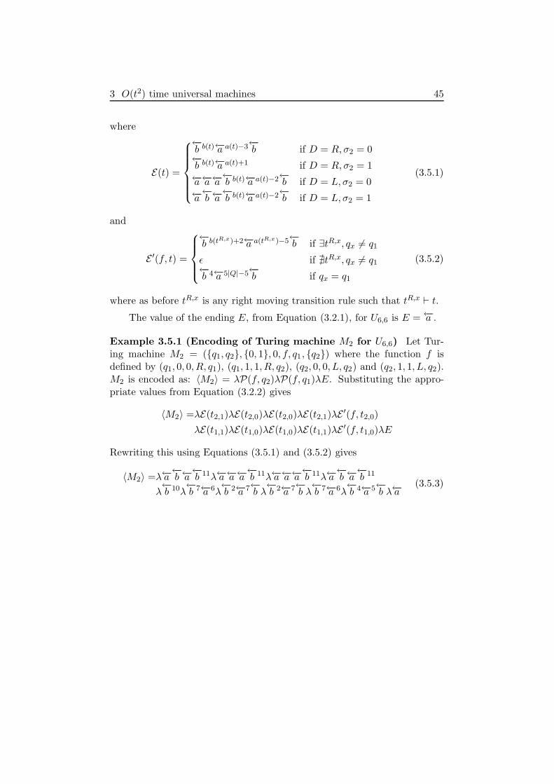
3 O(t2) time universal machines 45
where
E(t) =
←−b b(t)←−a a(t)−3←−b if D = R,σ2 = 0←−b b(t)←−a a(t)+1 if D = R,σ2 = 1←−a←−a←−a
←−b b(t)←−a a(t)−2←−b if D = L, σ2 = 0
←−a←−b←−a←−b b(t)←−a a(t)−2←−b if D = L, σ2 = 1
(3.5.1)
and
E ′(f, t) =
←−b b(tR,x)+2←−a a(tR,x)−5←−b if ∃tR,x, qx 6= q1
ǫ if ∄tR,x, qx 6= q1←−b 4←−a 5|Q|−5←−b if qx = q1
(3.5.2)
where as before tR,x is any right moving transition rule such that tR,x ⊢ t.
The value of the ending E, from Equation (3.2.1), for U6,6 is E =←−a .
Example 3.5.1 (Encoding of Turing machine M2 for U6,6) Let Tur-ing machine M2 = ({q1, q2}, {0, 1}, 0, f, q1 , {q2}) where the function f isdefined by (q1, 0, 0, R, q1), (q1, 1, 1, R, q2), (q2, 0, 0, L, q2) and (q2, 1, 1, L, q2).M2 is encoded as: 〈M2〉 = λP(f, q2)λP(f, q1)λE. Substituting the appro-priate values from Equation (3.2.2) gives
〈M2〉 =λE(t2,1)λE(t2,0)λE(t2,0)λE(t2,1)λE′(f, t2,0)
λE(t1,1)λE(t1,0)λE(t1,0)λE(t1,1)λE′(f, t1,0)λE
Rewriting this using Equations (3.5.1) and (3.5.2) gives
〈M2〉 =λ←−a←−b←−a←−b 11λ←−a←−a←−a
←−b 11λ←−a←−a←−a
←−b 11λ←−a
←−b←−a←−b 11
λ←−b 10λ
←−b 7←−a 6λ
←−b 2←−a 7←−b λ
←−b 2←−a 7←−b λ
←−b 7←−a 6λ
←−b 4←−a 5←−b λ←−a
(3.5.3)
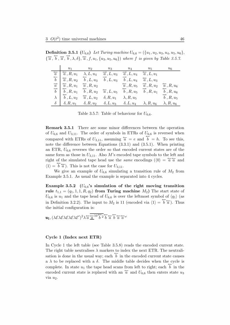
3 O(t2) time universal machines 46
Definition 3.5.1 (U6,6) Let Turing machine U6,6 = ({u1, u2, u3, u4, u5, u6},
{←−a ,←−b ,−→a ,
−→b , λ, δ},←−a , f, u1, {u3, u5, u6}) where f is given by Table 3.5.7.
u1 u2 u3 u4 u5 u6←−a ←−a ,R, u1 λ,L, u4
−→a ,L, u3−→a ,L, u4
←−a ,L, u1←−b ←−a ,R, u2
←−b , L, u3
−→b , L, u3
−→b , L, u4
←−a ,L, u3−→a ←−a ,R, u1
←−a ,R, u2←−a ,R, u5
−→a ,R, u2←−a ,R, u6
−→b←−b ,R, u1
←−b ,R, u2
←−a ,L, u5←−b ,R, u5
−→b ,R, u1
←−b ,R, u6
λ←−b , L, u2
←−a ,L, u2 δ,R, u1 λ,R, u5−→b ,R, u5
δ δ,R, u1 δ,R, u2 δ, L, u3 δ, L, u4 λ,R, u6 λ,R, u6
Table 3.5.7: Table of behaviour for U6,6.
Remark 3.5.1 There are some minor differences between the operationof U6,6 and U3,11. The order of symbols in ETRs of U6,6 is reversed when
compared with ETRs of U3,11, assuming ←−a = e and←−b = h. To see this,
note the difference between Equations (3.3.1) and (3.5.1). When printingan ETR, U6,6 reverses the order so that encoded current states are of thesame form as those in U3,11. Also M ’s encoded tape symbols to the left andright of the simulated tape head use the same encodings (〈0〉 = ←−a←−a and
〈1〉 =←−b←−a ). This is not the case for U3,11.
We give an example of U6,6 simulating a transition rule of M2 fromExample 3.5.1. As usual the example is separated into 4 cycles.
Example 3.5.2 (U6,6’s simulation of the right moving transitionrule t1,1 = (q1, 1, 1, R, q2) from Turing machine M2) The start state ofU6,6 is u1 and the tape head of U6,6 is over the leftmost symbol of 〈q1〉 (as
in Definition 3.2.2). The input to M2 is 11 (encoded via 〈1〉 =←−b←−a ). Thus
the initial configuration is:
u1u1u1, (λEλEλEλEλE′)2λ←−a←−a
10←−b 2←−b←−a←−b←−a←−a ω
Cycle 1 (Index next ETR)
In Cycle 1 the left table (see Table 3.5.8) reads the encoded current state.The right table neutralises λ markers to index the next ETR. The neutrali-
sation is done in the usual way; each←−b in the encoded current state causes
a λ to be replaced with a δ. The middle table decides when the cycle is
complete. In state u1 the tape head scans from left to right; each←−b in the
encoded current state is replaced with an ←−a and U6,6 then enters state u3
via u2.

3 O(t2) time universal machines 47
u1←−a ←−a ,R, u1←−b ←−a ,R, u2−→a ←−a ,R, u1−→b←−b ,R, u1
δ δ,R, u1
u2←−a λ,L, u4←−b←−b , L, u3
u3←−a −→a ,L, u3←−b−→b , L, u3
λ δ,R, u1
δ δ, L, u3
Table 3.5.8: Sub-tables for Cycle 1 of U6,6.
We have replaced the shorthand notation E with the word←−b 7←−a 6 de-
fined by E(t1,1). The word←−b 7←−a 6 appears in the location defined by Equa-
tion (3.5.3). After the initial configuration we have:
u1u1u1, (λE)4λE ′(λE)3λ
←−b 7←−a 6λE ′λ←−a←−a 10
←−b←−b←−b←−a←−b←−a←−b←−a←−b←−a←−a ω
u2u2u2, (λE)4λE ′(λE)3λ
←−b 7←−a 6λE ′λ←−a←−a 10←−a
←−b←−b←−a←−b←−a←−b←−a←−b←−a←−a ω
u3u3u3, (λE)4λE ′(λE)3λ
←−b 7←−a 6λE ′λ←−a←−a 10←−a
←−b←−b←−a←−b←−a←−b←−a←−b←−a←−a ω
u3u3u3, (λE)4λE ′(λE)3λ
←−b 7←−a 6λE ′λ−→a −→a 10−→a
←−b←−b←−a←−b←−a←−b←−a←−b←−a←−a ω
u1u1u1, (λE)4λE ′(λE)3λ
←−b 7←−a 6λE ′δ−→a −→a 10−→a
←−b←−b←−a←−b←−a←−b←−a←−b←−a←−a ω
The neutralisation process continues until U6,6 reads the final←−b , moves
right to test for the end of the encoded current state and read symbol in u2,and then reads an←−a . When this occurs U6,6 is finished reading the encodedcurrent state and read symbol. Skipping to the end of this cycle gives:
u4u4u4, (λE)4λE ′(λE)3λ
←−b 7←−a 6δE ′δ←−a←−a 10←−a←−a←−a λ
←−b←−a←−a ω
U6,6 has neutralised two λ markers to index the next ETR.
u4←−a −→a ,L, u4←−b−→b , L, u4
−→a ←−a ,R, u5−→b←−b ,R, u5
λ λ,R, u5
δ δ, L, u4
u5−→a −→a ,R, u2−→b−→b ,R, u1
δ λ,R, u6
u1−→a ←−a ,R, u1−→b←−b ,R, u1
λ←−b , L, u2
δ δ,R, u1
u2←−a λ,L, u4−→a ←−a ,R, u2−→b←−b ,R, u2
λ ←−a ,L, u2
δ δ,R, u2
Table 3.5.9: Sub-tables for Cycle 2 of U6,6.

3 O(t2) time universal machines 48
Cycle 2 (Print ETR)
This cycle copies an ETR to M ’s simulated tape head position. The leftmosttable scans left and locates the next symbol of the ETR to be printed. Thesecond table from the left records the symbol to be printed or ends the cycle.The rightmost two tables scan right and print the appropriate symbol. In theconfigurations below, U6,6 scans left until a λ is read. Then U6,6 moves rightand records the symbol read by entering state u1 or u2. In the configurations
below when all the←−b and ←−a symbols in an E ′ are replaced with
−→b and −→a
symbols then the resulting word is denoted−→E ′ .
u4u4u4, (λE)4λE ′(λE)3λ
−→b−→b−→b 5−→a 6δ
−→E ′δ−→a −→a 12−→a λ
←−b←−a←−a ω
u5u5u5, (λE)4λE ′(λE)3λ
−→b−→b−→b 5−→a 6δ
−→E ′δ−→a −→a 12−→a λ
←−b←−a←−a ω
u1u1u1, (λE)4λE ′(λE)3λ
−→b←−b←−b 5←−a 6δE ′δ←−a←−a 12←−a λ
←−b←−a←−a ω
u2u2u2, (λE)4λE ′(λE)3λ
−→b←−b←−b 5←−a 6δE ′δ←−a←−a 12←−a
←−b←−b←−a←−a ω
u4u4u4, (λE)4λE ′(λE)3λ
−→b−→b−→b 5−→a 6δ
−→E ′δ−→a −→a 12λ
←−b←−b←−a←−a ω
u5u5u5, (λE)4λE ′(λE)3λ
←−b−→b−→b 5−→a 6δ
−→E ′δ−→a −→a 12λ
←−b←−b←−a←−a ω
On the first pass U6,6 located the symbol to be printed by using λ as amarker. On subsequent passes U6,6 locates the symbol to be printed by
locating an −→a or−→b . This printing process is iterated until U6,6 is finished
printing the ETR. The completion of this process occurs on reading a δ instate u5 which switches control to u6:
u4u4u4, (λE)4λE ′(λE)3λ
←−b 7←−a 5−→a δ
−→E ′δ−→a λ←−a 6
←−b 7←−b←−a←−a ω
u5u5u5, (λE)4λE ′(λE)3λ
←−b 7←−a 5←−a δ
−→E ′δ−→a λ←−a 6
←−b 7←−b←−a←−a ω
u6u6u6, (λE)4λE ′(λE)3λ
←−b 7←−a 5←−a λ
−→E ′δ−→a λ←−a 6
←−b 7←−b←−a←−a ω
Cycle 3 (Restore tape)
This table restores M ’s simulated tape and encoded table of behaviour. U6,6
moves right restoring each −→a to ←−a , each−→b to
←−b , and each δ to λ. This
continues until U6,6 reads λ, sending control to state u5.
u6u6u6, (λE)4λE ′(λE)3λ
←−b 7←−a 6λE ′λ←−a λ←−a←−a 5
←−b 7←−b←−a←−a ω
u5u5u5, (λE)4λE ′(λE)3λ
←−b 7←−a 6λE ′λ←−a
−→b←−a←−a 5
←−b 7←−b←−a←−a ω

3 O(t2) time universal machines 49
u6−→a ←−a ,R, u6−→b←−b ,R, u6
λ−→b ,R, u5
δ λ,R, u6
Table 3.5.10: Cycle 3 of U6,6.
Cycle 4 (Choose read or write symbol)
u5←−a ←−a ,L, u1←−b ←−a ,L, u3
λ
u3−→b ←−a ,L, u5
u1←−a ←−a ,R, u1−→b←−b ,R, u1
Table 3.5.11: Sub-tables for Cycle 4 of U6,6.
This cycle either (i) begins the indexing of an ETR or (ii) completesthe execution of an ETR. More precisely: (i) if U6,6 is immediately aftersimulating a left move then this cycle reads the encoded read symbol to theleft of the encoded current state, (ii) if U6,6 is simulating a right move thenthis cycle prints the encoded write symbol to the left of the encoded currentstate. Case (ii) follows:
u1u1u1, (λE)4λE ′(λE)3λ
←−b 7←−a 6λE ′λ←−a
−→b←−a←−a 5
←−b 7←−b←−a←−a ω
u1u1u1, (λE)4λE ′(λE)3λ
←−b 7←−a 6λE ′λ←−a
←−b←−b←−b←−a←−a←−a←−a 5
←−b 7←−b←−a←−a ω
In the configuration immediately above we have shortened the overlinedsection; the two symbols to the left of 〈M2〉’s encoded current state encodethe write symbol 1.
The example simulation of transition rule t1,1 = (q1, 1, 1, R, q2) is now
complete. The correct encoded write symbol 〈1〉 =←−b←−a has been written
and the new encoded current state is of the correct form. M2’s simulatedtape head (the new encoded current state) is configured so U6,6 reads thenext encoded read symbol to the right when searching for the next ETR.
Left moving transition rules are simulated in a similar fashion to the rightmoving transition rule given above, except in this case the write symbolis written on the right hand side of the encoded current state as shown inFigure 3.2.3 (cL). After the left move M2’s simulated tape head (encodedcurrent state) is configured to read the encoded tape symbol to its left whensearching for the next ETR.
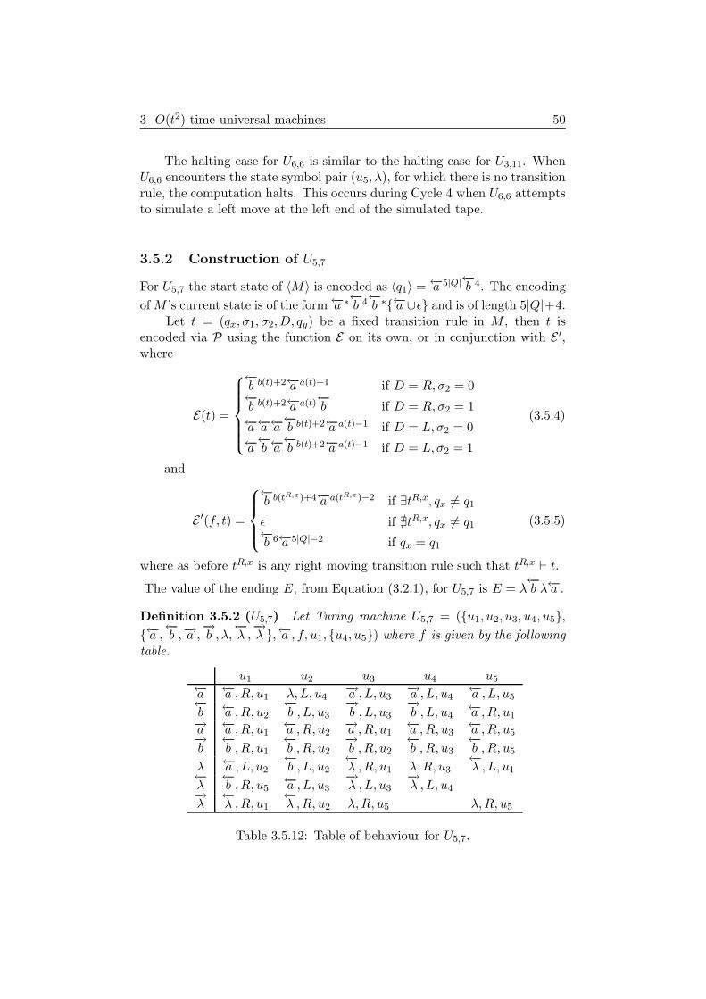
3 O(t2) time universal machines 50
The halting case for U6,6 is similar to the halting case for U3,11. WhenU6,6 encounters the state symbol pair (u5, λ), for which there is no transitionrule, the computation halts. This occurs during Cycle 4 when U6,6 attemptsto simulate a left move at the left end of the simulated tape.
3.5.2 Construction of U5,7
For U5,7 the start state of 〈M〉 is encoded as 〈q1〉 =←−a 5|Q|←−b 4. The encoding
of M ’s current state is of the form←−a ∗←−b 4←−b ∗{←−a ∪ǫ} and is of length 5|Q|+4.
Let t = (qx, σ1, σ2,D, qy) be a fixed transition rule in M , then t isencoded via P using the function E on its own, or in conjunction with E ′,where
E(t) =
←−b b(t)+2←−a a(t)+1 if D = R,σ2 = 0←−b b(t)+2←−a a(t)←−b if D = R,σ2 = 1←−a←−a←−a
←−b b(t)+2←−a a(t)−1 if D = L, σ2 = 0
←−a←−b←−a←−b b(t)+2←−a a(t)−1 if D = L, σ2 = 1
(3.5.4)
and
E ′(f, t) =
←−b b(tR,x)+4←−a a(tR,x)−2 if ∃tR,x, qx 6= q1
ǫ if ∄tR,x, qx 6= q1←−b 6←−a 5|Q|−2 if qx = q1
(3.5.5)
where as before tR,x is any right moving transition rule such that tR,x ⊢ t.
The value of the ending E, from Equation (3.2.1), for U5,7 is E = λ←−b λ←−a .
Definition 3.5.2 (U5,7) Let Turing machine U5,7 = ({u1, u2, u3, u4, u5},
{←−a ,←−b ,−→a ,
−→b , λ,
←−λ ,−→λ },←−a , f, u1, {u4, u5}) where f is given by the following
table.
u1 u2 u3 u4 u5←−a ←−a ,R, u1 λ,L, u4
−→a ,L, u3−→a ,L, u4
←−a ,L, u5←−b ←−a ,R, u2
←−b , L, u3
−→b , L, u3
−→b , L, u4
←−a ,R, u1−→a ←−a ,R, u1
←−a ,R, u2−→a ,R, u1
←−a ,R, u3←−a ,R, u5
−→b←−b ,R, u1
←−b ,R, u2
−→b ,R, u2
←−b ,R, u3
←−b ,R, u5
λ ←−a ,L, u2←−b , L, u2
←−λ ,R, u1 λ,R, u3
←−λ ,L, u1
←−λ←−b ,R, u5
←−a ,L, u3−→λ ,L, u3
−→λ ,L, u4
−→λ←−λ ,R, u1
←−λ ,R, u2 λ,R, u5 λ,R, u5
Table 3.5.12: Table of behaviour for U5,7.

3 O(t2) time universal machines 51
Remark 3.5.2 There are some minor differences between the operationof U5,7 and U3,11. The order of symbols in ETRs of U5,7 is reversed when
compared with ETRs of U3,11, assuming ←−a = e and←−b = h. To see this,
note the difference between Equations (3.3.1) and (3.5.4). When printingan ETR, U5,7 reverses the order so that encoded current states are of thesame form as those in U3,11. Also M ’s encoded tape symbols to the left andright of the simulated tape head use the same encodings (〈0〉 = ←−a←−a and
〈1〉 =←−b←−a ). This is not the case for U3,11.
We give a brief overview of the computation of U5,7.
Cycle 1 (Index next ETR)
u1←−a ←−a ,R, u1←−b ←−a ,R, u2−→a ←−a ,R, u1−→b←−b ,R, u1
−→λ←−λ ,R, u1
u2←−a λ,L, u4←−b←−b , L, u3
u3←−a −→a ,L, u3←−b−→b , L, u3
λ←−λ ,R, u1
←−λ−→λ ,L, u3
Table 3.5.13: Sub-tables for Cycle 1 of U5,7.
In Cycle 1 the leftmost table (above) reads the encoded current state.
The rightmost table neutralises λ markers by replacing them with←−λ or
−→λ
to index the next ETR. The middle table decides when the cycle is complete.
Each←−b in the encoded current state is replaced with←−a and then U5,7 enters
state u3 via u2.
Cycle 2 (Print ETR)
u4←−a −→a ,L, u4←−b−→b , L, u4
−→a ←−a ,R, u3−→b←−b ,R, u3
λ λ,R, u3←−λ−→λ ,L, u4
u3−→a −→a ,R, u1−→b−→b ,R, u2
−→λ λ,R, u5
u2←−a λ,L, u4−→a ←−a ,R, u2−→b←−b ,R, u2
λ←−b , L, u2
−→λ←−λ ,R, u2
u1−→a ←−a ,R, u1−→b←−b ,R, u1
λ ←−a ,L, u2−→λ←−λ ,R, u1
Table 3.5.14: Sub-tables for Cycle 2 of U5,7.

3 O(t2) time universal machines 52
This cycle copies an ETR to M ’s simulated tape head position. Theleftmost table scans left and locates the next symbol of the ETR to beprinted. The second table from the left records the symbol to be printed orends the cycle. The rightmost two tables scan right and print the appropriatesymbol.
Cycle 3 (Restore tape)
u5−→a ←−a ,R, u5−→b←−b ,R, u5
λ←−λ ,L, u1
−→λ λ,R, u5
Table 3.5.15: Cycle 3 of U5,7.
Table 3.5.15 restores M ’s simulated tape and encoded table of be-
haviour. U5,7 moves right restoring each −→a to ←−a , each−→b to
←−b , and each
−→λ to λ. This continues until U5,7 reads λ, sending U5,7’s control into u1.
Cycle 4 (Choose read or write symbol)
u1←−a ←−a ,R, u1←−b ←−a ,R, u2←−λ←−b ,R, u5
u2←−λ ←−a ,L, u3
u5←−a ←−a ,L, u5←−b ←−a ,R, u1
Table 3.5.16: Sub-tables for Cycle 4 of U5,7.
This cycle either (i) begins the indexing of an ETR or (ii) completesthe execution of an ETR. More precisely: (i) if U5,7 is immediately aftersimulating a left move then this cycle reads the encoded read symbol to theleft of the encoded current state, (ii) if U5,7 is simulating a right move thenthis cycle prints the encoded write symbol to the left of the encoded currentstate. The halting case for U5,7 is more complex than the previous universal
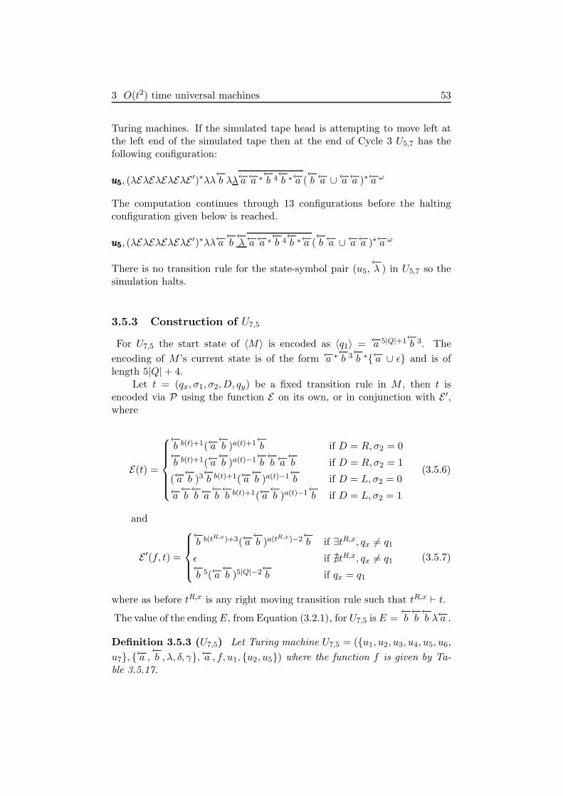
3 O(t2) time universal machines 53
Turing machines. If the simulated tape head is attempting to move left atthe left end of the simulated tape then at the end of Cycle 3 U5,7 has thefollowing configuration:
u5u5u5, (λEλEλEλEλE′)∗λλ
←−b λλ←−a←−a ∗
←−b 4←−b ∗←−a (
←−b←−a ∪←−a←−a )∗←−a ω
The computation continues through 13 configurations before the haltingconfiguration given below is reached.
u5u5u5, (λEλEλEλEλE′)∗λλ←−a
←−b←−λ←−a←−a ∗
←−b 4←−b ∗←−a (
←−b←−a ∪←−a←−a )∗←−a ω
There is no transition rule for the state-symbol pair (u5,←−λ ) in U5,7 so the
simulation halts.
3.5.3 Construction of U7,5
For U7,5 the start state of 〈M〉 is encoded as 〈q1〉 = ←−a 5|Q|+1←−b 3. The
encoding of M ’s current state is of the form ←−a ∗←−b 3←−b ∗{←−a ∪ ǫ} and is of
length 5|Q|+ 4.Let t = (qx, σ1, σ2,D, qy) be a fixed transition rule in M , then t is
encoded via P using the function E on its own, or in conjunction with E ′,where
E(t) =
←−b b(t)+1(←−a
←−b )a(t)+1←−b if D = R,σ2 = 0
←−b b(t)+1(←−a
←−b )a(t)−1←−b
←−b←−a←−b if D = R,σ2 = 1
(←−a←−b )3←−b b(t)+1(←−a
←−b )a(t)−1←−b if D = L, σ2 = 0
←−a←−b←−b←−a←−b←−b b(t)+1(←−a
←−b )a(t)−1←−b if D = L, σ2 = 1
(3.5.6)
and
E ′(f, t) =
←−b b(tR,x)+3(←−a
←−b )a(tR,x)−2←−b if ∃tR,x, qx 6= q1
ǫ if ∄tR,x, qx 6= q1←−b 5(←−a
←−b )5|Q|−2←−b if qx = q1
(3.5.7)
where as before tR,x is any right moving transition rule such that tR,x ⊢ t.
The value of the ending E, from Equation (3.2.1), for U7,5 is E =←−b←−b←−b λ←−a .
Definition 3.5.3 (U7,5) Let Turing machine U7,5 = ({u1, u2, u3, u4, u5, u6,
u7}, {←−a ,←−b , λ, δ, γ},←−a , f, u1, {u2, u5}) where the function f is given by Ta-
ble 3.5.17.

3 O(t2) time universal machines 54
u1 u2 u3 u4←−a ←−a ,R, u1 γ, L, u4
←−a ,L, u3←−a ,L, u4
←−b ←−a ,R, u2
←−b , L, u3 λ,L, u3 λ,L, u4
λ←−b ,R, u1 γ,R, u1 δ,R, u1 λ,R, u5
δ δ,R, u1 δ, L, u3 δ, L, u4
γ ←−a ,L, u2←−b ,R, u6
←−a ,R, u5←−b ,R, u5
u5 u6 u7←−a ←−a ,R, u2
←−a ,R, u6←−a ,R, u7
←−b ←−a ,R, u3
←−a ,L, u7←−a ,R, u1
λ γ,R, u6←−b ,R, u6
←−b ,R, u7
δ λ,R, u7 δ,R, u6 λ,R, u7
γ←−b , L, u2 γ, L, u5
Table 3.5.17: Table of behaviour for U7,5.
Remark 3.5.3 There are some minor differences between the operationof U7,5 and U3,11. The order of symbols in ETRs of U7,5 is reversed when
compared with ETRs of U3,11, assuming ←−a←−b = e and
←−b = h. To see this,
note the difference between Equations (3.3.1) and (3.5.6). When printingan ETR, U7,5 reverses the order so that encoded current states are of thesame form as those in U3,11. Also, M ’s encoded tape symbols to the left andright of the simulated tape head use the same encodings (〈0〉 = ←−a←−a and
〈1〉 =←−b←−a ). This is not the case for U3,11.
We give a brief overview of U7,5’s computation.
Cycle 1 (Index next ETR)
u1←−a ←−a ,R, u1←−b ←−a ,R, u2
λ←−b ,R, u1
δ δ,R, u1
u2←−a γ,L, u4←−b←−b , L, u3
u3←−a ←−a ,L, u3←−b λ, L, u3
λ δ,R, u1
δ δ, L, u3
Table 3.5.18: Sub-tables for Cycle 1 of U7,5.
In Cycle 1 the left table (above) reads the encoded current state. Theright table neutralises λ markers by replacing them with δ symbols to indexthe next ETR. The middle table decides when the cycle is complete. Each←−b in the encoded current state is replaced with←−a and U7,5 then enters stateu3 via u2.

3 O(t2) time universal machines 55
Cycle 2 (Print ETR)
u2 u4←−a γ,L, u4
←−a ,L, u4←−b λ, L, u4
λ λ,R, u5
δ δ, L, u4
γ←−b ,R, u5
u5←−a ←−a ,R, u2
λ γ,R, u6
δ λ,R, u7
u6←−a ←−a ,R, u6
λ←−b ,R, u6
δ δ,R, u6
γ←−b , L, u2
u1 u2←−a ←−a ,R, u1
λ←−b ,R, u1 γ,R, u1
δ δ,R, u1
γ ←−a ,L, u2
Table 3.5.19: Sub-tables for Cycle 2 of U7,5.
This cycle copies an ETR to M ’s simulated tape head position. The topleft table scans left and locates the next symbol of the ETR to be printed.The top right table records the symbol to be printed or ends the cycle. Thebottom two tables scan right and print the appropriate symbol.
Cycle 3 (Restore tape)
This table restores M ’s simulated tape and encoded table of behaviour. U7,5
moves right restoring each λ to←−b , and each δ to λ. This continues until
U7,5 reads γ, sending U7,5’s control to u5.
u7←−a ←−a ,R, u7
λ←−b ,R, u7
δ λ,R, u7
γ γ, L, u5
Table 3.5.20: Cycle 3 of U7,5.

3 O(t2) time universal machines 56
Cycle 4 (Choose read or write symbol)
u5←−a ←−a ,R, u2←−b ←−a ,R, u3
u2 u3
γ←−b ,R, u6
←−a ,R, u5
u6←−a ←−a ,R, u6←−b ←−a ,L, u7
u7←−a ←−a ,R, u7←−b ←−a ,R, u1
Table 3.5.21: Sub-tables for Cycle 4 of U7,5.
This cycle either (i) begins the indexing of an ETR or (ii) completesthe execution of an ETR. More precisely: (i) if U7,5 is immediately aftersimulating a left move then this cycle reads the encoded read symbol to theleft of the encoded current state, (ii) if U7,5 is simulating a right move thenthis cycle prints the encoded write symbol to the left of the encoded currentstate.
The halting case for U7,5 is more complex than the first two univer-sal Turing machines in this chapter. When the simulated tape head is at-tempting to move left at the left end of the simulated tape then the lastconfiguration of Cycle 3 for U7,5 has the following form:
u7u7u7, (λEλEλEλEλE′)∗λ←−b←−b←−b λγ←−b←−a←−a ∗
←−b 3←−b ∗←−a (
←−b←−a ∪←−a←−a )∗←−a ω
The computation continues through 42 configurations before the haltingconfiguration given below is reached.
u5u5u5, (λEλEλEλEλE′)∗λ←−b←−b←−b γ←−b←−b←−b←−a ∗
←−b 3←−b ∗←−a (
←−b←−a ∪←−a←−a )∗←−a ω
There is no transition rule for the state-symbol pair (u5, γ) in U7,5 so thesimulation halts.
3.5.4 Construction of U8,4
For U8,4 the start state of 〈M〉 is encoded as 〈q1〉 =←−a 5|Q|←−b 2. The encoding
of M ’s current state is of the form←−a ∗←−b 2←−b ∗{←−a ∪ǫ} and is of length 5|Q|+2.
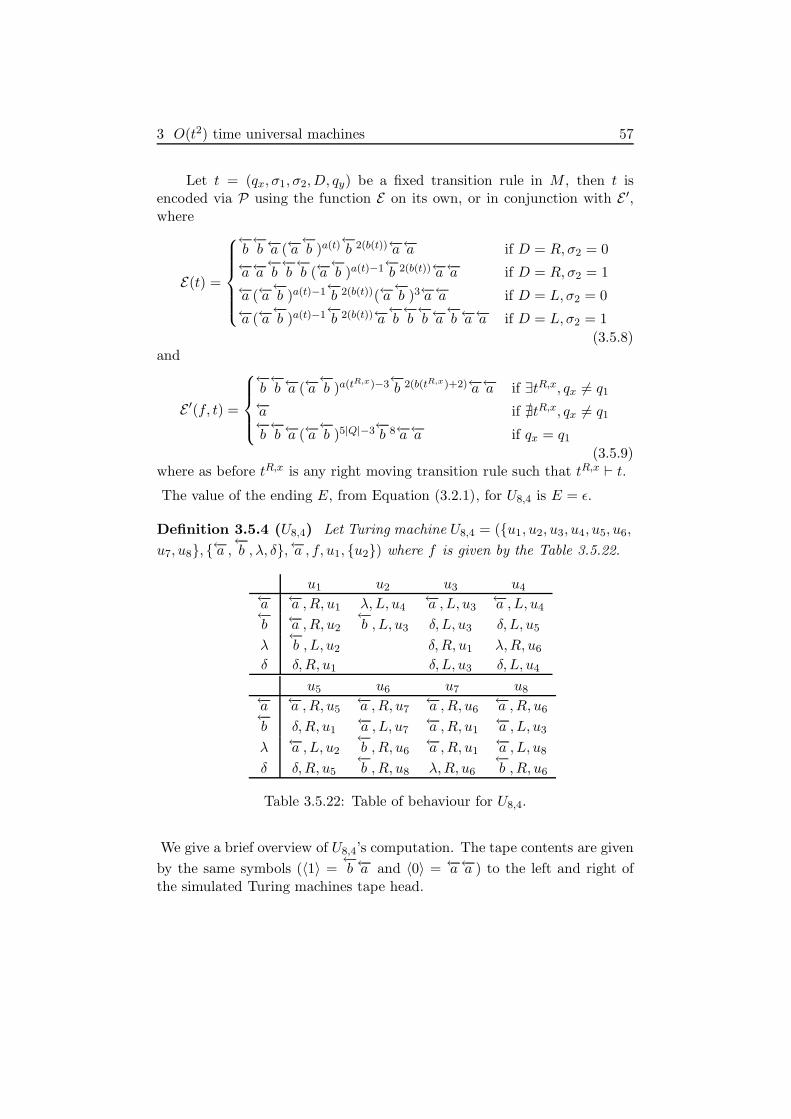
3 O(t2) time universal machines 57
Let t = (qx, σ1, σ2,D, qy) be a fixed transition rule in M , then t isencoded via P using the function E on its own, or in conjunction with E ′,where
E(t) =
←−b←−b←−a (←−a
←−b )a(t)←−b 2(b(t))←−a←−a if D = R,σ2 = 0
←−a←−a←−b←−b←−b (←−a
←−b )a(t)−1←−b 2(b(t))←−a←−a if D = R,σ2 = 1
←−a (←−a←−b )a(t)−1←−b 2(b(t))(←−a
←−b )3←−a←−a if D = L, σ2 = 0
←−a (←−a←−b )a(t)−1←−b 2(b(t))←−a
←−b←−b←−b←−a←−b←−a←−a if D = L, σ2 = 1
(3.5.8)and
E ′(f, t) =
←−b←−b←−a (←−a
←−b )a(tR,x)−3←−b 2(b(tR,x)+2)←−a←−a if ∃tR,x, qx 6= q1
←−a if ∄tR,x, qx 6= q1←−b←−b←−a (←−a
←−b )5|Q|−3←−b 8←−a←−a if qx = q1
(3.5.9)where as before tR,x is any right moving transition rule such that tR,x ⊢ t.
The value of the ending E, from Equation (3.2.1), for U8,4 is E = ǫ.
Definition 3.5.4 (U8,4) Let Turing machine U8,4 = ({u1, u2, u3, u4, u5, u6,
u7, u8}, {←−a ,←−b , λ, δ},←−a , f, u1, {u2}) where f is given by the Table 3.5.22.
u1 u2 u3 u4←−a ←−a ,R, u1 λ,L, u4
←−a ,L, u3←−a ,L, u4
←−b ←−a ,R, u2
←−b , L, u3 δ, L, u3 δ, L, u5
λ←−b , L, u2 δ,R, u1 λ,R, u6
δ δ,R, u1 δ, L, u3 δ, L, u4
u5 u6 u7 u8←−a ←−a ,R, u5
←−a ,R, u7←−a ,R, u6
←−a ,R, u6←−b δ,R, u1
←−a ,L, u7←−a ,R, u1
←−a ,L, u3
λ ←−a ,L, u2←−b ,R, u6
←−a ,R, u1←−a ,L, u8
δ δ,R, u5←−b ,R, u8 λ,R, u6
←−b ,R, u6
Table 3.5.22: Table of behaviour for U8,4.
We give a brief overview of U8,4’s computation. The tape contents are given
by the same symbols (〈1〉 =←−b←−a and 〈0〉 = ←−a←−a ) to the left and right of
the simulated Turing machines tape head.

3 O(t2) time universal machines 58
Cycle 1 (Index next ETR)
u1←−a ←−a ,R, u1←−b ←−a ,R, u2
δ δ,R, u1
u2←−a λ,L, u4←−b←−b , L, u3
u3←−a ←−a ,L, u3←−b δ, L, u3
λ δ,R, u1
δ δ, L, u3
Table 3.5.23: Sub-tables for Cycle 1 of U8,4.
In Cycle 1 the leftmost table (above) reads the encoded current state.The rightmost table neutralises markers to index the next ETR. The middletable decides when the cycle is complete. In state u1 the tape head scans
from left to right; each←−b in the encoded current state is replaced with ←−a
and U8,4 then enters state u3 via u2.
Cycle 2 (Print ETR)
u2 u4←−a λ,L, u4
←−a ,L, u4←−b δ, L, u5
λ λ,R, u6
δ δ, L, u4
u5←−a ←−a ,R, u5←−b δ,R, u1
λ ←−a ,L, u2
δ δ,R, u5
u1←−a ←−a ,R, u1
λ←−b , L, u2
δ δ,R, u1
Table 3.5.24: Sub-tables for Cycle 2 of U8,4.
Before we explain this cycle we mention why ETRs for U8,4 are longerthan ETRs for the other universal Turing machines (e.g. compare Equa-tions (3.5.8) and (3.3.1)). In U8,4’s ETRs there are multiple copies of the
subwords ←−a←−b and
←−b←−b . During the Print ETR cycle, the subword ←−a
←−b
will cause an ←−a to be printed and the subword←−b←−b will cause a
←−b to be
printed. During this cycle the next symbol to be printed is the symbol to the
left of the rightmost←−b in the ETR. The rightmost
←−b of the subwords←−a
←−b
and←−b←−b is simply a marker and the symbol directly to its left is the symbol
that is to be printed. Extra ←−a symbols appear in U8,4’s ETRs that do notresult in symbols being printed during the print ETR cycle. These extra ←−asymbols are added to allow the restore tape cycle to execute correctly.
This cycle copies an ETR to M ’s simulated tape head position. Theleftmost table scans left and locates the next symbol of the ETR to be
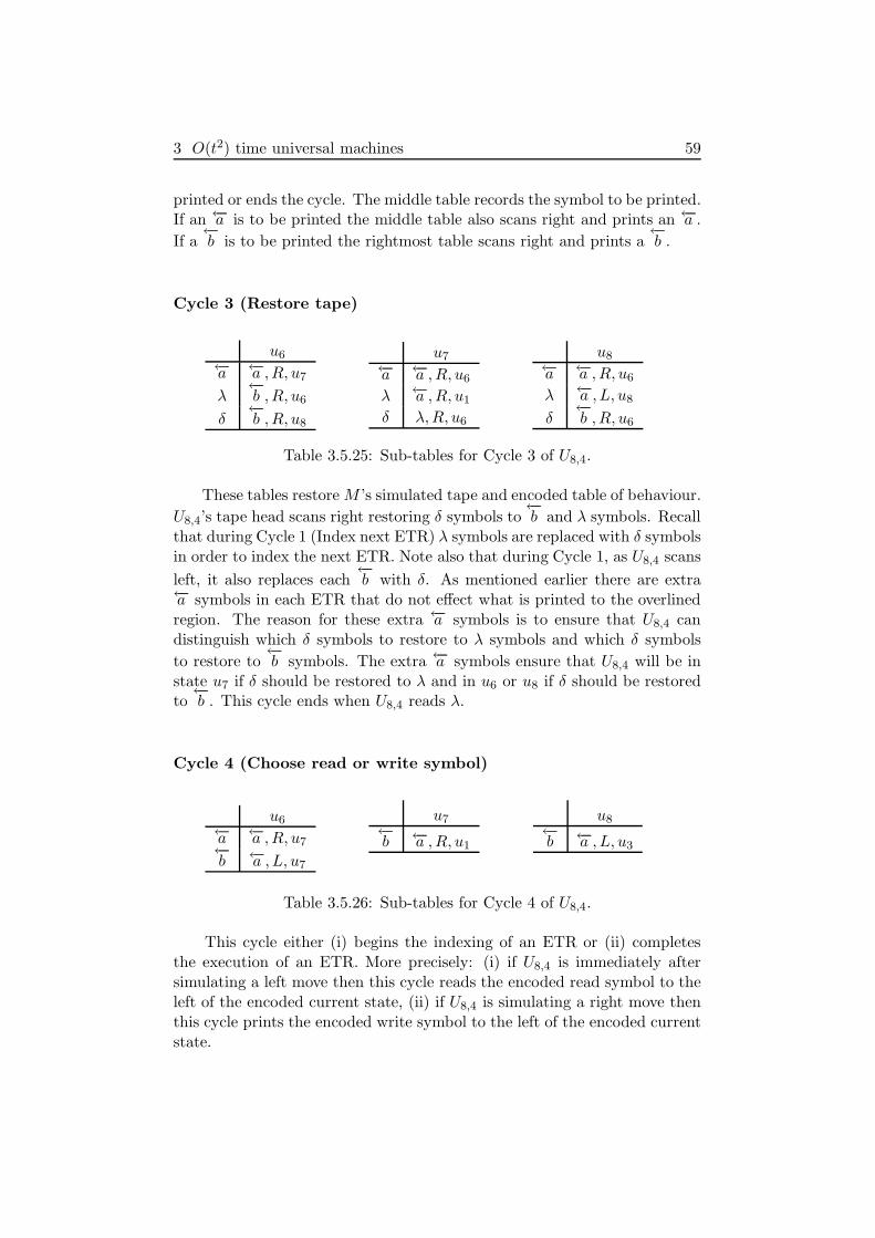
3 O(t2) time universal machines 59
printed or ends the cycle. The middle table records the symbol to be printed.If an ←−a is to be printed the middle table also scans right and prints an ←−a .
If a←−b is to be printed the rightmost table scans right and prints a
←−b .
Cycle 3 (Restore tape)
u6←−a ←−a ,R, u7
λ←−b ,R, u6
δ←−b ,R, u8
u7←−a ←−a ,R, u6
λ ←−a ,R, u1
δ λ,R, u6
u8←−a ←−a ,R, u6
λ ←−a ,L, u8
δ←−b ,R, u6
Table 3.5.25: Sub-tables for Cycle 3 of U8,4.
These tables restore M ’s simulated tape and encoded table of behaviour.
U8,4’s tape head scans right restoring δ symbols to←−b and λ symbols. Recall
that during Cycle 1 (Index next ETR) λ symbols are replaced with δ symbolsin order to index the next ETR. Note also that during Cycle 1, as U8,4 scans
left, it also replaces each←−b with δ. As mentioned earlier there are extra
←−a symbols in each ETR that do not effect what is printed to the overlinedregion. The reason for these extra ←−a symbols is to ensure that U8,4 candistinguish which δ symbols to restore to λ symbols and which δ symbols
to restore to←−b symbols. The extra ←−a symbols ensure that U8,4 will be in
state u7 if δ should be restored to λ and in u6 or u8 if δ should be restoredto←−b . This cycle ends when U8,4 reads λ.
Cycle 4 (Choose read or write symbol)
u6←−a ←−a ,R, u7←−b ←−a ,L, u7
u7←−b ←−a ,R, u1
u8←−b ←−a ,L, u3
Table 3.5.26: Sub-tables for Cycle 4 of U8,4.
This cycle either (i) begins the indexing of an ETR or (ii) completesthe execution of an ETR. More precisely: (i) if U8,4 is immediately aftersimulating a left move then this cycle reads the encoded read symbol to theleft of the encoded current state, (ii) if U8,4 is simulating a right move thenthis cycle prints the encoded write symbol to the left of the encoded currentstate.

3 O(t2) time universal machines 60
Remark 3.5.4 Halting case U8,4. Recall that all our universal Turingmachines (in this chapter) simulate halting by attempting to simulate aleft move at the left end of the simulated tape. This is also true for U8,4.However, the halting case for U8,4 differs slightly from the halting case forU3,11. U3,11 halts during Cycle 4 (Choose read or write symbol). U8,4 haltsin the configuration immediately after printing the last symbol of the leftmoving ETR at the end of Cycle 2 (Print ETR). When U8,4 prints the lastsymbol of the ETR it enters state u2 and its tape head moves left. The tapehead is now over the tape cell which contains the leftmost symbol of 〈M〉.The leftmost symbol of 〈M〉 is λ but during Cycle 2 this tape cell containsa δ (a neutralised λ). There is no transition rule for the state-symbol pair(u2, δ) in U8,4 so the simulation halts.
3.6 Conclusion and future work
We have improved the state of the art in small efficient universal Turing ma-chines giving the smallest machines that simulate Turing machines in O(t2)time. They are also the smallest known machines where direct simulation ofTuring machines is the technique used to establish their universality. Themost recent small universal Turing machines simulate Turing machines via2-tag systems, in O(t4 log2 t) time [Bai01, KR02, Rog96, Rog98]. Beforethe advent of Minsky’s universal Turing machine [Min62a], the smallest uni-versal Turing machines used the technique of direct simulation of Turingmachines [Ike58, Wat61]. One problem in the construction of these univer-sal Turing machines was the addressing of states, that is locating the nextencoded state during the simulation of a transition rule. Some approachesto solving this problem are briefly discussed in Section 3.1 of Minsky’s pa-per [Min62a]. A major advantage of our algorithm is the fact that theencoded current state is located at the simulated tape head position. Thistechnique simplifies the addressing of states.
As future work it would be of interest to use our algorithm to constructuniversal Turing machines with state-symbol pairs of (2, n) and (n, 2). Thiswould give a more complete polynomial O(t2) time curve. Also, our 6-state,6-symbol universal Turing machine uses only 32 of 36 available transitionrules and so it seems possible that it could be improved to a 6-state, 5-symbolmachine or a 5-state, 6-symbol machine.
What about small universal Turing machines with less than polynomialtime complexity? For example, consider the construction of a linear timeuniversal Turing machine. Our universal Turing machines stores the en-coded current state at the simulated tape head location. Suppose the entireencoded table of behaviour is stored at this location. Simulating a transi-tion rule merely involves scanning through the encoded table of behaviour,
3 O(t2) time universal machines 61
it is not necessary to scan the entire simulated tape contents. The idea isstraightforward, however we expect that a significant number of transitionrules would be required to move the entire encoded table of behaviour eachtime a tape head movement is simulated. Trying to construct small lineartime universal Turing machines using this idea could be difficult, and weleave this as an open problem.
4
The P-completeness of cellular
automaton Rule 110
4.1 Introduction
In this chapter we solve an open problem regarding the computational com-plexity of Rule 110 which is one of the most intuitively simple cellular au-tomata. We show that Rule 110 is efficiently universal and that its predictionproblem is P-complete. Rule 110 is a nearest neighbour, one-dimensional,binary cellular automaton [Wol83]. It is composed of a sequence of cells. . . p−1p0p1 . . . where each cell has a binary state pi ∈ {0, 1}. At timesteps+1, the value pi,s+1 = F (pi−1,s, pi,s, pi+1,s) of the cell at position i is givenby the synchronous local update function F
F (0, 0, 0) = 0 F (1, 0, 0) = 0
F (0, 0, 1) = 1 F (1, 0, 1) = 1
F (0, 1, 0) = 1 F (1, 1, 0) = 1
F (0, 1, 1) = 1 F (1, 1, 1) = 0
The problem of Rule 110 prediction is defined as follows.
Definition 4.1.1 (Rule 110 prediction) Given an initial Rule 110 con-figuration, a cell index i and a natural number t written in unary. Is cell pi
in state 1 at time t?
This problem is in P as a Turing machine simulates the cellular automaton inO(t2) steps by repeatedly traversing from left to right. From Cook’s [Coo04]result one infers a NC [GHR95] lower bound on the problem. Cook showedthat Rule 110 simulates Turing machines via the following sequence of sim-ulations
Turing machine 7→ 2-tag system 7→ cyclic tag system 7→ Rule 110 (4.1.1)
where A 7→ B denotes that A is simulated by B. The universality of 2-tagsystems [CM64] is well-known. Cook supplied the latter two simulations (asketch of Cook’s proof is also to be found in Wolfram’s book [Wol02]). Each
62
4 P-completeness of Rule 110 63
of these simulations runs in polynomial time (that is, B runs in a number ofsteps that is polynomial in the number of A’s steps) with the exception ofthe exponentially slow 2-tag system simulation of Turing machines [CM64].This slowdown is due to the 2-tag system’s unary encoding of Turing machinetape contents. Thus from Equation (4.1.1), using the result in [CM64], Rule110 is an exponentially slow simulator of Turing machines and so it hasremained open as to whether Rule 110 prediction is P-complete.
In this work we eliminate the 2-tag system to give the following chain ofsimulations
Turing machine 7→ cyclic tag system 7→ Rule 110 (4.1.2)
Each simulation runs in polynomial time and the reduction from Turingmachine to Rule 110 is computable by a logspace Turing machine. Thus ourwork shows that Rule 110 simulates Turing machines efficiently, giving thefollowing result.
Theorem 4.1.2 Rule 110 prediction is logspace complete for P.
Rule 110 is a very simple (2-state, nearest neighbour, one dimensional) cel-lular automaton and Cook and Eppstein [Coo04], and Wolfram [Wol02] gavefour weakly universal Turing machines that simulate its computation. Theirsize given as (number of states, number of symbols), are respectively (2, 5),(3, 4), (4, 3) and (7, 2). Previously, these machines were exponentially slowsimulators of Turing machines. A corollary of our work is that these smallweakly universal machines are now polynomial time simulators of Turingmachines. The results we present in this chapter improves on the time over-head of the version presented in [NW06a, NW06b].
The prediction problem for a number of classes of cellular automata hasbeen shown to be P-complete. However, Rule 110 is the simplest so far, in thesense that previous P-completeness results have been shown for more generalcellular automata (e.g. more states, neighbours or dimensions). For exam-ple, prediction of cellular automata of dimension d > 1 with an arbitrarynumber of states is known to be P-complete [GHR95]. Ollinger’s [Oll02]result shows that prediction for one-dimensional nearest neighbour cellularautomata is P-complete for six states. Richard’s [Ric06] result reduces thisto 4 states. Moore [Moo97a] shows that prediction of binary majority votingcellular automata is P-complete for dimension d > 3. On the other hand, theprediction problem for a variety of linear and quasilinear cellular automatais in NC [Moo97b, Moo98]. The question of whether Rule 110 prediction
is P-complete has been asked, either directly or indirectly, in a number ofprevious works (for example [Moo97b, Moo98, Aar02]).
An interesting decidability result has been given for the reachabilityproblem in binary cellular automata. The reachability problem is as fol-lows: will a given cellular automata configuration evolve from another given

4 P-completeness of Rule 110 64
configuration? Codd [Cod68] has shown that the reachability problem isdecidable for 2-dimensional binary cellular automata with von Neumannneighbourhood on a blank background. Sutner [Sut03] notes that the proofof universality for Rule 110 depends on a periodic background and thatthe reachability problem is decidable for Rule 110 on a blank backgroundfollowing Codd’s result.
4.2 Cyclic tag systems
Cyclic tag systems were used by Cook [Coo04] to show that Rule 110 isuniversal.
Definition 4.2.1 (cyclic tag system) A cyclic tag system C is a list ofbinary words α0, . . . , αp−1 called appendants where αm ∈ {0, 1}
∗.
A configuration of a cyclic tag system consists of (i) a marker that pointsto a single appendant αm in C, and (ii) a word w = w0 . . . w|w|−1 ∈ {0, 1}
∗.We call w the dataword. Intuitively the list C is a program with the markerpointing to instruction αm. In the initial configuration the marker points toappendant α0 and w is the binary input word.
Definition 4.2.2 (computation step of a cyclic tag system) A com-putation step is deterministic and acts on a configuration in one of two ways:
• If w0 = 0 then w0 is deleted and the marker moves to appendantα(m+1 mod p).
• If w0 = 1 then w0 is deleted, the word αm is appended onto the rightend of w, and the marker moves to appendant α(m+1 mod p).
A cyclic tag system completes its computation if (i) the dataword is theempty word or (ii) it enters a repeating sequence of configurations. Thecomplexity measures of time and space are defined in the obvious way.
Example 4.2.1 (cyclic tag system computation) Let C = 001, 01, 11 be acyclic tag system with input word 011. Below we give the first four stepsof the computation. In each configuration C is given on the left with themarked appendant highlighted in bold font.
001001001, 01, 11 011 ⊢ 001,010101, 11 11 ⊢ 001, 01,111111 101
⊢ 001001001, 01, 11 0111 ⊢ 001,010101, 11 111 ⊢ . . .

4 P-completeness of Rule 110 65
4.3 Cyclic tag systems efficiently simulate Turing
machines
In an earlier version of this work [NW06a] the time efficiency of cyclic tagsystems is proved by replacing the 2-tag system in Equation (4.1.1) with aclockwise Turing machine to give the following chain of simulations
Turing machine 7→ clockwise Turing machine
7→ cyclic tag system 7→ Rule 110(4.3.1)
From the sequence of simulations in Equation (4.3.1) we get Theorem 4.3.1.
Theorem 4.3.1 ([NW06a]) Let M be a deterministic binary Turing ma-chine with a single tape that computes in time t. Then there is a cyclic tagsystem that simulates the computation of M in time O(t3 log t).
While Theorem 4.3.1 is not explicitly given in [NW06a] the result maybe obtained by a relatively straightforward analysis of Lemmata 1 and 2in [NW06a]. This is similar to the analysis used in Chapter 5 to get thetime bound in Theorem 5.2.6.
In this work the clockwise Turing machine in Equation (4.3.1) is elim-inated to give the chain of simulations in Equation (4.1.2). This gives usthe improved simulation time given in Theorem 4.3.2. Much of the proof ofTheorem 4.1.2 is given by Theorem 4.3.2.
In order to simplify this proof we state the result for Turing machinesthat have a binary tape alphabet Σ = {a, b}. The proof runs for a numberof pages.
Theorem 4.3.2 Let M be a binary Turing machine with |Q| states thatruns in time t. Then there is a cyclic tag system CM that simulates thecomputation of M in time O(|Q|t2 log t).
Proof. Let M = (Q, {a, b}, b, f, q1, q|Q|) where Q = {q1, . . . , q|Q|} are thestates, {a, b} is the binary alphabet, f is the transition function, b is theblank symbol and q1, q|Q| ∈ Q are the initial and final states, respectively.In the sequel σj ∈ {a, b}. The bulk of the proof is concerned with sim-ulating a single (but arbitrary) left moving transition rule of M in timeO(|Q|t log t). The simulation of a right moving transition rule was givenpreviously in [NW06a] and is similar to a restriction of the method for sim-ulating a left moving transition rule so we do not give it here.
Encoding
We define the cyclic tag system (program) to be of the following formCM = α0, . . . , α2z−1 where z = 60|Q| + 121. Given a configuration of
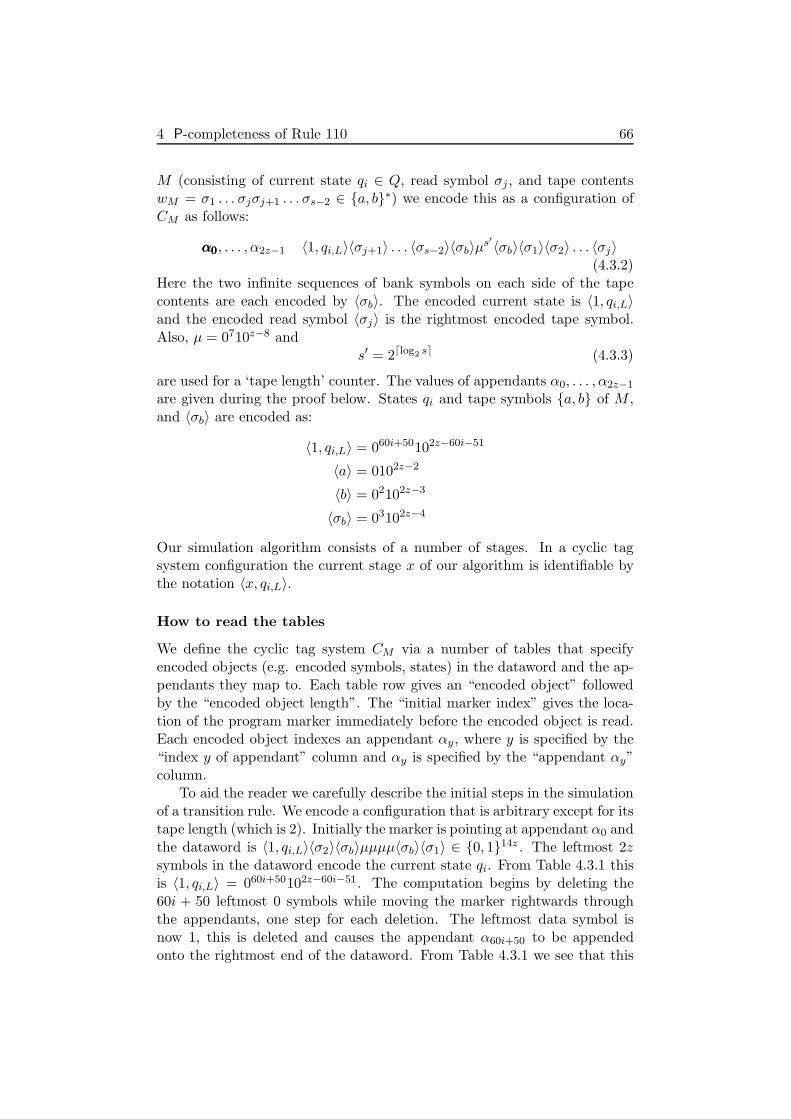
4 P-completeness of Rule 110 66
M (consisting of current state qi ∈ Q, read symbol σj , and tape contentswM = σ1 . . . σjσj+1 . . . σs−2 ∈ {a, b}∗) we encode this as a configuration ofCM as follows:
α0α0α0, . . . , α2z−1 〈1, qi,L〉〈σj+1〉 . . . 〈σs−2〉〈σb〉µs′〈σb〉〈σ1〉〈σ2〉 . . . 〈σj〉
(4.3.2)Here the two infinite sequences of bank symbols on each side of the tapecontents are each encoded by 〈σb〉. The encoded current state is 〈1, qi,L〉and the encoded read symbol 〈σj〉 is the rightmost encoded tape symbol.Also, µ = 0710z−8 and
s′ = 2⌈log2 s⌉ (4.3.3)
are used for a ‘tape length’ counter. The values of appendants α0, . . . , α2z−1
are given during the proof below. States qi and tape symbols {a, b} of M ,and 〈σb〉 are encoded as:
〈1, qi,L〉 = 060i+50102z−60i−51
〈a〉 = 0102z−2
〈b〉 = 02102z−3
〈σb〉 = 03102z−4
Our simulation algorithm consists of a number of stages. In a cyclic tagsystem configuration the current stage x of our algorithm is identifiable bythe notation 〈x, qi,L〉.
How to read the tables
We define the cyclic tag system CM via a number of tables that specifyencoded objects (e.g. encoded symbols, states) in the dataword and the ap-pendants they map to. Each table row gives an “encoded object” followedby the “encoded object length”. The “initial marker index” gives the loca-tion of the program marker immediately before the encoded object is read.Each encoded object indexes an appendant αy, where y is specified by the“index y of appendant” column and αy is specified by the “appendant αy”column.
To aid the reader we carefully describe the initial steps in the simulationof a transition rule. We encode a configuration that is arbitrary except for itstape length (which is 2). Initially the marker is pointing at appendant α0 andthe dataword is 〈1, qi,L〉〈σ2〉〈σb〉µµµµ〈σb〉〈σ1〉 ∈ {0, 1}
14z . The leftmost 2zsymbols in the dataword encode the current state qi. From Table 4.3.1 thisis 〈1, qi,L〉 = 060i+50102z−60i−51. The computation begins by deleting the60i + 50 leftmost 0 symbols while moving the marker rightwards throughthe appendants, one step for each deletion. The leftmost data symbol isnow 1, this is deleted and causes the appendant α60i+50 to be appendedonto the rightmost end of the dataword. From Table 4.3.1 we see that this

4 P-completeness of Rule 110 67
encoded encoded initial index y of appendant
object object marker appendant αy
length index
〈1, qi,L〉 = 060i+50102z−60i−51 2z 0 60i + 50 〈 1′, qi,L〉
〈1, qi,L〉 = 060i+50102z−60i−51 2z z z + 60i + 50 0z〈1′, qi,L,s<s′〉
〈1, qi,L,s<s′〉 = 060i+55102z−60i−56 2z 0 60i + 55 〈1′, qi,L,s<s′〉
〈1, qi,L,s<s′〉 = 060i+55102z−60i−56 2z z z + 60i + 55 0z〈1′, qi,L,s<s′〉
〈a〉 = 0102z−2 2z 0 1 〈a〉
〈a〉 = 0102z−2 2z z z + 1 〈a〉
〈b〉 = 02102z−3 2z 0 2 〈b〉
〈b〉 = 02102z−3 2z z z + 2 〈b〉
〈σb〉 = 03102z−4 2z 0 3 〈σb〉
〈σb〉 = 03102z−4 2z z z + 3 〈σb〉
〈a/〉 = 04102z−5 2z 0 4 〈a/〉
〈a/〉 = 04102z−5 2z z z + 4 〈a/〉
〈b/〉 = 05102z−6 2z 0 5 〈b/〉
〈b/〉 = 05102z−6 2z z z + 5 〈b/〉
〈σb/ 〉 = 06102z−7 2z 0 6 〈σb/ 〉
〈σb/ 〉 = 06102z−7 2z z z + 6 〈σb/ 〉
µ = 0710z−8 z 0 7 µ/
µ = 0710z−8 z z z + 7 µ′
µ′ = 08102z−9 2z 0 8 µ′
µ′ = 08102z−9 2z z z + 8 µ′
µ/ = 09102z−10 2z 0 9 µ/
µ/ = 09102z−10 2z z z + 9 µ/
Table 4.3.1: (Stage 1. Halve counter). Every odd numbered µ = 0710z−8 ismarked off by being changed to µ/ = 09102z−10.
is α60i+50 = 〈1′, qi,L〉. Then 2z − 60i − 51 contiguous 0 symbols are deletedwhile moving the marker one step for each deletion. Since |〈1, qi,L〉| = 2z andthere are exactly 2z appendants in CM , the marker is once again positionedat α0. We write these 2z steps as
α0α0α0, . . . , α2z−1 〈1, qi,L〉〈σ2〉〈σb〉µµµµ〈σb〉〈σ1〉
⊢2z α0α0α0, . . . , α2z−1 〈σ2〉〈σb〉µµµµ〈σb〉〈σ1〉〈1′, qi,L〉

4 P-completeness of Rule 110 68
cyclic tag systemprogram
sections of programcurrently in use
〈1, qi,L〉〈σ〉〈σb〉µµµµ〈σb〉〈σj〉
〈2, qi,L〉〈σ〉〈σb〉µ/µµ/µ〈σb〉〈σj〉
〈1, qi,L〉〈σ/〉〈σb〉µ/µµ/µ〈σ/b〉〈σj〉
〈2, qi,L〉〈σ/〉〈σb〉µ/µ/µ/µ〈σ/b〉〈σj〉
〈1, qi,L〉〈σ/〉〈σ/b〉µ/µ/µ/µ〈σ/b〉〈σj〉
〈3, qi,L〉〈σ/〉〈σ/b〉µ/µ/µ/µ/〈σ/b〉〈σj〉
〈1, qk,L〉〈σp〉〈σ〉〈σb〉µµµµ〈σb〉
Figure 4.3.1: Cyclic tag system simulation of transition rule (qi, σj , σp, L, qk).The cyclic tag system program is illustrated on the left. In the datawordthe encoded current state 〈x, qi,L〉 directs the control flow by determiningthe sections of the cyclic tag system program that are used in algorithmStage x.
Algorithm overview
Our cyclic tag system algorithm has three stages. Stages 1 and 2 isolate theencoded read symbol 〈σ1〉 of M which is located immediately to the left1
of the encoded current state 〈1, qi,L〉. These stages make use of the tape-length counter specified by Equations (4.3.2) and (4.3.3). In Stage 1 everyodd numbered µ is marked and then in Stage 2 every even number 〈σ〉 ismarked. This process is iterated until all µ objects are marked (1 + log2 s′
iterations). The first six configurations of Figures 4.3.1 and 4.3.2 illustratethis process. The encoded read symbol is now isolated as it is the onlyunmarked encoded tape symbol. The computation then enters Stage 3 whichuses the encoded current state and (isolated) encoded read symbol to indexan appendant that encodes the write symbol and next state. Finally thecounter is doubled if necessary to maintain the equality in Equation (4.3.3).The last two configurations of Figure 4.3.2 illustrate this process.
Stage 1. Halve counter
The counter value is specified by Equation (4.3.3) as the number of µ (orlater, µ′) objects. This value is halved by marking half of the µ objects(changing µ to µ/) using Table 4.3.1. In this table we see that |µ| = z so ex-actly two µ objects are read for a single traversal of the marker through all 2zappendants. Every odd numbered µ indexes µ/ and every even numberedµ indexes µ′. The encoded state 〈1, qi,L〉 indexes 〈1′, qi,L〉 or 〈1′, qi,L,s<s′〉,
1The manner in which a cyclic tag system reads its dataword is circular, hence therightmost object in a dataword can be considered to be immediately to the left of the left-most object. To see this, note that 〈1, qi,L〉 is the leftmost object in the first configurationand 〈1′, qi,L〉 is the rightmost object in the second configuration.

4 P-completeness of Rule 110 69
which sends control to Table 4.3.2.We continue the above simulation (we later generalise to an arbitrary
number of tape symbols).
α0α0α0, . . . , α2z−1 〈σ2〉〈σb〉µµµµ〈σb〉〈σ1〉〈1′, qi,L〉
⊢2z α0α0α0, . . . , α2z−1 〈σb〉µµµµ〈σb〉〈σ1〉〈1′, qi,L〉〈σ2〉
⊢2z α0α0α0, . . . , α2z−1 µµµµ〈σb〉〈σ1〉〈1′, qi,L〉〈σ2〉〈σb〉
⊢z α0, . . . ,αzαzαz, . . . , α2z−1 µµµ〈σb〉〈σ1〉〈1′, qi,L〉〈σ2〉〈σb〉µ/
⊢z α0α0α0, . . . , α2z−1 µµ〈σb〉〈σ1〉〈1′, qi,L〉〈σ2〉〈σb〉µ/µ
′
⊢6z α0α0α0, . . . , α2z−1 〈1′, qi,L〉〈σ2〉〈σb〉µ/µ′µ/µ′〈σb〉〈σ1〉
The algorithm tests if the counter is 0 by checking if exactly one un-marked µ was read. If so 〈3, qi,L〉 or 〈3, qi,L,s<s′〉 is appended and we enterStage 3. Otherwise 〈2, qi,L〉 or 〈2, qi,L,s<s′〉 is appended and we enter Stage 2.Table 4.3.2 simulates this ‘if’ statement.
As we continue our simulation we note from Table 4.3.2 that the word〈1′, qi,L〉 is of length 2z + 10. Hence the marker is at appendant α10 after〈1′, qi,L〉 is read. The computation proceeds as follows:
α0α0α0, . . . , α2z−1 〈1′, qi,L〉〈σ2〉〈σb〉µ/µ′µ/µ′〈σb〉〈σ1〉
⊢2z+10 α0, . . . ,α10α10α10, . . . , α2z−1 〈σ2〉〈σb〉µ/µ′µ/µ′〈σb〉〈σ1〉〈2, qi,L〉
⊢16z α0, . . . ,α10α10α10, . . . , α2z−1 〈2, qi,L〉〈σ′2〉〈σ
′b〉µ/µ
′µ/µ′〈σ′b〉〈σ′1〉
Immediately above is the first configuration of Stage 2.
Stage 2. Mark half of the encoded tape symbols
There are three rather large tables for Stage 2. To simplify the proof for thereader we give summary tables. If an encoded object points to an appendantwith it is own value no table entry is given.
The ultimate aim of this stage is to isolate the encoded read symbol.Each iteration of this stage uses Table 4.3.5 to mark off every even numberedencoded tape symbol 〈σ〉. We must ensure that the encoded read symbol〈σ′1〉 immediately to the left of 〈2, qi,L〉 is at an odd numbered position so itis not marked off during the execution of Table 4.3.5. Tables 4.3.3 and 4.3.4test if the encoded read symbol is at an even numbered position and if sothe dummy symbol 〈σ′d〉 is appended to place the encoded read symbol atan odd numbered position.
Note from Table 4.3.3 that encoded state 〈2, qi,L〉 or 〈2, qi,L,s<s′〉 is oflength 2z +10. Hence the marker is at appendant α20 after reading 〈2, qi,L〉.When the initial marker index is moved to α20 this causes each encodedobject to index a copy of itself (e.g. µ′ indexes µ′). Thus the computation

4 P-completeness of Rule 110 70
encoded encoded initial index y of appendant
object object marker appendant αy
length index
〈1′, qi,L〉 = 060i+51102z−60i−42 2z + 10 0 60i + 51 〈2, qi,L〉
〈1′, qi,L〉 = 060i+51102z−60i−42 2z + 10 z z + 60i + 51 〈3, qi,L〉
〈1′, qi,L,s<s′〉 = 060i+56102z−60i−47 2z + 10 0 60i + 56 〈2, qi,L,s<s′〉
〈1′, qi,L,s<s′〉 = 060i+56102z−60i−47 2z + 10 z z + 60i + 56 〈3, qi,L,s<s′〉
〈a〉 = 0102z−2 2z 10 11 〈a′〉
〈a〉 = 0102z−2 2z z + 10 z + 11 〈a〉
〈b〉 = 02102z−3 2z 10 12 〈b′〉
〈b〉 = 02102z−3 2z z + 10 z + 12 〈b〉
〈σb〉 = 03102z−4 2z 10 13 〈σ′b〉
〈σb〉 = 03102z−4 2z z + 10 z + 13 〈σb〉
〈a/〉 = 04102z−5 2z 10 14 〈a/〉
〈a/〉 = 04102z−5 2z z + 10 z + 14 〈a/〉
〈b/〉 = 05102z−6 2z 10 15 〈b/〉
〈b/〉 = 05102z−6 2z z + 10 z + 15 〈b/〉
〈σb/ 〉 = 06102z−7 2z 10 16 〈σb/ 〉
〈σb/ 〉 = 06102z−7 2z z + 10 z + 16 〈σb/ 〉
µ′ = 08102z−9 2z 10 18 µ′
µ′ = 08102z−9 2z z + 10 z + 18 µ′
µ/ = 09102z−10 2z 10 19 µ/
µ/ = 09102z−10 2z z + 10 z + 19 µ/
Table 4.3.2: (Stage 1. Check counter value). Here 〈1′, qi,L〉 or 〈1′, qi,L,s<s′〉is used to check if the counter is 0.
proceeds as follows.
α0, . . . ,α10α10α10, . . . , α2z−1 〈2, qi,L〉〈σ′2〉〈σ
′b〉µ/µ
′µ/µ′〈σ′b〉〈σ′1〉
⊢2z+10 α0, . . . ,α20α20α20, . . . , α2z−1 〈σ′2〉〈σ′b〉µ/µ
′µ/µ′〈σ′b〉〈σ′1〉〈2
′, qi,L〉
⊢12z α0, . . . ,α20α20α20, . . . , α2z−1 〈2′, qi,L〉〈σ′2〉〈σ
′b〉µ/µ
′µ/µ′〈σ′b〉〈σ′1〉
Each encoded tape symbol 〈σ′〉 is of length z. If an odd number of 〈σ′〉objects are read during execution of Table 4.3.3 then the initial marker willbe at 20 + z and rows 2 or 4 of Table 4.3.4 will execute. If an even numberof encoded tape symbols 〈σ′〉 are read then the initial marker will be at20 and rows 1 or 3 of Table 4.3.4 will execute appending the dummy object〈σ′d〉. In our simulation an even number of 〈σ′〉 symbols were read during theexecution of Table 4.3.3 hence the initial marker index is at appendant α20.The encoded state 〈2′, qi,L〉 moves the initial marker index to appendant α30.This causes each encoded object to index a copy of itself (e.g. µ′ indexes µ′).

4 P-completeness of Rule 110 71
encoded encoded initial index y of appendant
object object marker appendant αy
length index
〈2, qi,L〉 = 060i+42102z−60i−33 2z + 10 10 60i + 52 〈2′, qi,L〉
〈2, qi,L,s<s′〉 = 060i+47102z−60i−38 2z + 10 10 60i + 57 〈2′, qi,L,s<s′〉
Table 4.3.3: (Stage 2. Read σ′ symbols.) Each encoded object omitted fromthis summary table indexes a copy of itself (e.g. µ′ indexes µ′).
Thus continuing our simulation gives:
α0, . . . ,α20α20α20, . . . , α2z−1 〈2′, qi,L〉〈σ′2〉〈σ
′b〉µ/µ
′µ/µ′〈σ′b〉〈σ′1〉
⊢2z+10 α0, . . . ,α30α30α30, . . . , α2z−1 〈σ′2〉〈σ′b〉µ/µ
′µ/µ′〈σ′b〉〈σ′1〉〈σd〉〈2
′′, qi,L〉〈σ′d〉
⊢14z α0, . . . ,α30α30α30, . . . , α2z−1 〈2′′, qi,L〉〈σ′d〉〈σ
′2〉〈σ
′b〉µ/µ
′µ/µ′〈σ′b〉〈σ′1〉〈σ
′d〉
In a manner similar to that of Table 4.3.1, in which every odd numbered µwas marked off, Table 4.3.5 marks off even numbered 〈σ′〉. To see this note|〈a′〉| = |〈b′〉| = |〈σ′b〉| = |〈σ
′d〉| = z. Thus every even numbered 〈σ′〉 indexes
〈σ/〉 and every odd numbered 〈σ′〉 indexes 〈σ〉. Continuing our simulationgives:
α0, . . . ,α30α30α30, . . . , α2z−1 〈2′′, qi,L〉〈σ′d〉〈σ
′2〉〈σ
′b〉µ/µ
′µ/µ′〈σ′b〉〈σ′1〉〈σ
′d〉
⊢2z+10 α0, . . . ,α40α40α40, . . . , α2z−1 〈σ′d〉〈σ′2〉〈σ
′b〉µ/µ
′µ/µ′〈σ′b〉〈σ′1〉〈σ
′d〉0
2z−40〈1, qi,L〉
⊢z α0, . . . ,αz+40αz+40αz+40, . . . , α2z−1 〈σ′2〉〈σ′b〉µ/µ
′µ/µ′〈σ′b〉〈σ′1〉〈σ
′d〉0
2z−40〈1, qi,L〉
⊢z α0, . . . ,α40α40α40, . . . , α2z−1 〈σ′b〉µ/µ′µ/µ′〈σ′b〉〈σ
′1〉〈σ
′d〉0
2z−40〈1, qi,L〉〈σ/2〉
⊢z α0, . . . ,αz+40αz+40αz+40, . . . , α2z−1 µ/µ′µ/µ′〈σ′b〉〈σ′1〉〈σ
′d〉0
2z−40〈1, qi,L〉〈σ/2〉〈σb〉
⊢13z−40 α0α0α0, . . . , α2z−1 〈1, qi,L〉〈σ/2〉〈σb〉µ/µµ/µ〈σ/b〉〈σ1〉
The simulation continues as follows iterating Stages 1 and 2:
encoded encoded initial index y of appendant
object object marker appendant αy
length index
〈2′, qi,L〉 = 060i+33102z−60i−24 2z + 10 20 60i + 53 〈σd〉〈2′′, qi,L〉〈σ
′d〉
〈2′, qi,L〉 = 060i+33102z−60i−24 2z + 10 z + 20 z + 60i + 53 〈2′′, qi,L〉
〈2′, qi,L,s<s′〉 = 060i+38102z−60i−29 2z + 10 20 60i + 58 〈σd〉〈2′′, qi,L,s<s′〉〈σ
′d〉
〈2′, qi,L,s<s′〉 = 060i+38102z−60i−29 2z + 10 z + 20 z + 60i + 58 〈2′′, qi,L,s<s′〉
〈σd〉 = 013102z−14 2z 30 43 〈σ′d〉
Table 4.3.4: (Stage 2. Is the number of σ′ symbols odd or even.) Eachencoded object omitted from this summary table indexes a copy of itself(e.g. µ′ indexes µ′).
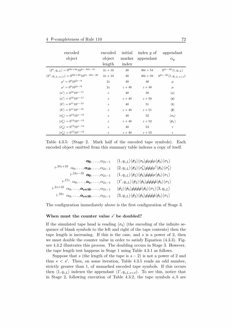
4 P-completeness of Rule 110 72
encoded encoded initial index y of appendant
object object marker appendant αy
length index
〈2′′, qi,L〉 = 060i+24102z−60i−15 2z + 10 30 60i + 54 02z−40〈1, qi,L〉
〈2′′, qi,L,s<s′〉 = 060i+29102z−60i−20 2z + 10 30 60i + 59 02z−40〈1, qi,L,s<s′〉
µ′ = 08102z−9 2z 40 48 µ
µ′ = 08102z−9 2z z + 40 z + 48 µ
〈a′〉 = 01010z−11 z 40 50 〈a〉
〈a′〉 = 01010z−11 z z + 40 z + 50 〈a/〉
〈b′〉 = 01110z−12 z 40 51 〈b〉
〈b′〉 = 01110z−12 z z + 40 z + 51 〈b/〉
〈σ′b〉 = 01210z−13 z 40 52 〈σb〉
〈σ′b〉 = 01210z−13 z z + 40 z + 52 〈σb/ 〉
〈σ′d〉 = 01310z−14 z 40 53 ǫ
〈σ′d〉 = 01310z−14 z z + 40 z + 53 ǫ
Table 4.3.5: (Stage 2. Mark half of the encoded tape symbols). Eachencoded object omitted from this summary table indexes a copy of itself.
α0α0α0, . . . , α2z−1 〈1, qi,L〉〈σ/2〉〈σb〉µ/µµ/µ〈σ/b〉〈σ1〉
⊢34z+10 α0, . . . ,α10α10α10, . . . , α2z−1 〈2, qi,L〉〈σ/2〉〈σ′b〉µ/µ/µ/µ
′〈σ/b〉〈σ′1〉
⊢54z−10 α0α0α0, . . . , α2z−1 〈1, qi,L〉〈σ/2〉〈σ/b〉µ/µ/µ/µ〈σ/b〉〈σ1〉
⊢17z α0, . . . ,αzαzαz, . . . , α2z−1 〈1′, qi,L〉〈σ/2〉〈σ/b〉µ/µ/µ/µ/〈σ/b〉〈σ1〉
⊢2z+10 α0, . . . ,αz+10αz+10αz+10, . . . , α2z−1 〈σ/2〉〈σ/b〉µ/µ/µ/µ/〈σ/b〉〈σ1〉〈3, qi,L〉
⊢16z α0, . . . ,αz+10αz+10αz+10, . . . , α2z−1 〈3, qi,L〉〈σ/2〉〈σ/b〉µ/µ/µ/µ/〈σ/b〉〈σ1〉
The configuration immediately above is the first configuration of Stage 3.
When must the counter value s′ be doubled?
If the simulated tape head is reading 〈σb〉 (the encoding of the infinite se-quence of blank symbols to the left and right of the tape contents) then thetape length is increasing. If this is the case, and s is a power of 2, thenwe must double the counter value in order to satisfy Equation (4.3.3). Fig-ure 4.3.2 illustrates this process. The doubling occurs in Stage 3. However,the tape length test happens in Stage 1 using Table 4.3.1 as follows.
Suppose that s (the length of the tape is s− 2) is not a power of 2 andthus s < s′. Then, on some iteration, Table 4.3.5 reads an odd number,strictly greater than 1, of unmarked encoded tape symbols. If this occursthen 〈1, qi,L〉 indexes the appendant 〈1′, qi,L,s<s′〉. To see this, notice thatin Stage 2, following execution of Table 4.3.2, the tape symbols a, b are

4 P-completeness of Rule 110 73
cyclic tag systemprogram
sections of programcurrently in use
〈1, qi,L〉〈σ〉〈σ〉〈σb〉µµµµ〈σb〉
〈2, qi,L〉〈σ〉〈σ〉〈σb〉µ/µµ/µ〈σb〉
〈1, qi,L〉〈σ/〉〈σ〉〈σ/b〉µ/µµ/µ〈σb〉
〈2, qi,L〉〈σ/〉〈σ/〉〈σ/b〉µ/µ/µ/µ〈σb〉
〈1, qi,L〉〈σ/〉〈σ/〉〈σ/b〉µ/µ/µ/µ〈σb〉
〈3, qi,L〉〈σ/〉〈σ/〉〈σ/b〉µ/µ/µ/µ/〈σb〉
D〈σb〉〈1, qk,L〉〈σp〉〈σ〉〈σ〉〈σb〉µµµµ
〈1, qk,L〉〈σp〉〈σ〉〈σ〉〈σb〉µµµµµµµµ〈σb〉
Figure 4.3.2: Cyclic tag system simulation of transition rule (qi, σb, σp, L, qk).The beginning of the simulation is the same as the simulation in Figure 4.3.1.However this simulation differs as the tape length is increasing and so thecounter value (number of µ symbols) must be doubled to maintain the equal-ity in Equation (4.3.3).
encoded as 〈a′〉, 〈b′〉 and the infinite sequence of blank symbols to the leftand right is encoded as 〈σ′b〉 where |〈σ′b〉| = |〈a
′〉| = |〈b′〉| = z. If CM reads anodd number of these during execution of Table 4.3.5 then the initial markerindex is at z. Suppose otherwise that s is not a power of 2. Then 〈1, qi,L〉will always index the appendant 〈1′, qi,L〉 during some iteration of Stage 1.In summary, if 〈1′, qi,L,s<s′〉 is not appended before Stage 3 begins then thenumber of 〈σ〉 objects in the dataword is a power of 2 and s = s′.
Stage 3. Complete simulation of transition rule
In this stage an appendant αy is indexed, based on the value of the encodedcurrent state and encoded read symbol using Table 4.3.6. The printing ofappendant αy simulates the encoded write symbol, encoded next state, andthe tape head movement.
Using Table 4.3.6 we read the encoded current state 〈3, qi,L〉 or 〈3, qi,L,s<s′〉after which the initial marker index is 60i+ 60 or 60i+ 70 respectively. Theencoded read symbol was already isolated and uniquely retains its originalvalue of 〈a〉, 〈b〉 or 〈σb〉; this value points at the appendant αy (rows 3 to6). All other (non-isolated) encoded tape symbols are of the form 〈a/〉, 〈b/〉or 〈σ/b〉 and they point to the appendants 〈a〉, 〈b〉 or 〈σb〉 respectively.
The transitions rule (qi, σj , σp, L, qk) is encoded by each of the appen-dants given in rows 3 to 6 of Table 4.3.6. The simulated tape head is notreading 〈σb〉 and hence the appendant appended is of the form 〈1, qk,L〉〈σp〉.

4 P-completeness of Rule 110 74
encoded encoded initial index y of appendant
object object marker appendant αy
length index
〈3, qi,L〉 = 060i+4410z+5 z + 60i + 50 z + 10 z + 60i + 54 02z−60i−60
〈3, qi,L,s<s′〉 = 060i+4910z+10 z + 60i + 60 z + 10 z + 60i + 59 02z−60i−70
〈a〉 = 0102z−2 2z 60i + v 60i + v + 1 〈1, qk,L〉〈σp〉
〈b〉 = 02102z−3 2z 60i + v 60i + v + 2 〈1, qk,L〉〈σp〉
〈σb〉 = 03102z−4 2z 60i + 60 60i + 63 〈σb〉D〈1, qk,L〉〈σp〉
〈σb〉 = 03102z−4 2z 60i + 70 60i + 73 〈σb〉〈1, qk,L〉〈σp〉
〈a/〉 = 04102z−5 2z 60i + v 60i + v + 4 〈a〉
〈b/〉 = 05102z−6 2z 60i + v 60i + v + 5 〈b〉
〈σb/ 〉 = 06102z−7 2z 60i + v 60i + v + 6 〈σb〉
µ/ = 09102z−10 2z 60i + v 60i + v + 9 µ
Table 4.3.6: (Stage 3. Simulate transition rule (qi, σj , σp, L, qk)). This tableprints the encoded write symbol σp and establishes the new encoded cur-rent state 〈1, qk,L〉. If the counter does not need to be doubled this tablecompletes simulation of the transition rule. Also, v ∈ {60, 70}.
Continuing the simulation we get:
α0, . . . ,αz+10αz+10αz+10, . . . , α2z−1 〈3, qi,L〉〈σ/2〉〈σ/b〉µ/µ/µ/µ/〈σ/b〉〈σ1〉
⊢z+60i+50 α0, . . . ,α60i+60α60i+60α60i+60, . . . , α2z−1 〈σ/2〉〈σ/b〉µ/µ/µ/µ/〈σ/b〉〈σ1〉02z−60i−60
⊢14z α0, . . . ,α60i+60α60i+60α60i+60, . . . , α2z−1 〈σ1〉02z−60i−60〈σ2〉〈σb〉µµµµ〈σb〉
⊢2z α0, . . . ,α60i+60α60i+60α60i+60, . . . , α2z−1 02z−60i−60〈σ2〉〈σb〉µµµµ〈σb〉〈1, qk,L〉〈σp〉
⊢12z−60i−60 α0α0α0, . . . , α2z−1 〈1, qk,L〉〈σp〉〈σ2〉〈σb〉µ/µ′µ/µ′〈σb〉
The transition rule simulation is now complete. The appendant markerof CM ’s program is at appendant α0. The encoded write symbol is written,the new encoded state 〈1, qk,L〉 is established and the tape head movement issimulated. Although the counter has already been halved this does not alterthe algorithm control flow during simulation of the next transition rule.
We have given a sequence of configurations that explicitly simulate theapplication of a left moving transition rule of M . We used arbitrary initialand next states qi, qk ∈ Q, and arbitrary tape symbols σj , σp ∈ {a, b}.
The transition rule simulation is specific in the sense that the length ofthe tape data is fixed and the encoded read symbol is not of the form 〈σb〉. Ifthe simulated tape head is reading 〈σb〉 (it has moved beyond the edge of theencoded tape contents) the tape length is increasing. If this is the case ands is a power of 2, then we must double the counter value in order to satisfyEquation (4.3.3). This means the appendant in row 5 of Table 4.3.6 will beappended. The D in this appendant causes Table 4.3.7 to execute doubling
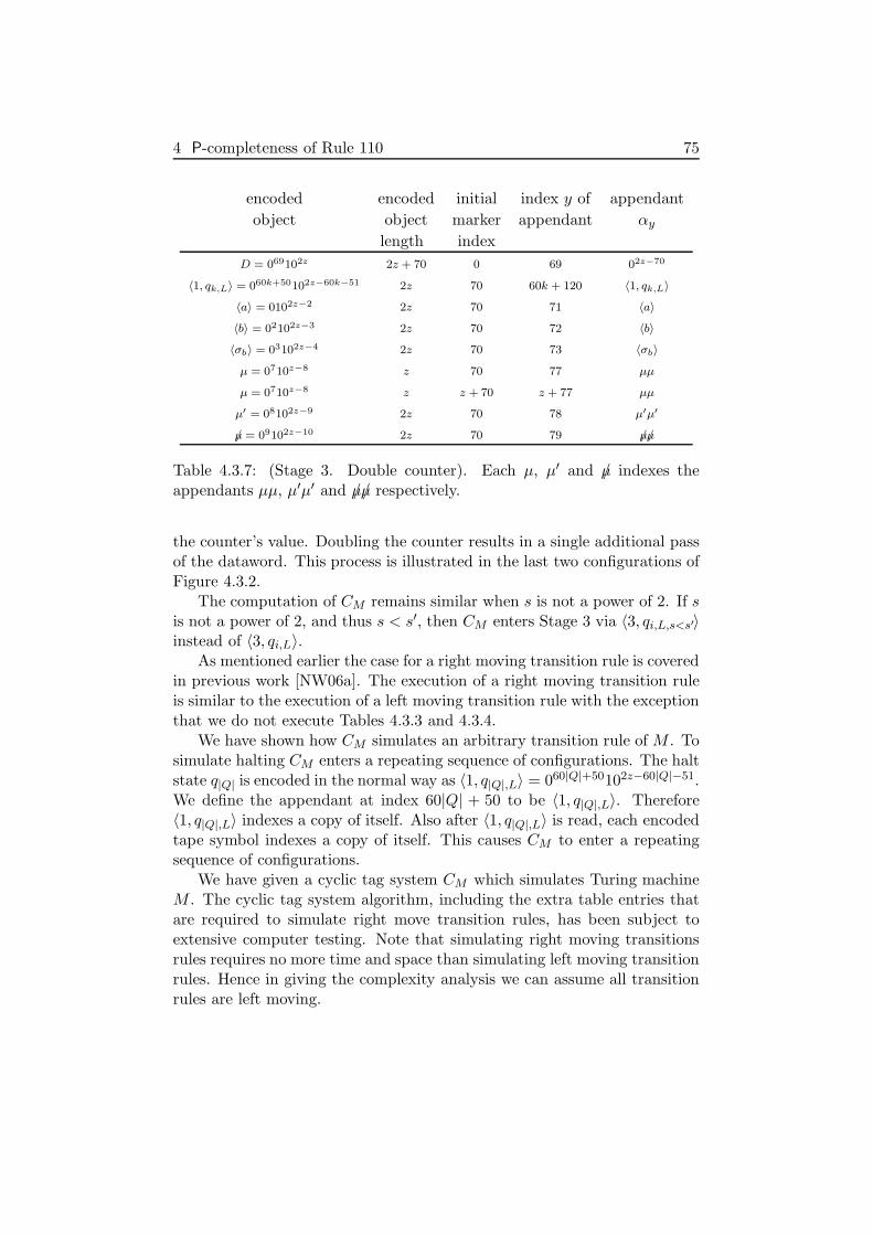
4 P-completeness of Rule 110 75
encoded encoded initial index y of appendant
object object marker appendant αy
length index
D = 069102z 2z + 70 0 69 02z−70
〈1, qk,L〉 = 060k+50102z−60k−51 2z 70 60k + 120 〈1, qk,L〉
〈a〉 = 0102z−2 2z 70 71 〈a〉
〈b〉 = 02102z−3 2z 70 72 〈b〉
〈σb〉 = 03102z−4 2z 70 73 〈σb〉
µ = 0710z−8 z 70 77 µµ
µ = 0710z−8 z z + 70 z + 77 µµ
µ′ = 08102z−9 2z 70 78 µ′µ′
µ/ = 09102z−10 2z 70 79 µ/µ/
Table 4.3.7: (Stage 3. Double counter). Each µ, µ′ and µ/ indexes theappendants µµ, µ′µ′ and µ/µ/ respectively.
the counter’s value. Doubling the counter results in a single additional passof the dataword. This process is illustrated in the last two configurations ofFigure 4.3.2.
The computation of CM remains similar when s is not a power of 2. If sis not a power of 2, and thus s < s′, then CM enters Stage 3 via 〈3, qi,L,s<s′〉instead of 〈3, qi,L〉.
As mentioned earlier the case for a right moving transition rule is coveredin previous work [NW06a]. The execution of a right moving transition ruleis similar to the execution of a left moving transition rule with the exceptionthat we do not execute Tables 4.3.3 and 4.3.4.
We have shown how CM simulates an arbitrary transition rule of M . Tosimulate halting CM enters a repeating sequence of configurations. The haltstate q|Q| is encoded in the normal way as 〈1, q|Q|,L〉 = 060|Q|+50102z−60|Q|−51.We define the appendant at index 60|Q| + 50 to be 〈1, q|Q|,L〉. Therefore〈1, q|Q|,L〉 indexes a copy of itself. Also after 〈1, q|Q|,L〉 is read, each encodedtape symbol indexes a copy of itself. This causes CM to enter a repeatingsequence of configurations.
We have given a cyclic tag system CM which simulates Turing machineM . The cyclic tag system algorithm, including the extra table entries thatare required to simulate right move transition rules, has been subject toextensive computer testing. Note that simulating right moving transitionsrules requires no more time and space than simulating left moving transitionrules. Hence in giving the complexity analysis we can assume all transitionrules are left moving.

4 P-completeness of Rule 110 76
Space analysis
At time t there are O(t) encoded objects (state and symbols) in the datawordof CM ; each of length O(|Q|). Thus CM uses O(|Q|t) space.
Time analysis
Simulating a transition rule involves 3 stages. Each stage executes in O(|Q|t)steps. To simulate a single transition rule the counter is halved O(log t)times, (i.e. Stages 1 and 2 are executed O(log t) times) and Stage 3 isexecuted once. Thus O(|Q|t log t) time is sufficient to simulate a transitionrule and O(|Q|t2 log t) time is sufficient to simulate the computation of M .
This completes the proof of Theorem 4.3.2. �
A consequence of Theorem 4.3.2 is that Rule 110 simulates Turing ma-chines in polynomial time. The weak machines in [Coo04, Wol02] simulateRule 110 in quadratic time, which in turn (using Cook’s construction withthe 2-tag systems in [CM64]) simulates Turing machines in exponential time.We have improved this time bound to polynomial.
Corollary 4.3.3 The small weakly universal Turing machines in [Coo04]simulate Turing machines in O(t4 log2 t) polynomial time.
4.4 P-completeness of Rule 110
Finally we show that the reduction from the generic machine simulation
problem (GMSP) [GHR95] to Rule 110 prediction is computable bya logspace transducer Turing machine. The GMSP is stated as: given aword wM , an encoding 〈M〉 of a single-tape Turing machine M , and aninteger t in unary, does M accept wM within t steps?
Lemma 4.4.1 The GMSP is logspace reducible to Rule 110 prediction.
Proof. We reduce the simulation problem for M to the analogous prob-lem for cyclic tag systems. In the proof of Theorem 4.3.2 we showed howto construct CM . We encode CM as a word 〈CM 〉. The value z used inthe proof of Theorem 4.3.2 is linear in |Q|, the number of states of M .There are 2z appendants, each of length O(|Q|), giving an encoded pro-gram length of O(|Q|2). From Equation (4.3.2) the input 〈wM 〉 to CM is oflength O(|Q||wM |). Thus the encoded appendants and input are logspaceconstructable.
To show that a logspace transducer Turing machine generates a Rule110 instance from 〈CM 〉#〈wM 〉#
t we examine Cook’s Rule 110 simulationof cyclic tag systems [Coo04]. The input is written directly as the states ofO(|〈wM 〉|) contiguous cells beginning at, say, cell p0. On the left of the input

4 P-completeness of Rule 110 77
a constant word (representing Cook’s ‘ossifiers’) is repeated O(t) times. Onthe right the cyclic tag system program (list of appendants and ‘leaders’) iswritten O(t) times. �
Since we already know that Rule 110 prediction is in P, the proof ofTheorem 4.1.2 is complete.
4.5 Discusion
We have proved that the prediction problem of Rule 110, one of the simplestcellular automata, is P-complete. In fact, we have established the strongerresult of improving the simulation time of Turing machines by Rule 110from exponential [Coo04, Wol02] to quadratic time. What about improvingthe simulation of Turing machines by Rule 110 to linear time? This resultcould be achieved by giving a direct simulation of Turing machines usingRule 110 or proving Rule 110 intrinsically universal [Oll02]. Another alter-native would be to prove that cyclic tag systems simulate Turing machinesin linear time. This however may not be possible. The simulation tech-niques of Turing machines using different variants of tag systems (bi-tagsystems, 2-tag systems and cyclic tag systems) involve reading the entireinput to simulate a single transition rule. Such a simulation technique im-plies a polynomial time simulation. It may not be possible to significantlyimprove on this technique.
The time efficiency of cyclic tag systems, established in this chapter,has already found applications. We have shown that 2-tag systems simu-late cyclic tag systems [WN06a] and thus the small universal Turing ma-chines of Minsky and Rogozhin et al. are efficient polynomial time sim-ulators of Turing machines. The semi-weakly universal Turing machinesin [WN07b, WNb] efficiently simulate cyclic tag systems, therefore thesesemi-weak machines are efficiently universal.

5
Tag systems
5.1 Introduction
In this chapter we give results on tag systems. We present a new form oftag system which we call bi-tag systems. Bi-tag systems were introduced toallow for the construction of small universal Turing machines. Prior to thisall of the smallest universal Turing machines simulated Turing machines via2-tag systems. A computation step of a bi-tag system is similar to that of a2-tag system so many of the techniques used by small 2-tag simulators can beadapted to give small bi-tag simulators. In fact some of the smallest knownuniversal Turing machines simulate bi-tag systems. We will encounter thesemachines in Chapter 6. In Section 5.2 we prove that bi-tag systems simulateTuring machine efficiently in polynomial time. This result has previouslyappeared in [NW05a].
In this chapter we also prove that 2-tag systems efficiently simulate Tur-ing machines. We give a proof outline that 2-tag systems simulate Turingmachines in polynomial time. As an immediate corollary of this result, wefind that the small universal Turing machines of Minsky and Rogozhin etal. simulate Turing machines in polynomial time, an exponential improve-ment.
In the early 1960s, Cocke and Minsky [CM64] showed that 2-tag sys-tems simulate Turing machines, but in an exponentially slow fashion. Min-sky [Min62a] constructed a small 7-state, 4-symbol universal Turing machinethat simulates 2-tag systems in polynomial time. Later, Rogozhin [Rog96]and others [Bai01, KR02, Rob91] used Minsky’s simulation technique to findsmall universal Turing machines for a number of different state-symbol pairs.All of these small machines efficiently simulate 2-tag systems. However,since Cocke and Minsky’s 2-tag simulation of Turing machines is exponen-tially slow it has remained an open problem as to whether these universalTuring machines can be made to run in polynomial time.
In Section 5.3 we give a brief outline of a proof that 2-tag systems effi-ciently simulate cyclic tag systems in polynomial time. This leads us to oursecond main result of this chapter, which is given by Theorem 5.1.1
78

5 Tag systems 79
b : universal, direct simulation, O(t2)
bc : universal, 2-tag simulation, O(t4 log2 t)
: O(t2) polynomial curve
: new O(t4 log2 t) polynomial curve
0 1 2 3 4 5 6 7 8 9 10 11 12 13 14 15 16 17 18 19
0
1
2
3
4
5
6
7
8
9
10
11
12
13
14
15
16
17
18
states
symbols
b
b
b
b
b
bc
bc
bc
bc
bc
bc
bc
Figure 5.1.1: State-symbol plot of small universal Turing machines. Theplot shows the improvement in the polynomial time curve following Corol-lary 5.1.2.
Theorem 5.1.1 Let M be a deterministic Turing machine with a singletape that computes in time t, then there is a 2-tag system TM that simulatesthe computation of M in time O(t2 log t).
This immediately gives the following interesting result.
Corollary 5.1.2 The small universal Turing machines of Minsky, Rogozhinand others [Bai01, KR02, Rob91, Min62a, Rog96] are O(t4 log2 t) polynomialtime simulators of Turing machines.
Before our result it was entirely plausible that there was an exponentialtrade-off between universal Turing machine program size complexity, andtime/space complexity; the smallest universal Turing machines seemed tobe exponentially slow. However, our result shows there is currently littleevidence for such a claim.
Early examples of time efficient small universal Turing machines werefound by Ikeno and Watanabe [Ike58, Wat61]. Prior to our result the small-
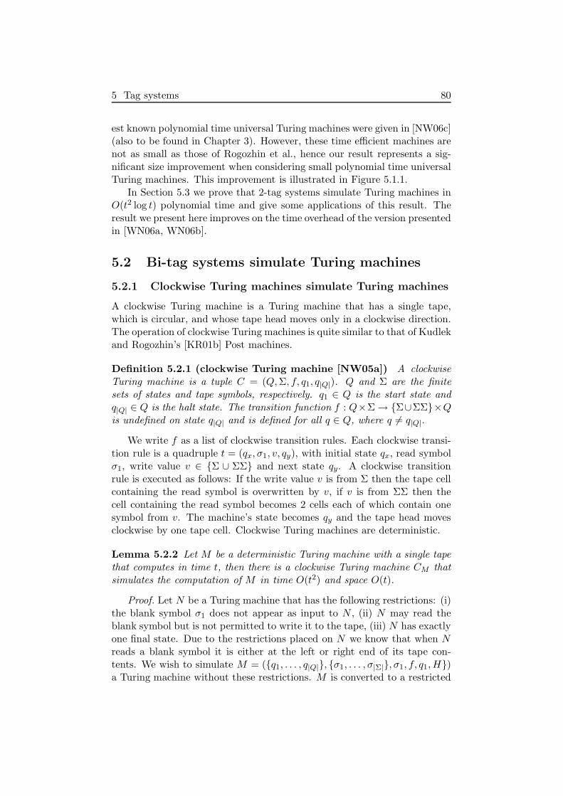
5 Tag systems 80
est known polynomial time universal Turing machines were given in [NW06c](also to be found in Chapter 3). However, these time efficient machines arenot as small as those of Rogozhin et al., hence our result represents a sig-nificant size improvement when considering small polynomial time universalTuring machines. This improvement is illustrated in Figure 5.1.1.
In Section 5.3 we prove that 2-tag systems simulate Turing machines inO(t2 log t) polynomial time and give some applications of this result. Theresult we present here improves on the time overhead of the version presentedin [WN06a, WN06b].
5.2 Bi-tag systems simulate Turing machines
5.2.1 Clockwise Turing machines simulate Turing machines
A clockwise Turing machine is a Turing machine that has a single tape,which is circular, and whose tape head moves only in a clockwise direction.The operation of clockwise Turing machines is quite similar to that of Kudlekand Rogozhin’s [KR01b] Post machines.
Definition 5.2.1 (clockwise Turing machine [NW05a]) A clockwiseTuring machine is a tuple C = (Q,Σ, f, q1, q|Q|). Q and Σ are the finitesets of states and tape symbols, respectively. q1 ∈ Q is the start state andq|Q| ∈ Q is the halt state. The transition function f : Q×Σ→ {Σ∪ΣΣ}×Qis undefined on state q|Q| and is defined for all q ∈ Q, where q 6= q|Q|.
We write f as a list of clockwise transition rules. Each clockwise transi-tion rule is a quadruple t = (qx, σ1, v, qy), with initial state qx, read symbolσ1, write value v ∈ {Σ ∪ ΣΣ} and next state qy. A clockwise transitionrule is executed as follows: If the write value v is from Σ then the tape cellcontaining the read symbol is overwritten by v, if v is from ΣΣ then thecell containing the read symbol becomes 2 cells each of which contain onesymbol from v. The machine’s state becomes qy and the tape head movesclockwise by one tape cell. Clockwise Turing machines are deterministic.
Lemma 5.2.2 Let M be a deterministic Turing machine with a single tapethat computes in time t, then there is a clockwise Turing machine CM thatsimulates the computation of M in time O(t2) and space O(t).
Proof. Let N be a Turing machine that has the following restrictions: (i)the blank symbol σ1 does not appear as input to N , (ii) N may read theblank symbol but is not permitted to write it to the tape, (iii) N has exactlyone final state. Due to the restrictions placed on N we know that when Nreads a blank symbol it is either at the left or right end of its tape con-tents. We wish to simulate M = ({q1, . . . , q|Q|}, {σ1, . . . , σ|Σ|}, σ1, f, q1,H})a Turing machine without these restrictions. M is converted to a restricted
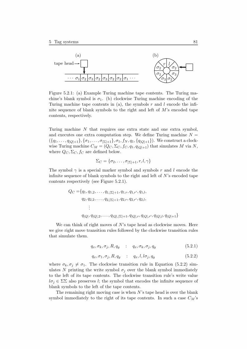
5 Tag systems 81
(a)
. . . σ1 σ2 σ3 σ2 σ3 σ2 σ2 σ1. . .
tape head
(b)
lrσ2
σ3
σ2σ3
σ2
σ2
Figure 5.2.1: (a) Example Turing machine tape contents. The Turing ma-chine’s blank symbol is σ1. (b) clockwise Turing machine encoding of theTuring machine tape contents in (a), the symbols r and l encode the infi-nite sequence of blank symbols to the right and left of M ’s encoded tapecontents, respectively.
Turing machine N that requires one extra state and one extra symbol,and executes one extra computation step. We define Turing machine N =({q1, . . . , q|Q|+1}, {σ1, . . . , σ|Σ|+1}, σ1, fN , q1, {q|Q|+1}). We construct a clock-wise Turing machine CM = (QC ,ΣC , fC , q1, q|Q|+1) that simulates M via N ,where QC ,ΣC , fC are defined below.
ΣC = {σ2, . . . , σ|Σ|+1, r, l, γ}
The symbol γ is a special marker symbol and symbols r and l encode theinfinite sequence of blank symbols to the right and left of N ’s encoded tapecontents respectively (see Figure 5.2.1).
QC ={q1, q1,2, . . . , q1,|Σ|+1, q1,r, q1,r′ , q1,l,
q2, q2,2, . . . , q2,|Σ|+1, q2,r, q2,r′ , q2,l,
...
q|Q|, q|Q|,2, . . . , q|Q|,|Σ|+1, q|Q|,r, q|Q|,r′, q|Q|,l, q|Q|+1}
We can think of right moves of N ’s tape head as clockwise moves. Herewe give right move transition rules followed by the clockwise transition rulesthat simulate them.
qx, σk, σj , R, qy : qx, σk, σj, qy (5.2.1)
qx, σ1, σj , R, qy : qx, l, lσj , qy (5.2.2)
where σk, σj 6= σ1. The clockwise transition rule in Equation (5.2.2) sim-ulates N printing the write symbol σj over the blank symbol immediatelyto the left of its tape contents. The clockwise transition rule’s write valuelσj ∈ ΣΣ also preserves l; the symbol that encodes the infinite sequence ofblank symbols to the left of the tape contents.
The remaining right moving case is when N ’s tape head is over the blanksymbol immediately to the right of its tape contents. In such a case CM ’s

5 Tag systems 82
tape head is initially over r, and then immediately after simulation of thetransition rule, CM ’s tape head is again over r. Immediately below are theclockwise transition rules that simulate this case.
qx, σ1, σj , R, qy :qx, r, σjr, qy,r′ (∗)
qy,r′ , κ, κ, qy,r′ (∗∗)
where κ ∈ ΣC−{γ, r}. The clockwise transition rule (*) prints N ’s encodedwrite symbol σj and sends CM ’s control into state qy,r′ . State qy,r′ movesCM ’s tape head to the cell containing r. This completes the simulation ofthe transition rule.
Left moving transition rules are more difficult to simulate as CM ’s tapehead moves only clockwise. CM begins by marking the current location ofthe tape head with the symbol γ. CM now moves each symbol clockwiseby one cell. When CM ’s tape head reads γ the left move is complete. Thisprocess moves the tape head anti-clockwise relative to the tape contents, thussimulating a left move. Immediately below is given the clockwise transitionrules that mark the tape head’s location with the symbol γ.
qx, σ1, σj , L, qy : qx, l, lγ, qy,j
qx, σ1, σj , L, qy : qx, r, γσj , qy,r
qx, σk, σj , L, qy : qx, σk, γ, qy,j
The clockwise transition rules that move each symbol clockwise by one cellare of the form:
qy,υ, ρ, υ, qy,ρ
where υ, ρ ∈ ΣC − {γ}. When CM ’s tape head reads γ then CM is in astate of the form qy,ρ and the unique clockwise transition rule defined bythe state-symbol pair (qy,ρ, γ) will begin simulation of the next transitionrule. This transition rule is of the form (qy, σ1, σk,D, qz) if ρ = r, l and ofthe form (qy, ρ, σk,D, qz) if ρ 6= r, l.
Input to N is encoded for CM by a finite state transducer. Given thisencoded input CM simulates the sequence of t transition rules in N ’s com-putation and halts in state q|Q|+1 the encoding of N ’s halt state q|Q|+1. CM
uses space of O(t). A single computation step of N is simulated in O(t)steps of CM . Thus the computation time of CM is O(t2). �
5.2.2 Bi-tag systems simulate clockwise Turing machines
In this section we present the bi-tag system, our new variant on the tagsystem, and prove that it simulates Turing machines via clockwise Turingmachines. The operation of a bi-tag system is similar to that of a standardtag system [Min67]. Bi-tag systems are essentially 1-tag systems (and sothey read and delete one symbol per timestep), augmented with additionalcontext sensitive rules that read, and delete, two symbols per timestep.

5 Tag systems 83
Definition 5.2.3 (Bi-tag system) A bi-tag system is a tuple (A,E, eh, P ).Here A and E are disjoint finite sets of symbols and eh ∈ E is the halt sym-bol. P is the finite set of productions. Each production is of one of thefollowing 3 forms:
P (a) = a, P (e, a) ∈ AE, P (e, a) ∈ AAE,
where a ∈ A, e ∈ E, and P is defined on all elements of {A∪((E−{eh})×A)}and undefined on all elements of {eh}×A. Bi-tag systems are deterministic.
A configuration of a bi-tag system is a word of the form w = A∗(AE∪EA)A∗.We call w the dataword.
Definition 5.2.4 (BTS computation step) A production is applied inone of two ways:
(i) if s = as′ then as′ ⊢ s′P (a),
(ii) if s = eas′ then eas′ ⊢ s′P (e, a).
A bi-tag system computation is a finite sequence of computation stepsthat are consecutively applied to an initial dataword. If eh is the leftmostsymbol in the dataword then the computation halts.
Example 5.2.1 (Bi-tag system computation.) Let bi-tag system B1 =({a0, a1}, {e0, e1, e2}, e2, P ) where the set P = {a0 → a0, a1 → a1, e0a0 →a1e0, e0a1 → a1e2, e1a0 → a0e0, e1a1 → a1e2}. Given the word a1e0a0, thecomputation of B1 proceeds as follows:
a1e0a0 ⊢ e0a0a1 ⊢ a1a1e0 ⊢ a1e0a1 ⊢ e0a1a1 ⊢ a1a1e2 ⊢ a1e2a1 ⊢ e2a1a1
The computation halts because the halt symbol e2 has become the leftmostsymbol.
Lemma 5.2.5 Let C be a clockwise Turing machine that runs in time t,then there is a bi-tag system BC that simulates the computation of C intime O(t2) and space O(t).
Before giving the proof of Lemma 5.2.5 we explain the proof idea. EachA symbol of BC encodes a symbol of C’s tape alphabet. Each E symbolof BC encodes a state of C. The location of the E symbol in the datawordrepresents the location of C’s tape head, as illustrated in Figure 5.2.2.
Each clockwise transition rule of C is simulated in the following way. Thechange of state, symbol and tape head position is simulated by executing aP production over the E × A pair that encodes the current state and readsymbol (see Figure 5.2.2(c)). A production is then applied to each symbolin the dataword. This moves the new E×A pair to the left of the dataword,in order to prepare for the simulation of the next clockwise transition rule.
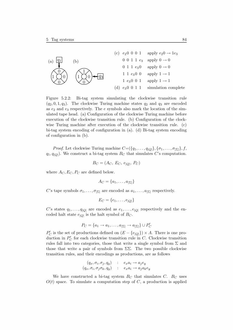
5 Tag systems 84
(a)
0
01
0
q2 (b)
1
01
0
q3
(c) e20 0 0 1 apply e20→ 1e3
0 0 1 1 e3 apply 0→ 0
0 1 1 e30 apply 0→ 0
1 1 e30 0 apply 1→ 1
1 e30 0 1 apply 1→ 1
(d) e30 0 1 1 simulation complete
Figure 5.2.2: Bi-tag system simulating the clockwise transition rule(q2, 0, 1, q3). The clockwise Turing machine states q2 and q3 are encodedas e2 and e3 respectively. The e symbols also mark the location of the sim-ulated tape head. (a) Configuration of the clockwise Turing machine beforeexecution of the clockwise transition rule. (b) Configuration of the clock-wise Turing machine after execution of the clockwise transition rule. (c)bi-tag system encoding of configuration in (a). (d) Bi-tag system encodingof configuration in (b).
Proof. Let clockwise Turing machine C=({q1, . . . , q|Q|}, {σ1, . . . , σ|Σ|}, f,q1, q|Q|). We construct a bi-tag system BC that simulates C’s computation.
BC = (AC , EC , e|Q|, PC)
where AC , EC , PC are defined below.
AC = {a1, . . . , a|Σ|}
C’s tape symbols σ1, . . . , σ|Σ| are encoded as a1, . . . , a|Σ| respectively.
EC = {e1, . . . , e|Q|}
C’s states q1, . . . , q|Q| are encoded as e1, . . . , e|Q| respectively and the en-coded halt state e|Q| is the halt symbol of BC .
PC = {a1 → a1, . . . , a|Σ| → a|Σ|} ∪ P ′C
P ′C is the set of productions defined on (E − {e|Q|})×A. There is one pro-duction in P ′C for each clockwise transition rule in C. Clockwise transitionrules fall into two categories, those that write a single symbol from Σ andthose that write a pair of symbols from ΣΣ. The two possible clockwisetransition rules, and their encodings as productions, are as follows
(qx, σi, σj , qy) : exai → ajey
(qx, σi, σjσk, qy) : exai → ajakey
We have constructed a bi-tag system BC that simulates C. BC usesO(t) space. To simulate a computation step of C, a production is applied

5 Tag systems 85
to each symbol in the dataword that encodes the current configuration ofC. This takes O(t) steps and yields a new dataword that encodes the nextconfiguration of C’s computation. In this way BC simulates t steps of C’scomputation in time O(t2). The simulation halts when the halt symbole|Q| that encodes the halt state of C becomes the leftmost symbol in thedataword. �
Given a single tape deterministic Turing machine M that runs in time t,we conclude from Lemmata 5.2.2 and 5.2.5 that M is simulated by a bi-tagsystem in time O(t4). However this overhead is easily improved to O(t3) asthe next theorem shows.
Theorem 5.2.6 Let M be a deterministic Turing machine with a singletape that computes in time t, then there is a bi-tag system BM that simulatesthe computation of M in time O(t3) and space O(t).
Proof. From Lemmata 5.2.2 and 5.2.5 a bi-tag system simulates the compu-tation of M via a clockwise Turing machine CM . From Lemma 5.2.2 CM
simulates M in time O(t2). However, CM uses O(t) space and hence BM
uses O(t) space. BM applies O(t) productions to simulate a clockwise tran-sition rule of CM . Thus BM executes O(t2) clockwise transition rules tosimulate M via CM in time O(t3). �
5.3 Time complexity of 2-tag systems and small
universal Turing machines
Tag systems where introducted by Post [Pos36] and proved universal byMinsky [Min61]. Later Cocke and Minsky [CM64] proved 2-tag systemsuniversal.
Definition 5.3.1 (2-tag system) A tag system consists of a finite alpha-bet of symbols Σ, a finite set of rules R : Σ → Σ∗ and a deletion numberβ ∈ N, β > 1. For a 2-tag system β = 2.
The 2-tag systems we consider are deterministic. The computation of a 2-tag system acts on a dataword w = σ1σ2 . . . σl. The entire configurationis given by w. In a computation step, the symbols σ1σ2 are deleted and ifthere is a rule for σ1, i.e. a rule of the form σ1 → σl+1 . . . σl+c, then the wordσl+1 . . . σl+c is appended. A dataword (configuration) w2 is obtained fromw1 via a single computation step as follows:
σ1σ2σ3 . . . σl ⊢ σ3 . . . σlσl+1 . . . σl+c
where σ1 → σl+1 . . . σl+c ∈ R. A 2-tag system completes its computationif (i) |w| < β, or (ii) there is no rule for the leftmost symbol.

5 Tag systems 86
In an earlier version of this work [WN06a] the efficiency of 2-tag systemswas proved by the following chain of simulations
Turing machine 7→ Cyclic tag system 7→ 2-tag system (5.3.1)
In [NW06a] cyclic tag systems are proved efficient polynomial time simu-lators of Turing machines and in [WN06a] it is proved that 2-tag systemsare efficient simulators of cyclic tag systems. Hence from the sequence ofsimulations in Equation (5.3.1) we get the Theorem 5.3.2.
Theorem 5.3.2 ([WN06a]) Let M be a deterministic Turing machine witha single tape that computes in time t, then there is a 2-tag system TM thatsimulates the computation of M in time O(t4 log2 t).
In the sequel we eliminate the cyclic tag system in Equation (5.3.1) to givethe following simulation:
Turing machine 7→ 2-tag system (5.3.2)
This gives the O(t2 log t) overhead in Theorem 5.1.1 whose proof is outlinedbelow. The new proof outlined here uses ideas from the proof given inSection 4.3, that cyclic tag systems simulate Turing machines efficiently. Theproof is also similar to the previous proof given in [WN06a] and makes use ofmany of the techniques therein. Hence the techniques used in [WN06a] andSection 4.3 may be applied to the outline given below in order to constructa detailed simulation.
Proof outline of Theorem 5.1.1
The bulk of the proof is concerned with simulating an arbitrary right mov-ing transition rule (qy, σ1, σj , R, qz) of M in time O(t log t). The followingequation encodes a Turing machine configuration as a 2-tag dataword:
〈qy, σ1 σ2 σ3 · · · σn〉 = xy1x
y1 x
y2x
y2 x
y3x
y3 · · · x
ynx
yn (aa)2
⌈log2(n)⌉(5.3.3)
where the current state of the Turing machine is qy, the read symbol isσ1 and the tape contents is σ1σ2σ3 . . . σn. Each xixi pair of 2-tag systemsymbols encoded the Turing machine symbol σi. Note that we decorate xi
symbols with underscripts and slashes. The 2-tag word (aa)2⌈log2(n)⌉
is usedas a counter. Our 2-tag system algorithm has three stages given below.
Stages 1 and 2 (isolate encoded read symbol)
Stages 1 and 2 isolate the encoded read symbol x1x1 which is the leftmostencoded Turing machine symbol in Equation (5.3.3). These stages make use
of the tape-length counter (aa)2⌈log2(n)⌉
. In Stage 1 every aa pair at an odd

5 Tag systems 87
numbered position is marked by changing it to a/a/ and then in Stage 2 everyxx pair at an even numbered position is marked by changing it to x/x/. Thisprocess is iterated until all aa pairs are marked (1 + log2 n iterations), thisgives:
xy1x
y1 x/
02x/
02 x/
03x/
03 . . . x/
0nx/
0n (a/a/)2
⌈log2(n)⌉
In the configuration above the encoded read symbol has been isolated as itis the only unmarked encoded tape symbol.
Stages 3 (simulate transition rule)
Note in the initial configuration each encoded 2-tag symbol also carries thecurrent state information qy. Thus the encoded read symbol that was iso-lated during Stages 1 and 2 contains all the information required to printthe encoded write symbol, establish the new encoded state, and simulatethe right move. The rule x
y1 → x/
0jx/0j s2z
encodes the write symbol σj and thecurrent state qz.
This rule is applied to give:
x/02x/
02 x/
03x/
03 . . . x/
0nx/
0n (a/a/)2
⌈log2(n)⌉x/0jx/
0j s2z
The slashes are removed to give:
s2z
x02x
02 x
03x
03 . . . x
0nx
0n aa2⌈log2(n)⌉
x0
jx0
j
The dataword is read and the number of s symbols is halved to give:
s2z−1x12x
12 x
13x
13 . . . x
1nx
1n aa2⌈log2(n)⌉
x1
jx1
j
Note that when the dataword is read each dataword symbol xiv becomes
x1+i
v this process is repeated, thus halving the number of s symbols witheach iteration. This continues until only a single s symbol remains after ziterations. At this point each x
iv symbol in the dataword is of the form x
zv
and contains the state information. Finally this s symbol is deleted fromthe dataword to give:
xz2x
z2 x
z3x
z3 . . . x
znx
zn aa2⌈log2(n)⌉
xz
jxz
j
The simulation of transition rule (qy, σ1, σj , R, qz) is now complete. A leftmoving transition rule may be simulated in a similar manner with someminor changes. Following simulation of a left moving transition rule theencoded read symbol will be the rightmost (instead of the leftmost) encodedread symbol. So in the initial dataword (i.e. Equation (5.3.3)) the encodedread symbol would be x
ynx
yn instead of x
y1x
y1. Recall that Stage 2 marks

5 Tag systems 88
encoded tape symbols at even numbered positions. In order to make surethis rightmost encoded symbol x
ynx
yn is not marked we must make sure it
remains in an odd numbered position during Stage 2. Thus, if the encodedread symbol is at an even numbered position a dummy symbol is appendedto place the encoded read symbol at an odd numbered position. A similartechnique is used during Stage 2 in the proof of Theorem 4.3.2. Finally, ifnecessary, the counter value aa2⌈log2(n)⌉
is updated at the end of Stage 3, ina manner similar to that given in Lemma 3 of [WN06a]. This completes ourproof outline.
Using our proof outline, we show that the 2-tag systems simulate Turingmachines in O(t2 log t) giving the result in Theorem 5.1.1. At timestep t thespace used by M is bounded by t. This is encoded as O(t) symbols in thedataword of TM . Thus O(t) space is sufficient to simulate M . Simulatinga transition rule involves 3 stages. Each Stage executes in O(t) steps. Tosimulate a single transition rule the counter is halved O(log t) times, (i.e.Stages 1 and 2 are executed O(log t) times) and Stage 3 is executed once.Thus O(t log t) time is sufficient to simulate a transition rule and O(t2 log t)time is sufficient to simulate the computation of M .
5.3.1 Applications of efficient 2-tag systems
There are numerous applications of Theorem 5.1.1 besides the improved sim-ulation time of the small universal Turing machines given in Corollary 5.1.2.Following our result, many biologically inspired models of computation nowsimulate Turing machines in polynomial time instead of exponential time.Some of these models include neural networks, H-systems and P-systems.For example, Siegelmann and Margenstern [SM99] give a neural networkthat uses only nine high-order neurons to simulate 2-tag systems. Takingeach synchronous update of the nine neurons as a single parallel timestep,their neural network simulates 2-tag systems in linear time. They note that“tag systems suffer a significant slow-down ... and thus our result provesonly Turing universality and should not be interpreted complexity-wise asa Turing equivalent.” Our work shows that their neural network is in factefficiently universal. Rogozhin and Verlan [RV06] give a tissue P-systemwith eight rules that simulates 2-tag systems in linear time, and thus wehave improved its simulation time overhead from exponential to polyno-mial. This system uses splicing rules (from H-systems) with membranes(from P-systems) and is non-deterministic. Harju and Margenstern [HM05]gave an extended H-system with 280 rules that generates recursively enu-merable sets using Rogozhin’s 7-state, 4-symbol universal Turing machine.Using our result from 2-tag systems, the time efficiency of their constructionis improved from exponential to polynomial, with a possible small constantincrease in the number of rules. The efficiency of Hooper’s [Hoo69] small2-tape universal Turing machine is also improved from exponential to poly-

5 Tag systems 89
nomial. The technique of simulation via 2-tag systems is at the core of manyof the universality proofs in Margenstern’s survey [Mar00]. Our work expo-nentially improves the time overheads in these simulations, such as Lindgrenand Nordahl’s cellular automata [LN90], Margenstern’s non-erasing Turingmachines [Mar93, Mar95a], and Robinson’s tiling [Rob71].
5.4 Discussion
We have seen from the previous section that our 2-tag system result hasmany applications. Bi-tag systems have applications in finding small uni-versal Turing machine as we will see in Chapter 6. Also, bi-tag systems maybe useful as an alternative to 2-tag systems to give universality results forother simple models.
As future work, it would be interesting to see if the time efficiency of2-tag systems and bi-tag systems may be improved further. The differentforms of tag systems including cyclic tag systems seem restricted in how theywork on their dataword. Each symbol is read and the result is appendedto the end of the dataword and thus, the entire configuration must be readbefore the appended result can be read. This is similar to placing the resultat the bottom of a queue. A Turing machine seems less restricted in thisway as it can repeatedly work on a section of its tape before moving to someother location. It remains to be seen if the time efficiency of these systemsmay be further improved.

6
Four small universal Turing
machines
6.1 Introduction
In this chapter we present (standard) universal Turing machines with state-symbol pairs of (5, 5), (6, 4), (9, 3) and (15, 2). These are the smallest knownuniversal machines with 5, 4, 3, and 2 symbols, respectively. Our machinessimulate Turing machines via bi-tag systems, a form of tag system which wedefined in Chapter 5. Each machine is plotted as a triangle in Figure 6.1.1.
The earliest small universal Turing machines simulated Turing machinesdirectly [Ike58, Wat61]. Subsequently, the technique of indirect simulation,via 2-tag systems, was applied by Minsky [Min62a]. In 1962 Minsky [Min62a]constructed a 7-state, 4-symbol universal Turing machine that simulatesTuring machines via 2-tag systems [CM64]. Minsky’s technique of 2-tagsimulation was extended by Rogozhin [Rog96, Rog98] to construct smalluniversal Turing machines with state-symbol pairs of (22, 2), (10, 3), (7, 4),(5, 5), (4, 6), (3, 10) and (2, 18). Subsequently, some of these machines werereduced in size to give machines with state-symbol pairs of (3, 9) [KR02],(19, 2) [Bai01] and (7, 4) [Bai01]. The current smallest 2-tag simulators ofRogozhin et al. are plotted as hollow circles in Figure 6.1.1.
Our 5-symbol machine uses the same number of instructions (22) asthe smallest known universal Turing machine (Rogozhin’s 6-symbol ma-chine [Rog96]). Also, our 5-symbol machine has less instructions than Ro-gozhin’s 5-symbol machine. Since Minsky [Min62a] constructed his 7-state,4-symbol machine, a number of authors [Bai01, Rob91, Rog96] have de-creased the number of transition rules used for 4-symbol machines. How-ever, the 6-state, 4-symbol machine we present here is the first reduction inthe number of states.
The halting problem has been proved decidable for the following state-symbol pairs: (2, 2) [Kud96, Pav73], (3, 2) [Pav78], (2, 3) (Pavlotskaya, un-published), (1, n) [Her68c], and (n, 1) (trivial) for n > 1. These resultsinduce the decidable halting problem curve given in Figure 6.1.1. Also,these decidability results imply that a universal Turing machine, that simu-lates any Turing machine M and halts if and only if M halts, is not possible
90
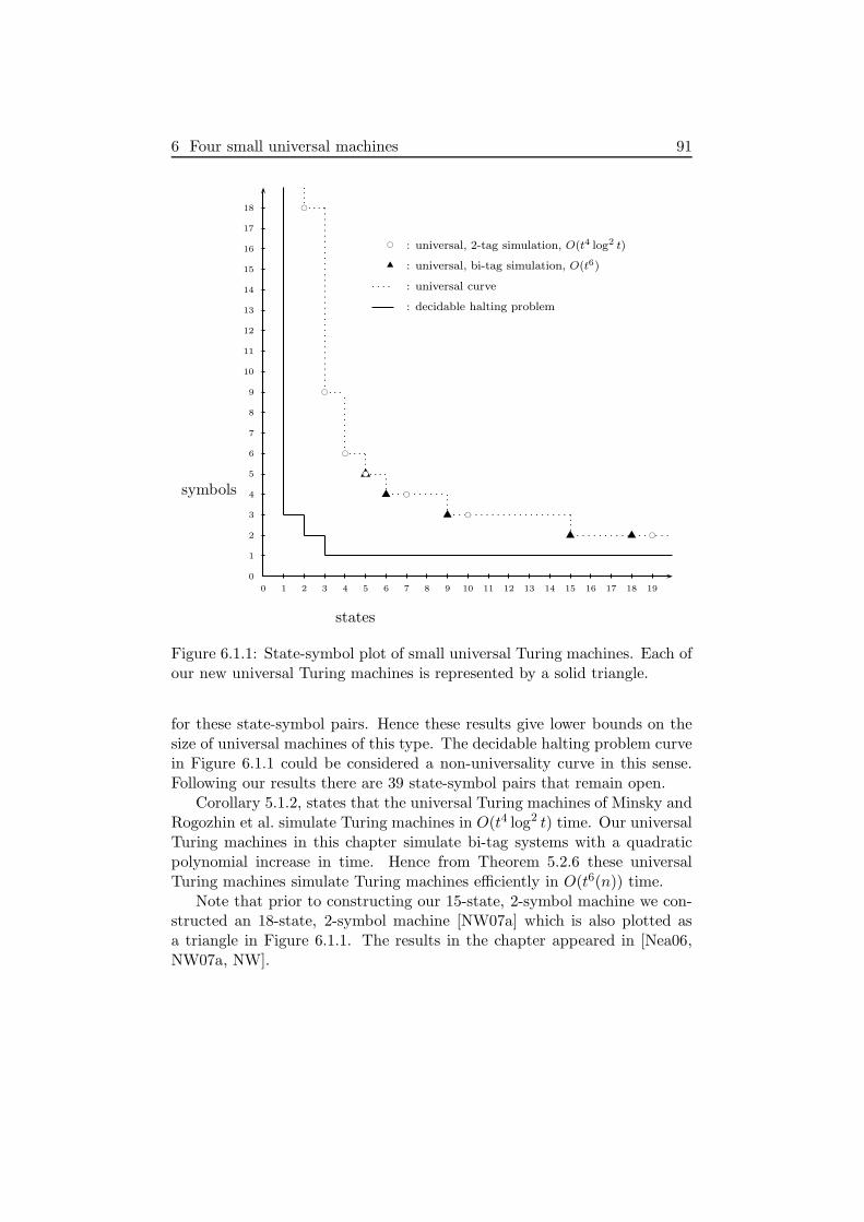
6 Four small universal machines 91
bc : universal, 2-tag simulation, O(t4 log2 t)
u : universal, bi-tag simulation, O(t6)
: universal curve
: decidable halting problem
0 1 2 3 4 5 6 7 8 9 10 11 12 13 14 15 16 17 18 19
0
1
2
3
4
5
6
7
8
9
10
11
12
13
14
15
16
17
18
states
symbols u
u
uu
u
bc
bc
bc
bc
bc
bc
bc
Figure 6.1.1: State-symbol plot of small universal Turing machines. Each ofour new universal Turing machines is represented by a solid triangle.
for these state-symbol pairs. Hence these results give lower bounds on thesize of universal machines of this type. The decidable halting problem curvein Figure 6.1.1 could be considered a non-universality curve in this sense.Following our results there are 39 state-symbol pairs that remain open.
Corollary 5.1.2, states that the universal Turing machines of Minsky andRogozhin et al. simulate Turing machines in O(t4 log2 t) time. Our universalTuring machines in this chapter simulate bi-tag systems with a quadraticpolynomial increase in time. Hence from Theorem 5.2.6 these universalTuring machines simulate Turing machines efficiently in O(t6(n)) time.
Note that prior to constructing our 15-state, 2-symbol machine we con-structed an 18-state, 2-symbol machine [NW07a] which is also plotted asa triangle in Figure 6.1.1. The results in the chapter appeared in [Nea06,NW07a, NW].
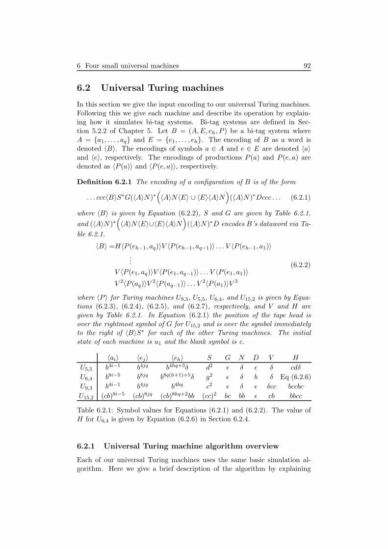
6 Four small universal machines 92
6.2 Universal Turing machines
In this section we give the input encoding to our universal Turing machines.Following this we give each machine and describe its operation by explain-ing how it simulates bi-tag systems. Bi-tag systems are defined in Sec-tion 5.2.2 of Chapter 5. Let B = (A,E, eh, P ) be a bi-tag system whereA = {a1, . . . , aq} and E = {e1, . . . , eh}. The encoding of B as a word isdenoted 〈B〉. The encodings of symbols a ∈ A and e ∈ E are denoted 〈a〉and 〈e〉, respectively. The encodings of productions P (a) and P (e, a) aredenoted as 〈P (a)〉 and 〈P (e, a)〉, respectively.
Definition 6.2.1 The encoding of a configuration of B is of the form
. . . ccc〈B〉S∗G(〈A〉N)∗(
〈A〉N〈E〉 ∪ 〈E〉〈A〉N)
(〈A〉N)∗Dccc . . . (6.2.1)
where 〈B〉 is given by Equation (6.2.2), S and G are given by Table 6.2.1,
and (〈A〉N)∗(
〈A〉N〈E〉∪〈E〉〈A〉N)
(〈A〉N)∗D encodes B’s dataword via Ta-
ble 6.2.1.
〈B〉 =H〈P (eh−1, aq)〉V 〈P (eh−1, aq−1)〉 . . . V 〈P (eh−1, a1)〉
...
V 〈P (e1, aq)〉V 〈P (e1, aq−1)〉 . . . V 〈P (e1, a1)〉
V 2〈P (aq)〉V2〈P (aq−1)〉 . . . V
2〈P (a1)〉V3
(6.2.2)
where 〈P 〉 for Turing machines U9,3, U5,5, U6,4, and U15,2 is given by Equa-tions (6.2.3), (6.2.4), (6.2.5), and (6.2.7), respectively, and V and H aregiven by Table 6.2.1. In Equation (6.2.1) the position of the tape head isover the rightmost symbol of G for U15,2 and is over the symbol immediatelyto the right of 〈B〉S∗ for each of the other Turing machines. The initialstate of each machine is u1 and the blank symbol is c.
〈ai〉 〈ej〉 〈eh〉 S G N D V H
U5,5 b4i−1 b4jq b4hq+3δ d2 ǫ δ ǫ δ cdδ
U6,4 b8i−5 b8jq b8q(h+1)+5δ g2 ǫ δ b δ Eq (6.2.6)
U9,3 b4i−1 b4jq b4hq c2 ǫ δ ǫ δcc bccbc
U15,2 (cb)8i−5 (cb)8jq (cb)8hq+2bb (cc)2 bc bb ǫ cb bbcc
Table 6.2.1: Symbol values for Equations (6.2.1) and (6.2.2). The value ofH for U6,4 is given by Equation (6.2.6) in Section 6.2.4.
6.2.1 Universal Turing machine algorithm overview
Each of our universal Turing machines uses the same basic simulation al-gorithm. Here we give a brief description of the algorithm by explaining

6 Four small universal machines 93
encoding of bi-tag system B -�encoding
of dataword� -
〈a〉� -
δ · · · δ δ δ δ δ〈P 〉 〈P 〉 〈P 〉 〈P 〉 b b b δ 〈a〉 〈e〉 δ
δ · · · δ δ δ δ δ〈P 〉 〈P 〉 〈P 〉 〈P 〉 b b b δ 〈a〉 〈e〉 δ⇑ � tape head of U
δ · · · δ δ δ δ δ〈P 〉 〈P 〉 〈P 〉 〈P 〉 b/ b b δ 〈a〉 〈e〉 δ⇑
δ · · · δ δ δ δ δ/〈P 〉 〈P 〉 〈P 〉 〈P 〉 b/ b b δ 〈a〉 〈e〉 δ⇑
δ · · · δ δ δ δ δ/〈P 〉 〈P 〉 〈P 〉 〈P 〉 b/ b/ b δ 〈a〉 〈e〉 δ⇑
δ · · · δ δ δ δ/ δ/〈P 〉 〈P 〉 〈P 〉 〈P 〉 b/ b/ b δ 〈a〉 〈e〉 δ⇑
δ · · · δ δ δ δ/ δ/〈P 〉 〈P 〉 〈P 〉 〈P 〉 b/ b/ b/ δ 〈a〉 〈e〉 δ⇑
(i) δ · · · δ δ δ/ δ/ δ/〈P 〉 〈P〉 〈P 〉 〈P 〉 b/ b/ b/ δ 〈a〉 〈e〉 δ⇑indexed encoded
production
Figure 6.2.1: Indexing of an encoded production during simulation of aproduction of B. The encoded production 〈P 〉, to be executed, is indexedby reading the leftmost encoded symbol 〈a〉 in the encoded dataword andmarking off δ symbols in the encoding of B.
how our machines locate and simulate a production. The encoded produc-tion to be simulated is located using a unary indexing method as illustratedin Figure 6.2.1. The encoded production, 〈P (ai)〉 or 〈P (ej , ai)〉 in Equa-tion (6.2.2), is indexed (pointed to) by the number of symbols containedin the leftmost encoded symbol or pair of symbols in the encoded data-word (Equation (6.2.1)). For illustration purposes we assume that we areusing U9,3. If the leftmost encoded symbol is 〈ai〉 = b4i−1 (Table 6.2.1) thenthe value 4i − 1 is used to index 〈P (ai)〉. If the leftmost encoded symbolis 〈ej〉 = b4jq, and 〈ai〉 = b4i−1 is adjacent, then the value 4jq + 4i − 1 isused to index 〈P (ej , ai)〉. The number of b symbols in the encoded symbol,or pair of encoded symbols, is equal to the number of δc∗ words betweenthe leftmost encoded symbol and the encoded production to be simulated.To locate this production, U9,3 simply changes each δc∗ to δb∗, for each bin the leftmost encoded symbol or pair of encoded symbols. This processcontinues until the δ that separates two encoded symbols in the datawordis read. Note from Equation (6.2.1) that there is no δ marker between each〈E〉 and the 〈A〉 to its right, thus allowing 〈ej〉〈ai〉 to be read together dur-ing indexing. After indexing, our machines print the indexed productionimmediately to the right of the encoded dataword as shown in Figure 6.2.2.

6 Four small universal machines 94
encoding of bi-tag system B -�
〈P 〉� -
(i) δ · · · δ δ δ/ δ/ δ/〈P 〉 c c c 〈P 〉 〈P 〉 b/ b/ b/ δ 〈a〉 〈e〉 δ c c c · · ·⇑
δ · · · δ δ δ/ δ/ δ/〈P 〉 c c c 〈P 〉 〈P 〉 b/ b/ b/ δ 〈a〉 〈e〉 δ c c c · · ·⇑
δ · · · δ δ δ/ δ/ δ/〈P 〉 c c c/ 〈P 〉 〈P 〉 b/ b/ b/ δ 〈a〉 〈e〉 δ c c c · · ·⇑
δ · · · δ δ δ/ δ/ δ/〈P 〉 c c c/ 〈P 〉 〈P 〉 b/ b/ b/ δ 〈a〉 〈e〉 δ b c c · · ·⇑
δ · · · δ δ δ/ δ/ δ/〈P 〉 c c/ c/ 〈P 〉 〈P 〉 b/ b/ b/ δ 〈a〉 〈e〉 δ b c c · · ·⇑
δ · · · δ δ δ/ δ/ δ/〈P 〉 c c/ c/ 〈P 〉 〈P 〉 b/ b/ b/ δ 〈a〉 〈e〉 δ b b c c · · ·⇑
δ · · · δ δ δ/ δ/ δ/〈P 〉 c/ c/ c/ 〈P 〉 〈P 〉 b/ b/ b/ δ 〈a〉 〈e〉 δ b b c c · · ·⇑
(ii) δ · · · δ δ δ/ δ/ δ/〈P 〉 c/ c/ c/ 〈P 〉 〈P 〉 b/ b/ b/ δ 〈a〉 〈e〉 δ b b b c · · ·⇑
(iii) δ · · · δ δ δ δ δ〈P 〉 c c c 〈P 〉 〈P 〉 c c c c 〈a〉 〈e〉 δ b b b c · · ·⇑
encodingof dataword
� -
〈a〉� -
Figure 6.2.2: Printing of an encoded production during simulation of a pro-duction of B. Over a number of timesteps, the encoded production 〈P 〉,indexed in configuration (i) of Figure 6.2.1, is printed to the right of theencoded dataword.
After the indexed production has been read, then 〈B〉, the encoding of B,is restored to its original value as illustrated in configurations (ii) and (iii)of Figure 6.2.2. This completes the simulation of the production. Exten-sive computer testing has been carried out on each of our universal Turingmachines.
6.2.2 U9,3
The following equation is used with Definition 6.2.1 to encode bi-tag systemconfigurations for U9,3.
〈P 〉 =
δδccδc8i if P (ai)
δccδδc8mq+2δc8k if P (ej , ai) = akem
δδc8mq+2δc8kδc8v if P (ej , ai) = avakem
(6.2.3)

6 Four small universal machines 95
u1 u2 u3 u4 u5 u6 u7 u8 u9
c bRu1 cLu3 cLu3 bLu9 cRu6 bLu4 δLu4 cRu7 bLu5
b cLu2 cLu2 bLu4 bLu4 bRu6 bRu7 cRu9 cRu8
δ δRu3 δLu2 δRu1 δLu4 δLu8 δRu6 δRu7 δRu8 cRu1
Table 6.2.2: Table of behaviour for U9,3.
Example 6.2.1 (U9,3 simulating the execution of the productionP (a1)) This example is presented using three cycles. The tape head ofU9,3 is given by an underline. The current state of U9,3 is given to theleft in bold. The dataword a1ejai is encoded via Equation (6.2.1) and Ta-ble 6.2.1 as bbbδb4jqb4i−1δ and P (a1) is encoded via Equation (6.2.3) as〈P (a1)〉 = δδccδc8 . From Equation (6.2.1) we get the initial configuration:
u1u1u1, . . . 〈P (a2)〉(δcc)2δδccδc8δccδccδccbbbδb4jqb4i−1δccc . . .
Cycle 1 (Index next production). In Cycle 1 (Table 6.2.3), U9,3 readsthe leftmost encoded symbol and locates the next encoded production toexecute (see Figure 6.2.1). U9,3 scans right until it reads b in state u1.Then U9,3 scans left in states u2 and u3 until it reads the subword δc∗.This subword is changed to δb∗ as U9,3 scans right in states u1 and u3. Theprocess is repeated until U9,3 reads b in state u3. This indicates that we havefinished reading the leftmost encoded symbol, or pair of encoded symbols,and that the encoded production to be executed has been indexed. Thissignals the end of Cycle 1 and the beginning of Cycle 2.
u1 u2 u3
c bRu1 cLu3 cLu3
b cLu2 cLu2 bLu4
δ δRu3 δLu2 δRu1
Table 6.2.3: Cycle 1 of U9,3.
u4 u5 u6 u7 u8 u9
c bLu9 cRu6 bLu4 δLu4 cRu7 bLu5
b bLu4 bRu6 bRu7
δ δLu4 δLu8 δRu6 δRu7 δRu8
Table 6.2.4: Cycle 2 of U9,3.
⊢ u2u2u2, . . . 〈P (a2)〉(δcc)2δδccδc8δccδccδcccbbδb4jqb4i−1δccc . . .
⊢2 u3u3u3, . . . 〈P (a2)〉(δcc)2δδccδc8δccδccδcccbbδb4jqb4i−1δccc . . .
⊢4 u1u1u1, . . . 〈P (a2)〉(δcc)2δδccδc8δccδccδbbbbbδb4jqb4i−1δccc . . .
⊢44 u1u1u1, . . . 〈P (a2)〉(δcc)2δδccδc8δbbδbbδbbbbbδb4jqb4i−1δccc . . .
⊢2 u4u4u4, . . . 〈P (a2)〉(δcc)2δδccδc8δbbδbbδbbbbbδb4jqb4i−1δccc . . .
In the configuration immediately above the encoded production 〈P (a1)〉 hasbeen indexed and we have entered Cycle 2.
Cycle 2 (Print production). Cycle 2 (Table 6.2.4) prints the encodedproduction, that was indexed in Cycle 1, immediately to the right of the

6 Four small universal machines 96
encoded dataword (see Figure 6.2.2). U9,3 scans left in state u4 and recordsthe next symbol of the encoded production to be printed. If U9,3 reads thesubword ccc it enters state u6, scans right, and prints b at the right end ofthe encoded dataword. A single b is printed for each cc pair that does nothave δ immediately to its left. If U9,3 reads the subword cδcc it scans rightin state u7 and prints δ at the right end of the encoded dataword. Thisprocess is repeated until the end of the encoded production is detected byreading the subword δδcc which causes U9,3 to enter Cycle 3.
⊢13 u4u4u4, . . . 〈P (a2)〉(δcc)2δδccδc6cc(δbb)3bbbδb4jqb4i−1δccc . . .
⊢3 u6u6u6, . . . 〈P (a2)〉(δcc)2δδccδc6bb(δbb)3bbbδb4jqb4i−1δccc . . .
⊢4(jq+i)+15 u6u6u6, . . . 〈P (a2)〉(δcc)2δδccδc6bb(δbb)3bbbδb4jqb4i−1δccc . . .
⊢ u4u4u4, . . . 〈P (a2)〉(δcc)2δδccδc6bb(δbb)3bbbδb4jqb4i−1δbccc . . .
In the configuration immediately above the first symbol of the encoded pro-duction 〈P (a1)〉 has been printed. Following the printing of the final symbolof the encoded production we get:
⊢∗ u4u4u4, . . . 〈P (a2)〉(δcc)2δδccδb8(δbb)3bbbδb4jqb4i−1δb3δccc . . .
⊢3 u8u8u8, . . . 〈P (a2)〉(δcc)2δδbbδb8(δbb)3bbbδb4jqb4i−1δb3δccc . . .
In the configuration immediately above we have finished printing the en-coded production 〈P (a1)〉 to the right of the dataword and we have enteredCycle 3.
Cycle 3 (Restore tape). Cycle 3 (Table 6.2.5) restores 〈B〉 to its originalvalue (see configurations (ii) and (iii) of Figure 6.2.2). The tape head ofU9,3 scans right switching between states u8 and u9 changing b symbols to csymbols. This continues until U9,3 reads the δ marking the leftmost end ofthe dataword in u9. Note from Equations (6.2.2) and (6.2.3) that there is aneven number of b symbols between each pair of δ symbols in 〈B〉 hence eachδ symbol in 〈B〉 will be read in state u8. Each ai symbol in the dataword isencoded by an odd number of b symbols (〈ai〉 = b4i−1) and hence the firstδ symbol in the dataword will be read in state u9. This δ symbol marksthe left end of the new dataword and causes U9,3 to enter state u1 thuscompleting Cycle 3 and the production simulation.
u8 u9
b cRu9 cRu8
δ δRu8 cRu1
Table 6.2.5: Cycle 3 of U9,3.
⊢25 u9u9u9, . . . 〈P (a2)〉(δcc)2δδccδc8(δcc)3cccδb4jqb4i−1δb3δccc . . .
⊢ u1u1u1, . . . 〈P (a2)〉(δcc)2δδccδc8(δcc)3ccccbb4jq−1b4i−1δb3δccc . . .
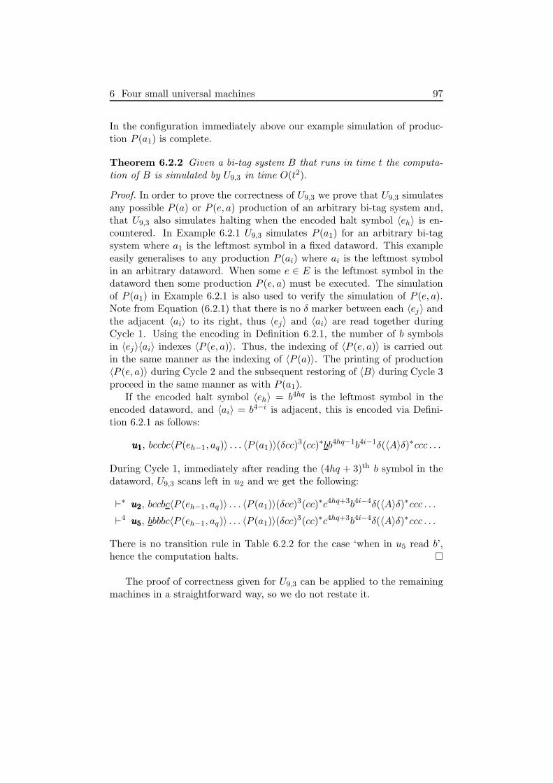
6 Four small universal machines 97
In the configuration immediately above our example simulation of produc-tion P (a1) is complete.
Theorem 6.2.2 Given a bi-tag system B that runs in time t the computa-tion of B is simulated by U9,3 in time O(t2).
Proof. In order to prove the correctness of U9,3 we prove that U9,3 simulatesany possible P (a) or P (e, a) production of an arbitrary bi-tag system and,that U9,3 also simulates halting when the encoded halt symbol 〈eh〉 is en-countered. In Example 6.2.1 U9,3 simulates P (a1) for an arbitrary bi-tagsystem where a1 is the leftmost symbol in a fixed dataword. This exampleeasily generalises to any production P (ai) where ai is the leftmost symbolin an arbitrary dataword. When some e ∈ E is the leftmost symbol in thedataword then some production P (e, a) must be executed. The simulationof P (a1) in Example 6.2.1 is also used to verify the simulation of P (e, a).Note from Equation (6.2.1) that there is no δ marker between each 〈ej〉 andthe adjacent 〈ai〉 to its right, thus 〈ej〉 and 〈ai〉 are read together duringCycle 1. Using the encoding in Definition 6.2.1, the number of b symbolsin 〈ej〉〈ai〉 indexes 〈P (e, a)〉. Thus, the indexing of 〈P (e, a)〉 is carried outin the same manner as the indexing of 〈P (a)〉. The printing of production〈P (e, a)〉 during Cycle 2 and the subsequent restoring of 〈B〉 during Cycle 3proceed in the same manner as with P (a1).
If the encoded halt symbol 〈eh〉 = b4hq is the leftmost symbol in theencoded dataword, and 〈ai〉 = b4−i is adjacent, this is encoded via Defini-tion 6.2.1 as follows:
u1u1u1, bccbc〈P (eh−1, aq)〉 . . . 〈P (a1)〉(δcc)3(cc)∗bb4hq−1b4i−1δ(〈A〉δ)∗ccc . . .
During Cycle 1, immediately after reading the (4hq + 3)th b symbol in thedataword, U9,3 scans left in u2 and we get the following:
⊢∗ u2u2u2, bccbc〈P (eh−1, aq)〉 . . . 〈P (a1)〉(δcc)3(cc)∗c4hq+3b4i−4δ(〈A〉δ)∗ccc . . .
⊢4 u5u5u5, bbbbc〈P (eh−1, aq)〉 . . . 〈P (a1)〉(δcc)3(cc)∗c4hq+3b4i−4δ(〈A〉δ)∗ccc . . .
There is no transition rule in Table 6.2.2 for the case ‘when in u5 read b’,hence the computation halts. �
The proof of correctness given for U9,3 can be applied to the remainingmachines in a straightforward way, so we do not restate it.
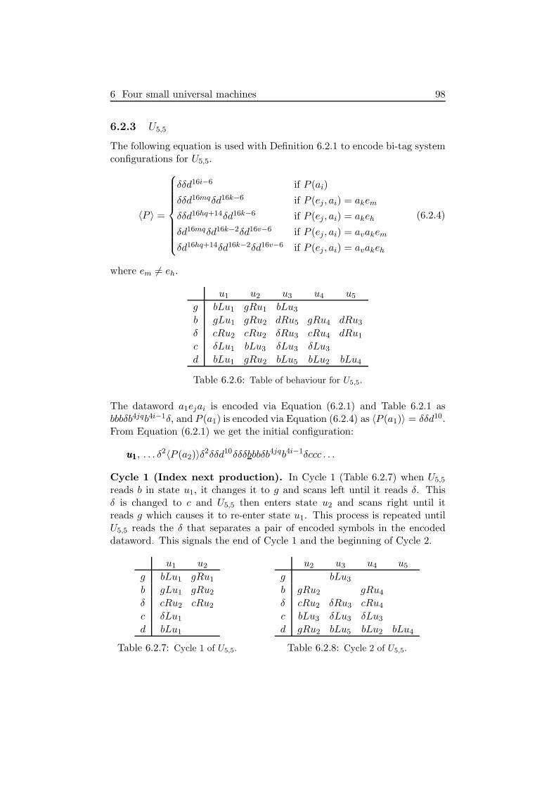
6 Four small universal machines 98
6.2.3 U5,5
The following equation is used with Definition 6.2.1 to encode bi-tag systemconfigurations for U5,5.
〈P 〉 =
δδd16i−6 if P (ai)
δδd16mqδd16k−6 if P (ej , ai) = akem
δδd16hq+14δd16k−6 if P (ej , ai) = akeh
δd16mqδd16k−2δd16v−6 if P (ej , ai) = avakem
δd16hq+14δd16k−2δd16v−6 if P (ej , ai) = avakeh
(6.2.4)
where em 6= eh.
u1 u2 u3 u4 u5
g bLu1 gRu1 bLu3
b gLu1 gRu2 dRu5 gRu4 dRu3
δ cRu2 cRu2 δRu3 cRu4 dRu1
c δLu1 bLu3 δLu3 δLu3
d bLu1 gRu2 bLu5 bLu2 bLu4
Table 6.2.6: Table of behaviour for U5,5.
The dataword a1ejai is encoded via Equation (6.2.1) and Table 6.2.1 asbbbδb4jqb4i−1δ, and P (a1) is encoded via Equation (6.2.4) as 〈P (a1)〉 = δδd10.From Equation (6.2.1) we get the initial configuration:
u1u1u1, . . . δ2〈P (a2)〉δ2δδd10δδδbbbδb4jqb4i−1δccc . . .
Cycle 1 (Index next production). In Cycle 1 (Table 6.2.7) when U5,5
reads b in state u1, it changes it to g and scans left until it reads δ. Thisδ is changed to c and U5,5 then enters state u2 and scans right until itreads g which causes it to re-enter state u1. This process is repeated untilU5,5 reads the δ that separates a pair of encoded symbols in the encodeddataword. This signals the end of Cycle 1 and the beginning of Cycle 2.
u1 u2
g bLu1 gRu1
b gLu1 gRu2
δ cRu2 cRu2
c δLu1
d bLu1
Table 6.2.7: Cycle 1 of U5,5.
u2 u3 u4 u5
g bLu3
b gRu2 gRu4
δ cRu2 δRu3 cRu4
c bLu3 δLu3 δLu3
d gRu2 bLu5 bLu2 bLu4
Table 6.2.8: Cycle 2 of U5,5.

6 Four small universal machines 99
⊢3 u1u1u1, . . . δ2〈P (a2)〉δ2δδd10δδcgbbδb4jqb4i−1δccc . . .
⊢18 u1u1u1, . . . δ2〈P (a2)〉δ2δδd10cccgggδb4jqb4i−1δccc . . .
⊢ u2u2u2, . . . δ2〈P (a2)〉δ2δδd10cccgggcbb4jq−1b4i−1δccc . . .
Cycle 2 (Print production). Cycle 2 (Table 6.2.8) begins with U5,5
scanning right and printing b to the right of the encoded dataword. Followingthis U5,5 scans left in state u3 and records the next symbol of the encodedproduction to be printed. If U5,5 reads the subword dddd it enters state u2,scans right, and prints b at the right end of the encoded dataword. If U5,5
reads the subword δdd it scans right in state u4 and prints δ at the rightend of the encoded dataword. This process is repeated until the end of theencoded production is detected by reading δ in state u3, which causes U5,5
to enter Cycle 3.
⊢∗ u3u3u3, . . . δ2〈P (a2)〉δ2δδd6ddddδδδbbbδb4jqb4i−1δbccc . . .
⊢3 u2u2u2, . . . δ2〈P (a2)〉δ2δδd6dbbbδδδbbbδb4jqb4i−1δbccc . . .
⊢∗ u3u3u3, . . . δ2〈P (a2)〉δ2δδddb8δδδbbbδb4jqb4i−1δbbbccc . . .
⊢2 u4u4u4, . . . δ2〈P (a2)〉δ2δδbbb8δδδbbbδb4jqb4i−1δbbbccc . . .
⊢∗ u3u3u3, . . . δ2〈P (a2)〉δ2δδbbb8δδδbbbδb4jqb4i−1δbbbδccc . . .
Cycle 3 (Restore tape). In Cycle 3 (Table 6.2.9) the tape head of U5,5
scans right switching between states u3 and u5 changing b symbols to dsymbols. This continues until U5,5 reads the δ marking the leftmost end ofthe encoded dataword in u5. Note from Equations (6.2.4) and (6.2.2) thatthere is an even number of d symbols between each pair of δ symbols in 〈B〉hence each δ symbol in 〈B〉 will be read in state u3. Each ai symbol in thedataword is encoded by an odd number of symbols (〈ai〉 = b4i−1) and hencethe first δ symbol in the dataword will be read in state u5. This causes U5,5
to enter state u1 thus completing Cycle 3 and the production simulation.
u3 u5
b dRu5 dRu3
δ δRu3 dRu1
Table 6.2.9: Cycle 3 of U5,5.
⊢19 u1u1u1, . . . δ2〈P (a2)〉δ2δδd10δδδddddbb4jq−1b4i−1δbbbδccc . . .
Halting for U5,5. If the encoded halt symbol 〈eh〉 = b4hq+3δ is the leftmostsymbol in the encoded dataword then this is encoded via Definition 6.2.1 asfollows:
u1u1u1, cdδ〈P (eh−1, aq)〉δ . . . δ2〈P (a1)〉δ3(dd)∗bb4hq+2δ(〈A〉δ)∗ccc . . .
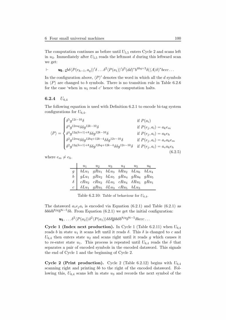
6 Four small universal machines 100
The computation continues as before until U5,5 enters Cycle 2 and scans leftin u3. Immediately after U5,5 reads the leftmost d during this leftward scanwe get:
⊢ u5u5u5, cbδ〈P (eh−1, aq)〉′δ . . . δ2〈P (a1)〉
′δ3(dd)∗b4hq+3δ(〈A〉δ)∗bccc . . .
In the configuration above, 〈P 〉′ denotes the word in which all the d symbolsin 〈P 〉 are changed to b symbols. There is no transition rule in Table 6.2.6for the case ‘when in u5 read c’ hence the computation halts.
6.2.4 U6,4
The following equation is used with Definition 6.2.1 to encode bi-tag systemconfigurations for U6,4.
〈P 〉 =
δ5g12i−10δ if P (ai)
δ4g12mqδδg12k−10δ if P (ej , ai) = akem
δ4g12q(h+1)+8δδg12k−10δ if P (ej , ai) = akeh
δ2g12mqδδg12hq+12k−4δδg12v−10δ if P (ej , ai) = avakem
δ2g12q(h+1)+8δδg12hq+12k−4δδg12v−10δ if P (ej , ai) = avakeh
(6.2.5)where em 6= eh.
u1 u2 u3 u4 u5 u6
g bLu1 gRu1 bLu3 bRu2 bLu6 bLu4
b gLu1 gRu2 bLu5 gRu4 gRu6 gRu5
δ cRu2 cRu2 δLu5 cRu4 δRu5 gRu1
c δLu1 gRu5 δLu3 cRu5 bLu3
Table 6.2.10: Table of behaviour for U6,4.
The dataword a1ejai is encoded via Equation (6.2.1) and Table (6.2.1) asbbbδb8jqb8i−5δb. From Equation (6.2.1) we get the initial configuration:
u1u1u1, . . . δ2〈P (a2)〉δ2〈P (a1)〉δδδbbbδb
8jqb8i−5δbccc . . .
Cycle 1 (Index next production). In Cycle 1 (Table 6.2.11) when U6,4
reads b in state u1 it scans left until it reads δ. This δ is changed to c andU6,4 then enters state u2 and scans right until it reads g which causes itto re-enter state u1. This process is repeated until U6,4 reads the δ thatseparates a pair of encoded symbols in the encoded dataword. This signalsthe end of Cycle 1 and the beginning of Cycle 2.
Cycle 2 (Print production). Cycle 2 (Table 6.2.12) begins with U6,4
scanning right and printing bb to the right of the encoded dataword. Fol-lowing this, U6,4 scans left in state u3 and records the next symbol of the

6 Four small universal machines 101
u1 u2
g bLu1 gRu1
b gLu1 gRu2
δ cRu2 cRu2
c δLu1
Table 6.2.11: Cycle 1 of U6,4.
u2 u3 u4 u5 u6
g bLu3 bRu2 bLu6 bLu4
b gRu2 bLu5 gRu4
δ cRu2 δLu5 cRu4 δRu5
c gRu5 δLu3 cRu5 bLu3
Table 6.2.12: Cycle 2 of U6,4.
encoded production to be printed. If U6,4 reads the subword gggδ or gggbit enters state u2, scans right, and prints bb at the right end of the encodeddataword. If U6,4 reads the subword δggb it scans right in state u4 andprints δb at the right end of the encoded dataword. This process is repeateduntil the end of the encoded production is detected by reading δ in state u5,which causes U6,4 to enter Cycle 3.
Cycle 3 (Restore tape). In Cycle 3 (Table 6.2.13) the tape head of U6,4
scans right switching between states u5 and u6, changing b symbols to gsymbols. This continues until U6,4 reads the δ marking the leftmost end ofthe encoded dataword in u6. Note from Equations (6.2.5) and (6.2.2) thatthere is an even number of g symbols between each pair of δ symbols in〈B〉, hence each δ symbol in 〈B〉 is read in state u5. Each ai symbol in thedataword is encoded by an odd number of symbols (〈ai〉 = b8i−5) and hencethe first δ symbol in the dataword is read in state u6. This causes U6,4 toenter state u1, thus completing Cycle 3 and the production simulation.
u5 u6
b gRu6 gRu5
δ δRu5 gRu1
Table 6.2.13: Cycle 3 of U6,4.
Special case for U6,4. If we are simulating a production of the formP (e, a) = avakem we have a special case. Note from the fourth row ofEquation 6.2.5 and Cycle 2 that the simulation of P (e, a) = avakem for U6,4
results in the word b8v−5δb8hq+8k−3δb8mqb being printed to the right of theencoded dataword. From Table 6.2.1 it is clear that ak is not encoded in thisword in its usual from. However when U6,4 reads the subword b8hq+8k−3δ itindexes 〈P (ak)〉 in H which results in 〈ak〉 being printed to the dataword.To see this, note that the value of H from Equation (6.2.2) for U6,4 is asfollows:
H = cgbV 2〈P (aq)〉V2〈P (aq−1)〉 . . . V
2〈P (a1)〉V3 (6.2.6)
The halting condition for U6,4 occurs in a similar manner to that of U5,5.Halting occurs during the first scan left in Cycle 2 when U6,4 reads c in state
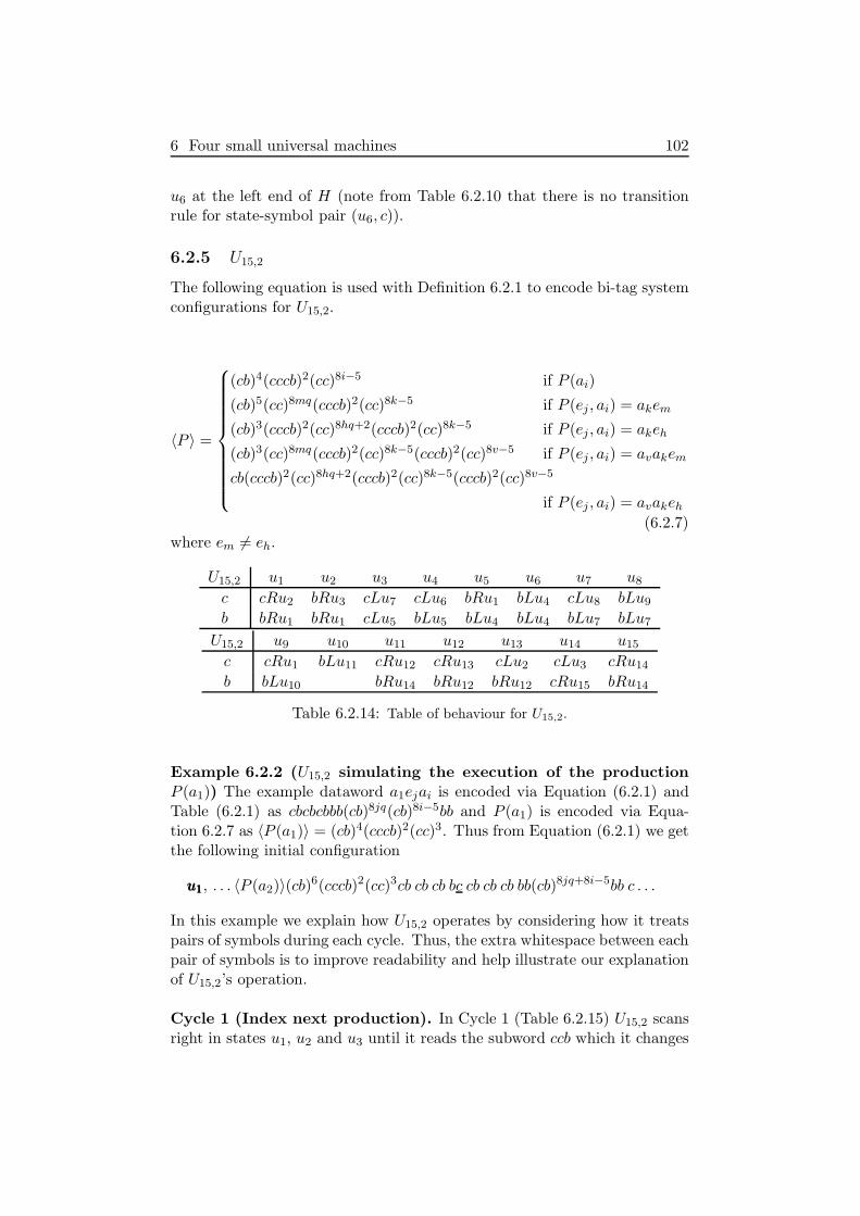
6 Four small universal machines 102
u6 at the left end of H (note from Table 6.2.10 that there is no transitionrule for state-symbol pair (u6, c)).
6.2.5 U15,2
The following equation is used with Definition 6.2.1 to encode bi-tag systemconfigurations for U15,2.
〈P 〉 =
(cb)4(cccb)2(cc)8i−5 if P (ai)
(cb)5(cc)8mq(cccb)2(cc)8k−5 if P (ej , ai) = akem
(cb)3(cccb)2(cc)8hq+2(cccb)2(cc)8k−5 if P (ej , ai) = akeh
(cb)3(cc)8mq(cccb)2(cc)8k−5(cccb)2(cc)8v−5 if P (ej , ai) = avakem
cb(cccb)2(cc)8hq+2(cccb)2(cc)8k−5(cccb)2(cc)8v−5
if P (ej , ai) = avakeh
(6.2.7)where em 6= eh.
U15,2 u1 u2 u3 u4 u5 u6 u7 u8
c cRu2 bRu3 cLu7 cLu6 bRu1 bLu4 cLu8 bLu9
b bRu1 bRu1 cLu5 bLu5 bLu4 bLu4 bLu7 bLu7
U15,2 u9 u10 u11 u12 u13 u14 u15
c cRu1 bLu11 cRu12 cRu13 cLu2 cLu3 cRu14
b bLu10 bRu14 bRu12 bRu12 cRu15 bRu14
Table 6.2.14: Table of behaviour for U15,2.
Example 6.2.2 (U15,2 simulating the execution of the productionP (a1)) The example dataword a1ejai is encoded via Equation (6.2.1) andTable (6.2.1) as cbcbcbbb(cb)8jq(cb)8i−5bb and P (a1) is encoded via Equa-tion 6.2.7 as 〈P (a1)〉 = (cb)4(cccb)2(cc)3. Thus from Equation (6.2.1) we getthe following initial configuration
u1u1u1, . . . 〈P (a2)〉(cb)6(cccb)2(cc)3cb cb cb bc cb cb cb bb(cb)8jq+8i−5bb c . . .
In this example we explain how U15,2 operates by considering how it treatspairs of symbols during each cycle. Thus, the extra whitespace between eachpair of symbols is to improve readability and help illustrate our explanationof U15,2’s operation.
Cycle 1 (Index next production). In Cycle 1 (Table 6.2.15) U15,2 scansright in states u1, u2 and u3 until it reads the subword ccb which it changes

6 Four small universal machines 103
to cbc. Following this, it scans left in states u4, u5 and u6 until it reads thesubword cb. This cb is changed to bb and U15,2 re-enters state u1 and scansright. This process is repeated until U15,2 has finished reading the encodedread symbol 〈ai〉 or symbols 〈ej〉 and 〈ai〉. This occurs when the subwordccb no longer appears to the right of the tape head and signals the end ofCycle 1 and the beginning of Cycle 2.
U15,2 u1 u2 u3 u4 u5 u6
c cRu2 bRu3 cLu7 cLu6 bRu1 bLu4
b bRu1 bRu1 cLu5 bLu5 bLu4 bLu4
Table 6.2.15: Cycle 1 of U15,2.
⊢3 u5u5u5, . . . 〈P 〉(cb)6(cccb)2(cc)3cb cb cb bc bc cb cb bb(cb)8jq+8i−5bbc . . .
⊢4 u5u5u5, . . . 〈P 〉(cb)6(cccb)2(cc)3cb cb cb bc bc cb cb bb(cb)8jq+8i−5bbc . . .
⊢4 u2u2u2, . . . 〈P 〉(cb)6(cccb)2(cc)3cb cb bb bc bc cb cb bb(cb)8jq+8i−5bbc . . .
⊢20 u2u2u2, . . . 〈P 〉(cb)6(cccb)2(cc)3cb bb bb bc bc bc cb bb(cb)8jq+8i−5bbc . . .
⊢28 u2u2u2, . . . 〈P 〉(cb)6(cccb)2(cc)3bb bb bb bc bc bc bc bb(cb)8jq+8i−5bbc . . .
Note that in the configuration immediately above each cb subword in theencoded read symbol 〈a1〉 = cbcbcb has been changed to the subword bc.Note also that the subword ccb which causes a scan to the left in u4, u5,and u6 no longer appears in the configuration to the right of the tape head.This causes U15,2 to enter Cycle 2.
Cycle 2 (Print production). Cycle 2 (Table 6.2.16) begins with U15,2
scanning right and printing cb to the right of the encoded dataword. Follow-ing this U15,2 scans left in states u7, u8, u9, u10 and u11 and records the nextsymbol of the encoded production to be printed. If, during a scan left, U15,2
reads the subword ccc then it scans right in states u1 and u2 and changesthe cc immediately to the right of the encoded dataword to cb. If, during ascan left, U15,2 reads the subword ccbcc it scans right in states u12 and u13
and changes the first c to the right of the encoded dataword to a b. Thisprocess is repeated until the end of the encoded production is detected byreading the subword bcbcc during the scan left. This causes U15,2 to enterCycle 3.
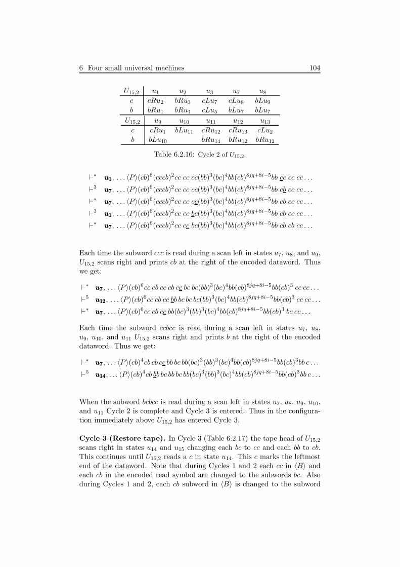
6 Four small universal machines 104
U15,2 u1 u2 u3 u7 u8
c cRu2 bRu3 cLu7 cLu8 bLu9
b bRu1 bRu1 cLu5 bLu7 bLu7
U15,2 u9 u10 u11 u12 u13
c cRu1 bLu11 cRu12 cRu13 cLu2
b bLu10 bRu14 bRu12 bRu12
Table 6.2.16: Cycle 2 of U15,2.
⊢∗ u1u1u1, . . . 〈P 〉(cb)6(cccb)2cc cc cc(bb)3(bc)4bb(cb)8jq+8i−5bb cc cc cc . . .
⊢3 u7u7u7, . . . 〈P 〉(cb)6(cccb)2cc cc cc(bb)3(bc)4bb(cb)8jq+8i−5bb cb cc cc . . .
⊢∗ u7u7u7, . . . 〈P 〉(cb)6(cccb)2cc cc cc(bb)3(bc)4bb(cb)8jq+8i−5bb cb cc cc . . .
⊢3 u1u1u1, . . . 〈P 〉(cb)6(cccb)2cc cc bc(bb)3(bc)4bb(cb)8jq+8i−5bb cb cc cc . . .
⊢∗ u7u7u7, . . . 〈P 〉(cb)6(cccb)2cc cc bc(bb)3(bc)4bb(cb)8jq+8i−5bb cb cb cc . . .
Each time the subword ccc is read during a scan left in states u7, u8, and u9,U15,2 scans right and prints cb at the right of the encoded dataword. Thuswe get:
⊢∗ u7u7u7, . . . 〈P 〉(cb)6cc cb cc cb cc bc bc(bb)3(bc)4bb(cb)8jq+8i−5bb(cb)3 cc cc . . .
⊢5 u12u12u12, . . . 〈P 〉(cb)6cc cb cc bb bc bc bc(bb)3(bc)4bb(cb)8jq+8i−5bb(cb)3 cc cc . . .
⊢∗ u7u7u7, . . . 〈P 〉(cb)6cc cb cc bb(bc)3(bb)3(bc)4bb(cb)8jq+8i−5bb(cb)3 bc cc . . .
Each time the subword ccbcc is read during a scan left in states u7, u8,u9, u10, and u11 U15,2 scans right and prints b at the right of the encodeddataword. Thus we get:
⊢∗ u7u7u7, . . . 〈P 〉(cb)4cb cb cc bb bc bb(bc)3(bb)3(bc)4bb(cb)8jq+8i−5bb(cb)3bb c . . .
⊢5 u14u14u14, . . . 〈P 〉(cb)4cb bb bc bb bc bb(bc)3(bb)3(bc)4bb(cb)8jq+8i−5bb(cb)3bb c . . .
When the subword bcbcc is read during a scan left in states u7, u8, u9, u10,and u11 Cycle 2 is complete and Cycle 3 is entered. Thus in the configura-tion immediately above U15,2 has entered Cycle 3.
Cycle 3 (Restore tape). In Cycle 3 (Table 6.2.17) the tape head of U15,2
scans right in states u14 and u15 changing each bc to cc and each bb to cb.This continues until U15,2 reads a c in state u14. This c marks the leftmostend of the dataword. Note that during Cycles 1 and 2 each cc in 〈B〉 andeach cb in the encoded read symbol are changed to the subwords bc. Alsoduring Cycles 1 and 2, each cb subword in 〈B〉 is changed to the subword

6 Four small universal machines 105
bb. Thus c will not be read in u14 until we encounter the subword cb at theleft end of the next encoded symbol to be read in the dataword.
⊢9 u15u15u15, . . . 〈P 〉(cb)4cb cb cc cb cc cb(bc)3(bb)3(bc)4bb(cb)8jq+8i−5bb(cb)3bb c . . .
⊢∗ u14u14u14, . . . 〈P 〉(cb)6(cccb)2(cc)3(cb)3(cc)4 cb cb(cb)8jq+8i−6bb(cb)3bb c . . .
⊢3 u1u1u1, . . . 〈P 〉(cb)6(cccb)2(cc)3(cb)3(cc)4 bc cb(cb)8jq+8i−6bb(cb)3bb c . . .
In the configuration immediately above the example simulation of produc-tion 〈P (a1)〉 is complete. The encoded symbol 〈a1〉 = (cb)3 has been ap-pended onto the right end of the dataword, the encoded tag system 〈B〉 hasbeen restored to its original value and U15,2 is ready to read the encodedsymbols 〈ej〉 and 〈ai〉.
U15,2 u3 u5 u14 u15
c bRu1 cLu3 cRu14
b cLu5 cRu15 bRu14
Table 6.2.17: Cycle 3 of U15,2.
Halting for U15,2. If the encoded halt symbol 〈eh〉 = (cb)8hq+2 is theleftmost symbol in the encoded dataword then this is encoded via Defini-tion 6.2.1 as follows:
u1u1u1, bb cc〈P (eh−1, aq)〉 . . . 〈P (a1)〉(cb)3(cc)∗bc (cb)8hq+2bb(〈A〉bb)∗cc c . . .
The computation continues as before until U15,2 enters Cycle 2 and scansleft in u7, u8, and u9. This scan ends with the following configuration:
⊢∗ u10u10u10, bb bc〈P (eh−1, aq)〉′ . . . 〈P (a1)〉
′(bb)3(bc)∗(bc)8hq+2bb(〈A〉bb)∗cb c . . .
In the configuration above, 〈P 〉′ denotes the word in which each cc and cbsubword in 〈P 〉 is changed to the subword bc and bb, respectively. There isno transition rule in Table 6.2.14 for the case ‘when in u10 read c’ hence thecomputation halts.
6.3 Discussion
We noted in the introduction to this chapter that 39 state-symbol pairsremain open, as can be seen in Figure 6.1.1. It is not known which pairshave a decidable halting problem and which pairs contain standard universalTuring machines.
Following Minsky’s [Min62a] 7-state, 4 symbol universal machine all ofthe smallest universal Turing machines (including our bi-tag simulators)

6 Four small universal machines 106
have used a similar algorithm. Since Rogozhin [Rog79, Rog82] establishedthe universal curve there have been incremental reductions in the size ofmany of his machines. However the smallest of Rogozhin’s machines, the6-symbol machine, has not been improved upon since it was first presentedalmost 30 years ago. In order to significantly reduce the space between thedecidable halting problem curve and the universality curve we suspect thata radically new approach must be taken. Below we give three methods toaid in the search for smaller universal Turing machines.
The first approach is to look for some universal systems other that 2-tagor bi-tag systems that would require less instructions to simulate. Cyclictag systems (see Chapter 4) may be used to give smaller machines. Howeverthe operation of cyclic tag systems is similar to that of tag systems so thismay not give much of an improvement. Perhaps a simple universal cellularautomaton could be simulated. The cellular automaton Rule 110 has givenrise to very small weakly universal Turing machines (see Chapter 7). Perhapsa sufficiently simple universal cellular automaton could be found that allowsus to construct small Turing machines that are universal, rather than onlyweakly universal.
Another approach is to simplify some existing universal model in order tomake it easier to simulate. As an interesting example we will briefly considersmall semi-weak machines. Watanabe [Wat61] gave a small semi-weakly uni-versal Turing machine with 6 states and 5 symbols that simulates Turingmachines directly. Later, Watanabe [Wat72] gave a small semi-weakly uni-versal Turing machine with 5 states and 4 symbols that simulates restrictedTuring machines. Watanabe noted that Turing machines with a binary{0, 1} tape alphabet where the tape head always moves right on a 1 and lefton a 0 are universal. Because of this restriction, Watanabe’s encoded tableof behaviour for each Turing machine had no need to include informationabout the direction of movement of the tape head. This in turn simplifiedthe problem of simulating Turing machines.
A third approach is to find an encoding that allows many different oper-ations to be carried out by the same group of instructions. In Chapter 3 wegave small universal Turing machines that simulate Turing machine directly.The encoding used by these machines allowed each set of transition rules toserve more than one purpose. A single set of transition rules reads boththe encoded current state and the encoded read symbol. Another set oftransition rules, prints the encoded write symbol, moves the simulated tapehead, and establishes the new encoded current state. Combining steps inthis way has reduced the number of transition rules needed by our universalmachines in Chapter 3.
The number of state-symbol pairs that remain open could also be reducedby searching for decidability results. Decidability results provide useful lowerbounds for small universal Turing machines. To date, there has been noimprovement on Pavlotskaya’s [Pav78] 1978 proof that the halting problem
6 Four small universal machines 107
is decidable for 3-state, 2-symbol machines. Pavlotskaya’s proof is quitelong and complex and improving on this result may well be difficult. As thestate-symbol product increases, the number of possible machines increasesexponentially. Thus it seems that a new approach needs to be taken. To findnew lower bounds one possible method is to prove that some non-universalsystem simulates all of the Turing machines for a given state-symbol pair.

7
Small weakly universal Turing
machines
7.1 Introduction
In this chapter we present small universal Turing machines with state-symbolpairs of (6, 2), (3, 3) and (2, 4). These machines are weakly universal, whichmeans that they have an infinitely repeated word to the left of their inputand another to the right. They simulate Rule 110 and are currently thesmallest known weakly universal Turing machines.
We recall that, beginning in the early sixties Minsky and Watanabe en-gaged in a vigorous competition to see who could come up with the smallestuniversal Turing machine [Min60a, Min62a, Wat60, Wat61, Wat72]. In 1961Watanabe [Wat61] gave a 6-state, 5-symbol universal Turing machine, thefirst weakly universal machine. In 1962, Minsky [Min62a] found a small7-state, 4-symbol universal Turing machine. Not to be out-done, Watan-abe improved on his earlier machine to give 5-state, 4-symbol and 7-state,3-symbol weakly universal machines [Wat72, Noz69]. Some of the earliestsmall universal machines are given in Table 1.1.1.
The 7-state universal Turing machine of Minsky has received much at-tention. Minsky’s machine simulates Turing machines via 2-tag systems,which were proved universal by Cocke and Minsky [CM64]. The techniqueof simulating 2-tag systems, pioneered by Minsky, was extended by Ro-gozhin [Rog82] to give the (then) smallest known universal Turing machinesfor a number of state-symbol pairs. These 2-tag simulators were subse-quently reduced in size by Rogozhin [Rog96], Kudlek and Rogozhin [KR02],and Baiocchi [Bai01]. In Chapter 6 we gave small universal machines thatsimulate Turing machines via a new variant of tag systems called bi-tag sys-tems. In Figure 7.1.1 each of the smallest 2-tag simulators are plotted ashollow circles and each of the smallest bi-tag simulators are plotted as solidtriangles. These (standard) machines induce a universal curve.
The small weak machines of Watanabe have received little attention. Inparticular the 5-state and 7-state machines seem little known and are largelyignored in the literature. It is worth noting that unlike other weak Turingmachines the weak machines of Watanabe are proved universal using the
108
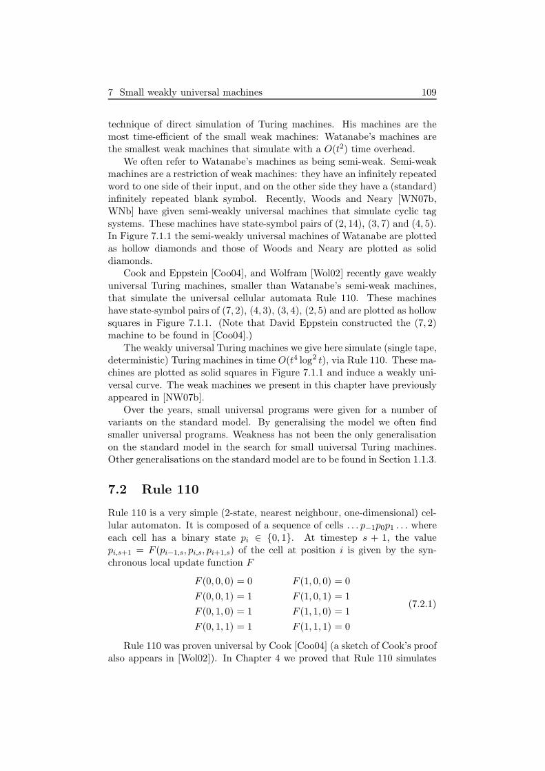
7 Small weakly universal machines 109
technique of direct simulation of Turing machines. His machines are themost time-efficient of the small weak machines: Watanabe’s machines arethe smallest weak machines that simulate with a O(t2) time overhead.
We often refer to Watanabe’s machines as being semi-weak. Semi-weakmachines are a restriction of weak machines: they have an infinitely repeatedword to one side of their input, and on the other side they have a (standard)infinitely repeated blank symbol. Recently, Woods and Neary [WN07b,WNb] have given semi-weakly universal machines that simulate cyclic tagsystems. These machines have state-symbol pairs of (2, 14), (3, 7) and (4, 5).In Figure 7.1.1 the semi-weakly universal machines of Watanabe are plottedas hollow diamonds and those of Woods and Neary are plotted as soliddiamonds.
Cook and Eppstein [Coo04], and Wolfram [Wol02] recently gave weaklyuniversal Turing machines, smaller than Watanabe’s semi-weak machines,that simulate the universal cellular automata Rule 110. These machineshave state-symbol pairs of (7, 2), (4, 3), (3, 4), (2, 5) and are plotted as hollowsquares in Figure 7.1.1. (Note that David Eppstein constructed the (7, 2)machine to be found in [Coo04].)
The weakly universal Turing machines we give here simulate (single tape,deterministic) Turing machines in time O(t4 log2 t), via Rule 110. These ma-chines are plotted as solid squares in Figure 7.1.1 and induce a weakly uni-versal curve. The weak machines we present in this chapter have previouslyappeared in [NW07b].
Over the years, small universal programs were given for a number ofvariants on the standard model. By generalising the model we often findsmaller universal programs. Weakness has not been the only generalisationon the standard model in the search for small universal Turing machines.Other generalisations on the standard model are to be found in Section 1.1.3.
7.2 Rule 110
Rule 110 is a very simple (2-state, nearest neighbour, one-dimensional) cel-lular automaton. It is composed of a sequence of cells . . . p−1p0p1 . . . whereeach cell has a binary state pi ∈ {0, 1}. At timestep s + 1, the valuepi,s+1 = F (pi−1,s, pi,s, pi+1,s) of the cell at position i is given by the syn-chronous local update function F
F (0, 0, 0) = 0 F (1, 0, 0) = 0
F (0, 0, 1) = 1 F (1, 0, 1) = 1
F (0, 1, 0) = 1 F (1, 1, 0) = 1
F (0, 1, 1) = 1 F (1, 1, 1) = 0
(7.2.1)
Rule 110 was proven universal by Cook [Coo04] (a sketch of Cook’s proofalso appears in [Wol02]). In Chapter 4 we proved that Rule 110 simulates
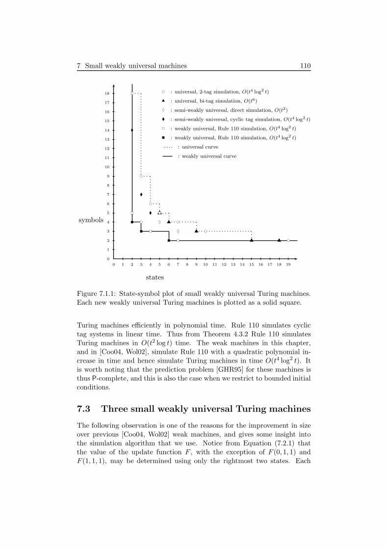
7 Small weakly universal machines 110
bc : universal, 2-tag simulation, O(t4 log2 t)
u : universal, bi-tag simulation, O(t6)
ld : semi-weakly universal, direct simulation, O(t2)
l : semi-weakly universal, cyclic tag simulation, O(t4 log2 t)
rs : weakly universal, Rule 110 simulation, O(t4 log2 t)
r : weakly universal, Rule 110 simulation, O(t4 log2 t)
: universal curve
: weakly universal curve
0 1 2 3 4 5 6 7 8 9 10 11 12 13 14 15 16 17 18 19
0
1
2
3
4
5
6
7
8
9
10
11
12
13
14
15
16
17
18
states
symbols u
u
uu
u
r
r
r
bc
bc
bc
bc
bc
bc
bc
l
l
l
ld
ld
rs
rs
rs
rs
Figure 7.1.1: State-symbol plot of small weakly universal Turing machines.Each new weakly universal Turing machines is plotted as a solid square.
Turing machines efficiently in polynomial time. Rule 110 simulates cyclictag systems in linear time. Thus from Theorem 4.3.2 Rule 110 simulatesTuring machines in O(t2 log t) time. The weak machines in this chapter,and in [Coo04, Wol02], simulate Rule 110 with a quadratic polynomial in-crease in time and hence simulate Turing machines in time O(t4 log2 t). Itis worth noting that the prediction problem [GHR95] for these machines isthus P-complete, and this is also the case when we restrict to bounded initialconditions.
7.3 Three small weakly universal Turing machines
The following observation is one of the reasons for the improvement in sizeover previous [Coo04, Wol02] weak machines, and gives some insight intothe simulation algorithm that we use. Notice from Equation (7.2.1) thatthe value of the update function F , with the exception of F (0, 1, 1) andF (1, 1, 1), may be determined using only the rightmost two states. Each

7 Small weakly universal machines 111
c0
c1
c2
c3...
. . . -9 -8 -7 -6 -5 -4 -3 -2 -1 0 1 2 3 4 5 6 7 8 9 . . .
Figure 7.2.1: Seven consecutive timesteps of Rule 110. These seventimesteps are taken from the background ether that is used in theproof [Coo04] of universality of Rule 110. Each black or each white squarerepresents, a Rule 110 cell containing, state 1 or 0 respectively. Each cell isidentified by the index given above it. To the left of each row of cells thereis a configuration label that identifies that row.
of our universal Turing machines exploit this fact as follows. The machinesscan from right to left, and in six of the eight cases they need only rememberthe cell immediately to the right of the current cell i in order to compute theupdate for i. Thus for these six cases we need only store a single cell value,rather than two values. The remaining two cases are simulated as follows.If two consecutive encoded states with value 1 are read, it is assumed thatthere is another encoded 1 to the left and the update F (1, 1, 1) = 0 issimulated. If our assumption proves false (we instead read an encoded 0),then our machine returns to the wrongly updated cell and simulates theupdate F (0, 1, 1) = 1.
Before giving our three small Rule 110 simulators, we give some furtherbackground explanation. Rule 110 simulates Turing machines via cyclic tagsystems. A Rule 110 instance that simulates a cyclic tag system computa-tion is of the following form (for more details see [Coo04]). The input to thecyclic tag system is encoded in a contiguous finite number of Rule 110 cells.On the left of the input a fixed constant word (representing the ‘ossifiers’) isrepeated infinitely many times. On the right, another fixed constant word(representing the cyclic tag system program/appendants, and the ‘leaders’)is repeated infinitely many times. Both of these repeated words are inde-pendent of the input.
Our weakly universal machines operate by traversing a finite amountof the tape from right to left and then from left to right. This simulates asingle timestep of Rule 110 over a finite part of the encoded infinite Rule 110instance. With each simulated timestep the length of a traversal increases.To ensure that each traversal is of finite length, the left blank word l andthe right blank word r of each of our weak machines must have a specialform. These words contain special subwords or symbols that terminate

7 Small weakly universal machines 112
each traversal, causing the tape head to turn. When the head is turningit overwrites any symbols that caused a turn. Thus the number of cellsthat are being updated increases monotonically over time. This techniquesimulates Rule 110 properly if the initial condition is set up so that withineach repeated blank word, the subword between each successive turn pointis shifted one timestep forward in time.
In the sequel we describe the computation of our three machines byshowing a simulation of the update on the ether in Figure 7.2.1. In the nextparagraph below, we outline why this example is in fact general enough toprove universality. First, we must define blank words that are suitable forthis example. The left blank word l, on the Turing machine tape, encodesthe Rule 110 sequence 0001. In the initial configuration as we move lefteach subsequent sequence 0001 is one timestep further ahead. To see thisnote from Figure 7.2.1 that 0001 occupies, cells −7 to −4 in configurationc1, cells −11 to −8 in c2, cells −15 to −12 in c3, etc. Similarly, the rightblank word r encodes the Rule 110 sequence 110011. Looking at the initialconfiguration, as we move right from cell 0, in the first blank word the firstfour cells 1100 are shifted two timesteps ahead, and the next two cells 11are shifted a further one timestep. To see this note from Figure 7.2.1 that1100 occupies cells 1 to 4 in c2 and 11 occupies cells 5 and 6 in c3. In eachsubsequent sequence the first four cells 1100 are shifted only one timestepahead and the last two cells 11 are shifted one further timestep. In each rowthe ether in Figure 7.2.1 repeats every 14 cells and if the number of timestepss between two rows is s ≡ 0 mod 7 then the two rows are identical. Theperiodic nature of the ether, in both time and space, allows us to constructsuch blank words.
It should be noted that the machines we present here, and those in [Coo04],require suitable blank words to simulate a Rule 110 instance directly. If nosuitable blank words can be found (i.e. if it is not possible to construct thespecific subwords that we use to terminate traversals in the encoding) thenit may be the case that the particular instance can not be simulated directly.However, in the sequel our machines simulate the background ether that isused in the universality proof of Rule 110 [Coo04]. The gliders used byCook [Coo04] that move through this ether are periodic in time and space.Thus, we can construct blank words that included these gliders and placethe subwords that terminate traversals in the ether. By this reasoning, ourexample is sufficiently general to prove that our machines simulate Turingmachines via Rule 110 and we do not give a full (and possibly tedious)proof of correctness. For U3,3 we explicitly simulate three updates fromFigure 7.2.1, which is general enough so that an update [Equation (7.2.1)]on each of the eight possible three state combinations is simulated. Wegive shorter examples for the machines U2,4 and U6,2 as they use the samesimulation algorithm as U3,3.
The machines we present here do not halt. Cook [Coo04] shows how a

7 Small weakly universal machines 113
special glider may be produced during the simulation of a Turing machineby Rule 110. This glider may be used to simulate halting as the encodingcan be such that it is generated by Rule 110 if and only if the simulatedmachine halts. The glider would be encoded on the tape of our machines asa unique, constant word.
7.3.1 U3,3
We begin by describing an initial configuration of U3,3. To the left of, andincluding, the tape head position, the Rule 110 state 0 is encoded by 0, andthe Rule 110 state 1 is encoded by either 1 or b. The word 1b0 is used toterminate a left traversal. (Note an exception: the 1 in the subword 1b0encodes the Rule 110 state 0.) To the right of the tape head position, theRule 110 state 0 is encoded by 1, and the Rule 110 state 1 is encoded by 0or b. The tape symbol 0 is used to terminate a right traversal. The left andright blank words, described in paragraph 4 of Section 7.3, are encoded as0 0 1 b and 0 b 1 1 0 b respectively.
u1 u2 u3
0 1Lu1 0Ru1 bLu1
1 bLu2 1Lu2 0Ru3
b bLu3 1Ru3
Table 7.3.1: Table of behaviour for U3,3.
We give an example of U3,3 simulating the three successive Rule 110timesteps c0 ⊢ c1 ⊢ c2 ⊢ c3 given in Figure 7.2.1. In the below configurationsthe current state of U3,3 is highlighted in bold, to the left of its tape contents.The tape head position of U3,3 is given by an underline and the start state isu1. The configuration immediately below encodes c0 from Figure 7.2.1 withthe tape head over cell index 0.
u1u1u1, . . . 0 0 1 b 0 0 1 b 0 0 1 b 0 0 0 1 0 b 1 1 0 b 0 b 1 1 0 b . . .
⊢ u2u2u2, . . . 0 0 1 b 0 0 1 b 0 0 1 b 0 0 0 b 0 b 1 1 0 b 0 b 1 1 0 b . . .
⊢ u1u1u1, . . . 0 0 1 b 0 0 1 b 0 0 1 b 0 0 0 b 0 b 1 1 0 b 0 b 1 1 0 b . . .
⊢ u3u3u3, . . . 0 0 1 b 0 0 1 b 0 0 1 b 0 0 0 b 0 b 1 1 0 b 0 b 1 1 0 b . . .
⊢ u1u1u1, . . . 0 0 1 b 0 0 1 b 0 0 1 b 0 0 b b 0 b 1 1 0 b 0 b 1 1 0 b . . .
⊢2 u1u1u1, . . . 0 0 1 b 0 0 1 b 0 0 1 b 1 1 b b 0 b 1 1 0 b 0 b 1 1 0 b . . .
⊢ u3u3u3, . . . 0 0 1 b 0 0 1 b 0 0 1 b 1 1 b b 0 b 1 1 0 b 0 b 1 1 0 b . . .
When the tape head reads the subword 1b0 the left traversal is complete

7 Small weakly universal machines 114
and the right traversal begins.
⊢6 u3u3u3, . . . 0 0 1 b 0 0 1 b 0 0 0 1 0 0 1 1 0 b 1 1 0 b 0 b 1 1 0 b . . .
⊢ u1u1u1, . . . 0 0 1 b 0 0 1 b 0001 0011 b b 1 1 0 b 0 b 1 1 0 b . . .
Immediately after the tape head reads a 0, during a right traversal, thesimulation of timestep c0 ⊢ c1 is complete. To see this, compare the partof the Turing machine tape in bold with cells −7 to 0 of configuration c1 inFigure 7.2.1. We continue our simulation to give timestep c1 ⊢ c2.
⊢ u2u2u2, . . . 0 0 1 b 0 0 1 b 0 0 0 1 0 0 1 b b b 1 1 0 b 0 b 1 1 0 b . . .
⊢ u2u2u2, . . . 0 0 1 b 0 0 1 b 0 0 0 1 0 0 1 b b b 1 1 0 b 0 b 1 1 0 b . . .
⊢ u1u1u1, . . . 0 0 1 b 0 0 1 b 0 0 0 1 0 0 1 b b b 1 1 0 b 0 b 1 1 0 b . . .
⊢ u2u2u2, . . . 0 0 1 b 0 0 1 b 0 0 0 1 0 0 b b b b 1 1 0 b 0 b 1 1 0 b . . .
⊢3 u1u1u1, . . . 0 0 1 b 0 0 1 b 0 0 0 1 0 b b b b b 1 1 0 b 0 b 1 1 0 b . . .
⊢2 u2u2u2, . . . 0 0 1 b 0 0 1 b 0 0 0 b 1 b b b b b 1 1 0 b 0 b 1 1 0 b . . .
⊢3 u1u1u1, . . . 0 0 1 b 0 0 1 b 0 0 b b 1 b b b b b 1 1 0 b 0 b 1 1 0 b . . .
⊢3 u3u3u3, . . . 0 0 1 b 0 0 1 b 1 1 b b 1 b b b b b 1 1 0 b 0 b 1 1 0 b . . .
⊢15 u1u1u1, . . . 0 0 1 b 0001 0011 0111 1100 b b 0 b 1 1 0 b . . .
The simulation of timestep c1 ⊢ c2 is complete. To see this, compare thepart of the Turing machine tape in bold with cells −11 to 4 of configurationc2 in Figure 7.2.1. We continue our simulation to give timestep c2 ⊢ c3.
⊢3 u2u2u2, . . . 0 0 1 b 0 0 0 1 0 0 1 1 0 1 1 1 1 b 1 1 b b 0 b 1 1 0 b . . .
⊢4 u2u2u2, . . . 0 0 1 b 0 0 0 1 0 0 1 1 0 1 1 1 1 b 1 1 b b 0 b 1 1 0 b . . .
⊢5 u1u1u1, . . . 0 0 1 b 0 0 0 1 0 0 1 1 b b 1 1 1 b 1 1 b b 0 b 1 1 0 b . . .
⊢2 u2u2u2, . . . 0 0 1 b 0 0 0 1 0 0 1 b b b 1 1 1 b 1 1 b b 0 b 1 1 0 b . . .
⊢5 u1u1u1, . . . 0 0 1 b 0 0 0 1 0 b b b b b 1 1 1 b 1 1 b b 0 b 1 1 0 b . . .
⊢2 u2u2u2, . . . 0 0 1 b 0 0 0 b 1 b b b b b 1 1 1 b 1 1 b b 0 b 1 1 0 b . . .
⊢6 u3u3u3, . . . 0 0 1 b 1 1 b b 1 b b b b b 1 1 1 b 1 1 b b 0 b 1 1 0 b . . .
⊢21 u1u1u1, . . . 0001 0011 0111 1100 010011 b b 1 1 0 b . . .
The simulation of timestep c2 ⊢ c3 is complete. To see this, compare thepart of the Turing machine tape in bold with cells −15 to 6 of configurationc3 in Figure 7.2.1.
7.3.2 U2,4
We begin by describing an initial configuration of U2,4. To the left of, andincluding, the tape head position, the Rule 110 state 0 is encoded by either 0

7 Small weakly universal machines 115
or 0/ and the Rule 110 state 1 is encoded by either 1 or 1/ . The word 0/ 1 isused to terminate a left traversal. To the right of the tape head position,the Rule 110 state 0 is encoded by 0/ and the Rule 110 state 1 is encodedby 1/ or 0. The tape symbol 0 is used to terminate a right traversal. Theleft and right blank words, from paragraph 4 of Section 7.3, are encoded as0 0 0/ 1 and 0 1/ 0/ 0/ 0 1/ respectively.
u1 u2
0 0/Lu1 1/Ru1
1 1/Lu2 0/Lu2
0/ 1/Lu1 0Ru2
1/ 1/Lu1 1Ru2
Table 7.3.2: Table of behaviour for U2,4.
By way of example we give U2,4 simulating the two successive Rule 110timesteps c0 ⊢ c1 ⊢ c2 given in Figure 7.2.1. The configuration immediatelybelow encodes c0 from Figure 7.2.1 with the tape head over cell index 0.
u1u1u1, . . . 0 0 0/ 1 0 0 0/ 1 0 0 0/ 1 0 0 0 1 0 1/ 0/ 0/ 0 1/ 0 1/ 0/ 0/ 0 1/ . . .
⊢6 u1u1u1, . . . 0 0 0/ 1 0 0 0/ 1 0 0 0/ 1 0/ 0/ 1/ 1/ 0 1/ 0/ 0/ 0 1/ 0 1/ 0/ 0/ 0 1/ . . .
⊢ u2u2u2, . . . 0 0 0/ 1 0 0 0/ 1 0 0 0/ 1/ 0/ 0/ 1/ 1/ 0 1/ 0/ 0/ 0 1/ 0 1/ 0/ 0/ 0 1/ . . .
When the tape head reads the subword 0/ 1 the left traversal is complete andthe right traversal begins.
⊢6 u2u2u2, . . . 0 0 0/ 1 0 0 0/ 1 0 0 0 1 0 0 1 1 0 1/ 0/ 0/ 0 1/ 0 1/ 0/ 0/ 0 1/ . . .
⊢ u1u1u1, . . . 0 0 0/ 1 0 0 0/ 1 0001 0011 1/ 1/ 0/ 0/ 0 1/ 0 1/ 0/ 0/ 0 1/ . . .
Immediately after the tape head reads a 0, during a right traversal, thesimulation of timestep c0 ⊢ c1 is complete. To see this, compare the partof the Turing machine tape in bold with cells −7 to 0 of configuration c1 inFigure 7.2.1. We continue our simulation to give timestep c1 ⊢ c2.
⊢2 u1u1u1, . . . 0 0 0/ 1 0 0 0/ 1 0 0 0 1 0 0 1 1 1/ 1/ 0/ 0/ 0 1/ 0 1/ 0/ 0/ 0 1/ . . .
⊢2 u2u2u2, . . . 0 0 0/ 1 0 0 0/ 1 0 0 0 1 0 0 0/ 1/ 1/ 1/ 0/ 0/ 0 1/ 0 1/ 0/ 0/ 0 1/ . . .
⊢ u1u1u1, . . . 0 0 0/ 1 0 0 0/ 1 0 0 0 1 0 1/ 0/ 1/ 1/ 1/ 0/ 0/ 0 1/ 0 1/ 0/ 0/ 0 1/ . . .
⊢4 u2u2u2, . . . 0 0 0/ 1 0 0 0/ 1 0 0 0 1/ 0/ 1/ 1/ 1/ 1/ 1/ 0/ 0/ 0 1/ 0 1/ 0/ 0/ 0 1/ . . .
⊢5 u1u1u1, . . . 0 0 0/ 1 0 0 0/ 1 0/ 0/ 1/ 1/ 0/ 1/ 1/ 1/ 1/ 1/ 0/ 0/ 0 1/ 0 1/ 0/ 0/ 0 1/ . . .
⊢ u2u2u2, . . . 0 0 0/ 1 0 0 0/ 1/ 0/ 0/ 1/ 1/ 0/ 1/ 1/ 1/ 1/ 1/ 0/ 0/ 0 1/ 0 1/ 0/ 0/ 0 1/ . . .
⊢15 u1u1u1, . . . 0 0 0/ 1 0001 0011 0111 1100 1/ 1/ 0 1/ 0/ 0/ 0 1/ . . .
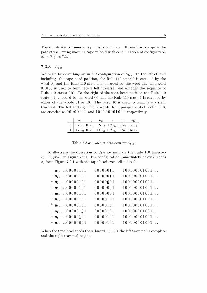
7 Small weakly universal machines 116
The simulation of timestep c1 ⊢ c2 is complete. To see this, compare thepart of the Turing machine tape in bold with cells −11 to 4 of configurationc2 in Figure 7.2.1.
7.3.3 U6,2
We begin by describing an initial configuration of U6,2. To the left of, andincluding, the tape head position, the Rule 110 state 0 is encoded by theword 00 and the Rule 110 state 1 is encoded by the word 11. The word010100 is used to terminate a left traversal and encodes the sequence ofRule 110 states 010. To the right of the tape head position the Rule 110state 0 is encoded by the word 00 and the Rule 110 state 1 is encoded byeither of the words 01 or 10. The word 10 is used to terminate a righttraversal. The left and right blank words, from paragraph 4 of Section 7.3,are encoded as 0 0 0 0 0 1 0 1 and 1 0 0 1 0 0 0 0 1 0 0 1 respectively.
u1 u2 u3 u4 u5 u6
0 0Lu1 0Lu6 0Ru2 1Ru5 1Lu4 1Lu1
1 1Lu2 0Lu3 1Lu3 0Ru6 1Ru4 0Ru4
Table 7.3.3: Table of behaviour for U6,2.
To illustrate the operation of U6,2 we simulate the Rule 110 timestepc0 ⊢ c1 given in Figure 7.2.1. The configuration immediately below encodesc0 from Figure 7.2.1 with the tape head over cell index 0.
u1u1u1, . . . 0 0 0 0 0 1 0 1 0 0 0 0 0 0 1 1 1 0 0 1 0 0 0 0 1 0 0 1 . . .
⊢ u2u2u2, . . . 0 0 0 0 0 1 0 1 0 0 0 0 0 0 1 1 1 0 0 1 0 0 0 0 1 0 0 1 . . .
⊢ u3u3u3, . . . 0 0 0 0 0 1 0 1 0 0 0 0 0 0 0 1 1 0 0 1 0 0 0 0 1 0 0 1 . . .
⊢ u2u2u2, . . . 0 0 0 0 0 1 0 1 0 0 0 0 0 0 0 1 1 0 0 1 0 0 0 0 1 0 0 1 . . .
⊢ u6u6u6, . . . 0 0 0 0 0 1 0 1 0 0 0 0 0 0 0 1 1 0 0 1 0 0 0 0 1 0 0 1 . . .
⊢ u1u1u1, . . . 0 0 0 0 0 1 0 1 0 0 0 0 0 1 0 1 1 0 0 1 0 0 0 0 1 0 0 1 . . .
⊢5 u1u1u1, . . . 0 0 0 0 0 1 0 1 0 0 0 0 0 1 0 1 1 0 0 1 0 0 0 0 1 0 0 1 . . .
⊢ u2u2u2, . . . 0 0 0 0 0 1 0 1 0 0 0 0 0 1 0 1 1 0 0 1 0 0 0 0 1 0 0 1 . . .
⊢ u6u6u6, . . . 0 0 0 0 0 1 0 1 0 0 0 0 0 1 0 1 1 0 0 1 0 0 0 0 1 0 0 1 . . .
⊢ u4u4u4, . . . 0 0 0 0 0 0 0 1 0 0 0 0 0 1 0 1 1 0 0 1 0 0 0 0 1 0 0 1 . . .
When the tape head reads the subword 1 0 1 0 0 the left traversal is completeand the right traversal begins.

7 Small weakly universal machines 117
⊢ u5u5u5, . . . 0 0 0 0 0 0 1 1 0 0 0 0 0 1 0 1 1 0 0 1 0 0 0 0 1 0 0 1 . . .
⊢ u4u4u4, . . . 0 0 0 0 0 0 1 1 0 0 0 0 0 1 0 1 1 0 0 1 0 0 0 0 1 0 0 1 . . .
⊢ u5u5u5, . . . 0 0 0 0 0 0 1 1 1 0 0 0 0 1 0 1 1 0 0 1 0 0 0 0 1 0 0 1 . . .
⊢ u4u4u4, . . . 0 0 0 0 0 0 1 1 1 1 0 0 0 1 0 1 1 0 0 1 0 0 0 0 1 0 0 1 . . .
⊢ u6u6u6, . . . 0 0 0 0 0 0 1 1 0 1 0 0 0 1 0 1 1 0 0 1 0 0 0 0 1 0 0 1 . . .
⊢ u4u4u4, . . . 0 0 0 0 0 0 1 1 0 0 0 0 0 1 0 1 1 0 0 1 0 0 0 0 1 0 0 1 . . .
⊢4 u4u4u4, . . . 0 0 0 0 0 0 1 1 0 0 0 0 0 1 0 1 1 0 0 1 0 0 0 0 1 0 0 1 . . .
⊢ u5u5u5, . . . 0 0 0 0 0 0 1 1 0 0 0 0 1 1 0 1 1 0 0 1 0 0 0 0 1 0 0 1 . . .
⊢ u4u4u4, . . . 0 0 0 0 0 0 1 1 0 0 0 0 1 1 0 1 1 0 0 1 0 0 0 0 1 0 0 1 . . .
⊢2 u4u4u4, . . . 0 0 0 0 0 0 1 1 0 0 0 0 1 1 1 1 1 0 0 1 0 0 0 0 1 0 0 1 . . .
⊢ u6u6u6, . . . 0 0 0 0 0 0 1 1 0 0 0 0 1 1 1 1 0 0 0 1 0 0 0 0 1 0 0 1 . . .
⊢ u1u1u1, . . .00000011 00001111 0 1 0 1 0 0 0 0 1 0 0 1 . . .
Immediately after the tape head reads a 10, during a right traversal, thesimulation of timestep c0 ⊢ c1 is complete. To see this, compare the part ofthe Turing machine tape in bold (recall 0 and 1 are encoded as 00 and 11respectively) with cells −7 to 0 of configuration c1 in Figure 7.2.1.
7.4 Discussion
The pursuit to find the smallest possible universal Turing machine mustalso involve the search for lower bounds, finding the largest set of Turingmachines that are in some sense non-universal. One approach is to settlethe decidability of the halting problem, but this approach is not suitable forthe non-halting machines we have presented.
It is known that the halting problem is decidable for (standard) Tur-ing machines with the following state-symbol pairs (2, 2) [Kud96, Pav73],(3, 2) [Pav78], (2, 3) (claimed by Pavlotskaya [Pav73]), (1, n) [Her68c] and(n, 1) (trivial), where n > 1. Then, these decidability results imply that auniversal Turing machine, that simulates any Turing machine M and haltsif and only if M halts, is not possible for these state-symbol pairs. Hencethese results give lower bounds on the size of universal machines of thistype. While it is trivial to prove that the halting problem is decidable for(possibly halting) weak machines with state-symbol pairs of the form (n, 1),it is not known whether the above decidability results generalise to (possiblyhalting) weak Turing machines.
The weakly universal machines presented in this chapter, and thosein [Coo04], do not halt. Hence the non-universality results discussed in theprevious paragraph would have to be generalised to non-halting weak ma-chines to give lower bounds. This may prove difficult for two reasons. The
7 Small weakly universal machines 118
first issue is that, intuitively speaking, weakness gives quite an advantage.For instance, the program of a universal machine may be encoded in one ofthe infinitely repeated blank words of the weak machine. The second issueis related to the problem of defining a computation. Informally, a computa-tion could be defined as a sequence of configurations that ends with a specialterminal configuration. For non-halting machines, there are many ways todefine a terminal configuration. Given a definition of terminal configurationwe may prove that the terminal configuration problem (will a machine everenter a terminal configuration?) is decidable for a machine or set of ma-chines. However this result may not hold as a proof of non-universality ifwe subsequently alter our definition of terminal configuration.
It is trivial that no weakly universal Turing machines exist for the state-symbol pair (n, 1) even when we consider machines with no halting condition.We also believe that such relevant decidability results for the state-symbolpair (2, 2) may also be given. If this is true, then the problem for 2-stateand 3-state weakly universal machines only remains open for (2, 3) and (3, 2)respectively.
Margenstern [Mar00] and Baiocchi [Bai98] constructed small machinesthat simulate iterations of the Collatz (3x + 1) problem. The size of thesmallest known weakly universal machines are quite close to the possibleminimum size for weakly universal machines. Implementing the Collatzproblem on weak machines could be an interesting way of exploring thelittle space remaining between these machines and the state-symbol pairswhere weak universality is not possible.

8
Conclusion
Our results reduce the size and improve the time efficiency of many of thesimplest known models of computation.
We presented new polynomial time (standard) universal Turing machineswith state-symbol pairs of (5, 5), (6, 4), (9, 3) and (15, 2). These machinessimulate our new variant of tag system, the bi-tag system, and are thesmallest known universal Turing machines with 5, 4, 3 and 2-symbols re-spectively. Our 5-symbol machine uses the same number of instructions(22) as the smallest known universal Turing machine (Rogozhin’s 6-symbolmachine [Rog96]).
We have shown that 2-tag systems efficiently simulate Turing machines.As a corollary, we find that the small universal Turing machines of Rogozhin,Minsky and others simulate Turing machines in polynomial time. This is anexponential improvement on the previously known simulation time overheadand improves on a forty-year old result. We also introduced a new form of tagsystem which we call a bi-tag system. We prove bi-tag systems are universalby showing they efficiently simulate Turing machines in polynomial time.
We have shown that cyclic tag systems are polynomial simulators ofTuring machines. This result is used to prove that Rule 110, one of themost intuitively simple cellular automata, is P-complete to predict. In fact,we proved that Rule 110 is a polynomial simulator of Turing machines. Asa corollary of this result, we find that the smallest weakly universal Turingmachines simulate Turing machines efficiently in polynomial time. All ofthese results represent an exponential improvement.
We have given the smallest efficient universal Turing machines that sim-ulate Turing machines in O(t2) time. They are also the smallest knownmachines where direct simulation of Turing machines is the technique usedto establish their universality. This result also gives a new algorithm forsmall universal Turing machines.
We presented the smallest known weakly universal Turing machines.These machines have state-symbol pairs of (6, 2), (3, 3) and (2, 4). The3-state and 2-state machines are very close to the minimum possible size forweakly universal machines with 3 and 2 states, respectively.
We have given new results for many different simple universal modelsincluding Turing machines, weak Turing machines, tag systems and cellular
119

8 Conclusion 120
automata. These models have applications for a variety of other results. Forinstance the results surveyed in Section 5.3.1 rely on simulations of 2-tagsystems. Many of these results also rely on simulation of small universalTuring machines. It is possible that the (much smaller) weakly universalmachines from Chapter 7 may also be of use in some of these simulations togive further improvements. In particular our weak machines may be usedwith the results of Lindgren and Nordahl [LN90] to give simple universalcellular automata that use periodic backgrounds. We have already seenan application of Rule 110 in constructing small efficient weakly universalmachines in Chapter 7 and similar applications of cyclic tag systems inconstructing efficient semi-weakly universal machines in [WN07b, WNb].More recently, our new 4-symbol universal Turing machine from Chapter 6was used to give a small universal spiking neural P system [Nea08a]. Nodoubt, other interesting applications are out there waiting to be discovered.
8.1 Future work
8.1.1 Standard Turing machines and program size
Perhaps one of the most obvious aims is to further reduce the size of thesmallest (standard) universal Turing machines. As noted in Section 6.3 wesuspect that some radically new techniques are needed to significantly reducethe size of the smallest known machines.
The search for the smallest universal Turing machine goes hand-in-handwith the search for decidability results. Decidability results provide usefullower bounds for small universal Turing machines. In Section 6.1 we saw thatthe universality/non-universality question still remains open for 39 state-symbol pairs. There has been no improvement on Pavlotskaya’s [Pav78]result that the halting problem is decidable for 3-state, 2-symbol machines,which was given in 1978. Pavlotskaya’s proof is quite long and complex.As the state-symbol product increases, the number of possible machinesincreases exponentially, thus it seems that a new approach needs to be taken.To find new lower bounds one possible method is to prove that some non-universal system simulates all of the standard Turing machines for a givenstate-symbol pair.
8.1.2 Weak Turing machines and program size
It would be interesting to give decidability results (lower bounds) for non-halting weak Turing machines. To date, no relevant decidability results havebeen given for such machines. Such results would provide lower boundsrelevant to our weakly universal machines in Chapter 7. We discussed theproblem of giving these lower bounds in Section 7.4. It is trivial that noweakly universal Turing machine exists for the state-symbol pair (n, 1) even
8 Conclusion 121
when we consider machines with no halting condition. We also conjecturethat relevant decidability results for the state-symbol pair (2, 2) may also begiven. If this is true, the problem for 2-state and 3-state weakly universalmachines only remains open for (2, 3) and (3, 2) respectively.
Margenstern [Mar00] and Baiocchi [Bai98] constructed small machinesthat simulate iterations of the Collatz (3x + 1) problem. It would be in-teresting to construct weak machines to simulate this problem. The size ofthe smallest known weakly universal machines are quite close to the possi-ble minimum size for weakly universal machines. Implementing the Collatzproblem on weak machines could be an interesting way of exploring the littlespace remaining between these machines and the state-symbol pairs whereweak universality is not possible.
8.1.3 Time efficiency of simple universal models
It would be interesting to study the time complexity of small multitape Tur-ing machines. For instance, what about simple universal Turing machineswith more than one tape that simulate Turing machines in linear time? Wenoted in Section 3.6 that the algorithm we suggested for linear time uni-versal Turing machines may require many transition rules. Constructing asmall 2-tape linear time simulator could perhaps be more easily achieved:one tape could contain the simulated tape contents and tape head positionand the other tape could contain the encoded table of behaviour to searchfor the next instruction. This would avoid scanning back and forth throughthe tape contents to simulate a transition rule.
It would also be interesting to see if the time efficiency of 2-tag systems,bi-tag systems and cyclic tag systems may be improved further.
8.1.4 The not halting problem
In Section 2.2 we discuss a number of different definitions of universal Turingmachine. A number of authors have given definitions for universal Turingmachines that do not require the machine to halt. Our small weakly univer-sal Turing machines in Chapter 7 are non-halting. What about proving rel-evant non-universality results? Such non-universality results are not achiev-able by proving the halting problem decidable. Before we attempt such anendeavor we must agree on the assumptions for the definition of universalTuring machine. We allow the following generalisation of Definition 2.1.7,instead of the computation ending with a single terminal configuration, thecomputation ends with a finite configuration sequence called the terminalconfiguration sequence. The output of the simulated Turing machine is re-trieved by applying the recursive decoding function to this sequence. Thereare many ways to define a terminal configuration sequence. Some examplesof possible terminal configuration sequences are:

8 Conclusion 122
• The configurations containing a given sequence of states.
• A sequence containing two identical configurations.
• A single configuration containing a constant word.
Given a definition of a terminal configuration sequence we may prove thatthe terminal sequence problem (will a machine ever execute a terminal con-figuration sequence) is decidable. This gives non-universal lower bounds thatare relevant to universal machines that end their computation with such asequence. However, this result may not hold as a proof of non-universality ifwe subsequently alter our definition of terminal configuration sequence. Onemore general approach is to prove that the terminal sequence problem for allpossible terminal sequences, of a machine or set of machines, is decidable.
Definition 2.1.7, augmented with the notion of terminal configurationsequences, is a generalisation on the definitions of Davis and Priese, whichwere discussed in Section 2.2. We propose this definition as an attempt toinclude as many reasonable models as possible.
8.1.5 Some final questions
In Figure 1.3.1 the smallest (standard) universal machines are currently notsymmetric about the line where states equals symbols. Are the smallest pos-sible universal Turing machines symmetric about the states equals symbolsline?
Following the work in this thesis, all of the smallest known weakly, semi-weakly, and standard universal Turing machines now simulate Turing ma-chines efficiently in polynomial time. Are all of the smallest possible univer-sal Turing machines efficient polynomial time simulators?
Currently the smallest weakly universal Turing machines are significantlysmaller than the smallest standard universal Turing machines. The 3-state,3-symbol weakly universal machine, given in Chapter 7, sits in the armchairthat is the current decidability curve for standard machines. Is this weaklyuniversal machine smaller than the smallest possible standard universal Tur-ing machine?
Finally, there is no need to restate Shannon’s famous question here!

Notation
M single tape deterministic Turing machine
qx an internal state of M
t the running time of M
U a universal Turing machine
Um,n a universal Turing machine with m state and n symbols
ux an internal state of Um,n
⊢ a single computation step
⊢s a sequence of s computation steps
⊢∗ a sequence of > 0 computation steps
N non-negative integers
Σ∗ set of all words of length > 0 over alphabet Σ = {σ1, σ1, . . . , σn}
w a word over some alphabet Σ
|w| the length of the word w
ǫ the empty word, |ǫ| = 0
ω cardinality of N
〈X〉 the encoding of object X as a word
A−B The set containing all the elements of set A that are not elements of set B
A×B The set of ordered pairs (a, b) such that a ∈ A and b ∈ B
123
Bibliography
[Aar02] Scott Aaronson. Book review: A new kind of science. QuantumInformation and Computation, 2(5):410–423, August 2002.
[AC87] Jurgen Albert and Karel Culik II. A simple universal cellularautomaton and its one-way and totalistic version. ComplexSystems, 1(1):1–16, 1987.
[AF67] Stal Aanderaa and Patrick C. Fischer. The solvability of thehalting problem for 2-state Post machines. Journal of theAssociation for Computing Machinery (ACM), 14(4):677–682,1967.
[AFR06] Artiom Alhazov, Rudolf Freund, and Yurii Rogozhin. Com-putational power of symport/antiport: history, advances andopen problems. In Rudolf Freund, Georg Lojka, Marion Os-wald, and Gheorghe Paun, editors, Sixth international Work-shop on Membrane Computing (2005), volume 3850 of LNCS,pages 1–30, Vienna, July 2006. Springer.
[AKR02] Artiom Alhazov, Manfred Kudlek, and Yurii Rogozhin. Nineuniversal circular Post machines. Computer Science Journalof Moldova, 10(3):247–262, 2002.
[AR06] Artiom Alhazov and Yurii Rogozhin. Towards a characteri-zation of P systems with minimal symport/antiport and twomembranes. In Hendrik Jan Hoogenboom, Gheorghe Paun,Grzegorz Rozenberg, and Arto Salomaa, editors, Seventh in-ternational Workshop on Membrane Computing, volume 4361of LNCS, pages 135–153, Leiden, The Netherlands, July 2006.Springer.
[Bai98] Claudio Baiocchi. 3n+1, UTM e tag-system. Technical ReportPubblicazione 98/38, Dipartimento di Matematico, Universitadi Roma, 1998. (In Italian).
124

BIBLIOGRAPHY 125
[Bai01] Claudio Baiocchi. Three small universal Turing machines.In Maurice Margenstern and Yurii Rogozhin, editors, Ma-chines, Computations, and Universality (MCU), volume 2055of LNCS, pages 1–10, Chisinau, Moldova, May 2001. Springer.
[Ban70] Edwin R. Banks. Universality in cellular automata. In Confer-ence Record of the Eleventh Annual Symposium on Switchingan Automata Theory (FOCS), pages 194–215, Santa Monica,California, 1970. IEEE.
[BCG82] Elwyn Berlekamp, John Conway, and Richard Guy. Winningways for your mathematical plays, vol 2: Games in particular.Academic Press, New York, 1982.
[Ben73] Charles H. Bennett. Logical reversibility of computation. IBMJournal of Research and Development, 17(6):525–532, Novem-ber 1973.
[Bra83] Allen Brady. The determination of the value of Rado’s non-computable function Σ(k) for four-state Turing machines.Mathematics of Computation, 40(162):647–665, April 1983.
[CM63] John Cocke and Marvin Minsky. Universality of tag systemswith P = 2, April 1963. AIM-52, A.I. memo 52, Computer Sci-ence and Artificial Intelligence Laboratory, MIT, Cambridge,Massachusetts.
[CM64] John Cocke and Marvin Minsky. Universality of tag systemswith P = 2. Journal of the Association for Computing Ma-chinery (ACM), 11(1):15–20, 1964.
[Cod68] Edgar F. Codd. Cellular Automata. Academic Press, NewYork, 1968.
[Coo66] Stephen Cook. The solvability of the derivability problem forone-normal systems. Journal of the Association for ComputingMachinery (ACM), 13(2):233–225, 1966.
[Coo04] Matthew Cook. Universality in elementary cellular automata.Complex Systems, 15(1):1–40, 2004.
[CVMVV07] Erzsebet Csuhaj-Varju, Maurice Margenstern, Gyorgy Vaszil,and Sergey Verlan. On small universal antiport P systems.Theoretical Computer Science, 372(2-3):152–164, 2007.
[Dav56] Martin Davis. A note on universal Turing machines. AutomataStudies, Annals of Mathematics Studies, 34:167–175, 1956.

BIBLIOGRAPHY 126
[Dav57] Martin Davis. The definition of universal Turing machine.Proceedings of the American Mathematical Society, 8(6):1125–1126, dec 1957.
[Dav58] Martin Davis. Computability and Unsolvability. McGraw-Hill,New York, 1958.
[Dav65] Martin Davis. The undecidable: basic papers on undecidablepropositions, unsolvable problems and computable functions.Raven Press, New York, 1965.
[De Mol07] Liesbeth De Mol. Study of the limits of solvability in tag sys-tems. In Jerome Durand-Lose and Maurice Margenstern, ed-itors, Machines, Computations, and Universality (MCU), vol-ume 4664 of LNCS, pages 170–181, Orleans, France, Septem-ber 2007. Springer.
[DK89] Volker Diekert and Manfred Kudlek. Small deterministic Tur-ing machines. Papers on Automata and Languages, Depart-ment of Mathematics, Karl Marx University of Economics,Budapest, 1988-4:77–87, 1989.
[DKB04] Jean-Charles Delvenne, Petr Kurka, and Vincent Blondel.Computational universality in symbolic dynamical systems. InMaurice Margenstern, editor, Machines, Computations, andUniversality (MCU), volume 3354 of LNCS, pages 104–115,Saint Petersburg, Russia, September 2004. Springer.
[Fis65] Patrick C. Fischer. On formalisms for Turing machines.Journal of the Association for Computing Machinery (ACM),12(4):570–580, 1965.
[FMKY00] Claudio Ferretti, Giancarlo Mauri, Satoshi Kobayashi, andTakashi Yokomori. On the universality of Post and splicingsystems. Theoretical Computer Science, 231(2):157–170, Jan-uary 2000.
[FO06] Rudolf Freund and Marion Oswald. Small universal antiportP systems and universal multiset grammars. In Carmen Gra-ciani Dıaz, Gheorghe Paun, Alvaro Romero-Jimenez, and Fer-nando Sancho-Caparrini, editors, Fourth Brainstorming Weekon Membrane Computing (Volume II), pages 51–64, Sevilla,Spain, 2006.
[GHR95] Raymond Greenlaw, H. James Hoover, and Walter L. Ruzzo.Limits to parallel computation: P -completeness theory. Ox-ford University Press, Oxford, 1995.

BIBLIOGRAPHY 127
[Hea87] Tom Head. Formal language theory and DNA: An analysisof the generative capacity of specific recombinant behaviours.Bulletin of Mathematical Biology, 49(6):737–759, 1987.
[Her66a] Gabor T Hermann. The halting problem of generalized onestate Turing machines. Master’s thesis, University of Califor-nia, Berkeley, 1966.
[Her66b] Gabor T Hermann. On the impossibility of a one state univer-sal Turing machines. Technical report, Electronics ResearchLaboratory, University of California, Berkeley, 1966.
[Her68a] Gabor T Hermann. The halting problem of one state Turingmachines with n-dimensional tape. Zeitshrift fur Mathema-tische Logik-und Grundlagen der Matematik, 14(2):185–191,1968.
[Her68b] Gabor T Hermann. Simulation of one abstract computingmachine by another. Communications of the Association forComputing Machinery (ACM), 11(12):802 and 813, 1968.
[Her68c] Gabor T Hermann. The uniform halting problem for gener-alized one state Turing machines. In Proceedings, Ninth An-nual Symposium on Switching and Automata Theory (FOCS),pages 368–372, Schenectady, New York, October 1968. IEEEComputer Society Press.
[HM03] Fracine Herrmann and Maurice Margenstern. A universal cel-lular automaton in the hyperbolic plane. Theoretical ComputerScience, 296(2):327–364, 2003.
[HM05] Tero Harju and Maurice Margenstern. Splicing systems foruniversal Turing machines. volume 3384 of LNCS, pages 149–158, Milan, Italy, 2005. Springer, Heiedlberg.
[Hoo63] Philip Hooper. Some small, multitape universal Turing ma-chines. Technical report, Computation Labortory, HarvardUniversity, Cambridge, Massachusetts, 1963.
[Hoo69] Philip Hooper. Some small, multitape universal Turing ma-chines. Information Sciences, 1(2):205–215, 1969.
[HU79] John E. Hopcroft and Jeffrey D. Ullman. Introduction to au-tomata theory, languages, and computation. Addison-WesleySeries in Computer Science. Addison-Wesley, Reading, Mas-sachusetts, 1979.
BIBLIOGRAPHY 128
[IIM07] Katsunobu Iami, Chuzo Iwanmoto, and Kenichi Morita. Afive-state von Neumann neighbor universal hyperbolic cellularautomaton. Journal of Cellular Automata, 1(4):275–297, 2007.
[Ike58] N Ikeno. A 6-symbol 10-state universal Turing machine. InProceedings, Institute of Electrical Communications Tokyo,1958.
[Ind95] Piotr Indyk. Optimal simulation of automata by neural nets.In Ernst Mayr and Claude Puech, editors, Twelfth AnnualSymposium on Theoretical Aspects of Computer Science, vol-ume 900, pages 337–348, 1995.
[IPY06] Mihai Ionescu, Gheorghe Paun, and T Yokomori. Spikingneural P systems. Fundamenta Informaticae, 71(2-3):279–308,2006.
[KB77] Hans Kleine-Buning. Uber probleme bei homogener Parket-tierung von Z × Z durch Mealy-automaten bei normierterverwendung. PhD thesis, Institut fur Mathematische Logik,Munster, 1977.
[KBO77] Hans Kleine-Buning and Thomas Ottmann. Kleine universellemehrdimensionale Turingmaschinen. Elektronische Informa-tionsverarbeitung und Kybernetik, 13(4-5):179–201, 1977.
[KCG94] Pascal Koiran, Michel Cosnard, and Max H. Garzon. Com-putability with low dimensional dynamical systems. Theoret-ical Computer Science, 132(1-2):113–128, 1994.
[Kor96] Ivan Korec. Small universal register machines. TheoreticalComputer Science, 168(2):267–301, 1996.
[KR01a] Manfred Kudlek and Yurii Rogozhin. New small universal cir-cular Post machines. In Rusins Freivalds, editor, Fundamentalsof Computation Theory (FCT), volume 2138 of LNCS, pages217–227, Riga, Latvia, August 2001. Springer.
[KR01b] Manfred Kudlek and Yurii Rogozhin. Small universal circu-lar Post machines. Computer Science Journal of Moldova,9(1):34–52, 2001.
[KR02] Manfred Kudlek and Yurii Rogozhin. A universal Turing ma-chine with 3 states and 9 symbols. In Werner Kuich, Grze-gorz Rozenberg, and Arto Salomaa, editors, Developments inLanguage Theory (DLT) 2001, volume 2295 of LNCS, pages311–318, Vienna, May 2002. Springer.

BIBLIOGRAPHY 129
[KR03] Manfred Kudlek and Yurii Rogozhin. Small universal Turingand circular Post machines. Pure Mathematics and Applica-tions, 13(1-2):197–210, 2003.
[Kry67] Y Kryukov. Turing machines with two symbols and threestates. Algebra i Logka, 16(3):54–60, 1967.
[Kry71] Y Kryukov. Turing machines with three states and two sym-bols and with one state and n symbols. Kibernetika, 1:12–13,1971.
[KS96] Joe Kilian and Hava Siegelmann. The dynamic universalityof sigmoidal neural networks. Information and Computation,128(1):48–56, 1996.
[Kud96] Manfred Kudlek. Small deterministic Turing machines. Theo-retical Computer Science, 168(2):241–255, 1996.
[LN90] Kristian Lindgren and Mats G. Nordahl. Universal compu-tation in simple one-dimensional cellular automata. ComplexSystems, 4(3):299–318, 1990.
[LP07] Gregory Lafitte and Christophe Papazian. The fabric of smallTuring machines. In S. Barry Cooper, Thomas Kent, BenediktLowe, and Andrea Sorbi, editors, Computation and Logic inthe Real World (CIE 2007), Universita Degli Studi di Siena,Dipartimento di Scienze Matematiche ed Informariche, Tech-nical Report number 487, pages 219–227, Siena, Italy, June2007. Springer.
[LR65] Shen Lin and Tibor Rado. Computer studies of Turing ma-chine problems. Journal of the Association for Computing Ma-chinery (ACM), 12(2):196–212, 1965.
[Mar92] Maurice Margenstern. Sur la frontiere entre machines de Tur-ing a arret decidable et machines de Turing universelles. Tech-nical Report 92-83, LITP Institut Blaise Pascal, 1992.
[Mar93] Maurice Margenstern. Non-erasing Turing machines: A fron-tier between a decidable halting problem and universality. InZoltan Esik, editor, FCT, volume 710 of LNCS, pages 375–385,Szeged, Hungry, August 1993. Springer, Heidelberg.
[Mar94] Maurice Margenstern. Une machine de Turing universelle sur{0,1}, non-effacante et a trois instructions gauches. TechnicalReport 94-08, LITP Institut Blaise Pascal, 1994.

BIBLIOGRAPHY 130
[Mar95a] Maurice Margenstern. Non-erasing Turing machines: A newfrontier between a decidable halting problem and universal-ity. In Ricardo A. Baeza-Yates, Patricio V. Poblete, and EricGoles, editors, LATIN, volume 911 of LNCS, pages 386–397,Valparaıso, Chile, 1995. Springer, Heidelberg.
[Mar95b] Maurice Margenstern. Une machine de Turing universellenon-effacante a exactement trois instructions gauches. CRAS,Paris, 320(I):101–106, 1995.
[Mar97a] Maurice Margenstern. Decidability and undecidability of thehalting problem on Turing machines, a survey. In SergeiAdian and Anil Nerode, editors, Logical Foundations of Com-puter Science (LFCS), volume 1234 of LNCS, pages 226–236,Yaroslav, Russia, July 1997. Springer.
[Mar97b] Maurice Margenstern. The laterality problem for non-erasingTuring machines on {0,1} is completely solved. TheoreticalInformatics and Applications, 31(2):159–204, 1997.
[Mar98] Maurice Margenstern. Frontier between decidability and un-decidability: a survey. In Maurice Margenstern, editor, Ma-chines, Computations, and Universality (MCU) volume 1,pages 141–177, France, May 1998. IUT, Metz.
[Mar00] Maurice Margenstern. Frontier between decidability andundecidability: a survey. Theoretical Computer Science,231(2):217–251, 2000.
[Mar01] Maurice Margenstern. On quasi-unilateral universal Turingmachines. Theoretical Computer Science, 257(1–2):153–166,2001.
[Mar06] Maurice Margenstern. An algorithm for building intrinsicallyuniversal cellular automata in hyperbolic spaces. In Hamid R.Arabnia and Mark Murgin, editors, Proceedings of the 2006International Conference on Foundation of Computer Science,pages 3–9, Las Vegas, Nevada, June 2006. CSREA Press.
[MB90] Heiner Marxen and Jurgen Butrock. Attacking the BusyBeaver 5. Bulletin of the European Association for TheoreticalComputer Science, 40:247–251, 1990.
[MF05] Daniel Miller and Edward Fredkin. Two-state, reversible, uni-versal cellular automata in three dimensions. In 2nd Confer-ence on Computing Frontiers, pages 45–51, Ischia, Italy, 2005.ACM Press.
BIBLIOGRAPHY 131
[MH89] Kenichi Morita and Masateru Harao. Computation universal-ity of one-dimensional reversible (injective) cellular automata.The Transactions of the IEICE Japan, E72(6):758–762, 1989.
[Mic93] Pascal Michel. Busy beaver competition and Collatz-like prob-lems. Archive Mathematical Logic, 32(5):351–367, 1993.
[Mic04] Pascal Michel. Small Turing machines and the general-ized busy beaver competition. Theoretical Computer Science,326:45–56, 2004.
[Min60a] Marvin Minsky. A 6-symbol 7-state universal Turing machines.Technical Report 54-G-027, Licoln Laboratory, MIT, Cam-bridge, Massachusetts, August 1960.
[Min60b] Marvin Minsky. Recursive unsolvability of Post’s tag prob-lem. Technical Report 54 G-023, Licoln Laboratory, MIT,Cambridge, Massachusetts, June 1960.
[Min61] Marvin Minsky. Recursive unsolvability of Post’s problem oftag and other topics in theory of Turing machines. Annals ofMathematics, 74(3):437–455, 1961.
[Min62a] Marvin Minsky. Size and structure of universal Turing ma-chines using tag systems. In Recursive Function Theory, Pro-ceedings, Symposium in Pure Mathematics, volume 5, pages229–238, Provelence, 1962. American Mathematical Society.
[Min62b] Marvin Minsky. Universality of (p=2) tag systems and a 4symbol 7 state universal Turing machine, 1962. AIM-33, A.I.memo 33, Computer Science and Artificial Intelligence Labo-ratory, MIT, Cambridge, Massachusetts.
[Min67] Marvin Minsky. Computation, finite and infinite machines.Prentice-Hall, Englewood Cliffs, New Jersey, 1967.
[Moo52] Edgar F. Moore. A simplified universal Turing machine. InACM national meeting, pages 50–54, Toronto, Canada, 1952.ACM Press.
[Moo97a] Cristopher Moore. Majority-vote cellular automata, Ising dy-namics, and P-completeness. Journal of Statistical Physics,88(3-4):795–805, 1997.
[Moo97b] Cristopher Moore. Quasi-linear cellular automata. Physica D,103:100–132, 1997.

BIBLIOGRAPHY 132
[Moo98] Cristopher Moore. Predicting non-linear cellular automataquickly by decomposing them into linear ones. Physica D,111:27–41, 1998.
[Mor96] Kenichi Morita. Universality of a reversible two-counter ma-chine. Theoretical Computer Science, 168(2):303–320, Novem-ber 1996.
[MP43] Warren McCulloch and Walter Pitts. A logical calculus ofideas immanent in nervous activity. Bulletin of MathematicalBiophysics, 5:115–133, 1943.
[MP95a] Maurice Margenstern and Liudmila Pavlotskaya. Deux ma-chines de Turing universelles a au plus deux instructionsgauches. Technical Report I, CRAS, Paris, 1995.
[MP95b] Maurice Margenstern and Liudmila Pavlotskaya. Vers ue nou-velle approche de l’universalite concernant les machines deTuring. Technical Report 95-58, LITP Institut Blaise Pascal,1995.
[MP03] Maurice Margenstern and Liudmila Pavlotskaya. On the opti-mal number of instructions for universality of Turing machinesconnected with a finite automaton. International Journal ofAlgebra and Computation, 13(2):133–202, 2003.
[MR02] Maurice Margenstern and Yurii Rogozhin. A universal time-varying distributed H system of degree 1. In Natasa Jonoskaand Nadrain C. Seeman, editors, DNA-7(2001), volume 2340of LNCS, pages 371–380, Tampa, Florida, 2002. Springer.
[MSG89] Kenichi Morita, Akihiko Shirasaki, and Yoshifumi Gono. A1-tape 2-symbol reversible Turing machine. The Transactionsof the IEICE Japan, E72(3):223–228, 1989.
[MY07] Kenichi Morita and Yoshikazu Yamaguchi. A universal re-versible Turing machine. In Jerome Durand-Lose and MauriceMargenstern, editors, Machines, Computations, and Univer-sality (MCU), volume 4664 of LNCS, pages 90–98, Orleans,France, September 2007. Springer.
[Nea06] Turlough Neary. Small polynomial time universal Turing ma-chines. In Ted Hurley, A. Seda, et al., editors, 4th Irish Con-ference on the Mathematical Foundations of Computer Scienceand Information Technology(MFCSIT), pages 325–329, Cork,Ireland, August 2006.

BIBLIOGRAPHY 133
[Nea08a] Turlough Neary. On the computational complexity of spikingneural P systems. In Unconventional Computation, 7th Inter-national Conference, UC 2008, volume 5204 of LNCS, pages189–205, Vienna, August 2008. Springer.
[Nea08b] Turlough Neary. A small universal spiking neural P system.In International Workshop on Computing with Biomolecules,pages 65–74, Vienna, August 2008. Austrian Computer Soci-ety.
[Noz69] A. Nozaki. On the notion of universality of Turing machine.Kybernetika Academia Praha, 5(1):29–43, 1969.
[NPRP06] Hitesh Nagda, Andrei Paun, and Alfonso Rodrıguez-Paton.P systems with symport/antiport and time. In Hendrik JanHoogenboom, Gheorghe Paun, Grzegorz Rozenberg, and ArtoSalomaa, editors, Seventh international Workshop on Mem-brane Computing, volume 4361 of LNCS, pages 463–476, Lei-den, The Netherlands, 2006.
[NW] Turlough Neary and Damien Woods. Four small universalTuring machines. Fundamenta Informaticae. (Accepted).
[NW05a] Turlough Neary and Damien Woods. A small fast universalTuring machine. Technical Report NUIM-CS-TR-2005-12, De-partment of Computer Science, National university of Ireland,Maynooth, 2005.
[NW05b] Turlough Neary and Damien Woods. Small fast universal Tur-ing machines. Technical Report NUIM-CS-TR-2005-11, De-partment of Computer Science, National university of Ireland,Maynooth, 2005.
[NW06a] Turlough Neary and Damien Woods. P-completeness of cel-lular automaton Rule 110. In Michele Bugliesi, Bart Preneel,Vladimiro Sassone, and Ingo Wegener, editors, InternationalColloquium on Automata Languages and Programing 2006,(ICALP) Part I, volume 4051 of LNCS, pages 132–143, Venice,July 2006. Springer.
[NW06b] Turlough Neary and Damien Woods. P-completeness of cel-lular automaton Rule 110. Technical Report 04/2006, BooleCentre for Research in Informatics, University College Cork,Ireland, 2006.
[NW06c] Turlough Neary and Damien Woods. Small fast universal Tur-ing machines. Theoretical Computer Science, 362(1–3):171–195, October 2006.

BIBLIOGRAPHY 134
[NW07a] Turlough Neary and Damien Woods. Four small universalTuring machines. In Jerome Durand-Lose and Maurice Mar-genstern, editors, Machines, Computations, and Universal-ity (MCU), volume 4664 of LNCS, pages 242–254, Orleans,France, September 2007. Springer.
[NW07b] Turlough Neary and Damien Woods. Small weakly universalTuring machines. Technical Report arXiv:0707.4489v1 [cs.CC],July 2007.
[Oll02] Nicolas Ollinger. The quest for small universal cellular au-tomata. In Peter Widmayer et al., editor, International Collo-quium on Automata, Languages and Programming (ICALP),volume 2380 of LNCS, pages 318–329, Malaga, Spain, July2002. Springer.
[Ott75a] Thomas Ottmann. Eine universelle Turingmaschine mit zwei-dimensionalem band. Elektronische Informationsverarbeitungund Kybernetik, 11(1-2):27–38, 1975. (In German).
[Ott75b] Thomas Ottmann. Einfache universelle mehrdimensionaleTuringmaschinen. Habilitationsschrift, Karlsruhe, 1975.
[Pap95] Christos Papadimitriou. Computational complexity. Addison-Wesley, 1995.
[Pau00] Gheorghe Paun. Computing with membranes. Journal ofComputer and System Sciences, 61(1):108–143, 2000.
[Pau02] Gheorghe Paun. Membrane Computing: An Introduction.Springer, 2002.
[Pav73] Liudmila Pavlotskaya. Solvability of the halting problemfor certain classes of Turing machines. Mathematical Notes(Springer), 13(6):537–541, June 1973. (Translated fromMatematicheskie Zametki, Vol. 13, No. 6, pages 899–909, June,1973.).
[Pav75] Liudmila Pavlotskaya. O minimal’nom chisle razlichnykhkodov vershin v grafe universal’noj mashiny T’juringa. Disket-nyj analiz, Sbornik trudov instituta matematiki SO AN SSSR,27:52–60, 1975. (On the minimal number of distinct codes forthe vertices of the graph of a universal Turing machine. InRussian).
[Pav78] Liudmila Pavlotskaya. Dostatochnye uslovija razreshimostiproblemy ostanovki dlja mashin T’juring. Problemi Kiber-

BIBLIOGRAPHY 135
netiki, 27:91–118, 1978. (Sufficient conditions for the haltingproblem decidability of Turing machines. In Russian).
[Pav96] Liudmila Pavlotskaya. On machines, universal by extensions.Theoretical Computer Science, 168(2):257–266, 1996.
[Pav02] Liudmila Pavlotskaya. Turing machines connected to theundecidability of the halting problem. Mathematical Notes,71(5):667–675, 2002.
[Pol87] J Pollack. On connectionist models of natural language process-ing. PhD thesis, Computer Science Department, University ofIllinois, Urbana, 1987.
[Pos36] Emil Post. Finite combinatory processes. formulation I. TheJournal of Symbolic Logic, 1(3):103–105, sep 1936. (Also to befound in [Dav65] pages 289–291).
[Pos43] Emil Post. Formal reductions of the general combinatorial de-cision problem. American Journal of Mathmatics, 65(2):197–215, April 1943.
[Pos47] Emil Post. Recursive unsolvability of a problem of Thue. TheJournal of Symbolic Logic, 12(1):1–11, March 1947. (Also tobe found in [Dav65] pages 293–303).
[Pos65] Emil Post. Absolutely unsolvable problems and relatively un-decidable propositions - account of an anticipation. In MartinDavis, editor, The undecidable: basic papers on undecidablepropositions, unsolvable problems and computable functions,pages 340–406. Raven Press, New York, 1965.
[PP07] Andrei Paun and Gheorghe Paun. Small universal spikingneural P systems. BioSystems, 90(1):48–60, 2007.
[Pri79] Lutz Priese. Towards a precise characterization of the com-plexity of universal and non-universal Turing machines. Siamjournal of Computing, 8(4):508–523, November 1979.
[PRS98] Gheorghe Paun, Grzegorz Rozenberg, and Arto Salomaa.DNA Computing: New Computing Paradigms. Springer, 1998.
[Rad62] Tibor Rado. On non-computable functions. The Bell SystemsTechnical Journal, 41(3):877–884, 1962.
[Ric06] Gaetan Richard. A particular universal cellular automa-ton. HAL research report (oai:hal.archives-ouvertes.fr:hal-00095821 v1), September 2006.
BIBLIOGRAPHY 136
[Rob71] Raphael Robinson. Undecidability and nonperiodicity fortilings of the plane. Inventiones Mathematicae, 12(3):177–209,1971.
[Rob91] Raphael Robinson. Minsky’s small universal Turing machine.International Journal of Mathematics, 2(5):551–562, 1991.
[Rog79] Yurii Rogozhin. Sem’ universal’nykh mashin T’juringa. InFifth all union conference on Mathematical Logic, Akad. NaulSSSR. Otdel. Inst. Mat., Novosibirsk, page 27, 1979. (Sevenuniversal Turing machines. In Russian).
[Rog82] Yurii Rogozhin. Sem’ universal’nykh mashin T’juringa. Sys-tems and theoretical programming, Matematicheskie Issle-dovanija, 69:76–90, 1982. (Seven universal Turing machines.In Russian).
[Rog92] Yurii Rogozhin. Universal’naja mashina T’juringa s 10 sos-tojanijami i 3 simvolami. Izvestiya Akademii Nauk RespublikiMoldova, Matematika, 4(10):80–82, 1992. (A universal Turingmachine with 10 states and 3 symbols. In Russian).
[Rog93] Yurii Rogozhin. About Shannon’s problem for Turing ma-chines. Computer Science Journal of Moldova, 1(3):108–111,1993.
[Rog96] Yurii Rogozhin. Small universal Turing machines. TheoreticalComputer Science, 168(2):215–240, 1996.
[Rog98] Yurii Rogozhin. A universal Turing machine with 22 statesand 2 symbols. Romanian Journal of Information Science andTechnology, 1(3):259–265, 1998. (In Russian).
[RV06] Yurii Rogozhin and Sergey Verlan. On the rule complexityof universal tissue P systems. In Rudolf Freund, Georg Lo-jka, Marion Oswald, and Gheorghe Paun, editors, Sixth inter-national Workshop on Membrane Computing(2005), volume3850 of LNCS, pages 356–362, Vienna, July 2006. Springer,Heidelberg.
[Sha56] Claude Elwood Shannon. A universal Turing machine withtwo internal states. Automata Studies, Annals of MathematicsStudies, 34:157–165, 1956.
[Sie98] Hava Siegelmann. Neural networks and analog computation:beyond the Turing limit. Birkhauser, Boston, 1998.
BIBLIOGRAPHY 137
[Sip97] Micheal Sipser. Introduction to the theory of computation.PWS, Boston, 1997.
[SM99] Halva Siegelmann and Maurice Margenstern. Nine switch-affine neurons suffice for Turing universality. Neural Networks,12(4-5):593–600, 1999.
[Smi71] Alvy Smith III. Simple computation-universal cellular spaces.Journal of the Association for Computing Machinery (ACM),18(3):339–353, July 1971.
[SS91] Hava Siegelmann and Eduardo Sontag. Turing computabilitywith neural nets. Applied Mathematics Letters, 4(6):77–80,1991.
[SS95] Hava Siegelmann and Eduardo Sontag. On the computationalpower of neural nets. Journal of Computer and System Sci-ences, 50(1):132–150, 1995.
[Sut03] K Sutner. Almost periodic configurations on linear cellularautomata. Fundamenta Informaticae, 58(3-4):223–240, 2003.
[Tak58] H Takahashi. Keisankikai II. Iwanami, Tokyo, 1958. (Com-puting machine II. In Japanese.).
[Tof77] Tommaso Toffoli. Computation and construction universal-ity of reversible cellular automata. Journal of Computer andSystems Science, 15(2):213–231, 1977.
[Tur37] Alan Turing. On computable numbers with application to theentscheidungsproblem. Proceedings of the London Mathemat-ical Society, 42:230–265, 1937. (Also to be found in [Dav65]pages 116–154).
[vEB90] Peter van Emde Boas. Machine models and simulations. InJan van Leeuwen, editor, Handbook of Theoretical ComputerScience: Volume A, pages 1–66. Elsevier, 1990.
[vN66] John von Neumann. The theory of self-reproducing automata.University of Illinois Press, Urbana, 1966.
[Wag73] Klaus Wagner. Universelle Turingmaschinen mit n-dimensionale band. Elektronische Informationsverarbeitungund Kybernetik, 9(7-8):423–431, 1973.
[Wan57] Hao Wang. A variant to Turing’s theory of computing ma-chines. Journal of the Association for Computing Machinery(ACM), 4(1):63–92, January 1957.

BIBLIOGRAPHY 138
[Wan63] Hao Wang. Tag systems and lag systems. Mathematical An-nals, 152(4):65–74, 1963.
[Wat60] Shigeru Watanabe. On a minimal universal Turing machine.Technical report, MCB Report, Tokyo, August 1960.
[Wat61] Shigeru Watanabe. 5-symbol 8-state and 5-symbol 6-state uni-versal Turing machines. Journal of the Association for Com-puting Machinery (ACM), 8(4):476–483, 1961.
[Wat72] Shigeru Watanabe. Four-symbol five-state universal Turingmachine. Information Processing Society of Japan Magazine,13(9):588–592, September 1972. (In Japanese).
[WNa] Damien Woods and Turlough Neary. The complexity of smalluniversal Turing machines: A survey. Theoretical ComputerScience. (Accepted).
[WNb] Damien Woods and Turlough Neary. Small semi-weakly uni-versal Turing machines. Fundamenta Informaticae. (Ac-cepted).
[WN06a] Damien Woods and Turlough Neary. On the time complexityof 2-tag systems and small universal Turing machines. In 47th
Annual IEEE Symposium on Foundations of Computer Sci-ence (FOCS), pages 439–446, Berkeley, California, October2006. IEEE.
[WN06b] Damien Woods and Turlough Neary. On the time complexityof 2-tag systems and small universal Turing machines. Tech-nical Report arXiv:cs/0612089v1 [cs.CC], December 2006.
[WN06c] Damien Woods and Turlough Neary. Remarks on the com-putational complexity of small universal Turing machines. InTed Hurley, A. Seda, et al., editors, Fourth Irish Conferenceon the Mathematical Foundations of Computer Science andInformation Technology(MFCSIT), pages 334–338, Cork, Ire-land, August 2006.
[WN07a] Damien Woods and Turlough Neary. The complexity of smalluniversal Turing machines. In S. Barry Cooper, BenediktLowe, and Andrea Sorbi, editors, Computation and Logic inthe Real World, Third Conference on Computability in Europe,CIE 2007, volume 4497 of LNCS, pages 791–799, Siena, Italy,June 2007. Springer.

BIBLIOGRAPHY 139
[WN07b] Damien Woods and Turlough Neary. Small semi-weakly uni-versal Turing machines. In Jerome Durand-Lose and MauriceMargenstern, editors, Machines, Computations, and Univer-sality (MCU), volume 4664 of LNCS, pages 303–315, Orleans,France, September 2007. Springer.
[Wol83] Stephen Wolfram. Statistical mechanics of cellular automata.Reviews of Modern Physics, 55(3):601–644, July 1983.
[Wol02] Stephen Wolfram. A new kind of science. Wolfram Media,2002.
[ZZP] Xingyi Zhang, Xiangxiang Zeng, and Linqiang Pan. Smalleruniversal spiking neural P systems. In submission.