Embed Size (px)
Citation preview

Progress In Electromagnetics Research B, Vol. 44, 405–425, 2012
SMALL TARGET DETECTION IN HEAVY SEACLUTTER
S. J. Chen*, L. J. Kong, and J. Y. Yang
School of Electronic Engineering, University of Electronic Science andTechnology of China, Chengdu, Sichuan 611731, China
Abstract—This paper mainly deals with the detection problem ofthe target with low Radar Cross-Section (RCS) in heavy sea clutterwith unknown Power Spectral Density (PSD). Since the performanceof traditional single-scan detectors degrades as the target of interest issmaller and weaker, three adaptive detectors, based upon a two-stepdesign procedure, are proposed within the framework of the multiple-scan signal model. Firstly, the Multiple-Scan Detectors (MSDs) arederived according to the Generalized Likelihood Ratio Test (GLRT),Rao and Wald tests respectively under the assumption that the PSDof primary data is known. Secondly, three strategies are resorted toestimate the unknown PSD, and their Constant False Alarm Rate(CFAR) properties are assessed. Finally, numerical simulation resultsshow that the adaptive MSDs outperform the traditional single-scandetector using Monte Carlo method.
1. INTRODUCTION
Detection for small targets has become a critical application forHigh Resolution (HR) radar [1–4], specially the buoys, human divers,or small boats in the marine surveillance radar [5]. Since HRreduces the resolution cell size in the scenario illuminated by a radarsystem, the statistical assumption that the sea clutter is Gaussian orRayleigh distributed [6, 7] may not be appropriate for the real world.Consequently, for the sake of accurately describing the distribution ofthe sea clutter to avoid the deterioration of the detection performancein HR radar, numerous research efforts are devoted to both thetheoretical modeling of sea backscatter [8–10] and the statisticalanalysis of the recorded live data of HR sea clutter [11–15].
Received 21 July 2012, Accepted 8 October 2012, Scheduled 8 October 2012* Corresponding author: Si Jia Chen ([email protected]).
406 Chen, Kong, and Yang
The results of both the theoretical and empirical analysis showthat HR sea clutter can be modeled as a physically motivatedcompound-Gaussian process, which can be mathematically describedas Spherically Invariant Random Process (SIRP) of the produce of twocomponents, speckle and texture. The speckle component representsthe local backscattering, and the texture component denotes thelocal clutter power fluctuation along the resolution cells. Meanwhile,the experimental evidence indicates that more heavy-tailed cluttermodels should be considered in HR radar, especially at low grazingangles [16]. In particular, the K-distributed clutter, a kind ofcompound-Gaussian clutter, has fairly mathematical benefits thatother heavy-tailed distributions lack and is thereby popular in theliterature [8].
Traditionally, the backscattered energy of large obstacles withhigh Radar Cross-Section (RCS), such as icebergs or ships, is generallygreater than that of sea clutter. Hence, they can be easily detectablegiven the observational samples corresponding to the output of HRradar system. Conversely, since the target with low RCS is commonlycovered by the heavy sea clutter, many conventional single-scanprocessors, such as the Kelly detector, the Adaptive Matched Filter(AMF) and the Normalized Adaptive Matched Filter (NAMF), sufferserious performance loss and present low detectability. Consequently,in order to improve the detectability for the small target in anoceanic environment, some multiple-scan methods are proposed in theliterature. The researchers provide the method of multiple-scan signalaveraging to mitigate the effect of noise (not clutter), resulting in thedetection performance improvement [17]. The scan-to-scan processorsof fast scan rates have been extensively used to suppress approximatelyGaussian clutter and detect the radar target of interest [18, 19].Recently, the detection performance of a multiple-scan application, so-called Radon transform, is tested against the real HR sea clutter [20].According to these methods, both the empirical results with the realsea clutter and the theoretical counterparts with Gaussian-distributednoise or clutter, ensure that the detectability for the small target can beefficiently improved by using multiple-scan procedures. However, thesemethods do not concentrate on the theoretical analysis of adaptivemultiple-scan detection for a signal of interest under a background ofcompound-Gaussian clutter.
Therefore, within the multiple-scan framework, the theoreticalderivation of optimum, yet nonadaptive Multiple-Scan Detector (MSD)based on Neyman-Pearson (NP) criterion is first proposed. In orderto adapt the MSD to unknown clutter covariance matrix, threesuboptimum MSDs are then presented. More precisely, the adaptive
Progress In Electromagnetics Research B, Vol. 44, 2012 407
MSDs are designed by two-step procedure. In the first step, resortingto the Generalized Likelihood Ratio Test (GLRT), Rao and Waldtests, respectively, the MSDs are derived under the assumption for theknown prior information of the clutter, i.e., the Power Spectral Density(PSD), also referred to as the clutter covariance matrix. Obviously, ingeneral conditions, the PSD of the clutter is unknown. Therefore,three methods, i.e., the Sample Covariance Matrix (SCM) estimation,the Normalized Sample Covariance Matrix (NSCM) estimation andthe Recursive Maximum Likelihood Estimation (RMLE), are used toestimate the PSD based upon the training data set in the secondstep. Subsequently, the Constant False Alarm Rate (CFAR) propertiesof the estimation strategies are thoroughly evaluated under the nullhypothesis. Finally, the simulation results, using a comprehensiveMonte Carlo method, show that the detection performance of theadaptive MSDs is superior to that of the traditional single-scandetector in the presence of different target types. Meanwhile, theeffects of the three estimators on the performance are analyzed underthe various scenarios.
The remainder of the paper is organized as follows. Section 2describes the signal models of the target echo and the compound-Gaussian clutter. The MSDs are introduced in Section 3. In Section 4,numerical simulation results based on Monte Carlo are presented. Theconclusions are provided in Sections 5.
2. SIGNAL MODEL
To simplify the signal processing considerations associated with thetarget migration, the data returned from the small target with lowspeed appear in the same resolution cell for all pluses. Clearly thisassumption is commonly unrealistic under real surveillance operations,but selective alignment techniques can be implemented to achieve thesame end [21].
Then, assume that a radar transmits a coherent train of NCoherent Processing Interval (CPI) pulses in a single scan and thatthe receiver properly demodulates, filters and samples the incomingwaveform. The observation vector zls ∈ CN×1 (CN×1 denotes theN × 1 dimensional complex vector space), independent between twoscans, corresponds to the output of the lth range cell and the sthazimuth cell, given by
zls = [zls(1), zls(2), . . . , zls(N)]T ∈ CN×1 (1)
where (·)T denotes the transposition operation. Moreover, the problemof detecting a target, occupied in the lkth range cell and skth azimuth
408 Chen, Kong, and Yang
cell in the kth scan (k = 1, . . . ,K), can be formulated in terms of thefollowing binary hypothesis test:
H0 :zlksk= clksk
, lk ∈ {1, . . . , L}, sk ∈ {1, . . . , S}
H1 :
zlksk=alksk
plksk+clksk
, lk∈{1, . . . , L}, sk∈{1, . . . , S}zlkwskw
= clkwskw,
lkw∈{1, . . . , L}\{lk}, skw∈{1, . . . , S}\{sk}, w=1, . . . ,W
(2)
where alkskis the unknown parameter, accounting for the target and
the channel propagation effects, and plkskindicates the known steering
vector while zlkwskwstands for the observation sample of target free in
kth scan and W denotes the number of secondary data. Additionally,A\B means the set that contains all those elements of A that are notin B.
In (2), clkskis modeled as a Spherically Invariant Random Vector
(SIRV) of the produce of two components: speckle and texture.Precisely, it is represented as
clksk=√
τlkskxlksk
(3)
where the speckle component xlkskis a complex, circle, zero mean
stationary Gaussian vector, and covariance matrix M is assumed thesame for every scan:
M = E[xlksk
xHlksk
](4)
where (·)H denotes the complex conjugate transpose operation, andE[·] is the statistical expectation. The texture component τlksk
isa nonnegative real random variable with the Probability DensityFunction (PDF) pτlksk
(τlksk).
Given τlksk, a conditional covariance matrix of clksk
denotes
Mlksk|τlksk= E
[clksk
cHlksk
|τlksk
]= τlksk
M (5)
Under H0, the PDF of zlkskcan be expressed as
p (zlksk|M;H0)=
1πN‖M‖hN (q0(zlksk
))
=1
πN‖M‖∫ ∞
0τ−Nlksk
exp(− q0(zlksk
)τlksk
)pτlksk
(τlksk)dτlksk
(6)
withq0(zlksk
) = zHlksk
M−1zlksk(7)
where ‖ · ‖ denotes the determinant of a square matrix.
Progress In Electromagnetics Research B, Vol. 44, 2012 409
And under H1, the PDF of zlkskcan be written as
p(zlksk|alksk
,M;H1)=1
πN‖M‖hN (q1(zlksk))
=1
πN‖M‖∫ ∞
0τ−Nlksk
exp(−q1(zlksk
)τlksk
)pτlksk
(τlksk)dτlksk
(8)
with
q1(zlksk) = (zlksk
− alkskplksk
)H M−1 (zlksk− alksk
plksk) (9)
In the slow scan HR radar typically operating with scan ratesof about 6–60 rpm, the independence of data is commonly consideredbetween kth scan and (k + 1)th scan [19], and thereby the joint PDFsof K scans under H0 and H1 are:
p(zl1s1:lKsK|M;H0)
=1
πKN‖M‖K
K∏
k=1
∫ ∞
0τ−Nlksk
exp(− q0(zlksk
)τlksk
)·pτlksk
(τlksk) dτlksk
(10)
and
p(zl1s1:lKsK|al1s1:lKsK
,M; H1)
=1
πKN‖M‖K
K∏
k=1
∫ ∞
0τ−Nlksk
exp(− q1(zlksk
)τlksk
)pτlksk
(τlksk) dτlksk
(11)
3. MULTIPLE-SCAN DETECTORS
According to the NP criterion, the optimum detector is the LikelihoodRatio Test (LRT):
ΛNP (zl1s1:lKsK)=
p(zl1s1:lKsK|al1s1:lKsK
,M; H1)p(zl1s1:lKsK
|M;H0)
=K∏
k=1
∫∞0 τ−N
lkskexp
(−q1(zlksk
)
τlksk
)pτlksk
(τlksk)dτlksk
∫∞0 τ−N
lkskexp
(−q0(zlksk
)
τlksk
)pτlksk
(τlksk)dτlksk
H1
≷H0
γNP (12)
where γNP is the detection threshold to be set according to the desiredvalue of the probability of false-alarm (Pfa).
In many real scenarios, the prior information of τlksk, alksk
or Mis hardly known, and the NP detector needs a heavy computationalintegration in test (12). The references [21, 22] show that it is difficult
410 Chen, Kong, and Yang
1
Scan
.
.
.
.
.
.
K
Range
Azimuth
Secondary data
Secondary data
Secondary data
Secondary data
Secon
dary
data
Secon
dary
data
Secon
dary
data
Second
ary da
ta
.
.
.
.
.
.
Assume M known
.
.
.
.
.
.
Covariance matrix estimation M
HH
Step twoStep one
CUT
0
1CUT
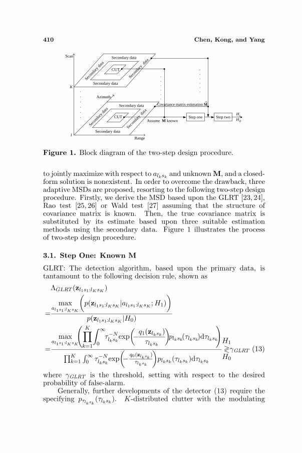
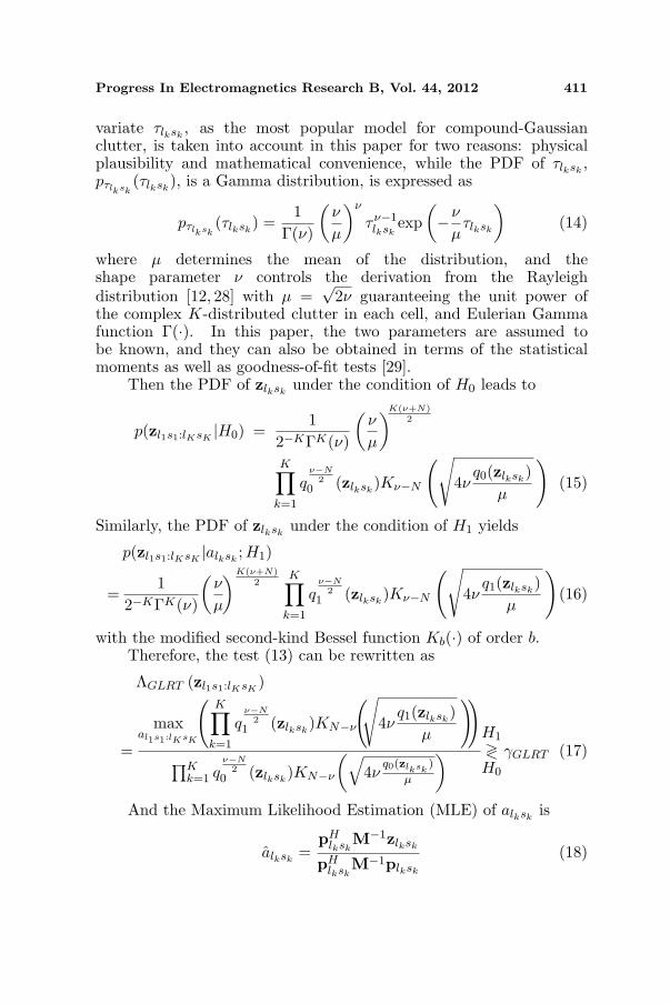
Figure 1. Block diagram of the two-step design procedure.
to jointly maximize with respect to alkskand unknown M, and a closed-
form solution is nonexistent. In order to overcome the drawback, threeadaptive MSDs are proposed, resorting to the following two-step designprocedure. Firstly, we derive the MSD based upon the GLRT [23, 24],Rao test [25, 26] or Wald test [27] assuming that the structure ofcovariance matrix is known. Then, the true covariance matrix issubstituted by its estimate based upon three suitable estimationmethods using the secondary data. Figure 1 illustrates the processof two-step design procedure.
3.1. Step One: Known M
GLRT: The detection algorithm, based upon the primary data, istantamount to the following decision rule, shown as
ΛGLRT (zl1s1:lKsK)
=max
al1s1:lKsK
(p(zl1s1:lKsK
|al1s1:lKsK; H1)
)
p(zl1s1:lKsK|H0)
=
maxal1s1:lKsK
(K∏
k=1
∫ ∞
0τ−Nlksk
exp(−q1(zlksk
)τlksk
)plksk
(τlksk)dτlksk
)
∏Kk=1
∫∞0 τ−N
lkskexp
(− q0(zlksk
)
τlksk
)plksk
(τlksk)dτlksk
H1
≷H0
γGLRT (13)
where γGLRT is the threshold, setting with respect to the desiredprobability of false-alarm.
Generally, further developments of the detector (13) require thespecifying pτlksk
(τlksk). K-distributed clutter with the modulating
Progress In Electromagnetics Research B, Vol. 44, 2012 411
variate τlksk, as the most popular model for compound-Gaussian
clutter, is taken into account in this paper for two reasons: physicalplausibility and mathematical convenience, while the PDF of τlksk
,pτlksk
(τlksk), is a Gamma distribution, is expressed as
pτlksk(τlksk
) =1
Γ(ν)
(ν
µ
)ν
τν−1lksk
exp(−ν
µτlksk
)(14)
where µ determines the mean of the distribution, and theshape parameter ν controls the derivation from the Rayleighdistribution [12, 28] with µ =
√2ν guaranteeing the unit power of
the complex K-distributed clutter in each cell, and Eulerian Gammafunction Γ(·). In this paper, the two parameters are assumed tobe known, and they can also be obtained in terms of the statisticalmoments as well as goodness-of-fit tests [29].
Then the PDF of zlkskunder the condition of H0 leads to
p(zl1s1:lKsK|H0) =
12−KΓK(ν)
(ν
µ
)K(ν+N)2
K∏
k=1
qν−N
20 (zlksk
)Kν−N
(√4ν
q0(zlksk)
µ
)(15)
Similarly, the PDF of zlkskunder the condition of H1 yields
p(zl1s1:lKsK|alksk
;H1)
=1
2−KΓK(ν)
(ν
µ
)K(ν+N)2
K∏
k=1
qν−N
21 (zlksk
)Kν−N
(√4ν
q1(zlksk)
µ
)(16)
with the modified second-kind Bessel function Kb(·) of order b.Therefore, the test (13) can be rewritten as
ΛGLRT (zl1s1:lKsK)
=
maxal1s1:lKsK
(K∏
k=1
qν−N
21 (zlksk
)KN−ν
(√4ν
q1(zlksk)
µ
))
∏Kk=1 q
ν−N2
0 (zlksk)KN−ν
(√4ν
q0(zlksk)
µ
)H1
≷H0
γGLRT (17)
And the Maximum Likelihood Estimation (MLE) of alkskis
alksk=
pHlksk
M−1zlksk
pHlksk
M−1plksk
(18)
412 Chen, Kong, and Yang
Substitute alkskinto the test (17), then, it is reduced to
ΛGLRT
(zl1s1:lKsK
)=
K∏
k=1
qν−N
21
(zlksk
)KN−ν
(√4ν
q1
(zlksk
)µ
)
qν−N
20
(zlksk
)KN−ν
(√4ν
q0
(zlksk
)µ
)
H1
≷H0
γGLRT (19)
with
q1 (zlksk)=(zlksk
− alkskplksk
)H M−1 (zlksk− alksk
plksk)
=zHlksk
M−1zlksk− |pH
lkskM−1zlksk
|2pH
lkskM−1plksk
(20)
while | · | denotes the modulus of a complex number.According to [30], we model the texture as unknown deterministic
parameter in the Rao and Wald tests. Then the joint PDFs under H0
and H1 are:
p(zl1s1:lKsK|τl1s1:lKsK
;H0)=1
πKN‖M‖K
K∏
k=1
1τNlksk
exp(q0 (zlksk
)τlksk
)(21)
and
p (zl1s1:lKsK|al1s1:lKsK
, τl1s1:lKsK;H1)
=1
πKN‖M‖K
K∏
k=1
1τNlksk
exp(
q1(zlksk)
τlksk
)(22)
Rao test: Starting from the primary data and assuming the knownM, the detection algorithm implementing the Rao test can be obtainedexpanding the likelihood ratio in the neighborhood of the MLEs ofparameters.
In order to evaluate the decision statistic, we denote with
• alksk,R and alksk,I are the real and the imaginary parts of alksk, k =
1, . . . , K, respectively;• θr = [al1s1,R, al1s1,I , . . . , alKsK ,R, alKsK ,I ]T a 2K-dimensional real
vector;• θu = [τl1s1 , .., τlKsK
]T a K-dimensional real column vector ofnuisance parameters;
• θ = [θTr , θT
u ]T a 3K-dimensional real vector.
Progress In Electromagnetics Research B, Vol. 44, 2012 413
Therefore, the Rao test for the problem of interest is the followingdecision rule:
ΛRao (zl1s1:lKsK)
=∂lnp(zl1s1:lKsK
|θ)∂θr
∣∣∣∣Tθ=θ0
[I−1
(θ0
)]θr,θr
∂lnp (zl1s1:lKsK|θ)
∂θr
∣∣∣∣θ=θ0
H1
≷H0
γRao (23)
where
• γRao is the detection threshold to be set with respect to the desiredvalue of the probability of false-alarm;
• p(zl1s1:lKsK|θ) denotes the PDF of the data under H1;
• ∂θr = [ ∂∂al1s1,R
, ∂∂al1s1,I
, . . . , ∂∂alKsK,R
, ∂∂alKsK,I
]T denotes thegradient operator with respect to θr;
• θ0 = [θTr,0, θ
Tu,0]
T , where θTr,0 = [0, . . . , 0]T and θu,0 is the MLE of
θu under H0;• I(θ) = I(θr, θu) is the Fisher Information Matrix (FIM) [24], which
can be partitioned as
I(θ) =[Iθr,θr(θ) Iθr,θu(θ)Iθu,θr(θ) Iθu,θu(θ)
](24)
• I−1(θ)θr,θr =(Iθr,θr(θ)− Iθr,θuIθu,θu(θ)Iθu,θr(θ)
)−1
.
Hence, according to the Rao test rule, θu,0 can be easily obtainedas
θu,0 =1N
[q0(zl1s1), q0(zl2s2), . . . , q0(zlKsK)]T (25)
Moreover,
∂lnp(zl1s1:lKsK|θ)
∂alksk,R= 2Re
(pH
lkskM−1(zlksk
− alkskplksk
)τlksk
)(26)
∂lnp(zl1s1:lKsK|θ)
∂alksk,I= 2Im
(pH
lkskM−1(zlksk
− alkskplksk
)τlksk
)(27)
where Re(·) and Im(·) are the real and the imaginary part of theargument, respectively.
414 Chen, Kong, and Yang
Considering θTr,0 = [0, . . . , 0]T , therefore,
∂lnp(zl1s1:lKsK|θ)
∂θr
∣∣∣T
θ=θ0
= 2
[Re
(pH
l1s1M−1zl1s1
τl1s1
), Im
(pH
l1s1M−1zl1s1
τl1s1
),
. . . , Re
(pH
lKsKM−1zlKsK
τlKsK
), Im
(pH
lKsKM−1zlKsK
τlKsK
)](28)
Further developments require evaluating the blocks of FIM. Then,it can be shown that
Iθr,θr(θ) = 2diag
(pH
l1s1M−1pl1s1
τl1s1
,pH
l1s1M−1pl1s1
τl1s1
,
. . . ,pH
lKsKM−1plKsK
τlKsK
,pH
lKsKM−1plKsK
τlKsK
)(29)
andIθr,θu(θ) = 02K,K (30)
where 02K,K is a 2K × K matrix of zeros and diag(·) denotes thediagonal matrix.
As a consequence, plugging (25), (28), (29), (30) into (23), aftersome algebra, yields
ΛRao (zl1s1:lKsK)=N
K∑
k=1
|pHlksk
M−1zlksk|2
pHlksk
M−1plkskzH
lkskM−1zlksk
H1
≷H0
γRao (31)
Wald test: The Wald test, based on the primary data, can beobtained exploiting the asymptotic efficiency of the MLE. Precisely,its decision rule denotes
ΛWald(zl1s1:lKsK) = θT
r,1
([I−1(θ1)]θr,θr
)−1θr,1
H1
≷H0
γwald (32)
where• γwald is the detection threshold to be set with respect to the desired
value of the probability of false-alarm;• θ1 = [θT
r,1, θTu,1]
T is the MLE of θ under H1, i.e.,
θ1 = argmaxθ1
(1
πKN‖M‖K
K∏
k=1
1τNlksk
exp(
q1(zlksk)
τlksk
))(33)
Progress In Electromagnetics Research B, Vol. 44, 2012 415
Maximizing the expression (33) yields
θr,1 =
[Re
(pH
l1s1M−1zl1s1
pHl1s1
M−1pl1s1
), Im
(pH
l1s1M−1zl1s1
pHl1s1
M−1pl1s1
),
. . . ,Re
(pH
lKsKM−1zlKsK
pHlKsK
M−1plKsK
), Im
(pH
lKsKM−1zlKsK
pHlKsK
M−1plKsK
)]T
(34)
and
θu,1 =1N
[zH
l1s1M−1zl1s1 −
|pHl1s1
M−1zl1s1 |2pH
l1s1M−1pl1s1
,
. . . , zHlKsK
M−1zlKsK− |pH
lKsKM−1zlKsK
|2pH
lKsKM−1plKsK
]T
(35)
Hence, substituting (29), (34) and (35) into (32), we can getΛWald(zl1s1:lKsK
)
=NK∑
k=1
|pHlksk
M−1zlksk|2
pHlksk
M−1plkskzH
lkskM−1zlksk
−|pHlksk
M−1zlksk|2
H1
≷H0
γwald (36)
In general, the GLRT, Rao and Wald tests have the sameasymptotic performance. However, the Rao test does not requireevaluating the MLEs of the unknown parameters under H1 hypothesis,leaving only the MLEs under H0 to be found, and the Wald test onlyadopts the data components orthogonal to the useful signal subspace.Therefore, the Rao and Wald tests might require a lower computationalcomplexity than the GLRT for their implementation.
3.2. Step Two: Estimation of M
In order to adapt the MSDs fully to the covariance matrix ofclutter, several covariance matrix estimations substitute M in thetests (19), (31) and (36), respectively.
Herein, the simple and widely method used in Gaussianenvironment is SCM. In the kth scan, it is shown as
MSCMk=
1W
W∑
w=1
zlkwskwzH
lkwskw(37)
When in non-Gaussian clutter scenarios, the NSCM method inthe kth scan is commonly applied and written as
MNSCM k=
N
W
W∑
w=1
zlkwskwzH
lkwskw
zHlkwskw
zlkwskw
(38)
416 Chen, Kong, and Yang
The NSCM eliminates the effect of the data-dependent normal-ization factor τlkwskw
= zHlkwskw
zlkwskwaccounted for the random local
power change from cell to cell.The third estimation method is called RMLE, in the kth scan,
which is
MRMLEk(t)=
N
W
W∑
w=1
zlkwskwzH
lkwskw
zHlkwskw
MRMLEk(t−1)−1zlkwskw
, t=2,. . . ,Nt (39)
while the original estimation is
MRMLEk(1) =
N
W
W∑
w=1
zlkwskwzH
lkwskw
zHlkwskw
zlkwskw
(40)
with Nt = 4 [21].Finally, the CFAR properties of three strategies of covariance
matrix estimation are evaluated. The adaptive MSDs withSCM estimation strategy have an independent relationship withGaussian clutter, yet dependent on the texture component incompound-Gaussian environment. Although in the compound-Gaussian background, the MSDs with NSCM estimation strategyare independent of the texture component for considering thenormalization factor, they still depend on the structure of M [31].And it has been proved that the RMLE is independent of both texturecomponent and M [32].
4. SIMULATION
This section is devoted to the performance assessment on the adaptiveMSDs based on the GLRT, Rao and Wald tests with different Mestimators, SCM, NSCM and RMLE (M-SCM, M-NSCM, M-RMLEin simulation). Assuming that the speckle component of the generatedclutter data has an exponential correlation structure covariance matrix,hence M can be expressed as
[M]NiNj = ρ|Ni−Nj |, 1 ≤ Ni, Nj ≤ N (41)
where ρ is the one-lag correlation coefficient. Additionally, the targetis set as Swerling 0 or Swerling 1 [33], usually encountered in variousreal conditions.
Since the closed-form expressions for both the Pfa and theprobability of detection (Pd) are not available, we resort to standardMonte Carlo technique. More precisely, in order to evaluate thethreshold necessary to ensure a preassigned value of Pfa and to
Progress In Electromagnetics Research B, Vol. 44, 2012 417P
d
0.1
0.2
0.3
0.4
0.5
0.6
0.7
0.8
0.9
1
0 -20 -15 -10 -5 0 5 10
SCR, dB
M RMLE GLRT MSDM NSCM GLRT MSDM SCM GLRT MSDM RMLE Rao MSDM NSCM Rao MSDM SCM Rao MSDM RMLE Wald MSDM NSCM Wald MSDM SCM Wald MSDM RMLE NAMFM NSCM NAMFM SCM NAMF
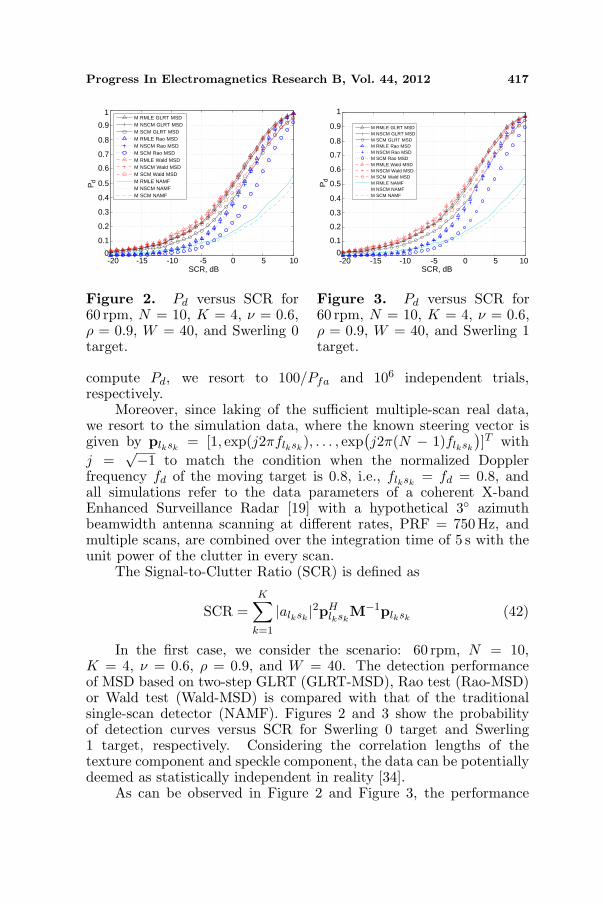
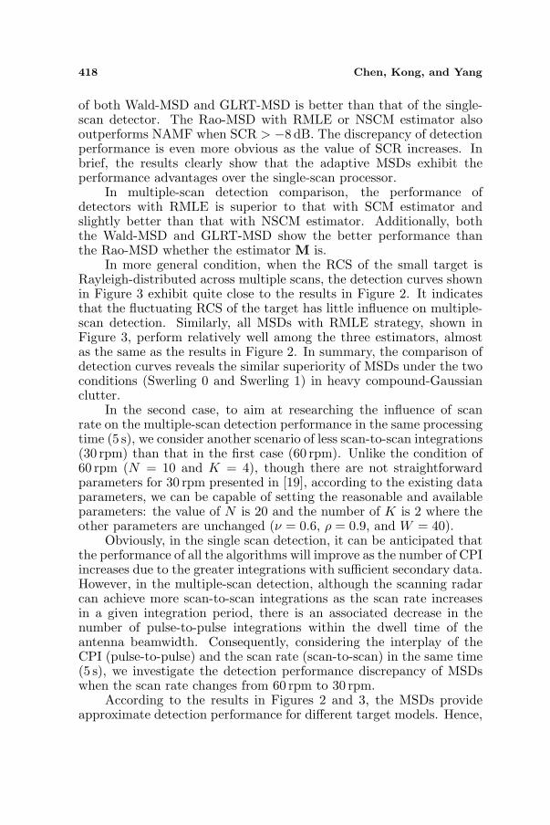
Figure 2. Pd versus SCR for60 rpm, N = 10, K = 4, ν = 0.6,ρ = 0.9, W = 40, and Swerling 0target.
-20 -15 -10 -5 0 5 10
0.1
0.2
0.3
0.4
0.5
0.6
0.7
0.8
0.9
1
SCR, dB
Pd
M RMLE GLRT MSDM NSCM GLRT MSDM SCM GLRT MSDM RMLE Rao MSDM NSCM Rao MSDM SCM Rao MSDM RMLE Wald MSDM NSCM Wald MSDM SCM Wald MSDM RMLE NAMFM NSCM NAMFM SCM NAMF
0
Figure 3. Pd versus SCR for60 rpm, N = 10, K = 4, ν = 0.6,ρ = 0.9, W = 40, and Swerling 1target.
compute Pd, we resort to 100/Pfa and 106 independent trials,respectively.
Moreover, since laking of the sufficient multiple-scan real data,we resort to the simulation data, where the known steering vector isgiven by plksk
= [1, exp(j2πflksk), . . . , exp
(j2π(N − 1)flksk
)]T with
j =√−1 to match the condition when the normalized Doppler
frequency fd of the moving target is 0.8, i.e., flksk= fd = 0.8, and
all simulations refer to the data parameters of a coherent X-bandEnhanced Surveillance Radar [19] with a hypothetical 3◦ azimuthbeamwidth antenna scanning at different rates, PRF = 750 Hz, andmultiple scans, are combined over the integration time of 5 s with theunit power of the clutter in every scan.
The Signal-to-Clutter Ratio (SCR) is defined as
SCR =K∑
k=1
|alksk|2pH
lkskM−1plksk
(42)
In the first case, we consider the scenario: 60 rpm, N = 10,K = 4, ν = 0.6, ρ = 0.9, and W = 40. The detection performanceof MSD based on two-step GLRT (GLRT-MSD), Rao test (Rao-MSD)or Wald test (Wald-MSD) is compared with that of the traditionalsingle-scan detector (NAMF). Figures 2 and 3 show the probabilityof detection curves versus SCR for Swerling 0 target and Swerling1 target, respectively. Considering the correlation lengths of thetexture component and speckle component, the data can be potentiallydeemed as statistically independent in reality [34].
As can be observed in Figure 2 and Figure 3, the performance
418 Chen, Kong, and Yang
of both Wald-MSD and GLRT-MSD is better than that of the single-scan detector. The Rao-MSD with RMLE or NSCM estimator alsooutperforms NAMF when SCR > −8 dB. The discrepancy of detectionperformance is even more obvious as the value of SCR increases. Inbrief, the results clearly show that the adaptive MSDs exhibit theperformance advantages over the single-scan processor.
In multiple-scan detection comparison, the performance ofdetectors with RMLE is superior to that with SCM estimator andslightly better than that with NSCM estimator. Additionally, boththe Wald-MSD and GLRT-MSD show the better performance thanthe Rao-MSD whether the estimator M is.
In more general condition, when the RCS of the small target isRayleigh-distributed across multiple scans, the detection curves shownin Figure 3 exhibit quite close to the results in Figure 2. It indicatesthat the fluctuating RCS of the target has little influence on multiple-scan detection. Similarly, all MSDs with RMLE strategy, shown inFigure 3, perform relatively well among the three estimators, almostas the same as the results in Figure 2. In summary, the comparison ofdetection curves reveals the similar superiority of MSDs under the twoconditions (Swerling 0 and Swerling 1) in heavy compound-Gaussianclutter.
In the second case, to aim at researching the influence of scanrate on the multiple-scan detection performance in the same processingtime (5 s), we consider another scenario of less scan-to-scan integrations(30 rpm) than that in the first case (60 rpm). Unlike the condition of60 rpm (N = 10 and K = 4), though there are not straightforwardparameters for 30 rpm presented in [19], according to the existing dataparameters, we can be capable of setting the reasonable and availableparameters: the value of N is 20 and the number of K is 2 where theother parameters are unchanged (ν = 0.6, ρ = 0.9, and W = 40).
Obviously, in the single scan detection, it can be anticipated thatthe performance of all the algorithms will improve as the number of CPIincreases due to the greater integrations with sufficient secondary data.However, in the multiple-scan detection, although the scanning radarcan achieve more scan-to-scan integrations as the scan rate increasesin a given integration period, there is an associated decrease in thenumber of pulse-to-pulse integrations within the dwell time of theantenna beamwidth. Consequently, considering the interplay of theCPI (pulse-to-pulse) and the scan rate (scan-to-scan) in the same time(5 s), we investigate the detection performance discrepancy of MSDswhen the scan rate changes from 60 rpm to 30 rpm.
According to the results in Figures 2 and 3, the MSDs provideapproximate detection performance for different target models. Hence,
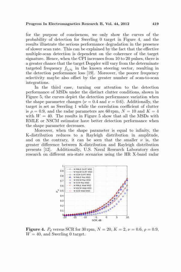
Progress In Electromagnetics Research B, Vol. 44, 2012 419
for the purpose of conciseness, we only show the curves of theprobability of detection for Swerling 0 target in Figure 4, and theresults illustrate the serious performance degradation in the presenceof slower scan rate. This can be explained by the fact that the effectivemultiple-scan detection is dependent on the coherence of the targetsignature. Hence, when the CPI increases from 10 to 20 pulses, there isa greater chance that the target Doppler will vary from the determinatetargeted frequency flksk
in the known steering vector, resulting inthe detection performance loss [19]. Moreover, the poorer frequencyselectivity maybe also offset by the greater number of scan-to-scanintegrations.
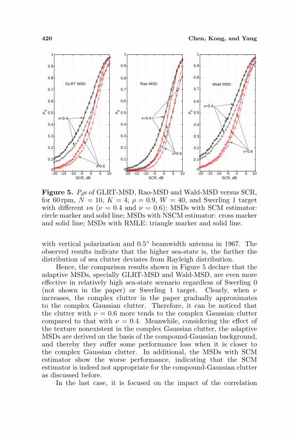
In the third case, turning our attention to the detectionperformance of MSDs under the distinct clutter conditions, shown inFigure 5, the curves depict the detection performance variation whenthe shape parameter changes (ν = 0.4 and ν = 0.6). Additionally, thetarget is set as Swerling 1 while the correlation coefficient of clutteris ρ = 0.9, and the radar parameters are 60 rpm, N = 10 and K = 4with W = 40. The results in Figure 5 show that all the MSDs withRMLE or NSCM estimator have better detection performance whenthe shape parameter decreases.
Moreover, when the shape parameter is equal to infinity, theK-distribution reduces to a Rayleigh distribution in amplitude,and on the contrary, it can be seen that the smaller ν is, thegreater difference between K-distribution and Rayleigh distributionpresents [12]. Additionally, U.S. Naval Research Laboratory doesresearch on different sea-state scenarios using the HR X-band radar
-20 -15 -10 -5 0 5 10
0.1
0.2
0.3
0.4
0.5
0.6
0.7
0.8
0.9
1
SCR, dB
Pd
M RMLE GLRT MSDM NSCM GLRT MSDM SCM GLRT MSDM RMLE Rao MSDM NSCM Rao MSDM SCM Rao MSDM RMLE Wald MSDM NSCM Wald MSDM SCM Wald MSD
0
Figure 4. Pd versus SCR for 30 rpm, N = 20, K = 2, ν = 0.6, ρ = 0.9,W = 40, and Swerling 0 target.
420 Chen, Kong, and Yang
-20 -15 -10 -5 0 5 10SCR, dB
Pd
GLRT MSD
-20 -15 -10 -5 0 5 10SCR, dB
Rao MSD
-20 -15 -10 -5 0 5 10SCR, dB
Wald MSD
v=0.4
v=0.6
v=0.4
v=0.6
v=0.4
v=0.6
0.1
0.2
0.3
0.4
0.5
0.6
0.7
0.8
0.9
1
0
Pd
0.1
0.2
0.3
0.4
0.5
0.6
0.7
0.8
0.9
1
0
Pd
0.1
0.2
0.3
0.4
0.5
0.6
0.7
0.8
0.9
1
0
Figure 5. Pds of GLRT-MSD, Rao-MSD and Wald-MSD versus SCR,for 60 rpm, N = 10, K = 4, ρ = 0.9, W = 40, and Swerling 1 targetwith different νs (ν = 0.4 and ν = 0.6); MSDs with SCM estimator:circle marker and solid line; MSDs with NSCM estimator: cross markerand solid line; MSDs with RMLE: triangle marker and solid line.
with vertical polarization and 0.5◦ beamwidth antenna in 1967. Theobserved results indicate that the higher sea-state is, the farther thedistribution of sea clutter deviates from Rayleigh distribution.
Hence, the comparison results shown in Figure 5 declare that theadaptive MSDs, specially GLRT-MSD and Wald-MSD, are even moreeffective in relatively high sea-state scenario regardless of Swerling 0(not shown in the paper) or Swerling 1 target. Clearly, when νincreases, the complex clutter in the paper gradually approximatesto the complex Gaussian clutter. Therefore, it can be noticed thatthe clutter with ν = 0.6 more tends to the complex Gaussian cluttercompared to that with ν = 0.4. Meanwhile, considering the effect ofthe texture nonexistent in the complex Gaussian clutter, the adaptiveMSDs are derived on the basis of the compound-Gaussian background,and thereby they suffer some performance loss when it is closer tothe complex Gaussian clutter. In additional, the MSDs with SCMestimator show the worse performance, indicating that the SCMestimator is indeed not appropriate for the compound-Gaussian clutteras discussed before.
In the last case, it is focused on the impact of the correlation
Progress In Electromagnetics Research B, Vol. 44, 2012 421
-20 -15 -10 -5 0 5 10 15SCR, dB
P d
ρ=0.9
ρ=0.95
ρ=0.99
0
0.1
0.2
0.3
0.4
0.5
0.6
0.7
0.8
0.9
1
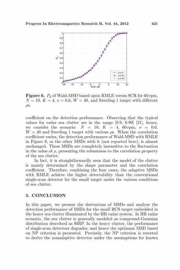
Figure 6. Pd of Wald-MSD based upon RMLE versus SCR for 60 rpm,N = 10, K = 4, ν = 0.6, W = 40, and Swerling 1 target with differentρs.
coefficient on the detection performance. Observing that the typicalvalues for radar sea clutter are in the range [0.9, 0.99] [21], hence,we consider the scenario: N = 10, K = 4, 60 rpm, ν = 0.6,W = 40 and Swerling 1 target with various ρs. When the correlationcoefficient varies, the detection performance of Wald-MSD with RMLEin Figure 6, or the other MSDs with it (not reported here), is almostunchanged. These MSDs are completely insensitive to the fluctuationin the value of ρ, presenting the robustness to the correlation propertyof the sea clutter.
In fact, it is straightforwardly seen that the model of the clutteris mainly determined by the shape parameter and the correlationcoefficient. Therefore, combining the four cases, the adaptive MSDswith RMLE achieve the higher detectability than the conventionalsingle-scan detector for the small target under the various conditionsof sea clutter.
5. CONCLUSION
In this paper, we present the derivations of MSDs and analyze thedetection performance of MSDs for the small RCS target embedded inthe heavy sea clutter illuminated by the HR radar system. In HR radarscenario, the sea clutter is generally modeled as compound-Gaussiandistribution described as SIRP. In the heavy clutter, the performanceof single-scan detectors degrades, and hence the optimum MSD basedon NP criterion is presented. Precisely, the NP criterion is resortedto derive the nonadaptive detector under the assumptions for known
422 Chen, Kong, and Yang
clutter covariance matrix M, the texture component τlkskand the
parameter alksk. However, the prior knowledge of M, τlksk
or alksk
is commonly absent in the realistic environment. Consequently, forthe purpose of overcoming this drawback, the adaptive MSDs basedon the two-step GLRT, Rao and Wald tests are proposed, and threemethods are used to estimate the unknown PSD.
Finally, Monte Carlo simulation results show that the adaptiveMSDs significantly outperform the traditional single-scan detectorfor different targets. Obviously, the MSDs can availably reduce theeffect of clutter outlier in a single scan, and also allow the target tobe detectable with the smaller values of SCR across multiple scans.Additionally, the MSDs can attain more training data even in theheterogeneous scenarios where it is difficult to obtain enough secondarydata in single-scan detection. Meanwhile, the results show that theperformance of MSDs with RMLE is superior to that of MSDs withSCM or NSCM estimator in various backgrounds of sea clutter.
ACKNOWLEDGMENT
This work is sponsored by the National Natural Science Foundationof China (61178068) and by Sichuan Youth Science and TechnologyFoundation (2011JQ0024).
REFERENCES
1. Hatam, M., A. Sheikhi, and M. A. Masnadi-Shirazi, “Targetdetection in pulse-train MIMO radars applying ICA algorithms,”Progress In Electromagnetics Research, Vol. 122, 413–435, 2012.
2. Qu, Y., G. S. Liao, S. Q. Zhu, and X. Y. Liu, “Pattern synthesis ofplanar antenna array via convex optimization for airborne forwardlooking radar,” Progress In Electromagnetics Research, Vol. 84, 1–10, 2008.
3. Qu, Y., G. S. Liao, S. Q. Zhu, X. Y. Liu, and H. Jiang,“Performance analysis of beamforming for MIMO radar,” ProgressIn Electromagnetics Research, Vol. 84, 123–134, 2008.
4. Sabry, R. and P. W. Vachon, “Advanced polarimetric syntheticaperture radar (SAR) and electro-optical (EO) data fusionthrough unified coherent formulation of the scattered EM field,”Progress In Electromagnetics Research, Vol. 84, 189–203, 2008.
5. Herselman, P. L. and H. J. de Wind, “Improved covariancematrix estimation in spectrally inhomogeneous sea clutter with
Progress In Electromagnetics Research B, Vol. 44, 2012 423
application to adaptive small boat detection,” InternationalConference on Radar, 94–99, 2008.
6. Lerro, D. and Y. Bar-Shalom, “Interacting multiple modeltracking with target amplitude feature,” IEEE Transactions onAerospace and Electronic Systems, Vol. 29, No. 2, 494–509, 1993.
7. Rutten, M. G., N. J. Gordon, and S. Maskell, “Recursive track-before-detect with target amplitude fluctuations,” IEE Proceedingon Radar, Sonar and Navigation, Vol. 152, No. 5, 345–352, 2005.
8. Ward, K. D., J. A. Tough, and S. Watts, “Sea clutter: Scattering,the k-distribution and radar performance,” IET Radar, Sonar andNavigation Series, Vol. 20, 45–95, 2006.
9. Haykin, S., R. Bakker, and B. W. Currie, “Uncovering nonlineardynamics-the case study of sea clutter,” Proceedings of the IEEE,Vol. 90, No. 5, 860–881, 2002.
10. Unsworth, C. P., M. R. Cowper, S. McLaughlin, and B. Mulgrew,“Re-examining the nature of radar sea clutter,” IEE Processingon Rader Signal Processing, Vol. 149, No. 3, 105–114, 2002.
11. Farina, A., F. Gini, M. V. Greco, and L. Verrazzani, “Highresolution sea clutter data: Statistical analysis of recorded livedata,” IEE Processing on Rader Signal Processing, Vol. 144, No. 3,121–130, 1997.
12. Nohara, T. J. and S. Haykin, “Canadian East Coast radartrials and the K-distribution,” IEE Processing on Rader SignalProcessing, Vol. 138, No. 2, 80–88, 1991.
13. Conte, E., A. De Maio, and C. Galdi, “Statistical analysis ofreal clutter at different range resolutions,” IEEE Transactions onAerospace and Electronic Systems, Vol. 40, No. 3, 903–918, 2004.
14. Greco, M., F. Bordoni, and F. Gini, “X-band sea-clutternonstationarity: Influence of long waves,” IEEE Journal ofOceanic Engineering, Vol. 29, No. 2, 269–293, 2004.
15. Greco, M., F. Gini, and M. Rangaswamy, “Non-stationarityanalysis of real X-band clutter data at different resolutions,” IEEENational Radar Conference, 44–50, 2006.
16. Ward, K. D., C. J. Baker, and S. Watts, “Maritime surveillanceradar. I. Radar scattering from the ocean surface,” IEEProceedings F on Radar and Signal Processing, Vol. 137, No. 2,51–62, 1990.
17. Panagopoulos, S. and J. J. Soraghan, “Small-target detectionin sea clutter,” IEEE Transactions on Geoscience and RemoteSensing, Vol. 42, No. 7, 1355–1361, 2004.
18. Schleher, D. C., “Periscope detection radar,” Record of the IEEE
424 Chen, Kong, and Yang
International Radar Conference, 704–707, 1995.19. McDonald, M. and S. Lycett, “Fast versus slow scan radar
operation for coherent small target detection in sea clutter,” IEEProceedings on Radar, Sonar and Navigation, Vol. 152, No. 6,429–435, 2005.
20. Carretero-Moya, J., J. Gismero-Menoyo, A. Asensio-Lopez, andA. Blanco-del-Campo, “Application of the Radon transform todetect small-targets in sea clutter,” IET Radar, Sonar andNavigation, Vol. 3, No. 2, 155–166, 2009.
21. Gini, F. and M. Greco, “Covariance matrix estimation for CFARdetection in correlated heavy tailed clutter,” Signal Processing,Vol. 82, No. 12, 1847–1859, 2002.
22. Gini, F. amd A. Farina, “Vector subspace detection in compound-Gaussian clutter, Part I: Survey and new results,” IEEETransactions on Aerospace and Electronic Systems, Vol. 38, No. 4,1295–1311, 2002.
23. Gini, F. and M. Greco, “Suboptimum approach for adaptivecoherent radar detection in compound-Gaussian clutter,” IEEETransactions on Aerospace and Electronic Systems, Vol. 35, No. 3,1095–1104, 1999.
24. Conte, E., A. De Maio, and G. Ricci, “Asymptoticallyoptimum radar detection in compound Gaussian clutter,” IEEETransactions on Aerospace and Electronic Systems, Vol. 31, No. 2,617–625, 1995.
25. Wang, P., H. Li, and B. Himed, “Parametric Rao testsfor multichannel adaptive detection in partially homogeneousenvironment,” IEEE Transactions on Aerospace and ElectronicSystems, Vol. 47, No. 3, 1850–1862, 2011.
26. De Maio, A., S. M. Kay, and A. Farina, “On the invariance,coincidence, and statistical equivalence of the GLRT, Rao test,and Wald test,” IEEE Transactions on Signal Processing, Vol. 58,No. 4, 1967–1979, 2010.
27. De Maio, A. and S. Iommelli, “Coincidence of the Rao test, Waldtest, and GLRT in partially homogeneous environment,” IEEESignal Processing Letter, Vol. 15, 385–388, 2008.
28. Sangston, K. J. and K. R. Gerlach, “Coherent detection of radartargets in a non-gaussian background,” IEEE Transactions onAerospace and Electronic Systems, Vol. 30, No. 2, 330–340, 1994.
29. Anastassopoulous, V., G. A. Lampropoulos, A. Drosopoulos,and M. Rey, “High resolution radar clutter statistics,” IEEETransactions on Aerospace and Electronic Systems, Vol. 35, No. 1,
Progress In Electromagnetics Research B, Vol. 44, 2012 425
43–60, 1999.30. Gini, F., G. B. Giannakis, M. Greco, and G. T. Zhou, “Time-
averaged subspace methods for radar clutter texture retrieval,”IEEE Transactions on Signal Processing, Vol. 49, No. 9, 1896–1898, 2001.
31. Gini, F., “Performance analysis of two structured covariance ma-trix estimators in compound-Gaussian clutter,” Signal Processing,Vol. 80, No. 2, 365–371, 2000.
32. Pascal, F., Y. Chitour, P. Forster, and P. Larzabal, “Covariancestructure maximum-likelihood estimates in compound Gaussiannoise: Existence and algorithm analysis,” IEEE Transactions onSignal Processing, Vol. 56, No. 1, 34–48, 2008.
33. Swerling, P., “Radar probability of detection for some additionalfluctuating target cases,” IEEE Transactions on Aerospace andElectronic Systems, Vol. 33, No. 2, 698–709, 1997.
34. Gunturkun, U., “Toward the development of radar scene analyzerfor cognitive radar,” IEEE Journal of Oceanic Engineering,Vol. 35, No. 2, 303–313, 2010.


![Detection in Gaussian clutter - unipi.itThe detection algorithm is optimized for a specific Doppler. ... [Kay98] S.M. Kay, Fundamentals of Statistical Signal Processing. Detection](https://img.pdfslide.us/doc/110x75/5ebab00ae1f4d806b07cacc4/detection-in-gaussian-clutter-unipiit-the-detection-algorithm-is-optimized-for.jpg)

![56 IEEE JOURNAL OF SELECTED TOPICS IN SIGNAL …nehorai/DARPA/publications/04200713.pdf · detection [1], [2] or simplistic clutter models [3], [4]. ... a high clutter-to-noise ratio](https://img.pdfslide.us/doc/110x75/5ad3b3a47f8b9afa798e4ef0/56-ieee-journal-of-selected-topics-in-signal-nehoraidarpapublications-1.jpg)