October 2002

NASA/CR-2002-211670

Small Engine Technology (SET)Task 33 – Final ReportAirframe, Integration, and CommunityNoise Study

Lys S. Lieber and Daniel ElkinsHoneywell Engines, Systems, and Services, Phoenix, Arizona

The NASA STI Program Office . . . in Profile

Since its founding, NASA has been dedicated to theadvancement of aeronautics and space science. TheNASA Scientific and Technical Information (STI)Program Office plays a key part in helping NASAmaintain this important role.

The NASA STI Program Office is operated byLangley Research Center, the lead center for NASA’sscientific and technical information. The NASA STIProgram Office provides access to the NASA STIDatabase, the largest collection of aeronautical andspace science STI in the world. The Program Office isalso NASA’s institutional mechanism fordisseminating the results of its research anddevelopment activities. These results are published byNASA in the NASA STI Report Series, whichincludes the following report types:

• TECHNICAL PUBLICATION. Reports ofcompleted research or a major significant phaseof research that present the results of NASAprograms and include extensive data ortheoretical analysis. Includes compilations ofsignificant scientific and technical data andinformation deemed to be of continuingreference value. NASA counterpart of peer-reviewed formal professional papers, but havingless stringent limitations on manuscript lengthand extent of graphic presentations.

• TECHNICAL MEMORANDUM. Scientificand technical findings that are preliminary or ofspecialized interest, e.g., quick release reports,working papers, and bibliographies that containminimal annotation. Does not contain extensiveanalysis.

• CONTRACTOR REPORT. Scientific andtechnical findings by NASA-sponsoredcontractors and grantees.

• CONFERENCE PUBLICATION. Collectedpapers from scientific and technicalconferences, symposia, seminars, or othermeetings sponsored or co-sponsored by NASA.

• SPECIAL PUBLICATION. Scientific,technical, or historical information from NASAprograms, projects, and missions, oftenconcerned with subjects having substantialpublic interest.

• TECHNICAL TRANSLATION. English-language translations of foreign scientific andtechnical material pertinent to NASA’s mission.

Specialized services that complement the STIProgram Office’s diverse offerings include creatingcustom thesauri, building customized databases,organizing and publishing research results ... evenproviding videos.

For more information about the NASA STI ProgramOffice, see the following:

• Access the NASA STI Program Home Page athttp://www.sti.nasa.gov

• E-mail your question via the Internet tohelp@sti.nasa.gov

• Fax your question to the NASA STI Help Deskat (301) 621-0134

• Phone the NASA STI Help Desk at(301) 621-0390

• Write to:NASA STI Help DeskNASA Center for AeroSpace Information7121 Standard DriveHanover, MD 21076-1320

National Aeronautics andSpace Administration

Langley Research Center Prepared for Langley Research CenterHampton, Virginia 23681-2199 under Contract NAS3-27483, Task 33

October 2002

NASA/CR-2002-211670

Small Engine Technology (SET)Task 33 – Final ReportAirframe, Integration, and CommunityNoise Study

Lys S. Lieber and Daniel ElkinsHoneywell Engines, Systems, and Services, Phoenix, Arizona

Available from:

NASA Center for AeroSpace Information (CASI) National Technical Information Service (NTIS)7121 Standard Drive 5285 Port Royal RoadHanover, MD 21076-1320 Springfield, VA 22161-2171(301) 621-0390 (703) 605-6000

iii

TABLE OF CONTENTS

Page

1. INTRODUCTION 1

1.1 Objectives 1

1.2 Description of Work 11.2.1 Airframe Noise Reduction Technology Study 11.2.2 Jet Shear Layer Refraction and Attenuation Study 21.2.3 Engine Source Noise Changes With Altitude Study 21.2.4 Lateral Attenuation Experiments 2

2. AIRFRAME NOISE REDUCTION TECHNOLOGY STUDY 2

2.1 Airframe Noise Reduction Technology Evaluation 22.1.1 Boeing Airframe Noise Program Activity 22.1.2 Airframe Noise Evaluations 32.1.3 Special Considerations for Business Jets 32.1.4 Current Status of Airframe Noise – Airframe Noise for the 1992 Baseline Technology Business Jet 42.1.5 Evaluation of Effectiveness of AST Noise Reduction Technologies for Airframe Noise, Using Boeing Code 122.1.6 Comparison With Goals 142.1.7 1/3-Octave SPL Time Histories of Airframe Noise 15

2.2 Array Processing of Distributed Source Noise 152.2.1 Introduction 152.2.2 Summary of the Array Processing Methodology 192.2.3 Summary of Results 212.2.4 List of Symbols 35

3. JET SHEAR LAYER REFRACTION AND ATTENUATION STUDY 36

3.1 Introduction and Review of Correction Procedures 363.1.1 Static-to-Flight Correction Procedures 363.1.2 Flyover Noise Prediction Process 373.1.3 Traditional Static-to-Flight Corrections 393.1.4 Shear Layer Corrections 40

3.2 Static-to-Flight Jet Shear Layer Correction Procedure for Internally Generated Engine Exhaust Noise 41

3.2.1 Overview 413.2.2 Problem Geometry 423.2.3 Static-to-Flight Angle Correction 433.2.4 Static-to-Flight Amplitude Correction 453.2.5 Angle Relationships 463.2.6 Implementation of the Corrections 493.2.7 Summary of the Static-to-Flight Correction Process 533.2.8 Computer Program 54

iv

TABLE OF CONTENTS (Cont)

Page

3.2.9 Sample Application of the Procedure 553.2.10 Limitations of the Method 55

3.3 Implementation in the NASA Aircraft Noise Prediction Program (ANOPP) 56

3.4 List of Symbols 56

4. ENGINE SOURCE NOISE CHANGES WITH ALTITUDE STUDY 57

4.1 Modeling Approach 57

4.2 Differences Between INM Versions 5.2a and 6.0. 58

4.3 Analysis Results 58

5. LATERAL ATTENUATION EXPERIMENTS 62

5.1 Introduction 62

5.2 Honeywell Participation 64

5.3 Data Analysis 66

6. REFERENCES 73

APPENDIXES

I 1/3-Octave Band SPL Time Histories of Estimated Airframe Noise (3 pages)II ANOPP Theoretical Manual Chapter for the Shear Layer Correction Module (14 pages)

III ANOPP User Manual Chapter for the Shear Layer Correction Module (3 pages)IV INM Case Summary of 1992 Baseline Results (4 pages)V INM Case Summary for New Noise/Altitude Results (4 pages)

v

LIST OF FIGURES

Page

Figure 1. Comparison of Airframe Noise Sources for 1992 Baseline Technology Business Jet. 5Figure 2. Wing and Landing Gear Contributions to Total Airframe Noise for Baseline

Business Jet and Boeing 737 at Approach. 6Figure 3. Flap and Slat Contributions to Wing Noise for Baseline Business Jet and

Boeing 737 at Approach. 7Figure 4. Main and Nose Landing Gear Contributions to the Total Landing Gear Noise

for the Baseline Business Jet at Approach. 8Figure 5. Landing Gear Component Contributions to the Total Landing Gear Noise

for the Baseline Business Jet at Approach. 9Figure 6. Landing Gear Component Contributions to the Total Landing Gear Noise

for the Baseline Business Jet and Boeing 737 at Approach. 11Figure 7. Spectra Plot of Landing Gear Noise Sources at 90 Degrees for the Baseline

Business Jet and the Boeing 737 at Approach. 12Figure 8. Impact of Noise Reduction Technologies for Baseline Business Jet at Approach. 14Figure 9. Schematic of a Leading Edge Slat and Wing Main Element Leading Edge. 16Figure 10. Pressure Side (Flyover) View of Distributed Slat Noise With Local

Discontinuities at the Side Plates. 19Figure 11. Pressure-Squared Values as a Function of Spanwise Position. 20Figure 12. Breakdown of Slat Noise Contributions for M=0.17, δs = 20°, δw = 26°, Ψ = 0°,

and Φ = 107o. 22

Figure 13. Schematic Diagram of the Slat/Wing Model and Elevation Angle Position (Side View). 22

Figure 14. Effect of the Main Element Angle-of-Attack on the Leading Edge Slat Noise. 27Figure 15. Effect of Slat Element Angle-of-Attack for a Main Element Angle-of-Attack

of 26 Degrees. 27Figure 16. Effect of Slat Element Angle-of-Attack for a Main Element Angle-of-Attack

of 32 Degrees. 28Figure 17. Effect of Slat Gap/Overlap on the Sound Pressure Level of the Leading Edge

Slat Noise. 28Figure 18. Effect of the Teardrop Insert in the Slat Gap on the Sound Pressure Level

of the Leading Edge Slat Noise. 29Figure 19. Effect of Mach Number on the Teardrop Insert Leading Edge Slat Noise. 29Figure 20. Effect of Directivity Angle on the Sound Pressure Level of the Baseline

Leading Edge Slat Configuration. 30Figure 21. Normalized Directivity (Using Adjusted Angles) of the Baseline Leading Edge

Slat Configuration. 30Figure 22. Directivity Characteristics of the Sound Pressure Level for the 6-Notch

Gap/Overlap Conditions. 31Figure 23. Normalized Directivity (Using Adjusted Angles) of the 6-Notch Gap/Overlap

Conditions. 31Figure 24. Effect of Trailing Edge Thickness on the Leading Edge Slat Noise. 32

vi

LIST OF FIGURES (Cont)

Page

Figure 25. Directivity Characteristics of the Sound Pressure Level for the Trailing Edge Thickness of 0.155”. 32

Figure 26. Normalized Directivity (Using Adjusted Angles) for the Trailing Edge Thickness of 0.155”. 33

Figure 27. Directivity Characteristics of the Sound Pressure Level for the Trailing Edge Thickness of 0.07”. 33

Figure 28. Normalized Directivity (Using Adjusted Angles) for the Trailing Edge Thickness of 0.07”. 34

Figure 29. Summary of the Noise Benefit for the Two Slat Noise Reduction Concepts. 34Figure 30. A Description of The In-Flight Sound Pressure Levels Requires a Clear

Distinction of the Coordinates System Used. 38Figure 31. The Static-to-Flight Correction Procedure is Based Upon Cylindrical Model

Geometry. 43Figure 32. The Refraction Angle Correction is Derived by Considering Plane Wave

Interaction With a Vortex Sheet. 44Figure 33. A Relationship Between the Measurement Angle θm and Wave Normal

Angle φas Can Be Derived From Geometrical Considerations. 47Figure 34. The Ray Path Angle θc and the Wavenormal Angle φ Are Geometrically Related. 48Figure 35. The Relationship Between θc and φ is Derived From Triangle Relationships. 48Figure 36. Sample Refraction Results From the Simplified Model for M j = 0 5. , Ma = 0 2. ,

and c cj a= . 51

Figure 37. Collapsing the Shear Layer Intersection Points Onto the Origin Allows for Simplifications to the Correction Procedure. 52

Figure 38. The Approximation Improves as the Sideline Distance From the Shear Layer Increases. 53

Figure 39. Small Changes Are Evident Flyover Noise Time History for the Cutback Takeoff Conditions. 55

Figure 40. EPNL Contour of Baseline 1992 Results With New Flight Profile. 59Figure 41. EPNL Contour of New Noise/Altitude Results. 59Figure 42. Approach Flight Segment. 60Figure 43. Departure Flight Segment. 60Figure 44. Noise Power Distance Curves From 1992 Baseline. 61Figure 45. Noise Power Distance Curves for Noise/Altitude Study. 62Figure 46. Diagram of Microphone Layout for the Lateral Attenuation Experiments at

Wallops Island, VA. 63Figure 47. The Honeywell Falcon 900EX, Waiting for the Winds to Calm and the Ceiling

to Rise. 64Figure 48. The Honeywell Falcon 2000 Arrived to an Almost Perfect Sky and No Winds

on the Next Day. 65Figure 49. The Falcon 2000 Flying Through the Microphone Cranes at Wallops Island. 65

vii

LIST OF FIGURES (Cont)

Page

Figure 50. The Measured and Projected Tone-Corrected Perceived Noise Level Time Histories Agree Well for the Falcon 2000 at the Takeoff Power Condition (82% N1) at Overhead. 66

Figure 51. The Comparison of the Measured and Projected Spectra Before Overhead (x=-252.0 ft) Agree Well for the Low Frequency Jet Noise and the Blade Passage Tone at Take-off Power (82% N1). 67

Figure 52. The Comparison of the Measured and Projected Spectra Near Overhead (x=-92.6 ft) Agree Well for the Low Frequency Jet Noise and the Blade Passage Tone at Take-off Power (82% N1). 67

Figure 53. The Comparison of the Measured and Projected Spectra Past Overhead (x=226.1 ft) Agree Well for the Low Frequency Jet Noise and the Blade Passage Tone at Take-off Power (82% N1). 68

Figure 54. The Measured and Projected Tone-Corrected Perceived Noise Level Time Histories Agree Well for the Falcon 2000 at the High Power Approach Condition (60% N1). 68

Figure 55. The Comparison of the Measured and Projected Spectra Before Overhead (x=-189.2 ft) Agree Well at High-Power Approach (60% N1). 69

Figure 56. The Comparison of the Measured and Projected Spectra Near Overhead (x=-21.1 ft) Agree Well at High-Power Approach (60% N1). 69

Figure 57. The Comparison of the Measured and Projected Spectra Past Overhead (x=315.0 ft) Agree Well at High-Power Approach (60% N1). 70

Figure 58. The Measured and Projected Tone-Corrected Perceived Noise Level Time Histories Agree Well for the Falcon 2000 at the Low Power Approach Condition (48% N1). 70

Figure 59. The Comparison of the Measured and Projected Spectra Before Overhead (x=-108.8 ft) at the Low-Power Approach (48% N1). 71

Figure 60. The Comparison of the Measured and Projected Spectra Near Overhead (x=+51.9 ft) at the Low-Power Approach (48% N1). 71

Figure 61. The Comparison of the Measured and Projected Spectra Past Overhead (x=+212.6 ft) at the Low-Power Approach (48% N1). 72

viii

LIST OF TABLES

Page

Table 1. Noise Reductions Required to Meet Pillar Goals for Business Jet at Approach. 15Table 2. Processed Baseline Configurations. 23Table 3. Processed Trailing Edge Thickness Configurations. 24Table 4. Processed Teardrop Insert Configurations. 25Table 5. The Following Inputs Are Supplied to Subroutine REFRACT. 54Table 6. The Following Outputs Are Returned by Subroutine REFRACT. 54Table 7. Differences in Effective Perceived Noise Levels Between Predictions Made

With and Without Shear Layer Corrections Are Relatively Modest. 55Table 8. Summary of Altitude Effects on EPNL Contours. 58

1

SMALL ENGINE TECHNOLOGY (SET) – TASK 33AIRFRAME, INTEGRATION, AND COMMUNITY NOISE STUDIES

FINAL REPORT

1. INTRODUCTION

1.1 Objectives

Task Order 33 had four primary objectives as follows:

(1) Identify and prioritize the airframe noise reduction technologies needed toaccomplish the NASA Pillar goals for business and regional aircraft.

(2) Develop a model to estimate the effect of jet shear layer refraction and attenuationof internally generated source noise of a turbofan engine on the aircraft systemnoise.

(3) Determine the effect on community noise of source noise changes of a genericturbofan engine operating from sea level to 15,000 feet.

(4) Support lateral attenuation experiments conducted by NASA Langley at WallopsIsland, VA, by coordinating opportunities for Contractor Aircraft to participate asa noise source during the noise measurements.

1.2 Description of Work

1.2.1 Airframe Noise Reduction Technology Study

1.2.1.1 Airframe Noise Reduction Technology Evaluation

Noise data and noise prediction tools, including airframe noise codes, from the NASAAdvanced Subsonic Technology (AST) program were applied to assess the current status of noisereduction technologies relative to the NASA pillar goals for regional and small business jetaircraft. In addition, the noise prediction tools were applied to evaluate the effectiveness ofairframe-related noise reduction concepts developed in the AST program on reducing the aircraftsystem noise. The AST noise data and acoustic prediction tools used in this study were furnishedby NASA.

1.2.1.2 Array Processing of Distributed Source Noise

Airframe noise mechanisms associated with a wing-slat model tested in the NASA LangleyQuiet Flow Facility under the Advanced Subsonic Technology Program were assessed anddocumented. Documentation addressed aeroacoustic scaling, directivity, noise reduction, andarray-processing techniques associated with this specific wing-slat model. NASA Langleyresearchers provided the data to be assessed in this study.

2

1.2.2 Jet Shear Layer Refraction and Attenuation Study

A jet shear layer refraction and attenuation model was identified that will calculate sourcenoise changes due to propagation of sound through a shear layer produced by the jet/aircraft flowfield interaction. An algorithm based on the approved model was developed and verified. Thisalgorithm was designed for compatibility with NASA’s Aircraft Noise Prediction Program(ANOPP). Once the algorithm was implemented in Fortran code, it was used to quantify theeffect of the jet shear layer on the far field noise levels for a typical regional aircraft installation.

1.2.3 Engine Source Noise Changes With Altitude Study

Engine performance parameters required for prediction of the engine noise from sea level to15,000 feet altitude were obtained for the 1992-technology baseline business jet. Using thisinformation, altitude-related changes in engine source noise were predicted for a typical takeoffand landing profile, using the methods in ANOPP. The resulting new source noise characteristicswith altitude were input into the Federal Aviation Administration (FAA) Integrated Noise Model(INM) program. INM was used to compute changes in the Sound Exposure Level contours due tothe new source noise characteristics.

1.2.4 Lateral Attenuation Experiments

Two Contractor aircraft were provided to support the flight experiment conducted by NASALangley at Wallops Island, VA. The aircraft have aft-mounted engines with a takeoff bypassratio of at least 4.0. In addition, the Contractor supported test data evaluation and correlation withthe primary engine parameters. This support included providing on-board engine performancedata, and post-test comparison with static engine data for at least 3 key operating points.

2. AIRFRAME NOISE REDUCTION TECHNOLOGY STUDY

2.1 Airframe Noise Reduction Technology Evaluation

2.1.1 Boeing Airframe Noise Program Activity

Boeing provided the airframe noise prediction program to Honeywell per NASA’s request.The software was successfully compiled and executed for the supplied test case. However,examination of the software revealed that the directivity module was not included. The completeprogram was then requested from Boeing. A modified version of the airframe noise program,AFMTOT2, was received from NASA Langley on 30 November 2000. The complete programfrom Boeing was received on 6 December 2000. It was this latter version of the program that wasused for the study effort in this task.

Validation of the complete version of the Boeing airframe noise prediction program wascompleted. However, a number of inconsistencies between versions of the program wereidentified and corrected. In addition, the capability to compute noise spectra at a user-specifiedconstant radius, including atmospheric effects, has been included in the program, in addition to\the capability to run at any fly-over distance, or flight angle. The ability to independentlyinclude or exclude specific flap and slat components was added to the program, in order toaccommodate smaller business jet aircraft, which typically do not have two sets of flaps or slats.

3

To represent the effects of the AST noise reduction technologies on the overall airframenoise, the Boeing airframe noise prediction program was modified to allow the adjustment of thevarious airframe-component noise sources. These adjustments were included as “delta” valuesadded to the component SPL values at 90 degrees. The user specifies the delta values in theappropriate input file NAMELIST.

2.1.2 Airframe Noise Evaluations

For the purposes of this study, it was assumed that the airframe noise characteristics ofbusiness and regional aircraft were similar, due to similarities in size. Therefore, all studies wereperformed using the 1992 Baseline Technology Business Jet. Actual airframe dimensions wereobtained from aircraft representative of the 1992 Baseline Business Jet in airframe size andconfiguration.

2.1.3 Special Considerations for Business Jets

Because the Boeing airframe noise prediction program was developed using componentnoise models based on larger aircraft, these models were not completely representative of thecomponents on smaller aircraft, such as business jets. For this reason, special considerations andassumptions were made when performing the airframe noise predictions for the business jet.Accuracy of the predictions cannot be established until appropriate calibrations are performed forsmaller aircraft.

The business jet wing configuration differed from that modeled in the Boeing noiseprediction program. The Boeing wing model assumed a configuration consisting of four noisesources: Inboard Flaps, Outboard Flaps, Ailerons, and Slats. This was appropriate for the largeraircraft in the Baseline study (small twin, medium twin, and large quad).

However, the typical business jet has only one set of flaps, because of its smaller sizerelative to the other study aircraft. In addition, the aileron noise model was found to beinappropriate for the smaller aircraft. Further, the representative business jet does not have a slatcove or gap, when the slat is deployed, which is inconsistent with the slat noise model.

In the Boeing airframe noise prediction program, the “Aileron” model refers to a High-Speed Aileron (HSA) between the inboard and outboard flaps. Noise from the HSA representscombined effects of the adjacent inboard and outboard flap edge noise sources. The “OutboardFlap” model represents the noise generated by the outboard edge of the outboard flap. (The HSAmodel accounts for the inboard edge of the outboard flap.)

Boeing recommended that, for the Business Jet configuration, the “Aileron” model not beused, because the Business Jet does not have the Inboard Flap/HSA/Outboard Flap configuration.Instead, he recommended using the “Outboard Flap” model only. The outboard flap model wouldbe more representative of the actual wing loading for the business jet, with a single flap set.

For business jets representative of the 1992 Baseline, slat configurations are simplified,compared to the larger airframes. Separated slat designs normally are not used. Therefore, thenoise generated by the gap and cove of a separated flap is not present. The slat noise for such aconfiguration would be expected to be much lower than the slat model in the Boeing code wouldpredict.

4

2.1.4 Current Status of Airframe Noise – Airframe Noise for the 1992 Baseline Technology Business Jet

To establish the current status of airframe noise, a prediction was performed for the airframenoise for the 1992 Baseline Technology Business Jet. The results were obtained by executing theBoeing airframe noise prediction program for a constant radius of 100 feet. The resultingairframe SPL values were then supplied to the Honeywell flyover noise prediction program,GASP. GASP was run at Approach, to obtain the EPNL predictions for airframe noise. Only theApproach condition was studied, because airframe noise is not a significant contributor to overallnoise at the Cutback and Sideline takeoff conditions.

The following assumptions were made for the Baseline analysis:

(a) No aileron (HSA) contribution.

(b) Slat noise was reduced from the Boeing slat model noise level by –2.9 dB, due to thelack of a cove and gap (representative of 1/2 of the predicted reduction due toelimination of the cove and gap in Boeing’s studies).

(c) No inboard flaps.

(d) Business jet flap noise was represented by the Outboard Flap model.

(e) Flap circulation and cross-flow velocity were based on an existing HoneywellFLUENT analysis of the business jet wing, with undeployed flaps. (The resultinginfluence on noise predictions was not great, and a full panel analysis with thedeployed flap configuration was beyond the scope of the task.).

(f) The Landing Gear Dirtiness Factor, for the High-Frequency gear component was set toXI = 2.97 for all analyses, as recommended by Boeing.

(g) Some of the input for the business aircraft was obtained by scaling values from theBoeing 737 test case provided with the program, for those aerodynamic parameterswhich were not readily available (lift coefficients for the slats and flaps).

The Boeing airframe noise prediction program is currently unable to process both main andnose landing gear in the same case. Therefore, to include the effect of the nose gear, a secondcase was considered, in which only the nose gear was analyzed. This nose gear result was thensummed logarithmically with the rest of the noise sources to obtain the total airframe noise.

The total airframe noise at Approach for the 1992 Baseline Technology Business Jet waspredicted by the Boeing program, with GASP fly-over analysis, to be 86.5 dB EPNL (includingthe nose gear). Coincidentally, this level matches the level used in the original 1992 BaselineTechnology study. The original airframe noise value came from an ANOPP prediction, using theFink airframe noise model.

To obtain the individual component contributions to the overall EPNL predicted by GASP,the Boeing program was run multiple times, shutting off all but one component in each analysis.This permitted airframe SPL values to be generated for each airframe component. RunningGASP with each set of SPLs produced EPNL values for each individual airframe component. Asseen in Figure 1, the flaps have a significantly higher contribution than the other sources. Themain gear is second, followed by the slats, and then the nose gear.

5

Figure 1. Comparison of Airframe Noise Sources for 1992 Baseline Technology Business Jet.

To better understand the character of the noise sources for the business jet relative to thelarger airframes, each component was examined in more detail and compared to the Boeing 737(B737) characteristics. Source directivity plots of SPL were generated for all components ofairframe noise by executing the Boeing program at the Approach condition (394 feet altitude overthe microphone, 3-degree glide slope).

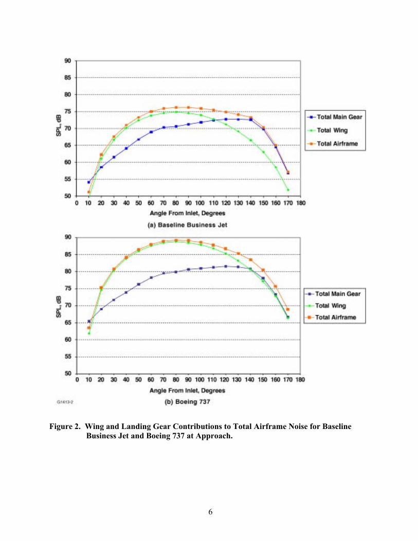
The summary plot of wing and landing gear components (Figure 2) shows that the mainlanding gear is a more significant contributor to overall airframe noise for the Business Jet thanfor the B737, particularly at the aft angles. This tends to sustain a higher overall noise level at theaft angles for the Business Jet.

In the wing noise plot (Figure 3), the flap noise is considerably higher than the slat noise forthe business jet. However, for the B737, the flap and slat noise are more similar in level. Torepresent the “cleaner” business jet slat, the slat noise was reduced by 1/2 of the benefit projectedby Boeing for the near-term cove fill and gap reduction.

The landing gear plot in Figure 4 shows that the nose gear contribution is only about 3 dBbelow the main gear for the Business Jet. In contrast, the nose gear noise levels for the largeraircraft are approximately 7-12 dB below those of the main gear. The difference becomes greateras the aircraft size increases, indicating the relative increase in main gear size/complexity relativeto the nose gear. Therefore, for a smaller aircraft, the contribution of the nose gear is moresignificant. The nose gear was modeled assuming the strut diameter, hydraulic line diameter, etc.remained the same as the main gear. Tire diameter was reduced to reflect the smaller size of thenose gear tires.

6

Figure 2. Wing and Landing Gear Contributions to Total Airframe Noise for BaselineBusiness Jet and Boeing 737 at Approach.

7

Figure 3. Flap and Slat Contributions to Wing Noise for Baseline Business Jet and Boeing737 at Approach.

8

Figure 4. Main and Nose Landing Gear Contributions to the Total Landing Gear Noise forthe Baseline Business Jet at Approach.

As shown in Figure 5, for both the nose and main gear of the business jet, the low-frequencynoise is the primary contributor, with the mid- and high-frequency noise having minimal effect.However, tire noise is a much larger contributor, relative to the mid-and high-frequency sources,for the main gear than for the nose gear. This may be explained by the larger tire diameter for themain gear.

9

Figure 5. Landing Gear Component Contributions to the Total Landing Gear Noise for theBaseline Business Jet at Approach.

As shown in Figure 6, for the main gear, the character of the low-frequency noise is similarfor the bizjet and the B737. Also, the character and level of tire noise, relative to the low-frequency noise, is similar for the bizjet and B737. However, the mid- and high frequencysources are somewhat more significant contributors to overall landing gear noise for the B737.

10

High-frequency noise for the B737 is almost on a par with the tire noise, but is about 5 dB belowthe tire noise for the bizjet. Differences in the relative diameter of hydraulic lines versus landinggear struts for the two aircraft types contribute to this behavior. The high frequency noise sourcesare affected by the smaller diameter components, such as hydraulic lines. For the B737, thehydraulic line diameters relative to the landing gear strut diameters are approximately 0.17; incontrast, the ratio for the bizjet is 0.12. This would account for the approximately 3 dB largerdifference between the low- and high-frequency SPLs for the bizjet than for the B737.

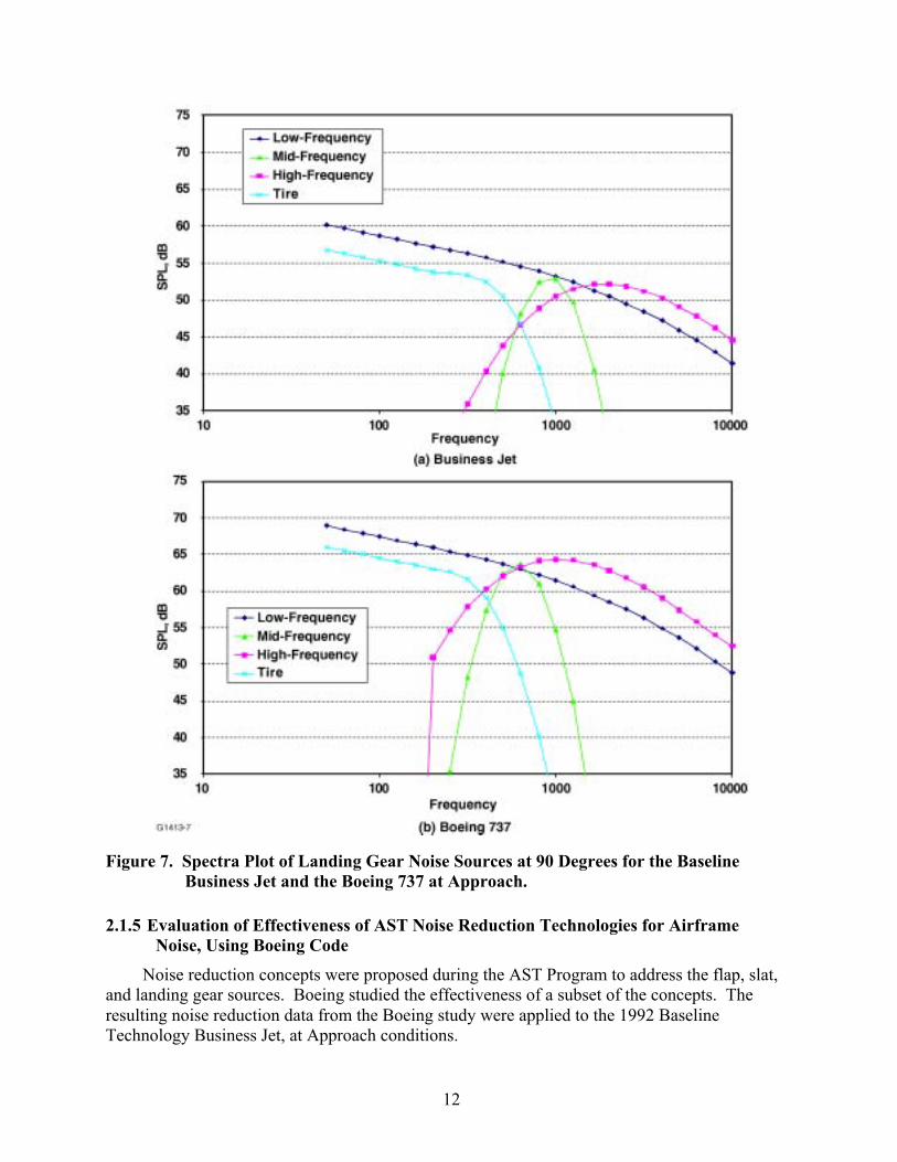
To further understand the character of the various landing gear sources, a spectra plot at 90degrees was produced for all landing gear noise sources, for both the business jet and B737 (referto Figure 7). As seen from the plots, the peak frequencies of the sources are shifted higher for thebizjet, compared to the B737. This shift is most significant for the mid- and high frequencysources. The shift is explained by the smaller diameter of the noise-generating components (strutand hydraulic line diameters) for the bizjet, compared to the B737.

11

Figure 6. Landing Gear Component Contributions to the Total Landing Gear Noise for theBaseline Business Jet and Boeing 737 at Approach.

12

Figure 7. Spectra Plot of Landing Gear Noise Sources at 90 Degrees for the BaselineBusiness Jet and the Boeing 737 at Approach.

2.1.5 Evaluation of Effectiveness of AST Noise Reduction Technologies for Airframe Noise, Using Boeing Code

Noise reduction concepts were proposed during the AST Program to address the flap, slat,and landing gear sources. Boeing studied the effectiveness of a subset of the concepts. Theresulting noise reduction data from the Boeing study were applied to the 1992 BaselineTechnology Business Jet, at Approach conditions.

13

Slat Concepts – The only slat noise reduction technology considered by Boeing consisted ofa cove fill and gap reduction. This was projected to yield an 11.4 dB reduction in slat noise overthe long-term, with a 5.8 dB reduction near-term. However, the business jet slat configuration didnot have a cove gap. Therefore, the baseline slat noise level was reduced to reflect the absence ofa slat gap. In addition, further reductions in slat noise were not expected to be as substantial.

Because the noise reduction technology techniques used for the near-term reductions werealready employed in the simplified flap of the Baseline Business Jet, it was assumed that the slatnoise was already reduced by 1/2 of the Boeing Near-Term reduction, due to the absence of thecove and gap. Further, it was assumed that no additional reduction would be achieved in thenear-term, because the primary noise generators were not present. It was assumed that the long-term benefit would be 1/2 of the Boeing long-term benefit. Therefore, the AST noise reductiontechnologies for the business jet slat noise were modeled as:

(a) Near-Term -2.9 dB (Same as Baseline)

(b) Long-Term -5.7 dB

Landing Gear Concepts – Only high-and mid-frequency noise reductions were considered inthe Boeing study. Such reductions could possibly be achieved by placing fairings over smallcomponents and moving lines and brackets out of the flowpath. However, the high- and mid-frequency noise sources do not contribute as much to overall gear noise for the business jet asthey do for the B737. Therefore, not as much overall benefit would be expected. Applying thesame levels of component reduction predicted by Boeing, the AST noise reduction technologiesfor the business jet landing gear were modeled as:

(a) Near-Term -1.4 dB (High-Frequency)

(b) Long-Term -3.0 dB (High- and Mid-Frequency)

The same levels of reduction were applied for the nose and main gear.

Flap Concepts – Fences of various thicknesses, microtabs, and porous flap tips were allexamined in the Boeing study for near-term noise reduction. However, at most, these conceptsyielded a 1.4 dB reduction in outboard flap noise (for fences with 2x flap thickness). Similarbenefits were assumed for the bizjet. In addition, for the long-term case, no flap noise wasassumed.

Based on the Boeing AST Noise Reduction Technology numbers, the following reductionswere applied for the business jet, using the outboard flaps:

(a) Near-Term -1.4 dB

(b) Long-Term -20.0 dB (To model the “No Flap Effects” condition)

The flap models in the Boeing program were not considered accurate for the 0-degreedeflection case (“No Flap Effects”). The flap models were based on configurations of 20, 30 and40 degrees deflection, and would tend to underpredict the actual trailing edge noise for anundeflected flap. Therefore, this condition was modeled by reducing the flap noise level (-20 dB)to the point at which it was insignificant.

14

Combined Concepts – To determine the maximum overall benefit for the business jet, allnoise reduction technologies were combined, for Near-Term and Long-Term evaluations. Theeffect of the noise reduction technologies is shown in the bar chart in Figure 8.

Figure 8. Impact of Noise Reduction Technologies for Baseline Business Jet at Approach.

As shown in Figure 8, in the near-term, the flaps were still the major contributor, and onlyslight reductions were seen in gear noise. Therefore, the overall airframe noise reduction wasonly 0.9 dB. In the long-term, the flaps did not contribute at all. The primary source was themain gear, with the slats and nose gear approximately equal. The overall airframe noise reductionwas 5.9 dB.

Gear noise was not reduced substantially with noise reduction technologies, because thereductions were applied to the mid- and high-frequency sources, but the low-frequency sourcesclearly dominated. Therefore, not much benefit was seen.

2.1.6 Comparison With Goals

The Pillar Goals for airframe noise reduction may be represented as follows:

(a) Near-Term -4 dB (QAT Goal – 1997-2007)

(b) Long-Term -8 dB (QAT + Follow-on – 2002-2022)

15

The Near-Term AST noise reduction technology does not satisfy the goal of a 4 dBreduction in airframe noise. Similarly, the long-term noise reduction technology does not satisfythe goal of an 8 dB reduction in airframe noise.

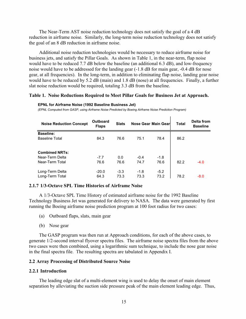
Additional noise reduction technologies would be necessary to reduce airframe noise forbusiness jets, and satisfy the Pillar Goals. As shown in Table 1, in the near-term, flap noisewould have to be reduced 7.7 dB below the baseline (an additional 6.3 dB), and low-frequencynoise would have to be addressed for the landing gear (-1.8 dB for main gear, -0.4 dB for nosegear, at all frequencies). In the long-term, in addition to eliminating flap noise, landing gear noisewould have to be reduced by 5.2 dB (main) and 1.8 dB (nose) at all frequencies. Finally, a furtherslat noise reduction would be required, totaling 3.3 dB from the baseline.

Table 1. Noise Reductions Required to Meet Pillar Goals for Business Jet at Approach.

EPNL for Airframe Noise (1992 Baseline Business Jet)(EPNL Computed from GASP, using Airframe Noise Predicted by Boeing Airframe Noise Prediction Program)

Noise Reduction ConceptOutboard

FlapsSlats Nose Gear Main Gear Total

Delta from Baseline

Baseline:Baseline Total 84.3 76.6 75.1 78.4 86.2

Combined NRTs:Near-Term Delta -7.7 0.0 -0.4 -1.8Near-Term Total 76.6 76.6 74.7 76.6 82.2 -4.0

Long-Term Delta -20.0 -3.3 -1.8 -5.2Long-Term Total 64.3 73.3 73.3 73.2 78.2 -8.0

2.1.7 1/3-Octave SPL Time Histories of Airframe Noise

A 1/3-Octave SPL Time History of estimated airframe noise for the 1992 BaselineTechnology Business Jet was generated for delivery to NASA. The data were generated by firstrunning the Boeing airframe noise prediction program at 100 foot radius for two cases:

(a) Outboard flaps, slats, main gear

(b) Nose gear

The GASP program was then run at Approach conditions, for each of the above cases, togenerate 1/2-second interval flyover spectra files. The airframe noise spectra files from the abovetwo cases were then combined, using a logarithmic sum technique, to include the nose gear noisein the final spectra file. The resulting spectra are tabulated in Appendix I.

2.2 Array Processing of Distributed Source Noise

2.2.1 Introduction

The leading edge slat of a multi-element wing is used to delay the onset of main elementseparation by alleviating the suction side pressure peak of the main element leading edge. Thus,

16

the leading edge slat serves the purpose of potentially improving the lift capability (CLmax) of theaircraft. A more detailed description of complex flow field between the slat and main elementwould involve the viscous interactions of the slat wake and the main element boundary layer. Aswith most aeroacoustic occurrences, acoustic improvements often correlate highly withaerodynamic performance degradation. It has been reported (Reed [1] ) that slat noise reductioncan be attained by reducing the gap distance between the slat trailing edge and the main elementleading edge; however, less than optimal lift performance can be the consequence of a relativelysmall gap size (Thomas et al. [2] ). Figure 9 illustrates the slat and main element and some keyterminology pertaining to the geometrical configuration of these wing elements.

Figure 9. Schematic of a Leading Edge Slat and Wing Main Element Leading Edge.

It was observed in early airframe noise investigations that the addition of a loaded leadingedge slat not only resulted in increased noise levels in the vicinity of the wing leading edge butalso influenced the noise associated with the airframe flaps (Hayes et al. [3] ). A significantincrease in the outboard flap noise levels of a 4.7% scale DC-10 model was observed by Hayes etal. while the inboard flap levels were only nominally influenced by the presence of the loadedleading edge slat. This effect was postulated to be the result of the leading edge slats influence onthe wing aerodynamic loading primarily on the outboard side although no clarification wasprovided. Through the use of flap-tip fences, Hayes et al. also demonstrated that the reduction offlap source noise accentuated the contributions of the leading edge slats to the overall noise ofthis aircraft model. This demonstration emphasized the fact that in order to achieve significantairframe noise reduction equal attention must be given to leading edge slat. In a series of NASAreports also utilizing a 4.7% scale DC-10 model, Guo et al. [4][5][6] further demonstrated theimportance of the leading edge slat on airframe noise noting the dominant role of leading edgeslat sources at the moderate to low flap deflection angles. This finding is germane to the newerairframes such as the 777 due to the usually lower flap settings relative to the DC-10. Utilizationof a phased array of microphones, strategically located surface mounted pressure transducers, andfree field noise measurements resulted in a number of significant findings by Guo et al. pertainingto slat noise. Most notably are the significant slat noise levels observed at the lower flapdeflection settings and the distributed nature of the leading edge slat source.

Detailed experimental work on specific component behavior has proceeded almost inparallel to the more global aforementioned airframe noise studies. Dobrzynski et al. [7] of theDLR used a 1/10th scaled Airbus-type high lift wing to quantify wing noise sources. Theirfindings did confirm the initial assumptions of Guo that under certain slat configurations vortex

17

shedding from the slat edge cove can result in excessive noise in the vicinity of the slat. Thisvortex shedding or unsteady flow separation at the slat cove and the ensuing unsteady massfluctuations flowing through the slat trailing edge and main element leading edge formed thebasis of Gou’s initial formulation for slat noise prediction. However the tones present in theexperiment were the result of laminar shedding off the slat cove. These tones were reduced byboundary layer tripping just upstream of the cove leading edge. Corresponding tonal behaviorwas observed in the surface measurements on the pressure side of the slat with broadband andtonal amplification observed in the sensors approaching the slat trailing edge. They conjecturedthat the noise produced from this laminar vortex shedding led to mean flow oscillations in the gapbetween the slat trailing edge and main element leading edge. Trailing edge noise was alsoidentified as a slat source mechanism that influenced the low to intermediate frequencies of theirstudy. Although it was observed that the flap side was the more dominate source in terms ofnoise per area (more localized) the noise emanating from the slat dominated the low tointermediate frequency ranges. It should be noted that the noise levels in the vicinity of the slattracks or supports were typically ~ 8 dB higher than the levels in other slat regions in the 20 kHzrange. It was suggested that his vortex shedding mechanism could be significantly reduced withthe design of streamlined tracks and aligned in the flow direction.

Storms et al. [8] focused their aeroacoustic measurements on the leading edge slat using ahigh lift model consisting of several slat brackets, a main element, and a partial span outboardflap. Their phased array noise maps contained highly localized noise sources across the span ofthe slat that appeared to move outboard with frequency, a consequence of the modelconfiguration. Static pressure measurements indicated that higher slat deflections resulted inhigher suction at the slat trailing edge, lower slat loading, and a higher suction peak on the mainelement leading edge. Slat gap velocities were higher than the freestream velocity a result alsoobserved in the PIV data of Moriarty et. al. [9] where gap velocities near 2x the freestream weremeasured. The integrated noise data did suggest that the noise levels were reduced as a functionof decreasing slat deflection or decreasing slat gap velocity (for a fixed Mach number); however,using an M5 amplitude correction the noise data did not collapse favorably with these gapvelocities. Varying the main-element angle of attack indicated a non-linear relation between slatnoise and slat gap velocity with main element deflection. They theorized that this behavior mightbe due to the state of the upper boundary layer of the slat. The higher slat deflections may havebeen laminar over the upper surface resulting in flow conditions inherently more sensitive todisturbances. Their computational analysis coupled with measurements suggest a feedbackmechanism between vortex shedding at the slat trailing edge and Kelvin-Helmholtz instabilitiesfrom the slat cove region. Moriarty et. al. verified the mean flow behavior of Storms et. al. withPIV measurements but also observed that Turbulent Kinetic Energy (TKE) levels were highest inthe slat gap region where the separating shear layer reattaches to the backside of the slat. Theysuggested that this region is likely to be the most energetic if feedback from the slat trailing edgeamplifies disturbances in this region.

A number of computational studies have attempted to model slat noise generation and farfield radiation (Guo [4], Khorrami, et. al. [10] , Singer et. al. [11] , and Khorrami et. al. [12] ).Guo attempted to model the unsteady flow field around the cusp and through the slat gap usingunsteady panel methods to solve the near field and the method of asymptotic expansion to derivethe far field sound. Aside from presenting a simplified computational method, Guo’scomputations indicated that the slat radiates sound dominantly in the aft direction (fly-over).

18

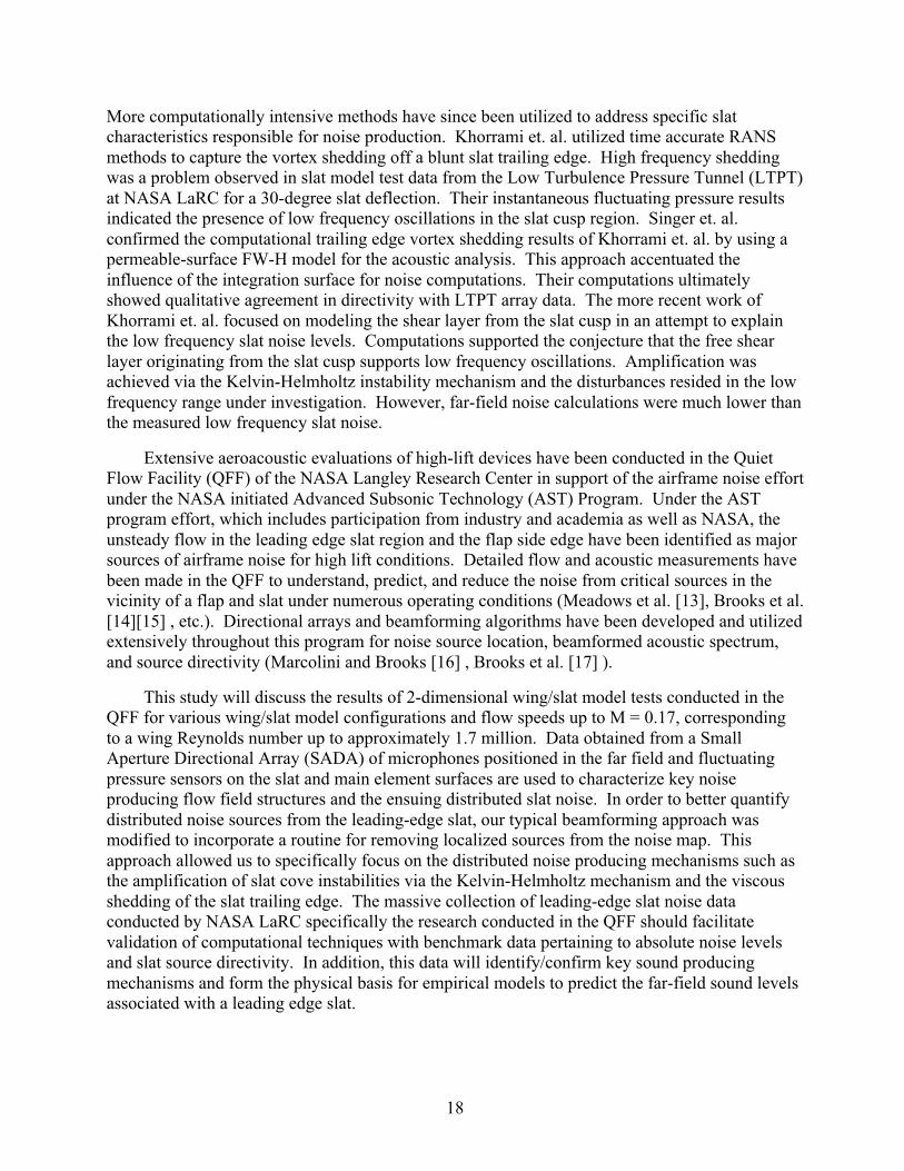
More computationally intensive methods have since been utilized to address specific slatcharacteristics responsible for noise production. Khorrami et. al. utilized time accurate RANSmethods to capture the vortex shedding off a blunt slat trailing edge. High frequency sheddingwas a problem observed in slat model test data from the Low Turbulence Pressure Tunnel (LTPT)at NASA LaRC for a 30-degree slat deflection. Their instantaneous fluctuating pressure resultsindicated the presence of low frequency oscillations in the slat cusp region. Singer et. al.confirmed the computational trailing edge vortex shedding results of Khorrami et. al. by using apermeable-surface FW-H model for the acoustic analysis. This approach accentuated theinfluence of the integration surface for noise computations. Their computations ultimatelyshowed qualitative agreement in directivity with LTPT array data. The more recent work ofKhorrami et. al. focused on modeling the shear layer from the slat cusp in an attempt to explainthe low frequency slat noise levels. Computations supported the conjecture that the free shearlayer originating from the slat cusp supports low frequency oscillations. Amplification wasachieved via the Kelvin-Helmholtz instability mechanism and the disturbances resided in the lowfrequency range under investigation. However, far-field noise calculations were much lower thanthe measured low frequency slat noise.

Extensive aeroacoustic evaluations of high-lift devices have been conducted in the QuietFlow Facility (QFF) of the NASA Langley Research Center in support of the airframe noise effortunder the NASA initiated Advanced Subsonic Technology (AST) Program. Under the ASTprogram effort, which includes participation from industry and academia as well as NASA, theunsteady flow in the leading edge slat region and the flap side edge have been identified as majorsources of airframe noise for high lift conditions. Detailed flow and acoustic measurements havebeen made in the QFF to understand, predict, and reduce the noise from critical sources in thevicinity of a flap and slat under numerous operating conditions (Meadows et al. [13], Brooks et al.[14][15] , etc.). Directional arrays and beamforming algorithms have been developed and utilizedextensively throughout this program for noise source location, beamformed acoustic spectrum,and source directivity (Marcolini and Brooks [16] , Brooks et al. [17] ).

This study will discuss the results of 2-dimensional wing/slat model tests conducted in theQFF for various wing/slat model configurations and flow speeds up to M = 0.17, correspondingto a wing Reynolds number up to approximately 1.7 million. Data obtained from a SmallAperture Directional Array (SADA) of microphones positioned in the far field and fluctuatingpressure sensors on the slat and main element surfaces are used to characterize key noiseproducing flow field structures and the ensuing distributed slat noise. In order to better quantifydistributed noise sources from the leading-edge slat, our typical beamforming approach wasmodified to incorporate a routine for removing localized sources from the noise map. Thisapproach allowed us to specifically focus on the distributed noise producing mechanisms such asthe amplification of slat cove instabilities via the Kelvin-Helmholtz mechanism and the viscousshedding of the slat trailing edge. The massive collection of leading-edge slat noise dataconducted by NASA LaRC specifically the research conducted in the QFF should facilitatevalidation of computational techniques with benchmark data pertaining to absolute noise levelsand slat source directivity. In addition, this data will identify/confirm key sound producingmechanisms and form the physical basis for empirical models to predict the far-field sound levelsassociated with a leading edge slat.

19

2.2.2 Summary of the Array Processing Methodology

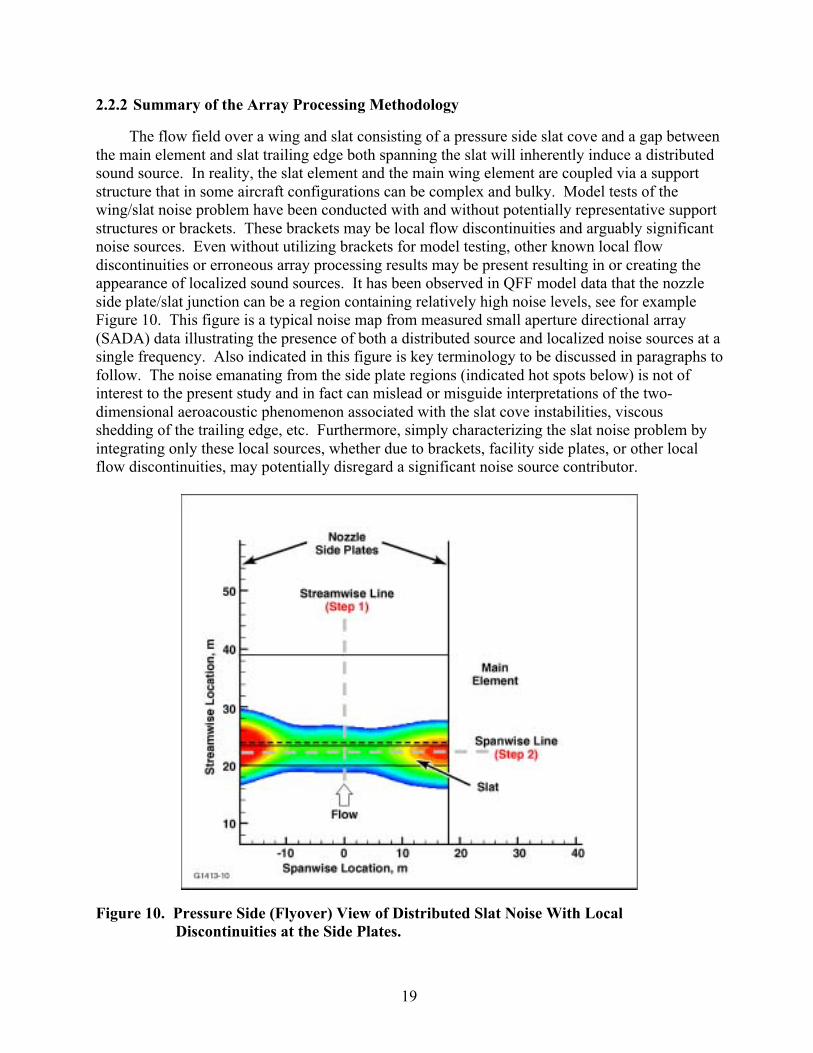
The flow field over a wing and slat consisting of a pressure side slat cove and a gap betweenthe main element and slat trailing edge both spanning the slat will inherently induce a distributedsound source. In reality, the slat element and the main wing element are coupled via a supportstructure that in some aircraft configurations can be complex and bulky. Model tests of thewing/slat noise problem have been conducted with and without potentially representative supportstructures or brackets. These brackets may be local flow discontinuities and arguably significantnoise sources. Even without utilizing brackets for model testing, other known local flowdiscontinuities or erroneous array processing results may be present resulting in or creating theappearance of localized sound sources. It has been observed in QFF model data that the nozzleside plate/slat junction can be a region containing relatively high noise levels, see for exampleFigure 10. This figure is a typical noise map from measured small aperture directional array(SADA) data illustrating the presence of both a distributed source and localized noise sources at asingle frequency. Also indicated in this figure is key terminology to be discussed in paragraphs tofollow. The noise emanating from the side plate regions (indicated hot spots below) is not ofinterest to the present study and in fact can mislead or misguide interpretations of the two-dimensional aeroacoustic phenomenon associated with the slat cove instabilities, viscousshedding of the trailing edge, etc. Furthermore, simply characterizing the slat noise problem byintegrating only these local sources, whether due to brackets, facility side plates, or other localflow discontinuities, may potentially disregard a significant noise source contributor.

Figure 10. Pressure Side (Flyover) View of Distributed Slat Noise With Local Discontinuities at the Side Plates.

20

To overcome these potential pitfalls, a method was developed and implemented to decouplethe noise due to localized sources from the noise of interest, the distributed noise sources in thewing/slat region. A breakdown into the three aforementioned sound sources is justified herebecause the noise map illustrated in Figure 10 is indeed typical of the noise maps encountered inour slat noise measurements. The decoupling approach takes into account the frequencydependent beam characteristics of the SADA culminating in distributed source spectra that ispresented on a per foot basis (i.e., SPL/ft). The two dimensional spectral representation of thedistributed noise spectra is used throughout to facilitate aeroacoustic scaling of the observed slatnoise. The developed procedure to go from the measured SADA output to a distributed noiselevel per foot consists of essentially 6 steps. This process is summarized as follows:

(1) Generate standard beamformed noise maps at each narrowband frequency foreach test configuration. Search a standard noise map for the maximum noise levelalong the streamwise line located at the center of the slat (see Figure 10).

(2) With the maximum streamwise location identified from step 1, search along thespanwise line passing through this point for peak levels PaT2

2 and PaT32 and a

minimum PaTmin2 near the slat center. Note these levels and corresponding

spanwise locations (see Figure 11). It is assumed that the noise sources at y2 andy3 are simple sources and that each of the identified P2 terms containscontributions from each of the other sources.

Figure 11. Pressure-Squared Values as a Function of Spanwise Position.

(3) Compute the theoretical beam pattern characteristics at each narrow bandfrequency of interest along the spanwise line identified in step 2. The beampatterns are computed from the spatial filter function, W, for a point sourcelocated at the center of the scan line based on the following relation:

W k x x w kr

rik r r r ro m

mmo m m

o

mtot

o( , , ) ( ) exp

r r= ⋅ ⋅ −( ) + −

=

∑1

21

Where mtot is the total number of microphones, wm(k) are known weightingfactors associated with the SADA, ro is the point source location relative to thearray center, r is the scan point location relative to the array center , rmo is themicrophone to source distance, rm is the microphone to scan point distance.

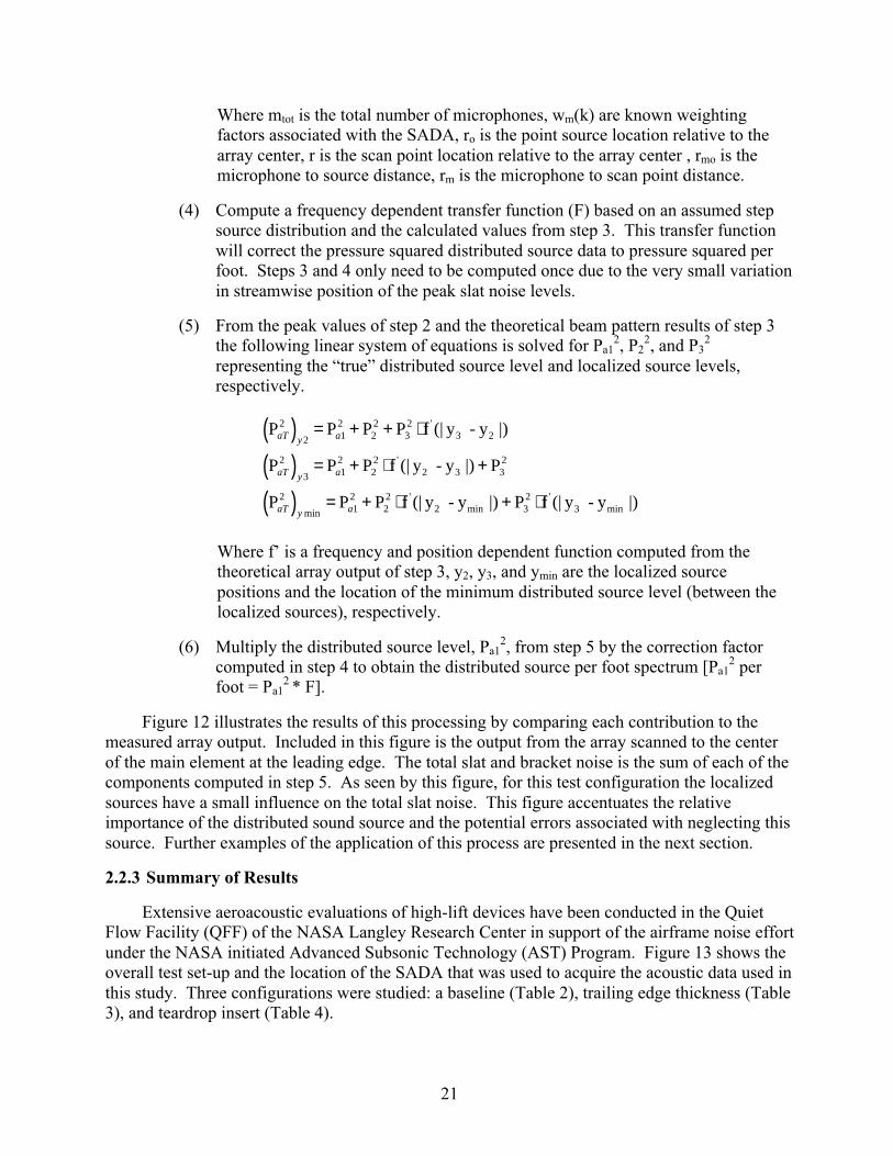
(4) Compute a frequency dependent transfer function (F) based on an assumed stepsource distribution and the calculated values from step 3. This transfer functionwill correct the pressure squared distributed source data to pressure squared perfoot. Steps 3 and 4 only need to be computed once due to the very small variationin streamwise position of the peak slat noise levels.

(5) From the peak values of step 2 and the theoretical beam pattern results of step 3the following linear system of equations is solved for Pa1

2, P22, and P3

2

representing the “true” distributed source level and localized source levels,respectively.

P P P P f (| y - y |)

P P P f (| y - y |) P

P P P f (| y - y |) P f (| y - y |)

'3 2

'2 3

'2 min

'3 min

aT y a

aT y a

aT y a

2

2 12

22

32

2

3 12

22

32

21

222

32

( ) = + + ⋅

( ) = + ⋅ +

( ) = + ⋅ + ⋅min

Where f’ is a frequency and position dependent function computed from thetheoretical array output of step 3, y2, y3, and ymin are the localized sourcepositions and the location of the minimum distributed source level (between thelocalized sources), respectively.

(6) Multiply the distributed source level, Pa12, from step 5 by the correction factor

computed in step 4 to obtain the distributed source per foot spectrum [Pa12 per

foot = Pa12 * F].

Figure 12 illustrates the results of this processing by comparing each contribution to themeasured array output. Included in this figure is the output from the array scanned to the centerof the main element at the leading edge. The total slat and bracket noise is the sum of each of thecomponents computed in step 5. As seen by this figure, for this test configuration the localizedsources have a small influence on the total slat noise. This figure accentuates the relativeimportance of the distributed sound source and the potential errors associated with neglecting thissource. Further examples of the application of this process are presented in the next section.

2.2.3 Summary of Results

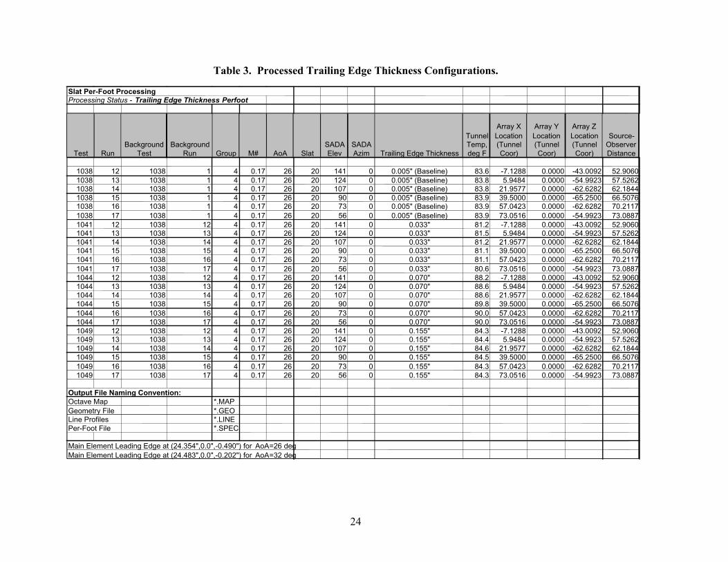
Extensive aeroacoustic evaluations of high-lift devices have been conducted in the QuietFlow Facility (QFF) of the NASA Langley Research Center in support of the airframe noise effortunder the NASA initiated Advanced Subsonic Technology (AST) Program. Figure 13 shows theoverall test set-up and the location of the SADA that was used to acquire the acoustic data used inthis study. Three configurations were studied: a baseline (Table 2), trailing edge thickness (Table3), and teardrop insert (Table 4).

22

Figure 12. Breakdown of Slat Noise Contributions for M=0.17, δs = 20°°°°, δw = 26°°°°, Ψ = 0°°°°,

and Φ = 107o.

Figure 13. Schematic Diagram of the Slat/Wing Model and Elevation Angle Position (Side View).

23

Table 2. Processed Baseline Configurations.

Slat Per-Foot ProcessingProcessing Status - Baseline Perfoot

Test RunBackground

Run Group M# AoA SlatSADA Elev

SADA Azim Treatment

Tunnel Temp, deg F

Array X Location (Tunnel Coor)

Array Y Location (Tunnel Coor)

Array Z Location (Tunnel Coor)

Source-Observer Distance

1020 12 1 4 0.17 26 20 141 0 Baseline 82.1 -7.1288 0.0000 -43.0092 52.90601020 13 1 4 0.17 26 20 124 0 Baseline 82.6 5.9484 0.0000 -54.9923 57.52621020 14 1 4 0.17 26 20 107 0 Baseline 82.8 21.9577 0.0000 -62.6282 62.18441020 15 1 4 0.17 26 20 90 0 Baseline 82.9 39.5000 0.0000 -65.2500 66.50761021 2 1 4 0.17 26 20 73 0 Baseline 80.6 57.0423 0.0000 -62.6282 70.21171021 3 1 4 0.17 26 20 56 0 Baseline 80.8 73.0516 0.0000 -54.9923 73.08871066 12 1 4 0.17 26 20 141 0 Slat Moved Closer to Main Element 87.0 -7.1288 0.0000 -43.0092 52.90601067 2 1 4 0.17 26 20 124 0 Slat Moved Closer to Main Element 80.4 5.9484 0.0000 -54.9923 57.52621067 3 1 4 0.17 26 20 107 0 Slat Moved Closer to Main Element 80.2 21.9577 0.0000 -62.6282 62.18441067 4 1 4 0.17 26 20 90 0 Slat Moved Closer to Main Element 80.3 39.5000 0.0000 -65.2500 66.50761067 5 1 4 0.17 26 20 73 0 Slat Moved Closer to Main Element 80.3 57.0423 0.0000 -62.6282 70.21171067 6 1 4 0.17 26 20 56 0 Slat Moved Closer to Main Element 80.5 73.0516 0.0000 -54.9923 73.08871166 12 1 4 0.17 26 20 141 0 50% Closed, 6 Notches 56.5 -7.1288 0.0000 -43.0092 52.90601166 13 1 4 0.17 26 20 124 0 50% Closed, 6 Notches 56.5 5.9484 0.0000 -54.9923 57.52621166 14 1 4 0.17 26 20 107 0 50% Closed, 6 Notches 56.4 21.9577 0.0000 -62.6282 62.18441166 15 1 4 0.17 26 20 90 0 50% Closed, 6 Notches 55.9 39.5000 0.0000 -65.2500 66.50761166 16 1 4 0.17 26 20 73 0 50% Closed, 6 Notches 55.9 57.0423 0.0000 -62.6282 70.21171166 17 1 4 0.17 26 20 56 0 50% Closed, 6 Notches 55.9 73.0516 0.0000 -54.9923 73.0887

Output File Naming Convention:Octave Map *.MAPGeometry File *.GEOLine Profiles *.LINEPer-Foot File *.SPEC

Main Element Leading Edge at (24.354",0.0",-0.490") for AoA=26 deg

24

Table 3. Processed Trailing Edge Thickness Configurations.

Slat Per-Foot ProcessingProcessing Status - Trailing Edge Thickness Perfoot

Test RunBackground

TestBackground

Run Group M# AoA SlatSADA Elev

SADA Azim Trailing Edge Thickness

Tunnel Temp, deg F

Array X Location (Tunnel Coor)

Array Y Location (Tunnel Coor)

Array Z Location (Tunnel Coor)

Source-Observer Distance

1038 12 1038 1 4 0.17 26 20 141 0 0.005" (Baseline) 83.6 -7.1288 0.0000 -43.0092 52.90601038 13 1038 1 4 0.17 26 20 124 0 0.005" (Baseline) 83.8 5.9484 0.0000 -54.9923 57.52621038 14 1038 1 4 0.17 26 20 107 0 0.005" (Baseline) 83.8 21.9577 0.0000 -62.6282 62.18441038 15 1038 1 4 0.17 26 20 90 0 0.005" (Baseline) 83.9 39.5000 0.0000 -65.2500 66.50761038 16 1038 1 4 0.17 26 20 73 0 0.005" (Baseline) 83.9 57.0423 0.0000 -62.6282 70.21171038 17 1038 1 4 0.17 26 20 56 0 0.005" (Baseline) 83.9 73.0516 0.0000 -54.9923 73.08871041 12 1038 12 4 0.17 26 20 141 0 0.033" 81.2 -7.1288 0.0000 -43.0092 52.90601041 13 1038 13 4 0.17 26 20 124 0 0.033" 81.5 5.9484 0.0000 -54.9923 57.52621041 14 1038 14 4 0.17 26 20 107 0 0.033" 81.2 21.9577 0.0000 -62.6282 62.18441041 15 1038 15 4 0.17 26 20 90 0 0.033" 81.1 39.5000 0.0000 -65.2500 66.50761041 16 1038 16 4 0.17 26 20 73 0 0.033" 81.1 57.0423 0.0000 -62.6282 70.21171041 17 1038 17 4 0.17 26 20 56 0 0.033" 80.6 73.0516 0.0000 -54.9923 73.08871044 12 1038 12 4 0.17 26 20 141 0 0.070" 88.2 -7.1288 0.0000 -43.0092 52.90601044 13 1038 13 4 0.17 26 20 124 0 0.070" 88.6 5.9484 0.0000 -54.9923 57.52621044 14 1038 14 4 0.17 26 20 107 0 0.070" 88.6 21.9577 0.0000 -62.6282 62.18441044 15 1038 15 4 0.17 26 20 90 0 0.070" 89.8 39.5000 0.0000 -65.2500 66.50761044 16 1038 16 4 0.17 26 20 73 0 0.070" 90.0 57.0423 0.0000 -62.6282 70.21171044 17 1038 17 4 0.17 26 20 56 0 0.070" 90.0 73.0516 0.0000 -54.9923 73.08871049 12 1038 12 4 0.17 26 20 141 0 0.155" 84.3 -7.1288 0.0000 -43.0092 52.90601049 13 1038 13 4 0.17 26 20 124 0 0.155" 84.4 5.9484 0.0000 -54.9923 57.52621049 14 1038 14 4 0.17 26 20 107 0 0.155" 84.6 21.9577 0.0000 -62.6282 62.18441049 15 1038 15 4 0.17 26 20 90 0 0.155" 84.5 39.5000 0.0000 -65.2500 66.50761049 16 1038 16 4 0.17 26 20 73 0 0.155" 84.3 57.0423 0.0000 -62.6282 70.21171049 17 1038 17 4 0.17 26 20 56 0 0.155" 84.3 73.0516 0.0000 -54.9923 73.0887

Output File Naming Convention:Octave Map *.MAPGeometry File *.GEOLine Profiles *.LINEPer-Foot File *.SPEC

Main Element Leading Edge at (24.354",0.0",-0.490") for AoA=26 degMain Element Leading Edge at (24.483",0.0",-0.202") for AoA=32 deg

25

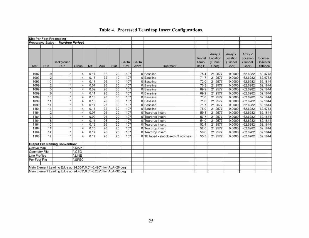
Table 4. Processed Teardrop Insert Configurations.

Slat Per-Foot ProcessingProcessing Status - Teardrop Perfoot

Test RunBackground

Run Group M# AoA SlatSADA Elev

SADA Azim Treatment

Tunnel Temp, deg F

Array X Location (Tunnel Coor)

Array Y Location (Tunnel Coor)

Array Z Location (Tunnel Coor)

Source-Observer Distance

1087 9 1 4 0.17 32 20 107 0 Baseline 75.4 21.9577 0.0000 -62.6282 62.47731093 2 1 4 0.17 32 10 107 0 Baseline 71.7 21.9577 0.0000 -62.6282 62.47731095 10 1 4 0.17 26 10 107 0 Baseline 72.0 21.9577 0.0000 -62.6282 62.18441099 2 1 4 0.07 26 30 107 0 Baseline 70.3 21.9577 0.0000 -62.6282 62.18441099 3 1 4 0.09 26 30 107 0 Baseline 69.9 21.9577 0.0000 -62.6282 62.18441099 6 1 4 0.11 26 30 107 0 Baseline 69.9 21.9577 0.0000 -62.6282 62.18441099 10 1 4 0.13 26 30 107 0 Baseline 71.0 21.9577 0.0000 -62.6282 62.18441099 11 1 4 0.15 26 30 107 0 Baseline 71.0 21.9577 0.0000 -62.6282 62.18441099 14 1 4 0.17 26 30 107 0 Baseline 71.7 21.9577 0.0000 -62.6282 62.18441154 14 1 4 0.17 32 30 107 0 Baseline 76.0 21.9577 0.0000 -62.6282 62.47731164 2 1 4 0.07 26 20 107 0 Teardrop insert 59.1 21.9577 0.0000 -62.6282 62.18441164 3 1 4 0.09 26 20 107 0 Teardrop insert 57.7 21.9577 0.0000 -62.6282 62.18441164 6 1 4 0.11 26 20 107 0 Teardrop insert 54.0 21.9577 0.0000 -62.6282 62.18441164 10 1 4 0.13 26 20 107 0 Teardrop insert 52.4 21.9577 0.0000 -62.6282 62.18441164 11 1 4 0.15 26 20 107 0 Teardrop insert 52.0 21.9577 0.0000 -62.6282 62.18441164 14 1 4 0.17 26 20 107 0 Teardrop insert 50.6 21.9577 0.0000 -62.6282 62.18441168 14 1 4 0.17 26 20 107 0 TE taped - slat closed - 9 notches 55.3 21.9577 0.0000 -62.6282 62.1844

Output File Naming Convention:Octave Map *.MAPGeometry File *.GEOLine Profiles *.LINEPer-Foot File *.SPEC

Main Element Leading Edge at (24.354",0.0",-0.490") for AoA=26 degMain Element Leading Edge at (24.483",0.0",-0.202") for AoA=32 deg

26

Figure 14 shows the comparison of the narrowband sound pressure level for the wing at 26°angle of attack for Test 1020 (Table 2) and 32° angle of attack for Test 1087 (Table 4). The

figure shows that the noise levels decrease as the angle of attack decreases. Figure 15 shows theaffect of changing slat angle of attack for a wing angle of attack of 26° by comparing the slat

angles of 10° for Test 1095 (Table 4), 20° for Test 1020 (Table 2), and 30° for Test 1099 (Table

4). The measured sound levels decrease as the slat angle of attack decreases. Figure 16 showsthe same slat angle of attack trends for the wing angle of attack of 32° using Tests 1087, 1093,

and 1154 (Table 4).

Figure 17 shows that decreasing the slat gap (or increasing the overlap) also reduces theleading edge slat noise. Tests 1020, 1067, and 1166 (Table 2) and 1168 (Table 4) are plotted toshow the trend.

Figure 18 shows the effect of the teardrop insert from Test 1164 (Table 4) as compared tothe baseline configuration from Test 1020 (Table 2). It is clearly seen that the teardrop insertlowered the leading edge slat noise in the mid frequency range of 10 kHz to 45kHz. However,the low frequency noise appeared to be amplified by the teardrop insert. Figure 19 shows theeffect of increasing Mach number on the teardrop insert configuration. The increasing Machnumber consistently results in an increase noise level.

Figure 20 to Figure 23 show the directivity characteristics, in both absolute and normalizedform, of the baseline configuration from Test 1020 and 6-notch gap/overlap configuration fromTest 1166 (Table 2). It can be seen that once properly normalized, the directivity effect can beremoved.

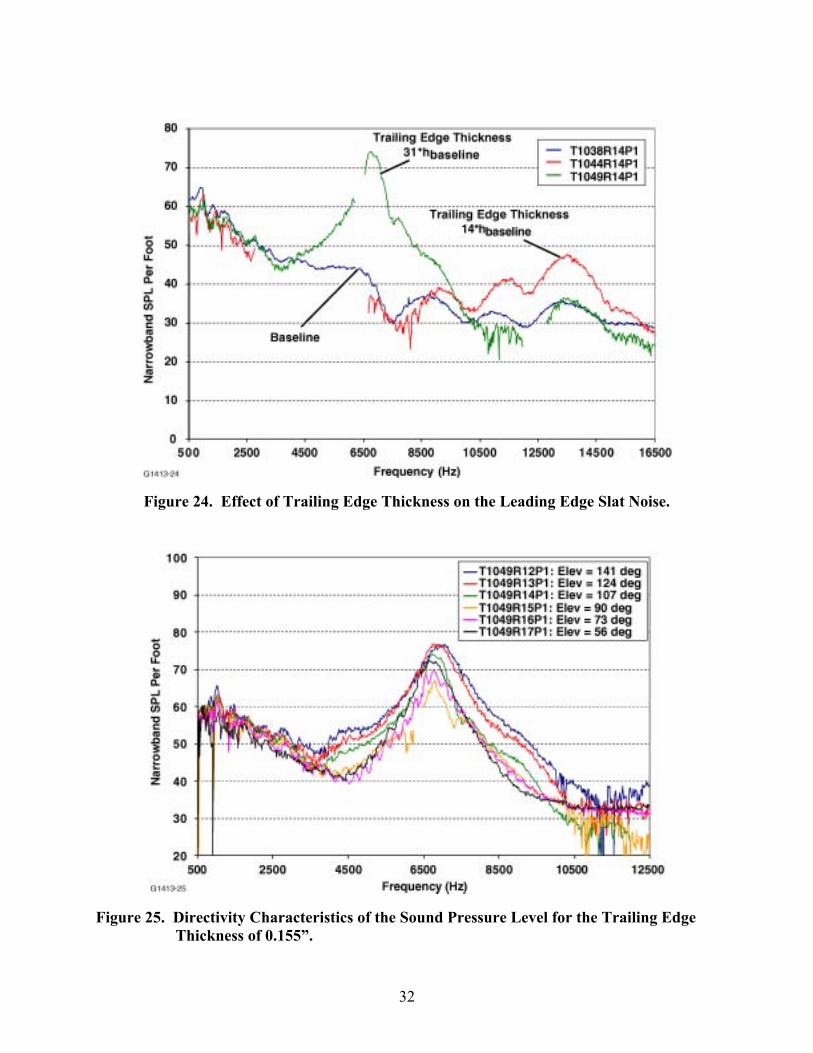
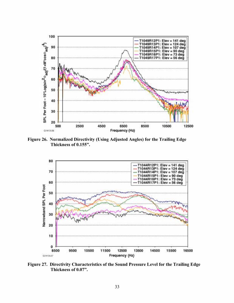
Figure 24 to Figure 28 show the effects of trailing edge thickness using the data from Tests1038, 1044, and 1049 (Table 3). Figure 24 shows that the baseline trailing edge thickness of0.005” has the lowest noise levels, and that increasing the thickness produces an additional noisesource that has a peak frequency related to the trailing edge thickness. The directivitycharacteristics of the sound pressure level are also changed by the new apparent source.

Finally, Figure 29 provides a summary of the noise reduction techniques evaluated in thisstudy. Clearly the most effective reduction was obtained by losing the slat gap. However, amoderate reduction was achieved with the use of the teardrop insert.

27

Figure 14. Effect of the Main Element Angle-of-Attack on the Leading Edge Slat Noise.

Figure 15. Effect of Slat Element Angle-of-Attack for a Main Element Angle-of-Attack of 26 Degrees.

28

Figure 16. Effect of Slat Element Angle-of-Attack for a Main Element Angle-of-Attack of 32 Degrees.

Figure 17. Effect of Slat Gap/Overlap on the Sound Pressure Level of the Leading Edge Slat Noise.

29

Figure 18. Effect of the Teardrop Insert in the Slat Gap on the Sound Pressure Level of the Leading Edge Slat Noise.

Figure 19. Effect of Mach Number on the Teardrop Insert Leading Edge Slat Noise.

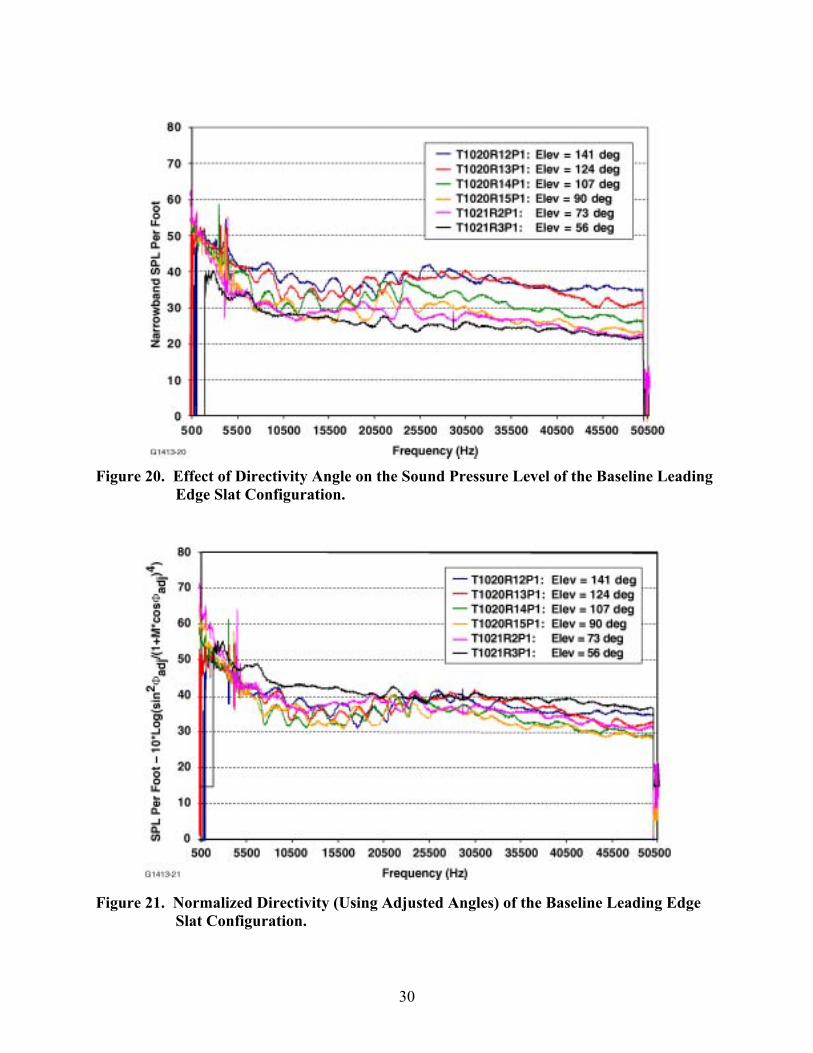
30

Figure 20. Effect of Directivity Angle on the Sound Pressure Level of the Baseline Leading Edge Slat Configuration.

Figure 21. Normalized Directivity (Using Adjusted Angles) of the Baseline Leading Edge Slat Configuration.

31

Figure 22. Directivity Characteristics of the Sound Pressure Level for the 6-Notch Gap/Overlap Conditions.

Figure 23. Normalized Directivity (Using Adjusted Angles) of the 6-Notch Gap/Overlap Conditions.

32

Figure 24. Effect of Trailing Edge Thickness on the Leading Edge Slat Noise.

Figure 25. Directivity Characteristics of the Sound Pressure Level for the Trailing Edge Thickness of 0.155”.

33

Figure 26. Normalized Directivity (Using Adjusted Angles) for the Trailing Edge Thickness of 0.155”.

Figure 27. Directivity Characteristics of the Sound Pressure Level for the Trailing Edge Thickness of 0.07”.

34

Figure 28. Normalized Directivity (Using Adjusted Angles) for the Trailing Edge Thickness of 0.07”.

Figure 29. Summary of the Noise Benefit for the Two Slat Noise Reduction Concepts.

35

2.2.4 List of Symbols

f’ Frequency dependent function based on theoretical array pattern

F Transfer function for per-foot processing of spectra

m Microphone number

mtot Total number of microphones

M Freestream flow Mach number

Pa12 True distributed source pressure squared

P22 True localized source pressure squared at y2

P32 True localized source pressure squared at y3

PaTmin2 = (PaT

2)ymin Minimum pressure squared along span line as measured by SADA

PaT22 = (PaT

2)y2 Peak pressure squared along span line as measured by SADA

PaT32 = (PaT

2)y3 Peak pressure squared along span line as measured by SADA

r Scan point location relative to array center

ro Point source location relative to array center

rm Microphone to scan point distance

rmo Microphone to source distance

ymin Spanwise location of minimum pressure squared

y2 Spanwise location of peak pressure squared

y3 Spanwise location of peak pressure squared

W Spatial filter function

wm SADA weighting factors

δs Slat angle of attack

δw Wing angle of attack

Ψ Array azimuth angle

Φ Array elevation angle

36

3. JET SHEAR LAYER REFRACTION AND ATTENUATION STUDY

3.1 Introduction and Review of Correction Procedures

3.1.1 Static-to-Flight Correction Procedures

Aircraft fly-over noise prediction programs such as ANOPP [41] play a central role incommunity noise assessments. Successful prediction methods require a proper accounting of anumber of noise generation and propagation effects [25]. Static engine noise measurements areoften used with these programs to provide increased accuracy over direct component noisepredictions, but not without difficulty. A fundamental problem is that the noise levels acquiredstatically, even under controlled conditions using inflow control devices, do not faithfullyrepresent the noise levels that are encountered in flight. The sound spectra and directivity aremodified by source motion, and in order to use static engine noise measurements for aircraftnoise prediction, several motion-related effects must be accounted for. One familiar effect is theDoppler shift in frequency of the sound received by a stationary observer, and is easily accountedfor applying a Doppler correction factor to the statically measured frequency spectrum. Anequally important effect is the modification of the sound amplitude arising from changes to thenoise generation or propagation process when the source is in motion. Correction proceduresthat account for these so-called convective or dynamic amplification effects are more difficult toestablish.

Convective amplification is concerned with fundamental differences between noise fieldsradiated by stationary and moving sources. Differences may arise as a result of changes in thenoise generating mechanisms themselves, as in the case of jet noise where the shear layerstrength and hence the noise generation process is significantly altered by aircraft motion.Differences may also arise simply from the dynamics of the motion, as in the case of a movingmonopole where the noise generating mechanism (an oscillating point mass flux) remainsunchanged but the radiated sound field is modified by motion. Differences may also arise as aresult of changes in the surrounding flowfield that alter the propagation of the sound. Thecorrections that are used to account for convective amplification effects then depend upon thephysical mechanisms involved.

Corrections that account for changes in the noise generating mechanisms require aunderstanding of the major parameters that govern the noise generation, one example being thejet-noise correction procedure described in reference [39]. Correction procedures that accountfor changes in the sound field of moving sources whose characteristic generating mechanismsare left essentially unchanged require a thorough understanding of how the noise radiation ismodified by motion. Simple corrections based on analytical for idealized point sources areavailable, and are often used as approximate corrections for realistic noise sources. Correctionprocedures that account for changes in the sound field due to propagation differences when thesource is in motion require an understanding of how the surrounding flow is modified by motion.

The present effort is concerned with the effects of a flow-field modification that takes placein the exhaust region. Internally generated engine exhaust noise that propagates through thepropulsive jet must transit the jet shear layer on its way to an observer. As this sound crosses theshear layer, it can be refracted, reflected, and scattered. The degree to which the sound is

37

modified depends upon the shear layer strength and downstream development, which in turndepends upon the characteristics of the jet and ambient flows. When the jet is taken from staticto flight conditions, changes in the shear layer affect how the sound is refracted, reflected, andscattered. The purpose of this effort is to define a simple correction procedure that accounts forthe change in far-field noise levels that results from modifications to the jet shear layer due toambient flow.

Before describing the theoretical basis and operation of the proposed correction procedure,it is first useful to briefly review the flyover noise prediction process for which flight-correctedengine noise data is required. This will assist in the formulation of an intelligible correctionprocedure and will demonstrate how the process can be integrated into flyover noise predictionprograms such as ANOPP. It is also useful to briefly review shear layer corrections that havebeen developed for use with acoustic measurements in anechoic wind tunnels, since these resultscan be adapted for use in the present static-to-flight correction procedure.

3.1.2 Flyover Noise Prediction Process

One of the principal goals in aircraft noise prediction is to determine the noise level heardby an observer during a standard aircraft operation such as takeoff or landing. A metric that iswidely used for evaluating the noise received by an observer is the Effective Perceived NoiseLevel (EPNL). The process of computing the EPNL requires that sound pressure level spectra ata stationary observer position be acquired at half-second intervals over a certain period duringthe aircraft operation. These half-second increments in reception time correspond to incrementsin source emission time of varying duration. The sound emitted by the source at time te isreceived by the observer at time tr given by

t tr t

cr ee= + ( )

0

The distance r te( ) between the source and observer at the time the sound was emitteddivided by the speed of sound c0 (assumed constant over the propagation path) is simply thetime it takes the sound to traverse the source-to-observer distance. In order to predict the noisereceived by the observer as a function of reception time, it is necessary to predict the sound thatis radiated towards the observer as a function of emission time. Thus, it becomes necessary tocompute the noise field that is produced by the engines, airframe, and other noise sources on themoving aircraft.

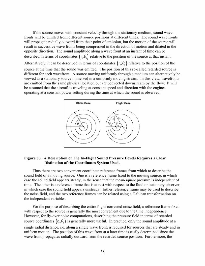
The noise field produced by an engine in motion is most frequently obtained by applyingstatic-to-flight corrections to static engine noise measurements or predictions. It is important todistinguish the coordinates that are used to describe the pressure field in the static and flightcases, and a simple example is useful here. Consider a monopole source in a stationary medium.Sound wave fronts emitted by the source will propagate radially outward and form concentriccircles as shown in Figure 30. The far-field pressure is conveniently described in terms ofcoordinates rm m,θ( ) relative to the stationary source position (the overbar will be used to denote

angles measured relative to the inlet or the direction of motion).

38

If the source moves with constant velocity through the stationary medium, sound wavefronts will be emitted from different source positions at different times. The sound wave frontswill propagate radially outward from their point of emission, but the motion of the source willresult in successive wave fronts being compressed in the direction of motion and dilated in theopposite direction. The sound amplitude along a wave front at an instant of time can bedescribed in terms of coordinates rs s,θ( ) relative to the position of the source at that instant.

Alternatively, it can be described in terms of coordinates re e,θ( ) relative to the position of the

source at the time that the sound was emitted. The position of this so-called retarded source isdifferent for each wavefront. A source moving uniformly through a medium can alternatively beviewed as a stationary source immersed in a uniformly moving stream. In this view, wavefrontsare emitted from the same physical location but are convected downstream by the flow. It willbe assumed that the aircraft is traveling at constant speed and direction with the enginesoperating at a constant power setting during the time at which the sound is observed.

Static Case Flight Case

mθ

mr

sθ

sr

eθ

er

S SrS

Figure 30. A Description of The In-Flight Sound Pressure Levels Requires a Clear Distinction of the Coordinates System Used.

Thus there are two convenient coordinate reference frames from which to describe thesound field of a moving source. One is a reference frame fixed to the moving source, in whichcase the sound field appears steady, in the sense that the mean-square pressure is independent oftime. The other is a reference frame that is at rest with respect to the fluid or stationary observer,in which case the sound field appears unsteady. Either reference frame may be used to describethe noise field, and the two reference frames can be related using a Galilean transformation onthe independent variables.

For the purpose of describing the entire flight-corrected noise field, a reference frame fixedwith respect to the source is generally the most convenient due to the time independence.However, for fly-over noise computations, describing the pressure field in terms of retardedsource coordinates re e,θ( ) is generally more useful. In practice, only the sound amplitude at a

single radial distance, i.e. along a single wave front, is required for sources that are steady and inuniform motion. The position of this wave front at a later time is easily determined since thewave front propagates radially outward from the retarded source position. Furthermore, the

39

amplitude along the wave front at the different position can be simply computed by applying adistance correction based on the inverse square law for acoustic energy and a correction foratmospheric attenuation. The sound received by a distant observer situated at an angle eθ and

radius eR from the retarded source position is then easily calculated.

3.1.3 Traditional Static-to-Flight Corrections

As a minimum, static-to-flight corrections must account for Doppler shifting of theobserved frequency spectra and convective amplification of the sound field. The Dopplerfrequency shift, which occurs when the source and observer are in relative motion, is a functionof the angle between the direction of source motion and the line connecting source and observer.The source frequency fsource and the observed frequency fobserved are related via

ff

Mobservedsource

e

=−1 cosθ

( 1 )

M is the Mach number of the source and the emission angle θe is the angle between thedirection of source motion and the line connecting the retarded source position and the observer.

Convective amplification is also a function of the Mach number M and emission angle θe ,but exact corrections are available only for idealized sources. The intent of the correction is toobtain an estimate of the in-flight mean-square sound pressure p rf e e

2 ,θ( ) given the statically

measured or predicted mean-square sound pressure p rs m m2 ,θ( ) . This correction is generally done

by multiplying p rs m m2 ,θ( ) with an angle-dependent flight-correction factor to obtain p rf e e

2 ,θ( ).Usually the measured and retarded distances are chosen to be equal to avoid the need to accountfor distance or atmospheric absorption corrections at this stage. The flight-corrected levelsrepresent the mean-square sound pressure that would be measured along a wave front describedby coordinates re e,θ( ) relative to the retarded source position. The convective amplification

factor is typically based upon analytical results derived for idealized moving point sources. Forthese simple sources, the form of the correction factor is dependent upon the sourcecharacteristics but is often of the form

p rp r

Mf e e

s e e

e

22

1,

,

cosθ

θ

θα( ) = ( )

−( )( 2 )

where the angle eθ is measured relative to the direction of source motion and α is a constant that

depends on the source type. Note that em rr = and em θθ = in this equation. It can be shown that

this is the appropriate correction for a monopole source moving at constant speed, in which case

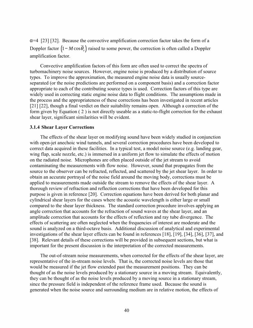
40

α=4 [23] [32]. Because the convective amplification correction factor takes the form of a

Doppler factor 1−( )M ecosθ raised to some power, the correction is often called a Doppler

amplification factor.

Convective amplification factors of this form are often used to correct the spectra ofturbomachinery noise sources. However, engine noise is produced by a distribution of sourcetypes. To improve the approximation, the measured engine noise data is usually source-separated (or the noise predictions are performed on a component basis) and a correction factorappropriate to each of the contributing source types is used. Correction factors of this type arewidely used in correcting static engine noise data to flight conditions. The assumptions made inthe process and the appropriateness of these corrections has been investigated in recent articles[21] [22], though a final verdict on their suitability remains open. Although a correction of theform given by Equation ( 2 ) is not directly useable as a static-to-flight correction for the exhaustshear layer, significant similarities will be evident.

3.1.4 Shear Layer Corrections

The effects of the shear layer on modifying sound have been widely studied in conjunctionwith open-jet anechoic wind tunnels, and several correction procedures have been developed tocorrect data acquired in these facilities. In a typical test, a model noise source (e.g. landing gear,wing flap, scale nozzle, etc.) is immersed in a uniform jet flow to simulate the effects of motionon the radiated noise. Microphones are often placed outside of the jet stream to avoidcontaminating the measurements with flow noise. However, sound that propagates from thesource to the observer can be refracted, reflected, and scattered by the jet shear layer. In order toobtain an accurate portrayal of the noise field around the moving body, corrections must beapplied to measurements made outside the stream to remove the effects of the shear layer. Athorough review of refraction and reflection corrections that have been developed for thispurpose is given in reference [20]. Correction equations have been derived for both planar andcylindrical shear layers for the cases where the acoustic wavelength is either large or smallcompared to the shear layer thickness. The standard correction procedure involves applying anangle correction that accounts for the refraction of sound waves at the shear layer, and anamplitude correction that accounts for the effects of reflection and ray tube divergence. Theeffects of scattering are often neglected when the frequencies of interest are moderate and thesound is analyzed on a third-octave basis. Additional discussion of analytical and experimentalinvestigations of the shear layer effects can be found in references [18], [19], [34], [36], [37], and[38]. Relevant details of these corrections will be provided in subsequent sections, but what isimportant for the present discussion is the interpretation of the corrected measurements.

The out-of-stream noise measurements, when corrected for the effects of the shear layer, arerepresentative of the in-stream noise levels. That is, the corrected noise levels are those thatwould be measured if the jet flow extended past the measurement positions. They can bethought of as the noise levels produced by a stationary source in a moving stream. Equivalently,they can be thought of as the noise levels produced by a moving source in a stationary stream,since the pressure field is independent of the reference frame used. Because the sound isgenerated when the noise source and surrounding medium are in relative motion, the effects of

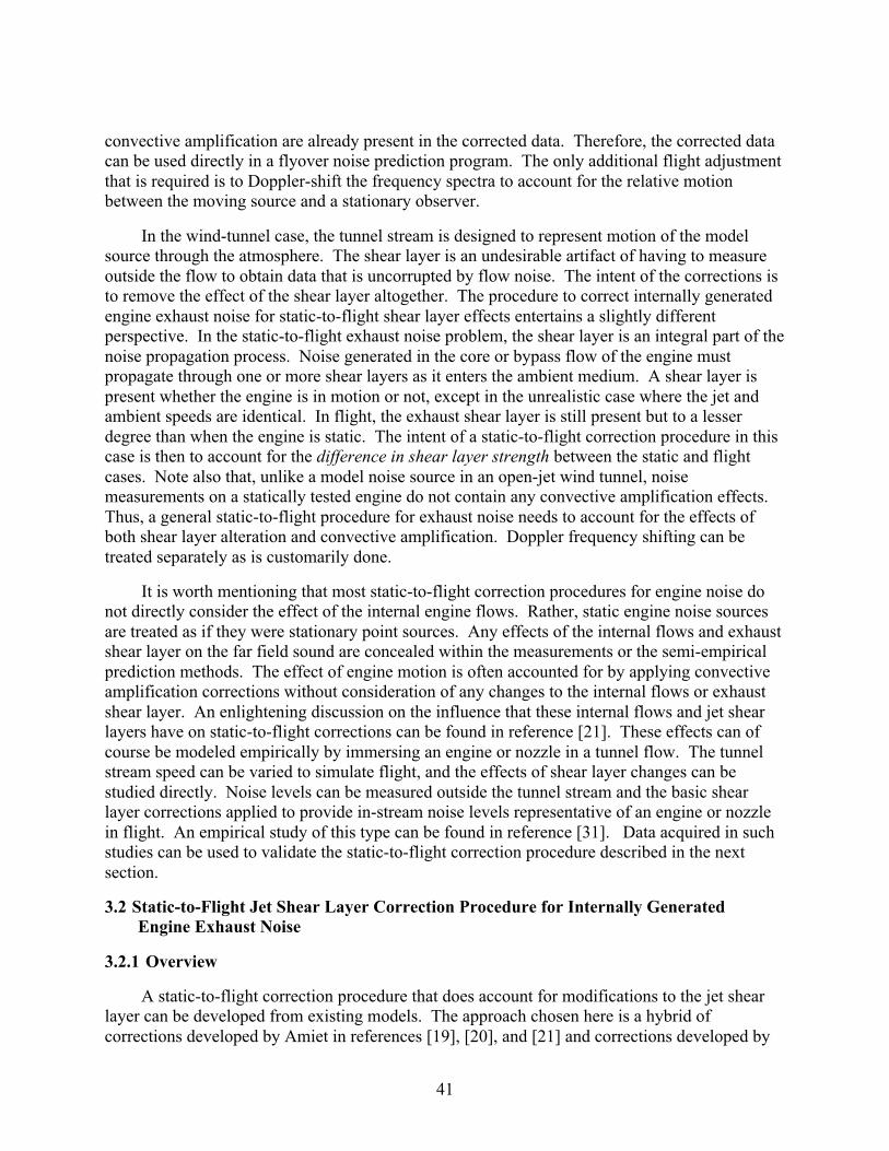
41

convective amplification are already present in the corrected data. Therefore, the corrected datacan be used directly in a flyover noise prediction program. The only additional flight adjustmentthat is required is to Doppler-shift the frequency spectra to account for the relative motionbetween the moving source and a stationary observer.

In the wind-tunnel case, the tunnel stream is designed to represent motion of the modelsource through the atmosphere. The shear layer is an undesirable artifact of having to measureoutside the flow to obtain data that is uncorrupted by flow noise. The intent of the corrections isto remove the effect of the shear layer altogether. The procedure to correct internally generatedengine exhaust noise for static-to-flight shear layer effects entertains a slightly differentperspective. In the static-to-flight exhaust noise problem, the shear layer is an integral part of thenoise propagation process. Noise generated in the core or bypass flow of the engine mustpropagate through one or more shear layers as it enters the ambient medium. A shear layer ispresent whether the engine is in motion or not, except in the unrealistic case where the jet andambient speeds are identical. In flight, the exhaust shear layer is still present but to a lesserdegree than when the engine is static. The intent of a static-to-flight correction procedure in thiscase is then to account for the difference in shear layer strength between the static and flightcases. Note also that, unlike a model noise source in an open-jet wind tunnel, noisemeasurements on a statically tested engine do not contain any convective amplification effects.Thus, a general static-to-flight procedure for exhaust noise needs to account for the effects ofboth shear layer alteration and convective amplification. Doppler frequency shifting can betreated separately as is customarily done.

It is worth mentioning that most static-to-flight correction procedures for engine noise donot directly consider the effect of the internal engine flows. Rather, static engine noise sourcesare treated as if they were stationary point sources. Any effects of the internal flows and exhaustshear layer on the far field sound are concealed within the measurements or the semi-empiricalprediction methods. The effect of engine motion is often accounted for by applying convectiveamplification corrections without consideration of any changes to the internal flows or exhaustshear layer. An enlightening discussion on the influence that these internal flows and jet shearlayers have on static-to-flight corrections can be found in reference [21]. These effects can ofcourse be modeled empirically by immersing an engine or nozzle in a tunnel flow. The tunnelstream speed can be varied to simulate flight, and the effects of shear layer changes can bestudied directly. Noise levels can be measured outside the tunnel stream and the basic shearlayer corrections applied to provide in-stream noise levels representative of an engine or nozzlein flight. An empirical study of this type can be found in reference [31]. Data acquired in suchstudies can be used to validate the static-to-flight correction procedure described in the nextsection.

3.2 Static-to-Flight Jet Shear Layer Correction Procedure for Internally Generated Engine Exhaust Noise

3.2.1 Overview

A static-to-flight correction procedure that does account for modifications to the jet shearlayer can be developed from existing models. The approach chosen here is a hybrid ofcorrections developed by Amiet in references [19], [20], and [21] and corrections developed by

42

Morfey in references [29] and [30]. The procedure relates the in-flight, far field, mean-squaresound pressure to the statically measured, far field, mean-square sound pressure as a function offlight speed. The correction process entails applying angle corrections to account for refractionat the shear layer and amplitude corrections to account for ray-tube divergence changes andforward flight effects. The effects of reflection of sound by the shear layer and scattering ofsound by shear layer turbulence are ignored. These corrections are developed using a geometricacoustics approach for cylindrical shear layer geometry. The angle correction is based upon avortex sheet model of the shear layer. The amplitude correction is based on the assumption ofenergy conservation across the shear layer.

The resulting correction equations are compact and can be conveniently integrated withflyover-noise prediction codes. In the following sections, the model geometry is described andthe angle and amplitude corrections are discussed. Various angle relationships that are needed inthe procedure are derived. The implementation of the individual corrections into a procedure isdescribed, and sample aircraft flyover noise predictions are presented. The impact ofassumptions made in the derivation of the correction equations is reviewed.

3.2.2 Problem Geometry

The model geometry for the correction procedure presented here is shown in Figure 31. Anaxially symmetric point source S is situated at the exhaust plane on the centerline of acylindrical jet. A uniform flow of Mach number M j exists in the jet, which has a constant

density ρ j and constant speed of sound c j . A shear layer of constant radius h separates the jet

from the ambient fluid, which maintains a constant density ρa and constant speed of sound ca .The source S emits sound in all directions. Sound emitted in the wave normal direction φj is

convected by the jet flow. The resulting ray path makes an angle θc with respect to the sourceand intersects the shear layer at the point C . In the static case, the sound is refracted by theshear layer to a wave normal angle φas. The sound propagates through the ambient medium inthe wave normal direction φasat speed ca . The sound arrives at the measurement position M ,which lies a distance rm and angle θm from the source. In the flight case, the sound is refractedby the shear layer to a different wavenormal angle φaf . The sound propagates through the

ambient medium in the wavenormal direction φaf at speed ca , and is also convected by the

ambient flow at speed M ca a . Sound traveling in the upstream direction is considered to re-enterthe nozzle and thus does not contribute to the far-field noise.

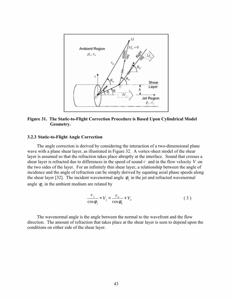
43

Figure 31. The Static-to-Flight Correction Procedure is Based Upon Cylindrical Model Geometry.

3.2.3 Static-to-Flight Angle Correction

The angle correction is derived by considering the interaction of a two-dimensional planewave with a plane shear layer, as illustrated in Figure 32. A vortex-sheet model of the shearlayer is assumed so that the refraction takes place abruptly at the interface. Sound that crosses ashear layer is refracted due to differences in the speed of sound c and in the flow velocity V onthe two sides of the layer. For an infinitely thin shear layer, a relationship between the angle ofincidence and the angle of refraction can be simply derived by equating axial phase speeds alongthe shear layer [32]. The incident wavenormal angle φj in the jet and refracted wavenormal

angle φa in the ambient medium are related by

cV

cVj

jj

a

aacos cosφ φ

+ = + ( 3 )

The wavenormal angle is the angle between the normal to the wavefront and the flowdirection. The amount of refraction that takes place at the shear layer is seen to depend upon theconditions on either side of the shear layer.

44

Figure 32. The Refraction Angle Correction is Derived by Considering Plane Wave Interaction With a Vortex Sheet.

Equation ( 3 ) can be used to describe how the ambient wavenormal angle is modified whenthe engine nozzle is taken from static to flight conditions. Using additional subscripts “ s” and“ f ” to denote the static and flight conditions, and writing the refraction equation for each caseyields

Static case:c

Vcjs

jsjs

as

ascos cosφ φ+ = ( 4 )

Flight case:c

Vc

Vjf

jfjf

af

afafcos cosφ φ

+ = + ( 5 )

It is assumed that the jet velocity remains constant when moving from static to flightconditions, so that V V Vjs jf j= ≡ . It is also assumed that the temperature in the jet and ambient

regions do not change when moving from static to flight conditions, so that c c cjs jf j= ≡ and

c c cas af a= ≡ . Finally, it is assumed that the external flow does not affect the generation and

propagation of the noise inside the jet. Then the wavenormal angle within the jet is identical inthe static and flight cases, so that φ φjs jf= . Under these assumptions, Equations ( 4 ) and ( 5 )

can then be combined to provide the following relationship between the ambient wavenormalangles in the static and flight cases:

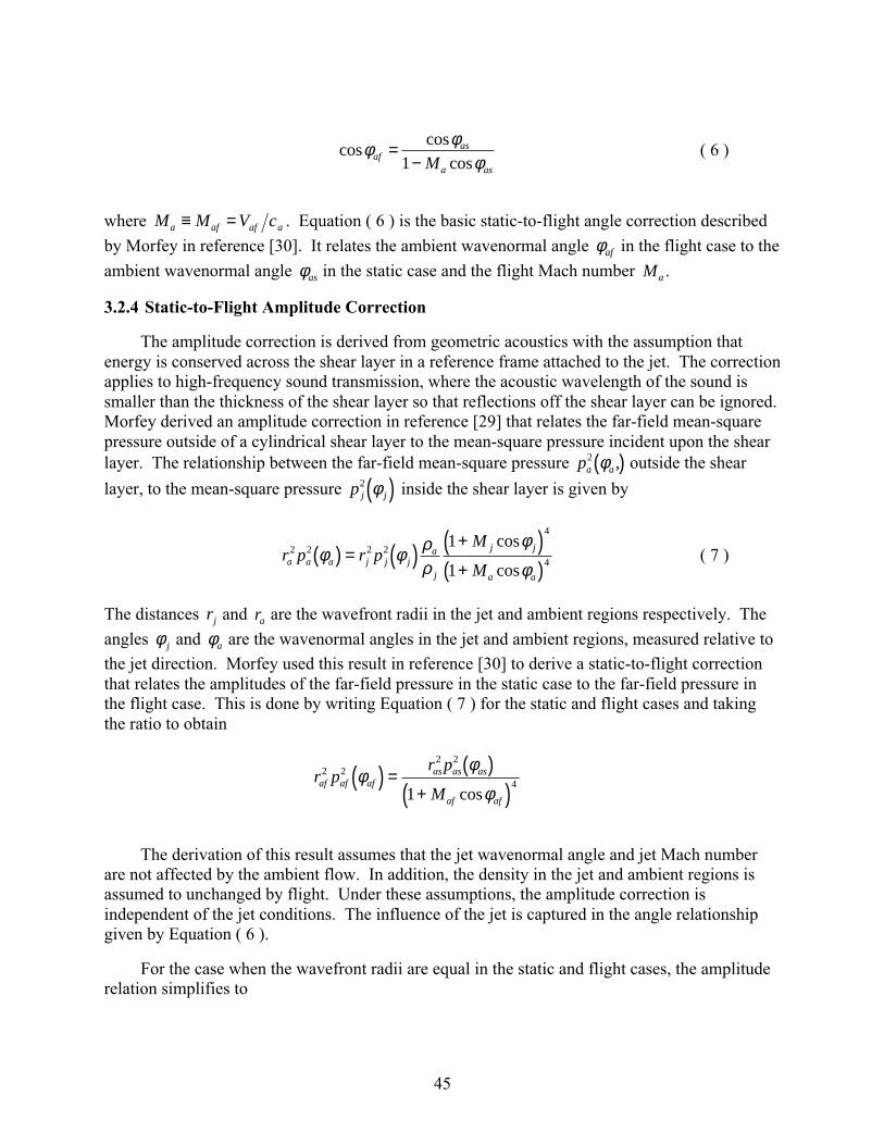
45

coscos

cosφ φ

φafas

a asM=

−1( 6 )

where M M V ca af af a≡ = . Equation ( 6 ) is the basic static-to-flight angle correction described

by Morfey in reference [30]. It relates the ambient wavenormal angle φaf in the flight case to the

ambient wavenormal angle φas in the static case and the flight Mach number Ma .

3.2.4 Static-to-Flight Amplitude Correction

The amplitude correction is derived from geometric acoustics with the assumption thatenergy is conserved across the shear layer in a reference frame attached to the jet. The correctionapplies to high-frequency sound transmission, where the acoustic wavelength of the sound issmaller than the thickness of the shear layer so that reflections off the shear layer can be ignored.Morfey derived an amplitude correction in reference [29] that relates the far-field mean-squarepressure outside of a cylindrical shear layer to the mean-square pressure incident upon the shearlayer. The relationship between the far-field mean-square pressure pa a

2 φ ,( ) outside the shear

layer, to the mean-square pressure p j j2 φ( ) inside the shear layer is given by

r p r pM

Ma a a j j j

a

j

j j

a a

2 2 2 2

4

4

1

1φ φ ρ

ρφ

φ( ) = ( ) +( )

+( )cos

cos( 7 )

The distances rj and ra are the wavefront radii in the jet and ambient regions respectively. The

angles φj and φa are the wavenormal angles in the jet and ambient regions, measured relative to

the jet direction. Morfey used this result in reference [30] to derive a static-to-flight correctionthat relates the amplitudes of the far-field pressure in the static case to the far-field pressure inthe flight case. This is done by writing Equation ( 7 ) for the static and flight cases and takingthe ratio to obtain

r pr p

Maf af af

as as as

af af

2 22 2

41

φφ

φ( ) = ( )

+( )cos

The derivation of this result assumes that the jet wavenormal angle and jet Mach numberare not affected by the ambient flow. In addition, the density in the jet and ambient regions isassumed to unchanged by flight. Under these assumptions, the amplitude correction isindependent of the jet conditions. The influence of the jet is captured in the angle relationshipgiven by Equation ( 6 ).

For the case when the wavefront radii are equal in the static and flight cases, the amplituderelation simplifies to

46

pp

Maf af

as as

af af

22

41

φφ

φ( ) = ( )

+( )cos( 8 )

Equation ( 8 ) is the amplitude correction that is used in the present correction procedure. Itstates that the far-field mean-square sound pressure at a flight wave normal angle φaf can be

calculated by dividing the mean-square sound pressure measured at a static wave normal angle

φas by the Doppler factor 14

+( )Maf afcosφ . This equation assumes that the measurements are

made in the far field, which is generally the case for static engine noise testing.

Equation ( 8 ) has a form reminiscent of the convective amplification correction of Equation( 2 ) when 4=α . However, the two equations are not identical. Presuming that the direction ofmotion is directly opposite the jet flow direction, the two equations can be compared. WritingEquation ( 2 ) in terms of an angle θ π θe e= − measured relative to the jet direction gives

p rp r

Mf e e

s e e

e

22

41

,,

cosθ

θθ

( ) = ( )+( )

The difference between the correction equations is now apparent. In the traditionalconvective amplification correction, the flight sound amplitude at θe is related to the static soundamplitude at the same wave normal angle θe . In the shear layer correction, the flight soundamplitude at φaf is related to the static sound amplitude at a different wave normal angle φas.

The difference is a result of the ambient flow modifying the refraction through the shear layer.

It is assumed in the above comparison that the direction of motion is opposite to thedirection of the exhaust flow. In reality, the engine centerline might not be aligned exactly withthe direction of aircraft motion. In this case, the inclination of the engine relative to the directionof motion should be accounted for in the Doppler and convective amplification corrections. Thiscan be done with an appropriate angle substitution, such as θ π φ α= − + where α is theinclination angle of the engine centerline relative to direction of motion.

3.2.5 Angle Relationships

An attractive feature of the angle and amplitude corrections is that they are straightforwardand easily computed. To apply the corrections, the statically measured mean-square pressuremust be provided as a function of the ambient wave normal angle φas, measured relative to thejet axis. Far-field static engine noise measurements are usually described in terms of a source-to-observer measurement angle θm (usually measured relative to the inlet, but the oppositeconvention is used here). Thus a relationship between θm and φas is needed. As described byAmiet in reference [19], a relationship between the two angles can be easily derived fromgeometrical considerations. The derivation is provided here since the current case allows forsome generalization in that the speed of sound is allowed to differ in the jet and ambient regions.

47

C

S

M

mθ

cθ

mr asr

asφ

( ) hr mm −θsin

h

( )ch θcot ( )[ ] ( )asmm hr φθ cotsin −

( )mmr θcos

Figure 33. A Relationship Between the Measurement Angle θm and Wave Normal Angle φas Can Be Derived From Geometrical Considerations.

Referring to Figure 33, a relationship between the ambient wave normal angle φas, thesource-to-observer angleθm , and the corrected angle θc can be derived from trianglerelationships. Relating the length of the bases of the three right triangles in the Figure yields

r h r hm m c m m ascos cot sin cotθ θ θ φ( ) = ( ) + ( ) −[ ] ( ) ( 9 )

The wavenormal distance ras over which the sound travels in the ambient region can also becomputed from triangle relationships, and is given by

r r h r has m m m m as= ( ) −( ) + ( ) −( ) ( )( )sin sin cotθ θ φ2 2

( 10 )

Note that the corrected angle θc appears in Equation ( 9 ) as a parameter. It can beexpressed in terms of the ambient wave normal angle φas as follows. First, a relation betweenthe ray path angle θc and the jet wave normal angle φjs is derived.

Figure 34 shows how ray paths and wave normal angles can be related. A stationary pointsource S situated on the x-axis is immersed in a uniform flow of subsonic Mach number M . Forpurposes of illustration, S is a monopole source emitting sound at a single frequency. Theconstant phase surfaces or wavefronts form circles that are convected downstream by the flow.Sound emitted by the source at a wavenormal angle φ propagates radially outward from thesource in this direction at the speed of sound c . The sound is also convected downstream by theflow at speed V . Figure 34 displays the wave fronts at successive increments in time. An opencircle marks the portion of the wave front that was originally emitted in the φ direction by the

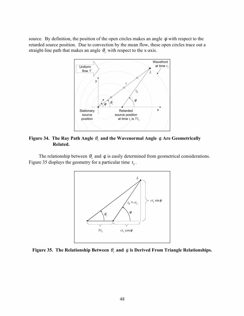
48

source. By definition, the position of the open circles makes an angle φ with respect to theretarded source position. Due to convection by the mean flow, these open circles trace out astraight-line path that makes an angle θc with respect to the x-axis.

x

y

Wavefrontat time

Retardedsource position

at time is

Uniformflow

Stationarysourceposition

cθ φφ

r

φr

L

Lt

Lt LVt

V

Figure 34. The Ray Path Angle θc and the Wavenormal Angle φ Are Geometrically Related.

The relationship between θc and φ is easily determined from geometrical considerations.Figure 35 displays the geometry for a particular time tL .

LVt φcosLct

cθ φ

Lctr =φφsinLct

L

Figure 35. The Relationship Between θc and φ is Derived From Triangle Relationships.

49

Considering triangle relationships, θc and φ are related via:

tansin

cossin

cosθ φ

φφ

φcL

L L

ct

Vt ct M( ) =

+=

+

Returning now to the geometry of Figure 33, the relationship between θc and φjs is

tansin

cosθ

φφc

js

js jsM( ) =

+( 11 )

This relationship can be expressed in terms of the ambient wave normal angle φas using thestatic angle refraction relation, Equation ( 4 ). First note that Equation ( 4 ) implies

coscos

coscos

cosφ

φφ

φ

φjs

j as

a j as

as

a

jj as

c

c V c

cM

=−

=−

and

sin

cos cos

cosφ

φ φ

φjs

a

jj as as

a

jj as

c

cM

c

cM

=

−

−

−

2

2

Substituting into Equation ( 11 ) produces the desired relationship between θc and φas

tan

cos cos

cosθ

φ φ

φc

a

jj as as

a

jj j as

c

cM

c

cM M

( ) =

−

−

+ −( )

2

2

21( 12 )

This reduces to Equation (1) of Reference [20] when the temperatures of the jet andambient regions are the identical. Thus, given θm , rm , h and M j , the static ambient wave

normal angle φas can be determined using Equation ( 9 ) and ( 12 ).

3.2.6 Implementation of the Corrections

An exhaust shear layer static-to-flight correction procedure can now be described. Staticengine noise measurements are obtained at far-field coordinates θm mr,( ) relative to the sourceposition, with θm measured relative to the exhaust centerline. At a given measurement location,

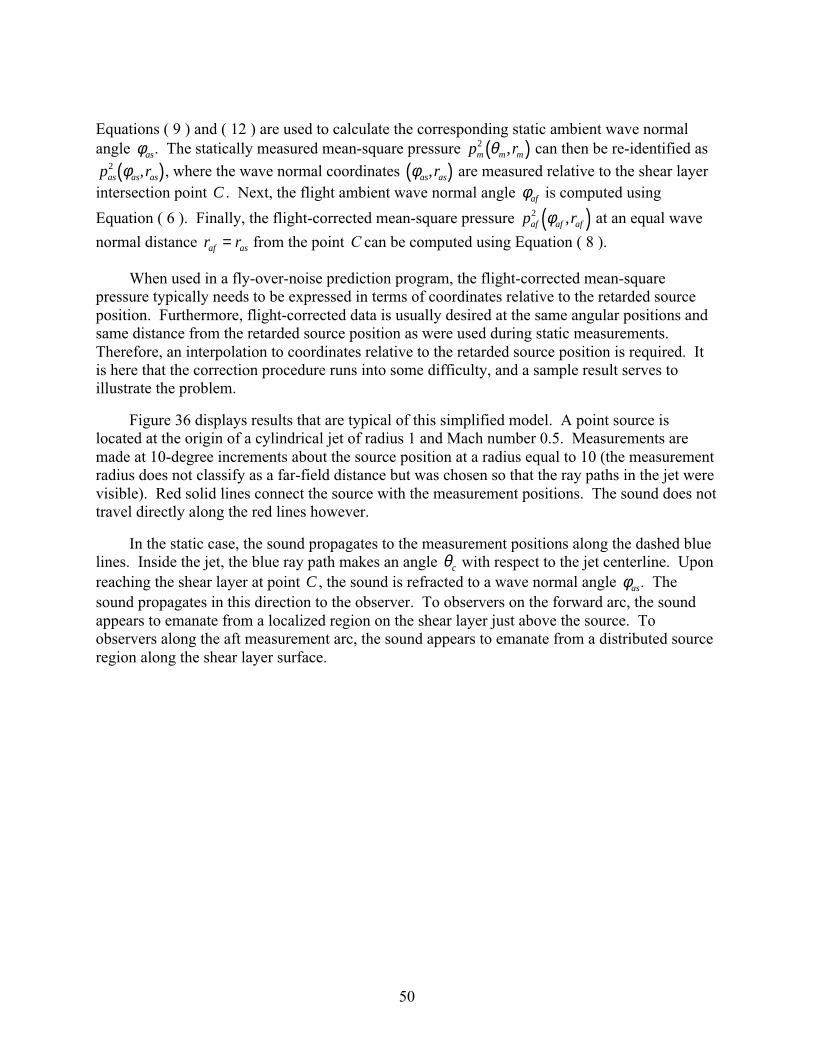
50

Equations ( 9 ) and ( 12 ) are used to calculate the corresponding static ambient wave normalangle φas. The statically measured mean-square pressure p rm m m

2 θ ,( ) can then be re-identified as

p ras as as2 φ ,( ), where the wave normal coordinates φas asr,( ) are measured relative to the shear layer

intersection point C . Next, the flight ambient wave normal angle φaf is computed using

Equation ( 6 ). Finally, the flight-corrected mean-square pressure p raf af af2 φ ,( ) at an equal wave

normal distance r raf as= from the point C can be computed using Equation ( 8 ).

When used in a fly-over-noise prediction program, the flight-corrected mean-squarepressure typically needs to be expressed in terms of coordinates relative to the retarded sourceposition. Furthermore, flight-corrected data is usually desired at the same angular positions andsame distance from the retarded source position as were used during static measurements.Therefore, an interpolation to coordinates relative to the retarded source position is required. Itis here that the correction procedure runs into some difficulty, and a sample result serves toillustrate the problem.

Figure 36 displays results that are typical of this simplified model. A point source islocated at the origin of a cylindrical jet of radius 1 and Mach number 0.5. Measurements aremade at 10-degree increments about the source position at a radius equal to 10 (the measurementradius does not classify as a far-field distance but was chosen so that the ray paths in the jet werevisible). Red solid lines connect the source with the measurement positions. The sound does nottravel directly along the red lines however.

In the static case, the sound propagates to the measurement positions along the dashed bluelines. Inside the jet, the blue ray path makes an angle θc with respect to the jet centerline. Uponreaching the shear layer at point C , the sound is refracted to a wave normal angle φas. Thesound propagates in this direction to the observer. To observers on the forward arc, the soundappears to emanate from a localized region on the shear layer just above the source. Toobservers along the aft measurement arc, the sound appears to emanate from a distributed sourceregion along the shear layer surface.

51

Figure 36. Sample Refraction Results From the Simplified Model for M j = 0 5. , Ma = 0 2. , and c cj a= .

In the flight case, the propagation within the jet remains unchanged (by assumption).However, the mean flow alters the refraction at the shear layer interface. For an ambient Machnumber of 0.2, the sound waves are refracted in the direction of the green dotted-dashed lines,which make an angle φaf with respect to the downstream direction. The angular change is quite

pronounced in the upstream direction, and relatively modest in the aft arc.

The set of shear layer intersection points Ci{ } can be thought of as a collection of retardedsources, each of which radiates sound in only one direction. If the jet is imagined to move to theleft with the flight velocity, then the sound will propagate from each of these points along thegreen dotted-dashed lines to a distant observer. Note also that sound emitted when the source isat the origin will take a different amount of time to reach the shear layer, so the sound is notemitted from each of the intersection points simultaneously.

It must be noted that the propagation within the jet at these extreme angles is unrealistic, asno account has been made of the mixing of the jet with the ambient flow. Nevertheless, thedifficulty with this simplified model is that the source is somewhat smeared out in space andtime. This source non-compactness makes it difficult to implement a shear layer correctionprocedure in a rigorous way for the aft angles. Since many fly-over noise programs lack thecapability to model distributed sources, some further simplification is needed. Theapproximation (commensurate with other approximations made within fly-over noise programs)introduced here is to consider that the effect of the shear layer is mainly to alter the direction ofwave normal propagation of the sound. In this simplification, the points Ci{ } are all forced to becoincident with the retarded source position. Pictorially, this causes the blue lines to collapseonto the red lines. The green lines are simply offset from the merged blue-red lines by anamount equal to the difference between static and flight ambient wave normal angles, as shownin Figure 37.

52

Figure 37. Collapsing the Shear Layer Intersection Points Onto the Origin Allows for Simplifications to the Correction Procedure.

With this simplification, the effect of refraction changes due to flight is to simply shift thedirectivity by an amount equal to the difference between the static and flight ambient wavenormal angles. That is, in flight, sound will be emitted from the source in a direction Φ f given

by

Φ f m as af= − −( )θ φ φ ( 13 )

The mean-square pressure in this direction at a wave normal distance (i.e., distance fromthe retarded source position) equal to rm is still provided by Equation ( 8 ) but written using thevariable Φ f ,

p rp r

Mf f m

m m m

f f

22

41

ΦΦ

,,

cos( ) = ( )

+( )θ

( 14 )

The values of pf2 at the original angles θm can be obtained by interpolation. The accuracy

of these approximations improves when r hm msinθ >> . Referring to Figure 38, ash rm msinθ( ) → 0 with CF CM ras= = , then ∠ → ∠ = −FSM FCM af asφ φ and r rf m→ . So for

distant sideline observers, as is the case in fly-over noise studies, the approximation becomesquite acceptable.

53

ShearLayer

cθmθ

asφ

afφ

S

C

MF

mr

asr fr

fΦ

h

Figure 38. The Approximation Improves as the Sideline Distance From the Shear LayerIncreases.

Some additional comments are worth mentioning regarding special treatment at the extremeangles. Consider the upstream direction of the current sample problem. In the static case, soundthat propagates within the jet at wave normal angles greater than 131.8 degrees is internallyreflected. In the flight case, sound that propagates at jet wave normal angles greater than 141.3degrees is internally reflected. Thus, sound that propagates at wave normal angles in between131.8 and 141.3 degrees will theoretically escape to the free stream in the flight case. The soundlevel corresponding to these jet wave normal angles is indeterminable from static measurementsthat are made outside the jet. Thus, some approximation must be made in the forward arcbeyond this limiting angle. In the current model, sound is not expected to radiate from thenozzle at these upstream angles anyway, so this effect is unimportant.

Consider now the effects in the downstream direction. In the static case, no sound leavesthe jet at wave normal angles less than 48.2 degrees. In the flight case, no sound leaves the jet atwave normal angles less than 39.7 degrees. These regions are the so-called zones of silence.However, it does not imply that sound cannot be measured at an observer angle less than thezone of silence angle, because the sound can propagate down the jet before escaping to theambient region. It is worth mentioning that these shallow angles are typically not important inthe open jet wind tunnel scenario, because the jet wave normal angles corresponding to thesedownstream angles are quite small. In the current example, for the measurement angle of 40degrees, the jet wave normal angle in the jet is only 25 degrees, and noise radiated at such ashallow angle is not a contributor to fly-over noise levels.

3.2.7 Summary of the Static-to-Flight Correction Process

The simplified jet shear layer static-to-flight correction procedure for internally generatedengine exhaust noise can be summarized in the following steps:

54

1. Measure or predict the static mean-square pressure p rm m m2 ,θ( ) of the internally generated

engine exhaust noise at a fixed radius rm and at various angles θm from the source. Source-separation techniques may be required.

2. For a given measurement angle θm , compute the static ambient wave normal angle φas usingEquations ( 4 ), ( 9 ), & ( 11 ). An iterative procedure must be used, since φas cannot beexpressed explicitly in terms of mθ .

3. Compute the flight ambient wave normal angle φaf using Equation ( 6 ).

4. Compute the approximate flight emission angle Φ f using Equation ( 13 ).

5. Compute the flight-corrected mean-square pressure p rf f m2 Φ ,( ) using Equation ( 14 ).

6. Interpolate the flight-corrected mean-square pressure p rf f m2 Φ ,( ) back to the original

measurement angles θm , if desired.

3.2.8 Computer Program

A FORTRAN computer program to compute the jet shear layer static-to-flight correctionswas developed. The program follows the sequence of steps described in the previous section.The first three steps are performed in subroutine REFRACT. The last three steps are performedin the component noise routines. Details of the implementation can be found in the commentswithin the code.

The subroutine REFRACT requires the inputs listed in Table 5. The inputs are usuallyavailable from engine and aircraft performance data. They include the measurement radius andmeasurement angles (relative to the jet centerline) and the conditions of the jet and ambient flow.

Table 5. The Following Inputs Are Supplied to Subroutine REFRACT.

Variable Description UnitsNM Number of measurement positionsRM Measurement radius FtTHETAM Measurement angles relative to the jet axis (array) DegreesRJET Jet radius FtVJ Jet velocity ft/secTJ Jet temperature °F

VA Ambient flight velocity ft/secTA Ambient temperature °F

Table 6. The Following Outputs Are Returned by Subroutine REFRACT.

Variable Description UnitsPHIAS Ambient wavenormal angle for the static case DegreesPHIAF Ambient wavenormal angle for the flight case Degrees

55

3.2.9 Sample Application of the Procedure

The static-to-flight correction procedure described herein has been used to flyover noisepredictions for a generic business jet. Static engine noise data, measured along a 100-ft arc in 10degree increments, was source separated into narrowband, broadband, and jet noise components.Predictions of the aircraft flyover noise were made with and without the shear layer correctionsapplied to the internally generated engine exhaust noise. For the purposes of this example, theinternally generated engine exhaust noise was considered to consist of narrowband andbroadband noise measured at angles of 90 degrees and lower relative to the jet centerline. Noiseat angles greater than 90 degrees from the jet centerline were assumed to radiate from the inlet.

Predictions were made for approach, cutback-takeoff, and sideline according to standardFAR 36 procedures [25][26]. The differences in Effective Perceived Noise Levels, displayed inTable 7, are seen to be quite modest. The differences would be more substantial for cases wherethe exhaust noise exhibits more pronounced directivity lobes.

Table 7. Differences in Effective Perceived Noise Levels Between Predictions Made Withand Without Shear Layer Corrections Are Relatively Modest.

Approach Cutback-Takeoff Sideline∆EPNL 0.0 0.1 0.3

Figure 39. Small Changes Are Evident Flyover Noise Time History for the Cutback Takeoff Conditions.

3.2.10 Limitations of the Method

Numerous assumptions are associated with the correction procedure described here, manyof which are tied to the geometric acoustic approach that is used. The angle correction assumes

56

the observer to be in the geometric far field of the source, so that the observed sound originatesfrom only a single location. The angle correction also assumes an infinitely thin shear layer.This does not appear to be a substantial limitation, as numerical ray-tracing solutions usingLilley’s equation [20] suggest that incorporation of thickness does not significantly the anglecorrection. The amplitude correction assumes that the observer is in the acoustic far field of thesource, and is strictly applicable only to high frequency noise, since the shear layer was assumedto be non-reflective. The effects of reflection can be incorporated in an approximate way byusing analytical results for low-frequency plane wave reflection. However, analyticalinvestigations [20] have shown that the effects are only substantial at the extreme angles. Ifimproved accuracy is needed, then the effects of multiple reflections must be addressed.Unfortunately, modeling multiple reflections requires detailed knowledge of the sourcecharacteristics, and this is usually unavailable.

The effects of scattering by shear layer turbulence have been ignored in this model.Scattering can modify the transmitted sound most notably in two ways. One effect is spectralbroadening of discrete tones, and the other is reflection or absorption of the sound. Experimentalinvestigations [37] suggest that while spectral broadening is important for narrowband analyses,sound analyzed on a third-octave basis is not significantly impacted. Scattering and absorptionof sound does not have a significant impact on the third-octave noise levels except at extremeangles and high frequencies.

Many of the difficulties with the model are due to the model’s simplicity. Closed formanalytical solutions are obtained at the expense of unrealistic non-mixing mean flows. Moresophisticated modeling of the jet flow and shear layer would be necessary to more accuratelyaccount for propagation paths. The shear layer and mixing region could be modeled withanalytical approximations, but the ray paths would have to be solved for numerically and eventhis approach suffers from the same limitations of geometrical acoustics. More sophisticatedmodeling of the distribution and composition of the noise sources would be needed to accountfor reflections by the shear layer and for source non-compactness effects. This information isusually unavailable in engine testing. Despite its limitations, the present method does provide anexpedient first-order indication of shear layer static-to-flight effects.

3.3 Implementation in the NASA Aircraft Noise Prediction Program (ANOPP)

The shear layer correction analysis has been implemented for ANOPP. Appendix IIprovides the Theoretical Manual Documentation and Appendix III provides the Users ManualDocumentation. The code will be made available through ANOPP standard distributionprocedures controlled by NASA Langley Research Center.

3.4 List of Symbols

θe , θe Angle between retarded source position and “measurement” position in the flight caseθm , θm Angle between source position and the measurement observer in the static caseθc Angle of acoustic ray propagation in the jet regionφj , φjs, φjf Wave normal angle in the jet region - general case, static case, flight case

φa , φas , φaf Wave normal angle in the ambient region - general case, static case, flight case

57

h Distance between source and shear layer, assumed equal to nozzle radius

raf Wave normal radius in the ambient region for the flight case

ras Wave normal radius in the ambient region for the static casere Distance between retarded source position and “measurement” position in the flight caserm Distance between source and measurement position in the static caseV j , V js , V jf Velocity of the uniform flow in the jet region - general case, static case, flight case

Va , Vas , Vaf Velocity of the uniform flow in the ambient region - general case, static case, flight

caseM j Mach number in the jet region

Ma Mach number in the ambient regionρ j Fluid density in the jet region

ρa Fluid density in the ambient regionc j , c js, c jf Speed of sound in the jet region - general case, static case, flight case

ca , cas, caf Speed of sound in the ambient region - general case, static case, flight case

Note: Angles with overbars are measured relative to the inlet direction or direction of sourcemotion. Angles without overbars are measured relative to the jet axis.

4. ENGINE SOURCE NOISE CHANGES WITH ALTITUDE STUDY

4.1 Modeling Approach

The initial approach for modeling engine source noise changes with altitude was to generateengine cycle data for the 1992 Baseline Technology Business Jet, at altitudes from sea level to15,000 feet, at appropriate thrust and velocity conditions. For each of these cycle points, anengine source noise prediction would be performed, using the methods of the ANOPP program,as a level flyover at the altitude of the cycle point. The resulting noise prediction would then beincluded as an element in the Noise-Power-Distance (NPD) table of the Integrated Noise Model(INM) program, where “distance” was assumed to be altitude. Thus, the INM NPD table wouldbe populated with essentially “Noise-Power-Altitude” data.

This modeling approach was not workable, however, due to the fact that for exposure-basednoise level metrics (SEL, EPNL, etc.) INM treats the “distance” in the NPD table as a slantdistance, rather than an altitude. INM calculates the EPNL at each observer point using thepower associated with each flight segment and the distance from the observer to the flightsegment (the slant range). The problem arises when the calculated slant range is e.g., 16,000 ft.,but the flight segment has an altitude of only 500 ft. (i.e., the observer point is far from the flightsegment). The EPNL value that INM will extract from the NPD table will be based on thecorrect power level, but an altitude of 16,000 ft. rather than 500 ft.

To “force” the INM program to access the proper predicted noise levels from the NPD table(i.e. the EPNL representing the correct altitude effects on engine source noise), the thrust levelsin the INM flight profiles were modified slightly. This modification ensured that a unique thrust

58

level is associated with each altitude. Cycle sheets for each altitude/thrust level combinationwere generated, and noise predictions were obtained for level fly over altitudes which willrepresent the slant range “distances” in the INM NPD table. This technique ensured that thecorrect altitude is accessed (via a unique thrust level), no matter what slant range is appropriateat a particular observer point in the INM analysis. Therefore, the altitude effects for the sourcenoise were modeled properly.

4.2 Differences Between INM Versions 5.2a and 6.0.

Differences between calculated computer contours between INM v5.2a and v6.0 werediscovered. The same INM input that was used for the 1992 Baseline study using INM v5.2awas used in INM v6.0 and generated a 70 EPNL contour that was about 2 square miles smallerthan the v5.2a 70 EPNL contour. It was decided that v5.2a will be used to fulfil the requirementsof this study and be consistent with the 1992 baseline business aircraft study. Performancecalculations were made at each of the flight profile altitude, thrust, and velocity settings.Corresponding input decks have been developed for the level flyover EPNL computations. Thenoise-power-distance curves were generated based on these EPNL level flyover values and usedin INM v5.2a for comparison.

4.3 Analysis Results

Engine performance parameters required to predict engine noise from sea level to 15,000feet altitude were obtained based on a takeoff and landing flight profile consistent with the 1992technology baseline business jet. Using this engine performance data, altitude-related changes inengine source noise and airframe noise were predicted for a number of level flyover conditions,using the internally developed General Aviation Synthesis Program (GASP). The resulting newsource noise characteristics with altitude where then input into the Federal AviationAdministration (FAA) Integrated Noise Model (INM) program to compute changes in the SoundExposure Level contours due to the new source noise characteristics. To ensure a consistentcomparison, the 1992 Baseline INM Results were re-defined to incorporate the new (longer)flight profile of the present study.

The results from this study are summarized in Table 8 corresponding to the EPNL contourdata contained in Figure 40 and Figure 41. These results illustrate significant differences in thelower EPNL contours.

Table 8. Summary of Altitude Effects on EPNL Contours.

Square Miles 65 EPNL 70 EPNL 75 EPNL 80 EPNL 85 EPNL 90 EPNL1992 Baseline 113.71 45.39 15.38 6.63 2.86 1.22Task 33 143.63 56.70 17.27 7.30 3.16 1.32

“Case Echo Reports” from INM version 5.2a are provided in Appendix IV and Appendix Vfor the baseline and the new altitude effects, respectively. These reports summarize the input(aircraft type, airport information, runways, flight profiles, npd curves, etc.) that went into thecomputation of the EPNL contours illustrated in Figure 40 and Figure 41. The approach anddeparture flight segments tabulated in these case echo reports can be seen in Figure 42 and

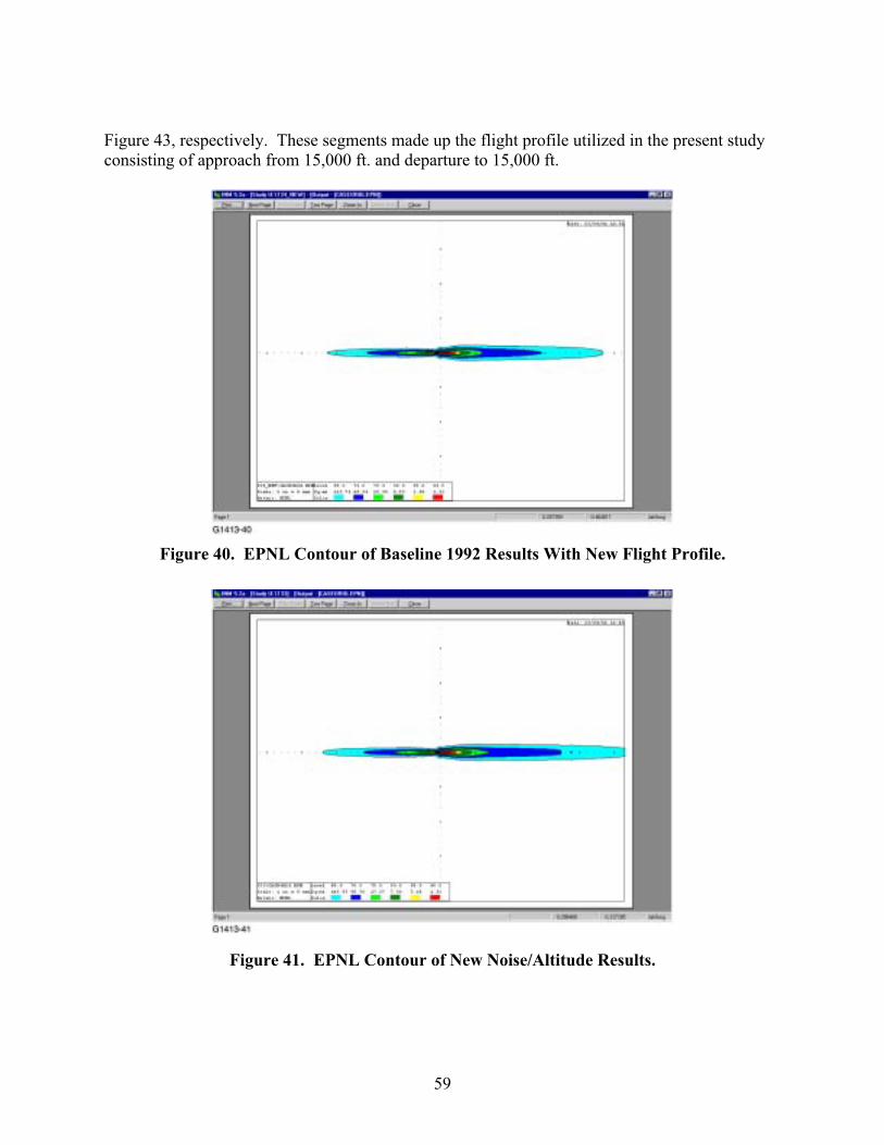
59

Figure 43, respectively. These segments made up the flight profile utilized in the present studyconsisting of approach from 15,000 ft. and departure to 15,000 ft.

Figure 40. EPNL Contour of Baseline 1992 Results With New Flight Profile.

Figure 41. EPNL Contour of New Noise/Altitude Results.

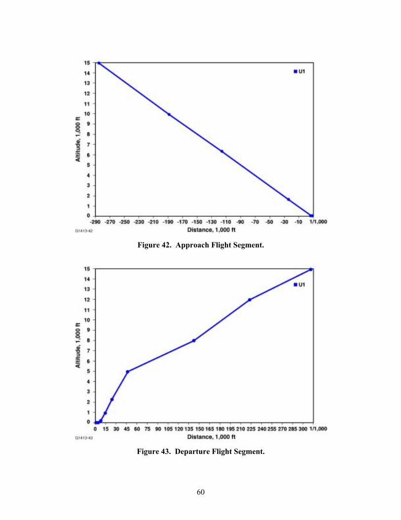
60

Figure 42. Approach Flight Segment.

Figure 43. Departure Flight Segment.

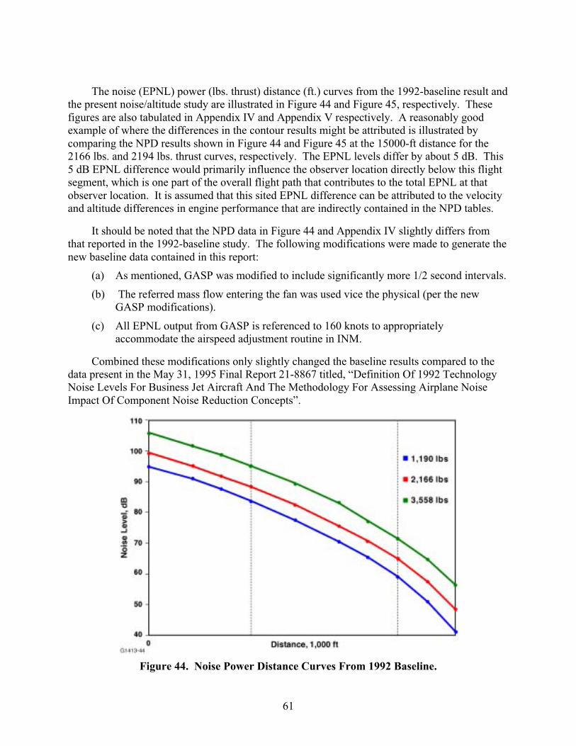
61

The noise (EPNL) power (lbs. thrust) distance (ft.) curves from the 1992-baseline result andthe present noise/altitude study are illustrated in Figure 44 and Figure 45, respectively. Thesefigures are also tabulated in Appendix IV and Appendix V respectively. A reasonably goodexample of where the differences in the contour results might be attributed is illustrated bycomparing the NPD results shown in Figure 44 and Figure 45 at the 15000-ft distance for the2166 lbs. and 2194 lbs. thrust curves, respectively. The EPNL levels differ by about 5 dB. This5 dB EPNL difference would primarily influence the observer location directly below this flightsegment, which is one part of the overall flight path that contributes to the total EPNL at thatobserver location. It is assumed that this sited EPNL difference can be attributed to the velocityand altitude differences in engine performance that are indirectly contained in the NPD tables.

It should be noted that the NPD data in Figure 44 and Appendix IV slightly differs fromthat reported in the 1992-baseline study. The following modifications were made to generate thenew baseline data contained in this report:

(a) As mentioned, GASP was modified to include significantly more 1/2 second intervals.

(b) The referred mass flow entering the fan was used vice the physical (per the newGASP modifications).

(c) All EPNL output from GASP is referenced to 160 knots to appropriatelyaccommodate the airspeed adjustment routine in INM.

Combined these modifications only slightly changed the baseline results compared to thedata present in the May 31, 1995 Final Report 21-8867 titled, “Definition Of 1992 TechnologyNoise Levels For Business Jet Aircraft And The Methodology For Assessing Airplane NoiseImpact Of Component Noise Reduction Concepts”.

Figure 44. Noise Power Distance Curves From 1992 Baseline.

62

Figure 45. Noise Power Distance Curves for Noise/Altitude Study.

5. LATERAL ATTENUATION EXPERIMENTS

5.1 Introduction

Noise predictions in the FAA Integrated Noise Model for aircraft at elevation angles lessthan 60 degrees currently use an empirical algorithm which combines all known lateralattenuation effects (ground attenuation, atmospheric effects, installation effects). The objectiveis to replace this single empirical algorithm with component, scientifically defensible models.The approach is to conduct a controlled flight test to isolate installation effects.

This objective was accomplished by flying a variety of aircraft with different engine andinstallation configurations over an array of microphones. The flybys simulated aircraftdepartures and approaches. The microphone array consisted of one line of microphones on thirtyfoot, guyed poles spaced across the runway and two lines of microphones suspended vertically ashigh as 200 ft. from cranes located at a distance of 425 ft. to each side of the runway. Theacoustic signals recorded from these aircraft flybys of the microphone array were correlated withaircraft position, aircraft engine and aircraft state parameters, and locally measured weatherparameters. The resulting database of correlated acoustics information was analyzed to isolateand quantify the lateral attenuation patterns of the different engine and installationconfigurations.

Level flights at 200-600 feet above ground level with 20 microphones, position data, andweather data were conducted. A schematic diagram of the microphone layout is shown in Figure 46.

63

Figure 46. Diagram of Microphone Layout for the Lateral Attenuation Experiments atWallops Island, VA.

The Volpe Center’s video system was the method for position data collection for some ofthe aircraft included in the study. The video camera tracking system consists of two CanonOptura digital video cameras and four reference optical targets, all deployed at known, fixedlocations within the site’s local coordinate system. Traditional surveying equipment was used todetermine the relative heights of the digital video cameras and targets used for aircraft tracking.Post-processing of the digital video data using classic triangulation techniques determinedaccurate time and position information for each aircraft event.

Two types of meteorological data were collected during the measurement study: (1)ground-based meteorological data and (2) meteorological data aloft. For the ground-basedmeteorological data, Qualimetrics Transportable Automated Meteorological Stations (TAMS)was set up at two locations. The TAMS recorded temperature, relative humidity, wind speed anddirection, and ambient atmospheric pressure at one-second intervals.

In addition to ground-based data, meteorological data aloft was measured and recordedusing a LaRC tethered weather balloon system. The balloon was deployed to a maximum heightof 700 ft. for readings each day prior to beginning test flight runs, after completion of test flightruns, and at approximately two hour intervals during the test flight runs. The balloon waslocated approximately 700 ft. from the runway centerline. The tethered weather balloon systemconsisted of an electric winch-controlled, tethered, helium-filled balloon, an instrument/telemetrypod, a ground-based receiver/data-controller, and a ground-based support computer.

Additional balloon weather data was obtained from the Wallops MET OPS group. Normally,MET OPS launches a meteorological balloon at 0700 and 1900 daily. These launches wereaugmented with a third launch at approximately noon, at the end of the measurements for each day.As with the ground-based sensors, the balloon-based sensors were setup to measure and recordtemperature, relative humidity, wind speed and direction, and ambient atmospheric pressure.

64

5.2 Honeywell Participation

Honeywell identified two aircraft to participate in the Lateral Attenuation Experiments atWallops Island VA.

The Falcon 900EX is a 3 aft-mounted engine aircraft powered by TFE731-60 engines (BPR= 4.3 at take-off). The aircraft has an 18.4 EPNdB cumulative margin to Stage 3. The TFE731-60 is the engine used in all of the Honeywell engine validation work for AST Noise Reduction.The aircraft arrived at Wallops Island on September 26, 2000. A picture of the aircraft is shownin Figure 47. Unfortunately, weather conditions prohibited data collection, and there was no dayavailable for a rescheduled test.

Figure 47. The Honeywell Falcon 900EX, Waiting for the Winds to Calm and the Ceiling to Rise.

The Falcon 2000 is a 2 aft-mounted engine aircraft powered by CFE738-1 engines (BPR =6.2 at take-off). The aircraft has a 22.1 EPNdB cumulative margin to Stage 3. Honeywell andGE jointly produce the CFE738-1 engine. The aircraft arrived on the morning of September 27,2000 to excellent weather. All elements of the test matrix were completed. Figure 48 shows theFalcon 2000 at Wallops and Figure 49 shows the Falcon 2000 flying over (and through) themicrophone array.

Static data and engine information exists for the CFE738 engine that can be used to aid ininterpreting the results of the measurements.

65

Figure 48. The Honeywell Falcon 2000 Arrived to an Almost Perfect Sky and No Winds on the Next Day.

Figure 49. The Falcon 2000 Flying Through the Microphone Cranes at Wallops Island.

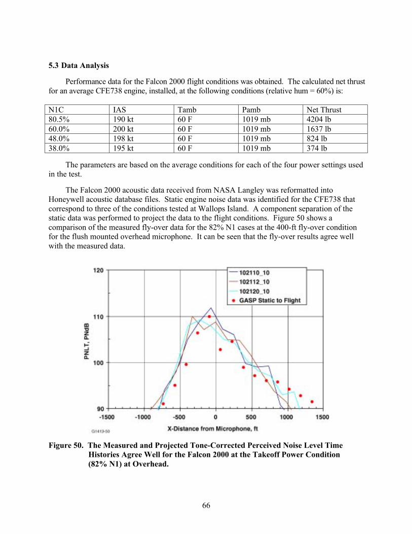
66

5.3 Data Analysis

Performance data for the Falcon 2000 flight conditions was obtained. The calculated net thrustfor an average CFE738 engine, installed, at the following conditions (relative hum = 60%) is:

N1C IAS Tamb Pamb Net Thrust80.5% 190 kt 60 F 1019 mb 4204 lb60.0% 200 kt 60 F 1019 mb 1637 lb48.0% 198 kt 60 F 1019 mb 824 lb38.0% 195 kt 60 F 1019 mb 374 lb

The parameters are based on the average conditions for each of the four power settings usedin the test.

The Falcon 2000 acoustic data received from NASA Langley was reformatted intoHoneywell acoustic database files. Static engine noise data was identified for the CFE738 thatcorrespond to three of the conditions tested at Wallops Island. A component separation of thestatic data was performed to project the data to the flight conditions. Figure 50 shows acomparison of the measured fly-over data for the 82% N1 cases at the 400-ft fly-over conditionfor the flush mounted overhead microphone. It can be seen that the fly-over results agree wellwith the measured data.

Figure 50. The Measured and Projected Tone-Corrected Perceived Noise Level TimeHistories Agree Well for the Falcon 2000 at the Takeoff Power Condition(82% N1) at Overhead.

67

Figure 51. The Comparison of the Measured and Projected Spectra Before Overhead(x=-252.0 ft) Agree Well for the Low Frequency Jet Noise and the Blade PassageTone at Take-off Power (82% N1).

Figure 52. The Comparison of the Measured and Projected Spectra Near Overhead(x=-92.6 ft) Agree Well for the Low Frequency Jet Noise and the Blade PassageTone at Take-off Power (82% N1).

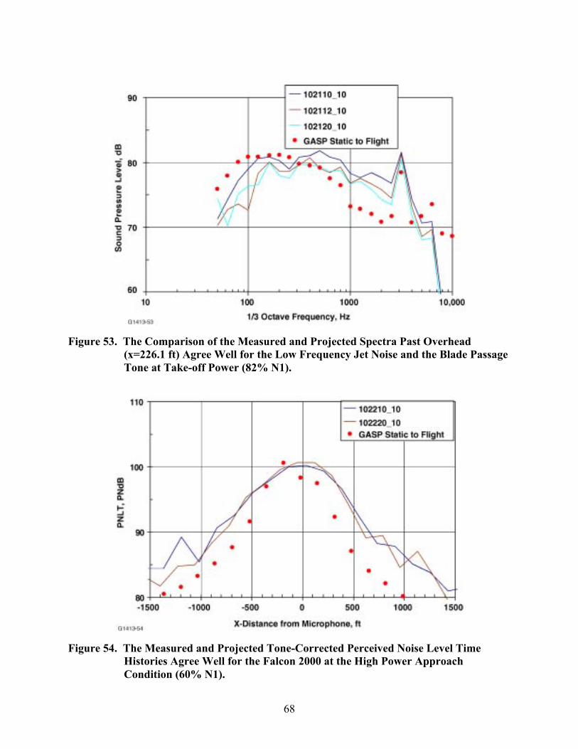
68

Figure 53. The Comparison of the Measured and Projected Spectra Past Overhead(x=226.1 ft) Agree Well for the Low Frequency Jet Noise and the Blade PassageTone at Take-off Power (82% N1).

Figure 54. The Measured and Projected Tone-Corrected Perceived Noise Level TimeHistories Agree Well for the Falcon 2000 at the High Power ApproachCondition (60% N1).

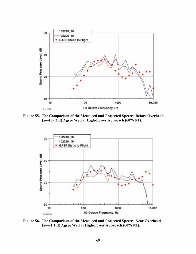
69

Figure 55. The Comparison of the Measured and Projected Spectra Before Overhead(x=-189.2 ft) Agree Well at High-Power Approach (60% N1).

Figure 56. The Comparison of the Measured and Projected Spectra Near Overhead(x=-21.1 ft) Agree Well at High-Power Approach (60% N1).

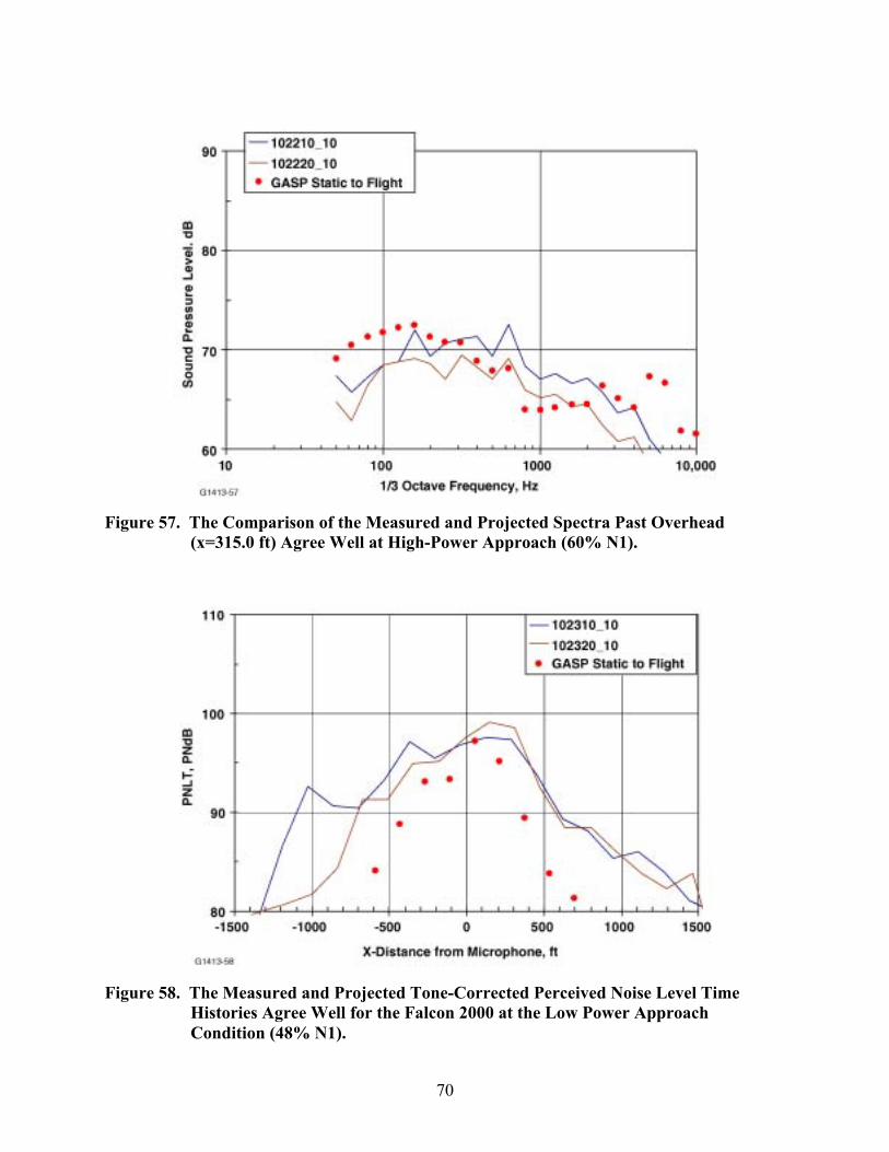
70

Figure 57. The Comparison of the Measured and Projected Spectra Past Overhead(x=315.0 ft) Agree Well at High-Power Approach (60% N1).

Figure 58. The Measured and Projected Tone-Corrected Perceived Noise Level TimeHistories Agree Well for the Falcon 2000 at the Low Power ApproachCondition (48% N1).

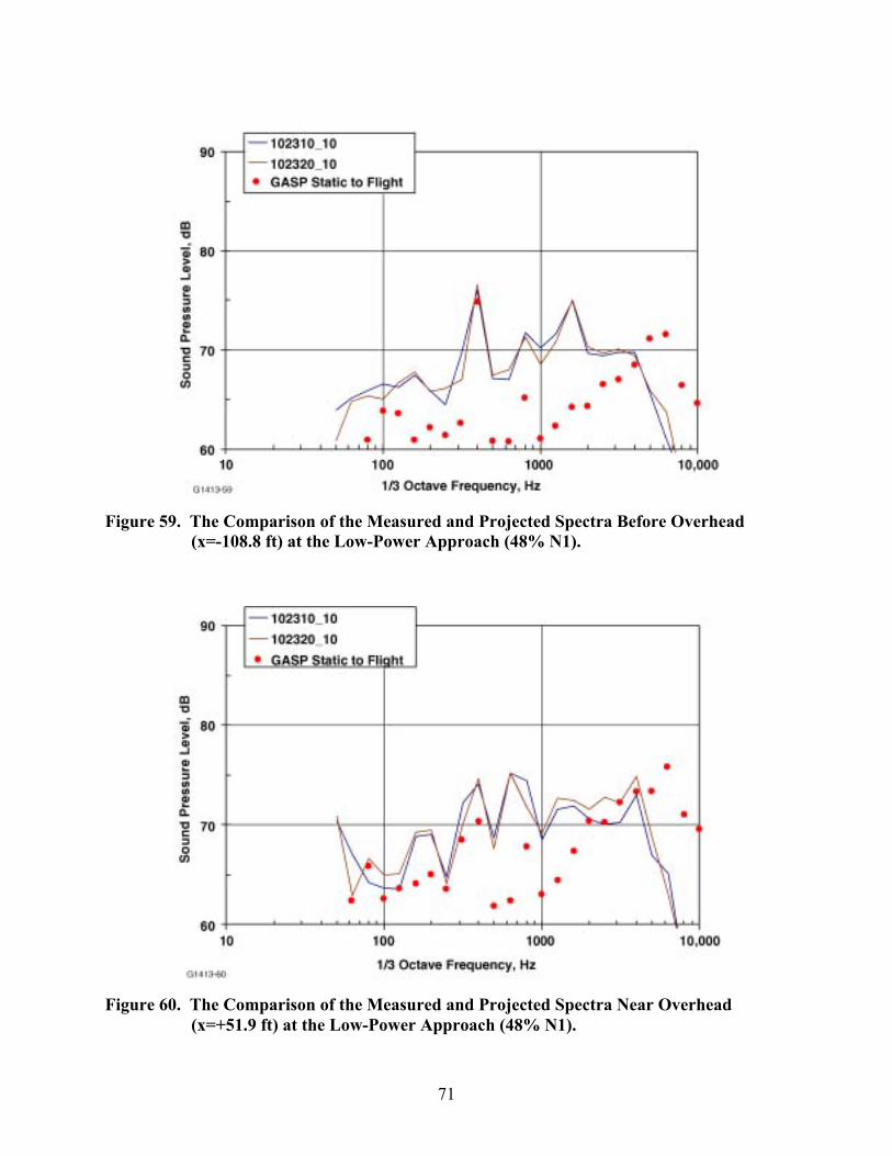
71

Figure 59. The Comparison of the Measured and Projected Spectra Before Overhead(x=-108.8 ft) at the Low-Power Approach (48% N1).

Figure 60. The Comparison of the Measured and Projected Spectra Near Overhead(x=+51.9 ft) at the Low-Power Approach (48% N1).

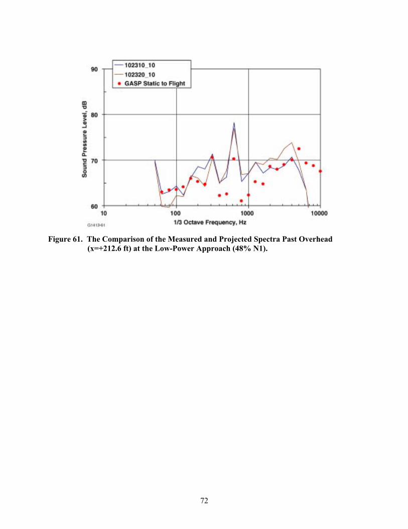
72

Figure 61. The Comparison of the Measured and Projected Spectra Past Overhead(x=+212.6 ft) at the Low-Power Approach (48% N1).

73

6. REFERENCES

[1] Reed, D., Unpublished Presentation by Boeing, 2001.

[2] Thomas, F.O., Nelson, R.C., and Lui, X., “Experimental Investigation of the ConfluentBoundary Layer of a High-Lift System”, AIAA Journal, Volume 38, Number 6, pp. 978-988, June, 2000.

[3] Hayes, J.A., Horne, C.W., Soderman, P.T., and Bent, P.H., “Airframe NoiseCharacteristics of a 4.7% Scale DC-10 Model ”, AIAA Paper 97-1594-CP, 3rd

AIAA/CEAS Aeroacoustics Conference and Exhibit, Atlanta, GA, May, 1997.

[4] Guo, Y.P., “A Model for Slat Noise Generation ”, AIAA Paper 97-1647, 3rd AIAA/CEASAeroacoustics Conference and Exhibit, Atlanta, GA, May, 1997.

[5] Guo, Y.P., Hardy, B., Bent, P., Yamamoto, K., and Joshi, M., “Surface PressureFluctuations on DC-10 High Lift System and their Correlation with Far Field Noise”,NASI-20103, Task 2, NASA CRAD-9310-4872, 1998.

[6] Guo, Y.P., Hardy, B., Bent, P., Yamamoto, K., and Joshi, M., “Noise Characteristics ofDC-10 Aircraft High Lift Systems”, NASI-20103, Task 2, NASA CRAD-9310-4893,1998.

[7] Dobrzynski, W., Nagakura, K., Gehlhar, B., and Buschbaum, A., “Airframe NoiseStudies on Wings with Deployed High-Lift Devices ”, AIAA Paper 99-1805, 5th

AIAA/CEAS Aeroacoustics Conference and Exhibit, Bellevue, WA, May, 1999.

[8] Storms, B.L., Hayes, J.A., Moriarity, P.J., and James, R.C., “Aeroacoustic Measurementsof Slat Noise on a Three-Dimensional High-Lift System”, AIAA Paper 99-1957, 5th

AIAA/CEAS Aeroacoustics Conference and Exhibit, Bellevue, WA, May, 1999.

[9] Moriarty, P.J., and Heineck, J.T., “PIV Measurements Near a Leading Edge Slat”Proceedings of the 3rd International Workshop on PIV, 1999.

[10] Khorrami, M.R., Berkman, M.E., Choudhari, M., Singer, B.A.,Lockard, D.P., andBrentner, K.S., “Unsteady Flow Computations of a Slat with a Blunt Trailing Edge ”,AIAA Paper 99-1805, 5th AIAA/CEAS Aeroacoustics Conference and Exhibit, Bellevue,WA, May, 1999.

[11] Singer, B.A., Lockard, D.P., Brentner, K.S.Khorrami, M.R., Berkman, M.E., andChoudhari, M, “Computational Aeroacoustic Analysis of Slat Trailing Edge Flow”, AIAAPaper 99-1802, 5th AIAA/CEAS Aeroacoustics Conference and Exhibit, Bellevue, WA,May, 1999.

74

[12] Khorrami, M.R., Singer, B.A., Berkman, M.E., “Time Accurate Simulations andAcoustic Analysis of Slat Free-Shear Layer”, AIAA Paper 01-2155, 7th AIAA/CEASAeroacoustics Conference and Exhibit, Maastricht, Netherlands, May, 2001.

[13] Meadows, K.R., Brooks, T.F., Humphreys, W.M., Hunter, W.W., and Gerhold, C.H.,“Aeroacoustic Measurements of a Wing-Flap Configuration”, AIAA Paper 97-1595, 3rd

AIAA/CEAS Aeroacoustics Conference, Atlanta, GA, May, 1997.

[14] Brooks, T.F., Marcolini, M.A., Pope, D.S., “Airfoil Trailing-Edge Flow Measurements”,AIAA Journal, Volume 24, Number 8, pp. 1245-1251, 1986.

[15] Brooks, T.F., Marcolini, M.A., and Pope, D.S., “A Directional Array Approach for theMeasurement of Rotor Noise Source Distributions with Controlled Spatial Resolution”,Journal of Sound and Vibration, Volume 112, Number 1, pp. 192-197, 1987.

[16] Marcolini, M.A., and Brooks, T.F., “Rotor Noise Measurement Using a DirectionalMicrophone Array”, Journal of the American Helicopter Society, pp. 11-22, 1992.

[17] Brooks, T.F., Pope, D.S., Marcolini, M.A., “Airfoil Self-Noise and Prediction”, NASAReference Publication 1218, July, 1989.

[18] Ahuja, K. K., Tanna, H. K., and Tester, B. J, “An experimental study of transmission,reflection, and scattering of sound in a free jet flight simulation facility and comparisonwith theory”, Journal of Sound and Vibration 75, 51-85 (1981).

[19] Amiet, R. K., “Correction of open jet wind tunnel measurements for shear layerrefraction”, American Institute of Aeronautics and Astronautics Paper 75-532 (1975).

[20] Amiet, R. K., “Refraction of sound by a shear layer”, Journal of Sound and Vibration 58,467-482 (1978).

[21] Amiet, R. K., “Correction of fan noise for the effects of forward flight”, Journal of Soundand Vibration 89, 243-259 (1983).

[22] Dowling, A. P., “Convective amplification of real simple sources”, Journal of FluidMechanics 74, 529-546 (1976).

[23] Dowling, A. P. and Ffowcs Williams, J. E., Sound and Sources of Sound, Ellis HorwoodLimited (1893).

[24] Graham E. W. and Graham, B. B., “Effect of a shear layer on plane waves of sound in afluid”, Journal of the Acoustical Society of America 46, 169-175 (1969).

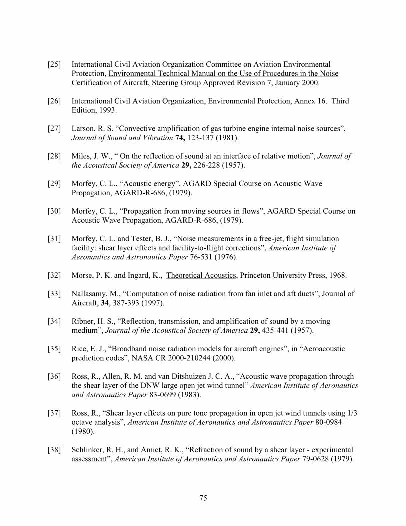
75

[25] International Civil Aviation Organization Committee on Aviation EnvironmentalProtection, Environmental Technical Manual on the Use of Procedures in the NoiseCertification of Aircraft, Steering Group Approved Revision 7, January 2000.

[26] International Civil Aviation Organization, Environmental Protection, Annex 16. ThirdEdition, 1993.

[27] Larson, R. S. “Convective amplification of gas turbine engine internal noise sources”,Journal of Sound and Vibration 74, 123-137 (1981).

[28] Miles, J. W., “ On the reflection of sound at an interface of relative motion”, Journal ofthe Acoustical Society of America 29, 226-228 (1957).

[29] Morfey, C. L., “Acoustic energy”, AGARD Special Course on Acoustic WavePropagation, AGARD-R-686, (1979).

[30] Morfey, C. L., “Propagation from moving sources in flows”, AGARD Special Course onAcoustic Wave Propagation, AGARD-R-686, (1979).

[31] Morfey, C. L. and Tester, B. J., “Noise measurements in a free-jet, flight simulationfacility: shear layer effects and facility-to-flight corrections”, American Institute ofAeronautics and Astronautics Paper 76-531 (1976).

[32] Morse, P. K. and Ingard, K., Theoretical Acoustics, Princeton University Press, 1968.

[33] Nallasamy, M., “Computation of noise radiation from fan inlet and aft ducts”, Journal ofAircraft, 34, 387-393 (1997).

[34] Ribner, H. S., “Reflection, transmission, and amplification of sound by a movingmedium”, Journal of the Acoustical Society of America 29, 435-441 (1957).

[35] Rice, E. J., “Broadband noise radiation models for aircraft engines”, in “Aeroacousticprediction codes”, NASA CR 2000-210244 (2000).

[36] Ross, R., Allen, R. M. and van Ditshuizen J. C. A., “Acoustic wave propagation throughthe shear layer of the DNW large open jet wind tunnel” American Institute of Aeronauticsand Astronautics Paper 83-0699 (1983).

[37] Ross, R., “Shear layer effects on pure tone propagation in open jet wind tunnels using 1/3octave analysis”, American Institute of Aeronautics and Astronautics Paper 80-0984(1980).

[38] Schlinker, R. H., and Amiet, R. K., “Refraction of sound by a shear layer - experimentalassessment”, American Institute of Aeronautics and Astronautics Paper 79-0628 (1979).

76

[39] Society of Automotive Engineers, “Gas turbine jet exhaust noise prediction”, SAEAerospace Recommended Practice 876, 1978.

[40] Tester, B. J. and Morfey, C. L., “ Developments in jet noise modeling - theoreticalpredictions and comparisons with measured data, Journal of Sound and Vibration 46, 79-103 (1976).

[41] Zorumski, William E., Aircraft Noise Prediction Program Theoretical Manual, NASATechnical Memorandum 83199, 1982.

I-i

APPENDIX I

1/3-OCTAVE BAND SPL TIME HISTORIES OF ESTIMATED AIRFRAME NOISE

(3 pages)

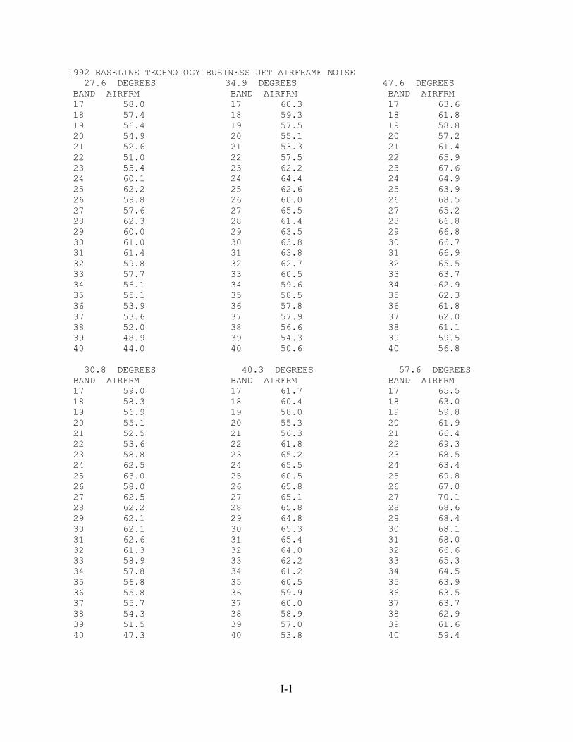
I-1

1992 BASELINE TECHNOLOGY BUSINESS JET AIRFRAME NOISE 27.6 DEGREES BAND AIRFRM 17 58.0 18 57.4 19 56.4 20 54.9 21 52.6 22 51.0 23 55.4 24 60.1 25 62.2 26 59.8 27 57.6 28 62.3 29 60.0 30 61.0 31 61.4 32 59.8 33 57.7 34 56.1 35 55.1 36 53.9 37 53.6 38 52.0 39 48.9 40 44.0

30.8 DEGREES BAND AIRFRM 17 59.0 18 58.3 19 56.9 20 55.1 21 52.5 22 53.6 23 58.8 24 62.5 25 63.0 26 58.0 27 62.5 28 62.2 29 62.1 30 62.1 31 62.6 32 61.3 33 58.9 34 57.8 35 56.8 36 55.8 37 55.7 38 54.3 39 51.5 40 47.3

34.9 DEGREES BAND AIRFRM 17 60.3 18 59.3 19 57.5 20 55.1 21 53.3 22 57.5 23 62.2 24 64.4 25 62.6 26 60.0 27 65.5 28 61.4 29 63.5 30 63.8 31 63.8 32 62.7 33 60.5 34 59.6 35 58.5 36 57.8 37 57.9 38 56.6 39 54.3 40 50.6

40.3 DEGREES BAND AIRFRM 17 61.7 18 60.4 19 58.0 20 55.3 21 56.3 22 61.8 23 65.2 24 65.5 25 60.5 26 65.8 27 65.1 28 65.8 29 64.8 30 65.3 31 65.4 32 64.0 33 62.2 34 61.2 35 60.5 36 59.9 37 60.0 38 58.9 39 57.0 40 53.8

47.6 DEGREES BAND AIRFRM 17 63.6 18 61.8 19 58.8 20 57.2 21 61.4 22 65.9 23 67.6 24 64.9 25 63.9 26 68.5 27 65.2 28 66.8 29 66.8 30 66.7 31 66.9 32 65.5 33 63.7 34 62.9 35 62.3 36 61.8 37 62.0 38 61.1 39 59.5 40 56.8

57.6 DEGREES BAND AIRFRM 17 65.5 18 63.0 19 59.8 20 61.9 21 66.4 22 69.3 23 68.5 24 63.4 25 69.8 26 67.0 27 70.1 28 68.6 29 68.4 30 68.1 31 68.0 32 66.6 33 65.3 34 64.5 35 63.9 36 63.5 37 63.7 38 62.9 39 61.6 40 59.4

I-2

70.9 DEGREES BAND AIRFRM 17 66.5 18 63.3 19 62.0 20 66.2 21 69.9 22 71.0 23 67.4 24 68.0 25 71.5 26 69.4 27 69.8 28 70.0 29 69.8 30 69.5 31 68.7 32 67.2 33 66.3 34 65.5 35 65.0 36 64.6 37 64.7 38 64.1 39 62.8 40 60.8

87.4 DEGREES BAND AIRFRM 17 66.6 18 63.3 19 63.7 20 68.0 21 71.2 22 71.3 23 66.2 24 70.7 25 71.0 26 71.5 27 70.0 28 70.5 29 70.1 30 69.2 31 68.4 32 66.9 33 66.1 34 65.4 35 64.8 36 64.5 37 64.4 38 63.7 39 62.5 40 60.7

105.0 DEGREES BAND AIRFRM 17 68.1 18 64.7 19 64.2 20 68.5 21 71.6 22 72.1 23 67.4 24 69.9 25 71.4 26 70.4 27 69.2 28 69.5 29 69.2 30 67.9 31 67.0 32 65.7 33 64.7 34 63.9 35 63.2 36 62.7 37 62.5 38 61.6 39 60.4 40 58.5

120.8 DEGREES BAND AIRFRM 17 69.8 18 66.8 19 63.9 20 66.5 21 70.5 22 72.4 23 70.2 24 65.5 25 71.2 26 66.6 27 69.6 28 68.4 29 67.6 30 66.7 31 65.5 32 64.0 33 62.9 34 62.1 35 61.0 36 60.1 37 59.5 38 58.4 39 56.8 40 54.8

133.3 DEGREES BAND AIRFRM 17 70.9 18 68.6 19 65.2 20 63.7 21 67.4 22 71.1 23 71.3 24 67.1 25 66.3 26 68.9 27 65.7 28 66.1 29 66.2 30 65.3 31 63.7 32 61.9 33 60.7 34 59.7 35 58.6 36 57.2 37 56.3 38 54.8 39 52.8 40 50.5

142.4 DEGREES BAND AIRFRM 17 71.2 18 69.4 19 66.8 20 63.4 21 63.3 22 67.8 23 69.8 24 68.9 25 62.8 26 65.9 27 65.2 28 65.2 29 64.4 30 63.4 31 61.2 32 59.4 33 58.3 34 57.1 35 55.7 36 54.2 37 53.0 38 51.2 39 48.7 40 46.0

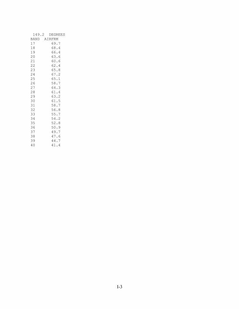
I-3

149.2 DEGREES BAND AIRFRM 17 69.7 18 68.4 19 66.4 20 63.6 21 60.6 22 62.4 23 65.8 24 67.2 25 65.1 26 58.7 27 64.3 28 61.4 29 63.2 30 61.5 31 58.7 32 56.8 33 55.7 34 54.2 35 52.8 36 50.9 37 49.7 38 47.6 39 44.7 40 41.4

II-i

APPENDIX II

ANOPP THEORETICAL MANUAL CHAPTER FOR THE SHEAR LAYERCORRECTION MODULE

(14 pages)

II-1

INTRODUCTION

A static-to-flight correction procedure that does account for modifications to the jet shear

layer is developed from existing models. The approach chosen here is a hybrid of corrections

developed by Amiet in references [1], [2], and [3] and corrections developed by Morfey in

references [4] and [5]. The procedure relates the in-flight, far-field, mean-square sound pressure

to the statically measured, far-field, mean-square sound pressure as a function of flight speed.

The correction process entails applying angle corrections to account for refraction at the shear

layer and amplitude corrections to account for ray-tube divergence changes and forward flight

effects. The effects of reflection of sound by the shear layer and scattering of sound by shear

layer turbulence are ignored. These corrections are developed using a geometric acoustics

approach for cylindrical shear layer geometry. The angle correction is based upon a vortex sheet

model of the shear layer. The amplitude correction is based on the assumption of energy

conservation across the shear layer.

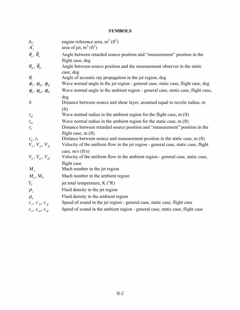
II-2

SYMBOLS

Ae engine reference area, m2 (ft2)A j

* area of jet, m2 (ft2)

θe , θe Angle between retarded source position and “measurement” position in theflight case, deg

θm , θm Angle between source position and the measurement observer in the staticcase, deg

θc Angle of acoustic ray propagation in the jet region, degφj , φjs, φjf Wave normal angle in the jet region - general case, static case, flight case, deg

φa , φas, φaf Wave normal angle in the ambient region - general case, static case, flight case,

degh Distance between source and shear layer, assumed equal to nozzle radius, m

(ft)raf Wave normal radius in the ambient region for the flight case, m (ft)

ras Wave normal radius in the ambient region for the static case, m (ft)re Distance between retarded source position and “measurement” position in the

flight case, m (ft)rm , rs Distance between source and measurement position in the static case, m (ft)V j , V js, V jf Velocity of the uniform flow in the jet region - general case, static case, flight

case, m/s (ft/s)Va , Vas, Vaf Velocity of the uniform flow in the ambient region - general case, static case,

flight caseM j Mach number in the jet region

Ma , M∞ Mach number in the ambient region

Tj jet total temperature, K (°R)

ρ j Fluid density in the jet region

ρa Fluid density in the ambient regionc j , c js, c jf Speed of sound in the jet region - general case, static case, flight case

ca , cas, caf Speed of sound in the ambient region - general case, static case, flight case

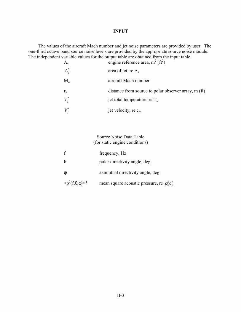
II-3

INPUT

The values of the aircraft Mach number and jet noise parameters are provided by user. Theone-third octave band source noise levels are provided by the appropriate source noise module.The independent variable values for the output table are obtained from the input table.

Ae engine reference area, m2 (ft2)

A j* area of jet, re Ae

M∞ aircraft Mach number

rs distance from source to polar observer array, m (ft)

Tj* jet total temperature, re T∞

V j* jet velocity, re c∞

Source Noise Data Table(for static engine conditions)

f frequency, Hz

θ polar directivity angle, deg

φ azimuthal directivity angle, deg

<p2(f,θ,φ)>* mean square acoustic pressure, re ρ∞ ∞2 4c

II-4

OUTPUT

The output of this module is a table of the mean-square acoustic pressure as a function offrequency, polar directivity angle, and azimuthal directivity angle corrected for jet shear layereffects.

Shear Layer Corrected Source Noise Data Table

f frequency, Hz

θ polar directivity angle, deg

φ azimuthal directivity angle, deg

<p2(f, θ,φ)>* mean square acoustic pressure, re ρ∞ ∞2 4c

METHOD

Problem Geometry

The model geometry for the correction procedure is shown in Figure II-1. An axiallysymmetric point source S is situated at the exhaust plane on the centerline of a cylindrical jet. Auniform flow of Mach number M j exists in the jet, which has a constant density ρ j and constant

speed of sound c j . A shear layer of constant radius h separates the jet from the ambient fluid,

which maintains a constant density ρa and constant speed of sound ca . The source S emitssound in all directions. Sound emitted in the wave normal direction φj is convected by the jet

flow. The resulting ray path makes an angle θc with respect to the source and intersects theshear layer at the point C . In the static case, the sound is refracted by the shear layer to a wavenormal angle φas. The sound propagates through the ambient medium in the wave normaldirection φasat speed ca . The sound arrives at the measurement position M , which lies adistance rm and angle θm from the source. In the flight case, the sound is refracted by the shearlayer to a different wave normal angle φaf . The sound propagates through the ambient medium

in the wave normal direction φaf at speed ca , and is also convected by the ambient flow at speed

M ca a . Sound traveling in the upstream direction is considered to re-enter the nozzle and thusdoes not contribute to the far-field noise.

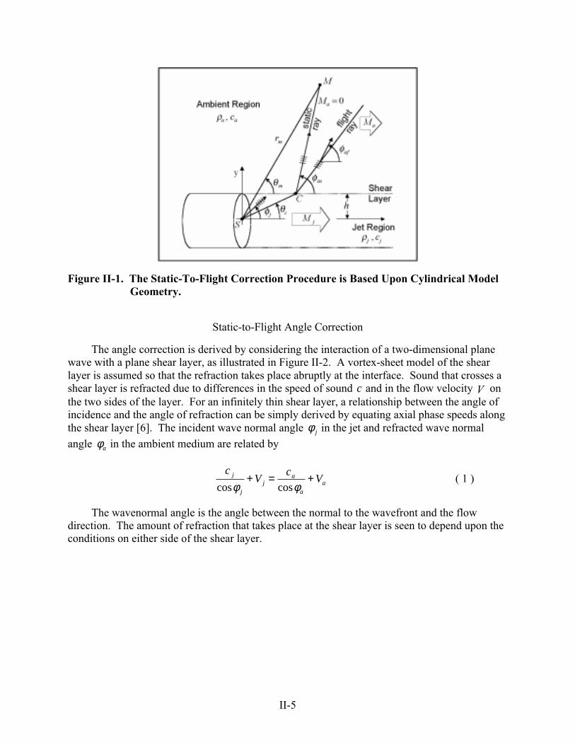
II-5

Figure II-1. The Static-To-Flight Correction Procedure is Based Upon Cylindrical ModelGeometry.

Static-to-Flight Angle Correction

The angle correction is derived by considering the interaction of a two-dimensional planewave with a plane shear layer, as illustrated in Figure II-2. A vortex-sheet model of the shearlayer is assumed so that the refraction takes place abruptly at the interface. Sound that crosses ashear layer is refracted due to differences in the speed of sound c and in the flow velocity V onthe two sides of the layer. For an infinitely thin shear layer, a relationship between the angle ofincidence and the angle of refraction can be simply derived by equating axial phase speeds alongthe shear layer [6]. The incident wave normal angle φj in the jet and refracted wave normal

angle φa in the ambient medium are related by

cV

cVj

jj

a

aacos cosφ φ

+ = + ( 1 )

The wavenormal angle is the angle between the normal to the wavefront and the flowdirection. The amount of refraction that takes place at the shear layer is seen to depend upon theconditions on either side of the shear layer.

II-6

Figure II-2. The Refraction Angle Correction is Derived by Considering Plane WaveInteraction With a Vortex Sheet.

Equation ( 1 ) can be used to describe how the ambient wave normal angle is modifiedwhen the engine nozzle is taken from static to flight conditions. Using additional subscripts “ s”and “ f ” to denote the static and flight conditions, and writing the refraction equation for eachcase yields

Static case:c

Vcjs

jsjs

as

ascos cosφ φ+ = ( 2 )

Flight case:c

Vc

Vjf

jfjf

af

afafcos cosφ φ

+ = + ( 3 )

It is assumed that the jet velocity remains constant when moving from static to flightconditions, so that V V Vjs jf j= ≡ . It is also assumed that the temperature in the jet and ambient

regions do not change when moving from static to flight conditions, so that c c cjs jf j= ≡ and

c c cas af a= ≡ . Finally, it is assumed that the external flow does not affect the generation and

propagation of the noise inside the jet. Then the wavenormal angle within the jet is identical inthe static and flight cases, so that φ φjs jf= . Under these assumptions, Equations ( 2 ) and ( 3 )

can then be combined to provide the following relationship between the ambient wavenormalangles in the static and flight cases:

coscos

cosφ φ

φafas

a asM=

−1( 4 )

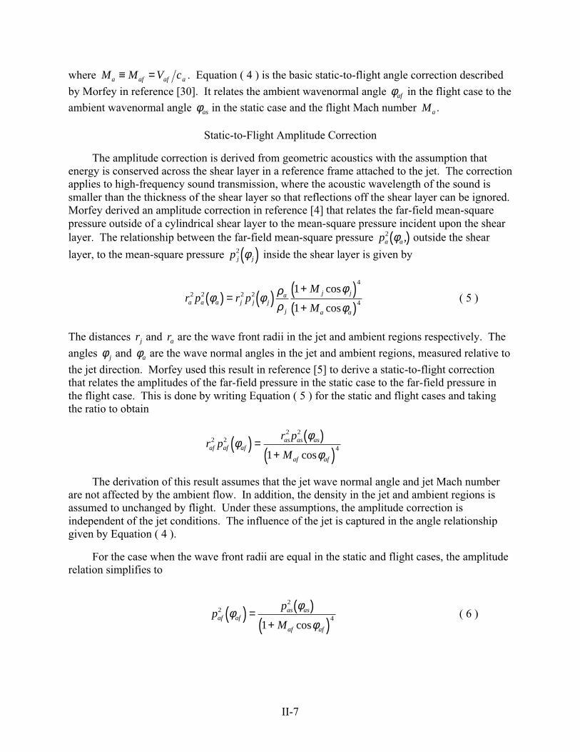
II-7

where M M V ca af af a≡ = . Equation ( 4 ) is the basic static-to-flight angle correction described

by Morfey in reference [30]. It relates the ambient wavenormal angle φaf in the flight case to the

ambient wavenormal angle φas in the static case and the flight Mach number Ma .

Static-to-Flight Amplitude Correction

The amplitude correction is derived from geometric acoustics with the assumption thatenergy is conserved across the shear layer in a reference frame attached to the jet. The correctionapplies to high-frequency sound transmission, where the acoustic wavelength of the sound issmaller than the thickness of the shear layer so that reflections off the shear layer can be ignored.Morfey derived an amplitude correction in reference [4] that relates the far-field mean-squarepressure outside of a cylindrical shear layer to the mean-square pressure incident upon the shearlayer. The relationship between the far-field mean-square pressure pa a

2 φ ,( ) outside the shear

layer, to the mean-square pressure p j j2 φ( ) inside the shear layer is given by

r p r pM

Ma a a j j j

a

j

j j

a a

2 2 2 2

4

4

1

1φ φ ρ

ρφ

φ( ) = ( ) +( )

+( )cos

cos( 5 )

The distances rj and ra are the wave front radii in the jet and ambient regions respectively. The

angles φj and φa are the wave normal angles in the jet and ambient regions, measured relative to

the jet direction. Morfey used this result in reference [5] to derive a static-to-flight correctionthat relates the amplitudes of the far-field pressure in the static case to the far-field pressure inthe flight case. This is done by writing Equation ( 5 ) for the static and flight cases and takingthe ratio to obtain

r pr p

Maf af af

as as as

af af

2 22 2

41

φφ

φ( ) = ( )

+( )cos

The derivation of this result assumes that the jet wave normal angle and jet Mach numberare not affected by the ambient flow. In addition, the density in the jet and ambient regions isassumed to unchanged by flight. Under these assumptions, the amplitude correction isindependent of the jet conditions. The influence of the jet is captured in the angle relationshipgiven by Equation ( 4 ).

For the case when the wave front radii are equal in the static and flight cases, the amplituderelation simplifies to

pp

Maf af

as as

af af

22

41

φφ

φ( ) = ( )

+( )cos( 6 )

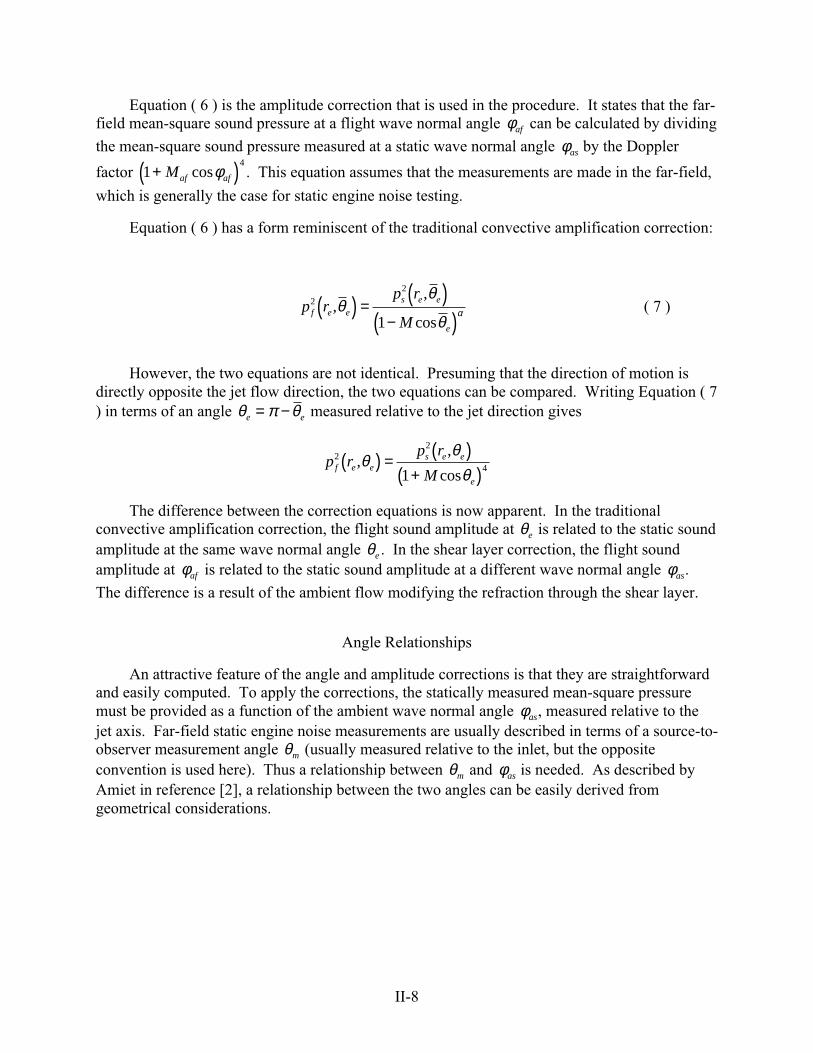
II-8

Equation ( 6 ) is the amplitude correction that is used in the procedure. It states that the far-field mean-square sound pressure at a flight wave normal angle φaf can be calculated by dividing

the mean-square sound pressure measured at a static wave normal angle φas by the Doppler

factor 14

+( )Maf afcosφ . This equation assumes that the measurements are made in the far-field,

which is generally the case for static engine noise testing.

Equation ( 6 ) has a form reminiscent of the traditional convective amplification correction:

p rp r

Mf e e

s e e

e

22

1,

,

cosθ

θ

θα( ) = ( )

−( )( 7 )

However, the two equations are not identical. Presuming that the direction of motion isdirectly opposite the jet flow direction, the two equations can be compared. Writing Equation ( 7) in terms of an angle θ π θe e= − measured relative to the jet direction gives

p rp r

Mf e e

s e e

e

22

41

,,

cosθ

θθ

( ) = ( )+( )

The difference between the correction equations is now apparent. In the traditionalconvective amplification correction, the flight sound amplitude at θe is related to the static soundamplitude at the same wave normal angle θe . In the shear layer correction, the flight soundamplitude at φaf is related to the static sound amplitude at a different wave normal angle φas.

The difference is a result of the ambient flow modifying the refraction through the shear layer.

Angle Relationships

An attractive feature of the angle and amplitude corrections is that they are straightforwardand easily computed. To apply the corrections, the statically measured mean-square pressuremust be provided as a function of the ambient wave normal angle φas, measured relative to thejet axis. Far-field static engine noise measurements are usually described in terms of a source-to-observer measurement angle θm (usually measured relative to the inlet, but the oppositeconvention is used here). Thus a relationship between θm and φas is needed. As described byAmiet in reference [2], a relationship between the two angles can be easily derived fromgeometrical considerations.

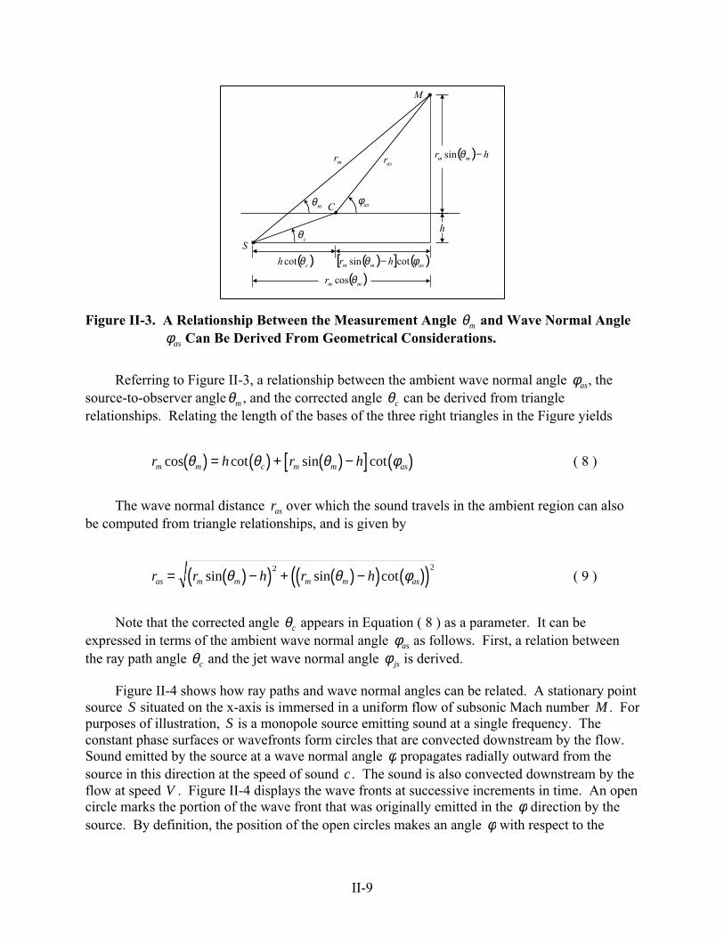
II-9

C

S

M

mθ

cθ

mr asr

asφ

( ) hr mm −θsin

h

( )ch θcot ( )[ ] ( )asmm hr φθ cotsin −

( )mmr θcos

Figure II-3. A Relationship Between the Measurement Angle θm and Wave Normal Angleφas Can Be Derived From Geometrical Considerations.

Referring to Figure II-3, a relationship between the ambient wave normal angle φas, thesource-to-observer angleθm , and the corrected angle θc can be derived from trianglerelationships. Relating the length of the bases of the three right triangles in the Figure yields

r h r hm m c m m ascos cot sin cotθ θ θ φ( ) = ( ) + ( ) −[ ] ( ) ( 8 )

The wave normal distance ras over which the sound travels in the ambient region can alsobe computed from triangle relationships, and is given by

r r h r has m m m m as= ( ) −( ) + ( ) −( ) ( )( )sin sin cotθ θ φ2 2

( 9 )

Note that the corrected angle θc appears in Equation ( 8 ) as a parameter. It can beexpressed in terms of the ambient wave normal angle φas as follows. First, a relation betweenthe ray path angle θc and the jet wave normal angle φjs is derived.

Figure II-4 shows how ray paths and wave normal angles can be related. A stationary pointsource S situated on the x-axis is immersed in a uniform flow of subsonic Mach number M . Forpurposes of illustration, S is a monopole source emitting sound at a single frequency. Theconstant phase surfaces or wavefronts form circles that are convected downstream by the flow.Sound emitted by the source at a wave normal angle φ propagates radially outward from thesource in this direction at the speed of sound c . The sound is also convected downstream by theflow at speed V . Figure II-4 displays the wave fronts at successive increments in time. An opencircle marks the portion of the wave front that was originally emitted in the φ direction by thesource. By definition, the position of the open circles makes an angle φ with respect to the

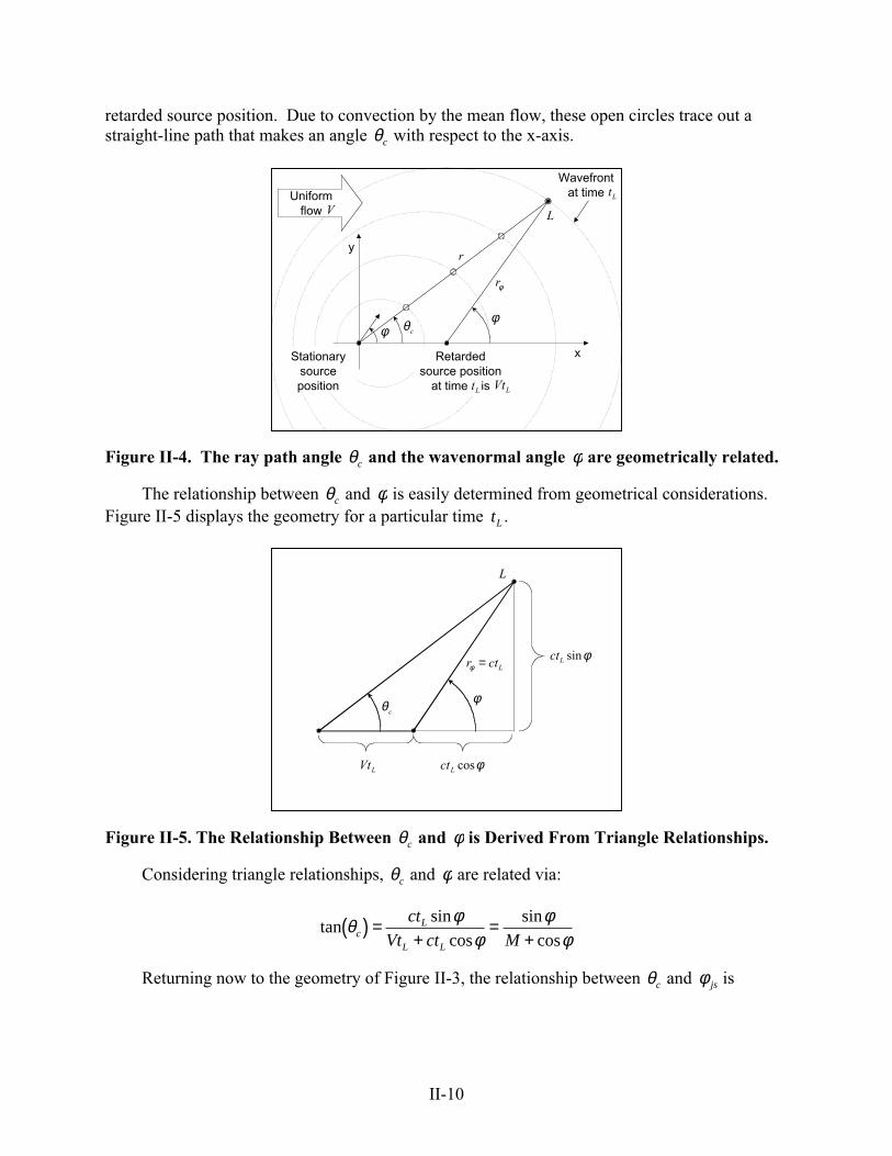
II-10

retarded source position. Due to convection by the mean flow, these open circles trace out astraight-line path that makes an angle θc with respect to the x-axis.

x

y

Wavefrontat time

Retardedsource position

at time is

Uniformflow

Stationarysourceposition

cθ φφ

r

φr

L

Lt

Lt LVt

V

Figure II-4. The ray path angle θc and the wavenormal angle φ are geometrically related.

The relationship between θc and φ is easily determined from geometrical considerations.Figure II-5 displays the geometry for a particular time tL .

LVt φcosLct

cθ φ

Lctr =φφsinLct

L

Figure II-5. The Relationship Between θc and φ is Derived From Triangle Relationships.

Considering triangle relationships, θc and φ are related via:

tansin

cossin

cosθ φ

φφ

φcL

L L

ct

Vt ct M( ) =

+=

+

Returning now to the geometry of Figure II-3, the relationship between θc and φjs is

II-11

tansin

cosθ

φφc

js

js jsM( ) =

+( 10 )

This relationship can be expressed in terms of the ambient wave normal angle φas using thestatic angle refraction relation, Equation ( 2 ). First note that Equation ( 2 ) implies

coscos

coscos

cosφ

φφ

φ

φjs

j as

a j as

as

a

jj as

c

c V c

cM

=−

=−

and

sin

cos cos

cosφ

φ φ

φjs

a

jj as as

a

jj as

c

cM

c

cM

=

−

−

−

2

2

Substituting into Equation ( 10 ) produces the desired relationship between θc and φas

tan

cos cos

cosθ

φ φ

φc

a

jj as as

a

jj j as

c

cM

c

cM M

( ) =

−

−

+ −( )

2

2

21( 11 )

This reduces to Equation (1) of Reference [3] when the temperatures of the jet and ambientregions are identical. Thus, given θm , rm , h and M j , the static ambient wave normal angle φas

can be determined using Equation ( 8 ) and ( 11 ).

Implementation of the Corrections

Static engine noise measurements are obtained at far-field coordinates θm mr,( ) relative tothe source position, with θm measured relative to the exhaust centerline. At a givenmeasurement location, Equations ( 8 ) and ( 11 ) are used to calculate the corresponding staticambient wave normal angle φas. The statically measured mean-square pressure p rm m m

2 θ ,( ) can

then be re-identified as p ras as as2 φ ,( ), where the wave normal coordinates φas asr,( ) are measured

relative to the shear layer intersection point C . Next, the flight ambient wave normal angle φaf

is computed using Equation ( 4 ). Finally, the flight-corrected mean-square pressure p raf af af2 φ ,( )

at an equal wave normal distance r raf as= from the point C is computed using Equation ( 6 ).

II-12

Continuing the assumption of a point source, the effect of refraction changes due to flight isto simply shift the directivity by an amount equal to the difference between the static and flightambient wave normal angles. That is, in flight, sound will be emitted from the source in adirection Φ f given by

Φ f m as af= − −( )θ φ φ ( 12 )

The mean-square pressure in this direction at a wave normal distance (i.e., distance fromthe retarded source position) equal to rm is still provided by Equation ( 6 ) but written using thevariable Φ f ,

p rp r

Mf f m

m m m

f f

22

41

ΦΦ

,,

cos( ) = ( )

+( )θ

( 13 )

The values of pf2 at the original angles θm can be obtained by interpolation. The accuracy

of these approximations improves when r hm msinθ >> . Referring to Figure II-6, ash rm msinθ( ) → 0 with CF CM ras= = , then ∠ → ∠ = −FSM FCM af asφ φ and r rf m→ . So for

distant sideline observers, as is the case in fly-over noise studies, the approximation becomesquite acceptable.

ShearLayer

cθmθ

asφ

afφ

S

C

MF

mr

asr fr

fΦ

h

Figure II-6. The approximation improves as the sideline distance from the shear layerincreases.

Noise Prediction

The simplified jet shear layer static-to-flight correction procedure for internally generated engineexhaust noise can be summarized in the following steps:

II-13

1. Measure or predict the static mean-square pressure p rm m m2 ,θ( ) of the internally generated

engine exhaust noise at a fixed radius rm and at various angles θm from the source taken fromthe input table <p2(f, θ,φ)>*. Source-separation techniques may be required.

2. For a given measurement angle θm , compute the static ambient wave normal angle φas usingEquations ( 2 ), ( 8 ), and ( 10 ). An iterative procedure must be used, since φas cannot beexpressed explicitly in terms of θm .

3. Compute the flight ambient wave normal angle φaf using Equation ( 4 ).

4. Compute the approximate flight emission angle Φ f using Equation ( 12 ).

5. Compute the flight-corrected mean-square pressure p rf f m2 Φ ,( ) using Equation ( 13 ).

6. Interpolate the flight-corrected mean-square pressure p rf f m2 Φ ,( ) back to the original

measurement angles θm .

II-14

REFERENCES

[1] Ahuja, K. K., Tanna, H. K., and Tester, B. J, “An experimental study of transmission,reflection, and scattering of sound in a free jet flight simulation facility and comparisonwith theory”, Journal of Sound and Vibration 75, 51-85 (1981).

[2] Amiet, R. K., “Correction of open jet wind tunnel measurements for shear layerrefraction”, American Institute of Aeronautics and Astronautics Paper 75-532 (1975).

[3] Amiet, R. K., “Refraction of sound by a shear layer”, Journal of Sound and Vibration 58,467-482 (1978).

[4] Morfey, C. L., “Acoustic energy”, AGARD Special Course on Acoustic WavePropagation, AGARD-R-686, (1979).

[5] Morfey, C. L., “Propagation from moving sources in flows”, AGARD Special Course onAcoustic Wave Propagation, AGARD-R-686, (1979).

[6] Morse, P. K. and Ingard, K., Theoretical Acoustics, Princeton University Press, 1968.

III-i

APPENDIX III

ANOPP USER MANUAL CHAPTER FOR THE SHEAR LAYER CORRECTIONMODULE

(3 pages)

III-1

***** PURPOSE - TO COMPUTE THE IN-FLIGHT, FAR-FIELD, MEAN-SQUARE SOUND* PRESSURE TO STATIC FAR-FIELD, MEAN SQUARE SOUND* PRESSURE AS A FUNCTION OF FLIGHT SPEED** AUTHOR - DSW(L03/02/XX)** INPUT* USER PARAMETERS DEFAULT* AE - ENGINE REFERENCE AREA (RS), M**2 (FT**2) PI/4* RS - DISTANCE FROM SOURCE TO OBSERVER (RS) SQRT(AE)* AJ - AREA OF FULLY EXPANDED PRIMARY JET, 1.0* RE ENGINE REFERENCE AREA (RS)* TJ - ABSOLUTE TOTAL TEMPERATURE OF THE 1.0* PRIMARY JET, RE AMBIENT TEMPERATURE (RS)* VJ - VELOCITY OF PRIMARY JET RELATIVE TO 1.0* NOZZLE EXIT, RE AMBIENT SPEED OF SOUND (RS)* MA - AIRCRAFT MACH NUMBER (RS) 0.* SCRXXX - THREE LETTER CODE, XXX, USED TO FORM 3HXXX* INPUT TABLE NAME NOISE(XXXNNN) AND* OUTPUT TABLE NAME, NOISES (XXXNNN)* SCRNNN - INTEGER VALUE, NNN, .GT. 0 USED TO FORM 001* INPUT TABLE NAME NOISE(XXXNNN) AND* OUTPUT TABLE NAME, NOISES (XXXNNN)* IPRINT - PRINT FLAG (I) 3* =0, NO PRINT DESIRED* =1, INPUT PRINT ONLY* =2, OUTPUT PRINT ONLY* =3, BOTH INPUT AND OUTPUT PRINT* RHOA - AMBIENT DENSITY (RS), KG/M**3 1.225* (SLUG/FT**3)* CA - AMBIENT SPEED OF SOUND (RS), M/S 340.294* (FT/SEC)* IOUT - OUTPUT CODE ( FOR TABLE AND/OR 3* PRINTED OUTPUT )* 0 NO PRINT, BUT GENERATE TABLE* NOISES(XXXNNN)* -1 PRINT OUTPUT IN DB UNITS, BUT DO* NOT GENERATE TABLE NOISES(XXXNNN)* -2 PRINT OUTPUT IN DIMENSIONLESS UNITS,* BUT DO NOT GENERATE TABLE* NOISES(XXXNNN)* -3 BOTH OPTIONS -1 AND -2* 1 PRINT OUTPUT IN DB UNITS AND* GENERATE TABLE NOISES(XXXNNN)* 2 PRINT OUTPUT IN DIMENSIONLESS UNITS* AND GENERATE TABLE NOISES(XXXNNN)* 3 BOTH OPTIONS 1 AND 2* IUNITS - INPUT UNITS FLAG SI* 2HSI, SI UNITS* 7HENGLISH, ENGLISH UNITS** DATA BASE UNIT MEMBERS* (DESCRIBED UNDER DATA BASE STRUCTURES)* NOISE (XXXNNN) NOTE MEMBER NAME XXXNNN IS FORMED FROM* USER PARAMETERS SCRXXX AND SCRNNN.

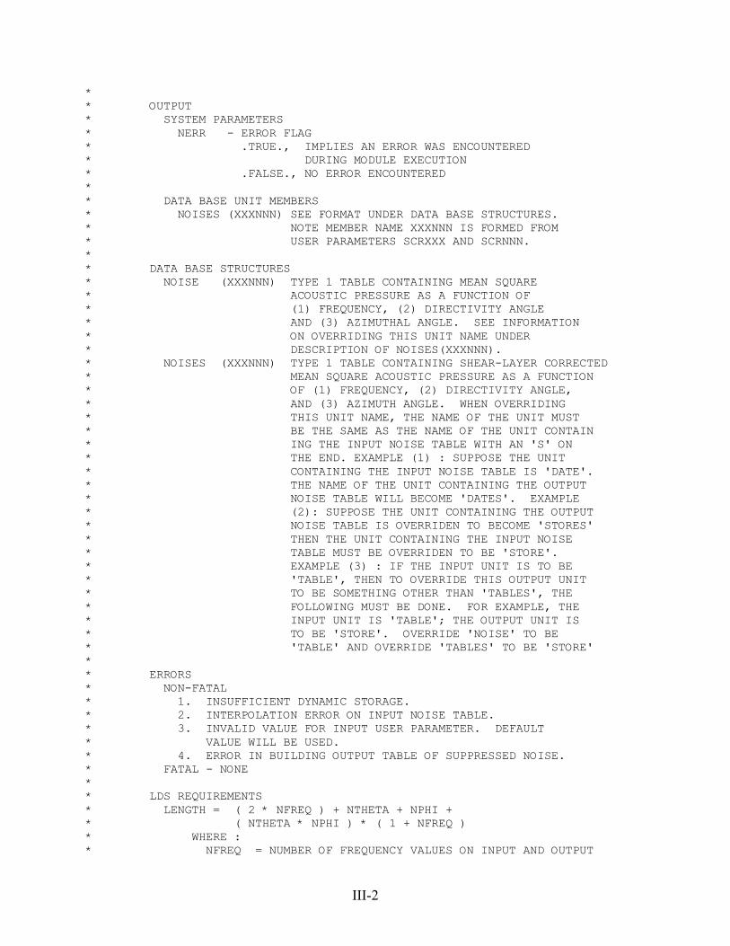
III-2

** OUTPUT* SYSTEM PARAMETERS* NERR - ERROR FLAG* .TRUE., IMPLIES AN ERROR WAS ENCOUNTERED* DURING MODULE EXECUTION* .FALSE., NO ERROR ENCOUNTERED** DATA BASE UNIT MEMBERS* NOISES (XXXNNN) SEE FORMAT UNDER DATA BASE STRUCTURES.* NOTE MEMBER NAME XXXNNN IS FORMED FROM* USER PARAMETERS SCRXXX AND SCRNNN.** DATA BASE STRUCTURES* NOISE (XXXNNN) TYPE 1 TABLE CONTAINING MEAN SQUARE* ACOUSTIC PRESSURE AS A FUNCTION OF* (1) FREQUENCY, (2) DIRECTIVITY ANGLE* AND (3) AZIMUTHAL ANGLE. SEE INFORMATION* ON OVERRIDING THIS UNIT NAME UNDER* DESCRIPTION OF NOISES(XXXNNN).* NOISES (XXXNNN) TYPE 1 TABLE CONTAINING SHEAR-LAYER CORRECTED* MEAN SQUARE ACOUSTIC PRESSURE AS A FUNCTION* OF (1) FREQUENCY, (2) DIRECTIVITY ANGLE,* AND (3) AZIMUTH ANGLE. WHEN OVERRIDING* THIS UNIT NAME, THE NAME OF THE UNIT MUST* BE THE SAME AS THE NAME OF THE UNIT CONTAIN* ING THE INPUT NOISE TABLE WITH AN 'S' ON* THE END. EXAMPLE (1) : SUPPOSE THE UNIT* CONTAINING THE INPUT NOISE TABLE IS 'DATE'.* THE NAME OF THE UNIT CONTAINING THE OUTPUT* NOISE TABLE WILL BECOME 'DATES'. EXAMPLE* (2): SUPPOSE THE UNIT CONTAINING THE OUTPUT* NOISE TABLE IS OVERRIDEN TO BECOME 'STORES'* THEN THE UNIT CONTAINING THE INPUT NOISE* TABLE MUST BE OVERRIDEN TO BE 'STORE'.* EXAMPLE (3) : IF THE INPUT UNIT IS TO BE* 'TABLE', THEN TO OVERRIDE THIS OUTPUT UNIT* TO BE SOMETHING OTHER THAN 'TABLES', THE* FOLLOWING MUST BE DONE. FOR EXAMPLE, THE* INPUT UNIT IS 'TABLE'; THE OUTPUT UNIT IS* TO BE 'STORE'. OVERRIDE 'NOISE' TO BE* 'TABLE' AND OVERRIDE 'TABLES' TO BE 'STORE'** ERRORS* NON-FATAL* 1. INSUFFICIENT DYNAMIC STORAGE.* 2. INTERPOLATION ERROR ON INPUT NOISE TABLE.* 3. INVALID VALUE FOR INPUT USER PARAMETER. DEFAULT* VALUE WILL BE USED.* 4. ERROR IN BUILDING OUTPUT TABLE OF SUPPRESSED NOISE.* FATAL - NONE** LDS REQUIREMENTS* LENGTH = ( 2 * NFREQ ) + NTHETA + NPHI +* ( NTHETA * NPHI ) * ( 1 + NFREQ )* WHERE :* NFREQ = NUMBER OF FREQUENCY VALUES ON INPUT AND OUTPUT

III-3

* NOISE TABLES* NTHETA = NUMBER OF DIRECTIVITY ANGLE VALUES ON INPUT* AND OUTPUT NOISE TABLES* NPHI = NUMBER OF AZIMUTH ANGLE VALUES ON INPUT AND* OUTPUT NOISE TABLES** GDS REQUIREMENTS* SUFFICIENT ALLOCATION FOR THE FOLLOWING TABLES* 1. NOISE (XXXNNN)* 2. NOISES (XXXNNN)****

IV-i

APPENDIX IV

INM CASE SUMMARY OF 1992 BASELINE RESULTS

(4 pages)

IV-1

INM 5.2a ECHO REPORT 09-Mar-01 10:52

STUDY: U:\T24_NEW\ Created : 10-Dec-99 08:13 Units : English Airport : EW1 Description : NASA SET Task 24: System Studies New INM V5.2A Study of 1992 Baseline Bizjet and Configurations 1-5 EPNL and SEL Takeoff and Approach Contours

CASE: CASEORIG Created date: 19-Jan-00 16:15 Description : New Original 1992 Baseline Case

STUDY AIRPORT Lat : 0.000000 deg Long : 0.000000 deg Elev : 0.00 ft Temp : 59.00 F Press : 29.92 in-Hg Wind : 8.00 knt

STUDY RUNWAYS 09 Lat : 0.000000 deg Long : 0.000000 deg X : 0.0000 nmi Y : 0.0000 nmi Elevation: 0.0 ft OtherEnd : 27 Length : 10000 ft Gradient : 0.00% Wind : 8.0 knt TkoThrsh : 0 ft AppThrsh : 0 ft 27 Lat : 0.000000 deg Long : 0.027381 deg X : 1.6458 nmi Y : 0.0000 nmi Elevation: 0.0 ft OtherEnd : 09 Length : 10000 ft Gradient : 0.00% Wind : 8.0 knt TkoThrsh : 0 ft AppThrsh : 0 ft

STUDY TRACKS RwyId-OpType-TrkId Sub PctSub TrkType Delta(ft) 09 -APP-TR2 0 100.00 Vectors 0.0 09 -DEP-TR1 0 100.00 Vectors 0.0

IV-2

STUDY TRACK DETAIL RwyId-OpType-TrkId-SubTrk SegType Param1 Param2(nmi) 09 -APP-TR2 -0 1 Straight 10.0000 nmi 09 -DEP-TR1 -0 1 Straight 20.0000 nmi

STUDY AIRCRAFT BIZJET User-defined Descrip : 1992 Technology Baseline Bizjet (Orig) UserID : GA WgtCat : Small OwnerCat : GenAviation EngType : Jet NoiseCat : 1 Type : Jet NumEng : 1 NoiseId : BIZBAS ATRS : No TkoWgt : 27399 lb LndWgt : 18887 lb LndDist : 3000 ft StaticThr : 3558 lb

STUDY SUBSTITUTION AIRCRAFT

USER-DEFINED NOISE Type Thrust Crv 200 400 630 1000 2000 4000 6300 10000 1600025000 BIZBAS ThrustType:pounds ModelType:INM EPNL 1190.0 N 95.3 91.0 87.8 84.0 77.7 70.7 65.4 59.2 51.141.2 EPNL 2166.0 N 99.6 95.4 92.2 88.6 82.7 75.9 70.8 65.0 57.548.2 EPNL 3558.0 N 106.1 102.0 98.9 95.5 89.7 83.1 77.3 71.7 64.756.2

USER-DEFINED PROFILES OpType Prof Weight(lb) BIZJET APP U1 18887 DEP U1 27398

USER-DEFINED PROFILE POINTS Distance(ft) Altitude(ft) Speed(knt) Thrust Curve BIZJET-APP-U1 1 -286217.1 15000.0 126.0 951.1 lb N 2 -190811.4 10000.0 126.0 949.1 lb N 3 -119916.0 6336.0 126.0 947.1 lb N 4 -30139.0 1631.0 126.0 945.1 lb N 5 0.0 50.0 126.0 943.1 lb N 6 960.0 0.0 126.0 202.2 lb N 7 1500.0 0.0 70.0 200.2 lb N 8 3000.0 0.0 1.0 198.2 lb N BIZJET-DEP-U1 1 0.0 0.0 30.0 3444.7 lb N

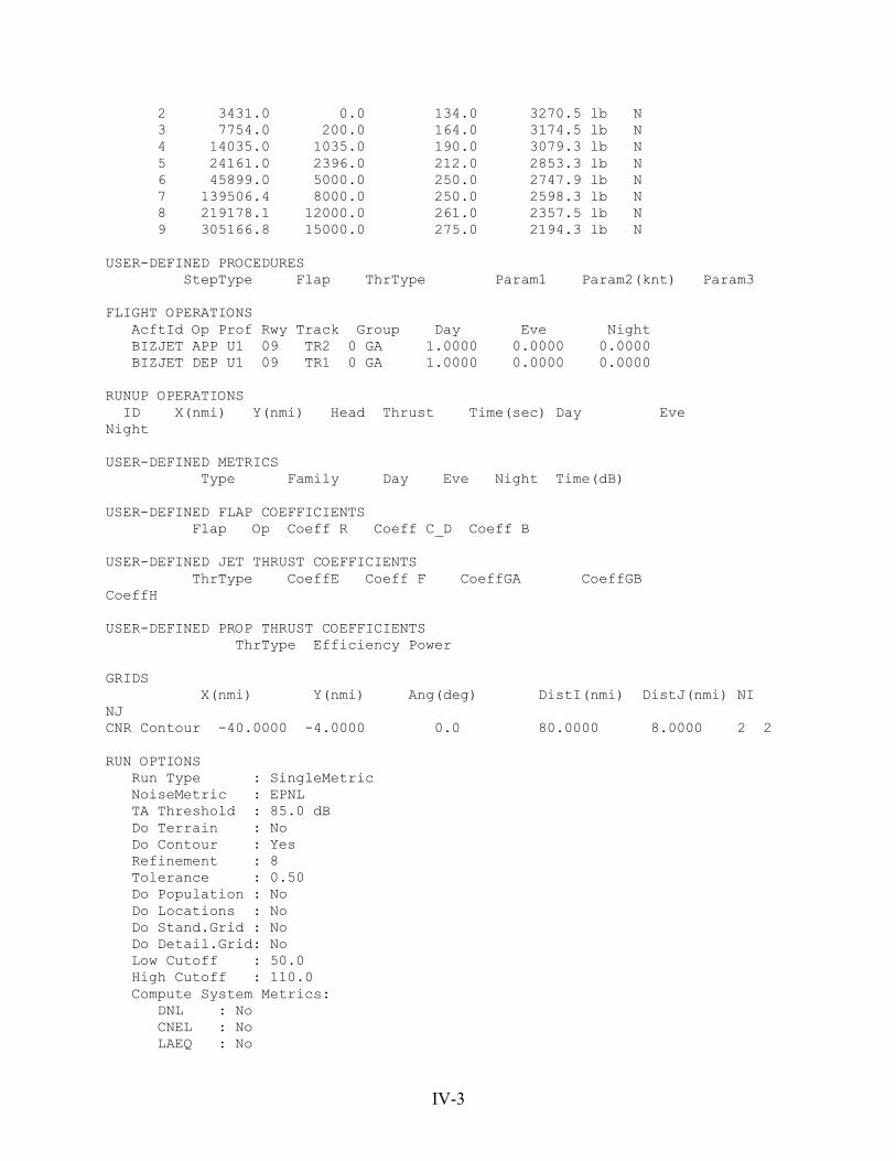
IV-3

2 3431.0 0.0 134.0 3270.5 lb N 3 7754.0 200.0 164.0 3174.5 lb N 4 14035.0 1035.0 190.0 3079.3 lb N 5 24161.0 2396.0 212.0 2853.3 lb N 6 45899.0 5000.0 250.0 2747.9 lb N 7 139506.4 8000.0 250.0 2598.3 lb N 8 219178.1 12000.0 261.0 2357.5 lb N 9 305166.8 15000.0 275.0 2194.3 lb N

USER-DEFINED PROCEDURES StepType Flap ThrType Param1 Param2(knt) Param3

FLIGHT OPERATIONS AcftId Op Prof Rwy Track Group Day Eve Night BIZJET APP U1 09 TR2 0 GA 1.0000 0.0000 0.0000 BIZJET DEP U1 09 TR1 0 GA 1.0000 0.0000 0.0000

RUNUP OPERATIONS ID X(nmi) Y(nmi) Head Thrust Time(sec) Day EveNight

USER-DEFINED METRICS Type Family Day Eve Night Time(dB)

USER-DEFINED FLAP COEFFICIENTS Flap Op Coeff R Coeff C_D Coeff B

USER-DEFINED JET THRUST COEFFICIENTS ThrType CoeffE Coeff F CoeffGA CoeffGBCoeffH

USER-DEFINED PROP THRUST COEFFICIENTS ThrType Efficiency Power

GRIDS X(nmi) Y(nmi) Ang(deg) DistI(nmi) DistJ(nmi) NINJCNR Contour -40.0000 -4.0000 0.0 80.0000 8.0000 2 2

RUN OPTIONS Run Type : SingleMetric NoiseMetric : EPNL TA Threshold : 85.0 dB Do Terrain : No Do Contour : Yes Refinement : 8 Tolerance : 0.50 Do Population : No Do Locations : No Do Stand.Grid : No Do Detail.Grid: No Low Cutoff : 50.0 High Cutoff : 110.0 Compute System Metrics: DNL : No CNEL : No LAEQ : No

IV-4

LAEQD : No LAEQN : No SEL : No LAMAX : No TALA : No NEF : No WECPNL : No EPNL : Yes PNLTM : No TAPNL : No

V-i

APPENDIX V

INM CASE SUMMARY FOR NEW NOISE/ALTITUDE RESULTS

(4 pages)

V-1

INM 5.2a ECHO REPORT 09-Mar-01 11:31

STUDY: U:\T33SHRT\ Created : 10-Dec-99 08:13 Units : English Airport : EW1 Description : NASA SET Task 24: System Studies New INM V5.2A Study of 1992 Baseline Bizjet and Configurations 1-5 EPNL and SEL Takeoff and Approach Contours

CASE: CASEORIG Created date: 19-Jan-00 16:15 Description : New Original 1992 Baseline Case

STUDY AIRPORT Lat : 0.000000 deg Long : 0.000000 deg Elev : 0.00 ft Temp : 59.00 F Press : 29.92 in-Hg Wind : 8.00 knt

STUDY RUNWAYS 09 Lat : 0.000000 deg Long : 0.000000 deg X : 0.0000 nmi Y : 0.0000 nmi Elevation: 0.0 ft OtherEnd : 27 Length : 10000 ft Gradient : 0.00% Wind : 8.0 knt TkoThrsh : 0 ft AppThrsh : 0 ft 27 Lat : 0.000000 deg Long : 0.027381 deg X : 1.6458 nmi Y : 0.0000 nmi Elevation: 0.0 ft OtherEnd : 09 Length : 10000 ft Gradient : 0.00% Wind : 8.0 knt TkoThrsh : 0 ft AppThrsh : 0 ft

STUDY TRACKS RwyId-OpType-TrkId Sub PctSub TrkType Delta(ft) 09 -APP-TR2 0 100.00 Vectors 0.0 09 -DEP-TR1 0 100.00 Vectors 0.0

V-2

STUDY TRACK DETAIL RwyId-OpType-TrkId-SubTrk SegType Param1 Param2(nmi) 09 -APP-TR2 -0 1 Straight 10.0000 nmi 09 -DEP-TR1 -0 1 Straight 20.0000 nmi

STUDY AIRCRAFT BIZJET User-defined Descrip : 1992 Technology Baseline Bizjet (Orig) UserID : GA WgtCat : Small OwnerCat : GenAviation EngType : Jet NoiseCat : 1 Type : Jet NumEng : 1 NoiseId : BIZBAS ATRS : No TkoWgt : 27399 lb LndWgt : 18887 lb LndDist : 3000 ft StaticThr : 3558 lb

STUDY SUBSTITUTION AIRCRAFT

USER-DEFINED NOISE Type Thrust Crv 200 400 630 1000 2000 4000 6300 10000 1600025000 BIZBAS ThrustType:pounds ModelType:INM EPNL 198.0 N 92.4 88.4 85.5 82.3 76.8 70.0 64.9 58.7 50.640.5 EPNL 200.0 N 90.5 86.5 83.6 80.4 74.9 68.1 63.0 56.8 48.738.6 EPNL 202.0 N 90.9 86.8 84.0 80.7 75.0 68.2 63.1 56.8 48.738.5 EPNL 943.0 N 94.0 89.7 86.6 82.9 76.7 69.8 64.5 58.1 50.139.8 EPNL 945.0 N 94.1 89.8 86.7 83.0 76.7 69.8 64.5 58.2 50.140.0 EPNL 947.0 N 94.5 90.4 87.1 83.4 77.0 70.0 64.7 58.4 50.340.4 EPNL 949.0 N 95.0 90.7 87.6 83.8 77.4 70.3 65.0 58.7 50.640.8 EPNL 951.0 N 95.6 91.2 87.9 84.1 77.8 70.7 65.5 59.2 51.241.5 EPNL 2194.0 N 104.6 100.0 96.7 93.3 87.3 80.6 75.2 69.7 62.754.3 EPNL 2358.0 N 104.0 99.4 96.7 93.1 87.2 80.3 74.8 69.2 62.253.6 EPNL 2598.0 N 103.8 100.0 96.6 93.1 87.2 80.3 74.8 69.2 62.253.6 EPNL 2748.0 N 103.9 100.0 96.6 92.9 87.1 80.0 74.3 68.6 61.552.8 EPNL 2853.0 N 103.7 99.8 96.7 93.0 87.2 80.0 74.3 68.6 61.552.8

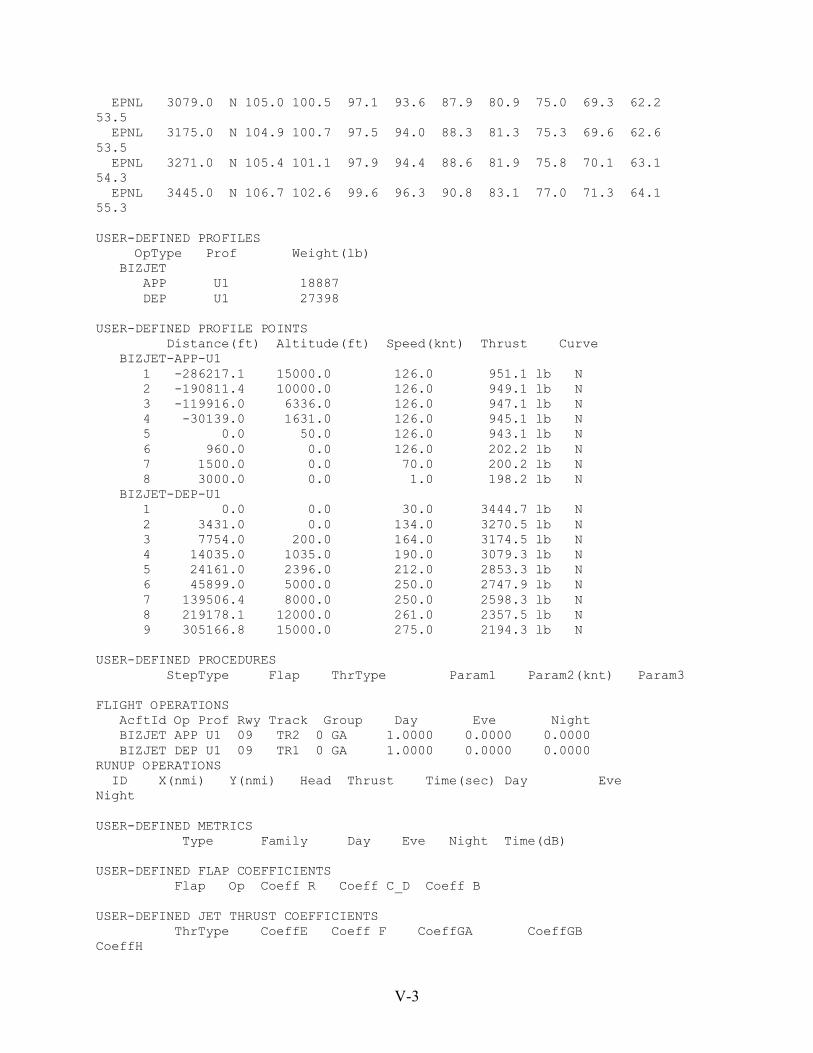
V-3

EPNL 3079.0 N 105.0 100.5 97.1 93.6 87.9 80.9 75.0 69.3 62.253.5 EPNL 3175.0 N 104.9 100.7 97.5 94.0 88.3 81.3 75.3 69.6 62.653.5 EPNL 3271.0 N 105.4 101.1 97.9 94.4 88.6 81.9 75.8 70.1 63.154.3 EPNL 3445.0 N 106.7 102.6 99.6 96.3 90.8 83.1 77.0 71.3 64.155.3

USER-DEFINED PROFILES OpType Prof Weight(lb) BIZJET APP U1 18887 DEP U1 27398

USER-DEFINED PROFILE POINTS Distance(ft) Altitude(ft) Speed(knt) Thrust Curve BIZJET-APP-U1 1 -286217.1 15000.0 126.0 951.1 lb N 2 -190811.4 10000.0 126.0 949.1 lb N 3 -119916.0 6336.0 126.0 947.1 lb N 4 -30139.0 1631.0 126.0 945.1 lb N 5 0.0 50.0 126.0 943.1 lb N 6 960.0 0.0 126.0 202.2 lb N 7 1500.0 0.0 70.0 200.2 lb N 8 3000.0 0.0 1.0 198.2 lb N BIZJET-DEP-U1 1 0.0 0.0 30.0 3444.7 lb N 2 3431.0 0.0 134.0 3270.5 lb N 3 7754.0 200.0 164.0 3174.5 lb N 4 14035.0 1035.0 190.0 3079.3 lb N 5 24161.0 2396.0 212.0 2853.3 lb N 6 45899.0 5000.0 250.0 2747.9 lb N 7 139506.4 8000.0 250.0 2598.3 lb N 8 219178.1 12000.0 261.0 2357.5 lb N 9 305166.8 15000.0 275.0 2194.3 lb N

USER-DEFINED PROCEDURES StepType Flap ThrType Param1 Param2(knt) Param3

FLIGHT OPERATIONS AcftId Op Prof Rwy Track Group Day Eve Night BIZJET APP U1 09 TR2 0 GA 1.0000 0.0000 0.0000 BIZJET DEP U1 09 TR1 0 GA 1.0000 0.0000 0.0000RUNUP OPERATIONS ID X(nmi) Y(nmi) Head Thrust Time(sec) Day EveNight

USER-DEFINED METRICS Type Family Day Eve Night Time(dB)

USER-DEFINED FLAP COEFFICIENTS Flap Op Coeff R Coeff C_D Coeff B

USER-DEFINED JET THRUST COEFFICIENTS ThrType CoeffE Coeff F CoeffGA CoeffGBCoeffH

V-4

USER-DEFINED PROP THRUST COEFFICIENTS ThrType Efficiency Power

GRIDS X(nmi) Y(nmi) Ang(deg) DistI(nmi) DistJ(nmi) NINJCNR Contour -40.0000 -4.0000 0.0 80.0000 8.0000 2 2

RUN OPTIONS Run Type : SingleMetric NoiseMetric : EPNL TA Threshold : 85.0 dB Do Terrain : No Do Contour : Yes Refinement : 8 Tolerance : 0.50 Do Population : No Do Locations : No Do Stand.Grid : No Do Detail.Grid: No Low Cutoff : 50.0 High Cutoff : 110.0 Compute System Metrics: DNL : No CNEL : No LAEQ : No LAEQD : No LAEQN : No SEL : No LAMAX : No TALA : No NEF : No WECPNL : No EPNL : Yes PNLTM : No TAPNL : No

REPORT DOCUMENTATION PAGE Form Approved

Public reporting burden for this collection of information is estimated to average 1 hour per response, including the time for reviewing instructions, searching existing datasources, gathering and maintaining the data needed, and completing and reviewing the collection of information. Send comments regarding this burden estimate or anyother aspect of this collection of information, including suggestions for reducing this burden, to Washington Headquarters Services, Directorate for Information Operationsand Reports, 1215 Jefferson Davis Highway, Suite 1204, Arlington, VA 22202-4302, and to the Office of Management and Budget, Paperwork Reduction Project (0704-0188), Washington, DC 20503.1. AGENCY USE ONLY (Leave blank) 2. REPORT DATE

October 20023. REPORT TYPE AND DATES COVERED

Contractor Report4. TITLE AND SUBTITLE

Small Engine Technology (SET) Task 33 - Final ReportAirframe, Integration, and Community Noise Study

5. FUNDING NUMBERS

NAS3-27483, Task 33

6. AUTHOR(S)

Lys S. Lieber and Daniel Elkins781-20-12-01

7. PERFORMING ORGANIZATION NAME(S) AND ADDRESS(ES)

Honeywell Engines, Sysytems, and Services 111 South 34th Street Phoenix, AZ 85034

8. PERFORMING ORGANIZATIONREPORT NUMBER

9. SPONSORING/MONITORING AGENCY NAME(S) AND ADDRESS(ES)

National Aeronautics and Space AdministrationLangley Research CenterHampton, VA 23681-2199

10. SPONSORING/MONITORINGAGENCY REPORT NUMBER

NASA/CR-2002-211670

11. SUPPLEMENTARY NOTES

Lieber and Elkins, Honeywell Engines and SystemsNASA Technical Monitor: Robert A. Golub

12a. DISTRIBUTION/AVAILABILITY STATEMENT

Unclassified-UnlimitedSubject Category 71 Distribution: NonstandardAvailability: NASA CASI (301) 621-0390

12b. DISTRIBUTION CODE

13. ABSTRACT (Maximum 200 words)

Task Order 33 had four primary objectives as follows: (1) Identify and prioritize the airframe noise reductiontechnologies needed to accomplish the NASA Pillar goals for business and regional aircraft. (2) Develop amodel to estimate the effect of jet shear layer refraction and attenuation of internally generated source noise of aturbofan engine on the aircraft system noise. (3) Determine the effect on community noise of source noisechanges of a generic turbofan engine operating from sea level to 15,000 feet. (4) Support lateral attenuationexperiments conducted by NASA Langley at Wallops Island, VA, by coordinating opportunities for ContractorAircraft to participate as a noise source during the noise measurements. Noise data and noise prediction tools,including airframe noise codes, from the NASA Advanced Subsonic Technology (AST) program were appliedto assess the current status of noise reduction technologies relative to the NASA pillar goals for regional andsmall business jet aircraft. In addition, the noise prediction tools were applied to evaluate the effectiveness ofairframe-related noise reduction concepts developed in the AST program on reducing the aircraft system noise.The AST noise data and acoustic prediction tools used in this study were furnished by NASA.

14. SUBJECT TERMS

Airframe Noise, Engine Noise, Noise reduction, Final report, Jet Shear Layer,15. NUMBER OF PAGES

120Noise Prediction code, lateral Attenuation, Aircraft Systems Noise 16. PRICE CODE

17. SECURITY CLASSIFICATION

OF REPORT

Unclassified

18. SECURITY CLASSIFICATIONOF THIS PAGE

Unclassified

19. SECURITY CLASSIFICATION OF ABSTRACT

Unclassified

20. LIMITATION OF ABSTRACT

UL

NSN 7540-01-280-5500 Standard Form 298 (Rev. 2-89)Prescribed by ANSI Std. Z-39-18298-102