Slosh Characteristics of Aggregated Intermediate Bulk Containers on Single-Unit

Trucks

August 2016

FOREWORD The Federal Motor Carrier Safety Administration (FMCSA) revised the definition of “tank vehicle” in 2011 to include any commercial vehicle transporting tanks (such as intermediate bulk containers, or IBCs) of liquids or gases with an aggregate capacity of 1,000 gallons or more. The revision of the definition of “tank vehicle” requires that a person driving a commercial vehicle carrying an aggregate of 1,000 gallons or more in IBCs must hold a commercial driver’s license (CDL) with a tank vehicle (N) endorsement. For more than 5 years, drivers transporting IBCs with an aggregate capacity of 1,000 gallons or more have been required to have a tank vehicle (N) endorsement on their CDL.

This project, which produced technical information to be considered in deciding whether to amend the rule, included engineering modeling and testing to ascertain whether the slosh characteristics of IBCs aggregated to 1,000 gallons or more are similar to a single cargo tank of the same capacity. Liquid sloshing generally refers to the transient movement of liquid within a confined space. Slosh, like any load shift, can make a motor vehicle more difficult to control. Slosh can be in the fore-aft direction (i.e., front-to-back), from braking or accelerating, or in the lateral direction (i.e., side-to-side), from cornering or turning.

NOTICE This document is disseminated under the sponsorship of the U.S. Department of Transportation (USDOT) in the interest of information exchange. The U.S. Government assumes no liability for the use of the information contained in this document. The contents of this report reflect the views of the contractor, who is responsible for the accuracy of the data presented herein. The contents do not necessarily reflect the official policy of the USDOT. This report does not constitute a standard, specification, or regulation.

The U.S. Government does not endorse products or manufacturers named herein. Trademarks or manufacturers’ names appear in this report only because they are considered essential to the objective of this report.

QUALITY ASSURANCE STATEMENT The Federal Motor Carrier Safety Administration (FMCSA) provides high-quality information to serve Government, industry, and the public in a manner that promotes public understanding. Standards and policies are used to ensure and maximize the quality, objectivity, utility, and integrity of its information. FMCSA periodically reviews quality issues and adjusts its programs and processes to ensure continuous quality improvement.

Technical Report Documentation Page 1. Report No. FMCSA-RRT-16-006

2. Government Accession No.

3. Recipient's Catalog No.

4. Title and Subtitle Slosh Characteristics of Aggregated Intermediate Bulk Containers on Single-Unit Trucks

5. Report Date August 2016

6. Performing Organization Code 100056090

7. Author(s) Pape, Doug; Thornton, Ben; Yugulis, Kevin

8. Performing Organization Report No.

9. Performing Organization Name and Address Battelle Memorial Institute 505 King Ave. Columbus, OH 43201

10. Work Unit No. (TRAIS) 11. Contract or Grant No. DTMC75-14-D-00008

12. Sponsoring Agency Name and Address U.S. Department of Transportation Federal Motor Carrier Safety Administration Office of Analysis, Research, and Technology 1200 New Jersey Ave. SE Washington, DC 20590

13. Type of Report and Period Covered Final Report, October 2014–March 2016

14. Sponsoring Agency Code FMCSA

15. Supplementary Notes Contracting Officer’s Representative: Quon Kwan

16. Abstract Drivers of cargo tank trucks need special knowledge of vehicle and load dynamics, including slosh, to handle their vehicles safely. This knowledge is reflected by a tank vehicle (N) endorsement to the commercial driver’s license (CDL). Drivers of vehicles that carry intermediate bulk containers (IBCs) aggregating to 1,000 gallons capacity or more must hold an N endorsement, according to current regulations. The Federal Motor Carrier Safety Administration (FMCSA) requires technical information to help determine whether to modify this requirement. This research used simulations and experiments to identify the conditions and extent to which a commercial motor vehicle (CMV) with IBCs behaves differently from a conventional cargo tank truck of similar capacity and load. The simulations modeled the slosh of liquid loads in a single cargo tank and several combinations of IBCs. The slosh was simulated both by computational fluid dynamics (CFD) and by a simplified pendulum model that could be integrated with a commercially available model of a single-unit truck. Quantitative performance metrics showed that the effect of slosh in the IBCs was less than the effect of slosh in the 1,100-gallon tank in nearly all cases. Only in extreme cases were the slosh forces in the IBCs more than a few percent greater than the forces produced by an equivalent rigid, solid load. In the experimental portion of the research, professional tank drivers drove trucks carrying IBCs similar to those simulated. The drivers reported that, in the extreme maneuvers, they sensed the slosh slightly more than they would in a similar truck with dry freight.

17. Key Words Intermediate bulk container, IBC, slosh, CDL.

18. Distribution Statement No restrictions

19. Security Classif. (of this report) Unclassified

20. Security Classif. (of this page) Unclassified

21. No. of Pages 116

22. Price

Form DOT F 1700.7 (8-72) Reproduction of completed page authorized.

ii

SI* (MODERN METRIC) CONVERSION FACTORS Approximate Conversions to SI Units

Symbol When You Know Multiply By To Find Symbol Length

in inches 25.4 millimeters mm ft feet 0.305 meters m yd yards 0.914 meters m mi miles 1.61 kilometers km

Area in² square inches 645.2 square millimeters mm² ft² square feet 0.093 square meters m² yd² square yards 0.836 square meters m² ac Acres 0.405 hectares ha mi² square miles 2.59 square kilometers km²

Volume (volumes greater than 1,000L shall be shown in m³) fl oz fluid ounces 29.57 milliliters mL gal gallons 3.785 liters L ft³ cubic feet 0.028 cubic meters m³ yd³ cubic yards 0.765 cubic meters m³

Mass oz ounces 28.35 grams g lb pounds 0.454 kilograms kg T short tons (2,000 lb) 0.907 megagrams (or “metric ton”) Mg (or “t”)

Temperature (exact degrees) °F Fahrenheit 5(F-32)/9 or (F-32)/1.8 Celsius °C

Illumination fc foot-candles 10.76 lux lx fl foot-Lamberts 3.426 candela/m² cd/m²

Force and Pressure or Stress lbf poundforce 4.45 newtons N lbf/in² poundforce per square inch 6.89 kilopascals kPa

Approximate Conversions from SI Units Symbol When You Know Multiply By To Find Symbol

Length mm millimeters 0.039 inches in m meters 3.28 feet ft m meters 1.09 yards yd km kilometers 0.621 miles mi

Area mm² square millimeters 0.0016 square inches in² m² square meters 10.764 square feet ft² m² square meters 1.195 square yards yd² Ha hectares 2.47 acres ac km² square kilometers 0.386 square miles mi²

Volume mL milliliters 0.034 fluid ounces fl oz L liters 0.264 gallons gal m³ cubic meters 35.314 cubic feet ft³ m³ cubic meters 1.307 cubic yards yd³

Mass g grams 0.035 ounces oz kg kilograms 2.202 pounds lb Mg (or “t”) megagrams (or “metric ton”) 1.103 short tons (2,000 lb) T

Temperature (exact degrees) °C Celsius 1.8c+32 Fahrenheit °F

Illumination lx lux 0.0929 foot-candles fc cd/m² candela/m² 0.2919 foot-Lamberts fl

Force and Pressure or Stress N newtons 0.225 poundforce lbf kPa kilopascals 0.145 poundforce per square inch lbf/in²

* SI is the symbol for the International System of Units. Appropriate rounding should be made to comply with Section 4 of ASTM E380. (Revised March 2003, Section 508-accessible version September 2009.)

iii

TABLE OF CONTENTS

EXECUTIVE SUMMARY ......................................................................................................... xi

1. INTRODUCTION.................................................................................................................1

1.1 BACKGROUND ...........................................................................................................1

1.2 HOW INTERMEDIATE BULK CONTAINERS ARE USED IN COMMERCE .......2

1.3 OVERVIEW OF THE RESEARCH .............................................................................3 1.3.1 Literature Review.............................................................................................. 4 1.3.2 Experimental Work ........................................................................................... 4 1.3.3 Independent Review.......................................................................................... 5

2. APPROACH ..........................................................................................................................7

2.1 CHARACTERIZING SLOSH: SIMULATION AND EXPERIMENTS......................7

2.2 EQUIPMENT: CONTAINERS AND VEHICLES .......................................................8

2.3 MANEUVERS .............................................................................................................13 2.3.1 Stop at a Red Light ......................................................................................... 15 2.3.2 Sudden Deceleration in Traffic ....................................................................... 15 2.3.3 Curve on an Exit Ramp ................................................................................... 15 2.3.4 Lane Change ................................................................................................... 17

3. SIMULATIONS ..................................................................................................................19

3.1 TRUCK MODEL .........................................................................................................19

3.2 SIMPLIFIED PENDULUM MODEL .........................................................................20

3.3 COMPUTATIONAL FLUID DYNAMICS MODELS ..............................................22

3.4 PERFORMANCE METRICS ......................................................................................23

3.5 RESULTS ....................................................................................................................24 3.5.1 Stop at a Red Light ......................................................................................... 25 3.5.2 Curve on an Exit Ramp ................................................................................... 28 3.5.3 Lane Change ................................................................................................... 30 3.5.4 Lane Change with Large-Footprint Containers .............................................. 34

4. EXPERIMENTS .................................................................................................................39

4.1 CONDITIONS AND EQUIPMENT ...........................................................................40

4.2 MANEUVERS .............................................................................................................42 4.2.1 Stop at a Red Light ......................................................................................... 43 4.2.2 Sudden Deceleration ....................................................................................... 44 4.2.3 Curve on an Exit Ramp ................................................................................... 44

iv

4.2.4 Lane Change ................................................................................................... 45

4.3 DRIVERS ....................................................................................................................46

4.4 QUESTIONNAIRE .....................................................................................................47

4.5 RESULTS ....................................................................................................................48 4.5.1 Stop at a Red Light and Sudden Deceleration ................................................ 48 4.5.2 Curve on an Exit Ramp ................................................................................... 49 4.5.3 Lane Change ................................................................................................... 49

4.6 DISCUSSION ..............................................................................................................50

5. CONCLUSIONS .................................................................................................................53

6. FURTHER WORK .............................................................................................................55

v

LIST OF FIGURES (AND FORMULAS) Figure 1. Graph. Lateral force exerted by liquid slosh on a vehicle during a typical lane change.

A single 1,100-gallon cargo tank is shown for reference. Two sets of IBCs, both of 1,100 gallon aggregate capacity, are shown in solid blue. The effect of slosh in IBCs of aggregate capacity of 1,100 gallons was less than the effect of slosh in a single 1,100-gallon tank. .................................................................................................................... xii

Figure 2. Photo. IBCs come in many kinds of construction. The most common is the poly in a steel frame, as shown in the foreground. IBCs of stainless steel are in the background at the left. These three sizes all have a footprint of 40 x 48 in., the same as a standard wooden pallet. ..................................................................................................................3

Figure 3. Photo. The two 550-gallon IBCs were mounted at the rear of the truck. (The strap that held them in place during the tests is not shown in this photo.) ....................................10

Figure 4. Photo. Two of four 275-gallon IBCs were visible in the rear of the truck; the other two were at the front of the truck. The truck had just completed a lane change maneuver. .11

Figure 5. Sketch. The 1,100-gallon single-bore cargo tank was positioned at the center of the truck bed for the models. ................................................................................................11

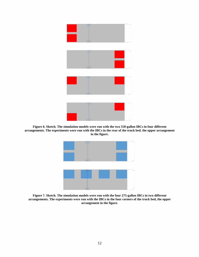
Figure 6. Sketch. The simulation models were run with the two 550-gallon IBCs in four different arrangements. The experiments were run with the IBCs in the rear of the truck bed, the upper arrangement in the figure. ....................................................................................12

Figure 7. Sketch. The simulation models were run with the four 275-gallon IBCs in two different arrangements. The experiments were run with the IBCs in the four corners of the truck bed, the upper arrangement in the figure. .......................................................................12

Figure 8. Sketch. The simulations were run with two arrangements of mixed sizes of IBCs. The 550-gallon IBC (red) was always in the left rear of the truck bed. The two 275-gallon IBCs (blue) were on the left side with the 550-gallon IBC or both in the front of the truck bed. ........................................................................................................................13

Figure 9. Sketch. The static position of the liquid is level (left). The liquid rises up the side of the tank on the outside of a curve in a steady-state sloshing condition (right). ...................16

Figure 10. Screenshot. The simulated paths were a spiral into a constant curvature on level ground. ............................................................................................................................17

Figure 11. Graph. The single lane change was planned to simulate side-to-side sloshing. ...........18 Figure 12. Photo. The cones were arranged to direct the driver to make a 12-foot lane change

over a distance of 171 feet. The four cones for the entry gate are in the foreground. The set of cones for the exit gate is by the sport utility vehicle. ...........................................18

Figure 13. Screenshot. One frame of a TruckSim animation. .......................................................20 Figure 14. Sketch. Illustration of the pendulum method for modeling slosh in a rectangular

container. ........................................................................................................................21 Figure 15. Graphs. The force of the sloshing water against an IBC was simulated for a lane

change at 40 mi/h. The force (left) and roll moment (right) were simulated for a 275-gallon IBC. The force and moment about the bottom center of the tank predicted by the pendulum (blue lines) match the force and moment predicted by CFD (green line). ....22

vi

Figure 16. Screenshot. Visualization of transient simulation showing water interface of 1,100-gallon tank at four instants during a simulated stop at a red light (35 mi/h to stopped in 150 feet). .........................................................................................................................23

Figure 17. Equation. Load transfer ratio. .......................................................................................24 Figure 18. Graph. Force exerted on the truck by the two 550-gallon IBCs during a brake to stop

(from 35 mi/h in 100 feet). .............................................................................................25 Figure 19. Graph. Force exerted on the truck by a single 1,100-gallon tank during a brake to stop

(from 35 mi/h in 100 feet). .............................................................................................26 Figure 20. Graph. Stopping distances calculated by the simulations, in feet. ...............................27 Figure 21. Graph. Amplitudes of oscillating slosh force while braking to a stop (from 35 mi/h in

100 feet). .........................................................................................................................27 Figure 22. Graph. Lateral force exerted by the loads against the truck navigating a 575-foot-

radius curve at 55 mi/h. In this configuration, the truck is carrying four 275-gallon IBCs, all on the left side of the bed. ...............................................................................28

Figure 23. Graph. Lateral load transfer ratio of a truck navigating a 575-foot-radius curve at 55 mi/h. In this configuration, the truck is carrying four 275-gallon IBCs, all on the left side of the bed. ...............................................................................................................29

Figure 24. Graph. Peak lateral forces exerted by the loads against the truck entering a 575-foot-radius curve at 55 mi/h. ..................................................................................................30

Figure 25. Graph. Steady state lateral load transfer ratio for a rigid load in a 575-foot-radius curve at 55 mi/h, and showing the increase when the load is a liquid free to slosh. ......30

Figure 26. Graph. The force applied by the liquid was comparable to that applied by the rigid load as the truck with two 550-gallon IBCs was simulated through a 12-foot lane change at 45 mi/h. ..........................................................................................................31

Figure 27. Graph. The force applied by the liquid was slightly higher than that applied by the rigid load as the truck with four 275-gallon IBCs was simulated through a 12-foot lane change at 45 mi/h. ..........................................................................................................32

Figure 28. Graph. The force applied by the liquid was significantly higher than that applied by the rigid load as the single 1,100-gallon tank was subjected to a 12-foot lane change at 45 mi/h. ...........................................................................................................................32

Figure 29. Graph. The lateral load transfer ratios for the truck with two 550-gallon IBCs were simulated through a 12-foot lane change at 45 mi/h. .....................................................33

Figure 30. Graph. The lateral load transfer ratios for the truck with four 275-gallon IBCs were simulated through a 12-foot lane change at 45 mi/h. .....................................................33

Figure 31. Graph. Peak lateral forces exerted by the loads against the truck during the 12-foot lane change at 45 mi/h. ...................................................................................................34

Figure 32. Graph. Peak in the lateral load transfer ratio during the 12-foot lane change at 45 mi/h.34 Figure 33. Photo. The 550-gallon cylindrical IBC is lower and wider than those in common use.35 Figure 34. Sketch. 793-gallon container combined with a 275-gallon container (top); 550-gallon

containers oriented longitudinally (middle) and laterally (bottom). ..............................35 Figure 35. Graph. Peak lateral forces exerted by loads against the truck during the 12-foot lane

change at 45 mi/h. ..........................................................................................................36 Figure 36. Graph. The lateral load transfer ratios for the truck with two laterally oriented 550-

gallon IBCs were simulated through a 12-foot lane change at 45 mi/h. ........................37

vii

Figure 37. Scanned image. Example of a checklist table filled out by drivers during the experiments. ...................................................................................................................40

Figure 38. Photo. The IBCs were mounted two similar van trucks (as pictured here). .................41 Figure 39. Sketch. The stop, deceleration, and lane change maneuvers were conducted on the

skid pad at TRC Inc. .......................................................................................................42 Figure 40. Sketch. Freeway ramp curves were represented by the vehicle dynamics area at TRC

Inc. ..................................................................................................................................43 Figure 41. Sketch. The cone layout for the full lane change. ........................................................45 Figure 42. Sketch. The cone layout for the tighter lane change. ...................................................46 Figure 43. Sketch. Indecision zone boundaries on a typical intersection approach. .....................51 Figure 44. Sketch. Five-step literature review approach. ..............................................................58 Figure 45. Sketch. The location of liquid in a tank under the static condition (left) and a steady-

state sloshing condition (right). ......................................................................................61 Figure 46. Plot. Results from simulation of sloshing dynamics. Interface between water and air is

shown in blue. ................................................................................................................62 Figure 47. Photo. A single-bore cargo tank on a straight truck. ....................................................63 Figure 48. Photo. In 2012, group of researchers found that liquid in cubical containers behaved

similarly to an equivalent volume of liquid in cylindrical containers. ...........................64 Figure 49. Sketch. Adams model of a 15-ton military truck used in Elliott et al., 2005. ..............70 Figure 50. Plot. Time history of the roll moment of the liquid cargo sloshing within the 50

percent volume-filled tank under ay = 0.3 g, together with the quasi-static roll moment.72 Figure 51. Sketch. Co-Simulation Methodology. ..........................................................................75 Figure 52. Sketch. Indecision zone boundaries on a typical intersection approach ......................77 Figure 53. Graph. Distance to the beginning and end of the indecision zone. ..............................78 Figure 54. Sketch. Pendulum model used to simulate sloshing in a rectangular tank. ..................80 Figure 55. Equations for pendulum model parameters. .................................................................80 Figure 56. Sketch. Degrees of freedom of a pendulum, Ѱ and ϴ. .................................................82 Figure 57. Differential equations of motion of a spherical pendulum. ..........................................82 Figure 58. Equation. Reaction force due to the pendulum. ...........................................................82 Figure 59. Equation. Reaction moment about the bottom center of the container due to the

pendulum. .......................................................................................................................82 Figure 60. Equation. Reaction force due to the stationary mass. ...................................................83 Figure 61. Equation. Reaction moment about the bottom center of the container due to the

stationary mass. ..............................................................................................................83 Figure 62. Equation. Combined reaction moment of pendulum and stationary mass. ..................83 Figure 63. Equation. Combined reaction force of pendulum and stationary mass. .......................83 Figure 64. Graphs. Reaction forces (left) and moments summed at the bottom of the container

(right) generated by the pendulum model (solid lines) and the CFD model (dashed lines) of a 275-gallon IBC while braking to a stop from 55 mi/h in 140 feet. ...............84

Figure 65. Graphs. Reaction forces (left) and moments (right) generated by the pendulum model (solid lines) and the CFD model (dashed lines) of a 275-gallon IBC while on a 575-foot radius exit ramp at 55 mi/h with a lateral acceleration of 0.35 gravitational units. .......84

viii

Figure 66. Graphs. Reaction forces (left) and moments (right) generated by the pendulum model (solid lines) and the CFD model (dashed lines) of a 275-gallon IBC while performing a 12-foot lane change at 55 mi/h with a lateral acceleration of 0.5 gravitational units. ...84

Figure 67. Graphs. Reaction forces (left) and moments summed at the bottom of the container (right) generated by the pendulum model (solid lines) and the CFD model (dashed lines) of a 550-gallon IBC while braking to a stop from 55 mi/h in 140 feet. ...............85

Figure 68. Graphs. Reaction forces (left) and moments (right) generated by the pendulum model (solid lines) and the CFD model (dashed lines) of a 550-gallon IBC while on a 575-foot radius exit ramp at 55 mi/h with a lateral acceleration of 0.35 gravitational units. .......85

Figure 69. Graphs. Reaction forces (left) and moments (right) generated by the pendulum model (solid lines) and the CFD model (dashed lines) of a 550-gallon IBC while performing a 12-foot lane change at 55 mi/h with a lateral acceleration of 0.5 gravitational units. ...85

Figure 70. Graph. Sample acceleration profile used in a lane change maneuver. .........................88 Figure 71. Graph. Forces predicted by the CFD model in the lateral (side-to-side) direction for a

275-gallon IBC during a lane change maneuver. ...........................................................89 Figure 72. Screenshot. The water-air interface with the baseline (left) and fine (right) mesh of the

1,100-gallon cylindrical cargo tank in stop maneuver. ..................................................89 Figure 73. Graph. The forces predicted by the baseline and fine mesh in the simulation of the

1,100-gallon cargo tank in a stop at a red light are quite similar; therefore, the baseline mesh can be accepted. ....................................................................................................90

ix

LIST OF TABLES Table 1. The test matrix provided for four tank configurations, three maneuvers, and two load

conditions. ........................................................................................................................7 Table 2. Four configurations of tanks used in simulations and experiments. ..................................9 Table 3. This project had four basic maneuvers. ...........................................................................14 Table 4. Roads of three curvatures were built for the simulations; all three were simulated at

three speeds. ...................................................................................................................16 Table 5. Conditions for the lane change maneuver. .......................................................................18 Table 6. Specifications of the two trucks. ......................................................................................42 Table 7. For the stopping maneuver, the project staff in the cab with the test driver carried this

checklist for instructions/recording immediate observations. ........................................43 Table 8. For the deceleration maneuver, the project staff in the cab with the test driver carried

this checklist for instructions and recording immediate observations. ..........................44 Table 9. For the exit ramp maneuver, the project staff in the cab with the test driver carried this

checklist for instructions/recording immediate observations. ........................................45 Table 10. For the lane change maneuver, the project staff in the cab with the test driver carried

this checklist for instructions and recording immediate observations ...........................46 Table 11. The drivers reported whether they felt the slosh in every maneuver, using a scale of 1–

10. ...................................................................................................................................49 Table 12. Literature matrix. ...........................................................................................................65 Table 13. Codes for stop at a red light. ..........................................................................................92 Table 14. Codes for curve on an exit ramp. ...................................................................................92 Table 15. Codes for lane change. ...................................................................................................92 Table 16. Stopping distance (ft). ....................................................................................................93 Table 17. Slosh amplitude (lb). ......................................................................................................93 Table 18. Peak slosh force. ............................................................................................................94 Table 19. Steady-state load transfer ratio. .....................................................................................94 Table 20. Peak lateral slosh force (lb). ..........................................................................................95 Table 21. Peak load transfer ratio. .................................................................................................95 Table 22. Peak yaw moment (1,000 ft-lb, or ft-kip). .....................................................................96 Table 23. Specifications of the two trucks. ....................................................................................97

x

ABBREVIATIONS, ACRONYMS, AND SYMBOLS

Acronym Definition

AASHTO American Association of State Highway and Transportation Officials

CDL commercial driver’s license

CFD computational fluid dynamics

CFR Code of Federal Regulations

CMV commercial motor vehicle

FMCSA Federal Motor Carrier Safety Administration

FMCSR Federal Motor Carrier Safety Regulations

FMVSS Federal Motor Vehicle Safety Standard

FR Federal Register

IBC intermediate bulk container

GPS global positioning system

Hz Hertz

IRB Institutional Review Board

ISO International Organization for Standardization

LTL less-than-truckload

mi/h miles per hour

TRC Inc. Transportation Research Center Inc.

USDOT U.S. Department of Transportation

xi

EXECUTIVE SUMMARY The Federal Motor Carrier Safety Administration (FMCSA) revised the definition of “tank vehicle” in 2011 to include any commercial vehicle transporting tanks (such as intermediate bulk containers, or IBCs) of liquids or gases with an aggregate capacity of 1,000 gallons or more. The revision of the definition of “tank vehicle” requires that a person driving a commercial vehicle carrying an aggregate of 1,000 gallons or more in IBCs must hold a commercial driver’s license (CDL) with a tank vehicle (N) endorsement. For more than 5 years, drivers transporting IBCs with an aggregate capacity of 1,000 gallons or more have been required to have a tank vehicle (N) endorsement on their CDL.

This project, which produced technical information to be considered in deciding whether to amend the rule, included engineering modeling and testing to ascertain whether the slosh characteristics of IBCs aggregated to 1,000 gallons or more are similar to a single cargo tank of the same capacity. Liquid sloshing generally refers to the transient movement of liquid within a confined space. Slosh, like any load shift, can make a motor vehicle more difficult to control. Slosh can be in the fore-aft direction (i.e., front-to-back), from braking or accelerating, or in the lateral direction (i.e., side-to-side), from cornering or turning.

The engineering modeling consisted of simulations of several IBC configurations, and variations on three maneuvers, to produce slosh. The liquid slosh was simulated by both computational fluid dynamics (CFD) and by a simplified pendulum model that could be integrated with a commercially available model of a single-unit truck.

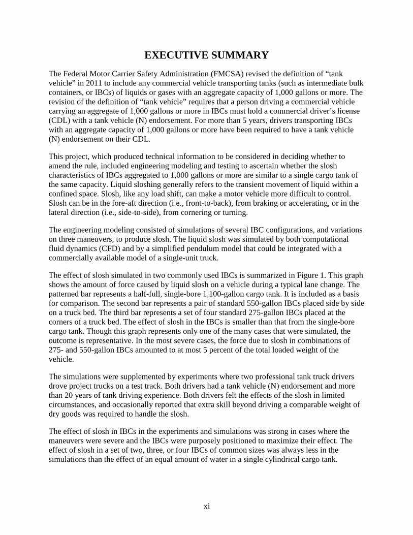
The effect of slosh simulated in two commonly used IBCs is summarized in Figure 1. This graph shows the amount of force caused by liquid slosh on a vehicle during a typical lane change. The patterned bar represents a half-full, single-bore 1,100-gallon cargo tank. It is included as a basis for comparison. The second bar represents a pair of standard 550-gallon IBCs placed side by side on a truck bed. The third bar represents a set of four standard 275-gallon IBCs placed at the corners of a truck bed. The effect of slosh in the IBCs is smaller than that from the single-bore cargo tank. Though this graph represents only one of the many cases that were simulated, the outcome is representative. In the most severe cases, the force due to slosh in combinations of 275- and 550-gallon IBCs amounted to at most 5 percent of the total loaded weight of the vehicle.

The simulations were supplemented by experiments where two professional tank truck drivers drove project trucks on a test track. Both drivers had a tank vehicle (N) endorsement and more than 20 years of tank driving experience. Both drivers felt the effects of the slosh in limited circumstances, and occasionally reported that extra skill beyond driving a comparable weight of dry goods was required to handle the slosh.

The effect of slosh in IBCs in the experiments and simulations was strong in cases where the maneuvers were severe and the IBCs were purposely positioned to maximize their effect. The effect of slosh in a set of two, three, or four IBCs of common sizes was always less in the simulations than the effect of an equal amount of water in a single cylindrical cargo tank.

xii

Figure 1. Graph. Lateral force exerted by liquid slosh on a vehicle during a typical lane change. A single

1,100-gallon cargo tank is shown for reference. Two sets of IBCs, both of 1,100 gallon aggregate capacity, are shown in solid blue. The effect of slosh in IBCs of aggregate capacity of 1,100 gallons was less than the effect

of slosh in a single 1,100-gallon tank.

1

1. INTRODUCTION This document records the research (simulations and experiments) conducted to determine the slosh characteristics of aggregated intermediate bulk containers (IBCs) on single-unit trucks. Liquid sloshing generally refers to the transient movement of liquid within a confined space. Slosh, like any load shift, can make a motor vehicle more difficult to control. Slosh can be in the fore-aft direction (i.e., front-to-back), from braking or accelerating, or in the lateral direction (i.e., side-to-side), from cornering or turning.

Federal regulations require that drivers of cargo tank trucks hold a commercial driver’s license (CDL) with a tank vehicle (N) endorsement. The definition of “tank vehicle” in current regulations requires that a person driving a commercial vehicle carrying an aggregate of 1,000 gallons or more in IBCs must hold a CDL with a tank vehicle (N) endorsement. IBCs are often used for transporting smaller amounts liquids or gases. They can be made of plastic, steel, or other materials, and usually hold between 119 and 793 gallons.

Because simulations are less expensive than equivalent experiments and their conditions are easier to control, a larger set of simulations in various IBC combinations was carried out. Experiments with professional tank drivers in a truck carrying IBCs supplemented the findings of the simulations.

1.1 BACKGROUND

Liquid loads behave differently from dry freight. The load can move in response to the motion of the motor vehicle. Sloshing is most pronounced when a cargo tank is partly full, but even a tank at capacity is not “shell full” because headspace needs to be left for thermal expansion. The interaction of the liquid load and the vehicle dynamics must be appreciated by drivers if they are to handle a liquid load safely. Therefore, the Federal Motor Carrier Safety Regulations (FMCSRs) require special knowledge for a tank vehicle (N) endorsement, as described below:

49 Code of Federal Regulations (CFR) 383.119 – Requirements for tank vehicle endorsement.

In order to obtain a tank vehicle endorsement, each applicant must have knowledge covering the following:

a) Causes, prevention, and effects of cargo surge on motor vehicle handling.

b) Proper braking procedures for the motor vehicle when it is empty, full, and partially full.

c) Differences in handling of baffled/compartmented tank interiors versus non-baffled motor vehicles.

d) Differences in tank vehicle type and construction.

e) Differences in cargo surge for liquids of varying product densities.

2

f) Effects of road grade and curvature on motor vehicle handling with filled, half-filled, and empty tanks.

g) Proper use of emergency systems.

h) For drivers of DOT specification tank vehicles, retest and marking requirements.

i) Operating practices and procedures not otherwise specified.(1)

The need for this research stems from the definition of a “tank vehicle” in the current regulations:

Tank vehicle means any commercial motor vehicle that is designed to transport any liquid or gaseous materials within a tank or tanks having an individual rated capacity of more than 119 gallons and an aggregate rated capacity of 1,000 gallons or more that is either permanently or temporarily attached to the vehicle or the chassis.(2)

This is the definition requiring that a person driving a commercial vehicle carrying an aggregate capacity of 1,000 gallons or more of liquids or gases in IBCs must hold a CDL with a tank vehicle (N) endorsement.

The current regulations define an IBC as:

…a rigid or flexible portable packaging, other than a cylinder or portable tank, which is designed for mechanical handling.(3)

Regulations specify a number of different types of IBCs. Most have a capacity between 119 and 793 gallons.(4)

1.2 HOW INTERMEDIATE BULK CONTAINERS ARE USED IN COMMERCE

IBCs (or totes as they are nicknamed in industry) are used to transport small and moderate quantities of liquid or gas. They are smaller than true bulk shipments that would fill an entire cargo tank, and they are larger than 55-gallon drums or buckets. IBCs are defined in the hazardous materials code, but they are often used to haul liquids that are not regulated as hazardous. Figure 2 shows two sizes of poly containers (250-gallon and 330-gallon) and one size of stainless steel container (550-gallon).

IBCs are commonly shipped by flatbed, van truck, and intermodal container. A 53-foot trailer will typically reach its allowable gross weight with 18–20 IBCs, depending on the density of the product. That is not enough to fill the floor of the trailer, so proper securement is important to prevent the IBCs from shifting. When the IBCs are on a flatbed, they should be secured with conventional straps, usually one strap per row of IBCs across the bed. IBCs are often double stacked, especially in a 20-foot intermodal container, which can usually be filled with IBCs.

3

Although products in IBCs are occasionally shipped through less-than-truckload (LTL) common carriers, they are commonly shipped together as part of a dedicated truck.

Chemical plants receiving liquid products in IBCs typically order an IBC in the size that corresponds to one batch. If the amount of product needed does not correspond to an integer number of IBCs, then common practice for the shipper is to fill all but one of the IBCs, and leave only one with a partial load. It is not economical to ship the air in more than one partially filled container per load if avoidable.

Figure 2. Photo. IBCs come in many kinds of construction. The most common is the poly in a steel frame, as shown in the foreground. IBCs of stainless steel are in the background at the left. These three sizes all have a

footprint of 40 x 48 in., the same as a standard wooden pallet.

IBCs are often carried individually on smaller trucks with, for example, liquids for landscaping or paint for road striping.

1.3 OVERVIEW OF THE RESEARCH

The engineering study consisted of computer simulations and driving experiments on a test track. In both the experiments and the simulations, IBCs half-filled with water were mounted in a two-axle truck. Identical simulations were run twice—once with the water free to slosh and once with a rigid load with size and weight identical to the water. Experiments were run only with sloshing loads. The trucks on the test track were driven by experienced tank drivers, who compared the sloshing behaviors they experienced on the test track to sloshing behaviors they had experienced while transporting bulk tank loads in a real-world driving environment.

4

The research team developed computer models of liquid cargoes that were half-filled IBCs of two sizes. The IBCs had a nominally rectangular footprint. Simplified models of slosh were used so that they could be combined with the dynamic model of a truck. The simplified models were verified by comparison with more sophisticated computational fluid dynamics (CFD) models. The simulated vehicle executed maneuvers of stopping, turning, and obstacle avoidance to explore the interaction between the dynamics of the aggregated IBCs and the dynamics of the vehicle.

1.3.1 Literature Review

A literature review was completed early in this study to document the current state of knowledge on the following topics:

• The effects of slosh in aggregated liquid containers on vehicle dynamics.

• Slosh analysis methods.

• Driver training and qualifications needed for transport of aggregated liquid containers.

Researchers identified an abundance of research pertaining to slosh analysis methods, but no examples of these methods being applied specifically to slosh in aggregated containers. Several publications provided information that could be used to deduce some of the effects of slosh in aggregated containers, but the overall knowledge of the topic is insufficient for drawing any firm conclusions. Moreover, no research was found pertaining to driver training or qualifications needed when transporting aggregated liquid containers.

Despite the lack of previous research on slosh in aggregated containers, this literature review was useful in two ways:

• It confirmed the gap in knowledge related to transport of aggregated liquid containers.

• It was successful in identifying and evaluating potential slosh analysis methods to be used later in this project.

1.3.2 Experimental Work The experimental work was carried out at the Transportation Research Center, Inc. (TRC Inc.), near Marysville, OH. Two 550-gallon IBCs were loaded on one truck and four 275-gallon IBCs on another truck, so both trucks had an aggregate capacity of 1,100 gallons. The trucks were driven through a series of planned maneuvers to induce slosh, similar to the maneuvers in the simulations. The drivers compared the feel of sloshing in IBCs with the turning and braking performance of the bulk tank loads they had driven in their careers. The maneuvers were not intended to approach the limits of vehicle stability, and outriggers were not necessary.

Although the simulations and experiments were run under comparable conditions, the experiments were not formally used to verify the computer models.

5

1.3.3 Independent Review Independent review was an important part of this study. Following the literature review, the research team developed a draft research plan, which outlined the test matrix for the simulations and experiments and specified the maneuvers and the sizes of the IBCs. Modifications to the research plan were applied upon receipt of comments from FMCSA. The research team then convened a panel of independent reviewers—an experienced tank driver and a professor with expertise in sloshing—who met with project staff and two representatives from FMCSA to critique the research plan. Subsequently, two additional professors, from different institutions, read the plan and submitted written comments. The independent reviewers agreed that the overall plan was sound for answering the overall questions within the budget and time constraints. They offered constructive suggestions, which were incorporated into the plan. After completing the research, the research team drafted a final report and revised the report in response to comments from FMCSA. The same four review panel members commented on the revised report. Three of the reviewers met with FMCSA and the research team to discuss the research and its findings. The research team made minor revisions following the review and submitted the final version of the report to FMCSA for publication.

6

[This page intentionally left blank.]

7

2. APPROACH Complementary approaches in simulation and experimentation were used to assess the effect of slosh in IBCs on the vehicle and the driver’s assessment of the effect of the slosh. The simulations yielded quantitative results to be analyzed, and the experiments sought drivers’ perspectives.

The container configurations were selected to represent IBCs that are frequently used in commerce. Two sizes were obtained for the experiments, and the simulations modeled containers approximating the size and weight of those containers. In both the simulations and experiments, the IBCs were on single-unit trucks at the lower threshold of weight for a CDL. Three classes of maneuvers were selected to produce slosh in different directions.

This section outlines the commonalities between the simulations and the experiments and discusses the attributes of the containers, vehicles, and maneuvers. The details of preparing the simulations and their results are discussed in Section 3. The procedures for the experiments and their results are in Section 4.

Table 1 summarizes the test matrix of the entire project. There were four tank configurations—one of a conventional cargo tank and three combinations of IBCs. All of the configurations were in the simulations; two were in the experiments. There were three maneuvers in both the simulations and the experiments. All were run with a number of variations, such as speed and path. All simulations were run with a sloshing liquid and again with a rigid solid, for a direct comparison of sloshing and not sloshing. The experiments had only the sloshing liquid. The liquid loads were filled to half capacity, as this is known to produce the most intense sloshing.(5)

Table 1. The test matrix provided for four tank configurations, three maneuvers, and two load conditions.

Approach 1 x 1,100 gallons

2 x 550 gallons

4 x 275 gallons

1 x 550 gallons

+ 2 x 275 gallons

Stop Maneuver

Curve Maneuver

Lane Change

Maneuver Slosh Load

Rigid Solid Load

Simulation Yes Yes Yes Yes Yes Yes Yes Yes Yes Experiment No Yes Yes No Yes Yes Yes Yes No

2.1 CHARACTERIZING SLOSH: SIMULATION AND EXPERIMENTS

Part of the research was computer simulations. Calculations predicted how a two-axle truck would be affected by a tank with sloshing liquid. The advantage of simulations is that many cases can be analyzed quickly. With computer simulations, it is possible to vary only one thing at a time. Other conditions—the pavement, the weather, and the truck—can be held the same from run-to-run.

The research team used a commercially available package to model the truck dynamics. Two approaches were used for the liquid dynamics. The IBCs that were in the experiments and most other cases were modeled with a simplified sloshing model that was integrated with the truck model. (Section 3 and Appendix C explain how this was done.) The single 1,100-gallon tank and

8

a limited number of other cases had slosh that was so significant that a more comprehensive liquid dynamics model was necessary. In these cases, accelerations from the truck model were applied as input to the CFD model of the liquid in the larger tank.

Experiments on a test track were run in parallel with the simulations. Experienced tank drivers drove configurations that were similar to some of the simulations. They described the slosh of water in IBCs and assessed the skill levels required to handle the truck with the IBCs. The purpose of the test track experiments was to provide a driver-related assessment of the effects of slosh; it was not intended to be a verification of the simulations.

2.2 EQUIPMENT: CONTAINERS AND VEHICLES

The containers and vehicles were selected to be at the lower weight threshold for which a CDL with a tank endorsement is required (i.e., a gross vehicle weight rating [GVWR] of 26,000 pounds). The aggregate capacity in all simulations and experiments was 1,100 gallons. The simulations and experiments were run with no load other than the half-filled tanks, to give the slosh the greatest opportunity to affect the vehicle dynamics.

IBCs are manufactured in a variety of different sizes. Two commonly manufactured sizes include 275-gallon capacity and 550-gallon capacity IBCs. Four 275-gallon IBCs can carry 1,100 gallons, as can two 550-gallon IBCs. Therefore, the reference container was a single tank with a capacity of 1,100 gallons. The simulations and experiments were run with no load other than the half-filled tanks, to give the slosh the greatest opportunity to affect the vehicle dynamics. The tank configurations used in the simulations and the experiments are listed in Table 2.

The 1,100-gallon cargo tank is a reasonable representation of a truck in commerce. A manufacturer provided the research team with the overall dimensions and tare weight of a truck with a vacuum tank having a capacity of 1,250 gallons. It has a wheelbase of 189 inches, somewhat smaller than the 253-inch and 261-inch wheelbases of the trucks rented for the experiments.

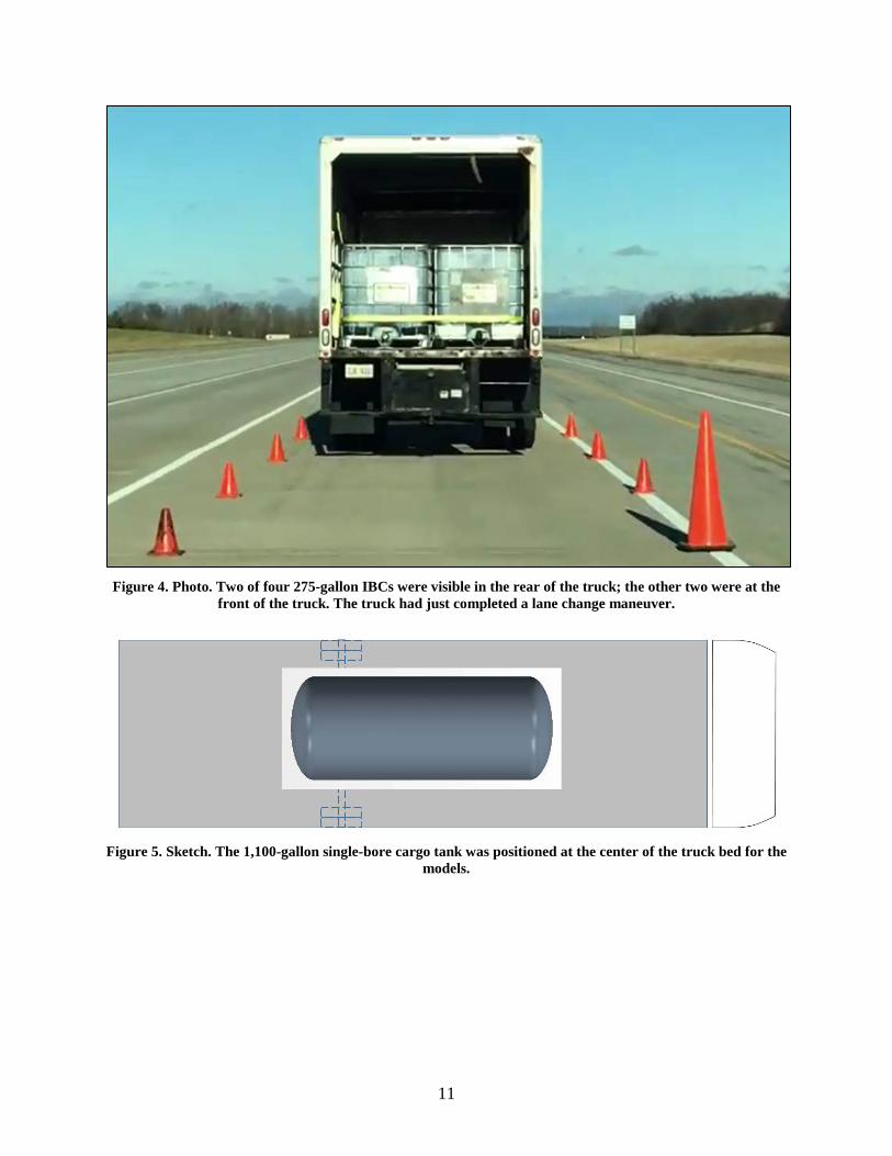
Two arrangements of IBCs on the bed of the truck were used in the experiments. The two 550-gallon IBCs were mounted side-by-side at the rear of the truck (as shown in Figure 3), and the four 275-gallon IBCs were in the four corners (as shown in Figure 4). These two arrangements of the containers and several others were modeled in the simulations.

A number of arrangements of IBCs were simulated. Figure 5 shows the arrangement for the 1,100-gallon cargo tank; it was centered in the bed of the truck. (Note that these figures are looking down at the truck interior. The cab is to the right. The silhouette of the rear axle is shown dotted.) As shown in Figure 6, simulations were run with four arrangements of the two 550-gallon IBCs. The arrangements of the four 275-gallon IBCs are shown in Figure 7. When both sizes of IBCs were simulated together, they were in one of the arrangements shown in Figure 8.

9

Table 2. Four configurations of tanks used in simulations and experiments.

# Tank

Configuration

Total Capacity (gallons)

Fore-aft Internal

Dimensions of one tank

(inches)

Side-side Internal

Dimensions of one tank

(inches)

Height Internal

Dimensions of one tank

(inches) Comments

Arrangements on the Truck

Bed Simulation Experiment

1 1 cargo tank of 1,100 gallons

1,100 121 54 54 Reference case See Figure 5 C N/A

2 2 IBCs of 550 gallons each

1,100 42 48 65 Simple case of two IBCs

See Figure 6 P X

3 4 IBCs of 275 gallons each

1,100 37 45 40 Smaller IBCs See Figure 7 P X

4 1 IBC of 550 and 2 of 275 gallons

1,100 See above See above See above Mixed sizes of IBCs

See Figure 8 P N/A

Note 1: All IBCs were essentially square or rectangular when viewed on one of their axes. The single tank of 1,100 gallons was a cylinder 54 inches in diameter. Its cylindrical section was 100 inches, and its spherical end caps extended the overall length to 121 inches.

Note 2: Two simulation approaches were used. Where the tanks could be reasonably approximated by a pendulum, then an integrated model of a truck with two or more pendulums representing IBCs was used. These cases are indicated by a “P” in the “Simulation” column. Where CFD was required to represent the slosh properly, the CFD model was run separately from the truck path model. These cases are indicated by a “C” in the “Simulation” column.

Note 3: Only the two configurations marked by an “X” in the “Experiment” column were included in the experiments. Note 4: Containers were half filled with water in all cases, for a total of 550 gallons. The water was free to slosh in all of the experiments. All simulations

were run twice, once with the water modeled as sloshing and once with an equivalent rigid load.

10

Figure 3. Photo. The two 550-gallon IBCs were mounted at the rear of the truck. (The strap that held them in

place during the tests is not shown in this photo.)

11

Figure 4. Photo. Two of four 275-gallon IBCs were visible in the rear of the truck; the other two were at the

front of the truck. The truck had just completed a lane change maneuver.

Figure 5. Sketch. The 1,100-gallon single-bore cargo tank was positioned at the center of the truck bed for the

models.

12

Figure 6. Sketch. The simulation models were run with the two 550-gallon IBCs in four different

arrangements. The experiments were run with the IBCs in the rear of the truck bed, the upper arrangement in the figure.

Figure 7. Sketch. The simulation models were run with the four 275-gallon IBCs in two different

arrangements. The experiments were run with the IBCs in the four corners of the truck bed, the upper arrangement in the figure.

13

Figure 8. Sketch. The simulations were run with two arrangements of mixed sizes of IBCs. The 550-gallon IBC (red) was always in the left rear of the truck bed. The two 275-gallon IBCs (blue) were on the left side

with the 550-gallon IBC or both in the front of the truck bed.

The vehicles in the simulations and the experiments were single-unit van trucks with a GVWR of 25,500 pounds. Their beds were nominally 24 feet long by 7.5 feet wide. The two trucks rented for the experiments were the largest size available from a company that serves the consumer market. The dimensions, mass distribution, and suspension properties of the vehicles in the simulations roughly approximated those in the experiments.

2.3 MANEUVERS

Three maneuvers were selected to produce the sloshing. The maneuvers were similar in the computer simulations and in the experiments on the test track. A hard stop and a sudden deceleration in traffic were intended to produce fore-aft sloshing in the IBCs. A turn toward a freeway exit ramp will cause the liquid to move toward one side of its container and make the vehicle lean outwards. There were two versions of a lane change, with the second being more of an avoidance maneuver. These maneuvers were planned to create a rocking motion in the truck. A variation on the stopping maneuver was applied for the second of the two drivers.

Table 3 summarizes the maneuvers; they are described more fully in the following paragraphs.

14

Table 3. This project had four basic maneuvers.

Number Maneuver Parameters in the Experiments Possible Effect of Slosh Metrics in the Simulations Simulations Experiments

1a Stop at a Red Light

35 miles per hour (mi/h) to stopped in 69–184 feet

Surges the truck forward following the stop.

Liquid: Longitudinal force Vehicle: Stopping distance

X X

1b Deceleration in Traffic

50–20 mi/h Pitch oscillations make the truck difficult to steer.

N/A N/A X

2 Entrance to a Steady Curve

60 mi/h in a 45-mi/h curve ; 50 mi/h in a 37-mi/h curve

Movement to the side of the tank can lead to rollover.

Liquid: Lateral force Vehicle: Lateral load transfer from tires on the inside to the outside

X X

3 Lane Change

12-foot change over 171 feet traveled; 3-foot change over 86 feet traveled

Side-to-side sloshing makes the truck difficult to steer and may roll it over.

Liquid: Lateral force and yaw moment Vehicle: Lateral load transfer from tires on the inside to the outside

X X

Notes: The third column lists the parameters for the experiments. The simulations covered a broad range that included the experimental conditions. The exact conditions are noted in the following pages. All maneuvers had two metrics to assess the results of the simulations. One metric quantified the slosh itself, and one quantified the vehicle’s response. The metric for the slosh was the ratio of the force exerted on the vehicle by the liquid to the force exerted by the equivalent rigid load. The direction of the force corresponded to the maneuver, as noted in the table. The metric for the vehicle response was also chosen to be appropriate for the maneuver.

15

2.3.1 Stop at a Red Light The simplest maneuver is a sudden stop from 35 mi/h. This is common when a traffic signal turns to red. The liquid will surge forward as the vehicle is slowing. It will return to the rear of the tank when the vehicle is stopped, and it will surge forward again. A professional driver knows the importance of keeping a foot firmly on the brake after the truck stops so the surge does not push the vehicle into the intersection. This maneuver was on a straight path. The drivers in the experiments were instructed for the first stop to brake as hard as they normally would for a red light. On subsequent stops, they were asked to use harder braking to produce more slosh. The instructions were to brake as they would once a week or once a month. With these purposely qualitative instructions, one driver braked harder than the other. The stopping distances ranged from 58 to 184 feet. The stopping distances for the simulations ranged from 55 to 222 feet. Traffic engineering guidelines assume a braking distance of 118 feet for timing the yellow phase of a traffic signal on a street with a speed limit of 35 mi/h. See Appendix B for a fuller discussion of the range of braking distances.

The simulation compared the surge forces in the different IBC configurations. On the test track, the drivers described whether they felt the surge in the tanks.

After a few runs of this maneuver on the test track, the drivers were instructed to stop the truck and then immediately release the brakes. The effect of surge on the vehicle’s motion was observed by video recording the truck’s motion and measuring the total movement after the stop.

2.3.2 Sudden Deceleration in Traffic The “sudden deceleration in traffic” maneuver was not included in the simulations and it was not driven by the first driver. It was added for the second driver following the first driver’s observation that the slosh was felt strongly only after braking.

The deceleration maneuver was similar to the stop, but the truck continued after it slowed down. The maneuver duplicates a situation where a truck on a highway suddenly encounters slowed traffic. The truck began at 50 mi/h in a straight path. The driver braked and quickly slowed the truck to approximately 20 mi/h. In the first two runs, the driver continued to follow a straight path. On subsequent runs, the driver attempted a lane change after releasing the brake.

The intent here was to induce fore-aft slosh in the IBCs and learn whether the driver can feel the slosh and whether slosh inhibits the driver’s ability to control the vehicle.

This was the only maneuver that was not quantified. The deceleration rate was not measured, and the lane changes were without cones so that the beginning and ending points of the lane change were left to the driver’s discretion.

2.3.3 Curve on an Exit Ramp The next maneuver was an entrance to a steady curve at a high speed. A liquid load will ride up on the side of the tank as shown in Figure 9, which shows the profile of a gasoline tank. Because the mass of the load moves toward the outside of the curve, its effect is to destabilize the vehicle.

16

Figure 9. Sketch. The static position of the liquid is level (left). The liquid rises up the side of the tank on the

outside of a curve in a steady-state sloshing condition (right).

The neutral speeds on the two curves of the vehicle dynamics area (VDA) at TRC Inc. are 34 mi/h on the north turnaround loop and 47 mi/h on the south loop. The truck drove laps around the VDA, at first entering each loop at its neutral speed. As the truck continued its laps, it entered each loop at successively higher increments of 5 mi/h. The goal was to cause the liquid to move within the tank, but not endanger the truck.

The simulations were run at a greater variety of speeds and curvatures. The test matrix is shown in Table 4. For simplicity in developing and understanding, the simulations of this maneuver were all on level pavement with no banking (super elevation). The path began as a straight line, with a spiral into the constant-radius curve, as shown in Figure 10.

Table 4. Roads of three curvatures were built for the simulations; all three were simulated at three speeds.

Variable Curvature

1a Curvature

1b Curvature

1c Curvature

2a Curvature

2b Curvature

2c Curvature

3a Curvature

3b Curvature

3c

Curve radius 900 ft 900 ft 900 ft 764 ft 764 ft 764 ft 575 ft 575 ft 575 ft Speed 35 mi/h 45 mi/h 55 mi/h 35 mi/h 45 mi/h 55 mi/h 35 mi/h 45 mi/h 55 mi/h Lateral acceleration (gravitational units)

0.09 0.15 0.22 0.11 0.18 0.26 0.14 0.24 0.35

The greatest peril to a truck on a steady curve is rolling over toward the outside of the curve. In the simulations, the amount of weight that shifted from one side’s tires to the other side was calculated, as explained under the heading on performance metrics. The drivers in the experiments told the researchers how strongly they felt the slosh.

17

Figure 10. Screenshot. The simulated paths were a spiral into a constant curvature on level ground.

2.3.4 Lane Change The final maneuver was a lane change. A vehicle at highway speed suddenly changed lanes as in an avoidance maneuver. This caused the liquid to move first to one side of the tank and then suddenly to the other side. The dynamics of the slosh can impart significant roll and yaw moments on the vehicle. That is to say, it can make the vehicle roll over or at least be hard to steer.

The lane change path was based on the single lane change maneuver defined in International Organization for Standardization (ISO) 14791:2000, Road vehicles—Heavy commercial vehicle combinations and articulated buses—Lateral stability test methods. Figure 11 is an example of the lane change. The path began with the truck in a straight line at the test speed. As with the curve maneuver, the lateral load transfer was calculated for the simulations of the lane change. Drivers described the behavior in comparison to a cargo tank in regular service.

The conditions of the lane changes in the simulations are shown in Table 5. There were two geometries. One was a normal lane change of 12 feet, which occurred over a distance of 176 feet. The other geometry was more of an avoidance maneuver, where the path shifted 3 feet to the side over a distance of 88 feet. The standard explains how minor differences in the downrange distance could be used to set the peak lateral (side-to-side) acceleration experienced by the vehicle. The lane change produces an oscillation, and the frequency of the oscillation, calculated according to the standard, is in the table.

The conditions shown in the table are those that were simulated. In the experiments, cones were laid out for both of the geometries. Figure 12 is a photograph of the cones arranged to guide the driver through the 12-foot lane change. Drivers took the two trucks through the cones at successively higher speeds until they reached 55 mi/h.

18

Figure 11. Graph. The single lane change was planned to simulate side-to-side sloshing.

Table 5. Conditions for the lane change maneuver.

Variable Lane Change

1a Lane Change

1b Lane Change

2a Lane Change

2b Lane Change

3a Lane Change

3b

Speed 35 mi/h 35 mi/h 45 mi/h 45 mi/h 55 mi/h 55 mi/h Sideways path shift 12 ft 3 ft 12 ft 3 ft 12 ft 3 ft Peak lateral acceleration (gravitational units)

0.2 0.2 0.35 0.35 0.5 0.5

Downrange distance to make the change

176 ft 88 ft 171 ft 85 ft 175 ft 87 ft

Frequency of excitation 0.29 Hz 0.58 Hz 0.39 Hz 0.77 Hz 0.47 Hz 0.92 Hz

Figure 12. Photo. The cones were arranged to direct the driver to make a 12-foot lane change over a distance of 171 feet. The four cones for the entry gate are in the foreground. The set of cones for the exit gate is by the

sport utility vehicle.

0 20 40 60 80 100 120 140 160 180-6

0

6

12

18

Longitudinal Distance (ft)

Late

ral D

ista

nce

(ft)

Experimental 12 ft Lange Change Profile

19

3. SIMULATIONS The simulations of liquid motion used a combination of simplified models (a pendulum) and full CFD. The pendulum models could be integrated with the truck model to form a single, combined model where the truck and the liquid would affect each other. The CFD was not integrated with the truck model, but a container was simulated as it moved on a path identical to what the simulated truck had followed.

The simulation part of the project consisted of two stages of model validation and multiple approaches to using the models in the simulation. Two models of the liquid sloshing were used, and they were applied to the truck dynamics in different ways.

The model of the truck itself was built in TruckSim, a commercially available truck dynamics modeling software that is widely accepted in industry and academia.(i) The TruckSim model of a single-unit vehicle was integrated with the simplified model of sloshing. A single model of the truck and IBCs calculated their effects on each other. The modeled vehicle was a two-axle single-unit truck (also known as a straight truck). It was similar to the two trucks used in the experiments and was simulated with different configurations of tanks.

The basis for comparison was a single 1,100-gallon cargo tank. There were three combinations of sizes of IBCs, each in different arrangements on the bed of the truck. In each combination, the total capacity was 1,100 gallons. Half of the simulations were run with containers half full with water that was free to slosh. In the other half of the simulations, the weights and placements were identical, but the water was replaced with a model of a solid block of the same size and weight. This way, the effect of sloshing in the various combinations of IBCs could be compared with the behavior of a non-sloshing load.

The CFD models were used in two ways in this project. First, they were used to corroborate the simplified pendulum models. Second, CFD was used as the only way to model slosh in cases of extreme liquid motion with part of the liquid splashing away from the rest of the liquid. This was necessary only for the single-bore 1,100-gallon tank, where the liquid motion was too large to be represented by the pendulum model.

This section describes the simulations. The next section describes the experiments run on the test track.

3.1 TRUCK MODEL

The TruckSim software package allows engineers to develop with efficiency the mathematical equations that describe the motion of heavy vehicles. A simulation case is established by parameters to describe the vehicle, road, and maneuver. TruckSim uses the information to carry out accurate simulations that predict the forces on vehicle components and the resulting motions. TruckSim simulations generate a variety of data including animation of the vehicle motion.

i TruckSim was developed by the Mechanical Simulation Corporation, out of Ann Arbor, MI.

20

These animations are helpful in: 1) qualitatively confirming that the equations of motion are correct, and 2) qualitatively evaluating the performance of the vehicle. A frame from a TruckSim animation is shown in Figure 13. Other data, such as vehicle position or tire forces versus time, are useful for quantitative evaluation of a vehicle’s performance.

Figure 13. Screenshot. One frame of a TruckSim animation.

The parameters in the TruckSim model were set to describe one of the trucks used in the experiments. Dimensions that were set included wheelbase, track width, and position of the bed relative to the axles. These all corresponded to the values in Table 6. The mass in the model was distributed to approximate the four wheel loads measured for the empty vehicle. The suspension properties were selected to approximate the properties specified online for the approximate make and model of the truck. Other parameters of the truck model were the default properties in TruckSim for a two-axle van body truck.

3.2 SIMPLIFIED PENDULUM MODEL

In the majority of cases that were modeled, the top surface of the liquid remained calm and no part of the liquid splashed away from the rest. This simpler case can be modeled by a pair of masses. One mass remains fixed at the bottom of the container, representing the liquid that does not move much during the slosh. The upper mass is on a pendulum, and it represents the moving part of the liquid. This method is illustrated in Figure 14.

21

Figure 14. Sketch. Illustration of the pendulum method for modeling slosh in a rectangular container.

Appendix C presents the mathematics used to develop the pendulum model. The models for the 275-gallon and 550-gallon IBCs were identical in form, with the masses and dimensions changed to represent the two sizes.

The model was coded in Simulink,(ii) which was integrated with the truck model. One instance of the pendulum represented each container. In the cases where four IBCs were mounted in the bed of the truck, there were four independent pendulums running simultaneously. At each instant in time as the computer model ran, the truck model calculated the position and orientation at the base of every IBC. This information was passed to the pendulum models, which calculated the force of the liquid against the container at that location. The forces from the IBCs were combined into one set of forces and moments that the IBCs exerted against the truck at that instant in time. The simulated truck and its cargo proceeded down the path, each influencing the other’s motion.

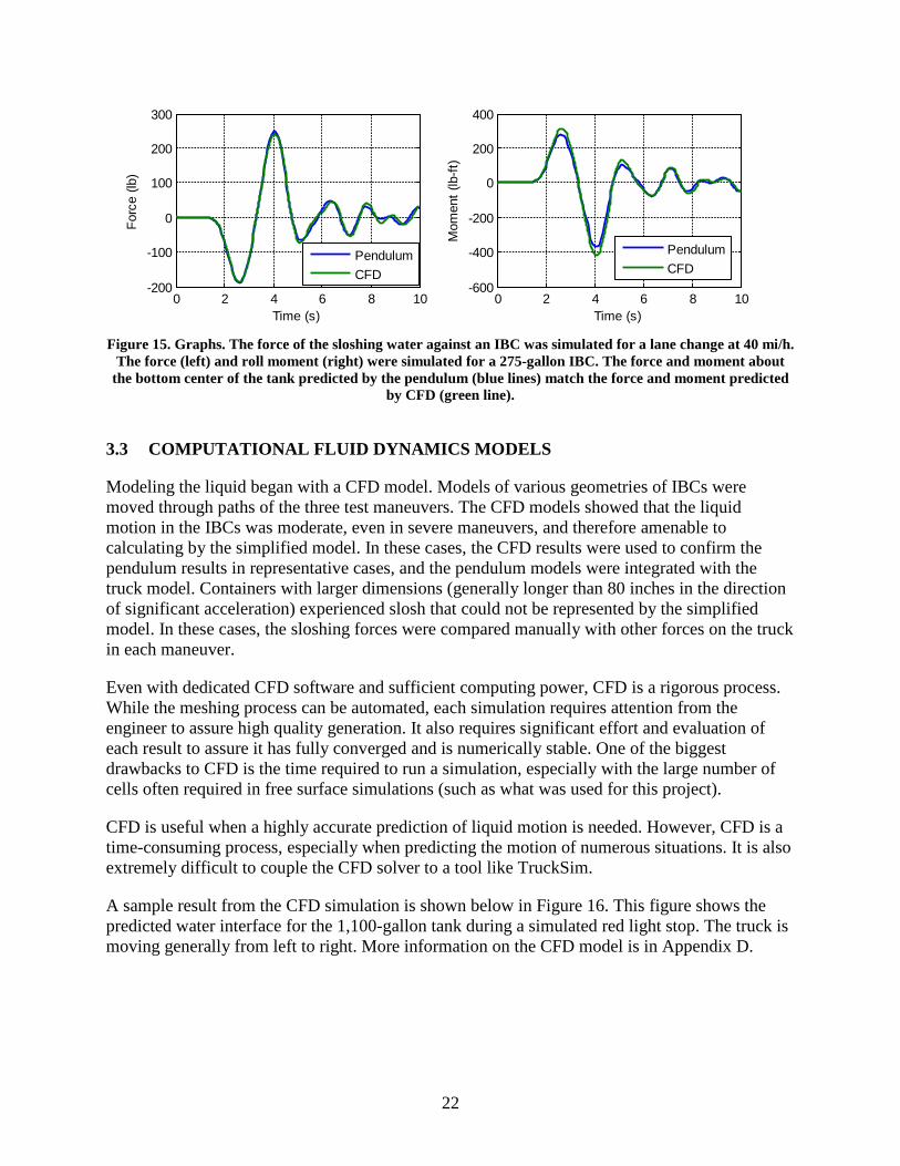
A CFD container model (which was the same size and shape of the IBC modeled by a pendulum) was subjected to the same motions as the simplified pendulum model. The forces and moments that the liquid exerted against the container in the two models were compared. Confidence in the CFD itself came from using an accepted package and by scrutinizing the selection of the modeling mesh. Figure 15 shows the force exerted by the liquid on the container as calculated by a CFD model and a pendulum model. This is the case of a half-filled 275-gallon IBC undergoing a lane change at 40 mi/h. The two agree well. Similar comparisons for other maneuvers and the 550-gallon IBC are in Appendix C.

ii Simulink is a graphical programming environment for modeling, simulating and analyzing multi-domain dynamic systems. Simulink was developed by Mathworks, out of Natick, MA.

22

Figure 15. Graphs. The force of the sloshing water against an IBC was simulated for a lane change at 40 mi/h.

The force (left) and roll moment (right) were simulated for a 275-gallon IBC. The force and moment about the bottom center of the tank predicted by the pendulum (blue lines) match the force and moment predicted

by CFD (green line).

3.3 COMPUTATIONAL FLUID DYNAMICS MODELS

Modeling the liquid began with a CFD model. Models of various geometries of IBCs were moved through paths of the three test maneuvers. The CFD models showed that the liquid motion in the IBCs was moderate, even in severe maneuvers, and therefore amenable to calculating by the simplified model. In these cases, the CFD results were used to confirm the pendulum results in representative cases, and the pendulum models were integrated with the truck model. Containers with larger dimensions (generally longer than 80 inches in the direction of significant acceleration) experienced slosh that could not be represented by the simplified model. In these cases, the sloshing forces were compared manually with other forces on the truck in each maneuver.

Even with dedicated CFD software and sufficient computing power, CFD is a rigorous process. While the meshing process can be automated, each simulation requires attention from the engineer to assure high quality generation. It also requires significant effort and evaluation of each result to assure it has fully converged and is numerically stable. One of the biggest drawbacks to CFD is the time required to run a simulation, especially with the large number of cells often required in free surface simulations (such as what was used for this project).

CFD is useful when a highly accurate prediction of liquid motion is needed. However, CFD is a time-consuming process, especially when predicting the motion of numerous situations. It is also extremely difficult to couple the CFD solver to a tool like TruckSim.

A sample result from the CFD simulation is shown below in Figure 16. This figure shows the predicted water interface for the 1,100-gallon tank during a simulated red light stop. The truck is moving generally from left to right. More information on the CFD model is in Appendix D.

0 2 4 6 8 10-200

-100

0

100

200

300

Time (s)

Forc

e (lb

)

PendulumCFD

0 2 4 6 8 10-600

-400

-200

0

200

400

Time (s)

Mom

ent (

lb-ft

)

PendulumCFD

23

Figure 16. Screenshot. Visualization of transient simulation showing water interface of 1,100-gallon tank at

four instants during a simulated stop at a red light (35 mi/h to stopped in 150 feet).

3.4 PERFORMANCE METRICS

The output of the liquid models was the force that the sloshing liquid applied to the vehicle. Quantitative performance metrics were used to assess the effect of slosh in the various IBC configurations on the truck. Each maneuver was interpreted through two metrics. One was the force that the slosh in the combined set of IBCs applied to the vehicle. The other metric was a response of the vehicle. The first metric, the excess force due to slosh, is a direct measure of the slosh. It can be readily applied to different vehicle cases, for example, a truck of similar size but with a rigid load in addition to the few IBCs. Similarly, the effect of mounting, for example, twice as many IBCs on the truck can be calculated. The purpose of the vehicle-related metric is to put the slosh in context by showing how it would affect the vehicle, the driver, or surrounding traffic. These metrics were introduced in Table 3 and are explained in greater detail here.

Of the three maneuvers, the stop at a red light is the simplest to interpret. The maneuver produces slosh in the fore-aft direction, so the force in this direction was tabulated and compared between conditions. The vehicle measure for the stopping maneuver was the stopping distance. The stops were produced in the simulation by applying a fixed pressure in the brake line. Any variability in the stopping distance is due to the vehicle’s response. In a mathematical model, the tires, suspension, and other features are exactly identical from run to run. Therefore, the difference in stopping distance with a sloshing load and distance with a rigid load is due to the effect of the liquid.

24

For the exit ramp and lane change maneuvers, the side-to-side slosh was the most important direction. A truck that takes a curve too fast is prone to roll over, and liquid riding up on the side of the tank (Figure 9) increases the propensity to roll.

The vehicle measure for the exit ramp and lane change maneuvers was the lateral load transfer ratio. When an evenly loaded truck is driving on straight, level road, the loads on its tires are the same on both ends of the rear axle. In a steady or transient curve, the trailer will lean and some of the load will transfer from the tires on one end of the axle to those on the other end. If the load on one side falls to zero, the result can be a rollover. The formula for calculating the lateral load transfer ratio of an axle is shown in Figure 17:

Figure 17. Equation. Load transfer ratio.

where:

FL is the vertical force on the left-side tires and FR is the vertical force on the right-side tires.

When an evenly loaded vehicle is driving straight on level road, the ratio on both axles is zero. When the load on one end of the axle is completely removed, the ratio is one. A ratio of one means that a set of tires has lifted from the pavement momentarily, but it does not necessarily mean that the truck has rolled over. The load transfer ratio depends strongly on the properties of an axle’s suspension. The actual value of a load transfer ratio in a simulation has little meaning; the change in load transfer ratio between a rigid and a sloshing load is meaningful. Clearly, a lower ratio means the vehicle is more stable in the maneuver.

3.5 RESULTS

The effect of the slosh was apparent in many of the simulations. The slosh in IBCs had a minor effect on the path or stability of the vehicle. The slosh in the single-compartment 1,100-gallon cargo tank was evident in the stopping maneuver and the more severe lane changes.

During the stopping maneuver, the liquid sloshed back and forth in the IBCs, causing a small pulsating force against the truck. The stopping distances of the trucks with IBCs was imperceptibly different from simulations where an identical brake pedal input was applied to a corresponding rigid load.

The curve entry maneuver did not strongly distinguish between rigid and sloshing loads.

In the lane change maneuver, the dynamic forces from the slosh in the 1,100-gallon cargo tank were several times greater than those from any of the IBC arrangements. In the most extreme conditions of the lane change maneuver, the sloshing contributed toward momentarily relieving the load on one of the tires, but only in cases where the equivalent rigid load almost did so.

LTR= (| FR-FL |)/(FR+FL)

25

3.5.1 Stop at a Red Light When a vehicle is traveling straight ahead at a steady speed, its load presents essentially no forward force on the vehicle. As the vehicle brakes at a uniform deceleration, a rigid load will apply a uniform force against the vehicle in the forward direction. This effect is visible in the dotted red line in Figure 18. This is the stop from 35 mi/h with two 550-gallon IBCs in the rear of the truck. The truck began braking at the 2-second mark, and the dotted red line went up to approximately 2,000 pounds. Considering the dynamics of the braking system on the truck, the deceleration does not instantly jump to its peak value, nor does it remain constant at that value. The dotted red line has a rounded rising edge, and it tapers slowly during the stop.

The solid line in the figure represents the combined force applied by the slosh in two IBCs. It rises the same as the force from the rigid load, but then continues to rise as the liquid moves toward and pushes against the front of the containers. When the liquid has sloshed back toward the rear surface of the container, the solid line indicates that the force from the IBCs is momentarily less than what the rigid load is providing. When the truck comes to a stop, at about 6 seconds, the force from both loads goes to zero. The forces continue to oscillate as both loads work with the truck’s suspension and the liquid continues to slosh. The suspension-related oscillation diminishes quickly, while the liquid continues to slosh. The highest force from the continuing slosh is about 800 pounds, which is a small force on a truck with a loaded weight on the order of 20,000 pounds. This delayed slosh force occurs about a second after the vehicle comes to a stop.

Figure 18. Graph. Force exerted on the truck by the two 550-gallon IBCs during a brake to stop (from 35

mi/h in 100 feet).

Figure 19 shows the cargo force produced by a single 1,100-gallon tank in the same braking maneuver. The effect is different from that of the 550-gallon IBCs in two ways. The first and most obvious is that the peak force produced by the single 1,100-gallon tank is about 500 pounds greater even though quantity of liquid is the same. The more subtle difference is that the oscillations in force are occurring at a much lower frequency. This is important after the vehicle comes to a stop because the slosh will be more delayed and therefore more likely to catch the driver off guard.

0 1 2 3 4 5 6 7 8-2000

-1000

0

1000

2000

3000

Time (s)

Long

itudi

nal C

argo

For

ce (l

bf)

g p p y

LiquidRigid

26

Figure 19. Graph. Force exerted on the truck by a single 1,100-gallon tank during a brake to stop (from 35

mi/h in 100 feet).

It can be seen in Figure 18 that, although the liquid force oscillates, the average force during braking is approximately the same whether the cargo is liquid or rigid. If the two forces have approximately the same average, then the stopping distance of the two cases will be about the same. The stopping distances of the two cases were both between 103 and 104 feet, a difference that is insignificant.

The stopping distances of all the simulations are shown in Figure 20. A constant brake force was applied in all simulations, so the differences in stopping distance are due to the differences in the load. In all pairs, the difference in stopping distance between the liquid load and the rigid load was less than 1 foot. The figure has no bar for the truck with the 1,100-gallon cargo tank. The CFD model necessary to simulate this larger container could not be integrated with the truck model. (This figure presents the results from one of the stopping maneuvers graphically. Numerical results of all simulation cases are presented in Appendix E.)

0 1 2 3 4 5 6 7 8-2000

-1000

0

1000

2000

3000

Time (s)

Long

itudi

nal C

argo

For

ce (l

b)

g

LiquidRigid

27

Figure 20. Graph. Stopping distances calculated by the simulations, in feet.

A metric of the simulation that is more directly related to the liquid itself is the amplitude of the sloshing force that the cargo exerts against the truck. If the force amplitude is considerably large, then the driver might feel the sloshing and conceivably have to take action to keep the vehicle stable. Figure 21 shows the amplitude of the sloshing force for every configuration during the nominal 100-foot stops from 35 mi/h. In no case did the slosh amplitude in the IBCs become comparable to that of the single tank. The largest amplitude that occurs in the IBCs is 488 pounds. Such a small variation against a truck with loaded weight on the order of 20,000 pounds would not be significant, so it should not impair the driver’s ability to control the vehicle.

Figure 21. Graph. Amplitudes of oscillating slosh force while braking to a stop (from 35 mi/h in 100 feet).

28

3.5.2 Curve on an Exit Ramp A vehicle in a steady curve leans toward the outside of the curve. While in the curve, the tires on the side of the truck on the outside of the curve carry an extra share of the truck’s weight. If liquid in a tank is free to move within the tank, it will move toward the outside of the curve and increase the transfer of weight from the tires on one side of the truck to the tires on the other side. The quantities of most interest in the simulations of an entry to a steady curve were: 1) the amount of sideways force that the cargo applies to the truck, and 2) the amount of weight transferred from the tires on one side of the truck to the tires on the other side.

Figure 22 shows the lateral force applied by the loads to the truck as it enters and negotiates a curve. The speed of the truck is 55 mi/h and the radius of the curve is 575 feet, so the nominal lateral acceleration is 0.35 gravitational units. As with other cases, what is shown is the net combined force of all of the IBCs. Figure 22 shows the lateral force applied by four 275-gallon IBCs secured on the left side of the truck bed. Because the curve goes to the right, having all of the IBCs on the outside of the curve is where they will have the most effect. The lateral force rises as the truck drives the spiral into the curve. After a slight peak, the force settles into a steady value while the truck is in a constant curvature. In steady state, the solid line for the liquid load oscillates slightly above and below the dotted line representing the rigid load. That is because the two masses are the same and both must be forced to stay in the same curved path.

Figure 23 shows the lateral load transfer ratio for this case. Again, the quantity increases as the truck enters the spiral into the curve. More load transfers from the inside tires to the outside tires on the tighter curve. The difference between the liquid and rigid loads is greatest in the tightest curve. Although the liquid and rigid loads are applying approximately the same lateral force to the truck, the liquid load has shifted and has a correspondingly longer lever arm to lean the truck over. In these cases, as in all simulations, the load transfer ratio depends strongly on the speed and curvature and only slightly on the liquid slosh.

Figure 22. Graph. Lateral force exerted by the loads against the truck navigating a 575-foot-radius curve at

55 mi/h. In this configuration, the truck is carrying four 275-gallon IBCs, all on the left side of the bed.

0 1 2 3 4 5 6 7 80

500

1000

1500

2000

Time (s)

Late

ral C

argo

For

ce (l

b)

g

LiquidRigid

29

Figure 23. Graph. Lateral load transfer ratio of a truck navigating a 575-foot-radius curve at 55 mi/h. In this

configuration, the truck is carrying four 275-gallon IBCs, all on the left side of the bed.

Figure 24 and Figure 25 summarize the results of all of the configurations during the most severe exit ramp maneuver that was simulated. Figure 24 compares the peak lateral forces exerted by the cargo. The effect of the slosh is small. In some cases, the slosh reduces the peak force, within the accuracy of the simulation. In the worst cases, the peak force is increased by less than 30 pounds. The vehicle performance metric for this maneuver was the lateral load transfer ratio, which is plotted for example cases in Figure 23. The key to determining the effect of the slosh is to determine the extent to which the liquid’s movement increases the steady state lateral load transfer ratio.

Figure 25 shows this quantity for various configurations for the most severe exit ramp maneuver. The effect of slosh was negligible in all cases except where two 275-gallon IBCs and one 550-gallon IBC are all placed on the left side of the truck, i.e. on the outside of the turn. (This case is labeled “mixed, left side” in the figures.) In this case, the load transfer ratio was increased from 0.66 to 0.79. In this curve, the load transfer ratio depends strongly on how the IBCs are positioned in the truck bed and little on whether their contents are sloshing.

0 1 2 3 4 5 6 7 80

0.2

0.4

0.6

0.8

1

Time (s)

Late

ral L

oad

Tran

sfer

Rat

io

Axle 1 (Liquid)Axle 2 (Liquid)Axle 1 (Rigid)Axle 2 (Rigid)

30

Figure 24. Graph. Peak lateral forces exerted by the loads against the truck entering a 575-foot-radius curve

at 55 mi/h.

Figure 25. Graph. Steady state lateral load transfer ratio for a rigid load in a 575-foot-radius curve at 55

mi/h, and showing the increase when the load is a liquid free to slosh.

3.5.3 Lane Change A lane change requires a vehicle to undergo a transient lateral acceleration in one direction, followed by an equal acceleration in the opposite direction. This temporarily transfers the load to each side of the vehicle. The cargo that a vehicle carries has a significant effect on the extent of this load transfer as it can create additional forces on the vehicle. During a lane change, liquid cargo will slosh to the side creating even larger cargo forces. The most important metrics for studying the effect of liquid sloshing during a lane change are: 1) the amount of sideways force that the cargo applies to the truck, and 2) the amount of weight transferred from the tires on one side of the truck to the tires on the other side.

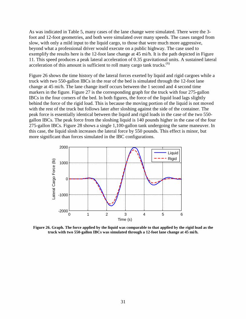
31

As was indicated in Table 5, many cases of the lane change were simulated. There were the 3-foot and 12-foot geometries, and both were simulated over many speeds. The cases ranged from slow, with only a mild input to the liquid cargo, to those that were much more aggressive, beyond what a professional driver would execute on a public highway. The case used to exemplify the results here is the 12-foot lane change at 45 mi/h. It is the path depicted in Figure 11. This speed produces a peak lateral acceleration of 0.35 gravitational units. A sustained lateral acceleration of this amount is sufficient to roll many cargo tank trucks.(6)

Figure 26 shows the time history of the lateral forces exerted by liquid and rigid cargoes while a truck with two 550-gallon IBCs in the rear of the bed is simulated through the 12-foot lane change at 45 mi/h. The lane change itself occurs between the 1 second and 4 second time markers in the figure. Figure 27 is the corresponding graph for the truck with four 275-gallon IBCs in the four corners of the bed. In both figures, the force of the liquid load lags slightly behind the force of the rigid load. This is because the moving portion of the liquid is not moved with the rest of the truck but follows later after sloshing against the side of the container. The peak force is essentially identical between the liquid and rigid loads in the case of the two 550-gallon IBCs. The peak force from the sloshing liquid is 140 pounds higher in the case of the four 275-gallon IBCs. Figure 28 shows a single 1,100-gallon tank undergoing the same maneuver. In this case, the liquid slosh increases the lateral force by 550 pounds. This effect is minor, but more significant than forces simulated in the IBC configurations.

Figure 26. Graph. The force applied by the liquid was comparable to that applied by the rigid load as the

truck with two 550-gallon IBCs was simulated through a 12-foot lane change at 45 mi/h.

0 1 2 3 4 5 6-2000

-1000

0

1000

2000

Time (s)

Late

ral C

argo

For

ce (l

b)

LiquidRigid

32

Figure 27. Graph. The force applied by the liquid was slightly higher than that applied by the rigid load as

the truck with four 275-gallon IBCs was simulated through a 12-foot lane change at 45 mi/h.

Figure 28. Graph. The force applied by the liquid was significantly higher than that applied by the rigid load

as the single 1,100-gallon tank was subjected to a 12-foot lane change at 45 mi/h.

Figure 29 shows the lateral load transfer ratio of the same maneuver for the truck with two 550-gallon IBCs. Figure 30 is the corresponding graph for the truck with four 275-gallon IBCs in the four corners of the bed. According to the definition of this ratio (Figure 17), it is always positive. The lateral load transfer ratios on the front axles are higher in these cases because the front axles are more lightly loaded than the rear axle, so their load transfer ratio is more sensitive to the shift. A lateral load transfer ratio that peaks momentarily at 0.5 is indicative of a harsh maneuver, but the truck is not in danger of rolling over.

0 1 2 3 4 5 6-2000

-1000

0

1000

2000

Time (s)

Late

ral C

argo

For

ce (l

b)

LiquidRigid

0 1 2 3 4 5 6 7 8-2000

-1000

0

1000

2000

Time (s)

Late

ral C

argo

For

ce (l

b)

Liquid (CFD)Rigid

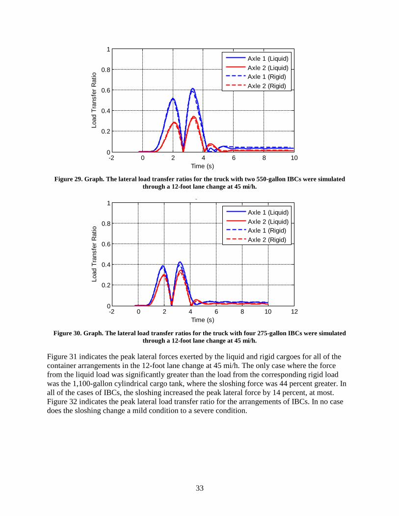
33

Figure 29. Graph. The lateral load transfer ratios for the truck with two 550-gallon IBCs were simulated

through a 12-foot lane change at 45 mi/h.

Figure 30. Graph. The lateral load transfer ratios for the truck with four 275-gallon IBCs were simulated

through a 12-foot lane change at 45 mi/h.

Figure 31 indicates the peak lateral forces exerted by the liquid and rigid cargoes for all of the container arrangements in the 12-foot lane change at 45 mi/h. The only case where the force from the liquid load was significantly greater than the load from the corresponding rigid load was the 1,100-gallon cylindrical cargo tank, where the sloshing force was 44 percent greater. In all of the cases of IBCs, the sloshing increased the peak lateral force by 14 percent, at most. Figure 32 indicates the peak lateral load transfer ratio for the arrangements of IBCs. In no case does the sloshing change a mild condition to a severe condition.

-2 0 2 4 6 8 100

0.2

0.4

0.6

0.8

1

Time (s)

Load

Tra

nsfe

r Rat

io

Axle 1 (Liquid)Axle 2 (Liquid)Axle 1 (Rigid)Axle 2 (Rigid)

-2 0 2 4 6 8 10 120

0.2

0.4

0.6

0.8

1

Time (s)

Load

Tra

nsfe

r Rat

io

g

Axle 1 (Liquid)Axle 2 (Liquid)Axle 1 (Rigid)Axle 2 (Rigid)

34

Figure 31. Graph. Peak lateral forces exerted by the loads against the truck during the

12-foot lane change at 45 mi/h.

Figure 32. Graph. Peak in the lateral load transfer ratio during the 12-foot lane change at 45 mi/h.

3.5.4 Lane Change with Large-Footprint Containers Two less common sizes of IBCs were simulated in the 12-foot lane change: 1) a 793-gallon IBC with square footprint, and 2) two 550-gallon IBCs with a horizontal cylinder (shown in Figure 33). These cylindrical IBCs are commercially available, though not commonly used for transportation due to their large footprint. However, if used on a vehicle, they can have greater slosh forces than tall, slender IBCs, depending on their orientation.

Due to the large horizontal dimensions, the surface of the liquid can become highly nonlinear in these containers. This is an effect that the simplified pendulum model cannot simulate. Thus,

35

CFD was used to simulate slosh in large-footprint containers, and only the nominal 12-foot lane change at 45 mi/h was simulated.

Figure 33. Photo. The 550-gallon cylindrical IBC is lower and wider than those in common use.

Note: Photograph used with permission of Precision IBC.

The arrangements of the IBCs on the truck bed are shown in Figure 34. The 793-gallon IBC was positioned in the center of the bed, and it was combined with a 275-gallon IBC in the rear corner, providing an aggregated capacity of 1,068 gallons. Pairs of 550-gallon horizontal IBCs were oriented longitudinally or laterally.

Figure 34. Sketch. 793-gallon container combined with a 275-gallon container (top); 550-gallon containers

oriented longitudinally (middle) and laterally (bottom).

Figure 35 indicates the peak lateral forces exerted by the liquid and rigid cargoes for three arrangements of large-footprint IBCs. The 1,100-gallon cargo tank and a set of four standard

36

275-gallon IBCs are shown patterned in the figure for reference. The larger footprint containers all exhibited larger slosh forces than did the standard size IBCs. In most cases, the effect of the slosh was still significantly smaller than that of a single 1,100-gallon tank. The exception is in the 550-gallon container that is oriented laterally. In this case, the effect of slosh is large. This is the only case in this study in which the effect of slosh exceeds that of a single 1,100-gallon tank.

Figure 35. Graph. Peak lateral forces exerted by loads against the truck during the 12-foot lane change at 45

mi/h.

The effect that this type of container (i.e., cylindrical 550-gallon IBC) has on a vehicle was not directly simulated because the CFD simulations were not fully coupled to truck models. In order to estimate this effect, the forces predicted by the CFD model were applied to the vehicle during a lane change maneuver. This method is a one-way coupling and is less accurate than the two-way coupling used for all other vehicle simulations.

Figure 36 shows the lateral load transfer ratio during this simulation. The effect of the slosh is significant, and the vehicle approaches the limits of stability in a maneuver that is typically mild. A more severe maneuver would be in danger of causing a rollover.

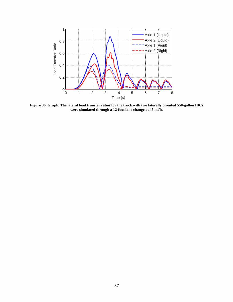
37

Figure 36. Graph. The lateral load transfer ratios for the truck with two laterally oriented 550-gallon IBCs

were simulated through a 12-foot lane change at 45 mi/h.

0 1 2 3 4 5 6 7 80

0.2

0.4

0.6

0.8

1

Time (s)

Load

Tra

nsfe

r Rat

io

Axle 1 (Liquid)Axle 2 (Liquid)Axle 1 (Rigid)Axle 2 (Rigid)

38

[This page intentionally left blank.]

39

4. EXPERIMENTS The previous section described computer simulations, which were well controlled and covered a range of conditions. In addition to the simulations, the project included a small set of driving experiments at a test track. Trucks were operated by experienced, professional drivers who sensed the behavior of the vehicle. The experiments provided an opportunity for drivers to feel the effects of slosh when driving a vehicle with aggregated IBCs.

The experiments were conducted with four 275-gallon IBCs and with two 550-gallon IBCs. IBCs were mounted on two single-unit trucks. The containers were half filled with water (roughly). Two experienced tank drivers drove the trucks through three maneuvers that were similar to those in the simulations.

The two drivers provided comments on the behavior of the truck with the IBCs and a comparison of their experience with driving the aggregated IBCs on the test track versus their professional tank experience. The only numerical measurements were the stopping distance and, for a few stops, the distance that the surge pushed the truck forward. The trucks in the experiments had no sensors and produced no engineering data. Note that many of the tables presented in this section are entry forms that were used to record information on paper during the tests. One of the forms as it was filled in during testing is shown in Figure 37.

40

Figure 37. Scanned image. Example of a checklist table filled out by drivers during the experiments.

The drivers reported that they felt the slosh only in the harshest maneuvers. They occasionally expressed slight agreement with a statement that special skills beyond ordinary truck driving skills were needed. They also said that handling the trucks with IBCs was comparable to handling a truck with dry freight in similar circumstances, in terms of the skill level required.

4.1 CONDITIONS AND EQUIPMENT

Two essentially identical van trucks were rented from a national truck rental company. One of the trucks is pictured in Figure 38. Both trucks had a GVWR of 25,500 pounds and nominal bed dimensions of 24 feet long by 7.5 feet wide. Both were two-axle trucks and had dual tires on the rear. Specifications of the trucks are shown in Table 6. Two 550-gallon IBCs were mounted at the rear of one truck, as shown in Figure 3 and Figure 6, and four 275-gallon IBCs were mounted in the four corners of the bed of the other truck, as shown in Figure 4 and Figure 7. TRC Inc. built load frames and strapped the IBCs in place to ensure that they did not shift during the tests. There were two people in the cab for all tests—the test driver and a staff member from TRC Inc. (also an experienced truck driver)—to provide directions and record immediate thoughts. The trucks had no load other than the IBCs.

41

The drivers relied on the speedometers in the trucks to set their speeds. Speeds were checked by the speedometer and a hand-held global positioning system (GPS) device in a chase vehicle. While the instruments were not calibrated laboratory instruments, their general agreement means they were adequate for the purpose. The experiments were not intended to make precise measurements, but to get drivers’ sense of the slosh in conditions representative of actual driving.

The pavement was dry for the entirety of both test days. The sky was overcast at times and sunny at other times. Winds were roughly 10 mi/h, and the temperature ranged from the mid-30s to about 50 degrees Fahrenheit.

Both trucks weighed about the same—14,400 pounds, empty. In the test condition, the truck with four 275-gallon IBCs was 19,410 pounds, so the load added about 34 percent to the total weight of the vehicle. It could have carried another 6,000 pounds before reaching its maximum weight, so its load was not quite half of the available capacity. The truck with two 550-gallon IBCs weighed 21,270 pounds in the test condition, or 48 percent above its empty weight. The additional available load in the second truck was more than 4,000 pounds, so it was carrying slightly over half its capacity. The complete list of weights on the tires is provided in Appendix F.

Figure 38. Photo. The IBCs were mounted two similar van trucks (as pictured here).

42

Table 6. Specifications of the two trucks.

Property Truck 1 Truck 2

Bed size (ft) 7-1/2 x 24 7-1/2 by 24 GVWR (lb) 25,500 25,500 Wheelbase (in) 253 261 Rear axle to back of bed (in) 108 102 Track width, measured on centers (in) Front: 80.7; Rear: 85.4 Front: 82.1; Rear: 85.0 Empty weight (lb) 14,350 14,410 Weight with IBCs, water, and two people (lb) 19,410 21,270 Containers carried Four 275-gallon poly Two 550-gallon stainless

4.2 MANEUVERS

The stop, deceleration, and lane change maneuvers were run on the straight lanes of the skid pad at TRC Inc. (Figure 39). The project had exclusive use of two adjacent lanes on the days of testing. Entrances to freeway ramps were represented by loops at the two sides of the VDA (Figure 40).

Figure 39. Sketch. The stop, deceleration, and lane change maneuvers were conducted on the skid pad at

TRC Inc.

43

Figure 40. Sketch. Freeway ramp curves were represented by the vehicle dynamics area at TRC Inc.

4.2.1 Stop at a Red Light The drivers were instructed to achieve a steady speed of 35 mi/h in a straight path. When they reached a cone placed on the pavement for reference, they braked to a stop. On the first stop, the driver was to stop normally. On at least two subsequent stops, the driver was to brake more quickly, as hard as might happen “once a week or once a month” during the driver’s regular operations on the road. The instructions that were in the cab are provided in Table 7.

Table 7. For the stopping maneuver, the project staff in the cab with the test driver carried this checklist for instructions/recording immediate observations.

Stop Condition

OBSERVER IN THE CAB: Check when finished

PERSONNEL ON THE TRACK: Stopping distance (feet)

1 Ask the driver to get to 35 mi/h, hold for a few seconds, and then stop normally.

–

2 Get to 35 mi/h again and then stop harder—like you would “once a week or once a month.”

–

3 Repeat: Get to 35 mi/h again and then stop—like you would “once a week or once a month.”

–

4 Repeat again, but this time the driver will release the brake when the truck stops. Any fluid surge will push the truck forward.

Stopping distance: Surge distance:

5 Driver’s discretion #1 (if he wants to). – 6 Driver’s discretion #2 (if he wants to). –

44

The stopping distance was measured. No particular distance was required; the purpose of the measurement was to document what the driver did. The drivers were asked whether they felt the surge in the tanks.

After repetitions of stops like this, similar maneuvers were completed to characterize the effect of surge on the truck. The driver was asked to place the (automatic) transmission in neutral while the vehicle was decelerating, and the driver released the brake as soon as the truck came to a stop. The truck was free to be moved by the continuing liquid motion in the IBCs. The surge was recorded by distance measurements and by video recording.

4.2.2 Sudden Deceleration This maneuver was similar to the stop, but the truck continued driving after it slowed down. It duplicates a situation where a truck on a highway suddenly encounters slowed traffic. The truck began at 50 mi/h in a straight path. The driver was instructed to brake and quickly slow the truck to approximately 20 mi/h. The driver continued to follow a straight path. After three runs in a straight path, the driver attempted a lane change after releasing the brake.

The intent here was to induce fore-aft slosh in the IBCs and to learn whether the driver can feel the slosh and whether slosh inhibits the driver’s ability to control the vehicle. This maneuver was added after the first test driver reported feeling significant slosh only after the truck came to a stop. The strong deceleration would induce slosh, which might affect the continued driving.

The written instructions that were in the cab are provided in Table 8.

Table 8. For the deceleration maneuver, the project staff in the cab with the test driver carried this checklist for instructions and recording immediate observations.

Pass Condition Check if slosh cannot be felt:

Check if slosh is barely

noticeable:

Check if slosh can definitely

be felt:

1 Brake from 50 to 20 mi/h in a straight line. – – – 2 Brake from 50 to 20 mi/h in a straight line. – – – 3 Brake from 50 to 20 mi/h in a straight line. – – – 4 Brake from 50 to 20 mi/h.

After reaching 20 mi/h, move to the next lane. – – –

5 Brake from 50 to 20 mi/h. After reaching 20 mi/h, move to the next lane.

– – –

4.2.3 Curve on an Exit Ramp The exit ramps were simulated by driving loops around the VDA at TRC Inc. Figure 40 shows the loop at the north end, which has a neutral speed of 34 mi/h, and the loop at the south end, which has a gentler radius and a neutral speed of 47 mi/h. The truck drove laps around the VDA, at first entering each loop at its neutral speed. Then the truck continued, entering each loop at increasing successive increments of 5 mi/h. The TRC Inc. staff member riding in the truck with the test driver carried a checklist to keep track of the speeds needed for each loop and to record the immediate observations of the test driver. The checklist is shown in Table 9.

45

Table 9. For the exit ramp maneuver, the project staff in the cab with the test driver carried this checklist for instructions/recording immediate observations.

Lap Loop

Entry Speed (mi/h)

Check when entering the loop:

Driver barely notices the slosh:

Driver definitely notices the slosh:

1 South 35 – – – 1 North 35 – – – 2 South 45 – – – 2 North 35 – – – 3 South 50 – – – 3 North 40 – – – 4 South 55 – – – 4 North 45 – – – 5 South 60 – – – 5 North 50 – – –

Drivers described how the swaying felt in comparison to driving a conventional cargo tank.

4.2.4 Lane Change There were two variations on the lane change. Figure 41 and Figure 42 show how the cones were placed on the pavement to mark these variations. The path began with the truck driving in a straight line at 45 mi/h (after working up from slower entry speeds). Cones directed the driver to make a sudden lane change. The spacing of the cones on the track and the speed of the maneuver were selected from the simulations, to maximize the effect of sloshing. The distance allowed for the lane change was selected to use the skill of the driver but not endanger the truck.

Figure 41. Sketch. The cone layout for the full lane change.

46

Figure 42. Sketch. The cone layout for the tighter lane change.

The TRC Inc. staff member riding in the truck with the test driver carried a checklist to keep track of the speeds needed for each pass and to record the immediate observations of the test driver. The checklist is provided in Table 10.

Table 10. For the lane change maneuver, the project staff in the cab with the test driver carried this checklist for instructions and recording immediate observations

Lap Direction

Entry Speed (mi/h)

Check when entering the cones:

Driver barely notices the slosh:

Driver definitely notices the slosh:

1 South 20 – – – 1 North 20 – – – 2 South 25 – – – 2 North 25 – – – 3 South 30 – – – 3 North 30 – – – 4 South 35 – – – 4 North 35 – – – 5 South 40 – – – 5 North 40 – – – 6 South 45 – – – 6 North 45 – – –

4.3 DRIVERS

Two professional tank truck drivers drove the rental trucks used in the project. Both drivers had a CDL with a tank vehicle (N) endorsement and more than 20 years of tank driving experience. One had a Class B CDL. The other had a Class A CDL and regularly drove both single-unit and combination-unit trucks. Both drove in local service, though their employers were in different businesses. The two drivers completed the test runs on separate days. Both spent a full day driving the two trucks through the various maneuvers, which provided adequate time to repeat the maneuvers as desired and to discuss the sloshing behavior. Both were articulate and were able to express honest descriptions of the sloshing.

47

One of the two drivers rated the feeling of the slosh higher than did the other in most, but not all, cases. Generalizing the opinions of drivers from these two is impossible, so their impressions are not attributed to one or the other in the results or discussion.

Before conducting the project, the research plan was discussed with Battelle’s Human Protections Administrator, as a representative of the Battelle Institutional Review Board (IRB), to determine if any special approvals for human subjects research were necessary. The administrator wrote a letter stating that this project was not human subjects research because there was no intention to collect information about a living individual and no personally identifiable information about the drivers would be included in the final report.

4.4 QUESTIONNAIRE

When developing the questionnaire, project engineers consulted with two Battelle staff members who had experience eliciting opinions of individuals, including truck drivers. Through a joint discussion of the project’s goals and standard principles of psychology research, the team developed written instruments to obtain standardized responses.

The project staff member in the cab with the driver had the checklists shown in Table 8, Table 9, and Table 10. In addition to keeping track of the speed for the next maneuver, the checklist allowed the project staff member to record the drivers’ immediate impression of the sloshing behavior. There is a principle in psychology of the “just noticeable difference,” which is used to measure sensations that are difficult to quantify. In instances where they felt the effect of the slosh, the drivers were able to indicate where they first began to notice it.

Following each maneuver, the drivers were asked again whether they felt the slosh, and if so, when they first felt it. If they did feel the slosh, they were asked two more questions. They were asked to rate on a scale of 1–10 how much they felt the slosh. They were told that higher numbers meant they felt the slosh more, but no further verbal descriptions were assigned to the numbers. Finally, the drivers were given a Likert scale to rate the statement, special skills were needed to handle the sloshing. The wording avoided directly asking the question of whether a tank endorsement was required. The wording asked whether special skills were needed rather than whether the driver had difficulty handling the situation. This was intended to remove the driver’s assessment of the driver’s own skills and ask about a separate driver. The Likert scale ranged from “Strongly Disagree” at 1, to “Neither Agree nor Disagree” at 4, to “Strongly Agree” at 7. In practice, when the drivers thought no special skills were necessary, they simply said so. When they did feel special skills were necessary, they chose 5 in most cases, and 5 or 6 in one. The test for a tank endorsement is a knowledge (written) test, not a skills (driving) test. The drivers were asked about skills required to handle the situations, because skills relate better to a recent experience than knowledge does. In some cases, after the maneuver, the Likert scale was shown to the driver by the project engineer.

In addition to the written questions, there was open discussion with the drivers about the test procedures and the behavior of the liquid. The drivers were asked to rate maneuvers by whether they agreed with the statement, “Special skills were needed to handle the sloshing.”

48

4.5 RESULTS

The drivers’ reports of when they felt the slosh are summarized in Table 11. The first driver did not feel the slosh in the stop at the red light, but the second driver, who stopped in a much shorter distance, did feel the slosh, more so in the 550-gallon IBCs. One of the drivers felt slosh when taking the steady curve well above its neutral speed. Both drivers felt the slosh in the 550-gallon IBCs in the 12-foot lane change at higher speeds. Neither driver felt the slosh at any speed during the 3-foot lane change. The deceleration in traffic, which was added for the second driver, did lead the driver to feel the slosh.

In only a few cases did either driver report feeling any slosh in the 275-gallon IBCs. Slosh was perceptible in the 550-gallon IBCs in several of the maneuvers. The 550-gallon IBCs were both at the rear of the vehicle, well behind the drive axle, and the water that was sloshing in them was up higher than it was in the smaller containers. The size and position of the 550-gallon containers could be expected to have a greater effect.

When a driver reported feeling the slosh, discussion followed to put the slosh in context. Their fuller remarks are presented for each maneuver.

4.5.1 Stop at a Red Light and Sudden Deceleration The occasion when both drivers reported the most significant effect of slosh was after the truck came to a stop following the braking. (In fact, all who incidentally drove the trucks during the project, professional or not, readily felt the slosh when the truck was stopped.) To take advantage of slosh induced by sudden braking, the extra 50- to 20-mi/h maneuver was added for the second driver. After a few runs of this in a straight line, the driver quickly turned to an adjacent lane, as in an avoidance maneuver. The driver felt the sloshing during the lane change. This driver said that special skills would be needed, but only after the maneuver with the 550-gallon IBCs.

A consideration when stopping a cargo tank vehicle is whether the liquid surge will push the vehicle beyond its initial stopping point. After several ordinary stops, more stops tested the propensity to surge. The driver was asked to shift the (automatic) transmission to neutral during the deceleration and to release the brake as soon as the truck came to a stop. The truck was free to move in response to the continuing liquid motion. In the typically described situation in a single-bore cargo tank, the liquid load surges forward, reaching the front of the tank after the vehicle stops, and, if brakes have been unwisely released, pushes the truck across the crosswalk and into the intersection before the driver can react. In this project’s experiments, the liquid did continue to slosh back and forth after the truck stopped. A single back-and-forth cycle took 1 or 2 seconds. The amount that the truck moved in each cycle of slosh was on the order of 6 in. Because of a slight grade (0.5 percent) on the pavement, the truck moved in the same direction on every cycle. Over several cycles, the un-braked truck accumulated a travel of more than 5 feet after some stops. This is a smaller concern than the liquid in a single, large cargo tank pushing the truck a large distance in a single surge. Because the movement on any one cycle was measured in inches, a driver would have time to react and reapply the brakes before much distance was traveled.

49

4.5.2 Curve on an Exit Ramp Neither driver reported feeling slosh in the 275-gallon IBCs on the simulated freeway ramp. Both reported a slight sensation at the highest speeds in the truck with 550-gallon IBCs. One driver said that no special skills were needed, and the other slightly agreed that special skills were needed in the case where all the liquid weight was in the back of the truck (the two 550-gallon IBCs).

Table 11. The drivers reported whether they felt the slosh in every maneuver, using a scale of 1–10.

Maneuver 275-gallon IBCs 550-gallon IBCs Stop at a red light

One driver felt no slosh in stops of: • 35 mi/h 184 ft • 35 mi/h 130 ft • 45 mi/h 148 ft

The other driver felt “very little” slosh immediately after applying the brakes, but only on the first stop:

• 35 mi/h 57 ft • 35 mi/h 58 ft

One driver felt no slosh in stops of: • 35 mi/h 87 ft • 35 mi/h 118 ft

The other driver felt slosh (rated 8/10) on stops of:

• 35 mi/h 100 ft • 35 mi/h 81 ft • 35 mi/h 69 ft

Deceleration in traffic

The driver (only one driver) felt the slosh only when the lane change followed the deceleration. (Rated 7/10)

The slosh was barely noticeable in the straight line. The driver (only one driver who is same as for the 275-gallon IBCs) definitely felt slosh in the lane change. (Rated 7/10)

Curve on freeway exit ramp

Neither driver felt slosh. One driver felt slosh. (Rated 7/10). On the Likert scale of 1–7, this driver agreed at level “5” that special skills were needed. He definitely felt the slosh when steering at 15 mi/h greater than the neutral speed. The other driver felt slosh (Rated 7/10) and noted the slosh was caused more by a bump in the pavement than the curve itself, which he rated as 3/10.

Lane change 12 ft over a distance of 171 ft

One driver rated the slosh 3/10 at 20 to 40 mi/h, and rated the slosh 9/10 (intense) at 45 mi/h. The other driver felt no slosh.

One driver felt no slosh at 40 mi/h and below, but felt slosh at 45, 50, and 55 mi/h (Rated 5/10), and made the remark, “Feels more like a steering problem.” The other driver felt no slosh or slight slosh below 45 mi/h, but at 45 mi/h, he felt slosh (Rated 7/10).

Lane change 3 ft over a distance of 86 ft

Neither driver felt slosh. One tested up to 45 mi/h; the other, to 55 mi/h.

Neither driver felt slosh. Both tested up to 45 mi/h.

4.5.3 Lane Change The biggest difference between the two drivers’ observations was in the lane change. The difference was due in large part to how the drivers handled the truck in maneuver. The drivers were instructed to follow a straight line through a first set of cones and then change lanes to pass through a second, offset set of cones (Figure 41). One driver steered smoothly through the cones with gradual steering motion. The truck’s path was so gentle that the driver often struck cones at the entry to the second gate. This path minimized the lateral acceleration of the truck, and the driver reported that the slosh was a lesser concern than the top-heaviness of the truck itself. The

50

other driver made more sudden steering inputs. At the lower speeds, the driver had the truck aligned with the second set of cones well before reaching them. This driver struck a cone only once. This path with sharper corners had greater lateral acceleration, and this driver reported a strong sense of the slosh at the higher speeds. When asked whether they agreed with a statement that special skills were needed to handle the truck, they said after most maneuvers that no special skills were necessary. Both drivers gave their own strongest opinion that special skills were needed for the 12-foot lane change. One driver said so only following the test with the pair of 550-gallon IBCs, where he allowed that the problem might be with the truck’s steering system. The other said that the height of the truck might be a factor.

The second driver reported perceiving gradually more slosh as the speed increased for the 12-foot lane change with the 550-gallon IBCs. The driver felt nothing at 20 and 25 mi/h. Slosh was “very slight” at 30 mi/h, and “more, still slight” at 35 and 40 mi/h. Slosh was “a lot” at 45 mi/h.

The case where both drivers agreed that special skills were necessary was the 12-foot lane change maneuver with two 550-gallon IBCs. One driver agreed with the statement “Special skills were needed to handle the sloshing” at a scale rating of 5 out of 7 at 40 mi/h. (The driver felt the slosh at 40 mi/h, but not 45 mi/h, possibly due to a difference in steering.) The driver went on to say that someone with no experience could overreact and that the situation could “get worse in a hurry.” The driver continued to drive the lane change at 50 and 55 mi/h. Again the feeling of slosh was 5 on the 10-point scale, and the driver agreed with the special skills statement at 5 on the 7-point Likert scale. When pressed about the opinion, the driver allowed that someone ought to have a CDL to handle the maneuver, but that a CDL without the tank endorsement would be good enough. The other driver disagreed with the statement that special skills were necessary at speeds of 40 mi/h and lower, but agreed at the 5 or 6 level at 45 mi/h. This was the only occasion where either driver suggested a 6 on the 7-point Likert scale.

4.6 DISCUSSION

The rear door of the truck with the poly IBCs was tied open during the tests, so the sloshing would be visible to the project staff in a separate vehicle following the truck. Normal, straight driving caused motion in the water. Side-to-side motion of roughly 4–6 inches peak-to-peak amplitude was visible during the lane changes at higher speeds. Observers outside the truck noted that the truck body did not appear to have a significant roll angle during these maneuvers. Fore-aft slosh of 2–3 inches peak amplitude was visible following the stops, and it was in time with the intermittent motion of the truck when the brakes were released.

The two drivers were given qualitative instructions on how to stop for the red light maneuver. For the first stop, drivers were instructed to stop as they “normally would” when a light turns red. Subsequent stops were to be harder. The two drivers interpreted the instructions differently, with all but one of the first driver’s stopping distances being longer than all but one of the second driver’s. The driver with the longer distances felt no slosh while the truck was in motion; the driver with harder braking did feel the effect of the moving liquid.

To put their stopping distances in perspective, consider Figure 43. The driver who applied harder braking of 57–100 feet was stopping in less than the minimum stopping distance assumed by

51

traffic engineers for passenger cars. The truck stopped well within the “probable go” zone in the figure. Feeling the slosh at these significant decelerations should be expected. The driver with stopping distances ranging from 87 to 184 feet was within the “indecision zone” on the figure. The stops were in the low range of stopping distance expected by traffic engineers. In those hard, but more reasonable stops, the driver did not feel the slosh.

Figure 43. Sketch. Indecision zone boundaries on a typical intersection approach.

Source: Koonce et al., 2008.(7)

The conclusion to be drawn is that a driver in such a truck encountering a yellow traffic signal in normal circumstances would be expected to feel little or no slosh. A driver forced by circumstances to brake unusually hard, but not near the limits of the vehicle, would be expected feel some slosh.

The conditions of some of the experimental cases were at the threshold of where the two drivers thought that special skills were needed to handle the sloshing. When no slosh was felt, no special skills were needed. Both drivers identified several cases where the slosh could be felt, but expressed an opinion that special skills were not needed in those cases.

The combination of load and truck were chosen to be near the lower weight threshold (i.e., GVWR) in which a CDL with a tank endorsement is required. The maneuvers, in their most severe forms, were reported by the drivers to be near the threshold of where the slosh can be sensed by the driver. The drivers reported that they did not feel the slosh or that they felt it only at the highest speeds or greatest brake rates. When the drivers with tank-driving skills were asked whether special skills were necessary to handle the situations, they replied that skills were not necessary, or they only marginally agreed that the maneuvers required special skills.

52

[This page intentionally left blank.]

53

5. CONCLUSIONS The sloshing forces in commonly used 275-gallon or 550-gallon IBCs aggregated to 1,100 gallons were less than the sloshing forces in a single 1,100-gallon cargo tank in all cases that were simulated. In the most severe cases, the force due to slosh amounted to (at most) 5 percent of the total loaded weight of the vehicle. This small change in the load is not sufficient to affect the vehicle dynamics significantly, as was borne out by the simulations. This corresponds to the results of the experiments, where the drivers reported sensing the liquid motion only in the most severe cases.

In both the simulations and the experiments, the effect of the sloshing was insignificant in all but the most severe cases. The stopping maneuver was run for many configurations of IBCs of various sizes in different placements in the bed of the truck. A constant braking input was applied, so comparisons could be made where the only difference was whether the load was a sloshing liquid or a rigid solid. The increase due to slosh never amounted to more than 1 percent of the braking distance. One arrangement of IBCs rarely used in transportation did have significant slosh. For conventional IBCs, in both the steady curve and the lane change, the behavior of the vehicle was less affected by the slosh in the IBCs than it was by their position on the truck bed.

In the experimental maneuver that represented a stop at a red light, a driver reported sensing the slosh as the truck was slowing only when the truck stopped in a distance about half of what is expected by traffic engineers. In instances where the driver’s foot was released from the brake following the stop, the surge propelled the truck only several inches at a time—an amount small enough that a driver could react and reapply the brakes. This motion would not cause significant damage if the truck struck an adjacent vehicle. The period between surges in the IBCs, approximately 1 second, was comparable in the experiments and the simulations.

The project tested the worst combinations of conditions. The aggregated capacity of the IBCs was barely above the minimum threshold where a tank vehicle (N) endorsement is required. The IBCs were half filled to make the slosh as strong as possible. The truck was at the lower threshold of GVWR that requires a CDL, providing the greatest opportunity for the sloshing forces to affect the truck. The IBCs were positioned in the truck bed in arrangements that maximized their effect on the truck. The maneuvers were at and occasionally beyond the limits of prudent driving. This combination would not be normal in commerce, but it is possible. When driving a truck at the edge of the test conditions, both drivers reported instances where the slosh was palpable.

The effect of slosh in aggregated IBCs is far less than the effect in a comparable sized single-bore cargo tank, in all but extreme combinations of conditions.

54

[This page intentionally left blank.]

55

6. FURTHER WORK Perhaps the greatest unanswered question is the effect of IBCs with longer dimensions on the direction of motion. The two 550-gallon IBCs in this project were both vertical; that is, they were taller than they are wide. IBCs with a capacity of 550 gallons where the long dimension is horizontal are commercially available. A single case of a horizontally oriented IBC was simulated with CFD in this project, and the force of the slosh was greater than that of the vertical IBC. Two such IBCs mounted adjacent to each other might approximate a 1,100-gallon cargo tank. Larger IBCs should be simulated as well to fully explore the available products.

The limited experiments could be extended to include more drivers and a variety of levels of experience, including novices without tank experience. Two of the maneuvers, the 3-foot lane change and the freeway curve, did not develop significant slosh and need not be repeated. Another question to ask the drivers, perhaps at the end of their day, would be: “What one new question should be on the written test for a tank endorsement?” A complete set of instruments to measure the slosh would be expensive. A limited set of instruments to document the drivers’ input (hand wheel angle and vehicle speed, both recorded at 10 Hz) would help to explain differences in what the drivers actually experienced. Triaxial accelerometers and gyroscopes would be valuable, as well, especially to compare the experiments with the simulated cases.

All of the experimental and computational work was done with water. It is more dense than oils but not as dense as some acids. Other liquids could be simulated easily.

Only the pendulum model, not the CFD model, was integrated with the truck model. A model combining CFD with the vehicle model could be developed, though it would not run as quickly as the pendulum model does. With the combined CFD model, a greater variety of maneuvers and container conditions could be simulated.

The effects of larger numbers of IBCs and larger trucks were not explored. The IBCs used in this project were roughly half the available payload capacity of the trucks. Extrapolating in approximate terms, the forces from the IBCs could have been doubled by loading twice as many (for 2,200 gallons aggregate capacity) on the truck. The trucks in this project were marginally below the weight threshold where a CDL is required. Heavier trucks and larger non-sloshing loads would dilute the effect of slosh in the IBCs.

56

[This page intentionally left blank.]

57

APPENDIX A: SUMMARY OF THE LITERATURE REVIEW This appendix presents the literature review that was conducted during Task 2 of this project. The review was comprehensive and sought to identify and assess the current state of knowledge on slosh in aggregated liquid containers, slosh analysis methods, and the need for driver training when transporting aggregated liquid containers.

No studies were found that compare the dynamics of multiple coupled containers with those of a single container of equal volume. One study of two half-full containers in a military vehicle showed that the simulated driver model was able to follow a double lane change. The two individual compartments were more than 1,000 gallons and no comparison was made with a single, larger compartment, so the study is not directly relevant to the skills required for driving aggregated IBCs. The modeling approach may prove useful in modeling aggregated IBCs. Another study did attempt to compare IBCs with single-compartment cargo tanks. The comparison was on the shape of the tank (square versus rounded cross section) and the analysis was qualitative, so the study provides no insight on the behavior of aggregated IBCs.

The literature search produced numerous studies relating to slosh in vehicles. These studies used several types of slosh analysis methods. Each of these methods has advantages and disadvantages that are well known. The methods can be grouped into the following categories:

• Quasi-static liquid shifting.

• Dynamic mechanical analogy.

• Dynamic liquid sloshing.

Each method could feasibly be used to perform the work for this project. Thus, these methods were assessed to determine which would be most useful for this project. After careful review, it was determined that the dynamic mechanical analogy and the dynamic liquid sloshing were the preferred methods, each offering significant advantages.

Much curriculum is available to train tank drivers. Recent research on rollover of cargo tank vehicles has focused more on corporate safety culture than on the particular skills of handling a liquid load. Nothing was found on the specific topic of driving a set of IBCs.

This literature review was successful in identifying the gap in knowledge relating to the transport of liquids in aggregated bulk containers. It provided confidence that further research on the issue is valuable. It also provided a context for such research. Finally, it laid out options on analysis methodologies to be used as further research is conducted.

58

INTRODUCTION

This literature review addresses sloshing in cargo motor vehicles, the implications of sloshing on driver knowledge requirements, and mathematical models to simulate sloshing. Slosh in tank vehicles of various descriptions has long been a topic of study. To be comprehensive, the literature review examined 1) publications on the topic of slosh in general, to identify any that are relevant to aggregated containers, and 2) useful slosh analysis methods. The literature review also sought specific information on the subject of slosh characteristics of IBCs (with a capacity of at least 119 gallons) aggregated to 1,000 gallons or more. Finally, the review sought research pertaining to the value of driver training related to liquid cargo. The specific question to be answered in this project is whether drivers of trucks carrying intermediate bulk containers that aggregate to 1,000 gallons need to adhere to 49 CFR 383.119, which requires that drivers understand the challenges of braking and turning while carrying liquid cargo of various viscosities and various combinations of container sizes. No literature was found to answer this question in full, so the most important outcome was to identify the gap between the current state of the knowledge and the answer to the fundamental question.

In order to accomplish the objectives of this literature review, the researcher used a five-step approach, outlined in Figure 44. This approach began with the development and implementation of extensive search strategies based on combinations of search terms selected to capture literature pertinent to specific topics. When necessary, iterative strategies were used to ensure that the search was comprehensive. The next step was to scan the literature found in the initial search and discard all irrelevant sources. Sources deemed relevant were then individually summarized and analyzed for importance. After the information within the individual sources was collected, the cumulative knowledge was then analyzed to assess the fundamental research question. The final step was to document the findings.

Figure 44. Sketch. Five-step literature review approach.

APPROACH AND SEARCH TERMS

Three topic categories were identified prior to conducting the literature search. Each phase of the literature search sought sources from one of the three topics. These categories were:

• Slosh in multiple coupled containers.

• Simulation of sloshing in vehicles.

• Driver training or qualifications.

Sources pertaining to slosh in multiple coupled containers were sought in an effort to find research that quantitatively or qualitatively evaluated the effects of multiple small containers of

59

liquid on the dynamics of vehicles. The search for research relating to simulation of sloshing in vehicles was intended to identify and compare the various methods that have been used to model the problem of liquid sloshing in vehicles. The ideal result of this search was an indication of which modeling method was best suited for FMCSA’s application, based on a balance between cost and accuracy. Research pertaining to driver training and qualifications was also sought, particularly on the need for driver training or qualifications when transporting liquids in small or compartmentalized volumes.

Slosh in Coupled Containers The category of slosh in multiple coupled containers received the highest priority. Thus, there were several iterations in the search for sources in this category. Below is a list of the terms used in each iteration. Various combinations of these terms were used as search criteria.

Iteration 1—Search Terms for Slosh in Aggregated Containers:

• Liquid cargos: – Sloshing.

• Intermediate: – Bulk. – Individual. – Portable. – Container(s).

• Semi(s): – Trailer(s). – Freight(s). – Truck(s).

Iteration 2—Search Terms for Slosh in Multiple Coupled Containers:

• Liquid cargos: – Sloshing.

• Compartments: – Partitions(s). – Baffle(s).

• Semi(s): – Trailer(s). – Freight(s). – Truck(s).

60

Iteration 3—Search Terms for Slosh in Multiple Coupled Containers:

• Vehicles: – Truck(s). – Trailer(s). – Semi(s).

• Tote(s): – IBC(s). – Containers.

Iteration 4—Search Terms for Slosh in Multiple Coupled Containers:

• Dynamic(s): – Slosh(ing).

• Tote(s): – IBC(s) – Container(s).

Simulation of Sloshing in Vehicles The following shows the search terms for this search. The category of simulation of sloshing in vehicles is heavily researched. Numerous relevant publications were returned in the first iteration. No subsequent iterations were necessary.

Iteration 1—Simulation Search Terms:

• Slosh(ing). – Liquids.

• Simulate. – Simulation(s). – Model(s)(ing).

• Semi(s). – Trailer(s). – Truck(s).

Driver Training or Qualifications The search for driver training returned material on safety and truck driving. This gave some confidence that the search was directed in the right places. Few articles were available. An additional informal search for trade publications or other works returned little new information.

61

Iteration 1—Search Terms for Driver Training or Qualifications:

• Train(s)(ing)(ed). – Endorsements.

• Liquid(s). – Fluid(s). – Tank(s). – Slosh(ing). – Container(s). – IBC(s). – Tote(s).

• Truck(s). – Trailer(s). – Vehicle(s). – Driver(s).

PRINCIPLES OF SLOSH

Liquid sloshing generally refers to the transient movement of liquid within a confined space. Slosh, like any load shift, can make a motor vehicle more difficult to control. Slosh can be in the fore-aft direction (i.e., front-to-back) from acceleration or (more likely) braking, or in the lateral direction (i.e., side-to-side) from cornering or turning.

Distinguishing between steady-state slosh and dynamic slosh is important, particularly when slosh is in the lateral direction and affects the roll plane of the vehicle. When a vehicle is driving straight on a level road, the liquid surface is horizontal, as in the left of Figure 9. While the vehicle is in a steady curve, the liquid can ride up on the side of the tank, as in the right portion of the figure. The liquid is higher in the tank than it was on the straight, and this lowers the rollover threshold of the vehicle. That is, the vehicle is easier to tip over, even when the liquid is not in motion.

Figure 45. Sketch. The location of liquid in a tank under the static condition (left) and a steady-state sloshing

condition (right).

62

Dynamic slosh is illustrated in Figure 46. This dynamic model was created using the commercial CFD software Star CCM+. The simulated tank, 25 inches long by 10 inches wide by 10 inches high, was filled to approximately a quarter of its height with water. It was subjected to a 1.5-Hz sinusoidal lateral acceleration of approximately 0.5 g amplitude. The interface of the liquid and air, shown in blue, changes as a function of time. The sloshing imparts dynamic forces to its container when the inertia of the liquid is changed by the physical walls of the container or by the gray bar suspended across the surface. The moving liquid rapidly impacts the wall, the wall imparts a force to stop the liquid and in return feels a pressure exerted by the liquid. This is why tank drivers are trained to avoid sudden maneuvers whenever possible.

Slosh in cargo tanks, such as the one shown in Figure 47, has been well studied. Further, many different methods of simulating liquid slosh have been developed to gain a different level of understanding into the physics involved.

Figure 46. Plot. Results from simulation of sloshing dynamics. Interface between water and air is shown in

blue.

63

Figure 47. Photo. A single-bore cargo tank on a straight truck.

FINDINGS

The literature that was reviewed is cross-referenced by topic in Table 12. The three main categories of the search are addressed in order.

Slosh in Coupled Containers The results of the literature search contained very little useful information regarding the effect of slosh in multiple coupled containers on vehicle stability. The vast majority of slosh research pertaining to vehicle stability focused on long horizontal tanks, because this is likely the scenario in which liquid slosh has the greatest effect. Previous research recognized that liquids are transported in road containers of various shapes and sizes and conducted studies to determine the dynamic effects of shape and size. Also, simple analysis methods presented in the literature can be used to show that confining the liquid to smaller containers increases the liquid’s natural frequency; that is, the liquid takes less time to slosh back and forth in the container. Raising the frequency of the slosh may reduce its effect on vehicle dynamics. However, no comprehensive study has been conducted to determine the full effect of aggregated liquid containers on vehicle stability. Two articles that peripherally addressed the topic of IBCs were reviewed.

Shape of IBCs

In 2012, Azmi et al.(8) recognized that liquid transported in IBCs may have a combined volume comparable to that of a dedicated cargo tank vehicle, as in Figure 48. The research was limited to an experiment comparing the slosh amplitudes of cylindrical and cubical containers. In the one

64

case of the experiment, half-filled cubical and cylindrical containers of comparable size produced steady-state wave amplitudes that were only marginally different.

Figure 48. Photo. In 2012, group of researchers found that liquid in cubical containers behaved similarly to

an equivalent volume of liquid in cylindrical containers. Source: Azmi, et al., 2012. (9) Image used with permission.

65

Table 12. Literature matrix.

Reference Year

Quasi Static

Method

Mechanical Analogy Method

Dynamic Sloshing Method

Coupled Liquid-Vehicle Model

Dynamic Sloshing

with Closed-

Loop Driver Model

Tank Truck

Aggregated Containers Baffles

Driver Training

Liquid Natural

Frequency

Abramson, 1966(10) 1966 No YES YES No No No No No No YES Aliabadi, Johnson, & Abedi, 2003(11)

2003 No YES YES No No YES No No No No

Arafa, 2006(12) 2006 No No YES No No YES No YES No No Azmi, et al., 2012(13) 2012 No No YES No No No YES No No No Barton, Corson, Quigley, Emami, & Kush, 2014(14)

2014 No No YES YES YES YES No No No No

Bauer, 1972(15) 1972 No YES No No No No No YES No YES Biglarbegian & Zu, 2006(16)

2006 No No YYES YES No YES No No No No

Bohn, Butler, Dunkle, & Eshleman, 1981(17)

1981 No No YES No YES YES No YES No No

Cheli, D'Alessandro, Premoli, & Sabbioni, 2013(18)

2013 No No YES YES No No No No No No

D'Alessandro, 2011(19) 2011 No No YES YES No YES No No No No Dodge, Analytical representation of lateral sloshing by equivalent mechanical models, 1966(20)

1966 No YES No YES No YES No No No No

Dodge, Dynamics of Partially Filled Tanks, 1996(21)

1996 No YES No YES No YES No No No No

66

Reference Year

Quasi Static

Method

Mechanical Analogy Method

Dynamic Sloshing Method

Coupled Liquid-Vehicle Model

Dynamic Sloshing

with Closed-

Loop Driver Model

Tank Truck

Aggregated Containers Baffles

Driver Training

Liquid Natural

Frequency

Elliott, Status Update on Advanced, General-Purpose Co-Simulation with ADAMS, 2002(22)

2002 No No No YES No No No No No No

Elliott, Slattengren, & Buijk, Fully Coupled Fluid/Mechanical Response Prediction for Truck-Mounted Tank Sloshing Using Cosimulation of MSC.Adams and MSC.Dytran, 2005(23)

2005 No No YES YES YES No YES No No No

Federal Motor Carrier Safety Administration, 2010(24)

2010 No No No No No No No No YES No

Federal Motor Carrier Safety Administration, Undated(25)

N/A No No No No No No No No YES No

Fleissner, Lehnart, & Eberhard, 2010(26)

2010 No No YES YES No YES No No No No

Godderidge, Turnock, & Tan, 2012(27)

2012 No YES No No No No No No No No

Ibrahim R. , 2005(28) 2005 YES YES YES No No No No YES No YES Ibrahim, Pilipchuk, & Ikeda, 2001(29)

2001 No No YES No No No No No No No

67

Reference Year

Quasi Static

Method

Mechanical Analogy Method

Dynamic Sloshing Method

Coupled Liquid-Vehicle Model

Dynamic Sloshing

with Closed-

Loop Driver Model

Tank Truck

Aggregated Containers Baffles

Driver Training

Liquid Natural

Frequency

Ikeda, Harata, & Ibrahim, Nonlinear liquid sloshing in square tanks subjected to horizontal random excitation, 2013(30)

2013 No No YES No No No No No No YES

Ikeda, Ibrahim, Harata, & Kuriyama, 2012(31)

2012 No No YES No No No No No No YES

Kandasamy, 2008(32) 2008 YES No YES No No YES No YES No No Kolaei, Rakheja, & Richard, 2014(33)

2014 No No YES No No YES No No No No

Li, Zheng, Ren, Wang, & Cheng, 2013(34)

2013 No YES No YES No YES No No No No

Liu, Zhao, Zhang, Xin, & Liu, 2012(35)

2012 No No YES No No YES No No No YES

Love & Tait, 2011(36) 2011 No YES YES No No No No No No YES Modaressi-Tehrani, Rakheja, & Stiharu, 2007(37)

2007 YES No YES No No YES No YES No No

National Transportation Safety Board, 2011(38)

2011 No No No No No No No No YES No

Pape, Fredman, Murray, Lueck, Abkowitz, & Fleming, 2012(39)

2012 No No No No No No No No YES No

Popov, Sankar, Sankar, & Vatistas, 1992(40)

1992 YES No YES No No No No No No YES

Rakheja, Ranganathan, & Sankar, 1992(41)

1992 YES No No YES No YES No No No No

68

Reference Year

Quasi Static

Method

Mechanical Analogy Method

Dynamic Sloshing Method

Coupled Liquid-Vehicle Model

Dynamic Sloshing

with Closed-

Loop Driver Model

Tank Truck

Aggregated Containers Baffles

Driver Training

Liquid Natural

Frequency

Ranganathan, Ying, & Miles, Analysis of Fluid Slosh in Partially Filled Tanks and Their Impact on the Directional Response of Tank Vehicles, 1993(42)

1993 No YES No YES No YES No No No No

Ranganathan, Ying, & Miles, Development of a Mechanical Analogy Model to Predict the Dynamic Behavior of Liquids in Partially Filled Tank Vehicles, 1994(43)

1994 No YES No YES No YES No No No No

Rumold, 2001(44) 2001 No No YES YES No No No No No No Salem, Rollover stability of partially filled heavy-duty elliptical tankers using trammel pendulums to simulate fluid sloshing, 2000(45)

2000 No YES No YES No YES No No No No

Salem, Mucino, Saunders, & Gautam, 2009(46)

2009 No YES No No No YES No No No No

Sankar, Ranganathan, & Rakheja, 1992(47)

1992 YES No YES YES No YES No No No No

Thomassy, Wendel, Green, & Jank, 2003(48)

2003 No No YES YES No No No No No No

Wendel, Green, & Burkey, 2002(49)

2002 No No YES YES No No No No No No

69

Reference Year

Quasi Static

Method

Mechanical Analogy Method

Dynamic Sloshing Method

Coupled Liquid-Vehicle Model

Dynamic Sloshing

with Closed-

Loop Driver Model

Tank Truck

Aggregated Containers Baffles

Driver Training

Liquid Natural

Frequency

Xue-lian, Xian-sheng, & Yuan-yuan, 2012(50)

2012 No YES No No No YES No No No No

Yan, 2008(51) 2008 No No YES No No YES No YES No YES Yang, Yan, & Rakheja, 2014(52)

2014 No No YES YES No YES No YES No No

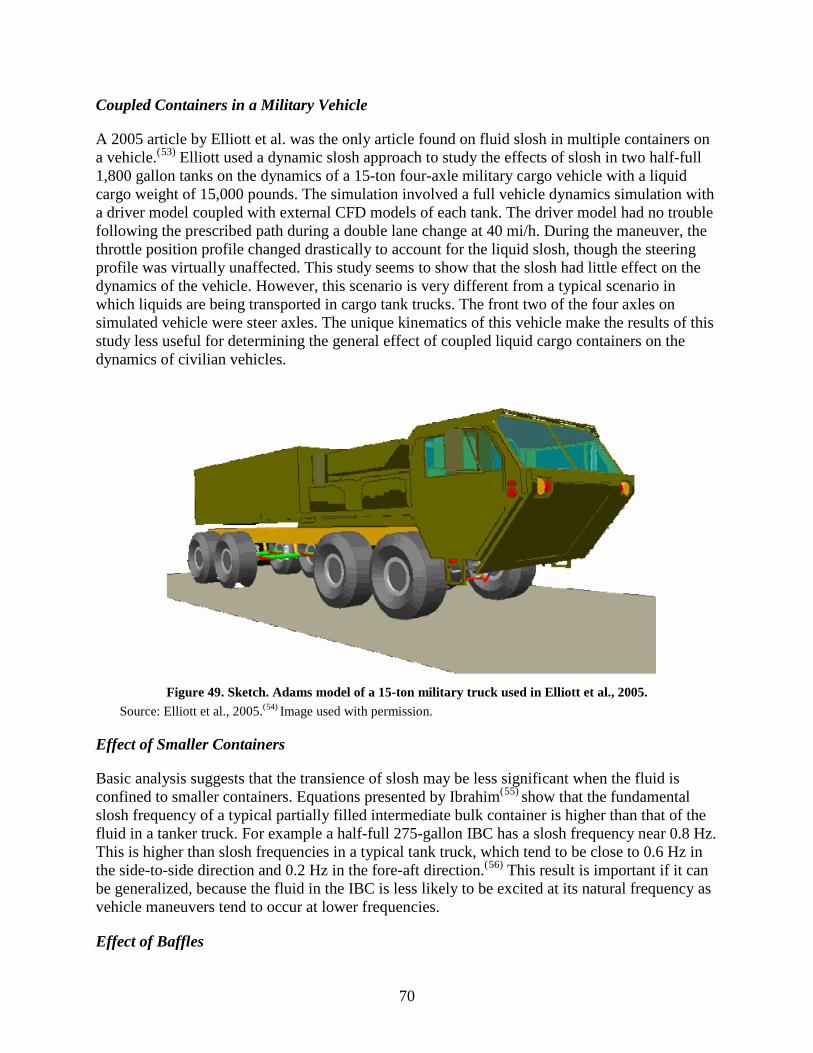
70

Coupled Containers in a Military Vehicle

A 2005 article by Elliott et al. was the only article found on fluid slosh in multiple containers on a vehicle.(53) Elliott used a dynamic slosh approach to study the effects of slosh in two half-full 1,800 gallon tanks on the dynamics of a 15-ton four-axle military cargo vehicle with a liquid cargo weight of 15,000 pounds. The simulation involved a full vehicle dynamics simulation with a driver model coupled with external CFD models of each tank. The driver model had no trouble following the prescribed path during a double lane change at 40 mi/h. During the maneuver, the throttle position profile changed drastically to account for the liquid slosh, though the steering profile was virtually unaffected. This study seems to show that the slosh had little effect on the dynamics of the vehicle. However, this scenario is very different from a typical scenario in which liquids are being transported in cargo tank trucks. The front two of the four axles on simulated vehicle were steer axles. The unique kinematics of this vehicle make the results of this study less useful for determining the general effect of coupled liquid cargo containers on the dynamics of civilian vehicles.

Figure 49. Sketch. Adams model of a 15-ton military truck used in Elliott et al., 2005.

Source: Elliott et al., 2005.(54) Image used with permission.

Effect of Smaller Containers

Basic analysis suggests that the transience of slosh may be less significant when the fluid is confined to smaller containers. Equations presented by Ibrahim(55) show that the fundamental slosh frequency of a typical partially filled intermediate bulk container is higher than that of the fluid in a tanker truck. For example a half-full 275-gallon IBC has a slosh frequency near 0.8 Hz. This is higher than slosh frequencies in a typical tank truck, which tend to be close to 0.6 Hz in the side-to-side direction and 0.2 Hz in the fore-aft direction.(56) This result is important if it can be generalized, because the fluid in the IBC is less likely to be excited at its natural frequency as vehicle maneuvers tend to occur at lower frequencies.

Effect of Baffles

71

Numerous studies have shown that baffles, annular discs within tanks, are effective at reducing the ratio of peak transient slosh force to quasi-static slosh force. Modaressi-Tehrani, Rakheja, and Stiharu showed that the addition of baffles reduced this ratio from 2.0 to 1.3 during braking.(57) D’Alessandro went a step further to study the effect of baffles on stopping distance.(58) He found that slosh in a clean-bore tank increased the stopping distance by 4.1 percent over an equivalent rigid load. Slosh in a tank with two baffles increased the stopping distance by only 2.4 percent and did not cause rear wheel lockup. A fully compartmentalized fluid will behave differently from fluid in a baffled tank, so these results cannot be extrapolated to aggregated separate containers.

Methods to Model Sloshing in Vehicles Numerous studies have been completed in the last half century on the topic of sloshing in liquid containers. Researchers have simulated the phenomenon using a variety of methods, each of which has strengths and weaknesses. These methods can be grouped into three general categories. These are

• Quasi-static liquid shifting.

• Dynamic mechanical analogy.

• Dynamic liquid sloshing.

Each of these categories has remained relevant and no one category stands out as an obvious favorite. Each of these types of methods is discussed in this section.

Quasi-Static Liquid Shifting

Numerous studies have evaluated the quasi-static effects of liquid cargo shifting on vehicle stability by neglecting transient liquid slosh. Under this assumption, the problem is reduced to a calculation of the location of the liquid’s center of gravity as a function of container acceleration. The main advantage of this method is its low computational cost and ease of implementation. While the quasi-static method has been proven effective at calculating the mean force exerted by the liquid during steady cornering,(59) it does not capture transient liquid forces, which are significant in some maneuvers. Many studies have compared quasi-static methods to dynamic methods by reporting the ratio of the peak transient force on the wetted tank surfaces to the force due to quasi-static liquid shifting. Modaressi-Tehrani, Rakheja, and Stiharu(60) found that the transient peak force was almost twice that in the quasi-static analysis. Yan’s 2008 study found a transient to quasi-static ratio of approximately 1.4.(61) Yan also noted that during a steady lateral acceleration event, the fluid force tends to oscillate for a long duration with a low rate of decay, as in Figure 50. This oscillation, which would not be represented in a quasi-static model, would impart lateral forces on the vehicle for long durations.

72

Figure 50. Plot. Time history of the roll moment of the liquid cargo sloshing within the 50 percent volume-

filled tank under ay = 0.3 g, together with the quasi-static roll moment. Source: Yan, 2008.(62)

The advantages of the quasi-static method are its convenience and low cost. However, its inability to represent transient slosh makes it appropriate only when transient slosh forces can be neglected.

Dynamic Mechanical Analogy

Equivalent mechanical models such as pendulums or mass-spring systems have been used to capture some of the transience of the liquid without adding excessive complexity to the model. In this method, the parameters of the mechanical system are tuned such that the system behaves dynamically similar to fluid in a tank. The method captures the transience of the liquid center of gravity shift but does not capture other dynamics of liquid sloshing.

Mechanical models representing slosh in rectangular, upright cylindrical, and elliptical containers were first developed in the 1960s by Abramson(63) for spacecraft applications, and discussed in numerous references (see references 64, 65, 66, 67, and 68). In 1993, Ranganathan et al.(69) integrated a two-dimensional pendulum model into a full vehicle model to study the effect of lateral slosh during steady cornering. Ranganathan compared the results to those of a quasi-static fluid model and showed that the pendulum oscillates about the quasi-static location at the natural frequency of the liquid. In 2003, Aliabadi Johnson, and Abedi(70) compared the results obtained using a very simple mechanical pendulum method to the results using non-linear CFD. The two models agreed well for low-to-moderate fill levels during a steady cornering maneuver. As the fill level approached 50 percent, the amplitude and frequency of the slosh oscillations differed significantly between the two methods. In 2012, Godderidge, Turnock, and Tan et al.(71) presented and validated a modified pendulum method that he referred to as the “Rapid Sloshing Model.” He validated this model by simulating partially filled rectangular tanks periodically excited at frequencies near the first sloshing mode. Results of the model matched computational dynamic methods typically within 5–10 percent for both magnitude and frequency. He also noted that runtimes were extremely short, approximately 0.1 percent of real time on a desktop computer.

0 5 10 15 200

1000

2000

3000

4000

5000

6000

7000

Time (s)

Late

ral F

orce

(N)

TransientQuasi-Static

73

Mechanical analogy methods are a good option if some error can be tolerated in the transient solution. The method is relatively easy to implement and the equations are already well established. Model parameters are available from several sources for rectangular containers such as IBCs.(72,73) Ibrahim(74) has also published analytical methods for determining the parameters for containers of various other shapes. It should be noted that the mechanical analogy method is generally only used to model slosh during lateral vehicle maneuvers. This is because simple models (e.g., a single pendulum) are unable to capture the large liquid displacement that occurs in tank trucks during longitudinal maneuvers. For the case of aggregated liquid containers which have similar lateral and longitudinal dimensions, it is likely that a pendulum can represent slosh in both directions.

There was some question whether a simplified pendulum formulation could handle the vertical rectangular geometries that needed to be addressed in this project. Work by Love and Tait(75) used an equivalent linearized mechanical model to represent fluid sloshing in a rectangular tank. The method computes the natural frequencies and mode shapes of the sloshing fluid, which define the velocity potential and wave height as functions of a time in generalized coordinates. The frequency response of the model was validated against shaker table data and exhibited excellent agreement. However, the work addresses some concern about the validity of this approach to linear modeling. In actuality, nonlinear effects will be present and will govern the character of the liquid, at times. Such nonlinear effects might be described in terms of those which arise primarily as a consequence of the geometry of the container and are apparent even for rather small amplitudes of excitation and liquid response. In such cases, the approach of using a linear approach may not be applicable.

There have been nonlinear studies of sloshing, which are reviewed in Ibrahim, Pilipchuk, and Ikeda(76) and Ibrahim.(77) More recently, Ikeda et al.(78,79) examined the nonlinear sloshing response of partially filled squared tanks to horizontal sine wave and random excitation. The nonlinear behavior was represented by a nonlinear model using the linear eigenfunctions as a basis, a method that involves building up the complete liquid motion from several simple components. Chaotic, nonlinear behavior was present under some excitations, which was shown by mathematical examination of the Lyapunov exponents. In 2013, Ikeda, Harata, and Ibrahim(80) showed the linear amplitude response was compared to the nonlinear solution, showing substantial differences between the two. Nonlinear predictions were favorably compared to experiments.

Vertical tanks of rectangular cross section, which are similar to some types of IBCs, have been analyzed by Love and Tait(81) and by Ikeda et al.(82,83) Love and Tait found excellent agreement with experiments in steady-state, forced vibration motions. The nonlinear analyses of Ikeda et al. agreed with experiments.

Dynamic Liquid Sloshing

Dynamic liquid sloshing models have become more widely used in recent years. Though the method has been used for decades, the recent availability of substantial computing power has made this method faster, more accurate, and overall more practical for simulating fluid dynamics than it was in the past. Many studies have validated computational dynamic liquid sloshing methods against experimental results and reported very high accuracy. In 2008, Yan(84) validated

74

a liquid tank model at a variety of fill levels and excitations and reported only small deviations in the reaction forces and moments of less than 8 percent. He noted that the natural frequency of the tank showed agreement as well. In 2002, Wendel, Green, and Burkey(85) used a computational dynamic method to simulate slosh in a tank with excitations representing typical vehicle maneuvers and also found agreement during experimental validation.

The difficulty in using a dynamic liquid sloshing approach to study slosh in vehicles is coupling the slosh model with the vehicle model. One of the earliest studies to do this was that of Bohn, Butler, Dunkle, and Eshleman(86) in 1981, which coupled a vehicle model with a linear dynamic liquid slosh model. The model, though it captured dynamics, was highly simplified and involved a course fluid mesh with a simple analytical solution for each fluid element. The simplicity of this model allowed it to be easily solved simultaneously with a simple vehicle model. However, they found that some of the assumptions used to simplify the fluid model broke down during maneuvers that approached the vehicle’s stability limits. Because of this and other issues, Bohn’s model was only qualitatively useful. Accurate results would require a more sophisticated slosh model.

Sophisticated dynamic slosh models cannot be solved in closed form; that is, they cannot be written as an equation with the motion on one side of the equals sign (=) and all the inputs on the other side. Therefore, modern methods use computational approximations to find solutions. Computational models are usually developed using commercial CFD software. Typical CFD software does not offer the flexibility to include a vehicle model easily. Some software allows for user-defined functions to be written, which can read outputs from the fluid model and compute new inputs during run time. Cheli et al.(87) and D’Alessandro(88) used this feature by developing a simple vehicle model and coupling it with commercial CFD software FLUENT, using user-defined functions. This method has the disadvantage that the vehicle model must be developed and validated. Also, it would be difficult to accurately model the more nonlinear systems such as the tires and shock absorbers. Furthermore, it does not allow for a closed-loop driver model, which is valuable when studying vehicle handling and stability.

Some researchers, such as Sankar et al.(89) and Rumold(90) proposed methods which couple a mechanical subsystem model with a fluid subsystem model without requiring that the two subsystems be solved in the same simulation environment. Elliott et al.(91) built on this method and used it to link a highly sophisticated vehicle simulation software called Adams with a modern CFD software called Dytran. The result was a fully coupled tank truck simulation that used state-of-the-art models for both the vehicle and the fluid. The method was not easy to implement since vehicle simulations and fluid simulations are generally solved using very different methods. Vehicle simulations use an implicit method in which time within the simulation is virtually continuous, whereas fluid simulations use an explicit method in which the simulation time is broken into discrete instants. In order to pass variables between the two simulations, Elliott developed “glue code,” which handles the exchange of data between the two solvers. This process has come to be known as co-simulation and is illustrated in Figure 51. More recently, Barton et al.(92) has demonstrated the same method using software developed by Altair.

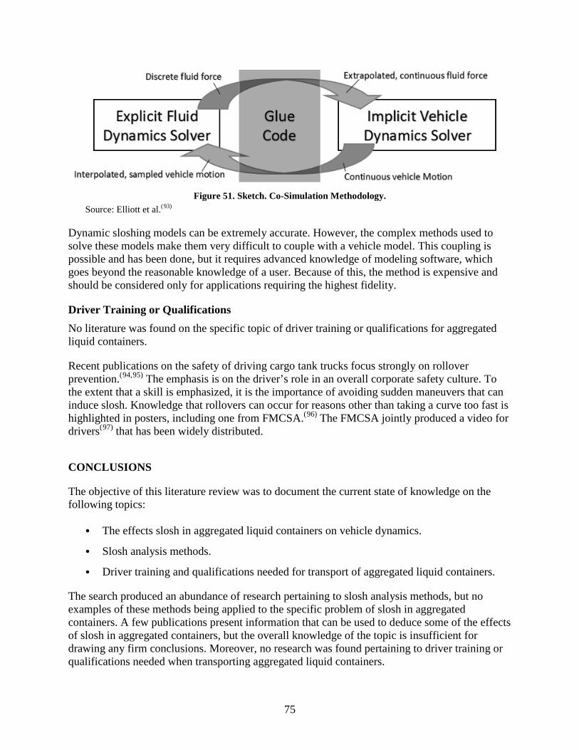
75

Figure 51. Sketch. Co-Simulation Methodology.

Source: Elliott et al.(93)

Dynamic sloshing models can be extremely accurate. However, the complex methods used to solve these models make them very difficult to couple with a vehicle model. This coupling is possible and has been done, but it requires advanced knowledge of modeling software, which goes beyond the reasonable knowledge of a user. Because of this, the method is expensive and should be considered only for applications requiring the highest fidelity.

Driver Training or Qualifications No literature was found on the specific topic of driver training or qualifications for aggregated liquid containers.

Recent publications on the safety of driving cargo tank trucks focus strongly on rollover prevention.(94,95) The emphasis is on the driver’s role in an overall corporate safety culture. To the extent that a skill is emphasized, it is the importance of avoiding sudden maneuvers that can induce slosh. Knowledge that rollovers can occur for reasons other than taking a curve too fast is highlighted in posters, including one from FMCSA.(96) The FMCSA jointly produced a video for drivers(97) that has been widely distributed.

CONCLUSIONS

The objective of this literature review was to document the current state of knowledge on the following topics:

• The effects slosh in aggregated liquid containers on vehicle dynamics.

• Slosh analysis methods.

• Driver training and qualifications needed for transport of aggregated liquid containers.

The search produced an abundance of research pertaining to slosh analysis methods, but no examples of these methods being applied to the specific problem of slosh in aggregated containers. A few publications present information that can be used to deduce some of the effects of slosh in aggregated containers, but the overall knowledge of the topic is insufficient for drawing any firm conclusions. Moreover, no research was found pertaining to driver training or qualifications needed when transporting aggregated liquid containers.

76

Despite the lack of previous research on slosh in aggregated containers, this literature review has been useful in two ways:

• It confirmed the gap in knowledge related to transport of aggregated liquid containers.

• It has been successful in identifying and evaluating potential slosh analysis methods to be used later in this project.

Each of the three analysis methods discussed in Section 4.2 has specific advantages. In particular, the equivalent mechanical model offers moderate accuracy combined with fast preparation and execution times, and the dynamic models offer high accuracy but at the expense of long preparation and execution times. This suggests that the latter method is most appropriate for critical cases where accuracy is most important, and the former for less critical cases. For instance, the equivalent mechanical model may be helpful in large parameter studies to identify the conditions of concern, and the dynamic sloshing models may be helpful in assessing those conditions.

77

APPENDIX B: DISTANCE AT A RED LIGHT Stopping sight distance is the total distance travelled by a vehicle in the process of bringing it to a complete stop and is an important factor for geometric layout of roads and many traffic engineering applications. In the context of designing traffic signal timing, stopping sight distance is widely applied to determine the boundary of the indecision zone (also known as dilemma zone) of an intersection approach, as shown in Figure 52. Other methods used in determining the indecision zone are the distance from stop line method, which considers the distance from the stop bar where 90th and 10th percentiles of drivers would stop as the beginning and end of the indecision zone respectively, and the travel time method, which defines the beginning and end of the indecision zone as the 5 and 2 seconds of the travel time to the stop bar regardless of the vehicle speeds. The ranges by these methods are shown graphically in Figure 53.

As defined by the American Association of State Highway and Transportation Officials (AASHTO),(98) stopping sight distance has two components: brake reaction distance, which is the distance traveled during the perception-reaction time, and braking distance, which is the distance traveled from the moment the brakes were applied until the vehicle comes to a complete stop. AASHTO provides the brake reaction distances, braking distances, and the stopping sight distances of vehicles for different design speeds in its Table 3-1. The braking distance on level pavement for 35 mi/h is 118 feet. AASHTO observed that trucks would take longer to stop than this distance for light vehicles, but this effect is compensated by truck drivers’ better view.

From Figure 52, then, the indecision zone at 35 mi/h ranges roughly from 100 to 250 feet; the actual minimum allowance for braking distance from AASHTO is 118 feet.(99)

Figure 52. Sketch. Indecision zone boundaries on a typical intersection approach

Source: Koonce et al, 2008.(100)

78

Figure 53. Graph. Distance to the beginning and end of the indecision zone.

Source: Koonce et al, 2008.(101)

If a vehicle stops from 35 mi/h over a distance of 118 feet with a uniform deceleration, the deceleration is approximately 3.5 gravitational units. Hobbs(102) says that the braking rate when coming to a stop is typically 3.6 gravitational units and that higher braking rates cause discomfort.

79

APPENDIX C: DEVELOPING THE PENDULUM MODEL Running many simulations of different cases was made possible by a simplified model of the sloshing fluid. This model can predict the sloshing forces with considerably less calculation than can a CFD model. The predictions of this model were compared with the predictions of the corresponding CFD model in several cases to confirm that this model is adequate for the task.

OVERVIEW

The method used to model slosh was based on the method presented by Ibrahim in Liquid Sloshing Dynamics, Chapter 5.(103) A series of masses is used to represent the liquid in a container. The first mass is stationary and represents the mass at the bottom of the container that remains still with respect to the container even when other liquid in the container is sloshing. The subsequent masses swing on pendulums. The pendulum masses and pendulum lengths are calculated such that the frequency and amplitude of the reaction force at the pendulum hinge is equal to that of the dynamic force the liquid exerts on the walls of the container. In order to simulate sloshing, a minimum of two masses must be used, one stationary mass and one pendulum. This minimal configuration is enough to simulate the first slosh mode. Any number of additional pendulum masses can be added to simulate additional modes. However, the containers used in this study are shaped in such a way that the slosh response is dominated by the first mode and hardly affected by the subsequent modes. Preliminary simulations indicated negligible difference when subsequent modes were simulated. For this reason, the final simulations included only two masses—one fixed and one swinging.

PARAMETER EVALUATION

The pendulum model and its associated parameters are illustrated in Figure 54.

80

Figure 54. Sketch. Pendulum model used to simulate sloshing in a rectangular tank.

The parameters shown in Figure 54 were calculated as follows:

Figure 55. Equations for pendulum model parameters.

where

𝑏𝑏 is the tank breadth,

81

a is the tank width,

𝐼𝐼𝐹𝐹 is the moment of inertia of the sloshing fluid,

ρ is the density of the liquid,

n is the number of the pendulum (always 1 in the final simulations).

SPHERICAL PENDULUM

The model above is typically implemented as a one-dimensional pendulum that rotates about a single axis (e.g., a child swinging). In this study, the pendulum model was implemented as a two-dimensional pendulum. A two-dimensional pendulum is free to rotate about any axis passing through the pendulum’s upper attachment point. The two-dimensional pendulum can be thought of as being attached through a spherical joint.

A two-dimensional pendulum free to swing in any direction essentially models a cylindrical container. In the maneuvers of this project, the accelerations in the axis normal to the main input are minimal. In these cases, representation is valid for a rectangular container of appropriate size. More complicated maneuvers, including steering while braking, would require a more sophisticated model. The footprint of an IBC is not exactly square—nominal dimensions are 40 by 48 inches. The pendulum model is adjusted slightly so that it best matches dimension in the primary direction of fluid motion.

PENDULUM EQUATIONS OF MOTION

The two degrees of freedom of a two dimensional pendulum are psi (Ѱ) and theta (ϴ). The motion that they represent physically is shown in Figure 56. Psi is the angle between the pendulum and the vertical, and theta is the azimuth of the angle of motion, projected in the horizontal x-y plane.

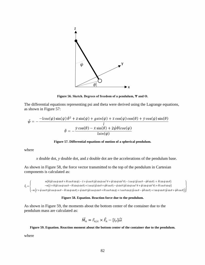
82

Figure 56. Sketch. Degrees of freedom of a pendulum, Ѱ and ϴ.

The differential equations representing psi and theta were derived using the Lagrange equations, as shown in Figure 57:

Figure 57. Differential equations of motion of a spherical pendulum.

where

x double dot, y double dot, and z double dot are the accelerations of the pendulum base.

As shown in Figure 58, the force vector transmitted to the top of the pendulum in Cartesian components is calculated as:

Figure 58. Equation. Reaction force due to the pendulum.

As shown in Figure 59, the moments about the bottom center of the container due to the pendulum mass are calculated as:

Figure 59. Equation. Reaction moment about the bottom center of the container due to the pendulum.

where

y

z

x

83

𝑟𝑟𝑛𝑛/𝑐𝑐 (vector variable r sub n/c) is the location of the top of the nth pendulum relative to the bottom center of the container, [IF] is the moment of inertia matrix of the sloshing fluid, and 𝜔𝜔��⃗ ̇ (single dotted vector variable w) is the angular acceleration of the container.

As shown in Figure 60, the reaction force due to the stationary liquid is calculated as:

Figure 60. Equation. Reaction force due to the stationary mass.

The moments about the bottom center of the container due to the stationary mass are calculated as shown in Figure 61:

Figure 61. Equation. Reaction moment about the bottom center of the container due to the stationary mass.

where

𝑟𝑟0/𝑐𝑐 (r sub zero c) is the location of the stationary mass relative to the bottom center of the container, and [I0] is the moment of inertia matrix of the stationary mass.

As shown in Figure 62 and Figure 63, the total force and moment at the bottom center of the container are:

Figure 62. Equation. Combined reaction moment of pendulum and stationary mass.

and

Figure 63. Equation. Combined reaction force of pendulum and stationary mass.

CORROBORATING THE MODEL WITH CFD

CFD simulations were used to confirm that this model is producing adequate predictions of the slosh forces. The most extreme cases are shown below in Figure 64, Figure 65, Figure 66, Figure 67, Figure 68, and Figure 69. These extreme cases have the weakest correlation with the CFD since the liquid sloshing is very complex. These extreme cases show acceptable correlation. The correlation is much stronger in more moderate cases.

84

Figure 64. Graphs. Reaction forces (left) and moments summed at the bottom of the container (right)

generated by the pendulum model (solid lines) and the CFD model (dashed lines) of a 275-gallon IBC while braking to a stop from 55 mi/h in 140 feet.

Figure 65. Graphs. Reaction forces (left) and moments (right) generated by the pendulum model (solid lines) and the CFD model (dashed lines) of a 275-gallon IBC while on a 575-foot radius exit ramp at 55 mi/h with a

lateral acceleration of 0.35 gravitational units.

Figure 66. Graphs. Reaction forces (left) and moments (right) generated by the pendulum model (solid lines)

and the CFD model (dashed lines) of a 275-gallon IBC while performing a 12-foot lane change at 55 mi/h with a lateral acceleration of 0.5 gravitational units.

85

Figure 67. Graphs. Reaction forces (left) and moments summed at the bottom of the container (right)

generated by the pendulum model (solid lines) and the CFD model (dashed lines) of a 550-gallon IBC while braking to a stop from 55 mi/h in 140 feet.

Figure 68. Graphs. Reaction forces (left) and moments (right) generated by the pendulum model (solid lines) and the CFD model (dashed lines) of a 550-gallon IBC while on a 575-foot radius exit ramp at 55 mi/h with a

lateral acceleration of 0.35 gravitational units.

Figure 69. Graphs. Reaction forces (left) and moments (right) generated by the pendulum model (solid lines)

and the CFD model (dashed lines) of a 550-gallon IBC while performing a 12-foot lane change at 55 mi/h with a lateral acceleration of 0.5 gravitational units.

The pendulum model does not represent rotation about the vertical axis well. The yaw moment about the container’s center calculated by the pendulum model is not a good match with the CFD calculation. However, the yaw moment of the fluid itself contributes only a small amount to the

86

cargo’s yaw moment on the vehicle. Most of the fluid’s yaw moment contribution comes from its position away from the vehicle’s center. The model is adequate for the purpose.

INTEGRATION WITH TRUCKSIM

The dynamic inputs to the model are the acceleration of the pendulum base: x double dot, y double dot, and z double dot. The pendulum model was coded in Simulink and coupled with TruckSim such that these inputs could be passed from TruckSim to Simulink at the beginning of each simulation time increment. The accelerations passed to the pendulum model corresponded to the location within the vehicle of the tank represented by that pendulum.

The models in the simulations had two, three, or four IBCs on every truck. Each of these IBCs was represented by a separate pendulum model, so there were always at least two such pendulums in every simulation. At every time step during the maneuver, the equations for the pendulums were solved independently. Because the IBCs were positioned away from the truck’s center of gravity, the forces from each IBC generated a moment. The forces and moments from the pendulum models resolved and passed to the TruckSim model as a single resultant vector of three forces and three moments applied at the truck’s center of gravity.

87

APPENDIX D: DEVELOPING THE COMPUTATIONAL FLUID DYNAMICS MODELS

The research team used a widely accepted commercially available CFD model for this project. The primary use of the model was to corroborate the simplified pendulum model described in this appendix. The CFD model was also used to calculate the slosh in the single 1,100-gallon cargo tank, which was too complicated for the pendulum model.

The CFD model itself has been validated through its use in industry and academia; the models were validated by comparison with smaller elements and time steps.

The commercial CFD code Star CCM+ was used for this project. It is a finite volume code and is well validated against experimental data. It was selected in part for its ability to model free surface flows, its ease of meshing, and its ease of inputting time-dependent parameters such as accelerations.

Three different geometries were simulated for this project, and they correspond to the 275- and 550-gallon IBCs, and a representative 1,100-gallon cylindrical cargo tank. The baseline computational mesh was created using a Cartesian mesh (also called trim, or cutcell) with an average edge length of 1 inch. This yields between 140,000 cells for the 275-gallon IBC and 370,000 cells for the 1,100-gallon cargo tank. Each simulation started with the tanks half full of liquid water with a density of 997.5 kg/m3 and a viscosity of 0.001 Pa-s. Air was simulated as an isothermal ideal gas with a density of 1.177 kg/m3 and a viscosity of 1.85508E-5 Pa-s. The baseline time step used in each analysis was 0.005 seconds, yielding 2,000 time steps per 10 seconds of simulated time.

The inputs to the CFD model were determined by first running the truck model through one of the maneuvers. The six accelerations (three linear and three rotational) at the bottom center of the container location were recorded. The acceleration was applied to the CFD model as a body force, just as gravity is applied. A sample plot for the lane change maneuver is shown in Figure 70. The tank rotation was not significant in the stopping maneuver and was ignored in the simulation.

88

Figure 70. Graph. Sample acceleration profile used in a lane change maneuver.

The forces on the tank walls and the moments on the tank walls about the centroid of the tank bottom were recorded throughout the run. These values were used in validation of the pendulum model. For the 1,100-gallon cylindrical tank, they were also used in the analysis because the pendulum model could not be used for this case.

Each time step converged over the course of 20 inner iterations. This was more than enough iterations for the forces to converge at each time step. Mesh and time step independent studies for several scenarios and tank sizes were completed and showed that the baseline mesh size and time step were sufficient to capture the peak force and moment, as well as subsequent peaks in most cases. Figure 71 shows the forces in the later (side-to-side) direction for a 275-gallon IBC in a lane change maneuver with various settings. Note that the variations in the force exhibited on the tank walls are minor. Similar mesh refinement and time step refinement studies were conducted for the 550-gallon IBC and 1,100-gallon cylindrical tank in more severe stopping conditions. Figure 72 shows a comparison of the water interface from the baseline mesh and the refined mesh for the 1,100-gallon tank during a red light stop. Note that the interface is noticeably better resolved with the refined mesh; however, force monitors shown in Figure 73 indicate that the wall forces are captured equally well in both cases.

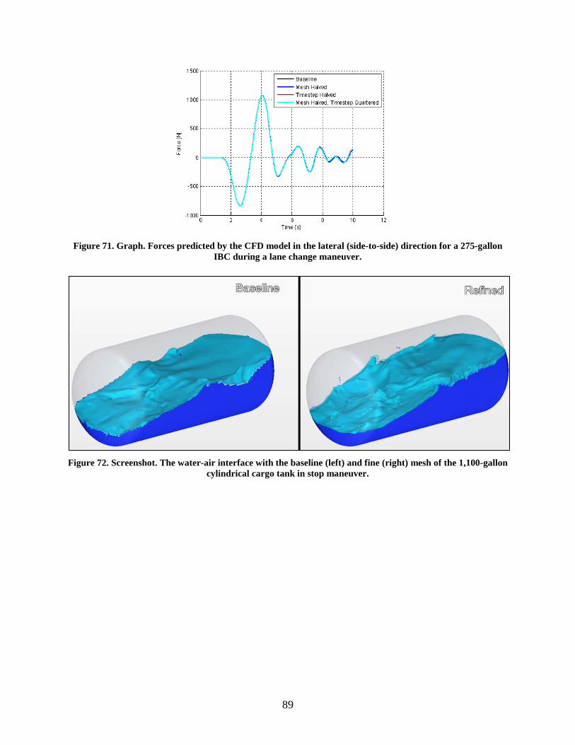
89

Figure 71. Graph. Forces predicted by the CFD model in the lateral (side-to-side) direction for a 275-gallon

IBC during a lane change maneuver.

Figure 72. Screenshot. The water-air interface with the baseline (left) and fine (right) mesh of the 1,100-gallon

cylindrical cargo tank in stop maneuver.

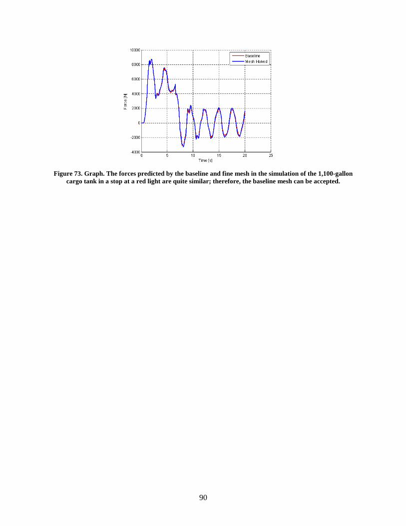
90

Figure 73. Graph. The forces predicted by the baseline and fine mesh in the simulation of the 1,100-gallon

cargo tank in a stop at a red light are quite similar; therefore, the baseline mesh can be accepted.

91

APPENDIX E: RESULTS OF THE SIMULATIONS The main text defined scalar metrics to summarize the result of every simulation case. The results were presented graphically for selected conditions. This appendix has the numerical results for more of the conditions that were simulated. Refer to Figure 5 to Figure 8 in the main text for descriptions of the IBC positions in the truck bed.

MANEUVER DEFINITIONS

The codes in these tables were used in the tables of results to identify the conditions of the maneuver.

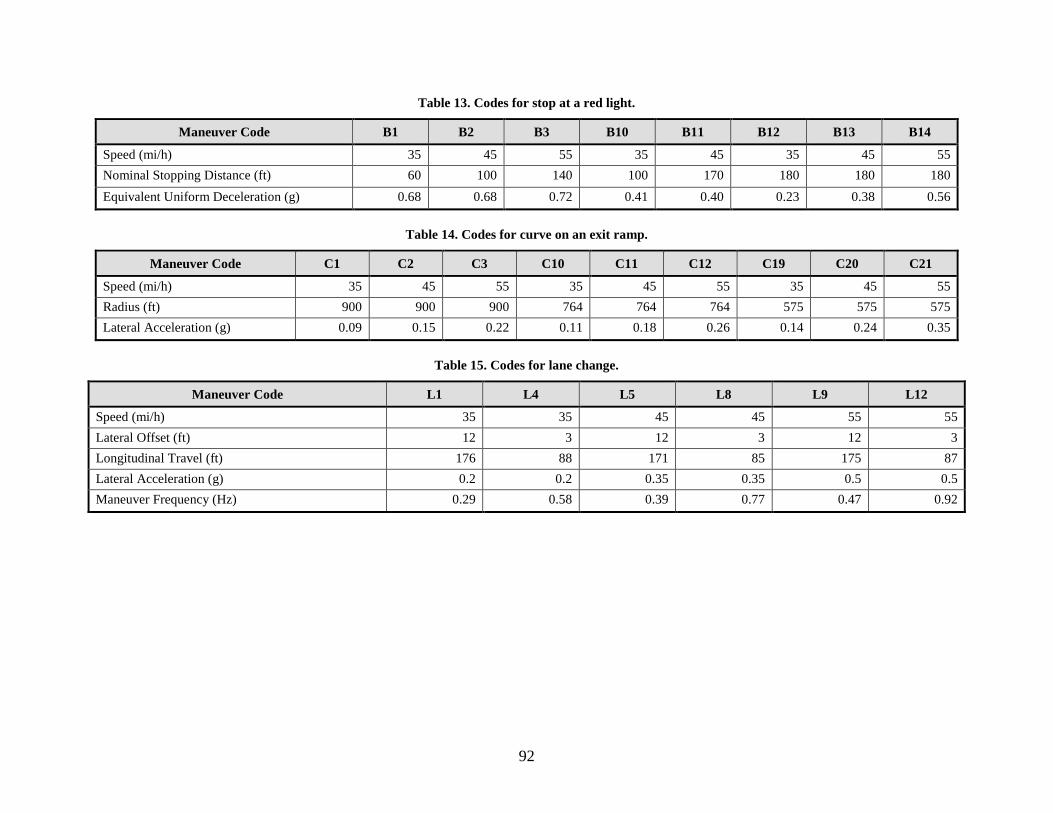
92

Table 13. Codes for stop at a red light.

Maneuver Code B1 B2 B3 B10 B11 B12 B13 B14

Speed (mi/h) 35 45 55 35 45 35 45 55 Nominal Stopping Distance (ft) 60 100 140 100 170 180 180 180 Equivalent Uniform Deceleration (g) 0.68 0.68 0.72 0.41 0.40 0.23 0.38 0.56

Table 14. Codes for curve on an exit ramp.

Maneuver Code C1 C2 C3 C10 C11 C12 C19 C20 C21

Speed (mi/h) 35 45 55 35 45 55 35 45 55 Radius (ft) 900 900 900 764 764 764 575 575 575 Lateral Acceleration (g) 0.09 0.15 0.22 0.11 0.18 0.26 0.14 0.24 0.35

Table 15. Codes for lane change.

Maneuver Code L1 L4 L5 L8 L9 L12

Speed (mi/h) 35 35 45 45 55 55 Lateral Offset (ft) 12 3 12 3 12 3 Longitudinal Travel (ft) 176 88 171 85 175 87 Lateral Acceleration (g) 0.2 0.2 0.35 0.35 0.5 0.5 Maneuver Frequency (Hz) 0.29 0.58 0.39 0.77 0.47 0.92

93

STOP AT A RED LIGHT

Table 16. Stopping distance (ft).

Maneuver Code/Cargo

Type B1

Liquid B1

Rigid B2

Liquid B2

Rigid B3

Liquid B3

Rigid B10

Liquid B10

Rigid B11

Liquid B11

Rigid B12

Liquid B12

Rigid B13

Liquid B13

Rigid B14

Liquid B14

Rigid

550s both rear

58 58 94 94 138 138 103 103 167 167 183 183 184 184 154 154

550s both front

65 61 105 98 153 142 104 103 167 167 183 183 184 184 155 154

550s left side 66 65 107 105 154 154 104 103 167 167 183 183 184 184 154 154

550s opposite

56 56 88 89 129 130 104 103 167 167 183 183 184 184 154 154

275s corners 56 55 90 88 130 128 103 103 167 167 183 183 184 185 154 154

275s left side 65 65 106 105 156 155 104 103 167 167 183 183 184 185 154 154

Mixed, left side

67 65 107 105 156 155 103 103 167 167 183 183 184 184 154 154

Mixed, 3 corners

60 59 97 96 140 141 103 103 167 167 183 183 184 184 154 154

Table 17. Slosh amplitude (lb).

Maneuver Code/Cargo Type B10 Liquid B11 Liquid B12 Liquid B13 Liquid B14 Liquid

1,100 centered 743 -- -- -- -- 550s both rear 259 269 174 246 343 550s both front 225 239 175 233 315 550s left side 238 250 170 243 316 550s opposite 236 247 184 240 316 275s corners 479 482 355 467 679 275s left side 466 482 353 467 689 Mixed, left side 360 361 263 353 490 Mixed, 3 corners 365 366 268 355 492

94

CURVE ON AN EXIT RAMP

Table 18. Peak slosh force.

Maneuver Code C1 C1 C2 C2 C3 C3 C10 C10 C11 C11 C12 C12 C19 C19 C20 C20 C21 C21

1,100 centered -- -- -- -- -- -- -- -- 879 840 -- -- -- -- -- -- -- --

550s both rear 434 435 731 733 1,128 1,128 510 511 863 866 1,327 1,325 670 673 1,145 1,146 1,762 1,769

550s both front 1,424 426 1,399 708 1,369 1,067 1,424 499 1,399 830 1,369 1,251 1,424 656 1,399 1,099 1,667 1,672

550s left side 1,169 695 1,149 719 1,131 1,093 1,169 695 1,149 846 1,291 1,282 1,168 695 1,149 1,121 1,728 1,718

550s opposite 1,233 429 1,214 718 1,189 1,091 1,233 503 1,214 844 1,278 1,279 1,233 663 1,213 1,117 1,707 1,711

275s corners 728 433 723 723 1,104 1,099 728 507 848 850 1,291 1,289 7,28 668 1,122 1,126 1,761 1,724

275s left side 907 541 891 724 1,133 1,099 907 541 891 851 1,285 1,288 908 669 1,144 1,128 1,737 1,727

Mixed, left side 1,010 433 993 725 1,136 1,104 1,010 508 993 853 1,287 1,295 1,010 669 1,148 1,130 1,745 1,733

Mixed, 3 corners 1,014 431 996 721 1,118 1,096 1,013 506 996 848 1,281 1,285 1,013 666 1,131 1,123 1,727 1,720

Table 19. Steady-state load transfer ratio.

Maneuver Code/ Cargo Type

C1 Liquid

C1 Rigid

C2 Liquid

C2 Rigid

C3 Liquid

C3 Rigid

C10 Liquid

C10 Rigid

C11 Liquid

C11 Rigid

C12 Liquid

C12 Rigid

C19 Liquid

C19 Rigid

C20 Liquid

C20 Rigid

C21 Liquid

C21 Rigid

550s both rear

0.17 0.15 0.28 0.27 0.43 0.41 0.20 0.18 0.33 0.32 0.51 0.50 0.26 0.25 0.45 0.44 0.70 0.69

550s both front

0.10 0.10 0.17 0.17 0.27 0.26 0.12 0.12 0.21 0.20 0.32 0.31 0.16 0.16 0.28 0.28 0.44 0.43

550s left side

0.34 0.33 0.43 0.42 0.55 0.53 0.36 0.36 0.47 0.46 0.61 0.60 0.42 0.41 0.57 0.56 0.76 0.74

550s opposite

0.13 0.12 0.21 0.21 0.33 0.32 0.15 0.14 0.25 0.25 0.39 0.38 0.20 0.20 0.35 0.34 0.54 0.53

275s corners

0.12 0.11 0.20 0.19 0.31 0.30 0.14 0.14 0.24 0.23 0.37 0.36 0.19 0.18 0.33 0.32 0.51 0.49

275s left side

0.34 0.33 0.42 0.41 0.53 0.52 0.36 0.35 0.46 0.45 0.59 0.58 0.41 0.40 0.55 0.54 0.73 0.71

Mixed, left side

0.36 0.24 0.45 0.33 0.57 0.44 0.38 0.26 0.50 0.37 0.64 0.51 0.44 0.31 0.59 0.46 0.79 0.66

Mixed, 3 corners

0.22 0.22 0.31 0.30 0.42 0.42 0.25 0.24 0.35 0.35 0.49 0.48 0.30 0.29 0.45 0.44 0.63 0.62

95

LANE CHANGE

Table 20. Peak lateral slosh force (lb).

Maneuver Code/Cargo Type

L1 Liquid

L1 Rigid

L4 Liquid

L4 Rigid

L5 Liquid

L5 Rigid

L8 Liquid

L8 Rigid

L9 Liquid

L9 Rigid

L12 Liquid

L12 Rigid

1,100 centered -- -- -- -- 1,961 1,405 -- -- -- -- -- --

550s both rear 954 901 810 626 1,962 1,811 1,242 1,013 4,062 3,668 1,595 1,420

550s both front 803 765 601 464 1,381 1,304 848 612 2,478 2,217 1,071 748

550s left side 837 780 559 461 1,498 1,416 839 707 2,858 2,554 1,237 966

550s opposite 811 778 557 460 1,532 1,424 875 707 2,841 2,572 1,231 970

275s corners 825 776 617 454 1,615 1,412 977 696 2,925 2,577 1,345 956

275s left side 838 778 624 458 1,590 1,405 991 699 3,041 2,522 1,422 953

Mixed, left side 857 799 629 485 1,626 1,485 982 757 3,079 2,753 1,394 1,045

Mixed, 3 corners 824 778 578 458 1,562 1,413 926 701 2,919 2,548 1,332 961

Table 21. Peak load transfer ratio.

Maneuver Code/Cargo Type

L1 Liquid

L1 Rigid

L4 Liquid

L4 Rigid

L5 Liquid

L5 Rigid

L8 Liquid

L8 Rigid

L9 Liquid

L9 Rigid

L12 Liquid

L12 Rigid

550s both rear 0.31 0.30 0.16 0.17 0.62 0.59 0.25 0.23 1.00 1.00 0.37 0.32

550s both front 0.24 0.23 0.17 0.16 0.39 0.38 0.24 0.22 0.66 0.61 0.29 0.28

550s left side 0.45 0.44 0.33 0.33 0.66 0.64 0.39 0.37 1.00 0.95 0.47 0.43

550s opposite 0.24 0.23 0.14 0.14 0.45 0.42 0.19 0.20 0.82 0.75 0.25 0.26

275s corners 0.23 0.22 0.14 0.14 0.42 0.39 0.19 0.19 0.75 0.67 0.25 0.25

275s left side 0.44 0.43 0.33 0.32 0.65 0.61 0.38 0.37 0.98 0.90 0.45 0.42

Mixed, left side 0.47 0.35 0.36 0.23 0.70 0.55 0.42 0.28 1.00 0.88 0.49 0.34

Mixed, 3 corners 0.34 0.33 0.23 0.22 0.55 0.51 0.29 0.26 0.92 0.82 0.37 0.31

96

Table 22. Peak yaw moment (1,000 ft-lb, or ft-kip).

Maneuver Code/Cargo Type

L1 Liquid

L1 Rigid

L4 Liquid

L4 Rigid

L5 Liquid

L5 Rigid

L8 Liquid

L8 Rigid

L9 Liquid

L9 Rigid

L12 Liquid

L12 Rigid

1,100 centered -- -- -- -- 10.11 7.25 -- -- -- -- -- --

550s both rear 15.9 14.8 13.01 12.22 29.46 27.35 18.90 18.77 53.51 52.27 26.18 26.46

550s both front 2.2 2.2 1.70 1.36 3.86 3.72 2.37 1.73 6.83 6.28 2.94 2.04

550s left side 7.1 6.5 6.25 5.79 13.66 12.34 9.61 9.38 27.90 26.20 13.80 14.18

550s opposite 6.9 6.5 6.52 5.80 13.54 12.32 9.79 9.44 27.82 26.20 8.49 14.10

275s corners 7.3 6.5 7.34 5.79 14.46 12.34 10.67 9.37 29.27 26.30 14.17 14.25

275s left side 6.8 5.9 5.38 4.71 12.57 10.81 8.17 7.46 23.82 21.44 11.42 11.12

Mixed, left side 9.1 8.1 7.06 6.63 16.71 15.00 10.71 10.52 31.84 29.74 15.42 15.46

Mixed, 3 corners 7.0 6.5 6.42 5.81 13.62 12.37 9.42 9.42 27.74 26.18 13.41 14.13

97

APPENDIX F: NOTES ON THE EXPERIMENTS This table has the load measured on all axle ends on the two trucks in the empty and as-tested conditions.

Table 23. Specifications of the two trucks.

Property Truck 1 Truck 2

Bed size (ft) 7-1/2 x 24 7-1/2 by 24

GVWR (lb) 25,500 25,500

Wheelbase (in.) 253 261

Rear axle to back of bed (in.) 108 102

Track width, measured on centers (in.)

Front: 80.7 Rear: 85.4

Front: 82.1 Rear: 85.0

Front axle loads, empty (lb) Left: 3,310 Total: 6,350 Right: 3,040

Left: 3,450 Total: 6,810 Right: 3,360

Rear axle loads, empty (lb) Left: 4,090 Total: 8,000 Right: 3,910

Left: 3,730 Total: 7,600 Right: 3,870

Total axle loads, empty (lb) Left: 7,400 Total: 14,350 Right: 6,950

Left: 7,180 Total: 14,410 Right: 7,230

Front axle loads, with IBCs, water, and two people (lb) Left: 3,690 Total: 7,300 Right: 3,610

Left: 2,670 Total: 5,220 Right: 2,550

Rear axle loads, with IBCs, water, and two people (lb) Left: 6,200 Total: 12,110 Right: 5,910

Left: 8,010 Total: 16,050 Right: 8,040

Total axle loads, with IBCs, water, and two people (lb) Left: 9,890 Total: 19,410 Right: 9,520

Left: 10,680 Total: 21,270 Right: 10,590

Containers Four 275-gallon poly Two 550-gallon stainless

98

[This page intentionally left blank.]

99

REFERENCES 1 76 FR 26890, May 9, 2011 2 49 CFR 383.5 3 49 CFR 171.8 4 49 CFR 178 Subpart N, §§178.705 to 178.710 5 Popov, G., Sankar, S., Sankar, T.S., Vatistas, G.H., “Liquid Sloshing in Rectangular Road Containers,” Computers Fluids, vol.21 no. 4, p. 551, 1992. 6 Winkler, C.B., D. Blower, R. Ervin, and R.M. Chalasani. Rollover of Heavy Commercial Vehicles. SAE International. 2000. 7 Koonce, P., Rodegerdts, L., Lee, K., Quayle, S., Beaird, S., Braud, C., Bonneson, J., Tarnoff, P. and Urbanik, T., 2008. Traffic signal timing manual (No. FHWA-HOP-08-024). (Available online at http://ops.fhwa.dot.gov/publications/fhwahop08024/fhwa_hop_08_024.pdf). 8 M. I. M. Azmi, M. N. A. Nordin, M. S. Mahmud, A. Putra, F. A. Munir, M. R. M. Zin, N. Razali, M. A. Shaharuzaman and N. R. M. Nuri, "Experimental Investigation on the Effect of Container Geometry Change to Liquid Sloshing," Applied Mechanics and Materials, vol. 165, pp. 160-164, 2012. 9 Ibid. 10 N. H. Abramson, "Dynamic behaviour of liquids in moving containers," National Aeronautics and Space Administration, Washington D.C., 1966. 11 S. Aliabadi, A. Johnson and J. Abedi, "Comparison of finite element and pendulum models for simulation of sloshing," Computers & Fluids, vol. 32, pp. 535-545, 2003. 12 M. Arafa, "Finite Element Analysis of Sloshing in Liquid-Filled Containers," Production Engineering & Design For Development, vol. 7, pp. 793-803, 2006. 13 Azmi et al., 2012. 14 M. S. Barton, D. Corson, J. Quigley, B. Emami and T. Kush, "Tanker Truck Sloshing Simulation Using Bi-Directinoally Coupled CFD and Multi-Body Dynamics Solvers," SAE Technical Paper, 2014. 15 H. F. Bauer, "On the Destabilizing Effect of Liquids in Various Vehicles," Vehicle System Dynamics: International Journal of Vehicle Mechanics and Mobility, vol. 1, no. 3-4, pp. 227-260, 1972. 16 M. Biglarbegian and J. W. Zu, "Tractor-semitrailer model for vehicles carrying liquids," Vehicle System Dynamics: International Journal of Vehicle Mechanics and Mobility, vol. 44, no. 11, pp. 871-885, 2006. 17 P. F. Bohn, M. C. Butler, H. D. Dunkle and R. L. Eshleman, "Computer Simulation of the Effect of Cargo Shifting on Articulated Vehicles Performing Braking and Cornering Maneuvers Volume 1, Executive Summary," Laurel, Maryland, 1981. 18 F. Cheli, V. D'Alessandro, A. Premoli and E. Sabbioni, "Simulation of Sloshing in Tank Trucks," International Journal Heavy Vehicle Systems, vol. 20, no. 1, pp. 1-18, 2013. 19 V. D'Alessandro, "Modeling of Tank Vehicle Dynamics By Fluid Sloshing Coupled Simulation," 2011. 20 F. T. Dodge, "Analytical representation of lateral sloshing by equivalent mechanical models," in The Dynamic Behavior of Liquids in Moving Containers, N. H. Abramson, Ed., Washington, D.C., NASA SP-106, 1966, p. 199. 21 F. T. Dodge, "Dynamics of Partially Filled Tanks," in Handbook of Fluid Dynamics and Fluid Machinery, A. E. Fuhs, Ed., Hoboken, John Wiley & Sons, Inc, 1996, p. 2776. 22 A. S. Elliott, "Status Update on Advanced, General-Purpose Co-Simulation with Adams," MSC Software, Mesa, 2002. 23 A. S. Elliott, J. Slattengren and A. Buijk, "Fully Coupled Fluid/Mechanical Response Prediction for Truck-Mounted Tank Sloshing Using Cosimulation of MSC.Adams and MSC.Dytran," SAE International, 2005. 24 Federal Motor Carrier Safety Administration, Cargo Tank Truck Rollover Prevention Video, 2010. 25 Federal Motor Carrier Safety Administration, "Keep the Load on the Road: A Driver's Guide to Cargo Tank Truck Rollover Prevention," Undated. 26 F. Fleissner, A. Lehnart and P. Eberhard, "Dynamic simulation of sloshing fluid and granular cargo in transport vehicles," Vehicle System Dynamics: International Journal of Vehicle Mechanics and Mobility, vol. 48, no. 1, pp. 3-15, 2010. 27 B. Godderidge, S. R. Turnock and M. Tan, "Evaluation of a rapid method for the simulation of sloshing in rectangular and octagonal containers at intermediate filling levels," Computers & Fluids, vol. 57, pp. 1-24, 2012.

100

28 R. A. Ibrahim, Liquid Sloshing Dynamics: Theory and Applications, Cambridge: Cambridge University Press, 2005. 29 R. A. Ibrahim, V. N. Pilipchuk and T. Ikeda, "Recent advances in liquid sloshing dynamics," Applied Mechanics Reviews, vol. 54, pp. 133-199, 2001. 30 T. Ikeda, Y. Harata and R. A. Ibrahim, "Nonlinear liquid sloshing in square tanks subjected to horizontal random excitation," Nonlinear Dynamics, vol. 72, pp. 439-453, 2013. 31 T. Ikeda, R. A. Ibrahim, Y. Harata and T. Kuriyama, "Nonlinear liquid sloshing in a square tank subjected to obliquely horizontal excitation," Journal of Fluid Mechanics, vol. 700, pp. 304-328, 2012. 32 T. Kandasamy, "Analysis of Baffles Design for Limiting Fluid Slosh in Partly Filled Vehicle Tanks," Concordia University, Montreal, 2008. 33 A. Kolaei, S. Rakheja and M. J. Richard, "Range of applicability of the linear fluid slosh theory for predicting transient lateral slosh and roll stability of tank vehicles," Journal of Sound and Vibration, vol. 333, pp. 263-282, 2014. 34 X.-s. Li, X.-l. Zheng, Y.-y. Ren, Y.-n. Wang and Z.-q. Cheng, "Study on Driving Stability of Tank Trucks Based on Equivalent Trammel Pendulum for Liquid Sloshing," Discrete Dynamics in Nature and Science, vol. 2013, p. 15, 2013. 35 N. Liu, J. Zhao, H. Zhang, H. Xin and J. Liu, "Modal Analysis and Optimization Design on a Vehicle-load Rectange Liquid Containers under Fluid-structure Coupling," Applied Mechanics and Materials, vol. 120, pp. 444-447, 2012. 36 J. S. Love and M. J. Tait, "Equivalent Linearized Mechanical Model for Tuned Liquid Dampers of Arbitrary Tank Shape," J. Fluids Eng, vol. 133, no. 6, p. 9, 2011. 37 K. Modaressi-Tehrani, S. Rakheja and I. Stiharu, "Three-dimensional analysis of transient slosh within a partly-filled tank equipped with baffles," Vehicle System Dynamics: International Journal of Vehicle Mechanics and Mobility, vol. 45, no. 6, pp. 525-548, 2007. 38 National Transportation Safety Board, "Rollover of a Truck-Tractor and Cargo Tank Semitrailer Carrying Liquefied Petroleum Gas and Subsequent Fire, Indianapolis, Indiana, October 22, 2009," (See especially section 1.12.4.), Washington, D.C., 2011. 39 D. B. Pape, S. R. Fredman, D. C. Murray, M. Lueck, M. D. Abkowitz and J. Fleming, "Role of Human Factors in Preventing Cargo Tank Truck Rollovers, HMCRP Report 7," Transportation Research Board, Washington, D.C., 2012. 40 G. Popov, S. Sankar, T. S. Sankar and G. H. Vatistas, "Liquid Sloshing in Rectangular Road Containers," Computers Fluids, vol. 21, no. 4, pp. 551-569, 1992. 41 S. Rakheja, R. Ranganathan and S. Sankar, "Field Testing and Validation of Directional Dynamics Model of a Tank Truck," International Journal of Vehicle Design, vol. 13, no. 3, pp. 251-275, 1992. 42 R. Ranganathan, Y. Ying and J. Miles, "Analysis of Fluid Slosh in Partially Filled Tanks and Their Impact on the Directional Response of Tank Vehicles," SAE Technical Paper, 1993. 43 R. Ranganathan, Y. Ying and J. B. Miles, "Development of a Mechanical Analogy Model to Predict the Dynamic Behavior of Liquids in Partially Filled Tank Vehicles," SAE Technical Paper, 1994. 44 W. Rumold, "Modeling and Simulation of Vehicles Carrying Liquid Cargo," Multibody System Dynamics, vol. 5, pp. 351-374, 2001. 45 M. I. Salem, "Rollover stability of partially filled heavy-duty elliptical tankers using trammel pendulums to simulate fluid sloshing," 2000. 46 M. I. Salem, V. H. Mucino, E. Saunders and M. Gautam, "Lateral Sloshing in partially filled elliptical tanker trucks using a trammel pendulum," International Journal Heavy Vehicle Systems, vol. 16, pp. 207-224, 2009. 47 S. Sankar, R. Ranganathan and S. Rakheja, "Impact of Dynamic Fluid Slosh Loads on the Directional Response of Tank Vehicles," Vehicle System Dynamics, vol. 21, pp. 385-404, 1992. 48 F. A. Thomassy, G. R. Wendel, S. T. Green and A. C. Jank, "Coupled Simulation of Vehicle Dynamics and Tank Slosh: Phase 2," U.S. Army, Warren, 2003. 49 G. R. Wendel, S. T. Green and R. C. Burkey, "Coupled Simulation of Vehicle Dynamics and Tank Slosh Phase 1 Report," Defense Technical Information Center, Fort Belvoir, 2002. 50 Z. Xue-lian, L. Xian-sheng and R. Yuan-yuan, "Equivalent Mechanical Model for Lateral Liquid Sloshing in Partially Filled Tank Vehicles," Mathematical Problems in Engineering, vol. 2012, p. 22, 2012.

101

51 G. Yan, "Liquid Slosh and its Influence on Braking and Roll Responses of Partly Filled Tank Vehicles," Montreal, 2008. 52 F. Yang, G. Yan and S. Rakheja, "Anti-Slosh Effectiveness of Baffles and Braking Performance of a Partly-Filled Tank Truck," Applied Mechanics and Materials, Vols. 541-542, pp. 674-683, 2014. 53 Elliott et al., 2005. 54 Ibid. 55 Ibrahim R., 2005. 56 Modaressi-Tehrani, Rakheja, & Stiharu, 2007. 57 Ibid. 58 D'Alessandro, 2011. 59 Rakheja, Ranganathan, & Sankar, 1992. 60 Modaressi-Tehrani, Rakheja, & Stiharu, 2007. 61 Yan, 2008. 62 Ibid. 63 Abramson, 1966. 64 Dodge, 1966. 65 Dodge, 1996. 66 Love & Tait, 2011. 67 Salem, 2000. 68 Xue-lian, Xian-sheng, & Yuan-yuan, 2012. 69 Ranganathan et al., 1993. 70 Aliabadi, Johnson, & Abedi, 2003. 71 Godderidge, Turnock, & Tan, 2012. 72 Ibid. 73 Ibrahim R. , 2005. 74 Ibid. 75 Love & Tait, 2011. 76 Ibrahim, Pilipchuk, & Ikeda, 2001. 77 Ibrahim R. , 2005. 78 Ikeda, Harata, & Ibrahim, 2013. 79 Ikeda, Harata, Ibrahim, & Kuriyama, 2012. 80 Ikeda, Harata, & Ibrahim, 2013. 81 Love & Tait, 2011. 82 Ikeda, Harata, & Ibrahim, 2013. 83 Ikeda, Harata, Ibrahim, & Kuriyama, 2012. 84 Yan, 2008. 85 Wendel, Green, & Burkey, 2002. 86 Bohn, Butler, Dunkle, & Eshleman, 1981 87 Cheli, D'Alessandro, Premoli, & Sabbioni, 2013. 88 D'Alessandro, 2011. 89 Sankar, Ranganathan, & Rakheja, 1992. 90 Rumold, 2001. 91 Elliott, Slattengren, & Buijk, 2005. 92 Barton, Corson, Quigley, Emami, & Kush, 2014. 93 Elliott, Slattengren, & Buijk, 2005. 94 Pape, Fredman, Murray, Lueck, Abkowitz, & Fleming, 2012. 95 National Transportation Safety Board, 2011. 96 Federal Motor Carrier Safety Administration, Undated. 97 Federal Motor Carrier Safety Administration, 2010. 98 AASHTO, 2001. Policy on geometric design of highways and streets. American Association of State Highway and Transportation Officials, Washington, DC. (Available online at http://nacto.org/docs/usdg/geometric_design_highways_and_streets_aashto.pdf).

102

99 Ibid. 100 Koonce et al., 2008. 101 Ibid. 102 Hobbs, FD. Traffic Planning and Engineering, 2nd Edition. Oxford: Pergamon Press. 1979. 103 Ibrahim R. , 2005.