SLIDING MODE CONTROL IN ENGINEERING - read.pudn.comread.pudn.com/downloads75/ebook/276183/Sliding Mode Control in... · Adaptive and Sliding Mode Control G. BARTOLINI University of

Chapter 9

Adaptive and SlidingMode Control

G. BARTOLINIUniversity of Cagliari, Cagliari, Italy

9.1 Introduction

Adaptive control allows the treatment of uncertain dynamic systems, linearand nonlinear, the uncertainties of which can be expressed as the productof an uncertain constant matrix and a vector of known time function

6*X(t)

that is, 0* is an unknown constant matrix and X is a matrix the entries ofwhich are known functions of the time, where X is defined as the regressor.

This situation is encountered in both identification and control pro-blems. In particular for the control of dynamic systems, the techniquesthat can be applied to systems with uncertainties of this kind rely on two-step procedures. The first step consists of solving the control problem forthe system where the matrix & is regarded as known. The outcome of thisstep consists in a control law characterized by a specific parametrizationthat is

The class of problems which can be dealt with are those for which Xu doesnot depend on the parameter 6*, but only on the available signal X that

Copyright 2002 by Marcel Dekker, Inc. All Rights Reserved.

s

in the sequel u* — Q*UXU.The second step is to use a control, in the uncertain G* case, which has

the same parametrization of the ideal u but with time varying parameters

u = Qu (t) Xu

This actual control signal can be expressed as

u — Q*uXu + 6U (t) Xu

The uncertain term 6U (t) Xu is usually called prediction error. This signalplays a fundamental role in the adaptation mechanism where the explicitidentification of 6* is required. The regressor vector Xu is usually con-stituted by known time functions derived from the available system statesthrough linear operations like linear filtering and linear combination. Insome cases the Xu components result to be known nonlinear functions ofthe state.

It is well known that the adaptive control scheme can be divided intotwo categories:

• Direct adaptive control schemes

• Indirect adaptive control schemes

Within the first category are found those control schemes which explicitlycompare system state trajectories with that of a reference model, traducingthe expected ideal behavior of the system, which is active on line during thecontrol process. The control aim is that of forcing some, suitably defined,error function to zero despite the parametric uncertainties of the system.In principle, the attainment of this objective does not require the identifi-cation of the unknown parameters which, in this case, are the regulator'sparameters.

The second category is based on the so called certainty equivalenceprinciple which means that the system is identified through an adaptiveprocedure which yields, an estimation 6, of the unknown plant parameter,which, as t —> oo tends to 0* and in the meantime the control law ismodified according to

u = Q: (0) Xu (X] (9.1)

where Q* f 0J means that the controller parameters are chosen at any

instant as the 6(i) parameters were the true system parameters 6*. This


situation corresponds to the ideal one only if Q(t) = 0* and it is realisticonly if t —> oo. During the transient, the assumed separation between theidentification process and the closed-loop control raises a certain numberof sensible questions:

• Is the identification process relevant to the plant or to one of thepossible closed-loop systems generated (feedback changes system dy-namics) by the control ul

• Is the overall nonlinear system, identification plus control loops, sta-ble during the adaptation process?

• Is the ideal controlled plant the only equilibrium point of the proce-dure or are there other possible limiting behaviors which do not fitthe stated control objectives?

A considerable amount of literature has been devoted to these types ofproblems and is out of the scope of this chapter to provide a deep insightto such a matter. Here we prefer to stress the fact that identification isan important issue for any control strategy, since identification means thepossibility to predict the future evolution (at least on the basis of the actualand past system states) and prediction is a prerequisite for dealing withany form of optimization problem. Therefore even if we do not deal withcertainty equivalence methods in a systematic manner, we consider a goodway to start this chapter would be to describe an identification procedurefor continuous linear systems.

9.2 Identification of continuous linearsystems in I/O form

Consider a linear system described by

n—l n—1

i=0 i=0

where y W and u^ are the ith derivative of y and u respectively. The systemcan be written as

with6* = [-a0 ... - an_i 60 • • • bn-i]XT = ...(n-Vu...u(n-V


if ?/") and X were accessible and 6* an unknown, it is possible to build anestimate y(n}(t] = Q(t)X so that

y(n} (t] - y(n}(t} = 9(t)x = 9(t)x - 9*x

This results in the prediction error. The first step in the identificationprocedure consists in generating a prediction error by means of data derivedfrom the available signals, in particular from u(t) and y ( t ) .

Consider two filters

xu — Xi2 X2i — X22

Let xn = up and #21 = yp be the filtered values of u and y, all the firstnih derivatives, if up and yp are available for measurement. The zero stateequation relating up and yp is

i=0 i=0

where i/)T = ±2n = — Y^=Q dix<2(i+\] + y is available. (9.3) can be rewrit-ten as

with9* = [-a0 . . . - an_i 60 ... 6n-i]vT r (n- 1) (n~l)iXJ = [yF . . . y> >UF...V>F '}

Note that in this case the components of the regressor Xp are available.The identification procedure is based on the realization of an estimate

y(™> = Q(t)Xp so that the prediction error ep(t) is

ep(t] = y(F

l) - y(p} - Q(f)xF

The adaptation is chosen to be

eT(t) - &T(t) = -r(t)XFep(t]

where F(t) is chosen according to the least squares with forgetting factorcriteria [11], that is

f (X) = -YTxFxlT + \(t) [rTr -


= XFXTF - \(t] [r-1 - i/ko]

which corresponds to the minimization [11] of

-* *<*•>*• ||yF(a) _ e(t)XF(s)\\2ds

The convergence of the parametric error to zero is guaranteed by the fol-lowing procedure.

Choose a scalar function V (^M) = ^QT~l(t)QT. Its time derivativeis

v(eJt) = -exFep(t) + ±et-l(t)QT

(9.4)

If F l — •£- is positive definite, it is possible to apply Lyapunov stabilityL J ^

criterion to state the exponential convergence of 0 to zero.

A sufficient condition for the positive definiteness of F"1 — ̂ M is rep-

resented by the so called Persistent Excitation (PE) condition which canbe written as: there exist a time instant t* and a time interval 6 so thatfor t > £*,

rt+5

\ XF(r}Xl(r}dr > a0IJt

In [10] and [7], it was proved that such a property can be guaranteed ifthe plant input u has at least y spectral lines, with N being the dimensionof the regressor.

A very important property of the adaptation mechanism, based on pre-diction error, is its robustness with respect to bounded disturbances. As-sume that the prediction error is available with a bounded disturbance,that is ep = ep + 77, IT/] < A, an adaptation mechanism

with

r-1 = XXT + A


is analyzed by means of the Lyapunov function

v

V = -Q(t}XXTQT(t] -

+ A)2 + ~ - xe(t) \r-l(t) - 1] eT(t)/ 2 L fcoj

This means that ||0(£)|| — » O(A). This fact is a strong motivation to theuse of sliding mode control effect in adaptive control schemes.

9.3 MRAC model referenceadaptive control

Any model reference adaptive control is characterized by the following com-mon feature :

• The tracking problem can be solved univocally, in the known param-eter case, by means of a control strategy of the form

where 0£is the vector of the ideal controller parameters and Xu is aregressor vector of known function or available signals

If the actual system (with uncertain parameters), is controlled by acontrol with the same parametrization but with time-varying parameters

u(t) = Qu(t}Xu

then a suitable reference model is put on line in parallel with the controlledplant. The resulting tracking error equation can be described in general bya differential equation

ye = Wm(s)QuXu(t)

where s = ^, Gu = Ou(t) — 0*, and Wm(s) represents a transfer functionassociated to the model.

Equation errors of this kind with an adaptation mechanism of the type

0u = ©u = ~TXye

have proved to give rise to an asymptotically vanishing error, if Wm(s) ispositive real, that is


• Re [Wm(s)} > 0 when Re [s] > 0

• Let (A,B,C) be a realization of Wm(s) then there exists positivedefinite matrices P and Q such that

C = BTP

9.3.1 MRAC with accessible states

(9'5)

In this section we consider the case of an adaptive control system for linearplants with measurable states. Consider the linear system

x = Ax + Bu

with A, B uncertain, x e !Rn, u € U C 5R1, and the model

Xm — •A-m-Em ' *3rnU"m

Define the state error as

e = x — xm , ê = Ame + [Bu - Bmum - (Am - A) x\ ^Dj

If A, B were known and rank [B] = rank [B\Am — A\Bm] (matchingconditions), the ideal control law

~l

u* = (BBT)~ BT [(Am -A)x + Bmum] =

u* = Q*XT r i

X1 = [xUm]

would cancel the terms within the brackets of the Equation (9.6) and as a re-sult the state error converges exponentially to zero, therefore u = Q(t)X =Q*X — Q(t)X and the state error equation is

e = Ame + BQ(t)X (9.7)

To solve the problem, an artificial output v = D e must be chosen so thatD(sl — Am}~lB is positive real. An adaptation mechanism

§ = G = -GXv

guarantees that limôo e(t) — 0.


Indeed choose

thenV = eTPAe + eTATPe + XTQTBTPe + eTPBQX

from (9.5)V = -eTQe

this means that V is zero in a subset and therefore Lyapunov stabilitycriterion cannot be applied. Nevertheless since F(e, 8) is monotone positiveand upper-bounded if V is uniformly continuous, e — > 0 asymptotically fromBarbalat lemma. V is uniformly continuous if V is bounded

V = -eTQAme - eTQBQX

e is bounded, 6 is bounded, X is bounded if arm, um are bounded, andtherefore V is bounded. As a result e(t) — > 0 asymptotically.

For exponential stability it is required that V results in a negativequadratic form of both e and 6. Exponential stability implies that theidentification problem must also be considered.

If the adaptation gain matrix is time varying

V = -eTQe +4W

a term which is quadratic in Q(t] appears in the time derivative of theLyapunov function. The problem is to identify G(t), which guaranteesthat

V < -eTQe -

This problem could be solved in an analogy with the identification problemby means of a matrix G(t) derived from the least squares with the forgettingfactor approach. But in the case under consideration, the prediction errorQ(t)X is not available, only the tracking error is measurable. This factdeserves some attention because it is one point in which the combinationwith the sliding modes approach makes sense. One possible way to attaina prediction error in order to use a time varying adaptation gain matrix(within the adaptive control approach), is the following: consider the errorequation

e = Ame + BQX


v = D(sl - Am}

where D(sl — Am}~lB is positive real with relative degree one transferfunction. Without affecting the generality of the problem, D(sl — Am}~lBcan be reduced to

s + a P(s)

where P(s) is a strictly Hurwitz polynomial, so that

s + a

Consider rj = v + ©(*)<£ — ̂ +^©(0^1 where <p = —a<f> + X, i.e. ip =

- X b y exploiting t h e fact that

s+a(9.8)

It results in 77 = Q(t)y>, which is a prediction error. Now 77 = Q(p with77 available is of the same form of the identification procedure previouslypresented. Therefore the following adaptation mechanism can be used.

e =

In this case, under persistent excitation of </?, the application of the sameprocedure (used for identification), guarantees that both 77 and Q(t) tendexponentially to zero.

9.3.2 Adaptive control for SISO plant in I/Oform: an introductory example with relativedegree equal to one

For more general, linear time-invariant systems, for which either matchingconditions are not satisfied or the stae is not completely available, it isnecessary to develop a methodology pursuing the same objective, that is,on line tracking of a suitably chosen reference model. Given a system withtransfer function

kp(s + b)y = o — • u

s2 + ais + ao


that isy kpbu

and k, 6, ai and ao uncertain, find a control law u(t) so that y asymptoti-cally tracks the output of a reference model

(9.9)am0

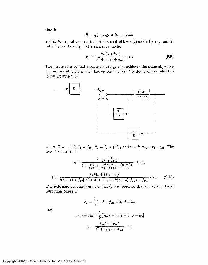
The first step is to find a control strategy that achieves the same objectivein the case of a plant with known parameters. To this end, consider thefollowing structure

where D = s + d, FI — /io, F2 = /2is + fzo and u = kium - y\ - 2/2- Thetransfer function is

s+b

y =/10 J ,s+d ' s'

k(s+b) /"21S+/20s+d

y r/ i j\ i r I / 9 i i \ i ; / , LW r i r \ ^m ^"-lUJ[(s + d) + /io](s2 + ais + a0) + k(s + b)(f2is + fw)

The pole-zero cancellation involving (5 4- b) requires that the system be atminimum phase if

k- ~, d + fw - 6, d — br

K

and

/20 = T am0 -

y = am0


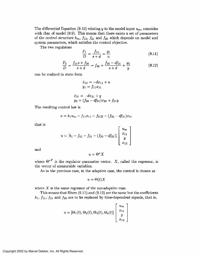
The differential Equation (9.10) relating y to the model input itm, coincideswith that of model (9.9). This means that there exists a set of parametersof the control structure fcm, /i2, /2i and /2o which depends on model andsystem parameters, which satisfies the control objective.

The two regulatorsF f_L = *w

D s + d

/20 /20 -

D s + d

can be realized in state form

= —dxu + u

x2i = -dx2i + yyi — (/2o - d/2i)z2i + h\y

The resulting control law is

u = - (/2o -

that is

= [ k i - f u - /21 - (/20 -

and

(9.11)

(9.12)

where 9*T is the regulator parameter vector. X, called the regressor, isthe vector of measurable variables.

As in the previous case, in the adaptive case, the control is chosen as

u = Q(t}X

where X is the same regressor of the nonadaptive case.This means that filters (9.11) and (9.12) are the same but the coefficients

&i5 /ii) /2i and /2o are to be replaced by time-dependent signals, that is,


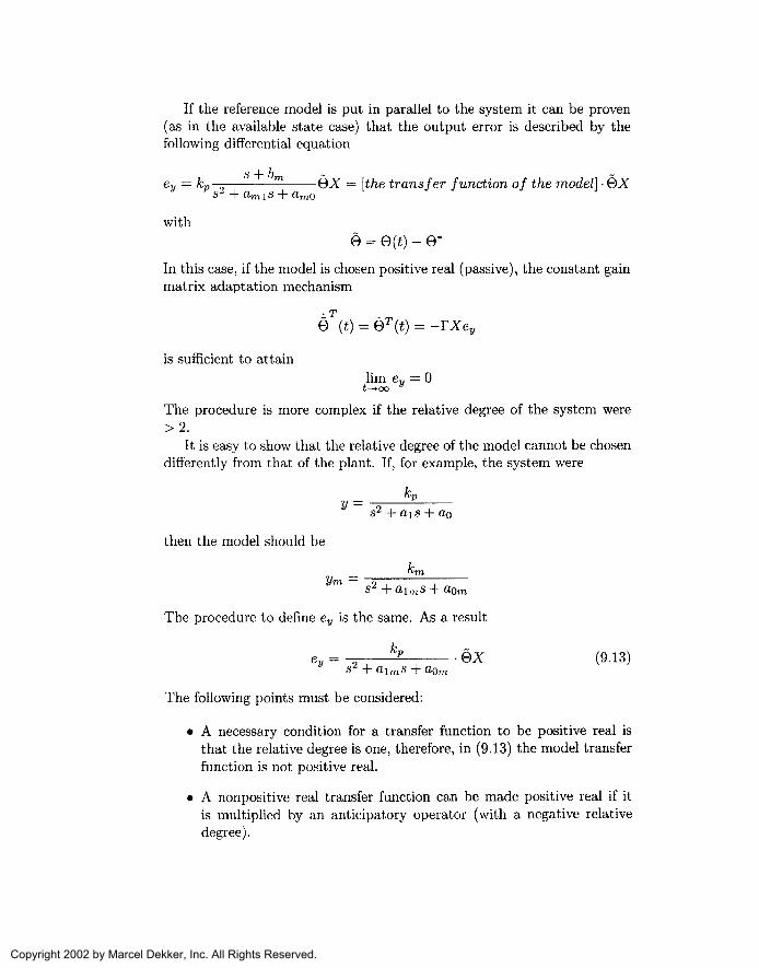
If the reference model is put in parallel to the system it can be proven(as in the available state case) that the output error is described by thefollowing differential equation

s -f- bey = /cp — — QX — [the transfer function of the model] • QXys2 + amis + am0

withe = em - e*

In this case, if the model is chosen positive real (passive), the constant gainmatrix adaptation mechanism

is sufficient to attain

§ (t) = QT(t) = -TXe,

lim ev = 0t-*oo y

The procedure is more complex if the relative degree of the system were>2 .

It is easy to show that the relative degree of the model cannot be chosendifferently from that of the plant. If, for example, the system were

y = s2 + ais +

then the model should be

Km.-m 9S + O-lmS +

The procedure to define ey is the same. As a result

kp -QX (9.13)s2 + aims + a0

The following points must be considered:

• A necessary condition for a transfer function to be positive real isthat the relative degree is one, therefore, in (9.13) the model transferfunction is not positive real.

• A nonpositive real transfer function can be made positive real if itis multiplied by an anticipatory operator (with a negative relativedegree).


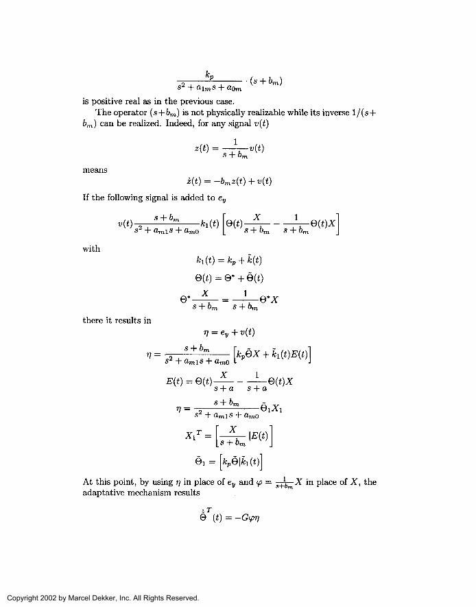
kp

is positive real as in the previous case.The operator (s + 6m) is not physically realizable while its inverse

6m) can be realized. Indeed, for any signal v(t)

meansz(t] = -bmz(t) + v(t)

If the following signal is added to ey

with

S + Om 5 + O

there it results in7 = e + « *

77 =

= [kpQ\ki(t)]

At this point, by using 77 in place of ey and (p = s^h X in place of X, theadaptative mechanism results


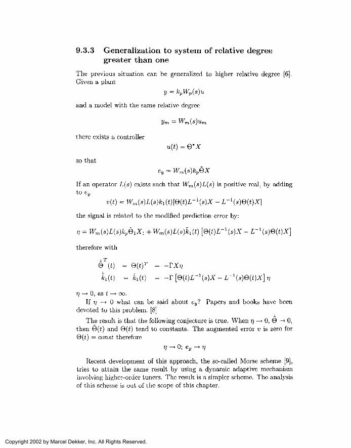
9.3.3 Generalization to system of relative degreegreater than one

The previous situation can be generalized to higher relative degree [6].Given a plant

y = kpWp(s)u

and a model with the same relative degree

y-m = Wm(s}um

there exists a controller

u(t) = Q*X

so thatey = Wm(s}kpeX

If an operator L(s] exists such that Wm(s)L(s) is positive real, by addingto ey

v(t) = Wm(s)L(s)kl(t)[e(t)L-l(s)X - L-l(s)Q(t)X]

the signal is related to the modified prediction error by:

77 = Wm(s}L(s)kpQlXl + WMLWWt) [Q(t)L~l(s)X - L~l(s)e(t)X]

therefore with

6 (t) = Q(t}T = -TXr]

k i ( t ) = ki(t) = -r[Q(t)L-l(s)X-L-l(s)Q(t)X]r]

rj —>• 0, as t —> oo.If 77 —> 0 what can be said about eyl Papers and books have been

devoted to this problem. [8]

The result is that the following conjecture is true. When 77 —> 0, O —» 0,then 6(t) and 6(t) tend to constants. The augmented error v is zero for0(t) = const therefore

77 -> 0; ey -> rj

Recent development of this approach, the so-called Morse scheme [9],tries to attain the same result by using a dynamic adaptive mechanisminvolving higher-order tuners. The result is a simpler scheme. The analysisof this scheme is out of the scope of this chapter.


9.4 Sliding mode and adaptive controlIn this section the basic features of sliding mode control, which are suitableto introduce an approach within the framework of adaptive control, areconsidered.

Result 1

Givenx = a(x) + b(x)uy = u

and given s(x) and u — —H(x)s sign{s} with H(x] so that

s(x) [Ga(x] - Gb(x}H(x}s sign{s}] < -fc2|s(z)|

after a finite time s(x) = 0. By the Filippov [3] solution method as theequivalent control method, the system is represented by

x = a(x) - b(x) [G(x)b(x}}~1 G(x)a(xy = -[G(x)b(x)]~lG(x}a(x)-i ̂ V x (9-14)

where — [G(x)b(x)] l G(x)a(x) is the so-called equivalent control.The representation is robust with respect to nonidealities, causing a

motion close to the sliding manifold s(x) = 0 if the system (9.14) is asymp-totically stable.

Result 2

Let s*(x) = s(x) + r](t), being r?(£) a signal free to be selected by thedesigner. Consider

x(t) = a(x) + b(x}u (9.15)

letu = — H (x, T)(£)) sign{s*(t)}

so that

a*(f} \Cln('r\ -\- ri(t} — rthH (r ri f} sinn -f <?*(VH < — k2\a*(i-}\]o 16 / Vjru/lX I ]^ I I \ L I \jrUJ.J. t*t') ij^ t'/ ot/yil 1o \v I j _^ "/ ^ \ /

then after a finite time 5 —> 0 and the Filippov representation of the sys-tem (9.15) is

x(t] — a(x) — b(x) [G(x)b(x)}~ [Ga(x] + r)(t)]s*(x) =0

which is a reduced order continuous system evolving under the action ofthe control r)(i).


Example 1

±i = x2 + A(£)X2 = f ( x i , x 2 ) + g(x)u

with s = x<2 + ex i the equivalent system on s = 0 is x\ = —cx\ + A(£) andno counteraction to A is possible. If

s* = x-2 + ex i = rj(t)

on s*(x, £) = 0, the system is equivalent to

±1 - -cxi + A(i) - rj(t)

Through the choice of r)(i) the disturbance A(i) can be counteracted.The sliding manifold is chosen so that the reduced system evolving on it(the so-called zero-dynamics [5]) is characterized by a sufficient degree offreedom to attain the final control objective, e.g., stabilization disturbancerejection and counteraction of residual uncertainties.

Result 3Given a system

x = a (re) + b(x}u

and s(x) = 0, assume that by the action of a control u(t) the system motionresults confined in a boundary layer \s(x)\ < 6. How is it possible to achieveinformation relevant to the ideal equivalent control

Leq — — [G(x)b(x)] a(x)

Utkin proved [12] that under reasonable assumptions regarding system dy-namics that if the control u(t) is filtered by an high-gain linear filter

then

|ti«,(t) - ueq(t}\ < 0(5) + 0(r) + O

which tends to zero if r = O ( V6j and 6 — > 0.

This result is extremely important when the problem of reducing thecontrol amplitude is dealt with or when, as in the case of the combinedadaptive sliding mode control, the equivalent control is explicitly used inevaluating the prediction error.


9.5 Combining sliding mode withadaptive control

From adaptive control.e = Ame + BQX

£ = WmQX

rj = WmQX + WmL (BIT1 - L~1QX^ = WmLQL~lX

The same situation arises if a control Ud is introduced at suitable points ofthe controller structure by adding Ud + QX in the relevant error equation.This could be the first link between the sliding mode control approach andadaptive control.

Every equation can be represented by means of an I/O relationship be-tween an input QX and an output: v, £, rj respectively. This input /outputis of relative degree 1 .

In pure model-tracking problems, under the assumption that overesti-mation of the controller parameters of the type

max|O*|i

it is possible to steer the output errors v, £, r\ to zero in finite time as follows

u = Q(t)X - \2QM ̂ \Xi + h2] sign{v, e, 77}

e = Ame + B \QX - (2OM ̂ N + h?] sign{v]

77 = LWm [eir1* - (2QM Y^ M + h2} sign{r)}]

As a result, v, £ and 77 tend to zero in finite time.Among the three considered cases, the third one, namely the case of I/O

with relative degree greater than 1, deserves particular attention. Whilethe attainment of the condition v = 0, £ = 0 are a direct expression ofthe control objective, the condition rj = 0 does not imply that the trackingerror is zero.

Indeed r\ = 0 implies that the equivalent control Udeq is equal to — QL~1Xand nothing else:

udeq = -QL~1X


The true tracking error is £ = WmQX and it is not directly affected by Ud-A way consists in modifying the adaptive mechanism as follows:

§ = -Fr; + r(t)ud

which in sliding mode is equivalent to

where F(t) is the least square with bounded forgetting gain matrix satisfy-ing

dr-^t) T

The first term vanishes as 77 = 0. During sliding motion it is possible, asdone previously, to choose a Lyapunov function for the equivalent system

U= -QT

If the regressor </? is persistently exciting, F-1 — ̂ - is positive definite and

therefore 0 — > 0 exponentially. If 0 — > 0 also the tracking error e = Wm0Xtends to zero since Wm is an asymptotical stable I/O relationship.

This way is the most direct manner to couple MRAC with VSS controlrequires the persistent excitation of the regressor <£>, which is obtained byfiltering the regressor X. Sastry and Bodson [10] proved that the persistentexcitation depends on the number of spectral lines contained in the modelreference input.

Another way to deal with this problem exploits the second importantproperty of the sliding mode control approach which is that the practicalavailability of the equivalent control at the output of an high-gain filter hasdiscontinuous control at the input [4],

To clarify this procedure, we consider as a starting point the error equa-tion

^ = WmQX

with Wm having relative degree r. By multiplying for an operator

then LWm has relative degree 1.


Adding to £ the signal LWmUd we obtain

A sliding mode on £ implies

udeq = -L

Assume that this signal is available at the output of a filter

udeq = -L~1OX = Fû^t)

Consider a control uid(t) as follows. Let

yi = -ayi + uid(t)

Also consider

1

21 ~UC

exieq - Vi

— i it-, ex

is attained by uid = —kisign{z\}. If z\ = 0

U\A =69 -. - r(s + a)r~2

and is available at the output of an high-gain filter.Continuing this procedure,

exs + a

ex

.s + a

Ur_ld = +exdeq -

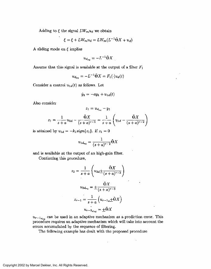
ur-ide can be used in an adaptive mechanism as a prediction error. Thisprocedure requires an adaptive mechanism which will take into account theerrors accumulated by the sequence of filtering.

The following example has dealt with the proposed procedure


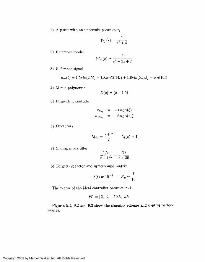
1) A plant with an uncertain parameter,

Wp(s} = -Jj-^

2) Reference model

Wm(s] =s2 + 3s + 2

3) Reference signal

um(t} = 1.5sm(2.5i) — 1.8sm(3.14t) +

4) Monic polynomial

5) Equivalent controls

uideq =

6) Operators

7) Sliding mode filter1/r 30

s + l/T s + 30

8) Forgetting factor and upperbound matrix

A(t) = 10-3 X0 =

The vector of the ideal controller parameters is

6* = [2, 3, -19.5, 2.5]

Figures 9.1, 9.2 and 9.3 show the simulink scheme and control perfor-mances.


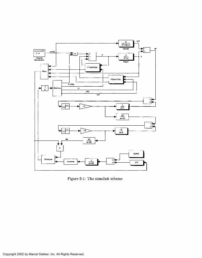
Figure 9.1: The simulink scheme


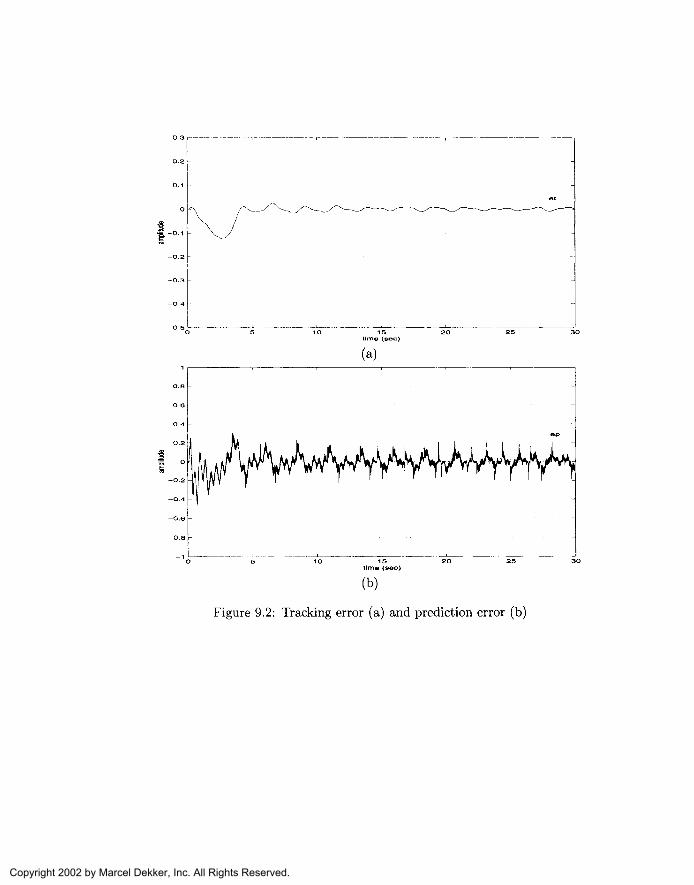
(a)

Figure 9.2: Tracking error (a) and prediction error (b)


(a)

(b)

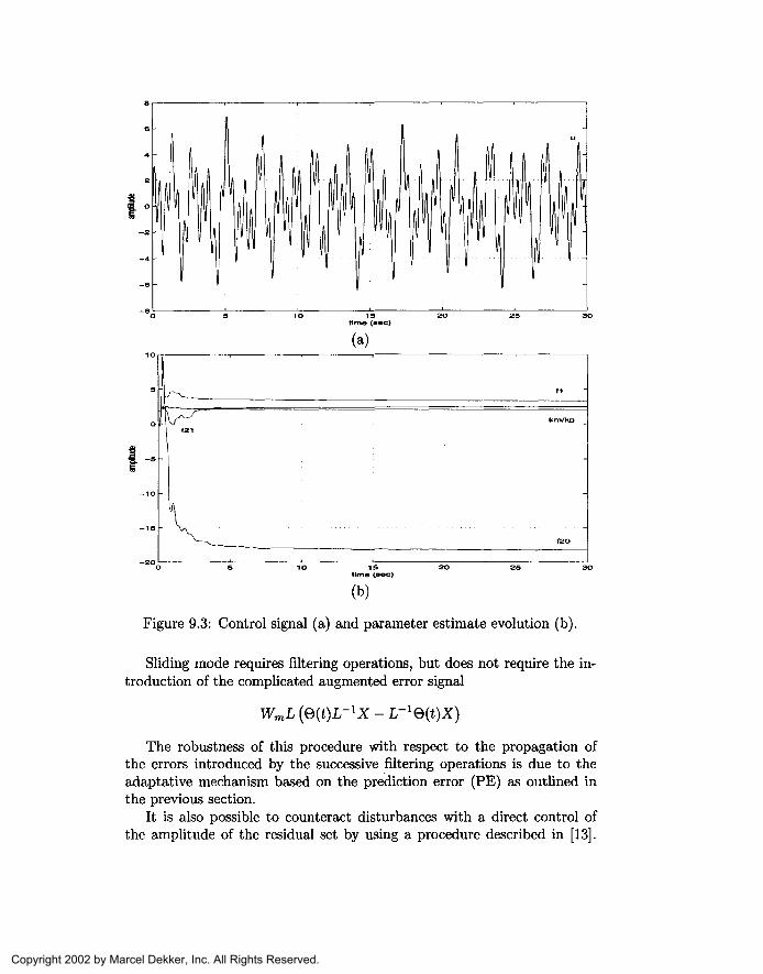
Figure 9.3: Control signal (a) and parameter estimate evolution (b).

Sliding mode requires filtering operations, but does not require the in-troduction of the complicated augmented error signal

WmL (Q(t)L~lX - L~lQ(t}X)

The robustness of this procedure with respect to the propagation ofthe errors introduced by the successive filtering operations is due to theadaptative mechanism based on the prediction error (PE) as outlined inthe previous section.

It is also possible to counteract disturbances with a direct control ofthe amplitude of the residual set by using a procedure described in [13].


Disturbance can be considered as external signals, as a residual error due tothe sequence of operations described above or even as part of the predictionerror, when for example, due to a lack of PE it is desired to identify someparameters neglecting the other.

This procedure starts from a prediction error of the type OX + d(t) andthe aim is make | 9 \\< EQ, where e$ is an arbitrarily small positive number.To this end the scalar v, defined by

v = -av + 9X + d(t) + ua (i) (9.16)

where ua(t] is an auxiliary signal to be defined in the sequel. Our aim isto force 9(i] to be less than any prespecified small constant.

To this end we prove that a signal

(9.17)

where e and t] are chosen according to

e(t) = -p£(t) + Pav(t) -

ri(t) = -f3r1(t}-(3X(t]

This represents an estimation of d(t) such that

lim \ d ( t ) - d ( t )

(9.18)

(9.19)

where h\ is any small positive constant. Note that d, due to last addendum,is not available. Indeed choosing

2V = d-d = d-e-3v-

we have

V = (d-e-/3v-f)8-r)8\

= ld-p(d-£-pi>- rj9\\ (d-£-pv-

(9.20)

V < -0V + (9.21)


This means that

(9.22)

where | d — d \< —. Now we show how it is possible to introduce d in

Equation (9.16). Choose ua(t} = —e(3v so that i — fiav — r\Q and (9.16)becomes

9X + d(t) -e-

v = -av (9.23)

which can be interpreted as a new error equation with a prediction errorthat has a modified regressor and a disturbance which is arbitrarily small.

The second step is that of making available 6(r) + X] + I d — d J , to end

we can introduce ua = — e — (3v 4- Ud and as a result (9.16) becomes

v = -av + 6(r] + X) + (d - d\

choose Ud = —ksign(v]

+ (9.24)

k> d(0) - (9.25)

In finite time v —» 0 and Udeq = —Q(n -4- X) + (d — d J .

We now consider the following adaptative mechanism

where

(9.26)

(9.27)

We shall prove that the estimate 0(t) converges to a residual set arbitrar-ily small of #*, which is the true unknown value under reduced persistentexcitation condition. Just a single parameter needs to be identified.

Indeed using

V = 7(t)£2 (9.28)


V = -

1 ' 5 2

/ - \21\ 1 ( d - d )i.WÎ + A 'kQ

D2

(9.30)

with (3 a project parameter which, not affecting any physical input of the

plant but only the artificial systems ( V " = • • • , £ = • • • , ? ) = • • • ) , can

be made arbitrarily small. The parameters 8 = -M7 ~ JT ) "K*) can ê

ensured to be positive by exploiting the natural excitation of the appliedcontrol since only one regressor is involved.

Problems involving nonlinear systemsConsider a nonlinear system with the actuator

x = Ax + Buu = f ( x , u ) + g(x}v

From adaptive control we know that there exists a control u* — Q*(x) sothat x = Ax + Bu* tracks a reference model

2-m — •"im^'Tn i -Drn^m

It is possible to define the following sliding manifold

s ( x , t ) =u(t}-@(t}X

which can be forced to be zero in a finite time if the upper bounds of theuncertainties appearing in the actuator dynamic are available. After thattime, the zero dynamic of the system is characterized by an error equation

e = Ame + BQX v = De

and e -> 0 if 9(t) - -TXe.


This first combination of sliding mode control and adaptive control canbe generalized to single input system with nonmatching uncertainties ofthe type

x\ = £2

(x) + g(x)u

with \f(x)\ < F(x) gi < g(x) < §2, 6* an uncertain constant parametervector and $(x) a regressor vector whose components are known nonlinearfunctions of the states.

s(x) = xn

&m = [amn_2 ' ' ' - am0 |&m] X =

with 5 = 0 the zero dynamic is

Xi = X-2

xn-i = - YZ=o aixi+i + bmum

which can be dealt with by standard adaptive control. This situation canbe generalized to systems in strict parametric or pure parametric form, forwhich the back-stepping procedure is applicable. The result is that with theuse of the sliding mode control, a step in this rather cumbersome procedurecan be saved.

9.6 ConclusionsIn this chapter some basic features of control algorithms were derived fromthe suitable combination of sliding mode and adaptive control theory, westressed the importance of extracting the prediction error from the equiv-alent control in order to cope with the problem of the controlling systemwith higher-order relative degree. Hints to the possibility of dealing withnonlinear systems through a suitable combination of the two approacheswas also presented. The complementarity of the two approaches was basedon the fact that with sliding mode it is possible to force system motionin a manifold of the state space so that the associated zero dynamics canbe stabilized by adaptive control or equivalent passivity-based nonlinearalgorithms.

These topics are related to the existing literature. The next step in thisdirection will be based on the introduction of new, recently developed toolslike terminal control and higher-order sliding modes.


References

[1] G. Bartolini and A. Ferrara "Model-Following VSC Using an Input-Output Approach." in Variable Structure and Lyapunov Control,Springer-Verlag, London, 1994.

[2] G. Bartolini, A. Ferrara, and A. Stotsky "Stability and ExponentialStability of an Adaptive Control Scheme for Plants of any RelativeDegree." IEEE Trans. Automat. Contr., Vol. 40, pp. 100-104, 1995.

[3] A.F. Filippov "Differential Equations with Discontinuous Right-Hand Sides." Mathematicheskii Sbornik, Vol. 51, No. 1, 1960, in Rus-sian. Translated in English Am. Math. Soc. Trans., Vol. 62, No. 199,1964.

[4] L. Hsu "Variable Structure Model Reference Adaptive Control Usingonly Input and Output Measurements: the General Case." IEEETrans. Automat. Contr., Vol. 35, pp. 1238-1243, 1990.

[5] A. Isidori Nonlinear Control System. Springer-Verlag, New York, 1989.

[6] R.V. Monopoli "Model Reference Adaptive Control with an Aug-mented Error Signal." IEEE Trans. Automat. Contr., Vol. 19, No. 4,pp. 474-484, 1974.

[7] K. Narendra and A. Annaswamy Stable Adaptive Systems. EnglewoodCliffis, NJ: Prentice Hall, 1989.

[8] K. Narendra, Y.H.Lin, and L.S. Valavani "Stable Adaptive ControllerDesign, part II: Proof of Stability." IEEE Trans. Automat. Contr.,Vol. 25, pp. 440-448, 1980.

[9] R. Ortega "On Morse's New Adaptive Controller: Parametr Conver-gence and Transient Performance." IEEE Trans. Automat. Contr.,Vol. 38, No. 8, pp. 1191-1202.

[10] S. Sastry and M. Bodson Adaptive Control: Stability, Convergenceand Robustness. Englewood Cliffis, NJ: Prentice Hall, 1989.

[11] J.J.E. Slotine, and W. Li Applied Nonlinear Control. Prentice Hall,1991.

[12] V.I. Utkin Sliding Modes In Control And Optimization. Springer-Verlag, Berlin, 1992.


[13] G. Bartolini, A. Ferrara, A A. Stotsky "Robustness and Performanceof an Indirect Adaptive Control Scheme in Presence of Bounded Dis-turbances." IEEE Trans. Automat. Contr., Vol. 44, No. 4, pp. 789-793.


Documents

SLIDING MODE CONTROL IN ENGINEERING - read.pudn.comread.pudn.com/downloads75/ebook/276183/Sliding Mode Control in... · Adaptive and Sliding Mode Control G. BARTOLINI University of