Slides Panel Data Analysis 2012

Introduction to Panel Data Analysis

Oliver Lipps / Ursina Kuhn

Swiss Centre of Expertise in the Social Sciences (FORS)c/o University of Lausanne

Lugano Summer School, August 27-31 2012

Introduction panel data, data management 1 Introducing panel data (OL)2 The SHP (OL)3 Data Management with Stata

(UK)

Regressions with panel data: basic 4 Regression refresher (UK)5 Fixed effects (FE) models (OL)6 Introducing random effects (RE) models (OL)7 Nonlinear regression (UK)

Additional topics8 Level 1 and 2 growth models (OL)9 Missing data (OL)10 Dynamic models (UK)

Start: 8.30Breaks:

10.30-10.4515.30-15.45

Lunch Breaks: 12.30-13.30

End: 17.30

1 Introducing panel data

1 - 4

Surveys over time: repeated cross-sections vs. panels

•

Cross-Section: Survey conducted at several points in time (“rounds”) using different sample members in each round

•

Panel: Survey conducted at several points in time (“waves”) using

the same individuals over waves

-> panel data mostly from panel surveys-> If from cross-sectional surveys: retrospective

(“biographical”) questionnaire

1 - 5

Panel Surveys: to distinguish

Length and sample size:•

Time Series: N small (mostly=1), T large (T→)→ time series models

•

Panel Surveys: N large, T small (N→)→ social science panel surveys

Sample•

General population:

-

rotating: only few (pre-defined number) waves per individual (in CH: SILC, LFS)

-

indefinitely long (in CH: SHP)

•

Special population:-

e.g., age/birth cohorts (in CH e.g.: TREE, SHARE, COCON) representative for population of special agegroup

/ birthyears

1 - 6

Panel surveys increasingly important

Changing focus in social sciences→ Life course research: effects of events within individuals→ Large investments in social science household panels

surveys, high data quality!→ Concern about causality in cross-sectional studies

Analysis potential of panel data-

close to experimental design: before and after studies

-

control unobserved individual characteristics (exogenous independent variables; implicit in regression analyses)

1 - 7

Identification of individual dynamics (poverty in SHP)

-> individual dynamics can only be measured with panel data!

10.5% 9.0% 7.7% 8.8% 9.4%

89.5% 91.0% 92.3% 91.2% 90.6%

0%

100%

1999 2000 2001 2002 2003

poor not poor

54%

46%

51%

49%

48%

52%

50%

50%

96%

4%

1 - 8

Identification of age, time, and (birth) cohort effects

Fundamental relationship:

ait

= t -

ci•

Effects from “formative”

years (childhood, youth) -> cohort effect (eg

taste in music )•

Time may affect behavior

-> time effect (eg

computer performance)•

Behavior

may change with age

-> age effect (eg

health)

•

In a cross-section, t is constant →

age and cohort collinear (only joint effect estimable)•

In a cohort study, cohort is constant →

age and time collinear (only joint effect estimable)•

In a panel, t varies, but Ait , t, and ci collinear. →

only two of the three effects can be estimated→

we can use (t,ci

), (Ait

,ci

), or (Ait

,t), but not all three

1 - 9

Age, time, cohort effects: interpretation

(age effect) (no aging effect)

(no age effect) (aging and cohort effect)

(no cohort effect) (aging effect)

1 - 10

Problems of panels

Fieldwork / data quality related•

High costs (panel care, tracking households, incentives)

•

Initial nonresponse (wave 1) and attrition (=drop-out of panel after wave 1)

•

Finally: you design a panel for the next generation …

Modeling related•

Sometimes strong assumptions for applicability of appropriate models necessary (later)

1 - 11

Advantages of panel data

•

Allow to study individual dynamics+

•

Control for unobserved characteristics between individuals by repeated observation

+•

Higher precision of change

+•

Data

can be pooled

2 Introducing the Swiss Household Panel (SHP)

2-2

Swiss Household Panel: history

•

Primary goal: observe social change and changing life conditions in Switzerland

•

Started as a common project of the Swiss National Science Foundation, Swiss Federal Statistical Office, University of Neuchâtel

•

First wave in 1999, more than 5,000 households

•

Refreshment sample in 2004, more than 2,500 households, several new questions

•

Since 2008, integrated into FORS (Swiss Centre of Expertise in the Social Sciences ), c/o University of Lausanne

2-3

Disciplines working with SHP data

2-4

SHP –

sample and methods

•

Representative of the Swiss residential population•

Each individual surveyed every year (Sept.-Jan.)

•

All household members from 14 years on surveyed (proxy questionnaire if child or unable)

•

Telephone interviews (central CATI), languages D/F/I

•

Metadata: biographic, interviewers

•

Paradata: call data (from address management)

Following rules:

•

OSM followed if moving, from 2007 on all individuals

•

All new household entrants surveyed

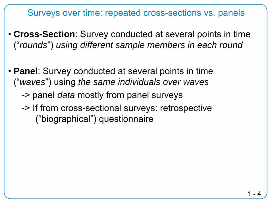
2-5

Befragte Haushalte

50744425 4139 3582 3227 2837 2457 2537 2817 2718 2930 2985 2977

2538

1799 1684 1494 1546 1476 1557 1520

1999 2000 2001 2002 2003 2004 2005 2006 2007 2008 2009 2010 2011

SHPI SHP II

Cross-sectional and longitudinal (SHPI and SHP I+II combined)

weights to account for nonresponse and attrition

SHP –

sample size (households) and attrition

2-6

Persons 18+ years « reference person»

Persons 14+ years

Persons 13- years + « unable to respond»

Household Questionnaire: housing, finances, family roles, …

Grid Questionnaire: Inventory and characteristics of hh-members

Individual Questionnaires: work, income, health, politics, leisure, satisfaction of life …

Individual Proxy Questionnaires: school, work, income, health, …

SHP: Survey

process and questionnaires

2-7

SHP: Questionnaire Content

•

Social structure: socio-demography, socio-ecomomy, work, education

→ social stratification and social mobility•

Life events: marriages, births, deaths, deceases, accidents, conflicts with close persons, etc.

→ life course•

Social participation: politics (attitudes, elections, party preferences and -choice), culture, social network, leisure

→ social integration, political attitude and behavior•

Perception and values: trust, confidence, gender

→ values and social capital•

Satisfaction and health: physical and mental health self-

evaluation, chronic problems, different satisfaction issues → quality of life

2-8

SHP –

Household: composition and housing

« objective » elements •

Characteristics of household members (sex, age, civil status, education, occupation)

•

Relationships between all household members

•

Since when at this place•

Type of house•

Size, number of rooms of house•

State of house (heating, noise, pollution, etc.)

•

Costs and subsidy, etc.

•

External help for domestic work•

Child care•

Division of labor•

Who takes decisions, etc.

« subjective » elements •

Satisfaction with

house, noise, pollution, etc.

•

Assessment of state of house

2-9

SHP –

Household: standard of living


Activities and (durable) goods•

Reason why absence of goods (financial, other)

•

Financial difficulties•

Debts (+reason)•

Total household income•

Taxes•

Social and private financial transfers


Satisfaction with

financial situation

2-10

SHP –

Individual level: family« objective » elements •

Children out of the house•

Division of housework, care for dependents

•

Disagreement about family problems etc.


Satisfaction with

private situation•

Satisfaction with

living alone or together

•

Satisfaction with

division of housework

SHP –

Individual level: health, well-being« objective » elements •

Health problems•

Physical activities•

Doctor visits, hospitalization•

Improvement of health•

Long and short term handicaps


Subjective

health state•

Satisfaction with

health•

Satisfaction with

life in general

2-11

Social origin and education

Leisure« objective » elements •

Activities: holidays, invitation of and meeting friends, reading, Internet use, restaurant, etc.


Satisfaction with

leisure time and leisure activities

•

Satisfaction with

work-life balance

•

Profession of parents•

Level of education of parents•

Nationality of parents•

Financial problems in childhood

•

Education level•

Current training•

Language capabilities

2-12

Individual level –

work


Job sector•

Social stratification•

Private or public•

Position•

Working time, commuting time•

Size of company


Satisfaction with

work (general, income, interests, working conditions, amount, atmosphere)

•

Risk of unemployment•

Job security•

Chances to get promoted

Income« objective » elements •

Total personal income•

Total personal income from work•

Social transfers received•

Private transfers received•

Other income


Satisfaction with

financial situation•

Assessment whether financial situation improved or not

•

Possible reactions on financial problems

2-13

Values and politics


Right to vote•

Political activities•

Member of a political party


Satisfaction with

democracy•

Confidence in federal government•

Political interest•

Left-right political positioning•

Opinions on political questions

Participation, integration, social network« objective » elements •

Frequency of contacts•

Voluntary work outside the household

•

Participation and membership in associations

•

Belief and religious participation


Satisfaction with personal relationships•

Assessment of amount of practical help received from partner, parents, friends, etc.

•

Assessment of amount of emotional help received from partner, parents, friends, etc.

•

General trust in people

2-14

Biographical (retrospective) questionnaire

•

N = 5’560•

Written questionnaire in 2001/2002, sent to all individuals surveyed in 2000, aged 14 or over

•

Questions since birth about family, education, and professional biography:-

with whom lived together

-

periods out of Switzerland-

changes of civil status

-

learned professions-

education

-

professional and non-professional biography-

family life events (divorce-re-marriage of parents)

2-15

International ContextSHP is part of the Cross National Equivalent File (CNEF):General population panel surveys from:

–

USA (PSID since 1980)–

D (SOEP, since 1984)–

UK (BHPS since 1991)–

Canada (SLID since 1993)–

CH (SHP since 1999)–

Australia (HILDA since 2001)–

Korea (KLIPS since 2007)More countries will join (Russia, South Africa, …)

•

Each panel includes subset of all variables (variables from original files can be merged)

•

Variables ex-post harmonized, names, categories•

Missing income variables are

imputed

Frick, Jenkins, Lillard, Lipps and Wooden (2007): “The Cross-National Equivalent File (CNEF) and its member country household panel studies.“

Journal of Applied Social Science Studies (Schmollers

Jahrbuch)

2-16

SHP Questionnaire: Rotation

Module 2010 2011 2012 2013 2014 2015 2016 2017 2018 2019 2020

Social network

X X X X

Religion X X X

Social participation

X X X X

Politics X X X X

Leisure X X X X

Psychologi- cal Scales

X X X

2-17

Outlook: new sample (LIVES)

•

SHP III (2013, based on individual register)–

Biographic questionnaire in

1. Wave SHP III (with

NCCR LIVES)

•

NCCR LIVES–

(Precarious) life course

–

University of Lausanne and Geneva–

15 research projects, 12 years

–

Use of SHP

2-18

SHP –

structure of the data

•

2 yearly files (currently available: 1999-2010 (+beta 2011))–

household–

Individual

•

5 unique files–

master person (mp)–

master household (mh)–

social origin (so)–

last job (lj)–

activity (employment) calendar (ca)

•

Complementary files–

biographical questionnaire–

Interviewer data (2000, and yearly since 2003)–

Call data (since 2005)–

CNEF SHP data variables

2-19

Documentation (Website: D/E/F)

http://www.swisspanel.ch/

e.g.,:•

User Guide

•

Questionnaires•

Variable Search (by variable name and topic)

•

Construction of variables•

Syntax examples-

Merge data files with SPSS, SAS, Stata-

Documentation Data Management with SHP

•

…


2-20

SHP –

data delivery

•

Data ready about 1 year after end of fieldwork – downloadable from SHP-server:

http://www.swisspanel.ch/spip.php?rubrique181&lang=en

•

Signed contract with FORS•

Upon contract receipt, login and password sent by e-mail

•

Data free of charge•

Users become

member of SHP scientific network and

document all publications based on SHP data•

Data on request:–

Imputed income–

Call data–

Interviewer matching ID–

Context data (special contract); data is matched at FORS

More info: http://www.swisspanel.ch


3Stata and panel data

3_2

Why Stata?

Capabilities— Data management— Broad range of statistics

– Powerful for panel data!– Many commands ready for analysis– User-written extensions

Beginners and experienced users— For beginners: analysis through menus (point and

click)— Advanced users: good programmable capacities

3_3

Starting with Stata

Basics— Look at the data, variables— Descriptive statistics— Regression analysis

→ Handout Stata basics

Working with panel data— Merge— Creating « long files »— Working with the long file— Add information from other household members

→ Handout data management of SHP with Stata (includes Syntax examples, exercises)

3_4

1. Merge: _merge variable

idpers p07c4442 843 744 945 10

idpers p08c4444 945 546 1047 3

idpers p07c44 p08c4442 8 .43 7 .46 . 1047 . 344 9 945 10 5

Master file

using file

_merge112233

Merge variable

1 only in master file

2 only in user file

3 in both files

3_5

Merge: identifieridpers p07c44

42 843 744 945 10

idpers p08c4444 945 546 1047 3

idpers p07c44 p08c4442 8 .43 7 .46 . 1047 . 344 9 945 10 5

Master file

using file

_merge112233

3_6

Merge files: identifiersfilename identifiers

Individual master file shp_mp idpers, idhous$$, idfath__, idmoth__

Individual annual files shp$$_p_user idpers, idint, idhous$$, idspou__, refper$$

Additional ind. files(Social origin, last job, calendar, biographic)

shp_so, shp_lj shp_ca, shp0_*

idpers

Interviewer data shp$$_v_user idint

Household annual files shp$$_h_user idhous$$, refpers, idint, canton$$, (gdenr)

Biographic files idpers

CNEF files shpequiv_$$$$ x11101ll (=idpers)

3_7

The merge command

• Stata merge command

merge [type] [varlist] using filename [filename ...] [, options]

varlist identifier(s), e.g. idpersfilename data set to be merged

type 1:1 each observation has a unique

identifier in both data sets 1:m, m:1 some observations have the

same identifier in one data set

3_8

Basic merge example

I

2 annual individual files

use shp08_p_user, clearmerge 1:1 idpers using shp00_p_user

_merge | Freq. Percent Cum.------------+-----------------------------------

1 | 5,845 34.93 34.932 | 5,056 30.21 65.143 | 5,833 34.86 100.00

------------+-----------------------------------Total | 16,734 100.00

3_9

Basic merge example

II

• annual individual file and individual master file

use shp08_p_user, clear // opens the file (master)count //there are 10’889 casesmerge 1:1 idpers using shp_mp //identif. & using filetab _merge


2 | 11,111 50.50 50.503 | 10,889 49.50 100.00

------------+-----------------------------------Total | 22,000 100.00

drop if _merge==2 //if only ind. from 2008 wanteddrop _merge

3_10

Basic merge example III

• annual individual file and annual household file

use shp08_p_user, clear //master filemerge m:1 idhous08 using shp08_h_user /*identifier & using file */


3 | 10,889 100.00 100.00------------+-----------------------------------

Total | 10,889 100.00

3_11

More on merge• Options of merge command

– keepusing (varlist): selection of variables from using file

– keep: selection of observations from master and/or using file

– for more options: type help merge• Merge many files

– loops (see handout)• Create partner files (see handout)

3_12

2. Wide and long format

• Wide format

• Long format(person-period-file)

idpers year iempyn4101 2004 1031904101 2005 1077304101 2006 1134004101 2007 122470

42101 2004 6318042101 2005 6950056102 2004 3547356102 2006 4140056102 2007 45500

idpers i04empyn i05empyn i06empyn i07empyn4101 103190 107730 113400 122470

42101 63180 69500 . .56102 35473 . 41400 45500

3_13

Use of long data format in stata

—All panel applications: xt commands – descriptives– panel data models

• fixed effects models, random effects, multilevel• discrete time event-history analysis

—declare panel structure panel identifier, time identifier xtset idpers wave

3_14

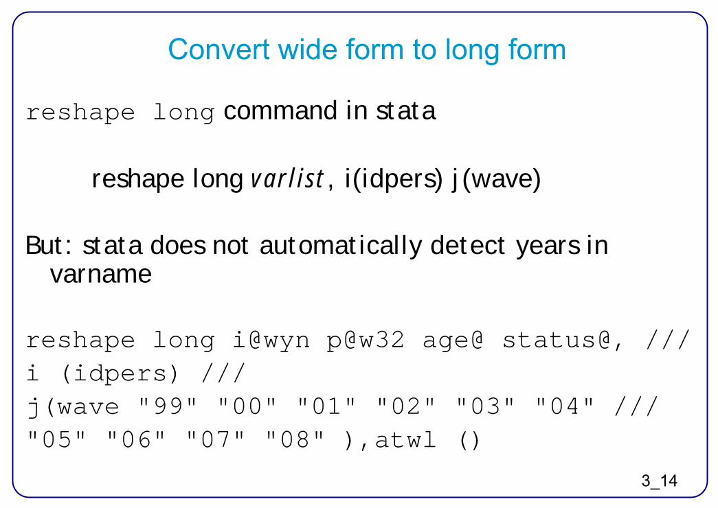
Convert wide

form

to long form

reshape long command in stata

reshape long varlist, i(idpers) j(wave)

But: stata does not automatically detect years in varname

reshape long i@wyn p@w32 age@ status@, ///i (idpers) ///j(wave "99" "00" "01" "02" "03" "04" ///"05" "06" "07" "08" ),atwl ()

3_15

Create a long file with

append

1. Modify datasets for each wave

2. Stack data setsuse temp1, clearforval y = 2/10 {append using temp`y'}

idpers wave iwyn4101 1 50’0004102 1 24’8005683 1 108’000

idpers i99wyn4101 50’0004102 24’8005683 108’000

temp1.dta

idpers wave iwyn4101 2 51’0004102 2 24’5008052 2 280’300

temp2.dta

idpers i99wyn4101 50’0004102 24’8005683 108’000

3_16

Work with

time lags

—If data in long format and defined as panel data (xtset)

—l. indicates time lag

—Example: social class of last job (see handout)

3_17

Missing data in the SHP

Missing data in the SHP: negative values-1 does not know-2 no answer-3 inapplicable (question has not been asked)-8/-4 other missings

Missing data in Stata: . .a .b .c .d etc– negative values are treated as real values– missing data (. .a .b etc) are defined as the highest possible

values; . < .a < .b < .c < .d

→ recode to missing or analyses only positive values

e.g. sum i08empyn if i08empyn>=0→

care with operator >

e.g. count if i08empyn>100000 counts also missing values→

write <. instead of !=.

3_18

Longitudinal data analysis with

Stata

xt commandsdescriptive statistics

– xtdescribe– xtsum, xttab, xttrans

regression analysis– xtreg, xtgls, xtlogit, xtpoisson, xtcloglog

xtmixed, xtmelogit, …diagrams: xtline

3_19

Descriptive analysis

• Get to know the data• Usually: similar findings to complicated models• Visualisation• Accessible results to a wider public• Assumptions more explicit than in complicated models

3_20

Example: variability of party preferences

Kuhn (2009), Swiss Political

Science Review

15(3): 463-94

3_21

Oesch and Lipps (2012), European

Sociological Review

(online first)

5.0

5.5

6.0

6.5

7.0

7.5

8.0

8.5

Employed Year beforeunemployed

1st yearunemployed

2nd yearunemployed

West

East

5.0

5.5

6.0

6.5

7.0

7.5

8.0

8.5

Employed Year beforeunemployed

1st yearunemployed

2nd yearunemployed

German-speaking

French-speaking

Germany, 1984-2010 Switzerland, 2000-2010

Example: becoming unemployedHappiness with life

3_22

Example: Income mobility

Grabka and Kuhn (2012), Swiss

Journal of Sociology

38(2), 311–334

Switzerland Low income 2009

Middle income 2009

High income 2009

Total

Low income 2005 56.2 % 40.8 % 3.1 % 100 %

Middle income 2005 13.5 % 75.8 % 10.8 % 100 %

High income 2005 4.4 % 34.4 % 61.1 % 100 %

Germany Low income 2009

Middle income 2009

High income 2009

Total

Low income 2005 61.7 % 36.4 % 1.9 % 100 %

Middle income 2005 12.4 % 78.4 % 9.2 % 100 %

High income 2005 2.6 % 29.6 % 67.8 % 100 %

4_1

4Linear regression(Refresher course)

4_2

Aim and content

Refresher course on linear regression—

What is a regression?

— How do we obtain regression coefficients?

— How to interpret regression coefficients?

— Inference from sample to population of interest (significance tests)

— Assumptions of linear regression

— Consequences when assumptions are violated

4_3

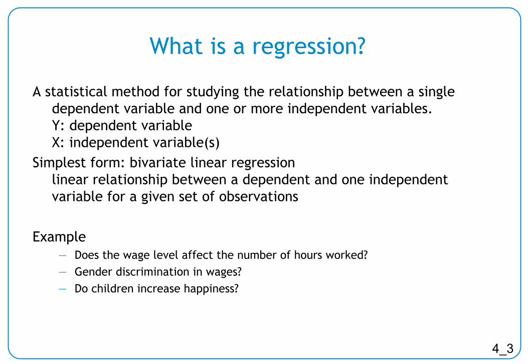
What is a regression?

A statistical method for studying the relationship between a single dependent variable and one or more independent variables.

Y: dependent variable

X: independent variable(s)Simplest form: bivariate

linear regression

linear relationship between a dependent and one independent variable for a given set of observations

Example—

Does the wage level affect the number of hours worked? —

Gender discrimination in wages?—

Do children increase happiness?

4_4

Linear regression: “fitting a line”

02468

10121416

0 1 2 3 4 5 6 7 8X

Y

Y = 1 + 2 x

xi

yi

ŷiei

slope

1 unit

4_5

20000

60000

40000

80000

100000

120000

year

ly in

com

e fro

m e

mpl

oym

ent

0 10 20 30 40 50number of years spent in paid work

“scatter plot”

of

observations

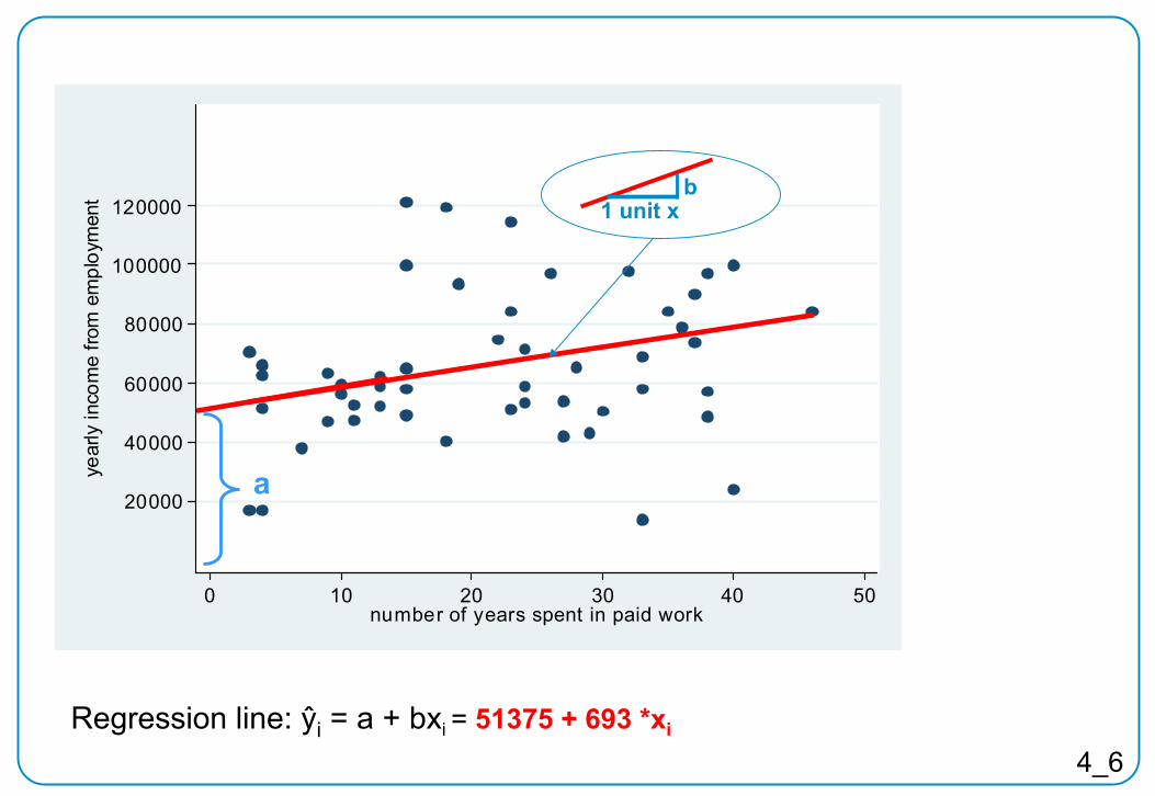
4_6Regression

line: ŷi

= a + bxi

= 51375 + 693 *xi

20000

60000

40000

80000

100000

120000

year

ly in

com

e fro

m e

mpl

oym

ent


a

1 unit xb

4_7

Regression line: ŷi

= a + bxi

= 51375 + 693 *xi

Estimated regression equation: yi

= a + bxi

+ ei

20000

60000

40000

80000

100000

120000

year

lyin

com

efro

mem

ploy

men

t

0 10 20 30 40 50number

of years

spent

in paid

work

4_8

Components (linear) regression equation


= a + bxi

+ ei

y dependent variablex independent variable(s) (predictor(s), regressor(s)) a intercept

(predicted value of Y if x =0)b regression coefficients (slope)

measure of the effect of X on Y

e part of y not explained by x (residual), due to- omitted variables-

measurement errors-

stochastic shock- disturbance

4_9

Scales of independent variables

Independent variables–

Continuous variables: linear

– Binary variables (Dummy variables) (0, 1) (e.g. female=1, male=0)

– Ordinal or multivariate variables (n categories)

Create n-1 dummy variables (base category)

Examples: educational levels–

1 low educational level

2 intermediate educational level 3 high educational level

– Include 2 dummy variables in regression model

4_10

Example: multivariate regression

— Including other covariates: Regression coefficients represent the

portion of y explained by x that is not explained by the other x’s—

Example: gender wage gap (sample: full-time employed, yearly salary between 20’000 and 200’000 CHF)

— Bivariate

model y = a + b x + ei

salary = 98’790 – 17’737 female + ei

— Multivariate model y = a + b1

x1

+ b2

x2

+ b3

x3 + … + ei

bconstant 45'369female -9'090education (Ref: compulsory)

secondary education 9'197tertiary education 30'786

supervision 17'128financial sector 15'592number of years in paid work 729

4_11

Assumptions for OLS-estimations: coefficients

Assumptions for OLS-estimation (necessary to calculate slope coefficients)1)

No perfect multicollinearity

(None of the regressors

can be written as a linear function of the other regressors)

2)

E(e) = 03)

None of the x is correlated with e; Cov(x,e) = 0; (all x’s

are exogenous)

–

If assumptions 1-3 hold: OLS is consistent (regression coefficients asymptotically unbiased)

4_12

Inference from linear regression I–

Inference from OLS-estimations if random sample

–

But: OLS coefficients are estimations–


= a + bxi

+ ei

–

True regression equation: yi

= α + βxi

+ εi

True coefficients (α, β) unknown, true «error term»

unknown

–

Distribution of coefficients (a, b)

E(β)

σ β

2ˆ)()(

bVarbE

4_13

E(β)

σ β

Inference from linear regression II

pnxxbVar i

i

22

2

22 )(

where)(

)(

Variation of b (σβ2): decreases if•

n increases •

x are more spread out •

squared residuals decrease Distribution of b

•

Student t-distribution Depends on n and number of x’s

= normal distribution if n large

4_14

Inference from linear regression: testing whether b ≠

0

–

If β = 0 (in population), there is no

relationship between x and y →

test how likely it is, that β

= 0

–

H0

: Distribution if β = 0

→ critical values for coefficients

→ compare estimated coefficient

with critical value→

if abs(b)

>abs(critical

value), b

significant

b

bvaluetb

stand

b

Critical value for standardized normal distribution and 95% confidence level: 1.96

4_15

Regression line: ŷi

= a + b *xi

example: ŷi

= 51375 + 693 *xi

20000

60000

40000

80000

100000

120000

year

ly in

com

e fro

m e

mpl

oym

ent


Inference from

linear

regression: example

4_16

Inference from

linear

regression: example

| Coef. st.e. t P>|t| [95% Conf. Interval]-----------+---------------------------------------------------years work.| 692.6 289.1 2.40 0.020 112.1 1273.0

_cons |51375.9 7340.4 7.00 0.000 36639.4 66112.5

R2: 0.101

| Coef. St.e. t P>|t| [95% Conf. Interval]----------------------------------------------------------------years work.| 931.4 50.6 18.40 0.000 832.1 1030.7

_cons |51218.6 1271.2 40.29 0.000 48725.5 53711.7-----------------------------------------------------------------

R2: 0.159

Sample

n=53

Sample

n=1787

4_17

Inference : assumptionsAssumptions on error terms

– Independence of error terms , no autocorrelation: Cov

(εi

, εk

) = 0 for all i,k, i≠k

– Constant error variance : Var(εi

)=σ2ε

for all i; (Homoscedasticity)

Preferentially: e is normally distributed

Matrix of error terms

2

2

2

2

2

2

2

00000000000010000000050000004000000300000020000001

154321;

nn

nnki

4_18

Autocorrelation

Reason: Nested observations (e.g. households, schools,

time, communities)→

standard errors

underestimated

→ OLS, adjust

standard errors

2σ2σ

2σ2σ

2σ2σ

2σ2σ

2σ2σ2σ

2σ2σ2σ

2σ2σ2σ

12

21

12

21

122

212

221

00000000001

00000005000004000030000200001

154321;

nn

nnki

2

2

2

2

2

2

000000000000100000000500000040000003000000200000021

154321;

nn

nnki

autocorrelation no autocorrelation

4_19

Heteroskedasticity

Variance is not consistent

→ standard errors

overestimated

or

underestimated→

OLS, adjust

standard errors

(White standard errors)→

Weighted

least squares (WLS)

23

23

22

22

21

21

21

σ0000000σ0000010000σ00005000σ00040000σ00300000σ02000000σ1

154321;

nn

nnki

20

20

20

20

20

20

0

000000000000100000000500000040000003000000200000021

154321;

nn

nnki

HomoskedasticityHeteroskedasticity

4_20

Summary: assumptions of OLS regression

GeneralContinuous dependent variableRandom sample

Coefficient estimationNo perfect multicollinearityE(e) = 0No endogeneity Cov(x,e) = 0

•

Omitted variables•

Measurement error in indep. variables•

Simultaneity•

Nonlinearity in parameters

Inference•

No autocorrelation Cov

(ei, ek)=0•

Constant variance (no heterogeneity)•

Preferentially: residuals normally distributed

Coefficients biased

(inconsistent)

Standard errors of coefficients biased

4_21

Traditional meaningVariable is determined within a model

EconometricsAny situation where an explanatory variable is correlated with the residual

If a variable is endogenousCare with interpretation: model cannot be interpreted as causal

Endogeneity

4_22

Endogeneity: reasons

– Omitted variables

– Measurement error (in explanatory variables)

– Simultaneity

– Nonlinearity in parameters

– x contains lagged values of y (see later, dynamic models)

4_23

Consequence of endogeneity–

ALL estimators may be biased!

(exception: if a variable is completely exogenous controlling for the endogenous variable)

Detection of endogeneity–

Difficult to detect and correct !

– Caution for causal interpretation

– Theory, literature (variable selection and interpretation) !!!!

Endogeneity: consequences and detection

4_24

Endogeneity: correction

— Test for nonlinear relationship and interactions

— Omitted variables • Proxy variables, instrumental variables (2sls estimation)

• Panels: FE-models (within estimators), Difference-in-Difference models

• Propensity score analysis, Regression discontinuity,Heckman selection models,

— Simultaneity• Structural equations modelling, Panel data for time ordering

— Theory, literature (variable selection and interpretation) !!!!

4_25

Example: Control of unobserved heterogeneity

Example: effect of partnership on happinesshappiness = e (partnership)

—

We know (from literature, e.g.): happiness = f (attractiveness, leisure activities, health, ...) [not measured!]

Similarly: partnership = g (attractiveness, leisure activities, health, ...)

—

Cross-sectional data happiness = e(partnership) but we know that there are positive effects on partnership from income, fitness, attractiveness, health, ...

-> which part of effects are due to attractiveness, leisure activities, health, ...?

—

Panel data1.

Happiness (at times with a partner)2.

Happiness (at times without partner)

of the same individualsCare: reversed causality, time-dependent unmeasured effects!)

4_26

– Sample: individuals in employment, 20 to 60 years

– Dependent variable: Working hours per week (paid work)

– Independent variables:hourly wage, number of children, married, sex, age

– Summary statistics

sum workhours wage age08 married_nokid onekid twokids threepkids ///if workhours>0 & age08>=20 & age08<=60

Variable | Obs Mean Std. Dev. Min Max----------------+--------------------------------------------------------

workhours | 3712 36.97117 14.74141 1 98wage | 3199 44.58235 40.15307 .2325581 1500

age08 | 3922 42.25268 10.65961 20 60married_no kids | 3922 .2353391 .4242647 0 1

onekid | 3922 .1573177 .3641465 0 1twokids | 3922 .1932687 .3949123 0 1

three+ kids | 3922 .0739419 .2617096 0 1

Example: Regression analysis using Stata

4_27

Example: check hourly wages

graph box wage

010

020

030

040

0gr

oss

hour

ly w

age

020

040

060

080

0Fr

eque

ncy

0 100 200 300 400gross hourly wage

4_28

Example: transform hourly

wages

histogram wage, freq

histogram lnwage, freq

020

040

060

080

0Fr

eque

ncy

0 100 200 300 400gross hourly wage

010

020

030

0Fr

eque

ncy

2 3 4 5 6lnwage

4_29

reg workhours wagesd wagesq agerec agerecsq married_nokid /// onekid twokids threepkids if workhours>0 & age08>20 & age08<=60

Source | SS df MS Number of obs = 3069-------------+------------------------------ F( 8, 3060) = 216.53

Model | 213427.567 8 26678.4459 Prob > F = 0.0000Residual | 377024.005 3060 123.210459 R-squared = 0.3615

-------------+------------------------------ Adj R-squared = 0.3598Total | 590451.572 3068 192.45488 Root MSE = 11.1

------------------------------------------------------------------------------workhours | Coef. Std. Err. t P>|t| [95% Conf. Interval]

-------------+----------------------------------------------------------------female | -12.41099 .414501 -29.94 0.000 -13.22372 -11.59826lnwage | 16.26171 2.974045 5.47 0.000 10.43038 22.09304

lnwagesq | -1.371871 .4193693 -3.27 0.001 -2.194145 -.549597onekid | -5.12046 .6194891 -8.27 0.000 -6.335117 -3.905803

twokids | -6.561456 .5773265 -11.37 0.000 -7.693443 -5.429469threepkids | -7.204904 .8579049 -8.40 0.000 -8.887032 -5.522776

married_no~d | -3.181037 .593523 -5.36 0.000 -4.344781 -2.017293agerec | -.0426564 .0214263 -1.99 0.047 -.0846678 -.0006449_cons | 6.083153 5.289422 1.15 0.250 -4.288026 16.45433

------------------------------------------------------------------------------

4_30

Diagnostic plot: heteroskedasticity

-4-2

02

46

stan

dard

ised

resi

dual

s

10 20 30 40 50Fitted values

4_31

Diagnostic plot: normal distribution of residuals

0.2

.4.6

Den

sity

-4 -2 0 2 4 6Standardized residuals

-4-2

02

46

stan

dard

ised

resi

dual

s

-4 -3 -2 -1 0 1normal scores

4_32

Regression with

panel data:

Data structure―

Wide

data format

― Long data format(person-period-file, pooled

data)

idpers year wage4101 2004 1031904101 2005 1077304101 2006 1134004101 2007 122470

42101 2004 6318042101 2005 6950056102 2004 3547356102 2006 4140056102 2007 45500

idpers wage04 wave05 wave06 wage074101 103190 107730 113400 122470

42101 63180 69500 . .56102 35473 . 41400 45500

4_33

OLS with pooled

panel data: problems

I

―

OLS for cross-sectional

analysis

(one wave) →

no particular

problem!

―

OLS for pooled

data (different

years

in one file)

•

Problem: assumption

of independent

observations violated

(autocorrelation)•

Possible correction: Correct for clustering

in error

terms

(coefficients unaffected)•

But: OLS is

not the best estimator

for pooled

data (not efficient)

b t b tlnwage 17.44 (13.76) 17.44 -7.85lnwage squared -1.71 (-9.57) -1.71 (-5.55)female -4.48 (-15.34) -4.48 (-11.04)1 child 0.78 (2.05) 0.78 (1.53)female*1 child -10.72 (-20.43) -10.72 (-14.00)2 children 1.74 (4.91) 1.74 (3.84)female*2 children -16.36 (-33.4) -16.36 (-16.36)3+ children 2.85 (5.88) 2.85 (2.85)female*3+ children -18.80 (-26.73) -18.80 (-18.84)married, no child 2.04 (5.63) 2.04 (4.53)female*married, no child -9.56 (-19.95) -9.36 (-13.63)age -0.06 (-6.89) -0.06 (-4.39)

number of working hours per week

OLS OLS, cluster in se

4_34

OLS with panel data: problems

II

OLS does not take

advantage

of panel structure

Two different types of variation in panel data–

Variation within individuals

– Variation between individuals

Control for unobservable variables (stable personal characteristics)–

Fixed Effects Models (only within variation)

– Random Effect Models

(multilevel /random intercept / frailty for event history)

4_35

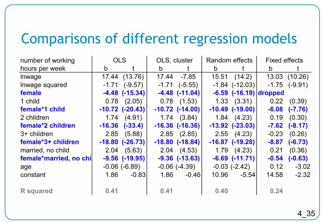
Comparisons of different

regression

models

b t b t b t b tlnwage 17.44 (13.76) 17.44 -7.85 15.51 (14.2) 13.03 (10.26)lnwage squared -1.71 (-9.57) -1.71 (-5.55) -1.84 (-12.03) -1.75 (-9.91)female -4.48 (-15.34) -4.48 (-11.04) -6.59 (-16.19) dropped1 child 0.78 (2.05) 0.78 (1.53) 1.33 (3.31) 0.22 (0.39)female*1 child -10.72 (-20.43) -10.72 (-14.00) -10.49 (-19.00) -6.08 (-7.76)2 children 1.74 (4.91) 1.74 (3.84) 1.84 (4.23) 0.19 (0.30)female*2 children -16.36 (-33.4) -16.36 (-16.36) -13.92 (-23.03) -7.62 (-8.17)3+ children 2.85 (5.88) 2.85 (2.85) 2.55 (4.23) -0.23 (0.26)female*3+ children -18.80 (-26.73) -18.80 (-18.84) -16.87 (-19.28) -8.87 (-6.73)married, no child 2.04 (5.63) 2.04 (4.53) 1.79 (4.23) 0.21 (0.36)female*married, no chi -9.56 (-19.95) -9.36 (-13.63) -6.69 (-11.71) -0.54 (-0.63)age -0.06 (-6.89) -0.06 (-4.39) -0.03 (-2.42) 0.12 -3.02constant 1.86 -0.83 1.86 -0.46 10.96 -5.54 14.58 -2.32

R squared 0.41 0.41 0.40 0.24

number of working hours per week

Fixed effectsRandom effectsOLS OLS, cluster

5Introducing Fixed Effects

Models(“within” effects)

5-2

Example: BMI after stopping smokingHypothesis: BMI increases after stopping smoking

Hypothetical data: Random sample of former smokers with year after stopping and BMI at that time for 3 individuals

time bmi1 bmi2 bmi30 26 . .1 26 242 27 24 213 28 25 224 29 25 225 31 26 246 . 26 247 . . 25

5-3

BMI after stopping smoking: pooled OLS21

2223

2425

2627

2829

3031

BM

I

0 2 4 6 8years after stop smoke

bmi Fitted values

2122

2324

2526

2728

2930

31B

MI


bmi Fitted values

5-4

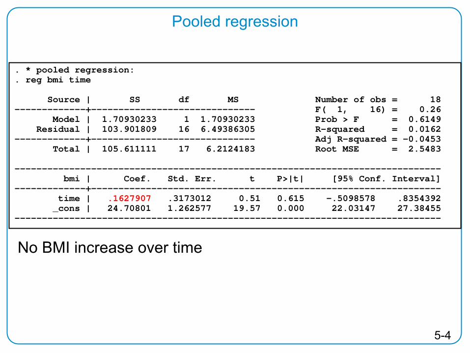
Pooled regression

. * pooled regression:

. reg bmi time

Source | SS df MS Number of obs = 18 -------------+------------------------------ F( 1, 16) = 0.26

Model | 1.70930233 1 1.70930233 Prob > F = 0.6149 Residual | 103.901809 16 6.49386305 R-squared = 0.0162

-------------+------------------------------ Adj R-squared = -0.0453 Total | 105.611111 17 6.2124183 Root MSE = 2.5483

------------------------------------------------------------------------------ bmi | Coef. Std. Err. t P>|t| [95% Conf. Interval]

-------------+---------------------------------------------------------------- time | .1627907 .3173012 0.51 0.615 -.5098578 .8354392 _cons | 24.70801 1.262577 19.57 0.000 22.03147 27.38455

------------------------------------------------------------------------------

No BMI increase over time

5-5

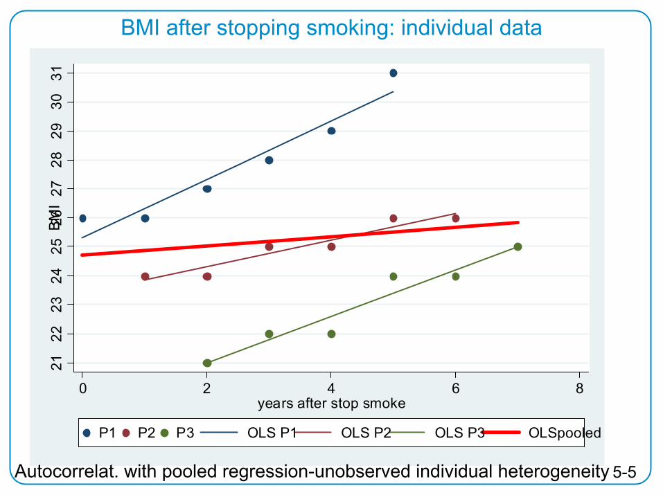
BMI after stopping smoking: individual data21

2223

2425

2627

2829

3031

BM

I


P1 P2 P3 OLS P1 OLS P2 OLS P3 OLSpooled

Autocorrelat. with pooled regression-unobserved individual heterogeneity

5-6

Individual regressions

. forval

j=1/3 { /* loop over each individual*/

2. reg

bmi`j' time

3. }

bmi1 | Coef. Std. Err. t P>|t| [95% Conf. Interval]

-------------+----------------------------------------------------------------

time | 1

.1380131 7.25 0.002 .6168142 1.383186

_cons | 25.33333 .4178554 60.63 0.000 24.17318 26.49349

------------------------------------------------------------------------------


-------------+----------------------------------------------------------------

time | .4571429

.0699854 6.53 0.003 .2628322 .6514535

_cons | 23.4 .2725541 85.85 0.000 22.64327 24.15673

------------------------------------------------------------------------------


-------------+----------------------------------------------------------------

time | .8

.1069045 7.48 0.002 .5031855 1.096814

_cons | 19.4 .5145502 37.70 0.000 17.97138 20.82862

------------------------------------------------------------------------------

All individuals have significant BMI increase over time

5-7

Excursus: unobserved heterogeneity

Omitted variables bias:

•

Many individual characteristics are not observed–

e.g. enthusiasm, ability, willingness to take risks, our example: physical activities, calories intake, muscle mass, genes, cohort

•

These have generally an effect on dependent variable, and are correlated with independent variables. Then regression coefficients will be biased!

Note: these (formerly) unobserved measures are increasingly included in surveys

5-8

2122

2324

2526

2728

2930

31B

MI


P1 P2 P3 OLS P1 OLS P2 OLS P3 OLSpooled

What about the between-effect?21

2223

2425

2627

2829

3031

BM

I


P1 P2 P3 OLS P1 OLS P2 OLS P3

5-9

Which models are appropriate to analyze the effects of ‘time’?

Data transformation necessary

5-10

Panel Data and within- Regression (FE)

5-11

Error components in panel data models

•

We separate the error components:eit

= ui

+ εit

, ui

= person-specific unobserved heterogeneity (level) = „fixed effects“

(e.g., physical activities, calories intake, genetics, cohort)

εit

= „residual“

Model:

•

Remember: Pooled OLS assumes that x is not correlated with both error components ui

and εit

(omitted variable bias)

itiitit uxbmi 10

5-12

Fixed effects regression•

We can eliminated the fixed effects ui

by estimating them as person specific dummies

•

-> remains only within-variation

•

Corresponds to “de-meaning”

for each individual:(1)

individual

mean:

(2)

•

subtract (2) from (1):

-> Fixed (all time invariant) effects ui disappear, i.e. time- constant unobserved heterogeneity is eliminated

itiitit uxbmi 1

iiii uxbmi 1

)()(1 iitiitiit xxbmibmi

5-13

2122

2324

2526

2728

2930

31B

MI



De-meaned

values with OLS regression-2

-1.5

-1-.5

0.5

11.

52

2.5

33.

5de

-mea

ned

BM

I

-2 0 2de-meaned years after stop smoke


5-14

OLS of individually de-meaned

Data

We

de-mean and regress the Data:. bysort id: egen bmi_m=mean(bmi). gen bmi_dem=bmi-bmi_m

. bysort id: egen time_m=mean(time)

. gen time_dem=time-time_m

. reg bmi_dem time_dem


Model | 29.7190476 1 29.7190476 Prob > F = 0.0000Residual | 5.11428571 16 .319642857 R-squared = 0.8532

-------------+------------------------------ Adj R-squared = 0.8440Total | 34.8333333 17 2.04901961 Root MSE = .56537

------------------------------------------------------------------------------bmi_dem | Coef. Std. Err. t P>|t| [95% Conf. Interval]

-------------+----------------------------------------------------------------time_dem | .752381 .0780284 9.64 0.000 .5869681 .9177938

_cons | -2.12e-07 .1332589 -0.00 1.000 -.2824965 .2824961------------------------------------------------------------------------------

5-15

Direct modeling of fixed Effects in Stata

xtreg

bmi

time, fe

(calculates correct df; this causes higher Std. Err.) . xtreg bmi time, fe

Fixed-effects (within) regression Number of obs = 18Group variable: id Number of groups = 3

R-sq: within = 0.8532 Obs per group: min = 6between = 0.9902 avg = 6

time since stop smoking explains parts of individual heterogeneity!max = 6

overall = 0.0162 (from pooled OLS)

F(1,14) = 81.35corr(u_i, Xb) = -0.4301 Prob > F = 0.0000

------------------------------------------------------------------------------bmi | Coef. Std. Err. t P>|t| [95% Conf. Interval]

-------------+----------------------------------------------------------------time | .752381 .0834159 9.02 0.000 .5734716 .9312903_cons | 22.64444 .3248582 69.71 0.000 21.94769 23.3412

-------------+----------------------------------------------------------------sigma_u | 3.1781651sigma_e | .60440559

rho | .96509605 (fraction of variance due to u_i)------------------------------------------------------------------------------F test that all u_i=0: F(2, 14) = 137.55 Prob > F = 0.0000

5-16

Alternative: OLS with individual dummies controlled

. xi i.id, noomit

. reg bmi time _I*, noconst


Model | 11601.8857 4 2900.47143 Prob > F = 0.0000Residual | 5.11428571 14 .365306122 R-squared = 0.9996!

-------------+------------------------------ Adj R-squared = 0.9994Total | 11607 18 644.833333 Root MSE = .60441


-------------+----------------------------------------------------------------time | .752381 .0834159 9.02 0.000 .5734716 .9312903

_Iid_1 | 25.95238 .3230684 80.33 0.000 25.25947 26.64529_Iid_2 | 22.36667 .3822597 58.51 0.000 21.5468 23.18653_Iid_3 | 19.61429 .4492084 43.66 0.000 18.65083 20.57774

------------------------------------------------------------------------------

useful for small N, the ui

are estimated (only approximate)

5-17

•

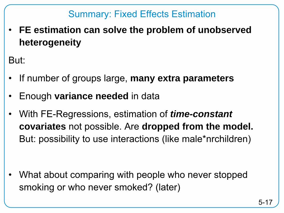
FE estimation can solve the problem of unobserved heterogeneity

But:

•

If number of groups large, many extra parameters

•

Enough variance needed in data

•

With FE-Regressions, estimation of time-constant covariates not possible. Are

dropped from the model.

But: possibility to use interactions (like male*nrchildren)

•

What about comparing with people who never stopped smoking or who never smoked? (later)

Summary: Fixed Effects Estimation

5-18

No identification of time-invariant covariates zi

Consider the model: yit

= azi

+ bxit

+ ui

+ εit

(1)let

be an arbitrary number; add and subtract zi on the rhs:

yit

= (azi

+ zi ) + bxit

+ (ui

- zi ) + εit

and rewrite this as:yit

= a*zi

+ bxit

+ ui

*+ εit

with a* = a +

and ui

* = ui

-

zi

(2)

But (1) and (2) have exactly the same form so it is not clear if a or a* = a +

is estimated

-> separate effects of azi and ui cannot be distinguished without further assumptions (e.g., no correlation between zi

and ui

)

5-19

Example: DiD

(control group comparison)Hypothesis: financial support increases BMI of low-income

women (Schmeisser

2009)*

(hypothetical) experiment:Survey: Sample of low income female patients of doctoral

surgeries randomized into

program “social aid” (50% in program and 50% not)

4 measurements of bmi

(2 x before program start, 2 x after)

*Expanding wallets and waistlines: the impact of family income on

the bmi

of women and men eligible for the earned income tax credit. Health Econ. 18: 1277–1294

5-20

Data: BMI-increase through “social aid”?Effects:

causal effect: BMI increase due to more fast food (more money available)

Time (age-) effect: BMI increases with age

Start “social aid”

Programm

2122

2324

2526

2728

2930

3132

bmi

1 2 3 4time

NO aid aid

BMI of low income Women

5-21

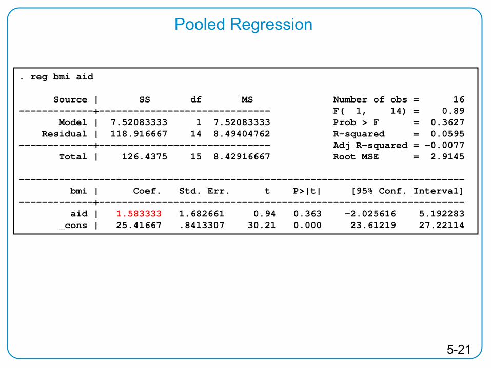
Pooled Regression

. reg bmi aid


Model | 7.52083333 1 7.52083333 Prob > F = 0.3627Residual | 118.916667 14 8.49404762 R-squared = 0.0595

-------------+------------------------------ Adj R-squared = -0.0077Total | 126.4375 15 8.42916667 Root MSE = 2.9145


-------------+----------------------------------------------------------------aid | 1.583333 1.682661 0.94 0.363 -2.025616 5.192283

_cons | 25.41667 .8413307 30.21 0.000 23.61219 27.22114

5-22

Fixed effects

xtreg

bmi

aid, fe. xtreg bmi aid, fe


R-sq: within = 0.3596 Obs per group: min = 4between = 0.0054 avg = 4.0overall = 0.0595 max = 4

F(1,11) = 6.18corr(u_i, Xb) = -0.0704 Prob > F = 0.0303


-------------+----------------------------------------------------------------aid | 2 .8048151 2.49 0.030 .228614 3.771386

_cons | 25.3125 .3484951 72.63 0.000 24.54547 26.07953-------------+----------------------------------------------------------------

sigma_u | 2.9606798sigma_e | 1.1381804


5-23

One step back: a causal model

• With cross-sectional data: only between-estimation:

Crucial assumption:

Random sample (no unobserved heterogeneity)

• With Panel data I: within-estimation (before and after)

problem: time effects, panel conditioning

• With Panel data II: “difference-in-difference” (DID):

)()( ontrolCreatmentT YY00 ti,ti,

CT YY01 ti,ti,

)()( CCCT YYYY 0101 tj,tj,ti,ti,

5-24

Now: causal effect of ‘aid’

• We have-

Before-after comparison (within)

-

Treatment- and control groups (between)•

We compare the within-effect of aid (“treatment”) with that without aid (“control”)

i.e., we calculate treatment effect and control for time‘DID’ – estimator:

=(afteraid - beforeaid )- (afternoaid – beforenoaid )

25.5.2475.262527

422212827

423233130

424242626

426252928

5-25

DiD

effects. xi i.time, noomit. xtreg bmi aid _I* , fenote: _Itime_4 omitted because of collinearity



F(4,8) = 15.80corr(u_i, Xb) = -0.0055 Prob > F = 0.0007


-------------+----------------------------------------------------------------aid | -.25 .559017 -0.45 0.667 -1.539096 1.039096

_Itime_1 | -2.875 .4841229 -5.94 0.000 -3.991389 -1.758611_Itime_2 | -2.375 .4841229 -4.91 0.001 -3.491389 -1.258611_Itime_3 | -.75 .3952847 -1.90 0.094 -1.661528 .1615282_Itime_4 | 0 (omitted)

_cons | 27.375 .3952847 69.25 0.000 26.46347 28.28653-------------+----------------------------------------------------------------

sigma_u | 2.952753sigma_e | .55901699


5-26

•

FE easier, no control group

•

DID: control group can control simultaneous effects (like time): find “statistical twin”, such that research variables is only variable

-> DID useful for estimating

causal effects from

non- experimental data. Especially for

small samples

Excursus: First-Difference (FD) estimators: Stable similarities of adjacent observations eliminated. Problem:

•

level differences not taken into account (6-5 children = 1-0 ch)•

for lasting effects (like children): FD not useful because only immediate changes taken into account

Summary: within estimators

6-1

6Introducing Random

Effects Models

6-2

We have both -within and -between variance:

yit

= a + eit

= a + ui

+ εit„fixed effects“

= within: u0i

for each person (≈ANOVA)

Towards RE: error components in panel models

a

u1

11

two residuals:

- it

on lowest (1.) level: time point

- ui

on highest (2.) level: individuals

6-3

Necessary, if data have different levels with-

observations are not independent

of levels

- true social interactions

Examples: Schools –

classes –

students: first applications

Networks: people are influenced by their peersSpatial context: from environment (e.g., poor people are less happy

if they live in a rich environment) – US: “neighborhood-effects”

Interviewer - effects: respondents clustered in interviewers

Panel-surveys: waves clustered in respondents (households)

Motivation: multilevel models

6-4

Hierarchical-

Households in neighborhoods

-

Students in schools in classes (three levels)-

Respondents in interviewers-

Panel Surveys: Waves in respondents (crossed?)Crossed

-

Questions in respondents→ longitudinal?

Attention:Do not confuse variables and levels:(total) variance can be attributed to levels, not to variables!E.g., 100 hospitals are probably a level, 7 nations are probably

dummy variables. Think of a population the sample represents!

Note: “30 rule of thumb”

in contexts: ≥30 second level units, randomly chosen

Levels in clustered data

6-5

• Improved

regression models

-

unbiased estimators for regression coefficients-

unbiased estimators for standard errors (usually higher std.err. than OLS)-

model true covariance structure

(autocorrelation, heteroscedasticity, …)

• Decomposition of total variance into those in different levels (within-between)

• Similar to Analysis of variance (ANOVA), but parsimonious

(number of estimation parameter independent on number of contexts)

→ can handle large number of contexts

(in parts) modeling of unobserved heterogeneity / self selection

Multilevel models: analytic advantages

6-6

mixed school boy school girl school

Typical results: one-level vs. multilevel modelD

epen

dent

Var

iabl

e

Underestimated variance:Kish design effect

„deff”:

larger N necessary

6-7

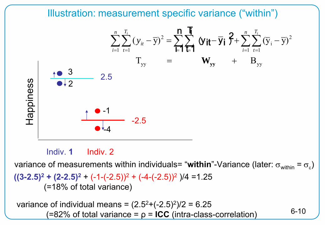
Example: 2 individuals each asked 2x about their happiness (continuous), here measurements not time ordered!

Which variance is due to individuals, which to observations?

Total Mean= (3+2+(-1)+(-4)) / 4 = 0

Total (“Grand”) Mean (=0)

32

-1

-4

Hap

pine

ss

Indiv. 2Indiv. 1

Illustration: variance decomposition between levels

6-8

Total Mean (=0)

32

-1

-4

Hap

pine

ss

Indiv.

2Indiv.

1

Total Variance is equal to the Square of the Differences of all Observations from the Total Mean divided by the Sample Size (4) =

{ (3-0)2 + (2-0)2 + (-1-0)2+(-4-0)2

} / 4 = (9+4+1+16)/4 = 7.5

Illustration: calculation of the total variance

yyyy

1 1

2i

1 1

2i

B W

)yy()y(

yyT

n

i

T

t

n

i

T

tit

ii

yn

1i

T

1t

2it

i

︶y︵y

6-9

32

-1

-4

Hap

pine

ss

Indiv.

2Indiv.

1

Total Mean (=0)

2.5

-2.5

variance of the individual means = “between”-variance (between

= u

)

(remember: total variance = 7.5)

(2.52+(-2.5)2)/2 = 6.25

Illustration: individual specific variance (“between”)

yyB W T

)y()y(

yyyy

1 1

2i

1 1

2

n

1i

T

1t2i

i

︶yy︵

n

i

T

tit

n

i

T

tit

ii

yy

6-10

32

-1

-4

Hap

pine

ss

Indiv.

2Indiv.

1

2.5

-2.5

variance of measurements within individuals= “within”-Variance (later: within

=

)

variance of individual means = (2.52+(-2.5)2)/2 = 6.25(=82% of total variance = ρ

= ICC (intra-class-correlation)

((3-2.5)2

+ (2-2.5)2

+ (-1-(-2.5))2

+ (-4-(-2.5))2

)/4 =1.25 (=18% of total variance)

Illustration: measurement specific variance (“within”)

yyyy

1 1

2i

1 1

2

B T

)yy()y(

yyW

n

i

T

t

n

i

T

tit

ii

yn

1i

T

1t2iit

i

︶y︵y

6-11

ICC

≈

0.2

ICC

≈

0.8Examples of ΘICC

=

0

(maximum clustering)

ICC

= 1

(zero clustering → use OLS)

6-12

Starting point: “null” (“Variance Components”

(VC)) model

:iondecomposit variance for allows model VCthe

assumed) )σ(N(0, meanspecific individual from deviationεassumed) )σ(N(0, variable randomspecific individualu

:wheremodel) VCin a intercept no :(note

εit

u00i

itiit uy 0

necessary) model multilevel tsignifican ρ :(note

Panels) in ationautocorrel ncorrelatio-class-intraICC( σσ

σρ

:i individual an withint points time different between ncorrelatio ρ

2ε

2u0

2u0

6-13

Idea RE: better estimate of ui

(modeling intercept)

To estimate mean of individual i (=ui

) only within (FE) suboptimal if

- sample small (Ti small)- variance

high- n large (inefficient)

idea: use information uj

from other sample members (between) in the same population group (e.g., education)

a

u0

high edu

low edu

random intercept (“borrowing strength” from others):

6-14

0))ucov(x, (if term error in remains u because biased RE u variables invariant time of estimation allows RE

variation between and withinof ncombinatio optimal uses RE

1θ0 Tσσ

σ and ,1θ with

))ε θ(εθ)(1(u)x θ(xβθ)(1β)y θ(y:tionTransforma the after OLS pooled to equivalent is Regression -RE

ii

i

2u

2ε

2ε

iitiiit10iit

,

Idea RE: weighted within and between

6-15

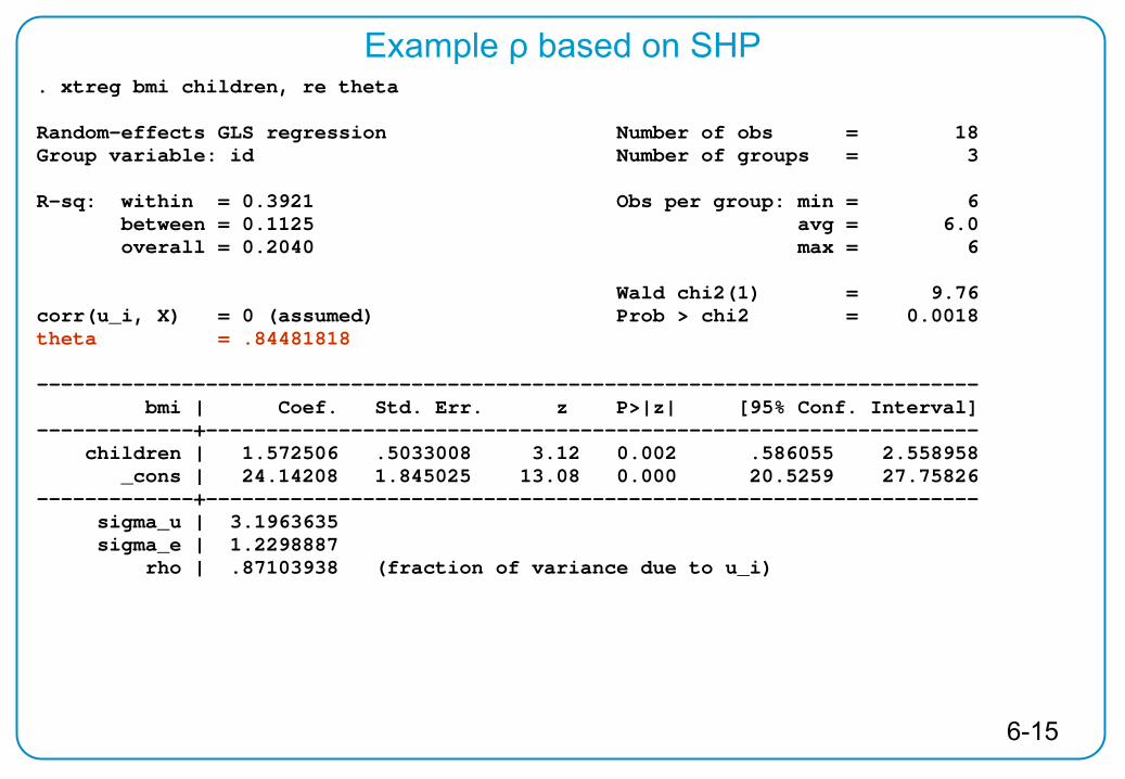
Example ρ based

on SHP

. xtreg bmi children, re theta

Random-effects GLS regression Number of obs = 18Group variable: id Number of groups = 3


Wald chi2(1) = 9.76corr(u_i, X) = 0 (assumed) Prob > chi2 = 0.0018theta = .84481818

------------------------------------------------------------------------------bmi | Coef. Std. Err. z P>|z| [95% Conf. Interval]

-------------+----------------------------------------------------------------children | 1.572506 .5033008 3.12 0.002 .586055 2.558958

_cons | 24.14208 1.845025 13.08 0.000 20.5259 27.75826-------------+----------------------------------------------------------------

sigma_u | 3.1963635sigma_e | 1.2298887

rho | .87103938 (fraction of variance due to u_i)

6-16

Random-Effects estimation

6-17

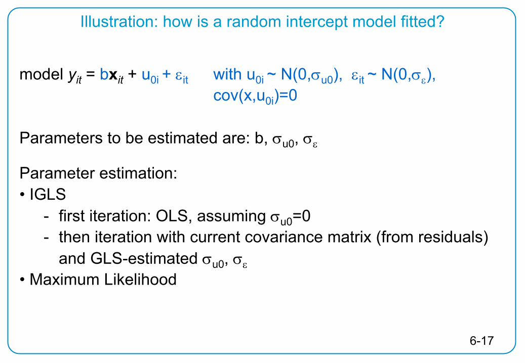
model yit

= bxit

+ u0i + it

with u0i ~ N(0,u0

), it ~ N(0,

), cov(x,u0i

)=0

Parameters to be estimated are: b, u0

,

Parameter estimation: • IGLS

- first iteration: OLS, assuming u0

=0-

then iteration with current covariance matrix (from residuals) and GLS-estimated u0

,

• Maximum Likelihood

Illustration: how is a random intercept model fitted?

6-18

Intuition of multilevel (random intercept)

ui

εit

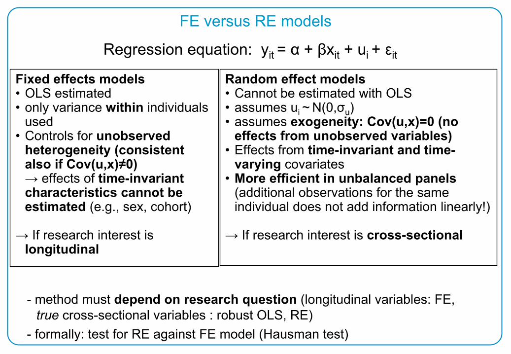
FE versus RE models

Fixed effects models•

OLS estimated•

only variance within

individuals used

•

Controls for unobserved heterogeneity (consistent also if Cov(u,x)≠0)→ effects of time-invariant characteristics cannot be estimated

(e.g., sex, cohort)

→ If research interest is

longitudinal

Random effect models•

Cannot be estimated with OLS•

assumes

ui

~ N(0,σu

)•

assumes

exogeneity: Cov(u,x)=0 (no effects from unobserved variables)

•

Effects from time-invariant

and time-

varying

covariates•

More efficient in unbalanced panels

(additional observations for the same individual does not add information linearly!)

→ If research interest is

cross-sectional

Regression equation: yit

= α + βxit

+ ui

+ εit

-

method must depend on research question

(longitudinal variables: FE, true cross-sectional variables : robust OLS, RE)

- formally: test for RE against FE model (Hausman

test)

6-20

Hausman test

Test if FE or RE model (basic assumption: FE unbiased)Test H0

: E(ui

| xit

) = cov(ui ,

xit

) = 0

cov(ui

,xit

) = 0

-> FE and RE unbiased, FE is inefficient

-> REcov(ui

,xit

) ≠

0

-> FE is unbiased and RE is biased -> FE

If H0

is true (between-coeff.=within-coeff.), no differences between FE and RE

not β but unbiased β , H if

))βvar( )β(var( efficient more β and β β , H if

β and β tscoefficien estimation compares Hausman

:lyequivalent

REFE1

REFEREREFE0

REFE

ˆˆ

ˆˆˆˆˆ

ˆˆ

Note: -

H0 almost always rejected (sample size high enough even with small differences)-

Test does not

replace research question driven check for model appropriateness

6-21

Hausman test: example

* Hausman Test: RE or FE estimate?. qui xtreg bmi children, re

. estimates store random

. qui xtreg bmi children, fe

. estimates store fixed

. hausman fixed random

---- Coefficients ----| (b) (B) (b-B) sqrt(diag(V_b-V_B))| fixed random Difference S.E.

-------------+----------------------------------------------------------------children | 1.575758 1.572506 .0032511 .1473474

------------------------------------------------------------------------------b = consistent under Ho and Ha; obtained from xtreg

B = inconsistent under Ha, efficient under Ho; obtained from xtreg

Test: Ho: difference in coefficients not systematic

chi2(1) = (b-B)'[(V_b-V_B)^(-1)](b-B)= 0.00

Prob>chi2 = 0.9824

6-22

• RE more

efficient

than FE

because RE also models person

specific time-invariant effects (uses more information)

• RE uses combination of within-

and between-

estimator

• RE uses coefficients of time-invariant regressors

(between-

Variation)

• RE not useful for causal effects of time-variant regressors–

Main assumption of RE (and limitation vs. FE): Person specific effect ui

must not correlate with regressors

–

Hausman

test

can test this assumption

Summary: RE estimation

6-23

RE models•

RE controls for unobserved heterogeneity (under strong assumptions)•

Unbiased standard errors (and inferences)•

Decomposition of total variance

on different levels•

Modeling of variance•

Allows for covariance that is appropriate for

panel data (autocorrelation, heteroscedasticity, etc.)

Longitudinal models (e.g., FE, DiD)

•

Full control for unobserved heterogeneity•

Fixed effects models: within-variance only•

Difference-in-Difference (DID): before –

after comparisons (within-

treatment –

effect), controlled for observed (between) effects•

Other models possible (FD)

Summary: models for panel data

6-24

Specifically for linear regression models•

“Within”

research questions –

“causal”

effects of time-variant

variables: →

modeling intrapersonal change (FE models)

If in addition interest in

time-invariant variables:

→ hybrid models (RE, include individual means)

• Cross-sectional

research questions –

effects of time-invariant

effects, (“correlations”)→ OLS with robust standard errors In unbalanced panels:→ RE models

• Interpretation (eg

children):

within: effect of additional childrenbetween: differences between people with a different number of children

6-25

Models result example

* Data: bmi

sample

estout

m1 m2 m3 m4, cells(b

se)

----------------------------------------------------------------------OLS OLS_cluster_pers

FE RE b/se b/se b/se b/se

----------------------------------------------------------------------working -.5276885 -.5276885

-.2835562 -.3273556 .1002146 .1605462 .0774774 .0716089

working_bar

working_dem

_cons 25.92231 25.92231

25.76707 25.69604.0799125 .1390252 .0519713 .0941936

----------------------------------------------------------------------

6-26

FE is preferred for causal statementsBUT: no inclusion of time-constant variablesIdea: hybrid-models

simultaneous within and between regression:

Hybrid models (“regression with context variables”)

itiiiitit ay zxxx )(

• Estimated as RE model

• Hybrid-models separate within and between -

effects

• Hybrid-models eliminate the part of unobserved heterogeneity correlated with the independent variables (→ unbiased estimators)

6-27

+ hybrid (1)* Data: bmi sampleestout m1 m2 m3 m4 m5, cells(b se) stats(N r2 r2_w r2_b sigma_u sigma_e thta_max)----------------------------------------------------------------------------

OLS OLS_cluster_pers

FE RE REb/se b/se b/se b/se

----------------------------------------------------------------------------working -.5276885 -.5276885

-.2835562 -.3273556 .1002146 .1605462 .0774774 .0716089

working_bar

-

working_dem

-

_cons 25.92231 25.92231

25.76707 25.69604 .0799125 .1390252 .0519713 .0941936

----------------------------------------------------------------------------N 9189 9189 9189 9189r2 .0030089 .0030089 .0021589 r2_w .0021589 .0021589r2_b .0032241 .0032241sigma_u 4.517998 4.393536sigma_e 1.586554 1.586554thta_max .8223176

6-28

hybrid (2)

SHP 2000-2010RE (combin.)

FE (dem(x))

BE (mean(x))

hybrid (both)

Happiness b b b bnb children 0.013** -0.017* 0.102***

health 0.391*** 0.288*** 0.954*** 0.393***male 0.065*** 0.128*** 0.062**

intermed. educ. -0.089*** -0.192*** -0.065** -0.096***high educ. -0.083*** -0.255*** -0.062* -0.088***childmean 0.064***childwithin -0.016*

_cons 6.482*** 7.049*** 4.072*** 6.438***N 74315 74315 74315 74315

7-1

7Non linear regression

7-2

Non‐linear regression: motivation

―Linear regression: requires continuous dependent variablee.g. BMI, income, satisfaction on scale from 0‐10 (?)

―Most variables in social science are not continuous but discrete

– Opinions: agree vs. disagree

– Poverty status

– Party voted for

– Number of visits to the doctor

– Having a partner

―We need appropriate regression models!

7-3

Dependent variable is not continuous: non‐linear regression

Binary variables (dummy variables, 0 or 1) (e.g. yes‐no)

Logistic Reg., Probit Regression

Complementary log‐log Regression

Multinomial (unordered variables) (e.g. vote choice, occupation)

Multinomal logistic Regression

Multinomial probit Regression

Ordinal (e.g. satisfaction)

Ordinal Regression

Count variable (e.g. doctor visits)

Poisson Regression Negative Binomial Regression

Non‐linear models

7-4

Linear probability model for binary variables

0

x

1

Binary variables (y = 0 or 1)E(y)=π

(probability y=1)

Linear probability model: π =

+ β1

x1

+ ….

7-5

Problems of linear probability model

Violation of regression assumptions– The variance of y for binary variables is π(1‐π)

→ residual variance depends on xi → heteroskedasticity

– Relationship between response probability and x may not be linear, especially for π

close to 0 and π

close to 1

– Predicted response probabilities may be negative or greater than one

– Residuals can take only take two values for fixed x → residuals are not normally distributed

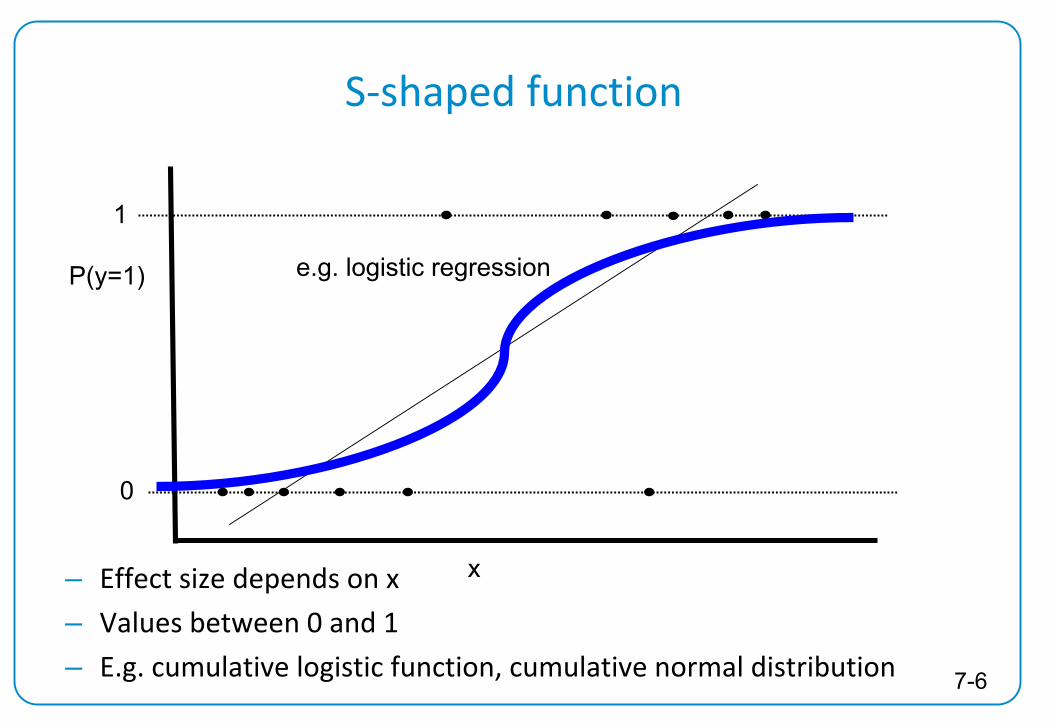
S‐shaped function

7-6

0

P(y=1)

x

1

e.g. logistic regression

– Effect size depends on x– Values between 0 and 1 – E.g. cumulative logistic function, cumulative normal distribution

7-7

Non‐linear transformations for binary variables

Logistic transformation

ei

follow a logistic distribution: logit model

Normal transformation

ei

follow normal distribution: Probit model

Pr(y=1) = Ф (α + βx)

where Ф is the cdf

of a standard normal distribution

For practical purposes, logit and probit models are equivalent for statistical

analysis (very similar predicted probabilities)

...xβxβα1

LnLogit

11)1Pr(

2211

...)( 2211

PP

ePy xx

7-8

Generalised linear model

– A latent (unobserved) continuous variable y* which underlies the observed data

y* = a + b1

x1

+….+ e*– Assume yi

* is generated by a linear regression structure– Link function between y and y*

E(y) = g‐1(y*) = g‐1(a + b1

x1

+….+ e*)

• Choice of the link function depends on distribution of e*e.g. logit, probit, poisson, negative binomial

– Scale of y* is variable, variance of ei

* assumed Probit

model: assume ei

*~N(0,1) Logit model: assume ei

* standard logistic (with var=π2/3 ~3.29)– → in general, coefficients cannot be compared across different models

7-9

Most frequent link functions

Distribution Link functionNormal Identity y=y*Poisson Log y=exp(y*)Binomial Logistic

Probit

y=1/(1+exp(y*))

y= Ф(y*)

7-10

Maximum likelihood estimation

– Usually, non‐linear models are estimated by maximum likelihood (MLE)

– Advantages of MLE• MLE is extremely flexible and can easily handle both

linear and non‐linear models• Desirable asymptotic properties: consistency, efficiency,

normality, (consistent if missing at random MAR)– Disadvantages of ML estimation

• Requires assumptions on distribution of residuals

• Desired properties hold only if model correctly specified

• Best suited for large samples

7-11

Parameter estimation with ML

― Principle for MLE: Which set of parameters has the highest likelihood

to generate the data actually observed (xi

, yi

)?

― Observed values (xi

, yi

) are a function of the unknown model parameters θ

L=f( xi

, yi

| θ) (likelihood function)

― The maximum likelihood estimate θ

is that value which maximizes L

― Often, there is no closed form (algebraic) solution. Coefficients have

to be estimated through numerical methods (iterative algorithms)

― For practical reasons, often the log‐likelihood is used instead of the

likelihood

― Linear model: MLE = OLS estimator

7-12

Example: logistic regression (y: 1 vote SVP; 0 vote other party)

M1 M2

Female -0.510*** -0.380***18-30 years -0.004 0.087 46-60 years 0.013 0.08160+ years 0.091 0.192 Education: intermed -0.239* -0.240

Education: high -1.121*** -0.929***Income (hh, log) -0.395*** -0.281***

EU: against joining 2.101***

Foreigners: prefer Swiss 1.070***

Nuclear energy: pro 0.570***

Satisfaction with democracy -0.233***

constant 3.510*** -0.233***

N 3879 3879

7-13

Example: logit vs probit

logit probitb t b t

female -0.380*** (-3.7) -0.222*** (-3.8)18 - 30 years 0.087 (0.6) 0.041 (0.6)46 - 60 years 0.081 (0.6) 0.047 (0.6)over 60 years 0.192 (1.4) 0.108 (1.4)intermed.edu. -0.240 (-1.8) -0.146 (-1.9)high edu. -0.929*** (-5.6) -0.552*** (-5.9)hh income (log) -0.281*** (-3.5) -0.163*** (-3.6)stay outside EU 2.101*** (15.0) 1.123*** (16.1)prefer Swiss 1.070*** (11.0) 0.625*** (11.2)pro nuc. energy 0.570*** (5.6) 0.334*** (5.8)satisf.democracy-0.233*** (-9.1) -0.132*** (-9.1)_cons 1.260 (1.4) 0.801 (1.6)

Pseudo R-Square 0.253 0.257 N 3879 3879

7-14

Interpretation of non linear models– Because of the non‐linearity, coefficients cannot be interpreted directly

– Predicted probabilities

have to be

computed through

a non‐linear

transformation

according to the

link function

e.g. πi

= F(α

+ βxi

)

– Interpretation of

Odds ratios (OR)

problematic

7-15

Odds ratios (OR)

OR Often misunderstood as relative risk

P Odds OR RRA Group 1 0.10 0.11 2.10 2.00

Group 2 0.05 0.05B Group 1 0.40 0.67 2.70 2.00

Group 2 0.20 0.25C Group 1 0.80 4.00 6.00 2.00

Group 2 0.40 0.67D Group 1 0.60 1.50 6.00 3.00

Group 2 0.20 0.25E Group 1 0.40 0.67 6.00 4.00

Group 2 0.10 0.11

Ref.: Best and Wolf 2012, Kölner Zeitschrift für Soziologie

7-16

Predicted probabilities: exampleLogit model

Example Individual i with x1

=2 and x2

=1,

exp(logit)1exp(logit)

11)1Pr( )( 2211

xxey

0.5 ; -2 3;α^^^

21

62.01

11

1

5.0

)5.02)2(3(

^

e

ei

7-17

Calculate predicted probabilities

– Remember: predicted probabilities depend on values of x and parameter estimates (and unobserved heterogeneity)

– It is often useful to vary only one covariate and hold the others constant

• at their mean

• at realistic values (mean for continuous variables, median for

ordinal variables, mode for nominal variables)

– Note: Regression parameter are estimates (sampling variability, confidence intervals)

→ also predicted probabilities are estimates → confidence intervals also for predicted probabilities

7-18

How does change in x affect predicted probability (y)?

– Discrete change The change in predicted probability as one moves from one (discrete)

value of a predictor to another, holding all else equal.

– Marginal effect (MFX) or Partial effect The slope of y* at x, holding all else equal.

– Average partial effect (APE) The average change in predicted probability at different given values

of a predictor (calculate effect for each individual i).

– Average marginal effect (AME) The average slope of y* at x (calculate effect for each individual i).

(in Stata: margins)

7-19

Example: predict discrete change

Variation of one variable, others at their mean or mode

Vote intention for SVP 2009margins i.eu_contra i.for_contra i.nuc_pro, ///atmeans at (female=0 edulevel=2 agegr=2 )

Discrete

change95% Confidence

Intervall

Sex Men 13.3 10.2 16.4

Women 9.5 7.3 11.7

Education Low 16.4 11.4 21.3

Intermediate 13.3 10.2 16.4

High 7.2 5.3 9.0

EU Pro or neither 4.7 3.1 6.2

Contra 28.8 23.6 34.0

Foreigners Same changes or neither 10.2 7.7 12.8

Better changes for Swiss 24.9 19.4 30.3

Satisfaction

DemocracyMinimal (0) 39.7 30.3 49.1

Maximal 6.0 4.0 8.0

7-20

Example: Average Partial effects

Vote intention for SVP 2009margins i.female

i.edulevel

i. agegrAPE 95% Confidence

Intervall

Sex Men 20.4 18.8 22.1

Women 16.2 14.7 17.6

Education Low 23.0 19.8 26.2

Intermediate 20.0 18.4 21.5

High 12.6 10.8 14.5

EU Pro or neither 36.8 35.0 38.7

Contra 5.3 51.5 54.8

Foreigners Same changes or neither 42.9 41.4 44.3

Better changes for Swiss 53.4 51.8 55.8

Satisfaction

DemocracyMinimal 70.1 67.1 74.6

Maximal 30.1 27.5 32.8

Marginal effects-.0

8-.0

6-.0

4-.0

20

Effe

cts

on P

r(S

vp)

0 1 2 3 4 5 6 7 8 9 10satisf. democracy

Conditional Marginal Effects of satdem with 95% CIs

margins, atmeans at (satdem=(0(1)10)) dydx (satdem)

Average Marginal effect-.0

5-.0

4-.0

3-.0

2-.0

1E

ffect

s on

Pr(S

vp)

0 1 2 3 4 5 6 7 8 9 10satisf. democracy

Average Marginal Effects of satdem with 95% CIs

margins, at (satdem=(0(1)10)) dydx (satdem)

7-23

Model performance

Linear regression: R2, adjusted R2

Non linear regression - variance of the residual not observed

- many so‐called pseudo‐R2 (0,1) (Stata: fitstat)

Example:voting model

y in var. totaly in var. explainedR 2

M1 M2

McFadden's R2 0.050 0.253

McFadden's Adj R2 0.044 0.247

ML (Cox-Snell) R2 0.046 0.214

Cragg-Uhler(Nagelkerke) R2 0.046 0.214

Count R2 0.816 0.827

Adj Count R2 0.003 0.051

AIC 3513.6 2772

7-24

Model performance ctd.

MLE: likelihood as a measure of fit—

Compare likelihood estimated model to the likelihood of empty

model (no covariates): equivalent to McFadden R2

— Compare likelihood of nested models: likelihood‐ratio (LR) test• Test joint significance of variables, or nested models

— Test non‐nested models: AIC, BIC

How many observations are predicted correctly?– Best prediction without covariates: mode (correct prediction

in π of

cases)

– How much better is the prediction than compared to modes‐ guess?

7-25

The likelihood ratio test

— To test hypotheses involving several predictors (multiple constraints) (e.g. Test β2

= β3

= 0)

— Compare log‐likelihoods of constrained and unconstrained model, e.g.

• Mu

: π=(F(α + β1

x1

+β2

x2

+ β3

x3

)

• Mc

= π=(F(α + β1

x1

)

—Generally: Lc

≤ Lu

• Constraints valid: Lu‐

Lc

= 0

• Constraints invalid: Lu‐

Lc

> 0

— Test statistic: LR = 2 ( Lu

‐ Lc

) ~ Х2(q) ; (q: number of constraints, d.o.f.)

— Prerequisites of LR test

• Models are based on the same sample

• Models are nested

7-26

LR test example: test for joint significance

Vote intention model, probability to support SVP vs. supporting another party

– π=F(α + β1

(contra EU) +β2

(satisfaction democracy) +β3

(female) +β4

(lnincome) +β5

(age))

– Do demographic variables (age, sex) matter? H0: β3

=β5

=0

– Model fits: Lc

=‐900.13, Lu

=‐911.90

– LR = 2*(‐ 900.13 – (‐

911.90))=23.04

– Chi‐squared distribution with 2 degrees of freedom: p=0.000 ‐> we reject H0

(demographic variables seem to affect the probability to vote for SVP)

7-27

Difficulties of nonlinear models: frequent mistakes

― Interpretation of coefficients (Logits, OR)

― Comparison of estimates across models and samples

(estimates reflect also unobserved heterogeneity)• Be cautious with interpretation

• Use different measures to show effects (MFX, AME)

• Correction proposed by Karlson

et al. (2012)

References: Mood 2010, Best and Wolf 2012, Karlson

et al. 2012,

Stata: ado khb―

Interaction effect

• Cannot be interpreted as in linear models

References: Ai and Norton 2003, Norton Wan and Ai 2004, Stata: ado

inteff

― Model performance

7-28

Multinomial dependent variables

More than two response categories (m categories)Unordered

e.g. Voting preference (different parties, no party), type of education, social class

→Multinomial regression– compare each pair of response categories – estimate probability for each category

(1 reference category, m‐1 equations)Ordered

e.g. Opinions (strongly agree, agree, neither , disagree, strongly disagree), health status

→ Ordinal regression– latent variable with m‐1 thresholds– estimate cumulative probability (prob. y ≤

mi)

(one equation with dummies for m‐1 thresholds)

7-29

Example: multinomial regressionVoting: FDP/CVP, SP/Greens, other parties; Base category: vote for SVP

FDP & CVP SP & Greens Other party No party

female 0.377*** (3.5) 0.406*** (3.6) 0.274* (2.0) 0.583*** (5.9)

age1830 ‐0.162 (‐1.0) 0.070 (0.4) ‐0.167 (‐0.8) ‐0.220 (‐1.5)

age4660 ‐0.092 (‐0.7) 0.031 (0.2) ‐0.129 (‐0.7) ‐0.075 (‐0.6)

age60plus ‐0.052 (‐0.4) ‐0.413** (‐2.8) ‐0.584** (‐3.1) ‐0.274* (‐2.1)

edu2 0.179 (1.2) 0.300* (2.0) 0.206 (1.0) ‐0.135 (‐1.1)

edu3 0.780*** (4.5) 0.982*** (5.4) 1.114*** (4.8) 0.287 (1.8)

lnincome 0.317*** (3.7) 0.229** (2.6) 0.397*** (3.5) 0.113 (1.5)

eu_contra ‐1.704*** (‐11.8) ‐2.790*** (‐18.9) ‐1.559*** (‐9.2) ‐1.665*** (‐11.9)

for_contra ‐0.746*** (‐7.2) ‐1.608*** (‐13.4) ‐1.254*** (‐8.4) ‐0.862*** (‐9.1)

nuc_pro ‐0.064 (‐0.6) ‐1.542*** (‐13.0) ‐0.967*** (‐6.7) ‐0.570*** (‐5.9)

satdem 0.252*** (9.4) 0.193*** (6.9) 0.183*** (5.0) 0.044 (1.9)

_cons ‐3.138*** (‐3.3) ‐0.694 (‐0.7) ‐4.259*** (‐3.3) 1.364 (1.6)

7-30

Refresher: Panel data models

Fixed effects modelsYit

= β1

xi

+ β1

xi

+ui

+ ε—

ui:

unobservable stable individual characteristics

— Only variance within individuals

taken account—

Equivalent to OLS with dummies

for each individual—

Controls for unobserved

heterogeneity (consistent also if Cov(u,x)≠0)

‐> causal interpretation—

Effects of time‐invariant

characteristics cannot be estimated (e.g., sex, cohorts)

Random effect modelsYit

= α + β1

xi

+ β1

xi

+ui

+ εit—assumes ui

~N(0,σu

)—ui

: unobservable stable individual characteristics

—Multilevel model with random intercepts

—Controls for unobserved heterogeneity (but consistent only if

Cov(u,x)=0)—Effects of time‐invariant and time‐

varying covariates—Test for RE against FE model:

Hausman test

7-31

Fixed effects for non‐linear models

― Linear model: by differencing out (or including dummy variables), the

ui

disappears from (FE) equation

― Non‐linear model: there is no equivalent FE model

• Incidental parameter problem ‐> inconsistent estimates

― Instead: Conditional ML estimation (similar to FE)

• Technical trick to eliminate individual‐specific intercepts

• (Also called Chamberlain fixed‐effects model)

• Only possible for logit and poisson

(they use exponentials)

• Only subsample of individuals for whom there is some change in yit

‐> information loss

‐> potential bias because stable individuals are excluded

7-32

Random effects for non‐linear models

RE model equivalent to linear regression yit

= F(α0

+ αi

+ x1it

β1

+ x2it

β2

+ …

+ ui

+

εit

)

with ui

~ N(0, σu

), Cov(ui

,xi

)=0

But in contrast to linear models– Predicted probabilities depend on values of ui

: we have to assume a value for ui

to estimate predicted probabilities– Measures for variance decomposition questionable

• only variance of unobserved heterogeneity estimated

• within variance is fixed (usually at 1)proportion of the variance of error components (ρ)not meaningful • Alternative: How much can the unexplained variance between

individuals be reduced relative to the empty model?

7-33

Stata commands for non‐linear panel models

Stata built‐in commands

—Random intercept models: xt prefix

xtlogit, xtprobit, xtpoisson, xttobit, xtcloglog, xtnbreg

—Random slope models: xtmelogit, xtmepoisson

Other software necessary for multinomial panel models (run from Stata)

—gllamm add‐on (Rabe‐Hesketh

and Skrondal) to Stata

(very powerful, freely available (but Stata necessary), slow, become

familiar with syntax)

— runmlwin: command to run mlwin software from within Stata

(Mlwin software needs to be purchased)

7-34

svp logit random fe b b b

female 0.116** 0.214*** .o 18 - 30 years -0.133** -0.033 0.620***46 - 60 years -0.119** -0.162** -0.306***over 60 years -0.097* -0.250*** -0.601***med education -0.229*** -0.497*** -0.318* high education -0.633*** -1.350*** -0.537***hh income, log -0.128*** -0.159*** -0.013 stay outside EU 0.749*** 0.622*** 0.049 prefer Swiss 0.471*** 0.402*** -0.010 nuc_pro 0.225*** 0.076 -0.073 satisf. democracy -0.160*** -0.153*** -0.043***_cons 1.190*** 1.818*** Lnsig2u _cons 2.034*** Pseudo R-Square 0.077 0.005 N 55177 55177 26420

7-35

Example: RE‐model for event history analysis

―Example for discrete event history analysis―Dependent variable

― 0 event has not occurred― 1 event has occurred (since last observation)

―Independent variable• Time until event occurrence

• Any other variable

8-1

8The Multilevel model for

growth

8-2

Motivation

•

Many phenomena in social sciences have high variation of rates of growth

between individuals over time

and•

There are many unobserved variables

with effects on these rates of growth

given this, alternative hypotheses:•

do very motivated people have high initial score and high increase over time?

or•

does high initial score of very motivated people rather level out over time?

8-3

Graphical interpretation of multilevel models

Random intercept model

-

Distribution of individual intercepts random

-

all lines parallel (same slope)

Random slope model

-

Distribution of individual intercepts and slopes random

-

Intercepts and slopes correlated

Other name: mixed effects models

8-4

Level-1 and level-2 submodels

–

steps

Level-1 Submodel: within-behavior— Q.: functional form?

Level-2 Submodels: between-behavior— Q.: parameters of this function?

Model estimation Interpretation of results

-

regression coefficients-

variance components

•

If only within: no multilevel model !•

If in addition level (u0

)

between: random intercept•

If in addition slope (u1

)

between: random slope

8-5

Suppose we change the model yit

= u0i + b

xit

+ it

toyit

= u0i + bi

xit

+ itwith u0i ~ N(0,u0

)andbi = b + u1i and u1i ~ N(0,u1

)to give the random slope

model

yit

= u0i

+ (b + u1i

)

xit

+ it = b

xit

+ (u0i + u1i

xit

) + it

Parameters to be estimated are:b,

u0

, u1

,

,+ covariance between u0 and u1 = cov(u0

, u1

) = u01heteroscedasticity: because variance depends on x

All other covariances

are assumed to be 0: cov(x,ui

) = cov(ui

,i

) = cov(i

,j

) = 0

The Multilevel idea II: letting the slope (time) become random

8-6

Random parameters in random slope model

a, b : Intercept and slope of average line

u1 : Standard Deviation of random slopes across individuals

u0 : Standard Deviation of random intercepts across individ.

u01 : Covariance between random intercepts and rand. slopes

yit

= ai

+ bi

xit

+ it

withai

= a + u0ibi

= b + u1iu01

= cov(u0

, u1

)it

~ N(0,

), u.i

~ N(0,u.

)

8-7

Interpretation of covariance in random slope models

u01 is not defined (no slope variation)

u01 < 0 → “fanning”

in

u01 > 0 → “fanning”

out

u01 = 0 → no pattern

8-8

Example: body mass index (bmi) change

Data: subsample of the CNEF-

Adults

from CNEF-CH

(2004-2007), CNEF-US (1999/2001/3/5), CNEF-DE

(2002/4/6/8)

-

Random 999 individuals per survey (country)-

Context (between persons): sex, age, health, education, working, wife in household, children under 16 in household, country

Design:Each individual measured up to 4 times

Research Question:Level and change of bmi

for different subgroups (e.g.,

cohorts by country)

8-9

. list survey pers1 y bmi age male, sepby(pers1)

+--------------------------------------------+| survey pers1 year bmi age male ||--------------------------------------------|

1. | PSID 2955 1999 20.38 85 1 ||--------------------------------------------|

2. | PSID 1258 1999 25.64 34 1 |3. | PSID 1258 2005 28.86 34 1 |4. | PSID 1258 2001 26.37 34 1 |5. | PSID 1258 2003 23.38 34 1 |

|--------------------------------------------|6. | PSID 1454 1999 20.87 59 0 |7. | PSID 1454 2005 21.08 59 0 |8. | PSID 1454 2003 21.08 59 0 |9. | PSID 1454 2001 19.96 59 0 |

|--------------------------------------------|10. | SHP 13787 2004 25.88 72 1 |11. | SHP 13787 2005 25.56 72 1 |

|--------------------------------------------|12. | SHP 9077 2006 18.07 35 0 |

|--------------------------------------------|13. | SHP 11737 2005 24.61 79 0 |14. | SHP 11737 2004 24.22 79 0 |

|--------------------------------------------|15. | SHP 12575 2005 19.71 36 0 |16. | SHP 12575 2007 19.33 36 0 |17. | SHP 12575 2006 19.71 36 0 |18. | SHP 12575 2004 19.33 36 0 |

|--------------------------------------------|19. | SOEP 34958 2006 33.46 48 0 |20. | SOEP 34958 2008 31.60 48 0 |21. | SOEP 34958 2004 33.46 48 0 |22. | SOEP 34958 2002 30.86 48 0 |

………

Data structure: person-period: 1 line per person and period

Unbalanced Panel,

1-4 waves per adult

(measured in years)

8-10

ai

+ bi

Coefficients,

true individual growth curve

Level-1 model (within) we assume linear change

Random Part, interpreted as measurement error of person i at time t

wave

Health

i: individualt: time

ai

: intercept

of i’s

true

trajectory

bi:

: slope of i’s

true

trajectory

i’s

true

trajectoryi1

, …

i4:

deviation of i’s

true

trajectory

2

itbmi

bmi

time

+ ittime

8-11

Level-2 model (between): random intercept / slopes models

Data: CNEF 2007 subsample

2025

3035

40

0 2 4 6 0 2 4 6 0 2 4 6

PSID SHP SOEP

Participation YearGraphs by Survey: USA (PSID), Germany (SOEP) or Switzerland (SHP)

8-12

Level-2 coefficients

difference

of intercepts ai (dep

survey)

ii uSurveyaaa 010

ii uSurveybbb 110

Level-2 Intercept

Level-2 Slope

grand mean of intercepts

ai

(dep.survey)

grand mean

of slopes bi (

dep

survey)

difference

of slopes

bi (

dep

survey)

8-13

Level-2 random effects

Idea: Individual specific deviations from mean

(intercept u0i

and slope u1i

) may be correlated

2110

0120

1

0 ,00

~uu

uui

i Nuu

ii uSurveybbb 110

ii uSurveyaaa 010

variance of slopes bi (survey controlled)

co-variance of intercepts ai

and slopes bi

variance of intercepts ai

(survey controlled)

8-14

We model:Level-1 variance σ

2

Level-2 “grand” intercept (a)

and its

variance σu02

Level-2 “grand”

slope (b)

and its variance

σu12

Level-2 covariance cov(σu0

,σu1

) (check if ≠0

Estimation methods:depends on softwareCoefficients (a,b) are weighted means of

the individual

OLS results (max. flexible) and of the population curves (max. stable), weights depend on preciseness of the OLS-estimation)

Parameters of level-1 and level-2 model

Level 2ii uaa 0 ii ubb 1Level 1

Residuals

bmiit = ai + bi time + it

rit = u0i + u1i time + it

8-15

Multilevel as weighted individual OLS and population curvesPopulation average (OLS between Var.

survey, male): stable,efficient

→ Weight high if OLS imprecise

Individual OLS: unbiased but inefficient →

Weight high if OLS precise

ML: biased but efficient

0 2 4 6 0 2 4 6

PSID, 0, 363 PSID, 1, 210

SHP, 0, 213 SHP, 1, 719

SOEP, 0, 623 SOEP, 1, 394

Data points OLSPopulation average ML random slope

Participation Year

Graphs by survey, Sex: Male, and Unique person number in each survey

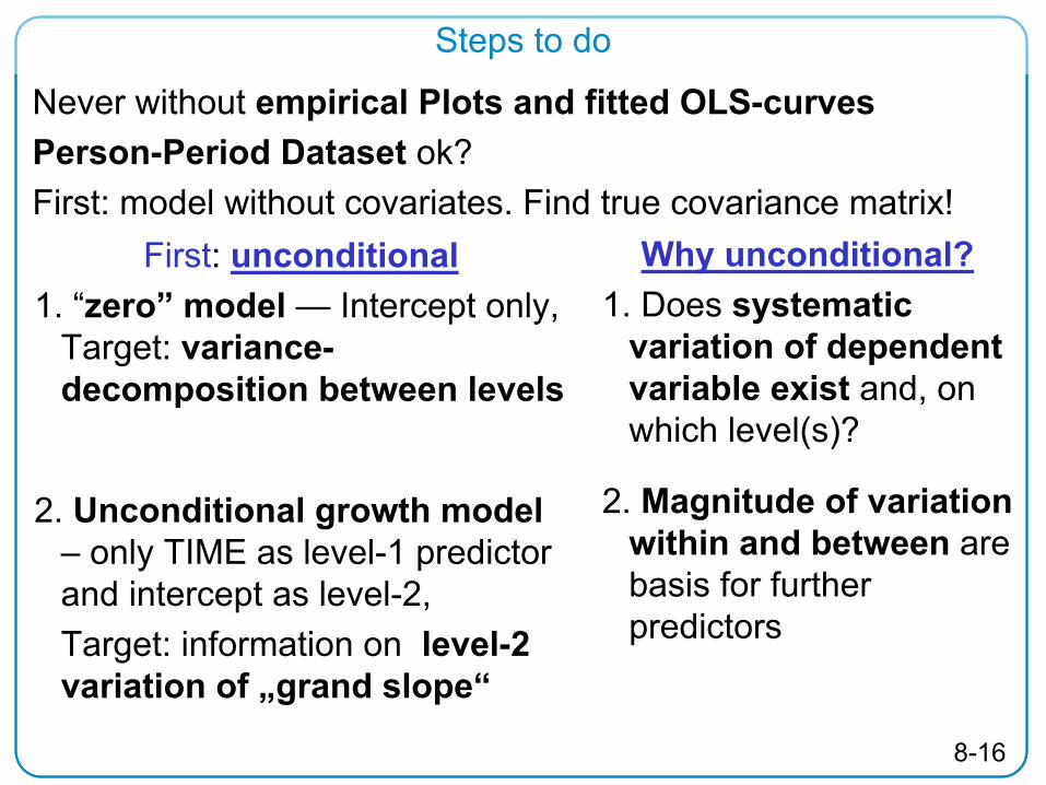
8-16

Steps to do

Never without empirical Plots and fitted OLS-curvesPerson-Period Dataset

ok?

First: model without covariates. Find true covariance matrix!First: unconditional

1. “zero”

model — Intercept only, Target: variance-

decomposition between levels

2. Unconditional growth model –

only TIME as level-1 predictor

and intercept as level-2, Target: information on level-2 variation of „grand slope“

Why unconditional?1. Does systematic

variation of dependent variable exist and, on which level(s)?

2. Magnitude of variation within and between are basis for further predictors

8-17

. xtreg

bmi, i(pers) /* VC modfel

*/Random-effects

GLS regression

Number

of obs

= 9189Group variable: pers

Number

of groups

= 2997R-sq: within

= 0.0000 Obs

per group: min = 1between

= 0.0000 avg

= 3.1overall

= 0.0000 max

= 4Wald chi2(0) = .

corr(u_i, X) = 0 (assumed) Prob > chi2 = .------------------------------------------------------------------------------

bmi

| Coef. Std. Err. z P>|z| [95% Conf. Interval]-------------+----------------------------------------------------------------

_cons

| 25.48776 .082556 308.73 0.000 25.32595 25.64957-------------+----------------------------------------------------------------

sigma_u

| 4.400013sigma_e

| 1.5881408rho

| .88473832 (fraction

of variance

due

to u_i)------------------------------------------------------------------------------

. xtmixed

bmi

year

|| pers:year, cov(unst) mleMixed-effects

ML regression

Number

of obs

= 9189…Log likelihood

= -21557.826 Prob > chi2 = 0.0000

------------------------------------------------------------------------------bmi

| Coef. Std. Err. z P>|z| [95% Conf. Interval]-------------+----------------------------------------------------------------

year

| .1386832 .0112017 12.38 0.000 .1167283 .1606381_cons

| 25.22705 .082938 304.17 0.000 25.0645 25.38961------------------------------------------------------------------------------

------------------------------------------------------------------------------Random-effects

Parameters | Estimate

Std. Err. [95% Conf. Interval]-----------------------------+------------------------------------------------pers: Unstructured

|sd(year) | .364826 .0120562 .3419454 .3892377

sd(_cons) | 4.38887 .060836 4.271238 4.509741corr(year,_cons) | -.0842973 .0320786 -.1467533 -.0211718

-----------------------------+------------------------------------------------sd(Residual) | 1.330571 .0147404 1.301992 1.359777

------------------------------------------------------------------------------LR test vs. linear regression: chi2(3) = 11010.72 Prob > chi2 = 0.0000

Unconditional means/growth model (max. likelihood estimation)

8-18

For regression coefficients

: use z-Test (5% if IzI>1.96)

For random effects

: use the likelihood ratio test: - test current model against base model-

Important: current models uses same data

(“nested”) but

more parameters

(regression coefficients, random effects, covariance)

-

Null Hypothesis: these coefficients are all 0-

Test statistic: = 2*[loglikelihood(current) -

loglikelihood(base)]-

This statistic is χ2-distributed

with the additional number of

coefficients as degree of freedom

Excursus: hypotheses testing

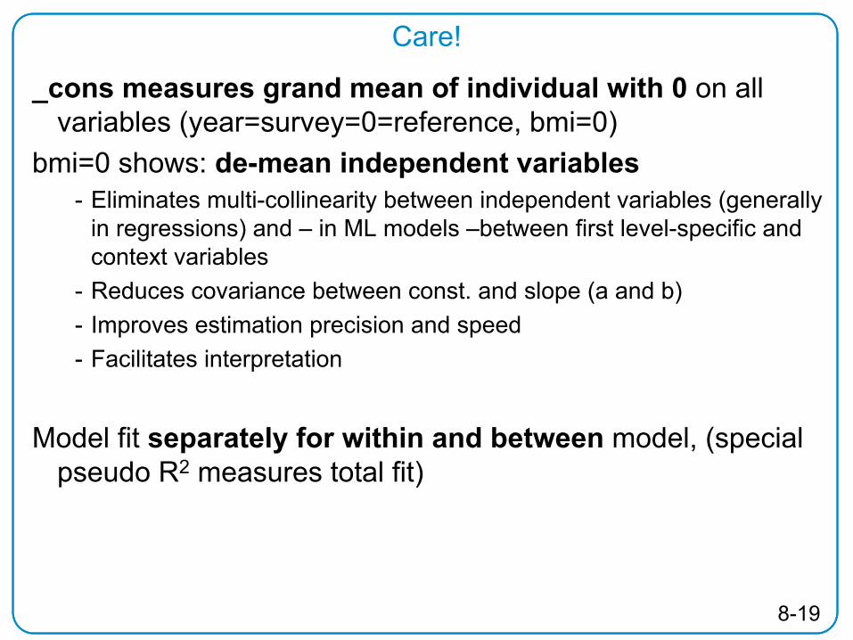
8-19

_cons measures grand mean of individual with 0

on all variables (year=survey=0=reference, bmi=0)

bmi=0 shows: de-mean independent variables-

Eliminates multi-collinearity

between independent variables (generally in regressions) and –

in ML models –between first level-specific and context variables

-

Reduces covariance between const. and slope (a and b)-

Improves estimation precision and speed-

Facilitates interpretation

Model fit separately for within and between

model, (special pseudo R2

measures total fit)

Care!

9-1

9Missing Data:

Incomplete panels, imputation techniques

9-2

Underrepresentation

Sampling frame errors (mostly undercoverage)

Unit

non-response:• First wave

(“initial”) nonresponse

• Attrition: respondents drop out or are temporary absentReasons:

-

Non-contact

(out-of-home, no telephone answer, or unsuccessful tracking of movers)

- Refusal (also on behalf of others)

Item

non-response • Respondents fail to answer particular questions, e.g.

income

9-3

Initial nonresponse vs attrition

Initial nonresponse• Only little information

on non-participants (from sampling

frame eventually sex, age, nationality, civil status, region…)

Attrition• Rich information

on these individuals from at least one wave

• Methodological research: attitudinal characteristics (e.g. political interest, political orientation, social integration) more biased than socio-demography

Bias• correction of bias easier for attrition than for undercoverage or

initial nonresponse

9-4

Missing completely at random (MCAR)

Missing at random (MAR) – conditional on observables (xit ), response is random= systematic differences in response can be explained by

observable characteristics.

Not missing at random (NMAR) – non-ignorable: systematic differences in response

remain after controlling for observables (xit )

Types of missingness

9-5

Missing completely at random (MCAR) – Statistics unbiased– Loss of efficiency (smaller n)

Missing at random (MAR)– Univariate statistics: biased

Example: if the politically uninterested do not take part in the survey we will overestimate the political interest rate

– Multivariate statistics: unbiased if controlled for variables which explain missingness

Not missing at random (NMAR) – Statistics biased

Consequences of missingness

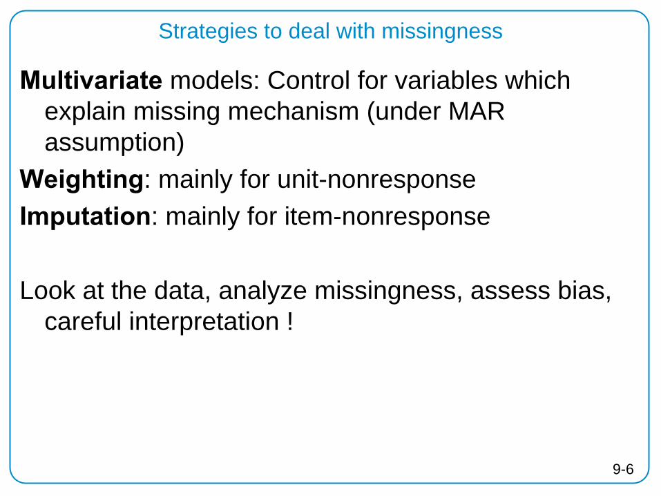
9-6

Multivariate

models: Control for variables which explain missing mechanism (under MAR assumption)

Weighting: mainly for unit-nonresponseImputation: mainly for item-nonresponse

Look at the data, analyze missingness, assess bias, careful interpretation !

Strategies to deal with missingness

9-7

Univariate

statistics: use weightsMultivariate

statistics

Weights may or may not be appropriate:depends on research question, model, construction of weights

Use of weights is not always possiblenot implemented in RE models in Stata, but possible in xtmixed or with gllamm software

– Sensitivity analysis: run models with and without weights

Weighting

9-8

Exclude

cases from analysis (listwise deletion in regression)Assumes MCARLoss of statistical power

Mean or median

imputationAssumes MCAR, variance reduction, “bias to the Mean“

Regression

imputationAssumes MAR, variance reduction, regression to the mean

„Hot Deck“Identification of donor with same characteristics of co-varying observed

variables assumes MAR, variance reduction

Cold deckdonor comes from another surveyassumes MAR, variance reduction, loss of statistical power

Imputation strategies I

9-9

Imputation strategies II

Nearest neighborfor continuous variables; donor has smallest distance assumes MAR, variance reduction

Multiple Imputationseveral imputations per missing value, stochastic

In Panel Surveys: information of the same unit (individual) from other waves Simple carryover:take value from another wave (longitudinal change reduction)

„Row and Column“: uses longitudinal and cross-sectional information, stochastic

(longitudinal change reduction)

9-10

Testing for attrition bias

Compare individuals who drop out with individuals who stay: characteristics of first waveexample: individuals present in 2003 vs. not:

political interest in 1999

stayers | mean se(mean) N---------+------------------------------

0 | 4.688572 .0518871 34391 | 5.293807 .0433594 4360

---------+------------------------------Total | 5.026927 .0335037 7799

----------------------------------------

9-11

Testing form non-random missing

Missing value is random

(MCAR or MAR after control) response rit

is independent of ui

or εit

1. check whether rit

explains the outcome yit

after controlling for other characteristics

Functions of rit

can be added to the equation and their significance tested. E.g.:– lagged response indicator rit-1– number of waves present– correction models (eg Heckman Selection)

2. compare results from the unbalanced panel with the balanced sub-panel– regressor differences (use Hausman test)

10_1

10Dynamic models

10_2

Longitudinal models

— Within estimators: Fixed effects (FE), Difference in Difference (DID)— Long panels: causal influence— Short panels: policy evaluation

— Dynamic panel models (complex!)— Model pathways through which variables measured over time

are associated— Model stability over time, true state dependence— Lagged dependent variable as a regressor

— Cross-lagged models— Lagged dependent and lagged independent variables as

regressors— Establish causality through time ordering

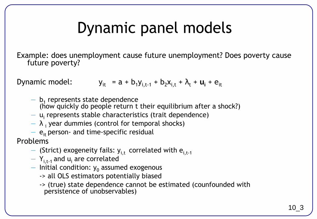
10_3

Dynamic panel models

Example: does unemployment cause future unemployment? Does poverty cause future poverty?

Dynamic model: yit

= a + b1

yi,t-1

+ b2

xi,t

+ λt

+ ui + eit

—

b1

represents state dependence (how quickly do people return t their equilibrium after a shock?)

—

ui

represents stable characteristics (trait dependence)—

λ

i

year dummies (control for temporal shocks)—

eit

person-

and time-specific residualProblems

—

(Strict) exogeneity fails: yi,t

correlated with ei,t-1—

Yi,t-1 and ui

are correlated—

Initial condition: y0

assumed exogenous -> all OLS estimators potentially biased-> (true) state dependence cannot be estimated (counfounded

with persistence of unobservables)

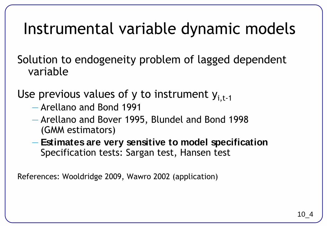
10_4

Instrumental variable dynamic models

Solution to endogeneity problem of lagged dependent variable

Use previous values of y to instrument yi,t-1 — Arellano and Bond 1991— Arellano and Bover

1995, Blundel

and Bond 1998

(GMM estimators)— Estimates are very sensitive to model specification

Specification tests: Sargan test, Hansen test

References: Wooldridge 2009, Wawro

2002 (application)

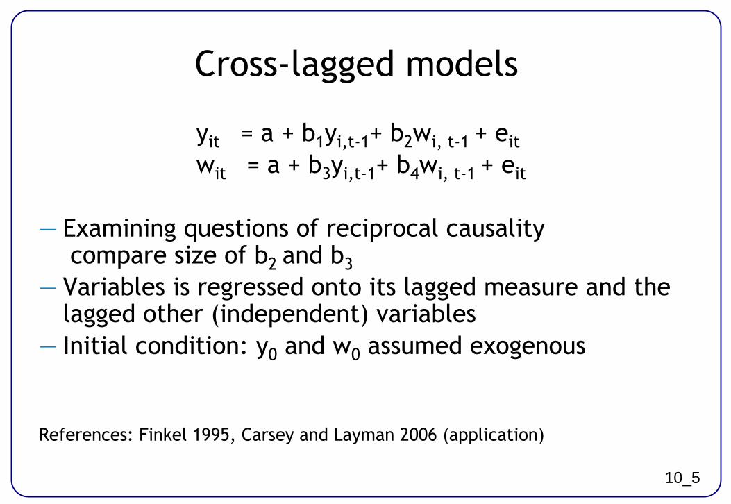
10_5

Cross-lagged models

yit

= a + b1

yi,t-1

+ b2

wi, t-1 + eit

wit = a + b3

yi,t-1

+ b4

wi, t-1 + eit

— Examining questions of reciprocal causality

compare size of b2 and b3

— Variables is regressed onto its lagged measure and the lagged other (independent) variables

— Initial condition: y0

and w0

assumed exogenous

References: Finkel

1995, Carsey

and Layman 2006 (application)

Documents

Slides Panel Data Analysis 2012