Embed Size (px)
Citation preview

Princeton University Press, 2017
slides
chapter 9
nominal rigidity
exchange rates, and
unemployment
Chapter 9: Nominal Rigidity, Exchange Rates, And Unemployment Uribe & Schmitt-Grohe
Contents
9.1 An Open Economy With Downward Nominal Wage Rigidity
9.2 Currency Pegs
9.3 Optimal Exchange Rate Policy
9.4 Empirical Evidence On Downward Nominal Wage Rigidity
9.5 The Case of Equal Intra- And Intertemporal Elasticities of Substitution
9.6 Approximating Equilibrium Dynamics
9.7 Parameterization of the Model
9.8 External Crises and Exchange-Rate Policy: A Quantitative Analysis
9.9 Empirical Evidence On The Expansionary Effects of Devaluations
9.10 The Welfare Costs of Currency Pegs
9.11 Symmetric Wage Rigidity
9.12 The Mussa Puzzle
9.13 Endogenous Labor Supply
9.14 Production in the Traded Sector
9.15 Product Price Rigidity
9.16 Staggered Price Setting: The Calvo Model
1

Chapter 9: Nominal Rigidity, Exchange Rates, And Unemployment Uribe & Schmitt-Grohe
Roadmap
• Chapter 9 develops a theoretical framework in which nominal rigidi-
ties result in inefficient adjustments to aggregate disturbances
• framework can be used in an intuitive graphical manner to demon-
strate how nominal rigidities amplify the business cycle in open
economies
• but framework can also be used to derive quantitative predictions
useful for policy evaluation
2

Chapter 9: Nominal Rigidity, Exchange Rates, And Unemployment Uribe & Schmitt-Grohe
Some Motivation: Peripheral Europe and the Global Crisis of 2008
Take a look at the next slide.
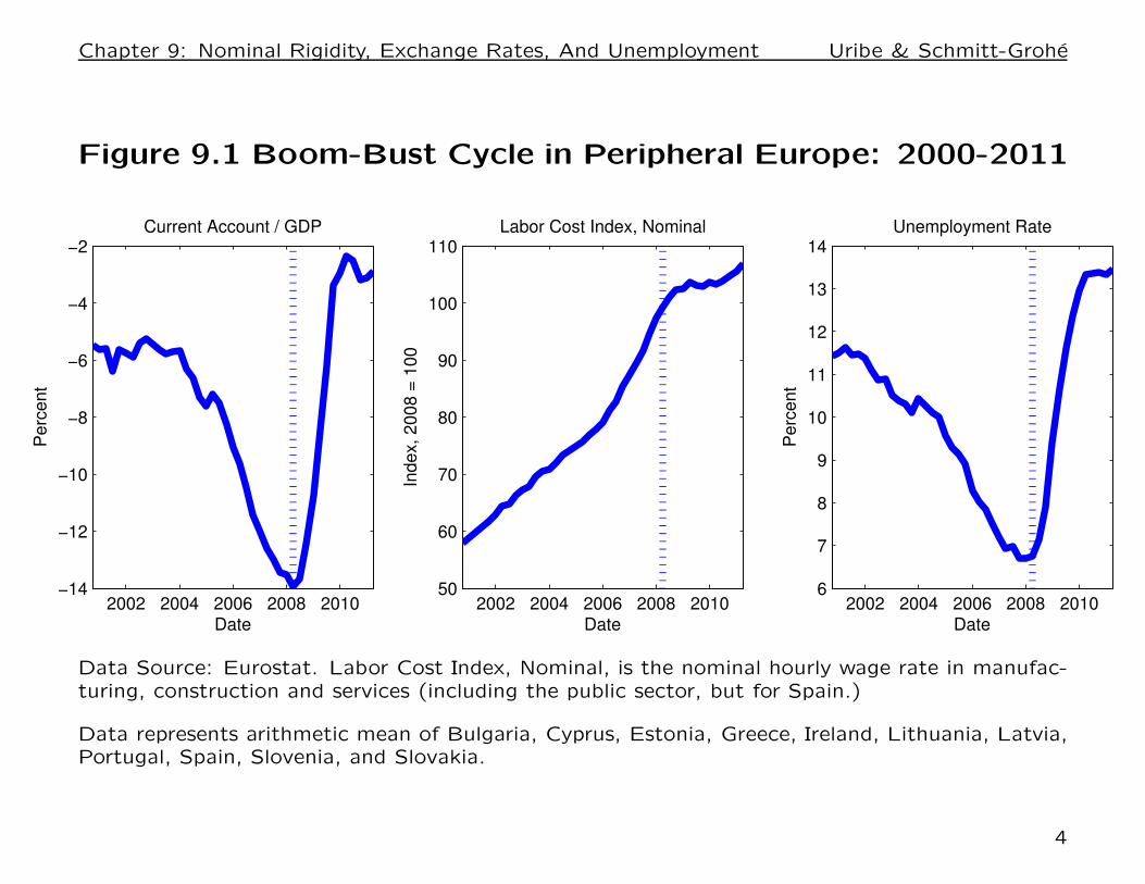
• The inception of the Euro in 1999 was followed by massive capi-
tal inflows into the region, possibly driven by expectations of quick
convergence of peripheral and core Europe.
• Large current account deficits and large increases in nominal hourly
wages, with declining rates of unemployment between 2000 and
2008.
• When the global crisis of 2008 starts, capital inflows dry up
abruptly. Peripheral Europe suffers a severe sudden stop (sharp
reductions in current account deficits).
• In spite of the collapse in aggregate demand and the lack of a
devaluation, nominal hourly wages remain as high as at the peak of
the boom.
• Massive unemployment affects all countries in the region.
3
Chapter 9: Nominal Rigidity, Exchange Rates, And Unemployment Uribe & Schmitt-Grohe
Figure 9.1 Boom-Bust Cycle in Peripheral Europe: 2000-2011
2002 2004 2006 2008 20106
7
8
9
10
11
12
13
14
Perc
ent
Date
Unemployment Rate
2002 2004 2006 2008 201050
60
70
80
90
100
110
Index, 2008 =
100
Date
Labor Cost Index, Nominal
2002 2004 2006 2008 2010−14
−12
−10
−8
−6
−4
−2
Perc
ent
Date
Current Account / GDP
Data Source: Eurostat. Labor Cost Index, Nominal, is the nominal hourly wage rate in manufac-turing, construction and services (including the public sector, but for Spain.)
Data represents arithmetic mean of Bulgaria, Cyprus, Estonia, Greece, Ireland, Lithuania, Latvia,Portugal, Spain, Slovenia, and Slovakia.
4
Chapter 9: Nominal Rigidity, Exchange Rates, And Unemployment Uribe & Schmitt-Grohe
2000 2005 20102
4
6
8
10Unemployment Rate: Cyprus
Pe
rce
nt
2000 2005 20105
10
15
20
25Unemployment Rate: Greece
Pe
rce
nt
2000 2005 20100
5
10
15Unemployment Rate: Ireland
Pe
rce
nt
2000 2005 20100
5
10
15Unemployment Rate: Portugal
Pe
rce
nt
2000 2005 20105
10
15
20
25Unemployment Rate: Spain
Pe
rce
nt
2000 2005 201060
80
100
120
Ind
ex,
20
08
= 1
00
Nominal Hourly Wages: Cyprus
2000 2005 201060
80
100
120
Ind
ex,
20
08
= 1
00
Nominal Hourly Wages: Greece
2000 2005 201060
80
100
120
Ind
ex,
20
08
= 1
00
Nominal Hourly Wages: Ireland
2000 2005 201070
80
90
100
110
Ind
ex,
20
08
= 1
00
Nominal Hourly Wages: Portugal
2000 2005 201060
80
100
120
Ind
ex,
20
08
= 1
00
Nominal Hourly Wages: Spain
2000 2005 2010−20
−10
0
10
Pe
rce
nt
Current Account / GDP: Cyprus
2000 2005 2010−20
−15
−10
−5
Pe
rce
nt
Current Account / GDP: Greece
2000 2005 2010−10
−5
0
5
Pe
rce
nt
Current Account / GDP: Ireland
2000 2005 2010−14
−12
−10
−8
−6
Pe
rce
nt
Current Account / GDP: Portugal
2000 2005 2010−15
−10
−5
0
Pe
rce
nt
Current Account / GDP: Spain
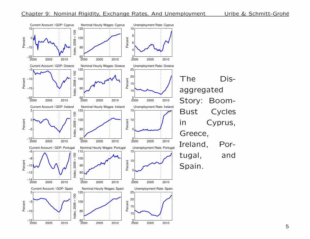
The Dis-
aggregated
Story: Boom-
Bust Cycles
in Cyprus,
Greece,
Ireland, Por-
tugal, and
Spain.
5
Chapter 9: Nominal Rigidity, Exchange Rates, And Unemployment Uribe & Schmitt-Grohe
The previous two figures suggest the following narrative:
Countries in the periphery of the European Union, such as Ireland, Portugal, Greece, and anumber of small eastern European countries adopted a fixed exchange rate regime by joining theEuroarea. Most of these countries experienced an initial transition into the Euro characterized bylow inflation, low interest rates, and economic expansion.
However, history has shown time and again that fixed exchange rate arrangements areeasy to adopt but difficult to maintain. (Example: Argentina’s 1991 convertibility plan.)
The Achilles’ heel of currency pegs is that they hinder the efficient adjustment of the economy tonegative external shocks, such as drops in the terms of trade or hikes in the interest-rate. Suchshocks produce a contraction in aggregate demand that requires a decrease in the relative priceof nontradables, that is, a real depreciation of the domestic currency, in order to bring aboutan expenditure switch away from tradables and toward nontradables. In turn, the required realdepreciation may come about via a nominal devaluation of the domestic currency or via a fall innominal prices or both.
The currency peg rules out a devaluation. Thus, the only way the necessary real depreciation canoccur is through a decline in the nominal price of nontradables. However, when nominal wagesare downwardly rigid, producers of nontradables are reluctant to lower prices, for doing so mightrender their enterprises no longer profitable. As a result, the necessary real depreciation takesplace too slowly, causing recession and unemployment along the way.
This narrative goes back at least to Keynes (1925) who argued that Britain’s 1925 decision toreturn to the gold standard at the 1913 parity despite the significant increase in the aggregate pricelevel that took place during World War I would force deflation in nominal wages with deleteriousconsequences for unemployment and economic activity. Similarly, Friedman’s (1953) seminal essaypoints at downward nominal wage rigidity as the central argument against fixed exchange rates.
6

Chapter 9: Nominal Rigidity, Exchange Rates, And Unemployment Uribe & Schmitt-Grohe
To formalize this narrative let’s build an open economy model with
• downward nominal wage rigidity
• a traded and a nontraded sector
• involuntary unemployment
To produce quantitative predictions
• Estimate the key parameters of the model (with particular at-
tention on the parameter governing downward wage rigidity) and
estimate the driving forces.
• Characterize response to large negative external shock under a peg
and show that the model can explain the observed sudden stop.
• Characterize optimal exchange rate policy.
• Quantify the costs of currency pegs in terms of unemployment
and welfare.
The material is based on Schmitt-Grohe and Uribe (JPE, 2016).
7
Chapter 9: Nominal Rigidity, Exchange Rates, And Unemployment Uribe & Schmitt-Grohe
9.1 An Open Economy with
Downward Nominal Wage Rigidity
(The DNWR Model)
8
Chapter 9: Nominal Rigidity, Exchange Rates, And Unemployment Uribe & Schmitt-Grohe
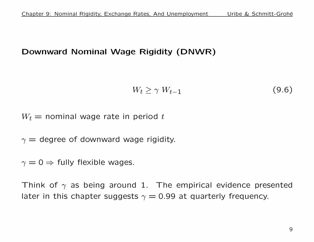
Downward Nominal Wage Rigidity (DNWR)
Wt ≥ γ Wt−1 (9.6)
Wt = nominal wage rate in period t
γ = degree of downward wage rigidity.
γ = 0 ⇒ fully flexible wages.
Think of γ as being around 1. The empirical evidence presented
later in this chapter suggests γ = 0.99 at quarterly frequency.
9
Chapter 9: Nominal Rigidity, Exchange Rates, And Unemployment Uribe & Schmitt-Grohe
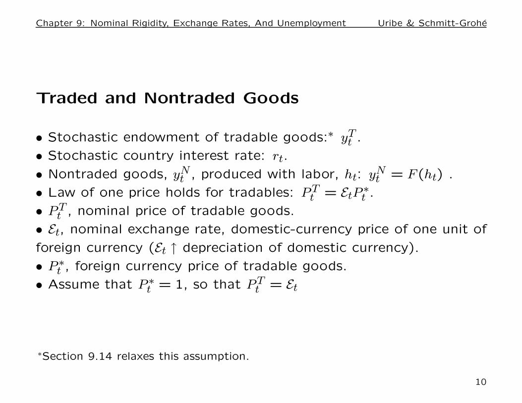
Traded and Nontraded Goods
• Stochastic endowment of tradable goods:∗ yTt .
• Stochastic country interest rate: rt.
• Nontraded goods, yNt , produced with labor, ht: yN
t = F (ht) .
• Law of one price holds for tradables: PTt = EtP
∗t .
• PTt , nominal price of tradable goods.
• Et, nominal exchange rate, domestic-currency price of one unit of
foreign currency (Et ↑ depreciation of domestic currency).
• P ∗t , foreign currency price of tradable goods.
• Assume that P ∗t = 1, so that PT
t = Et
∗Section 9.14 relaxes this assumption.
10
Chapter 9: Nominal Rigidity, Exchange Rates, And Unemployment Uribe & Schmitt-Grohe
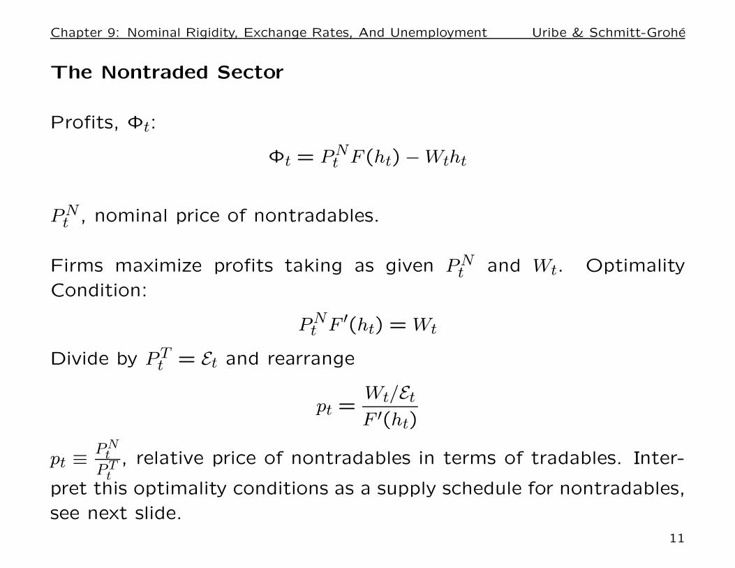
The Nontraded Sector
Profits, Φt:
Φt = PNt F (ht) − Wtht
PNt , nominal price of nontradables.
Firms maximize profits taking as given PNt and Wt. Optimality
Condition:
PNt F ′(ht) = Wt
Divide by PTt = Et and rearrange
pt =Wt/Et
F ′(ht)
pt ≡PN
t
PTt, relative price of nontradables in terms of tradables. Inter-
pret this optimality conditions as a supply schedule for nontradables,
see next slide.
11
Chapter 9: Nominal Rigidity, Exchange Rates, And Unemployment Uribe & Schmitt-Grohe
The Supply Schedule of Nontradables
Let’s derive the supply schedule for nontradables in the space (yN , p)
given the real wage, Wt/Et.
Note that real marginal cost of one unit of nontraded good
marginal cost =Wt/Et
F ′(ht)
Use h = F−1(yN) to obtain
marginal cost =Wt/Et
F ′(F−1(yN)
By the profit maximization condition marginal cost equals price or
pt =Wt/Et
F ′(F−1(yNt ))
Interpret this relation as a supply schedule of nontradables given the
real wage.
12
Chapter 9: Nominal Rigidity, Exchange Rates, And Unemployment Uribe & Schmitt-Grohe
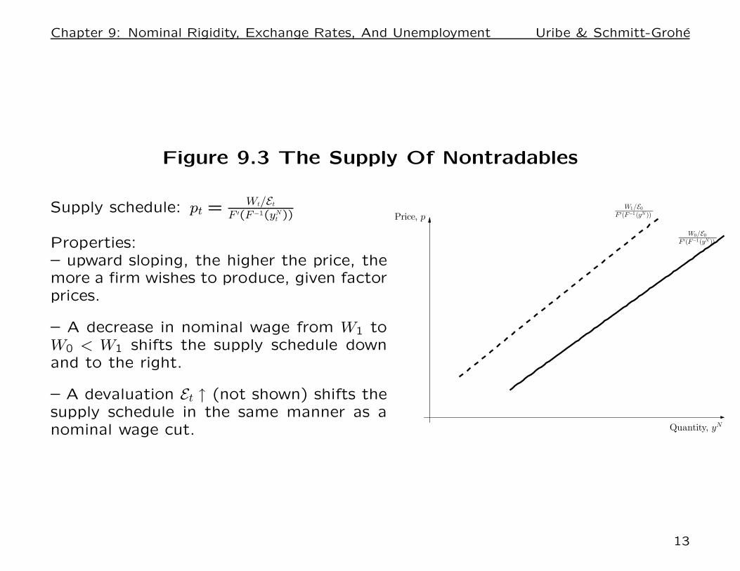
Figure 9.3 The Supply Of Nontradables
Supply schedule: pt =Wt/Et
F ′(F−1(yNt ))
Properties:– upward sloping, the higher the price, themore a firm wishes to produce, given factorprices.
– A decrease in nominal wage from W1 toW0 < W1 shifts the supply schedule downand to the right.
– A devaluation Et ↑ (not shown) shifts thesupply schedule in the same manner as anominal wage cut.
W0/E0F ′(F−1(yN ))
W1/E0F ′(F−1(yN ))
Quantity, yN
Price, p
13
Chapter 9: Nominal Rigidity, Exchange Rates, And Unemployment Uribe & Schmitt-Grohe
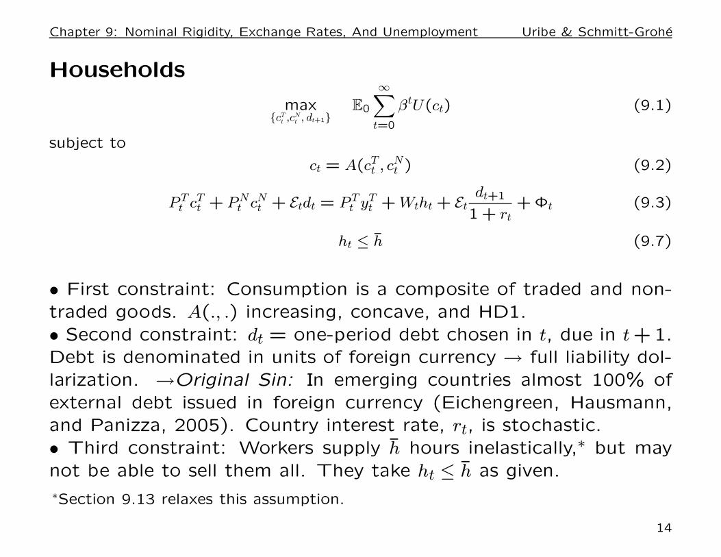
Households
maxcT
t ,cNt , dt+1
E0
∞∑
t=0
βtU(ct) (9.1)
subject to
ct = A(cTt , cN
t ) (9.2)
P Tt cT
t + PNt cN
t + Etdt = P Tt yT
t + Wtht + Etdt+1
1 + rt+ Φt (9.3)
ht ≤ h (9.7)
• First constraint: Consumption is a composite of traded and non-
traded goods. A(., .) increasing, concave, and HD1.
• Second constraint: dt = one-period debt chosen in t, due in t +1.
Debt is denominated in units of foreign currency → full liability dol-
larization. →Original Sin: In emerging countries almost 100% of
external debt issued in foreign currency (Eichengreen, Hausmann,
and Panizza, 2005). Country interest rate, rt, is stochastic.
• Third constraint: Workers supply h hours inelastically,∗ but may
not be able to sell them all. They take ht ≤ h as given.
∗Section 9.13 relaxes this assumption.
14
Chapter 9: Nominal Rigidity, Exchange Rates, And Unemployment Uribe & Schmitt-Grohe
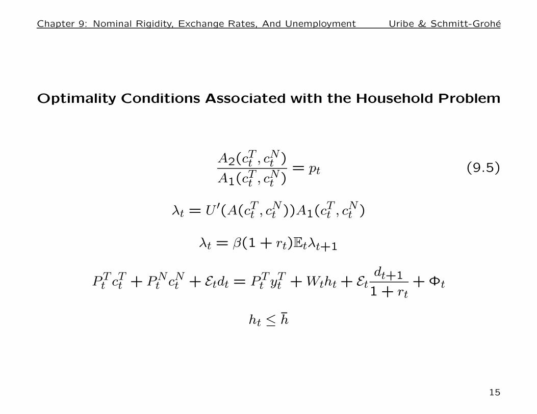
Optimality Conditions Associated with the Household Problem
A2(cTt , cN
t )
A1(cTt , cN
t )= pt (9.5)
λt = U ′(A(cTt , cN
t ))A1(cTt , cN
t )
λt = β(1 + rt)Etλt+1
PTt cT
t + PNt cN
t + Etdt = PTt yT
t + Wtht + Etdt+1
1 + rt+ Φt
ht ≤ h
15

Chapter 9: Nominal Rigidity, Exchange Rates, And Unemployment Uribe & Schmitt-Grohe
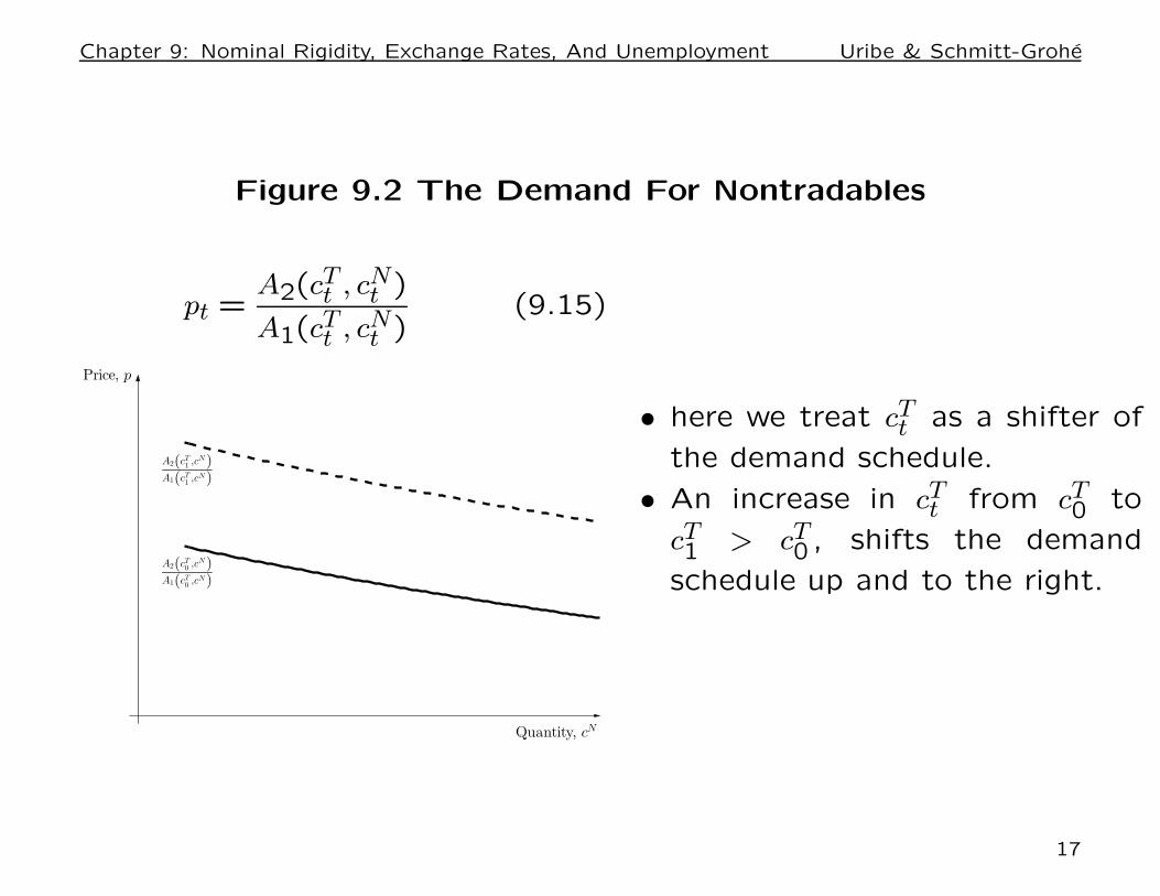
The Demand For NontradablesLook again at the optimality condition (9.15)
A2(cTt , cN
t )
A1(cTt , cN
t )= pt. (9.15)
If A(cT , cN) is concave and HD1, then given cTt , the left-hand side
is decreasing in cNt . This means that, all other things equal, an
increase in pt reduces the desired demand for nontradables, giving
rise to the downward sloping demand schedule shown in the next
slide.
Note that cTt acts as a shifter of the demand schedule for nontrad-
ables: given pt, an increase in cTt is associated with an equipropor-
tional desired increase in cNt . Of course, this shifter is endogenously
determined.
16
Chapter 9: Nominal Rigidity, Exchange Rates, And Unemployment Uribe & Schmitt-Grohe
Figure 9.2 The Demand For Nontradables
pt =A2(c
Tt , cN
t )
A1(cTt , cN
t )(9.15)
A2(cT0 ,cN)A1(cT0 ,cN)
A2(cT1 ,cN)A1(cT1 ,cN)
Quantity, cN
Price, p
• here we treat cTt as a shifter of
the demand schedule.
• An increase in cTt from cT
0 to
cT1 > cT
0 , shifts the demand
schedule up and to the right.
17
Chapter 9: Nominal Rigidity, Exchange Rates, And Unemployment Uribe & Schmitt-Grohe
Closing of the Labor Market
Nominal wages are downwardly rigid
Wt ≥ γWt−1 (9.6)
Labor demand may not exceed supply
ht ≤ h (9.7)
Impose the following slackness condition:
(h − ht)(
Wt − γWt−1)
= 0 (9.8)
This slackness condition says that, if there is involuntary unemploy-
ment (ht < h), then the lower bound on nominal wages must be
binding. It also says that if the lower bound on nominal wages is
not binding(
Wt > γWt−1)
, then the labor market must feature full
employment.
Market clearing in the Nontraded Sector
cNt = yN
t = F (ht)
18
Chapter 9: Nominal Rigidity, Exchange Rates, And Unemployment Uribe & Schmitt-Grohe
A competitive equilibrium is a set of stochastic processes cTt , ht, wt, dt+1, pt,
λt∞t=0 satisfying
cTt + dt = yT
t +dt+1
1 + rt(9.9)
λt = U ′(A(cTt , F(ht)))A1(c
Tt , F(ht)) (9.13)
λt
1 + rt= βEtλt+1 (9.14)
pt =A2(cT
t , F(ht))
A1(cTt , F(ht))
(9.15)
pt =wt
F ′(ht)(9.16)
wt ≥ γwt−1
εt(9.17)
ht ≤ h (9.18)
(h − ht)
(
wt − γwt−1
εt
)
= 0 (9.19)
given an exchange rate policy εt∞t=0, initial conditions w−1 and d0, and exogenousstochastic processes rt, yT
t ∞t=0.
To characterize the eqm we must specify the exchange-rate regime. We will turnto this next.
19
Chapter 9: Nominal Rigidity, Exchange Rates, And Unemployment Uribe & Schmitt-Grohe
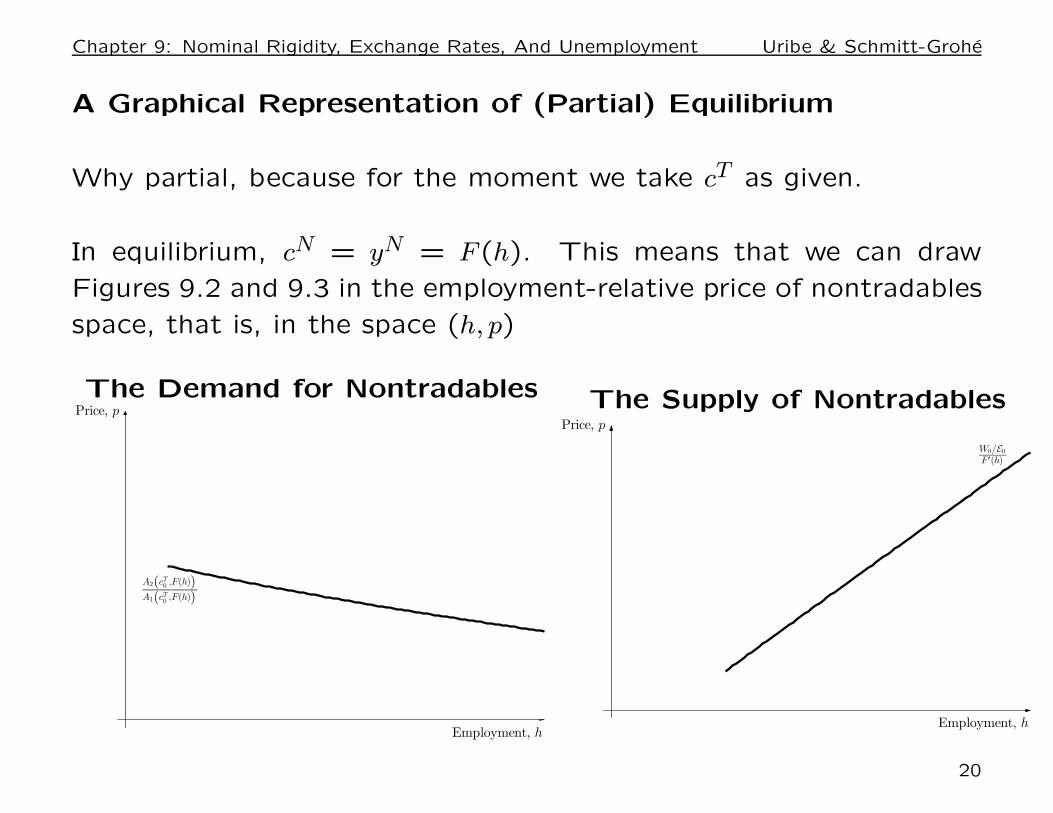
A Graphical Representation of (Partial) Equilibrium
Why partial, because for the moment we take cT as given.
In equilibrium, cN = yN = F (h). This means that we can draw
Figures 9.2 and 9.3 in the employment-relative price of nontradables
space, that is, in the space (h, p)
The Demand for Nontradables
A2(cT0 ,F(h))A1(cT0 ,F(h))
Employment, h
Price, p The Supply of Nontradables
W0/E0F ′(h)
Employment, h
Price, p
20
Chapter 9: Nominal Rigidity, Exchange Rates, And Unemployment Uribe & Schmitt-Grohe
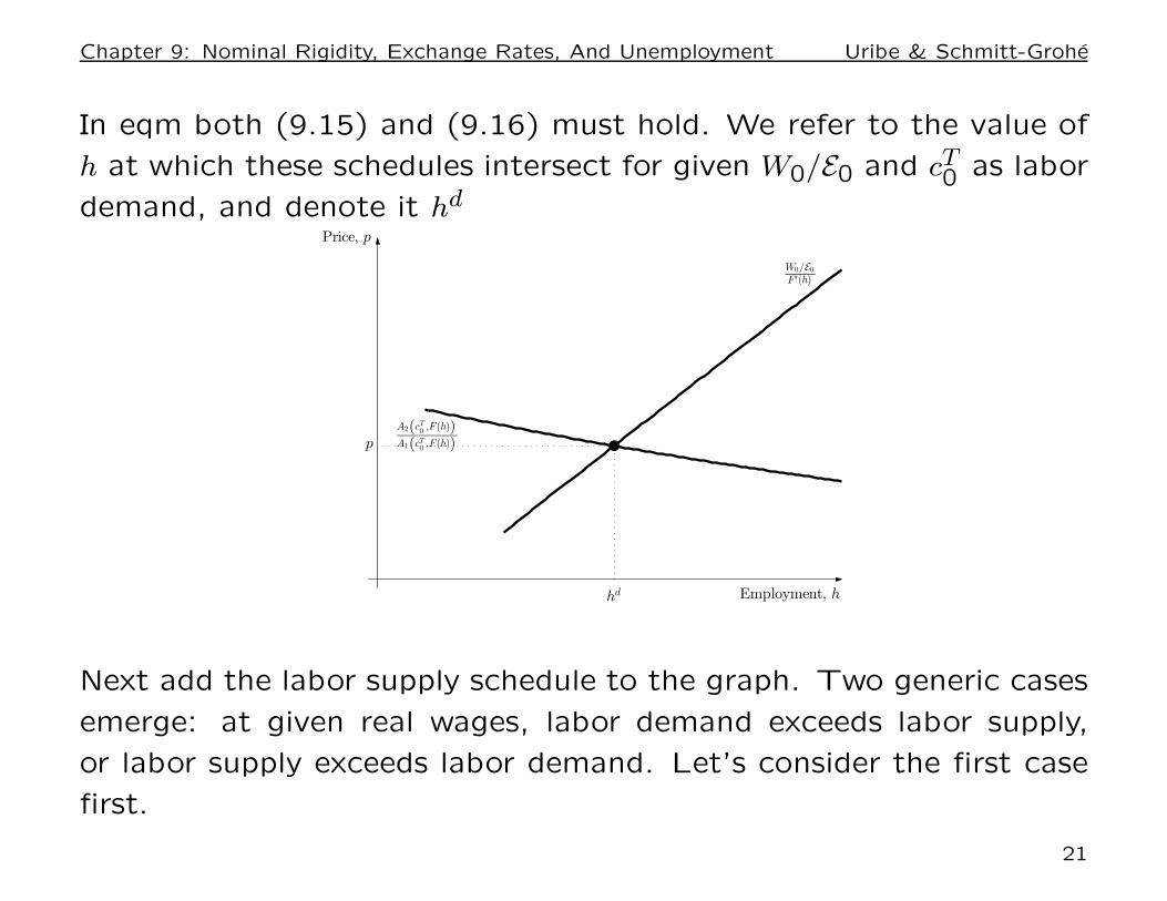
In eqm both (9.15) and (9.16) must hold. We refer to the value of
h at which these schedules intersect for given W0/E0 and cT0 as labor
demand, and denote it hd
A2(cT0 ,F(h))A1(cT0 ,F(h))
W0/E0F ′(h)
p
hd Employment, h
Price, p
Next add the labor supply schedule to the graph. Two generic cases
emerge: at given real wages, labor demand exceeds labor supply,
or labor supply exceeds labor demand. Let’s consider the first case
first.
21
Chapter 9: Nominal Rigidity, Exchange Rates, And Unemployment Uribe & Schmitt-Grohe
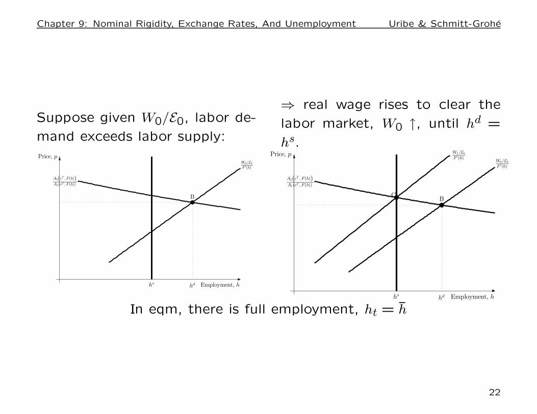
Suppose given W0/E0, labor de-
mand exceeds labor supply:
A2(cT , F(h))A1(cT , F(h))
W0/E0F ′(h)
B
hs hd Employment, h
Price, p
⇒ real wage rises to clear the
labor market, W0 ↑, until hd =
hs.
A2(cT , F(h))A1(cT , F(h))
W0/E0F ′(h)
W1/E0F ′(h)
BC
hshd Employment, h
Price, p
In eqm, there is full employment, ht = h
22
Chapter 9: Nominal Rigidity, Exchange Rates, And Unemployment Uribe & Schmitt-Grohe
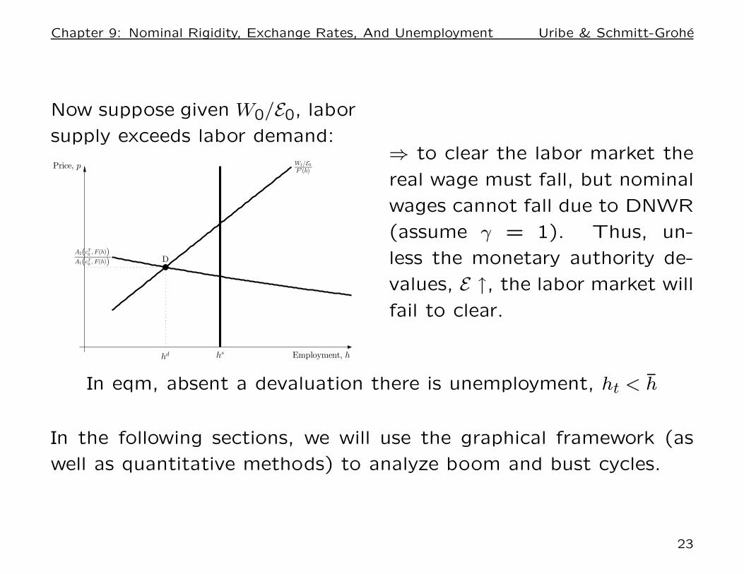
Now suppose given W0/E0, labor
supply exceeds labor demand:
A2(cT0 , F(h))A1(cT0 , F(h))
W1/E0F ′(h)
D
hshd Employment, h
Price, p⇒ to clear the labor market the
real wage must fall, but nominal
wages cannot fall due to DNWR
(assume γ = 1). Thus, un-
less the monetary authority de-
values, E ↑, the labor market will
fail to clear.
In eqm, absent a devaluation there is unemployment, ht < h
In the following sections, we will use the graphical framework (as
well as quantitative methods) to analyze boom and bust cycles.
23

Chapter 9: Nominal Rigidity, Exchange Rates, And Unemployment Uribe & Schmitt-Grohe
9.2 Currency Pegs
24
Chapter 9: Nominal Rigidity, Exchange Rates, And Unemployment Uribe & Schmitt-Grohe
The exchange rate policy is a peg
Et = E0; ∀t ≥ 0.
Use the graphical apparatus just developed to show that a boom-
bust cycle leads—as documented in Figure 9.1—to
– nominal wage growth and real appreciation during the boom phase
– involuntary unemployment and insufficient real depreciation during
the bust phase
25
Chapter 9: Nominal Rigidity, Exchange Rates, And Unemployment Uribe & Schmitt-Grohe
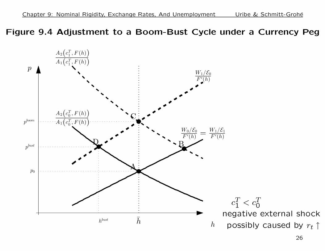
Figure 9.4 Adjustment to a Boom-Bust Cycle under a Currency Peg
A2(cT0 , F (h))A1(cT0 , F (h))
A2(cT1 , F (h))A1(cT1 , F (h))
W0/E0F ′(h) = W1/E1
F ′(h)
W1/E0F ′(h)
h
A
B
C
D
p0
pbust
pboom
hbusth
p
cT1 < cT
0
negative external shock
possibly caused by rt ↑
26
Chapter 9: Nominal Rigidity, Exchange Rates, And Unemployment Uribe & Schmitt-Grohe
Observations on Figure 9.4: Adjustment in a Boom-Bust Episode
The initial situation is point A. At point A there is full employment, h = h.
Now a boom starts. We capture this by an increase in cT (perhaps because rfalls). Given nominal wages the economy moves to point B. But at point B, thereis excess demand for labor. Thus nominal wages will rise. By how much? Untilthe excess demand for labor has disappeared. That will be at point C. Thus theboom leads to an increase in nominal wages (W ↑) and a real appreciation (p ↑).The economy continues to operate at full employment.
Next the boom is over and the bust comes. We capture this by assuming that cT
falls back to its original level, cT0 .
This shifts the demand for nontradables back to its original position. The newintersection between supply and demand is at point D. At D, labor supply exceedslabor demand. However, because nominal wages are downwardly rigid and thenominal exchange rate is fixed, the supply schedule does not shift, (for simplicity,in the figure, we assume γ = 1). Thus the economy is stuck at point D. Atpoint D, there is involuntary unemployment (h−hbust) and there is insufficient realdepreciation, i.e., pt does not fall enough (that is, does not fall to p0) to restorefull employment.
27
Chapter 9: Nominal Rigidity, Exchange Rates, And Unemployment Uribe & Schmitt-Grohe
The Link between Volatility and Average Unemployment
The present model predicts that aggregate volatility increases the
mean level of unemployment.
This prediction gives rise to large welfare benefits of stabilization
policy.
— This prediction is not due to the assumption of downward nominal
wage rigidity, but due to the assumption that employment is deter-
mined by the minimum of labor demand and labor supply. (Note: key
difference with Calvo-style sticky wage models in which employment
is always demand determined.)
— Downward nominal wage rigidity amplifies the connection be-
tween aggregate volatility and mean unemployment.
28
Chapter 9: Nominal Rigidity, Exchange Rates, And Unemployment Uribe & Schmitt-Grohe
To see this consider the following example:
U(A(cTt , cN
t )) = ln cTt + ln cN
t
dt = 0 (no access to international financial markets)
⇒ cTt = yT
t .
yTt =
1 + σ prob 12
1 − σ prob 12
E(yTt ) = 1 and var(yT
t ) = σ2.
F (ht) = hαt
h = 1
Et = E (currency peg)
W−1 = αE
29
Chapter 9: Nominal Rigidity, Exchange Rates, And Unemployment Uribe & Schmitt-Grohe
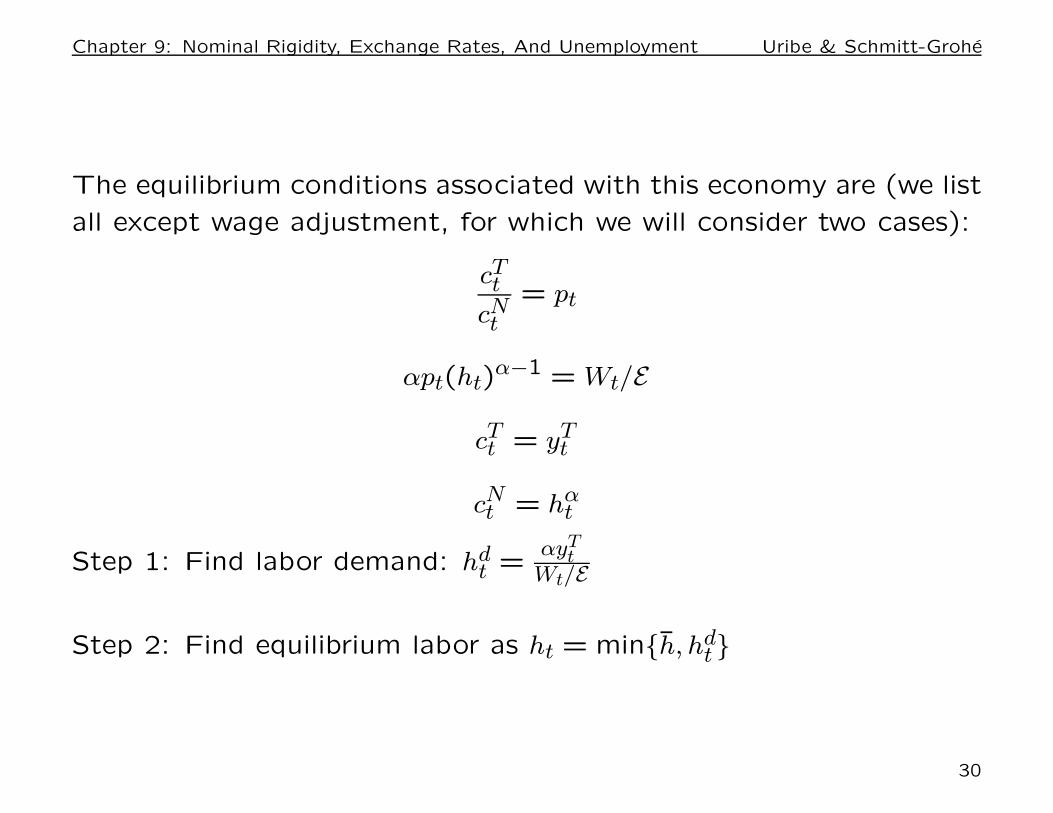
The equilibrium conditions associated with this economy are (we list
all except wage adjustment, for which we will consider two cases):
cTt
cNt
= pt
αpt(ht)α−1 = Wt/E
cTt = yT
t
cNt = hα
t
Step 1: Find labor demand: hdt =
αyTt
Wt/E
Step 2: Find equilibrium labor as ht = minh, hdt
30
Chapter 9: Nominal Rigidity, Exchange Rates, And Unemployment Uribe & Schmitt-Grohe
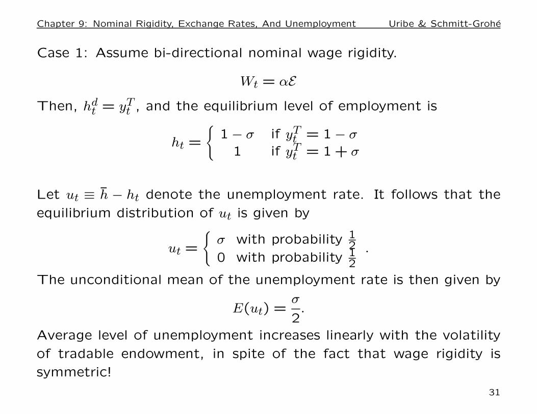
Case 1: Assume bi-directional nominal wage rigidity.
Wt = αE
Then, hdt = yT
t , and the equilibrium level of employment is
ht =
1 − σ if yTt = 1 − σ
1 if yTt = 1 + σ
Let ut ≡ h − ht denote the unemployment rate. It follows that the
equilibrium distribution of ut is given by
ut =
σ with probability 12
0 with probability 12
.
The unconditional mean of the unemployment rate is then given by
E(ut) =σ
2.
Average level of unemployment increases linearly with the volatility
of tradable endowment, in spite of the fact that wage rigidity is
symmetric!
31
Chapter 9: Nominal Rigidity, Exchange Rates, And Unemployment Uribe & Schmitt-Grohe
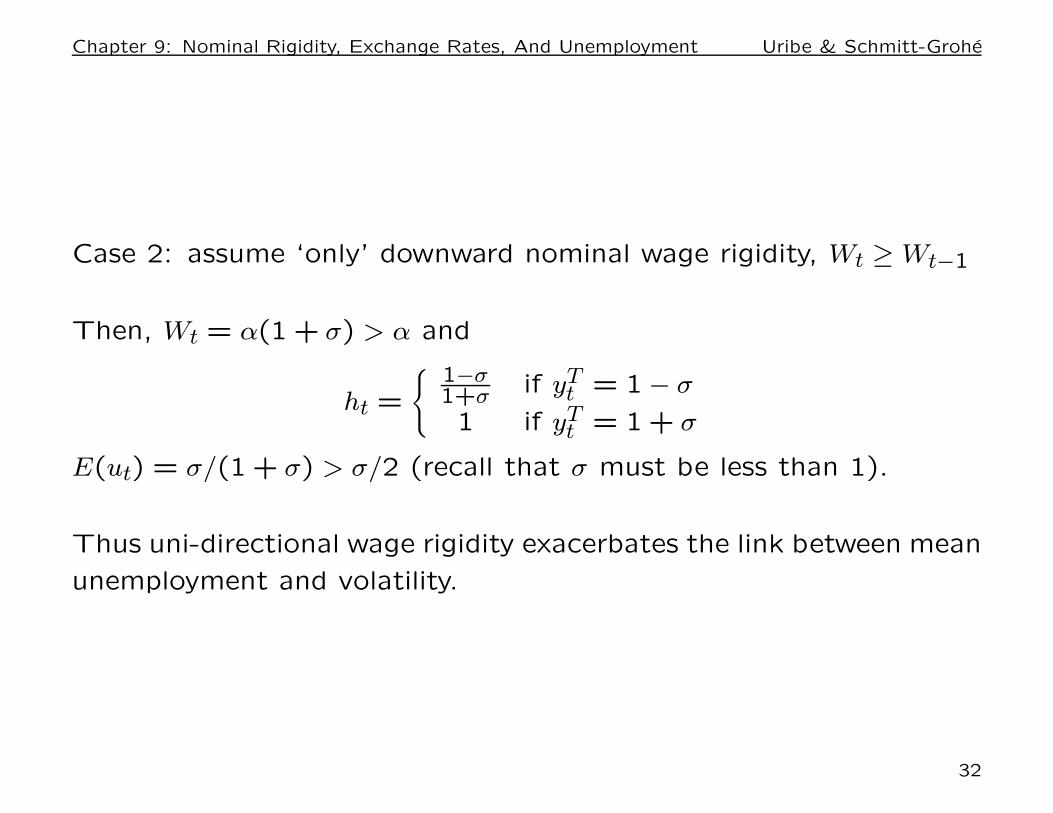
Case 2: assume ‘only’ downward nominal wage rigidity, Wt ≥ Wt−1
Then, Wt = α(1 + σ) > α and
ht =
1−σ1+σ if yT
t = 1 − σ
1 if yTt = 1 + σ
E(ut) = σ/(1 + σ) > σ/2 (recall that σ must be less than 1).
Thus uni-directional wage rigidity exacerbates the link between mean
unemployment and volatility.
32
Chapter 9: Nominal Rigidity, Exchange Rates, And Unemployment Uribe & Schmitt-Grohe
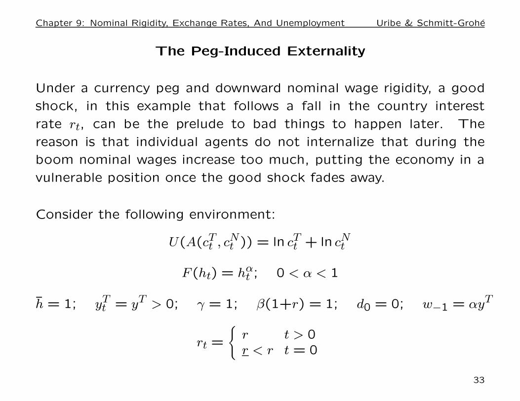
The Peg-Induced Externality
Under a currency peg and downward nominal wage rigidity, a good
shock, in this example that follows a fall in the country interest
rate rt, can be the prelude to bad things to happen later. The
reason is that individual agents do not internalize that during the
boom nominal wages increase too much, putting the economy in a
vulnerable position once the good shock fades away.
Consider the following environment:
U(A(cTt , cN
t )) = ln cTt + ln cN
t
F (ht) = hαt ; 0 < α < 1
h = 1; yTt = yT > 0; γ = 1; β(1+r) = 1; d0 = 0; w−1 = αyT
rt =
r t > 0r < r t = 0
33
Chapter 9: Nominal Rigidity, Exchange Rates, And Unemployment Uribe & Schmitt-Grohe
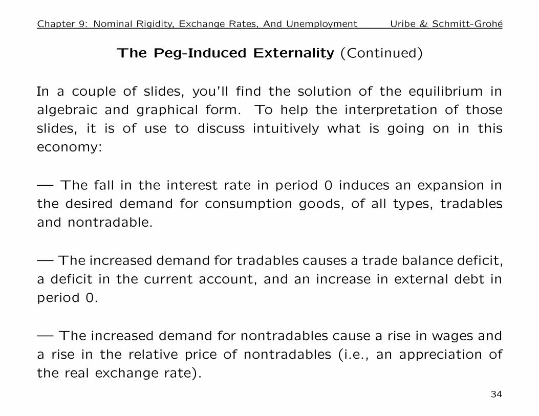
The Peg-Induced Externality (Continued)
In a couple of slides, you’ll find the solution of the equilibrium in
algebraic and graphical form. To help the interpretation of those
slides, it is of use to discuss intuitively what is going on in this
economy:
— The fall in the interest rate in period 0 induces an expansion in
the desired demand for consumption goods, of all types, tradables
and nontradable.
— The increased demand for tradables causes a trade balance deficit,
a deficit in the current account, and an increase in external debt in
period 0.
— The increased demand for nontradables cause a rise in wages and
a rise in the relative price of nontradables (i.e., an appreciation of
the real exchange rate).
34
Chapter 9: Nominal Rigidity, Exchange Rates, And Unemployment Uribe & Schmitt-Grohe
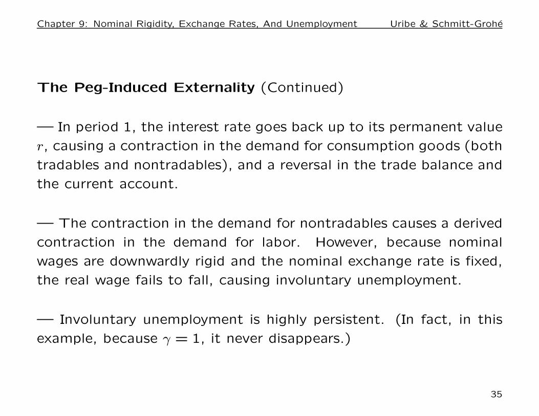
The Peg-Induced Externality (Continued)
— In period 1, the interest rate goes back up to its permanent value
r, causing a contraction in the demand for consumption goods (both
tradables and nontradables), and a reversal in the trade balance and
the current account.
— The contraction in the demand for nontradables causes a derived
contraction in the demand for labor. However, because nominal
wages are downwardly rigid and the nominal exchange rate is fixed,
the real wage fails to fall, causing involuntary unemployment.
— Involuntary unemployment is highly persistent. (In fact, in this
example, because γ = 1, it never disappears.)
35
Chapter 9: Nominal Rigidity, Exchange Rates, And Unemployment Uribe & Schmitt-Grohe
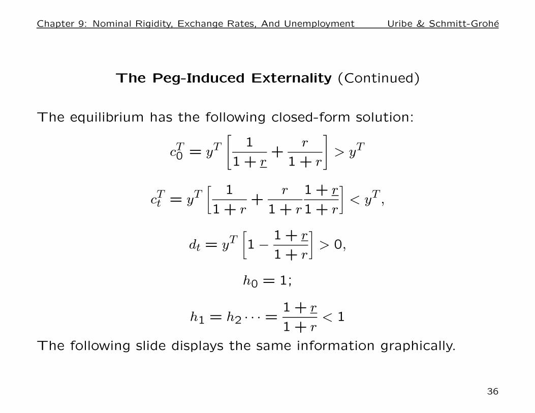
The Peg-Induced Externality (Continued)
The equilibrium has the following closed-form solution:
cT0 = yT
[
1
1 + r+
r
1 + r
]
> yT
cTt = yT
[
1
1 + r+
r
1 + r
1 + r
1 + r
]
< yT ,
dt = yT[
1 −1 + r
1 + r
]
> 0,
h0 = 1;
h1 = h2 · · · =1 + r
1 + r< 1
The following slide displays the same information graphically.
36
Chapter 9: Nominal Rigidity, Exchange Rates, And Unemployment Uribe & Schmitt-Grohe
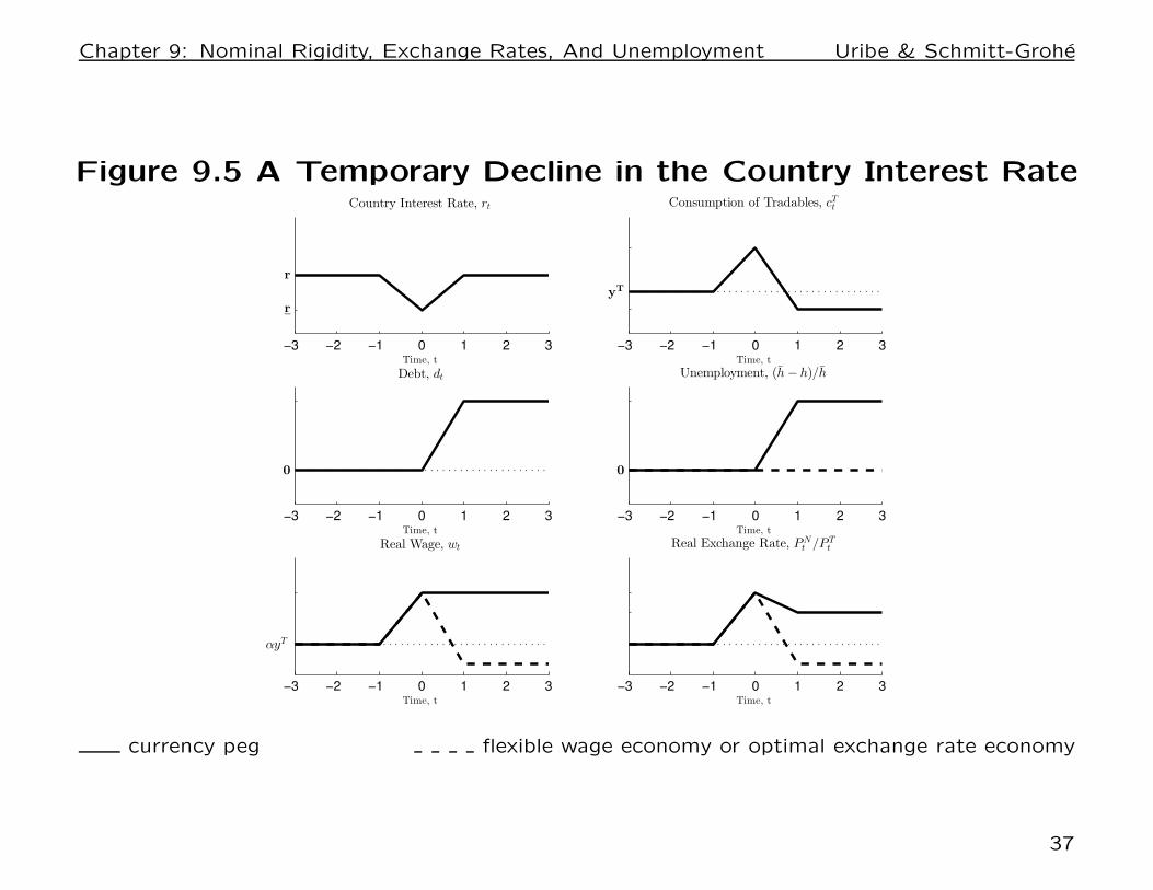
Figure 9.5 A Temporary Decline in the Country Interest Rate
−3 −2 −1 0 1 2 3Time, t
Country Interest Rate, rt
r
r
−3 −2 −1 0 1 2 3Time, t
Consumption of Tradables, cTt
yT
−3 −2 −1 0 1 2 3
Debt, dt
Time, t
0
−3 −2 −1 0 1 2 3
Unemployment, (h− h)/h
Time, t
0
−3 −2 −1 0 1 2 3
Real Wage, wt
Time, t
αyT
−3 −2 −1 0 1 2 3
Real Exchange Rate, PNt /PT
t
Time, t
currency peg flexible wage economy or optimal exchange rate economy
37
Chapter 9: Nominal Rigidity, Exchange Rates, And Unemployment Uribe & Schmitt-Grohe
Section 9.3
Optimal Exchange Rate Policy
38
Chapter 9: Nominal Rigidity, Exchange Rates, And Unemployment Uribe & Schmitt-Grohe
Motivation
• We have just seen that under an exchange rate peg a negative
external shock may lead to involuntary unemployment. How would
optimal exchange rate policy look like?
• In this section we show that under optimal policy there is (1) full
employment and (2) negative external shocks call for devaluations.
• We begin with a graphical explanation.
39
Chapter 9: Nominal Rigidity, Exchange Rates, And Unemployment Uribe & Schmitt-Grohe
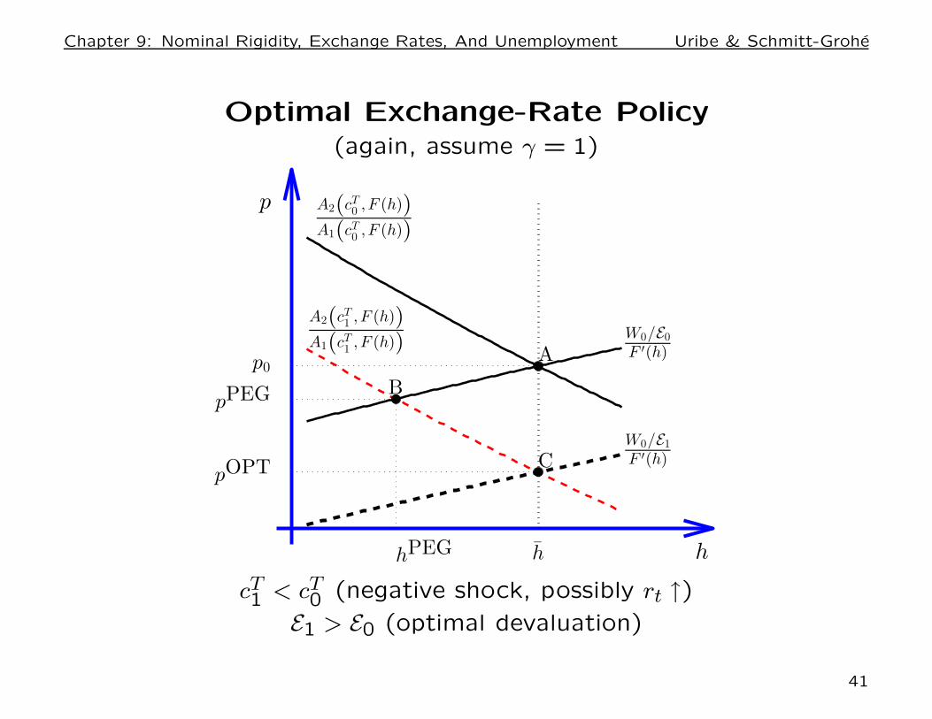
The graph on the next slide illustrates how the optimal ex-change rate policy worksThe initial situation is point A. Suppose a negative shock (possibly an increasein the country interest rate), shifts the demand schedule down and to the left.Without government intervention, the supply schedule does not move, becauseW is downwardly rigid. The equilibrium would then be point B, with involuntaryunemployment equal to h − hPEG.
Suppose now that the government devalues the domestic currency from E0 toE1 > E0. The devaluation lowers the real wage from W0/E0 to W0/E1, causingthe supply schedule to shift down and to the right.
If the devaluation is just right, the new supply schedule will cross the new demandschedule at point C, preserving full employment (we say preserving and not restor-ing full employment because the economy jumps from A to C, without visitingB).
Note: the fall in labor cost caused by the drop in the real wage allows firms to cutprices from p0 to pOPT and induces households to switch expenditure away fromtradables and toward nontradables.
Take another look at the graph for the analytical example in of a temporary fall inr0. The broken lines display the equilibrium under optimal exchange-rate policy.
40
Chapter 9: Nominal Rigidity, Exchange Rates, And Unemployment Uribe & Schmitt-Grohe
Optimal Exchange-Rate Policy(again, assume γ = 1)
h
p A2(cT0 , F (h))A1(cT0 , F (h))
A2(cT1 , F (h))A1(cT1 , F (h)) W0/E0
F ′(h)
W0/E1F ′(h)
A
B
C
p0
pPEG
pOPT
hhPEG
cT1 < cT
0 (negative shock, possibly rt ↑)
E1 > E0 (optimal devaluation)
41
Chapter 9: Nominal Rigidity, Exchange Rates, And Unemployment Uribe & Schmitt-Grohe
The Ramsey Optimal Exchange-Rate Policy
The Ramsey government solves the problem:
max E0
∞∑
t=0
βtU(A(cTt , F (ht)))
subject to (9.9) and (9.13)-(9.19).
Strategy: solve a less constrained problem and then show that its
solution satisfies (9.9) and (9.13)-(9.19).
42
Chapter 9: Nominal Rigidity, Exchange Rates, And Unemployment Uribe & Schmitt-Grohe
Consider the less restricted problem of choosing cTt , ht, dt+1
∞t=0 to
max E0
∞∑
t=0
βtU(A(cTt , F (ht)))
subject to the following subsect of the equilibrium coditions:
cTt + dt = yT
t +dt+1
1 + rt(9.9)
ht ≤ h (9.18)
Clearly, the solution for labor is ht = h for all t or full employment at all times.
Intuition: One nominal friction and one instrument that can fully offset it. Hence
possible to obtain the flexible wage allocation (which here coincides with the first
best). But to show that this is indeed the allocation under the optimal exchange-
rate policy, we must show that the solution to the above social planner’s problem
satisfies the all of the competitive equilibrium conditions, that is, conditions (9.9)
and (9.13)-(9.19). To see this, proceed by construction: set λt to satisfy (9.13),
pt to satisfy (9.15), wt to satisfy (9.16), εt to satisfy (9.17), (9.18) is a constraint
of the social planner’s problem, and so is (9.9). Because ht = h, (9.19) holds.
That (9.14) holds follows from the definition of λt and the first-order condition
of the social planner.
43
Chapter 9: Nominal Rigidity, Exchange Rates, And Unemployment Uribe & Schmitt-Grohe
An important reference point: The full-employment real wage,
denoted ω(cTt ), defined as the real wage that clears the labor market,
ω(cTt ) ≡
A2(cTt , F (h))
A1(cTt , F (h))
F ′(h); ω′(cTt ) > 0
Set the (gross) devaluation rate, εt = Et/Et−1, to eliminate unem-
ployment:
εt ≥γWt−1/Et−1
ω(cTt )
Note: There is a whole family of optimal exchange-rate policies.
Under any member of this policy, ht = h and wt = ω(cTt ) for all t.
44
Chapter 9: Nominal Rigidity, Exchange Rates, And Unemployment Uribe & Schmitt-Grohe
When is it inevitable to devalue?
Optimal exchange rate policy is:
εt ≥γWt−1/Et−1
ω(cTt )
Because ω′(cTt ) > 0, optimal devaluations occur in periods of con-
traction of aggregate demand. It follows that contractions are de-
valuatory as opposed to devaluations being contractionary.
45
Chapter 9: Nominal Rigidity, Exchange Rates, And Unemployment Uribe & Schmitt-Grohe
Under optimal exchange rate policy external debt and tradable con-
sumption are determined by the solution to
vOPT (yTt , rt, dt) = max
dt+1,cTt
U(A(cTt , F (h)) + βEtv
OPT (yTt+1, rt+1, dt+1)
subject to
yTt +
dt+1
1 + rt= dt + cT
t
46
Chapter 9: Nominal Rigidity, Exchange Rates, And Unemployment Uribe & Schmitt-Grohe
9.4 Empirical Evidence On
Downward Nominal Wage Rigidity
47
Chapter 9: Nominal Rigidity, Exchange Rates, And Unemployment Uribe & Schmitt-Grohe
• Downward nominal wage rigidity is the central friction in the
present model ⇒ natural to ask if it is empirically relevant.
• Downward nominal wage rigidity has been studied empirically from
a number of perspectives:
— Evidence from micro and macro data.
— Studies focusing on rich, emerging, and poor countries.
— Studies focusing on formal and informal labor markets.
• By product: Will obtain an estimate of the parameter γ governing
wage stickiness in the model (useful for quantitative analysis).
48

Chapter 9: Nominal Rigidity, Exchange Rates, And Unemployment Uribe & Schmitt-Grohe
Downward Nominal Wage Rigidity
A.) Evidence From Micro Data from Developed Countries
1. United States, 1986-1993, SIPP panel data
2. United States, 1996-1999, SIPP panel data
3. United States, 1997-2016, CPS panel data
4. Other Developed Countries
49
Chapter 9: Nominal Rigidity, Exchange Rates, And Unemployment Uribe & Schmitt-Grohe
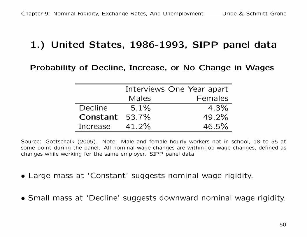
1.) United States, 1986-1993, SIPP panel data
Probability of Decline, Increase, or No Change in Wages
Interviews One Year apartMales Females
Decline 5.1% 4.3%Constant 53.7% 49.2%Increase 41.2% 46.5%
Source: Gottschalk (2005). Note: Male and female hourly workers not in school, 18 to 55 atsome point during the panel. All nominal-wage changes are within-job wage changes, defined aschanges while working for the same employer. SIPP panel data.
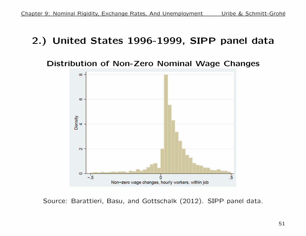
• Large mass at ‘Constant’ suggests nominal wage rigidity.
• Small mass at ‘Decline’ suggests downward nominal wage rigidity.
50
Chapter 9: Nominal Rigidity, Exchange Rates, And Unemployment Uribe & Schmitt-Grohe
2.) United States 1996-1999, SIPP panel data
Distribution of Non-Zero Nominal Wage Changes
Source: Barattieri, Basu, and Gottschalk (2012). SIPP panel data.
51
Chapter 9: Nominal Rigidity, Exchange Rates, And Unemployment Uribe & Schmitt-Grohe
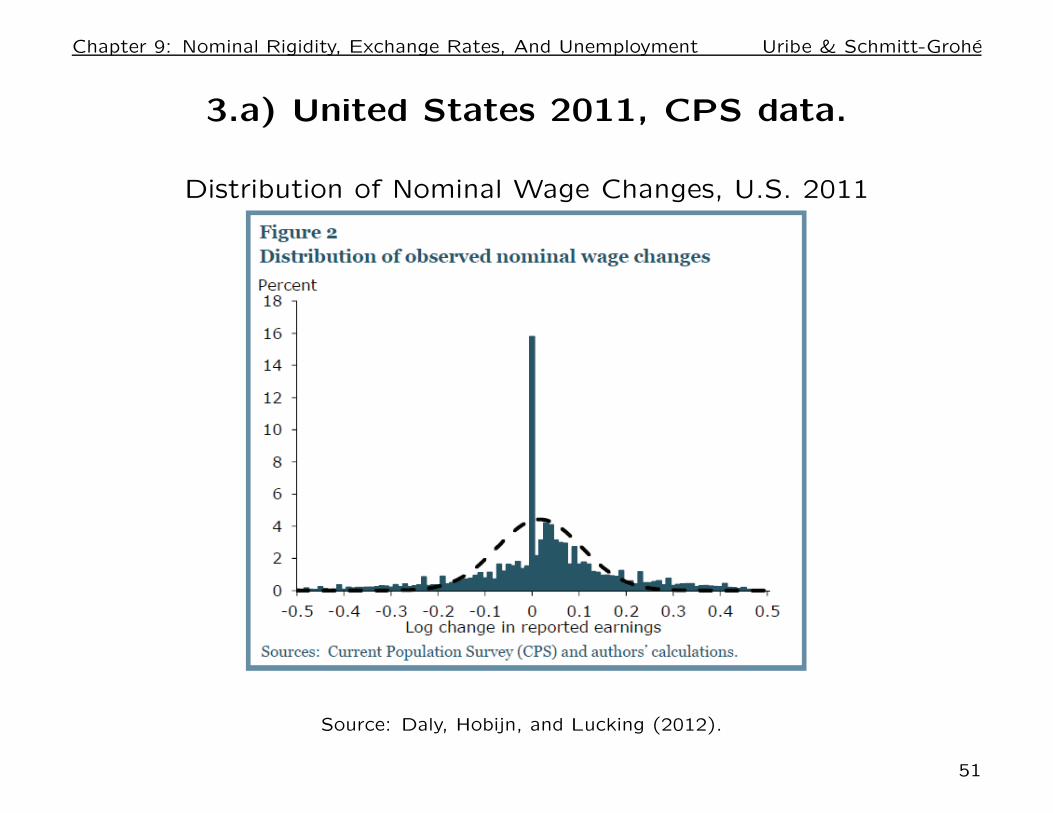
3.a) United States 2011, CPS data.
Distribution of Nominal Wage Changes, U.S. 2011
Source: Daly, Hobijn, and Lucking (2012).
51
Chapter 9: Nominal Rigidity, Exchange Rates, And Unemployment Uribe & Schmitt-Grohe
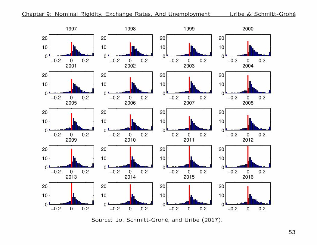
3.b) The next slide shows the distributions of Nom-inal Wage Changes in the United States for eachyear from 1997 to 2016, from CPS panel data
Nominal wage change: Year-over-year log changes in nominal
hourly wages of hourly-paid job stayers.
• In each panel, the horizontal axis shows bins of year-over-year per-
cent change in the nominal hourly wage of an hourly-paid jobstayer.
The bin size is two percent, with the exception of a wage-freeze bin,
which is defined as an exact zero change.
• The vertical axis measures the share of workers in each bin.
• Each wage change distribution is based on about 5,000 workers.
52
Chapter 9: Nominal Rigidity, Exchange Rates, And Unemployment Uribe & Schmitt-Grohe
−0.2 0 0.20
10
20
1997
−0.2 0 0.20
10
20
1998
−0.2 0 0.20
10
20
1999
−0.2 0 0.20
10
20
2000
−0.2 0 0.20
10
20
2001
−0.2 0 0.20
10
20
2002
−0.2 0 0.20
10
20
2003
−0.2 0 0.20
10
20
2004
−0.2 0 0.20
10
20
2005
−0.2 0 0.20
10
20
2006
−0.2 0 0.20
10
20
2007
−0.2 0 0.20
10
20
2008
−0.2 0 0.20
10
20
2009
−0.2 0 0.20
10
20
2010
−0.2 0 0.20
10
20
2011
−0.2 0 0.20
10
20
2012
−0.2 0 0.20
10
20
2013
−0.2 0 0.20
10
20
2014
−0.2 0 0.20
10
20
2015
−0.2 0 0.20
10
20
2016
Source: Jo, Schmitt-Grohe, and Uribe (2017).
53
Chapter 9: Nominal Rigidity, Exchange Rates, And Unemployment Uribe & Schmitt-Grohe
Observations on the figure
• Large spike at zero wage changes.
• Many more wage increases than wage cuts.
• Fraction of wage freezes is cyclical, rises from 15 percent in 2007
to 20 percent in 2009.
• Much smaller cyclical increase in wage cuts.
54
Chapter 9: Nominal Rigidity, Exchange Rates, And Unemployment Uribe & Schmitt-Grohe
4.) Micro Evidence On Downward Nominal WageRigidity From Other Developed Countries
• Canada: Fortin (1996).
• Japan: Kuroda and Yamamoto (2003).
• Switzerland: Fehr and Goette (2005).
• Industry-Level Data: Holden and Wulfsberg (2008), 19 OECD
countries from 1973 to 1999.
55
Chapter 9: Nominal Rigidity, Exchange Rates, And Unemployment Uribe & Schmitt-Grohe
B.) Evidence From Informal Labor Markets
• Are nominal wages downwardly flexible in in informal labor markets,
where labor unions, wage legislation, or regulation play, if any, a small
role?
• Kaur (2012) addresses this issue by examining the behavior of
nominal wages, employment, and rainfall in casual daily agricultural
labor markets in rural India (500 districts from 1956 to 2008).
• Finds asymmetric nominal wage adjustment:
— Wt increases in response to positive rainfall shocks
— Wt failure to fall, labor rationing, and unemployment are observed
in response to negative rain shocks.
• Inflation (uncorrelated with local rain shocks) tends to moderate
rationing and unemployment during negative rain shocks, suggesting
downward rigidity in nominal rather than real wages.
56
Chapter 9: Nominal Rigidity, Exchange Rates, And Unemployment Uribe & Schmitt-Grohe
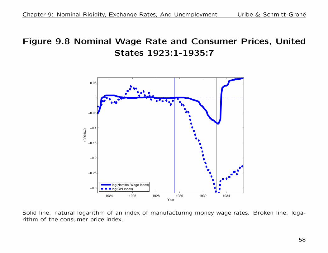
C.) Evidence From the Great Depression in the U.S.
• How do nominal wages behave during extraordinary contractions?
• The next slide shows the nominal wage rate and the consumer
price index in the United States from 1923:1-1935:7.
• Between 1929 and 1931 the U.S. economy experienced an enor-
mous contraction in employment of 31%.
• Nonetheless, during this period nominal hourly wages fell by 0.6%
per year, while consumer prices fell by 6.6% per year. See the figure
on the next slide.
• A similar pattern is observed during the second half of the Depres-
sion. By 1933, real wages were 26% higher than in 1929, in spite
of a highly distressed labor market.
57
Chapter 9: Nominal Rigidity, Exchange Rates, And Unemployment Uribe & Schmitt-Grohe
Figure 9.8 Nominal Wage Rate and Consumer Prices, United
States 1923:1-1935:7
1924 1926 1928 1930 1932 1934
−0.3
−0.25
−0.2
−0.15
−0.1
−0.05
0
0.05
Year
1929:8
=0
log(Nominal Wage Index)
log(CPI Index)
Solid line: natural logarithm of an index of manufacturing money wage rates. Broken line: loga-rithm of the consumer price index.
58

Chapter 9: Nominal Rigidity, Exchange Rates, And Unemployment Uribe & Schmitt-Grohe
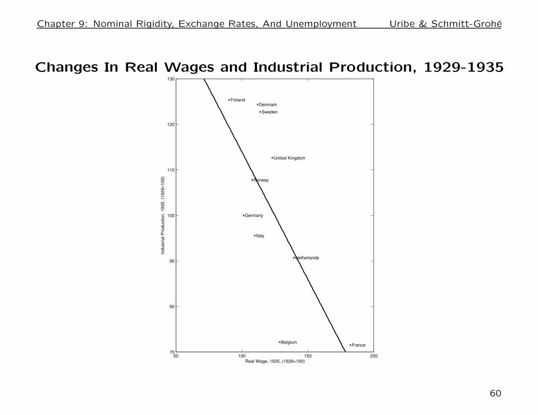
D.) Evidence From the Great Depression In Europe
• Countries that left the gold standard earlier recovered faster than
countries that remained on gold.
— Left Gold Early (sterling bloc): United Kingdom, Sweden, Fin-
land, Norway, and Denmark.
— Countries That Stuck To Gold (gold bloc): France, Belgium,
the Netherlands, and Italy.
• The gold standard is akin to a currency peg. A peg not to another
currency, but to gold.
• When the sterling-bloc left gold, they effectively devalued, as their
currencies lost value against gold.
• The figure on the next slide shows that between 1929 and 1935 the
sterling-bloc experienced less real wage growth and a larger increase
in industrial production than the gold bloc.
59
Chapter 9: Nominal Rigidity, Exchange Rates, And Unemployment Uribe & Schmitt-Grohe
Changes In Real Wages and Industrial Production, 1929-1935
50 100 150 20070
80
90
100
110
120
130
Belgium
DenmarkFinland
France
Germany
Italy
Netherlands
Norway
Sweden
United Kingdom
Real Wage, 1935, (1929=100)
Industr
ial P
roduction, 1935, (1
929=
100)
60
Chapter 9: Nominal Rigidity, Exchange Rates, And Unemployment Uribe & Schmitt-Grohe
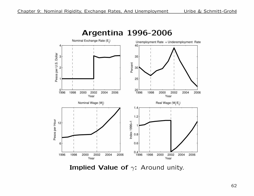
E.) Evidence From Emerging Countries
• Argentina pegged the peso at a 1-to-1 rate to the dollar between
1991 and 2001.
• Starting in 1998, the economy was buffeted by a number of large
negative shocks (weak commodity prices, large devaluation in Brazil,
large increase in country premium).
• Not surprisingly, between 1998 and 2001, unemployment rose
sharply. See the figure on the next slide.
• Nonetheless, nominal wages remained remarkably flat.
• This evidence is consistent with downward nominal wage rigid-
ity, and suggests that γ, the parameter governing downward wage
rigidity in the model, is about 1.
•Why γ ≈ 1? The slackness condition (h − ht)(Wt − γWt−1) (recall εt = 1 between
1991 and 2001), implies that if unemployment is growing, then wages must grow
at the gross rate γ. Argentine wages were flat ⇒ γ ≈ 1.
61
Chapter 9: Nominal Rigidity, Exchange Rates, And Unemployment Uribe & Schmitt-Grohe
Argentina 1996-2006
1996 1998 2000 2002 2004 20060
1
2
3
4
Year
Pe
so
s p
er
U.S
. D
olla
r
Nominal Exchange Rate (Et)
1996 1998 2000 2002 2004 2006
6
12
Year
Nominal Wage (Wt)
Pe
so
s p
er
Ho
ur
1996 1998 2000 2002 2004 20060.4
0.6
0.8
1
1.2
1.4
Real Wage (Wt/E
t)
Year
Ind
ex 1
99
6=
1
1996 1998 2000 2002 2004 200620
25
30
35
40Unemployment Rate + Underemployment Rate
Pe
rce
nt
Year
Implied Value of γ: Around unity.
62

Chapter 9: Nominal Rigidity, Exchange Rates, And Unemployment Uribe & Schmitt-Grohe
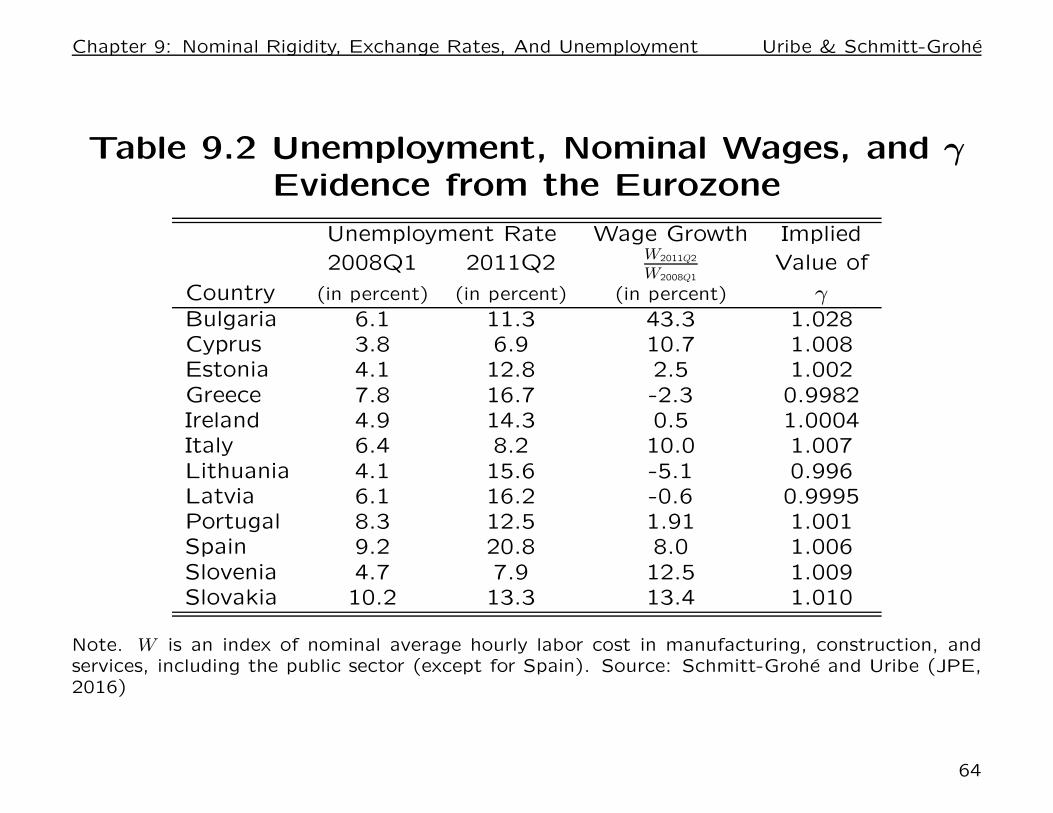
Evidence From Peripheral Europe (2008-2011)
• The next slide shows the unemployment rate and nominal wage
growth between 2008:Q1 and 2011:Q2 in 12 European countries
that were either in the eurozone or pegging to the euro.
• Between 2008 and 2011, all countries in the periphery of Europe
experienced increases in unemployment; Some very large increases.
• In spite of extreme duress in the labor market, nominal hourly
wages experienced increases in most countries and modest declines
in only a few.
• The slide following the table explains how to use the information
in the table to infer a range for γ.
63
Chapter 9: Nominal Rigidity, Exchange Rates, And Unemployment Uribe & Schmitt-Grohe
Table 9.2 Unemployment, Nominal Wages, and γ
Evidence from the Eurozone
Unemployment Rate Wage Growth Implied
2008Q1 2011Q2 W2011Q2
W2008Q1Value of
Country (in percent) (in percent) (in percent) γBulgaria 6.1 11.3 43.3 1.028Cyprus 3.8 6.9 10.7 1.008Estonia 4.1 12.8 2.5 1.002Greece 7.8 16.7 -2.3 0.9982Ireland 4.9 14.3 0.5 1.0004Italy 6.4 8.2 10.0 1.007Lithuania 4.1 15.6 -5.1 0.996Latvia 6.1 16.2 -0.6 0.9995Portugal 8.3 12.5 1.91 1.001Spain 9.2 20.8 8.0 1.006Slovenia 4.7 7.9 12.5 1.009Slovakia 10.2 13.3 13.4 1.010
Note. W is an index of nominal average hourly labor cost in manufacturing, construction, andservices, including the public sector (except for Spain). Source: Schmitt-Grohe and Uribe (JPE,2016)
64
Chapter 9: Nominal Rigidity, Exchange Rates, And Unemployment Uribe & Schmitt-Grohe
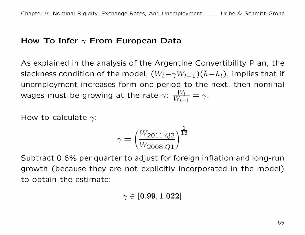
How To Infer γ From European Data
As explained in the analysis of the Argentine Convertibility Plan, the
slackness condition of the model, (Wt−γWt−1)(h−ht), implies that if
unemployment increases form one period to the next, then nominal
wages must be growing at the rate γ: WtWt−1
= γ.
How to calculate γ:
γ =
(
W2011:Q2
W2008:Q1
)113
Subtract 0.6% per quarter to adjust for foreign inflation and long-run
growth (because they are not explicitly incorporated in the model)
to obtain the estimate:
γ ∈ [0.99, 1.022]
65
Chapter 9: Nominal Rigidity, Exchange Rates, And Unemployment Uribe & Schmitt-Grohe
Quantitative Analysis
(Sections 9.5-9.8 and 9.10)
Replication files: usg_dnwr.zip available online with the materials
for this chapter.
66
Chapter 9: Nominal Rigidity, Exchange Rates, And Unemployment Uribe & Schmitt-Grohe
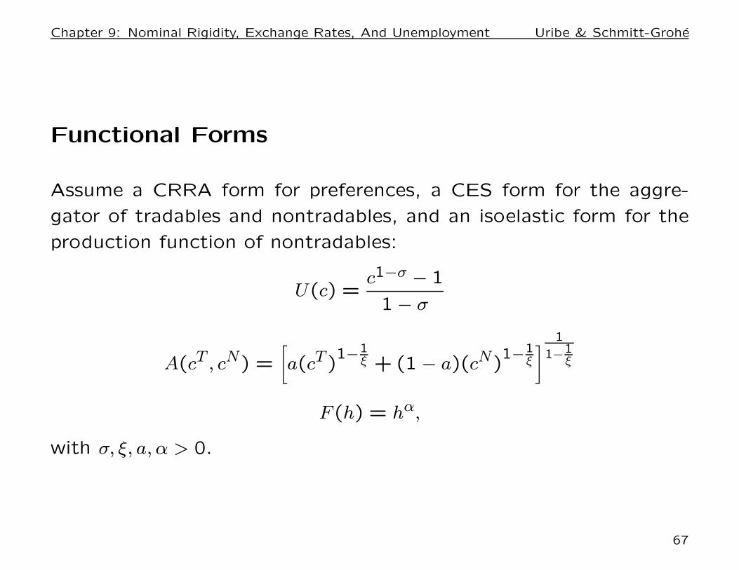
Functional Forms
Assume a CRRA form for preferences, a CES form for the aggre-
gator of tradables and nontradables, and an isoelastic form for the
production function of nontradables:
U(c) =c1−σ − 1
1 − σ
A(cT , cN) =
[
a(cT )1−1
ξ + (1 − a)(cN)1−1
ξ
]
1
1−1ξ
F (h) = hα,
with σ, ξ, a, α > 0.
67
Chapter 9: Nominal Rigidity, Exchange Rates, And Unemployment Uribe & Schmitt-Grohe
The case of Equal Intra- and Intertemporal Elasticities of Sub-
stitution
Consider the case
ξ =1
σ
Why this case is of interest:
• It makes the determination of the equilibrium levels of debt, dt, and
consumption of tradables, cTt , independent of the level of activity in
the nontraded sector (see the next slide). As a result, the welfare
consequences of exchange-rate policy or nominal wage rigidity are
fully attributable to their effect on unemployment, and not on their
effect on the accumulation of external debt.
• It facilitates the computation of equilibrium, as the equilibrium dy-
namics of dt and cTt can be computed separately from the equilibrium
dynamics of ht, wt, cNt , and pt.
• As we will argue shortly, σ = 1/ξ = 2 is empirically plausible.
68
Chapter 9: Nominal Rigidity, Exchange Rates, And Unemployment Uribe & Schmitt-Grohe
Debt and Tradable Consumption when ξ = 1σ
In this case,
U(A(cTt , cN
t )) =acT
t1−σ
+ (1 − a)cNt
1−σ− 1
1 − σ,
which is separable in cTt and cN
t . Then dt and cTt solve
cTt + dt = yT
t +dt+1
1 + rt
(cTt )−σ = β(1 + rt)Et(c
Tt+1)
−σ
This subsystem is independent of ht, wt, pt, and cNt .
It can be cast as a Bellman equation problem, which facilitates the
quantitative analysis (more on the next slide).
69
Chapter 9: Nominal Rigidity, Exchange Rates, And Unemployment Uribe & Schmitt-Grohe
Approximating Equilibrium Dynamics Under Opti-mal Exchange-Rate Policy when ξ = 1/σEquilibrium processes cT
t , dt+1 solve the Bellman equation problem
vOPT (yTt , rt, dt) = max
dt+1,cTt
U(A(cTt , F (h))) + βEtv
OPT (yTt+1, rt+1, dt+1)
(1)
subject to cTt + dt = yT
t +dt+1
1 + rt; and dt+1 ≤ d. (2)
Approximate by value function iteration over a discretized statespace (yT
t , rt, dt). Use 21 values for yTt and 11 for rt (the estimated
joint process (yTt , rt) is given below). Use 501 equally spaced points
for dt between 1 and 8.34.
Given approximated solutions to dt+1 and cTt , all other variables of
the model can be backed out:ht = h,
pt =A2(c
Tt ,F(h))
A1(cTt ,F(h))
,
wt = ptF′(h),
and a chosen member of the family εt ≥ γwt−1/wt.
70
Chapter 9: Nominal Rigidity, Exchange Rates, And Unemployment Uribe & Schmitt-Grohe
Approximating Equilibrium Under Currency Pegs with ξ = 1/σ
When ξ = 1/σ, the solution for dt+1 and cTt is as before, since
it does not depend on the exchange-rate policy. for the optimal
exchange-rate policy
The determination of wt requires knowledge of past real wages. So,
wt−1 is a relevant endogenous state. This is different from the
equilibrium under optimal exchange-rate policy.
Given wt−1 and cTt , the solution for wt is static (simple): First,
conjecture that ht = h, and obtain wt =A2(c
Tt ,F(h))
A1(cTt ,F(h))
F ′(h). If wt ≥
γwt−1, this is the solution. Otherwise, wt = γwt−1, and ht solves
wt =A2(c
Tt ,F(ht))
A1(cTt ,F(ht))
F ′(ht).
Discretization of wt−1 grid: 500 points between 0.25 and 6, equally
spaced in logs.
71
Chapter 9: Nominal Rigidity, Exchange Rates, And Unemployment Uribe & Schmitt-Grohe
Approximating Equilibrium when ξ 6= 1/σ
Optimal Exchange-Rate Policy: As before, the solution is sepa-
rable. First, the processes dt+1 and cTt solve the Bellman equation
problem (1)-(2). Then, all other variables (wt, pt, cNt ) are then easily
backed out.
Currency Peg: The the solution is no longer separable. All equi-
librium conditions must be solved jointly and becomes more compli-
cated. Schmitt-Grohe and Uribe (JPE, 2016) develop an algorithm
to handle this case.
72
Chapter 9: Nominal Rigidity, Exchange Rates, And Unemployment Uribe & Schmitt-Grohe
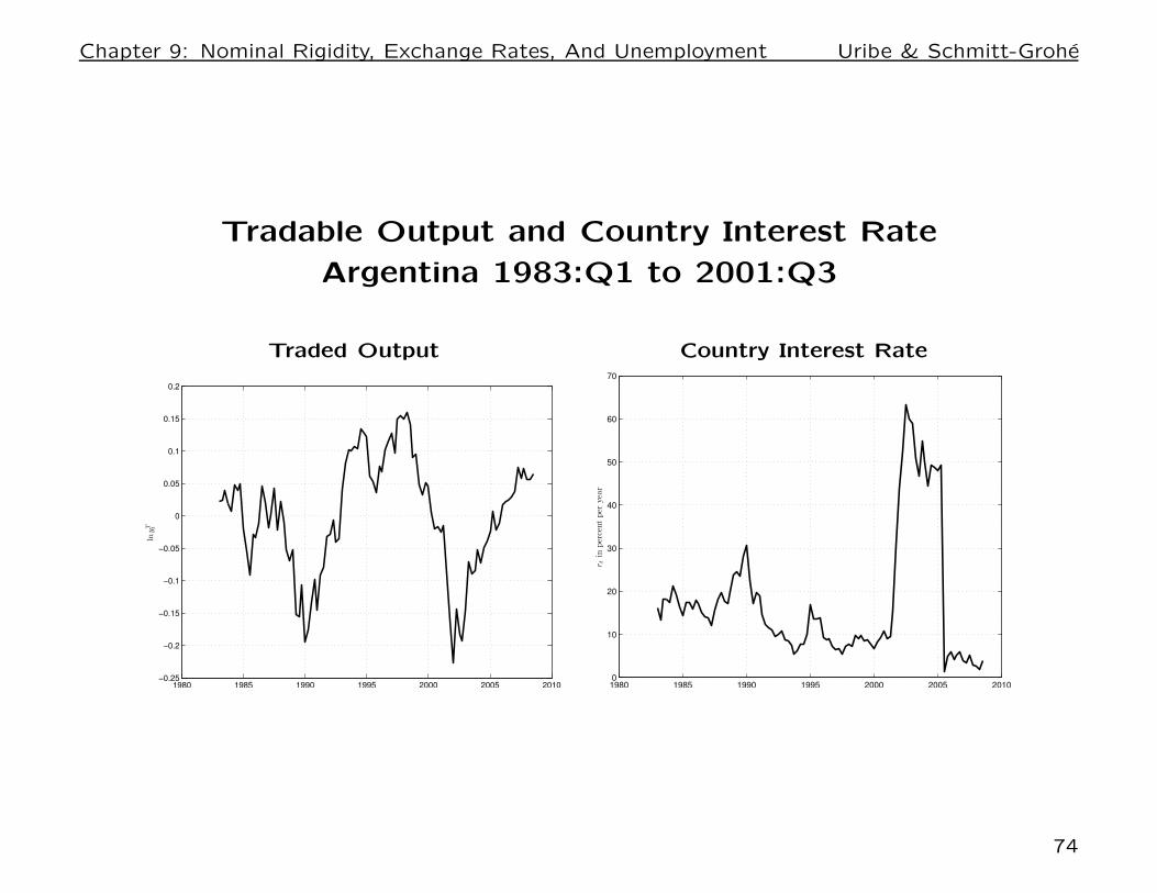
The Driving Process:
Data: Argentine data over the period 1983:Q1—2001:Q3. Exclude
the period 2001:Q4 to present, because of the default episode in
2002 (no default in the model).
Empirical Measure of yTt : sum of GDP in agriculture, manufac-
turing, fishing, forestry, and mining. Quadratically detrended.
Empirical Measure of rt: Sum of Argentine EMBI+ plus 90-day
Treasury-Bill rate minus a measure of U.S. expected inflation.
The following slide displays the two time series.
73
Chapter 9: Nominal Rigidity, Exchange Rates, And Unemployment Uribe & Schmitt-Grohe
Tradable Output and Country Interest Rate
Argentina 1983:Q1 to 2001:Q3
Traded Output Country Interest Rate
1980 1985 1990 1995 2000 2005 2010−0.25
−0.2
−0.15
−0.1
−0.05
0
0.05
0.1
0.15
0.2
lny
T t
1980 1985 1990 1995 2000 2005 20100
10
20
30
40
50
60
70
rt
inperc
ent
per
year
74

Chapter 9: Nominal Rigidity, Exchange Rates, And Unemployment Uribe & Schmitt-Grohe
Estimate the AR(1) system
[
ln yTt
ln 1+rt1+r
]
= A
ln yTt−1
ln1+rt−11+r
+ εt,
OLS Estimate of the Driving Process
A =
[
0.79 −1.36−0.01 0.86
]
; Σε =
[
0.00123 −0.00008−0.00008 0.00004
]
;
r = 0.0316 (3.16% per quarter).
75
Chapter 9: Nominal Rigidity, Exchange Rates, And Unemployment Uribe & Schmitt-Grohe
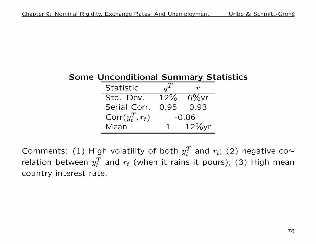
Some Unconditional Summary Statistics
Statistic yT rStd. Dev. 12% 6%yrSerial Corr. 0.95 0.93
Corr(yTt , rt) -0.86
Mean 1 12%yr
Comments: (1) High volatility of both yTt and rt; (2) negative cor-
relation between yTt and rt (when it rains it pours); (3) High mean
country interest rate.
76
Chapter 9: Nominal Rigidity, Exchange Rates, And Unemployment Uribe & Schmitt-Grohe
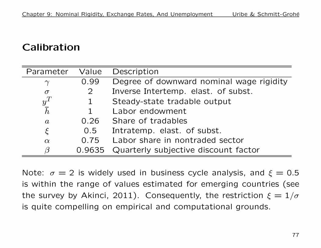
Calibration
Parameter Value Description
γ 0.99 Degree of downward nominal wage rigidityσ 2 Inverse Intertemp. elast. of subst.
yT 1 Steady-state tradable outputh 1 Labor endowmenta 0.26 Share of tradablesξ 0.5 Intratemp. elast. of subst.α 0.75 Labor share in nontraded sectorβ 0.9635 Quarterly subjective discount factor
Note: σ = 2 is widely used in business cycle analysis, and ξ = 0.5
is within the range of values estimated for emerging countries (see
the survey by Akinci, 2011). Consequently, the restriction ξ = 1/σ
is quite compelling on empirical and computational grounds.
77
Chapter 9: Nominal Rigidity, Exchange Rates, And Unemployment Uribe & Schmitt-Grohe
Crisis Dynamics Under A Currency Peg
and Under Optimal Exchange-Rate Policy
We are interested in characterizing quantitatively the response of
the model economy to large contractions like the ones observed
in Argentina in 2001 and in the periphery of Europe in 2008. In
Argentina, for instance, traded output fell by 2 standard deviations
in a period of two and a half years (10 quarters). Accordingly, we
use the following operational definition of an external crisis.
Definition of an External Crisis. A crisis is a situation in which in
period t tradable output, yTt , is at or above average, and 10 quarters
later, in period t + 10, it is at least two standard deviations below
trend.
The Typical External Crisis: Simulate the model for 20 million
periods. Extract all windows of time in which yTt conforms to the
definition of a crisis. For each variable of interest, average all win-
dows and subtract its unconditional mean (i.e., the mean taken over
the 20 million observations).
78
Chapter 9: Nominal Rigidity, Exchange Rates, And Unemployment Uribe & Schmitt-Grohe
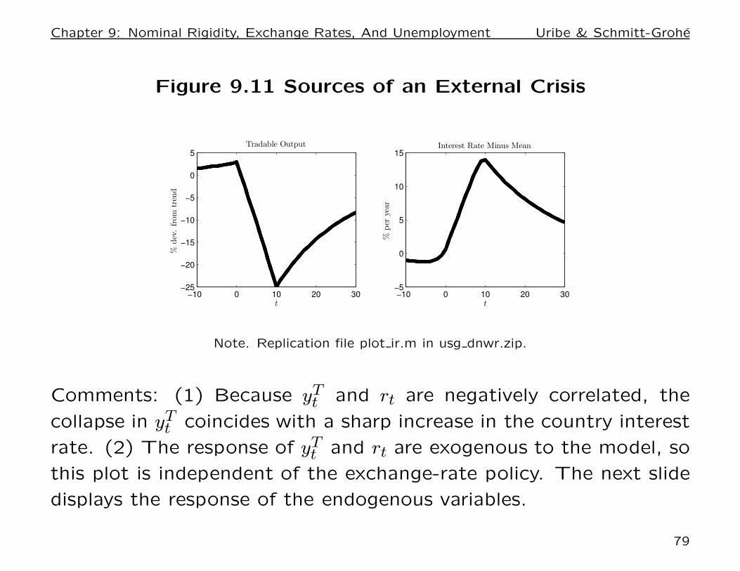
Figure 9.11 Sources of an External Crisis
−10 0 10 20 30−25
−20
−15
−10
−5
0
5Tradable Output
%dev.from
trend
t−10 0 10 20 30
−5
0
5
10
15Interest Rate Minus Mean
%per
year
t
Note. Replication file plot ir.m in usg dnwr.zip.
Comments: (1) Because yTt and rt are negatively correlated, the
collapse in yTt coincides with a sharp increase in the country interest
rate. (2) The response of yTt and rt are exogenous to the model, so
this plot is independent of the exchange-rate policy. The next slide
displays the response of the endogenous variables.
79
Chapter 9: Nominal Rigidity, Exchange Rates, And Unemployment Uribe & Schmitt-Grohe
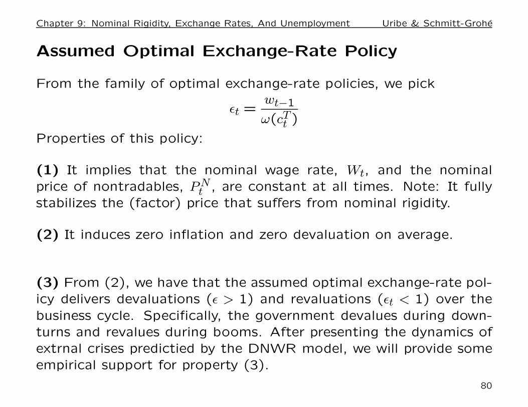
Assumed Optimal Exchange-Rate Policy
From the family of optimal exchange-rate policies, we pick
εt =wt−1
ω(cTt )
Properties of this policy:
(1) It implies that the nominal wage rate, Wt, and the nominal
price of nontradables, PNt , are constant at all times. Note: It fully
stabilizes the (factor) price that suffers from nominal rigidity.
(2) It induces zero inflation and zero devaluation on average.
(3) From (2), we have that the assumed optimal exchange-rate pol-
icy delivers devaluations (ε > 1) and revaluations (εt < 1) over the
business cycle. Specifically, the government devalues during down-
turns and revalues during booms. After presenting the dynamics of
extrnal crises predictied by the DNWR model, we will provide some
empirical support for property (3).
80
Chapter 9: Nominal Rigidity, Exchange Rates, And Unemployment Uribe & Schmitt-Grohe
External Crisis under
Alternative Exchange-rate Policies withDownward Niminal Wage Rigidity
We are now ready to present the predicted equilibrium dynamics
during a typical crisis under a currency peg and under the optimal
exchange rate policy we selected.
The next slide shows with solid lines the response of the economy
under a currency peg and with broken lines the response under the
assumed optimal exchange-rate policy.
81
Chapter 9: Nominal Rigidity, Exchange Rates, And Unemployment Uribe & Schmitt-Grohe
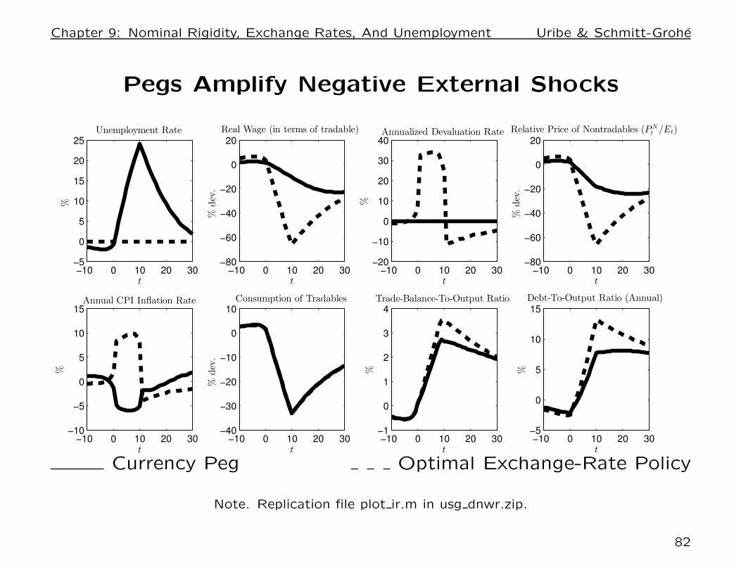
Pegs Amplify Negative External Shocks
−10 0 10 20 30−5
0
5
10
15
20
25Unemployment Rate
%
t−10 0 10 20 30
−80
−60
−40
−20
0
20Real Wage (in terms of tradable)
%dev.
t−10 0 10 20 30
−20
−10
0
10
20
30
40Annualized Devaluation Rate
%
t−10 0 10 20 30
−80
−60
−40
−20
0
20Relative Price of Nontradables (PN
t /Et)
%dev.
t
−10 0 10 20 30−10
−5
0
5
10
15Annual CPI Inflation Rate
%
t−10 0 10 20 30
−40
−30
−20
−10
0
10Consumption of Tradables
%dev.
t−10 0 10 20 30
−1
0
1
2
3
4Trade-Balance-To-Output Ratio
%
t−10 0 10 20 30
−5
0
5
10
15Debt-To-Output Ratio (Annual)
%
t
Currency Peg Optimal Exchange-Rate Policy
Note. Replication file plot ir.m in usg dnwr.zip.
82
Chapter 9: Nominal Rigidity, Exchange Rates, And Unemployment Uribe & Schmitt-Grohe
Observations
• Large contraction in cT , driven primarily by the hike in the country
interest rate. The the trade balance, yTt − cT
t , actually improves in
spite of the fact that yT falls sharply. The response of cT is inde-
pendent of exchange-rate policy, because ξ = 1/σ.
• Currency Pegs: large increase in unemployment (25%), because
the real wage does not fall sufficiently (stays 40% above the full-
employment real wage). Firms don’t cut prices because labor cost
remains high. As a result, consumers don’t switch spending away
from tradables and toward nontradables.
• Optimal Exchange-Rate Policy: It cannot avoid the contrac-
tion in the tradable sector. But it can prevent the external cri-
sis to spreead to the nontradable sector. In fact, it preserves full
employment throughout the crisis (this result was also established
analytically earlier in this chapter). Large devaluations of around
30% per year for 2.5 years. Consistent with devaluations post Con-
vertibility in Argentina. Devaluations bring the real wage down
(E ↑⇒ w = W/E ↓), fostering employment and allowing the real
exchange to depreciate (p = PN/E ↓). Real depreciation facilitates
expenditure switch toward nontradables.
83
Chapter 9: Nominal Rigidity, Exchange Rates, And Unemployment Uribe & Schmitt-Grohe
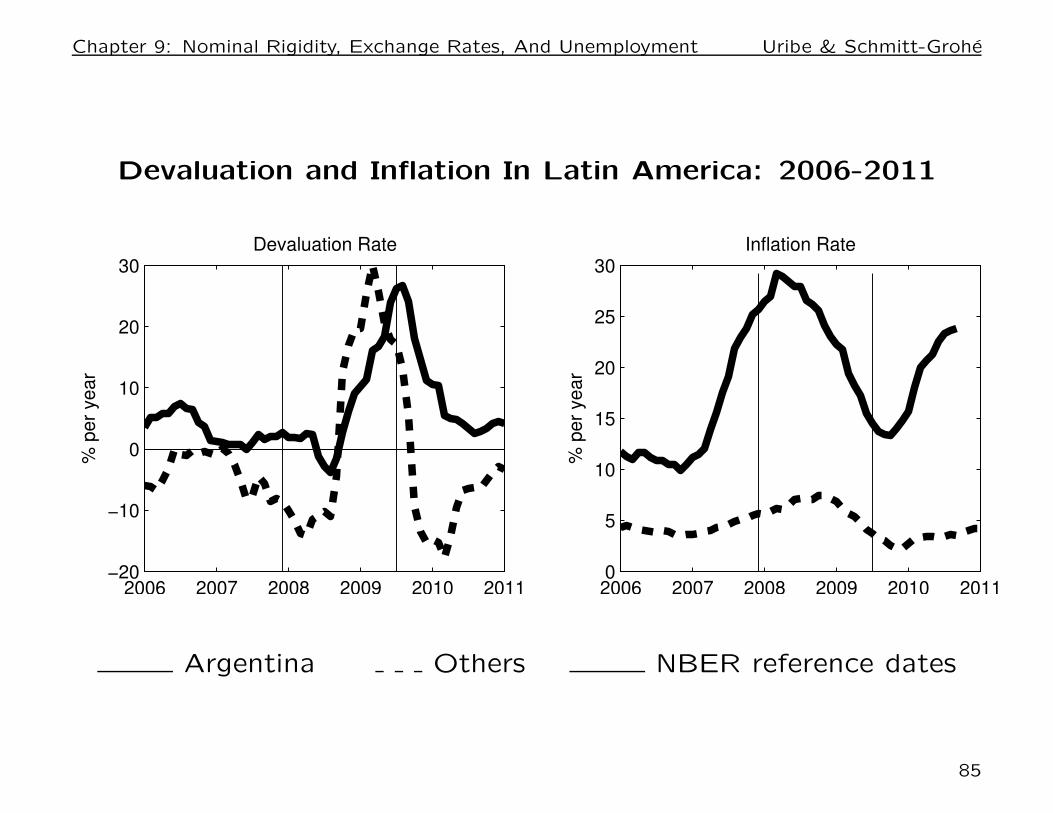
Devaluations and Revaluations in Reality
Do countries devalue during crises and revalue when the crisis is
over, and why? Look at the next graph. It displays the devaluation
rate and the inflation rate for two sets of Latin American countries
during the global crisis of 2008. One set is Argentina, and the other
includes Chile, Colombia, Mexico, Peru, and Uruguay.
During the crisis, all countries devalued significantly. However, dur-
ing the recovery, all countries but Argentina revalued their curren-
cies. The countries that revalued experienced lower inflation than
Argentina.
84
Chapter 9: Nominal Rigidity, Exchange Rates, And Unemployment Uribe & Schmitt-Grohe
Devaluation and Inflation In Latin America: 2006-2011
2006 2007 2008 2009 2010 2011−20
−10
0
10
20
30
% p
er
year
Devaluation Rate
2006 2007 2008 2009 2010 20110
5
10
15
20
25
30
% p
er
year
Inflation Rate
Argentina Others NBER reference dates
85
Chapter 9: Nominal Rigidity, Exchange Rates, And Unemployment Uribe & Schmitt-Grohe
Are devaluations expansionary as predicted by theDNWR model?
Two address this issue, we take another look at two episodes of
exiting a currency peg:
• Ending Convertibility: Argentina 1996-2006
• Exiting the Gold Standard: Europe 1929-1935
86

Chapter 9: Nominal Rigidity, Exchange Rates, And Unemployment Uribe & Schmitt-Grohe
Argentina Post Convertibility 1996-2006
1996 1998 2000 2002 2004 20060
1
2
3
4
Year
Pesos p
er
U.S
. D
olla
r
Nominal Exchange Rate (Et)
1996 1998 2000 2002 2004 2006
6
12
Year
Nominal Wage (Wt)
Pesos p
er
Hour
1996 1998 2000 2002 2004 20060.4
0.6
0.8
1
1.2
1.4
Real Wage (Wt/E
t)
Year
Index 1
996=
1
1996 1998 2000 2002 2004 200620
25
30
35
40Unemployment Rate + Underemployment Rate
Perc
ent
Year
Memo: Average annual CPI inflation 1998-2001: -0.86%
Observations:• Argentine peso pegged to the U.S.dollar from April 1991 to December 2001. (Con-vertibility Plan) • Since 1998 severe recession, sube-mployment rate reaches 35 percent. • but no nom-inal wage decline in 1998-2001; • December 2001Argentina devalues by 250%; • leads to large declinein the real wage; • labor market conditions then im-proved quickly. • sizable fall in real wages right afterthe Dec 2001 devaluation suggests that the 1998-2001 period was one of censored wage deflation.• nominal wage growth after devaluation suggestsupward flexibility of nominal wages;
Overall, predicted expansionary effects of devalua-tion are consistent with dynamics in Argentina postConvertibility
87

Chapter 9: Nominal Rigidity, Exchange Rates, And Unemployment Uribe & Schmitt-Grohe
Exiting the Gold Standard: Europe 1929 to 1935
• Friedman and Schwartz (1963) observe that countries that left
gold early (the sterling bloc) enjoyed more rapid recoveries than
countries that stayed on gold longer (the gold bloc).
• Sterling bloc: United Kingdom, Sweden, Finland, Norway, Den-
mark.
• Gold bloc: France, Belgium, the Netherlands, and Italy.
• Eichengreen and Sachs (1986) observe that real wages behaved
differently in countries that left gold early (ie devalued) and in coun-
tries that stayed on gold longer (ie stayed on the peg). Take a look
at the next figure, which is redrawn from Eichengreen and Sachs.
88
Chapter 9: Nominal Rigidity, Exchange Rates, And Unemployment Uribe & Schmitt-Grohe
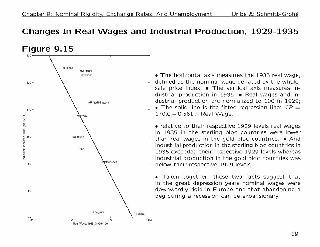
Changes In Real Wages and Industrial Production, 1929-1935
Figure 9.15
50 100 150 20070
80
90
100
110
120
130
Belgium
DenmarkFinland
France
Germany
Italy
Netherlands
Norway
Sweden
United Kingdom
Real Wage, 1935, (1929=100)
Industr
ial P
roduction, 1935, (1
929=
100)
• The horizontal axis measures the 1935 real wage,defined as the nominal wage deflated by the whole-sale price index; • The vertical axis measures in-dustrial production in 1935; • Real wages and in-dustrial production are normalized to 100 in 1929;• The solid line is the fitted regression line: IP =170.0 − 0.561 × Real Wage.
• relative to their respective 1929 levels real wagesin 1935 in the sterling bloc countries were lowerthan real wages in the gold bloc countries. • Andindustrial production in the sterling bloc countries in1935 exceeded their respective 1929 levels whereasindustrial production in the gold bloc countries wasbelow their respective 1929 levels.
• Taken together, these two facts suggest thatin the great depression years nominal wages weredownwardly rigid in Europe and that abandoning apeg during a recession can be expansionary.
89
Chapter 9: Nominal Rigidity, Exchange Rates, And Unemployment Uribe & Schmitt-Grohe
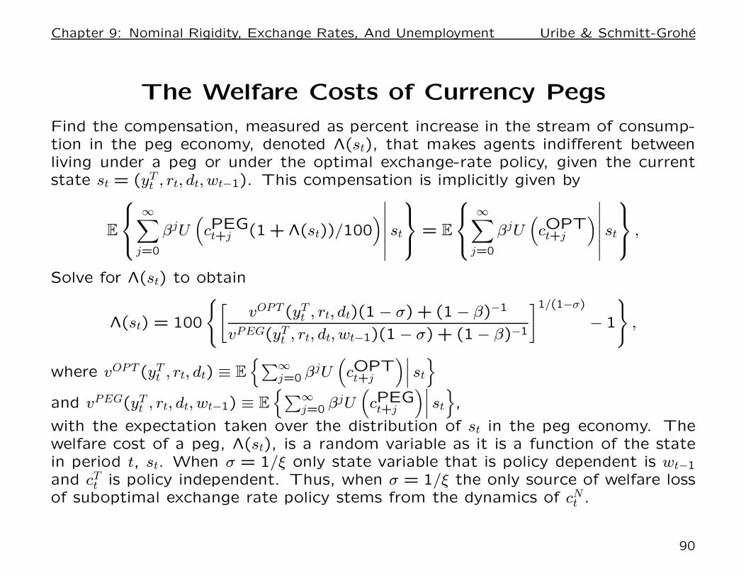
The Welfare Costs of Currency Pegs
Find the compensation, measured as percent increase in the stream of consump-tion in the peg economy, denoted Λ(st), that makes agents indifferent betweenliving under a peg or under the optimal exchange-rate policy, given the currentstate st = (yT
t , rt, dt, wt−1). This compensation is implicitly given by
E
∞∑
j=0
βjU(
cPEGt+j (1 + Λ(st))/100
)
∣
∣
∣
∣
∣
∣
st
= E
∞∑
j=0
βjU(
cOPTt+j
)
∣
∣
∣
∣
∣
∣
st
,
Solve for Λ(st) to obtain
Λ(st) = 100
[
vOPT (yTt , rt, dt)(1 − σ) + (1 − β)−1
vPEG(yTt , rt, dt, wt−1)(1 − σ) + (1 − β)−1
]1/(1−σ)
− 1
,
where vOPT (yTt , rt, dt) ≡ E
∑∞j=0 βjU
(
cOPTt+j
)∣
∣
∣st
and vPEG(yTt , rt, dt, wt−1) ≡ E
∑∞j=0 βjU
(
cPEGt+j
)∣
∣
∣st
,
with the expectation taken over the distribution of st in the peg economy. Thewelfare cost of a peg, Λ(st), is a random variable as it is a function of the statein period t, st. When σ = 1/ξ only state variable that is policy dependent is wt−1
and cTt is policy independent. Thus, when σ = 1/ξ the only source of welfare loss
of suboptimal exchange rate policy stems from the dynamics of cNt .
90
Chapter 9: Nominal Rigidity, Exchange Rates, And Unemployment Uribe & Schmitt-Grohe
The Welfare Costs of Currency Pegs
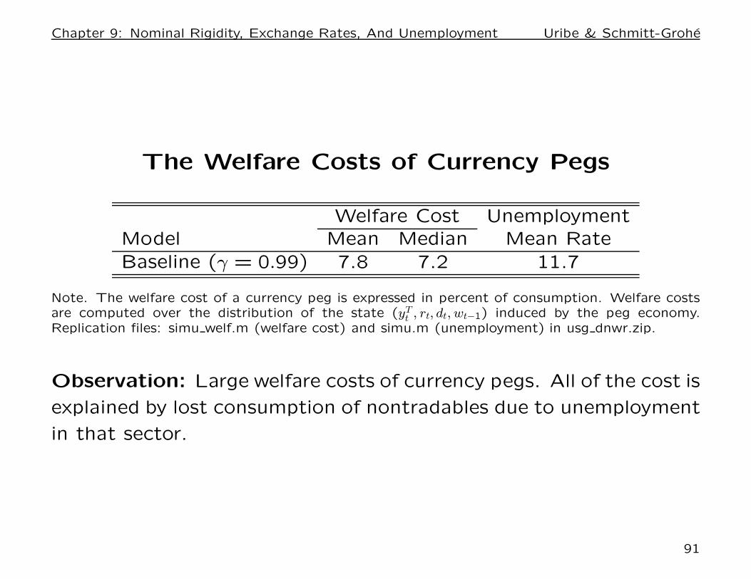
Welfare Cost UnemploymentModel Mean Median Mean Rate
Baseline (γ = 0.99) 7.8 7.2 11.7
Note. The welfare cost of a currency peg is expressed in percent of consumption. Welfare costsare computed over the distribution of the state (yT
t , rt, dt, wt−1) induced by the peg economy.Replication files: simu welf.m (welfare cost) and simu.m (unemployment) in usg dnwr.zip.
Observation: Large welfare costs of currency pegs. All of the cost is
explained by lost consumption of nontradables due to unemployment
in that sector.
91
Chapter 9: Nominal Rigidity, Exchange Rates, And Unemployment Uribe & Schmitt-Grohe
Probability Density Function of the Welfare Cost of Currency Pegs
4 6 8 10 12 14 16 18 20 220
0.05
0.1
0.15
0.2
0.25
0.3
0.35
welfare cost of a peg (% of ct per quarter)
density
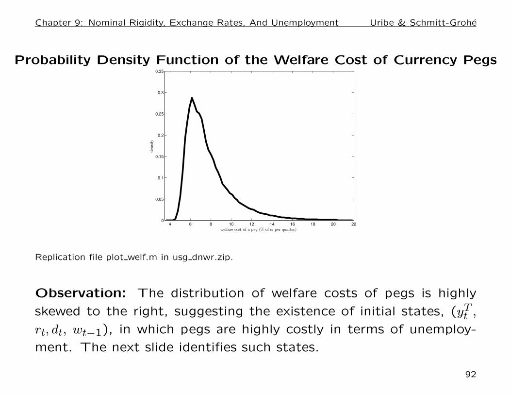
Replication file plot welf.m in usg dnwr.zip.
Observation: The distribution of welfare costs of pegs is highly
skewed to the right, suggesting the existence of initial states, (yTt ,
rt, dt, wt−1), in which pegs are highly costly in terms of unemploy-
ment. The next slide identifies such states.
92
Chapter 9: Nominal Rigidity, Exchange Rates, And Unemployment Uribe & Schmitt-Grohe
Welfare Cost of Currency Pegs and the Initial State
1 2 3 4
6
8
10
12
14
16
18
wt− 1
welfare
cost
1 2 3 4 5
6
7
8
9
10
dt
welfare
cost
−0.2 −0.1 0 0.1 0.2
6.5
7
7.5
8
8.5
9
log(yTt )
welfare
cost
0 5 10 15 20 256.5
7
7.5
8
8.5
9
welfare
cost
rt (annual)
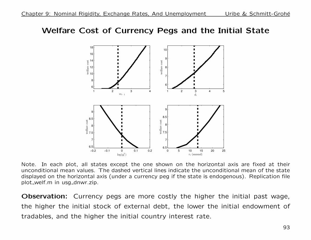
Note. In each plot, all states except the one shown on the horizontal axis are fixed at theirunconditional mean values. The dashed vertical lines indicate the unconditional mean of the statedisplayed on the horizontal axis (under a currency peg if the state is endogenous). Replication fileplot welf.m in usg dnwr.zip.
Observation: Currency pegs are more costly the higher the initial past wage,
the higher the initial stock of external debt, the lower the initial endowment of
tradables, and the higher the initial country interest rate.
93
Chapter 9: Nominal Rigidity, Exchange Rates, And Unemployment Uribe & Schmitt-Grohe
Alternative Parameterizations and Model Specifica-tions
9.10 Varying the Degree of Wage Rigidity
9.11 Symmetric Wage Rigidity
9.13 Endogenous Labor Supply
9.14 Production in the Traded Sector
9.15 Product Price Rigidity
94
Chapter 9: Nominal Rigidity, Exchange Rates, And Unemployment Uribe & Schmitt-Grohe
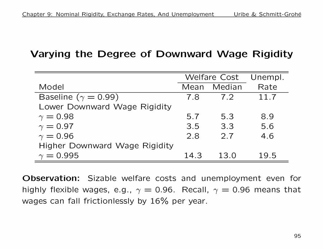
Varying the Degree of Downward Wage Rigidity
Welfare Cost Unempl.Model Mean Median Rate
Baseline (γ = 0.99) 7.8 7.2 11.7Lower Downward Wage Rigidityγ = 0.98 5.7 5.3 8.9γ = 0.97 3.5 3.3 5.6γ = 0.96 2.8 2.7 4.6Higher Downward Wage Rigidityγ = 0.995 14.3 13.0 19.5
Observation: Sizable welfare costs and unemployment even for
highly flexible wages, e.g., γ = 0.96. Recall, γ = 0.96 means that
wages can fall frictionlessly by 16% per year.
95
Chapter 9: Nominal Rigidity, Exchange Rates, And Unemployment Uribe & Schmitt-Grohe
Symmetric Wage Rigidity
Is more wage flexibility always welfare increasing?
Not always. We have just seen that the welfare costs of a currency
peg increase as the degree of downward wage rigidity, γ, increases.
So the answer here is Yes.
We now consider a different way of increasing wage rigidity, namely,
bi-directional wage rigidity:
1
γ≥
Wt
Wt−1≥ γ
We will see that this increase in wage rigidity is welfare enhancing.
96
Chapter 9: Nominal Rigidity, Exchange Rates, And Unemployment Uribe & Schmitt-Grohe
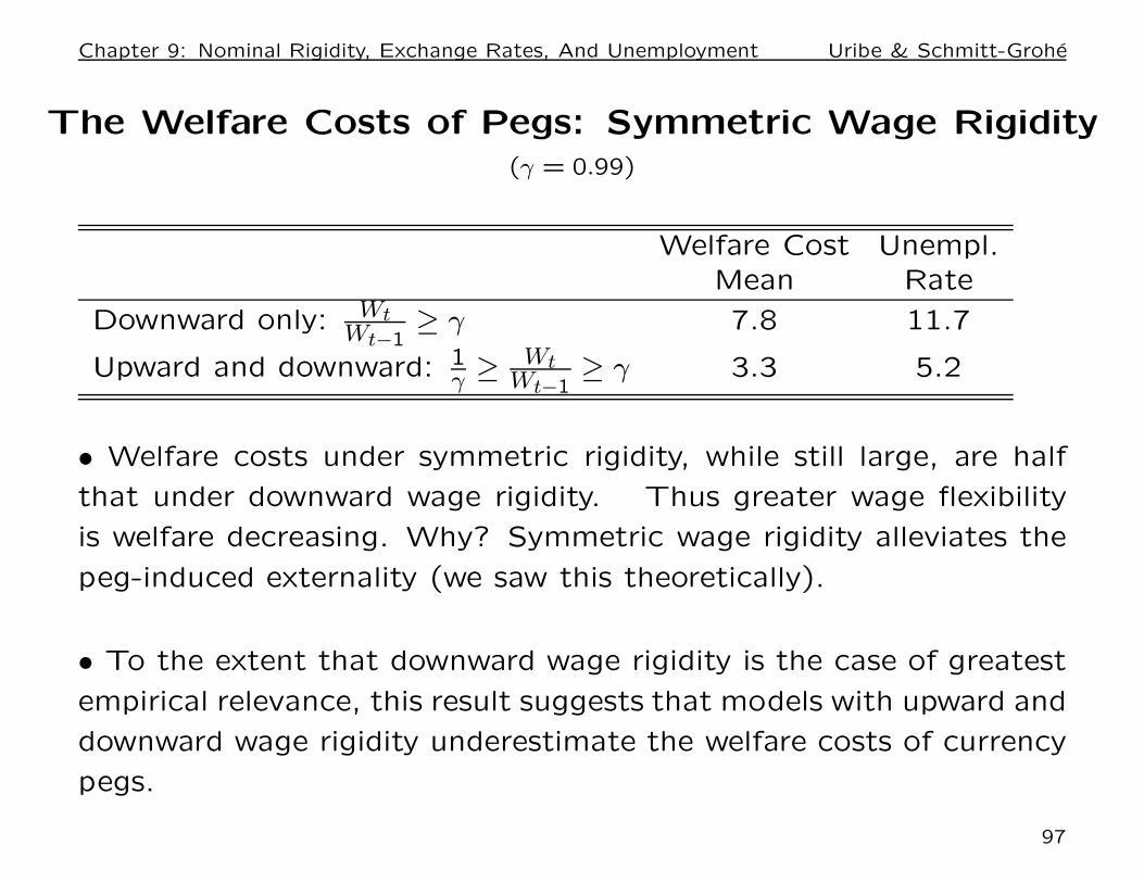
The Welfare Costs of Pegs: Symmetric Wage Rigidity(γ = 0.99)
Welfare Cost Unempl.Mean Rate
Downward only: WtWt−1
≥ γ 7.8 11.7
Upward and downward: 1γ ≥ Wt
Wt−1≥ γ 3.3 5.2
• Welfare costs under symmetric rigidity, while still large, are half
that under downward wage rigidity. Thus greater wage flexibility
is welfare decreasing. Why? Symmetric wage rigidity alleviates the
peg-induced externality (we saw this theoretically).
• To the extent that downward wage rigidity is the case of greatest
empirical relevance, this result suggests that models with upward and
downward wage rigidity underestimate the welfare costs of currency
pegs.
97
Chapter 9: Nominal Rigidity, Exchange Rates, And Unemployment Uribe & Schmitt-Grohe
Endogenous Labor Supply
Thus far, we have assumed that households supply h units of labor
inelastically. How should an endogenous labor supply affect the main
predictions of the model?
• Now negative income shocks (e.g., yT ↓), may cause an increase
in labor supply, elevating the level of involuntary unemployment.
• Thus far, the model included only one type of non-work activity,
namely involuntary unemployment. Now there will be two, invol-
untary unemployment (or involuntary lesure) and voluntary leisure
(or voluntary unemployment). How do voluntary and involuntary
unemployment enter in the utility function? Are they substitutes or
complements? How substitutable are they? This margin will make
a difference in determining the welfare costs of currency pegs.
With these questions in mind, let’s now introduce a labor choice
more formally.
98
Chapter 9: Nominal Rigidity, Exchange Rates, And Unemployment Uribe & Schmitt-Grohe
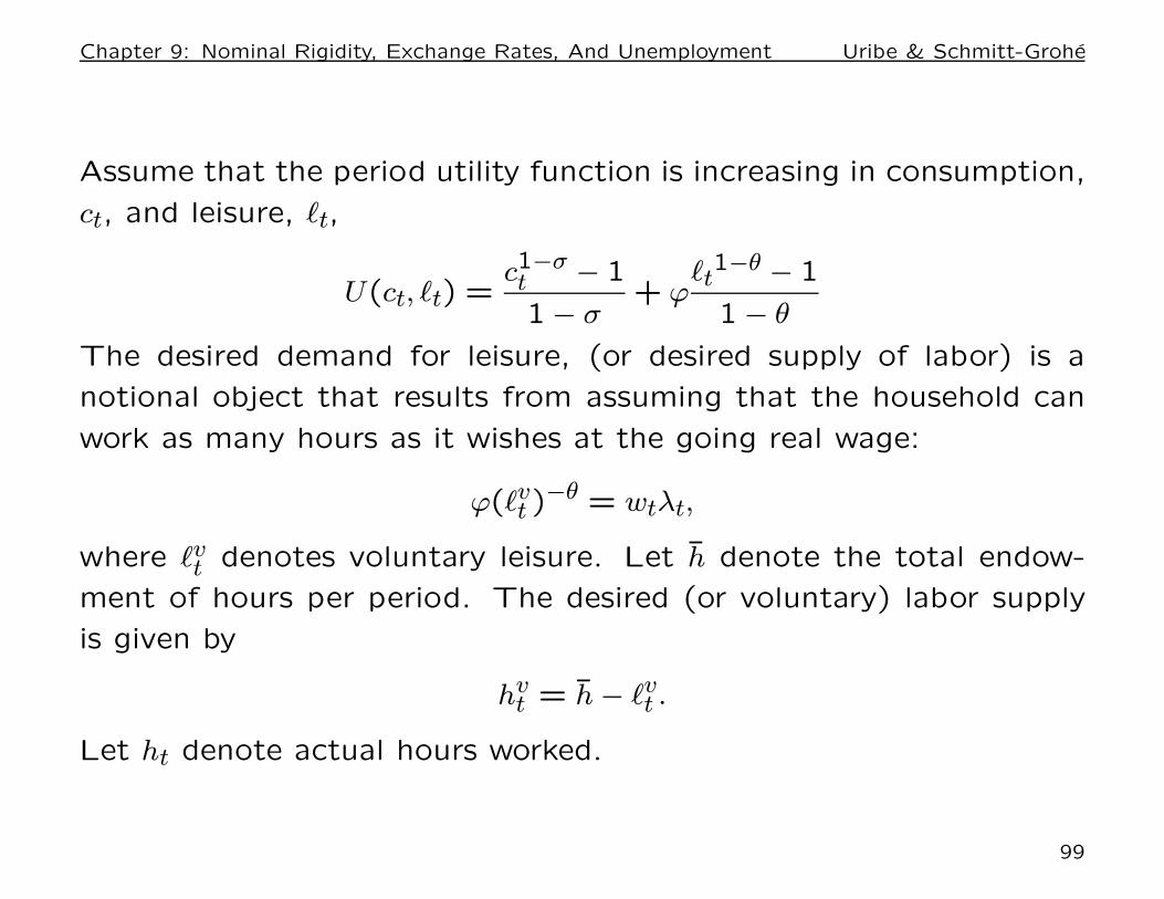
Assume that the period utility function is increasing in consumption,
ct, and leisure, `t,
U(ct, `t) =c1−σt − 1
1 − σ+ ϕ
`t1−θ − 1
1 − θ
The desired demand for leisure, (or desired supply of labor) is a
notional object that results from assuming that the household can
work as many hours as it wishes at the going real wage:
ϕ(`vt )
−θ = wtλt,
where `vt denotes voluntary leisure. Let h denote the total endow-
ment of hours per period. The desired (or voluntary) labor supply
is given by
hvt = h − `v
t .
Let ht denote actual hours worked.
99
Chapter 9: Nominal Rigidity, Exchange Rates, And Unemployment Uribe & Schmitt-Grohe
A no-slavery condition:
hvt ≥ ht,
Closing the labor market
(hvt − ht)
(
wt − γwt−1
εt
)
= 0.
The above four equations replace the conditions ht ≤ h and (h −
ht)(wt − γwt−1/εt) = 0 of the economy with inelastic labor supply.
The rest of the equilibrium conditions are unchanged.
Involuntary unemployment, or, synonymously, involuntary leisure,
denoted ut, is given by
ut = hvt − ht
100
Chapter 9: Nominal Rigidity, Exchange Rates, And Unemployment Uribe & Schmitt-Grohe
Policy evaluation requires addressing an important question:
How should voluntary and involuntary leisure enter in the pe-
riod utility function?
One possibility is to assume that `vt and ut are perfect substitutes.
In this case, the second argument of the utility function becomes
`t = `vt + ut. Is this assumption empirically realistic?
101
Chapter 9: Nominal Rigidity, Exchange Rates, And Unemployment Uribe & Schmitt-Grohe
The existing empirical literature seems to reject this assumption:
• Krueger and Mueller (2012): the unemployed enjoy leisure activi-
ties to a lesser degree than the employed and on a typical day report
higher levels of sadness than the employed.
• Winkelmann and Winkelmann (1998): Unemployment has a large
non-pecuniary detrimental effect on life satisfaction.
• Krueger and Mueller (2012): Unemployed spend 101 minutes more
per day on job search than employed (not surprising). However, job
search generates the highest feeling of sadness after personal care
out of 13 time-use categories.
⇒ Better specification appears to be : `t = `vt + δut
with δ < 1. Will consider three values, 1, 0.75, and 0.5.
102
Chapter 9: Nominal Rigidity, Exchange Rates, And Unemployment Uribe & Schmitt-Grohe
Endogenous Labor Supply And
The Welfare Costs of Currency Pegs
Welfare Cost UnemploymentParameterization Mean Median Rate
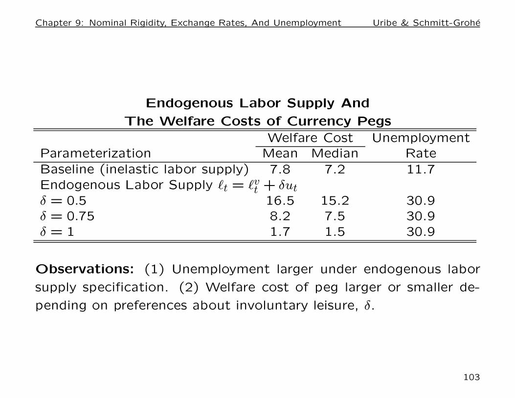
Baseline (inelastic labor supply) 7.8 7.2 11.7Endogenous Labor Supply `t = `v
t + δutδ = 0.5 16.5 15.2 30.9δ = 0.75 8.2 7.5 30.9δ = 1 1.7 1.5 30.9
Observations: (1) Unemployment larger under endogenous labor
supply specification. (2) Welfare cost of peg larger or smaller de-
pending on preferences about involuntary leisure, δ.
103
Chapter 9: Nominal Rigidity, Exchange Rates, And Unemployment Uribe & Schmitt-Grohe
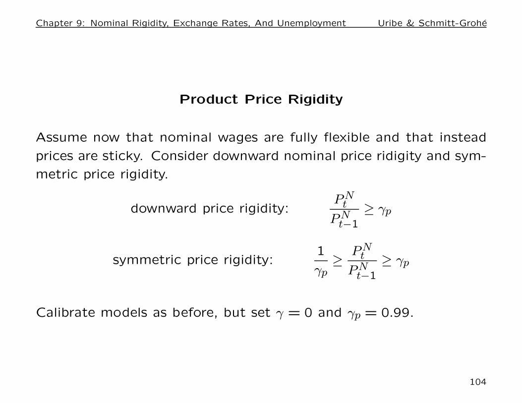
Product Price Rigidity
Assume now that nominal wages are fully flexible and that instead
prices are sticky. Consider downward nominal price ridigity and sym-
metric price rigidity.
downward price rigidity:PN
t
PNt−1
≥ γp
symmetric price rigidity:1
γp≥
PNt
PNt−1
≥ γp
Calibrate models as before, but set γ = 0 and γp = 0.99.
104
Chapter 9: Nominal Rigidity, Exchange Rates, And Unemployment Uribe & Schmitt-Grohe
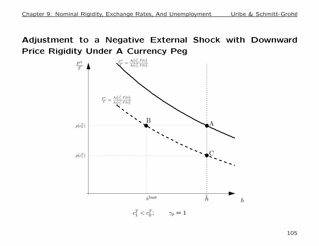
Adjustment to a Negative External Shock with Downward
Price Rigidity Under A Currency Peg
h
PN
E
PN
E=
A2(cT1 , F(h))A1(cT1 , F(h))
PN
E=
A2(cT0 , F(h))A1(cT0 , F(h))
h
C
AB
ρ(cT1 )
ρ(cT0 )
hbust
cT1 < cT
0 ; γp = 1
105
Chapter 9: Nominal Rigidity, Exchange Rates, And Unemployment Uribe & Schmitt-Grohe
Observations: When cT falls from cT0 to cT
1 , full employment would
occur if prices could decline to ρ(cT1), point C in the figure. But
because of downward nominal price rigidity, PNt /E remains at ρ(cT
0).
At this price households only demand F (hbust) units of nontradables
and the economy suffers of unemployment due to week demand.
Optimal policy calls for a devaluation that lowers PNt /Et down to
ρ(cT1) and restores full employment. Hence contractions continue to
be devaluatory!
The economy continues to suffer from a peg induced externality.
Increases in PNt during booms should be limited to avoid unemploy-
ment during the recession phase of the cycle.
106
Chapter 9: Nominal Rigidity, Exchange Rates, And Unemployment Uribe & Schmitt-Grohe
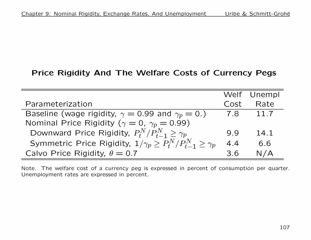
Price Rigidity And The Welfare Costs of Currency Pegs
Welf UnemplParameterization Cost Rate
Baseline (wage rigidity, γ = 0.99 and γp = 0.) 7.8 11.7Nominal Price Rigidity (γ = 0, γp = 0.99)
Downward Price Rigidity, PNt /PN
t−1 ≥ γp 9.9 14.1
Symmetric Price Rigidity, 1/γp ≥ PNt /PN
t−1 ≥ γp 4.4 6.6
Calvo Price Rigidity, θ = 0.7 3.6 N/A
Note. The welfare cost of a currency peg is expressed in percent of consumption per quarter.Unemployment rates are expressed in percent.
107
Chapter 9: Nominal Rigidity, Exchange Rates, And Unemployment Uribe & Schmitt-Grohe
Observations. The welfare costs of pegs under downward price
rigidity are as large as under downward wage rigidity. The welfare
costs under symmetric price rigidity are only about half as large
as under downward price rigidity. It follows that adding upward
price rigidity ameliorates the peg induced externality, just like adding
upward wage rigidity amerliorates it in the model model with wage
rigidity.
The last line, labeled Calvo pricing, pertains to an economy with
Calvo-type price rigidity in the nontraded sector. The probability of
not being able to change the nominal price is θ = 0.7 per period.
The calibration of the shocks is the same as in the baseline model.
The Calvo model is one of symmetric price rigidity and so it is not
surprising that the welfare costs of pegs are most similar to those
associated with the economy with the bi-directional price rigidity
studied earlier.
108
Chapter 9: Nominal Rigidity, Exchange Rates, And Unemployment Uribe & Schmitt-Grohe
Summary of Theoretical results:
• Analytical results — The combination of a currency peg and downward
nominal wage rigidity creates an externality that amplifies the severity of contrac-
tions.
— The model predicts that the average rate of unemployment is increasing in the
degree of aggregate volatility.
— The DNWR model predicts significant amplification of booms-bust cycles un-
der suboptimal monetary policy (and in particular under currency pegs.).
• Quantitative Results:
— The costs of currency pegs due to downward nominal wage rigidity are large,
· in terms of welfare, 4 to 10% of consumption per period.
· and in terms of unemployment, 10 to 30%.
— These results are robust to a variety of changes parameter values and model
specifications, including endogenous labor supply, bidirectional nominal rigidity,
and product price rigidity.
— The welfare costs of currency pegs are higher the higher the past real wage,
the higher the level of external debt, the lower the level of tradable output, and
the higher the country interest rate.
109

Chapter 9: Nominal Rigidity, Exchange Rates, And Unemployment Uribe & Schmitt-Grohe
Section 9.12The Mussa Puzzle
110
Chapter 9: Nominal Rigidity, Exchange Rates, And Unemployment Uribe & Schmitt-Grohe
Mussa (1986) is an empirical paper that provides evidence against
the “nominal exchange rate regime neutrality” hypothesis.
Methodology: compare variations in nominal and real exchange rates
in quarterly data from 13 industrialized countries during the fixed
exchange rate period (1957-1970) with variations in the floating
exchange rate period (1973-1984)
Observables:
Et = nominal exchange rate vis-a-vis the U.S. dollar
P ∗t = U.S. Consumer Price Index
Pt = Domestic Consumer Price Index
RERt =EtP
∗t
Pt
Take a look at the next figure. It shows 3 series: (1) the natural
logarithms of the dollar French franc nominal and real exchange
rates as well as the log of the relative CPIs.
111
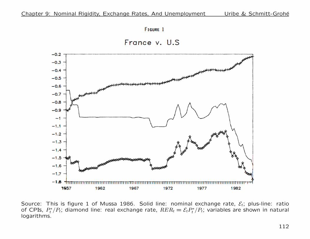
Chapter 9: Nominal Rigidity, Exchange Rates, And Unemployment Uribe & Schmitt-Grohe
Source: This is figure 1 of Mussa 1986. Solid line: nominal exchange rate, Et; plus-line: ratioof CPIs, P ∗
t /Pt; diamond line: real exchange rate, RERt = EtP ∗t /Pt; variables are shown in natural
logarithms.
112
Chapter 9: Nominal Rigidity, Exchange Rates, And Unemployment Uribe & Schmitt-Grohe
Comments on the figure:
Quarterly data, 1957:Q2 to 1984:Q3.
Fixed exchange rate: Bretton Woods, 1957:Q2-1970:Q4.
French franc was pegged to the U.S. dollar.
Floating exchange rate: Post-Bretton Woods, 1973:Q1-1984:Q3.
Selection of sample period: Why a gap in the sample period? Mussa
argues that 1970Q4 to 1973Q1 is a transition period. The float
starts in March 1973. Why does Mussa start his sample in 1957,
this was afterall not the beginning of the Bretton Woods agreement?
Mussa justifies the start date by saying that this is when the IFS
tapes start having the raw data. Why does Mussa end the sample
1983Q3? This must be the most recent observation when he wrote
the paper.
113
Chapter 9: Nominal Rigidity, Exchange Rates, And Unemployment Uribe & Schmitt-Grohe
• The graph shows that during the Bretton Woods period (1957-
1970) the nominal exchange rate was basically constant. In the post-
Bretton Woods period (1973-1984) it fluctuates quite a bit. This
confirms treating these two periods as having a different nominal
exchange rate regime.
• The striking feature of the graph is that the real exchange rate
mimics the behavior of the nominal exchange rate throughout.
• The flipside of this observation is that the times series properties
of relative prices, P ∗t /Pt, remained remarkable constant across the
two periods.
• Mussa argues that under the ‘nominal exchange rate regime neu-
trality’ hypothesis one should not observe such a high correlation
between nominal and real exchange rates.
114
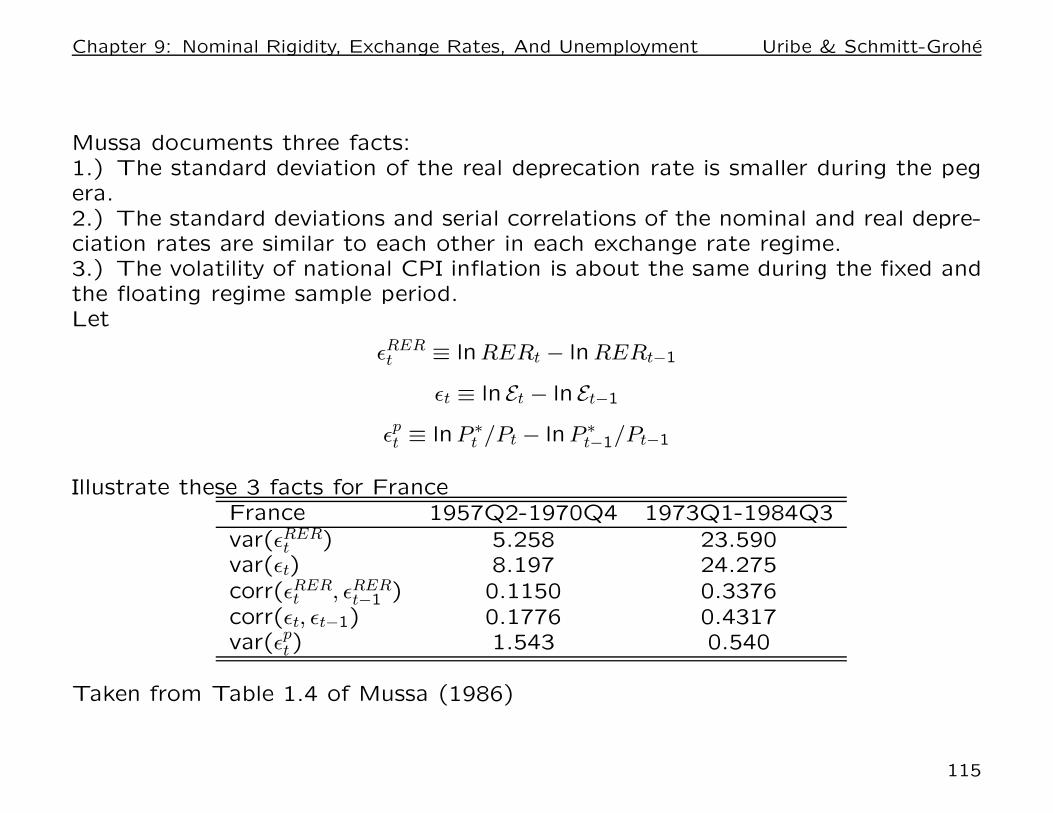
Chapter 9: Nominal Rigidity, Exchange Rates, And Unemployment Uribe & Schmitt-Grohe
Mussa documents three facts:1.) The standard deviation of the real deprecation rate is smaller during the pegera.2.) The standard deviations and serial correlations of the nominal and real depre-ciation rates are similar to each other in each exchange rate regime.3.) The volatility of national CPI inflation is about the same during the fixed andthe floating regime sample period.Let
εRERt ≡ lnRERt − ln RERt−1
εt ≡ ln Et − ln Et−1
εpt ≡ lnP ∗
t /Pt − lnP ∗t−1/Pt−1
Illustrate these 3 facts for FranceFrance 1957Q2-1970Q4 1973Q1-1984Q3
var(εRERt ) 5.258 23.590
var(εt) 8.197 24.275corr(εRER
t , εRERt−1 ) 0.1150 0.3376
corr(εt, εt−1) 0.1776 0.4317var(εp
t) 1.543 0.540
Taken from Table 1.4 of Mussa (1986)
115
Chapter 9: Nominal Rigidity, Exchange Rates, And Unemployment Uribe & Schmitt-Grohe
Theoretical Implications of the Mussa Puzzle
• The Mussa facts are referred to as a puzzle because they sug-
gest that relative prices depend on the behavior of nominal prices.
This is inconsistent with flexible-price models in the RBC tradition,
possibly augmented with a demand for money, which represented
the predominant paradigm around the time of Mussa’s writing (e.g.,
Stockman, 1988).
• The Mussa puzzle suggests a role for nominal rigidities, which
gained renewed popularity since the mid 1990s. An early analysis
of the Mussa puzzle through the lens of a sticky-price model is
Monacelli (2004).
• Here, we wish to address two questions:
(a) Are the predictions of the DNWR model consistent with the
Mussa facts.
(b) When seen through the lens of the DNWR model, do the
Mussa facts tell us anything about the optimality or not of the
monetary/exchange-rate regime post Bretton Woods?
116
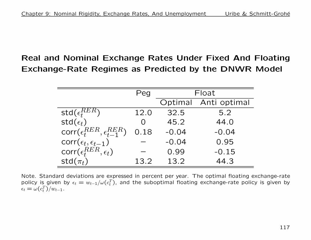
Chapter 9: Nominal Rigidity, Exchange Rates, And Unemployment Uribe & Schmitt-Grohe
Real and Nominal Exchange Rates Under Fixed And Floating
Exchange-Rate Regimes as Predicted by the DNWR Model
Peg FloatOptimal Anti optimal
std(εRERt ) 12.0 32.5 5.2
std(εt) 0 45.2 44.0
corr(εRERt , εRER
t−1 ) 0.18 -0.04 -0.04
corr(εt, εt−1) – -0.04 0.95
corr(εRERt , εt) – 0.99 -0.15
std(πt) 13.2 13.2 44.3
Note. Standard deviations are expressed in percent per year. The optimal floating exchange-ratepolicy is given by εt = wt−1/ω(cT
t ), and the suboptimal floating exchange-rate policy is given byεt = ω(cT
t )/wt−1.
117
Chapter 9: Nominal Rigidity, Exchange Rates, And Unemployment Uribe & Schmitt-Grohe
Observations on the Table
• In line with Mussa’s first fact, the predicted standard deviation of
the real depreciation rate is much larger under the optimal floating
exchange rate policy than under the peg (first line of the table).
• In line with Mussa’s second fact, under the optimal flexible ex-
change rate regime, the nominal and real exchange rates have similar
standard deviation and first-order serial correlations, and are highly
positively contemporaneously correlated (lines 2-5 of the table).
• In line with Mussa’s third fact, the predicted volatility of CPI
inflation is the same under the peg and the optimal floating regime
(last line of the table).
118
Chapter 9: Nominal Rigidity, Exchange Rates, And Unemployment Uribe & Schmitt-Grohe
Was Post-Bretton-Woods Exchange-Rate Policy Optimal?
• A common practice that needs clarification: Often, empirical stud-
ies classify exchange-rate regimes into fixed or floating, and then
derive stylized facts associated with each regime. This practice is
problematic because in reality there is an infinite family of floating
exchange-rate rebimes, not just one, which can induce different dy-
namics of nominal and real variables.
• As an illustration, consider the ‘anti optimal’ exchange rate policy:
εt =ω(cT
t )wt−1
.
which is the inverse of the optimal policy studied earlier in the quan-
titative analysis.
• The last column of the previous table shows that under the anti
optimal floating exchange-rate policy, the model fails to capture all
three of the Mussa facts.
• Seen through the lens of the DNWR model, it follows that Mussa’s
facts can be interpreted as suggesting that during the early post-
Bretton-Woods period, overall, the dynamics of inflation and nom-
inal and real exchange rates were consistent with the optimal ex-
change rate policy.
119
Chapter 9: Nominal Rigidity, Exchange Rates, And Unemployment Uribe & Schmitt-Grohe
Empirical Evidence on Real Effects of Monetary Instability
1. Industrialized countries, Mussa 1986, method, compare fixed and
float.
2. United States, Christiano, Eichenbaum, Evans 2005, method,
VAR identification.
3. small open economies, to be added, method, VAR identification.
120
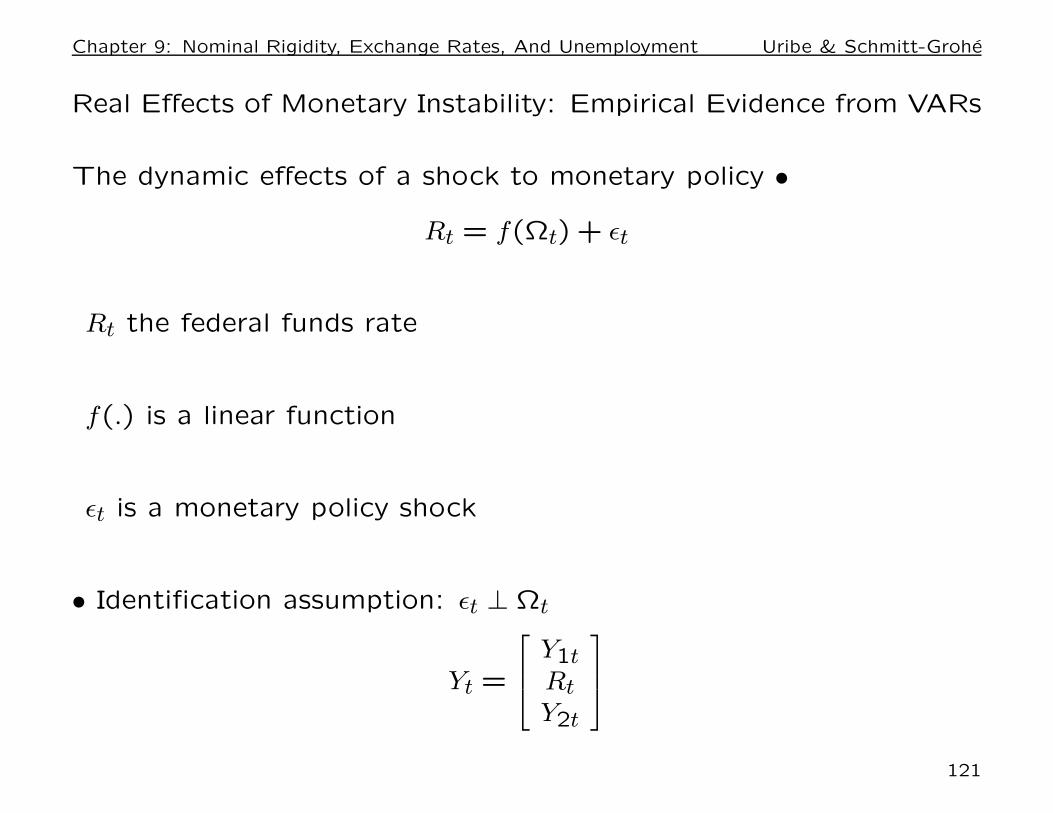
Chapter 9: Nominal Rigidity, Exchange Rates, And Unemployment Uribe & Schmitt-Grohe
Real Effects of Monetary Instability: Empirical Evidence from VARs
The dynamic effects of a shock to monetary policy •
Rt = f(Ωt) + εt
Rt the federal funds rate
f(.) is a linear function
εt is a monetary policy shock
• Identification assumption: εt ⊥ Ωt
Yt =
Y1tRtY2t
121
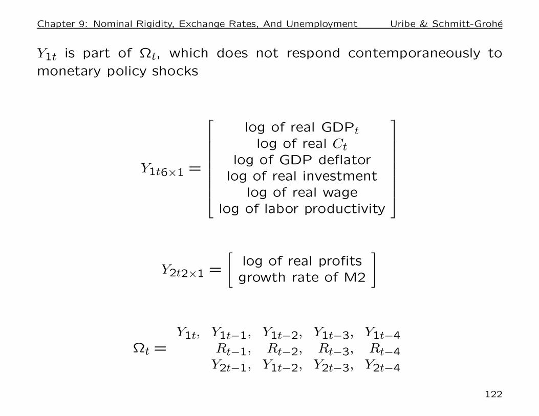
Chapter 9: Nominal Rigidity, Exchange Rates, And Unemployment Uribe & Schmitt-Grohe
Y1t is part of Ωt, which does not respond contemporaneously to
monetary policy shocks
Y1t6×1 =
log of real GDPtlog of real Ct
log of GDP deflatorlog of real investment
log of real wagelog of labor productivity
Y2t2×1 =
[
log of real profitsgrowth rate of M2
]
Ωt =Y1t, Y1t−1, Y1t−2, Y1t−3, Y1t−4
Rt−1, Rt−2, Rt−3, Rt−4Y2t−1, Y1t−2, Y2t−3, Y2t−4
122
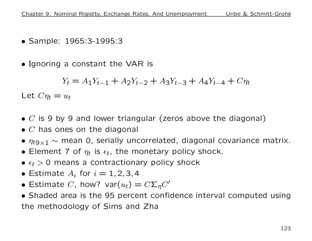
Chapter 9: Nominal Rigidity, Exchange Rates, And Unemployment Uribe & Schmitt-Grohe
• Sample: 1965:3-1995:3
• Ignoring a constant the VAR is
Yt = A1Yt−1 + A2Yt−2 + A3Yt−3 + A4Yt−4 + Cηt
Let Cηt = ut
• C is 9 by 9 and lower triangular (zeros above the diagonal)
• C has ones on the diagonal
• ηt9×1 ∼ mean 0, serially uncorrelated, diagonal covariance matrix.
• Element 7 of ηt is εt, the monetary policy shock.
• εt > 0 means a contractionary policy shock
• Estimate Ai for i = 1,2,3,4
• Estimate C, how? var(ut) = CΣηC ′
• Shaded area is the 95 percent confidence interval computed using
the methodology of Sims and Zha
123
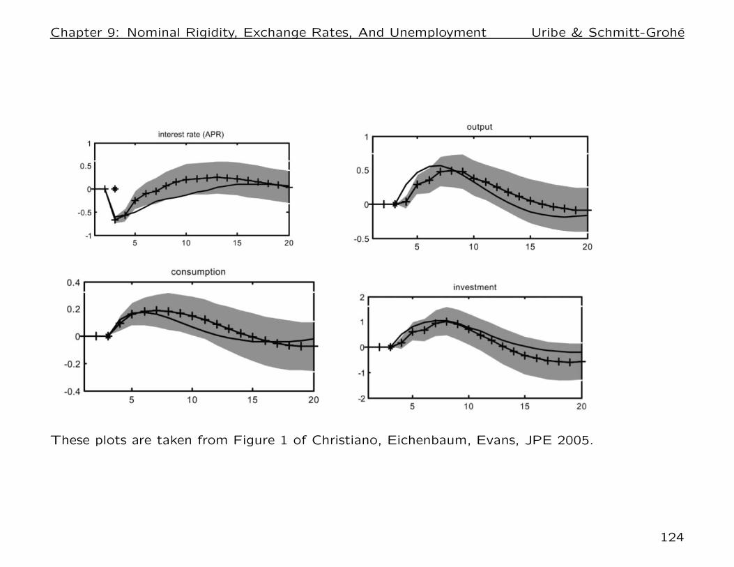
Chapter 9: Nominal Rigidity, Exchange Rates, And Unemployment Uribe & Schmitt-Grohe
These plots are taken from Figure 1 of Christiano, Eichenbaum, Evans, JPE 2005.
124
Chapter 9: Nominal Rigidity, Exchange Rates, And Unemployment Uribe & Schmitt-Grohe
Real Effects of an expansionary monetary policy shock from CEE
1.) Y, C, I
• Y, C, I respond in a hump-shaped fashion
• Y peaks 4-6 quarters after the shock
• C peaks 4 quarters after the monetary policy shock
• I peaks 5 quarters after the monetary policy shock
• The impulse response is significant until t = 8.
2.) R
• increases by 60 basis points
• peak response on impact
• is over after 4-5 quarters [long before peak output]
While there is quite some debate about what are the correct iden-
tification assumptions, there is considerable agreement about the
qualitative effects of a monetary policy shock in the sense that in-
ference is robust across a large subset of the identification schemes
that have been considered in the literature.
125
Chapter 9: Nominal Rigidity, Exchange Rates, And Unemployment Uribe & Schmitt-Grohe
Section 9.16
large Staggered Price Setting:
The Calvo Model
126
Chapter 9: Nominal Rigidity, Exchange Rates, And Unemployment Uribe & Schmitt-Grohe
The Calvo model:
— is perhaps the canonical models used in monetary economics
— assumes staggered price setting
— proposed by Calvo (1983) and later refined by Woodford (1996)
and Yun (1996)
— price rigidity is bidirectional, that is, the upward and downward
adjustment of nominal prices is sluggish
127
Chapter 9: Nominal Rigidity, Exchange Rates, And Unemployment Uribe & Schmitt-Grohe
Differences to the models of nominal rigidities studied earlier in the
chapter:
(1) firms are forced to satisfy demand even if the price is below
marginal cost. An implication of this difference is that in the Calvo
model the labor supply must be wage elastic for price stickiness to
have first-order effects
(2) Calvo model assumes imperfect competition in product markets.
This assumption allows firms be price setters and to have nonzero
finite demand even when their prices differ from those of their closest
competitors.
(3) wages are flexible and there is no involuntary unemployment.
128
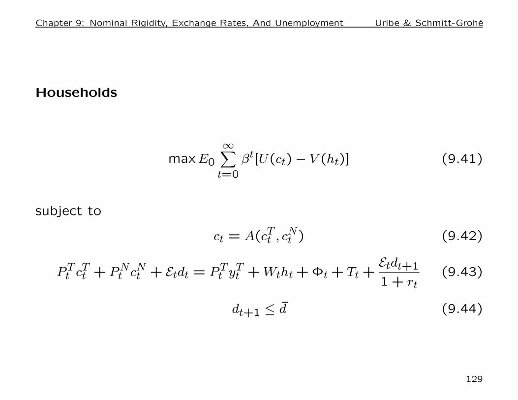
Chapter 9: Nominal Rigidity, Exchange Rates, And Unemployment Uribe & Schmitt-Grohe
Households
maxE0
∞∑
t=0
βt[U(ct) − V (ht)] (9.41)
subject to
ct = A(cTt , cN
t ) (9.42)
PTt cT
t + PNt cN
t + Etdt = PTt yT
t + Wtht + Φt + Tt +Etdt+1
1 + rt(9.43)
dt+1 ≤ d (9.44)
129
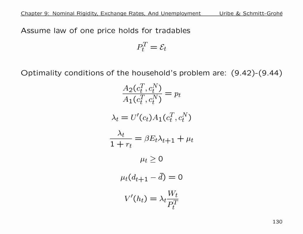
Chapter 9: Nominal Rigidity, Exchange Rates, And Unemployment Uribe & Schmitt-Grohe
Assume law of one price holds for tradables
PTt = Et
Optimality conditions of the household’s problem are: (9.42)-(9.44)
A2(cTt , cN
t )
A1(cTt , cN
t )= pt
λt = U ′(ct)A1(cTt , cN
t )
λt
1 + rt= βEtλt+1 + µt
µt ≥ 0
µt(dt+1 − d) = 0
V ′(ht) = λtWt
PTt
130
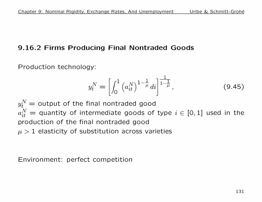
Chapter 9: Nominal Rigidity, Exchange Rates, And Unemployment Uribe & Schmitt-Grohe
9.16.2 Firms Producing Final Nontraded Goods
Production technology:
yNt =
[
∫ 1
0
(
aNit
)1−1µ di
] 1
1−1µ , (9.45)
yNt = output of the final nontraded good
aNit = quantity of intermediate goods of type i ∈ [0,1] used in the
production of the final nontraded good
µ > 1 elasticity of substitution across varieties
Environment: perfect competition
131
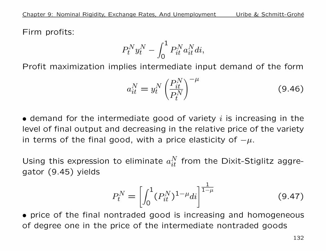
Chapter 9: Nominal Rigidity, Exchange Rates, And Unemployment Uribe & Schmitt-Grohe
Firm profits:
PNt yN
t −∫ 1
0PN
it aNit di,
Profit maximization implies intermediate input demand of the form
aNit = yN
t
(
PNit
PNt
)−µ
(9.46)
• demand for the intermediate good of variety i is increasing in the
level of final output and decreasing in the relative price of the variety
in terms of the final good, with a price elasticity of −µ.
Using this expression to eliminate aNit from the Dixit-Stiglitz aggre-
gator (9.45) yields
PNt =
[
∫ 1
0(PN
it )1−µdi
]1
1−µ
(9.47)
• price of the final nontraded good is increasing and homogeneous
of degree one in the price of the intermediate nontraded goods
132
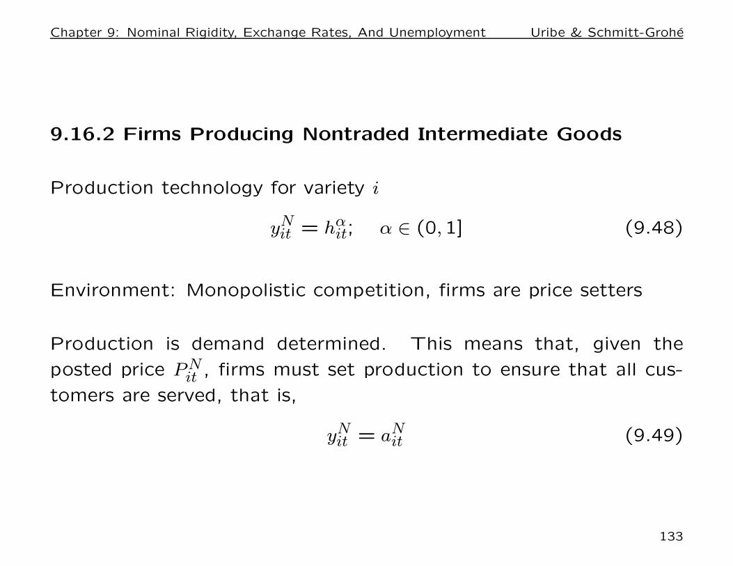
Chapter 9: Nominal Rigidity, Exchange Rates, And Unemployment Uribe & Schmitt-Grohe
9.16.2 Firms Producing Nontraded Intermediate Goods
Production technology for variety i
yNit = hα
it; α ∈ (0,1] (9.48)
Environment: Monopolistic competition, firms are price setters
Production is demand determined. This means that, given the
posted price PNit , firms must set production to ensure that all cus-
tomers are served, that is,
yNit = aN
it (9.49)
133
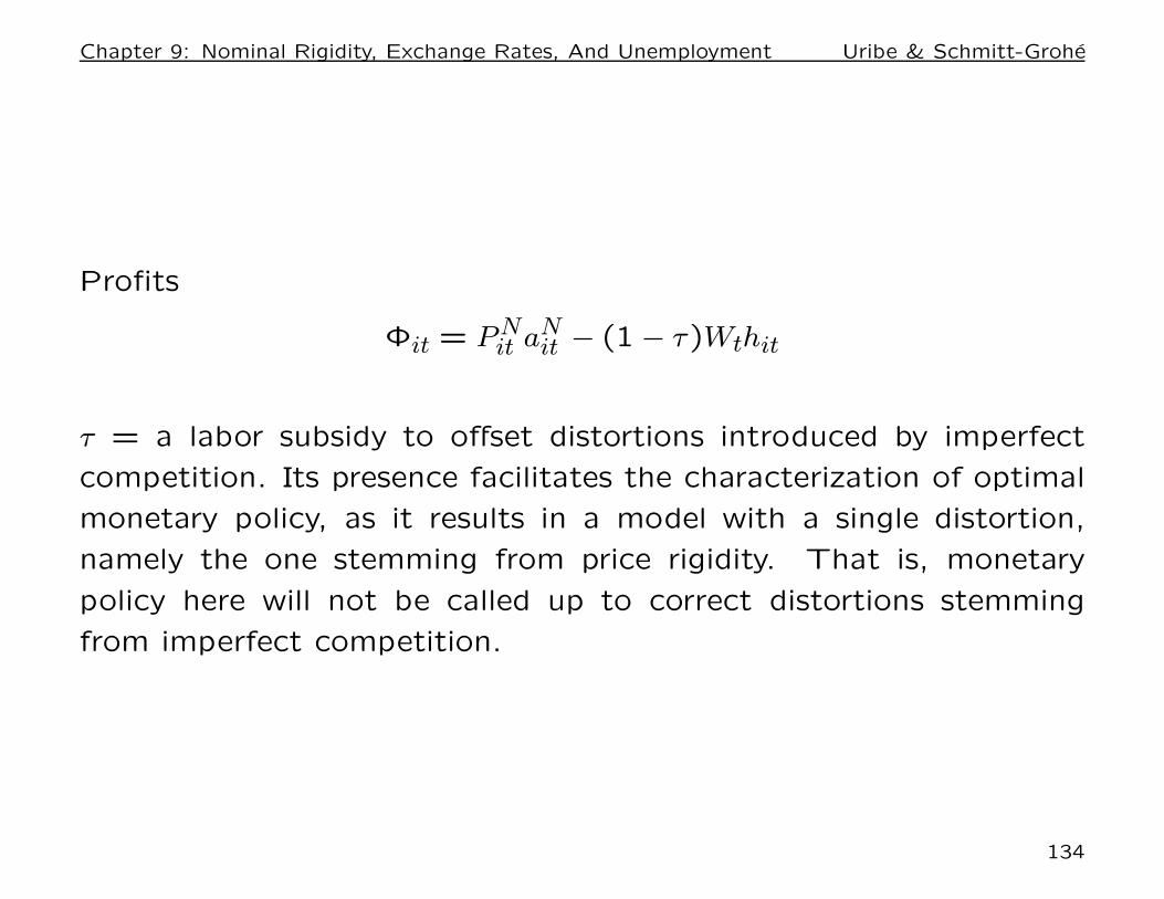
Chapter 9: Nominal Rigidity, Exchange Rates, And Unemployment Uribe & Schmitt-Grohe
Profits
Φit = PNit aN
it − (1 − τ)Wthit
τ = a labor subsidy to offset distortions introduced by imperfect
competition. Its presence facilitates the characterization of optimal
monetary policy, as it results in a model with a single distortion,
namely the one stemming from price rigidity. That is, monetary
policy here will not be called up to correct distortions stemming
from imperfect competition.
134
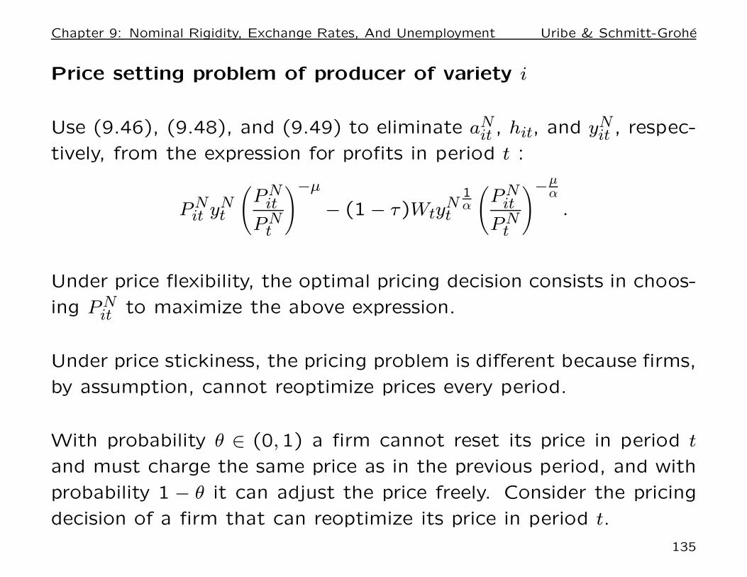
Chapter 9: Nominal Rigidity, Exchange Rates, And Unemployment Uribe & Schmitt-Grohe
Price setting problem of producer of variety i
Use (9.46), (9.48), and (9.49) to eliminate aNit , hit, and yN
it , respec-
tively, from the expression for profits in period t :
PNit yN
t
(
PNit
PNt
)−µ
− (1 − τ)WtyNt
1α
(
PNit
PNt
)−µα
.
Under price flexibility, the optimal pricing decision consists in choos-
ing PNit to maximize the above expression.
Under price stickiness, the pricing problem is different because firms,
by assumption, cannot reoptimize prices every period.
With probability θ ∈ (0,1) a firm cannot reset its price in period t
and must charge the same price as in the previous period, and with
probability 1 − θ it can adjust the price freely. Consider the pricing
decision of a firm that can reoptimize its price in period t.
135
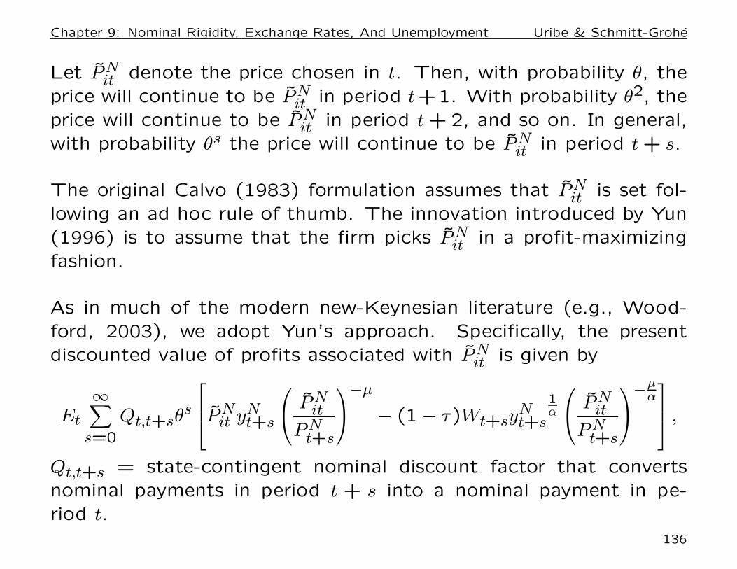
Chapter 9: Nominal Rigidity, Exchange Rates, And Unemployment Uribe & Schmitt-Grohe
Let PNit denote the price chosen in t. Then, with probability θ, the
price will continue to be PNit in period t+1. With probability θ2, the
price will continue to be PNit in period t + 2, and so on. In general,
with probability θs the price will continue to be PNit in period t + s.
The original Calvo (1983) formulation assumes that PNit is set fol-
lowing an ad hoc rule of thumb. The innovation introduced by Yun
(1996) is to assume that the firm picks PNit in a profit-maximizing
fashion.
As in much of the modern new-Keynesian literature (e.g., Wood-
ford, 2003), we adopt Yun’s approach. Specifically, the present
discounted value of profits associated with PNit is given by
Et
∞∑
s=0
Qt,t+sθs
PN
it yNt+s
PNit
PNt+s
−µ
− (1 − τ)Wt+syNt+s
1α
PNit
PNt+s
−µα
,
Qt,t+s = state-contingent nominal discount factor that converts
nominal payments in period t + s into a nominal payment in pe-
riod t.
136
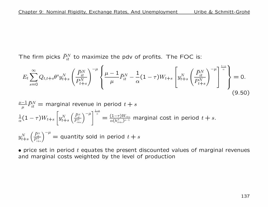
Chapter 9: Nominal Rigidity, Exchange Rates, And Unemployment Uribe & Schmitt-Grohe
The firm picks PNit to maximize the pdv of profits. The FOC is:
Et
∞∑
s=0
Qt,t+sθsyN
t+s
(
PNit
PNt+s
)−µ
µ − 1
µPN
it −1
α(1 − τ)Wt+s
yNt+s
(
PNit
PNt+s
)−µ
1−α
α
= 0.
(9.50)
µ−1µ
PNit = marginal revenue in period t + s
1α(1 − τ)Wt+s
[
yNt+s
(
P Nit
P Nt+s
)−µ]
1−α
α
= (1−τ)Wt+s
α(hNit+s)
α−1 marginal cost in period t + s.
yNt+s
(
P Nit
P Nt+s
)−µ= quantity sold in period t + s
• price set in period t equates the present discounted values of marginal revenuesand marginal costs weighted by the level of production
137
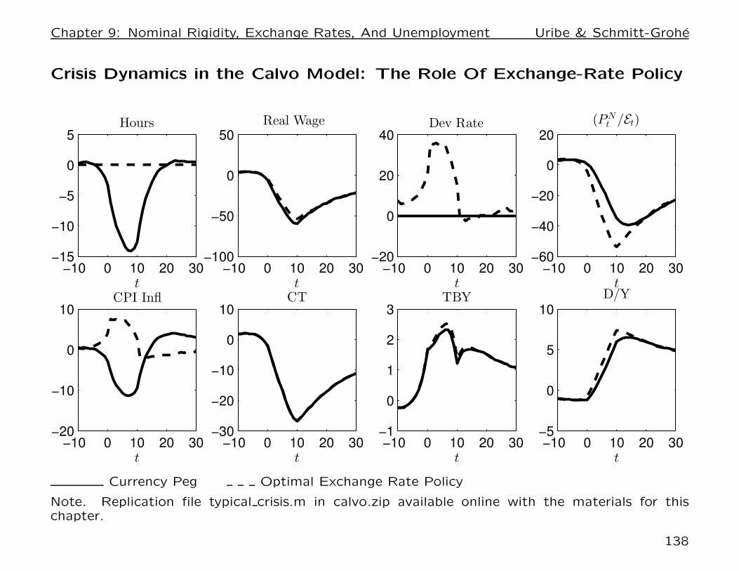
Chapter 9: Nominal Rigidity, Exchange Rates, And Unemployment Uribe & Schmitt-Grohe
Crisis Dynamics in the Calvo Model: The Role Of Exchange-Rate Policy
−10 0 10 20 30−15
−10
−5
0
5Hours
t−10 0 10 20 30
−100
−50
0
50Real Wage
t−10 0 10 20 30
−20
0
20
40Dev Rate
t−10 0 10 20 30
−60
−40
−20
0
20(PN
t /Et)
t
−10 0 10 20 30−20
−10
0
10CPI Infl
t−10 0 10 20 30
−30
−20
−10
0
10CT
t−10 0 10 20 30
−1
0
1
2
3TBY
t−10 0 10 20 30
−5
0
5
10D/Y
t
Currency Peg Optimal Exchange Rate Policy
Note. Replication file typical crisis.m in calvo.zip available online with the materials for thischapter.
138