Embed Size (px)
Citation preview
Genetic Analysis of Complex TraitsJing Hua ZhaoJuly 20, 2010, NIST
2010
About the title
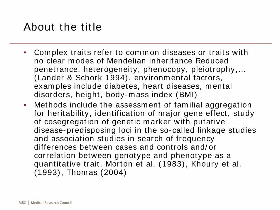
• Complex traits refer to common diseases or traits with no clear modes of Mendelian inheritance Reduced penetrance, heterogeneity, phenocopy, pleiotrophy,…(Lander & Schork 1994), environmental factors, examples include diabetes, heart diseases, mental disorders, height, body-mass index (BMI)
• Methods include the assessment of familial aggregation for heritability, identification of major gene effect, study of cosegregation of genetic marker with putative disease-predisposing loci in the so-called linkage studies and association studies in search of frequency differences between cases and controls and/or correlation between genotype and phenotype as a quantitative trait. Morton et al. (1983), Khoury et al. (1993), Thomas (2004)
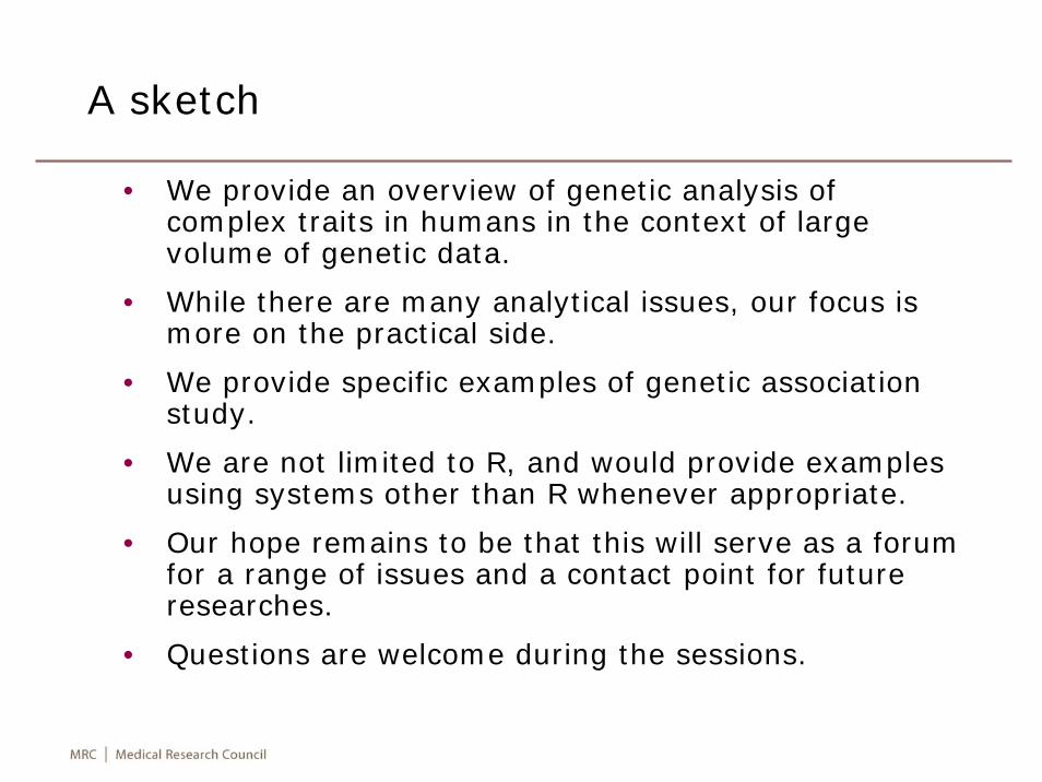
• We provide an overview of genetic analysis of complex traits in humans in the context of large volume of genetic data.
• While there are many analytical issues, our focus is more on the practical side.
• We provide specific examples of genetic association study.
• We are not limited to R, and would provide examples using systems other than R whenever appropriate.
• Our hope remains to be that this will serve as a forum for a range of issues and a contact point for future researches.
• Questions are welcome during the sessions.
A sketch
• The presentation consists of four parts:
I. Overview
II. Analytic tools and association testing
III. Miscellaneous topics
IV. OpenMx and NCBI2R
V. Conclusion
• You may find materials from useR!2008 and useR!2009tutorials relevant. They are both available from mypersonal home page.
Contents
What have changed?
• We are quite far with topics in both useR!2008 and useR!2009, esp. genome-wide association studies (GWAS) of directly genotyped and imputed SNPs and interaction analysis. It is routine with Stata function which automating analysis by SNPTEST. We have updated results regarding genetic predisposition score from the EPIC-Norfolk study. We have a better understanding of the SNP annotation, via UCSC/galaxy and in particular NCBI2R. There are other changes, e.g., functions MiMa has been replaced with metafor package.
• I am more proficient with R and have consolidated R/gap functions fbsize, pbsize, ccsize, and added ab and masize. We have explored ‘raw’ storage mode in R which is central to snpMatrix and GenABEL.
• We provide further examples. We add examples forchromosome X data, and obtained imputed genotypes for analysis. We also add materials regarding OpenMx. In the future, more materials on Bioconductor can be added.
Monographs
• Morton NE. Rao DC, Lalouel JM. Methods in Genetic Epidemiology. Karger, 1983.
• Khoury MJ, Beaty TH, Cohen BH. Fundamentals of Genetic Epidemiology. Oxford University Press, 1993.
• Falconer DS, Mackay TFC. Introduction to Quantitative Genetics, 4e. Longman, 1996
• Hartl D, Clark AG. Principles of Population Genetics, 3e. Sinauer Associates, Inc. 1997
• Lange K. Mathematical and Statistical Methods for Genetics Analysis. 2e, Springer 2002
• Sorensen D, Gianola D. Likelihood, Bayesian, and MCMC Methods in Quantitative Genetics. Springer 2002
• Thomas DC. Statistical Methods in Genetic Epidemiology, Oxford University Press, 2004
• Armitage P, Colton T (Eds). Encyclopedia of Biostistics, 2e, Wiley, 2005
Monographs
• Elston RC, Johnson WD. Basic Biostatistics for Geneticists and Epidemiologists, A Practical Approach. Wiley, 2005
• Ahrens W, Pigeot I (Eds). Handbook of Epidemiology. Springer, 2005
• Balding DJ, Bishop M, Cannings C (Eds). Handbook of Statistical Genetics, 3e, Wiley, 2007
• Siegmund D, Yakir B. The Statistics of Gene Mapping. Springer 2007
• Wu R, Ma C-X, Casella G. Statistical Genetics of Quantitative Traits-Linkage, Maps and QTL. Springer, 2007
• Speicher MR, Antonarakis SE, Motulsky AG. Vogel and Motulsky’s Human Genetics: Problems and Approaches, 4e, Springer, 2010
• Lin S, H Zhao (Eds). Handbook on Analyzing Human Genetic Data: Computational Approaches and Software. Springer, 2010

I Overview
Terminology
• Genes, Chromosome, markers• Alleles, genotypes, haplotypes• Phenotypes, mode of inheritance, penetrance• Mendelian laws of inheritance, Hardy-Weinberg
equilibrium, linkage disequilibrium• Association tests for single or multiple SNPs• Population stratification• Multiple testing• Gene-environment interaction (GEI)
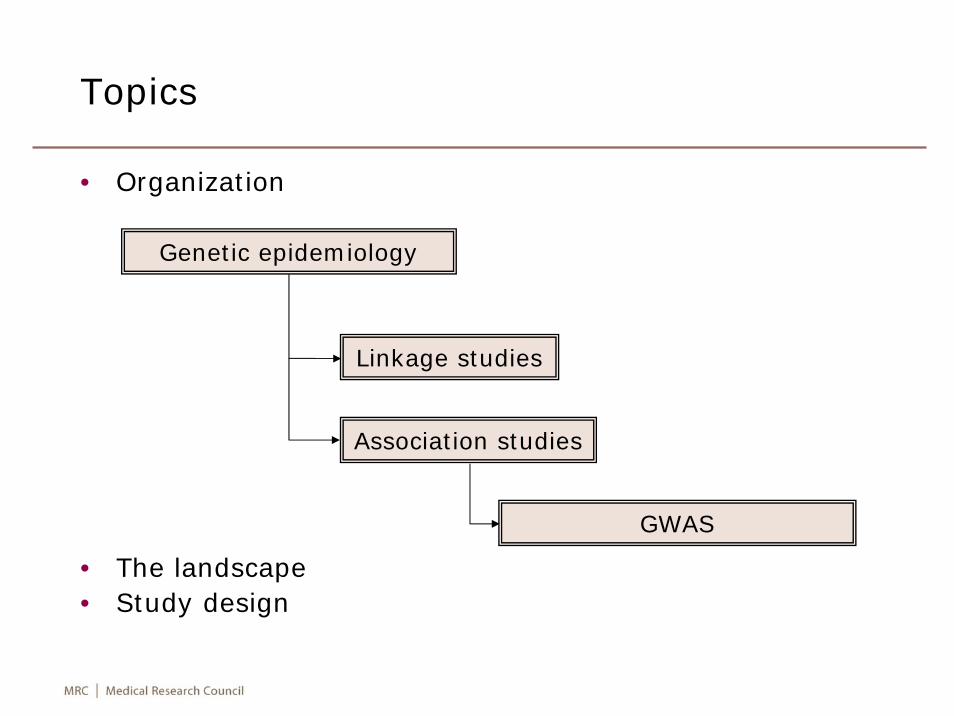
Topics
• Organization
• The landscape• Study design
GWAS
Linkage studies
Association studies
Genetic epidemiology
Genetic epidemiology
• It is the study of the role of genetic factors in determining health and disease in families and in populations, and the interplay of such genetic factors with environmental factors, or “a science which deals with the aetiology, distribution, and control of diseases in groups of relatives and with inherited causes of disease in populations” (http://en.wikipedia.org).
• It customarily includes study of familial aggregation, segregation, linkage and association. It is closely associated with the development of statistical methods for human genetics which deals with these four questions. The last two questions can only be answered if appropriate genetic markers available (Elston & Ann Spence. Stat Med 2006;25:3049-80).
Linkage studies
• It is the study of cosegregation between genetic markers and putative disease loci, and has been very successful in localizing rare, Mendelian disorders but since has difficulty for traits which do not strictly follow Mendelian mode of inheritance, considerable linkage heterogeneity and it has limited resolution.
• It typically involves parametric (model-based) and nonparametric (model-free) methods, the latter most commonly refers to allele-sharing methods.
• The underlying concepts are nevertheless very important. It can still be useful in providing candidates for fine-mapping and association studies.
• With availability of whole genome data, it is possible to infer relationship or correlation between any individuals in a population.
Association studies
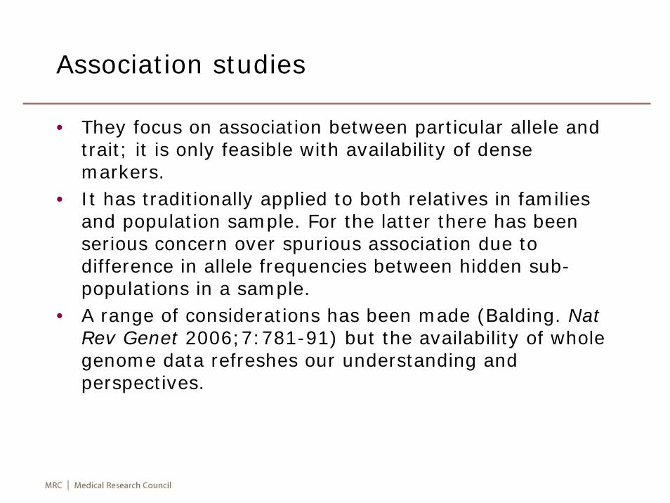
• They focus on association between particular allele and trait; it is only feasible with availability of dense markers.
• It has traditionally applied to both relatives in families and population sample. For the latter there has been serious concern over spurious association due to difference in allele frequencies between hidden sub-populations in a sample.
• A range of considerations has been made (Balding. Nat Rev Genet 2006;7:781-91) but the availability of whole genome data refreshes our understanding and perspectives.
GWAS
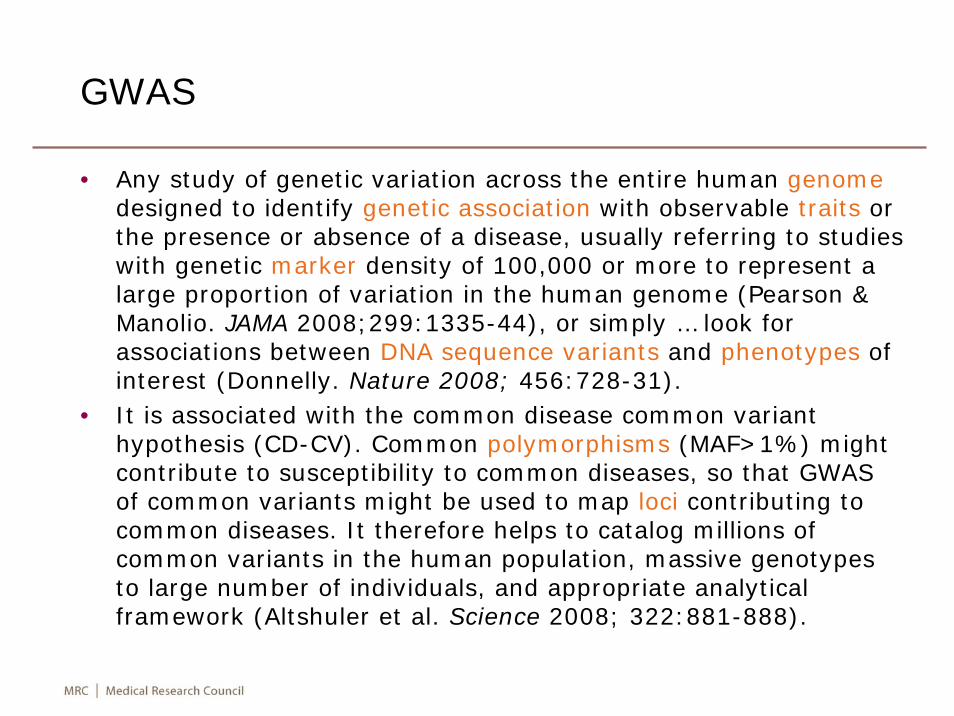
• Any study of genetic variation across the entire human genomedesigned to identify genetic association with observable traits or the presence or absence of a disease, usually referring to studies with genetic marker density of 100,000 or more to represent a large proportion of variation in the human genome (Pearson & Manolio. JAMA 2008;299:1335-44), or simply … look for associations between DNA sequence variants and phenotypes of interest (Donnelly. Nature 2008; 456:728-31).
• It is associated with the common disease common variant hypothesis (CD-CV). Common polymorphisms (MAF>1%) might contribute to susceptibility to common diseases, so that GWAS of common variants might be used to map loci contributing to common diseases. It therefore helps to catalog millions of common variants in the human population, massive genotypes to large number of individuals, and appropriate analytical framework (Altshuler et al. Science 2008; 322:881-888).
The landscape
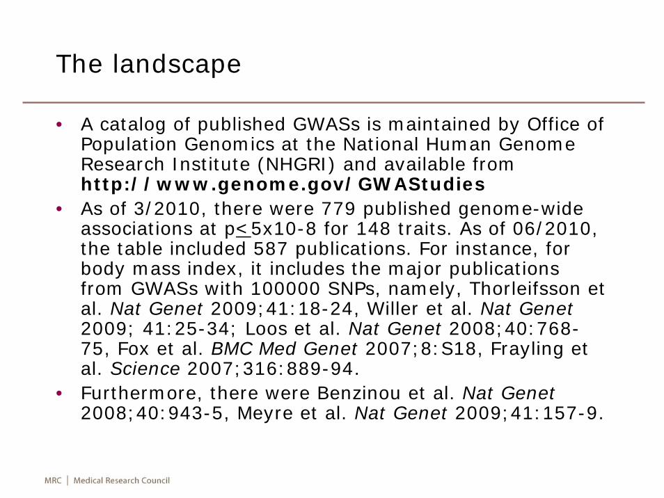
• A catalog of published GWASs is maintained by Office of Population Genomics at the National Human Genome Research Institute (NHGRI) and available from http://www.genome.gov/GWAStudies
• As of 3/2010, there were 779 published genome-wide associations at p<5x10⁻⁸ for 148 traits. As of 06/2010, the table included 587 publications. For instance, for body mass index, it includes the major publications from GWASs with 100000 SNPs, namely, Thorleifsson et al. Nat Genet 2009;41:18-24, Willer et al. Nat Genet2009; 41:25-34; Loos et al. Nat Genet 2008;40:768-75, Fox et al. BMC Med Genet 2007;8:S18, Frayling et al. Science 2007;316:889-94.
• Furthermore, there were Benzinou et al. Nat Genet2008;40:943-5, Meyre et al. Nat Genet 2009;41:157-9.
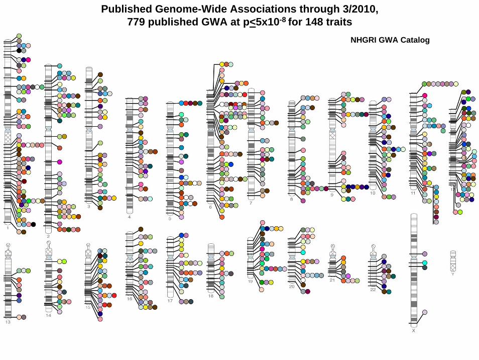
Published Genome-Wide Associations through 3/2010, 779 published GWA at p<5x10⁻⁸ for 148 traits
NHGRI GWA Catalog
Context
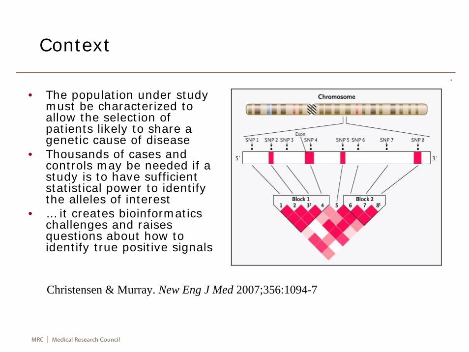
• The population under study must be characterized to allow the selection of patients likely to share a genetic cause of disease
• Thousands of cases and controls may be needed if a study is to have sufficient statistical power to identify the alleles of interest
• … it creates bioinformatics challenges and raises questions about how to identify true positive signals
Christensen & Murray. New Eng J Med 2007;356:1094-7
International collaborative projects
• The HapMap project (http://hapmap.ncbi.nlm.nih.gov/) was a study of 270 people from the Yoruba in Nigeria (30 trios), Japanese (45 unrelated individuals), Han Chinese (45 unrelated individuals) and CEPH (30 trios).
• The 1000 genome project (http://www.1000genomes.org) aims to sequence at least one thousand anonymous participants. It still undergoes revision.
• The database of genotypes and phenotypes (dbGaP) (http://www.ncbi.nlm.nih.gov/sites/entrez?db=gap) was developed to archive and distribute the results of studies that have investigated the interaction of genotype and phenotype.
• The genetic analysis workshops (GAWs) (http://www.gaworkshop.org/) are a collaborative effort among genetic epidemiologists to evaluate and compare statistical genetic methods. For each GAW, topics are chosen that are relevant to current analytical problems through simulated or real data.
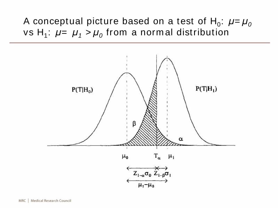
A conceptual picture based on a test of H0: μ=μ0vs H1: μ= μ1 >μ0 from a normal distribution
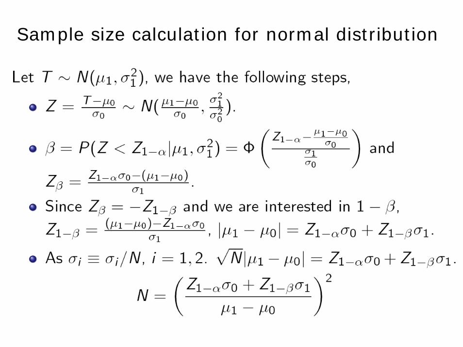
Sample size calculation for normal distribution
Study designs
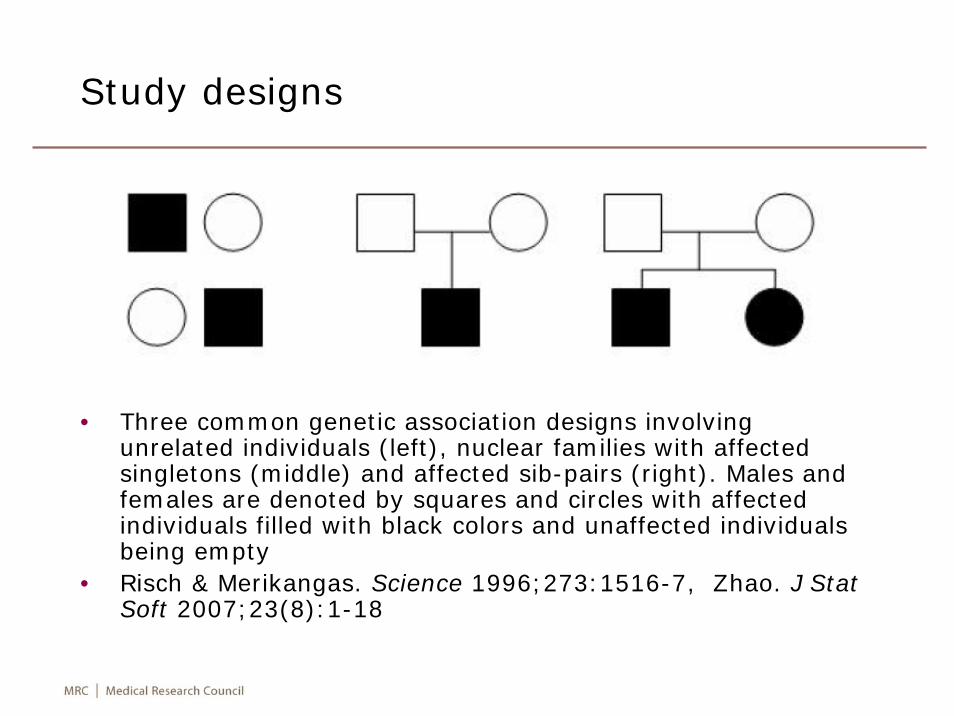
• Three common genetic association designs involving unrelated individuals (left), nuclear families with affected singletons (middle) and affected sib-pairs (right). Males and females are denoted by squares and circles with affected individuals filled with black colors and unaffected individuals being empty
• Risch & Merikangas. Science 1996;273:1516-7, Zhao. J Stat Soft 2007;23(8):1-18
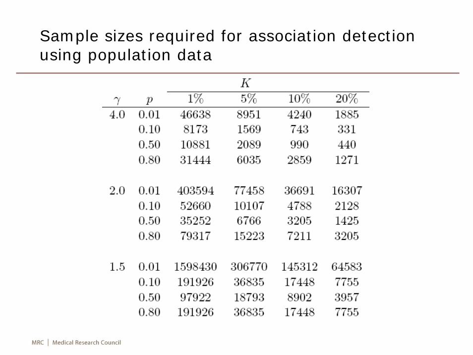
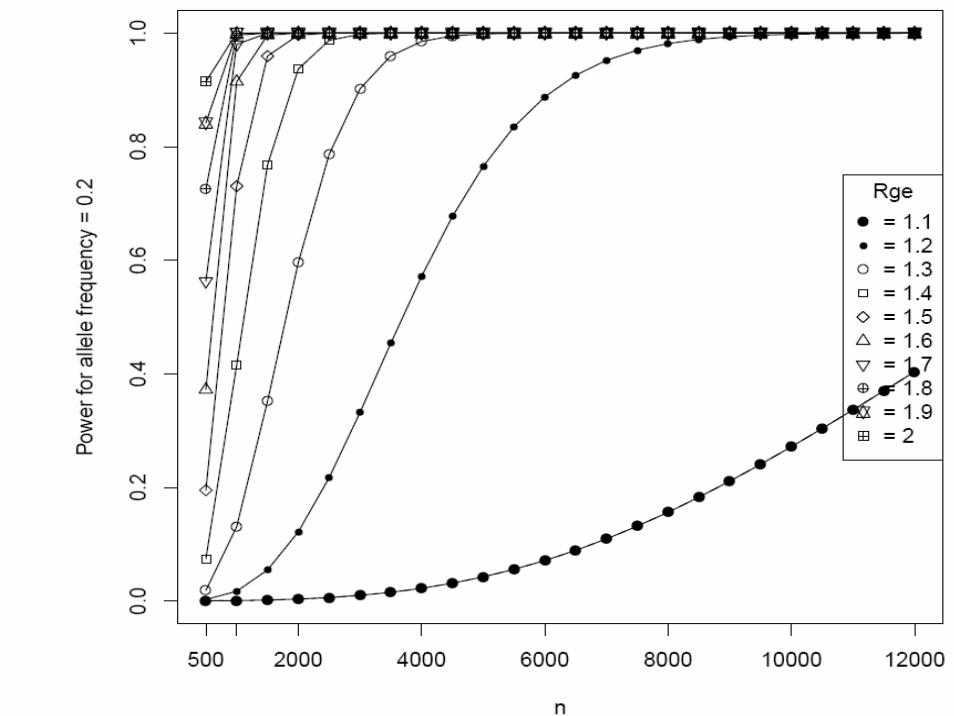
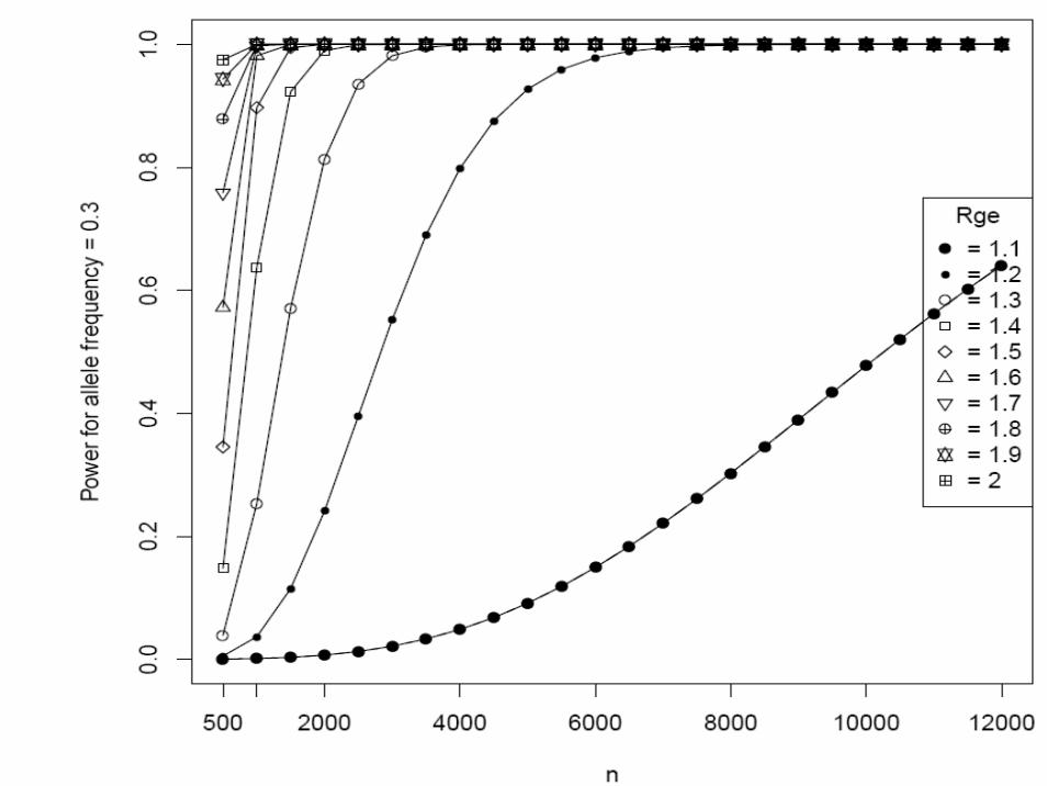
Sample sizes required for association detection using population data
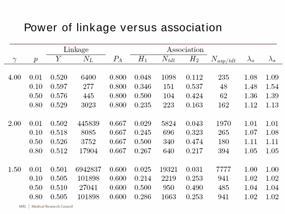
Power of linkage versus association
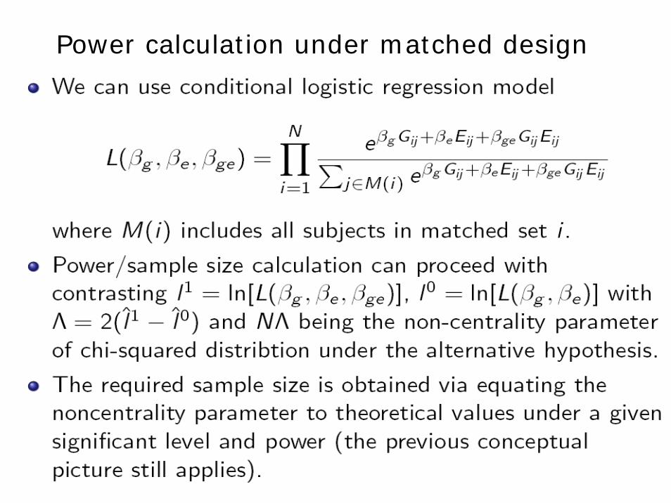
Power calculation under matched design
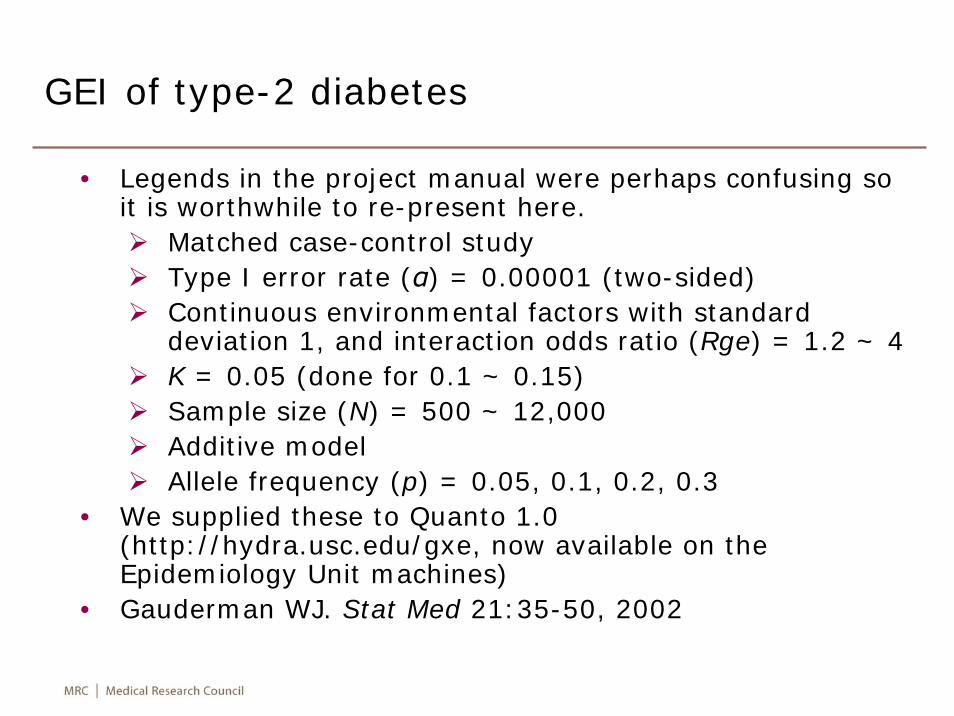
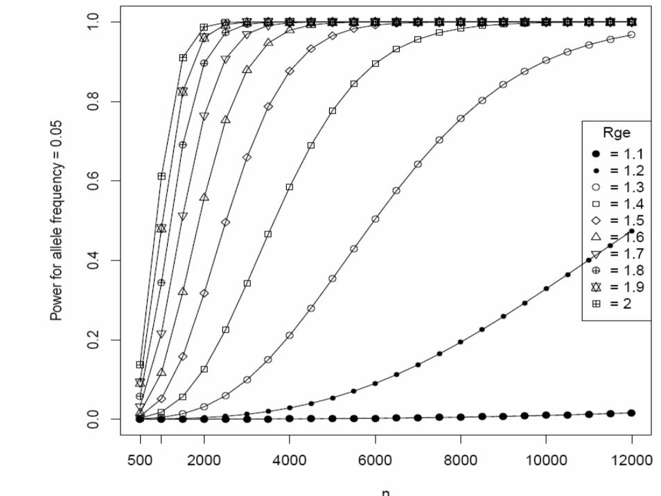
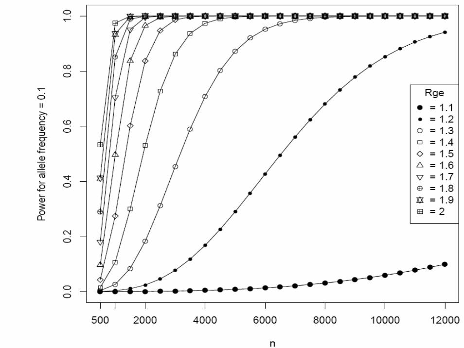
GEI of type-2 diabetes
• Legends in the project manual were perhaps confusing so it is worthwhile to re-present here.
Matched case-control studyType I error rate (α) = 0.00001 (two-sided)Continuous environmental factors with standard deviation 1, and interaction odds ratio (Rge) = 1.2 ~ 4K = 0.05 (done for 0.1 ~ 0.15)Sample size (N) = 500 ~ 12,000Additive modelAllele frequency (p) = 0.05, 0.1, 0.2, 0.3
• We supplied these to Quanto 1.0 (http://hydra.usc.edu/gxe, now available on the Epidemiology Unit machines)
• Gauderman WJ. Stat Med 21:35-50, 2002
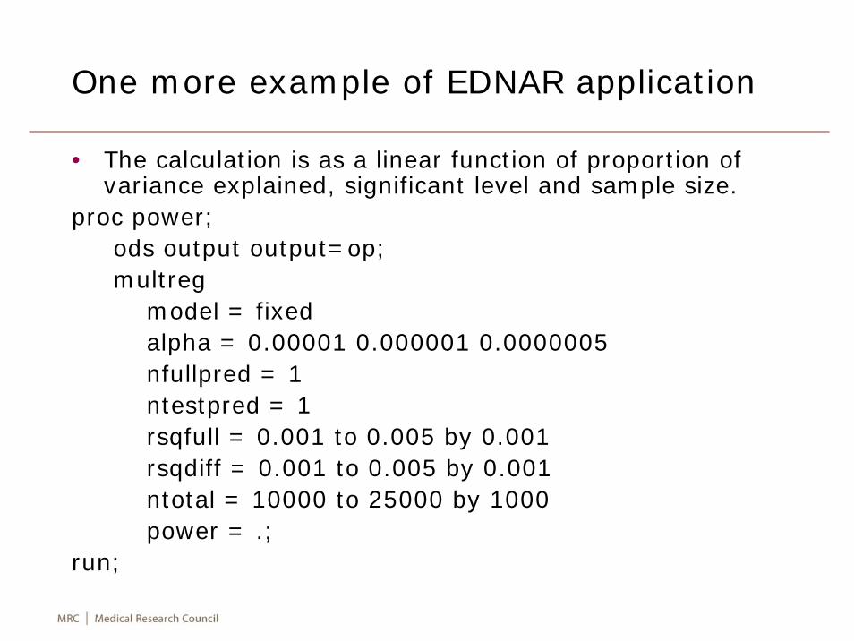
One more example of EDNAR application
• The calculation is as a linear function of proportion of variance explained, significant level and sample size.
proc power;ods output output=op;multreg
model = fixedalpha = 0.00001 0.000001 0.0000005nfullpred = 1ntestpred = 1rsqfull = 0.001 to 0.005 by 0.001rsqdiff = 0.001 to 0.005 by 0.001ntotal = 10000 to 25000 by 1000power = .;
run;
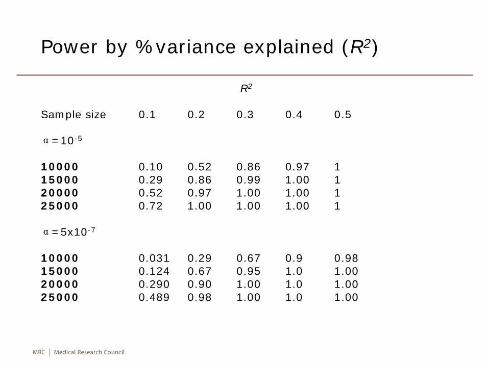
Power by %variance explained (R2)
R2
Sample size 0.1 0.2 0.3 0.4 0.5
α=10-5
10000 0.10 0.52 0.86 0.97 115000 0.29 0.86 0.99 1.00 120000 0.52 0.97 1.00 1.00 125000 0.72 1.00 1.00 1.00 1
α=5x10⁻⁷
10000 0.031 0.29 0.67 0.9 0.9815000 0.124 0.67 0.95 1.0 1.0020000 0.290 0.90 1.00 1.0 1.0025000 0.489 0.98 1.00 1.0 1.00
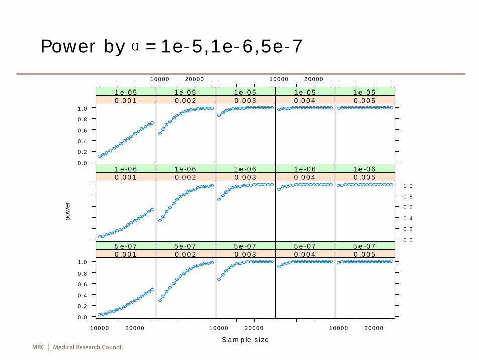
Power byα=1e-5,1e-6,5e-7
S a m p le s ize
pow
er
0 .0
0 .2
0 .4
0 .6
0 .8
1 .0
10 0 0 0 2 0 0 0 0
0 .0 0 15 e -0 7
0 .0 0 25 e -0 7
1 0 0 00 2 0 00 0
0 .0 0 35 e -0 7
0 .0 0 45 e -0 7
1 0 0 0 0 2 0 0 0 0
0 .0 0 55 e -0 7
0 .0 0 11 e -0 6
0 .0 0 21 e -0 6
0 .0 0 31 e -0 6
0 .0 0 41 e -0 6
0.0
0 .2
0 .4
0 .6
0 .8
1 .00 .0 0 51 e -0 6
0 .0
0 .2
0 .4
0 .6
0 .8
1 .00 .0 0 11 e -0 5
1 0 0 0 0 2 0 0 0 0
0 .0 0 21 e -0 5
0 .0 0 31 e -0 5
10 0 0 0 2 0 0 0 0
0 .0 0 41 e -0 5
0 .0 0 51 e -0 5
Two-stage design on main effect
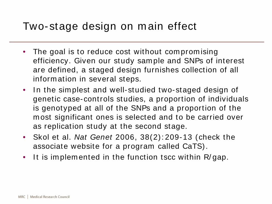
• The goal is to reduce cost without compromising efficiency. Given our study sample and SNPs of interest are defined, a staged design furnishes collection of all information in several steps.
• In the simplest and well-studied two-staged design of genetic case-controls studies, a proportion of individuals is genotyped at all of the SNPs and a proportion of the most significant ones is selected and to be carried over as replication study at the second stage.
• Skol et al. Nat Genet 2006, 38(2):209-13 (check the associate website for a program called CaTS).
• It is implemented in the function tscc within R/gap.
FTO-BMI-T2D Mendelian randomisation
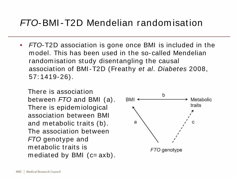
• FTO-T2D association is gone once BMI is included in the model. This has been used in the so-called Mendelianrandomisation study disentangling the causal association of BMI-T2D (Freathy et al. Diabetes 2008, 57:1419-26).
There is association between FTO and BMI (a). There is epidemiological association between BMI and metabolic traits (b). The association between FTO genotype and metabolic traits is mediated by BMI (c=axb).
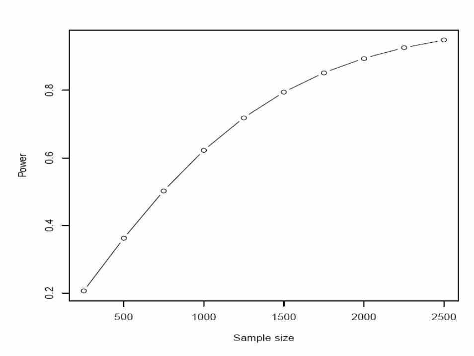
Power calculation
• We can of course perform simulations to obtain power estimate but it would be somewhat involved.
• Instead, we calculate standard error of FTO-BMI-T2D can be calculated which can form the basis of power calculation (Kline RB. Principles and Practice of Structural Equation Modeling, 2nd Edition, The Guilford Press 2005).
• We implement this in ab function in R/gap.• We have for EPIC-Norfolk 25,000, SNP-BMI regression
coefficient (SE) of 0.15 (0.01), and BMI-T2D log(1.19) (0.01). We consider α=0.05.
• Criticism arised from this posthoc power calculation could be alleviated when we allow for a range of sample sizes to be considered in the next slide.
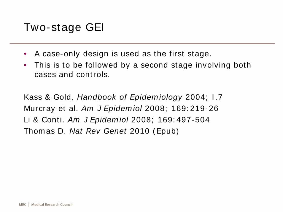
Two-stage GEI
• A case-only design is used as the first stage.• This is to be followed by a second stage involving both
cases and controls.
Kass & Gold. Handbook of Epidemiology 2004; I.7Murcray et al. Am J Epidemiol 2008; 169:219-26Li & Conti. Am J Epidemiol 2008; 169:497-504Thomas D. Nat Rev Genet 2010 (Epub)
References
• Armitage P, Colton T. Encyclopedia of Biostatistics, Second Edition, Wiley 2005
• Balding DJ, Bishop M, Cannings C. Handbook of Statistical Genetics, Third Edition, Wiley 2007
• Elston RC, Johnson W. Basic Biostatistics for Geneticists and Epidemiologists: A Practical Approach. Wiley 2008
• Haines JL, Pericak-Vance M. Genetic Analysis of Complex Diseases, Second Edition. Wiley 2006
• Rao DC, Gu CC (Eds). Genetic Dissection of Complex Traits, Volume 60, Second Edition (Advances in Genetics). Academic Press 2008
• Thomas DC. Statistical Methods for Genetic Epidemiology. Oxford University Press 2004
A summary
• We have restricted our focus and leave out a lot of details to cover a rapid moving field with limited time.
• It seems that the practice of study designs and data analysis cannot be changed in a short run, but we have already seen steady increase in use of R.
Case study: GWAS of obesity-related traits
• Background• Study design• Statistical analysis• On-going research

EPIC study
The European Prospective Investigation into Cancer andNutrition (EPIC) is coordinated by Dr Elio Riboli, Head ofthe Division of Epidemiology, Public Health and PrimaryCare at the Imperial College London.
EPIC was designed to investigate the relationshipsbetween diet, nutritional status, lifestyle andenvironmental factors and the incidence of cancer andother chronic diseases. EPIC is the largest study of dietand health ever undertaken, having recruited over halfa million (520,000) people in ten European countries:Denmark, France, Germany, Greece, Italy, TheNetherlands, Norway, Spain, Sweden and the UnitedKingdom.
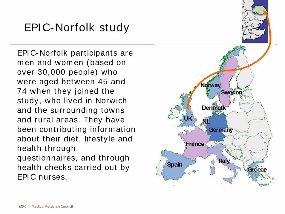
EPIC-Norfolk study
EPIC-Norfolk participants are men and women (based on over 30,000 people) who were aged between 45 and 74 when they joined the study, who lived in Norwich and the surrounding towns and rural areas. They have been contributing information about their diet, lifestyle and health through questionnaires, and through health checks carried out by EPIC nurses.
Case-cohort design for EPIC-Norfolk study
• It originally followed case-control design (e.g., WTCCC with seven cases and common controls) with 3425 cases and 3400 controls.
It is potentially more powerful.Controls are selected.
• It has then been changed into case-cohort design, in which cases are defined to be individuals whose BMI above 30 and controls are a random sample (subcohort) of the EPIC-Norfolk cohort which includes obese individuals.
The subcohort is representative of the whole population and allows for a range of traits to be examined.The analysis is potentially more involved but established.
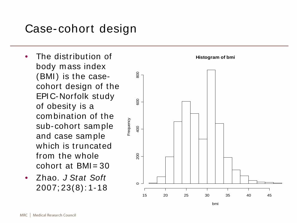
Case-cohort design
• The distribution of body mass index (BMI) is the case-cohort design of the EPIC-Norfolk study of obesity is a combination of the sub-cohort sample and case sample which is truncated from the whole cohort at BMI=30
• Zhao. J Stat Soft2007;23(8):1-18
Histogram of bmi
bmi
Freq
uenc
y
15 20 25 30 35 40 45
020
040
060
080
0
Power/sample size
• It started with assessment of how the power is compromised relative to the original case-control design.
• This was followed by power/sample size calculation using methods established by Cai and Zeng (2004) as implemented in an R function, noting a number of assumptions.
• More practically, it was also envisaged that a proper representative sample of a total of 25,000 individuals would be 10%; the subcohort is then approximately 2,500.
• The total sample was split between two stages.
GeneChips
• Affymetrix 500KData were available for 3850 individuals
• Illumina 317KIt came at a later time。Data quality appears to be poor?
• The focus has therefore been Affy500K, but with a possible comeback.
Analysis
• An incremental approach was adopted since the storage and computing power were somewhat uncertain.
• This was predated with controls from the breast cancer study, involving about 400 individuals with Perlegen250K GeneChips.
• QC including call rates and HWE was feasible with SAS/Genetics (~30GB) which provides a good estimate of the storage for all individuals (~380GB).
• The Linux platform seemed favourable.
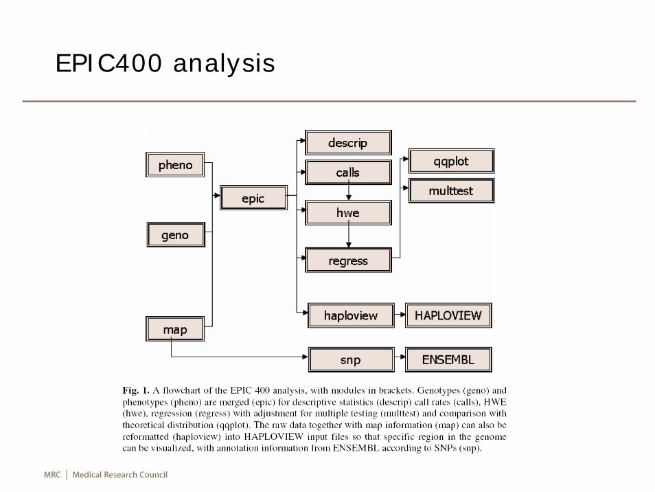
EPIC400 analysis
The analysis for GWAS
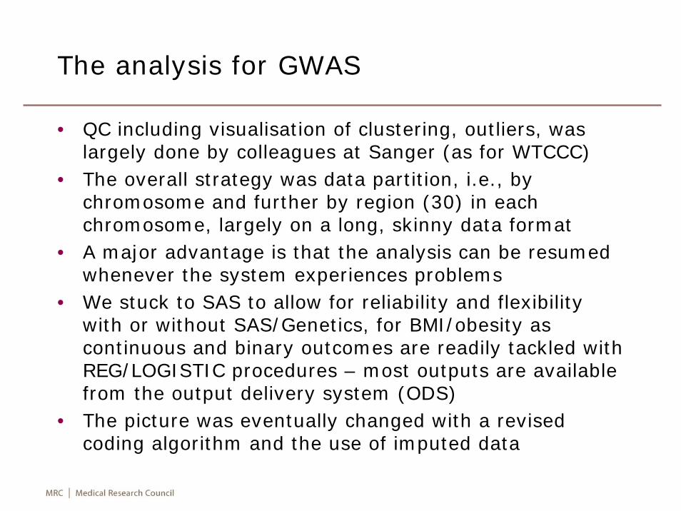
• QC including visualisation of clustering, outliers, was largely done by colleagues at Sanger (as for WTCCC)
• The overall strategy was data partition, i.e., by chromosome and further by region (30) in each chromosome, largely on a long, skinny data format
• A major advantage is that the analysis can be resumed whenever the system experiences problems
• We stuck to SAS to allow for reliability and flexibility with or without SAS/Genetics, for BMI/obesity as continuous and binary outcomes are readily tackled with REG/LOGISTIC procedures – most outputs are available from the output delivery system (ODS)
• The picture was eventually changed with a revised coding algorithm and the use of imputed data
Additional analysis
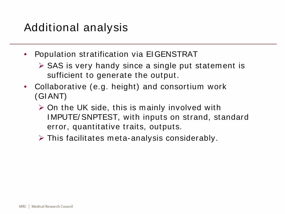
• Population stratification via EIGENSTRATSAS is very handy since a single put statement is sufficient to generate the output.
• Collaborative (e.g. height) and consortium work (GIANT)
On the UK side, this is mainly involved with IMPUTE/SNPTEST, with inputs on strand, standard error, quantitative traits, outputs.This facilitates meta-analysis considerably.
The first report
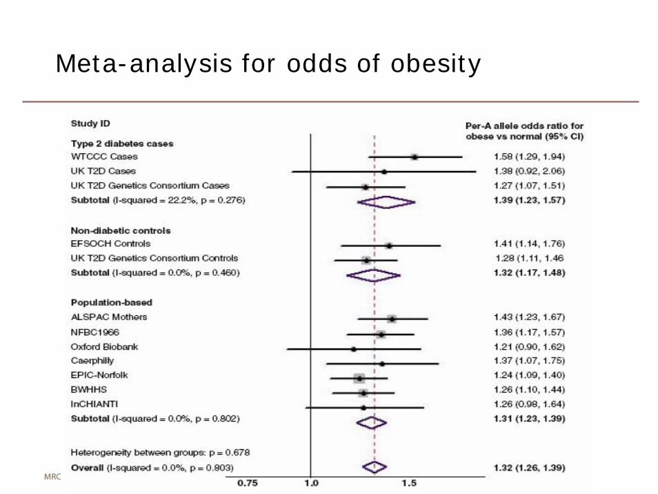
Meta-analysis for odds of obesity
LDL
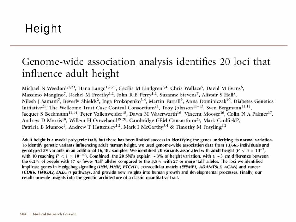
Height
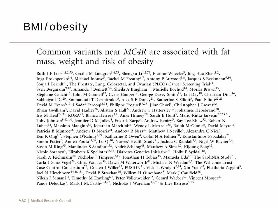
BMI/obesity
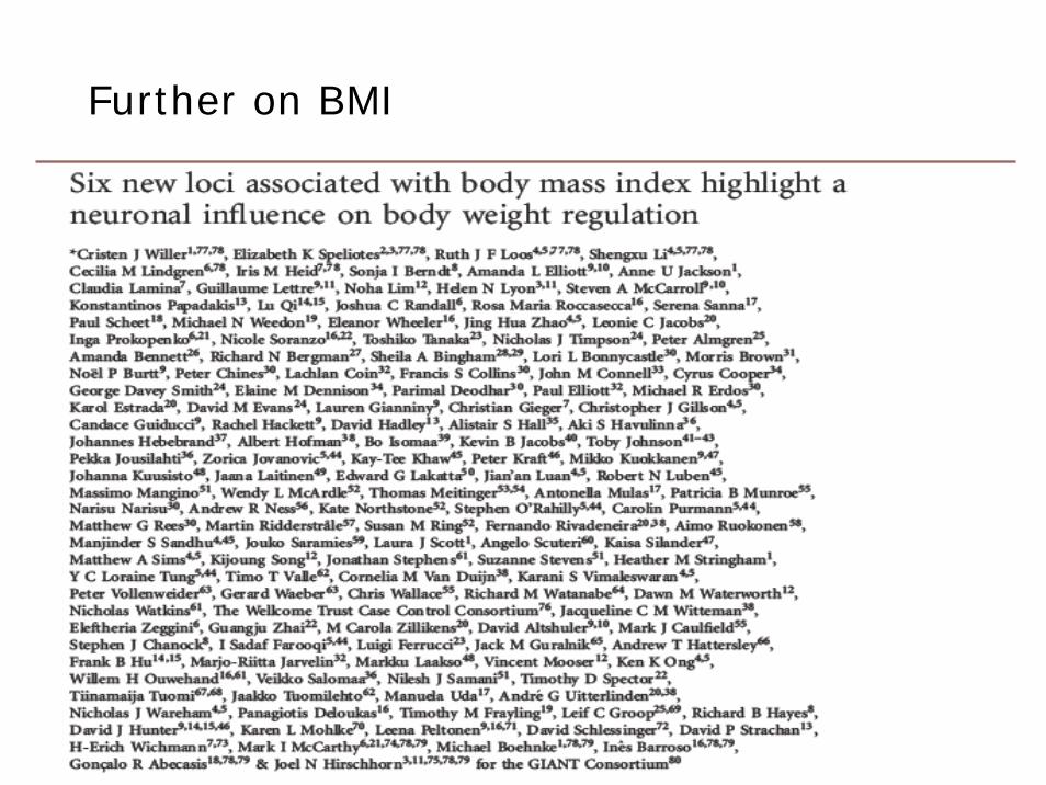
Further on BMI
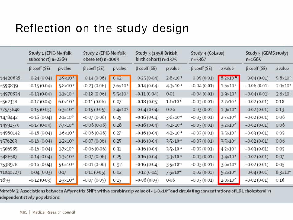
Reflection on the study design
Current practice
• Linux clusters are now ready for comprehensive analyses and greatly facilitated by Linux/awk script which is light. awk proves very useful and can be transformed to Perl. In fact, any statistical package which processes data elements would be less efficient. An example is the transformation of long, wide, transposed format noted earlier. They call C/C++ programs such as IMPUTE/SNPTEST.
• We use Stata package to automate SNPTEST, and in some instances involved C/C++ code.
• SAS is still useful for data preparation, and in a sense less professional than DBMS such as Oracle but enjoys a large user community and has facility for data analysis.
• SAS 9.2 PROTO procedure allows for C/C++ to be called.
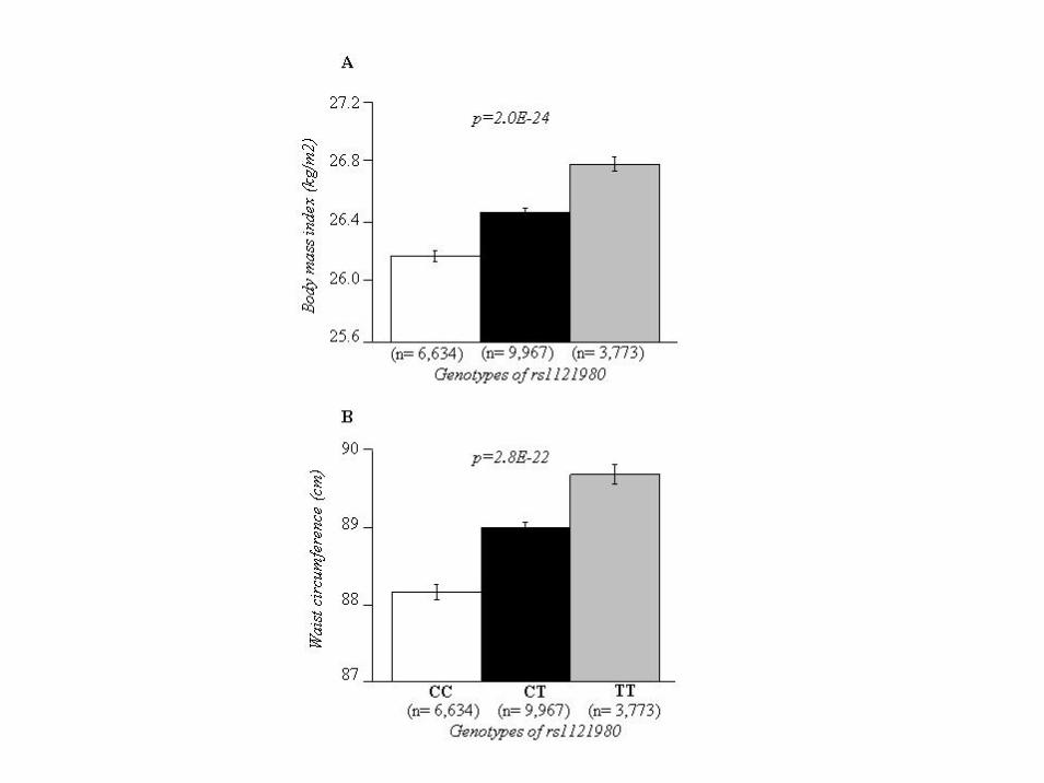
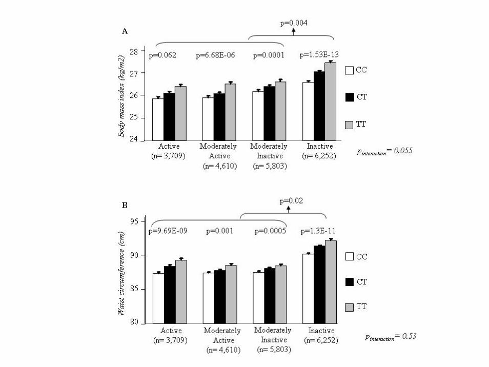
• FTO variant, rs1121980, was genotyped in 20,374 participants (39-79 years) from the EPIC-Norfolk Study. Physical activity (PA) was assessed by a validated self-reported questionnaire. The interaction between rs1121980 and PA on BMI and waist circumference (WC) was examined by including the interaction term in mixed effect models.
• Our results show that PA attenuates the effect of FTOrs1121980 genotype on BMI and WC.
FTO/physical activity--BMI/WC association
Main effect of FTO
FTO--physical activity interaction
References
• Bodmer W, Bonilla C. Nat Genet 2008;40:695-701• EPIC: http://epic.iarc.fr/• EPIC-Norfolk: http://www.srl.cam.ac.uk/epic• Long AD et al.. Science 1997; 275:1328• Loos R et al. Nat Genet 2008; 40:468-75• Prentice RL. Biometrika 1986;73:1-11• Risch N, Merkangas K (1996) Science 1997;273:1516-7• Sandhu MS et al. Lancet 2008; 371:483-91• Thomas DC. Net Rev Genet 2010; 11:259-72• Vimaleswaran KS. Am J Clin Nutr 2009; 90:425-428• Weedon MN et al. Nat Genet 2008;40:575-83• Willer et al. Nat Genet 2009; 41:25-34• Zhao JH. J Stat Soft 2007;23(8):1-18• Zhao JH et al. CCIS 2007;2:781-90

II Association analysis
Topics
• Elements of association analysis• Analytic tools• R packages• Examples • Appendix
Elements of association analysis
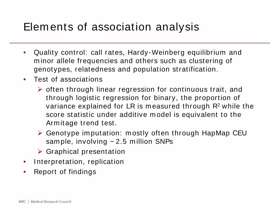
• Quality control: call rates, Hardy-Weinberg equilibrium and minor allele frequencies and others such as clustering of genotypes, relatedness and population stratification.
• Test of associationsoften through linear regression for continuous trait, and through logistic regression for binary, the proportion of variance explained for LR is measured through R2 while the score statistic under additive model is equivalent to the Armitage trend test.Genotype imputation: mostly often through HapMap CEU sample, involving ~2.5 million SNPsGraphical presentation
• Interpretation, replication• Report of findings
GRAMMAR
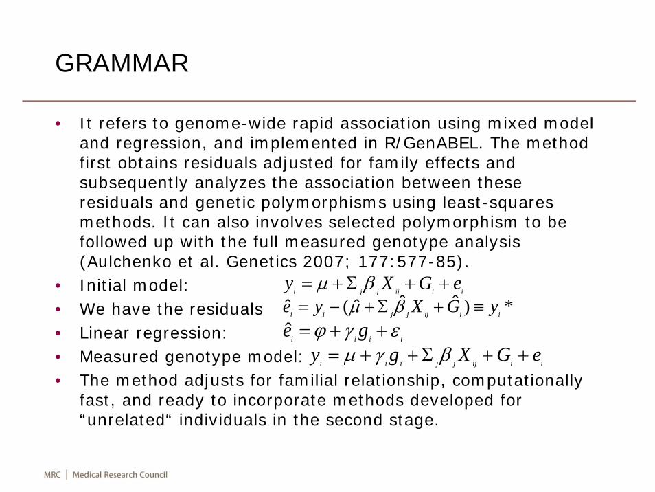
• It refers to genome-wide rapid association using mixed model and regression, and implemented in R/GenABEL. The method first obtains residuals adjusted for family effects and subsequently analyzes the association between these residuals and genetic polymorphisms using least-squares methods. It can also involves selected polymorphism to be followed up with the full measured genotype analysis (Aulchenko et al. Genetics 2007; 177:577-85).
• Initial model: • We have the residuals • Linear regression: • Measured genotype model: • The method adjusts for familial relationship, computationally
fast, and ready to incorporate methods developed for “unrelated“ individuals in the second stage.
iiijjji eGXy ++Σ+= βμ*)ˆˆˆ(ˆ
iiijjjii yGXye ≡+Σ+−= βμiiii ge εγϕ ++=ˆ
iiijjjiii eGXgy ++Σ++= βγμ
Graphics and association plots
• Plot of summary statistics• Pedigree-drawing• LD plot• Q-Q plot -- contrasting observed versus expected log-p
values• Manhattan plot -- distribution of genome-wide p values• Regional association plot -- including recombination,
contribution from imputed SNPs and top hits from consortium meta-analysis
Analytical tools
• There are several reviews on Human Genomics, and an active list is maintained at http://linkage.rockefeller.edu
• LINKAGE, GENEHUNTER, Merlin, PAP, SAGE, SOLAR• ETDT, EHPLUS, FBAT, QTDT, UNPHASED, SAS/Genetics• R (genetics, gap, haplo.stats, haplin, kinship)• For GWAS
HaploViewPLINK, SNPGWAIMPUTE, MACH, BinBamEIGENSTRATMETALSAS, Stata, R (snpMatrix, GenABEL, SNPassoc)
Connections with R
• Occasionally, these software will be cross-referenced.• Analyses with specialized programs such as
IMPUTE/SNPTEST and PLINK are illustrated in the useR!2008 tutorial.
• snpMatrix provide connect with PLINK file, e.g., narac<- read.plink("narac.bed","narac.bim","narac.fam")
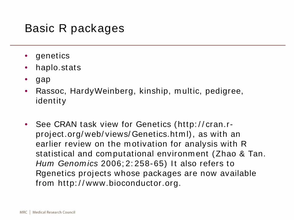
Basic R packages
• genetics• haplo.stats• gap• Rassoc, HardyWeinberg, kinship, multic, pedigree,
identity
• See CRAN task view for Genetics (http://cran.r-project.org/web/views/Genetics.html), as with an earlier review on the motivation for analysis with R statistical and computational environment (Zhao & Tan. Hum Genomics 2006;2:258-65) It also refers to Rgenetics projects whose packages are now available from http://www.bioconductor.org.
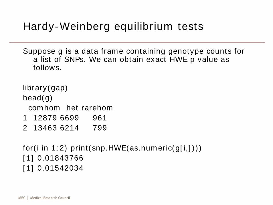
Hardy-Weinberg equilibrium tests
Suppose g is a data frame containing genotype counts for a list of SNPs. We can obtain exact HWE p value as follows.
library(gap)head(g)comhom het rarehom
1 12879 6699 9612 13463 6214 799
for(i in 1:2) print(snp.HWE(as.numeric(g[i,])))[1] 0.01843766[1] 0.01542034
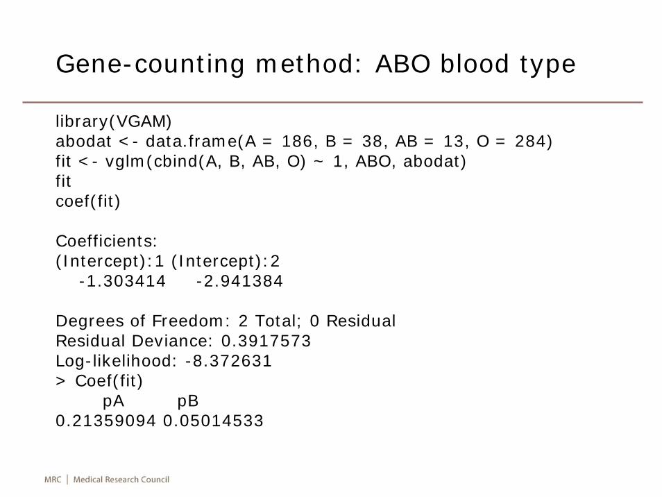
Gene-counting method: ABO blood type
library(VGAM)abodat <- data.frame(A = 186, B = 38, AB = 13, O = 284)fit <- vglm(cbind(A, B, AB, O) ~ 1, ABO, abodat)fitcoef(fit)
Coefficients:(Intercept):1 (Intercept):2
-1.303414 -2.941384
Degrees of Freedom: 2 Total; 0 ResidualResidual Deviance: 0.3917573Log-likelihood: -8.372631> Coef(fit)
pA pB0.21359094 0.05014533
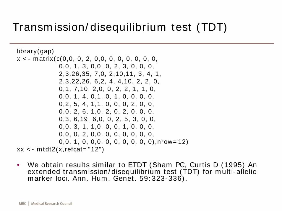
Transmission/disequilibrium test (TDT)
library(gap) x <- matrix(c(0,0, 0, 2, 0,0, 0, 0, 0, 0, 0, 0,
0,0, 1, 3, 0,0, 0, 2, 3, 0, 0, 0,2,3,26,35, 7,0, 2,10,11, 3, 4, 1,2,3,22,26, 6,2, 4, 4,10, 2, 2, 0,0,1, 7,10, 2,0, 0, 2, 2, 1, 1, 0,0,0, 1, 4, 0,1, 0, 1, 0, 0, 0, 0,0,2, 5, 4, 1,1, 0, 0, 0, 2, 0, 0,0,0, 2, 6, 1,0, 2, 0, 2, 0, 0, 0,0,3, 6,19, 6,0, 0, 2, 5, 3, 0, 0,0,0, 3, 1, 1,0, 0, 0, 1, 0, 0, 0,0,0, 0, 2, 0,0, 0, 0, 0, 0, 0, 0,0,0, 1, 0, 0,0, 0, 0, 0, 0, 0, 0),nrow=12)
xx <- mtdt2(x,refcat="12")
• We obtain results similar to ETDT (Sham PC, Curtis D (1995) An extended transmission/disequilibrium test (TDT) for multi-allelic marker loci. Ann. Hum. Genet. 59:323-336).
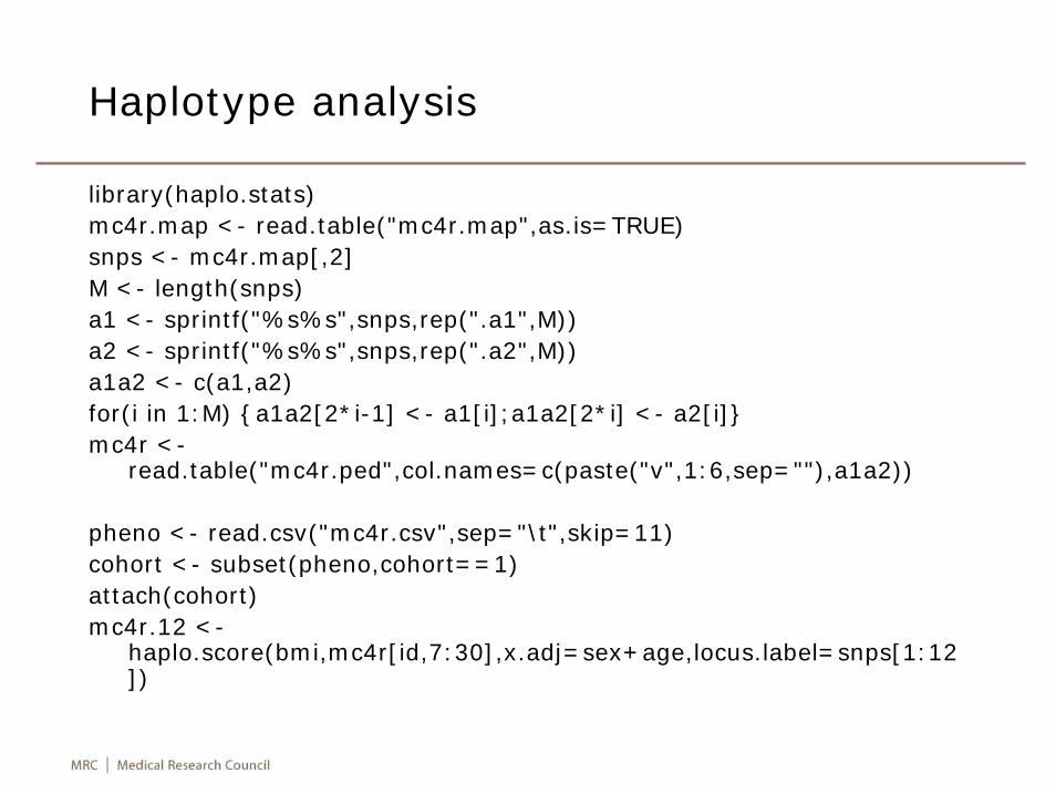
Haplotype analysis
library(haplo.stats)mc4r.map <- read.table("mc4r.map",as.is=TRUE)snps <- mc4r.map[,2]M <- length(snps)a1 <- sprintf("%s%s",snps,rep(".a1",M))a2 <- sprintf("%s%s",snps,rep(".a2",M))a1a2 <- c(a1,a2)for(i in 1:M) {a1a2[2*i-1] <- a1[i];a1a2[2*i] <- a2[i]}mc4r <-
read.table("mc4r.ped",col.names=c(paste("v",1:6,sep=""),a1a2))
pheno <- read.csv("mc4r.csv",sep="\t",skip=11)cohort <- subset(pheno,cohort==1)attach(cohort)mc4r.12 <-
haplo.score(bmi,mc4r[id,7:30],x.adj=sex+age,locus.label=snps[1:12])
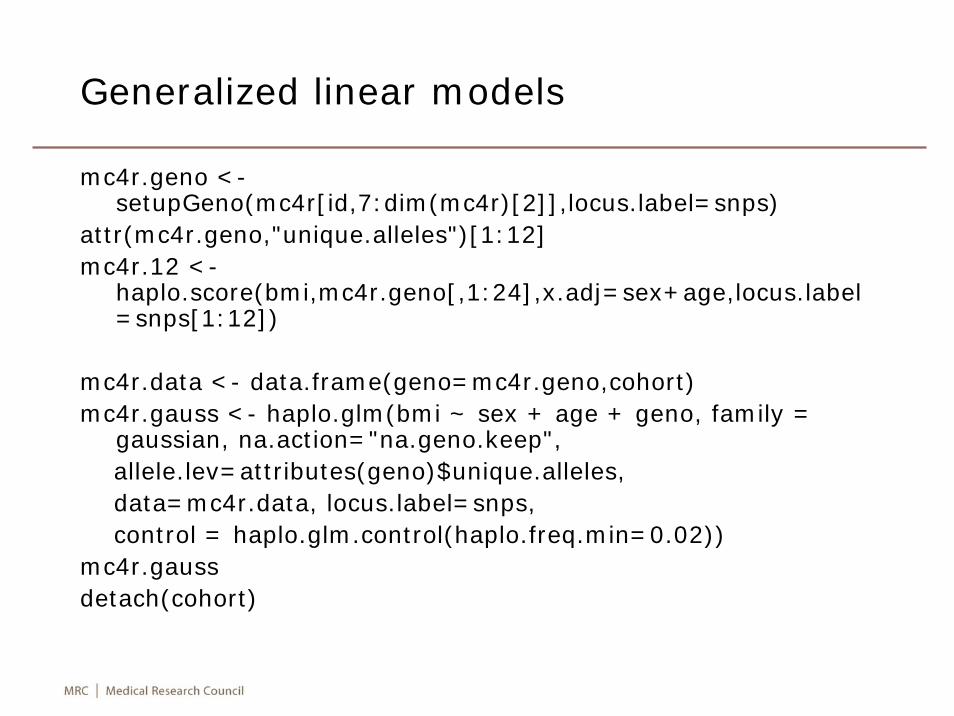
Generalized linear models
mc4r.geno <-setupGeno(mc4r[id,7:dim(mc4r)[2]],locus.label=snps)
attr(mc4r.geno,"unique.alleles")[1:12]mc4r.12 <-
haplo.score(bmi,mc4r.geno[,1:24],x.adj=sex+age,locus.label=snps[1:12])
mc4r.data <- data.frame(geno=mc4r.geno,cohort)mc4r.gauss <- haplo.glm(bmi ~ sex + age + geno, family =
gaussian, na.action="na.geno.keep",allele.lev=attributes(geno)$unique.alleles,data=mc4r.data, locus.label=snps,control = haplo.glm.control(haplo.freq.min=0.02))
mc4r.gaussdetach(cohort)
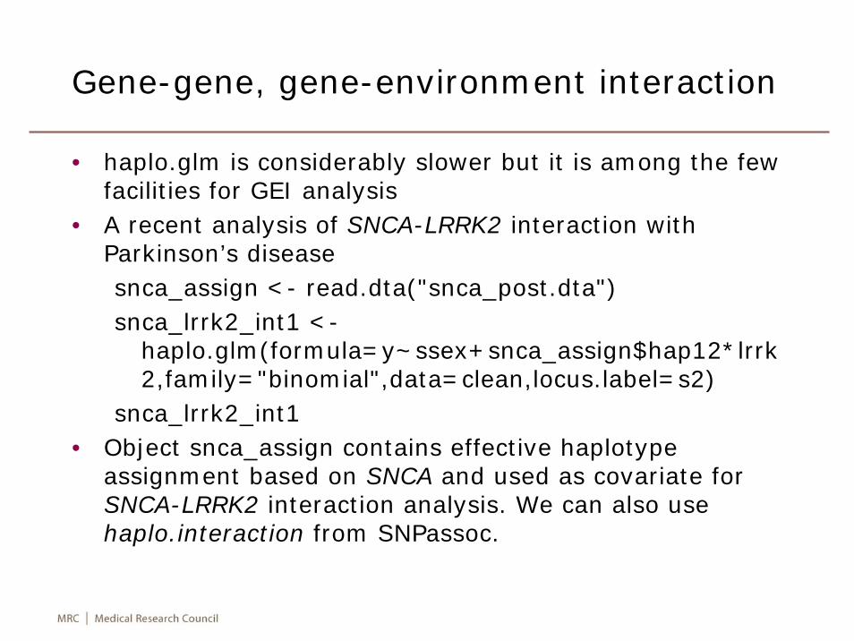
Gene-gene, gene-environment interaction
• haplo.glm is considerably slower but it is among the few facilities for GEI analysis
• A recent analysis of SNCA-LRRK2 interaction with Parkinson’s disease snca_assign <- read.dta("snca_post.dta")snca_lrrk2_int1 <-
haplo.glm(formula=y~ssex+snca_assign$hap12*lrrk2,family="binomial",data=clean,locus.label=s2)
snca_lrrk2_int1• Object snca_assign contains effective haplotype
assignment based on SNCA and used as covariate for SNCA-LRRK2 interaction analysis. We can also use haplo.interaction from SNPassoc.
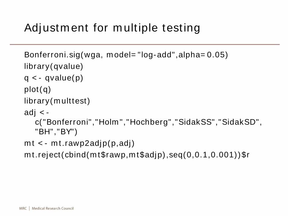
Adjustment for multiple testing
Bonferroni.sig(wga, model="log-add",alpha=0.05)library(qvalue)q <- qvalue(p)plot(q)library(multtest)adj <-
c("Bonferroni","Holm","Hochberg","SidakSS","SidakSD","BH","BY")
mt <- mt.rawp2adjp(p,adj)mt.reject(cbind(mt$rawp,mt$adjp),seq(0,0.1,0.001))$r
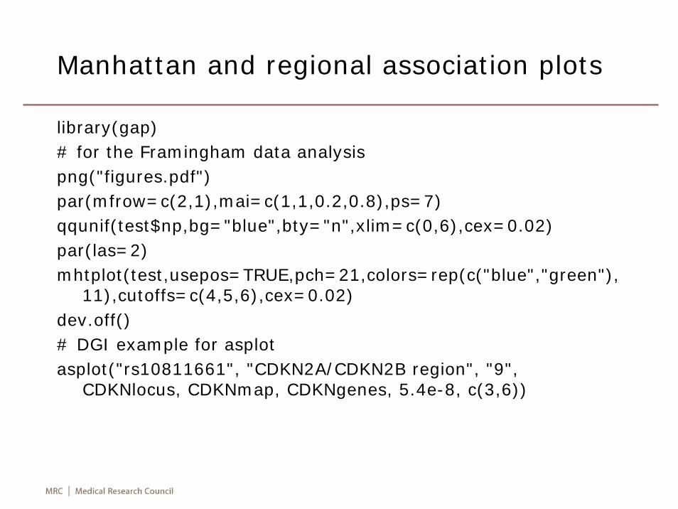
Manhattan and regional association plots
library(gap)# for the Framingham data analysispng("figures.pdf")par(mfrow=c(2,1),mai=c(1,1,0.2,0.8),ps=7)qqunif(test$np,bg="blue",bty="n",xlim=c(0,6),cex=0.02)par(las=2)mhtplot(test,usepos=TRUE,pch=21,colors=rep(c("blue","green"),
11),cutoffs=c(4,5,6),cex=0.02)dev.off()# DGI example for asplotasplot("rs10811661", "CDKN2A/CDKN2B region", "9",
CDKNlocus, CDKNmap, CDKNgenes, 5.4e-8, c(3,6))
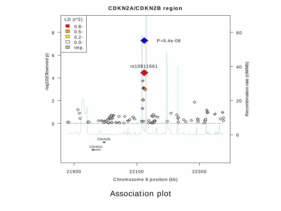
Association plot
C D K N2A/C D K N2B reg io n
C hromosome 9 position (kb)
21900 22100 22300
0
2
4
6
8
-log1
0(O
bser
ved
p)
0
20
40
60
Rec
ombi
natio
n ra
te (c
M/M
b)rs10811661
P =5.4e-08
CDKN2A
CDKN2B
LD (r^2)0 .8-0 .5-0 .2-0 .0-imp.
R packages for GWAS
• SNPassoc• GenABEL• P2BAT• snpMatrix
• While the first three are available from CRAN, snpMatrixis available from BioConductor.
• Other packages include, multtest, meta, rmeta, CAMAN, qvalue, ROCR.
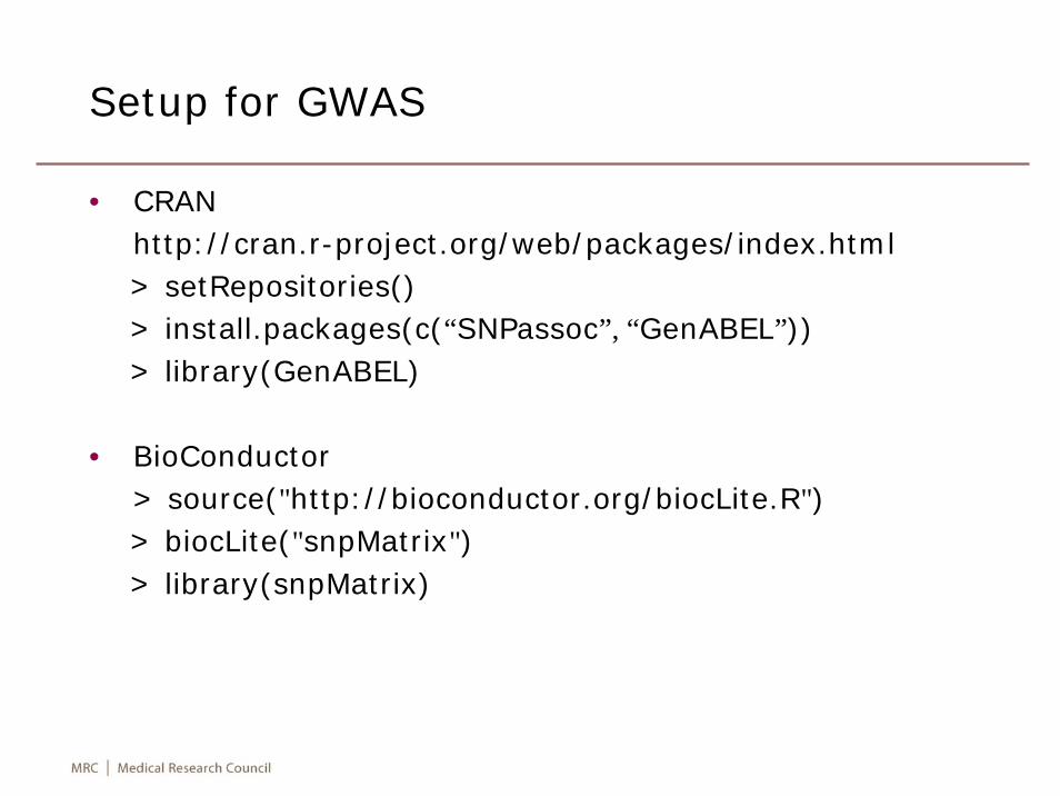
Setup for GWAS
• CRANhttp://cran.r-project.org/web/packages/index.html> setRepositories()> install.packages(c(“SNPassoc”, “GenABEL”))> library(GenABEL)
• BioConductor> source("http://bioconductor.org/biocLite.R")> biocLite("snpMatrix")> library(snpMatrix)
Notes on S4 class
• We illustrate with two classes> library(snpMatrix)> showClass(“snpMatrix”)> library(GenABEL)> showClass(“scan.gwaa”)
• It is more informative with the following commands> class?snpMatrix> class?scan.gwaa
• Later we will omit the command prompt (>). We will also give examples of creating object with new() function.
Example – MC4R SNPs and BMI
• To make a smooth exposition we use our study of SNPsnear MC4R and body mass index as reported by Loos et al. Nat Genet 2008;40:768-775.
• The MC4R gene is located on chromosome 18 and we will focus on SNPs rs17782313 and rs17700633 at positions 56002077 and 57000671 according to NCBI build 35, all genotypes being on forward strand.
• These were based on 3850 population-based individuals at stage 1 of the case-cohort study from which 3552 individuals remained after quality controls.
• We will run through SNPassoc, snpMatrix and GenABELpackages on data as contained in files mc4r.ped, mc4r.map and mc4r.csv
SNPassoc
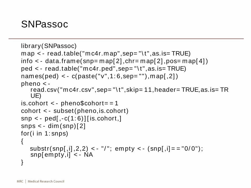
library(SNPassoc)map <- read.table("mc4r.map",sep="\t",as.is=TRUE)info <- data.frame(snp=map[2],chr=map[2],pos=map[4])ped <- read.table("mc4r.ped",sep="\t",as.is=TRUE)names(ped) <- c(paste("v",1:6,sep=""),map[,2])pheno <-
read.csv("mc4r.csv",sep="\t",skip=11,header=TRUE,as.is=TRUE)
is.cohort <- pheno$cohort==1cohort <- subset(pheno,is.cohort)snp <- ped[,-c(1:6)][is.cohort,]snps <- dim(snp)[2]for(i in 1:snps){
substr(snp[,i],2,2) <- "/"; empty <- (snp[,i]=="0/0"); snp[empty,i] <- NA
}
Analysis
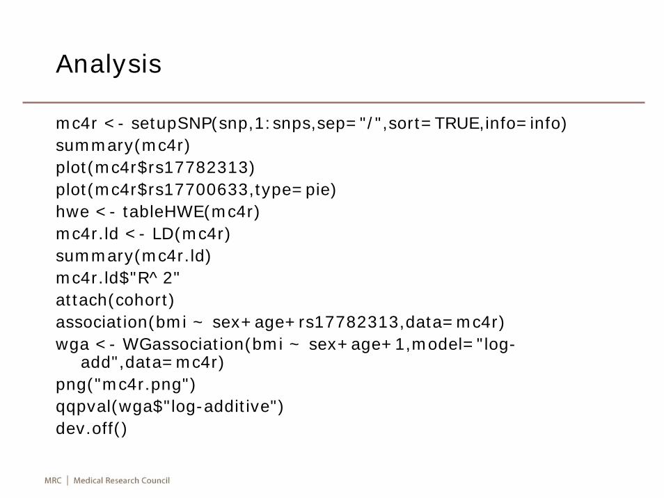
mc4r <- setupSNP(snp,1:snps,sep="/",sort=TRUE,info=info)summary(mc4r)plot(mc4r$rs17782313)plot(mc4r$rs17700633,type=pie)hwe <- tableHWE(mc4r)mc4r.ld <- LD(mc4r)summary(mc4r.ld)mc4r.ld$"R^2"attach(cohort)association(bmi ~ sex+age+rs17782313,data=mc4r)wga <- WGassociation(bmi ~ sex+age+1,model="log-
add",data=mc4r)png("mc4r.png")qqpval(wga$"log-additive")dev.off()
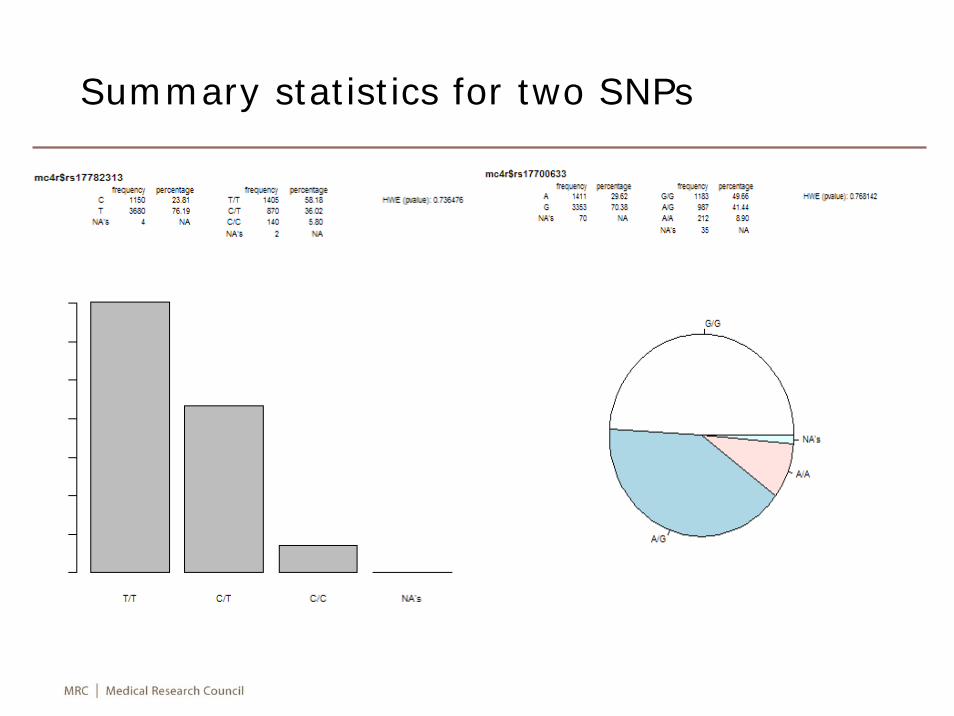
Summary statistics for two SNPs
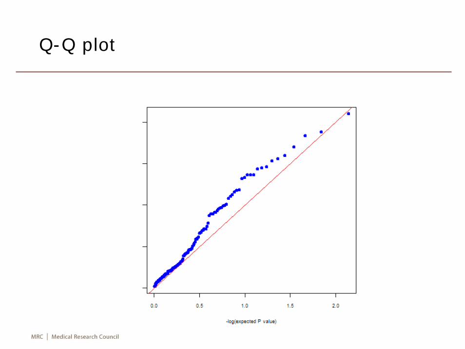
Q-Q plot
Comments
• SNPassoc is essentially designed for dealing with unrelated individuals but with considerable enhancements from genetics and haplo.stats.
• It implements permutation tests for binary traits through scanWGassociation(,nperm=) and permTest()
• It is possible to conduct gene-gene interaction:mc4r.ip <-
interactionPval(bmi~sex+age,data=mc4r,model="log-add")
plot(mc4r.ip)• We got a very good feel of the kind of analysis it may
involve and this is a very simple example.
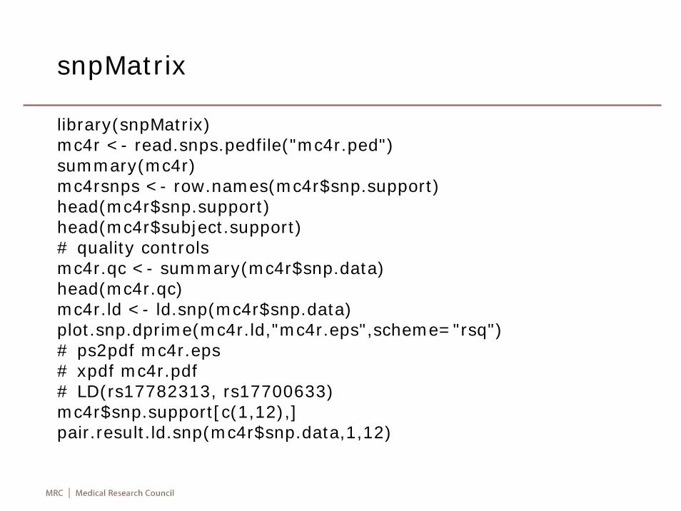
snpMatrix
library(snpMatrix)mc4r <- read.snps.pedfile("mc4r.ped")summary(mc4r)mc4rsnps <- row.names(mc4r$snp.support)head(mc4r$snp.support)head(mc4r$subject.support)# quality controlsmc4r.qc <- summary(mc4r$snp.data)head(mc4r.qc)mc4r.ld <- ld.snp(mc4r$snp.data)plot.snp.dprime(mc4r.ld,"mc4r.eps",scheme="rsq")# ps2pdf mc4r.eps# xpdf mc4r.pdf# LD(rs17782313, rs17700633)mc4r$snp.support[c(1,12),]pair.result.ld.snp(mc4r$snp.data,1,12)
PCA and identity-by-state analysis
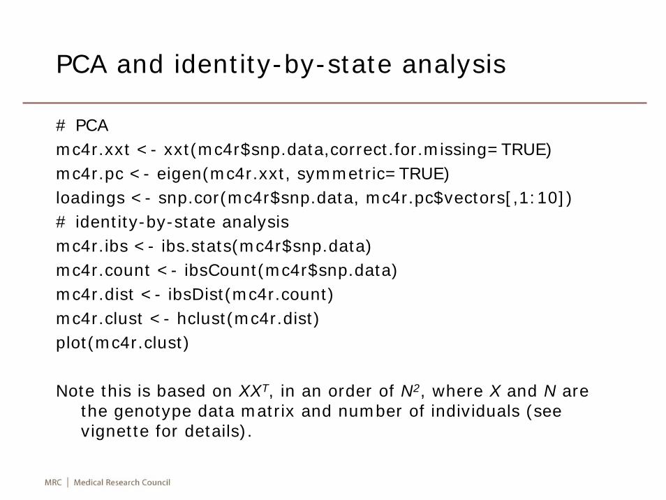
# PCAmc4r.xxt <- xxt(mc4r$snp.data,correct.for.missing=TRUE)mc4r.pc <- eigen(mc4r.xxt, symmetric=TRUE)loadings <- snp.cor(mc4r$snp.data, mc4r.pc$vectors[,1:10])# identity-by-state analysismc4r.ibs <- ibs.stats(mc4r$snp.data)mc4r.count <- ibsCount(mc4r$snp.data)mc4r.dist <- ibsDist(mc4r.count)mc4r.clust <- hclust(mc4r.dist)plot(mc4r.clust)
Note this is based on XXT, in an order of N2, where X and N are the genotype data matrix and number of individuals (see vignette for details).
Phenotype data and case-control analysis
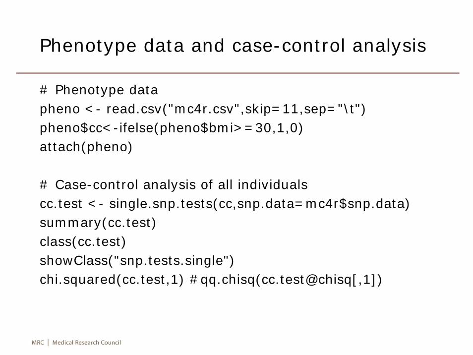
# Phenotype datapheno <- read.csv("mc4r.csv",skip=11,sep="\t")pheno$cc<-ifelse(pheno$bmi>=30,1,0)attach(pheno)
# Case-control analysis of all individualscc.test <- single.snp.tests(cc,snp.data=mc4r$snp.data)summary(cc.test)class(cc.test)showClass("snp.tests.single")chi.squared(cc.test,1) #qq.chisq(cc.test@chisq[,1])
Meta-analysis
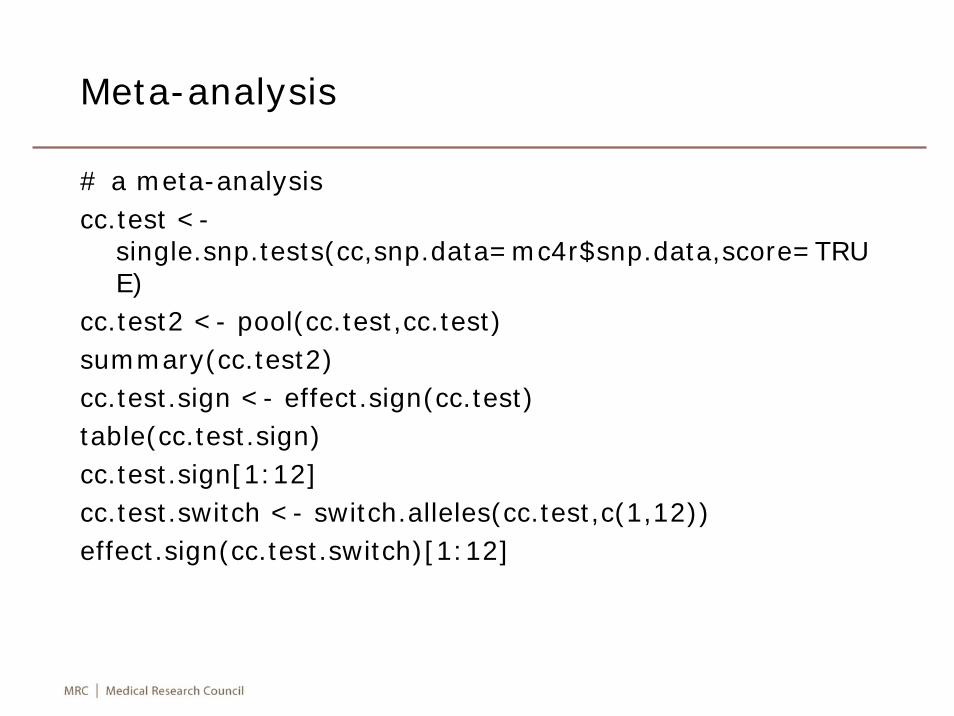
# a meta-analysiscc.test <-
single.snp.tests(cc,snp.data=mc4r$snp.data,score=TRUE)
cc.test2 <- pool(cc.test,cc.test)summary(cc.test2)cc.test.sign <- effect.sign(cc.test)table(cc.test.sign)cc.test.sign[1:12]cc.test.switch <- switch.alleles(cc.test,c(1,12))effect.sign(cc.test.switch)[1:12]
OLS estimation and retrospective analysis
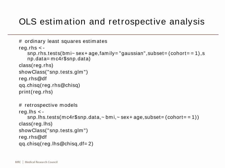
# ordinary least squares estimatesreg.rhs <-
snp.rhs.tests(bmi~sex+age,family="gaussian",subset=(cohort==1),snp.data=mc4r$snp.data)
class(reg.rhs)showClass("snp.tests.glm")[email protected](reg.rhs@chisq)print(reg.rhs)
# retrospective modelsreg.lhs <-
snp.lhs.tests(mc4r$snp.data,~bmi,~sex+age,subset=(cohort==1))class(reg.lhs)showClass("snp.tests.glm")[email protected](reg.lhs@chisq,df=2)
Genotype imputation
• It is customarily to impute genotypes in a large study based on a small sample of fully-genotyped individuals, e.g., hapmap, so as to conduct association tests for large number of SNPs.
• It is also useful for meta-analysis of SNPs from different platforms such as Affymetrix 500K and Illumina 550K.
• As it is snpMatrix implements genotype imputation between sets of markers based on same individuals; more generally this involves genotypes from HapMap.
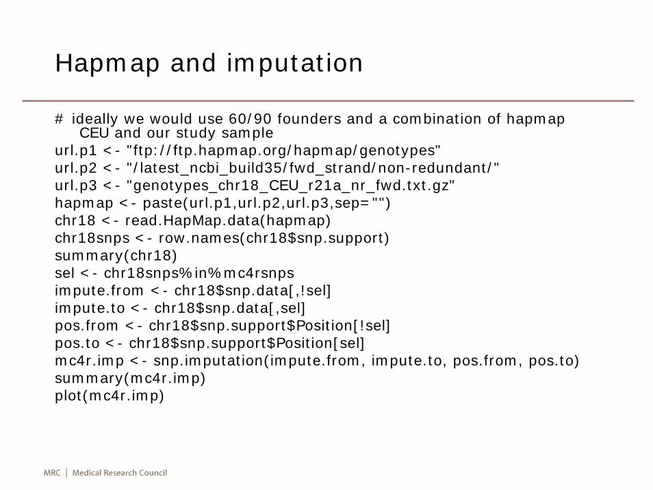
Hapmap and imputation
# ideally we would use 60/90 founders and a combination of hapmapCEU and our study sample
url.p1 <- "ftp://ftp.hapmap.org/hapmap/genotypes"url.p2 <- "/latest_ncbi_build35/fwd_strand/non-redundant/"url.p3 <- "genotypes_chr18_CEU_r21a_nr_fwd.txt.gz"hapmap <- paste(url.p1,url.p2,url.p3,sep="")chr18 <- read.HapMap.data(hapmap)chr18snps <- row.names(chr18$snp.support)summary(chr18)sel <- chr18snps%in%mc4rsnpsimpute.from <- chr18$snp.data[,!sel]impute.to <- chr18$snp.data[,sel]pos.from <- chr18$snp.support$Position[!sel]pos.to <- chr18$snp.support$Position[sel]mc4r.imp <- snp.imputation(impute.from, impute.to, pos.from, pos.to)summary(mc4r.imp)plot(mc4r.imp)
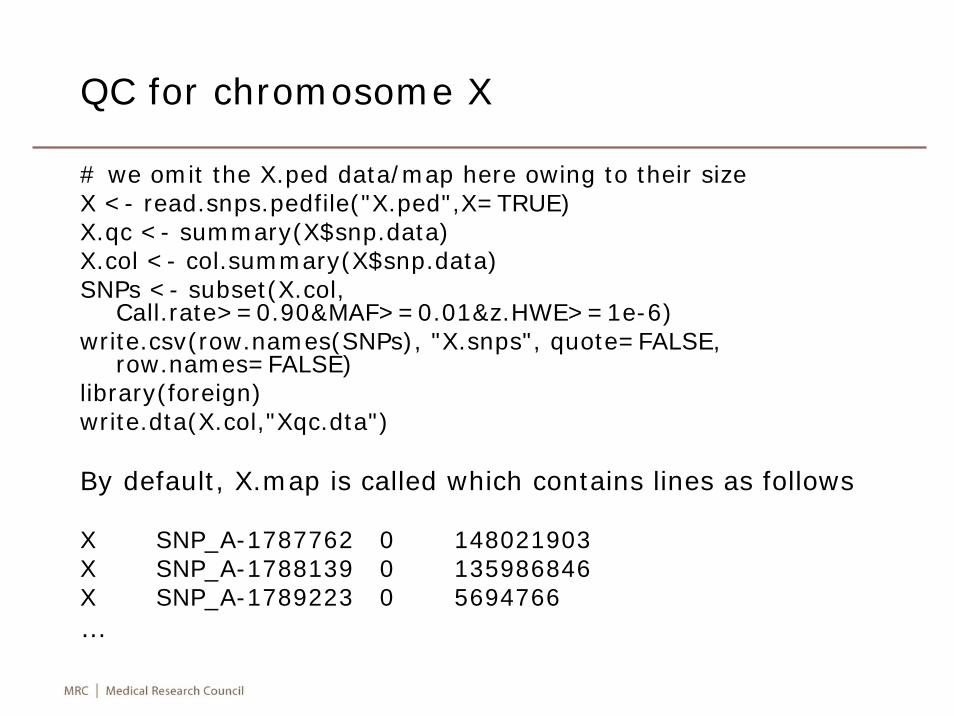
QC for chromosome X
# we omit the X.ped data/map here owing to their sizeX <- read.snps.pedfile("X.ped",X=TRUE)X.qc <- summary(X$snp.data)X.col <- col.summary(X$snp.data)SNPs <- subset(X.col,
Call.rate>=0.90&MAF>=0.01&z.HWE>=1e-6)write.csv(row.names(SNPs), "X.snps", quote=FALSE,
row.names=FALSE)library(foreign)write.dta(X.col,"Xqc.dta")
By default, X.map is called which contains lines as follows
X SNP_A-1787762 0 148021903X SNP_A-1788139 0 135986846X SNP_A-1789223 0 5694766…
snp.imputation
• It is notable with the definition of snp.imputation that given two set of SNPs typed in the same subjects, this function calculates regression equations which can be used to impute one set from the other in a subsequent sample.
• We customarily use external data (e.g., available from HapMap, 1000 genomes or elsewhere) and our sample jointly, treating non-typed SNPs as missing.
• CRAN packages such as mice should facilitate this on the phenotype side.
Comments
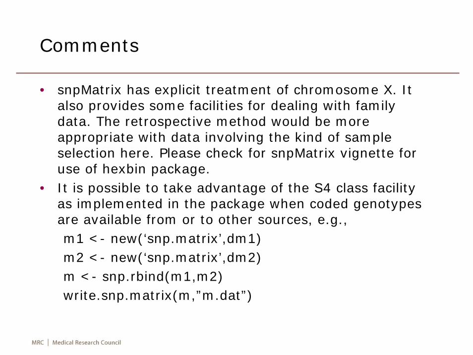
• snpMatrix has explicit treatment of chromosome X. It also provides some facilities for dealing with family data. The retrospective method would be more appropriate with data involving the kind of sample selection here. Please check for snpMatrix vignette for use of hexbin package.
• It is possible to take advantage of the S4 class facility as implemented in the package when coded genotypes are available from or to other sources, e.g.,m1 <- new(‘snp.matrix’,dm1)m2 <- new(‘snp.matrix’,dm2)m <- snp.rbind(m1,m2)write.snp.matrix(m,”m.dat”)
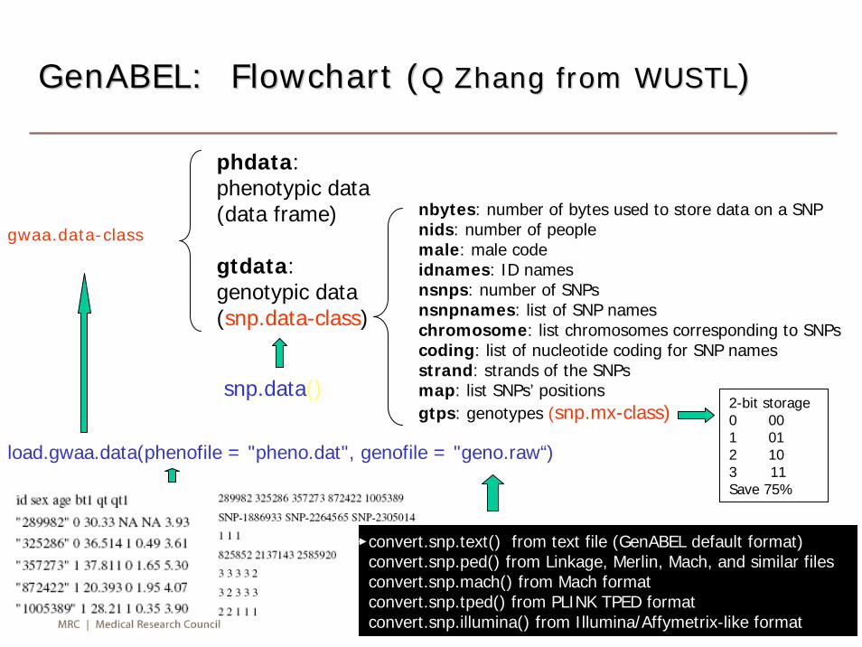
GenABEL: Flowchart (GenABEL: Flowchart (Q Zhang from WUSTLQ Zhang from WUSTL))
gwaa.data-class
phdata: phenotypic data (data frame)
gtdata:genotypic data (snp.data-class)
load.gwaa.data(phenofile = "pheno.dat", genofile = "geno.raw“)
nbytes: number of bytes used to store data on a SNPnids: number of peoplemale: male codeidnames: ID namesnsnps: number of SNPsnsnpnames: list of SNP nameschromosome: list chromosomes corresponding to SNPscoding: list of nucleotide coding for SNP namesstrand: strands of the SNPsmap: list SNPs’ positionsgtps: genotypes (snp.mx-class)
snp.data()
convert.snp.text() from text file (GenABEL default format)convert.snp.ped() from Linkage, Merlin, Mach, and similar filesconvert.snp.mach() from Mach formatconvert.snp.tped() from PLINK TPED formatconvert.snp.illumina() from Illumina/Affymetrix-like format
2-bit storage0 001 012 103 11Save 75%
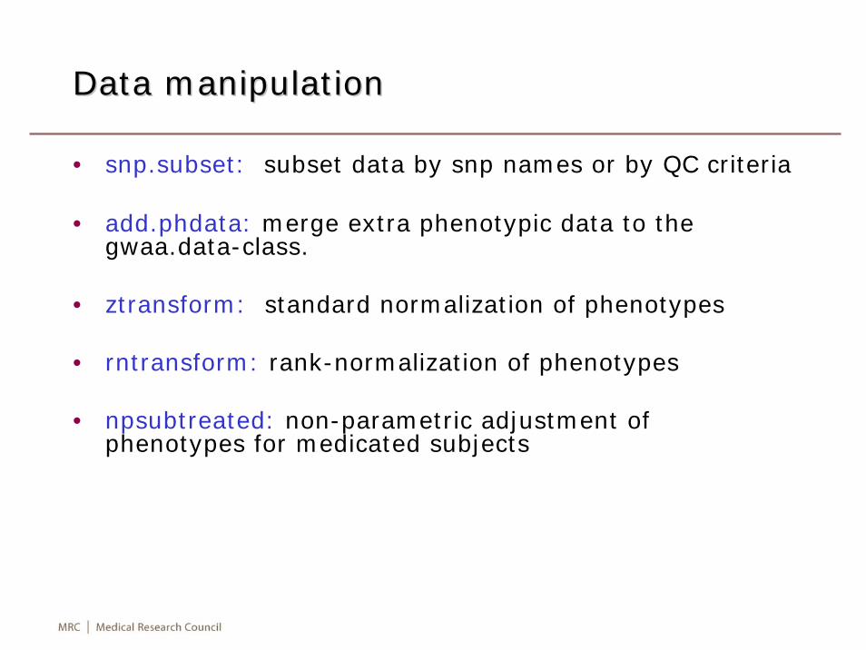
Data manipulationData manipulation
• snp.subset: subset data by snp names or by QC criteria
• add.phdata: merge extra phenotypic data to the gwaa.data-class.
• ztransform: standard normalization of phenotypes
• rntransform: rank-normalization of phenotypes
• npsubtreated: non-parametric adjustment of phenotypes for medicated subjects
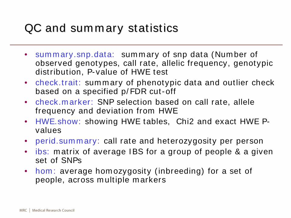
QC and summary statisticsQC and summary statistics
• summary.snp.data: summary of snp data (Number of observed genotypes, call rate, allelic frequency, genotypic distribution, P-value of HWE test
• check.trait: summary of phenotypic data and outlier check based on a specified p/FDR cut-off
• check.marker: SNP selection based on call rate, allele frequency and deviation from HWE
• HWE.show: showing HWE tables, Chi2 and exact HWE P-values
• perid.summary: call rate and heterozygosity per person• ibs: matrix of average IBS for a group of people & a given
set of SNPs• hom: average homozygosity (inbreeding) for a set of
people, across multiple markers
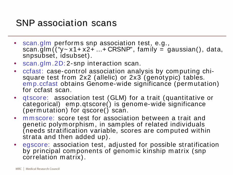
SNP association scansSNP association scans
• scan.glm performs snp association test, e.g., scan.glm((“y~x1+x2+…+CRSNP", family = gaussian(), data, snpsubset, idsubset).
• scan.glm.2D:2-snp interaction scan.• ccfast: case-control association analysis by computing chi-
square test from 2x2 (allelic) or 2x3 (genotypic) tables. emp.ccfast obtains Genome-wide significance (permutation) for ccfast scan.
• qtscore: association test (GLM) for a trait (quantitative or categorical) emp.qtscore() is genome-wide significance (permutation) for qscore() scan.
• mmscore: score test for association between a trait and genetic polymorphism, in samples of related individuals (needs stratification variable, scores are computed within strata and then added up).
• egscore: association test, adjusted for possible stratification by principal components of genomic kinship matrix (snpcorrelation matrix).
HaplotypeHaplotype association scansassociation scans
• scan.haplo: haplotype association test using GLM in R library
• scan.haplo.2D: 2-haplotype interaction scan
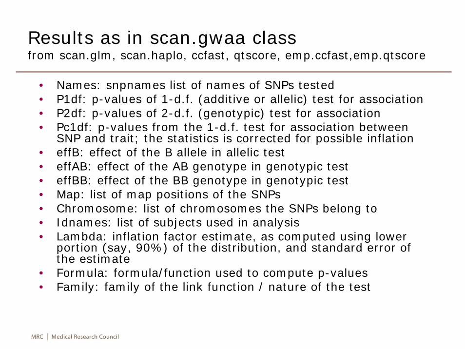
Results as in scan.gwaa class from scan.glm, scan.haplo, ccfast, qtscore, emp.ccfast,emp.qtscore
• Names: snpnames list of names of SNPs tested• P1df: p-values of 1-d.f. (additive or allelic) test for association• P2df: p-values of 2-d.f. (genotypic) test for association• Pc1df: p-values from the 1-d.f. test for association between
SNP and trait; the statistics is corrected for possible inflation• effB: effect of the B allele in allelic test• effAB: effect of the AB genotype in genotypic test• effBB: effect of the BB genotype in genotypic test• Map: list of map positions of the SNPs• Chromosome: list of chromosomes the SNPs belong to• Idnames: list of subjects used in analysis• Lambda: inflation factor estimate, as computed using lower
portion (say, 90%) of the distribution, and standard error of the estimate
• Formula: formula/function used to compute p-values• Family: family of the link function / nature of the test
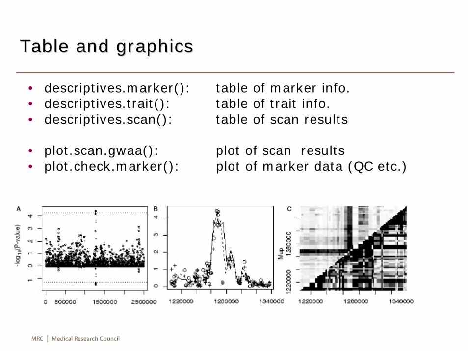
Table and graphicsTable and graphics
• descriptives.marker(): table of marker info.• descriptives.trait(): table of trait info.• descriptives.scan(): table of scan results
• plot.scan.gwaa(): plot of scan results• plot.check.marker(): plot of marker data (QC etc.)
ParallABEL
• An R Library for Generalized Parallelization of Genome-Wide Association Studies
• http://parallabel.r-forge.r-project.org/• http://www.sci.psu.ac.th/units/genome/CGBR/ParallABE
L/index.html• Sangket et al. BMC Bioinformatics 2010; 11:217
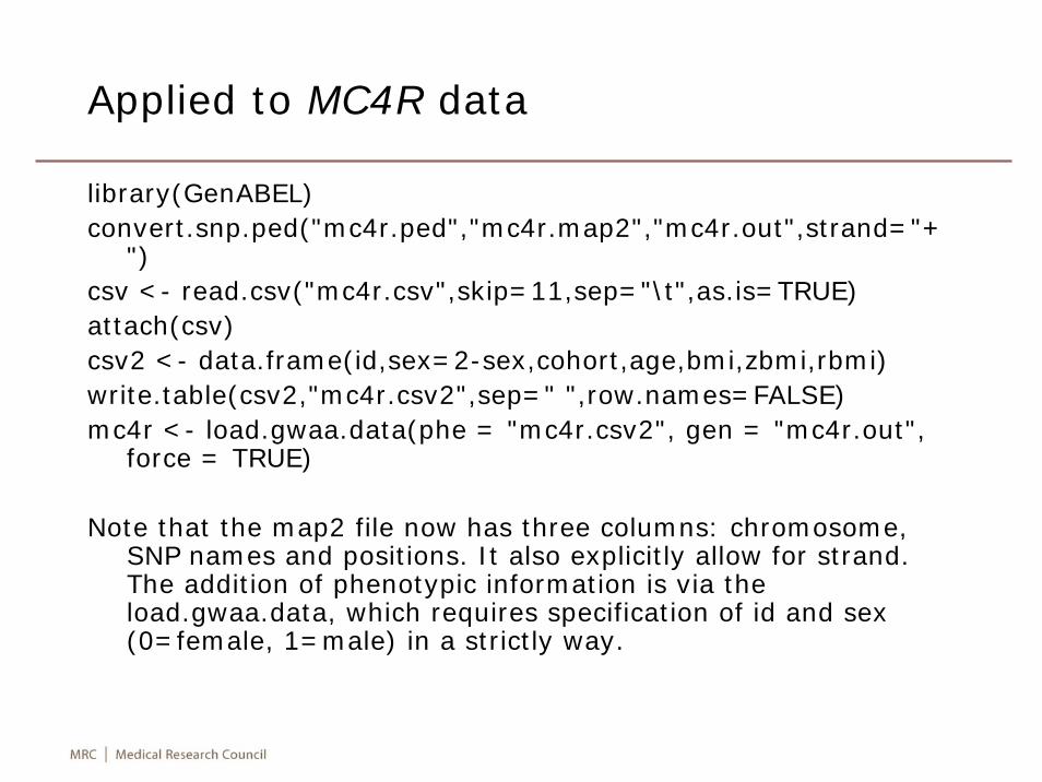
Applied to MC4R data
library(GenABEL)convert.snp.ped("mc4r.ped","mc4r.map2","mc4r.out",strand="+
")csv <- read.csv("mc4r.csv",skip=11,sep="\t",as.is=TRUE)attach(csv)csv2 <- data.frame(id,sex=2-sex,cohort,age,bmi,zbmi,rbmi)write.table(csv2,"mc4r.csv2",sep=" ",row.names=FALSE)mc4r <- load.gwaa.data(phe = "mc4r.csv2", gen = "mc4r.out",
force = TRUE)
Note that the map2 file now has three columns: chromosome, SNP names and positions. It also explicitly allow for strand. The addition of phenotypic information is via the load.gwaa.data, which requires specification of id and sex (0=female, 1=male) in a strictly way.
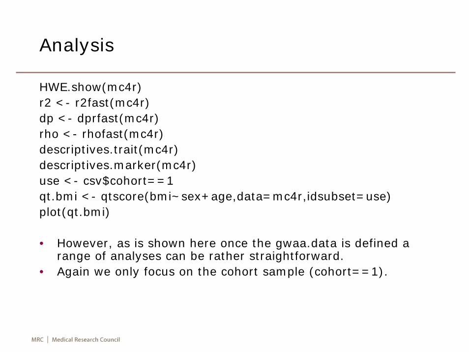
Analysis
HWE.show(mc4r)r2 <- r2fast(mc4r)dp <- dprfast(mc4r)rho <- rhofast(mc4r)descriptives.trait(mc4r)descriptives.marker(mc4r)use <- csv$cohort==1qt.bmi <- qtscore(bmi~sex+age,data=mc4r,idsubset=use)plot(qt.bmi)
• However, as is shown here once the gwaa.data is defined a range of analyses can be rather straightforward.
• Again we only focus on the cohort sample (cohort==1).
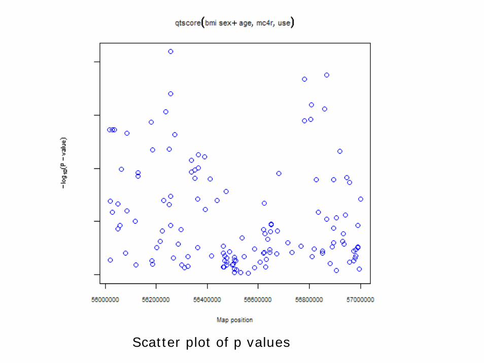
Scatter plot of p values
GAW15 Expression quantitative trait
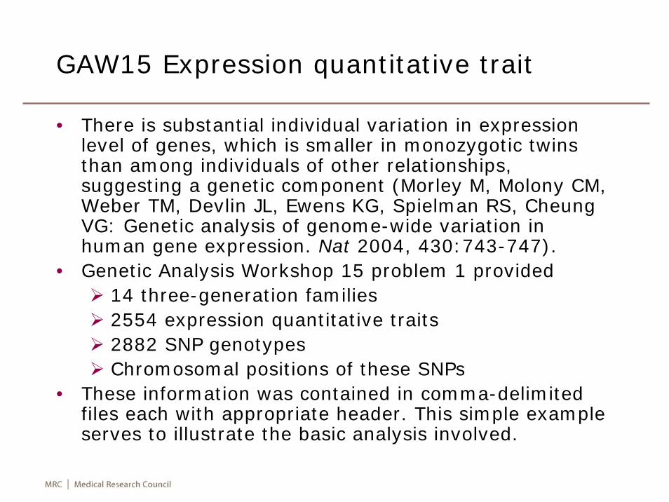
• There is substantial individual variation in expression level of genes, which is smaller in monozygotic twins than among individuals of other relationships, suggesting a genetic component (Morley M, Molony CM, Weber TM, Devlin JL, Ewens KG, Spielman RS, Cheung VG: Genetic analysis of genome-wide variation in human gene expression. Nat 2004, 430:743-747).
• Genetic Analysis Workshop 15 problem 1 provided14 three-generation families2554 expression quantitative traits2882 SNP genotypesChromosomal positions of these SNPs
• These information was contained in comma-delimited files each with appropriate header. This simple example serves to illustrate the basic analysis involved.
Getting data into R
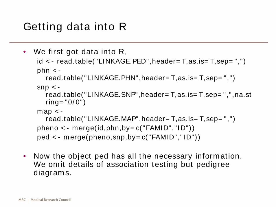
• We first got data into R,id <- read.table("LINKAGE.PED",header=T,as.is=T,sep=",")phn <-
read.table("LINKAGE.PHN",header=T,as.is=T,sep=",")snp <-
read.table("LINKAGE.SNP",header=T,as.is=T,sep=",",na.string="0/0")
map <-read.table("LINKAGE.MAP",header=T,as.is=T,sep=",")
pheno <- merge(id,phn,by=c("FAMID","ID"))ped <- merge(pheno,snp,by=c("FAMID","ID"))
• Now the object ped has all the necessary information. We omit details of association testing but pedigree diagrams.
Pedigree diagrams
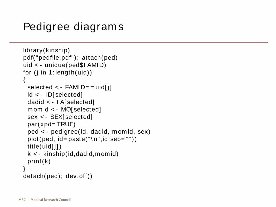
library(kinship)pdf("pedfile.pdf"); attach(ped)uid <- unique(ped$FAMID)for (j in 1:length(uid)){
selected <- FAMID==uid[j]id <- ID[selected]dadid <- FA[selected]momid <- MO[selected]sex <- SEX[selected]par(xpd=TRUE)ped <- pedigree(id, dadid, momid, sex)plot(ped, id=paste(“\n”,id,sep=“”))title(uid[j])k <- kinship(id,dadid,momid)print(k)
}detach(ped); dev.off()
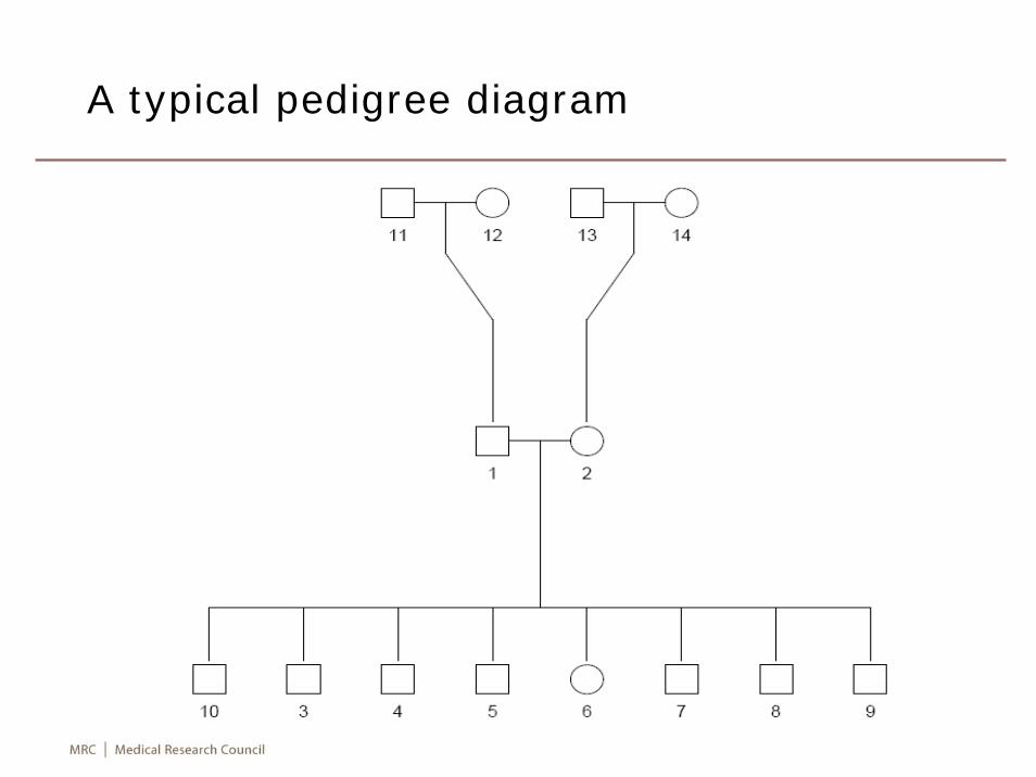
A typical pedigree diagram
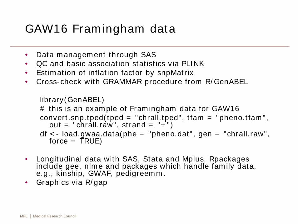
GAW16 Framingham data
• Data management through SAS• QC and basic association statistics via PLINK• Estimation of inflation factor by snpMatrix• Cross-check with GRAMMAR procedure from R/GenABEL
library(GenABEL)# this is an example of Framingham data for GAW16convert.snp.tped(tped = "chrall.tped", tfam = "pheno.tfam",
out = "chrall.raw", strand = "+")df <- load.gwaa.data(phe = "pheno.dat", gen = "chrall.raw",
force = TRUE)
• Longitudinal data with SAS, Stata and Mplus. Rpackagesinclude gee, nlme and packages which handle family data, e.g., kinship, GWAF, pedigreemm.
• Graphics via R/gap
References
• Elston RC. Introduction and overview. Stat Meth Med Res 9(6, special issue), 2000
• Balding DJ. Nat Rev Genet 7:781-791, 2006• Elston RC, Anne Spence M. Stat Med 25:3049-3080,
2006• McCarthy MI, Abecasis GR, Cardon LR, Goldstein DB,
Little J, Ioannidis JPA, Hirschhorn JN. Genome-wide association studies for complex traits: Consensus, uncertainty and challenges. Nat Rev Genet 9:356–369, 2008
• Zheng G, Marchini J, Geller NL. Introduction to the special issue: Genome-wide association studies. Stat Sci24(4, special issue), 2009
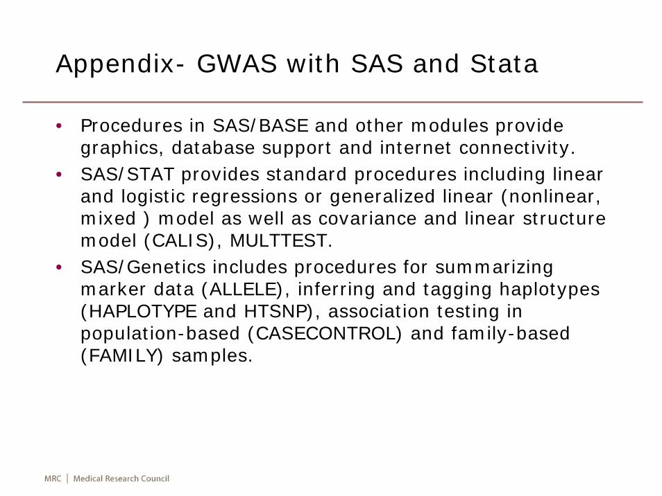
Appendix- GWAS with SAS and Stata
• Procedures in SAS/BASE and other modules provide graphics, database support and internet connectivity.
• SAS/STAT provides standard procedures including linear and logistic regressions or generalized linear (nonlinear, mixed ) model as well as covariance and linear structure model (CALIS), MULTTEST.
• SAS/Genetics includes procedures for summarizing marker data (ALLELE), inferring and tagging haplotypes(HAPLOTYPE and HTSNP), association testing in population-based (CASECONTROL) and family-based (FAMILY) samples.
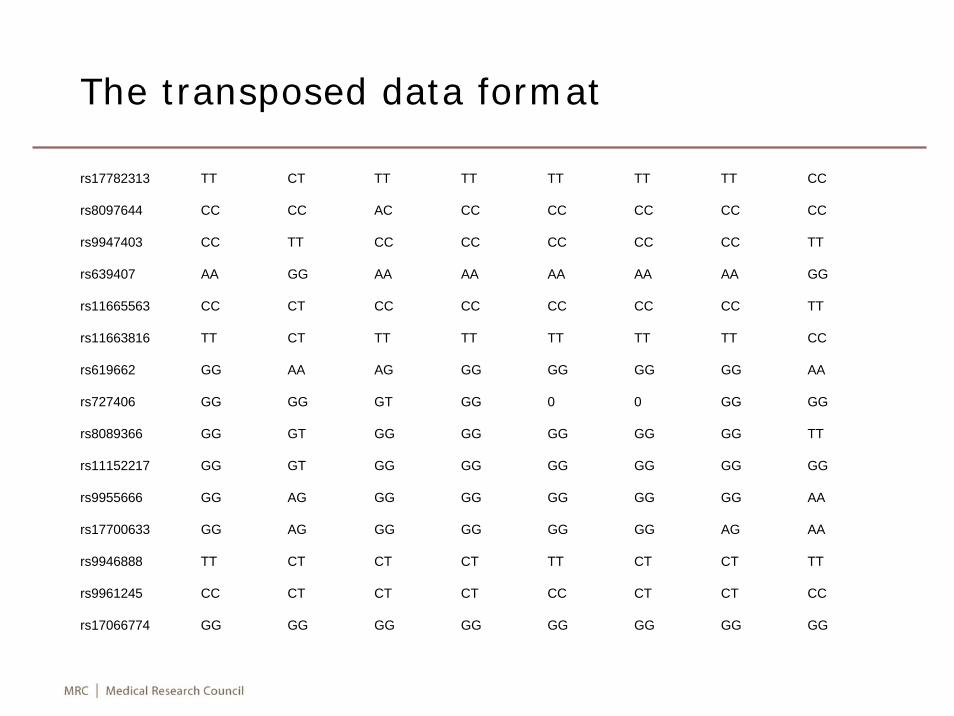
The transposed data format
rs17782313 TT CT TT TT TT TT TT CC
rs8097644 CC CC AC CC CC CC CC CC
rs9947403 CC TT CC CC CC CC CC TT
rs639407 AA GG AA AA AA AA AA GG
rs11665563 CC CT CC CC CC CC CC TT
rs11663816 TT CT TT TT TT TT TT CC
rs619662 GG AA AG GG GG GG GG AA
rs727406 GG GG GT GG 0 0 GG GG
rs8089366 GG GT GG GG GG GG GG TT
rs11152217 GG GT GG GG GG GG GG GG
rs9955666 GG AG GG GG GG GG GG AA
rs17700633 GG AG GG GG GG GG AG AA
rs9946888 TT CT CT CT TT CT CT TT
rs9961245 CC CT CT CT CC CT CT CC
rs17066774 GG GG GG GG GG GG GG GG
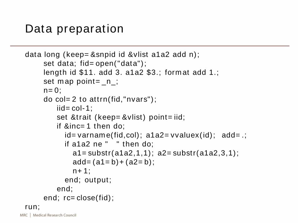
Data preparation
data long (keep=&snpid id &vlist a1a2 add n);set data; fid=open("data"); length id $11. add 3. a1a2 $3.; format add 1.;set map point=_n_;n=0;do col=2 to attrn(fid,"nvars");
iid=col-1;set &trait (keep=&vlist) point=iid;if &inc=1 then do;
id=varname(fid,col); a1a2=vvaluex(id); add=.;if a1a2 ne " " then do;
a1=substr(a1a2,1,1); a2=substr(a1a2,3,1);add=(a1=b)+(a2=b);n+1;
end; output;end;
end; rc=close(fid);run;
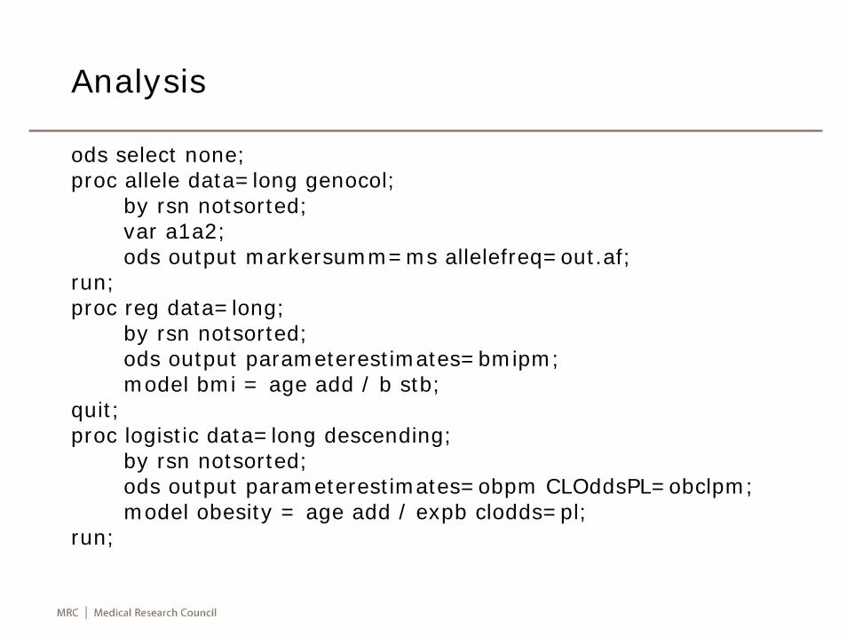
Analysis
ods select none;proc allele data=long genocol;
by rsn notsorted;var a1a2;ods output markersumm=ms allelefreq=out.af;
run;proc reg data=long;
by rsn notsorted;ods output parameterestimates=bmipm;model bmi = age add / b stb;
quit;proc logistic data=long descending;
by rsn notsorted;ods output parameterestimates=obpm CLOddsPL=obclpm;model obesity = age add / expb clodds=pl;
run;
Stata
• It is a general-purpose, modern and easy to use statistical analysis system (e.g., http://en.wikipedia.org/wiki/Stata).
• Functions for genetic data includes summary statistics, test of Hardy-Weinberg equilibrium, haplotypeestimation, tagging and association analysis.
• It allows for C/C++ routines to be used for computer intensive tasks. My colleague has implemented SNPTEST-based GWA analysis to automate a variety of sample and analyses for imputed genotypes.
• There is also a good implementation for meta-analysis (metan, etc), as with a set of functions for instrumental variable regressions in our context.
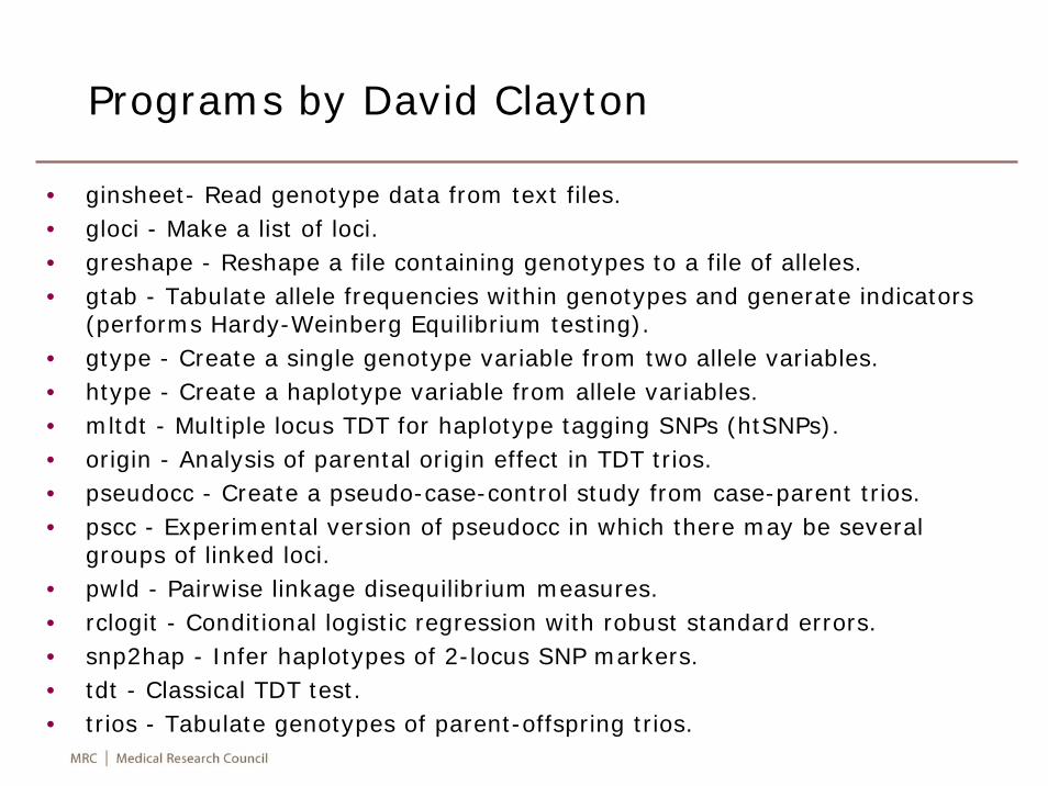
Programs by David Clayton
• ginsheet- Read genotype data from text files.• gloci - Make a list of loci.• greshape - Reshape a file containing genotypes to a file of alleles.• gtab - Tabulate allele frequencies within genotypes and generate indicators
(performs Hardy-Weinberg Equilibrium testing).• gtype - Create a single genotype variable from two allele variables.• htype - Create a haplotype variable from allele variables.• mltdt - Multiple locus TDT for haplotype tagging SNPs (htSNPs).• origin - Analysis of parental origin effect in TDT trios.• pseudocc - Create a pseudo-case-control study from case-parent trios.• pscc - Experimental version of pseudocc in which there may be several
groups of linked loci.• pwld - Pairwise linkage disequilibrium measures.• rclogit - Conditional logistic regression with robust standard errors.• snp2hap - Infer haplotypes of 2-locus SNP markers.• tdt - Classical TDT test.• trios - Tabulate genotypes of parent-offspring trios.
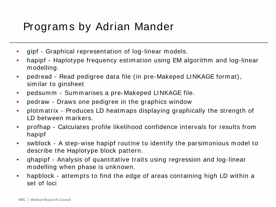
Programs by Adrian Mander
• gipf - Graphical representation of log-linear models.• hapipf - Haplotype frequency estimation using EM algorithm and log-linear
modelling.• pedread - Read pedigree data file (in pre-Makeped LINKAGE format),
similar to ginsheet• pedsumm - Summarises a pre-Makeped LINKAGE file.• pedraw - Draws one pedigree in the graphics window• plotmatrix - Produces LD heatmaps displaying graphically the strength of
LD between markers.• profhap - Calculates profile likelihood confidence intervals for results from
hapipf• swblock - A step-wise hapipf routine to identify the parsimonious model to
describe the Haplotype block pattern.• qhapipf - Analysis of quantitative traits using regression and log-linear
modelling when phase is unknown.• hapblock - attempts to find the edge of areas containing high LD within a
set of loci
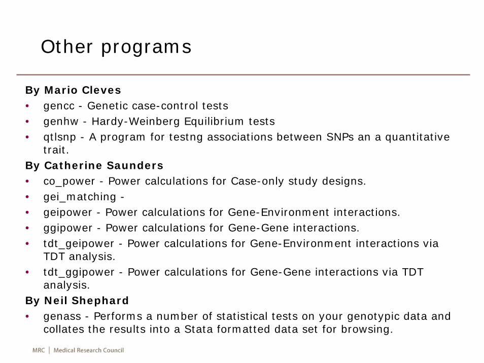
Other programs
By Mario Cleves• gencc - Genetic case-control tests• genhw - Hardy-Weinberg Equilibrium tests• qtlsnp - A program for testng associations between SNPs an a quantitative
trait.By Catherine Saunders• co_power - Power calculations for Case-only study designs.• gei_matching -• geipower - Power calculations for Gene-Environment interactions.• ggipower - Power calculations for Gene-Gene interactions.• tdt_geipower - Power calculations for Gene-Environment interactions via
TDT analysis.• tdt_ggipower - Power calculations for Gene-Gene interactions via TDT
analysis.By Neil Shephard• genass - Performs a number of statistical tests on your genotypic data and
collates the results into a Stata formatted data set for browsing.
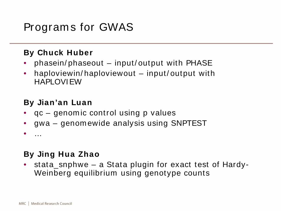
Programs for GWAS
By Chuck Huber• phasein/phaseout – input/output with PHASE• haploviewin/haploviewout – input/output with
HAPLOVIEW
By Jian’an Luan• qc – genomic control using p values• gwa – genomewide analysis using SNPTEST• …
By Jing Hua Zhao• stata_snphwe – a Stata plugin for exact test of Hardy-
Weinberg equilibrium using genotype counts

III Miscellaneous topics
• Meta-analysis
• Risk prediction• Instrumental variable method and structural
equation modeling• Gaussian graphical models and networks• Extreme value modeling
Topics
Meta-analysis
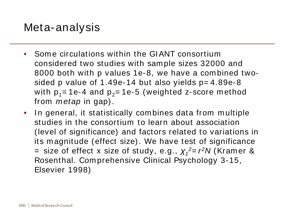
• Some circulations within the GIANT consortium considered two studies with sample sizes 32000 and 8000 both with p values 1e-8, we have a combined two-sided p value of 1.49e-14 but also yields p=4.89e-8 with p1=1e-4 and p2=1e-5 (weighted z-score method from metap in gap).
• In general, it statistically combines data from multiple studies in the consortium to learn about association (level of significance) and factors related to variations in its magnitude (effect size). We have test of significance = size of effect x size of study, e.g., χ1
2=r2N (Kramer & Rosenthal. Comprehensive Clinical Psychology 3-15, Elsevier 1998)
Combining independent tests
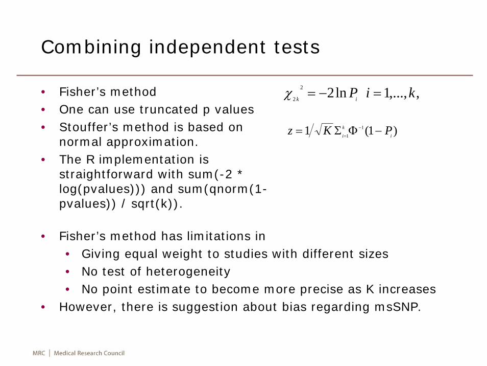
• Fisher’s method• One can use truncated p values• Stouffer’s method is based on
normal approximation.• The R implementation is
straightforward with sum(-2 * log(pvalues))) and sum(qnorm(1-pvalues)) / sqrt(k)).
)1(1 1
1 i
k
i PKz −ΦΣ= −
=
,,...,1ln22
2 kiPik =−=χ
• Fisher’s method has limitations in• Giving equal weight to studies with different sizes• No test of heterogeneity• No point estimate to become more precise as K increases
• However, there is suggestion about bias regarding msSNP.
Regression models for meta-analysis
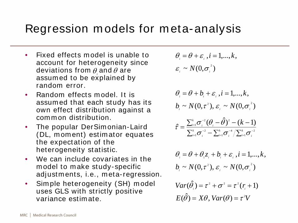
• Fixed effects model is unable to account for heterogeneity since deviations from and are assumed to be explained by random error.
• Random effects model. It is assumed that each study has its own effect distribution against a common distribution.
• The popular DerSimonian-Laird (DL, moment) estimator equates the expectation of the heterogeneity statistic.
• We can include covariates in the model to make study-specific adjustments, i.e., meta-regression.
• Simple heterogeneity (SH) model uses GLS with strictly positive variance estimate.
iθ θ
∑ ∑∑−∑ −−−
== =
−
=
−−
=
−
ki
ki i
ki ii
ki ii k
1 12
142
122 )1()ˆ(ˆ
σσσθθστ
),0(~),,0(~
,,...,1,22
iii
iii
NNb
kib
σετ
εθθ =++=
),0(~
,,...,1,2
ii
ii
N
ki
σε
εθθ =+=
),0(~),,0(~
,,...,1,22
1
iii
iiii
NNb
kibz
σετ
εθθθ =+++=
VVarXE
rVar ii
2
222
)(,)ˆ(
)1()ˆ(
τθθθ
τστθ
==
+=+=
Measure of Heterogeneity
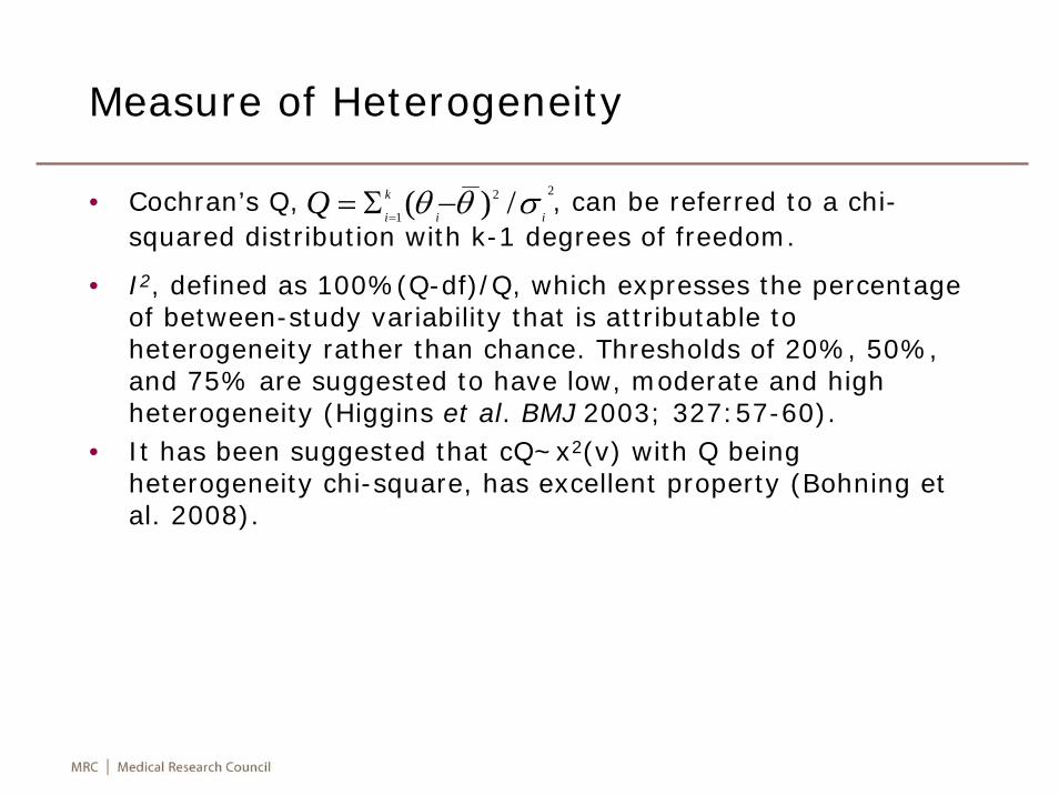
• Cochran’s Q, , can be referred to a chi-squared distribution with k-1 degrees of freedom.
• I2, defined as 100%(Q-df)/Q, which expresses the percentage of between-study variability that is attributable to heterogeneity rather than chance. Thresholds of 20%, 50%, and 75% are suggested to have low, moderate and high heterogeneity (Higgins et al. BMJ 2003; 327:57-60).
• It has been suggested that cQ~x2(v) with Q being heterogeneity chi-square, has excellent property (Bohning et al. 2008).
22
1 /)( ii
k
iQ σθθ −Σ==
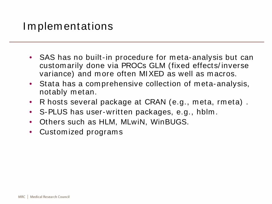
Implementations
• SAS has no built-in procedure for meta-analysis but can customarily done via PROCs GLM (fixed effects/inverse variance) and more often MIXED as well as macros.
• Stata has a comprehensive collection of meta-analysis, notably metan.
• R hosts several package at CRAN (e.g., meta, rmeta) .• S-PLUS has user-written packages, e.g., hblm.• Others such as HLM, MLwiN, WinBUGS.• Customized programs
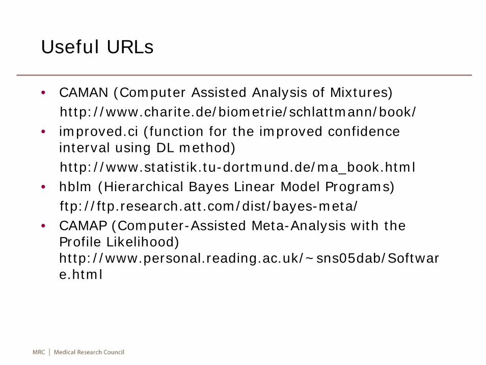
Useful URLs
• CAMAN (Computer Assisted Analysis of Mixtures)http://www.charite.de/biometrie/schlattmann/book/
• improved.ci (function for the improved confidence interval using DL method)http://www.statistik.tu-dortmund.de/ma_book.html
• hblm (Hierarchical Bayes Linear Model Programs)ftp://ftp.research.att.com/dist/bayes-meta/
• CAMAP (Computer-Assisted Meta-Analysis with the Profile Likelihood) http://www.personal.reading.ac.uk/~sns05dab/Software.html
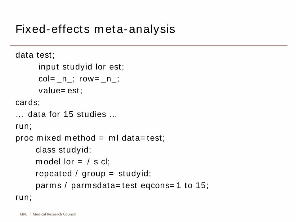
Fixed-effects meta-analysis
data test;input studyid lor est;col=_n_; row=_n_;value=est;
cards;… data for 15 studies …run;proc mixed method = ml data=test;
class studyid;model lor = / s cl;repeated / group = studyid;parms / parmsdata=test eqcons=1 to 15;
run;
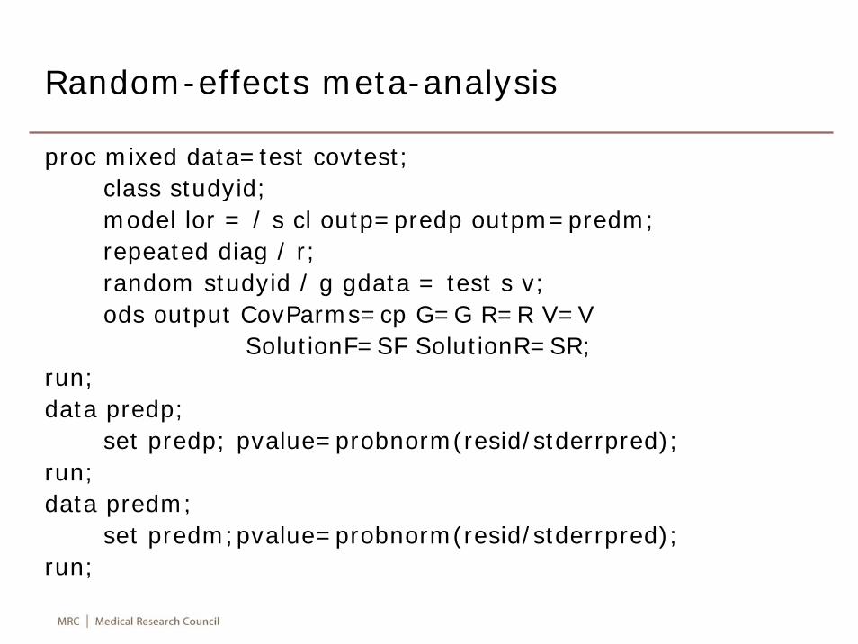
Random-effects meta-analysis
proc mixed data=test covtest;class studyid;model lor = / s cl outp=predp outpm=predm;repeated diag / r;random studyid / g gdata = test s v;ods output CovParms=cp G=G R=R V=V
SolutionF=SF SolutionR=SR;run;data predp;
set predp; pvalue=probnorm(resid/stderrpred);run;data predm;
set predm;pvalue=probnorm(resid/stderrpred);run;
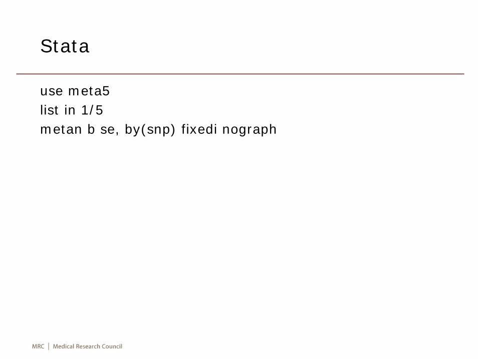
Stata
use meta5list in 1/5metan b se, by(snp) fixedi nograph
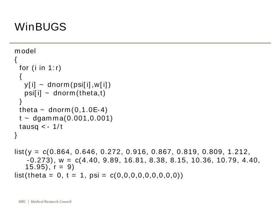
WinBUGS
model{
for (i in 1:r){
y[i] ~ dnorm(psi[i],w[i])psi[i] ~ dnorm(theta,t)
}theta ~ dnorm(0,1.0E-4)t ~ dgamma(0.001,0.001)tausq <- 1/t
}
list(y = c(0.864, 0.646, 0.272, 0.916, 0.867, 0.819, 0.809, 1.212, -0.273), w = c(4.40, 9.89, 16.81, 8.38, 8.15, 10.36, 10.79, 4.40,15.95), r = 9)
list(theta = 0, t = 1, psi = c(0,0,0,0,0,0,0,0,0))
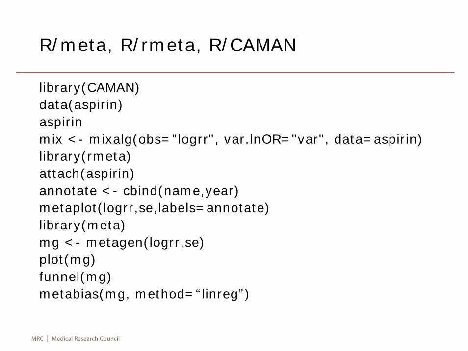
R/meta, R/rmeta, R/CAMAN
library(CAMAN)data(aspirin)aspirinmix <- mixalg(obs="logrr", var.lnOR="var", data=aspirin)library(rmeta)attach(aspirin)annotate <- cbind(name,year)metaplot(logrr,se,labels=annotate)library(meta)mg <- metagen(logrr,se)plot(mg)funnel(mg)metabias(mg, method=“linreg”)
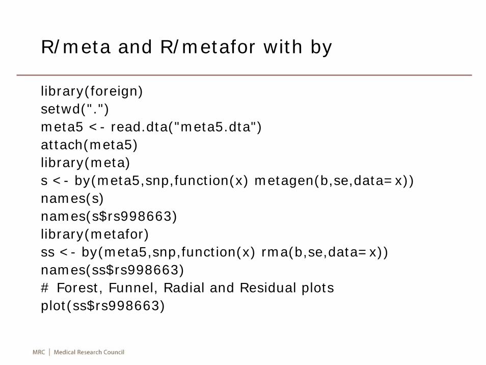
R/meta and R/metafor with by
library(foreign)setwd(".")meta5 <- read.dta("meta5.dta")attach(meta5)library(meta)s <- by(meta5,snp,function(x) metagen(b,se,data=x))names(s)names(s$rs998663)library(metafor)ss <- by(meta5,snp,function(x) rma(b,se,data=x))names(ss$rs998663)# Forest, Funnel, Radial and Residual plotsplot(ss$rs998663)
Customized programs
• META• METAL• MetABEL• R/snpMatrix
A cautionary note
• In a meta-analysis, we compute effect size for each study and combine them but not combine summary data and compute an effects size for the combined data.
• This allows for a check of consistence regarding effect sizes across studies and minimizes the potential confounders.
• If we were to pool data across studies and then compute the effect size from the pooled data, we may get the wrong answer, due to Simpon’s paradox.
See Chapter 13 of Borenstein M, Hedges LV, Higgins JPT, Rothstein HR. Introduction to Meta-Analysis. Wiley 2009
Extensions: multivariate Meta-Analysis
• Background• A gene-based association testing (Neale & Sham) not
dissimilar to the usual Fisher p value method• Multilocus scan statistics (Hoh & Ott) not taking off• Bayesian meta-analysis is more involved and the
formulation via summary data as in Verzilli et al. is not notnecessarily used.
• P values adjusted for correlated tests (p_ACT, Conneely & Boehnke) addresses the following question: What is the minimum p value and more importantly given it is obtained what are the significant levels for all others?
• Problems• Covariance of association tests can be poorly estimated
given multicollinearity between SNPs at a region/gene.
Statistical models
• The data typically involve b, SE from linear regression of nearby SNPs to allow for fixed- and random effects modeling and assessment of statistical significance.
• It is not obvious how to infer covariance matrix involving these b’s. However, we can work around with respect to pair-wise correlations (r).
• For linear regression, it is known that r and t (=b/SE) is related via a simple expression r2=t2/(n-2+t2).
• The covariance between pair-wise correlation has the following form.
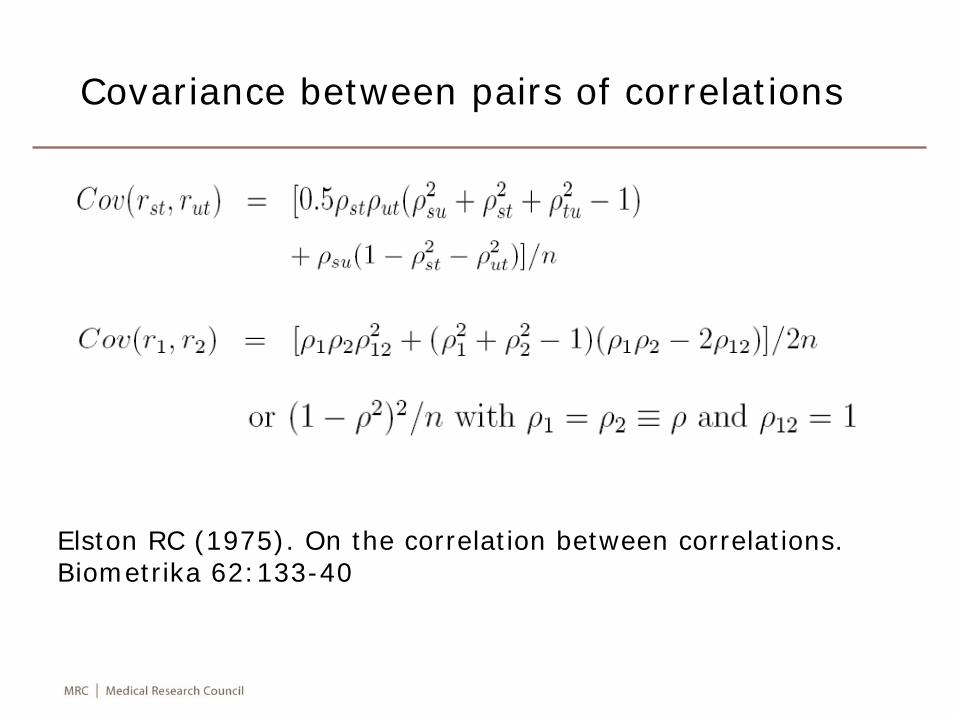
Covariance between pairs of correlations
Elston RC (1975). On the correlation between correlations. Biometrika 62:133-40
Combination of SNPs via GLS
• The results of k independent studies, each with p correlations, can be expressed as the concatenation of the vectors of all available correlations. The large sample variance-covariance matrix is then block diagonal. The estimation of the pooled correlation matrix can then be done via weighting or via a generalized least squares (GLS) framework.
• A test of homogeneity of correlation matrices among studies can be performed (Becker 1992). We can accommodate the heterogeneity via a random effects model such that population correction for specific study is a result of the population correlation and study specific factor.
• The implementation (e.g., in R) accounts for variable number of SNPs from each study (Verzilli et al. 2008).
p_ACT and p_ACT_meta
• p_ACT is based on multivariate normal (MVN) assumption originally for sample with individual genotypes but recently extended to results from consortium meta-analysis.
• The basic idea with p_ACT_meta is to find the minimum p value from the collection of correlated SNPs and obtain subsequent p values based on MVN conditional distributions (Holm’s procedure) using R/mvtnorm.
• It uses a James-Stein shrinkage estimate as implemented in R/corpcor. A description of mvtnormappears in The R Journal.
• However, the omnibus approach noted earlier is appealing.
Summary
• It is far from a comprehensive overview but offers some flavour of the kind of thinking and practice.
• Evidence synthesis with conscious recognition of heterogeneity is in the heart of meta-analysis.
• Fixed effects analysis is restricted to data of the type found in the studies included, but random effects model generalizes to all studies of the type from which our studies were drawn. Results from both models together with SH model are highly recommended.
• We have omitted the graphical aspects, e.g., Bax et al. AJE 2009; 169:249-55. An Excel macro is available from http://www.mix-for-meta-analysis.info/index.html
Risk prediction
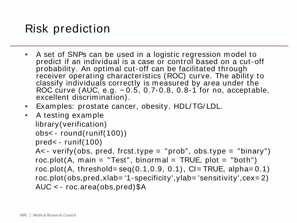
• A set of SNPs can be used in a logistic regression model to predict if an individual is a case or control based on a cut-off probability. An optimal cut-off can be facilitated through receiver operating characteristics (ROC) curve. The ability to classify individuals correctly is measured by area under the ROC curve (AUC, e.g. ~0.5, 0.7-0.8, 0.8-1 for no, acceptable, excellent discrimination).
• Examples: prostate cancer, obesity, HDL/TG/LDL.• A testing example
library(verification)obs<- round(runif(100))pred<- runif(100)A<- verify(obs, pred, frcst.type = "prob", obs.type = "binary")roc.plot(A, main = "Test", binormal = TRUE, plot = "both")roc.plot(A, threshold=seq(0.1,0.9, 0.1), CI=TRUE, alpha=0.1)roc.plot(obs,pred,xlab=‘1-specificity',ylab='sensitivity',cex=2)AUC <- roc.area(obs,pred)$A
0
500
1000
1500
2000
2500
≤6 7 8 9 10 11 12 13 14 15 16 ≥1724
25
26
27
28
0
500
1000
1500
2000
2500
≤6 7 8 9 10 11 12 13 14 15 16 ≥1780
85
90
95
Waist (cm
)
Genetic Risk Score
Freq
uenc
y
Freq
uenc
yBM
I (kg/m2)
Genetic Risk Score
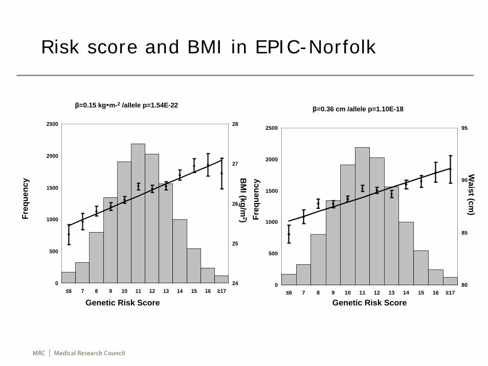
β=0.15 kg m-2 /allele p=1.54E-22 β=0.36 cm /allele p=1.10E-18
Risk score and BMI in EPIC-Norfolk
0.1
1
10
≤6 7 8 9 10 11 12 13 14 15 16 ≥17
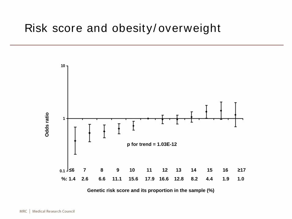
%: 1.4 2.6 6.6 11.1 15.6 17.9 16.6 12.8 8.2 4.4 1.9 1.0
p for trend = 1.03E-12
Odd
s ra
tio
Genetic risk score and its proportion in the sample (%)
Risk score and obesity/overweight
0
0.1
0.2
0.3
0.4
0.5
0.6
0.7
0.8
0.9
1
0 0.1 0.2 0.3 0.4 0.5 0.6 0.7 0.8 0.9 1
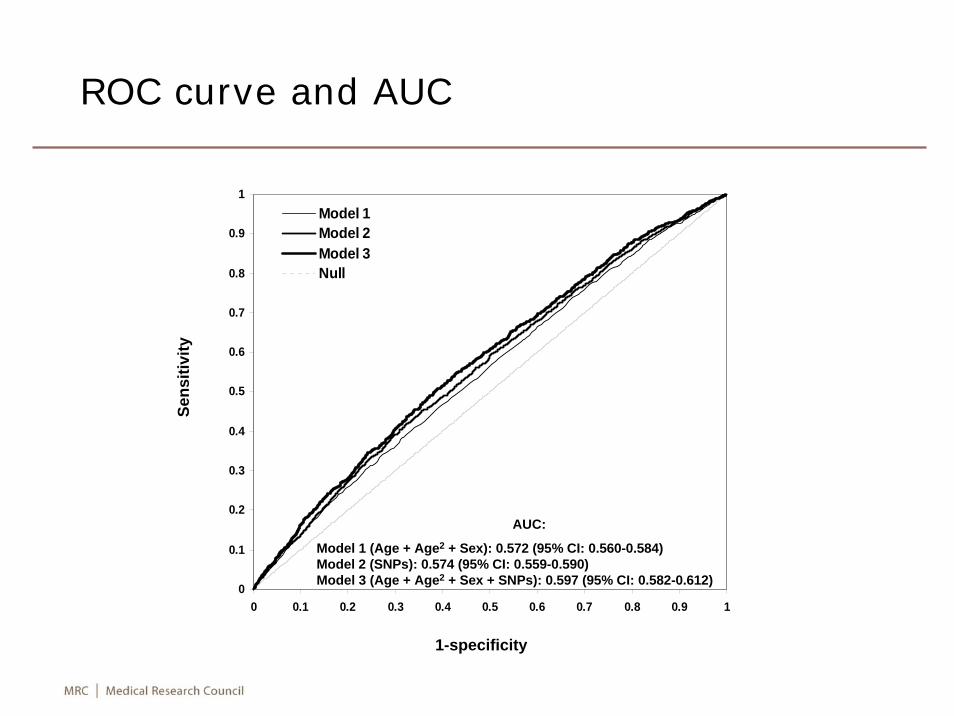
Model 1Model 2Model 3Null
AUC:
Model 1 (Age + Age2 + Sex): 0.572 (95% CI: 0.560-0.584)Model 2 (SNPs): 0.574 (95% CI: 0.559-0.590)Model 3 (Age + Age2 + Sex + SNPs): 0.597 (95% CI: 0.582-0.612)
ROC curve and AUC
Sens
itivi
ty
1-specificity
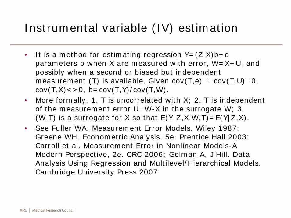
Instrumental variable (IV) estimation
• It is a method for estimating regression Y=(Z X)b+eparameters b when X are measured with error, W=X+U, and possibly when a second or biased but independent measurement (T) is available. Given cov(T,e) = cov(T,U)=0, cov(T,X)<>0, b=cov(T,Y)/cov(T,W).
• More formally, 1. T is uncorrelated with X; 2. T is independent of the measurement error U=W-X in the surrogate W; 3. (W,T) is a surrogate for X so that E(Y|Z,X,W,T)=E(Y|Z,X).
• See Fuller WA. Measurement Error Models. Wiley 1987; Greene WH. Econometric Analysis, 5e. Prentice Hall 2003; Carroll et al. Measurement Error in Nonlinear Models-A Modern Perspective, 2e. CRC 2006; Gelman A, J Hill. Data Analysis Using Regression and Multilevel/Hierarchical Models. Cambridge University Press 2007
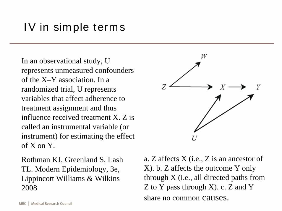
IV in simple terms
In an observational study, U represents unmeasured confounders of the X–Y association. In a randomized trial, U represents variables that affect adherence to treatment assignment and thus influence received treatment X. Z is called an instrumental variable (or instrument) for estimating the effect of X on Y.
Rothman KJ, Greenland S, Lash TL. Modern Epidemiology, 3e, Lippincott Williams & Wilkins 2008
a. Z affects X (i.e., Z is an ancestor of X). b. Z affects the outcome Y only through X (i.e., all directed paths from Z to Y pass through X). c. Z and Y share no common causes.
Instrumental-variables regression (IVLS)
• We can generalize the model as Ynx1=Xnxpβpx1+δ, IVLS or two-stage least squares (2SLS) requires that (i) Xnxpand Znxq with n>q≥p. (ii) Z’X and Z’Z have full rank, pand q respectively. (iii) Y=Xβ+δ. (iv) The δi are i.i.d. with mean 0 and variance σ2. (v) Z is exogeneous, i.e., Z is independent of δ. The cases with q>, =, and < pare called over-, just-, and under- identified, respectively.
• Solution to the system proceeds by multiplying Z on the Y-X model and rescaling by variance such that (Z’Z)−1/2Z’Y=(Z’Z)−1/2Z’Xβ + η, where η = (Z’Z)−1/2Zδ
Freeman DA. Statistical Models-Theory and Practice, Revised Edition. Cambridge University Press, 2009.
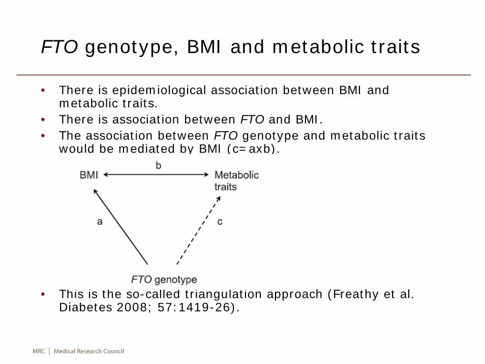
FTO genotype, BMI and metabolic traits
• There is epidemiological association between BMI and metabolic traits.
• There is association between FTO and BMI.• The association between FTO genotype and metabolic traits
would be mediated by BMI (c=axb).
• This is the so-called triangulation approach (Freathy et al. Diabetes 2008; 57:1419-26).
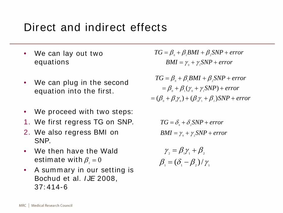
Direct and indirect effects
• We can lay out two equations
• We can plug in the second equation into the first.
• We proceed with two steps: 1. We first regress TG on SNP. 2. We also regress BMI on
SNP.• We then have the Wald
estimate with • A summary in our setting is
Bochud et al. IJE 2008, 37:414-6
errorSNPBMIerrorSNPBMITG
++=+++=
10
210
γγβββ
errorSNPerrorSNP
errorSNPBMITG
++++=+++=+++=
)()()(
211010
1010
210
βγβγββγγββ
βββ
errorSNPTG ++= 20 δδ
errorSNPBMI ++= 20 γγ
1211
2112
/)( γβδββγβγ
−=+=
02 =β
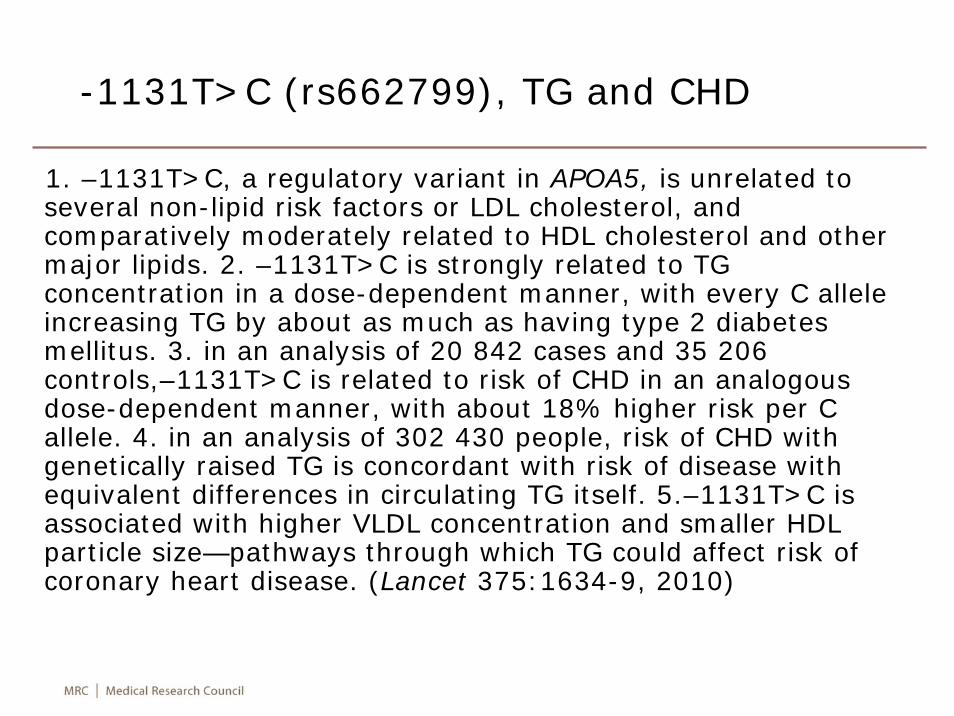
-1131T>C (rs662799), TG and CHD
1. –1131T>C, a regulatory variant in APOA5, is unrelated to several non-lipid risk factors or LDL cholesterol, and comparatively moderately related to HDL cholesterol and other major lipids. 2. –1131T>C is strongly related to TG concentration in a dose-dependent manner, with every C allele increasing TG by about as much as having type 2 diabetes mellitus. 3. in an analysis of 20 842 cases and 35 206 controls,–1131T>C is related to risk of CHD in an analogous dose-dependent manner, with about 18% higher risk per C allele. 4. in an analysis of 302 430 people, risk of CHD with genetically raised TG is concordant with risk of disease with equivalent differences in circulating TG itself. 5.–1131T>C is associated with higher VLDL concentration and smaller HDL particle size—pathways through which TG could affect risk of coronary heart disease. (Lancet 375:1634-9, 2010)
SLC2A9, urate levels and metabolic syndrome
• This example was reported recently by McKeigue et al. Int J Epidemiol. 2010; 39:907-18
• The data contains 583 individuals with sex, age and seven SNPs, one of which is non-synonymous and used as instrumental variable.
• The R package mediation only accepts data without missing values, so we used 493 individuals.
• The authors implemented a Bayesian logistic models and have applied JAGS and have argued in favor of this model over probit model.
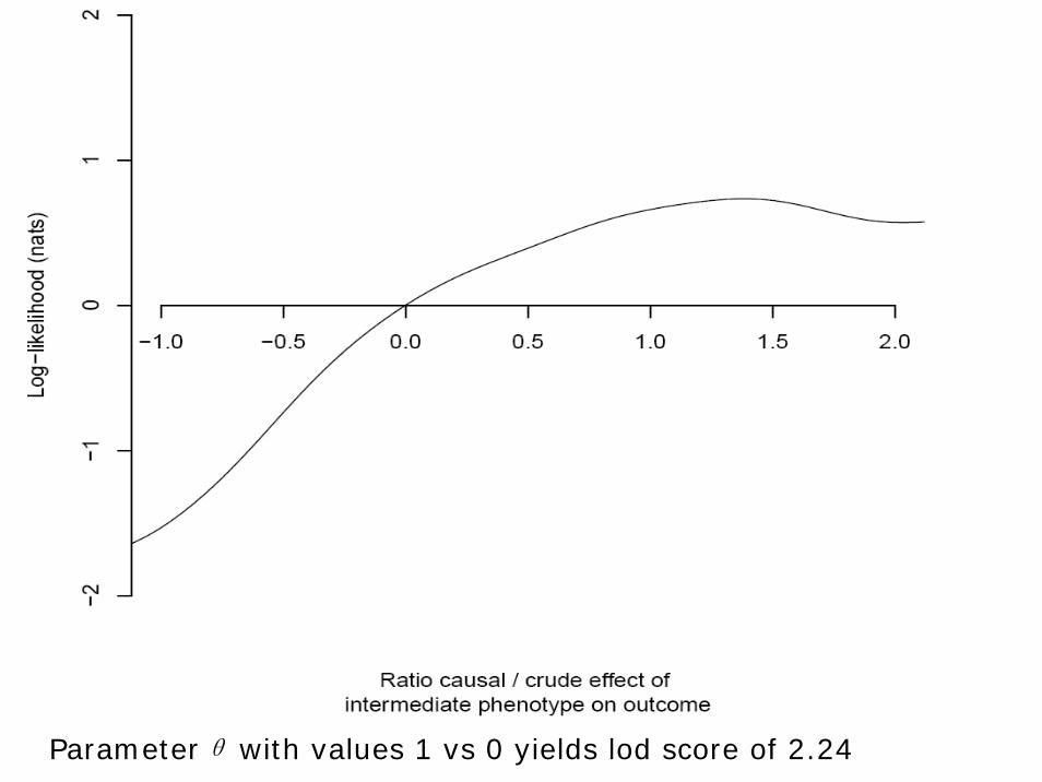
Parameterθ with values 1 vs 0 yields lod score of 2.24
Issues with IV
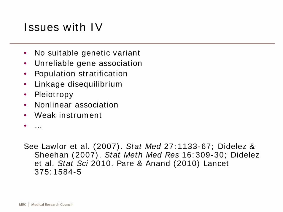
• No suitable genetic variant• Unreliable gene association• Population stratification• Linkage disequilibrium• Pleiotropy• Nonlinear association• Weak instrument• …
See Lawlor et al. (2007). Stat Med 27:1133-67; Didelez & Sheehan (2007). Stat Meth Med Res 16:309-30; Didelezet al. Stat Sci 2010. Pare & Anand (2010) Lancet 375:1584-5
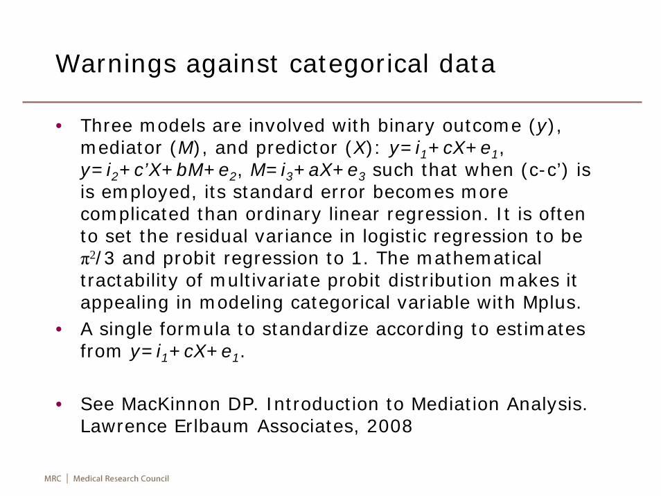
Warnings against categorical data
• Three models are involved with binary outcome (y), mediator (M), and predictor (X): y=i1+cX+e1, y=i2+c’X+bM+e2, M=i3+aX+e3 such that when (c-c’) is is employed, its standard error becomes more complicated than ordinary linear regression. It is often to set the residual variance in logistic regression to be π2/3 and probit regression to 1. The mathematical tractability of multivariate probit distribution makes it appealing in modeling categorical variable with Mplus.
• A single formula to standardize according to estimates from y=i1+cX+e1.
• See MacKinnon DP. Introduction to Mediation Analysis. Lawrence Erlbaum Associates, 2008
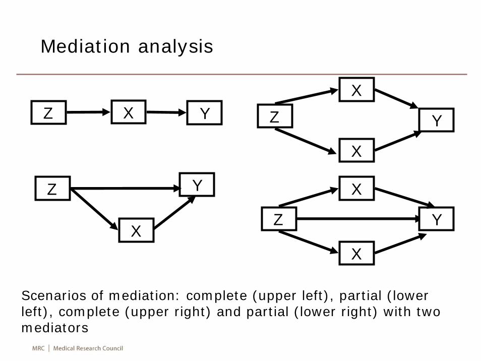
Mediation analysis
Scenarios of mediation: complete (upper left), partial (lower left), complete (upper right) and partial (lower right) with twomediators
Z X Y
Y
X
Z
X
Z Y
X
X
Z Y
X
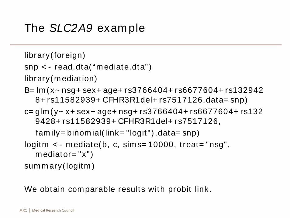
The SLC2A9 example
library(foreign)snp <- read.dta(“mediate.dta”)library(mediation)B=lm(x~nsg+sex+age+rs3766404+rs6677604+rs132942
8+rs11582939+CFHR3R1del+rs7517126,data=snp)c=glm(y~x+sex+age+nsg+rs3766404+rs6677604+rs132
9428+rs11582939+CFHR3R1del+rs7517126,family=binomial(link="logit"),data=snp)
logitm <- mediate(b, c, sims=10000, treat="nsg", mediator="x")
summary(logitm)
We obtain comparable results with probit link.

Results
Quasi-Bayesian Confidence Intervals
Mediation Effect: -0.006834 95% CI -0.022355 0.002811
Direct Effect: -0.1205 95% CI -0.19597 -0.02652Total Effect: -0.1273 95% CI -0.20195 -0.03293Proportion of Total Effect via Mediation: 0.04556 95% CI
0.02904 0.15595
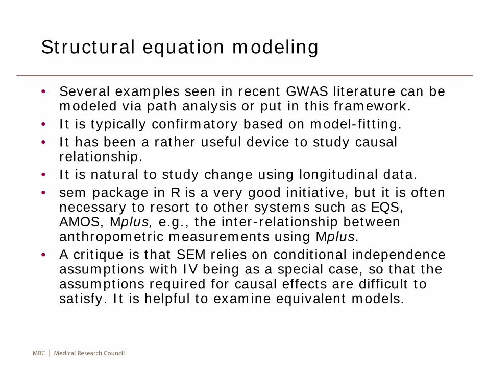
Structural equation modeling
• Several examples seen in recent GWAS literature can be modeled via path analysis or put in this framework.
• It is typically confirmatory based on model-fitting. • It has been a rather useful device to study causal
relationship.• It is natural to study change using longitudinal data.• sem package in R is a very good initiative, but it is often
necessary to resort to other systems such as EQS, AMOS, Mplus, e.g., the inter-relationship between anthropometric measurements using Mplus.
• A critique is that SEM relies on conditional independence assumptions with IV being as a special case, so that the assumptions required for causal effects are difficult to satisfy. It is helpful to examine equivalent models.
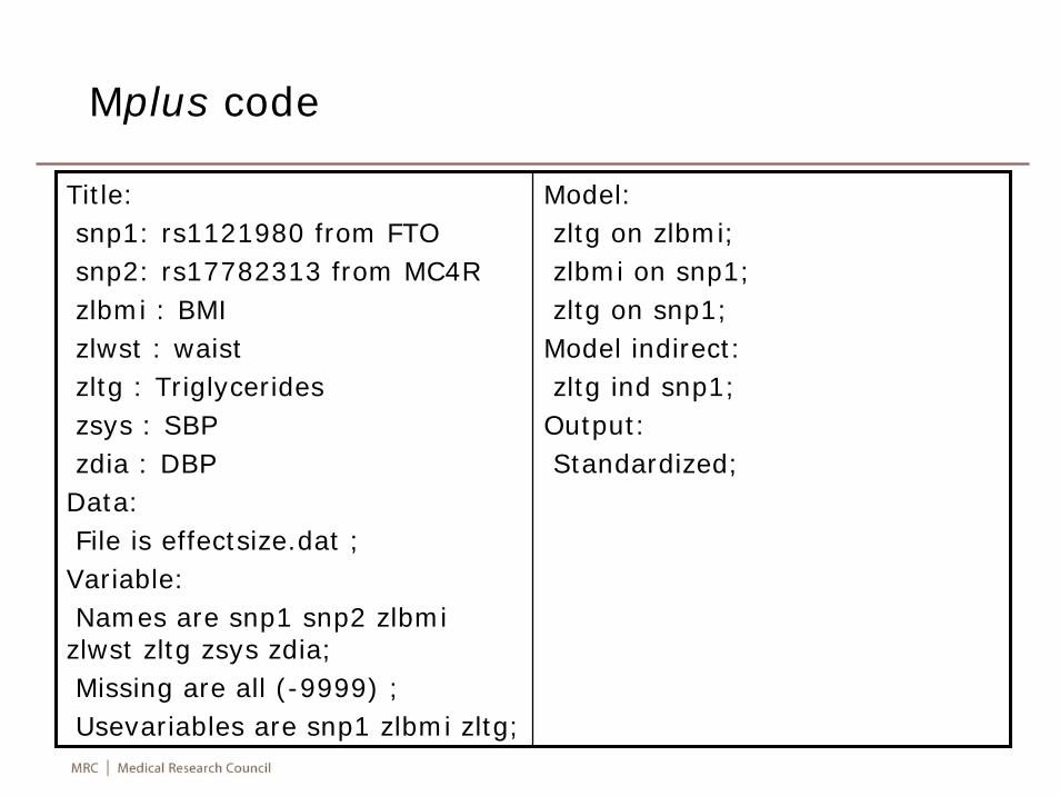
Mplus code
Title:snp1: rs1121980 from FTOsnp2: rs17782313 from MC4Rzlbmi : BMIzlwst : waistzltg : Triglycerideszsys : SBPzdia : DBP
Data:File is effectsize.dat ;
Variable:Names are snp1 snp2 zlbmi
zlwst zltg zsys zdia;Missing are all (-9999) ;Usevariables are snp1 zlbmi zltg;
Model:zltg on zlbmi;zlbmi on snp1;zltg on snp1;
Model indirect:zltg ind snp1;
Output:Standardized;
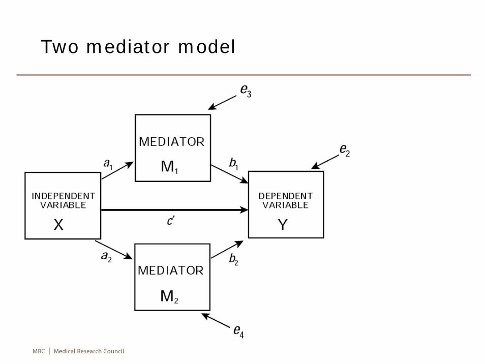
Two mediator model
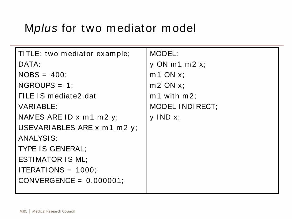
Mplus for two mediator model
TITLE: two mediator example;DATA:NOBS = 400;NGROUPS = 1;FILE IS mediate2.datVARIABLE:NAMES ARE ID x m1 m2 y;USEVARIABLES ARE x m1 m2 y;ANALYSIS:TYPE IS GENERAL;ESTIMATOR IS ML;ITERATIONS = 1000;CONVERGENCE = 0.000001;
MODEL:y ON m1 m2 x;m1 ON x;m2 ON x;m1 with m2;MODEL INDIRECT;y IND x;
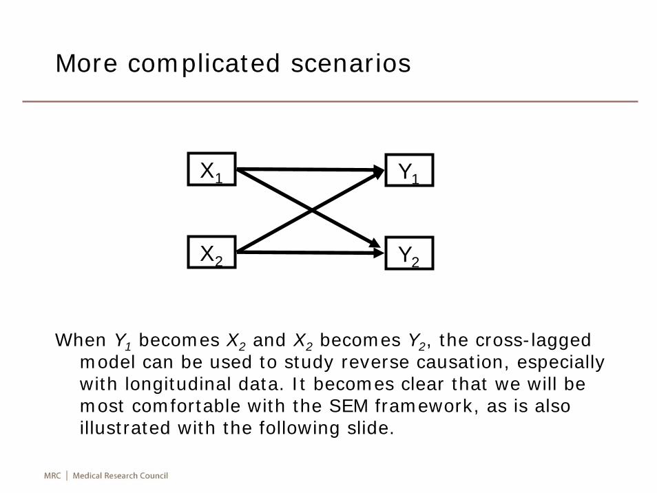
More complicated scenarios
When Y1 becomes X2 and X2 becomes Y2, the cross-lagged model can be used to study reverse causation, especially with longitudinal data. It becomes clear that we will be most comfortable with the SEM framework, as is also illustrated with the following slide.
X1 Y1
X2 Y2
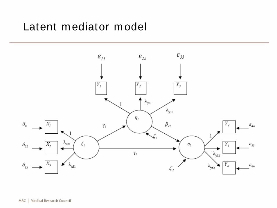
Latent mediator model
Bayesian networks
• Rule-based systems with certainty factors have serious limitations as a method for knowledge representation and reasoning under uncertainty, and attention towards a probabilistic interpretation of certainty factors leads to Bayesian networks.
• It can be described briefly as an acyclic directed graph (DAG) which defines a factorization of a joint probability distribution over the variables represented by the nodes of the DAG.
• The process of construction involves identification of the relevant variables and their causal relations, which leads to DAG specified in terms of a set of conditional probabilities.
Example-GAW15 Problem 1 data
• It was a published data (Morley et al Nature 2004, 430:743-74) on baseline expression levels of 8793 genes in immortalised B cells from 194 individuals in 14 CEPH pedigrees, shown to have linkage and association and evidence of substantial individual variations. In particular, correlation was examined on expression levels of 31 genes and 25 target genes corresponding to two master regulatory regions. We apply Bayesian network analysis to gain further insight into these findings.
• If the expression level of a given gene is regulated by certain proteins then it should be a function of the active levels of these proteins. Due to biological variability and measurement errors, the function would be stochastic rather than deterministic.
• Expression levels of genes are proxies for the activity level of the proteins they encode, although there are numerous examples where activation or silencing of a regulator is carried out by post-transcriptional protein modifications
Methods
• Gene expression levels as continuous variables were assumed to follow a multivariate normal distribution, and consistent with a Bayesian network with linear Gaussian conditional densities. The prior of this network is characterised by a priornetwork reflecting our belief in the joint distribution of the variables in question, and equivalent sample size (ESS) effectively behaving as if it was calculated from a “prior” data set of that size. For instance, without a priori knowledge of the regulatory network, the prior network could be one where all expression levels are independent in order to avoid explicitly biasing the learning procedure to a particular edge.
• The learning procedure starts with a training set and evaluates networks according to an asymptotically consistent scoring function that is obtained through the Bayesian framework. The so-called causal structure assumes that dependencies between variables are due to causal relationships between variables in the model.
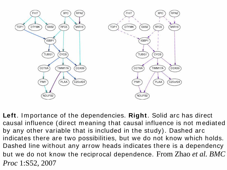
Left. Importance of the dependencies. Right. Solid arc has direct causal influence (direct meaning that causal influence is not mediated by any other variable that is included in the study). Dashed arcindicates there are two possibilities, but we do not know which holds. Dashed line without any arrow heads indicates there is a dependency but we do not know the reciprocal dependence. From Zhao et al. BMC Proc 1:S52, 2007
Highlights of the analysis
• The series of papers on these data stress the importance of Intermediate phenotypes. Without a priori biological hypothesis, it serves as an exploratory tool for subsequent confirmatory analysis.
• This particular analysis highlights the potential usefulness of pathway analysis. An apparent limitation of this work, though not uncommon in gene-expression studies, is the relatively small sample size used. To fully elucidate the biological pathways involved may be difficult, as for instance CYCS is involved in a number of pathways.
• Statistical robustness and biological interpretability remain asthe two main challenges for Bayesian network analyses, to which replication, bootstrap and benchmarking have been proposed.
• Our inference of gene networks also exploits the covariance structure of the data, like structural equation modelling, but is exploratory or hypothesis-generating rather than confirmatory or hypothesis-driven. A number of other software systems are of interest.
A Gaussian graphical model
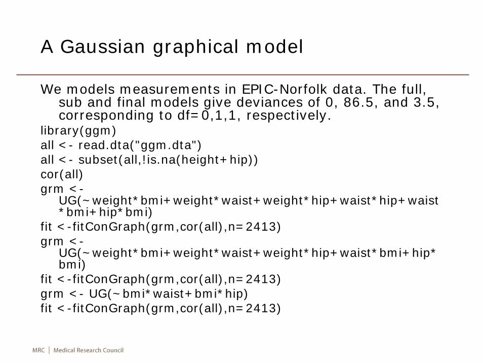
We models measurements in EPIC-Norfolk data. The full, sub and final models give deviances of 0, 86.5, and 3.5, corresponding to df=0,1,1, respectively.
library(ggm)all <- read.dta("ggm.dta")all <- subset(all,!is.na(height+hip))cor(all)grm <-
UG(~weight*bmi+weight*waist+weight*hip+waist*hip+waist*bmi+hip*bmi)
fit <-fitConGraph(grm,cor(all),n=2413)grm <-
UG(~weight*bmi+weight*waist+weight*hip+waist*bmi+hip*bmi)
fit <-fitConGraph(grm,cor(all),n=2413)grm <- UG(~bmi*waist+bmi*hip)fit <-fitConGraph(grm,cor(all),n=2413)
Extreme value theory
• It is concerned with questions related to extreme values in sequences of random variables and in stochastic processes, e.g. Mn=max(X1,…,Xn). An established results state that P((Mn-bn)/an)->H(x) which are of three types and can be combined into a single Generalized Extreme Value (GEV) distribution.
• The distribution of X conditionally on some high threshold often has a limit which follows Generalized Pareto Distribution (GPD).
• An associate model considers r largest order statistics.• See Finkenstädt B, Rootzén H. Extreme Values in
Finance, Telecommunications, and the Environment Chapman and Hall/CRC 2003 and also http://www.stat.unc.edu/postscript/rs/semstatrls.pdf
Annual maximal levels of River Nidd
The data can be used as follows,
library(evir)qplot(nidd.annual)data(nidd.annual)nidd.gev <- gev(nidd.annual)plot(nidd.gev)meplot(nidd.annual)shape(nidd.annual)pfit <- gpd(nidd.annual, threshold=200)plot(pfit)quant(nidd.annual)
Summary
• We have covered a variety of topics ranging from meta-analysis to causal modelling, which is expected to be more familiar with more genetic variants being established.
• They are general since some topics are also quite familiar to researchers at other fields (e.g., psychology, social science, econometrics) where for instance structural equation modelling are routinely used.
References
• Bohning D, Kuhnert R, Rattanasiri S. Meta-Analysis of Binary Data Using Profile Likelihood. CRC Press, 2008
• Conneely KN, Boehnke M. AJHG 2007;81:1158-68• Demidenko E. Mixed Models. Wiley, 2004• Harris et al. Stata J 2008; 8:3-28• Hartung J, Guido K, Sinha BK. Statistical Meta-Analysis with
Applications. Wiley, 2008• Normand S-L. T. Stat Med 1999;18:321-59• Rao DC, Gu CC. Genetic Dissection of Complex Traits, 2e.
Academic Press, 2008• Schlattmann P. Medical Applications for Finite Mixture Models.
Wiley, 2009• Sidik & Jonkman. Appl Stat 2005; 54:367-84• Sterne J. Meta-Analysis in Stata. Stata Press, 2009.• Sutton AJ, Abrams KR, Jones DR, Sheldon TA, Song F. Methods
for Meta-Analysis in Medical Research. Wiley, 2000• Verzilli et al. AJHG 2008; 82:859-72• Whitehead A. Meta-Analysis of Controlled Clinical Trials. Wiley,
2002
References
• Krzanowski WJ, Hand DJ. ROC Curves for Continuous Data. CRC 2009• Pepe, M.S. The Statistical Evaluation of Medical Tests for
Classification and Prediction. Oxford University Press, 2003• Gonen M. Analyzing Receiver Operating Characteristic Curves with
SAS, SAS Institute Inc., 2007• Loehlin JC. Latent Variable Models-An Introduction to Factor, Path,
and Structural Equation Analysis. 4e, Lawrence Erlbaum Associates, 2004
• Kline RB. Principles and Practice of Structural Equation Modeling. 2e, The Guiford Press, 2005
• Bollen KA, PJ Curran. Latent Curve Models-A Structural Equation Perspective. Wiley, 2006
• Kjaerulff UB, AL Madsen. Bayesian Networks and Influence Diagrams-A Guide to Construction and Analysis. Springer, 2008
• Emmert-Streib F, Matthias D. Analysis of Microarray Data-A Network-Based Approach. Wiley-VCH, 2008
• Junker BH, F Schreiber (Ed). Analysis of Biological Networks. Wiley, 2008

IV OpenMx and NCBI2R
Topics
• Heritability estimation
BackgroundFamily dataTwin dataOpenMxSummary
• Information retrieval with NCBI2R• Further information
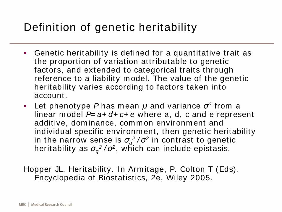
Definition of genetic heritability
• Genetic heritability is defined for a quantitative trait as the proportion of variation attributable to genetic factors, and extended to categorical traits through reference to a liability model. The value of the genetic heritability varies according to factors taken into account.
• Let phenotype P has mean μ and variance σ2 from a linear model P=a+d+c+e where a, d, c and e represent additive, dominance, common environment and individual specific environment, then genetic heritability in the narrow sense is σa
2 /σ2 in contrast to genetic heritability as σg
2 /σ2, which can include epistasis.
Hopper JL. Heritability. In Armitage, P. Colton T (Eds). Encyclopedia of Biostatistics, 2e, Wiley 2005.
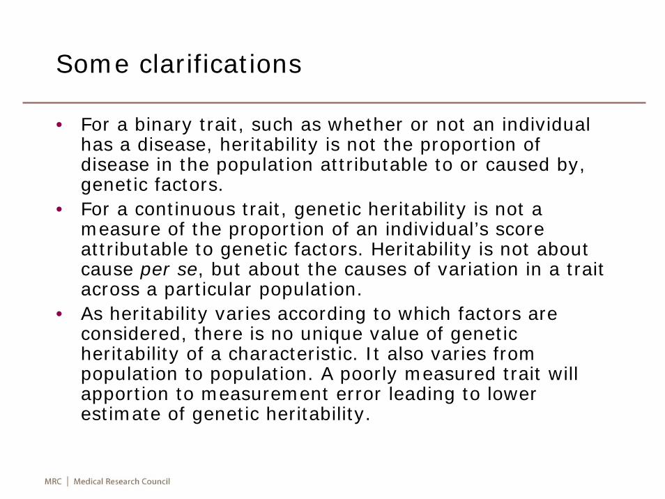
Some clarifications
• For a binary trait, such as whether or not an individual has a disease, heritability is not the proportion of disease in the population attributable to or caused by, genetic factors.
• For a continuous trait, genetic heritability is not a measure of the proportion of an individual’s score attributable to genetic factors. Heritability is not about cause per se, but about the causes of variation in a trait across a particular population.
• As heritability varies according to which factors are considered, there is no unique value of genetic heritability of a characteristic. It also varies from population to population. A poorly measured trait will apportion to measurement error leading to lower estimate of genetic heritability.
Heritability studies
• Family studies• Adoption (rearing of a nonbiological child) studies• Migrant studies – migrants carry a risk reflecting country of
origin• Twin study – differences between monozygotic and dizygotic
twins can be attributed to genetic influence
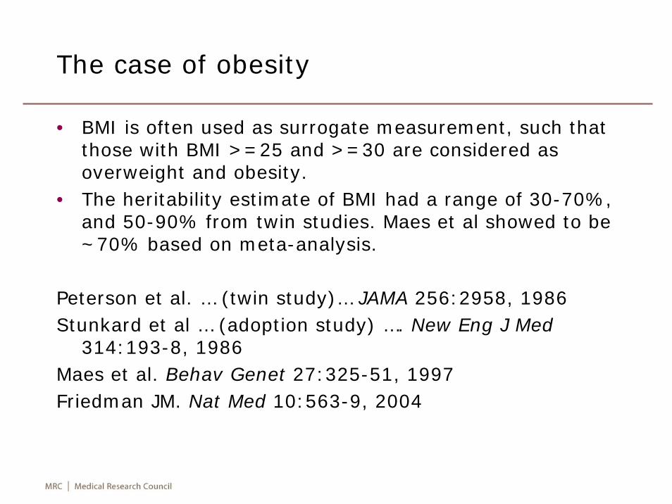
The case of obesity
• BMI is often used as surrogate measurement, such that those with BMI >=25 and >=30 are considered as overweight and obesity.
• The heritability estimate of BMI had a range of 30-70%, and 50-90% from twin studies. Maes et al showed to be ~70% based on meta-analysis.
Peterson et al. … (twin study)… JAMA 256:2958, 1986Stunkard et al … (adoption study) …. New Eng J Med
314:193-8, 1986Maes et al. Behav Genet 27:325-51, 1997Friedman JM. Nat Med 10:563-9, 2004
Path analysis of nuclear family data
• Recall that for the model P=G+C+E, can be re-expressed with path coefficients so that P=hG+cC+Eand to allow for intergenerational difference this can be written as P=hzG+cyC+E for parents.
• We can also allow for correlation between parental phenotypes (homogamy) as with gene-environment correlations.
• We have the following path analysis model, noting that it uses the notion of “environmental indices” and sometime transformation of the phenotype for normality.
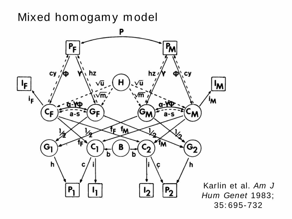
Mixed homogamy model
Karlin et al. Am J Hum Genet 1983;
35:695-732
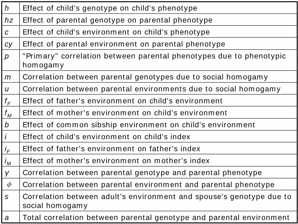
h Effect of child's genotype on child's phenotype
hz Effect of parental genotype on parental phenotype
c Effect of child's environment on child's phenotype
cy Effect of parental environment on parental phenotype
p "Primary" correlation between parental phenotypes due to phenotypichomogamy
m Correlation between parental genotypes due to social homogamy
u Correlation between parental environments due to social homogamy
fF Effect of father's environment on child's environment
fM Effect of mother's environment on child's environment
b Effect of common sibship environment on child's environment
i Effect of child's environment on child's index
iF Effect of father's environment on father's index
iM Effect of mother's environment on mother's index
γ Correlation between parental genotype and parental phenotype
φ Correlation between parental environment and parental phenotype
s Correlation between adult's environment and spouse's genotype due to social homogamy
a Total correlation between parental genotype and parental environment
Segregation analysis of family data
• When family data is available, we can examine major gene effect(s) together with collective loci with small and individually unmeasurable effects in a so-called mixed model (Morton NE, MacLean CJ. Am J Hum Genet1974;26:489-503).
• It can also incorporate parameters for covariates such as age, sex and race.
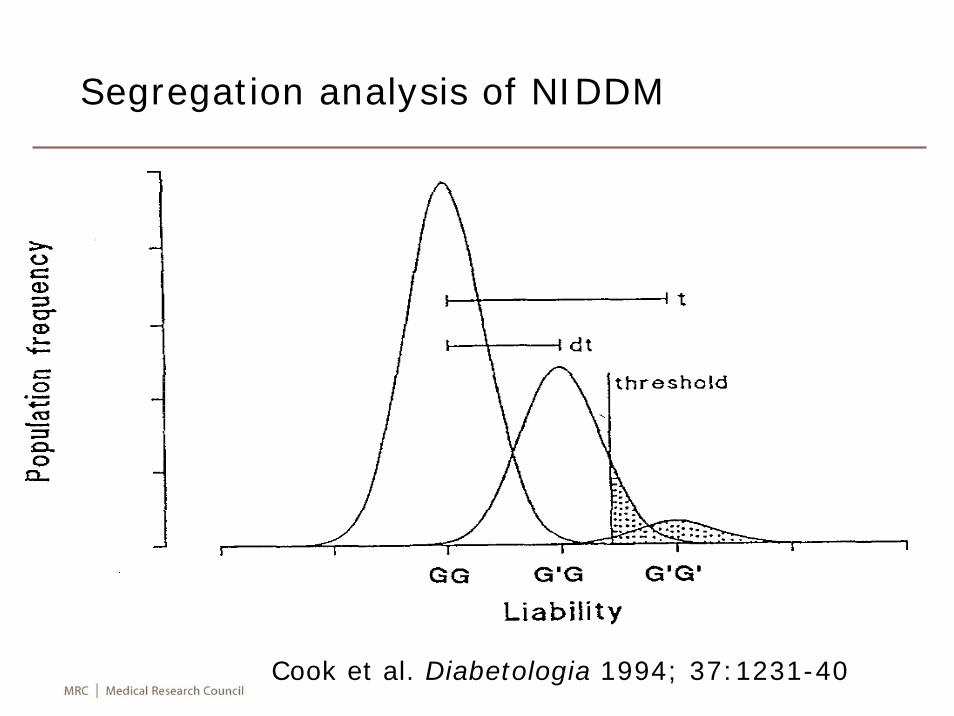
Segregation analysis of NIDDM
Cook et al. Diabetologia 1994; 37:1231-40
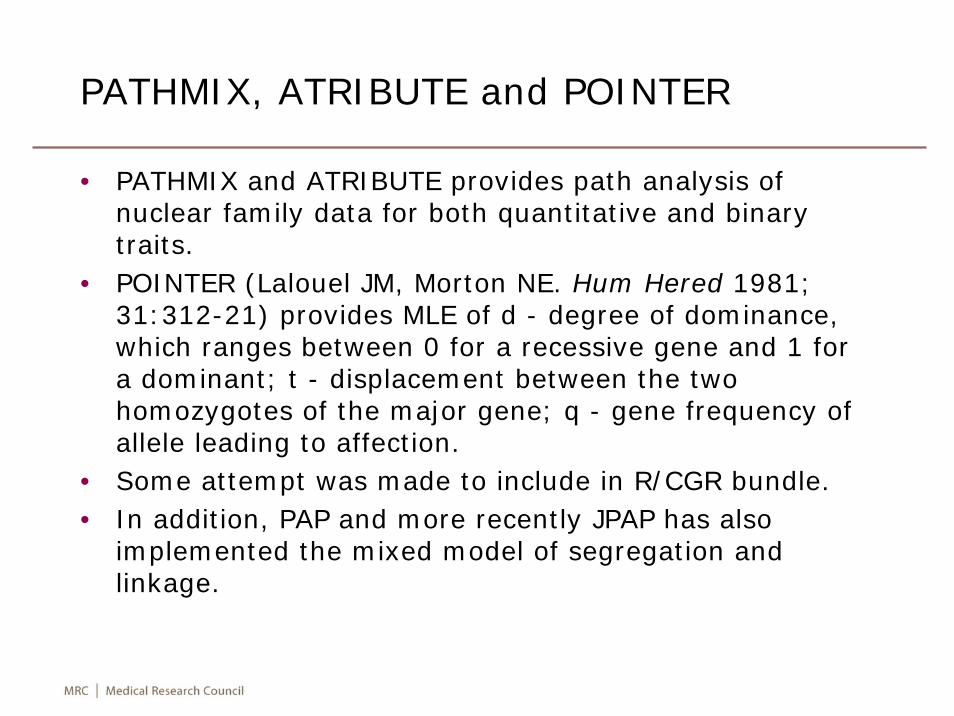
PATHMIX, ATRIBUTE and POINTER
• PATHMIX and ATRIBUTE provides path analysis of nuclear family data for both quantitative and binary traits.
• POINTER (Lalouel JM, Morton NE. Hum Hered 1981; 31:312-21) provides MLE of d - degree of dominance, which ranges between 0 for a recessive gene and 1 for a dominant; t - displacement between the twohomozygotes of the major gene; q - gene frequency of allele leading to affection.
• Some attempt was made to include in R/CGR bundle.• In addition, PAP and more recently JPAP has also
implemented the mixed model of segregation and linkage.
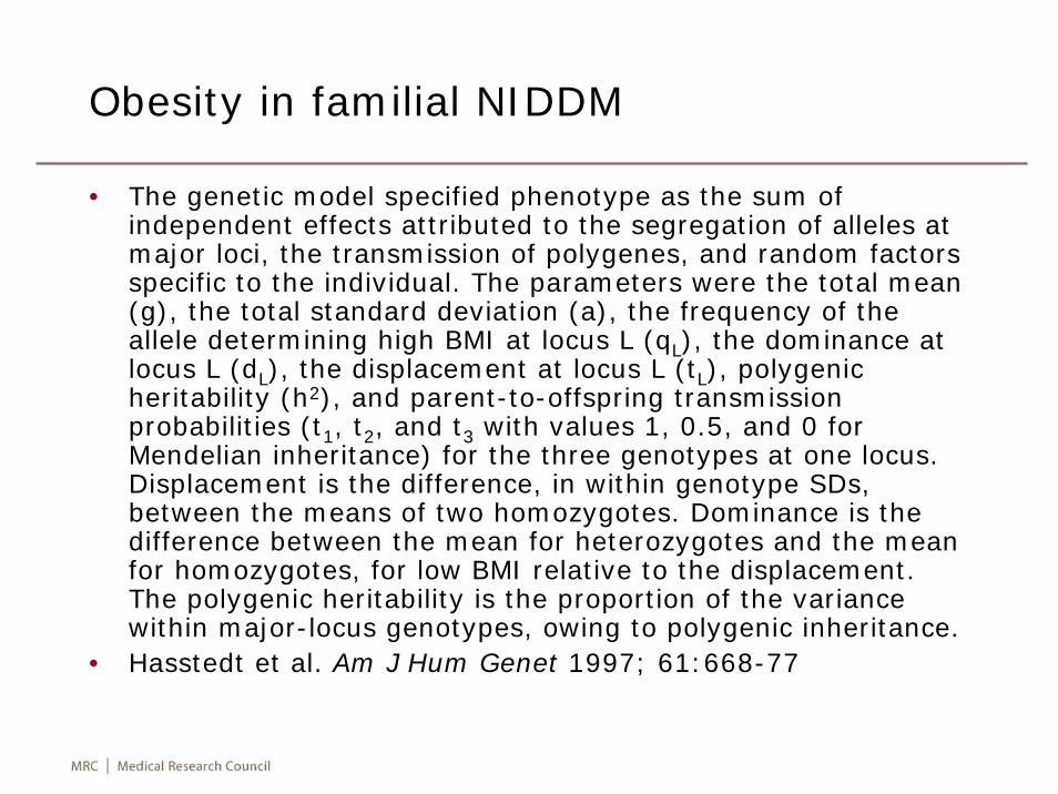
Obesity in familial NIDDM
• The genetic model specified phenotype as the sum of independent effects attributed to the segregation of alleles at major loci, the transmission of polygenes, and random factors specific to the individual. The parameters were the total mean(g), the total standard deviation (a), the frequency of the allele determining high BMI at locus L (qL), the dominance at locus L (dL), the displacement at locus L (tL), polygenic heritability (h2), and parent-to-offspring transmission probabilities (t1, t2, and t3 with values 1, 0.5, and 0 for Mendelian inheritance) for the three genotypes at one locus. Displacement is the difference, in within genotype SDs, between the means of two homozygotes. Dominance is the difference between the mean for heterozygotes and the mean for homozygotes, for low BMI relative to the displacement. The polygenic heritability is the proportion of the variance within major-locus genotypes, owing to polygenic inheritance.
• Hasstedt et al. Am J Hum Genet 1997; 61:668-77
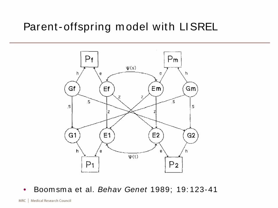
Parent-offspring model with LISREL
• Boomsma et al. Behav Genet 1989; 19:123-41

SOLAR
• SOLAR (Sequential Oligogenci Linkage Analysis Routine, Almasy L, Blangero J. Am J Hum Genet 1998; 62:1198-211) uses likelihood ratio tests to evaluate heritability by comparing a purely polygenic model with a sporadic model in the case of testing heritability.
• In a polygenic model, h2r is the total additive genetic heritability. In a linkage model (with one or more locus specific elements) h2q1 represents the heritability associated with the first locus, and h2r represents the residual genetic variance. In a oligogenic model, there may also be h2q2, h2q3, etc.
• Sung J, et al. JCEM 2009; 94:4946-52. reported a recent study of twins with adjusted (age, sex, age2, age2 x sex, total calorie intake, smoking and alcohol use) heritabilities for waist circumference (59%), glucose (59%), HDL (77%), TG (46%).
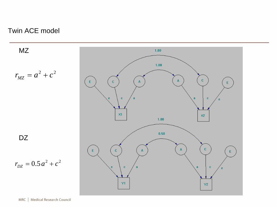
MZ
DZ
Twin ACE model
22 carMZ +=
225.0 carDZ +=
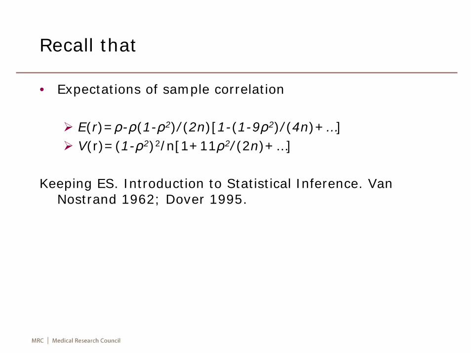
Recall that
• Expectations of sample correlation
E(r)=ρ-ρ(1-ρ2)/(2n)[1-(1-9ρ2)/(4n)+…]V(r)=(1-ρ2)2/n[1+11ρ2/(2n)+…]
Keeping ES. Introduction to Statistical Inference. Van Nostrand 1962; Dover 1995.
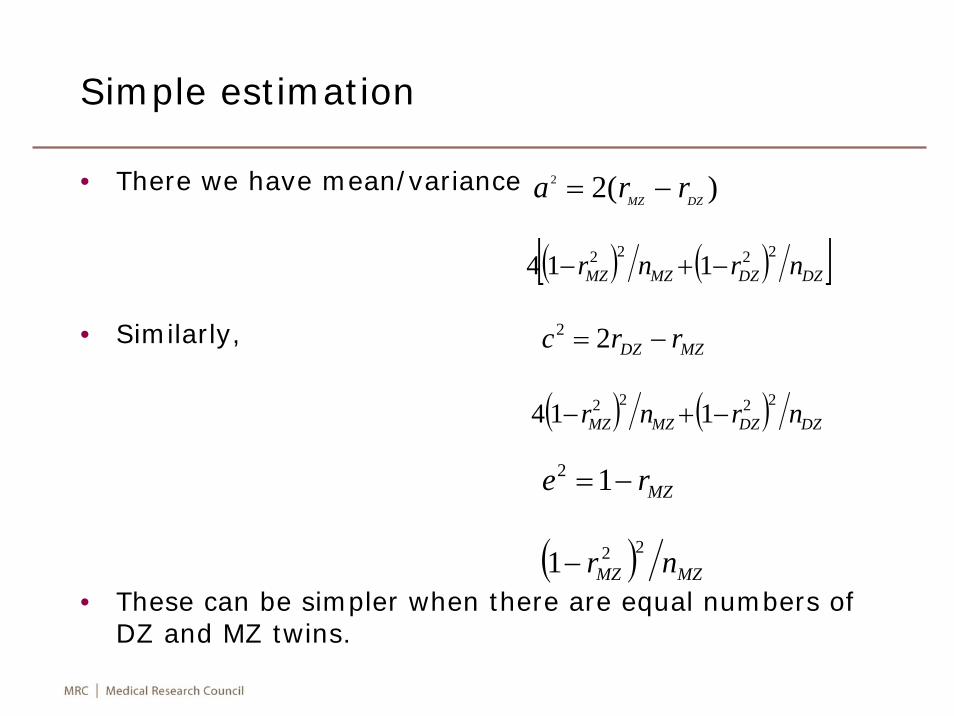
Simple estimation
• There we have mean/variance
• Similarly,
• These can be simpler when there are equal numbers of DZ and MZ twins.
( ) ( )[ ]DZDZMZMZ nrnr 2222 114 −+−
)(22
DZMZ rra −=
( ) ( ) DZDZMZMZ nrnr 2222 114 −+−
MZDZ rrc −= 22
( ) MZMZ nr 221−
MZre −=12
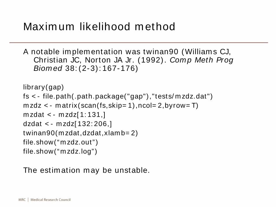
Maximum likelihood method
A notable implementation was twinan90 (Williams CJ, Christian JC, Norton JA Jr. (1992). Comp Meth ProgBiomed 38:(2-3):167-176)
library(gap)fs <- file.path(.path.package("gap"),"tests/mzdz.dat")mzdz <- matrix(scan(fs,skip=1),ncol=2,byrow=T)mzdat <- mzdz[1:131,]dzdat <- mzdz[132:206,]twinan90(mzdat,dzdat,xlamb=2)file.show(“mzdz.out”)file.show(“mzdz.log”)
The estimation may be unstable.
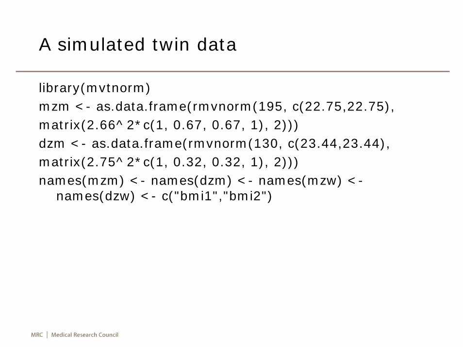
A simulated twin data
library(mvtnorm)mzm <- as.data.frame(rmvnorm(195, c(22.75,22.75), matrix(2.66^2*c(1, 0.67, 0.67, 1), 2)))dzm <- as.data.frame(rmvnorm(130, c(23.44,23.44), matrix(2.75^2*c(1, 0.32, 0.32, 1), 2)))names(mzm) <- names(dzm) <- names(mzw) <-
names(dzw) <- c("bmi1","bmi2")
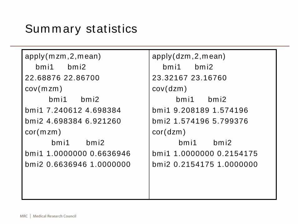
Summary statistics
apply(mzm,2,mean)bmi1 bmi2
22.68876 22.86700cov(mzm)
bmi1 bmi2bmi1 7.240612 4.698384bmi2 4.698384 6.921260cor(mzm)
bmi1 bmi2bmi1 1.0000000 0.6636946bmi2 0.6636946 1.0000000
apply(dzm,2,mean)bmi1 bmi2
23.32167 23.16760cov(dzm)
bmi1 bmi2bmi1 9.208189 1.574196bmi2 1.574196 5.799376cor(dzm)
bmi1 bmi2bmi1 1.0000000 0.2154175bmi2 0.2154175 1.0000000
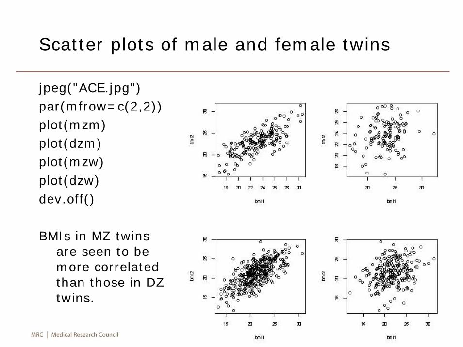
Scatter plots of male and female twins
jpeg("ACE.jpg")par(mfrow=c(2,2))plot(mzm)plot(dzm)plot(mzw)plot(dzw)dev.off()
BMIs in MZ twins are seen to be more correlated than those in DZ twins.
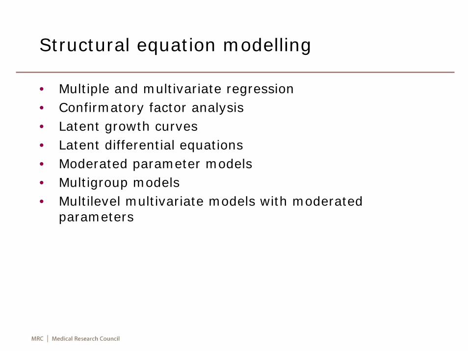
Structural equation modelling
• Multiple and multivariate regression• Confirmatory factor analysis• Latent growth curves• Latent differential equations• Moderated parameter models• Multigroup models• Multilevel multivariate models with moderated
parameters
Mx, MxGUI, OpenMx
• Mx is a well-established software for structural equation modeling and in particular widely used in twin modeling.
• MxGUI is Windows-based program which greatly facilitate the modeling process.
• OpenMx is a recent initiative to take advantage of the R environment. It carries over a variety of features from Mx/MxGUI.
• As it implies, the software is freely available from http://openmx.psyc.virginia.edu
• As it is written in R, it is considerably simple in our context to explore functionality it provides. We have adapted some examples from OpenMx website and for extended description, it is recommended to visit there.
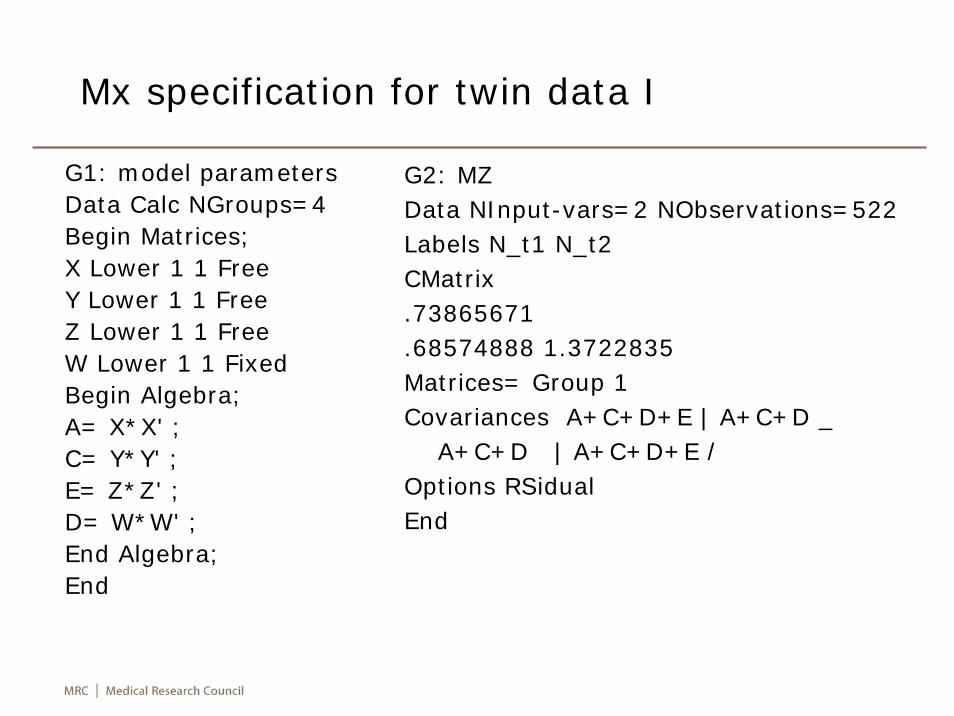
Mx specification for twin data I
G1: model parametersData Calc NGroups=4Begin Matrices;X Lower 1 1 FreeY Lower 1 1 FreeZ Lower 1 1 FreeW Lower 1 1 FixedBegin Algebra;A= X*X' ;C= Y*Y' ;E= Z*Z' ;D= W*W' ;End Algebra;End
G2: MZData NInput-vars=2 NObservations=522Labels N_t1 N_t2CMatrix.73865671.68574888 1.3722835Matrices= Group 1Covariances A+C+D+E | A+C+D _
A+C+D | A+C+D+E /Options RSidualEnd
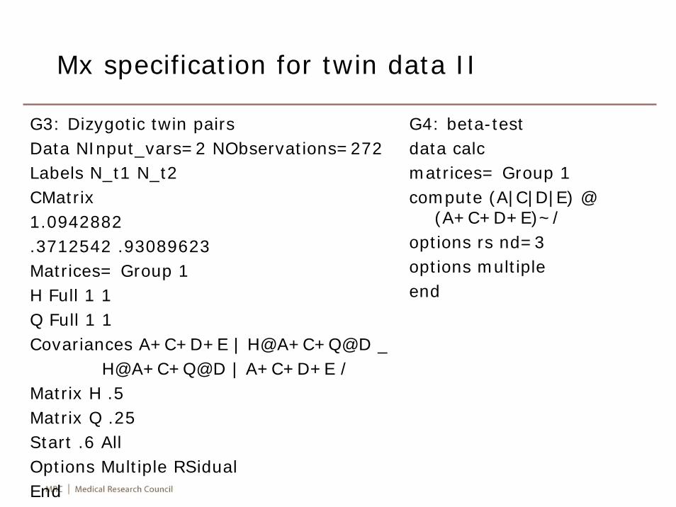
Mx specification for twin data II
G3: Dizygotic twin pairsData NInput_vars=2 NObservations=272Labels N_t1 N_t2CMatrix1.0942882.3712542 .93089623Matrices= Group 1H Full 1 1Q Full 1 1Covariances A+C+D+E | H@A+C+Q@D _
H@A+C+Q@D | A+C+D+E /Matrix H .5Matrix Q .25Start .6 AllOptions Multiple RSidualEnd
G4: beta-testdata calcmatrices= Group 1compute (A|C|D|E) @
(A+C+D+E)~/options rs nd=3options multipleend
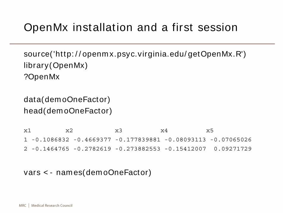
OpenMx installation and a first session
source('http://openmx.psyc.virginia.edu/getOpenMx.R')library(OpenMx)?OpenMx
data(demoOneFactor)head(demoOneFactor)
x1 x2 x3 x4 x5
1 -0.1086832 -0.4669377 -0.177839881 -0.08093113 -0.07065026
2 -0.1464765 -0.2782619 -0.273882553 -0.15412007 0.09271729
vars <- names(demoOneFactor)
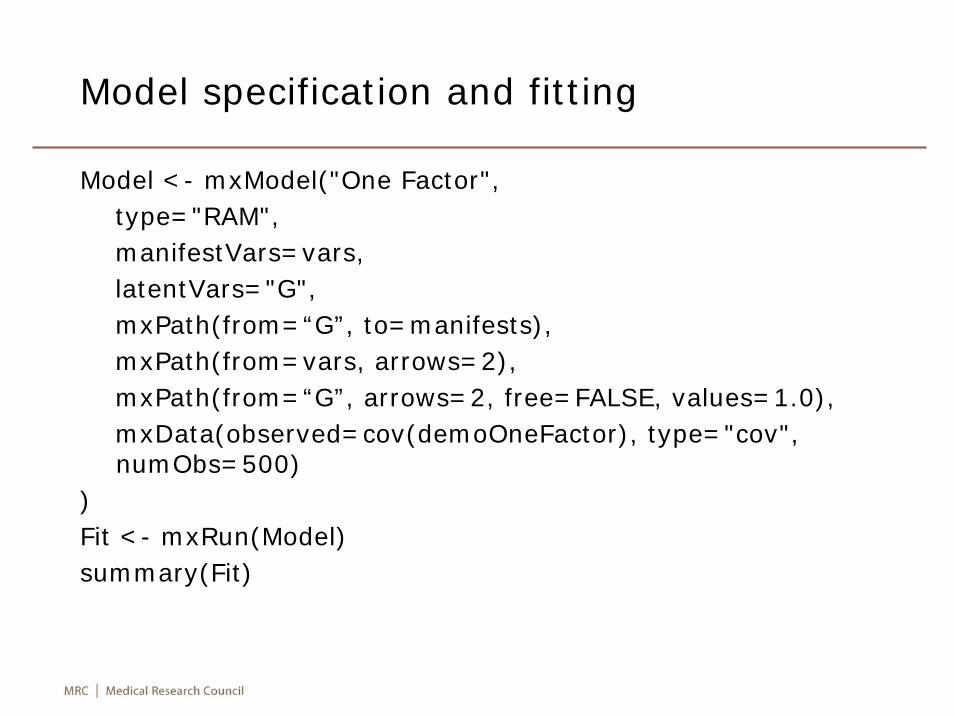
Model specification and fitting
Model <- mxModel("One Factor", type="RAM",manifestVars=vars, latentVars="G",mxPath(from=“G”, to=manifests),mxPath(from=vars, arrows=2),mxPath(from=“G”, arrows=2, free=FALSE, values=1.0),mxData(observed=cov(demoOneFactor), type="cov", numObs=500)
)Fit <- mxRun(Model)summary(Fit)
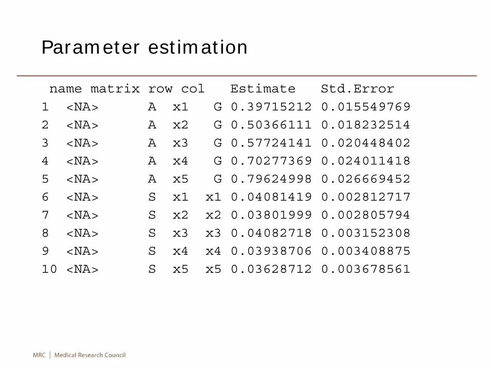
Parameter estimation
name matrix row col Estimate Std.Error1 <NA> A x1 G 0.39715212 0.015549769
2 <NA> A x2 G 0.50366111 0.018232514
3 <NA> A x3 G 0.57724141 0.0204484024 <NA> A x4 G 0.70277369 0.024011418
5 <NA> A x5 G 0.79624998 0.0266694526 <NA> S x1 x1 0.04081419 0.002812717
7 <NA> S x2 x2 0.03801999 0.002805794
8 <NA> S x3 x3 0.04082718 0.0031523089 <NA> S x4 x4 0.03938706 0.003408875
10 <NA> S x5 x5 0.03628712 0.003678561
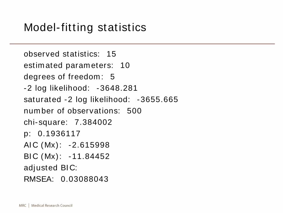
Model-fitting statistics
observed statistics: 15estimated parameters: 10degrees of freedom: 5-2 log likelihood: -3648.281saturated -2 log likelihood: -3655.665number of observations: 500chi-square: 7.384002p: 0.1936117AIC (Mx): -2.615998BIC (Mx): -11.84452adjusted BIC:RMSEA: 0.03088043
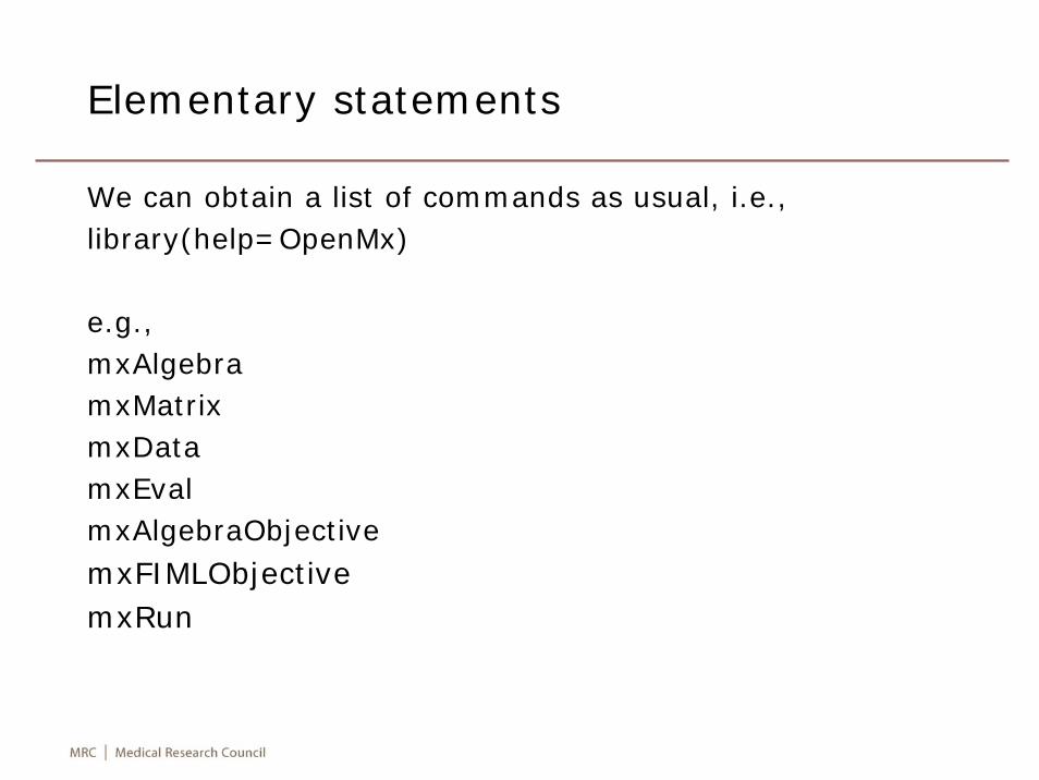
Elementary statements
We can obtain a list of commands as usual, i.e.,library(help=OpenMx)
e.g.,mxAlgebramxMatrixmxDatamxEvalmxAlgebraObjectivemxFIMLObjectivemxRun
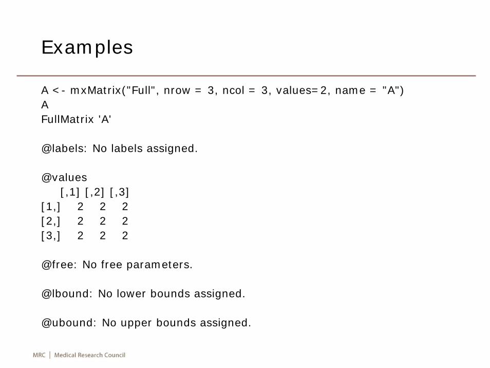
Examples
A <- mxMatrix("Full", nrow = 3, ncol = 3, values=2, name = "A")AFullMatrix 'A'
@labels: No labels assigned.
@values[,1] [,2] [,3]
[1,] 2 2 2[2,] 2 2 2[3,] 2 2 2
@free: No free parameters.
@lbound: No lower bounds assigned.
@ubound: No upper bounds assigned.
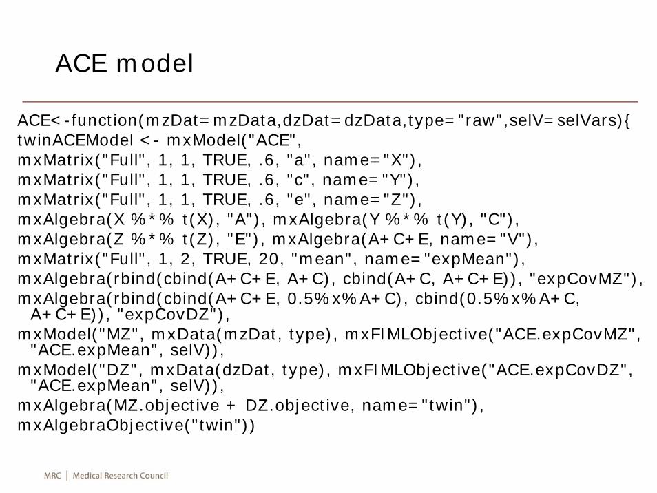
ACE model
ACE<-function(mzDat=mzData,dzDat=dzData,type="raw",selV=selVars){twinACEModel <- mxModel("ACE",mxMatrix("Full", 1, 1, TRUE, .6, "a", name="X"),mxMatrix("Full", 1, 1, TRUE, .6, "c", name="Y"),mxMatrix("Full", 1, 1, TRUE, .6, "e", name="Z"),mxAlgebra(X %*% t(X), "A"), mxAlgebra(Y %*% t(Y), "C"),mxAlgebra(Z %*% t(Z), "E"), mxAlgebra(A+C+E, name="V"),mxMatrix("Full", 1, 2, TRUE, 20, "mean", name="expMean"),mxAlgebra(rbind(cbind(A+C+E, A+C), cbind(A+C, A+C+E)), "expCovMZ"),mxAlgebra(rbind(cbind(A+C+E, 0.5%x%A+C), cbind(0.5%x%A+C,
A+C+E)), "expCovDZ"),mxModel("MZ", mxData(mzDat, type), mxFIMLObjective("ACE.expCovMZ",
"ACE.expMean", selV)),mxModel("DZ", mxData(dzDat, type), mxFIMLObjective("ACE.expCovDZ",
"ACE.expMean", selV)),mxAlgebra(MZ.objective + DZ.objective, name="twin"),mxAlgebraObjective("twin"))
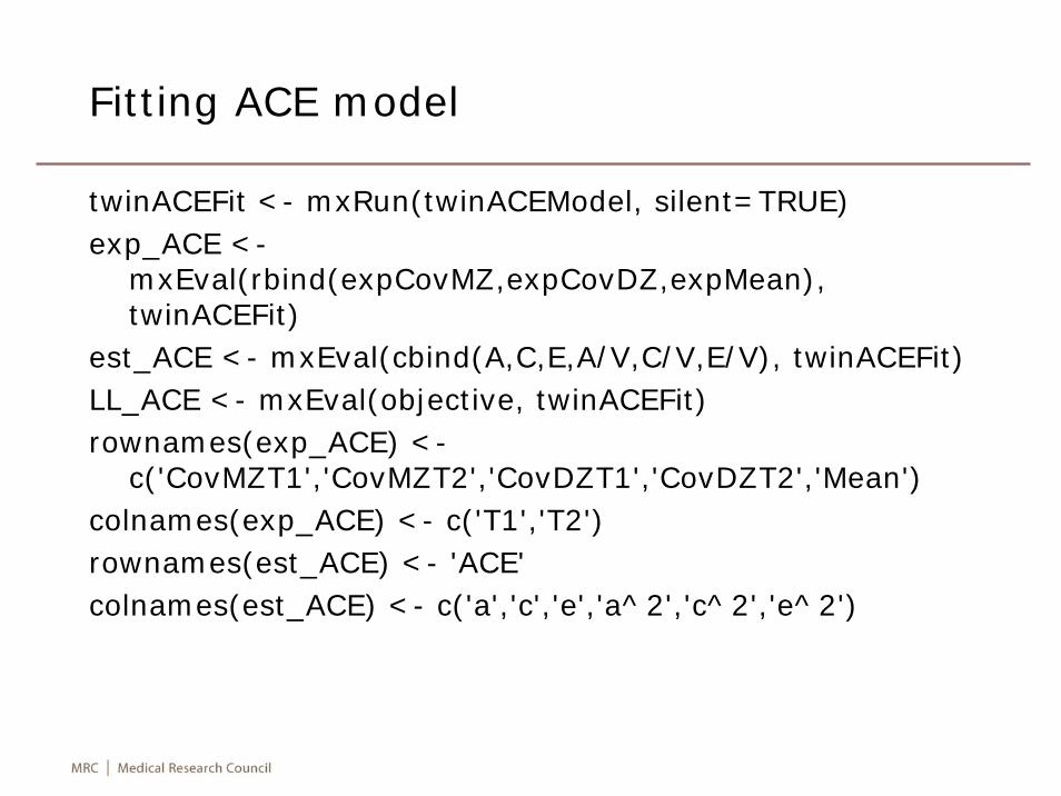
Fitting ACE model
twinACEFit <- mxRun(twinACEModel, silent=TRUE)exp_ACE <-
mxEval(rbind(expCovMZ,expCovDZ,expMean), twinACEFit)
est_ACE <- mxEval(cbind(A,C,E,A/V,C/V,E/V), twinACEFit)LL_ACE <- mxEval(objective, twinACEFit)rownames(exp_ACE) <-
c('CovMZT1','CovMZT2','CovDZT1','CovDZT2','Mean')colnames(exp_ACE) <- c('T1','T2')rownames(est_ACE) <- 'ACE'colnames(est_ACE) <- c('a','c','e','a^2','c^2','e^2')

Fitting AE model
twinAEModel <- mxModel(twinACEModel, mxMatrix("Full", 1, 1, FALSE, 0, "c", name="Y"))
twinAEFit <- mxRun(twinAEModel, silent=TRUE)exp_AE <- mxEval(rbind(expCovMZ,expCovDZ,expMean),
twinAEFit)est_AE <- mxEval(cbind(A,C,E,A/V,C/V,E/V), twinAEFit)rownames(est_AE) <- 'AE'LL_AE <- mxEval(objective, twinAEFit)LRT_ACE_AE <- LL_AE - LL_ACE
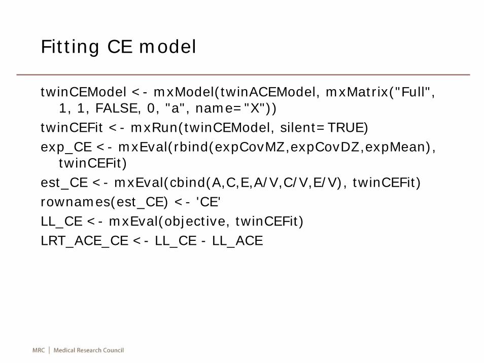
Fitting CE model
twinCEModel <- mxModel(twinACEModel, mxMatrix("Full", 1, 1, FALSE, 0, "a", name="X"))
twinCEFit <- mxRun(twinCEModel, silent=TRUE)exp_CE <- mxEval(rbind(expCovMZ,expCovDZ,expMean),
twinCEFit)est_CE <- mxEval(cbind(A,C,E,A/V,C/V,E/V), twinCEFit)rownames(est_CE) <- 'CE'LL_CE <- mxEval(objective, twinCEFit)LRT_ACE_CE <- LL_CE - LL_ACE
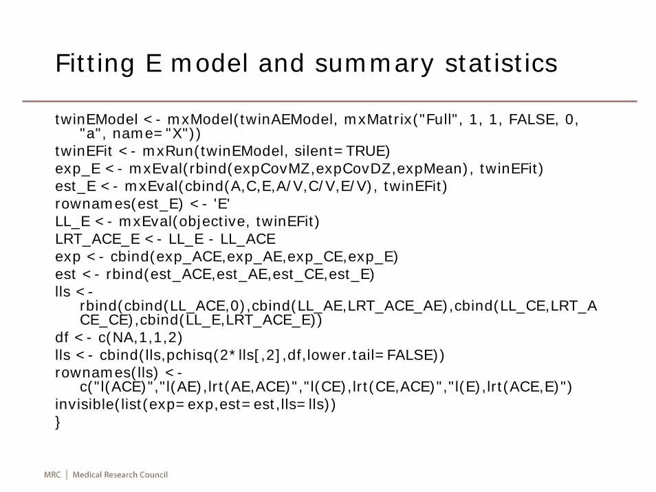
Fitting E model and summary statistics
twinEModel <- mxModel(twinAEModel, mxMatrix("Full", 1, 1, FALSE, 0, "a", name="X"))
twinEFit <- mxRun(twinEModel, silent=TRUE)exp_E <- mxEval(rbind(expCovMZ,expCovDZ,expMean), twinEFit)est_E <- mxEval(cbind(A,C,E,A/V,C/V,E/V), twinEFit)rownames(est_E) <- 'E'LL_E <- mxEval(objective, twinEFit)LRT_ACE_E <- LL_E - LL_ACEexp <- cbind(exp_ACE,exp_AE,exp_CE,exp_E)est <- rbind(est_ACE,est_AE,est_CE,est_E)lls <-
rbind(cbind(LL_ACE,0),cbind(LL_AE,LRT_ACE_AE),cbind(LL_CE,LRT_ACE_CE),cbind(LL_E,LRT_ACE_E))
df <- c(NA,1,1,2)lls <- cbind(lls,pchisq(2*lls[,2],df,lower.tail=FALSE))rownames(lls) <-
c("l(ACE)","l(AE),lrt(AE,ACE)","l(CE),lrt(CE,ACE)","l(E),lrt(ACE,E)")invisible(list(exp=exp,est=est,lls=lls))}
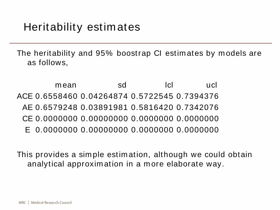
Heritability estimates
The heritability and 95% boostrap CI estimates by models are as follows,
mean sd lcl uclACE 0.6558460 0.04264874 0.5722545 0.7394376AE 0.6579248 0.03891981 0.5816420 0.7342076CE 0.0000000 0.00000000 0.0000000 0.0000000E 0.0000000 0.00000000 0.0000000 0.0000000
This provides a simple estimation, although we could obtain analytical approximation in a more elaborate way.
Summary
• The pursuit of precise estimation of genetic vsenvironmental contributions to complex traits have a long history and currently an indispensible part of genetic epidemiology or statistical genetics.
• The literature we focused here is largely from 1970s onwards. However, we have gone quite far with our understanding and implementation of procedures. The former includes simple estimation, maximum likelihood methods, path analysis and structural equation modeling while the latter evolves from Fortran, LISREL/Mx/MxGUI to R.
• Our focus is on the practical side. The new practice with OpenMx rests on the flexible and powerful R computing environment, which makes collaborative work truly possible.
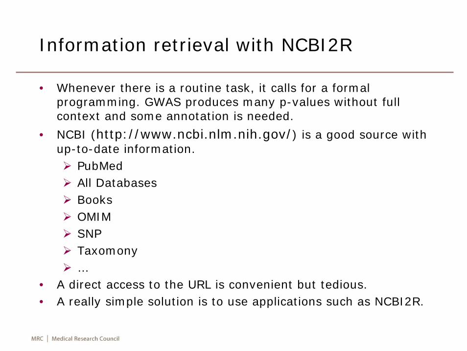
Information retrieval with NCBI2R
• Whenever there is a routine task, it calls for a formal programming. GWAS produces many p-values without full context and some annotation is needed.
• NCBI (http://www.ncbi.nlm.nih.gov/) is a good source with up-to-date information.
PubMedAll DatabasesBooksOMIMSNPTaxomony…
• A direct access to the URL is convenient but tedious.• A really simple solution is to use applications such as NCBI2R.
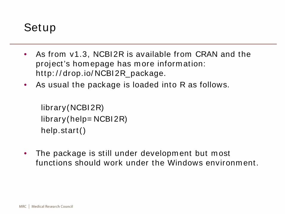
Setup
• As from v1.3, NCBI2R is available from CRAN and the project’s homepage has more information: http://drop.io/NCBI2R_package.
• As usual the package is loaded into R as follows.
library(NCBI2R)library(help=NCBI2R)help.start()
• The package is still under development but most functions should work under the Windows environment.
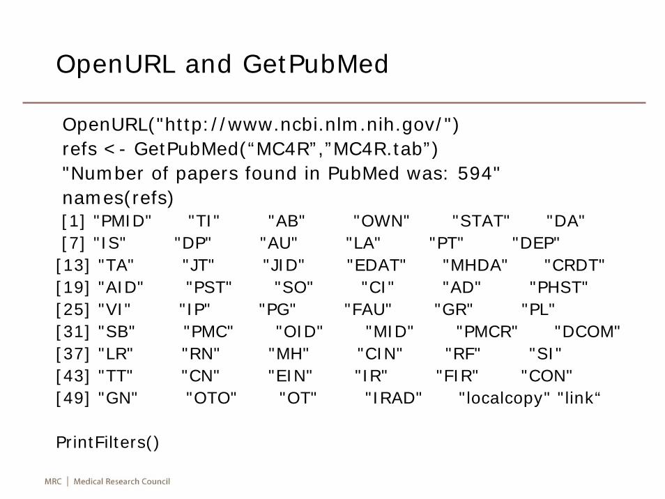
OpenURL and GetPubMed
OpenURL("http://www.ncbi.nlm.nih.gov/")refs <- GetPubMed(“MC4R”,”MC4R.tab”)"Number of papers found in PubMed was: 594"names(refs)[1] "PMID" "TI" "AB" "OWN" "STAT" "DA"[7] "IS" "DP" "AU" "LA" "PT" "DEP"[13] "TA" "JT" "JID" "EDAT" "MHDA" "CRDT"[19] "AID" "PST" "SO" "CI" "AD" "PHST"[25] "VI" "IP" "PG" "FAU" "GR" "PL"[31] "SB" "PMC" "OID" "MID" "PMCR" "DCOM"[37] "LR" "RN" "MH" "CIN" "RF" "SI"[43] "TT" "CN" "EIN" "IR" "FIR" "CON"[49] "GN" "OTO" "OT" "IRAD" "localcopy" "link“
PrintFilters()
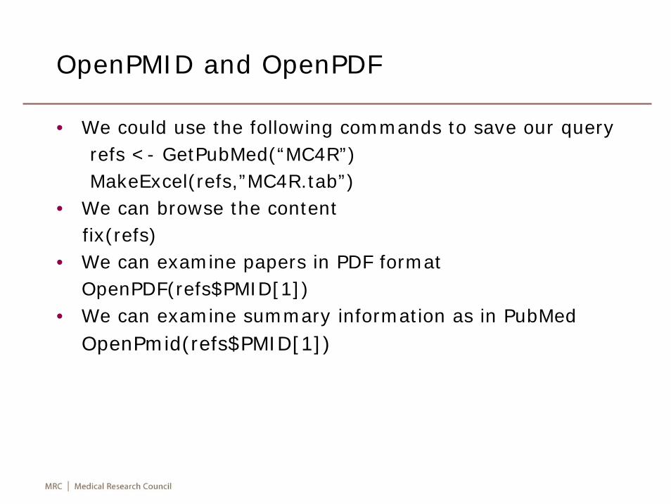
OpenPMID and OpenPDF
• We could use the following commands to save our queryrefs <- GetPubMed(“MC4R”)MakeExcel(refs,”MC4R.tab”)
• We can browse the contentfix(refs)
• We can examine papers in PDF formatOpenPDF(refs$PMID[1])
• We can examine summary information as in PubMedOpenPmid(refs$PMID[1])
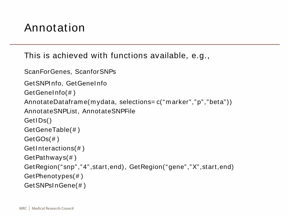
Annotation
This is achieved with functions available, e.g.,
ScanForGenes, ScanforSNPs
GetSNPInfo, GetGeneInfoGetGeneInfo(#)AnnotateDataframe(mydata, selections=c(“marker”,”p”,”beta”))AnnotateSNPList, AnnotateSNPFileGetIDs()GetGeneTable(#)GetGOs(#)GetInteractions(#)GetPathways(#)GetRegion(“snp”,”4”,start,end), GetRegion(“gene”,”X”,start,end)GetPhenotypes(#)GetSNPsInGene(#)
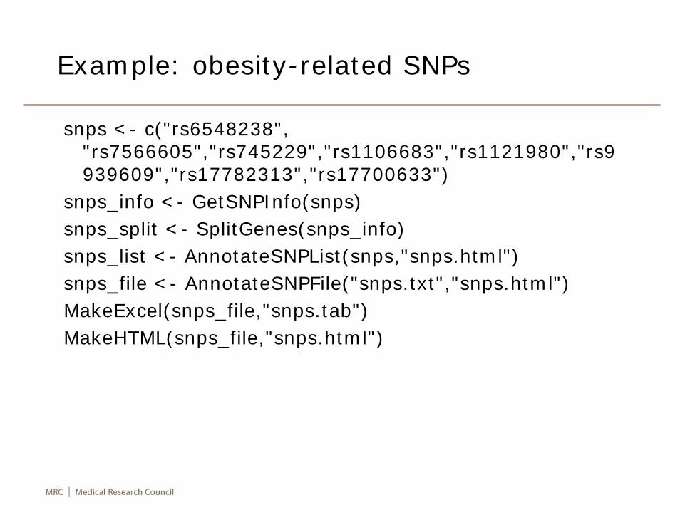
Example: obesity-related SNPs
snps <- c("rs6548238", "rs7566605","rs745229","rs1106683","rs1121980","rs9939609","rs17782313","rs17700633")
snps_info <- GetSNPInfo(snps)snps_split <- SplitGenes(snps_info)snps_list <- AnnotateSNPList(snps,"snps.html")snps_file <- AnnotateSNPFile("snps.txt","snps.html")MakeExcel(snps_file,"snps.tab")MakeHTML(snps_file,"snps.html")
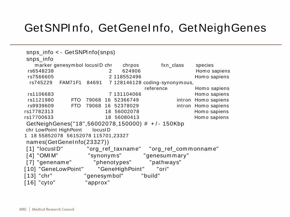
GetSNPInfo, GetGeneInfo, GetNeighGenes
snps_info <- GetSNPInfo(snps)snps_info
marker genesymbol locusID chr chrpos fxn_class speciesrs6548238 2 624906 Homo sapiensrs7566605 2 118552496 Homo sapiensrs745229 FAM71F1 84691 7 128146128 coding-synonymous,
reference Homo sapiensrs1106683 7 131104066 Homo sapiensrs1121980 FTO 79068 16 52366749 intron Homo sapiensrs9939609 FTO 79068 16 52378029 intron Homo sapiens
rs17782313 18 56002078 Homo sapiensrs17700633 18 56080413 Homo sapiensGetNeighGenes("18",56002078,150000) # +/- 150Kbpchr LowPoint HighPoint locusID1 18 55852078 56152078 115701,23327names(GetGeneInfo(23327))[1] "locusID" "org_ref_taxname" "org_ref_commonname"[4] "OMIM" "synonyms" "genesummary"[7] "genename" "phenotypes" "pathways"[10] "GeneLowPoint" "GeneHighPoint" "ori"[13] "chr" "genesymbol" "build"[16] "cyto" "approx"
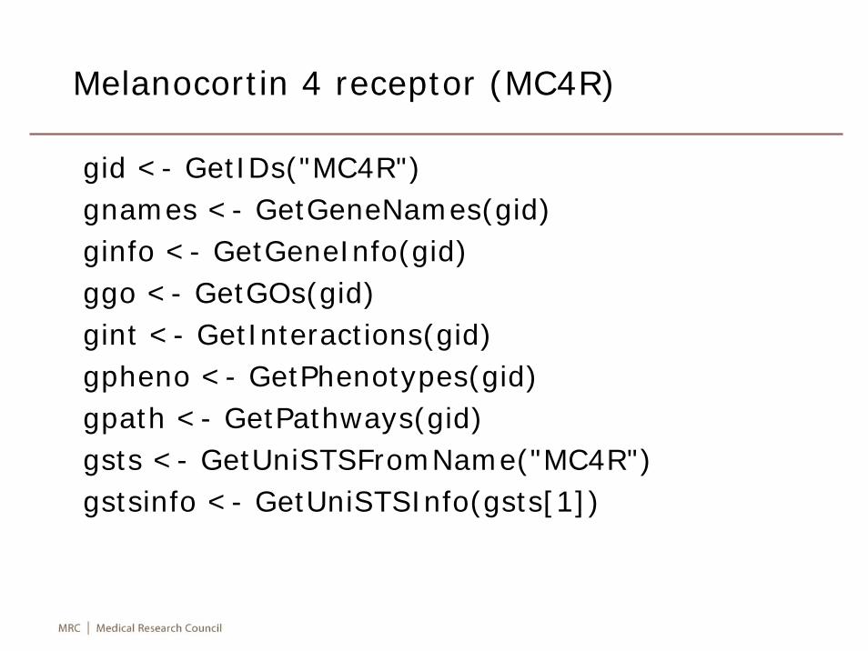
Melanocortin 4 receptor (MC4R)
gid <- GetIDs("MC4R")gnames <- GetGeneNames(gid)ginfo <- GetGeneInfo(gid)ggo <- GetGOs(gid)gint <- GetInteractions(gid)gpheno <- GetPhenotypes(gid)gpath <- GetPathways(gid)gsts <- GetUniSTSFromName("MC4R")gstsinfo <- GetUniSTSInfo(gsts[1])
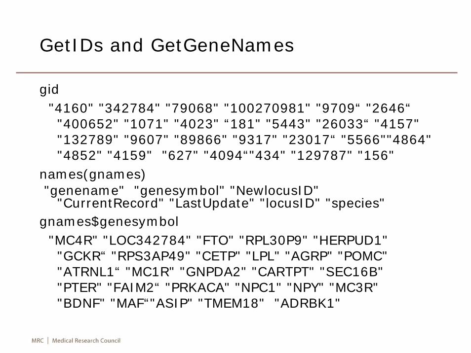
GetIDs and GetGeneNames
gid"4160" "342784" "79068" "100270981" "9709“ "2646“"400652" "1071" "4023" “181" "5443" "26033“ "4157" "132789" "9607" "89866" "9317" "23017“ "5566""4864" "4852" "4159" "627" "4094“"434" "129787" "156"
names(gnames)"genename" "genesymbol" "NewlocusID"
"CurrentRecord" "LastUpdate" "locusID" "species" gnames$genesymbol"MC4R" "LOC342784" "FTO" "RPL30P9" "HERPUD1" "GCKR“ "RPS3AP49" "CETP" "LPL" "AGRP" "POMC" "ATRNL1“ "MC1R" "GNPDA2" "CARTPT" "SEC16B" "PTER" "FAIM2“ "PRKACA" "NPC1" "NPY" "MC3R" "BDNF" "MAF“"ASIP" "TMEM18" "ADRBK1"
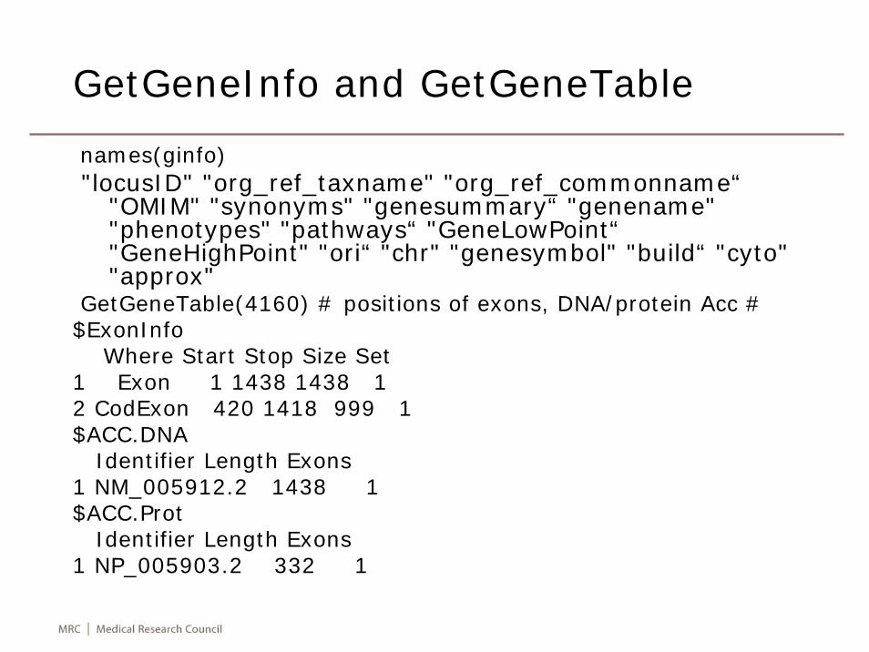
GetGeneInfo and GetGeneTable
names(ginfo)"locusID" "org_ref_taxname" "org_ref_commonname“
"OMIM" "synonyms" "genesummary“ "genename" "phenotypes" "pathways“ "GeneLowPoint“"GeneHighPoint" "ori“ "chr" "genesymbol" "build“ "cyto" "approx"
GetGeneTable(4160) # positions of exons, DNA/protein Acc #$ExonInfo
Where Start Stop Size Set1 Exon 1 1438 1438 12 CodExon 420 1418 999 1$ACC.DNA
Identifier Length Exons1 NM_005912.2 1438 1$ACC.Prot
Identifier Length Exons1 NP_005903.2 332 1
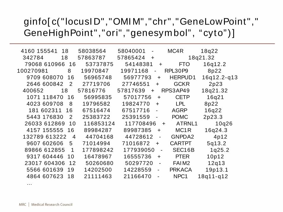
ginfo[c("locusID","OMIM","chr","GeneLowPoint","GeneHighPoint","ori","genesymbol”, “cyto”)]
4160 155541 18 58038564 58040001 - MC4R 18q22342784 18 57863787 57865424 + 18q21.3279068 610966 16 53737875 54148381 + FTO 16q12.2
100270981 8 19970847 19971168 - RPL30P9 8p229709 608070 16 56965748 56977793 + HERPUD1 16q12.2-q132646 600842 2 27719706 27746551 + GCKR 2p23
400652 18 57816776 57817639 + RPS3AP49 18q21.321071 118470 16 56995835 57017756 + CETP 16q214023 609708 8 19796582 19824770 + LPL 8p22181 602311 16 67516474 67517716 - AGRP 16q225443 176830 2 25383722 25391559 - POMC 2p23.326033 612869 10 116853124 117708496 + ATRNL1 10q264157 155555 16 89984287 89987385 + MC1R 16q24.3
132789 613222 4 44704168 44728612 - GNPDA2 4p129607 602606 5 71014994 71016872 + CARTPT 5q13.289866 612855 1 177898242 177939050 - SEC16B 1q25.29317 604446 10 16478967 16555736 + PTER 10p1223017 604306 12 50260680 50297720 - FAIM2 12q135566 601639 19 14202500 14228559 - PRKACA 19p13.14864 607623 18 21111463 21166470 - NPC1 18q11-q12…
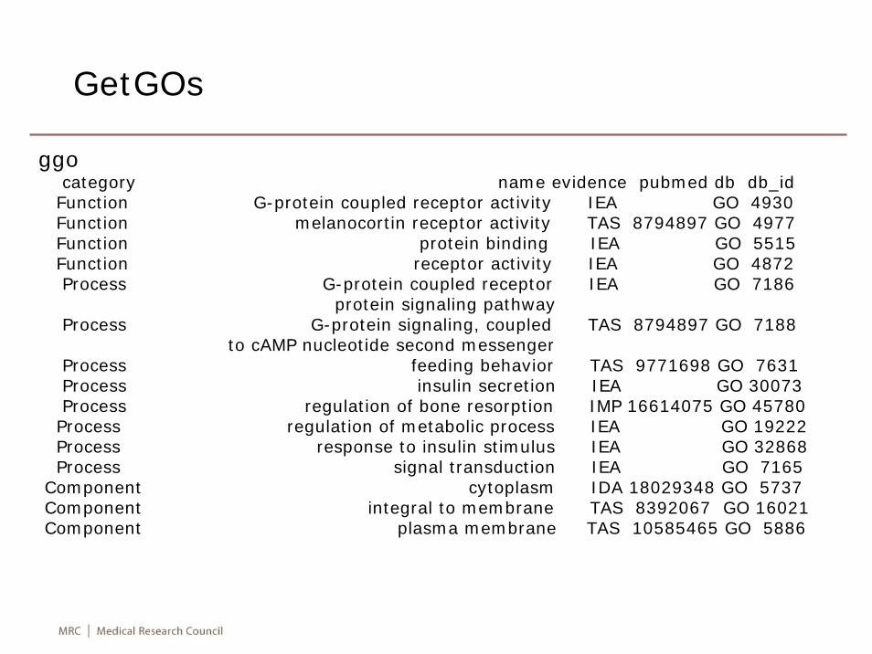
GetGOs
ggocategory name evidence pubmed db db_idFunction G-protein coupled receptor activity IEA GO 4930Function melanocortin receptor activity TAS 8794897 GO 4977Function protein binding IEA GO 5515Function receptor activity IEA GO 4872Process G-protein coupled receptor IEA GO 7186
protein signaling pathwayProcess G-protein signaling, coupled TAS 8794897 GO 7188
to cAMP nucleotide second messengerProcess feeding behavior TAS 9771698 GO 7631Process insulin secretion IEA GO 30073Process regulation of bone resorption IMP 16614075 GO 45780Process regulation of metabolic process IEA GO 19222Process response to insulin stimulus IEA GO 32868Process signal transduction IEA GO 7165
Component cytoplasm IDA 18029348 GO 5737Component integral to membrane TAS 8392067 GO 16021Component plasma membrane TAS 10585465 GO 5886
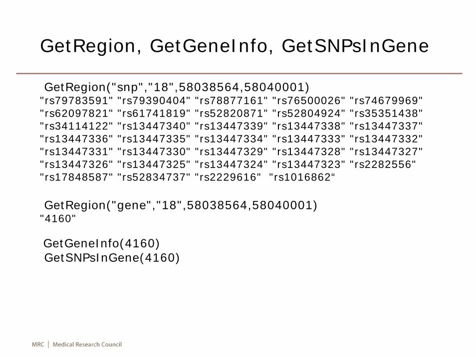
GetRegion, GetGeneInfo, GetSNPsInGene
GetRegion("snp","18",58038564,58040001)"rs79783591" "rs79390404" "rs78877161" "rs76500026" "rs74679969""rs62097821" "rs61741819" "rs52820871" "rs52804924" "rs35351438""rs34114122" "rs13447340" "rs13447339" "rs13447338" "rs13447337""rs13447336" "rs13447335" "rs13447334" "rs13447333" "rs13447332""rs13447331" "rs13447330" "rs13447329" "rs13447328" "rs13447327""rs13447326" "rs13447325" "rs13447324" "rs13447323" "rs2282556""rs17848587" "rs52834737" "rs2229616" "rs1016862“
GetRegion("gene","18",58038564,58040001)"4160"
GetGeneInfo(4160)GetSNPsInGene(4160)
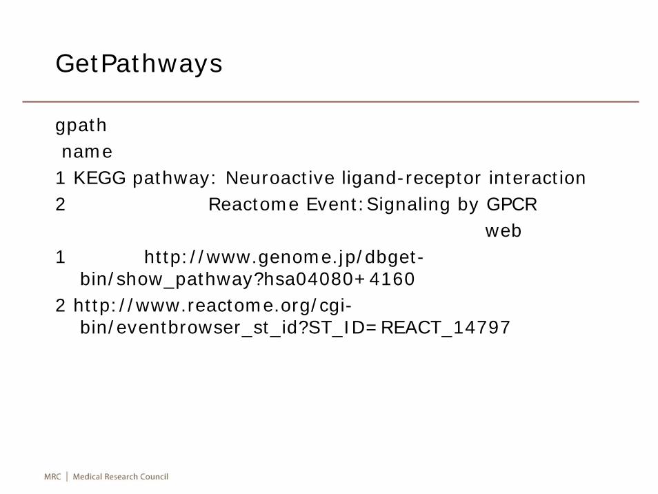
GetPathways
gpathname1 KEGG pathway: Neuroactive ligand-receptor interaction2 Reactome Event:Signaling by GPCR
web1 http://www.genome.jp/dbget-
bin/show_pathway?hsa04080+41602 http://www.reactome.org/cgi-
bin/eventbrowser_st_id?ST_ID=REACT_14797
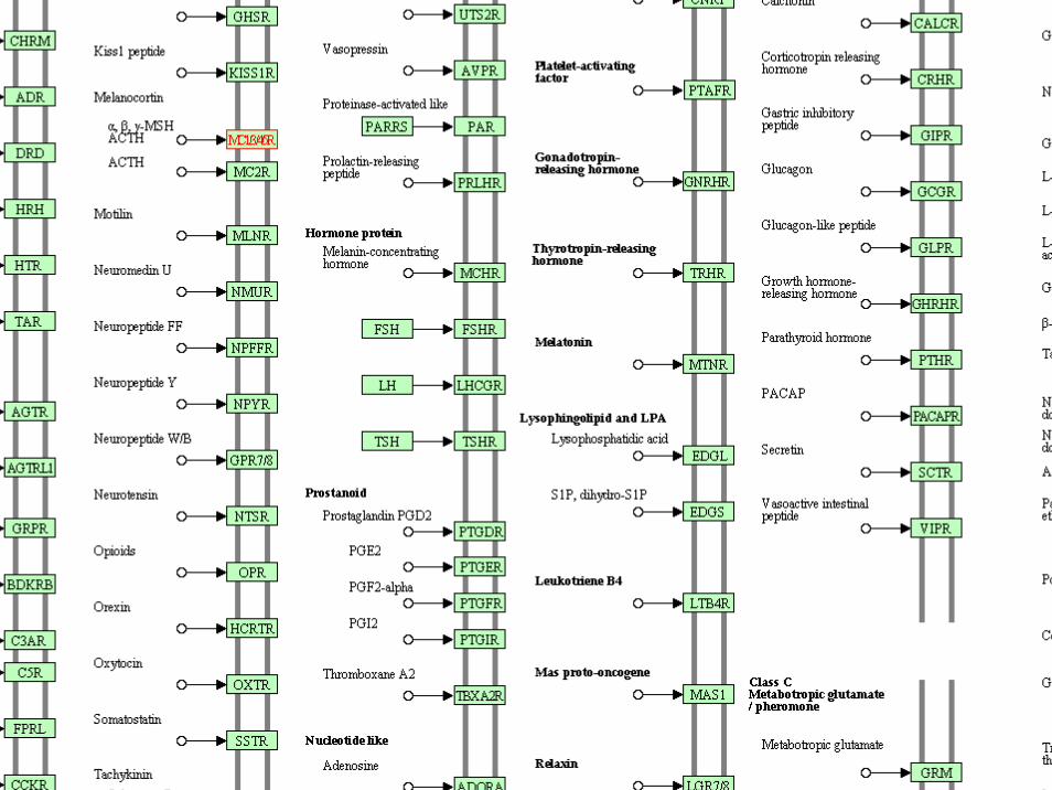
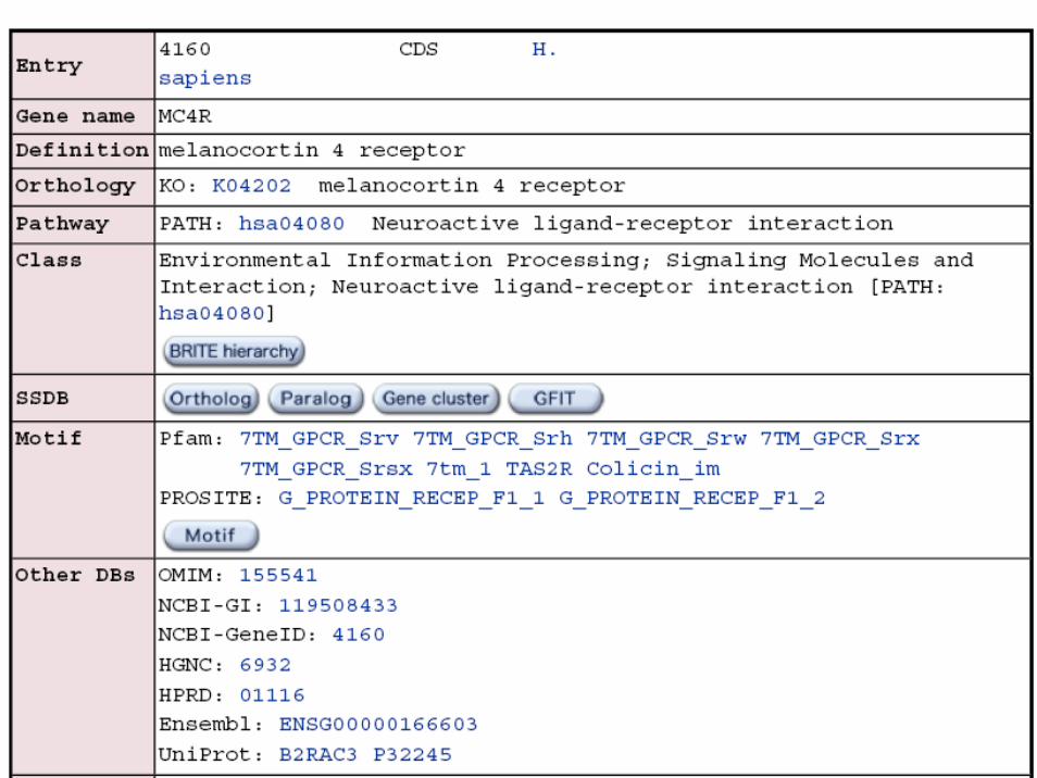
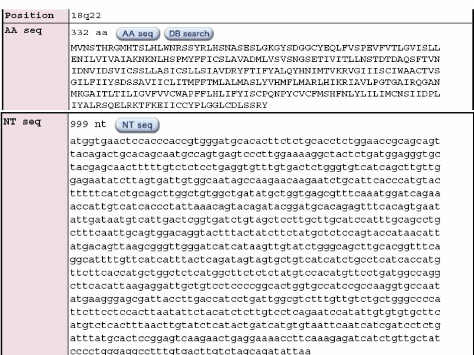
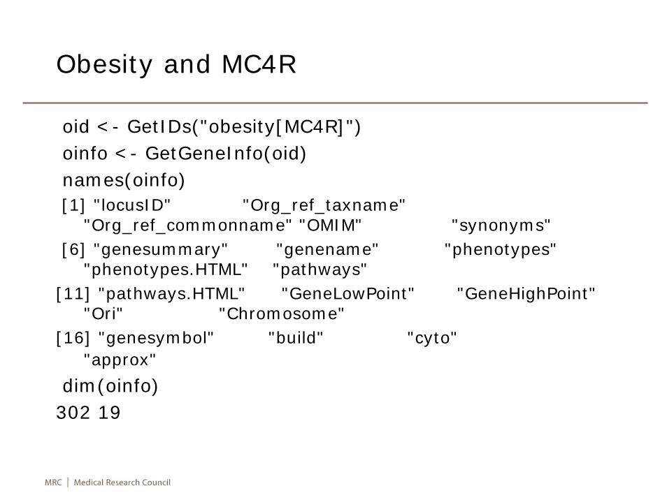
Obesity and MC4R
oid <- GetIDs("obesity[MC4R]")oinfo <- GetGeneInfo(oid)names(oinfo)[1] "locusID" "Org_ref_taxname"
"Org_ref_commonname" "OMIM" "synonyms" [6] "genesummary" "genename" "phenotypes"
"phenotypes.HTML" "pathways" [11] "pathways.HTML" "GeneLowPoint" "GeneHighPoint"
"Ori" "Chromosome" [16] "genesymbol" "build" "cyto"
"approx"
dim(oinfo) 302 19
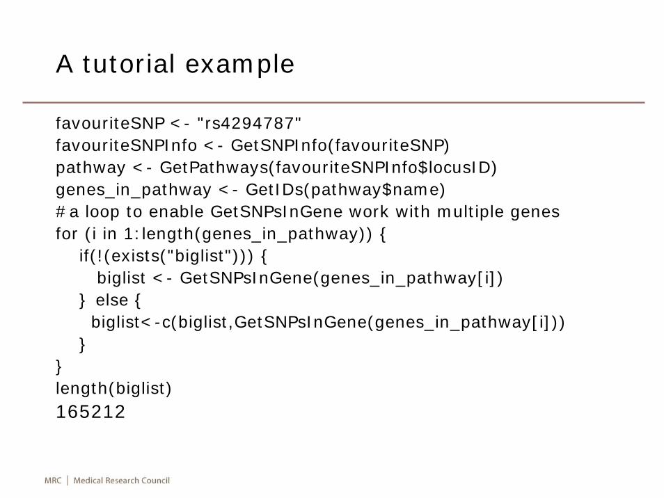
A tutorial example
favouriteSNP <- "rs4294787"favouriteSNPInfo <- GetSNPInfo(favouriteSNP)pathway <- GetPathways(favouriteSNPInfo$locusID)genes_in_pathway <- GetIDs(pathway$name)#a loop to enable GetSNPsInGene work with multiple genesfor (i in 1:length(genes_in_pathway)) {
if(!(exists("biglist"))) {biglist <- GetSNPsInGene(genes_in_pathway[i])
} else {biglist<-c(biglist,GetSNPsInGene(genes_in_pathway[i]))
}}length(biglist)165212
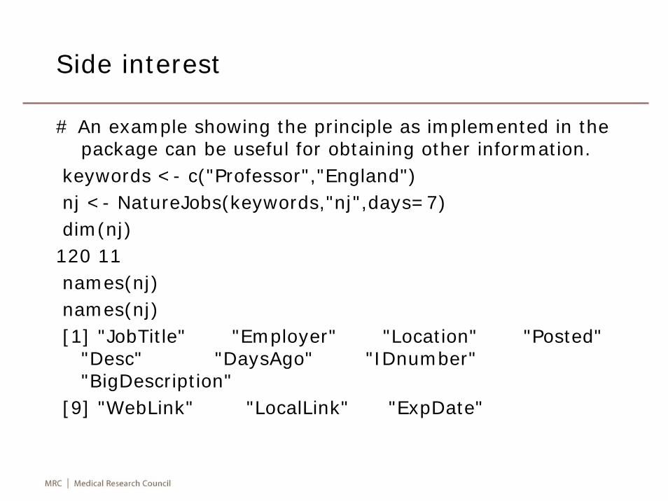
Side interest
# An example showing the principle as implemented in the package can be useful for obtaining other information.
keywords <- c("Professor","England")nj <- NatureJobs(keywords,"nj",days=7)dim(nj)120 11names(nj)names(nj)[1] "JobTitle" "Employer" "Location" "Posted"
"Desc" "DaysAgo" "IDnumber" "BigDescription"
[9] "WebLink" "LocalLink" "ExpDate"
A summary
• NCBI, especially PubMed, has been a major source of biomedical information retrieval in daily research. The process can considerably be facilitated by R/NCBI2R package. A minor issue is that it only retrieves the latest information but earlier information is very useful (e.g., build 35). Hence more experiences need to be gathered.
• “NCBI2R annotates lists of SNPs and/or genes, with current information from NCBI … designed to allow those performing the genome analysis to produce output that could easily be understood by a person not familiar with R”. It is easy to anticipate that more functionality can be added from the same principle. It is helpful to keep an eye on the package development even if implementation may not necessarily be a priority in our research.
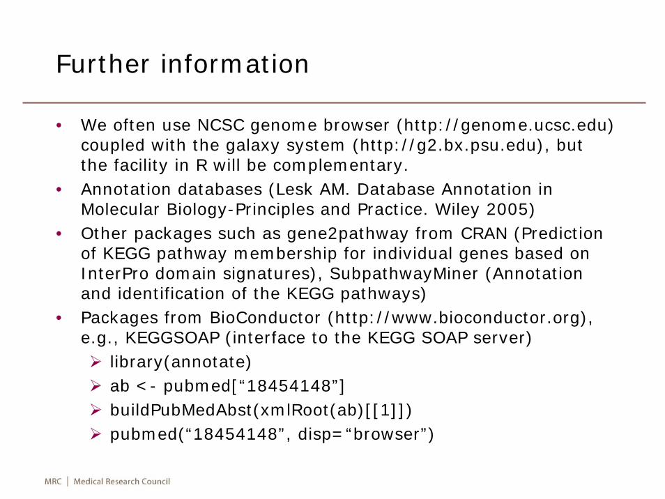
Further information
• We often use NCSC genome browser (http://genome.ucsc.edu) coupled with the galaxy system (http://g2.bx.psu.edu), but the facility in R will be complementary.
• Annotation databases (Lesk AM. Database Annotation in Molecular Biology-Principles and Practice. Wiley 2005)
• Other packages such as gene2pathway from CRAN (Prediction of KEGG pathway membership for individual genes based on InterPro domain signatures), SubpathwayMiner (Annotation and identification of the KEGG pathways)
• Packages from BioConductor (http://www.bioconductor.org), e.g., KEGGSOAP (interface to the KEGG SOAP server)
library(annotate)ab <- pubmed[“18454148”]buildPubMedAbst(xmlRoot(ab)[[1]])pubmed(“18454148”, disp=“browser”)
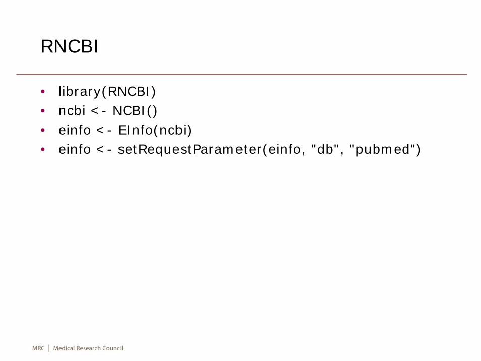
RNCBI
• library(RNCBI)• ncbi <- NCBI()• einfo <- EInfo(ncbi)• einfo <- setRequestParameter(einfo, "db", "pubmed")

V Conclusion
General comments
• As has been driven by technological advances in genotyping and computational technology, the genetic analysis of complex trait is a dynamic topic in a fast-moving field.
• The R environment is now indispensible with a great deal of recognition and stability. Nevertheless, there are areas which can be further advanced, e.g., graphics. A range of models available from R remains to be explored and have been supplementary to the main analysis.
Scientific aspects of GWAS
• What are the uses?Discovery of new susceptibility lociElucidate biologic pathwaysIdentify links between these loci and covariatesRisk prediction
• Where would they go?Expanding well-characterized study populationsExpanding the range of genetic variation including structural variants and lower-frequency common variantsDocumenting functional mechanisms responsible for the association signals.
Chanock (Personal Communication) and Altshuler et al. Science 2008, 322:881-8
Limitations and practical issues
• LimitationsIt requires large sample sizesIt only identifies loci, not genesIt detects only common alleles in a populationIt usually does not go into the expression level
• Practical issuesFor individual studies, the issues as of epidemiological studies in general remain and there is uncertainty to declare statistical significanceFor consortium meta-analysis, there may be difference in quality control, data sharing and variation in complexity of analysis
• Technological advances, e.g., sequencing, remain to have profound influences.
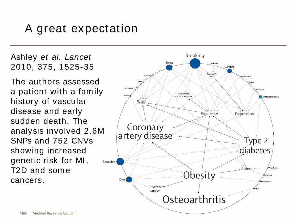
A great expectation
Ashley et al. Lancet2010, 375, 1525-35
The authors assessed a patient with a family history of vascular disease and early sudden death. The analysis involved 2.6M SNPs and 752 CNVsshowing increased genetic risk for MI, T2D and some cancers.
Summary
• The need from various analyses seeds the development in R and shares much in common with many other problems involving large data, such as interactive graphics in combination with publicly available databases, the use of statistical and computational facilities available from the R system.
• Applications in substantive areas are the constant source of motivation in package development. The implementation is likely to be patchy but with a great prospect, e.g., advanced models and causal pathways.
• Alternative computing environments are complementary.
References
• Murrell P. R Graphics. Chapman & Hall/CRC, 2005• Gentleman R, Carey V, Huber W, Irizarry R, Dudoit S.
Bioinformatics and Computational Biology Solutions Using R and Bioconductor. Springer, 2005
• Hahne F, Huber W, Gentleman R, Falcon F. BioconductorCase Studies. Springer, 2008
• Spector P. Data Manipulation with R. Springer, 2008• Foulkes AS. Applied Statistical Genetics with R for Population-
based Association Studies. Springer, 2009• Broman KW, Sen S. A Guide to QTL Mapping with R/qtl.
Springer, 2009• Gentleman R. R Programming for Bioinformatics. Chapman &
Hall/CR, 2009
• Robert C, Casella G. Introducing Monte Carlo Methods with R. Springer, 2010


![Apha slides tfah sanyal slides[1]](https://img.pdfslide.us/doc/110x75/557c653ad8b42a855d8b46d1/apha-slides-tfah-sanyal-slides1.jpg)