Embed Size (px)
Citation preview

Slides 05Slides 0511
The Principal-Type The Principal-Type AlgorithmAlgorithm
• In general a typable term has an infinite set of types in TA.
• For example, it is possible to assign to I xx every type with the form , by the following deduction:
x: ↦ x: (I) ↦ (xx):
• All the types in this infinite set are substitution-instances of the one type aa.

Slides 05Slides 0522
• By the subject-construction theorem, every deduction for I must have the simple form shown before.
• The type aa is called a principal type for I.
• The existence of a principal type is a property of all typable terms, not just I.
• The principal type of a term is the most general type it can receive in TA.
• We shall learn that every typable term has a principal type.

Slides 05Slides 0533
• A principal-type (PT) or type-checking algorithm will decide whether a given term M is typable and, if the answer is "yes", will output a principal type for M.
• The existence of a PT algorithm is what gives TA and its extensions such as Haskell and ML their practical value, since if the typability of a program is regarded as a safety criterion then the programmer will want to be able to decide effectively whether a newly created program satisfies this criterion.
• In order to understand the PT algorithm, we need the knowledge of substitution and unification.

Slides 05Slides 0544
• Definition (3A1) A type-substitution s is any expression [1/a1, ..., n/an], where a1, ..., an are distinct type-variables and 1, ..., n are any types. For any we define s() to be the type obtained by simultaneously substituting 1 for a1, ..., n for an
throughout . In more detail, we definei. s(ai) i
ii. s(b) b if b is an atom {a1, ..., an}iii. s() s()s().
We call s() an instance of .

Slides 05Slides 0555
• Example:Let s [(ab)/c] and (ab)(bc)ac,thens() (ab)(bab)aab.

Slides 05Slides 0566
• The case n = 0 is called the empty substitution, e.
e() .• If n = 1, s will be called a single substitution.• Each part-expression i/ai of s will be called a
component of s, and called trivial if i ai.• If all trivial components are deleted from s
the resulting substitution will be called the nontrivial kernel of s.
• {a1, ..., an}: Dom(s)
Vars(1, ..., n): Range(s)

Slides 05Slides 0577
• Definition (3A2) The action of a substitution s is extended to finite sequences of types, to type-contexts and to TA-formulas, as follows:
s(<1, ..., n>) = <s(1), ..., s(n)>,
s() = {x1:s(1), ..., xm:s(m)}
if = {x1:1, ..., xm:m},s( ↦ M:) = s() ↦ M:s().
s() is the result of applying s to every TA-formula in deduction .

Slides 05Slides 0588
• Besides the concept of substitution s for type-variables just mentioned, we also have the concept of substitution for term-variables.
• Lemma (2B6) Let 1 be consistent with 2 and let
1, x: ⊢ M:, 2 ⊢ N:
then1 2 ⊢ [N/x]M:.

Slides 05Slides 0599
• Definition (3A3) In TA, a principal type or PT of a term M is a type such that
i. ⊢ M: for some ,
ii. if ' ⊢ M: for some ' and , then is an instance of .
• A PT of M completely characterizes the set of all types assignable to M.
Slides 05Slides 051010
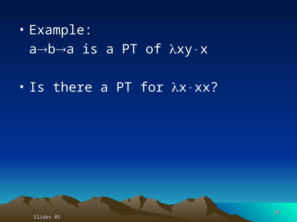
• Example:aba is a PT of xyx
• Is there a PT for xxx?

Slides 05Slides 051111
• Definition (3A4) A principal pair for a term M is a pair <,> such that the formula ↦ M: is TA-deducible and every other TA-deducible formula ' ↦ M: is an instance of ↦ M:.
• Example: <,aba> is a principal pair for xyx.
Slides 05Slides 051212
• Definition (3A5) A principal deduction for a term M is a deduction of a formula ↦ M: such that every other deduction, whose conclusion's subject is M, is an instance of .To abbreviate "there exists a principal deduction of ↦ M:", we shall write
⊢p M:.
• We will see that a typable term M has not only a most general type but also a deduction whose every step is most general.

Slides 05Slides 051313
Principal-Type TheoremPrincipal-Type Theorem (3A6)(3A6)
Every typable term has a principal deduction and a principal type in TA. Further, there is an algorithm that will decide whether a given -term M is typable in TA, and if the answer is "yes", will output a principal deduction and principal type for M.

Slides 05Slides 051414
More details on type-More details on type-substitutionsubstitution
• Definition (3B2) Substitutions s and t are extensionally equivalent (s =ext t ) iff s () t () for all .
• Lemma (3B2.1) (i) b Dom(s) s(b) b.(ii) s =ext t iff s and t have the same non-trivial kernel.

Slides 05Slides 051515
• Definition (3B3) If s [1/a1, ..., n/an] and V is a given set of variables, the restriction s↾V of s to V is the substitution consisting of the components i/ai of s such that ai V.
• Lemma (3B3.1) (s↾Vars())() s().

Slides 05Slides 051616
• Definition (3B4) If s [1/a1, ..., n/an] and t [1/b1, ..., p/bp] and either a1, ..., an, b1, ..., bp are all distinct or ai bj i j, we define
s t [1/a1, ..., n/an, 1/b1, ..., p/bp]
with repetitions omitted.• Lemma (3B4.1)
(i) Dom(s t) = Dom(s ) Dom(t ).(ii) If s =ext s' and t =ext t' and s t is defined, then so is s' t' and
s t =ext s' t'.
Slides 05Slides 051717
• The composition of two substitutions s and t is a simultaneous substitution that will have the same effect as applying t and s in succession.
• Definition (3B5) If s and t are any substitutions, say s [1/a1, ..., n/an] and t [1/b1, ..., p/bp],
we define s∘t [i1/ai1, ..., ih/aih, s(1)/b1, ..., s(p)/bp]
where {ai1, ..., aih} = Dom(s)-Dom(t) and 0 h n.

Slides 05Slides 051818
• Example:s [(cd)/a,(ba)/b], t [(ba)/b]
ab
s(t ()) (cd)(ba)(cd)s∘t [(cd)/a,(s(ba))/b]
[(cd)/a,((ba)(cd))/b] (s∘t)() (cd)(ba)(cd)
But (s t )() s() (cd)ba

Slides 05Slides 051919
• [a/b] ∘ [b/a] ?
ab([a/b] ∘ [b/a])() ?[a/b]([b/a]()) ?
Slides 05Slides 052020
• Lemma (3B5.1) 1. Dom(s∘t) = Dom(s) ∪ Dom(t).2. (s∘t)() s(t()). This also means
an instance of an instance of is an instance of .
3. r∘(s∘t) =ext (r∘s)∘t.
4. s =ext s', t =ext t' s∘t =ext s'∘t'.

Slides 05Slides 052121
• The next lemma, which is important in the correctness proof of the PT algorithm, says that if a composition s∘t is extended to r (s∘t), the extended substitution can also be expressed as a composition with t, under certain conditions on r to prevent clashes.
• Lemma (3B6:composition-extension) Let r, s, t be substitutions such that(i) Dom(r) (Dom(s)Dom(t)) = ,(ii) Dom(r) Range(t) = .Then r (s∘t) and (r s)∘t are both defined and
r (s∘t) (r s)∘t.

Slides 05Slides 052222
• Definition (3B7) A variables-for-variables substitution is a substitution s [b1/a1, ..., bn/an] where b1, ..., bn are variables (not necessarily distinct). If b1, ..., bn are distinct , s is called one-to-one, and if also {a1, ..., an} = Vars() for a given , s is called a renaming in .
• Note: A one-to-one substitution may be a renaming in one type but not in another. For example, [b/a] is a renaming in aa but not in ab.

Slides 05Slides 052323
• Definition (3B8) We say is an alphabetic variant of , or and are identical modulo renaming, iff s() for some renaming s in .
• Lemma (3B8.2: Uniqueness) Let be a principal type of a term M. Then is unique modulo renaming.
Slides 05Slides 052424
Main ideas for the PT Main ideas for the PT algorithmalgorithm
• The two main steps in the PT algorithm:
1. the computation of PT(xM) from PT(M),
2. the computation of PT(PQ) from PT(P) and PT(Q).
• The first is easy, the second needs more work which is the core of the PT algorithm.

Slides 05Slides 052525
• Suppose we are trying to decide whether an application PQ is typable in TA, and we already know that
PT(P) , PT(Q) .
For simplicity suppose PQ has no free variables. Then the types assignable to P are generated from by substitution and those assignable to Q are generated from . Hence, if we can find substitutions s1 and s2 such that
s1() s2(),
we will be able to deduce a type for PQ by rule (E), as follows:
↦ P:s1()s1() ↦ Q:s2()
(E) ↦ PQ:s1()
Slides 05Slides 052626
• Thus the problem of deciding whether PQ is typable reduces to that of finding substitutions s1 and s2 such that s1() s2().
• This suggests the next two definitions.

Slides 05Slides 052727
• Definition (3C2) (i) If s1() s2() we call a common instance (c.i.) of the pair <,>, and we call <s1,s2> a pair of converging substitutions for <,>.(ii) If <1, ..., n> s1(<1, ..., n>) s2(<1, ..., n>) we call <1, ..., n> a common instance of <1, ..., n> and <1, ..., n>.
• Example: A c.i. of <a(bc),(ab)a> is the type (())(), and the corresponding converging substitutions are
s1 [(())/a, /b, /c], s2 [()/a, /b].

Slides 05Slides 052828
• Does every pair of types has a common instance?No. For example the pair <aa,(bb)b> has none.

Slides 05Slides 052929
• Definition (3C3) A most general common instance (m.g.c.i) of
<,> is a common instance 0 such that every other common instance is an instance of 0. If 0 is an m.g.c.i. of <,> we call any pair <s1,s2> such that s1() s2() 0 an m.g.c.i.-generator for <,>.
• M.g.c.i.'s are unique modulo renaming.

Slides 05Slides 053030
• Example: The pair <a(bc),(ab)a> has an m.g.c.i m0 (())().
Proof:Let a(bc), (ab)a. In slide 27 we have shown that m0 is a c.i. of and . To show that m0 is most general, let m be any other c.i., then we havem s1(a)(s1(b)s1(c)) (s2(a)s2(b))s2(a), which gives s1(a) s2(a)s2(b), s2(a) s1(b)s1(c).
Therefore, s1(a) (s1(b)s1(c))s2(b) and
m ((s1(b)s1(c))s2(b))(s1(b)s1(c)). Thus, m is an instance of m0.

Slides 05Slides 053131
• The problem of finding PT(PQ) reduces to that of finding an m.g.c.i of <,>.
• We will need Robinson's unification algorithm.

Slides 05Slides 053232
• Definition (3D1) (i) If there is a substitution s such that s() s() we say <,> is unifiable; we call any such s a unifier of <,> and call s() a unification of <,>.(ii) A unifier of a pair of sequences <<1, ..., n>, <1, ..., n>> is a substitution s such that
s(<1, ..., n>) s(<1, ..., n>).

Slides 05Slides 053333
• Note: A unification of <,> is just a c.i. obtained by making the same substitution in as in . But not every c.i. is a unification. A pair <,> may have a c.i. but no unifier. For example, consider
a(bc), (ab)a.We have seen in slide 27 that this pair has a c.i.; but no substitution s can exist such that s() s(), because this would imply s(a) s(a)s(b) which is impossible.

Slides 05Slides 053434
• Definition (3D2) A most general unifier (m.g.u.) of <,> is a unifier u such that for every other unifier s of <,> we have
s() s'(u())for some s'. If u() for some m.g.u. u of <,> we call a most general unification of <,>.
• Lemma If u is an m.g.u. of <,> and v is a renaming of variables in u(), then v∘u is an m.g.u. of <,>.

Slides 05Slides 053535
• The m.g.u. of a pair <,> may differ from its m.g.c.i. However, in the special case that and have no common variables, every c.i. is also a unification. Why? Because if
s1() s2()
and Dom(s1) Vars() and Dom(s2) Vars() then s1 s2 is defined and
(s1 s2)() (s1 s2)().

Slides 05Slides 053636
• Lemma (3D3) (i) If and have no common variables, <,> has an m.g.u. iff it has an m.g.c.i., and the two are identical.(ii) For all and : if we change to an alphabetic variant * with no variables in common with , the unifications of <,*> will be exactly the common instances of <,> and the most general unification of <,*> will be the m.g.c.i. of <,>.
• Thus the problem of finding m.g.c.i.'s has been reduced to that of finding most general unifications of pairs <,> with no variables in common.

Slides 05Slides 053737
• Unification Theorem (3D4)(i) There is an algorithm which decides whether a pair of types <,> has a unifier, and, if the answer is "yes", constructs its m.g.u.(ii) If a pair <,> has a unifier it has an m.g.u.(iii) Parts (i) and (ii) hold also for pairs of deductions and for pairs of finite type-sequences.

Slides 05Slides 053838
Unification Algorithm (Robinson 1965)Input: any pair <,> of types.Output: either a correct statement that <,> is not
unifiable or an m.g.u. u of <,>.Step 0. Choose k = 0 and u0 e (the empty substitution).
Step k+1. Given k and uk, construct k uk() and k uk(), and apply the comparison procedure to <k,k>. That procedure will output either a correct statement that k k or a disagreement pair <a,> such that ≢ a.If k k, choose u uk.
If k ≢ k and the output of the comparison procedure is <a,>, decide whether a Vars(). If a Vars(), state that <,> is not unifiable and stop. If a Vars(), then replace k by k+1, choose uk+1 [/a]∘uk, and go to Step k+2.

Slides 05Slides 053939
Comparison ProcedureGiven a pair <,> of types, write and as symbol-strings, say s1...sm, t1...tn (m, n 1)
where each of s1, ..., sm, t1, ..., tn is an occurrence of a
parenthesis, arrow or variable.If , then state that and stop.If ≢ , choose the least p Min{m,n} such that sp ≢ tp. One of sp, tp must be a variable and the other must be a left parenthesis or a different variable. Further, sp is the leftmost symbol of a unique subtype * of . (If sp is a variable, * sp.) Similarly tp is the leftmost symbol of a unique subtype * of . Choose one of *, * that is a variable and call it "a". (If both are variables, choose the one that is first in the alphabet.) Then call the remaining member of <*,*> ""; the pair <a,> is called the disagreement pair for <,>.

Slides 05Slides 054040
the PT algorithmthe PT algorithmInput: any -term M, closed or not.Output: either a principal deduction M for M or a correct
statement that M is not typable.Case I. If M is a variable, say M x, choose M to be the
one-formula deduction x:a ↦ x:a, where a is any type-variable.
Case II. If M xP and x FV(P), say FV(P) = {x, x1, ..., xt}, apply the algorithm to P. If P is not typable, neither is M. If P has a principal deduction P its conclusion must have the form x:, x1:1, ..., xt:t ↦ P:
for some types , 1, ..., t, . Apply rule (I)main to make a deduction of x1:1, ..., xt:t ↦ (xP):.
Call this deduction xP.

Slides 05Slides 054141
Case III. If M xP and x FV(P), say FV(P) = {x1, ..., xt}, apply the algorithm to P. If P is not typable, neither is M. If P has a principal deduction P its conclusion must have the form x1:1, ..., xt:t ↦ P:
for some types 1, ..., t, . Choose a new type-variable d not in P and apply (I)vac, vacuously discharging x:d, to get a deduction of
x1:1, ..., xt:t ↦ (xP):d.
Call this deduction xP.

Slides 05Slides 054242
Case IV. If M PQ, apply the algorithm to P and Q. If P or Q is untypable then so is M. If P and Q are both typable, suppose they have principal deductions P and Q. First rename type-variables, if necessary, to ensure that P and Q have no common type-variables. Next list the free term-variables in P and those in Q (noting that these lists may overlap); say
FV(P) = {u1, ..., up, w1, ..., wr} (p, r 0),
FV(Q) = {v1, ..., vq, w1, ..., wr} (q 0),
where u1, ..., up, v1, ..., vq, w1, ..., wr are distinct.

Slides 05Slides 054343
Subcase IVa. M PQ and PT(P) is composite, say PT(P) . Then the conclusions of P and Q have the form, respectively,(1) u1:1, ..., up:p, w1:1, ..., wr:r ↦ P:,
(2) v1:1, ..., vq:q, w1:1, ..., wr:r ↦ Q:.
Apply the unification algorithm to the pair of sequences(3) <1, ..., r, >, <1, ..., r, >.
Subcase IVa1. The pair (3) has no unifier. Then PQ is not typable.

Slides 05Slides 054444
Subcase IVa2. The pair (3) has a unifier. Then the unification algorithm gives a most general unifier u; apply a renaming if necessary to ensure that(4) Dom(u) = Vars(1, ..., r, , 1, ..., r, ),
(5) Range(u) V = , where(6) V = (Vars(P) Vars(Q)) – Dom(u).
Then apply u to P and Q; this changes their conclusions to, respectively,
u1:1*, ..., up:p*, w1:1*, ..., wr:r* ↦ P:**,
v1:1*, ..., vq:q*, w1:1*, ..., wr:r* ↦ Q:*,
where 1* u(1), etc. And by the definition of u we have
1* 1*, ..., r* r*, * *.
Hence (E) can be applied to the conclusions of u(P) and u(Q). Call the resulting combined deduction PQ; its conclusion is
(7) u1:1*, ..., up:p*, v1:1*, ..., vq:q*, w1:1*, ..., wr:r* ↦ PQ:*.

Slides 05Slides 054545
Subcase IVb. M PQ and PT(P) is atomic, say PT(P) b. Then the conclusions of P and Q have the form, respectively,(8) u1:1, ..., up:p, w1:1, ..., wr:r ↦ P:b,
(9) v1:1, ..., vq:q, w1:1, ..., wr:r ↦ Q:.
Choose any variable c Vars(P) Vars(Q) and apply the unification algorithm to the pair of sequences(10) <1, ..., r, b>, <1, ..., r, c>.
Subcase IVb1. The pair (10) has no unifier. Then PQ is not typable.

Slides 05Slides 054646
Subcase IVb2. The pair (10) has a unifier. Then the unification algorithm gives a most general unifier u; apply a renaming if necessary to ensure that(11) Dom(u) = Vars(1, ..., r, b, 1, ..., r, c),
(12) Range(u) V = , where V = (Vars(P) Vars(Q)) – Dom(u).Then apply u to P and Q. By the definition of u,
u(b) u(c) u()u(c), and thus the conclusions of u(P) and u(Q) are
u1:1*, ..., up:p*, w1:1*, ..., wr:r* ↦ P:*c*,
v1:1*, ..., vq:q*, w1:1*, ..., wr:r* ↦ Q:*,
where * denotes application of the substitution u, and 1* 1*, ..., r* r*.
Hence (E) can be applied to the conclusions of u(P) and u(Q). Call the resulting combined deduction PQ; its conclusion is
u1:1*, ..., up:p*, v1:1*, ..., vq:q*, w1:1*, ..., wr:r* ↦ PQ:c*.

Slides 05Slides 054747
• Theorem (3E3)The relation ⊢ M: is decidable, i.e. there is an algorithm which accepts any M and and decides whether or not ⊢ M:.
Proof: Apply the PT algorithm to M. If M is not closed or not typable we cannot have ⊢ M:. If M is closed and typable, decide whether is an instance of PT(M).

Slides 05Slides 054848
• Example: Apply the PT algorithm to check that the -term W xyxyy has the principal type (aab)ab.