Slide 11.1

4E1 Project Management

Costing – 2

Marginal Costing, ABC and Depreciation

Slide 11.2

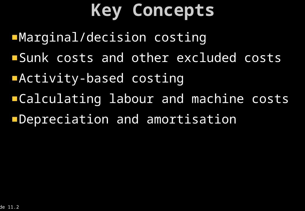
Key Concepts

Marginal/decision costing

Sunk costs and other excluded costs

Activity-based costing

Calculating labour and machine costs

Depreciation and amortisation

Slide 11.3

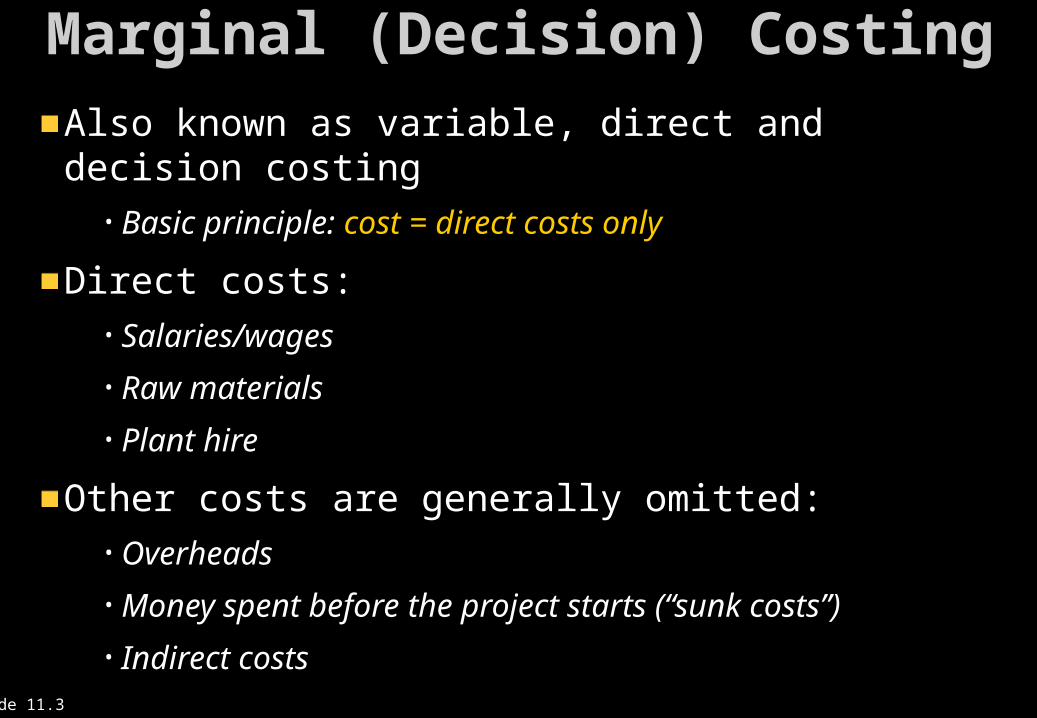
Marginal (Decision) Costing

Also known as variable, direct and decision costing• Basic principle: cost = direct costs only

Direct costs:• Salaries/wages

• Raw materials

• Plant hire

Other costs are generally omitted:• Overheads

• Money spent before the project starts (“sunk costs”)

• Indirect costs

Slide 11.4

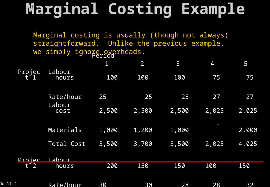
    Period    1 2 3 4 5Project 1 Labour hours 100 100 100 75 75   Rate/hour 25 25 25 27 27   Labour cost 2,500 2,500 2,500 2,025 2,025   Materials 1,000 1,200 1,000 - 2,000   Total Cost 3,500 3,700 3,500 2,025 4,025              Project 2 Labour hours 200 150 150 100 150   Rate/hour 30 30 28 28 32   Labour cost 6,000 4,500 4,200 2,800 4,800   Materials 5,000 6,000 3,000 600 600   Subtotal 11,000 10,500 7,200 3,400 5,400                Overhead 4,000 4,000 4,000 4,000 4,000

Marginal Costing Example

Marginal costing is usually (though not always) straightforward. Unlike the previous example, we simply ignore overheads.

Slide 11.5

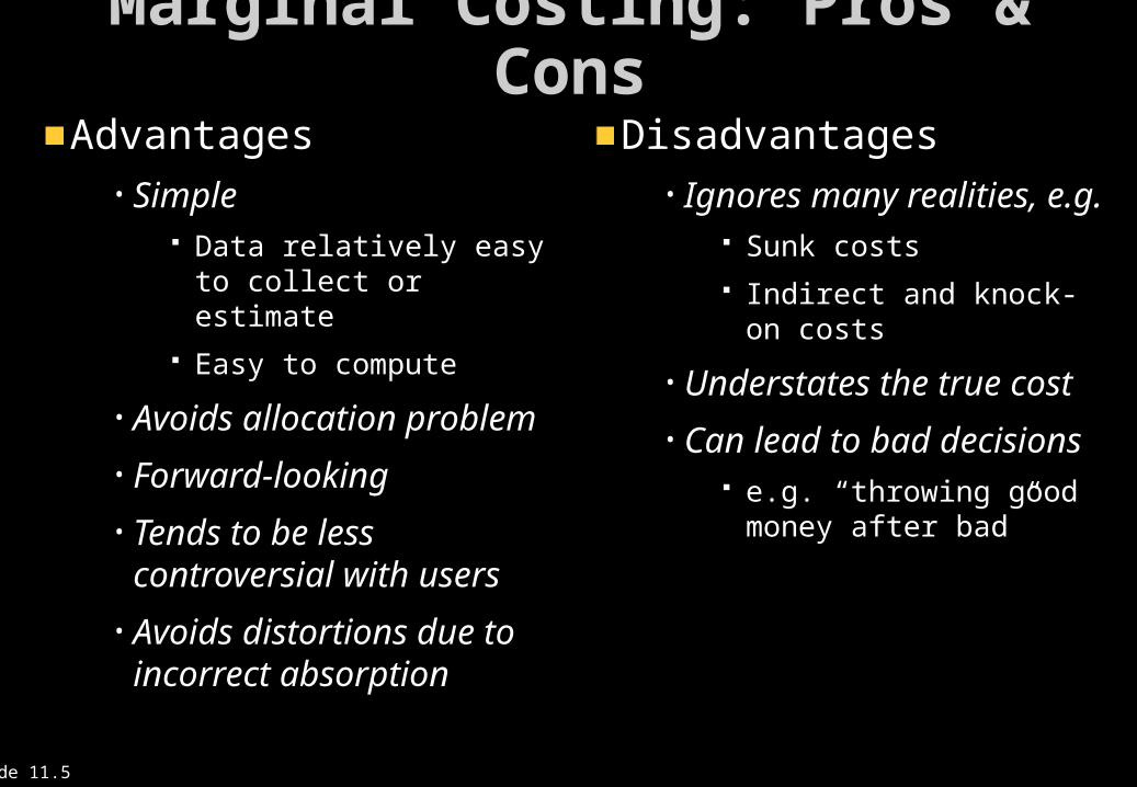
Marginal Costing: Pros & Cons

Advantages• Simple

Data relatively easy to collect or estimate

Easy to compute

• Avoids allocation problem

• Forward-looking

• Tends to be less controversial with users

• Avoids distortions due to incorrect absorption

Disadvantages• Ignores many realities,

e.g. Sunk costs

Indirect and knock-on costs

• Understates the true cost

• Can lead to bad decisions e.g. “throwing good money

after bad”

Slide 11.6

Marginal Cost: Weaknesses

Startup/Preacquisition

Costs

Post completionCosts

SecondaryCosts

DisruptionCosts

Opportunity Costs

DisplacementCosts

Start Finish

Marginal Cost

Slide 11.7

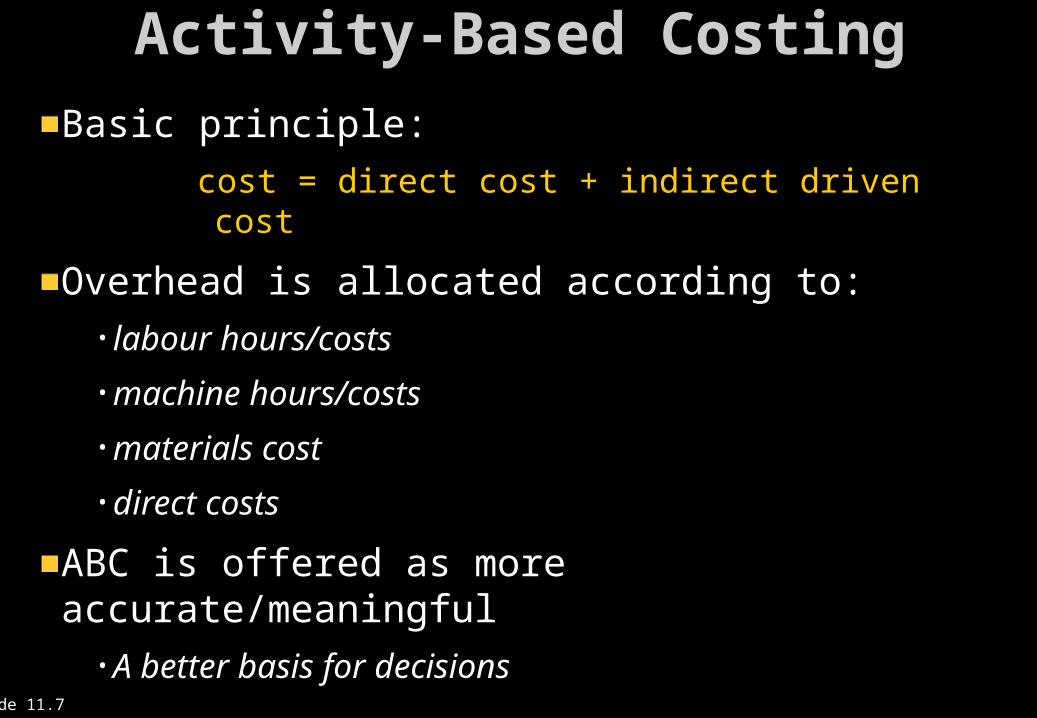
Activity-Based Costing

Basic principle:

cost = direct cost + indirect driven cost

Overhead is allocated according to:• labour hours/costs

• machine hours/costs

• materials cost

• direct costs

ABC is offered as more accurate/meaningful• A better basis for decisions

Slide 11.8

ABC Versus Absorption

Illustration using an industrial example• A company produces two products X and Y

• Using traditional cost accounting:

X Y

Units 1,000 1,500Materials/unit (€) 25 30Labour hour/unit 0.5 1.0Labour cost/hour €20

Overhead €50,000

Hours 500 1,500Overhead allocation €12,500 €37,500Per unit €12.50 €25.00Cost/unit €47.50 €75.00

Slide 11.9

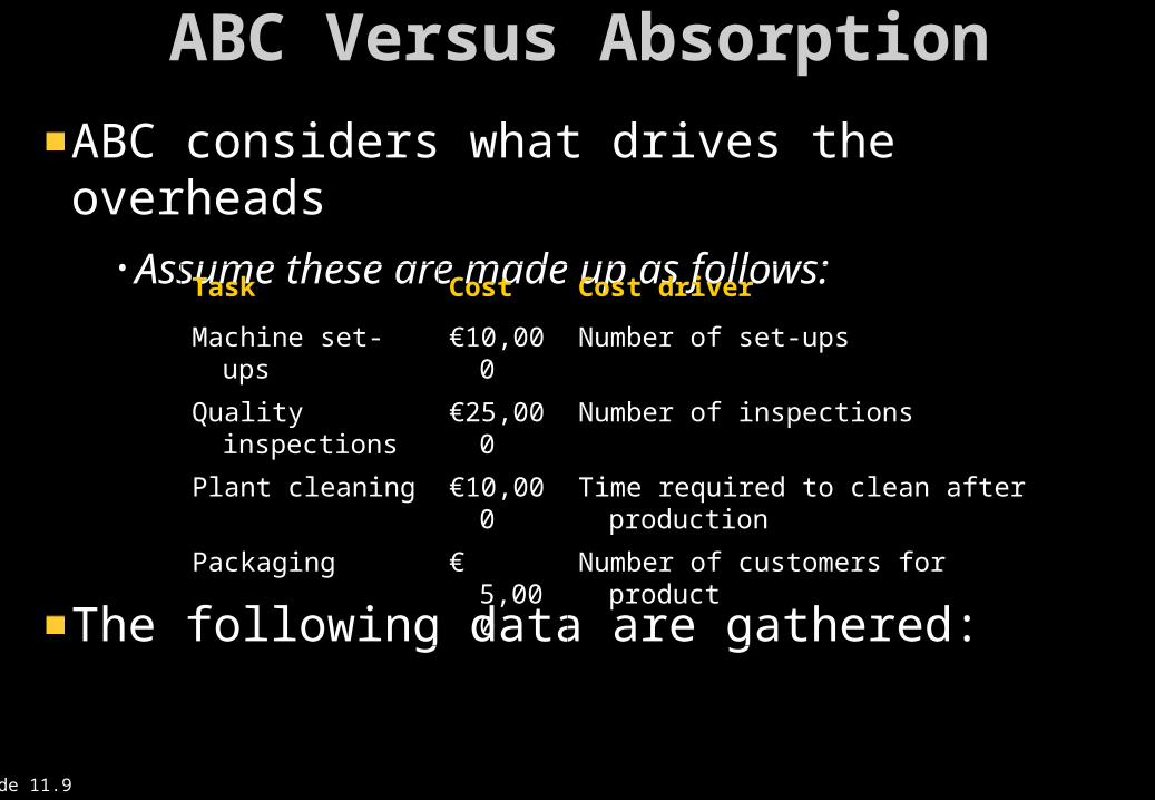
ABC Versus Absorption

ABC considers what drives the overheads• Assume these are made up as follows:

The following data are gathered:

Task Cost Cost driver

Machine set-ups €10,000 Number of set-ups

Quality inspections €25,000 Number of inspections

Plant cleaning €10,000 Time required to clean after production

Packaging € 5,000 Number of customers for product

Slide 11.10

ABC Versus Absorption

Activity Cost (€)

ProductX

ABC(€)

Product Y

ABC (€)

Set-ups 2,000 4 8,000 1 2,000

Inspections 2,500 7 17,500 3 7,500

Cleaning 1,000 8 8,000 2 2,000

Packaging 1,000 1 1,000 4 4,000

Total 34,500 15,500

Units 1,000 1,500

Per unit 34.50 10.33

Cost per unit 69.50 60.33

Absorption cost/unit 47.50 75.00

Slide 11.11

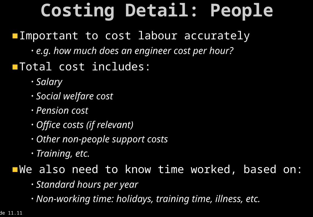
Costing Detail: PeopleImportant to cost labour accurately

• e.g. how much does an engineer cost per hour?

Total cost includes:• Salary• Social welfare cost• Pension cost• Office costs (if relevant)• Other non-people support costs• Training, etc.

We also need to know time worked, based on:• Standard hours per year• Non-working time: holidays, training time, illness, etc.

Slide 11.12

Costing People - Example

Joe is paid €36,400 p.a. and works a 35-hour week (1,820 hours/year)

• Gives an hourly cost of €20

But:• Joe’s pension, social welfare and perks add another €4,000

• Joe works only 1,155 hours a year 4 weeks annual leave plus 10 days of public holiday

one week’s sick leave

one week’s training

and Joe effectively works about 6 hours in every 8

1155 hours @ €40,400 ≈ €35 per working hour

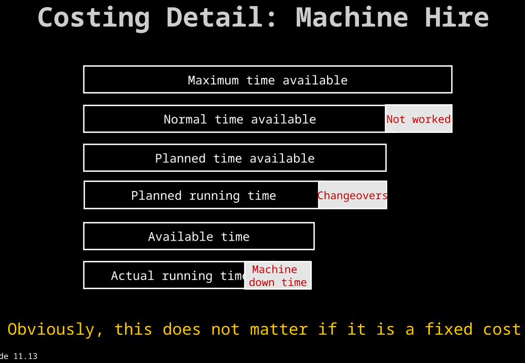
Slide 11.13

Maximum time available

Planned time available

Available time

Normal time available Not worked

Planned running time Changeovers

Actual running timeMachine down time

Obviously, this does not matter if it is a fixed cost.

Costing Detail: Machine Hire

Slide 11.14

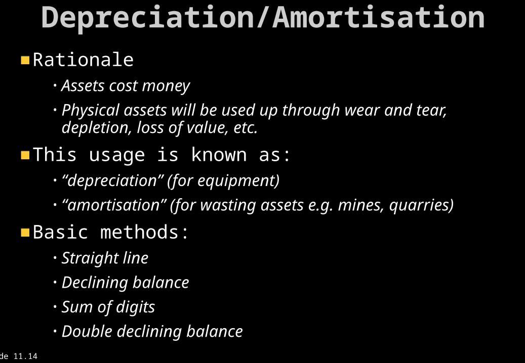
Depreciation/AmortisationRationale

• Assets cost money• Physical assets will be used up through wear and tear,

depletion, loss of value, etc.

This usage is known as:• “depreciation” (for equipment)• “amortisation” (for wasting assets e.g. mines, quarries)

Basic methods:• Straight line• Declining balance• Sum of digits• Double declining balance

Slide 11.15

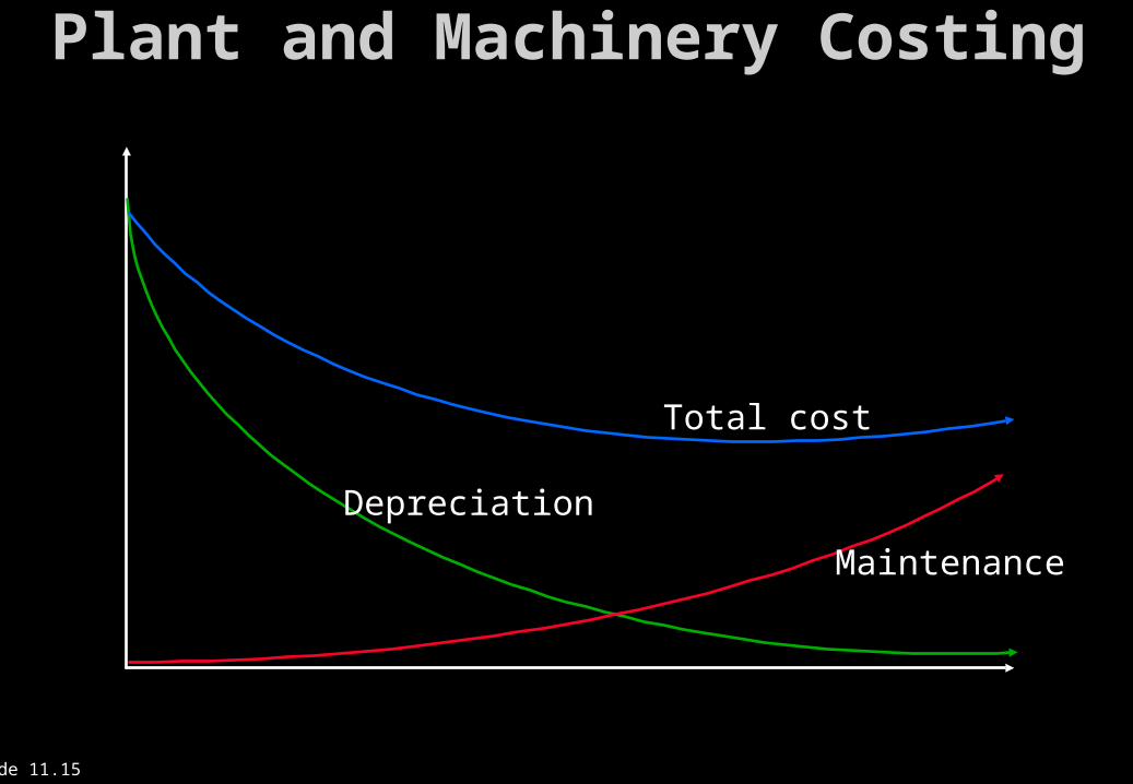
Plant and Machinery Costing

Total cost

Depreciation

Maintenance

Slide 11.16

Straight Line Depreciation

Based on no. years over which asset will be written off• Machine press bought for €200,000, written off over 4 years

• Therefore, depreciation charge is 25% per year

Pros: simple to compute; writes off assets cleanly (no residual balance problem)

Cons: not always realistic

Year Charge Balance

1 €50,000 €150,000

2 €50,000 €100,000

3 €50,000 € 50,000

4 €50,000 € 0

Slide 11.17

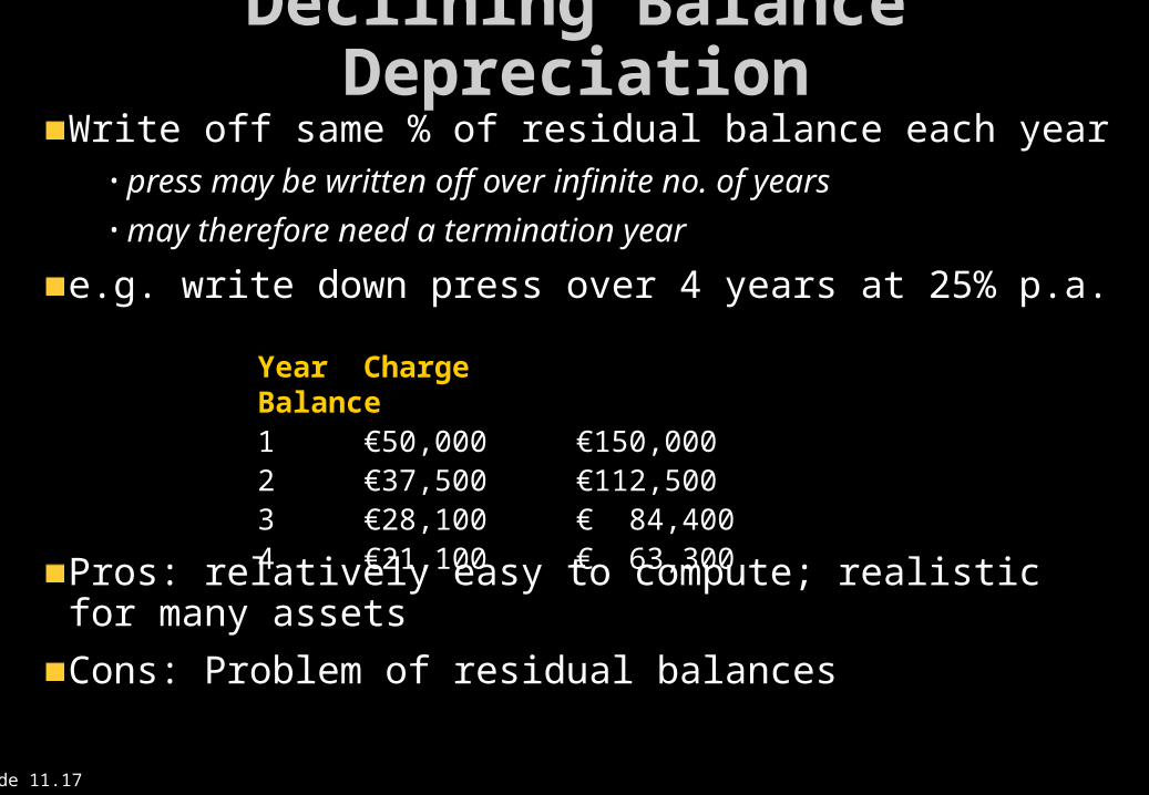
Declining Balance DepreciationWrite off same % of residual balance each year

• press may be written off over infinite no. of years• may therefore need a termination year

e.g. write down press over 4 years at 25% p.a.

Pros: relatively easy to compute; realistic for many assets

Cons: Problem of residual balances

Year Charge Balance1 €50,000 €150,0002 €37,500 €112,5003 €28,100 € 84,4004 €21,100 € 63,300

Slide 11.18

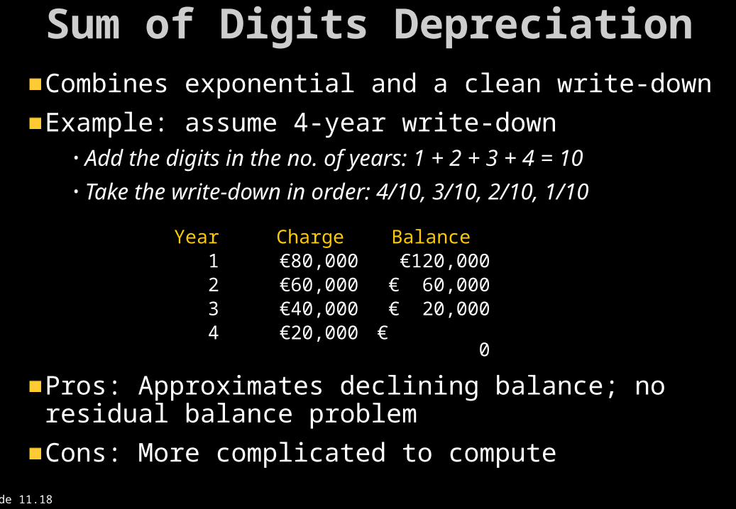
Sum of Digits DepreciationCombines exponential and a clean write-down

Example: assume 4-year write-down• Add the digits in the no. of years: 1 + 2 + 3 + 4 = 10• Take the write-down in order: 4/10, 3/10, 2/10, 1/10

Pros: Approximates declining balance; no residual balance problem

Cons: More complicated to compute

Year Charge Balance 1 €80,000 €120,000 2 €60,000 € 60,000 3 €40,000 € 20,000 4 €20,000 € 0

Slide 11.19

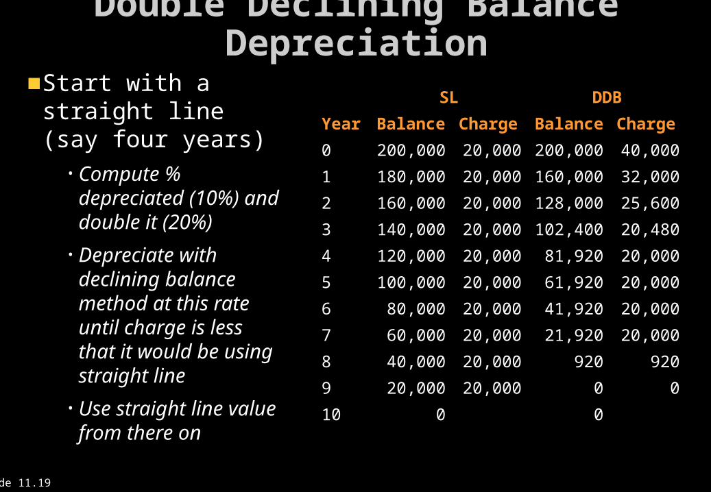
Double Declining Balance Depreciation

Start with a straight line (say four years)

• Compute % depreciated (10%) and double it (20%)

• Depreciate with declining balance method at this rate until charge is less that it would be using straight line

• Use straight line value from there on

SL DDB

Year Balance Charge Balance Charge

0 200,000 20,000 200,000 40,000

1 180,000 20,000 160,000 32,000

2 160,000 20,000 128,000 25,600

3 140,000 20,000 102,400 20,480

4 120,000 20,000 81,920 20,000

5 100,000 20,000 61,920 20,000

6 80,000 20,000 41,920 20,000

7 60,000 20,000 21,920 20,000

8 40,000 20,000 920 920

9 20,000 20,000 0 0

10 0 0

Slide 11.20

Shared Costs

Costs shared with other activities• e.g. Machines used part of the time

• Part-time staff

Shared overheads• e.g. Management

• Insurance

Not always clear how to account for shared costs

Slide 11.21

Case Study 1: New Building

How is the cost overrun to be accounted for?

Completion due early 2003

Funding problems during design• Number of floors reduced to six

• Atrium design change - chimneys on adjacent building need to be raised

• Makes change of occupancy necessary; new occupants need existing wall to be knocked down to put in equipment

Delays: building handed over late 2004

Later, power system fails and must be repaired at considerable expense

Slide 11.22

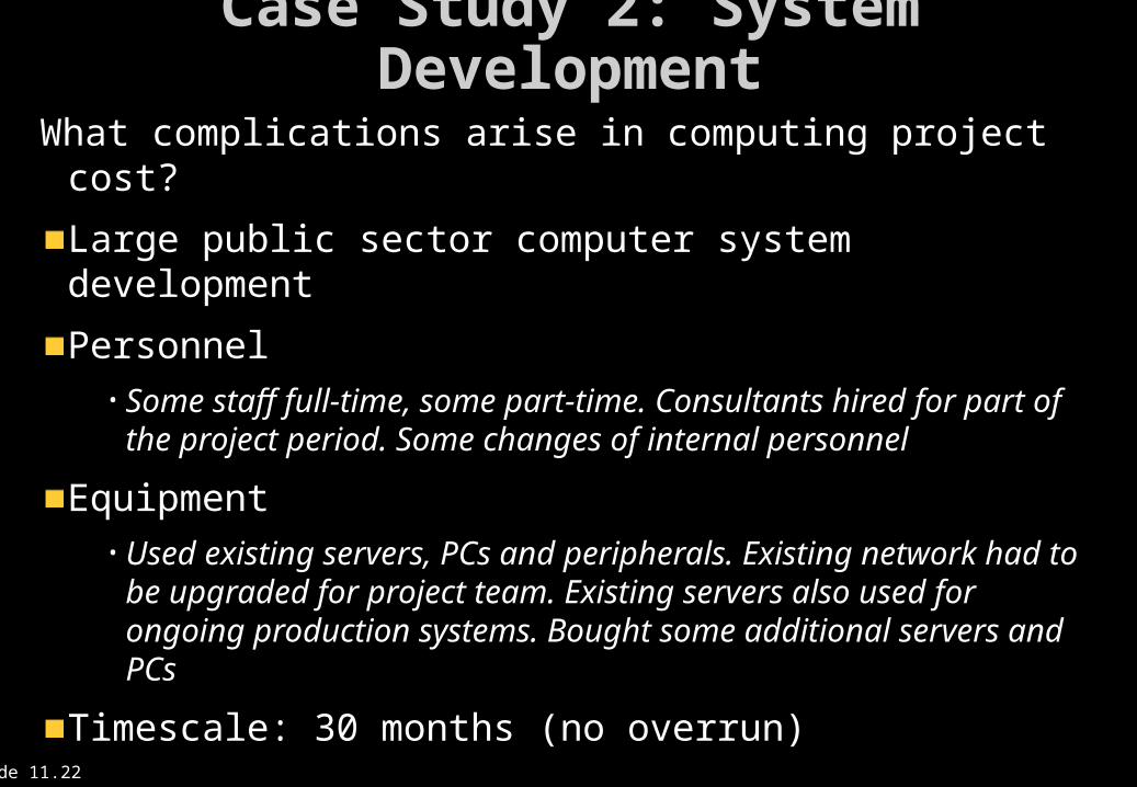
Case Study 2: System Development

What complications arise in computing project cost?

Large public sector computer system development

Personnel• Some staff full-time, some part-time. Consultants hired for part

of the project period. Some changes of internal personnel

Equipment• Used existing servers, PCs and peripherals. Existing network

had to be upgraded for project team. Existing servers also used for ongoing production systems. Bought some additional servers and PCs

Timescale: 30 months (no overrun)

Slide 11.23

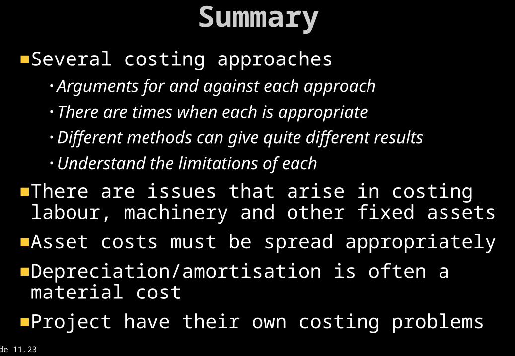
SummarySeveral costing approaches

• Arguments for and against each approach• There are times when each is appropriate• Different methods can give quite different results • Understand the limitations of each

There are issues that arise in costing labour, machinery and other fixed assets

Asset costs must be spread appropriately

Depreciation/amortisation is often a material cost

Project have their own costing problems