0 100 200 300 400 500 600 70010

-10

10-8

10-6

10-4

10-2

100

102

104

106

108

1010

Number of MV’s

rela

tive

re

sid

ua

l n

orm

CGS2CGSBi-CGSTABBi-CGstab(2)

-...-.---

GENERALIZEDCONJUGATE GRADIENT SQUAREDbyDiederik R. Fokkema, Gerard L. G. Sleijpen andHenk A. Van der VorstTo be published in J. of Computational and Applied Mathemat-ics, June 1996

Universiteit Utrecht*DepartmentofMathematics

Preprintnr. 851May 1994Revised:Okt. 1995

GENERALIZED CONJUGATE GRADIENT SQUAREDzDIEDERIK R. FOKKEMA�, GERARD L. G. SLEIJPEN�, ANDHENK A. VAN DER VORST�Abstract. The Conjugate Gradient Squared (CGS) is an iterative method for solving non-symmetric linear systems of equations. However, during the iteration large residual norms may appear,which may lead to inaccurate approximate solutions or may even deteriorate the convergence rate.Instead of squaring the Bi-CG polynomial as in CGS, we propose to consider products of two nearby Bi-CG polynomials which leads to generalized CGS methods, of which CGS is just a particular case. Thisapproach allows the construction of methods that converge less irregular than CGS and that improveon other convergence properties as well. Here, we are interested in a property that got less attentionin literature: we concentrate on retaining the excellent approximation qualities of CGS with respectto components of the solution in the direction of eigenvectors associated with extreme eigenvalues.This property seems to be important in connection with Newton's scheme for non-linear equations:our numerical experiments show that the number of Newton steps may decrease signi�cantly whenusing a generalized CGS method as linear solver for the Newton correction equations.Key words. Non-Symmetric Linear Systems, Krylov Subspace, Iterative Solvers, Bi-CG, CGS,BiCGstab(`), Non-Linear Systems, Newton's Method.AMS subject classi�cation. 65F10.1. Introduction. There is no best iterative method for solving linear systemsof equations [15]. However, in many applications a particular method is preferred.CGS [24] is a frequently used method, but the popularity of CGS has diminished overtime, because of its irregular convergence behavior. Nevertheless, in some situations,for instance, when in combination with Newton's method for non-linear equations inthe context of device simulations, CGS is often still the method of choice1.The observation is that a Newton scheme in combination with CGS usually solvesthe nonlinear problem in less Newton steps than a Newton scheme in combination withother iterative methods. And although other methods, e.g., Bi-CGSTAB, sometimesneed less iteration steps to solve the linear equations involved, Newton in combinationwith CGS turns out to be more e�cient (see also our examples in Section 7).For other situations where CGS or CGS-type of methods, i.e., TFQMR [7], arepreferred, see [13, pp. 128{133], [1].However, the large intermediate residuals produced by CGS badly a�ect its speedof convergence and limit its attainable accuracy [23], and this in turn has a (very)negative e�ect on the convergence of the overall Newton process.In this paper we discuss variants of CGS that have improved convergence proper-ties, while still having the important \quadratic reduction" property discussed below.We will now try to explain why CGS may be so successful as a linear solver in aNewton scheme. In our heuristic arguments the eigensystem, the eigenvalues �j , andthe eigenvectors vj , of the local Jacobian matrices (the matrices of partial derivativesof the non-linear problem, evaluated at the approximation) play a role. We consider�Mathematical Institute, Utrecht University, P.O. Box 80.010, NL-3508 TA Utrecht, The Nether-lands. E-mail: fokkema@math.ruu.nl, sleijpen@math.ruu.nl, vorst@math.ruu.nl.zRevised version, November 1, 1995.1Personal communication by W. Schilders and M. Driessen, Philips Research Laboratories. Theyhave also observed that for their semiconductor device modeling, where the system is often expressedin terms of voltages, the conservation of currents is better maintained when working with CGS.

2 D. R. Fokkema, G. L. G. Sleijpen, and H. A. Van der Vorstthe components of the approximate solutions and residuals in the direction of theseeigenvectors, distinguishing between components associated with exterior eigenvalues(\exterior components") and components associated with interior eigenvalues (\in-terior components"). By \exterior" and \interior" we refer to the position of theeigenvalue in the convex hull of the spectrum of the Jacobian matrix.CGS (cf. Section 2) is based on Bi-CG [6, 12]. This linear solver tends to ap-proximate the exterior components of the solution better and faster than the interiorcomponents [11, 19]. Any residual of a linear solver that we consider can be repre-sented by a polynomial in the matrix representing the linear system (for instance,the Bi-CG residual can be written as rBi-CGk = �k(A)r0, where �k is a polynomial ofdegree k) and the size of the eigenvector components of the residual is proportionalto the (absolute) value of the polynomial in the associated eigenvalue (for instance forBi-CG rBi-CGk =Pnj=1 �k(�j)vj).The absolute value of Bi-CG polynomials tends to be smaller in the exterior eigen-values than in the interior ones. A small component �k(�j)vj of the residual rk meansthat the corresponding component of the solution xk is well approximated. CGS poly-nomials are the squares of Bi-CG polynomials: the residual of CGS can be writtenas rCGSk = �2k(A)r0. Therefore, CGS approximations tend to have very accurate exte-rior components. A polynomial associated with, for instance, the BiCGstab methodsis the product of a Bi-CG polynomial and another polynomial of the same degree(rBiCGstabk = e�k(A)�k(A)r0). This other polynomial (a product of locally minimiz-ing degree 1 polynomials for Bi-CGSTAB (e�k(t) = Qki=1(1 � !it)) and a product ofsuch polynomials of degree ` for BiCGstab(`)) does not have this strong tendency ofreducing in exterior eigenvalues better than in the interior ones. Therefore, compar-ing approximations with residuals of comparable size (2-norm), we may expect thatapproximate solutions as produced by a BiCGstab method have exterior componentsthat are less accurate than those of the CGS approximations, since the error compo-nents are larger. Of course, with respect to interior components, the situation will bein favor of the BiCGstab methods.Now, we come to the implication for Newton's method. The non-linearity of theproblem seem often stronger in the (linear combination of) exterior components thanin the (linear combination of) interior ones. This fact explains the nice convergenceproperties in the outer iteration when CGS is used in the inner iteration of Newton'sprocess. CGS tends to deliver approximate solutions of which the exterior componentsare very accurate. With respect to these components, the Newton process, in whichthe linear systems are solved approximately by CGS, compares to a Newton process inwhich the linear systems are solved exactly, while this may not be true for the Newtonprocess in combination with the BiCGstab methods (or others).In summary, we wish to retain in our modi�cations the attractive property ofCGS that it converges faster with respect to exterior components within a Newtonmethod, without losing its e�ciency, the fact that it is transpose free, and its fastconvergence. However, we wish to avoid irregular convergence and large intermediateresiduals, since they may badly a�ect the speed of convergence of the inner iteration.Techniques as proposed in, e.g.,, [26, 16, 22] smooth down the convergence byoperating a posteriori on approximates and residuals. Although they may lead tomore accurate approximates (see the \additional note" in Section 7 or [22]), they donot change the speed of convergence. For a detailed discussion, see [22].

Generalized Conjugate Gradient Squared 3The polynomial associated with our new methods is the product of the Bi-CGpolynomial with another \nearby" polynomial of the same degree (cf. Section 4). Werefer to these methods as generalized CGS methods. They are about as e�cient asCGS per iteration step (cf. Section 4). We pay special attention to the case where thissecond polynomial is a Bi-CG polynomial (cf. Section 6.1) of another (nearby) Bi-CGprocess, or a polynomial closely related to such a Bi-CG polynomial (cf. Section 6.2).The di�erence between the square of a Bi-CG polynomial and the product of two\nearby" Bi-CG polynomials of the same degree may seem insigni�cant, but, as wewill see in our numerical examples in Section 7, this approach may lead to fasterconvergence in norm as well as to more accurate results. Moreover, this approachseems to improve the convergence of (exterior components in) nonlinear schemes. Adiscussion on the disadvantages of squaring the Bi-CG polynomial can be found inSection 3. Since we are working with products of Bi-CG polynomials, the new methodsreduce exterior components comparable fast as CGS (cf. Section 6.1). It is obviousthat Bi-CG and the ideas behind CGS are essential in deriving the new methods andtherefore Bi-CG and CGS are discussed in Section 2. In that Section we also introducemost of our notation.2. Bi-CG and CGS. The Bi-CG method [6, 12] is an iterative solution schemefor linear systems Ax = bin which A is some given non-singular n� n matrix and b some given n-vector. Typ-ically n is large and A is sparse. For ease of presentation, we assume A and b to bereal.Starting with an initial guess x0, each iteration of Bi-CG computes an approxima-tion xk to the solution. It is well-known that the Bi-CG residual rk = b�Axk can bewritten as �k(A)r0 where �k is a certain polynomial in the space P1k of all polynomials of degree k for which (0) = 1. The Bi-CG polynomial �k is implicitly de�ned bythe Bi-CG algorithm through a coupled two term recurrence:uk = rk � �kuk�1;rk+1 = rk � �kAuk:The iteration coe�cients �k and �k follow from the requirement that rk and Auk areorthogonal to the Krylov subspace Kk(AT ; er0) of order k, generated by AT and anarbitrary, but �xed er0.If (e�k) is some sequence of polynomials of degree k with a non-trivial leadingcoe�cient �k then (see [24] or [20]):�k = �k�1�k �k�k�1 and �k = �k�k ;(1)where �k = (rk; e�k(AT )er0) and �k = (Auk; e�k(AT )er0):(2)In standard Bi-CG the polynomial e�k is taken to be the same as the Bi-CG polynomial:e�k = �k, where �k is such that rk = �k(A)r0. This leads to another coupled two-termrecurrence in the Bi-CG algorithm:euk = erk � �keuk�1;erk+1 = erk � �kAT euk :

4 D. R. Fokkema, G. L. G. Sleijpen, and H. A. Van der VorstSince A and b are assumed to be real, this means that erk and AT euk are orthogonalto the Krylov subspace Kk(A; r0), in particular the sequences (rk) and (erk) are bi-orthogonal. Of course, other choices for e�k are possible. For instance, when A andb are complex and if we still want to have bi-orthogonality, then we should choosee�k = ��k.The leading coe�cient of �k is (��k�1)(��k�2) � � �(��0) and therefore we havethat �k�1�k = �1�k�1and thus �k = �1�k�1 �k�k�1 and �k = �k�k :A pseudo code for the standard Bi-CG algorithm is given in Alg. 1.It was Sonneveld [24] who suggested to rewrite the inner products so as to avoidthe operations with AT , e.g.,,�k = (rk; e�k(AT )er0) = (e�k(A)rk; er0);(3)and to take advantage of both �k and e�k for the reduction of the residual by generatingrecurrences for the vectors rk = e�k(A)rk. In fact, he suggested to take e�k = �k, whichled to the CGS method: rk = � 2k (A)r0. The corresponding search directions uk forthe corresponding approximation xk can be easily constructed. In this approach theBi-CG residuals rk and search directions uk themselves are not computed explicitly,nor are they needed in the process. See Alg. 2 for CGS.Choose an initial guess x0 and some er0r0 = b� Ax0u�1 = eu�1 = 0, ��1 = ��1 = 1for k = 0; 1; 2; : : : do�k = (rk; erk)�k = (�1=�k�1)(�k=�k�1)uk = rk � �kuk�1euk = erk � �keuk�1c = Auk�k = (c; erk)�k = �k=�kxk+1 = xk + �kukif xk+1 is accurate enough, then quitrk+1 = rk � �kcerk+1 = erk � �kAT eukend Algorithm 1: Bi-CGChoose an initial guess x0 and some er0r0 = b�Ax0u�1 = w�1 = 0, ��1 = ��1 = 1for k = 0; 1; 2; : : : do�k = (rk; er0)�k = (�1=�k�1)(�k=�k�1)vk = rk � �kuk�1wk = vk � �k(uk�1 � �kwk�1)c = Awk�k = (c; er0)�k = �k=�kuk = vk � �kcxk+1 = xk + �k(vk + uk)if xk+1 is accurate enough, then quitrk+1 = rk � �kA(vk + uk)end Algorithm 2: CGSAs is explained in [25], �k(A) may not be a particularly well suited reductionoperator for �k(A)r0. But, as we will see in Section 3, there are more argumentsfor not selecting e�k = �k . For instance, we wish to avoid irregular convergence andlarge intermediate residuals. In [25] it was suggested to choose e�k as a product oflinear factors, which were constructed to minimize residuals in only one direction

Generalized Conjugate Gradient Squared 5at a time. This led to the Bi-CGSTAB algorithm. This was further generalizedto a composite of higher degree factors which minimize residuals over `-dimensionalsubspaces: BiCGStab2, for ` = 2, in [10] and BiCGstab(`), the more e�cient andmore stable variant also for general `, in [20, 23] (see also [21]).Obviously, there is a variety of possibilities for the polynomials e�k. In the nextsections we investigate polynomials that are similar to the Bi-CG polynomial, i.e.,polynomials that are de�ned by a coupled two term recurrence. This leads to a gen-eralized CGS (GCGS) algorithm, of which CGS and Bi-CGSTAB are just particularinstances.3. Disadvantages of squaring the iteration polynomial. For an eigenvalue� of A, the component of the CGS residual, in the direction of the eigenvector asso-ciated with �, is equal to ���k(�)2, where �� is the component of r0 in the directionof the same eigenvector (assuming � is a semi-simple eigenvalue). The correspondingcomponent of the Bi-CG residual is precisely ���k(�) and the tendency of j�k(�)j tobe small for non-large k and for exterior � explains the good reduction abilities ofCGS with respect to the exterior components.Unfortunately, squaring has disadvantages: j�k(�)j2 may be large even if j���k(�)jis moderate. This may happen especially during the initial stage of the process (whenk is small) and the CGS component will be extremely large. In such a case, the CGSresidual rk is extremely large. Although the next residual rk+1 may be moderate,a single large residual is enough to prevent the process of �nding an accurate �nalapproximate solution in �nite precision arithmetic: in [23], Section 2.2 (see also [21]),it was shown thatjkrmk2 � kb�Axmk2j � � � maxk�m krkk2 with � := mnA kA�1k2 k jAj k2;(4)where � is the relative machine precision and nA is the maximum number of non-zeroentries per row of A. Except for the constant � this estimate seems to be sharp inpractice: in actual computations we do not see the factor � (see [21]). Moreover thelocal bi-orthogonality, essential for Bi-CG and (implicitly) for CGS, will seriously bedisturbed2. This will slow down the speed of convergence. CGS is notorious for largeintermediate residuals and erratic convergence behavior. The fact that j�k(�)j2 canbe large was precisely the reason in [25] to reject the choice e�k = �k and to considera product of degree 1 factors that locally minimize the residual with respect to thenorm k � k2. As anticipated, this approach usually improves the attainable accuracy,(i.e., the distance between krmk2 and kb � Axmk2; cf. (4)) as well as the rate ofconvergence. However, the degree 1 factors do not tend to favor the reduction of theexterior components as we wish here.In summary, we wish to avoid \quadratically large" residual components, whileretaining \quadratically small" components.Of course the selected polynomials e�k should also lead to an e�cient algorithm.Before specifying polynomials e�k in the Sections 5 and 6, we address this e�ciencysubject in Section 4.2The Neumaier trick (cf. the \additional note" in Section 7) cures the loss of accuracy, but it doesnot improve the speed of convergence [22].

6 D. R. Fokkema, G. L. G. Sleijpen, and H. A. Van der Vorst4. Generalized CGS: methods of CGS type. In this section we derive analgorithm that delivers rk = e�k(A)�k(A)r0, where e�k is a polynomial de�ned by acoupled two term recurrence and where �k is the Bi-CG polynomial.Consider the Bi-CG recurrence for the search directions uk and the residuals rk+1u�1 = 0; r0 = b� Ax0;(5) uk = rk � �kuk�1;(6) rk+1 = rk � �kAuk ;(7)and the polynomial recurrence for the polynomials e�k+1 and e k evaluated in Ae �1(A) � 0; e�0(A) � 1;(8) e k(A) = e�k(A)� e�k e k�1(A);(9) e�k+1(A) = e�k(A)� e�kA e k(A);(10)for scalar sequences (e�k) and (e�k). For ease of notation we will write �k for e�k(A)and k for e k(A) from now on. Our goal is to compute rk+1 = �k+1rk+1. We willconcentrate on the vector updates �rst, i.e., for the moment we will assume that theiteration coe�cients e�k and e�k are explicitly given.Suppose we have the following vectors at step k:k�1uk�1; k�1rk; �kuk�1 and �krk:(11)Note that for k = 0 these vectors are well de�ned. We proceed by showing how theindex of vectors in (11) can be increased.We use the Bi-CG recurrence (6) to update �kuk:�kuk = �krk � �k�kuk�1:Before we can update kuk a similar way, i.e.,kuk = krk � �kkuk�1;(12)we need the vectors krk and kuk�1. These vectors follow from (9):krk = �krk � e�kk�1rk;(13) kuk�1 = �kuk�1 � e�kk�1uk�1:(14)This in combination with (12) gives us kuk. The vectors krk+1 and �k+1uk followfrom (7) and (10): krk+1 = krk � �kAkuk ;�k+1uk = �kuk � e�kAkuk :Finally, to obtain �k+1rk+1 we apply the recurrences (7) and (10):�krk+1 = �krk � �kA�kuk;(15) �k+1rk+1 = �krk+1 � e�kAkrk+1:(16)

Generalized Conjugate Gradient Squared 7When �k and e�k are known before updating (15) and (16), we can avoid one of thematrix-vector products by combining these equations. This leads to�k+1rk+1 = �krk �A(�k�kuk � e�kkrk+1);and, hence, we only need Akuk and A(�k�kuk� e�kkrk+1) in order to complete oneiteration step, and the corresponding computational scheme needs two matrix-vectormultiplications per iteration step, just as CGS.The iteration coe�cients �k and �k have to be computed such that rk and Aukare orthogonal to the Krylov subspace Kk(AT ; er0). According to (1) and (2), thesecoe�cients are determined by �k�1=�k , �k and �k. From (10) it follows that the leadingcoe�cient of e�k is (�e�k�1)(�e�k�2) � � �(�e�0) and hence�k�1�k = �1e�k :For the scalar �k we can rewrite the inner product (cf. (3)):�k = (�krk; er0):Note that the vector �krk is available. However, for the scalar �k rewriting theinner product does not help because A�kuk is no longer available, since we havecombined (15) and (16). Fortunately, we can replace A�kuk by the vector Akuk,which is available. It follows from (9) that the degree of e k � e�k is smaller than k+1and thus that (A(�k � k)uk; er0) = (Auk; (e�k(AT )� e k(AT ))er0) = 0:Therefore, we have that �k = (Akuk; er0):The algorithm for this generalized CGS (GCGS) method is given as Alg. 3. Inthis algorithm, the following substitutions have been made:uk�1 = �kuk�1; vk = �kuk; wk = kuk ;rk = �krk; sk = krk+1; and tk = krk;and the equations (12) and (13) are combined to one single equation.The algorithm is very similar to the algorithm as Alg. 2. In terms of computa-tional work per iteration step (per 2 matrix-vector multiplications) GCGS needs onlytwo more vector updates than CGS; moreover, GCGS needs only storage for two morevectors.In Sections 5 and 6 we will discuss some possible choices for the recurrence coe�-cients of the polynomials e�k. Section 5 contains the well known CGS and Bi-CGSTABmethod. The new methods can be found in Section 6.5. Well known methods of CGS type. We present here the CGS and theBi-CGSTAB method to show that they �t in the frame of generalized CGS methodsand to facilitate e�ciency comparison.5.1. CGS: using the Bi-CG polynomials. The choice e�k = �k , e�k = �k leadsto CGS. In Alg. 3 the vectors vk and tk as well as the vectors uk and sk are identicalin this situation and some computational steps are now redundant.

8 D. R. Fokkema, G. L. G. Sleijpen, and H. A. Van der VorstChoose an initial guess x0 and some er0r0 = b� Ax0u�1 = w�1 = s�1 = 0,��1 = ��1 = e��1 = e��1 = 1for k = 0; 1; 2; : : : do�k = (rk; er0)�k = (�1=e�k�1)(�k=�k�1)vk = rk � �kuk�1choose e�ktk = rk � e�ksk�1wk = tk � �k(uk�1 � e�kwk�1)c = Awk�k = (c; er0)�k = �k=�ksk = tk � �kcchoose e�kuk = vk � e�kcxk+1 = xk + �kvk + e�kskif xk+1 is accurate enough, then quitrk+1 = rk � A(�kvk + e�ksk)end Algorithm 3: GCGS5.2. Bi-CGSTAB: using products of optimal �rst degree factors. Asexplained in Section 3, to avoid irregular convergence and large intermediate residuals,a product of degree 1 factors that locally minimize the residual is suggested in [25].In our formulation Bi-CGSTAB can be obtained as follows. Take e�k = 0, so thatthe recurrences (12)-(16) reduce to�kuk = �krk � �k�kuk�1;(17) �krk+1 = �krk � �kA�kuk;(18) �k+1uk = �kuk � e�kA�kuk;(19) �k+1rk+1 = �krk+1 � e�kA�krk+1;(20)and take e�k such that k�krk+1 � e�kA�krk+1k2 is minimal. Hence,e�k = (�krk+1; A�krk+1)(A�krk+1; A�krk+1) :For e�ciency reasons one usually combines (17) and (19). Notice that e�k is now aproduct of the linear factors (1� e�k�).A pseudo code for Bi-CGSTAB is given in Alg. 4.6. New methods of CGS type. The BiCGstab methods generally convergemore smoothly than CGS, but they do not approximate the exterior components ofthe solution as well as CGS. We wish to preserve this approximation property, whilesmoothing the convergence at the same time3.3As explained in Section 3, we wish the smooth convergence by avoiding a priori extremely largecomponents. The smoothing techniques in, e.g., [26], work a posteriori and do not a�ect the rate of

Generalized Conjugate Gradient Squared 9Choose an initial guess x0 and some er0r0 = b� Ax0u�1 = w�1 = s�1 = 0,��1 = ��1 = e��1 = e��1 = 1for k = 0; 1; 2; : : : do�k = (rk; er0)�k = (�1=e�k�1)(�k=�k�1)wk = rk � �k(wk�1 � e�kck�1)ck = Awk�k = (ck; er0)�k = �k=�ksk = rk � �kctk = Aske�k = (sk; tk)=(tk; tk)xk+1 = xk + �kwk + e�kskif xk+1 is accurate enough, then quitrk+1 = sk � e�tkend Algorithm 4: Bi-CGSTAB6.1. CGS2: using related Bi-CG polynomials. We will argue that a relatedBi-CG polynomial will meet our conditions to a certain extent: in this subsection, e�kis the Bi-CG polynomial generated by r0 and es0 some vector di�erent from er0. Fores0 one may take, for instance, a random vector. The roots of the Bi-CG polynomial�k converge (for increasing k) towards eigenvalues corresponding to eigenvectors withnon-zero weights ��. The roots of this e�k will converge to the same eigenvalues, but,and this is important, in a di�erent manner. If both �k and e�k reduce a componentof r0 poorly, as may be the case initially, then both corresponding roots have not yetconverged to the corresponding eigenvalue. In other words, both �k(�) and e�k(�) aresigni�cantly di�erent from zero. But, since both polynomials are distinct, the productje�k(�)�k(�)j is smaller than max(j�k(�)j2; je�k(�)j2) and one may hope that applyinge�k(A)�k(A) as a reduction operator to r0 will not lead to as bad an ampli�cation ofthis component as �k(A)2 (CGS). If both �k and e�k reduce a component of r0 well,as may be the case later in the iteration process, then both corresponding roots haveconverged to the same corresponding eigenvalue. In this case we have a quadraticreduction of that component.We give more details for the resulting scheme. The scheme is very e�cient: al-though we work (implicitly) with two di�erent Bi-CG processes the iteration steps donot require matrix-vector multiplications in addition to the ones in the GCGS scheme(Alg. 3). As before, we write e�k(A) as �k (and e k(A) as k).As with the Bi-CG polynomial �k (see Section 2), we seek coe�cients e�k ande�k such that �kr0 and Akr0 are orthogonal to the Krylov subspace Kk(AT ; es0).According to (1) and (2) we may writee�k = e�k�1e�k e�ke�k�1 and e�k = e�ke�k ;convergence nor the attainable accuracy.

10 D. R. Fokkema, G. L. G. Sleijpen, and H. A. Van der Vorstwhere e�k = (�kr0; �k(AT )es0) and e�k = (Akr0; �k(AT )es0)(21)and e�k is the leading coe�cient of some polynomial �k of degree k and �k(0) = 1.Normally, like in Bi-CG, practically any choice for �k would lead to another twoterm recurrence in order to construct a basis for Kk(AT ; es0). That would make thealgorithm expensive, especially since matrix multiplications are involved. Surprisingly,we can avoid this construction, and thus the computational work because we can usethe Bi-CG polynomial �k, which is already (implicitly) available. Replacing �k by �kin (21) gives us for the iteration coe�cients thate�k = �1�k�1 e�ke�k�1 and e�k = e�ke�k ;where e�k = (�kr0; �k(AT )es0) = (�k�k(A)r0; es0) = (rk; es0) ande�k = (Akr0; �k(AT )es0) = (Ak�k(A)r0; es0) = (Avk; es0):Here we used the fact that multiplication with polynomials in A is commutative:�k(A) e�(A)r0 = e�k(A)�k(A)r0 = �krk and �k(A) e k(A)r0 = e k(A)�k(A)r0 = krk.A pseudo code for this computational scheme, which we will call CGS2, is given inAlg. 5. Compared to CGS, CGS2 needs two more vector updates and two more innerproducts per iteration and storage for three additional vectors.6.2. Shifted CGS: using delayed Bi-CG polynomials. We wish to avoidextremely large factors je�k(�)�k(�)j . Such factors may occur if e�k�k has a (nearly)double root corresponding to an eigenvector component that has not converged (yet).The choice of e�k in the preceding section does not exclude this possibility. In ourapproach below, we explicitly try to avoid these unwanted double roots associatedwith eigenvector components that have not converged yet. As before, we still want tohave near double roots corresponding to converged components.It is well-known that for A = AT the roots of the Bi-CG polynomial �k�1 separatethose of �k and a product of these two polynomials seems to be a good candidate foravoiding large residuals. This idea can be implemented as follows.For some � 2 C , take e�k(�) = (1� ��)�k�1(�);or equivalently, take e�k = 0 and e�k = �; for k = 0,e�k = �k�1 and e�k = �k�1 for k > 0:in the GCGS algorithm in Alg. 3.A possible choice for � is, for instance, the inverse of an approximation for thelargest eigenvalue of A. This value for � can be roughly determined with Gersh-gorin disks or with a few steps of Arnoldi's algorithm. As explained in the previoussection, one may expect a smoother convergence behavior for symmetric problems.Additionally, the choice of � may reduce the in uence of the largest eigenvalue onthe convergence behavior. For general unsymmetric problems, where complex rootsmay appear, one may hope for a similar behavior of this scheme. We will refer to thisapproach as Shifted CGS. Note that in terms of computational work we save 2 innerproducts as compared to CGS2.

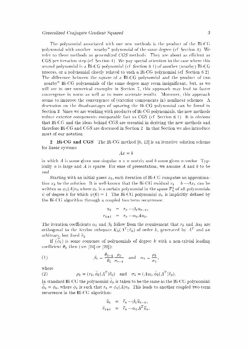
Generalized Conjugate Gradient Squared 11Choose an initial guess x0, some er0 and some es0r0 = b�Ax0u�1 = w�1 = s�1 = 0,��1 = ��1 = e��1 = e��1 = 1for k = 0; 1; 2; : : : do�k = (rk; er0)�k = (�1=e�k�1)(�k=�k�1)vk = rk � �kuk�1e�k = (rk; es0)e�k = (�1=�k�1)(e�k=e�k�1)tk = rk � e�ksk�1wk = tk � �k(uk�1 � e�kwk�1)c = Awk�k = (c; er0)�k = (�k=�k)sk = tk � �kce�k = (c; es0)e�k = e�k=e�kuk = vk � e�kcxk+1 = xk + �kvk + e�kskif xk+1 is accurate enough, then quitrk+1 = rk �A(�kvk + e�ksk)end Algorithm 5: CGS27. Numerical examples. The new GCGS methods (in Section 6) do not seemto be superior to BiCGstab(`) as solvers of linear equations (although it seems theycan compete). This should not come as a surprise, because they were not designedfor this purpose. However, as we will see, they can be attractive as linear solver in aNewton scheme for non-linear equations. The GCGS methods improve on CGS, withsmoother and faster convergence, avoiding large intermediate residuals, leading tomore accurate approximations (see, Section 7.1 for CGS2, and Section 7.2 for ShiftedCGS). At the same time, they seem to maintain the good reduction properties of CGSwith respect to the exterior components, and thus improving on BiCGstab methodsas solvers in a Newton scheme (see, Section 7.3 and 7.4).For large realistic problems, it is hard to compare explicitly the e�ects of thelinear solvers on, say, the exterior components. Below, we increase con�dence in thecorrectness of our heuristic arguments by showing that the convergence behavior inthe numerical examples is in line with our predictions.7.1. Characteristics of CGS2. The CGS2 algorithm (Alg. 5), which uses aproduct of two nearby Bi-CG polynomials, was tested with success at IIS in Z�urich(this Section) and at Philips in Eindhoven (Section 7.3).At IIS the package PILS [18] written in C and FORTRAN was used for solving twolinear systems extracted from the simulation of two devices called dr15c and mct70crespectively. The computations were done on a Sun Sparc 10 in double precision(� � 0:5 � 10�15) and ILU(0) [18, 14] was used as a preconditioner. The plots

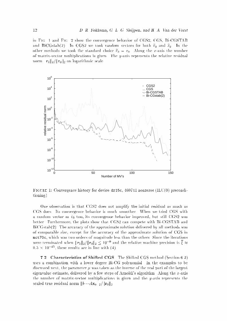
12 D. R. Fokkema, G. L. G. Sleijpen, and H. A. Van der Vorstin Fig. 1 and Fig. 2 show the convergence behavior of CGS2, CGS, Bi-CGSTABand BiCGstab(2). In CGS2 we took random vectors for both er0 and es0. In theother methods we took the standard choice er0 = r0. Along the x-axis the numberof matrix-vector multiplications is given. The y-axis represents the relative residualnorm krkk2=kr0k2 on logarithmic scale.0 50 100 150

10-12

10-10

10-8

10-6

10-4

10-2

100

102

104

106

Number of MV’s

rela

tive

resi

dual

nor

m

CGS2CGSBi-CGSTABBi-CGstab(2)

-...-.---

Figure 1: Convergence history for device dr15c, 469741 nonzeros (ILU(0) precondi-tioning).One observation is that CGS2 does not amplify the initial residual as much asCGS does. Its convergence behavior is much smoother. When we tried CGS witha random vector as er0 too, its convergence behavior improved, but still CGS2 wasbetter. Furthermore, the plots show that CGS2 can compete with Bi-CGSTAB andBiCGstab(2). The accuracy of the approximate solution delivered by all methods wasof comparable size, except for the accuracy of the approximate solution of CGS inmct70c, which was two orders of magnitude less than the others. Since the iterationswere terminated when krkk2=kr0k2 � 10�9 and the relative machine precision is � �0:5 � 10�15, these results are in line with (4).7.2. Characteristics of Shifted CGS. The Shifted CGS method (Section 6.2)uses a combination with a lower degree Bi-CG polynomial. In the examples to bediscussed next, the parameter � was taken as the inverse of the real part of the largesteigenvalue estimate, delivered by a few steps of Arnoldi's algorithm. Along the x-axisthe number of matrix-vector multiplications is given and the y-axis represents thescaled true residual norm kb�Axkk2=kr0k2.

Generalized Conjugate Gradient Squared 130 100 200 300 400 500 600 700

10-10

10-8

10-6

10-4

10-2

100

102

104

106

108

1010

Number of MV’s

rela

tive

resi

dual

nor

mCGS2CGSBi-CGSTABBi-CGstab(2)

-...-.---

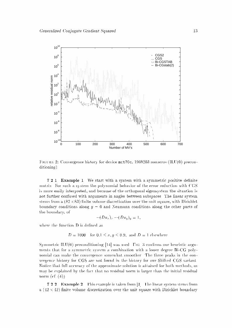
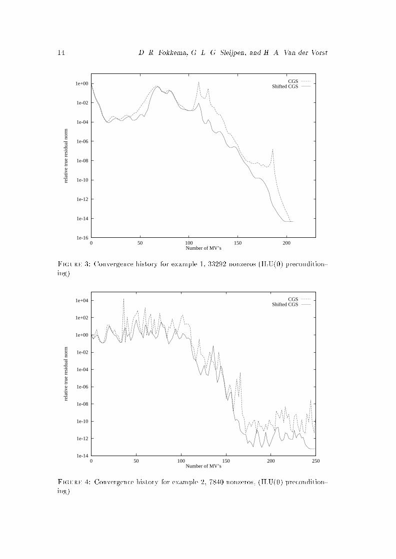
Figure 2: Convergence history for device mct70c, 1969203 nonzeros (ILU(0) precon-ditioning).7.2.1. Example 1. We start with a system with a symmetric positive de�nitematrix. For such a system the polynomial behavior of the error reduction with CGSis more easily interpreted, and because of the orthogonal eigensystem the situation isnot further confused with arguments in angles between subspaces. The linear systemstems from a (82�83) �nite volume discretization over the unit square, with Dirichletboundary conditions along y = 0 and Neumann conditions along the other parts ofthe boundary, of �(Dux)x � (Duy)y = 1;where the function D is de�ned asD = 1000 for 0:1 � x; y � 0:9; and D = 1 elsewhere.Symmetric ILU(0) preconditioning [14] was used. Fig. 3 con�rms our heuristic argu-ments that for a symmetric system a combination with a lower degree Bi-CG poly-nomial can make the convergence somewhat smoother. The three peaks in the con-vergence history for CGS are not found in the history for our Shifted CGS variant.Notice that full accuracy of the approximate solution is attained for both methods, asmay be explained by the fact that no residual norm is larger than the initial residualnorm (cf. (4)).7.2.2. Example 2. This example is taken from [3]. The linear system stems froma (42� 42) �nite volume discretization over the unit square with Dirichlet boundary

14 D. R. Fokkema, G. L. G. Sleijpen, and H. A. Van der Vorst1e-16

1e-14

1e-12

1e-10

1e-08

1e-06

1e-04

1e-02

1e+00

0 50 100 150 200

rela

tive

true

res

idua

l nor

m

Number of MV’s

Shifted CGSCGS

Figure 3: Convergence history for example 1, 33292 nonzeros (ILU(0) precondition-ing).1e-14

1e-12

1e-10

1e-08

1e-06

1e-04

1e-02

1e+00

1e+02

1e+04

0 50 100 150 200 250

rela

tive

true

res

idua

l nor

m

Number of MV’s

Shifted CGSCGS

Figure 4: Convergence history for example 2, 7840 nonzeros, (ILU(0) precondition-ing).

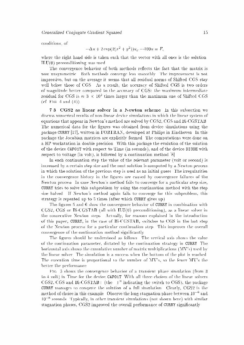
Generalized Conjugate Gradient Squared 15conditions, of ��u+ 2 exp(2(x2 + y2))ux � 100u = F;where the right hand side is taken such that the vector with all ones is the solution.ILU(0) preconditioning was used.The convergence behavior of both methods re ects the fact that the matrix isnow unsymmetric. Both methods converge less smoothly. The improvement is notimpressive, but on the average it seems that all residual norms of Shifted CGS staywell below those of CGS. As a result, the accuracy of Shifted CGS is two ordersof magnitude better compared to the accuracy of CGS: the maximum intermediateresidual for CGS is � 3 � 102 times larger than the maximum one of Shifted CGS(cf. Fig. 4 and (4)).7.3. CGS2 as linear solver in a Newton scheme. In this subsection wediscuss numerical results of non-linear device simulations in which the linear system ofequations that appear in Newton's method are solved by CGS2, CGS and Bi-CGSTAB.The numerical data for the �gures was obtained from device simulations using thepackage CURRY [17], written in FORTRAN, developed at Philips in Eindhoven. In thispackage the Jocabian matrices are explicitly formed. The computations were done ona HP workstation in double precision. With this package the evolution of the solutionof the device CAP01T with respect to Time (in seconds), and of the device DIODE withrespect to voltage (in volt), is followed by a continuation method [8].In each continuation step the value of the relevant parameter (volt or second) isincreased by a certain step size and the next solution is computed by a Newton processin which the solution of the previous step is used as an initial guess. The irregularitiesin the convergence history in the �gures are caused by convergence failures of theNewton process. In case Newton's method fails to converge for a particular step size,CURRY tries to solve this subproblem by using the continuation method with the stepsize halved. If Newton's method again fails to converge for this subproblem, thisstrategy is repeated up to 5 times (after which CURRY gives up).The �gures 5 and 6 show the convergence behavior of CURRY in combination withCGS2, CGS or Bi-CGSTAB (all with ILU(0) preconditioning), as a linear solver inthe consecutive Newton steps. Actually, for reasons explained in the introductionof this paper, CURRY, in the case of Bi-CGSTAB, switches to CGS in the last stepof the Newton process for a particular continuation step. This improves the overallconvergence of the continuation method signi�cantly.The �gures should be understood as follows. The vertical axis shows the valueof the continuation parameter, dictated by the continuation strategy in CURRY. Thehorizontal axis shows the cumulative number of matrix multiplications (MV's) used bythe linear solver. The simulation is a success when the bottom of the plot is reached.The execution time is proportional to the number of MV's, so the fewer MV's thebetter the performance.Fig. 5 shows the convergence behavior of a transient phase simulation (from 3to 4 volt) in Time for the device CAP01T. With all three choices of the linear solversCGS2, CGS and Bi-CGSTAB+ (the \+" indicating the switch to CGS), the packageCURRY manages to compute the solution of a full simulation. Clearly, CGS2 is themethod of choice in this example. Observe the long stagnation phase between 10�9 and10�8 seconds. Typically, in other transient simulations (not shown here) with similarstagnation phases, CGS2 improved the overall performance of CURRY signi�cantly.

16 D. R. Fokkema, G. L. G. Sleijpen, and H. A. Van der Vorst

0 1000 2000 3000 4000 5000 600010

−5

10−6

10−7

10−8

10−9

10−10

10−11

10−12

CGS2CGSBi−CGSTAB+

−...−.−

Number of MV’s

Sec

onds

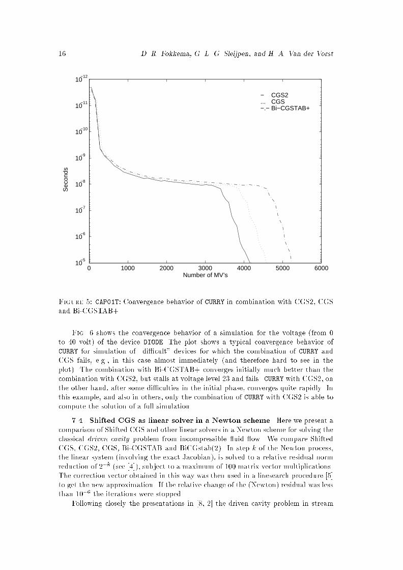
Figure 5: CAP01T: Convergence behavior of CURRY in combination with CGS2, CGSand Bi-CGSTAB+.Fig. 6 shows the convergence behavior of a simulation for the voltage (from 0to 40 volt) of the device DIODE. The plot shows a typical convergence behavior ofCURRY for simulation of \di�cult" devices for which the combination of CURRY andCGS fails, e.g., in this case almost immediately (and therefore hard to see in theplot). The combination with Bi-CGSTAB+ converges initially much better than thecombination with CGS2, but stalls at voltage level 23 and fails. CURRY with CGS2, onthe other hand, after some di�culties in the initial phase, converges quite rapidly. Inthis example, and also in others, only the combination of CURRY with CGS2 is able tocompute the solution of a full simulation.7.4. Shifted CGS as linear solver in a Newton scheme. Here we present acomparison of Shifted CGS and other linear solvers in a Newton scheme for solving theclassical driven cavity problem from incompressible uid ow. We compare ShiftedCGS, CGS2, CGS, Bi-CGSTAB and BiCGstab(2). In step k of the Newton process,the linear system (involving the exact Jacobian), is solved to a relative residual normreduction of 2�k (see [4]), subject to a maximum of 100 matrix vector multiplications.The correction vector obtained in this way was then used in a linesearch procedure [5]to get the new approximation. If the relative change of the (Newton) residual was lessthan 10�6 the iterations were stopped.Following closely the presentations in [8, 2] the driven cavity problem in stream

Generalized Conjugate Gradient Squared 17

0 1000 2000 3000 4000 5000 6000 7000 40

35

30

25

20

15

10

5

0

CGS2CGS (no convergence)Bi−CGSTAB+

−...−.−

Number of MV’s

Vol

t

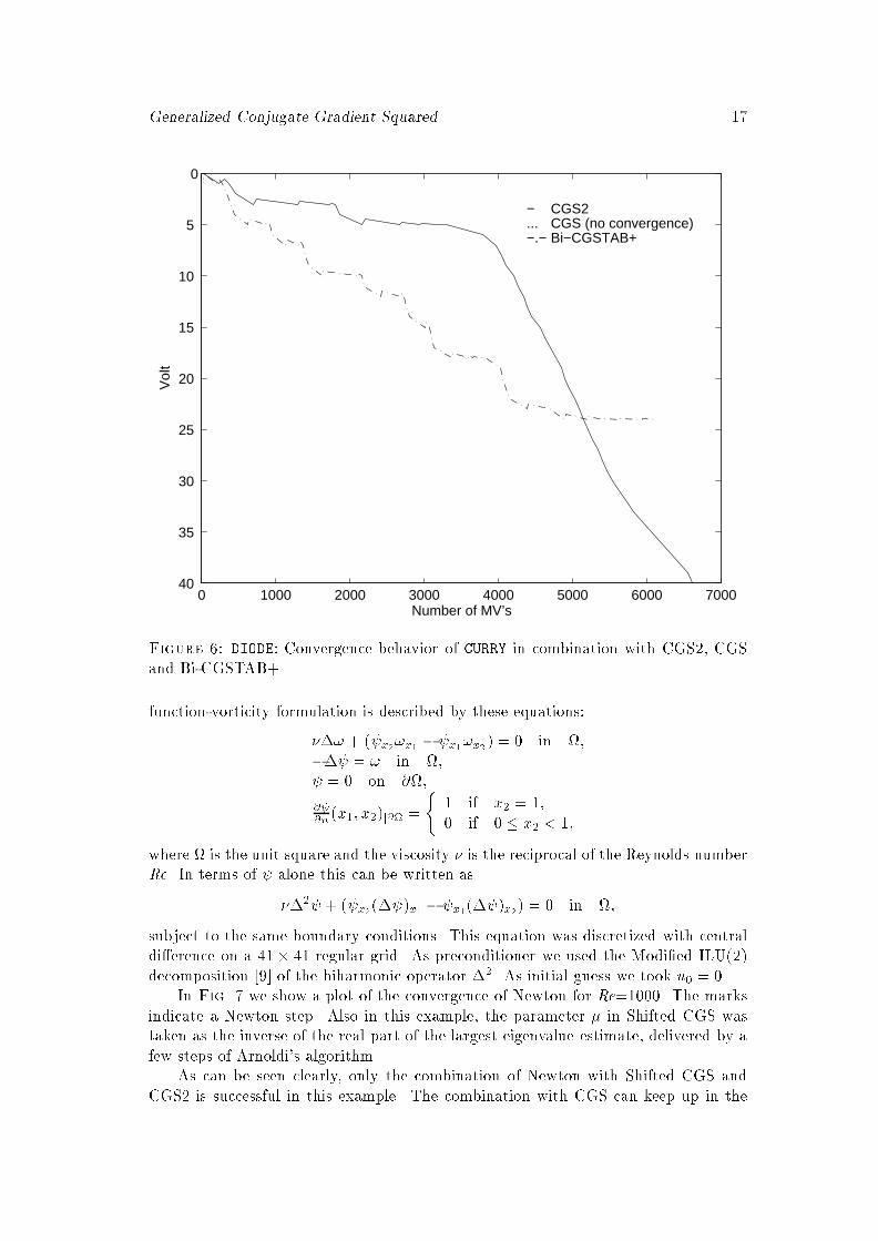
Figure 6: DIODE: Convergence behavior of CURRY in combination with CGS2, CGSand Bi-CGSTAB+.function-vorticity formulation is described by these equations:��! + ( x2!x1 � x1!x2) = 0 in ;�� = ! in ; = 0 on @;@ @n (x1; x2)j@ = ( 1 if x2 = 1;0 if 0 � x2 < 1;where is the unit square and the viscosity � is the reciprocal of the Reynolds numberRe. In terms of alone this can be written as��2 + ( x2(� )x1 � x1(� )x2) = 0 in ;subject to the same boundary conditions. This equation was discretized with centraldi�erence on a 41� 41 regular grid. As preconditioner we used the Modi�ed ILU(2)decomposition [9] of the biharmonic operator �2. As initial guess we took u0 = 0.In Fig. 7 we show a plot of the convergence of Newton for Re=1000. The marksindicate a Newton step. Also in this example, the parameter � in Shifted CGS wastaken as the inverse of the real part of the largest eigenvalue estimate, delivered by afew steps of Arnoldi's algorithm.As can be seen clearly, only the combination of Newton with Shifted CGS andCGS2 is successful in this example. The combination with CGS can keep up in the

18 D. R. Fokkema, G. L. G. Sleijpen, and H. A. Van der Vorst1e-12

1e-11

1e-10

1e-09

1e-08

1e-07

1e-06

1e-05

1e-04

1e-03

1e-02

1e-01

1e+00

1e+01

0 100 200 300 400 500 600 700

resi

dual

nor

m

Number of matrix multiplications

Shifted CGSCGS2CGS

Bi-CGSTABBiCGstab(2)

Figure 7: Driven Cavity: Convergence behavior of Newton in combination withdi�erent linear solvers.beginning but then CGS has trouble solving the linear system, which causes the stag-nation. The combination with Bi-CGSTAB stagnates all together. This could beattributed to the fact that Bi-CGSTAB is not able to solve the linear systems, be-cause they are very unsymmetric [20]. BiCGstab(2) on the other hand is able to solvethe linear systems (in the beginning) but apparently delivers a correction that is notof much use to Newton.Note that in this case the combination of Newton with Shifted CGS is preferable,because it is more e�cient: Shifted CGS uses two inner products less than CGS2.Additional note. In [25] it was observed that replacing the residual rk in CGSby the true residual b�Axk has a negative e�ect on the iteration process. Recently, itcame to our attention that Neumaier [16] reports good results with a di�erent strategythat does include the use of the true residual. His strategy can be summarized asfollows: Add the line \xbest = 0" after the �rst line in CGSand replace the last line withrk+1 = b�Axk+1if krk+1k2 � krbestk2 thenb = rbest = rk+1xbest = xbest + xk+1xk+1 = 0endifWe have tested this approach on several problems and for those problems wecon�rm the observation that indeed this modi�cation to CGS has no adverse in uence

Generalized Conjugate Gradient Squared 19on the convergence behavior and that accuracy is reached within machine precision(i.e., j krmk2 � kb � Axmk2j . � � kr0k2 with � as in (4)). For an explanation andother related strategies, see [22].8. Conclusions. We have shown how the CGS algorithm can be generalizedto a method that uses the product of two nearby Bi-CG polynomials as a reductionoperator on the initial residual. Two methods are suggested to improve the accuracyand the speed of convergence, without losing the quadratic reduction of errors inconverged eigenvector directions. This is important, since the Newton process seemsto bene�t from this property. Several numerical examples are given that con�rm ourheuristic arguments.Acknowledgment. We appreciate the help of Marjan Driessen at Philips Re-search Laboratories (Eindhoven). She provided the numerical data for the examplesin Section 7.3. REFERENCES[1] H. G. Brachtendorf, Simulation des eingeschwungenen Verhaltens elektronischer Schaltun-gen, PhD thesis, Universi�at Bremen, 1994.[2] P. N. Brown and Y. Saad, Hybrid Krylov methods for nonlinear systems of equations, SIAMJ. Sci. Statist. Comput., 11 (1990), pp. 450{481.[3] T. F. Chan, E. Gallopoulos, V. Simoncini, T. Szeto, and C. H. Tong, A quasi-minimalresidual variant of the Bi-CGSTAB algorithm for nonsymmetric systems, SIAM J. Sci. Com-put., 15 (1994), pp. 338{347.[4] R. S. Dembo, S. C. Eisenstat, and T. Steihaug, Inexact newton methods, SIAM J. Numer.Anal., 19 (1982), pp. 400{408.[5] J. E. Dennis, Jr. and R. B. Schnabel, Numerical Methods for Unconstrained Optimizationand Nonlinear Equations, Prentice-Hall, Englewood Cli�s, New Yersey 07632, 1983.[6] R. Fletcher, Conjugate gradient methods for inde�nite systems, in Numerical Analysis Dundee1975, Lecture Notes in Mathematics 506, G. A. Watson, ed., Berlin, Heidelberg, New York,1976, Springer-Verlag, pp. 73{89.[7] R. Freund, A transpose-free quasi-minimal residual algorithm for non-Hermitian linear systems,SIAM J. Sci. Comput., 14 (1993), pp. 470{482.[8] R. Glowinski, H. B. Keller, and L. Reinhart, Continuation-conjugate gradient methodsfor the least squares solution of nonlinear boundary value problems, SIAM J. Sci. Statist.Comput., 6 (1985), pp. 793{832.[9] I. Gustafsson, A class of �rst order factorizations methods, BIT, 18 (1978), pp. 142{156.[10] M. H. Gutknecht, Variants of BiCGStab for matrices with complex spectrum, SIAM J. Sci.Comput., 14 (1993), pp. 1020{1033.[11] Y. Huang and H. A. Van der Vorst, Some observations on the convergence behaviour ofGMRES, Tech. Report 89-09, Delft University of Technology, Faculty of Tech. Math., 1989.[12] C. Lanczos, Solution of systems of linear equations by minimized iteration, J. Res. Nat. Bur.Standards, 49 (1952), pp. 33{53.[13] A. Liegmann, E�cient solution of large sparse linear systems, master's thesis, ETH Z�urich,1995.[14] J. A. Meijerink and H. A. Van der Vorst, An iterative solution method for linear systems ofwhich the coe�cient matrix is a symmetric M-matrix, Math. Comp., 31 (1977), pp. 148{162.[15] N. M. Nachtigal, S. C. Reddy, and L. N. Trefethen, How fast are nonsymmetric matrixiterations?, SIAM J. Matrix Anal. Appl., 13 (1992), pp. 778{795.[16] A. Neumaier. Oral presentation at the Oberwolfach meeting, April 1994.[17] S. J. Polak, C. den Heijer, W. H. A. Schilders, and P. Markowich, Semiconductordevice modelling from the numerical point of view, Int. J. for Num. Methods in Eng., 24(1987), pp. 763{838.[18] C. Pommerell and W. Fichtner, PILS: An iterative linear solver package for ill-conditionedsystems, in Supercomputing '91, Albuquerque, NM, Nov. 1991, ACM-IEEE, pp. 588{599.

20 D. R. Fokkema, G. L. G. Sleijpen, and H. A. Van der Vorst[19] A. Ruhe, Rational Krylov algorithms for nonsymmetric eigenvalue problems II. Matrix Pairs,Lin. Alg. and its Appl., 197/198 (1994), pp. 283{295.[20] G. L. G. Sleijpen and D. R. Fokkema, BiCGstab(`) for linear equations involving matriceswith complex spectrum, ETNA, 1 (1993), pp. 11{32.[21] G. L. G. Sleijpen and H. A. Van der Vorst,Maintaining convergence properties of BiCGstabmethods in �nite precision arithmetic, Preprint 861, Dept. Math., University Utrecht, 1994.To appear in Numerical Algorithms.[22] , Reliable updated residuals in hybrid Bi-CG methods, Preprint 886, Dept. Math., UniversityUtrecht, 1994. To appear in Computing.[23] G. L. G. Sleijpen, H. A. Van der Vorst, and D. R. Fokkema, BiCGstab(`) and otherhybrid Bi-CG methods, Numerical Algorithms, 7 (1994), pp. 75{109.[24] P. Sonneveld, CGS, a fast Lanczos-type solver for nonsymmetric linear systems, SIAM J. Sci.Statist. Comput., 10 (1989), pp. 36{52.[25] H. A. Van der Vorst, Bi-CGSTAB: A fast and smoothly converging variant of Bi-CG forthe solution of nonsymmetric linear systems, SIAM J. Sci. Statist. Comput., 13 (1992),pp. 631{644.[26] L. Zhou and H. F. Walker, Residual smoothing techniques for iterative methods, SIAM J. Sci.Comput., 15 (1994), pp. 297{312.