SLAM: Robotic Simultaneous Location

and MappingWilliam Regli

Department of Computer Science(and Departments of ECE and MEM)

Drexel University

Acknowledgments to Sebastian Thrun & others…

SLAM Lecture Outline

• SLAM

• Robot Motion Models

• Robot Sensing and Localization

• Robot Mapping

SLAM stands for simultaneous localization and mapping

The task of building a map while estimating the pose of the robot relative to this map

Why is SLAM hard?Chicken and egg problem: a map is needed to localize the robot and a pose estimate is needed to build a map

The SLAM Problem

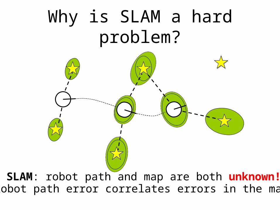
Why is SLAM a hard problem?

SLAM: robot path and map are both unknown! Robot path error correlates errors in the map

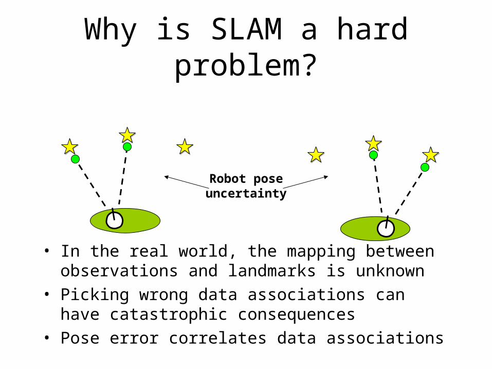
Why is SLAM a hard problem?

• In the real world, the mapping between observations and landmarks is unknown

• Picking wrong data associations can have catastrophic consequences

• Pose error correlates data associations

Robot poseuncertainty

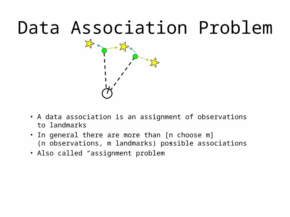
Data Association Problem

• A data association is an assignment of observations to landmarks

• In general there are more than [n choose m](n observations, m landmarks) possible associations

• Also called “assignment problem”

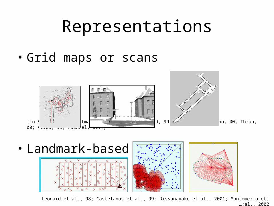
Representations

• Grid maps or scans

[Lu & Milios, 97; Gutmann, 98: Thrun 98; Burgard, 99; Konolige & Gutmann, 00; Thrun, 00; Arras, 99; Haehnel, 01;…]

• Landmark-based

[Leonard et al., 98; Castelanos et al., 99: Dissanayake et al., 2001; Montemerlo et al., 2002…;

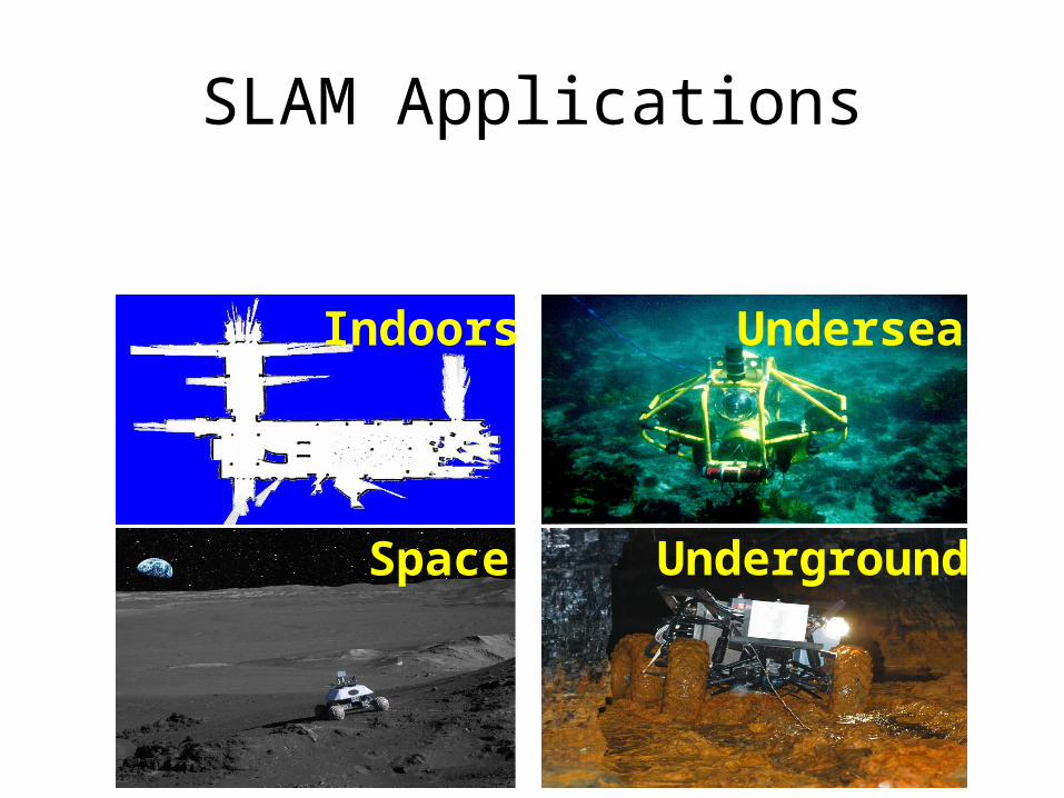
SLAM Applications

Indoors

Space

Undersea

Underground

SLAM Lecture Outline

• SLAM

• Robot Motion Models

• Robot Sensing and Localization• Robot Mapping

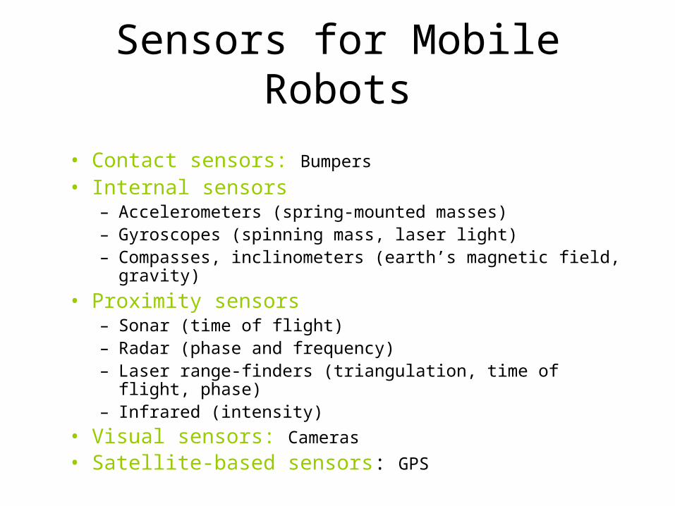
Sensors for Mobile Robots

• Contact sensors: Bumpers

• Internal sensors– Accelerometers (spring-mounted masses)– Gyroscopes (spinning mass, laser light)– Compasses, inclinometers (earth’s magnetic field, gravity)

• Proximity sensors– Sonar (time of flight)– Radar (phase and frequency)– Laser range-finders (triangulation, time of flight, phase)– Infrared (intensity)

• Visual sensors: Cameras

• Satellite-based sensors: GPS

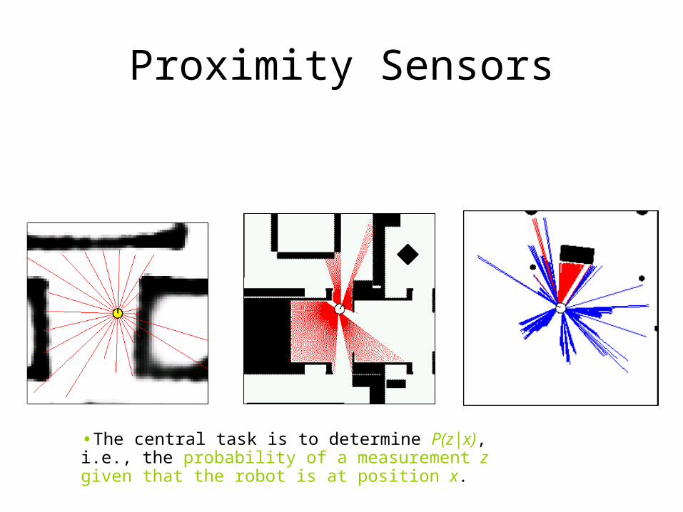
Proximity Sensors

•The central task is to determine P(z|x), i.e., the probability of a measurement z given that the robot is at position x.

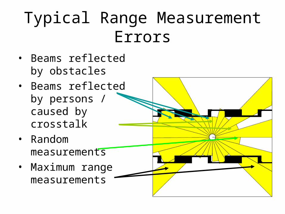
Typical Range Measurement Errors

• Beams reflected by obstacles

• Beams reflected by persons / caused by crosstalk

• Random measurements

• Maximum range measurements

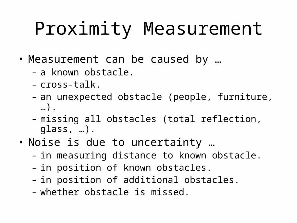
Proximity Measurement

• Measurement can be caused by …– a known obstacle.– cross-talk.– an unexpected obstacle (people, furniture, …).– missing all obstacles (total reflection, glass, …).

• Noise is due to uncertainty …– in measuring distance to known obstacle.– in position of known obstacles.– in position of additional obstacles.– whether obstacle is missed.

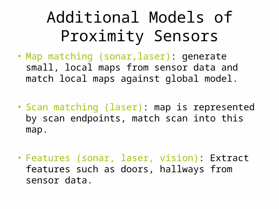
Additional Models of Proximity Sensors

• Map matching (sonar,laser): generate small, local maps from sensor data and match local maps against global model.

• Scan matching (laser): map is represented by scan endpoints, match scan into this map.

• Features (sonar, laser, vision): Extract features such as doors, hallways from sensor data.

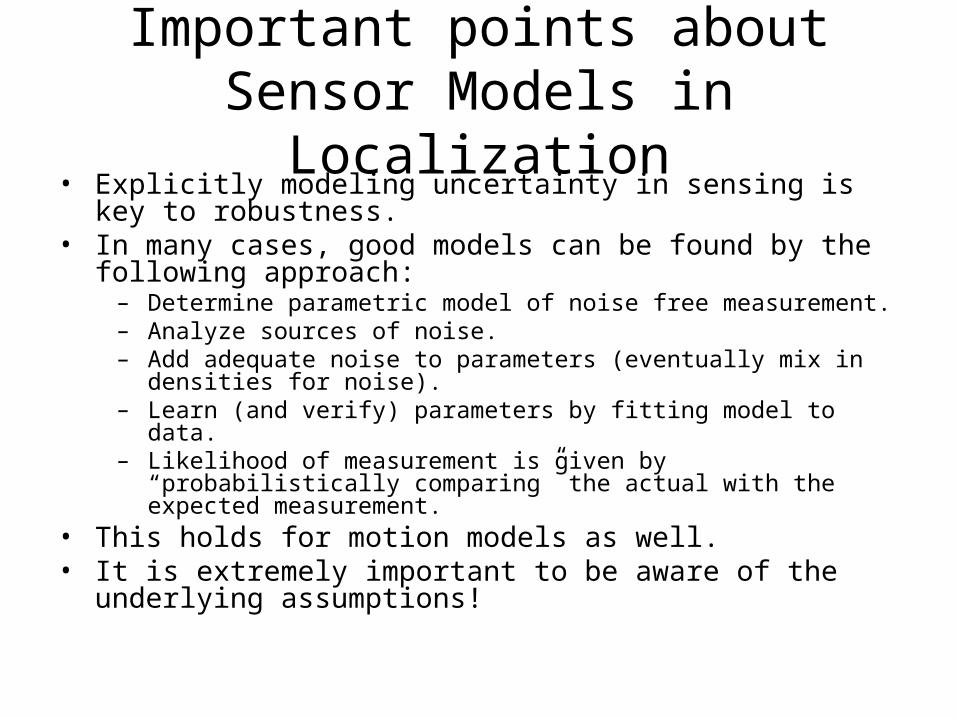
Important points about Sensor Models in Localization

• Explicitly modeling uncertainty in sensing is key to robustness.

• In many cases, good models can be found by the following approach:

– Determine parametric model of noise free measurement.– Analyze sources of noise.– Add adequate noise to parameters (eventually mix in densities

for noise).– Learn (and verify) parameters by fitting model to data.– Likelihood of measurement is given by “probabilistically

comparing” the actual with the expected measurement.• This holds for motion models as well.• It is extremely important to be aware of the underlying

assumptions!

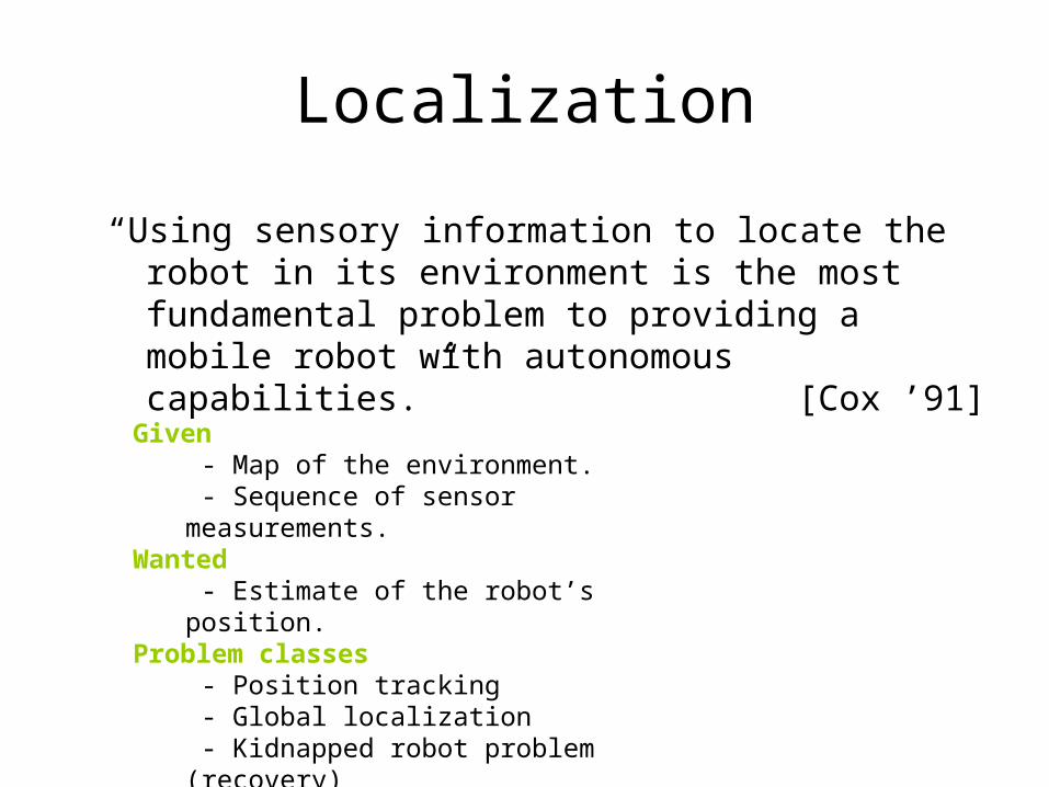
Localization

“Using sensory information to locate the robot in its environment is the most fundamental problem to providing a mobile robot with autonomous capabilities.” [Cox ’91]

Given - Map of the environment. - Sequence of sensor measurements.

Wanted - Estimate of the robot’s position.

Problem classes - Position tracking - Global localization - Kidnapped robot problem (recovery)

Localization using Kinematics

● Issue: We can’t tell direction from encoders alone

● Solution: Keep track of forward/backward motor command sent to each wheel

● Localization program: Build new arrays into behavior/priority-based controller and use to continually update location

● Doesn’t solve noise problems, though

Localization Using Landmarks

• Active beacons (e.g., radio, GPS)

• Passive (e.g., visual, retro-reflective)

• Standard approach is triangulation

• Sensor provides– distance, or– bearing, or– distance and bearing.

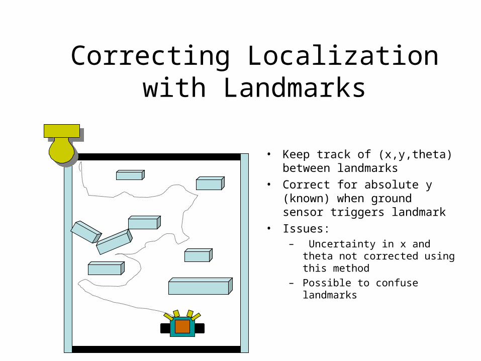
Correcting Localization with Landmarks

• Keep track of (x,y,theta) between landmarks

• Correct for absolute y (known) when ground sensor triggers landmark

• Issues: – Uncertainty in x and theta not

corrected using this method– Possible to confuse landmarks

Particle Filters Represent belief by random samples

Estimation of non-Gaussian, nonlinear processes

Sampling Importance Resampling (SIR) principle

Draw the new generation of particles

Assign an importance weight to each particle

Resampling

Typical application scenarios are tracking, localization, …

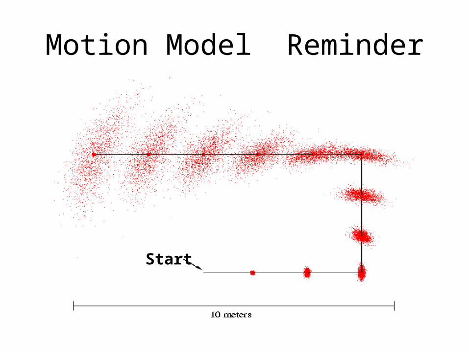
Motion Model Reminder

StartStart

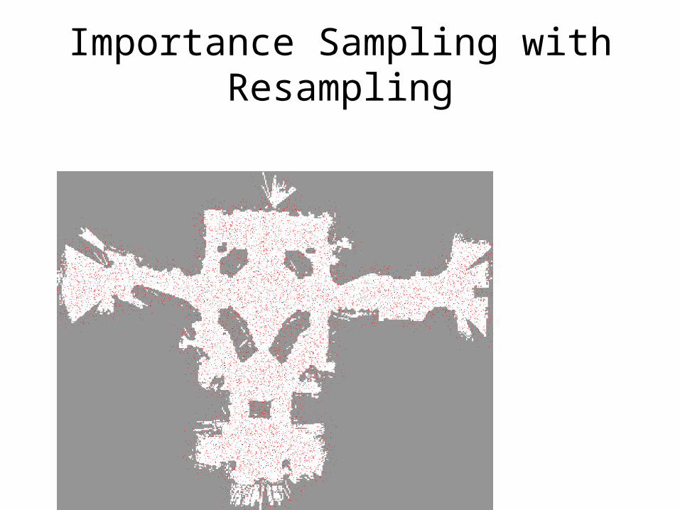
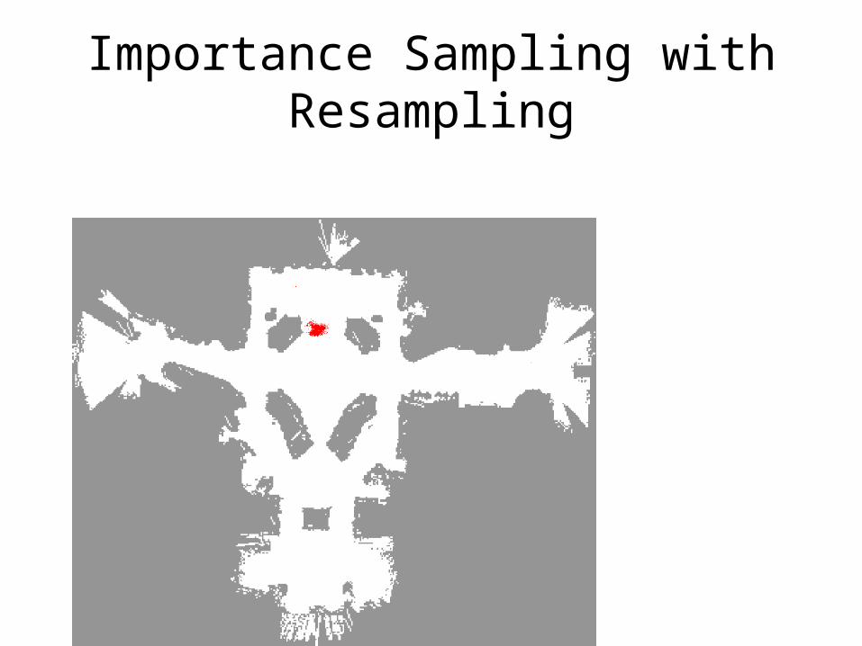
Importance Sampling with Resampling

Importance Sampling with Resampling

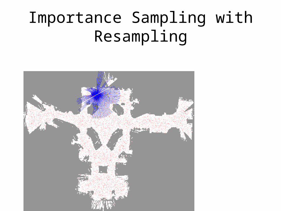
Importance Sampling with Resampling

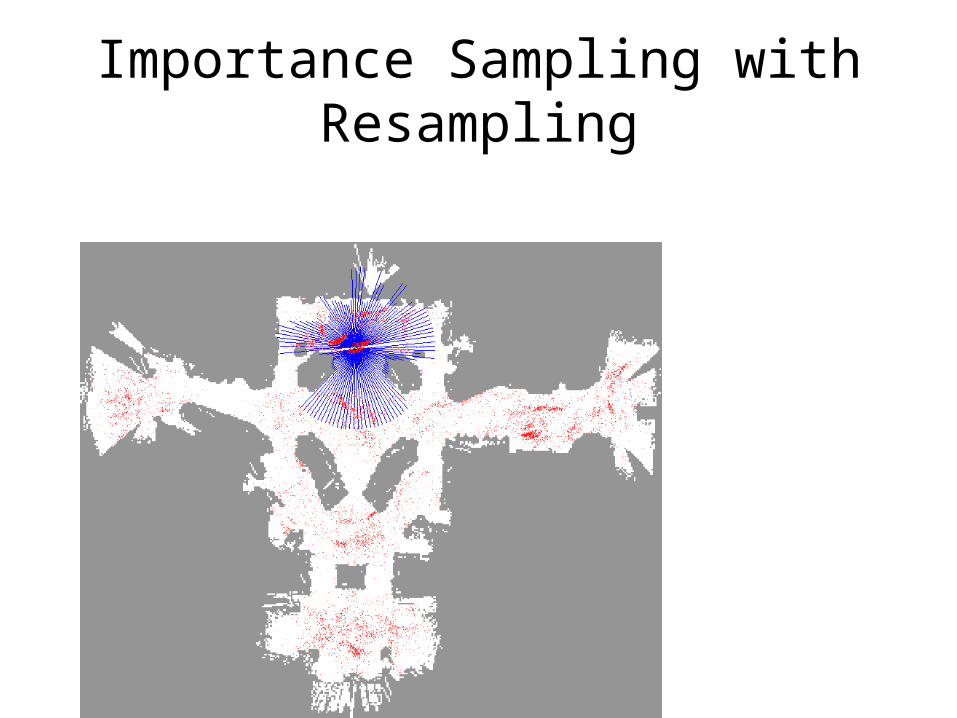
Importance Sampling with Resampling

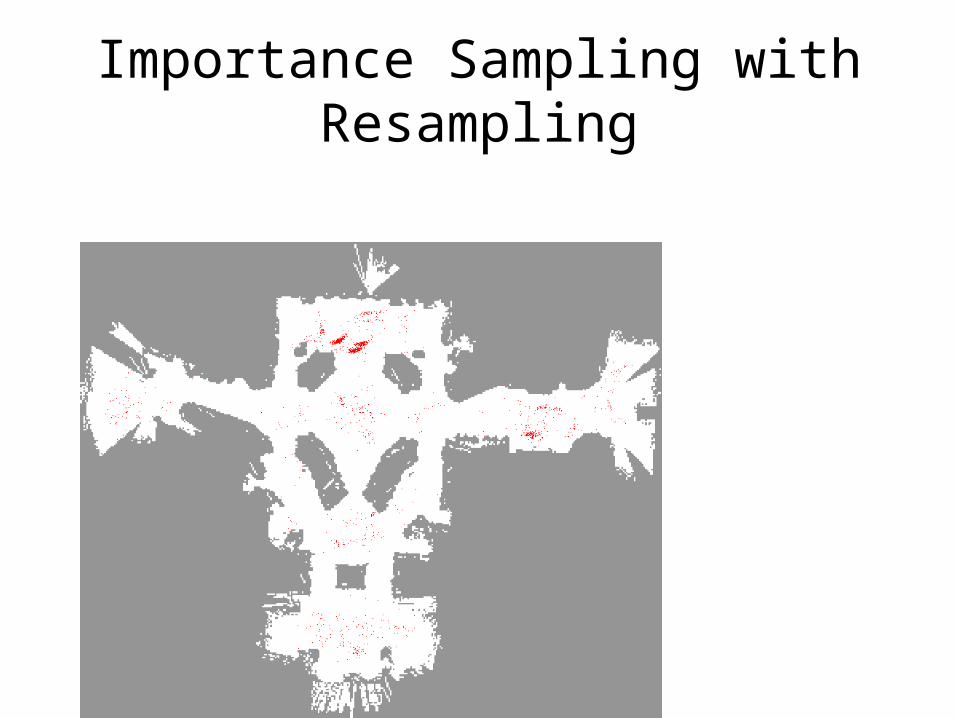
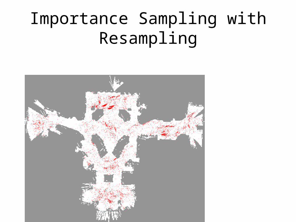
Importance Sampling with Resampling

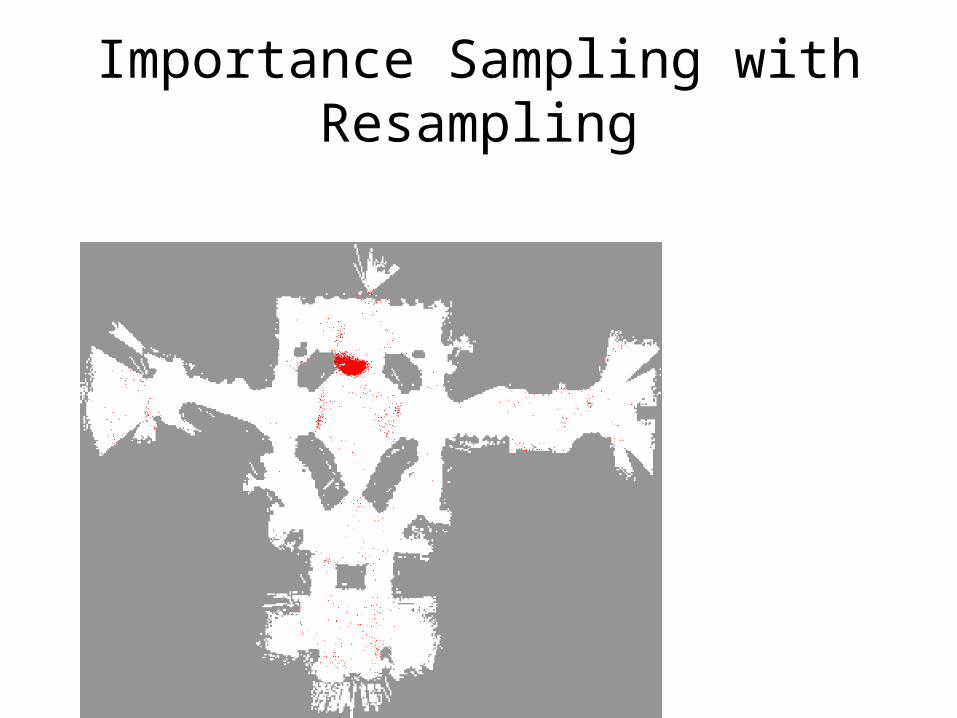
Importance Sampling with Resampling

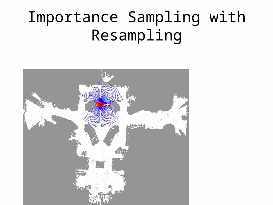
Importance Sampling with Resampling

Importance Sampling with Resampling

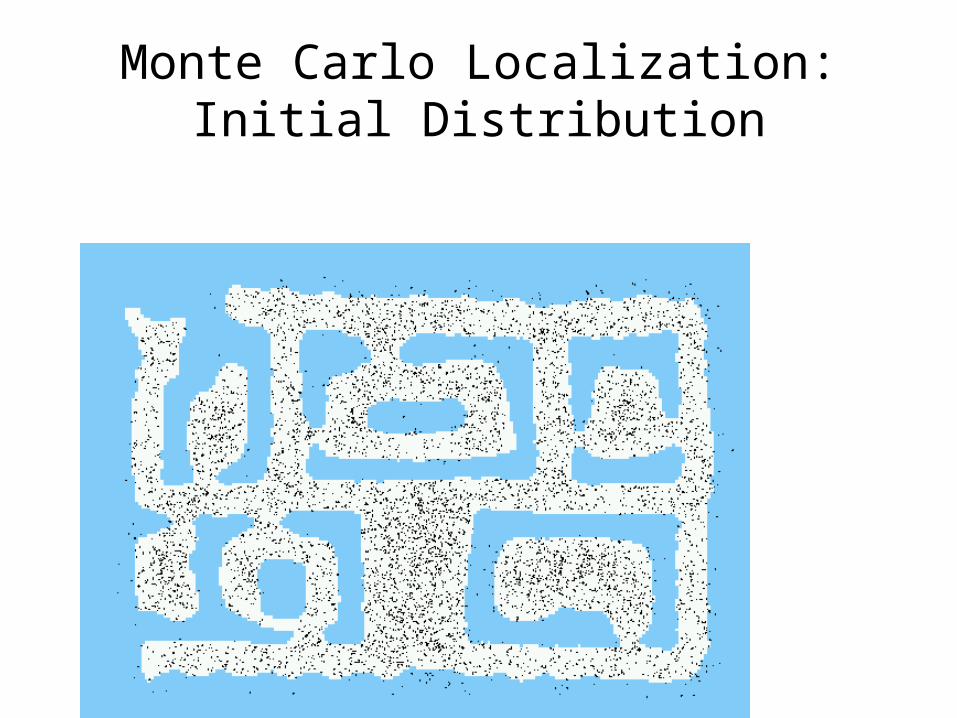
Monte Carlo Localization: Initial Distribution

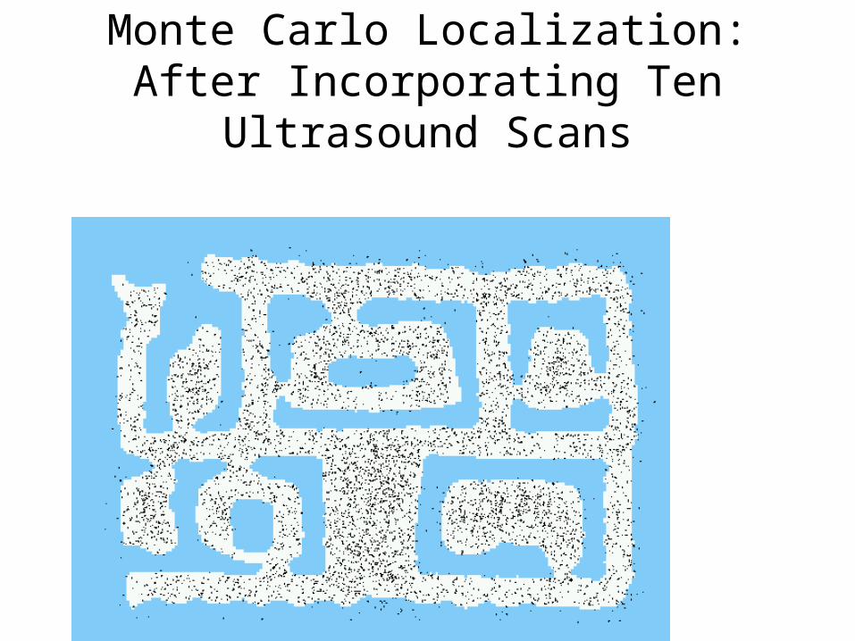
Monte Carlo Localization: After Incorporating Ten Ultrasound Scans

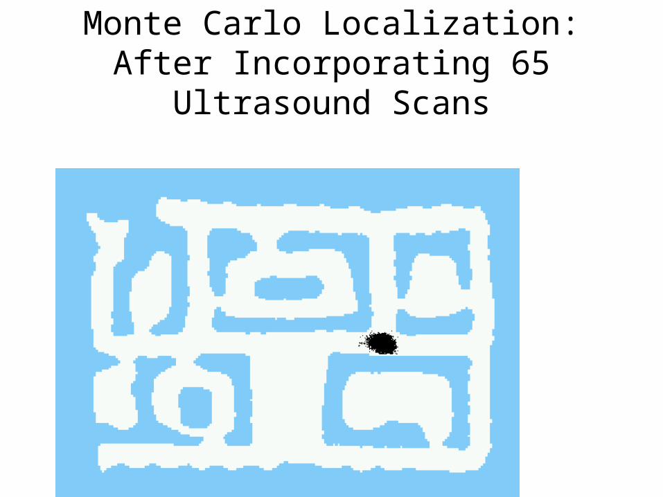
Monte Carlo Localization: After Incorporating 65 Ultrasound Scans

SLAM Lecture Outline

• SLAM

• Robot Motion Models

• Robot Sensing and Localization

• Robot Mapping

Why Mapping?

• Learning maps is one of the fundamental problems in mobile robotics

• Maps allow robots to efficiently carry out their tasks, allow localization …

• Successful robot systems rely on maps for localization, path planning, activity planning etc.

The General Problem of Mapping

What does the environment look like?

Formally, mapping involves, given the sensor data, to calculate the most likely map

Mapping as a Chicken and Egg Problem

• So far we learned how to estimate the pose of the vehicle given the data and the map (localization).

• Mapping, however, involves to simultaneously estimate the pose of the vehicle and the map.

• The general problem is therefore denoted as the simultaneous localization and mapping problem (SLAM).

• Throughout this section we will describe how to calculate a map given we know the pose of the vehicle

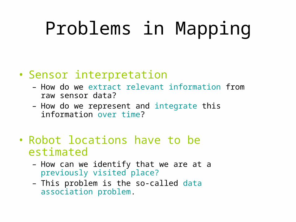
Problems in Mapping

• Sensor interpretation– How do we extract relevant information from raw sensor

data?– How do we represent and integrate this information over

time?

• Robot locations have to be estimated– How can we identify that we are at a previously visited

place?– This problem is the so-called data association problem.

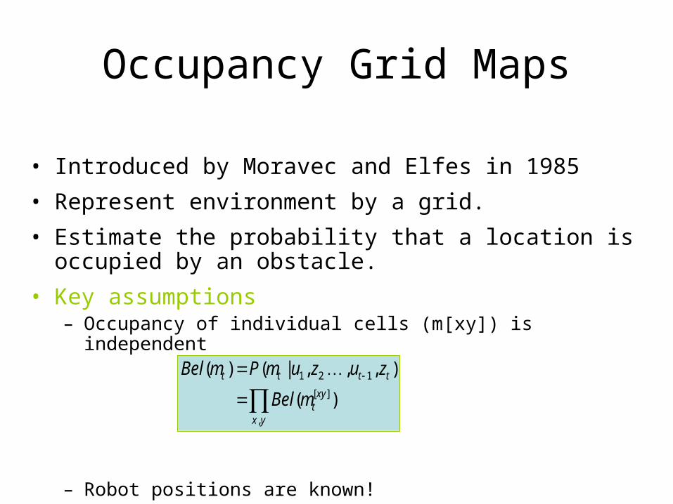
Occupancy Grid Maps

           

                                                                                              

                     

• Introduced by Moravec and Elfes in 1985

• Represent environment by a grid.

• Estimate the probability that a location is occupied by an obstacle.

• Key assumptions– Occupancy of individual cells (m[xy]) is independent

– Robot positions are known!

yx

xyt

tttt

mBel

zuzumPmBel

,

][

121

)(

),,,|()(

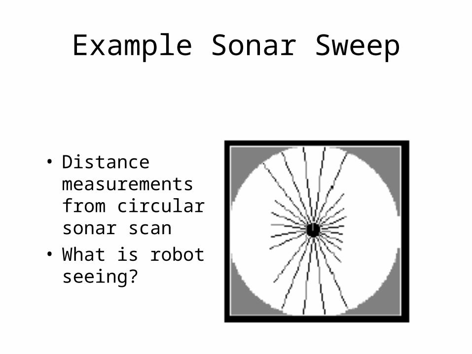
Example Sonar Sweep

• Distance measurements from circular sonar scan

• What is robot seeing?

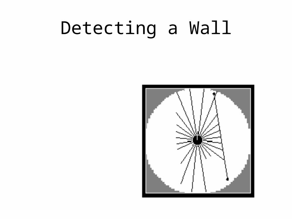
Detecting a Wall

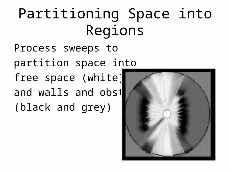
Partitioning Space into Regions

Process sweeps to

partition space into

free space (white),

and walls and obstacles

(black and grey)

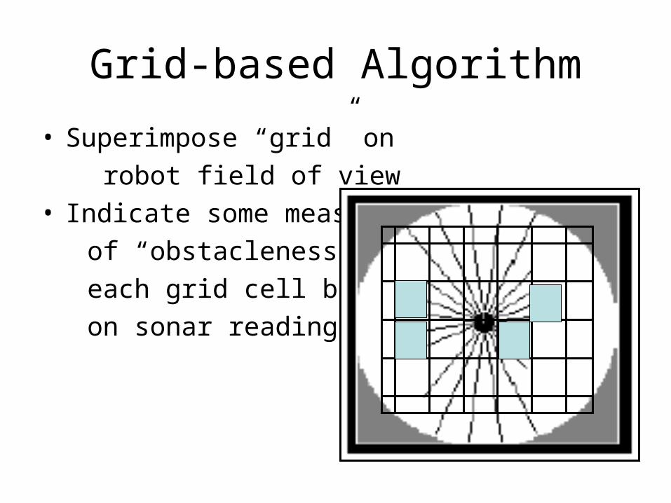
Grid-based Algorithm

• Superimpose “grid” on

robot field of view• Indicate some measure

of “obstacleness” in

each grid cell based

on sonar readings

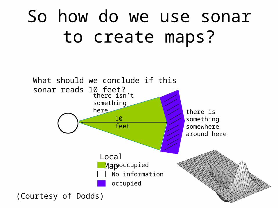
So how do we use sonar to create maps?

What should we conclude if this sonar reads 10 feet?

there isn’t something here there is

something somewhere around here

Local Mapunoccupied

No information

occupied

(Courtesy of Dodds)

10 feet

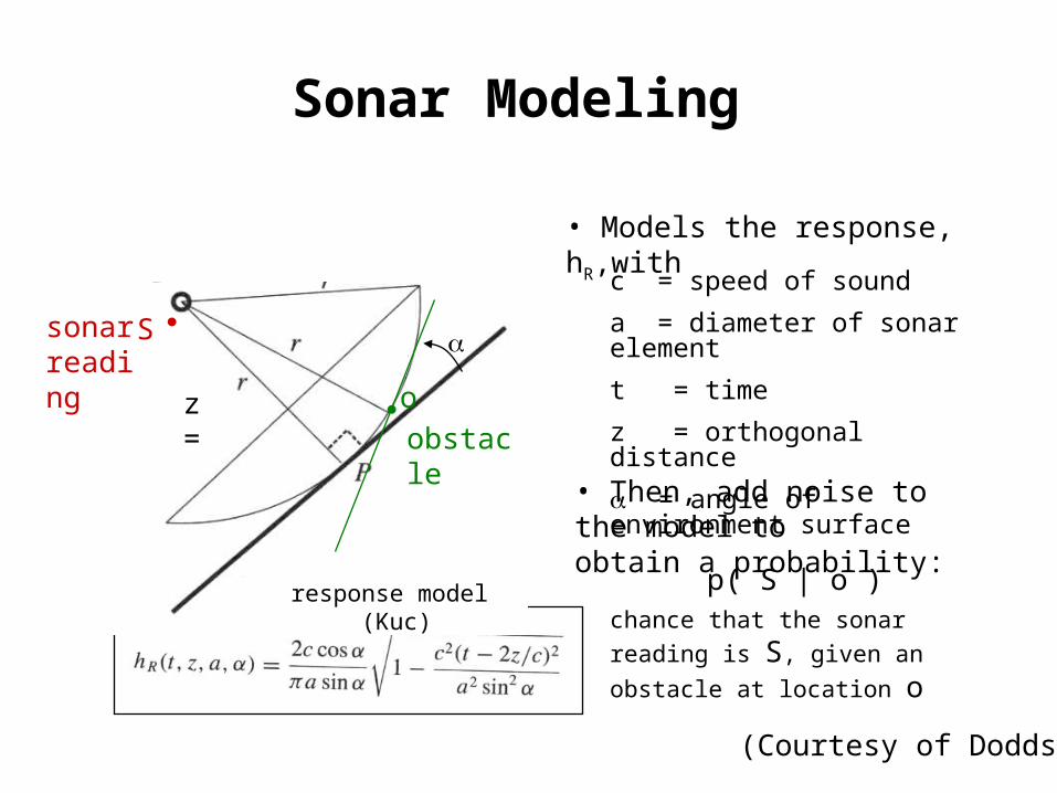
Sonar Modeling

response model (Kuc)

sonar reading

obstacle

c = speed of sound

a = diameter of sonar element

t = time

z = orthogonal distance

= angle of environment surface

• Models the response, hR,with

• Then, add noise to the model to obtain a probability:

p( S | o )chance that the sonar reading is S, given an obstacle at location o

z =

S

o

(Courtesy of Dodds)

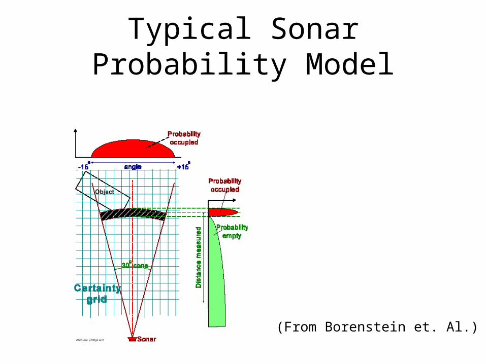
Typical Sonar Probability Model

(From Borenstein et. Al.)

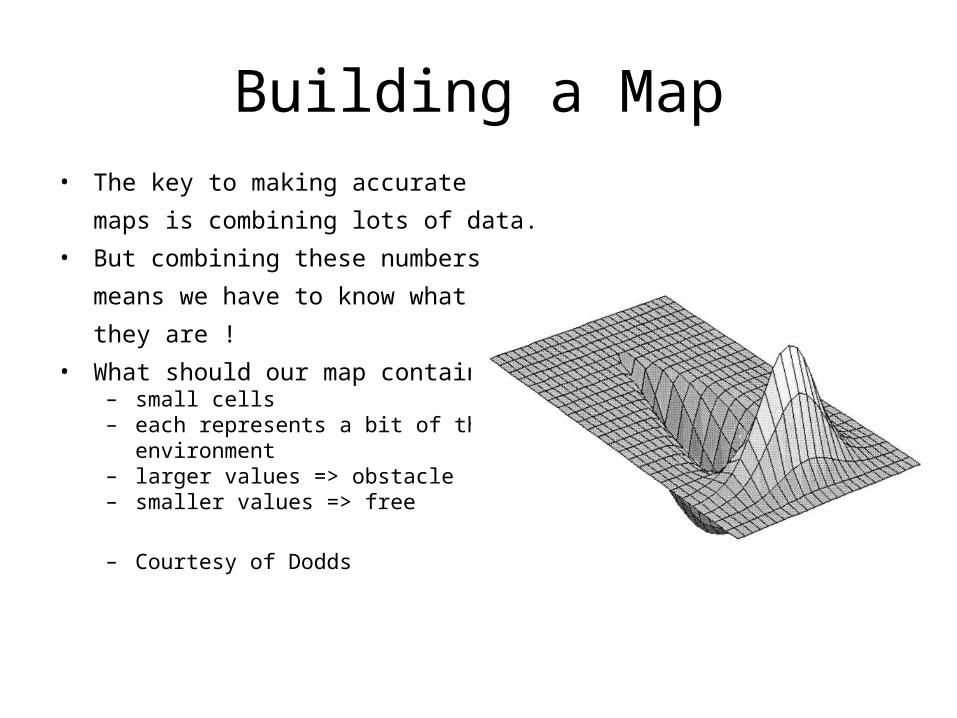
Building a Map• The key to making accurate

maps is combining lots of data.

• But combining these numbers

means we have to know what

they are !

• What should our map contain ?– small cells– each represents a bit of the robot’s

environment– larger values => obstacle– smaller values => free

– Courtesy of Dodds

Alternative: Simple Counting

• For every cell count– hits(x,y): number of cases where a beam

ended at <x,y>– misses(x,y): number of cases where a beam

passed through <x,y>

Difference between Occupancy Grid Maps and Counting

• The counting model determines how often a cell reflects a beam.

• The occupancy model represents whether or not a cell is occupied by an object.

• Although a cell might be occupied by an object, the reflection probability of this object might be very small (windows etc.).

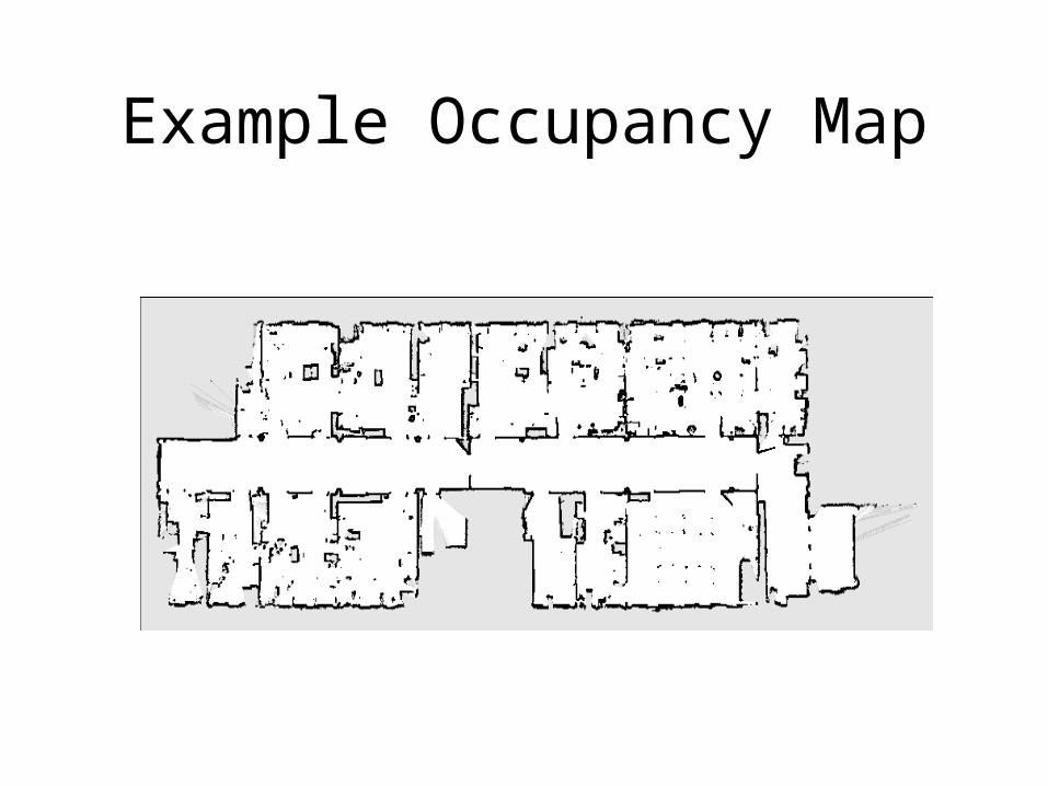
Example Occupancy Map

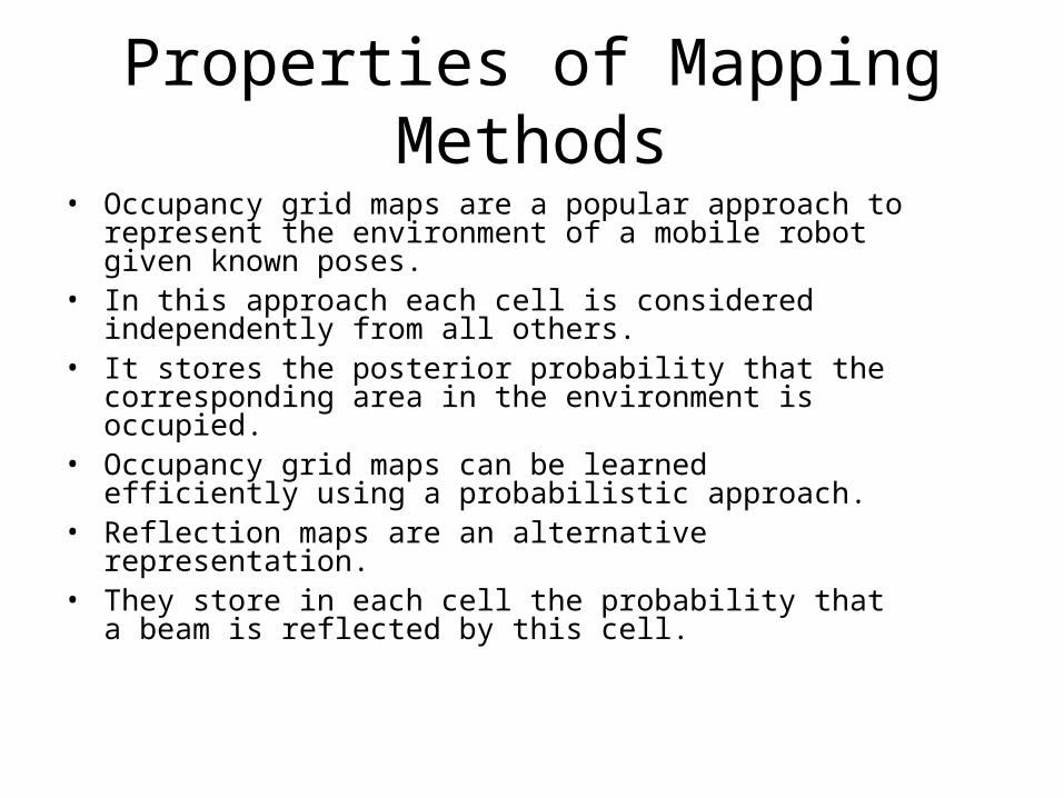
Properties of Mapping Methods• Occupancy grid maps are a popular approach to represent

the environment of a mobile robot given known poses.• In this approach each cell is considered independently from

all others.• It stores the posterior probability that the corresponding area

in the environment is occupied.• Occupancy grid maps can be learned efficiently using a

probabilistic approach.• Reflection maps are an alternative representation.• They store in each cell the probability that a beam is reflected

by this cell.

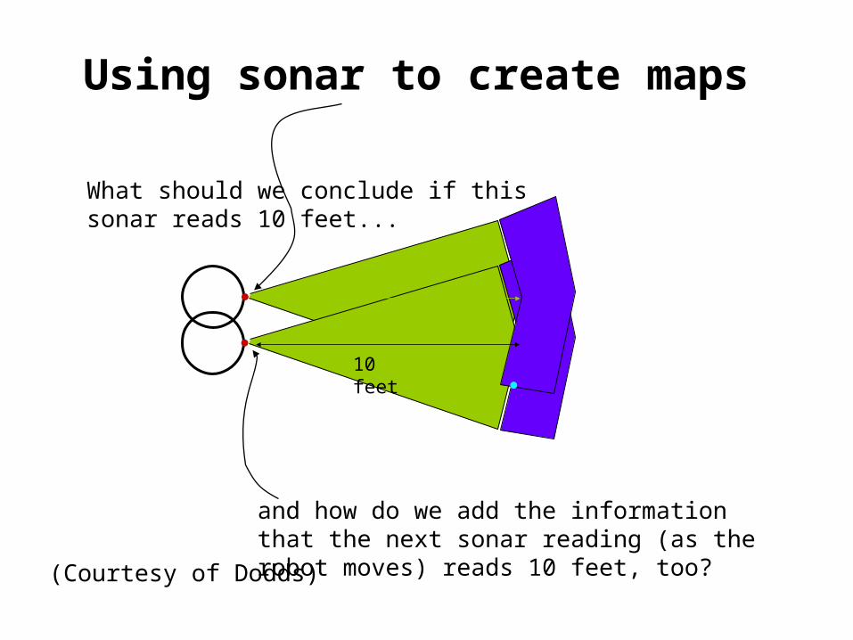
Using sonar to create maps

What should we conclude if this sonar reads 10 feet...

10 feet

and how do we add the information that the next sonar reading (as the robot moves) reads 10 feet, too?

10 feet

(Courtesy of Dodds)

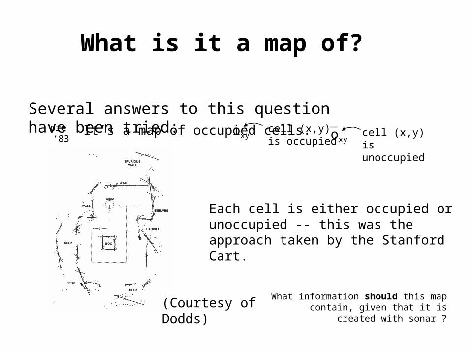
What is it a map of?

Several answers to this question have been tried:It’s a map of occupied cells.oxy

oxy

cell (x,y) is occupied

cell (x,y) is unoccupied

Each cell is either occupied or unoccupied -- this was the approach taken by the Stanford Cart.

pre ‘83

What information should this map contain, given that it is

created with sonar ?

(Courtesy of Dodds)

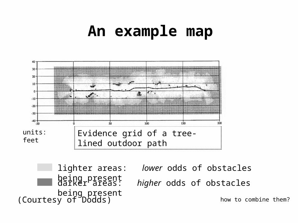
An example map

units: feet

Evidence grid of a tree-lined outdoor path

lighter areas: lower odds of obstacles being present

darker areas: higher odds of obstacles being present

how to combine them?(Courtesy of Dodds)

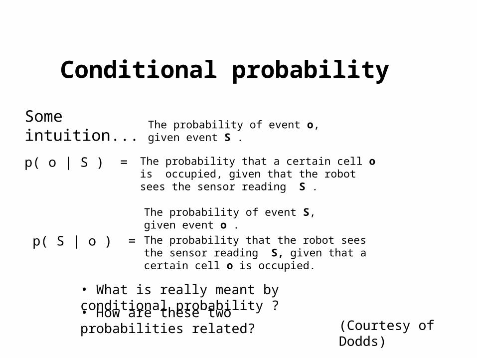
Conditional probability

Some intuition...

p( o | S ) =

The probability of event o, given event S .

The probability that a certain cell o is occupied, given that the robot sees the sensor reading S .

p( S | o ) =

The probability of event S, given event o .The probability that the robot sees the sensor reading S, given that a certain cell o is occupied.

• What is really meant by conditional probability ?

• How are these two probabilities related?(Courtesy of Dodds)

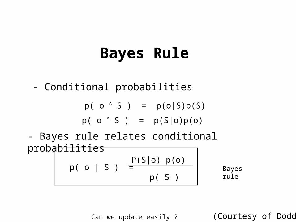
Bayes Rule

- Bayes rule relates conditional probabilities

p( o | S ) =

P(S|o) p(o)

p( S )Bayes rule

p( o S ) = p(o|S)p(S)

- Conditional probabilities

Can we update easily ? (Courtesy of Dodds)

p( o S ) = p(S|o)p(o)

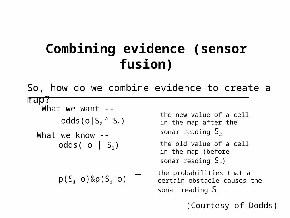
Combining evidence (sensor fusion)

So, how do we combine evidence to create a map?

What we want --

odds(o|S2 S1)

the new value of a cell in the map after the sonar reading S2 What we know --

odds( o | S1) the old value of a cell in the map (before sonar reading S2)

p(Si|o)&p(Si|o) the probabilities that a certain obstacle causes the sonar reading Si

(Courtesy of Dodds)

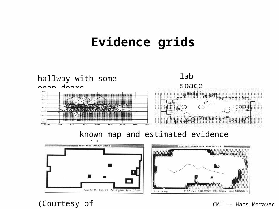
Evidence grids

hallway with some open doors

known map and estimated evidence grid

lab space

CMU -- Hans Moravec(Courtesy of Dodds)

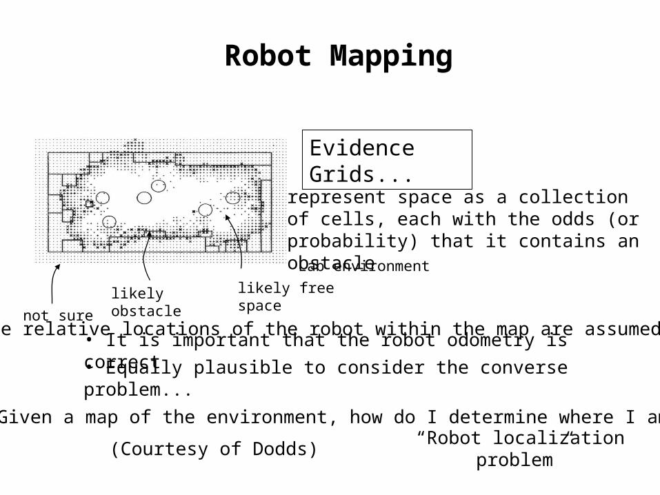
Robot Mapping

represent space as a collection of cells, each with the odds (or probability) that it contains an obstacleLab environment

not sure

likely obstacle

likely free space

• The relative locations of the robot within the map are assumed known.• It is important that the robot odometry is correct

• Equally plausible to consider the converse problem...

Evidence Grids...

Given a map of the environment, how do I determine where I am?

“Robot localization problem”(Courtesy of Dodds)

SLAM Lecture Outline

• SLAM

• Robot Motion Models• Robot Sensing and Localization

• Robot Mapping

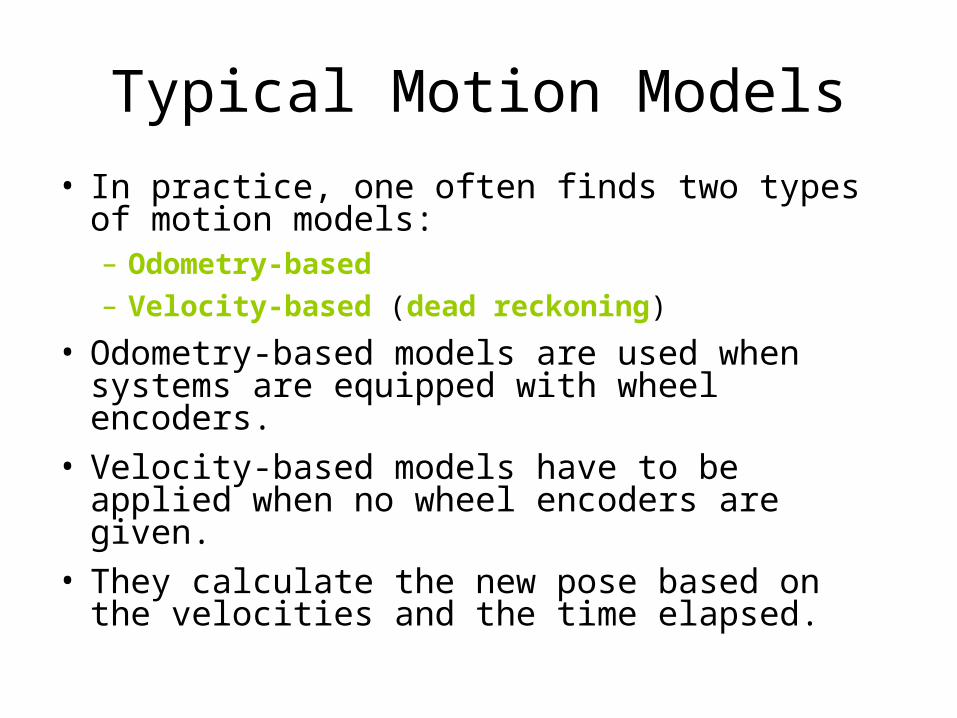
Typical Motion Models

• In practice, one often finds two types of motion models:– Odometry-based

– Velocity-based (dead reckoning)

• Odometry-based models are used when systems are equipped with wheel encoders.

• Velocity-based models have to be applied when no wheel encoders are given.

• They calculate the new pose based on the velocities and the time elapsed.

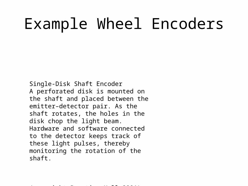
Example Wheel Encoders

Single-Disk Shaft EncoderA perforated disk is mounted on the shaft and placed between the emitter–detector pair. As the shaft rotates, the holes in the disk chop the light beam. Hardware and software connected to the detector keeps track of these light pulses, thereby monitoring the rotation of the shaft.

(copyright Prentice Hall 2001)

Dead Reckoning

• Derived from “deduced reckoning” though this is greatly disputed (see the straight dope)

• Mathematical procedure for determining the present location of a vehicle.

• Achieved by calculating the current pose of the vehicle based on its velocities and the time elapsed.

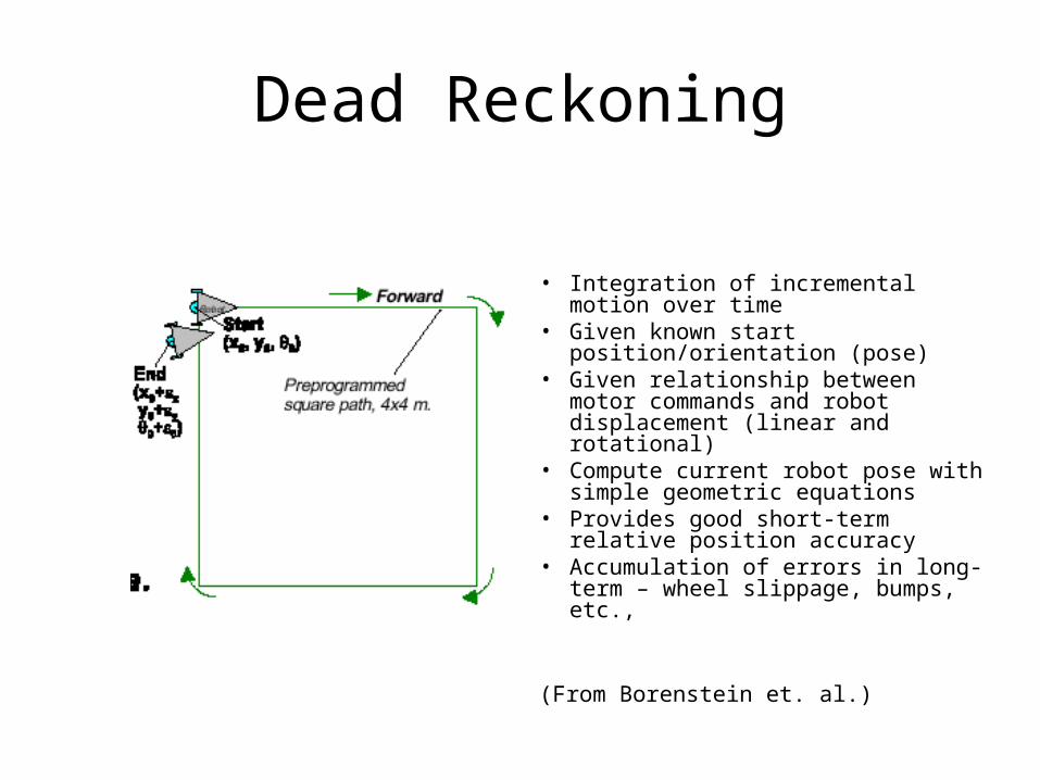
Dead Reckoning

• Integration of incremental motion over time

• Given known start position/orientation (pose)

• Given relationship between motor commands and robot displacement (linear and rotational)

• Compute current robot pose with simple geometric equations

• Provides good short-term relative position accuracy

• Accumulation of errors in long-term – wheel slippage, bumps, etc.,

(From Borenstein et. al.)

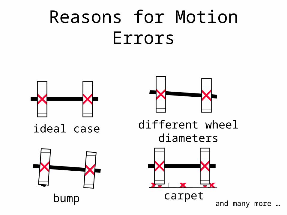
Reasons for Motion Errors

ideal case different wheeldiameters

bump carpetand many more …

Reducing Odometry Error with Absolute Measurements

• Uncertainty Ellipses

• Change shape based on other sensor information

• Artificial/natural landmarks

• Active beacons

• Model matching – compare sensor-induced features to features of known map – geometric or topological

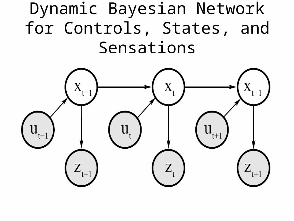
Dynamic Bayesian Network for Controls, States, and Sensations

Probabilistic Motion Models

• To implement the Bayes Filter, we need the transition model p(x | x’, u).

• The term p(x | x’, u) specifies a posterior probability, that action u carries the robot from x’ to x.

• p(x | x’, u) can be modeled based on the motion equations.

Simultaneous Localization and Mapping

Brian Clipp

Comp 790-072 Robotics

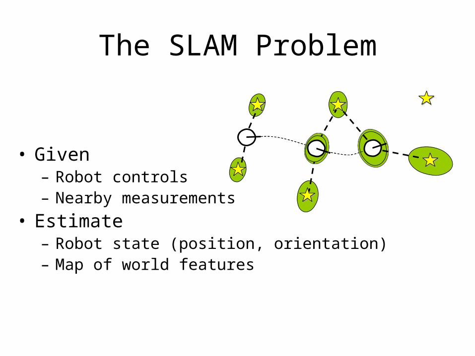
The SLAM Problem

• Given – Robot controls– Nearby measurements

• Estimate– Robot state (position, orientation)– Map of world features

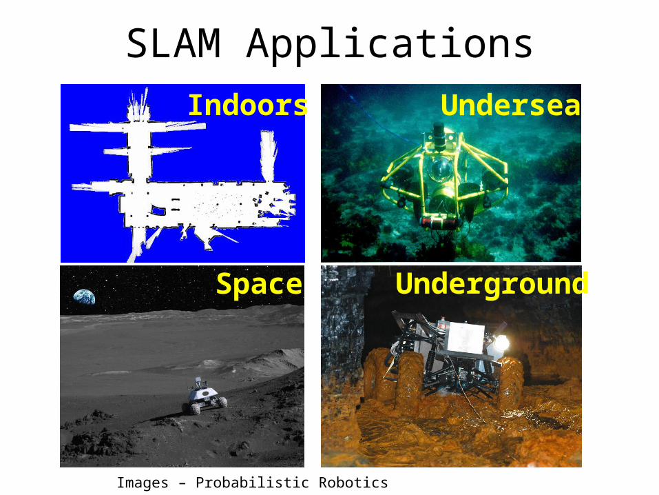
SLAM Applications

Images – Probabilistic Robotics

Indoors

Space

Undersea

Underground

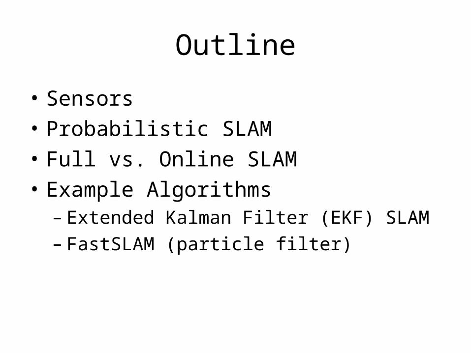
Outline

• Sensors

• Probabilistic SLAM

• Full vs. Online SLAM

• Example Algorithms– Extended Kalman Filter (EKF) SLAM– FastSLAM (particle filter)

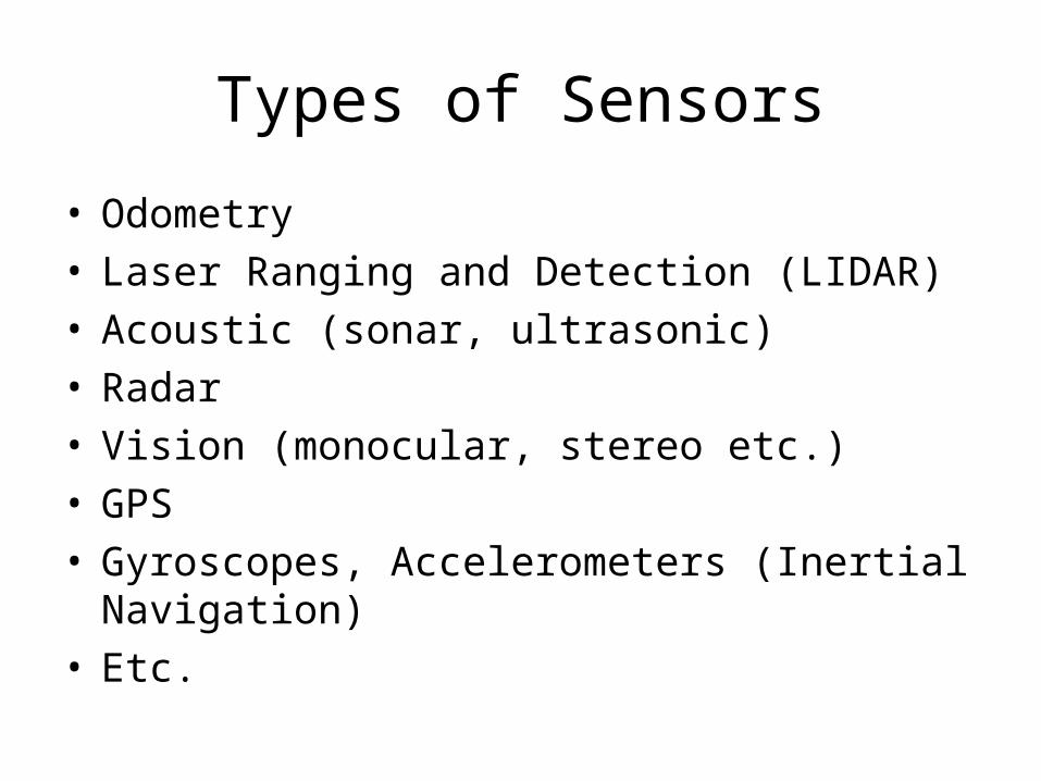
Types of Sensors

• Odometry• Laser Ranging and Detection (LIDAR)• Acoustic (sonar, ultrasonic)• Radar• Vision (monocular, stereo etc.)• GPS• Gyroscopes, Accelerometers (Inertial

Navigation)• Etc.

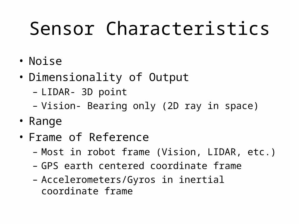
Sensor Characteristics

• Noise• Dimensionality of Output

– LIDAR- 3D point– Vision- Bearing only (2D ray in space)

• Range• Frame of Reference

– Most in robot frame (Vision, LIDAR, etc.)– GPS earth centered coordinate frame– Accelerometers/Gyros in inertial coordinate frame

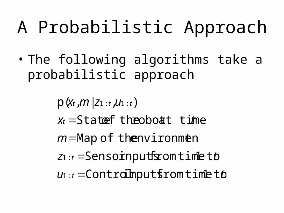
A Probabilistic Approach

• The following algorithms take a probabilistic approach

tu

tz

m

tx

uzmx

t

t

t

ttt

to1 timefrom imputs Control

to1 timefrom inputsSensor

tenvironmen theof Map

at timerobot theof State

),|,p(

:1

:1

:1:1

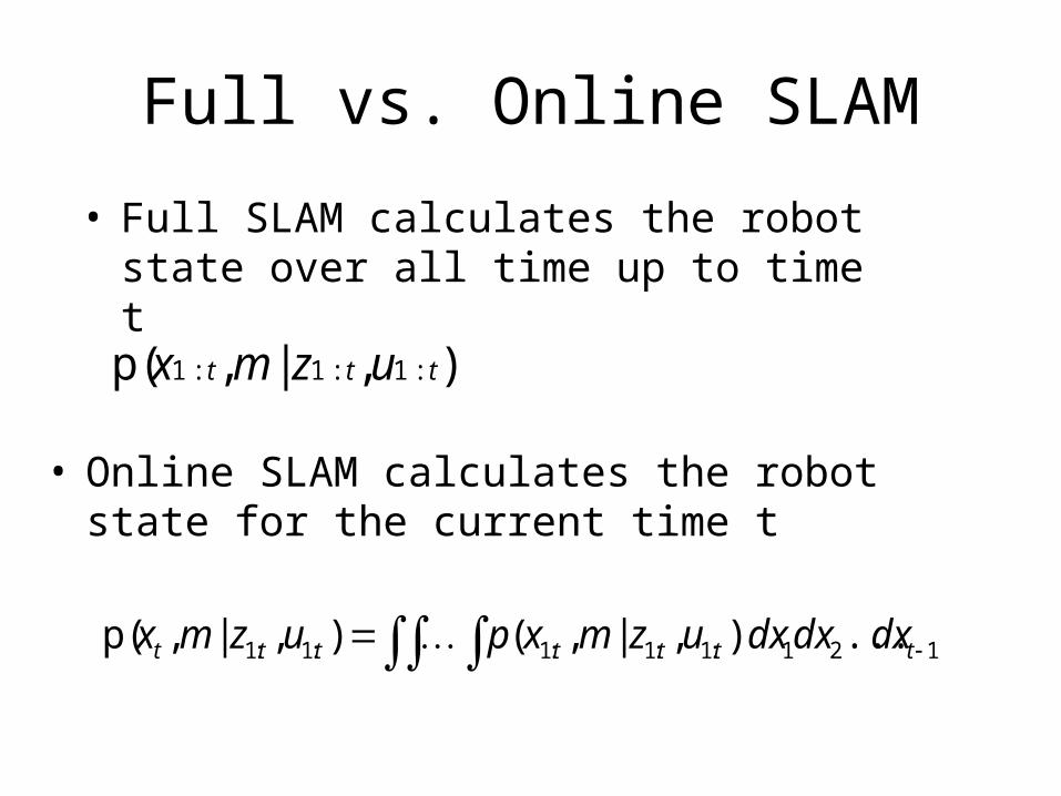
Full vs. Online SLAM

• Full SLAM calculates the robot state over all time up to time t

),|,p( :1:1:1 ttt uzmx

• Online SLAM calculates the robot state for the current time t

121:1:1:1:1:1 ...),|,(),|,p( ttttttt dxdxdxuzmxpuzmx

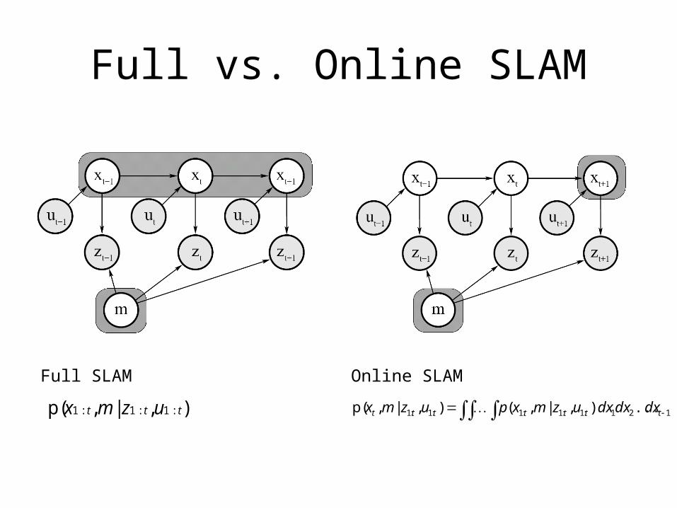
Full vs. Online SLAM

),|,p( :1:1:1 ttt uzmx

Full SLAM Online SLAM

121:1:1:1:1:1 ...),|,(),|,p( ttttttt dxdxdxuzmxpuzmx

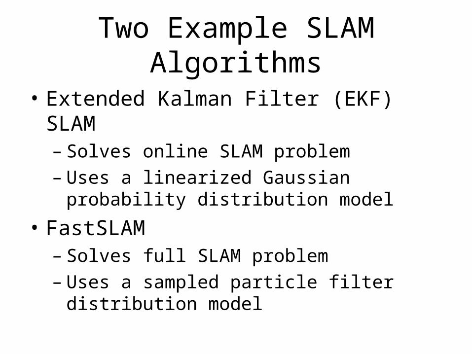
Two Example SLAM Algorithms

• Extended Kalman Filter (EKF) SLAM– Solves online SLAM problem– Uses a linearized Gaussian probability

distribution model

• FastSLAM– Solves full SLAM problem– Uses a sampled particle filter distribution

model

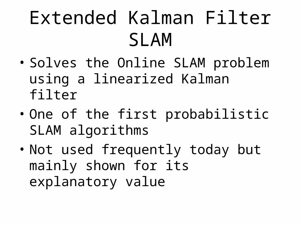
Extended Kalman Filter SLAM

• Solves the Online SLAM problem using a linearized Kalman filter

• One of the first probabilistic SLAM algorithms

• Not used frequently today but mainly shown for its explanatory value

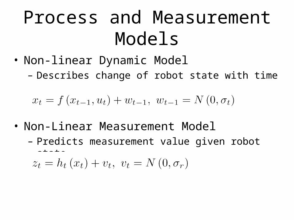
Process and Measurement Models

• Non-linear Dynamic Model– Describes change of robot state with time

• Non-Linear Measurement Model– Predicts measurement value given robot state

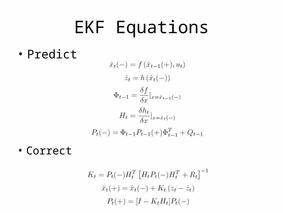
EKF Equations

• Predict

• Correct

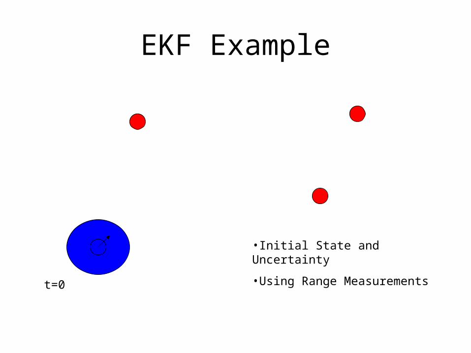
EKF Example

t=0

•Initial State and Uncertainty

•Using Range Measurements

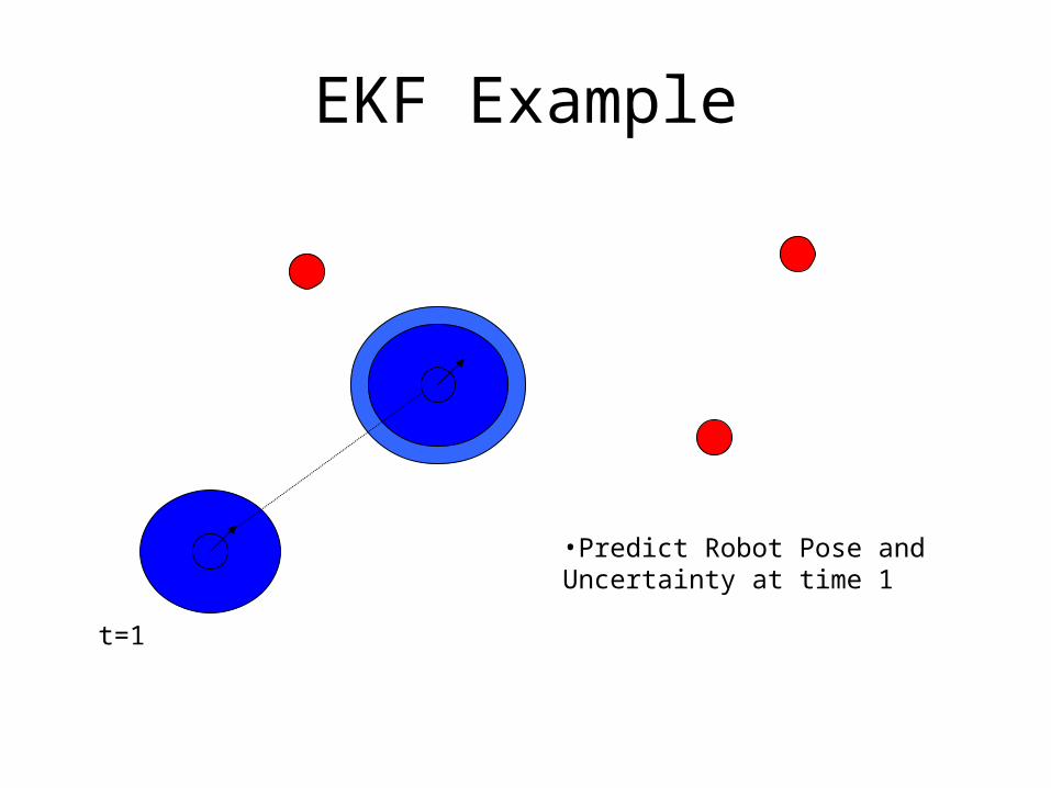
EKF Example

t=1

•Predict Robot Pose and Uncertainty at time 1

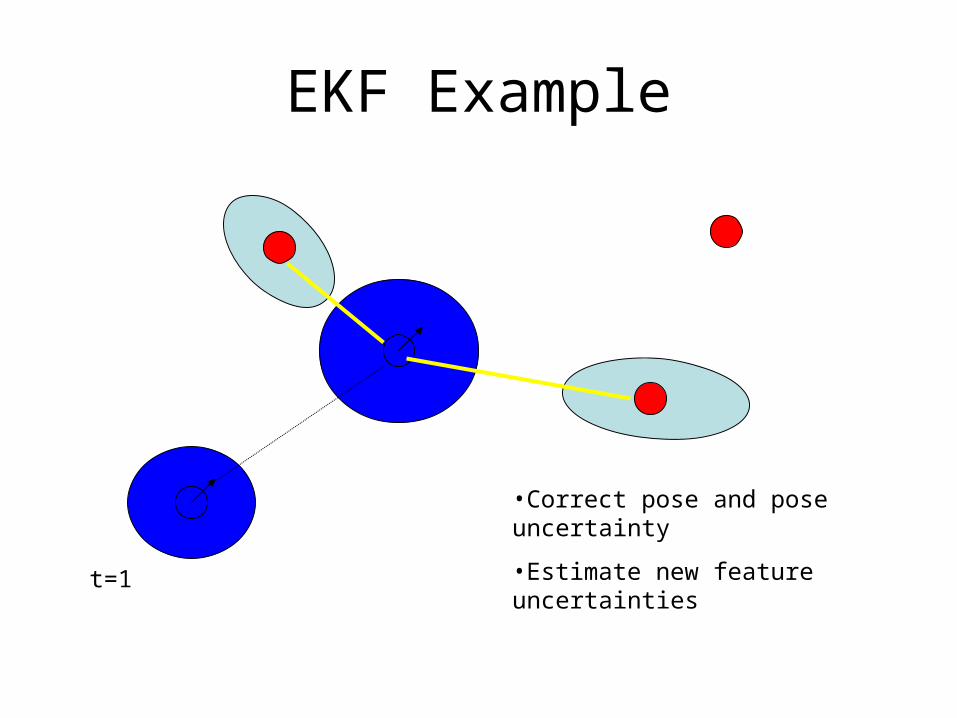
EKF Example

t=1

•Correct pose and pose uncertainty

•Estimate new feature uncertainties

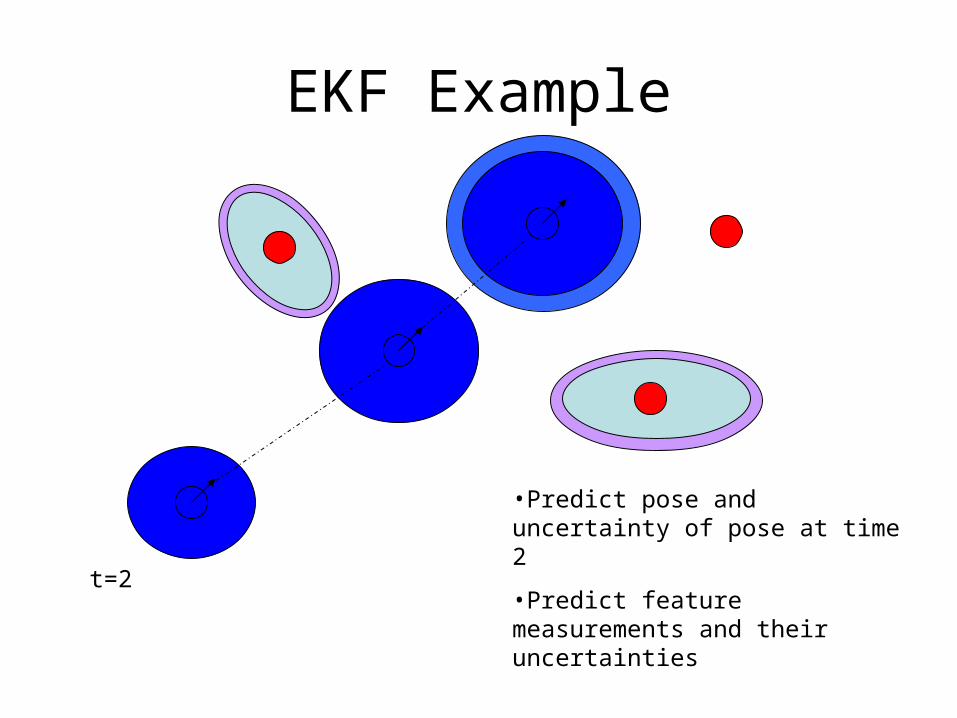
EKF Example

t=2

•Predict pose and uncertainty of pose at time 2

•Predict feature measurements and their uncertainties

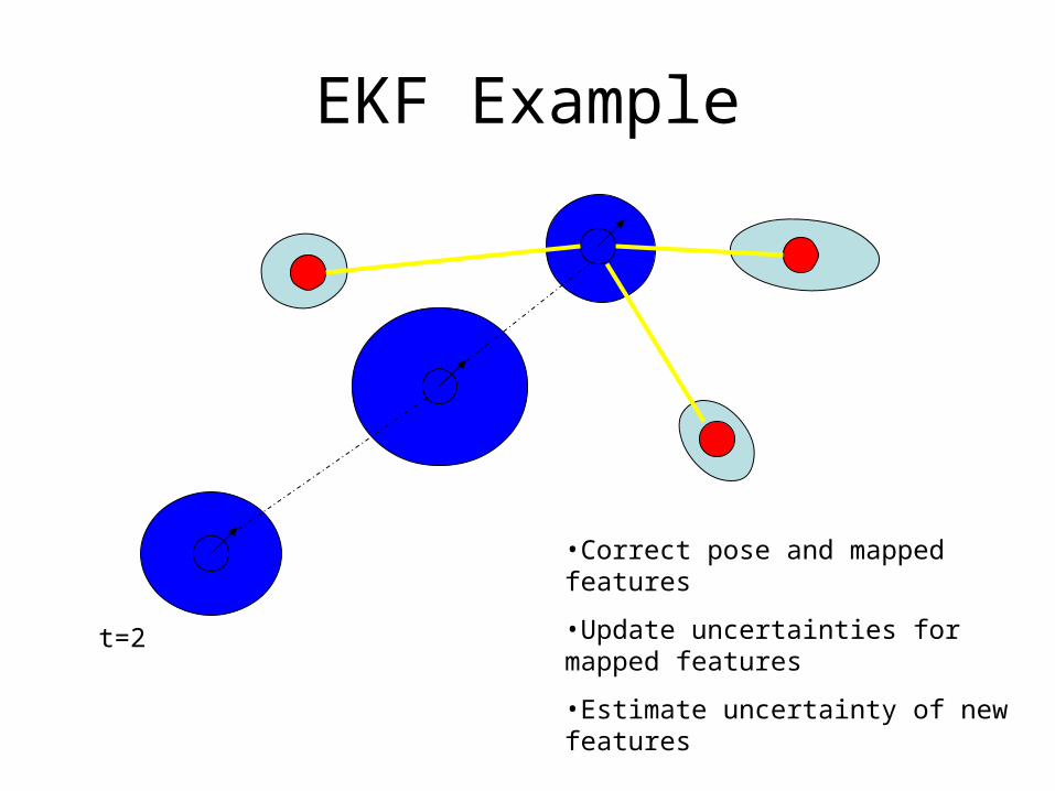
EKF Example

t=2

•Correct pose and mapped features

•Update uncertainties for mapped features

•Estimate uncertainty of new features

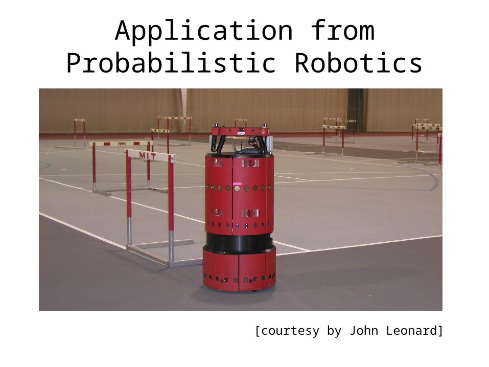
Application from Probabilistic Robotics

[courtesy by John Leonard]

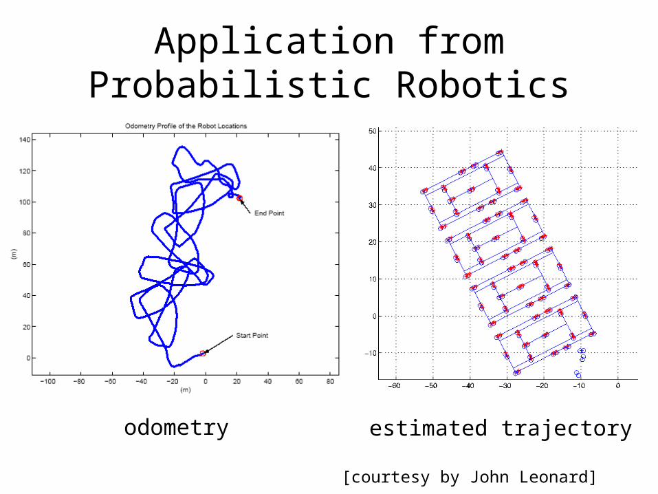
Application from Probabilistic Robotics

odometry estimated trajectory

[courtesy by John Leonard]

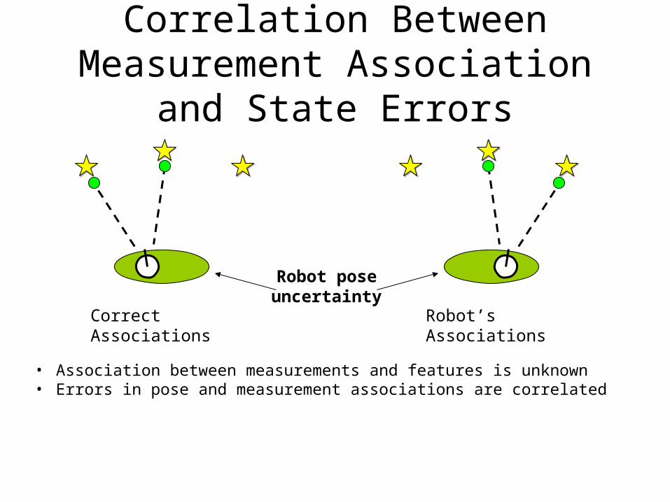
Correlation Between Measurement Association and State Errors

• Association between measurements and features is unknown• Errors in pose and measurement associations are correlated

Robot poseuncertainty

Correct Associations

Robot’s Associations

Measurement Associations

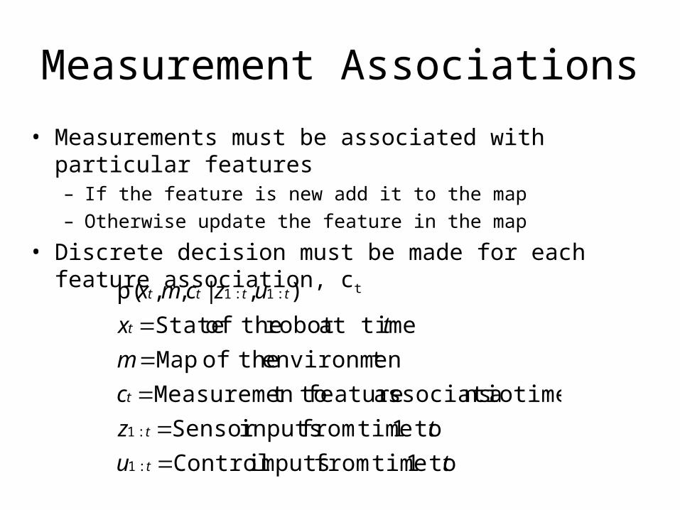
• Measurements must be associated with particular features– If the feature is new add it to the map– Otherwise update the feature in the map

• Discrete decision must be made for each feature association, ct

tu

tz

c

m

tx

uzcmx

t

t

t

t

tttt

to1 timefrom imputs Control

to1 timefrom inputsSensor

t timea nsassociatio feature t toMeasuremen

tenvironmen theof Map

at timerobot theof State

),|,,p(

:1

:1

:1:1

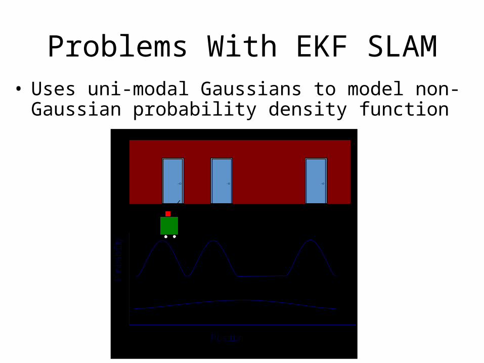
Problems With EKF SLAM• Uses uni-modal Gaussians to model non-Gaussian

probability density functionP

roba

bilit

y

Position

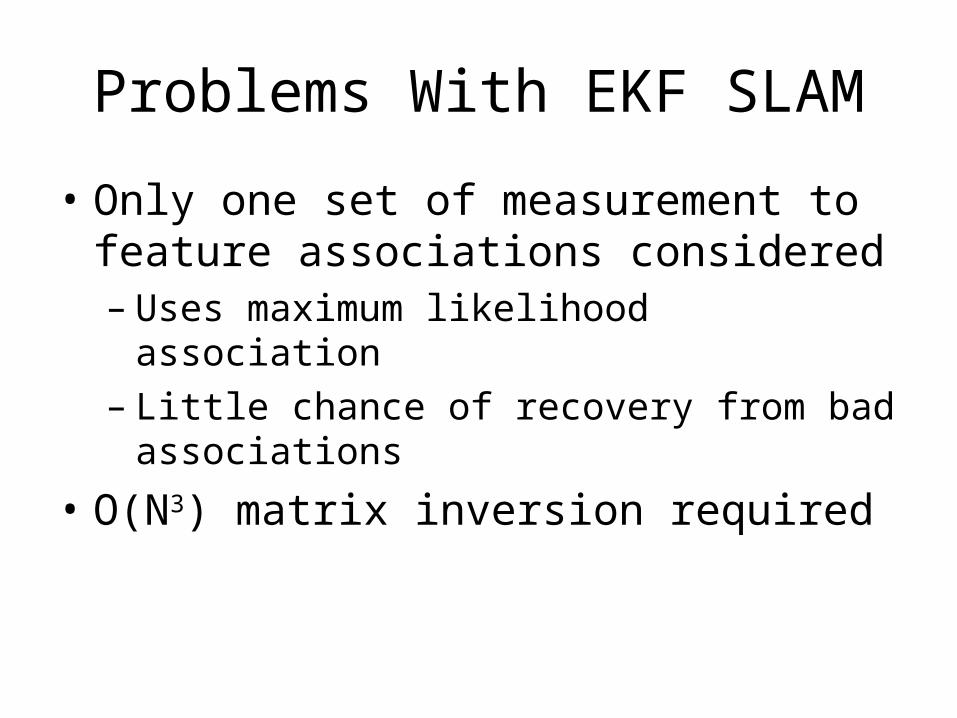
Problems With EKF SLAM

• Only one set of measurement to feature associations considered– Uses maximum likelihood association– Little chance of recovery from bad

associations

• O(N3) matrix inversion required

FastSLAM

• Solves the Full SLAM problem using a particle filter

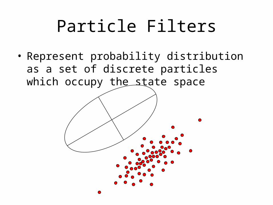
Particle Filters

• Represent probability distribution as a set of discrete particles which occupy the state space

Particle Filter Update Cycle

• Generate new particle distribution given motion model and controls applied

• For each particle– Compare particle’s prediction of

measurements with actual measurements– Particles whose predictions match the

measurements are given a high weight

• Resample particles based on weight

Resampling

• Assign each particle a weight depending on how well its estimate of the state agrees with the measurements

• Randomly draw particles from previous distribution based on weights creating a new distribution

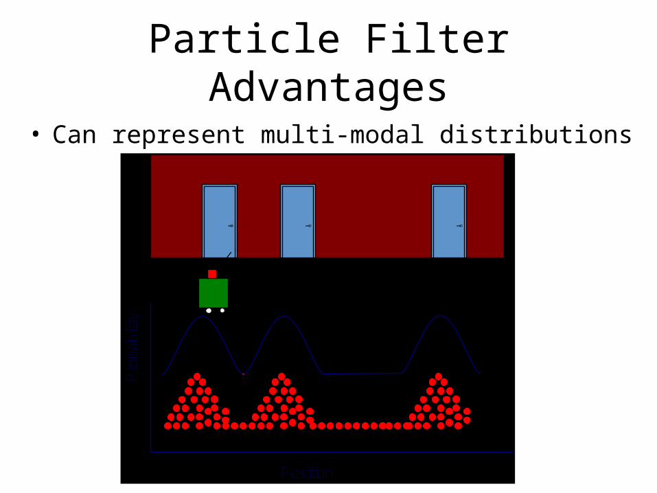
Particle Filter Advantages

• Can represent multi-modal distributionsP

roba

bilit

y

Position

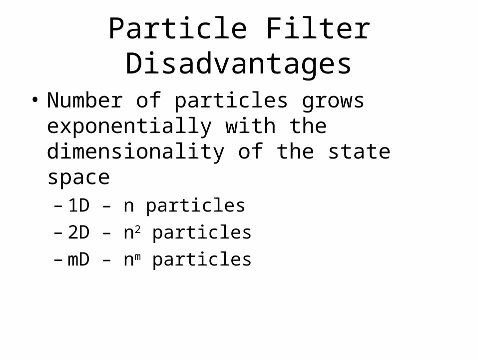
Particle Filter Disadvantages

• Number of particles grows exponentially with the dimensionality of the state space– 1D – n particles– 2D – n2 particles– mD – nm particles

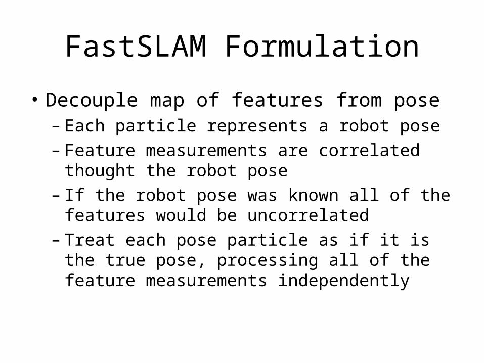
FastSLAM Formulation

• Decouple map of features from pose– Each particle represents a robot pose– Feature measurements are correlated thought

the robot pose– If the robot pose was known all of the features

would be uncorrelated– Treat each pose particle as if it is the true

pose, processing all of the feature measurements independently

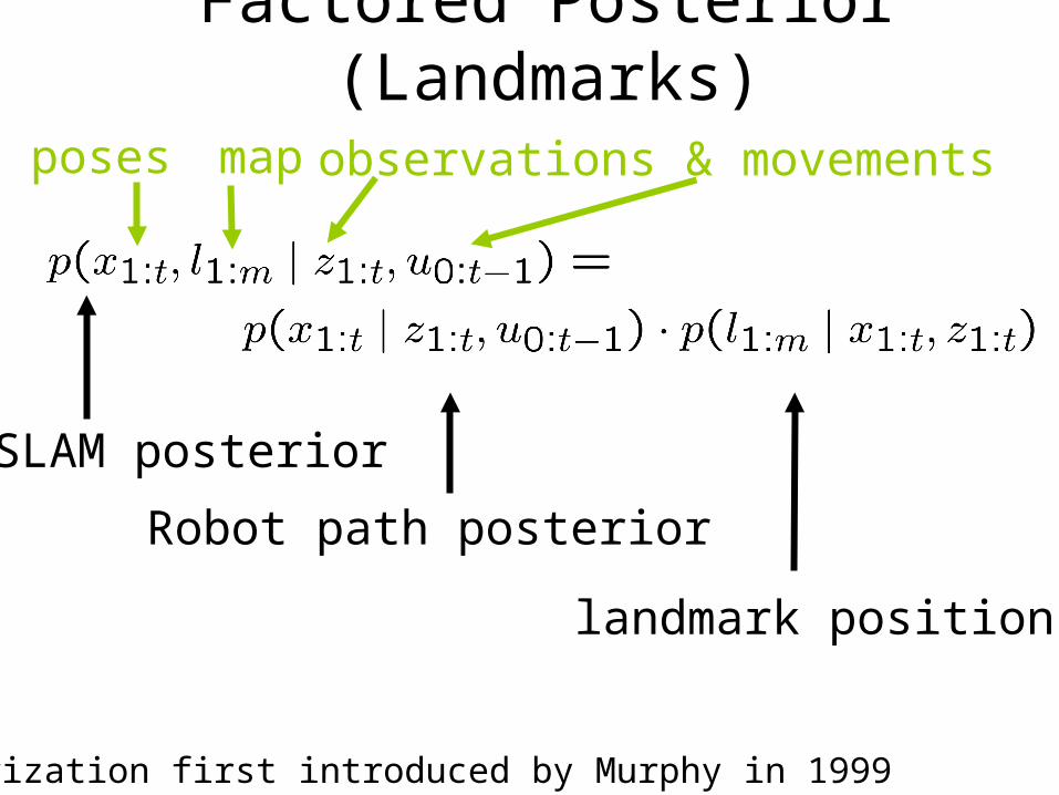
Factored Posterior (Landmarks)

SLAM posterior

Robot path posterior

landmark positions

poses map observations & movements

Factorization first introduced by Murphy in 1999

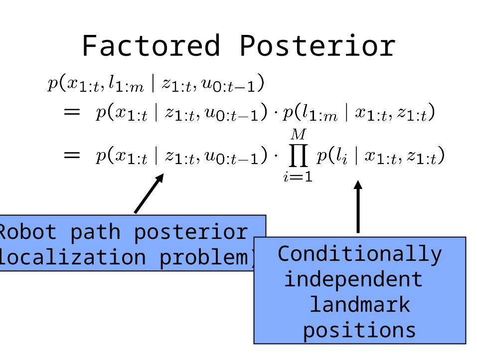
Factored Posterior

Robot path posterior(localization problem) Conditionally

independent landmark positions

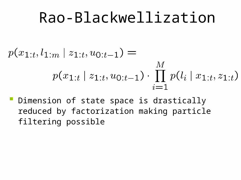
Rao-Blackwellization

Dimension of state space is drastically reduced by factorization making particle filtering possible

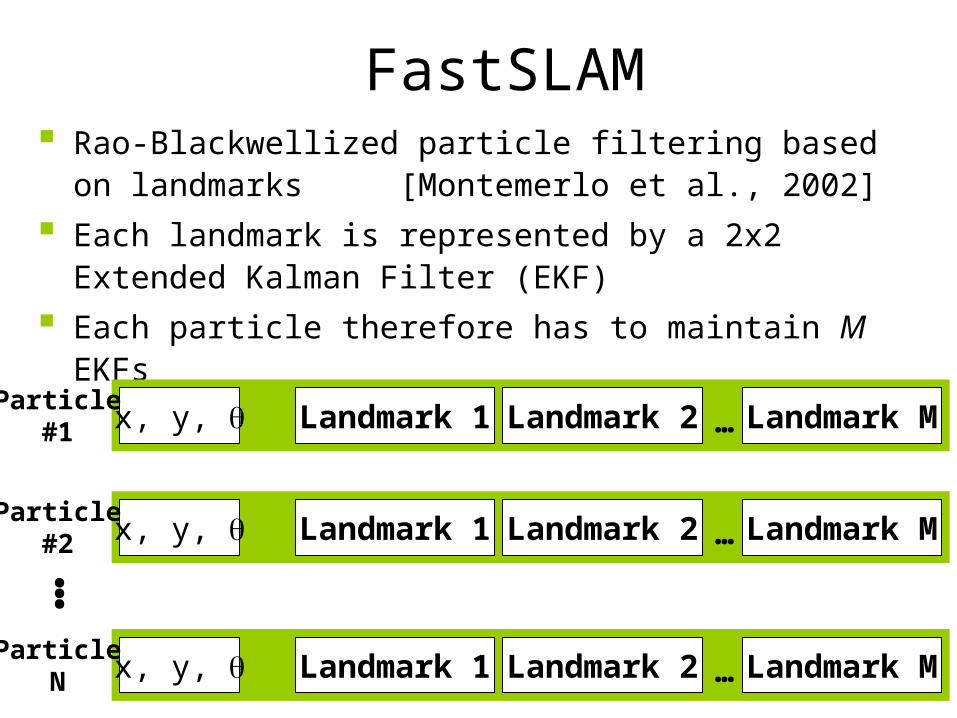
FastSLAM Rao-Blackwellized particle filtering based on

landmarks [Montemerlo et al., 2002]

Each landmark is represented by a 2x2 Extended Kalman Filter (EKF)

Each particle therefore has to maintain M EKFs

Landmark 1 Landmark 2 Landmark M…x, y,

Landmark 1 Landmark 2 Landmark M…x, y, Particle#1

Landmark 1 Landmark 2 Landmark M…x, y, Particle#2

ParticleN

…

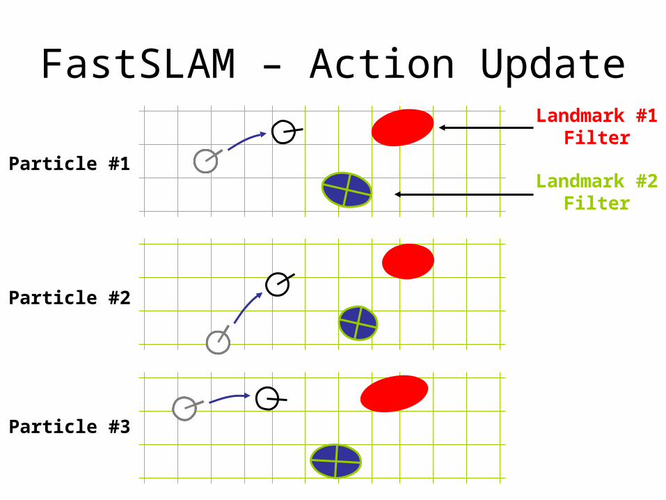
FastSLAM – Action Update

Particle #1

Particle #2

Particle #3

Landmark #1Filter

Landmark #2Filter

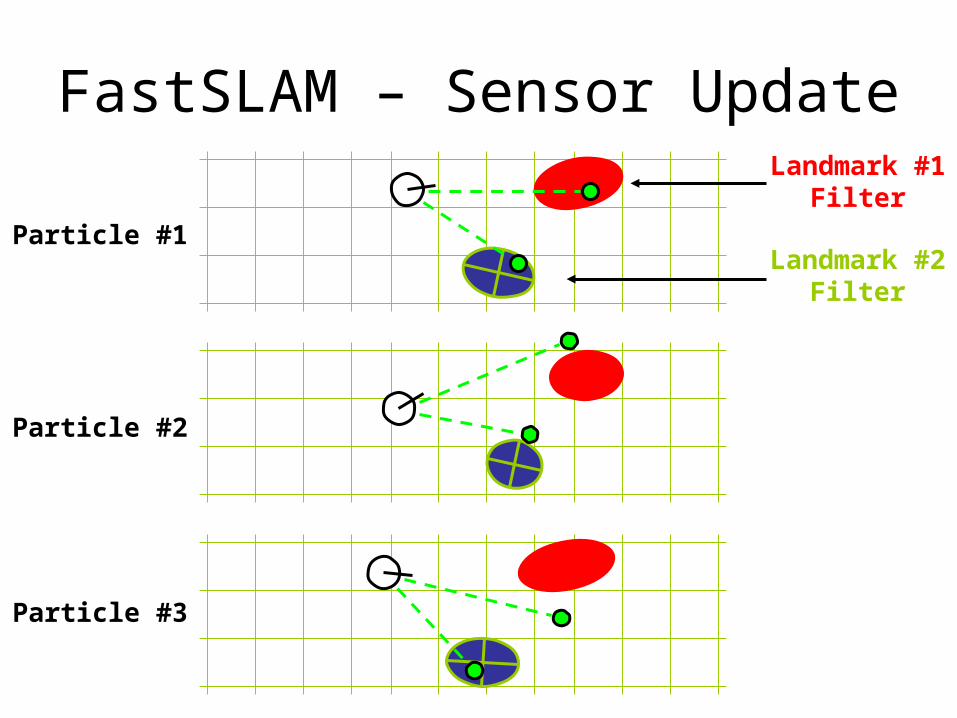
FastSLAM – Sensor Update

Particle #1

Particle #2

Particle #3

Landmark #1Filter

Landmark #2Filter

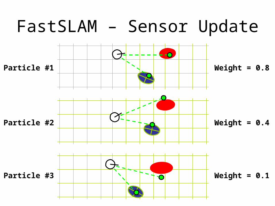
FastSLAM – Sensor Update

Particle #1

Particle #2

Particle #3

Weight = 0.8

Weight = 0.4

Weight = 0.1

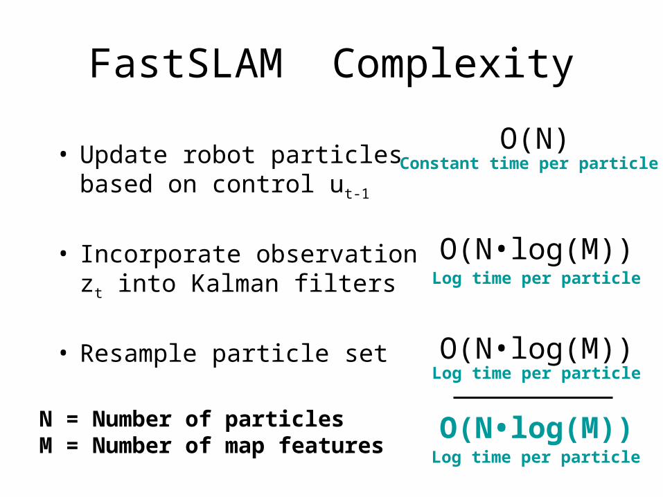
FastSLAM Complexity

• Update robot particles based on control ut-1

• Incorporate observation zt into Kalman filters

• Resample particle set

N = Number of particlesM = Number of map features

O(N)Constant time per particle

O(N•log(M))Log time per particle

O(N•log(M))

O(N•log(M))Log time per particle

Log time per particle

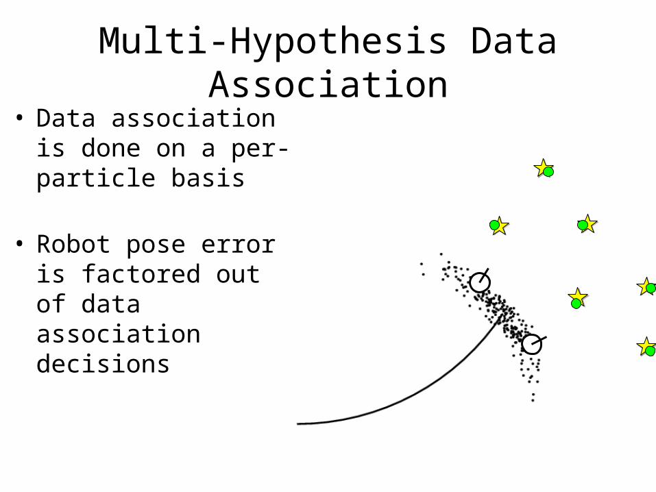
Multi-Hypothesis Data Association• Data association is

done on a per-particle basis

• Robot pose error is factored out of data association decisions

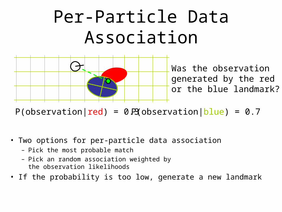
Per-Particle Data Association

Was the observationgenerated by the redor the blue landmark?

P(observation|red) = 0.3 P(observation|blue) = 0.7

• Two options for per-particle data association– Pick the most probable match– Pick an random association weighted by

the observation likelihoods

• If the probability is too low, generate a new landmark

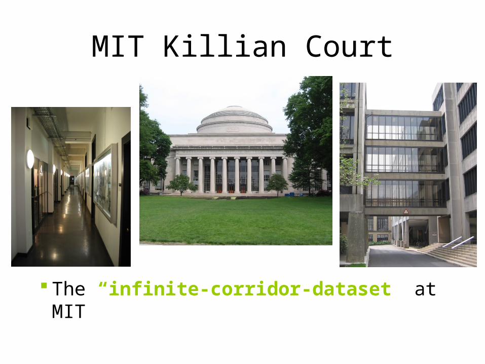
MIT Killian Court

The “infinite-corridor-dataset” at MIT

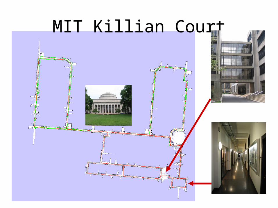
MIT Killian Court

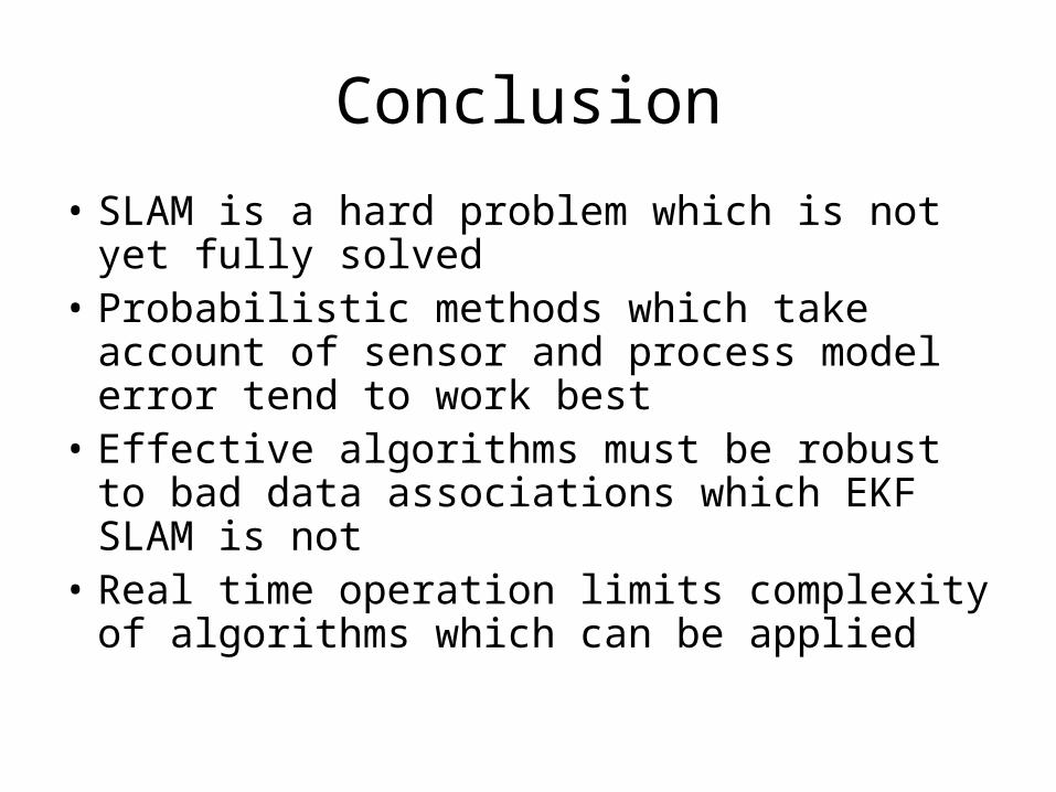
Conclusion

• SLAM is a hard problem which is not yet fully solved

• Probabilistic methods which take account of sensor and process model error tend to work best

• Effective algorithms must be robust to bad data associations which EKF SLAM is not

• Real time operation limits complexity of algorithms which can be applied

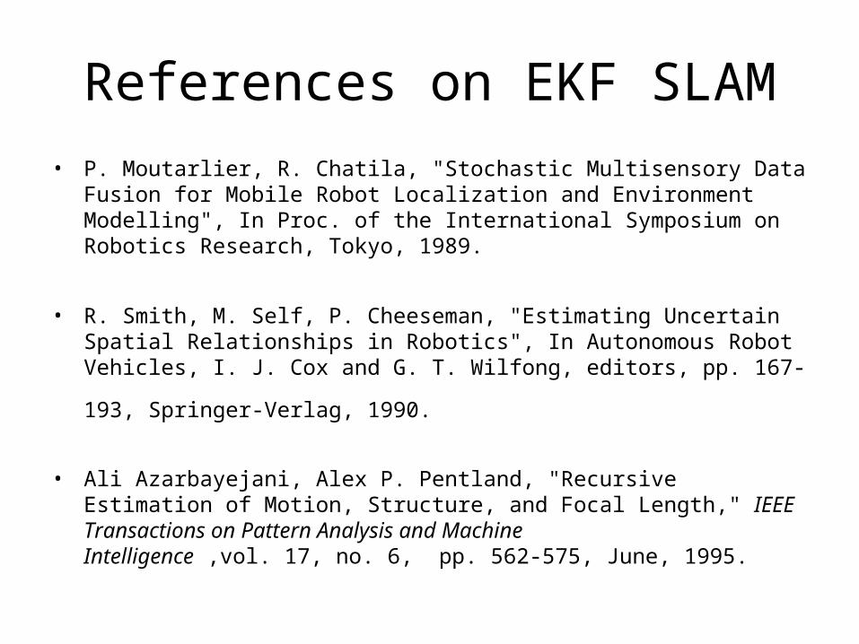
References on EKF SLAM

• P. Moutarlier, R. Chatila, "Stochastic Multisensory Data Fusion for Mobile Robot Localization and Environment Modelling", In Proc. of the International Symposium on Robotics Research, Tokyo, 1989.

• R. Smith, M. Self, P. Cheeseman, "Estimating Uncertain Spatial Relationships in Robotics", In Autonomous Robot Vehicles, I. J. Cox and G.

T. Wilfong, editors, pp. 167-193, Springer-Verlag, 1990.

• Ali Azarbayejani, Alex P. Pentland, "Recursive Estimation of Motion, Structure, and Focal Length," IEEE Transactions on Pattern Analysis and Machine Intelligence ,vol. 17, no. 6,  pp. 562-575, June, 1995.

References on FastSLAM• M. Montemerlo, S. Thrun, D. Koller, and B. Wegbreit. FastSLAM: A factored

solution to simultaneous localization and mapping, AAAI02

• D. Haehnel, W. Burgard, D. Fox, and S. Thrun. An efficient FastSLAM algorithm for generating maps of large-scale cyclic environments from raw laser range measurements, IROS03

• M. Montemerlo, S. Thrun, D. Koller, B. Wegbreit. FastSLAM 2.0: An Improved particle filtering algorithm for simultaneous localization and mapping that provably converges. IJCAI-2003

• G. Grisetti, C. Stachniss, and W. Burgard. Improving grid-based slam with rao-blackwellized particle filters by adaptive proposals and selective resampling, ICRA05

• A. Eliazar and R. Parr. DP-SLAM: Fast, robust simultanous localization and mapping without predetermined landmarks, IJCAI03

Additional Reference

• Many of the slides for this presentation are from the book Probabilistic Robotic’s website– http://www.probabilistic-robotics.org