Embed Size (px)
Citation preview
SLAC-163 UC-34d tE)
AN EXPERIMENTAL STUDY OF THE REACTION
no +p -p” + p AT 15.0 GeV/c*
WILLIAM TYLER KAUNE
STANFORD LINEAR ACCELERATOR CENTER
STANFORD UNIVERSITY
Stanford, California 94305
PREPARED FOR THE U.S. ATOMIC ENERGY
COMMISSION UNDER CONTRACT NO. AT (04-3)-515
June, 19’73
Printed in the United States of America. Available from National Technical Service, U. S. Department of Commerce, 5285 Port Royal Road, Springfield Virginia 22151. Price: Printed Copy $5.45.
*Ph. D. dissertation,
ABSTRACT
The &one-particle t-channel exchange mechanism which is thought to con--
tribute to the reaction no + p--p’ + p involves the exchange of a (u meson. We
use our measurements of the differential cross sections and densily matrices f
of the reactions ?I + p- p* + p and II- + p-p’ + n to calculate the differential
cross section and density matrix for r” + p-p’ + p at 15.0 GeV/c.
To make the required measurements a new technique was developed using
optical spark chambers to vi&w the decay products of the p mesons. The re-
coil proton was viewed for events where the square momentum transfer to the
proton exceeded about .04 (GeV/c)‘. In the experiment, conducted at the
Stanford Linear Accelerator Center, we obtained at 15.0 GeV/c 811 events
from the channel r++ p-p++ p, 772 from T-+ p- p-i p, and 817 from
r- + p -p” + n.
We present the differential cross sections and density matrix elements for
these three channels. The energy dependence of these quantities is determined
by including data from other experiments.
The differential cross section and density matrix elements for the reaction
7r” + p ‘PO + p at 15.0 GeV/c are calculated. This data has the general fea-
tures expected in a reaction dominated by w-exchange but fails to agree in the
region 1 tl Ik 0.3 (GeV/c)2 with a detailed calculation based on the dual-absorption
model.
A test of the vector dominance model is performed by comparing the two
reactions y + p -p”+pand~o+p-po+p. We find agreement in shape but
an overall normalization difference consistent only with a significantly lower
value of yz/4*.
ii
ACKNOWLEDGEMENTS
There were many people who helped and encouraged me in my graduate
years and I want to thank them all very much. There are two people of
special influence whom I would like to mention individually. Professor
Martin L. Per1 served as my advisor for this experiment. He always
held my professional development of primary importance and was ready
to listen and discuss any problems and ideas; all of this I deeply appreciate.
From Bill Toner I first began to learn the most difficult and important
lesson of all which is objectivity.
iii
TABLE OF CONTENTS
I. Introduction and General Considerations .............
A. Physics of no + p --pO+p .................
B. MethodtoMeasureIr”+p-p”+p .............
C. Present Experimental Status - - - - - - l - - l - - - - - -
D. Choice of Apparatus; General Considerations ........
II. Apparatus ..........................
A. General Description ....................
B. Beam ..........................
C. Liquid Hydrogen Target ..................
D. Charged Particle Spectrometer ...............
E. x0 Detector ........................
III.
E3E 1
1
2
‘4
6
8
8
8
11
11
13
F. Proton Spectrometer . . . .
G. Veto Counters . . . . . . .
H. Optics . . . . . . . . . . .
I. Electronics System . . . . .
J. Performance of the Apparatus
Data Reduction and Event Selection
A. Introduction . . . . . . . .
B. Scanning . . . . . . . . . .
C. Measuring . . . . . . . . .
D. Geometrical Reconstruction .
E. Selection of Elastic Events . .
F. Selection of K* Events . . . .
G. Selection of p” Events . . . .
. . . . . . . . . . . . . . . 15
. . . . . . . . . . . . . . . 16
. . . . . . . . . . . . . . . 19
............... 19
............... 22
. . . . . . . . . . . . . . . 24
............... 24
............... 24
............... 26
............... 26
............... 27
............... 27
...... ;.....;;i 28
iv
H. Selection of High-t p* Events ................
I. &de&ion of Low-t p- Events ................
J. Data Reduction and Event Selection Efficiency ........
IV. Extraction of p Cross Sections and Density Matrices .......
A. Introduction .......................
B. Extraction of dN/dt and ptm, ...............
C. Correction for Experimental Event Losses ..........
D. Backgrounds and Contaminations ...............
E. du/dtandp&, ......................
F. Overall Statistical and Systematic Errors ..........
V.’ DiscussionoftheReactionsr*+p-p*+p ...........
VI. The Reaction no + p - p" + p and Conclusions ..........
du A. Calculation of dt md &Em1 for r”+p-p”+p .......
B. Basic Tests of the Data ..................
C. Comparison with Other Experiments; The Dual Absorption Model .
D. Energy Dependence of cp(rop - pop) .............
E. Comparisonof ~r~+p-p~+pandy+p-x~+p;
The Vector Dominance Model ..............
F. Summary and Conclusions .................
30
34 / I
38
44
44
44
48
53
60
6’7
70
74
74
‘78
80
82
83
91
References . . . . . . . . . . . . . . . . . . . . . . . . . . 94
V
LIST OF TABLES
1. Estimated p” Event Loss from Neutron Vetoes ..........
2. Apparatus Absorption Losses ..................
3. Backgrounds and Contaminations From m Mass Fits .......
4.
5.
6.
7.
8.
9.
10.
11.
Total r Fluxes Through the Hydrogen Target . .
Target Empty Subtractions . . . . . . . . . .
&T H dt’ pmmc for n+ + p - p’ + p at 15.0 GeV/c .
du H dt’ pd for II- + p -p-+pat 15.0 GeV/c . .
Q H dt’Pmm , for r- + p -p”+nat15.0GeV/c. .
Overall Statistical Errors . . . - - - - - l l
Overall Systematic Errors . . . . . . . . l .
du dt and Errors for x0 + p 4,~’ + p at 15.0 GeV/c
.........
.........
.........
. . . . . . . . . 65
.........
.........
.........
.........
12. PZrn, for r” + p -p”+pat15.0GeV/c. . . . . . . . . . . . .
Page 50
52
56
‘61
61
64
66
68
69
75
76
* vi
. . 1.
2.
3.
4.
5.
6.
7.
8.
9.
10.
11.
12.
LIST OF FIGURES
Feynman diagram showing possible t-channel exchanges in the
reactionsnN-pN . . . . . . . . . . . . . . . . . . . .
Elevation view of the apparatus . . . . . . . . . . . . . . . . .
The LH2 target and supporting structure . . . . . . . . . . . . S
Trigger counter hodoscopes . . . . . . . . . . . . . . . . . .
Elevation and cross-sectional views of the target veto
lead-scintillator sandwich counters . . . . . . . . . . . . .
DV lead-scintillator sandwich veto counters . . . . . . . . . . .
CT fast multiplicity counting circuit . . . . . . . . . . . . . . .
Missing mass spectrum (MX) for the reaction n-p - x+x-X,
all events,and events with 665 I Mm < 865 MeV . . . . . . . .
Invariant mass spectrum (i$&) for the reaction n-p - x+x-n . . . .
Cuts made to select events belonging to the channel nip - flrOp
when the proton is detected: (a) Minimum distance of approach
of the extrapolated x’ and p tracks; (b,c) Vertex location within
the target volume; (d) Mass of the recoil system is that of a
proton; (e) Effective mass of the w system is that of a r” . . .
The ability of the scanuers to correctly select from two y-ray
showers the one with more energy as a function of : (a) The
no rest frame decay angle; (b) The reconstructed energy dif-
ference between two photons . . . . . . . . . . . . . . . .
Calculated resolutions as a function of momentum transfer.
Curve (a) assumes there is no x0 ambiguity; (b) assumes the
scanner always makes the incorrect choice; (c) attempts to
model the actual scanner based onthe data in Fig. 11 . . . . .
vii
1
9
12
14
17
18
21
29
31
33
36
37
Page 13.
14.
15.
16.
17.
18.
19.
20.
21.
22.
23.
The r’r” and x-r0 invariant mass distribution for the reaction * *0 sp-rap . . . . ..*................ 39
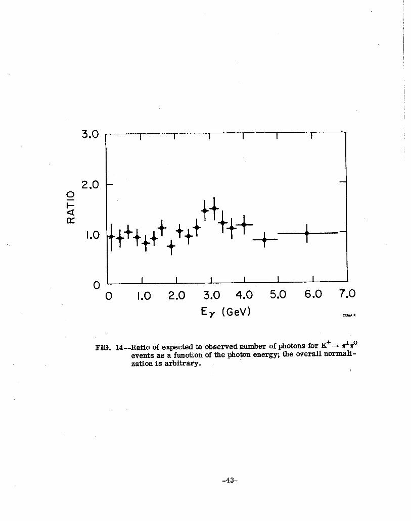
Ratio of expected to observed number of photons for K* f0 -Ii-A
events as a function of the photon energy; the overall normali-
zation is arbitrary . . . . . . . . . . . . . . . . . . . .
The apparatus acceptance as a function of the “physics variables.”
The cos C”p and @ distributions assume t = -.Ol (GeV/c)2
and Mxr= 765 MeV. The t and Mlrr distributions assume iso-
tropic distributions in cos Gz and 7$ . . . . . . . . . . . .
Comparison of the angular distribution of observed events (histo-
grammed) and the underlying distribution obtained when the
apparatus acceptance is removed (solid curve) . . . . . . .
Typical Mrr spectrum and associated theoretical fit (see text) . .
Mass and momentum transfer distributions of the high-t sample
of contamination events. The low-t backgrounds obtained from
the mass fits are also shown . . . . . . . . . . . . . . .
The s-p wave interference density matrix elements as a function
of momentum transfer f or the reactions ?r*p -p*p and n-p -pOn .
The differential cross sections as a function of momentum transfer
for the reactions rip - p*p and n-p - pan . . . . . . . - .
The p density matrix elements as a function of momentum transfer
for the reactions n*p -+ p’p and n-p -pan . . . . . . . . .
The energy dependence of the cross sections for r*p - P&P.
Reference 20 traces the sources used in this figure. . . . . .
The cross section and density matrix elements as a function of the
momentum transfer for the reaction lr’p - p” p at 15.0 GeV/c . . .
VI11
. 43
. 47
. 49
. 55
57
. 59
. 62
. 63
. 71
. 77
24. Absorption corrections to the reaction nap -. pop. The bubbles
represent elastic scattering . . . . . . . . . . . . . . . . . 79
25. Comparison of our measurement of the cross section for
TOP - pop with the dual-absorption fit to the 16.0 GeV/c data . . 81
26. The energy dependence of the cross section for lr’p -. pop. The
curve is a fit of a Regge form (see text) . . . . . . . . . . . 84
27. Vector dominance expansion for the reaction ‘yp + nap . . . . . . . 85
28. The ratio of r” photoproduction from neutrons and protons
as a function of momentum transfer . . . . . . . . . . . . . 88
29. A comparison of yp - x”p and lr’p - pop as a test of the vector
dominarxx model . . . . . . . . . . . . . . . . . . . . . 89
ix
CHAPTER I
INTRODUCTION AND GENERAL CONSIDERATIONS
A. Physics of 1~’ + p-p’ + p
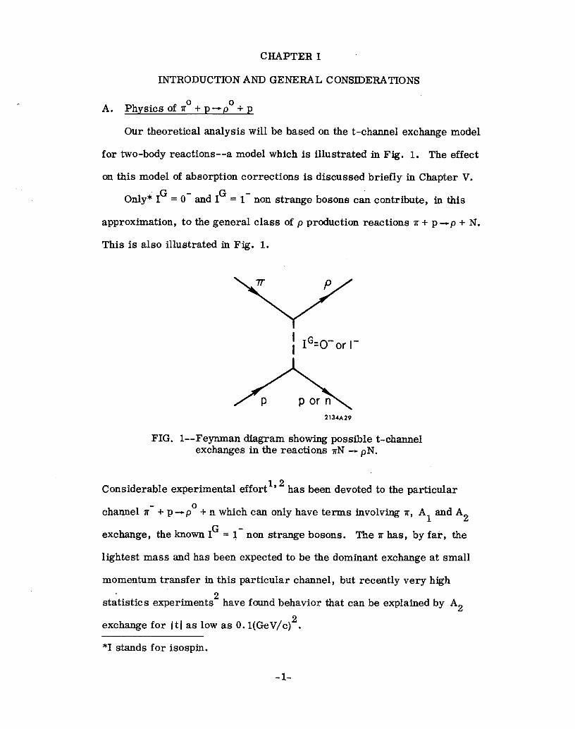
Our theoretical analysis will be based on the t-channel exchange model
for two-body reactions--a model which is illustrated in Fig. 1. The effect
on this model of absorption corrections is discussed briefly in Chapter V.
Only* IG = 0- and IG = l- non strange bosons can contribute, in this
approximation, to the general class of p production reactions ‘IT + p-p + N.
This is also illustrated in Fig. 1.
FIG. 1--Feynman diagram showing possible t-channel exchanges in the reactions rN - pN.
Considerable experimental effort” 2 has been devoted to the particular
channel K- + p-p’ + n which can only have terms involving r, AI and A2 G exchange, the known I = l- non strange bosons. The r has, by far, the
lightest mass and has been expected to be the dominant exchange at small
momentum transfer in this particular channel, but recently very high
statistics experiments2 have found behavior that can be explained by A2
exchange for ItI as low as 0. l(GeV/c)2.
*I stands for isospin.
-l-
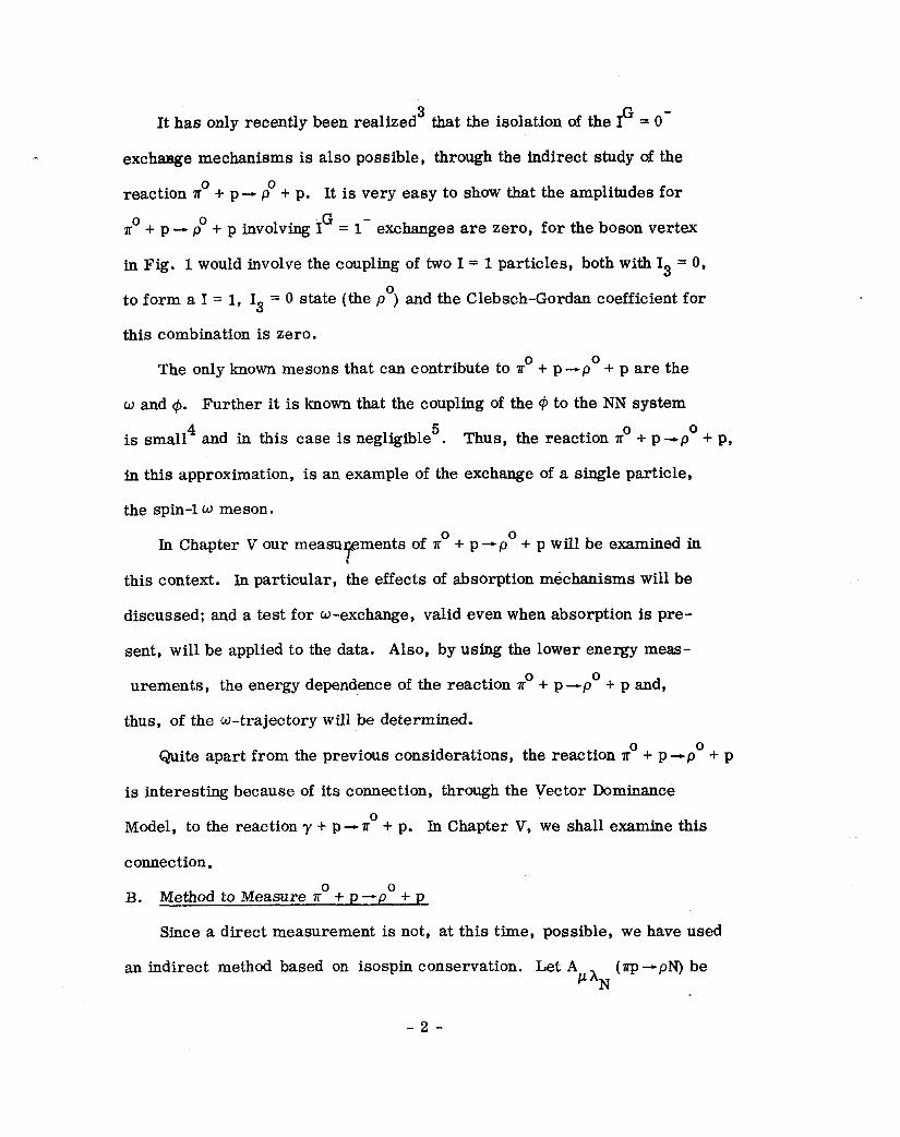
It has only recently been realized’ that the isolation of the IG = O-
exchange mechanisms is also possible, through the indirect study of the
reaction x0 + p -, co + p. It is very easy to show that the amplitudes for
no+ p - p” + p involving IG = l- exchanges are zero, for the boson vertex
in Fig. 1 would involve the coupling of two I = 1 particles, both with I3 = 0,
to form a I = 1, I3 = 0 state (the p”) and the Clebsch-Gordan coefficient for
this combination is zero.
The only known mesons that can contribute to r” + p-p’ + p are the
o and @. Further it is known that the coupling of the 9 to the NN system
is small4 and in this case is negligible5. Thus, the reaction x0 + p-p’ + p,
in this approximation, is an example of the exchange of a single particle,
the spin-l W meson.
In Chapter V our measu 7
ments of x0 + p+p” + p will be examined in
this context. In particular, the effects of absorption mechanisms will be
discussed; and a test for w-exchange, valid even when absorption is pre-
sent, will be applied to the data. Also, by using the lower energy meas-
urements, the energy dependence of the reaction r” + p-p’ + p and,
thus, of the w-trajectory will be determined.
Quite apart from the previous considerations, the reaction no + p-co’ + p
is interesting because of its connection, through the Vector Dominance
Model, to the reaction y + p-r’ + p. In Chapter V, we shall examine this
connection. 0 B. Method to Measure r” f p-p + p
Since a direct measurement is not, at this time, possible, we have used
an indirect method based on isospin conservation. Let A pLAN (~rp -PN) be
-2-
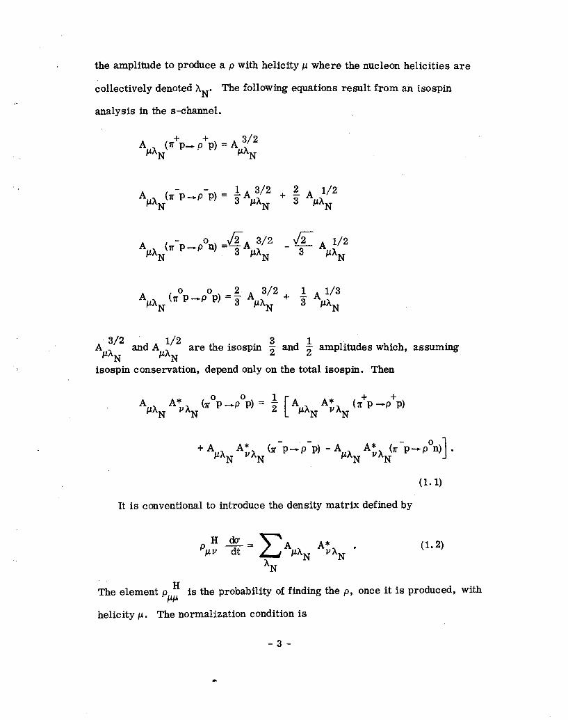
the amplitude to produce a p with helicity 1 where the nucleon helicities are
collectively denoted hN. The following equations result from an isospin
analysis in the s-channel.
A nhN(l;h- P+P) = APy2 N
A ,bN(x-p,p-p) = +A,$” + ; AP;/2 N N
A PhN(r-p -p’n) =$APz’” N
- $ APi/ N
A FAN (1Top -pop) = i AP;‘2 + 1. A 1’3 N 3 PAN
A 3/g
PAN and Apt’” are the isospin
N i and i amplitudes which, assuming
isospin conservation, depend only on the total isospin. Then
A A* PAN ‘AN
trap -pop) = ; APh AEh (l;tp -P+P) N N
+A A* PAN VAN
(n-p.+pP-p) - Aph AEh (r-p-p”N] - N N
(1.1)
It is conventional to introduce the density matrix defined by
H& Ppv dt= c
A A*,A ’
hN pAN N
(1.2)
The element pkF is the probability of finding the p, once it is produced, with
helicity p. The normalization condition is
-3-
In terms of the density matrix Eq. (1.1) becomes
p~v dt H Le (PP- POP, = + I
Ppv H +r+, - P+P)
+ PFv -g (n-P-P-P) - P;v $ (T-P -PO*) 1
(1.3)
Setting p = v and summing gives
dU0 1 dt\lr P-POP) = z
I ck7 + --&-(s p-p+p) + J$-(n-P-P-P) -+-P-Pa*)
I
(1.4)
Equations (1.3) and (1.4) represent a complete prescription for extracting
the cross section and densit$matrix elements for the reaction II” + pdp” + p
from measurements of the reactions
r’+p--p*+p
0 r-+p-p +n. (1.5)
Experimentally, the p is observed indirectly through the decay
p--r + x. Using the experimental measurement of the xx four-momentum
the four variables of interest can be calculated. These are: t, the square
of the four-momentum transfer to the p; M xx, the invariant mass of the
m system ad of the P; and cos ei and ‘P* , the spherical angles of the P
xr pair in the m rest frame. We shall hereafter refer to this set of four
variables as the “physics variables.”
c. Present Experimental Status
To this date, three experiments have been reported which study the.
-4-
reaction no + p -p” + p. All have used bubble chambers as their means
of particle detection. Michael and Gidal’ have studied the reaction
T+ + p-p” + p at 2.67 GeV/c. By combining this measurement with sim-
ilar measurements7 using a zr- beam the cross sections and density matrix
elements for no + p -p” + p were obtained. Michael and Gidal have sep-
arated the x0 + p dp” + p cross section into natural and unnatural parity
exchange components and, at small-t, find significant unnatural parity
contributions, rather surprising as the w is a natural parity particle.
However, this experiment does use data from two distinct measurements
to isolate the reaction r” + p-p’+ p with Eq. (1.3) and Eq. (1.4) and
is highly sensitive to any relative normalization errors.
A 6.0 GeV/c experiment8 at Brookhaven has used the same apparatus
to measure all three of the reactions (1.5). The authors conclude that
their results are consistent with pure w-exchange in the reaction no + p -.
p” + p, in definite contrast to the 2.67 GeV/c data. The authors fit
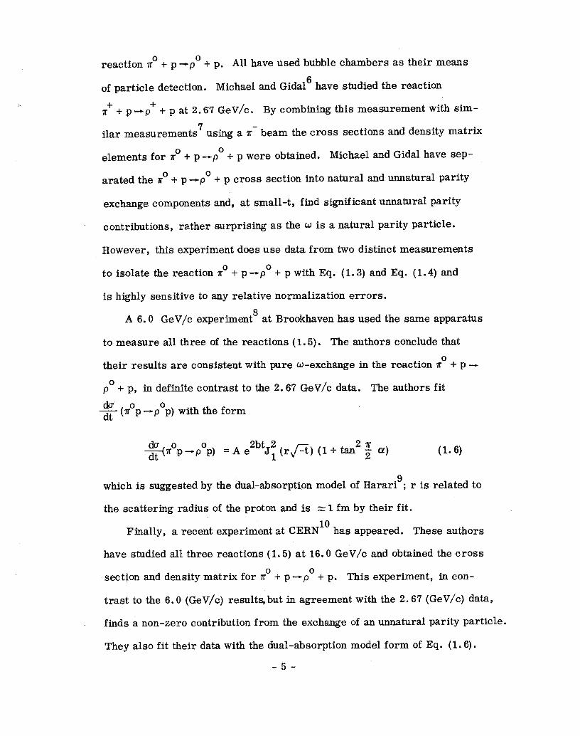
s (n’p &pop) with the form
da o at\” P-POP) =Ae
2bt 2 J1 (rfi) (l+ tan 2r
z (Y)
which is suggested by the dual-absorption model of Harari’; r is related to
the scattering radius of the proton and is z 1 fm by their fit.
Finally, a recent experiment at CERN 10
has appeared. These authors
have studied all three reactions (1.5) at 16.0 GeV/c and obtained the cross
section and density matrix for no + p-p’ + p. This experiment, in con-
trast to the 6.0 (GeV/c) results, but in agreement with the 2.67 (GeV/c) data,
finds a non-zero contribution from the exchange of an unnatural parity particle.
They also fit their data with the dual-absorption model form of Eq. (1.6).
-5-
At this point there is no consistent interpretation of these results.
All three experiments show results qualitatively in agreement with the form
of Eq. (1.6), but differing amounts of unnatural parity contribution. More
experimental information is needed. Further, there are compelling rea-
sons to attempt the experiment using different experimental techniques.
D. Choice of Apparatus; General Considerations
In studying the reactions f + p -cp* + p bubble chambers have an
intrinsic difficulty for small values of t. The r” from the p decay is not
detected so the recoil proton must be detected, which at low values of t
is difficult because of the short proton range. This bias becomes serious
for It I LO. 1 (GeV/c) 2 8,ll . All the bubble chamber experiments discussed
in Section C have observed pronounced dips ins (ropepop). These dips
are suggested by the dual-absorption model’ but may, in fact, be attributable f
to scanning biases in the s*ti- p-p* + p data.
To overcome this difficulty we developed a new method of investigating
the reactions ri + p+p’ + p. An optical spark chamber system was de-
signed to detect both the f and ?y”, through the decay of ~‘-7 + y; no longer
is it necessary to detect the recoil proton. However, a different type of
problem, again associated with small-t values, may occur.
In this method the four-momentum of the r* and the angles of the two
photons are measured. To reconstruct the recoil four-momentum and the
two photon energies at all one must assume that the recoil system is, in
fact, a proton and that the two photons do, in fact, come from the decay 0
K -y + y, and even then two solutions for the unmeasured variables result
because of the identical nature of the two photons; this is the so-called x0
ambiguity.
-6-
In order for us to observe a lr” and two photons and yet mistakenly label
the recoil particle as a proton or mistakenly assume the photons come from
one x0 decay, additional particles must have been produced; for example
the recoil system might have been a A” (1238). Our solution is to detect
these additional particles with high efficiency either in the spark chambers
or in an extensive veto counter system, both sensitive to charged particles
and photons. We then veto these events either optically from extra spark
chamber tracks or electronically. In addition, we provided spark chambers
to detect the recoil proton when it was able to penetrate the hydrogen target
and support structure. For I tl >. 08 (GeV/c)2the proton was always ob-
served.
This proton measurement also allowed us to resolve the no ambiguity.
When the proton was not observed other information was required. In about
half the cases the mere knowledge that the proton was not seen, hence that
1 tl (,. 08 (GeV/c)2 was sufficient. Otherwise we determined the relative
energies of the two photons from the spark chamber data.
-7-
CHAPTER II
APPARATUS
A. General Description
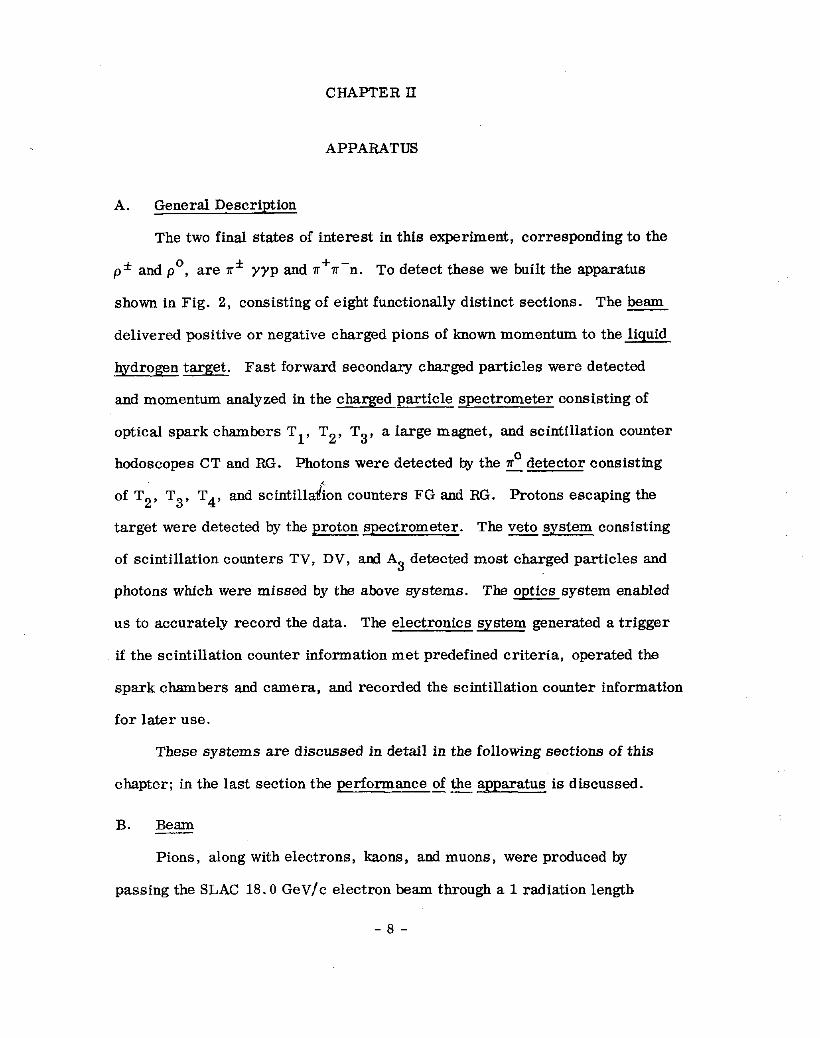
The two final states of interest in this experiment, corresponding to the
p* and p”, are r* yyp and r’r-n. To detect these we built the apparatus
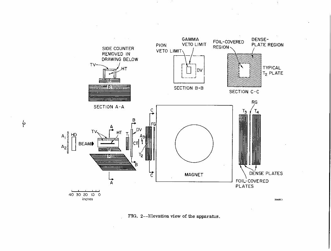
shown in Fig. 2, consisting of eight functionally distinct sections. The beam
delivered positive or negative charged pions of known momentum to the liquid
hydrogen target. Fast forward secondary charged particles were detected
and momentum analyzed in the charged particle spectrometer consisting of
optical spark chambers T1, T2, T3, a large magnet, and scintillation counter
hodoscopes CT and RG. Photons were detected by the no detector consisting - 4
of T2, T3, T4, and scintilla&on counters FG and RG. Protons escaping the
target were detected by the proton spectrometer. The veto system consisting
of scintillation counters TV, DV, and A3 detected most charged particles and
photons which were missed by the above systems. The optics system enabled
us to accurately record the data. The electronics system generated a trigger
if the scintillation counter information met predefined criteria, operated the
spark chambers and camera, and recorded the scintillation counter information
for later use.
These systems are discussed in detail in the following sections of this
chapter; in the last section the performance of the apparatus is discussed. --
B. Beam
Pions, along with electrons, kaons, and muons, were produced by
passing the SLAC 18.0 GeV/c electron beam through a 1 radiation length
-8-
SIDE COUNTER REMOVED IN DRAWING BELOW
TV HT
GAMMA PION VETO LIMIT
VETO LIMIT\ /
SECTION B-B
FOIL-COVERED DENSE-
REGION PLATE REGION \ /
TYPICAL T2 PLATE
SECTION C-C
SECTION A-A
s7
A, HD
A2 lo
(I-::.
MAGNET
A
40 inches
SE PLATES
FOlLkOVERED PLATES
FIG. 2--Elevation view of the apparatus.
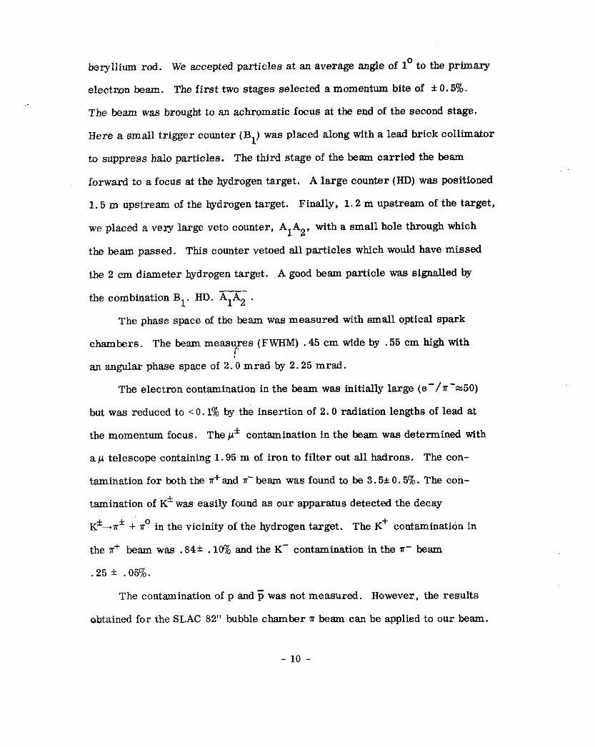
beryllium rod. We accepted particles at an average angle of lo to the primary
electron beam. The first two stages selected a momentum bite of f 0.5%.
The beam was brought to an achromatic focus at the end of the second stage.
Here a small trigger counter (BL) was placed along with a lead brick collimator
to suppress halo particles. The third stage of the beam carried the beam
forward to a focus at the hydrogen target. A large counter (HD) was positioned
1.5 m upstream of the hydrogen target. Finally, 1.2 m upstream of the target,
we placed a very large veto counter, A1A2, with a small hole through which
the beam passed. This counter vetoed all particles which would have missed
the 2 cm diameter hydrogen target. A good beam particle was signalled by
the combination BL. HD. A1A2 .
The phase space of the beam was measured with small optical spark
chambers. The beam measu f
es (FWHM) .45 cm wide by .55 cm high with
an angular phase space of 2.0 mrad by 2.25 mrad.
The electron contamination in the beam was initially large (e-/r-=50)
but was reduced to ~0.1% by the insertion of 2.0 radiation lengths of lead at
the momentum focus. The p’ contamination in the beam was determined with
a ~1 telescope containing 1.95 m of iron to filter out all hadrons. The con-
tamination for both the ?ieand ?r- beam was found to be 3.5* 0.5%. The con-
tamination of K* was easily found as our apparatus detected the decay
K*-+?T* + or’ in the vicinity of the hydrogen target. The K+ contamination in
the n+ beam was .84* .lO?t~ and the K- contamination in the ?r- beam
.25* .05%.
The contamination of p and 5 was not measured. However, the results
obtained for the SLAC 82” bubble chamber ?r beam can be applied to our beam.
- 10 -
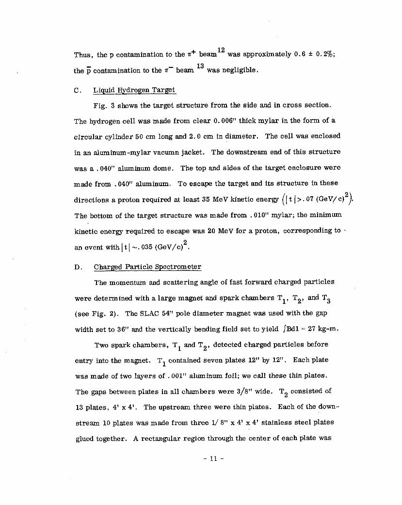
Thus, the p contamination to the or+ beam l2 was approximately 0.6 f 0.2%;
the 5 contamination to the ?r- beam l3 was negligible.
C. Liquid Hydrogen Target
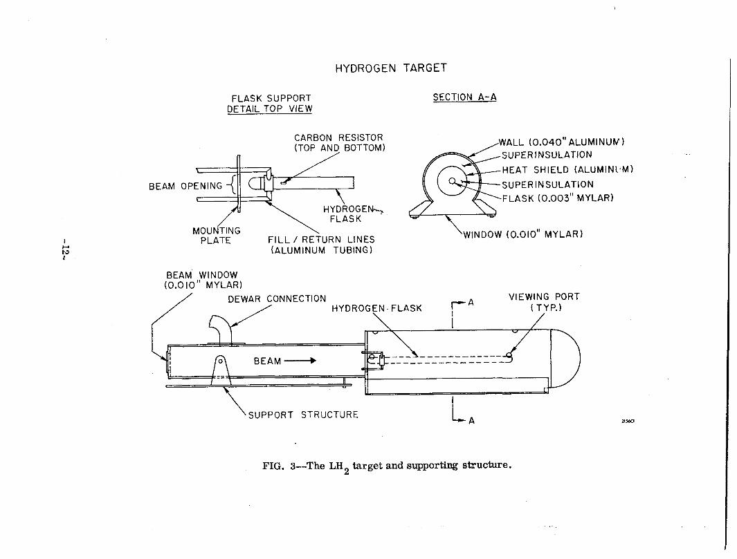
Fig. 3 shows the target structure from the side and in cross section.
The hydrogen cell was made from clear 0.006” thick mylar in the form of a
circular cylinder 50 cm long and 2.0 cm in diameter. The cell was enclosed
in an aluminum-mylar vacumn jacket. The downstream end of this structure
was a .040” aluminum dome. The top and sides of the target enclosure were
made from .040” aluminum. To escape the target and its structure in these
directions a proton required at least 35 MeV kinetic energy ([ t I> .07 (GeV/ c)2).
The bottom of the target structure was made from . 010” mylar; the minimum
kinetic energy required to escape was 20 MeV for a proton, corresponding to .
an event with 1 t I-. 035 (GeV/c)2.
D. Charged Particle Spectrometer
The momentum and scattering angle of fast forward charged particles
were determined with a large magnet and spark chambers T1, T2, and T3
(see Fig. 2). The SLAC 54” pole diameter magnet was used with the gap
width set to 36” and the vertically bending field set to yield fE%dl = 2’7 kg-m.
Two spark chambers, T1 and T2, detected charged particles before
entry into the magnet. T1 contained seven plates 12” by 12”. Each plate
was made of two layers of . 001” aluminum foil; we call these thin plates.
The gaps between plates in all chambers were 3/8” wide. T2 consisted of
13 plates, 4’ x 4’. The upstream three were thin plates. Each of the down-
stream 10 plates was made from three l/ 8” x 4’ x 4’ stainless steel plates
glued together. A rectangular region through the center of each plate was
- 11 -
HYDROGEN TARGET
FLASK SUPPORT DETAIL TOP VIEW
CARBON RESISTOR (TOP AND BOTTOM)
MOUtiTlNG \ PLATE FILL / RETURN LINES
(ALUMINUM TuBiNGI
SECTION A-A
WALL (0.040” ALUMINUN) SUPERINSULATION
HEAT SHIELD (ALUMIN1.M)
SUPERINSULATION FLASK (0.003” MYLAR)
WINDOW (0.010” MYLAR)
BEAM WINDOW (0.0 IO” MYLAR)
DEWAR CONNECTION VIEWING PORT HYDROGEN. FLASK 1 TYP.)
SUPPORT STRUCTURE
FIG. %-The LH2 target and supporting structure.
cut out, then both sides covered with . 001” aluminum foil. Thus, the central
region of these plates formed a thin plate chamber while the outer region
formed a thick plate chamber. These rectangular holes varied smoothly in
size from 9.5” wide by 1’7.4” high for the upstream plate to 10.9” by 19.9”
for the downstream plate. Mylar patches were used to deaden T1 and T2
to beam particles. This technique was moderately successful.
Charged particles exiting the magnet were detected in the first seven
plates of T3 which were 4’ x 6’ thin plates. Mylar patches deadened these
plates to the beam.
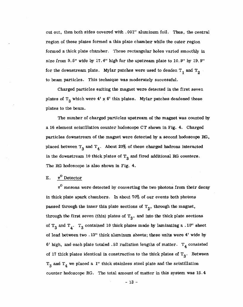
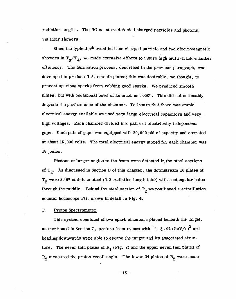
The number of charged particles upstream of the magnet was counted by
a 16 element scintillation counter hodoscope CT shown in Fig. 4. Charged
particles downstream of the magnet were detected by a second hodoscope RG,
placed between T3 and T4. About ~O$J of these charged hadrons interacted
in the downstream 10 thick plates of T3 and fired additional RG counters.
The RG hodoscope is also shown in Fig. 4.
E. 8’ Detector
r” mesons were detected by converting the two photons from their decay
in thick plate spark chambers. In about 70% of our events both photons
passed through the inner thin plate sections of T2, through the magnet,
through the first seven (thin) plates of T3, and into the thick plate sections
of T3 and T4. T3 contained 10 thick plates made by laminating a . 10” sheet
of lead between two .13” thick aluminum sheets; these units were 4’ wide by
6’ high, and each plate totaled .52 radiation lengths of matter. T4 consisted
of 17 thick plates identical in construction to the thick plates of T3. Between
T3 and T4 we placed a 1” thick stainless steel plate and the scintillation
counter hodoscope RG. The total amount of matter in this system was 15.4
- 13 -
(a) CT HODOSCOPE (b) RGT HODOSCOPE (cl FGT HODOSCOPE
TO 56AVP PHOTOTUBES
l/8” NE102 SCINITILLATOR
b ! TO 56AvP PHOTOTUBES
I_ 49’--
TO 56AVP PHOTOTUBES -- /“lf
\BEAM HOLE /I
FIG. 4--Trigger counter hodoscopes.
radiation lengths. The RG counters detected charged particles and photons,
via their showers.
Since the typical p* event had one charged particle and two electromagnetic
showers in T3/T4, we made extensive efforts to insure high multi-track chamber
efficiency. The lamination process, described in the previous paragraph, was
developed to produce flat, smooth plates; this was desirable, we thought, to
prevent spurious sparks from robbing good sparks. We produced smooth
plates, but with occasional bows of as much as ‘. 050”. This did not noticeably
degrade the performance of the chamber. To insure that there was ample
electrical energy available we used very large electrical capacitors and very
high voltages. Each chamber divided into pairs of electrically independent
gaps. Each pair of gaps was equipped with 20,000 pfd of capacity and operated
at about 15,000 volts. The total electrical energy stored for each chamber was
18 joules.
Photons at larger angles to the beam were detected in the steel sections
of T2. As discussed in Section D of this chapter, the downstream 10 plates of
T2 were 3/8” stainless steel (5.3 radiation length total) with rectangular holes
through the middle. Behind the steel section of T2 we positioned a scintillation
counter hodoscope FG, shown in detail in Fig. 4.
F. Proton Spectrometer
This system consisted of two spark chambers placed beneath the target;
as mentioned in Section C, protons from events with [ t 12 .04 (GeV/c)2 and
heading downwards were able to escape the target and its associated struc-
ture. The seven thin plates of RI (Fig. 2) and the upper seven’thin plates of
R2 measured the proton recoil angle. The lower 24 plates of R2 were made
- 15 -

of aluminum sheet enclosed on both sides with aluminum foil. This could, in
principle, provide a measure of the proton’s momentum through its range; in
this experiment only the proton angle measurement was used.
G. Veto Counters
As mentioned in Chapter I an extensive veto system was of crucial im-
portance to suppress contaminations. Surrounding the hydrogen target on the
three sides not covered by the proton spectrometer were placed four-layer
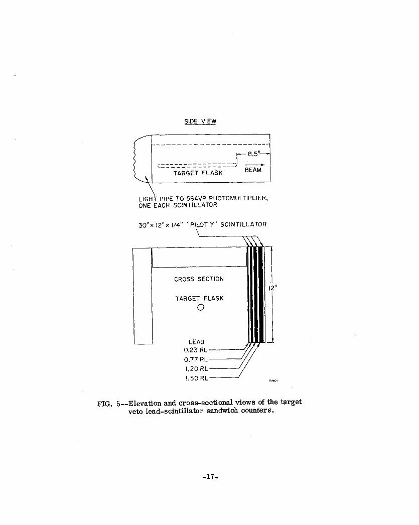
lead-scintillator sandwich counters (TV in Fig. 2). These units are shown
in detail in Fig. 5. Between the target and the inner TV counter we placed
0.050” of lead in addition to the .16” of aluminum in the TV and target
structure to suppress accidental vetoes from knock-on electrons coming
from the hydrogen target. Approximately 37 MeV of kinetic energy was re-
quired for a proton to reach &id fire a TV. Thus, events with It 1 2 .07
(GeV/e)2 were either vetoed or seen in the proton spectrometer.
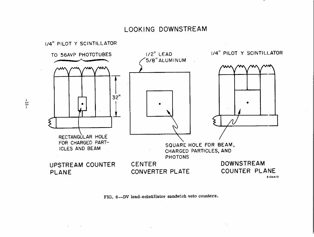
Downstream of the target we placed a second veto system named the
DV. This consisted of two layers of scintillator separated by lead and
aluminum, totalling 2.4 radiation lengths. This unit is shown in detail in
Fig. 6. An inner rectangular hole about 7” by 10” allowed charged particles
to pass through while a larger hole in the le ad-aluminum layer and in the
downstream counter plane allowed photons to proceed to the thick plate of
T3/T4 and to the thick plate sections of T2.
Finally, we placed a small counter (A3 in Fig. 2) in the beam 1.0 meter
downstream of the hydrogen target. A good p* or po event had no count in
A3*
- 16 -
SIDE VIEW
r__-___- ____ ------, \__-__---__-_--- TARGET FLASK BEAM
LlGHi PIPE TO 56AVP PHOTOMOLTIPLIER, ONE EACH SCINTILLATOR
30” x 12” x l/4” “PILOT Y” SCINTILLATOR
\
pi 12” I I CROSS SECTION
I
I I TARGET FLASK 0 I
LEAD - 0.23 RL
0.77 RL
1.20 RL
1.50 RL 2llKI
FIG. S--Elevation and cross-sectional views of the target veto lead-scintillator sandwich counters.
-17-
LOOKING DOWNSTREAM
l/4” PILOT Y SCINTILLATOR
TO 56AVP PHOTOTUBES
RECTANGGLAR HOLE FOR CHARGED PART- ICLES AND BEAM
l/2” LEAD 5/B” ALUM I NUM
l/4” PILOT Y SCINTILLATOR
. I
SQUARi HOLE FOR BEAM, CHARGED PARTICLES, AND PHOTONS
UPSTREAM COUNTER PLANE
CENTER DOWNSTREAM CONVERTER PLATE COUNTER PLANE
JlJ4AlO
FIG. 6--DV lead-scintillator sandwich veto counters.
H. optics
The spark chambers were viewed directly by a 70 mm csmera positioned
70’ from the magnet and with a demagnification of 75. To obtain the third
(depth) dimension each chamber was equipped with a stereo mirror view.
Fiducial marks (zenon flash tubes) were placed at the four corners of
the magnet and were flashed for every picture. They were measured for
every frame and defined the origin, tilt angle of the film in the camera, and
magnification. Numerous other flashing fiducials were spread about but
never used in the data analysis. In addition, each chamber was equipped with
so-called dc Elducials which were turned on at the beginning of each roll for
a few frames. These fiducials supplied a check of the mirror constants; no
changes in the mirror orientation from the survey values were found except
for a slight displacement of the T1 mirror.
Pictures of straight through beam tracks allowed a check of any syste-
matic shift of a chamber mirror; a small ( x 1 mm) shift in the T1 origin was
found and corrected.
I. Electronics System
The electronics system served many functions: The number of beam
particles incident on the target was counted; an event trigger was generated
when the scintillation counter information matched a preset “trigger” pattern;
and data was sent to the data box to be recorded on film and to an on-line
PDP-8 for diagnostic use.
As discussed in Section B of this chapter, a good beam particle was de-
fined by the combination BI.HD* (AlA+; that is, a count from the Bl and HD
counters in coincidence and no count from the hole-veto counter A1A2.
- 19 -
The information from the CT hodoscope (see Section D) was used to de-
termine the multiplicity of charged particles upstream of the magnet. The
technique used is illustrated in the logical diagram of Fig. 7. The signals
from the 16 CT counters were sent to discriminators producing standardized
-0.7 volt 12 nsec wide pulses. All the CT pulses were combined in an OR
circuit and the resultant pulse, clipped to 7 nsec width by a discriminator,
was used to select the interior 7 nsec of the 12 nsec CT pulses; this technique
eliminated time jitter differences between CT counters.
The strobed pulses were then added in linear mixers; the height of the
output pulse was directly proportional to the number of counters firing. A
window discriminator selected signals with pulse height in a given range.
For p* runs we used CT = 1 and for p” runs CT = 2.
The RG and FG counter-mformation was treated in a similar fashion to
the CT. The multiplicity was determined with the same design circuit. For
our p* data, we required (RG + FG) L 2 and RG 1 1, and for the p” data,
RG 2 2, FG = 0.
The veto information from the TV, DV, and A3 counters was combined
with OR circuits. A master coincidence was finally formed with all the
above information input. For the p* we required a beam particle upstream
of the magnet, one and only one count from the CT (i.e., one r*), at least
one count from the RG counter (i.e. , at least one x* downstream of the magnet),
and at least one additional count from the RG or from the FG hodoscopes (at
least one photon), and no veto firing. Symbolically, our trigger is written
as (B1* HD. (A1A2) ) . (CT = 1) .(RG>l)*(RG+FG> 2).(TV+DV+AS).
- 20 -

.
.
. CT16 -
CT1
JSTROBE
CLIPS TO 7nsec PULSE
FIG. T--CT fast multiplicity counting circuit.
-21-
For the p” we required two charged particles upstream and two charged
narticles downstream of the magnet and no particl& in the thick plate section
of T2. Symbolically this reads (B1.HD.AT2) . (CT = 2) . (RG 1 2).
(TV+DV+AS+FG).
Once the trigger condition was met, a signal was sent to trigger the
spark chambers, Also, the state of all of the counters was recorded via a
latch system. This information was sent to the data box and to an on-line
PDP-8. A counter that had fired was indicated on the data box - and on film -
by a neon light. The roll and frame number was also displayed on the data
box both with nixie tubes and with neon lights in BCD code.
We monitored accidental vetoes by forming B . Tdel where B is the beam
signal and Tdel means the veto signal out of time (delayed). This loss averaged
around 8% and was correctedfor roll by roll.
J. Performance of the Apparatus
All counters were checked on cosmic rays before installation. The
efficiency was invariably high. We use loons’% as the trigger counter efficiency.
No anomalous effects in the data associated with an inefficient trigger counter
were found.
The veto counters were also highly efficient on cosmic rays. In the
experiment they were in regions populated by many low energy particles; thus
it is not clear what to give for an efficiency. Inefficiencies in those counters
will only result in more background pictures.
- 22 -
The spark chamber efficiency is a complicated function as it may depend
on many variables. On single charged tracks the chambers are known to
be z 100% efficient. To gain information about the chamber performance in
the actual experimental condition we studied, for charged tracks, the distri-
bution of the number of sparks measured per track. Chamber inefficiency
losses occur when a track has too few sparks to be measured. For T2, T3,
R1, and R2, the requirement was three or more to be measured; for T2 we
only required two or more. Ry this method we found our apparatus efficiency
+o to detect a charged track was 100 _ l%.
The previous technique is not a useful way to determine the photon de-
tection efficiency, for the dominant problem is one of finding the photons on a
scan. We have no way, in this experiment, of calibrating absolutely the chamber
photon detection efficiency. However, by studying the decays of the K” mesons
in the beam we are able to determine the relative chamber, scanning, and
measuring efficiency as a function of photon energy. This will be discussed in
the next chapter. To summarize, we find no change in the T3/T4 chamber
efficiencies over the photon energy range 200 MeVl Ey 5 13 GeV. As the
chamber detection efficiency should be very high for E Y = 13 GeV (showers
here typically have 1 20 sparks) we will assume the chamber detection effi-
ciency to detect both photons is lOOJ$%.
- 23 -
CHAPTER HI
DATA REDUCTION AND EVENT SELECTION
A. Introduction
Our data consists of 66 rolls (3400 pictures/roll) of p* target full, nine
p’ target empty, 65 p- target full, 10 o- target empty, 6 l/2 Q” target full,
and one p” target empty roll. We also have some 8.0 GeV/c data but have
not been able to analyze it because of poor beam quality and high backgrounds.
All the rolls were scanned and candidates for events sent to the meas-
uring table; here the event was rescanned and, if still a potential good event,
measured. Next, the real space positions of tracks were reconstructed from
the film measurements. Our data contains four known types of events: elas-
tic events, K* decay events, p* events, and p” events. Methods to identify
each type of event were devel&ed. In the o’ case, this included a special
scan of all the events to determine the relative photon energy; as explained
in Chapter I, this was needed to resolve the r” ambiguity. The final results
+ 0 of this process were three sets of events, p , p , and o-. Finally, the effi-
ciency of this process, and of each substep, to find good events was deter-
mined.
B. scanning
The film was first scanned by the SLAC Hummingbird flying spot digi-
tizer which decoded the data box; the trigger counter information and the
roll and frame number were obtained. Next, scanners of the SLAC CDA
group examined the film; briefly they recorded the following information:
1. NRN
For the p’ data the number of rear neutrals in T3/T4 was recorded.
- 24 -
A rear neutral was defined as a shower-like track beginning in the thick
plate regions of T3 or in the first or second gap of T4 which pointed in a
general way toward the target in both the direct and stereo views.
2. NRPI
For p* and p” data, thesmber of rear p&ns (charged tracks) was
recorded. A rear pion consisted of three or more sparks laying on a straight
line in the thin plates of T3 which pointed generally toward the target in the
stereo view (the magnet bends vertically) and made an angle to the nominal
beam line (i.e., to the horizontal) of not more than 45O.
3. NFPI
The Eumber offrontpions was recorded. A front pion was defined
as a track in both T1 (two or more sparks) and in T2 (three or more sparks
with at least one in the first three gaps) which formed a straight line in the
direct view pointing toward the hydrogen target.
4. NFN
For the pf data, thenumber offront_neutrals was recorded. The
scanners were requested to look for a front neutral only if a FG trigger
counter had fired; as discussed later this was a mistake. A front neutral
was a shower-like track appearing in the thick plate section of T2 (i.e., not
in the first three gaps) which pointed in the general direction of the target
in both direct and stereo views.
5. NPRO
The_number of proton tracks in R1 and R2 was recorded. While
fairly broad classifications were used, we included in later analysis only
those tracks appearing in both Rl and R2 pointing toward the target in the
direct view.
- 25 -

The efficiency of the scan will be discussed at the end of this chapter.
c. Measuring
Potential events were sent to the measure table. The scan was veri-
fied by the measurer and the event measured on the SLAC NRI system.
For the of data, we normally chose as p candidates, events with two,
and only two, neutrals (NRN + NFN = 2) and with at least one charged part-
icle in TI, T2, and T3; this is in the spirit of the optical veto as discussed
in Chapter I. However, we measured events with two or more neutrals for
about 15 rolls of data. By selecting K* events in this sample (a 3-C fit) we
were able to determine the event loss (accidental veto rate) when restricting
ourselves to two neutral events; this will be discussed in detail in the next
chapter.
For the p” data, we measured all events with two or more charged
particles both upstream and downstream of the magnet. By using the CT
counter information we were able to throw out, with excellent ( -10 nsec)
time resolution, accidental tracks.
The measurers were asked to measure all the visible sparks on charged
tracks, in both direct and stereo views, and three points, including the initial
spark, along a neutral track (by using the first spark measurement we veri-
fied the neutral track did indeed start in the thick plate section of T2 or T3/T4).
The four main fiducials were also measured.
D. Geometrical Reconstruction
The measurement data and data box information were sent to the com-
puter program LOCUS which performed the following tasks:
1. The fiducial measurements established the relation between the
real space and film coordinates. Using the known mirror positions the
- 26 -
real space three dimensional coordinates were reconstructed from the NRI
measurements of tracks.
2. Tracks in T1 and T2 were matched together by fitting straight lines
simultaneously in direct and stereo views. The x2 distribution from these
fits indicated a measuring and reconstruction accuracy per spark of 0.75 mm
in real space.
3. The CT counter information was used to discard TlT2 tracks not
passing through an active counter.
4. Remaining TlT2 tracks were extrapolated through the magnet in
the stereo view (the magnet bends in the vertical) and matched with T3
charged tracks. The direct view information was then used to determine the
track’s momentum. The momentum resolution of our system for a track with
momentum P is (FWRM) d P/P = 4% x P/(15.0 GeV/c). This number has
been checked on 3.0 and 15.0 GeV/c beam tracks.
E. Selection of Elastic Events
The presence of elastic events in our p’ data is seen as a sharp peak
around 15.0 GeV/c in the f momentum spectra. We remove elastic events
by applying the r* momentum cut of 14.1 GeV/c; this removes no p’ events.
The presence of elastics may seem a bit strange as our trigger requires two
or more counters downstream of the magnet and we require two neutral tracks
to be seen on the scan. Elastically scattered pions frequently fire two RG I
counters by interacting in the thick plates of T3; and accidental tracks
and/or products from the thick plate interactions are occasionally perceived
as neutrals.
F. Selection of K* Events
Our beam contained a small K* meson component. Our apparatus
- 27 -
accepted with high efficiency the K* decays in the region of the hydrogen
target. We have about 2000 K’ decays and 800 K- decays. These K events
have many uses, as we shall find, and must also be removed as a contamina-
tion to our pk events. We identify K events by the following procedure: the
beam and charged pion four-momentum are known, hence we can reconstruct
the missing mass which should be that of a TO. Actually, we do a least-
squares fitting procedure assuming the missing particle is a no (a 1-C fit).
Potential K’s are selected by a x2 cut. The no must be coplanar with
the observed two photon plane: we make a coplanarity cut. Next we recon-
struct the energies of the two photons. This process is straightforward
and rather similar to the methods used to select p* events when the recoil
proton is seen.
Fairly broad cuts are made when rejecting K emnts from our p data. h
When selecting K events for kagnostic purposes we use tighter cuts and,
usually, restrict the decay region to the target area.
G. Selection of p” Events
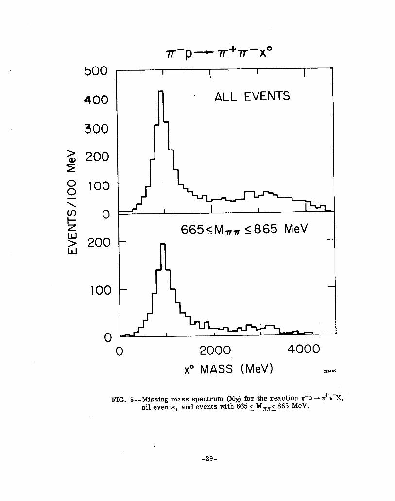
Our p” trigger selects events r-p + 7r+r-X”. We measure the beam r-
and the final state n+ and ?r- four-momentum and consequently can determine
the four-momentum of the X0 system. The X0 mass distribution is shown in
Fig. 8a. The neutron peak is seen strongly with a long high mass tail with
no clear structure. In particular no sign of the AO(1238) nucleon resonance is
seen; however, the mass resolution is inadequate to rule out the presence of a
A0 signal completely. We have tried to enhance any A0 signal by selecting
events with a rcn- mass in the p band 665 5 mnT ( 865 MeV. Figure 8b shows
this distribution. Again there is no A” seen.
Our Monte Carlo simulations indicate that the neutron mass distribution
- 28 -
500
400
300
200
100
0
200
100
0
I I I I
ALL EVENTS
665<,M,, 5865 MeV
0 2000
x0 MASS (MeV) aYAP
FIG. 8--Missing mass spectrum (Md for the reaction r-p - ~+lr%, all events, and events with 665 2 M,,c 865 MeV.
-29-
should be symmetric. We have used the low mass side of the neutron peak
to subtract off the high mass side of the peak; again no A0 signal is seen.
Finally we have restricted our data to symmetric lr’r- decays where our
missfng mass resolution is sharpest and find no A0 signal. We estimate
our A0 contamination to the p” data to be 5 * 5%.
This result is reasonable even though the p”Ao cross section is larger
than the pan cross section. 14 Even at t N tmfn the A0 appears with about
50 MeV kinetic energy added to the Q value for the decay of about 160 MeV.
‘The decay state is 2/3 lr’n and l/3 r-p; our veto system is sensitive to both
of these. Thus, we would expect to veto (and evidently do) A0 events with
high efficiency.
Next we select Y?T- events with the X0 mass cut. The X0 mass reso-
lution is a function of the x+x- decay; for symmetric decays we choose events
with the X0 mass within 300 MeV of the nominal neutron mass while for
asymmetric decays we take events within 600 MeV of the neutron. These
points correspond to a three standard deviation cut.
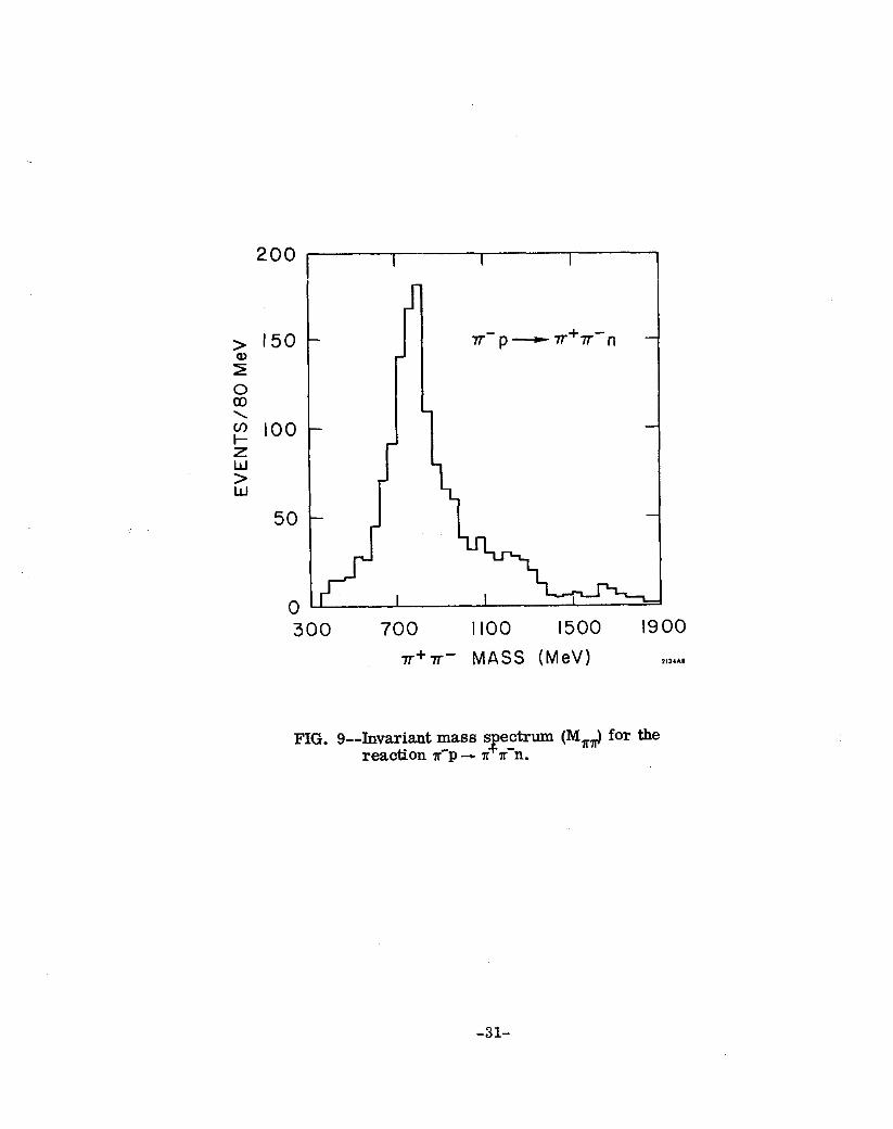
The p” meson is clearly seen in the r’n-n mass distribution (Fig. 9).
We select p” events in the range 665 5 m,r 5 865 MeV; 817 events in the
region O-5 Itl 5 1.0 (GeV/c)2 were found.
H. Selection of High-t pi Events
The high-t p* region is defined by ItI 2.08 (GeV/c)2. In this region
the recoil proton from good r* p -. r*r”p events must be visible in RI and
R2 or have been detected in the TV veto counters. Events with protons
were kinematically analyzed with a program which shall be referred to as
PROE. PROE selected visible proton events fitting the above reaction in
the following way:
- 30 -
200
150
100
50
0 300 700 II00 1500 1900
TT+TT- MASS (MeV) ,114..
FIG. 9--Invariant mass spectrum (MT,,.) for the reaction r-p-+ B r-n.
-31-
1. Only two neutral events were considered; the loss of good events
due .to accidental picture vetos will be determined in the next
chapter.
2. There must be one and only one x* track passing through a firing
or trigger counter.
3. There must be at least one recoil track.
4. All tracks must pass the fiducial cuts (See Section G).
5. K’ and elastic events are rejected (Sections F and G).
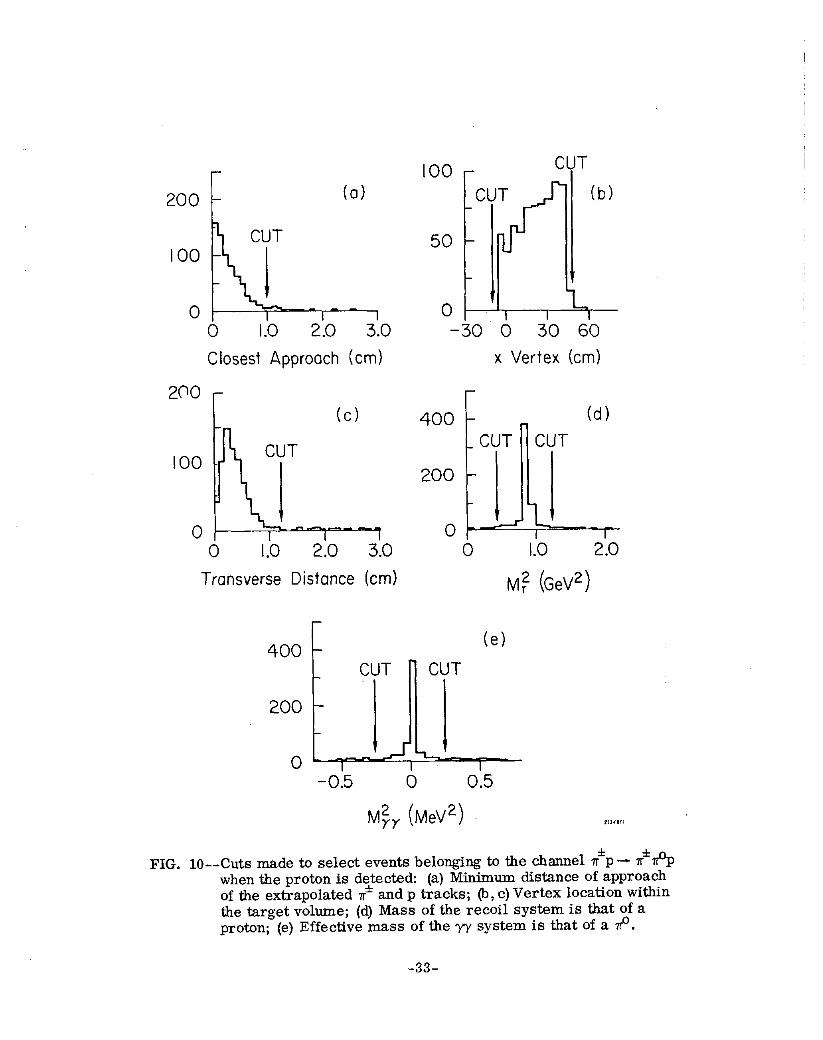
6. The distance of closest approach between the x* and p is computed;
Fig, 10a shows this distribution and our good vertex cut.
7. The interaction vertex must fall within the hydrogen target volume.
Fig. 10b shows the vertex distribution along the beam and the tar-
get cut. Fig. 1Oc shows the transverse distance distribution and
cut.
8. Four-momentum conservation is used to complte the recoil and
each photon’s momenta. The invariant photon-photon mass squared
2 “YY ’
is calculated and a x0 mass cut made; Fig. 10e shows this.
The recoil mass squared, mr2, is also calculated and a proton mass
cut made as shown in Fig. 10d.
All high-t events must pass PROE. J.n addition we eliminated from our
fmal sample events with one neutral in T3 and one neutral in T2. This was
because of our belated realization that the low energy photons typical in T2
did not necessarily fire the FG counters; our T2 neutral scan was conditioned
on a FG firing. Once we had decided not to use this data, we rejected all
events with a FG firing. This, of course, will cause a slight accidental loss
of good events which we shall determine in the next chapter.
- 32 -
(a)
100
0
200
100
0
6 I.0 2.0
Closest Approach
3.0
(cm)
0 1.0
Transverse Distance (cm)
r 400
200
0
100
50
0
CUT
CUT (b)
r:i -30 0 30 60
x Vertex (cm)
r 400
200
(d)
CUT
Mf (GeV*)
(e)
MFr (MeV*)
FIG. lo--Cuts made to select events belonging to the channel asp - 1~*8p when the proton is detected: (a) Minimum distance of approach of the extrapolated f and p tracks; (b, c) Vertex location within the target volume; (d) Mass of the recoil system is that of a proton; (e) Effective mass of the r/ system is that of a 8).
-33-
Our final sample contained 146 15.0 GeV/c pf high-t events and 144 15.0
GeV/c +I hign-t events.
I. Selection of Low-t pi Events
The low-t region is defined by ItI5 0.08 (Gev/~)~. For Itl 5 0.03 (Gev/~)~
no protons are seen while for 0.03 2 Itl~O.08 (GeV/c)2 about 20% of the events
will have protons. We are not able to separate the proton and no-proton region
because of limited azimuthal angle resolution in this region; if there is a
proton seen we use PROE, described in Section H, to select events. If no
proton is seen we use a second program, NOPROE, to select events. However,
before NOPROE cau be used we must concern ourselves with the .r” ambiguity
present when the proton is not observed.
In order for NOPROE to determine the unmeasured variables when the
proton is not seen it must assume the recoil system is a proton and the two
photons come from the decay of a x0; and it must know how to match the part-
icles in the hypothesis with the tracks observed in the experiment. Additional
information must be supplied to tell it which gamma goes with which neutral
track. Depending on the assignment made, it can obtain two kinematically
different solutions; in 45% of the cases one or the other solution can be rejected
because it has ItI > 0.08 (GeV/c)2 which is not allowed since we have seen no recoil
track. In the other 55% we determine which photon has the higher energy
and so resolve the ambiguity.
All two neutral events were returned to the scan table. Three methods
of relative energy determination were investigated: the number of sparks
in each shower was counted; the length of each shower was measured (and if
it went out the back of the chamber); a subjective estimate based on shower
opening angle and spark brightness was made. All methods yielded similar
- 34 -
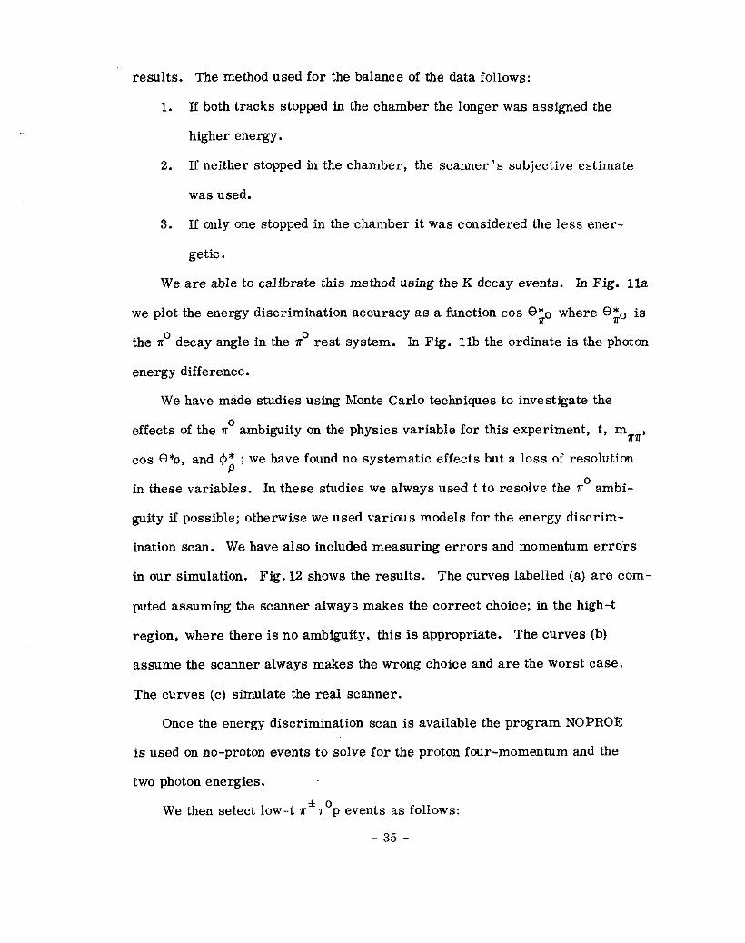
results. The method used for the balance of the data follows:
1. If both tracks stopped in the chamber the longer was assigned the
higher energy.
2. If neither stopped in the chamber, the scanner’s subjective estimate
was used.
3. If only one stopped in the chamber it was considered the less ener-
getic.
We are able to calibrate this method using the K decay events. III Fig. lla
we plot the energy discrimination accuracy as a function cos 02 where @go is
the r” decay angle in the r” rest system. In Fig. llb the ordinate is the photon
energy difference.
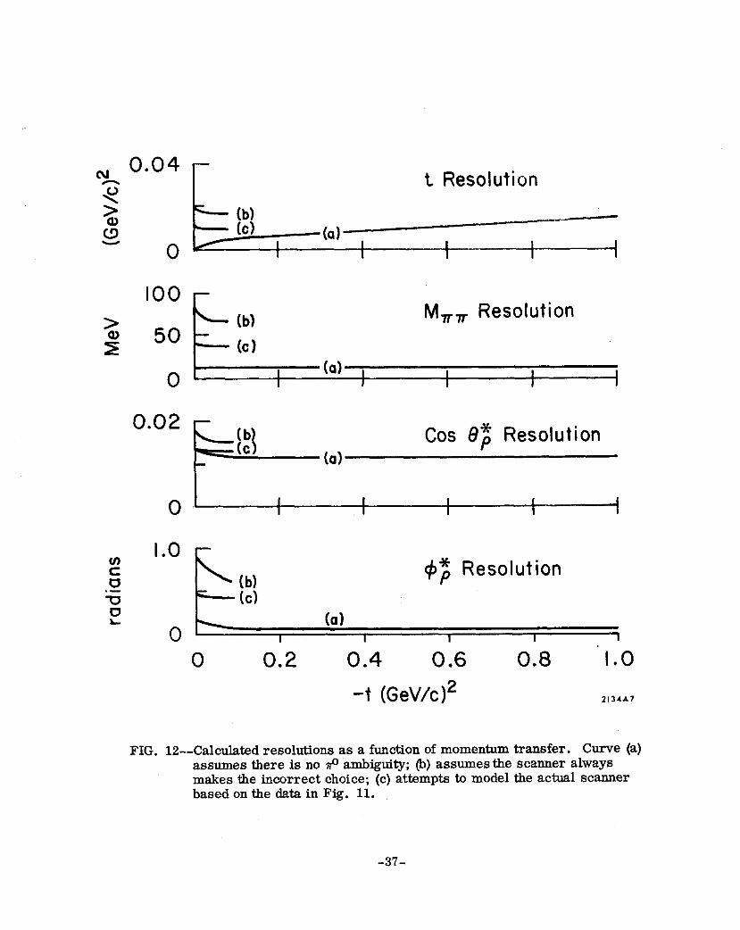
We have made studies using Monte Carlo techniques to investigate the
effects of the x0 ambiguity on the physics variable for this experiment, t, mrv,
cos 0% and $ , . we have found no systematic effects but a loss of resolution
in these variables. In these studies we always used t to resolve the v” ambi-
guity if possible; otherwise we used various models for the energy discrim-
ination scan. We have also included measuring errors and momentum errors
in our simulation. Fig. I.2 shows the results. The curves labelled (a) are com-
puted assuming the scanner always makes the correct choice; in the high-t
region, where there is no ambiguity, this is appropriate. The curves (b)
assume the scanner always makes the wrong choice and are the worst case.
The curves (c) simulate the real scanner.
Once the energy discrimination scan is available the program NOPROE
is used on no-proton events to solve for the proton four-momentum and the
two photon energies.
We then select low-t r*x*Op events as follows:
- 35 -

100
80
60
40
20
0
80
60
40
20
0 I I I I I I I I I
0 0.5 1.0
I cos e$ol
I I I I I I I I I I I I I I
_ (b) +++++-i++ +
-++ .i
t
-
I I I I I I I I I I I I I I
0 5 IO
FYI-EY*I (GM .1”
FIG. 11--The ability of scanners to correctly select from two y-ray showers the one with more energy as a function of: (a) The #’ rest frame decay angle; (b) The reconstructed energy difference between two photons.
-36-
cu 0.04 -
F t Resolution
2 - (b)
52 - (c)
0- (al __c_- I
I P--t---i
100 -
2 L (b) M TT Resolution
ZE 5o f- (c)
0 - I (a) , I I I I I
0.02
(a) Cos 8; Resolution
0 .I
z 1.0 -
0 \tbl $$ Resolution
.- u - (c) i?
0- (a)
I I I I I 0 0.2 0.4 0.6 0.8 ‘1.0
-t (GeV/c)* 2134h7
FIG. 12--Calculated resolutions as a function of momentum transfer. Curve (a) assumes there is no ff ambiguity; @) assumes the scanner always makes the incorrect choice; (c) attempts to model the actual scanner based on the data in Fig. 11.
-37-
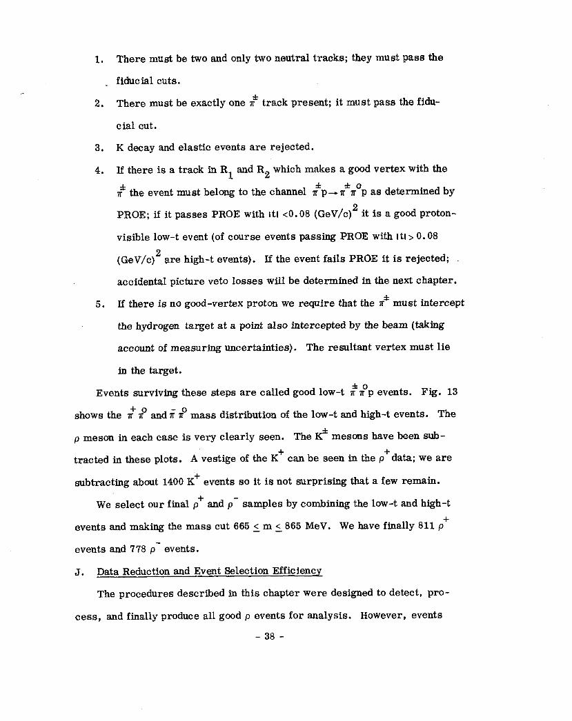
1. There must be two and only two neutral tracks; they must pass the
_ fiduckl cuts.
2. There must be exactly one I? track present; it must pass the fidu-
cial cut.
3. K decay and elastic events are rejected.
4. If there is a track in RI and R2 which makes a good vertex with the
lr” the event must belong to the channel Ifp+ fn’p as determined by
PROE; if it passes PROE with Itl ~0.08 (GeV/c)2 it is a good proton-
visible low-t event (of course events passing PROE with I tl> 0.08
(GeV/c)2 are high-t events). If the event fails PROE it is rejected;
accidental picture veto losses will be determined in the next chapter.
5. If there is no good-vertex proton we require that the r* must intercept
the hydrogen target at a point also intercepted by the beam (taking
account of measuring uncertainties). The resultant vertex must lie
in the target.
Events surviving these steps are called good low-t $$p events. Fig. 13
shows the I? n” and ?r no mass distribution of the low-t and high-t events. The
p meson in each case is very clearly seen. The J? mesons have been sub-
tracted in these plots. A vestige of the K’ can be seen in the p+data; we are
subtracting about 1400 K’ events so it is not surprising that a few remain.
We select our final p” and p- samples by combining the low-t and high-t
events and making the mass cut 665 5 m 5 865 MeV. We have finally 811 p”
events and 778 p- events.
J. Data Reduction and Event Selection Efficiency
The procedures described in this chapter were designed to detect, pro-
cess, and finally produce all good p events for analysis. However, events
- 38 -

180 Ill1 1 Ill I 11 11 II I l 11
160
80
15p+
80
40
0 500 1000 1500 2000
mr Mass (MeV) 2156N
FIG. 13--The z-*r” and ?rp invariant mass distribution for the reaction Il’tp- I&+$.
-39-
were occasionally lost, either in the scanning and measuring step or by
subsequent failure to pass the various cuts.
We considered several ways to deal with this problem. We could have
put all our film through the process again and again until all events were
found, but this approach was considered impractical. Instead we chose to
reprocess a sample of the data and, by comparison with the initial pass, at-
tempt to understand our efficiency function. We sent through the data ,anal-
ysis system for the second time eight rolls of p”, eight rolls of p-, and
one half each of two different rolls of p”.
It is important to understand any correlations between the data analysis
process efficiency and the physics variable of the experiment; we may, for
example, expect a loss for p* events when cos 8 - 1 for this corresponds P
to low energy photons which may be more difficult for the scanner to detect.
Or, we may expect a loss of events in the high-t region because a visible
proton must be measured.
Let PI denote the original pass and P2 the extra pass. Let the data be
.th divided into Nk kinematical regions such that within the 1 region there
is a uniform efficiency ei per pass to detect an event; for example, we may
divide the data into low-t and high-t regions and further subdivide the data
by photon energy. Within each region we must make the statistical as-
sumption that each event has an equal chance of being detected by the data
analysis process.
Let Nibe the number of events in the i th region detected on PI and
g2 the number detected on the second pass, and Ni2 the number detected
on both passes. The best estimate of the efficiency from this data is
- 40 -
with statistical error
The co data was analyzed in this way. No systematic biases were
found and we obtained the efficiency for the data analysis step of
EDA +- = .77*.05 lrr
We have divided cur p* data into low-t and high-t regions and into low
photon energy and high photon energy regions. We have also looked for
inefficiencies associated with proximity of the spark chamber tracks to
the beam areas which were deadened with mylar patches which sometimes
flared. The only effect discovered is a low-t /high-t difference. We thus
give our results in terms of a data analysis efficiency to detect a x and two
photons, E DA DA KY-Y’
and an efficiency to detect a proton, E P *
We find, com-
bining the $ and p- data, which within statistics are identical, that
EDA EYY = .73*.02
DA eP
= .84* .05
We have determined the loss rate within each substep of the data anal-
ysis procedure and find, for the low-t data:
1. Scanning: =.12% of the good events are lost here.
2. Measuring: ~4% of the good events are lost here.
- 41-
3. Geometrical reconstruction: ~6% lost here; this step catches most
measurer errors.
4. Event selection: ~4% lost here; this step is sensitive to measurer
accuracy.
Finally, we emphasize these efficiencies are for the data analysis step
only and do not include apparatus inefficiencies. We have argued in the
last chapter that the apparatus efficiency to detect charged particles is
high, consistent with 100%. We have just concluded that the data analysis
efficiency is uniform in the photon energy. By using the I? decay events
we can investigate’ the combined apparatus and data analysis detection
efficiency . We have simulated K’ events, including the apparatus accept-
ance assuming 100% photon acceptance in T3/T4; these events have been
binned according to the energy of the softer photon. The data has also been
binned and a ratio of the data to prediction formed. Fig. 14 shows the result.
The normalization is arbitrary, but no loss in efficiency is seen for low
photon energy.
- 42 -
3.0 - -- -r--- --T---~l-- -1
2.0 -
1.0 + pt+t+ ttt
tt
t
O- I I II ++t++
0 1.0 2.0 3.0 4.0 5.0 6.0 7.0
ET (GeV) IWAI2
FIG. 14--Ratio of expected to observed number of photons for K* -. lflr’ events as a function of the photon energy; the overall normali- zation is arbitrary.
-43-
CHAPTER IV
EXTRACTION OF p CROSS SECTIONS AND DENSITY MATRICES
A. Introduction
In this chapter the extraction of the cross sections and density matrix
elements from our raw p+, pot and p- data is discussed. Using a maximum
likelihood method we fit for dN/dt, the unnormalized cross section, and
P mm’ ’ the density matrix elements, taking into account the acceptance of
the apparatus. dN/dt is corrected for known losses. Non-p xx backgrounds
are subtracted. Estimates of contaminations from other channels are made
and appropriate subtractions performed. The p cross sections and density
matrix elements are presented and the systematic errors are estimated.
B. Extraction of dN/dt and p&l
Our raw data consists of events selected by methods described in the
previous chapter and with the cut 665 I Ma.,r I 865 MeV. lf the apparatus
detection efficiency is perfect, dN/dt is extracted by counting the number
of events in a t bin, and pm, 1 by studying the xx rest frame angular dis-
tribution. However, when the detection efficiency is finite and a function
of the physics variables of the experiment, the problem is more difficult
and, in the extreme case of zero detection efficiency in some regions
(generally the case in practical experiments), one must make assumptions
about the underlying angular distributions to proceed at all.
We assume only P = 0 and 1= 1 partial waves are present in the xx
angular distributions. This provides a completely adequate description
of our data; a high statistics 15.0 GeV/c p” experiment has also fa.md this
to be true15. We also assume parity conservation which in any xx rest
- 44 -
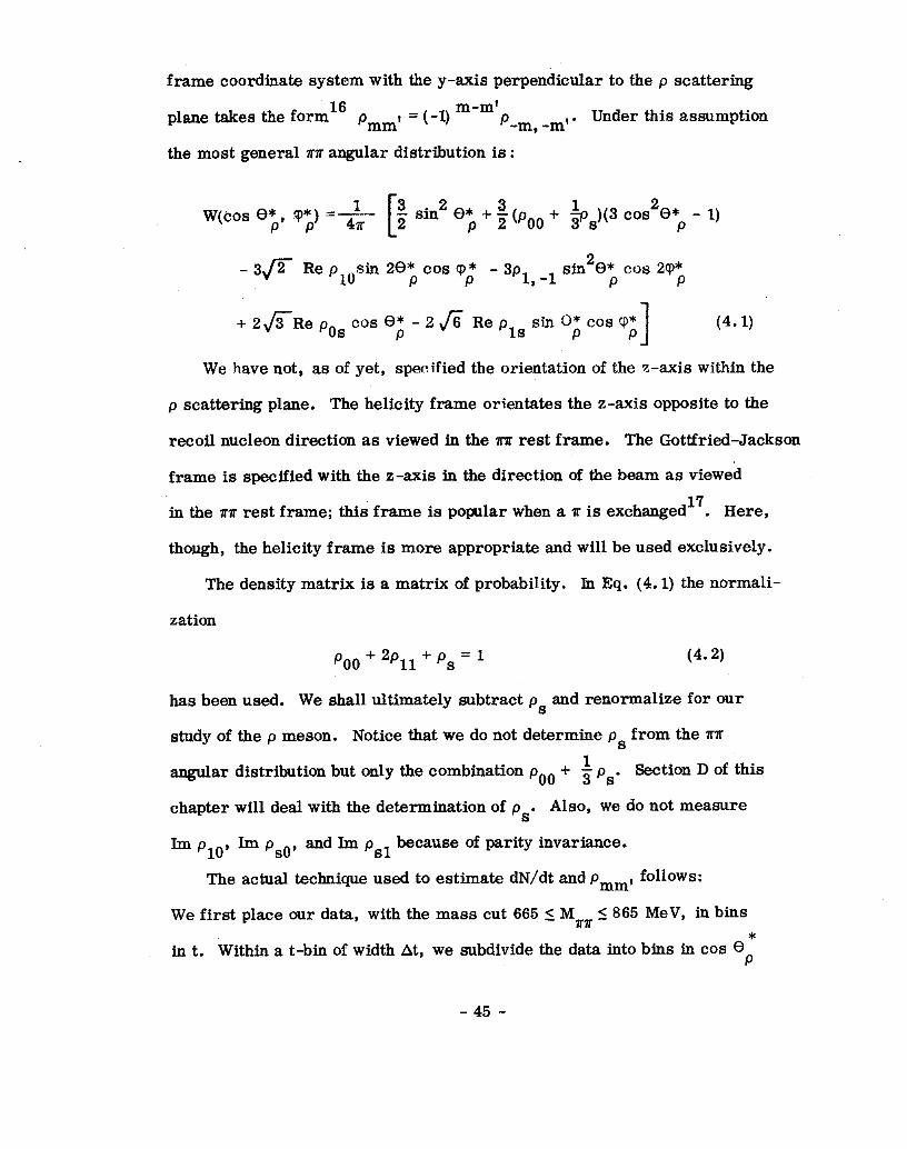
frame coordinate system with the y-axis perpendicular to the p scattering
plane takes the form 16 pmmt = (-1) m-m’p-m, -m,. Under this assumption
the most general ~TP angular distribution is :
W(bOS e* p, v;) =~i- E
i sin’ G*p + $(poo + $Js)(3 cos2e*p - 1)
- 3c Re pLOsin 20; cos q; - 3p1, -1 sin2e; COY 29;
+ 26Re pas COB e* - 2 fi Re pls sin 0; cos cp* P P 1
We have not, as of yet, specified the orientation of the z-axis within the
p scattering plane. The helicity frame orientates the z-axis opposite to the
recoil nucleon direction as viewed in the n-x rest frame. The Gottfried-Jackson
frame is specified with the z-axis in the direction of the beam as viewed
in the xx rest frame; this frame is popular when a x is exchanged 17 . Here,
though, the helicity frame is more appropriate and will be used exclusively.
The density matrix is a matrix of probability. In Eq. (4.1) the normali-
zation
PO0 + 2Pll + P, = 1 (4.2)
has been used. We shall ultimately subtract p, and renormalize for our
study of the p meson. Notice that we do not determine p, from the xx
angular distribution but only the combination poo + 5 p,. Section D of this
chapter will deal with the determination of p,. Also, we do not measure
h plos h-n psos and b psl because of parity invariance.
The actual technique used to estimate dN/dt and pm,, fdows:
We first place our data, with the mass cut 665 s Mxx I865 MeV, in bins
in t. Within a t-bin of width At, we subdivide the data into bins in cos G * P
- 45 -
.th and cp* such that nij is the number of observed events in the 1 P cos 5 and
cp* bin. P . We now make a prediction sij for this bin. Let D(MxJ represent a
Breit-Wigner ,mass distribution and e(t, Mxx, cos Gz, (PIT) the apparatus
detection efficiency. Then
$ = ij
x jth W-s e;‘dQ;T W(cos “;: ,m;l4t, MrT, cos “2; $1 Bill
1 865
665 D@5rP%7r
We then minimize -f!n L with respect to dN/dt and pm,, where the like-
lihood function is defined as
Rt llij .J$
L=*+Le ij .
ij n..! 4
The errors in dN/dt andSpmm, are defined as the increment necessary to
increase -&nL by 0.5 while maintaining a minimum in all other variables.
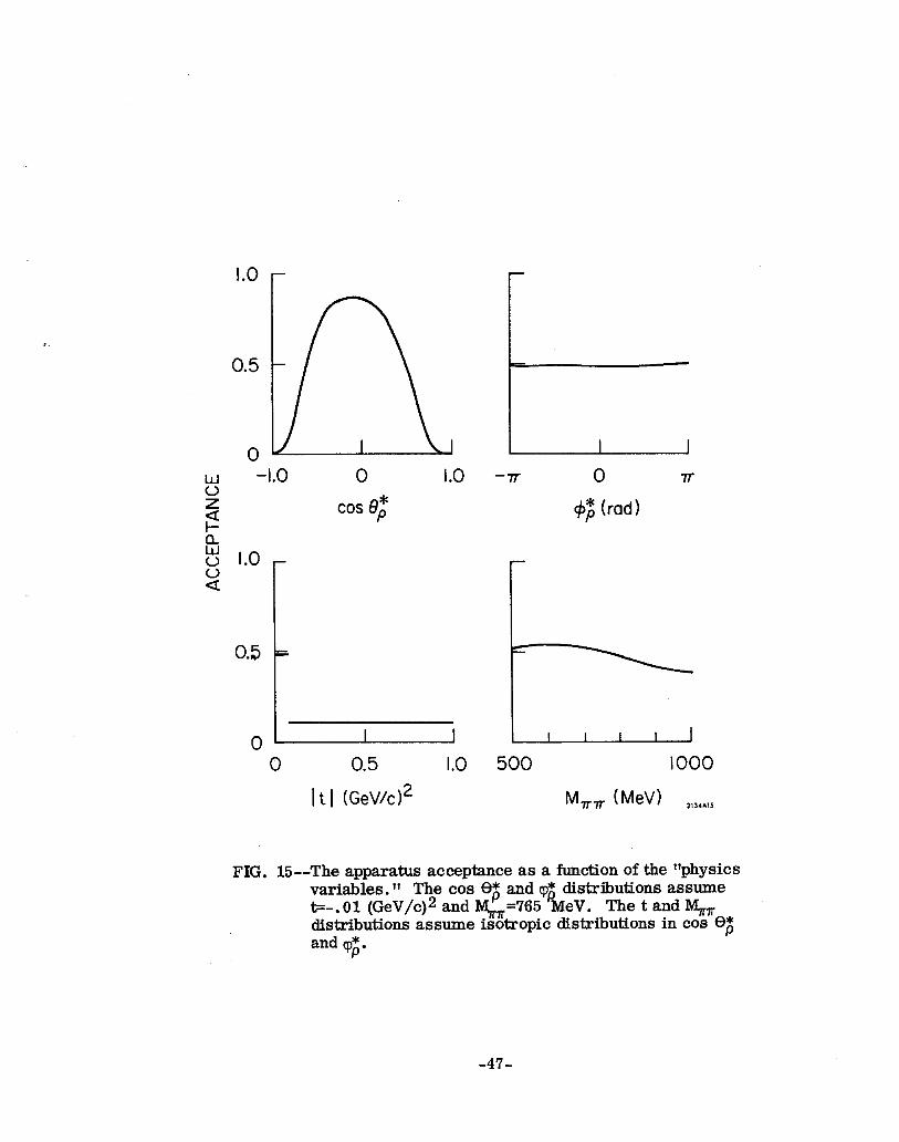
The acceptance function E(t, Mxx , cos G* , cp* ) has been calculated P P
with a Monte Carlo program which determines if a specified event is de-
tected by the apparatus and then integrates over the interaction vertex
location, the production azimuthal angle, and the IT” decay. We show in
Fig. 15a and Fig 15b the calculated p* acceptance as a function of cos G* P
and 9; with Mxx = 765 MeV and t = -. 01 (GeV/c)2. Also, we show in Fig.
15~ and Fig. 15d the dependence of E on t and Mxx assuming an isotropic
1 decay distribution (poo + 3 p, = 3. The most significant feature is the
decreasing acceptance as cos G; -&l. This limit corresponds to asymmet-
ric p decays; the low acceptance results from high energy n’ mesons being
- 46 -
0 0.5 1.0 500 1000
1 t 1 (GeVk12 M TT ( MeV) llllAjl
FIG. 15--The apparatus acceptance as a function of the “physics variables. 1t The cos ES; and r$ distributions assume t=-. 01 (GeV/c)z and IV&=765 MeV. The t and %, distributions assume isotropic distributions in COB
and q$. e$
-47-
lost in the deadened beam areas of the spark chambers, low energy x* mesons being
swept out by the magnet, and photons from a low energy x0 missing the
chambers.
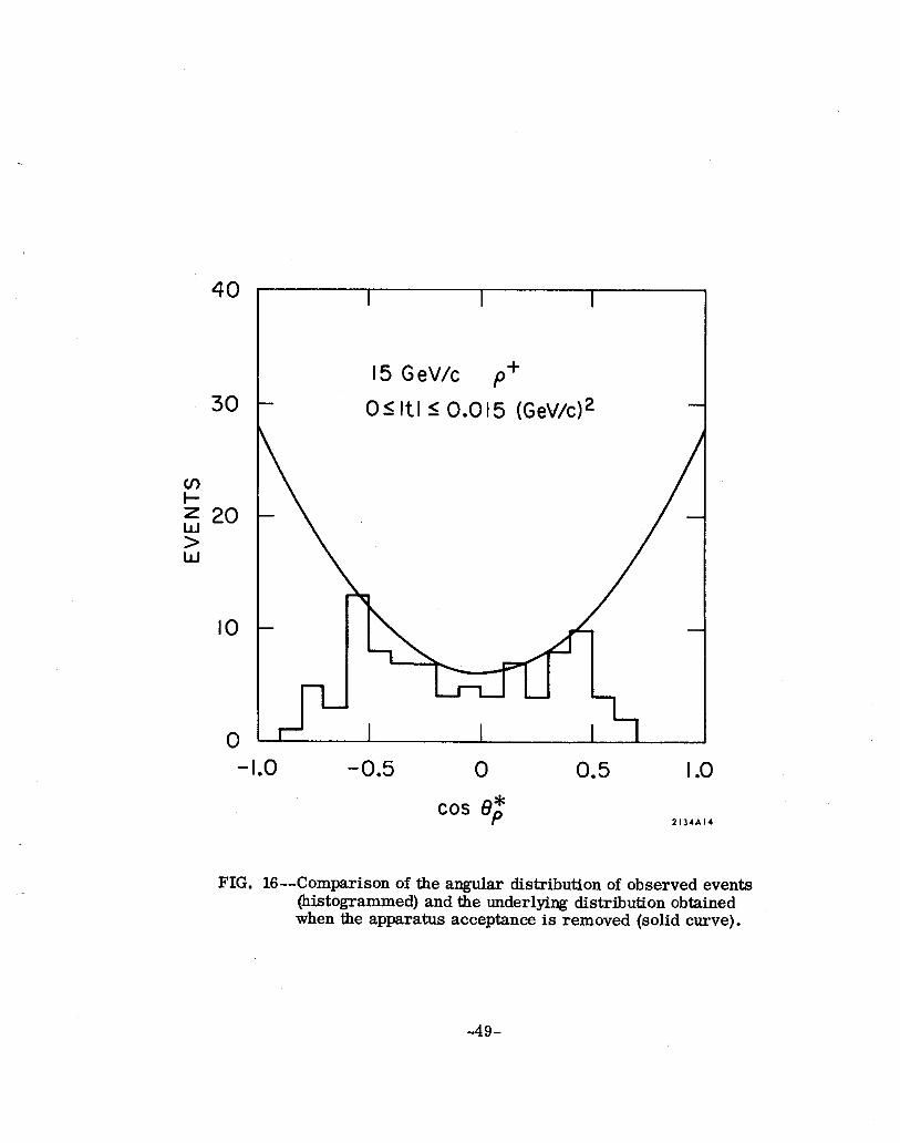
In Fig. 16 the modification of an underlying angular distribution by our
acceptance function is illustrated for low-t p+ data. The curve is the under-
lying distribution; the observed events are histogramed.
C. Correction for Experimental Event Losses
In this section all known possible sources of event losses are tabulated.
1. Events Vetoed by Knock-on Electrons.
Here we are concerned only with the case of a knock-on electron
from a charged particle associated with the event in question firing a veto.
Purely accidental vetoes, no matter what the source, are dealt with in item
(3). Moving perpendicular to the beam line a knock-on electron had to pene-
trate 1 cm of hydrogen (on the average), .15” of aluminum, .05” of lead,
and exceed the counter threshold to fire a TV. Of course, higher energy
knock-ens do not move perpendicular to the beam line and so must penetrate
a correspondingly greater thickness. Quantitatively we calculate a negli-
gible probability for such a veto.
2. Neutron Vetoes
This applies to p” events and refers to vetoes in the TV counters
from the recoil neutron. We have estimated this correction in a simpIe way.
but, because of our lack of knowledge of counter thresholds, can not deter-
mine it accurately. Table 1 shows the results and the estimated systematic
errors.
- 48 -
40
30
if = 20 > W
IO
0
I I
I5 GeV/c p+
OS Itl IO.015 (GeV/c)*
-1.0
FIG. 16--Comparison of the anguIar distribution of observed events (histogrammed) and the underlying distribution obtained when the apparatus acceptance is removed (solid curve).
-49-
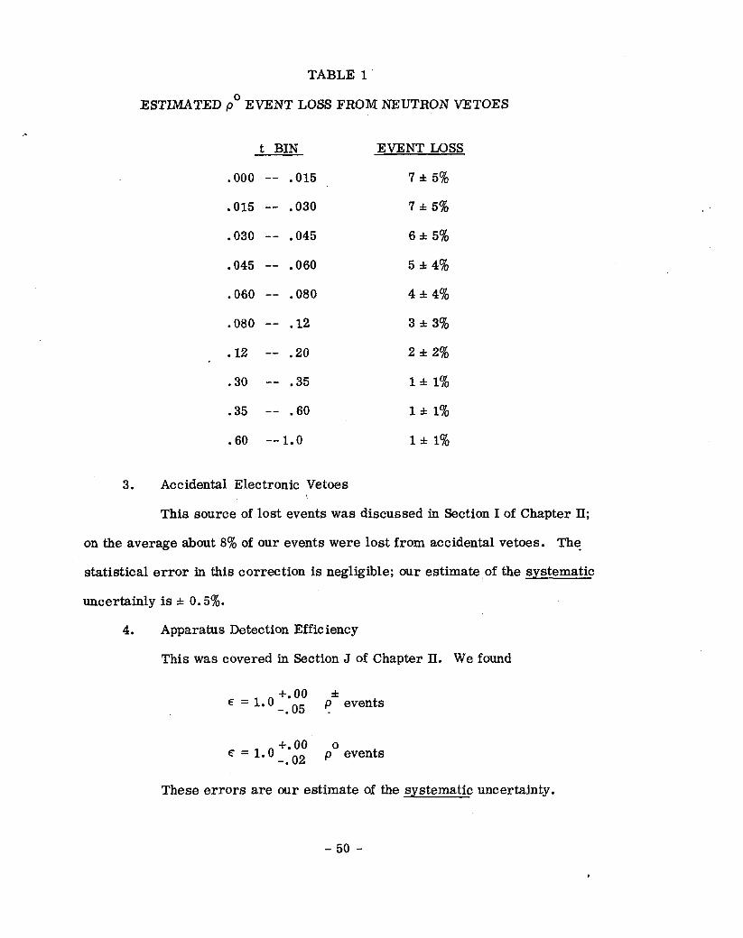
TABLE 1
ESTIMATED p” EVENT LOSS FROM NEUTRON VETOES
t BIN
.ooo -- .015
.015 -- .030
.030 -- .045
.045 -- .060
.060 -- ,080
.080 -- .12
.12 -- .20
.30 -- .35
.35 -- -60
.60 -- 1.0
EVENT LCSS
7 f 5%
7+5%
6 f 5%
5 i 4%
4 * 4%
3 j: 3%
2 f 2%
1 f 1%
1 f 1%
1 f 1%
3. Accidental Electronic Vetoes
This source of lost events was discussed in Section I of Chapter II;
on the average about 8% of our events were lost from accidental vetoes. The
statistical error in this correction is negligible; our estimate of the systematic
uncertainly is * 0.5%.
4. Apparatus Detection Efficiency
This was covered in Section J of Chapter II. We found
f. 00 E =l.O-*05 . pi events
i.00 E = 1.0-,02 p” events
These errors are our estimate of the systematic uncertainty.
- 50 -
5. Absorption of Initial and Final State Particles
Here we refer to the loss of events through secondary interactions
with various elements of the apparatus. We have studied this loss by Monte
Carlo simulations. For each t-bin we used the observed p angular distri-
bution; the path length in the hydrogen target was computed and found to be,
on the average, 25 cm for the beam particle, 14 cm for each secondary n,
and 15 cm for each photon. We also looked at the loss rate as a function of the
xx decay angles and found, when all secondary particles were included, only
a weak dependence. We thus make only an overall correction as shown in
Table 2; our estimate of the systematic uncertainty is included.
6. Loss of Events by ?r Decay
To first approximation the decay x-q + v changes only the track
momentum. As Mxx and t depend only weakly on the x* momentum, we suffer
no loss of events in the low-t p* regions. In the high-t and in the p” regions a
loss of events will occur because the recoil mass is altered sufficiently to fail
the proton or neutron cut. We have estimated this and find losses of
0 low-t p*
1* 0.5% high-t p”
1 f 0.5% PO
The estimated systematic uncertainty is shown.
7. Data Analysis Efficiency
Chapter III was entirely devoted to the data analysis process and
the last section to its efficiency. We found
‘DA = .73 f .02 low-t p*
‘DA = .61* .05 high-t p*
‘DA = .77 f .05 PO
- 51 -
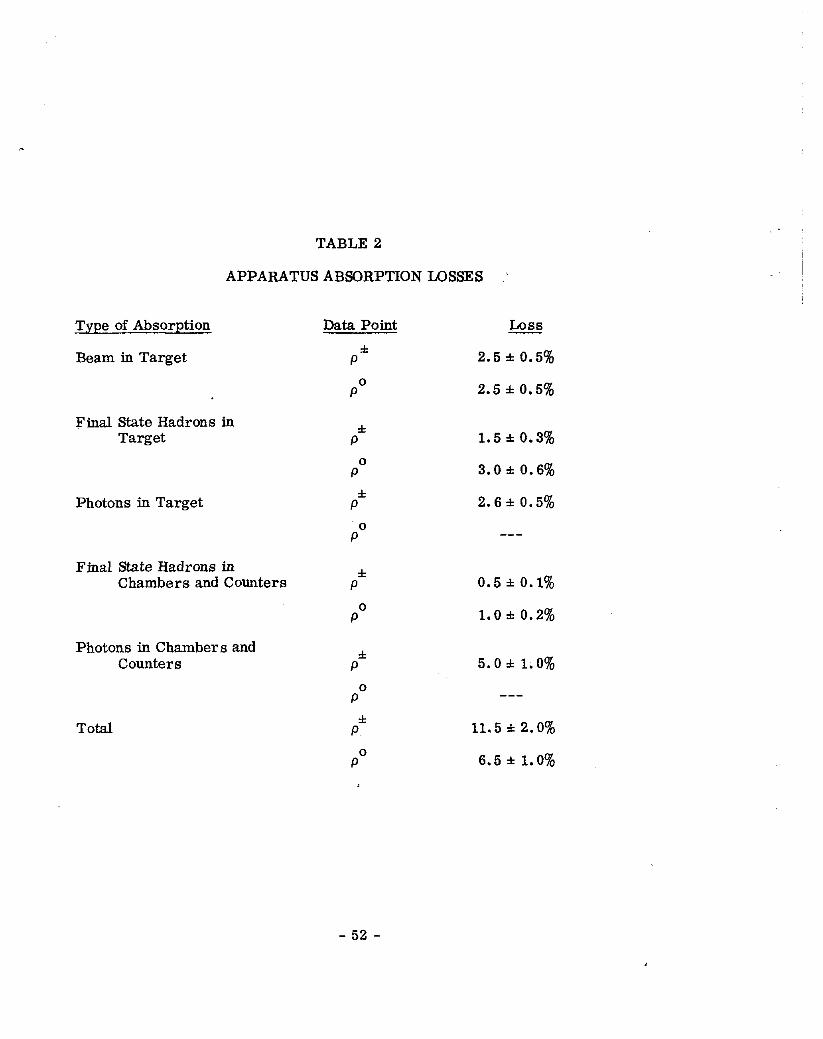
Type of Absorption
Beam in Target
Final State Hadrons in Target
Photons in Target
TABLE 2
APPARATUS ABSORPTION LOSSES
Final State Hadrons in Chambers and Counters
Photons in Chambers and Counters
Total
Data Point *
P
PO
Pi
PO
P”
PO
P*
PO
P”
PO
P”
PO
Loss
2.5iO.5%
2.5 f 0.5%
1.5* 0.3%
3.0* 0.6%
2.6iO.5%
---
0.5 f 0.1%
1.0 t 0.2%
5.0 * 1.0%
---
11.5 * 2.0%
6.5 * 1.0%
- 52 -

The errors shown here are statistical. In addition, we estimate
there is an overall systematic uncertainty of 5% in this correction.
8. Picture Veto Loss: Neutrals
We rejected p” events with more than two neutral tracks found on
the scan. Occasionally, a good event was accidentally rejected. By using
our sample of events with more than two neutrals and identifying K* mesons
we measured this loss rate to be 8% for p* events with a statistical error
of 3%. We estimate a negligible systematic error.
9. Picture Veto Loss: H
We rejected p* events with a second charged track in the R spectrom-
meter which survived the CT cut. The accidental veto rate was 1.9 i 0.50/o,
with an estimated negligible systematic error.
10. Picture Veto Loss: Recoil
We rejected p* events with a recoil track in RI and R2 which made
an acceptable vertex with the x track but did not have an acceptable pi fit. The
accidental veto loss as determined from K* decay events was 0.6 * 0.2%,
with an estimated negligible systematic error.
11. Accidental Veto Loss: FG Veto
We ultimately did not use the data with neutrals in T2. We then rejected
all events with a FG counter firing. This introduces an accidental veto rate
which was found from the K* decay events to be 1.1 f 3% with an estimated
negligible systematic error. .
12. Failure to Convert a Photon
In scanning for events we required both photons to convert before the
third gap of T4. The probability of this is 99.6% and is a neglibible correction.
D. Backgrounds and Contaminations
In this experiment we are concerned with the states pip and pan but
- 53 -
detect the states .‘r”p snd n+nn. The existence of a p* or p” in the inter-
mediate state must be inferred from the ‘IIB invariant mass and from the
~~ angular distribution. We term as backgrounds events belonging to the
channel rrN but not having a p in the intermediate state. Also our data
(particularly our low-t p*) may have contaminations from other (higher
multiplicity) channels which are misidentified as belonging to the channel
mN.
In addition to the two usual sources of information about this problem -
the ITT invariant mass and angular distributions - we have a third way of studying
the low-t p* contaminations. In the high-t region we can use the proton recoil
angle measurement to isolate a sample of high-t contamination events; this
sample can then be extrapolated into the low-t region.
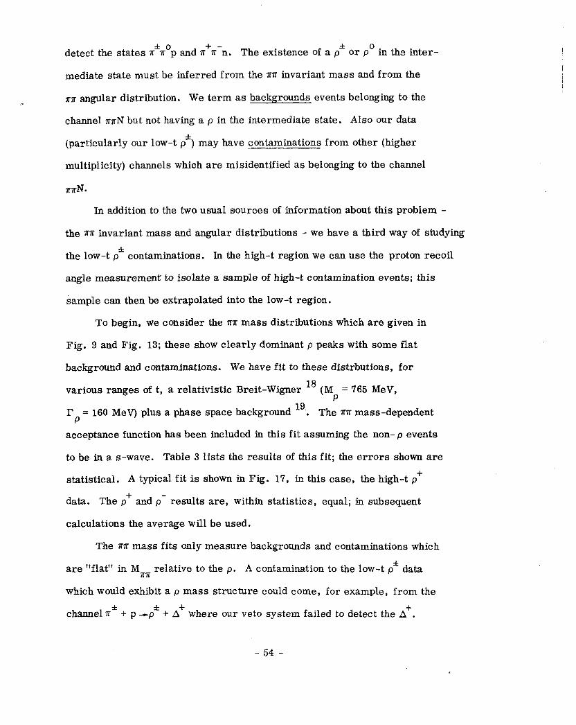
To begin, we consider the ?TP mass distributions which are given in
Fig. 9 and Fig. 13; these show clearly dominant p peaks with some flat
background and contaminations. We have fit to these distrbutions, for
various ranges of t, a relativistic Breit-Wigner l8 (Mp = 765 MeV,
rp = 160 MeV) plus a phase space background 19 . The ITK mass-dependent
acceptance function has been included in this fit assuming the non-p events
to be in a s-wave. Table 3 lists the results of this fit; the errors shown are
statistical. A typical fit is shown in Fig. 17, in this case, the high-t pf
data. The p+ and p- results are, within statistics, equal; in subsequent
calculations the average will be used.
The rn mass fits only measure backgrounds and contaminations which
are “flat” in M ~‘H relative to the p. A contamination to the low-t pf data
which would exhibit a p mass structure could come, for example, from the
channel ?r* + p -p* + A’ where our veto system failed to detect the $.
- 54 -
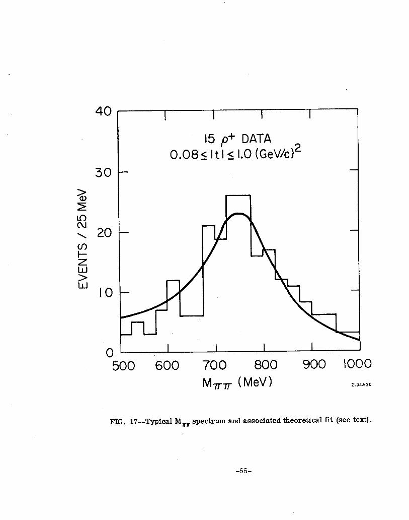
EVEN
TS /
25
MeV
0
I I
I
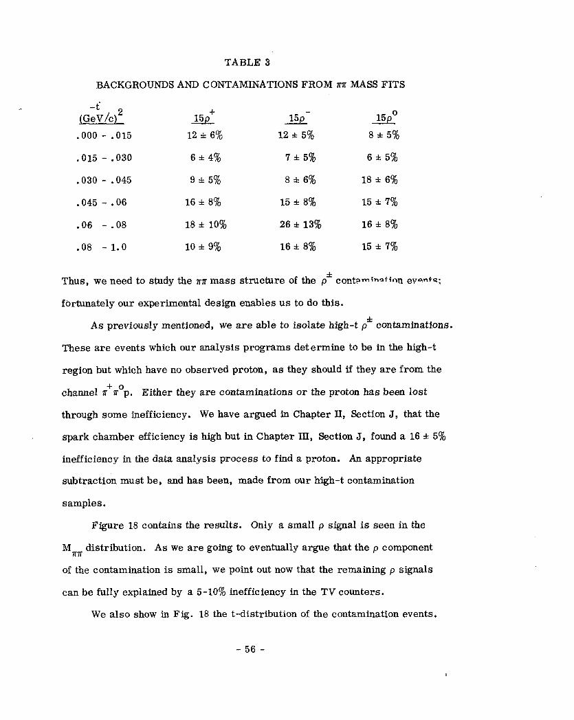
TABLE 3
BACKGROUNDS AND CONTAMINATIONS FROM n,i~ MASS FITS
.ooo - .015 12 zt 6% 12 -+ 5% 8 f 5%
.015 - .030 6 f 4% 7 f 5% 6 f 5%
.030 - .045 9 A 5% 8 rt: 6% 18 + 6%
.045 - .06 16 rt 8% 15 f 8% 15 f 7%
.06 - .08 18 32 10% 26 i 13% 16 It 8%
.08 - 1.0 10 * 9% 16 A 8% 15 * 7%
Thus, we need to study the TT mass structure of the p’ contPminn+inn evanfs;
fortunately our experimental design enables us to do this.
As previously mentioned, we are able to isolate high-t pi contaminations.
These are events which our analysis programs determine to be in the high-t
region but which have no observed proton, as they should if they are from the
channel ~r+r’p. Either they are contaminations or the proton has been lost
through some inefficiency. We have argued in Chapter II, Section J, that the
spark chamber efficiency is high but in Chapter III, Section J, found a 16 f 5%
inefficiency in the data analysis process to find a proton. An appropriate
subtraction must be, and has been, made from our high-t contamination
samples.
Figure 18 contains the results. Only a small p signal is seen in the
Mnr distribution. As we are going to eventually argue that the p component
of the contamination is small, we point out now that the remaining p signals
can be fully explained by a 5-10% inefficiency in the TV counters.
We also show in Fig. 18 the t-distribution of the contamination events.
- 56 -
15 GeV/c P+
M T,, (MeW
0 0.2 0.4 0.6 0.8 1.0
-t (GeV/c)*
15 GeV/c P-
I
_ --~-.,-'--l----~-'
1
, I 1 I I 500 700 900
M KT (MeV)
I I
Contamination Events
X From Low-t Mass Fits Z
I I I I 0 0.2 0.4 0.6 0.8 I.0
-t (GeV/c)* IlUC16
FIG. B--Mass and momentum transfer distributions of the high-t sample of contamination events. The low-t backgrounds obtained from the mass fits are also shown.
-57-
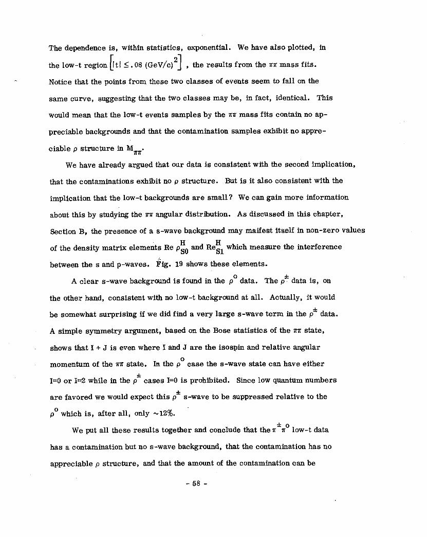
The dependence is, within statistics, exponential. We have also plotted, in
the low-t region 1 t 1 2.08 [ (GeV/c)2 1 , the results from the ?rz mass fits.
Notice that the points from these two classes of events seem to fall on the
same curve, suggesting that the two classes may be, in fact, identical. This
would mean that the low-t events samples by the rr mass fits contain no ap-
preciable backgrounds and that the contamination samples exhibit no appre-
ciable p structure in Mnn.
We have already argued that our data is consistent with the second implication,
that the contaminations exhibit no p structure. But is it also consistent with the
implication that the low-t backgrounds are small? We can gain more information
about this by studying the nr angular distribution. As discussed in this chapter,
Section B, the presence of a s-wave background may maifest itself in non-zero values H H
of the density matrix elements Re pso and ReSl which measure the interference : -
between the s and p-waves. Fig. 19 shows these elements.
A clear s-wave background is found in the p” data. The p* data is, on
the other hand, consistent with no low-t background at all. Actually, it would
be somewhat surprising if we did find a very large s-wave term in the p” data.
A simple symmetry argument, based on the Bose statistics of the 11s state,
shows that I + J is even where I and J are the isospin and relative angular
momentum of the xx state. In the p” case the s-wave state can have either
I=0 or I=2 while in the pi cases I=0 is prohibited. Since low quantum numbers
are favored we would expect this p* s-wave to be suppressed relative to the
p” which is, after all, only -12%.
We put all these results together and conclude that the s*z” low-t data
has a contamination but no s-wave background, that the contamination has no
appreciable p structure, and that the amount of the contamination can be
- 58 -
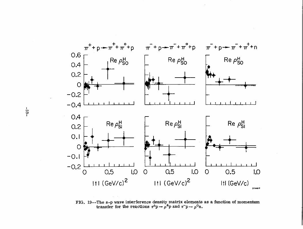
t a +
‘k a 0+ I=
0
- +
-59-
adequately determined from the x?r mass fits. In the high-t p* data a small
baokground subtraction, determined from the so mass fits, must be made.
A s-wave background subtraction, determined from ox mass fitting,
must also be made to the p" data. In addition, in Section G of Chapter II
we identified a 5 * 5% p”Ao contamination which must be subtracted.
Corrections to the density matrices for these contaminations must also
be made. In all cases, except for the p”Ao contaminations, we have assumed
the average ?rx angular distrbution to be isotropic. For the p”Ao contamination
we assumed the same angular distribution as the pan signal; this approximation
is not good for very small t (1 tl < mn2) but is adequate for our purposes.
Some caution is in order for we can not rule out the possibility of a
p-like contamination with a considerably steeper slope than that shown in
Fig. 18. This contamination would be small in the high-t region but could
be of quite significant size for low values of t. In fact, the typical particle
production cross sections tend to have slopes of 8-11 (GeV/c) -2 whereas the
slopes of the overall contamination, shown in Fig. 18, are around 5 (GeV/c) -2 .
The possible systematic error has been estimated by taking a slope of
12 (GeV/c)-2; we use the conservative figure off 15%.
E. da/dt and P,",,
To compute the cross section we must normalize the experiment. The
beam and electronics used in monitoring the beam were discussed in Chapter
II. Table 4 lists the total beam fluxes after correction for the K, p, and p
contaminations; the errors shown are purely statistical in origin.
The hydrogen target was (50.0 * 0.5) cm long and was operated at an
average pressure of 33.5 & 3 psi corresponding to a number density of
(.405 f .005) x 1023cm-3.
- 60 -
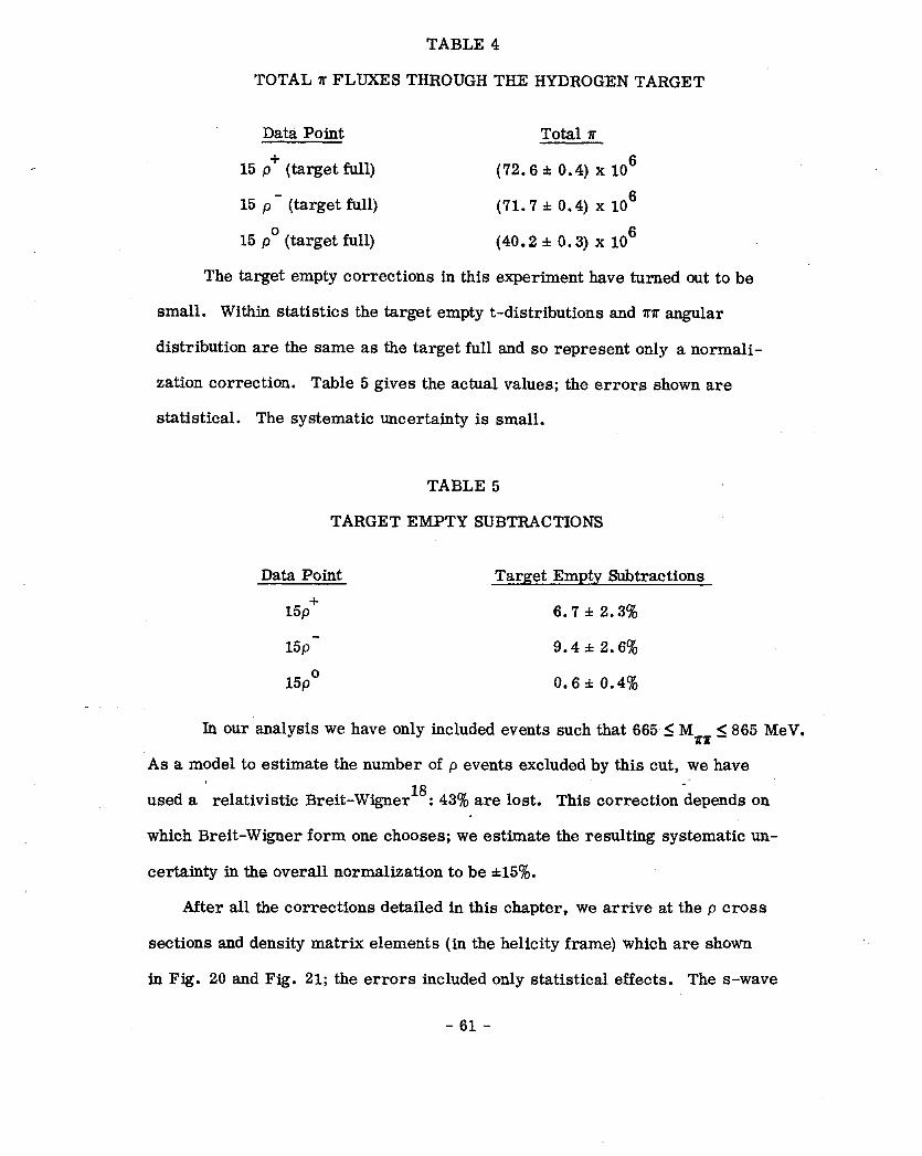
TABLE 4
TOTALnFLUXESTHROUGHTHEHYDROGENTARGET
Data Point Total z
15 p+ (target full) (72.6 t 0.4) x lo6
15 p - (target full) (71.7 f 0.4) x IO6
15 p” (target full) (40.2 f 0.3) x lo6
The target empty corrections in this experiment have turned out to be
small. Within statistics the target empty t-distributions and RH angular
distribution are the same as the target full and so represent only a normali-
zation correction. Table 5 gives the actual values; the errors shown are
statistical. The systematic uncertainty is small.
TABLE 5
TARGET EMPTY SUBTRACTIONS
Data Point Target Empty Subtractions
15p+ 6.7 it 2.3%
15p- 9.4 f 2.6%
15p” 0.6 rt 0.4%
In our analysis we have only included events such that 665, -< Mzz ,< 865 MeV.
As a model to estimate the number of p events excluded by this cut, we have 18
.- used a relativistic Breit-Wigner : 43% are lost. This correction depends on
which Breit-Wigner form one chooses; we estimate the resulting systematic un-
certainty in the overall normalization to be i15%.
After all the corrections detailed in this chapter, we arrive at the p cross
sections and density matrix elements (in the helicity frame) which are shown
in Fig. 20 and Fig. 21; the errors included only statistical effects. The s-wave
- 61 -
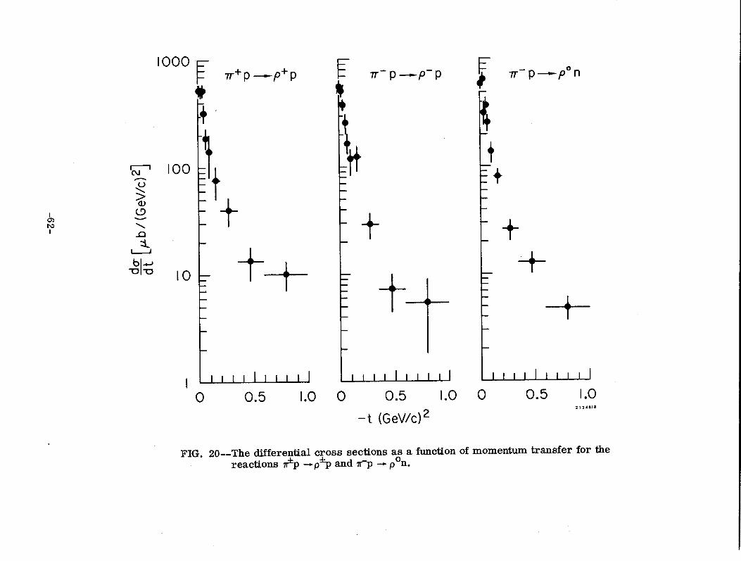
t
- 9;
c _
---" L1 "Q
I -0
a 'k t
-6
+ -
+,y-,,, ,
h-+1 m
I
IIIII I
l l
I -0
-0 n
2 I Q
N
I ';;
a i-i
'P +
+ ?Z
-Og
ILL&+ I
IIIII I
I I
-0
4 I
--9 - a
+ Q I
t
+
-Lo a
-6
+k *+
lLLL*I+-III I
' I
Illll I
l I
-0 0
- -
-62-
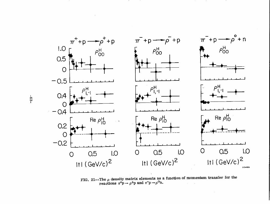
t J IL- Q
t t
J!l IT!- Q
t +
- c
0 0 2 N
-
ul 6
0 3 (5 - - t
0
- C
-
0
-63-
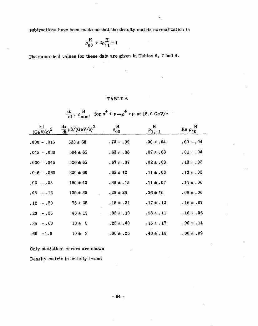
\
subtractions have been made so that the density matrix normalization is
H PO0 + 2pf1 = 1
The numerical values for these data are given in Tables 6, ‘7 and 8.
TABLE 6
du H dt’ pmmt for 7r+ + p-p+ +p at 15.0 GeV/c
ItI 2 $$ pb/(GeV/c)2 H (GeV/c) PO0 p1:-1 Re plt
.ooo - .015 533 i 65 .70 f .09 .oo f .04 .oo * .04
.015 - .030 504 i 65 .63 i .08 .07 zt .03 .01* .04
.030 - .045 526 f 65 .67* .07 .02 * .03 .13 f .03
.045 - .060 320 f 60 .65a 12 .llzt .03 .13* .03
.06 - .08 190 f 40 .38 rt .15 .ll* .07 .14i .06
.08 - .12 139 i 35 .25 +z 25 .36 & 10 .08 f .06
. 12 - .20 75 -I 25 .15* .21 .17rt .12 .16* .07
.20 - .35 40 f 12 .33 f .19 .28 zt .ll .16* .06
.35 - .60 13-+ 5 .23* .40 .15* .17 .oo * .14
.60 -1.0 lo& 3 .OO f .25 .43& .14 .oo i .09
Only statistical errors are shown
Density matrix in helicity frame
- 64 -
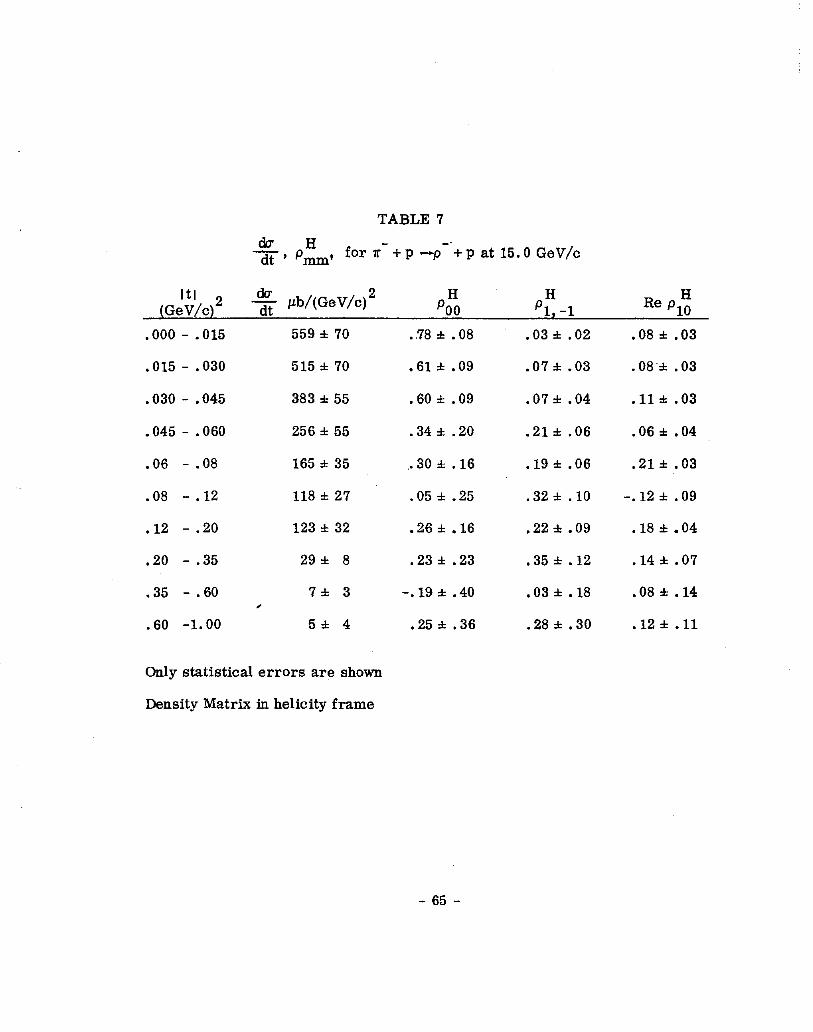
TABLE 7
dw H dt' pmmf for n-+p q--+p at15.0 GeV/c
ItI (GeV/c) 2 %- pb/(GeV/c12 H
PO0 H
p1,-1 Re plf
.ooo -.015 559h 70 ..78 f .08 .03*.02 .08 * .03
.015 -.030 515 rt 70 .61* .09 .07*.03 .08*.03
.030 - .045 383 f 55 .60& .09 .07* .04 .11*.03
.045 - .060 256* 55 .34* .20 .21k .06 .06* .04
.06 -.08 165 k 35 .30*.16 .19*.06 .21* .03
.08 -.12 118* 27 .05-+.25 .32zt .lO -.12 i.09
. 12 -.20 123 zk 32 .26&.16 .22-+.09 .18rt.O4
.20 -.35 29ck 8 .231t.23 n35k.12 .14*.07
.35 -.60 7* 3 -.19* .40 .03*.18 .08*.14 I
.60 -1.00 5* 4 .25zt.36 .28*.30 .12*.11
Only statistical errors are shown
Density Matrix iu helicity frame
- 65 -
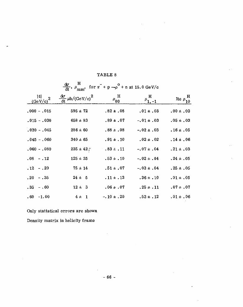
.-
TABLE 8
cb H dt’ pmmf for II- + p y” + n at 15.0 GeV/c
ItI 2 s @/(GeV/c)2 H H
(GeV/c) poo p1, -1 Re pl:
.ooo - .015 595 f 72 .82i .08 .Ol f .03 .ooct .03
.015 -.030 658 f 83 .89&.07 -.Ol f .03 .05*.03
.030 -.045 286zt 60 .88~ .08 -.02i.O3 .16i.O5
.045 -.060 340 f 65 .91a .lO .02&.02 .14zt.O6
.060 - .080 235 zt 42: .83* .ll -.07* .04 .21i.o3
.08 -.12 125 f 25 .53* .lO -.02k .04 .24;t .05
. 12 -.20 75 i 14 .51*.07 -.03* .04 .25&.05
.20 - .35 24i 5 . 11 f .13 .36& .lO .Ol f .05
.35 - .60 12i 3 .06h .07 .25* .ll .07* .07
.60 -1.00 4% 1 -. 10 f .20 .52zt.12 .Ol i .06
Only statistical errors are shown
Density matrix in helicity frame
- 66 -
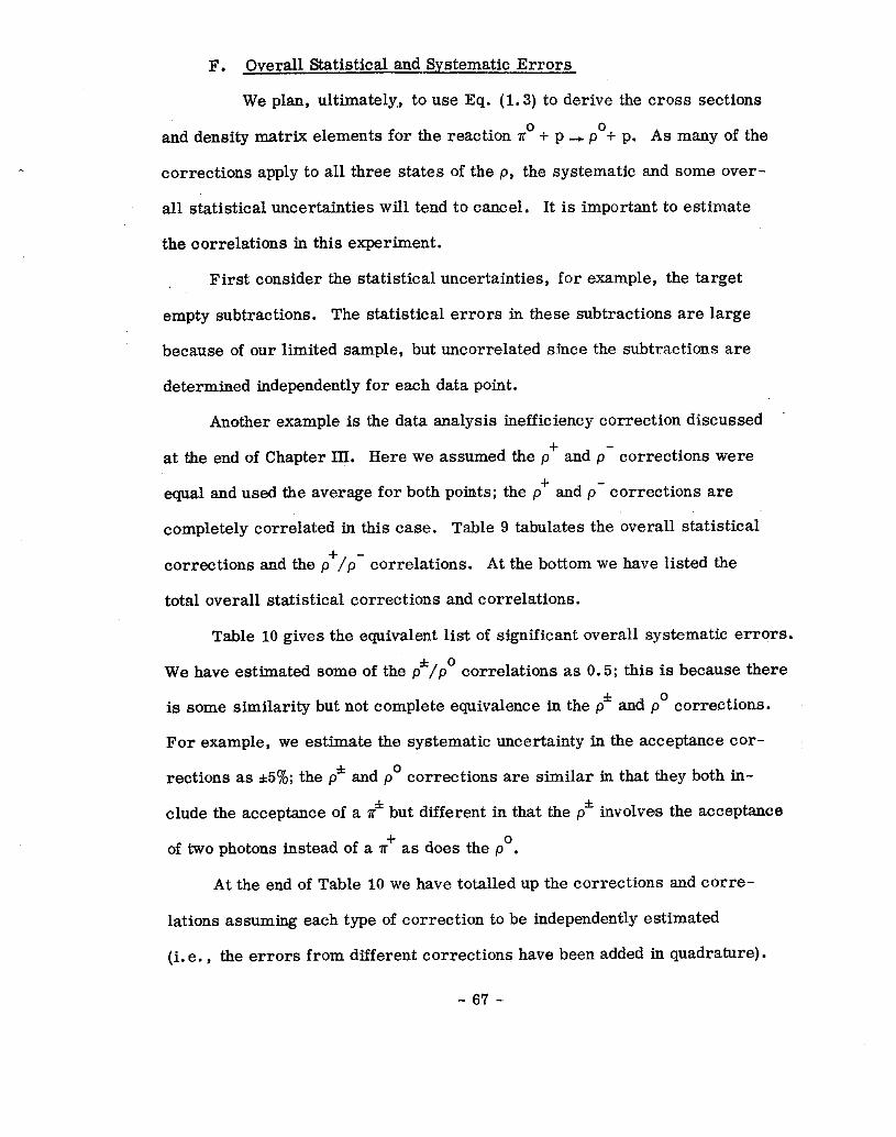
F. Overall Statistical and Systematic Errors
We plan, ultimately,, to use Eq. (1.3) to derive the cross sections
and density matrix elements for the reaction no + p + p”+ p. As many of the
corrections apply to all three states of the p, the systematic and some over-
all statistical uncertainties will tend to cancel. It is important to estimate
the correlations in this experiment.
First consider the statistical uncertainties, for example, the target
empty subtractions. The statistical errors in these subtractions are large
because of our limited sample, but uncorrelated since the subtractions are
determined independently for each data point.
Another example is the data analysis inefficiency correction discussed
at the end of Chapter III. Here we assumed the pf and p- corrections were
equal and used the average for both points; the p’ and p- corrections are
completely correlated in this case. Table 9 tabulates the overall statistical
corrections and the p’/p- correlations. At the bottom we have listed the
total overall statistical corrections and correlations.
Table 10 gives the equivalent list of significant overall systematic errors.
We have estimated some of the p*/p” correlations as 0.5; this is because there
is some similarity but not complete equivalence in the p* and p” corrections.
For example, we estimate the systematic uncertainty in the acceptance cor-
rections as &5%; the p* and p” corrections are similar in that they both in-
clude the acceptance of a X’ but different in that the p* involves the acceptance
of two photons instead of a 1;’ as does the p”.
At the end of Table 10 we have totalled up the corrections and corre-
lations assuming each type of correction to be independently estimated
(i.e., the errors from different corrections have been added in quadrature).
- 67 -
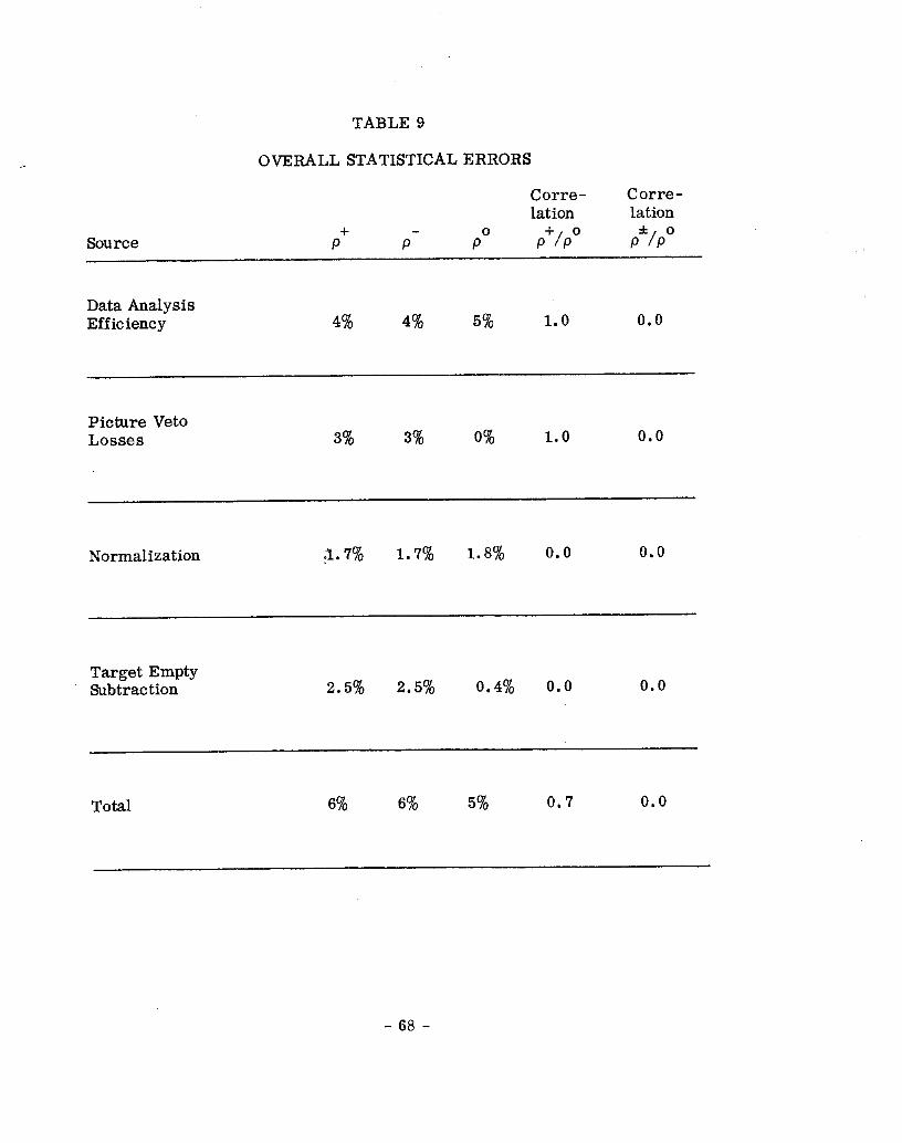
TABLE 9
OVERALL STATISTICAL ERRORS
Source Pf P- PO
Corre- lation
Pf/PO
Corre- lation
Pi/P0
Data Analysis Efficiency 4% 4% 5% 1.0 0.0
Picture Veto Losses 3% 3% 0% 1.0 0.0
Normalization ;1.7% 1.7% 1.8% 0.0 0.0
Target Empty Subtraction 2.5% 2.5% 0.4% 0.0 0.0
Total 6% 6% 5%
- 68 -
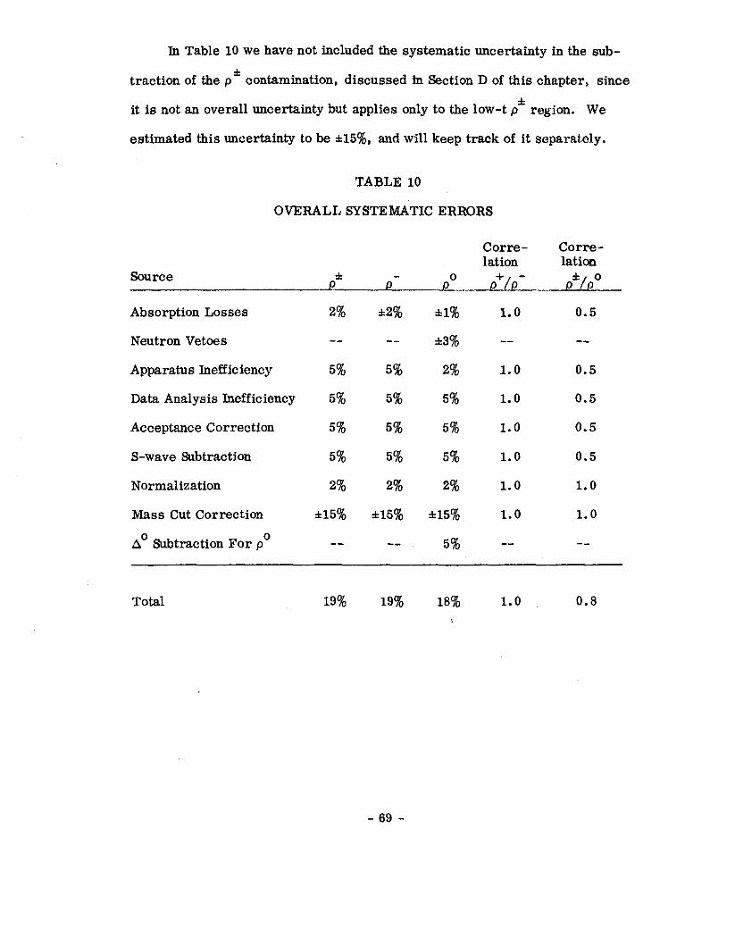
In Table 10 we have not included the systematic uncertainty in the sub-
traction of the p’ contamination, discussed in Section D of this chapter, since
it is not an overall uncertainty but applies only to the low-t p* region. We
estimated this uncertainty to be *15%, and will keep track of it separately.
TABLE 10
OVERALL SYSTEMATIC ERRORS
Corre- lation
Corre- lation
Source * P PO p+/p- Pi/P0
Absorption Losses
Neutron Vetoes
Apparatus Inefficiency
Data Analysis Inefficiency
Acceptance Correction
S-wave Subtraction
Normalization
Mass Cut Correction
A” Subtraction For p”
2% *2%
-- --
5% 5%
5% 5%
5% 5%
5% 5%
2% 2%
*15% l 15%
-- --
al%
*3%
2%
5%
5%
5%
2%
*15%
5%
1.0
--
1.0
1.0
1.0
1.0
1.0
1.0
0.5
-e
0.5
0.5
0.5
0.5
1.0
1.0
-0
Total 19% 19% 18% 1.0 0.8
- 69 -
CHAPTER V
DISCUSSION OF THE REACTIONS s’* + p +I* + p . .
At the end of Chapter IV we gave the differential cross sections and
density matrix elements for the reactions n* + p -rp* + p. The basic aim
of this paper is to combine these measurements to study the reaction
so + p +p” + p. However, in this chapter we briefly discuss these channels
as separate entities.
Looking at Fig. 20 we see that, as expected from other measurements,
the differential cross section is dominated by a sharp forward peak. Most
of the total channel cross section comes from the range 05 1 tj 5 0.5 (GeV/c)2.
Thus, the total channel cross section o(r* p -p*p) is to good approximation
only a measure of the forward peak. We find
o(s+p -$+p) = 50 & 9 pb
@r-p-p-p) = 47 .jz 9 I.lb
The errors include the -I 17% overall systematic uncertainty previously
discussed.
In Fig. 22 we plot these total cross section values as a function of pLAB,
the total incident laboratory momentum. We also include lower energy
bubble chamber data 20 on this plot. We have fit to this data the conventional
equation
cr= Kp” LAB’
We find
n(lr+p-p+p) = 1.80 & 0.08
n(n-p-p- p) = 1.87 i 0.15.
- 70 -
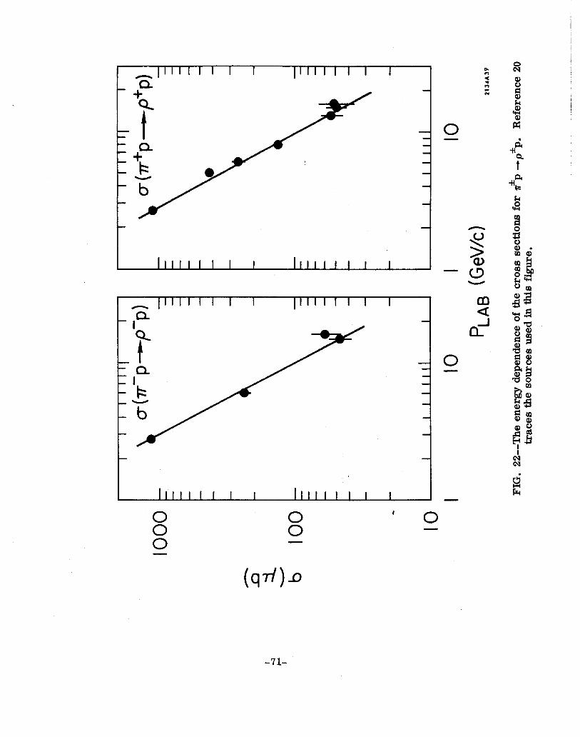
- “11 I I I I I”“’ ’ ’ I n I
I IIIII I I I I IIIIII I I I -
8 8
I 0 - 0 - -
-71-
These results are in good agreement with other determinations of this
quantity. 21
Returning to the shape of the forward peaks in Fig. 20, we find that
for (tl~ 0.03 (GeV/c)2 our do/dt’s are in fair agreement with a bubble chamber
measurement lo at 16 GeV/c. And cur do/dt’s represent reasonable extra-
polations of lower energy du,,dt measurements. Rut for 1 t I s 0.03 (GeV/c)2
we must observe that we have not been able to resolve one of the questions
which led us to carry out this experiment. With large errors &/dt (r-p -+ p-p)
shows a peak as t-+0, while da/dt(lr’p-rp+ p) is roughly flat as t -0. This
is in ‘disagreement with the hydrogen bubble chamber results 10 at 16 GeV/c.
The bubble chamber data shows a dip in both differential cross sections as
t +o, Now, the basic experimental question is whether the bubble chamber ex-
periments have a bias & finding low-t events in the reactions r* + p-+o*+ p.
This bias could occur in scanning because the low-t events have short proton
tracks and may have a small angle between the initial and final charged pion
tracks. There is disagreement between experimentalists as to whether this
bias can be tested for and corrected. The experimenters who carried out
the 16 GeV/c bubble chamber measurement looked for this bias, found it
only in one of the reactions, and corrected for it. On the other hand, the
authors of a paper describing a 6 GeV/c bubble chamber measurement of
these reactions8 believed that there is a significant scanning loss for
1 tl<O . 1 (GeV/c)2 events, even at this lower energy where the bias should
be less severe. Therefore, they do not use their data for 1 tl < 0.1 (Ge,V/c)2.
In our experiment we had hoped to resolve this question for we do not
have a bias against low-t events. We do not see the forward dip observed
- 72 -
in the bubble chamber experiment, but we have the possibility of the low-
est-t bins having an excess of events through contamination by events from
other topologies. We have discussed this in detail in the previous chapters;
we do not believe that there could hl- !uff;cien? contamination to fill Fn the
dip, but we cannot prove this. Therefore, we regard the question as to
the very small-t behavior of the reactions lr* + p+p* + p as still unresolved.
The theoretical prejudice is certainly that a very forward dip should
exist, but it is wrong for an experimentalist to be swayed in his observation
by this consideration.
- 73 -

CHAPTER VI
THE REACTION no + p-+p” + p AND CONCLUSIONS
H 0 A.
da - Calculation of dt and pmm, for no + p -rp + p ~. -- _I _-
Jn Chapter I we deduced the following formulae:
du x MOP +P”P, = ; [ -$++p+p+p) + -~$~-p-+p-pj -~(~-P-+P~~) 1
(6.1)
(6.2)
Because of various correlations some care in the propagation of errors
through these formulae must be exercised. We have already touched on
the subject of correlations yhe systematic errors (Section F, Chapter Iv).
Because of the loss of acceptance when COB C*d* 1 there sre ah corre- P
lations in the statistical errors on pz, du
and dt . H In particular, poo
da and dt are strongly correlated. These correlations are known and have
been systematically used in the error propagation.
By dividing Eq. (6.2) by Eq. (6.1) the density matrix elements for
x0 + p +p” + p are obtained, It is advantageous to do this as the systematic da
errors on dt, strongly correlated between the three reactions, tend to
cancel. In fact, the systematic errors on pmm, ?F H f0 p -pop) turn out to be
rather small and will be neglected; on the other hand, the systematic errors
on -$ (~r’p + pop) are large and may not be neglected.
The values obtained for dt da (rap --pop) are given in Table 11 along with
the estimated systematic errors. We have quoted two systematic errors, \
- 74 -

-$ And Errors for Ir’+p-p’+pAt 15,OGeV/c
t du (GeV/c)2 C
dt pb/(GeV/c)2 * I
TABLE 11
Overall Svstematic Low-t Svstematic ” 2
fib/(GeV/c)2 1 .ooo - .015
,015 - .30
.030 - .045
.045 -.060
.06 -.08
.08 - .12
. 12 - .20
.20 -.35
.35 - .60
.60 - 1.00
249 k60
181zk 65
312 f 55
118 zk 55
60 f 35
66i25
61zt 22
23 -I 8
4-+3
5*3
50 90 *
50 90
40 75
30 45
16 30
12
10
3
1
1
*The errors in this column are statistical
- 75 -
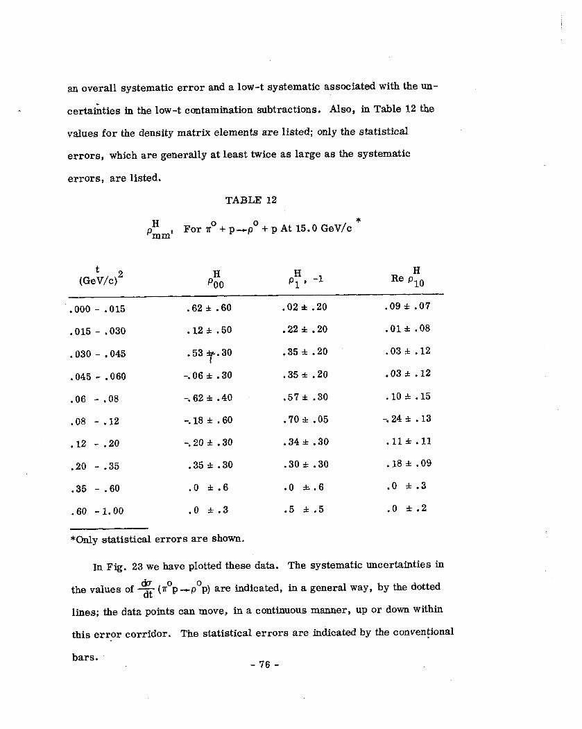
an overall systematic error and a low-t systematic associated with the un-
certainties in the low-t ccmtamination subtractions. Also, in Table 12 the
values for the density matrix elements are listed; only the statistical
errors, which are generally at least twice as large as the systematic
errors, are listed.
TABLE 12
H mm, For no + p-p’ + p At 15.0 GeV/c *
P
(Ge:/c)2
.ooo - .015
.015 - .030
H PO0
.62i.60
. 12* .50
H H Pl' -1 Re p10
.02*.20 .09*.07
.22& .20 .Olzt .08
.030 -.045 .53 T.30 .35i.20 .03* .12
.045 -.060 -.06zt .30 .35*.20 .03* .12
.06 -.08 -.62zt .40 .57* .30 . 10 * .15
.08 - .12 -. 18 i .60 .70* .05 -.24 zt .13
12 - .20 -..oi.30 .34*.30 . 11 f .ll .
.20 - .35 .35*.30 .30*.30 . 18i.09
.35 -.60 .O a.6 .O ~t.6 .o zt.3
.60 -1.00 .o k.3 .5 *.5 .o zk.2
*Only statistical errors are shown.
In Fig. 23 we have plotted these data. The systematic uncertainties in
the values of dt K (rap -pop) are indicated, in a general way, by the dotted
lines; the data points can move, in a continuous manner, up or down within
this error corridor. The statistical errors are indicated by the conventional
bars. - '76 -
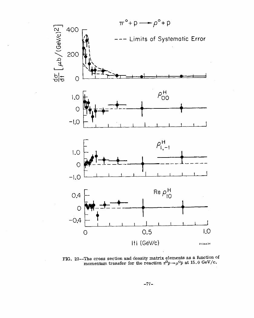
1.0
0
-1.0
1.0
0
-1.0
0.4
0
-0.4
7T”+ p -PO+ P
--- Limits of Systematic Error
I I I I I I I I I I I
t I
I I I I I I I I J
I I I I I I I I I I I
0.5
It I (GeV/c) 2134*3.
FIG. 2%-The cross section and density matrix elements as a function of momentum transfer for the reaction rap ‘pop at 15.0 GeV/c.
-77-
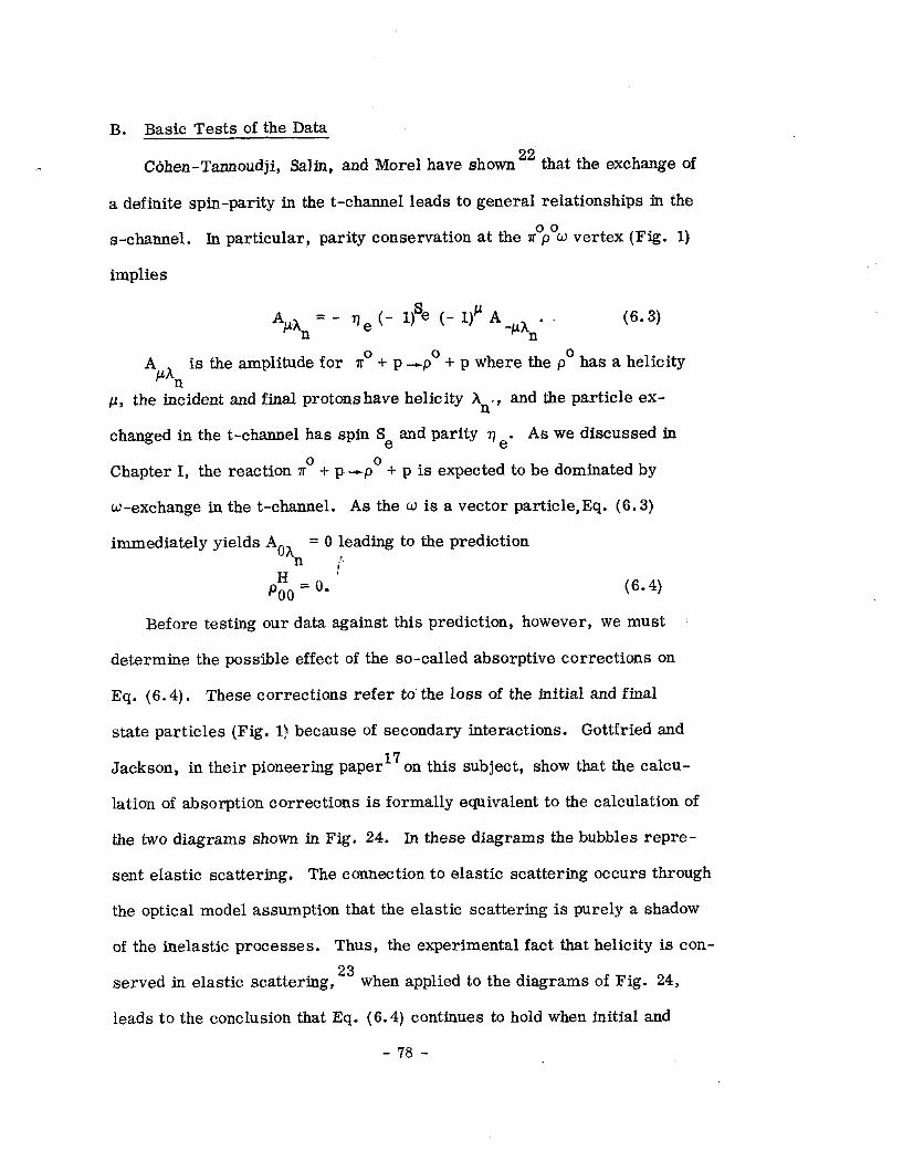
B. Basic Tests of the Data
Cohen-Tannoudji, Salin, and Morel have shown 22 that the exchange of
a definite spin-parity in the t-channel leads to general relationships in the
s-channel. In particular, parity conservation at the r”pow vertex (Fig. 1)
implies
4h, = - ?J, (- i)‘e (- l)c( A -PQ’
A I”%
is the amplitude for r” + p -p” + p where the p” has a helicity
p, the incident and final protonshave helicity h,,, and the particle ex-
changed in the t-channel has spin Se and parity TJ,. As we discussed in
Chapter I, the reaction x0 + p-p’ + p is expected to be dominated by
w-exchange in the t-channel. As the w is a vector particle,Eq. (6.3)
immediately yields Aohn = 0 leading to the prediction .‘,
H ’ PO0 = 0.
Before testing our data against this prediction, however, we must
determine the possible effect of the so-called absorptive corrections on
Eq. (6.4). These corrections refer to the loss of the initial and final
state particles (Fig. 1) because of secondary interactions. Gottfried and
Jackson, in their pioneering paper 17 on this subject, show that the calcu-
lation of absorption corrections is formally equivalent to the calculation of
the two diagrams shown in Fig. 24. In these diagrams the bubbles repre-
sent elastic scattering. The connection to elastic scattering occurs through
the optical model assumption that the elastic scattering is purely a shadow
of the inelastic processes. Thus, the experimental fact that helicity is con-
served in elastic scattering, 23 when applied to the diagrams of Fig. 24,
leads to the conclusion that Eq. (6.4) continues to hold when initial and
- 78 -
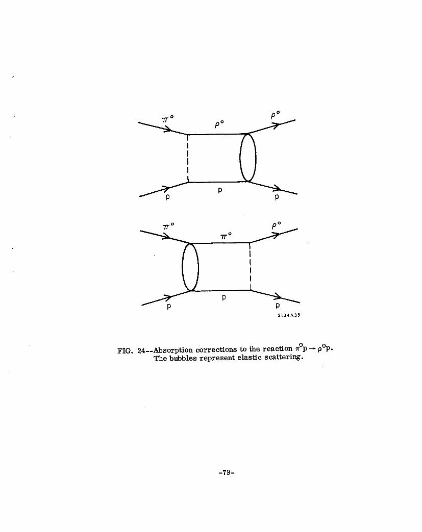
FIG. 24--Absorption corrections to the reaction rap - pop. The bubbles represent elastic scattering.
-79-
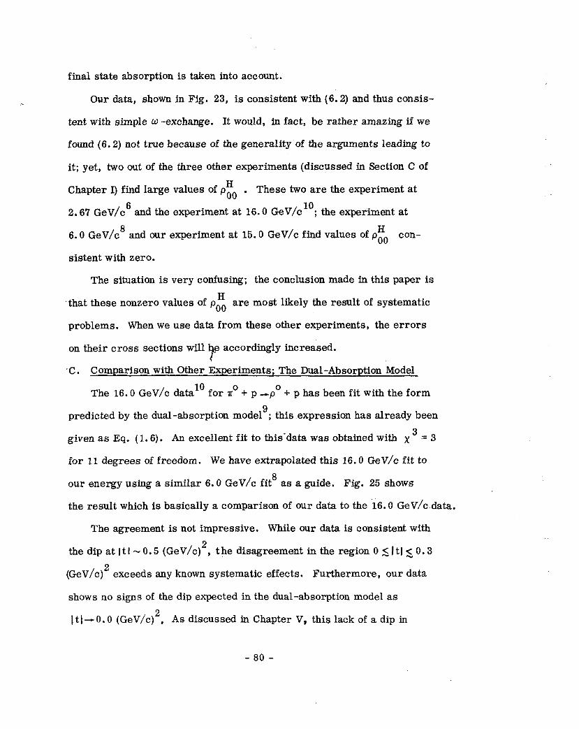
final state absorption is taken into account.
.- Our data, shown in Fig. 23, is consistent with (6.2) and thus consis-
tent with simple w -exchange. It would, in fact, be rather amazing if we
found (6.2) not true because of the generality of the arguments leading to
it; yet, two out of the three other experiments (discussed in Section C of
H Chapter I) find large values of ~00 . These two are the experiment at
2.67 GeV/c’ and the experiment at 16.0 GeV/cl’; the experiment at
H 6.0 GeV/c’ and our experiment at 15.0 GeV/c find values of poo con-
sistent with zero.
The situation is very confusing; the conclusion made in this paper is
‘that these nonzero values of pfo are most likely the result of systematic
problems. When we use data from these other experiments, the errors
on their cross sections will ?
e accordingly increased.
‘C. Comparison with Other Experiments; The Dual-Absorption Model
The 16.0 GeV/c data” for x0 + p -+J’ + p has been fit with the form
predicted by the dual-absorption model’; this expression has already been
given as Eq. (1.6). An excellent fit to this-data was obtained with x 3=3
for 11 degrees of freedom. We have extrapolated this 16.0 GeV/c fit to
our energy using a similar 6.0 GeV/c fit8 as a guide. Fig. 25 shows
the result which is basically a comparison of our data to the 16.0 GeV/c data.
The agreement is not impressive. While our data is consistent with
the dip at 1 t I - 0.5 (GeV/c)2, the disagreement in the region 0 s 1 t 12 0.3
(GeV/c)2 exceeds any known systematic effects. Furthermore, our data
shows no signs of the dip expected in the dual-absorption model as ”
Itj-0.0 (GeV/c)‘. As discussed in Chapter V, this lack of a dip in
- 80 -

100
b.- I u-0
I I I I
t P
i
t t
\
-t
0 This Experiment
- 16 GeV/c Duol-Absorption Fit
Itl (GeV/cj2 2134A33
FIG. 25--Comparison of our measurement of the cross section for ?pp -pop with the dual-absorption fit to the 16.0 GeV/c data.
-8 l-
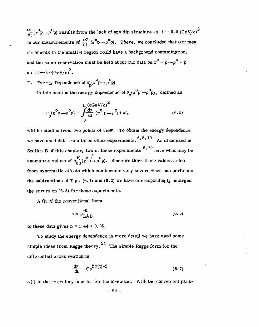
-$( sop-pop) results from the lack of any dip structure as t - 0.0 (GeV/c)2
in our.measurements of dt da (s*p---pip). There, we concluded that our mea-
surements in the smaIl-t region could have a background contamination,
and the same reservation must be held about our data on no + p-p0 + p
as I tl -0. O(GeV/c)2.
D. Energy Dependence of c x0 _(
In this section the energy dependence of cp(sop -pop), defined as
1. O(GeV/c)2
Up(7r0P--P0P) = J- + ho P--POP) dt, (6.5)
0
will be studied from two points of view. To obtain the energy dependence
we have used data from three other experiments. 6,8,10 As disucssed in
Section B of this chapter, two of these experiments 6,10 have what may be f’
anomalous values of p~o(xop,pop). Since we think these values arise
from systematic effects which can become very severe when one performs
the subtractions of Eqs. (6.1) and (6.2) we have correspondingly enlarged
the errors on (6.5) for these experiments.
A fit of the conventional form
-n aocpLAB (6.6)
to these data gives n = 1.44 * 0.25.
To study the energy dependence in more detail we have used some
simple ideas from Regge theory. 24 The simple Regge form for the
differential cross section is
do dt
= (le2ww (6.7)
o(t) is the trajectory function for the W-meson. With the convenient para-
- 82 -
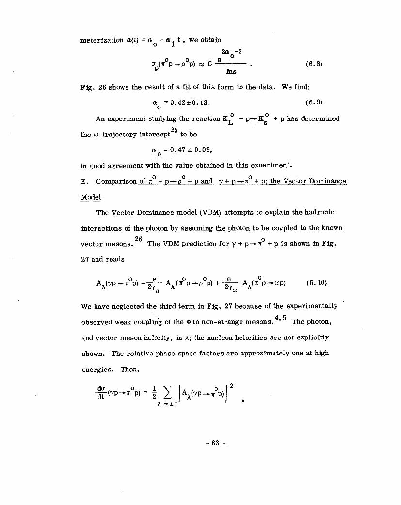
meterization a(t) = a0 - a1 t , we obtain
upprop --pop) x c s
2ao-2
. hS
(6-Q
Fig. 26 shows the result of a fit of this form to the data. We find:
Q o = 0.42&O. 13. (6.9)
An experiment studying the reaction K: + p-K: + p has determined
the w-trajectory intercept 25 to be
o! o = 0.47 * 0.09,
m good agreement with the value obtained in this exneriment.
E. Comparison of x0 + pdp” + p and y + p-x’ + p; the Vector Dominance
Model
The Vector Dominance model (VDM) attempts to explain the hadronic
interactions of the photon by assuming the photon to be coupled to the known
vector mesons. 26
The VDM prediction for y + p-x’ + p is shown in Fig.
27 and reads
0 A+YP -x P) =$- A,(~‘P--POP) + + A+x’P+wp) (6.10)
P W
We have neglected the third term in Fig. 2’7 because of the experimentally
observed weak coupling of the @J to non-strange mesons. 495 The photon,
and vector meson helicity, is A; the nucleon helicities are not explicitly
shown. The relative phase space factors are approximately one at high
energies. Then,
da -&YP’xOP) = + A-&YP+ TOP)
I
2
h =*l ,
- 83 -
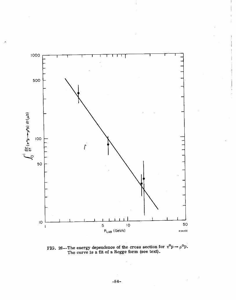
1000 , I I I I I I III1 I I I i
500 -
50 -
IO ’ I I I I I I IllI I I I
I 5 IO 50 PLAB (GeV/c) 2134*32
FIG. 26--The energy dependence of the cross section for lr’p - pop. The curve is a fit of a Regge form (see text).
-84-
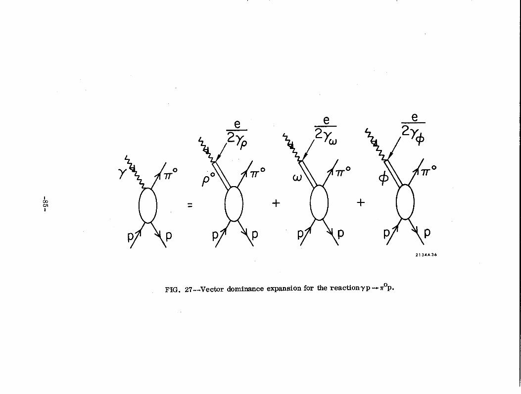
+
-85-
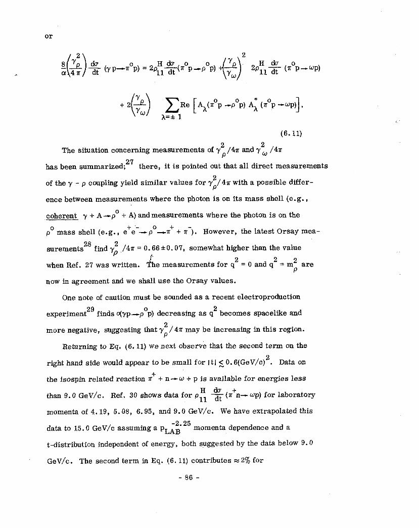
c 2 > 2 s2 do dt (Yp-xOP) = 2plK,+r”P--PoP) -32 a 4ir
0 y
w 2F5 s (rOP-@P)
+ ~(2) AZ; [AhMop --POP) A; (TOP --wp)].
(6.11)
The situation concerning measurements of y2,/4x and y”, /4x
has been summarized; 27 there, it is pointed out that all direct measurements
of the y - p coupling yield similar values for y:/4x with a possible dfffer-
ence between measurements where the photon is on its mass shell (e.g.,
cohere& y + A-p’ + A) andmeasurements where the photon is on the *
p” mass shell (e.g., eTe--potin’ + n-). However, the latest Orsay mea-
surements 28 find yp” /4r = 0.66 f 0.0’7, somewhat higher than the value
t when Ref. 2’7 was written. The measurements for q2 = 0 and q2 = rnz are
now in agreement and we shall use the Orsay values.
One note of caution must be sounded as a recent electroproduction
experiment” finds c(yp--pop) decreasing as q2 becomes spacelike and 2
more negative, suggesting that yp /4x may be increasing in this region.
Returning to Eq. (6.11) we next observe that the second term on the
right hand side would appear to be small for I t I <, 0.6( GeV/c)‘. Data on
the isospin related reaction 7c” + n -0 + p is available for energies less Hdu +
than 9.0 Ge,V/c. Ref. 30 shows data for pll dt(r n-wp) for laboratory
momenta of 4.19, 5.08, 6.95, and 9.0 GeV/c. We have extrapolated this -2.25
data to 15.0 GeV/c assuming a pLAB momenta dependence and a
t-distribution independent of energy, both suggested by the date below 9.0
GeV/c. The second term in Eq. (6.11) contributes x 2% for
- 86 -
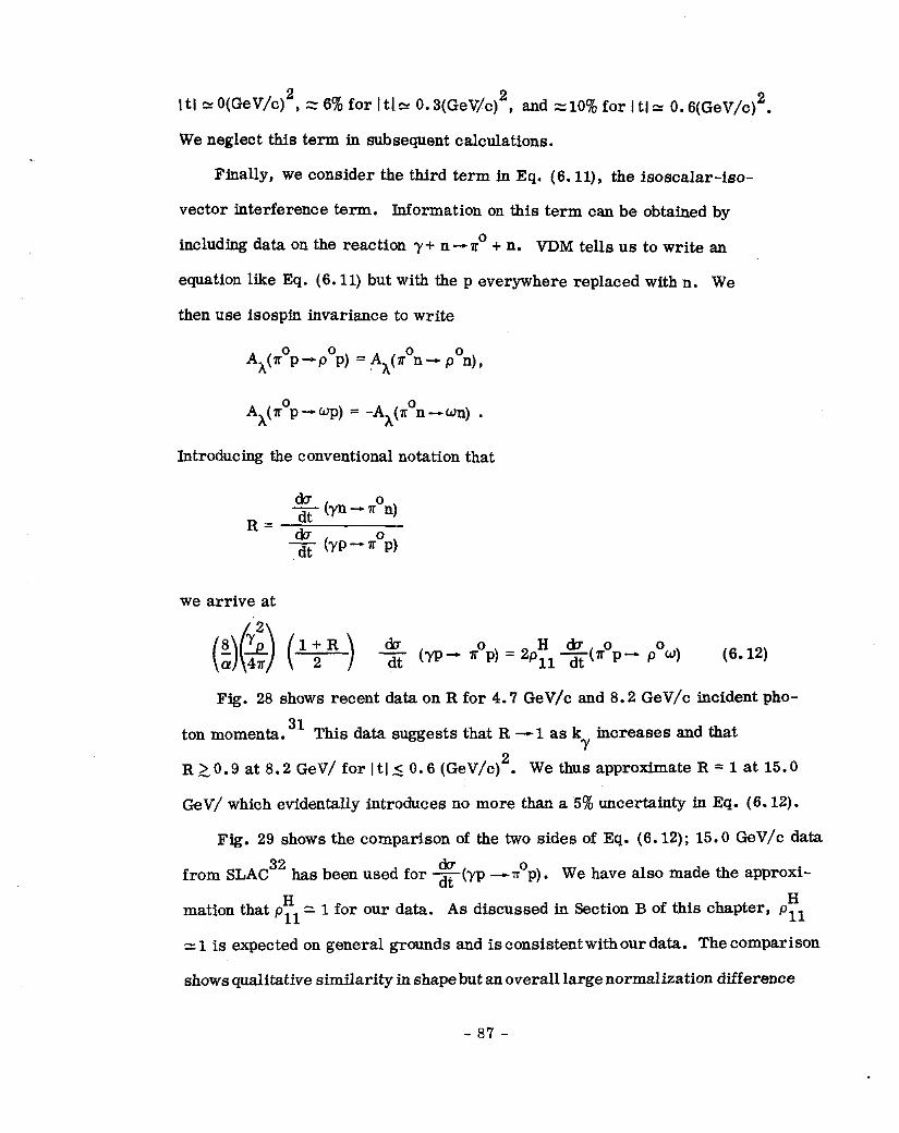
I tl N O(GeV/c)2, z 6% for I tl= 0.3(GeV/c)‘, and ~10% for I tl zz 0.6(GeV/c)‘.
We neglect this term in subsequent calculations.
Finally, we consider the third term in Eq. (6. ll), the isoscalar-iso-
vector interference term. Information on this term can be obtained by
including data on the reaction y+ n-no + n. VDM tells us to write an
equation like Eq. (6.11) but with the p everywhere replaced with n. We
then use isospin invariance to write
A,(n’p-pop) = Ah(xon-- con),
Ax(xop -up) = -A h (non --Wn) .
Introducing the conventional notation that
R= g (Yn - *On)
+g (YP-xOP)
we arrive at
(@) ( l;R ) + (yP’ 7T0P) = 2P;l+(x”P- POW) (6.12)
Fig. 28 shows recent data on R for 4.7 GeV/c and 8.2 GeV/c incident pho-
ton momenta. 31 This data suggests that R -1 as kY increases and that
Rk0.9 at 8.2 GeV/ for Itl( 0.6 (GeV/c)‘. We thus approximate R = 1 at 15.0
GeV/ which evidentally introduces no more than a 5% uncertainty in Eq. (6.12).
Fig. 29 shows the comparison of the two sides of Eq. (6.12); 15.0 GeV/c data
from SLAC3’ has been used for +YP --Rp). We have also made the approxi-
H mation that pll H
= 1 for our data. As discussed in Section B of this chapter, pl1
z 1 is expected on general grounds and is consistentwith our data. The comparison
showsqualitative similarity in shape but anoverall large normalization difference
- 87 -
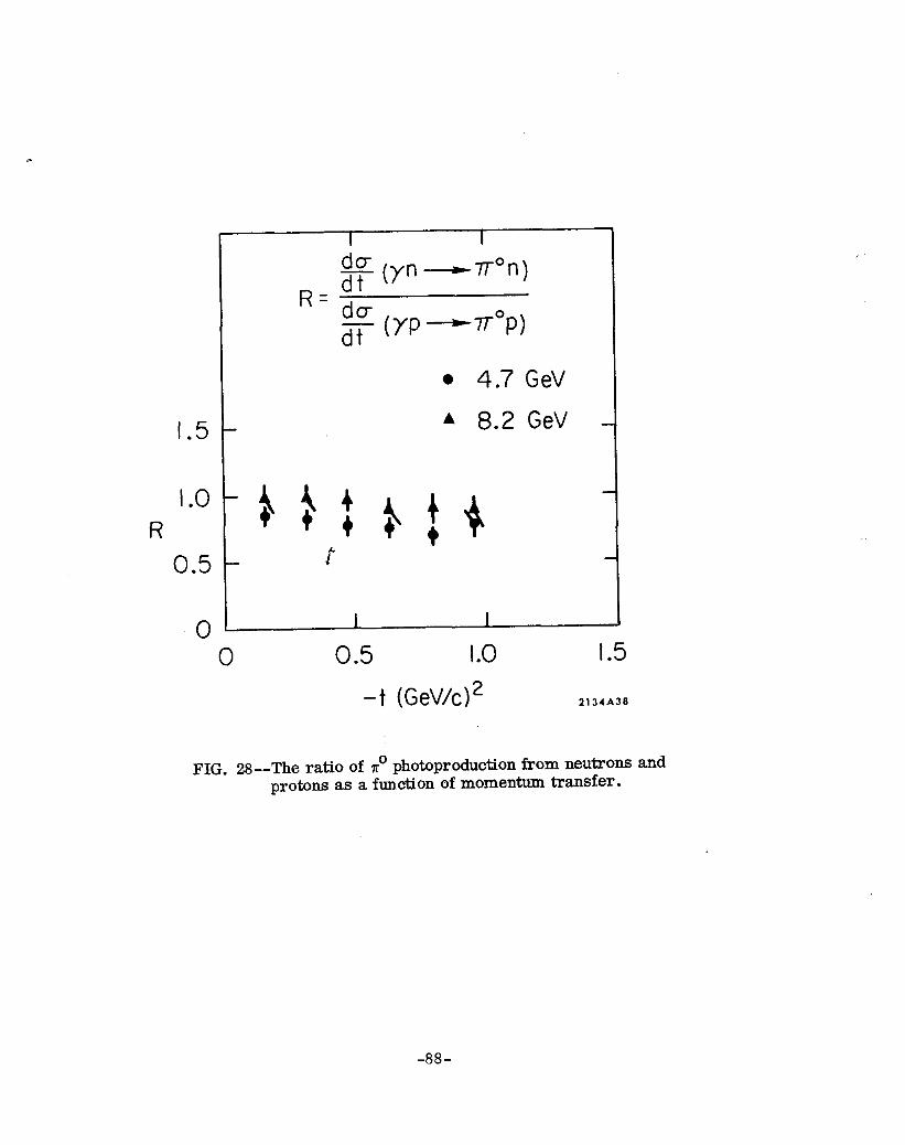
1.5
1.0 R
0.5
0
g (Y” -7-rOn)
R= dcr &- (YP ----OP)
l 4.7 GeV
A 0.2 GeV
I I
0 0.5 1.0 1.5
-t (GeVk)2 2134A38
FIG. 28--The ratio of r” photoproduction from neutrons and protons as a function of momentum transfer.
-88-
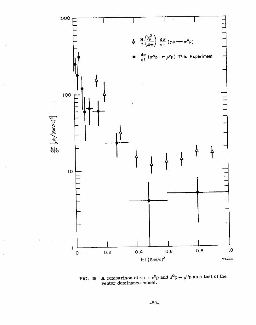
IO
I I 0 0.2 0.4
-pop) This Experiment
I I 0.6 0.6 1.0
Itl (GeV/c12 21-l4n37
FIG. 29--A comparison of yp -+ #p and lr’p -. pop as a test of the vector dominance model.
-89-
which cannot be accaunted for by any known systematic effect in our data
(see Table 11).
This discrepancy could arise because of the use of an incorrect
value of yz/ 4x . If we let our data determine yz /4x we find
0
This is especially interesting because other experiments relating photo-
production reactions to their hadronic counterparts also tend to find
lower values of yp” /4x. 27 For example, one test of VDM is to check the
equality
ti)g)t’;“) -d& (yp-xn+n) = 2j~~I~ (x-p-p’nj (6.13)
f
Formally, this is almost identical to our test in Eq. (6.12). However,
the dynamics of the particular reactions involved are quite different, as
discussed in Chapter I. Yet, a test of Eq. (6.13) at 15.0 GeV/c incident
momentum 13’ 33 and at very small t has found a qualitative similarity in
shape but a normalization difference which can be accounted for by a sub-
stantially smaller value of y,2/ 4x.
A fair summary of the situation would seem to be that experiments
which are able to isolate the y - p coupling find y;/4n z 0.7 while exp-
eriments which do not isolate this coupling but depend on various arguments
as to the size of the other contributions find yi/47r z 0.3. 27
It has been suggested that the existence of additional vector mesons
could explain this. 27 In this model our VDM diagram in Fig. 27 would have
-90 -
to include additional terms corresponding to these additional vector mesons.
And, in fact, recent data 34
indicates the existence of a heavy vector meson
with a mass of z 1,. 6 GeV and I = 1. However, this enhancement seems
to couple predominantly to the pan system which would preclude its par-
ticipation in Fig. 27. Thus, the disagreement in Fig. 29 is unresolved
and appears to be a serious violation of the Vector Dominance Model.
F. Summary and Conclusions
In summary, we have extracted the cross section and density matrix
elements for the reaction r” + p---p’ + p at 15.0 GeV/c. This data ex-
hibits no signs of the presence of unnatural parity exchanges and is con-
sistent with the basic characteristics expected from w-exchange; however,
the data does not agree with detailed dual-absorption model calculations
for w-exchange. There is disagreement between this experiment and a
16.0 GeV/c bubble chamber experiment.
The energy dependence of the cross section for w-exchange determines
the intercept of the a--trajectory,o!(o); we find (Y(O) = 0.42 f 0.13, in agree-
ment with other measurements. Finally, the relation between the processes
y + p-r’ f p and x0 + p-p’ + p was investigated as a test of the Vector
Dominance Model. We find qualitative agreement in shape but a signifi-
cant normalization discrepancy consistent only with a lower value of </ 4x
than is currently obtained from direct measurements of the y - p coupling.
At the present time three bubble chamber experiments and one spark
chamber experiment (this experiment) on 7~’ + p-p’ + p have been re-
ported. What conclusions can one reasonably make about the relative
merits of the two methods based on this experience?
At all but the lowest values of t, the spark chamber has a significant
-9l-
I
advantage in that it views not only the proton, as the bubble chambers do,
but also the two phtons from the r” decay. This extra information provides
for a more complete separation of the pp signal from the background than is
possible in bubble chamber experiments. This feature becomes especially
important at high energies. The signal to noise ratio is even more enhanced
in the spark chamber method because of the triggerability not present in
the normal bubble chamber experiment.
At low-t the two methods are in disagreement, as discussed in Chapter
V. This is clearly seen in dc/dt (r*p -p*p). These general features are
propagated into our x0 + p do0 f p data. The bubble chambers may pro-
duce dips in da/dt (Ir*p-p&p) because of scanning losses whereas the spark
chamber method may fill in dips because of a lack of signal to noise reso-
lution due to the absence of a measurement of the recoil proton angle.
In fact, our result for J /dt(r’p-pop) may be criticized in the low-t
region on fairly general grounds. For t’ = I t - tmm small, angular 1 momentum conservation requires that scattering amplitudes have a leading
behavior in t’ as follows: 35
Il AA” It’1 ’
Here, n is the total helicity flip. We have argued in Section B of this chap-
ter that the helicity changes by 1 at the boson vertex. Vector Dominance
tells us that the wpp coupling is largely vector, and at high energies vector
couplings do not change the helicity. 36 Thus, we would expect a leading
behavior of It’1 in dv/dt(lr’p e p*p), predicting a dip as t’& -0. As we con-
cluded in Chapter V, the low-t behavior must be regarded as unresolved at the
present time.
- 92 -

Perhaps, the most fruitful approach would be to combine the advan-
tages of the two methods in a hybrid bubble chamber-spark chamber ex-
periment.
- 93 -
REFERENCES
1. P: B. Johnson a., Phys. Rev. 176, 1651 (1968);
J. A. Poirier et., Phys. Rev. 163, 1462 (1967);
2.
3.
4.
5.
6.
7.
8.
9.
10.
11.
12.
13.
14. E. Flaminio et. , CERN/HERA 70-7 (1970).
15. F. J3ulos et., Phys. Rev. Letters 3, 1453 (1971).
16. M. Jacob and G. C. Wick, Ann. Phys. 1, 404 (1959).
17. K. Gottfried and J. D. Jackson, Nuovo Cimento 2, 735 (1964).
B. D. Hyams et al. , Nucl. Phys. B7, 1 (1968);
H. H. Williams, Report No. SLAC-142. Stanford Linear Accelerator
Center, (1971); Reference 15.
G. Grayer et al., Proceed-s of the Fourth International Conference
on High Energy Collisions, Oxford, England, 1972.
A. P. Contogouris et al., Phys. Rev. Letters E, 1352 (1967).
A. Dar and V. F. Weisskopf, Phys. Rev. Lettersg, 762 (1968).
L. Dilella, Proceedings of the Lund International Conference on
Elementary Particles, Lund, Sweden, 1969.
W. Michael and G. Gida k
Phys. Rev. Letters 28, 1475 (1972).
J. P. Baton and G. Laurens, Nucl. Phys. B21, 551(1970). -
D. J. Crennell et al., Phys. Rev. Lettersg, 1674 (1971).
Haim Harari, Phys. Rev. Lettersz, 1400 (1971).
J. Bartsch et., Nucl. Phys. B46, 46 (1972).
Robert Yamartino, private communication.
SLAC User’s Note No. 8, (September, 1967).
B. N. Ratcliff, Report No. SLAC-141 Stanford Linear Accelerator Center,
(1971).
- 94 -
18.
19.
20.
21.
22.
23.
24.
25.
26.
27.
28.
29.
30.
31.
32.
33.
J. D. Jackson, Nuovo Cimento 2, 1644 (1964).
0. Slrjeggestad, Proceedings of the 1964 Easter School for Physicists,
Vol. 2.
J. C. Pratte., Phys. Letters- 383 (1972); this reference gives a
list of all sources used in Fig. 22.
G. Giacomelli, Proceedings of the Sixteenth International Conference on Hi&r - --.-- - ----
Energy Physics, Batavia, Illinois, 1972.
G. Cohen-Tarmoudji, Ph. Salm, and A. Morel, Nuovo Cimento 5%
412 (1968).
J. Ballam et al., Phys. Rev. D5, 545 (1972).
J. K. Storrow, “Regge Theory for Experimentalists, ” Daresbury Lecture
Note Series No. 6 (1971).
A. D. Brodye, Phys. Rev. Letters s, 1050 (1971).
N. M. Kroll, T. D. Lee, and B. Zumino, Phys. Rev. m,l376 (1967).
D. W. G. S. Leith, “Lectures to the Scottish Universities Summer School
in Physics”, Report No. SLAC-PUB-1041, SLAC (1970).
J. Lefrancois, Proceedjngs of the 1971 International Symposium on Electron
and Photon Interactions at High Energies, Cornell, 1971.
J. T. Dakin et., Phys. Rev. Letters 30, 142 (1973) ;
J. T. Dakm &. , Report No. SLAC-PUB-1211, SLAC (March, 1973)
( submitted to Phys . Rev. ) .
F. D. Gault, A. D. Martin, and G. L. Kane, Nucl. Phys. B32, 429 (1971). -
A. M. Osborne Gal., Phys. Rev. Letters 3, 1621(1972);
A. M. Osborne a., CLNS-189, (July, 1972).
R. Anderson @. , Phys. Rev. E, 27 (1970).
F. Bulos aal. , Phys. Rev. Letters 2, 1457 (1971).
- 95 -
34. M. Davier, Proceedings of the Sixteenth International Conference on High
Energy Physics, Batavia, Illinois, 1972.
. . 35. G. L. Kane and Marc Ross, Phys. Rev. 177, 2353 (1969).
36. James D. Bjorken and Sidney D. Drell, Relativistic Quantum Mechanics,
(McGraw-Hill, New York, 1964).
- 96 -