Erlangen program in geometry and analysisSL2(R) case study: Geometry

Vladimir V. Kisil

School of MathematicsUniversity of Leeds (England)

email: kisilv@maths.leeds.ac.uk

Web: http://www.maths.leeds.ac.uk/~kisilv

Varna, 2016

Mathematics and the WorldEvolution of views

A common habit now is to divide mathematics into pure and applied, theformer is considered as a kind of an intellectual game or an exercise inabstract thinking only loosely related to real world.

This attitude is rather recent. Pythagoras said “The whole thing is anumber”, Euclid wrote his Elements about geometry—measurement ofland, Newton described heavens with differential equations. Cartesianphilosophy considered the Euclidean space-time as the only logicalpossibility and the true model for the real Newtonian mechanics.

At the first half of XIX century non-Euclidean geometry was discovered,with many other (projective, conformal, differential, . . . ) to follow. Thisbroke the link between the reality and geometry.

Why do “non-real” geometries exist?

How many are there of them?

Riemann vs. KleinTwo inauguration lectures

Riemann (1852): “Local to global” approach: take an non-degenerate(pseudo-)Riemannian metric gij. The most of geometry is encoded in theLaplace(–Beltrami) operator, e.g. on the plane:

∆ = ∂2x + ∂

2y, and � = ∂2

x − ∂2y.

With the help of imaginary i and hyperbolic j units the Laplacian andwave operator can be factorised, e.g.:

∂2x + ∂

2y = (∂x + i∂y)(∂x − i∂y), i2 = −1,

∂2x − ∂

2y = (∂x + j∂y)(∂x − j∂y), j2 = 1.

A connection with analysis: null solutions of ∆ are harmonic functionsand null solutions of D are holomorphic.

However, what to do with parabolic operators, e.g. ∂2x + ∂y?

Klein’s Erlangen programinfluenced by S. Lie

Klein (1872): Geometry is the theory of invariants of a transitivetransformation group.

However the theory of groups and representations was missing at thetime, therefore Erlangen program was not in a daily toolkit of a geometer(in contrast to Riemannian geometry).

Family roots of Erlangen program:

• Descartes (1637): geometrical problems reduce to algebraicequations through the coordinate method.

• Galois (1831): solvability of algebraic equations is determined fromcertain groups.

• S. Lie (1872): solutions of differential equations through their groupof continuous symmetries (a marriage of differential geometry withErlangen approach).

Erlangen Programme at LargeA great manifestation of the Klein’s approach is the Special Relativity:the theory of invariants in the Minkowski space-time under the Lorentztransformations.

There is no reason to limit Erlangen programme to geometry or physics.We shall study invariant properties of functions and operators as well.

The demonstration can be based on a single (but very important!)example of the group SL2(R). Thus we will escape references to generaltheory of Lie groups and representation, direct calculations will be doneinstead. There are a lot of open questions and possibilities to generalisethis approach we will mention due to course.Course outline:

• Introduction to SL2(R): subgroups and homogeneous spaces.

• Geometry of homogeneous spaces and cycles.

• Linear representations.

• Analytic function theories.

• Functional calculus and quantization.

The group SL2(R)

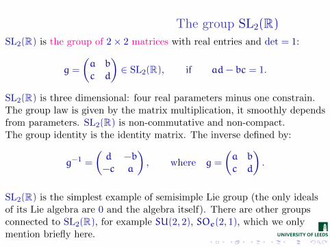
SL2(R) is the group of 2× 2 matrices with real entries and det = 1:

g =

Ça b

c d

å∈ SL2(R), if ad− bc = 1.

SL2(R) is three dimensional: four real parameters minus one constrain.The group law is given by the matrix multiplication, it smoothly dependsfrom parameters. SL2(R) is non-commutative and non-compact.The group identity is the identity matrix. The inverse defined by:

g−1 =

Çd −b−c a

å, where g =

Ça b

c d

å.

SL2(R) is the simplest example of semisimple Lie group (the only idealsof its Lie algebra are 0 and the algebra itself). There are other groupsconnected to SL2(R), for example SU(2, 2), SOe(2, 1), which we onlymention briefly here.

One-parameter subgroupsand Lie algebra

Consider a one-parameter continuous subgroup of SL2(R), that is acollection of elements g(t) ∈ SL2(R), t ∈ R such that g(t)g(s) = g(t+ s).

Here is an example: g(t) =

Çcos t sin t− sin t cos t

å, t ∈ R.

Then we can calculate the derivative:

d

dtg(t) = lim

s→0

g(t+ s) − g(t)

s= lims→0

g(s) − e

sg(t) = Xg(t),

where X turns to be a matrix with zero trace and is called generator ofthe subgroup g(t).Conversely, any 1-param subgroup g(t) is a solution to the differentialequation g ′(t) = Xg(t). Thus, we have the representation:

g(t) = etX =∞∑n=0

tn

n!Xn.

The collection of all generators is a three-dimensional Lie algebra, closedunder commutator [X, Y] = XY − YX.

Groups and Homogeneous SpacesFrom homogeneous space to subgroup

Let X be a set and let be defined an action G : X→ X of G on X. There isan equivalence relation on X, say, x1 ∼ x2 ⇔ ∃g ∈ G : gx1 = x2, withrespect to which X is a disjoint union of distinct orbits.

Without loss of a generality, we assume that the operation of G on X istransitive, i. e. for every x ∈ X we have

Gx :=⋃g∈G

g(x) = X.

If we fix a point x ∈ X then the set of elements Gx = {g ∈ G | g(x) = x}forms the isotropy (sub)group of x.

For any group G we could define its action on X = G:

• The conjugation g : x 7→ gxg−1 (is trivial for a commutative group).

• The left shift λ(g) : x 7→ gx and the right shift ρ(g) : x 7→ xg−1.

Groups and Homogeneous SpacesSubgroup to homogeneous space

Let G be a group and H be its subgroup. Let us define the space of cosetsX = G/H by the equivalence relation: g1 ∼ g2 if there exists h ∈ H suchthat g1 = g2h.The space X = G/H is a homogeneous space under the left G-actiong : g1 7→ gg1. For practical purposes it is more convenient to have aparametrisation of X.We define a continuous function (section) s : X→ G such that it is a rightinverse to the natural projection p : G→ G/H, i.e. p(s(x)) = x for allx ∈ X.Check that, for any g ∈ G, we have s(p(g)) = gh for some h ∈ Hdepending from g.Then, any g ∈ G has the unique decomposition of the form g = s(x)h,where x = p(g) ∈ X and h ∈ H.We also define a map r : g 7→ h associated to p and s by:

r(g) := s(x)−1g where x = p(g), thus g = s(p(g))r(g).

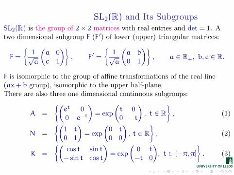
SL2(R) and Its SubgroupsSL2(R) is the group of 2× 2 matrices with real entries and det = 1. Atwo dimensional subgroup F (F ′) of lower (upper) triangular matrices:

F =

®1√a

Ça 0c 1

å´, F ′ =

®1√a

Ça b

0 1

å´, a ∈ R+, b, c ∈ R.

F is isomorphic to the group of affine transformations of the real line(ax+ b group), isomorphic to the upper half-plane.There are also three one dimensional continuous subgroups:

A =

®Çet 00 e−t

å= exp

Çt 00 −t

å, t ∈ R

´, (1)

N =

®Ç1 t

0 1

å= exp

Ç0 t

0 0

å, t ∈ R

´, (2)

K =

®Çcos t sin t− sin t cos t

å= exp

Ç0 t

−t 0

å, t ∈ (−π,π]

´. (3)

. . . and Nothing Else(up to a conjugacy)

Proposition

Any one-parameter subgroup of SL2(R) is conjugate to either A, N or K.

Proof.Any one-parameter subgroup is obtained through the exponentiation

etX =∞∑n=0

tn

n!Xn (4)

of an element X of the Lie algebra sl2 of SL2(R). Such X is a 2× 2 matrixwith the zero trace. The behaviour of the Taylor expansion (4) dependsfrom properties of powers Xn. This can be classified by a straightforwardcalculation.

Elliptic, Parabolic, Hyperbolicthe First Appearance

Lemma

The square X2 of a traceless matrix X =

Ça b

c −a

åis the identity matrix

times a2 + bc = −detX. The factor can be negative, zero or positive,which corresponds to the three different types of the Taylor expansion (4)of etX =

∑ tn

n!Xn.

It is a simple exercise in the Gauss elimination to see that through thematrix similarity we can obtain from X a generator

• of the subgroup K if (− detX) < 0;

• of the subgroup N if (− detX) = 0;

• of the subgroup A if (− detX) > 0.

The determinant is invariant under the similarity, thus these cases aredistinct.

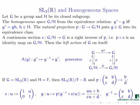
SL2(R) and Homogeneous SpacesLet G be a group and H be its closed subgroup.The homogeneous space G/H from the equivalence relation: g ′ ∼ g iffg ′ = gh, h ∈ H. The natural projection p : G→ G/H puts g ∈ G into itsequivalence class.A continuous section s : G/H→ G is a right inverse of p, i.e. p ◦ s is anidentity map on G/H. Then the left action of G on itself:

Λ(g) : g ′ 7→ g−1 ∗ g ′, generates

G

p

��

g∗ // G

p

��G/H

s

OO

g· // G/H

s

OO

If G = SL2(R) and H = F, then SL2(R)/F ∼ R and p :

Ça b

c d

å7→ b

d:

s : u 7→Ç

1 u

0 1

å, g : u 7→ p(g−1 ∗ s(u)) = au+ b

cu+ d, g−1 =

Ça b

c d

å.

SL2(R) and Imaginary UnitsConsider G = SL2(R) and H be any subgroup in the Iwasawa decomp:Ç

a b

c d

å=

Çα 00 α−1

åÇ1 ν

0 1

åÇcosφ − sinφsinφ cosφ

å. (5)

A right inverse s to the natural projection p : G→ G/H:

s : (u, v) 7→ 1√v

Çv u

0 1

å, (u, v) ∈ R2, in the diagram

G

p

��

g−1∗ // G

p

��G/H

s

OO

g· // G/H

s

OO

defines the G-action g · x = p(g · s(x)) on the homogeneous space G/H:Ça b

c d

å: (u, v) 7→

Ç(au+ b)(cu+ d) − σcav2

(cu+ d)2 − σ(cv)2,

v

(cu+ d)2 − σ(cv)2

å.

This becomes a Mobius map in (hyper)complex numbers:Ça b

c d

å: w 7→ aw+ b

cw+ d, w = u+ iv, i2(:= σ) = −1, 0, 1.

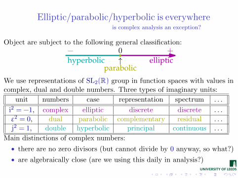
Elliptic/parabolic/hyperbolic is everywhereis complex analysis an exception?

Object are subject to the following general classification:+− 0

↑parabolic

elliptichyperbolic

We use representations of SL2(R) group in function spaces with values incomplex, dual and double numbers. Three types of imaginary units:

unit numbers case representation spectrum . . .

i2 = −1, complex elliptic discrete discrete . . .

ε2 = 0, dual parabolic complementary residual . . .

j2 = 1, double hyperbolic principal continuous . . .

Main distinctions of complex numbers:

• there are no zero divisors (but cannot divide by 0 anyway, so what?)

• are algebraically close (are we using this daily in analysis?)

Elliptic/parabolic/hyperbolic is everywhereis complex analysis an exception?

Object are subject to the following general classification:+− 0

↑parabolic

elliptichyperbolic

We use representations of SL2(R) group in function spaces with values incomplex, dual and double numbers. Three types of imaginary units:

unit numbers case representation spectrum . . .

i2 = −1, complex elliptic discrete discrete . . .

ε2 = 0, dual parabolic complementary residual . . .

j2 = 1, double hyperbolic principal continuous . . .

Main distinctions of complex numbers:

• there are no zero divisors (but cannot divide by 0 anyway, so what?)

• are algebraically close (are we using this daily in analysis?)

Elliptic/parabolic/hyperbolic is everywhereis complex analysis an exception?

Object are subject to the following general classification:+− 0

↑parabolic

elliptichyperbolic

We use representations of SL2(R) group in function spaces with values incomplex, dual and double numbers. Three types of imaginary units:

unit numbers case representation spectrum . . .

i2 = −1, complex elliptic discrete discrete . . .

ε2 = 0, dual parabolic complementary residual . . .

j2 = 1, double hyperbolic principal continuous . . .

Main distinctions of complex numbers:

• there are no zero divisors (but cannot divide by 0 anyway, so what?)

• are algebraically close (are we using this daily in analysis?)

Mobius Transformations of R2

For all numbers define Mobius’ transformation of R2 → R2,(in elliptic and parabolic cases this is even R2

+ → R2+!):Ç

a b

c d

å: u+ iv 7→ a(u+ iv) + b

c(u+ iv) + d. (6)

Product

Ça b

c d

å=

Çτ 00 τ−1

åÇ1 ν

0 1

åÇcosφ sinφ− sinφ cosφ

ågives Iwasawa

SL2(R) = ANK. In all A subgroups A and N acts uniformly:

1

1

1

1

Mobius Transformations of R2

For all numbers define Mobius’ transformation of R2 → R2,(in elliptic and parabolic cases this is even R2

+ → R2+!):Ç

a b

c d

å: u+ iv 7→ a(u+ iv) + b

c(u+ iv) + d. (6)

Product

Ça b

c d

å=

Çτ 00 τ−1

åÇ1 ν

0 1

åÇcosφ sinφ− sinφ cosφ

ågives Iwasawa

SL2(R) = ANK. In all A subgroups A and N acts uniformly:

1

1

1

1

Mobius Transformations of R2

For all numbers define Mobius’ transformation of R2 → R2,(in elliptic and parabolic cases this is even R2

+ → R2+!):Ç

a b

c d

å: u+ iv 7→ a(u+ iv) + b

c(u+ iv) + d. (6)

Product

Ça b

c d

å=

Çτ 00 τ−1

åÇ1 ν

0 1

åÇcosφ sinφ− sinφ cosφ

ågives Iwasawa

SL2(R) = ANK. In all A subgroups A and N acts uniformly:

1

1

1

1

1

1

1

1

1

1

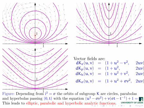
Vector fields are:dKe(u, v) = (1 + u2 − v2, 2uv)dKp(u, v) = (1 + u2, 2uv)dKh(u, v) = (1 + u2 + v2, 2uv)

dKσ(u, v) = (1 + u2 + σv2, 2uv)

Figure: Depending from i2 = σ the orbits of subgroup K are circles, parabolasand hyperbolas passing (0, t) with the equation (u2 − σv2) + v(σt− t−1) + 1 = 0.This leads to elliptic, parabolic and hyperbolic analytic functions.

1

1

1

1

1

1

Vector fields are:dKe(u, v) = (1 + u2 − v2, 2uv)dKp(u, v) = (1 + u2, 2uv)dKh(u, v) = (1 + u2 + v2, 2uv)

dKσ(u, v) = (1 + u2 + σv2, 2uv)

Figure: Depending from i2 = σ the orbits of subgroup K are circles, parabolasand hyperbolas passing (0, t) with the equation (u2 − σv2) + v(σt− t−1) + 1 = 0.This leads to elliptic, parabolic and hyperbolic analytic functions.

1

1

1

1

1

1

Vector fields are:dKe(u, v) = (1 + u2 − v2, 2uv)dKp(u, v) = (1 + u2, 2uv)dKh(u, v) = (1 + u2 + v2, 2uv)

dKσ(u, v) = (1 + u2 + σv2, 2uv)

Figure: Depending from i2 = σ the orbits of subgroup K are circles, parabolasand hyperbolas passing (0, t) with the equation (u2 − σv2) + v(σt− t−1) + 1 = 0.This leads to elliptic, parabolic and hyperbolic analytic functions.

Unification in higher dimensions

Figure: K-orbits as conic sections: elliptic case

Parabolic and hyperbolic sections

Figure: K-orbits as conic sections: parabolic and hyperbolic cases

The cone rotated as the whole

Figure: K-orbits as conic sections: a cone generator passing three orbits at thesame values of φ.

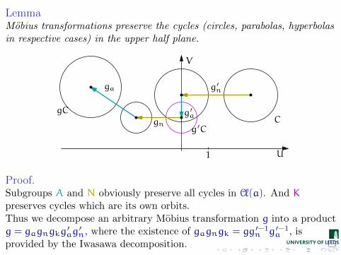
LemmaMobius transformations preserve the cycles (circles, parabolas, hyperbolasin respective cases) in the upper half plane.

1 U

V

g′n

g′a

gn

ga

Cg′C

gC

Proof.Subgroups A and N obviously preserve all cycles in C (a). And Kpreserves cycles which are its own orbits.Thus we decompose an arbitrary Mobius transformation g into a productg = gagngkg

′ag′n, where the existence of gagngk = gg ′−1

n g ′−1a , is

provided by the Iwasawa decomposition.

Fix subgroups of i, ε and j

1

1

1

1

1

1

K =

Çcos t − sin tsin t cos t

åN ′ =

Ç1 0t 1

åA ′ =

Çcosh t sinh tsinh t cosh t

åFix subgroups of (0, 1) are S(t) = exp

Ç0 σt

t 0

å, that is

K = exp

Ç0 −tt 0

å—elliptic, N ′ = exp

Ç0 0t 0

å—parabolic and

A ′ = exp

Ç0 t

t 0

å—hyperbolic cases.

Compactification of Re and Rp

Figure: Riemann sphere, stereographic projection and their paraboliccounterpart. Ideal elements (images of infinity) are shown in red. They are thepoint in the elliptic case and the line in the parabolic.

Compactification of Rh

Figure: Hyperbolic counterpart of the Riemann sphere (incomplete so far!) Idealelements for the light cone at infinity.In all EPH cases ideal points comprise the corresponding zero-radius cycle atinfinity.

Schwerdtfeger–Fillmore–Springer–CnopsConstruction

Cycles may be put to correspondence with certain matrices:

k(u2 − i2v2) − 2 〈(l,n), (u, v)〉+m = 0 ←→Çl+ ısn −mk −l+ ısn

å

ce

cpch

r0

ce

cp

ch

r1

A cycle is defined by four numbers(k, l,n,m) ∈ R4 up to a scalar fac-tor, i.e. this is a vector in a projec-tive space.For any such vector there three pos-sibility to draw a cycle as circle,parabola or hyperbola.

Its centre is at the point

Ål

k,−σ

n

k

ãFigure: Different EPH implementations of the same cycles

Cycles: Three Facesand two normalisations

We have the following maps between different faces of cycles:

P388

Q

xx

bbM

""Quadrics on Rσ oo Q◦M //M2(A)

We may try to make the correspondence 1-1, that is remove projectivityby normalisation. However this cannot be done globally.

DefinitionIf k 6= 0 we may use the leading normalisation: the quadruple to(1, lk , nk , mk ) with highlighted centre of a cycle. Moreover in this casedetCsσ is equal to the square of cycle radius.

Kirillov’s normalisation is give by detCsσ = 1. It highlights curvature andgives a nice condition for touching circles.

Foci of a cycleThen the classical invariants of a matrix (the trace and determinant) willrepresent some geometric invariants of cycles.

ce

fe

fp

fh

ce

fe

fp

fh

The determinant

Dσ = km− l2 + σn2

of matrix

Çl+ ısn −mk −l+ ısn

åplays

the important role.For example, foci of a cycle is defined

as

Ål

k,Dσk2

ã. Foci are defined by this

expression also for circles and hyper-bolas but are different from the clas-sic foci.

Figure: Foci of two parabolas with the same focal length.

Zero-radius cycles

Figure: Different σ-implementations of the same σ-zero-radius cycles, i.e.detCsσ = 0. Any implementation of p-zero-radius cycle touches the real line.The corresponding focus belongs to the real line as well. In the case σσ = 1zero-radius cycles are either point (elliptic case) or the light cone at the point.

Linearisation of Mobius maps

Theorem

Let a matrix M =

Ça b

c d

å∈ SL2(R) defines a Mobius transformation

M : (u+ iv)→ a(u+ iv) + b

c(u+ iv) + d.

Then any cycle C defined k(u2 − σv2) − 2lu− 2nv+m = 0 istransformed to a cycle C2 associated to the matrix MCM−1, where

C =

Çl+ ısn −mk −l+ ısn

å.

Proof.A proof can be done through algebraic manipulation by a CAS. Is thisthe ultimate goal of Descartes’ coordinate method?An alternative smart reasoning is based on the orthogonality of cycleswhich is described below.

Inner product and OrthogonalityThe orthogonality is defined by the condition:¨

Csσ, Csσ∂= 0, where

¨Csσ, Csσ

∂= < tr(CsσC

sσ).

which is Mobius invariant, since it is invariant under matrixconjugation.This is exactly the definition used in the GNS construction inC∗-algebras. The explicit expression for the inner product is:¨

Csσ, Csσ∂= 2σnn− 2ll+ km+ mk.

For matrices representing cycles we obtain the second classical invariant(determinant) under similarities from the first (trace) as follows:

〈Csσ,Csσ〉 = −2 detCsσ.

To describe ghost cycle we need the Heaviside function χ(σ):

χ(t) =

®1, t > 0;−1, t < 0.

Orthogonality of cyclesthe elliptic space

ab

c

d

σ = −1, σ = −1

1

1 ab

c

d

σ = −1, σ = 0

1

1 ab

c

d

σ = −1, σ = 1

1

1

TheoremA cycle is σ-orthogonal to cycle Csσ if it is orthogonal in the usual sense

to the σ-realisation of “ghost” cycle Csσ, which is defined by the followingtwo conditions:

1 χ(σ)-centre of Csσ coincides with σ-centre of Csσ.

2 Cycles Csσ and Csσ have the same roots, moreover

det C1σ = detC

χ(σ)σ .

Orthogonality of cycles in thehyperbolic space

a

b

cd

σ = 1, σ = −1

1

1 a

b

c

d

σ = 1, σ = 0

1

1 a

b

c

d

σ = 1, σ = 1

1

1

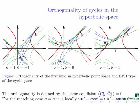
Figure: Orthogonality of the first kind in hyperbolic point space and EPH typeof the cycle space

The orthogonality is defined by the same condition¨Csσ, Csσ

∂= 0.

For the matching case σ = σ it is locally uu ′ − σvv ′ = uu ′ − vv ′ = 0.

Parabolic orthogonality of cycles

a

b

c

d

σ = 0, σ = −1

1

1

a

b

c

d

σ = 0, σ = 0

1

1

a

b

c

d

σ = 0, σ = 1

1

1

Figure: Orthogonality of the first kind in parabolic point space and EPH type ofthe cycle space. Note intersection of lines in the centre of the red parabola.

This orthogonality is defined by the same condition¨Csσ, Csσ

∂= 0.

It is not reduced locally to uu ′ = uu ′ − σvv ′ = 0.

Elliptic Inversion in a cycle

(a) (b)

Figure: The initial rectangular grid (a) is inverted elliptically in the unit circle(shown in red) on (b). The blue cycle (collapsed to a point at the origin on (b))represent the image of the cycle at infinity under inversion.

Parabolic and Hyperbolic Inversions

(c) (d)

Figure: The initial rectangular grid (a) is inverted in the unit circle parabolicallyon (c) and hyperbolically on (d). The blue cycle represent the image of the cycleat infinity under inversion.

Higher order invariantsFor any polynomial p(x1, x2, . . . , xn) of several non-commuting variablesone may define an invariant joint disposition of n cycles jCsσ by thecondition:

trp(1Csσ, 2Csσ, . . . ,nCsσ) = 0, (7)

there all cycles are used in Kirillov’s normalisation.It is clear, that the condition (7) is SL2(R)-invariant, i.e preserved by thetransformations Csσ 7→MCsσM

−1, M ∈ SL2(R). Moreover, in this matrixsimilarity we can replace element M ∈ SL2(R) by an arbitrary matrixcorresponding to another cycle:

LemmaThe product CsσC

sσCsσ is again the FSCc matrix of a cycle. This cycle

may be considered as the reflection of Csσ in Csσ.

RemarkWe can reduce the order of invariant (7) replacing some of cycles jCsσ bythe real line, which is SL2(R)-invariant as well.

Focal Orthogonalityand non-commutative behaviour

We illustrate the above construction by the following invariant of thirdorder which is obtained from some fourth order invariant by thereduction with real line.

DefinitionA cycle Csσ is f-orthogonal to a cycle Csσ if the reflection of Csσ in Csσ isorthogonal (in the previous sense) to the real line.Analytically this is defined by:

tr(CsσCsσCsσRsσ) = 0. (8)

RemarkIt is important to note that this is a non-commutative relation: there isC1 which is f-orthogonal to C2 but C2 is not f-orthogonal to C1. This willbe later a source of a non-commutative distance: |AB| 6= |BA|. As we willsee, this fancy distance still possesses a conformal property!

Focal Orthogonality (elliptic)

ab

c

d

σ = −1, σ = −1

1

1 ab

c

d

σ = −1, σ = 0

1

1 ab

c

d

σ = −1, σ = 1

1

1

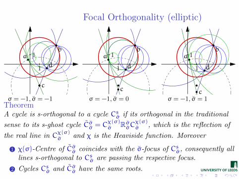
TheoremA cycle is s-orthogonal to a cycle Csσ if its orthogonal in the traditional

sense to its s-ghost cycle Cσσ = Cχ(σ)σ RσσC

χ(σ)σ , which is the reflection of

the real line in Cχ(σ)σ and χ is the Heaviside function. Moreover

1 χ(σ)-Centre of Cσσ coincides with the σ-focus of Csσ, consequently alllines s-orthogonal to Csσ are passing the respective focus.

2 Cycles Csσ and Cσσ have the same roots.

Focal Orthogonalityhyperbolic space

a

bc

d

σ = 1, σ = −1

1

1

a

b

c d

σ = 1, σ = 0

1

1

a

b

cd

σ = 1, σ = 1

1

1

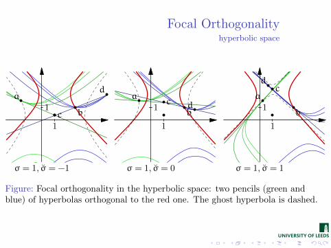
Figure: Focal orthogonality in the hyperbolic space: two pencils (green andblue) of hyperbolas orthogonal to the red one. The ghost hyperbola is dashed.

Focal Orthogonalityparabolic space

a

b

c

d

σ = 0, σ = −1

1

1

a

b

c

d

σ = 0, σ = 0

1

1

a

b

c

d

σ = 0, σ = 1

1

1

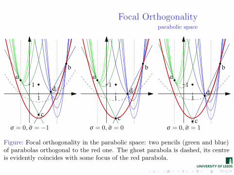
Figure: Focal orthogonality in the parabolic space: two pencils (green and blue)of parabolas orthogonal to the red one. The ghost parabola is dashed, its centreis evidently coincides with some focus of the red parabola.

Diameters and distances

DefinitionThe diameter of the cycle is determinant of its matrix.

(a)

z1z2 z3 z4

(b)

z1

z2

z3

z4

de

dp

Figure: (a) Square of the parabolic diameter is square of the distance betweenroots if they are real (z1 and z2), otherwise minus square of the distancebetween the adjoint roots (z3 and z4).(b) Distance as extremum in elliptic (z1 and z2) and parabolic (z3 and z4) cases.

Lengths from Centres and Foci

DefinitionA length of a directed interval AB is the half-diameter of a cycle witheph-centre or eph-focus at A passing B. There are 3× 3× 3× 2 = 54.

1

−ι

ιce

1

−ι

ι

fp

(a) (b)

(a) Concentricparabolas“shrinkingaround” ce .

(b) Co-focalparabolas“shrinkingaround” fp.

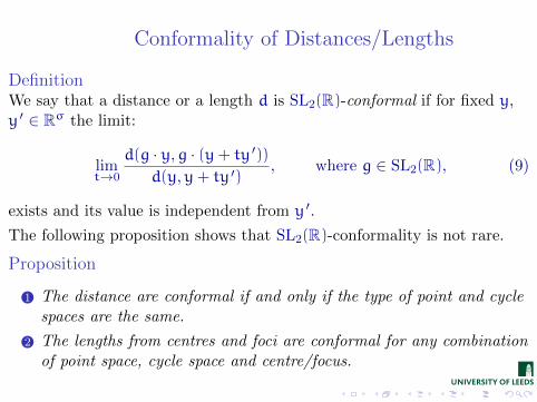
Conformality of Distances/Lengths

DefinitionWe say that a distance or a length d is SL2(R)-conformal if for fixed y,y ′ ∈ Rσ the limit:

limt→0

d(g · y,g · (y+ ty ′))d(y,y+ ty ′)

, where g ∈ SL2(R), (9)

exists and its value is independent from y ′.

The following proposition shows that SL2(R)-conformality is not rare.

Proposition

1 The distance are conformal if and only if the type of point and cyclespaces are the same.

2 The lengths from centres and foci are conformal for any combinationof point space, cycle space and centre/focus.

Isometric Action

Q. Is their a distance in the upper half-plane such that Mobiustransformations are isometries?A. Yes: d2(w1,w2) = F

((w1−w2)(w1−w2)

=w1·=w2

)Definition (L.M. Blumenthal)

Line is a curve such that distance is additive along it.

TheoremThe lines in parabolic geometry with the distance function

sin−1σ

|z−w|p

2√

=[z]=[w]are parabolas of the form (σ+ 4t2)u2 − 8tu− 4v+ 4 = 0,

where:

sin−1σ x =

sinh−1 x, if σ = −1.;2x, if σ = 0;sin−1 x, if σ = 1.

Parabolic Lines(sin(2 ∗ t), [cos(2 ∗ t), 0],−sin(2 ∗ t))

E

(−1 + 4 ∗ t2, [4 ∗ t, 2], 4)

PE

(sinh(2 ∗ t), [1.0 + 4 ∗ cosh(2 ∗ t), 0], sinh(2 ∗ t))

HS

(4 ∗ t2, [4 ∗ t, 2], 4)

PP

(1 + 4 ∗ t2, [4 ∗ t, 2], 4)

PH

(1, [t, 0], 1)

HT

Figure: Geodesics (blue) and equidistant orbits (green) in EPH geometries.

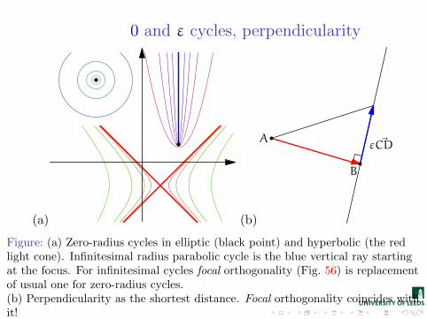
0 and ε cycles, perpendicularity

(a) (b)

A

B

ε ~CD

Figure: (a) Zero-radius cycles in elliptic (black point) and hyperbolic (the redlight cone). Infinitesimal radius parabolic cycle is the blue vertical ray startingat the focus. For infinitesimal cycles focal orthogonality (Fig. 56) is replacementof usual one for zero-radius cycles.(b) Perpendicularity as the shortest distance. Focal orthogonality coincides withit!

Cayley Transform and Unit “Circles”The colour code of ANK match to the model, where subgroup isdiagonalised.In elliptic case the standard Cayley transform diagonalises K:Çα β

β α

å=

1»1 − |u|2

Çeiω 00 e−iω

åÇ1 u

u 1

å, with

ω = argα,u = βα−1,

by

Ç1 ii 1

åand |u| < 1 follows from |α|2 − |β|2 = 1. i2 = −1. Cf. Figs. 6 and 1.

1

E : A

1

E : N

1

E : K

In hyperbolic case we analogously diagonalise A:Ça b−b a

å= |a|

(a|a| 0

0 a|a|

)Ç1 a−1b

−a−1b 1

åby

Ç1 i−i 1

å

1

H : A

1

H : N

1

H : K

However we could not deduce∣∣a−1b

∣∣ < 1 now! (Figure 1 cheats)

Geometry: R2 is not split by the unit circle into “interior” and “exterior”, see a movie;

Analysis: Hardy space is not a proper subset of L2;

Physics: Past and future could be reversed continuously.

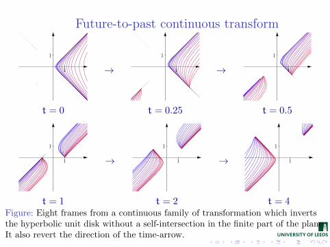
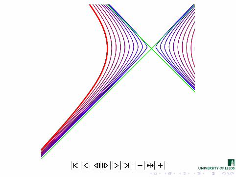
Future-to-past continuous transform

1

1

t = 0

→ 1

1

t = 0.25

→ 1

1

t = 0.5

1

1

t = 1

→ 1

1

t = 2

→ 1

1

t = 4Figure: Eight frames from a continuous family of transformation which invertsthe hyperbolic unit disk without a self-intersection in the finite part of the plane.It also revert the direction of the time-arrow.

Double cover of a hyperbolic plane

(a) C

E′

A ′

D ′

C ′

B ′

A ′′

D ′′

C ′′

E′′

A

B

1

1

1

1

(b) C

E′

A ′

D ′

C ′

B ′

A ′′

D ′′

C ′′

E′′

A

B

1

1

1

1

Figure: Hyperbolic objects in the double cover of Rh:(a) the “upper” half-plane;(b) the interior part of the unit circle.

Compactification of Rh

Figure: Hyperbolic counterpart of the Riemann sphere, complete this time!

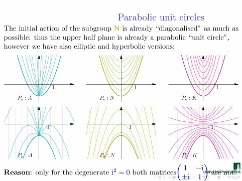
Parabolic unit circlesThe initial action of the subgroup N is already “diagonalised” as much aspossible: thus the upper half plane is already a parabolic “unit circle”,however we have also elliptic and hyperbolic versions:

1

Pe : A

1

Pe : N

1

Pe : K

1

Ph : A

1

Ph : N

1

Ph : K

Reason: only for the degenerate i2 = 0 both matrices

Ç1 −i±i 1

åare not!

1

E : A

1

E : N

1

E : K

1

Pe : A

1

Pe : N

1

Pe : K

1

Pp : A

1

Pp : N

1

Pp : K

1

Pp : A

1

Pp : N

1

Pp : K

1

Ph : A

1

Ph : N

1

Ph : K

1

H : A

1

H : N

1

H : K

1

−ι

ι

E : K

1

−ι

ι

P0

1

−ι

ι

H : A ′

1

−ι

ι

E : K

1

−ι

ι

P : N

1

−ι

ι

P : N ′

1

−ι

ι

H : A ′

Figure: Rotation as multiplication (the first row) and Mobius transformations(the second row). Orbits are level lines for the respective norm. Straight linesjoin points with the same value of “angle” (argument). Note that orbits of thesubgroup N are concentric parabolas and orbits of N ′—are co-focal ones. Theyare Cayley transforms of the fix subgroups of the point (0, 1) from Fig. 37

Induced RepresentationsLet G be a group, H its closed subgroup, χ be a linear representation ofH in a space V. The set of V-valued functions with the property

F(gh) = χ(h)F(g),

is invariant under left shifts.The restriction of the left regular representation to this space is called aninduced representation.Equivalently we consider the lifting of f(x), x ∈ X = G/H to F(g):

F(g) = χ(h)f(p(g)), p : G→ X, g = s(x)h, p(s(x)) = x.

This is a 1-1 map which transform the left regular representation on G tothe following action:

[ρ ′(g)f](x) = χ(h)f(g · x), where gs(x) = s(g · x)h.

In the case of SL2(R) we have three different types of actions.