SKYDIVING CONTROL SYSTEM

_______________________________________

A Thesis

presented to

the Faculty of the Graduate School

at the University of Missouri-Columbia

_______________________________________________________

In Partial Fulfillment

of the Requirements for the Degree

Master of Science

_____________________________________________________

by

CODY ALLARD

Dr. Ming Xin, Thesis Supervisor

JULY 2015

The undersigned, appointed by the dean of the Graduate School, have examined the thesis entitled

SKYDIVING CONTROL SYSTEM

presented by Cody Allard,

a candidate for the degree of master of science,

and hereby certify that, in their opinion, it is worthy of acceptance.

Professor Ming Xin

Professor Zaichun Feng

Professor Shi-Jie Chen

ii

ACKNOWLEDGEMENTS First and foremost I would like to thank my research advisor, Dr. Ming Xin, for

being an excellent advisor, professor, and companion throughout this unique research

project. I am thankful for him for accepting my offer to work with me and for being a

great partner in this project. I would like to thank another professor that had a large

impact on my education: Dr. Craig Kluever. He was an extremely influential professor

and was the one who sparked my interest in dynamic systems and control. Also, I would

like to thank the rest of the members on my defense committee for their time and

commitment to my education.

I would like to thank my family and friends who have supported me throughout

my entire academic career. I would like to specifically thank my parents; they have been

nothing but extremely supportive and have always placed education as a very high

importance in my life. And above all, I would like to thank my wife, Jordon, for all that

she has done for me throughout this process. I would not have been able to accomplish

my goals without her love and support.

iii

TABLE OF CONTENTS Acknowledgements………………………………………………………………………..ii List of Figures……………………………………………………………………...……...v List of Tables…………………………………………………………………………….vii Chapter

1. Introduction……………………………………………………………………1 Motivation……………………………………………………………………..1 Application…………………………………………………………………….2 Introduction to Skydiving……………………………………………………...3 Problem Statement……………….……………………………………………5 Project Goals………………………………………………………………….5

2. Design…………………………………………………………………………6 Preliminary Design……………………………………………………………6 Design Concept 1..…………………………………………………………….8 Design Concept 2…………………………………………………………….11 Design Concept 3…………………………………………………………….13 Design Selection……………………………………………………………...16

3. Dynamics and Stability………………………………………………………19 Body Fixed Coordinate Frame………………………………………………19 Local North-East-Down Reference Frame (NED)…………………………..20 Orientation Definitions………………………………………………………21 Governing Equations – Pitch Motion………………………………………..25 Governing Equations – Roll Motion…………………………………………33

iv

Governing Equations – Yaw Motion…………………………………………37 Governing Equations – Translational Motion……………………………….38 Definition of Constants – Pitch Motion……………………………………...40 Definition of Constants – Roll Motion……………………………………….41 Definition of Constants – Yaw Motion……………………………………….41 Definition of Constants – Translational Motion……………………………..42 Static and Dynamic Stability Analysis – Pitch and Roll Motion…………….42

4. Control……………………………………………………………………….46 Linearization…………………………………………………………………46 Introduction to Control………………………………………………………49 LQR Method………………………………………………………………….49 Pitch Control…………………………………………………………………50 Roll Control……………………………………….…………………………54 Yaw Control……………………………………….…………………………57 Translational Control………………………………………………………..61

5. Research Conclusion…………………………………………………………68

Research Limitations…………………………………….………………..…68 Future Work………………………………………………………………….68 Conclusion…………………………………………………………………...69

Bibliography……………………………………………………………………………..71

v

LIST OF FIGURES

Figure 1. A skydiver during free fall in stable orientation………………………………..4 Figure 2. Preliminary design of the Skydiving Control System…………………………...6 Figure 3. Preliminary design performing a maneuver using the control surfaces……….7 Figure 4. Translational motion maneuver in skydiving…………………………………..8 Figure 5. 3D rendering of the first design concept……………………………………….9 Figure 6. Visualization of a maneuver with the first design concept……………………10 Figure 7. 3D rendering of second design concept……………………………………….11 Figure 8. Visualization of a maneuver with the second design concept………………...12 Figure 9. 3D rendering of second design concept………………………………………14 Figure 10. Visualization of a maneuver of the third design concept……………………15 Figure 11. Definition of the body-fixed coordinate frame………………………………19 Figure 12. Definition of the NED coordinate frame [8]………………………………...21 Figure 13. Pitch angle definition………………………………………………………..23 Figure 14. Definition of the roll angle…………………………………………………...24 Figure 15. Definition of the yaw angle…………………………………………………..25 Figure 16. Free-body diagram for the pitch motion…………………………………….26 Figure 17. Definition of input angle, Gf……………………………………….………...29 Figure 18. Lift and drag coefficients with respect to the angle of attack [10]………….31 Figure 19. Lift and drag coefficients of circular flat plate with respect to […………...32 Figure 20. Free-body diagram of the roll motion……………………………………….34 Figure 21. Definition of left control surface input angle………………………………..36 Figure 22. Free-body diagram simulating the yaw motion……………………………..37

vi

Figure 23. Open loop response of pitch angle for stability analysis……………………44 Figure 24. Open loop response of roll angle for stability analysis……………………..45 Figure 25. Effect of linearization for the pitch motion………………………………….48 Figure 26. Comparing open loop and closed loop response of pitch motion……………53 Figure 27. Control input of the pitch motion…………………………………………….54 Figure 28. Comparing open loop and closed loop response of roll motion……………..56 Figure 29. Control input of the pitch motion…………………………………………….57 Figure 30. Visualization of the yaw control……………………………………………...58 Figure 31. Closed loop response of the yaw motion…………………………………….60 Figure 32. Control input of the yaw motion……………………………………………..61 Figure 33. Translational control – displacement from equilibrium……………………..64 Figure 34. Pitch angle response during translational control…………………………..65 Figure 35. Control input during translational control…………………………………..66

vii

LIST OF TABLES

Table 1. Pitch Motion Constants………………………………………………………..40 Table 2. Roll Motion Constants…………………………………………………………41 Table 3. Yaw Motion Constants…………………………………………………………42

1

Chapter 1: Introduction Motivation Albert Einstein once said, “If at first the idea is not absurd, then there is no hope

for it” [1]. This quote has a lot of meaning for scientists, engineers and explorers. For the

human race to progress and continue to innovate, we have to come up with novel and

“absurd” ideas. This has been true throughout our history. Humans have always been

trying to push the limits on human innovation and exploration. In particular, the

aerospace industry has been pushing the boundaries of our capabilities beginning with the

Wright Brothers building the first successful controllable and powered aircraft [2]. When

the Wright Brothers began their quest for flight, they were viewed as “crazy” and were

attempting the impossible. Now, airplanes are commonplace and we fly humans around

the world every day.

One goal of an engineer is to be a pioneer and create new and innovative

technology. The research project, Skydiving Control System, was sparked by a stunt

performed by an individual pushing the boundaries of human ability. On May 23rd 2012,

Gary Connery, a base jumper and stuntman, jumped from a helicopter at a height of 2,400

feet above the ground with a wingsuit, and landed in a pile of boxes without the aid of a

parachute [3]. After watching the video of this stunt, the idea of jumping out of airplanes

without the need of a parachute became extremely intriguing. Could a device be designed

to reliably guide a human occupant from an aircraft safely to the ground without the need

of a parachute? This is the question that this research project is attempting to answer.

2

Application

During certain tactical military situations, soldiers skydive out of aircrafts and

release their parachute between 1600 and 2000 feet. 1600 feet is considered the absolute

minimum altitude that a trained military skydiver must release their parachute, otherwise

the skydiver risks not having enough time for the parachute to fully deploy [4]. The

purpose of the parachute is for the obvious reason: to slow the skydiver to a speed that

would not injure the skydiver upon impact with the ground. Deploying the parachute

places the soldier in a vulnerable position against enemy forces. The skydiver is stuck in

a fixed speed downward motion, the enemy might spot the skydiver as a result of the

parachute being deployed, and the envelope or target that results from the parachute

being deployed is much larger than when the parachute is not deployed. All of these

factors create a need to solve this problem.

In addition to the military application, this would have recreational applications.

Skydiving is a sport and hobby for people who are seeking the thrill of extreme stunts.

Being able to skydive without deploying a parachute and landing into a foam pit or net

traveling at terminal velocity would certainly be an extreme thrill. Skydiving in this form

would be an addition to the skydiving industry and would help grow the market for

skydiving.

If this concept is successful in military and recreational applications, there could

also be an impact on the human transportation system. This concept of transporting

humans from aircraft in a precise manner could translate to the commercial airline

industry, where people could be dropped from airplanes at locations between the

departure and destination locations. This could decrease travel time, the number of

3

flights needed, and save money for both the consumer and the airline industry. Although

this concept is futuristic, it could be feasible. With all of the applications specified, there

is a necessity for exploring this concept.

Introduction to Skydiving

Humans have been skydiving from aircrafts practically ever since the aircraft was

developed. The concept of skydiving is relatively simple: a person leaps from a moving

aircraft, controls his/her position during free fall using aerodynamic forces on parts of

their body, and then deploys a parachute that slows them down to a safe speed to land on

the ground. The main development in skydiving has been in the parachute design;

innovation has been focused on the reliability of the parachutes, the maneuverability of

the parachutes, and the speed of deployment of parachutes. However, since this project

will be analyzing the possibility of skydiving without the use of a parachute, parachute

development will not be analyzed.

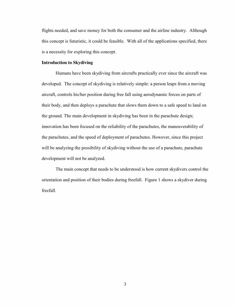
The main concept that needs to be understood is how current skydivers control the

orientation and position of their bodies during freefall. Figure 1 shows a skydiver during

freefall.

4

Figure 1. A skydiver during free fall in stable orientation

Figure 1 gives a good visualization of how skydiver uses aerodynamic forces to control

his/her orientation in space. A skydiver typically arches his/her back with feet and hands

behind his/her center of gravity. The reason for this is because if the person is perturbed

from his/her desired horizontal orientation, the arching of the back will create a restoring

torque and naturally return the skydiver to the desired horizontal orientation. Another

way that a skydiver controls his/her orientation and position in space is by changing the

location and orientation of their arms, legs, hands and feet. For example, a skydiver can

vector his/her hands in different directions to make minor adjustments of his/her

orientation.

In more advanced skydiving, maneuverability and precise attitude control is

implemented. This type of skydiving is called “formation skydiving.” Formation

skydiving involves multiple skydivers working in harmony to produce geometric patterns

and shapes [5]. This involves precise control of the individual skydivers because they

have to control their positions relative to other moving skydivers. Minor adjustments in

5

the skydiver’s appendages and center of gravity is crucial to ensuring proper execution of

these advanced maneuvers.

Problem Statement

Human skydivers have the ability to control their position and attitude in space

using the techniques discussed previously. This indicates that it would be possible to

design a system that imitates the control methods of skydivers. If an accurate and reliable

system could be developed, skydivers could skydive without a parachute; there could be a

net or foam pit in which the skydiver could land into. Therefore, to determine whether

this concept is feasible or not, research needs to be completed on a device that could

control the position and attitude of a human skydiver.

Project Goals

The overall goal of this research project, Skydiving Control System, is to develop

a method of transporting a free falling human from an aircraft without the use of a

parachute while retaining the similar method of control that skydivers use today to

control their orientation and position in the airspace. To accomplish this overarching

goal, a list of narrower goals have been developed that outlines the specific tasks needed.

The following is a list of goals for the research project:

1. Develop a design concept for a skydiving control system

2. Develop the equations of motion for the system

3. Analyze the static and dynamic stability of the system

4. Develop a control system for the pitch, roll and yaw motions

5. Develop a control system for the horizontal position of the system

This paper will step through the process and results from each goal.

6

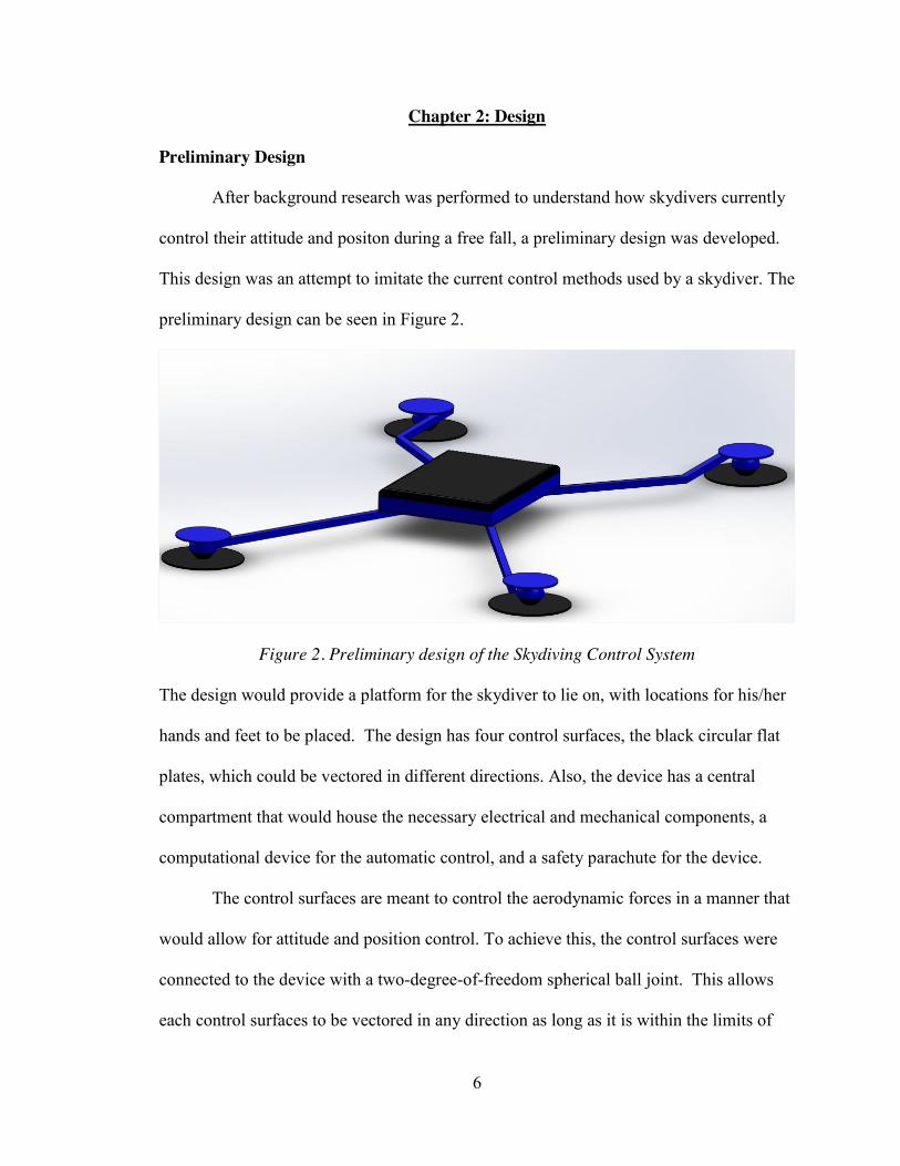
Chapter 2: Design

Preliminary Design

After background research was performed to understand how skydivers currently

control their attitude and positon during a free fall, a preliminary design was developed.

This design was an attempt to imitate the current control methods used by a skydiver. The

preliminary design can be seen in Figure 2.

Figure 2. Preliminary design of the Skydiving Control System

The design would provide a platform for the skydiver to lie on, with locations for his/her

hands and feet to be placed. The design has four control surfaces, the black circular flat

plates, which could be vectored in different directions. Also, the device has a central

compartment that would house the necessary electrical and mechanical components, a

computational device for the automatic control, and a safety parachute for the device.

The control surfaces are meant to control the aerodynamic forces in a manner that

would allow for attitude and position control. To achieve this, the control surfaces were

connected to the device with a two-degree-of-freedom spherical ball joint. This allows

each control surfaces to be vectored in any direction as long as it is within the limits of

7

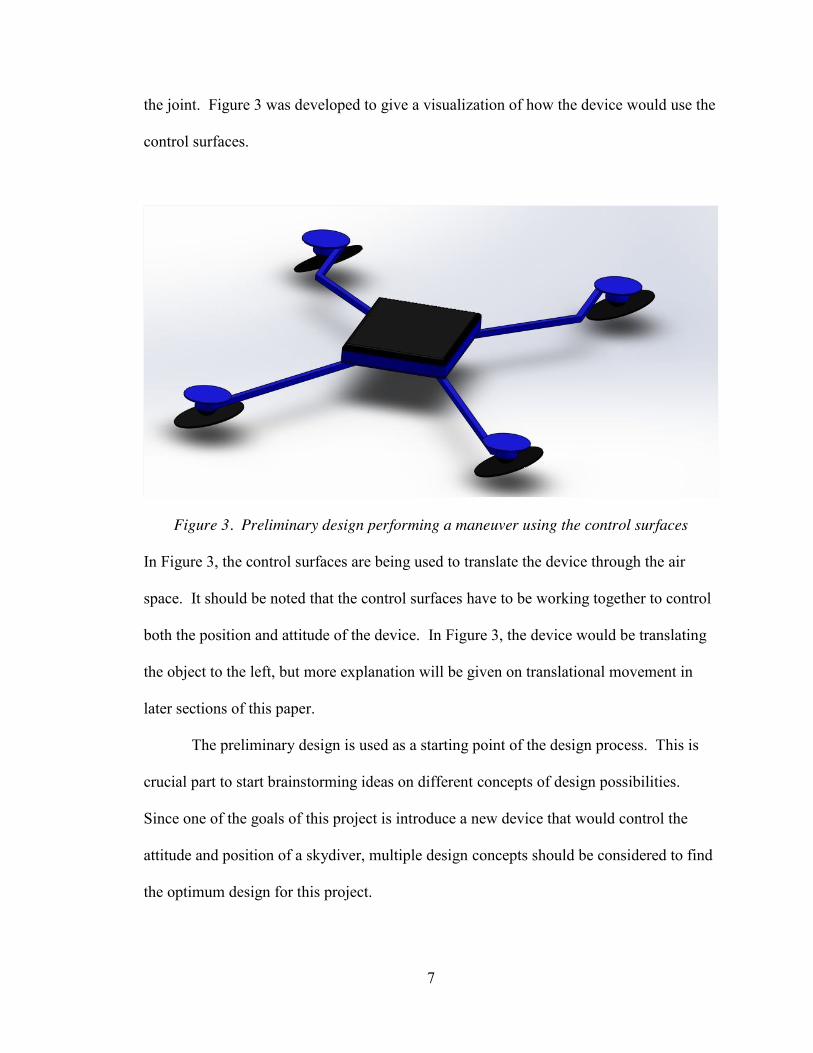
the joint. Figure 3 was developed to give a visualization of how the device would use the

control surfaces.

Figure 3. Preliminary design performing a maneuver using the control surfaces

In Figure 3, the control surfaces are being used to translate the device through the air

space. It should be noted that the control surfaces have to be working together to control

both the position and attitude of the device. In Figure 3, the device would be translating

the object to the left, but more explanation will be given on translational movement in

later sections of this paper.

The preliminary design is used as a starting point of the design process. This is

crucial part to start brainstorming ideas on different concepts of design possibilities.

Since one of the goals of this project is introduce a new device that would control the

attitude and position of a skydiver, multiple design concepts should be considered to find

the optimum design for this project.

8

Design Concept 1

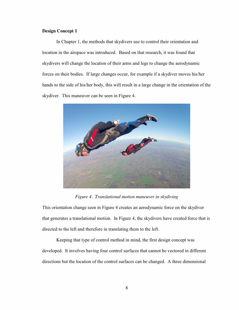
In Chapter 1, the methods that skydivers use to control their orientation and

location in the airspace was introduced. Based on that research, it was found that

skydivers will change the location of their arms and legs to change the aerodynamic

forces on their bodies. If large changes occur, for example if a skydiver moves his/her

hands to the side of his/her body, this will result in a large change in the orientation of the

skydiver. This maneuver can be seen in Figure 4.

Figure 4. Translational motion maneuver in skydiving

This orientation change seen in Figure 4 creates an aerodynamic force on the skydiver

that generates a translational motion. In Figure 4, the skydivers have created force that is

directed to the left and therefore in translating them to the left.

Keeping that type of control method in mind, the first design concept was

developed. It involves having four control surfaces that cannot be vectored in different

directions but the location of the control surfaces can be changed. A three dimensional

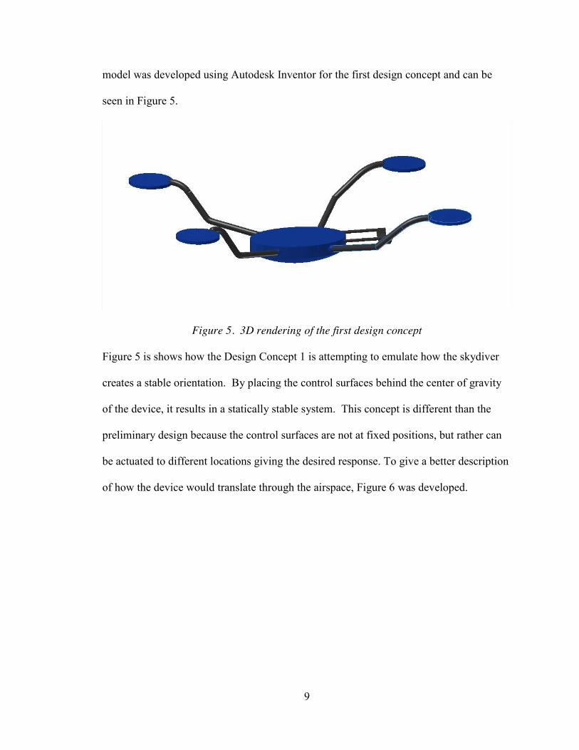
9

model was developed using Autodesk Inventor for the first design concept and can be

seen in Figure 5.

Figure 5. 3D rendering of the first design concept

Figure 5 is shows how the Design Concept 1 is attempting to emulate how the skydiver

creates a stable orientation. By placing the control surfaces behind the center of gravity

of the device, it results in a statically stable system. This concept is different than the

preliminary design because the control surfaces are not at fixed positions, but rather can

be actuated to different locations giving the desired response. To give a better description

of how the device would translate through the airspace, Figure 6 was developed.

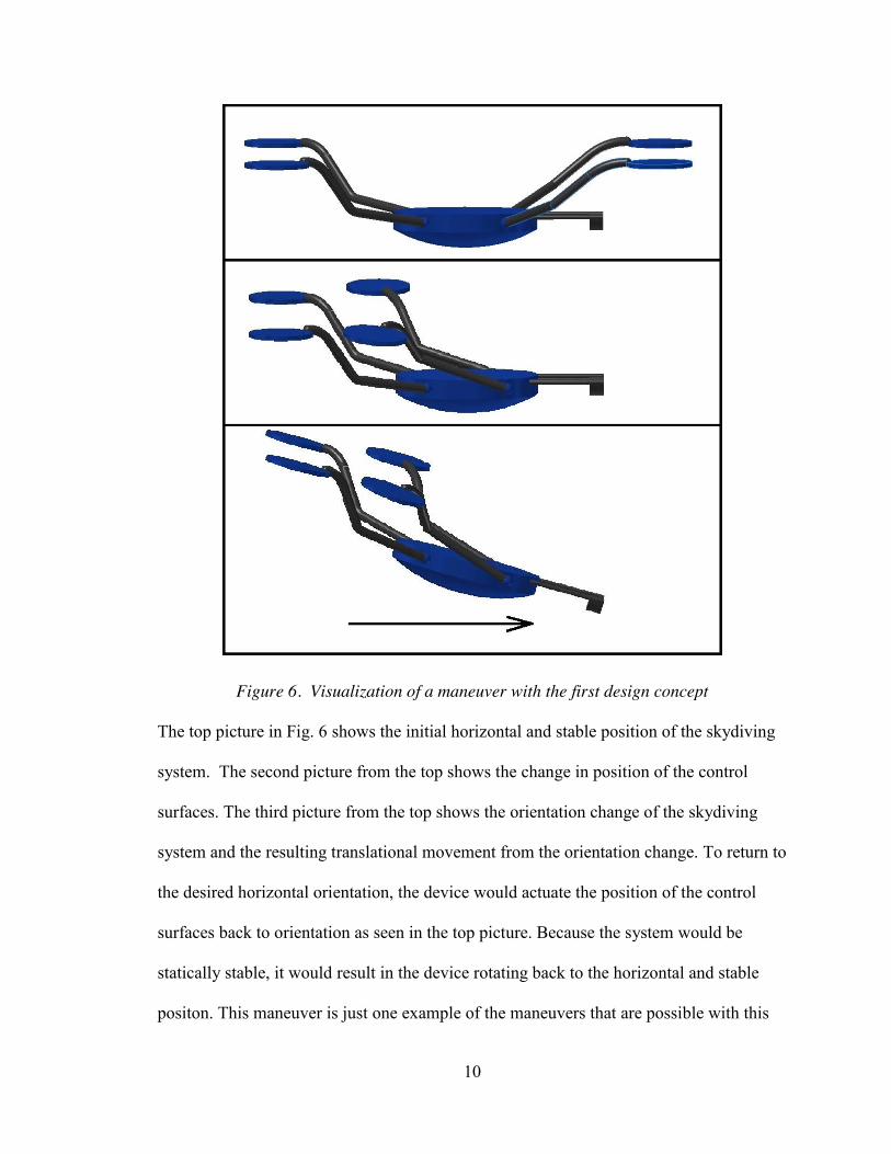
10

Figure 6. Visualization of a maneuver with the first design concept

The top picture in Fig. 6 shows the initial horizontal and stable position of the skydiving

system. The second picture from the top shows the change in position of the control

surfaces. The third picture from the top shows the orientation change of the skydiving

system and the resulting translational movement from the orientation change. To return to

the desired horizontal orientation, the device would actuate the position of the control

surfaces back to orientation as seen in the top picture. Because the system would be

statically stable, it would result in the device rotating back to the horizontal and stable

positon. This maneuver is just one example of the maneuvers that are possible with this

11

device. The control surfaces could be actuated in different locations to create different

responses.

Design Concept 2

The first design concept was developed by considering a control technique

currently used by skydivers. Another type of control introduced in Chapter 1 is when

skydivers vector their hands in different directions, while keeping their hands in the same

location, to produce a minor change in their attitude and position. With this type of

control in mind, the second design concept was developed. This design concept is similar

to the design concept as seen in the preliminary design. It would have four control

surfaces that are at fixed locations but can be vectored in different directions to control

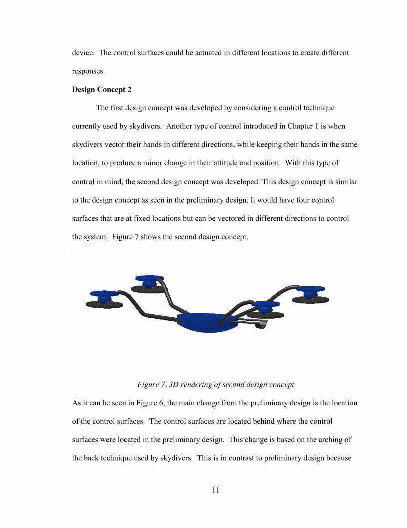
the system. Figure 7 shows the second design concept.

Figure 7. 3D rendering of second design concept

As it can be seen in Figure 6, the main change from the preliminary design is the location

of the control surfaces. The control surfaces are located behind where the control

surfaces were located in the preliminary design. This change is based on the arching of

the back technique used by skydivers. This is in contrast to preliminary design because

12

the control surfaces are located in front of the center of gravity of the skydiver/device

system which would result in instability of the system.

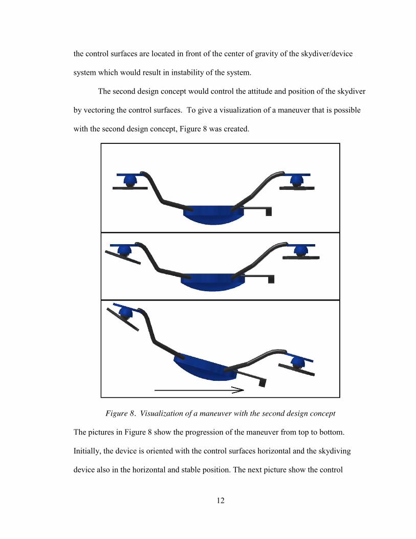
The second design concept would control the attitude and position of the skydiver

by vectoring the control surfaces. To give a visualization of a maneuver that is possible

with the second design concept, Figure 8 was created.

Figure 8. Visualization of a maneuver with the second design concept

The pictures in Figure 8 show the progression of the maneuver from top to bottom.

Initially, the device is oriented with the control surfaces horizontal and the skydiving

device also in the horizontal and stable position. The next picture show the control

13

surfaces have changed orientation to create rotation of the device. The last picture shows

the device has been rotated which results in the device to translate in the direction

indicated by the arrow in Figure 8. Again, this is just one example of a maneuver that is

possible with this design.

Design Concept 3

The first and second design concepts were attempting to emulate the current

control methods that skydivers use to control their orientation and position in the

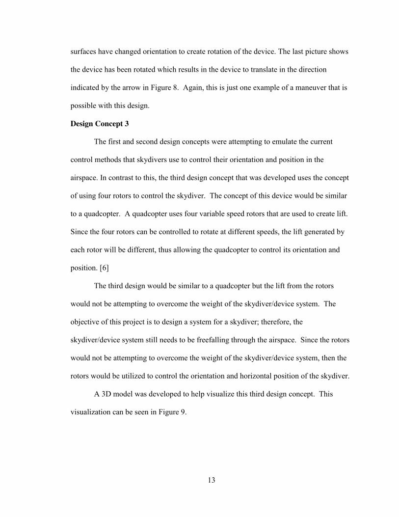
airspace. In contrast to this, the third design concept that was developed uses the concept

of using four rotors to control the skydiver. The concept of this device would be similar

to a quadcopter. A quadcopter uses four variable speed rotors that are used to create lift.

Since the four rotors can be controlled to rotate at different speeds, the lift generated by

each rotor will be different, thus allowing the quadcopter to control its orientation and

position. [6]

The third design would be similar to a quadcopter but the lift from the rotors

would not be attempting to overcome the weight of the skydiver/device system. The

objective of this project is to design a system for a skydiver; therefore, the

skydiver/device system still needs to be freefalling through the airspace. Since the rotors

would not be attempting to overcome the weight of the skydiver/device system, then the

rotors would be utilized to control the orientation and horizontal position of the skydiver.

A 3D model was developed to help visualize this third design concept. This

visualization can be seen in Figure 9.

14

Figure 9. 3D rendering of second design concept

In Figure 9, the four independently controlled rotors can be seen. These rotors are at

fixed locations, cannot be vectored in different directions, but the rotor speeds can be

changed. The rotors are placed behind the center of gravity of the skydiver/device

system to make the system naturally stable. Placing the rotors behind the center of

gravity of the system is common in quadcopters to increase stability [6].

The spinning rotors could be used to control the orientation and positon of the

skydiver/device system. Figure 10 was developed to give a visualization of a maneuver

of the third design concept.

15

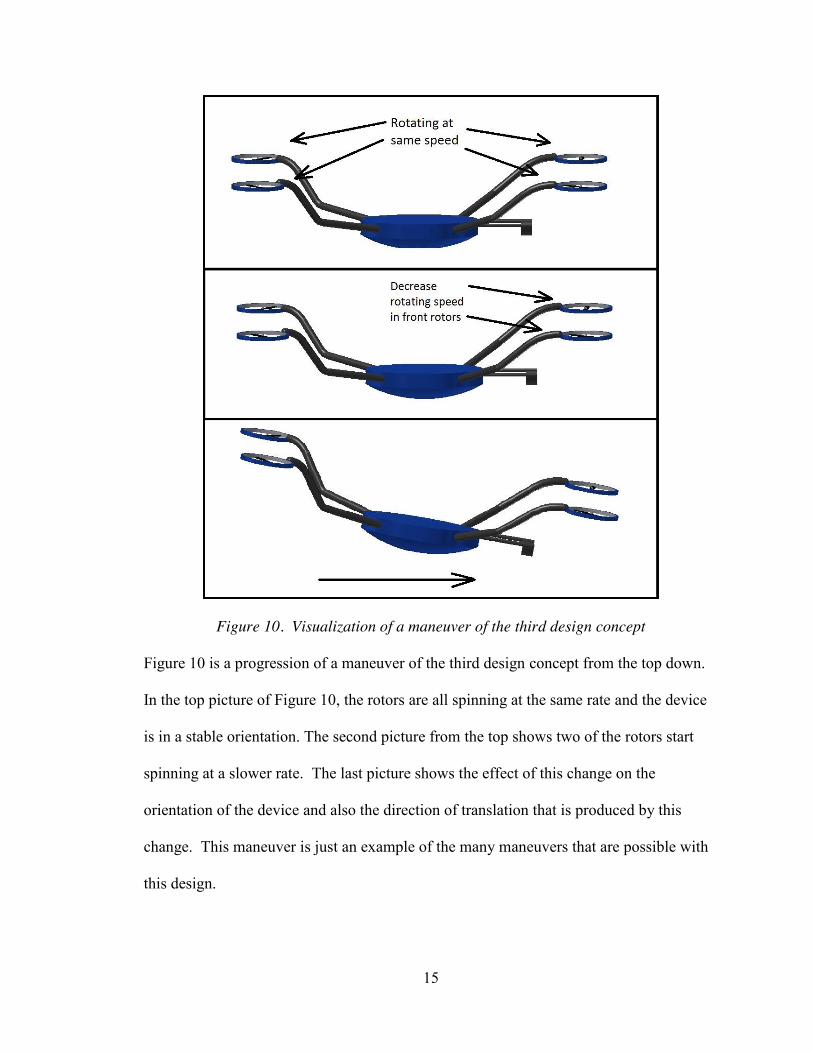
Figure 10. Visualization of a maneuver of the third design concept

Figure 10 is a progression of a maneuver of the third design concept from the top down.

In the top picture of Figure 10, the rotors are all spinning at the same rate and the device

is in a stable orientation. The second picture from the top shows two of the rotors start

spinning at a slower rate. The last picture shows the effect of this change on the

orientation of the device and also the direction of translation that is produced by this

change. This maneuver is just an example of the many maneuvers that are possible with

this design.

16

Design Selection

Three design concepts have been developed and explained but now need to be

analyzed to determine the optimum design for this project. Each design has positive and

negative attributes; therefore, a list of positive and negative attributes for each design was

developed.

The first design concept is the design that has four control surfaces that cannot be

vectored but the location of the control surfaces can be changed. The following is a list

of the positive attributes of the first design concept:

1. Emulates a current control method used by skydivers

2. Has high maneuverability capabilities

3. Has a wide range of response possibilities

4. Does not require thrust or rotors to generate movement

In contrast to the positive attributes, the first design also has the following negative

attributes:

1. Actuation of the location of the control surfaces would be difficult to

implement

2. Skydiver would be moving along with the actuating arms, therefore it could

be uncomfortable to the skydiver

From analyzing the positive and negative attributes of the first design concept, the

negative attributes are outweighing the positive attributes. The possibility of the skydiver

being uncomfortable is a large concern. The comfort of the user is extremely important

in this design. Also, the difficulty of implementation of the actuators controlling the

location of the control surfaces is alarming.

17

The list of positive and negative attributes of the second design concept was

developed. The following is a list of the positive attributes:

1. Emulates a current control method used by skydivers

2. Keeps the skydiver in a fixed position during flight

3. Has a wide range of response possibilities

4. Does not require thrust or rotors to generate movement

The following is a list of the negative attributes:

1. Not as maneuverable as the other design concepts

Although the maneuverability is an important factor to consider, the second design

concept has more positive attributes than negative attributes. The positive and negative

attributes of the third design need to be introduced to discuss the decision for the final

design. The following is a list of the positive attributes of the third design:

1. Has high maneuverability capabilities

2. The air velocity direction would have less of an effect on this design

3. Control would be similar to the widely-used control of quadcopters

The following is a list of the negative attributes

1. Design has high frequency rotating parts

2. Does not emulate current control methods used by skydivers

Now that all of the design concepts have been analyzed based on their positive

and negative attributes, a decision on what design concept would be best for this project

can be reached. The first design concept has two particularly alarming negative attributes

and should not be considered. Therefore, the discussion is limited to design concept two

and three. The main difference between the two design concepts is that design concept

18

three has high frequency rotating parts and design concept two does not. This is an

important characteristic to consider because of mechanical reliability. Design concept

two would be more mechanically reliable. Also, because design concept three does not

emulate current control by skydivers, it does not seem as appropriate for this project as

design concept two. Design concept three does not seem as good of a fit for this project.

Therefore, design concept two was chosen. For the remainder of this paper, design

concept two will be the device that is being considered.

19

Chapter 3: Dynamics and Stability

Body Fixed Coordinate Frame

The skydiver/device system is assumed to be a rigid body that will be rotating and

translating through the airspace. The orientation of the system will have an effect on the

translational motion therefore this system could not be considered a point mass. A

coordinate system needs to be introduced to describe the orientation of the system. This

coordinate frame will be called the body-fixed coordinate frame. This coordinate frame

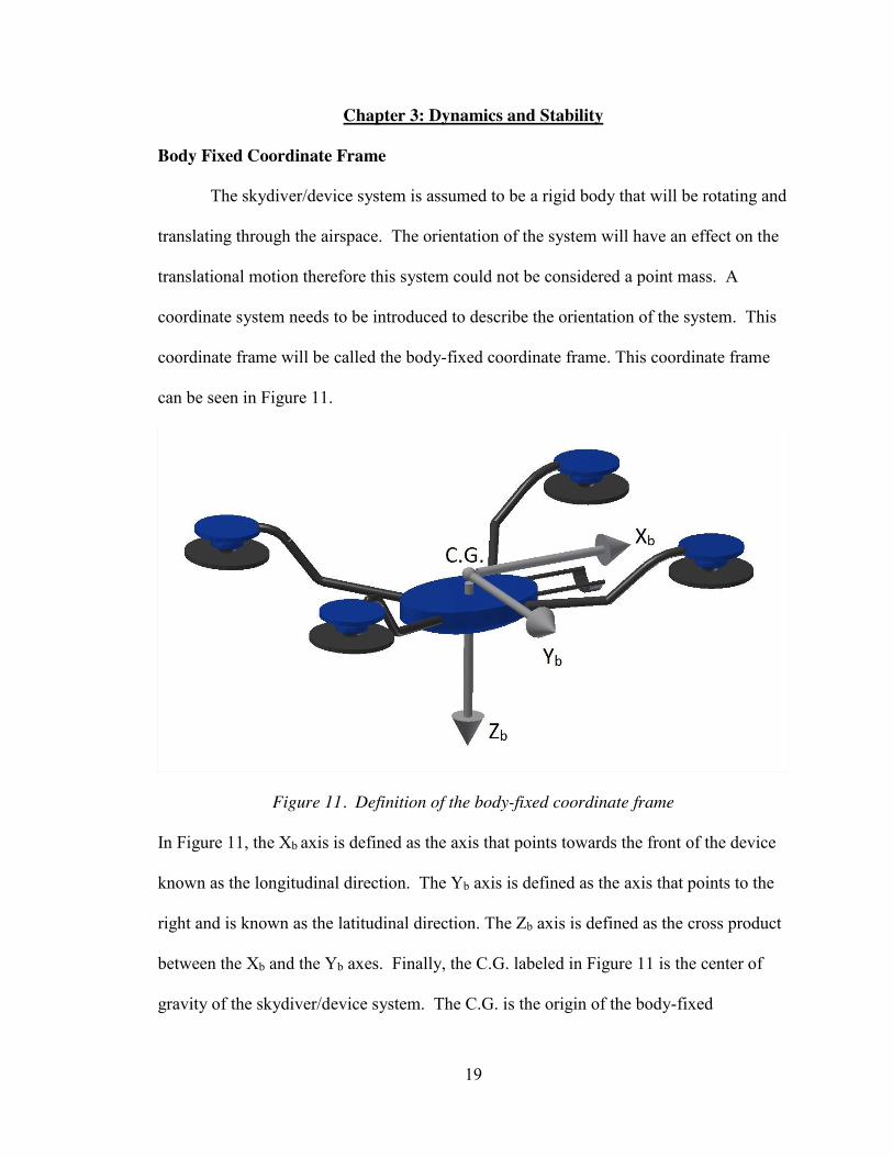
can be seen in Figure 11.

Figure 11. Definition of the body-fixed coordinate frame

In Figure 11, the Xb axis is defined as the axis that points towards the front of the device

known as the longitudinal direction. The Yb axis is defined as the axis that points to the

right and is known as the latitudinal direction. The Zb axis is defined as the cross product

between the Xb and the Yb axes. Finally, the C.G. labeled in Figure 11 is the center of

gravity of the skydiver/device system. The C.G. is the origin of the body-fixed

20

coordinate frame. This body-fixed coordinate frame is similar to most body-fixed

coordinate frame definitions in aviation [7].

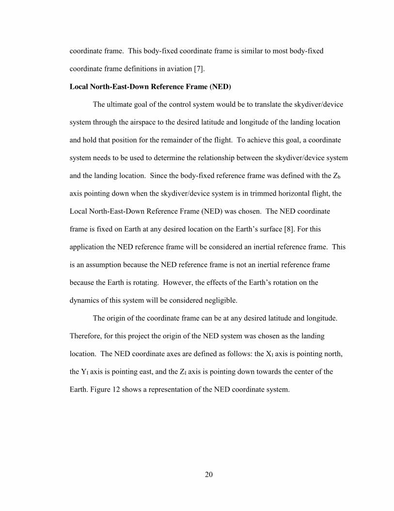
Local North-East-Down Reference Frame (NED)

The ultimate goal of the control system would be to translate the skydiver/device

system through the airspace to the desired latitude and longitude of the landing location

and hold that position for the remainder of the flight. To achieve this goal, a coordinate

system needs to be used to determine the relationship between the skydiver/device system

and the landing location. Since the body-fixed reference frame was defined with the Zb

axis pointing down when the skydiver/device system is in trimmed horizontal flight, the

Local North-East-Down Reference Frame (NED) was chosen. The NED coordinate

frame is fixed on Earth at any desired location on the Earth’s surface [8]. For this

application the NED reference frame will be considered an inertial reference frame. This

is an assumption because the NED reference frame is not an inertial reference frame

because the Earth is rotating. However, the effects of the Earth’s rotation on the

dynamics of this system will be considered negligible.

The origin of the coordinate frame can be at any desired latitude and longitude.

Therefore, for this project the origin of the NED system was chosen as the landing

location. The NED coordinate axes are defined as follows: the XI axis is pointing north,

the YI axis is pointing east, and the ZI axis is pointing down towards the center of the

Earth. Figure 12 shows a representation of the NED coordinate system.

21

Figure 12. Definition of the NED coordinate frame [8]

Orientation Definitions

Now that the coordinate frames have been developed, the variables that will

define the orientation and position of the skydiver/device system need to be explained.

The orientation of the skydiver/device system is the relationship between the body-fixed

coordinate frame and inertial NED coordinate frame. The method in quantifying this

relationship typically uses Euler Angles. Euler Angles are angles that are developed by

performing three successive rotations from one reference frame to another. The symbols

for the Euler Angles are T, I, and \. In aviation, it is typical to use a 3-2-1 Euler Angle

rotation sequence [7]. This means that the inertial reference frame is first rotated through

an angle of \ about the ZI axis. This defines a new coordinate frame R1. The next

rotation is taking the R1 reference frame and rotating it through an angle of T about the Y

22

axis of R1. This defines a new coordinate frame R2. Finally, the reference frame R2 is

rotated through an angle of I about the X axis of R2 until R2 is aligned with the body-

fixed coordinate frame. Performing these rotations defines the orientation of the aircraft

with respect to the inertial reference frame by the Euler Angles T, I, and \ [9].

Now that the Euler Angles have been introduced, it is important to introduce

terminology surrounding the Euler Angles in aviation. When a 3-2-1 rotation sequence is

used the T angle is known as the pitch angle. Therefore, a rotation about the Yb axis is

defined as the pitch motion. The I angle is known as the roll angle; a rotation about the

Xb axis is defined as the roll motion. Finally, the \ angle is known as the yaw angle and a

rotation about the Zb axis is known as the yaw motion.

When developing the goals of this research project it was determined that the

pitch, roll and yaw motions would be analyzed separately. This is common practice

when first developing the natural dynamics of a new system in aviation [7]. In reality,

the skydiver/device system will be pitching, rolling and yawing simultaneously and these

motions will have effect on each other. In the future the pitch, roll and yaw motions could

be placed in a higher fidelity model that would include the coupling dynamics. The

impact of this assumption simplifies the Euler Angle definitions, and the Euler Angles

can be visualized. This is generally not the case because as discussed earlier, each Euler

Angle is actually defined in a different reference frame.

The first motion that will be analyzed in this project is the pitch motion, therefore

the definition of the pitch angle for the skydiving control system will be introduced first.

The pitch angle definition can be seen in Figure 13.

23

Figure 13. Pitch angle definition

As it can be seen in Figure 13, since the pitch motion is considered separately, the pitch

angle can be directly defined as the angle between the ZI axis and the Zb axis. Again, if

the roll and yaw angles were not considered to be zero, then this Euler Angle T could not

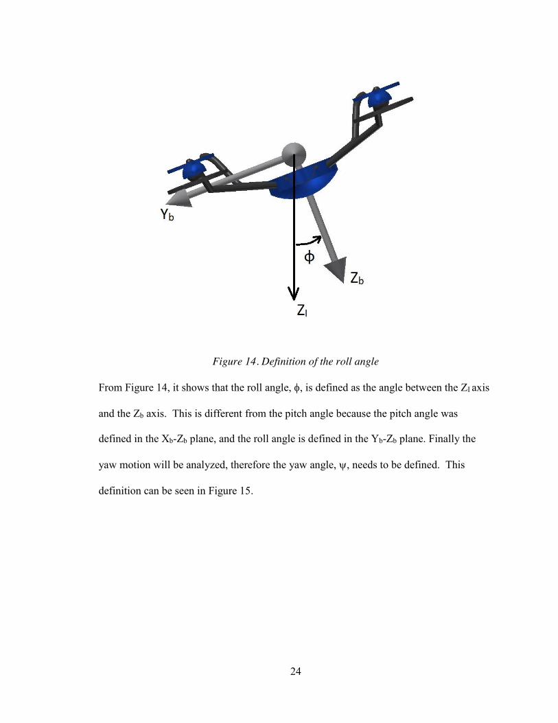
be defined as it has been in Figure 13. Next the roll motion will be analyzed, and the

definition of the roll angle, I, can be seen in Figure 14.

24

Figure 14. Definition of the roll angle

From Figure 14, it shows that the roll angle, I, is defined as the angle between the ZI axis

and the Zb axis. This is different from the pitch angle because the pitch angle was

defined in the Xb-Zb plane, and the roll angle is defined in the Yb-Zb plane. Finally the

yaw motion will be analyzed, therefore the yaw angle, \, needs to be defined. This

definition can be seen in Figure 15.

25

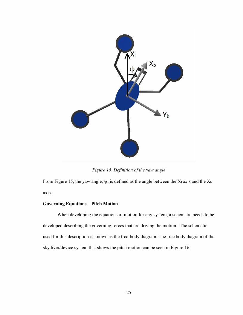
Figure 15. Definition of the yaw angle

From Figure 15, the yaw angle, \, is defined as the angle between the XI axis and the Xb

axis.

Governing Equations – Pitch Motion

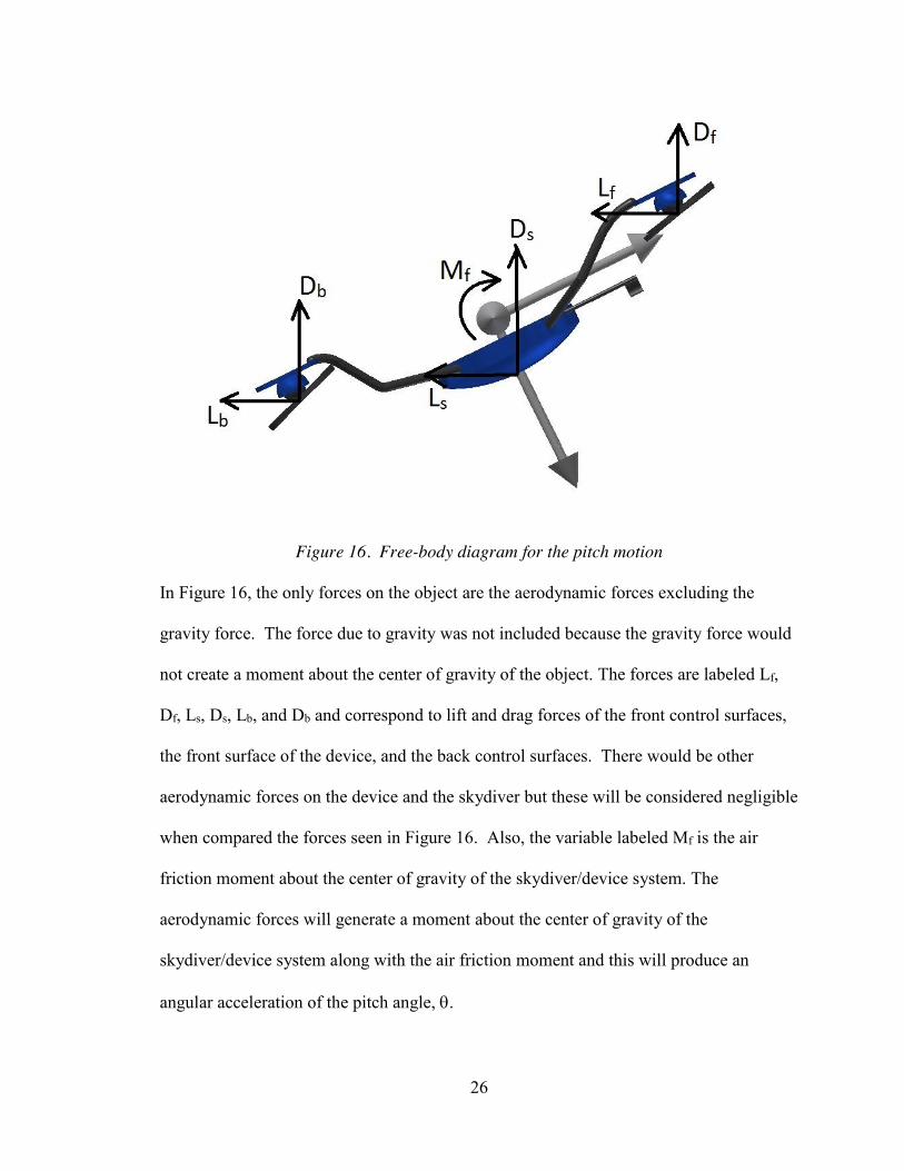
When developing the equations of motion for any system, a schematic needs to be

developed describing the governing forces that are driving the motion. The schematic

used for this description is known as the free-body diagram. The free body diagram of the

skydiver/device system that shows the pitch motion can be seen in Figure 16.

26

Figure 16. Free-body diagram for the pitch motion

In Figure 16, the only forces on the object are the aerodynamic forces excluding the

gravity force. The force due to gravity was not included because the gravity force would

not create a moment about the center of gravity of the object. The forces are labeled Lf,

Df, Ls, Ds, Lb, and Db and correspond to lift and drag forces of the front control surfaces,

the front surface of the device, and the back control surfaces. There would be other

aerodynamic forces on the device and the skydiver but these will be considered negligible

when compared the forces seen in Figure 16. Also, the variable labeled Mf is the air

friction moment about the center of gravity of the skydiver/device system. The

aerodynamic forces will generate a moment about the center of gravity of the

skydiver/device system along with the air friction moment and this will produce an

angular acceleration of the pitch angle, T.

27

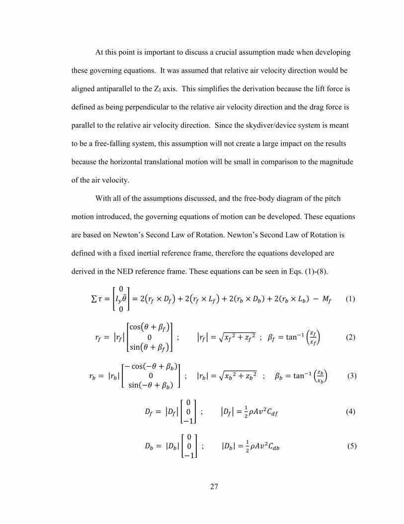
At this point is important to discuss a crucial assumption made when developing

these governing equations. It was assumed that relative air velocity direction would be

aligned antiparallel to the ZI axis. This simplifies the derivation because the lift force is

defined as being perpendicular to the relative air velocity direction and the drag force is

parallel to the relative air velocity direction. Since the skydiver/device system is meant

to be a free-falling system, this assumption will not create a large impact on the results

because the horizontal translational motion will be small in comparison to the magnitude

of the air velocity.

With all of the assumptions discussed, and the free-body diagram of the pitch

motion introduced, the governing equations of motion can be developed. These equations

are based on Newton’s Second Law of Rotation. Newton’s Second Law of Rotation is

defined with a fixed inertial reference frame, therefore the equations developed are

derived in the NED reference frame. These equations can be seen in Eqs. (1)-(8).

∑ 𝜏 = [0

𝐼𝑦��0

] = 2(𝑟𝑓 × 𝐷𝑓) + 2(𝑟𝑓 × 𝐿𝑓) + 2(𝑟𝑏 × 𝐷𝑏) + 2(𝑟𝑏 × 𝐿𝑏) − 𝑀𝑓 (1)

𝑟𝑓 = |𝑟𝑓| [cos(𝜃 + 𝛽𝑓)

0sin(𝜃 + 𝛽𝑓)

] ; |𝑟𝑓| = √𝑥𝑓2 + 𝑧𝑓

2 ; 𝛽𝑓 = tan−1 (𝑧𝑓

𝑥𝑓) (2)

𝑟𝑏 = |𝑟𝑏| [− cos(−𝜃 + 𝛽𝑏)

0sin(−𝜃 + 𝛽𝑏)

] ; |𝑟𝑏| = √𝑥𝑏2 + 𝑧𝑏

2 ; 𝛽𝑏 = tan−1 (𝑧𝑏𝑥𝑏

) (3)

𝐷𝑓 = |𝐷𝑓| [00

−1] ; |𝐷𝑓| = 1

2𝜌𝐴𝑣2𝐶𝑑𝑓 (4)

𝐷𝑏 = |𝐷𝑏| [00

−1] ; |𝐷𝑏| = 1

2𝜌𝐴𝑣2𝐶𝑑𝑏 (5)

28

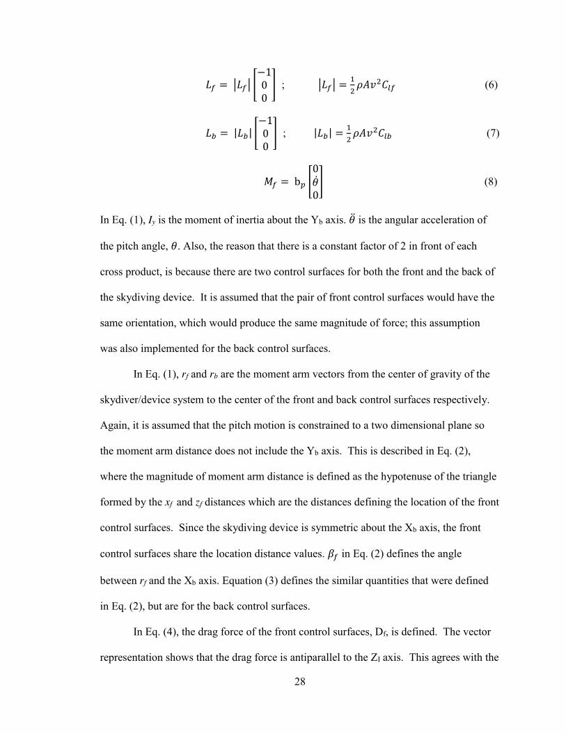
𝐿𝑓 = |𝐿𝑓| [−100

] ; |𝐿𝑓| = 12

𝜌𝐴𝑣2𝐶𝑙𝑓 (6)

𝐿𝑏 = |𝐿𝑏| [−100

] ; |𝐿𝑏| = 12

𝜌𝐴𝑣2𝐶𝑙𝑏 (7)

𝑀𝑓 = b𝑝 [0��0

] (8)

In Eq. (1), Iy is the moment of inertia about the Yb axis. �� is the angular acceleration of

the pitch angle, 𝜃. Also, the reason that there is a constant factor of 2 in front of each

cross product, is because there are two control surfaces for both the front and the back of

the skydiving device. It is assumed that the pair of front control surfaces would have the

same orientation, which would produce the same magnitude of force; this assumption

was also implemented for the back control surfaces.

In Eq. (1), rf and rb are the moment arm vectors from the center of gravity of the

skydiver/device system to the center of the front and back control surfaces respectively.

Again, it is assumed that the pitch motion is constrained to a two dimensional plane so

the moment arm distance does not include the Yb axis. This is described in Eq. (2),

where the magnitude of moment arm distance is defined as the hypotenuse of the triangle

formed by the xf and zf distances which are the distances defining the location of the front

control surfaces. Since the skydiving device is symmetric about the Xb axis, the front

control surfaces share the location distance values. 𝛽𝑓 in Eq. (2) defines the angle

between rf and the Xb axis. Equation (3) defines the similar quantities that were defined

in Eq. (2), but are for the back control surfaces.

In Eq. (4), the drag force of the front control surfaces, Df, is defined. The vector

representation shows that the drag force is antiparallel to the ZI axis. This agrees with the

29

assumption of the relative air velocity direction be aligned antiparallel to the ZI axis.

Also, in Eq. (4), the magnitude of the drag force is represented. The drag force depends

on the air density, 𝜌, the control surface area, 𝐴, the magnitude of the air velocity, 𝑣, and

the coefficient of the drag force for the front control surfaces, 𝐶𝑑𝑓. All of the parameters

are assumed to be constant except for the drag coefficient. The drag coefficient depends

on the orientation of the control surface with respect to the relative air velocity direction.

Since the control surfaces can be vectored in different directions to control the device, the

drag coefficient is not only a function of the pitch angle but also the input angle of the

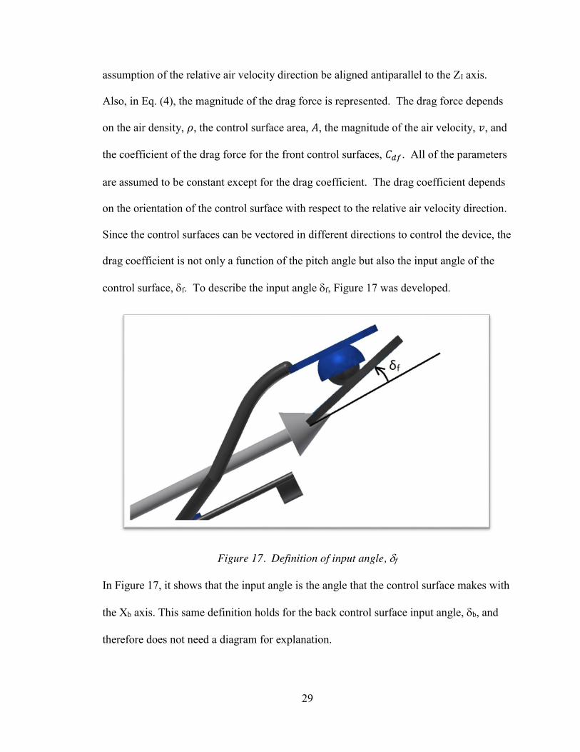
control surface, Gf. To describe the input angle Gf, Figure 17 was developed.

Figure 17. Definition of input angle, Gf

In Figure 17, it shows that the input angle is the angle that the control surface makes with

the Xb axis. This same definition holds for the back control surface input angle, Gb, and

therefore does not need a diagram for explanation.

30

The pitch angle and input angle have been defined, therefore the drag coefficient

that is in terms of both the pitch and input angle can be developed. In most aviation

applications, the lift and drag coefficients are based on aerodynamic surfaces. These

aerodynamic surfaces are shaped in a way to produce the desired lift and drag

characteristics. For example, the wing cross section known as the airfoil, is shaped in

different ways to produce the desired aerodynamics. However, for this project the

skydiving control system does not use the aerodynamics forces in the same way that an

airplane does. The skydiving control system is a free-falling object that is using non-

aerodynamic flat plates as the control surfaces to balance the forces on the

skydiver/device system. Since, this system does not use typical control surfaces that are

used in aviation, the drag coefficient of a circular flat plate has not been rigorously

analyzed. After researching, a graph of the lift and drag coefficients for a circular flat

plate was found. This relationship can be seen in Figure 18.

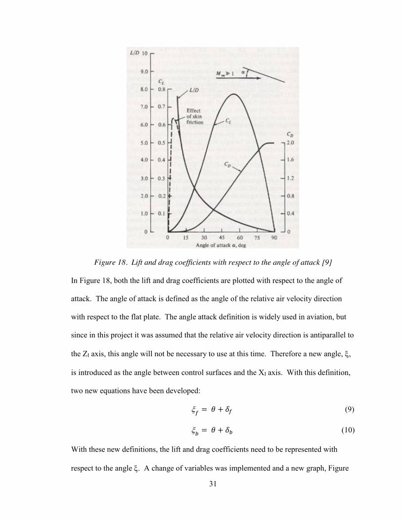
31

Figure 18. Lift and drag coefficients with respect to the angle of attack [9]

In Figure 18, both the lift and drag coefficients are plotted with respect to the angle of

attack. The angle of attack is defined as the angle of the relative air velocity direction

with respect to the flat plate. The angle attack definition is widely used in aviation, but

since in this project it was assumed that the relative air velocity direction is antiparallel to

the ZI axis, this angle will not be necessary to use at this time. Therefore a new angle, [,

is introduced as the angle between control surfaces and the XI axis. With this definition,

two new equations have been developed:

[𝑓 = 𝜃 + 𝛿𝑓 (9)

[𝑏 = 𝜃 + 𝛿𝑏 (10)

With these new definitions, the lift and drag coefficients need to be represented with

respect to the angle [. A change of variables was implemented and a new graph, Figure

32

19, was created to show the relationship between the lift and drag coefficients and the

angle [.

Figure 19. Lift and drag coefficients of circular flat plate with respect to [

In Figure 19, the drag coefficient was approximated as a second order function and the

lift coefficient was approximated as a first order function. In the range of [ from -35 to 35

degrees this approximation is accurate. A test of accuracy for a set of data against a

curve fit is using the method of least-squares approximation. This was conducted and the

drag coefficient second order approximation yielded a R2 value of 0.998, and the lift

coefficient yielded a R2 value of 0.975. Since an R2 value of 1 represents a perfect

approximation, it can be concluded that this approximation for the lift and drag

coefficient will suffice for this research project.

33

Now that the drag coefficient has been defined, all of the variables in Eq. (4) have

been discussed. Equation (5) uses the same concept as Eq. (4), but it is for the back

control surfaces. Equation (6) defines the lift force of the front control surfaces, Lf. The

magnitude of the lift force is dependent on the same variable as the drag force expect

instead of the drag force coefficient, it is in terms of the lift coefficient of the front

control surfaces, Clf. Equation (7) defines the lift force for the back control surfaces, Lb

and follows a similar description in Eq. (6). Equation (8) represents the moment about

the center of gravity of the skydiver/device system due to the air friction. This is

represented by the air friction constant, bp, and the pitch rate, ��. Finally, it is important to

notice that in Eqs. (1)-(8), LS and DS are not included, but are in the free-body diagram in

Figure 16. The torque generated by LS was considered negligible because the front

surface is curved which would result in a small lift force. The torque generated by DS

was neglected because the front surface is curved which would result in the drag force

being approximately collinear with the center of gravity.

Governing Equations – Roll Motion

Following the same method used for developing the pitch motion dynamics, a

free-body diagram was created for the roll motion of the skydiver/device system. This

free-body diagram can be seen in Figure 20.

34

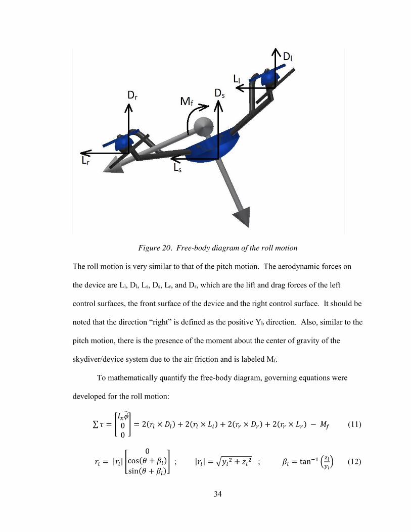
Figure 20. Free-body diagram of the roll motion

The roll motion is very similar to that of the pitch motion. The aerodynamic forces on

the device are Ll, Dl, Ls, Ds, Lr, and Dr, which are the lift and drag forces of the left

control surfaces, the front surface of the device and the right control surface. It should be

noted that the direction “right” is defined as the positive Yb direction. Also, similar to the

pitch motion, there is the presence of the moment about the center of gravity of the

skydiver/device system due to the air friction and is labeled Mf.

To mathematically quantify the free-body diagram, governing equations were

developed for the roll motion:

∑ 𝜏 = [𝐼𝑥I00

] = 2(𝑟𝑙 × 𝐷𝑙) + 2(𝑟𝑙 × 𝐿𝑙) + 2(𝑟𝑟 × 𝐷𝑟) + 2(𝑟𝑟 × 𝐿𝑟) − 𝑀𝑓 (11)

𝑟𝑙 = |𝑟𝑙| [0

cos(𝜃 + 𝛽𝑙)sin(𝜃 + 𝛽𝑙)

] ; |𝑟𝑙| = √𝑦𝑙2 + 𝑧𝑙

2 ; 𝛽𝑙 = tan−1 (𝑧𝑙𝑦𝑙

) (12)

35

𝑟𝑟 = |𝑟𝑟| [0

− cos(−𝜃 + 𝛽𝑟)sin(−𝜃 + 𝛽𝑟)

] ; |𝑟𝑟| = √𝑦𝑟2 + 𝑧𝑟

2 ; 𝛽𝑟 = tan−1 (𝑧𝑟𝑦𝑟

) (13)

𝐷𝑙 = |𝐷𝑙| [00

−1] ; |𝐷𝑙| = 1

2𝜌𝐴𝑣2𝐶𝑑𝑙 (14)

𝐷𝑟 = |𝐷𝑟| [00

−1] ; |𝐷𝑟| = 1

2𝜌𝐴𝑣2𝐶𝑑𝑟 (15)

𝐿𝑙 = |𝐿𝑙| [0

−10

] ; |𝐿𝑙| = 12

𝜌𝐴𝑣2𝐶𝑙𝑙 (16)

𝐿𝑟 = |𝐿𝑟| [0

−10

] ; |𝐿𝑟| = 12

𝜌𝐴𝑣2𝐶𝑙𝑟 (17)

𝑀𝑓 = b𝑟 [0I0

] (18)

When analyzing Eqs. (11)-(18), it should be seen that the equations are very similar to the

pitch motion equations. This makes intuitive sense because the skydiving control system

controls the roll motion in the same manner that the pitch motion is controlled. The main

difference in the equations is that the roll motion is confined to the Yb-Zb plane, therefore

in Eq. (11), the moment of inertia, Ix, is the moment of inertia of the skydiver/device

system about the Xb axis. Also, the angular acceleration is the roll angle acceleration, I.

In Eq. (18), br is the air friction constant for the roll motion, and I is the angular velocity

of the roll angle I. The variables, rl and rr, are the moment arm vectors from the center

of gravity of the skydiver/device system to the left and right control surfaces respectively.

The rest of the variables follow the same convention as introduced in the pitch motion

dynamics.

36

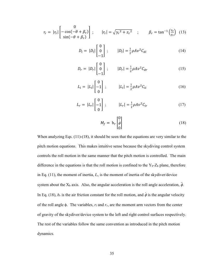
A schematic was developed to visualize the right and left control surface inputs, Gr

and Gl. This can be seen in Figure 21.

Figure 21. Definition of left control surface input angle

In Figure 21, the left control surface input is defined by the angle between the –Yb axis

and the left control surface. A similar description holds for the right control surface input

angle, Gr, which is not shown in Figure 21.

The lift and drag coefficients will use the same concept developed in the pitch

motion governing equations explanation. Therefore, Eqs. (19) and (20) were developed

to show the relationship between [, the roll angle, and the input angles.

[𝑙 = I + 𝛿𝑙 (19)

[𝑟 = I + 𝛿𝑟 (20)

All of the necessary equations have been introduced and explained for the roll motion.

37

Governing Equations – Yaw Motion

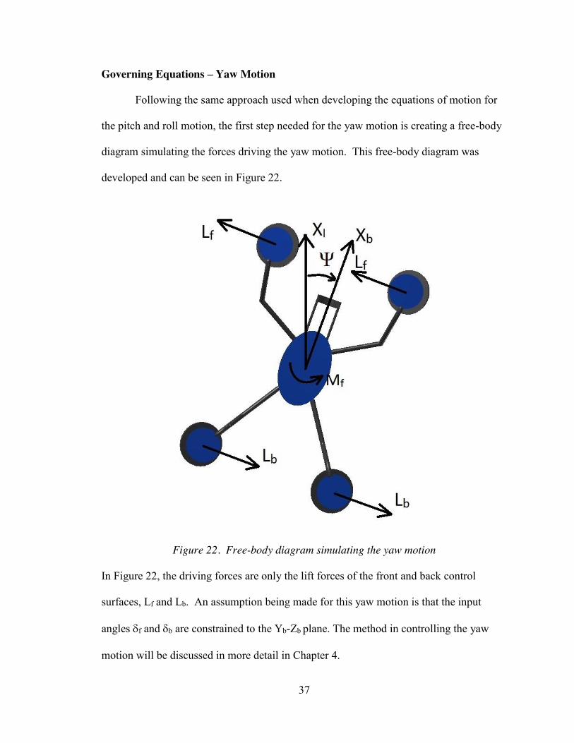
Following the same approach used when developing the equations of motion for

the pitch and roll motion, the first step needed for the yaw motion is creating a free-body

diagram simulating the forces driving the yaw motion. This free-body diagram was

developed and can be seen in Figure 22.

Figure 22. Free-body diagram simulating the yaw motion

In Figure 22, the driving forces are only the lift forces of the front and back control

surfaces, Lf and Lb. An assumption being made for this yaw motion is that the input

angles Gf and Gb are constrained to the Yb-Zb plane. The method in controlling the yaw

motion will be discussed in more detail in Chapter 4.

38

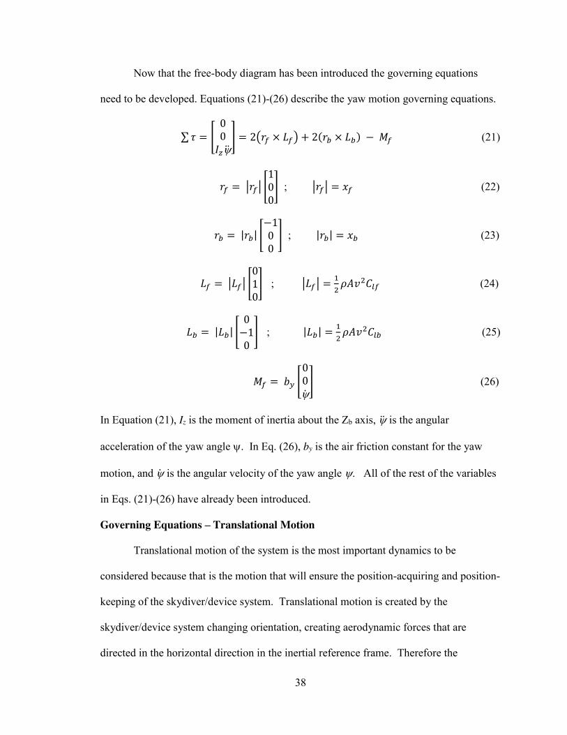
Now that the free-body diagram has been introduced the governing equations

need to be developed. Equations (21)-(26) describe the yaw motion governing equations.

∑ 𝜏 = [00

𝐼𝑧\] = 2(𝑟𝑓 × 𝐿𝑓) + 2(𝑟𝑏 × 𝐿𝑏) − 𝑀𝑓 (21)

𝑟𝑓 = |𝑟𝑓| [100

] ; |𝑟𝑓| = 𝑥𝑓 (22)

𝑟𝑏 = |𝑟𝑏| [−100

] ; |𝑟𝑏| = 𝑥𝑏 (23)

𝐿𝑓 = |𝐿𝑓| [010

] ; |𝐿𝑓| = 12

𝜌𝐴𝑣2𝐶𝑙𝑓 (24)

𝐿𝑏 = |𝐿𝑏| [0

−10

] ; |𝐿𝑏| = 12

𝜌𝐴𝑣2𝐶𝑙𝑏 (25)

𝑀𝑓 = 𝑏𝑦 [00\

] (26)

In Equation (21), Iz is the moment of inertia about the Zb axis, \ is the angular

acceleration of the yaw angle \. In Eq. (26), by is the air friction constant for the yaw

motion, and \ is the angular velocity of the yaw angle \. All of the rest of the variables

in Eqs. (21)-(26) have already been introduced.

Governing Equations – Translational Motion

Translational motion of the system is the most important dynamics to be

considered because that is the motion that will ensure the position-acquiring and position-

keeping of the skydiver/device system. Translational motion is created by the

skydiver/device system changing orientation, creating aerodynamic forces that are

directed in the horizontal direction in the inertial reference frame. Therefore the

39

translational motion dynamics are coupled with the rotational dynamics of the

skydiver/device system. To simplify the analysis of the translational motion, the

translational motion will be constrained along the Xb axis. Furthermore, the

skydiver/device system will be constrained to the pitch motion.

Since the pitch motion equations have already been developed, the translational

motion in terms of the pitch angle is remaining to fully describe the translational motion.

Figure 16 will be used as the free-body diagram from which the equations will be

developed. Equation (27) is the translational motion equation and it is derived from using

Newton’s Second Law of translational motion.

∑ 𝐹𝑥 = 𝐿𝑓 + 𝐿𝑏 + 𝐿𝑠 − 𝑏𝑥�� = 𝑚�� (27)

𝐿𝑠 = |𝐿𝑠| [−100

] ; |𝐿𝑠| = 12

𝜌𝐴𝑣2𝐶𝑙𝑠 (28)

In Eq. (27), bx is the air friction constant for translational motion in the X direction, �� is

the linear velocity, m is the mass, and �� is the linear acceleration of the skydiver/device

system. The forces 𝐿𝑓 and 𝐿𝑏 are in terms of the pitch angle, T, and the input angles, Gf

and Gb which can be seen in Eqs. (6) and (7). In Eq. (28), the lift force due to the front

surface is introduced. 𝐿𝑠 is in terms of the pitch angle, T because the lift coefficient for

the front surface, 𝐶𝑙𝑠. 𝐶𝑙𝑠, unlike the other lift coefficients introduced, does not depend

on in input angle because the orientation of the front surface only depends on the pitch

angle. Therefore, [𝑠 needs to be defined. The equation for [𝑠 can be seen in Eq. (29).

[𝑠 = 𝜃 (29)

Now that [𝑠 has been defined, the relationship between the lift coefficient and [ that was

introduced in Figure 19 can be used.

40

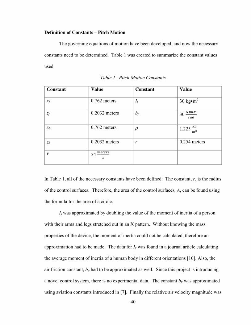
Definition of Constants – Pitch Motion

The governing equations of motion have been developed, and now the necessary

constants need to be determined. Table 1 was created to summarize the constant values

used:

Table 1. Pitch Motion Constants

Constant Value Constant Value

xf 0.762 meters Iy 30 kgxm2

zf 0.2032 meters bp 30 𝑁x𝑚x𝑠𝑟𝑎𝑑

xb 0.762 meters U 1.225 𝑘𝑔𝑚3

zb 0.2032 meters r 0.254 meters

v 54 𝑚𝑒𝑡𝑒𝑟𝑠𝑠

In Table 1, all of the necessary constants have been defined. The constant, r, is the radius

of the control surfaces. Therefore, the area of the control surfaces, A, can be found using

the formula for the area of a circle.

Iy was approximated by doubling the value of the moment of inertia of a person

with their arms and legs stretched out in an X pattern. Without knowing the mass

properties of the device, the moment of inertia could not be calculated, therefore an

approximation had to be made. The data for Iy was found in a journal article calculating

the average moment of inertia of a human body in different orientations [10]. Also, the

air friction constant, bp had to be approximated as well. Since this project is introducing

a novel control system, there is no experimental data. The constant bp was approximated

using aviation constants introduced in [7]. Finally the relative air velocity magnitude was

41

approximated as similar to the terminal velocity of skydivers. Skydiver’s terminal

velocity typically ranges between 100-120 mph or 44 – 54 m/s [11].

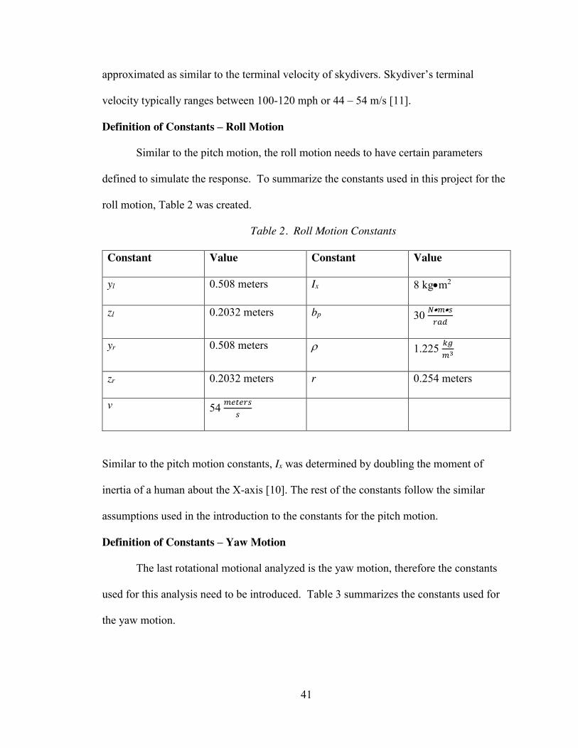
Definition of Constants – Roll Motion

Similar to the pitch motion, the roll motion needs to have certain parameters

defined to simulate the response. To summarize the constants used in this project for the

roll motion, Table 2 was created.

Table 2. Roll Motion Constants

Constant Value Constant Value

yl 0.508 meters Ix 8 kgxm2

zl 0.2032 meters bp 30 𝑁x𝑚x𝑠𝑟𝑎𝑑

yr 0.508 meters U 1.225 𝑘𝑔𝑚3

zr 0.2032 meters r 0.254 meters

v 54 𝑚𝑒𝑡𝑒𝑟𝑠𝑠

Similar to the pitch motion constants, Ix was determined by doubling the moment of

inertia of a human about the X-axis [10]. The rest of the constants follow the similar

assumptions used in the introduction to the constants for the pitch motion.

Definition of Constants – Yaw Motion

The last rotational motional analyzed is the yaw motion, therefore the constants

used for this analysis need to be introduced. Table 3 summarizes the constants used for

the yaw motion.

42

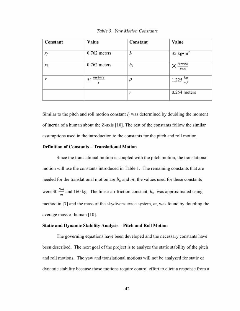
Table 3. Yaw Motion Constants

Constant Value Constant Value

xf 0.762 meters Iz 35 kgxm2

xb 0.762 meters by 30 𝑁x𝑚x𝑠𝑟𝑎𝑑

v 54 𝑚𝑒𝑡𝑒𝑟𝑠𝑠

U 1.225 𝑘𝑔𝑚3

r 0.254 meters

Similar to the pitch and roll motion constant Iz was determined by doubling the moment

of inertia of a human about the Z-axis [10]. The rest of the constants follow the similar

assumptions used in the introduction to the constants for the pitch and roll motion.

Definition of Constants – Translational Motion

Since the translational motion is coupled with the pitch motion, the translational

motion will use the constants introduced in Table 1. The remaining constants that are

needed for the translational motion are 𝑏𝑥 and 𝑚; the values used for these constants

were 30 𝑁x𝑠𝑚

and 160 kg. The linear air friction constant, 𝑏𝑥 was approximated using

method in [7] and the mass of the skydiver/device system, m, was found by doubling the

average mass of human [10].

Static and Dynamic Stability Analysis – Pitch and Roll Motion

The governing equations have been developed and the necessary constants have

been described. The next goal of the project is to analyze the static stability of the pitch

and roll motions. The yaw and translational motions will not be analyzed for static or

dynamic stability because those motions require control effort to elicit a response from a

43

perturbed state. In other words, by inspection, if the states of the yaw and translational

motion are perturbed from desired state, there will not be a response from the system.

Static and dynamic stability analysis is important because it can help limit control

effort, shows that a desirable design was obtained from the design process, and can give

more understanding of the natural behavior of the system. Static stability is defined as

the “initial tendency of the vehicle to return to its equilibrium state after a disturbance”

[7]. Static stability will show the initial response of the system. Furthermore, dynamic

stability is defined as the time history tendency of a vehicle to return to the desired state

[7]. Both the static and dynamic stability analysis is based on having no control input so

the input angles for the control surfaces are assumed to be zero. This is also regarded as

the “open loop” response of the system. In both the pitch and roll cases, the desired state

is the horizontal positon of the skydiver/device system.

To analyze the static and dynamic stability of the system, a perturbed state from

the equilibrium needs to be defined. For the pitch motion, the perturbed pitch angle was

chosen to be 20q, and the pitch rate was chosen to be zero. A MATLAB script was

developed using the governing equations to simulate this response. Equations (1)-(8) for

the pitch motion are nonlinear equations that could not be solved analytically. Therefore

the built-in function ode45 was used to approximate the response of this system. The

results from this analysis can be seen in Figure 23.

44

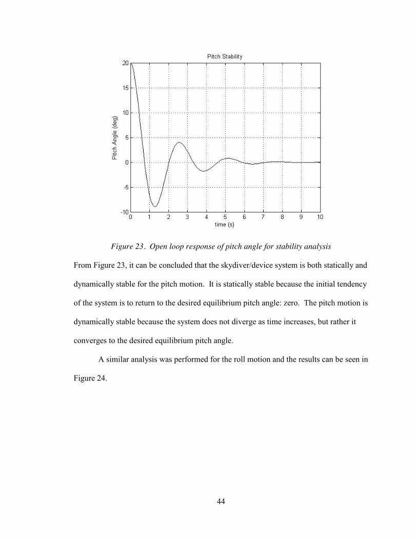
Figure 23. Open loop response of pitch angle for stability analysis

From Figure 23, it can be concluded that the skydiver/device system is both statically and

dynamically stable for the pitch motion. It is statically stable because the initial tendency

of the system is to return to the desired equilibrium pitch angle: zero. The pitch motion is

dynamically stable because the system does not diverge as time increases, but rather it

converges to the desired equilibrium pitch angle.

A similar analysis was performed for the roll motion and the results can be seen in

Figure 24.

45

Figure 24. Open loop response of roll angle for stability analysis

The results from the roll angle open loop response are similar to the pitch angle open loop

response. This agrees with intuition considering the similar dynamical equations for the

pitch and roll motions. It can be concluded that the roll motion is also statically and

dynamically stable.

The results from the stability analysis of the pitch and roll motions are positive

because this will limit the control effort needed by the control system. Static and

dynamic stability were desired design characteristics for those reasons.

46

Chapter 4: Control

Linearization

The equations of motion developed are highly nonlinear equations except for the

yaw motion which are linear equations of the state variables. Developing control

algorithms for nonlinear equations is a difficult task. To avoid these nonlinear equation

complexities, linearization was a technique used. Linearization is a method of

approximating the dynamics of the system by a linear set of differential equations, which

then can be used to develop the control algorithms. A first order linearization was

performed on the pitch, roll, and translational motion dynamics.

To explain the method of linearization, the linearization of the pitch motion will

be discussed. The pitch motion is a second order differential equation of the pitch angle,

T, and was introduced in Eq. (1). The first step in the linearization method is converting

the higher order differential equation into multiple first order differential equations. This

is done by defining state variables. Since the pitch motion is a second order differential

equation, two new state variables are needed to be defined. The new state variables can

be seen in Eqs. (30) and (31).

𝑋1 = T (30)

𝑋2 = T (31)

Now that these new variables have been defined, taking the time derivative of Eqs. (30)

and (31) will produce following relationship:

𝑋1 = 𝑋2 (32)

𝑋2 = T (33)

47

In Eq. (33), T is in terms of the state variables, therefore, the result is two first order

differential equations. However, Eq. (32) and (33) are still nonlinear equations of the

state variables, thus need linearization. The following equations define the generic

linearization based on the small perturbation method [12].

�� = 𝒇(𝑿, 𝑼) (34)

G𝑿 = 𝑿 − 𝑿∗ (35)

G𝑼 = 𝑼 − 𝑼∗ (36)

𝑨 = 𝜕𝒇𝜕𝑿

|∗ (37)

𝑩 = 𝜕𝒇𝜕𝑼

|∗ (38)

G�� = 𝑨G𝑿 + 𝑩G𝑼 (39)

𝑿 = G𝑿(𝑡) + 𝑿∗(𝑡) (40)

In Eqs. (34)-(40), X is the state variable vector, U is the input vector, G𝑿 is the perturbed

state variable vector with 𝑿∗ being the operating condition also known as the reference

state vector, G𝑼 is the perturbed input vector with 𝑼∗ being the operating input also

known as the input state vector, A and B are the state space representation matrices that

will be used for control methods. It should be noted that the state space representation

matrices C and D are not changed from the linearization if the state output equations are

linear equations of the state variables and inputs. For the pitch, roll, and translational

motion equations, the output equation are all linear equations of the state variables and

inputs.

48

Linearization is a method to approximate the response of the system. This

approximation was completed for the pitch, roll, and translational motion equations while

the yaw motion did not need to be linearized. The result is four state space

representations of the dynamics. The pitch, roll, and yaw equations each have two state

variables and two inputs. The translational motion linearization results in two state

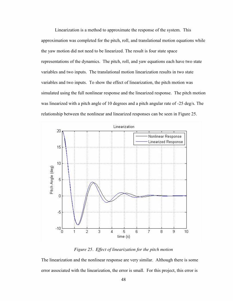
variables and two inputs. To show the effect of linearization, the pitch motion was

simulated using the full nonlinear response and the linearized response. The pitch motion

was linearized with a pitch angle of 10 degrees and a pitch angular rate of -25 deg/s. The

relationship between the nonlinear and linearized responses can be seen in Figure 25.

Figure 25. Effect of linearization for the pitch motion

The linearization and the nonlinear response are very similar. Although there is some

error associated with the linearization, the error is small. For this project, this error is

49

considered negligible and the linearized responses will be used for the remainder of the

analysis.

Introduction to Control

While performing the static stability analysis, the open loop response for the pitch

motion was found. The open loop response is important because it shows the natural

dynamics of the system. In Figures 23 and 24, it shows that the system naturally returns

to the desired state. Even though the system naturally returns to the desired equilibrium

state, the system needs to be able to control the pitch motion and create a fast response.

Also, the pitch, roll, and yaw motions are coupled with the translational motions,

therefore controlling the pitch, roll and yaw motions is a necessity.

Since the equations of motion have been linearized, there is a wealth of control

methods to choose from. This problem is defined as a regulator problem because it is

desired to have all of the state variables settle to zero. The Linear Quadratic Regulator

(LQR) method was the method chosen to develop the control algorithms for this problem.

The LQR method used will be discussed in further detail in the following section.

LQR Method

The LQR method involves minimizing a cost functional that is a function of the

state and control variables. Although the LQR method has a general cost functional

form, the cost functional introduced will be the simplified form for this specific problem.

This cost functional, J, can be seen in Eq. (41).

𝐽 = 12 ∫ [𝑿′𝑸𝑿 + 𝑼′𝑹𝑼]𝑑𝑡𝑇

0 (41)

In Eq. (41), Q is the state weighting matrix, and R is the control weighting matrix. Q and

R are typically diagonal matrices. Q needs to be positive semi-definite and R needs to be

50

positive definite. The weighting matrices can be varied to give the desired result. For

example, if there are limits on the control or if control input is expensive, the R matrix

values can be weighted more than Q. The individual values within Q and R can also be

varied because each element in the matrices correspond to specific state variable or input.

This gives versatility in designing the optimum response based on the specific problem

and constraints [12].

The solution to the LQR method has an analytical solution which makes the

computation simpler and can be done offline. This solution involves solving the

Algebraic Riccati Equation (ARE). The ARE can be seen in Eq. (42)

−�� = 0 = ��𝑨 + 𝑨′�� − ��𝑩𝑹−𝟏𝑩′�� + 𝑸 (42)

where M is the Riccati matrix that satisfies equation. Solving for M gives the optimal

control for the LQR method which can be seen in Eq. (43).

𝑼 = −𝑹−𝟏𝑩′�� = −𝑲𝑿 (43)

MATLAB has a built-in function, lqr, where the inputs of the function are A, B, Q, and

R. The function solves the ARE and gives the optimum constant feedback gain matrix K.

For the pitch, roll, yaw, and translational motion control development, the Q and R

matrices used will be introduced and the optimum gain matrix found will be discussed.

Also, the closed loop feedback control response will be displayed and a discussion of the

results will be given [12].

Pitch Control

The pitch motion has been linearized to a system of two states and two inputs. For

the control motion, the operating input condition needs to be defined. The input operating

condition was 5 degrees for both the front and back control surfaces. The state space

51

matrices that define the linearized dynamics of the pitch motion can be seen in Eqs. (44)

and (45).

𝑨 = [ 𝟎 𝟏−𝟔. 𝟑𝟕 −𝟏. 𝟐𝟓] (44)

𝑩 = [ 𝟎 𝟎−𝟒. 𝟕𝟓 𝟐𝟑. 𝟏𝟖] (45)

Since there are two states and two inputs, the weighting matrices, Q and R, will both be

2x2 diagonal matrices. The weighting matrices will first be introduced and then

discussed. Q and R for the pitch motion can be seen in Eqs. (46) and (47), respectively.

𝑸 = [𝟔 𝟎𝟎 𝟏] (46)

𝑹 = [𝟐 𝟎𝟎 𝟐] (47)

The weighing matrices were found by varying the individual values to achieve the

desired response. These values were not varied arbitrarily, there was a method in the

determining these values.

The first row and first column value of Q corresponds to the pitch angle which is

the state that is the most important. The goal is to have the pitch angle return to zero,

horizontal flight, as quickly as possible. The second row and second column value of Q

corresponds to the rate of change of the pitch angle, and this does not have as much

importance. The diagonal elements of R correspond to the input angles of the front and

back control surfaces. There is not one that is more important than the other, therefore,

the two values are equal. Finally, the relative magnitudes between Q and R are

important. Placing a weight on the input is important because the input should not exceed

±15 degrees, and the control response should not be too quick because it would make the

skydiver uncomfortable. However, ultimately the pitch angle is the most important factor

52

because it is desired to be able to control the pitch motion quickly. Therefore, the first

row and first column element of Q is larger than the elements in R. A more rigorous

analysis of the optimum response could be conducted in the future, but based on the

limitations of this project, the analysis is sufficient.

The optimum gain matrix, K was found using lqr in MATLAB and can be seen in

Eq. (48).

𝑲 = [−𝟎. 𝟐𝟗𝟕𝟖 −𝟎. 𝟏𝟒𝟖𝟓𝟏. 𝟒𝟓𝟑𝟑 𝟎. 𝟕𝟐𝟒𝟕 ] (48)

All of the parameters needed to determine the closed loop response have been found.

However, although the input angle constraint of needing to be less than ±15 degrees was

considered in the LQR weighting matrices, this does not ensure that the input angles will

not exceed the limits. To completely ensure that this limit is not exceeded, a saturation

limit needs to be placed on the two input angles. To complete this task, Simulink from

MATLAB was used. A model of the system was put into Simulink and a saturation

block was placed on the two input angles.

The closed loop response was simulated using the same parameters seen in Table

1, and the same initial condition of the pitch angle as 20 degrees. Also, the pitch angular

rate was set to zero. The controlled response was placed in a figure with the open loop

response (no control) to show the effect of the control. This can be seen in Figure 26.

53

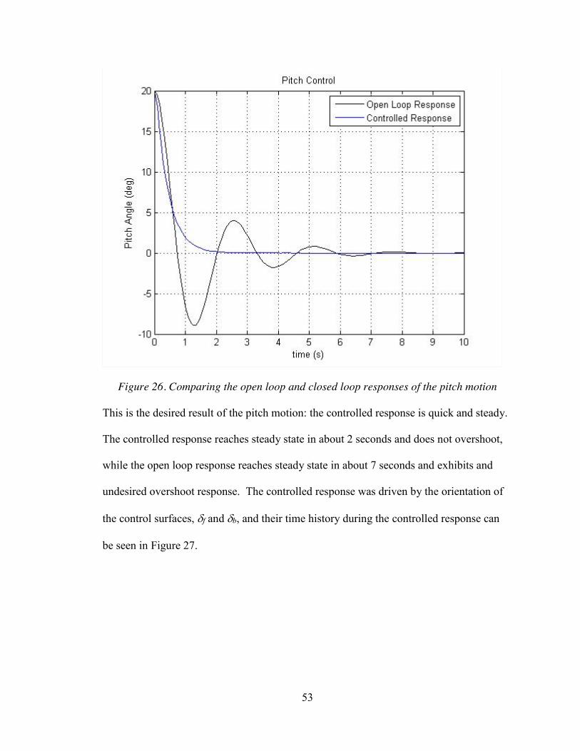
Figure 26. Comparing the open loop and closed loop responses of the pitch motion

This is the desired result of the pitch motion: the controlled response is quick and steady.

The controlled response reaches steady state in about 2 seconds and does not overshoot,

while the open loop response reaches steady state in about 7 seconds and exhibits and

undesired overshoot response. The controlled response was driven by the orientation of

the control surfaces, Gf and Gb, and their time history during the controlled response can

be seen in Figure 27.

54

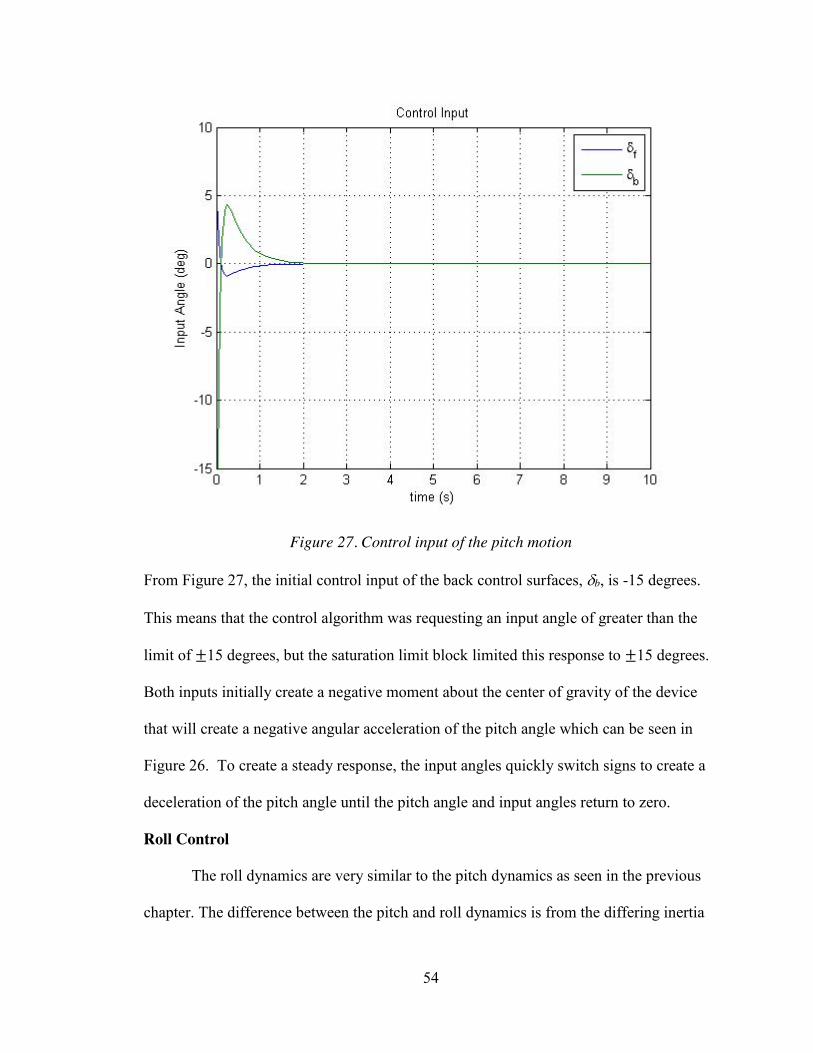
Figure 27. Control input of the pitch motion

From Figure 27, the initial control input of the back control surfaces, Gb, is -15 degrees.

This means that the control algorithm was requesting an input angle of greater than the

limit of ±15 degrees, but the saturation limit block limited this response to ±15 degrees.

Both inputs initially create a negative moment about the center of gravity of the device

that will create a negative angular acceleration of the pitch angle which can be seen in

Figure 26. To create a steady response, the input angles quickly switch signs to create a

deceleration of the pitch angle until the pitch angle and input angles return to zero.

Roll Control

The roll dynamics are very similar to the pitch dynamics as seen in the previous

chapter. The difference between the pitch and roll dynamics is from the differing inertia

55

values and the location of the control surfaces. Therefore the method for developing a

control algorithm for the roll motion will follow the same process as the pitch control.

The roll control was linearized using the following operating condition: the roll angle was

10 degrees, and the roll angular rate was -20 deg/s. Similar to the pitch control, the

operating control input for the right and left control surfaces was 5 degrees. The result

from the linearization can be seen in Eqs. (49) and (50) which define the linearized state

space matrices.

𝑨 = [ 𝟎 𝟏−𝟏𝟐. 𝟕𝟒 −𝟐. 𝟓] (49)

𝑩 = [ 𝟎 𝟎−𝟑. 𝟓𝟔 𝟒𝟎. 𝟒𝟐] (50)

Using the LQR method, the Q and R matrices need to be determined to create the desired

control response. The Q matrix used can be seen in Eq. (51).

𝑸 = [𝟓 𝟎𝟎 𝟏] (51)

The Q matrix for the roll motion is similar to the pitch motion: there is a higher weight on

the roll angle, I, rather than the rate of change of the roll angle, I. The values in Q

matrix were varied until a desired response was acquired: a fast response with no

overshoot. The weighting matrix on the control input can be seen in Eq. (52).

𝑹 = [𝟐 𝟎𝟎 𝟐] (52)

The R matrix shows that there is an equal weight on both inputs, which agrees with the

pitch control analysis. Again, there is more weight on the roll angle than the control

inputs.

56

Now that the Q and R matrices have been introduced, the LQR method can be

used to determine the optimum gain matrix K. Using MATLAB’s lqr function, K was

found and can be seen in Eq. (53).

𝑲 = [−𝟎. 𝟏𝟏𝟒𝟎 −𝟎. 𝟎𝟔𝟎𝟕𝟏. 𝟐𝟗𝟐𝟗 𝟎. 𝟔𝟖𝟗𝟐 ] (53)

Equation (53) is now combined with the linearized roll motion equations to get the closed

loop response. Again, MATLAB’s Simulink was used to implement the control response.

The same limit of ±15 degrees was placed on the control inputs. The controlled response

can be seen in Figure 28.

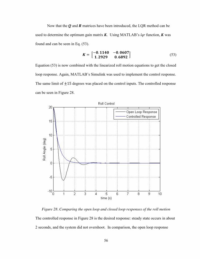
Figure 28. Comparing the open loop and closed loop responses of the roll motion

The controlled response in Figure 28 is the desired response: steady state occurs in about

2 seconds, and the system did not overshoot. In comparison, the open loop response

57

exhibited a settling time of 4 seconds and had overshoot. The controlled response was

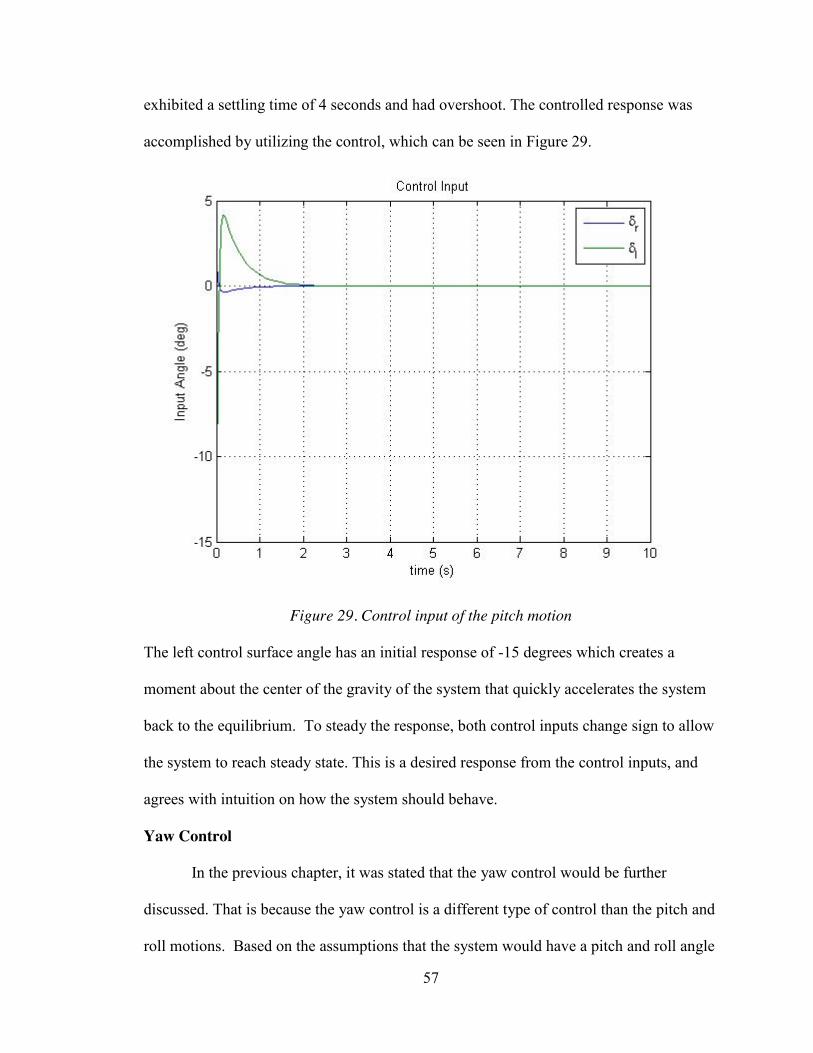
accomplished by utilizing the control, which can be seen in Figure 29.

Figure 29. Control input of the pitch motion

The left control surface angle has an initial response of -15 degrees which creates a

moment about the center of the gravity of the system that quickly accelerates the system

back to the equilibrium. To steady the response, both control inputs change sign to allow

the system to reach steady state. This is a desired response from the control inputs, and

agrees with intuition on how the system should behave.

Yaw Control

In the previous chapter, it was stated that the yaw control would be further

discussed. That is because the yaw control is a different type of control than the pitch and

roll motions. Based on the assumptions that the system would have a pitch and roll angle

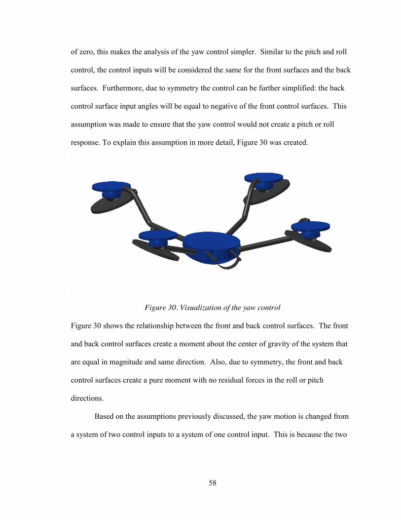
58

of zero, this makes the analysis of the yaw control simpler. Similar to the pitch and roll

control, the control inputs will be considered the same for the front surfaces and the back

surfaces. Furthermore, due to symmetry the control can be further simplified: the back

control surface input angles will be equal to negative of the front control surfaces. This

assumption was made to ensure that the yaw control would not create a pitch or roll

response. To explain this assumption in more detail, Figure 30 was created.

Figure 30. Visualization of the yaw control

Figure 30 shows the relationship between the front and back control surfaces. The front

and back control surfaces create a moment about the center of gravity of the system that

are equal in magnitude and same direction. Also, due to symmetry, the front and back

control surfaces create a pure moment with no residual forces in the roll or pitch

directions.

Based on the assumptions previously discussed, the yaw motion is changed from

a system of two control inputs to a system of one control input. This is because the two

59

inputs are not considered independent of one another. The state space representation of

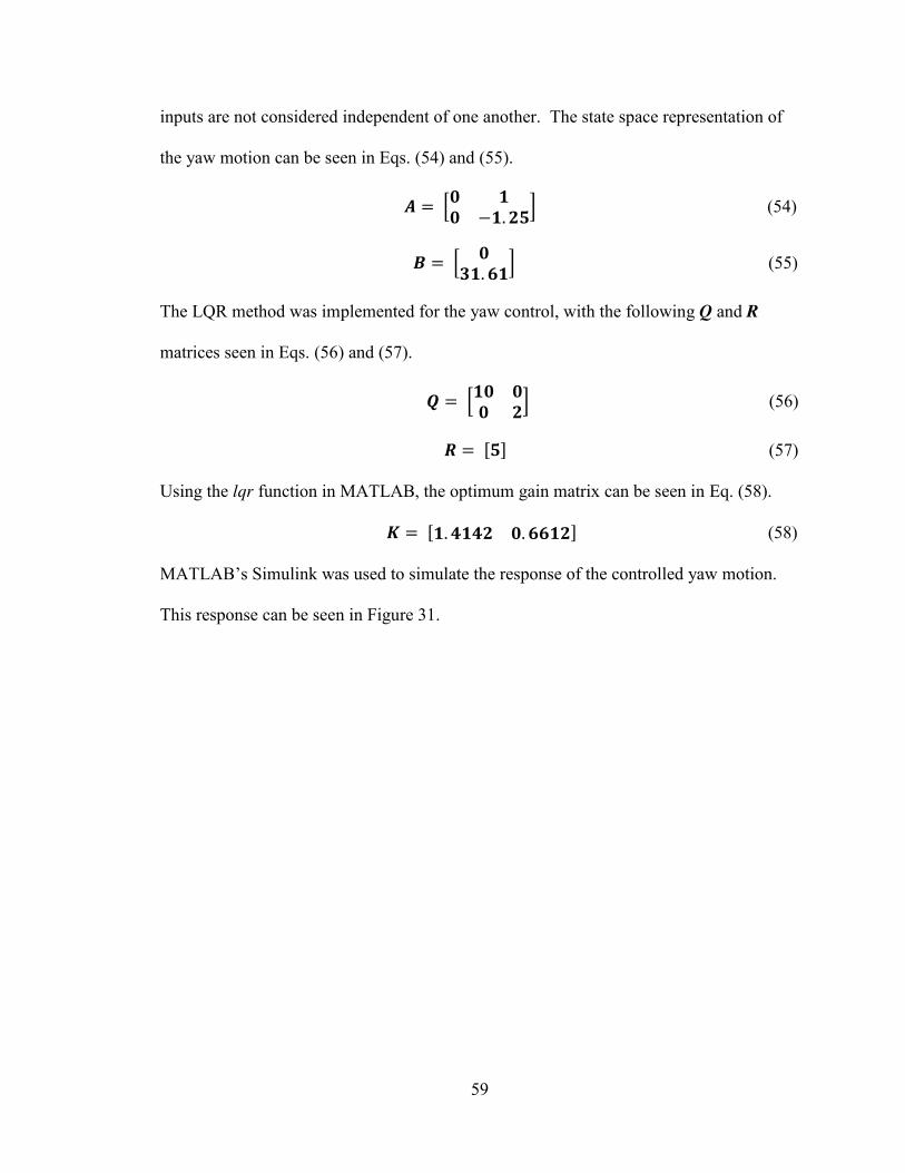
the yaw motion can be seen in Eqs. (54) and (55).

𝑨 = [𝟎 𝟏𝟎 −𝟏. 𝟐𝟓] (54)

𝑩 = [ 𝟎𝟑𝟏. 𝟔𝟏] (55)

The LQR method was implemented for the yaw control, with the following Q and R

matrices seen in Eqs. (56) and (57).

𝑸 = [𝟏𝟎 𝟎𝟎 𝟐] (56)

𝑹 = [𝟓] (57)

Using the lqr function in MATLAB, the optimum gain matrix can be seen in Eq. (58).

𝑲 = [𝟏. 𝟒𝟏𝟒𝟐 𝟎. 𝟔𝟔𝟏𝟐] (58)

MATLAB’s Simulink was used to simulate the response of the controlled yaw motion.

This response can be seen in Figure 31.

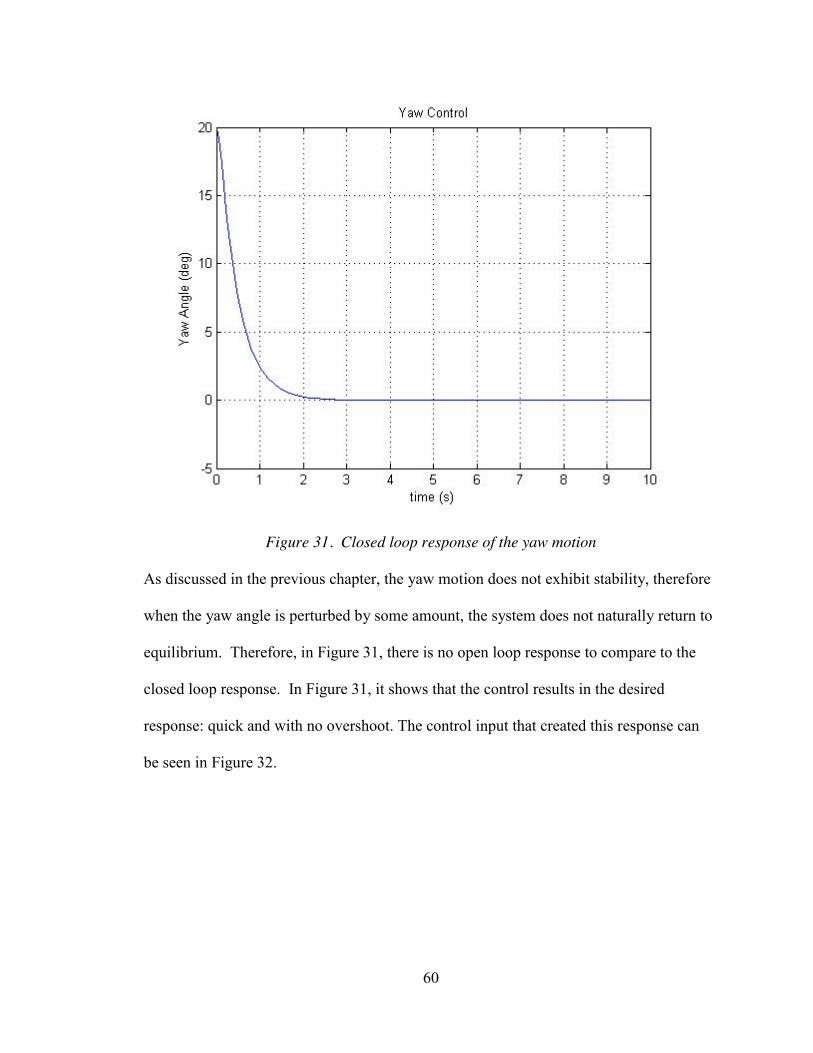
60

Figure 31. Closed loop response of the yaw motion

As discussed in the previous chapter, the yaw motion does not exhibit stability, therefore

when the yaw angle is perturbed by some amount, the system does not naturally return to

equilibrium. Therefore, in Figure 31, there is no open loop response to compare to the

closed loop response. In Figure 31, it shows that the control results in the desired

response: quick and with no overshoot. The control input that created this response can

be seen in Figure 32.

61

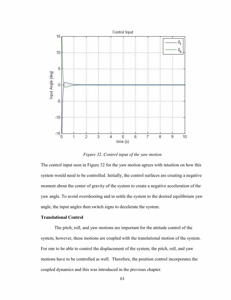
Figure 32. Control input of the yaw motion

The control input seen in Figure 32 for the yaw motion agrees with intuition on how this

system would need to be controlled. Initially, the control surfaces are creating a negative

moment about the center of gravity of the system to create a negative acceleration of the

yaw angle. To avoid overshooting and to settle the system to the desired equilibrium yaw

angle, the input angles then switch signs to decelerate the system.

Translational Control

The pitch, roll, and yaw motions are important for the attitude control of the

system, however, these motions are coupled with the translational motion of the system.

For one to be able to control the displacement of the system, the pitch, roll, and yaw

motions have to be controlled as well. Therefore, the position control incorporates the

coupled dynamics and this was introduced in the previous chapter.

62

For this analysis, it was chosen to isolate the motion to a pure pitch motion when

performing a translational maneuver. This results in a system with four states and two

control inputs. The four states are the linear displacement, linear velocity, pitch angle,

and the rate of change of the pitch angle. The two control inputs are the front and back

control surface angles. The equations of motion developed in the previous chapter for the

translational motion were linearized and placed into state space representation to perform

the LQR method. The operating condition for the translational motion linearization is as

follows: the displacement was 5 meters, the velocity was -3 m/s, the pitch angle was 10

degrees, and the pitch angular rate was -25 deg/s. Also, the operating input condition was

5 degrees. The linearization resulted in the state space matrices seen in Eqs. (59) and

(60).

𝑨 = [ 𝟎 𝟏 𝟎 −𝟎. 𝟖

𝟎 𝟎−𝟐𝟐. 𝟕 𝟎

𝟎 𝟎𝟎 𝟎

𝟎 𝟏−𝟔. 𝟑𝟕 −𝟏. 𝟐𝟓

] (59)

𝑩 = [𝟎 𝟎

−𝟑. 𝟗𝟖 −𝟑. 𝟗𝟖𝟎 𝟎

−𝟒. 𝟕𝟓 𝟐𝟑. 𝟏𝟖

] (60)

The Q and R matrices used in this control can be seen in Eq. (61) and (62).

𝑸 = [𝟐𝟎 𝟎𝟎 𝟏

𝟎 𝟎 𝟎 𝟎

𝟎 𝟎 𝟎 𝟎

𝟏𝟎 𝟎𝟎 𝟏

] (61)

𝑹 = [𝟓 𝟎𝟎 𝟓] (62)

In Eq. (61), the first row, first column of Q is the weight on the displacement away from

the desired location. This has the largest value over all of the weighting elements. The

third row, third column is the weighting element on the pitch angle. It is desirable for the

63

pitch angle to return quickly to the horizontal position. The other two elements in Q are

the weighting values on the rate of change of the displacement and pitch angle and these

are not as important. In Eq. (62), the R matrix elements are equal to each other indicating

that neither control surfaces are more important or pose limitations compared to the other

control surface. The Q and R matrices introduced in Eqs. (61) and (62) were used to find

the optimum gain matrix, K, using MATLAB’s lqr function. Matrix K can be seen in Eq.

(63).

𝑲 = [−𝟏. 𝟖𝟔𝟖𝟓 −𝟎. 𝟖𝟑𝟔𝟏−𝟏. 𝟐𝟐𝟖𝟒 −𝟎. 𝟔𝟎𝟑𝟖

𝟎. 𝟏𝟗𝟕𝟏 −𝟎. 𝟐𝟑𝟒𝟎𝟕. 𝟗𝟖𝟒𝟕 𝟎. 𝟗𝟒𝟕𝟐 ] (63)

Following the same method used for the pitch, roll and yaw control responses, the

translational control response was simulated using MATLAB’s Simulink. The initial

conditions for the displacement was 10 meters away from the desired location, zero initial

velocity. The input angles were again limited to ±15 degrees. The translational

controlled response can be seen in Figure 33.

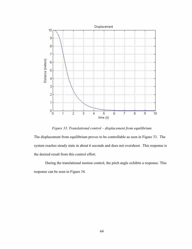
64

Figure 33. Translational control – displacement from equilibrium

The displacement from equilibrium proves to be controllable as seen in Figure 33. The

system reaches steady state in about 6 seconds and does not overshoot. This response is

the desired result from this control effort.

During the translational motion control, the pitch angle exhibits a response. This

response can be seen in Figure 34.

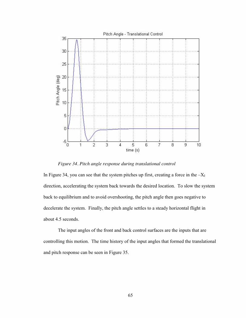
65

Figure 34. Pitch angle response during translational control

In Figure 34, you can see that the system pitches up first, creating a force in the –XI

direction, accelerating the system back towards the desired location. To slow the system

back to equilibrium and to avoid overshooting, the pitch angle then goes negative to

decelerate the system. Finally, the pitch angle settles to a steady horizontal flight in

about 4.5 seconds.

The input angles of the front and back control surfaces are the inputs that are

controlling this motion. The time history of the input angles that formed the translational

and pitch response can be seen in Figure 35.

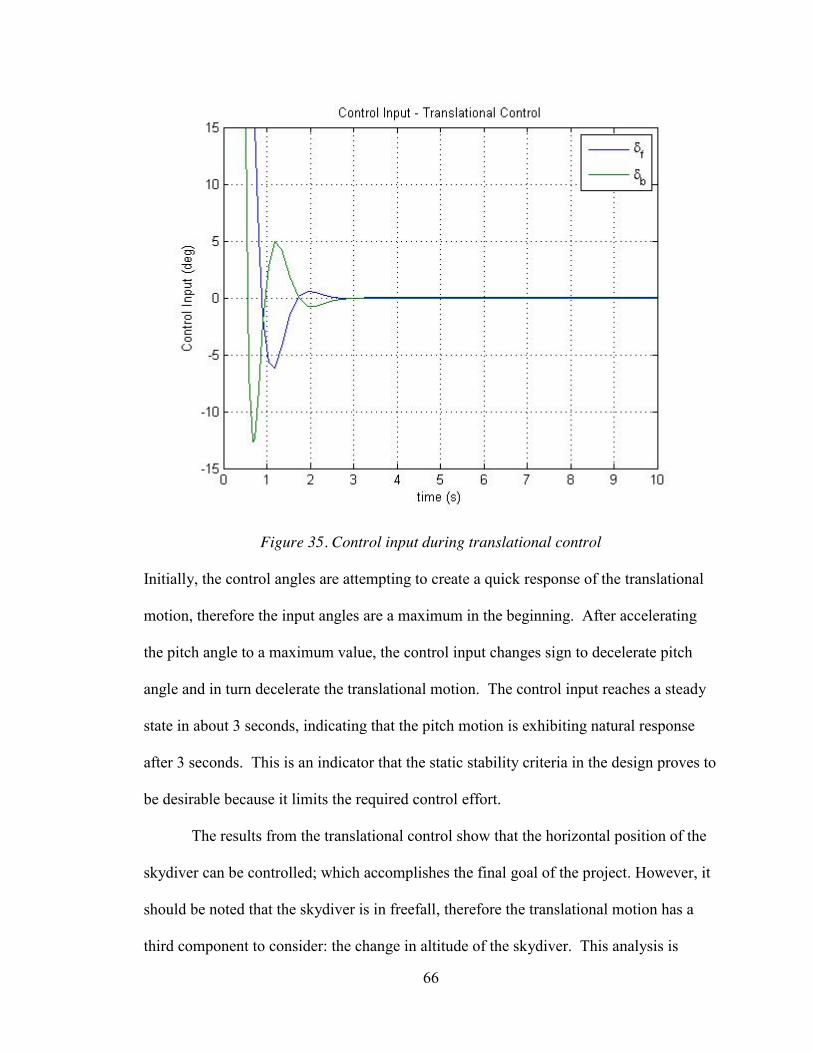
66

Figure 35. Control input during translational control

Initially, the control angles are attempting to create a quick response of the translational

motion, therefore the input angles are a maximum in the beginning. After accelerating

the pitch angle to a maximum value, the control input changes sign to decelerate pitch

angle and in turn decelerate the translational motion. The control input reaches a steady

state in about 3 seconds, indicating that the pitch motion is exhibiting natural response

after 3 seconds. This is an indicator that the static stability criteria in the design proves to

be desirable because it limits the required control effort.

The results from the translational control show that the horizontal position of the

skydiver can be controlled; which accomplishes the final goal of the project. However, it

should be noted that the skydiver is in freefall, therefore the translational motion has a

third component to consider: the change in altitude of the skydiver. This analysis is

67

beyond the scope of the project but for future analysis the vertical position of the

skydiver will be included in the six degree of freedom dynamical model that will be

developed.

68

Chapter 5: Research Conclusion

Research Limitations

This research project was a novel concept and has not been analyzed before.

Therefore, there was no prior research or experimental information to be leveraged

during the research project. This proved to place limitations on the analysis that could be

completed. For example, in most aircraft simulations, the lift and drag coefficients are

taken from experimental data. Since this aircraft is a new concept, there was no

experimental data to use. Furthermore, since there has not been any previous research

conducted, there was no research to leverage the dynamic modeling or control methods.

However, this yields an exciting outcome; future research can be conducted leveraging

the design, dynamics and control introduced in this research project and can be further

explored.

Future Work

The next logical step in the research project would be to develop a fully coupled 6

degree of freedom model of the system. The analysis for this project was sufficient to

understanding the natural dynamics of the system. Isolating the pitch, roll and yaw

motions is a typical approach when analyzing new systems. However, the actual system

is a six degree of freedom system with coupled dynamics between the pitch, roll, yaw and

translational motion. Developing this model would allow for analysis on how the system

can respond to perturbations in pitch, roll, and yaw simultaneously.

In addition to developing a six degree of freedom model, higher fidelity dynamics

would also need to be included. Some of these higher order effects are: modeling the

effects of turbulence around the control surfaces and the system, including an

69

atmospheric model into the simulation which includes the change in air density with

altitude, modeling variation in wind and wind direction, and implementing a more

accurate model of the lift and drag coefficients.

After the dynamics have been updated and a control method has been

implemented with the new dynamics, experiments on the design could start being

conducted. To achieve this, a prototype would need to be built. This prototype would

result in getting accurate lift and drag coefficients, updating the dynamic model to match

the actual dynamics, and be able to test the control algorithms on the prototype. For this

type of problem, safety is the number one priority, therefore many testing flights would

need to be performed.

Conclusion

The goals of this research project were completed. A design was introduced for a

completely new aircraft that would allow a person to skydive without a parachute.

Equations of motions were developed for the system and a static and dynamic stability

analysis was performed on the pitch and roll motions of the system. The design proved

to be both statically and dynamically stable in the pitch and roll motions, which was a

design requirement for this system. Since the design is statically and dynamically stable,

the system naturally wants to return to equilibrium which will limit the amount of

required control effort. Using the dynamics developed for the system, control methods

were implemented on the pitch, roll, yaw and translational motions. The system proved

to be controllable for all modes, and the result for each case was a desired response.

A major assumption in the project was that the pitch, roll and yaw motions were

individually isolated to understand the natural dynamics of the system. Although in

70

reality, the dynamics would involve all three rotations simultaneously, it was sufficient

for the research goals for this project. It can be concluded that since all three rotational

motions can be controlled individually, a six degree of freedom dynamical model would

also be controllable. This result is a major accomplishment and shows that the research

should be continued to achieve the goal of skydiving without a parachute.

In conclusion, the concept of skydiving without a parachute still remains an

“absurd” idea. It pushes the boundaries of human limitations, and would be a completely

new technical achievement. Based on the research conducted in this project, this goal is

achievable. A person skydiving from an aircraft could be controlled using a design

similar to the one introduced in this project, and with future research, this could be done

reliably. This concept will be further pursued and hopefully one day, people will be

skydiving without parachutes.

71

Bibliography

[1]. Good Reads Inc., 2015, Quotes, http://www.goodreads.com/quotes/110518-if-at-first-the-idea-is-not-absurd-then-there (5 May 2015).

[2]. Shaw, R. J., 2014, “History of Flight” https://www.grc.nasa.gov/www/k-

12/UEET/StudentSite/historyofflight.html (13 April 2015). [3]. Pilon, M., 2012, “Stuntman Takes a Superhero Plunge” http://www.nytimes.com/

2012/05/24/sports/englishman-connery-completes-successsful-wing-suit-landing. html?_r=0 (12 Dec. 2014).

[4]. Starr, J. 2013, “Skydiving: How high is too high?” http://www.fabulousrocketeers.

com/Photo_See_Ya.htm (29 Feb. 2015). [5]. Dropzone, 2013, “Formation Skydiving” http://www.dropzone.com/safety/

Disciplines/Formation_Skydiving_58.html (11 Dec. 2014). [6]. Magnussen, O., 2011. “Modeling, Design and Experimental Study for a Quadcopter

System Construction” MS thesis, University of Agder, Kristiansand S, Norway. [7]. Nelson, R. C., 1989, Flight Stability and Automatic Control, WCB/McGraw-Hill,

Singapore. [8]. Basic Air Data, 2015. “Coordinate System” http://www.basicairdata.eu/coordinate-

system.html (14 Jun. 2015). [9]. Anderson, John D., Jr., Hypersonic and High Temperature Gas Dynamics. NY:

McGraw-Hill, 1989. [10]. Erdmann, W. S., “Geometry and inertia of the human body” Acta of Bioengineering

and Biomechanics, Vol. 1, No. 1, 1999. [11]. Tipler, Paul A. College Physics. New York: Worth, 1987: 105. [12]. Kluever, C. A., “Modern Control,” Class Notes, Spring 2013.