To appear in International Journal of Computer Vision, Vol. 62: No. 1/2, pp. 97-119, April/May, 2005

Skin Texture Modeling

Oana G. Cula and Kristin J. DanaDepartment of Computer Science

Department of Electrical and Computer EngineeringRutgers UniversityPiscataway, NJ

Frank P. Murphy, MD and Babar K. Rao, MDDepartment of Dermatology

University of Medicine and Dentistry of New JerseyNew Brunswick, NJ

Abstract

Quantitative characterization of skin appearance is an important but difficult task. The skin surface is adetailed landscape, with complex geometry and local optical properties. In addition, skin features depend onmany variables such as body location (e.g. forehead, cheek), subject parameters (age, gender) and imagingparameters (lighting, camera). As with many real world surfaces, skin appearance is strongly affected by thedirection from which it is viewed and illuminated. Computational modeling of skin texture has potential usesin many applications including realistic rendering for computer graphics, robust face models for computervision, computer-assisted diagnosis for dermatology, topical drug efficacy testing for the pharmaceutical in-dustry and quantitative comparison for consumer products. In this work we present models and measurementsof skin texture with an emphasis on faces. We develop two models for use in skin texture recognition. Bothmodels are image-based representations of skin appearance that are suitably descriptive without the need forprohibitively complex physics-based skin models. Our models take into account the varied appearance of theskin with changes in illumination and viewing direction. We also present a new face texture database com-prised of more than 2400 images corresponding to 20 human faces, 4 locations on each face (forehead, cheek,chin and nose) and 32 combinations of imaging angles. The complete database is made publicly available forfurther research.

Keywords: texture, 3D texture, bidirectional texture, skin texture, bidirectional texture function, BTF, bidi-

rectional feature histogram, texton, image texton, symbolic texture primitive.

1 Introduction

Skin is a complex landscape that is difficult to model for many reasons. Reflection and interreflection of light

are affected by the complex optical properties of skin layers as well as the surface microgeometry of pores and

wrinkles. As with many real world surfaces, skin appearance is strongly affected by the direction from which it

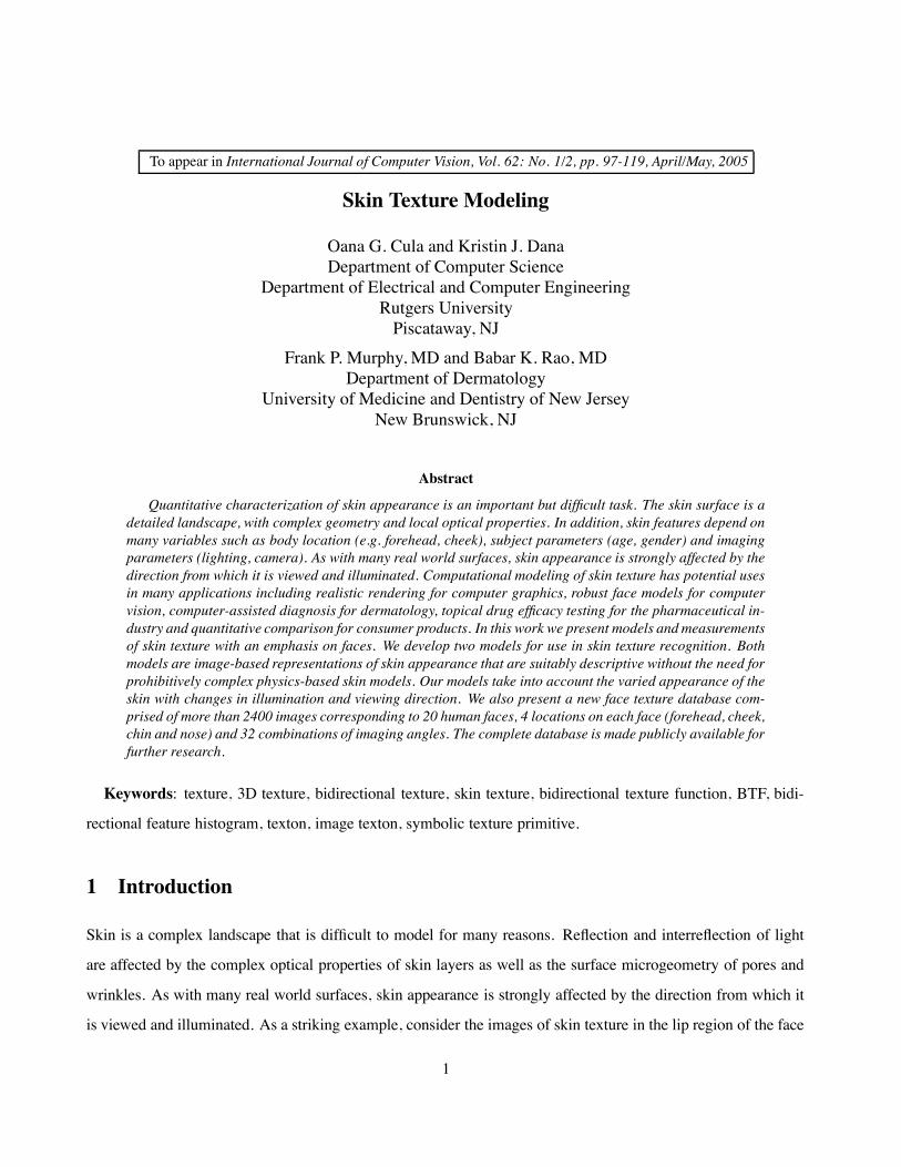
is viewed and illuminated. As a striking example, consider the images of skin texture in the lip region of the face

1

Figure 1: Skin texture in the lip region of the face, as the illumination source is repositioned. The appearance ofthe skin surface varies significantly, yet only the light direction is changed.

shown in Figure 1. The three images shown in this figure vary only in the direction of incident illumination and

yet the skin surface appears vastly different. To illustrate another example of appearance variation with imaging

parameters, consider Figure 12 (a), where each row shows a skin surface patch imaged under several different

viewing and illumination directions.

Skin texture is a 3D texture, i.e. a texture in which the fine scale geometry affects overall appearance. Increas-

ingly, recent work (Chantler, 1995) (Koenderink and van Doorn, 1996) (Dana et al., 1997) (Suen and Healey,

1998) (Dana and Nayar, 1998) (Koenderink et al., 1999) (Dana et al., 1999) (Dana and Nayar, 1999b) (Dana and

Nayar, 1999a) (van Ginneken et al., 1999) (Suen and Healey, 2000) (McGunnigle and Chantler, 2000) (Leung

and Malik, 2001) (Cula and Dana, 2001b) (Cula and Dana, 2001a) (Zalesny and van Gool, 2001) (Dong and

Chantler, 2002) (Varma and Zisserman, 2002) (Penirschke et al., 2002) (Pont and Koenderink, 2002) (Cula and

Dana, 2002) (Cula and Dana, 2004) addresses this type of texture and its variation with viewing and illumination

direction. Terminology for texture that depends on imaging parameters was introduced in (Dana et al., 1997)

(Dana et al., 1999). Specifically, the term bidirectional texture function (BTF) is used to describe image texture

as a function of the four imaging angles (viewing and light source directions). The BTF is analogous to the

bidirectional reflectance distribution function (BRDF). While BRDF is a term for the reflectance of a point, most

real world surfaces exhibit a spatially varying BRDF and the term BTF is used for this situation.

Simple models of skin appearance are not sufficient to support the demands for high performance algorithms

in computer vision and computer graphics. For example, in computer vision, algorithms for face recognition,

shape estimation and facial feature-tracking rely on accurately predicting appearance so that local matching

can be done among images obtained with different imaging parameters. In computer graphics, the popular

technique of image-based rendering typically creates new views of local texture by warping reference images.

This approach cannot capture local variations in occlusions, foreshortening and shadowing due to fine scale

geometry of textured surfaces. Therefore skin renderings lack realistic surface detail. Other methods are designed

2

specifically for rendering skin texture: (Ishii et al., 1993) (Nahas et al., 1990) (Boissieux et al., 2000); but truly

accurate synthesis of skin and the changes that occur with imaging parameters is still an open issue. Although

much work has been done in modeling for facial animation (Lee et al., 1995) (Guenter et al., 1998) (DeCarlo

et al., 1998) (Blanz and Vetter, 1999), accurately rendering surface detail has not been the primary emphasis and

remains an open topic.

In addition to computer vision and graphics, accurate skin models may be useful in dermatology and several

industrial fields. In dermatology, these skin models can be used to develop methods for computer-assisted di-

agnosis of skin disorders. In the pharmaceutical industry, quantification is useful when applied to measuring

healing progress. Such measurements can be used to evaluate and compare treatments and can serve as an early

indicator of the success or failure of a particular treatment course. Consumer products and cosmetic industries

can use computational skin representations to substantiate claims of appearance changes.

One difficulty in building skin texture models is acquiring good data. In general, bidirectional measurements

are hard because there are four imaging parameters: two angles for the viewing direction and two angles for

the illumination direction. Therefore the light source and camera should be moved on a hemisphere of possible

directions. These measurements can be quite difficult to obtain because of mechanical requirements of the setup.

When the sample is non-planar, non-rigid and not fixed, as is the case for human skin, measurements are even

more difficult.

In this work we describe our skin texture study which has a measurement component and a modeling com-

ponent. For the measurements, we have created a publicly available face texture database (Cula et al., 2003).

Rather than use highly specialized equipment that can align with the shape contours of the skin surface, we take

advantage of the fact that our modeling approach does not require images at exact viewing and illumination

directions. For each surface area, we take a sampling of camera and lighting positions at approximate directions

and employ fiducial markers so that the camera position and lighting can be recovered more precisely if needed.

In our approach, four viewing directions are used, and for each viewing direction, eight lighting directions are

measured, therefore each skin surface is characterized by 32 images. These images are high magnification and

high resolution so that fine-scale skin features such as pores and fine wrinkles are readily apparent. The viewing

direction is obtained with a boom stand augmented with an articulated arm allowing six degrees of freedom.

Illumination is controlled by a rotating arm which spans two circles of the hemisphere of all possible light di-

rections. The database is comprised of more than 2400 images corresponding to 20 human faces, 4 locations

on each face (forehead, cheek, chin and nose) and 32 combinations of imaging angles. The complete database

is made publicly available for further texture research at URL http://www.caip.rutgers.edu/rutgers texture. The

3

details of the methods and imaging protocol are discussed in Section 2.1.

The modeling effort of our skin texture study has resulted in two new bidirectional texture models that are

used in representing and recognizing skin texture. The first model is also described in our prior work (Cula and

Dana, 2001b) (Cula and Dana, 2001a), but here we apply the method to skin analysis. Based on this first model,

we present recognition results using clinical skin measurements from several locations on the hand, as shown in

Figure 12.

We present a new approach as the second model, that computes image features without clustering. The

resulting texture descriptor is simple and captures salient local structure. The motivation for developing the

second model was the difficult problem of face texture recognition where the inter-class variability is small.

The second model is tested with the face texture database in two recognition tasks: (1) discriminating among

locations on the face and (2) recognizing human subjects based on skin texture. These tests are quite different

from the typical texture recognition experiments in the literature that distinguish among surfaces that are visually

dissimilar, e.g. rocks, sand, grass. The goal of this paper is to perform a classification of skin texture where the

visual differences in appearance are far more subtle.

Both models support recognition methods that have several desirable properties. Specifically, a single image

can be used for fast non-iterative recognition, the illumination and viewing directions of the images need not be

known, and no image alignment is needed.

1.1 Prior Work in 3D Texture Recognition

Study of bidirectional texture began with the CUReT database (Dana et al., 1997) (Dana et al., 1999), and was

continued with the work in (Dana and Nayar, 1998) and (Dana and Nayar, 1999b), which models the bidirectional

histogram and correlation function for Gaussian rough surfaces. Other early efforts in bidirectional texture

analysis are presented in (Koenderink et al., 1999) and (van Ginneken et al., 1999). In (Koenderink et al., 1999)

the BRDF of opaque surfaces that are rough on both the macro and micro scale is derived. In (van Ginneken

et al., 1999), based on a model for rough surfaces with locally diffuse and/or specular reflection properties, an

investigation of the grey level histograms of a set of surfaces as a function of the view and light direction is

performed.

More recent work concerned with the dependency of texture appearance as the imaging conditions change

includes (McGunnigle and Chantler, 2000) (Dong and Chantler, 2002). The work in (McGunnigle and Chantler,

2000) proposes an approach for rough surface classification based on point statistics from photometric estimates

of the surface derivatives. In (Dong and Chantler, 2002) several approaches for capturing, synthesizing and

4

relighting of real world 3D textures are presented and compared.

Lately, recognition work has concentrated on example based methods that support recognition for a wide

range of texture classes. This recognition work includes (Dana and Nayar, 1999a) (Leung and Malik, 1999)

(Cula and Dana, 2001a) (Cula and Dana, 2004) (Zalesny and van Gool, 2001). In (Dana and Nayar, 1999a) the

texture representations are the conditional histograms of the response to a small multiscale filter bank. Principal

Component Analysis (PCA) is performed on the histograms of filter outputs and recognition is achieved with the

histogram vectors forming the appearance-based feature vectors. In (Leung and Malik, 1999) the 3D texton is

defined as the surface feature, and the 3D texture is modeled by a 3D texton histogram. In (Cula and Dana, 2001a)

(Cula and Dana, 2004) the image texton encodes the local feature within an image texture, and the 3D textured

surface is modeled by the collection of image texton histograms, as a function of the imaging parameters. The

work in (Zalesny and van Gool, 2001) presents an exemplar based texture model which accounts for the view

dependent changes of texture appearance.

It is interesting to compare and contrast some of the recent work in more detail. A common theme in prior

efforts is to examine how key texture features (Leung and Malik, 2001) or feature distributions (Cula and Dana,

2004) (Varma and Zisserman, 2002) change with viewing and illumination directions. In the 3D texton method

(Leung and Malik, 1999) (Leung and Malik, 2001), a 3D texton is created by using a multiscale filter bank

applied to an image set for a particular sample. The filter responses as a function of viewing and illumination

directions are clustered to form features that are called 3D textons. In (Cula and Dana, 2001a) (Cula and Dana,

2004), clustering of filter outputs from a single image is done to obtain image textons and the texton histograms

vary with viewing and illumination direction. There is an important difference between the 3D texton method

and the approach we take here and in (Cula and Dana, 2001a) (Cula and Dana, 2004). In general, texture repre-

sentations consist of a primitive and a statistical distribution of this primitive over space. For bidirectional texture

representations, either the primitive or the statistical distribution should be a function of the imaging parameters.

The 3D texton method uses a primitive that is a function of imaging parameters, while our method uses a sta-

tistical distribution that is a function of imaging parameters. The advantages of our method in recognition tasks

are compelling: the images need not be registered, a single image is sufficient for recognition and the imaging

parameters of novel images need not be known. With this bidirectional histogram approach, we accomplish

precise recognition of textured surfaces with less prior information and a fundamentally simpler computational

representation.

The methods of (Varma and Zisserman, 2002) and (Penirschke et al., 2002) are recent 3D texture recognition

methods which have the property of rotation invariance. The classifier in (Penirschke et al., 2002) can classify

5

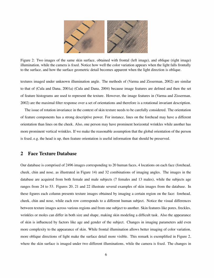
Figure 2: Two images of the same skin surface, obtained with frontal (left image), and oblique (right image)illumination, while the camera is fixed. Notice how well the color variation appears when the light falls frontallyto the surface, and how the surface geometric detail becomes apparent when the light direction is oblique.

textures imaged under unknown illumination angle. The methods of (Varma and Zisserman, 2002) are similar

to that of (Cula and Dana, 2001a) (Cula and Dana, 2004) because image features are defined and then the set

of feature histograms are used to represent the texture. However, the image features in (Varma and Zisserman,

2002) are the maximal filter response over a set of orientations and therefore is a rotational invariant description.

The issue of rotation invariance in the context of skin texture needs to be carefully considered. The orientation

of feature components has a strong descriptive power. For instance, lines on the forehead may have a different

orientation than lines on the cheek. Also, one person may have prominent horizontal wrinkles while another has

more prominent vertical wrinkles. If we make the reasonable assumption that the global orientation of the person

is fixed, e.g. the head is up, then feature orientation is useful information that should be preserved.

2 Face Texture Database

Our database is comprised of 2496 images corresponding to 20 human faces, 4 locations on each face (forehead,

cheek, chin and nose, as illustrated in Figure 14) and 32 combinations of imaging angles. The images in the

database are acquired from both female and male subjects (7 females and 13 males), while the subjects age

ranges from 24 to 53. Figures 20, 21 and 22 illustrate several examples of skin images from the database. In

these figures each column presents texture images obtained by imaging a certain region on the face: forehead,

cheek, chin and nose, while each row corresponds to a different human subject. Notice the visual differences

between texture images across various regions and from one subject to another. Skin features like pores, freckles,

wrinkles or moles can differ in both size and shape, making skin modeling a difficult task. Also the appearance

of skin is influenced by factors like age and gender of the subject. Changes in imaging parameters add even

more complexity to the appearance of skin. While frontal illumination allows better imaging of color variation,

more oblique directions of light make the surface detail more visible. This remark is exemplified in Figure 2,

where the skin surface is imaged under two different illuminations, while the camera is fixed. The changes in

6

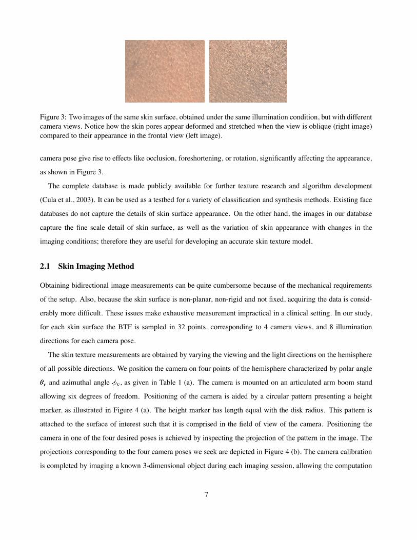
Figure 3: Two images of the same skin surface, obtained under the same illumination condition, but with differentcamera views. Notice how the skin pores appear deformed and stretched when the view is oblique (right image)compared to their appearance in the frontal view (left image).

camera pose give rise to effects like occlusion, foreshortening, or rotation, significantly affecting the appearance,

as shown in Figure 3.

The complete database is made publicly available for further texture research and algorithm development

(Cula et al., 2003). It can be used as a testbed for a variety of classification and synthesis methods. Existing face

databases do not capture the details of skin surface appearance. On the other hand, the images in our database

capture the fine scale detail of skin surface, as well as the variation of skin appearance with changes in the

imaging conditions; therefore they are useful for developing an accurate skin texture model.

2.1 Skin Imaging Method

Obtaining bidirectional image measurements can be quite cumbersome because of the mechanical requirements

of the setup. Also, because the skin surface is non-planar, non-rigid and not fixed, acquiring the data is consid-

erably more difficult. These issues make exhaustive measurement impractical in a clinical setting. In our study,

for each skin surface the BTF is sampled in 32 points, corresponding to 4 camera views, and 8 illumination

directions for each camera pose.

The skin texture measurements are obtained by varying the viewing and the light directions on the hemisphere

of all possible directions. We position the camera on four points of the hemisphere characterized by polar angle

and azimuthal angle , as given in Table 1 (a). The camera is mounted on an articulated arm boom stand

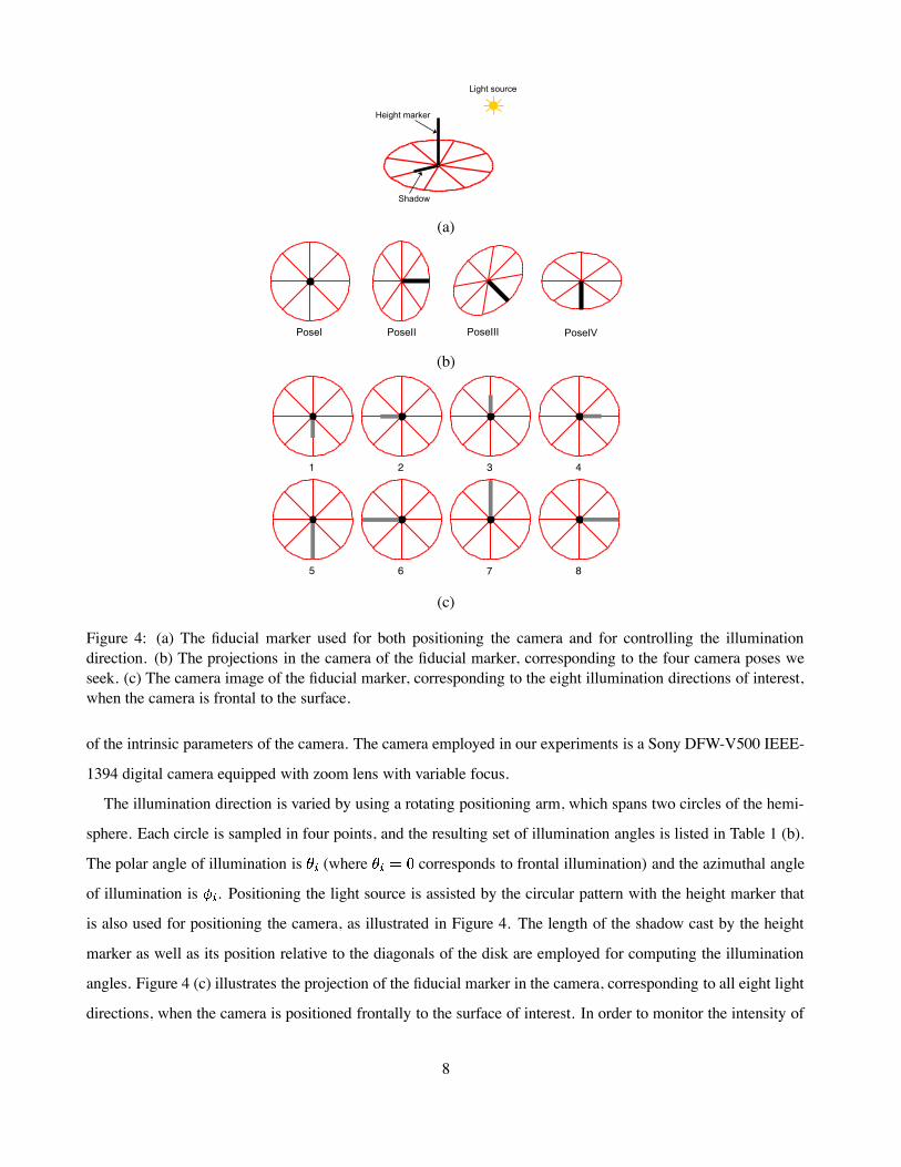
allowing six degrees of freedom. Positioning of the camera is aided by a circular pattern presenting a height

marker, as illustrated in Figure 4 (a). The height marker has length equal with the disk radius. This pattern is

attached to the surface of interest such that it is comprised in the field of view of the camera. Positioning the

camera in one of the four desired poses is achieved by inspecting the projection of the pattern in the image. The

projections corresponding to the four camera poses we seek are depicted in Figure 4 (b). The camera calibration

is completed by imaging a known 3-dimensional object during each imaging session, allowing the computation

7

Light�source

Shadow

Height�marker

(a)

PoseII PoseIII PoseIVPoseI(b)

1 2 3 4

5 6 7 8

(c)

Figure 4: (a) The fiducial marker used for both positioning the camera and for controlling the illuminationdirection. (b) The projections in the camera of the fiducial marker, corresponding to the four camera poses weseek. (c) The camera image of the fiducial marker, corresponding to the eight illumination directions of interest,when the camera is frontal to the surface.

of the intrinsic parameters of the camera. The camera employed in our experiments is a Sony DFW-V500 IEEE-

1394 digital camera equipped with zoom lens with variable focus.

The illumination direction is varied by using a rotating positioning arm, which spans two circles of the hemi-

sphere. Each circle is sampled in four points, and the resulting set of illumination angles is listed in Table 1 (b).

The polar angle of illumination is (where corresponds to frontal illumination) and the azimuthal angle

of illumination is . Positioning the light source is assisted by the circular pattern with the height marker that

is also used for positioning the camera, as illustrated in Figure 4. The length of the shadow cast by the height

marker as well as its position relative to the diagonals of the disk are employed for computing the illumination

angles. Figure 4 (c) illustrates the projection of the fiducial marker in the camera, corresponding to all eight light

directions, when the camera is positioned frontally to the surface of interest. In order to monitor the intensity of

8

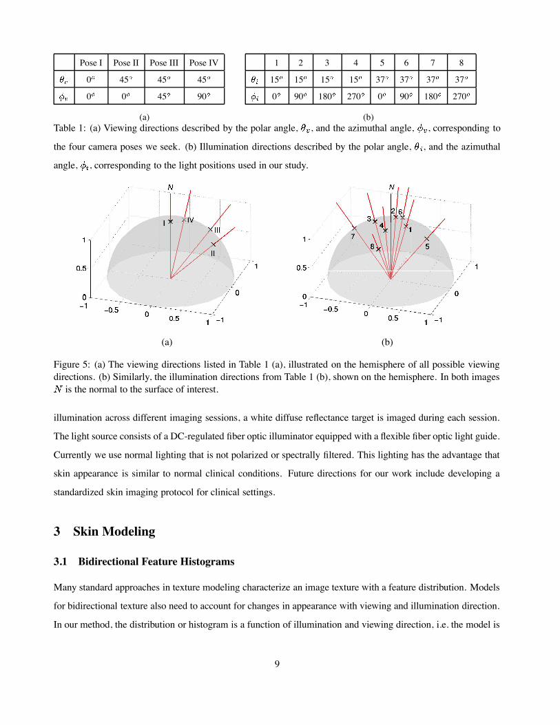
Pose I Pose II Pose III Pose IV

0 45 45 45

0 0 45 90

(a)

1 2 3 4 5 6 7 8

15 15 15 15 37 37 37 37

0 90 180 270 0 90 180 270

(b)Table 1: (a) Viewing directions described by the polar angle, , and the azimuthal angle, , corresponding to

the four camera poses we seek. (b) Illumination directions described by the polar angle, , and the azimuthal

angle, , corresponding to the light positions used in our study.

(a) (b)

Figure 5: (a) The viewing directions listed in Table 1 (a), illustrated on the hemisphere of all possible viewingdirections. (b) Similarly, the illumination directions from Table 1 (b), shown on the hemisphere. In both imagesis the normal to the surface of interest.

illumination across different imaging sessions, a white diffuse reflectance target is imaged during each session.

The light source consists of a DC-regulated fiber optic illuminator equipped with a flexible fiber optic light guide.

Currently we use normal lighting that is not polarized or spectrally filtered. This lighting has the advantage that

skin appearance is similar to normal clinical conditions. Future directions for our work include developing a

standardized skin imaging protocol for clinical settings.

3 Skin Modeling

3.1 Bidirectional Feature Histograms

Many standard approaches in texture modeling characterize an image texture with a feature distribution. Models

for bidirectional texture also need to account for changes in appearance with viewing and illumination direction.

In our method, the distribution or histogram is a function of illumination and viewing direction, i.e. the model is

9

a bidirectional feature histogram. We have used this method in earlier work (Cula and Dana, 2001a) (Cula and

Dana, 2004) for object recognition and we adapt it here for skin texture classification. We develop two models

that both use bidirectional feature histograms but differ in their definition of an image feature. In the first model,

the feature is an image texton obtained by clustering the output of oriented multiscale filters, and in the second

model, the feature is a symbolic texture primitive. In this section we describe the details of these two approaches.

3.2 Image Textons as Features

Based on the classic concept of textons (Julesz, 1981), and also on modern generalizations (Leung and Malik,

2001), we follow the theory that there is a finite set of local structural features that can be found within a large

collection of texture images from various samples. This reduced set of local structural representatives is called

the image texton library.

A widely used computational approach for encoding the local structural attributes of textures is based on

multichannel filtering (Bovik et al., 1990) (Jain et al., 1999) (Randen and Husoy, 1999) (Leung and Malik,

2001). This type of analysis is inspired by various evidences of similar processing in human vision system. In

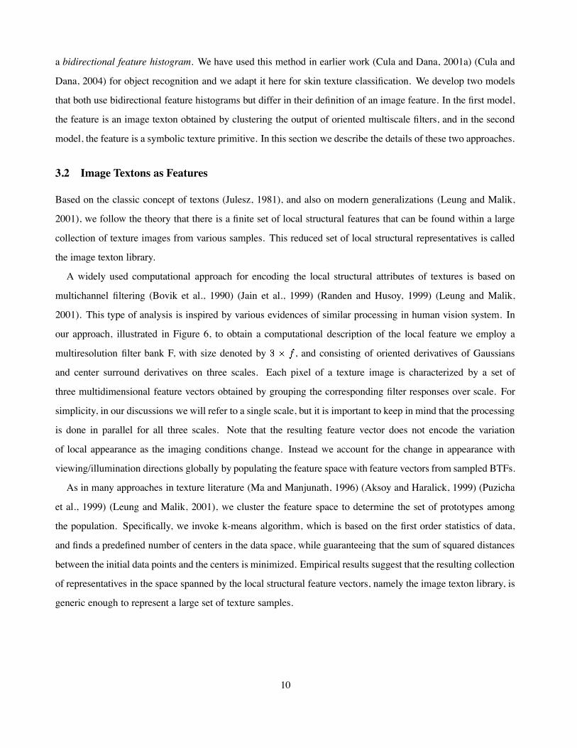
our approach, illustrated in Figure 6, to obtain a computational description of the local feature we employ a

multiresolution filter bank F, with size denoted by , and consisting of oriented derivatives of Gaussians

and center surround derivatives on three scales. Each pixel of a texture image is characterized by a set of

three multidimensional feature vectors obtained by grouping the corresponding filter responses over scale. For

simplicity, in our discussions we will refer to a single scale, but it is important to keep in mind that the processing

is done in parallel for all three scales. Note that the resulting feature vector does not encode the variation

of local appearance as the imaging conditions change. Instead we account for the change in appearance with

viewing/illumination directions globally by populating the feature space with feature vectors from sampled BTFs.

As in many approaches in texture literature (Ma and Manjunath, 1996) (Aksoy and Haralick, 1999) (Puzicha

et al., 1999) (Leung and Malik, 2001), we cluster the feature space to determine the set of prototypes among

the population. Specifically, we invoke k-means algorithm, which is based on the first order statistics of data,

and finds a predefined number of centers in the data space, while guaranteeing that the sum of squared distances

between the initial data points and the centers is minimized. Empirical results suggest that the resulting collection

of representatives in the space spanned by the local structural feature vectors, namely the image texton library, is

generic enough to represent a large set of texture samples.

10

Sample 1

qSample 2 . . . Sample Q

K-Means Clustering on Size f

Feature Vectors}Texton Labels

. . .

Unregistered Images from Unknown View/Illumination

*

F

*

F

*

F

Figure 6: Creation of the image texton library. The unregistered texture images of different BTFs are filteredwith the filter bank F. The filter responses for each pixel are grouped to form the feature vectors. The featurespace is clustered via k-means to determine the collection of key features, i.e. the image texton library.

3.2.1 Texton Histograms

The histogram of image textons is used to encode the global distribution of the local structural attribute over the

texture image. This histogram, denoted by , is a discrete function of the labels induced by the image texton

library and is computed as described in Figure 7. Note that in our approach, neither the image texton nor the

texton histogram encode the change in local appearance of texture with the imaging conditions. These quantities

are local to a single texture image. We represent the surface using a collection of image texton histograms,

acquired as a function of viewing and illumination direction. This surface representation may be described by the

term bidirectional feature histogram. It is worthwhile to explicitly note the difference between the bidirectional

feature histogram and the BTF. While the BTF is the set of measured images as a function of viewing and

illumination, the bidirectional feature histogram is a representation of the BTF suitable for use in classification.

In our work, each texture class is modeled using a collection of texton histograms. The dimensionality of

the histogram space is given by the cardinality of the image texton library, which should be inclusive enough to

represent a large range of textured surfaces. Therefore the histogram space is high dimensional, and a compres-

sion of this representation to a lower-dimensional one is suitable, providing that the statistical properties of the

bidirectional feature histograms are still preserved. To accomplish dimensionality reduction we employ principal

component analysis (PCA), which finds an optimal new orthogonal basis in the space, while best describing the

data. This approach follows (Murase and Nayar, 1995), where a similar problem is treated, specifically an object

is represented by set of images taken from various poses, and PCA is used to obtain a compact lower-dimensional

representation.

11

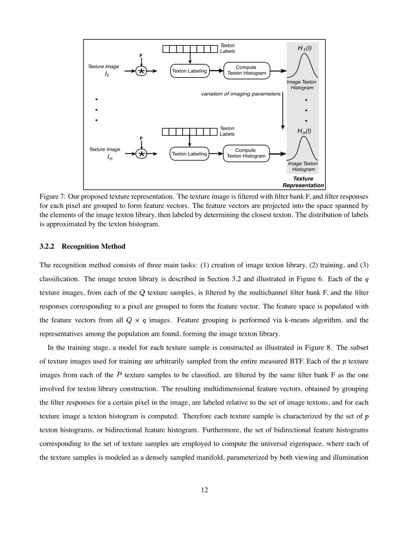
Image Texton Histogram

H (l)

Texton Labeling Compute

Texton Histogram

Texton Labels

H (l)

Texton Labeling Compute

Texton Histogram

Texton Labels

.

.

.

.

.

.

Texture ImageI1

Texture ImageIn

variation of imaging parameters

Image Texton Histogram

1

n

Texture Representation

*

F

*

F

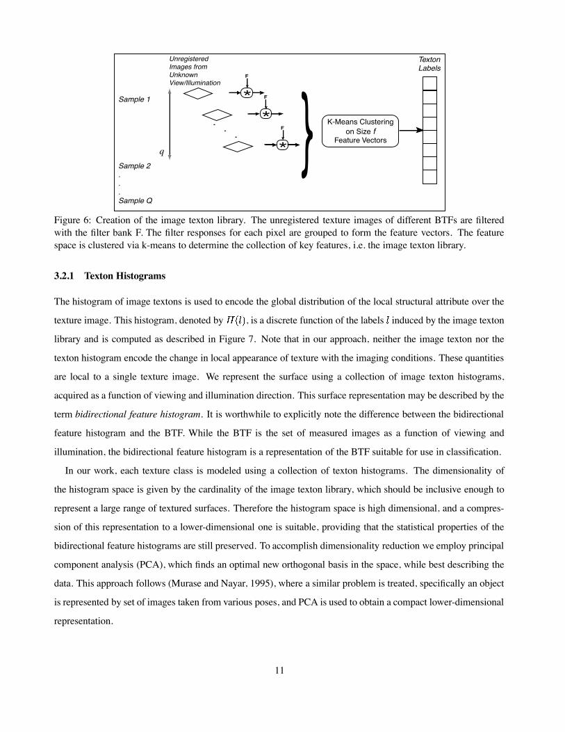
Figure 7: Our proposed texture representation. The texture image is filtered with filter bank F, and filter responsesfor each pixel are grouped to form feature vectors. The feature vectors are projected into the space spanned bythe elements of the image texton library, then labeled by determining the closest texton. The distribution of labelsis approximated by the texton histogram.

3.2.2 Recognition Method

The recognition method consists of three main tasks: (1) creation of image texton library, (2) training, and (3)

classification. The image texton library is described in Section 3.2 and illustrated in Figure 6. Each of the

texture images, from each of the texture samples, is filtered by the multichannel filter bank F, and the filter

responses corresponding to a pixel are grouped to form the feature vector. The feature space is populated with

the feature vectors from all images. Feature grouping is performed via k-means algorithm, and the

representatives among the population are found, forming the image texton library.

In the training stage, a model for each texture sample is constructed as illustrated in Figure 8. The subset

of texture images used for training are arbitrarily sampled from the entire measured BTF. Each of the texture

images from each of the texture samples to be classified, are filtered by the same filter bank F as the one

involved for texton library construction. The resulting multidimensional feature vectors, obtained by grouping

the filter responses for a certain pixel in the image, are labeled relative to the set of image textons, and for each

texture image a texton histogram is computed. Therefore each texture sample is characterized by the set of

texton histograms, or bidirectional feature histogram. Furthermore, the set of bidirectional feature histograms

corresponding to the set of texture samples are employed to compute the universal eigenspace, where each of

the texture samples is modeled as a densely sampled manifold, parameterized by both viewing and illumination

12

Image 1 . . . Image p

Texton Labeling Compute Texton Histogram }Sample 1

Sample 2 . . . Sample P

PCA

Texton Labels Texton

Histograms

Unregistered Images from Unknown View/Illumination

Universal Eigenspace

Project to EigenspaceTexton Labeling Compute

Texton HistogramFind Nearest

NeighborTexture Image

Texton Labels

Training

Classification

Figure 8: Training and classification stages of image texton recognition method. During training, PCA is per-formed on the histograms of image textons. Recognition is accomplished by finding the closest neighbor to thenovel point in the texton histogram eigenspace.

directions.

In the classification stage, illustrated in Figure 8, the subset of testing texture images is disjoint from the subset

used for training. Again, each image is filtered by F, the resulting feature vectors are projected in the image texton

space and labeled according to the texton library. The classification is based on a single novel texture image,

and it is accomplished by projecting the corresponding texton histogram onto the universal eigenspace created

during training, and by determining the closest point in the eigenspace. The texture sample corresponding to

the manifold onto which the closest point lies is reported as the texture class of the testing texture image. To

demonstrate the versatility of the image texton library we design two classification experiments, described in

Section 4.1.

3.3 Symbolic Texture Primitives as Features

Although the image texton method works well when inter-class variability is large, there are several drawbacks

to this approach. Clustering in high dimensional space is difficult and the results are highly dependent on the

prechosen number of clusters. Furthermore, pixels which have very different filter responses are often part of the

same perceptual texture primitive.

13

Figure 9: The appearance of a typical skin surface. An important skin feature is the pore, which can slightly varyin size or shape for different face regions or from one person to another.

Consider the texture primitive of a skin pore. The appearance of a typical skin pore is shown in Figure 9.

To identify this texture primitive, the local geometric arrangement of intensity edges is important. However, the

exact magnitude of the edge pixels is not of particular significance. In the clustering approach, two horizontal

edges with different gradient magnitude may be given different labels and this negatively affects the quality of

the texture classification.

We seek a simplified representation that preserves the commonality of edges of the same orientation regardless

of the strength of the filter response. The important entity is the label of the filter that has a large response relative

to the other filters. If we use a filter bank F, consisting of N filters F1,...,FN , the index of the filter with the

maximal response is retained as the feature for each pixel. In this sense, the feature is symbolic. While a single

symbolic feature is not particularly descriptive, we observe that the local configuration of these symbolic features

is a simple and useful texture primitive. The dimensionality of the texture primitive depends on the number of

pixels in the local configuration and can be kept quite low. No clustering is necessary as the texture primitive is

directly defined by the spatial arrangement of symbolic features.

3.3.1 Recognition Method

Each training image provides a primitive histogram and several training images obtained with different imaging

parameters are collected for each texture class. The histograms from all training images for all texture classes are

used to create an eigenspace and recognition is done in a strategy very similar to that described in Section 3.2.2.

That is, the primitive histograms from a certain class are projected to points in this eigenspace and represent a

sampling of the manifold of points for the appearance of this texture class. In theory, the entire manifold would be

obtained by histograms from the continuum of all possible viewing and illumination directions. For recognition,

the primitive histograms from novel texture images are projected into the eigenspace and compared with each

point in the training set. The class of the nearest K neighbors is the classification result. In our experiments K is

set to 5. Figure 10 illustrates the main steps of the recognition method.

14

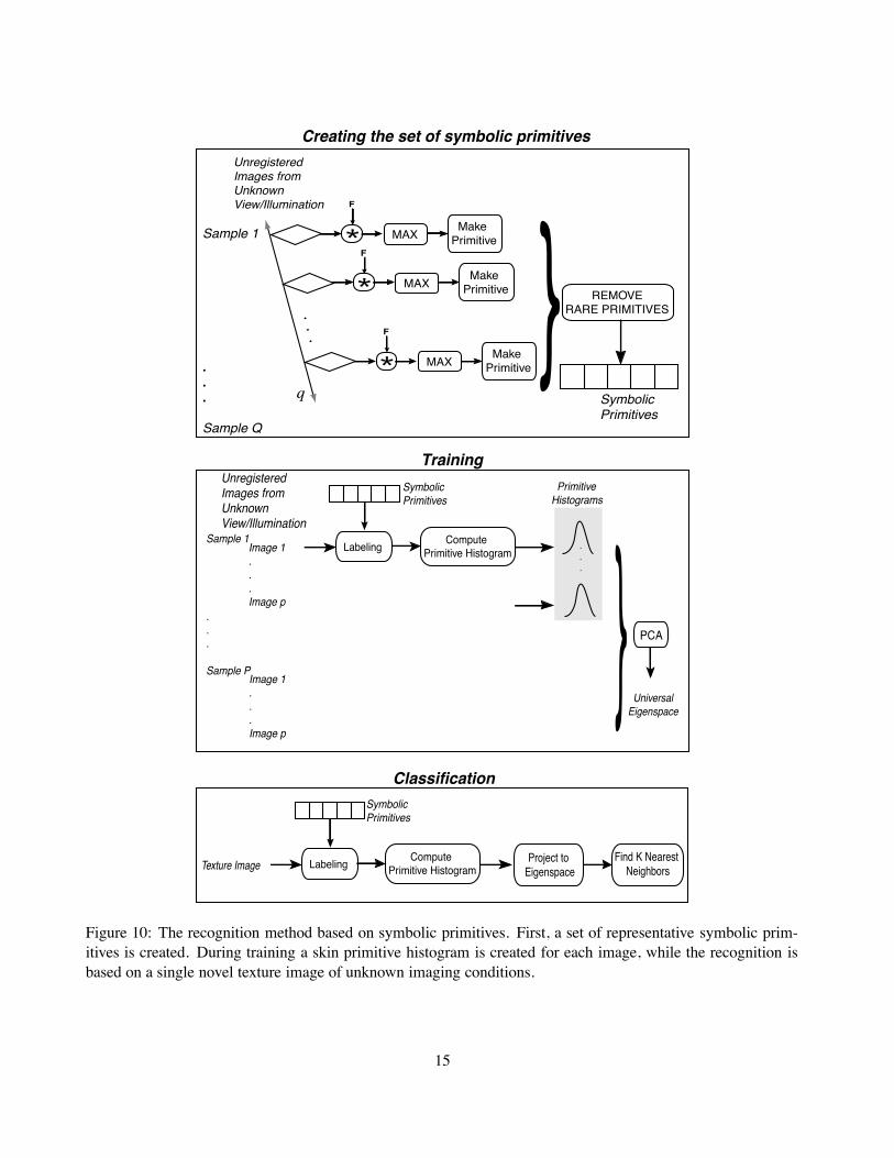
Image 1 . . . Image p }

Sample 1

.

.

. Sample P

PCA

Unregistered Images from Unknown View/Illumination

Universal Eigenspace

Training

Image 1 . . . Image p

Labeling Compute Primitive Histogram

Symbolic Primitives

.

.

.

Classification

Texture Image Project to EigenspaceLabeling Compute

Primitive Histogram

Symbolic Primitives

Find K Nearest Neighbors

Sample 1

q. . . Sample Q

Symbolic Primitives

Unregistered Images from Unknown View/Illumination

...

*

F

MAX Make Primitive } REMOVE

RARE PRIMITIVES

*

F

MAX Make Primitive

*

F

MAX Make Primitive

Creating the set of symbolic primitives

Primitive Histograms

Figure 10: The recognition method based on symbolic primitives. First, a set of representative symbolic prim-itives is created. During training a skin primitive histogram is created for each image, while the recognition isbased on a single novel texture image of unknown imaging conditions.

15

Class 1Class 2

Class 3

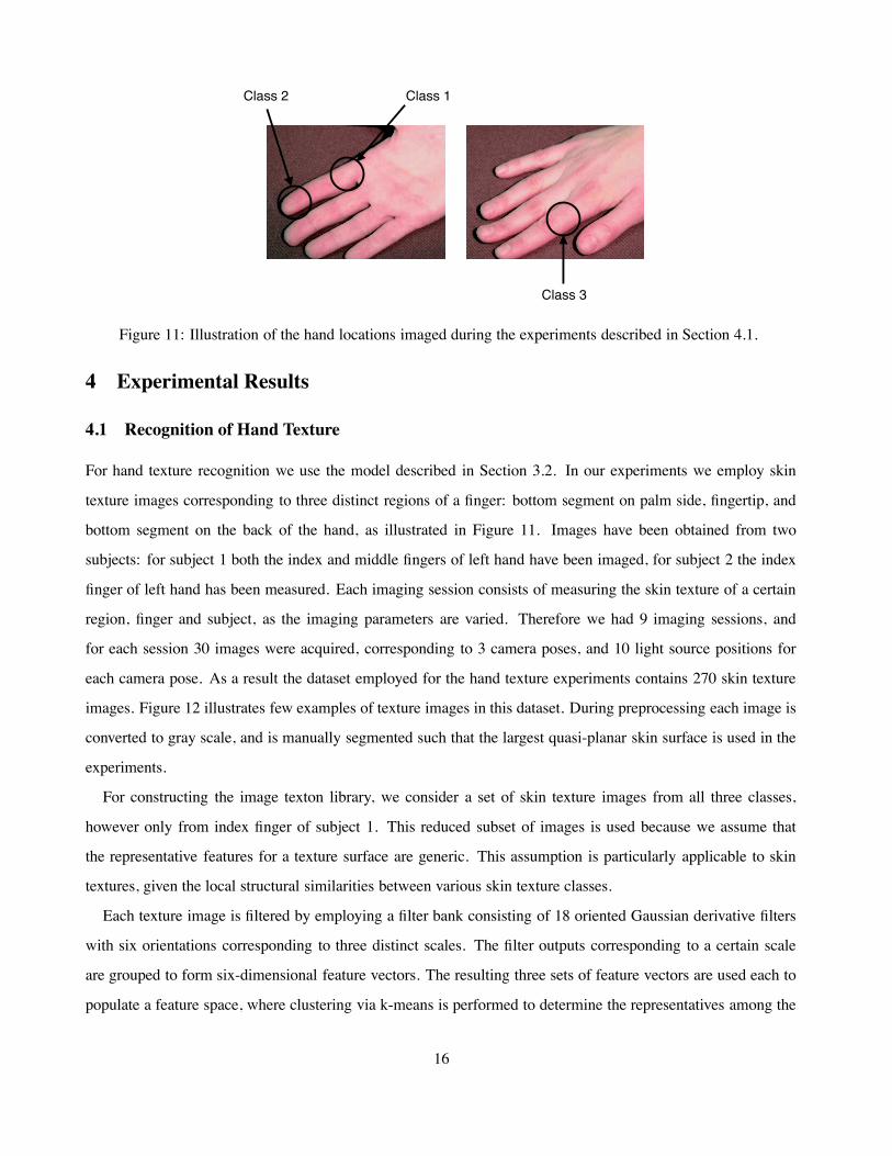
Figure 11: Illustration of the hand locations imaged during the experiments described in Section 4.1.

4 Experimental Results

4.1 Recognition of Hand Texture

For hand texture recognition we use the model described in Section 3.2. In our experiments we employ skin

texture images corresponding to three distinct regions of a finger: bottom segment on palm side, fingertip, and

bottom segment on the back of the hand, as illustrated in Figure 11. Images have been obtained from two

subjects: for subject 1 both the index and middle fingers of left hand have been imaged, for subject 2 the index

finger of left hand has been measured. Each imaging session consists of measuring the skin texture of a certain

region, finger and subject, as the imaging parameters are varied. Therefore we had 9 imaging sessions, and

for each session 30 images were acquired, corresponding to 3 camera poses, and 10 light source positions for

each camera pose. As a result the dataset employed for the hand texture experiments contains 270 skin texture

images. Figure 12 illustrates few examples of texture images in this dataset. During preprocessing each image is

converted to gray scale, and is manually segmented such that the largest quasi-planar skin surface is used in the

experiments.

For constructing the image texton library, we consider a set of skin texture images from all three classes,

however only from index finger of subject 1. This reduced subset of images is used because we assume that

the representative features for a texture surface are generic. This assumption is particularly applicable to skin

textures, given the local structural similarities between various skin texture classes.

Each texture image is filtered by employing a filter bank consisting of 18 oriented Gaussian derivative filters

with six orientations corresponding to three distinct scales. The filter outputs corresponding to a certain scale

are grouped to form six-dimensional feature vectors. The resulting three sets of feature vectors are used each to

populate a feature space, where clustering via k-means is performed to determine the representatives among the

16

(a)

(b)

(c)

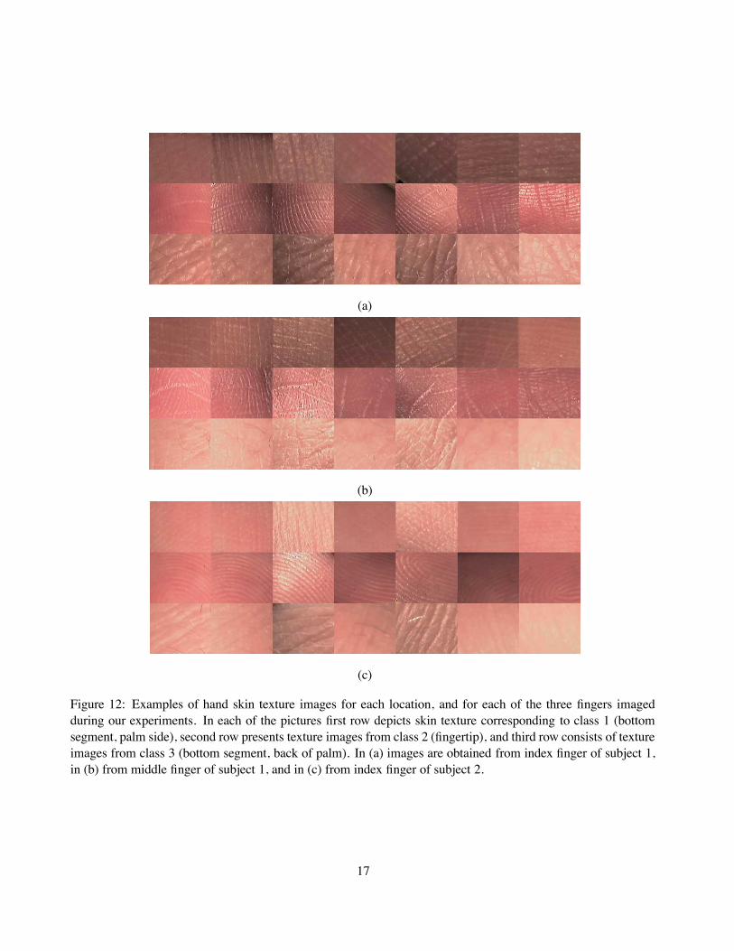
Figure 12: Examples of hand skin texture images for each location, and for each of the three fingers imagedduring our experiments. In each of the pictures first row depicts skin texture corresponding to class 1 (bottomsegment, palm side), second row presents texture images from class 2 (fingertip), and third row consists of textureimages from class 3 (bottom segment, back of palm). In (a) images are obtained from index finger of subject 1,in (b) from middle finger of subject 1, and in (c) from index finger of subject 2.

17

Class 1Class 2Class 3 Global

45 50 55 600.80.820.840.860.880.90.920.940.960.98

1

Class 1Class 2Class 3Global

5 10 15 20 25 300.50.550.60.650.70.750.80.850.90.95

1

3 5 10 15 20 25 300.50.550.60.650.70.750.80.850.90.95

1

3

Class 1Class 2Class 3Global

(a) (b) (c)

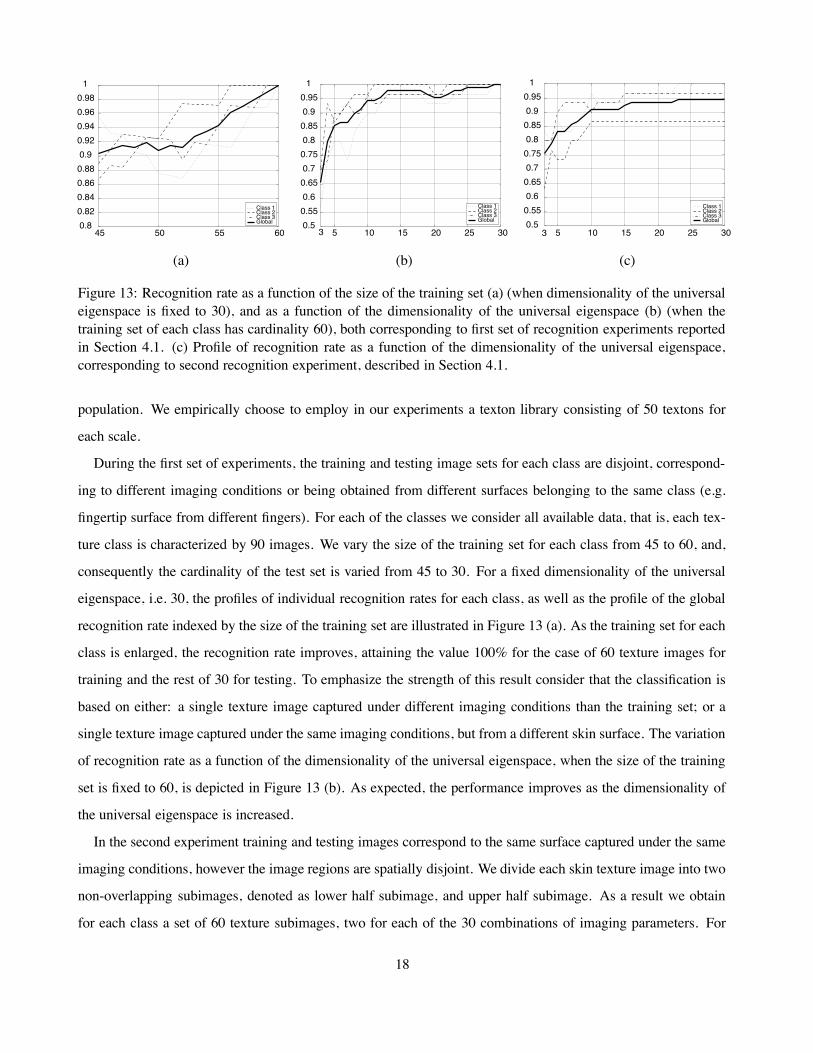
Figure 13: Recognition rate as a function of the size of the training set (a) (when dimensionality of the universaleigenspace is fixed to 30), and as a function of the dimensionality of the universal eigenspace (b) (when thetraining set of each class has cardinality 60), both corresponding to first set of recognition experiments reportedin Section 4.1. (c) Profile of recognition rate as a function of the dimensionality of the universal eigenspace,corresponding to second recognition experiment, described in Section 4.1.

population. We empirically choose to employ in our experiments a texton library consisting of 50 textons for

each scale.

During the first set of experiments, the training and testing image sets for each class are disjoint, correspond-

ing to different imaging conditions or being obtained from different surfaces belonging to the same class (e.g.

fingertip surface from different fingers). For each of the classes we consider all available data, that is, each tex-

ture class is characterized by 90 images. We vary the size of the training set for each class from 45 to 60, and,

consequently the cardinality of the test set is varied from 45 to 30. For a fixed dimensionality of the universal

eigenspace, i.e. 30, the profiles of individual recognition rates for each class, as well as the profile of the global

recognition rate indexed by the size of the training set are illustrated in Figure 13 (a). As the training set for each

class is enlarged, the recognition rate improves, attaining the value 100% for the case of 60 texture images for

training and the rest of 30 for testing. To emphasize the strength of this result consider that the classification is

based on either: a single texture image captured under different imaging conditions than the training set; or a

single texture image captured under the same imaging conditions, but from a different skin surface. The variation

of recognition rate as a function of the dimensionality of the universal eigenspace, when the size of the training

set is fixed to 60, is depicted in Figure 13 (b). As expected, the performance improves as the dimensionality of

the universal eigenspace is increased.

In the second experiment training and testing images correspond to the same surface captured under the same

imaging conditions, however the image regions are spatially disjoint. We divide each skin texture image into two

non-overlapping subimages, denoted as lower half subimage, and upper half subimage. As a result we obtain

for each class a set of 60 texture subimages, two for each of the 30 combinations of imaging parameters. For

18

Forehead

NoseCheek

Chin

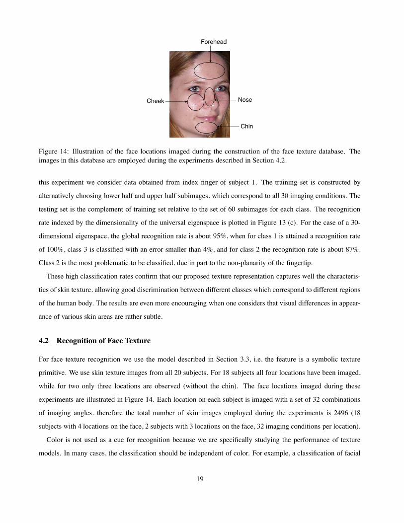
Figure 14: Illustration of the face locations imaged during the construction of the face texture database. Theimages in this database are employed during the experiments described in Section 4.2.

this experiment we consider data obtained from index finger of subject 1. The training set is constructed by

alternatively choosing lower half and upper half subimages, which correspond to all 30 imaging conditions. The

testing set is the complement of training set relative to the set of 60 subimages for each class. The recognition

rate indexed by the dimensionality of the universal eigenspace is plotted in Figure 13 (c). For the case of a 30-

dimensional eigenspace, the global recognition rate is about 95%, when for class 1 is attained a recognition rate

of 100%, class 3 is classified with an error smaller than 4%, and for class 2 the recognition rate is about 87%.

Class 2 is the most problematic to be classified, due in part to the non-planarity of the fingertip.

These high classification rates confirm that our proposed texture representation captures well the characteris-

tics of skin texture, allowing good discrimination between different classes which correspond to different regions

of the human body. The results are even more encouraging when one considers that visual differences in appear-

ance of various skin areas are rather subtle.

4.2 Recognition of Face Texture

For face texture recognition we use the model described in Section 3.3, i.e. the feature is a symbolic texture

primitive. We use skin texture images from all 20 subjects. For 18 subjects all four locations have been imaged,

while for two only three locations are observed (without the chin). The face locations imaged during these

experiments are illustrated in Figure 14. Each location on each subject is imaged with a set of 32 combinations

of imaging angles, therefore the total number of skin images employed during the experiments is 2496 (18

subjects with 4 locations on the face, 2 subjects with 3 locations on the face, 32 imaging conditions per location).

Color is not used as a cue for recognition because we are specifically studying the performance of texture

models. In many cases, the classification should be independent of color. For example, a classification of facial

19

F1 F3 F4 F5F2 P1 P3P2 P4 P5(a) (b)

Figure 15: (a) The set of five filters (Fi, i=1...5) used during the face skin modeling: four oriented Gaussianderivative filters, and one Laplacian of Gaussian derivative filter. (b) The set of five local configurations (Pi,i=1...5) used for constructing the symbolic primitives.

regions such as forehead vs. cheek should not depend on the color of the training subjects. A novel subject’s face

may be of a different color than the training subjects, yet the underlying skin texture characteristics can enable

classification. The images are converted to gray scale before processing, and they are manually segmented such

that the largest quasi-planar skin surface is used in the experiments.

We construct the skin texture representation using symbolic texture primitives as described in Section 3.3.

We define the symbolic texture feature by employing a filter bank consisting of five filters: 4 oriented Gaussian

derivative filters, and one Laplacian of Gaussian filter. These filters are chosen to efficiently identify the local

oriented patterns evident in skin structures such as those illustrated in Figure 9. The filter bank is illustrated in

Figure 15 (a). Each filter has size 15x15. We define several types of symbolic texture primitives by grouping

symbolic features corresponding to nine neighboring pixels. Specifically, we define five types of local configu-

rations, denoted by Pi, i=1...5, and illustrated in Figure 15 (b). As described in Section 3.3, a symbolic feature

corresponding to a pixel in the image is the index of the maximal response filter at that pixel. The pertinent

question is how a featureless region in the image would be characterized in this context. To solve this issue we

define a synthetic filter, denoted by F0, which corresponds to pixels in the image where features are weak, that is,

where the maximum filter response is not larger than a threshold. Therefore the symbolic texture primitive can

be viewed as a string of nine features, where each feature can have values in the set . A comprehensive

set of primitives can be quite extensive, therefore the dimensionality of the primitive histogram can be very large.

Hence the need to prune the initial set of primitives to a subset consisting of primitives with high probability of

occurrence in the image. Also, this reasoning is consistent with the repetitiveness of the local structure that is

characteristic property of texture images.

We construct the set of representative symbolic primitives by using 384 images from 3 randomly selected

subjects and for all four locations per subject. We first construct the set of all symbolic primitives from all

384 skin images, then we eliminate the ones with low probability. The resulting set of representative symbolic

primitives is further employed for labeling the images, and consequently to construct the primitive histogram

20

for each image. Figure 19 exemplifies five instances of images labeled with various symbolic primitives. The

left column illustrates the original images, while the right column presents the images with pixels labeled by

certain symbolic primitives (white spots). In detail, the first row shows pixels in the image labeled by primitives

of type P1, where all filters are horizontally oriented. The second row illustrates an image labeled with P2-

type primitives where all filters are vertically oriented. The third and fourth rows present images labeled with

primitives of type P3 and P4, where all filters are oriented at -45 , and 45 , respectively. The last row shows

a labeled image using a P5 primitive where all filters are center surround derivatives. Notice that indeed the

symbolic primitives successfully capture the local structure in the image.

We further analyze the descriptive power of the primitive set by computing the intra- and inter-class variability

of the primitive histograms. Specifically, we compute both the distribution of distances between histograms of

images belonging to the same class, and the distribution of distances between histograms of images belonging

to different classes. Note that the class is defined either as a certain region on the face independent on the

human subject (i.e. forehead vs. cheek), or it can refer to a certain human subject (i.e. subject i vs. subject j).

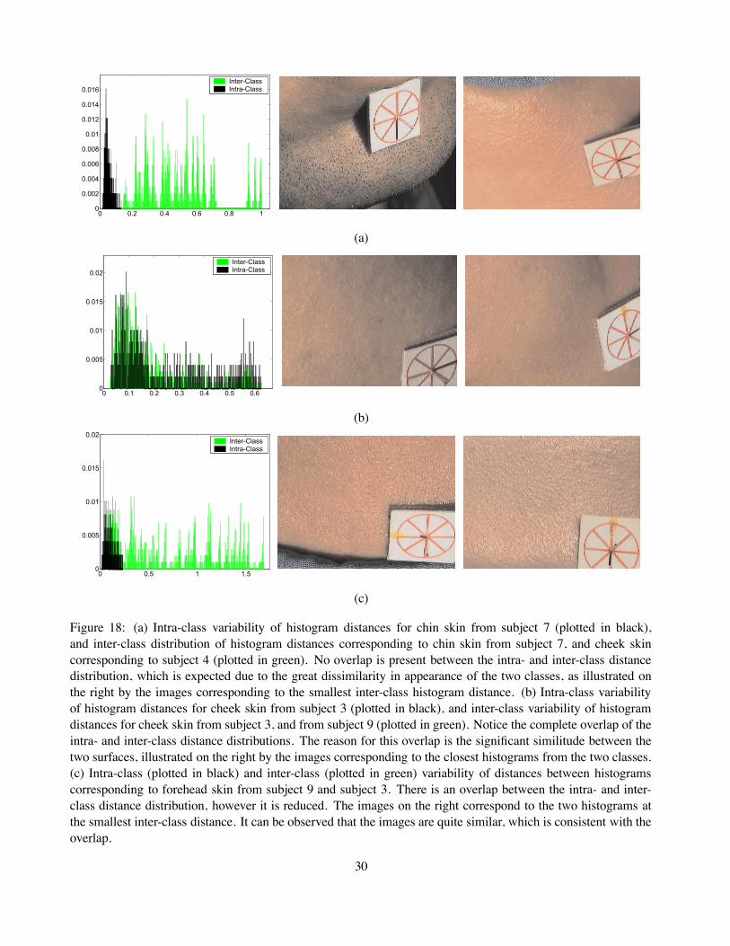
Figure 18 illustrates three of the cases we analyzed. In Figure 18 (a), on the left, the intra-class distribution of

distances between histograms corresponding to chin skin from subject 7 is plotted in black, while the inter-class

distribution of distances between histograms corresponding to chin skin from subject 7 and cheek skin of subject

4 is plotted in green. Notice that there is no overlap between the two distributions. On the right both skin surfaces

from subjects 7 and 4 are illustrated by the images corresponding to the smallest inter-class histogram distance.

The great dissimilarity in appearance of the two surfaces is consistent with the fact that there is no overlap of

the intra- and inter-class distance distributions. Figure 18 (b) illustrates the same type of analysis as in Figure 18

(a), but for cheek skin from subject 3 and subject 9. On the left, the intra-class distance distribution for cheek

skin from subject 3 is plotted in black, while the inter-class distance distribution is plotted in green. Notice the

complete overlap of the intra- and inter-class distance distributions. On the right the two classes are depicted

by images corresponding to the smallest inter-class distance. The significant similarity in appearance of the two

surfaces explains the overlap of the distributions. Finally, Figure 18 (c) depicts another case, where the intra-

class variability for forehead skin from subject 9 is compared with the inter-class variability for forehead skin

from subject 9 and from subject 3. Notice that the distributions overlap, however the overlap is reduced. The

images on the right correspond to the two histograms at the smallest inter-class distance. It can be observed that

the images are quite similar, which is consistent with the overlap.

We use this type of analysis of the intra- and inter-class variability of the primitive histograms as guideline

to design the classification experiments. Specifically, as Figure 18 (a) suggests, we find that there exists a

21

350 400 450 5000.3

0.4

0.5

0.6

0.7

0.8

0.9

1

Number of training images per class

Rec

ogni

tion

Rat

e

P1P2P3P4P5Global

350 400 450 5000.3

0.4

0.5

0.6

0.7

0.8

0.9

1

Number of training images per class

Rec

ogni

tion

Rat

e

ForeheadChinNoseGlobal

350 400 450 5000.3

0.4

0.5

0.6

0.7

0.8

0.9

1

Number of training images per class

Rec

ogni

tion

Rat

e

ForeheadChinNoseGlobal

(a) (b) (c)

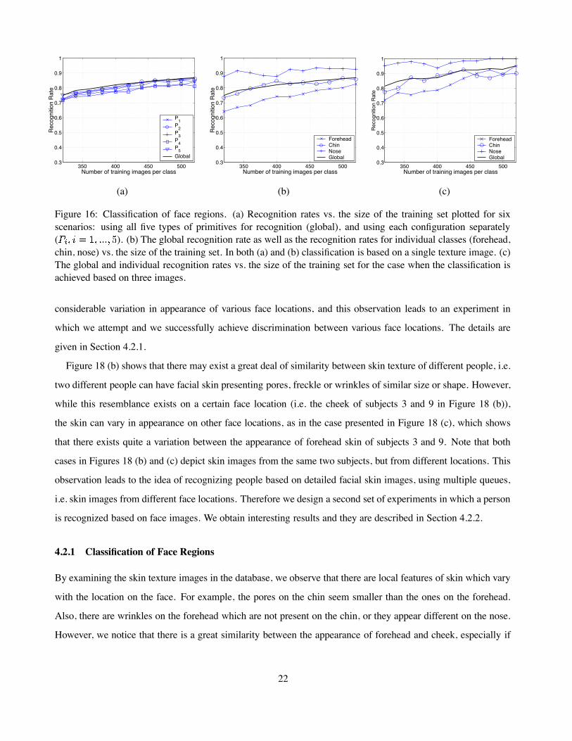
Figure 16: Classification of face regions. (a) Recognition rates vs. the size of the training set plotted for sixscenarios: using all five types of primitives for recognition (global), and using each configuration separately( ). (b) The global recognition rate as well as the recognition rates for individual classes (forehead,chin, nose) vs. the size of the training set. In both (a) and (b) classification is based on a single texture image. (c)The global and individual recognition rates vs. the size of the training set for the case when the classification isachieved based on three images.

considerable variation in appearance of various face locations, and this observation leads to an experiment in

which we attempt and we successfully achieve discrimination between various face locations. The details are

given in Section 4.2.1.

Figure 18 (b) shows that there may exist a great deal of similarity between skin texture of different people, i.e.

two different people can have facial skin presenting pores, freckle or wrinkles of similar size or shape. However,

while this resemblance exists on a certain face location (i.e. the cheek of subjects 3 and 9 in Figure 18 (b)),

the skin can vary in appearance on other face locations, as in the case presented in Figure 18 (c), which shows

that there exists quite a variation between the appearance of forehead skin of subjects 3 and 9. Note that both

cases in Figures 18 (b) and (c) depict skin images from the same two subjects, but from different locations. This

observation leads to the idea of recognizing people based on detailed facial skin images, using multiple queues,

i.e. skin images from different face locations. Therefore we design a second set of experiments in which a person

is recognized based on face images. We obtain interesting results and they are described in Section 4.2.2.

4.2.1 Classification of Face Regions

By examining the skin texture images in the database, we observe that there are local features of skin which vary

with the location on the face. For example, the pores on the chin seem smaller than the ones on the forehead.

Also, there are wrinkles on the forehead which are not present on the chin, or they appear different on the nose.

However, we notice that there is a great similarity between the appearance of forehead and cheek, especially if

22

16 18 20 22 24 260.3

0.35

0.4

0.45

0.5

0.55

0.6

0.65

0.7

0.75

Number of training images per class

Rec

ogni

tion

Rat

e

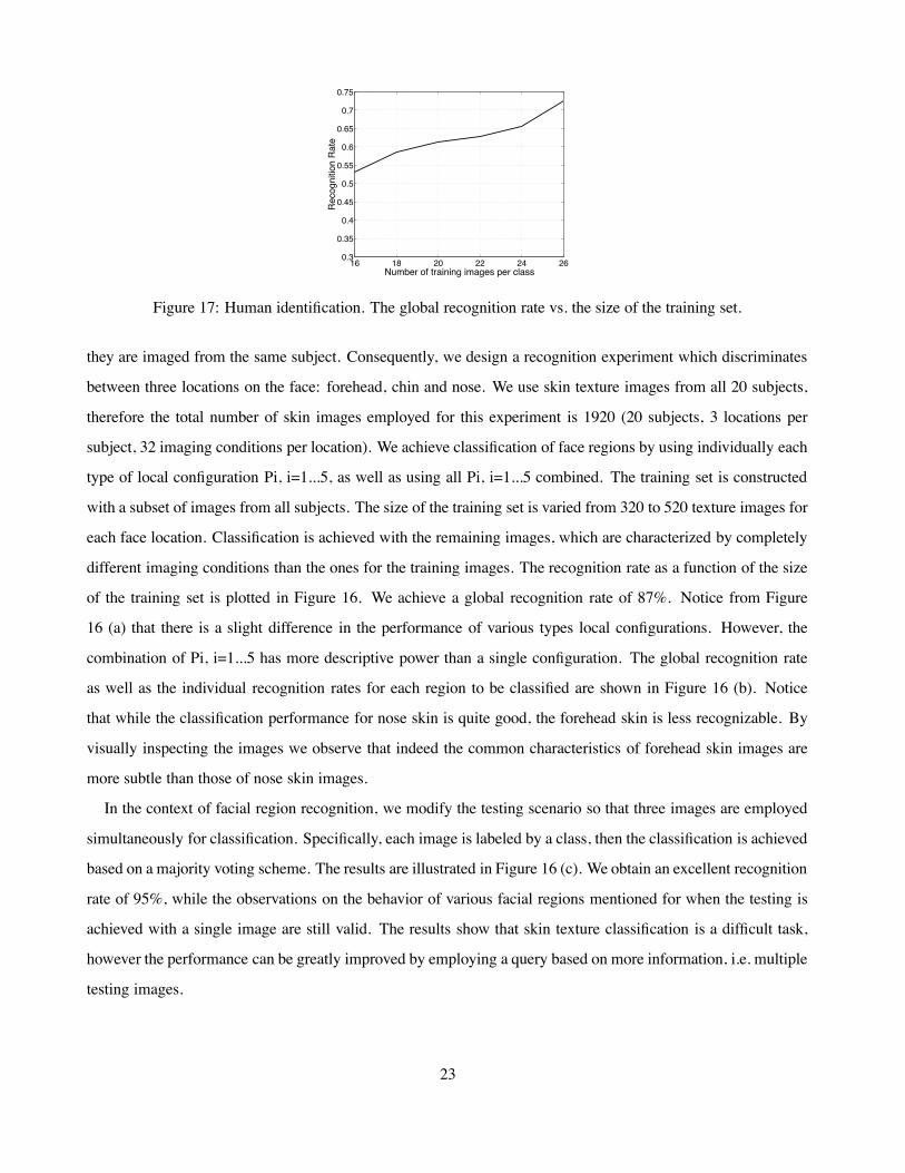
Figure 17: Human identification. The global recognition rate vs. the size of the training set.

they are imaged from the same subject. Consequently, we design a recognition experiment which discriminates

between three locations on the face: forehead, chin and nose. We use skin texture images from all 20 subjects,

therefore the total number of skin images employed for this experiment is 1920 (20 subjects, 3 locations per

subject, 32 imaging conditions per location). We achieve classification of face regions by using individually each

type of local configuration Pi, i=1...5, as well as using all Pi, i=1...5 combined. The training set is constructed

with a subset of images from all subjects. The size of the training set is varied from 320 to 520 texture images for

each face location. Classification is achieved with the remaining images, which are characterized by completely

different imaging conditions than the ones for the training images. The recognition rate as a function of the size

of the training set is plotted in Figure 16. We achieve a global recognition rate of 87%. Notice from Figure

16 (a) that there is a slight difference in the performance of various types local configurations. However, the

combination of Pi, i=1...5 has more descriptive power than a single configuration. The global recognition rate

as well as the individual recognition rates for each region to be classified are shown in Figure 16 (b). Notice

that while the classification performance for nose skin is quite good, the forehead skin is less recognizable. By

visually inspecting the images we observe that indeed the common characteristics of forehead skin images are

more subtle than those of nose skin images.

In the context of facial region recognition, we modify the testing scenario so that three images are employed

simultaneously for classification. Specifically, each image is labeled by a class, then the classification is achieved

based on a majority voting scheme. The results are illustrated in Figure 16 (c). We obtain an excellent recognition

rate of 95%, while the observations on the behavior of various facial regions mentioned for when the testing is

achieved with a single image are still valid. The results show that skin texture classification is a difficult task,

however the performance can be greatly improved by employing a query based on more information, i.e. multiple

testing images.

23

4.2.2 Human Identification

We design a second set of classification experiments where we attempt to discriminate between various human

subjects based on skin images from all four locations on the face. Specifically, we use skin images from forehead,

cheek, chin and nose to recognize 20 subjects. For each subject, the images are acquired within the same day and

do not incorporate changes with aging. A human subject is characterized by a set of 32 texture images for each

face location, i.e. 128 images per subject. Therefore we employ all the images in the database during this second

experiment. Classification is achieved based on a set of four testing images, one for each location. Each of the

four test images is labeled by a class, then the final decision is obtained by taking the majority of classes. The

training set is varied from 16 to 26 texture images for each subject and location. Consequently the final testing

is achieved with four subsets of 16 to 6 texture images per subject, each subset corresponding to a certain face

location. The global recognition rate as a function of the size of the training set is shown in Figure 17. We obtain

a recognition rate of 73%. This result suggests that human identification can be aided by including skin texture

recognition as a biometric subtask.

Some general patterns can be observed about the dependence of skin appearance on imaging conditions. (e.g.

freckles/moles are apparent is some views, specularities enhance pores and surface texture). This observation

places loose guidelines on our choice of training images. The idea is to choose training images which are likely

to show all the key features even though the exact imaging parameters of the training images are unknown.

5 Conclusions

5.1 Multidisciplinary Applications

The ability to recognize or classify skin textures has a wide range of useful multidisciplinary applications. For

example, skin texture as a biometric can be used to assist face recognition in security applications. Biomedical

evaluation of skin appearance with this method can provide quantitative measures to test topical skin treatments.

Such tests can be used to: determine whether a treatment is effective, objectively compare two treatments or

predict the outcome of a treatment in the early stages. Computer-assisted diagnosis in dermatology is another

potential application. A dermatologist can use the computational texture representation to assist an initial diag-

nosis of potentially malignant moles and lesions. In data mining applications, a representative image of a surface

can be used to search a database for matches. This search is applicable in e-commerce to enable a customer

to find a particular material in a database of product imagery. Another application is advanced watermarking

where the appearance of an induced fine scale texture is used as an object identifier. In military applications, a

24

camouflage design can be improved by comparing the appearance of the prototype design and the background

under various viewing and illumination angles.

5.2 Broader Implications for Computer Vision

Representation and classification of skin texture has broad implications in many areas of computer vision. Image

segmentation using texture can be improved by accounting for varied texture appearance with imaging param-

eters. An object with a 3D shape can be thought of as being comprised of many textured regions, each with a

different surface tilt. The task of grouping these textured regions together requires bidirectional texture models

for classification. Finding point correspondences is a fundamental component of computer vision algorithms for

shape and motion estimation. Current methods of determining correspondences typically rely on the brightness

constancy assumption. This assumption is clearly violated whenever the two images are obtained with different

imaging parameters and the surface exhibits 3D texture. Models of surface appearance change can be used to

develop more advanced and robust methods for finding point correspondences.

5.3 Summary and Future Work

In summary, we have developed a novel texture representation which accounts for changes of skin surface ap-

pearance as the imaging conditions are varied. We employ this texture representation for skin classification in

two contexts: we discriminate between different facial and hand regions, and we classify human subjects based

on detailed facial skin images. We have developed a skin imaging protocol for clinical setting, which was em-

ployed for constructing a facial skin database. The database consists of more than 2400 images, collected from

20 subjects, and from four locations on the face: forehead, cheek, chin and nose. Each skin surface is imaged

under more than 30 combinations of viewing and illumination angles. This collection of skin images is made

publicly available for further texture research (Cula et al., 2003).

Future work includes expanding the current texture model to support efficient synthesis. The difficulty in

using image-based representations for synthesis is that even large measurements are still a sparse sampling of

the continuous six-dimensional bidirectional texture function. Therefore interpolation must be used to get image

texture between sample locations. However, interpolation of intensities is an incorrect approach because many

of the changes that occur with varying imaging parameters are fundamentally geometric. Consider for example

a cast shadow that grows with the angle of the oblique illumination. The shadow edge appears to move and

intensity interpolation will not capture this effect. Methods such as (Liu et al., 2001) which model the surfaces

as geometry+reflectance do not yield realistic renderings for complex texture (e.g. hair) for two main reasons:

25

(1) they tend to obtain smooth geometry where rough surfaces are inherently non-smooth, (2) simple reflectance

modeling is not sufficient to capture the actual appearance. A combined approach of geometry or geometric

transformations and image-based rendering is needed, although exactly how this combination is achieved is an

open issue.

Acknowledgments

This material is based upon work supported by the National Science Foundation under Grant No. 0092491 and

Grant No. 0085864.

26

References

Aksoy, S. and Haralick, R. M., 1999, “Graph-theoretic clustering for image grouping and retrieval”, Proceedings

of the IEEE Conference on Computer Vision and Pattern Recognition 1, 63–68

Blanz, V. and Vetter, T., 1999, “A morphable model for the synthesis of 3D faces”, Proceedings of SIGGRAPH

187–194

Boissieux, L., Kiss, G., Thalman, N., and Kalra, P., 2000, “Simulation of skin aging and wrinkles with cosmetics

insight”, Eurographics Workshop on Animation and Simulation (EGCAS 2000) , pp. 15–28

Bovik, A. C., Clark, M., and Geisler, W. S., 1990, “Multichannel texture analysis using localized spatial filters”,

IEEE Transactions on Pattern Analysis and Machine Intelligence 12, 55–73

Chantler, M., 1995, “Why illuminant direction is fundamental to texture analysis”, IEE Proceedings Vision,

Image and Signal Processing 142(4), 199–206

Cula, O. G. and Dana, K. J., 2001a, “Compact representation of bidirectional texture functions”, Proceedings of

the IEEE Conference on Computer Vision and Pattern Recognition I, 1041–1047

Cula, O. G. and Dana, K. J., 2001b, “Recognition methods for 3D textured surfaces”, Proceedings of SPIE

Conference on Human Vision and Electronic Imaging VI 4299, 209–220

Cula, O. G. and Dana, K. J., 2002, “Image-based skin analysis”, Proceedings of Texture 2002 - The 2nd interna-

tional workshop on texture analysis and synthesis 35–40

Cula, O. G. and Dana, K. J., 2004, “3D texture recognition using bidirectional feature histograms”, International

Journal of Computer Vision 59(1), 33–60

Cula, O. G., Dana, K. J., Murphy, F. P., and Rao, B. K., 2003, “http://www.caip.rutgers.edu/rutgers texture/”,

Dana, K. J. and Nayar, S. K., 1998, “Histogram model for 3D textures”, Proceedings of the IEEE Conference on

Computer Vision and Pattern Recognition 618–624

Dana, K. J. and Nayar, S. K., 1999a, “3D textured surface modeling”, IEEE Workshop on the Integration of

Appearance and Geometric Methods in Object Recognition 46–56

Dana, K. J. and Nayar, S. K., 1999b, “Correlation model for 3D texture”, International Conference on Computer

Vision 1061–1067

Dana, K. J., van Ginneken, B., Nayar, S. K., and Koenderink, J. J., 1997, “Reflectance and texture of real world

surfaces”, Proceedings of the IEEE Conference on Computer Vision and Pattern Recognition 151–157

Dana, K. J., van Ginneken, B., Nayar, S. K., and Koenderink, J. J., 1999, “Reflectance and texture of real world

surfaces”, ACM Transactions on Graphics 18(1), 1–34

DeCarlo, D., Metaxas, D., and Stone, M., 1998, “An anthropometric face model using variational techniques”,

27

Proceedings of SIGGRAPH 67–74

Dong, J. and Chantler, M., 2002, “Capture and synthesis of 3D surface texture”, Proceedings of Texture 2002 -

The 2nd international workshop on texture analysis and synthesis 41–46

Guenter, B., Grimm, C., Wood, D., Malvar, H., and Pighin, F., 1998, “Making faces”, Proceedings of SIGGRAPH

55–66

Ishii, T., Yasuda, T., Yokoi, S., and Toriwaki, J., 1993, “A generation model for human skin texture”, Communi-

cating with Virtual Worlds , pp. 139–150

Jain, A., Prabhakar, S., and Hong, L., 1999, “A multichannel approach to fingerprint classification”, IEEE

Transactions on Pattern Analysis and Machine Intelligence 21(4), 348–369

Julesz, B., 1981, “Textons, the elements of texture perception and their interactions”, Nature (290), 91–97

Koenderink, J. J. and van Doorn, A. J., 1996, “Illuminance texture due to surface mesostructure”, Journal of the

Optical Society of America A 13(3), 452–63

Koenderink, J. J., van Doorn, A. J., Dana, K. J., and Nayar, S. K., 1999, “Bidirectional reflection distribution

function of thoroughly pitted surfaces”, International Journal of Computer Vision 31(2-3), pp. 129–144

Lee, Y., Terzopoulos, D., and Walters, K., 1995, “Realistic modeling for facial animation”, Proceedings of

SIGGRAPH 55–62

Leung, T. and Malik, J., 1999, “Recognizing surfaces using three-dimensional textons”, International Confer-

ence on Computer Vision 2, 1010–1017

Leung, T. and Malik, J., 2001, “Representing and recognizing the visual appearance of materials using three-

dimensional textons”, International Journal of Computer Vision 43(1), 29–44

Liu, X., Yu, Y., and Shum, H., 2001, “Synthesizing bidirectional texture functions for real-world surfaces”,

Proceedings of SIGGRAPH 97–106

Ma, W. Y. and Manjunath, B. S., 1996, “Texture features and learning similarity”, Proceedings of the IEEE

Conference on Computer Vision and Pattern Recognition 425–430

McGunnigle, G. and Chantler, M. J., 2000, “Rough surface classification using first order statistics from photo-

metric stereo”, Pattern Recognition Letters 21, 593–604

Murase, H. and Nayar, S. K., 1995, “Visual learning and recognition of 3-D objects from appearance”, Interna-

tional Journal of Computer Vision 14(1), 5–24

Nahas, M., Huitric, H., Rioux, M., and Domey, J., 1990, “Facial image synthesis using skin texture recording”,

Visual Computer 6(6), pp. 337–43

Penirschke, A., Chantler, M., and Petrou, M., 2002, “Illuminant rotation invariant classification of 3D surface

28

textures using Lissajous’s ellipses”, Proceedings of Texture 2002 - The 2nd international workshop on texture

analysis and synthesis , pp. 103–108

Pont, S. C. and Koenderink, J. J., 2002, “Bidirectional texture contrast function”, Proceedings of the European

Conference on Computer Vision 2353(IV), pp. 808–822

Puzicha, J., Hoffman, T., and Buchmann, J., 1999, “Histogram clustering for unsupervized image segmentation”,

International Conference on Computer Vision 2, 602–608

Randen, T. and Husoy, J. H., 1999, “Filtering for texture classification: a comparative study”, IEEE Transactions

on Pattern Analysis and Machine Intelligence 21(4), 291–310

Suen, P. and Healey, G., 1998, “Analyzing the bidirectional texture function”, Proceedings of the IEEE Confer-

ence on Computer Vision and Pattern Recognition 753–758

Suen, P. and Healey, G., 2000, “The analysis and recognition of real-world textures in three dimensions”, IEEE

Transactions on Pattern Analysis and Machine Intelligence 22(5), 491–503

van Ginneken, B., Koenderink, J. J., and Dana, K. J., 1999, “Texture histograms as a function of irradiation and

viewing direction”, International Journal of Computer Vision 31(2-3), 169–184

Varma, M. and Zisserman, A., 2002, “Classifying images of materials”, Proceedings of the European Conference

on Computer Vision 255–271

Zalesny, A. and van Gool, L., 2001, “Multiview texture models”, Proceedings of the IEEE Conference on

Computer Vision and Pattern Recognition 1, pp. 615–622

29

0 0.2 0.4 0.6 0.8 100.0020.0040.0060.0080.010.0120.0140.016 Inter-ClassIntra-Class

(a)

0 0.1 0.2 0.3 0.4 0.5 0.600.005

0.010.015

0.02 Inter-ClassIntra-Class

(b)

0 0.5 1 1.500.0050.01

0.0150.02 Inter-ClassIntra-Class

(c)

Figure 18: (a) Intra-class variability of histogram distances for chin skin from subject 7 (plotted in black),and inter-class distribution of histogram distances corresponding to chin skin from subject 7, and cheek skincorresponding to subject 4 (plotted in green). No overlap is present between the intra- and inter-class distancedistribution, which is expected due to the great dissimilarity in appearance of the two classes, as illustrated onthe right by the images corresponding to the smallest inter-class histogram distance. (b) Intra-class variabilityof histogram distances for cheek skin from subject 3 (plotted in black), and inter-class variability of histogramdistances for cheek skin from subject 3, and from subject 9 (plotted in green). Notice the complete overlap of theintra- and inter-class distance distributions. The reason for this overlap is the significant similitude between thetwo surfaces, illustrated on the right by the images corresponding to the closest histograms from the two classes.(c) Intra-class (plotted in black) and inter-class (plotted in green) variability of distances between histogramscorresponding to forehead skin from subject 9 and subject 3. There is an overlap between the intra- and inter-class distance distribution, however it is reduced. The images on the right correspond to the two histograms atthe smallest inter-class distance. It can be observed that the images are quite similar, which is consistent with theoverlap.

30

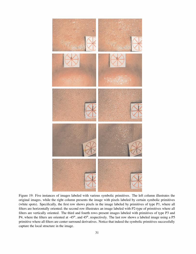
Figure 19: Five instances of images labeled with various symbolic primitives. The left column illustrates theoriginal images, while the right column presents the image with pixels labeled by certain symbolic primitives(white spots). Specifically, the first row shows pixels in the image labeled by primitives of type P1, where allfilters are horizontally oriented; the second row illustrates an image labeled with P2-type of primitives where allfilters are vertically oriented. The third and fourth rows present images labeled with primitives of type P3 andP4, where the filters are oriented at -45 , and 45 , respectively. The last row shows a labeled image using a P5primitive where all filters are center surround derivatives. Notice that indeed the symbolic primitives successfullycapture the local structure in the image.

31

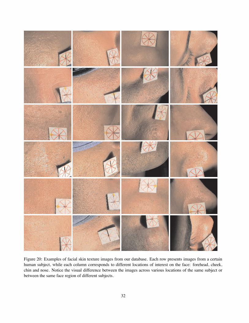
Figure 20: Examples of facial skin texture images from our database. Each row presents images from a certainhuman subject, while each column corresponds to different locations of interest on the face: forehead, cheek,chin and nose. Notice the visual difference between the images across various locations of the same subject orbetween the same face region of different subjects.

32

Figure 21: More examples of facial skin texture images from our database. Each row presents images from acertain human subject, while each column corresponds to different locations of interest on the face: forehead,cheek, chin and nose.

33

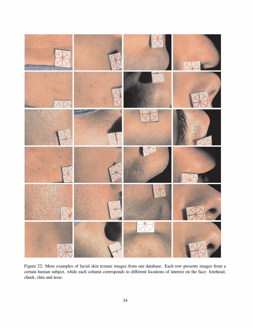
Figure 22: More examples of facial skin texture images from our database. Each row presents images from acertain human subject, while each column corresponds to different locations of interest on the face: forehead,cheek, chin and nose.

34